Sparse random graphs: Eigenvalues and eigenvectors

Sparse random graphs: Eigenvalues and Eigenvectors

Linh V. Tran, Van H. Vu∗ and Ke WangDepartment of Mathematics, Rutgers, Piscataway, NJ 08854

Abstract

In this paper we prove the semi-circular law for the eigenvalues of regular random graph Gn,d in the cased→∞, complementing a previous result of McKay for fixed d. We also obtain a upper bound on the infinity normof eigenvectors of Erdos-Renyi random graph G(n, p), answering a question raised by Dekel-Lee-Linial.

1 Introduction

1.1 Overview

In this paper, we consider two models of random graphs, the Erdos-Renyi random graph G(n, p)and the random regular graph Gn,d. Given a real number p = p(n),0 ≤ p ≤ 1, the Erdos-Renyigraph on a vertex set of size n is obtained by drawing an edge between each pair of vertices,randomly and independently, with probability p. On the other hand, Gn,d, where d = d(n)denotes the degree, is a random graph chosen uniformly from the set of all simple d-regulargraphs on n vertices. These are basic models in the theory of random graphs. For furtherinformation, we refer the readers to the excellent monographs [4], [19] and survey [33].

Given a graph G on n vertices, the adjacency matrix A of G is an n×n matrix whose entry aijequals one if there is an edge between the vertices i and j and zero otherwise. All diagonal entriesaii are defined to be zero. The eigenvalues and eigenvectors of A carry valuable informationabout the structure of the graph and have been studied by many researchers for quite some time,with both theoretical and practical motivations (see, for example, [2], [3], [12], [25] [16], [13], [15],[14], [30], [10], [27], [24]).

The goal of this paper is to study the eigenvalues and eigenvectors of G(n, p) and Gn,d. Weare going to consider:

∗V. Vu is supported by NSF grants DMS-0901216 and AFOSAR-FA-9550-09-1-0167.

1

arX

iv:1

011.

6646

v1 [

mat

h.C

O]

30

Nov

201

0

• The global law for the limit of the empirical spectral distribution (ESD) of adjacencymatrices of G(n, p) and Gn,d. For p = ω(1/n), it is well-known that eigenvalues of G(n, p)(after a proper scaling) follows Wigner’s semicircle law (we include a short proof in theAppendix A for completeness). Our main new result shows that the same law holds forrandom regular graph with d → ∞ with n. This complements the well known result ofMcKay for the case when d is an absolute constant (McKay’s law) and extends recentresults of Dumitriu and Pal [9] (see Section 1.2 for more discussion).

• Bound on the infinity norm of the eigenvectors. We first prove that the infinity normof any (unit) eigenvector v of G(n, p) is almost surely o(1) for p = ω(log n/n). Thisgives a positive answer to a question raised by Dekel, Lee and Linial [7]. Further-

more, we can show that v satisfies the bound ‖v‖∞ = O

(√log2.2 g(n)log n/np

)for

p = ω(log n/n) = g(n) log n/n, as long as the corresponding eigenvalue is bounded awayfrom the (normalized) extremal values −2 and 2.

We finish this section with some notation and conventions.

Given an n× n symmetric matrix M , we denote its n eigenvalues as

λ1(M) ≤ λ2(M) ≤ . . . ≤ λn(M),

and let u1(M), . . . , un(M) ∈ Rn be an orthonormal basis of eigenvectors of M with

Mui(M) = λiui(M).

The empirical spectral distribution (ESD) of the matrix M is a one-dimensional function

FMn (x) =

1

n|1 ≤ j ≤ n : λj(M) ≤ x|,

where we use |I| to denote the cardinality of a set I.

Let An be the adjacency matrix of G(n, p). Thus An is a random symmetric n×n matrix whoseupper triangular entries are iid copies of a real random variable ξ and diagonal entries are 0.ξ is a Bernoulli random variable that takes values 1 with probability p and 0 with probability1− p.

Eξ = p,Varξ = p(1− p) = σ2.

Usually it is more convenient to study the normalized matrix

Mn =1

σ(An − pJn)

2

where Jn is the n × n matrix all of whose entries are 1. Mn has entries with mean zero andvariance one. The global properties of the eigenvalues of An and Mn are essentially the same(after proper scaling), thanks to the following lemma

Lemma 1.1. (Lemma 36, [30]) Let A,B be symmetric matrices of the same size where B hasrank one. Then for any interval I,

|NI(A+B)−NI(A)| ≤ 1,

where NI(M) is the number of eigenvalues of M in I.

Definition 1.2. Let E be an event depending on n. Then E holds with overwhelming probabilityif P(E) ≥ 1− exp(−ω(log n)).

The main advantage of this definition is that if we have a polynomial number of events, each ofwhich holds with overwhelming probability, then their intersection also holds with overwhelmingprobability.

Asymptotic notation is used under the assumption that n → ∞. For functions f and g ofparameter n, we use the following notation as n → ∞: f = O(g) if |f |/|g| is bounded fromabove; f = o(g) if f/g → 0; f = ω(g) if |f |/|g| → ∞, or equivalently, g = o(f); f = Ω(g) ifg = O(f); f = Θ(g) if f = O(g) and g = O(f).

1.2 The semicircle law

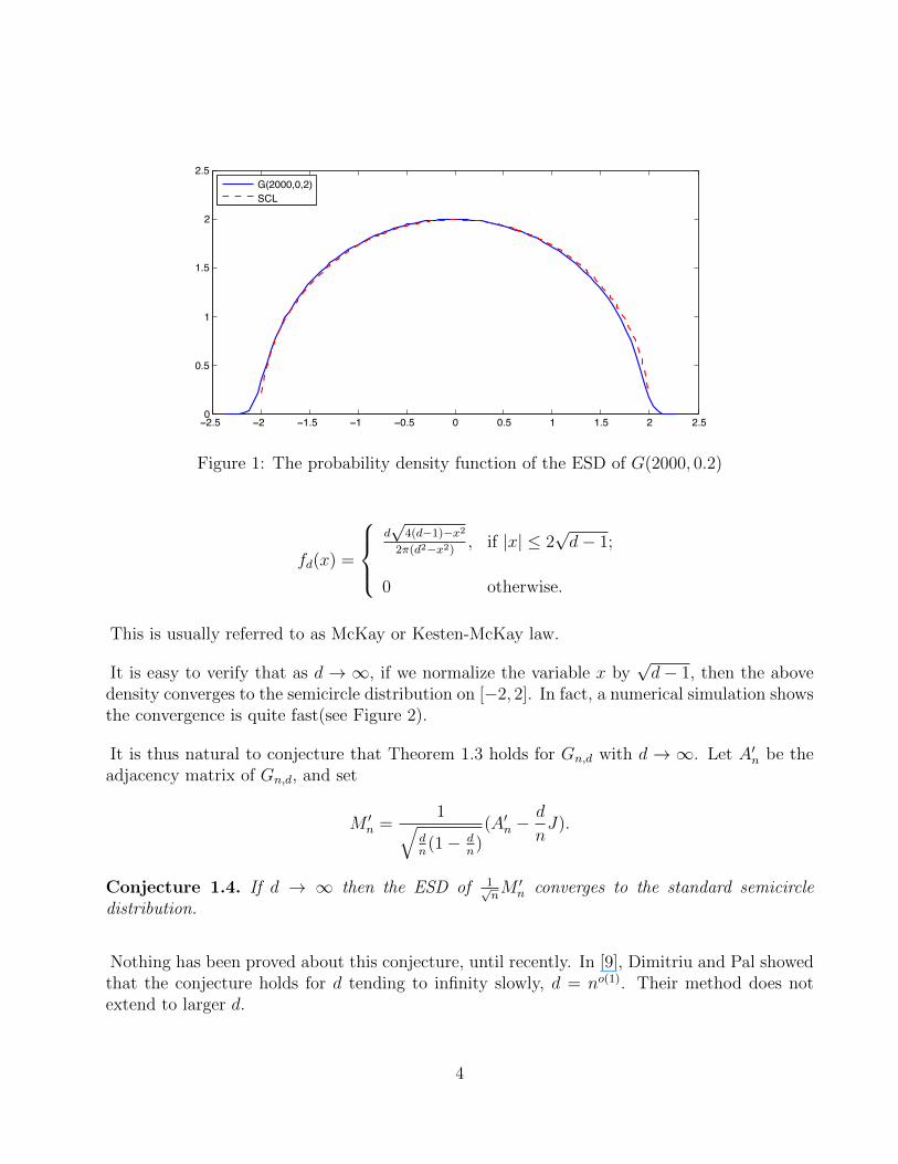
In 1950s, Wigner [32] discovered the famous semi-circle for the limiting distribution of theeigenvalues of random matrices. His proof extends, without difficulty, to the adjacency matrixof G(n, p), given that np→∞ with n. (See Figure 1 for a numerical simulation)

Theorem 1.3. For p = ω( 1n), the empirical spectral distribution (ESD) of the matrix 1√

nσAn

converges in distribution to the semicircle distribution which has a density ρsc(x) with supporton [−2, 2],

ρsc(x) :=1

2π

√4− x2.

If np = O(1), the semicircle law no longer holds. In this case, the graph almost surely hasΘ(n) isolated vertices, so in the limiting distribution, the point 0 will have positive constantmass.

The case of random regular graph, Gn,d, was considered by McKay [21] about 30 years ago.He proved that if d is fixed, and n→∞, then the limiting density function is

3

!2.5 !2 !1.5 !1 !0.5 0 0.5 1 1.5 2 2.50

0.5

1

1.5

2

2.5

f(x)

x

G(2000,0,2)

SCL

Figure 1: The probability density function of the ESD of G(2000, 0.2)

fd(x) =

d√

4(d−1)−x22π(d2−x2)

, if |x| ≤ 2√d− 1;

0 otherwise.

This is usually referred to as McKay or Kesten-McKay law.

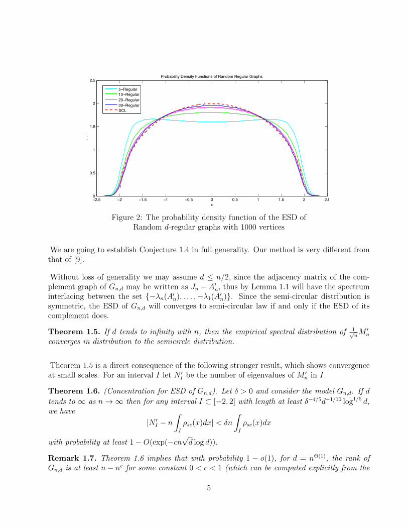
It is easy to verify that as d → ∞, if we normalize the variable x by√d− 1, then the above

density converges to the semicircle distribution on [−2, 2]. In fact, a numerical simulation showsthe convergence is quite fast(see Figure 2).

It is thus natural to conjecture that Theorem 1.3 holds for Gn,d with d → ∞. Let A′n be theadjacency matrix of Gn,d, and set

M ′n =

1√dn(1− d

n)(A′n −

d

nJ).

Conjecture 1.4. If d → ∞ then the ESD of 1√nM ′

n converges to the standard semicircledistribution.

Nothing has been proved about this conjecture, until recently. In [9], Dimitriu and Pal showedthat the conjecture holds for d tending to infinity slowly, d = no(1). Their method does notextend to larger d.

4

!2.5 !2 !1.5 !1 !0.5 0 0.5 1 1.5 2 2.50

0.5

1

1.5

2

2.5

f(x)

Probability Density Functions of Random Regular Graphs

x

5!Regular

10!Regular

20!Regular

30!Regular

SCL

Figure 2: The probability density function of the ESD ofRandom d-regular graphs with 1000 vertices

We are going to establish Conjecture 1.4 in full generality. Our method is very different fromthat of [9].

Without loss of generality we may assume d ≤ n/2, since the adjacency matrix of the com-plement graph of Gn,d may be written as Jn − A′n, thus by Lemma 1.1 will have the spectruminterlacing between the set −λn(A′n), . . . ,−λ1(A′n). Since the semi-circular distribution issymmetric, the ESD of Gn,d will converges to semi-circular law if and only if the ESD of itscomplement does.

Theorem 1.5. If d tends to infinity with n, then the empirical spectral distribution of 1√nM ′

n

converges in distribution to the semicircle distribution.

Theorem 1.5 is a direct consequence of the following stronger result, which shows convergenceat small scales. For an interval I let N ′I be the number of eigenvalues of M ′

n in I.

Theorem 1.6. (Concentration for ESD of Gn,d). Let δ > 0 and consider the model Gn,d. If d

tends to ∞ as n→∞ then for any interval I ⊂ [−2, 2] with length at least δ−4/5d−1/10 log1/5 d,we have

|N ′I − n∫I

ρsc(x)dx| < δn

∫I

ρsc(x)dx

with probability at least 1−O(exp(−cn√d log d)).

Remark 1.7. Theorem 1.6 implies that with probability 1 − o(1), for d = nΘ(1), the rank ofGn,d is at least n− nc for some constant 0 < c < 1 (which can be computed explicitly from the

5

lemmas). This is a partial result toward the conjecture by the second author that Gn,d almostsurely has full rank (see [31]).

1.3 Infinity norm of the eigenvectors

Relatively little is known for eigenvectors in both random graph models under study. In [7],Dekel, Lee and Linial, motivated by the study of nodal domains, raised the following question.

Question 1.8. Is it true that almost surely every eigenvector u of G(n, p) has ||u||∞ = o(1)?

Later, in their journal paper [8], the authors added one sharper question.

Question 1.9. Is it true that almost surely every eigenvector u of G(n, p) has ||u||∞ =n−1/2+o(1)?

The bound n−1/2+o(1) was also conjectured by the second author of this paper in an NSF pro-posal (submitted Oct 2008). He and Tao [30] proved this bound for eigenvectors correspondingto the eigenvalues in the bulk of the spectrum for the case p = 1/2. If one defines the adjacencymatrix by writting −1 for non-edges, then this bound holds for all eigenvectors [30, 29].

The above two questions were raised under the assumption that p is a constant in the interval(0, 1). For p depending on n, the statements may fail. If p ≤ (1−ε) logn

n, then the graph has

(with high probability) isolated vertices and so one cannot expect that ‖u‖∞ = o(1) for everyeigenvector u. We raise the following questions:

Question 1.10. Assume p ≥ (1+ε) lognn

for some constant ε > 0. Is it true that almost surelyevery eigenvector u of G(n, p) has ||u||∞ = o(1)?

Question 1.11. Assume p ≥ (1+ε) lognn

for some constant ε > 0. Is it true that almost surelyevery eigenvector u of G(n, p) has ||u||∞ = n−1/2+o(1)?

Similarly, we can ask the above questions for Gn,d:

Question 1.12. Assume d ≥ (1+ ε) log n for some constant ε > 0. Is it true that almost surelyevery eigenvector u of Gn,d has ||u||∞ = o(1)?

Question 1.13. Assume d ≥ (1+ ε) log n for some constant ε > 0. Is it true that almost surelyevery eigenvector u of Gn,d has ||u||∞ = n−1/2+o(1)?

6

As far as random regular graphs is concerned, Dumitriu and Pal [9] and Brook and Linden-strauss [5] showed that for any normalized eigenvector of a sparse random regular graph isdelocalized in the sense that one can not have too much mass on a small set of coordinates.The readers may want to consult their papers for explicit statements.

We generalize our questions by the following conjectures:

Conjecture 1.14. Assume p ≥ (1+ε) lognn

for some constant ε > 0. Let v be a random unitvector whose distribution is uniform in the (n − 1)-dimensional unit sphere. Let u be a uniteigenvector of G(n, p) and w be any fixed n-dimensional vector. Then for any δ > 0

P(|w · u− w · v| > δ) = o(1).

Conjecture 1.15. Assume d ≥ (1 + ε) log n for some constant ε > 0. Let v be a random unitvector whose distribution is uniform in the (n − 1)-dimensional unit sphere. Let u be a uniteigenvector of Gn,d and w be any fixed n-dimensional vector. Then for any δ > 0

P(|w · u− w · v| > δ) = o(1).

In this paper, we focus on G(n, p). Our main result settles (positively) Question 1.8 and almostQuestion 1.10 . This result follows from Corollary 2.3 obtained in Section 2.

Theorem 1.16. (Infinity norm of eigenvectors) Let p = ω(log n/n) and let An be the adjacencymatrix of G(n, p). Then there exists an orthonormal basis of eigenvectors of An, u1, . . . , un,such that for every 1 ≤ i ≤ n, ||ui||∞ = o(1) almost surely.

For Questions 1.9 and 1.11, we obtain a good quantitative bound for those eigenvectors whichcorrespond to eigenvalues bounded away from the edge of the spectrum.

For convenience, in the case when p = ω(log n/n) ∈ (0, 1), we write

p =g(n) log n

n,

where g(n) is a positive function such that g(n)→∞ as n→∞ (g(n) can tend to∞ arbitrarilyslowly).

Theorem 1.17. Assume p = g(n) log n/n ∈ (0, 1), where g(n) is defined as above. LetBn = 1√

nσAn. For any κ > 0, and any 1 ≤ i ≤ n with λi(Bn) ∈ [−2 + κ, 2 − κ], there

exists a corresponding eigenvector ui such that ||ui||∞ = Oκ(√

log2.2 g(n) lognnp

)with overwhelming

probability.

The proofs are adaptations of a recent approach developed in random matrix theory (as in[30],[29],[10], [11]). The main technical lemma is a concentration theorem about the number ofeigenvalues on a finer scale for p = ω(log n/n).

7

2 Semicircle law for regular random graphs

2.1 Proof of Theorem 1.6

We use the method of comparison. An important lemma is the following

Lemma 2.1. If np→∞ then G(n, p) is np-regular with probability at least exp(−O(n(np)1/2).

For the range p ≥ log2 n/n, Lemma 2.1 is a consequence of a result of Shamir and Upfal [26](see also [20]). For smaller values of np, McKay and Wormald [23] calculated precisely theprobability that G(n, p) is np-regular, using the fact that the joint distribution of the degreesequence of G(n, p) can be approximated by a simple model derived from independent randomvariables with binomial distribution. Alternatively, one may calculate the same probabilitydirectly using the asymptotic formula for the number of d-regular graphs on n vertices (againby McKay and Wormald [22]). Either way, for p = o(1/

√n), we know that

P(G(n, p) is np-regular) ≥ Θ(exp(−n log(√np)).

which is better than claimed in Lemma 2.1.

Another key ingredient is the following concentration lemma, which may be of independentinterest.

Lemma 2.2. Let M be a n×n Hermitian random matrix whose off-diagonal entries ξij are i.i.d.random variables with mean zero, variance 1 and |ξij| < K for some common constant K. Fixδ > 0 and assume that the forth moment M4 := supi,j E(|ωij|4) = o(n). Then for any interval

I ⊂ [−2, 2] whose length is at least Ω(δ−2/3(M4/n)1/3), the number NI of the eigenvalues of1√nM which belong to I satisfies the following concentration inequality

P(|NI − n∫I

ρsc(t)dt| > δn

∫I

ρsc(t)dt) ≤ 4 exp(−cδ4n2|I|5

K2).

Apply Lemma 2.2 for the normalized adjacency matrix Mn of G(n, p) with K = 1/√p we

obtain

Corollary 2.3. Consider the model G(n, p) with np→∞ as n→∞ and let δ > 0. Then for

any interval I ⊂ [−2, 2] with length at least( log(np)

δ4(np)1/2

)1/5, we have

|NI − n∫I

ρsc(x)dx| ≥ δn

∫I

ρsc(x)dx

with probability at most exp(−cn(np)1/2 log(np)).

8

Remark 2.4. If one only needs the result for the bulk case I ⊂ [−2 + ε, 2− ε] for an absolute

constant ε > 0 then the minimum length of I can be improved to( log(np)

δ4(np)1/2

)1/4.

By Corollary 2.3 and Lemma 2.1, the probability that NI fails to be close to the expected valuein the model G(n, p) is much smaller than the probability that G(n, p) is np-regular. Thus theprobability that NI fails to be close to the expected value in the model Gn,d where d = np is theratio of the two former probabilities, which is O(exp(−cn√np log np)) for some small positiveconstant c. Thus, Theorem 1.6 is proved, depending on Lemma 2.2 which we turn to next.

2.2 Proof of Lemma 2.2

Assume I = [a, b] and a− (−2) < 2− b.

We will use the approach of Guionnet and Zeitouni in [18]. Consider a random Hermitianmatrix Wn with independent entries wij with support in a compact region S. Let f be a realconvex L-Lipschitz function and define

Z :=n∑i=1

f(λi)

where λi’s are the eigenvalues of 1√nWn. We are going to view Z as the function of the atom

variables wij. For our application we need wij to be random variables with mean zero andvariance 1, whose absolute values are bounded by a common constant K.

The following concentration inequality is from [18]

Lemma 2.5. Let Wn, f, Z be as above. Then there is a constant c > 0 such that for any T > 0

P(|Z − E(Z)| ≥ T ) ≤ 4 exp(−c T 2

K2L2).

In order to apply Lemma 2.5 for NI and M , it is natural to consider

Z := NI =n∑i=1

χI(λi)

where χI is the indicator function of I and λi are the eigenvalues of 1√nMn. However, this

function is neither convex nor Lipschitz. As suggested in [18], one can overcome this problem

9

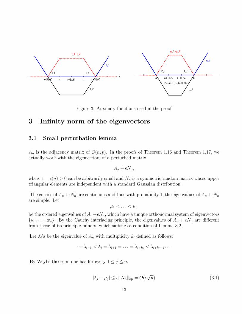
by a proper approximation. Define Il = [a − |I|C, a], Ir = [b, b + |I|

C] and construct two real

functions f1, f2 as follows(see Figure 3):

f1(x) =

− C|I|(x− a)− 1 if x ∈ (−∞, a− |I|

C)

0 if x ∈ I ∪ Il ∪ IrC|I|(x− b)− 1 if x ∈ (b+ |I|

C,∞)

f2(x) =

− C|I|(x− a)− 1 if x ∈ (−∞, a)

−1 if x ∈ IC|I|(x− b)− 1 if x ∈ (b,∞)

where C is a constant to be chosen later. Note that fj’s are convex and C|I| -Lipschitz. Define

X1 =n∑i=1

f1(λi), X2 =n∑i=1

f2(λi)

and apply Lemma 2.5 with T = δ8n∫Iρsc(t)dt for X1 and X2. Thus, we have

P(|Xj − E(Xj)| ≥δ

8n

∫I

ρsc(t)dt) ≤ 4 exp(−cδ2n2|I|2(

∫Iρsc(t)dt)

2

K2C2).

At this point we need to estimate the value of∫Iρsc(t)dt. There are two cases: if I is in the

“bulk” i.e. I ⊂ [−2+ε, 2−ε] for some positive absolute constant ε, then∫Iρsc(t)dt = α|I| where

α is a constant depending on ε. But if I is very near the edge of [−2, 2] i.e. a−(−2) < |I| = o(1),then

∫Iρsc(t)dt = α′|I|3/2 for some absolute constant α′. Thus in both case we have

P(|Xj − E(Xj)| ≥δ

8n

∫I

ρsc(t)dt) ≤ 4 exp(−c1δ2n2|I|5

K2C2)

Let X = X1 −X2, then

P(|X − E(X)| ≥ δ

4n

∫I

ρsc(t)dt) ≤ O(exp(−c1δ2n2|I|5

K2C2)).

Now we compare X to Z, making use of a result of Gotze and Tikhomirov [17]. We haveE(X−Z) ≤ E(NIl +NIr). In [17], Gotze and Tikhomirov obtained a convergence rate for ESDof Hermitian random matrices whose entries have mean zero and variance one, which impliesthat for any I ⊂ [−2, 2]

|E(NI)− n∫I

ρsc(t)dt| < βn

√M4

n,

10

where β is an absolute constant, M4 = supi,j E(|ωij|4). Thus

E(X) ≤ E(Z) + n

∫Il∪Ir

ρsc(t)dt+ βn

√M4

n.

In the “edge” case we can choose C = (4/δ)2/3, then because |I| ≥ Ω(δ−2/3(M4/n)1/3), we have

n

∫Il∪Ir

ρsc(t)dt = Θ(n(|I|C

)3/2) > Ω(n

√M4

n)

and

n

∫Il∪Ir

ρsc(t)dt+ βn

√M4

n= Θ(n(

|I|C

)3/2) = Θ(δ

4n

∫I

ρsc(t)dt).

In the “bulk” case we choose C = 4/δ, then

n

∫Il∪Ir

ρsc(t)dt+ βn

√M4

n= Θ(n

|I|C

) = Θ(δ

4n

∫I

ρsc(t)dt).

Therefore in both cases, with probability at least 1−O(exp(−c1δ4n2|I|5K2 )), we have

Z ≤ X ≤ E(X) +δ

4n

∫I

ρsc(t)dt < E(Z) +δ

2n

∫I

ρsc(t)dt.

The convergence rate result of Gotze and Tikhomirov again gives

E(NI) < n

∫I

ρsc(t)dt+ βn

√M4

n< (1 +

δ

2)n

∫I

ρsc(t)dt,

hence with probability at least 1−O(exp(−c1δ4n2|I|5K2 ))

Z < (1 + δ)n

∫I

ρsc(t)dt,

which is the desires upper bound.

The lower bound is proved using a similar argument. Let I ′ = [a+ |I|C, b− |I|

C], I ′l = [a, a+ |I|

C],

I ′r = [b − |I|C, b] where C is to be chosen later and define two functions g1, g2 as follows (see

Figure 3):

g1(x) =

− C|I|(x− a) if x ∈ (−∞, a)

0 if x ∈ I ′ ∪ I ′l ∪ I ′rC|I|(x− b) if x ∈ (b,∞)

11

g2(x) =

− C|I|(x− a) if x ∈ (−∞, a+ |I|

C)

−1 if x ∈ I ′C|I|(x− b) if x ∈ (b− |I|

C,∞)

DefineY1 =

∑i=1

g1(λi), Y2 =∑i=1

g2(λi).

Applying Lemma 2.5 with T = δ8n∫Iρsc(t)dt for Yj and using the estimation for

∫Iρ(t)dt as

above, we have

P(|Yj − E(Yj)| ≥δ

8n

∫I

ρsc(t)dt) ≤ 4 exp(−c2δ2n2|I|5

K2C2).

Let Y = Y1 − Y2, then

P(|Y − E(Y )| ≥ δ

4n

∫I

ρsc(t)dt) ≤ O(exp(−c2δ2n2|I|5

K2C2)).

We have E(Z − Y ) ≤ E(NI′l+ NI′r). A similar argument as in the proof of the upper bound

(using the convergence rate of Gotze and Tikhomirov) shows

E(Y ) ≥ E(Z)− n∫I′l∪I′r

ρsc(t)dt− βn√M4

n> E(Z)− δ

4n

∫I

ρsc(t)dt.

Therefore with probability at least 1−O(exp(−c2δ2n2|I|5K2C2 )), we have

Z ≥ Y ≥ E(Y )− δ

4n

∫I

ρsc(t)dt > E(Z)− δ

2n

∫I

ρsc(t)dt,

and by the convergence rate, with probability at least 1−O(exp(−c2 δ2n2|I|5K2C2 ))

Z > (1− δ)n∫I

ρsc(t)dt.

Thus, Theorem 2.2 is proved.

12

a-|I|/C a b b+|I|/C

f_1

f_2

f_1-f_2

I_l I_r

I=[a,b] a a+|I|/C b-|I|/C b

g_1-g_2

g_1

g_2

I'_l I'_r

I'=[a+|I|/C,b-|I|/C]

Figure 3: Auxiliary functions used in the proof

3 Infinity norm of the eigenvectors

3.1 Small perturbation lemma

An is the adjacency matrix of G(n, p). In the proofs of Theorem 1.16 and Theorem 1.17, weactually work with the eigenvectors of a perturbed matrix

An + εNn,

where ε = ε(n) > 0 can be arbitrarily small and Nn is a symmetric random matrix whose uppertriangular elements are independent with a standard Gaussian distribution.

The entries of An+εNn are continuous and thus with probability 1, the eigenvalues of An+εNn

are simple. Letµ1 < . . . < µn

be the ordered eigenvalues of An+εNn, which have a unique orthonormal system of eigenvectorsw1, . . . , wn. By the Cauchy interlacing principle, the eigenvalues of An + εNn are differentfrom those of its principle minors, which satisfies a condition of Lemma 3.2.

Let λi’s be the eigenvalue of An with multiplicity ki defined as follows:

. . . λi−1 < λi = λi+1 = . . . = λi+ki < λi+ki+1 . . .

By Weyl’s theorem, one has for every 1 ≤ j ≤ n,

|λj − µj| ≤ ε||Nn||op = O(ε√n) (3.1)

13

Thus the behaviors of eigenvalues of An and An + εNn are essentially the same by choosing εsufficiently small. And everything (except Lemma 3.2) we used in the proofs of Theorem 1.16and Theorem 1.17 for An also applies for An + εNn by a continuity argument. We will notdistinguish An from An + εNn in the proofs.

The following lemma will allow us to transfer the eigenvector delocaliztion results of An + εNn

to those of An at some expense.

Lemma 3.1. In the notations of above, there exists an orthonormal basis of eigenvectors ofAn, denoted by u1, . . . , un, such that for every 1 ≤ j ≤ n,

||uj||∞ ≤ ||wj||∞ + α(n),

where α(n) can be arbitrarily small provided ε(n) is small enough.

Proof. First, since the coefficients of the characteristic polynomial of An are integers, thereexists a positive function l(n) such that either |λs − λt| = 0 or |λs − λt| ≥ l(n) for any1 ≤ s, t ≤ n.

By (3.1) and choosing ε sufficiently small, one can get

|µi − λi−1| > l(n) and |µi+ki − λi+ki+1| > l(n)

For a fixed index i, let E be the eigenspace corresponding to the eigenvalue λi and F be thesubspace spanned by wi, . . . , wi+ki. Both of E and F have dimension ki. Let PE and PF bethe orthogonal projection matrices onto E and F separately.

Applying the well-known Davis-Kahan theorem (see [28] Section IV, Theorem 3.6) to An andAn + εNn, one gets

||PE − PF ||op ≤ε||Nn||op

l(n):= α(n),

where α(n) can be arbitrarily small depending on ε.

Define vj = PFwj ∈ E for i ≤ j ≤ i + ki, then we have ||vj − wj||2 ≤ α(n). It is clear thatvi, . . . , vki are eigenvectors of An and

||vj||∞ ≤ ||wj||∞ + ||vj − wj||2 ≤ ||wj||∞ + α(n).

By choosing ε small enough such that nα(n) < 1/2, vi, . . . , vki are linearly independent.Indeed, if

∑kij=i cjvj = 0, one has for every i ≤ s ≤ i+ ki,

∑kij=i cj〈PFwj, ws〉 = 0, which implies

cs = −∑ki

j=i cj〈PFwj − wj, ws〉. Thus |cs| ≤ α(n)∑ki

j=i |cj|, summing over all s, we can get∑kij=i |cj| ≤ kα(n)

∑kij=i |cj| and therefore cj = 0.

14

Furthermore the set vi, . . . , vki is ’almost’ an orthonormal basis of E in the sense that

| ||vs||2 − 1 | ≤ ||vs − ws||2 ≤ α(n) for any i ≤ s ≤ i+ ki

|〈vs, vt〉| = |〈PFws, PFwt〉|= |〈PFws − ws, PFwt〉+ 〈ws, PFwt − wt〉|= O(α(n)) for any i ≤ s 6= t ≤ i+ ki

We can perform a Gram-Schmidt process on vi, . . . , vki to get an orthonormal system ofeigenvectors ui, . . . , uki on E such that

||uj||∞ ≤ ||wj||∞ + α(n),

for every i ≤ j ≤ i+ ki.

We iterate the above argument for every distinct eigenvalue of An to obtain an orthonormalbasis of eigenvectors of An.

3.2 Auxiliary lemmas

Lemma 3.2. (Lemma 41, [30]) Let

Bn =

(a X∗

X Bn−1

)be a n×n symmetric matrix for some a ∈ C and X ∈ Cn−1, and let

(xv

)be a eigenvector of

Bn with eigenvalue λi(Bn), where x ∈ C and v ∈ Cn−1. Suppose that none of the eigenvaluesof Bn−1 are equal to λi(Bn). Then

|x|2 =1

1 +∑n−1

j=1 (λj(Bn−1)− λi(Bn))−2|uj(Bn−1)∗X|2,

where uj(Bn−1) is a unit eigenvector corresponding to the eigenvalue λj(Bn−1).

The Stieltjes transform sn(z) of a symmetric matrix W is defined for z ∈ C by the formula

sn(z) :=1

n

n∑i=1

1

λi(W )− z.

15

It has the following alternate representation:

Lemma 3.3. (Lemma 39, [30]) Let W = (ζij)1≤i,j≤n be a symmetrix matrix, and let z be acomplex number not in the spectrum of W . Then we have

sn(z) =1

n

n∑k=1

1

ζkk − z − a∗k(Wk − zI)−1ak

where Wk is the (n − 1) × (n − 1) matrix with the kth row and column of W removed, andak ∈ Cn−1 is the kth column of W with the kth entry removed.

We begin with two lemmas that will be needed to prove the main results. The first lemma,following the paper [30] in Appendix B, uses Talagrand’s inequality. Its proof is presented inthe Appendix B.

Lemma 3.4. Let Y = (ζ1, . . . , ζn) ∈ Cn be a random vector whose entries are i.i.d. copies ofthe random variable ζ = ξ−p (with mean 0 and variance σ2). Let H be a subspace of dimensiond and πH the orthogonal projection onto H. Then

P(| ‖ πH(Y ) ‖ −σ√d| ≥ t) ≤ 10 exp(−t

2

4).

In particular,‖ πH(Y ) ‖= σ

√d+O(ω(

√log n)) (3.2)

with overwhelming probability.

The following concentration lemma for G(n, p) will be a key input to prove Theorem 1.17. LetBn = 1√

nσAn

Lemma 3.5 (Concentration for ESD in the bulk). (Concentration for ESD in the bulk) Assumep = g(n) log n/n. For any constants ε, δ > 0 and any interval I in [−2 + ε, 2 − ε] of width|I| = Ω(log2.2 g(n) log n/np), the number of eigenvalues NI of Bn in I obeys the concentrationestimate

|NI(Bn)− n∫I

ρsc(x) dx| ≤ δn|I|

with overwhelming probability.

The above lemma is a variant of Corollary 2.3. This lemma allows us to control the ESD ona smaller interval and the proof, relying on a projection lemma (Lemma 3.4), is a differentapproach. The proof is presented in Appendix C.

16

3.3 Proof of Theorem 1.16:

Let λn(An) be the largest eigenvalue of An and u = (u1, . . . , un) be the corresponding uniteigenvector. We have the lower bound λn(An) ≥ np. And if np = ω(log n), then the maximumdegree ∆ = (1 + o(1))np almost surely (See Corollary 3.14, [4]).

For every 1 ≤ i ≤ n,

λn(An)ui =∑j∈N(i)

uj,

where N(i) is the neighborhood of vertex i. Thus, by Cauchy-Schwarz inequality,

||u||∞ = maxi|∑

j∈N(i) uj|λn(An)

≤√

∆

λn(An)= O(

1√np

).

Let Bn = 1√nσAn. Since the eigenvalues of Wn = 1√

nσ(An − pJn) are on the interval [−2, 2], by

Lemma 1.1, λ1(Bn), . . . , λn−1(Bn) ⊂ [−2, 2].

Recall that np = g(n) log n. By Corollary 2.3, for any interval I with length at least ( log(np)

δ4(np)1/2)1/5(say

δ = 0.5),with overwhelming probability, if I ⊂ [−2 +κ, 2−κ] for some positive constant κ, onehas NI(Bn) = Θ(n

∫Iρsc(x)dx) = Θ(n|I|); if I is at the edge of [−2, 2], with length o(1), one

has NI(Bn) = Θ(n∫Iρsc(x)dx) = Θ(n|I|3/2). Thus we can find a set J ⊂ 1, . . . , n − 1 with

|J | = Ω(n|I0|) or |J | = Ω(n|I0|3/2) such that |λj(Bn−1) − λi(Bn)| |I0| for all j ∈ J , whereBn−1 is the bottom right (n− 1)× (n− 1) minor of Bn. Here we take |I0| = (1/g(n)1/20)2/3. It

is easy to check that |I0| ≥ ( log(np)

δ4(np)1/2)1/5.

By the formula in Lemma 3.2, the entry of the eigenvector of Bn can be expressed as

|x|2 =1

1 +∑n−1

j=1 (λj(Bn−1)− λi(Bn))−2|uj(Bn−1)∗ 1√nσX|2

≤ 1

1 +∑

j∈J(λj(Bn−1)− λi(Bn))−2|uj(Bn−1)∗ 1√nσX|2

≤ 1

1 +∑

j∈J n−1|I0|−2|uj(Bn−1)∗ 1

σX|2

=1

1 + n−1|I0|−2||πH(Xσ

)||2

≤ 1

1 + n−1|I0|−2|J |

(3.3)

with overwhelming probability, where H is the span of all the eigenvectors associated to Jwith dimension dim(H) = Θ(|J |), πH is the orthogonal projection onto H and X ∈ Cn−1 has

17

entries that are iid copies of ξ. The last inequality in (3.3) follows from Lemma 3.4 (by takingt = g(n)1/10

√log n) and the relations

||πH(X)|| = ||πH(Y + p1n)|| ≥ ||πH1(Y + p1n)|| ≥ ||πH1(Y )||.

Here Y = X − p1n and H1 = H ∩H2, where H2 is the space orthogonal to the all 1 vector 1n.For the dimension of H1, dim(H1) ≥ dim(H)− 1 .

Since either |J | = Ω(n|I0|) or |J | = Ω(n|I0|3/2), we have n−1|I0|−2|J | = Ω(|I0|−1) or n−1|I0|−2|J | =Ω(|I0|−1/2). Thus |x|2 = O(|I0|) or |x|2 = O(

√|I0|). In both cases, since |I0| → 0, it follows

that |x| = o(1).

3.4 Proof of Theorem 1.17

With the formula in Lemma 3.2, it suffices to show the following lower bound

n−1∑j=1

(λj(Bn−1)− λi(Bn))−2|uj(Bn−1)∗1√nσ

X|2 np

log2.2 g(n) log n(3.4)

with overwhelming probability, where Bn−1 is the bottom right n− 1× n− 1 minor of Bn andX ∈ Cn−1 has entries that are iid copies of ξ. Recall that ξ takes values 1 with probability pand 0 with probability 1− p, thus Eξ = p,Varξ = p(1− p) = σ2.

By Theorem 3.5, we can find a set J ⊂ 1, . . . , n − 1 with |J | log2.2 g(n) lognp

such that

|λj(Bn−1)− λi(Bn)| = O(log2.2 g(n) log n/np) for all j ∈ J . Thus in (3.4), it is enough to prove∑j∈J

|uj(Bn−1)T1

σX|2 = ||πH(

X

σ)||2 |J |

or equivalently||πH(X)||2 σ2|J | (3.5)

with overwhelming probability, where H is the span of all the eigenvectors associated to J withdimension dim(H) = Θ(|J |).

Let H1 = H ∩ H2, where H2 is the space orthogonal to 1n. The dimension of H1 is at leastdim(H)− 1. Denote Y = X − p1n. Then the entries of Y are iid copies of ζ. By Lemma 3.4,

||πH1(Y )||2 σ2|J |

18

with overwhelming probability.

Hence, our claim follows from the relations

||πH(X)|| = ||πH(Y + p1n)|| ≥ ||πH1(Y + p1n)|| = ||πH1(Y )||.

Appendices

In this appendix, we complete the proofs of Theorem 1.3, Lemma 3.4 and Lemma 3.5.

A Proof of Theorem 1.3

We will show that the semicircle law holds for Mn. With Lemma 1.1, it is clear that Theorem1.3 follows Lemma A.1 directly. The claim actually follows as a special case discussed in thepaper [6]. Our proof here uses a standard moment method.

Lemma A.1. For p = ω( 1n), the empirical spectral distribution (ESD) of the matrix Wn =

1√nMn converges in distribution to the semicircle law which has a density ρsc(x) with support

on [−2, 2],

ρsc(x) :=1

2π

√4− x2.

Let ηij be the entries of Mn = σ−1(An − pJn). For i = j, ηij = −p/σ; and for i 6= j, ηij areiid copies of random variable η, which takes value (1− p)/σ with probability p and takes value−p/σ with probability 1− p.

Eη = 0,Eη2 = 1,Eηs = O

(1

(√p)s−2

)for s ≥ 2.

For a positive integer k, the kth moment of ESD of the matrix Wn is∫xkdFW

n (x) =1

nE(Trace(Wn

k)),

19

and the kth moment of the semicircle distribution is∫ 2

−2

xkρsc(x)dx.

On a compact set, convergence in distribution is the same as convergence of moments. Toprove the theorem, we need to show, for every fixed number k,

1

nE(Trace(Wn

k))→∫ 2

−2

xkρsc(x)dx, as n→∞. (A.1)

For k = 2m+ 1, by symmetry,

∫ 2

−2

xkρsc(x)dx = 0.

For k = 2m, ∫ 2

−2

xkρsc(x)dx =1

π

∫ 2

0

xk√

4− x2dx =2k+2

π

∫ π/2

0

sink θcos2 θdx

=2k+2

π

Γ(k+12

)Γ(32)

Γ(k+42

)=

1

m+ 1

(2m

m

)

Thus our claim (A.1) follows by showing that

1

nE(Trace(Wn

k)) =

O( 1√

np) if k = 2m+ 1;

1m+1

(2mm

)+O( 1

np) if k = 2m.

(A.2)

We have the expansion for the trace of Wnk,

1

nE(Trace(Wn

k)) =1

n1+k/2E(Trace(σ−1Mn)k)

=1

n1+k/2

∑1≤i1,...,ik≤n

Eηi1i2ηi2i3 · · · ηiki1(A.3)

Each term in the above sum corresponds to a closed walk of length k on the complete graphKn on 1, 2, . . . , n. On the other hand, ηij are independent with mean 0. Thus the term isnonzero if and only if every edge in this closed walk appears at least twice. And we call such awalk a good walk. Consider a good walk that uses l different edges e1, . . . , el with corresponding

20

multiplicities m1, . . . ,ml, where l ≤ m, each mh ≥ 2 and m1 + . . . + ml = k. Now thecorresponding term to this good walk has form

Eηm1e1· · · ηml

el.

Since such a walk uses at most l + 1 vertices, a naive upper bound for the number of goodwalks of this type is nl+1 × lk.

When k = 2m+ 1, recall Eηs = Θ((√p)2−s) for s ≥ 2, and so

1

nE(Trace(Wn

k)) =1

n1+k/2

m∑l=1

∑good walk of l edges

Eηm1e1· · · ηml

el

≤ 1

nm+3/2

m∑l=1

nl+1lk(1√p

)m1−2 . . . (1√p

)ml−2

= O(1√np

).

When k = 2m, we classify the good walks into two types. The first kind uses l ≤ m−1 differentedges. The contribution of these terms will be

1

n1+k/2

m−1∑l=1

∑1st kind of good walk of l edges

Eηm1e1· · · ηml

el≤ 1

n1+m

m∑l=1

nl+1lk(1√p

)m1−2 . . . (1√p

)ml−2

= O(1

np).

The second kind of good walk uses exactly l = m different edges and thus m + 1 differentvertices. And the corresponding term for each walk has form

Eη2e1· · · η2

el= 1.

The number of this kind of good walk is given by the following result in the paper ([1], Page617–618):

Lemma A.2. The number of the second kind of good walk is

nm+1(1 +O(n−1))

m+ 1

(2m

m

).

21

Then the second conclusion of (A.1) follows.

B Proof of Lemma 3.4:

The coordinates of Y are bounded in magnitude by 1. Apply Talagrand’s inequality to the mapY → ||πH(Y )||, which is convex and 1-Lipschitz. We can conclude

P(| ‖ πH(Y ) ‖ −M(‖ πH(Y ) ‖)| ≥ t) ≤ 4 exp(− t2

16) (B.1)

where M(‖ πH(Y ) ‖) is the median of ‖ πH(Y ) ‖.

Let P = (pij)1≤i,j≤n be the orthogonal projection matrix onto H. One has traceP 2 =traceP =∑i pii = d and |pii| ≤ 1, as well as,

‖ πH(Y ) ‖2 =∑

1≤i,j≤n

pijζiζj =n∑i=1

piiζ2i +

∑i 6=j

pijζiζj

and

E‖ πH(Y ) ‖2 = E(n∑i=1

piiζ2i ) + E(

∑i 6=j

pijζiζj) = σ2d.

Take L = 4/σ. To complete the proof, it suffices to show

|M(‖ πH(Y ) ‖)− σ√d| ≤ Lσ. (B.2)

Consider the event E+ that ‖ πH(Y ) ‖≥ σL+ σ√d, which implies that ‖ πH(Y ) ‖2 ≥ σ2(L2 +

2L√d+ d2).

Let S1 =∑n

i=1 pii(ζ2i − σ2) and S2 =

∑i 6=j pijζiζj.

Now we have

P(E+) ≤ P(n∑i=1

piiζ2i ≥ σ2d+ L

√dσ2) + P(

∑i 6=j

pijζiζj ≥ σ2L√d).

22

By Chebyshev’s inequality,

P(n∑i=1

piiζ2i ≥ σ2d+ L

√dσ2) = P(S1 ≥ L

√dσ2)) ≤ E(|S1|2)

L2dσ4,

where E(|S1|2) = E(∑

i pii(ζ2i − σ2))2 =

∑i p

2iiE(ζ4

i − σ4) ≤ dσ2(1− 2σ2).

Therefore, P(S1 ≥ L√dσ4) ≤ dσ2(1− 2σ2)

L2dσ4<

1

16.

On the other hand, we have E(|S2|2) = E(∑

i 6=j p2ijζ

2i ζ

2j ) ≤ σ4d and

P(∑i 6=j

pijζiζj ≥ σ2L√d) = P(S2 ≥ L

√dσ2) ≤ E(|S2|2)

L2dσ4<

1

10

It follows that E(E+) < 1/4 and hence M(‖ πH(Y ) ‖) ≤ Lσ +√dσ.

For the lower bound, consider the event E− that ‖ πH(Y ) ‖≤√dσ − Lσ and notice that

P(E−) ≤ P(S1 ≤ −L√dσ2) + P(S2 ≤ −L

√dσ2).

The same argument applies to get M(‖ πH(Y ) ‖) ≥√dσ − Lσ. Now the relations (B.1) and

(B.2) together imply (3.2).

C Proof of Lemma 3.5:

Recall the normalized adjacency matrix

Mn =1

σ(An − pJn),

where Jn = 1n1Tn is the n× n matrix of all 1’s, and let Wn = 1√

nMn.

Lemma C.1. For all intervals I ⊂ R with |I| = ω(log n)/np, one has

NI(Wn) = O(n|I|)

with overwhelming probability.

23

The proof of Lemma C.1 uses the same proof as in the paper [30] with the relation (3.2).

Actually we will prove the following concentration theorem for Mn. By Lemma 1.1, |NI(Wn)−NI(Bn)| ≤ 1, therefore Lemma C.2 implies Lemma 3.5.

Lemma C.2. (Concentration for ESD in the bulk) Assume p = g(n) log n/n. For any constantsε, δ > 0 and any interval I in [−2 + ε, 2− ε] of width |I| = Ω(g(n)0.6 log n/np), the number ofeigenvalues NI of Wn = 1√

nMn in I obeys the concentration estimate

|NI(Wn)− n∫I

ρsc(x) dx| ≤ δn|I|

with overwhelming probability.

To prove Theorem C.2, following the proof in [30], we consider the Stieltjes transform

sn(z) :=1

n

n∑i=1

1

λi(Wn)− z,

whose imaginary part

Imsn(x+√−1η) =

1

n

n∑i=1

η

η2 + (λi(Wn)− x)2> 0

in the upper half-plane η > 0.

The semicircle counterpart

s(z) :=

∫ 2

−2

1

x− zρsc(x) dx =

1

2π

∫ 2

−2

1

x− z√

4− x2 dx,

is the unique solution to the equation

s(z) +1

s(z) + z= 0

with Ims(z) > 0.

The next proposition gives control of ESD through control of Stieltjes transform (we will takeL = 2 in the proof):

24

Proposition C.3. (Lemma 60, [30]) Let L, ε, δ > 0. Suppose that one has the bound

|sn(z)− s(z)| ≤ δ

with (uniformly) overwhelming probability for all z with |Re(z)| ≤ L and Im(z) ≥ η. Then forany interval I in [−L+ ε, L− ε] with |I| ≥ max(2η, η

δlog 1

δ), one has

|NI − n∫I

ρsc(x) dx| ≤ δn|I|

with overwhelming probability.

By Proposition C.3, our objective is to show

|sn(z)− s(z)| ≤ δ (C.1)

with (uniformly) overwhelming probability for all z with |Re(z)| ≤ 2 and Im(z) ≥ η, where

η =log2 g(n) log n

np.

In Lemma 3.3, we write

sn(z) =1

n

n∑k=1

1

− ζkk√nσ− z − Yk

(C.2)

whereYk = a∗k(Wn,k − zI)−1ak,

Wn,k is the matrix Wn with the kth row and column removed, and ak is the kth row of Wn withthe kth element removed.

The entries of ak are independent of each other and of Wn,k, and have mean zero and variance1/n. By linearity of expectation we have

E(Yk|Wn,k) =1

nTrace(Wn,k − zI)−1 = (1− 1

n)sn,k(z)

where

sn,k(z) =1

n− 1

n−1∑i=1

1

λi(Wn,k)− z

25

is the Stieltjes transform of Wn,k. From the Cauchy interlacing law, we get

|sn(z)− (1− 1

n)sn,k(z)| = O(

1

n

∫R

1

|x− z|2dx) = O(

1

nη) = o(1),

and thusE(Yk|Wn,k) = sn(z) + o(1).

In fact a similar estimate holds for Yk itself:

Proposition C.4. For 1 ≤ k ≤ n, Yk = E(Yk|Wn,k)+o(1) holds with (uniformly) overwhelmingprobability for all z with |Re(z)| ≤ 2 and Im(z) ≥ η.

Assume this proposition for the moment. By hypothesis, | ζkk√nσ| = | −p√

nσ| = o(1). Thus in (C.2),

we actually get

sn(z) +1

n

n∑k=1

1

sn(z) + z + o(1)= 0 (C.3)

with overwhelming probability. This implies that with overwhelming probability either sn(z) =s(z) + o(1) or that sn(z) = −z + o(1). On the other hand, as Imsn(z) is necessarily positive,the second possibility can only occur when Imz = o(1). A continuity argument (as in [11]) thenshows that the second possibility cannot occur at all and the claim follows.

Now it remains to prove Proposition C.4.

Proof of Proposition C.4. Decompose

Yk =n−1∑j=1

|uj(Wn,k)∗ak|2

λj(Wn,k)− z

and evaluate

Yk − E(Yk|Wn,k) = Yk − (1− 1

n)sn,k(z) + o(1)

=n−1∑j=1

|uj(Wn,k)∗ak|2 − 1

n

λj(Wn,k)− z+ o(1)

=n−1∑j=1

Rj

λj(Wn,k)− z+ o(1),

(C.4)

26

where we denote Rj = |uj(Wn,k)∗ak|2 −

1

n, uj(Wn,k) are orthonormal eigenvectors of Wn,k.

Let J ⊂ 1, . . . , n− 1, then

∑j∈J

Rj = ||PH(ak)||2 −dim(H)

n

where H is the space spanned by uj(Wn,k) for j ∈ J and PH is the orthogonal projectiononto H.

In Lemma 3.4, by taking t = h(n)√

log n, where h(n) = log0.001 g(n), one can conclude withoverwhelming probability

|∑j∈J

Rj| 1

n

(h(n)

√|J | log n√p

+h(n)2 log n

p

). (C.5)

Using the triangle inequality,

∑j∈J

|Rj| 1

n

(|J |+ h(n)2 log n

p

)(C.6)

with overwhelming probability.

Let z = x+√−1η, where η = log2 g(n) log n/np and |x| ≤ 2− ε, define two parameters

α =1

log4/3 g(n)and β =

1

log1/3 g(n).

First, for those j ∈ J such that |λj(Wn,k)−x| ≤ βη, the function 1λj(Wn,k)−x−

√−1η

has magnitude

O( 1η). From Lemma C.1, |J | nβη, and so the contribution for these j ∈ J is,

|∑j∈J

Rj

λj(Wn,k)− z| 1

nη

(nβη +

h(n)2

log2 g(n)

)= O(

1

log1/3 g(n)) = o(1).

For the contribution of the remaining j ∈ J , we subdivide the indices as

27

a ≤ |λj(Wn,k)− x| ≤ (1 + α)a

where a = (1 + α)lβη, for 0 ≤ l ≤ L, and then sum over l.

For each such interval, the function 1λj(Wn,k)−x−

√−1η

has magnitude O( 1a) and fluctuates by at

most O(αa). Say J is the set of all j’s in this interval, thus by Lemma C.1, |J | = O(nαa).

Together with bounds (C.5), (C.6), the contribution for these j on such an interval,

|∑j∈J

Rj

λj(Wn,k)− z| 1

an

(h(n)

√|J | log n√p

+h(n)2 log n

p

)+

α

an

(|J |+ h(n)2 log n

p

)

= O

( √α√

(1 + α)lh(n)√

β log g(n)+

h2(n)

(1 + α)lβ log2 g(n)+ α2

)

= O

(1√αβ

h(n)

log g(n)+ α log

1

βη

)

Summing over l and noticing that (1 + α)Lη/g(n)1/4 ≤ 3, we get

|∑

j∈J,allJ

Rj

λj(Wn,k)− z| = O

(1√αβ

h(n)

log g(n)+ α log

1

βη

)= O

(h(n)

log1/6 g(n)

)= o(1).

Acknowledgement. The authors thank Terence Tao for useful conversations.

References

[1] Z.D. Bai. Methodologies in spectral analysis of large dimensional random matrices, a re-view. In Advances in statistics: proceedings of the conference in honor of Professor ZhidongBai on his 65th birthday, National University of Singapore, 20 July 2008, volume 9, page174. World Scientific Pub Co Inc, 2008.

[2] M. Bauer and O. Golinelli. Random incidence matrices: moments of the spectral density.Journal of Statistical Physics, 103(1):301–337, 2001.

28

[3] S. Bhamidi, S.N. Evans, and A. Sen. Spectra of large random trees. Arxiv preprintarXiv:0903.3589, 2009.

[4] B. Bollobas. Random graphs. Cambridge Univ Pr, 2001.

[5] S. Brooks and E. Lindenstrauss. Non-localization of eigenfunctions on large regular graphs.Arxiv preprint arXiv:0912.3239, 2009.

[6] F. Chung, L. Lu, and V. Vu. The spectra of random graphs with given expected degrees.Internet Mathematics, 1(3):257–275, 2004.

[7] Y. Dekel, J. Lee, and N. Linial. Eigenvectors of random graphs: Nodal domains. InAPPROX ’07/RANDOM ’07: Proceedings of the 10th International Workshop on Ap-proximation and the 11th International Workshop on Randomization, and Combinato-rial Optimization. Algorithms and Techniques, pages 436–448, Berlin, Heidelberg, 2007.Springer-Verlag.

[8] Y. Dekel, J. Lee, and N. Linial. Eigenvectors of random graphs: Nodal domains. Approx-imation, Randomization, and Combinatorial Optimization. Algorithms and Techniques,pages 436–448, 2008.

[9] I. Dumitriu and S. Pal. Sparse regular random graphs: spectral density and eigenvectors.Arxiv preprint arXiv:0910.5306, 2009.

[10] L. Erdos, B. Schlein, and H.T. Yau. Semicircle law on short scales and delocalization ofeigenvectors for Wigner random matrices. Ann. Probab, 37(3):815–852, 2009.

[11] L. Erdos, B. Schlein, and H.T. Yau. Local semicircle law and complete delocalization forWigner random matrices. Accepted in Comm. Math. Phys. Communications in Mathe-matical Physics, 287(2):641–655, 2010.

[12] U. Feige and E. Ofek. Spectral techniques applied to sparse random graphs. RandomStructures and Algorithms, 27(2):251, 2005.

[13] J. Friedman. On the second eigenvalue and random walks in random d-regular graphs.Combinatorica, 11(4):331–362, 1991.

[14] J. Friedman. Some geometric aspects of graphs and their eigenfunctions. Duke Math. J,69(3):487–525, 1993.

[15] J. Friedman. A proof of Alon’s second eigenvalue conjecture. In Proceedings of the thirty-fifth annual ACM symposium on Theory of computing, pages 720–724. ACM, 2003.

[16] Z Furedi and J. Komlos. The eigenvalues of random symmetric matrices. Combinatorica,1(3):233–241, 1981.

29

[17] F. Gotze and A. Tikhomirov. Rate of convergence to the semi-circular law. ProbabilityTheory and Related Fields, 127(2):228–276, 2003.

[18] A. Guionnet and O. Zeitouni. Concentration of the spectral measure for large matrices.Electron. Comm. Probab, 5:119–136, 2000.

[19] S. Janson, T. Luczak, and A. Rucinski. Random graphs. Citeseer, 2000.

[20] M. Krivelevich, B. Sudakov, V.H. Vu, and N.C. Wormald. Random regular graphs of highdegree. Random Structures and Algorithms, 18(4):346–363, 2001.

[21] B.D. McKay. The expected eigenvalue distribution of a large regular graph. Linear Algebraand its Applications, 40:203–216, 1981.

[22] B.D. McKay and N.C. Wormald. Asymptotic enumeration by degree sequence of graphswith degrees o(n1/2). Combinatorica 11 , no. 4, 369–382., 1991.

[23] B.D. McKay and N.C. Wormald. The degree sequence of a random graph. I. The models.Random Structures Algorithms 11, no. 2, 97–117, 1997.

[24] A. Pothen, H.D. Simon, and K.P. Liou. Partitioning sparse matrices with eigenvectors ofgraphs. SIAM Journal on Matrix Analysis and Applications, 11:430, 1990.

[25] G. Semerjian and L.F. Cugliandolo. Sparse random matrices: the eigenvalue spectrumrevisited. Journal of Physics A: Mathematical and General, 35:4837–4851, 2002.

[26] E Shamir and E Upfal. Large regular factors in random graphs. Convexity and graphtheory (Jerusalem, 1981), 1981.

[27] J. Shi and J. Malik. Normalized cuts and image segmentation. IEEE Transactions onpattern analysis and machine intelligence, 22(8):888–905, 2000.

[28] G.W. Stewart and Ji-guang. Sun. Matrix perturbation theory. Academic press New York,1990.

[29] T. Tao and V. Vu. Random matrices: Universality of local eigenvalue statistics up to theedge. Communications in Mathematical Physics, pages 1–24, 2010.

[30] T. Tao and V. Vu. Random matrices: Universality of the local eigenvalue statistics,submitted. Institute of Mathematics, University of Munich, Theresienstr, 39, 2010.

[31] V. Vu. Random discrete matrices. Horizons of Combinatorics, pages 257–280, 2008.

[32] E.P. Wigner. On the distribution of the roots of certain symmetric matrices. Annals ofMathematics, 67(2):325–327, 1958.

[33] N.C. Wormald. Models of random regular graphs. London Mathematical Society LectureNote Series, pages 239–298, 1999.

30