Sparse-promoting Full Waveform Inversion based on · PDF fileSparse-promoting Full Waveform Inversion based on Online Orthonormal Dictionary Learning Lingchen Zhu, Entao Liu, and James

Sparse-promoting Full Waveform Inversion based

on Online Orthonormal Dictionary Learning

Lingchen Zhu, Entao Liu, and James H. McClellan

Center for Energy and Geo Processing (CeGP) at Georgia Techand KFUPM

75 Fifth Street NW, Atlanta, GA 30308

November 7, 2016

Abstract

Full waveform inversion (FWI) delivers high-resolution images of thesubsurface by minimizing iteratively the misfit between the recorded andcalculated seismic data. It has been attacked successfully with the Gauss-Newton method and sparsity promoting regularization based on fixed mul-tiscale transforms that permit significant subsampling of the seismic datawhen the model perturbation at each FWI data-fitting iteration can berepresented with sparse coefficients. Rather than using analytical trans-forms with predefined dictionaries to achieve sparse representation, we in-troduce an adaptive transform called the Sparse Orthonormal Transform(SOT) whose dictionary is learned from many small training patches takenfrom the model perturbations in previous iterations. The patch-baseddictionary is constrained to be orthonormal and trained with an onlineapproach to provide the best sparse representation of the complex featuresand variations of the entire model perturbation. The complexity of thetraining method is proportional to the cube of the number of samples inone small patch. By incorporating both compressive subsampling and theadaptive SOT-based representation into the Gauss-Newton least-squaresproblem for each FWI iteration, the model perturbation can be recoveredafter an `1-norm sparsity constraint is applied on the SOT coefficients.Numerical experiments on synthetic models demonstrate that the SOT-based sparsity promoting regularization can provide robust FWI resultswith reduced computation.

1 Introduction

Seismic imaging reveals properties of the Earth’s subsurface by recordingand processing seismic waves. One way to achieve this goal is by full waveforminversion (FWI), which is a data-fitting procedure that minimizes the misfit

1

arX

iv:1

511.

0519

4v2

[ph

ysic

s.ge

o-ph

] 4

Nov

201

6

between recorded and calculated seismic data to create high-resolution models.A conventional FWI method is carried out iteratively. Each iteration consistsof solving wave equations with the current model parameters to generate seis-mic data, calculating the value as well as the gradient of the misfit function,and updating the model parameters with an optimization method [Tarantola,1984, Tarantola, 1986, Virieux and Operto, 2009]. The efficiency of these threecomponents determines the industrial applicability of FWI in the real world.By recording the response of sequential sources on the surface or in the water,a wide-aperture seismic survey typically covers a large area of interest. Becausethe discretized sizes of seismic datasets and models could both be huge, com-putation of forward modeling, misfit calculation and model updating in FWIcould be very intensive. In this paper, we discretize the wave equations inthe frequency domain with a finite-difference method, which yields compact ex-pressions and numerical advantages [Pratt, 1999]. Since each source, or eachfrequency component, parametrizes an individual wave equation to solve, thecomputational cost is proportional to the number of frequency components (forfrequency-domain forward modeling) and/or sources (for iterative solvers). Sucha computational burden is usually termed the “curse of dimensionality” [Her-rmann et al., 2012] and has to be relieved by reducing the problem dimension-ality.

1.1 Related Work

Reducing the computational cost of FWI has been an active research areafor many years. When a frequency-domain FWI is carried out, one can di-vide the frequency range of interest into several bands [Bunks et al., 1995],and invert only a few frequencies per band, sequentially from the low to highfrequency bands, to help reduce the cost [Sirgue and Pratt, 2004]. Another well-known method for cost reduction is to generate simultaneous shots by linearlycombining one or several different sequential shots at different source positionswith random weights [Krebs et al., 2009,Moghaddam and Herrmann, 2010,Ben-Hadj-Ali et al., 2011, Castellanos et al., 2015], or randomly choosing a few se-quential shots at each FWI iteration [Li and Herrmann, 2012, Warner et al.,2013]. Though these methods employ different data acquisition strategies, theyessentially reduce the amount of data used in the FWI misfit function in thefrequency and spatial domains.

In recent years, compressive sensing (CS) has attracted considerable atten-tion by proving that it is possible to recover sparse information vectors froma subsampled dataset with high robustness in the presence of noise and ar-tifacts. CS has been widely applied in seismic data processing tasks such asrecovery [Herrmann et al., 2008,Yu et al., 2015] and denoising [Hennenfent andHerrmann, 2006]. The basic idea is that seismic data can be represented witha sparse set of coefficients over a carefully chosen domain, which then impliesthat we no longer need to maintain high temporal or spatial sampling rates.Instead, we can acquire data at a much reduced sampling rate and process thesmaller data sets in the compressed domain to reduce complexity. A typical CS

2

problem involves three steps: (1) data randomization, (2) subsampling and (3)sparsity promotion. Randomization of the data plays an important role due toits ability to suppress coherent subsampling-related interferences such as alias-ing and crosstalk into relatively harmless Gaussian noise [Donoho and Tanner,2010]. It is then safe to extract the underlying sparsity through the solution ofan optimization problem coupled with an `p-norm (0 ≤ p ≤ 1) constraint, evenwhen the signal sampling rate is well below Nyquist.

Researchers have extended the above idea from seismic data processing tomore sophisticated seismic imaging and inversion problems by assuming spar-sity on the velocity models. For example, [Loris et al., 2007] regularized themodel in the wavelet domain with `1-norm constraints, allowing sharp velocitydiscontinuities (model perturbations) to be superimposed on a smooth back-ground model. Celebrated works reported by [Herrmann et al., 2011], [Li et al.,2012] and [Li et al., 2016] discover the `1-norm sparsity of model perturbationsin the curvelet domain [Candes and Demanet, 2005,Candes et al., 2006] so thatthey can be efficiently updated via a random subset of the full data. [Ma et al.,2012] introduced the image-guided gradient to FWI which leads to a significantreduction in the number of model parameters to be inverted. [Xue and Zhu,2015] imposed seislet-domain `1-norm sparsity regularization on the model toimprove the robustness and efficiency of FWI. All these methods reduce thecomputational complexity of the FWI problem without degrading the qualityof the result by regularizing the sparsity of the model (or its perturbation) overa predefined transform domain.

1.2 Main Contribution

In this paper, we propose a new framework for the FWI Gauss-Newtonmethod where the model perturbation is compressed by adaptive data-drivendictionaries [Sezer, 2012, Cai et al., 2014, Sezer et al., 2015, Zhu et al., 2016]so that it has a very sparse representation in the resulting adaptive transform.Each data-driven dictionary is learned from a set of small patches taken from amodel perturbation. Based on the resulting sparsity promoting transform, thedimensionality of FWI can then be greatly reduced via randomized phase encod-ing and subsampling. Compared to the traditional model-based transforms suchas wavelet, curvelet and seislet with predefined dictionaries, dictionary learningmethods are better able to adapt to nonintuitive signal regularities beyond piece-wise smoothness. Therefore, they have become a promising technique for sparsesignal representation and approximation. In fact, the complex subsurface modelparameters may be difficult to capture with any concise analytical model, leav-ing dictionary learning as the only alternative. However, prevailing dictionarylearning algorithms such as K-Singular Value Decomposition (K-SVD) [Aharonet al., 2006], as well as its variants [Rubinstein et al., 2010, Rubinstein et al.,2013] are too expensive, so we prefer to learn orthonormal dictionaries that havesimple implementations for sparse representation in FWI.

The contributions in this paper are the following:

3

• We propose an online approach for orthonormal dictionary learning byminimizing the expectation of the cost function when new training patchesjoin.

• We design a fast block-wise orthonormal transform called the sparse or-thonormal transform (SOT) based on the learned dictionaries in order toexploit the sparsity of model perturbations.

• We implement a CS framework in the FWI problems by admitting sparserepresentation of model perturbations over learned dictionaries and reduc-ing the problem dimensionality by selecting random sequential shots.

• Tests on several synthetic velocity models demonstrate that our methodcan significantly reduce the amount of data needed for FWI and thereforedecrease the computation time without introducing visible artifacts.

1.3 Notation

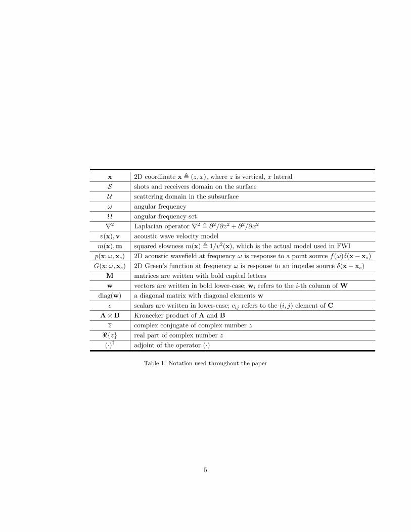
Although our work is exemplified on 2D models in this paper, an extensionto 3D case would not be difficult. Before we describe our methodology in detail,we give a summary of the notation that is going to be used throughout thispaper in Table 1.

1.4 Outline

The rest of the paper is organized as follows: In the second section, we re-view the FWI problem in the frequency domain based on updating the modelperturbation via the Gauss-Newton method. The following section describesthe orthonormal dictionary learning method and introduces an online learningapproach designed for FWI. The next section combines the above two topicstogether and formulates an FWI framework based on CS that comes with ran-domized phase encoding, subsampling and sparsity regularization. A practicalmethod to solve this problem is also presented in this section. Numerical resultsfrom synthetic models are given in the next section, followed by discussion andconclusions.

2 Full Waveform Inversion

The purpose of FWI [Tarantola, 1984] is to recover velocity models by fittingthe forward modeling data to the recorded data. The recorded data are acquiredfrom an array of seismic receivers and denoted as dobs. The forward modelingdata are calculated by simulating full wave equations in a model m with finite-difference methods and then sampling the wavefields at the receiver positions.Note that the model m , [m(x1), . . . ,m(xNzNx

)]T is a vector of parameters oflength NzNx where Nz and Nx are the number of grid points in the verticaland lateral directions, respectively, i.e., the size of model can be regarded as

4

x 2D coordinate x , (z, x), where z is vertical, x lateral

S shots and receivers domain on the surface

U scattering domain in the subsurface

ω angular frequency

Ω angular frequency set

∇2 Laplacian operator ∇2 , ∂2/∂z2 + ∂2/∂x2

v(x),v acoustic wave velocity model

m(x),m squared slowness m(x) , 1/v2(x), which is the actual model used in FWI

p(x;ω,xs) 2D acoustic wavefield at frequency ω is response to a point source f(ω)δ(x− xs)

G(x;ω,xs) 2D Green’s function at frequency ω is response to an impulse source δ(x− xs)

M matrices are written with bold capital letters

w vectors are written in bold lower-case; wi refers to the i-th column of W

diag(w) a diagonal matrix with diagonal elements w

c scalars are written in lower-case; cij refers to the (i, j) element of C

A⊗B Kronecker product of A and B

z complex conjugate of complex number z

<z real part of complex number z

(·)† adjoint of the operator (·)

Table 1: Notation used throughout the paper

5

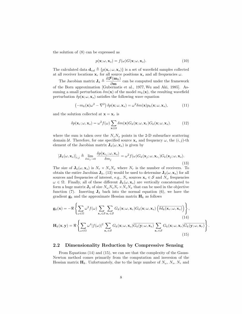
Nz × Nx. In the model, m(xi) indicates the squared-slowness value at the 2Dcoordinate xi, ∀i = 1, . . . , NzNx. Such a calculation process from model to datacan be denoted as dcal , F(m) where F(·) is the nonlinear forward modelingoperator. Based on these definitions, FWI seeks a model m that minimizes thefollowing nonlinear least-squares misfit function

E(m) ,1

2‖dobs − dcal‖22 =

1

2‖dobs −F(m)‖22. (1)

In practice, the minimum of E(m) needs to be searched in an iterativemanner mk+1 = mk + δmk, k = 0, 1, 2, . . . where δmk is the optimal modelperturbation that minimizes E(m) in the vicinity of the current model mk.Hence, we expand E(m) in a small vicinity δm of mk with a Taylor polynomialof degree two

E(m) = E(mk) + δmTgk +1

2δmTHkδm + o(‖δm‖3), (2)

where gk ,∂E(mk)

∂mdenotes the gradient of the misfit function E(m) evaluated

at mk and Hk ,∂2E(mk)

∂m2denotes the Hessian matrix whose elements are the

second-order partial derivatives of E(m) at mk. In each iteration, FWI seeksa model perturbation δm such that E(mk + δm) is a minimum. Setting thegradient of (2) with respect to δm equal to zero yields the solution δmk thatsatisfies

Hkδmk = −gk. (3)

Specifically, by taking the gradient of the misfit function in (1), gk can beevaluated as

gk ,∂E(mk)

∂m= −<

[∂F(mk)

∂m

]†(dobs −F(mk))

= −<

J†kδdk

, (4)

where δdk , dobs −F(mk), and Jk ,∂F(mk)

∂mis the Jacobian matrix of F(·)

which indicates the sensitivity of the forward modeling data with respect to themodel perturbation. By taking another derivative, the Hessian matrix Hk canbe expressed as

Hk ,∂2E(mk)

∂m2= <

J†kJk

−<

[(∂J†k∂m1

)δdk, · · · ,

(∂J†k∂mN

)δdk

]. (5)

The second term of Hk is often dropped off due to its complexity [Tarantola,1987, Pratt et al., 1998]. When Hk in (5) is approximated with its first term

Hk = <

J†kJk

, we have the Gauss-Newton method in which the solution δmk

satisfies the normal equation[<

J†kJk

]δmk = <

J†kδdk

. (6)

6

When Jk is full-rank, (6) has a unique solution δmk that actually minimizesthe following linear least-squares objective function

Jk(δm) ,1

2‖δdk − Jkδm‖22. (7)

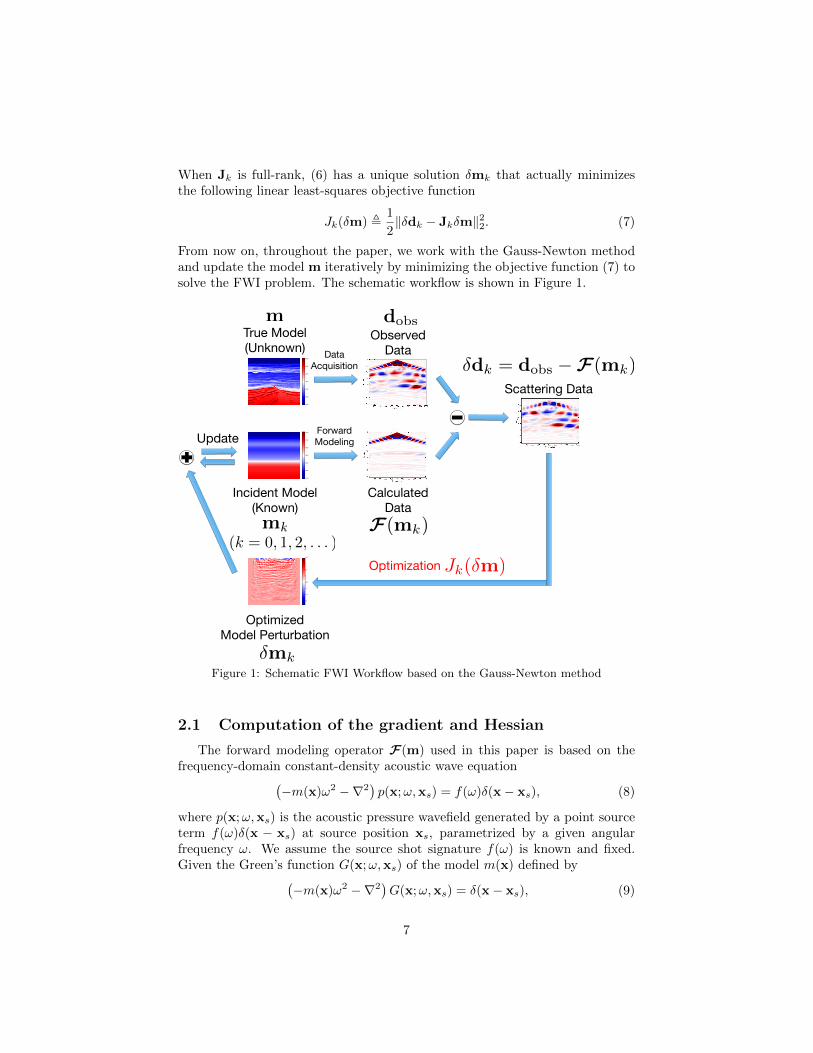
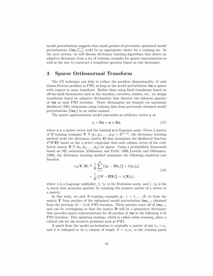
From now on, throughout the paper, we work with the Gauss-Newton methodand update the model m iteratively by minimizing the objective function (7) tosolve the FWI problem. The schematic workflow is shown in Figure 1.

True Model(Unknown)

Incident Model(Known)

ObservedData

CalculatedData

Scattering Data

m

mk

dobs

F(mk)

Optimization

OptimizedModel Perturbation

mk

Update

dk = dobs

F(mk)

Jk(m)

(k = 0, 1, 2, . . . )

1500

2000

2500

3000

3500

4000

4500

1500

2000

2500

3000

3500

4000

4500

−2

−1.5

−1

−0.5

0

0.5

1

x 10−7

ForwardModeling

DataAcquisition

Figure 1: Schematic FWI Workflow based on the Gauss-Newton method

2.1 Computation of the gradient and Hessian

The forward modeling operator F(m) used in this paper is based on thefrequency-domain constant-density acoustic wave equation(

−m(x)ω2 −∇2)p(x;ω,xs) = f(ω)δ(x− xs), (8)

where p(x;ω,xs) is the acoustic pressure wavefield generated by a point sourceterm f(ω)δ(x − xs) at source position xs, parametrized by a given angularfrequency ω. We assume the source shot signature f(ω) is known and fixed.Given the Green’s function G(x;ω,xs) of the model m(x) defined by(

−m(x)ω2 −∇2)G(x;ω,xs) = δ(x− xs), (9)

7

the solution of (8) can be expressed as

p(x;ω,xs) = f(ω)G(x;ω,xs). (10)

The calculated data dcal , p(xr;ω,xs) is a set of wavefield samples collectedat all receiver locations xr for all source positions xs and all frequencies ω.

The Jacobian matrix Jk ,∂F(mk)

∂mcan be computed under the framework

of the Born approximation [Gubernatis et al., 1977, Wu and Aki, 1985]. As-suming a small perturbation δm(x) of the model mk(x), the resulting wavefieldperturbation δp(x;ω,xs) satisfies the following wave equation(

−mk(x)ω2 −∇2)δp(x;ω,xs) = ω2δm(x)pk(x;ω,xs), (11)

and the solution collected at x = xr is

δp(xr;ω,xs) = ω2f(ω)∑x∈U

δm(x)Gk(x;ω,xr)Gk(x;ω,xs). (12)

where the sum is taken over the NzNx points in the 2-D subsurface scatteringdomain U . Therefore, for one specified source xs and frequency ω, the (i, j)-thelement of the Jacobian matrix Jk(ω,xs) is given by

[Jk(ω,xs)]i,j , limδmj→0

δp(xri ;ω,xs)

δmj= ω2f(ω)Gk(xj ;ω,xri)Gk(xj ;ω,xs).

(13)The size of Jk(ω,xs) is Nr × NzNx where Nr is the number of receivers. Toobtain the entire Jacobian Jk, (13) would be used to determine Jk(ω,xs) for allsources and frequencies of interest, e.g., Ns sources xs ∈ S and Nω frequenciesω ∈ Ω. Finally, all of these different Jk(ω,xs) are vertically concatenated toform a huge matrix Jk of size NωNsNr×NzNx that can be used in the objectivefunction (7). Inserting Jk back into the normal equation (6), we have thegradient gk and the approximate Hessian matrix Hk as follows

gk(x) = −<∑ω∈Ω

ω2f(ω)∑xs∈S

∑xr∈S

Gk(x;ω,xr)Gk(x;ω,xs)(δdk(xr;ω,xs)

),

(14)

Hk(x,y) = <∑ω∈Ω

ω4|f(ω)|2∑xs∈S

Gk(x;ω,xs)Gk(y;ω,xs)∑xr∈S

Gk(x;ω,xr)Gk(y;ω,xr)

.

(15)

2.2 Dimensionality Reduction by Compressive Sensing

From Equations (14) and (15), we can see that the complexity of the Gauss-Newton method comes primarily from the computation and inversion of theHessian matrix Hk. Unfortunately, due to the large number of Nω, Ns, Nr and

8

Nz, Nx, it is prohibitive to compute H−1k directly with all data in industrial-

scale FWI problems. In order to reduce the computational complexity of FWI,it has been widely reported that for the cases with large acquisition apertureand wide frequency bandwidth, Hk is almost diagonally dominant and H−1

k

can be approximated with a diagonal matrix [Beylkin, 1985, Shin et al., 2001,Plessix and Mulder, 2004, Jang et al., 2009, Ren et al., 2013, Pan et al., 2015].The computational complexity can also be reduced by approximating Hk withquasi-Newton methods such as the limited-memory Broyden-Fletcher-Goldfarb-Shanno (l-BFGS) algorithm [Nocedal, 1980,Nocedal and Wright, 2006].

The development of CS theories provides another perspective to lower thecomplexity of Gauss-Newton FWI by reducing the problem dimensionality ratherthan simplifying the Hessian matrix, when sparsity of the model can be ex-ploited. This suggests minimizing the linear least-squares objective function in(7) for each Gauss-Newton iteration can be replaced by the following optimiza-tion problem

minα

J

(W)k (α) ,

1

2‖Wkδdk −WkJkD(α)‖22

s.t. ‖α‖1 ≤ τk (16)

where Wk is a compressive sampling matrix for dimensionality reduction whichcan be different for each iteration k for better performance [Krebs et al., 2009,Herrmann et al., 2011,Warner et al., 2013,Li et al., 2012,Li et al., 2016]; D is atransform such that the model perturbation can be represented as δm = D(α)with the coefficient vector α being sparse. Each element of α corresponds to ascalar weighting factor of a unique function called atom and a collection of theseatoms is called a dictionary D. An atom is used interchangeably as a columnvector of D if it is an explicit matrix.

Leaving the design of Wk aside for a while, a fundamental considerationin employing this representation of the model perturbation is the choice of thetransform D. It is usually appealing to choose multiscale transforms such aswavelets, curvelets, seislets, etc. These fixed transforms have proven their an-alytical optimality on sparse representation of multidimensional signals withassumed features such as smooth lines or curves, and hence their success inapplications relies on how suitable the signals in question fit the assumptions.In most cases, these multiscale transforms have efficient algorithmic implemen-tations in the spatial-frequency domain and, as a result, their representationsas dictionaries D are implicit. In the last several years, many authors [Loriset al., 2007, Herrmann et al., 2011, Li et al., 2012, Xue and Zhu, 2015, Li et al.,2016] have developed methods that exploit the sparsity of δm by using variousmultiscale transforms to solve FWI problems efficiently.

In this paper, we investigate how to exploit the sparsity of δm with a noveltransform based on explicit adaptive dictionaries rather than implicit fixed dic-tionaries for some assumed feature characteristic. Particularly, in the FWIiteration (16), we leave a place for an adaptive transform that changes at eachFWI iteration. The key to this approach is to infer explicit dictionary matri-ces Dk from a set of training examples and construct a transform Dk basedon these dictionaries that synthesizes α to δm. The similarity among different

9

model perturbations suggests that small patches of previously optimized modelperturbations δmik−1

i=0 could be an appropriate choice for a training set. Inthe next section, we will discuss dictionary learning algorithms that derive anadaptive dictionary from a set of training examples for sparse representation aswell as the way to construct a transform operator based on this dictionary.

3 Sparse Orthonormal Transform

The CS technique can help to reduce the problem dimensionality of eachGauss-Newton problem in FWI, as long as the model perturbation δm is sparsewith respect to some transform. Rather than using fixed transforms based onoff-the-shelf dictionaries such as the wavelets, curvelets, seislets, etc., we designtransforms based on adaptive dictionaries that discover the inherent sparsityof δm at each FWI iteration. These dictionaries are learned via maximumlikelihood (ML) estimation using training data from previously obtained modelperturbations δmi in an online manner.

The sparse approximation model represents an arbitrary vector y as

y = Dx + n ≈ Dx (17)

where x is a sparse vector and the residual n is Gaussian noise. Given a matrixof R training examples Y , [y1,y2, . . . ,yR] ∈ RN×R, the dictionary learningmethod seeks the dictionary matrix D that maximizes the likelihood functionP (Y|D) based on the a priori constraint that each column vector of the coef-ficient matrix X , [x1,x2, . . . ,xR] be sparse. Using a probabilistic frameworkbased on ML estimation [Olshausen and Field, 1996, Lewicki and Olshausen,1999], the dictionary learning method minimizes the following empirical costfunction

eR(Y,D) ,1

R

R∑i=1

(‖yi −Dxi‖22 + λ‖xi‖0

)=

1

R

(‖Y −DX‖2F + λ‖X‖0

),

(18)

where λ is a Lagrange multiplier, ‖ · ‖F is the Frobenius norm, and ‖ · ‖0 is the`0-norm that promotes sparsity by counting the nonzero entries of a vector ora matrix.

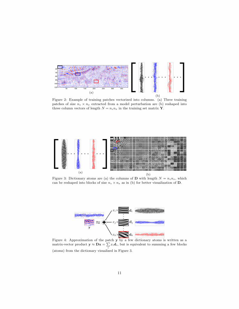
In this work, we pick R training examples yi, i = 1, . . . , R, to form thematrix Y from patches of the optimized model perturbation δmk−1 obtainedfrom the previous (k − 1)-th FWI iteration. These patches cover all of δmk−1

and can be overlapping so that the matrix D will be a generative dictionarythat provides sparse representations for all patches of δm in the following k-thFWI iteration. This updating strategy, which is called online learning, plays acritical role for the iterative problems such as FWI.

A patch from the model perturbation is originally a matrix of size nz × nxand it is reshaped to be a column of length N = nznx in the training patch

10

50 100 150 200 250 300 350

20

40

60

80

100

120

(a)

[ ]· · · · · · · · ·

(b)

Figure 2: Example of training patches vectorized into columns. (a) Three trainingpatches of size nz × nx extracted from a model perturbation are (b) reshaped intothree column vectors of length N = nznx in the training set matrix Y.

[ ]· · · · · · · · ·

(a)(b)

Figure 3: Dictionary atoms are (a) the columns of D with length N = nznx, whichcan be reshaped into blocks of size nz × nx as in (b) for better visualization of D.

xi

xj

xk

······y

di

dj

dk

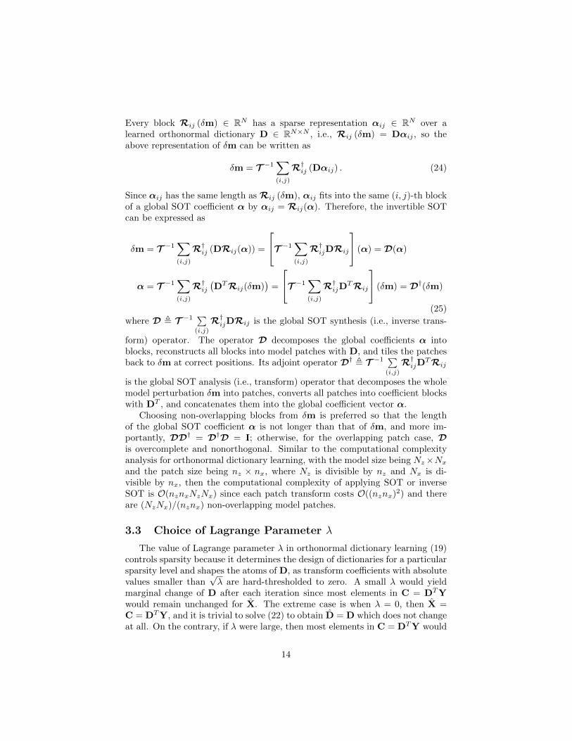
Figure 4: Approximation of the patch y by a few dictionary atoms is written as amatrix-vector product y ≈ Dx =

∑i

xidi, but is equivalent to summing a few blocks

(atoms) from the dictionary visualized in Figure 3.

11

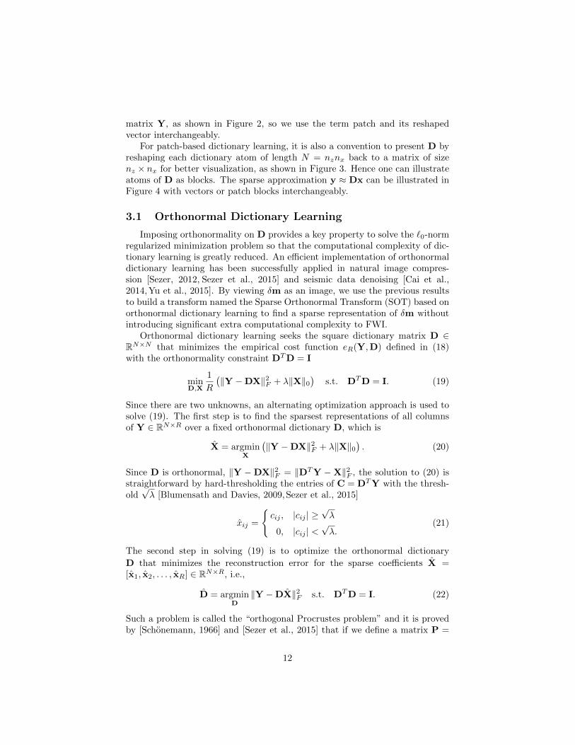
matrix Y, as shown in Figure 2, so we use the term patch and its reshapedvector interchangeably.

For patch-based dictionary learning, it is also a convention to present D byreshaping each dictionary atom of length N = nznx back to a matrix of sizenz × nx for better visualization, as shown in Figure 3. Hence one can illustrateatoms of D as blocks. The sparse approximation y ≈ Dx can be illustrated inFigure 4 with vectors or patch blocks interchangeably.

3.1 Orthonormal Dictionary Learning

Imposing orthonormality on D provides a key property to solve the `0-normregularized minimization problem so that the computational complexity of dic-tionary learning is greatly reduced. An efficient implementation of orthonormaldictionary learning has been successfully applied in natural image compres-sion [Sezer, 2012, Sezer et al., 2015] and seismic data denoising [Cai et al.,2014,Yu et al., 2015]. By viewing δm as an image, we use the previous resultsto build a transform named the Sparse Orthonormal Transform (SOT) based onorthonormal dictionary learning to find a sparse representation of δm withoutintroducing significant extra computational complexity to FWI.

Orthonormal dictionary learning seeks the square dictionary matrix D ∈RN×N that minimizes the empirical cost function eR(Y,D) defined in (18)with the orthonormality constraint DTD = I

minD,X

1

R

(‖Y −DX‖2F + λ‖X‖0

)s.t. DTD = I. (19)

Since there are two unknowns, an alternating optimization approach is used tosolve (19). The first step is to find the sparsest representations of all columnsof Y ∈ RN×R over a fixed orthonormal dictionary D, which is

X = argminX

(‖Y −DX‖2F + λ‖X‖0

). (20)

Since D is orthonormal, ‖Y −DX‖2F = ‖DTY −X‖2F , the solution to (20) isstraightforward by hard-thresholding the entries of C = DTY with the thresh-old√λ [Blumensath and Davies, 2009,Sezer et al., 2015]

xij =

cij , |cij | ≥

√λ

0, |cij | <√λ.

(21)

The second step in solving (19) is to optimize the orthonormal dictionary

D that minimizes the reconstruction error for the sparse coefficients X =[x1, x2, . . . , xR] ∈ RN×R, i.e.,

D = argminD

‖Y −DX‖2F s.t. DTD = I. (22)

Such a problem is called the “orthogonal Procrustes problem” and it is provedby [Schonemann, 1966] and [Sezer et al., 2015] that if we define a matrix P =

12

XYT ∈ RN×N and let P = UΣVT denote its singular value decomposition(SVD), then the orthonormal matrix D = VUT solves (22). The orthonormaldictionary D can thus be learned by alternating between the above two stepsiteratively until the cost function eR(Y,D) reaches a limit.

For each learning iteration, orthonormal dictionary learning needs three ma-trix multiplications that cost O(2RN2 +N3) and one SVD operation that costsO(N3) to obtain both the sparse coding and the updated dictionary. Specifi-cally, the model size is Nz × Nx and the training patch size is nz × nx, wherenz Nz, nx Nx, and N = nznx. If all possible overlapping patches are usedfor training, then the number of training patches R = (Nz−nz+1)(Nx−nx+1),and each training iteration costs O((nznx)2(Nz−nz+1)(Nx−nx+1)+(nznx)3).The number of training iterations does not depend on these sizes, hence the over-all complexity does not change in the sense of the Big-O notation. Such analysismotivates the fact that the patch size should be small for dictionary learningalgorithms; otherwise, the complexity would grow dramatically if large nz or nxwere used.

Compared to the overcomplete dictionary learning method K-SVD [Aharonet al., 2006,Elad and Aharon, 2006], the computational complexity of orthonor-mal dictionary learning is much less because it does not involve complex itera-tive algorithms such as Basis Pursuit (BP) [Chen et al., 1998], Least AbsoluteShrinkage and Selection Operator (LASSO) [Tibshirani, 1994] or Matching Pur-suit (MP) [Mallat and Zhang, 1993, Pati et al., 1993, Tropp and Gilbert, 2007]that have been widely used in K-SVD.

3.2 Dictionary-based Block-wise Transform

Dictionary learning methods use patches to form dictionaries, and thereforethe learned dictionary can only be applied on the patches (see Figure 4) ratherthan the whole image. Generally, dictionary learning is used in “nearly-local”problems such as signal denoising [Beckouche and Ma, 2014,Zhu et al., 2015] orinpainting [Yu et al., 2015] where patches are processed one by one. However,the FWI problem needs to recover the entire model perturbation δm from com-pressive measurements, so an invertible transform that can be applied to thewhole δm is required. In this section we show how to convert the local dictio-naries D into a global transform D that can be applied on the whole domain ofδm, and such a transform is named the Sparse Orthonormal Transform (SOT).

It is always true that the whole model perturbation δm can be exactlyrepresented as

δm = T −1∑(i,j)

R†ij (Rij (δm)) (23)

where the operator Rij extracts the (i, j)-th block of size N = nznx from

δm, and its adjoint R†ij tiles the (i, j)-th block of size N = nznx back to δm.

The operator T ,∑

(i,j)

R†ijRij is an invertible diagonal matrix if the set of all

(i, j) patches fully covers δm in which case T −1 is a grid-by-grid operation.

13

Every block Rij (δm) ∈ RN has a sparse representation αij ∈ RN over alearned orthonormal dictionary D ∈ RN×N , i.e., Rij (δm) = Dαij , so theabove representation of δm can be written as

δm = T −1∑(i,j)

R†ij (Dαij) . (24)

Since αij has the same length as Rij (δm), αij fits into the same (i, j)-th blockof a global SOT coefficient α by αij = Rij(α). Therefore, the invertible SOTcan be expressed as

δm = T −1∑(i,j)

R†ij (DRij(α)) =

T −1∑(i,j)

R†ijDRij

(α) = D(α)

α = T −1∑(i,j)

R†ij(DTRij(δm)

)=

T −1∑(i,j)

R†ijDTRij

(δm) = D†(δm)

(25)

where D , T −1 ∑(i,j)

R†ijDRij is the global SOT synthesis (i.e., inverse trans-

form) operator. The operator D decomposes the global coefficients α intoblocks, reconstructs all blocks into model patches with D, and tiles the patchesback to δm at correct positions. Its adjoint operator D† , T −1 ∑

(i,j)

R†ijDTRij

is the global SOT analysis (i.e., transform) operator that decomposes the wholemodel perturbation δm into patches, converts all patches into coefficient blockswith DT , and concatenates them into the global coefficient vector α.

Choosing non-overlapping blocks from δm is preferred so that the lengthof the global SOT coefficient α is not longer than that of δm, and more im-portantly, DD† = D†D = I; otherwise, for the overlapping patch case, Dis overcomplete and nonorthogonal. Similar to the computational complexityanalysis for orthonormal dictionary learning, with the model size being Nz×Nxand the patch size being nz × nx, where Nz is divisible by nz and Nx is di-visible by nx, then the computational complexity of applying SOT or inverseSOT is O(nznxNzNx) since each patch transform costs O((nznx)2) and thereare (NzNx)/(nznx) non-overlapping model patches.

3.3 Choice of Lagrange Parameter λ

The value of Lagrange parameter λ in orthonormal dictionary learning (19)controls sparsity because it determines the design of dictionaries for a particularsparsity level and shapes the atoms of D, as transform coefficients with absolutevalues smaller than

√λ are hard-thresholded to zero. A small λ would yield

marginal change of D after each iteration since most elements in C = DTYwould remain unchanged for X. The extreme case is when λ = 0, then X =C = DTY, and it is trivial to solve (22) to obtain D = D which does not changeat all. On the contrary, if λ were large, then most elements in C = DTY would

14

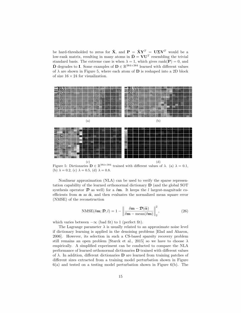
be hard-thresholded to zeros for X, and P = XYT = UΣVT would be alow-rank matrix, resulting in many atoms in D = VUT resembling the trivialstandard basis. The extreme case is when λ = 1, which gives rank(P) = 0, and

D degrades to I. Some examples of D ∈ R384×384 learned with different valuesof λ are shown in Figure 5, where each atom of D is reshaped into a 2D blockof size 16× 24 for visualization.

(a) (b)

(c) (d)

Figure 5: Dictionaries D ∈ R384×384 trained with different values of λ. (a) λ = 0.1,(b) λ = 0.2, (c) λ = 0.5, (d) λ = 0.8.

Nonlinear approximation (NLA) can be used to verify the sparse represen-tation capability of the learned orthonormal dictionary D (and the global SOTsynthesis operator D as well) for a δm. It keeps the l largest-magnitude co-efficients from α as α, and then evaluates the normalized mean square error(NMSE) of the reconstruction

NMSE(δm;D, l) = 1−∥∥∥∥ δm−D(α)

δm−mean(δm)

∥∥∥∥2

2

, (26)

which varies between −∞ (bad fit) to 1 (perfect fit).The Lagrange parameter λ is usually related to an approximate noise level

if dictionary learning is applied in the denoising problems [Elad and Aharon,2006]. However, its selection in such a CS-based sparsity recovery problemstill remains an open problem [Starck et al., 2015] so we have to choose λempirically. A simplified experiment can be conducted to compare the NLAperformance of learned orthonormal dictionaries D trained with different valuesof λ. In addition, different dictionaries D are learned from training patches ofdifferent sizes extracted from a training model perturbation shown in Figure6(a) and tested on a testing model perturbation shown in Figure 6(b). The

15

Distance (m)

Dep

th (

m)

500 1000 1500 2000 2500 3000 3500

200

400

600

800

1000

1200

δm

−3

−2

−1

0

1

2

3

4x 10

−8

(a)

Distance (m)

Dep

th (

m)

500 1000 1500 2000 2500 3000 3500

200

400

600

800

1000

1200

δm

−3

−2

−1

0

1

2

3

4x 10

−8

(b)

Figure 6: Two model perturbations δm extracted from consecutive FWI iterationsand used for the nonlinear approximation test, (a) for training, (b) for testing.

16

0 0.2 0.4 0.6 0.8 1

0.4

0.5

0.6

0.7

0.8

0.9

1

√

λ

Nor

mal

ized

Mea

n S

quar

e E

rror

(N

MS

E)

1% SOT coefficients2% SOT coefficients5% SOT coefficients

(a)

0 0.2 0.4 0.6 0.8 10.65

0.7

0.75

0.8

0.85

0.9

0.95

1

√

λ

Nor

mal

ized

Mea

n S

quar

e E

rror

(N

MS

E)


(b)

0 0.2 0.4 0.6 0.8 10.65

0.7

0.75

0.8

0.85

0.9

0.95

1

√

λ

Nor

mal

ized

Mea

n S

quar

e E

rror

(N

MS

E)


(c)

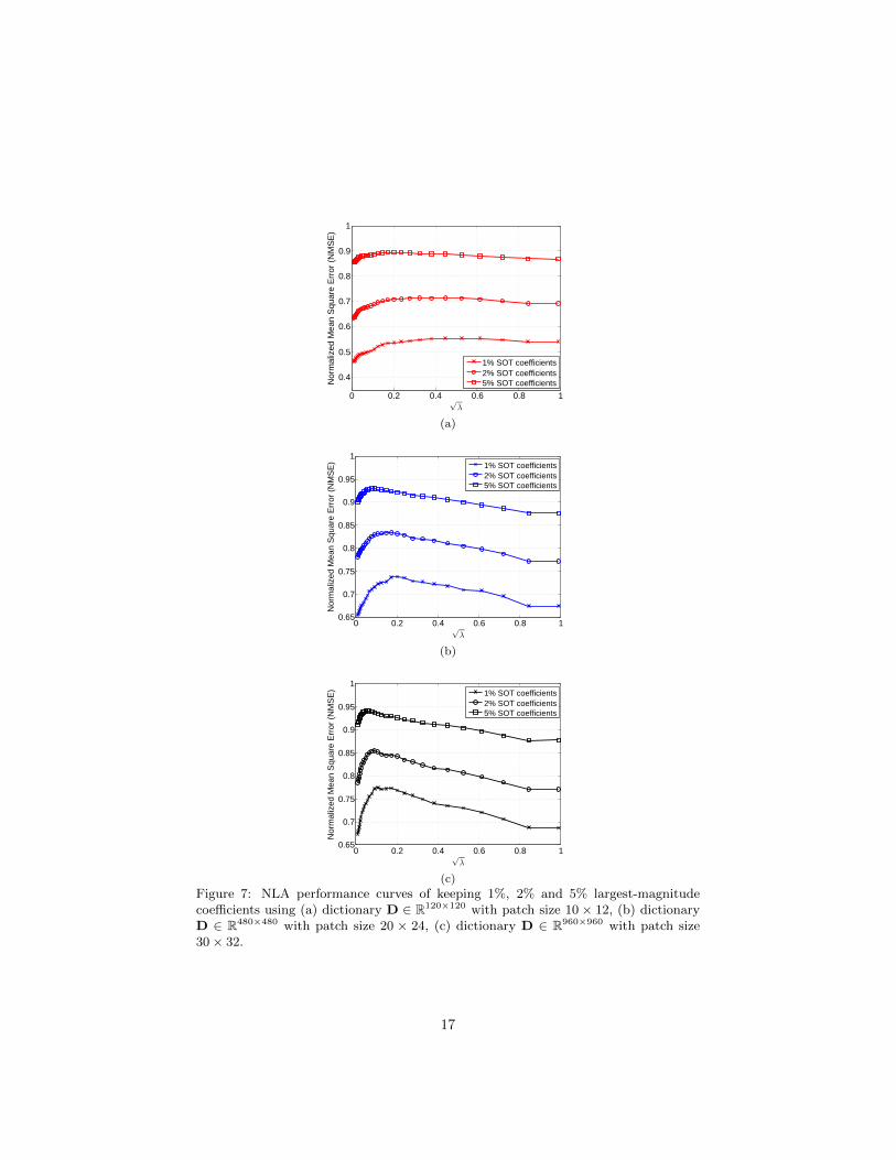
Figure 7: NLA performance curves of keeping 1%, 2% and 5% largest-magnitudecoefficients using (a) dictionary D ∈ R120×120 with patch size 10× 12, (b) dictionaryD ∈ R480×480 with patch size 20 × 24, (c) dictionary D ∈ R960×960 with patch size30× 32.

17

NLA performance curves that indicate the relationship between NMSE and λfor different sparsity levels l (1%, 2% and 5% of largest-magnitude coefficients)are shown in Figure 7. In Figures 7(a) to 7(c), we see that the optimal λ thatyields the highest NMSE depends on both the sparsity level l and the patchsize nz ×nx, and the optimal λ tends to decrease if either the sparsity level l orthe patch size nz × nx increases. These results indicate that λ ∈ (0.152, 0.252)is expected to deliver good reconstructions for reasonable sparsity levels andpatch sizes.

3.4 Online Orthonormal Dictionary Learning

The above orthonormal dictionary learning algorithm takes the trainingpatch set as a whole so that a dictionary D could be learned offline and wouldremain static as a sparse representation. Generally speaking, such an offlineapproach cannot effectively handle very large training sets, or dynamic trainingsets that vary over time. In practice, FWI is an iterative problem where the op-timized δmk that offers training patches is changing over iterations. Therefore,to exploit the availability of new training patches from δmk, we propose an on-line approach for orthonormal dictionary learning that minimizes the followingexpected cost function

e(D) , Ey

[‖y −Dx‖22 + λ‖x‖0

]= limR→∞

eR(Y,D) almost surely. (27)

Rather than spending too much effort on accurately minimizing the empiricalcost function eR(Y,D) in (18), [Bousquet and Bottou, 2007] suggest minimizinge(D) since eR(Y,D) is merely an approximation of e(D). Minimizing e(D) doesnot rely on the number of patches R, but instead on the (unknown) stochas-tic characteristics of the training patches. The online approach learns a newdictionary Dk every time a new δmk−1 is ready, and the sequence of learneddictionaries can adapt to the variations of patches in later iterations.

Algorithm 1 summarizes a general version of the online orthonormal dictio-nary learning method in which the training examples y are drawn from a datastream source. In particular, at the end of the (k − 1)-th FWI iteration, wefirst draw a batch of R training patches from δmk−1, each of size nz × nx, toform the matrix Yk−1 ∈ RN×R and normalize each column into the range of[0, 1]. Then we use the previous dictionary Dk−1 ∈ RN×N as a warm startto represent Yk−1 with sparse coefficients Xk−1 ∈ RN×R by hard thresholdingwith

√λ, and obtain the updated dictionary Dk for the following k-th FWI

iteration with the orthonormal matrices of singular vectors of Pk ∈ RN×N thataccumulates XiY

Ti for i = 0, 1, . . . , k−1. Essentially, the above two alternating

steps for learning Dk keep reducing the value of the function

ek(D) ,1

kR

k−1∑i=0

(‖Yi −DXi‖2F + λ‖Xi‖0

)(28)

which, in effect, takes training patches of all previously optimized model per-turbations δmik−1

i=0 into account. It is proved in [Bousquet and Bottou, 2007]

18

that ek(D) converges to e(D) with probability one if k is sufficiently large and,therefore, the online orthonormal dictionary learning converges to a stationarypoint.

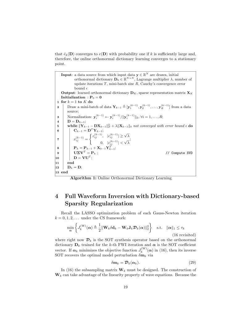
Input: a data source from which input data y ∈ RN are drawn, initialorthonormal dictionary D0 ∈ RN×N , Lagrange multiplier λ, number ofupdate iterations T , mini-batch size R, Cauchy’s convergence errorbound ε

Output: learned orthonormal dictionary DK , sparse representation matrix XK

Initialization : P0 = 01 for k = 1 to K do

2 Draw a mini-batch of data Yk−1 , [y(k−1)1 ,y

(k−1)2 , . . . ,y

(k−1)R ] from a data

source;

3 Normalization: y(k−1)i ← y

(k−1)i /‖y(k−1)

i ‖2, ∀i = 1, . . . , R;4 D = Dk−1;5 while ‖Yk−1 −DXk−1‖2F + λ‖Xk−1‖0 not converged with error bound ε do6 Ck−1 = DTYk−1;

7 x(k−1)ij =

c(k−1)ij , |c(k−1)

ij | ≥√λ

0, |c(k−1)ij | <

√λ

;

8 Pk = Pk−1 + Xk−1YTk−1;

9 UΣVT = Pk ; // Compute SVD

10 D = VUT ;

11 end12 Dk = D;

13 end

Algorithm 1: Online Orthonormal Dictionary Learning

4 Full Waveform Inversion with Dictionary-basedSparsity Regularization

Recall the LASSO optimization problem of each Gauss-Newton iterationk = 0, 1, 2, . . . under the CS framework:

minα

J

(W)k (α) ,

1

2‖Wkδdk −WkJkDk(α)‖22

s.t. ‖α‖1 ≤ τk

(16 revisited)where right now Dk is the SOT synthesis operator based on the orthonormaldictionary Dk trained for the k-th FWI iteration and α is the SOT coefficient

vector. If αk minimizes the objective function J(W)k (α) in (16), then its inverse

SOT recovers the optimal model perturbation δmk via

δmk = Dk(αk). (29)

In (16) the subsampling matrix Wk must be designed. The construction ofWk can take advantage of the linearity property of wave equations. Because the

19

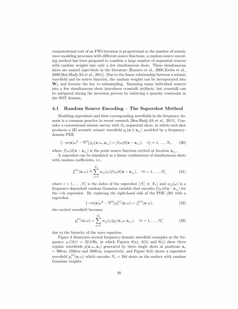
computational cost of an FWI iteration is proportional to the number of seismicwave modeling processes with different source functions, a random source encod-ing method has been proposed to combine a large number of sequential sourceswith random weights into only a few simultaneous shots. These simultaneousshots are named supershots in the literature [Romero et al., 2000, Krebs et al.,2009,Ben-Hadj-Ali et al., 2011]. Due to the linear relationship between a seismicwavefield and its source function, the random weights can be incorporated intoWk and become the key to subsampling. Summing many individual sourcesinto a few simultaneous shots introduces crosstalk artifacts, but crosstalk canbe mitigated during the inversion process by enforcing a sparsity constraint inthe SOT domain.

4.1 Random Source Encoding – The Supershot Method

Modeling supershots and their corresponding wavefields in the frequency do-main is a common practice in recent research [Ben-Hadj-Ali et al., 2011]. Con-sider a conventional seismic survey with Ns sequential shots, in which each shotproduces a 2D acoustic seismic wavefield pj(x, t; xsj ) modeled by a frequency-domain PDE(

−m(x)ω2 −∇2)pj(x;ω,xsj ) = f(ω)δ(x− xsj ), ∀j = 1, . . . , Ns (30)

where f(ω)δ(x− xsj ) is the point source function excited at location xsj .A supershot can be simulated as a linear combination of simultaneous shots

with random coefficients, i.e.,

f(s)i (x;ω) ,

Ns∑j=1

wij(ω)f(ω)δ(x− xsj ), ∀i = 1, . . . , N ′s (31)

where i = 1, . . . , N ′s is the index of the supershot (N ′s Ns) and wij(ω) is afrequency-dependent random Gaussian variable that encodes f(ω)δ(x−xsj ) forthe i-th supershot. By replacing the right-hand side of the PDE (30) with asupershot, (

−m(x)ω2 −∇2)p

(s)i (x;ω) = f

(s)i (x;ω), (32)

the excited wavefield becomes

p(s)i (x;ω) =

Ns∑j=1

wij(ω)pj(x;ω,xsj ), ∀i = 1, . . . , N ′s (33)

due to the linearity of the wave equation.Figure 8 illustrates several frequency-domain wavefield examples at the fre-

quency ω/(2π) = 22.8 Hz, in which Figures 8(a), 8(b) and 8(c) show threeregular wavefields p(x;ω,xs) generated by three single shots at positions xs= 960 m, 1920 m and 2880 m, respectively, and Figure 8(d) shows a supershot

wavefield p(s)i (x;ω) which encodes Ns = 384 shots on the surface with random

Gaussian weights.

20

Distance (m)

Dep

th (

m)

500 1000 1500 2000 2500 3000 3500

200

400

600

800

1000

1200 −400

−300

−200

−100

0

100

200

(a)

Distance (m)

Dep

th (

m)

500 1000 1500 2000 2500 3000 3500

200

400

600

800

1000

1200 −400

−300

−200

−100

0

100

200

(b)

Distance (m)

Dep

th (

m)

500 1000 1500 2000 2500 3000 3500

200

400

600

800

1000

1200 −400

−200

0

200

(c)

Distance (m)

Dep

th (

m)

500 1000 1500 2000 2500 3000 3500

200

400

600

800

1000

1200−4000

−2000

0

2000

4000

(d)

Figure 8: Wavefield examples generated by a single shot in (a) at position xs = 960 m,(b) at position xs = 1920 m, (c) at position xs = 2880 m and (d) a supershot encodingNs = 384 shots with random Gaussian weights with frequency 22.8 Hz

21

FWI uses the wavefield sample set d(s) ,p

(s)i (xr;ω)

collected at all re-

ceiver locations xr for all supershots with different frequencies ω. Since eachfrequency is processed independently in frequency-domain modeling, the num-ber of frequencies used in FWI can also be reduced to N ′ω < Nω, and this setof frequencies can be randomly selected among all Nω frequencies, which thenreduces the dimension of d(s) to N ′ωN

′sNr. According to (33), the relationship

between d(s) and the full-dimension data d for all receivers, single shots andfrequencies can be written in a compact matrix form as

d(s) , F (s)(m) = Wd = WF(m). (34)

The subsampling matrix W of size N ′ωN′sNr ×NωNsNr is structured as

W ,

(RN ′ω×Nω ⊗ IN ′

s

)w(ω1). . .

w(ωNω )

⊗ INr (35)

where the restriction matrix RN ′ω×Nω

of size N ′ω × Nω randomly chooses N ′ωrows from an identity matrix of size Nω × Nω for random frequency selection.Each w(ω) is a random encoding matrix of size N ′s×Ns whose (i, j)-th entry iswij(ω) so that the block diagonal matrix in the center is of size N ′sNω ×NsNω,and IN ′

s, INr

are identity matrices of size N ′s ×N ′s, Nr ×Nr, respectively.According to the perturbation analysis based on Born approximation theory,

the relationship between the supershot Jacobian matrix J(s) and the sequentialshot Jacobian matrix J can be written as

J(s) = WJ. (36)

For each FWI iteration k, different wij(ω) encoding supershots can be gen-erated so that the random subsampling matrix, denoted as Wk, is not static.This approach suppresses crosstalk artifacts into incoherent Gaussian noise andyields better reconstruction results. Meanwhile, no artificial bias towards a spe-cific random source encoding pattern would be introduced into the solution byredrawing Wk. Such an approach has been recommended in previous researchon FWI that utilizes CS [Herrmann et al., 2011,Herrmann and Li, 2012,Li et al.,2012,Warner et al., 2013,Li et al., 2016].

Therefore, in (16), Wkδdk can be obtained as a whole by calculating the

difference between the recorded receiver data d(s)obs , Wkdobs encoded by Wk

and the calculated receiver data d(s)k generated by supershots. WkJk can be

regarded as the compressive Jacobian whose components includes non-alteredGreen’s functions for receivers and random encoded Green’s functions for sources.

The solution αk of the LASSO problem (16) relies on the choice of thesparsity constraint τk. As suggested by [van den Berg and Friedlander, 2009],every LASSO problem implies a convex and non-increasing function φ(τ) thatassociates the least-squares residual to the sparsity level τ . In this problem, eachFWI iteration k = 0, 1, 2, . . . needs to solve (16) and, therefore, has an implicit

22

φk(τ). Following the same idea used by [Herrmann et al., 2011, Li et al., 2012]and [Li et al., 2016], one can estimate τk by using a linear approximation ofφ′k(τ) at τ = 0, given in Theorem 2.1 of [van den Berg and Friedlander, 2009]

τk ≈ −φk(0)

φ′k(0)=

‖Wkδdk‖22∥∥∥D†k ([WkJk]†

(Wkδdk))∥∥∥∞

(37)

where ‖ · ‖∞ is the maximum norm, [WkJk]†

is the adjoint of the compressiveJacobian WkJk and performs the following calculation over the vector Wkδdk

[WkJk]†

(Wkδdk)

=

N ′ω∑

m=1

ω2mf(ωm)

Nr∑n=1

Gk(xrn ;ωm,x)

N ′s∑

i=1

Ns∑j=1

[wk(ωm)]ij Gk(x;ωm,xsj )[δp

(s)k

]i(xrn ;ωm).

(38)The above expression is a function with respect to the medium grid points x, soit can be interpreted as a wavefield or image and hence can also be decomposedinto global SOT coefficient by D†k.

4.2 Projected Quasi-Newton Method for solving the LASSOproblems

The computational complexity of the FWI problem is reduced considerablyafter reducing the data dimensionality from NωNsNr to N ′ωN

′sNr. However,

in order to minimize the objective function J(W)k (α) in (16) with sparsity pro-

motion on the global SOT coefficient α, the descent direction of α must beprojected into an `1-norm ball with radius τk.

A limited-memory projected quasi-Newton method (l-PQN) proposed by[Schmidt et al., 2009] can solve the LASSO problem (16) iteratively, based ona two-layer strategy. In each iteration l = 0, 1, 2, . . . , the outer layer formulates

a quadratic approximation function Q(l)(α) of the objective function J(W)k (α)

around the current iterate α(l)

Q(l)(α) , J(W)k

(α(l)

)+(α−α(l)

)Tγ(l) +

1

2

(α−α(l)

)TB(l)

(α−α(l)

)(39)

where γ(l) is the gradient of J(W)k (α) evaluated for α(l)

γ(l) ,∂J

(W)k

∂α

(α(l)

)= −<

D†k(

[WkJk]†(Wkδdk −WkJkDk

(α(l)

)))(40)

and B(l) denotes a positive-definite approximation matrix of [WkJkDk]†WkJkDk,

the Hessian matrix of J(W)k (α), at the l-th iteration of l-PQN. The inner layer it-

eratively searches for a feasible descent direction by minimizing Q(l)(α) subjectto the `1-norm constraints

α = argminα

Q(l)(α) subject to ‖α‖1 ≤ τk. (41)

23

Input: Step length bounds 0 < amin < amax, γ(l), B(l), sufficientdecrease parameter ν, `1-norm bound τk

Initialization: αnew ← α(l), initial step length a =

[p(l−1)

]Tp(l−1)[

p(l−1)]T

q(l−1),

function maximum fmax ← −∞1 while not converged do2 αold ← αnew;3 a← minamax,maxamin, a;4 d← P(`1)

τk

(αold − a∇Q(l)(αold)

)−αold ; // ∇Q(l)(α) = B(l)α + γ(l)

5 a← 1;

6 fmax ← maxfmax, J

(W )k (αold)

;

7 while Q(l)(αold + ad) > fmax + νa∇Q(l)(αold)Td do8 Choose a ∈ (0, a) by backtracking;9 end

10 αnew ← αold + ad;

11 a← [αnew −αold]T

[αnew −αold]

[αnew −αold]T [∇Q(l)(αnew)−∇Q(l)(αold)

]12 end

Output: α← αnew

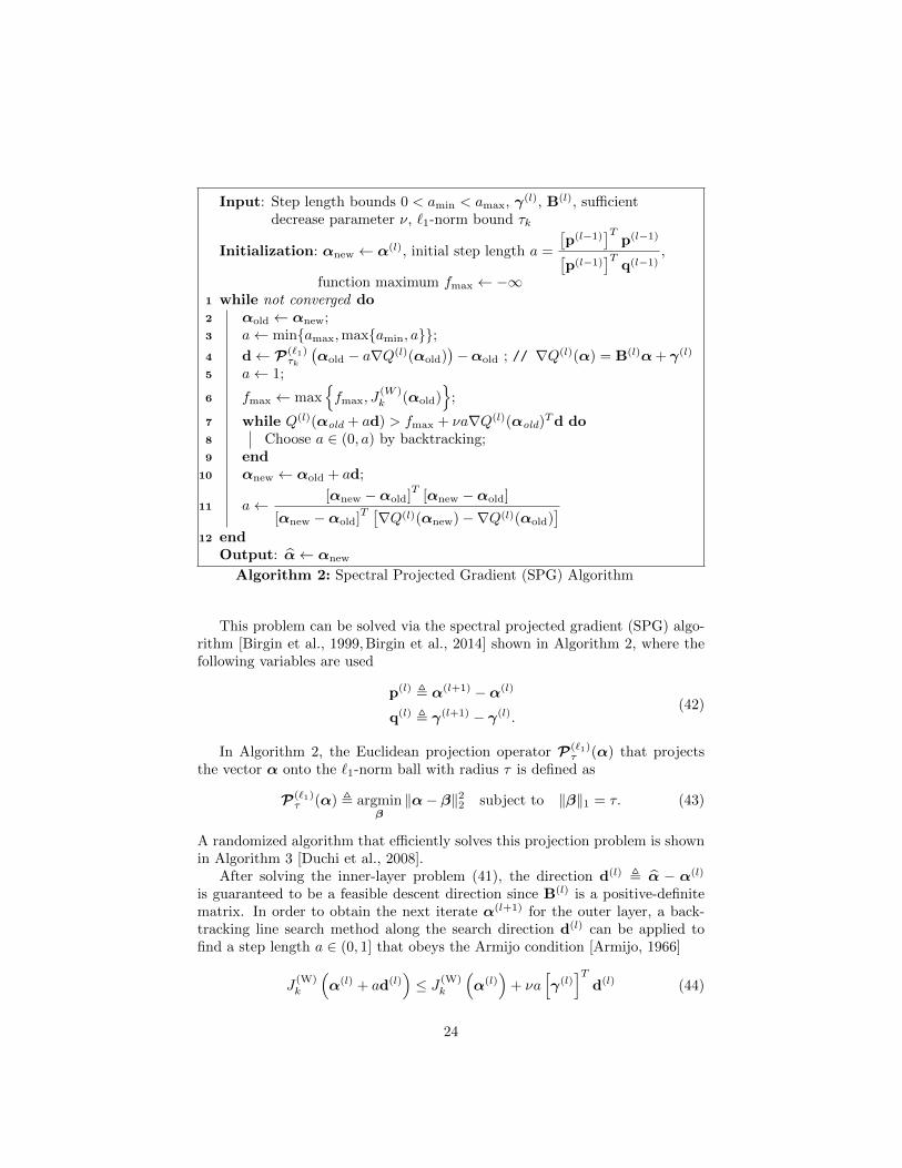
Algorithm 2: Spectral Projected Gradient (SPG) Algorithm

This problem can be solved via the spectral projected gradient (SPG) algo-rithm [Birgin et al., 1999, Birgin et al., 2014] shown in Algorithm 2, where thefollowing variables are used

p(l) , α(l+1) −α(l)

q(l) , γ(l+1) − γ(l).(42)

In Algorithm 2, the Euclidean projection operator P(`1)τ (α) that projects

the vector α onto the `1-norm ball with radius τ is defined as

P(`1)τ (α) , argmin

β‖α− β‖22 subject to ‖β‖1 = τ. (43)

A randomized algorithm that efficiently solves this projection problem is shownin Algorithm 3 [Duchi et al., 2008].

After solving the inner-layer problem (41), the direction d(l) , α − α(l)

is guaranteed to be a feasible descent direction since B(l) is a positive-definitematrix. In order to obtain the next iterate α(l+1) for the outer layer, a back-tracking line search method along the search direction d(l) can be applied tofind a step length a ∈ (0, 1] that obeys the Armijo condition [Armijo, 1966]

J(W)k

(α(l) + ad(l)

)≤ J (W)

k

(α(l)

)+ νa

[γ(l)

]Td(l) (44)

24

Input: α ∈ RN , τ > 01 Sort α s.t. |α1| ≥ |α2| ≥ · · · ≥ |αN |;

2 Find ρ = argmaxj

(|αj | − 1

j

(j∑r=1|αr| − τ

));

3 Define θ = 1ρ

(ρ∑i=1

|αi| − τ)

;

Output: β ∈ RN such that βi = sign(αi) ·max|αi| − θ, 0Algorithm 3: Projection onto an `1-norm ball

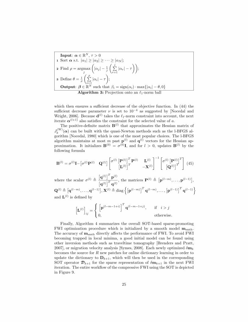
which then ensures a sufficient decrease of the objective function. In (44) thesufficient decrease parameter ν is set to 10−4 as suggested by [Nocedal andWright, 2006]. Because d(l) takes the `1-norm constraint into account, the nextiterate α(l+1) also satisfies the constraint for the selected value of a.

The positive-definite matrix B(l) that approximates the Hessian matrix of

J(W)k (α) can be built with the quasi-Newton methods such as the l-BFGS al-

gorithm [Nocedal, 1980] which is one of the most popular choices. The l-BFGSalgorithm maintains at most m past p(l) and q(l) vectors for the Hessian ap-proximation. It initializes B(0) = σ(0)I, and for l > 0, updates B(l) by thefollowing formula

B(l) = σ(l)I−[σ(l)P(l) Q(l)

] [σ(l)[P(l)

]TP(l) L(l)[

L(l)]T −X(l)

]−1 [σ(l)

[P(l)

]T[Q(l)

]T]

(45)

where the scalar σ(l) ,

[q(l)]T

p(l)[q(l)]T

q(l), the matrices P(l) ,

[p(l−m), . . . ,p(l−1)

],

Q(l) ,[q(l−m), . . . ,q(l−1)

], X(l) , diag

[p(l−m)

]Tq(l−m), . . . ,

[p(l−1)

]Tq(l−1)

and L(l) is defined by

[L(l)

]ij

=

[p(l−m−1+i)

]Tq(l−m−1+j), if i > j

0, otherwise.

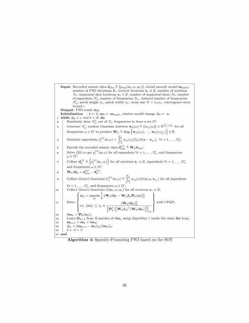
Finally, Algorithm 4 summarizes the overall SOT-based sparse-promotingFWI optimization procedure which is initialized by a smooth model msmth.The accuracy of msmth directly affects the performance of FWI. To avoid FWIbecoming trapped in local minima, a good initial model can be found usingother inversion methods such as traveltime tomography [Brenders and Pratt,2007], or migration velocity analysis [Symes, 2008]. Each newly optimized δmk

becomes the source for R new patches for online dictionary learning in order toupdate the dictionary to Dk+1, which will then be used in the correspondingSOT operator Dk+1 for the sparse representation of δmk+1 in the next FWIiteration. The entire workflow of the compressive FWI using the SOT is depictedin Figure 9.

25

Input: Recorded seismic data dobs , pobs(xr;ω,xs), initial smooth model msmth,number of FWI iterations K, receiver locations xr ∈ S, number of receiversNr, sequential shot locations xs ∈ S, number of sequential shots Ns, numberof supershots N ′s, number of frequencies Nω , reduced number of frequenciesN ′ω , patch height nz , patch width nx, atom size N = nznx, convergence errorbound ε

Output: FWI result mK

Initialization : k ← 0, m0 ←msmth, relative model change ∆0 ←∞1 while ∆k > ε and k < K do2 Randomly draw N ′ω out of Nω frequencies to form a set Ω′;

3 Generate N ′ω random Gaussian matrices wk(ω) , wij(ω) ∈ RN′s×Ns for all

frequencies ω ∈ Ω′ to produce Wk , diagwk(ω1), . . . ,wk(ωN′

ω)⊗ I;

4 Generate supershots f(s)i (x;ω) =

Ns∑j=1

wij(ω)f(ω)δ(x− xsj ), ∀i = 1, . . . , N ′s;

5 Encode the recorded seismic data d(s)obs , Wkdobs;

6 Solve (32) to get p(s)i (x;ω) for all supershots ∀i = 1, . . . , N ′s, and frequencies

ω ∈ Ω′;

7 Collect d(s)k ,

p(s)i (xr;ω)

for all receivers xr ∈ S, supershots ∀i = 1, . . . , N ′s,

and frequencies ω ∈ Ω′;

8 Wkδdk = d(s)obs − d

(s)k ;

9 Collect Green’s functions G(s)i (x;ω) ,

Ns∑j=1

wij(ω)G(x;ω,xsj ) for all supershots

∀i = 1, . . . , N ′s, and frequencies ω ∈ Ω′;10 Collect Green’s functions G(xr;ω,xj) for all receivers xr ∈ S;

11 Solve

αk = argmin

α

1

2‖Wkδdk −WkJkDk(α)‖22

s.t. ‖α‖1 ≤ τk ≈‖Wkδdk‖22∥∥∥D†k ([WkJk]† (Wkδdk)

)∥∥∥∞

with l-PQN;

12 δmk = Dk(αk);13 Learn Dk+1 from R patches of δmk using Algorithm 1 inside the outer for loop;14 mk+1 = mk + δmk;15 ∆k = ‖mk+1 −mk‖2/‖mk‖2;16 k ← k + 1;

17 end

Algorithm 4: Sparsity-Promoting FWI based on the SOT

26

−2

−1.5

−1

−0.5

0

0.5

1

x 10−7

True Model(Unknown)

Incident Model(Known)

ObservedData

CalculatedData

m

mk

dobs

F (s)(mk)

Optimization

OptimizedModel Perturbation

mk

Update

Wkdk = Wkdobs

F (s)(mk)

J(W)k (↵)

(k = 0, 1, 2, . . . )

1500

2000

2500

3000

3500

4000

4500

1500

2000

2500

3000

3500

4000

4500 ForwardModeling

DataAcquisition

OptimizedCoefficients

↵k

Sparse Representation

Dictionary Learning

mk = Dk(↵k)

Dk ! Dk+1

OrthonormalDictionary

Dk

usingSupershots

Wk

Distance (m)

Tim

e (s

)

200 400 600 800 1000

0

0.2

0.4

0.6

0.8

1

1.2

1.4

Distance (m)

Tim

e (s

)

200 400 600 800 1000

0

0.2

0.4

0.6

0.8

1

1.2

1.4

Distance (m)

Tim

e (s

)

200 400 600 800 1000

0

0.2

0.4

0.6

0.8

1

1.2

1.4

Figure 9: FWI workflow using SOT-domain sparsity promotion with adaptive trans-form Dk based on online orthonormal dictionary learning

5 Results

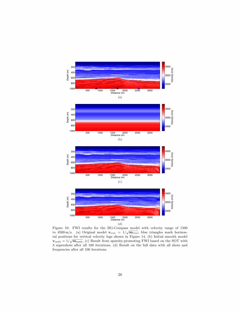
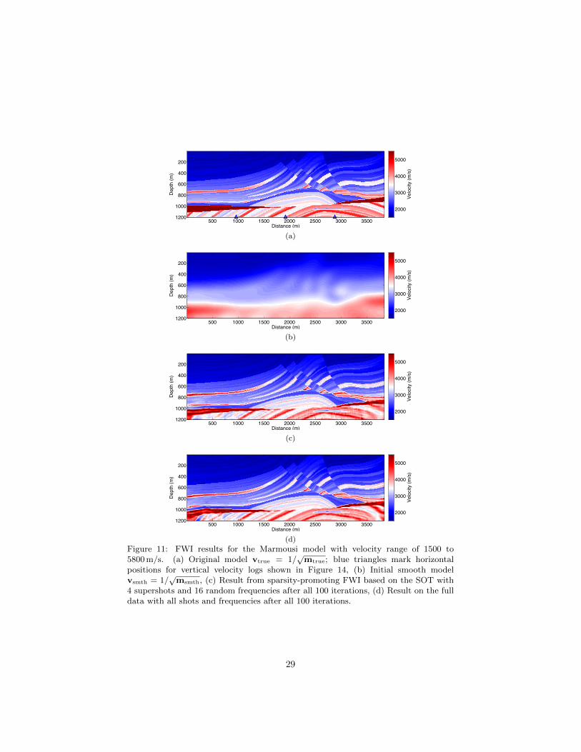
In the following experiments, the proposed FWI method is tested on twosynthetic velocity models that are often used to verify inversion algorithmsin realistic settings. One velocity model is from the BG-Compass benchmarkmodel whose exact form is shown in Figure 10(a). This model is rescaled toNz × Nx = 100 × 350 grid points and covers a width of 3.5 km and a depthof 1 km. Full data generated by Ns = 350 sequential shots are recorded byNr = 350 receivers equispaced along the surface of the model. Another bench-mark velocity model is the well-known Marmousi model shown in Figure 11(a).This model is rescaled to Nz ×Nx = 120× 384 grid points and covers a widthof 3.84 km and a depth of 1.2 km. Full data from Ns = 384 sequential shots onthe model surface are recorded over Nr = 384 equispaced receivers. The gridspacing of 10 m guarantees that a sufficient number of grid points are used torepresent the expected wavelengths and no grid dispersion happens. We sim-ulate wavefields by discretizing the PDE (8) as a Helmholtz system and solv-ing with a direct solver based on the 8th-order staggered-grid finite differencefrequency-domain method [Ajo-Franklin, 2005] in which the left, right and bot-tom boundary reflections are absorbed by perfectly matched layers [Komatitschand Martin, 2007].

The shot source is a Ricker wavelet centered at 20 Hz with 256 frequencycomponents spanning 3.0 to 48.1 Hz, and its spectrum f(ω) is assumed known

27

Distance (m)

Dep

th (

m)

500 1000 1500 2000 2500 3000

200

400

600

800

1000

Vel

ocity

(m

/s)

2000

3000

4000

(a)

Distance (m)

Dep

th (

m)

500 1000 1500 2000 2500 3000

200

400

600

800

1000

Vel

ocity

(m

/s)

2000

3000

4000

(b)

Distance (m)

Dep

th (

m)

500 1000 1500 2000 2500 3000

200

400

600

800

1000V

eloc

ity (

m/s

)2000

3000

4000

(c)

Distance (m)

Dep

th (

m)

500 1000 1500 2000 2500 3000

200

400

600

800

1000

Vel

ocity

(m

/s)

2000

3000

4000

(d)

Figure 10: FWI results for the BG-Compass model with velocity range of 1500to 4500 m/s. (a) Original model vtrue = 1/

√mtrue; blue triangles mark horizon-

tal positions for vertical velocity logs shown in Figure 14, (b) Initial smooth modelvsmth = 1/

√msmth, (c) Result from sparsity-promoting FWI based on the SOT with

3 supershots after all 100 iterations, (d) Result on the full data with all shots andfrequencies after all 100 iterations.

28

Distance (m)

Dep

th (

m)

500 1000 1500 2000 2500 3000 3500

200

400

600

800

1000

1200

Vel

ocity

(m

/s)

2000

3000

4000

5000

(a)

Distance (m)

Dep

th (

m)

500 1000 1500 2000 2500 3000 3500

200

400

600

800

1000

1200

Vel

ocity

(m

/s)

2000

3000

4000

5000

(b)

Distance (m)

Dep

th (

m)

500 1000 1500 2000 2500 3000 3500

200

400

600

800

1000

1200

Vel

ocity

(m

/s)

2000

3000

4000

5000

(c)

Distance (m)

Dep

th (

m)

500 1000 1500 2000 2500 3000 3500

200

400

600

800

1000

1200

Vel

ocity

(m

/s)

2000

3000

4000

5000

(d)

Figure 11: FWI results for the Marmousi model with velocity range of 1500 to5800 m/s. (a) Original model vtrue = 1/

√mtrue; blue triangles mark horizontal

positions for vertical velocity logs shown in Figure 14, (b) Initial smooth modelvsmth = 1/

√msmth, (c) Result from sparsity-promoting FWI based on the SOT with

4 supershots and 16 random frequencies after all 100 iterations, (d) Result on the fulldata with all shots and frequencies after all 100 iterations.

29

and fixed. FWI starts from an initial smooth model shown in Figure 10(b)for BG-Compass, or Figure 11(b) for Marmousi. In practical implementations,FWI is carried out sequentially in several consecutive frequency bands to avoidlocal minima caused by cycle skipping [Bunks et al., 1995, Sirgue and Pratt,2004]. Here we use five frequency bands within 3.0 to 48.1 Hz, so the averagenumber of frequencies per band is Nω = 256/5 ≈ 52. In each frequency band,K = 20 FWI iterations are executed. After 20 FWI iterations are completedon one frequency band, the resulting more accurate model serves as the initialmodel for another 20 FWI iterations on the next higher frequency band.

For every data-reduced FWI iteration in our experiments based on CS, weonly use N ′s = (1/100)Ns supershots (3 for BG-Compass and 4 for Marmousi),and N ′ω = 16 random frequencies from one of five frequency bands. Thus,

the problem dimensionality of the compressed objective function J(W)k (α) in

Equation (16) is (NωNs)/(N′ωN′s) ≈ 320 times smaller than that of the full-

data Gauss-Newton objective function Jk(δm) in (7). This does not necessarilymean that a data-reduced FWI iteration runs 320 times faster than a full-dataFWI iteration as actual implementations may vary, but the reduced time on bothforward modeling and objective function minimization, as well as the reducedRAM costs, are still considerable in our case. The data-reduced FWI results areshown in Figures 10(c) and 11(c) for BG-Compass and Marmousi, respectively.As a comparison, the FWI results on the full data with all shots and frequenciesare shown in Figures 10(d) and 11(d) for both models, respectively. The sparsitypromotion introduced by the adaptive SOT moves the problem to a much lowerdimensional space, so we are able to achieve comparable inversion results withmuch lower computational cost.

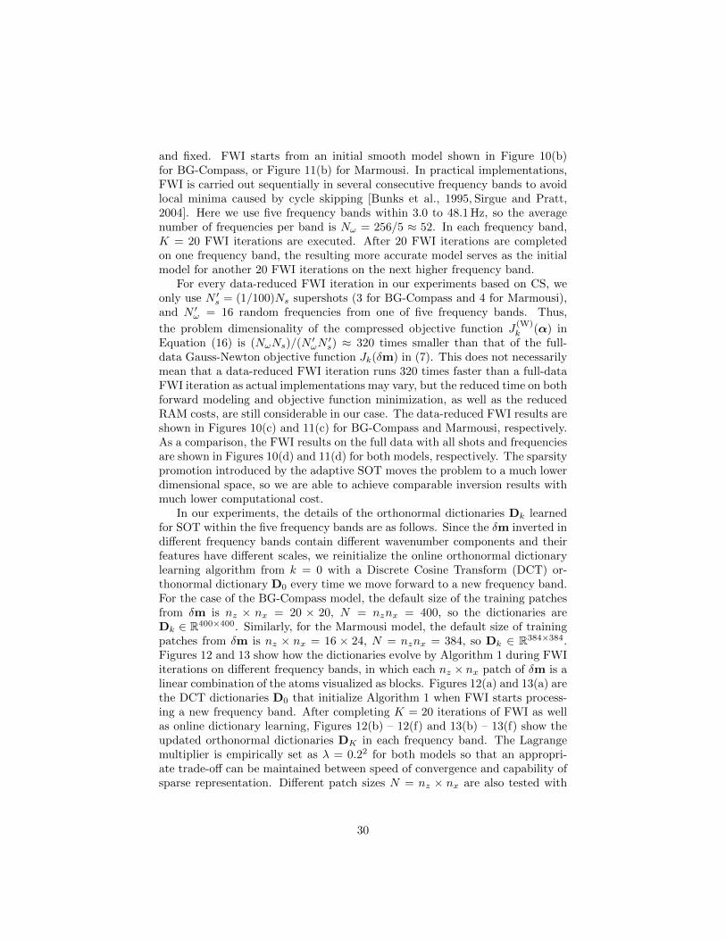
In our experiments, the details of the orthonormal dictionaries Dk learnedfor SOT within the five frequency bands are as follows. Since the δm inverted indifferent frequency bands contain different wavenumber components and theirfeatures have different scales, we reinitialize the online orthonormal dictionarylearning algorithm from k = 0 with a Discrete Cosine Transform (DCT) or-thonormal dictionary D0 every time we move forward to a new frequency band.For the case of the BG-Compass model, the default size of the training patchesfrom δm is nz × nx = 20 × 20, N = nznx = 400, so the dictionaries areDk ∈ R400×400. Similarly, for the Marmousi model, the default size of trainingpatches from δm is nz × nx = 16 × 24, N = nznx = 384, so Dk ∈ R384×384.Figures 12 and 13 show how the dictionaries evolve by Algorithm 1 during FWIiterations on different frequency bands, in which each nz × nx patch of δm is alinear combination of the atoms visualized as blocks. Figures 12(a) and 13(a) arethe DCT dictionaries D0 that initialize Algorithm 1 when FWI starts process-ing a new frequency band. After completing K = 20 iterations of FWI as wellas online dictionary learning, Figures 12(b) – 12(f) and 13(b) – 13(f) show theupdated orthonormal dictionaries DK in each frequency band. The Lagrangemultiplier is empirically set as λ = 0.22 for both models so that an appropri-ate trade-off can be maintained between speed of convergence and capability ofsparse representation. Different patch sizes N = nz × nx are also tested with

30

different sized dictionaries Dk ∈ RN×N in order to study the robustness of themethod (see Figures 14, 15, and 16).

(a) (b) (c)

(d) (e) (f)

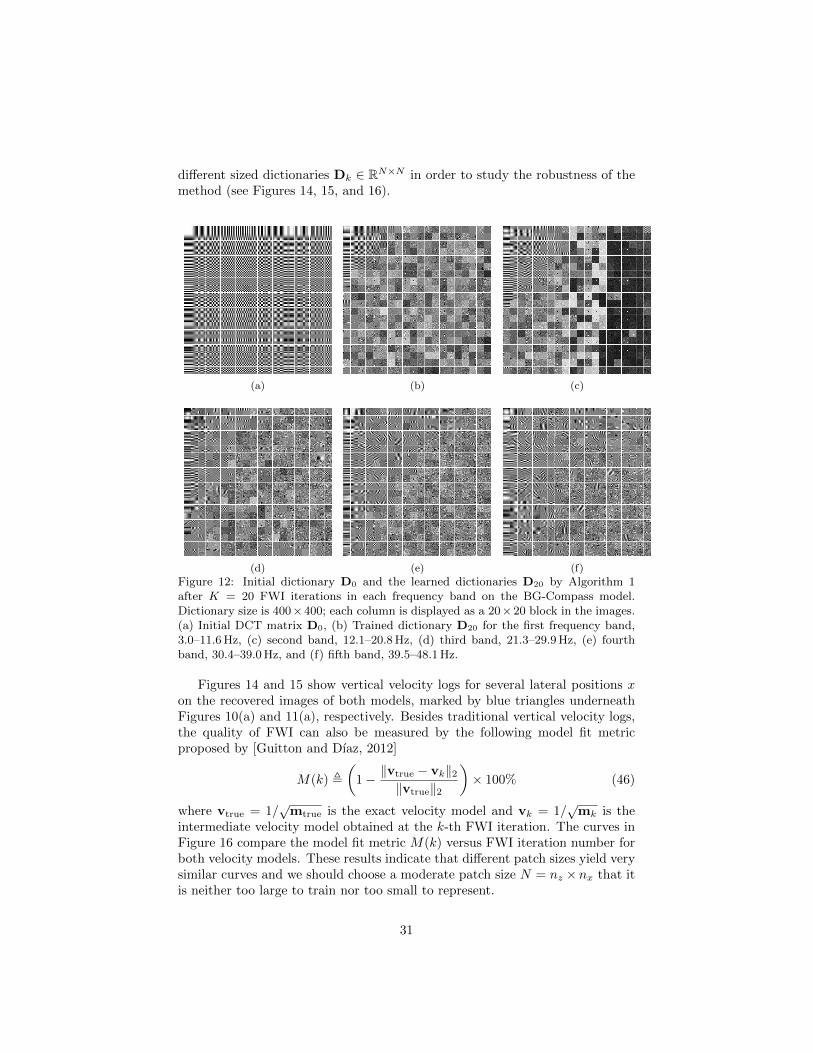
Figure 12: Initial dictionary D0 and the learned dictionaries D20 by Algorithm 1after K = 20 FWI iterations in each frequency band on the BG-Compass model.Dictionary size is 400×400; each column is displayed as a 20×20 block in the images.(a) Initial DCT matrix D0, (b) Trained dictionary D20 for the first frequency band,3.0–11.6 Hz, (c) second band, 12.1–20.8 Hz, (d) third band, 21.3–29.9 Hz, (e) fourthband, 30.4–39.0 Hz, and (f) fifth band, 39.5–48.1 Hz.

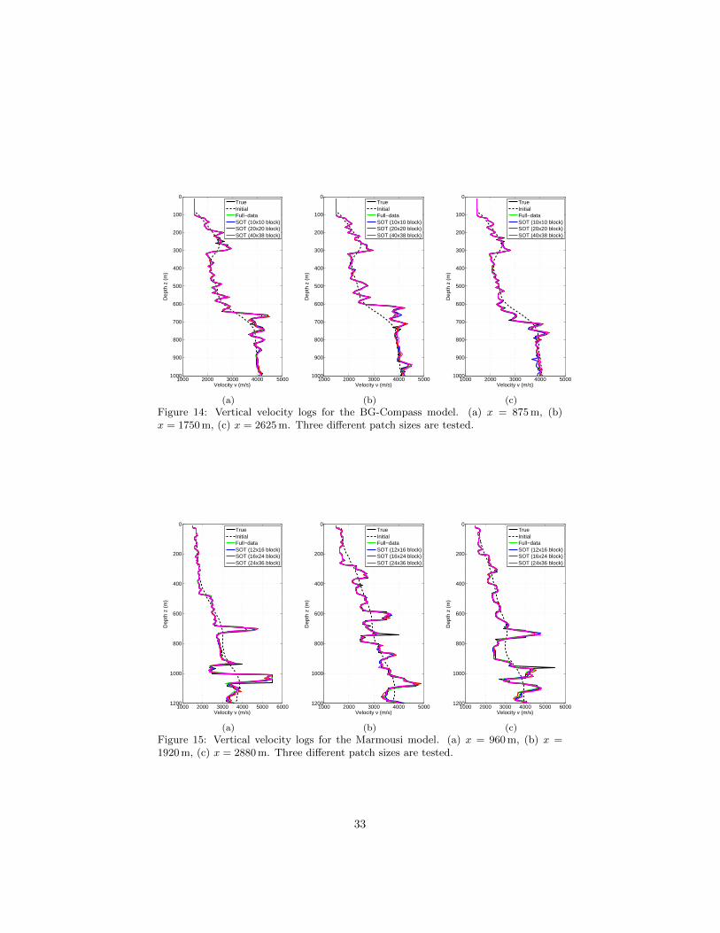
Figures 14 and 15 show vertical velocity logs for several lateral positions xon the recovered images of both models, marked by blue triangles underneathFigures 10(a) and 11(a), respectively. Besides traditional vertical velocity logs,the quality of FWI can also be measured by the following model fit metricproposed by [Guitton and Dıaz, 2012]

M(k) ,

(1− ‖vtrue − vk‖2

‖vtrue‖2

)× 100% (46)

where vtrue = 1/√

mtrue is the exact velocity model and vk = 1/√

mk is theintermediate velocity model obtained at the k-th FWI iteration. The curves inFigure 16 compare the model fit metric M(k) versus FWI iteration number forboth velocity models. These results indicate that different patch sizes yield verysimilar curves and we should choose a moderate patch size N = nz × nx that itis neither too large to train nor too small to represent.

31

(a) (b)

(c) (d)

(e) (f)

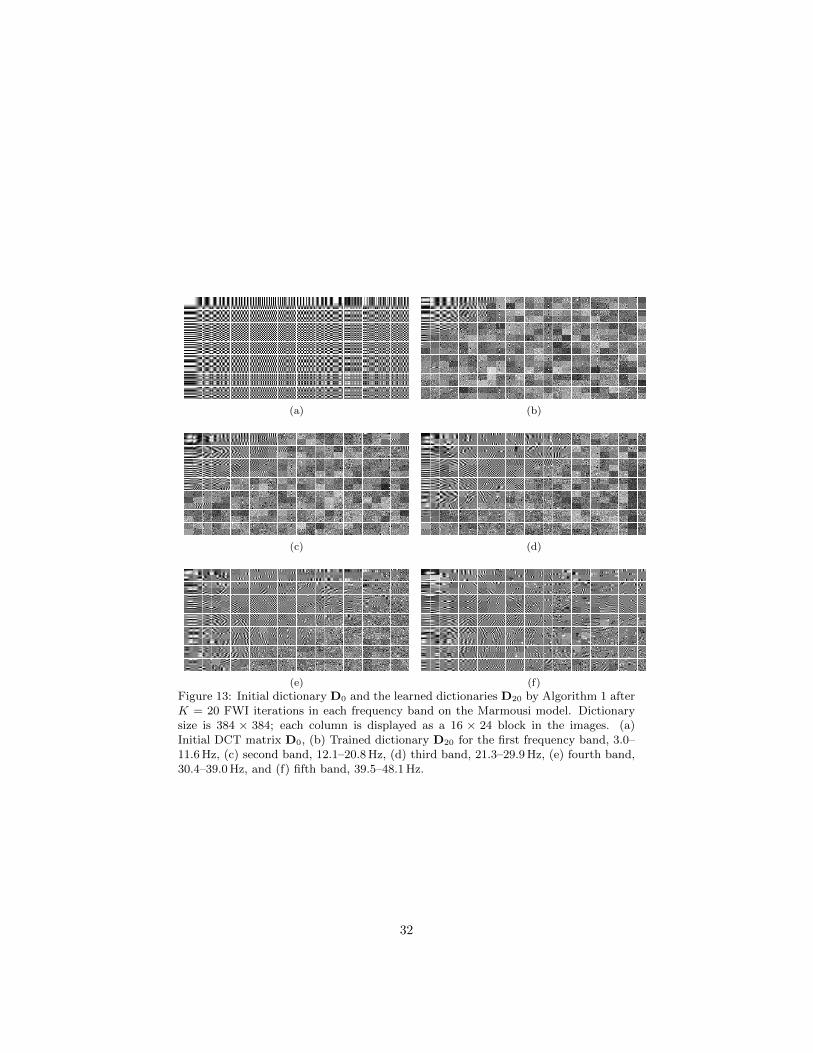
Figure 13: Initial dictionary D0 and the learned dictionaries D20 by Algorithm 1 afterK = 20 FWI iterations in each frequency band on the Marmousi model. Dictionarysize is 384 × 384; each column is displayed as a 16 × 24 block in the images. (a)Initial DCT matrix D0, (b) Trained dictionary D20 for the first frequency band, 3.0–11.6 Hz, (c) second band, 12.1–20.8 Hz, (d) third band, 21.3–29.9 Hz, (e) fourth band,30.4–39.0 Hz, and (f) fifth band, 39.5–48.1 Hz.

32

1000 2000 3000 4000 5000

0

100

200

300

400

500

600

700

800

900

1000

Velocity v (m/s)

Dep

th z

(m

)

TrueInitialFull−dataSOT (10x10 block)SOT (20x20 block)SOT (40x38 block)

(a)

1000 2000 3000 4000 5000

0

100

200

300

400

500

600

700

800

900

1000

Velocity v (m/s)

Dep

th z

(m

)


(b)

1000 2000 3000 4000 5000

0

100

200

300

400

500

600

700

800

900

1000

Velocity v (m/s)

Dep

th z

(m

)


(c)

Figure 14: Vertical velocity logs for the BG-Compass model. (a) x = 875 m, (b)x = 1750 m, (c) x = 2625 m. Three different patch sizes are tested.

1000 2000 3000 4000 5000 6000

0

200

400

600

800

1000

1200

Velocity v (m/s)

Dep

th z

(m

)


(a)

1000 2000 3000 4000 5000

0

200

400

600

800

1000

1200

Velocity v (m/s)

Dep

th z

(m

)


(b)

1000 2000 3000 4000 5000 6000

0

200

400

600

800

1000

1200

Velocity v (m/s)

Dep

th z

(m

)


(c)

Figure 15: Vertical velocity logs for the Marmousi model. (a) x = 960 m, (b) x =1920 m, (c) x = 2880 m. Three different patch sizes are tested.

33

0 20 40 60 80 10090

92

94

96

98

FWI Iterations

Mod

el F

it (%

)

Full−dataSOT (10x10 block)SOT (20x20 block)SOT (40x38 block)

(a)

0 20 40 60 80 10075

80

85

90

95

FWI Iterations

Mod

el F

it (%

)

Full−dataSOT (12x16 block)SOT (16x24 block)SOT (24x36 block)

(b)

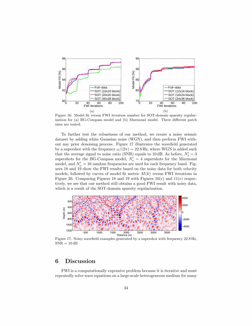
Figure 16: Model fit versus FWI iteration number for SOT-domain sparsity regular-ization for (a) BG-Compass model and (b) Marmousi model. Three different patchsizes are tested.

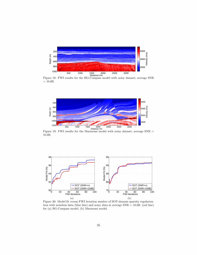
To further test the robustness of our method, we create a noisy seismicdataset by adding white Gaussian noise (WGN), and then perform FWI with-out any prior denoising process. Figure 17 illustrates the wavefield generatedby a supershot with the frequency ω/(2π) = 22.8 Hz, where WGN is added suchthat the average signal to noise ratio (SNR) equals to 10 dB. As before, N ′s = 3supershots for the BG-Compass model, N ′s = 4 supershots for the Marmousimodel, and N ′ω = 16 random frequencies are used for each frequency band. Fig-ures 18 and 19 show the FWI results based on the noisy data for both velocitymodels, followed by curves of model fit metric M(k) versus FWI iterations inFigure 20. Comparing Figures 18 and 19 with Figures 10(c) and 11(c) respec-tively, we see that our method still obtains a good FWI result with noisy data,which is a result of the SOT-domain sparsity regularization.

Distance (m)

Dep

th (

m)

500 1000 1500 2000 2500 3000 3500

200

400

600

800

1000

1200

−4000

−2000

0

2000

4000

Figure 17: Noisy wavefield examples generated by a supershot with frequency 22.8 Hz,SNR = 10 dB

6 Discussion

FWI is a computationally expensive problem because it is iterative and mustrepeatedly solve wave equations on a large-scale heterogeneous medium for many

34

Distance (m)

Dep

th (

m)

500 1000 1500 2000 2500 3000

200

400

600

800

1000

Vel

ocity

(m

/s)

2000

3000

4000

Figure 18: FWI results for the BG-Compass model with noisy dataset; average SNR= 10 dB.

Distance (m)

Dep

th (

m)

500 1000 1500 2000 2500 3000 3500

200

400

600

800

1000

1200

Vel

ocity

(m

/s)

2000

3000

4000

5000

Figure 19: FWI results for the Marmousi model with noisy dataset; average SNR =10 dB.

0 20 40 60 80 10090

92

94

96

98

FWI Iterations

Mod

el F

it (%

)

SOT (SNR=∞)SOT (SNR=10dB)

(a)

0 20 40 60 80 10075

80

85

90

95

FWI Iterations

Mod

el F

it (%

)

SOT (SNR=∞)SOT (SNR=10dB)

(b)

Figure 20: Model fit versus FWI iteration number of SOT-domain sparsity regulariza-tion with noiseless data (blue line) and noisy data at average SNR = 10 dB. (red line)for (a) BG-Compass model, (b) Marmousi model.

35

sources. In order to reduce the computational cost without compromising theresults, CS techniques suggest using only a small fraction of the data volumeafter some randomness has been injected as long as the model perturbation δmcan be transformed into sparse coefficients. Then it is still possible to invertthe velocity model by iteratively minimizing a modified Gauss-Newton objectivefunction with an `1-norm constraint. Different from using predefined transformswith implicit dictionaries such as wavelets or curvelets, this paper introducesa sparse transform called the SOT based on learning patch-sized adaptive dic-tionaries from the inverted model perturbations. Predefined transforms aredesigned to optimally represent a specific class of signals, so they cannot guar-antee sparse representations of all signals with different features. Recent resultsin signal processing have shown that learning adaptive dictionaries by trainingon the signals themselves leads to sparse signal representation and state-of-the-art performance in various applications.

To introduce dictionary learning into FWI, two features were emphasized.First, the learned dictionaries are made orthonormal, yielding a fast and straight-forward alternating optimization scheme for SOT dictionary learning. An or-thonormal dictionary is a Parseval frame, therefore finding sparse coefficientvectors only requires simple matrix multiplication. On the other hand, an over-complete dictionary loses this simplicity and makes sparse representation a basispursuit problem. Second, SOT dictionary learning is configured to work online,taking the iterative Gauss-Newton optimization process of FWI into account.After each iteration, the optimized model perturbation not only serves to updatethe velocity model, but also provides a resource to get many training patchesfor learning a new dictionary that adapts to the specific feature variations ofdifferent model perturbations.

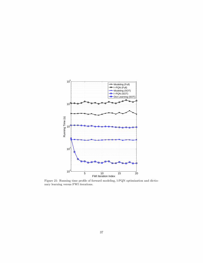
The extra computational overhead involved in learning the orthonormal dic-tionary for SOT has been analyzed in the previous section “Sparse OrthonormalTransform”. In addition to the theoretical complexity analysis, we now reportone instance of the actual running time of forward modeling, l-PQN optimiza-tion and orthonormal dictionary learning (with 16 × 24 patches) for 20 FWIiterations (in one frequency band) on the Marmousi model with 4 supershotsand 16 random frequencies. As a comparison, the running times of forwardmodeling and l-PQN optimization for the full-data FWI are also provided (seeFigure 21). The computing cluster is based on 12-core Intel R© Xeon R© CPUwith 64GB RAM and we have accelerated the forward modeling by parallelcomputing.

Figure 21 shows that the running time of forward modeling and l-PQN op-timization for the full-data FWI is over 10 times of that for the data-reducedFWI. It is also noticeable that, after the first FWI iteration, the running timefor orthonormal dictionary learning falls rapidly to a negligible level comparedto the cost of the other two phases. The online learning approach exhibitsthis behavior because it always updates the latest and best dictionary for theincoming model perturbation at each FWI iteration. Once a good dictionaryhas been obtained, many fewer training iterations are required for the updates.Therefore, it is safe to say that the actual overhead from orthonormal dictionary

36

5 10 15 2010

1

102

103

104

105

FWI Iteration Index

Run

ning

Tim

e (s

)

Modeling (Full)l−PQN (Full)Modeling (SOT)l−PQN (SOT)Dict Learning (SOT)

Figure 21: Running time profile of forward modeling, l-PQN optimization and dictio-nary learning versus FWI iterations.

37

learning is not significant.The extension of orthonormal dictionary learning, SOT, as well as the FWI

using SOT for sparse representation to 3D models should be feasible. Thoughsolving 3D forward modeling problems is much more expensive than 2D prob-lems, recent development on the direct solvers eventually relieves the diffi-culty [Operto et al., 2015]. Besides, compressive sensing schemes using SOTcould offer more flexibility and efficiency to 3D problems as 3D grid geome-try provides more freedom for subsampling. Since dictionary learning reshapesmodel patches and atoms into vectors no matter how many dimensions in spacethey occupy, we can reasonably infer their computational complexity accordingto the learning steps in Algorithm 1. The 3D model size is Nz×Nx×Ny and the3D patch size is nz ×nx×ny, where nz Nz, nx Nx, ny Ny. If all possi-ble overlapping patches are used for training, then each orthonormal dictionarylearning iteration costs O((nznxny)2(Nz −nz + 1)(Nx−nx + 1)(Ny −ny + 1) +(nznxny)3), and applying the SOT with the 3D dictionary to a 3D model costsO(nznxnyNzNxNy). The training patch size is the one parameter that needsto be chosen in order to get sparse representation of the model perturbations.Small patches are desirable for training the orthonormal dictionary. The othertwo parameters in the algorithm, τk and λ are chosen based on the data or viaempirical testing.

7 Conclusion

In this paper, a novel and efficient compressive sensing scheme that signif-icantly reduces the computational complexity of the FWI problem has beenpresented. The new method exploits the sparsity representation of model per-turbations with a sparse orthonormal transform (SOT) such that each block ofmodel perturbation can be represented with sparse coefficients over adaptivedata-driven dictionaries trained from previous results. Compared to traditionalmodel-based transforms that are only optimal for objects with piecewise smooth-ness, the SOT is better able to adapt to nonintuitive signal regularities such ascomplex geophysical features. Compared to the traditional overcomplete dic-tionary learning methods, the orthonormal dictionary learning method is muchmore efficient and can adapt in an online manner. Therefore, the SOT enablesus to significantly reduce the amount of data used in FWI by invoking the strat-egy of compressive sampling. We randomly select sources and frequencies andencode the data with random phases so that this scheme works for both landand marine scenarios. After that, the original Gauss-Newton problem becomesa LASSO problem and can be effectively solved using a projected quasi-Newtonalgorithm.

The experiments clearly indicate that we can obtain high-quality invertedvelocity models with both simple and complex geophysical features by workingwith a small subset of the full seismic dataset, even in the presence of noise.

38

References

[Aharon et al., 2006] Aharon, M., M. Elad, and A. Bruckstein, 2006, K-SVD:An algorithm for designing overcomplete dictionaries for sparse representa-tion: Signal Processing, IEEE Transactions on, 54, 4311–4322.

[Ajo-Franklin, 2005] Ajo-Franklin, J. B., 2005, Frequency-domain modelingtechniques for the scalar wave equation: an introduction: Technical report,Earth Resources Laboratory, Dept. of Earth, Atmospheric, and PlanetarySciences, Massachusetts Institute of Technology.

[Armijo, 1966] Armijo, L., 1966, Minimization of functions having lipschitz con-tinuous first partial derivatives.: Pacific J. Math., 16, 1–3.

[Beckouche and Ma, 2014] Beckouche, S., and J. Ma, 2014, Simultaneous dic-tionary learning and denoising for seismic data: Geophysics, 79, A27–A31.

[Ben-Hadj-Ali et al., 2011] Ben-Hadj-Ali, H., S. Operto, and J. Virieux, 2011,An efficient frequency-domain full waveform inversion method using simulta-neous encoded sources: GEOPHYSICS, 76, R109–R124.

[Beylkin, 1985] Beylkin, G., 1985, Imaging of discontinuities in the inverse scat-tering problem by inversion of a causal generalized radon transform: Journalof Mathematical Physics, 26, 99–108.

[Birgin et al., 2014] Birgin, E., J. Martınez, and M. Raydan, 2014, Spectralprojected gradient methods: Review and perspectives: Journal of StatisticalSoftware, 60, 1–21.

[Birgin et al., 1999] Birgin, E. G., J. M. Martınez, and M. Raydan, 1999, Non-monotone spectral projected gradient methods on convex sets: SIAM J. onOptimization, 10, 1196–1211.

[Blumensath and Davies, 2009] Blumensath, T., and M. E. Davies, 2009, Iter-ative hard thresholding for compressed sensing: Applied and ComputationalHarmonic Analysis, 27, 265 – 274.

[Bousquet and Bottou, 2007] Bousquet, O., and L. Bottou, 2007, The tradeoffsof large scale learning, in Advances in Neural Information Processing Systems20: MIT Press, 161–168.

[Brenders and Pratt, 2007] Brenders, A. J., and R. G. Pratt, 2007, Full wave-form tomography for lithospheric imaging: results from a blind test in arealistic crustal model: Geophysical Journal International, 168, 133–151.

[Bunks et al., 1995] Bunks, C., F. M. Saleck, S. Zaleski, and G. Chavent, 1995,Multiscale seismic waveform inversion: GEOPHYSICS, 60, 1457–1473.

[Cai et al., 2014] Cai, J.-F., H. Ji, Z. Shen, and G.-B. Ye, 2014, Data-driventight frame construction and image denoising: Applied and ComputationalHarmonic Analysis, 37, 89 – 105.

[Candes et al., 2006] Candes, E., L. Demanet, D. Donoho, and L. Ying, 2006,Fast discrete curvelet transforms: Multiscale Modeling and Simulation, 5,861–899.

39

[Candes and Demanet, 2005] Candes, E. J., and L. Demanet, 2005, Thecurvelet representation of wave propagators is optimally sparse: Commu-nications on Pure and Applied Mathematics, 58, 1472–1528.

[Castellanos et al., 2015] Castellanos, C., L. Metivier, S. Operto, R. Brossier,and J. Virieux, 2015, Fast full waveform inversion with source encoding andsecond-order optimization methods: Geophysical Journal International, 200,720–744.

[Chen et al., 1998] Chen, S. S., D. L. Donoho, and M. A. Saunders, 1998,Atomic decomposition by basis pursuit: SIAM Journal on Scientific Com-puting, 20, 33–61.

[Donoho and Tanner, 2010] Donoho, D. L., and J. Tanner, 2010, Precise under-sampling theorems: Proceedings of the IEEE, 98, 913–924.

[Duchi et al., 2008] Duchi, J., S. Shalev-Shwartz, Y. Singer, and T. Chandra,2008, Efficient projections onto the `1-ball for learning in high dimensions:Proceedings of the 25th International Conference on Machine Learning, ACM,272–279.

[Elad and Aharon, 2006] Elad, M., and M. Aharon, 2006, Image denoising viasparse and redundant representations over learned dictionaries: Image Pro-cessing, IEEE Transactions on, 15, 3736–3745.

[Gubernatis et al., 1977] Gubernatis, J., E. Domany, J. Krumhansl, and M.Huberman, 1977, The Born approximation in the theory of the scattering ofelastic waves by flaws: Journal of Applied Physics, 48, 2812–2819.

[Guitton and Dıaz, 2012] Guitton, A., and E. Dıaz, 2012, Attenuating crosstalknoise with simultaneous source full waveform inversion: GeophysicalProspecting, 60, 759–768.

[Hennenfent and Herrmann, 2006] Hennenfent, G., and F. Herrmann, 2006,Seismic denoising with nonuniformly sampled curvelets: Computing in Sci-ence Engineering, 8, 16–25.

[Herrmann et al., 2012] Herrmann, F., M. Friedlander, and O. Yilmaz, 2012,Fighting the curse of dimensionality: Compressive sensing in exploration seis-mology: Signal Processing Magazine, IEEE, 29, 88–100.

[Herrmann and Li, 2012] Herrmann, F. J., and X. Li, 2012, Efficient least-squares imaging with sparsity promotion and compressive sensing: Geophys-ical Prospecting, 60, 696–712.

[Herrmann et al., 2011] Herrmann, F. J., X. Li, A. Y. Aravkin, and T. vanLeeuwen, 2011, A modified, sparsity-promoting, Gauss-Newton algorithm forseismic waveform inversion.

[Herrmann et al., 2008] Herrmann, F. J., D. Wang, G. Hennenfent, and P. P.Moghaddam, 2008, Curvelet-based seismic data processing: A multiscale andnonlinear approach: GEOPHYSICS, 73, A1–A5.

[Jang et al., 2009] Jang, U., D.-J. Min, and C. Shin, 2009, Comparison of scal-ing methods for waveform inversion: Geophysical Prospecting, 57, 49–59.

40

[Komatitsch and Martin, 2007] Komatitsch, D., and R. Martin, 2007, An un-split convolutional perfectly matched layer improved at grazing incidence forthe seismic wave equation: GEOPHYSICS, 72, SM155–SM167.

[Krebs et al., 2009] Krebs, J. R., J. E. Anderson, D. Hinkley, R. Neelamani,S. Lee, A. Baumstein, and M.-D. Lacasse, 2009, Fast full-wavefield seismicinversion using encoded sources: GEOPHYSICS, 74, WCC177–WCC188.

[Lewicki and Olshausen, 1999] Lewicki, M. S., and B. A. Olshausen, 1999,Probabilistic framework for the adaptation and comparison of image codes:J. Opt. Soc. Am. A, 16, 1587–1601.

[Li et al., 2012] Li, X., A. Y. Aravkin, T. van Leeuwen, and F. J. Herrmann,2012, Fast randomized full-waveform inversion with compressive sensing:GEOPHYSICS, 77, A13–A17.

[Li et al., 2016] Li, X., E. Esser, and F. J. Herrmann, 2016, Modified gauss-newton full-waveform inversion explained – why sparsity-promoting updatesdo matter: To appear in Geophysics.

[Li and Herrmann, 2012] Li, X., and F. J. Herrmann, 2012, Efficient full-waveform inversion with marine acquisition geometry: GeoConvention2012:Vision.

[Loris et al., 2007] Loris, I., G. Nolet, I. Daubechies, and F. A. Dahlen, 2007,Tomographic inversion using `1-norm regularization of wavelet coefficients:Geophysical Journal International, 170, 359–370.

[Ma et al., 2012] Ma, Y., D. Hale, B. Gong, and Z. J. Meng, 2012, Image-guidedsparse-model full waveform inversion: GEOPHYSICS, 77, R189–R198.

[Mallat and Zhang, 1993] Mallat, S., and Z. Zhang, 1993, Matching pursuitswith time-frequency dictionaries: Signal Processing, IEEE Transactions on,41, 3397–3415.

[Moghaddam and Herrmann, 2010] Moghaddam, P. P., and F. J. Herrmann,2010, Randomized full-waveform inversion: a dimensionality-reduction ap-proach: SEG Technical Program Expanded Abstracts 2010, 977–982.

[Nocedal, 1980] Nocedal, J., 1980, Updating quasi-Newton matrices with lim-ited storage: Mathematics of computation, 35, 773–782.

[Nocedal and Wright, 2006] Nocedal, J., and S. Wright, 2006, Numerical opti-mization: Springer Science & Business Media.

[Olshausen and Field, 1996] Olshausen, B. A., and D. J. Field, 1996, Naturalimage statistics and efficient coding: Network: Computation in Neural Sys-tems, 7, 333–339. (PMID: 16754394).

[Operto et al., 2015] Operto, S., A. Miniussi, R. Brossier, L. Combe, L.Metivier, V. Monteiller, A. Ribodetti, and J. Virieux, 2015, Efficient 3-dfrequency-domain mono-parameter full-waveform inversion of ocean-bottomcable data: application to valhall in the visco-acoustic vertical transverseisotropic approximation: Geophysical Journal International, 202, 1362–1391.

41

[Pan et al., 2015] Pan, W., K. A. Innanen, G. F. Margrave, and D. Cao, 2015,Efficient pseudo-Gauss-Newton full-waveform inversion in the τ -p domain:GEOPHYSICS, 80, R225–R14.

[Pati et al., 1993] Pati, Y., R. Rezaiifar, and P. Krishnaprasad, 1993, Orthogo-nal matching pursuit: recursive function approximation with applications towavelet decomposition: Signals, Systems and Computers, 1993. 1993 Confer-ence Record of The Twenty-Seventh Asilomar Conference on, 40–44 vol.1.

[Plessix and Mulder, 2004] Plessix, R.-E., and W. A. Mulder, 2004, Frequency-domain finite-difference amplitude-preserving migration: Geophysical JournalInternational, 157, 975–987.

[Pratt, 1999] Pratt, R. G., 1999, Seismic waveform inversion in the frequencydomain, part 1: Theory and verification in a physical scale model: GEO-PHYSICS, 64, 888–901.

[Pratt et al., 1998] Pratt, R. G., C. Shin, and G. J. Hick, 1998, Gauss-Newtonand full Newton methods in frequency–space seismic waveform inversion:Geophysical Journal International, 133, 341–362.

[Ren et al., 2013] Ren, H., H. Wang, and S. Chen, 2013, Least-squares reversetime migration in frequency domain using the adjoint-state method: Journalof Geophysics and Engineering, 10, 035002.

[Romero et al., 2000] Romero, L. A., D. C. Ghiglia, C. C. Ober, and S. A.Morton, 2000, Phase encoding of shot records in prestack migration: GEO-PHYSICS, 65, 426–436.

[Rubinstein et al., 2013] Rubinstein, R., T. Peleg, and M. Elad, 2013, AnalysisK-SVD: A dictionary-learning algorithm for the analysis sparse model: SignalProcessing, IEEE Transactions on, 61, 661–677.

[Rubinstein et al., 2010] Rubinstein, R., M. Zibulevsky, and M. Elad, 2010,Double sparsity: Learning sparse dictionaries for sparse signal approxima-tion: Signal Processing, IEEE Transactions on, 58, 1553–1564.

[Schmidt et al., 2009] Schmidt, M. W., E. Berg, M. P. Friedlander, and K. P.Murphy, 2009, Optimizing costly functions with simple constraints: Alimited-memory projected quasi-Newton algorithm: International Conferenceon Artificial Intelligence and Statistics, 456–463.

[Schonemann, 1966] Schonemann, P., 1966, A generalized solution of the or-thogonal procrustes problem: Psychometrika, 31, 1–10.

[Sezer et al., 2015] Sezer, O., O. Guleryuz, and Y. Altunbasak, 2015, Approxi-mation and compression with sparse orthonormal transforms: Image Process-ing, IEEE Transactions on, 24, 2328–2343.

[Sezer, 2012] Sezer, O. G., 2012, Data-driven transform optimization for nextgeneration multimedia applications: PhD thesis, Georgia Institute of Tech-nology.

42

[Shin et al., 2001] Shin, C., S. Jang, and D.-J. Min, 2001, Improved amplitudepreservation for prestack depth migration by inverse scattering theory: Geo-physical Prospecting, 49, 592–606.

[Sirgue and Pratt, 2004] Sirgue, L., and R. G. Pratt, 2004, Efficient waveforminversion and imaging: A strategy for selecting temporal frequencies: GEO-PHYSICS, 69, 231–248.

[Starck et al., 2015] Starck, J.-L., F. Murtagh, and J. Fadili, 2015, Sparse imageand signal processing: Wavelets and related geometric multiscale analysis:Cambridge University Press.

[Symes, 2008] Symes, W. W., 2008, Migration velocity analysis and waveforminversion: Geophysical Prospecting, 56, 765–790.

[Tarantola, 1984] Tarantola, A., 1984, Inversion of seismic reflection data in theacoustic approximation: GEOPHYSICS, 49, 1259–1266.

[Tarantola, 1986] ——–, 1986, A strategy for nonlinear elastic inversion of seis-mic reflection data: GEOPHYSICS, 51, 1893–1903.

[Tarantola, 1987] ——–, 1987, Inverse problem theory: Methods for data fittingand parameter estimation: Elsevier, Amsterdam.

[Tibshirani, 1994] Tibshirani, R., 1994, Regression shrinkage and selection viathe LASSO: Journal of the Royal Statistical Society, Series B, 58, 267–288.

[Tropp and Gilbert, 2007] Tropp, J., and A. Gilbert, 2007, Signal recovery fromrandom measurements via orthogonal matching pursuit: Information Theory,IEEE Transactions on, 53, 4655–4666.

[van den Berg and Friedlander, 2009] van den Berg, E., and M. P. Friedlander,2009, Probing the Pareto frontier for basis pursuit solutions: SIAM Journalon Scientific Computing, 31, 890–912.

[Virieux and Operto, 2009] Virieux, J., and S. Operto, 2009, An overviewof full-waveform inversion in exploration geophysics: GEOPHYSICS, 74,WCC1–WCC26.

[Warner et al., 2013] Warner, M., A. Ratcliffe, T. Nangoo, J. Morgan, A.Umpleby, N. Shah, V. Vinje, I. Stekl, L. Guasch, C. Win, G. Conroy, and A.Bertrand, 2013, Anisotropic 3d full-waveform inversion: GEOPHYSICS, 78,R59–R80.

[Wu and Aki, 1985] Wu, R., and K. Aki, 1985, Scattering characteristics of elas-tic waves by an elastic heterogeneity: GEOPHYSICS, 50, 582–595.

[Xue and Zhu, 2015] Xue, Z., and H. Zhu, 2015, Full waveform inversion withsparsity constraint in seislet domain: SEG Technical Program Expanded Ab-stracts 2015, 1382–1387.

[Yu et al., 2015] Yu, S., J. Ma, X. Zhang, and M. D. Sacchi, 2015, Interpolationand denoising of high-dimensional seismic data by learning a tight frame:GEOPHYSICS, 80, V119–V132.

43

[Zhu et al., 2015] Zhu, L., E. Liu, and J. H. McClellan, 2015, Seismic data de-noising through multiscale and sparsity-promoting dictionary learning: GEO-PHYSICS, 80, WD45–WD57.

[Zhu et al., 2016] ——–, 2016, Fast online orthonormal dictionary learning forefficient full waveform inversion: 2016 IEEE International Conference onAcoustics, Speech and Signal Processing (ICASSP), 1427–1431.

44

Sparse-promoting Full Waveform Inversion based on · PDF fileSparse-promoting Full Waveform Inversion based on Online Orthonormal Dictionary Learning Lingchen Zhu, Entao Liu, and James

Documents