Sparse multidimensional scaling using landmark pointspeyre/cours/x2005signal/dimreduc... · cal multidimensional scaling (MDS) algorithm, called Landmark MDS (LMDS), for use when

Sparse multidimensional scaling

using landmark points

Vin de Silva∗ & Joshua B. Tenenbaum†

June 30, 2004

Corresponding author: Vin de Silva, Department of Mathematics, Building 380, Stanford

University, Stanford. CA 94305-2125 <[email protected]>

Running title: Sparse MDS using landmark points.

Abstract: In this paper, we discuss a computationally efficient approximation to the classi-

cal multidimensional scaling (MDS) algorithm, called Landmark MDS (LMDS), for use when the

number of data points is very large. The first step of the algorithm is to run classical MDS to em-

bed a chosen subset of the data, referred to as the ‘landmark points’, in a low-dimensional space.

Each remaining data point can be located within this space given knowledge of its distances to the

landmark points. We give an elementary and explicit theoretical analysis of this procedure, and

demonstrate with examples that LMDS is effective in practical use.

Keywords: visualization, embedding, online algorithms, feature discovery, unsupervised learn-

ing

∗Department of Mathematics, Stanford University <[email protected]>†Department of Brain and Cognitive Sciences, Massachussetts Institute of Technology <[email protected]>

1

1 Introduction

Metric-preserving dimensionality reduction has long been an important basic task in data analysis

and machine learning. Given suitable metric information (such as similarity or dissimilarity mea-

sures) about a collection ofN objects, the task is to embed the objects as points in a low-dimensional

Euclidean space Rk, while preserving the geometry as faithfully as possible. Low-dimensional

metric-preserving embeddings have seen numerous applications – such as visualization, feature

construction and selection, compression, and data interpolation – in disciplines ranging across the

natural and social sciences. For tutorials and reviews see Shepard [1], Cox and Cox [2], Kruskal

and Wish [3], or Borg and Lingoes [4].

The original and still best-known approach to this problem is known as classical multidimen-

sional scaling (MDS). Classical MDS has many appealing features. Its domain of natural appli-

cability can be defined precisely: when the given metric on the input data points truly has a

low-dimensional Euclidean structure, classical MDS is guaranteed to find a Euclidean embedding

which exactly preserves that metric. It is based on an efficient (polynomial time) matrix algo-

rithm that finds the global optimum of a sensible cost function in closed form. The complexity

is approximately O(kN2), where N is the number of data points and k is the dimension of the

embedding.

Unfortunately, when the number of points is very large, this algorithm may be too expensive

in practice. This limitation has become more pressing recently, with the increasing availability of

very large data sets and the corresponding increasing need for scalable dimensionality reduction

algorithms. The bottleneck in classical MDS is the calculation of the top k eigenvalues and eigen-

vectors of an N ×N matrix derived from the input distance matrix D. If the number of points is

very large compared to the intrinsic dimensionality—typically, the situation where dimensionality

2

reduction is called for—there should be a better approach than computing the eigendecomposition

of this full matrix.

In this paper we describe a variation on classical MDS which preserves all of the attractive

properties but is much more efficient, the cost being essentially linear in the number of data points

(Section 2.5). Yet it also achieves the correct solution if the data really have a low-dimensional

Euclidean structure; and the algorithm is stable under small perturbations of the input distances

so good results are obtained even for noisy data. The required input is an n×N submatrix of D,

giving the distances between the N data points and a set of n distinguished points referred to as

“landmarks”. There are two steps; first we apply classical MDS to the landmark points. The second

step is a distance-based triangulation procedure, which uses distances to the already-embedded

landmark points to determine where the remaining points should go. Our contribution is this

two-stage decomposition, and a formulation of the triangulation procedure as a linear problem.

Together, these two steps give our procedure for Landmark MDS. However, our analysis of the

second step—the linear solution to distance-based triangulation—may be of general interest in

itself, because that is a problem we may often wish to solve (for example, in global positioning

systems).

Landmark MDS is effectively online with respect to the introduction of new data points. After

the landmark points are fixed and the initial calculation carried out, all other points are embedded

independently from each other using a fixed linear transformation. A global calculation is necessary

only if the embedding coordinates are required to be aligned with the principal axes of the data.

There seems to be no reason to do this repeatedly, rather than once or twice as called for.

The Landmark MDS algorithm was introduced by the authors in [5], in the context of finding

an efficient approximation to the Isomap algorithm for nonlinear dimensionality reduction suitable

for processing large data sets. Related ideas have appeared in the machine learning and pattern

3

recognition literatures in the contexts of various applications [6–8]. Yet MDS is still often dismissed

as too computationally demanding for real-time use with large data sets [9–13]. Our goal in this

paper is to make Landmark MDS accessible and appealing to a broad audience, by giving a more

thorough and more general treatment than has previously been available, including an extensive

theoretical analysis, an investigation of the effects of noise, discussion and explanation of potential

pitfalls, and pointers to interesting applications. We also present a number of experiments on

synthetic and real data to illustrate and verify our analytical results. The remaining sections are

organised as follows. In Section 2 we describe the algorithm and its complexity. In Section 3 we

run LMDS on two classes of example data sets. The theoretical analysis is in Section 4, and further

applications are discussed briefly in Section 5.

2 Landmark MDS

We are given a collection of N objects which we wish to embed in the Euclidean space Rk. Their

dissimilarities are represented by an N ×N matrix DN . Landmark MDS consists of four steps:

1. Designate a set of n landmark points.

2. Apply classical MDS to find a k × n matrix L representing an embedding of the n landmark

points in Rk. As input, use the n × n matrix Dn of distances between pairs of landmark

points.

3. Apply distance-based triangulation (described later) to find a k ×N matrix X representing

an embedding of the N data points in Rk. As input, use the n×N matrix Dn,N of distances

between landmark points and data points. The new coordinates are derived from the squared

distances by an affine linear transformation.

4

4. Recenter the data about their mean, and use PCA to align the principal axes of the newly-

embedded data with the coordinate axes, in order of decreasing significance.

Pseudocode for the algorithm is given in Figure 1. Before discussing each step in detail, we make

some brief remarks:

• The embedding obtained in Step 3 is consistent with the embedding of the landmark points

in Step 2. In other words, L agrees with the corresponding k × n submatrix of X.

• The landmarks may be chosen by any reasonable method. For a k-dimensional embedding,

we require at least k+1 landmarks; specifically the affine span of the landmarks (as embedded

in Step 2) must be k-dimensional. For stability reasons it is better to avoid configurations

which lie close to some (k−1)- or lower-dimensional affine subspace. It is generally advisable

to to choose rather more landmark points than the strict minimum.

• Landmark MDS use only the n×N matrix Dn,N , and not the full N×N matrix DN . If there

is a substantial cost associated with calculating or storing the full matrix, this kind of spar-

sification can lead to a significant savings. As we discuss later, Landmark MDS substantially

improves the performance of Isomap [14] and allows us to embed a sparse similarity graph

efficiently.

• The final PCA stage is not essential, but it normalises the output. In addition, if k′ < k

then a good embedding in Rk′is obtained by restricting to the first k′ coordinates of the

PCA-aligned embedding. It is better to use a higher value of k and restrict to k′-dimensions

at the end, than to use a low value of k throughout.

2.1 Step 1: Selecting the landmark points

We suggest two ways of selecting the landmark set:

5

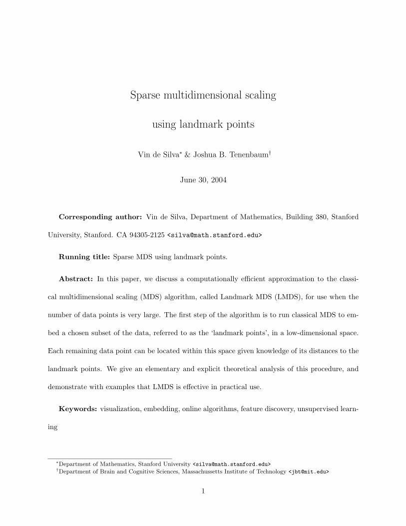
Input:N ← number of data points;∆ ← squared-distance function (two arguments);n ← desired number of landmark points;k ← desired number of output dimensions;

Step 1: select landmark points (randomly).P(1:N) ← randperm(N); // random permutation`(:) ← P(1:n);

Step 2: classical MDS on landmarks.for (i = 1:n, j = 1:n)

∆n(i,j) ← ∆(`(i),`(j));for i = (1:n)

~µn(i) ← mean(∆n(i,:));µ ← mean(~µn(:));for (i = 1:n, j = 1:n)

Bn(i,j) ← −(∆n(i, j)− ~µn(i)− ~µn(j) + µ)/2;[V,λ] ← eigensolve(Bn,k);

// V(i,j) = i-th component of j-th eigenvector// λ(j) = j-th eigenvalue, in descending order

k+ ← min(k, number of positive eigenvalues);for (i = 1:k+, j = 1:n)

L(i,j) ← V(j,i) ∗ sqrt(λ(i));

Step 3: distance-based triangulation.for (i = 1:k+, j = 1:n)

L](i,j) ← V(j,i) / sqrt(λ(i));for (j = 1:N)

X(:,j) ← −L] ∗ (∆(`(:),j)−µn(:))/2;// matrix-vector multiplication

Step 4: PCA normalisation (optional).for (i = 1:k+)

X(i) = mean(X(i,:));for (j = 1:N)

X(:,j) ← X(:,j)− X(:);[U,κ] ← eigensolve(X ∗ XT,k+); // matrix multiplicationXpca ← UT ∗ X; // matrix multiplication

Output:k+ → actual number of output dimensionsL → k+-dimensional embedding of landmarksX → k+-dimensional embedding of dataXpca→ PCA-normalised k+-dimensional embedding of data

Figure 1: Pseudocode for LMDS.

6

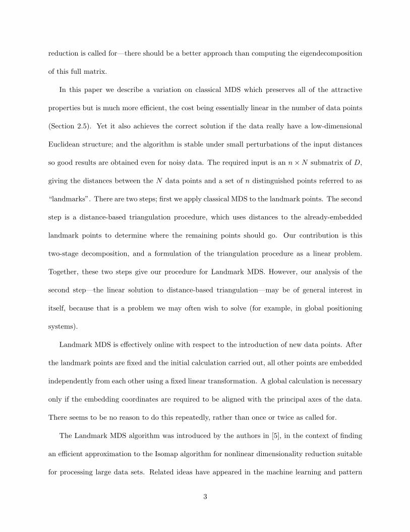
Input:N ← number of data points;∆ ← squared-distance function (two arguments);n ← desired number of landmark points;s ← desired number of seed points;

Step 1a: select landmark points by MaxMin.

// choose s seed points randomlyP(1:N) ← randperm(N);`(1:s) ← P(1:s);

for (j = 1:N)m(j) ← min[i = 1:s](∆n(`(i),j));

for (i = s+1:n)`(i) ← argmax[j = 1:N](m(j));

for (j = 1:N)m(j) = min(m(j),∆n(`(i),j));

Output:` → list of indices of n landmark points

Figure 2: Pseudocode for MaxMin landmark selection, as an alternative to Step 1 of Figure 1.

• Random choice.

• MaxMin (greedy optimisation): landmark points are chosen one at a time, and each new

landmark maximises, over all unused data points, the minimum distance to any of the exisiting

landmarks. The first point is chosen arbitrarily.

MaxMin is deterministic after the first landmark point. Sometimes it may be desirable to start

MaxMin with s ‘seed’ points, chosen randomly, for s ≥ 1. At any stage the only information

required is the matrix of distances between the existing landmark points and the remaining points,

so these entries can be accessed/computed on a need-to-know basis. The cost of using MaxMin

instead of random choice amounts to O(nN) extra operations. See Figure 2.

Random choice works quite well in practice, and we use it for all the examples in this paper.

MaxMin has the advantage of being controllable, which may be useful in some contexts where

7

reproducible results are desired. There is further discussion in Section 4.4.

Remark. At first glance, the choice of landmark points may seem to be a clustering problem. The

landmarks can be regarded as a set of n cluster centers whose distribution should be in genral

agreement with the distribution of the full data set of N points. On the other hand, it is expensive

to solve an n-center clustering problem on N points, and it may require access to the entire distance

matrix rather than just a selected set of rows. This is not in the spirit of LMDS, which is meant

to be a quick approximation. For this reason we do not endorse the use of full-blooded clustering

algorithms. Random choice and MaxMin are cheap and effective.

2.2 Step 2: Classical MDS on landmarks

We recall the procedure, first used in this context by Torgerson [15].

• Input: the n× n matrix ∆n of squared distances; so [∆n]ij = [Dn]2ij .

• Construct the mean-centered “inner-product” matrix

Bn = −12Hn∆nHn (1)

where Hn is the mean-centering matrix, defined by [Hn]ij = δij − 1/n.

• Compute the k largest positive eigenvalues of Bn together with an orthonormal set of eigen-

vectors. Write λi for the i-th largest positive eigenvalue and ~vi for the corresponding eigen-

vector (written as a column vector). Nonpositive eigenvalues are ignored; this includes a zero

eigenvalue with eigenvector ~1 = [1, 1, . . . , 1]T.

• Output: the required k-dimensional embedding vectors ~1, ~2, . . . , ~n are given by the columns

8

of the following1 matrix:

Lk =

√λ1 · ~vT

1

√λ2 · ~vT

2

...

√λk · ~vT

k

(2)

The embedding is automatically mean-centered, so ~1 + . . .+ ~n = ~0, or equivalently LkHn =

Lk. This follows from the orthogonality of eigenvectors, which gives ~vTi~1 = 0 for all i.

The justification for this construction lies in the following theorems.

Theorem 1 (Young and Householder [16]) Suppose ∆n is the Euclidean squared-distance matrix

for a collection of data points ~y1, ~y2, . . . , ~yn ∈ Rd. By translating if necessary we can assume that

the ~yj are mean-centered. In that case the i-th row of Lk gives the components of each data point

when projected onto the i-th principal axis of the data (up to an overall ± for each row). �

The next result is valid for any symmetric distance matrix.

Theorem 2 (Eckart and Young [17]) The embedding vectors ~i have the inner product matrix which

best approximates Bn. In other words,

‖LTkLk −Bn‖ ≤ ‖LTL−Bn‖

for all k×n matrices L; this is true in both the Frobenius norm and the `2 operator norm. Equality

‖LTkLk−Bn‖ = 0 is achieved if and only if k ≥ p and Bn has no negative eigenvalues. In that case

the Euclidean distance matrix of the ~i is equal to Dn. �

1If k > p, then the last k − p rows are set to zero.

9

Negative eigenvalues of Bn signify that the original distance matrix Dn is non-Euclidean. In

real data, noise in Dn can account for negative eigenvalues of small magnitude. If there are large

negative eigenvalues, then no Euclidean embedding can recover Dn even approximately.

Remark. It may seem more natural to minimise (in a suitable norm) the difference between Dn

and the distance matrix of the ~i, or the difference between ∆n and the squared-distance matrix

of the ~i. In fact, both the set of distances and the set of mean-centered inner products uniquely

characterise the intrinsic geometry of the data. Zero error in distances is equivalent to zero error

in mean-centered inner products. However, because they use different ‘units’, the corresponding

optimisation problems give different answers in the case of non-zero error. We use mean-centered

inner products since closed-form solutions are unavailable in the other cases.

2.3 Step 3: Distance-based triangulation

Having embedded the landmark points in Rk, we now compute embedding coordinates for the

remaining data points based on their distances from the landmark points. The new coordinates of

a point a are obtained by an affine linear transformation of the vector ~δa of its squared distances

to the landmark points. First we compute the transformation (which does not depend on a).

• Let ~δ1, ~δ2, . . . , ~δn denote the columns of ∆n (so ~δi is the vector of squared distances from the

i-th landmark to all the landmarks). Compute the mean ~δµ = (~δ1 + ~δ2 + · · ·+ ~δn)/n.

• Compute the pseudoinverse transpose L]k of Lk. This can be constructed directly from the

10

eigenvalues and eigenvectors of Step 2, by the following explicit formula:

L]k =

~vT1 /√λ1

~vT2 /√λ2

...

~vTk /√λk

Each data point a is embedded as follows.

• Input: the vector ~δa of squared distances between the point a and the n landmark points.

• Output: the embedding vector ~xa, given by the formula:

~xa = −12L

]k(~δa − ~δµ) (3)

Theorem 3 In the situation of Theorem 1, suppose ~ya ∈ Rd is an additional data point, and

~δa is its squared-distance vector to the original (landmark) points. Then the vector ~xa defined

by formula (3) gives the components of ~ya when projected onto the first k principal axes of the

landmark points. [By ‘first k principal axes’ we mean the axes corresponding to the first k principal

components of the set of landmarks.]

The proof of this theorem appears in section 4.1. We conclude this section with a consistency

result, valid for any symmetric distance matrix.

Proposition 4 The new embedding is consistent with the old embedding for the landmark points,

meaning that

−12L

]k(~δj − ~δµ) = ~

j

11

for j = 1, 2, . . . , n.

Proof. Note that ~δj − ~δµ is the j-th column of ∆nHn, and ~j is the j-th column of Lk. Note also

that L]k = L]

kHn since ~vTi~1 = 0 for all i. Thus what we have to prove is −1

2L]kHn∆nHn = Lk, that

is L]kBn = Lk. For each eigenvector ~vi of Bn we have

~vTi Bn√λi

=λi~v

Ti√λi

=√λi · ~vT

i

so the i-th row of L]kBn equals the i-th row of Lk, for every i. This completes the proof. �

2.4 Step 4: PCA normalisation

Once the full data set has been embedded in Rk, it may be appropriate to reorient the axes to

reflect the overall distribution, rather than the distribution of the much smaller landmark set. If

X denotes the k × N matrix of embedding coordinates, then X = XHN represents the mean-

centered coordinates. We solve the symmetric eigenvalue problem for XXT = XHNXT by finding

a solution to the equation (XXT)U = UM , where U is orthogonal and M is diagonal with entries

listed in decreasing order. The PCA-normalised coodinates are then given by the matrix UTX.

2.5 Sparseness and computational complexity

Landmark MDS leads to savings at three possible bottlenecks in the classcal MDS algorithm:

storage and calculation of the distance matrix, and the eigenvalue problem. We discuss these in

order.

• Storing the distance matrix: Classical MDS requires O(N2) storage while LMDS requires O(nN).

When N is very large, this may be decisive in itself.

12

• Accessing the distance matrix: Assuming a cost of C to compute or access each entry of the

distance matrix D (= DN or Dn,N ), classical MDS requires O(CN2) as compared to O(CnN)

for LMDS. It does sometimes happen that C is large enough to cause a bottleneck here,

for example when using a complex metric such as tangent distance [18]. For Euclidean

distance in Rk, C = O(k). When LMDS is used to augment the Isomap algorithm [14], as

discussed in Section 5.1, each row of the distance matrix gives the answer to a single-source

shortest paths problem on a neighbourhood graph. Using Dijkstra’s algorithm the cost per

row is O(δN logN), where δ is the degree of the graph; so the amortised cost per entry is

C = O(δ logN).

• Finding the embedding: the cost of classical MDS is dominated by the bottleneck eigenvalue

problem on a full symmetric N×N matrix, which costs O(N3) using typical iterative methods

and assuming rapid convergence. Given the distance matrix, the dominant costs of running

Landmark MDS are as follows: O(n3) for the n×n eigenvalue problem in Step 2, and O(knN)

for the distance-based triangulation in Step 3. The remaining two steps are dominated by

this: Step 1 costs O(nN) if random choice is replaced by the more expensive MaxMin; and

the PCA normalisation at Step 4 costs O(k2N).)

In summary, classical MDS requires O(N2) space and O(CN2 + N3) time, while LMDS requires

O(nN) space and O(CnN + knN + n3) time.

Remark. Note the distinction between local sparsity, which is characteristic of the optimisation

problems in LLE, Hessian Eigenmaps, and similar; versus global or rectangular sparsity, as used in

LMDS and Landmark Isomap. In both cases there is a square matrix whose rows (and corresponding

columns) are identified with points in a Euclidean space. In a local problem, non-zero entries occur

in the matrix only when the row and column involved correspond to nearby points in the space.

13

In contrast, classical MDS deals with a global problem involving a full matrix. To sparsify the

problem, we choose a small subset of the points which is nonetheless globally representative of the

whole data set, and work with the resulting rectangular submatrix. In a different mathematical

context, locally sparse matrices are discussed in [19], where a general concept of geometric sparsity

is developed.

3 Examples

3.1 Example: noisy grid

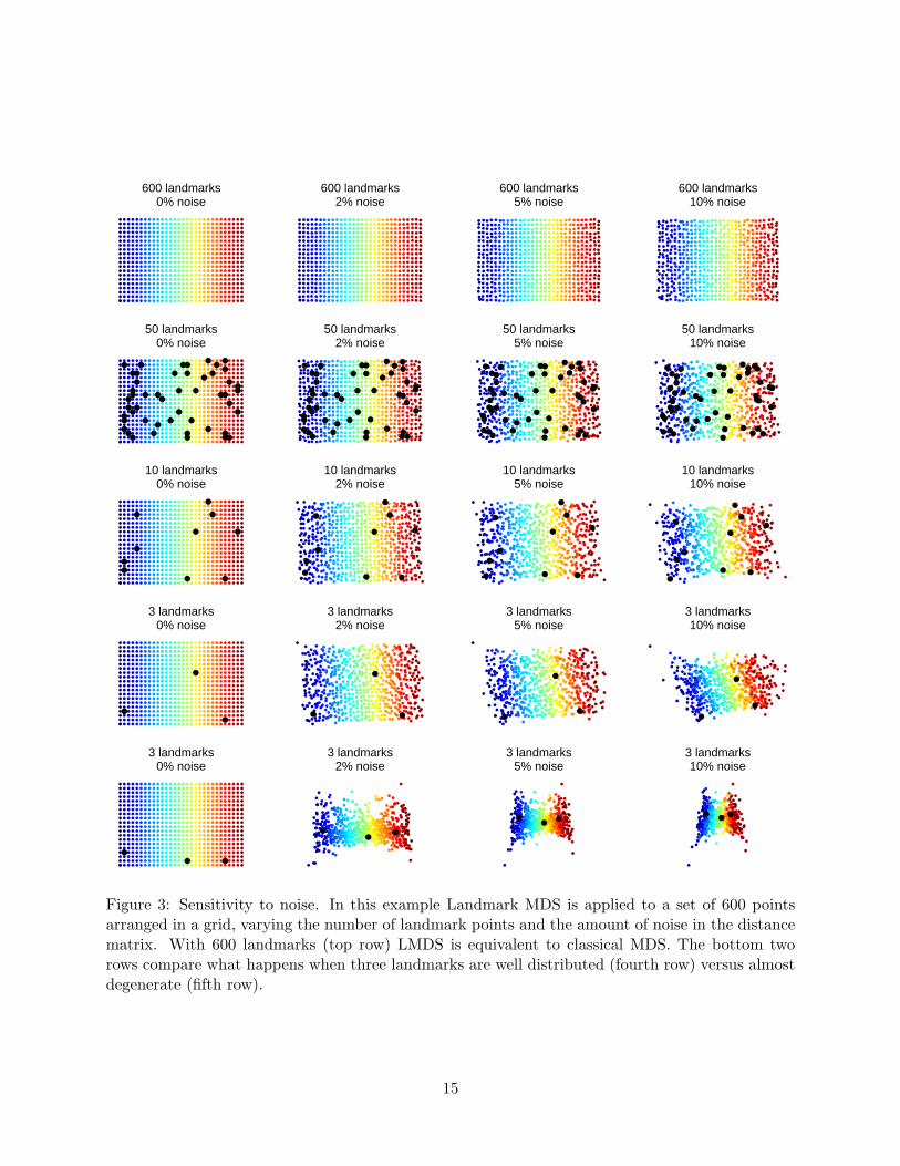
To illustrate the noise-sensitivity of Landmark MDS, we consider the example of a regular grid

subjected to varying degrees of noise and using different numbers of landmark points (Figure 3).

The initial data set consists of 600 data points in a rectangular grid of aspect ratio 1.5. To add

noise to the data, the Euclidean distance matrix was multiplied entrywise by independent random

variables distributed as exp(N(0, σ)) and then symmetrized. The noise levels ν% referred to in

the figure are defined by ν = 100(exp(σ) − 1). This modified distance matrix was then passed

to LMDS with varying numbers of landmark points, chosen randomly but consistently across the

different noise levels. PCA normalisation was used as a final step. Figure 4 plots the 2-dimensional

embeddings output by LMDS using a colour spectrum to indicate the x-coordinate of the original

configuration.

As predicted by Theorem 3, LMDS works perfectly in the absence of noise (left column), right

down to 3 landmark points. When there is noise (columns 2–4), more landmarks means better

results. Classical MDS itself (top row, equivalent to LMDS with 600 landmarks) is highly robust to

noise up to at least the 10% level. With 50 or 10 landmarks, the overall quality of the embeddings

is still quite high, though there is noticeable deterioration at finer scales and at the extremities.

14

600 landmarks0% noise












3 landmarks0% noise

3 landmarks2% noise

3 landmarks5% noise


3 landmarks0% noise

3 landmarks2% noise

3 landmarks5% noise


Figure 3: Sensitivity to noise. In this example Landmark MDS is applied to a set of 600 pointsarranged in a grid, varying the number of landmark points and the amount of noise in the distancematrix. With 600 landmarks (top row) LMDS is equivalent to classical MDS. The bottom tworows compare what happens when three landmarks are well distributed (fourth row) versus almostdegenerate (fifth row).

15

In all three cases (600, 50, 10 landmarks) the embedding is accurate at a coarse resolution. We

discuss the dependence of fine-resolution noise on the number of landmarks n in Section 4.4.

The remaining two cases show what happens when we use the bare minimum number of land-

marks, namely 3, for a 2-dimensional embedding. The situation is degenerate if the three points are

collinear, and in that case there is no 2-dimensional embedding at all. We contrast what happens

when the three landmarks are almost degenerate (fifth row) and when they are well-distributed, or

far from degenerate (fourth row).

Perhaps surprisingly for only three landmark points, the results in the well-distributed case are

moderately acceptable; at least at the lower noise levels. However, there is a systematic distortion,

which we call foreshortening, which is most easily observed in the case with 5% noise. The overall

shape of the data appears to be a parallelogram rather than a rectangle. This can be ascribed to

a uniform diminution of all coordinate values in a diagonal direction corresponding to the second

coordinate function of the initial LMDS embedding (before PCA normalisation). We give an

explanation of foreshortening in Section 4.4.

In the almost-degenerate case the results are much worse. There is a foreshortening effect,

as before, in the perpendicular direction to the principal axis of the three points. However, this

is dominated by a noise amplification effect in the same direction. Noise amplification is easily

explained. When the landmark set is almost degenerate, the second eigenvalue λ2 of Bn is close to

zero, and hence the 1/√λ2 factor causes the second row of L] to be large. If all the distances are

true then this causes no problem, but any noise is amplified by this factor in the second component

of the initial LMDS embedding.

Figure 4 shows the same data coloured by the y-coordinate of the original configuration. Evi-

dently, in the almost-degenerate case at the higher noise levels, we have lost the original y-coordinate

altogether. With 2% noise there remains some visible correlation. Still, both of the systematic

16

3 landmarks0% noise

3 landmarks2% noise

3 landmarks5% noise


3 landmarks0% noise

3 landmarks2% noise

3 landmarks5% noise


Figure 4: With three well-distributed landmark points (top row), the second coordinate of theLMDS embedding correlates strongly with second principal coordinate of the original data, evenat the higher noise levels. When the three landmark points are in almost degenerate configuration(bottom row) this is not so.

distortions—foreshortening and noise amplification—can be seen at work.

3.2 Example: digits from the MNIST database

Landmark MDS is particularly useful when dealing with large data sets for which the cost of

classical MDS may be rather high. In this section we apply both algorithms to digit sets taken

from from the MNIST database of handwritten digits [20]. We find that it is considerably cheaper

to run LMDS with 200 landmark points than to run classical MDS; but in this case the results turn

out to be of comparable quality.

Each digit set in the MNIST database consists of about 6000 instances of a given numeral (‘0’

to ‘9’) scanned in as 28 × 28 pixel grayscale images from actual handwritten ZIP codes. These

data sets are natural candidates for dimensionality reduction, since the images themselves are

high-dimensional but much of the variation in the data can be explained by a small number of

17

−2000 −1000 0 1000 2000−1500

−1000

−500

0

500

1000

1500

−2000 −1000 0 1000 2000−1500

−1000

−500

0

500

1000

1500

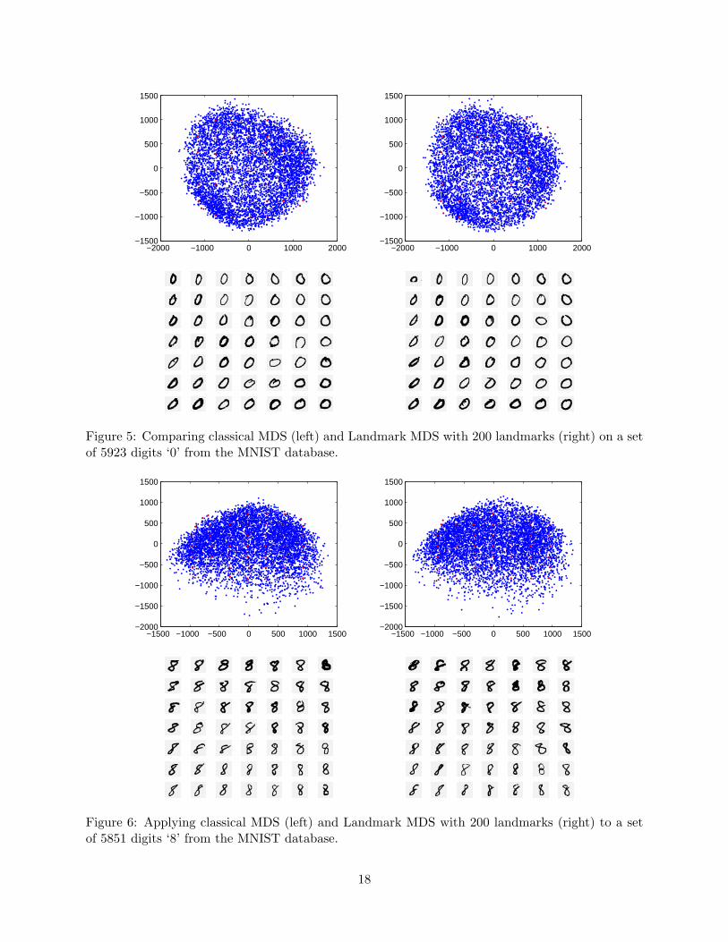
Figure 5: Comparing classical MDS (left) and Landmark MDS with 200 landmarks (right) on a setof 5923 digits ‘0’ from the MNIST database.

−1500 −1000 −500 0 500 1000 1500−2000

−1500

−1000

−500

0

500

1000

1500

−1500 −1000 −500 0 500 1000 1500−2000

−1500

−1000

−500

0

500

1000

1500

Figure 6: Applying classical MDS (left) and Landmark MDS with 200 landmarks (right) to a setof 5851 digits ‘8’ from the MNIST database.

18

−1500 −1000 −500 0 500 1000 1500−1500

−1000

−500

0

500

1000

−1500 −1000 −500 0 500 1000 1500−1500

−1000

−500

0

500

1000

Figure 7: Applying classical MDS (left) and Landmark MDS with 200 landmarks (right) to a setof 6742 digits ‘1’ from the MNIST database.

natural parameters such as left-right slope, height, and loop size. The relationship between these

parameters and the images is highly non-linear, which would suggest the use of Isomap, LLE or

some other NLDR algorithm. However, the simpler linear methods can sometimes detect one or

two salient degrees of variation, and this turns out to be the case here.

For each digit, we adopted the following procedure. Every 28×28 grayscale image was rasterised

to a vector of length 784 of intensity values in the range 0 ≤ s ≤ 1. From the approximately

6000 images, 200 were chosen randomly to be landmark points. Using the Euclidean metric in R784,

both classical MDS and Landmark MDS (with the chosen 200 landmarks) were applied to obtain

a 2-dimensional embedding. A selection of the results is shown in Figures 5, 6 and 7, with classical

MDS in the left column compared with Landmark MDS in the right column. Red highlights mark

the points in each embedding closest to the vertices of a superimposed regular grid; the images

corresponding to these points are displayed below in a grid, as a visual aid.

19

The ten digits are not equally suitable candidates for classical MDS. Some of the digit sets do

exhibit a clear correlation between the first coordinate and any natural variation parameter. For

other digits such as ‘1’, there is too much non-linearity to find a consistent correspondence. In

the best cases, ‘0’ and ‘8’, there are identifiable features corresponding to each of the first two

coordinates. For ‘0’ (Figure 5), the left–right axis corresponds to area and eccentricity of the oval:

smaller, more eccentric ovals on the left; and larger, rounder figures on the right. Variation along

the other direction corresponds to the angle of the major axis of the ‘0’, running from vertical (at

the top) to 45◦ clockwise (at the bottom). In the case of the ‘8’ data, the left–right axis corresponds

to the angle of the major axis of the ‘8’; and the top–bottom direction correlates with ‘weight’:

dark, heavily written characters at the top, and lighter characters at the bottom. For both digits,

it is evident that Landmark MDS performs comparably well with classical MDS (subject to the

caveat below); certainly the same trends can be seen in the LMDS results.

In contrast to ‘0’ and ‘8’, the space of digits ‘1’ seems to be significantly non-linear; the 2-

dimensional embedding coordinates produced by classical MDS (Figure 7, left) fail to correlate

consistently with discernible features. Indeed, the curved shape of the data distribution gives fair

warning of this, and strongly suggests the use of non-linear techniques. Landmark MDS (right)

produces very similar output, confirming that its diagnostic value is comparable to classical MDS.

Finally we compare running times for these calculations, under a straightforward MATLAB

implementation. To the nearest 0.1 s, classical MDS on the ‘8’ data took 160.6 s to calculate the

distance matrix and 57.2 s to calculate the embedding, and a total of 217.9 s. Landmark MDS

took 1.9 s to calculate the reduced distance matrix and 0.4 s for the embedding calculation, making

2.2 s in total. There was a similar ‘improvement factor’ of about 100 for each of the ten digits. These

results support our claim that Landmark MDS is an effective, computationally efficient substitute

for classical MDS in a range of real-world data analysis situations, both linear and non-linear.

20

Caveat. We have taken care to show typical results for these experiments with 200 randomly-

chosen landmarks. For some of the digits where the data space is highly nonlinear, such as ‘8’,

it happened once or twice in every ten runs that the two-dimensional embedding given by LMDS

differed significantly from classical MDS in the second coordinate. This raises the question of how

to choose good landmarks (and how many of them). We discuss this question in the analysis section.

4 Analysis

We now discuss the theoretical performance of LMDS in terms of the following question: If classical

MDS is applied to an all-pairs distance matrix ∆N and LMDS is applied to a landmark-to-point

rectangular submatrix ∆n,N then are the two embeddings the same? Here ‘the same’ means ‘con-

gruent up to a rigid transformation’.

We answer this in three parts. First, if there is an exact Euclidean embedding preserving ∆N ,

we verify that LMDS recovers this configuration exactly provided that all the data points are

contained in the affine span of the landmark points. If the landmarks span a lower-dimensional

affine subspace, then LMDS recovers the orthogonal projection of the points onto this subspace.

Second, we study the perturbation properties of LMDS. We give first-order perturbation formu-

las for classical MDS and LMDS and identify the parameters which lead to poor stability. Under

reasonable conditions, LMDS and classical MDS both behave well with respect to small perturba-

tions of the input. As a consequence if the distance matrix is approximately Euclidean, then LMDS

and classical MDS will give approximately the same embedding.

Third, we give an example of a non-Euclidean data set for which the two algorithms give quite

different results. It is therefore wrong to assume that LMDS is always a good approximation to

21

classical MDS. More precisely, if a data set is not well suited to classical MDS, then Landmark MDS

may give unpredictable results. On the other hand, for data sets where the use of classical MDS is

appropriate, the preceding results imply that Landmark MDS is a good approximation.

4.1 The Euclidean case

When classical MDS is applied to a distance matrix originating from a set of Euclidean data, the

resulting k-dimensional embedding recovers the projection of the data onto its first k mean-centered

principal axes. This is the content of Theorem 1. Note that if the affine span of the data is p-

dimensional, then there are exactly p non-zero principal components. Thus the configuration is

recovered perfectly up to isometry when k = p; nothing is gained by taking k > p.

Similarly, Theorem 3 implies that when Landmark MDS is applied to a set of distances origi-

nating from Euclidean data, the resulting k-dimensional embedding recovers the projection of the

data points onto the first k mean-centered principal axes of the designated landmark points. If the

landmark points span a p-dimensional affine subspace, then by taking k = p we recover up to an

isometry the projection of the data onto this subspace. Since the affine span of n points is at most

(n− 1)-dimensional, we need at least k+1 landmark points in general position for a k-dimensional

embedding.

In the remainder of this section we prove Theorem 3. First we fix our notation. Given a

collection of landmark points ~y1, ~y2, . . . , ~yn ∈ Rm let ∆n denote their squared-distance matrix, with

columns ~δj and column mean ~δµ. By translation we may assume that the landmarks are mean

centered, or equivalently Y Hn = Y where Y = [~y1, ~y2, . . . , ~yn]. The principal axes are given by

the eigenvectors of Y Y T; let ~pi denote a unit eigenvector for the i-th positive eigenvalue λ′i. By

Theorem 1 we have the relation √λi~v

Ti = ~pT

i Y (4)

22

where ~vi (chosen with the appropriate sign) and λi are defined as in classical MDS. Then

λi =√λi~v

Ti ~vi

√λi = ~pT

i Y YT~pi = λ′i~p

Ti ~pi = λ′i

so we can write λi for λ′i.

Proof of Theorem 3. We must show that the i-th component of −12L

]k(~δa − ~δµ) is equal to the

projection of ~ya onto the i-th principal axis. That is:

−12

~vTi√λi

(~δa − ~δµ) = ~pTi ~ya (5)

First we compute the j-th entries of ~δa and ~δµ:

[~δa]j = |~ya|2 − 2~yTj ~ya + |~yj |2

[~δµ]j = 1n

∑nk=1 |~yk|2 − 2~yT

j

(1n

∑nk=1 ~yk

)+ |~yj |2

The left-hand terms are independent of j, and the middle term on the second row is zero since

the ~yk are mean centered. Thus we can subtract to derive the vector equation:

~δa − ~δµ = c~1− 2Y T~ya

where c = |~ya|2− 1n

∑nk=1 |~yk|2 is a scalar. Since ~vT

i~1 = 0 we can drop the term c~1 when substituting

this formula into the left-hand side of (5).

Using (4) and this last observation, equation (5) becomes equivalent to

~pTi Y Y

T~ya = λi~pTi ~ya

23

which is plainly true since ~pi is the i-th eigenvector of Y Y T with eigenvalue λi. �

4.2 The approximately Euclidean case

The discussion in the previous section assumes that we have ideal data whose metric structure is

exactly Euclidean. In practice it is more common for the distance matrix to be approximately but

not exactly Euclidean. This may be due to noise, but it also happens systematically in applications

such as Isomap, where larger entries in the distance matrix are extrapolated from smaller entries,

resulting in a matrix that is at best an approximation to any underlying Euclidean structure.

In this section we study perturbation theory for classical MDS and Landmark MDS: given

a small change in the distance matrix, what are the corresponding changes in the resulting k-

dimensional embeddings? For example, what is the effect of perturbing the entries of the distance

matrix away from an exactly Euclidean situation? If the answer is “there is not much change”

then the results of the previous section apply more generally, with small error, to approximately

Euclidean situations.

It turns out that classical MDS and Landmark MDS are stable up to orthogonal transformations,

provided that λk and (λk − λk+1) are not too small, where λj denotes the j-th largest eigenvalue

of the inner-product matrix Bn. The key technical result is the following theorem.

Theorem 5 Let ∆n be the squared-distance matrix of the set of landmark points; let Bn be the

corresponding inner-product matrix with eigenvalues λ1 ≥ . . . ≥ λn and λk > max(0, λk+1) for

some k; and let Lk, L]k be the k-dimensional embedding matrix from classical MDS together with

its pseudoinverse transpose. Consider a perturbation ∆n = ∆n + tφ + O(t2). Then there are

24

perturbations

Bn = Bn + tβ + O(t2)

Lk = Lk + tχ + O(t2)

L]k = L]

k + tψ + O(t2)

and an orthogonal matrix Q = Q(t) such that Bn, QLk and QL]k are the corresponding matrices

derived from ∆n. Moreover there are bounds

‖β‖ ≤ ‖φ‖/2

‖χ‖ ≤

[1

4λ1/2k

+λ

1/21

2(λk − λk+1)

]‖φ‖

‖ψ‖ ≤

[1

4λ3/2k

+1

2λ1/2k (λk − λk+1)

]‖φ‖

in the Frobenius norm.

These are bounds on the first-order behaviour of the error terms, following the tradition of

Sibson [21]. These first-order estimates make it clear how the perturbation theory for classical and

Landmark MDS depends on the eigenvalues λ1, λk and λk+1. To obtain absolute bounds one would

apply techniques of the kind used in [22], at considerably greater effort.

Corollary 6 Let δa = ~δa + t~ζa + O(t2) be a perturbation family for the vector of squared distances

between the point a and the landmark points of Theorem 5. Then the perturbation family xa =

~xa − t(L]k~ζa + ψ~δa)/2 + O(t2) agrees with the family of embedding vectors for a given by applying

LMDS, up to a rotation and translation which depend on t but are independent of a.

Proof. This is immediate from Theorem 5 and equation (3); the rotation is by Q and the translation

deals with the term −(1/2)L]k~δµ and its perturbation. �

25

Corollary 6 establishes the overall stability of Landmark MDS in the following sense: the k-

dimensional embedding given by a particular set of data closely approximates the k-dimensional

embedding given by a approximation to that set of data, up to a rigid motion, provided the

eigenvalue condition is satisfied for the landmark points. If we follow up with a PCA normalisation

step, then the qualification “up to a rigid motion” is moot, in that the results of PCA remain

essentially unchanged after a rigid motion is applied. The only ambiguity is that each coordinate

is only well-defined up to a ± sign, and that principal components having the similar eigenvalues

may become exchanged after perturbation; there is no real way round this. (Note the distinction

between the eigenvalues of Bn—which are defined by reference to the landmark points only—and

the eigenvalues at the PCA normalisation—which depend on the distribution of the entire data set

at that time.)

The stability of classical MDS follows from Theorem 5, since Lk is the embedding matrix when

all the points are regarded as landmark points.

Remark. Our approach differs from Sibson’s analysis of classical MDS [21] in the following way.

Sibson compares the embedding matrix Lk directly with the embedding Lk for a nearby perturbed

problem, estimating the error ‖Lk−Lk‖. In contrast we permit an orthogonal change of coordinates

to improve the fit; essentially we are estimating ‖Lk − QLk‖ for a suitable orthogonal matrix Q.

Sibson’s approach gives poor bounds if any pair of eigenvalues is not well separated, since the

individual ranked eigenvectors are required to be stable. In our case it is good enough for the

subspace spanned by the the highest k eigenvectors to be stable; the final PCA normalisation step

depends only on this subspace and not on the set of basis vectors which span it.

We now return to our main theorem. The proof is somewhat technical.

Proof of Theorem 5. First, the transformation ∆n 7→ Bn is linear and has norm 1/2, giving us β

26

and the bound on its norm immediately.

Let Vk = [~v1~v2 . . . ~vk] be the matrix whose columns are the first k eigenvectors of Bn and let

V⊥ = [~vk+1~vk+2 . . . ~vn] be the matrix containing the remaining eigenvectors. Let Λk be the diagonal

matrix of eigenvalues for Vk, defined Λk = V Tk BnVk. We can also define Λ⊥ = V T

⊥BnV⊥. Then

Lk = Λ1/2k V T

k and L]k = Λ−1/2

k V Tk by definition. The columns of Vk span a subspace Ek. Suppose

we have a matrix Wk = [~w1 ~w2 . . . ~wk] whose columns form another orthonormal basis of Ek. Then

we can write Wk = VkQ for some uniquely determined k × k orthogonal matrix Q.

Lemma 7 We have the equations:

Lk = Q(WTk BnWk)1/2WT

k

L]k = Q(WT

k BnWk)−1/2WTk

Proof. The formulae are derived by making substitutions into Lk = Λ1/2k V T

k and L]k = Λ−1/2

k V Tk ,

and using Λk = V Tk BnVk. �

We apply the lemma not just to Bn, Vk and Wk, but also to their perturbation families. We

will define a perturbation family Wk of orthonormal bases for the perturbed subspaces Ek and set

Lk = (WTk BnWk)1/2WT

k and L]k = (WT

k BnWk)−1/2WTk . The family Wk will be more controllable

than the naturally defined family Vk whose columns give the first k eigenvectors in order. By the

lemma, we recover the “correct” embedding matrices as QLk and QL]k.

The family Wk and a complementary family W⊥ of orthonormal vectors take the following form,

where Θ is an (n− k)× k matrix:

Wk = Vk + tV⊥Θ + O(t2)

W⊥ = V⊥ − tVk ΘT + O(t2)

27

For any choice of Θ, it is easy to check to first order that the families Wk and W⊥ are orthonormal

and mutually orthogonal. By considering a suitable exponential family of rotations, we can take

families where this holds in fact, and not just to first order.

We now determine Θ. The column space of Wk must equal the column space of Vk, and so must

be an invariant subspace of Bn. This leads to the condition WT⊥ BnWk = 0. On expansion, we find

that the zeroth-order part V T⊥BnVk = 0 is automatically true, so we are left with the first-order

part of the equation

ΘV Tk BnVk − V T

⊥BnV⊥Θ = V T⊥ βVk

which is equivalent to ΘΛk − Λ⊥Θ = V T⊥ βVk and has the following componentwise solution:

Θij =[V T

⊥ βVk]ijλj − λk+i

(6)

Since min(|λj − λk+i|) = λk − λk+1, it follows that ‖Θ‖ ≤ ‖β‖/(λk − λk+1).

Next we expand the following crucial term:

WTk BnWk = (V T

k + tΘTV T⊥ )(Bn + tβ)(Vk + tV⊥Θ) + O(t2)

= V Tk BnVk + t

(ΘTV T

⊥BnVk + V Tk βVk + V T

k BnV⊥Θ)

+ O(t2)

= Λk + t(V Tk βVk) + O(t2)

In order to take a square root, note that (Λk + tν + O(t2))1/2 = Λ1/2k + tη + O(t2) is equivalent

to Λ1/2k η + ηΛ1/2

k = ν and so (WTk BnWk)1/2 = Λ1/2

k + tη + O(t2) where:

ηij =[V T

k βVk]ijλ

1/2i + λ

1/2j

(7)

28

It follows that ‖η‖ ≤ ‖β‖/2λ1/2k . This at last yields:

Lk = (WTk BnWk)1/2WT

k

= Λ1/2k V T

k + t(ηV Tk + Λ1/2

k ΘTV T⊥ ) + O(t2)

= Lk + tχ+ O(t2)

where ‖χ‖ ≤ ‖ηV Tk ‖+ ‖Λ1/2

k ΘTV T⊥ ‖ = ‖η‖+ ‖Λ1/2

k ΘT‖ ≤ ‖η‖+ λ1/21 ‖Θ‖. This gives the bound in

the theorem.

To compute the inverse square root, (Λk + tν+ O(t2))−1/2 = Λ−1/2k + tξ+ O(t2) is equivalent to

Λ−1/2k ξ + ξΛ−1/2

k = −Λ−1k νΛ−1

k and so (WTk BnWk)−1/2 = Λ−1/2

k + tξ + O(t2) where:

ξij = −[V T

k βVk]ijλiλj(λ

−1/2i + λ

−1/2j )

(8)

It follows that ‖ξ‖ ≤ ‖β‖/2λ3/2k . Finally:

L]k = (WT

k BnWk)−1/2WTk

= Λ−1/2k V T

k + t(ξV Tk + Λ−1/2

k ΘTV T⊥ ) + O(t2)

= L]k + tψ + O(t2)

where ‖ψ‖ ≤ ‖ξV Tk ‖+ ‖Λ

−1/2k ΘTV T

⊥ ‖ = ‖ξ‖+ ‖Λ−1/2k ΘT‖ ≤ ‖ξ‖+λ

−1/2k ‖Θ‖. This gives the bound

stated in the theorem, and completes the proof. �

29

0 2 4 6 8 10−20

0

20

40

60

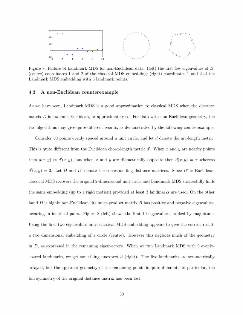
Figure 8: Failure of Landmark MDS for non-Euclidean data: (left) the first few eigenvalues of B;(centre) coordinates 1 and 2 of the classical MDS embedding; (right) coordinates 1 and 2 of theLandmark MDS embedding with 5 landmark points.

4.3 A non-Euclidean counterexample

As we have seen, Landmark MDS is a good approximation to classical MDS when the distance

matrix D is low-rank Euclidean, or approximately so. For data with non-Euclidean geometry, the

two algorithms may give quite different results, as demonstrated by the following counterexample.

Consider 50 points evenly spaced around a unit circle, and let d denote the arc-length metric.

This is quite different from the Euclidean chord-length metric d′. When x and y are nearby points

then d(x, y) ≈ d′(x, y), but when x and y are diametrically opposite then d(x, y) = π whereas

d′(x, y) = 2. Let D and D′ denote the corresponding distance matrices. Since D′ is Euclidean,

classical MDS recovers the original 2-dimensional unit circle and Landmark MDS successfully finds

the same embedding (up to a rigid motion) provided at least 3 landmarks are used. On the other

hand D is highly non-Euclidean: its inner-product matrix B has positive and negative eigenvalues,

occuring in identical pairs. Figure 8 (left) shows the first 10 eigenvalues, ranked by magnitude.

Using the first two eigenvalues only, classical MDS embedding appears to give the correct result:

a two dimensional embedding of a circle (centre). However this neglects much of the geometry

in D, as expressed in the remaining eigenvectors. When we run Landmark MDS with 5 evenly-

spaced landmarks, we get something unexpected (right). The five landmarks are symmetrically

arrayed, but the apparent geometry of the remaining points is quite different. In particular, the

full symmetry of the original distance matrix has been lost.

30

The moral is that in the non-Euclidean setting the low-dimensional embeddings given by classical

MDS and Landmark MDS need not approximate each other particularly well. To be fair, these are

situations where the use of classical MDS may not be all that appropriate. For data sets which are

well-suited to classical MDS, with a clear k-dimensional metric embedding and small eigenvalues

for the remaining ‘noise’ coordinates, we emphasise that Landmark MDS does indeed give a good

approximation to classical MDS.

Remark. Genuinely non-Euclidean data sets such as the circle example in Section 4.3 cannot

sensibly be treated as ‘Euclidean but noisy’. One possibility is to think of such a data set as living

in Minkowski space, with imaginary (‘timelike’) dimensions alongside real (‘spacelike’) dimensions,

and carry out a similar analysis to the Euclidean case. Goldfarb [6] lays out some of the foundations

for this point of view. We do not pursue the idea here.

4.4 Choosing a good landmark set

What constitutes a good set of landmark points? From the example of the noisy grid, we know that

there is better accuracy with more landmarks; and that there are systematic errors in the output

when the landmarks are in degenerate configuration (lying close to a low-dimensional subspace such

as a line)

The situation can be described in the following way. Suppose first that we have a mean-

centered Euclidean configuration of N points in Rd, represented by a d×N matrix Z. The first k

principal components are obtained by projection onto the top k eigenvectors of the covariance

matrix CZ = (1/N)ZZT. Let EkZ denote the subspace spanned by these top k eigenvectors. A set

of n landmark points is represented by a submatrix Y , and has (mean-centered) covariance matrix

CY = (1/n)Y HnYT and an associated subspace Ek

Y spanned by the top k eigenvectors of CY .

We now seek a k-dimensional embedding. Running classical MDS is equivalent to projecting

31

the points onto the subspace EkZ , with axes being the eigenvectors of CZ in order. Running LMDS

with the given landmark points is equivalent to projecting the data onto EkY , and then realigning

the data according to the new principal components of the projected data. Informally, we can say:

Proposition 8 For Euclidean data, Landmark MDS succeeds when the subspace EkY is close to the

subspace EkZ , and more specifically when the data has a similar covariance structure when projected

onto each of the two subspaces. �

More generally, if j ≤ k one can restrict the k-dimensional embeddings produced by classical

MDS and LMDS to the first j coordinates. Landmark MDS succeeds when the corresponding j-

dimensional subspaces of EkY and Ek

Z are close and have similar covariance structure for the data.

The remaining dimensions of EkY and Ek

Z need not agree closely.

This gives an argument in favour of choosing landmark points randomly from the given data

set; with enough landmark points the covariance matrix of the sample is a good approximation to

the covariance matrix of the data. Provided that the k-th and (k+1)-st eigenvalues are sufficiently

well separated (or the j-th and (j + 1)-st, if restricting), the corresponding subspaces will be close

and Landmark MDS will succeed.

When the covariance matrix of the landmark points satisfies the separation condition and is

close to the true covariance matrix of the full data, we may still observe noise at fine scales. The

variance of this noise behaves as ∼ n−1, where n is the number of landmarks. The back-of-the-

envelope calculation runs as follows: ‖Lk‖ ∼ n1/2 so ‖L]k‖ ∼ n−1‖Lk‖. For a given point a there

are n entries in ~δa. If each entry independently is subject to a certain amount of noise, then the

discrepancy in the embedding of a takes the form n−1 · (n independent random variables), which

has variance ∼ n−1 as claimed.

When the covariance matrix of the landmark points has poorly separated k-th and (k + 1)-st

32

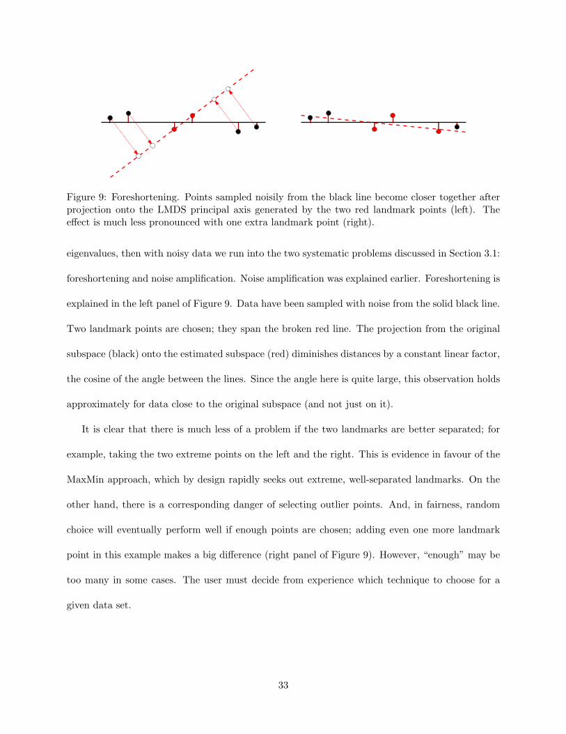
Figure 9: Foreshortening. Points sampled noisily from the black line become closer together afterprojection onto the LMDS principal axis generated by the two red landmark points (left). Theeffect is much less pronounced with one extra landmark point (right).

eigenvalues, then with noisy data we run into the two systematic problems discussed in Section 3.1:

foreshortening and noise amplification. Noise amplification was explained earlier. Foreshortening is

explained in the left panel of Figure 9. Data have been sampled with noise from the solid black line.

Two landmark points are chosen; they span the broken red line. The projection from the original

subspace (black) onto the estimated subspace (red) diminishes distances by a constant linear factor,

the cosine of the angle between the lines. Since the angle here is quite large, this observation holds

approximately for data close to the original subspace (and not just on it).

It is clear that there is much less of a problem if the two landmarks are better separated; for

example, taking the two extreme points on the left and the right. This is evidence in favour of the

MaxMin approach, which by design rapidly seeks out extreme, well-separated landmarks. On the

other hand, there is a corresponding danger of selecting outlier points. And, in fairness, random

choice will eventually perform well if enough points are chosen; adding even one more landmark

point in this example makes a big difference (right panel of Figure 9). However, “enough” may be

too many in some cases. The user must decide from experience which technique to choose for a

given data set.

33

4.4.1 Cross-validation

As a precaution against the kind of bad luck arising from a poor landmark configuration, it may

be wise to cross-validate by running LMDS several times and computing correlations between the

respective coordinates. Those trials which closely approximate the (uncomputed) classical MDS

embedding will closely correlate with each other. The occasional ‘bad’ embedding is easily detected

by its comparatively low average correlation with the remaining trials.

More generally, this leads to a method for determining the ideal number of landmark points.

Run Landmark MDS repeatedly in batches, where each batch consists of several trials with the

same number of landmarks chosen randomly, and compute correlations between the trials. This

process is repeated, with an increasing number of landmarks, until there are consistent correlations

across (most of) the trials in a batch. This is still much cheaper than running full MDS on a large

set.

5 Discussion

We briefly describe some of the more important applications of Landmark MDS, and mention some

of its connections with related work.

5.1 Landmark Isomap

The initial motivation for Landmark MDS was the need to speed up the Isomap algorithm [14] for

nonlinear dimensionality reduction (NLDR). Isomap constructs a low-dimensional embedding of of

nonlinear data set observed in a high-dimensional space. There are three steps: (i) a neighbourhood

relation is determined in the form of a sparse graph, with edges connecting data point pairs that are

deemed to be “close” (for example, x, y are neighbours iff x is one of the pnearest neighbours of y

34

and vice versa); (ii) a new metric is defined: the distance between a pair of data points is the length

of the shortest path between them, with edges weighted by length in the observation space; (iii)

classical MDS is applied to the new metric find the low-dimensional embedding. This procedure

emphasises the local structure of the data, but at the same time it globalises this information so

that the embedding can be found using aglobal optimisation (here classical MDS). Highly non-

linear data sets can be successfully linearised in this way, for example, a sample of images of a face

under varying pose and lighting conditions, or a sample of images of a hand as the fingers and wrist

move [14].

For a large data set of N points the main bottleneck is the classical MDS stage, which reduces

to an O(N3) eigenvalue problem on a dense N × N matrix. Storage of the full distance matrix

is also an issue. Other well-known NLDR algorithms such as Locally Linear Embedding [23] and

Laplacian Eigenmaps [24] involve eigenvalue problems on sparse N × N matrices, so they do not

suffer from either of these issues. Landmark MDS solves both problems, since it only requires

an n × N submatrix of the full distance matrix, and the eigenvalue problem is O(n3). Using

Dijkstra’s algorithm, the shortest-paths distance can be calculated row-by-row, so there are no

extraneous calculations. If the neighbourhood graph is given, the cost of running Isomap with

N points and p nearest neighbours is O(N3 + pN2 logN) as opposed to O(pnN logN + knN + n3)

for Landmark Isomap with n landmarks in k dimensions, a huge savings. The cost of building

the p-nearest-neighbours graph—the same in both cases—softens the advantage slightly. Standard

methods have complexity O(N2), but there are more sophisticated techniques [25, 26] which give

an expected bound of cO(1)(pN + N logN log logN) for data sets with an expansion coefficient

of c. For data sampled randomly from a k-dimensional submanifold of Euclidean space Rd, the

expansion coefficient is essentially c = 2k.

35

5.2 Sparsely observed distance matrices

Isomap imposes a sparsification of the original distance metric of the data, by using only the

distance information for pairs of neighbouring points. A different situation occurs for large data

sets when the metric information is inherently sparsely observed, for instance when the metric

comes from human judgments of similarity [7] or association [27]. This leads to the problem of

multidimensional scaling with incomplete information – how does one find a good low-dimensional

representation of data from a sparse set of dissimilarity coefficients? One possible answer is to

estimate the missing coefficients using shortest paths in the weighted graph having an edge for

every observed comparison, with weight equal to the dissimilarity coefficient; and then use classical

MDS. This is formally analogous to Isomap, except that the graph is not a neighbourhood graph.

Steyvers et al [27] use this approach to estimate the missing coefficients in a matrix of similarities

generated by human test subjects. Platt [7] shows that good results can be obtained by combining

this method with LMDS; this avoids having to deal with the full dissimilarity matrix.

5.3 Nystrom method

Landmark MDS is similar in spirit to the well-known Nystrom method, which finds approximate

solutions to a positive semi-definite symmetric eigenvalue problem using just a few of the columns

of the matrix, and it is natural to suspect that they are closely related. In fact, Bengio et al. [8] es-

tablish a precise connection, using a Nystrom-like approach to derive formulae equivalent to Step 3

of LMDS for the purposes of projecting new points into a pre-existing MDS solution. Bengio et al.

also derive Nystrom-based out-of-sample extensions to other dimensionality reduction algorithms,

including Locally Linear Embedding [10,23] and Laplacian Eigenmaps [24] (where the initial eigen-

value problem is not as acutely expensive as it is for Isomap). Our work here shows that this

approach provides a rigorous basis for efficient and accurate landmark-based approximations to the

36

full MDS computation on large data sets.

5.4 FastMap

An early example of cheaply approximating classical MDS comes from Faloutsos and Lin [9], with

their FastMap algorithm. The idea is to construct a k-dimensional embedding one dimension at a

time. To determine an axis, two points are selected from the data and the distances of all points

to these two points are used to find the first embedding coordinate. The distance matrix is then

modified to take the first dimension into account, and the process is repeated, with a new axis, to

find second and subsequent coordinates. In fact, FastMap is exactly an iterated form of LMDS in

the simplest case of 2 landmarks.

An inherent weakness of FastMap is that each projection axis is specified by only two points, so

the alignment of these axes with the true principal axes of the data is unstable at best. In contrast,

Landmark MDS makes use of as many landmarks as provided, even if the required embedding is

much lower dimensional. Redundancy brings stability; and LMDS is not that much more expensive

than FastMap to run. In tests carried out by Platt [7], LMDS gives better performance than

FastMap.

Conclusion

Dimensionality reduction and effective visualization of the intrinsic structure of a data set constitute

a major challenge in statistics, machine learning, information retrieval, and knowledge discovery.

Classical multidimensional scaling has proved to be an excellent approach to these problems, either

by itself, or as part of a larger scheme dealing with cases where the data are nonlinear or incomplete.

However, modern data sets present a challenge not well addressed by the classical technique of

MDS: how does one deal with large volumes of data? This paper has addressed that challenge,

37

describing an approximation to the algorithm which works tractably with very large data sets, and

providing a theoretical analysis that explains when and where our more efficient methods can be

trusted to give results faithful to the output of classical MDS.

Given its simplicity, efficiency and accuracy, Landmark MDS should be an important part of

the next generation data analyst’s toolkit.

Acknowledgements

This research was supported in part by NSF grant DMS-0101364 and by a grant from the Schlum-

berger Foundation. JBT was supported by a Paul E. Newton Career Development Chair. We also

wish to thank Mark Steyvers, for his considerable help in implementing and testing early versions

of LMDS; and Yoav Git, Carrie Grimes and John Langford, for many helpful discussions.

References

[1] R. N. Shepard, “Multidimensional scaling, tree-fitting, and clustering,” Science, vol. 210, pp.

390–398, 1980.

[2] T. F. Cox and M. A. A. Cox, Multidimensional Scaling. London: Chapman & Hall, 1994.

[3] J. Kruskal and M. Wish, Multidimensional Scaling. Beverly Hills, CA: Sage Publications,

1978.

[4] I. Borg and J. Lingoes, “A model and algorithm for multidimensional scaling with external

constraints on the distances,” Psychometrika, vol. 45, pp. 25–38, 1980.

[5] V. de Silva and J. B. Tenenbaum, “Global versus local methods in nonlinear dimensionality

reduction,” in Advances in Neural Information Processing Systems 15, S. T. S. Becker and

K. Obermayer, Eds. Cambridge, MA: MIT Press, 2003, pp. 705–712.

38

[6] L. Goldfarb, “A unified approach to pattern recognition,” Pattern Recognition, vol. 17, no. 5,

pp. 575–582, 1984.

[7] J. C. Platt, “Fast embedding of sparse music similarity graphs,” in Advances in Neural Infor-

mation Processing Systems 16, S. Thrun, L. Saul, and B. Scholkopf, Eds. Cambridge, MA:

MIT Press, 2004.

[8] Y. Bengio, J. Paiement, P. Vincent, O. Delalleau, N. Le Roux, and M. Ouimet, “Out-of-sample

extensions for LLE, Isomap, MDS, eigenmaps, and spectral clustering,” in Advances in Neural

Information Processing Systems 16, S. Thrun, L. Saul, and B. Scholkopf, Eds. Cambridge,

MA: MIT Press, 2004.

[9] C. Faloutsos and K.-I. Lin, “FastMap: A fast algorithm for indexing, data-mining and visu-

alization of traditional and multimedia datasets,” in Proceedings of the 1995 ACM SIGMOD

International Conference on Management of Data, M. J. Carey and D. A. Schneider, Eds.,

San Jose, California, 1995, pp. 163–174.

[10] L. Saul and S. Roweis, “Think globally, fit locally: Unsupervised learning of low dimensional

manifolds,” Journal of Machine Learning Research, vol. 4, pp. 119–155, 2003.

[11] A. Buja, D. Swayne, M. Littman, N. Dean, and H. Hofmann, “Interactive data visualization

with multidimensional scaling,” 2004, [manuscript under review].

[12] K. Borner, C. Chen, and K. W. Boyack, “Visualizing knowledge domains,” Annual Review of

Information Science and Technology, no. 37, [in press].

[13] M. Quist and G. Yona, “Distributional scaling: An algorithm for structure-preserving em-

bedding of metric and nonmetric spaces,” Journal of Machine Learning Research, vol. 5, pp.

399–420, Apr. 2004.

39

[14] J. B. Tenenbaum, V. de Silva, and J. C. Langford, “A global geometric framework for nonlinear

dimensionality reduction,” Science, vol. 290, pp. 2319–2323, Dec. 2000.

[15] W. S. Torgerson, Theory and Methods of Scaling. New York: Wiley, 1958.

[16] G. Young and A. S. Householder, “Discussion of a set of points in terms of their mutual

distances,” Psychometrika, vol. 3, pp. 19–22, 1938.

[17] C. Eckart and G. Young, “The approximation of one matrix by another of lower rank,” Psy-

chometrika, vol. 1, pp. 211–218, 1936.

[18] P. Simard, Y. Le Cun, and J. Denker, “Efficient pattern recognition using a new transformation

distance,” in Advances in Neural Information Processing Systems 5, S. Hanson, J. Cowan, and

C. Giles, Eds. San Mateo, CA: Morgan Kaufmann, 1993, pp. 50–58.

[19] G. Carlsson and V. de Silva, “A geometric framework for sparse matrix problems,” Advances

in Applied Mathematics, vol. 33, no. 1, pp. 1–25, 2004.

[20] Y. LeCun, L. Bottou, Y. Bengio, and H. Patrick, “Gradient-based learning applied to document

recognition,” Proceedings of the IEEE, vol. 86, no. 11, pp. 2278–2324, 1998.

[21] R. Sibson, “Studies in the robustness of multidimensional scaling: Perturbational analysis of

classical scaling,” Journal of the Royal Statistical Society, Series B, vol. 41, no. 2, pp. 217–229,

1979.

[22] G. W. Stewart, “Error and perturbation bounds for subspaces associated with certain eigen-

value problems,” SIAM Review, vol. 15, no. 4, pp. 727–764, Oct. 1973.

[23] S. Roweis and L. Saul, “Nonlinear dimensionality reduction by locally linear embedding,”

Science, vol. 290, pp. 2323–2326, Dec. 2000.

40

[24] M. Belkin and P. Niyogi, “Laplacian eigenmaps and spectral techniques for embedding and

clustering,” in Advances in Neural Information Processing Systems 14, T. Diettrich, S. Becker,

and Z. Ghahramani, Eds. Cambridge, Massachussetts: MIT Press, 2002, pp. 585–591.

[25] D. R. Karger and M. Ruhl, “Finding nearest neighbors in growth-restricted metrics,” in Pro-

ceedings of the 34th Annual ACM Symposium on the Theory of Computing, 2002, pp. 63–66.

[26] R. Krauthgamer and J. R. Lee, “Navigating nets: Simple algorithms for proximity search,” in

15th Annual ACM-SIAM Symposium on Discrete Algorithms, Jan. 2004, pp. 791–801.

[27] M. Steyvers, R. Shiffrin, and D. Nelson, “Word association spaces for predicting semantic

similarity effects in episodic memory,” in Cognitive Psychology and its Applications: Festschrift

in Honor of Lyle Bourne, Walter Kintsch, and Thomas Landauer, H. A., Ed. Washington,

DC: American Psychological Association, [in press].

41

Sparse multidimensional scaling using landmark pointspeyre/cours/x2005signal/dimreduc... · cal multidimensional scaling (MDS) algorithm, called Landmark MDS (LMDS), for use when

Documents