MANUSCRIPT, IEEE TRANSACTIONS ON AUDIO, SPEECH AND LANGUAGE PROCESSING 1 Sparse Classifier Fusion for Speaker Verification Ville Hautam¨ aki, Tomi Kinnunen, Filip Sedl´ ak, Kong Aik Lee, Bin Ma, and Haizhou Li Senior Member, IEEE Abstract—State-of-the-art speaker verification systems take advantage of a number of complementary base classifiers by fusing them to arrive at reliable verification decisions. In speaker verification, fusion is typically implemented as a weighted linear combination of the base classifier scores, where the combination weights are estimated using a logistic regression model. An alternative way for fusion is to use classifier ensemble selection, which can be seen as sparse regularization applied to logistic regression. Even though score fusion has been extensively studied in speaker verification, classifier ensemble selection is much less studied. In this study, we extensively study an integrated process of classifier selection and fusion over a collection of twelve I4U spectral subsystems on the NIST 2008 and 2010 speaker recognition evaluation (SRE) corpora. Index Terms—Classifier ensemble selection, linear fusion, speaker verification, experimentation I. I NTRODUCTION S PEAKER verification is the task of accepting or rejecting an identity claim based on a person’s speech sample [1]. Modern speaker verification systems utilize ensembles of base classifiers to arrive at an accurate verification decision by classifier fusion. The base classifiers might utilize, for instance, different speech parameterizations (e.g. spectral, prosodic or high-level features), classifiers (e.g. Gaussian mixture models [2] or support vector machines [3]) or channel compensation techniques (e.g. joint factor analysis [4] or nuisance attribute projection [5]). In this study, we consider weighted linear combinations of the base classifier scores to implement fusion. With a small number of adjustable parameters, linear fusion scheme often shows good generalization performance. But it is crucial for the weights to be optimized using robust method which tolerates reasonable deviations in the base classifier score distributions. In speaker verification, the scores may vary considerably between the training and runtime data due to dif- ferences in acoustic environments and transmission channels. The obvious weight optimization strategy, minimizing error rate on the training set, easily overfits. This is because error counting, corresponding to the 0-1 loss function [6] of the linear classifier, defines a non-differentiable and non-convex error surface having multiple local minima. A natural solution is to use a convex surrogate loss function instead that serves as an upper bound to the 0-1 loss function. Optimizing an upper bound will also reduce the classification V. Hautam¨ aki, T. Kinnunen and F. Sedl´ ak are with the Univ. of East- ern Finland, Joensuu, Finland (email: {villeh,tkinnu,fsedlak}@cs.joensuu.fi). K.A. Lee, B. Ma and H. Li are with Inst. for Infocomm Research (I2R), Singapore (email: {kalee, mabin, hli}@i2r.a-star.edu.sg) The work of F. Sedl´ ak was supported by Nanyang Technological Univ. (NTU), Singapore, works of T. Kinnunen and V. Hautam¨ aki by Academy of Finland and the work of H. Li by Nokia foundation. Manuscript submitted 03.01.2011, revised 26.06.2011 error rate on the unseen data while strict convexity ensures the existence of a unique global minimum. Well-known loss functions with these desiderata include the hinge loss used in training SVMs [7] and the logistic loss, also known as logistic regression [8]. The latter one has been found reliable in independent studies of fusion in speaker verification [8], [9], [10]. Considered as the de facto standard in speaker verification studies, with readily available implementations (e.g. [11], [12]), we take the logistic regression model as our baseline. One further advantage of the model is that the fused scores have an interpretation as automatically calibrated log- likelihood ratios (LLRs). In addition to producing interpretable scores, this enables designing the verification threshold using the standard Bayes’ minimum risk classifier design [13] based on known class priors and pre-specified misclassification costs. Logistic regression is a probabilistic model of the decision boundary between two classes and its parameters (weights) are usually found as the maximum likelihood (ML) estimate on a training set [7]. ML solution easily overfits when the number of training scores (trials) is low relative to the dimensionality (number of base classifiers) or when the scores show large dataset-to-dataset variations. In statistical vocabulary, the ML- trained weights have large variance over different instances of the training set which manifests itself as fusion weights with large magnitude; consequently, even a small change in the base classifier outputs causes large change in the fusion score leading to unreliable decisions. Motivated by this observation, we consider regularized [14] logistic regression whereby weight vectors with large norm are penalized. Regularization defines a constrained optimization problem where one finds a compromise between training data accuracy while avoiding weights with large magnitude. Importantly, regularized solution can also be viewed as max- imum a posteriori (MAP) estimate whereby one imposes a prior distribution over the weights [14]. As in any practical Bayesian learning method, two additional design concerns are now introduced: (1) choosing the regularizer (functional form of the weight prior) and (2) training its parameters (regularization parameters) that act as hyperparameters. To exemplify, ridge regression [14] or squared Euclidean norm regularization corresponds to choosing an isotropic Gaussian prior with zero mean where the variance parameter determines the degree of regularization applied. In this study, we train the regularization parameters using a held-out validation dataset and focus on the first design question, the choice of the regularizer. In this paper, we advocate integrating sparse regularization to logistic regression model training in speaker verification. This means that, rather than optimizing fusion weights for the full classifier ensemble, we would like to implement simultaneous classifier ensemble selection and fusion. There

Welcome message from author
This document is posted to help you gain knowledge. Please leave a comment to let me know what you think about it! Share it to your friends and learn new things together.
Transcript
MANUSCRIPT, IEEE TRANSACTIONS ON AUDIO, SPEECH AND LANGUAGE PROCESSING 1
Sparse Classifier Fusion for Speaker VerificationVille Hautamaki, Tomi Kinnunen, Filip Sedlak, Kong Aik Lee, Bin Ma, and Haizhou LiSenior Member, IEEE
Abstract—State-of-the-art speaker verification systems takeadvantage of a number of complementary base classifiers byfusing them to arrive at reliable verification decisions. In speakerverification, fusion is typically implemented as a weighted linearcombination of the base classifier scores, where the combinationweights are estimated using a logistic regression model. Analternative way for fusion is to use classifier ensemble selection,which can be seen as sparse regularization applied to logisticregression. Even though score fusion has been extensively studiedin speaker verification, classifier ensemble selection is much lessstudied. In this study, we extensively study an integrated processof classifier selection and fusion over a collection of twelveI4U spectral subsystems on the NIST 2008 and 2010 speakerrecognition evaluation (SRE) corpora.
Index Terms—Classifier ensemble selection, linear fusion,speaker verification, experimentation
I. I NTRODUCTION
SPEAKER verification is the task of accepting or rejectingan identity claim based on a person’s speech sample [1].
Modern speaker verification systems utilize ensembles ofbaseclassifiers to arrive at an accurate verification decision byclassifier fusion. The base classifiers might utilize, for instance,different speech parameterizations (e.g. spectral, prosodic orhigh-level features), classifiers (e.g. Gaussian mixture models[2] or support vector machines [3]) or channel compensationtechniques (e.g. joint factor analysis [4] or nuisance attributeprojection [5]).
In this study, we consider weighted linear combinationsof the base classifier scores to implement fusion. With asmall number of adjustable parameters, linear fusion schemeoften shows good generalization performance. But it is crucialfor the weights to be optimized using robust method whichtolerates reasonable deviations in the base classifier scoredistributions. In speaker verification, the scores may varyconsiderably between the training and runtime data due to dif-ferences in acoustic environments and transmission channels.The obvious weight optimization strategy, minimizing errorrate on the training set, easily overfits. This is because errorcounting, corresponding to the 0-1loss function[6] of thelinear classifier, defines a non-differentiable and non-convexerror surface having multiple local minima.
A natural solution is to use a convex surrogate loss functioninstead that serves as an upper bound to the 0-1 loss function.Optimizing an upper bound will also reduce the classification
V. Hautamaki, T. Kinnunen and F. Sedlak are with the Univ. of East-ern Finland, Joensuu, Finland (email:{villeh,tkinnu,fsedlak}@cs.joensuu.fi).K.A. Lee, B. Ma and H. Li are with Inst. for Infocomm Research (I2R),Singapore (email:{kalee, mabin, hli}@i2r.a-star.edu.sg)
The work of F. Sedlak was supported by Nanyang Technological Univ.(NTU), Singapore, works of T. Kinnunen and V. Hautamaki by Academy ofFinland and the work of H. Li by Nokia foundation.
Manuscript submitted 03.01.2011, revised 26.06.2011
error rate on the unseen data while strict convexity ensuresthe existence of a unique global minimum. Well-known lossfunctions with these desiderata include thehinge lossusedin training SVMs [7] and the logistic loss, also known aslogistic regression[8]. The latter one has been found reliablein independent studies of fusion in speaker verification [8],[9], [10]. Considered as thede facto standard in speakerverification studies, with readily available implementations(e.g. [11], [12]), we take the logistic regression model as ourbaseline. One further advantage of the model is that the fusedscores have an interpretation as automatically calibratedlog-likelihood ratios(LLRs). In addition to producing interpretablescores, this enables designing the verification threshold usingthe standard Bayes’ minimum risk classifier design [13] basedon known class priors and pre-specified misclassification costs.
Logistic regression is a probabilistic model of the decisionboundary between two classes and its parameters (weights) areusually found as themaximum likelihood(ML) estimate on atraining set [7]. ML solution easily overfits when the numberof training scores (trials) is low relative to the dimensionality(number of base classifiers) or when the scores show largedataset-to-dataset variations. In statistical vocabulary, the ML-trained weights have largevariance over different instancesof the training set which manifests itself as fusion weightswith large magnitude; consequently, even a small change inthe base classifier outputs causes large change in the fusionscore leading to unreliable decisions.
Motivated by this observation, we considerregularized[14]logistic regression whereby weight vectors with large normarepenalized. Regularization defines a constrained optimizationproblem where one finds a compromise between trainingdata accuracy while avoiding weights with large magnitude.Importantly, regularized solution can also be viewed asmax-imum a posteriori(MAP) estimate whereby one imposes aprior distribution over the weights [14]. As in any practicalBayesian learning method, two additional design concernsare now introduced: (1) choosing the regularizer (functionalform of the weight prior) and (2) training its parameters(regularization parameters) that act as hyperparameters.Toexemplify, ridge regression[14] or squared Euclidean normregularization corresponds to choosing an isotropic Gaussianprior with zero mean where the variance parameter determinesthe degree of regularization applied. In this study, we train theregularization parameters using a held-out validation datasetand focus on the first design question, the choice of theregularizer.
In this paper, we advocate integratingsparseregularizationto logistic regression model training in speaker verification.This means that, rather than optimizing fusion weights forthe full classifier ensemble, we would like to implementsimultaneous classifier ensemble selection and fusion. There
MANUSCRIPT, IEEE TRANSACTIONS ON AUDIO, SPEECH AND LANGUAGE PROCESSING 2
are several arguments favoring such approach. Firstly, eventhough the full system may consist of up to a dozen ofbase classifiers (e.g. [15]), these are often redundant; theymight utilize only slightly different spectral front-ends, train-ing parameters, acoustic models and development corpora. Itis therefore reasonable to assume that the effective numberofbase classifiers contributing further uncertainty reduction inthe fused score is relatively small. An experimental validationfor this hypothesis comes from our recent study [16]. Applyingexhaustive classifier selection and weight optimization from apool of 12 classifiers [15], we found that a classifier ensemblewith only 4 or 5 classifiers outperformed full ensemble inaccuracy. Secondly, reducing the effective number of modelparameters is expected to improve generalization performancebecause of reduced model variance [17]. Finally, from apractical point of view, classifier selection would lead tocomputationally more feasible system as well.
Even though joint selection of the classifier ensembleand training the fusion weights is a combinatorial optimiza-tion problem, it can be mathematically formulated asℓ0-regularization [14] where the regularizer (zeroth norm) countsthe number of non-zero weights, corresponding to the selectedclassifier ensemble. Unfortunately, its time complexity isex-ponential with respect to the number of base classifiers. Theusual workaround is to useℓ1-regularization instead, a methodknown as LASSO (least absolute shrinkage and selectionoperator) [18]. LASSO shrinks all the coefficients, with someof them forced to be exactly zero. By regularizing logisticregression with the LASSO constraint, we can simultane-ously optimize fusion weights and perform classifier selection.Convex combination of ridge regression and LASSO leadsto another regularization technique known aselastic-net(E-net) [19], which retains the the zeroing capability of LASSO,but because of ridge term it does not push base classifierweights to zero as aggressively as LASSO or classifier en-semble selection.
The contributions of the present study are summarized asfollows. We propose that fusion device, implemented as aweight vector, is necessarily sparse. Subset of all classifierswill then bring best performance. As a practical implementa-tion, we propose to use LASSO regularized logistic regression,to overcome the computational burden.
II. L INEAR SCOREFUSION IN SPEAKER VERIFICATION
A. Problem Setup
We assume that, during the development phase, one hasaccess to a development setD = {(si, yi), i = 1, 2, . . . , Ndev}containingNdev score vectors fromL base classifiers,si ∈R
L. Here, yi ∈ {0, 1} indicates whether the correspondingspeech sample originates from a target speaker(yi = 1) orfrom a non-target(yi = 0). Though not always the caseduring the NIST SRE campaigns, here we assume that theselabels contain no errors. We consider linear score fusion ofthe form fw(s) = w0 +
∑Ll=1 wlsl = wTs, where w =
(w0, w1, . . . , wL)T contains the classifier weightsw1, . . . , wL
(discrimination component) and the biasw0 (calibration com-ponent). The augmented score vectors = (1, s1, s2, . . . , sL)
T
contains constant 1 and the base classifier output scores.
Our goal is to find the optimal weight vector (say,w∗) sothat classification errors are minimized on unseen evaluationdata. Therefore, let us first introduce our classification costfunction used in evaluation. Here we adopt thedetectioncost function(DCF) commonly used in the NIST speakerrecognition evaluations1 to assess the accuracy of any speakerverification system:
DCF(θ) = CmissPmiss(θ)Ptar + CfaPfa(θ)(1− Ptar). (1)
Here,Pmiss(θ) andPfa(θ) are the miss and false alarm prob-abilities as a function of the decision thresholdθ, Ptar is theprior probability of a target (true) speaker,Cmiss is the costof a miss (false rejection) andCfa is the cost of a false alarm(false acceptance). As an example, in the core condition ofthe latest NIST SRE 2010 evaluation, these were fixed asCmiss = Cfa = 1 andPtar = 0.001.
In speaker verification, (1) is used for computing both theactual (ActDCF) andminimum(MinDCF) values. The actualcost refers to the DCF value obtained whenever the decisionthresholdθ is fixed to a particular value beforehand, whereasMinDCF indicates the oracle value (minimum) on the testset that can easily be found by linear search over the rangeof θ. Therefore, by definition ActDCF≥ MinDCF, and thedifference ActDCF - MinDCF can be used as a measure ofcalibration error.
B. Logistic regression
To train the fusion device, in theory one can optimize (1)directly, for instance by using a neural network [20]. For thereasons discussed above, we optimize the weights using aconvex loss function instead.Logistic regressionis a proba-bilistic linear model, which is based on the fact that posteriorprobability of the class label being the target class can bewritten asp(y = 1|s) = (1 + exp{−g(s)})−1 for any class-conditional densities [21]. The functiong(s) takes the formwTs when the class-conditional densities follow exponentialfamily of distributions with a shared dispersion parameter(e.g.variance). We can thus express the target class posterior asp(y = 1|s) = (1 + exp{−(wTs)})−1 = σ(wTs) [21], whereσ(.) is a logistic sigmoid function. The posterior for the non-target class is thenp(y = 0|s) = 1− p(y = 1|s) = σ(−wTs)by the properties ofσ(.). Furthermore, the quantitywTs has aninterpretation as thelog odds, i.e. ln[p(y = 1|s)/p(y = 0|s)][7], as one can verify by straightforward algebra.
Using the development above, we are now able to write thelikelihood function for the logistic regression model [7]:
p(y|w) =
Ndev∏
n=1
{
σ(wTs)ynσ(−wTs))1−yn}
. (2)
Maximum likelihood (ML) estimate ofw can be found bytaking the negative logarithm of (2), which yields thecross-entropycost [7]:
−
Ndev∑
n=1
{
yn lnσ(wTsn) + (1− yn) lnσ(−wTsn)
}
. (3)
1http://www.itl.nist.gov/iad/mig/tests/spk/
MANUSCRIPT, IEEE TRANSACTIONS ON AUDIO, SPEECH AND LANGUAGE PROCESSING 3
This is also known as theCllr cost [22] in the speakerverification context. Minimum of (3) does not have closedform soluton [7], however it is convex, so iterative gradientdescent methods can then be used to find the optimalw.
The above formulation assumes that costs of miss andfalse alarm are equal(Cmiss = Cfa) and thatPtar = 0.5.To re-calibrate the model according to the pre-specified costparameters(Cmiss, Cfa andPtar), the following modificationis required [22]:
p(y = 1|s) = σ(wTs+ logitPeff), (4)
where Peff is known aseffective prior, which summarizesthe three application dependent parameters into a single pa-rameter,Peff = logit−1(logit(Ptar) + log(Cmiss/Cfa)), withlogitP = log (P/(1− P )) = −θ. Bayes-optimal decision isthen achieved by placing the threshold to− logit(Peff).
In addition to DCF parameters, the ratio of the positiveand negative examples in the development set might be highlyimbalanced. This is the case with the bi-annual NIST evalua-tions. As an example, in the female itv-itv condition in NISTSRE 2010 only 3.45% of the trials are target (positive) trials.This would mean that the cross-entropy objective (3) will bestrongly dominated by the nontarget scores (yi = 0) leadingto biased weights. To take this class imbalance problem intoaccount, the cost was modified in [9] as follows:
Cwlr(w, s) =Peff
Nt
Nt∑
i=1
log(
1 + e−wTsi−logitP
)
+1− Peff
Nf
Nf∑
j=1
log(
1 + ewTsj+logitP
)
, (5)
where the two sums go through theNt target score vectorssiand theNf non-target score vectorssj , respectively.
C. Score pre-warping
Since the raw base classifier scores may have different inter-pretations (e.g. log-likelihood ratios, SVM scores or i-vectorcosine distances) with considerable variation in their scales, itis important to properly align the score distributions [23]. Notethat the base classifiers typically include their internal scorenormalization such as T-norm [24], used for normalizing theclassifier outputs across varying test segments and speakerswith the help of external cohort models. Here the concernis to make global score alignment at the classifier level. Toavoid confusion with speaker score normalization techniques,we refer to global classifier-level score pre-processing asscorewarping.
Most common warping ismean and variance normalization(MVN), also known as z-normalization. Mean (µ) and standarddeviation (σ) of the entire score distribution, is estimated fromthe training data and applied to the held out score (s) ass 7→ (s−µ)/σ. MVN defines affine score normalization whoseparameters can also be discriminatively learned. Attaching theclass labelsy to the score vectors one can find optimal linearwarping parameters in terms of the cross-entropy criterion(3). We call this method asunclipped z-calibration. However,as the method to learn the fusion weights also optimizes
the same cost function, it is expected that optimizing fusionweights without pre-warping by (5) will automatically learnthe unclipped z-calibration of the scores.
TABLE I: Score warping methods used in this study.
Type of No. params. Discr.warping Training?
MVN 2 NoZ-cal (unclipped) 2 YesZ-cal (clipped) 4 YesS-cal 4 Yes
In addition to the previously mentioned variants wherethe range of the warping function was unbounded, we alsoconsiderz-cal [25] ands-cal [9] methods that intentionally setupper and lower limits on the scores. We thus call these meth-ods clipped variants. These methods were originally devisedto overcome the problem of labeling errors, assumption beingthat small portion of target trials were accidentally marked asnon-target and vice versa. In [9], s-cal was applied on thefusion output but we apply it to theinputs before fusion.By introducing clipping in the score warping, non-linearityis applied. This leads to a score warping effect that fusiontraining is not able to recreate.
Both z-cal and s-cal aim at converting arbitrary scores towell-calibrated log-likelihood ratios (LLRs). The s-cal warpingis,
LLRscal(s) = log(logit−1α)(exs+y − 1) + 1
(logit−1β)(exs+y − 1) + 1, (6)
where the saturation parametersα, β and the affine parametersx and y are optimized using the development set, with theattached ground truth labels so that theCllr cost in (3) isoptimized [22]. As the problem is no more convex in theunknowns, we utilize unconstrained nonlinear Nelder-Meadoptimization algorithm to find locally optimum values forα, β,x, y. In each new estimate of the parameters, the developmentset scores are warped using (6) andCllr in (3) computed whichthe optimizer uses for local optimization; we utilize Matlab’sfminsearch function to implement this. Occassionally theoptimizer produced singular solutions. Those were detected,by noticing that thenCllr is one, and rejected. If a solution wasrejected then new one is computed by stronger regularization.
The z-cal warping function is defined similarly to s-cal, onlydifference being that instead of smooth sigmoidal shape, z-caldefines a piece-wise linear function with hard thresholding(clipping). Z-cal is defined as:
LLRzcal(s) = (s− xmin)ymax − ymin
xmax − xmin+ ymin, (7)
where we setLLRZcal(s) = ymin for all scores satisfyingLLRzcal(s) < ymin; similarly LLRzcal(s) = ymax for allscores withLLRzcal(s) > ymax. Z-cal parameters are op-timized in a same was as S-cal parameters. Score warpingmethods selected for this study have been summarized inTable I.
MANUSCRIPT, IEEE TRANSACTIONS ON AUDIO, SPEECH AND LANGUAGE PROCESSING 4
w1
w2
−2 −1 0 1 2−2
−1
0
1
2
w1
w2
−2 −1 0 1 2−2
−1
0
1
2
w1
w2
−2 −1 0 1 2−2
−1
0
1
2
Trainset (NIST 2008) Devset (NIST 2008) Testset (NIST 2010)
Unconstrainedminimum
Minima optimizedon devset
True minimum
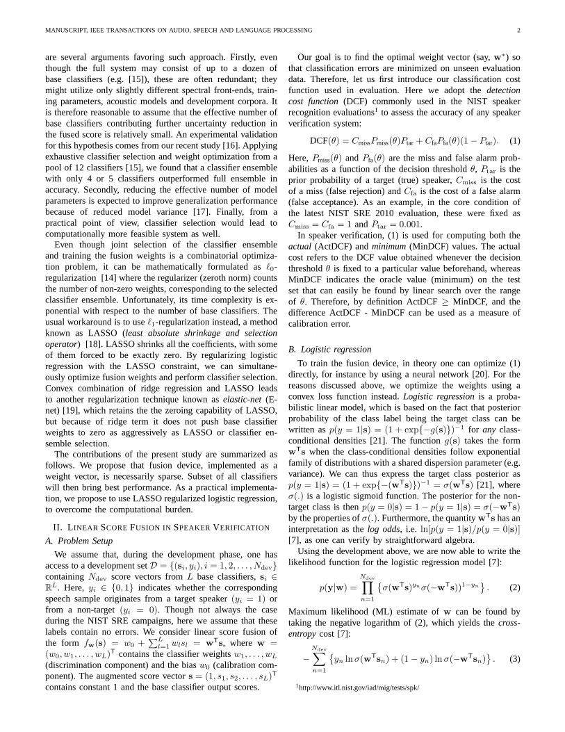
Fig. 1: Visual intuition behind sparse classifier fusion. Wedisplay the contours of theCwlr cost function for score fusion oftwo classifiers. In each panel, the global minimum ofCwlr is indicated by a red cross. In the constrained optimizationcase, wesearch for the minimum instead inside a constraint region specified by(wp
1 + wp2)
(1/p) ≤ 1 (here, the casesp = 1 andp = 2are visualized). As can be seen, the casep = 1 finds asparsesolution in the sense that classifier 2 is zeroed out. Luckilythissolution hits closest to the true minimum on the unseen test data. EvenL2 regularization (p = 2) gives smaller cost than theunconstrained solution, suggesting that regularization and sparsification might be particularly useful for classifier fusion underunpredictable data mismatches.
0.1 0.5 1 2 5 10 20 40
0.10.2
0.51
2
5
10
20
40
False Alarm probability (in %)
Missprobability(in%)
0.2 0.5 1
2
5
10
20
False Alarm probability (in %)
Best single
Equal weights
Grad. Cwlr
Grad. MinDCF
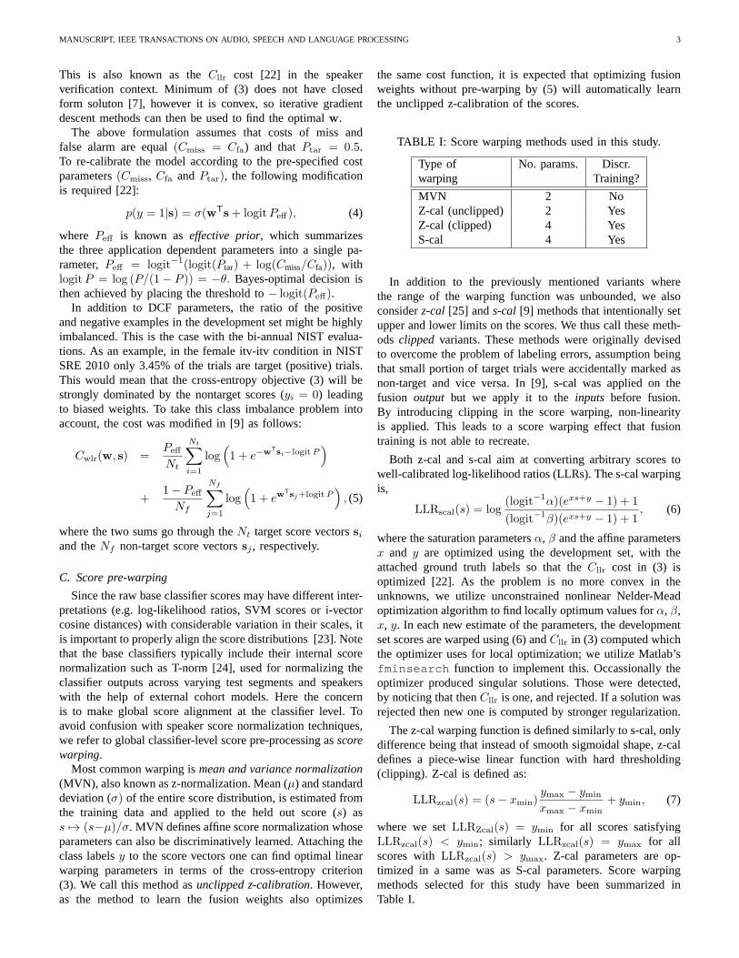
Fig. 2: Comparison of fusion methods using the full ensembleS-cal warping on Trainset. The best individual classifier (forActDCF) is also shown. The circles indicate the ActDCFpoints.
III. SPARSECLASSIFIER FUSION
In this study, we propose to useℓ0 andℓ1 regularization toobtain sparsew. It is then natural to ask whether unregularizedlogistic regression (i.e. maximum likelihood training) canproduce a sparse solution.
Maximum likelihood solution of thew can be characterizedas [21]:
w = Σ−1(µ1 − µ0), (8)
if class-conditional densities follow Gaussian distribution. In(8), Σ is the shared covariance matrix andµ1 andµ0 are theclass-conditional mean vectors. If we takeΣ to be diagonal,as was assumed in [8], then for one base classifier,
wi =1
σidi, (9)
wheredi is the difference between the means. It is clear that,under these assumptions,wi can be exactly zero only whenmeans of target and non-target score distributions completely
match.
A. Classifier Ensemble Selection as Regularization
Up to this point, we have defined the standard fusionframework, assuming a full ensemble ofL classifiers. Now,instead of optimizing the weights in theL-dimensional space,we are in search of both the optimal classifier ensembleand weights. For the moment, assume that we have decidedon an appropriate size of the ensemble given by integervariableK, K < L. We would like to minimize (5) subjectto this constraint. Obviously, one can simply enumerate allthe
(
LK
)
= L!K!(L−K)! possible classifier ensembles to ensure
that the size constraint is satisfied, and optimize the weightsby minimizing Cwlr for each of these ensemble candidatesand choosing the one that minimizes the cost function. Inpseudocode, of the subset selection method is presented inAlgorithm 1.
Algorithm 1 Joint ensemble selection and fusion training.
1: Given: labeled scores fromL classifiers and requiredensemble sizeK ≤ L
2: Let C = {c ∈ {0, 1}L; |c| ≤ K} contain all the binarymasks with exactlyK nonzero elements
3: for each maskcn ∈ B do4: Find optimal weightsw∗(n) using Trainset by mini-
mizing (5) on scores corresponding to classifiers withnonzero index incn. Record the corresponding valueCwlr(n).
5: end for6: Return {c(n∗),w(n∗)}, where n∗ = argminn Cwlr(n)
for Evalset.
Interestingly, this can also be casted in a regularizationframework as follows. First, note that theℓ0-norm of vector
MANUSCRIPT, IEEE TRANSACTIONS ON AUDIO, SPEECH AND LANGUAGE PROCESSING 5
w, defined as [14]‖w‖0 ,∑
i |wi|0, counts the number
of nonzero elements inw. This is because|wi|0 equals 1
everywhere except forwi = 0 one defines it as 0. Thus, anequivalent formulation of the above combinatorial optimiza-tion problem is
minw
Cwlr(w,S) s.t. ‖w‖0 ≤ K, (10)
But the minimizer of (10) is the same as that of
minw
{Cwlr(w,S) + λ‖w‖0} , (11)
since the function in (11) is the Lagrangian of the constrainedoptimization problem in (10) [26]. This merely states thatAlgorithm 1 is equivalent with (11) but does not change thecomplexity of the problem
Although it is clear that that the combinatorial searchoutlined above is not very practical for largeL, it is guaranteedto give the optimum classifier ensemble choice for a givenset of data. In this study, we find it a useful analysis toolfor studying the generalization properties of other sparsity-promoting fusion schemes given below; analogous to thecommon use of the difference ActDCF - MinDCF as a measureof calibration error, we can determine the bestrealizableclassifier ensemble (found from training set) and compare theresult to the best achievableoracle result on the evaluationset.
B. Practical Regularization via Ridge, LASSO and Elastic Net
For computational reasons‖w‖0 constraint is typically,approximated as‖w‖1 constraint [14]. This constraint isknown as LASSO. Norm can also be constrained by‖w‖22,which corresponds then toridge regression, however ridgeconstraint is not an sparsity promoting constraint whereasLASSO is [14].
In the case of LASSO constraint, (10) takes the followingform:
minw
Cwlr(w,S) s.t. ‖w‖1 ≤ t. (12)
Then the Lagrange coefficients will give us,
minw
{Cwlr(w,S) + λ‖w‖1} . (13)
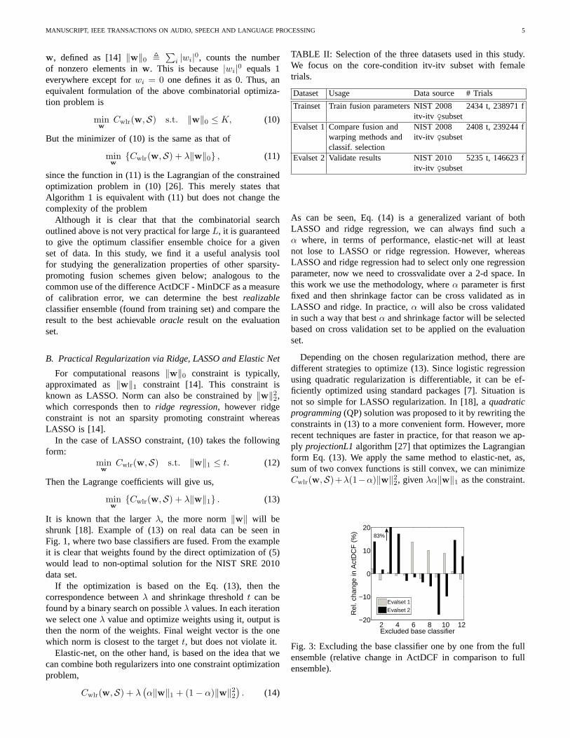
It is known that the largerλ, the more norm‖w‖ will beshrunk [18]. Example of (13) on real data can be seen inFig. 1, where two base classifiers are fused. From the exampleit is clear that weights found by the direct optimization of (5)would lead to non-optimal solution for the NIST SRE 2010data set.
If the optimization is based on the Eq. (13), then thecorrespondence betweenλ and shrinkage thresholdt can befound by a binary search on possibleλ values. In each iterationwe select oneλ value and optimize weights using it, output isthen the norm of the weights. Final weight vector is the onewhich norm is closest to the targett, but does not violate it.
Elastic-net, on the other hand, is based on the idea that wecan combine both regularizers into one constraint optimizationproblem,
Cwlr(w,S) + λ(
α‖w‖1 + (1− α)‖w‖22)
. (14)
TABLE II: Selection of the three datasets used in this study.We focus on the core-condition itv-itv subset with femaletrials.
Dataset Usage Data source # Trials
Trainset Train fusion parameters NIST 2008 2434 t, 238971 fitv-itv ♀subset
Evalset 1Compare fusion and NIST 2008 2408 t, 239244 fwarping methods and itv-itv♀subsetclassif. selection
Evalset 2Validate results NIST 2010 5235 t, 146623 fitv-itv ♀subset
As can be seen, Eq. (14) is a generalized variant of bothLASSO and ridge regression, we can always find such aα where, in terms of performance, elastic-net will at leastnot lose to LASSO or ridge regression. However, whereasLASSO and ridge regression had to select only one regressionparameter, now we need to crossvalidate over a 2-d space. Inthis work we use the methodology, whereα parameter is firstfixed and then shrinkage factor can be cross validated as inLASSO and ridge. In practice,α will also be cross validatedin such a way that bestα and shrinkage factor will be selectedbased on cross validation set to be applied on the evaluationset.
Depending on the chosen regularization method, there aredifferent strategies to optimize (13). Since logistic regressionusing quadratic regularization is differentiable, it can be ef-ficiently optimized using standard packages [7]. Situationisnot so simple for LASSO regularization. In [18], aquadraticprogramming(QP) solution was proposed to it by rewriting theconstraints in (13) to a more convenient form. However, morerecent techniques are faster in practice, for that reason weap-ply projectionL1algorithm [27] that optimizes the Lagrangianform Eq. (13). We apply the same method to elastic-net, as,sum of two convex functions is still convex, we can minimizeCwlr(w,S)+λ(1−α)‖w‖22, givenλα‖w‖1 as the constraint.
2 4 6 8 10 12−20
−10
0
10
20
Excluded base classifier
Rel
. cha
nge
in A
ctD
CF
(%
)
Evalset 1
Evalset 2
83%
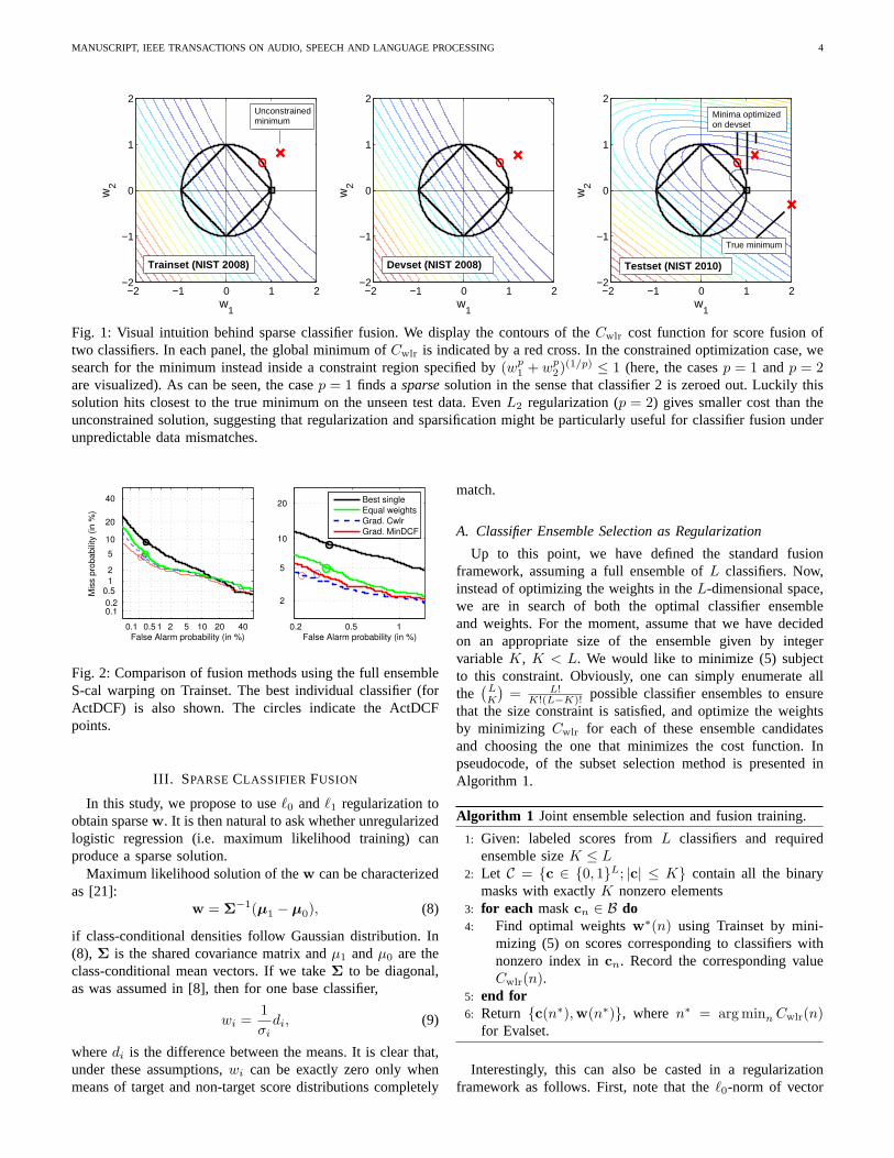
Fig. 3: Excluding the base classifier one by one from the fullensemble (relative change in ActDCF in comparison to fullensemble).
MANUSCRIPT, IEEE TRANSACTIONS ON AUDIO, SPEECH AND LANGUAGE PROCESSING 6
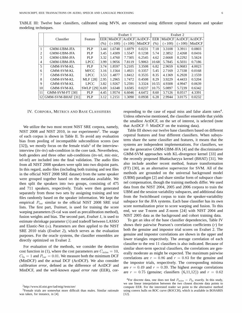
TABLE III: Twelve base classifiers, calibrated using MVN, are constructed using different cepstral features and speakermodeling techniques.
Classifier FeatureEvalset 1 Evalset 2
EER MinDCF ActDCF ActDCF- EER MinDCF ActDCF ActDCF-(%) (×100) (×100) MinDCF (%) (×100) (×100) MinDCF
1 GMM-UBM-JFA PLP 3.44 1.6748 1.6979 0.0231 7.18 3.3108 3.3911 0.08032 GMM-UBM-JFA PLP 3.45 1.4309 1.5547 0.1238 5.74 2.3852 2.4268 0.04163 GMM-UBM-JFA PLP 3.32 1.4760 7.7305 6.2545 4.62 2.6668 8.2292 5.56244 GMM-UBM-JFA LPCC 3.99 1.9056 7.8119 5.9063 10.68 5.7845 6.5031 0.71865 GMM-SVM-KL PLP 3.74 1.8597 5.2105 3.3508 6.82 2.9659 6.9683 4.00236 GMM-SVM-KL MFCC 3.16 1.1564 1.4921 0.3357 5.45 2.7169 2.7338 0.01687 GMM-SVM-KL LPCC 3.53 1.4877 1.8412 0.3535 8.35 4.1369 6.2928 2.15598 GMM-SVM-KL MLF [28] 2.95 1.2965 1.7472 0.4508 8.29 3.9229 4.4433 0.52049 GMM-SVM-KL LPCC 3.82 1.9267 5.2591 3.3324 10.55 4.9308 4.9947 0.063910 GMM-SVM-KL SWLP [29] 6.69 3.6348 3.6585 0.0237 10.75 5.0897 5.7239 0.634211 GMM-SVM-FT [30] PLP 4.45 1.9574 6.6046 4.6472 8.60 3.7126 8.0517 4.339112 GMM-SVM-BHAT [31] PLP 3.12 1.2151 1.3090 0.0938 6.28 2.9944 3.0175 0.0232
IV. CORPORA, METRICS AND BASE CLASSIFIERS
We utilize the two most recent NIST SRE corpora, namely,NIST 2008 and NIST 2010, in our experiments2. The usageof each corpus is shown in Table II. To avoid any evaluationbias from pooling of incompatible subcondition scores (see[32]), we mostly focus on the female trials3 of the interview-interview (itv-itv) sub-condition in the core task. Nevertheless,both genders and three other sub-conditions (itv-tel, mic-mic,tel-tel) are included into the final validation. The audio filesfrom all NIST 2008 speakers were split into two disjoint parts.In this regard, audio files (including both training and testfilesin the official NIST 2008 SRE dataset) from the same speakerwere grouped together based on the metadata available. Wethen split the speakers into two groups, consisting of 475and 711 speakers, respectively. Trials were then generatedseparately from those two sets by assigning training and testfiles randomly based on the speaker information. We kept theempirical Ptar similar to the official NIST 2008 SRE triallists. The first part,Trainset, is used for training the scorewarping parameters (S-cal was used as precalibration method),fusion weights and bias. The second part,Evalset 1, is used toestimate shrinkage parameter (λ) and tradeoff between LASSOand Elastic-Net (α). Parameters are then applied to the NISTSRE 2010 trials (Evalset 2), which serves as the evaluationpurposes. For the oracle systems, the classifier ensembles aredirectly optimized on Evalset 2.
For evaluation of the methods, we consider the detectioncost function in (1), where the cost parameters areCmiss = 10,Cfa = 1 andPtar = 0.01. We measure both the minimum DCF(MinDCF) and the actual DCF (ActDCF). We also considercalibration error, defined as the difference of ActDCF andMinDCF, and the well-knownequal error rate (EER), cor-
2http://www.itl.nist.gov/iad/mig//tests/sre/3Female trials are somewhat more difficult than males. Similar rationale
was taken, for instance, in [4].
responding to the case of equal miss and false alarm rates4.Unless otherwise mentioned, the classifier ensemble that yieldsthe smallest ActDCF, on the set of interest, is selected (notethat ActDCF, MinDCF on the training data).
Table III shows our twelve base classifiers based on differentcepstral features and four different classifiers. When subsys-tems share the same classifier and features, it means that thesystems are independent implementations. For classifiers,weuse the generative GMM-UBM-JFA [4] and the discriminativeGMM-SVM approaches with KL-divergence kernel [33] andthe recently proposed Bhattacharyya kernel (BHAT) [31]. Wealso include another recent method, feature transformation(FT) [30], as an alternative supervector for SVM. All of themethods are grounded on the universal background model(UBM) paradigm [2] and share similar form of subspace chan-nel compensation, though the training methods differ. We useddata from the NIST 2004, 2005 and 2006 corpora to train theUBM and the session variability subspaces, and additional datafrom the Switchboard corpus to train the speaker-variabilitysubspace for the JFA systems. Each base classifier has its ownscore normalization prior to score warping and fusion. To thisend, we use T-norm and Z-norm [24] with NIST 2004 andNIST 2005 data as the background and cohort training data.
To get an idea of the base classifier dependencies, Table IVshows their pairwise Pearson’s correlation coefficients (r) forboth the genuine and impostor trial scores on Evalset 2. Thegenuine and impostor correlations are shown in the upper andlower triangles respectively. The average correlation of eachclassifier to the rest 11 classifiers is also indicated. Because ofsimilar short-term spectral classifiers, the correlationsare gen-erally moderate as might be expected. The maximum pairwisecorrelations arer = 0.86 and r = 0.83 for the genuine andthe impostor trials, respectively. The corresponding minimaare r = 0.49 and r = 0.39. The highest average correlationsare r = 0.75 (genuine; classifiers{6,11,12}) and r = 0.62
4For discrete data, one does not findPmiss = Pfa exactly. In this study,we use linear interpolation between the two closest discrete data points tocompute EER. For the interested reader we point to the alternative methodusing convex hulls on ROC curve (ROCCH), which is available in BOSARIS[12].
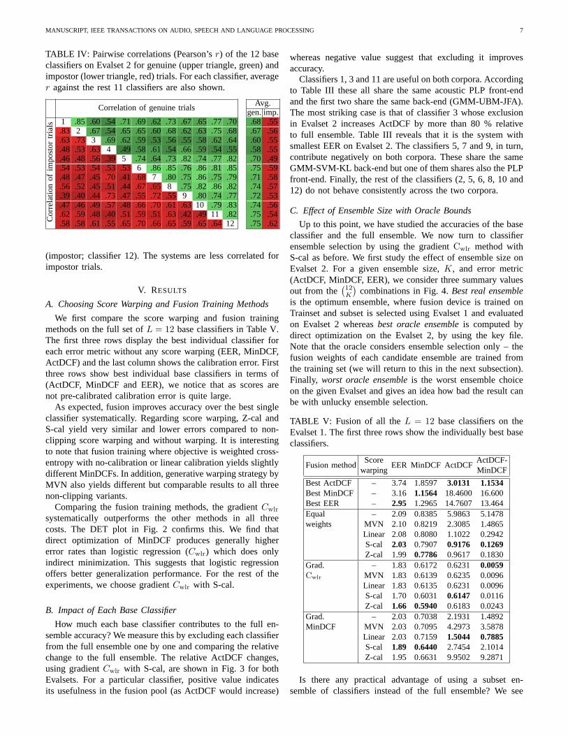
MANUSCRIPT, IEEE TRANSACTIONS ON AUDIO, SPEECH AND LANGUAGE PROCESSING 7
TABLE IV: Pairwise correlations (Pearson’sr) of the 12 baseclassifiers on Evalset 2 for genuine (upper triangle, green)andimpostor (lower triangle, red) trials. For each classifier,averager against the rest 11 classifiers are also shown.
Correlation of genuine trials Avg.gen.imp.
Cor
rela
tion
ofim
post
ortr
ials 1 .85 .60 .54 .71 .69 .62 .73 .67 .65 .77 .70 .68 .55
.83 2 .67 .54 .65 .65 .60 .68 .62 .63 .75 .68 .67 .56
.63 .73 3 .69 .62 .59 .53 .56 .55 .58 .62 .64 .60 .55
.48 .53 .63 4 .49 .58 .61 .54 .66 .59 .54 .55 .58 .55
.46 .48 .56 .39 5 .74 .64 .73 .82 .74 .77 .82 .70 .49
.54 .53 .54 .53 .53 6 .86 .85 .76 .86 .81 .85 .75 .59
.48 .47 .45 .70 .41 .68 7 .80 .75 .86 .75 .79 .71 .58
.56 .52 .45 .51 .44 .67 .65 8 .75 .82 .86 .82 .74 .57
.39 .40 .44 .73 .47 .55 .72 .55 9 .80 .74 .77 .72 .53
.47 .46 .49 .57 .48 .66 .70 .61 .63 10 .79 .83 .74 .56
.62 .59 .48 .40 .51 .59 .51 .63 .42 .49 11 .82 .75 .54
.58 .58 .61 .55 .65 .70 .66 .65 .59 .65 .64 12 .75 .62
(impostor; classifier 12). The systems are less correlated forimpostor trials.
V. RESULTS
A. Choosing Score Warping and Fusion Training Methods
We first compare the score warping and fusion trainingmethods on the full set ofL = 12 base classifiers in Table V.The first three rows display the best individual classifier foreach error metric without any score warping (EER, MinDCF,ActDCF) and the last column shows the calibration error. Firstthree rows show best individual base classifiers in terms of(ActDCF, MinDCF and EER), we notice that as scores arenot pre-calibrated calibration error is quite large.
As expected, fusion improves accuracy over the best singleclassifier systematically. Regarding score warping, Z-calandS-cal yield very similar and lower errors compared to non-clipping score warping and without warping. It is interestingto note that fusion training where objective is weighted cross-entropy with no-calibration or linear calibration yields slightlydifferent MinDCFs. In addition, generative warping strategy byMVN also yields different but comparable results to all threenon-clipping variants.
Comparing the fusion training methods, the gradientCwlr
systematically outperforms the other methods in all threecosts. The DET plot in Fig. 2 confirms this. We find thatdirect optimization of MinDCF produces generally highererror rates than logistic regression (Cwlr) which does onlyindirect minimization. This suggests that logistic regressionoffers better generalization performance. For the rest of theexperiments, we choose gradientCwlr with S-cal.
B. Impact of Each Base Classifier
How much each base classifier contributes to the full en-semble accuracy? We measure this by excluding each classifierfrom the full ensemble one by one and comparing the relativechange to the full ensemble. The relative ActDCF changes,using gradientCwlr with S-cal, are shown in Fig. 3 for bothEvalsets. For a particular classifier, positive value indicatesits usefulness in the fusion pool (as ActDCF would increase)
whereas negative value suggest that excluding it improvesaccuracy.
Classifiers 1, 3 and 11 are useful on both corpora. Accordingto Table III these all share the same acoustic PLP front-endand the first two share the same back-end (GMM-UBM-JFA).The most striking case is that of classifier 3 whose exclusionin Evalset 2 increases ActDCF by more than 80 % relativeto full ensemble. Table III reveals that it is the system withsmallest EER on Evalset 2. The classifiers 5, 7 and 9, in turn,contribute negatively on both corpora. These share the sameGMM-SVM-KL back-end but one of them shares also the PLPfront-end. Finally, the rest of the classifiers (2, 5, 6, 8, 10and12) do not behave consistently across the two corpora.
C. Effect of Ensemble Size with Oracle Bounds
Up to this point, we have studied the accuracies of the baseclassifier and the full ensemble. We now turn to classifierensemble selection by using the gradientCwlr method withS-cal as before. We first study the effect of ensemble size onEvalset 2. For a given ensemble size,K, and error metric(ActDCF, MinDCF, EER), we consider three summary valuesout from the
(
12K
)
combinations in Fig. 4.Best real ensembleis the optimum ensemble, where fusion device is trained onTrainset and subset is selected using Evalset 1 and evaluatedon Evalset 2 whereasbest oracle ensembleis computed bydirect optimization on the Evalset 2, by using the key file.Note that the oracle considers ensemble selection only – thefusion weights of each candidate ensemble are trained fromthe training set (we will return to this in the next subsection).Finally, worst oracle ensembleis the worst ensemble choiceon the given Evalset and gives an idea how bad the result canbe with unlucky ensemble selection.
TABLE V: Fusion of all theL = 12 base classifiers on theEvalset 1. The first three rows show the individually best baseclassifiers.
Fusion methodScore
EER MinDCF ActDCFActDCF-
warping MinDCF
Best ActDCF – 3.74 1.8597 3.0131 1.1534Best MinDCF – 3.16 1.1564 18.4600 16.600Best EER – 2.95 1.2965 14.7607 13.464Equal – 2.09 0.8385 5.9863 5.1478weights MVN 2.10 0.8219 2.3085 1.4865
Linear 2.08 0.8080 1.1022 0.2942S-cal 2.03 0.7907 0.9176 0.1269Z-cal 1.99 0.7786 0.9617 0.1830
Grad. – 1.83 0.6172 0.6231 0.0059Cwlr MVN 1.83 0.6139 0.6235 0.0096
Linear 1.83 0.6135 0.6231 0.0096S-cal 1.70 0.6031 0.6147 0.0116Z-cal 1.66 0.5940 0.6183 0.0243
Grad. – 2.03 0.7038 2.1931 1.4892MinDCF MVN 2.03 0.7095 4.2973 3.5878
Linear 2.03 0.7159 1.5044 0.7885S-cal 1.89 0.6440 2.7454 2.1014Z-cal 1.95 0.6631 9.9502 9.2871
Is there any practical advantage of using a subset en-semble of classifiers instead of the full ensemble? We see

MANUSCRIPT, IEEE TRANSACTIONS ON AUDIO, SPEECH AND LANGUAGE PROCESSING 8
that ensemble sizes 6-9 bring real benefit in contrast to fullensemble. Smaller subset sizes, from 2-5, shows unpredictablebehaviour on the real system. As is expected, predicted realsystem does not reach oracle performance, showing that evenmore improvement can be obtained by better prediction of thesubset.
Another interesting observation is that, for all the three errormetrics, the empirical bounds on best and worst performanceapproach each other for increased ensemble size. This canbe understood by noting that
(
12K
)
is small whenK is closeto 12; thus, there are simply less choices to make bad (orgood) classifier selection. Being more fair and comparingensemble pools ofequal size, say,
(
122
)
=(
1210
)
= 66 or(
123
)
=(
129
)
= 220, it is clear from Fig. 4 that using the largerensemble leads to more stable fusion, which is intuitivelyreasonable. Averaging similar spectral system scores helps inreducing variance (uncertainty) of the fused score as discussedin [34], [35].
Table VI summarizes the subset selection cross-validationresults on Evalset 2. Real system performance is contrastedagainst oracle selection rule. In the table best individual(“bestind.”) and full ensemble (“full ens.”) accuracies are alsoindicated, and as before,bestmeans best in ActDCF.
As earlier, the results in Table VI are divided intoreal andoracleperformances.Subset ensemble(“subset ens.”) refers tothe best joint ensemble selection and fusion choice, out fromall the 212 − 1 = 4095 possibilities. For the real and oraclesystems, the ensemble selection is carried out on Evalset 1 andEvalset 2, respectively. Oracle ensemble results are similar toFig.4, where the weights of the 4095 ensemble candidates areoptimized on Trainset, and the oracle selects the best ensembleon the Evalset 2.
We make the following observations from Table VI:
• Realistic subset ensemble has better performance on allthe three metrics over full ensemble. Relative improve-ment is 4.4% for EER, 2.8% for MinDCF and 8.7% forActDCF.
• On the oracle scenario, subset ensemble fusion givessmaller error rates using smaller ensemble size (5) thanpredicted ensemble (7).
• For the subset ensemble, improvement in EER from thereal to oracle system is larger than for MinDCF, relativereduction of 10% and 6.5% respectively.
• Subset selected by oracle contains classifiers{2,3,5,6}which have low EER (Table III). For the classifier 10with EER of 10.75 % it is less clear why it is included inthe oracle set. The correlations in Table IV do not revealthis either.
• In the real systems, all three error metrics are reduced byfusion, using both subset and full ensemble methods, overthe best individual system. This confirms that fusing evena rather homogenous set of low-level spectral classifiersis beneficial.
D. Extended Results on Other Conditions
Throughout the experiments, we have restricted ourselvesto female trials of the interview-interview subcondition.To
TABLE VI: Comparing different ensemble selections onEvalset 2. The best individual classifier (best for ActDCF)is selected using Evalset 1 (real systems) or Evalset 2 (oraclesystems).
FusionWeights Ensemble Included EER MinDCF ActDCFtraining selection classifiers (%) (×100) (×100)
Rea
l Best ind. – Evalset 1 {6} 5.45 2.7169 3.6453Subset ens.Trainset Evalset 1 {1,2,3,4,5,6,9} 3.40 1.7506 2.6119Full ens. Trainset – all 3.55 1.8072 2.8420
Orc
l. Best ind. – Evalset 2 {2} 5.74 2.3852 2.6063Subset ens.Trainset Evalset 2 {2,3,5,6,10} 3.08 1.6426 1.7747
2 4 6 8 10 122
4
6
Ensemble size
ActDCF (x100)
(a)
2 4 6 8 10 12
1.8
2
2.2
2.4
2.6
Ensemble size
MinDCF (x100)
Worst oracle ens.Best real ens.Best oracle ens.
(b)
2 4 6 8 10 12
3.5
4
4.5
5
Ensemble size
EER (%)
(c)
Fig. 4: Effect of ensemble size to accuracy (Evalset 2). For afixed ensemble size (K), the lowest (green) and highest (red)lines show the best and worst possible selections out from the(
12K
)
choices from Evalset 2 (NIST SRE 2010). The middle(blue) line indicates the actual ensemble selected by cross-validation Evalset 1.
TABLE VII: Chosen NIST 2010 subconditions.
NIST 2010 common cond.1 2 3 4 5 6 7 8 9
itv-itv × ×
itv-tel ×
mic-mic × ×
tel-tel × × ×
validate our observations on a broader set of conditions, TableVIII shows accuracies for other selected subconditions of theNIST 2010 core task, for only female trials. We consider foursubconditions that correspond to pooled data from the NIST2010 common conditions as listed in Table VII.
All fusion strategies – best individual, full ensemble andregularized variants – are in non-oracle setting, that is, fusiontraining are carried out on a training set and regularizationparameters are estimated using Evalset 1. In this experiment,we also make sure that NIST 2008 training set and NIST 2010evaluation set are condition-matched under each subcondition.
In addition to ActDCF, MinDCF and EER, we report theactual number of misses (Nmiss) and false alarms (Nfa) ateach operating point. Further, we carried out McNemar’ssignificance testing [36], [37] on both types of errors at 95 %confidence level, to find when they differ between the subsetand full ensemble fusions. The significantly differing cases(from the full ensemble) are denoted by⋆.
In Table VIII, we show the recognition results for differentNIST SRE 2010 sub-conditions (itv-itv, itv-tel, mic-mic andtel-tel). Here, baseline method refers to the unregularized
MANUSCRIPT, IEEE TRANSACTIONS ON AUDIO, SPEECH AND LANGUAGE PROCESSING 9
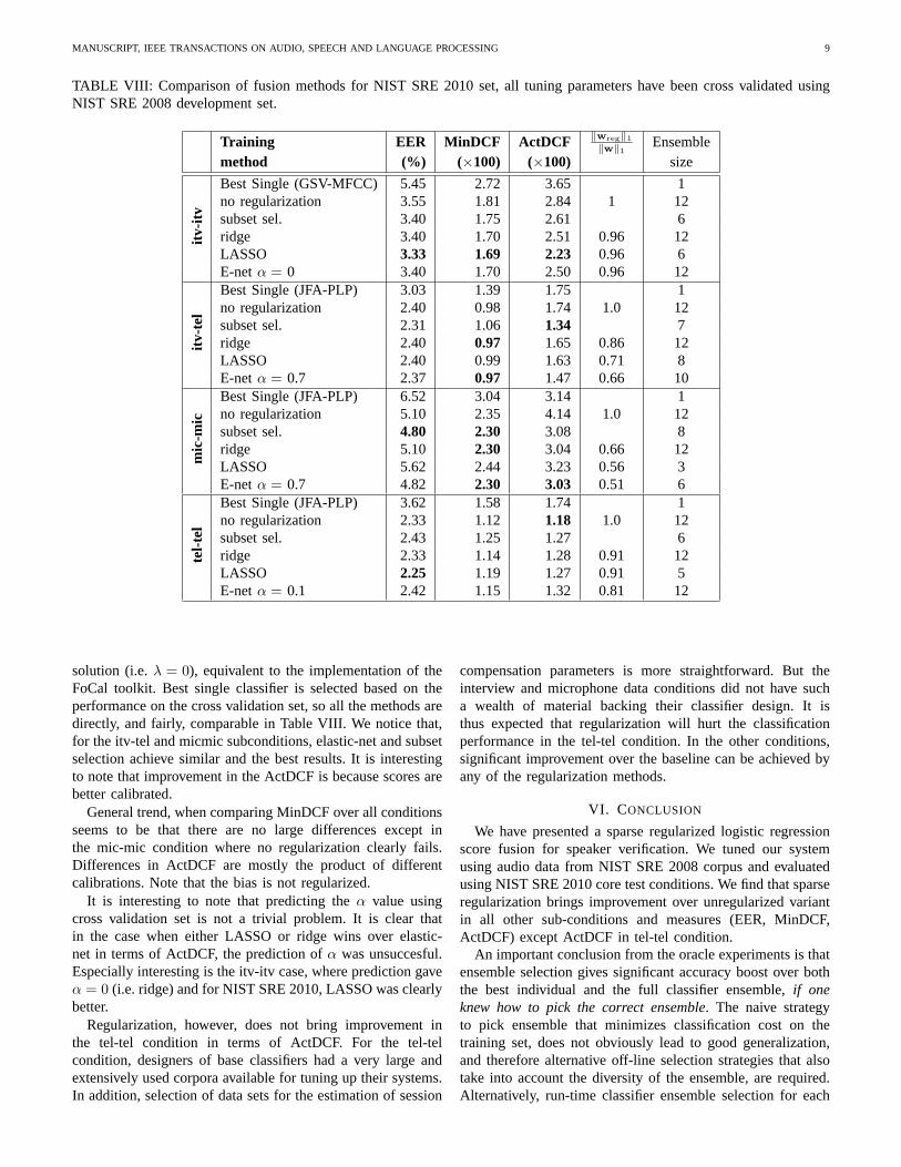
TABLE VIII: Comparison of fusion methods for NIST SRE 2010 set, all tuning parameters have been cross validated usingNIST SRE 2008 development set.
Training EER MinDCF ActDCF ‖wreg‖1
‖w‖1Ensemble
method (%) (×100) (×100) size
itv-it
vBest Single (GSV-MFCC) 5.45 2.72 3.65 1no regularization 3.55 1.81 2.84 1 12subset sel. 3.40 1.75 2.61 6ridge 3.40 1.70 2.51 0.96 12LASSO 3.33 1.69 2.23 0.96 6E-netα = 0 3.40 1.70 2.50 0.96 12
itv-t
el
Best Single (JFA-PLP) 3.03 1.39 1.75 1no regularization 2.40 0.98 1.74 1.0 12subset sel. 2.31 1.06 1.34 7ridge 2.40 0.97 1.65 0.86 12LASSO 2.40 0.99 1.63 0.71 8E-netα = 0.7 2.37 0.97 1.47 0.66 10
mic
-mic
Best Single (JFA-PLP) 6.52 3.04 3.14 1no regularization 5.10 2.35 4.14 1.0 12subset sel. 4.80 2.30 3.08 8ridge 5.10 2.30 3.04 0.66 12LASSO 5.62 2.44 3.23 0.56 3E-netα = 0.7 4.82 2.30 3.03 0.51 6
tel-t
el
Best Single (JFA-PLP) 3.62 1.58 1.74 1no regularization 2.33 1.12 1.18 1.0 12subset sel. 2.43 1.25 1.27 6ridge 2.33 1.14 1.28 0.91 12LASSO 2.25 1.19 1.27 0.91 5E-netα = 0.1 2.42 1.15 1.32 0.81 12
solution (i.e.λ = 0), equivalent to the implementation of theFoCal toolkit. Best single classifier is selected based on theperformance on the cross validation set, so all the methods aredirectly, and fairly, comparable in Table VIII. We notice that,for the itv-tel and micmic subconditions, elastic-net and subsetselection achieve similar and the best results. It is interestingto note that improvement in the ActDCF is because scores arebetter calibrated.
General trend, when comparing MinDCF over all conditionsseems to be that there are no large differences except inthe mic-mic condition where no regularization clearly fails.Differences in ActDCF are mostly the product of differentcalibrations. Note that the bias is not regularized.
It is interesting to note that predicting theα value usingcross validation set is not a trivial problem. It is clear thatin the case when either LASSO or ridge wins over elastic-net in terms of ActDCF, the prediction ofα was unsuccesful.Especially interesting is the itv-itv case, where prediction gaveα = 0 (i.e. ridge) and for NIST SRE 2010, LASSO was clearlybetter.
Regularization, however, does not bring improvement inthe tel-tel condition in terms of ActDCF. For the tel-telcondition, designers of base classifiers had a very large andextensively used corpora available for tuning up their systems.In addition, selection of data sets for the estimation of session
compensation parameters is more straightforward. But theinterview and microphone data conditions did not have sucha wealth of material backing their classifier design. It isthus expected that regularization will hurt the classificationperformance in the tel-tel condition. In the other conditions,significant improvement over the baseline can be achieved byany of the regularization methods.
VI. CONCLUSION
We have presented a sparse regularized logistic regressionscore fusion for speaker verification. We tuned our systemusing audio data from NIST SRE 2008 corpus and evaluatedusing NIST SRE 2010 core test conditions. We find that sparseregularization brings improvement over unregularized variantin all other sub-conditions and measures (EER, MinDCF,ActDCF) except ActDCF in tel-tel condition.
An important conclusion from the oracle experiments is thatensemble selection gives significant accuracy boost over boththe best individual and the full classifier ensemble,if oneknew how to pick the correct ensemble. The naive strategyto pick ensemble that minimizes classification cost on thetraining set, does not obviously lead to good generalization,and therefore alternative off-line selection strategies that alsotake into account the diversity of the ensemble, are required.Alternatively, run-time classifier ensemble selection foreach
MANUSCRIPT, IEEE TRANSACTIONS ON AUDIO, SPEECH AND LANGUAGE PROCESSING 10
speech utterance, similar to adaptable fusion using auxiliaryquality measures [38], [39], [40], would be an interestingdirection.
REFERENCES
[1] T. Kinnunen and H. Li, “An overview of text-independent speakerrecognition: from features to supervectors,”Speech Communication,vol. 52, no. 1, pp. 12–40, January 2010.
[2] D. Reynolds, T. Quatieri, and R. Dunn, “Speaker verification usingadapted gaussian mixture models,”Digital Signal Processing, vol. 10,no. 1, pp. 19–41, January 2000.
[3] W. Campbell, J. Campbell, D. Reynolds, E. Singer, and P. Torres-Carrasquillo, “Support vector machines for speaker and language recog-nition,” Computer Speech and Language, vol. 20, no. 2-3, pp. 210–229,April 2006.
[4] P. Kenny, P. Ouellet, N. Dehak, V. Gupta, and P. Dumouchel,“A study ofinter-speaker variability in speaker verification,”IEEE T. Audio, Speech& Lang. Proc., vol. 16, no. 5, pp. 980–988, July 2008.
[5] A. Solomonoff, W. Campbell, and I. Boardman, “Advances in channelcompensation for SVM speaker recognition,” inProc. ICASSP 2005,Philadelphia, Mar. 2005, pp. 629–632.
[6] C. P. Robert,The Bayesian Choice: from Decision-Theoretic Motivationsto Computational Implementation, 2nd ed. Springer-Verlag, 2001.
[7] C. Bishop, Pattern Recognition and Machine Learning. New York:Springer Science+Business Media, LLC, 2006.
[8] S. Pigeon, P. Druytsa, and P. Verlinde, “Applying logistic regressionto the fusion of the nist’99 1-speaker submissions,”Digital SignalProcessing, vol. 10, no. 1–3, pp. 237–248, January 2000.
[9] N. Brummer, L. Burget, J.Cernocky, O. Glembek, F. Grezl, M. Karafiat,D. Leeuwen, P. Matejka, P. Schwartz, and A. Strasheim, “Fusion ofheterogeneous speaker recognition systems in the STBU submission forthe NIST speaker recognition evaluation 2006,”IEEE Trans. Audio,Speech and Language Processing, vol. 15, no. 7, pp. 2072–2084,September 2007.
[10] L. Ferrer, K. Sonmez, and E. Shriberg, “An anticorrelation kernelfor subsystem training in multiple classifier systems,”J. of MachineLearning Research, vol. 10, pp. 2079–2114, 2009.
[11] N. Brummer, “Fusion and toolkit [software package],” WWW page, June2011, http://sites.google.com/site/nikobrummer/focal.
[12] “Bosaris toolkit [software package],” WWW page, June 2011,https://sites.google.com/site/bosaristoolkit/.
[13] R. Duda, P. Hart, and D. Stork,Pattern Classification, 2nd ed. NewYork: Wiley Interscience, 2000.
[14] T. Hastie, R. Tibshirani, and J. Friedman,The Elements of StatisticalLearning – Data Mining, Inference, and Prediction, 2nd ed. Springer,2008.
[15] H. Li, B. Ma, K. A. Lee, H. Sun, D. Zhu, K. C. Sim, C. H. You,R. Tong, I. Karkkainen, C.-L. Huang, V. Pervouchine, W. Guo, Y. Li,L. Dai, M. Nosratighods, T. Tharmarajah, J. Epps, E. Ambikairajah, E.-S. Chng, T. Schultz, and Q. Jin, “The I4U system in NIST 2008 speakerrecognition evaluation,” inProc. Int. conference on acoustics, speech,and signal processing (ICASSP 2009), Taipei, Taiwan, April 2009, pp.4201–4204.
[16] F. Sedlak, T. Kinnunen, K. A. L. Ville Hautamaki, and H. Li, “Classifiersubset selection and fusion for speaker verification,” inICASSP 2011,2011.
[17] S. Geman, E. Bienenstock, and R. Doursat, “Neural networks and thebias/variance dilemma,”Neural Computation, vol. 4, no. 1, pp. 1–58,January 1992.
[18] R. Tibshirani, “Regression shrinkage and selection via the lasso,”Jour-nal of the Royal Statistical Society, Series B, vol. 58, no. 1, pp. 267–288,1996.
[19] H. Zou and T. Hastie, “Regularization and variable selection via theelastic net,”Journal of Royal Statistical Society, Series B, vol. 67, pp.301–320, 2005.
[20] W. Campbell, D. Sturim, W. Shen, D. Reynolds, and J. Navratil,“The MIT-LL/IBM 2006 speaker recognition system: High-performancereduced-complexity recognition,” inProc. ICASSP 2007, vol. IV, 2007,pp. 217–220.
[21] M. I. Jordan, “Why the logistic function? a tutorial discussion on prob-abilities and neural networks,” Massachusetts Institute of Technology,Cambridge, MA, Tech. Rep., August 1995.
[22] N. Brummer and J. Preez, “Application-independent evaluation ofspeaker detection,”Computer Speech and Language, vol. 20, pp. 230–275, April-July 2006.
[23] A. Jain, K. Nandakumar, and A. Ross, “Score normalizationin multi-modal biometric systems,”Pattern Recognition, vol. 38, no. 3, pp. 2270–2285, 2005.
[24] R. Auckenthaler, M. Carey, and H. Lloyd-Thomas, “Score normaliza-tion for text-independent speaker verification systems,”Digital SignalProcessing, vol. 10, no. 1-3, pp. 42–54, January 2000.
[25] “Z-cal,” 2006, http://ww.dsp.sun.ac.za/∼nbrummer/focal/cllr/calibration/zcal/index.htm.[Online]. Available: http://ww.dsp.sun.ac.za/∼nbrummer/focal/cllr/calibration/zcal/index.htm
[26] C. H. Papadimitriou and K. Steiglitz,Combinatorial Optimization:Algorithms and Complexity. Dover Publications, 1998.
[27] M. Schmidt, G. Fung, and R. Rosales, “Fast optimization methods forL1 regularization: A comparative study and two new approaches,” inECML 2007, Warsaw, Poland, September 2007.
[28] C.-L. Huang, H. Su, B. Ma, and H. Li, “Speaker characterizationusing long-term and temporal information,” inProc. Interspeech 2010,Makuhari, Japan, September 2010, pp. 370–373.
[29] R. Saeidi, J. Pohjalainen, T. Kinnunen, and P. Alku, “Temporallyweighted linear prediction features for tackling additivenoise in speakerverification,” IEEE Sign. Proc. Lett., vol. 17, no. 6, pp. 599–602, 2010.
[30] D. Zhu, B. Ma, and H. Li, “Joint MAP adaptation of featuretransforma-tion and gaussian mixture model for speaker recognition,” inProc. Int.conference on acoustics, speech, and signal processing (ICASSP 2009),Taipei, Taiwan, April 2009, pp. 4045–4048.
[31] C. H. You, K. A. Lee, and H. Li, “GMM-SVM kernel with aBhattacharyya-based distance for speaker recognition,”IEEE Trans.Audio, Speech and Language Processing, vol. 18, no. 6, pp. 1300–1312,August 2010.
[32] D. Leeuwen, “A note on performance metrics for speaker recognitionusing multiple conditions in an evaluation,” Research note,June 2008,http://sites.google.com/site/sretools/cond-weight.pdf?attredirects=0.
[33] W. Campbell, D. Sturim, and D. Reynolds, “Support vector machinesusing GMM supervectors for speaker verification,”IEEE Signal Pro-cessing Letters, vol. 13, no. 5, pp. 308–311, May 2006.
[34] N. Poh and S. Bengio, “Why do multi-stream, multi-band and multi-modal approaches work on biometric user authentication tasks?” in Proc.ICASSP 2004, vol. 5, Montreal, Canada, May 2004, pp. 893–896.
[35] G. Brown, J. Wyatt, R. Harris, and X. Yao, “Diversity creation methods:A survey and categorisation,”Journal of Information Fusion, vol. 6,no. 1, pp. 5–20, March 2005.
[36] D. Leeuwen, A. Martin, M. Przybocki, and J. Bouten, “NIST and NFI-TNO evaluations of automatic speaker recognition,”Computer Speechand Language, vol. 20, pp. 128–158, April-July 2006.
[37] X. Huang, A. Acero, and H.-W. Hon,Spoken Language Processing: aGuide to Theory, Algorithm, and System Development. New Jersey:Prentice-Hall, 2001.
[38] L. Ferrer, M. Graciarena, A. Zymnis, and E. Shriberg, “System com-bination using auxiliary information for speaker verification,” in Proc.Int. Conf. on Acoustics, Speech, and Signal Processing (ICASSP 2008),Las Vegas, Nevada, March-April 2008, pp. 4853–4856.
[39] K. Kryszczuk, J. Richiardi, P. Prodanov, and A. Drygajlo, “Reliability-based decision fusion in multimodal biometric verification systems,”EURASIP Journal of Advances in Signal Processing, no. 1, p. ArticleID 86572, 2007.
[40] F. Huenupan, N. Yoma, C. Garreton, and C. Molina, “On-line linearcombination of classifiers based on incremental information inspeakerverification,” ETRI Journal, vol. 32, no. 3, pp. 395–405, June 2010.
Related Documents