Spare parts management improvement at KLM Equipment Services

Eindhoven, June 2012

Student identity number 0628216

in partial fulfilment of the requirements for the degree of

Master of Science

in Operations Management and Logistics

Supervisors:

dr.ir. S.D.P. Flapper, TU/e, OPAC

prof.dr.ir. G.J.J.A.N. van Houtum, TU/e, OPAC

drs. P.N. Bos, KLM Equipment Services

S. Buter, KLM Equipment Services

Spare parts management improvement at KLM Equipment Services

by

Anela Velagić

II

TUE. School of Industrial Engineering.

Series Master Theses Operations Management and Logistics

Subject headings: demand forecasting, inventory control, spare parts management, spare parts

classification

III

ABSTRACT

In this project a structured approach for spare parts management at KLM Equipment Services has been

developed. First, a classification scheme with respect to demand forecasting is proposed and evaluated.

Next, different time-series forecasting methods are initialized and compared in order to find the most

appropriate method for the underlying demand pattern within a particular class. Subsequently, a

classification scheme with respect to inventory control is proposed and evaluated. Special attention has

been paid to the criticality analysis. Finally, this project has analyzed how to improve the logistics

outsourcing relationship and scope between KLM Equipment Services and Sage Parts.

IV

PREFACE AND ACKNOWLEDGEMENTS

This report is the result of my master thesis project in completion of the master Operations Management

and Logistics at the Eindhoven University of Technology. The project has been carried out at the

Engineering department of KLM Equipment Services located at Amsterdam Airport Schiphol.

I would like to thank several people that helped me during my master thesis project. First of all, I would

like to thank Simme Douwe Flapper, my first supervisor, for guiding me through the process, his

constructive feedback, but especially for his confidence in me. Furthermore, I would like to thank Geert-

Jan van Houtum, my second supervisor, for his critical view on the project and the useful feedback.

At KLM Equipment Services, I would like to thank Peter Bos who gave me the opportunity to conduct my

master thesis project at his company. Besides that, I would like to thank him and Simon Buter as my

company supervisors for the time and effort they have invested in my project. Our weekly meetings have

been challenging and useful. Also, I would like to thank all the other colleagues at KLM Equipment

Services for providing me with valuable information and for the pleasant working atmosphere.

Finally, I would like to thank my dear family and friends for their support and interest during my entire

study and this project in particular. Special thanks to my parents, for the support they provided during my

whole life such that I could pursue my goals, their patience, and their everlasting and unconditional love.

Thank you all.

Anela Velagić

Helmond, June 2012

V

EXECUTIVE SUMMARY

This report is the result of a master thesis project conducted at KLM Equipment Services (KES). KES’s main

activity is the preventive and corrective maintenance of ground support equipment (GSE), that is, all

vehicles and equipment necessary for ground handling of airplanes. In August, 2008 inventory control and

procurement of spare parts has been outsourced to Sage Parts. Sage is responsible for the availability of

components needed for maintenance on GSE. KES receives each month a report from Sage about the Key

Performance Indicators (KPIs) in the previous month. These reports show every month that the actual

performance is above the target values. However, this does not match with the signals KES receives from

the maintenance shop – the maintenance shop is not satisfied with the availability of spare parts. KES

would like to get more insight in this mismatch between the monthly reports from Sage, and the

dissatisfaction at the maintenance shop.

Analysis current planning & control

First, an analysis of the current situation has been conducted. The environment in which KES operates

makes spare parts management a challenging task. In order to get more insight in these challenges

several people were interviewed until no new information emerged. The analysis revealed that the parts

supply time is variable, the demand for spare parts is heterogeneous and irregular, and there is a gap

between KES and Sage. Next, it has been analyzed how KES and Sage have set-up the current planning

and control of spare parts in order to operate in the described environment and its challenges. For this

analysis we have used the framework from Driessen et al. (2010) in order to find improvement

possibilities. This framework distinguishes eight aspects of planning and control, that is, assortment

management, demand forecasting, parts return forecasting, supply management, repair shop control,

inventory control, spare parts order handling, and deployment. The analysis shows that one of the

improvement possibilities is the classification of spare parts for inventory control; the current

classification uses only one criterion – annual usage. Another improvement possibility is demand

forecasting. From the available information we have concluded that Sage adopts “black-box forecasting”:

forecasts are generated by an information system, but the specific techniques are unknown to the users.

Finally, we have also seen that there are some ambiguities about the responsibilities between KES and

Sage which further increases the gap between KES and Sage.

Research questions

The main research question of this master thesis project is formulated as follows: “Can spare parts

management at KLM Equipment Services be improved?” The goal of this master thesis project was to find

out whether spare parts management can be improved, and if so, how spare parts management can be

improved. Based on the described improvement possibilities, we have formulated the following

subquestions in order to answer the main research question:

1. How can we improve demand forecasting, such that it better captures the demand pattern of the

spare parts?

2. How can we improve the current classification scheme for inventory control, such that it better

captures the characteristics of the spare parts?

3. How can we improve the logistics outsourcing performance?

VI

Demand forecasting

Currently, all items are forecasted based on historical demand but the specific technique is not known.

KES would like to include also information about explanatory variables in the forecasts (e.g. maintenance

planning, part failure rate). However, the use of forecasts based on explanatory variables is not always

possible, nor is the use of only historical demand data always possible. In this master thesis project we

have developed a classification scheme that can be used to choose between different forecasting

approaches and methods. We have first selected criteria for classifying parts with respect to demand

forecasting. The first classification criterion is the life cycle. Based on the life cycle phase one can choose

between causal (i.e. based on explanatory variables) and time-series methods (i.e. based on historical

demand) – the life cycle phase indicates whether sufficient historical data or data about explanatory

variables is available for making use of these forecasting approaches. Another purpose of the

classification is to determine the most appropriate time-series method for items in the in-use phase.

Empirical investigation of the demand pattern based on the average demand interval and demand size

variability revealed that the demand pattern for in-use items is mainly characterized by differences in

demand intermittence (i.e. demand frequency). Different time-series techniques specific for intermittent

demand, i.e. Croston, ES, SBA and TSB, are initialized and compared to each other for items in the in-use

phase of the life cycle. The results reveal that the TSB method outperforms the other methods in terms of

MSE and bias.

Inventory control

Currently, the spare parts inventory is classified by only one criterion – annual usage. When it comes to

spare parts inventory management, determining the importance of a spare part by annual usage is

insufficient, because spare parts are highly heterogeneous, with differing costs, service requirements, and

demand patterns. In this master thesis project we have shown that the current classification scheme with

respect to inventory control can be improved, such that it better captures the underlying demand of

spare parts by the design of a hierarchical multiple-criteria classification scheme with respect to inventory

control. First, we have selected collectively (KES’s management and the researcher) appropriate

classification criteria for which sufficient information is available. We have again used the life cycle of the

items, because the life cycle also influences inventory decisions. Besides the life cycle phase, another

important extension of the current classification scheme is the inclusion of the criticality factor.

In order to determine the criticality we have developed a two-step-filter: in the first step vehicles are

filtered based on the GSE criticality, and the type of order. In the second step, GSE vehicles are scored on

the number of failures compared to the total number of failures for GSE vehicles from the same supplier

type, and on the number of times that a particular item is replaced on the same GSE vehicle. To

determine objective weights for the scores in the second step, we have used a multiple-attribute, DEA-

like, decision model. Finally, critical items are further classified according to their part value in order to

help making stock/non-stock decisions. Non-critical items are further classified according to Sage’s

current classification scheme based on annual usage. No other criteria are explicitly considered at this

stage for classification related purposes. Other important factors such as the supply lead time and its

variability and the demand variability can be further considered in the calculation of safety stocks, when

such an exercise is required.

VII

Logistics outsourcing

Finally, we have analyzed how to improve the logistics outsourcing performance. The logistics outsourcing

relationship is characterized by a lack of information exchange and shared understanding, and there are

also ambiguities with respect to the responsibilities between KES and Sage. It has been explained that one

can create a shared understanding by focusing on the end-customer (i.e. user of GSE). KES and Sage

should aim for a low GSE downtime in order to prevent/minimize opportunistic behavior. Further, it has

been explained that information exchange can be improved by making use of the developed classification

schemes. The developed classification schemes create a higher awareness of spare parts characteristics

and their effect on demand forecasting and/or inventory control. The current classification scheme based

on annual usage does not trigger KES and Sage to exchange information about those aspects. Finally, it

has been argued to reconsider the logistics outsourcing scope and activities. KES should consider taking

demand forecasting and inventory control back in-house. The message is to outsource the execution, not

the management.

Conclusions and recommendations

By referring back to the main research question we have concluded that is possible to improve spare

parts management by adopting a structured approach for both demand forecasting and inventory

control, and by improving the logistics outsourcing performance. This master thesis project has shown

the benefits of a structured approach for dealing with the considerable number of heterogeneous items.

However, the developed classification schemes are only a starting point and can be used to make

strategic and tactical forecasting and inventory decisions. The next step is to choose inventory policies

and parameters for each class resulting from the classification scheme with respect to demand

forecasting. The inventory policies and parameters depend on forecasts of demand over lead-time so

inventory policies are influenced by the accuracy of demand forecasts. The classification scheme with

respect to demand forecasting can be used to choose appropriate forecasting methods. Only then one

can measure the real benefit of the classification schemes – that is, by integrated the outcomes of spare

parts classification, demand forecasting and inventory control.

The following recommendations are made for KES (and Sage):

Use the classification scheme in order to choose a forecasting method. In the initial phase one

can estimate important characteristics by comparing the part to technically similar parts. It is

recommended to use the TSB method for forecasting demand for parts in the in-use phase. For

the decline phase one could for example use a regression model on the logarithm of sales against

time, assuming an exponential decline in demand over time.

Determine and compare suitable inventory policies and parameters for each class resulting from

the classification scheme with respect to inventory control when the necessary data is available.

The real benefit of the developed classification schemes can be tested by using the forecasted

demand and the standard deviation (forecasted according to the classification scheme with

respect to demand forecasting) for determining the inventory parameters.

Collect more data on explanatory variables and validate the current data about explanatory

variables in order to make causal forecasting possible (i.e. forecasting based on explanatory

variables). Pay more attention to assortment management and gather parts (technical)

VIII

information from the initial phase of the life cycle instead of waiting till the in-use or decline

phase.

Consider increasing the number of preventive maintenances in order to reduce the number of

corrective maintenance (i.e. repairs and breakdowns), and thus, the number of hot orders.

In the criticality analysis we have used GSE criticality as a classification criterion. However, there

were mixed signals about the criticality of a particular GSE vehicle. Create more agreement about

the GSE criticality, and discuss together with fleet management and customers which GSE

vehicles are really critical.

The current KPIs do not provide sufficient insight in Sage’s actual performance. Consider

eliminating the supply lead time restrictions, and using only the target values for the fill rates.

Further, consider introducing a target value for the GSE downtime in order to increase the focus

on the end-customer.

IX

CONTENTS Abstract ........................................................................................................................................................ III

Preface and acknowledgements .................................................................................................................. IV

Executive summary ....................................................................................................................................... V

Contents ....................................................................................................................................................... IX

1 Introduction .......................................................................................................................................... 1

1.1 Company description ...................................................................................................................... 1

1.2 Introduction to the problem ........................................................................................................... 1

1.2.1 Supply vs demand ................................................................................................................... 2

1.2.2 Logistics outsourcing ............................................................................................................... 3

1.3 Outline of the report ....................................................................................................................... 4

2 Current planning & control ................................................................................................................... 5

2.1 Framework ...................................................................................................................................... 5

2.2 Assortment management ............................................................................................................... 7

2.2.1 Define spare parts assortment................................................................................................ 7

2.2.2 Gather parts (technical) information ...................................................................................... 7

2.3 Demand forecasting ........................................................................................................................ 8

2.4 Parts return forecasting .................................................................................................................. 9

2.5 Supply management ....................................................................................................................... 9

2.5.1 Manage supplier availability & other characteristics ............................................................. 9

2.5.2 Control supply time & other supply parameters .................................................................. 10

2.6 Repair shop control ....................................................................................................................... 10

2.7 Inventory control .......................................................................................................................... 11

2.7.1 Classify parts ......................................................................................................................... 11

2.7.2 Select replenishment policy and parameters ....................................................................... 12

2.8 Spare parts order handling ........................................................................................................... 12

2.9 Deployment................................................................................................................................... 13

2.10 Improvement possibilities ............................................................................................................. 13

3 Research design and methodology ..................................................................................................... 15

3.1 Problem definition ........................................................................................................................ 15

3.2 Scope ............................................................................................................................................. 16

3.3 Research question ......................................................................................................................... 16

3.4 Project Approach .......................................................................................................................... 17

3.5 Deliverables ................................................................................................................................... 18

4 Demand forecasting ............................................................................................................................ 19

4.1 Approach ....................................................................................................................................... 19

4.2 Classification for demand forecasting .......................................................................................... 19

4.2.1 Cut-off values ........................................................................................................................ 21

4.2.2 Application classification scheme for demand forecasting .................................................. 23

4.3 Time-series forecasting methods .................................................................................................. 24

4.3.1 Forecasts ............................................................................................................................... 25

X

4.3.2 Smoothing constants ............................................................................................................ 27

4.3.3 Seasonality ............................................................................................................................ 27

4.4 Forecast Initialization .................................................................................................................... 28

4.5 Choice forecasting method ........................................................................................................... 29

5 Inventory control ................................................................................................................................ 33

5.1 Classification for inventory control ............................................................................................... 33

5.1.1 Classification criteria ............................................................................................................. 33

5.1.2 Classification techniques ....................................................................................................... 35

5.2 Criticality analysis .......................................................................................................................... 36

5.2.1 Criticality factors ................................................................................................................... 37

5.2.2 Multi-criteria criticality scheme ............................................................................................ 39

5.2.3 Application of the criticality analysis .................................................................................... 41

5.2.4 Benefits of the criticality analysis ......................................................................................... 41

5.3 Application classification scheme for inventory control ............................................................... 43

6 Logistics outsourcing ........................................................................................................................... 46

6.1 Logistics outsourcing relationship ................................................................................................ 46

6.1.1 Information exchange ........................................................................................................... 46

6.1.2 Shared goals .......................................................................................................................... 47

6.2 Logistics outsourcing scope & activities........................................................................................ 48

7 Implementation .................................................................................................................................. 49

7.1 Demand forecasting ...................................................................................................................... 49

7.2 Inventory control .......................................................................................................................... 50

7.3 Reclassification .............................................................................................................................. 51

8 Conclusions and recommendations .................................................................................................... 53

8.1 Conclusions ................................................................................................................................... 53

8.2 Limitations..................................................................................................................................... 55

8.3 Academic relevance ...................................................................................................................... 56

8.4 Recommendations ........................................................................................................................ 57

References .................................................................................................................................................. 59

List of abbreviations .................................................................................................................................... 62

List of definitions ......................................................................................................................................... 63

List of figures and tables ............................................................................................................................. 64

Appendix A: Classification criteria .............................................................................................................. 65

Appendix B: Seasonality .............................................................................................................................. 67

Appendix C: Life cycle phase ....................................................................................................................... 69

Appendix D: Demand forecasting ............................................................................................................... 71

Appendix E: Implementation ...................................................................................................................... 73

1

1 INTRODUCTION

This chapter starts with a short introduction about KLM Equipment Services and its main supplier Sage

Parts (1.1). Next, the problem will be introduced (1.2). Finally, an outline of this master thesis preparation

report will be given (1.3).

1.1 COMPANY DESCRIPTION KLM Equipment Services (KES) is operating as an independent subsidiary of KLM Royal Dutch Airlines, and

is based at Amsterdam Airport Schiphol since 1952. KES’s main activity is the preventive and corrective

maintenance of ground support equipment (GSE), that is, all vehicles and equipment necessary for

ground handling of airplanes, including air conditioning units, air starter units, ambulifts, busses, cargo

tractors, baggage carts, cars, catering trucks, conveyer belts, de-icers, dollies, fuelling equipment, ground

power units, baggage loaders, lower and main deck loaders, pallet transporters, passenger steps, push

back tractors, toilets trucks, tow bars, vans, and water trucks. The maintenance division can be

subdivided into: motorized equipment, non-motorized equipment, truck maintenance, aircraft refueling

equipment, battery maintenance, hoisting maintenance, and service repair shop on the ramp. KES is

maintaining about 1500 GSE vehicles that can be subdivided in 250 different groups of vehicles.

Maintenance activities are not only focused on KLM’s GSE vehicles, but also on GSE vehicles from other

fleet owners operating at Amsterdam Airport Schiphol such as Transavia and Martinair.

In August 2008, inventory control and procurement of spare parts has been outsourced to Sage Parts

(hereafter Sage). Sage is responsible for the availability of parts needed for maintenance on the GSE

vehicles. More than 90% of the SKUs is under Sage’s responsibility, whereas the remaining 10% (e.g. oil

and raw materials) is controlled by KES. Sage is focused on cost-reduction, high quality spare parts, and

high know-how. Moreover, Sage has a geographically widespread distribution network in the GSE parts

marketplace. Sage has an onsite parts location at KES. By bringing parts closer to their point of use, Sage

is helping KES to reduce shipping costs and time, but also to avoid or eliminate costly GSE downtime.

1.2 INTRODUCTION TO THE PROBLEM KES receives each month a report from Sage about the Key Performance Indicators (KPIs) in the previous

month. These reports show every month that the actual performance is above the target values.

However, this does not match with the signals KES receives from the maintenance shop – the

maintenance shop is not satisfied with the availability of spare parts. KES would like to get more insight in

this mismatch between the monthly reports from Sage, and the dissatisfaction with the availability at the

maintenance shop. The main goal is to improve spare parts management in order to increase the

availability of spare parts at rather low costs. By increasing the spare parts availability one can decrease

the costly downtime of GSE vehicles. However, the environment in which KES operates makes spare parts

management a challenging task. In order to get more insight in these challenges, several people were

interviewed (amongst others KES’s director, maintenance manager, director production support, senior

consultant, and Sage Parts’ branch manager) until no new information emerged. Based on the

information from the interviews, an overview of the main observations with respect to the environment

in which KES operates is given in Figure 1.1.

2

Figure 1.1 expresses that spare parts management has to deal with a variable spare parts supply time and

demand. The variable spare parts supply time is influenced by the external supplier reliability, spare parts

in the end of the spare parts life cycle, and spare parts specificity. The heterogeneous and irregular

demand is influenced by spare parts specificity, seasonal factors, and corrective, inspection based

maintenance. Further, Figure 1.1 shows that spare parts management is depended on the success of the

logistics outsourcing relationship between KES and Sage. In Section 1.2.1 we will explain the mismatch

between the demand and supply side. In Section 1.2.2 we will discuss the problems caused by the

logistics outsourcing relationship.

Spare parts

management

DemandSupply

Gap between KES and

Sage

Heterogeneous and irregular

demand

Variable spare parts

supply time

Seasonal

factors

Corrective, inspection

based maintenanceEnd of spare parts

life cycle

Spare parts specificity

(GSE vehicle diversity)

External supplier

reliability

Logistics

outsourcing

Figure 1.1 Description of the environment in which KES operations

1.2.1 Supply vs demand

The first observation from Figure 1.1 is that spare parts management is influenced by a variable spare

parts supply time for spare parts that are out of stock or not kept on stock at all. Spare parts that are

required for old GSE vehicles, and for GSE vehicles that are delivered by small, non-established original

equipment manufacturers, have a long and unreliable part supply time. The number of available (reliable)

external spare parts suppliers is limited for these vehicles. The part supply time for spare parts that are in

the initial and in-use phase of their life cycle, and for standard spare parts is shorter and more reliable.

However, in the final phase of the life cycle they do encounter problems, because of the restricted

number of external spare parts suppliers. The length and uncertainty of the parts supply time are higher

in the final phase of the life cycle. According to Sage, the lead time uncertainty is, among others, caused

by the (un-)reliability of the external spare parts suppliers. The differences in reliability of external

suppliers lead to supply lead time uncertainty. To sum up, spare parts management is complicated by the

length of and uncertainty in spare parts supply lead time related to spare parts in the last phase of the

spare parts life cycle and non-standard spare parts, but also by the external supplier reliability.

3

Figure 1.1 further shows that spare parts management is complicated by the demand pattern KES and

Sage have to deal with. GSE vehicles are not highly complex, but the high number of different groups of

GSE vehicles (i.e. KES is maintaining about 1500 GSE vehicles that can be subdivided in 250 different

groups of vehicles) makes spare parts management complex, because of the low commonality between

spare parts. The demand for spare parts is highly heterogeneous because of the high diversity in GSE

vehicles. High spare parts heterogeneity makes demand forecasting and inventory control difficult. One of

the reasons for the high number of different groups of GSE vehicles is the fact that the GSE vehicles,

maintained by KES, are delivered by various, also small, suppliers. In addition, some GSE vehicles are

insufficiently developed and engineered at the moment they are delivered by their supplier. In that case,

KES has to make additional development and engineering steps in order to make the vehicle functioning

well. This implies that some GSE vehicles are unique which makes spare parts management even more

complicated. Further, maintenance activities, and thus the need for spare parts, are affected by seasonal

factors. The number of corrective maintenance activities is higher during the Fall/Winter period (de-icers

are for example only operated during the Winter) than during Spring/Summer period. Finally, the rate of

corrective maintenance is high compared to preventive maintenance. Demand resulting from corrective

maintenance has stochastic demand arrivals which makes demand forecasting and inventory

management difficult. To sum up, given the high number of different and specialized GSE vehicles, the

seasonal factors, and high rate of corrective maintenances compared to preventive maintenances, spare

parts management has to deal with a heterogeneous and irregular demand for spare parts.

1.2.2 Logistics outsourcing

As is discussed, spare parts management is also influenced by the success of logistics outsourcing to Sage.

From the interviews it follows that there is a gap between KES and Sage. One of the possible reasons for

this gap between KES and Sage is the lack of (necessary) information exchange between KES and Sage.

Sage states that they do not have all necessary information for appropriate spare parts planning and

control. They expect from KES to give them more, timely, information related to the KES’s maintenance

activities. One of the reasons for the lacking information exchange is the fact that KES’s and Sage’s

information system are not real-time aligned with each other. However, KES and Sage are already

working on this issue. Another possible reason for the gap between KES and Sage is the lack of shared

understanding between the maintenance, and inventory control functions. Maintenance people are not

concerned with the costs related to stocking parts with a low demand; they are more concerned with the

availability of spare parts. On the other hand, inventory control tries to reduce the costs while

maintaining a satisfying spare parts availability level. Both parties acknowledge that the communication

and coordination between them should be improved. A holistic perspective on system performance,

where the demand and supply side are integrated with each other is missing, because spare parts

management and maintenance are two separate entities in the current situation. They should be better

linked with each other in order to increase the availability of spare parts.

Overall, the main observations from Figure 1.1 are the (i) parts supply time variability, (ii) heterogeneous

and irregular demand, and (iii) the gap between KES and Sage. These observations explain the challenges

for appropriate spare parts management.

4

1.3 OUTLINE OF THE REPORT In this master thesis project we will analyze whether spare parts management can be improved, and if so,

how spare parts management can be improved. This master thesis project starts in Chapter 2 with an

analysis of the current situation to identify improvement possibilities by using a framework for planning

and control of the spare parts supply chain (Driessen, Arts, Van Houtum, Rustenburg & Hulsman, 2010).

Driessen et al. (2010) point out that the framework can be used to increase efficiency, consistency, and

sustainability of decisions on how to plan and control a spare parts supply chain, which in turn should

minimize maintenance delay due to unavailability of required spare parts. In Chapter 3 the research

design and methodology will be discussed. Chapter 3 starts with the problem statement and scope, after

which the research questions, project approach and the deliverables of the project will be presented.

Next, Chapter 4 will describe how to classify spare parts with respect to demand forecasting, after which

different time-series forecasting methods (i.e. forecasting based on historical demand data) will be

compared to each other in order to select to most appropriate forecasting method(s) per class. Chapter 5

will present a classification scheme with respect for inventory control. As part of this classification

scheme, a criticality analysis will be performed. Chapter 6 will describe how the logistics outsourcing

performance can be improved in order to foster a better link between the demand and supply side of

spare parts. In Chapter 7 an implementation plan will be presented. Finally, in Chapter 8 the main

conclusions, limitations, and recommendations from this master thesis project will be given.

5

2 CURRENT PLANNING & CONTROL

In this chapter it will be analyzed how KES and Sage have set-up the planning and control of spare parts in

order to identify improvement possibilities. All aspects from the framework of Driessen et al. (2010) for

spare parts planning and control will be discussed (2.1), that is, assortment management (2.2), demand

forecasting (2.3), parts return forecasting (2.4), supply management (2.5), repair shop control (2.6),

inventory control (2.7), spare parts order handling (2.8), and deployment (2.9). Finally, the improvement

possibilities will be elaborated (2.10).

2.1 FRAMEWORK In the first chapter of this report we have explained that the monthly reports from Sage show a good

performance, whereas the maintenance shop is actually not satisfied. In order to identify improvement

options, we will first have to understand how KES and Sage have set-up the planning and control of spare

parts. For this analysis we will use the framework from Driessen et al. (2010) in order to find

improvement possibilities. Note that this analysis is not the same as the analysis in Section 1.2 where we

have introduced the problem - Section 1.2 explains the environment in which KES operates, whereas this

analysis will show how KES and Sage have set-up the planning and control of spare parts in order to

operate in the environment that we have described in Section 1.2.

Before we start with the analysis, we will explain the framework from Driessen et al. (2010). Driessen et

al. (2010) have developed a detailed framework that can be used for planning and control of the spare

parts supply chain. Their framework presents a clustering of the involved tasks and decisions, and the

mutual connections between the task and decisions. They separate eight different processes and within

each process one can distinguish different decision levels, i.e. strategic, tactical, and operational

decisions. The processes are assortment management, demand forecasting, parts return forecasting,

supply management, repair shop control, inventory control, spare parts order handling, and deployment.

The framework is shown on the next page in Figure 2.1.

First of all, Driessen et al. (2010) express that different return rates can influence control in different

ways, and that the return rates therefore should be forecasted. Based on the available (technical)

information on the assortment, one can classify parts with respect to return forecasting. Besides demand

forecasting, and parts return forecasting, one can also use the (technical) information on the assortment

for supply management. Then, supply management is defined as the process of ensuring that one or

multiple supply sources are available to supply spare parts at any given moment in time with

predetermined supplier characteristics. Supply management is not only dependent on the connection

with assortment management, but also on demand forecasting, and repair shop control. It is also

explained that at the interface with supply structure management, agreements should be made on lead

times for the repair of each repairable, and also on the load imposed on the repair shop so that these

lead-times can be realized. Further, it is pointed out that spare parts classification and demand

forecasting (including parts return forecasting) should be related to stock control policies. That means

that inventory management should adopt a differentiated approach by assigning different inventory

policies among the spare parts classes.

6

Figure 2.1 Overview and clustering of decisions in maintenance logistics control (from Driessen et al., 2010, pp. 8)

7

Furthermore, inventory policies should be developed based on the information from demand forecasting.

One should also be aware of the interface with supply management which is among others related to the

repair of repairables. Finally, it is explained that one needs to define preconditions and rules to manage

the spare parts order handling steps. The process of replenishing spare parts inventories is explained by

describing the definition of the preconditions order process and the management of procurement and

repair orders.

Having shortly explained the framework and the processes, we will now analyze each of these processes

for the current situation at KES. In this analysis references will be made to the operational manual. The

operational manual is a report in which the topics (a) contact persons; (b) meeting structure KES and

Sage; (c) management information; and (d) process flows and/or descriptions are covered, and are

officially agreed on by both parties. Note that the analysis is also based on several interviews with both

KES and Sage (with amongst others KES’s managing director, maintenance manager, director production

support, senior consultant, and Sage Parts’ branch manager).

2.2 ASSORTMENT MANAGEMENT Assortment management is concerned with the decision to include a spare part in the assortment and

maintaining technical information of the included spare parts (Driessen et al., 2010). Driessen et al. (2010)

emphasize that the decision whether or not to include a part in the assortment is independent of the

decision to stock the part. For KES and Sage it is not a static decision. More specifically, in GSE, the sub-

components and sub-assemblies change over time, and as such the assortment needs to be reviewed on

a constant basis. The assortment is driven by the original equipment manufacturers (OEMs) and the

various parts and components they choose to use in the production of the GSE vehicles.

2.2.1 Define spare parts assortment

In the Sage/KES relationship, Sage manages the assortment, but with communication and input from KES.

The ultimate decision is driven by KES as they are confronted with the costs. Once the assortment is

determined, it is Sage’s responsibility to ensure that proper part levels are maintained. In practice,

whenever there are new GSE vehicles introduced to the KES vehicle database, KES has to inform Sage

about it. It is agreed that in an early stage of the project Sage has to receive technical information

concerning these vehicles. According to the operational manual, KES has to inform Sage about the

maintenance planning and modifications, and provide technical information about the manufacturer,

serial numbers, engine manufacturer, engine number, parts needed for preventive maintenance, and

recommended parts list (RSL). Sage in turn should create a stock level based on this information.

However, at this moment this information is not, sufficiently or not at all, exchanged. A part is only

included in the assortment when the part is also stocked. One of the reasons for this lack of information

exchange is the fact that KES does not have all the necessary information; OEMs do not always provide

useful RSLs and technical information.

2.2.2 Gather parts (technical) information

Once a part is included in the assortment, information of the part should be gathered and maintained

(Driessen et al., 2010). There are no “specific” agreements regarding what information should be

maintained. Sage believes that the OEMs should be providing much of this information to the vehicle

8

owner (KES/KLM). In that case, KES should have certain information, such as parts manuals, service

instructions and critical parts lists, and use it to order parts and to assist in deciding what parts should be

kept available despite no or low use. However, in reality, the amount of information that is received from

the OEMs is limited. Further, Sage believes that it is Sage’s responsibility to maintain information about

the supplier, alternative supplier, parts commonality, substitution, reparability and specification

information, along with lead time, costs, etc. There is however some ambiguity about the responsibility

for collecting (technical) information. KES considers Sage as the one who is responsible for collecting the

(technical) information, whereas Sage considers both companies responsible. Uncertainty about the

responsibility for collecting and maintaining the necessary information might result in insufficient and/or

incomplete information for appropriate spare parts management.

While “knowledge maintenance” costs are always a factor in the decisions, Sage thinks it is beneficial to

gather information on all parts. Knowledge is frequently the key to improving cost, availability and

inventory challenges. Historically, GSE equipment is used in the market place much longer than the

average lifespan of other or similar capital equipment. Suppliers and OEMs do evolve and parts and

components that were used in the production are now no longer available, or maybe alternatives are

available. Sage points out that they present options about price, lead time, reliability or quality

information it is aware of to the end-user, and in most cases make a recommendation. However, they

believe ultimately it is the customer’s capital equipment and they need to make the final decision

regarding the product that is installed on their equipment.

2.3 DEMAND FORECASTING Since KES rarely gives Sage future demand data, Sage’s forecasting is for 100% based on historical data

and utilizes algorithms that take into account dozens of data points across a wider range of products than

that owned by KES. However, it is not know how the demand is actually forecasted (i.e. which forecasting

methods are used). Additionally, Sage proactively works with their customers to identify certain items

that should be in stock due to criticality, as well as to identify parts that might need replacement due to

the age or utilization of the equipment.

While sophisticated demand plans can take into account information about the maintenance planning,

parts price, data on historical and unplanned demand, active parts assortment, installed base, mean time

between failures, failure rates, reliability tests, degradation of parts, substitution, redundancy,

commonality, etc., Sage believes it is more practical to start simple and build up. Sage does not get

sufficient reliability or even usage data (i.e. hours that the equipment is actually used) from KES regarding

its upcoming demand, but Sage realizes that KES is provided very little information from the actual

manufactures of the equipment. In a perfect world, the manufactures of the equipment have “service”

plans that would predict parts failure and schedule replacement in advance of that failure.

Unfortunately, the low volumes of similar equipment and the lack of resources of the manufactures do

not allow them to provide this information to the end-user. Many end-users are more proactive as they

have large fleet management departments and large fleets of the same vehicle type and they perform

reliability analysis and develop their own maintenance plans which attempt to replace the parts before

the failure occurs. Sage believes it is not practical to expect such sophisticated information from KES or

any customer, it is practical to expect information on the service plans for service parts requirements

9

(basic maintenance plans). Sage does receive this visibility from many of its customers, both large and

small. Sage believes it would be extremely helpful if KES could develop a pre-defined maintenance kit for

various service checks for the common and/or critical equipment types. If the kits could then be provided

with a 30 day plan, they could load this information into the demand system and pre-build the kits and

have the parts waiting when the equipment comes in for the planned maintenance. This would guarantee

100% availability as well as reduce the time it takes for Sage staff to pick the various components as they

would be pre-kitted.

2.4 PARTS RETURN FORECASTING Driessen et al. (2010) suggest that one needs to account for return rates and hand-in-times in the

planning and control of spare parts. At KES, it is possible and common for parts not used to be returned

to Sage. Sage believes they have a very liberal policy for KES whereby for a part to be returned to stock, it

must be in good order, unused, re-sellable and a stock item. They also take back repairable parts that are

then sent out for repair and put on the shelf for future use. With respect to new parts, for parts to be

returned to a supplier they must also be in original packaging free from damage and dirt. Parts that are

“deemed usable by the KES technicians”, even though used, can be returned to Sage’s warehouse for

future use by KES. KES is responsible for getting the parts back to the Sage stores and ensuring that Sage

has the correct data to allow the parts to be credited to the right job, etc. Sage is responsible for

reviewing the “worthiness” of the parts and placing them in the correct ownership store, or returning to

the supplier for full/partial credit (making the disposition). Additionally, Sage provides information on

parts that were ordered by KES personnel and not yet picked up. This information is useful in alerting all

parties of potential parts that may not be used. However, Sage does not plan or measure “return times”

since the volume currently does not necessitate such detail. Sage’s demand plan does take into account

the net use and net frequency, so they do “plan” for regular returns.

2.5 SUPPLY MANAGEMENT Supply management concerns the process of ensuring that one or multiple supply sources are available to

supply spare parts at any given moment in time with predetermined supplier characteristics, such as lead

time and underlying procurement contracts (Driessen et al., 2010).

2.5.1 Manage supplier availability & other characteristics

Several supply types are used to supply spare parts: (i) internal repair shop, (ii) external repair shop, (iii)

external suppliers, (iv) internal development, and (v) sporadic re-use of parts. Updating and maintaining

current contracts with external suppliers is a dynamic process, with multiple layers of triggers, internal

source/price reviews, stock reviews, lead time reviews, supplier price files, obsolescence, etc. If there is

no supply source available anymore, it becomes a collective effort for finding an alternative supply source

for all parts that need future resupply. Sage believes that in theory, the OEMs should take responsibility.

However, due to the age of the equipment some OEMs exit the business during the life of the equipment,

or stop supporting it after several years with the hopes this will drive new equipment purchases. As a

parts supplier, Sage claims that they will do their absolute best to find alternatives or options when parts

are no longer available. Sage believes they have resources with experience and knowledge, a supply base

that can assist, but they are always open to assistance and other sources of knowledge (including KES’s

10

staff). In some cases portions of the equipment might need a slight redesign to accommodate what is

available in the marketplace. In those cases Sage utilizes their in-house engineers, along with any support

from the OEM and the customer that is available. Sage points out that it is not possible for any one

organization to stand alone in this - it is a team effort.

When the only supply source is known to disappear, one needs to decide whether to search for an

alternative supply source or to place a final order at the current supply source. Sage believes that they are

in almost all cases, the starting point on finding alternatives when supply is no longer available. Sage’s

supply chain and sourcing groups are daily working on finding solutions for dozens of parts and

components that are no longer available or in limited supply. In practice, KES is the one is responsible for

deciding what to do when the only supply source of a part is known to disappear. Usually KES’s

engineering department is asked to analyze what one should do; one could for example decide to modify

the vehicle and/or to place a final order. To make the decision about the final order, KES makes a cost

trade-off.

2.5.2 Control supply time & other supply parameters

Sage explains that GSE equipment requires working with many dysfunctional suppliers/manufactures.

They use the lead times to assist in controlling their inventory and to fulfill commitments to service levels.

Sage points out that they been able to insulate their customer base from product shortages, supplier

factory closedowns/relocations by maintaining the proper inventory positions to account for these

factors as well as supplier reliability. Sage does this by holding inventory, smart forecasting, blanket

orders which scheduled releases and other methods.

However, the supply lead time of spare parts that are backordered is uncertain. KES believes that they do

not get information about the actual supply lead time in a timely manner. However, Sage believes that

they do inform KES about the actual supply lead time in a timely manner. According to Sage the lead time

uncertainty is, among others, caused by the (un-)reliability of the external spare parts suppliers. Most

suppliers are unrealistic in the lead time they quote or commit to. Sage points out that they are mainly

having problems with inventory management for old GSE equipment. On the other hand, they are

successful in fulfilling the service levels for newer GSE equipment. The number of available external spare

parts suppliers is limited for older GSE equipment, and in some cases there are no external suppliers at

all. Sage is working with a classification scheme to rank the external suppliers of spare parts, but KES does

not have sufficient insight in this classification scheme. Sage has acknowledged that they are willing to

give more information about the external suppliers to KES. For example, if the parts are from a C supplier,

it would be useful for KES to know in advance that the supply lead time might be unreliable. Exchange of

external supplier information was previously not possible, because KES and Sage work with two different

systems that are not real-time aligned, but they are working on this IT-issue right now.

2.6 REPAIR SHOP CONTROL Repaired items might have different warranty terms and prices than new parts. Evaluation of the price

and life cycle of the parts should make clear whether or not it stays a repairable item. Whenever the

repair price is higher than 60% of the new price, Sage has to deliver new, unless the delivery time of the

new part is too long. In practice KES is the one who makes the decision whether to make an item a

11

repairable or not. KES believes that Sage should be the one doing this, because Sage claims that they have

a worldwide network, and, KES believes that Sage has more information about external repair in order to

make the right trade-off decision - Sage knows for example where the part could be externally repaired,

at what price, lead time, etc., whereas KES has only knowledge about internal repair. On the other hand,

Sage believes that KES should decide about the repairability of the part. According to Sage, KES has more

knowledge about the repair possibilities.

Driessen et al. (2010) further describe that at the interface with supply structure management,

agreements should be made on lead times for the repair of each repairable. At the moment, there are no

agreements about the planned repair times at KES. KES does not determine the capacity of the repair

shop, and the repair jobs are not scheduled. The capacity of the repair shop depends on the number of

employees present in the maintenance shop. Internal repairs are performed ad hoc when there is

sufficient capacity left. However, this is not a major problem, because the number of repairables is small

compared to the total number of SKUs. For example, the number of unique SKUs requested during 2011

is 58, while the total number of unique SKUs requested during 2011 is 8273.

2.7 INVENTORY CONTROL The inventory control process is concerned with the decision which parts to stock, at which stocking

location, and in what quantity. Inventory control is primarily Sage’s responsibility. There are agreed

service levels and critical parts list. This needs to be balanced with the cost of capital to keep inventory.

That said, the list changes continuously, as one would expect in a dynamic maintenance environment.

Sage considers the responsibilities clear. KES is aware of all items stocked by Sage systems as well as of

the items stocked as a result of KES direction or input. For example, over the last year, each team in the

maintenance shop identified items they would like to see stocked. Each list was reviewed by both Sage

and KES with subsequent stocking decisions being made. Additionally, other items were stocked to

support new equipment such as the Powerstow and Safearo units. Furthermore, whenever KES receives

the information that some vehicles will be redundant or no longer will be maintained/repaired by KES, it

is agreed on that Sage should receive this information as soon as possible. In the operational manual it is

pointed out that on a mutual agreement with the responsible team Sage will have to make a proposal to

lower the stock accordingly to avoid financial losses due to obsolete parts. Driessen et al. (2010) indeed

suggest that information on parts redundancy decreases the number of stocked spare parts as it is known

in advance that part failure does not cause immediate system breakdown. However, because of the gap

between KES and Sage, KES does not always inform Sage about vehicles that will be no longer

maintained/repaired by KES.

2.7.1 Classify parts

Sage classifies the spare parts by the annual usage resulting in classes A, B, C, and D. For example, spare

parts from class A are items with a demand rate of more than 24 items per month. Those items are also

called fast-movers, and they have the highest service level. On the other hand, C-items are slow-movers,

and they have the lowest service level. The exact classification and the corresponding service levels as

reported in monthly report from Sage, are presented in Table 2.1. However, KES does not know how this

classification scheme is derived, because the contract with Sage is set-up by the previous management

team.

12

Classes Usage KPIs

Class A 24+ units per year Immediate fill 99%

Class B 12-23 units per year Successful fill at 95% within one business day

Class C 4-11 units per year Successful fill at 80% within three business days

Class D 1-3 units per year Successful fill at 65% within seven business days

Class E Manually controlled products with product/min/max levels

Class N New products for the reporting location

Table 2.1 Sage’s spare parts classification with KPIs

2.7.2 Select replenishment policy and parameters

Sage is responsible for defining the replenishment policy and parameters. In the operational manual it is

defined that Sage will manage the stock level to fulfill the KES requirements. Whenever there comes a

request from KES to increase the stock level above the quantity defined by Sage’s calculation, it should be

approved by KES’s management. Sage’s customers have input by means of “forecast demands, critical

parts lists, project planning”. Sage’s systems are designed to take into account requests/requirements

from customer, in their planning. A key component of inventory management is fiscal responsibility of the

current inventory levels and risk of obsolescence. It is a delicate balancing act between all components.

When the team leader asks for stock increase Sage should follow this advice. When, after a period of one

year, there is less than X sold, Sage should move the part to KES owned warehouse. Sage is allowed to

purchase KES Inventory from KES and sell it to other customers provided that: (a) KES agrees that such

products may be sold to other customers, and (b) KES and Sage agree upon a methodology for sharing the

purchase price payable by the other customers of such products. With the exception of KES owned

inventory, Sage owns the inventory of spare parts maintained in the storeroom. Risk of loss with respect

to the spare parts, within the KES owned inventory, remains with Sage until actual delivery to KES.

2.8 SPARE PARTS ORDER HANDLING Driessen et al. (2010) suggest that the first decision in handling spare parts orders is to accept, adjust or

reject the order. KES orders products from time to time by means mutually determined by Sage and KES,

including in-person, through the eSage website, by facsimile transmission, printed request or by phone.

Each order for products which is acknowledged by Sage will constitute a contract for the purchase and

sale of such products. If a part is not on stock, a “backorder” is created. When ordering new parts (not

known in the KES system), KES supplies all relevant information to Sage to make it easier to obtain the

part through original source of alternative suppliers. In practice all orders are accepted as they come in

electronically from KES. There are however some problems with the order priorities. On average there

are 10 “rode meldingen” (hereafter RMs) per day. That is, spare parts which are not on stock when

requested. A RM becomes a real problem if the vehicle is out of operation when required, i.e. hot order.

Usually one defines a hot order as a purchase request for a vehicle that is not operational due to the

missing part. Sage has to do their outmost to collect this part. The urgency is superior to the price. The

extra costs for these parts will be for KES when these parts are non-stock items or when there is an

abnormal high usage of the stock items. However, the problem is that not all hot orders are real hot

orders, because sometimes maintenance people assign an order as “hot” just to speed up the delivery.

Also, pressure from the end-customer leads to situations where orders are assigned as “hot”, while they

are not real “hot orders”.

13

2.9 DEPLOYMENT Sage sets replenishment parameters quarterly, but there are events that occur real time between these

quarterly reviews, and the KES/Sage’s branch personnel are allowed to make decisions, including all non-

stock purchasing. These events include customer requirements and information, but also supplier issues

such as holidays, inventory, closure, product shortages, etc.

2.10 IMPROVEMENT POSSIBILITIES In the first chapter of this report we have explained the difficulties with spare parts management caused

by the variable parts supply time, heterogeneous and irregular demand, and the gap between KES and

Sage. In order to identify the improvement possibilities we have analyzed the current planning and

control of spare parts. From this analysis we can make the following conclusions:

First of all, we can state that parts return forecasting is not a big issue, nor is repair shop control,

because the number of returned and repaired items is limited.

Further, assortment management can be improved by increasing the information exchange

between KES and Sage. However, as is discussed, KES does not receive sufficient information

about technical information and recommended parts from the OEMs. In order to improve the

information exchange about the technical information and recommended parts, KES will have to

demand more information from the OEMs. Further, KES should provide KES with more

information about planned maintenances. Overall, we can conclude that we do not need to

perform a research in order to analyze how to improve assort management – it is clear what has

to be improved and how it can be improved.

One of the improvement possibilities that we can identify from the previous analysis is the

classification of spare parts for inventory control. The current classification scheme uses only one

classification criterion, that is, annual usage. By using only one classification criterion, it is difficult

to discriminate all the control requirements of different parts as the variety of control

characteristics of parts increases. Recall that in the introduction of this report we have expressed

that the environment in which KES operates is characterized by a variable supply lead time and

heterogeneous and irregular demand. Classification based on only annual usage cannot capture

the variability in the supply lead time and demand.

Another improvement possibility is demand forecasting. From the available information we can

conclude that Sage adopts “black-box forecasting”: forecasts are generated by an information

system, but the specific techniques are unknown to the users. Furthermore, we know that

forecasts are for 100% based on historical demand data. However, in the literature study it is

pointed out that forecasts based solely on historic data are not accurate in every situation

(Velagić, 2012).

Finally, we have seen that there are no major problems with supply management, spare parts

order handling, and deployment. Those processes will not be analyzed in this master thesis

project.

14

Overall, we can conclude that there are improvement possibilities with respect to demand forecasting

and inventory control. This also means that the master thesis project will focus on the demand side

instead of the supply side. Moreover, the demand side is also the area where KES has most input. Recall

that we have explained that Sage’s customers have input by means of forecast demands, and critical parts

lists. The supply side (e.g. supply management and spare parts order handling) is Sage’s responsibility and

Sage does not depend much on input from KES. Finally, from the previous discussion we can also

conclude that there some ambiguities about the responsibilities between KES and Sage which further

increases the gap between KES and Sage that we have discussed in the introduction chapter of this

report. We will therefore also analyze how the logistics outsourcing performance can be improved.

To summarize, this master thesis project will analyze how demand forecasting, inventory control, and the

logistics outsourcing performance can be improved such that it better matches the environment in which

KES operates, and the corresponding challenges in this environment (see also Chapter 1). In the next

chapter we will describe the research design and the methodology of this master thesis project.

15

3 RESEARCH DESIGN AND METHODOLOGY

This chapter discusses the research design and methodology. First, the problem will be defined (3.1) and

scoped (3.2), after which the research question will be introduced (3.3). Finally, the project approach (3.4)

and the deliverables of the project will be presented (3.5).

3.1 PROBLEM DEFINITION From the analysis of the current planning and control of spare parts in Chapter 2, we have concluded that

there are improvement possibilities with respect to demand forecasting, inventory control and logistics

outsourcing performance. In order to define the problem we will extend this analysis by focusing

specifically on inventory classification, demand forecasting and logistics outsourcing.

Inventory classification: In Section 2.7 of this report we have presented the current inventory

classification, and the agreed KPIs for each class. As introduced in Chapter 1, KES receives

monthly reports from Sage about the KPIs per class. These reports show each month that the

actual performance is above the target values. However, the reports do not reflect the

dissatisfaction with spare parts availability in the maintenance shop. KES would like to get more

insight in this mismatch between the monthly reports from Sage, and the negative signals from

the maintenance shop. An explanation for Sage’s high performance, according to the monthly

reports, whereas the maintenance shop is dissatisfied with the spare parts availability is the

choice of classification criterion - the inventory is classified according to the annual usage. In the

introduction of this report we have described the environment in which KES operates. KES and

Sage carry a large amount of items in stock. These items are highly heterogeneous, with differing

costs, service requirements, and demand patterns. When it comes to spare parts inventory

management, determining the importance of a spare part by annual usage is insufficient.

Huiskonen (2001) points out that one-dimensional spare parts classification does not discriminate

all the control requirements of different parts as the variety of control characteristics of parts

increases. The traditional (i.e. one-dimensional) ABC-analysis is not able to provide a good

classification of inventory items in practice. This is also true for Sage’s ABC-classification of KES’s

spare parts based on annual usage. Sage applies this ABC-classification worldwide, and it has

shown to be a successful classification scheme. However, it is important to note that Sage’s

operations are mainly focused on the US market where the standardization among the GSE

vehicles is higher compared to the European market. For spare parts supply in European market it

might not be sufficient to classify spare parts merely on annual usage.

Demand forecasting: Spare parts classification has also implications for the applied forecasting

method(s). In Section 2.3 it has been explained that Sage makes forecasts based on historic

demand data. Sage points out that the accuracy of the forecasts is presented by their published

service levels on stocked items. The high accuracy of Sage’s forecasts based on historic demand

data can be explained by the used classification. Given that the inventory is classified according to

the annual usage, one can suffice with historic demand data for forecasting the demand for each

class. In the literature study it is discussed that forecasts based solely on historic data are not

accurate in every situation (Velagić, 2012). KES would like to extend demand forecasting by also

16

including information about explanatory variables which makes it possible to look forward (e.g.

part failure rate) instead of looking backward to the historical demand. However, both demand

forecasting based on historical demand data and demand forecasting based on explanatory

variables, are not appropriate for all spare parts. Forecasting techniques and methods should be

differentiated among different classes of spare parts.

Logistics outsourcing: In Chapter 1 of this report we have explained the gap between KES and

Sage caused by the lack of information exchange and lack of shared understanding. Because of

this gap it is difficult to link the demand and supply side of spare parts. Furthermore, in Chapter 2

we have seen that are also some ambiguities about the responsibilities between KES and Sage

which further increases the gap between KES and Sage. For appropriate spare parts management,

it is important to bridge this gap – KES and Sage have to cooperate.

From the analysis of the environment in which KES operates and the analysis of the planning and control

of spare parts, we can conclude that classification is an important step for spare parts management -

different kinds of parts (according to the classification step) are treated with different demand and

inventory management techniques. The focus of this master thesis project will be on spare parts

classification and its relation with demand forecasting and inventory management in order to improve

the availability of spare parts. Furthermore, we will analyze how to improve the logistics outsourcing

performance in order to improve the link between the demand and supply side of spare parts.

3.2 SCOPE This master thesis project is only focused on spare parts that are supplied by Sage, because KES

experiences especially problems with spare parts management related to the parts that are outsourced to

Sage Parts (more than 90 % of the spare parts). The parts that are not outsourced to Sage are not

influenced by the gap between KES and Sage Parts, they do not have the described specific spare parts

demand pattern, and they are not influenced by the spare parts life cycle. Therefore, they will not be

considered in this master thesis project. In addition, even do we will analyze inventory control, the

replenishment policies and replenishment policies parameters are out of scope, because there is no

information available about the replenishment lead times and the cost structure.

3.3 RESEARCH QUESTION At the moment KES and Sage do not know how to deal with the (i) gap between KES and Sage, (ii)

heterogeneous and irregular demand, and (iii) the part supply time variability. KES would like to improve

spare parts availability, but Sage’s monthly reports about the fulfillment of the service levels do not show

what is exactly going wrong. However, the service levels are defined based on a classification scheme that

is too basic to deal with KES’s heterogeneous and irregular demand, except for fast-moving spare parts.

Time and effort are lost, while the maintenance shop is still dissatisfied because of the unavailability of

spare parts. Insights in spare parts availability and its relation to the availability of critical GSE vehicles,

should lead to a differentiated, tailor-made, spare parts management scheme. This project analyzes the

relation between spare parts classification, demand forecasting and inventory management in order to

improve spare parts management. As a result, the research question can be defined as follows:

17

Can spare parts management at KLM Equipment Services be improved?

More specifically, the research question can be split up in the following sub-questions:

1. How can we improve demand forecasting, such that it better captures the demand pattern of the

spare parts?

a. What are useful criteria for classifying parts with respect to demand forecasting?

b. Which forecasting methods are applicable to forecast the characterized demand

processes?

2. How can we improve the current classification scheme for inventory control, such that it better

captures the characteristics of the spare parts?

a. What are useful criteria for classifying the spare parts assortment into different subsets

with respect to inventory control, such that each subset of spare parts has the same

stocking strategy?

b. How can the classification criteria be combined, such that the spare parts assortment is

clustered in homogeneous classes of items?

3. How can we improve the logistics outsourcing performance?

3.4 PROJECT APPROACH This section will elaborate on the line of the work in an operational project plan. The operational project

plan is a set of subsequent steps that has to be executed during the master thesis project in order to

answer the research question(s). The project plan is based on three building blocks of the master thesis

project which are the scientific literature, analysis of the current situation at KES, and the redesign. Note

that a review of the scientific literature is already presented in the master thesis preparation report

(Velagić, 2012). The remaining research steps are as follows:

Analysis of current spare parts management (Chapter 2): Analysis of current spare parts

management difficulties and possible causes.

Specification of a classification scheme with respect to demand forecasting (Chapter 4): It is

necessary to identify and select the criteria that influence the choice for a specific forecasting

approach and method.

Selection of forecasting method(s) (Chapter 4): Based on the identified classes one should select

the most appropriate forecasting method, and set the parameters for the selected forecasting

method.

Specification of a classification scheme with respect to inventory control (Chapter 5): It is

necessary to identify and select the criteria that influence logistics-related choices about

inventory management. The chosen criteria will be analyzed in detail and cut-off points will be

determined.

Specification of improvement options for the logistics outsourcing performance (Chapter 6): In

order to improve the link between the demand and supply side, possible improvements for the

logistics outsourcing performance will be specified.

18

Implementation plan (Chapter 7): Based on the findings from the master thesis project, it will be

explained how to apply the findings in practice. Furthermore, a reclassification framework will be

developed, because over time spare parts can move to other classes.

Conclusions and recommendations (Chapter 8): The main conclusions and recommendations will

be presented.

3.5 DELIVERABLES In this master thesis project a structured spare parts management scheme with respect to demand

forecasting will be designed and evaluated. Based on the resulting classes recommendations will be given

about the use of forecasting method(s). Further, also a spare parts management scheme with respect to

inventory control will be designed and evaluated. As part of this classification scheme, a criticality analysis

will be performed. Then, it will be discussed how the logistics outsourcing performance can be improved,

such that a better link is created between the demand and supply of spare parts. Finally, a change plan

will be presented.

19

4 DEMAND FORECASTING

In this chapter first the approach for demand forecasting will be explained (4.1). Next, the importance of

classifying spare parts for demand forecasting will be explained, after which the spare parts will be

classified (4.2). Based on the different classes resulting from the classification step, different time-series

forecasting methods will be described (4.3), initialized (4.4), and compared to each other in order to

identify the most appropriate forecasting method (4.5).

4.1 APPROACH In this section we will shortly explain the different decisions and steps that have to be taken with respect

to demand forecasting. First, spare parts have to be classified in order to determine appropriate

forecasting methods. In Section 4.2 we will select classification criteria and set cut-off values for each

criterion (4.2.1). The selected classification criteria and their cut-off values will then be applied on a real

dataset (4.2.2). Based on the resulting classification scheme, one can choose between different

forecasting approaches and methods. However, there is still no conclusive and practitioner-oriented

indication on which is “the best” forecasting method (Bacchetti & Saccani, 2011). We will therefore focus

on choosing specific forecasting methods. To be more specific, we will focus on time-series forecasting

methods, because there is not sufficient data available for causal forecasting method (i.e. based on

explanatory variables). Section 4.3 will explain the time-series forecasting methods that we will compare

to each other. Also, their forecasts will be given, it will be explained how to set smoothing constants, and

how to calculate the seasonality effects. Then, in Section 4.4 we will explain why one should initialize

forecasts and how to initialize forecasts. Finally, in Section 4.5 the choice of the time-series methods will

be discussed.

4.2 CLASSIFICATION FOR DEMAND FORECASTING Different spare parts are associated with different underlying demand patterns, which in turn require

different forecasting methods. Consequently, there is a need to classify spare parts and apply the most

appropriate method in each class. Forecasting methods may be broadly divided into two categories: time

series and causal methods. Time series methods are dependent on historical demand data, whereas

causal methods are dependent on explanatory variable(s). The choice for a forecasting approach is mainly

determined by the availability of data on explanatory variables such as part failure rate and the timing of

preventive maintenance activities. However, the choice for a forecasting approach is also driven by the

availability of demand history data which, in turn, is determined by the stage of part’s life cycle. (Boylan

and Syntetos, 2008). In the literature study we have discussed three phases that can be distinguished in

the life of spare parts, and each has special characteristics for spare parts demand:

Initial: in this phase simultaneous to the introduction of a new technology, new types of parts,

components and sub-assemblies are being introduced. Very little is known about their failure

behavior. As there is no historical data available, demand forecasting relies on data from other

items or judgmental forecasting (Fortuin, 1980).

In-use: during this phase information about demand patterns is still scarce, but some experience

has been gained for parts used longer than the initial phase. The difference with the initial phase

20

is that there exist some historical data that can be used for statistical forecasting. In that case

statistical forecasting can be reliable for fast-movers (Fortuin & Martin, 1999).

Decline: spare parts might not be available for long, and service managers are usually at the

beginning of the final phase obliged to place a final order (Fortuin & Martin, 1999; Teunter &

Fortuin, 1998).

Causal methods are particularly useful in the initial phase, when the part is introduced, since the lack of

an adequate length of demand history precludes the use of extrapolative time-series methods. However,

in the initial phase data about explanatory variables is also limited, but important characteristics can still

be estimated by comparing to technically similar parts. In the in-use phase, causal methods also have an

important role, if data on explanatory variables is available. However, at the moment historical data for

the explanatory variables, such as timing of preventive maintenance, usage rate or failure rate, is not

valid or not available at all. In that case it is more appropriate to use time-series methods. In the final

phase, when a last time buy from a supplier is required, regression-based extrapolations have been

recommended, assuming an exponential decline of demand. Example is a regression model on the

logarithm of sales against time, assuming an exponential decline in demand over time (Boylan & Syntetos,

2008).

However, within these two main categories of forecasting approaches, i.e. time-series and causal

approach, there are different forecasting methods one can choose from. Classification based solely on the

life cycle phase does not assist the choice among these methods. Moreover, besides the life cycle phase,

the specific method that should be employed depends also on other factors that characterize the demand

pattern. So a second goal of classification, for the in-use phase, is to determine the most appropriate

forecasting method. More specifically, to determine the most appropriate time-series forecasting

method, because not sufficient valid data is available for causal forecasting. In order to assists the choice

for a specific time-series method for items in the in-use phase, we will further classify these items by

examining their demand pattern. Syntetos’s (2001) has identified two key variables, namely the average

inter-demand interval ( ) and the variability of the demand sizes - typically expressed through the

squared coefficient of variation of the demand sizes ( ). Comparisons between forecasting methods

yield regions of superior performance were the cut-off values are set at and

(Syntetos, Boylan & Croston, 2005). Figure 4.1 shows the four demand pattern classes, i.e. intermittent,

erratic, slow moving, and lumpy demand. These four classes can be defined as follows:

Lumpy demand: occurs at random, with many time periods having no demand. Moreover,

demand, when it occurs, is (highly) variable. Thus, both the moment of demand and demand size

is uncertain.

Erratic demand: (highly) variable, where the erratic nature relates to the size of demand rather

than to the demand per unit time period. So the quantity of demand is uncertain, whereas the

moment of demand is not uncertain.

Intermittent (hereafter slow) demand: random, with many time periods having no demand. In

other words, moment of the demand is uncertain, but quantity demanded is not uncertain.

21

Smooth (hereafter fast) demand: occurs at random, with many time periods having no demand.

Demand, when it occurs, is for single or very few items. Thus, there is no great variation in inter-

demand intervals and in the demand size.

Figure 4.1 Demand pattern classification scheme

4.2.1 Cut-off values

In this section we will determine the cut-off values between the life cycle phases, and demand patterns.

Next, in Section 4.2.2 we will apply the cut-off values in order to develop the classification scheme with

respect to demand forecasting.

Life cycle phase cut-off values:

Given the importance of the product life cycle for the selection of a forecasting method, but, as we will

discuss later on, also for the selection of stock control policies, cut-off values between the life cycles

phases have to be set. The cut-off values are as follows:

Initial in-use: In Chapter 1 of this report we have discussed that seasonality influences the

demand pattern. In Appendix B it is confirmed that there are indeed seasonal effects. Given that

there are seasonal effects, one should adjust demand forecasts accordingly. However, in order to

calculate the seasonal effect one needs at least one complete year of demand history. We will set

the cut-off value between the initial and in-use phase at one year so that we can differentiate

demand data for which the seasonal effects can be calculated from the demand data for which it

is not yet possible.

In-use decline: To determine which item belongs to the decline phase instead of the in-use

phase, we will analyze their demand pattern by distinguishing between declining demand, and

sudden decline – demand for spare parts suddenly drops to zero after years of constant demand.

Furthermore, only items that have not been demanded in the past year (e.g. 2011) will be

considered appropriate for the decline phase in order exclude any seasonal factors. The

remaining items will be denoted as in-use.

22

Demand pattern cut-off values:

Syntetos et al. (2005) point out that demand classification according to the average inter-demand interval

and the variability of the demand sizes can be linked directly to forecasting and stock control decision-

making. Recall that the cut-off value is set to 1.32 review periods, and to 0.49. It is important to

note that those cut-off values are set to provide guidelines for choosing between two main intermittent

demand estimators: Croston’s method and Syntetos–Boylan Approximation (SBA). However, if the

objective of classification is the identification of the most appropriate methods then it is according to

Heinecke, Syntetos, and Wang (2012) more logical to first compare alternative methods for the purpose

of identifying regions of superior performance and then classify demand patterns based on the results.

We will only use the classification from Figure 4.1 to identify the underlying demand patterns, but we will

not use the recommended forecasting techniques for these four classes (i.e. Croston for smooth demand,

and SBA for erratic, lumpy, and intermittent demand). Depending on the results of the demand pattern

classification, we will compare alternative forecasting methods for the different classes.

Furthermore, we could also choose the cut-offs arbitrarily, but we prefer using the Syntetos et al. (2005)

scheme. This scheme provides insights into the behavior of the demand patterns, and it is also useful for

decision-making with regard to other aspects of an inventory system, such as the inventory policies to be

used (Heinecke et al., 2012). Figure 4.2 shows a decision-model for determining the demand pattern.

First, one will have to check the number of demand occurrences, because at least two time periods with a

demand occurrence are needed for the calculation of . Those items with only one demand

occurrence are classified as sporadic. The remaining parts are classified according to and ,

resulting in fast, erratic, slow, and lumpy parts.

CV²>0.49?

ADI>1.32?

CV²>0.49?

No Yes

Fast

No YesYesNo

Erratic Slow Lumpy

Demand

occurences>1?Yes

Sporadic

No

Figure 4.2 Determination of the demand pattern

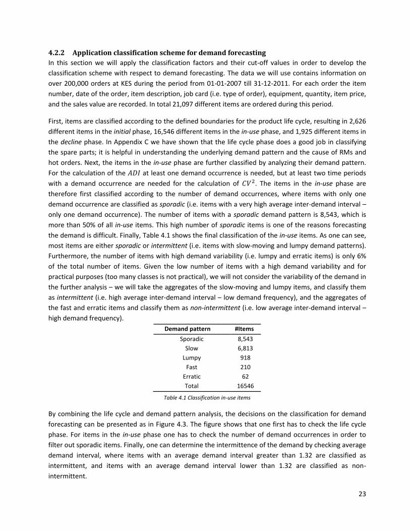
23

4.2.2 Application classification scheme for demand forecasting

In this section we will apply the classification factors and their cut-off values in order to develop the

classification scheme with respect to demand forecasting. The data we will use contains information on

over 200,000 orders at KES during the period from 01-01-2007 till 31-12-2011. For each order the item

number, date of the order, item description, job card (i.e. type of order), equipment, quantity, item price,

and the sales value are recorded. In total 21,097 different items are ordered during this period.

First, items are classified according to the defined boundaries for the product life cycle, resulting in 2,626

different items in the initial phase, 16,546 different items in the in-use phase, and 1,925 different items in

the decline phase. In Appendix C we have shown that the life cycle phase does a good job in classifying

the spare parts; it is helpful in understanding the underlying demand pattern and the cause of RMs and

hot orders. Next, the items in the in-use phase are further classified by analyzing their demand pattern.

For the calculation of the at least one demand occurrence is needed, but at least two time periods

with a demand occurrence are needed for the calculation of . The items in the in-use phase are

therefore first classified according to the number of demand occurrences, where items with only one

demand occurrence are classified as sporadic (i.e. items with a very high average inter-demand interval –

only one demand occurrence). The number of items with a sporadic demand pattern is 8,543, which is

more than 50% of all in-use items. This high number of sporadic items is one of the reasons forecasting

the demand is difficult. Finally, Table 4.1 shows the final classification of the in-use items. As one can see,

most items are either sporadic or intermittent (i.e. items with slow-moving and lumpy demand patterns).

Furthermore, the number of items with high demand variability (i.e. lumpy and erratic items) is only 6%

of the total number of items. Given the low number of items with a high demand variability and for

practical purposes (too many classes is not practical), we will not consider the variability of the demand in

the further analysis – we will take the aggregates of the slow-moving and lumpy items, and classify them

as intermittent (i.e. high average inter-demand interval – low demand frequency), and the aggregates of

the fast and erratic items and classify them as non-intermittent (i.e. low average inter-demand interval –

high demand frequency).

Demand pattern #Items

Sporadic 8,543

Slow 6,813

Lumpy 918

Fast 210

Erratic 62

Total 16546

Table 4.1 Classification in-use items

By combining the life cycle and demand pattern analysis, the decisions on the classification for demand

forecasting can be presented as in Figure 4.3. The figure shows that one first has to check the life cycle

phase. For items in the in-use phase one has to check the number of demand occurrences in order to

filter out sporadic items. Finally, one can determine the intermittence of the demand by checking average

demand interval, where items with an average demand interval greater than 1.32 are classified as

intermittent, and items with an average demand interval lower than 1.32 are classified as non-

intermittent.

24

Part life cycle status?

ADI>1.32?

New Intermittent Non-intermittent

No

Sporadic Decreasing

DeclineInitial

Yes

Demand

occurences>1?

No

Yes

In-use

Figure 4.3 Decisions on the classification with respect to demand forecasting

4.3 TIME-SERIES FORECASTING METHODS In Section 4.2 we have discussed that one can choose between time-series and causal forecasting

methods by analyzing the part life cycle. For items in the in-use phase it is argued to use time-series

methods, because not sufficient (valid) data is available about explanatory variables in order to perform

causal forecasting. In order to choose an appropriate time-series method, in-use items are further

classified into sporadic, intermittent and non-intermittent items. In Section 4.2.2 we have seen that most

in-use items have an intermittent or sporadic demand pattern. Forecasting intermittent demand patters

request special attention given the importance of demand forecasting on stock control. Also,

maintenance related decisions and consequently production efficiency as well are directly affected by

such forecasts. In addition, given that the intermittent items are often the items with the greatest risk of

obsolescence, improvements in forecasting and stock control may be translated to significant reductions

in wastage or scrap (Babai, Syntetos & Teunter, 2011).

The occurrence of (many) periods with zero demand renders traditional time-series forecasting

techniques such as simple exponential smoothing or simple moving average unsuitable (Teunter, Syntetos

& Babai, 2011). Croston (1972) proved the biased nature of simple exponential smoothing (SES) when

applied in an intermittent demand context and he proposed a method that relies explicitly upon

estimates of the inter-demand intervals and demand sizes. Croston (1972) suggested separately updating

the estimates of the inter-demand interval and demand sizes through simple exponential smoothing

(SES). Teunter et al. (2011) state that the Croston method is often applied in practice to forecast

intermittent demand requirements. The method is incorporated in Enterprise Resource Planning (ERP)

type of solutions such as SAP and specialized forecasting software such as Forecast Pro. The method was

claimed to be unbiased, but Syntetos and Boylan (2001) showed it to be positively biased (i.e. over-

forecasting mean demand) and they subsequently proposed an approximately unbiased estimator: SBA

25

(Syntetos–Boylan Approximation, Syntetos & Boylan, 2005). This estimation procedure applies a deflating

factor to the Croston estimates in order to take away the bias. A little bias though still remains, on the

opposite side (i.e. slightly under- estimating mean demand). Another disadvantage of the Croston

method and SBA is that the forecasts are only updated after periods with positive demand. According to

Teunter et al. (2011) these methods are therefore not up-to-date after (many) periods with zero demand

and cannot be used to estimate the risk of obsolescence and deal with the removal of excess/dead stock.

Teunter et al. (2011) have suggested a new forecasting procedure (called TSB after Teunter, Syntetos and

Babai) that links naturally to the issues of inventory obsolescence. TSB uses separate simply exponential

smoothed estimates of the demand probability and demand sizes. The estimate of the probability of

occurrence is updated every time period, whereas the estimate of the demand size is only updated at the

end of periods with positive demand (Teunter et al., 2011). Then, the product of the estimates for

demand size and demand probability provides the forecast of the demand per period. Two different

smoothing constants are required – both for updating the probability and the demand size. The use of

two separate smoothing constants for demand probability and demand size, makes it possible to “tune”

the TSB method for demand processes with different levels of non-stationarity (Teunter et al., 2011).

Teunter et al. (2011) show in their numerical investigation that TSB is suitable for situations with both

stationary and non-stationary demand – which allows to use data with increasing/decreasing trend

without having to eliminate the trend effect. In this chapter we will test whether the TSB is superior to

the Croston’s forecast method (CR), and the Syntetos-Boylan approximation (SBA), but also for which

class of items. Furthermore, will also include the exponential smoothing method (ES) in our analysis, even

though this forecasting method has important shortcomings for intermittent demand (there are no

separate estimates for demand probability and demand size obtained, although these are essential for

inventory control), it does respond quickly to situations with sudden obsolescence or decreasing demand.

Before we initialize and compare these forecasting methods, we will first describe the forecasts of each

forecasting method in Section 4.3.1, we will discuss the issues with selecting appropriate smoothing

constant(s) in Section 4.3.2, and finally, we will discuss seasonality in Section 4.3.3.

4.3.1 Forecasts

All methods forecast monthly demand for each type of spare part separately. Therefore, we use the

phrase demand instead of demand for spare parts of type i throughout this section. First, we give an

overview of the notation that we will use, with abbreviations of related methods between brackets

(Teunter et al., 2011).

forecast at the beginning of month of demand in month ;

demand in month ;

forecast in month of number of months between consecutive positive demand (CR, SBA);

number of months since the last positive demand at the beginning of month (CR, SBA);

forecast of demand in month , provided this demand is positive (CR, SBA, TSB);

forecast of the probability of a positive demand in month (TSB);

indicator variable that indicates whether or not there is a positive demand in month (TSB);

smoothing constants ( ).

26

Exponential smoothing (ES)

The exponential smoothing forecast (ES) uses the demand in month and the forecast for month

to predict demand in month . The ES forecast is

(4.1)

Croston’s forecast method (CR)

Croston proposes to update the demand size, , and the demand interval, , separately,

using

(4.2)

(4.3)

where . The Croston forecast (CR) is

(4.4)

Syntetos-Boylan approximation (SBA)

Syntetos and Boylan (2001) show that Croston’s method is positively biased. They propose to

deflate the Croston forecast by a factor to approximately correct for that bias. Thus, the

SBA forecast is

(4.5)

Forecasting method of Teunter et al. (2011) (TSB)

Teunter et al. (2011) propose an alternative to Croston’s method that is able to handle

obsolescence issues. They do not update the demand interval, but rather the probability of a

positive demand. The probability and the demand size are updated using,

(4.6)

and

(4.7)

where . The forecast of Teunter et al. (2011) (TSB) is

(4.8)

27

4.3.2 Smoothing constants

In this section we will discuss how to set a value for the smoothing constant(s). A common objective in

forecasting is to find the minimum variance, unbiased estimator, but this can only be achieved if the

underlying demand process is known (Teunter et al., 2011). However, in practice, especially for

intermittent demand, this is typically not the case – it is often unclear whether the demand process is

stationary or non-stationary (Teunter et al., 2011). Teunter et al. (2011) explain that a forecasting method

that adapts quickly is preferable if demand is suspected to be highly non-stationary. This is achieved by

choosing “sufficiently large” smoothing constants. Croston (1972) recommend the use of values in the

range 0.05-0.20, when demand is intermittent. He suggested that higher values of , in the range of 0.20-

0.30, may be found properly only if there is high proportion of items that is known to be non-stationary.

However, given the fact that we do not have perfect knowledge of the underlying demand process, one

cannot determine the optimal smoothing constants analytically. In that case, empirical optimization

based on the demand history offers an alternative. For the Croston and SBA methods, values between

0.05 and 0.2 are usually recommended if the demand is close to stationary, and higher than that if the

demand tends to be non-stationary (Syntetos and Boylan, 2005). Further, Babai et al. (2011) suggest for

the TSB method to set smaller than , because the demand probability is updated more often than the

demand size. So if the demand is very intermittent, that is, the demand probability is very low since the

demand intervals are high, should be much smaller than (Babai et al., 2011). In other words, if the

demand is stationary we could set and use simple averages. However, further research is

needed, and we will empirically investigate the most appropriate smoothing constants for the underlying

demand pattern. In order to analyze the forecasting methods, we will vary the smoothing constant

from 0.05 to 0.30 in steps of 0.05. The same values are also used for . However, given that Babai,

Syntetos, and Teunter (2011) recommend considering also smaller values for because the demand size

is updated less often than the demand probability for the TSB method, we will additionally consider

values from 0.01 to 0.04 in steps of 0.01.

4.3.3 Seasonality

In Appendix B we have already shown that seasonal effects are present, and one has to properly separate

out the seasonal effects in the historical data before making any forecasts. We will use the most

commonly used method, that is, the ratio-to-moving-average procedure (Silver, Pyke & Peterson, 1998).

Silver et al. (1998) state that his method can effectively handle changes in the underlying trend during the

historical period. Furthermore, it tends to eliminate cyclical effects. For statistical purposes it is desirable

to have several seasons worth of data because each specific seasonal period occurs only once per season.

Silver et al. (1998) point out that this is especially true for slow-moving items, or for items with highly

erratic demand, because the noise in the data can obscure the underlying seasonality. However, using too

much history increases the risk of the seasonal pattern having changed during the history which makes

the early portion no longer representative of current and future conditions. The minimum for calculating

the seasonal factors is two complete seasons. Silver et al. (1998) recommend using a minimum of four

complete seasons, but we will check for each item separately the number of complete seasons and

determine the seasonal effects based on the available data. The seasonal effects can subsequently be

updated every year.

28

We will calculate seasonal effects per month, because our period is “month”. The first step is to make an

initial estimation of level (including trend) at each historical period. To estimate the seasonal factors we

first have to remove the trend effect (Silver et al., 1998). The trend point for any particular month is

estimated by a moving average of a full season (that is, 12 months) centered at period . By using a full

season we can have the moving average free of seasonal effects. Given that the we have an even number

of periods, , the standard 12-period moving average ends up being centered between two

periods, and not right at the middle of a period as desired (Silver et al., 1998). Therefore, we will take the

average of two consecutive moving averages. Then the estimate of the seasonal factor for any particular

period is obtained by dividing the demand by the centered moving average. Furthermore, in order to

dampen the random effect we will average the seasonal factors for similar periods in different years.

Silver et al. (1998) express that the averages need not add up to exactly 12. Thus, we will normalize to

obtain estimates of seasonal factors that total to 12. From the figures in Appendix B we can also see that

there is up-ward trend. However, in order to estimate the level and trend we will have to fit a regression

line. We will not determine the trend, as the TSB is able to forecast demand for non-stationary demand

data. This implies that the TSB method is able to deal with the increasing trend. Later on we will see

whether the TSB method is superior to the other methods.

4.4 FORECAST INITIALIZATION When it comes to model fitting to the historical data, the model may fit very well, but do a terrible job

forecasting actual demand (Chase, 2009). A model that fits the demand history with an error close to zero

does not imply that it will do a good job forecasting actual demand. Several methods require therefore an

initial forecast to generate forecast during the performance evaluation period. In order to initialize the

forecast, we will divide the demand history into two datasets: an initial modeling set also known as the in-

sample dataset and a test dataset, or out-of-sample data (Chase, 2009). The in-sample data will be used

to estimate the parameters, including the smoothing constant(s), and initialize the method. Then we will

create and compare demand forecasts against the out-of-sample test dataset. Chase (2009) explains that

since the test dataset will not be used as part of the model-fitting initialization using the in-sample

dataset, these forecasts are actual projections created without using the values of the observations. This

way, forecasts can “stabilize” during the updating stage of the initialization. The forecast errors are

measured only for the out-of-sample test dataset. Chase (2009) recommends to hold-out one third of the

most current demand history as the out-of-sample dataset, and to fit the different models to the oldest

two thirds of the demand history. Given that we have 60 monthly periods of demand periods, we will

hold out the most current 24 months of history as our out-of-sample test dataset, and fit the different

models to the oldest 36 monthly periods. Then we will forecast the 24 most recent periods comparing the

forecasts to the out-of-sample test dataset to see how well the model is forecasting. Note that spare that

are not demanded during the initialization period are left out of examination. Also, the seasonality effects

will be separately calculated for the in-sample test dataset. Before we present the choice of a time-series

forecasting method, we will first give the initial forecasts for the different methods. The initial forecast for

the ES method is the mean over the first 36 months, i.e.,

(4.9)

29

For CR, SBA and TSB, the initialization is as follows – if we let denote the set of months in the first 36

months (i.e. in-sample dataset) with a positive demand then

(4.10)

(4.11)

. (4.12)

4.5 CHOICE FORECASTING METHOD This section shows the comparative results for the forecasting methods discussed in Section 4.3. The

forecasting methods are initialized during the initialization period as explained in Section 4.4. In order to

compare the methods to each other, we will a measure for the bias and the variance. These measures are

MSE ( ), and ME ( ). ME estimates the bias of the forecasting method, and the MSE is an

estimator of the variance. We are aware that more sophisticated performance measures are available,

but the benefit of MSE is that it can be defined for both zero and non-zero demand which is important in

an intermittent demand context. In addition, the MSE links naturally to inventory control (safety stocks

are determined based on the MSE), and is a commonly used measure. However, it is a scale dependent

measure, especially prone to distortion due to outliers, and as such it may lead to many difficulties in

interpreting its results (Heinecke et al., 2012). However, for comparative purposes this is not a major

issue. For each value of the smoothing constant considered and each estimation method, the MSE, and

ME empirical results are calculated across time for all time-series data. An arithmetic average is then used

in order to summarize results across all series. In this section we report the ME and MSE results for

intermittent and non-intermittent items, respectively.

In order to examine the effects of the smoothing constants on the performance of the methods, we first

focus on the ME results. The ME differences are more pronounced and ME played an important role in

the development of the various forecasting methods (Babai et al., 2011). Afterwards we will also discuss

the MSE results in relation to the smoothing constants. The results in Table 4.2 show that for non-

intermittent items, when increases, the bias of Croston’s and SBA’s method increases. The lowest value

of the bias for these two estimators corresponds to . The bias of the ES method is also low when

. Overall, the results show that can be a good smoothing constant that gives the

lowest bias for the Croston and SBA estimates. This confirms what is discussed about stationary demand

and what has been recommended in the academic literature. For the TSB estimate, when is fixed, the

bias is an increasing function of , and the lowest bias is obtained for . When is fixed, the bias

is an decreasing function of , i.e. the lowest bias are obtained for high values of .

The results in Table 4.3 show that for intermittent items (i.e. both slow and lumpy demand), when

increases, the bias of Croston’s estimate decreases. So, in this case the lowest bias for the Croston

estimate is obtained for . For the SBA and ES method we also see an decreasing bias for higher

values of . The lowest bias for the SBA method is obtained for and for the ES estimate for

30

. For the TSB estimate, when is fixed, the bias is an decreasing function of , and the lowest

bias is obtained for . When is fixed, the bias is an decreasing function of , i.e. the lowest bias

are obtained for high values of . Recall that larger smoothing constants are better for “less stationary”

demand patterns. The fact that we find higher smoothing constants for intermittent items than for non-

intermittent items is an indication that intermittent items are indeed less stationary. Non-stationary is a

cause of additional intermittence and lumpiness (Babai et al., 2011). This is an indication that the naïve

method provides the best ME performance for intermittent items, as this method can be seen as a special

case of the TSB method with both smoothing constants set to 1. The naïve estimator is updated at every

time period, in this case the last actual demand, zero or not, becomes the forecast for the next time

period.

Estimator smoothing constant – ME

0,05 0,10 0,15 0,20 0,25 0,30

SBA -0,05758 -0,1624 -0,36678 -0,61011 -0,86746 -1,1289

Croston 0,196258 0,353122 0,410837 0,428472 0,431099 0,429065

ES 0,111401 0,174315 0,166338 0,143416 0,12146 0,103501

TSB 0,271843 0,48608 0,564405 0,583279 0,577514 0,56274 0,01

0,222805 0,438605 0,51925 0,540415 0,536592 0,523329 0,02

0,178777 0,395872 0,478553 0,501771 0,499718 0,487856 0,03

0,13921 0,357368 0,441831 0,466886 0,466443 0,455878 0,04

-0,02845 0,192723 0,283896 0,316441 0,322948 0,318294 0,10

-0,10951 0,111747 0,205227 0,240911 0,250686 0,24909 0,15

-0,16148 0,05899 0,153269 0,190516 0,202168 0,202504 0,20

-0,19638 0,023014 0,117326 0,155245 0,16792 0,169443 0,25

-0,22084 -0,00255 0,091429 0,129526 0,14271 0,144932 0,30

Table 4.2 ME results for non-intermittent items

Estimator smoothing constant – ME

0,05 0,10 0,15 0,20 0,25 0,30

SBA -0,53525 -0,35961 -0,30054 -0,29422 -0,31043 -0,33639

Croston -0,49906 -0,27609 -0,16709 -0,11064 -0,07671 -0,05226

ES -0,26926 -0,05335 0,010735 0,027404 0,030096 0,028854

TSB -0,54165 -0,38317 -0,31542 -0,28225 -0,26112 -0,24375 0,01

-0,51294 -0,35378 -0,28792 -0,25701 -0,23785 -0,222 0,02

-0,48749 -0,32762 -0,26338 -0,23448 -0,21707 -0,2026 0,03

-0,46489 -0,30431 -0,24145 -0,2143 -0,19846 -0,18525 0,04

-0,3722 -0,20727 -0,14913 -0,12886 -0,11955 -0,11185 0,10

-0,32957 -0,16117 -0,10417 -0,08663 -0,08033 -0,07543 0,15

-0,3035 -0,1319 -0,07481 -0,05855 -0,05403 -0,05097 0,20

-0,28705 -0,11254 -0,05475 -0,03895 -0,03545 -0,03362 0,25

-0,27649 -0,09935 -0,04053 -0,02472 -0,02178 -0,02077 0,30

Table 4.3 ME results for intermittent items

31

When we analyze the MSE results for non-intermittent items in Table 4.4, it appears that MSE for the

Croston, SBA and ES decreases when increases, i.e. the lowest value is obtained for . For the

TSB estimate, when is fixed, MSE is an decreasing function of , i.e. the lowest MSE are obtained for

high values of , whereas the optimal value for is obtained for . The MSE results in Table 4.5

for intermittent items show that MSE is lowest for for the Croston, SBA, ES, and the TSB

estimators, and the optimal value for is obtained for which is in line with the expectations,

based on the fact that the demand probability is updated more than the demand size for intermittent

demand.

Estimator smoothing constant – MSE

0,05 0,10 0,15 0,20 0,25 0,30

SBA 571,2595 566,4571 562,1832 557,7181 553,1121 548,7871

Croston 573,2836 571,869 571,6095 571,391 571,0362 570,8886

ES 566,9604 556,6471 549,5284 545,0455 542,6674 542,1758

TSB 581,7706 586,8485 587,0741 584,3794 580,6532 577,1618 0,01

577,3176 581,9879 582,5505 580,4007 577,1973 574,1321 0,02

573,4791 577,7346 578,5479 576,8589 574,12 571,4495 0,03

570,1431 573,9824 574,9763 573,6768 571,3515 569,0463 0,04

556,8718 558,367 559,5489 559,5855 558,9584 558,3278 0,10

550,8264 550,6997 551,4807 551,8772 551,9967 552,2522 0,15

547,2681 545,8331 546,046 546,4607 546,9645 547,7859 0,20

545,3737 542,9018 542,5006 542,7388 543,3869 544,5401 0,25

544,678 541,3936 540,3846 540,3321 540,96 542,2716 0,30

Table 4.4 MSE results for non-intermittent items

Estimator smoothing constant - MSE

0,05 0,10 0,15 0,20 0,25 0,30

SBA 103678,7 104880,9 105772,4 106581,2 107379 108177,6

Croston 103692,6 105091,7 106300,7 107547,3 108918,2 110438,3

ES 105138,8 107842 110551,9 113538,1 116842,8 120469,3

TSB 103475,1 104598,1 105787,1 107194,5 108855,6 110777 0,01

103647,3 104779,4 105954,1 107347,9 109000,3 110917,3 0,02

103811,3 104954,3 106117,3 107499 109143,3 111056,3 0,03

103966,6 105122,7 106276,4 107647,6 109284,6 111193,9 0,04

104733,5 106001,7 107147,3 108487,2 110097,6 111992,2 0,10

105208 106597,5 107782,5 109130,6 110739,5 112632,3 0,15

105590,2 107111,8 108362 109740,7 111363,4 113263,6 0,20

105915,5 107573,9 108905,8 110331,6 111981,2 113897,4 0,25

106206 108003,5 109428,8 110914,9 112602,7 114543,4 0,30

Table 4.5 MSE results for intermittent items

32

In addition, we have also analyzed the ME and MSE performance of the different estimators for sporadic

and declining parts (see Appendix D). The TSB method outperforms the other methods for both declining

and sporadic demand. Only ES outperforms the TSB method for declining items in terms of bias. However,

ES is not useful for inventory planning, because there are no separate estimates for demand probability

and demand size obtained, although these are essential for inventory control. Overall, in terms of both

ME and MSE, the TSB method outperforms SBA and Croston for both intermittent and non-intermittent

demand. Therefore, we recommend using the TSB method for forecasting the demand. However, as we

have discussed, the optimal values for and are not the same for the bias and MSE. Therefore, we will

have to make a trade-off, as there are no exact recommendations in the literature available. By

combining the optimal values for and for the ME and MSE performance, we obtain and

for non-intermittent items, and and for intermittent items.

The developed classification scheme with respect to demand forecasting is only a starting point for spare

parts management. It can be used to make strategic and tactical decisions with respect to demand

forecasting. The next step is to use the forecasted demand for the development of inventory policies - the

inventory policies and parameters depend on forecasts of demand over lead-time. So the choice of the

forecasting approach (time-series or causal) and forecasting method affects the inventory policies and

parameters. The real benefit of the developed classification scheme with respect to demand forecasting

is reflected in the accuracy of the inventory policies and parameters set.

33

5 INVENTORY CONTROL

In this chapter a classification scheme with respect to inventory control will be designed (5.1). An

important classification factor is criticality. Currently, no information is available about spare parts

criticality. Therefore, we will perform a criticality analysis (5.2). Finally, we will apply the developed

classification scheme on a real dataset (5.3).

5.1 CLASSIFICATION FOR INVENTORY CONTROL KES and Sage carry a large amount of items in stock. These items are highly heterogeneous, with differing

costs, service requirements, and demand patterns. An important operational issue in spare parts

management is the classification of relevant SKUs in order to determine service requirements for

different spare parts classes and for facilitating the allocation of the most appropriate forecasting method

and stock control policies. In Chapter 4 we have already built a classification scheme with respect to

demand forecasting. In this chapter we will develop a classification scheme for facilitating the allocation

of the most appropriate inventory policies and service requirements. Note that we will not develop any

inventory policies, because we do not have the necessary data. In Section 5.1.1 we will first select the

classification criteria. Next, in Section 5.1.2 we will discuss classification techniques. An important

criterion is the criticality of an item which is at this moment not yet defined. In Section 5.2 we will

describe and apply the criticality factor. Finally, in Section 5.3 we will apply all the classification factors in

on a real dataset.

5.1.1 Classification criteria

Many papers recognize that a one-dimensional ABC-analysis is easy to use. It is especially appropriate for

the inventory management of spare parts that are fairly homogenous in nature and differ from each

other mainly by unit price or demand volume (Huiskonen, 2001). That is why ABC-analysis has retained its

popularity among the practitioners in directing the control efforts (Huiskonen, 2001). However,

Huiskonen (2001) points out that one-dimensional ABC-analysis does not discriminate all the control

requirements of different parts as the variety of control characteristics of parts increases. One-

dimensional ABC-analysis may not be able to provide a good classification of inventory items in practice.

This is also true for the Sage’s one-dimensional classification of KES’s spare parts based on the annual

usage. Sage applies this one-dimensional classification worldwide, and it has shown to be a successful

classification scheme. However, it is important to note that Sage’s operations are mainly focused on the

market in the US where the standardization among the GSE vehicles is higher compared to the European

market. For spare parts supply in European market it might not be sufficient to classify spare parts merely

on annual usage. Huiskonen (2001) states that using several criteria as a basis is especially useful for

spare parts that do possess several distinctive characteristics. Also in the literature study it is pointed out

that most papers propose using multiple criteria for classification of spare parts (Velagić, 2012). The table

in Appendix A can be used to choose the most promising criteria for classifying the spare parts. As one

can see, criteria that are frequently reported are the value, criticality, supply characteristics, demand

volume, and demand variability. Other criteria that are less frequently reported (see last column of the

table), but that also should be considered for the classification of spare parts are specificity, life cycle

phase, and repair efficiency.

34

Bacchetti and Saccani (2011) observe that little attention has been paid to identifying the context in

which one criterion may be preferable to others. This is a very important issue and one that has been

under-exposed in the academic literature. The criteria that are judged to be important for the purpose of

classifying KES’s spare parts are selected collectively (between KES’s management and the researcher).

For the classification of KES’ spare parts a multi-criteria approach will be used with the following criteria:

1. Spare parts life cycle: Parts are clustered in three main groups based on their remaining life cycle:

initial, in-use, and decline. Boundaries between these classes are already explained in Chapter 4.

The spare parts life cycle does not influence only the selection of the forecasting technique, but

also decisions on inventory management.

2. Criticality analysis: At this moment KES has not yet a defined the criticality of spare parts.

(Process) criticality is an important factor because it can be directly linked to the availability of

GSE vehicles. Moreover, criticality can be directly linked to the service level requirements. In

Section 5.2 we will analyze the criticality of an item based on a number of sub-criteria that cover

the essentials of GSE vehicles maintenance.

3. Part value: The cost of an item influences the overall inventory holding cost. The part value can

be used in order to dimension the parameters of order-up-to level policies and to make

stock/non-stock decisions. The boundaries will be determined based on the average price.

4. Demand frequency: Demand classification has been shown to link directly to forecasting and

stock control decision-making; in particular the average inter-demand interval ( ) and the

variability of the demand sizes have been shown to be important from a theoretical point of view

(Syntetos et al., 2005). However, Boylan and Syntetos (2007) showed, by means of

experimentation on a large dataset, that the variability of the demand sizes may not necessarily

be important in the real world. In Section 4.2.1 we have shown that this is also true for KES’s case.

On the other hand, the average inter-demand interval is not only relevant in real world practices,

but it is also an insensitive criterion with regards to the cut-off value assigned to it (i.e. 1.32

review periods).

5. Annual usage: This criterion refers to Sage’s one-dimensional spare parts classification, where

class A is defined as 24+ units per year, class B as 12-23 units per year, class C as 4-11 units per

year, and class D as 1-3 units per year (see also Table 2.1). It is however not known how Sage has

determined these cut-off values between the A, B, C and D-classes.

No other criteria are explicitly considered at this stage for classification related purposes. Management

can change the number and nature of the criteria depending on their preferences. Other important

factors such as the supply lead time and its variability and the demand variability will be further

considered in the calculation of safety stocks, when such an exercise is required. Having selected the

criteria that collectively are judged to be the most appropriate for the purpose of classifying spare parts,

the next step is to classify the spare parts. In the next section we will discuss different classification

techniques.

35

5.1.2 Classification techniques

In the literature study we have discussed several classification techniques (Velagić, 2012). It has been

pointed out that one can distinguish between quantitative and qualitative techniques. One of the most

popular quantitative techniques is the ABC approach (Pareto). Silver et al. (1998) suggest to list all SKUs in

descending order by demand frequency, volume or value. The ranked SKUs can then be divided into

relevant categories (A, B, C, etc.). For example, items from category A are assumed to be the most critical,

and, therefore, they require the highest service levels. However, Silver et al. (1998) were focused on only

one criterion for the ABC classification. Various methodologies have been proposed to implement multi-

criteria ABC classifications, including weighted linear programming, matrix models, artificial neural

networks, weighted Euclidian distance with quadratic optimization, and the fuzzy logic (Bacchetti &

Saccani, 2011). Besides ABC classification, there are also other quantitative techniques. Syntetos (2001)

proposes a demand-based classification. Yamashina (1989) proposes product-still-in-use quantity curves

and service part demand curves as inputs for spare parts classification, while Porras and Dekker (2008)

propose a hierarchical two- or three-dimensional quail-quantitative classification.

Besides quantitative techniques, one can also use qualitative techniques. Bacchetti and Saccani describe

qualitative techniques as techniques that “[…] try to assess the importance of keeping spare parts in stock

based on information on the specific usages of spares and on factors influencing their management

(costs, downtime, storage considerations, etc.)” (2011, pp. 2). A simple technique, but prone to subjective

judgments, is the VED technique. VED stands for vital, essential, and desirable, respectively

(Mukhopadhyay, Pathak & Guddu, 2003). VED is prone to subjective judgments, because it is done in

consultation with experts. Bacchetti and Saccani (2011) suggest combining VED with systematic

procedure for classifying spare parts in order to reduce the problem with the VED technique. They refer

to Gajpal, Ganshed and Rajendran (1994) who have proposed an AHP model for performing VED analysis.

AHP is a model developed by Saaty (1980) and stands for Analytic Hierarchy Process. It is a multi-criteria

decision-making tool to find out the relative priorities or weights to be assigned to different criteria and it

can effectively handle both qualitative and quantitative data. AHP involves the principles of

decomposition, pair-wise comparison, and priority vector generation and synthesis (Saaty, 1980). AHP

can be used to obtain absolute measurements of the criticality of spare parts, after which these

measurements can be compared to specific limits in order to classify spare parts as vital, essential, or

desirable (Gajpal et al., 1994). Besides VED analysis, there are also some other techniques that have been

combined with AHP analysis, e.g. reliability centered maintenance (RCM) (Braglia, Grassi & Montanari,

2004).

Studies that consider the comparative benefits of various approaches to classification (e.g. ABC vs. other

techniques) are lacking. Several authors recommend using multiple criteria ABC-analysis. We have tried

to apply a multiple criteria ABC-analysis with frequently recommended criteria like criticality, value-usage,

unit cost, lead time, etc. (see Appendix A). However, this approach does not allow differentiating

between different items – not all criteria are relevant for classifying for all items. An approach that is

more suitable for KES is to apply selected criteria hierarchically in order to define homogeneous spare

parts classes. By applying a hierarchical approach, one can differentiate the criteria among the different

spare parts (sub-classes). Figure 5.1 shows the resulting hierarchical multi-criteria spare parts

36

classification framework allowing the identification of 10 final homogeneous spare parts classes. As one

can see, not all criteria affect the selection of the final classes. Class 1 contains all items in the initial

phase of life cycle, class 2 are items with a sporadic demand in the in-use phase of the life cycle, class 3

are critical items with a low price, class 4 are critical items with a high price and high demand frequency,

class 5 are critical items with a high price and low demand frequency, class 6, 7, 8 and 9 are A-, B-, C,- and

D-items according to Sage’s classification, respectively, and finally, class 10 are items in the decline phase

of the life cycle.

Part life cycle status?

Annual usage?

1-3

DeclineInitial

24+

Criticality?Critical

Part value?

Non-critical

Class 1

ADI>1.32?

High

Low

NoYes

Demand

occurences>1?

In-use

Yes

12-23 4-11

No

Class 2 Class 3 Class 4 Class 5 Class 6 Class 7 Class 8 Class 9 Class 10

Figure 5.1 Spare parts classification with respect to inventory control

5.2 CRITICALITY ANALYSIS When it comes to spare parts inventory management, determining the importance of a spare part by

annual usage becomes insufficient. Classification by annual usage relies only on historic demand data – it

does not differentiate between critical and non-critical spare parts. Criticality, as a classification criterion,

does not only rely on demand data, it includes also information about explanatory variables (e.g. failure

rate). Immediate action is needed in case of a failure caused by an item with a high criticality but which is

not on stock, whereas some lead time is allowed to correct a failure caused by an item with a mediate

criticality (Huiskonen, 2001). Furthermore, Huiskonen (2001) distinguishes process and control criticality.

Process criticality is defined as “[…] the consequences caused by the failure of a part on the process in

case a replacement is not readily available” (Huiskonen, 2001, pp 130). Process criticality can be

evaluated by down time costs of the process. Control criticality is based on the possibilities to control the

situation, including predictability of failure, availability of spare part suppliers, lead-times, etc.

37

In order to perform the criticality analysis we will first select relevant criticality factors in Section 5.2.1.

Next, in Section 5.2.2 we will discuss how to combine the criticality factors in order to determine the

criticality of an item. Finally, in Section 5.2.3 we will evaluate the results of the criticality analysis.

5.2.1 Criticality factors

The first step of the criticality analysis is the identification of relevant criteria impacting item criticality.

We analyze the criticality of an item based on four sub-criteria, that is, GSE criticality, maintenance type,

ratio of GSE failures, and the number of item failures. These factors are selected by collectively (between

the company’s management and the researcher) judging their relevance for maintaining GSE vehicles, but

the selection is also influenced by the availability of the necessary data. Other criticality factors like

commonality and substitutability have also been considered. Commonality was defined as a measure of

how frequently the same part is used on different GSE vehicle. However, the impact of the resulting

commonality measures was negligible compared to the other criteria. Substitutability was defined as the

total number of GSE vehicles that a particular part has a use. First of all, this definition of substitutability

is a rough estimate of the real substitutability, and might bias the result. There was no data available to

make better estimates of substitutability. Furthermore, the resulting substitutability measures highly

impacted the result, because substitutability was given a high weight compared to other factors. We have

therefore decided to leave this measure out of the analysis. Finally, it is important to note that the four

selected criteria are measures of process criticality, whereas control criticality is neglected. Not sufficient

data was available to include a factor for control criticality, such as the number of available suppliers for a

part. The selected criticality factors are defined as follows:

1. GSE criticality: GSE criticality refers to the criticality of the GSE vehicles. Criticality of the GSE

vehicles can be defined by the position of the GSE vehicle in the chain. The chain position

describes the importance of a vehicle for handling the aircraft on the ground. GSE vehicles

that are directly related to processing the aircraft on the ground are critical. Those vehicles

should be up and running when necessary in order to minimize the turnaround time of the

aircraft on the ground. Three degrees of criticality might be distinguished on the following

basis:

a) High: Availability of this GSE vehicle is of high importance. Failures have to be corrected

and the spares should be supplied immediately.

b) Moderate: Non-availability of this GSE vehicle can be tolerated with temporary

arrangements for a short period of time, during which the failure can be corrected and

the spare supplied.

c) Low: This GSE-vehicle is not critical for ground-handling of an aircraft. The failure can be

corrected and the spares can be supplied after a long period of time.

Çelebi et al. (2008) suggest that quantification of the given critically degrees can be done by

assigning a penalty index for each item and setting it to 1 for critical vehicles, to 0.01

for a non-critical vehicles, and to 0.50 for a moderately critical vehicles. The criticality levels

are determined in discussion with management.

38

2. Maintenance type: Another aspect of criticality is the type of maintenance performed on the

equipment. In order to determine the type of maintenance we will look at the job card code

(i.e. type of order). The different job card codes and their description are given in Table 5.1.

Only two job card codes are considered to be important for the criticality analysis, namely

repair and breakdown, because these two job cards codes refer to corrective maintenance,

which is difficult to plan. In case a breakdown has occurred or repair is executed on the

vehicle, an item is considered to be of a higher criticality level in comparison to an item for

which an inspection is considered. In case of an inspection (i.e. preventive maintenance) one

is capable to prevent failures or to measure indication of failures (Molenaers, Baets, Pintelon

& Waeyenbergh, 2011). In addition, items for which damage repair is considered are not

critical, because the necessary items for damage repair are rather aesthetic than functional.

Items for modifications are also not considered to be critical, because their demand can be

planned separately. Further, job cards “banden”, “lekkage” and “fuelling” are not considered

for the criterion maintenance type, because these activities do not require any items. The

remaining job card codes are not relevant, given their low frequency as shown in Table 5.1.

Job card code Description #Job cards

B Banden 5216

C Claim 48

E Error by operator 5258

H Damage repair 11527

I Inspection 29825

L Lekkage 1383

O Modification 5949

R Repair 8337

S Breakdown 35194

T Fuelling 2

X Runner service 0

Table 5.1 Number of job cards per job card code

3. Ratio of GSE failures: Another measure of GSE criticality, and, therefore, the related spare

parts, is the number of GSE failures. The number of GSE failures can be calculated by counting

the number of “breakdown” and “repair” job cards based on the available job card data. We

will compare the number of “breakdown” and “repair” job cards for a GSE vehicle to the total

number of “breakdown” and “repair” job cards for all GSE vehicles within the same GSE

supplier type (i.e. type fabrikant). This ratio expresses which GSE vehicle is really critical

within a particular GSE supplier type. We will use a normalizing function which is useful for

making all criteria data between :

(5.1)

The GSE failure index, , has a positive impact on the importance of item where

represents the total number “breakdown” and “repair” job cards on vehicle . Here,

39

stands for the highest number “breakdown” and “repair” job cards, while stands for the

lowest number of “breakdown” and “repair” job cards.

4. Item failures: There is no exact information available about the item failure rates. In order to

get some information about the item failures, we will analyze how often a particular item is

replaced on the same GSE vehicle. We will again use a normalizing function which is useful

for making all criteria data between :

(5.2)

The item failure index, , has a positive impact on the importance of item where

represents the total number of item changes on vehicle . Here, stands for the highest

number of item changes on the same vehicle, while stands for the lowest number item

changes on the same vehicle.

5.2.2 Multi-criteria criticality scheme

Having selected the criteria, the next step is to calculate the weights and the scores of the different parts

in order to determine the criticality. We analyze the criticality based on a multi-criteria criticality scheme

consisting of three steps:

Step 1. First, GSE vehicles are filtered by GSE criticality and maintenance type. Only GSE vehicles with a

criticality level of 1 will remain, because these, critical, GSE vehicles should be up and running

when necessary. In addition, only “breakdown” and “repair” job cards will be used, because the

necessary parts are most unpredictable.

Step 2. Second, GSE vehicles, and indirectly parts, are scored on the number of failures compared to the

total number of failures for all GSE vehicles within the same GSE supplier type, and on the

number of item failures on that GSE vehicle. However, it is difficult to determine objectively the

weight for these two factors. Therefore, we will use a weighted linear optimization model which

is usually used for multi-criteria ABC inventory classification, but it can be applied in different

settings. The model we will use is an improvement on the model developed by Ng (2007) which

we will call the Ng-model. The Ng-model converts all criteria measures of an inventory item into a

scalar score, and with proper transformation, the Ng-model can obtain the scores of inventory

items without a linear optimized, which is of course beneficial for practical purposes (Hadi-

Vencheh, 2010). Ng converts first all measurement in [0,1]. To facilitate the classification under

multiple criteria, Ng defines a non-negative weight which is the weight of contribution of

performance of the th decision alternative with respect to the th criteria. The purpose is to

aggregate multiple performance scores of a decision alternative into a single score for the

subsequent classification, like ABC inventory classification (Hadi-Vencheh, 2010). The score of th

decision alternative (denoted as ) is expressed as the weighted sum of performance measures

under multiple criteria. The weighted linear optimization Ng-model is as follows for each item :

40

(5.3)

where is the normalized attribute value of the th decision alternative with respect to the th

criteria (e.g. performance of th inventory item with respect to the th classification criteria).

After the necessary transformations, the maximal score of the th decision alternative can be

easily obtained as

. Similar to the idea in Data Envelopment Analysis

(DEA), the Ng-model avoids subjectiveness in determining weights and provides an objective way

for multi-attribute decision making. However, as one can see from the score of each attribute,

the Ng-model leads to a situation where the score of each item is independent of the weighs

obtained from the model. In other words, the weights do not have any role for determining total

score of each item, and this might lead to wrong classifications. Hadi-Vencheh (2010) has

proposed an extended version of the Ng-model by considering weights values for multi-criteria

classification which we will use for the classification. The resulting multi-attribute decision making

model is as follows (Hadi-Vencheh, 2010):

(5.4)

where is the normalized attribute value of the th decision alternative with respect to the th

attribute, and the relative importance weight attached to the th criteria ( ) (Hadi-

Vencheh, 2010). The analytical solution to the model is as follows:

(5.5)

This analytical solution can only be used if there are no ordering constraints, otherwise one will

have to use a software package. For particular purposes we have not defined any ordering

constraints, because it is not easy to determine any order constraint, and for practical purpose it

is more easy to use the analytical solution.

41

Step 3. The first two steps are performed on vehicle level. However, in order to determine the criticality

of an item we will have to transform the findings on item level. Given that some items are used

on more than one vehicle, we will have to calculate the average of the criticality scores on vehicle

level (i.e. average of the scores calculated in step 2) to obtain the criticality score on item level.

Based on this score we will perform a Pareto-analysis, that is, we will apply the 20/80 rule to find

the most critical items.

5.2.3 Application of the criticality analysis

Before we present the results of the criticality analysis, it is important to note that the criticality analysis

is based on demand data between 01-01-2010 and 31-12-2011 which contains 7,046 different items. The

demand data from 2009 and earlier does not contain information about the job cards, which is required

for determining the criticality analysis (see also Section 5.2.1). In order to find the most critical spare part

we have performed the three steps of the multi-criteria criticality scheme. In the first step we have

analyzed the GSE criticality level and the maintenance type. The following vehicles have a criticality level

of 1, and are considered for further examination: air conditioning units, air starter units, container

loaders, de-icers, ground power units, oil service units, pallet loaders, toilet service units,

transportbanden, vliegtuigtrekkers, water service units, and fuel service units. Vehicles with criticality

levels of 0.5 and 0.01 are left out of further examination. Subsequently, the demand data is filtered on

job card type, where only orders with “repair” and “breakdown” job cards are left. In this first step about

60% of the items are filtered out. In the second step, we have employed the multi-attribute decision

making model. According to the third step, we have transformed the resulting scores from vehicle to item

level in order to determine the item criticality. The Pareto analysis shows that 41.35% of the remaining

items from the first filter determines 80% of the criticality. In other words, 16.83% of all items determines

80% of the criticality which is a good approximation of the 20/80 rule. In the following section we will

show the benefits of the criticality analysis over the current one-dimensional spare parts classification

scheme.

5.2.4 Benefits of the criticality analysis

Here, we will analyze the comparative benefits of the criticality analysis with regards to the current

practices employed by Sage. In order to show the benefits of the criticality analysis we will make use of

the available demand data of the first four months 2012. The used dataset is limited, because only the

most recent historical demand data contains information about the RMs and hot orders (to be more

precise, KES started collecting information about RMs and hot orders in November 2011). Note that the

results are only illustrative, more data is required to confirm the results that we will discuss in this

section.

First, we start in Table 5.2 were the demand and the RMs are classified as critical and non-critical. Then,

each class is further classified according to Sage’s classification based on annual usage. The table shows

that more than 50% of the A-items are critical – both from the criticality perspective and Sage’s service

level, these parts should be fulfilled immediately. It is however more interesting to check the classes B, C,

and D, as these classes do not require immediate fill, whereas critical items do. In other words, the critical

B-, C- and D- items should be fulfilled as soon as possible.

42

Class A B C D Total

Critical 3005 255 345 178 3783

Non-critical 5240 1317 1979 1192 9728

Critical rood 12 4 8 17 41

Non-critical rood 34 38 128 190 390

Table 5.2 Distribution of critical and non-critical parts for January-April 2012

In order to get an idea of the performance of Sage’s classification and the classification we proposed, we

will simulate both classification schemes for the demand during the period between 01-01-2012 and 30-

04-2012. Table 5.3 shows that Sage’s KPI performance is almost 99% for all classes, which is way better

than the required service levels as defined in the contract (see Table 2.1). The 7th column shows the

number of hot orders for critical parts. As is discussed, critical parts should be fulfilled immediately or as

soon as possible. If this is under control, the number of hot orders for critical parts should be zero. The 8th

column shows the KPI’s for the new classification scheme, that is, the classification scheme with the

criticality factor, which means that all critical parts should be fulfilled immediately – there should be no

hot orders. The last column shows the KPI improvement when the criticality factor is added to the

classification scheme. As one can see, the improvement over the current service level is minimal.

Sage class Demand #Rood #Hot KPI Sage #Critical rood #Critical hot KPI New Change %

A 8245 46 24 99,71 12 6 99,78 0,07

B 1572 42 14 99,11 4 1 99,17 0,06

C 2324 136 30 98,71 8 1 98,75 0,04

D 1370 207 20 98,54 17 0 98,54 0,00

Total 13511 431 88 99,35 41 8 99,41 0,06

Table 5.3 Performance based on current service levels

One explanation for the limited improvement of the new classification scheme over the current

classification scheme is the fact that there is no much room for improvement given the high KPI

performance. This still does not explain why the maintenance shop is dissatisfied with the availability of

spare parts. We will therefore analyze the KPI performance from a different perspective. We will take the

perspective of the maintenance shop – the maintenance shop wants spare parts to be there as soon as

possible. Let us know consider the KPI performance without the agreed spare parts supply lead times. In

that case, A-items should be fulfilled immediately (not within one day as in the current situation) at 99%,

B-items at 95%, C-items at 80%, and D-items at 65%. From Table 5.4 one can see that Sage’s KPI

performance is lower now, but still above the 99%, 95%, 80%, and 65% target service levels for A-, B-, C-,

and D-items, respectively. We will again compare the performance of the new classification scheme with

the current classification scheme. From the last two columns one can see the improvement over the

current classification scheme, but the improvement is again limited.

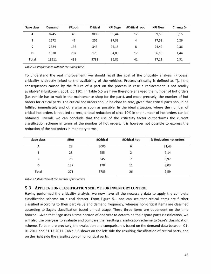
43

Sage class Demand #Rood Critical KPI Sage #Critical rood KPI New Change %

A 8245 46 3005 99,44 12 99,59 0,15

B 1572 42 255 97,33 4 97,58 0,26

C 2324 136 345 94,15 8 94,49 0,36

D 1370 207 178 84,89 17 86,13 1,44

Total 13511 431 3783 96,81 41 97,11 0,31

Table 5.4 Performance without the supply time

To understand the real improvement, we should recall the goal of the criticality analysis. (Process)

criticality is directly linked to the availability of the vehicles. Process criticality is defined as “[…] the

consequences caused by the failure of a part on the process in case a replacement is not readily

available” (Huiskonen, 2001, pp 130). In Table 5.5 we have therefore analyzed the number of hot orders

(i.e. vehicle has to wait in the maintenance shop for the part), and more precisely, the number of hot

orders for critical parts. The critical hot orders should be close to zero, given that critical parts should be

fulfilled immediately and otherwise as soon as possible. In the ideal situation, where the number of

critical hot orders is reduced to zero, a total reduction of circa 10% in the number of hot orders can be

obtained. Overall, we can conclude that the use of the criticality factor outperforms the current

classification scheme in terms of the number of hot orders. It is however not possible to express the

reduction of the hot orders in monetary terms.

Sage class #Hot #Critical #Critical hot % Reduction hot orders

A 28 3005 6 21,43

B 28 255 2 7,14

C 78 345 7 8,97

D 137 178 11 8,03

Total 271 3783 26 9,59

Table 5.5 Reduction of the number of hot orders

5.3 APPLICATION CLASSIFICATION SCHEME FOR INVENTORY CONTROL Having performed the criticality analysis, we now have all the necessary data to apply the complete

classification scheme on a real dataset. From Figure 5.1 one can see that critical items are further

classified according to their part value and demand frequency, whereas non-critical items are classified

according to Sage’s classification based annual usage. These three items are dependent on the time

horizon. Given that Sage uses a time horizon of one year to determine their spare parts classification, we

will also use one year to evaluate and compare the resulting classification scheme to Sage’s classification

scheme. To be more precisely, the evaluation and comparison is based on the demand data between 01-

01-2011 and 31-12-2011. Table 5.6 shows on the left-side the resulting classification of critical parts, and

on the right side the classification of non-critical parts.

44

Criticality Critical Non-critical

Part value High Low

Demand Frequency Low High

Usage A B C D

#Items 250 2 934 383 365 1192 3920

Table 5.6 Result classification scheme for 2011

As one can see from Table 5.6, the number of non-intermittent (i.e. high demand frequency) critical items

with a high price is rather low. Further classification of critical items based on demand frequency is not

necessary as more than 99% of the critical items with a high price have an intermittent demand pattern.

Figure 5.2 shows the final, modified and simplified, classification scheme with respect to inventory

control. Class 1 contains all items in the initial phase of life cycle, class 2 are items with a sporadic

demand in the in-use phase of the life cycle, class 3 are critical items with a low price, class 4 are critical

items with a high, class 5, 6, 7 and 8 are A-, B-, C,- and D-items according to Sage’s classification,

respectively, and finally, class 9 are items in the decline phase of the life cycle.

Part life cycle status?

Annual usage?

1-3

DeclineInitial

24+

Criticality?Critical

Part value?

Non-critical

Class 1

HighLow

Demand

occurences>1?

In-use

Yes

12-23 4-11

No

Class 2 Class 3 Class 5 Class 6 Class 7 Class 8Class 4 Class 9

Figure 5.2 Final spare parts classification scheme with respect to inventory control

However, from Table 5.6 it is not directly clear what has changed compared to the current classification

scheme. Therefore, we have compared the results of the new classification scheme with Sage’s

classification scheme in Table 5.7. Table 5.7 shows on the left-side the number of critical items that are

classified as A, B, C or D in the current classification scheme. As one can see, 58.09% of the items are

currently classified as D, which means that they have to be successfully filled at 65% within seven days.

However, according to the criticality definition, those items should be fulfilled immediately and otherwise

45

as soon as possible. This high number of critical items that are classified as D, but also as C and B, shows

why it is not sufficient to classify items only with one criterion. By classifying spare parts according to the

annual usage, important information about the part is not included. Adding criticality as a classification

criterion changes the resulting classes. The other classification criteria, i.e. part value and annual usage,

are added to manage the inventory control of critical and non-critical spare parts, respectively. The next

step is to determine inventory policies and parameters for each class. However, as is already pointed out,

we do not have any information about the replenishment lead times and the cost structure.

Critical Non-critical Total

Class #Items % #Items % #Items

A 142 11.97 383 6.54 525

B 85 7.17 365 6.23 450

C 270 22.77 1192 20.34 1462

D 689 58.09 3920 66.89 4609

Total 1186 100.00 5860 100.00 7046

Table 5.7 Sage's classification of critical parts

46

6 LOGISTICS OUTSOURCING

In this chapter first it will be discussed how to bridge the gap between KES and Sage (6.1). Next,

recommendations will be given regarding the logistics outsourcing scope and activities (6.2).

6.1 LOGISTICS OUTSOURCING RELATIONSHIP In the previous chapters we have developed spare parts classification schemes with respect to inventory

control and demand forecasting, in order to create a manageable number of control groups to focus

management efforts more effectively. However, the developed classification scheme covers only one part

of supply chain – it is focused on internal control factors. The controllability of spare parts also depends

on external factors, like supplier performance. In Chapter 2 we have discussed the current planning and

control of spare parts and we have concluded that are no major issues with the supply link (e.g. supply

management and spare parts order handling). For appropriate spare parts management the demand and

supply link should be linked to each other. In the first chapter of this report we have introduced the

problems with the logistics outsourcing relationship between KES and Sage which impedes the

integration of the demand and supply link, that is, lack of information exchange and lack of shared

understanding. Tsai, Lai, Lloyd and Lin (2012) reveal in their research that poor communication and lack

of shared goals are the most significant reasons precipitating relationship risk (i.e. possibility of

relationship failure). In the following sections we will discuss how relationship risk can be reduced by

improving the communication, and by creating alignment between KES and Sage. More specifically, in

Section 6.1.1 we will discuss how the information exchange between KES and Sage can be improved, and

in Section 6.1.2 we will discuss how KES and Sage can create a shared understanding.

6.1.1 Information exchange

In Chapters 1 and 2 we have introduced the problems of the lack of information exchange between KES

and Sage. Tsai et al. (2012) point out that for relationship risk, the presence of poor communications is

the most important antecedent of the partner relationship, which in turn puts the involved parties at risk

for their asset specific investments and service strategy development. Knemeyer and Murhpy (2004)

explain that those firms desiring to establish closer long-term relationships between their firm and a

logistics provider (i.e. Sage) in order to achieve possible benefits of this closeness (increased

performance) should realize that they may need to establish managerial components (activities and

processes that management establishes and controls) that demonstrate a higher level of trust toward

their provider and/or facilitate more effective communication with their provider.

In this section we want to explain that the new classification schemes can also be used as managerial

component for increasing the communication between KES and Sage. Unlike the current classification

scheme based on the annual usage, one cannot just rely on historic demand data for the new

classification schemes. More specifically, for appropriate classification based on the life cycle, KES has to

inform Sage about the introduction of new parts, planned maintenance activities, modifications and

redundancy. Further, given that the criticality analysis is among others based on information about the

GSE vehicles and the maintenance types (that is, information that Sage does not have), KES has to

perform the criticality analysis and provide Sage a list with the critical items, or KES should provide Sage

the necessary information so that Sage can perform the criticality analysis. Both options require

47

information exchange. Further, in Chapter 2 about the current planning and control of spare parts we

have also discussed that KES does not provide Sage sufficient reliability or even usage data (i.e. hours that

the equipment is actually used), but Sage does understand that is difficult to provide such information

because of the low volumes of similar equipment and the lack of resources that the GSE vehicle suppliers

have. Sage believes it would be helpful if KES could develop at least a pre-defined maintenance kit for

various service checks for the common and/or critical equipments types. It is possible to develop these

kits, because KES has been working with such kits in the past. It is recommended to develop these kits

and to provide them with a 30 day plan so that Sage can load this information info their demand system

and pre-build the kits and have the parts waiting when the equipment comes in for the scheduled service.

Sage points out that this would guarantee 100% availability as well as reduce the time it takes for Sage’s

staff to pick the various items as they would be pre-kitted.

Further, Gadde and Hulthén (2009) express that in the short-term efficiency of the logistics outsourcing

relationship is dependent on coordinated flow of information. They refer to Piplani, Pokharel and Tan

(2004, pp. 40) who claim that for logistics service providers to be successful “[…] it would become

imperative that they integrate [their information systems] with the IT-systems of their partners and

customers in order to increase the effectiveness of the systems and to get the real value out of them”.

Currently, Sage and KES are working on the integration of the IT-systems, which is thus a good initiative.

To sum up, the developed classification scheme(s) can be used to guide the information flow between

KES and Sage, as it creates more awareness about the spare parts characteristics and it triggers the

information exchange between KES and Sage. It is also important to further integrate the IT-systems of

both parties.

6.1.2 Shared goals

Besides the lack of information exchange, we have also pointed out that there is lack of shared

understanding because KES and Sage have no shared goals. Lack of shared goals reflects the contrast of

organization cultures and goals that may impede successful interaction with the relocated function (Tsai

et al., 2012). Differences in priorities between KES and Sage can trigger the onset of relationship risk. In

order to create alignment between KES and Sage, they should focus on the end-customer (i.e. owner of

the GSE fleet). Both parties have to realize the importance of a shared goal otherwise it might result in

opportunistic behavior where KES’s goal is to pay as low as possible for Sage’s services, whereas Sage’s

goal is to maximize the revenues. By joining forces, KES and Sage can work together to take costs out of

the logistics system, mutually boost profitability, and improve service to the end customer. To assure that

operations of KES and Sage are synchronized, information exchange is essential, as joint performance

towards shared goals requires open disclosure (Knemeyer & Murhpy, 2004).

Focusing on the end-customer impacts also the output related agreements in the contract – the goal is to

reduce the GSE downtime. GSE downtime is lost time and lost money. In terms of spare parts

management, one should aim for minimizing the number of hot orders, i.e. purchase request for a vehicle

that is not operational due to the missing part. Reduction of the hot orders, results also in a reduction of

the expensive GSE downtime. KES and Sage should consider to include the number of hot orders in the

month end report and to set a target value for the number of hot orders. Note that the developed

48

classification scheme with respect to inventory control is useful for focusing on the end-customer. In

Section 5.2.4 it has been shown that the real benefit of the criticality analysis is not the improvement

over the current service levels, but rather the reduction of the number of hot orders. In other words, by

making use of the criticality analysis one is more focused on what really matters for the end-customers –

GSE availability.

Overall, we recommend creating common goals and compatible interests by focusing on the end-

customer, to further improve the compatibility of the information systems, to frequently communicate

and exchange information where the new developed classification scheme can serve as a trigger to

exchange information. These measures should help bridging the gap between KES and Sage and reducing

the relationship risk.

6.2 LOGISTICS OUTSOURCING SCOPE & ACTIVITIES In the current situation, both demand forecasting and inventory control are outsourced to Sage.

However, as we have argued, there are improvement possibilities with respect to both demand

forecasting and inventory control. In this research we have developed spare parts classification schemes

for demand forecasting and inventory control in order to improve demand forecasting and inventory

control, respectively. Following from this research we recommend KES to reconsider the scope and the

type of activities to be outsourced. The new classification schemes express that Sage is highly dependent

on information from KES. With the current classification scheme based on annual usage this is not

apparent, because Sage can rely just on historical demand data. KES should think about bringing demand

forecasting and inventory control back in-house. By taking demand forecasting back in-house, KES can

more easily use installed base information (e.g. usage data, preventive maintenance planning,

redundancy of vehicles and modifications) for forecasting demand without being dependent on Sage.

Further, in terms of inventory control, KES should think about setting the base-stock levels by themselves.

Sage has already asked KES to help them with setting appropriate base-stock levels. Moreover, KES has

more knowledge about and expertise with the demand characteristics and the link with maintenance

then Sage does. In order to benefit from this knowledge KES should consider setting the base-stock levels

by themselves, whereas the actual procurement of parts can still be done by Sage.

Instead of also bringing the procurement back in-house, KES can benefit from Sage’s geographically

widespread distribution network in the GSE parts marketplace and quantum discounts. Also, Sage

minimizes the number of suppliers KES has to deal with. Further, in terms of inventory control KES can

benefit from the fact that Sage is allowed to purchase KES Inventory from KES and sell it to other

customers - for example parts that are not useful anymore because of a modification, can still be useful

for Sage’s other customers. Recall that in the analysis of the current planning and control of spare parts

we have pointed out that there are no major problems with respect to Sage’s procurement activities (e.g.

supply management and spare parts order handling), and, therefore, there are no major reasons to doubt

Sage’s procurement activities. To summarize, KES should think about bringing demand forecasting back

in-house and set the base-stock levels by themselves, while procurement activities can be performed by

Sage. Overall, we want to express that KES should consider focusing on the strategic side and let Sage

focus on the executive side of spare parts management – outsource the execution, not the management.

49

7 IMPLEMENTATION

In this chapter it will be described how the results of this master thesis project can be implemented in

order to improve spare parts management at KLM Equipment Services. First, recommendations with

respect to demand forecasting (7.1) and inventory control (7.2) will be given. Subsequently, it will be

described how to update the developed classification schemes (7.3). This implementation plan can be used

as a guideline by KES or Sage (depending on the outsourced activities – see the discussion in Section 6.2)

to implement and use the developed classification schemes in the daily activities.

7.1 DEMAND FORECASTING In this section we will describe how the results with respect to demand forecasting can be implemented

in the daily activities. The first step of the plan is to determine the transition point between the initial and

in-use phase of the life cycle, and between the in-use and decline phase. In Section 4.2.1 we have

explained how to derive the transition points and in Appendix E we have explained how one can use Excel

to determine the items in initial, in-use and decline phase. In this master thesis project it is explained how

the different life cycle phases can be used to choose a forecasting approach. The following

recommendations can be given with respect to demand forecasting:

Initial phase: For the initial phase it is explained that the lack of an adequate length of demand

history precludes the use of extrapolative time-series methods. Also, data about explanatory

variables is limited. Important characteristics can still be estimated by comparing to technically

similar parts. Further, it has been explained that KES is provided little information from the GSE

vehicle suppliers about failures rates, reliability tests, degradation of parts, substitution,

commonality, etc. Some suppliers do not provide RSLs or the RSLs contain limited information.

KES should, at the introduction of a new GSE vehicle, put more effort on negotiating with the GSE

suppliers on the supply of RSLs and reliability information.

In-use phase: For the in-use phase it is explained that causal methods also have an important role,

if data on explanatory variables is available. However, at this moment historical data for the

explanatory variables, such as timing of preventive maintenance, usage rate or failure rate, is not

valid or not available at all. In that case, it is more appropriate to use time-series methods. We

have compared several time-series methods and recommended to use the TSB forecasting

method. The value of the smoothing constants is depended on the intermittence of the demand.

The demand intermittence can be calculated as explained in Appendix E. In Section 4.5 we have

determined the optimal values for and ; for non-intermittent items we have obtained

and and for intermittent items and . However, we have

seen that there are also seasonal effects. The seasonal effects can be determined as explained in

Section 4.3.3. In Appendix E it is explained how the seasonality effects can be calculated in Excel

Finally, in Appendix E we have explained how the demand can be forecasted according to the TSB

forecasting in Excel.

Decline phase: We have seen that the TSB method is able to forecast obsolescence. The TSB

method can be used to determine the transition point between the in-use phase and the decline

phase. However, in the decline phase it is required to make a last time buy from a supplier. Here,

50

it is recommended to use regression-based extrapolations have been recommended, assuming an

exponential decline of demand. Example is a regression model on the logarithm of sales against

time, assuming an exponential decline in demand over time.

Finally, given that KES does not want to rely only on historical demand data for forecasting demand, they

should collect more data on explanatory variables and validate the data they have in order to generate

forecasts using explanatory variables. The benefit of the causal/reliability based forecasting is that it can

cope with changes in the installed base and varying operating decisions (Driessen et al., 2010). It is

applicable in the initial, in-use and in the decline phase of the life cycle. KES should pay more attention to

assortment management and gather parts (technical) information from the initial phase of a part’s life

cycle instead of waiting till the in-use or decline phase.

7.2 INVENTORY CONTROL Having forecasted the demand, the next step is inventory control. In this master thesis project we have

developed a spare parts classification scheme in order to establish inventory decisions. Because of the

lack of data about the cost structure and replenishment lead times, we could not develop and test

inventory policies and parameters. However, we have used the different life cycle phases to guide the

development of the inventory policies. We will therefore only shortly discuss inventory control on a

strategic and/or tactical decision level:

Initial phase: In the initial phase, when the part is introduced, there are two decisions: i) should

the item be stocked and ii) if so, what are the initial stock requirements? The initial phase is

characterized by a high number of new parts that are most probably needed for recently

introduced vehicles. New parts for recently introduced vehicles require a high service level, which

necessitates the satisfaction from stock even if the demand may be particularly low and sporadic.

However, data-shortage does not allow the calculation of an effective safety stock.

In-use phase: In the in-use phase, an inventory policy must be determined and the parameters

estimated. If an Order-Up-To (OUT) policy is adopted, for example, then the Order-Up-To-Level

must be calculated. The main benefit of the new classification scheme is the inclusion of the

criticality factor which results in a lower number of hot orders. In Section 5.2 we have explained

the criticality analysis and in Appendix E it is explained how to perform the criticality analysis in

Excel. The criticality factor can be used to determine service level requirements. For critical parts

with a low price safety stocks should be calculated. For critical parts with a high price Sage should

set-up time-guaranteed supplies from established suppliers (Huiskonen, 2001).

Decline phase: Based on the replenishment lead time one can make the decision whether to stock

the part or not. If the replenishment lead time is smaller or equal to the supply lead time, it is not

necessary to stock the part. For the parts that are currently stocked decisions should be made

whether to dispose the items or not. 4118 Of the items are classified as decline, from which 1129

are still in stock, that is, more than 25% of the items in the decline phase. Furthermore, as the

part nears the end of its life, suppliers may become reluctant to manufacture small volumes. In

this decline phase, a decision must be taken on the size of a single order to cover all remaining

demand (sometimes known as an “all time buy”).

51

In this master thesis project we have also discussed how to improve the outsourcing relationship

between KES and Sage. In Section 6.2 we have explained that KES should consider bringing demand

forecasting and inventory back in-house. However, if KES does not want to change the current

outsourcing contract, they will have to increase the information exchange between KES and Sage as

recommended in Section 6.1. More specifically, collect and provide Sage with installed base information,

give them information about the maintenance timing, develop a pre-defined maintenance kit for various

service checks for the common and/or critical equipments types, determine the criticality of spare parts

and provide this information to Sage, inform Sage about changes in the installed base and operating

conditions.

7.3 RECLASSIFICATION Finally, the designed classification scheme for demand forecasting and inventory control needs to be

updated during its application in order to allow for the re-classification of items. Figure 7.1 shows possible

reclassification scenario’s for the classification scheme with respect to demand forecasting. An initial item

(i.e. item in the initial phase of its life cycle) should move to the in-use phase after one year (the cut-off

value between the initial and in-use phase is one year). The item should then be classified as sporadic,

non-intermittent or intermittent. Figure 7.1 shows that a sporadic part in the in-use phase can become

intermittent if there is more than one demand occurrence. An intermittent demand becomes an non-

intermittent item if the average demand interval is smaller or equal to 1.32, whereas a non-intermittent

part becomes an intermittent part if the average demand interval is larger than 1.32. At this moment,

Sage analyzes the classification of items every three month. If KES decides to bring demand forecasting

back in-house, they have to decide whether they will also use the 3-month review period or not. If KES

decides to make also use of the 3-month review period, KES should check the intermittence of parts every

three months. Figure 7.1 also shows that parts can become a decline part (i.e. part in the decline phase of

the life cycle). Recall that only parts that have not been demanded in the past year will be considered

appropriate for the decline phase. So KES/Sage can check once a year whether a part should be

transferred to the decline phase. Note that parts can be earlier migrated to the decline phase if it is

known that the parts will not be required anymore. Overall, we recommend setting the reclassification

between initial, in-use and decline phase at once a year.

Also for the classification scheme for inventory control one should migrate initial parts to the in-use phase

after one year, and if necessary in-use parts to the decline phase. In addition, the criticality analysis of

spare parts should also be updated, but the criticality is not dynamic like the demand, and does not have

to be updated too often. From a practical point of view, one can decide to update the criticality once a

year, together with update of the life cycle phases. Note that after one year a part will migrate from the

initial phase to the in-use phase. For these parts one will have to determine the criticality – one can at the

same time update the criticality factor of all other items in the in-use phase.

52

Initial part

In-use:

sporadic part

In-use:

non-intermittent part

In-use:

intermittent part

Decline part

ADI>1,32

Demand occurences > 1

ADI≤1,32

Figure 7.1 Migration between the different spare parts classes with respect to demand forecasting

53

8 CONCLUSIONS AND RECOMMENDATIONS

This chapter first discusses the key conclusions of this master thesis project (8.1). Then, the limitations will

be shortly discussed (8.2). Subsequently, the academic relevance will be explained (8.3). Finally,

recommendations are given for both KES and for further research (8.4).

8.1 CONCLUSIONS This section summarizes the main conclusions of this master thesis project, by giving answers to the

research questions formulated in Chapter 3. The main research question as stated in Chapter 3 was:

“Can spare parts management at KLM Equipment Services be improved?”

This research question has been split in three sub-questions that are focused on demand forecasting,

inventory control, and the logistics outsourcing contract between KES and Sage, respectively. The

conclusions are structured accordingly:

Demand forecasting: The sub-question regarding demand forecasting was formulated as follows:

“How can we improve demand forecasting, such that it better captures the demand pattern of the

spare parts?” Currently, all items are forecasted based on historical demand data, but KES would

like to include also information about explanatory variables in the forecasts. However, in order to

choose between specific forecasting approaches and methods, parts should first be classified

with respect to demand forecasting (Driessen et al., 2010). First of all, one can use the life cycle to

choose between forecasting approaches: causal or time-series. For items in the initial and decline

phase of the life cycle phase it is recommended to use causal forecasting, because there is not

sufficient data for time-series forecasting methods. For the in-use phase one can also use causal

forecasting, but only if there is sufficient (valid) data on explanatory variables available. At this

moment, there is not sufficient (valid) data about explanatory variables available, and one will

have to rely on time-series methods. Items are further classified according to their intermittence

in order to choose the most appropriate time-series method for items in the in-use phase.

Different time-series techniques specific for intermittent demand, i.e. Croston, ES, SBA and TSB,

are initialized and compared to each other for items in the in-use phase of the life cycle. The

results reveal that the TSB method is most appropriate for forecasting intermittent and non-

intermittent items in the in-use phase. For sporadic items in the in-use phase it is more

appropriate to use a reactive approach (i.e. order the part when it is requested) because the

demand history is limited. Finally, we have tested the TSB method also for items in the decline

phase of the life cycle. The results show that the TSB method is able to forecast obsolescence. To

summarize, in this master thesis project we have shown that demand forecasting can be

improved, such that it better captures the underlying demand pattern of spare parts by first

classifying spare parts with respect to demand forecasting, and then, to choose appropriate

forecasting approach(es) and method(s) for the resulting classes. The real benefit of the new

approach can be determined by forecasting the demand according to the recommendations

resulting from the classification scheme, and to use the forecasted demand for inventory control.

54

Inventory control: The subquestion regarding inventory control was formulated as follows: “How

can we improve the current classification scheme with respect to inventory control, such that it

better captures the characteristics of the spare parts?” At this moment, the inventory is classified

according to only one criterion – annual usage. KES and Sage carry a large amount of items in

stock. These items are highly heterogeneous, with differing costs, service requirements, and

demand patterns. When it comes to spare parts inventory management, determining the

importance of a spare part by annual usage is insufficient. The current classification scheme is

first of all extended by the life cycle, because inventory decisions directly relate to a life cycle

phase classification. By using the life cycle phase one creates more awareness for the provisioning

decisions in the initial phase of the life cycle. Especially, given the fact that some GSE vehicle

suppliers do not provide RSLs or the RSLs contain limited information. In the in-use phase the

inventory policy and appropriate parameters must be determined. The inventory policies and

parameters depend on forecasts of demand over lead-time. Here, the importance of choosing

appropriate demand forecasting methods is expressed – demand forecasting impacts the

accuracy of the inventory policies. Finally, classification scheme based on the life cycle creates

also more awareness about the final order decisions and the obsolescence issue.

Besides the life cycle phase, another important extension of the current classification scheme is

the inclusion of the criticality criterion. The classification scheme is not anymore based on only

historical demand data, because the criticality analysis includes also information about the

maintenance type, vehicle and the part. A test, on a rather small sample of 4 months, shows that

the inclusion of the criticality criterion does not improve the service levels much, but it does

reduce the number of hot orders by 10%. Further, the criticality classification can be used to

support decisions about service level requirements - critical parts should be fulfilled immediately

and otherwise as soon as possible. Overall, we have shown in this master thesis project that the

current classification scheme with respect to inventory control can be improved, such that it

better captures the underlying demand pattern of spare parts by the design of a hierarchical

multiple-criteria classification scheme with respect to inventory control, including the life cycle

phase and a criticality analysis.

Logistics outscourcing: The subquestion regarding the logistics outsourcing was formulated as

follows: “How can we improve the logistics outsourcing performance?” Currently, there is a gap

between KES and Sage, because there is insufficient information exchange and there is a lack of

shared understanding. In order to improve the logistics outsourcing relationship KES and Sage

should focus on the end-customer – the focus should be on reducing the GSE vehicle downtime

instead of focusing on self-centered goals. Unlike the current classification scheme, the new

classification schemes create a higher awareness of spare parts characteristics and their effect on

demand forecasting and/or inventory control. For appropriate classification based on the life

cycle, KES has to inform Sage about the introduction of new parts, planned maintenance

activities, modifications and redundancy. Given that the criticality analysis is among others based

on information about the vehicle and maintenance types (that is, information that Sage does not

have), KES has to perform the criticality analysis and provide Sage a list with the critical items, or

55

KES should provide Sage the necessary information so that Sage can perform the criticality

analysis. In other words, the new classification scheme can be seen as a trigger for improving the

information exchange. The current one-dimensional classification scheme based on annual usage

does not trigger KES and Sage to exchange information about those aspects.

KES should also consider taking demand forecasting and inventory control back in-house. The

new classification schemes expresses that Sage is too much depended on information from KES.

With the current classification scheme based on annual usage this was not apparent, because for

Sage it was sufficient to rely on historical demand data. The new classification schemes show it is

not sufficient to just rely on historical demand data – it requires also installed base information,

and therefore more information exchange between KES and Sage. KES should consider focusing

on the strategic side and let Sage focus on the executive side of spare parts management –

outsource the execution, not the management.

By referring back to the main research question we can now conclude that is possible to improve spare

parts management by adopting a structured approach for both demand forecasting and inventory

control, and by improving the logistics outsourcing performance. This master thesis project has shown

the benefits of a structured approach for dealing with the considerable number of heterogeneous items.

However, the developed classification schemes are only a starting point for making strategic and tactical

decisions. The next step is to choose inventory policies and parameters for each class resulting from the

classification scheme with respect to demand forecasting. The inventory policies and parameters depend

on forecasts of demand over lead-time. In other words, the accuracy of inventory policies and parameters

is influenced by the used demand forecasting methods. The classification scheme with respect to demand

forecasting can be used to choose appropriate forecasting methods. Only then one can measure the real

benefit of the classification schemes – that is, by integrated the outcomes of spare parts classification,

demand forecasting and inventory control.

8.2 LIMITATIONS Several limitations can be recognized in this master thesis project:

The main limitation is that is not known how Sage exactly forecasts the demand. We only know

that Sage’s forecast is for 100% based on historical demand data. Given that we do not know the

exact forecasting method, we were not able to compare the time-series forecasting method that

we proposed, that is, the TSB method, to the current time-series forecasting method(s).

Another important limitation is the lack of necessary data. No information was available about

the cost structure, supply and replenishment lead times. Since KES only recently started with the

collection of supply lead time information, we had only useful supply lead time information from

01-11-2011 till now, whereas no information was available about the cost structure and the

replenishment lead times.

Given that we did not have any information about the replenishment lead times and the cost

structure, we could not analyze the performance of appropriate inventory policies. Furthermore,

we did not have any information about the inventory policies that Sage applies.

56

A limitation of the classification scheme with respect to inventory control is the lack of

information about the supply and/or replenishment lead time. Lead time information is useful for

making stock-non stock decisions.

Note that the selected criteria for the criticality analysis are measures of process criticality,

whereas control criticality is neglected. Again, there was not sufficient data available to include a

factor for control criticality, like the number of available suppliers for a part, etc.

In this master thesis project we have tried to evaluate the new classification scheme by

comparing it to the current classification scheme for inventory control (see Section 5.3). For this

evaluation we have used demand data from 2011, but this data did not contain information

about the actual classification of spare parts in 2011 (i.e. we did not know whether an item was a

A, B-, C or D-item during 2011). Therefore, we have “simulated” Sage’s classification scheme by

following Sage’s classification rules for A-, B-, C- and D-items.

8.3 ACADEMIC RELEVANCE Aspects about spare parts management that were only limited addressed in the literature, but that were

discussed in more detail in this master thesis project, are as follows:

Bacchetti and Saccani (2011) suggest that research should devote great effort to evaluate how

complex quantitative models for spare parts management can be taken into practice. They

encourage the use of case study methods for this purpose, as well as to facilitate the

transferability of the developed solutions. This master thesis project can be seen as case study for

this purpose.

Teunter et al. (2011) have recently suggested a new forecasting procedure (i.e. TSB method) that

links naturally to the issue of inventory obsolescence. The performance of this method was

assessed through an extensive simulation study on theoretically generated data and it was shown

to compare very well to the other methods discussed in the literature. However, this method has

never been evaluated on a real dataset. The empirical results in this project with regards to MSE

allowed us to gain some insight into the methods’ performance. Furthermore, Teunter et al.

(2011) suggest that an important avenue for further research is to empirically test the

performance of TSB against that of other methods. In this project we have compared the TSB

method to exponential smoothing, Croston and the SBA method. Again, the empirical results give

some insight into the methods’ performance compared to other methods.

One of the classification criteria for classifying spare parts with respect to inventory control is

item criticality. Item criticality, has been recognized in literature, but is not well defined and

certainly no consensus has been reached for measuring it (see for a discussion Molenaers et al.,

2011). Evaluating the criticality of items is not an easy task because various characteristics can

have an impact on the degree of criticality. In order to effectively deal with this multi-criteria

problem, we have proposed a combined methodology in this master thesis project. The model

presents the multi-criteria classification problem in a logic decision diagram where a multiple-

attribute decision model (DEA model) is proposed to solve the multi-criteria decision problems at

decision nodes of the diagram. The basic idea is to develop a decision diagram, which guides the

analyst towards the best criticality class of a spare part.

57

8.4 RECOMMENDATIONS This section can be split into two sections, namely recommendations for KES, but also for Sage, and then,

recommendations for further research.

The following recommendations can be made for KES and Sage:

In this report we have presented a classification with respect to demand forecasting and

explained how one can use the classification scheme in order to choose a forecasting approach

and method. In the initial phase one can estimate important characteristics by comparing to

technically similar parts. It is recommended to use the TSB method for forecasting demand for

items in the in-use phase. For the decline phase one could for example use a regression model on

the logarithm of sales against time, assuming an exponential decline in demand over time. Next,

we have presented a classification scheme for inventory control and shortly discussed an

inventory strategy for each class. However, because of the lack of data about the cost structure

and the replenishment lead times, we could not calculate and compare inventory policies and

parameters. It is recommended to determine and compare suitable inventory policies and

parameters for each class resulting from the classification scheme with respect to inventory

control as soon as one has the necessary data. The real benefit of the developed classification

schemes can be tested by using the forecasted demand and standard deviation (forecasted

according to the classification scheme with respect to demand forecasting) for determining the

inventory parameters.

Given that KES does not want to rely only on historical demand data for forecasting demand, they

should collect more data on explanatory variables and validate the data they have in order to

forecasts using explanatory variables. The benefit of the causal/reliability based forecasting is

that it can cope with changes in the installed base and varying operating decisions (Driessen et

al., 2010). It is applicable in the initial, in-use and in the decline phase of the life cycle. KES should

pay more attention to assortment management and gather parts (technical) information from the

initial phase of the life cycle instead of waiting till the in-use or decline phase.

In Appendix C it has been shown that a considerable number of hot orders is linked to parts

required for repairs and breakdowns. KES should consider increasing the number of preventive

maintenances in order to reduce the number of corrective maintenance (i.e. repairs and

breakdowns), and thus, the number of hot orders. Also, a high number of hot orders are linked to

parts required for damage repair. It is not possible to predict damages, but this issue does require

more attention. The damages are not only caused in maintenance shop, but also on the platform

where the vehicles are used by the end-customers. KES should therefore discuss with end-

customers the need for better prevention of damages.

If KES wants to continue as in the current situation, it is recommended to reconsider at least the

current KPIs. As is discussed in this master thesis project, Sage’s performance seems perfect with

the current KPIs. In Table 2.1 we have seen that the service levels decrease as the demand for an

item decreases. Furthermore, the table shows that the required supply lead time also decreases

as the demand decreases. For example, D-items have to be successfully filled at 65% within seven

business days. It is no surprise that Sage has a high performance, because both the required

58

service levels and supply lead times decline as the demand declines. The current KPIs do not

provide sufficient insight in Sage’s actual performance. We recommend to eliminate the supply

lead time restrictions, and to use only the required fill rates. The modified KPIs are presented in

Table 8.1. Further, consider introducing a target value for the GSE downtime in order to increase

the focus on the end-customer.

Classes Usage KPIs

Class A 24+ units per year Immediate fill 99%

Class B 12-23 units per year Successful fill at 95%

Class C 4-11 units per year Successful fill at 80%

Class D 1-3 units per year Successful fill at 65%

Class E Manually controlled products with product/min/max levels

Class N New products for the reporting location

Table 8.1 Modified Sage classification with KPIs

In the criticality analysis we have used the GSE criticality as a classification criterion. However,

there were mixed signals about the criticality of a particular GSE vehicle. We recommend to

create more agreement about the GSE criticality, and to discuss together with fleet management

and end-customers which GSE vehicles are really critical.

In the analysis of the current planning and control it has been concluded that parts return

forecasting is not a big issue, nor is repair shop control, because the number of returned and

repaired items is limited. In the future, KES should consider looking more conscious to parts

return and repair shop. At this moment both parts return and repair shop are not structurally

managed and controlled. Lack of parts returns forecasting and (indirectly) repair shop control

impacts inventory control negatively, because parts are “randomly” returned and repaired. The

lack of parts return forecasting influences also inventory control as it might lead to obsolescence.

The following recommendations can be made for further scientific research:

By using separate smoothing constants for the demand probability and demand size, the TSB

forecasting method can be “tuned” for demand processes with different (suspected) levels of

non-stationarity. Empirical investigation confirmed that the TSB method is suitable for situation

with both stationary and non-stationary demand. However, further research on what values to

use for the smoothing constant is still required. Moreover, further research should lead to

recommendations on what values to use under which circumstances.

From a methodological point of view, unlike a simple ABC-approach, multi-criteria classifications

models allow for the consideration of the specificity of a company’s environment. However, this

does raise issues related to their generalization and applications in different contexts. Further

research should analyze the trade-offs between various possible approaches for classifying spare

parts.

Finally, it would be interesting to assess the relevance of the classification criteria proposed in

this project in similar companies, smaller/bigger companies, or other industrial contexts.

59

REFERENCES

Babai, M.Z., Syntetos, A., and Teunter, R. (2011). Intermittent demand estimators: Empirical performance

and sensitivity to the smoothing constants used. Working papers: No. 138-11, France: Centre de

recherché de BEM Bordeaux Management School.

Bacchetti, A., and Saccani, N. (2011). Spare parts classification and demand forecasting for stock control:

Investigating the gap between research and practice. In press, Corrected Proof.

Boylan, J.E., and Syntetos, A.A. (2007). The accuracy of a modified Croston procedure. International

Journal of Production Economics, 107(2), 511-517.

Boylan, J.E., and Syntetos, A.A. (2008). Forecasting for inventory management of service parts. In (eds:

Kobbacy, K.A.H., and Murthy, D.N.P.) Complex System Maintenance Handbook, Springer Verlag:

London, 479-508.

Braglia, M., Grassi, A., and Montanari, R. (2004). Multi-attribute classification method for spare parts

inventory management. Journal of Quality in Maintenance Engineering, 10(1), 55-65.

Cavalieri, S., Garetti, M., Macchi, M., and Pinto, R. (2008). A decision-making framework for managing

maintenance spare parts. Production Planning & Control, 19(4), 379-396.

Çelebi, D., Bayraktar, D., Selcen, D., and Aykaç, Ö. (2008). Multi criteria classification for spare parts

inventory. 38th Computer and Industrial Engineering Conference, October 31-November 2, Beijing,

China, 1780-1787.

Chase, C. (2009). Demand-driven forecasting: A structured approach to forecasting. John Wiley & Sons:

Hoboko, New Jersey.

Croston, J.D. (1972). Forecasting and stock control for intermittent demand. Operational Research

Quarterly, 23(3), 289-304.

Driessen, M.A., Arts, J.J., Van Houtum, G.J.J.A.N., Rustenburg, W.D., and Huisman, B. (2010). Maintenance

spare parts planning and control: A framework for control and agenda for future research. (BETA

publication: Working papers, No. 325). Eindhoven: Technische Universiteit Eindhoven, 36.

Duchessi, P., Tayi, G.K, and Levy, J.B. (1988). A conceptual approach for managing of spare parts.

International Journal of Product Development, 18(5), 8-15.

Flores, B.E., and Whybark, D.C. (1987). Implementing multiple criteria ABC analysis. Journal of Operations

Management, 7(1-2), 79-85.

Fortuin, L. (1980). The all-time requirement of spare parts for service after sales: Theoretical analysis and

practical results. International Journal of Operations & Production Management, 1(1), 59-70.

Fortuin, L., and Martin, H. (1999). Control of service parts. International Journal of Operations &

Production Management, 19(9), 950-971.

Gadde, L.E., and Hulthén, K. (2009). Improving logistics outsourcing through increasing buyer-provider

interaction. Industrial Marketing Management, 38(6), 633-640.

Gajpal, P.P., Ganesh, L.S., and Rajendran, C. (1994). Criticality analysis of spare parts using the analytic

hierarchy process. International Journal of Production Economics, 35(1-3), 293-297.

Gutierrez, R.S., Solis, A.O., and Mukhopadhyay, S. (2008). Lumpy demand forecasting using neural

networks. International Journal of Production Economics, 111(2), 409-420.

Hadi-Vencheh, A. (2010). An improvement to multiple criteria ABC inventory classification. European

Journal of Operational Research, 201(3), 962-965.

60

Heinecke, G., Syntetos, A.A., and Wang, W. (2012). Forecasting-based SKU classification. International

Journal of Production Economics, in press.

Hua, Z.S., Zhang, B., Yang, J., and Tan, D.S. (2007). A new approach of forecasting intermittent demand for

spare parts inventories in the process industries. Journal of the Operational Research Society, 58(1),

52-61.

Huiskonen, J. (2001). Maintenance spare parts logistics: Special characteristics and strategic choices.

International Journal of Production Economics, 71(1-3), 125-133.

Huiskonen, J., and Pirttilä, T. (2002). Lateral coordination in a logistics outsourcing relationship.

International Journal of Production Economics, 78(2), 177-185.

Johnston, F.R., and Boylan, J.E. (1996). Forecasting for items with intermittend demand. The Journal of

the Operational Research Society, 47(1), 113-121.

Kalchschmidt, M., Zotteri, G., and Verganti, R. (2003). Inventory management in a multi-echelon spare

parts supply chain. International Journal of Production Economics, 81-82, 397-413.

Knemeyer, A.M., and Murphy, P.R. (2004). Evaluating the performance of third-party logistics

arrangements: A relationship marketing perspective. Journal of Supply Chain Management, 40(1), 35-

51.

Kranenburg, A.A., and Van Houtum, G.J. (2007). Effect of commonality on spare parts provisioning costs

for capital goods. International Journal of Production Economics, 108(1-2), 221-227.

Molenares, A., Baets, H., Pintelon, L., and Waeyenbergh, G. (2011). Criticality classification of spare parts:

A case study. International Journal of Production Economics, In press, Corrected Proof.

Mukhopadhyay, S.K., Pathak, K., and Guddu, K. (2003). Development of decision support system for stock

control at area level in mines. IE(I) Journal-MN, 84, 11-16.

Ng, W.L. (2007). A simple classifier for multiple criteria ABC analysis. European Journal of Operational

Research, 177(1), 344-353.

Partovi, F.Y., and Burton, J. (1993). Using the analytic hierarchy process for ABC analysis. International

Journal of Operations & Production management, 13(9), 29-44.

Persson, F., and Saccani, N. (2009). Managing the after sales logistic network: A simulation study.

Production Planning & Control, 20(2), 125-134.

Petrovic, D., and Petrovic, R. (1992). SPARTA II: Further development in an expert system for advising on

stocks of spare parts. International Journal of Production Economics, 24(3), 291-300.

Piplani, R., Pokharel, S., and Tan, A. (2004). Perspectives on the use of information technology at third

party logistics service providers in Singapore. Asia Pacific Journal of Marketing and Logistics, 16(1), 27-

41.

Porras, E., and Dekker, R. (2008). An inventory control system for spare parts at a refinery: An empirical

comparison of different re-order point methods. European Journal of Operational Research, 184(1),

101-132.

Ramanathan, R. (2006). ABC inventory classification with multiple-criteria using weighted linear

optimization. Computers & Operations Research, 33(3), 695-700.

Saaty, T.L. (1980). The analytic hierarchy processes. McGraw-Hill: New York.

Silver, E.A., Pyke, D.F., and Peterson, R. (1998). Inventory management and production planning and

scheduling (3rd ed.). John Wiley & Sons, Inc.: New York.

61

Syntetos, A.A. (2001). Forecasting of Intermittent Demand. Unpublished PhD Thesis, Buckinghamshire

Business School: Brunel University.

Syntetos, A.A., and Boylan, J.E. (2001). On the bias of intermittent demand estimates. International

Journal of Production Economics, 71(1-3), 457-466.

Syntetos, A.A., and Boylan, J.E. (2005). The accuracy of intermittent demand estimates. International

Journal of Forecasting, 21(2), 303-314.

Syntetos, A.A., Boylan, J.E., and Croston, J.D. (2005). On the categorization of demand patterns. Journal of

Operational Research Society, 56(5), 495-503.

Syntetos, A.A., Keyes, M., and Babai, M.Z. (2009). Demand categorization in a European spare parts

logistics network. International Journal of Operations & Production Management, 29(3), 292-316.

Teunter, R.H., Babai, M.Z., and Syntetos, A.A. (2010). ABC classification: Service levels and inventory costs.

Production and Operations Management, 19(3), 343-352.

Teunter, R.H., and Duncan, L. (2009). Forecasting intermittent demand: a comparative study. Journal of

the Operational Research Society, 60(3), 321-329.

Teunter, R.H., and Fortuin, L. (1998). End-of-life service: A case study. European Journal of Operations

Research, 107(1), 19-34.

Tsai, M.C., Lai, K.H., Lloyd, A.E., and Lin, H.J. (2012). The dark size of logistics outsourcing – Unraveling the

potential risks leading to failed relationships. Transportation Research Part E: Logistics and

Transportation Review, 48(1), 178-189.

Velagić, A. (2012). Master thesis preparation – Research proposal: Spare parts management improvement

at KLM Equipment Services. Eindhoven University of Technology.

Williams, T.M. (1984). Stock control with sporadic and slow-moving demand. Journal of the Operational

Research Society, 35(10), 939-948.

Yamashina, H. (1989). The service parts control problem. Engineering Costs and Production Economics,

16(3), 196-208.

Zhou, P., and Fan, L. (2007). A note on multi-criteria ABC inventory classification using weighted linear

optimization. European Journal of Operational Research, 182(3), 1488-1491.

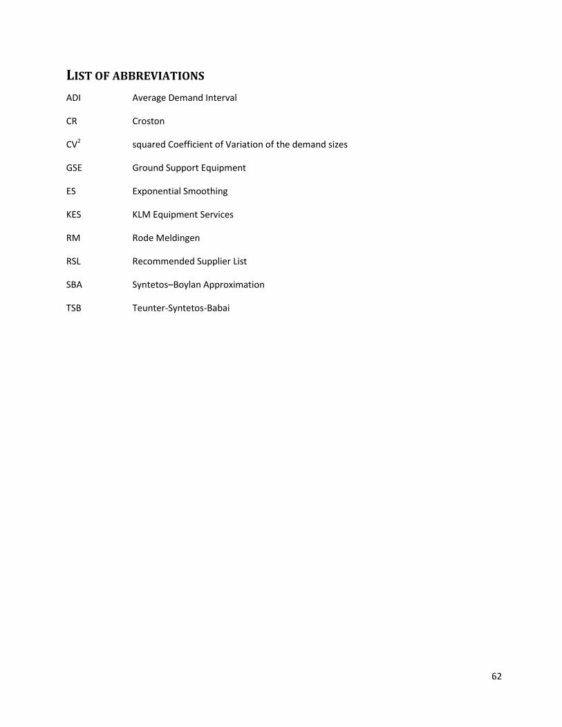
62

LIST OF ABBREVIATIONS

ADI Average Demand Interval

CR Croston

CV2 squared Coefficient of Variation of the demand sizes

GSE Ground Support Equipment

ES Exponential Smoothing

KES KLM Equipment Services

RM Rode Meldingen

RSL Recommended Supplier List

SBA Syntetos–Boylan Approximation

TSB Teunter-Syntetos-Babai

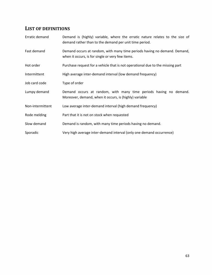
63

LIST OF DEFINITIONS

Erratic demand Demand is (highly) variable, where the erratic nature relates to the size of

demand rather than to the demand per unit time period.

Fast demand Demand occurs at random, with many time periods having no demand. Demand,

when it occurs, is for single or very few items.

Hot order Purchase request for a vehicle that is not operational due to the missing part

Intermittent High average inter-demand interval (low demand frequency)

Job card code Type of order

Lumpy demand Demand occurs at random, with many time periods having no demand.

Moreover, demand, when it occurs, is (highly) variable

Non-intermittent Low average inter-demand interval (high demand frequency)

Rode melding Part that it is not on stock when requested

Slow demand Demand is random, with many time periods having no demand.

Sporadic Very high average inter-demand interval (only one demand occurrence)

64

LIST OF FIGURES AND TABLES

Figure 1.1 Description of the environment in which KES operations ............................................................. 2

Figure 2.1 Overview and clustering of decisions in maintenance logistics control ....................................... 6

Figure 4.1 Demand pattern classification scheme ........................................................................................ 21

Figure 4.2 Determination of the demand pattern ........................................................................................ 22

Figure 4.3 Decisions on the classification with respect to demand forecasting ........................................... 24

Figure 5.1 Spare parts classification with respect to inventory control ....................................................... 36

Figure 5.2 Final spare parts classification scheme with respect to inventory control.................................. 44

Figure 7.1 Migration between the different spare parts classes with respect to demand forecasting ....... 52

Table 2.1 Sage’s spare parts classification with KPIs .................................................................................... 12

Table 4.1 Classification in-use items ............................................................................................................. 23

Table 4.2 ME results for non-intermittent items .......................................................................................... 30

Table 4.3 ME results for intermittent items ................................................................................................. 30

Table 4.4 MSE results for non-intermittent items ........................................................................................ 31

Table 4.5 MSE results for intermittent items................................................................................................ 31

Table 5.1 Number of job cards per job card code ........................................................................................ 38

Table 5.2 Distribution of critical and non-critical parts for January-April 2012............................................ 42

Table 5.3 Performance based on current service levels ............................................................................... 42

Table 5.4 Performance without the supply time .......................................................................................... 43

Table 5.5 Reduction of the number of hot orders ........................................................................................ 43

Table 5.6 Result classification scheme for 2011 ........................................................................................... 44

Table 5.7 Sage's classification of critical parts .............................................................................................. 45

Table 8.1 Modified Sage classification with KPIs .......................................................................................... 58

65

APPENDIX A: CLASSIFICATION CRITERIA

In this appendix we will discuss the results of a literature study about spare parts classification criteria

(Velagić, 2012). The literature study shows that traditionally, classification of spare parts is based on a

single criterion. However, most papers propose using multiple criteria (e.g. Flores & Whybark, 1987;

Partovi & Burton, 1993; Ramanthan, 2006; Ng, 2007, Zhou & Fan, 2007; Petrovic & Petrovic, 1992).

Bacchetti and Saccani (2011) show in their literature review that the most applied criteria for classifying

spare parts are parts criticality and parts costs/price (e.g. Duchessi, Tayi & Levi, 1988; Porras & Dekker,

2008; Zhou & Fan, 2007). Other frequently applied criteria for spare parts classification are amongst

others the demand (e.g. Porras & Dekker, 2008; Zhou & Fan, 2007; Syntetos, Keyes & Babai, 2009),

different supply characteristics, e.g. certainty of supply and lead time (e.g. Persson & Saccani, 2009; Zhou

& Fan, 2007; Ng, 2007), and demand variability (e.g. Cavalieri, Garetti, Macchi & Pinto, 2008; Yamashina,

1989). Other criteria that are proposed by fewer studies are part life cycle phase (e.g. Persson & Saccani,

2009; Yamashina, 1989), specificity (e.g. Huiskonen, 2001), and reliability (e.g. Yamashina, 1989).

The Table A.1 shows the criteria that have been suggested and/or used for a policy in scientific articles.

The disadvantage of using multiple criteria for classification is that it becomes more difficult to optimize,

and to implement the classification system (Syntetos et al., 2009). It is a balance between precision and

adequacy, and comprehension and simplicity. If all criteria are applied, the model will get enormous and

impracticable. However, if some criteria are not taken into account, it could lead to suboptimal solution.

Thus, one should find the right balance between classification adequacy and the ease of implementation.

The criteria that can be applied for the classification of KES’s spare parts depend on several factors. Some

criteria can be combined with other criteria, like demand volume and demand variability. Further, some

criteria might not be interesting with regard to availability, and the costs. Moreover, some criteria may

create different classifications, but that does not immediately means that one will have to apply different

policies for these classes. The table can be used to choose the most promising criteria for classifying the

spare parts. As one can see, criteria that are frequently reported are the value, criticality, supply

characteristics, demand volume, and demand variability (Bacchetti & Saccani, 2011). Other criteria that

are less frequently reported (see last column of the table), but that also could be considered for the

classification of spare parts are specificity, life cycle phase, and repair efficiency.

66

Author(s) Year Classification criteria employed

Valu

e

Criticality

Sup

ply

characteristics

Dem

and

volu

me

Dem

and

variability

Oth

er criteria

Braglia et al. 2004 X X X X

Cavalierli et al. 2008 X X X X X Part specificity

Duchessi et al. 1988 X X

Flores et al. 1988 X X

Gajpal et al. 1994 X

Huiskonen 2001 X X X X Part specificity

Ng 2007 X X X

Partovi et al. 2002 X X X X

Persson et al. 2009 X X X X X Life cycle phase

Petrovic et al. 1992 X X X X Weight, repair

efficiency

Porras et al. 2008 X X X

Ramanathan 2006 X X X X

Syntetos et al. 2009 X

Yamashina 1989 X X Part reliability, life

cycle phase

Zhou et al. 2006 X X X X

Table A.1 Classification criteria employed (from Bacchetti & Saccani, 2011, pp. 3)

67

APPENDIX B: SEASONALITY

This appendix assesses the seasonality of the demand. In Chapter 1 we have stated that maintenance

activities, and thus the need for spare parts, are affected by seasonal factors. The number of corrective

maintenance activities is higher during the Fall/Winter period (de-icers are for example only operated

during the Winter) than during Spring/Summer period. To illustrate this effect, Figures B.1, B.2 and B.3

show time-series, for all parts demanded between 2007 and 2011, on a yearly, monthly, and daily level,

respectively. Figure B.2 shows that each year the demand is lowest during May, June and July, the

demand is increasing between December and March, the highest demand is obtained during March, and

the demand decreases again after March. This confirms the information obtained from the interviews:

high demand during the Fall/Winter period and low demand during the Spring/Summer period. Thus, we

can conclude that there are indeed seasonal effects and demand forecasts will have to be adjusted for

seasonality. Note that all three figures also show an upward trend – increasing demand over time. Given

that the TSB method is able to forecast non-stationary demand, this is not an issue.

Figure B.1 Seasonality analysis - yearly level

0

10000

20000

30000

40000

50000

60000

2007 2008 2009 2010 2011

De

man

d

Year

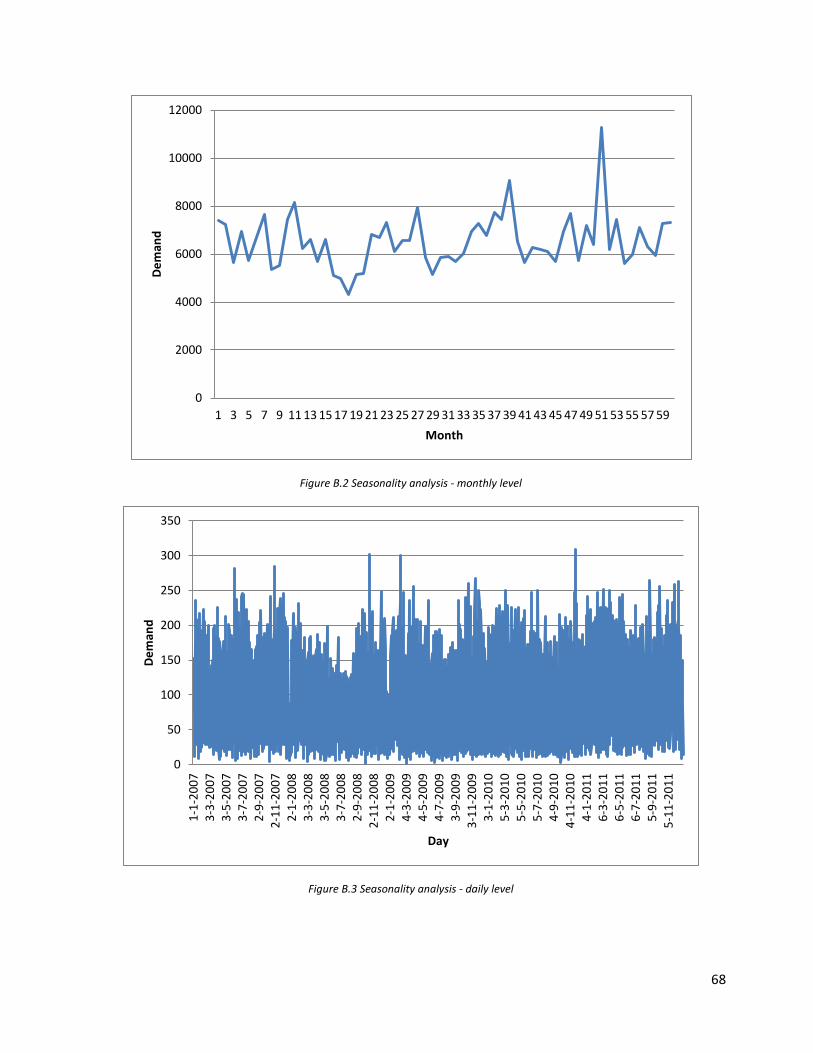
68

Figure B.2 Seasonality analysis - monthly level

Figure B.3 Seasonality analysis - daily level

0

2000

4000

6000

8000

10000

12000

1 3 5 7 9 11 13 15 17 19 21 23 25 27 29 31 33 35 37 39 41 43 45 47 49 51 53 55 57 59

De

man

d

Month

0

50

100

150

200

250

300

350

1-1

-20

07

3

-3-2

00

7

3-5

-20

07

3

-7-2

00

7

2-9

-20

07

2

-11

-20

07

2

-1-2

00

8

3-3

-20

08

3

-5-2

00

8

3-7

-20

08

2

-9-2

00

8

2-1

1-2

00

8

2-1

-20

09

4

-3-2

00

9

4-5

-20

09

4

-7-2

00

9

3-9

-20

09

3

-11

-20

09

3

-1-2

01

0

5-3

-20

10

5

-5-2

01

0

5-7

-20

10

4

-9-2

01

0

4-1

1-2

01

0

4-1

-20

11

6

-3-2

01

1

6-5

-20

11

6

-7-2

01

1

5-9

-20

11

5

-11

-20

11

De

man

d

Day

69

APPENDIX C: LIFE CYCLE PHASE

In this appendix the benefits of the life cycle criterion will be shown by making use of available demand

data of the first four months of 2012. We use only these four months, because only the most recent

demand data contains information about the “rode meldingen” (RMs) and hot orders which we want to

use to analyze the benefits. The first column of Table C.1 shows the different classes that we have

identified in the demand data from 2012. As one can, we have added the class “New 2012”. Those are

items that have not been demand during 2007-2011 – the demand history data that we have used for

classifying the items according to the life cycle phases. Most “New 2012”-items are items that have not

been asked before, except for a few very sporadic items for which we do not have any information.

Further, we have separated the sporadic items from the remaining in-use items. As one can see, more

than 80% of the demand is in the in-use phase. However, more than 50% of the RMs and hot orders are

linked to new parts. This high number of RMs and hot orders can be explained by the demand

unpredictability of new parts. Furthermore, in the literature study it has been pointed out that the spare

parts life cycle follows the vehicle life cycle. We have added the 6th, 7th and 8th column to check whether

the RMs are linked to vehicles that are younger than two years. However, the last column shows that only

5% of the RMs can be linked to “new” vehicles.

Class Demand #Rood #Hot orders KPI Vehicle age < 2 yr #Rood % of total

New 2012 1201 493 323 58,95 196 23 4,67

Initial 1121 196 136 82,52 73 11 5,61

Sporadic 296 106 75 64,19 6 2 1,89

Decline 149 24 21 83,89 2 0 0,00

In-use 13800 497 308 96,40 318 6 1,21

Total 16567 1316 863 92,06 595 42 3,19

Table C.1 Distribution of items among the life cycle phases

To get more insight in the relative high number of hot orders for new spare parts, we have analyzed the

number of RMs and hot orders among the different job cards codes (i.e. type of order). The different job

card codes and their description are given in Table C.2.

Job card Description

B Banden

C Claim

E Error by operator

H Damage repair

I Inspection

L Lekkage

O Modification

R Repair

T Fuelling

S Breakdown

X Runner service

Table C.2 Job card description

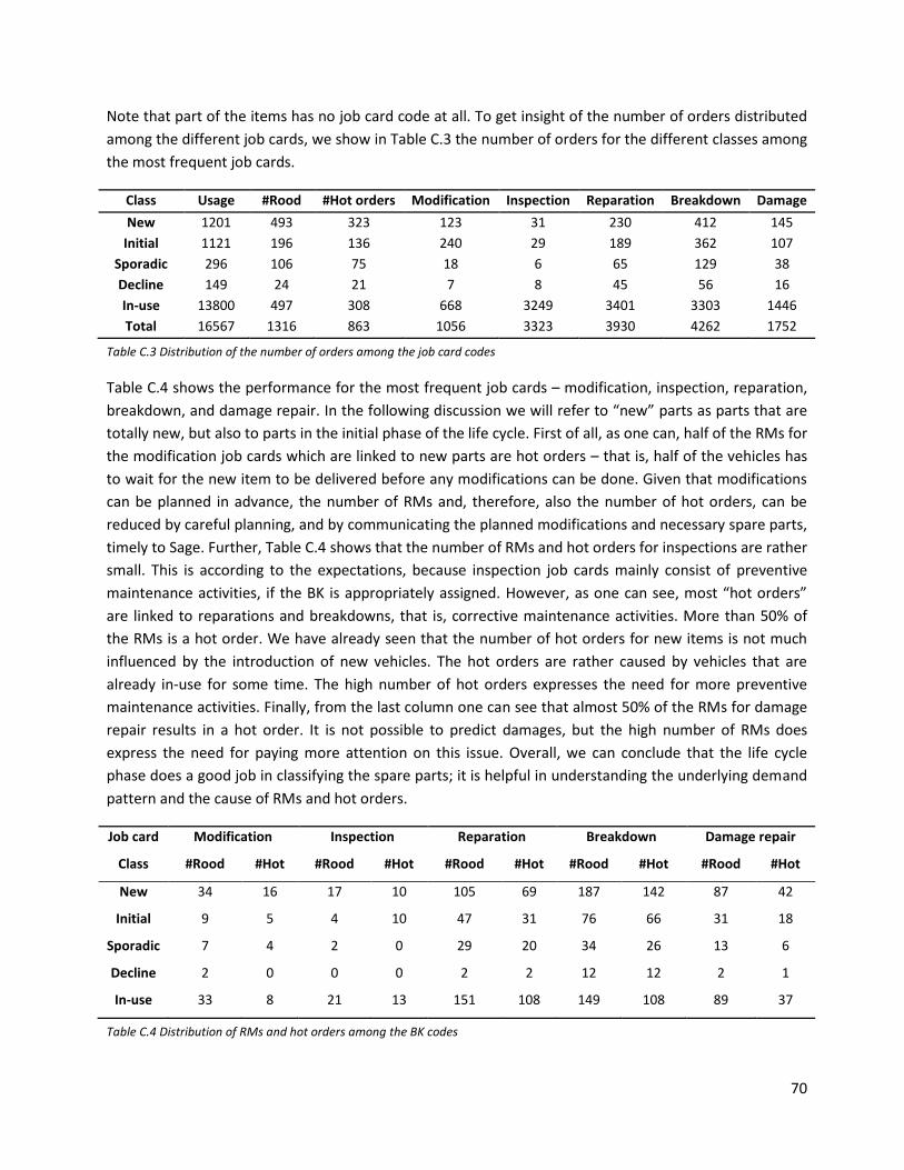
70

Note that part of the items has no job card code at all. To get insight of the number of orders distributed

among the different job cards, we show in Table C.3 the number of orders for the different classes among

the most frequent job cards.

Class Usage #Rood #Hot orders Modification Inspection Reparation Breakdown Damage

New 1201 493 323 123 31 230 412 145

Initial 1121 196 136 240 29 189 362 107

Sporadic 296 106 75 18 6 65 129 38

Decline 149 24 21 7 8 45 56 16

In-use 13800 497 308 668 3249 3401 3303 1446

Total 16567 1316 863 1056 3323 3930 4262 1752

Table C.3 Distribution of the number of orders among the job card codes

Table C.4 shows the performance for the most frequent job cards – modification, inspection, reparation,

breakdown, and damage repair. In the following discussion we will refer to “new” parts as parts that are

totally new, but also to parts in the initial phase of the life cycle. First of all, as one can, half of the RMs for

the modification job cards which are linked to new parts are hot orders – that is, half of the vehicles has

to wait for the new item to be delivered before any modifications can be done. Given that modifications

can be planned in advance, the number of RMs and, therefore, also the number of hot orders, can be

reduced by careful planning, and by communicating the planned modifications and necessary spare parts,

timely to Sage. Further, Table C.4 shows that the number of RMs and hot orders for inspections are rather

small. This is according to the expectations, because inspection job cards mainly consist of preventive

maintenance activities, if the BK is appropriately assigned. However, as one can see, most “hot orders”

are linked to reparations and breakdowns, that is, corrective maintenance activities. More than 50% of

the RMs is a hot order. We have already seen that the number of hot orders for new items is not much

influenced by the introduction of new vehicles. The hot orders are rather caused by vehicles that are

already in-use for some time. The high number of hot orders expresses the need for more preventive

maintenance activities. Finally, from the last column one can see that almost 50% of the RMs for damage

repair results in a hot order. It is not possible to predict damages, but the high number of RMs does

express the need for paying more attention on this issue. Overall, we can conclude that the life cycle

phase does a good job in classifying the spare parts; it is helpful in understanding the underlying demand

pattern and the cause of RMs and hot orders.

Job card Modification Inspection Reparation Breakdown Damage repair

Class #Rood #Hot #Rood #Hot #Rood #Hot #Rood #Hot #Rood #Hot

New 34 16 17 10 105 69 187 142 87 42

Initial 9 5 4 10 47 31 76 66 31 18

Sporadic 7 4 2 0 29 20 34 26 13 6

Decline 2 0 0 0 2 2 12 12 2 1

In-use 33 8 21 13 151 108 149 108 89 37

Table C.4 Distribution of RMs and hot orders among the BK codes

71

APPENDIX D: DEMAND FORECASTING

In Section 4.5 we have analyzed the performance of the SBA, Croston, ES and TSB forecasting methods for

intermittent and non-intermittent demand. In order to test the benefit of the TSB method compared to

the other methods, we have also analyzed the ME and MSE performance of the different estimators for

sporadic and declining parts. Tables D.1, D.2, D.3, and D.3 show the ME and MSE performance for

sporadic and declining demand, respectively. The TSB method outperforms the other methods for both

decline and sporadic demand. Only ES outperforms the TSB method for decline items in terms of bias. This

analysis confirms that the TSB method is able to deal with non-stationary demand and to forecast

obsolescence.

Estimator smoothing constant - ME

0,05 0,10 0,15 0,20 0,25 0,30

SBA 0,021366 0,020048 0,018731 0,017413 0,016096 0,014778

Croston 0,022683 0,022683 0,022683 0,022683 0,022683 0,022683

ES 0,011004 0,00967 0,008338 0,007131 0,006104 0,005259

TSB 0,007871 0,008086 0,008301 0,008516 0,008731 0,008946 0,01

0,004151 0,00455 0,004949 0,005348 0,005747 0,006146 0,02

0,000925 0,001482 0,002038 0,002595 0,003151 0,003708 0,03

-0,00188 -0,00119 -0,0005 0,000196 0,000887 0,001578 0,04

-0,01266 -0,01149 -0,01031 -0,00914 -0,00796 -0,00679 0,10

-0,01719 -0,01585 -0,0145 -0,01316 -0,01182 -0,01047 0,15

-0,01985 -0,01843 -0,01701 -0,01559 -0,01417 -0,01275 0,20

-0,02154 -0,02008 -0,01863 -0,01717 -0,01572 -0,01426 0,25

-0,02269 -0,02122 -0,01974 -0,01827 -0,0168 -0,01533 0,30

Table D.1 ME results for sporadic items

Estimator smoothing constant - MSE

0,05 0,10 0,15 0,20 0,25 0,30

SBA 0,556294 0,554648 0,553044 0,551482 0,549964 0,548488

Croston 0,557984 0,557984 0,557984 0,557984 0,557984 0,557984

ES 0,546104 0,556621 0,570341 0,58531 0,601383 0,618585

TSB 0,548223 0,548228 0,548237 0,548249 0,548264 0,548282 0,01

0,543707 0,543725 0,543755 0,543796 0,543849 0,543914 0,02

0,540307 0,540342 0,540401 0,540484 0,54059 0,540719 0,03

0,537718 0,537774 0,537867 0,537997 0,538164 0,538369 0,04

0,530481 0,530677 0,531005 0,531464 0,532053 0,532774 0,10

0,528451 0,528766 0,52929 0,530025 0,53097 0,532125 0,15

0,527442 0,527877 0,528602 0,529618 0,530923 0,532518 0,20

0,526858 0,527419 0,528353 0,52966 0,531341 0,533396 0,25

0,526489 0,527182 0,528336 0,529951 0,532029 0,534568 0,30

Table D.2 MSE results for sporadic items

72

Estimator

smoothing constant - ME

0,05 0,10 0,15 0,20 0,25 0,30

SBA 0,142116 0,137926 0,133802 0,129699 0,12561 0,121541

Croston 0,14606 0,145802 0,1456 0,145411 0,145226 0,145055

ES 0,088567 0,058761 0,04229 0,03248 0,026191 0,021889

TSB 0,276616 0,275285 0,273787 0,271978 0,269996 0,268012 0,01

0,238979 0,237812 0,236491 0,234876 0,233093 0,231307 0,02

0,210291 0,209222 0,208026 0,206556 0,204931 0,203303 0,03

0,188171 0,187154 0,186042 0,184683 0,183182 0,181683 0,04

0,124456 0,12333 0,122334 0,121262 0,120145 0,119065 0,10

0,106226 0,104885 0,103826 0,102802 0,101798 0,100858 0,15

0,097667 0,096124 0,094977 0,093948 0,092985 0,092109 0,20

0,093376 0,091648 0,090403 0,089339 0,08838 0,087525 0,25

0,09136 0,089457 0,088107 0,086988 0,086005 0,085144 0,30

Table D.3 ME results for declining items

Estimator smoothing constant - MSE

0,05 0,10 0,15 0,20 0,25 0,30

SBA 0,311348 0,298244 0,286026 0,273316 0,260095 0,246803

Croston 0,324591 0,324634 0,325515 0,325589 0,324614 0,322949

ES 0,168028 0,119963 0,10041 0,090629 0,085218 0,08217

TSB 0,131335 0,13115 0,130876 0,130555 0,130216 0,129875 0,01

0,118455 0,118299 0,118053 0,11776 0,117446 0,11713 0,02

0,107237 0,107106 0,106886 0,106617 0,106326 0,106031 0,03

0,097446 0,097338 0,097139 0,096891 0,096621 0,096346 0,04

0,059257 0,05923 0,059119 0,05896 0,058776 0,058583 0,10

0,042867 0,042872 0,0428 0,042682 0,04254 0,042387 0,15

0,033091 0,033113 0,033064 0,032973 0,032858 0,032732 0,20

0,026814 0,026846 0,026813 0,02674 0,026643 0,026535 0,25

0,022513 0,022552 0,022529 0,022469 0,022386 0,022291 0,30

Table D.4 MSE results for declining items

73

APPENDIX E: IMPLEMENTATION

In this appendix we will explain how one can determine the life cycle phases, calculate the intermittence

of demand, calculate the seasonality effects, forecast by making use of the TSB method and perform a

criticality analysis in Excel.

LIFE CYCLE PHASE An example of how to determine the life cycle phases is given in the spreadsheet “Status.xlsx”. In this

example we have determined the life cycle phases based on the demand between 2007 and 2011 as

explained in Section 4.2. Note that we have assumed that the current date is 01-01-2012. The worksheet

“Parts” shows per item number the total quantity demanded per month during 2007-2011. The life cycle

phase of the item is determined by the variable Status, where “N” (i.e. new) stands for items in the initial

phase of the life cycle, “SPO” (i.e. sporadic) are sporadic items in the in-use phase of the life cycle, “U”

(i.e. use) stands for items in the in-use phase, and both “SD” (i.e. sudden decline) and “D” (i.e. decline)

stand for items in the decline phase of the life cycle. Recall that an item can only be in the initial phase of

the life cycle if it is for first time demanded in the past year. In order to check this, we have added an

additional variable to determine whether an item is “N” or “SPO”, that is, the variable Check. This variable

calculates the number of days between the date that the price is set and one year before the current

date. In the used example this is 01-01-2011, because we have assumed that the current data is 01-01-

2012.

DEMAND PATTERN The spreadsheet “Demand pattern.xlsx” shows for items in the in-use phase (except for sporadic items)

how to determine the demand pattern as explained in Section 4.2. The worksheet “Demand pattern”

shows per item number the total quantity demanded per month during 2007-2011. The demand pattern

can be calculated as follows:

1. Use the variable N to calculate the number of positive demand occurrences.

2. Use the variable Seasonality to check how many years have passed since the first positive

demand occurrence.

3. Use the variable Interval to calculate the interval between the first year with a positive demand

occurrence and the last demand occurrence.

4. Use the variable ADI to calculate the average inter demand interval. ADI is calculated as follows:

ADI = N / Interval.

5. Use the variable Intermittence to check whether it is an intermittent or non-intermittent item.

6. Use the variable CV^2 if you want to check the variability of the demand.

7. Use the variable Pattern if you want to check whether an item is slow, lumpy, fast or erratic.

SEASONALITY The spreadsheet “Forecasting in-use.xlsx” shows an example for calculating the seasonality effects based

on the demand data between 2007 and 2011. The worksheet “Seasonality Int.” shows how to calculate

the seasonality effects for intermittent items in the in-use phase, and the worksheet “Seasonality Non-

Int.” shows how to calculate the seasonality effects for non-intermittent items in the in-use phase. The

74

principle is the same, only the used data is different. The seasonality effects are calculated as explained in

Section 4.3.3. In order to explain the worksheet, we will refer to the used colors in the header row.

1. The columns with a gray header row show the total demand for each item during the past 60

months (2007-2011). Use the variable Seasonality to check how many years have passed since

the first positive demand occurrence, because the calculation of the seasonality effect will be

based on the number of “available seasons”.

2. Use the columns with a yellow header row to estimate the trend point for any particular month

by a moving average of a full season (that is, 12 months) centered at period . Given that the we

have an even number of periods, , the standard 12-period moving average ends up being

centered between two periods, and not right at the middle of a period as desired. Therefore, we

will take the average of two consecutive moving averages.

3. Use the columns with a blue header row to estimate the seasonal factor for any particular period

by dividing the demand (from the columns with a grey header row) by the centered moving

average (from the columns with a yellow head row).

4. Use the columns with a red header row in order to dampen the random effect by averaging the

seasonal factors for similar periods in different years.

5. Silver et al. (1998) express that the averages need not add up to exactly 12. Use the columns with

a pink header row in order to normalize the columns with a red header row. One obtains

estimates of seasonal factors that add up to 12. So the columns with a pink header row show for

each item the seasonal factors for each month.

6. Finally, the columns with a green header row show the de-seasonalized demand from the

columns with a grey header row. The de-seasonalized demand can be used to forecast future

demand.

TSB METHOD The spreadsheet “Forecasting in-use.xlsx” shows an example for demand forecasting according to the TSB

method. The worksheet “Int. deseasonalized” shows how to forecast the demand for intermittent items

in the in-use phase, and the worksheet “Non-Int. deseasonalized” shows how to forecast the demand for

non-intermittent items in the in-use phase. However, the principle is the same, only the used data is

different. In this example we have used a 5-year of demand history data. Rather than initializing the TSB

method based on the whole 5-year period, we first use only the first 3 years and we will then update the

forecast for the remaining 2 years. This way, forecasts can “stabilize” during the updating stage of the

initialization. The variable T denotes the set of months in the first 3 year with a positive demand.

Variables s37, ^p37, and x37 are the initial forecasts of the demand and probability (see Section 4.3.1 for

the exact definition). Next, the columns with a yellow header row show the updating of the forecasts for

the remaining 2 years.

Then, an example is given for forecasting the demand for January 2012. The same procedure can be

followed for future demand forecasting. The following variables are used:

d_jan: the actual de-seasonalized demand of January 2012

s_jan: forecast of the demand in January provided that this demand is positive

75

^p_jan: forecast of the probability of a positive demand in January

^x_jan: forecast at the beginning of January for the demand in January

p_jan: indicator variable that indicates whether or not there is a positive demand in January. This

variable influences the forecasts for February.

x_jan: actual forecast of the demand in January. This variable is calculated by multiplying the de-

seasonalized forecast for January ^x_jan by the seasonal effect of January.

CRITICALITY ANALYSIS An example of a criticality analysis is shown in the spreadsheet “Criticality.xlsx”. This example is based on

demand data from 2010-2011 as explained in Section 5.2. In the worksheet “Afname” all the necessary

(and more) variables for performing the criticality analysis have been collected. The variables are defined

as follows:

Jobcard: job card number

Plantype: vehicle number

Item nr.: item number

Item price: price of the item

Entry: job card code as defined in Table 5.1.

GSE criticality: the criticality of the GSE vehicles as defined in Section 5.2.1, that is, the position of

the GSE vehicle in the chain.

For the first filter we will focus on the variables Entry and GSE criticality. First of all, only item numbers

with job card codes R (i.e. repair) and S (i.e. breakdown) as given in column Entry should be selected.

Also, only items numbers with a GSE criticality of 1 should be selected. Worksheet “Results 1st filer”

shows all the item numbers with job card codes R and S, and GSE criticality of 1. In this worksheet some

additional variables have to be calculated, that is:

#Jobcards/vehicle: number of (repair and breakdown) job cards per vehicle. Can be determined

by making use of a PivotTable.

Size supplier: number of vehicles within the same type of supplier

#Jobcards/supplier: number of (repair and breakdown) job cards within the same supplier type

Ratio/jc: ratio of the number of (repair and breakdown) job cards of a vehicle compared to the

total number of (repair and breakdown) job cards within the same supplier type. This variable can

be calculated by dividing the variable #Jobcards/vehicle by the variable #Jobcards/supplier.

#Item changes/vehicle: number of times that a particular item is replaced on the same vehicle.

Can be determined by making use of a PivotTable.

Given that all the necessary variables are determined, we can now calculate the criticality score as

presented in the Worksheet “Final results”. According to the model presented in Section 5.2.2 (formula

5.5), one first has to calculate the weight for the ratio of GSE failures (i.e. wRatio) and for item failures

(i.e. wItemChangesVehicle). First, the ratio of GSE failures and item failures are normalized, resulting in

variables sRatio and sItemChangesVehicle. The score can be calculated as follows:

76

1. Use the variable wRatio to calculate the weight of the ratio of GSE failures. wRatio is calculated as

follows: wRatio = sRatio / SQRT(SUM(sRatio : sItemChangesVehicle)).

2. Use the variable wItemChangesVehicle to calculate the weight item failures.

wItemChangesVehicle is calculated as follows: wItemChangesVehicle = sItemChangesVehicle /

SQRT(SUM(sRatio : sItemChangesVehicle)).

3. Use the variable score to calculate the criticality score based on the weights. The variable score is

calculated as follows: score = sRatio * wRatio + sItemChangesVehicle * wItemChangesVehicle

However, the criticality score is calculated on vehicle level. In order to shift from the vehicle level to item

level, one will have to use a PivotTable to calculate the average criticality score per item number. The

average score is shown in column Average of score. This column is sorted from the largest to the smallest

average score. The variable Pareto calculates the cumulative percentage per item number. All the items

with a cumulative percentage smaller than 20% are classified as critical.