Spanish wine consumer behaviour: a stated and revealed preferences analysis

Spanish wine consumer behaviour: A stated and revealed preferences analysis

Mtimet Nadhem and Albisu Luis Miguel [email protected]

Paper prepared for presentation at the I Mediterranean Conference of Agro-Food Social Scientists. 103rd EAAE Seminar ‘Adding Value to the Agro-Food Supply Chain in the Future Euromediterranean Space’. Barcelona, Spain, April 23rd - 25th, 2007 Copyright 2007 by [Mtimet Nadhem and Albisu Luis Miguel]. All rights reserved. Readers may make verbatim copies of this document for non-commercial purposes by any means, provided that this copyright notice appears on all such copies.

Spanish wine consumer behaviour:

A stated and revealed preferences analysis

Mtimet Nadhem1 ; Albisu Luis Miguel2

1 École Supérieure d’Agriculture de Mograne (Tunisia) ([email protected])

2 Agro-Food Economics Unit, CITA, Zaragoza (Spain) ([email protected])

Abstract: Overall wine consumption in Spain is decreasing while, at the same time,

Designation of Origin (DO) wine consumption is increasing gradually. This study

examines Spanish DO wine consumer behaviour through stated preferences (SP) and

revealed preferences (RP) data. Part-worth utilities are calculated and results from both

analyses are compared to look for similarities and differences between what respondents

say on surveys and what they really do on real purchases. Consumer segmentation is

undertaken based on purchase frequencies. In a second step, we try to pool the two data

sources in order to get more meaningful and robust results. Results indicate similarities

in the consumer choice process when comparing the two data sources, especially for the

preference of the DO and wine aging attributes. The only difference detected is the price

variable, where a concave price-utility function is obtained with the SP analysis and a

negative linear price coefficient is obtained with the RP analysis. Likelihood ratio

statistic indicates that equal parameters hypothesis is rejected, meaning that it is not

possible to merge the two data sources. This is mainly due to the difference on

consumers price perception which could be explained by the different purchase

occasion selected in each case.

Key words: wine, consumer behaviour, Spain, stated preference, revealed preference, DO.

Spanish wine consumer behaviour: A stated and revealed preferences

analysis

1. Introduction

Modern distribution channels have incorporated new technologies (lasers, specific

digital codes for each item, etc.) to collect data which helps to understand better

consumers behaviour and their preferences. In contrast with data gathered through

consumer surveys, known as stated preferences (SP), scanner data reveal real purchases

and are referred to as revealed preferences (RP). Combining SP and RP data, whenever

possible, allows exploiting strengths of each data source and ameliorate their

weaknesses, which lead to more robust estimations (Louviere et al., 2000).

The objective of this work is to estimate Designation of Origin (DO) wine consumers

preferences with the use of wine sales data from hypermarkets, showing revealed

preferences, and data from a survey undertaken to DO wine consumers, showing stated

preferences. In a second step, results obtained from each data source are compared, to

check between what consumers declare on the survey and what they really do on their

real purchase. Both data sources are combined to explore the advantages of a joint

analysis.

The paper is structured as follows. In section two there is a brief description of the

data used in the analysis; the next section explains the methodology; results are

presented in the fourth section and conclusions are reported in the last section.

2. Data

In order to undertake the revealed preference analysis, wine purchases data were

used from two hypermarkets located in the city of Zaragoza (Spain) during 2004.

Purchase of table wines plus DO white and rosé wines were not taken into

consideration. The reason was to concentrate only on DO red wines. The same decision

was undertaken for customers who did not participate in the SP survey or did not

purchase any bottle of DO wine from Cariñena, Rioja or Somontano. The new data base

contained 299 transactions, corresponding to 86 clients, 107 SKUs (Stock Keeping

Units) and 631 bottles sold.

Regarding the stated preference process, a questionnaire was undertaken in 2005 and

directed to DO wine consumers living in Zaragoza. The survey included questions about

DO wine consumption and purchase and it also included an experimental choice

experiment design. A total sample of 357 respondents, aged between 21 and 82 years

old, agreed to participate to the experiment. Nevertheless, in this research only

responses from the 86 respondents as well present in the RP database are analysed. The

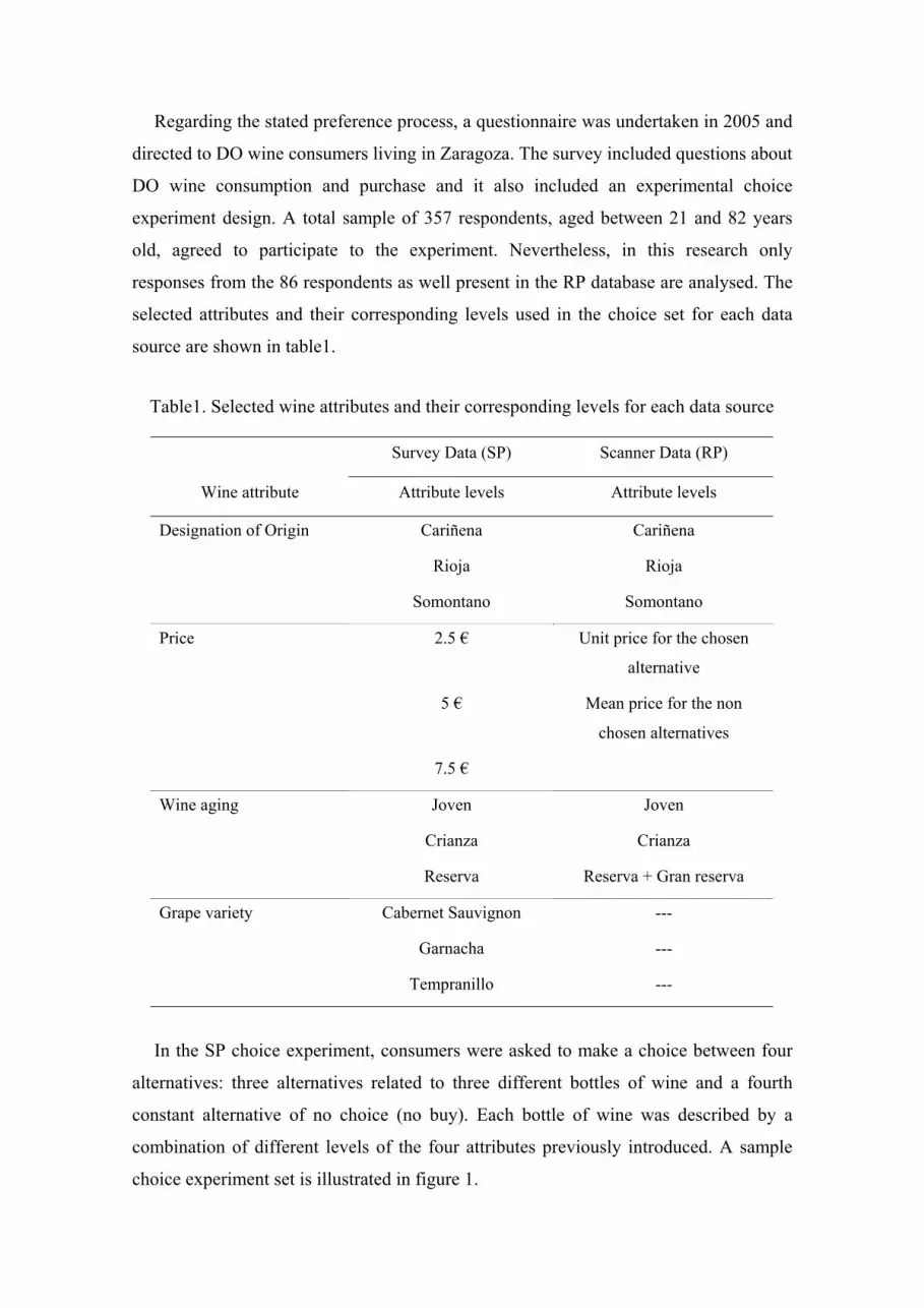
selected attributes and their corresponding levels used in the choice set for each data

source are shown in table1.

Table1. Selected wine attributes and their corresponding levels for each data source

Survey Data (SP) Scanner Data (RP)

Wine attribute Attribute levels Attribute levels

Designation of Origin Cariñena Cariñena

Rioja Rioja

Somontano Somontano

Price 2.5 € Unit price for the chosen

alternative

5 € Mean price for the non

chosen alternatives

7.5 €

Wine aging Joven Joven

Crianza Crianza

Reserva Reserva + Gran reserva

Grape variety Cabernet Sauvignon ---

Garnacha ---

Tempranillo ---

In the SP choice experiment, consumers were asked to make a choice between four

alternatives: three alternatives related to three different bottles of wine and a fourth

constant alternative of no choice (no buy). Each bottle of wine was described by a

combination of different levels of the four attributes previously introduced. A sample

choice experiment set is illustrated in figure 1.

Which bottle of red wine would you buy for dinner at home with guests?

Please check (X) on the corresponding option

Bottle 1 Bottle 2 Bottle 3 No bottle

Rioja Cariñena Somontano

5 € 2.5 € 7.5 €

Crianza Joven Reserva

Tempranillo Garnacha Cabernet Sauvignon

I will not buy any

of these 3 bottles

Figure 1. A Choice Experiment Sample Card

This class of choice experiment is referred to as unlabelled or generic (Louviere et

al., 2000) since the alternatives have no specific name or label. The purchase occasion

was highlighted, indicating that respondents wanted to buy a bottle of red wine for

dinner having guests at home. A purchase occasion evokes an involvement level of a

particular purchase situation and it is influenced by product attributes as well as the

situation (Houston and Rothschild, 1978). Laurent and Kapferer (1985) stated that the

level of involvement influences the consumer choice process. In this experiment the

purchase occasion was specified in order to avoid possible consumers misspecifications,

such as each respondent thinking of a specific occasion, which could result in biased

responses. In total, each respondent was asked to complete 9 choice sets.

3. Methodology

A choice experiment technique was selected to analyse the two data bases. Choice

experiments derive from the theory of Lancaster (1966) as well as from Random Utility

Theory (RUT). The former postulated that utility is derived from the characteristics that

goods possess (bundles of attributes), rather than the good per se. Random Utility

Theory states that the overall utility ijU can be expressed as the sum of a systematic

(deterministic) component ijV , which is expressed as a function of the attributes

presented (wine characteristics in this study), and a random (stochastic) component ijε .

Individual i chooses alternative j rather than alternative k if ikij UU f . On

probabilistic terms it can be expressed by the following equation:

)Ckj;εVεPr(VP iikikijijij ∈≠∀+≥+= (1)

where iC is the choice set for respondent i . In this study the choice set is constant and

it includes 4 alternatives for the SP data and 6 alternatives for the RP data. Equation (1)

means that consumers will choose an option, from among a number of choices, trying to

achieve their highest utility.

Different discrete choice models are obtained from different specifications of the

density function of the error term, which correspond to different assumptions about the

distribution of the unobserved portion of utility (Train, 2003). In this research it has

been assumed that the random components are identically and independently

distributed, type-I extreme value, across the j alternatives and N individuals, leading to

the following multinomial logit model (McFadden, 1974):

∑∈

=

n

ij

ij

Ck

μV

μV

e

ePr(j) (2)

Where, μ is the scale parameter known to be inversely related to the variance (Ben-

Akiva and Lerman, 1985). It is widely recognized that when operating in a random

utility context, the scale parameter is arbitrarily assumed to be unity (Adamowicz et al.,

1994). However, when combining two data sources (or more), the scale factor

differences must be isolated, and it is possible to identify the ratio of the scale

parameters by equalling to unity one scale parameter from a data source (generally the

RP scale) and estimating the other relative scale parameter of the second data source.

Swait and Louviere (1993) proposed a method to estimate this ratio by maximizing the

standard likelihood ratio statistics of the combined model. Thus, for each data source

equation (2) could be written as:

For revealed preference data: ∑∈

=

rn

rijr

rijr

Ck

Vμ

Vμ

e

ePr(j) (3)

with, rijij

rij

rrij

rij εωZXβαV +++= , r

iCj∈∀ (4)

For stated preference data: ∑∈

=

s

ss

ss

n

ij

ij

Ck

Vμ

Vμ

e

ePr(j) (5)

with, sssssijijijijij εδWXβαV +++= , s

iCj∈∀ (6)

where, j is an alternative from the choice set of the RP riC or of the SP s

iC ; the

coefficients α represent specific constants for each data source, rβ y sβ are the

coefficients of the common attributes levels, ω and δ are the coefficients of specific

attributes for each data source.

The method proposed by Swait and Louviere (1993) for the joint estimation of both

data sources consists, in a first step, to estimate separately the two models derived from

SP data and RP data. Then, the two data sources are combined and the maximum

likelihood statistics is reported for each new chosen value of the SP scale parameter sμ .

The estimation ends when a maximum coefficient of the likelihood statistic is obtained.

Finally, the obtained likelihood statistic is compared to the sum of the likelihood

statistics of the two separated models. The hypothesis of parameters equality is accepted

when there is no significant difference between likelihood statistics. Otherwise, the

parameters equality hypothesis is rejected.

4. Results and discussion

4.1. Separate estimates for each data source

The first step, in the estimation process, was to estimate each data source separately

by the use of the multinomial logit model (MNL). In both models, the price variable is

considered continuous and its linear form (price) and quadratic form (price2) are

estimated (Table 2).

The values of the log likelihood ratio test (LR1) indicate the overall significance of

both models including all explicative variables comparatively to a model including only

a constant. All coefficients of both models are statistically significant (except the

constant and Garnacha level in model 1). The estimated coefficients of the Designation

of Origin attribute, in the two models, show that consumers allocate higher utility to

wines from the Aragon designation Somontano. Although Rioja wines come from

another region, respondents are more likely to buy these wines than Cariñena wines.

Similar results are obtained for both models when considering the wine aging attribute.

In that sense, consumers have higher probabilities to buy Reserva wines than Crianza

and Joven wines. The more aged the wine is the more likely consumers will choose it.

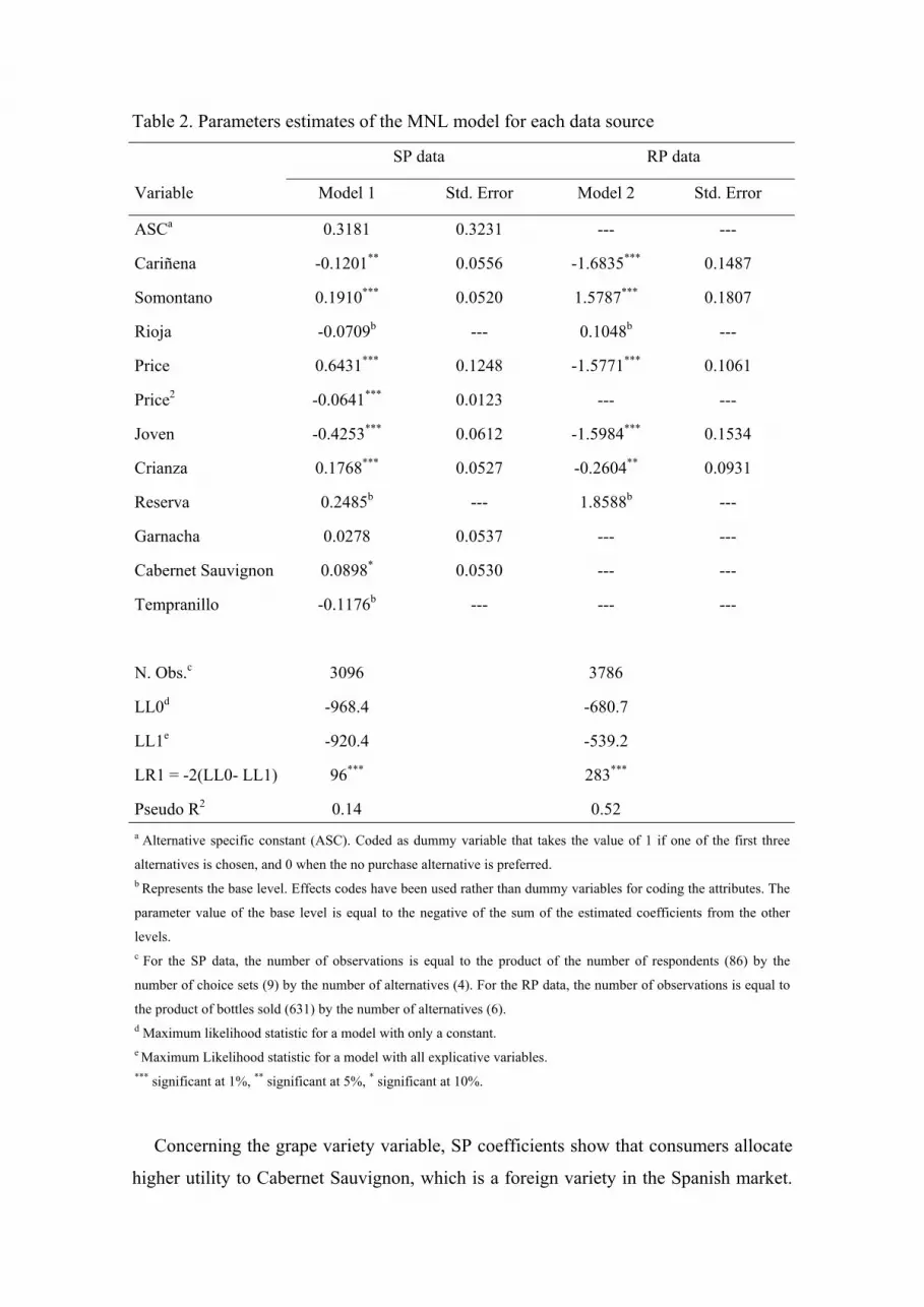
Table 2. Parameters estimates of the MNL model for each data source

SP data RP data

Variable Model 1 Std. Error Model 2 Std. Error

ASCa 0.3181 0.3231 --- ---

Cariñena -0.1201** 0.0556 -1.6835*** 0.1487

Somontano 0.1910*** 0.0520 1.5787*** 0.1807

Rioja -0.0709b --- 0.1048b ---

Price 0.6431*** 0.1248 -1.5771*** 0.1061

Price2 -0.0641*** 0.0123 --- ---

Joven -0.4253*** 0.0612 -1.5984*** 0.1534

Crianza 0.1768*** 0.0527 -0.2604** 0.0931

Reserva 0.2485b --- 1.8588b ---

Garnacha 0.0278 0.0537 --- ---

Cabernet Sauvignon 0.0898* 0.0530 --- ---

Tempranillo -0.1176b --- --- ---

N. Obs.c 3096 3786

LL0d -968.4 -680.7

LL1e -920.4 -539.2

LR1 = -2(LL0- LL1) 96*** 283***

Pseudo R2 0.14 0.52 a Alternative specific constant (ASC). Coded as dummy variable that takes the value of 1 if one of the first three

alternatives is chosen, and 0 when the no purchase alternative is preferred. b Represents the base level. Effects codes have been used rather than dummy variables for coding the attributes. The

parameter value of the base level is equal to the negative of the sum of the estimated coefficients from the other

levels. c For the SP data, the number of observations is equal to the product of the number of respondents (86) by the

number of choice sets (9) by the number of alternatives (4). For the RP data, the number of observations is equal to

the product of bottles sold (631) by the number of alternatives (6). d Maximum likelihood statistic for a model with only a constant. e Maximum Likelihood statistic for a model with all explicative variables. *** significant at 1%, ** significant at 5%, * significant at 10%.

Concerning the grape variety variable, SP coefficients show that consumers allocate

higher utility to Cabernet Sauvignon, which is a foreign variety in the Spanish market.

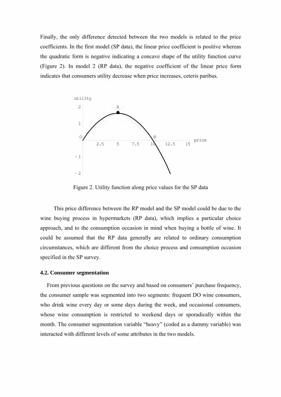
Finally, the only difference detected between the two models is related to the price

coefficients. In the first model (SP data), the linear price coefficient is positive whereas

the quadratic form is negative indicating a concave shape of the utility function curve

(Figure 2). In model 2 (RP data), the negative coefficient of the linear price form

indicates that consumers utility decrease when price increases, ceteris paribus.

2.5 5 7.5 10 12.5 15price

- 2

- 1

1

2

utility

A

BO

Figure 2. Utility function along price values for the SP data

This price difference between the RP model and the SP model could be due to the

wine buying process in hypermarkets (RP data), which implies a particular choice

approach, and to the consumption occasion in mind when buying a bottle of wine. It

could be assumed that the RP data generally are related to ordinary consumption

circumstances, which are different from the choice process and consumption occasion

specified in the SP survey.

4.2. Consumer segmentation

From previous questions on the survey and based on consumers’ purchase frequency,

the consumer sample was segmented into two segments: frequent DO wine consumers,

who drink wine every day or some days during the week, and occasional consumers,

whose wine consumption is restricted to weekend days or sporadically within the

month. The consumer segmentation variable “heavy” (coded as a dummy variable) was

interacted with different levels of some attributes in the two models.

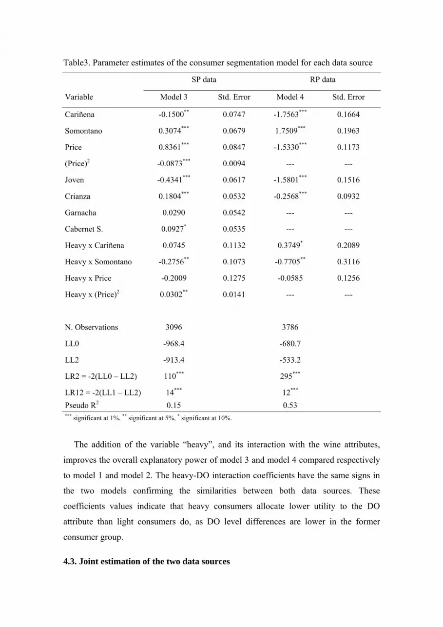
Table3. Parameter estimates of the consumer segmentation model for each data source

SP data RP data

Variable Model 3 Std. Error Model 4 Std. Error

Cariñena -0.1500** 0.0747 -1.7563*** 0.1664

Somontano 0.3074*** 0.0679 1.7509*** 0.1963

Price 0.8361*** 0.0847 -1.5330*** 0.1173

(Price)2 -0.0873*** 0.0094 --- ---

Joven -0.4341*** 0.0617 -1.5801*** 0.1516

Crianza 0.1804*** 0.0532 -0.2568*** 0.0932

Garnacha 0.0290 0.0542 --- ---

Cabernet S. 0.0927* 0.0535 --- ---

Heavy x Cariñena 0.0745 0.1132 0.3749* 0.2089

Heavy x Somontano -0.2756** 0.1073 -0.7705** 0.3116

Heavy x Price -0.2009 0.1275 -0.0585 0.1256

Heavy x (Price)2 0.0302** 0.0141 --- ---

N. Observations 3096 3786

LL0 -968.4 -680.7

LL2 -913.4 -533.2

LR2 = -2(LL0 – LL2) 110*** 295***

LR12 = -2(LL1 – LL2) 14*** 12*** Pseudo R2 0.15 0.53 *** significant at 1%, ** significant at 5%, * significant at 10%.

The addition of the variable “heavy”, and its interaction with the wine attributes,

improves the overall explanatory power of model 3 and model 4 compared respectively

to model 1 and model 2. The heavy-DO interaction coefficients have the same signs in

the two models confirming the similarities between both data sources. These

coefficients values indicate that heavy consumers allocate lower utility to the DO

attribute than light consumers do, as DO level differences are lower in the former

consumer group.

4.3. Joint estimation of the two data sources

Before pooling the two data sources and the estimation of the composite model, the

coefficients of the common variables in the two sources were plotted (Figure 3), as an

easy and rapid way to verify whether parameters equality hypothesis holds or not.

Figure 3. Plot of the of the SP and the RP coefficients

If the hypothesis of equal parameters holds, a graph of one parameter vector against

the second should exhibit a positive, proportional relationship, the slope of which

should equal the ratio of variances between the data sources (Hensher et al., 1999). This

implies that all points should be situated in regions I and III. However, three points are

situated outside these areas, especially point A which represents the linear price

coefficients for each data source. Thus, this graphic distribution implies that the equal

parameters hypothesis is rejected. However, it is important to confirm this assumption

with the composite estimation of the two data sources and to compare the likelihood

ratio obtained with the Chi squared statistic.

Following the method of Swait and Louviere (1993), two different joint-models

(Table 4) were estimated. In the first model (model 5) the same linear price coefficient

for both data sources was considered, whereas in model 6, two separate linear price

coefficients were introduced, each one specific for each data base. In model 5, equalling

the RP scale parameter to one, a SP scale parameter 0.01μ =s was obtained, indicating

higher variance of the latter data. Almost all variables coefficients are significant

(except Garnacha level). However, it is important to emphasis that the obtained pseudo

R2 is less than the pseudo R2 when considering only the RP data (model 2), and that the

variety attribute has coefficients levels higher than the other attributes coefficients.

-0,8

-0,6

-0,4

-0,2

0

0,2

0,4

0,6

0,8

-2 -1,5 -1 -0,5 0 0,5 1 1,5 2

RP Coefficients

SP C

oeffi

cien

tsI

II III

IVA

Table 4. Joint estimation of both data sources

SP RP SP-RP SP-RP

Variable Model 1 Model 2 Model 5 Model 6

ASC 0.3181

(0.3231)

--- --- ---

Cariñena -0.1201**

(0.0556)

-1.6835***

(0.1487)

-1.6873***

(0.1485)

-1.6480***

(0.1278)

Somontano 0.1910***

(0.0520)

1.5787***

(0.1807)

1.5834***

(0.1803)

1.5577***

(0.1553)

Rioja -0.0709a 0.1048a -0.1039a 0.0903a

Price 0.6431***

(0.1248)

-1.5771***

(0.1061)

-1.5743***

(0.1058)

5.3697*** / -1.5704***

(0.4475) (0.0925)

Price2 -0.0641***

(0.0123)

--- 1.2118***

(0.1566)

-0.5307***

(0.0496)

Joven -0.4253***

(0.0612)

-1.5984***

(0.1534)

-1.6070***

(0.1532)

-1.6091***

(0.1317)

Crianza 0.1768***

(0.0527)

-0.2604***

(0.0931)

-0.2625***

(0.0928)

-0.1988**

(0.0873)

Reserva 0.2485a 1.8588a 1.8695a 1.8079a

Garnacha 0.0278

(0.0537)

--- 3.0388

(5.7088)

0.1978

(0.3838)

Cabernet Sauvignon 0.0898*

(0.0530)

--- 10.0138*

(5.6162)

0.6404*

(0.3787)

Tempranillo -0.1176a --- -13.0526a -0.8382a

sμ 0.01 0.14

N. Observations 3096 3786 6882 6882

LL0 -968.4 -680.7 -2203.6 -2203.6

LL3 -920.4 -539.2 -1589.3 -1471.0

LR3 = -2(LL0- LL3) 96*** 283*** 1228.6*** -1465.2***

LR(PE/PR) = -2[LL3PE-PR – (LL3PE + LL3PR)] 259.4 22.8

N. parameters 9 5 8 9 Pseudo R2 0.14 0.52 0.51 0.55 Standard errors within brackets a Represents the base level. Effects codes have been used rather than dummy variables for coding the attributes. The

parameter value of the base level is equal to the negative of the sum of the estimated coefficients from the other

levels. *** significant at 1%, ** significant at 5%, * significant at 10%.

The likelihood ratio statistic equals to 259.4 and it is higher than the Chi-squared

critical value 12.6χ 20,05;6 = indicating the rejection of the hypothesis of equal parameters.

Thus, it is not possible to merge both data bases because there are differences in the

consumers’ choice process between the SP and RP data. However, the high likelihood

statistic is surprising since, in the two cases, purchasing data of the same product were

used. That is why, in a second step, it was decided to estimate a model considering a

separate estimate of the linear price coefficient for each data source since the separate

estimates of this variable (model 1 and model 2) have shown significant differences

between the two sources (point A in Figure 3).

The results obtained from this estimation (model 6) indicate that all variables are

significant, excepting the Garnacha coefficient. The overall model fit is very good with

pseudo R2 equals 0.55. The scale parameter 0.14μ =s , less than one, indicates higher

variance of the SP data. Chi-square statistic equals 22.8 and it is higher than the critical

value 11.1χ 20,05;5 = , indicating in this case also the rejection of the equal parameters

hypothesis at 95% confidence level.

However, although the parameters equality hypothesis was rejected, it is important to

emphasise that the likelihood statistic diminished considerably comparatively with the

same statistic when considering a unique linear price coefficient. These results indicate

that consumers’ choice difference between the two data has an effect on the price

attribute. In figure 4, the tendency line which better approximates the correlation

between SP and RP coefficients is plotted. In the first case, when including the price

coefficients (point A), a weak linear correlation (R2 = 0.056) is obtained. However, after

dropping the price coefficients, the R2 coefficient raises to 0.67 indicating a strong

linear correlation and the slope coefficient (0.139) is equal to the scale parameter

( 0.14)μ =s in model 6.

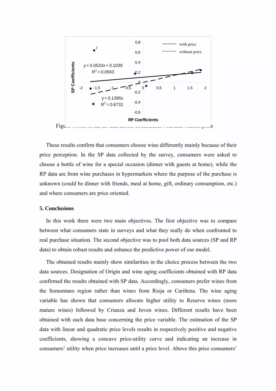
Figure 4. Plot of the SP and the RP coefficients with and without price

These results confirm that consumers choose wine differently mainly because of their

price perception. In the SP data collected by the survey, consumers were asked to

choose a bottle of wine for a special occasion (dinner with guests at home), while the

RP data are from wine purchases in hypermarkets where the purpose of the purchase is

unknown (could be dinner with friends, meal at home, gift, ordinary consumption, etc.)

and where consumers are price oriented.

5. Conclusions

In this work there were two main objectives. The first objective was to compare

between what consumers state in surveys and what they really do when confronted to

real purchase situation. The second objective was to pool both data sources (SP and RP

data) to obtain robust results and enhance the predictive power of our model.

The obtained results mainly show similarities in the choice process between the two

data sources. Designation of Origin and wine aging coefficients obtained with RP data

confirmed the results obtained with SP data. Accordingly, consumers prefer wines from

the Somontano region rather than wines from Rioja or Cariñena. The wine aging

variable has shown that consumers allocate higher utility to Reserva wines (more

mature wines) followed by Crianza and Joven wines. Different results have been

obtained with each data base concerning the price variable. The estimation of the SP

data with linear and quadratic price levels results in respectively positive and negative

coefficients, showing a concave price-utility curve and indicating an increase in

consumers’ utility when price increases until a price level. Above this price consumers’

y = 0.0533x + 0.1039R2 = 0.0563

y = 0.1395xR2 = 0.6731

-0,6

-0,4

-0,2

0

0,2

0,4

0,6

0,8

-2 -1,5 -1 -0,5 0 0,5 1 1,5 2

RP Coefficients

SP C

oeffi

cien

ts

with price

without price A

utility decreases when price increases. This confirms recent results obtained by

Lockshin et al. 2006 and Lockshin and Halstead (2005) on wine consumption.

However, when estimating the RP data with a linear price level, a negative coefficient is

obtained indicating a decrease in consumers’ utility when price increases, which

confirms previous expectations since RP data comes from hypermarket wine purchases

very sensitive to price. The negative sign of the linear price coefficient confirms the

results obtained using RP data by others researches (Blamey et al., 2001; Bonnet and

Simioni, 2001; Swait and Andrews, 2003).

Consumers’ segmentation based on consumption frequency showed in both cases

(SP and RP) that light consumers allocate higher utility to the DO attribute compared to

heavy consumers. These results indicate also a relative degree of coherence between

what consumers declare and what they really do.

The data enrichment process of estimating both data sources together has failed due

to differences between consumers’ price perception. The chi-squared test rejected the

parameters equality hypothesis. This result is not very surprising because previous

research combining SP and RP data found similar results concerning the incompatibility

of data (Swait and Adamowicz, 1996; Adamowicz et al., 1997; Earnhart, 2001;

Earnhart, 2002; Swait y Andrews, 2003). In this work, the SP data linked to the

purchase occasion (dinner with guests at home) could explain the difference between

price perceptions in each data source.

REFERENCES

Adamowicz W., Louviere J., Williams M., 1994. Combining revealed and stated

preference methods for valuing environmental amenities. Journal of Environmental

Economics and Management, 26(3), 271-292.

Adamowicz W., Swait J., Boxall P., Louviere J., Williams M., 1997. Perceptions versus

objective measures of environmental quality in combined revealed and stated

preference models of environmental valuation. Journal of Environmental Economics

and Management, 32(1), 65-84.

Ben-Akiva M., Lerman S., 1985. Discrete choice analysis: theory and application to

travel demand. Cambridge, Mass: MIT Press.

Blamey R., Bennett J., Louviere J., Morrison M., 2001. Green product choice. In J.

Bennett y R. Blamey (Ed.). The choice modelling approach to environmental

valuation. Northampton: Edward Elgar Publishing.

Bonnet C., Simioni, M., 2001. Assessing consumer response to Protected Designation

of Origin Labelling: a mixed multinomial logit approach. European Review of

Agricultural Economics, 28(4), 433-449.

Earnhart D., 2001. Combining revealed and stated preference methods to value

environmental amenities at residential locations. Land Economics, 77(1), 12-29.

Earnhart D., 2002. Combining revealed and stated data to examine housing decision

using discrete choice analysis. Journal of Urban Economics, 51(1), 143-169.

Hensher D., Louviere J., Swait J., 1999. Combining sources of preference data. Journal

of Econometrics, 89(1-2), 197-221.

Houston M., Rothschild M., 1978. Conceptual and methodological perspectives on

involvement, Educators Proceedings, Ed., S.C. Jain, Chicago: American Marketing

Association, 184-187.

Lancaster K., 1966. A new approach to consumer theory. Journal of Political Economy,

74, 132-157.

Laurent G., Kapferer J., 1985. Measuring consumer involvement profiles. Journal of

Marketing Research, 22, 41-53.

Lockshin L., Halstead L., 2005. A comparison of Australian and Canadian wine buyers

using discrete choice analysis. Paper presented at the International Wine Marketing

Symposium, Sonoma, California.

Lockshin L., Jarvis W., D´Hauteville F., Perrouty J. P., 2006. Using simulations from

discrete choice experiments to measure consumer sensitivity to brand, region, price,

and awards in wine choice. Food Quality and Preference, 17(3-4), 166-178.

Louviere J., Hensher D., Swait J., 2000. Stated choice methods: Analysis and

application. Cambridge: Cambridge University Press.

McFadden D., 1974. Conditional logit analysis of qualitative choice behavior. In

Zarembka, P. (Eds). Frontiers in econometrics. New York: Academic Press.

Swait J., Louviere J., 1993. The role of the scale parameter in the estimation and

comparison of multinomial logit models. Journal of Marketing Research, 30(3), 305-

314.

Swait J., Adamowicz W., 1996. The effect of choice complexity on random utility

models: An application to combined stated and revealed preference models or tough

choices: Contribution or confusion? Presented at the 1996 Association of

Environmental and Resource Economists Summer Workshop, Lake Tahoe, CA.

Swait J., Andrews R. L., 2003. Enriching scanner panel models with choice

experiments. Marketing Science, 22(4), 442-460.

Train K.E., 2003. Discrete choice methods with simulation. Cambridge: Cambridge

University Press.