SPADES - a process algebra for discrete event simulation

Process Algebra for Discrete Event SimulationP.G. Harrison� B. StruloyDepartment of ComputingImperial CollegeLONDON SW7 2BZAbstractWe present a process algebra or programming language, based on CCS, whichmay be used to describe discrete event simulations with parallelism. It has exten-sions to describe the passing of time and probabilistic choice, either discrete, be-tween a countable number of processes, or continuous to choose a random amountof time to wait. It has a clear operational semantics and we give approaches todenotational semantics given in terms of an algebra of equivalences over processes.It raises questions about when two simulations are equivalent and what we mean bynon-determinism in the context of the speci�cation of a simulation. It also exem-pli�es some current approaches to adding time and probability to process algebras.1 IntroductionImagine we wish to simulate the behaviour of a complex system with computerised com-ponents, such as a telephone network. First, let us look at the implementation of sucha complex system. When it is implemented, typically work will start with some typeof speci�cation of the system as a whole. Such a speci�cation may never be completelyexplicit but we certainly require some underlying understanding of the whole system.This will include parts of the system (we will call them modules) which are to be im-plemented and other parts (we will call them workloads) that represent the demands ofthe environment on the modules, such as customer calls in our telephone example. Fromthis the implementor will proceed to speci�cations of the actual modules, such as digitalexchanges and their software. Finally executable programs (or pieces of hardware or amixture) will be constructed for these modules.Two directions are apparent in the evolution of these implementation processes. Firstlythe development of appropriate high level languages, both for execution and speci�cation,has been essential to manage this complexity. Secondly much work has gone into un-derstanding the semantics of such languages formally with the intention of reasoningmathematically about the implementations.Now consider the process of making some model of the performance of such a system.We will refer to such a model as a simulation. By this we mean an explicit algorithmic�Supported by the CEC as part of the ESPRIT-BRA QMIPS project 7269ySupported by a grant from the SERC 115

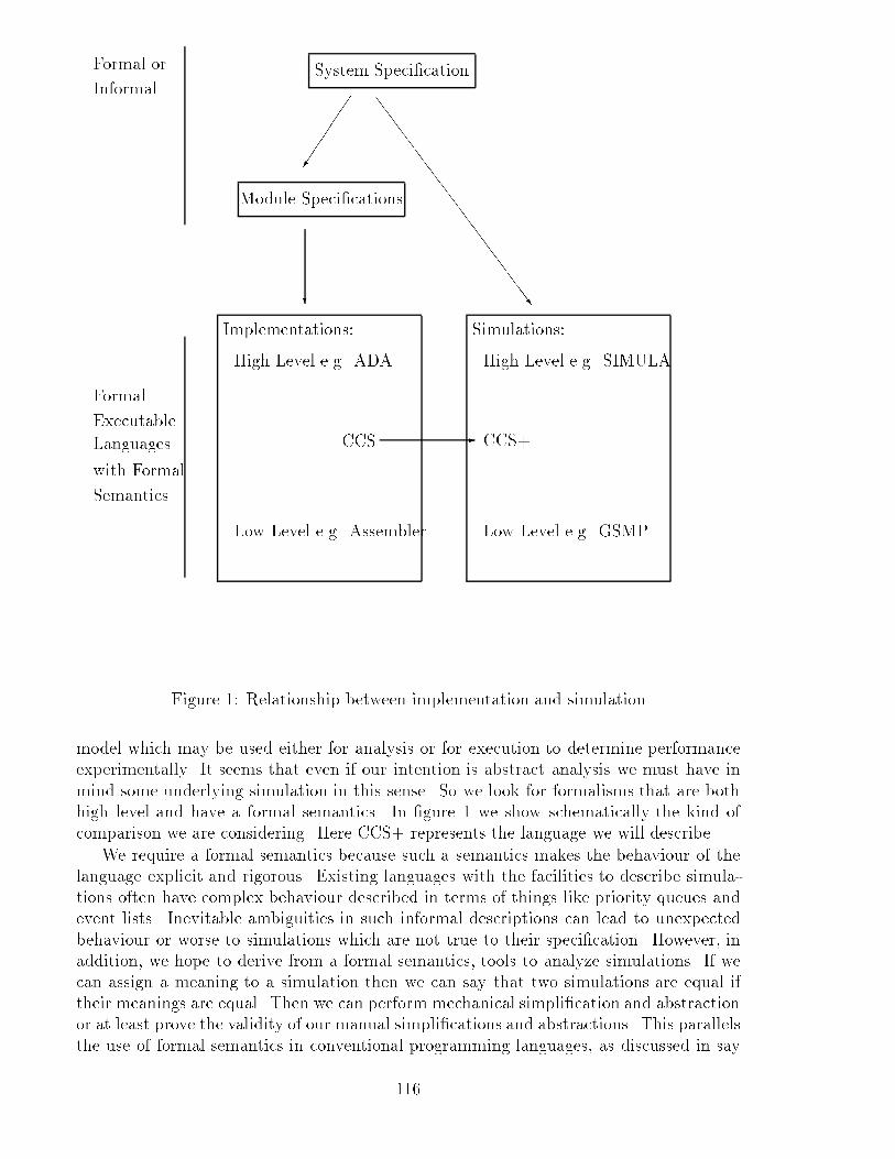
Formal orInformal System Speci�cationModule Speci�cations�FormalExecutableLanguageswith FormalSemantics Implementations: Simulations:?

SSSSSSSSSSSSSSSwHigh Level e.g. ADALow Level e.g. AssemblerCCS High Level e.g. SIMULALow Level e.g. GSMPCCS+-Figure 1: Relationship between implementation and simulationmodel which may be used either for analysis or for execution to determine performanceexperimentally. It seems that even if our intention is abstract analysis we must have inmind some underlying simulation in this sense. So we look for formalisms that are bothhigh level and have a formal semantics. In �gure 1 we show schematically the kind ofcomparison we are considering. Here CCS+ represents the language we will describe.We require a formal semantics because such a semantics makes the behaviour of thelanguage explicit and rigorous. Existing languages with the facilities to describe simula-tions often have complex behaviour described in terms of things like priority queues andevent lists. Inevitable ambiguities in such informal descriptions can lead to unexpectedbehaviour or worse to simulations which are not true to their speci�cation. However, inaddition, we hope to derive from a formal semantics, tools to analyze simulations. If wecan assign a meaning to a simulation then we can say that two simulations are equal iftheir meanings are equal. Then we can perform mechanical simpli�cation and abstractionor at least prove the validity of our manual simpli�cations and abstractions. This parallelsthe use of formal semantics in conventional programming languages, as discussed in say116

[7].We also want our language to be high level. We could certainly consider GeneralisedSemi-Markov Processes (GSMPs) as a semantics for simulation. But a GSMP descrip-tion is very far from any current notion of system speci�cation. Given a system of anycomplexity it is very hard to see that a GSMP description is a correct model of thatsystem. We need to �nd a formalism nearer to speci�cation, more high level and thusmore natural for describing real complex concurrent systems. But we must still have arigorous semantics and thus make our formalism a bridge between informal descriptionsof a system and mathematical models of that system.So by making the language high level we aim to reduce the chance of the originalsimulation being unfaithful to the speci�cation and by making its semantics formal weaim to reduce the chance of any simpli�cations being unfaithful to the original.What is the di�erence between an implementation and a simulation? Firstly, in asimulation, we need to be able to model our workloads while for an implementation theyare supplied by the outside world. Further we need to model them in some detail so as torepresent the demands we expect them to impose on our implementation. Similarly whenwe abstract from detail in our simulation by regarding sub-modules as black boxes weneed to describe their behaviour in more detail than may interest an implementor sincewe want to represent their performance in addition to their abstract behaviour. Thusin a simulation we need to be able to describe both probabilistic behaviour with explicitdistributions and also explicit behaviour in time.Secondly, in a simulation, we are often much more concerned directly with parallelism.Single modules in an implementation are generally sequential and so the implementor maybe able to use sequential languages both for implementation and for module speci�cation.Essentially he may be able to move consideration of parallelism up to the level of the sys-tem speci�cation. In simulation we are modelling the behaviour of the whole system. Oursimulation has to be faithful to the whole system speci�cation and so we will inevitablyneed to be able to describe parallelism explicitly if this is how the system is to operate.Work on formal semantics has very clearly elucidated the behaviour of sequentialsystems. Formal semantics for parallelism have proved more controversial and it is onlyrecently that some consensus about the main approaches has been reached. Surveying theliterature has suggested process algebras as one of the leading contenders [8, 12]. Manyapproaches to extending process algebras with actual time values [3, 1, 2, 6, 13, 16, 10]or with time and probabilities [5] have also been discussed.We use a selection from these approaches with some new techniques to obtain a pro-cess algebra which may be used to describe discrete event simulations. So we take arelatively high level language that has a formal semantics of parallelism (CCS from [8])and add constructs to represent a real-number time and various probabilistic features.We then extend its formal semantics to cover these additions. In this way we can derivesemantically sound axioms relating sub-expressions of a program. Such axioms can formthe basis of mechanisable program transformations which, for example, may allow sim-pler or more e�cient or more mathematically tractable simulations to be derived fromanother with a clearer speci�cation. Again this compares to program transformation indeclarative languages [4].We present a process algebra or programming language, based on CCS, which maybe used to describe concurrent processes. It has extensions to describe the passing oftime and probabilistic choice, either discrete, between a countable number of processes,117

or continuous to choose a random amount of time to wait. It thus has su�cient facilitiesto specify discrete event simulations. It has a clear operational semantics and we discussequivalences over these operational semantics that imply equations on processes that canbe used to work formally with processes.Because it allows both non-determinism and probabilistic choice, it can be used toshow the di�erence between these concepts and their relevance to simulation. It alsoexempli�es some current approaches to adding time and probability to process algebras.2 LanguageFirst we give the language syntax and informally present the intended meaning.The language is based on the timed CCS of [15] with some features of the temporalCCS of [9] though their calculus does not generalise directly to real number time and theyhave more power in that they have a weak + operator that we do not. It ends up veryclose to [2] except we have only two options for the upper limit to the time of execution ofan action. Our impatient pre�xing is equivalent to Chen's �j00 while our idling pre�xingis equivalent to his �(s)j10 .Our language is de�ned so that CCS is a sub-calculus in the sense that the operationalsemantics of the pure CCS terms in our language is the same as in CCS. Our rules forevolution (as in the mentioned calculi) does not behave in exactly the way expected for thetime required to compute. Thus for example it is easy to write programs which performan in�nite amount of computation in �nite time and thus force time to stop for the wholesystem. Other processes simply deadlock in time and also prevent time passing in thewhole system. We justify this by interpreting time evolution as representing simulatedtime rather than the time in which real calculation takes place.As in CCS, communication and synchronisation are represented via an alphabet ofatomic actions or labels. Each action has a conjugate action represented by an overlineand the conjugate to the conjugate is the original action. There is also a distinguishedself-conjugate invisible (or silent) action which represents internal activity of a processinvisible to the outside. Thus we have an alphabet Act including names, co-names andthe invisible action � .We use two sorts and two sets of variables, PVar of sort Process expression, and TVarof sort Time. We use an algebra of time expressions giving a set of expressions TExp.This has the operator + indicating addition and �: indicating non-negative subtractioni.e. x�: y = � x� y x � y0 otherwiseThe other symbols are 0 and an arbitrary number of other constant symbols. We willassume that these constants are non-negative real numbers (we will write R+). Equalityfor this sort is de�ned in the usual way. We will use time expressions and their valuesinterchangeably.Our language is then standard (basic) CCS with this new sort of Time. We then dis-tinguish four forms of pre�xing, one which describes a pre�x of a timed delay, represented(t). This uses the value of the time expression t which may have free variables. We usetwo separate forms of action pre�xing. Simple pre�xing �:P is distinguished from �[s t]where the action pre�x binds the time variable s to the time of occurrence of the action118

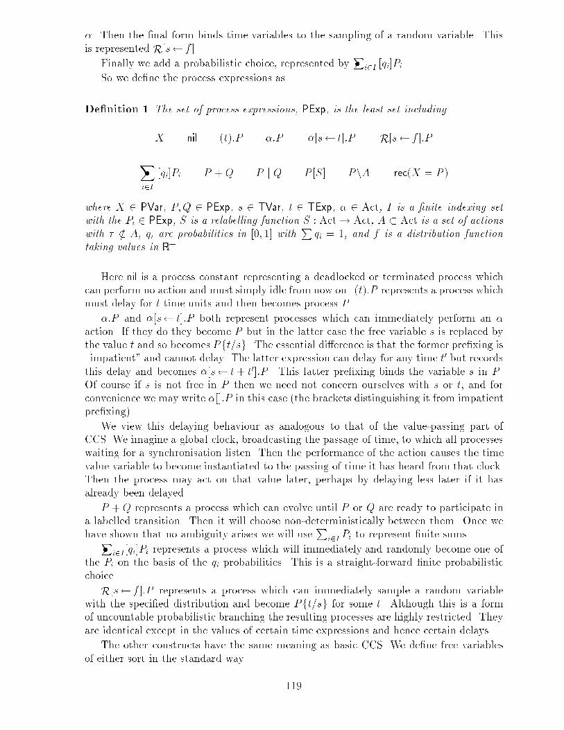
�. Then the �nal form binds time variables to the sampling of a random variable. Thisis represented R[s f ].Finally we add a probabilistic choice, represented by P� i2I [qi]Pi.So we de�ne the process expressions asDe�nition 1 The set of process expressions, PExp, is the least set includingX nil (t):P �:P �[s t]:P R[s f ]:PX�i2I [qi]Pi P +Q P j Q P [S] PnA rec(X = P )where X 2 PVar, P;Q 2 PExp, s 2 TVar, t 2 TExp, � 2 Act, I is a �nite indexing setwith the Pi 2 PExp, S is a relabelling function S : Act! Act, A � Act is a set of actionswith � =2 A, qi are probabilities in [0; 1] with P qi = 1, and f is a distribution functiontaking values in R+.Here nil is a process constant representing a deadlocked or terminated process whichcan perform no action and must simply idle from now on. (t):P represents a process whichmust delay for t time units and then becomes process P .�:P and �[s t]:P both represent processes which can immediately perform an �action. If they do they become P but in the latter case the free variable s is replaced bythe value t and so becomes Pft=sg. The essential di�erence is that the former pre�xing is\impatient" and cannot delay. The latter expression can delay for any time t0 but recordsthis delay and becomes �[s t+ t0]:P . This latter pre�xing binds the variable s in P .Of course if s is not free in P then we need not concern ourselves with s or t, and forconvenience we may write �[]:P in this case (the brackets distinguishing it from impatientpre�xing).We view this delaying behaviour as analogous to that of the value-passing part ofCCS. We imagine a global clock, broadcasting the passage of time, to which all processeswaiting for a synchronisation listen. Then the performance of the action causes the timevalue variable to become instantiated to the passing of time it has heard from that clock.Then the process may act on that value later, perhaps by delaying less later if it hasalready been delayed.P +Q represents a process which can evolve until P or Q are ready to participate ina labelled transition. Then it will choose non-deterministically between them. Once wehave shown that no ambiguity arises we will use Pi2I Pi to represent �nite sums.P� i2I [qi]Pi represents a process which will immediately and randomly become one ofthe Pi on the basis of the qi probabilities. This is a straight-forward �nite probabilisticchoice.R[s f ]:P represents a process which can immediately sample a random variablewith the speci�ed distribution and become Pft=sg for some t. Although this is a formof uncountable probabilistic branching the resulting processes are highly restricted. Theyare identical except in the values of certain time expressions and hence certain delays.The other constructs have the same meaning as basic CCS. We de�ne free variablesof either sort in the standard way. 119

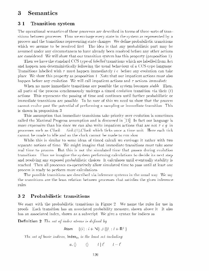
3 Semantics3.1 Transition systemThe operational semantics of these processes are described in terms of three sorts of tran-sitions between processes. Thus we envisage every state in the system as represented by aprocess and the transitions representing state changes. We de�ne probabilistic transitionswhich we assume to be resolved �rst. The idea is that any probabilistic part may beassumed under any circumstances to have already been resolved before any other actionsare considered. We will show that our transition system has this property (proposition 1).Then we have the standard CCS type of labelled transitions which are labelled from Actand happen non-deterministically following the usual behaviour of a CCS-type language.Transitions labelled with � must happen immediately i.e. before any evolution can takeplace. We show this property as proposition 4. Note that our impatient actions must alsohappen before any evolution. We will call impatient actions and � actions immediate.When no more immediate transitions are possible the system becomes stable. Then,all parts of the process synchronously undergo a timed evolution transition via their (t)actions. This represents the passing of time and continues until further probabilistic orimmediate transitions are possible. To be sure of this we need to show that the processcannot evolve past the potential of performing a sampling or immediate transition. Thisis shown in proposition 3.This assumption that immediate transitions take priority over evolution is sometimescalled the Maximal Progress assumption and is discussed in [15]. In fact our language ismore expressive than his since we can also write impatient actions that are not � e.g. inprocesses such as Clock = tick:(1):Clock which ticks once a time unit. Here each tickcannot be made to idle and so the clock cannot be made to run slow.While this is similar to some ideas of timed calculi we envisage it rather with twoseparate notions of time. We might imagine that immediate transitions must take somereal time to process. But this is not the simulated time that passes during evolutiontransitions. Thus we imagine the system performing calculations to decide its next stepand resolving any exposed probabilistic choices. It calculates until eventually stability isreached. Then all processes co-operatively allow simulated time to pass until at least oneprocess is ready to perform more calculations.The possible transitions are described via inference systems in the usual way. We saythe transitions are the least relation between processes that satis�es the given inferencerules.3.2 Probabilistic transitionsWe start with the probabilistic transitions in Figure 2. We name the rules for use inproofs. Each transition has an associated probability measure, shown above it. It alsohas an associated index, shown as a subscript. We give a syntax for indices asDe�nition 2 The set of index atoms is de�ned byAtom= f(i) : i 2 Ng [ f[t] : t 2 R+gThe set of basic indices, Index0, is the least set includinga: hi hi l j l0 l + l0120

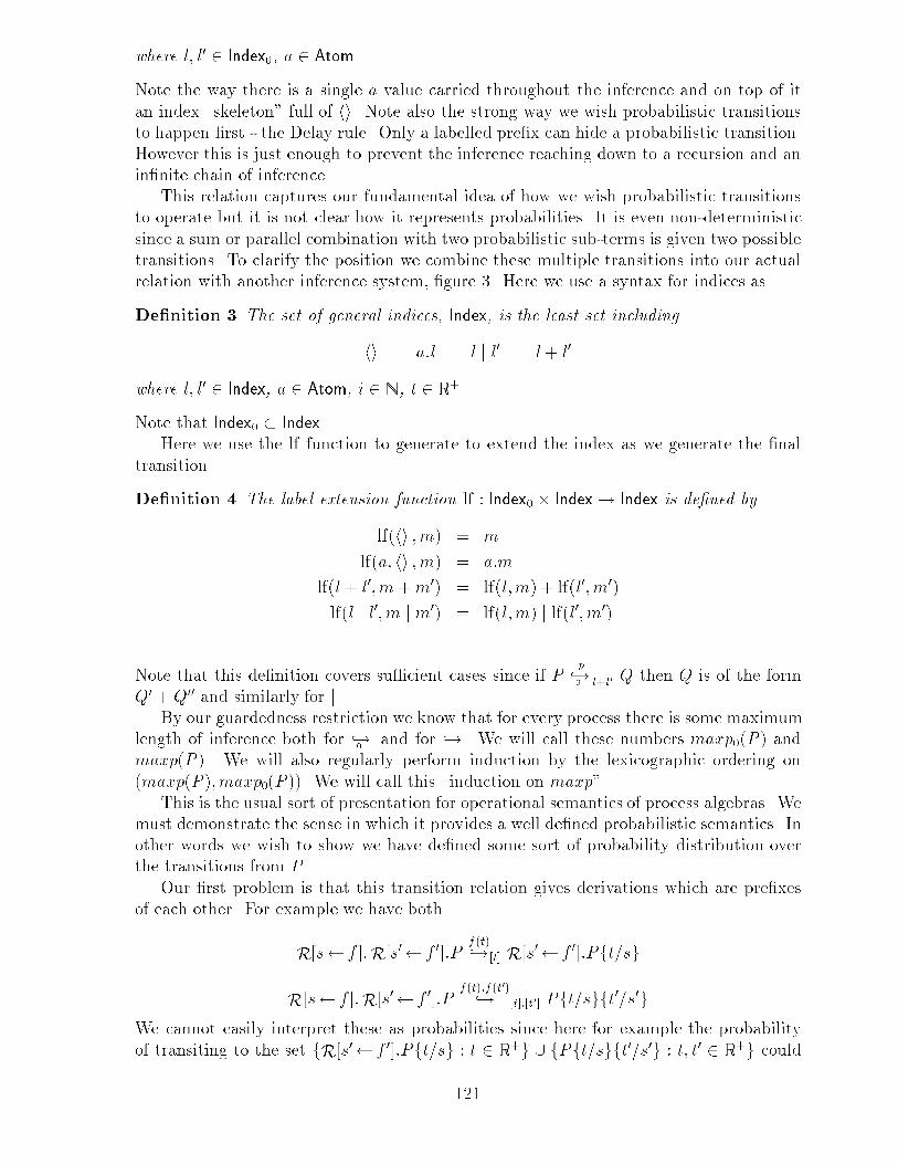
where l; l0 2 Index0, a 2 Atom.Note the way there is a single a value carried throughout the inference and on top of itan index \skeleton" full of hi. Note also the strong way we wish probabilistic transitionsto happen �rst - the Delay rule. Only a labelled pre�x can hide a probabilistic transition.However this is just enough to prevent the inference reaching down to a recursion and anin�nite chain of inference.This relation captures our fundamental idea of how we wish probabilistic transitionsto operate but it is not clear how it represents probabilities. It is even non-deterministicsince a sum or parallel combination with two probabilistic sub-terms is given two possibletransitions. To clarify the position we combine these multiple transitions into our actualrelation with another inference system, �gure 3. Here we use a syntax for indices asDe�nition 3 The set of general indices, Index, is the least set includinghi a:l l j l0 l+ l0where l; l0 2 Index, a 2 Atom, i 2 N, t 2 R+.Note that Index0 � Index.Here we use the lf function to generate to extend the index as we generate the �naltransition.De�nition 4 The label extension function lf : Index0 � Index! Index is de�ned bylf(hi ;m) = mlf(a: hi ;m) = a:mlf(l + l0;m+m0) = lf(l;m) + lf(l0;m0)lf(l j l0;m j m0) = lf(l;m) j lf(l0;m0)Note that this de�nition covers su�cient cases since if P p,!0 l+l0 Q then Q is of the formQ0 +Q00 and similarly for j.By our guardedness restriction we know that for every process there is some maximumlength of inference both for ,!0 and for ,!. We will call these numbers maxp0(P ) andmaxp(P ). We will also regularly perform induction by the lexicographic ordering on(maxp(P );maxp0(P )). We will call this \induction on maxp".This is the usual sort of presentation for operational semantics of process algebras. Wemust demonstrate the sense in which it provides a well de�ned probabilistic semantics. Inother words we wish to show we have de�ned some sort of probability distribution overthe transitions from P .Our �rst problem is that this transition relation gives derivations which are pre�xesof each other. For example we have bothR[s f ]:R[s0 f 0]:P f(t),![t] R[s0 f 0]:Pft=sgR[s f ]:R[s0 f 0]:P f(t):f(t0),! [t]:[t0] Pft=sgft0=s0gWe cannot easily interpret these as probabilities since here for example the probabilityof transiting to the set fR[s0 f 0]:Pft=sg : t 2 R+g [ fPft=sgft0=s0g : t; t0 2 R+g could121

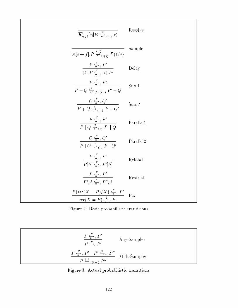
P� i2I [qi]Pi qi,!0 [i]:hi Pi ResolveR[s f ]:P f(t),!0 (t):hi Pft=sg SampleP q,!0 l P 0(t):P q,!0 l (t):P 0 DelayP q,!0 l P 0P +Q q,!0 (l+hi;a) P 0 +Q Sum1Q q,!0 l Q0P +Q q,!0 hi+l P +Q0 Sum2P q,!0 l P 0P j Q q,!0 ljhi P 0 j Q Parallel1Q q,!0 l Q0P j Q q,!0 hijl P j Q0 Parallel2P q,!0 l P 0P [S] q,!0 l P 0[S] RelabelP q,!0 l P 0PnA q,!0 l P 0nA RestrictPfrec(X = P )=Xg q,!0 l P 0rec(X = P ) q,!0 l P 0 FixFigure 2: Basic probabilistic transitionsP p,!0 l P 0P p,!l P 0 Any-SamplesP p,!0 l P 0 P 0 q,!m P 00P p:q,!lf(l;m) P 00 Mult-SamplesFigure 3: Actual probabilistic transitions122

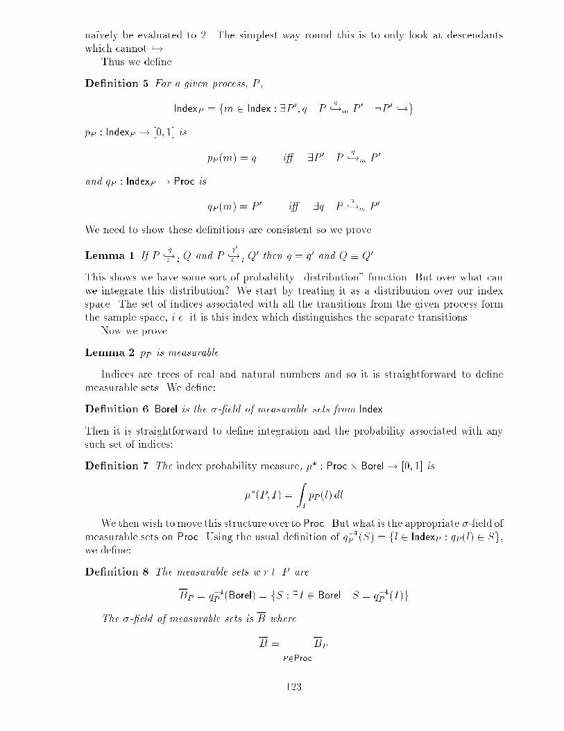
na��vely be evaluated to 2. The simplest way round this is to only look at descendantswhich cannot ,!.Thus we de�neDe�nition 5 For a given process, P ,IndexP = fm 2 Index : 9P 0; q P q,!m P 0 :P 0 ,!gpP : IndexP ! [0; 1] is pP (m) = q i� 9P 0 P q,!m P 0and qP : IndexP ! Proc isqP (m) = P 0 i� 9q P q,!m P 0We need to show these de�nitions are consistent so we proveLemma 1 If P q,!0 l Q and P q0,!0 l Q0 then q = q0 and Q � Q0.This shows we have some sort of probability \distribution" function. But over what canwe integrate this distribution? We start by treating it as a distribution over our indexspace. The set of indices associated with all the transitions from the given process formthe sample space, i.e. it is this index which distinguishes the separate transitions.Now we proveLemma 2 pP is measurable.Indices are trees of real and natural numbers and so it is straightforward to de�nemeasurable sets. We de�ne:De�nition 6 Borel is the �-�eld of measurable sets from Index.Then it is straightforward to de�ne integration and the probability associated with anysuch set of indices:De�nition 7 The index probability measure, �� : Proc� Borel! [0; 1] is��(P; I) = ZI pP (l) dlWe then wish to move this structure over to Proc. But what is the appropriate �-�eld ofmeasurable sets on Proc. Using the usual de�nition of q�1P (S) = fl 2 IndexP : qP (l) 2 Sg,we de�ne:De�nition 8 The measurable sets w.r.t. P areBP = q�1P (Borel) = fS : 9I 2 Borel S = q�1P (I)gThe �-�eld of measurable sets is B whereB = \P2ProcBP123

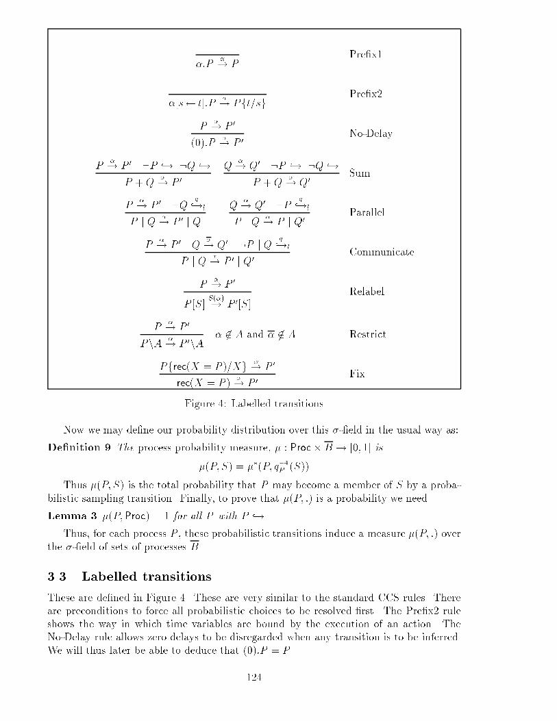
�:P �! P Pre�x1�[s t]:P �! Pft=sg Pre�x2P �! P 0(0):P �! P 0 No-DelayP �! P 0 :P ,! :Q ,!P +Q �! P 0 Q �! Q0 :P ,! :Q ,!P +Q �! Q0 SumP �! P 0 :Q q,!lP j Q �! P 0 j Q Q �! Q0 :P q,!lP j Q �! P j Q0 ParallelP �! P 0 Q �! Q0 :P j Q q,!lP j Q �! P 0 j Q0 CommunicateP �! P 0P [S] S(�)! P 0[S] RelabelP �! P 0PnA �! P 0nA � 62 A and � 62 A RestrictPfrec(X = P )=Xg �! P 0rec(X = P ) �! P 0 FixFigure 4: Labelled transitionsNow we may de�ne our probability distribution over this �-�eld in the usual way as:De�nition 9 The process probability measure, � : Proc�B ! [0; 1] is�(P; S) = ��(P; q�1P (S))Thus �(P; S) is the total probability that P may become a member of S by a proba-bilistic sampling transition. Finally, to prove that �(P; :) is a probability we needLemma 3 �(P;Proc) = 1 for all P with P ,!.Thus, for each process P , these probabilistic transitions induce a measure �(P; :) overthe �-�eld of sets of processes B.3.3 Labelled transitionsThese are de�ned in Figure 4. These are very similar to the standard CCS rules. Thereare preconditions to force all probabilistic choices to be resolved �rst. The Pre�x2 ruleshows the way in which time variables are bound by the execution of an action. TheNo-Delay rule allows zero delays to be disregarded when any transition is to be inferred.We will thus later be able to deduce that (0):P = P .124

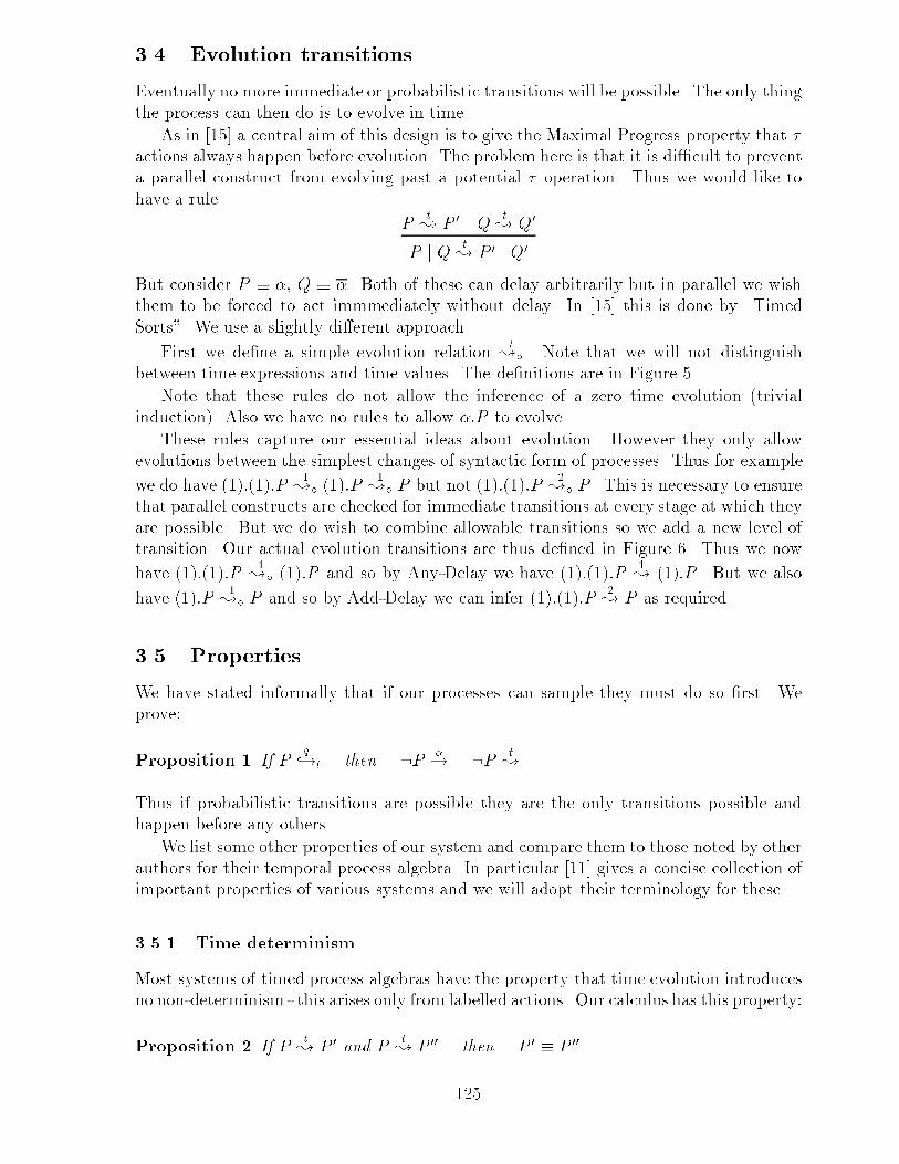
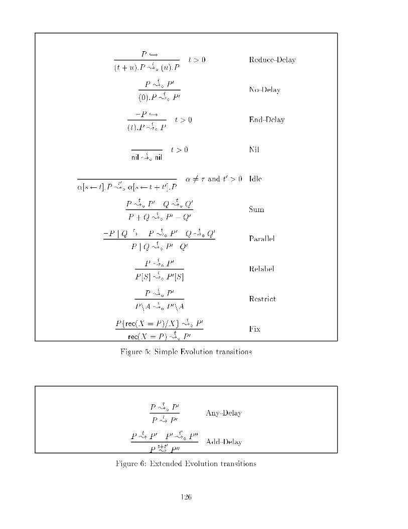
3.4 Evolution transitionsEventually no more immediate or probabilistic transitions will be possible. The only thingthe process can then do is to evolve in time.As in [15] a central aim of this design is to give the Maximal Progress property that �actions always happen before evolution. The problem here is that it is di�cult to preventa parallel construct from evolving past a potential � operation. Thus we would like tohave a rule P t; P 0 Q t; Q0P j Q t; P 0 j Q0But consider P � �, Q � �. Both of these can delay arbitrarily but in parallel we wishthem to be forced to act immmediately without delay. In [15] this is done by \TimedSorts". We use a slightly di�erent approach.First we de�ne a simple evolution relation t;�. Note that we will not distinguishbetween time expressions and time values. The de�nitions are in Figure 5.Note that these rules do not allow the inference of a zero time evolution (trivialinduction). Also we have no rules to allow �:P to evolve.These rules capture our essential ideas about evolution. However they only allowevolutions between the simplest changes of syntactic form of processes. Thus for examplewe do have (1):(1):P 1;� (1):P 1;� P but not (1):(1):P 2;� P . This is necessary to ensurethat parallel constructs are checked for immediate transitions at every stage at which theyare possible. But we do wish to combine allowable transitions so we add a new level oftransition. Our actual evolution transitions are thus de�ned in Figure 6. Thus we nowhave (1):(1):P 1;� (1):P and so by Any-Delay we have (1):(1):P 1; (1):P . But we alsohave (1):P 1;� P and so by Add-Delay we can infer (1):(1):P 2; P as required.3.5 PropertiesWe have stated informally that if our processes can sample they must do so �rst. Weprove:Proposition 1 If P q,!l then :P �! :P t;.Thus if probabilistic transitions are possible they are the only transitions possible andhappen before any others.We list some other properties of our system and compare them to those noted by otherauthors for their temporal process algebra. In particular [11] gives a concise collection ofimportant properties of various systems and we will adopt their terminology for these.3.5.1 Time determinismMost systems of timed process algebras have the property that time evolution introducesno non-determinism - this arises only from labelled actions. Our calculus has this property:Proposition 2 If P t; P 0 and P t; P 00 then P 0 � P 00.125

:P ,!(t+ u):P t;� (u):P t > 0 Reduce-DelayP t;� P 0(0):P t;� P 0 No-Delay:P ,!(t):P t;� P t > 0 End-Delaynil t;� nil t > 0 Nil�[s t]:P t0;� �[s t+ t0]:P � 6= � and t0 > 0 IdleP t;� P 0 Q t;� Q0P +Q t;� P 0 +Q0 Sum:P j Q �! P t;� P 0 Q t;� Q0P j Q t;� P 0 j Q0 ParallelP t;� P 0P [S] t;� P 0[S] RelabelP t;� P 0PnA t;� P 0nA RestrictPfrec(X = P )=Xg t;� P 0rec(X = P ) t;� P 0 FixFigure 5: Simple Evolution transitionsP t;� P 0P t; P 0 Any-DelayP t; P 0 P 0 t0;� P 00P t+t0; P 00 Add-DelayFigure 6: Extended Evolution transitions126

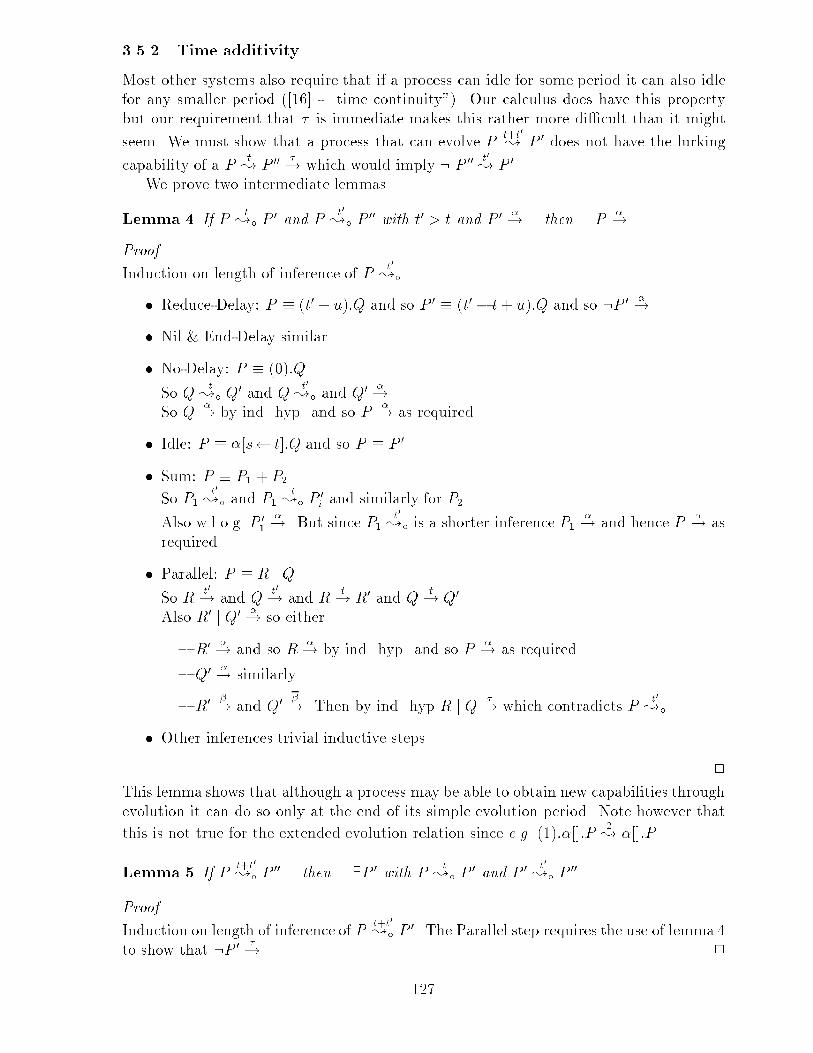
3.5.2 Time additivityMost other systems also require that if a process can idle for some period it can also idlefor any smaller period ([16] - \time continuity"). Our calculus does have this propertybut our requirement that � is immediate makes this rather more di�cult than it mightseem. We must show that a process that can evolve P t+t0; P 0 does not have the lurkingcapability of a P t; P 00 �! which would imply : P 00 t0; P 0.We prove two intermediate lemmas.Lemma 4 If P t;� P 0 and P t0;� P 00 with t0 > t and P 0 �! then P �!.ProofInduction on length of inference of P t0;�.� Reduce-Delay: P � (t0 + u):Q and so P 0 � (t0 � t+ u):Q and so :P 0 �!� Nil & End-Delay similar� No-Delay: P � (0):QSo Q t;� Q0 and Q t0;� and Q0 �!So Q �! by ind. hyp. and so P �! as required.� Idle: P � �[s t]:Q and so P � P 0� Sum: P � P1 + P2So P1 t0;� and P1 t;� P 0i and similarly for P2.Also w.l.o.g. P 01 �!. But since P1 t0;� is a shorter inference P1 �! and hence P �! asrequired.� Parallel: P � R j QSo R t0! and Q t0! and R t! R0 and Q t! Q0Also R0 j Q0 �! so either{ R0 �! and so R �! by ind. hyp. and so P �! as required.{ Q0 �! similarly.{ R0 �! and Q0 �!. Then by ind. hyp R j Q �! which contradicts P t0;�� Other inferences trivial inductive steps. 2This lemma shows that although a process may be able to obtain new capabilities throughevolution it can do so only at the end of its simple evolution period. Note however thatthis is not true for the extended evolution relation since e.g. (1):�[]:P 2; �[]:P .Lemma 5 If P t+t0;� P 00 then 9P 0 with P t;� P 0 and P 0 t0;� P 00.ProofInduction on length of inference of P t+t0;� P 0. The Parallel step requires the use of lemma 4to show that :P 0 �!. 2127

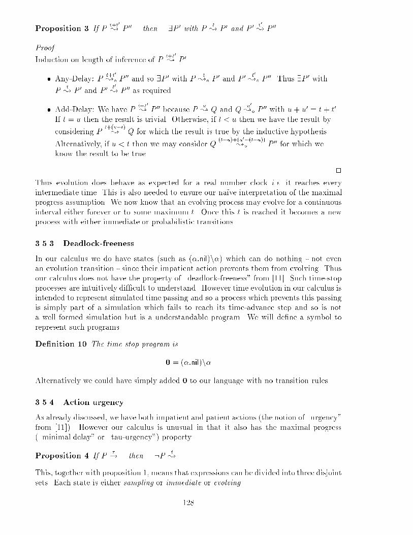
Proposition 3 If P t+t0; P 00 then 9P 0 with P t; P 0 and P 0 t0; P 00.ProofInduction on length of inference of P t+t0; P 0.� Any-Delay: P t+t0;� P 00 and so 9P 0 with P t;� P 0 and P 0 t0;� P 00. Thus 9P 0 withP t; P 0 and P 0 t0; P 00 as required.� Add-Delay: We have P t+t0; P 00 because P u; Q and Q u0;� P 00 with u+ u0 = t+ t0.If t = u then the result is trivial. Otherwise, if t < u then we have the result byconsidering P t+(u�t); Q for which the result is true by the inductive hypothesis.Alternatively, if u < t then we may consider Q (t�u)+(u0�(t�u));� P 00 for which weknow the result to be true. 2Thus evolution does behave as expected for a real number clock i.e. it reaches everyintermediate time. This is also needed to ensure our na��ve interpretation of the maximalprogress assumption. We now know that an evolving process may evolve for a continuousinterval either forever or to some maximum t. Once this t is reached it becomes a newprocess with either immediate or probabilistic transitions.3.5.3 Deadlock-freenessIn our calculus we do have states (such as (�:nil)n�) which can do nothing - not evenan evolution transition - since their impatient action prevents them from evolving. Thusour calculus does not have the property of \deadlock-freeness" from [11]. Such time-stopprocesses are intuitively di�cult to understand. However time evolution in our calculus isintended to represent simulated time passing and so a process which prevents this passingis simply part of a simulation which fails to reach its time-advance step and so is nota well formed simulation but is a understandable program. We will de�ne a symbol torepresent such programsDe�nition 10 The time stop program is0 = (�:nil)n�Alternatively we could have simply added 0 to our language with no transition rules.3.5.4 Action urgencyAs already discussed, we have both impatient and patient actions (the notion of \urgency"from [11]). However our calculus is unusual in that it also has the maximal progress(\minimal delay" or \tau-urgency") property.Proposition 4 If P �! then :P t;.This, together with proposition 1, means that expressions can be divided into three disjointsets. Each state is either sampling or immediate or evolving.128

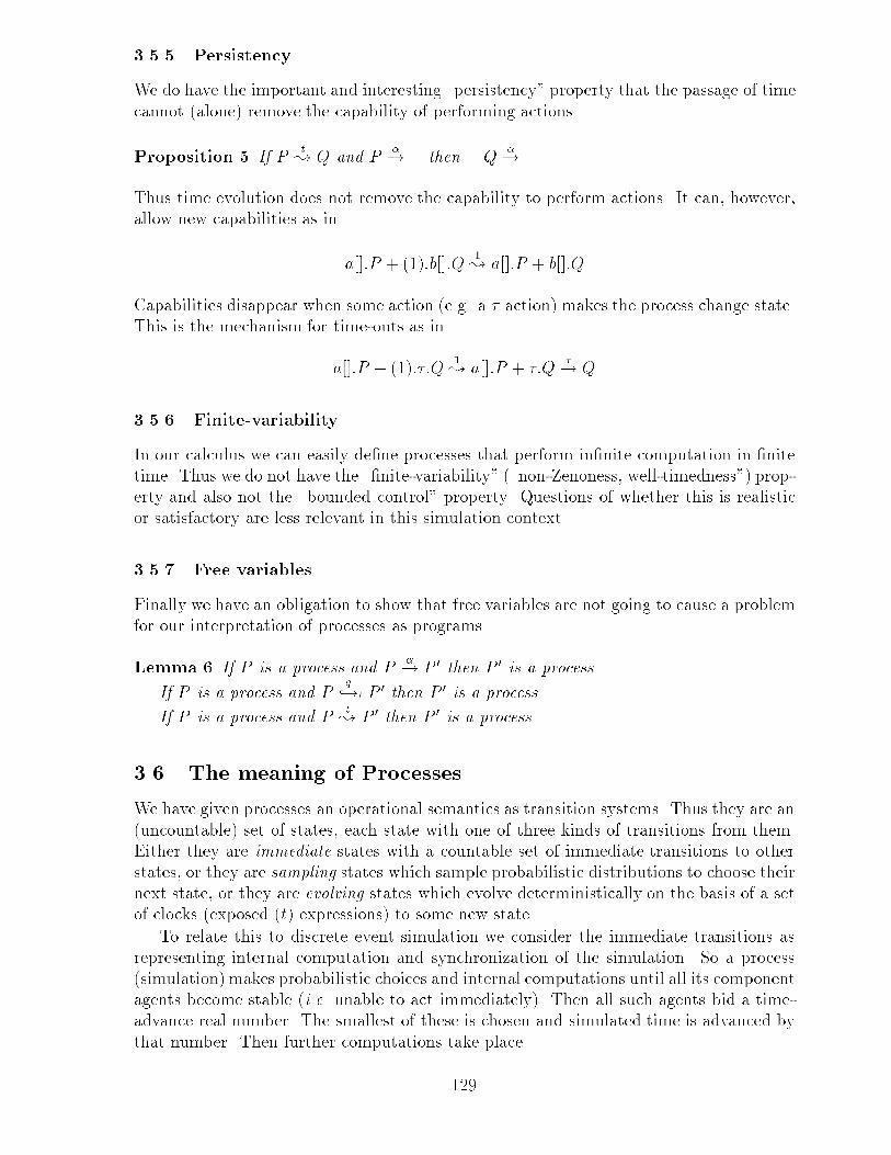
3.5.5 PersistencyWe do have the important and interesting \persistency" property that the passage of timecannot (alone) remove the capability of performing actions.Proposition 5 If P t; Q and P �! then Q �!.Thus time evolution does not remove the capability to perform actions. It can, however,allow new capabilities as in a[]:P + (1):b[]:Q 1; a[]:P + b[]:QCapabilities disappear when some action (e.g. a � action) makes the process change state.This is the mechanism for time-outs as ina[]:P + (1):�:Q 1; a[]:P + �:Q �! Q3.5.6 Finite-variabilityIn our calculus we can easily de�ne processes that perform in�nite computation in �nitetime. Thus we do not have the \�nite-variability" (\non-Zenoness, well-timedness") prop-erty and also not the \bounded control" property. Questions of whether this is realisticor satisfactory are less relevant in this simulation context.3.5.7 Free variablesFinally we have an obligation to show that free variables are not going to cause a problemfor our interpretation of processes as programs.Lemma 6 If P is a process and P �! P 0 then P 0 is a process.If P is a process and P q,!l P 0 then P 0 is a process.If P is a process and P t; P 0 then P 0 is a process.3.6 The meaning of ProcessesWe have given processes an operational semantics as transition systems. Thus they are an(uncountable) set of states, each state with one of three kinds of transitions from them.Either they are immediate states with a countable set of immediate transitions to otherstates, or they are sampling states which sample probabilistic distributions to choose theirnext state, or they are evolving states which evolve deterministically on the basis of a setof clocks (exposed (t) expressions) to some new state.To relate this to discrete event simulation we consider the immediate transitions asrepresenting internal computation and synchronization of the simulation. So a process(simulation) makes probabilistic choices and internal computations until all its componentagents become stable (i.e. unable to act immediately). Then all such agents bid a time-advance real number. The smallest of these is chosen and simulated time is advanced bythat number. Then further computations take place.129

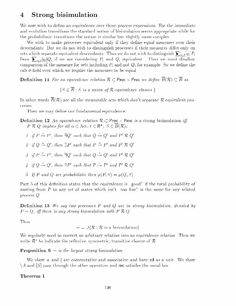
4 Strong bisimulationWe now wish to de�ne an equivalence over these process expressions. For the immediateand evolution transitions the standard notion of bisimulation seems appropriate while forthe probabilistic transitions the notion is similar but slightly more complex.We wish to make processes equivalent only if they de�ne equal measures over theirdescendants. But we do not wish to distinguish processes if their measures di�er only onsets which separate equivalent descendants. Thus we do not wish to distinguishP� i2I [qi]Pifrom P� i2I [qi]Qi if we are considering Pi and Qi equivalent. Thus we must disallowcomparison of the measure for sets including Pi and not Qi for example. So we de�ne thesub �-�eld over which we require the measures to be equal.De�nition 11 For an equivalence relation R � Proc� Proc we de�ne B(R) � B asfS 2 B : S is a union of R-equivalence classes gIn other words B(R) are all the measurable sets which don't separate R-equivalent pro-cesses.Then we may de�ne our fundamental equivalence:De�nition 12 An equivalence relation R � Proc� Proc is a strong bisimulation i�P R Q implies for all � 2 Act, t 2 R+, S 2 B(R):1. if P �! P 0, then 9Q0 such that Q �! Q0 and P 0 R Q0.2. if Q �! Q0, then 9P 0 such that P �! P 0 and P 0 R Q0.3. if P t; P 0, then 9Q0 such that Q t; Q0 and P 0 R Q0.4. if Q t; Q0, then 9P 0 such that P t; P 0 and P 0 R Q0.5. If P and Q are probabilistic then �(P; S) = �(Q;S).Part 5 of this de�nition states that the equivalence is \good" if the total probability ofmoving from P to any set of states which isn't \too �ne" is the same for any relatedprocess Q.De�nition 13 We say two processes P and Q are in strong bisimulation, denoted byP � Q, i� there is any strong bisimulation with P R Q.Thus � = [fR : R is a bisimulationgWe regularly need to convert an arbitrary relation into an equivalence relation. Thus wewrite R� to indicate the re exive, symmetric, transitive closure of R.Proposition 6 � is the largest strong bisimulationWe show + and j are commutative and associative and have nil as a unit. We shownA and [S] pass through the other operators and rec satisifes the usual law.Theorem 1 130

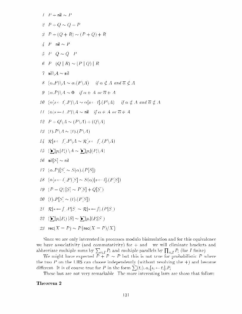
1. P + nil � P2. P +Q � Q+ P3. P + (Q+R) � (P +Q) +R4. P j nil � P5. P j Q � Q j P6. P j (Q j R) � (P j Q) j R7. nilnA � nil8. (�:P )nA � �:(PnA) if � =2 A and � =2 A9. (�:P )nA � 0 if � 2 A or � 2 A10. (�[s t]:P )nA � �[s t]:(PnA) if � =2 A and � =2 A11. (�[s t]:P )nA � nil if � 2 A or � 2 A12. P +QnA � (PnA) + (QnA)13. (t):PnA � (t):(PnA)14. R[s f ]:PnA � R[s f ]:(PnA)15. (P� [pi]Pi) nA �P� [pi](PinA)16. nil[S] � nil17. (�:P )[S] � S(�):(P [S])18. (�[s t]:P )[S] � S(�)[s t]:(P [S])19. (P +Q) [S] � P [S] +Q[S])20. (t):P [S] � (t):(P [S])21. R[s f ]:P [S] � R[s f ]:(P [S])22. (P� [pi]Pi) [S] �P� [pi](Pi[S])23. rec(X = P ) � Pfrec(X = P )=XgSince we are only interested in processes modulo bisimulation and for this equivalencewe have associativity (and commutativity) for + and j we will eliminate brackets andabbreviate multiple sums by Pi2I Pi and multiple parallels by Qi2I Pi (for I �nite).We might have expected P + P � P but this is not true for probabilistic P wherethe two P on the LHS can choose independently (without resolving the +) and becomedi�erent. It is of course true for P in the formP(ti): �i[si ti]:Pi.These last are not very remarkable. The more interesting laws are those that follow:Theorem 2 131

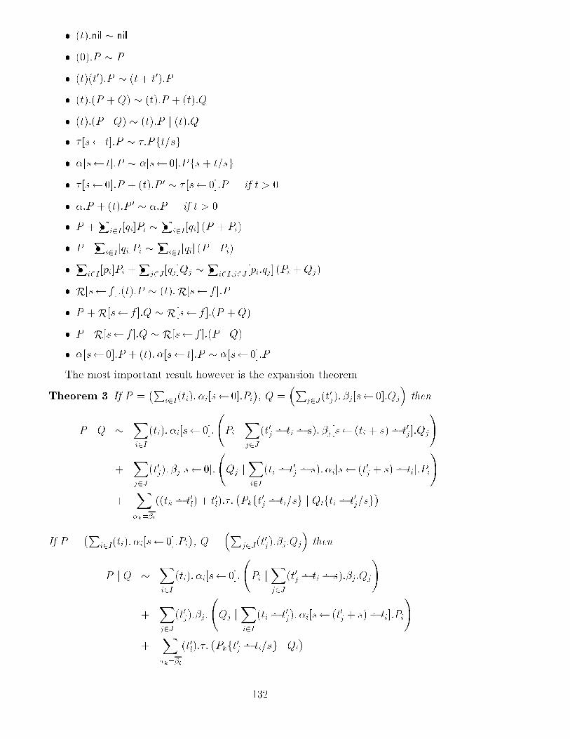
� (t):nil � nil� (0):P � P� (t)(t0):P � (t+ t0):P� (t):(P +Q) � (t):P + (t):Q� (t):(P j Q) � (t):P j (t):Q� � [s t]:P � �:Pft=sg� �[s t]:P � �[s 0]:Pfs+ t=sg� � [s 0]:P + (t):P 0 � � [s 0]:P if t > 0� �:P + (t):P 0 � �:P if t > 0� P +P� i2I [qi]Pi �P� i2I[qi] (P + Pi)� P jP� i2I[qi]Pi �P� i2I [qi] (P j Pi)� P� i2I[pi]Pi +P� j2J [qj]Qj �P� i2I;j2J [pi:qj] (Pi +Qj)� R[s f ]:(t):P � (t):R[s f ]:P� P +R[s f ]:Q � R[s f ]:(P +Q)� P j R[s f ]:Q � R[s f ]:(P j Q)� �[s 0]:P + (t): �[s t]:P � �[s 0]:PThe most important result however is the expansion theorem.Theorem 3 If P = �Pi2I(ti): �i[s 0]:Pi�, Q = �Pj2J (t0j): �j[s 0]:Qj� thenP j Q � Xi2I (ti): �i[s 0]: Pi jXj2J (t0j �: ti �: s): �j[s (ti + s)�: t0j]:Qj!+ Xj2J (t0j): �j[s 0]: Qj jXi2I (ti �: t0j �: s): �i[s (t0j + s)�: ti]:Pi!+ X�k=�l((tk �: t0l) + t0l):�: �Pkft0j �: ti=sg j Qlfti �: t0j=sg�If P = �Pi2I(ti): �i[s 0]:Pi�, Q = �Pj2J(t0j):�j:Qj� thenP j Q � Xi2I (ti): �i[s 0]: Pi jXj2J (t0j �: ti �: s):�j:Qj!+ Xj2J (t0j):�j: Qj jXi2I (ti �: t0j): �i[s (t0j + s)�: ti]:Pi!+ X�k=�l(t0l):�: �Pkft0j �: ti=sg j Ql�132

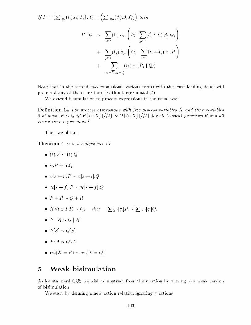
If P = �Pi2I(ti):�i:Pi�, Q = �Pj2J(t0j):�j:Qj� thenP j Q � Xi2I (ti):�i: Pi jXj2J (t0j �: ti):�j:Qj!+ Xj2J (t0j):�j: Qj jXi2I (ti �: t0j):�i:Pi!+ X�k=�l;tk=t0l(tk):�: (Pk j Ql)Note that in the second two expansions, various terms with the least leading delay willpre-empt any of the other terms with a larger initial (t).We extend bisimulation to process expressions in the usual way.De�nition 14 For process expressions with free process variables ~X and time variables~s at most, P � Q i� Pf ~R= ~Xgf~t=~sg � Qf ~R= ~Xgf~t=~sg for all (closed) processes ~R and allclosed time expressions ~t.Then we obtainTheorem 4 � is a congruence i.e.� (t):P � (t):Q� �:P � �:Q� �[s t]:P � �[s t]:Q� R[s f ]:P � R[s f ]:Q� P +R � Q+R� If 8i 2 I Pi � Qi then P� i2I[qi]Pi �P� i2I[qi]Qi� P j R � Q j R� P [S] � Q[S]� PnA � QnA� rec(X = P ) � rec(X = Q)5 Weak bisimulationAs for standard CCS we wish to abstract from the � action by moving to a weak versionof bisimulation.We start by de�ning a new action relation ignoring � actions.133

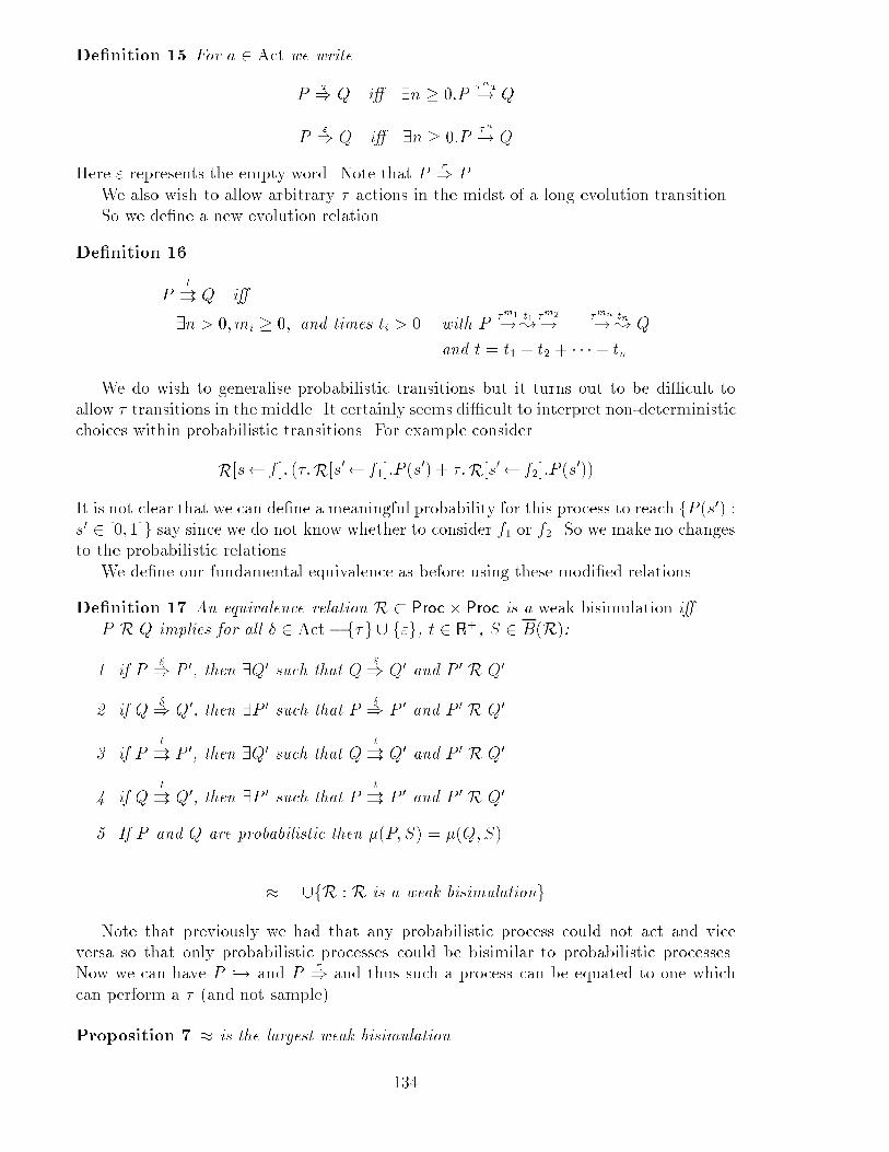
De�nition 15 For a 2 Act we writeP a) Q i� 9n � 0:P �na! QP ") Q i� 9n � 0:P �n! QHere " represents the empty word. Note that P ") P .We also wish to allow arbitrary � actions in the midst of a long evolution transition.So we de�ne a new evolution relation.De�nition 16P t� Q i�9n > 0;mi � 0; and times ti > 0 with P �m1! t1;�m2! . . . �mn! tn; Qand t = t1 + t2 + � � �+ tnWe do wish to generalise probabilistic transitions but it turns out to be di�cult toallow � transitions in the middle. It certainly seems di�cult to interpret non-deterministicchoices within probabilistic transitions. For example considerR[s f ]: (�:R[s0 f1]:P (s0) + �:R[s0 f2]:P (s0))It is not clear that we can de�ne a meaningful probability for this process to reach fP (s0) :s0 2 [0; 1]g say since we do not know whether to consider f1 or f2. So we make no changesto the probabilistic relations.We de�ne our fundamental equivalence as before using these modi�ed relationsDe�nition 17 An equivalence relation R � Proc� Proc is a weak bisimulation i�P R Q implies for all � 2 Act� f�g [ f"g, t 2 R+, S 2 B(R):1. if P �) P 0, then 9Q0 such that Q �) Q0 and P 0 R Q0.2. if Q �) Q0, then 9P 0 such that P �) P 0 and P 0 R Q0.3. if P t� P 0, then 9Q0 such that Q t� Q0 and P 0 R Q0.4. if Q t� Q0, then 9P 0 such that P t� P 0 and P 0 R Q0.5. If P and Q are probabilistic then �(P; S) = �(Q;S).� = [fR : R is a weak bisimulationgNote that previously we had that any probabilistic process could not act and viceversa so that only probabilistic processes could be bisimilar to probabilistic processes.Now we can have P ,! and P ") and thus such a process can be equated to one whichcan perform a � (and not sample).Proposition 7 � is the largest weak bisimulation134

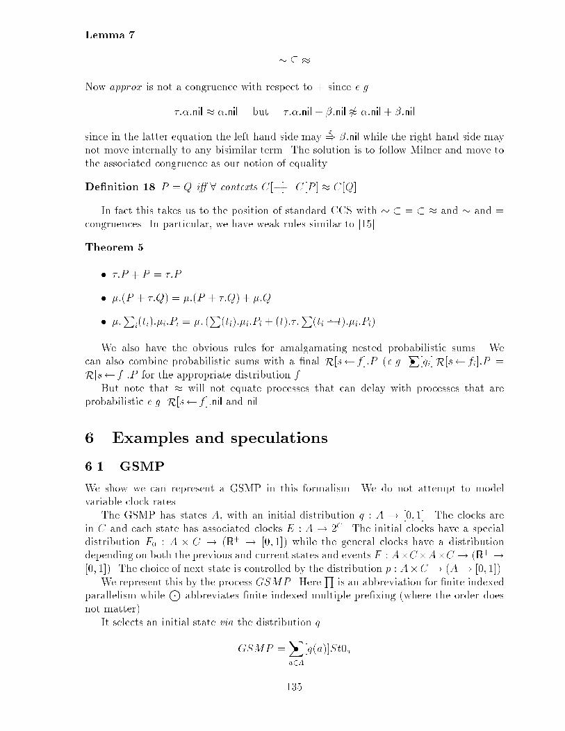
Lemma 7 � � �Now approx is not a congruence with respect to + since e.g.�:�:nil � �:nil but �:�:nil + �:nil 6� �:nil + �:nilsince in the latter equation the left hand side may ") �:nil while the right hand side maynot move internally to any bisimilar term. The solution is to follow Milner and move tothe associated congruence as our notion of equality.De�nition 18 P = Q i� 8 contexts C[�] C[P ] � C[Q].In fact this takes us to the position of standard CCS with � � = � � and � and =congruences. In particular, we have weak rules similar to [15].Theorem 5� �:P + P = �:P .� �:(P + �:Q) = �:(P + �:Q) + �:Q.� �:Pi(ti):�i:Pi = �: (P(ti):�i:Pi + (t):�:P(ti �: t):�i:Pi)We also have the obvious rules for amalgamating nested probabilistic sums. Wecan also combine probabilistic sums with a �nal R[s f ]:P (e.g. P� [qi]R[s fi]:P =R[s f ]:P for the appropriate distribution f .But note that � will not equate processes that can delay with processes that areprobabilistic e.g. R[s f ]:nil and nil.6 Examples and speculations6.1 GSMPWe show we can represent a GSMP in this formalism. We do not attempt to modelvariable clock rates.The GSMP has states A, with an initial distribution q : A ! [0; 1]. The clocks arein C and each state has associated clocks E : A ! 2C . The initial clocks have a specialdistribution F0 : A � C ! (R+ ! [0; 1]) while the general clocks have a distributiondepending on both the previous and current states and events F : A�C�A�C ! (R+ ![0; 1]). The choice of next state is controlled by the distribution p : A�C ! (A! [0; 1]).We represent this by the process GSMP . HereQ is an abbreviation for �nite indexedparallelism while J abbreviates �nite indexed multiple pre�xing (where the order doesnot matter).It selects an initial state via the distribution q.GSMP =X�a2A[q(a)]St0a135

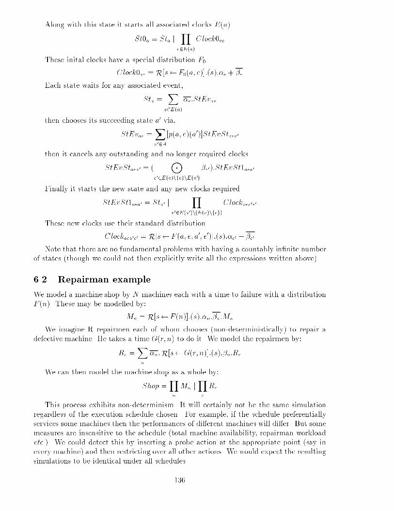
Along with this state it starts all associated clocks E(a).St0a = Sta j Ye2E(a)Clock0aeThese inital clocks have a special distribution F0.Clock0ae = R[s F0(a; e)]:(s):�e + �eEach state waits for any associated event,Sta = Xe2E(a)�e:StEvaethen chooses its succeeding state a0 via,StEvae = X�a02A[p(a; e)(a0)]StEvStaea0then it cancels any outstanding and no longer required clocks.StEvStaea0 = ( Ke02E(a)nfegnE(a0)�e0):StEvSt1aea0Finally it starts the new state and any new clocks required.StEvSt1aea0 = Sta0 j Ye02E(a0)n(E(a)nfeg)Clockaea0e0These new clocks use their standard distribution.Clockaea0e0 = R[s F (a; e; a0; e0)]:(s):�e0 + �e0Note that there are no fundamental problems with having a countably in�nite numberof states (though we could not then explicitly write all the expressions written above).6.2 Repairman exampleWe model a machine shop by N machines each with a time to failure with a distributionF (n). These may be modelled by:Mn = R[s F (n)]:(s):�n:�n:MnWe imagine R repairmen each of whom chooses (non-deterministically) to repair adefective machine. He takes a time G(r; n) to do it. We model the repairmen by:Rr =Xn �n:R[s G(r; n)]:(s):�n:RrWe can then model the machine shop as a whole by:Shop =Yn Mn jYr RrThis process exhibits non-determinism. It will certainly not be the same simulationregardless of the execution schedule chosen. For example, if the schedule preferentiallyservices some machines then the performances of di�erent machines will di�er. But somemeasures are insensitive to the schedule (total machine availability, repairman workloadetc.). We could detect this by inserting a probe action at the appropriate point (say inevery machine) and then restricting over all other actions. We would expect the resultingsimulations to be identical under all schedules.136

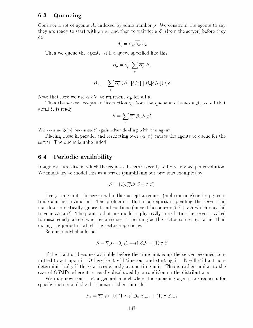
6.3 QueueingConsider a set of agents Ap indexed by some number p. We constrain the agents to saythey are ready to start with an �p and then to wait for a �p (from the server) before theydo. A0p = �p:�p:ApThen we queue the agents with a queue speci�ed like this:Bp = p:Xp �p:BpB1 =Xp �p:(B1[�= ] j Bp[�=�]) n �Note that here we use � etc. to represent �p for all p.Then the server accepts an instruction p from the queue and issues a �p to tell thatagent it is ready. S =Xp p:�p:S(p)We assume S(p) becomes S again after dealing with the agent.Placing these in parallel and restricting over f�; �g causes the agents to queue for theserver. The queue is unbounded.6.4 Periodic availabilityImagine a hard disc in which the requested sector is ready to be read once per revolution.We might try to model this as a server (simplifying our previous example) byS = (1):( :�:S + �:S)Every time unit this server will either accept a request (and continue) or simply con-tinue another revolution. The problem is that if a request is pending the server cannon-deterministically ignore it and continue (since it becomes �:�:S+ �:S which may failto generate a �). The point is that our model is physically unrealistic: the server is askedto instaneously assess whether a request is pending as the sector comes by, rather thanduring the period in which the sector approaches.So our model should be:S = [s 0]:(1�: s):�:S + (1):�:SIf the action becomes available before the time unit is up the server becomes com-mitted to act upon it. Otherwise it will time out and start again. It will still act non-deterministically if the arrives exactly at one time unit. This is rather similar to thecase of GSMPs where it is usually disallowed by a condition on the distributions.We may now construct a general model where the queueing agents are requests forspeci�c sectors and the disc presents them in order.Sn = n[s 0]:(1�: s):�n:Sn+1 + (1):�:Sn+1137

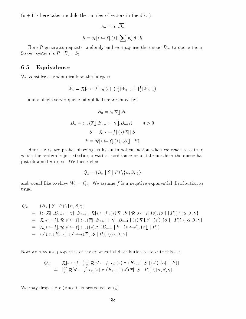
(n+ 1 is here taken modulo the number of sectors in the disc.)An = �n:�nR = R[s f ]:(s):X� [pi]Ai:RHere R generates requests randomly and we may use the queue B1 to queue them.So our system is R j B1 j S1.6.5 EquivalenceWe consider a random walk on the integers:W0 = R[s f ]:�0:(s): �[12]Wn�1 u [12]Wn+1�and a single server queue (simpli�ed) represented by:B0 = �0:�[]:B1Bn = �n: (�[]:Bn+1 + []:Bn+1) n > 0S = R[s f ]:(s): []:SP = R[s f ]:(s): (�[] j P )Here the �n are probes showing us by an impatient action when we reach a state inwhich the system is just starting a wait at position n or a state in which the queue hasjust obtained n items. We then de�neQn = (Bn j S j P ) nf�; �; gand would like to show Wn = Qn. We assume f is a negative exponential distribution asusual.Qn = (Bn j S j P ) nf�; �; g= (�n:�[]:Bn+1 + []:Bn�1 j R[s f ]:(s): []:S j R[s f ]:(s): (�[] j P )) nf�; �; g= R[s f ]:R[s0 f ]:�n: (�[]:Bn+1 + []:Bn�1 j (s): []:S j (s0): (�[] j P )) nf�; �; g= R[s f ]:R[s0 f ]:�n: ((s):�: (Bn�1 j S j (s�: s0): (�[] j P ))+ (s0):�: (Bn+1 j (s0 �: s): []:S j P )) nf�; �; gNow we may use properties of the exponential distribution to rewrite this as:Qn = R[s f ]: �[12]R[s0 f ]:�n:(s):�: (Bn�1 j S j (s0): (�[] j P ))u [12 ]R[s0 f ]:�n:(s):�: (Bn+1 j (s0): []:S j P )� nf�; �; gWe may drop the � (since it is protected by �n).138

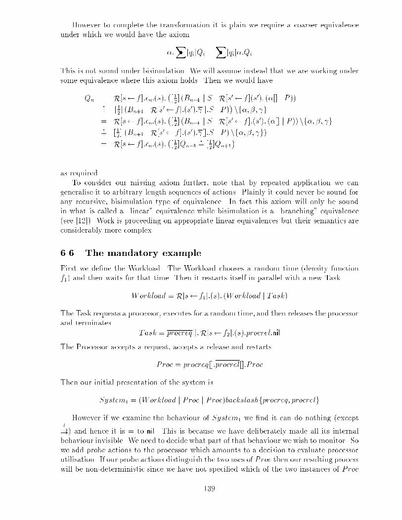
However to complete the transformation it is plain we require a coarser equivalenceunder which we would have the axiom�:X� [qi]Qi =X� [qi]�:QiThis is not sound under bisimulation. We will assume instead that we are working undersome equivalence where this axiom holds. Then we would haveQn = R[s f ]:�n:(s): �[12] (Bn�1 j S j R[s0 f ](s0): (�[] j P ))u [12] (Bn+1 j R[s0 f ]:(s0): []:S j P )� nf�; �; g= R[s f ]:�n:(s): �[12] (Bn�1 j S j R[s0 f ]:(s0): (�[] j P )) nf�; �; gu [12] (Bn+1 j R[s0 f ]:(s0): []:S j P ) nf�; �; g)= R[s f ]:�n:(s): �[12]Qn�1 u [12]Qn+1�as required.To consider our missing axiom further, note that by repeated application we cangeneralise it to arbitrary length sequences of actions. Plainly it could never be sound forany recursive, bisimulation type of equivalence. In fact this axiom will only be soundin what is called a \linear" equivalence while bisimulation is a \branching" equivalence(see [12]). Work is proceeding on appropriate linear equivalences but their semantics areconsiderably more complex.6.6 The mandatory exampleFirst we de�ne the Workload. The Workload chooses a random time (density functionf1) and then waits for that time. Then it restarts itself in parallel with a new Task.Workload = R[s f1]:(s): (Workload j Task)The Task requests a processor, executes for a random time, and then releases the processorand terminates. Task = procreq[]:R[s f2]:(s):procrel:nilThe Processor accepts a request, accepts a release and restarts.Proc = procreq[]:procrel[]:P rocThen our initial presentation of the system isSystem1 = (Workload j Proc j Proc)backslashfprocreq; procrelgHowever if we examine the behaviour of System1 we �nd it can do nothing (exceptt�) and hence it is = to nil. This is because we have deliberately made all its internalbehaviour invisible. We need to decide what part of that behaviour we wish to monitor. Sowe add probe actions to the processor which amounts to a decision to evaluate processorutilisation. If our probe actions distinguish the two uses of Proc then our resulting processwill be non-deterministic since we have not speci�ed which of the two instances of Proc139

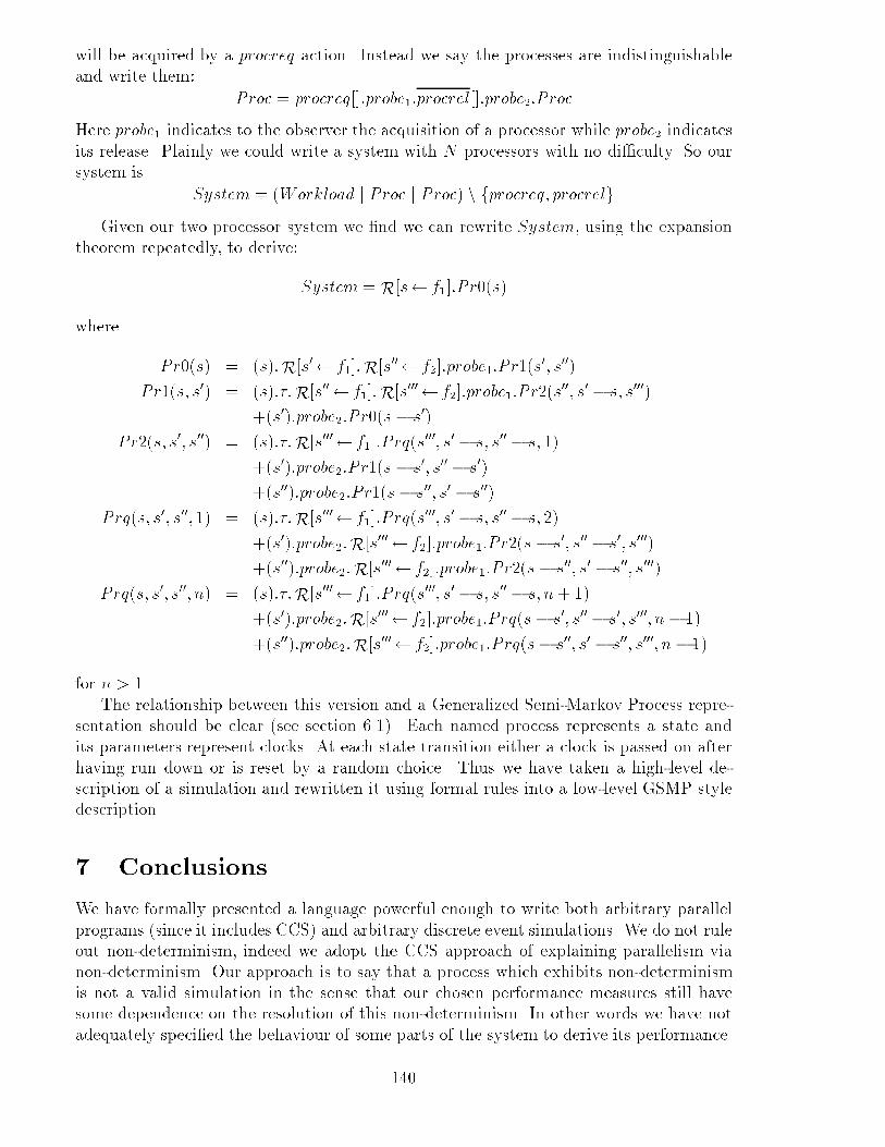
will be acquired by a procreq action. Instead we say the processes are indistinguishableand write them: Proc = procreq[]:probe1:procrel[]:probe2:P rocHere probe1 indicates to the observer the acquisition of a processor while probe2 indicatesits release. Plainly we could write a system with N processors with no di�culty. So oursystem is System = (Workload j Proc j Proc) n fprocreq; procrelgGiven our two processor system we �nd we can rewrite System, using the expansiontheorem repeatedly, to derive:System = R[s f1]:P r0(s)where Pr0(s) = (s):R[s0 f1]:R[s00 f2]:probe1:P r1(s0; s00)Pr1(s; s0) = (s):�:R[s00 f1]:R[s000 f2]:probe1:P r2(s00; s0 � s; s000)+(s0):probe2:P r0(s � s0)Pr2(s; s0; s00) = (s):�:R[s000 f1]:P rq(s000; s0 � s; s00 � s; 1)+(s0):probe2:P r1(s � s0; s00 � s0)+(s00):probe2:P r1(s� s00; s0 � s00)Prq(s; s0; s00; 1) = (s):�:R[s000 f1]:P rq(s000; s0 � s; s00 � s; 2)+(s0):probe2:R[s000 f2]:probe1:P r2(s � s0; s00 � s0; s000)+(s00):probe2:R[s000 f2]:probe1:P r2(s� s00; s0 � s00; s000)Prq(s; s0; s00; n) = (s):�:R[s000 f1]:P rq(s000; s0 � s; s00 � s; n+ 1)+(s0):probe2:R[s000 f2]:probe1:P rq(s� s0; s00 � s0; s000; n� 1)+(s00):probe2:R[s000 f2]:probe1:P rq(s� s00; s0 � s00; s000; n� 1)for n > 1.The relationship between this version and a Generalized Semi-Markov Process repre-sentation should be clear (see section 6.1). Each named process represents a state andits parameters represent clocks. At each state transition either a clock is passed on afterhaving run down or is reset by a random choice. Thus we have taken a high-level de-scription of a simulation and rewritten it using formal rules into a low-level GSMP styledescription.7 ConclusionsWe have formally presented a language powerful enough to write both arbitrary parallelprograms (since it includes CCS) and arbitrary discrete event simulations. We do not ruleout non-determinism, indeed we adopt the CCS approach of explaining parallelism vianon-determinism. Our approach is to say that a process which exhibits non-determinismis not a valid simulation in the sense that our chosen performance measures still havesome dependence on the resolution of this non-determinism. In other words we have notadequately speci�ed the behaviour of some parts of the system to derive its performance.140

Such a situation arises, for example, where some schedule for the behaviour of some partof the system is unspeci�ed (e.g. it depends on operating system behaviour).We have presented a formal semantics for the language and this allows us to proveproperties of programs written in the language at a semantic level. We have also derivedalgebraic tools which allow us to transform programs at a syntactic level and for example�nd out if they do exhibit non-determinism. We can use these tools to transform aprogram written in a clear high-level style into one that is closer to well understoodmodels of simulation such as GSMPs or is perhaps more e�cient or simpler to understand.We might then hope to derive analytical properties of the simulation such as recurrence.However we have also presented an example showing that our semantics distinguishescertain simulations that are generally accepted as being equal.A more complete description is in [14] where the complete language is presented withproofs of all results. Also a di�erent semantics is presented in terms of Hennessy and deNicola testing which overcomes the problems just noted.References[1] J.C.M. Baeten and J.A. Bergstra. Real time process algebra. Technical ReportCS-R9053, Centrum voor Wiskunde en Informatica, October 1990.[2] Liang Chen. An interleaving model for real-time systems. Technical Report ECS-LFCS-91-184, LFCS, University of Edinburgh, November 1991.[3] Liang Chen, Stuart Anderson, and Faron Moller. A Timed Calculus of Communi-cating Systems. Technical report, University of Edinburgh, 1990.[4] Anthony J. Field and Peter G. Harrison. Functional Programming. Addison Wesley,1988.[5] Hans A. Hansson. Time and Probability in Formal Design of Distributed Systems.PhD thesis, Uppsala University, P.O. Box 520, S-751 20 Uppsala, Sweden, 1991.[6] Matthew Hennessy and Tim Regan. A process algebra for timed systems. Technicalreport, Sussex University, April 1991.[7] R.E. Milne and C. Strachey. A Theory of Programming Language Semantics. Chap-man and Hall, 1976.[8] Robin Milner. Communication and Concurrency. Prentice Hall, 1989.[9] Faron Moller and Chris Tofts. A Temporal Calculus of Communicating Systems. InConcur '90, number 458 in LNCS, 1990.[10] Faron Moller and Chris Tofts. Behavioural abstraction in TCCS. In Proceedingsof the 19th Colloquium on Automata Languages and Programming, number 623 inLNCS, pages 579{570, 1992.[11] Xavier Nicollin and Joseph Sifakis. An overview and synthesis on timed processalgebras. In Kim G. Larsen and Arne Skou, editors, Proc. CAV 91, number 575 inLNCS, pages 376{398, 1991. 141

[12] A. Pnueli. Linear and branching structures in the semantics and logics of reactivesystems. In Proceedings of the Twelfth Colloquium on Automata Languages andProgramming, volume 194 of LNCS, 1985.[13] Steve Schneider. An operational semantics for timed CSP. Technical report, Pro-gramming Research Group, Oxford University, February 1991.[14] Ben Strulo. Process Algebra for Discrete Event Simulation. PhD thesis, to appear,1993.[15] Wang Yi. A Calculus of Real Time Systems. PhD thesis, Chalmers University ofTechnology, S-412 96 G�oteborg, Sweden, 1991.[16] Wang Yi. CCS + Time = an interleaving model for real time systems. In Proceedingsof the Eighteenth Colloquium on Automata Languages and Programming, number 510in LNCS, pages 217{228, 1991.

142