Space–Time Tradeoffs for Subset Sum: An Improved Worst Case Algorithm

SPACE–TIME TRADEOFFS FOR SUBSET SUM:AN IMPROVED WORST CASE ALGORITHM

PER AUSTRIN, PETTERI KASKI, MIKKO KOIVISTO, AND JUSSI MÄÄTTÄ

Abstract. The technique of Schroeppel and Shamir (SICOMP, 1981) haslong been the most efficient way to trade space against time for the SubsetSum problem. In the random-instance setting, however, improved tradeoffsexist. In particular, the recently discovered dissection method of Dinur et al.(CRYPTO 2012) yields a significantly improved space–time tradeoff curve forinstances with strong randomness properties. Our main result is that thesestrong randomness assumptions can be removed, obtaining the same space–time tradeoffs in the worst case. We also show that for small space usage thedissection algorithm can be almost fully parallelized. Our strategy for dealingwith arbitrary instances is to instead inject the randomness into the dissec-tion process itself by working over a carefully selected but random compositemodulus, and to introduce explicit space–time controls into the algorithm bymeans of a “bailout mechanism”.

1. Introduction

The protagonist of this paper is the Subset Sum problem.

Definition 1.1. An instance (a, t) of Subset Sum consists of a vector a ∈ Zn≥0

and a target t ∈ Z≥0. A solution of (a, t) is a vector x ∈ 0, 1n such that∑ni=1 aixi = t.

The problem is NP-hard (in essence, Karp’s formulation of the knapsack prob-lem [6]), and the fastest known algorithms take time and space that grow exponen-tially in n. We will write T and S for the exponential factors and omit the possiblepolynomial factors. The brute-force algorithm, with T = 2n and S = 1, was beatenfour decades ago, when Horowitz and Sahni [4] gave a simple yet powerful meet-in-the-middle algorithm that achieves T = S = 2n/2 by halving the set arbitrarily,sorting the 2n/2 subsets of each half, and then quickly scanning through the rele-vant pairs of subsets that could sum to the target. Some years later, Schroeppeland Shamir [10] improved the space requirement of the algorithm to S = 2n/4 bydesigning a novel way to list the half-sums in sorted order in small space. How-ever, if allowing only polynomial space, no better than the trivial time bound ofT = 2n is known. Whether the constant bases of the exponentials in these boundscan be improved is a major open problem in the area of moderately exponentialalgorithms [11].

The difficulty of finding faster algorithms, whether in polynomial or exponentialspace, has motivated the study of space–time tradeoffs. From a practical point of

P.A. supported by the Aalto Science Institute, the Swedish Research Council grant 621-2012-4546, and ERC Advanced Investigator grant 226203. P.K. supported by the Academy of Finland,grants 252083 and 256287. M.K. supported by the Academy of Finland, grants 125637, 218153,and 255675.

1

arX

iv:1

303.

0609

v1 [

cs.D

S] 4

Mar

201

3

2 PER AUSTRIN, PETTERI KASKI, MIKKO KOIVISTO, AND JUSSI MÄÄTTÄ

0

1/221/16

1/11

1/7

1/4

1/2 4/7 7/11 11/16 16/22 1

σ(spa

ce)

τ (time)

Schroeppel and Shamir (1981)Dinur et al. (2012)

Figure 1. Space–time tradeoff curves for the Subset Sum prob-lem [10, 3]. The space and time requirements are S = 2σn andT = 2τn, omitting factors polynomial in the instance size n.

view, large space usage is often the bottleneck of computation, and savings in spaceusage can have significant impact even if they come at the cost of increasing thetime requirement. This is because a smaller-space algorithm can make a betteruse of fast cache memories and, in particular, because a smaller-space algorithmoften enables easier and more efficient large-scale parallelization. Typically, oneobtains a smooth space–time tradeoff by combining the fastest exponential timealgorithm with the fastest polynomial space algorithm into a hybrid scheme thatinterpolates between the two extremes. An intriguing question is then whether onecan beat the hybrid scheme at some point, that is, to get a faster algorithm atsome space budget—if one can break the hybrid bound somewhere, maybe one canbreak it everywhere. For the Subset Sum problem, a hybrid scheme is obtainedby first guessing some g elements of the solution, and then running the algorithmof Schroeppel and Shamir for the remaining instance on n−g elements. This yieldsT = 2(n+g)/2 and S = 2(n−g)/4, for any 0 ≤ g ≤ n, and thereby the smooth tradeoffcurve S2T = 2n for 1 ≤ S ≤ 2n/4. We call this the Schroeppel–Shamir tradeoff.

While the Schroeppel–Shamir tradeoff has remained unbeaten in the usual worst-case sense, there has been remarkable recent progress in the random-instance set-ting [5, 1, 3]. In a recent result, Dinur, Dunkelman, Keller, and Shamir [3] gave atradeoff curve that matches the Schroeppel–Shamir tradeoff at the extreme pointsS = 1 and S = 2n/4 but is strictly better in between. The tradeoff is achievedby a novel dissection method that recursively decomposes the problem into smallersubproblems in two different “dimensions”, the first dimension being the currentsubset of the n items, and the other dimension being (roughly speaking) the bits ofinformation of each item. The algorithm of Dinur et al. runs in space S = 2σn andtime T = 2τ(σ)n on random instances (τ(σ) is defined momentarily). See Figure 1for an illustration and comparison to the Schroeppel–Shamir tradeoff. The tradeoffcurve τ(σ) is piecewise linear and determined by what Dinur et al. call the “magicsequence” 2, 4, 7, 11, 16, 22, . . ., obtained as evaluations of ρ` = 1 + `(` + 1)/2 at` = 1, 2, . . ..

SPACE–TIME TRADEOFFS FOR SUBSET SUM 3

Definition 1.2. Define τ : (0, 1] → [0, 1] as follows. For σ ∈ (0, 1/2], let ` be thesolution to 1/ρ`+1 < σ ≤ 1/ρ`. Then

(1) τ(σ) = 1− 1

`+ 1− ρ` − 2

`+ 1σ .

If there is no such `, that is, if σ > 1/2, define τ(σ) = 1/2.

For example, at σ = 1/8, we have ` = 3, and thereby τ(σ) = 19/32. Asymptotically,when σ is small, ` is essentially

√2/σ and τ(σ) ≈ 1−

√2σ.

In this paper, we show that this space–time tradeoff result by Dinur et al. [3]can be made to hold also in the worst case:

Theorem 1.3. For each σ ∈ (0, 1] there exists a randomized algorithm that solvesthe Subset Sum problem with high probability, and runs in O∗(2τ(σ)n) time andO∗(2σn) space. The O∗ notation suppresses factors that are polynomial in n, andthe polynomials depend on σ.

To the best of our knowledge, Theorem 1.3 is the first improvement to theSchroeppel–Shamir tradeoff in the worst-case setting. Here we should remarkthat, in the random-instance setting, there are results that improve on both theSchroeppel–Shamir and the Dinur et al. tradeoffs for certain specific choices of thespace budget S. In particular, Becker et al. give a 20.72n time polynomial space al-gorithm and a 20.291n time exponential space algorithm [1]. A natural question thatremains is whether these two results could be extended to the worst-case setting.Such an extension would be a significant breakthrough (cf. [11]).

We also prove that the dissection algorithm lends itself to parallelization verywell. As mentioned before, a general guiding intuition is that algorithms that useless space can be more efficiently parallelized. The following theorem shows that,at least in the case of the dissection algorithm, this intuition can be made formal:the smaller the space budget σ is, the closer we can get to full parallelization.

Theorem 1.4. The algorithm of Theorem 1.3 can be implemented to run inO∗(2τ(σ)n/P ) parallel time on P processors each using O∗(2σn) space, providedP ≤ 2(2τ(σ)−1)n.

When σ is small, τ(σ) ≈ 1 −√

2σ and the bound on P is roughly 2(τ(σ)−√

2σ)n.In other words we get a linear speedup almost all the way up to 2τ(σ)n processors,almost full parallelization.

1.1. Our contributions and overview of the proof. At a high level, our ap-proach will follow the Dinur et al. dissection framework, with essential differencesin preprocessing and low-level implementation to alleviate the assumptions on ran-domness. In particular, while we split the instance analogously to Dinur et al. torecover the tradeoff curve, we require more careful control of the sub-instances be-yond just subdividing the bits of the input integers and assuming that the inputis random enough to guarantee sufficient uniformity to yield the tradeoff curve.Accordingly we find it convenient to revisit the derivation of the tradeoff curve andthe analysis of the basic dissection framework to enable a self-contained exposition.

In contrast with Dinur et al., our strategy for dealing with arbitrary instancesis, essentially, to instead inject the required randomness into the dissection processitself. We achieve this by observing that dissection can be carried out over anyalgebraic structure that has a sufficiently rich family of homomorphisms to enable


us to inject entropy by selection of random homomorphisms, while maintainingan appropriate recursive structure for the selected homomorphisms to facilitatedissection. For the Subset Sum problem, in practice this means reduction from Zto ZM over a compositeM with a carefully selected (but random) lattice of divisorsto make sure that we can still carry out recursive dissections analogously to Dinuret al. This approach alone does not provide sufficient control over an arbitraryproblem instance, however.

The main obstacle is that, even with the randomness injected into the algorithm,it is very hard to control the resource consumption of the algorithm. To overcomethis, we add explicit resource controls into the algorithm, by means of a somewhatcavalier “bailout mechanism” which causes the algorithm to simply stop when toomany partial solutions have been generated. We set the threshold for such a bailoutto be roughly the number of partial solutions that we would have expected to seein a random instance. This allows us to keep its running time and space usage incheck, perfectly recovering the Dinur et al. tradeoff curve. The remaining challengeis then to prove correctness, i.e., that these thresholds for bailout are high enoughso that no hazardous bailouts take place and a solution is indeed found. To do thiswe perform a localized analysis on the subtree of the recursion tree that containsa solution. Using that the constructed modulus M contains a lot of randomness(a consequence of the density of the primes), we can show that the probability ofa bailout in any node of this subtree is o(1), meaning that the algorithm finds asolution with high probability.

A somewhat curious effect is that in order for our analysis to go through, werequire the original Subset Sum instance to have few, say O(1), distinct solutions.In order to achieve this, we preprocess the instance by employing routine isolationtechniques in ZP but implemented over Z to control the number of solutions over Z.The reason why we need to implement the preprocessing over Z rather than thanwork in the modular setting is that the dissection algorithm itself needs to be ableto choose a modulus M very carefully to deliver the tradeoff, and that choice isincompatible with having an extra prime P for isolation. This is somewhat curiousbecause, intuitively, the more solutions an instance has, the easier it should be tofind one. The reason why that is not the case in our setting is that, further down inthe recursion tree, when operating with a small modulus M , every original solutiongives rise to many additional spurious solutions, and if there are too many originalsolutions there will be too many spurious solutions.

A further property needed to support the analysis is that the numbers in theSubset Sum instance must not be too large, in particular we need log t = O(n).This we can also achieve by a simple preprocessing step where we hash down moduloa random prime, but again with implementation over the integers for the samereason as above.

1.2. Related work. The Subset Sum problem has recently been approached fromrelated angles, with the interest in small space. Lokshtanov and Nederlof [9] showthat the well-known pseudo-polynomial-time dynamic programming algorithm canbe implemented in truly-polynomial space by algebraization. Kaski, Koivisto, andNederlof [7] note that the sparsity of the dynamic programming table can be ex-ploited to speedup the computations even if allowing only polynomial space.

Smooth space–time tradeoffs have been studied also for several other hard prob-lems. Björklund et al. [2] derive a hybrid scheme for the Tutte polynomial that is a


host of various counting problems on graphs. Koivisto and Parviainen [8] considera class of permutation problems (including, e.g., the traveling salesman problemand the feedback arc set problem) and show that a natural hybrid scheme can bebeaten by a partial ordering technique.

1.3. Organization. In Section 2 we describe the dissection algorithm and give themain statements about its properties. In Section 3 we show that the algorithm runswithin the desired time and space bounds. Then, in Section 4 we show that given aSubset Sum instance with at most O(1) solutions, the dissection algorithm findsa solution. In Section 5 we give a standard isolation argument reducing generalSubset Sum to the restricted case when there are at most O(1) solutions, givingthe last puzzle piece to complete the proof of Theorem 1.3. In Section 6 we showthat the algorithm lends itself to efficient parallelization by proving Theorem 1.4.

2. The Main Dissection Algorithm

Before describing the main algorithm, we condense some routine preprocessingsteps into the following theorem, whose proof we relegate to Section 5.

Theorem 2.1. There is a polynomial-time randomized algorithm for preprocessinginstances of Subset Sum which, given as input an instance (a, t) with n elements,outputs a collection of O(n3) instances (a′, t′), each with n elements and log t′ =O(n), such that if (a, t) is a NO instance then so are all the new instances withprobability 1 − o(1), and if (a, t) is a YES instance then with probability Ω(1) atleast one of the new instances is a YES instance with at most O(1) solutions.

By applying this preprocessing we may assume that the main algorithm receivesan input (a, t) that has O(1) solutions and log t = O(n). We then introduce arandom modulus M and transfer into a modular setting.

Definition 2.2. An instance (a, t,M) of Modular Subset Sum consists of avector a ∈ Zn≥0, a target t ∈ Z≥0, and a modulus M ∈ Z≥1. A solution of (a, t,M)

is a vector x ∈ 0, 1n such that∑ni=1 aixi ≡ t (mod M).

The reason why we transfer to the modular setting is that the recursive dissectionstrategy extensively uses the fact that we have available a sufficiently rich familyof homomorphisms to split the search space. In particular, in the modular settingthis corresponds to the modulus M being “sufficiently divisible” (in a sense to bemade precise later) to obtain control of the recursion.

Pseudocode for the main algorithm is given in Algorithm 1. In addition tothe modular instance (a, t,M), the algorithm accepts as further input the spaceparameter σ ∈ (0, 1].

The key high-level idea in the algorithm is to “meet in the middle” by splitting aninstance of n items to two sub-instances of αn items and (1− α)n items, guessing(over a smaller modulus M ′ that divides M) what the sum should be after thefirst and before the second sub-instance, and then recursively solving the two sub-instances subject to the guess. Figure 2 illustrates the structure of the algorithm.

We continue with some further high-level remarks.(1) In the algorithm, two key parameters α and β are chosen, which control

how the Modular Subset Sum instance is subdivided for the recursivecalls. The precise choice of these parameters is given in Theorem 2.3 below,but at this point the reader is encouraged to simply think of them as some


Algorithm 1: GenerateSolutions(a, t,M, σ)

Data: (a, t,M) is an n-element Modular Subset Sum instance, σ ∈ (0, 1]Result: Iterates over up to Θ∗(2n/M) solutions of (a, t,M) while using

space O∗(2σn)1 begin2 if σ ≥ 1/4 then3 Report up to Θ∗(2n/M) solutions using the Shroeppel-Shamir

algorithm4 return

5 Choose α ∈ (0, 1), β ∈ (0, 1) appropriately (according to Theorem 2.3)based on σ

6 Let M ′ be a factor of M of magnitude Θ(2βn)

7 for s′ = 0, 1, . . . ,M ′ − 1 do8 Allocate an empty lookup table9 Let l = (a1, a2, . . . , aαn) be the first αn items of a

10 Let r = (aαn+1, aαn+2, . . . , an) be the remaining (1− α)n items of a11 for y ∈ GenerateSolutions(l, s′,M ′, σα ) do12 Let s =

∑αni=1 aiyi mod M

13 Store [s→ y] in the lookup table

14 for z ∈ GenerateSolutions(r, t− s′,M ′, σ1−α ) do

15 Let s = t−∑ni=αn+1 aizi mod M

16 foreach [s→ y] in the lookup table do17 Report solution x = (y, z)

18 if at least Θ∗(2n/M) solutions reported then19 Stop iteration and return

20 Release the lookup table

parameters which should be chosen appropriately so as to optimize runningtime.

(2) The algorithm also chooses a factor M ′ of M such that M ′ = Θ(2βn).The existence of sufficient factors at all levels of recursion is established inSection 4.

(3) The algorithm should be viewed as an iterator over solutions. In otherwords, the algorithm has an internal state, and a next item functionalitythat we tacitly use by writing a for-loop over all solutions generated bythe algorithm, which should be interpreted as a short-hand for repeatedlyasking the iterator for the next item.

(4) The algorithm uses a “bailout mechanism” to control the running time andspace usage. Namely, each recursive call will bail out after Θ∗(2n/M) solu-tions are reported. (The precise bailout bound has a further multiplicativefactor polynomial in n that depends on the top-level value of σ.) A pre-liminary intuition for the bound is that this is what one would expect toreceive in a particular congruence class modulo M if the 2n possible sumsare randomly placed into the congruence classes.


a1 . . . aαn aαn+1 . . . an

M

M′

s′ ∈ 0, . . . ,M ′ − 1

l1 . . . lαn r1 . . . r(1−α)n

Figure 2. Illustration of the recursive dissections made by the algorithm.

As a warmup to the analysis, let us first observe that, if we did not have thebailout step in line 19, correctness of the algorithm would be more or less immediate:for any solution x of (a, t,M), let s =

∑αni=1 aixi mod M . Then, when s′ = s mod

M ′ in the outer for-loop (line 7), by an inductive argument we will find y and z inthe two separate recursive branches and join the two partial solutions to form x.

The challenge, of course, is that without the bailout mechanism we lack controlover the resource consumption of the algorithm. Even though we have appliedisolation to guarantee that there are not too many solutions of the top-level instance(a, t), it may be that some branches of the recursion generate a huge number ofsolutions, affecting both running time and space (since we store partial solutions ina lookup table).

Let us then proceed to analyzing the algorithm with the bailout mechanism inplace. The two main claims are as follows.

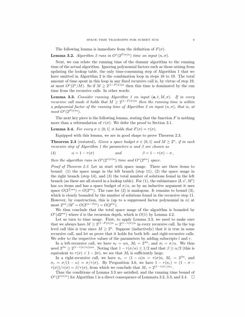
Theorem 2.3. Given a space budget σ ∈ (0, 1] and M ≥ 2n, if in each recursivestep of Algorithm 1 the parameters α and β are chosen as

α = 1− τ(σ) and β = 1− τ(σ)− σ ,(2)

then the algorithm runs in O∗(2τ(σ)n) time and O∗(2σn) space.

Theorem 2.4. For every σ ∈ (0, 1] there is a randomized algorithm that runs intime polynomial in n and chooses a top-level modulus M ≥ 2n so that Algorithm 1reports a solution of the non-modular instance (a, t) with high probability over thechoices of M , assuming that at least one and at most O(1) solutions exist and thatlog t = O(n).


Algorithm 2: DummyDissection(n, σ)

Data: σ ∈ (0, 1]1 begin2 if σ ≥ 1/4 then3 Run for 2n/2 steps4 return

5 Let α = 1− τ(σ), β = α− σ6 for 2βn steps do7 DummyDissection(αn, σ/α)

8 DummyDissection((1− α)n, σ/(1− α))

We prove Theorem 2.3 in Section 3 and Theorem 2.4 in Section 4.Let us however here briefly discuss the specific choice of α and β in Theorem 2.3.

We arrived at (2) by analyzing the recurrence relation describing the running time ofAlgorithm 1. Unfortunately this recurrence in its full form is somewhat complicated,and our process of coming up with (2) involved a certain amount of experimentingand guesswork. We do have some guiding (non-formal) intuition which might beinstructive:

(1) One needs to make sure that α − β ≤ σ. This is because for a randominstance, the left subinstance is expected to have roughly 2(α−β)n solutions,and since we need to store these there had better be at most 2σn of them.

(2) Since β ≥ α − σ and β has a very direct impact on running time (due tothe 2βn time outer loop), one will typically want to set α relatively small.The tension here is of course that the smaller α becomes, the larger 1− α(that is, the size of the right subinstance) becomes.

(3) Given this tension, setting α− β = σ is natural.So in an intuitive sense, the bottleneck for space comes from the left subinstance,

or rather the need to store all the solutions found for the left subinstance (this is nottechnically true since we give the right subinstance 2σn space allowance as well),whereas the bottleneck for time comes from the right subinstance, which tends tobe much larger than the left one.

3. Analysis of Running Time and Space Usage

In this section we prove Theorem 2.3 giving the running time upper bound onthe dissection algorithm. For this, it is convenient to define the following function,which is less explicit than τ but more naturally captures the running time of thealgorithm.

Definition 3.1. Define F : (0, 1]→ (0, 1) by the following recurrence for σ < 1/4:

(3) F (σ) = β + maxαF(σα

), (1− α)F

( σ

1− α)

,

where α = 1− τ(σ) and β = α− σ. The base case is F (σ) = 1/2 for σ ≥ 1/4.

To analyze the running time of the dissection algorithm, let us first define a“dummy” version of Algorithm 1, given as Algorithm 2. The dummy version is abare bones version of Algorithm 1 which generates the same recursion tree.


The following lemma is immediate from the definition of F (σ).

Lemma 3.2. Algorithm 2 runs in O∗(2F (σ)n) time on input (n, σ).

Next, we can relate the running time of the dummy algorithm to the runningtime of the actual algorithm. Ignoring polynomial factors such as those arising fromupdating the lookup table, the only time-consuming step of Algorithm 1 that wehave omitted in Algorithm 2 is the combination loop in steps 16 to 19. The totalamount of time spent in this loop in any fixed recursive call is, by virtue of step 19,at most O∗(2n/M). So if M ≥ 2(1−F (σ))n then this time is dominated by the runtime from the recursive calls. In other words:

Lemma 3.3. Consider running Algorithm 1 on input (a, t,M, σ). If in everyrecursive call made it holds that M ≥ 2(1−F (σ))n then the running time is withina polynomial factor of the running time of Algorithm 2 on input (n, σ), that is, atmost O∗(2F (σ)n).

The next key piece is the following lemma, stating that the function F is nothingmore than a reformulation of τ(σ). We defer the proof to Section 3.1.

Lemma 3.4. For every σ ∈ (0, 1] it holds that F (σ) = τ(σ).

Equipped with this lemma, we are in good shape to prove Theorem 2.3.

Theorem 2.3 (restated). Given a space budget σ ∈ (0, 1] and M ≥ 2n, if in eachrecursive step of Algorithm 1 the parameters α and β are chosen as

α = 1− τ(σ) and β = 1− τ(σ)− σ ,(4)

then the algorithm runs in O∗(2τ(σ)n) time and O∗(2σn) space.

Proof of Theorem 2.3. Let us start with space usage. There are three items tobound: (1) the space usage in the left branch (step 11), (2) the space usage inthe right branch (step 14), and (3) the total number of solutions found in the leftbranch (as these are all stored in a lookup table). For (1), the subinstance (l, s′,M ′)has αn items and has a space budget of σ/α, so by an inductive argument it usesspace O(2

σααn) = O(2σn). The case for (2) is analogous. It remains to bound (3),

which is clearly bounded by the number of solutions found in the recursive step 11.However, by construction, this is (up to a suppressed factor polynomial in n) atmost 2αn/M ′ = O(2(α−β)n) = O(2σn).

We thus conclude that the total space usage of the algorithm is bounded byO∗(d2σn) where d is the recursion depth, which is O(1) by Lemma 4.2.

Let us turn to time usage. First, to apply Lemma 3.3, we need to make surethat we always haveM ≥ 2(1−F (σ))n = 2(1−τ(σ))n in every recursive call. In the toplevel call this is true since M ≥ 2n. Suppose (inductively) that it is true in somerecursive call, and let us prove that it holds for both left- and right-recursive calls.We refer to the respective values of the parameters by adding subscripts l and r.

In a left-recursive call, we have nl = αn, Ml = 2βn, and σl = σ/α. We thusneed 2βn ≥ 2(1−τ(σ/α))αn. Noting that 1− τ(σ/α) ≤ 1/2 and that β ≥ α/2 (this isequivalent to τ(σ) < 1− 2σ), we see that Ml is sufficiently large.

In a right-recursive call, we have nr = (1 − α)n = τ(σ)n, Mr = 2βn, andσr = σ/(1 − α) = σ/τ(σ). By Proposition 3.6, we have 1 − τ(σr) = (1 − σ −τ(σ))/τ(σ) = β/τ(σ), from which we conclude that Mr = 2(1−τ(σr))nr .

Thus the conditions of Lemma 3.3 are satisfied, and the running time bound ofO∗(2τ(σ)n) for Algorithm 1 is a direct consequence of Lemmata 3.2, 3.3, and 3.4.


3.1. Proof of Lemma 3.4. We first prove some useful properties of the τ function.

Proposition 3.5. The map σ 7→ σ/τ(σ) is increasing in σ ∈ (0, 1]. Furthermore,for σ = 1/ρ`+1, we have σ/τ(σ) = 1/ρ`.

Proof. Let σ ∈ (0, 1], and let σ′ = σ/τ(σ). If σ > 1/2, then τ(σ) = 1/2, and thusσ′ = 2σ is increasing in σ. Otherwise 1/ρ`+1 < σ ≤ 1/ρ` for some ` ≥ 1, andτ(σ) = (`− (ρ` − 2)σ)/(`+ 1). Thus

1

σ′=τ(σ)

σ=`− (ρ` − 2)σ

(`+ 1)σ=`/σ − ρ` + 2

`+ 1,

from which it follows that σ′ is increasing in σ in the interval (1/ρ`+1, 1/ρ`].Suppose σ = 1/ρ`+1. Use first ρ`+1 = ρ` + ` + 1 and then `(` + 1) = 2(ρ` − 1)

to obtain1

σ′=`(ρ` + `+ 1)− ρ` + 2

`+ 1=

(`− 1)ρ` + 2(ρ` − 1) + 2

`+ 1= ρ` .

Proposition 3.6. Let σ ∈ (0, 1]. If σ > 1/2, then τ(σ) = 1/2, and otherwise

τ(σ) =1− σ

2− τ(σ/τ(σ)).

Proof. The case σ > 1/2 is obvious. Fix σ ≤ 1/2 and ` ≥ 1 such that 1/ρ`+1 < σ ≤1/ρ` and let σ′ = σ/τ(σ). By Proposition 3.5 we have that 1/ρ` < σ′ ≤ 1/ρ`−1.Using τ(σ′) = (`− 1− (ρ`−1 − 2)σ′)/` we obtain

2− τ(σ′) =`+ 1 + (ρ`−1 − 2)σ′

`.

Plugging in σ′ = σ/τ(σ) and using ρ`−1 = ρ` − ` gives

(5) 2− τ(σ′) =(`+ 1)τ(σ) + (ρ` − `− 2)σ

`τ(σ).

As τ(σ) = (`− (ρ` − 2)σ)/(`+ 1), the numerator of this expression equals

`− (ρ` − 2)σ + (ρ` − `− 2)σ = `(1− σ) .

Plugging this into (5) we conclude that

2− τ(σ′) =1− στ(σ)

,

which is a simple rearrangement of the desired conclusion.

We are now ready to prove Lemma 3.4.

Lemma 3.4 (restated). For every σ ∈ (0, 1] it holds that F (σ) = τ(σ).

Proof of Lemma 3.4. The proof is by induction on the value of ` such that 1/ρ`+1 <σ ≤ 1/ρ`. The base case, σ ≥ 1/4 (that is, ` ≤ 1) is clear from the definitions.

For the induction step, fix some value of ` ≥ 2, and assume that F (σ′) = τ(σ′)for all σ′ > 1/ρ`. We need to show that for any σ in the interval [1/ρ`+1, 1/ρ`), itholds that F (σ) = τ(σ). To this end, we set α = 1 − τ(σ) and β = 1 − τ(σ) − σ,and show that the two options in the max in (3) are bounded by τ(σ), one withequality.


σ = 0.0500 τ = 0.7167 α = 0.2833 β = 0.2333 γ = 0.2333

σ = 0.1765 τ = 0.5490 α = 0.4510 β = 0.2745 γ = 0.0778

σ = 0.0698 τ = 0.6744 α = 0.3256 β = 0.2558 γ = 0.1833

σ = 0.3913 σ = 0.3214σ = 0.2143 τ = 0.5238 α = 0.4762 β = 0.2619 γ = 0.0611

σ = 0.1034 τ = 0.6207 α = 0.3793 β = 0.2759 γ = 0.1333

σ = 0.4500 σ = 0.4091 σ = 0.2727σ = 0.1667 τ = 0.5556 α = 0.4444 β = 0.2778 γ = 0.0833

σ = 0.3750 σ = 0.3000

Figure 3. The dissection tree DT (0.05). For each internal nodev, we display the parameters σv, τv = τ(σv), αv, βv, γv as definedin Section 4.

Consider first the second option. Set σ′ = σ/(1 − α) = σ/τ(σ). By Proposi-tion 3.5, we have σ′ > 1/ρ`. Thus, by the induction hypothesis we have F (σ′) =τ(σ′), and hence the second option in (3) equals

β + (1− α)τ(σ′) = 1− τ(σ)− σ + τ(σ)τ(σ/τ(σ)) = τ(σ) ,

where the last step is an application of Proposition 3.6.Consider then the first option. Let σ′′ = σ/α be the value passed to F in this

branch. It is easy to check that σ′′ ≥ σ′ > 1/ρ`. So the induction hypothesisapplies, and we get an upper bound of

β + ατ(σ′′) < β + (1− α)τ(σ′) ≤ τ(σ) .

The first step uses τ(σ) ≥ 1/2 (yielding α < 1/2) and the monotonicity of τ , andthe last step uses the bound on the second option.

4. Choice of Modulus and Analysis of Correctness

In this section we prove Theorem 2.4, giving the correctness of the dissectionalgorithm.

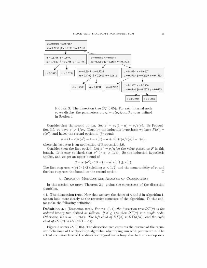
4.1. The dissection tree. Now that we have the choice of α and β in Algorithm 1,we can look more closely at the recursive structure of the algorithm. To this end,we make the following definition.

Definition 4.1 (Dissection tree). For σ ∈ (0, 1], the dissection tree DT (σ) is theordered binary tree defined as follows. If σ ≥ 1/4 then DT (σ) is a single node.Otherwise, let α = 1 − τ(σ). The left child of DT (σ) is DT (σ/α), and the rightchild of DT (σ) is DT (σ/(1− α)).

Figure 3 shows DT (0.05). The dissection tree captures the essence of the recur-sive behaviour of the dissection algorithm when being run with parameter σ. Theactual recursion tree of the dissection algorithm is huge due to the for-loop over


s′ in line 7, but if we consider a fixed choice of s′ in every recursive step then therecursion tree of the algorithm becomes identical to the corresponding dissectiontree.

Lemma 4.2. The recursion depth of Algorithm 1 is the height of DT (σ). Inparticular, the recursion depth is a constant that depends only on σ.

We now describe how to choose a priori a randomM that is “sufficiently divisible”for the algorithm’s desires, and to show correctness of the algorithm.

Fix a choice of the top-level value σ ∈ (0, 1]. Consider the corresponding dissec-tion tree DT (σ). For each node v of DT (σ), write σv for the associated σ value.For an internal node v let us also define αv = 1 − τ(σv) and βv = 1 − σv − τ(σv).In other words, if v1 and v2 are the two child nodes of v, then σv1 = σv/αv andσv2 = σv/(1− αv). Finally, define γv = βv · σ/σv.

Observe that each recursive call made by Algorithm 1 is associated with a uniqueinternal node v of the dissection tree DT (σ).

Lemma 4.3. Each recursive call associated with an internal node v requires afactor M ′ of magnitude Θ∗(2γvn).

Proof. Telescope a product of the ratio σp/σu for a node u and its parent p along thepath from v to the root node. Each such σp/σu is either αu or 1 − αu dependingon whether it is a left branch or right branch—precisely the factor by which ndecreases.

4.2. Choosing the modulus. The following lemma contains the algorithm thatchooses the random modulus.

Lemma 4.4. For every σ ∈ (0, 1] there exists a randomized algorithm that, givenintegers n and b = O(n) as input, runs in time polynomial in n and outputs foreach internal node v ∈ DT (σ) random moduli Mv, M ′v such that, for the root noder ∈ DT (σ), Mr ≥ 2b, and furthermore for every internal node v:

(1) M ′v is of magnitude Θ(2γvn),(2) Mv = M ′p, where p is the parent of v,(3) M ′v divides Mv, and(4) for any fixed integer 1 ≤ Z ≤ 2b, the probability that M ′v divides Z is

O∗(1/M ′v).

Proof. Let 0 < λ1 < λ2 < · · · < λk be the set of distinct values of γv ordered byvalue, and let δi = λi−λi−1 be their successive differences (where we set λ0 = 0 sothat δ1 = λ1). Since DT (σ) depends only σ and not on n, we have k = O(1). Foreach 1 ≤ i ≤ k independently, let pi be a uniform random prime from the interval[2δin, 2 · 2δin].

For a node v such that γv = λj , let M ′v =∏ji=1 pj . Condition 1 then holds by

construction. The values of Mv are the determined for all nodes except the rootthrough condition 2; for the root node r we set Mr = p0M

′r, where p0 is a random

prime of magnitude 2Θ(n) to make sure that Mr ≥ 2b.To prove condition 3 note that for any node v with parent p, we need to prove

that M ′v divides M ′p. Let jv be such that λjv = γv and jp such that λjp = γp.Noting that the value of γv decreases as one goes down the dissection tree, it thenholds that jv < jp, from which it follows that M ′v =

∏jvi=1 pi divides M

′p =

∏jpi=1 pi.


Finally, for condition 4, again let j be such that λj = γv, and observe that in orderfor Z to divide M ′v it must have all the factors p1, p2, . . . , pj . For each 1 ≤ i ≤ j, Zcan have at most log2 Z

δin= O(1) different factors between 2δin and 2 · 2δin, so by the

Prime Number Theorem, the probability that pi divides Z is at most O(n2−δin). Asthe pi’s are chosen independently the probability that Z divides all of p1, p2, . . . , pj(that is, M ′v) is O(nj2−(δ1+δ2+...+δj)n) = O(nk2−γvn) = O∗(1/M ′v), as desired.

4.3. Proof of correctness. We are now ready to prove the correctness of theentire algorithm, assuming preprocessing and isolation has been carried out.Theorem 2.4 (restated). For every σ ∈ (0, 1] there is a randomized algorithmthat runs in time polynomial in n and chooses a top-level modulus M ≥ 2n sothat Algorithm 1 reports a solution of the non-modular instance (a, t) with highprobability over the choices of M , assuming that at least one and at most O(1)solutions exist and that log t = O(n).Proof. The modulus M is chosen using Lemma 4.4, with b set to maxn, log nt =Θ(n). Specifically, it is chosen as Mr for the root node r of DT (σ).

Fix a solution x∗ of (a, t), that is,∑ni=1 aix

∗i = t. (Note that this is an equality

over the integers and not a modular congruence.) By assumption such an x∗ existsand there are at most O(1) choices.

If σ ≥ 1/2, the top level recursive call executes the Schroeppel–Shamir algorithmand a solution will be discovered. So suppose that σ ∈ (0, 1/4).

For an internal node v ∈ DT (σ) consider a recursive call associated with v, andlet Lv ⊆ [n] (resp. Rv ⊆ [n]) be the set of αvnv (resp. (1 − αv)nv) indices of theitems that are passed to the left (resp. right) recursive subtree of v. Note that theseindices are with respect to the top-level instance, and that they do not depend onthe choices of s′ made in the recursive calls. Let s′v ∈ 0, . . . ,M ′v be the choice ofs′ that could lead to the discovery of x∗, in other words s′v =

∑i∈Lv aix

∗i mod M ′v.

Let Iv = Lv ∪Rv.For a leaf node v ∈ DT (σ) and its parent p, define Iv = Lp if v is a left child of

p, and Iv = Rp if v is a right child of p.We now restrict our attention to the part of the recursion tree associated with

the discovery of x∗, or in other words, the recursion tree obtained by fixing thevalue of s′ to s′v in each recursive step, rather than trying all possibilities. Thisrestricted recursion tree is simply DT (σ). Thus the set of items av = (ai)i∈Iv andthe target tv associated with v is well-defined for all v ∈ DT (σ).

Denote by B(v) the event that (av, tv,Mv) has more than O∗(2nv/Mv) solu-tions. Clearly, if B(v) does not happen then there can not be a bailout at node v.1

We will show that ∪v∈DT (σ)B(v) happens with probability o(1) over the choices ofMv,M

′v from Lemma 4.4, which thus implies that x∗ is discovered with proba-

bility 1 − o(1). Because DT (σ) has O(1) nodes, by the union bound it suffices toshow that Pr[B(v)] = o(1) for every v ∈ DT (σ).

Consider an arbitrary node v ∈ DT (σ). There are two types of solutions xv ofthe instance (av, tv,Mv) associated with v.

First, a vector xv ∈ 0, 1nv is a solution if∑nvi=1 av,ixv,i =

∑i∈Iv aix

∗i . (Note

that this is an equality over the integers, not a modular congruence.) Because there

1The converse is not true though: it can be that B(v) happens but a bailout happens in one(or both) of the two subtrees of v, causing the recursive call associated with node v to not find allthe solutions to (av , tv ,Mv) and thereby not bail out.


are at most O(1) solutions to the top-level instance, there are at most O(1) suchvectors xv. Indeed, otherwise we would have more than O(1) solutions of the toplevel instance, a contradiction.

Second, consider a vector xv ∈ 0, 1nv such that∑nvi=1 av,ixv,i 6=

∑i∈Iv aix

∗i

(over the integers). Let Z = |∑nvi=1 av,ixv,i−

∑i∈Iv aix

∗i | 6= 0. Such a vector xv is a

solution of (av, tv,Mv) only ifMv divides Z. Since log t = O(n) and 1 ≤ Z ≤ nt, byLemma 4.4, item 4 we have that Z is divisible by Mv with probability O∗(1/Mv).

From the two cases it follows that the expected number of solutions xv of(av, tv,Mv) is E = O∗(2nv/Mv). (We remark that the degree in the suppressedpolynomial depends on σ but not on n.) Setting the precise bailout threshold ton · E, we then have by Markov’s inequality that Pr[B(v)] = Pr[#solutions xv >nE] < 1/n = o(1), as desired. Since v was arbitrary, we are done.

5. Preprocessing and Isolation

This section proves Theorem 2.1 using standard isolation techniques.

Theorem 2.1 (restated). There is a polynomial-time randomized algorithm forpreprocessing instances of Subset Sum which, given as input an instance (a, t) withn elements, outputs a collection of O(n3) instances (a′, t′), each with n elements andlog t′ = O(n), such that if (a, t) is a NO instance then so are all the new instanceswith probability 1− o(1), and if (a, t) is a YES instance then with probability Ω(1)at least one of the new instances is a YES instance with at most O(1) solutions.

Proof. We carry out the preprocessing in two stages. Each stage considers its inputinstances (a, t) one at a time and produces one or more instances (a′, t′) for thenext stage, the output of the second stage being the output of the procedure.

The first stage takes as input the instance (a, t) given as input to the algorithm.Without loss of generality we may assume that (a, t) satisfies ai ≤ t for all i =1, 2, . . . , n. Indeed, we may simply remove all elements i with ai > t. Hence0 ≤∑n

i=1 aixi ≤ nt for all x ∈ 0, 1n. A further immediate observation is that wemay assume that log nt ≤ 2n. Indeed, otherwise we can do an exhaustive searchover all the 2n subsets of the input integers in polynomial time in the input size(and then output a trivial YES or NO instance based on the outcome withoutproceeding to the second stage). Next, select a uniform random prime P with, say,3n + 1 bits. For each k = 0, 1, 2, . . . , n − 1, form one instance (a′, t′) by settingt′ = t mod P + kP and a′i = ai mod P for i = 1, 2, . . . , n. Observe that everysolution of (a, t) is a solution of (a′, t′) for at least one value of k. We claim thatwith high probability each of the n instances (a′, t′) has no other solutions beyondthe solutions of (a, t).

Consider an arbitrary vector x ∈ 0, 1n that is not a solution of (a, t) but is asolution of (a′, t′). This happens only if P divides Z = |t−∑n

i=1 aixi| 6= 0. Let usanalyze the probability for the event that P divides Z. Since Z ≤ nt has at most 2n

bits (recall that log nt ≤ 2n), there can be at most 2n/(3n) primes with 3n+ 1 bitsthat divide Z. By the Prime Number Theorem we know that there are Ω(23n+1/n)primes with 3n + 1 bits. Since P is a uniform random prime with 3n + 1 bits, wehave that P divides Z with probability O(2−2nn2). By linearity of expectation,the expected number of vectors x ∈ 0, 1n that are not solutions of (a, t) but aresolutions of (a′, t′) is thus O(2−nn2). By an application of Markov’s inequality andthe union bound, with probability 1 − o(1) each of the n instances (a′, t′) has no


other solutions beyond the solutions of (a, t). By construction, log t′ = O(n). Thiscompletes the first stage.

The second stage controls the number of solutions by a standard isolation tech-nique. Consider an instance (a, t) input to the second stage. Assume that the setof all solutions S ⊆ 0, 1n of (a, t) is nonempty and guess that it has size in therange 2s ≤ |S| ≤ 2s+1 for s = 0, 1, . . . , n− 1. (That is, we try out all values and atleast one will be the correct guess.) Select (arbitrarily) a prime P in the interval2s ≤ P ≤ 2s+1. Select r1, r2, . . . , rn and u independently and uniformly at randomfrom 0, 1, . . . , P − 1.

For any fixed x ∈ S, we have that

(6)n∑i=1

rixi ≡ u (mod P )

holds with probability 1/P over the random choices of r1, r2, . . . , rn, u. Similarly,any distinct x,x′ ∈ S both satisfy (6) with probability 1/P 2.

Fix a correct guess of s, so that 1 ≤ |S|/P ≤ 2, and let the random variable SPbe the number of solutions in S that also satisfy (6). Letting λ = |S|/P we thenhave

E[SP ] = λ and E[S2P ] = E[SP ] +

|S|(|S| − 1)

P 2< λ+ λ2,

so the first and second moment methods give

Pr[SP > 10] <E[SP ]

10=

λ

10< 1/5 and

Pr[SP > 0] >E[SP ]2

E[S2P ]

>1

1 + λ> 1/2 .

By a union bound, we have that for this correct guess of s at least 1 and at most10 of the solutions in S satisfy (6) with probability at least 1/4.

Let x ∈ S satisfy (6). Then, there exists a k = 0, 1, . . . , n − 1 such that∑ni=1 rixi = u + Pk. (Note that this is equality over the integers, not a modular

congruence!) Again we can guess this value k by iterating over all n possibilities.Put a′i = ai + (nt+ 1)ri for i = 1, 2, . . . , n and t′ = t+ (nt+ 1)(u+ Pk).

Now observe that if S is empty, then none of the n2 instances (a′, t′) has solutionswith probability 1. Conversely, if S is nonempty, then at least one of the instances(a′, t′) has at least 1 and at most 10 solutions with probability at least 1/4. Byconstruction, log t′ = O(n). Since the first stage gives n outputs, the second stagegives n3 outputs in total.

6. Parallelization

In this section we prove Theorem 1.4, restated here for convenience.

Theorem 1.4 (restated). The algorithm of Theorem 1.3 can be implemented to runin O∗(2τ(σ)n/P ) parallel time on P processors each using O∗(2σn) space, providedP ≤ 2(2τ(σ)−1)n.

Proof. We divide the P processors evenly among the roughly 2βn choices of s′ inline 7. If P ≤ 2βn, then this trivially gives full parallelization. Otherwise, fixa choice of s′. We have P ′ ≈ P/2βn processors available to solve the instancerestricted to this value of s′.


We now let each of the P ′ available processors solve the left recursive call online 11 in full, independently of each other. Only in the right recursive call online 14 do we split up the task and use the P ′ processors to get a factor P ′ speedup,provided that P ′ is not too large (cf. the theorem statement).

Let us write σl and nl (resp. σr and nr) for the values of σ and n on theleft (resp. right) recursive branch. The left branch takes time O∗(2τ(σl)nl). Byan inductive argument, if P ′ ≤ 2(2τ(σr)−1)nr , then the right branch takes timeO∗(2τ(σr)nr/P ′). Indeed, to set up the induction, observe that in the base casewhen σ ≥ 1/4, there is nothing to prove, since the bound on P is then simply 1.The overall time taken is within a constant of the maximum of these because therecursion depth is O(1).

Thus to complete the proof it suffices to establish the inequalities

max

2τ(σl)nl , 2τ(σr)nr/P ′≤ 2τ(σ)n/P ,(7)

P ′ ≤ 2(2τ(σr)−1)nr .(8)

Let us start with (7). For the left branch, we have nl = αn = (1− τ(σ))n. Usingthe assumption that P ≤ 2(2τ(σ)−1)n and the trivial bound τ(σl) ≤ 1, we see that2τ(σl)nl ≤ 2τ(σ)n/P as desired. For the right branch, we have

nr = (1− α)n = τ(σ)n ,

τ(σr) = τ(σ/τ(σ)) =2τ(σ)− 1 + σ

τ(σ),

where the last step uses Proposition 3.6. Thus,

τ(σr)nr = (2τ(σ)− 1 + σ)n ,

and hence,

2τ(σr)nr/P ′ = 2(2τ(σ)−1+σ)n/(P/2(1−τ(σ)−σ)n) = 2τ(σ)n/P .

It remains to establish (8). Because P ≤ 2(2τ(σ)−1)n, it suffices to show that

2(2τ(σ)−1)n/2(1−τ(σ)−σ)n ≤ 2(2τ(σr)−1)nr = 2(4τ(σ)−2+2σ−τ(σ))n .

Canceling exponents on the left and on the right, everything cancels except for oneof the two σn’s on the right.

References

[1] Anja Becker, Jean-Sébastien Coron, and Antoine Joux. Improved generic algorithms for hardknapsacks. In Kenneth G. Paterson, editor, EUROCRYPT, volume 6632 of Lecture Notes inComputer Science, pages 364–385. Springer, 2011.

[2] Andreas Björklund, Thore Husfeldt, Petteri Kaski, and Mikko Koivisto. Computing the Tuttepolynomial in vertex-exponential time. In FOCS, pages 677–686. IEEE Computer Society,2008.

[3] Itai Dinur, Orr Dunkelman, Nathan Keller, and Adi Shamir. Efficient dissection of compositeproblems, with applications to cryptanalysis, knapsacks, and combinatorial search problems.In Reihaneh Safavi-Naini and Ran Canetti, editors, CRYPTO, volume 7417 of Lecture Notesin Computer Science, pages 719–740. Springer, 2012.

[4] Ellis Horowitz and Sartaj Sahni. Computing partitions with applications to the knapsackproblem. J. ACM, 21(2):277–292, April 1974.

[5] Nick Howgrave-Graham and Antoine Joux. New generic algorithms for hard knapsacks. InHenri Gilbert, editor, EUROCRYPT, volume 6110 of Lecture Notes in Computer Science,pages 235–256. Springer, 2010.


[6] Richard M. Karp. Reducibility among combinatorial problems. In Raymond E. Miller andJames W. Thatcher, editors, Complexity of Computer Computations, The IBM ResearchSymposia Series, pages 85–103. Plenum Press, New York, 1972.

[7] Petteri Kaski, Mikko Koivisto, and Jesper Nederlof. Homomorphic hashing for sparse coeffi-cient extraction. In Dimitrios M. Thilikos and Gerhard J. Woeginger, editors, IPEC, volume7535 of Lecture Notes in Computer Science, pages 147–158. Springer, 2012.

[8] Mikko Koivisto and Pekka Parviainen. A space-time tradeoff for permutation problems. InMoses Charikar, editor, SODA, pages 484–492. SIAM, 2010.

[9] Daniel Lokshtanov and Jesper Nederlof. Saving space by algebraization. In Leonard J. Schul-man, editor, STOC, pages 321–330. ACM, 2010.

[10] Richard Schroeppel and Adi Shamir. A T = O(2n/2), S = O(2n/4) algorithm for certainNP-complete problems. SIAM J. Comput., 10(3):456–464, 1981.

[11] Gerhard J. Woeginger. Open problems around exact algorithms. Discrete Applied Mathemat-ics, 156(3):397–405, 2008.

Per Austrin, Aalto Science Institute, Aalto University, Finland and KTH RoyalInstitute of Technology, Sweden

Petteri Kaski, HIIT & Department of Information and Computer Science, AaltoUniversity, Finland

Mikko Koivisto, HIIT & Department of Computer Science, University of Helsinki,Finland

Jussi Määttä, HIIT & Department of Information and Computer Science, AaltoUniversity, Finland

Space–Time Tradeoffs for Subset Sum: An Improved Worst Case Algorithm

Documents