spacetime calculus - Geometric Calculus Research and Development

SPACETIME CALCULUS

David HestenesArizona State University

Abstract: This book provides a synopsis of spacetime calculus with applications to classical electrodynamics,

quantum theory and gravitation. The calculus is a coordinate-free mathematical language enabling a unified treatmentof all these topics and bringing new insights and methods to each of them.

CONTENTS

PART I: Mathematical Fundamentals

1. Spacetime Algebra2. Vector Derivatives and Differentials3. Linear Algebra4. Spacetime Splits5. Rigid Bodies and Charged Particles6. Electromagnetic Fields7. Transformations on Spacetime8. Directed Integrals and the Fundamental Theorem9. Integral Equations and Conservation Laws

PART II: Quantum Theory

10. The Real Dirac Equation11. Observables and Conservation Laws12. Electron Trajectories13. The Zitterbewegung Interpretation14. Electroweak Interactions

Part III. Induced Geometry on Flat Spacetime

15. Gauge Tensor and Gauge Invariance16. Covariant Derivatives and Curvature17. Universal Laws for Spacetime Physics

REFERENCES

Appendix A. Tensors and their ClassificationAppendix B: Transformations and InvariantsAppendix C: Lagrangian Formulation

1

PART I: Mathematical Fundamentals

1. SPACETIME ALGEBRA.

We represent Minkowski spacetime as a real 4-dimensional vector space M4. The two propertiesof scalar multiplication and vector addition in M4 provide only a partial specification of spacetimegeometry. To complete the specification we introduce an associative geometric product amongvectors a, b, c, . . . with the property that the square of any vector is a (real) scalar. Thus for anyvector a we can write

a2 = aa = ε| a |2 , (1.1)

where ε is the signature of a and | a | is a (real) positive scalar. As usual, we say that a is timelike,lightlike or spacelike if its signature is positive (ε = 1), null (ε = 0), or negative (ε = −1). To specifythe signature of M4 as a whole, we adopt the axioms: (a) M4 contains at least one timelike vector;and (b) Every 2-plane in M4 contains at least one spacelike vector.

The vector space M4 is not closed under the geometric product just defined. Rather, by multipli-cation and (distributive) addition it generates a real, associative (but noncommutative), geometricalgebra of dimension 24 = 16, called the spacetime algebra (STA). The name is appropriate becauseall the elements and operations of the algebra have a geometric interpretation, and it suffices forthe representation of any geometric structure on spacetime.

From the geometric product ab of two vectors it is convenient to define two other products. Theinner product a · b is defined by

a · b = 12 (ab + ba) = b · a , (1.2)

and the outer product a ∧ b is defined by

a ∧ b = 12 (ab− ba) = −b ∧ a . (1.3)

The three products are therefore related by the important identity

ab = a · b + a ∧ b , (1.4)

which can be seen as a decomposition of the product ab into symmetric and antisymmetric parts.From (1.1) it follows that the inner product a · b is scalar-valued. The outer product a∧b is neither

scalar nor vector but a new entity called a bivector, which can be interpreted geometrically as anoriented plane segment, just as a vector can be interpreted as an oriented line segment.

Inner and outer products can be generalized. The outer product and the notion of k-vector can bedefined iteratively as follows: Scalars are regarded as 0-vectors, vectors as 1-vectors and bivectorsas 2-vectors. For a given k-vector K the positive integer k is called the grade (or step) of K. Theouter product of a vector a with K is a (k + 1)-vector defined in terms of the geometric product by

a ∧K = 12 (aK + (−1)kKa) = (−1)kK ∧ a , (1.5)

The corresponding inner product is defined by

a ·K = 12 (aK + (−1)k+1Ka) = (−1)k+1K · a, (1.6)

and it can be proved that the result is a (k − 1)-vector. Adding (1.5) and (1.6) we obtain

aK = a ·K + a ∧K , (1.7)

which obviously generalizes (1.4). The important thing about (1.7) is that it decomposes aK into(k − 1)-vector and (k + 1)-vector parts.

2

Manipulations and inferences involving inner and outer products are facilitated by a host oftheorems and identities given in [1], of which the most important are recorded here. The outerproduct is associative, and

a1 ∧ a2 ∧ . . . ∧ ak = 0 (1.8)

if and only if the vectors a1, a2, . . . , ak are linearly dependent. Since M4 has dimension 4, (1.8)is an identity in STA for k > 4, so the generation of new elements by multiplication with vectorsterminates at k = 4. A nonvanishing k-vector can be interpreted as a directed volume element forM4 spanned by the vectors a1, a2, . . . , ak. In STA 4-vectors are called pseudoscalars, and for anyfour such vectors we can write

a1 ∧ a2 ∧ ... ∧ ak = λi , (1.9)

where i is the unit pseudoscalar and λ is a scalar which vanishes if the vectors are linearly dependent.The unit pseudoscalar is so important that the special symbol i is reserved for it. It has the

propertiesi2 = −1 , (1.10)

and for every vector a in M4

ia = −ai . (1.11)

Of course, i can be interpreted geometrically as the (unique) unit oriented volume element forspacetime. A convention for specifying its orientation is given below. Multiplicative properties ofthe unit pseudoscalar characterize the geometric concept of duality. The dual of a k-vector K inSTA is the (4 − k)-vector defined (up to a sign) by iK or Ki. Trivially, every pseudoscalar is thedual of a scalar. Every 3-vector is the dual of a vector; for this reason 3-vectors are often calledpseudovectors. The inner and outer products are dual to one another. This is easily proved by using(1.7) to expand the associative identity (aK)i = a(Ki) in two ways:

(a ·K + a ∧K)i = a · (Ki) + a ∧ (Ki) .

Each side of this identity has parts of grade (4−k±1) and which can be separately equated, becausethey are linearly independent. Thus, one obtains the duality identities

a · (K)i = a ∧ (Ki) , (1.12a)

a ∧ (K)i = a · (Ki) , (1.12b)

Note that (1.12b) can be solved for

a ·K = [a ∧ (Ki)]i−1 , (1.13)

which could be used to define the inner product from the outer product and duality.Unlike the outer product, the inner product is not associative. Instead, it obeys various identities,

of which the following involving vectors, k-vector K and s-vector B are most important:

(b ∧ a) ·K = b · (a ·K) = (K · b) · a = K · (b ∧ a) for grade k ≥ 2 , (1.14)

a · (K ∧B) = (a ·K) ∧B + (−1)kK ∧ (a ·B) . (1.15)

The latter implies the following identity involving vectors alone:

a · (a1 ∧ a2 ∧ . . . ∧ ak) = (a · a1)a2 ∧ . . . ∧ ak − (a · a2)a1 ∧ a3 . . . ∧ ak+

· · · + (−1)k−1(a · ak)a1 ∧ a2 . . . ∧ ak−1 . (1.16)

3

This is called the Laplace expansion, because it generalizes and implies the familiar expansion fordeterminants. The simplest case is used so often that it is worth writing down:

a · (b ∧ c) = (a · b)c− (a · c)b = a · b c− a · c b . (1.17)

Parentheses have been eliminated here by invoking a precedence convention, that in ambiguousalgebraic expressions inner products are to be formed before outer products, and both of thosebefore geometric products. This convention allows us to drop parentheses on the right side of (1.16)but not on the left.

The entire spacetime algebra is generated by taking linear combinations of k-vectors obtained byouter multiplication of vectors in M4. A generic element of the STA is called a multivector. Anymultivector M can be written in the expanded form

M = α + a + F + bi + βi =4∑

k=0

〈M〉k , (1.18)

where a and b are scalars, a and b are vectors and F is a bivector. This is a decomposition of Minto its “k-vector parts” 〈M〉k, where

〈M〉0 = 〈M〉 = α (1.19)

is the scalar part, 〈M〉1 = a is the vector part, 〈M〉2 = F is the bivector part, 〈M〉3 = bi is thepseudovector part and 〈M〉4 = βi is the pseudoscalar part. Duality has been used to simplify theform of the trivector part in (1.18) by expressing it as the dual of a vector. Like the decompositionof a complex number into real and imaginary parts, the decomposition (1.18) is significant becausethe parts with different grade are linearly independent of one another and have distinct geometricinterpretations. On the other hand, multivectors of mixed grade often have geometric significancethat transcends that of their graded parts.

Any multivector M can be uniquely decomposed into parts of even and odd grade as

M± = 12 (M ∓ iMi) . (1.20)

In terms of the expanded form (1.18), the even part can be written

M+ = α + F + βi , (1.21)

while the odd part becomesM− = a + bi . (1.22)

The set M+ of all even multivectors forms an important subalgebra of STA called the evensubalgebra. Spinors can be represented as elements of the even subalgebra.

Computations are facilitated by the operation of reversion, defined for arbitrary multivectors Mand N by

(MN)˜ = NM , (1.23a)

witha = a (1.23b)

for any vector a. For M in the expanded form (1.18), the reverse M is given by

M = α + a− F − bi + βi . (1.24)

Note that bivectors and trivectors change sign under reversion while scalars and pseudoscalars donot.

4

STA makes it possible to formulate and solve fundamental equations without using coordinates.However, it also facilitates the manipulation of coordinates, as shown below and in later sections.Let γµ;µ = 0, 1, 2, 3 be a right-handed orthonormal frame of vectors in M4 with γ0 in the forwardlight cone. In accordance with (1.2), we can write

ηµν ≡ γµ · γν = 12 (γµγν + γνγµ) . (1.25)

This may be recognized as the defining condition for the “Dirac algebra,” which is a matrix represen-tation of STA over a complex number field instead of the reals. Although the present interpretationof the γµ as an orthonormal frame of vectors is quite different from their usual interpretation asmatrix components of a single vector, it can be shown that these alternatives are in fact compatible.

The orientation of the unit pseudoscalar i relative to the frame γµ is set by the equation

i = γ0γ1γ2γ3 = γ0 ∧ γ1 ∧ γ2 ∧ γ3 . (1.26)

We shall refer to γµ as a standard frame, without necessarily associating it with the reference frameof a physical observer. For manipulating coordinates it is convenient to introduce the reciprocalframe γµ defined by the equations

γµ = ηµνγν or γµ · γν = δνµ . (1.27)

(summation convention assumed). “Rectangular coordinates” xν of a spacetime point x are thengiven by

xν = γν · x and x = xνγν . (1.28)

The γµ generate by multiplication a complete basis for STA, consisting of the 24 = 16 linearlyindependent elements

1, γµ, γµ ∧ γν , γµi, i . (1.29)

Any multivector can be expressed as a linear combination of these elements. For example, a bivectorF has the expansion

F = 12F

µνγµ ∧ γν , (1.30)

with its “scalar components” given by

Fµν = γµ · F · γν = γν · (γµ · F ) = (γν ∧ γµ) · F . (1.31)

However, such an expansion is seldom needed.Besides the inner and outer products defined above, many other products can be defined in terms

of the geometric product. The commutator product A×B is defined for any A and B by

A×B ≡ 12 (AB −BA) = −B ×A . (1.32)

Mathematicians classify this product as a “derivation” with respect to the geometric product, becauseit has the “distributive property”

A× (BC) = (A×B)C + B(A× C) . (1.33)

This implies the Jacobi Identity

A× (B × C) = (A×B) × C + B × (A× C) , (1.34)

which is a derivation on the commutator product. The relation of the commutator product to theinner and outer products is grade dependent; thus, for a vector a,

a× 〈M〉k = a ∧ 〈M〉k if k is odd , (1.35a)

5

a× 〈M〉k = a · 〈M〉k if k is even . (1.35b)

The commutator product is especially useful in computations with bivectors. With any bivector Athis product is grade preserving:

A× 〈M〉k = 〈A×M〉k . (1.36)

In particular, this implies that the space of bivectors is closed under the commutator product. Ittherefore forms a Lie algebra — which is, in fact, the Lie algebra of the Lorentz group. The geometricproduct of bivector A with M has the expanded form

AM = A ·M + A×M + A ∧M for grade M ≥ 2 . (1.37)

This should be compared with the corresponding expansion (1.4) for the product of vectors.

If ψ is an even multivector, then ψψ is also even but its bivector part must vanish according to

(1.24), since (ψψ)˜ = ψψ. Therefore, we can write

ψψ = ρeiβ , (1.38a)

where ρ and β are scalars. If ρ = 0 we can derive from ψ an even multivector R = ψ(ψψ)−12

satisfyingRR = RR = 1 . (1.38b)

Then ψ can be put in the canonical form

ψ = (ρeiβ)12R (1.38c)

We shall see that this invariant decomposition has a fundamental physical significance in the DiracTheory.

An important special case of the decomposition (1.38c) is its application to a bivector F , for

which it is convenient to write f = ρ12R. Thus, for any bivector F which is not null (F 2 = 0) we

have the invariant canonical form

F = feiϕ = f(cosϕ + i sinϕ) , (1.39)

where f2 = | f |2, so f is a “timelike bivector.” The dual if is a “spacelike bivector,” since (if)2 =| f |2. Thus the right side of (1.39) is the unique decomposition of F into a sum of mutuallycommuting timelike and spacelike parts. Equation (1.39) can be solved directly for ϕ and f interms of F , with the results

eiϕ =

(F 2

) 12[

F 2(F 2

)†] 14

=(F · F + F ∧ F )

12[

(F · F )2 + |F ∧ F |2] 1

4

, (1.40a)

and

f = Fe−iϕ =F (F · F − F ∧ F )

12[

(F · F )2 + |F ∧ F |2] 1

4

, (1.40b)

In later sections it will be seen that the decomposition (1.39) has important physical and practicalimplications, especially when applied to an electromagnetic field.

When F 2 = 0, F can still be written in the form (1.39) with

f = k ∧ e = ke , (1.40)

6

where k is a null vector and e is spacelike. In this case, the decomposition is not unique, and theexponential factor can always be absorbed in the definition of f .

2. Vector Derivatives and Differentials

To extend spacetime algebra into a complete spacetime calculus, suitable definitions for derivativesand integrals are required. In terms of the coordinates (1.28), an operator ∇ ≡ ∂x interpreted asthe derivative with respect to a spacetime point x can be defined by

∇ = γµ∂µ (2.1)

where

∂µ =∂

∂xµ= γµ ·∇ . (2.2)

The square of ∇ is the d’Alembertian

∇2 = ηµν∂µ∂ν . (2.3)

The matrix representation of (2.1) can be recognized as the “Dirac operator,” originally discoveredby Dirac by seeking a “square root” of the d’Alembertian (2.3) in order to find a first order “rel-ativistically invariant” wave equation for the electron. In STA however, where the γµ are vectorsrather than matrices, it is clear that ∇ is a vector operator; indeed, it provides an appropriatedefinition for the derivative with respect to any spacetime vector variable.

Contrary to the impression given by conventional accounts of relativistic quantum theory, theoperator ∇ is not specially adapted to spin- 1

2 wave equations. It is equally apt for electromagneticfield equations: in STA an electromagnetic field is represented by a bivector-valued function F =F (x) on spacetime. The field produced by a source with spacetime current density J = J(x) isdetermined by Maxwell’s Equation

∇F = J . (2.4)

Since ∇ is a vector operator the identity (1.7) applies, so that we can write

∇F = ∇ · F + ∇∧ F , (2.5)

where ∇ · F is the divergence of F and ∇ ∧ F is the curl. We can accordingly separate (2.4) intovector and trivector parts:

∇ · F = J , (2.6)

∇∧ F = 0 . (2.7)

As in conventional scalar calculus, the derivatives of elementary functions are often needed forcomputations. The most useful derivatives are listed here:

Table of vector derivatives: (2.8)

∇(x · a) = a ·∇x = a , ∇(x ·A) = A ·∇x = rA

∇|x |2 = ∇x2 = 2x , ∇(x ∧A) = A ∧∇x = (4 − r)A

∇∧ x = 0 , ∇(Ax) = γµAγµ = (−1)r(4 − 2r)A ,

∇x = ∇ · x = 4

7

∇|x |k = k|x |k−2x , ∇(

x

|x |k)

=4 − k

|x |k .

In the table, ∇ = ∂x, and obvious singularities at x = 0 are excluded; a is a “free vector” variable(i.e. independent of x), while A is a free r-vector.

The directional derivative a ·∇, that is, the “derivative in the direction of vector a” can beobtained from ∇ by applying the inner product. Alternatively, the directional derivative can bedefined directly by

a ·∇F = a · ∂xF (x) =d

dτF (x + aτ)

∣∣∣τ=0

= limτ→0

F (x + aτ) − F (x)

τ, (2.9)

where F = F (x) is any multivector valued function. Then the general vector derivative can beobtained from the directional derivative by using (2.8): thus,

∇F = ∂xF (x) = ∂aa · ∂xF (x) . (2.10)

This relation can serve as an alternative to the partial derivative in (2.1) for defining the vectorderivative. Of course, the directional derivative has the same limit properties as the partial deriva-tive, including the rules for differentiating sums and products, but the explicit display of the vectorvariable is advantageous in concept and calculation.

Equation (2.10) and the preceding equations above define the derivative ∂a with respect to anyspacetime vector a. As already indicated, we reserve the symbol “x” for a vector representing aposition in spacetime, and we use the special symbol ∇ ≡ ∂x for the derivative with respect to this“spacetime point.” When differentiating with respect to any other vector variable a, we indicatethe variable explicitly by writing ∂a. Mathematically, there is no difference between ∇ and ∂a.However, there is often an important difference in physical or geometrical interpretation associatedwith these operators.

The directional derivative (2.9) produces from F a tensor field called the differential of F , denotedvariously by

F(a) = Fa ≡ a ·∇F . (2.11)

As explained in the next section, the underbar notation serves to emphasize that F(a) is a linearfunction of a, though it is not a linear transformation unless it is vector valued. The argument amay be a free variable or a vector field a = a(x).

The second differential Fb(a) = Fab is defined by

Fb(a) ≡ b ·∇F(a) − F(b ·∇a) = b · ∇F(a) , (2.12)

where the accents over ∇ and F serve to indicate that only F is differentiated and a is not. Ofcourse, the accents can be dropped if a is a free variable. The second differential has the symmetryproperty

Fb(a) = Fa(b) . (2.13)

Using (1.14) and (1.17), this can be expressed as an operator identity:

(a ∧ b) · (∇∧∇) = [ a ·∇, b ·∇ ] = 0 , (2.14)

where the bracket denotes the commutator. Differentation by ∂a and ∂b puts this identity in theform

∇∧∇ = 0 . (2.15)

These last three equations are equivalent formulations of the integrability condition for vector deriva-tives.

8

Since the derivative ∇ has the algebraic properties of a vector, a large assortment of “differentialidentities” can be derived by replacing some vector by ∇ in any algebraic identity. The only caveatis to take proper account of the product rule for differentiation. For example, the product rule gives

∇ · (a ∧ b) = ∇ · (a ∧ b) + ∇ · (a ∧ b) ,

whence the algebraic identity (1.17) yields

a ·∇b− b ·∇a = ∇ · (a ∧ b) + a∇ · b− b∇ · a , (2.16)

The left side of this identity may be identified as a Lie bracket; a more general concept of the Liebracket is introduced later on. Other identities will be derived as needed.

3. Linear Algebra

The computational and representational power of linear algebra is greatly enhanced by integratingit with geometric algebra. In fact, geometric calculus makes it possible to perform coordinate-freecomputations in linear algebra without resorting to matrices. Integration of the two algebras canbe achieved with the few basic concepts, notations and theorems reviewed below. However, linearalgebra is a large subject, so we restrict our attention to the essentials needed for gravitation theory.

Though the approach works for vector spaces of any dimension, we will be concerned only withlinear transformations of Minkowski space, which map spacetime vectors into vectors. We needa notation which clearly distinguishes linear operators and their products from vectors and theirproducts. To this end, we distinguish symbols representing a linear transformation (or operator) byaffixing them with an underbar (or overbar). Thus, for a linear operator f acting on a vector a, wewrite

fa = f(a) . (3.1)

As usual in linear algebra, the parenthesis around the argument of f can be included or omitted,either for emphasis or to remove ambiguity.

Every linear transformation f on Minkowski space has a unique extension to a linear function onthe whole STA, called the outermorphism of f because it preserves outer products. It is convenientto use the same notation f for the outermorphism and the operator that “induces” it, distinguishingthem when necessary by their arguments. The outermorphism is defined by the property

f(A ∧B) = (fA) ∧ (fB) (3.2)

for arbitrary multivectors A, B, andfα = α (3.3)

for any scalar α. It follows that, for any factoring A = a1∧a2∧ . . .∧ar of an r-vector A into vectors,

f(A) = (fa1) ∧ (fa2) ∧ . . . ∧ (far) . (3.4)

This relation can be used to compute the outermorphism directly from the inducing linear operator.Since the outermorphism preserves the outer product, it is grade preserving, that is

f〈M〉k = 〈fM〉k (3.5)

for any multivector M . This implies that f alters the pseudoscalar i only by a scalar multiple.Indeed

f(i) = (det f)i or det f = −if(i) , (3.6)

9

which defines the determinant of f . Note that the outermorphism makes it possible to define (andevaluate) the determinant without introducing a basis or matrices.

The “product” of two linear transformations, expressed by

h = gf , (3.7)

applies also to their outermorphisms. In other words, the outermorphism of a product equals theproduct of outermorphisms. It follows immediately from (3.6) that

det ( gf) = (det g)(det f) , (3.8)

from which many other properties of the determinant follow, such as

det (f−1) = (det f)−1 (3.9)

whenever f−1 exists.

Every linear transformation f has an adjoint transformation f which can be extended to anoutermorphism denoted by the same symbol. The adjoint outermorphism can be defined in termsof f by

〈MfN〉 = 〈N fM〉 , (3.10)

where M and N are arbitrary multivectors and the bracket as usual indicates “scalar part.” Forvectors a, b this can be written

b · f (a) = a · f(b) . (3.11)

Differentiating with respect to b we obtain, with the help of (2.8),

f (a) = ∂ba · f(b) . (3.12)

This is the most useful formula for obtaining f from f . Indeed, it might well be taken as the

preferred definition of f .Unlike the outer product, the inner product is not generally preserved by outermorphisms. How-

ever, it obeys the fundamental transformation law

f [ f(A) ·B ] = A · f (B) (3.13)

for (grade A) ≤ (grade B). Of course, this law also holds with an interchange of overbar andunderbar. If f is invertible, it can be written in the form

f [A ·B ] = f−1(A) · f (B) . (3.14)

For B = i, since A · i = Ai, this immediately gives the general formula for the inverse outermorphism:

f−1A = [ f (Ai) ](f i)−1 = (det f)−1f (Ai)i−1 . (3.15)

This relation shows explicitly the double duality involved in computing the inverse.Although all linear transformations preserve the outer product (by definition of class preserves the

inner product. This is called the Lorentz group, and its members are called Lorentz transformations.The defining property for a Lorentz transformation L is

(La) · (Lb) = a · (LLb) = a · b . (3.16)

10

This is equivalent to the operator condition

L = L−1 (3.17)

STA makes it possible to express any L in the simple canonical form

L(a) = εLaL−1 , (3.18)

where the multivector L is either even with ε = 1 or odd with ε = −1. This defines a double-valued homomorphism between Lorentz transformations L and multivectors ±L, where thecomposition of two Lorentz transformations L1L2 corresponds to the geometric product ±L1L2.Thus, the Lorentz group has a double-valued representation as a multiplicative group of multivectors.This multivector representation of the Lorentz group greatly facilitates the analysis and applicationof Lorentz transformations in STA.

From (3.18) it follows immediately that, for arbitrary multivectors A and B,

L(AB) = (LA)(LB) . (3.19)

Lorentz transformations therefore preserve the geometric product. This implies that (3.16) general-izes to

L(A ·B) = (LA) · (LB) . (3.20)

in agreement with (3.14) when (3.17) is satisfied.From (3.18) it follows easily that

L(i) = εi , where ε = detL = ±1 . (3.21)

A Lorentz transformation L is said to be proper if ε = 1, and improper if ε = −1. It is said to beorthochronous if, for any timelike vector v,

v ·L(v) > 0 . (3.22)

A proper, orthochronous Lorentz transformation is called a Lorentz rotation (or a restricted Lorentztransformation). For a Lorentz rotation R the canonical form can be written

R(a) = RaR , (3.23)

where the even multivector R is called a rotor and is normalized by the condition

RR = 1 . (3.24)

The rotors form a multiplicative group called the Rotor group, which is a double-valued represen-tation of the Lorentz rotation group (also called the restricted Lorentz group).

The most elementary kind of Lorentz transformation is a reflection n by a (non-null) vector n,according to

n(a) = −nan−1 . (3.25)

This is a reflection with respect to a hyperplane with normal n. A reflection

v(a) = −vav (3.26)

with respect to a timelike vector v = v−1 is called a time reflection. Let n1, n2, n3 be spacelikevectors which compose the trivector

n3n2n1 = iv . (3.27)

11

A space inversion vs can then be defined as the composite of reflections with respect to these threevectors, so it can be written

vs(a) = n3n2n1an1n2n3 = ivavi = vav . (3.28)

Note the difference in sign between the right sides of (3.26) and (3.28). Although vs is determinedby v alone on the right side of (3.28), the multivector representation of vs must be the trivector ivin order to agree with (3.18). The composite of the time reflection (3.26) with the space inversion(3.28) is the spacetime inversion

vst(a) = vsv(a) = −iai−1 = −a , (3.29)

which is represented by the pseudoscalar i. Note that spacetime inversion is proper but not or-thochronous.

Two basic types of Lorentz rotation can be obtained from the product of two reflections, namelytimelike rotations (or boosts) and spacelike rotations. For a boost

V (a) = V aV , (3.30)

the rotor V can be factored into a product

V = v2v1 (3.31)

of two unit timelike vectors v1 and v2. The boost is a rotation in the timelike plane containing v1

and v2. The factorization (3.31) is not unique. Indeed, for a given V any timelike vector in theplane can be chosen as v1, and v2 then computed from (3.31). Similarly, for a spacelike rotation

Q(a) = QaQ , (3.32)

the rotor Q can be factored into a product

Q = n2n1 (3.33)

of two unit spacelike vectors in the spacelike plane of the rotation. Note that the product, sayn2v1, of a spacelike vector with a timelike vector is not a rotor, because the corresponding Lorentztransformation is not orthochronous. Likewise, the pseudoscalar i is not a rotor, even though it canbe expressed as the product of two pairs of vectors, for it does not satisfy the rotor condition (3.24).

Any Lorentz rotation R can be decomposed into the product

R = V Q (3.34)

of a boost V and spacelike rotation Q with respect to a given timelike vector v0 = v−10 . To compute

V and Q from R, first compute the vector

v = Rv0 = Rv0R . (3.35)

the timelike vectors v and v0 determine the timelike plane for the boost, which can therefore bedefined by

v = V v0 = V v0V = V 2v0 . (3.36)

This can be solved forV =

(vv0

) 12 = vw = wv0 , (3.37a)

12

where the unit vector

w =v + v0

| v + v0 | =v + v0[

2(1 + v · v0)] 1

2

(3.37b)

“bisects the angle” between v and v0. The rotor Q can then be computed from

Q = V R , (3.38)

so that the spacelike rotation satisfies

Qv0 = Qv0Q = v0 . (3.39)

This makes (3.36) consistent with (3.35) by virtue of (3.34).Equations (3.31) and (3.32) show how to parametrize boosts and spacelike rotations by vectors

in the plane of rotation. More specifically, (3.37a,b) parametrizes a boost in terms of initial andfinal velocity vectors. This is especially useful, because the velocity vectors are often given, orare of direct relevance, in a physical problem. Another useful parametrization is in terms of angle(Appendix B of [2]). Any rotor R can be expressed in the exponential form

±R = e12F =

∞∑k=0

1

k!

(12F

)k, (3.40)

where F is a bivector parametrizing the rotation. The positive sign can always be selected whenF 2 = 0, and, according to (1.39), F can be written in the canonical form

F = (α + iβ)f where f2 = 1, (3.41)

α and β being scalar parameters. Since the timelike unit bivector f commutes with its dual if ,which is a spacelike bivector, the rotor R can be decomposed into a product of commuting timelikeand spacelike rotors. Thus

R = V Q = QV , (3.42)

whereV = e

12αf = cosh 1

2α + f sinh 12α , (3.43)

andQ = e

12 iβf = cos 1

2β + if sin 12β . (3.44)

The parameter α is commonly called the rapidity of the boost. The parameter β is the usual angularmeasure of a spatial rotation.

When F 2 = 0, equation (3.40) can be reduced to the form

R = e12αf = 1 + 1

2αf , (3.45)

where f is a null bivector, and it can be expressed in the factored form (1.40). The two signs areinequivalent cases. There is no choice of null F which can eliminate the minus sign. The lightlikerotor in (3.45) represents a lightlike Lorentz rotation.

The spacelike rotations that preserve a timelike vector v0 are commonly called spatial rotationswithout mentioning the proviso (3.38). The set of such rotations is the 3-parameter spatial rotationgroup (of v0). More generally, for any given vector n, the subgroup of Lorentz transformations Nsatisfying

N(n) = NnN = n (3.46)

13

is called the little group of n. The little group of a lightlike vector can be parametrized as a lightlikerotor (3.40) composed with timelike and spacelike rotors.

The above classification of Lorentz transformations can be extended to more general linear trans-formations. For any linear transformation f the composite ff is a symmetric transformation. If

the latter has a well defined square root S = (ff)12 = S , then f admits to the polar decomposition

f = RS = S ′R , (3.47)

where R is a Lorentz rotation and S ′ = RSR−1. Symmetric transformations are, of course, definedby the condition

S = S . (3.48)

On Euclidean spaces every linear transformation has a polar decomposition, but on Minkowski spacethere are symmetric transformations (with null eigenvectors) which do not possess square roots andso do not admit a polar decomposition. A complete classification of symmetric transformations isgiven in the next section.

4. Spacetime Splits.

With STA we can describe physical processes by equations which are invariant in the sense thatthey are not referred to any inertial system. However, observations and measurements are usuallyexpressed in terms of variables tied to a particular inertial system, so we need to know how toreformulate invariant equations in terms of those variables. STA provides a very simple way to dothat called a space-time split.

In STA a given inertial system is completely characterized by a single future-pointing, timelikeunit vector. Refer to the inertial system characterized by the vector γ0 as the γ0-system. The vectorγ0 is tangent to the world line of an observer at rest in the γ0-system, so it is convenient to use γ0

as a name for the observer. The observer γ0 is represented algebraically in STA in the same way asany other physical system, and the spacetime split amounts to no more than comparing the motionof a given system (the observer) to other physical systems.

An inertial observer γ0 determines a unique mapping of spacetime into the even subalgebra ofSTA. For each spacetime point (or event) x the mapping is specified by

xγ0 = t + x , (4.1a)

wheret = x · γ0 (4.1b)

andx = x ∧ γ0 . (4.1c)

This defines the γ0-split of spacetime. In “relativistic units” where the speed of light c = 1, t is thetime parameter for the γ0-system. Equation (4.1b) assigns a unique time t to every event x; indeed,(4.1b) is the equation for a one parameter family of spacelike hyperplanes with normal γ0.

Equation (4.1c) assigns to each event x a unique position vector x in the γ0 system. Thus, toeach event x the single equation (4.1a) assigns a unique time and position in the γ0-system. Notethat the reverse of (4.1a) is

γ0x = γ0 · x + γ0 ∧ x = t− x ,

so, since γ20 = 1,

x2 = (xγ0)(γ0x) = (t− x)(t + x) = t2 − x2 . (4.2)

14

The form and value of this equation is independent of the chosen observer; thus we have provedthat the expression t2 − x2 is Lorentz invariant without even mentioning a Lorentz transformation.Henceforth, we use the term Lorentz invariant to mean independent of a chosen spacetime split. Incontrast to (4.2), equation (4.1a) is not Lorentz invariant; indeed, for a different observer γ′

0 we getthe split

xγ′0 = t′ + x′ . (4.3)

Mostly we shall work with manifestly Lorentz invariant equations, which are independent of evenan indirect reference to an inertial system.

The set of all position vectors (4.1c) is the 3-dimensional position space of the observer γ0, whichwe designate by P3 = P3(γ0) = x = x ∧ γ0. Note that P3 consists of all bivectors in STA withγ0 as a common factor. In agreement with common parlance, we refer to the elements of P3 asvectors. Thus, we have two kinds of vectors, those in M4 and those in P3. To distinguish betweenthem, we may refer to elements of M4 as proper vectors and to elements of P3 as relative vectors(relative to γ0, of course!). Also, relative vectors will be designated in boldface.

By the geometric product and sum the vectors in P3 generate the entire even subalgebra of STAas the geometric algebra of P3. This is made obvious by constructing a basis. Corresponding to astandard basis γµ for M4, we have a standard basis σk; k = 1, 2, 3 for P3, where

σk = γk ∧ γ0 = γkγ0 . (4.4a)

These generate a basis for the relative bivectors:

σi ∧ σj = σiσj = iσk = γjγi , (4.4b)

where the allowed values of the indices i, j, k are cyclic permutations of 1,2,3. The right sides of(4.4a) and (4.4b) show how the bivectors for spacetime are split into vectors and bivectors for P3.Remarkably, the right-handed pseudoscalar for P3 is identical to that for M4; thus,

σ1σ2σ3 = i = γ0γ1γ2γ3 . (4.4c)

The geometrical operation of reversion in the algebra of P3 can be defined by

σ†k = σk and (σiσj)

† = σjσi . (4.4d)

For an arbitrary multivector M , this is related to reversion (1.24) in the entire STA by

M† ≡ γ0Mγ0 . (4.5)

The explicit appearance of the timelike vector γ0 here shows the dependence of M† on a particularspacetime split.

Now let us rapidly survey the space-time splits of some important physical quantities. Let x = x(τ)be the history of a particle with proper time τ and proper velocity v = dx/dt. The space-time splitof v is obtained by differentiating (4.1a); whence

vγ0 = v0(1 + v) , (4.6a)

where

v0 = v · γ0 =dt

dτ=

(1 − v2

)− 12 (4.6b)

is the “time dilation” factor, and

v =dx

dt=

dτ

dt

dx

dτ=

v ∧ γ0

v · γ0(4.6c)

15

is the relative velocity in the γ0-system. The last equality in (4.6b) was obtained from

1 = v2 = (vγ0)(γ0v) = v0(1 + v)v0(1 − v) = v20(1 − v2) .

Let p be the proper momentum (i.e. energy-momentum vector) of a particle. The space-time splitof p into energy (or relative mass) E and relative momentum p is given by

pγ0 = E + p , (4.7a)

where

E = p · γ0 , (4.7b)

p = p ∧ γ0 . (4.7c)

Of course

p2 = (E + p)(E − p) = E2 − p2 = m2 , (4.8)

where m is the proper mass of the particle.An electromagnetic field is a bivector-valued function F = F (x) on spacetime. An observer γ0

splits it into an electric (relative vector) part E and, a magnetic (relative bivector) part iB; thus

F = E + iB , (4.9a)

where

E = (F · γ0)γ0 = 12 (F + F †) , (4.9b)

iB = (F ∧ γ0)γ0 = 12 (F − F †) , (4.9c)

and, in accordance with (4.5), F † = E − iB. Equation (4.9a) represents the field formally asa complex (relative) vector; but it must be remembered that the imaginary i here is the unitpseudoscalar and so has a definite geometric meaning. Indeed, (4.9a) shows that the magnetic fieldis actually a bivector quantity iB, and its conventional representation as a vector B is a historicalaccident in which the duality is hidden in the notion of “axial vector” [3,4].

Now consider the relation of the split (4.9a) to the invariant decomposition F = feiβ given by(1.39). If γ0 lies in the plane of the timelike bivector f , as expressed by f ∧γ0 = 0 so f = (f · γ0)γ0,then (4.9a, b) gives us E = f cosϕ and B = f sinϕ. Thus, to any such observer F consists of parallelelectric and magnetic fields, and these fields are the same for all such observers. Consequently, wecan interpret F = feiϕ physically as a Lorentz invariant decomposition of the field F into parallel(commuting) electric and magnetic parts. The decomposition is invariant, because it is independentof any observer; it characterizes an intrinsic structural property of the field.

At this point it is worth noting that the geometric product of relative vectors E and B can bedecomposed into symmetric and antisymmetric parts in the same way that we decomposed theproduct of proper vectors. Thus, we obtain

EB = E ·B = i(E×B) , (4.10a)

where

E ·B = 12 (EB + BE) (4.10b)

is the usual dot product for Euclidean 3-space, and

E×B =1

2i(EB − BE) = i−1(E ∧ B) (4.10c)

16

is usual cross product of Gibbs. Thus, the standard vector algebra of Gibbs is smoothly imbedded inSTA and simply related to invariant spacetime relations by a spacetime split. Consequently, trans-lations from STA to vector algebra are effortless. Moreover, the combination (4.10) of the dot andcross products into the single geometric product simplifies many aspects of classical nonrelativisticphysics, as demonstrated at length in Ref. l6.

The cross product (4.10c) is commonly used to represent relative angular momentum. To relatethat to proper angular momentum, consider a particle with proper momentum p at a spacetimepoint x. Employing the splits (4.1a) and (4.7a) we find

px = (E + p)(t− x) = Et + pt− Ex − px .

The scalar part of this gives the familiar split

p · x = Et− p · x , (4.11)

so often employed in the phase of a wave function. The bivector part gives us the proper angularmomentum

p ∧ x = pt− Ex − i(x×p) , (4.12)

where (4.10c) has been used. Note that the split of (4.12) into relative vector and bivector partscorresponds exactly to the split (4.9a) of the electromagnetic field into vector and bivector parts.

Our final application of the space-time split is to a Lorentz rotation. In this case, the split is donedifferently than in the previous examples. The Lorentz rotation (3.23) transforms a standard frameγµ into a new frame of vectors eµ given by

eµ = RγµR . (4.13)

A space-time split of the Lorentz rotation (4.13) by γ0 is accomplished by a split of the rotor R intothe product

R = LU , (4.14)

where U† = γ0Uγ0 = U orUγ0U = γ0 , (4.15)

and L† = γ0Lγ0 = L orγ0L = Lγ0 . (4.16)

This determines a split of (4.13) into a sequence of two Lorentz rotations determined by U and Lrespectively; thus,

eµ = RγµR = L(UγµU)L . (4.17)

In particular, by (4.15) and (4.16),

e0 = Rγ0R = Lγ0L = L2γ0 . (4.18)

Hence,L2 = e0γ0 . (4.19)

This determines L uniquely in terms of the timelike vectors e0 and γ0, which, in turn, uniquelydetermines the split (4.14) of R, since U can be computed from U = LR. Note that the split (4.14)is a special case of the decomposition (3.34).

Equation (4.15) for variable U defines the “little group” of Lorentz rotations which leave γ0

invariant; This is the group of “spatial rotations” in the γ0-system. Each such rotation takes aframe of proper vectors γk (for k = 1, 2, 3) into a new frame of vectors UγkU in the γ0-system.

17

Multiplication by γ0 expresses this as a rotation of relative vectors σk = γkγ0 into relative vectorsek; thus,

ek = UσkU† = UσkU . (4.20)

From (4.12) it follows that U can be parametrized in the exponential form

U = e−12 ia , (4.21)

where a is a relative vector specifying the axis and angle of rotation. This approach to spatialrotations is treated exhaustively with many applications to mechanics in Ref. 5.

Since (4.18) has the same form as (3.36), it can be solved for L in the form of (3.37a, b). If e0 = vis the proper velocity of a particle of mass m, then (4.6a) and (4.7a) enable us to write (4.19) in thealternative forms

L2 = vγ0 =pγ0

m=

E + p

m, (4.22)

so (3.37a, b) gives

L = (vγ0)2 =

1 + vγ0[2(1 + v · γ0)

] 12

=m + pγ0[

2m(m + p · γ0)] 1

2

=m + E + p[

2m(m + E)] 1

2

. (4.23)

Then L represents a boost of a particle from rest in the γ0-system to a relative momentum p.

5. Rigid Bodies and Charged Particles.

The equation

eµ = RγµR (5.1)

can be used to describe the relativistic kinematics of a rigid body (with negligible dimensions)traversing a world line x = x(τ) with proper time τ , provided we identify e0 with the propervelocity v of the body, so that

dx

dτ= x

.= v = e0 = Rγ0R . (5.2)

Then eµ = eµ(τ);µ = 0, 1, 2, 3 is a comoving frame traversing the world line along with theparticle, and the spinor R must also be a function of proper time, so that, at each time τ , equation(5.1) describes a Lorentz rotation of some arbitrarily chosen fixed frame γµ into the comovingframe eµ = eµ(τ). Thus, we have a rotor-valued function of proper time R = R(τ) determining a1-parameter family of Lorentz rotations eµ(τ) = R(τ)γµ(τ).

The spacelike vectors ek = RγkR (for k = 1, 2, 3) can be identified with the principle axes ofthe body. But the same equations can be used for modeling a particle with an intrinsic angularmomentum or spin, where e3 is identified with the spin direction s ; so we write

s = e3 = Rγ3R . (5.3)

Later it will be seen that this corresponds exactly to the spin vector in the Dirac theory where themagnitude of the spin has the constant value | s | = h/2.

The rotor equation of motion for R = R(τ) has the form

R = 12ΩR , (5.4)

18

where Ω = Ω(τ) is a bivector-valued function. The fact that Ω = 2RR = −Ω is necessarily a

bivector is easily proved by differentiating RR = 1. Differentiating (5.1) and using (5.4), we seethat the equations of motion for the comoving frame have the form

eµ = Ω · eµ . (5.5)

Clearly Ω can be interpreted as a generalized rotational velocity of the comoving frame.The dynamics of the rigid body, that is, the action of external forces and torques on the body

is completely characterized by specifying Ω as a definite function of proper time. The single rotorequation (5.4) is equivalent to the set of four frame equations (5.5). Besides the theoretical advantageof being closely related to the Dirac equation, it has the practical advantage of being simplerand easier to solve. The corresponding nonrelativistic rotor equation for a spinning top has beenanalyzed at length in Ref. 4. It should be noted that nonrelativistic rotor equation describes onlyrotational motion, while its relativistic generalization (5.4) describes rotational and translationalmotion together.

For a classical particle with mass m and charge e in an electromagnetic field F , the dynamics isspecified by

Ω =e

mF .

So (5.5) gives the particle equation of motion

mv = eF · v . (5.6)

This will be recognized as the classical Lorentz force with tensor components mvµ = eFµνvν . Ifself-interaction is neglected, it describes the motion of a “test charge” in an external field F .

Though (5.6) can be solved directly, it is usually much simpler to solve the rotor equation (5.4).For example, if F is a uniform field on spacetime, then Ω = 0 and (5.4) has the solution

R = e12ΩτR0 , (5.7)

where R0 = R(0) specifies the initial conditions. When this is substituted into (5.7) we get theexplicit τ dependence of the proper velocity v. The integration of (5.2) for the history x(t) ismost simply accomplished in the general case of arbitrary non-null F by exploiting the invariantdecomposition F = feiϕ given by (1.22). This separates Ω into commuting parts Ω1 = f(e/m) cosϕand Ω2 = f(e/m) sinϕ, so

e12Ωτ = e

12 (Ω1+Ω2)τ = e

12Ω1τe

12Ω2τ . (5.8)

It also determines an invariant decomposition of the initial velocity v(0) into a component v1 in thef -plane and a component v2 orthogonal to the f -plane; thus,

v(0) = f−1(f · v(0)) + f−1(f ∧ v(0)) = v1 + v2 . (5.9)

When this is substituted in (5.2) and (5.8) is used, we get

dx

dτ= v = e

12Ω1τv1 + e

12Ω2τv2 . (5.10)

Note that this is an invariant decomposition of the motion into “electriclike” and “magneticlike”components. It integrates easily to give the history

x(τ) − x(0) = (e12Ω1τ − 1)Ω−1

1 v1 + e12Ω2τΩ−1

2 v2 . (5.11)

19

This general result, which applies for arbitrary initial conditions and arbitrary uniform electric andmagnetic fields, has such a simple form because it is expressed in terms of invariants. It looksfar more complicated when subjected to a space-time split and expressed directly as a function of“laboratory fields” in an inertial system. Details are given in Ref. 6.

As a second example with important applications, we integrate the rotor equation for a “clas-sical test charge” in an electromagnetic plane wave. Any plane wave field F = F (x) with properpropagation vector k can be written in the canonical form

F = fz , (5.12a)

where f is a constant null bivector (f2 = 0), and the x-dependence of F is exhibited explicitly by

z(k · x) = α+ei(k·x) + α−e−i(k·x) , (5.12b)

withα± = ρ±e±iδ± , (5.12c)

where α± and ρ± ≥ 0 are scalars. It is crucial to note that the “imaginary” i here is the unitpseudoscalar, because it endows these solutions with geometrical properties not possessed by con-ventional “complex solutions.” Indeed, as explained in Ref. 3, the pseudoscalar property of i impliesthat the two terms on the right side of (5.12b) describe right and left circular polarizations. Thus,the orientation of i determines handedness of the solutions.

For the plane wave (5.12a,b,c), Maxwell’s equation (2.4) reduces to the algebraic condition,

kf = 0 . (5.13)

This implies k2 = 0 as well as f2 = 0. To integrate the rotor equation of motion

R =e

2mFR , (5.14)

it is necessary to express F as a function of τ . This can be done by using special properties of F tofind constants of motion. Multiplying (5.14) by k and using (5.13) we find immediately that kR is

a constant of the motion. So, with the initial condition R(0) = 1, we obtain k = kR = Rk = kR ;whence

RkR = k . (5.15)

Thus, the one parameter family of Lorentz rotations represented by R = R(τ) lies in the little groupof the lightlike vector k. Multiplying (5.15) by (5.1), we find the constants of motion k · eµ = k · γµ.This includes the constant

ω = k · v , (5.16)

which can be interpreted as the frequency of the plane wave “seen by the particle.” Since v = dx/dτ ,we can integrate (5.16) immediately to get

k · (x(τ) − x(0)) = ωτ . (5.17)

Inserting this into (5.12b) and absorbing k · x(0) in the phase factor, we get z(k · x) = z(ωτ),expressing the desired τ dependence of F . Equation (5.14) can now be integrated directly, with theresult

R = exp (efz1/2m) = 1 +e

2mfz1 , (5.18a)

where

z1 =2

ωsinh (ωτ/2)

[α+e

iωτ/2 + α−e−iωτ/2]. (5.18b)

20

This gives the velocity v and, by integrating (5.2), the complete particle history. Again, details aregiven in Ref. 6, where the problem of motion in a Coulomb field is also solved by the same method.

We have established that specification of kinematics by the rotor equation (5.4) and dynamics byΩ = (e/m)F is a geometrically perspicuous and analytically efficient means of characterizing themotion of a classical charged particle. But it is more than that! It also provides us automaticallywith a classical model of spin precession simply by assuming that the particle has an intrinsic spincharacterized by (5.3). Moreover, any dynamics of spin precession can be characterized by specifyinga functional form for Ω. This includes gravitational precession [7] and electron spin precession inthe Dirac theory. To facilitate the analysis for any given dynamical model, we shall first carry theanalysis as far as possible for arbitrary Ω. Then we shall give a specific application to measurementof the g-factor for a Dirac particle.

The rotor equation of motion (5.4) determines both translational and rotational motions of thecomoving frame (5.1), whatever the frame models physically. It is of interest to separate translationaland rotational modes, though they are generally coupled. This can be done by a space-time splitby the particle velocity v or by the reference vector γ0. We shall consider both ways and how theyare related.

To split the rotational velocity Ω by the velocity v, we write

Ω = Ωv2 = (Ω · v)v + (Ω ∧ v)v .

This produces the splitΩ = Ω+ + Ω− , (5.19a)

whereΩ+ = 1

2 (Ω + vΩv) = (Ω · v)v = vv , (5.19b)

andΩ− = 1

2 (Ω − vΩv) = (Ω ∧ v)v . (5.19c)

Note that Ω · v = v was used in (5.19b) to express Ω+ entirely in terms of the proper acceleration vand velocity v. This split has exactly the same form as the split (2.9 a,b,c) of the electromagneticbivector into electric and magnetic parts corresponding here to Ω+ and Ω− respectively. However,it is a split with respect the instantaneous “rest frame” of the particle rather than a fixed inertialframe. In the rest frame the relative velocity of the particle itself vanishes, of course, so the particle’sacceleration is entirely determined by the “electriclike force” Ω+, as (5.19b) shows explicitly. The“magneticlike” part Ω− is completely independent of the particle motion; it is the Larmor Precession(frequency) of the spin for a particle with a magnetic moment, so let us refer to it as the Larmorprecession in the general case.

Unfortunately, (5.19a) does not completely decouple precession form translation because Ω+ con-tributes to both. Also, we need a way to compare precessions at different points on the particlehistory. These difficulties can be resolved by adopting the γ0-split

R = LU , (5.20)

exactly as defined by (2.15) and subsequent equations. At every time τ , this split determines a

“deboost” of relative vectors eke0 = Rγkγ0R = RσkR (k = 1, 2, 3) into relative vectors

ek = L(eke0)L = UσkU (5.21)

in the fixed reference system of γ0. The particle is brought to rest, so to speak, so we can watch itprecess (or spin) in one place. The precession is described by an equation of the form

dU

dt= −1

2 iωU , (5.22)

21

so diffentiation of (5.21) and use of (2.10c) to define the cross product yields the familiar equationsfor a rotating frame

dekdt

= ω×ek . (5.23)

The problem now is to express ω in terms of the given Ω and determine the relative contributionsof the parts Ω+ and Ω−. To do that, we use the time dilation factor v0 = v · γ0 = dt/dτ to changethe time variable in (5.22) and write

ω = −iωv0 (5.24)

so (5.22) becomes U = 12ωU . Then differentiation of (5.20) and use of (5.4) gives

Ω = 2RR = 2LL + LωL .

Solving for ω and using the split (5.19a), we get

ω = LΩ−L + L vvL− 2LL .

Differentiation of (2.18) leads to

L(vv)L = L L + LL , (5.25)

while differentiation of (2.22) gives

2LL =v ∧ (v + γ0)

1 + v · γ0. (5.26)

These terms combine to give the well-known Thomas precession frequency

ωT =((2LL) ∧ γ0

)γ0 = LL − L L =

(v ∧ v ∧ γ0)γ0

1 + v · γ0= i

(v20

1 + v0

)v×v . (5.27)

The last step here, expressing the proper vectors in terms of relative vectors, was carried out bydifferentiating (2.6) to get

vv = v ∧ v = v20(v + i(v×v)) .

Finally, writingωL = L Ω−L (5.28)

for the transformed Larmor precession, we have the desired result

ω = ωT + ωL . (5.29)

The Thomas term describes the effect of motion on the precession explicitly and completely. Moredetails are given in Ref. 8, but some improvements have been introduced in the present account.

Now let us apply the rotor approach to a practica problem of spin precession. In general, for acharged particle with an intrinsic magnetic moment in a uniform electromagnetic field F = F++F−,

Ω =e

mc

(F+ +

g

2F−

)=

e

mc

[F + 1

2 (g − 2)F−]. (5.30)

where as defined by (5.19c) F− is the magnetic field in the instantaneous rest frame of the particle,and g is the gyromagnetic ratio. This yields the classical equation of motion (5.6) for the velocity,but by (5.3) and (5.5) the equation of motion for the spin is

s =e

m[F + 1

2 (g − 2)F− ] · s . (5.31)

22

This is the well-known Bargmann-Michel-Telegdi (BMT) equation, which has been applied to highprecision measurements of the g-factor for the electron and muon.

To apply the BMT equation, it must be solved for the rate of spin precession. The general solutionfor an arbitrary combination F = E + iB of uniform electric and magnetic fields is easily found byreplacing the BMT equation by the rotor equation

R =e

2mFR + R 1

2 (g − 2)( e

2m

)iB0 , (5.32)

whereiB0 = RF−R = 1

2

[RF−R− (RF−R)†

]. (5.33)

is the “effective magnetic field” in the γ0-system. With initial conditions R(0) = L0, U(0) = 1, fora boost without spatial rotation, the solution of (5.32) is

R = exp[ e

2mFτ

]L0 exp

[12 (g − 2)

( e

2m

)iB0τ

], (5.34)

where B0 has the constant value

B0 =1

2i

[L0FL0 − (L0FL0)

† ] = B +v200

1 + v00v0×(B×v0) + v00E×v0 , (5.35)

where v00 = v(0) · γ0 = (1 − v2)−12 . The first factor in (5.34) has the same effect on both the

velocity v and the spin s, so the last factor gives directly the change in the relative directions of therelative velocity v and the spin s. This can be measured experimentally.

To conclude this Section, some general remarks about the description of spin will be helpful inapplications and in comparisons with more conventional approaches. We have represented the spinby the proper vector s = | s |e3 defined by (5.3) and alternatively by the relative vector s = e3

where σ = | s |e3 is defined by (5.21). For a particle with proper velocity v = L2γ0, these tworepresentations are related by

sv = LσL (5.36)

or, equivalently, byσ = L(sv)L = LsLγ0 . (5.37)

A straightforward spacetime split of the proper spin vector s, like (4.6a) for the velocity vector,gives

sγ0 = s0 + s , (5.38a)

wheres = s ∧ γ0 (5.38b)

is the relative spin vector, and s · v = 0 implies that

s0 = v · s . (5.38c)

From, (5.36) and (5.38a), the relation of s to σ is found to be

s = σ + (v0 − 1)(σ · v)v , (5.39)

where v0 is given by (2.7) and v = v/|v |. Both vectors s and σ are sometimes used in the literature,and some confusion results from a failure to recognize that they come from two different kinds ofspacetime split. Of course either one can be used, since one determines the other, but σ is usually

23

simpler because its magnitude is constant. Note from (5.39) that they are indistinguishable in thenon-relativistic approximation.

6. ELECTROMAGNETIC FIELDS.

As observed in Section 2, STA makes it possible to reduce pairs of equations for the electromagneticfield F = F (x) to a single “Maxwell’s Equation”

F = J . (6.1)

This reduction brings many simplifications to electromagnetic theory. For example, as shown inSection 9, the operator has an inverse so (6.1) can be solved for

F = −1J , (6.2)

Actually, −1is an integral operator which depends on boundary conditions on F for the region

on which it is defined, so (6.2) is an integral form of Maxwell’s equation. However, if the “current”J = J(x) is the sole source of F , then (6.2) provides the unique solution to (6.1).

This section surveys other simplifications to the formulation and analysis of electromagneticequations. Differentiating (6.1) we obtain

2F = J = · J + ∧ J , (6.3)

where 2is the d’Alembertian (2.3). Separately equating scalar and bivector parts of (6.3), we

obtain the charge conservation law · J = 0 (6.4)

and an alternative equation for the E-M field

2F = ∧ J . (6.5)

A different field equation is obtained by using the fact that, under general conditions, a bivectorfield F = F (x) can be expressed as a derivative with the specific form

F = (A + Bi) , (6.6)

where A = A(x) and B = B(x) are vector fields, so F has a “vector potential” A and a “trivectorpotential” Bi. This is a generalization of the well-known “Helmholz theorem” in vector analysis [9].Since A = ·A+∧A with a similar equation for B, the bivector part of (6.6) can be written

F = ∧A + (∧B)i , (6.7)

while the scalar and pseudoscalar parts yield the so-called “Lorentz condition”

·A = 0 , ·B = 0 . (6.8)

Inserting (6.6) into Maxwell’s equation (6.1) and separating vector and trivector parts, we obtainthe usual wave equation for the vector potential

2A = J , (6.9)

24

as well as2

Bi = 0 . (6.10)

The last equation shows that B is independent of the source J , so it can be set to zero in (6.6).However, in a theory with magnetic charges, Maxwell’s equation takes the form

F = J + iK, (6.11)

where K = K(x) is a vector field, the “magnetic current density.” On substituting (6.6) into (6.11)we obtain in place of (6.10),

2Bi = iK . (6.12)

The pseudoscalar i can be factored out to make (6.12) appear symmetrical with (6.9), but thissymmetry between the roles of electric and magnetic currents is deceptive, because one is vectorialwhile the other is actually trivectorial.

The separation of Maxwell’s equation (6.11) into electric and magnetic parts can be achieveddirectly by using (2.5) again to write

F = · F + ∧ F . (6.13)

Then (6.11) can be separated into a vector part

· F = J (6.14)

and a trivector part∧ F = iK . (6.15)

This last equation can be made to look similar to (6.14) by using the duality relation (1.12a); thus,(6.15) becomes

· (Fi) = K . (6.16)

Note that the dual Fi of the bivector F is also a bivector. Hereafter we shall restrict our attentionto the “physical case” K = 0.

Sometimes the source current J can be decomposed into a conduction current JC and a magne-tization current ·M , where the generalized magnetization M = M(x) is a bivector field; thus

J = JC + ·M . (6.17)

The Gordon decomposition of the Dirac current is of this ilk. Because of the mathematical identity · ( ·M) = (∧) ·M = 0, the conservation law · J = 0 implies also that · JC = 0. Using(6.17), equation (6.14) can be put in the form

·G = JC (6.18)

where we have defined a new fieldG = F −M . (6.19)

A disadvantage of this approach is that it mixes up physically different kinds of entities, an E-Mfield F and a matter field M . However, in most materials M is a function of the field F , so when a“constitutive equation” M = M(F ) is known (6.18) becomes a well defined equation for F .

STA enables us to write the usual Maxwell energy-momentum tensor T (n) = T (n(x), x) for theelectromagnetic field in the compact form

T (n) = 12FnF = −1

2FnF . (6.20)

25

Recall that the tensor field T (n) is a vector-valued linear function on the tangent space at eachspacetime point x describing the flow of energy-momentum through a surface with normal n = n(x),By linearity T (n) = nµT

µ, where nµ = n · γµ and

Tµ ≡ T (γµ) = 12FγµF . (6.21)

The divergence of T (n) can be evaluated by using Maxwell’s equation (6.1), with the result

∂µTµ = T () = J · F . (6.22)

Its value is the negative of the Lorentz Force F · J , which is the rate of energy-momentum transferfrom the source J to the field F .

The compact, invariant form (6.20) enables us to solve easily the eigenvector problem for the E-Menergy-momentum tensor. If F is not a null field, it has the invariant decomposition F = feiϕ givenby (1.39), which, when inserted in (6.20), gives

T (n) = − 12fnf (6.23)

This is simpler than (6.20) because f is simpler than F . Note also that it implies that all fieldsdiffering only by an arbitrary “duality factor” eiϕ have the same energy-momentum tensor. Theeigenvalues can be found from (6.26) by inspection. The bivector f determines a timelike plane.Any vector n in that plane satisfies n ∧ f = 0, or equivalently, nf = −fn. On the other hand, if nis orthogonal to the plane, then n · f = 0 and nf = fn For these two cases, (6.23) gives us

T (n) = ±12f

2n . (6.24)

Thus T (n) has a pair of doubly degenerate eigenvalues ±12f

2 corresponding to “eigenbivectors” fand if , all expressible in terms of F by (1.40b). This approach should be compared with conventionalmatrix methods to appreciate the simplifications achieved by STA.

The versatility of STA is also illustrated by the ease with which the above invariant formulationof “Maxwell Theory” can be related to more conventional formulations. The tensor componentsFµν of the E-M field F are given by (1.31), whence, using (2.2), we find

∂µFµν = J · γν = Jν (6.25)

for the tensor components of Maxwell’s equation (6.14). Similarly, the tensor components of (6.15)are

∂[νFαβ] = Kµεµναβ , (6.26)

where the brackets indicate antisymmetrization and εµναβ = i · (γµγνγαγβ). The tensor componentsof the energy-momentum tensor (6.21) are

Tµν = γµ · T ν = − 12 (γµFγνF )(0) = (γµ · F ) · (F · γν) − 1

2γµ · γν(F 2)(0)

= FµαF να − 1

2gµνFαβFαβ (6.27)

A space-time split of Maxwell’s equation (6.1) puts it in the standard relative vector form for aninertial system. Thus, following the procedure in Section 4,

Jγ0 = J0 + J (6.28)

splits the current J into a charge density j0 = J · γ0 and a relative current J = J ∧ γ0 in theγ0-system. Similarly,

γ0 = ∂t + ∇ (6.29)

26

splits = ∂x into a time derivative ∂t = γ0 · and spatial derivative ∇ = γ0∧ = ∂∂x with respectto the relative position vector x = x ∧ γ0. Combining this with the split (4.9a) of F into electricand magnetic parts, we get Maxwell’s equation (6.1) in the split form

(∂t + ∇)(E + iB) = J0 − J . (6.30)

This can be separated into relative even and odd parts:

i∂tB + ∇E = J0 , (6.31a)

∂tE + i∇B = −J . (6.31b)

Equation (4.10a) gives us the decomposition

∇E = ∇ ·E + i(∇×E) . (6.32)

This enables us to split (6.31a) into two familiar Maxwell equations. In a similar way the other twoequations are obtained from (6.31b).

The vector field T 0 = T (γ0) = T (γ0) is the energy-momentum density in the γ0-system. Thesplit

T 0γ0 = T 0γ0 = T 00 + T0 (6.33)

separates it into an energy density T 00 = T 0 · γ0 and a momentum density T0 = T 0 ∧ γ0. Usingthe fact that γ0 anticommutes with relative vectors, from (6.26) we obtain

T 0γ0 = 12FF † = 1

2 (E + iB)(E − iB) . (6.34)

Whence, the familiar resultsT 00 = 1

2 (E2 + B2) , (6.35a)

T0 = E×B . (6.35b)

Mathematical advantages of writing the E-M field in the complex form F = E + iB have beennoted and exploited by many investigators (e.g. [10]), but without recognizing its geometrical basiswhere the imaginary is the unit pseudoscalar.

The spacetime split helps us with physical interpretation. Corresponding to the split F = E+ iB,the magnetization field M splits into

M = −P + iM , (6.36)

where P is the electric polarization density and M is the magnetic moment density. Writing

G = D + iH , (6.37)

we see that (6.19) gives us the familiar relations

D = E + P , (6.38a)

H = B − M . (6.38b)

27

7. Transformations on spacetime

This section describes the apparatus of geometric calculus for handling transformations of space-time and the induced transformations of multivector fields on spacetime. We concentrate on themappings of 4-dimensional regions, including the whole of spacetime, but the apparatus applieswith only minor adjustments to the mapping of any submanifold in spacetime. Throughout, weassume whatever differentiability is required to perform indicated operations, so that we might aswell assume that the transformations are diffeomorphisms and defer the analysis of discontinuities inderivatives. We therefore assume that all transformations are invertible unless otherwise indicated.

Let f be a diffeomorphism which transforms each point x in some region of spacetime into anotherpoint x′, as expressed by

f : x → x′ = f(x) . (7.1)

This induces a linear transformation of tangent vectors at x to tangent vectors at x′, given by thedifferential

f : a → a′ = f(a) = a ·∇f . (7.2)

More explicitly, this determines the transformation of a vector field a = a(x) into a vector field

a′ = a′(x′) ≡ f [ a(x); x ] = f [a(f−1(x′)); f−1(x′) ] . (7.3)

The outermorphism of f determines an induced transformation of specified multivector fields. Inparticular,

f(i) = Jf i, where Jf = det f = −ifi (7.4)

is the Jacobian of f .The transformation f also induces an adjoint transformation f which takes tangent vectors at x′

back to tangent vectors at x, as defined by

f : b′ → b = f (b′) ≡ ∇f · b′ = ∂xf(x) · b′ . (7.5)

More explicitly, for vector fields

f : b′(x′) → b(x) = f [ b′(x′); x ] = f [ b′(f(x)); x ] . (7.6)

The differential is related to the adjoint by

b′ · f(a) = a · f (b′) . (7.7)

According to (7.15), f determines the inverse transformation

f−1(a′) = f (a′i)(Jf i)−1 = a . (7.8)

Also, however,f−1(a′) = a′ · ∂x′f−1(x′) . (7.9)

Thus, the inverse of the differential equals the differential of the inverse.Since the adjoint maps “backward” instead of “forward,” it is often convenient to deal with its

inversef−1 : a(x) → a′(x′) = f−1 [ a(f−1(x′)) ] . (7.10)

This has the advantage of being directly comparable to f . Note that it is not necessary to distinguish

between f−1 and f −1.

28

Thus, we have two kinds of induced transformations for multivector fields: The first, by f, is

commonly said to be contravariant, while the second, by f or f−1, is said to be covariant. Thefirst is said to “transform like a vector,” while the second is said to “transform like a covector.”The term “vector” is thus associated with the differential while “covector” is associated with theadjoint. This linking of the vector concept to a transformation law is axiomatic in ordinary tensorcalculus. In geometric calculus, however, the two concepts are kept separate. The algebraic conceptof vector is determined by the axioms of geometric algebra without reference to any coordinates ortransformations. Association of a vector or a vector field with a particular transformation law is aseparate issue.

The transformation of a multivector field can also be defined by the rule of direct substitution:A field F = F (x) is transformed to

F ′(x′) ≡ F ′(f(x)) = F (x) . (7.11)

Thus, the values of the field are unchanged — although they are associated with different pointsby changing the functional form of the field. It is very important to note here that the alternativedefinition F ′(x) ≡ F (x′) is adopted in [11]. Each of these two alternatives has something torecommend it.

Directional derivatives of the two different functions in (7.11) are related by the chain rule:

a ·∇F = a · ∂xF ′(f(x)) = (a ·∇xf(x)) ·∇x′F ′(x′) = f(a) ·∇′F ′ = a′ ·∇′F ′ . (7.12)

The chain rule is more simply expressed as an operator identity

a ·∇ = a · f (∇′) = f(a) ·∇′ = a′ ·∇′ . (7.13)

Differentiation with respect to the vector a yields the general transformation law for the vectorderivative:

∇ = f (∇′) or ∇′ = f−1(∇) . (7.14)

This is the most basic formulation of the chain rule, from which its many implications are mosteasily derived. All properties of induced transformations are essentially implications of this rule,including the transformation law for the differential, as (7.13) shows.

The rule for the induced transformation of the curl is derived by using the integrability condition(2.15) to prove that the adjoint function has vanishing curl; thus, for the adjoint of a vector field,

∇ ∧ f (a′) = ∇b ∧ fb(a′) = ∇b ∧∇cfcb · a′ = ∇∧∇f · a′ = 0 . (7.15)

The transformation rule for the curl of a vector field a = f (a′) is therefore

∇∧ a = ∇∧ f (a′) = f (∇′ ∧ a′) . (7.16)

To extend this to multivector fields, note that the differential of an outermorphism is not itself anoutermorphism; rather it satisfies the “product rule”

fb(A′ ∧B′) = fb(A

′) ∧ f (B′) + f (A′) ∧ fb(B′) . (7.17)

Therefore, it follows from (7.15) that the curl of the adjoint outermorphism vanishes, and (7.16)generalizes to

∇∧A = f (∇′ ∧A′) or ∇′ ∧A′ = f−1(∇∧A) , (7.18)

where A = f (A′). Thus, the outermorphism of the curl is the curl of an outermorphism.

29

The transformation rule for the divergence is more complex, but it can be derived from that ofthe curl by exploiting the duality of inner and outer products (1.12) and the transformation law(7.14) relating them. Thus,

f (∇′ ∧ (A′i)) = f [ (∇′ ·A′)i ] = f−1(∇′ ·A′)f (i) .

Then, using (7.18) and (7.4) we obtain

∇∧ f (A′i) = ∇∧ [ f−1(A′)f (i) ] = ∇ · (JfA)i .

For the divergence, therefore, we have the transformation rule

∇′ ·A′ = ∇′ · f(A) = Jf−1 f [∇ · (JfA) ] = f [∇ ·A + (∇ lnJf ) ·A ] , (7.19)

where A′ = f(A). This formula can be separated into two parts:

∇′ f(A) = f [ (∇′ ln Jf ) ·A ] = (∇′ ln Jf ) · f(A) , (7.20)

∇′ · f(A) = f(∇ ·A) . (7.21)

The whole may be recovered from the parts by using the following generalization of (7.13) (whichcan also be derived from (7.14)):

f(A) ·∇′ = f(A ·∇) . (7.22)

8. Directed Integrals and the Fundamental Theorem

In the theory of integration, geometric calculus absorbs, clarifies and generalizes the calculus ofdifferential forms. Only the essentials are sketched here; details are given in [1], and [12] discussesthe basic concepts at greater length with applications to physics.

The integrand of any integral over a k-dimensional manifold is a differential k-form

L = L(dkx) = L [dkx; x ], (8.1)

where dkx is a k-vector-valued measure on the manifold. If the surface is not null at x, we can write

dkx = Ik | dkx | , (8.2)

where Ik = Ik(x) is a unit k-vector field tangent to the manifold at x, and | dkx | is an ordinaryscalar-valued measure. Thus, dkx describes the direction of the tangent space to the manifoldat each point. For this reason it is called a directed measure. Since the integrals are defined fromweighted sums, the integrand L(dkx) must be a linear function of its k-vector argument; accordinglyit is a k-form as defined in Section 4. Of course, the values of L may vary with x, as indicated bythe explicit x-dependence shown on the right side of (2.17).

The exterior differential of a k-form L is a (k + 1)-form dL defined by

dL = L[ (dk+1x) · ∇ ] = L[ (dk+1x) · ∇; x ] , (8.3)

where the accent indicates that only the implicit dependence of L on x is differentiated. The exteriorderivative of any “k-form” which is already the exterior derivative of another form necessarilyvanishes, as is expressed by

d2L = 0. (8.4)

30

This is an easy consequence of the integrability condition (2.15); thus,

d2L = dL[ (dk+1x) · ∇ ] = L[ (dk+1x) · (∇ ∧ ∇) ] = 0 .

The Fundamental Theorem of Integral Calculus (also known as the “Boundary Theorem” or the“Generalized Stokes’ Theorem”) can now be written in the compact form

∫dL =

∫dL (dk+1x) =

∮L(dkx) =

∮L . (8.5)

This says that the integral of any k-form L over a closed k-dimensional manifold is equal to theintegral of its exterior derivative over the enclosed (k + 1)-dimensional manifold. It follows from(8.4) that this integral vanishes if L = dN where N is a (k − 1)-form.

To emphasize their dependence on a directed measure, the integrals in (8.5) may be called directedintegrals. In conventional approaches to differential forms this dependence is disguised and all formsare scalar-valued. For that special case we can write

L = 〈Adkx〉 = (dkx) ·A(x) , (8.6a)

where A = A(x) is a k-vector field. Then

dL = [(dk+1x) ·∇ ] ·A = (dk+1x) · (∇∧A) . (8.6b)

In this case, therefore, the exterior derivative is equivalent to the curl.An alternative form of the Fundamental Theorem called “Gauss’s Theorem” is commonly used in

physics. If L is a 3-form, its 3-vector argument can be written as the dual of a vector, and a tensorfield T (n) = T [n(x); x ] can be defined by

T (n) = L(in) . (8.7)

According to (8.2) we can write

d4x = i | d4x | and d3x = in−1 | d3x | , (8.8)

where n is the outward unit normal defined by the relation I3n = I4 = i. Substitution into (8.5)then gives Gauss’s Theorem: ∫

T (∇) | d4x | =

∮T (n−1) | d3x | . (8.9)

where n−1 = εn with signature ε. Though T (∇) may be called the “divergence of the tensor T ,” itis not generally equivalent to the divergence as defined earlier for multivector fields. However, if Lis scalar-valued as in (8.6a), then (8.7) implies that

T (n) = n · a , (8.10a)

where a = a(x) = A(x)i is a vector field. In this case, we do have the divergence

T (∇) = ∇ · a . (8.10b)

Note that duality has changed the curl in (8.6b) into the divergence in (8.10b).

31

A change of integration variables in a directed integral is a transformation on a differential formby direct substitution. Thus, for the k-form defined in (8.1) we have

L′(dkx′) = L(dkx) , (8.11)

wheredkx′ = f(dkx) or dkx = f−1(dkx′) (8.12)

In other words, L′ = Lf−1 or, more explicitly,

L′(dkx′; x′) = L[ f−1(dkx); f−1(x) ] = L(dkx;x) . (8.13)

The value of the integral of (8.11) is thus unaffected by the change of variables,∫L′(dkx′) =

∫L[ f−1(dkx′) ] = L(dkx) . (8.14)

The exterior derivative and hence the fundamental theorem are likewise unaffected. In other words,

dL′ = dL . (8.15)

This follows from(dkx′) ·∇′ = f(dkx) · f (∇) = f [ (dkx) ·∇ ] (8.16)

anddf(dkx) = f [ (dkx) · ∇ ] = 0 . (8.17)

Like (8.4), the last equation is a consequence of the integrability condition.It has recently become popular to formulate Maxwell’s equations in terms of differential forms,

so it is important to understand how that articulates with STA. Let dx = γµdxµ be an arbitrary

“line element,” that is, a tangent vector at x. From the current J we can construct a 1-form

α = J · dx = Jµdxµ . (8.18)

Line elements d1x and d2x determine a directed area element d2x = d1x ∧ d2x. Projection of thebivector field F onto an arbitrary directed area defines the electromagnetic 2-form

ω = F · d2x = Fµνd1xµd2x

ν . (8.19)

The exterior derivative dω of the form ω can be defined in terms of the curl as the 3-form

dω = d3x · (∇∧ F ) , (8.20)

Defining a dual form ∗ω for ω by∗ω = d2x · (Fi) , (8.21)

with the help of the duality relation (1.12a), we obtain the exterior derivative

d∗ω = d3x · (∇∧ (Fi)) = d3x · ((∇ · F )i) . (8.22)

From the trivector Ji we get a current 3-form ∗α = d3x · (Ji). Now it should be evident that thetwo Maxwell equations (6.17) and (6.18) with K = 0 map into the differential form equations

d∗ω = ∗α , (8.23a)

32

dω = 0 . (8.23b)

The special notations from standard differential form theory (such as are used in (8.23a,b)) addnothing of value to the STA formalism. (Indeed, they detract from it, so we will not use them.)As (8.20) indicates, the exterior differential is completely equivalent to the curl; moreover, the d3xjust gets in the way unless one is performing an integration. Most important: standard form theorydoes not allow one to combine the two Maxwell forms (8.23a,b) into the single equation (6.4).

As an application of the Fundamental Theorem (8.5), we use it to derive scalar-valued integralforms for Maxwell’s equation. Inserting (8.19) and (8.20) into (8.5) and using ∇∧F = 0, we deducethat ∮

d2x · F = 0 (8.24)

for any closed 2-dimensional submanifold B in spacetime. A spacetime split shows that this integralformula is equivalent to Faraday’s Law or to “the absence of magnetic poles,” or a mixture of thetwo, depending on the choice of B.

To derived a similar integral formula for the vector part ∇ · F = J of Maxwell’s equation, definea unit normal n by writing

d3x = in | d3x | , (8.25)

where i is the unit dextral pseudoscalar for spacetime, and write (8.22) in the form

d3x · (∇∧ (Fi)) = d3x · (Ji) = J · n | d3x | . (8.26)

The different definitions of normal n in (8.8) and (8.25) are deliberate and noteworthy. Insertion of(8.26) into (8.5) yields the integral equation∮

d2x · (Fi) =

∫J · n | d3x |, (8.27)

which, like (8.24), holds for any closed 2-manifold B, where the integral on the right is over any3-manifold with boundary B. Again a spacetime split reveals that (8.27) is equivalent to Ampere’sLaw, Gauss’ Law, or a combination of the two, depending on the choice of B.

The two integral equations (8.24) and (8.27) are fully equivalent to the vector and trivector partsof Maxwell’s equation ∇F = J . They can be combined into a single equation. First multiply (8.27)by i and use (8.26) to put it in the less familiar form∮

(d2x) ∧ F =

∫(d3x) ∧ J. (8.28)

Adding (8.24) to (8.28), we can write the integral version of the whole Maxwell’s equation in theform ∮

〈d2xF 〉I =

∫〈d3xJ〉I , (8.29)

where 〈. . .〉I selects only the “invariant (= scalar+pseudoscalar) parts.” It remains to be seen if thisform has some slick physical applications.

9. Integral Equations and Conservation Laws

The main use of Gauss’s Theorem (8.9) are (1) to convert (local) field equations into integral equa-tions and (2) to convert local or (differential) conservation laws into global (or integral) conservationlaws. This section shows how.

33

Let M be a 4-dimensional region in spacetime. For any two spacetime points x and y, a Green’sfunction G = G(y, x) for Maxwell’s equation is defined on M as a solution to the differentialequation.

∂yG(y, x) = −G(y, x)∂x = δ4(y − x) , (9.1)

where the right side is the 4-dimensional delta function. Let T (n) in (8.9) be given by

T (n) = GnF , (9.2)

where F = F (x) is any differentiable function. If y is an interior point of M, substitution of (9.2)into (8.9) yields

F (y) =

∫M

G(y, x)∂xF (x)| d4x | −∮∂M

G(y, x)n−1F (x) | d3x | . (9.3)

This great formula allows us to calculate F at any point y inside M from its derivative ∇F = ∂xF (x)and its values on the boundary if G is known.

Now let u be a constant, unit, timelike vector (field) directed in the forward light cone. Thevector u determines a 1-parameter family of spacetime hyperplanes S(t) satisfying the equation

u · x = t . (9.4)

The vector u thus determines an inertial frame with time variable t, so S(t) is a surface of simulta-neous t.

Let V(t) be a convex 3-dimensional region (submanifold) in S(t) which sweeps out a 4-dimensionalregion M in the time interval t1 ≤ t ≤ t2. In this interval the 2-dimensional boundary ∂V(t) sweepsout a 3-dimensional wall W, so M is bounded by ∂M = V(t1)+V(t2)+W. We can use the integralformula (9.3) to solve Maxwell’s equation

∇F = J (9.5)

in the region M for the electromagnetic field F = F (x) “produced by” the charge current (density)J = J(x). The field F is bivector-valued while the current J is vector-valued. For simplicity, let usenlarge V(t) to coincide with S(t) and assume that the integral of F over ∂V is vanishingly small atspatial infinity. Then M is the entire region between the hyperplanes S1 = S(t1) and S2 = S(t2),and (9.3) gives us

F (y) =

∫M

G(y, x)J(x) | d4x | + F1 − F2 , (9.6)

where

Fk(y) =

∫Sk

G(y, x)uF (x) | d3x | . (9.7)

Because of the condition (9.1) on the Green’s function, the Fk satisfy the homogeneous equation

∇Fk = 0 . (9.8)

A retarded Green’s function Gk can be found which vanishes on S2, in which case F1 solves theCauchy problem for the homogeneous Maxwell equation (9.8).

Note that the right side of (9.6) can be regarded as defining an inverse ∇−1 to the vector derivative∇, as asserted previously in writing (6.5). Indeed, by operating on (9.6) with ∇ = ∂y and using(9.1), it is easily shown that F (y) satisfies Maxwell’s equation (9.5).

34

Green’s functions for spacetime have been extensively studied by physicists and the results, con-tained in many books, are easily adapted to the present formulation. Thus, from [13] we find thefollowing Green’s function for (9.6) and (9.7):

G(r) =1

4π∂rδ(r

2) =1

2πr δ′(r2) , (9.10)

where r = x − y and δ denotes a 1-dimensional delta function with derivative δ′. The analysis ofretarded and advanced parts of G and their implications is standard, so it need not be discussedhere.

Taking M to be all of spacetime so F1 and F2 can be set to zero, equation (9.6) with (9.10) canbe integrated to get the field produced by point charge. For a particle with charge q and world linez = z(τ) with proper time τ , the charge current can be expressed by

J(x) = q

∫ ∞

−∞dτ vδ4(x− z(τ)) , (9.11)

where v = v(τ) = dz/dτ . Inserting this into (9.6) and integrating, we find that the retarded fieldcan be expressed in the following explicit form

F (x) =q

4π

r ∧ [ v + r · (v ∧ v) ]

(r · v)3 =q

4π(r · v)2[

r ∧ v

|r ∧ v| +1

2

rvvr

r · v], (9.12)

where r = x − z satisfies r2 = 0 and z, v, v = dv/dτ are all evaluated at the intersection of thebackward light cone with vertex at x. This is an invariant form for the classical Lienard-Wiechartfield.

As the other major application of Gauss’s Theorem (8.9), we show that it gives us an immediateintegral formulation of any physics conservation law with a suitable choice of T (n). Introducing thenotations

T (∇) = f (9.13)

and

I =

∫M

f | d4x | =

∫ t2

t1

dt

∫V(t)

f | d3x | , (9.14)

for the region M defined above, we can write (8.9) in the form

I = P (t2) − P (t1) −∫ t2

t1

dt

∮∂V(t)

T (n) | d2x | , (9.15)

where

P (t) =

∫V(t)

T (u) | d3x | . (9.16)

Now for some applications.

Energy-Momentum Conservation:

We first suppose that T (n) is the energy-momentum tensor for some physical system, which couldbe a material medium, an electromagnetic field, or some combination of the two, and it could beeither classical or quantum mechanical. For example, it could be the energy-momentum tensor (6.23)for the electromagnetic field. In general, the tensor T (n) represents the flux of energy-momentumthrough a hypersurface with normal n.

35

For the vector field f = f(x) specified independently of the tensor field T (n) = T (x, n(x)),equation (9.13) is the local energy-momentum conservation law, where the work-force density fcharacterizes the effect of external influences on the system in question. Equation (9.15) is thenthe integral energy-momentum conservation law for the system. The vector P (t) given by (9.16) isthe total energy-momentum of the system contained in V(t) at time t. The quantity I is the totalImpulse delivered to the system in the region M.

In the limit t2 → t1 = t, the conservation law (9.15) can be written

dP

dt= F +

∮∂V

T (n) | d2x | , (9.17)

where

F(t) =

∫V(t)

f | d3x | (9.18)

is the total work-force on the system. We can decompose (9.17) into separate energy and momentumconservation laws by using a spacetime split: we write

Pu = E + p , (9.19)

where E = P · u is the energy and p = P ∧ u is the momentum of the system. Similarly we write

Fu = W + F , (9.20)

where W = F ·u is the work done on the system and F = F ∧u is the force exerted on it. We write

T (n)u = n · s + T(n) , (9.21)

where n · s = u · T (n) is the energy flux, T(n) = T (n) ∧ u is the stress tensor, and n = n ∧ u = nurepresents the normal as a “relative vector.” We also note that

xu = t + x (9.22)

splits x into a time t = x · u and a position vector x = x ∧ u. Finally, we multiply (9.17) by u andseparate scalar and relative vector parts to get the energy conservation law

dE

dt= W +

∮s · n | d2x | (9.23)

and the momentum conservation law

dp

dt= F +

∮T(n) | d2x | . (9.24)

These are universal laws applying to all physical systems.

Angular Momentum Conservation:

The “generalized orbital angular momentum tensor” for the system just considered is defined by

L(n) = T (n) ∧ x . (9.25)

With (4.9), its divergence isL(∇) = f ∧ x + T (∇) ∧ x . (9.26)

36

For a symmetric tensor such as (5.13) the last term vanishes. But, in general, there exits a bivector-valued tensor S(n), the spin tensor for the system, which satisfies

S(∇) = x ∧ T (∇) . (9.27)

Now define the total angular momentum tensor

M(n) = T (n) ∧ x + S(n) . (9.28)

Then the local angular momentum conservation law for the system is

M(∇) = f ∧ x . (9.29)

Replacing (9.13) by (9.29), we can reinterpret (9.15) as an integral law for angular momentum andanalyze it the way we did energy-momentum.

Charge Conservation:

From Maxwell’s equation we derive the local charge conservation law

∇ · J = ∇ · (∇ · F ) = (∇∧∇) · F = 0 . (9.30)

Now write T (n) = n · J and change the notion of (5.12) to

Q(t) =

∫V(t)

u · J | d3x | , (9.31)

an expression for the total charge contained in V(t). Then (9.15) becomes

Q(t2) −Q(t1) =

∫ t2

t1

dt

∮∂V(t)

n · J | d2x | . (9.23)

This is the charge conservation equation, telling us that the total charge in V(t) changes only byflowing through the boundary ∂V(t).

37

References

[1] D. Hestenes and G. Sobczyk. CLIFFORD ALGEBRA to GEOMETRIC CALCULUS, A Uni-fied Language for Mathematics and Physics, G. Reidel Publ. Co., Dordrecht/Boston (1984),paperback (1985). Third printing 1992.

[2] D. Hestenes. Space-Time Algebra. Gordon & Breach, New York, (1966).

[3] D. Hestenes, Vectors, Spinors and Complex Numbers in Classical and Quantum Physics, Am.J. Phys. 39, 1013–1028 (1971).

[4] D. Hestenes, New Foundations for Classical Mechanics, G. Reidel Publ. Co., Dordrecht/Boston (1985).

[5] P.A.M. Dirac, Quantum Mechanics, Oxford U. Press, London, 4th edition (1958).

[6.] D. Hestenes, Proper Dynamics of a Rigid Point Particle, J. Math. Phys. 15, 1778–1786 (1974).

[7] D. Hestenes, A Spinor Approach to Gravitational Motion and Precession, Int. J. Theo. Phys.,25, 589–598 (1986).

[8] D. Hestenes, Proper Particle Mechanics, J. Math. Phys. 15, 1768–1777 (1974).

[9] D. Hestenes and G. Sobczyk, Clifford Algebra to Geometric Calculus, A Unified Lan-guage for Mathematics and Physics, G Reidel Publ. Co., Dordrecht/Boston (1984).

[10] H.E. Moses, SIAM J. Appl. Math. 21, 14–144 (1971).

[11] A. Lasenby, C. Doran & S. Gull. Gravity, Gauge Theories and Geometric Algebra. Phys. Rev.(1995) submitted.

[12] D. Hestenes. Differential Forms in Geometric Calculus. In F. Brackx et al. (eds), CliffordAlgebras and their Applications in Mathematical Physics. Kluwer: Dordrecht/Boston (1993).p. 269–285.

[13] Barut, A.: 1980, Electrodynamics and the classical theory of fields and particles, Dover, NewYork.

[5] D. Hestenes. Curvature Calculations with Spacetime Algebra. Int. J. Theo. Phys., 25, 581–88(1986).

[6] D. Hestenes. The Design of Linear Algebra and Geometry. Acta Applicandae Mathematicae23, 65–93 (1991).

[7] D. Hestenes. Differential Forms in Geometric Calculus. In F. Brackx et al. (eds), CliffordAlgebras and their Applications in Mathematical Physics. Kluwer: Dordrecht/Boston (1993).p. 269–285.

[8] D. Hestenes. New Foundations for Classical Mechanics. G. Reidel Publ. Co., Dordrecht/Boston(1985), paperback (1987). Third printing with corrections (1993).

[9] Y. Choquet-Bruhat, C. De Witte-Morette & M. Dillard-Bleick. Analysis, Manifolds and Physics.North-Holland, New York (1977).

[10] H. Poincare. Science and Hypothesis. (English trans. 1905). Dover, New York (1951).

38

[11] D. Kramer, H. Stephani, E. Herlt & M. MacCallum. E. Schmutzer (Ed.). Exact Solutions ofEinstein’s Field Equations. Cambridge U. Press, Cambridge (1980).

[12] W. R. Davis. The Role of Tetrad and Flat-Metric Fields in the Framework of the GeneralTheory of Relativity. Nuovo Cimento 43B, 2816–20 (1966).

[13] D. Hestenes. Spinor Approach to Gravitational Motion and Precession. Int. J. Theo. Phys.,25, 589–98 (1986).

[14] G. Sobczyk. Killing Vectors and Embedding of Exact Solutions in General Relativity. In J.Chisholm & A. Common (eds.), Clifford Algebras and their Applications in MathematicalPhysics. D. Reidel, Dordrecht/Boston, p. 227–244 (1986).

[15] L. Eisenhart, Continuous Groups of Transformations. Dover, New York (1961).

[16] S. Hawking and G. Ellis, The Large Scale Structure of Space-time. Cambridge U. Press,Cambridge (1973).

39

PART II: QUANTUM THEORY

10. THE REAL DIRAC EQUATION.

To find a representation of the Dirac theory in terms of the STA, we begin with a Dirac spinorΨ, a column matrix of 4 complex numbers. Let u be a fixed spinor with the properties

u†u = 1 , (7.1a)

γ0u = u , (7.1b)

γ2γ1u = i′u . (7.1c)

In writing this we regard the γµ, for the time being, as 4 × 4 Dirac matrices, and i’ as the unitimaginary in the complex number field of the Dirac algebra. Now, we can write any Dirac spinor

Ψ = ψu , (7.2)

where Ψ is a matrix which can be expressed as a polynomial in the γµ. The coefficients in thispolynomial can be taken as real, for if there is a term with an imaginary coefficient, then (7.1c)enables us to make it real without altering (7.2) by replacing i′ in the term by γ2γ1 on the right.Furthermore, the polynomial can be taken to be an even multivector, for if any term is odd, then(7.1b) allows us to make it even by multiplying on the right by γ0. Thus, in (7.2) we may assume thatψ is a real even multivector. Now we may reinterpret the γµ in ψ as vectors in the STA instead ofmatrices. Thus, we have established a correspondence between Dirac spinors and even multivectorsin the STA. The correspondence must be one-to-one, because the space of even multivectors (likethe space of Dirac spinors) is exactly 8-dimensional, with 1 scalar, 1 pseudoscalar and 6 bivectordimensions.

There are other ways to represent a Dirac spinor in the STA,12 but all representations are, ofcourse, mathematically equivalent. The representation chosen here has the advantages of simplicityand, as we shall see, ease of interpretation.

To distinguish a spinor ψ in the STA from its matrix representation Ψ in the Dirac algebra, let uscall it a real spinor to emphasize the elimination of the ungeometrical imaginary i′. Alternatively,we might refer to ψ as the operator representation of a Dirac spinor, because, as shown below, itplays the role of an operator generating observables in the theory.

In terms of the real wave function ψ, the Dirac equation for an electron can be written in theform

γµ(∂µψγ2γ1h− eAµψ) = mψγ0 , (7.3)

where m is the mass and e = −| e | is the charge of the electron, while the Aµ = A · γµ are componentsof the electromagnetic vector potential. To prove that this is equivalent to the standard matrix formof the Dirac equation,21 we simply interpret the γµ as matrices, multiply by u on the right and use(7.1a, b, c) and (5.2) to get the standard form

γµ(i′h∂µ − eAµ)Ψ = mΨ . (7.4)

This completes the proof. Alternative proofs are given elsewhere.4,7 The original converse derivationof (7.3) from (7.4) was much more difficult.2

40

Henceforth, we can work with the real Dirac equation (7.3) without reference to its matrix repre-sentation (7.4). We know that computations in STA can be carried out without introducing a basis,so let us use (4.1) to write the real Dirac equation in the coordinate-free form

ψih− eAψ = mψγ0 , (7.5)

where A = Aµγµ is the electromagnetic vector potential, and the notation

i ≡ γ2γ1 = iγ3γ0 = iσ3 (7.6)

emphasizes that this bivector plays the role of the imaginary i′ that appears explicitly in the matrixform (7.4) of the Dirac equation. To interpret the theory, it is crucial to note that the bivector ihas a definite geometrical interpretation while i′ does not.

Equation (7.5) is Lorentz invariant, despite the explicit appearance of the constants γ0 and i =γ2γ1 in it. These constants need not be associated with vectors in a particular reference frame,though it is often convenient to do so. It is only required that γ0 be a fixed, future-pointing,timelike unit vector while i is a spacelike unit bivector which commutes with γ0. The constants canbe changed by a Lorentz rotation

γµ → γ′µ = UγµU , (7.7)

where U is a constant rotor, so UU = 1,

γ′0 = Uγ0U and i′ = U iU . (7.8)

A corresponding change in the wave function,

ψ → ψ′ = ψU , (7.9)

induces a mapping of the Dirac equation (7.5) into an equation of the same form:

ψi′h− eAψ′ = mψ′γ′0 . (7.10)

This transformation is no more than a change of constants in the Dirac equation. It need not becoupled to a change in reference frame. Indeed, in the matrix formulation it can be interpreted asa mere change in matrix representation, that is, in the particular matrices selected to be associatedwith the vectors γµ, for (7.2) gives

Ψ = ψu = ψ′u′ , (7.11)

where u′ = Uu.For the special case

U = eiϕ0 , (7.12)

where ϕ0 is a scalar constant, (7.8) gives γ′0 = γ0 and i′ = i, so ψ and

ψ′ = ψeiϕ0 (7.13)

are solutions of the same equation. In other words, the Dirac equation does not distinguish solutionsdiffering by a constant phase factor.

Note that σ2 = γ2γ0 anticommutes with both γ0 and i = iσ3, so multiplication of the Diracequation (7.5) on the right by σ2 yields

ψC ih− eAψC = mψCγ0 , (7.14)

41

where

ψC = ψσ2 . (7.15)

The net effect is to change the sign of the charge in the Dirac equation, therefore, the transformationψ → ψC can be interpreted as charge conjugation. Of course, the definition of charge conjugate isarbitrary up to a constant phase factor such as in (7.13). The main thing to notice here is that in(7.15) charge conjugation, like parity conjugation, is formulated as a completely geometrical trans-formation, without any reference to a complex conjugation operation of obscure physical meaning.Its geometrical meaning is determined by what it does to the “frame of observables” identified below.

Since the real Dirac wave function ψ = ψ(x) is an even multivector, we know from (1.21c) that ithas the Lorentz invariant decomposition

ψ = (ρeiβ)12R , (7.16)

where

RR = RR = 1 . (7.17)

At each spacetime point x, the rotor R = R(x) determines a Lorentz rotation of a given fixed frameof vectors γµ into a frame eµ = eµ(x) given by

eµ = RγµR (7.18)

In other words, R determines a unique frame field on spacetime.We shall see that that the physical interpretation given to the frame field eµ is a key to the

interpretation of the entire Dirac theory. Specifically, it will be seen that the eµ can be interpreteddirectly as descriptors of the kinematics of electron motion. It follows from (7.18), therefore, that

the rotor field R = R(x) is a descriptor of electron kinematics. The factor (ρeiβ)12 will be given a

statistical interpretation. Thus, the canonical form (7.16) is an invariant decomposition of the Dirac

wave function into a 2-parameter statistical factor (ρeiβ)12 and a 6-parameter kinematical factor R.

From (7.16) and (7.18) we find that

ψγµψ = ψ′γµψ′ = ρeµ . (7.19)

Note that that we have here a set of four linearly independent vector fields which are invariant underthe transformation specified by (7.7) and (7.8). Thus these fields do not depend on any coordinatesystem, despite the appearance of γµ on the left side of (7.19). Note also that the factor eiβ/2 in(7.16) does not contribute to (7.19), because the pseudoscalar i anticommutes with the γµ.

Two of the vector fields in (7.19) are given physical interpretations in the standard Dirac theory.First, the vector field

ψγ0ψ = ρe0 = ρv (7.20)

is the Dirac current, which, in accord with the standard Born interpretation, we interpret as aprobability current. Thus, at each spacetime point x the timelike vector v = v(x) = e0(x) isinterpreted as the probable (proper) velocity of the electron, and ρ = ρ(x) is the relative probability(i.e. proper probability density) that the electron actually is at x. The correspondence of (7.20) tothe conventional definition of the Dirac current is displayed in Table I.

The second vector field12 hψγ3ψ = ρ1

2 he3 = ρs (7.21)

will be interpreted as the spin vector density. Justification for this interpretation comes from angularmomentum conservation treated in the next Section. Note in Table I that this vector quantity is

42

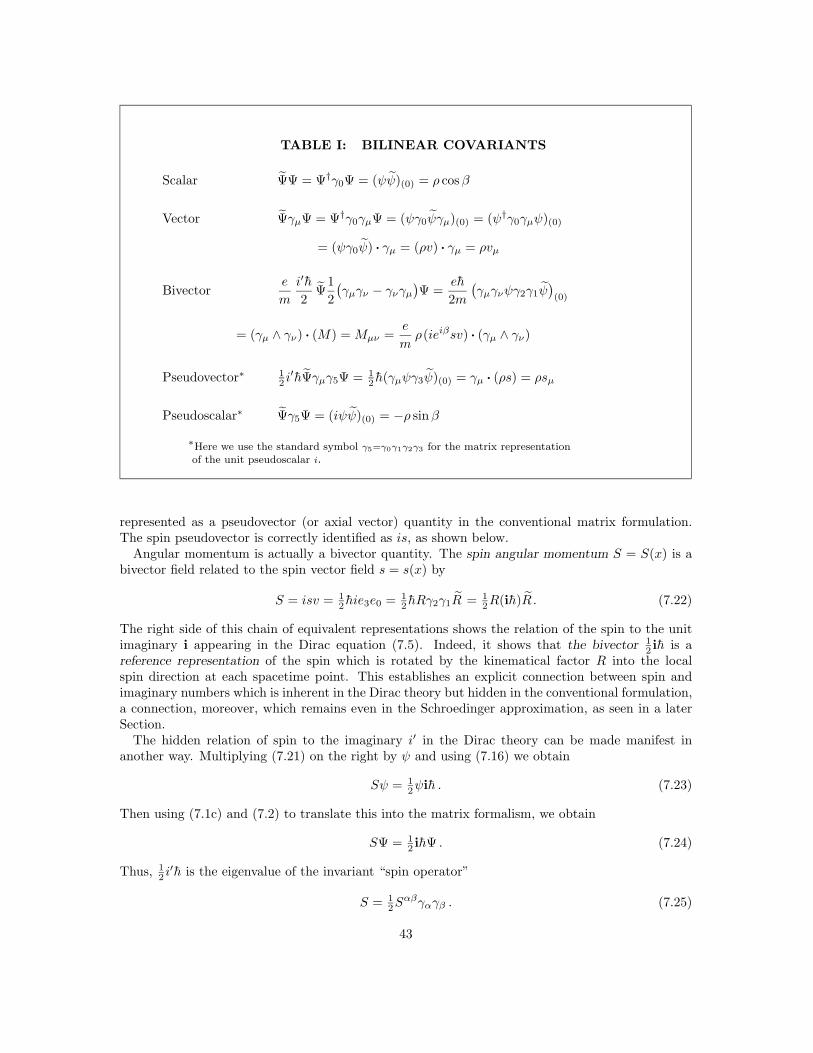
TABLE I: BILINEAR COVARIANTS

Scalar ΨΨ = Ψ†γ0Ψ = (ψψ)(0) = ρ cosβ

Vector ΨγµΨ = Ψ†γ0γµΨ = (ψγ0ψγµ)(0) = (ψ†γ0γµψ)(0)

= (ψγ0ψ) · γµ = (ρv) · γµ = ρvµ

Bivectore

m

i′h2

Ψ1

2

(γµγν − γνγµ

)Ψ =

eh

2m

(γµγνψγ2γ1ψ

)(0)

= (γµ ∧ γν) · (M) = Mµν =e

mρ(ieiβsv) · (γµ ∧ γν)

Pseudovector∗ 12 i

′hΨγµγ5Ψ = 12 h(γµψγ3ψ)(0) = γµ · (ρs) = ρsµ

Pseudoscalar∗ Ψγ5Ψ = (iψψ)(0) = −ρ sinβ

∗Here we use the standard symbol γ5=γ0γ1γ2γ3 for the matrix representationof the unit pseudoscalar i.

represented as a pseudovector (or axial vector) quantity in the conventional matrix formulation.The spin pseudovector is correctly identified as is, as shown below.

Angular momentum is actually a bivector quantity. The spin angular momentum S = S(x) is abivector field related to the spin vector field s = s(x) by

S = isv = 12 hie3e0 = 1

2 hRγ2γ1R = 12R(ih)R . (7.22)

The right side of this chain of equivalent representations shows the relation of the spin to the unitimaginary i appearing in the Dirac equation (7.5). Indeed, it shows that the bivector 1

2 ih is areference representation of the spin which is rotated by the kinematical factor R into the localspin direction at each spacetime point. This establishes an explicit connection between spin andimaginary numbers which is inherent in the Dirac theory but hidden in the conventional formulation,a connection, moreover, which remains even in the Schroedinger approximation, as seen in a laterSection.

The hidden relation of spin to the imaginary i′ in the Dirac theory can be made manifest inanother way. Multiplying (7.21) on the right by ψ and using (7.16) we obtain

Sψ = 12ψih . (7.23)

Then using (7.1c) and (7.2) to translate this into the matrix formalism, we obtain

SΨ = 12 ihΨ . (7.24)

Thus, 12 i

′h is the eigenvalue of the invariant “spin operator”

S = 12S

αβγαγβ . (7.25)

43

Otherwise said, the factor i′h in the Dirac theory is a representation of the spin bivector by itseigenvalue. The eigenvalue is imaginary because the “spin tensor” Sαβ is skewsymmetric. The factthat S = S(x) specifies a definite spacelike tangent plane at each point x is completely suppressedin the i′h representation. It should be noted also that (7.24) is completely general, applying to anyDirac wave function whatsoever.

The identification of Sαβ in (7.25) as spin tensor is not made in standard accounts of the Diractheory, though of course it must be implicated. Standard accounts (e.g. p. 59 of Ref. 22) eitherexplicitly or implicitly introduce the spin (density) tensor

ρSναβ =i′h2

Ψγν ∧ γα ∧ γβΨ =i′h2

Ψγ5γµΨεµναβ = ρsµεµναβ , (7.26)

where use has been made of the identity

γν ∧ γα ∧ γβ = γ5γµεµναβ (7.27a)

and the expression for sµ in Table I. Note that the “alternating tensor” εµναβ can be defined simplyas the product of two pseudoscalars, thus

εµναβ = i(γµ ∧ γν ∧ γα ∧ γβ) = (iγµγνγαγβ)(0)

= (γ3 ∧ γ2 ∧ γ1 ∧ γ0) · (γµ ∧ γν ∧ γα ∧ γβ) . (7.27b)

Alternatively,γµ ∧ γν ∧ γα ∧ γβ = −iεµναβ . (7.27c)

From (5.26) and (5.27b) we find

Sναβ = sµεµναβ = i(s ∧ γν ∧ γα ∧ γβ) = (is) · (γν ∧ γα ∧ γβ) . (5.28)

The last expression shows that the Sναβ are simply tensor components of the pseudovector is.Contraction of (5.28) with vν = v · γν and use of duality (1.16b) gives the desired relation betweenSναβ and Sαβ :

vνSναβ = i(s ∧ v ∧ γα ∧ γβ) = [ i(s ∧ v) ] · (γα ∧ γβ) = Sαβ . (5.29)

Its significance will be made clear in the discussion of angular momentum conservation.Note that the spin bivector and its relation to the unit imaginary is invisible in the standard

version of the bilinear covariants in Table I. The spin S is buried there in the magnetization (tensoror bivector). The magnetization M can be defined and related to the spin by

M =eh

2mψγ2γ1ψ =

eh

2mρeiβe2e1 =

e

2mρSeiβ . (5.30)

The interpretation of M as magnetization comes from the Gordon decomposition considered in thenext Section. Equation (5.30) reveals that in the Dirac theory the magnetic moment is not simplyproportional to the spin as often asserted; the two are related by a duality rotation represented bythe factor eiβ . It may be appreciated that this relation of M to S is much simpler than any relationof Mαβ to Sναβ in the literature, another indication that S is the most appropriate representationfor spin. By the way, note that (5.30) provides some justification for referring to β henceforth asthe duality parameter. The name is noncommittal to the physical interpretation of β, a debatableissue discussed later.

We are now better able to assess the content of Table I. There are 1 + 4 + 6 + 4 + 1 = 16distinct bilinear covariants but only 8 parameters in the wave function, so the various covariantsare not mutually independent. Their interdependence has been expressed in the literature by a

44

system of algebraic relations known as “Fierz Identities” (e.g., see Ref. 23). However, the invariantdecomposition of the wave function (5.16) reduces the relations to their simplest common terms.Table I shows exactly how the covariants are related by expressing them in terms of ρ, β, vµ,sµ, which constitutes a set of 7 independent parameters, since the velocity and spin vectors areconstrained by the three conditions that they are orthogonal and have constant magnitudes. Thisparametrization reduces the derivation of any Fierz identity practically to inspection. Note, forexample, that

ρ2 = (ΨΨ)2 + (Ψγ5Ψ)2 = (ΨγµΨ)(ΨγµΨ) = −(Ψγµγ5Ψ)(Ψγµγ5Ψ) .

Evidently Table I tells us all we need to know about the bilinear covariants and makes furtherreference to Fierz identities superfluous.

Note that the factor i′h occurs explicitly in Table I only in those expressions involving electronspin. The conventional justification for including the i′ is to make antihermitian operators hermitianso the bilinear covariants are real. We have seen however that this smuggles spin into the expressions.That can be made explicit by using (5.24) to derive the general identity

i′hΨΓΨ = ΨΓγαγβΨSαβ , (5.31)

where Γ is any matrix operator.Perhaps the most significant thing to note about Table I is that only 7 of the 8 parameters in the

wave function are involved. The missing parameter is the phase of the wave function. To understandthe significance of this, note also that, in contrast to the vectors e0 and e3 representing velocityand spin directions, the vectors e1 and e2 do not appear in Table I except indirectly in the producte2e1. The missing parameter is one of the six parameters implicit in the rotor R determining theLorentz rotation (5.18). We have already noted that 5 of these parameters are needed to determinethe velocity and spin directions e0 and e3. By duality, these vectors also determine the directione2e1 = ie3e0 of the “spin plane” containing e1 and e2. The remaining parameter therefore determinesthe directions of e1 and e2 in this plane. It is literally an angle of rotation in this plane and thespin bivector S = e2e1 = R iR is the generator of the rotation. Thus, we arrive at a geometricalinterpretation of the phase of the wave function which is inherent in the Dirac Theory. But all ofthis is invisible in the conventional matrix formulation.

The purpose of Table I is to explicate the correspondence of the matrix formulation to the real(STA) formulation of the Dirac theory. Once it is understood that the two formulations are com-pletely isomorphic, the matrix formulation can be dispensed with and Table I becomes superfluous.By revealing the geometrical meaning of the unit imaginary and the wave function phase along withthis connection to spin, STA challenges us to ascertain the physical significance of these geometricalfacts, a challenge that will be met in subsequent Sections.

6. OBSERVABLES AND CONSERVATION LAWS.

One of the miracles of the Dirac theory was the spontaneous emergence of spin in the theory whennothing about spin seemed to be included in the assumptions. This miracle has been attributedto Dirac’s derivation of his linearized relativistic wave equation, so spin has been said to be “arelativistic phenomenon.” However, we have seen that the Dirac operator (4.1) is equally suited tothe formulation of Maxwell’s equation (4.4), and we have concluded that the Dirac algebra arisesfrom spacetime geometry rather than anything special about quantum theory. The origin of spinmust be elsewhere.

Our objective here is to ascertain precisely what features of the Dirac theory are responsible for itsextraordinary empirical success and to establish a coherent physical interpretation which accounts

45

for all its salient aspects. The geometric insights of STA provide us with a perspective from which tocriticize some conventional beliefs about quantum mechanics and so leads us to some unconventionalconclusions.

The first point to be understood is that there is more to the Dirac theory than the Dirac equation.Indeed, the Dirac wave function has no physical meaning at all apart from assumptions that relateit to physical observables. Now, there is a strong tradition in quantum mechanics to associateHermitian Operators with Observables and their eigenvalues with observed values. Let’s call thisthe HOO Principle. There is no denying that impressive results have been achieved in quantummechanics using the HOO Principle. However, we shall see that certain features of the Dirac theoryconflict with the view that the HOO Principle is a universal principle of quantum mechanics. It iscontended that the successes of HOO Principle derive from one set of operators only, namely, thekinetic energy-momentum operators pµ defined in the convention matrix theory by

pµi = i′h∂µ − eAµ . (6.1)

Moreover, it will be seen that STA leads us to a new view on why these operators are so significantin quantum mechanics.

In the approach taken here observables are defined quite literally as quantities which can bemeasured experimentally either directly or indirectly. Observables of the Dirac theory are associateddirectly with the Dirac wave function rather than with operators, though operators may be used toexpress the association. A set of observables is said to be complete if it supplies a coherent physicalinterpretation for all mathematical features of the wave function. A complete set of observables isdetermined by the conservation laws for electron position, charge, energy-momentum and angularmomentum. The task now is to specify these observables and their conservation laws unambiguously.

We assume first of all that the Dirac theory describes the electron as a point particle, but thedescription is statistical and the position probability current is to be identified with the Diraccurrent (5.20). This interpretation can be upheld only if the Dirac current is rigorously conserved.To establish that, we follow Appendix B of Ref. 4, multiplying the Dirac equation (5.5) on the right

by iγ0γ3γµψ and using (5.18) to get

(ψ)hγµψ = −imρeiβe3eµ + eρAe1e2eµ .

The scalar part of this equation gives us

· (ρeµ) =2

hρeµ · (e3m sinβ + (e2e1) ·A) . (6.2)

Thus we have the four equations · (ρv) = ∂µ(ρvµ) = 0 , (6.3)

· (ρs) = −m sinβ , (6.4)

· (ρe1) =2

hρA · e2 , (6.5)

· (ρe2) = − 2

hρA · e1 . (6.6)

Equation (6.3) is the desired position probability conservation law. The meaning of the otherequations remains to be determined.

There are other conserved currents besides the Dirac current, so further argument is neededto justify its interpretation as probability current. We must establish the internal and externalvalidity of the interpretation, that is, we must show that internally it is logically coherent with theinterpretation of other observables and externally it agrees with empirical observations.

46

The Dirac current ρv assigns a unit timelike vector v(x) to each spacetime point x where ρ = 0.In keeping with the statistical interpretation of the Dirac current, we interpret v(x) as the expectedproper velocity of the electron at x, that is, the velocity predicted for the electron if it happens tobe at x. In the γ0-system, the probability that the electron actually is at x is given by

(ρv) · (γ0d3x) . (6.7)

It is normalized so that ∫d3x ρ0 = 1 , (6.8)

where the integral is over the spacelike hyperplane defined by the equation x · γ0 = t, and

ρ0 = ρv0 = (ρv) · γ0 = (ψγ0ψγ0)(0) = (ψψ†)(0) (6.9)

is the probability density in the γ0-system.The velocity v(x) defines a local reference frame at x called the electron rest frame. The proper

probability density ρ = (ρv) · v can be interpreted as the probability density in the rest frame. Bya well known theorem, the probability conservation law (6.3) implies that through each spacetimepoint there passes a unique integral curve which is tangent to v at each of its points. Let us call thesecurves (electron) streamlines. In any spacetime region where ρ = 0, a solution of the Dirac equationdetermines a family of streamlines which fills the region with exactly one streamline through eachpoint. The streamline through a specific point x0 is the expected history of an electron at x0, thatis, it is the optimal prediction for the history of an electron which actually is at x0 (with relativeprobability ρ(x0), of course!). Parametrized by proper time τ , the streamline x = x(τ) is determinedby the equation

dx

dτ= v(x(τ)) . (6.10)

The physical significance of these predicted electron histories is discussed in the next Section.Although our chief concern will be with observables describing the flow of conserved quantities

along streamlines, we pause to consider the main theorem relating local flow to the time developmentof spatially averaged observables. The result is helpful for comparison with the standard operatorapproach to the Dirac theory. Let f be some observable in the Dirac theory represented by amultivector-valued function f = f(x). The average value of f at time t in the γ0-system is definedby

〈f〉 =

∫d3x ρ0f . (6.11)

To determine how this quantity changes with time, we use

∂µ(ρvµf) = ρv ·f = ρdf

dτ= ρ0

df

dt, (6.12)

with the derivative on the right taken along an electron streamline. Assuming that ρ0 vanishes atspatial infinity, Gauss’s theorem enables us to put (6.12) in the useful integral form

d

dt

⟨f⟩

=

∫d3x ρv ·f =

⟨df

dt

⟩. (6.13)

This result is known as “Reynold’s Theorem” in hydrodynamics.Taking the proper position vector x as observable, we have the average position of the electron

given by

〈x〉 =

∫d3x ρ0x , (6.14)

47

and application of (6.13) gives the average velocity

d

dt〈x〉 =

∫d3x ρv =

⟨dx

dt

⟩. (6.15)

To see that this is a sensible result, use the space-time splits (2.1a) and (2.6) to get

〈x〉γ0 = 1 + 〈x〉 (6.16)

from (6.14), andd

dt〈x〉γ0 = 1 + 〈v〉 (6.17)

from, (6.15). Thus, we haved

dt〈x〉 = 〈v〉 =

⟨dx

dt

⟩. (6.18)

These elementary results have been belabored here because there is considerable dispute in the liter-ature on how to define position and velocity operators in the Dirac theory.24 The present definitionsof position and velocity (without operators!) are actually equivalent to the most straight- forwardoperator definitions in the standard formulation. To establish that we use Table I to relate thecomponents of in (6.18) to the matrix formulation; with the result

〈v〉 ·σk = 〈v ·σk〉 =

∫d3xΨ†αkΨ , (6.19)

where, as noted before, αk = γkγ0 = γ0γk is the matrix analog of σk = γkγ0 in STA.

The αk are hermitian operators often interpreted as “velocity operators” in accordance withthe HOO Principle. However, this leads to peculiar and ultimately unphysical conclusions.25 STAresolves the difficulty by revealing that the commutation relations for the αk have a geometricalmeaning independent of any properties of the electron. It shows that the αk are “velocity operators”in only a trivial sense. The role of the αk in (6.19) is isomorphic to the role of basis vectors σk

used to select components of the vector v. The velocity vector is inherent in the bilinear functionΨΨ†, not in the operators αk. The αk simply pick out its components in (6.19). Accordingly, theequivalence of STA representations to conventional operator representations exhibited in (6.19) andTable I leads to two important conclusions:7 The hermiticity of the αk is only incidental to their rolein the Dirac theory, and their eigenvalues have no physical significance whatever! These conceptsplay no role in the STA formulation.

Having chosen a particle interpretation for the Dirac theory, the assumption that the particleis charged implies that the charge current (density) J must be proportional to the Dirac current;specifically,

J = eψγ0ψ = eρv . (6.20)

Then charge conservation · J = 0 is an immediate consequence of probability conservation. Laterit will be seen that there is more to this story.

One more assumption is needed to complete the identification of observables in the Dirac theory.It comes from the interpretation of the pµ in (6.1) as kinetic energy-momentum operators. In theSTA formulation they are defined by

pµ = i h∂µ − eAµ , (6.21)

where the underbar signifies a “linear operator” and the operator i signifies right multiplication bythe bivector i = γ2γ1, as defined by

iψ = ψi . (6.22)

48

TABLE II: Observables of the energy-momentum operator,relating real and matrix versions.

Energy-momentum tensor Tµν = Tµ · γν = (γ0ψ γµpνψ)(0)

= ΨγµpνΨ

Kinetic energy density T 00 = (ψ†p0ψ)(0) = Ψ†p0Ψ

Kinetic momentum density T 0k = (ψ†pkψ)(0) = Ψ†pkΨ

Angular Momentum tensor Jναβ =[T ν ∧ x + iρ(s ∧ γν)

] · (γα ∧ γβ)

= T ναxβ − T νβxα − i′h2

Ψγ5γµΨεµναβ

Gordon current Kµ =e

m(ψ pµψ)(0) =

e

mΨpµΨ

The importance of (6.21) can hardly be overemphasized. Above all, it embodies the fruitful “minimalcoupling” rule, a fundamental principle of gauge theory which fixes the form of electromagneticinteractions. In this capacity it plays a crucial heuristic role in the original formulation of the Diracequation, as is clear when the equation is written in the form

γµpµψ = ψγ0m. (6.23)

However, the STA formulation tells us even more. It reveals geometrical properties of the pµ whichprovide clues to a deeper physical meaning. We have already noted a connection of the factor ihwith spin in (5.22). We establish below that this connection is a consequence of the form andinterpretation of the pµ. Thus, spin was inadvertently smuggled into the Dirac theory by the pµ,hidden in the innocent looking factor i′h. Its sudden appearance was only incidentally relatedto relativity. History has shown that it is impossible to recognize this fact in the conventionalformulation of the Dirac theory, with its emphasis on attributing physical meaning to operatorsand their commutation rules. The connection of i′h with spin is not inherent in the pµ alone. Itappears only when the pµ operate on the wave function, as is evident in (5.24). This leads to theconclusion that the significance of the pµ lies in what they imply about the physical meaning ofthe wave function. Indeed, the STA formulation reveals the pµ have something important to tell usabout the kinematics of electron motion.

The operators pµ or, equivalently, pµ = γµ · γν pν are given a physical meaning by using them todefine the components Tµν of the electron energy-momentum tensor:

Tµν = Tµ · γν = (γ0ψ γµpνψ)(0) . (6.24)

Its matrix equivalent is given in Table II. As mentioned in the discussion of the electromagneticenergy-momentum tensor,

Tµ = T (γµ) = Tµνγν (6.25)

49

is the energy-momentum flux through a hyperplane with normal γµ. The energy-momentum densityin the electron rest system is

T (v) = vµTµ = ρp . (6.26)

This defines the “expected” proper momentum p = p(x). The observable p = p(x) is the statisticalprediction for the momentum of the electron at x. In general, the momentum p is not collinear withthe velocity, because it includes a contribution from the spin. A measure of this noncollinearity isp ∧ v, which, by comparison with (2.7c), will be recognized as defining the relative momentum inthe electron rest frame.

From the definition (6.24) of Tµν in terms of the Dirac wave function, momentum and angularmomentum conservation laws can be established by direct calculation from the Dirac equation.First, we find that4 (See Appendix B for an alternative approach)

∂µTµ = J · F , (6.27)

where J is the Dirac charge current (6.20) and F = ∧ A is the electromagnetic field. The rightside of (6.27) is exactly the classical Lorentz force, so using (4.25) and denoting the electromagneticenergy-momentum tensor (4.24) by Tµ

EM , we can rephrase (6.27) as the total energy-momentumconservation law

∂µ(Tµ + TµEM ) = 0 . (6.28)

To derive the angular momentum conservation law, we identify Tµ ∧ x as the orbital angularmomentum tensor (See Table II for comparison with more conventional expressions). Noting that∂µx = γµ, we calculate

∂µ(Tµ ∧ x) = Tµ ∧ γµ − ∂µTµ ∧ x . (6.29)

To evaluate the first term on the right, we return to the definition (6.24) and find

γµTµν = [(pνψ)γ0ψ ](1) = 1

2

[(pνψ)γ0ψ + ψγ0(p

νψ)˜ ]= (pνψ)γ0ψ − ∂ν( 1

2 hψiγ3ψ) .

Summing with γν and using the Dirac equation (6.23) to evaluate the first term on the right whilerecognizing the spin vector (5.21) in the second term, we obtain

γνγµTµν = mψψ + (ρsi) . (6.30)

By the way, the pseudoscalar part of this equation proves (6.4), and the scalar part gives the curiousresult

Tµµ = Tµ · γµ = m cosβ . (6.31)

However, the bivector part gives the relation we are looking for:

Tµ ∧ γµ = Tµνγµ ∧ γν = · (ρsi) = −∂µ(ρSµ) , (6.32)

whereSµ = (is) · γµ = i(s ∧ γµ) (6.33)

is the spin angular momentum tensor already identified in (5.26) and (5.28). Thus from (6.29) and(6.27) we obtain the angular momentum conservation law

∂µJµ = (F · J) ∧ x , (6.34)

whereJ(γµ) = Jµ = Tµ ∧ x + ρSµ (6.35)

50

is the angular momentum tensor, representing the total angular momentum flux in the γµ direction.In the electron rest system, therefore, the angular momentum density is

J(v) = ρ(p ∧ x + S) , (6.36)

where recalling (2.12), p∧x is recognized as the expected orbital angular momentum and as alreadyadvertised in (5.22), S = isv can be indentified as an intrinsic angular momentum or spin. Thiscompletes the justification for interpreting S as spin. The task remaining is to dig deeper andunderstand its origin.

We now have a complete set of conservation laws for the observables r, v, S and p, but we stillneed to ascertain precisely how p is related to the wave function. For that purpose we employ theinvariant decomposition ψ = (ρeiβ)

12R. First we need some kinematics. By an argument used in

Section 3, it is easy to prove that the derivatives of the rotor R must have the form

∂µR = 12 ΩµR , (6.37)

where Ωµ = Ωµ(x) is a bivector field. Consequently the derivatives of the eν defined by (5.18) havethe form

∂µeν = Ωµ · eν . (6.38)

Thus Ωµ is the rotation rate of the frame eν as it is displaced in the direction γµ.Now, with the help of (5.23), the effect of pν on ψ can be put in the form

pνψ = [ ∂ν( ln ρ + iβ) + Ων ]Sψ − eAνψ . (6.39)

Whence

(pνψ)γ0ψ = [ ∂ν( ln ρ + iβ) + Ων ]iρs− eAνv . (6.40)

Inserting this in the definition (6.24) for the energy-momentum tensor, after some manipulationsbeginning with is = Sv, we get the explicit expression

Tµν = ρ[vµ(Ων · S − eAν) + (γµ ∧ v) · (∂νS) − sµ∂νβ

]. (6.41)

From this we find, by (6.26), the momentum components

pν = Ων · S − eAν . (6.42)

This reveals that (apart from the Aν contribution) the momentum has a kinematical meaning relatedto the spin: It is completely determined by the component of Ων in the spin plane. In other words,it describes the rotation rate of the frame eµ in the spin plane or, if you will “about the spin axis.”But we have identified the angle of rotation in this plane with the phase of the wave function. Thus,the momentum describes the phase change in all directions of the wave function or, equivalently, ofthe frame eµ. A physical interpretation for this geometrical fact will be offered in Section 8.

The kinematical import of the operator pν is derived from its action on the rotor R. To makethat explicit, use (6.37) and (5.22) to get

(∂νR)ihR = ΩνS = Ων · S + Ων ∧ S + ∂νS , (6.43)

where (5.22) was used to establish that

∂νS = 12 [ Ων , S ] = 1

2 (ΩνS − SΩν) . (6.44)

51

Introducing the abbreviation

iqν = Ων ∧ S , or qν = −(iS) ·Ων , (6.45)

we can put (6.43) in the form

(pνR)R = pν + iqν + ∂νS . (6.46)

This shows explicitly how the operator pν relates to kinematical observables, although the physicalsignificance of qν is obscure. Note that both pν and ∂νS contribute to Tµν in (6.41), but qν doesnot. By the way, it should be noted that the last two terms in (6.41) describe energy-momentumflux orthogonal to the v direction. It is altogether natural that this flux should depend on thecomponent of ∂νS as shown. However, the significance of the parameter β in the last term remainsobscure.

An auxiliary conservation law can be derived from the Dirac equation by decomposing the Diraccurrent as follows. Solving (6.23) for the Dirac charge current, we have

J = eψγ0ψ =e

m(pµψ)ψ . (6.47)

The identity (6.46) is easily generalized to

(pµψ)ψ = (pµ + iqµ)ρeiβ + ∂µ(ρSeiβ) . (6.48)

The right side exhibits the scalar, pseudoscalar and bivector parts explicitly. From the scalar partwe define the Gordon current:

Kµ =e

m[ (pµψ)ψ ](0) =

e

m(ψ pµψ)(0) =

e

m(pµρ cosβ − qµρ sinβ) . (6.49)

Or in vector form,

K =e

mρ(p cosβ − q sinβ) . (6.50)

As anticipated in the last Section, from the last term in (6.48) we define the magnetization

M =e

mρSeiβ . (6.51)

When (6.48) is inserted into (6.47), the pseudovector part must vanish, and vector part gives us theso-called“Gordon decomposition”

J = K + ·M . (6.52)

This is ostensibly a decomposition into a conduction current K and a magnetization current ·M ,both of which are separately conserved. But how does this square with the physical interpretationalready ascribed to J? It suggests that there is a substructure to the charge flow described by J .Evidently if we are to understand this substructure we must understand the role of the parameterβ so prominently displayed in (6.50) and (6.51). A curious fact is that β does not contribute tothe definition (5.20) for the Dirac current in terms of the wave function; β is related to J onlyindirectly through the Gordon Relation (6.52). This suggests that β characterizes some feature ofthe substructure.

So far we have supplied a physical interpretation for all parameters in the wave function (5.16)except “duality parameter” β. The physical interpretation of β is more problematic than that of theother parameters. Let us refer to this as the β-problem. This problem has not been recognized inconventional formulations of the Dirac theory, because the structure of the theory was not analyzedin sufficient depth to identify it. The problem arose, however, in a different guise when it was

52

noted that the Dirac equation admits negative energy solutions. The famous Klein paradox showedthat negative energy states could not be avoided in matching boundary conditions at a potentialbarrier. This was interpreted as showing that electron-positron pairs are created at the barrier, andit was concluded that second quantization of the Dirac wave function is necessary to deal with themany particle aspects of such situations. However, recognition of the β-problem provides a newperspective which suggests that second quantization is unnecessary, though this is not to deny thereality of pair creation. A resolution of the Klein Paradox from this perspective has been given bySteven Gull.26

In the plane wave solutions of the Dirac equation (next Section), the parameter β unequivocallydistinguishes electron and positron solutions. This suggests that β parametrizes an admixture ofelectron-positron states where cos β is the relative probability of observing an electron. Then, whileρ = ρ(x) represents the relative probability of observing a particle at x, ρ cosβ is the probabilitythat the particle is an electron, while ρ sinβ is the probability that it is an positron. On thisinterpretation, the Gordon current shows a redistribution of the current flow as a function of β.It leads also to a plausible interpretation for the β-dependence of the magnetization in (6.51). Inaccordance with (4.39), in the electron rest system determined by J , we can split M into

M = −P + iM , (6.53)

where, since v · s = 0,

iM =e

mSρ cosβ (6.54)

is the magnetic moment density, while

P = − e

miSρ sinβ (6.55)

is the electric dipole moment density. The dependence of P on sinβ makes sense, because paircreation produces electric dipoles. On the other hand, cancelation of magnetic moments by createdpairs may account for the reduction of M by the cosβ factor in (6.54). It is tempting, also, tointerpret equation (6.4) as describing a creation of spin concomitant with pair creation.

Unfortunately, there are difficulties with this straight forward interpretation of β as an antiparticlemixing parameter. The standard Darwin solutions of the Dirac hydrogen atom exhibit a strangeβ dependence which cannot reasonably be attributed to pair creation. However, the solutions alsoattribute some apparently unphysical properties to the Dirac current; suggesting that they may besuperpositions of more basic physical solutions. Indeed, Heinz Kruger has recently found hydrogenatom solutions with β = 0.27

It is easy to show that a superposition of solutions to the Dirac equation with β = 0 can producea composite solution with β = 0. It may be, therefore, that β characterizes a more general class ofstatistical superpositions than particle-antiparticle mixtures. At any rate, since the basic observablesv, S and p are completely characterized by the kinematical factor R in the wave function, it appearsthat a statistical interpretation for β as well as ρ is appropriate.

7. ELECTRON TRAJECTORIES

In classical theory the concept of particle refers to an object of negligible size with a continuoustrajectory. It is often asserted that it is meaningless or impossible in quantum mechanics to regardthe electron as a particle in this sense. On the contrary, it asserted here that the particle conceptis not only essential for a complete and coherent interpretation of the Dirac theory, it is also ofpractical value and opens up possibilities for new physics at a deeper level. Indeed, in this Sectionit will be explained how particle trajectories can be computed in the Dirac theory and how thisarticulates perfectly with the classical theory formulated in Section 3.

53

David Bohm has long been the most articulate champion of the particle concept in quantummechanics.28 He argues that the difference between classical and quantum mechanics is not in theconcept of particle itself but in the equation for particles trajectories. From Schroedinger’s equationhe derives an equation of motion for the electron which differs from the classical equation onlyin a stochastic term called the “Quantum Force.” He is careful, however, not to commit himselfto any special hypothesis about the origins of the Quantum Force. He accepts the form of theforce dictated by Schroedinger’s equation. However, he takes pains to show that all implications ofSchroedinger theory are compatible with a strict particle interpretation. The same general particleinterpretation of the Dirac theory is adopted here, and the generalization of Bohm’s equation derivedbelow provides a new perspective on the Quantum Force.

We have already noted that each solution of the Dirac equation determines a family of nonin-tersecting streamlines which can be interpreted as “expected” electron histories. Here we deriveequations of motion for observables of the electron along a single history x = x(τ). By a space-timesplit the history can always be projected into a particle trajectory x(τ) = x(τ)∧γ0 in a given inertialsystem. It will be convenient to use the terms ‘history’ and ‘trajectory’ almost interchangeably. Therepresentation of motion by trajectories is most helpful in interpreting experiments, but historiesare usually more convenient for theoretical purposes.

The main objection to a strict particle interpretation of the Dirac and Schroedinger theories isthe claim that a wave interpretation is essential to explain diffraction. This claim is false, as shouldbe obvious from the fact that, as we have noted, the wave function determines a unique familyof electron trajectories. For double slit diffraction these trajectories have been calculated fromSchroedinger’s equation.29 Sure enough, after flowing uniformly through the slits, the trajectoriesbunch up at diffraction maxima and thin out at the minima. According to Bohm, the cause ofthis phenomenon is the Quantum Force rather than wave interference. This shows at least thatthe particle interpretation is not inconsistent with diffraction phenomena, though the origin of theQuantum Force remains to be explained. The obvious objections to this account of diffraction havebeen adequately refuted in the literature.29,30 It is worth noting, though, that this account hasthe decided advantage of avoiding the paradoxical “collapse of the wave function” inherent in theconventional “dualist” explanation of diffraction. At no time is it claimed that the electron spreadsout like a wave to interfere with itself and then “collapse” when it is detected in a localized region.The claim is only that the electron is likely to travel one of a family of possible trajectories consistentwith experimental constraints; which trajectory is known initially only with a certain probability,though it can be inferred more precisely after detection in the final state. Indeed, it is possible thento infer which slit the electron passed through.29 These remarks apply to the Dirac theory as well asto the Schroedinger theory, though there are some differences in the predicted trajectories, becausethe Schroedinger current is the nonrelativistic limit of the Gordon current rather than the Diraccurrent.9

The probability density ρ0 is literally an observable in a diffraction pattern, though not in in-termediate states of a diffraction experiment. The same can be said for the velocities of detectedelectrons. This is justification for referring to ρ and v as “observables,” though they are not associ-ated with any operators save the Dirac wave function itself. But is it equally valid to regard them as“observables” in an atom? Though the Dirac theory predicts a family of orbits (or trajectories) inan atom, most physicists don’t take this seriously, and it is often asserted that it is meaningless tosay that the electron has a definite velocity in an atom. But here is some evidence to the contrarythat should give the sceptics pause: The hydrogen s-state wave function is spherically symmetricand its Schroedinger (or Gordon) current vanishes, so no electron motion is indicated. However,the radial probability distribution has a maximum at Bohr radius. This would seem to be no morethan a strange coincidence, except for the fact that the Dirac current does not vanish for an s-state,because the magnetization current is not zero. Moreover, the average angular momentum associatedwith this current is h,9 exactly as in the Bohr theory! Now comes the experimental evidence. Whennegative muons are captured in atomic s-states their lifetimes are increased by a time dilation factor

54

corresponding to a velocity of — you guessed it! — the Bohr velocity. Besides the idea that anelectron in an s-state has a definite velocity, this evidence supports the major contention that theelectron velocity is more correctly described by the Dirac current than by the Gordon current.

Now let us investigate the equations for motion along a Dirac streamline x = x(τ). On this curvethe kinematical factor in the Dirac wave function (5.16) can be expressed as a function of propertime

R = R(x(τ)) . (7.1)

By (5.18), (5.20) and (6.10), this determines a comoving frame

eµ = RγµR (7.2)

on the streamline with velocity v = e0, while the spin vector s and bivector S are given as beforeby (5.21) and (5.22). In accordance with (6.37), differentiation of (7.1) leads to

R = v ·R = 12ΩR , (7.3)

where the overdot indicates differentiation with respect to proper time, and

Ω = vµΩµ = Ω(x(τ)) (7.4)

is the rotational velocity of the frame eµ. Accordingly,

eµ = v · eµ = Ω · eµ . (7.5)

But these equations are identical in form to those for the classical theory in Section 3. This is aconsequence of the particle interpretation. In Bohmian terms, the only difference between classicaland quantum theory is in the functional form of Ω. Our main task, therefore, is to investigate whatthe Dirac theory tells us about Ω. Among other things, that automatically gives us the classical limitformulated as in Section 3, a limit in which the electron still has a nonvanishing spin of magnitudeh/2.

From (6.42) we immediately obtain

Ω · S = (p + eA) · v = 12 hω . (7.6)

This defines rate of rotation in the spin plane, ω = ω(x(τ)), as a function of the electron momentum.For a free particle (considered below), we find that it “spins” with the ultrahigh frequency

ω =2m

h= 1.6 × 1021 s−1 . (7.7)

According to (7.6), this frequency will be altered by external fields.Equation (7.6) is part of a more general equation obtained from (6.43):

ΩS = (p + eA) · v + i(q · v) + S . (7.8)

As an interesting aside, this can be solved for

Ω = SS−1 + (q · v)iS−1 + (p + eA) · vS−1 , (7.9)

where S−1 = is−1v. Whence,

v = Ω · v = (S · v)S−1 − (q · v)s−1 . (7.10)

55

This shows something about the coupling of spin and velocity, but it is not useful for solving theequations of motion.

A general expression for Ω in terms of observables can be derived from the Dirac equation. Thishas been done in two steps in Ref. 4. The first step yields the interesting result

Ω = −∧ v + v · (iβ) + (m cosβ + eA · v)S−1 . (7.11)

But this tells us nothing about particle streamlines, since

v = v · (∧ v) (7.12)

is a mere identity, which can be derived from (1.12) and the fact that v2 is constant. The secondstep yields

−∧ v + v · (iβ) = m−1(eFeiβ + Q) , (7.13)

where Q has the complicated form

Q = −eiβ [∂µWµ + γµ ∧ γν(W

µW ν)S−1](0) , (7.14)

withWµ = (ρeiβ)−1∂µ(ρeiβS) = ∂µS + S∂µ( ln ρ + iβ) . (7.15)

Inserting (7.13) in (7.11), we get from (7.5) and (6.44) the equations of motion for velocity and spin:

mv = e(Feiβ) · v + Q · v , (7.16)

S = F×( e

mSeiβ

)+ Q×S , (7.17)

where A×B = 12 (AB −BA) is the commutator product.

Except for the surprising factor eiβ , the first term on the right of (7.16) is the classical Lorentzforce. The term Q · v is the generalization of Bohm’s Quantum Force. A crucial fact to note from(7.15) is that the dependence of the Quantum Force on Plank’s constant comes entirely from thespin S. This spin dependence of the Quantum Force is hidden in the Schroedinger approximation,but it can be shown to be implicit there nevertheless.9 The classical limit can be characterizedfirst by ρ → 0 and ∂µ ln ρ → 0; second, by ∂µS = vµS, which comes from assuming that only the

variation of S along the history can affect the motion. Accordingly, (7.14) reduces to Q =..S , and

for the limiting classical equations of motion for a particle with intrinsic spin we obtain13

mv = (eF −..S ) · v , (7.18)

mS = (eF −..S )×S . (7.19)

These coupled equations have not been seriously studied. Of course, they should be studied inconjunction with the spinor equation (7.3).

In the remainder of this Section we examine classical solutions of the Dirac equation, that is,solutions whose streamlines are classical trajectories. For a free particle (A = 0), the Dirac equation(5.5) admits plane wave solutions of the form

ψ = (ρeiβ)12R = ρ

12 eiβ/2R0e

−ip·x/h , (7.20)

where the kinematical factor R has been decomposed to explicitly exhibit its spacetime dependencein a phase factor. Inserting this into (5.5) and using p · x = p, we obtain

pψ = ψγ0m. (7.21)

56

Solving for p we getp = meiβRγ0R = mve−iβ . (7.22)

This implies eiβ = ±1, soeiβ/2 = 1 or i , (7.23)

and p = ±mv corresponding to two distinct solutions. One solution appears to have negative energyE = p · γ0, but that can be rectified by changing the sign in the phase of the “trial solution” (7.20).

Thus we obtain two distinct kinds of plane wave solutions with positive energy E = p · γ0:

ψ− = ρ12R0e

−ip·x/h , (7.24)

ψ+ = ρ12 iR0e

+ip·x/h . (7.25)

We can identify these as electron and positron wave functions. Indeed, the two solutions are relatedby charge conjugation. According to (5.15), the charge conjugate of (7.24) is

ψC− = ψ−σ2 = ρ

12 iR′

0e−ip·x/h , (7.26a)

whereR′

0 = R0(−iσ2) . (7.26b)

As seen below, the factor −iσ2 represents a spatial rotation which just “flips” the direction of thespin vector. Evidently (7.25) and (7.26a) are both positron solutions, but with oppositely directedspins.

Determining the comoving frame (7.2) for the electron solution (7.24), we find that the velocity

v = R0γ0R0 and the spin s = 12 hR0γ3R0 are constant, but, for k = 1, 2,

ek(τ) = ek(0)e−p·x/S = ek(0)ee2e1ωτ , (7.27)

where τ = v · x and ω is given by (7.7). Thus, the streamlines are straight lines along which thespin is constant and e1 and e2 rotate about the “spin axis” with the ultrahigh frequency (7.7) asthe electron moves along the streamline. A similar result is found for the positron solution.

For applications, the constants in the solution must be specified in more detail. If the wavefunctions are normalized to one particle per unit volume V in the γ0-system, then we have

ρ0 = γ0 · (ρv) =1

Vor ρ =

m

EV=

1

γ0 · vV .

Following the procedure beginning with (2.13), we make the space-time split

R = LU where U = U0e−ip·x/h . (7.28)

The result of calculating L from γ0 and the momentum p has already been found in (2.24). As in(2.19) and (3.37), it is convenient to represent the spin direction by the relative vector

σ = Uσ3U . (7.29)

This is all we need to characterize spin. But to make contact with more conventional representations,we decompose it as follows: Choosing σ3 as “quantization axis,” we decompose U into spin up andspin down amplitudes denoted by U+ and U− respectively, and defined by

U±σ3 = ±σ3U± (7.30)

57

orU± = 1

2 (U ± σ3U) . (7.31)

ThusU = U+ + U− (7.32)

It follows thatUU = |U+ |2 + |U− |2 = 1 , (7.33)

U+U− + U−U+ = 0 , (7.34)

σ = Uσ3U =|U+ |2 − |U− |2σ3 + 2U−U+σ3 . (7.35)

since σσ3 = σ ·σ3 + i(σ×σ3),σ ·σ3 = |U+ |2 − |U− |2 , (7.36)

σ3×σ = 2iU−U+ . (7.37)

This decomposition into spin up and down amplitudes is usually given a statistical interpretationin quantum mechanics, but we see here its geometrical significance.

The classical limit is ordinarily obtained as an “eikonal approximation” to the Dirac equation.Accordingly, the wave function is set in the form

ψ = ψ0e−iϕ/h . (7.38)

Then the “amplitude” ψ0 is assumed to be slowly varying compared to “phase” ϕ, so the derivativesof ψ0 in the Dirac equation can be neglected to a good approximation. Thus, inserting (7.38) intothe Dirac equation, say in the form (6.47), we obtain

(ϕ− eA)eiβ = mv . (7.39)

As in the plane wave case (7.22) this implies eiβ = ±1, and the two values correspond to electronand positron solutions. For the electron case,

ϕ− eA = mv . (7.38)

This defines a family of classical histories in spacetime. For a given external potential A = A(x),the phase ϕ can be found by solving the “Hamilton-Jacobi equation”

(ϕ− eA)2 = m2 , (7.39)

obtained by squaring (7.38). On the other hand, the curl of (7.38) gives

m∧ v = −e∧A = −eF (7.40)

Dotting this with v and using the identity (7.12), we obtain exactly the classical equation (3.6) foreach streamline.

Inserting (7.40) into (7.11), we obtain

Ω =e

mF + (m + eA · v)S−1 . (7.41)

Whence the rotor equation (7.3) assumes the explicit form

R =e

2mFR−Ri(m + eA · v)/h . (7.42)

58

This admits a solution by separation of variables:

R = R0e−iϕ/h , (7.43)

whereR =

e

2mFR0 (7.44)

andϕ = v ·ϕ = m + eA · v . (7.45)

Equation (7.44) is identical with the classical equation in Section 3, while (7.45) can be obtainedfrom (7.38).

Thus, in the eikonal approximation the quantum equation for a comoving frame differs from theclassical equation only in having additional rotation in the spin plane. Quantum mechanics alsoassigns energy to this rotation, and an explicit expression for it is obtained by inserting (7.41) into(7.1), with the interesting result

p · v = m +e

mF · S . (7.46)

This is what one would expect classically if there were some sort of localized motion in the spinplane. That possibility will be taken up in the next Section.

The eikonal solutions characterized above are exact solutions of the Dirac equation when the ψ0

in (7.38) satisfiesψ0 = 0 . (7.47)

This equation has a whole class of exact solutions where ψ0 is not constant. This class is comparablein richness to the class of analytic functions in complex variable theory, for (7.47) can be regarded asa generalization of the Cauchy-Riemann equations.15 Considering the exact correspondence of theeikonal equations with classical theory, we can regard wave functions of this class as exact classicalsolutions of the Dirac equation. An important member of this class is the so-called Volkov solutionfor an electron in the field of an electromagnetic plane wave.32 We have already found the classicalsolution for this case, namely, the rotor (3.18a, b). Identifying this solution with R0 in (7.43), withthe help of (3.17) it is readily verified that R0 = 0. All that remains, then, is to determine thephase factor ϕ(x). This is easily done by integrating (7.45) or solving the Hamilton-Jacobi equation(7.39).

As a final observation about the eikonal approximation, we note that it rules out the possibility offinding any spin dependence of the streamlines such as that exhibited in equation (7.18). Evidentlythe spin dependence appears when the ϕ in (7.38) is generalized to a vector field with nonvanishingcurl.

59

8. THE ZITTERBEWEGUNG INTERPRETATION.

Now that we have the geometrical and physical interpretation of the Dirac wave function well inhand, we are prepared to examine deeper possibilities of the Dirac theory. We have seen that thekinematics of electron motion is completely characterized by the “Dirac rotor” R in the invariantdecomposition (5.16) of the wave function. The Dirac rotor determines a comoving frame eµ =

RγµR which rotates at high frequency in the e2e1-plane, the “spin plane,” as the electron movesalong a streamline. Moreover, according to (7.6) and (7.46), there is energy associated with thisrotation, indeed, all the rest energy p · v of the electron. These facts suggest that the electron mass,spin and magnetic moment are manifestation of a local circular motion of the electron. Mindful thatthe velocity attributed to the electron is an independent assumption imposed on the Dirac theoryfrom physical considerations, we recognize that this suggestion can be accommodated by giving theelectron a component of velocity in the spin plane. Accordingly, we now define the electron velocityu by

u = v − e2 = e0 − e2 . (8.1)

The choice u2 = 0 has the advantage that the electron mass can be attributed to kinetic energy ofself interaction while the spin is the corresponding angular momentum.11

This new identification of electron velocity makes the plane wave solutions a lot more physicallymeaningful. For p · x = mv · x = mτ , the kinematical factor for the solution (7.24) can be writtenin the form

R = e12ΩτR0 , (8.2)

where Ω is the constant bivector

Ω = mc2S−1 =2mc2

he1e2 . (8.3)

From (8.2) it follows that v is constant and

e2(τ) = eΩτe2(0) . (8.4)

So u = z can be integrated immediately to get the electron history

z(τ) = vτ + (eΩτ − 1)r0 + z0 , (8.5)

where r0 = Ω−1e2(0). This is a lightlike helix centered on the Dirac streamline x(τ) = vτ + z0 − r0.In the electron “rest system” defined by v, it projects to a circular orbit of radius

| r0 | = |Ω−1 | =h

2m= 1.9 × 10−13m . (8.6)

The diameter of the orbit is thus equal to an electron Compton wavelength. For r(τ) = eΩτr0, theangular momentum of this circular motion is, as intended, the spin

(mr) ∧ r = mrr = mr2Ω = mΩ−1 = S . (8.7)

Finally, if z0 is varied parametrically over a hyperplane normal to v, equation (8.5) describes a3-parameter family of spacetime filling lightlike helixes, each centered on a unique Dirac streamline.According to the Born statistical interpretation, the electron can be on any one of these helixes withuniform probability.

Let us refer to this localized helical motion of the electron by the name zitterbewegung (zbw)originally introduced by Schroedinger.33 Accordingly, we call ω = Ω · S the zbw frequency and

60

λ = ω−1 the zbw radius. The phase of the wave function can now be interpreted literally as thephase in the circular motion, so we can refer to that as the zbw phase.

Although the frequency and radius ascribed to the zbw are the same here as in Schroedinger’swork, its role in the theory is quite different. Schroedinger attributed it to interference between posi-tive and negative energy components of a wave packet,33,34 whereas here it is associated directly withthe complex phase factor of a plane wave. From the present point of view, wave packets and inter-ference are not essential ingredients of the zbw, although the phenomenon noticed by Schroedingercertainly appears when wave packets are constructed. Of course, the present interpretation was notan option open to Schroedinger, because the association of the unit imaginary with spin was notestablished (or even dreamed of), and the vector e2 needed to form the spacelike component of thezbw velocity u was buried out of sight in the matrix formalism. Now that it has been exhumed,we can see that the zbw must play a ubiquitous role in quantum mechanics. The present approachassociates the zbw phase and frequency with the phase and frequency of the complex phase factor inthe electron wave function. Henceforth, this will be referred to as the zitterbewegung interpretationof quantum mechanics.

The strength of the zbw interpretation lies first in its coherence and completeness in the Diractheory and second in the intimations it gives of more fundamental physics. It will be noted thatthe zbw interpretation is completely general, because the definition (8.1) of the zbw velocity is welldefined for any solution of the Dirac equation. It is also perfectly compatible with everything saidabout the interpretation of the Dirac theory in previous Sections. One need only recognize thatthe Dirac velocity can be interpreted as the average of the electron velocity over a zbw period, asexpressed by writing

v = u . (8.8)

Since the period is on the order of 10−21s, it is v rather than u that best describes electron motionin most experiments.

A possible difficulty with the interpretation of u as electron velocity is the fact that ρu is notnecessarily a conserved current, for from (6.6) we have

· (ρu) =2

hρA · e1 . (8.9)

However, it is probably sufficient that ρv is conserved.Perhaps the strongest theoretical support for the zbw interpretation is the fact that it is funda-

mentally geometrical; it completes the kinematical interpretation of R, so all components of R, eventhe complex phase factor, characterize features of the electron history. This kinematical interpreta-tion is made most explicitly in Ref. 14, where the comoving frame eµ is interpreted as a Frenetframe, with vectors e1 and e3 corresponding to first and third curvatures; the zbw radius is thenseen as the radius of curvature for the particle history.

The key ingredients of the zbw interpretation are the complex phase factor and the energy-momentum operators pµ defined by (6.21). The unit imaginary i appearing in both of these hasthe dual properties of representing the plane in which zbw circulation takes place and generatingrotations in that plane. The phase factor literally represents a rotation on the electron’s circularorbit in the i-plane. Operating on the phase factor, the pµ computes the phase rotation rates inall spacetime directions and associates them with the electron energy-momentum. Thus, the zbwinterpretation explains the physical significance of the mysterious “quantum mechanical operators”pµ.

The key ingredients of the zbw interpretation are preserved in the nonrelativistic limit and soprovide a zitterbewegung interpretation of Schroedinger theory. The nonrelativistic approximationto the STA version of the Dirac theory, leading through the Pauli theory to the Schroedinger theory,has been treated in detail elsewhere.15,13 But the essential point can be seen by a split of the Diracwave function y into the factors

ψ = ρ12 eiβ/2LUe−i(m/h)t . (8.10)

61

In the nonrelativistic approximation three of these factors are neglected or eliminated and ψ isreduced to the Pauli wave function

ψP = ρ12U0e

−i(ϕ/h) , (8.11)

where the kinematical factor U has been broken into a phase factor describing the zbw rotationand a spatial rotation factor U0 which rotates i into the direction of the spin. Many aspects ofspin and the zbw in the Pauli theory have already been discussed in Ref. 9. In the Schroedingerapproximation the factor U0 is neglected so ψP reduces to the Schroedinger wave function

ψS = ρ12 e−i(ϕ/h) . (8.12)

It follows from this derivation of the Schroedinger wave function that just as in the Dirac theory,the phase ϕ/h describes the zbw, and ∂µϕ describes the zbw energy and momentum. We see nowthe physical significance of the complex that phase factor e−i(ϕ/h) is kinematical rather than logicalor statistical as so often claimed.

The zbw interpretation explains much more than the electron spin and magnetic moment. Thatis especially clear in the Schroedinger theory where spin is ignored but the complex phase factoris essential. Stationary state solutions of both the Schroedinger and Dirac equations reveal animportant property of the zbw. The singlevaluedness of the wave function implies that the orbitalfrequency is a harmonic of the zbw frequency in stationary states. This opens the possibility ofzbw resonance as a fundamental explanatory principle in quantum mechanics. The Pauli principlemay be a consequence of zbw resonance between electron pairs, since it is linked to stationary stateconditions. Diffraction may be explained as zbw resonant momentum exchange. Thus we have thepossibility, or better, the challenge of finding zbw explanations for all the familiar phenomena ofquantum mechanics, including barrier penetration and the Aharonov-Bohm effect.

Further support for the zbw interpretation comes from recent successes of semiclassical mechanicsin molecular dynamics and electronic structure (Ref. Uzer etc.), often surpasing the results fromstandard quantum mechanical methods. Such success may be surprising from the conventionalview of quantum mechanics, but from the zbw perspective, the semiclassical approach of imposingquantum conditions on classical dynamics is just of way of meeting the conditions for zbw resonances.This constitutes further evidence for the possibility that standard quantum mechanics is dealing withensembles of particle orbits with zbw periodicity.

T. Uzer, D. Farrelly, J. Milligan, P. Raines & J. Skelton, Celestial Mechanics on a MacroscopicScale, Science 253, 42–48 (1991).

Quantum mechanics is characterized by phase coherence over distances very much larger thanan electron Compton wavelength defining the dimensions of the zbw. By what causal mechanismmight zbw coherence be established over such large distances? A tantalizing possibility arises byinterpreting the circular zbw orbit literally as the orbit of a point charge. For that implies thatthe electron must be the source of a (nonradiating) electromagnetic field which fluctuates with thezbw frequency. The observed Coulomb and magnetic dipole fields of the electron are averages ofthis field over times much longer than a zbw period. The zbw fluctuations are much too rapid toobserve directly, though perhaps they have been observed indirectly all along in quantum coherencephenomena. This rapidly fluctuating field is a prime candidate for Bohm’s Quantum Force. Aspeculative analysis of its quantum implications is given in Ref. 11.

Considering how well the zbw interpretation fits the Dirac theory, we can regard the Dirac theoryand all its successes as evidence that the zbw is a real physical phenomena. The Dirac theory, then,does not explain the zbw, it simply tells us that the zbw exists and describes some of its properties.To explain the zbw we must go beyond the Dirac theory to discover new physical mechanisms such asthe fluctuating “Quantum Force” proposed in the preceding paragraph. However, the Dirac theoryis not without clues as to what to look for. One important clue concerns the origin of electron

62

mass. The very form of the important equation (7.6) suggests that the electron’s mass may be aconsequence of magnetic self-interaction, as expressed by writing

m = S ·Ω = µ ·BS , (8.13)

where BS is the self-magnetic field presumed to be the origin of the free particle Ω. This is asuggestive starting point for a zbw approach to quantum electrodynamics, but that must be deferredto another day.

9. ELECTROWEAK INTERACTIONS.

The STA formulation of the Dirac theory has indubitable implications for the Weinberg-Salam(W-S) theory of electroweak interactions. The W-S theory generalizes the electromagnetic (E-M)gauge group to the electroweak (E-W) gauge group SU(2)×U(1). However, this was done withoutrealizing that the imaginary unit i which generates E-M gauge transformations in the Dirac theory isa spacelike bivector identified with the electron spin. This fact forces a strong geometrical constrainton the W-S theory: Since i has a spacetime interpretation, the generators of the larger E-W groupwhich include it must have related spacetime interpretations. Remarkably, this constraint can beeasily satisfied in the following way:

The Dirac current ψγ0ψ is a timelike vector field, so only 4 parameters are needed to specify it.However, 8 parameters are needed to specify the wave function ψ uniquely. Therefore, the Diraccurrent is invariant under a 4-parameter group of gauge transformations on the wave function:

ψ → ψG , (9.1)

where G = G(x) is an even multivector satisfying

Gγ0G = γ0 . (9.2)

It follows thatG = Ueiλ , (9.3)

where UU = 1. This exhibits explicitly the SU(2)×U(1) structure of the gauge group. Thus, theinvariance group of the Dirac current can be identified with the E-W gauge group. The subgroupwhich leaves the spin density ρs = ψγ3ψ invariant is characterized by the additional condition

Gγ3G = γ3 . (9.4)

The E-M gauge transformations belong to this subgroup. Note also that the U(1) factor in (9.3)is a duality factor exactly like the one parametrized by β/2 in the invariant decomposition of theDirac wave function (5.16). Thus, it may be that the fundamental physical role of β is to serve asa gauge parameter in electroweak theory.

Of course, the Dirac equation is not invariant under the entire E-W gauge group G, but it iseasily generalized to one that is by introducing a suitable “gauge invariant derivative” in the standardway. That has been done in Ref. 10, where the Weinberg-Salam model is completely reformulatedin terms of STA with the E-W gauge group defined as above. This opens up possibilities forintegrating the zitterbewegung idea with electroweak theory. Evidently that would obviate the needfor including Higgs bosons in the theory, since the zitterbewegung provides an alternative mechanismto account for the electron mass.

63

10. CONCLUSIONS.

The objective of this work has been to understand what makes quantum mechanics so successfulby analyzing the Dirac theory. The analysis has been developed progressively on three levels:reformulation, reinterpretation and modification. Let us take stock, now, to see how far we haveprogressed toward the objective.

A. REFORMULATION. We have seen that reformulation of the Dirac theory in terms of STAeliminated superfluous degrees of freedom in the Dirac algebra and reveals a hidden geometricalstructure in the Dirac equation and its solutions. The main results are:

(1.) The Dirac wave function has the invariant decomposition

ψ = (ρeiβ)12 R . (10.1)

(2.) The factor ih in the Dirac equation is a spacelike bivector related to the spin by

S = 12R(ih)R . (10.2)

(3.) The electron energy-momentum pν is related to the spin by

pν = Ων · S − eAν , (10.3)

where ∂νR = 12ΩνR.

These results are mathematical facts inherent in the original Dirac theory. By making the geo-metric structure of the theory explicit, however, they suggest a new, more coherent and completeinterpretation of the theory.

B. REINTERPRETATION. The new zitterbewegung interpretation is imposed on the Dirac the-ory simply by identifying the electron velocity with the lightlike vector u = R(γ0 − γ2)R . It followsthat the spin S in (10.2) is the angular momentum of the zitterbewegung, and (10.3) attributesenergy-momentum to this motion. The general helical character of the zitterbewegung is completelydetermined by the Dirac equation without further assumption.

This approach has the great formal advantage of providing the entire rotor R with a kinematicalinterpretation. In particular, the complex phase factor is interpreted as a direct representation of thezitterbewegung itself. Thus, a physical explanation is given for the appearance of complex numbersin quantum mechanics. Moreover, the zitterbewegung interpretation of the phase factor carries overto Schroedinger theory and so suggests a reinterpretation of quantum mechanics generally. This hasthe great advantage over variants of the Copenhagen interpretation of being grounded in the Diractheory.

Above all, the zitterbewegung interpretation presents us with an array of challenges. First, thereis a theoretical challenge to see how far we can go in providing zitterbewegung interpretations forthe standard results of quantum mechanics and even quantum electrodynamics. Second, there is achallenge to probe the zitterbewegung experimentally to see if it can be established as a “literallyreal” phenomenon. Finally, there is a challenge to see if the zitterbewegung can lead us beyondpresent quantum mechanics to deeper physical insights.

C. MODIFICATIONS. If indeed the zitterbewegung is physically real it is probably a consequenceof electromagnetic or electroweak self-interaction, and it may be the source of an electromagneticfield which fluctuates with the zitterbewegung frequency. Thus it opens up the possibility of a new

64

approach to the self-interaction problem and actually explaining the phenomenon of quantizationrather assuming it. Of course, such possibilities cannot be explored theoretically without goingbeyond the Dirac theory.

REFERENCES

1. D. Hestenes, Space-Time Algebra (Gordon & Breach, London, l966).

2. D. Hestenes, Real Spinor Fields, J. Math. Phys. 8, 798–808 (1967).

4. D. Hestenes, Local Observables in the Dirac Theory, J. Math. Phys. 14, 893–905 (1973).

5. D. Hestenes, Proper Particle Mechanics, J. Math. Phys. 15, 1768–1777 (1974).

6. D. Hestenes, Proper Dynamics of a Rigid Point Particle, J. Math. Phys. 15, 1778–1786 (1974).

7. D. Hestenes, Observables, Operators and Complex Numbers in the Dirac Theory, J. Math. Phys.16, 556-572 (1975).

8. R. Gurtler and D. Hestenes, Consistency in the formulation of the Dirac, Pauli and SchroedingerTheories, J. Math. Phys. 16, 573–583 (1975).

9. D. Hestenes, Spin and Uncertainty in the Interpretation of Quantum Mechanics, Am. J. Phys.,47, 339–415 (1979).

10. D. Hestenes, Space-Time Structure of Weak and Electromagnetic Interactions, Found. Phys.,12, l53–l68 (1982).

11. D. Hestenes, Quantum Mechanics from Self-Interaction, Found. Phys. 15, 63–87 (1985).

12. D. Hestenes, Clifford Algebra and the Interpretation of Quantum Mechanics. In Clifford Alge-bras and their Applications in Mathematical Physics, J.S.R. Chisholm & A. K. Common(eds.), (Reidel Publ. Co., Dordrecht/Boston, l986), p. 321–346.

13. D. Hestenes, On Decoupling Probability from Kinematics in Quantum Mechanics. In. Maxi-mum Entropy and Bayesian Methods, Dartmouth College l989, P. Fougere (Ed.) Kluwer,Dordrecht/Boston (1990).

14. D. Hestenes, The Zitterbewegung Interpretation of Quantum Mechanics, Found. Phys. (October,1990).

15. D. Hestenes and G. Sobczyk, Clifford Algebra to Geometric Calculus, A Unified Lan-guage for Mathematics and Physics, G Reidel Publ. Co., Dordrecht/Boston (1984).

16. D. Hestenes, New Foundations for Classical Mechanics, G. Reidel Publ. Co., Dordrecht/Boston (1985).

17. P.A.M. Dirac, Quantum Mechanics, Oxford U. Press, London, 4th edition (1958).

18. D. Hestenes, Vectors, Spinors and Complex Numbers in Classical and Quantum Physics, Am. J.Phys. 39, 1013–1028 (1971).

19. D. Hestenes, A Spinor Approach to Gravitational Motion and Precession, Int. J. Theo. Phys.,25, 589–598 (1986).

20. H.E. Moses, SIAM J. Appl. Math. 21, 14–144 (1971).

21. J. Bjorken and S. Drell, Relativistic Quantum Mechanics, McGraw-Hill, N.Y.(1964).

22. J. Jauch and F. Rohrlich, The Theory of Photons and Electrons, Addison-Wesley, ReadingMass. (1955).

23. J. P. Crawford, On the algebra of Dirac bispinor densities, J. Math. Phys. 26, 1439–1441 (1985).

65

24. T. D. Newton and E. P. Wigner, Localized States for Elementary Systems, Rev. Mod. Phys. 21,400–406 (1949).

25. R. P. Feynman, Quantum Electrodynamics, Benjamin, N.Y. (1961), p. 47–49.

26. S. Gull, The Klein Paradox, (to be published).

27. H. Kruger, private communication.

28. D. Bohm & B. Hiley, Unbroken Quantum Realism, from Microscopic to Macroscopic Levels,Phys. Rev. Letters 55, 2511 (1985).

29. C. Philippidis, C. Dewdney and B. J. Hiley, Quantum Interference and the Quantum Potential,Nuovo Cimento 52B, 15–28 (1979).

30. J.-P. Vigier, C. Dewdney, P.R. Holland & A. Kypriandis, Causal particle trajectories and theinterpretation of quantum mechanics. In Quantum Implications, B. J. Hiley & F. D. Peat(eds.), (Routledge and Kegan Paul, London, 1987).

31. M. P. Silberman, Relativistic time dilatation of bound muons and the Lorentz invariance ofcharge, Am. J. Phys. 50, 251–254 (1982).

32. L. S. Brown & T.W.G. Kibble, Phys. Rev. A 133, 705 (1964).

33. E. Schroedinger, Sitzungb. Preuss. Akad. Wiss. Phys.-Math. Kl. 24, 418 (1930).

34. K. Huang, On the Zitterbewegung of the Electron, Am. J. Phys. 47, 797 (1949).

35. A. O. Barut and A. J. Bracken, Zitterbewegung and the internal geometry of the electron, Phys.Rev. D23, 2454 (1981).

APPENDIX A: Transformations and Invariants.

This Appendix formulates general transformation laws for fields on spacetime and applies the re-sults to establish Poincare invariance of the field equations. The transformation law for spinor fieldsis shown to rest on a convention which can be chosen to make it identical with the transformationlaw for tensor fields.

Let f be a transformation of a 4-dimensional region (or manifold) R = x onto a region R′ = x′in a spacetime; the pointwise transformation is thus

f : x → x′ = f(x) . (A.1)

A transformation is understood to be a differentiable invertible mapping. It induces a transformationf of a vector field a = a(x) on R into a vector field a′ = a′(x′) on R′ defined by

f : a → a′ = fa = a ·f , (A.2)

where the derivative is evaluated at x = f−1(x′). A parenthesis has been dropped in writing fa inrecognition that f is a linear operator on tangent vectors.

The transformation f is called the differential of f . It has a natural extension from vector fieldsto arbitrary multivector fields. Thus, for vector fields a1, a2, . . . ak, the differential of the k-vectorfield a1 ∧ a2 ∧ · · · ∧ ak is defined by

f(a1 ∧ a2 ∧ · · · ∧ ak) = (fa1) ∧ (fa2) ∧ · · · ∧ (fak) . (A.3)

By linearity this determines the differential for any multivector field M = M(x):

fM =4∑

k=0

f(M)(k) , (A.4)

66

where it is understood that(fM)(0) = (M)(0) , (A.5)

which is to say that every scalar field is an invariant of f and hence of f . An extensive treatmentof the differential on differentiable manifolds is given in Ref. 15.

The differential of the unit pseudoscalar is given by

fi = idet f , (A.6)

wheredet f = i−1 fi = −ifi (A.7)

is the Jacobian of f .As an application of general interest, let us calculate the form of the differential for an arbitrary

infinitesimal transformationf(x) = x + ε(x) . (A.8)

It is understood that, for any unit vector a, ε · a is a small quantity. This is equivalent to thecondition that ε2 is small, except when ε is a null vector. For a vector field the correspondinginduced transformation is

fa = a ·(x + ε) = a + a · ε . (A.9)

Neglecting second order terms, therefore, for a bivector field a ∧ b, we have

f(a ∧ b) = a ∧ b + (a ·ε) ∧ b + a ∧ (b ·ε) = a ∧ b + [(a ∧ b) ·] ∧ ε . (A.10)

This result generalizes easily to the differential for an arbitrary multivector field:

fM = M + (M ·) ∧ ε , (A.11)

where

M · =

4∑k=0

f(M)(k) . (A.12)

Note that k = 0 is not included in the sum since the scalar part of M is invariant.As a significant example, we apply (A.11) to the pseudoscalar i and, using the duality relations

(1.16 a,b), we obtainfi = i + (i ·) ∧ ε = i(1 + · ε) . (A.13)

This gives us immediately the useful expression

det f = 1 + · ε (A.14)

for the Jacobian of f .Equation (A.11) determines a new function

M ′(x′) = M ′(x + ε) = M + [M(x) ·] ∧ ε .

To exhibit the ε-dependence of the argument explicitly, we make a Taylor expansion of the argumentand keep only first order terms to get

M ′(x) = M(x) − ε ·M(x) + [M(x) ·] ∧ ε . (A.15)

This tells us explicitly how the infinitesimal transformation changes the field M at a designatedpoint x.

67

Now let us turn to the question of Poincare invariance of the equations of physics. The Poincaregroup is the group of transformations on spacetime which leave invariant the “interval” (x2 −x1)

2 between every pair of spacetime points x1 and x2. We are concerned here only with theRestricted Poincare Group for physical reasons discussed below. This is the subgroup of Poincaretransformations continuously connected to the identity. Every such transformation is the compositeof a Lorentz rotation and a translation, so, according to (1.24), it can be written in the canonicalform

f(x) = RxR + c , (A.16)

where c is a constant vector and R is a constant rotor with RR = 1. From (A.2) we find immediatelythe differential

a′ = fa = RaR . (A.17)

For the product of two vector fields this gives the simple result

a′b′ = (fa)(fb) = RabR . (A.18)

By virtue of (1.3) this can be decomposed into a scalar part

a′ · b′ = a · b (A.19)

and a bivector parta′ ∧ b′ = f(a ∧ b) = R(a ∧ b)R . (A.20)

According to (A.3), the outer product is an invariant of the differential for any transformation. Theinner product and the geometric product are not generally invariant; however, (A.19) and (A.18)show that they are in the present case. It follows that for an arbitrary multivector field M thetransformation law is simply

M ′ = fM = RMR . (A.21)

From this the Poincare invariance of the basic equations of physics is easily established. For example,for Maxwell’s equation (4.4) we have

′F ′ = (f)(fF ) = (RR)(RFR) = RFR = RJR = J ′ (A.22)

Thus, the relation of field F to current J is a Poincare invariant.The physical significance of Poincare invariance deserves some comment, since the matter is fre-

quently muddled in the literature. Poincare transformations are commonly interpreted as relationsamong different inertial reference systems or observers. That is clearly not the correct interpreta-tion here, for no reference system has even been mentioned either in the formulation of Maxwell’sequation or of its induced transformation (A.22). Indeed, Maxwell’s equation F = J is manifestlyindependent of any coordinate system, so no argument at all is needed to establish its observerindependence. The Poincare invariance expressed by (A.22) should be interpreted as an equivalenceof spacetime points rather than an equivalence of observers. It describes a physical property of theMinkowski model of spacetime. Translation invariance implies that spacetime is homogeneous insense that the same laws of physics are the same at every spacetime point. Similarly, Lorentz rota-tion invariance implies that spacetime is isotropic in the sense that the laws of physics do not favorany particular timelike or spacelike directions. Poincare invariance thus provides the theoreticalbasis for comparing the results of physical experiments and observations made at different timesand places. It is the formal assertion that the laws of physics are the same everywherewhen.

The Poincare invariance of the Dirac equation (5.5) can be established in the same way as thatof Maxwell’s equation. Thus,

′ψ′i′h− eAψ′ = (RR)(RψR)(Ri′R)h− e(RAR)(RψR)

= R(ψih− eAψ)R = R(mψγ0)R = mψ′γ′0 . (A.23)

68

Note that the transformation law for the spinor wave function ψ has been taken to be

ψ′ = RψR (A.24)

in accordance with (A.21). However, the usual transformation law for a Dirac spinor is

ψ′ = Rψ (A.25)

or, in the conventional matrix representation (5.2),

Ψ′ = RΨ (A.26)

Nevertheless, the transformation laws (A.24) and (A.25) are physically equivalent, because all ob-servables are bilinear functions of the wave function. Indeed, as established by (5.7) through (5.11),

the factor R on the right of (A.24) can be transformed away at will. The choice between the trans-formation laws (A.24) and (A.25) is therefore a matter of convention. Though (A.25) is simpler,(A.24) has the advantage of conformity with (A.21) and hence the more general transformation law(A.4).

In the conventional formulation,It is of interest to consider briefly the infinitesimal Poincare transformations, since they play such

a prominent role in the conventional approach to relativistic quantum theory. For an infinitesimaltranslation, we take R = 1 and ε = c in (A.16), so (A.15) reduces to

M ′(x) = M(x− c) = (1 − c ·)M(x) . (A.27)

This applies equally to the electromagnetic field and the Dirac wave function. Writing c · = cµ∂µ,we recognized the ∂µ as generators of translations. It is noted that the ∂µ can be made hermitianby the artifice of introducing a unit imaginary factor i′, so the translation operators in quantummechanics are usually defined to be i′∂µ. These operators are then identified with momentumoperators. However, our analysis of the Dirac theory in Part II reveals that the success of thisformal procedure should be attributed to the physical interpretation of the Dirac wave functionrather than a general physical significance of hermitian operators.

For an infinitesimal Lorentz rotation, we take c = 0 in (A.16) and

R = e12B ≈ 1 + 1

2B , (A.28)

where B is an infinitesimal bivector. Then (A.16) reduces to

x′ = (1 + 12B)x(1 − 1

2B) ≈ x + B · x . (A.29)

Hence, ε = B · x in (A.15) and/or (A.30) in (A.21) gives

M ′(x) = [ 1 −B · (x ∧) + B× ]M(x) , (A.30)

where B×M is the commutator product. Alternatively, for a spinor ψ subject to the one-sidedtransformation law (A.27), the result is

ψ′(x) = [ 1 −B · (x ∧) + 12B ]ψ(x) . (A.31)

This is expressed in a more conventional form by expanding B with respect to a basis to get

ψ′(x) = (1 + 12B

µνJµν)ψ(x) , (A.32)

69

where theJµν = (γµ ∧ γν) · (x ∧) + 1

2γµ ∧ γν = xµ∂ν − xν∂µ + 12γµ ∧ γν (A.33)

are the usual “angular momentum operators” for a Dirac particle. In a similar way, angular mo-mentum operators for the electromagnetic field can be read off (A.30).

APPENDIX B: LAGRANGIAN FORMULATION

This appendix is concerned with the Lagrangian formulation of the Dirac theory. The Lagrangeapproach has the advantage of directly relating equations of motion to conservation laws. Thoughthis approach to the Dirac theory has been discussed many times in the literature, the STA formu-lation is sufficiently novel to merit one more version.

Let L = L(x) be the Lagrangian for some field on spacetime. The associated action integral overany region R is

A =

∫RL(x) | d4x | , (B.1)

where the oriented “volume element” for the region is the pseudoscalar

d4x = d1x ∧ d2x ∧ d3x ∧ d4x = i | d4x | . (B.2)

A general variation of the action involves both a change in the functional form of L and an infinites-imal displacement of R producing a new action

A′ = A + δA =

∫R′

L′(x′) | d4x′ | . (B.3)

For an infinitesimal displacement x → x′ + ε(x), (A.14) gives us

| d4x′ | = (1 + · ε) | d4x | . (B.4)

Hence, writing L′ = L + δL, to first order we have

δA =

∫R′

(δL + L · ε) | d4x | . (B.5)

Now for a given L, both field equations and conservation laws can be derived by requiring theinvariance condition δA = 0 subject to various constraints.

For the Dirac electron, we adopt the (nonunique) Lagrangian

L = 〈h(ψ)iγ3ψ − eAγ0ψ −mψψ〉 , (B.6)

where 〈. . .〉 = (. . .)(0) means “scalar part.” We derive the Dirac equation by requiring δA = 0 for anarbitrary variation δψ(x) = ψ′(x)−ψ(x) in the functional form of the wave function which vanisheson the boundary of R. In this case the boundary is fixed and ε = 0 in (B.5). The derivation employs

the scalar-part properties 〈M 〉 = 〈M〉 and 〈MN〉 = 〈NM〉. Thus, using (δψ)˜ = δψ the variationof the last term in (A.6) can be put in the form

δ〈ψψ〉 = 〈(δψ)ψ〉 + 〈ψδψ〉 = 2〈ψψ〉 .

Similarly, the variation of the second term in (B.6) involves

〈A(δψ)γ0ψ〉 = 〈ψγ0(δψ)A〉 = 〈Aψγ0δψ〉 .

70

for evaluate the variation of the first term in (B.6), we use δ(ψ) = (δψ) and

〈(δψ)γ3ψ〉 = 〈(δψiγ3ψ)〉 − 〈δψiγ3(ψ)˜ 〉= 〈(ψ)iγ3δψ〉 + · (δψiγ3ψ)(1) . (B.7)

The last term here does not contribute to δA in (B.5), because δψ vanishes on the boundary. Thus,we arrive at

δL = 2〈(hψiγ3 − eAψγ0 −mψ)δψ〉 . (B.8)

This vanishes for all values of the arbitrary even multivector δψ only if the Dirac equation (5.5) issatisfied.

CONSERVATION LAWS

Conservation Laws are derived by requiring invariance of the action under infinitesimal displace-ments preserving the field equations. For performing the calculation it is convenient to decomposeδψ into a part

δ ∗ψ = ψ′(x) − ψ(x) (B.9)

due to a change in the value of ψ and a part due to the shift ε = x′ − x in the argument. This iseasily done by writing

δψ = ψ′(x′) − ψ(x) = ψ′(x′) − ψ(x′) + ψ(x′) − ψ(x) .

To first order in small quantities δ ∗ψ(x′) = δ ∗ψ(x) and we have

δψ = δ ∗ψ(x) + ε ·ψ(x) . (B.10)

Applying the same argument to the integrand of (B.5), we have

δL + L · ε = δ ∗L + ε ·L + L · ε .

Thus, δA = 0 for any choice of the region R only if

δ ∗L + · (εL) = 0 . (B.11)

This is a Conservation Law for specified ε.To evaluate (B.11) for the electron Lagrangian (B.6), we note that δ ∗L will have the same form as

(B.8) except that the perfect divergence term in (A.7) must be included and an additional term dueto δ ∗A must be added. However, since we require that the Dirac equation be satisfied, the result issimply

δ ∗L = · (hδ ∗ψiγ3ψ)(1) − e〈δ∗Aψγ0ψ〉 . (B.12)

Inserting this into (B.11), we can express the general conservation law in the form

· [ h(δψ − ε ·ψ)iγ3ψ + εL](1)

= e〈(δA− ε ·A)ψγ0ψ〉 (B.13)

It will be helpful to reformulate this in terms of the energy-momentum operators pµ. From thedefinition (6.21) we have

ε · pψ = ε ·ψiγ3γ0 − eε ·Aψ . (B.14)

71

So from the definition of the energy-momentum tensor Tµ in (6.24) or Table II, we obtain

ε · Tµ = 〈γµ(ε · pψ)γ0ψ 〉 . (B.15)

Consequently,∂µ(ε · Tµ) = ∂µ〈γµ(ε ·ψ)iγ3ψ〉 − ∂µ(eε ·A〈γµψγ0ψ〉) , (B.16)

which relates one term on the left of (B.13) to Tµ. The Lagrangian (B.6) can also be expressed interms of Tµ, with the result

L = Tµµ − 〈mψψ〉 . (B.17)

But we have already observed in (6.31) that this vanishes in consequence of the Dirac equation.Finally, we note that the last term in (B.16) can be written

∂µ(ε ·AJµ) = J ·(ε ·A) , (B.18)

where J = eψγ0ψ is the Dirac charge current. Hence, with the help of the identity

ε · F · J = (ε ·A) · J −A · (J ·ε) , (B.19)

where F = ∧A, and we can put (B.13) in the form

∂µ(ε · Tµ − 〈γµδψiγ3ψ〉) = ε · F · J −A · (J ·ε) − J · (δA) . (B.20)

This is the desired final form of the general conservation law. Now it is a simple matter to assessthe implications of requiring Poincare invariance.

A. Translation Invariance. For an infinitesimal translation ε is constant, δψ = 0, and δA = 0.Hence, (B.20) reduces to

ε · (∂µTµ) = ε · (F · J) . (B.21)

Since ε is arbitrary, this implies the energy-momentum conservation law (6.27). Thus, energy-momentum conservation is a consequence of the homogeneity of spacetime.

B. Lorentz Invariance. For an infinitesimal Lorentz rotation, ε = B · x by (B.31), δA = B×A =B ·A by (A.32), and δψ = (1/2)Bψ by (A.33). In consequence, note the following:

A · [J ·(B · x) ] = (B · J) ·A = −J · (B ·A) = −J · (δA) ,

ε · Tµ = (B · x) · Tµ = B · (x · Tµ) ,

〈γµδψiγ3hψ〉 = 〈Bi(12 hψγ3ψ)γµψ〉 = B · (ρSµ) ,

where Sµ = i(s ∧ γµ) is the spin angular momentum tensor of (6.33). Inserting these results into(B.20), we obtain

B · [∂µ(Tµ ∧ x + ρSµ)] = B · [(f · J) ∧ x] . (B.22)

Since B is an arbitrary bivector, this implies the angular momentum conservation law (6.34). Thus,angular momentum conservation is a consequence of the isotropy of spacetime.

For the sake of completeness, we note that a complete Lagrangian for electron and E-M fieldstogether is obtained by adding to the Dirac Lagrangian (B.6) the term 1

2 〈F 2〉, where F = ∧ A.The electromagnetic part of the Lagrangian is then

LEM = 12 〈F 2〉 −A · J . (B.23)

72

From this the E-M field equation can be derived by the general variational principle. Thus, we notethat

δ[ 12 〈F 2〉] = 〈FδA〉 = δA · (F ) + ∂µ〈FγµδA〉 . (B.24)

The last term vanishes for δA = 0 on the boundary, so we have

δLEM = δA · (−F + J) = 0 .

Since δA is arbitrary, this implies Maxwell’s equation F = J .Conservation laws for the electromagnetic field can be obtained by inserting (B.23) into the general

Conservation Law (B.11). Thus, using (B.24) with δ∗A = δA − ε ·A and δ∗J = δJ − ε ·J , weobtain

∂µ[〈Fγµε ·A〉 − 1

2γµ · ε〈F 2〉 − 〈FγµδA〉]

= ε · (J · F ) + A · (J ·ε) −A · (δJ) − (J ·A) · ε (B.25)

Let us define the canonical energy-momentum tensor Tµc = Tc(γ

µ) by

Tc(n) = − 12FnF + n · F · ∇A

= ∇〈FnA〉 − 12n〈F 2〉 + A〈nF 〉 . (B.26)

where the reverse accents serve to indicate which functions are differentiated by . Inserting thisinto (B.25), we get the Conservation Law in the form

∂µ[ε · Tµc − 〈FγµδA〉 ] = ε · (J · F ) + A · (J ·ε) −A · (δJ) − J ·A · ε . (B.27)

As before, translation invariance yields the energy-momentum conseration law

∂µTµc = J · F = −F · J . (B.28)

And Lorentz invariance yields the angular momentum conservation law

∂µ[Tµc ∧ x + Sµ

c ] = (J · F ) ∧ x , (B.29)

where the E-M spin tensor Sµc = Sc(γ

µ) is given by

Sc(n) = (F · n) ∧A . (B.30)

of course, both (B.28) and (B.29) can be obtained by direct differentiation of (B.26). Also note thatwhen they are added to the corresponding equations (6.27) and (6.34) for the electron, the internalforces and torques cancel.

73