Project Number: SJB-GPM4 Space Technology 5 (ST5) Spacecraft Modeling A Major Qualifying Project Report: submitted to the Faculty of WORCESTER POLYTECHNIC INSTITUTE in partial fulfillment of the requirements for the Degree of Bachelor of Science by David Brennan [email protected] _____________________ Robert Lyons Jr. [email protected] _____________________ Michelle Porter [email protected] _____________________ Date: October 26, 2004 Robert Shendock Stephen J. Bitar Shendock@[email protected] [email protected] __________________ Federico Sanidad Fred J. Looft [email protected] [email protected] __________________ This document represents the work of WPI students. The opinions in this report are not necessarily those of the Goddard Space Flight Center or the National Aeronautics and Space Administration 100 Institute Road Worcester, MA 01609

Welcome message from author
This document is posted to help you gain knowledge. Please leave a comment to let me know what you think about it! Share it to your friends and learn new things together.
Transcript
Project Number: SJB-GPM4
Space Technology 5 (ST5) Spacecraft Modeling
A Major Qualifying Project Report: submitted to the Faculty of WORCESTER POLYTECHNIC INSTITUTE in partial fulfillment of the requirements for the
Degree of Bachelor of Science by
David Brennan
[email protected] _____________________
Robert Lyons Jr.
[email protected] _____________________
Michelle Porter
[email protected] _____________________
Date: October 26, 2004
Robert Shendock Stephen J. Bitar
Shendock@[email protected] [email protected] __________________
Federico Sanidad Fred J. Looft
[email protected] [email protected] __________________
This document represents the work of WPI students. The opinions in this report are not necessarily those of the Goddard Space Flight Center or the
National Aeronautics and Space Administration
100 Institute Road Worcester, MA 01609

ii
Table of Contents Table of Contents................................................................................................................ ii
Figures................................................................................................................................ iv
Tables................................................................................................................................. vi
Abstract ................................................................................................................................1
1 Project Introduction ..........................................................................................................2
1.1 Introduction............................................................................................................... 2 1.2 Space Technology 5.................................................................................................. 2 1.3 Problem Description ................................................................................................. 5 1.4 Summary................................................................................................................... 6
2 Background .......................................................................................................................7
2.1 Introduction............................................................................................................... 7 2.2 National Aeronautical and Space Administration..................................................... 7 2.3 NASA Goddard Space Flight Center........................................................................ 8 2.4 Satellite Orbit Determination.................................................................................... 8
2.4.1 Kepler’s Laws .................................................................................................... 8 2.4.2 Classical Orbital Elements (Keplerian Elements)............................................ 11 2.4.3 Earth Orbits...................................................................................................... 13 2.4.4 Orbit Propagator............................................................................................... 14
2.5 Spacecraft Attitude.................................................................................................. 15 2.6 Telemetry ................................................................................................................ 16
2.6.1 Institute for Scientific Research....................................................................... 18 2.7 ST5.......................................................................................................................... 19
2.7.1 ST5 Communication Subsystem...................................................................... 20 2.7.2 ST5 Antenna .................................................................................................... 22
2.8 Link Margin ............................................................................................................ 23 2.9 MATLAB/Simulink Software ................................................................................ 25 2.10 Summary............................................................................................................... 26
3 Project Statement ............................................................................................................28
3.1 Introduction............................................................................................................. 28 3.2 Project Goals........................................................................................................... 28 3.3 Summary................................................................................................................. 30
4 Model Structure ..............................................................................................................31
4.1 Introduction............................................................................................................. 31 4.2 Communications Model.......................................................................................... 31
4.2.1 Inputs/Outputs.................................................................................................. 31 4.2.2 Ground Station Visibility................................................................................. 32 4.2.3 Link Margin Calculation.................................................................................. 40 4.2.4 Zone of Interference (ZOI) Calculation........................................................... 44 4.2.5 Generating Output files.................................................................................... 53 4.2.6 Communications Model Verification .............................................................. 57
iii
4.3 Orbit Propagator...................................................................................................... 60 4.3.1 Algorithm......................................................................................................... 60 4.3.2 Improved Inter Range Vector (IIRV) .............................................................. 62 4.3.3 Earth Centered Fixed (ECF) to ECI Conversion ............................................. 64 4.3.4 Orbit Propagator Model Verification............................................................... 66
4.4 Model integration to Simulink ST5 ........................................................................ 67 4.5 Summary................................................................................................................. 67
5. Results............................................................................................................................69
5.1 Introduction............................................................................................................. 69 5.2 Communications Model.......................................................................................... 69 5.3 Orbit Propagator...................................................................................................... 75 5.4 Summary................................................................................................................. 76
6. Conclusions....................................................................................................................78
6.1 Introduction............................................................................................................. 78 6.2 Model Capabilities .................................................................................................. 78 6.3 Suggested Model Modifications ............................................................................. 79 6.4 Summary................................................................................................................. 79
Appendix 1: References .....................................................................................................81
Appendix 2: Contacts at NASA/GSFC..............................................................................85
Appendix 3: List of Terms.................................................................................................87
Appendix 4: List of Acronyms ..........................................................................................90
Appendix 5: ST5 Model Users’ Manual............................................................................92
Appendix 6: Authorship Information.................................................................................96

iv
Figures Figure 1: ST5 Satellite ........................................................................................................ 3 Figure 2: Magnetosphere Surrounding Earth Created by Solar Activity............................ 5 Figure 3: Kepler’s First Law............................................................................................... 9 Figure 4: Kepler’s Second Law ........................................................................................ 10 Figure 5: Kepler’s Third Law ........................................................................................... 11 Figure 6: A figure of the classical orbital elements .......................................................... 13 Figure 7: Common Earth Orbits ....................................................................................... 13 Figure 8: Attitude.............................................................................................................. 16 Figure 9: Telemetry........................................................................................................... 18 Figure 10: ST5 Communication subsystem...................................................................... 21 Figure 11: Quadrafilar Helix Antenna .............................................................................. 22 Figure 12: Evolved Antenna ............................................................................................. 23 Figure 13: Top Level Communications Simulink Model ................................................. 32 Figure 14: Latitude to ECI Conversion............................................................................. 35 Figure 15: Longitude to ECI conversion .......................................................................... 36 Figure 16: Azimuth and Elevation.................................................................................... 38 Figure 17: Topocentric-Horizon Coordinate System........................................................ 39 Figure 18: Link Margin Calculator ................................................................................... 40 Figure 19: Space Loss Calculator ..................................................................................... 41 Figure 20: Ground Station Transmission Gain Calculator ............................................... 42 Figure 21: High-Level Doppler Calculation Subsystem................................................... 43 Figure 22: Satellite Relative Velocity Calculation Subsystem......................................... 43 Figure 23: Doppler Shift Calculation Subsystem ............................................................. 44 Figure 24: Zone of Interference ........................................................................................ 44 Figure 25: ZOI Calculator................................................................................................. 46 Figure 26: Topocentric Equatorial Coordinate System .................................................... 48 Figure 27: Radiative Pattern Angle................................................................................... 49 Figure 28: RPA model ...................................................................................................... 50 Figure 29: RPA Subsystem Calculator ............................................................................. 51 Figure 30: QHA Patterns vs. EA Patterns......................................................................... 51 Figure 31: EA Radiative Pattern ....................................................................................... 52 Figure 32: Look-Up Table ................................................................................................ 53 Figure 33: Date/Time Information.................................................................................... 54 Figure 34: Start/End Dates for Line of Sight .................................................................... 55 Figure 35: Zone of Interference Plot and Date Calculation.............................................. 56 Figure 36: Acceleration Vector Calculation ..................................................................... 61 Figure 37: Position Vector Calculation............................................................................. 61 Figure 38: Satellite Coordinates to Workspace ................................................................ 62 Figure 39: IIRV.m Algorithm........................................................................................... 63 Figure 40: Satellite x-y-z position plot ............................................................................. 66 Figure 41: Ground Station Line of Sight .......................................................................... 70 Figure 42: Excel Spreadsheet provided by Marco Concha............................................... 71 Figure 43: Simulink ST5 Generated Excel Spreadsheet................................................... 71 Figure 44: Ground Station Line of Sight and Zone of Interference Line of Sight............ 73

v
Figure 45: Simulink ST5 ZOI Dates ................................................................................. 74 Figure 46: Ground Station Line of Sight, Doppler Shift, and Link Margin ..................... 75 Figure 47: IIRV correction................................................................................................ 76 Figure 48: ST5 Orbit ......................................................................................................... 76

vi
Tables Table 1: The Classical Orbital Elements .......................................................................... 12 Table 2: Test vectors and angles....................................................................................... 59

1
Abstract
The purpose of this project was to update an existing ST5 Simulink Radio Frequency
(RF) Communications model to provide more accurate line of sight predictions for long
term mission planning. The ST5 satellite consists of two omni directional antennas
mounted in opposition to each other resulting in an area of overlapping antenna patterns.
The composite RF transmission pattern exhibits a marked zone of destructive phase
interference. This area is referred to as the Zone of Interference (ZOI) which results in
insufficient link margins for reception. The modified RF model calculates the link
margin taking into account the radiative pattern as a function of satellite attitude and a
new orbit propagator will be utilized which is capable of maintaining accuracy for up to
three months to aid in long-term mission planning. Finally, the output of the Simulink
model provides black out dates and times for long term planning.

2
1 Project Introduction
1.1 Introduction
Space Technology 5 (ST5) is a division of the New Millennium Program (NMP), a
NASA supported program established in 1995 with the ambitious goal of advancing
space exploration through the development of advanced technologies. The NMP’s
primary focus is to conduct space flight validation of advanced instruments, spacecraft
systems/subsystems and concepts of flight. The goal of space flight validation of these
technologies is to eliminate risks to the user and promote hasty integration of these
technologies into future space missions. A secondary focus of the NMP is to conduct
earth-science data acquisition missions if the mission budget permits. The NMP has
proposed to do the following:
1. Reduce the size/weight of spacecraft, thus reducing costs
2. Help spacecraft become “intelligent,” able to think for themselves, to minimize
support of a mission operations team
3. Enable significantly improved (a several generation leap) technical capabilities in
future missions (NMP, 1995)
The NMP first generation missions were designed to provide a comprehensive, system-
level validation of high-priority spacecraft interaction and measurements. NMP first
generation missions include Deep Space 1 (DS1), Deep Space 2 (DS2) and Earth
Observing 1 (EO1). The NMP second generation missions were designed to make greater
use of a constellation of satellites as well as system validations. NMP second generation
missions include Earth Observing 3 (EO3) and Space Technology 5 (Crisp, Minning
2000).
1.2 Space Technology 5

3
The goal of the ST5 program is to create and test new components and technology that
will provide breakthroughs in performance, capabilities and applications and that can be
applied to future small-satellite missions. Figure 1 shows a diagram of the ST5 small-
satellite (small-sat) with dimensions.
Figure 1: ST5 Satellite
(nmp.jpl.nasa.gov/st5)
One of many reasons for creating smaller satellites is to simplify construction and reduce
cost. Smaller satellites are much easier to manage, move, deploy, and also create new
possibilities for launching methods. For example a small-sat can fit beneath a larger
spacecraft and be launched as a secondary payload, often referred to as “piggybacking”.
ST5 consists of three identical satellites weighing approximately 21.5 kg (47lbs),
measures 54.2 cm across, and 28.6 cm in height. The new technology components being
tested aboard the ST5 satellites include:
• Autonomous ground station software for scheduling and orbit determination,
specifically designed for constellations of spacecraft
• An X-Band Transponder for satellite communications, which requires less
than a quarter the voltage and half the power and weighs twelve (12) times
less and nine (9) times smaller than proven technology
• Advance Multifunctional Structures used for electrical interconnects which
will reduce cable mass by saving one (1) kilogram for every one-thousand
(1000) connections
4
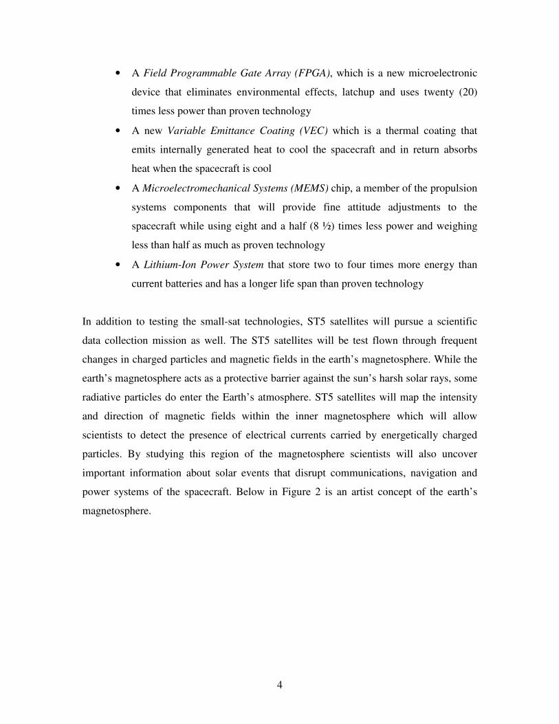
• A Field Programmable Gate Array (FPGA), which is a new microelectronic
device that eliminates environmental effects, latchup and uses twenty (20)
times less power than proven technology
• A new Variable Emittance Coating (VEC) which is a thermal coating that
emits internally generated heat to cool the spacecraft and in return absorbs
heat when the spacecraft is cool
• A Microelectromechanical Systems (MEMS) chip, a member of the propulsion
systems components that will provide fine attitude adjustments to the
spacecraft while using eight and a half (8 ½) times less power and weighing
less than half as much as proven technology
• A Lithium-Ion Power System that store two to four times more energy than
current batteries and has a longer life span than proven technology
In addition to testing the small-sat technologies, ST5 satellites will pursue a scientific
data collection mission as well. The ST5 satellites will be test flown through frequent
changes in charged particles and magnetic fields in the earth’s magnetosphere. While the
earth’s magnetosphere acts as a protective barrier against the sun’s harsh solar rays, some
radiative particles do enter the Earth’s atmosphere. ST5 satellites will map the intensity
and direction of magnetic fields within the inner magnetosphere which will allow
scientists to detect the presence of electrical currents carried by energetically charged
particles. By studying this region of the magnetosphere scientists will also uncover
important information about solar events that disrupt communications, navigation and
power systems of the spacecraft. Below in Figure 2 is an artist concept of the earth’s
magnetosphere.
5
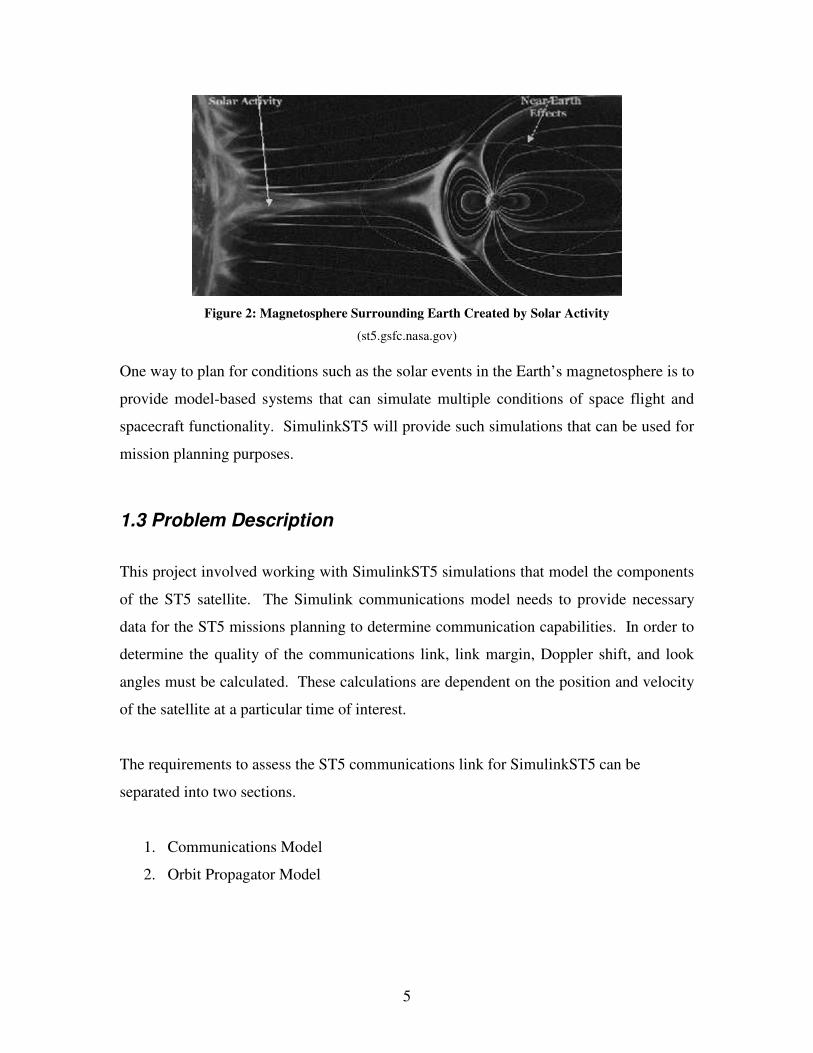
Figure 2: Magnetosphere Surrounding Earth Created by Solar Activity
(st5.gsfc.nasa.gov) One way to plan for conditions such as the solar events in the Earth’s magnetosphere is to
provide model-based systems that can simulate multiple conditions of space flight and
spacecraft functionality. SimulinkST5 will provide such simulations that can be used for
mission planning purposes.
1.3 Problem Description
This project involved working with SimulinkST5 simulations that model the components
of the ST5 satellite. The Simulink communications model needs to provide necessary
data for the ST5 missions planning to determine communication capabilities. In order to
determine the quality of the communications link, link margin, Doppler shift, and look
angles must be calculated. These calculations are dependent on the position and velocity
of the satellite at a particular time of interest.
The requirements to assess the ST5 communications link for SimulinkST5 can be
separated into two sections.
1. Communications Model
2. Orbit Propagator Model

6
The ST5 satellite consists of two omni antennas mounted in opposition of each other.
The composite antenna radiative pattern created by the two antennas creates an area of
destructive phase interference. This area is known as the Zone of Interference (ZOI) and
was accurately modeled by utilizing receiving antenna gain and line of sight calculations.
The communications model was updated to account for spacecraft attitude and the
antenna radiative pattern, as well as be able to determine ZOI occurrences and ground
station line of sight.
The communications model is highly dependent on accurately knowing the position and
velocity vectors of the spacecraft, which are in turn dependant on the accuracy of the
orbit propagator model. The propagator must be capable of providing output vectors for
long-term mission planning of up to 3-4 weeks. The orbit propagator must then be
integrated to the communications model which is used to determine the communication
link quality.
1.4 Summary
NASA’s New Millennium Program has advanced space exploration by developing
advanced technologies and integrating them into future spacecraft missions. Space
Technology 5, a second generation spacecraft cluster being developed as part of the
NMP, will be validating seven spacecraft technologies as well as the NMP second
generation goal of testing the satellite constellation theory. ST5 will also be recording
intensity and direction of magnetic fields within the Earth’s inner magnetosphere as a
secondary science objective to provide scientists with information about space weather
that may disrupt communications, navigations and power systems of the spacecraft.

7
2 Background
2.1 Introduction
In order to fully understand the goals and objectives of the project, a brief overview of
NASA, satellite orbits, communication variables including detailed and specific ST5
Communications model information as well as some key background information on link
margin and telemetry will be discussed in this chapter. Lastly an overview of the
MATLAB/Simulink software needed for SimulinkST5 modification will be discussed.
2.2 National Aeronautical and Space Administration
NASA was created on October 1, 1958, which aided U.S. space exploration. After the
Sputnik crisis, NASA inherited the National Advisory Committee for Aeronautics
(NACA) and other government agencies and initiated work on space exploration and
human space flight. NASA began to conduct space missions within months of its
creation and in its forty-five years has made historic achievements in many areas of
aeronautics and space research (Garber, 2003).
By conducting cutting-edge aeronautics research on aerodynamics, wind shear, and
related topics using wind tunnels, flight testing and computer simulations, NASA has
continued to build on what the NACA started. The technical and scientific
accomplishments of NASA demonstrate that humans can achieve what they never
imagined (Dick, 2003).
NASA’s aeronautics research has helped to enhance air transport safety, reliability,
efficiency, and speed through such programs as the X-15, lifting bodies, and general
aviation. NASA also contributes to Earth science missions, which deal with remote-
sensing satellites such as Landsat and meteorological spacecraft. These missions have

8
helped scientists understand the complex interactions between ecological systems on
Earth (Garber, 2003).
2.3 NASA Goddard Space Flight Center
NASA Goddard Space Flight Center (GSFC) is located in Greenbelt, Maryland about 6.5
miles from Washington D.C. The GSFC is in charge of many of NASA’s earth
observations, astronomy and space physics missions. Most of the missions include
developing and operating unmanned scientific spacecraft. GSFC also owns other
properties outside of Greenbelt, with the most recognized site being the Wallops Flight
Facility located near Chincoteague, Virginia.
2.4 Satellite Orbit Determination
In early times it was believed that planetary orbits were circular. In the 16th Century
scientists began gathering data that dispelled this belief. Then in the 17th century a
scientist named Johannes Kepler stated three laws of planetary motion which explained
how each planet moves in an elliptical orbit, with the sun at one of its foci.
2.4.1 Kepler’s Laws
German astronomer Johannes Kepler formulated three mathematical statements that
accurately described the revolutions of the planets around the sun. These laws can also be
applied to a satellite orbiting the earth. Kepler’s Laws paved the way for the application
of the laws of physics to the motions of heavenly bodies.
Kepler’s first law, which is also known as the Law of Elliptical Orbits states,
“Each planet moves in an elliptic orbit around the Sun, with the Sun occupying one of the
two foci of the ellipse.”

9
An ellipse is a circle with the opposite ends of the diameter pulled outward, making it
appear as an oval-shaped figure. The long axis of the ellipse is known as the major axis
and perpendicular to the major axis going through the center of the ellipse is the minor
axis. There are two points on the major axis called the foci, or focus for singular. The sun
occupies one focus and the other is empty.
Figure 3: Kepler’s First Law
(webphysics.iupui.edu/gpnew/gp2th4.htm)
In Figure 3 the Earth occupies one focus along the major axis. The length “a” represents
the semi-major axis, which is half of the major axis. The dot on the ellipse is the satellite
or moon orbiting the Earth in an elliptical orbit. The “�a” represents eccentricity.
Eccentricity is the ratio between the distances of a focus from the center of the ellipse to
the length of the semi-major axis. This determines the shape of an elliptical orbit. For
example an eccentricity equal to zero would describe a circular orbit and an eccentricity
equal to 1 would describe a highly elliptical orbit. The perigee is the point where the
moon or satellite is at its closest point to the earth. The apogee is the point where the
moon or satellite is at its farthest point from the earth. Both of these points are located
along the major axis.
Kepler’s Second Law, which is also known as the Law of Areas states,

10
“The imaginary line connecting any planet to the Sun sweeps over equal areas of the
ellipse in equal intervals of time.”
Figure 4: Kepler’s Second Law
(webphysics.iupui.edu/gpnew/gp2th4.htm)
Kepler's statement means, orbital speeds of a planet around the sun vary. The planets
move fastest when closest to the sun and slowest when farthest away. This speed change
is taken into account in Kepler’s Second Law. The distance covered in proportion to time
is shorter when farther away and the distance covered in proportion to time is longer at a
closer distance. “The satellite moves around an orbit in such a way that the radius vector
sweeps equal areas in equal times” (Gravity and Satellite Orbits, 2004).
Kepler’s Third Law, which is also known as the Harmonic Law states,
“The square of any planet's orbital period (its sidereal period) is proportional to the cube
of its mean distance (the length of the semimajor axis) from the Sun.”
The orbital period is the time for the planet to move 360° around the sun.

11
Figure 5: Kepler’s Third Law
(webphysics.iupui.edu/gpnew/gp2th4.htm)
This law relates the period of satellite motion to the size of the orbit. T is the orbital
period. G is the constant of universal gravitation and M is the mass of the Earth. Or if the
sun was at the focus of the ellipse M would be the mass of the sun. To simplify this
equation we can write it as,
T2 = Ka3
The constant K replaces all the other variables in the equation that are represented in the
figure. This new equation is a literal interpretation of Kepler’s third law as the square of
the orbital period is directly proportional to the cube of the semi-major axis.
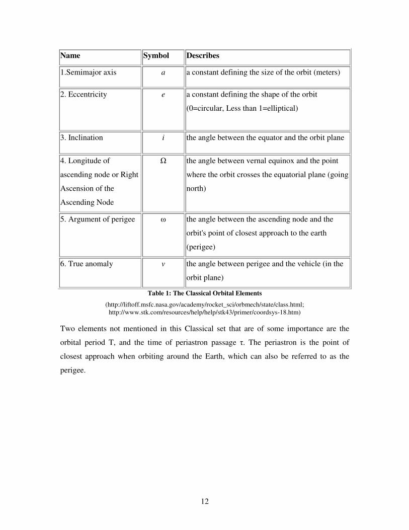
2.4.2 Classical Orbital Elements (Keplerian Elements)
There are six classical orbital elements that are needed to describe an orbit in space and
time. This set of elements describes an orbital ellipse around the earth and then orients it
three dimensionally and places a satellite along the ellipse in time.
The elements are listed in Table 1:
12
Name Symbol Describes
1.Semimajor axis a a constant defining the size of the orbit (meters)
2. Eccentricity e a constant defining the shape of the orbit
(0=circular, Less than 1=elliptical)
3. Inclination i the angle between the equator and the orbit plane
4. Longitude of
ascending node or Right
Ascension of the
Ascending Node
� the angle between vernal equinox and the point
where the orbit crosses the equatorial plane (going
north)
5. Argument of perigee � the angle between the ascending node and the
orbit's point of closest approach to the earth
(perigee)
6. True anomaly v the angle between perigee and the vehicle (in the
orbit plane)
Table 1: The Classical Orbital Elements
(http://liftoff.msfc.nasa.gov/academy/rocket_sci/orbmech/state/class.html; http://www.stk.com/resources/help/help/stk43/primer/coordsys-18.htm)
Two elements not mentioned in this Classical set that are of some importance are the
orbital period T, and the time of periastron passage �. The periastron is the point of
closest approach when orbiting around the Earth, which can also be referred to as the
perigee.
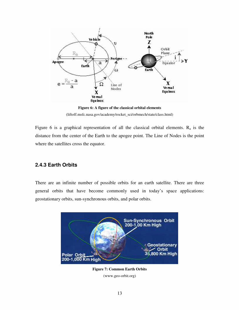
13
Figure 6: A figure of the classical orbital elements
(liftoff.msfc.nasa.gov/academy/rocket_sci/orbmech/state/class.html)
Figure 6 is a graphical representation of all the classical orbital elements. Ra is the
distance from the center of the Earth to the apogee point. The Line of Nodes is the point
where the satellites cross the equator.
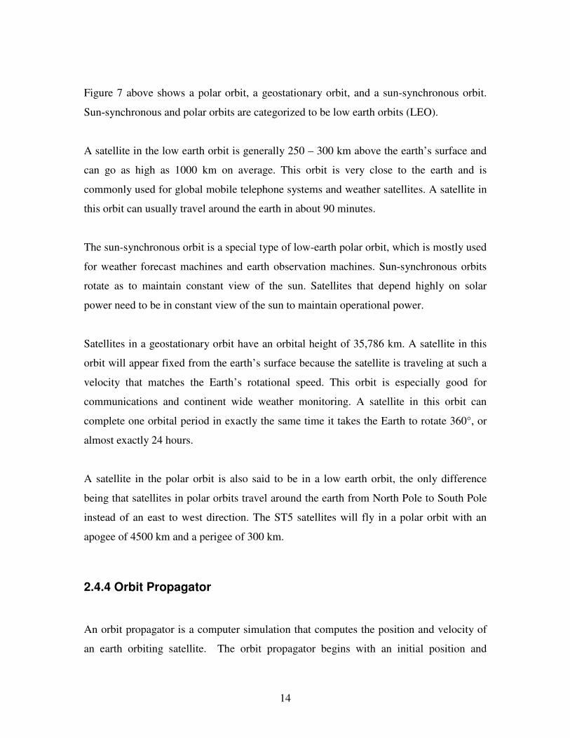
2.4.3 Earth Orbits
There are an infinite number of possible orbits for an earth satellite. There are three
general orbits that have become commonly used in today’s space applications:
geostationary orbits, sun-synchronous orbits, and polar orbits.
Figure 7: Common Earth Orbits
(www.geo-orbit.org)
14
Figure 7 above shows a polar orbit, a geostationary orbit, and a sun-synchronous orbit.
Sun-synchronous and polar orbits are categorized to be low earth orbits (LEO).
A satellite in the low earth orbit is generally 250 – 300 km above the earth’s surface and
can go as high as 1000 km on average. This orbit is very close to the earth and is
commonly used for global mobile telephone systems and weather satellites. A satellite in
this orbit can usually travel around the earth in about 90 minutes.
The sun-synchronous orbit is a special type of low-earth polar orbit, which is mostly used
for weather forecast machines and earth observation machines. Sun-synchronous orbits
rotate as to maintain constant view of the sun. Satellites that depend highly on solar
power need to be in constant view of the sun to maintain operational power.
Satellites in a geostationary orbit have an orbital height of 35,786 km. A satellite in this
orbit will appear fixed from the earth’s surface because the satellite is traveling at such a
velocity that matches the Earth’s rotational speed. This orbit is especially good for
communications and continent wide weather monitoring. A satellite in this orbit can
complete one orbital period in exactly the same time it takes the Earth to rotate 360°, or
almost exactly 24 hours.
A satellite in the polar orbit is also said to be in a low earth orbit, the only difference
being that satellites in polar orbits travel around the earth from North Pole to South Pole
instead of an east to west direction. The ST5 satellites will fly in a polar orbit with an
apogee of 4500 km and a perigee of 300 km.
2.4.4 Orbit Propagator
An orbit propagator is a computer simulation that computes the position and velocity of
an earth orbiting satellite. The orbit propagator begins with an initial position and

15
velocity vector. Using orbital mechanics the propagator then calculates new vectors with
the passing of time. The orbit propagator used for SimulinkST5 is a two body propagator
consisting of the earth and the sun. This propagator does not take into account the non-
spherical shape of the earth or atmospheric effects or gravitational effects of the moon.
For SimulinkST5 we incorporated an existing orbit propagator, and modified it to
incorporate Improved Inter Range Vectors for more accuracy, into our newly designed
communication model.
Improved Inter Range Vector (IIRV)
An IIRV is a standard message developed by GSFC, which contains six lines of ASCII
code describing multiple satellite parameters. The parameters we will use in this project
are a position vector, a velocity vector, and the current time. These parameters will be
integrated into our orbit propagator to produce a highly accurate simulated orbit of the
ST5 satellites.
IIRV satellite parameters are obtained by a NASA based satellite tracking system called
Tracking and Data Relay Satellite System, or TDRSS. White Sands Complex (WSC)
located in Las Cruces, New Mexico, extracts tracking data from the satellite’s
downlinked telemetry. This telemetry is then sent in TDRSS format to GSFC’s Flight
Dynamics Facility (FDF). FDF then temporarily stores this information as ephemeris
files, or tables giving the coordinates of a celestial body at a number of specific times
during a given period. Ephemeris files can then be transformed into acquisition data in an
IIRV format. IIRV’s are then sent to ground stations several times a day, centered on
every four hours, to provide accurate position and velocity vectors of orbiting satellites
(Tracking, 2005).
2.5 Spacecraft Attitude
In order to accurately model the communications link, spacecraft attitude must be known.
Attitude is the physical orientation of a satellite with respect to a defined spacecraft axis
system. The ST5 spacecraft axis system utilizes the Earth Centered Inertial coordinate

16
system. Attitude error, which is the spacecraft misalignment from the target position, will
be provided as a right ascension and declination with respect to the ECI coordinate
system shown in Figure 8. Right Ascension is the rotation angle about the x-y plane with
its reference point being along the y-axis. Declination is the angle above the x-y plane
with its reference point being zero degrees parallel to the x-y plane. The attitude data is
gathered from a combination of the Miniature Spinning Sun Sensor and the
Magnetometer aboard the ST5 spacecraft.
Figure 8: Attitude
The Attitude will change slightly each day in orbit due to atmospheric conditions and
gravitational forces. To correct the attitude, ST5 is equipped with a cold gas micro-
thruster, which will correctly orient the spacecraft when needed and will maintain 3�
(98.9%) precision of the spin axis.
2.6 Telemetry

17
Telemetry is the relaying of information from scientific instruments aboard a satellite to a
ground station. The information relayed is mostly health and safety information, or
spacecraft housekeeping information. This may include battery voltages, solar panel
currents and internal temperatures at certain points on the satellite. This information is
used to maintain the health and safety of the spacecraft.
When the spacecraft compiles the telemetry data, it is sent in a binary format. This binary
code is then converted to something that we can understand, such as degrees or volts, by
the receiving equipment at the ground station.
The use of international standards for formatting spacecraft data such as telemetry is
growing. The Consultative Committee for Space Data Systems, or CCSDS, has produced
a set of standards that are used in most spacecraft missions today. Space Technology 5 is
one of the 250 missions that are using these CCSDS standards. The benefits of these
standards are reduced cost, reduced risk and development time, and enhanced
interoperability and cross-support. CCSDS is standardizing spacecraft platforms and
space-qualified hardware components to ground support hardware and software (CCSDS
2004).
Telemetry data has two parts, a header field and an application data field. The header
contains the routing information such as the where and when part, and the application
data field contains the context of the telemetry information.
18
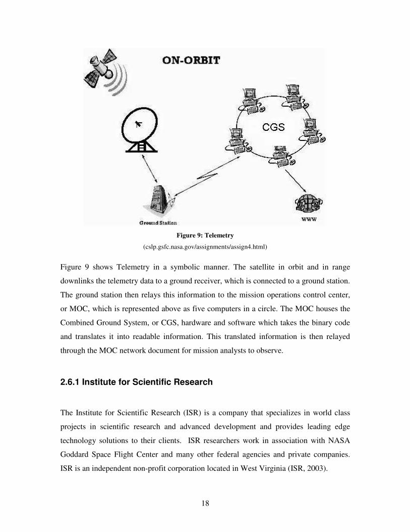
Figure 9: Telemetry
(cslp.gsfc.nasa.gov/assignments/assign4.html)
Figure 9 shows Telemetry in a symbolic manner. The satellite in orbit and in range
downlinks the telemetry data to a ground receiver, which is connected to a ground station.
The ground station then relays this information to the mission operations control center,
or MOC, which is represented above as five computers in a circle. The MOC houses the
Combined Ground System, or CGS, hardware and software which takes the binary code
and translates it into readable information. This translated information is then relayed
through the MOC network document for mission analysts to observe.
2.6.1 Institute for Scientific Research
The Institute for Scientific Research (ISR) is a company that specializes in world class
projects in scientific research and advanced development and provides leading edge
technology solutions to their clients. ISR researchers work in association with NASA
Goddard Space Flight Center and many other federal agencies and private companies.
ISR is an independent non-profit corporation located in West Virginia (ISR, 2003).
19
ISR developed a satellite interface utilizing the GMSEC bus that provides access to the
ST5 satellite telemetry. GMSEC stands for Goddard Space Flight Center Mission
Services Evolution Center. The GMSEC bus creates a standard way of transmitting data
from one application to another. Multiple applications will be accessing the bus at any
time and must be capable of communicating with each other.
2.7 ST5
For the ST5 model, specific components need to be identified to ensure proper function
of the satellite. The satellite can be broken down into eight subsystems.
• The structural/mechanical subsystem describes the satellite itself. The satellite
structure and all moving parts, instruments, and other systems are components of
the structural/mechanical subsystem.
• The thermal subsystem regulates the thermal characteristics of the satellites and
its multiple components. The ST5 thermal subsystem consists of blankets,
coatings and the Variable Emittance Coating (VEC) technology, which will be
flight validated.
• The power/electrical subsystem supplies the other subsystems with the necessary
power. The power is generated using solar panels that surround the ST5 satellite,
as well as a Li-Ion battery that can be recharged via the solar panels.
• The radio frequency (RF) communications system uses an X-band transponder,
low noise amplifier (LNA), high power amplifier (HPA), and two antennas
mounted on the top and bottom of the satellite. This system allows the satellite to
communicate with the ground stations.
• The guidance, navigation, and control subsystem uses a Miniature Spinning Sun
Sensor (MSSS) and a magnetometer to gather data which can be used to
determine the attitude of the satellite and ensure spin-stabilized control (Frisbee
like rotation).

20
• The propulsion subsystem utilizes cold gas micro-thrusters. These thrusters are
fired in pulses to conserve energy yet keep the satellites in orbit as well as a
proper distance from earth and each other.
• The Command and Data Handling (C&DH) subsystem monitors and records the
data gathered by the subsystem components, and magnetometer.
The SimulinkST5 behavioral model consists of the electrical power subsystem, the data
recorder, and the communication subsystem. For our goal we needed to familiarize
ourselves with the communication subsystem as well as the Simulink model developed
by the 2002 WPI MQP team.
2.7.1 ST5 Communication Subsystem
The ST5 communications subsystem utilizes the Deep Space Network (DSN) and
Ground Network (GN) ground stations. This subsystem consists of an X-band-
transponder, a diplexer, two antennas, a low noise amplifier, and a high-power amplifier
for transmission purposes. Figure 10 shows a block diagram of the ST5 Communication
subsystem.

21
Figure 10: ST5 Communication subsystem
(ST5 MQP 2002)
The X-band transponder is a NMP technology that will be tested on the ST5 mission.
The transponder has the following characteristics:
• Uplink data rate of 1Kbps
• Downlink data rate of 100Kbps
• Downlink data rate of 200Kbps
• Emergency real-time downlink rates of 10Kbps or 1 Kbps
• Transmission frequency approximately 8.5 GHz (transmission once per orbit)
Using the DSN and GN networks for ground station communications requires some extra
planning because each is a shared system. The time and duration of transmission must be
scheduled ahead of time to coincide with the projected orbit of ST5 satellites and the
availability (schedule) of DSN and GN stations. Data stored on the data recorder as well
22
as real-time housekeeping data is transmitted over a time period of approximately 6
minutes per satellite, per orbit.
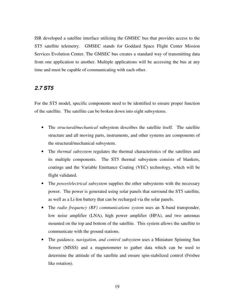
2.7.2 ST5 Antenna
Recent changes to the ST5 orbit from a geosynchronous orbit to a polar orbit have
affected the communication capabilities of the current ST5 antenna. The previous ST5
antenna known as the QHA (Quadrafilar Helix Antenna) shown in Figure 11, was
designed for long distance communications for the geosynchronous orbit which had an
apogee and perigee of 36,000 km and 300 km respectively. The new low earth orbit is
now one eighth the size of the old orbit with an apogee and perigee of 4500 km and 300
km. The QHA will meet the requirements of the new orbit but will not be as effective.
Figure 11: Quadrafilar Helix Antenna
(ST5 �CDR)
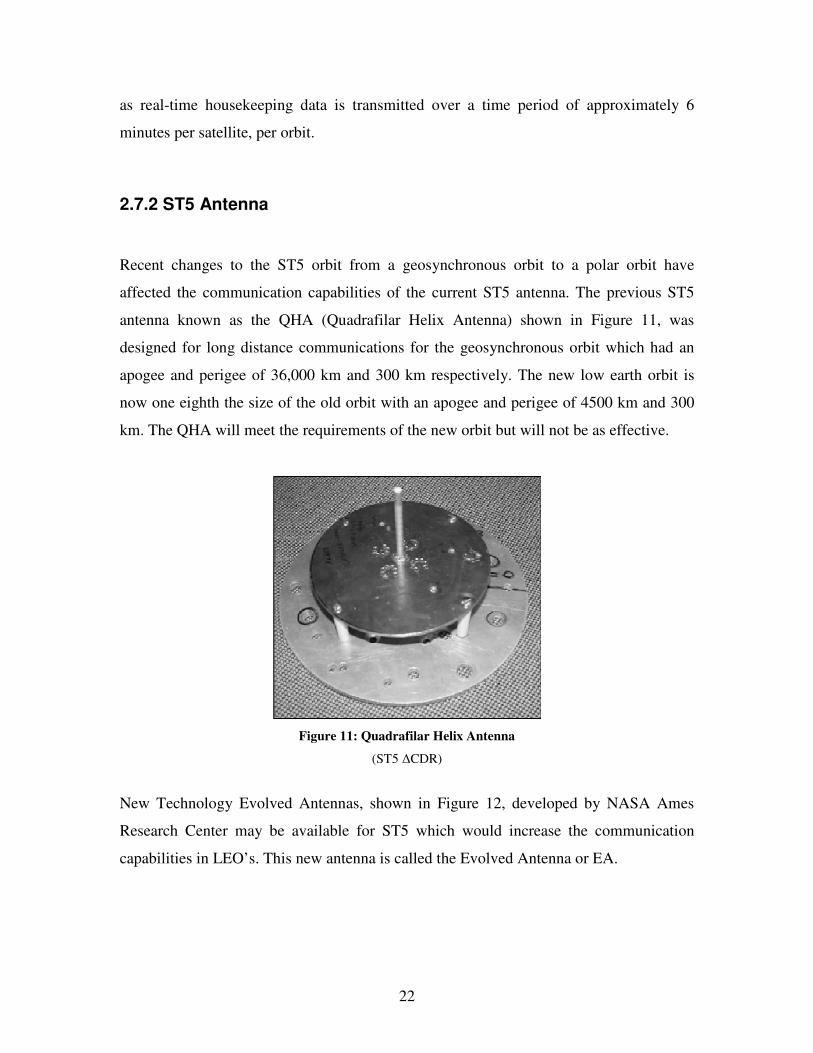
New Technology Evolved Antennas, shown in Figure 12, developed by NASA Ames
Research Center may be available for ST5 which would increase the communication
capabilities in LEO’s. This new antenna is called the Evolved Antenna or EA.
23
Figure 12: Evolved Antenna
(ST5 �CDR)
The wire form is designed using tree-structured computer algorithms. Each prong is
mathematically placed to provide maximum capabilities. This tree structure creates a
potential for high gain over a wider range of radiative pattern angles. The EA produces a
greater gain and can be manufactured at a lower cost than the QHA due to its limited
number of parts. The EA is still in test phases and the technical specifications were not
available. Predicted EA parameters are currently used by the Communications model.
2.8 Link Margin
To evaluate the communication systems performance we had to account for the Link
Margin (LM). The link margin is the difference between the required signal to noise ratio
and the actual signal to noise ratio.

24
LM = 0N
Eb - )(0
reqdNEb (2-1)
If the link margin is not sufficient enough, it will result in an undesired bit error rate at
the receiver.
Link margin calculations begin with signal-to-noise power ratio (SNR). The SNR is the
ratio of the signal power over the noise power as shown in Equation (2-2) below.
)()(
powerNoisepowersignal
SNR = (2-2)
A decrease in the signal power results in the SNR decreasing (loss). An increase in noise
power, as well as increases of interfering signal power (noise), will have the same effect.
Losses can also occur from the signal being absorbed, reflected, or scattered, before the
signal reaches the receiver.
There are four primary sources of noise when dealing with satellite transmission.
1. Thermal noise generated within the link
2. Atmospheric noise
3. System nonlinearities
4. Interference signals from other users
SNR is the quantity of greatest interest for this analysis because our system evaluation is
based on our ability to detect the signal, with an acceptable error probability (in the
presence of noise). The calculated signal to noise ratio takes into account the antenna
power and gain, the data rate, the frequency, and the various losses that would affect the
signal (free space loss, atmospheric losses, and passive losses). Equation (2-3) shows the
equation for signal to noise ratio. Link Margin (2-4) is simply Equation (2-3) minus a
required signal to noise ratio.
25
RTGLLEIRPNE
srasb −+−+++= κ0
(2-3)
LM = EIRP + Gr - R - K - T - Ls - Lo - )(0
reqdNEb (2-4)
Equation (2-4) has eight variables that need to be considered. sL is the space loss, Lo is
all other losses including the ones previously mentioned above, rG is the receiving
antenna gain (which includes diameter of antenna and half-length beamwidth), K is
Boltzmann’s Constant which is a constant equal to 228.6, R is the data rate, T is the
system temperature in Kelvin, and )(0
reqdNEb is the required signal to noise ratio which is
a constant requirement defined by ST5 parameters. The signal to noise ratio
requirements changes for uplink and downlink. EIRP is the Effective Isotropic Radiated
Power, which takes into account the transmitting power and gain, shown in Equation (2-
5).
EIRP = Pt + Gt (2-5)
Gt is the transmitting antenna gain. Pt is the transmitting antenna power. The required
signal to noise ratio for any downlink to either ground network is 4.45 dB. The required
signal to noise ratio for any uplink from either ground network is 9.6 dB. These variables
can all be found in the Radio Frequency Interface Control Document (RFICD) provided
to us by Victor Sank (ST5 RF/Communications, [email protected]).
2.9 MATLAB/Simulink Software
MATLAB is a high performance language for technical computing allowing for
integrating computation, visualization, and programming in an easy-to-use environment.
MATLAB problems and solutions are expressed in familiar mathematical notation,
whose basic data element is an array that does not require dimensioning. This software

26
solves many technical computing problems in a fraction of time than it would take to
write a program in a scalar non-interactive language such as C or FORTRAN (Learning
MATLAB, 2002).
Simulink is an interactive tool for modeling, simulating, and analyzing dynamic, multi-
domain systems. It is part of the MATLAB software package distributed by The
MathWorks, Inc. Simulink integrates seamlessly with MATLAB, providing immediate
access to an extensive range of analysis and design tools. Simulink allows the user to
build a block diagram, simulate the system’s behavior, evaluate its performance, and
refine the design. The software also allows for the modeling of linear and non-linear
systems in continuous time, sampled time (single-rate or multi-rate), or both. These
benefits make Simulink the tool of choice for control system design, digital signal
processing (DSP) design, communications system design, and other simulation
applications (Learning MATLAB, 2002).
Simulink models are hierarchical so that the user can use either a top-down or bottom-up
approach, allowing for comprehensive organization of systems, subsystems, and
components at different levels. This also provides the user with insight into how a model
is organized and how the different parts interact. Once a model is designed it is not
difficult to simulate it by using the simulation menus that Simulink provides, or by using
commands in MATLAB’s command prompt. The simulation menu is useful for
interactive simulations, while the command line is applicable for batches of simulations
(Dabney & Harman, 2001).
2.10 Summary
ST5 is composed of three small-satellites to be launched into a low earth orbit and flown
for three months in a “string of pearls” formation. The mission of ST5 is to verify new
technologies in space flight. Our project deals with link margin analysis, basic satellite
orbits, telemetry, antenna's, attitude, and MATLAB/Simulink software. The critical

27
system for verifying the new technology is the communications subsystem. In order to
ensure successful completion of the mission, a behavioral model needs to be created
focusing on the communication model using MATLAB/Simulink simulation software.

28
3 Project Statement
3.1 Introduction
The purpose of this project was to accurately determine ST5 satellite communication
capabilities using Simulink. In order to upgrade the communications model to provide
accuracy for long-term mission planning, new components were added to the orbit
propagator model and communications model. Below, we provide a detailed description
of our project goals, objectives and tasks.
3.2 Project Goals
The primary goal of this project is to accurately model the ST5 communications link for
long-term mission planning. Determining communication capabilities is dependant on
the location of the satellite at a specific time of interest; therefore the communications
model will need accurate position and velocity vectors describing the satellite orbit.
The orbit propagator outputs a position and velocity vector that is then interfaced with the
communications model. The previous communications model relied on a simple two
body propagator that provided accurate vectors for 3-4 hours. Since SimulinkST5 will be
running simulations for a period of 3 weeks, the propagator was upgraded for more
accuracy. The new orbit propagator utilizes Improved Inter Range Vectors (IIRV’s)
which provide discrete points describing the satellite location. The IIRV’s are
incorporated to the two body propagator to provide realignment of the satellite orbit,
correcting any propagation errors. Upgrading the orbit propagator model consisted of the
following primary objectives and tasks.
1) Orbit Propagator Model
a) Incorporate IIRV files

29
i) Understand Orbit Propagator Algorithm
ii) Interpret IIRV files
iii) Understand Coordinate Transformations
b) Interface Outputs to Communications Model
Using the orbit propagator, the ST5 communications model was updated to determine
communications capabilities. The updated model accounts for the ST5 antenna radiative
pattern that provides an antenna gain to be used for link margin calculations. The
antenna radiative pattern was also modeled to help determine the occurrence of the Zone
of Interference. Determining ZOI required the line of sight calculation and ZOI to be
upgraded as a function of spacecraft orbital geometry and attitude.
The communication model will asses the communications link for each ground station
that ST5 uses. A new DN ground station, McMurdo, will be used to help support the low
earth orbit of ST5. The location of McMurdo (Antarctica) provides the most frequent
communication possibilities for polar orbits. For each ground station link margin,
Doppler shift, and look angles are all calculated to determine communication capability.
The communications model can be broken down into several objectives and tasks.
1) Communications model
a) Incorporate GN ground station, McMurdo
i) Research GN antenna parameters
b) Model Antenna Radiative Pattern
i) Gather EA pattern data
c) Calculate Line of Sight
i) Understand Coordinate Transformations
d) Determine Zone of Interference
i) Understand Orbital Geometry

30
The communications model provides multiple output graphs of link margin, Doppler
Shift, ZOI, and line of sight. The model also provides output files of date and times
corresponding to line of sight and ZOI.
3.3 Summary
The primary goal of this project was to update the existing communications model to
support long-term mission planning to predict communication capabilities. To
accomplish this, the orbit propagator was upgraded to provide accurate positions and
velocity vectors that are then interface to the communications model. The
communications model was upgraded to model the antenna radiative pattern as a function
of attitude which is used to determine line of sight, and ZOI. The final output of the
model provides the necessary data to predict communications link capabilities.

31
4 Model Structure
4.1 Introduction
The communications model is designed to accurately determine the ST5 communication
link quality. Since the communications model is a function of the orbit propagator
outputs, the communications model can only be as accurate as the orbit propagator.
Therefore the orbit propagator is designed to provide better accuracy for long-term
mission planning. In this section we outline the structures of both the communications
model and orbit propagator model.
4.2 Communications Model
The purpose of the ST5 Communications model, shown in Figure 13, is to accurately
determine the link quality between ground stations and the satellite. Link quality is
dependent on ground station position, satellite position, and antenna parameters. The
model is used to calculate look angles, link margin, Zone of Interference and Doppler
Shift for each ground station. There are four inputs necessary for the Communications
model, date/time information, latitude/longitude/altitude of each ground station, satellite
ECI position and velocity vectors, and the spacecraft attitude.
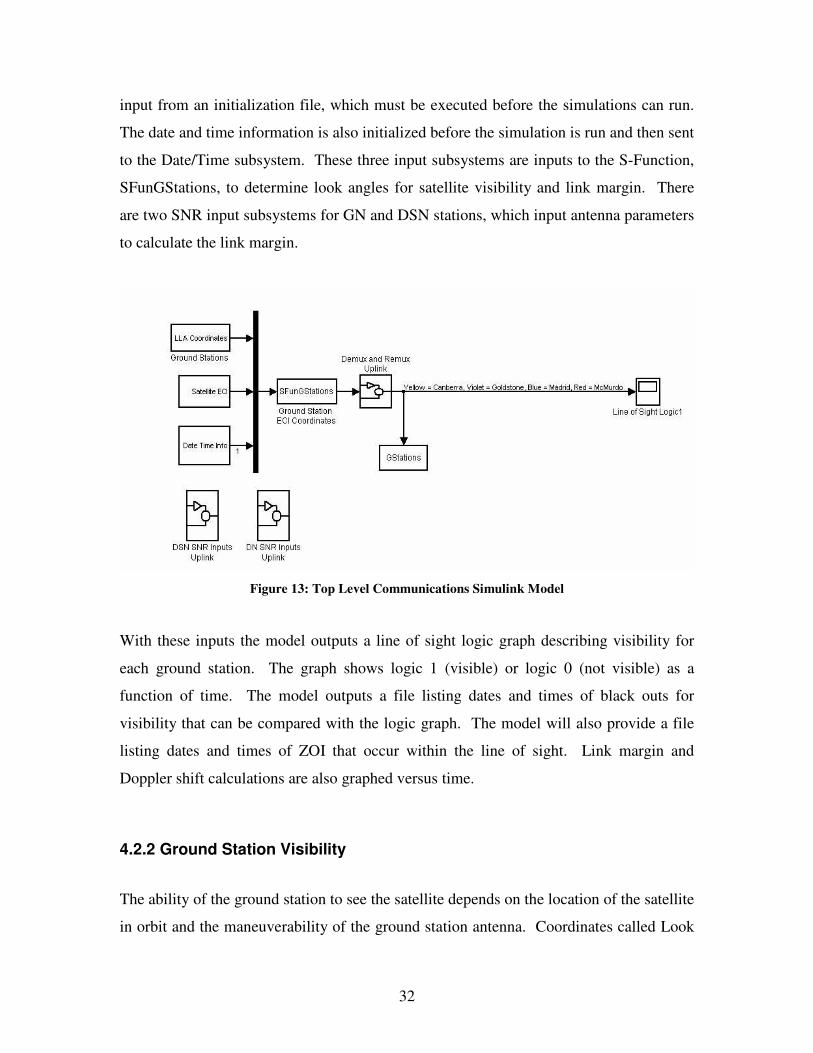
4.2.1 Inputs/Outputs
The communication model is dependent on ECI position and velocity vectors generated
from the orbit propagator. The ECI vectors are structured with time and stored in an
array that the model accesses through the Satellite ECI subsystem. The model requires
the ground station latitude/longitude/altitude (LLA) to determine the ground stations
position as a function of time. Ground Station LLA Coordinates subsystem takes user
32
input from an initialization file, which must be executed before the simulations can run.
The date and time information is also initialized before the simulation is run and then sent
to the Date/Time subsystem. These three input subsystems are inputs to the S-Function,
SFunGStations, to determine look angles for satellite visibility and link margin. There
are two SNR input subsystems for GN and DSN stations, which input antenna parameters
to calculate the link margin.
Figure 13: Top Level Communications Simulink Model
With these inputs the model outputs a line of sight logic graph describing visibility for
each ground station. The graph shows logic 1 (visible) or logic 0 (not visible) as a
function of time. The model outputs a file listing dates and times of black outs for
visibility that can be compared with the logic graph. The model will also provide a file
listing dates and times of ZOI that occur within the line of sight. Link margin and
Doppler shift calculations are also graphed versus time.
4.2.2 Ground Station Visibility
The ability of the ground station to see the satellite depends on the location of the satellite
in orbit and the maneuverability of the ground station antenna. Coordinates called Look
33
Angles give angular measurements of where the ground station antenna needs to be
pointed at a given time in order to communicate with the satellite.
For the Communications model, the look angles are calculated within the S-Function,
SFunGstations. The calculation can be broken up into four parts: the Julian Date
calculation, the Greenwich Sidereal Time calculation, the Latitude/Longitude/Altitude
(LLA) to Earth Centered Inertial Coordinates (ECI) conversion, and finally the ECI to
Look Angles conversion.
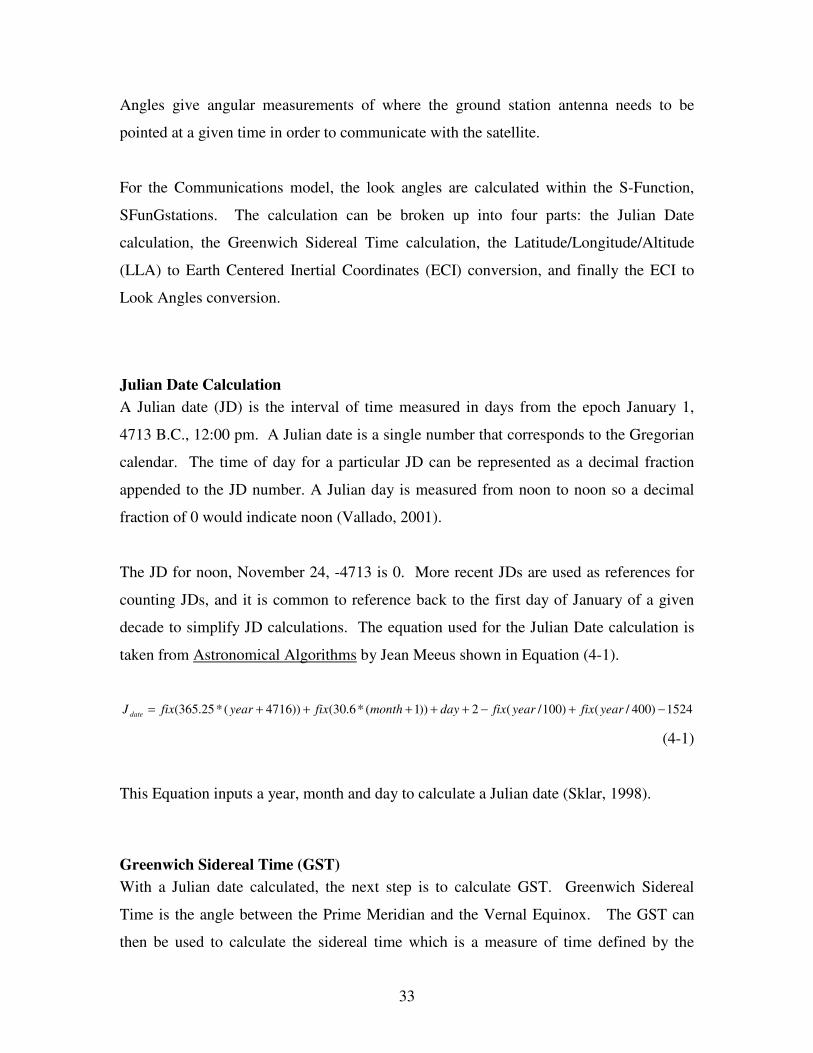
Julian Date Calculation A Julian date (JD) is the interval of time measured in days from the epoch January 1,
4713 B.C., 12:00 pm. A Julian date is a single number that corresponds to the Gregorian
calendar. The time of day for a particular JD can be represented as a decimal fraction
appended to the JD number. A Julian day is measured from noon to noon so a decimal
fraction of 0 would indicate noon (Vallado, 2001).
The JD for noon, November 24, -4713 is 0. More recent JDs are used as references for
counting JDs, and it is common to reference back to the first day of January of a given
decade to simplify JD calculations. The equation used for the Julian Date calculation is
taken from Astronomical Algorithms by Jean Meeus shown in Equation (4-1).
1524)400/()100/(2))1(*6.30())4716(*25.365( −+−+++++= yearfixyearfixdaymonthfixyearfixJ date
(4-1)
This Equation inputs a year, month and day to calculate a Julian date (Sklar, 1998).
Greenwich Sidereal Time (GST) With a Julian date calculated, the next step is to calculate GST. Greenwich Sidereal
Time is the angle between the Prime Meridian and the Vernal Equinox. The GST can
then be used to calculate the sidereal time which is a measure of time defined by the
34
motion of the vernal equinox in hour angles. For a given place (latitude) and instant in
time the sidereal time gives the hour angle of that equinox which is necessary to calculate
the ECI coordinates for a given point on the earth’s surface (Meeus, 98).
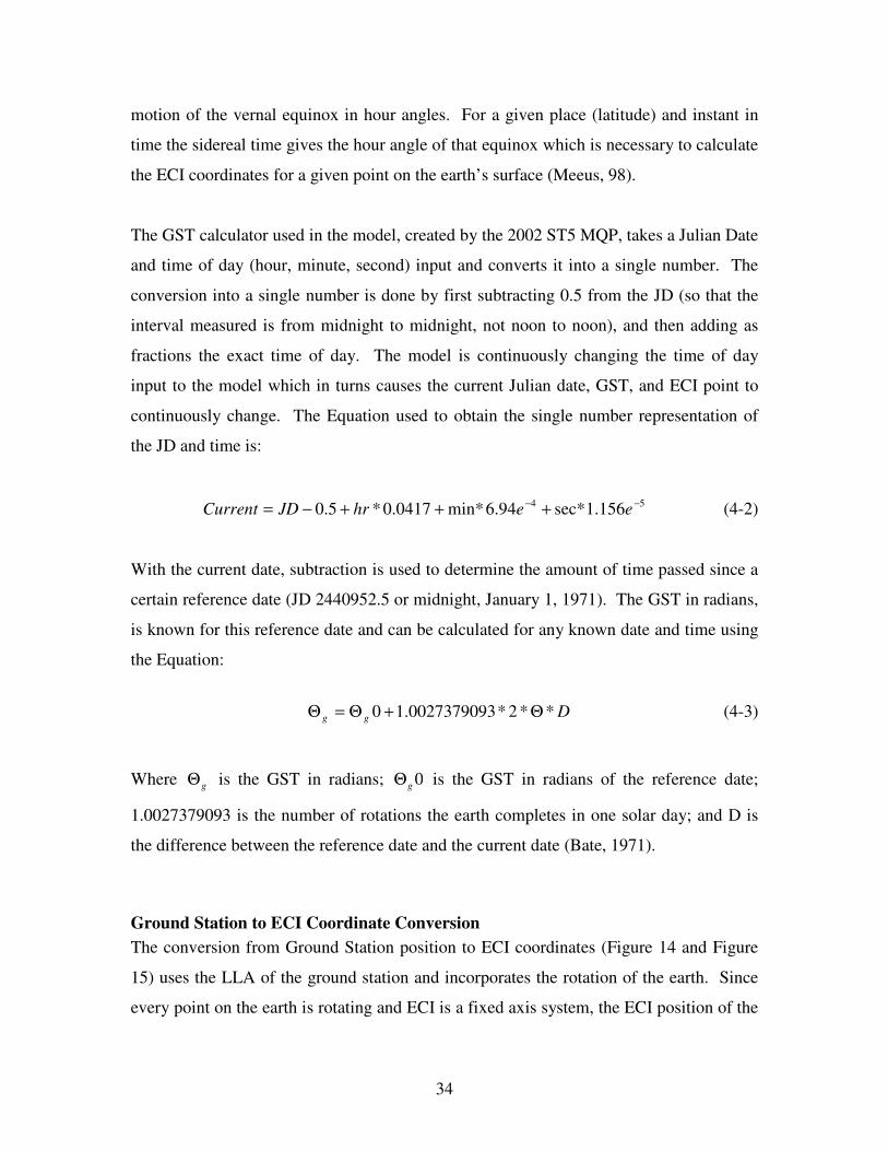
The GST calculator used in the model, created by the 2002 ST5 MQP, takes a Julian Date
and time of day (hour, minute, second) input and converts it into a single number. The
conversion into a single number is done by first subtracting 0.5 from the JD (so that the
interval measured is from midnight to midnight, not noon to noon), and then adding as
fractions the exact time of day. The model is continuously changing the time of day
input to the model which in turns causes the current Julian date, GST, and ECI point to
continuously change. The Equation used to obtain the single number representation of
the JD and time is:
54 156.1sec*94.6min*0417.0*5.0 −− +++−= eehrJDCurrent (4-2)
With the current date, subtraction is used to determine the amount of time passed since a
certain reference date (JD 2440952.5 or midnight, January 1, 1971). The GST in radians,
is known for this reference date and can be calculated for any known date and time using
the Equation:
Dgg **2*0027379093.10 Θ+Θ=Θ (4-3)
Where gΘ is the GST in radians; Θg 0 is the GST in radians of the reference date;
1.0027379093 is the number of rotations the earth completes in one solar day; and D is
the difference between the reference date and the current date (Bate, 1971).
Ground Station to ECI Coordinate Conversion The conversion from Ground Station position to ECI coordinates (Figure 14 and Figure
15) uses the LLA of the ground station and incorporates the rotation of the earth. Since
every point on the earth is rotating and ECI is a fixed axis system, the ECI position of the

35
ground station is a function of time. For this reason the conversion from LLA to ECI
coordinates is a necessary intermediate calculation to determine the visibility of each
ground station.
Figure 14: Latitude to ECI Conversion
(celestrak.com/columns/v02n01)

36
Figure 15: Longitude to ECI conversion
(celestrak.com/columns/v02n01)
The calculation method used in this model is the same calculation that the 2002 ST5
MQP used that was based on the FalconSat project. The first step is the computation of
the local sidereal time (LST), the angle between the Vernal Equinox and the local
longitude. The local sidereal time is calculated by adding the Greenwich Sidereal Time
to the local longitude.
LST = GST + longitude (4-4)
The second step is the computation of two geodetic constants c and d, which account for
the flattening of the Earth, b.
( ) ( )( )( )
( ) altitudebflatRd
altitudebRc
latitudeflatflatb
eq
eq
*001.0/1*
*001.0/
sin*21
2
2
+−=
+=−−=
(4-5)
37
Where flat is the flattening of the Earth and Req is the radius of the Earth at the equator in
meters.
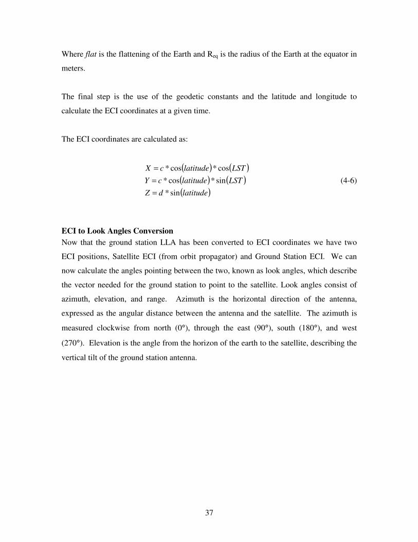
The final step is the use of the geodetic constants and the latitude and longitude to
calculate the ECI coordinates at a given time.
The ECI coordinates are calculated as:
( ) ( )( ) ( )( )latitudedZ
LSTlatitudecY
LSTlatitudecX
sin*sin*cos*cos*cos*
===
(4-6)
ECI to Look Angles Conversion Now that the ground station LLA has been converted to ECI coordinates we have two
ECI positions, Satellite ECI (from orbit propagator) and Ground Station ECI. We can
now calculate the angles pointing between the two, known as look angles, which describe
the vector needed for the ground station to point to the satellite. Look angles consist of
azimuth, elevation, and range. Azimuth is the horizontal direction of the antenna,
expressed as the angular distance between the antenna and the satellite. The azimuth is
measured clockwise from north (0°), through the east (90°), south (180°), and west
(270°). Elevation is the angle from the horizon of the earth to the satellite, describing the
vertical tilt of the ground station antenna.

38
Figure 16: Azimuth and Elevation
http://www.nhk-jn.co.jp/wp/img/antenna_e.gif
The first step in determining the look angles is calculating the range vector, the distance
between the ground station and satellite. The range vector is calculated by taking the
difference between the satellite’s ECI coordinates and the ground station’s ECI
coordinates.
rx,ry,rz[ ]= xs − xg , ys − yg,zs − zg[ ] (4-7)
Where [rx, ry, rz] is the range vector, [xs, ys, zs] are the satellite’s ECI coordinates, and [xg,
yg, zg] are the ground station’s ECI coordinates.
The range vector must be converted to the Topocentric-Horizon (SEZ) Coordinate
system, shown in Figure 17, in order to determine visibility of the satellite. SEZ
coordinates takes into account that the earth is not flat and that the azimuth and elevation
angles are with respect to the curvature of the earth not the ECI coordinate system. The
SEZ system rotates with the site and the local horizon forms the fundamental plane. The
transformation to SEZ is done by rotating through the local sidereal time about the Z-axis
(the Earth’s rotation axis), then rotating through the ground station’s latitude about the Y-
axis (Vallado 2001). The Equations used for these calculations are:
rS = sin(ϕ)cos(θ) * rx + sin(ϕ)sin(θ)* ry − sin(ϕ) * rz (4-8)

39
rE = −sin(θ) * rx + cos(θ) * ry (4-9)
rZ = cos(ϕ)cos(θ) * rx + cos(ϕ)sin(θ) * ry + sin(ϕ) * rz (4-10)
Where rS, rE, and rZ are the range vector expressed in SEZ coordinates, θ is the latitude
and ϕ is the local sidereal time (Vallado 2001).
Figure 17: Topocentric-Horizon Coordinate System
(http://celestrak.com/columns/v02n02)
The look angles can now be calculated using the SEZ coordinates with the following
equations.
range = (rS2 + rE
2 + rZ2) (4-11)
Elevation = sin−1(rZ /range) (4-12)
Azimuth = tan−1(−rE /rS ) (4-13)

40
The specifications for antenna visibility are dependant on the specific antenna in use.
The previous Communications model used a required 10° elevation and assumed no
restriction on the azimuth angle. So any time the elevation is between 10° and 170°, the
satellite is visible. Our communication model will use the same requirements.
4.2.3 Link Margin Calculation The link margin is the difference between the desired minimum signal to noise ratio and
the actual signal to noise ratio in dB. Link margins that are less than the desired
minimum can result in unacceptable bit error rates in the received signal. Figure 18
shows the Simulink model that calculates link margin.
Figure 18: Link Margin Calculator
The link margin calculator takes as constant inputs all variables from Equation (2-3),
except the EIRP, sL , and Gr. The gain of the receiver (Gr) is dependant on the antenna
radiative pattern and attitude of the spacecraft. Gr is determined in the Zone of
Interference subsystem and inputted into the link margin calculator. Space loss, sL , is

41
dependent on the system frequency and the range calculated from look angles, shown in
Equation (4-14).
( )���
����
�×−��
�
����
�−= Range
fc
Ls 1000log204
log20π
(4-14)
where Ls is equal to space loss, Range is the distance between the ground station and the
satellite, c is equal to the speed of light and f is equal to the system frequency.
Figure 19 shows the subsystem that calculates space loss.
Figure 19: Space Loss Calculator
EIRP takes into account transmission gain and transmission power. Transmission gain is
calculated by using Equation (4-15) and the calculation subsystem is shown in Figure 20
with inputs antenna diameter, antenna efficiency and frequency. Transmission power is a
constant specific to the ground station.
�����
�
�
�����
�
�×××
=100
log10
2
AecfAd
Gt
π
(4-15)

42
where Gt is equal to the transmission gain, Ad is equal to the antenna diameter, Ae is equal
to the antenna efficiency, f is equal to the system frequency and c is equal to the speed of
light.
Figure 20: Ground Station Transmission Gain Calculator
Doppler Shift Calculation Our model uses the same Doppler shift calculation as the 2002 ST5 MQP. The ST5
satellites transmitting frequency is 8.74 GHz and the frequency received by the ground
station antennas will be 8.74 GHz plus/minus the Doppler frequency shift. The model
calculates the Doppler shift as follows:
cfv
f rel *=∆ (4-16)
where f∆ is the change in frequency, relv is the velocity of the spacecraft relative to the
velocity of the ground station, f is the transmitted frequency, and c is the speed of light.
In Figure 21, a range input from the ground station s-function (SFunGStations) calculates
the continuously changing range as the satellite moves in orbit which is then used to
calculate relative velocity.
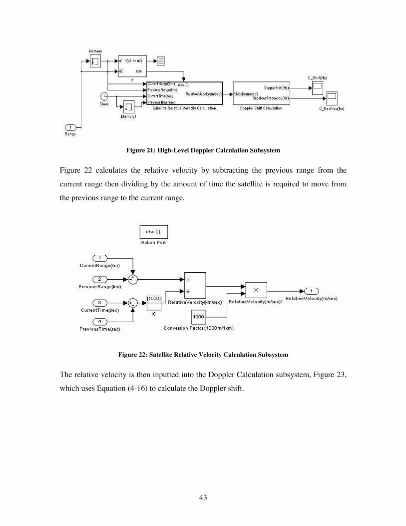
43
Figure 21: High-Level Doppler Calculation Subsystem
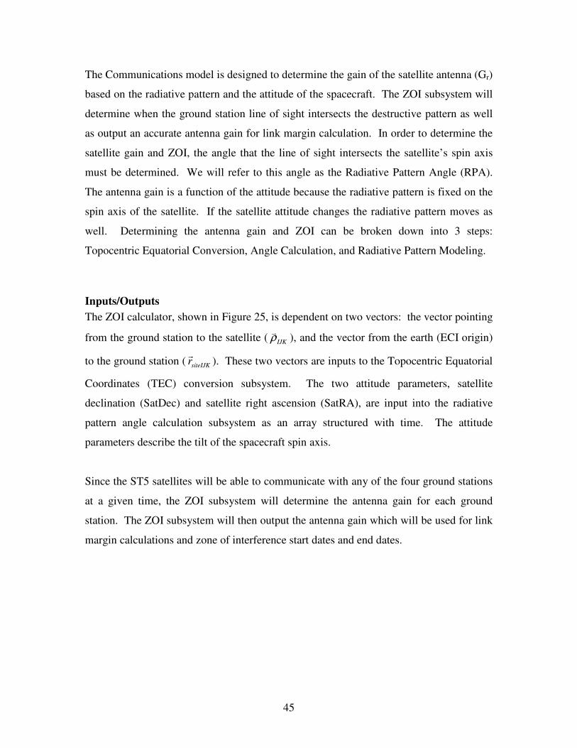
Figure 22 calculates the relative velocity by subtracting the previous range from the
current range then dividing by the amount of time the satellite is required to move from
the previous range to the current range.
Figure 22: Satellite Relative Velocity Calculation Subsystem
The relative velocity is then inputted into the Doppler Calculation subsystem, Figure 23,
which uses Equation (4-16) to calculate the Doppler shift.

44
Figure 23: Doppler Shift Calculation Subsystem
4.2.4 Zone of Interference (ZOI) Calculation The ST5 satellite is using a new technology, known as the Evolved Antenna which
provides a much better antenna gain for the ST5 orbit. The satellite consists of two
antennas (Top and Bottom) with each antenna providing a radiative pattern that describes
the gain of antenna at a given point surrounding the satellite (360 degrees). The ZOI is
caused by the two antenna patterns overlapping and creating destructive phase
interference (Figure 24), which will result in a 3-4 minute (maximum 10 minutes)
transmission loss.
Figure 24: Zone of Interference
45
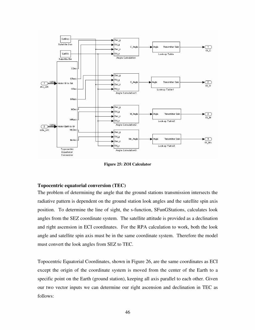
The Communications model is designed to determine the gain of the satellite antenna (Gr)
based on the radiative pattern and the attitude of the spacecraft. The ZOI subsystem will
determine when the ground station line of sight intersects the destructive pattern as well
as output an accurate antenna gain for link margin calculation. In order to determine the
satellite gain and ZOI, the angle that the line of sight intersects the satellite’s spin axis
must be determined. We will refer to this angle as the Radiative Pattern Angle (RPA).
The antenna gain is a function of the attitude because the radiative pattern is fixed on the
spin axis of the satellite. If the satellite attitude changes the radiative pattern moves as
well. Determining the antenna gain and ZOI can be broken down into 3 steps:
Topocentric Equatorial Conversion, Angle Calculation, and Radiative Pattern Modeling.
Inputs/Outputs The ZOI calculator, shown in Figure 25, is dependent on two vectors: the vector pointing
from the ground station to the satellite ( IJKρ� ), and the vector from the earth (ECI origin)
to the ground station ( siteIJKr�
). These two vectors are inputs to the Topocentric Equatorial
Coordinates (TEC) conversion subsystem. The two attitude parameters, satellite
declination (SatDec) and satellite right ascension (SatRA), are input into the radiative
pattern angle calculation subsystem as an array structured with time. The attitude
parameters describe the tilt of the spacecraft spin axis.
Since the ST5 satellites will be able to communicate with any of the four ground stations
at a given time, the ZOI subsystem will determine the antenna gain for each ground
station. The ZOI subsystem will then output the antenna gain which will be used for link
margin calculations and zone of interference start dates and end dates.
46
Figure 25: ZOI Calculator
Topocentric equatorial conversion (TEC) The problem of determining the angle that the ground stations transmission intersects the
radiative pattern is dependent on the ground station look angles and the satellite spin axis
position. To determine the line of sight, the s-function, SFunGStations, calculates look
angles from the SEZ coordinate system. The satellite attitude is provided as a declination
and right ascension in ECI coordinates. For the RPA calculation to work, both the look
angle and satellite spin axis must be in the same coordinate system. Therefore the model
must convert the look angles from SEZ to TEC.
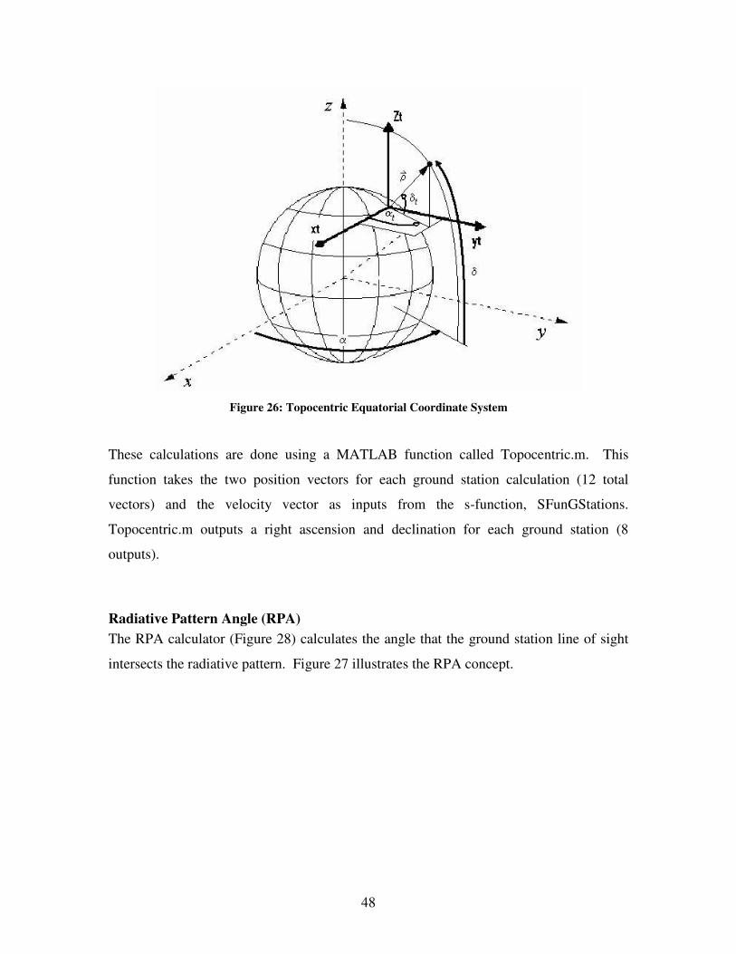
Topocentric Equatorial Coordinates, shown in Figure 26, are the same coordinates as ECI
except the origin of the coordinate system is moved from the center of the Earth to a
specific point on the Earth (ground station), keeping all axis parallel to each other. Given
our two vector inputs we can determine our right ascension and declination in TEC as
follows:

47
siteIJKIJKIJK rr��� +=ρ
ρρ �=
ρρδ k
t =)sin(
IF 022 ≠+ JI ρρ
22
)sin(JI
Jt
ρρ
ρδ+
= or 22
)cos(JI
It
ρρ
ρα+
=
ELSE
22)sin(
JI
Jt
ρρ
ρδ��
�
+= or
22)cos(
JI
It
ρρ
ρα��
�
+=
SiteIJKSiteIJK rv�×= ⊕ϖ
SiteIJKIJKIJK vv ���� −=ρ
(Vallado, 2001)
Where IJKr�
is the vector pointing from the earths center to the satellite and siteIJKr�
is the
vector pointing from the earths center to the ground station. IJKρ� can then be calculated
as the vector from the ground station to the satellite. With the magnitude of IJKρ� , the
right ascension ( tα ) and declination ( tδ ) of the satellite can be calculated. The ELSE
statement takes care of the case when the satellite is pointed directly over the spin axis of
the earth (z axis). For this case we need to know the velocity vector of the satellite which
is taken from the orbit propagator. ⊕ϖ is the earth’s rotational velocity and is often
assumed to be constant.
125 105.110292115.7 −−
⊕ ×±×=ϖ
48
Figure 26: Topocentric Equatorial Coordinate System
These calculations are done using a MATLAB function called Topocentric.m. This
function takes the two position vectors for each ground station calculation (12 total
vectors) and the velocity vector as inputs from the s-function, SFunGStations.
Topocentric.m outputs a right ascension and declination for each ground station (8
outputs).
Radiative Pattern Angle (RPA) The RPA calculator (Figure 28) calculates the angle that the ground station line of sight
intersects the radiative pattern. Figure 27 illustrates the RPA concept.
49
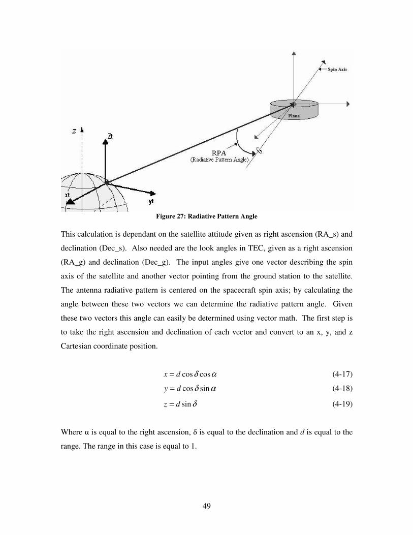
Figure 27: Radiative Pattern Angle
This calculation is dependant on the satellite attitude given as right ascension (RA_s) and
declination (Dec_s). Also needed are the look angles in TEC, given as a right ascension
(RA_g) and declination (Dec_g). The input angles give one vector describing the spin
axis of the satellite and another vector pointing from the ground station to the satellite.
The antenna radiative pattern is centered on the spacecraft spin axis; by calculating the
angle between these two vectors we can determine the radiative pattern angle. Given
these two vectors this angle can easily be determined using vector math. The first step is
to take the right ascension and declination of each vector and convert to an x, y, and z
Cartesian coordinate position.
αδ coscosdx = (4-17)
αδ sincosdy = (4-18)
δsindz = (4-19)
Where � is equal to the right ascension, � is equal to the declination and d is equal to the
range. The range in this case is equal to 1.
50
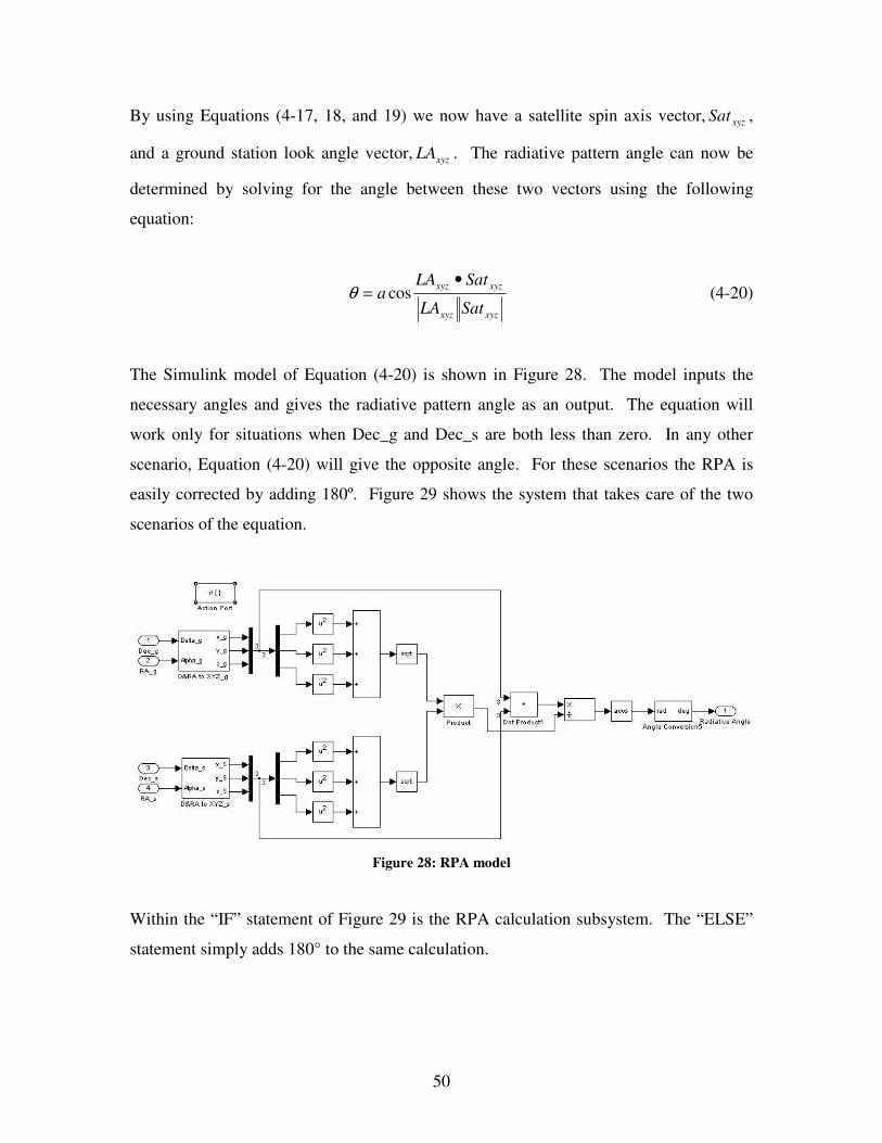
By using Equations (4-17, 18, and 19) we now have a satellite spin axis vector, xyzSat ,
and a ground station look angle vector, xyzLA . The radiative pattern angle can now be
determined by solving for the angle between these two vectors using the following
equation:
xyzxyz
xyzxyz
SatLA
SatLAa
•= cosθ (4-20)
The Simulink model of Equation (4-20) is shown in Figure 28. The model inputs the
necessary angles and gives the radiative pattern angle as an output. The equation will
work only for situations when Dec_g and Dec_s are both less than zero. In any other
scenario, Equation (4-20) will give the opposite angle. For these scenarios the RPA is
easily corrected by adding 180º. Figure 29 shows the system that takes care of the two
scenarios of the equation.
Figure 28: RPA model
Within the “IF” statement of Figure 29 is the RPA calculation subsystem. The “ELSE”
statement simply adds 180° to the same calculation.

51
Figure 29: RPA Subsystem Calculator
Radiative Pattern Modeling The EA antenna ST5 will be validating has not yet been fully tested and the results are
not attainable. For our project we approximated gain values of the EA by examining the
EA radiative pattern versus the QHA radiative pattern (Figure 30) given to us from the
ST5 Critical Design Review files. Figure 31 shows an approximated sample EA patterns
versus the old QHA patterns.
Figure 30: QHA Patterns vs. EA Patterns
(ST5 �CDR)

52
The EA has much better gain capabilities compared to the QHA in LEO. From this figure
we were able to construct our approximation of the EA radiative pattern.
Figure 31: EA Radiative Pattern
The pattern is now rotated to show the ZOI along the x-axis centered along the 90-270
degree axis. The rotational axis of the spacecraft, or z-axis, is aligned with 0-180 degrees.
Due to the constant rotation of the spacecraft about the z-axis we will be unable to
determine where the radiative pattern angle will intersect the three-hundred sixty degree
radiative pattern. For example, we can not distinguish the difference between 20 degrees
and 370 degrees. To solve this problem we created a 180 degree pattern and then
mirrored this pattern. We compared the mirrored angles of the 360 degree pattern and
recorded the worst case scenario.
From this 180 degree radiative pattern we can create a look up table to correspond a
certain angle to a certain transmission gain. This look up table was created using an excel
spreadsheet called “Look_up_EA”, and imported into our Simulink model using the

53
MATLAB function xlsread.m. The excel spreadsheet allows for easy modifications due
to future updated antenna patterns.
The previously calculated radiative pattern angle from our “Angle Calculation”
subsystem is inputted into our look up table. From the look up table a transmission gain is
outputted. Figure 32 shows the Simulink subsystems needed for this computation. The
Look-Up Table subsystem is an already existing Simulink function. The excel
spreadsheet we created is called from inside the Look-Up Table function.
Figure 32: Look-Up Table
The output gain is then used to determine line of sight logic, link margin, Doppler shift
and Zone of Interference dates.
4.2.5 Generating Output files The Communications model will output eight separate excel spreadsheets, along with two
separate graphs, of the each ground stations visibilities dates and each ground stations
ZOI visibility dates. The excel spreadsheets can easily be viewed after the model is run,
and the graphs can be viewed by using the scopes placed in the top-level diagram of the
Communications model.
Date/Time Information
In order to produce exact date/time information, a calendar/time function was added to
the model in the Date/Time input subsystem.
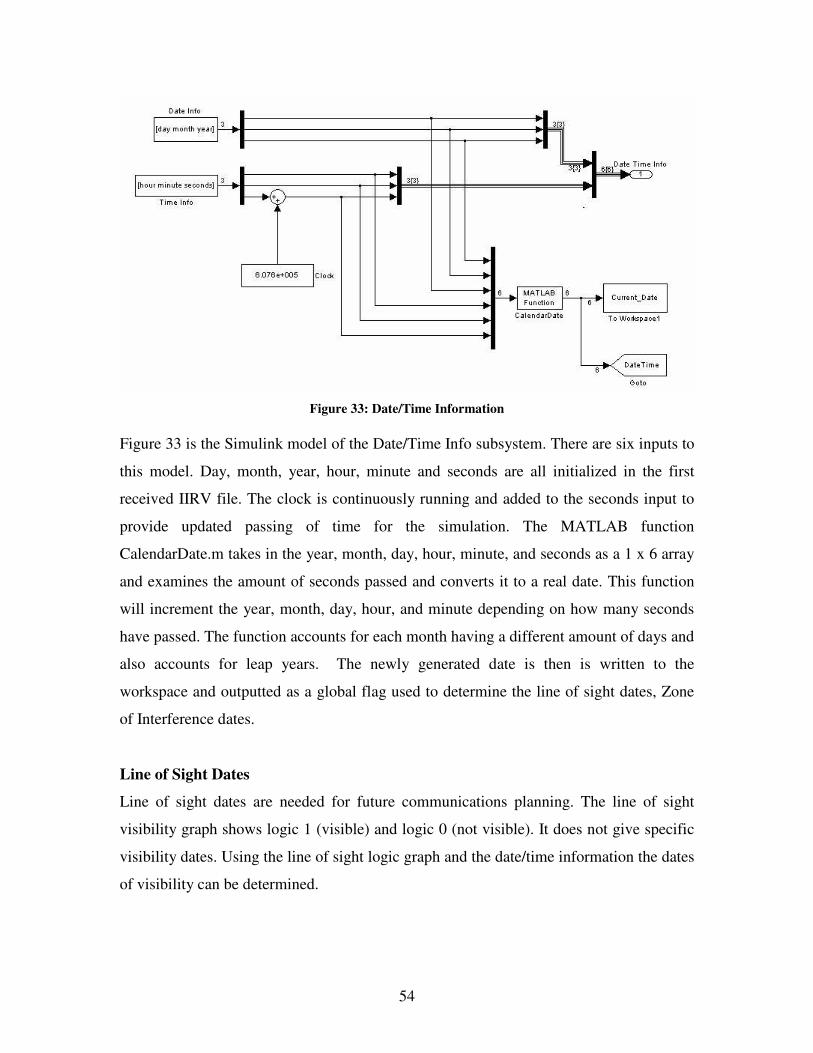
54
Figure 33: Date/Time Information
Figure 33 is the Simulink model of the Date/Time Info subsystem. There are six inputs to
this model. Day, month, year, hour, minute and seconds are all initialized in the first
received IIRV file. The clock is continuously running and added to the seconds input to
provide updated passing of time for the simulation. The MATLAB function
CalendarDate.m takes in the year, month, day, hour, minute, and seconds as a 1 x 6 array
and examines the amount of seconds passed and converts it to a real date. This function
will increment the year, month, day, hour, and minute depending on how many seconds
have passed. The function accounts for each month having a different amount of days and
also accounts for leap years. The newly generated date is then is written to the
workspace and outputted as a global flag used to determine the line of sight dates, Zone
of Interference dates.
Line of Sight Dates
Line of sight dates are needed for future communications planning. The line of sight
visibility graph shows logic 1 (visible) and logic 0 (not visible). It does not give specific
visibility dates. Using the line of sight logic graph and the date/time information the dates
of visibility can be determined.

55
Figure 34: Start/End Dates for Line of Sight
Figure 34 shows the line of sight start and end date calculation subsystem. The start and
end dates are measured by using a sample and hold system. The sample and hold system
has two inputs: the date/time information and the line of sight logic. The system monitors
the line of sight logic and associates a start date with a rising edge and an end date with a
falling edge. Eight separate work spaces are created using this method. A MATLAB
function called “output_times” is used to combine the start and end dates of a single
ground station and then print it as an excel spreadsheet for viewing. The “InitState”
subsystems account for the possibility of a logic 1 as an initial position. If an initial
position of logic 1 is present then the initial time is outputted as a start date.
Zone of Interference Graph and Dates

56
In order to determine the Zone of Interference dates and graphs, the elevation of the
ground station in SEZ and the radiative pattern gain are desired. Elevation is required
because it is not necessary to determine Zone of Interference dates and graphs if the
satellite is not visible by the ground station. The radiative pattern gain is required because
if the satellite is visible by the ground station, then the radiative pattern gain must be
sufficient enough to establish communication. If the radiative pattern gain is insufficient
then the line of sight falls in the Zone of Interference.
Figure 35: Zone of Interference Plot and Date Calculation
The elevations of each ground station are inputted from the Elevations global flag. If the
satellite is visible by the ground station the model assesses the gain and provides logic 1
for a failed communication and logic 0 for a successful communication. If the gain is less
than or equal to -10 dB then it is a failed communication and the line of sight falls in the
zone of interference. The “Date/Time of ZOI” subsystem is another series of sample and
hold systems that supply the dates for the start and end of the Zone of Interference. These
dates are also written to a workspace and outputted as excel spreadsheets.
57
4.2.6 Communications Model Verification To ensure the Communications model capabilities, each section was tested individually
before being integrated into the final model. By validating the model it will limit errors
that may happen when using the final product, since the final model can not be tested
without flight validation.
When verifying the look angle calculations we applied the same methodology that the
2002 ST5 MQP did. They used a scenario given in Orbital Coordinate Systems, Part III,
written by Dr T.S. Kelso, where the date was given as 18 Nov 1995, the time 12:46 pm,
ground site latitude was 45° N and longitude was 93° W, and the satellite ECI position
was [-4400.594, 1932.870, 4760.712]. With these given values, Dr. Kelso computed the
Azimuth as 100.36° and the Elevation as 81.62°. The communications subsystem, using
the same given input values, calculates the Azimuth as 102.92° and the Elevation as
83.11°. Since we used the same method as the 2002 ST5 MQP, our results are the same.
The Azimuth calculation error is 2.55% and in the Elevation calculation error is 1.83%.
This error includes any error generated by the latitude/longitude to ECI coordinate
conversion.
Similarly we also used the same method for testing the ground station latitude/longitude
to ECI coordinate conversion as the 2002 ST5 MQP. This was verified using another
scenario given by Dr. Kelso, where the date was 01 Oct 1995, the time was 9:00 am, and
the latitude and longitude were 40° N and 75° W, respectively. The ECI coordinates
given by Dr Kelso were [1703.295, 4586.650, 4077.984]. The ECI coordinates
calculated by the Communications model were [1694.65, 4589.85, 4077.99]. The error in
the ECI coordinates was [.51%, 0.07%, 0.00%] and the total position error was 9.22 km.
To test the Link Margin Calculator we compared the results to the ST5 RFICD provided
to us by Victor Sank. The RFICD was last revised on April 2, 2004. We first calculated
the available signal to noise ratio and then subtracted the required signal to noise ratio to
58
find the link margin. Space loss, antenna gain, transmitter power, passive loss,
atmospheric loss, implementation loss, receiver antenna gain, system temperature,
Boltzmann’s constant, and the data rate are all needed to calculate the available signal to
noise ratio. The calculated available signal to noise ratio from the RFICD is equal to
65.04 dB and the Link Margin is equal to 55.44 dB. The calculated available signal to
noise ratio from our model is equal to 64.91 dB and the Link Margin is equal to 55.31
dB. The total error between calculations was 0.2%.
To test the “Topocentric Equatorial Conversion” function we used Fundamentals of
Astrodynamics and Applications written by David A. Vallado. Chapter 4, example (4-1)
shows the conversion from SEZ coordinates to TEC. Our MATLAB function has three
inputs which are the vector from the satellite to the ground station ( IJKρ� ), the vector from
the ground station to the satellite ( siteIJKr�
), and the velocity vector ( IJKν� ), also known as
the position and velocity vectors. From the Vallado book we are given IJKr�
, siteIJKr�
, and
IJKν� as test values. IJKρ� can be determined using this equation:
siteIJKIJKIJK rr��� +=ρ
From this we can now enter the three inputs into the MATLAB function Topocentric.m.
For this test we will be using Vallado’s vectors and angles as test values which are shown
in Table 2:

59
SEZ
(Topocentric Horizon Coordinate
System)
TEC
(Topocentric Equatorial Coordinate
System)
ijk
(km)
[1,752,242,148.28
-3,759,560,585.46
-1,577,572,099.3]
Right Ascension
�
(degrees)
294.989 111 5
rsite(ijk)
(km)
[4,066.716
-2,874.545
3,994.302]
Declination
�
(degrees)
-20.823 562 3
vijk
(km/s)
[-18.324
18.332
7.777]
Table 2: Test vectors and angles
Given the SEZ coordinates we can now test our model. When executed the model outputs
a right ascension of -65.01 degrees and a declination of -20.82 degrees. The only
difference is the right ascension where 294.99 degrees and -65.01 degrees are not the
same number but are equal to the same angle on the x-y plane. The MATLAB function
only holds two decimal places compared to the seven decimal places that Vallado gives.
This error will amount to an error of less than 1% in both cases.
The RPA Calculation was tested by using sample numbers for the ground station and
satellite right ascension and declinations. For this test the ground stations right ascension
and declination was 180° and -45° respectively and the satellite right ascension and
declination was 90° and -87° respectively. These numbers were chosen because they are
simple to solve and can be solved by using a geometric approach as well as a calculated
approach. When using the geometric approach the approximated RPA was 48°. The hand
calculated RPA which was determined by using Equations (4-17) through (4-20), was
exactly the same as the Simulink models answer of 45.08°. The equations used to

60
calculate the RPA were directly implemented into the Simulink subsystem, which
provides accurate solutions.
The look-up table was tested by entering values for the RPA input. Transmission gain
values of the look-up table output were hand checked against the excel spreadsheet that
was created. All input values corresponded to the appropriate output values.
4.3 Orbit Propagator
The orbit propagator provides position and velocity vectors describing the satellites orbit
which are then used by the Communications model to determine look angles and line of
sight logic. The orbit propagator was created by Jim Morrissey (ST5 Attitude Control
System Analyst, [email protected]) and is the same propagator used in the
previous Communications models. The model uses some basic physics with an initial
position and velocity vector to determine the satellite orbit. The algorithm is based on
two body orbital mechanics, earth and satellite. The orbit propagator was designed to
provide short term propagation, of approximately 3-4 hours of accuracy. Newly
integrated Improved Inter Range Vector files will be received every four hours updating
the orbit propagator by providing new position and velocity vectors. These vector files
are received from a NASA generated satellite tracking system.
4.3.1 Algorithm
Newton’s 2nd law states that the rate of change of momentum is proportional to the forces
impressed and is in the same direction as that force. We know the force impressed on the
satellite due to our two-body model is the gravitational force from the earth. Newton's
Law of Universal Gravitation states that any two bodies attract one another with a force
proportional to the product of their masses and inversely proportional to the square of the

61
distance between them. Newton’s 2nd law also states that the gravitational force from the
earth would cause the satellite to accelerate toward the center of the earth.
Given Newton’s Laws we are able to calculate acceleration given an initial satellite
position vector. Newton’s Universal Gravitational law is a function of mass and distance.
Therefore given the mass of the earth and the satellite, as well as an initial position, the
acceleration of the satellite can be calculated. Calculation of the acceleration requires
some vector math with a position vector input. Figure 36 shows the necessary vector
math used to calculate acceleration vector due to gravity, based on a position vector.
Figure 36: Acceleration Vector Calculation
By integrating the given acceleration vector a velocity vector derived. We can then
integrate the velocity vector to receive the next position vector. The integration steps are
shown in Figure 37.
Figure 37: Position Vector Calculation

62
Once the new position vector is calculated it is fed back into the “Orbital Dynamics”
subsystem to recalculate a new acceleration vector and the process continues. If the orbit
propagator is run for a long enough time, the model will create enough position vectors to
propagate a whole orbit.
When the position and velocity vectors are created we need a way to access the
information to be used for the Communications model. To do this separate Simulink
subsystem was created that will take both vectors and structure them with time. Figure
38 shows the satellite ECI coordinates created by the orbit propagator stored in an array
with the simulation time that corresponds to each vector. The array is then sent to the
MATLAB workspace where it can be used by other models.
Figure 38: Satellite Coordinates to Workspace
4.3.2 Improved Inter Range Vector (IIRV)
The Communications model is designed to provide long-term mission planning, therefore
we require an orbit propagator that provides accuracy beyond a 1-2 hour time frame. One
way to improve the orbit propagator accuracy is to incorporate IIRV’s. An IIRV is a
message file provided by the ground station that tracks the satellite. The IIRV contains
six lines of ASCII code that provide multiple satellite parameters. The IIRV’s are sent
centered around every 4 hours that we will use to provide a satellite position and velocity
vector for a given time in orbit. For long term mission planning future IIRV’s are
predicted and propagated to provide orbit position and velocity vectors for the entire
mission duration.
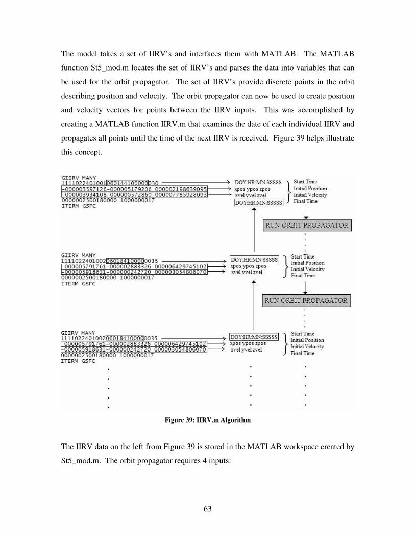
63
The model takes a set of IIRV’s and interfaces them with MATLAB. The MATLAB
function St5_mod.m locates the set of IIRV’s and parses the data into variables that can
be used for the orbit propagator. The set of IIRV’s provide discrete points in the orbit
describing position and velocity. The orbit propagator can now be used to create position
and velocity vectors for points between the IIRV inputs. This was accomplished by
creating a MATLAB function IIRV.m that examines the date of each individual IIRV and
propagates all points until the time of the next IIRV is received. Figure 39 helps illustrate
this concept.
Figure 39: IIRV.m Algorithm
The IIRV data on the left from Figure 39 is stored in the MATLAB workspace created by
St5_mod.m. The orbit propagator requires 4 inputs:

64
1. Starting Time
2. Initial Position Vector
3. Initial Velocity Vector
4. Final Time
The function IIRV.m reads the first IIRV (Blue) which provides a Starting Time, Initial
Position and Initial Velocity for the orbit propagator. The Final Time is recorded when
the next IIRV occurs. In order to accomplish this, the function imports the start time of
the next IIRV (Red) and uses it as a Final Time. The second column from Figure 39
shows the format the inputs are received in.
1. Start Time - Day of year (DOY): Hour (HR): Minute (MN): Seconds (ss.sss)
2. Position Vector – [xpos ypos zpos]
3. Velocity Vector – [xvel yvel zvel]
4. Final Time - Day of year (DOY): Hour (HR): Minute (MN): Seconds (ss.sss)
The orbit propagator can now create position and velocity vectors for the 3-4 hour period
between the IIRV inputs. The orbit propagator stops when it reaches the final time and
then reads in the next IIRV (red). The Final Time of the previous simulations becomes
the new Start Time while the next IIRV (green) will provide the new Final Time. This
process continues until there are no more available IIRV’s.
It should be noted that for the real-time state health assessment mode the IIRV’s are not
all received at once due to real-time. The orbit propagator would receive one IIRV and
propagate based on that single input. The Simulink model would then run until the next
IIRV is ready to be received.
4.3.3 Earth Centered Fixed (ECF) to ECI Conversion
An intermediate step exists before the IIRV’s can be used. The IIRV position and
velocity vectors are provided in the Earth Centered Fixed (ECF) coordinate system. Our

65
Communications model is dependant on the orbit propagator inputs being in ECI
coordinates. Therefore before IIRV.m can be run the IIRV input vectors must be
converted from ECF to ECI.
The transformation of an ECF position vector recf to an ECI position vector reci is given
by the following vector-matrix operation.
(4-21)
The transformation matrix [T] is dependant on the Greenwich Sidereal Time at the given
moment of interest. The elements of the transformation matrix T are given by
(4-22)
Where θ is the Greenwich Sidereal Time (GST). GST is defined as,
(4-23)
where 0gθ is the Greenwich sidereal time at 0 hours UT, eω is the inertial rotation rate of
the Earth, and t is the elapsed time since 0 hours UT. The ECI velocity vector is
determined by differentiating the following expression.
(4-24)
The elements of the matrix ][Τ� are as follows:

66
(4-25)
To convert from ECF to ECI we utilized the MATLAB orbital mechanics toolbox
provided by Marco Concha (ST5 Guidance and Navigation Control,
[email protected]). From this toolbox we created the function ecf2eci.m. Inputs
to this function are a date/time array (year month day hour minutes seconds), ECF
position vector, and an ECF velocity vector. The ECF input vectors are used directly by
Equations (4-21) and (4-24). The date/time array is input to the function juliandate.m to
calculate a Julian date. The Julian date is then inputted into the function GAST.m which
calculates the apparent Greenwich Sidereal Time that is used for the matrix
transformations (Equations 4-22, 4-25).
4.3.4 Orbit Propagator Model Verification
To verify the functionality of the orbit propagator we plotted the satellite position vectors
versus time.
Figure 40: Satellite x-y-z position plot
67
Figure 40 shows each component of the position vector plotted versus time. From the
graph it can be determined that the orbit propagator is working properly due to the
sinusoidal motion of the position. The period of each sinusoid shows one full orbit of the
satellite. Since the satellite completes one orbit in 136 minutes, the period of each
sinusoid from Figure 40 should be 136 minutes (8160 seconds). The first peak of the x-
position occurs at 5560 seconds and the second peak occurs at 13750 seconds. The
elapsed time between the two peaks gives a period of 8160 seconds which is equal to the
orbital period of the spacecraft of 136 minutes.
4.4 Model integration to Simulink ST5 ISR has developed the Simulink ST5 model which consists of the solid state data recorder
subsystem and the command and data handling subsystem. The C&DH subsystem
contains all the necessary telemetry data needed for the ST5 communications model.
They have also provided the necessary steps that are needed to add Simulink Models to
their existing SimulinkST5. All that is needed is the proper Simulink model information
that can be placed in an xml configuration file (ST5config.xml). This information
consists of the GMSEC profile directive related to the model, model identity, model
location, file, name, and optional initialization files. The next step is to add the
subsystems initial conditions and telemetry mnemonics to the ST5config.xml file. This
allows our model to use spacecraft and/or ground station telemetry as well as set up
necessary initial conditions. Once our model has been executed, the output information
is sent back to the bus for use by other applications.
4.5 Summary
The original SimulinkST5 model was modified by upgrading the existing orbit
propagator to provide mission planning for up to three months. The existing
Communications model was also improved to include Zone of Interference calculations,
antenna radiative pattern calculations, spacecraft attitude adjustments, simulated calendar
information, and dates of communication blackouts. The new functions were

68
incorporated into the model by adding subsystems and MATLAB functions into the
existing SimulinkST5 setup.
The Communications model is now able to calculate when the ST5 satellite is in the Zone
of Interference. This is done by examining ground station elevations and satellite antenna
gains determined from the antenna radiative pattern. The spacecraft attitude is also used
in the radiative pattern calculations. Calendar dates of communication blackouts are
given in year, month, date, hour, minute and seconds which are printed out as excel
spreadsheets for monitoring.
The restructured orbit propagator allows for updated satellite position and velocity
vectors every four hours from IIRV files. This new method replaces the old orbit
propagator which was only accurate for 2-3 days of propagation which did not meet long
term planning requirements.

69
5. Results
5.1 Introduction The SimulinkST5 Communications model was created to supply data to support short
term and long term modeling of the ST5 communications link. The Communications
model consists of two major subsystems, the orbit propagator and the Communications
model. The model generates several outputs that are written to the workspace. Among the
outputs is a line of sight graph, a Zone of Interference graph, a link margin graph, a
Doppler shift graph, and excel spreadsheets providing the exact visibility dates of the line
of sight and Zone of Interference. The generated outputs will provide the user with the
ability to plan for future communication links with the satellite.
The orbit propagator model was modified and tested in order to provide an accurate
position and velocity of the satellite to be used by the communications model to
determine the link margin, Doppler shift, line of sight, and Zone of Interference. The
orbit propagator must be run before the Communications model to provide ECI position
vectors for look angle calculations. The orbit propagator was tested by plotting the orbit
in MATLAB, and by plotting the x, y, and z position of the satellite.
The Communications model output was verified by comparing the actual visibility dates,
created by Marco Concha using STK software, with the Simulink produced visibility
dates. The Zone of Interference graph and dates can not be tested because there is no data
to compare it to.
5.2 Communications Model
Line of Sight When verifying the line of sight we consider the ground station look angles and link
margin as the only factor of visibility. Marco Concha’s line of sight spreadsheets are

70
based on when the ground station is able to detect the satellite based only on look angles.
In order to view the ground station line of sight, the logic was written to a workspace and
then plotted using a MATLAB script file. Figure 41 shows the line of sight output
obtained from the Communications model.
Figure 41: Ground Station Line of Sight
The elapsed time is measured along the x-axis in units of second. The y-axis reads a logic
high for visible and a logic low for not visible. We used arbitrary numbers as logic high
for each ground station to distinguish between them. Yellow corresponds to the Canberra
ground station, violet corresponds to Goldstone, blue corresponds to Madrid, and red
corresponds to McMurdo. McMurdo is visible most frequently because of its location
with respect to the apogee of the spacecraft orbit. McMurdo is available for
approximately 25 minutes each visibility pass.
From the line of sight graph we were able to create an output file that listed the start and
end dates of each ground station visibility pass. To do this the Simulink model tracks start
and end dates of each visibility pass and stores the data to the MATLAB workspace.
Once the information is in the workspace a MATLAB script can be used to write the
workspace into an excel spreadsheet with a desired format that we specified. The
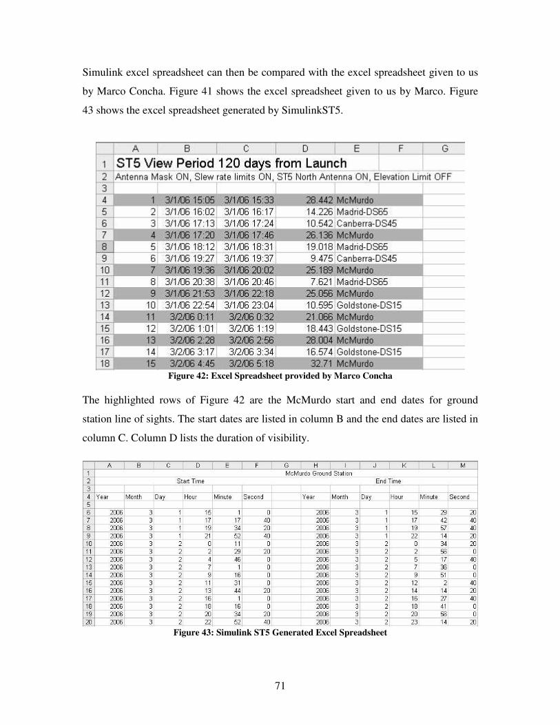
71
Simulink excel spreadsheet can then be compared with the excel spreadsheet given to us
by Marco Concha. Figure 41 shows the excel spreadsheet given to us by Marco. Figure
43 shows the excel spreadsheet generated by SimulinkST5.
Figure 42: Excel Spreadsheet provided by Marco Concha
The highlighted rows of Figure 42 are the McMurdo start and end dates for ground
station line of sights. The start dates are listed in column B and the end dates are listed in
column C. Column D lists the duration of visibility.
Figure 43: Simulink ST5 Generated Excel Spreadsheet

72
The SimulinkST5 generated output shows only the McMurdo visibility dates. Each
ground station was separated into its own individual spreadsheet unlike the spreadsheet
that was given to us. The SimulinkST5 spreadsheet is divided into two major columns, a
start date and an end date. The dates are listed in year, month, day, hour, minute, and
seconds. To create this spreadsheet, for this particular example, the user will execute a
MATLAB script file by typing McMurdo.m in the command prompt. Other ground
stations can be accessed by typing these commands:
- Canberra.m
- Goldstone.m
- Madrid.m
When analyzing the start and end dates from Figure 42 and 43 it should be noted that
there is a small difference in times. The difference between the two will range anywhere
from one to four minutes. These dates may be different due to the fact that Marco Concha
calculated the times using worse case scenarios which would limit the accuracy in his
model.
Zone of Interference When calculating the Zone of Interference the model accounts for the ground station
elevation, the satellite antenna gain, and satellite attitude. The elevation is taken from the
ground station look angles that are calculated in the S-Function. The satellite antenna
gain is calculated using the radiative pattern angle and look-up table. The attitude is a
text file input to the MATLAB workspace. When the ground station elevation is greater
than 10 degrees and less than 170 degrees the model will inspect the receiver gain. If the
gain is less than or equal to -10 dB then the communication link is in the Zone of
Interference. Figure 44 is a plot of the ground station line of sight and the Zone of
Interference line of sight.

73
Figure 44: Ground Station Line of Sight and Zone of Interference Line of Sight
Similar to the ground station line of sight graph the Zone of Interference graph shows
logic high for when transmission occurs in the Zone of Interference and logic low for not
in the Zone of Interference. The Zone of Interference always resides inside ground station
line of sight times.
In order to view the start and end dates of the Zone of Interference an excel spreadsheet
was created. The start and end dates are written to a workspace and then a MATLAB
script file writes the data to an excel file. Figure 45 shows the excel spreadsheet of start
and end dates for the Zone of Interference as well as the ground station visibility dates.

74
Figure 45: Simulink ST5 ZOI Dates
To create this the Zone of Interference spreadsheet the user will type McMurdoZOI.m in
the MATLAB command prompt. Other ground station Zone of Interference dates are
accessed by typing these commands:
- CanberraZOI.m
- GoldtsoneZOI.m
- MadridZOI.m
Link Margin and Doppler Shift Results Figure 46 shows the plots of ground station line of sight, Doppler shift, and link margin.
For the times of visibility the link margin and Doppler shift can be determined. The
ground stations will need to adjust their transmission frequencies to account for the
effects of Doppler shift. The link margin must be at least 3 dB for a successful
transmission. From Figure 46 we can see that the link margin of ST5 is always above 3
dB. The McMurdo ground stations link margin is much lower than the DSN stations but
never goes below 8 dB. The lower link margin from McMurdo is caused by a weaker
transmission power of the GN antenna.

75
Figure 46: Ground Station Line of Sight, Doppler Shift, and Link Margin
5.3 Orbit Propagator The orbit propagator model generates the satellite position and velocity state vectors that
describe the satellites orbit. The data is stored in arrays (FinalSatelliteECI,
FinalSatellitevECI) that the Communications model can use to asses the communication
link.
The orbit propagator reads in IIRV’s as initial state inputs to the model. The model then
propagates until the time of the next IIRV. This method provides hourly corrections to
the position and velocity vectors of the satellite, providing a more accurate orbit. The
IIRV’s are separated by 4 hours; therefore the first IIRV should be used 4 hours into the
simulation. Figure 47 is a graph of the x component of satellite position. This shows the
first IIRV making the first correction to the propagator. The blue circle is the point
where a new position and velocity vector is inputted to the orbit propagator. This point
occurs at 14400 seconds which is equivalent to 4 hours.
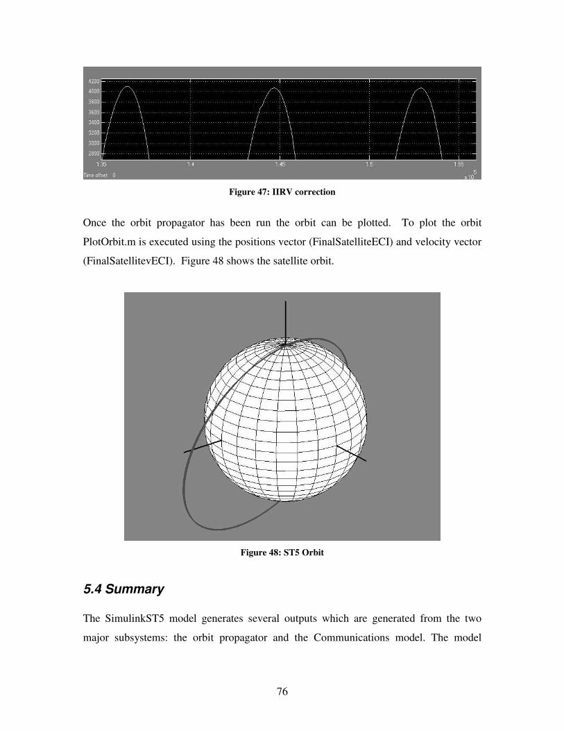
76
Figure 47: IIRV correction
Once the orbit propagator has been run the orbit can be plotted. To plot the orbit
PlotOrbit.m is executed using the positions vector (FinalSatelliteECI) and velocity vector
(FinalSatellitevECI). Figure 48 shows the satellite orbit.
Figure 48: ST5 Orbit
5.4 Summary The SimulinkST5 model generates several outputs which are generated from the two
major subsystems: the orbit propagator and the Communications model. The model

77
outputs are written to the workspace and can be viewed using MATLAB script files.
Outputs generated by the model are presented as readable and serviceable documents.
The orbit propagator produces a plot of the IIRV correcting the orbital path of the
satellite as well as a three-dimensional plot of the ST5 satellite orbit. The
Communications model provides graphs of the ground station line of sight, Zone of
Interference line of sight, link margin and Doppler shift. The Communications model also
provides excel spreadsheets giving the start and end dates of the line of sight for each
ground station as well as the start and end dates of the Zone of Interference occurrences.

78
6. Conclusions
6.1 Introduction
The Simulink modeling software was used to create a new communication model to
assess the ST5 communications link. The ST5 Communications model is a powerful and
user-friendly model that provides accurate line of sight logic and Zone of Interference
logic. The model provides an output graph and excel file that shows the black out times
due to line of sight and ZOI in an easy to view format.
6.2 Model Capabilities
After reviewing the results of the communications model, we can now state that the
model fulfills the goal of determining ST5 communication capabilities. The orbit
propagator is now able to accurately propagate the ST5 orbit for a 3-4 week period and
the communications model is able to accurately determine the link margin due to the new
ST5 antenna radiative pattern which will allow us to predict the zone of interference.
The orbit propagator will now provide orbital accuracy of up to 3-4 weeks. The
propagator model uses IIRV’s which will be received every 4 hours providing new
position and velocity vectors of the satellite. The model can then use the IIRV inputs to
properly adjust the satellites orbital position and velocity, correcting any error created by
the orbit propagator.
Using the IIRV position and velocity vectors the communications model now has the
necessary inputs to accurately determine the satellite communication capabilities. The
ST5 antenna radiative pattern was accurately modified to improve link margin
calculations for the ground station to satellite line of sight logic. The modeled antenna
pattern was then used to determine the occurrences of the zone of interference as a
function of spacecraft orbital geometry and satellite attitude. The model will output excel

79
spreadsheets that provide start and end dates for the line of sight logic and ZOI
occurrences of each ground station.
6.3 Suggested Model Modifications
There are some suggestions for the modification of the model that will help the
functionality, which would make it a more valuable tool for the mission.
At this time, our model only provides offline mission planning used for long-term
satellite health assesment. The model can be easily changed to incorporate the real-time
state health assessment. The orbit propagator model will take the input IIRV's in real
time and then propagate for a 4 hour period. The communications can then be run with
the new propagation and use real-time satellite attitude. When the next IIRV is ready the
orbit propagator and Communications model can be run again in the same manner. This
can provide ST5 mission planning with knowledge of the satellite communications
capabilities every 4 hours during the mission.
Another modification would be to use a more accurate propagator algorithm to provide
accurate propagation if the IIRV's should come to an end. Currently, the orbit propagator
takes in the IIRV's and adjusts the path of the orbit every four hours but if the IIRV
inputs should run out the orbit propagator would only be as accurate as the current two
body model. The two body model is accurate enough for our purposes because it will be
reset every 4 hours due to the IIRV’s.
6.4 Summary
The ST5 Communication model is a very powerful tool, which will aid in the ST5
mission planning. The model is very flexible and is easily updated by the user. The
model shows the successful implementation of SimulinkST5 provides an accurate model–

80
based mission operations tool. The communication model will accurately model ST5
communications link for successful mission planning.
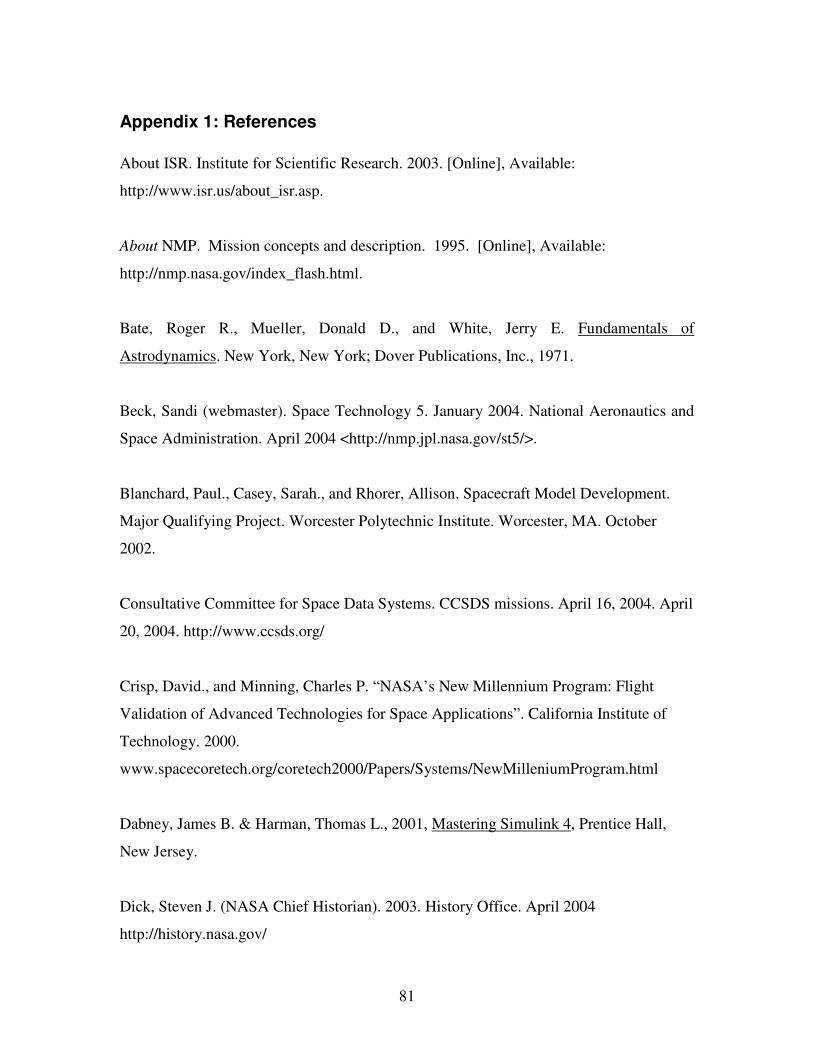
81
Appendix 1: References About ISR. Institute for Scientific Research. 2003. [Online], Available:
http://www.isr.us/about_isr.asp.
About NMP. Mission concepts and description. 1995. [Online], Available:
http://nmp.nasa.gov/index_flash.html.
Bate, Roger R., Mueller, Donald D., and White, Jerry E. Fundamentals of
Astrodynamics. New York, New York; Dover Publications, Inc., 1971.
Beck, Sandi (webmaster). Space Technology 5. January 2004. National Aeronautics and
Space Administration. April 2004 <http://nmp.jpl.nasa.gov/st5/>.
Blanchard, Paul., Casey, Sarah., and Rhorer, Allison. Spacecraft Model Development.
Major Qualifying Project. Worcester Polytechnic Institute. Worcester, MA. October
2002.
Consultative Committee for Space Data Systems. CCSDS missions. April 16, 2004. April
20, 2004. http://www.ccsds.org/
Crisp, David., and Minning, Charles P. “NASA’s New Millennium Program: Flight
Validation of Advanced Technologies for Space Applications”. California Institute of
Technology. 2000.
www.spacecoretech.org/coretech2000/Papers/Systems/NewMilleniumProgram.html
Dabney, James B. & Harman, Thomas L., 2001, Mastering Simulink 4, Prentice Hall,
New Jersey.
Dick, Steven J. (NASA Chief Historian). 2003. History Office. April 2004
http://history.nasa.gov/
82
Encyclopedia.com. Kepler’s Laws. 2004. Encyclopedia.com. April 20, 2004.
<http://www.encyclopedia.com/html/section/satelart_trackingandtelemetry.asp>
Encyclopedia.com. Satellite, Artificial: Tracking and Telemetry. 2004.
Encyclopedia.com. April 20, 2004.
http://www.encyclopedia.com/html/section/satelart_trackingandtelemetry.asp
Evans. J.C. Motions in the Heavens. October 26, 1998. George Mason University. April
20, 2004.
http://www.physics.gmu.edu/classinfo/astr103/CourseNotes/ECText/ch02_txt.htm#2.4.1.
Garber, Steve (NASA History Web Curator). NASA History Office. September 2003.
NASA’s Forty-fifth Anniversary. April 2004
http://history.nasa.gov/45thann/html/45home.htm
Geostationary, LEO, MEO, HEO Orbits. April 20, 2004. <http://www.geo-
orbit.org/sizepgs/geodef.html>
Glass, Marilyn. Assignment #4, Basics of Spacecraft Telemetry. Cooperative Satellite
Learning Project (CSLP). April 20, 2004.
http://cslp.gsfc.nasa.gov/assignments/assign4.html
Glossary of Terms. Satellite Tool Kit (STK). September 28, 2004.
http://snebulos.mit.edu/htdocs/stk/stk/glossary.htm#TopOfPage
Goddard Space Flight Center. NASA. ST5 Delta Critical Design Review. Goddard: 2004.
Gravity and Satellite Orbits. USAFA. April 20, 2004.
<http://webphysics.iupui.edu/gpnew/gp2th4.htm>

83
Grimaldy, Becki. Classical Orbital Elements. August 30, 1995. Liftoff. April 20, 2004.
<http://liftoff.msfc.nasa.gov/academy/rocket_sci/orbmech/state/class.html>
Jenner, Lynn (curator). NASA Goddard Space Flight Center. April 8, 2004. National
Aeronautics and Space Administration. April 2004 <http://www.gsfc.nasa.gov/>.
Kasser, Joe. Amateur Satellite Telemetry: Past, Present, and Future. Copyright 1991.
April 20, 2004. <http://ftp.newave.net.au/~g3zcz/amsat/telem.htm>
Learning MATLAB 6.5. (2002). Release 13. The Mathworks, Inc.
MATLAB/Simulink Resources, n.d. April 20, 2004.
<http://www.eng.fsu.edu/~cockburn/matlab/matlab_help.html>
Meeus, Jean. Astronomical Algorithms. Richmond, Virginia; Willmann-Bell, Inc., 1998.
New Millennium Space Technology 5 (ST5) Program. NASA/GSFC. X-Band
Communications Subsystem Radio Frequency Interface Control Document (RFICD).
Goddard: 2004.
Roy, A E. Orbital Motion. Bristol, Great Britain: IOP Publishing Ltd, 1988.
Sklar, Bernard. Digital Communications Fundamentals and Applications. Englewood
Cliffs, New Jersey: Prentice Hall, 1988.
Summary of Classical Orbital Elements. April 20, 2004.
<http://www.stk.com/resources/help/help/stk43/primer/coordsys-18.htm>
Taylor, Earl (webmaster). Wallops Flight Facility. April 2004. National Aeronautics and
Space Administration. April 2004 <http://www.wff.nasa.gov/>.

84
Tracking. Goddard Space Flight Center. NASA. 2005 [Online] Available:
http://nmsp.gsfc.nasa.gov/tdrss/tracking.html
Vallado, David A. Fundamentals of Astrodynamics and Applications. El Segundo,
California; Microcosm Press, Inc., 2001.
Varberg, Dale., Purcell, Edwin J., and Rigdon, Steven E. Calculus. Upper Saddle River,
New Jersey; Prentice Hall, 2000.
Wertz, James R. and, Larson, Wiley J. Space Mission Analysis and Design. Torrance,
California: W.J. Larson and Microcosm Inc., 1999.
Wertz, James R. Mission Geometry; Orbit Constellation Design and Management. El
Segundo, California: Microcosm, Inc., 2001.
What are Orbits?. March 8, 2004. European Space Agency. April 20, 2004.
<http://www.esrin.esa.it/esaLA/ASEHQOI4HNC_launchers_2.html>
White, James., Oldmixon, Matt. Space Technology 5. Major Qualifying Project.
Worcester Polytechnic Institute. Worcester, MA. October 2003.

85
Appendix 2: Contacts at NASA/GSFC Robert Shendock – ST5 Flight Operations System Engineer Shendock@[email protected] (301) 286-9398 Bob was the project mentor. Bob met with us everyday to check on progress and answer any questions. Bob set up meetings and conferences with other NASA Goddard engineers to further aid our progress. Federico Sanidad – ST5 Flight Operations System Engineer [email protected] (301) 286-9507 Rich acted as the assistant mentor to our project. Rich went over our project description and answered any basic questions we had. He also filled in for Bob when he was unable to attend meetings and presentations. Glenn Bock – ST5 Flight Operations Ground System Engineer [email protected] (301) 286-8706 Glenn helped us solve the radiative angle pattern problem. He also supplied us with documents that explained the basics of spaceflight to help us further understand aerospace engineering. Jim Morrissey – ST5 Attitude Control System Analyst [email protected] (301) 286-0529 Jim is the original creator of the orbit propagator. Jim met with us to help solve the new orbit propagator problem. Jim was supposed to be our project mentor but was transferred to a different mission before we arrived. Seth Shulman – E-01 Flight Operations Technical Lead [email protected] (301) 286-3437 Seth is a MATLAB expert. He provided us with MATLAB functions and gave us some guidance when writing MATLAB functions. Seth also helped solve the IIRV portion of the orbit propagator. Marco Concha – ST5 Guidance and Navigation Control [email protected] (301) 286-6038 Marco supplied us with sample IIRV’s to test in our model. He also met with us to solve IIRV portion of our orbit propagator. Marco also supplied us with the necessary MATLAB files to do some coordinate conversions. Victor Sank – ST5 RF/Communications

86
[email protected] (301) 286-2645 Victor provided us with the RFICD. The RFICD verified our Link Margin calculations and also provided us with ground station parameters and antenna parameters. We spoke with Victor on the phone to verify our results with the RFICD. Kevin Blahut - ST5 Mission Operations Engineer [email protected] (301) 286-5761 Kevin has acted as an assistant project mentor in the past. Kevin gave us a tour of the ST5 building facilities. We were able to see the actual ST5 satellite under construction. Kenneth J. Witt – ISR; Senior Member Research Staff, Information Systems Branch Supervisor [email protected] (304)368-9300 Kenneth is a member of the ISR team that provided the GMSEC bus that will be interfaced with our model. Jason W. Stanley – ISR; Member Research Staff, Software Systems Branch [email protected] (304)368-9300 Jason is a member of the ISR team that provided the GMSEC bus that will be interfaced with our model.

87
Appendix 3: List of Terms
Apogee: The point where the moon or satellite is at its farthest point from the earth.
Argument of perigee: The angle between the ascending node and the orbit's point of
closest approach to the earth (perigee).
Attitude: The orientation of a spacecraft relative to its direction of motion.
Azimuth: Horizontal angular distance from a reference direction, usually the northern
point of the horizon, to the point where a vertical circle through a celestial body intersects
the horizon, usually measured clockwise period.
Doppler Shift: An offset in frequency as perceived by a receiver, from the nominally
transmitted frequency caused by relative motion of the transmitter and receiver.
Eccentricity: A constant defining the shape of the orbit (0=circular, Less than
1=elliptical).
ECF (Earth Centered Fixed): A coordinate system with its origin at the center of the
Earth and axes which are fixed in the central body.
ECI (Earth Centered Inertial): A coordinate system with its origin at the center of the
Earth and axes which are fixed in inertial space.
Elevation: The height to which something is elevated above a point of reference such as
the ground.
Greenwich Sidereal Time: Angle between the Prime Meridian and the Vernal Equinox, at
a given time. Measure of time as a star, or sidereal, time rather than as a solar time.

88
Inclination: The angle between the equator and the orbit plane.
Julian Date: Single number representation of the year, month, day, and time information.
Link Margin: The difference between the required signal to noise ratio and the actual
signal to noise ratio.
Local Sidereal Time: Angle between the local Longitude and the Vernal Equinox, at a
given time. Can be calculated as the Greenwich Sidereal Time added to the local East
Longitude, in radians or degrees.
Longitude of ascending node or Right Ascension of the Ascending Node: the angle
between vernal equinox and the point where the orbit crosses the equatorial plane (going
north).
Perigee: The point where the moon or satellite is at its closest point to the earth.
Signal to Noise Ratio: average signal power and average noise power.
Telemetry: The relaying of information from the scientific instruments aboard the
satellite to the ground station.
The Line of Nodes: The point where the satellites cross the equator.
Topocentric: A coordinate system originating at a point on the Earth. The axes are
defined so that the x is in the local north location, y is in the local east direction, and z is
along the inward normal to the surface.
True anomaly: The angle between perigee and the vehicle (in the orbit plane).

89
Semi-major axis: one-half the maximum diameter, or the distance from the center of the
ellipse to one of the far ends.
Signal-to-noise power ratio: The ratio of the signal power over the noise power.
Vernal Equinox: The moment at which the sun passes through the point at which the
ecliptic intersects the celestial equator, about March 21, marking the beginning of the
spring in the northern hemisphere.
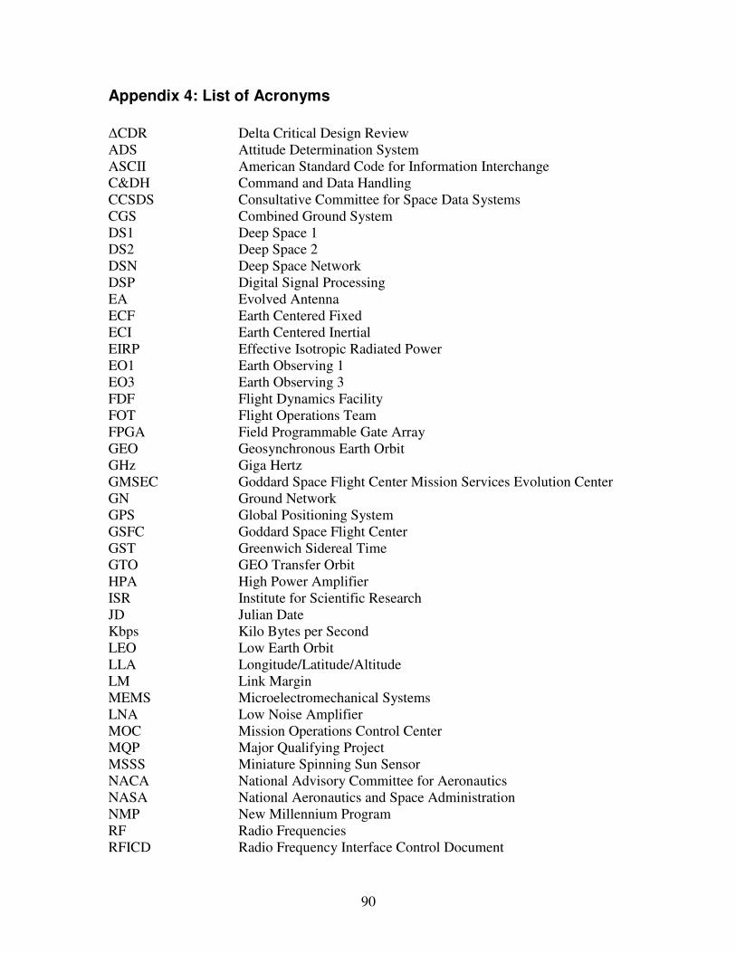
90
Appendix 4: List of Acronyms �CDR Delta Critical Design Review ADS Attitude Determination System ASCII American Standard Code for Information Interchange C&DH Command and Data Handling CCSDS Consultative Committee for Space Data Systems CGS Combined Ground System DS1 Deep Space 1 DS2 Deep Space 2 DSN Deep Space Network DSP Digital Signal Processing EA Evolved Antenna ECF Earth Centered Fixed ECI Earth Centered Inertial EIRP Effective Isotropic Radiated Power EO1 Earth Observing 1 EO3 Earth Observing 3 FDF Flight Dynamics Facility FOT Flight Operations Team FPGA Field Programmable Gate Array GEO Geosynchronous Earth Orbit GHz Giga Hertz GMSEC Goddard Space Flight Center Mission Services Evolution Center GN Ground Network GPS Global Positioning System GSFC Goddard Space Flight Center GST Greenwich Sidereal Time GTO GEO Transfer Orbit HPA High Power Amplifier ISR Institute for Scientific Research JD Julian Date Kbps Kilo Bytes per Second LEO Low Earth Orbit LLA Longitude/Latitude/Altitude LM Link Margin MEMS Microelectromechanical Systems LNA Low Noise Amplifier MOC Mission Operations Control Center MQP Major Qualifying Project MSSS Miniature Spinning Sun Sensor NACA National Advisory Committee for Aeronautics NASA National Aeronautics and Space Administration NMP New Millennium Program RF Radio Frequencies RFICD Radio Frequency Interface Control Document

91
RPA Radiative Pattern Angle SatDec Satellite Declination SatRA Satellite Right Ascension SEZ Topocentric Horizon Coordinate System SNR Signal to Noise Ratio SSR Solid State Recorder ST5 Space Technology 5 TDRSS Tracking and Data Relay Satellite System TEC Topocentric Equatorial Coordinate System UT Universal Time VEC Variable Emittance Coating WPI Worcester Polytechnic Institute WSC White Sands Complex WWW World Wide Web ZOI Zone of Interference

92
Appendix 5: ST5 Model Users’ Manual ST5 Communications Model This section is a manual providing directions on using the ST5 Communications model. It describes the steps to run the Communications model with the necessary inputs as well as how to edit input parameters. It also provides the methods for viewing the outputs of the model. Verifying Existence of Necessary Files Before using the Communications model it is important verify that the current work directory contains all necessary files. This can be done by typing “ls” into the MATLAB command prompt. >> ls The following is a list of the files necessary for simulation: OrbitPlot.m PlotLMDS.m PlotZOI.m GStationsPlot.m
Plotting script files
Init.m St_5mod.m IIRV.m
Files used to initialize constants
ST5_STK_WP.txt Look_up_EA.xls UDAP.txt Attitude.txt
Input Files to MATLAB
Communications2004.mdl OrbitProp.mdl
Models
CalenderDate.m DOY.m ecf2eci.m F_T.m GAST.m NUTATION.m MODULO.m juliandate.m Topocentric.m
MATLAB Functions used by models
Canberra.m Madrid.m Goldstone.m McMurdo.m CanberraZOI.m MadridZOI.m GoldstoneZOI.m McMurodZOI.m
MATLAB Output Functions
SFunGStations.m S-functions used by models
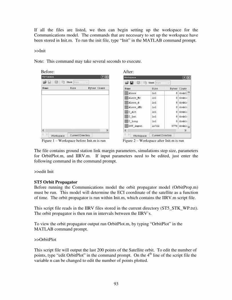
93
If all the files are listed, we then can begin setting up the workspace for the Communications model. The commands that are necessary to set up the workspace have been stored in Init.m. To run the init file, type “Init” in the MATLAB command prompt. >>Init Note: This command may take several seconds to execute. Before: After:
Figure 1 – Workspace before Init.m is run Figure 2 – Workspace after Init.m is run The file contains ground station link margin parameters, simulations step size, parameters for OrbitPlot.m, and IIRV.m. If input parameters need to be edited, just enter the following command in the command prompt. >>edit Init ST5 Orbit Propagator Before running the Communications model the orbit propagator model (OrbitProp.m) must be run. This model will determine the ECI coordinate of the satellite as a function of time. The orbit propagator is run within Init.m, which contains the IIRV.m script file. This script file reads in the IIRV files stored in the current directory (ST5_STK_WP.txt). The orbit propagator is then run in intervals between the IIRV’s. To view the orbit propagator output run OrbitPlot.m, by typing “OrbitPlot” in the MATLAB command prompt. >>OrbitPlot This script file will output the last 200 points of the Satellite orbit. To edit the number of points, type “edit OrbitPlot” in the command prompt. On the 4th line of the script file the variable n can be changed to edit the number of points plotted.
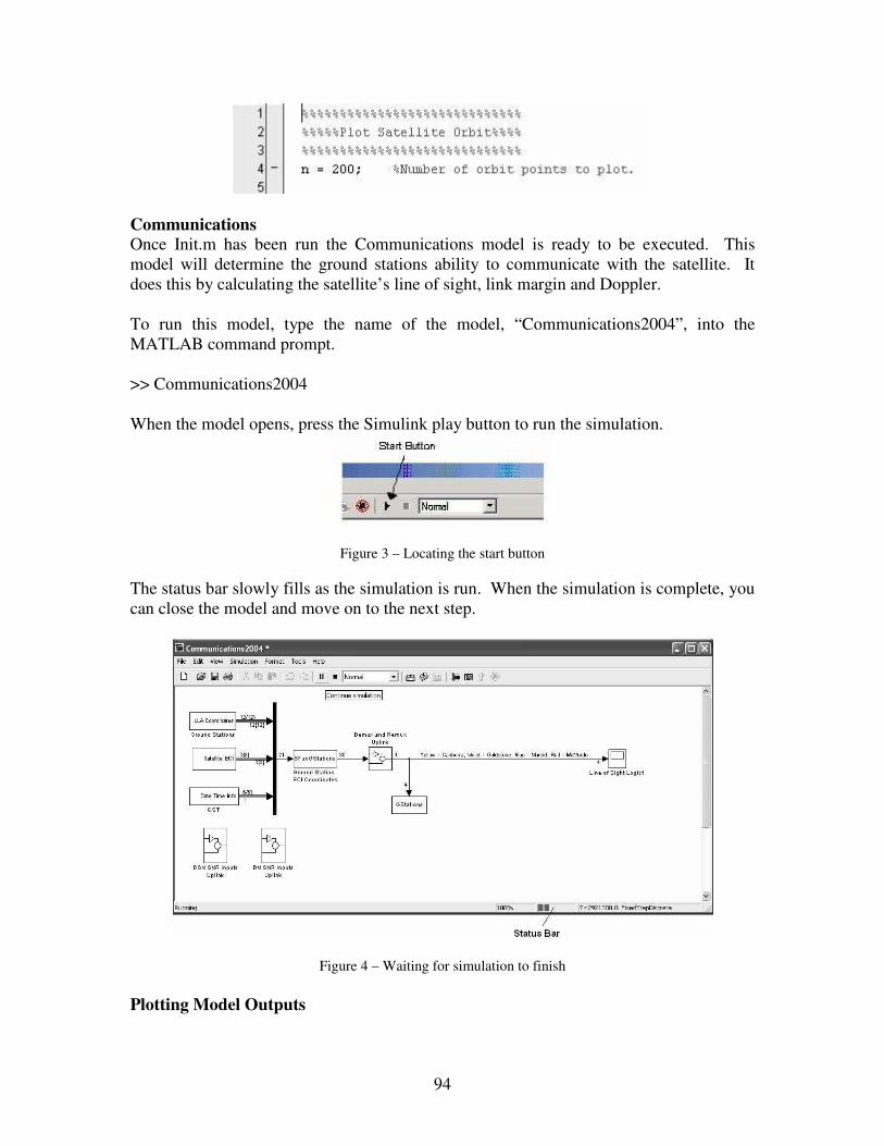
94
Communications Once Init.m has been run the Communications model is ready to be executed. This model will determine the ground stations ability to communicate with the satellite. It does this by calculating the satellite’s line of sight, link margin and Doppler. To run this model, type the name of the model, “Communications2004”, into the MATLAB command prompt. >> Communications2004 When the model opens, press the Simulink play button to run the simulation.
Figure 3 – Locating the start button
The status bar slowly fills as the simulation is run. When the simulation is complete, you can close the model and move on to the next step.
Figure 4 – Waiting for simulation to finish Plotting Model Outputs
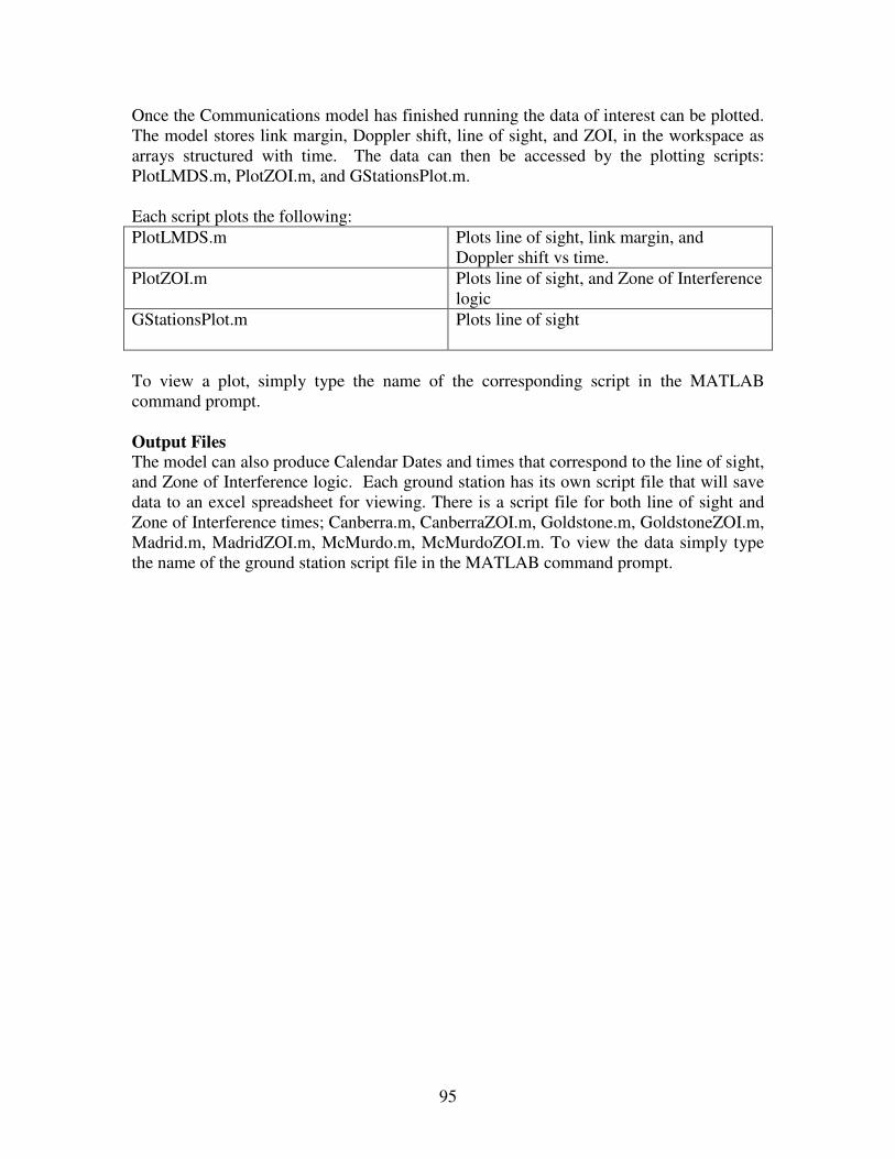
95
Once the Communications model has finished running the data of interest can be plotted. The model stores link margin, Doppler shift, line of sight, and ZOI, in the workspace as arrays structured with time. The data can then be accessed by the plotting scripts: PlotLMDS.m, PlotZOI.m, and GStationsPlot.m. Each script plots the following: PlotLMDS.m
Plots line of sight, link margin, and Doppler shift vs time.
PlotZOI.m
Plots line of sight, and Zone of Interference logic
GStationsPlot.m
Plots line of sight
To view a plot, simply type the name of the corresponding script in the MATLAB command prompt. Output Files The model can also produce Calendar Dates and times that correspond to the line of sight, and Zone of Interference logic. Each ground station has its own script file that will save data to an excel spreadsheet for viewing. There is a script file for both line of sight and Zone of Interference times; Canberra.m, CanberraZOI.m, Goldstone.m, GoldstoneZOI.m, Madrid.m, MadridZOI.m, McMurdo.m, McMurdoZOI.m. To view the data simply type the name of the ground station script file in the MATLAB command prompt.
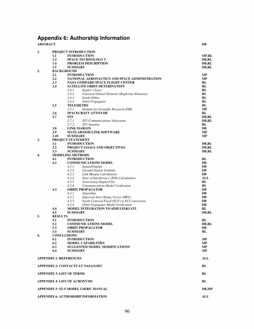
96
Appendix 6: Authorship Information ABSTRACT DB 1. PROJECT INTRODUCTION
1.1 INTRODUCTION MP,RL 1.3 SPACE TECHNOLOGY 5 DB,RL 1.4 PROBLEM DESCRIPTION DB,RL 1.5 SUMMARY DB,RL
2. BACKGROUND 2.1 INTRODUCTION MP 2.2 NATIONAL AERONAUTICS AND SPACE ADMINISTRATION MP 2.3 NASA GODDARD SPACE FLIGHT CENTER RL 2.4 SATELLITE ORBIT DETERINATION RL 2.4.1 Kepler’s Laws RL 2.4.2 Classical Orbital Elements (Keplerian Elements) RL 2.4.3 Earth Orbits RL 2.4.4 Orbit Propagator RL 2.5 TELEMETRY RL 2.5.1 Institute for Scientific Research (ISR) MP 2.6 SPACECRAFT ATTITUDE RL 2.7 ST5 DB,RL
2.7.1 ST5 Communications Subsystem DB,RL 2.7.2 ST5 Antenna RL
2.8 LINK MARGIN DB 2.9 MATLAB/SIMULINK SOFTWARE MP 2.10 SUMMARY MP
3. PROJECT STATEMENT 3.1 INTRODUCTION DB,RL 3.2 PROJECT GOALS AND OBJECTIVES DB,RL 3.3 SUMMARY DB,RL
4. MODELING METHODS 4.1 INTRODUCTION RL 4.2 COMMUNICATIONS MODEL DB 4.2.1 Inputs/Outputs DB 4.2.2 Ground Station Visibility DB 4.2.3 Link Margin Calculations DB 4.2.4 Zone of Interference (ZOI) Calculations ALL 4.2.5 Generating Output Files RL 4.2.6 Communications Model Verification RL 4.3 ORBIT PROPAGATOR DB 4.3.1 Algorithm DB 4.3.2 Improved Inter Range Vector (IIRV) DB 4.3.3 Earth Centered Fixed (ECF) to ECI conversion DB 4.3.4 Orbit Propagator Model Verification DB
4.4 MODEL INTEGRATION TO SIMULINKI ST5 RL 4.5 SUMMARY DB,RL
5. RESULTS 5.1 INTRODUCTION RL 5.2 COMMUNICATIONS MODEL DB,RL 5.3 ORBIT PROPAGATOR DB 5.4 SUMMARY RL
6. CONCLUSIONS 6.1 INTRODUCTION MP 6.2 MODEL CAPABILITIES MP 6.3 SUGGESTED MODEL MODIFICATIONS MP 6.4 SUMMARY MP APPENDIX 1: REFERENCES ALL APPENDIX 2: CONTACTS AT NASA/GSFC RL APPENDIX 3: LIST OF TERMS RL APPENDIX 4: LIST OF ACRONYMS RL APPENDIX 5: ST-5 MODEL USERS’ MANUAL DB,MP APPENDIX 6: AUTHORSHIP INFORMATION ALL
Related Documents