SP Metods y Densidad Neutron

Using Geophysical Logs to Estimate Porosity, ^Vater Resistivity, and Intrinsic Permeability

United States Geological SurveyWater-Supply Paper 2321

Using Geophysical Logs to Estimate Porosity, Water Resistivity, and Intrinsic Permeability

By DONALD G. JORGENSEN

U.S. GEOLOGICAL SURVEY WATER-SUPPLY PAPER 2321

DEPARTMENT OF THE INTERIOR DONALD PAUL MODEL, Secretary

U.S. GEOLOGICAL SURVEY Dallas L. Peck, Director

Any use of trade, product, industry, or firm names in this publication is for descriptive purposes only and does not imply endorsement by the U.S. Government.

UNITED STATES GOVERNMENT PRINTING OFFICE: 1989

For sale by theBooks and Open-File Reports SectionU.S. Geological SurveyFederal CenterBox 25425Denver, CO 80225

Library of Congress Cataloging-in-Publication Data

Jorgensen, Donald G.Using geophysical logs to estimate porosity, water resistivity, and intrinsic

permeability.

(U.S. Geological Survey Water-Supply Paper; 2321)Bibliography: p.Supt. of Docs, no.: I 19.13:23211. Water, Underground Methodology. 2. Geophysical well logging.

3. Porosity Measurement. 4. Groundwater flow Measurement. 5. Rocks Permeability Measurement. I. Title. II. Series. GB1001.72.G44J67 1988 622'.187 87-600025

CONTENTSNomenclature IVConversion factors VAbstract 1Introduction 1Estimating porosity and lithology 2Estimating water resistivity 4

Qualitative methods 4Spontaneous-potential method 4Cross-plot method 7

Estimating permeability 11Background and research 11Cross-plot method 17

Summary 19 References cited 20 Appendixes:

A. Estimating dissolved-solids concentration 22B. Estimating sodium-chloride concentration 22C. Estimating density 22D. Estimating viscosity 24

FIGURES

1. Dual-porosity, gamma-ray, and caliper logs 32. Idealized dual-porosity log calibrated to limestone matrix and gamma-ray

log 43. Electric log (spontaneous-potential and resisitivity logs) 54. Idealized electric log of shale and sandstone sequence containing fresh

and saline water 65. Flow chart of spontaneous-potential method of estimating resistivity of

formation water 7 6-14, Bl. Graphs showing:

6. Measured and estimated resistivity of water 87. Cross plot of resistivity and porosity measured on dolostone

cores 98. Porosity and lithology from formation-density log and

compensated-neutron log data 109. Cross plot of geophysical-log values of Ro and n 11

10. Viscosity, density, and temperature of freshwater 1211. Water viscosity at various temperatures and percentages of

salinity 1312. Water density at various temperatures and percentages of

salinity 1413. Relation between porosity factor and intrinsic permeability 1614. Permeability and porosity 17Bl. Resistivity of water as a function of salinity and temperature 23

Contents III

TABLES

1. Water-resistivity data 82. Porosity and permeability data 143. Permeability from formation factor and pore shape 174. Typical cementation factors, porosities, and permeabilities and calculated

permeabilities for various lithologies 185. Typical range of permeabilites of various consolidated and unconsolidated

rocks 18

NOMENCLATURE

A Coefficient relating dissolved-solids concentration to sodium-chlorideconcentration.

API Units defined by the American Petroleum Institute. BHT Bottom-hole temperature in a borehole, in units specified. Cds Concentration of dissolved solids in units specified. CNaCt Concentration of sodium chloride, in units specified. C(I) Tortuosity function. Dt Total depth of borehole, in feet. DS Dissolved-solids concentration, in units specified. F Formation factor, dimensionless. G Specific gravity, dimensionless. HR Hydraulic radius, in units of length specified. K Constant at a specified absolute temperature relating to spontaneous

potential, in millivolts.K Hydraulic conductivity, in feet per day. L Length of sample, in feet. Le Effective length of flow path, in feet. Ro Resistivity of water-rock system, in ohm-meters. Rm Resistivity of mud, in ohm-meters. Rmf Resistivity of mud filtrate, in ohm-meters. Rmfe Resistivity of mud-filtrate equivalent, in ohm-meters. Rw Resistivity of water equivalent, in ohm-meters.

Resistivity of water at 77°F, in ohm-meters.Resistivity of water at 75 °F, in ohm-meters.Specific conductance, in microsiemens.Geometric shape factor, dimensionless.Specific surface area of solids per unit volume of solids, in feet" 1 .Specific surface, in feet" 1 .Spontaneous potential, in millivolts.

Ta Absolute temperature, in degrees Rankine. Tc Temperature, in degrees Celsius. Tf Temperature, in degrees Fahrenheit. Tf Temperature of formation, in degrees Fahrenheit Tma Mean annual temperature, in degrees Fahrenheit. Tmf Temperature of mud filtrate, in degrees Fahrenheit. G Kozeny coefficient relates to pore geometry, dimensionless. P Porosity factor, dimensionless. T Tortuosity factor, dimensionless. a Empirical constant related to lithology, dimensionless. Ad Change of density in grams per cubic centimeter. d Density, in units specified of mass per unit volume. db Bulk density, which is density of matrix and fluid, in units specified of

mass per unit volume.

Rw: Rw. SC SF

SP SP

IV Contents

dj Density of fluid, in units specified of mass per unit volume.dma Density of matrix, in units specified of mass per unit volume.g Acceleration due to gravity, in specified units of length per unit of

time squared.k Intrinsic permeability, in millidarcies.n Porosity, dimensionless.nd Apparent porosity from a density log, dimensionless.nn Apparent porosity from a neutron log, dimensionless.m Cementation factor, dimensionless.m* Factor related to the number of reductions of the pore-size openings,

dimensionless.p Pressure, in Pascal.r2 Coefficient of determination, dimensionless.\L Dynamic viscosity, in units specified units of mass per length-time.

CONVERSION FACTORS

Factors to convert measurements in units other than the International System of Units (SI units) are presented. SI units are modernized metric units. The unit of time is s (second). The unit of mass is kg (kilogram). The unit of length is m (meter). The unit of force is N (newton) and is that force which gives a mass of 1 kilogram an acceleration of 1 meter per second per second. The unit of pressure or stress is Pa (pascal), which is 1 newton per square meter. SI units may use the following prefixes:

tera T 1012giga G 109mega M 106kilo k 103milli m 10"3micro \>. 10"6nano n 10~9pico p 10" 12

The following conversions may be useful to hydrologists, geologists, and geophysicists:acceleration due to gravity (g) = 9.807 m/s2centipoise (cp)=1.000x 10"3 Pa.s (pascal second)degree Fahrenheit (°F) = (1.8 TQ + 32)foot per day (ft/day) = 2.633 X 104 m/sfoot per second-second (ft/s2) = 3.048x 10' 1 m/s2foot (ft) = 3.048X10-' mgallon per day per square foot [(gal/d)/ft2] =4.716X 10'7 m/sgrams per cubic centimeter (g/cm3) = 1.000 X 103 kg/m3inch (in.) = 2.540 X 10'2 mkilogram per cubic centimeter (kg/cm3) = 9.807 XlO4 Pamillidarcy (mD) = 9.87x lO' 15 m2milligram per liter (mg/L)=1.000x 10'3 kg/m3millimho = millisiemenparts per million (ppm) = milligrams per liter/relative densitypercent salinity of sodium chloride = 10,000 ppm NaClpounds per square foot (lb/ft2 or psf) = 4.788XlO 1 Papounds per square foot (lb/in2 or psi) = 6.895x 103 Pasquare foot (ft2) = 9.290 XlO'2 m2

Contents

Using Geophysical Logs to Estimate Porosity, Water Resistivity, and Intrinsic Permeability

By Donald G. Jorgensen

Abstract

Geophysical logs can be used to estimate porosity, formation-water resistivity, and intrinsic permeability for geohydrologic investigations, especially in areas where meas urements of these geohydrologic properties are not available. The dual density and neutron porosity logs plus the gamma- ray log can be used to determine in-situ porosity and to qualitatively define lithology. Either a spontaneous-potential log or a resistivity log can be used to estimate relative resistivity of the formation water.

The spontaneous-potential and the cross-plot methods were tested for their usefulness as estimators of resistivity of the formation water. The spontaneous-potential method uses measurements of spontaneous potential and mud-filtrate resistivity to estimate the formation-water resistivity. The cross- plot method uses porosity values and observed resistivity of saturated rock to estimate the formation-water resistivity. Neither method was an accurate estimator. However, in areas of no data the methods can be used with caution.

A review of the literature of the basic relations for forma tion factor (F), porosity (n), and cementation factor (m) implies that the empirical Archie equation

is applicable to carbonates, coarse-grained elastics, and uni formly fractured media. The relation off, n, and m to intrinsic permeability (k) was also investigated. Merging the well-known Archie equation with the Kozeny equation establishes an equa tion for estimating intrinsic permeability. The resulting equa tion implies that intrinsic permeability is the function of a medium factor, (GISS 2), and a porosity factor -P, [nm + 2/(1-n) 2]. Where G is the Kozeny coefficient, 5S is the specific surface of grains per unit of volume of solids. Unfortunately, G and Ss values generally are impossible to determine from wireline geophysical logs.

A plot of the porosity factor as a function of intrinsic permeability defined the following empirical equation for k, in millidarcies:

/c=1.828x105 (-P1 ' 10),

where.p=

This equation for k was based on a selected data base of 10 sets, which included in-place measurements of permeability, in-place measurements of porosity from two dif ferent types of porosity logs, and a measurement of bulk resistivity of the rock and water from a resistivity log. The equa tion has a coefficient of determination (r2 ) of 0.90. The rela tion is applicable to permeable rocks in which surface conductance along grains is not dominant, such as most car bonate rocks, fractured rocks, and coarse elastics. Calculated permeability values for different lithologies using typical values of porosity and cementation factors compare well with typical permeability values of the different lithologies. Some data were available to support the equation, but considerably more data will be needed to better test the equation established for k.

INTRODUCTION

The problem of estimating rock, fluid, and hydraulic properties becomes more important as hydrologists are asked to solve problems related to ground-water flow in rock material about which little is known. For example, most studies of flow systems in deeply buried formations have little or no hydraulic data because those data are generally obtained from water wells, which are rare in deeply buried aquifers or aquifers containing saline water. Therefore, hydraulic property values of deep aquifers commonly are estimated using sparse and in direct data. Available analytical methods have been developed by petroleum engineers or geologists and are not widely known to hydrologists who study ground- water flow systems.

The purpose of this paper is to describe selected techniques of using borehole-geophysical logs for water- resources investigations. The procedure for each tech nique, the assumptions upon which it is based, and

Introduction

measured data for comparison and evaluation are presented for each technique. Special emphasis is given to techniques for estimating intrinsic permeability and water resistivity. Discussion of porosity and lithology is limited to those techniques directly related to the tech niques used for determining permeability and water resistivity.

This paper is directed to hydrologists investigating water resources in aquifers for which hydraulic data are sparse, such as most deeply buried rock sections, and assumes a cursory knowledge of geophysical logging. Hydraulic property values are expressed in their customary units. Calculated estimates are compared with measured values allowing evaluation of the results. In addition, methods of estimating in-situ water-quality properties, such as dissolved-solids concentration, sodium-chloride concentration, density, and viscosity are discussed in the appendixes.

Water resistivity is a measure of the resistance of a unit volume of water to electric flow and is related to water chemistry and temperature. Water that has a low concentration of dissolved solids has a high electrical resistance, whereas water that has a high concentration of dissolved solids has a low resistance. Quantitative tech niques are available for identifying water resistivity a characteristic related to water chemistry. The relation of dissolved solids and common chemical constituents to water resistivity commonly is known or can be deter mined. (See appendixes B and C.)

Intrinsic permeability, usually called permeability, is a measure of the relative ease with which a medium (rocks) can transmit a liquid under a potential gradient; it is a property of the medium alone. The cross-plot method determines intrinsic permeability from borehole geophysical logs using the cementation factor.

Methods of estimating water resistivity and permeability in aquifers of a porous medium whose freshwater contains less than about 700 mg/L dissolved- solids (Huntley, 1986, p. 469) were described by Biella and others (1983), Jones and Buford (1951), Alger (1966), Pfannkuch (1969), Worthington (1976), and Urish (1981). The methods usually require detailed information about the water chemistry and about the nature of the porous medium. For example, to estimate permeability of a coarse-grained porous medium, the average grain size and the uniformity coefficient, as well as the surface conduct ance of the water molecules surrounding the grains must be known. Those data are seldom known.

ESTIMATING POROSITY AND LITHOLOGY

Because the techniques discussed rely on data about porosity, lithology, and rock and water resistivity from wireline-geophysical logs, some discussion of wireline

geophysical logs with special reference to water is rele vant. A method allowing a "quick" qualitative lithology interpretation is available that uses the same borehole- geophysical logs used to determine porosity and to estimate water resistivity and permeability.

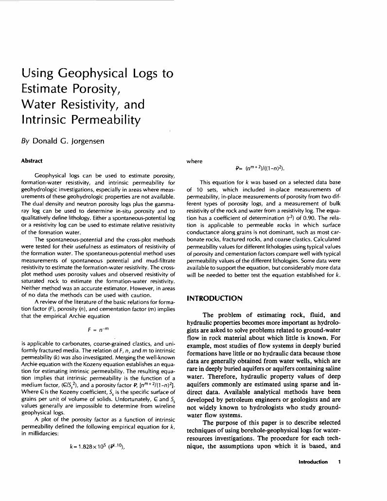
A suitable geophysical log for determining poros ity and lithology combines a compensated-neutron poros ity log and a compensated formation-density log, especially if traces of both are printed on the same log chart as is shown in figure 1 (right side). The combina tion log is termed a "dual-porosity log" in this paper. Figure 1 also shows a gamma-ray trace and a caliper trace (both left side). The gamma-ray log supplements the dual- porosity log in lithologic interpretations. The dual- porosity log is especially powerful because not only are porosity values recorded, but also the position of the den sity trace with respect to the neutron trace generally in dicates lithology. For example, if the density trace is to the right of the neutron trace on a dual-porosity log calibrated to limestone, either shale or dolostone or dolomite is implied. The gamma-ray trace defines the shale sequence; thus, shale and dolomite can be easily dif ferentiated (fig. 2). If the density trace is close to the neutron trace, calcite, such as limestone, is indicated. If the density trace is to the left of the neutron trace, silica, such as sandstone and chert, or a gas effect is indicated (fig. 2). As an example, figure 1 shows the top of a sand stone that underlies a dolostone at 2,000 ft.

Quantitative techniques are available for identify ing simple lithologies and for correcting for shaly condi tions. Most of the techniques use neutron, density (gamma-gamma), dielectric, and sonic logs to define porosity for cross-plotting methods. These techniques are described in log interpretation texts and manuals; some uses of these techniques are presented by MacCary (1978).

Before the compensated-porosity logs were avail able, porosity was determined using uncompensated sonic, gamma-gamma, and neutron logs". Interpretations were difficult because of unknown lithologic differences and variations in hole size. MacCary (1983) discussed how to use uncompensated and (or) uncalibrated porosity or other geophysical logs in investigating carbonate aquifers. The resistivity versus porosity cross-plotting method can be used with these logs.

Porosity values determined from sonic logs nor mally are assumed to represent nonfracture porosity. Therefore, fracture porosity may be estimated if the porosity determined from sonic logs is subtracted from total porosity determined from compensated dual- porosity logs. However, porosity values from some sonic logs sometimes exceed total porosity values. Thus, the assumption that sonic-porosity values represent only non- fractured porosity cannot be made without additional in formation about conditions in the hole or about shaliness. Likewise, because the fracture porosity is usually small,

Using Geophysical Logs to Estimate Porosity, Water Resistivity, and Permeability

CALIPER DIAMETER IN INCHES 13 POROSITY, IN PERCENT (LIMESTONE MATRIX)

COMPENSATED FORMATION-DENSITY POROSITY 30 20 10 0 -10

GAMMA RAY, IN API UNITS 150 COMPENSATED-NEUTRON POROSITY

20 10 0

Density porosity

Neutron porosity

Figure 1. Dual-porosity, gamma-ray, and caliper logs.

Estimating Porosity and Lithology 3

GAMMA-RAY LOG

Gamma-ray units

Gamma ray^

Depth

1

Shale

Limestone

Sandstone

Dolostone

DUAL-POROSITY LOG

Porosity

1 Compensated

neutron \ ^-porosity c

1 l 1 1 1 1

1 l1 1 1

ompensated density porosity

Figure 2. Idealized dual-porosity log calibrated to limestone matrix and gamma-ray log.

slight errors in either or both porosity logs can make frac ture porosity impossible to detect.

ESTIMATING WATER RESISTIVITY

Resistivity and spontaneous-potential logs contain information useful in estimating water resistivity. Resistivity logs are the most widely used and most com monly available type of geophysical log. A resistivity log records resistance of the electrical current flow in rock with depth. There are many types of resistivity logs; most variations refer to the specific method of measuring, such as a lateral log, an induction log, or a conductivity log. A typical resistivity log is shown in figure 3.

The spontaneous-potential log records the spon taneous potential (SP) of the fluid-filled borehole (fig. 3). The SP measured is largely an electromotive potential be tween the mud filtrate, the water within the rock, or the adjacent saturated rock materials.

The combined SP log and resistivity log is common and is here called an electric log. A hypothetical electric log of a sandstone and shale sequence is shown on figure 4. Each deeper sandstone contains water of increased salinity. Two resistivity traces are shown a deep and a shallow trace. Deep implies that the resistivity measured represents material at some distance from the well bore. In addition, deep resistivity measurements generally represent undisturbed formation water and rock. The shallow trace measures the resistivity of the material ad jacent to the borehole. This shallow resistivity is most likely to be affected by the invading drilling fluid. The following methods can be used to estimate water resistivity.

Qualitative Methods

Two little-known but easy to apply methods for qualitatively estimating relative water resistivity use the resistivity log and the spontaneous-potential log. Figure 4 shows that within sandstone D, the resistivities, as recorded on both the shallow and deep traces, are equal. Therefore, the formation-water resistivity can be assumed to be equal to the mud filtrate as measured by the shallow trace. Thus, the formation-water resistivity is equal to the mud-filtrate resistivity. Mud-filtrate resistivity usually is measured, and its value can be found on the log heading.

Spontaneous potential is a function of the log arithm of the ratio of the ionic activity of the formation water to the mud filtrate. Therefore, for the SP deflec tion to be zero, as shown for sandstone D in figure 4, the ratio is 1 and the activites are equal. If resistivities and activities are assumed to be proportional, the usual assumption in interpreting SP logs, it follows that the resistivity of the water equals the resistivity of the mud filtrate, which is usually recorded in the log heading. This unique condition is useful in quickly estimating the water resistivity at one point and for qualitatively evaluating the relative water resistivity in overlying or underlying permeable rocks, assuming other conditions are equal.

Spontaneous-Potential Method

The two quantitative techniques typically used to estimate water resistivity are (1) the spontaneous-potential method, which is the most common, and (2) the cross- plot method. Although both methods are usually presented in most well-logging manuals and texts, their accuracy is not. In the present paper, estimated values are compared with measured values to evaluate the use and accuracy of the method.

The spontaneous-potential method can be used to estimate resistivity of sodium-chloride-type water. The method is widely known and described in nearly all texts and well-logging manuals, such as "Application of borehole geophysics to water-resources investigations" (Keys and MacCary, 1971), and is based on the equation:

SP = -K logRmf

R\v(1)

where SP is the spontaneous potential, in millivolts, at the in-situ (formation) temperature; K, in millivolts, is a constant porportional to its absolute temperature within the formation; Rw is resistivity of water equivalent, in ohm-meters, at in-situ temperature; and Rmf'is the resistivity of mud filtrate, in ohm-meters, at in-situ temperature. This method of calculation requires spon taneous potential from an electric log and the mud-filtrate

4 Using Geophysical Logs to Estimate Porosity, Water Resistivity, and Permeability

SPONTANEOUS POTENTIAL

20 ,MILLIVOLTS

02

RESISTIVITY, IN OHM-METERS LATERIAL LOG

1.0 10 100 1000

I 0.2 1.0

I 1 MEDIUM INDUCTION

10 100

0.2 1.0

-- T -- --- I"'

DEEP INDUCTION 10 100

2000

1000 2000

1000 2000

-1,900-

-2,000-

-2,100-

;.- _g

VX^I-8*6 '8' '°9

Figure 3. Electric log (spontaneous-potential and resistivity logs).


ELECTRIC LOG

^Spontaneous potential

Shale-

_

-

]

Depth- *

Shale

Sandstone with very

fresh water

Shale

Sandstone with fresh water

Shale

Sandstone with fresh water

Shale

Sandstone with

saline water

Shale

Sandstone with very

saline water

Resistivity ^

A

B

C

D

1 "Deep" trace-^.

| "Shallow" trace

1

1 1

1

1 E

14- J

Rmf = 0.75 Rm (2)

Figure 4. Idealized electric log of shale and sandstone se quence containing fresh and saline water. Letters identify sandstone units whose waters range in salinity from very fresh (A) to very saline (E).

resistance measurement, generally recorded on the log heading.

The spontaneous-potential method is commonly used because SP logs are readily available. (More elec tric logs are available than any other type of geophysical log.) This method of estimating water resistivity is useful in sand-shale sequences where good SP differences ex ist, but reportedly is not usable or works poorly in car bonate rocks (MacCary, 1980, p. 3). However, no terms in equation 1 refer to lithology; thus, the equation should be applicable to any permeable rock type.

An algorithm, similar to the one presented by Bateman and Konen (1977), for using SP to determine Rw is shown in figure 5. Mud-filtrate resistivity values (Rmf) at specific temperature (Tmf) and the in-situ temperature of the permeable material (Tf) at which the SPis measured are required. The SP value, in millivolts, is the signed (4- or -) difference between the potential of the aquifer material and the potential at the reference shale line (vertical line along which most shale or clay sequences plot). If the value of Rmf is not known, an Rmf can be estimated from the mud resistivity (Rm):

The in-situ (formation) temperature (Tf) is rarely known unless temperature was measured in the borehole after drilling had been completed. However, Tf may be estimated by assuming that the temperature between the mean annual temperature near the surface and the temperature at the bottom of the borehole (BHT) in creases linearly with depth; mathematically, Tf can be shown as

Tf= Tma + (BHT-Tma) (Df) Dt

(3a)

where Df is formation depth, and Dt is the total hole depth at which BHT-was measured. A second and similar method of estimating 7/uses information on the geothermal gradient of the area:

Tf= Tma + (geothermal gradient) (Df), (3b)

where geothermal gradient is in degrees per unit depth. The procedure for the spontaneous-potential

method to estimate the water resistivity is:1. Determine Rmf and Tmf. Read values from the

log heading. If Rmf is not available, estimate from Rm using equation 2.

2. Determine SP from the spontaneous-potential trace on the electric log.

3. Determine 7/from temperature log or estimate using equations 3a or 3b.

4. Determine formation-water resistivity (Rw) using the algorithm shown in figure 5.

The spontaneous-potential method was used to estimate Rw for 11 rock sequences in boreholes for which the formation-water resistivity had been measured. Results of comparing Rw estimated from SP method versus Rw measured from chemical analyses are listed in table 1 and are shown in figure 6. A least-squares analysis for a linear relation indicates a coefficient of determina tion (r2) of 0.66. A coefficient of determination of zero indicates no correlation and a value of 1 indicates perfect correlation. The value of 0.66 indicates that a correla tion exists. Examination of figure 6 indicates that a scat ter of about 1 order of magnitude might be expected.

The coefficient of determination of 0.66 may be typical for the method if logs from the petroleum industry are used. The value of the coefficient might be interpreted as an inaccurate estimator. However, water resistivity in nature ranges from about 0.01 to more than 10 more than 3 orders of magnitude. Thus, if an accuracy of plus or minus one-half order of magnitude is acceptable, the method may be used with caution to estimate water resistivity in areas of no measured data.

Using Geophysical Logs to Estimate Porosity, Water Resistivity, and Permeability

Rmf, Tmf, SP, Tf

K=60+0.133 Tf Rwe=Rmfe WSP/K

NO

1Ru>=Ru> 75(82/(T/+7))

EXPLANATION

K Spontaneous potential constant at a specific temperature

Rmf Resistivity of mud filtrate, in ohm-meters

Rrnfe Resistivity of mud filtrate equivalent, in ohm-meters

Rm/75 Resistivity of mud at 75°F, in ohm-meters

Rw Resistivity of water, in ohm-meters

Rwe Resistivity of water equivalent, in ohm-meters

Ru>75 Resistivity of water at 75°F, in ohm-meters

SP Spontaneous potential, in millivolts

Tf Temperature of formation, in degrees Fahrenheit (°F)

Tmf Temperature of mud filtrate, in degrees Fahrenheit (°F)

Rw7575 Rwe+5

146-337 Rwe( 0^8 n\(069Ku,e-024Au;75 (( . 8 0) )

Figure 5. Flow chart of spontaneous-potential method of estimating resistivity of formation water.

The 11 rock sequences tested were mostly car bonates. No evidence was found to indicate that the method was better suited to sandstone than any other type of rock if the shale line for the SP curve could be established; however, only three sandstone sequences were used in the test.

The accuracy of the method depends on the ac curacy of the spontaneous-potential measurement, which is difficult to measure accurately because spurious elec tromotive forces are inadvertently included in the measurement. Equation 1 is most applicable if the for mation water is saline, sodium and chloride are the predominant ions, and the mud is fresh and contains no unusual additives.

Cross-Plot Method

The cross-plot method for determining water resis tivity is discussed in MacCary (1978). It is also referred to as the "carbonate" method or the "Pickett" cross- plot method and is not as widely used as the spontaneous- potential method.

As the name implies, the method requires a cross plot of resistivity and porosity values of saturated material. These values are plotted on log-log graph paper

and a line is fitted to the points. Ideally, the points define a straight line, and the intercept of the line projected to the 100-percent porosity value represents the water

100

I 10o

0.01

Method of Determination

A Cross ploto Spontaneous potential

A15

8,9° °

0.01 0.1 1.0 10

MEASURED WATER RESISTIVITY, IN OHM-METERS

100

Figure 6. Measured and estimated resistivity of water. Numbers are those of boreholes listed in table 1.


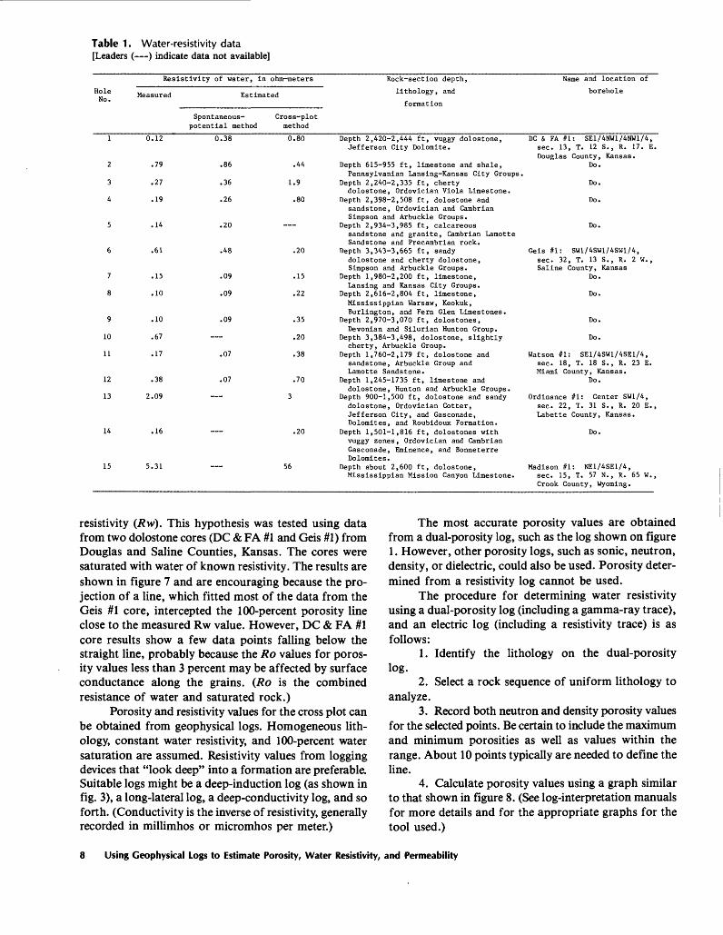
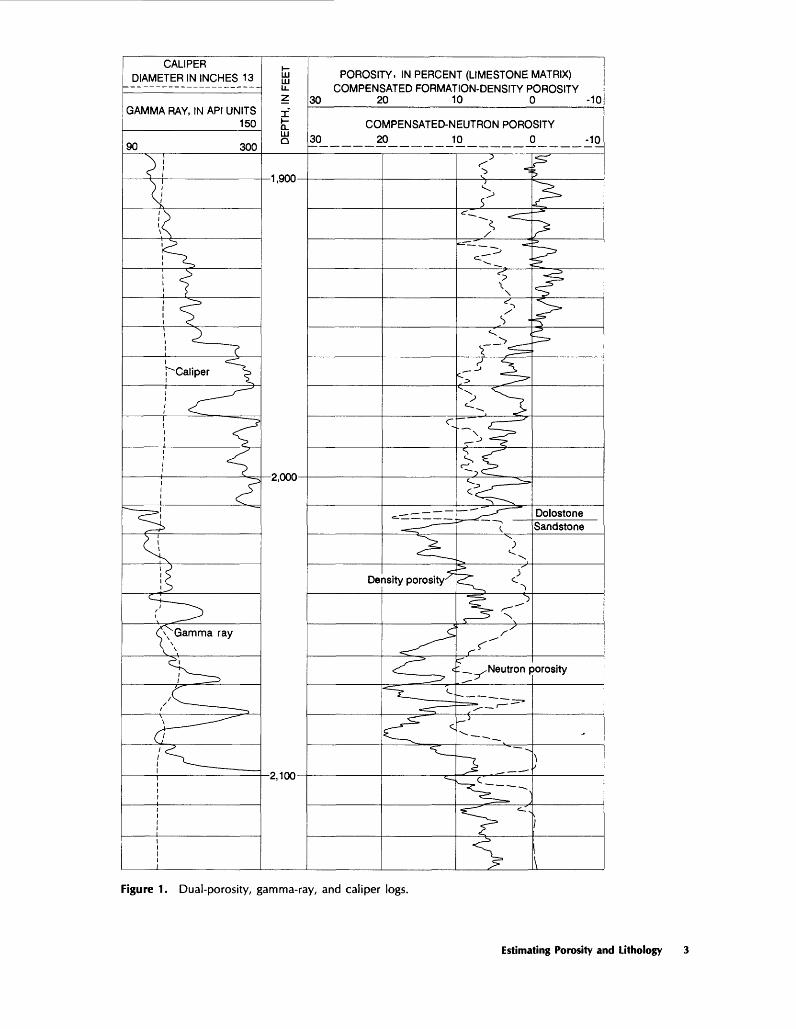
Table 1. Water-resistivity data [Leaders ( ) indicate data not available]

Hole No.

Resistivity of water, in ohm-meters

red Estimated

Spontaneous- Cross-plot potential method method

Rock-section depth,

lithology, and

formation

Name and location of

borehole

0.12

.79

.27

.19

.14

.61

.15

.10

.10

.67

.17

.38

2.09

.16

5.31

0.38

.86

.36

.26

.48

.09

.09

.09

.07

.07

0.80 Depth 2,420-2,444 ft, vuggy dolostone, Jefferson City Dolomite.

.44 Depth 615-955 ft, limestone and shale,Pennsylvanian Lansing-Kansas City Groups.

1.9 Depth 2,240-2,335 ft, chertydolostone, Ordovician Viola Limestone.

.80 Depth 2,398-2,508 ft, dolostone and sandstone, Ordovician and Cambrian Simpson and Arbuckle Groups.

Depth 2,934-3,985 ft, calcareoussandstone and granite, Cambrian Lamotte Sandstone and Precambrian rock.

.20 Depth 3,343-3,665 ft, sandydolostone and cherty dolostone, Simpson and Arbuckle Groups.

.15 Depth 1,980-2,200 ft, limestone, Lansing and Kansas City Groups.

.22 Depth 2,616-2,804 ft, limestone, Mississippian Warsaw, Keokuk, Burlington, and Fern Glen Limestones.

.35 Depth 2,970-3,070 ft, dolostones,Devonian and Silurian Hunton Group.

.20 Depth 3,384-3,498, dolostone, slightly cherty, Arbuckle Group.

.38 Depth 1,760-2,179 ft, dolostone and sandstone, Arbuckle Group and Lamotte Sandstone.

.70 Depth 1,245-1735 ft, limestone anddolostone, Hunton and Arbuckle Groups.

3 Depth 900-1,500 ft, dolostone and sandy dolostone, Ordovician Cotter, Jefferson City, and Gasconade, Dolomites, and Roubidoux Formation.

.20 Depth 1,501-1,816 ft, dolostones with vuggy zones, Ordovician and Cambrian Gasconade, Eminence, and Bonneterre Dolomites.

56 Depth about 2,600 ft, dolostone,Mississippian Mission Canyon Limestone.

DC & FA #1: SE1/4NW1/4NW1/4, sec. 13, T. 12 S., R. 17. E. Douglas County, Kansas.

Do.

Do.

Do.

Gels #1: SW1/4SW1/4SW1/4, sec. 32, T. 13 S., R. 2 W., Saline County, Kansas

Do.

Do.

Do.

Do.

Watson #1: SE1/4SW1/4SE1/4, sec. 18, T. 18 S., R. 23 E. Miami County, Kansas.

Do.

Ordinance #1: Center SW1/4, sec. 22, T. 31 S., R. 20 E. Labette County, Kansas.

Do.

Madison #1: NE1/4SE1/4,sec. 15, T. 57 N., R. 65 W., Crook County, Wyoming.

resistivity (Rw). This hypothesis was tested using data from two dolostone cores (DC & FA #1 and Geis #1) from Douglas and Saline Counties, Kansas. The cores were saturated with water of known resistivity. The results are shown in figure 7 and are encouraging because the pro jection of a line, which fitted most of the data from the Geis #1 core, intercepted the 100-percent porosity line close to the measured Rw value. However, DC & FA #1 core results show a few data points falling below the straight line, probably because the Ro values for poros ity values less than 3 percent may be affected by surface conductance along the grains. (Ro is the combined resistance of water and saturated rock.)

Porosity and resistivity values for the cross plot can be obtained from geophysical logs. Homogeneous lith ology, constant water resistivity, and 100-percent water saturation are assumed. Resistivity values from logging devices that "look deep" into a formation are preferable. Suitable logs might be a deep-induction log (as shown in fig. 3), a long-lateral log, a deep-conductivity log, and so forth. (Conductivity is the inverse of resistivity, generally recorded in millimhos or micromhos per meter.)

The most accurate porosity values are obtained from a dual-porosity log, such as the log shown on figure 1. However, other porosity logs, such as sonic, neutron, density, or dielectric, could also be used. Porosity deter mined from a resistivity log cannot be used.

The procedure for determining water resistivity using a dual-porosity log (including a gamma-ray trace), and an electric log (including a resistivity trace) is as follows:

1. Identify the lithology on the dual-porosity log.

2. Select a rock sequence of uniform lithology to analyze.

3. Record both neutron and density porosity values for the selected points. Be certain to include the maximum and minimum porosities as well as values within the range. About 10 points typically are needed to define the line.

4. Calculate porosity values using a graph similar to that shown in figure 8. (See log-interpretation manuals for more details and for the appropriate graphs for the tool used.)


100

EXPLANATION

DC&FA #1, Core, dolostone Geis #1, Core, dolostone Measured water resistivity Cementation factor

1.0 10 100

RESISTIVITY OF ROCK WATER SYSTEM (Ro), IN OHM-METERS

Figure 7. Cross plot of resistivity and porosity measured on dolostone cores.

1,000

5. Record resistivity values from the deep resistivity trace of the same points selected in step 3.

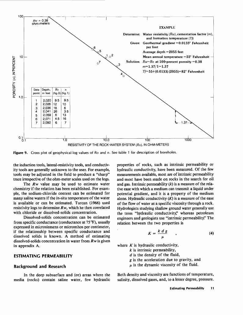
6. Plot the resistivity and porosity values as shown in figure 9 using log-log graph paper.

7. Fit a straight line to the data points. During the straight-line fitting, give less weight to the lower poros ity values because their resistivities may be affected by conductance along the grain. The resistivity indicated by this intercept is the water-formation resistivity. Project the straight line to 100-percent porosity.

When using the cross-plot method, points defining a straight line to the degree of desired accuracy cannot always be selected. Logs with expanded depth scales are easier to use in selecting better porosity and resistivity value sets because the same point on all logs can be located more accurately. An example of the method is shown in figure 9 using data from the logs shown in figures 1 and 3.

If the rock section is not 100-percent saturated with water, the rock-water system resistivity (Ro) values

obtained from the log will be larger than Ro values of the aquifer material if it had been 100-percent saturated. The values would plot to the right of the line defining n versus Ro for a 100-percent water-saturated section. The unusually large resistivity values may indicate an un- saturated zone, hydrocarbons, or gases.

Because the porosity and resistivity logarithms define a straight line, standard least-squares techniques can be applied to determine the standard estimate of error. Accordingly, the standard estimate of error for Rw can also be defined. Note that the estimated Rw is for formation conditions. The accuracy of the method was tested by estimating Rw for 15 rock sections for which Rw had been measured (fig. 6). A least-squares analysis gave a coefficient of determination of 0.88, a value that may be typical of estimates based on available logs. Figure 6 shows variations or scatter of about 1 order of magnitude in a range of more than 3 orders of magnitude that can be expected in nature. Thus, based on the results shown in figure 6, the method did not accurately estimate


FRESHWATER, LIQUID-FILLED HOLES

-1-15

0 10 20 30 40

POROSITY FROM NEUTRON LOG (n n ), IN PERCENT (APPARENT LIMESTONE POROSITY)

Figure 8. Porosity and lithology from formation-density log and compensated-neutron log (from Schlumberger Well Surveying Corp., 1979). Data are from figures 1 and 3. Arrows show how to solve the example problem.

/?w; however, the method can be used to estimate formation-water resistivity in areas of no data if an estimated accuracy of plus or minus one-half order of magnitude is acceptable. The method is applicable ir respective of whether the water is saline or fresh.

The accuracy of the method generally is proportional

to the range of porosity measured within the section of interest. The wider the range, the more accurately the line can be defined. The recorded measurement can be read more accurately from the log (trace) if the scale is ex panded. Also, the accuracy of the measurement is of con cern. The consistency of resistivity values as measured by


100

zLLJo ccLLJ P-

O oc OQ_

10

1.0

0.1

Rw = 0.38 ohm-meters

Data point

1234567

Depth, in feet

2,0202,026

2,0362,0412,0592,0712,092

Ro (fig.3)

9.512182664.56

n(fig-1)

9.51063.5

1316

7

EXAMPLE

Determine: Water resistivity (Rw), cementation factor (m)and formation temperature (Tfj

Given: Geothermal gradient =0.0133° Fahrenheitper foot

Average depth =2055 feet Mean annual temperature =55° Fahrenheit

Solution: Rw=Ro at 100-percent porosity =0.38 m=1.37/l = 1.37

T/=55+(0.0133) (2055)=82° Fahrenheit

0.1 1.0 10.0 100

RESISTIVITY OF THE ROCK-WATER SYSTEM (Ro), IN OHM-METERS

1000

Figure 9. Cross plot of geophysical-log values of Ro and n. See table 1 for description of boreholes.

the induction tools, lateral-resistivity tools, and conductiv ity tools are generally unknown to the user. For example, tools may be adjusted in the field to produce a "sharp" trace irrespective of the ohm-meter scales used on the logs.

The Rw value may be used to estimate water chemistry if the relation has been established. For exam ple, the sodium-chloride content can be estimated for many saline waters if the in-situ temperature of the water is available or can be estimated. Turcan (1966) used resistivity logs to determine Rw, which he then correlated with chloride or dissolved-solids concentration.

Dissolved-solids concentration can be estimated from specific conductance (conductance at 75 °F), usually expressed in microsiemens or micromhos per centimeter, if the relationship between specific conductance and dissolved solids is known. A method of estimating dissolved-solids concentration in water from Rw is given in appendix A.

ESTIMATING PERMEABILITY

Background and Research

In the deep subsurface and (or) areas where the media (rocks) contain saline water, few hydraulic

properties of rocks, such as intrinsic permeability or hydraulic conductivity, have been measured. Of the few measurements available, most are of intrinsic permeability and most have been made on rocks in the search for oil and gas. Intrinsic permeability (k) is a measure of the rela tive ease with which a medium can transmit a liquid under potential gradient, and it is a property of the medium alone. Hydraulic conductivity (^0 is a measure of the ease of the flow of water at a specific viscosity through a rock. Hydrologists studying shallow ground water generally use the term "hydraulic conductivity^ whereas petroleum engineers and geologists use "intrinsic permeability!' The relation between the two properties is

K = kdg (4)

where K is hydraulic conductivity, k is intrinsic permeability, d is the density of the fluid, g is the acceleration due to gravity, and H is the dynamic viscosity of the fluid.

Both density and viscosity are functions of temperature, salinity, dissolved gases, and, to a lesser degree, pressure.

Estimating Permeability 11

Water viscosity and density are functions of temperature and salinity. Density, viscosity, and temperature relations are shown in figures 10, 11, and 12. The viscosity-to- temperature relation for various sodium-chloride solu tions shown in figure 11 can be approximated by an equa tion derived by Weiss (1982), which is given in appendix D. Methods of estimating density from dissolved-solids concentration are given in appendix C.

Most intrinsic-permeability values are determined from testing cores in the laboratory or from a drill-stem test. Most drill-stem tests are conducted on petroleum reservoirs, and the results, even if accurate, must be used with care because they may represent hydrocarbon reser voirs rather than aquifers.

Intrinsic-permeability values determined from core tests usually do not completely represent conditions in the rock because any method of collecting cores disturbs the rock. Also, recovery of unconsolidated material is dif ficult and rarely successful. Laboratory tests should be run under conditions duplicating those in the subsurface. Determining k values of fractured rock from cores is ex tremely difficult because fractured core pieces are nearly impossible to arrange exactly as they were positioned in the subsurface. Also, the scale problem must be con sidered. Does a small volume of core represent the large volume of rock and fluid being considered? The scale problem arises when determining aquifer permeability that may be considered homogeneous over a thickness of tens or hundreds of feet, but that is extremely variable over a short distance, such as 1 inch. For example, the intrinsic permeability values for sample 10 listed in table 2 ranged from 4,890 mD to 0.01 mD. Obviously, an averaging technique, such as the geometric mean or a thickness-weighted mean, is required to determine the ef fective permeability of the core. Thus, even if an un disturbed fractured core could be obtained, how many point samples would be necessary to define the effective intrinsic permeability of the aquifer? From the discus sion, obviously the k value determined from a core or a drill-stem test must be carefully evaluated before assum ing the value is representative of a large rock mass.

The concept of relating formation factor to intrin sic permeability is appealing and has been investigated by many. Bear (1972, p. 113-117) related formation factor (F) to a tortuosity factor by

TEMPERATURE(7) ),IN DEGREES FAHRENHEIT (°F)

32 50 68 96 104 122 140 158

F = (5)

where C(1) is some tortuosity function, n is porosity, and m* is a function of the number of reductions in pore size openings. The function C(T^ may be 1 or less because the tortuosity factor is 1 or less. The tortuosity factor is de fined as:

0.976 Q "0 10 20 30 40 50 60 70

TEMPERATURE (Tc ), IN DEGREES CELSIUS (°C)

Figure 10. Viscosity, density, and temperature of fresh water (data from Weast, 1984).

where L is sample length, and Le is effective electrical- flow path length. Note that the tortuosity factor of equa tion 6 differs from the tortuosity defined by Winsauer and others (1952, p. 255). Equation 5 indicates that for mation factor depends on pore size and its reduction, and tortuosity. Equation 5 may be useful, but a procedure to apply data from geophysical logs to equations 5 and 6 has not yet been fully developed.

The relations among the resistivity recorded on a geophysical log, water resistivity, and rock-material resistivity is not entirely straightforward. Archie (1942) assumed that the rock material was nonconductive and derived empirical equations to define observed resistivities in terms of reservoir properties. The most generalized form of the Archie equation (Archie, 1942, p. 56) is

F = n~ (7)

where F is the formation factor (dimensionless),n is porosity (dimensionless), andm is the cementation factor (dimensionless).

T = (L/LJ2 (6)

The relation of formation factor to pressure and temperature is not completely known. In reference to temperature effect, Somerton (1982, fig. 12, p. 188) showed that the logarithm of the ratio of the formation factor at a specific temperature to formation factor at a specified reference temperature for the Berea Sandstone varied nonlinearly with temperature change.

For increasing pressure, Helander and Campbell (1966, p. 1) reported that formation factor changes can


2.1

2.0

1.9

1.8

1.7

1.6

1.5

1.4

1.3

1.2

1.1

1.0

8 °-

0.8

0.7

0.6

0.5

0.4

0.3

0.2

0.1

1.14

1 000 100 200 300 400

(7)), IN DEGREES FAHRENHEIT (°F)

Pressure correction factor (fp) for water versus (7))

Presumed applicable to brines but not confirmedexperimentally

Viscosity at elevated pressure ju. pT = (jn)(/p )

Viscosity at 1 atmosphere pressure below 212° F or at saturation pressure of water higher than 212° F

_ (1 percent concentration of sodium chloride = 10,000 parts per million)

r\ r\ _______|______|_______|_______|_______|_______|_______j_______|_______j______|______|_______|_______|_______|_______|_______|_______|_______|

'40 60 80 100 120 140 160 180 200 220 240 260 280 300 320 340 360 380 400

TEMPERATURE, (T,), IN DEGREES FAHRENHEIT (°F)

Figure 11. Water viscosity at various temperatures and percentages (%) of salinity (modified from Matthews and Russell, 1967).

be attributed to the following: (1) The increase in length the smallest pores, and (3) the effect of the double layerof the mean free path for current (increased tortuosity) is increased by the reduced area of the pores as porosityresults from increased constriction as pores close, (2) the decreases.amount of constriction is largely due to the closing of The cementation factor (rri) is a function of


1.25

ccUJ 1.20UJ

£ 1.15LUOO 1.10 m

o 1.05DC LU

C/5 1.00

<

O .95z

S .90

.85

.80

.75

(1 percent concentration of sodium chloride = 10,000 parts per million)

C\jCMCMC\JC\JCOCOCOOOCO'fr

TEMPERATURE, (Tf) IN DEGREES FAHRENHEIT (°F)

Figure 12. Water density at various temperatures and percent ages (%) of salinity (data from Arps, 1953).

tortuosity and pore geometry. Tortuosity is the ratio of the fluid path length to the sample length. Aquilera (1976) studied the effect of fractured rock on the formation and cementation factor, and used a double-porosity model to define m. The model implies that m will approach 1 for a rock mass in which all porosity is the result of frac tures (that is, there is no interconnected primary porosi ty). Because the length of the flow path in a fractured medium is much shorter than the length of flow path in a porous medium, the tortuosity of the fractured medium is small; the cementation factor is also small and ap proaches 1. The relation of porosity (ri), formation factor (F), and the tortuosity factor (1) is:

F = 1T/2

Archie further defined

F = Ro/Rw

(8)

(9)

where Ro is resistivity observed (log resistivity), and Rw is the formation-water resistivity. (In the present paper, Ro is assumed to be the bulk water and rock resistivity unaffected by fluid invasion, sometimes called true resistivity or Rt.)

Table 2. Porosity and permeability data[k, intrinsic permeability in millidarcies (mD); n, porosity, dimensionless; m, cementation factor, dimensionless; Rw, resistivity of water,in ohm-meters; F, formation factor, dimensionless; leaders ( ) indicate data not available]

Hole

No.k n m Ra F

Rock-section depth, lithology

remarks , and formation

Name and location of

borehole (source)

6.45 0.105 2.01 0.144

4.9

101

300

7 1,147

360

.13 2.37

4.74 .074 1.86 1.01

4.54 .092 2.15

.181 1.78

.125 1.09

.22 1.10 14.1

.10 1.26 5

.136 1.49

.149 1.49

Depth 2,420-2,443 ft, vuggy dolostone, maximum k=17 mD, minimum k=0.1 mD, core, Jefferson City Dolomite.

Depth 1,980-2,200 ft, oolitic limestone, drill-stem test, Lansing and Kansas City Groups.

Depth 3,482-3,493 ft, dolostone,maximum k=29 mD, minimum k=0.02 mD, core, Roubidoux Formation.

Depth 2,934-2,985 ft, calcareous sandstone and granite, drill-stem test No. 1, Lamotte Sandstone and Precambrian rock.

Depth 2,616-2,804 ft, cherty limestoneand dolostone, drill-stem test, Warsaw, Keokuk, and Burlington Limestones.

Depth 2,944-3,046 ft, porous dolostone, drill-stem test, Hunton Group.

5.29 Depth 210-610 ft, limestone, aquifer test on well tapping the Floridian aquifer.

Depth 2,500-2,760 ft, dolomite, breccia, some intensely fractured, some very dense, flow-dye test, Mission Canyon Limestone (maximum k=789 mD, minimum k=0.4, from core test).

Depth 2,760-3,030 ft, limestone anddolostone with some thin anhydrite and interbedded shale, flow-dye test (maximum k=320 mD; minumum k=0.1 mD).

Depth 3,100-3,400 ft, dolostone, some breccia texture, some crystalline, some vuggy, some dense; flow-dye test (from core test, maximum k=4,890 mD, minimum fe=0.1 mD).

DCL & FA #1: SE1/4NW1/4NW1/4, sec.13, T. 12 S., R. 17 E., DouglasCounty, Kansas (Gogel, 1981).

Geis #1: SW1/4SW1/4SW1/4, sec. 32,T. 13 S., R. 2 W., Saline County,Kansas (Gogel, 1981).

Do.

DCL & FA #1: SE1/4NW1/4NW1/4, sec. 13, R. 17 E., Douglas County, Kansas (Gogel, 1981).

Geis #1: SW1/4SW1/4SW1/4, sec. 32, T. 13 S., R. 2 W., Saline County, Kansas (Gogel, 1981).

Do.

GF 18: sec. 20, T. 7 S., R. 10 W.Gulf County, Florida (Kwader,1982).

Madison #1: NE1/4SE1/4, sec. 15,T. 57 N., R. 65 W., Crook County,Wyoming (Blankennagel and others,1977).

Do.

Do.


Combining equations 7 and 9 yields:

Rw = Ro nm (10)

If Rw is constant, equation 10 will yield a straight line with the slope of -m on a log-log plot of n versus Ro as shown in figures 7 and 9.

Sethi (1979) comprehensively reviewed the work of many researchers in defining formation-factor relations. The paper includes data originally presented by Winsauer and others (1952) in their resistivity study of brine- saturated sands and pore geometry. Raiga-Clemenceau (1977) reviewed the derivation and accuracy of the com mon forms of the modified Archie equation:

F = a (11)

where a is an empirically determined constant probably related to lithology. Some authors term "a" the cemen tation factor and "m" the cementation exponent (Dewan, 1983, p. 19). The two terms are covariant because they are not independent variables. Two variations of equa tion 11 are

F = 0.62 AT2 - 15 , and (12)

F = 1.0/7-2 . (13)

Equation 12 is sometimes called the Humble equation and is used for elastics. Equation 13 is sometimes called the carbonate equation. Raiga-Clemenceau (1977) noted that both equations are empirical and concluded that intrin sic permeability might be used to better define F. Accord ingly, he chose to define Fby setting a equal to 1, which is the Archie equation, and making m a function of k. The equation yielded a formation factor with less error than the formation factor estimated by the Humble equa tion. In conclusion, the Archie equation (eq. 7) may be as appropriate for elastics as it is for carbonates, especial ly considering the empirical nature of the equations.

The following discussion relates formation factor, cementation factors, and tortuosity factor to intrinsic permeability. Regression analysis is one technique for defining intrinsic permeability in terms of formation factor. Carothers (1968) derived two equations for intrin sic permeability (in millidarcies):

k = 4.0X108/F3 - 65

for limestone, and

k = 7.0X108/F4 - 5

(14)

(15)

for sandstone. Ogbe and Bassiouni (1978, p. 10) used a similar approach.

Croft (1971) successfully correlated the ratio Ro/Rw with intrinsic permeability. However, the correla tion requires information about water chemistry, which is not available from geophysical logs. The method works well locally where the change in Ro is primarily due to a change in porosity. MacCary (1984) pointed out that in thick hydrologic units, neither Rw nor Ro can be con sidered constant.

Stephens and Lin (1978) derived an equation for intrinsic permeability that includes a geometric shape factor (SF) of the pore and the hydraulic radius (HR), which is defined as the ratio between area of cross sec tion of the pore and its wetted perimeter. Their equation is

k = (16)

SF is 2 for circular pores and 3 for narrow cracks. Stephens and Lin reported good correlation between calculated values of intrinsic permeability and the meas ured permeability values presented by Brace (1977).

If equation 7 is substituted into equation 16,

k = (HR2/SF)-nV-5m-0 - 5) (17)

Equation 17 implies that intrinsic permeability is a func tion of the medium, the first set of terms, and a term that includes porosity and cementation factor.

The Kozeny equation is a common starting point for relating intrinsic permeability and resistivity of porous media. This equation as stated by Bear (1972, p. 166) and Herdan (1960, p. 196) is

k = G (18)

where Gis the Kozeny coefficient, and Sp is the specific surface, which is defined as the total interstitial surface area of the pores per unit volume of the medium.

The relation between specific surface area of the solids per unit volume of solids (S5) to specific surface (V is

(19)

Substituting equations 8 and 19 into equation 18 yields:

G *2k =

FS 2 (I-/*)2(20)

Equation 20 would be especially useful if F and Rw were independently known, but generally they are not. If equa tion 7 is substituted into equation 20:


k = nm + 2(21)

10,000

P = nm + 2 (22)

The numerator of P indicates that as the cementation fac tor (m) decreases, the porosity factor and the intrinsic permeability increase. Similarly, the denominator in dicates that as the porosity increases, the porosity factor and permeability increase. All values for the porosity factor can be evaluated from information from geophys ical logs. The factor Gcan be evaluated; however, efforts to evaluate Ss from geophysical logs are not straight forward. Nevertheless, equation 21 does imply that any relation for permeability should include a medium factor and a porosity factor.

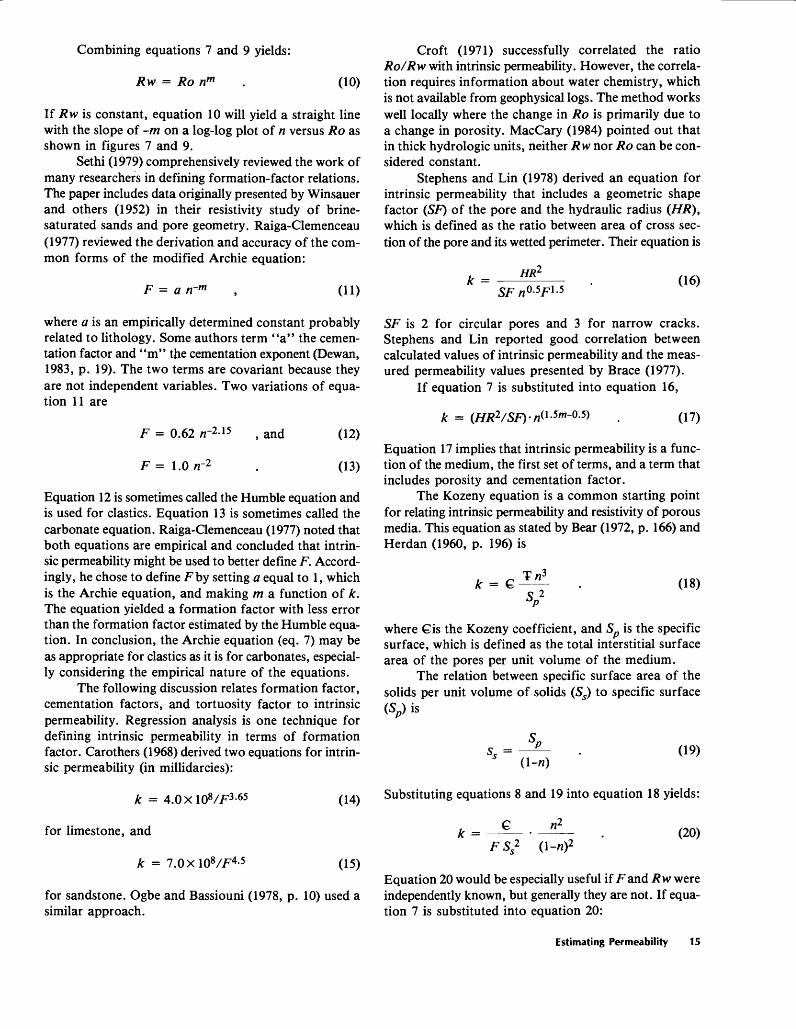
A search was made to find data sets of intrinsic permeability, porosity, and cementation factor for unconsolidated, consolidated, and fractured rock of various lithologies. The literature reports numerous values for cementation factor, core permeability, and empirical con stant (a), but little is said about how the properties were measured or what equation was used to determine the factors. Because several different procedures are com monly used, finding reported data to compare is difficult. The approach used here was that of Raiga-Clemenceau (1977); that is, equation 7 was considered an appropriate form of the Archie equation to use. The cementation factor was calculated from equation 10 or it was deter mined from the Ro versus porosity cross plot. Special preference was given to in-situ permeability and poros ity measurements from dual-porosity logs. Only a few sites were found that met the requirements (table 2). Near ly all data in table 2 are for carbonate rocks. The data from table 2 are plotted in figure 13, which shows poros ity factor versus intrinsic permeability. Because of the wide range in values, a log-log plot was chosen.

A least-squares line was used to fit data as shown on figure 13, and the regression in equation of the line is

k = 1.828X105 (P1 - 10) (23)

The correlation of determination (r2) is 0.90, which is a good correlation. With the limited data available, it can not be ascertained if the exponent 1.10 is significantly dif ferent from 1 if the factor 1.828X105 were reduced accordingly. Equation 23 does not include the medium factor as defined in equation 21. Medium factors for

Equation 21 indicates that permeability is a function of ^a medium factor (first set of terms right of the equal sign) dand a porosity factor (P) (the last set of terms). Specifical- zly, the porosity factor is ^

1,000

100

10

1x10,-5

1x10 1x10 1x10"'

POROSITY FACTOR (P)

1x10

Figure 13. Relation between porosity factor and intrinsic permeability.

many different samples have been plotted; no single line fits the data. Variations should be expected because the basic implied assumption that the flow of electricity in an aquifer is in all ways analogous to the flow of water is not completely true. Permeability is a function of porosity, surface area, and tortuosity. Electrical conduc tivity is a function of rock conductivity, ion mobility, temperature, pressure, surface area, charge on the sur face area, and the conductivity of the double layer sur rounding the grains. The straight line shown in figure 13 might be assumed to define an approximate relation ap plicable to coarse-grained elastics (such as sandstone and siltstone, most porous carbonates, and uniformly frac tured rocks) because surface conductance along the pore walls is not dominant. The relations in equation 23 are shown in figure 14, which relates porosity to permeabili ty for various cementation factors. The Humble sand stone reference samples reported by Winsauer and others (1952) whose permeability exceeds 1,000 mD (not shown on figure 13) correlate well with estimates using equation 23. Equation 23 was tested against data collated by Brace (1977) as listed in table 3. The correlation between calculated and measured permeabilities is good except if the hydraulic radius, in micrometers, was less than 1. Again, this comparison shows the importance of in cluding a geometric factor, such as Ss, Sp, or SF, to better estimate intrinsic permeability of a medium with large surface areas.

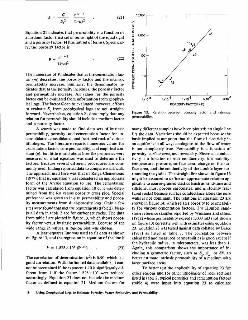
To better test the applicability of equation 23 for other regions and for other lithologies of rock sections listed in table 2, typical porosities and cementation factors (table 4) were input into equation 23 to calculate


10,000

(1-n) 2

m = cementation factor porosity

10 15 20

POROSITY (n), IN PERCENT

Figure 14. Permeability and porosity.

permeabilites of other lithologies. The comparison be tween typical permeabilities and calculated permeabilities

is good. Considering that the range of typical perme abilities in nature is about 12 orders of magnitude (from 10~4 to 108 mD as listed in table 5), the accuracy and usefulness of equation 23 are rather surprising because it allows use of data from borehole-geophysical logs to estimate intrinsic permeability with an accuracy of less than one-half an order of magnitude (fig. 3). The equa tion, based on available data, successfully estimates across a range of about 10~3 to 103 .

Cross-Plot Method

Equation 23 implies that intrinsic permeability can be estimated if the cementation factor and porosity are known. The value of m can be found from a resistivity- to-porosity cross plot, such as that shown in figure 9. The inverse of the slope of the cross plot is the cementation factor, m. The value of m can be scaled directly from the resistivity-to-porosity cross plot as follows. The slope of the cross plot (m) is

m = (horizontal distance)/(vertical distance).

The cross-plot method of estimating intrinsic permeability is as follows:

1-7. The first seven steps are the same as used in determining resistivity of water (Rw) using a resistivity- to-porosity cross plot.

8. Determine m from cross plot.9. Calculate the thickness-weighted mean porosi

ty of the section being tested.10. Calculate k using equation 23.The cross-plot method assumes that lithology is

constant except for variations in porosity. The method also assumes that Rw in the section is constant.

Table 3. Permeability from formation factor and pore shape [fim, micrometer]

Porosity Rock (n)

Western granite:50 megapascals 0.4 gigapascals

Sherman Granite -Berea Sandstone -

Nichols Buff -sandstone.

Eocene sandstone Pennsylvanian ------

sandstone 1.

sandstone 2.

0.01.01.03.22 .37.29

.20

.22

.16

.21

Formation factor

3,10016,300

88011.74.4 6.2

12.5

1320

13

Cementation factor

(m)

1.7462.1061.9331.6241.490 1.474

1.569

1.6941.635

1.644

Hydraulic Intrinsic permeability (fe) 1 , radius in millidarcies

f ITP\

in ym Calculated

0.1 l.lxlO"3.1 1.7xlO~4

6 .057 750

12 3,4002.2 990 4.2 538

4.4 6704.1 180

5.5 590

Observed

6.3xlO-54xlO~6

0.10890

3,900

230

340120

520

Reference

Brace and others (1968).DoDo

Wyllie and Ros<

DoDo Do

(1950).

Wyllie and Spangler (1952).Do.

Calculated fc=1.828x lO^P1 - 10), where P = (n m+2)/(l-n) 2 .


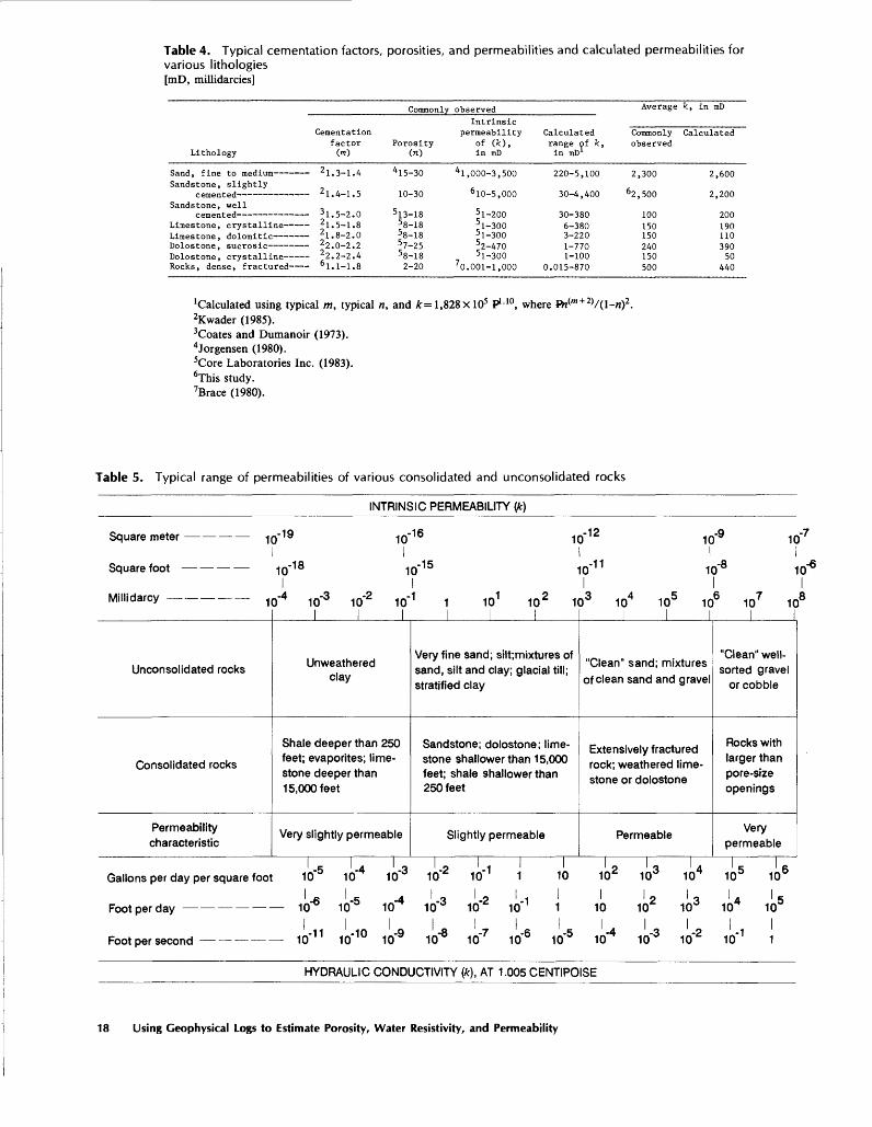
Table 4. Typical cementation factors, porosities, and permeabilities and calculated permeabilities for various lithologies [mD, millidarcies]

Commonly observed

Cementation factor

Lithology (m)

Sand, fine to medium 2 1.3- 1.4 Sandstone, slightly

Sandstone, well cemented 3 1.5-2.0

Limestone, crystalline 2 1.5-1.8

Dolostone, crystalline 22.2-2.4Rocks, dense, fractured 1.1-1.8

Porosity (n)

4 15-30

10-30

5 13-18 58-185o 1 Q

57-2558-182-20

Intrinsicpermeability

of (k), in mD

4 1, 000-3, 500

5 1-200

h-300 5 1-300

5 1-3007 0. 001-1, 000

Calculated range of k, in mD1

220-5,100

30-380 6-380

1-770 1-100

0.015-870

Average k , in mD

Commonly Calculated observed

2,300

62,500

100 150 150

150500

2,600

2,200

200 190 110390 50

440

'Calculated using typical m, typical n, and Ar=l,828xl05 P1 - 10, where Pn(m+2>/(l-n)2 .2Kwader (1985).3Coates and Dumanoir (1973).4Jorgensen (1980).5Core Laboratories Inc. (1983).6This study.7Brace (1980).

Table 5. Typical range of permeabilities of various consolidated and unconsolidated rocks

INTRINSIC PERMEABILITY (fe)

Square meter io"19 io"16i

Square foot 10'18 10' 15i i

Millidarcy 1Q-4 1Q-3 1Q-2 1Q-1 1 1Q 1 1Q 2

ID'12

10'11

103 104

10'9

10'8

105 106 107

10'7

I

108

Unconsolidated rocks

Consolidated rocks

Permeability characteristic

I I I I I

Unweathered clay

Shale deeper than 250 feet; evaporites; lime stone deeper than 15,000 feet

Very slightly permeable

Very fine sand; silt;mixtures of sand, silt and clay; glacial till; stratified clay

Sandstone; dolostone; lime stone shallower than 15,000 feet; shale shallower than 250 feet

Slightly permeable

I I I I

"Clean" sand; mixtures of clean sand and gravel

Extensively fractured rock; weathered lime stone or dolostone

Permeable

"Clean" well- sorted gravel

or cobble

Rocks with larger than pore-size openings

Very permeable

I 5 I 4 I 3 I 2 I , I I I 2 I 3 I 4 I 5 I 6 Gallons per day per square foot 10 10 10 10 10 1 10 10 10 10 10 10

' .ft .«? -4 7 .*> ' 1 9 ' * 'A ' 5Footperday 10* 10 5 10^ 10 3 10^ 10 1 1 10 10* 10"3 104 10°

Foot per second 10~ 11 10" 10 10"9 10"8 10"7 10~6 10*5 10"4 10"3 10"2 10" 1 1

HYDRAULIC CONDUCTIVITY (It), AT 1.005 CENTIPOISE


The data may not always closely define the resistivity-porosity curve. Resistivity and porosity logs with expanded depth scales are easiest to use and generally yield the most accurate data. If Rw is known from other sources and is plotted at 100-percent porosity, the line and its slope can be easily and accurately defined. Rw might be available from chemical analyses of a water sample. The value of m can sometimes be estimated if the type of porosity and lithology are known (Asquith, 1985).

Porosity values from other types of porosity logs, such as density, neutron, sonic, and dielectric, can also be used in the cross plot. Logs not in porosity units also can be used in cross plots to determine m (Aquilera, 1976, p. 767; Pickett, 1973). For example, a sonic log, which records transit time, can be used. A plot on log-log paper of the difference between the transit time from the log minus transit time of the matrix versus rock-water resistivity (Rd) will define a straight line with the slope of -m. Density logs recording bulk density can be used similarly as a plot on log-log paper of grain density minus bulk density versus Ro will define a straight line with a slope of -m. Porosity values from an epithermal-neutron log versus Ro when plotted on log-log paper also will define a straight line with the slope of -m. Values, in either counts per second or API units, from thermal neutron logs can be plotted on a linear scale versus values of Ro on a log scale. The slope of the line defined will be -m/D, where D is a function of borehole size and scale function. Thus, ideally, even uncalibrated logs can be used to determine m.

The resistivity-to-porosity cross-plot method gives average values within the logged section because the log ging tools have a "radius of investigation" and the values measured are a volumetric average for the material within their radius of investigation. The radius of investigation for a "resistivity-logging tool" might be 10 ft or more. A dielectric logging tool measures to about 2 in. depth beyond the borehole wall. The radius of investigation for a "radioactive-logging tool" might be 6 in. to 1 ft. Recorders for radioactive tools commonly average emis sions over a time period, which results in additional averaging. Also, the cross-plot method requires several sets of readings at different depths to define the empirical linear relationship; thus "averaging," which is needed to determine effective intrinsic permeability of the entire thickness of a formation, is inherent in the procedure.

The accuracy of the procedure can be checked and improved if the procedure can be calibrated to local aquifer conditions. For example, the results can be checked against permeability values from an aquifer test or a drill-stem test.

SUMMARY

Geophysical logs can be used in geohydrologic studies to estimate porosity, water resistivity, and intrinsic

permeability, especially in areas where few hydrologic data are available.

Dual density and neutron porosity logs can be used in conjunction with gamma-ray logs to determine in-situ porosity and to qualitatively identify lithology. Either a spontaneous-potential log or a resistivity log can be used to define relative water resistivity in a rock section.

The spontaneous-potential and cross-plot methods of estimating water resisitivity were tested. The spontaneous-potential method uses spontaneous-potential log measurements and mud-filtrate resistivity to estimate water resistivity. The cross-plot method uses the relation between porosity and the observed resistivity of the saturated rock to estimate water resistivity in the rock. Estimates of water resistivity were compared with meas ured values. A coefficient of determination of 0.66 for the spontaneous-potential method and 0.88 for the cross- plot method were determined. Plots of the estimated values relative to the measured values show variations of about 1 order of magnitude. The methods are not ac curate estimators, but can be used with caution to estimate water resistivity if no measurements are available.

The relations among resistivity measured on a geophysical log, formation-water resistivity, rock-matrix resistivity, and degree of cementation have been in vestigated by many, such as Archie (1942) and Winsauer and others (1952). Several empirical relations have been proposed and are described in the literature. Raiga- Clemenceau (1977) investigated the relations among cementation factor, permeability, and formation factor and questioned the validity of many of the empirical for mation factors that have been proposed since Archie's original work. Raiga-Clemenceau empirically defined the cementation factor as a function of permeability.

By merging the well-known Archie equation with the Kozeny equation, an equation for the intrinsic permeability is derived as shown:

k =,m + 2

(21)

The equation implies that permeability is a function of the medium, represented by the first set of terms, and a porosity factor (P) represented by the last set of terms. Porosity values can be determined from logs, such as neutron, density, sonic, and dielectric. A cross plot of observed resistivity to porosity defines the cementation factor. However, the Kozeney coefficient and surface area are not easily determined from borehole-geophysical logs.

The following linear regression equation, estab lished on the basis of 10 carefully selected data sets, describes the relationship between the porosity factor and intrinsic permeability plot.

Summary 19

k = 1.828X105 (P1 - 10). (23)

The regression equation has a coefficient of determina tion of 0.90 and applies to rocks in which surface con ductance along grains is not dominant, such as fractured rock, coarse-grained elastics, and most carbonates. Com monly observed porosities and cementation factors for different lithologies were used in the equation to calculate permeabilities. The calculated permeabilities compared well with typical permeabilities for the different litholo gies, indicating the general usefulness of the equation. However, additional data, which include in-situ perme ability measurements, are needed to better evaluate the relations.

REFERENCES CITED

Alger, R.P., 1966, Interpretation of electric logs in fresh water in unconsolidated formations: Society of Professional Well Log Analysts, 7th Annual Logging Symposium, Tulsa, Oklahoma, May 1966, Transactions, p. CC1-225.

Aquilera, R., 1976, Analysis of naturally fractured reservoirs from conventional well logs: Journal of Petroleum Tech nology, p. 764-772.

Archie, G.E., 1942, The electrical resistivity log as an aid in determining some reservoir characteristics: American In stitute of Mining and Metallurgical Engineers Transactions, v. 146, p. 54-62.

Arps, J.J., 1953, Technical note 195: Journal of Petroleum Technology, sec. 1, p. 18.

Asquith, G.B., 1985, Handbook of log evaluation techniques for carbonate reservoirs: American Association of Petro leum Geologists Methods in Exploration 5, 47 p.

Bateman, R.M., and Konen, C.E., 1977, The log analyst and the programmable pocket calculator: Log Analyst (September-October), v. 18, no. 5, p. 3-10.

Bear, Jacob, 1972, Dynamics of fluids in porous media: New York, American Elsevier, 764 p.

Biella, Giancarlo, Lozei, Alfredo, and Tabacco, Ignazio, 1983, Experimental study of some hydrogeophysical properties of unconsolidated porous media: Ground Water, v. 21, no. 6, p. 741-751.

Blannkenagel, R.K., Miller, W.R., Brown, D.L., and Gushing, E.M., 1977, Report on preliminary data for Madison Limestone test well No. 1, NE, SE, sec. 15, T. 57 N., R. 65 W., Crook County, Wyoming: U.S. Geological Survey Open-File Report 77-164, 97 p.

Brace, W.F., 1977, Permeability from resistivity and pore shape: Journal of Geophysical Research, v. 82, no. 23, p. 3343-3349.

____1980, Permeability of crystalline and argillaceous rocks: International Journal of Rock Mechanics, Mineral Sciences, and Geomechanics Abstracts, v. 17, p. 241-251,

Brace, W.F., Walsh, J.B., and Framgos, W.T., 1968, Permeability of granite under high pressure: Journal of Geophysical Research, v. 73, no. 6, p. 225-2236.

Carothers, J.E., 1968, A statistical study of the formation factor relation: Log Analyst, September-October, p. 13-20.

Coates, G.R., and Dumanoir, J.L., 1973, A new approach to log-derived permeability: Society of Professional Well Log Analysts, 14th Annual Logging Symposium, Transactions, p. 1-28.

Core Laboratories Inc., 1983, Variations of permeability with rock types, in Dewan, J.T., Modern open-hole log interpreta tions: Tulsa, Okla., Penn Well Publishing, figs. 7-8, 361 p.

Croft, M.G., 1971, A method of calculating permeability from electric logs: U.S. Geological Survey Professional Paper 750-B, p. 265-269.

Desai, K.P., and Moore, E.J., 1969, Equivalent NaCl solutions from ionic concentrations: Log Analyst, v. 10, no. 3, p. 12.

Dewan, J.T., 1983, Essentials of modern open-hole log inter pretation: Tulsa, Oklahoma, Penn Well Publishing, 361 p.

Gogel, Tony, 1981, Preliminary data from Arbuckle test wells, Miami, Douglas, Saline, and Labette Counties, Kansas: U.S. Geological Survey Open-File Report 81-1112, 155 p.

Hela»der, D.P., and Campbell, J.M., 1966, The effect of pore configuration, pressure, and temperature on rock resistivi ty: Society of Professional Well Log Analysts, 7th Annual Logging Symposium, Transactions, 29 p.

Herdan, George, 1960, Small particle statistics: London, But- terworth Scientific Publications, 418 p.

Huntley, David, 1986, Relation between permeability and elec trical resistivity in granular aquifers: Ground Water, v. 24, no. 4, p. 466-474.

Jones, P.H., and Buford, T.B., 1951, Electric logging applied to ground-water exploration: Geophysics, v. 16, no. 1, p. 115-139.

Jorgensen, D.G., 1980, Relationships between basic soil- engineering equations and basic ground-water flow equa tions: U.S. Geological Survey Water-Supply Paper 2064, 40 p.

Keys, S.W., and MacCary, L.M., 1971, Application of borehole geophysics to water-resources investigations: U.S. Geological Survey Techniques of Water-Resources In vestigations, book 2, chap. El, 123 p.

Kwader, Thomas, 1982, Interpretation of borehole geophysical logs in shallow carbonate environments and their applica tion to ground-water resources investigations: Tallahassee, Florida State University Ph.D. dissertation, 186 p.

_____1985, Estimating aquifer permeability from formation resistivity factor: Ground Water, v. 23, no. 6, p. 762-766.

MacCary, L.M., 1978, Interpretation of well logs in a carbonate aquifer: U.S. Geological Survey Water-Resources In vestigations Report 78-88, 30 p.

_____1980, Use of geophysical logs to estimate water-quality trends in carbonate aquifers: U.S. Geological Survey Water-Resources Investigations Report 80-57, 23 p.

_____1983, Geophysical logging in carbonate aquifers: Ground Water, v. 21, p. 334-342.

____1984, Relation of formation factor to depth of burialalong the Texas Gulf Coast, in Surface and borehole geophysical methods in ground-water investigations: U.S. Environmental Protection Agency and National Water Well Association (Feb. 6-9, 1984), p. 722-741.

Matthews, C.S., and Russell, D.C., 1967, Pressure build up and flow tests in wells: Dallas, Texas, Society of Petroleum Engineers of American Institute of Mining, Metallurgical, and Petroleum Engineers Monograph 1, 158 p.


Meyer, C.A., Mclntosh, R.B., Silvestri, G.J., and Spencer, R.C., 1968, 1967 steam tables (2d ed.): New York, American Society of Mechanical Engineers, 328 p.

Miller, R.W., 1977, A Galerkin finite-element analysis of steady- state flow and heat transport in the shallow hydrothermal system in the east Mesa area, Imperial Valley California: U.S. Geological Survey Journal of Research, v. 5, no. 4, p. 497-508.

Ogbe, David, and Bassiouni, Zaki, 1978, Estimating of aquifer permeabilities from electric well logs: Log Analyst, September-October, p. 21-27.

Pfannkuch, H.O., 1969, On the correlation of electrical con ductivity properties of porous systems with viscous flow tranport coefficients: Haifa, First International Symposium of the Fundamentals of Transport Phenomena in Porous Media, International Association of Hydraulic Research, p. 42-54.

Phillips, S.L., Igbene, A., Fair, J.A., and Ozebek, H., 1981, A technical databook for geothermal energy utilization: Lawrence Berkley Laboratory, University of California LBL-12810, 46 p.

Pickett, G.R., 1973, Pattern recognition as a means of forma tion evaluation: Society of Professional Well Log Analysts, 14th Annual Logging Symposium, Transactions, p. A1-A21.

Raiga-Clemenceau, J., 1977, The cementation exponent in the formation factor-porosity relation The effect of permeability: Society of Professional Well Log Analysts, 18th Annual Logging Symposium, Transactions, 13 p.

Schlumberger Limited, 1972, Log interpretation. Volume 1 Principles: New York, 112 p.

Schlumberger Well Surveying Corporation, 1979, Log inter pretation charts: Houston, Texas, 97 p.

Sethi, D.K., 1979, Some consideration about formation resistiv ity factor-porosity relations: Society of Professional Well

Log Analysts, 20th Annual Logging Symposium, Transac tions, 11 p.

Somerton, W.H., 1982, Porous rock-fluid systems at elevated temperatures and pressures: Geological Society of America Special Paper 189, p. 183-197.

Stephens, D.R., and Lin, W., 1978, Relationships of permeabil ity, porosity, and formation factor: University of Califor nia Research Letter 80856, 9 p.

Turcan, A.N., Jr., 1966, Calculation of water quality from elec trical logs Theory and practice: Louisiana Geological Survey Water Resources Pamphlet 19, 23 p.

Urish, D.W., 1981, Electrical resistivity-hydraulic conductiv ity relationships in glacial outwash aquifers: Water Resources Research, v. 17, no. 5, p. 1401-1408.

Weast, R.C., ed., 1984, CRC Handbook of chemistry and physics: Boca Raton, Florida, CRC Press, p. F-ll, F-38.

Weiss, Emanuel, 1982, A computer program for calculating relative transmissivity input arrays to aid model calibra tion: U.S. Geological Survey Open-File Report 82-447, 18 p.

Winsauer, W.O., Shearin, H.M., Masson, P.H., and Williams, M., 1952, Resistivity of brine-saturated sands in relation to pore geometries: American Association of Petroleum Geologists Bulletin, v. 36, no. 2, p. 253-277.

Worthington, P.F., 1976, Hydrogeophysical equivalence of water salinity, porosity, and matrix conduction in arena ceous aquifers: Ground Water, p. 224-232.

Wyllie, M.R.J., and Rose, W.D., 1950, Application of the Kozeny equation to consolidated porous media: Nature, no. 165, p. 972.

Wyllie, M.R.J., and Spangler, M.B., 1952, Application of elec trical resistivity measurements to the problem of fluid flow in porous media: American Association of Petroleum Geologists Bulletin, v. 36, no. 2, p. 359-403.

References Cited 21

APPENDIX A

Estimating Dissolved-Solids Concentration

Dissolved-solids concentration can be estimated from either resisitivity or specific conductance measure ments. Specific conductance is a measure of the conduct ance of electrical current through a fluid and is usually expressed in microsiemens or micromhos. A specific- conductance measurement is referenced to a specified temperature, usually 25 °C (77 °F).

Specific conductance (SC), which is the resistivity reciprocal at 77 °F, can be calculated from the equation:

SC =1X104

Rw(Al)

77

where Rw17 is the water resistivity at 77 °F, in ohm- meters.

Resistivity of water at any temperature, Tx, in degrees Fahrenheit, can be converted to RW-J-J by:

(A2)

The relation between dissolved-solids concentra tion, in parts per million, and specific conductance, in microsiemens is

DS ^ (P) (SC) (A3)

where P is a factor to be determined for each water, but which typically is about 0.67 for many ground waters if specific conductance is in microsiemens.

Dissolved-solids concentration can also be esti mated from the sodium-chloride concentration. The em pirical relation between sodium-chloride concentration (CNaC1) and dissolved-solids concentration (DS) is:

DS = (A) (CNaC1) (A4)

where DS and CNaC1 are both in the same units. The coefficient A should be determined for each water type; however, the value of A generally used is about 1.04 for many natural waters.

APPENDIX B

Estimating Sodium-Chloride Concentration

Many useful interpretations of geophysical-log data are based on relations for sodium-chloride solutions. Relations among water resistivity, temperature, and dissolved-solids concentration are shown on figure Bl.

Most of the curves on figure Bl can be approximated by the equation:

NaCl,ppm

where CNaC1 ppm is sodium-chloride concentration, in parts per million, and Rw15 is the resistivity, in ohm- meters, of the solution at 75 °F. 75 °F is the usual reference temperature in geophysical logging.

Values of resistivity, in ohm-meters, at any temperature, Tx, in degrees Fahrenheit, can be converted to resistivity at 75 °F by the equation:

(TX +1)/(S2) (B2)

Sodium-chloride concentration, in milligrams per liter, can be converted to concentration in parts per million:

'NaCl.ppm 'NaCl,mg/L (B3)

where G is specific gravity and is the solution density divided by pure-water density.

Concentration of a sodium-chloride solution in milligrams per liter (CNaC1 mg/L) can be converted to estimated concentrations in part per million (CNaC1 )ppm) by the following equation (Robert Leonard, U.S. Geological Survey, written commun., 1984):

NaCl,ppm -V- 6.7 X 10-7) CNaC1>mg/L (B4)

Investigators, such as Turcan (1966) and Desai and Moore (1969), list multipliers that allow resistivity of equivalent sodium-chloride solutions to be estimated for solutions that contain ions other than Na and Cl.

APPENDIX C

Estimating Density

Density is a function of temperature, pressure, and salinity (fig. 12). Miller (1977) reported a relation derived by J.W. Mercer (U.S. Geological Survey, written com mun., 1975) to estimate density (d) of freshwater, in kg/m3 (kilograms per cubic meter) as a function of temperature and pressure:

dTp = 2.0743 X103 + 5.56172X10-9/?

-4.26895 X\Q-5(\/Ta)

-2.35494X10-3 Ta2

+ 4.95912 Xl07(l/rfl2) ; (Cl)

where p is pressure, in Pa (pascals); and Ta is absolute temperature.


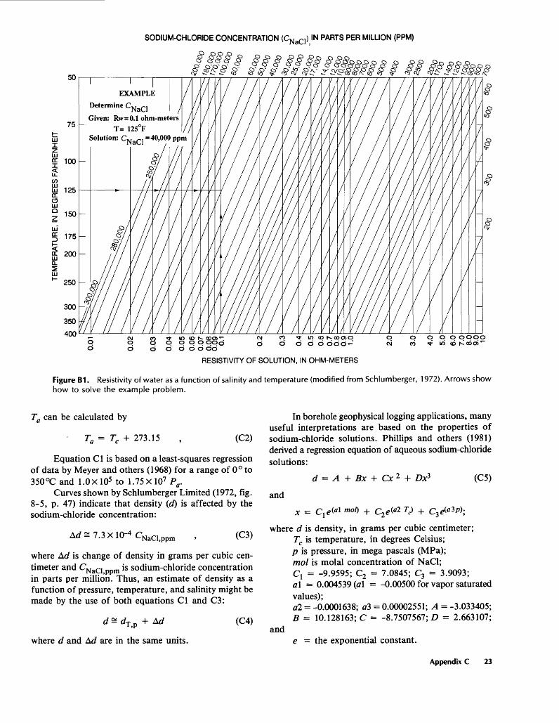
SODIUM-CHLORIDE CONCENTRATION (CNaC1 ) IN PARTS PER MILLION (PPM)

50

75

100

125

150

175

200

250

300

350

400

<v ^SS&Bfc

CO UJ UJccCDUJ Q

EXAMPLE

Determine C.^ /->i

Given: Rw=0.1 ohm-metersT= 125°F

Solution: CN <-,, =40,000 ppm

CO TJ- IO <Dq q q qqd

o d d> d do

* in <p N; opo>qd d C» odd*-1

q co

q q q qqqo *» 10 <b "

RESISTIVITY OF SOLUTION, IN OHM-METERS

Figure B1. Resistivity of water as a function of salinity and temperature (modified from Schlumberger, 1972). Arrows show how to solve the example problem.

Ta can be calculated by

Ta = Tc + 273.15 (C2)

Equation Cl is based on a least-squares regression of data by Meyer and others (1968) for a range of 0° to 350°C and l.OxlO5 to 1.75X107 Pa .

Curves shown by Schlumberger Limited (1972, fig. 8-5, p. 47) indicate that density (d) is affected by the sodium-chloride concentration:

Ad = 7.3 X 10-4 CNaappm (C3)

where Ad is change of density in grams per cubic cen timeter and CNaC1 ppm is sodium-chloride concentration in parts per million. Thus, an estimate of density as a function of pressure, temperature, and salinity might be made by the use of both equations Cl and C3:

d * dTp + Ad

where d and Ad are in the same units.

(C4)

In borehole geophysical logging applications, many useful interpretations are based on the properties of sodium-chloride solutions. Phillips and others (1981) derived a regression equation of aqueous sodium-chloride solutions:

d = A + Bx + Cx 2 + Dx3 (C5)

and

x =

where d is density, in grams per cubic centimeter; Tc is temperature, in degrees Celsius; p is pressure, in mega pascals (MPa); mol is molal concentration of NaCl; Cl = -9.9595; C2 = 7.0845; C3 = 3.9093; a\ = 0.004539 (a\ = -0.00500 for vapor saturated values);a2 = -0.0001638; a3 = 0.00002551; A = -3.033405; B = 10.128163; C = -8.7507567; D = 2.663107;

ande = the exponential constant.

Appendix C 23

Phillips and others (1981) reported that the experimen tal data were reproduced to a maximum deviation of ± 2 percent over the entire range of concentration, for temperatures of 0°-350°C, and for pressure as high as 50 MPa.

An empirical relation derived by Robert Leonard (U.S. Geological Survey, written commun., 1984) to esti mate specific gravity, which is solution density divided by density of pure water, is

G 3 i/(l- 6.7 XlO-7cNaC1)ppm (C6)

where G is specific gravity and CNaCljppm is sodium- chloride concentration in parts per million.

APPENDIX D

Estimating Viscosity

An equation to estimate dynamic viscosity of water, (n), was derived by Emanuel Weiss (1982, p. 4). The equa tion approximates the curves of Matthews and Russell (1967) shown in figure 11. The approximate equation is:

(Dl)

Where n is dynamic viscosity, in centipoise;Tj- is temperature, in degrees Fahrenheit; and C-ds.mg/L is dissolved-solids concentration, in milligrams per liter.

Weiss (1982) reported that the largest error is at 55 °F, at which temperature the value of the calculated /* from equation Dl is inaccurate by nearly 10 percent.

/* = [(38.37r/-5) - (14.6/7}-0 - 25) + 1.48]

Miller (1977) reported on the work of Meyer and others (1968) to estimate viscosity. If viscosity is a func tion of temperature alone, viscosity, in pascal-seconds, can be estimated by:

(D2)/*S (10-7) (241.4X10*)

The exponent x is:

x = (247.8)/(rc + 133.15)

where Tc is temperature in degrees Celsius. The equation is reported valid for liquid water along the saturation line from 0-300 degrees Celsius.

Phillips and others (1981) reported a correlation for sodium-chloride solutions using more than 1,500 selected experimental values. The model was originally developed for colloidal suspensions and solutions of nonelectrolytes; however, the equation has been used extensively for elec trolytes, such as NaCl, after suitable modification:

=1 + a mol + b mol2 + c mo/ 3

+ d Tc(\ - e l m°l) (D3)

where /* is viscosity of sodium-chloride solution, incentipoise;fjL w is viscosity of water, in centipoise;a = 0.0816; b = 0.0122;c = 0.000128; d = 0.000629;i = -0.7; Tc is temperature, in degrees Celsius;mol = molal concentration, in gram-moles NaClper kilogram of water;and e is the exponential constant.

Phillips and others (1981) reported that the equa tion reproduces data to an average of better than ± 2 per cent over the range 10 to 350 °C, 0.1 to 50 MPa, and 0-5 mol.


* U.S. GOVERNMENT PRINTING OFFICE: 1989-673-047/86048

SP Metods y Densidad Neutron

Documents

tf tma

intrinsic permeabilityby donald

geological survey water

porosity log calibrated

idealized electric log

kansas city groups

log graph paper

estimating intrinsic permeability