South American regional ionospheric maps computed by GESA: A pilot service in the framework of SIRGAS

Available online at www.sciencedirect.com

www.elsevier.com/locate/asr

Advances in Space Research 42 (2008) 737–744

South American regional ionospheric maps computed by GESA:A pilot service in the framework of SIRGAS

C. Brunini *, A. Meza, M. Gende, F. Azpilicueta

Facultad de Ciencias Astronomicas y Geofısicas, Universidad Nacional de La Plata,

Paseo del Bosque s/n, 1900, La Plata, Argentina

Consejo Nacional de Investigaciones Cientıficas y Tecnicas, Paseo del Bosque s/n, 1900, La Plata, Argentina

Received 30 April 2007; received in revised form 10 August 2007; accepted 22 August 2007

Abstract

SIRGAS (Geocentric Reference Frame for the Americas) is an international enterprise of the geodetic community that aims to realizethe Terrestrial Reference Frame in the America’s countries. In order to fulfill this commitment, SIRGAS manages a network of contin-uously operational GNSS receivers totalling around one hundred sites in the Caribbean, Central, and South American region. Althoughthe network was not planed for ionospheric studies, its potential to be used for such a purpose was recently recognized and SIRGASstarted a pilot experiment devoted to establish a regular service for computing and releasing regional vertical TEC (vTEC) maps basedon GNSS data. Since July, 2005, the GESA (Geodesia Espacial y Aeronomıa) laboratory belonging to the Facultad de Ciencias Astron-omicas y Geofısicas of the Universidad Nacional de La Plata computes hourly maps of vertical Total Electron Content (vTEC) in theframework of the SIRGAS pilot experiment. These maps exploit all the GNSS data available in the South American region and are com-puted with the LPIM (La Plata Ionospheric Model). LPIM implements a de-biasing procedure that improves data calibration in relationto other procedures commonly used for such purposes. After calibration, slant TEC measurements are converted to vertical and mappedusing local-time and modip latitude. The use of modip latitude smoothed the spatial variability of vTEC, especially in the South Amer-ican low latitude region and hence allows for a better vTEC interpolation. This contribution summarizes the results obtained by GESA inthe framework of the SIRGAS pilot experiment.� 2008 COSPAR. Published by Elsevier Ltd. All rights reserved.

Keywords: Total Electron Content; GPS; Regional ionosphere map; SIRGAS

1. Introduction

Since the early 90’s, a worldwide network of continu-ously operational dual-frequency GPS receivers has rap-idly grown under the management of the InternationalGNSS Service (IGS) (Beutler et al., 1999). Although itwas not conceived for ionospheric studies, this networkhas become a global-distributed observatory routinelyused for that purpose. Among other benefits, this observa-tory provides time continuity, worldwide coverage (at least

0273-1177/$34.00 � 2008 COSPAR. Published by Elsevier Ltd. All rights rese

doi:10.1016/j.asr.2007.08.041

* Corresponding author.E-mail addresses: [email protected] (C. Brunini), ameza@

fcaglp.unlp.edu.ar (A. Meza), [email protected] (M. Gende),[email protected] (F. Azpilicueta).

over lands), well-established standards for data inter-change, and easy and free data availability. In order toexploit these potentialities, on May 1998 IGS created theIonosphere Working Group (Feltens et al., 1998) and soonafter, five analysis centers started computing and deliver-ing to the community two-dimensional worldwide gridsof vertical Total Electron Content (vTEC) or, in the IGSargot, Global Ionospheric Maps (GIMs). The analysiscenters operate under the responsibility of the Jet Propul-sion Laboratory (JPL) (Manucci et al., 1999), the Euro-pean Space Agency (ESA) (Feltens, 1998), the Center forOrbit Determination in Europe (CODE) (Schaer, 1999),the Universidad Politecnica de Cataluna (UPC) (Hernan-dez-Pajares et al., 1999), and the Energy Mines andResources of Canada (EMR) (Gao et al., 1994). A combi-

rved.

738 C. Brunini et al. / Advances in Space Research 42 (2008) 737–744

nation center under the responsibility of UPC (Hernandez-Pajares, 2006) computes the final IGS GIMs, which resultfrom the weighted average of the individual GIMs com-puted by each analysis center.

SIRGAS was established during an international meet-ing in Asuncion, Paraguay, in October 1993 by representa-tives of most of the South American countries, theInternational Association of Geodesy, the Pan AmericanInstitute of Geography and History, and the NationalImagery and Mapping Agency, now National Geospatial-Intelligence Agency, as the ‘‘Sistema de Referencia Geo-centrico para America del Sur” (South American Geocen-tric Reference System) Project (Fortes et al., 2006). Theproject structure includes an Executive Committee madeup by the representatives of all participating countriesand international institutions, a Directive Board, a Scien-tific Council, and three Working Groups (WGs): WGI‘‘Reference Systems”, WGII ‘‘Geocentric Datum”, WGIII‘‘Vertical Datum”. In 2000, the project was extended toCentral and North America and it was renamed ‘‘Geocen-tric Reference System for the Americas”, keeping the acro-nym SIRGAS. In order to fulfill part of its commitments,SIRGAS manages, through its WGI, a network of contin-uously operational dual-frequency GPS receivers totalingaround one hundred sites in the Caribbean, Central, andSouth American regions. The network includes all IGS glo-

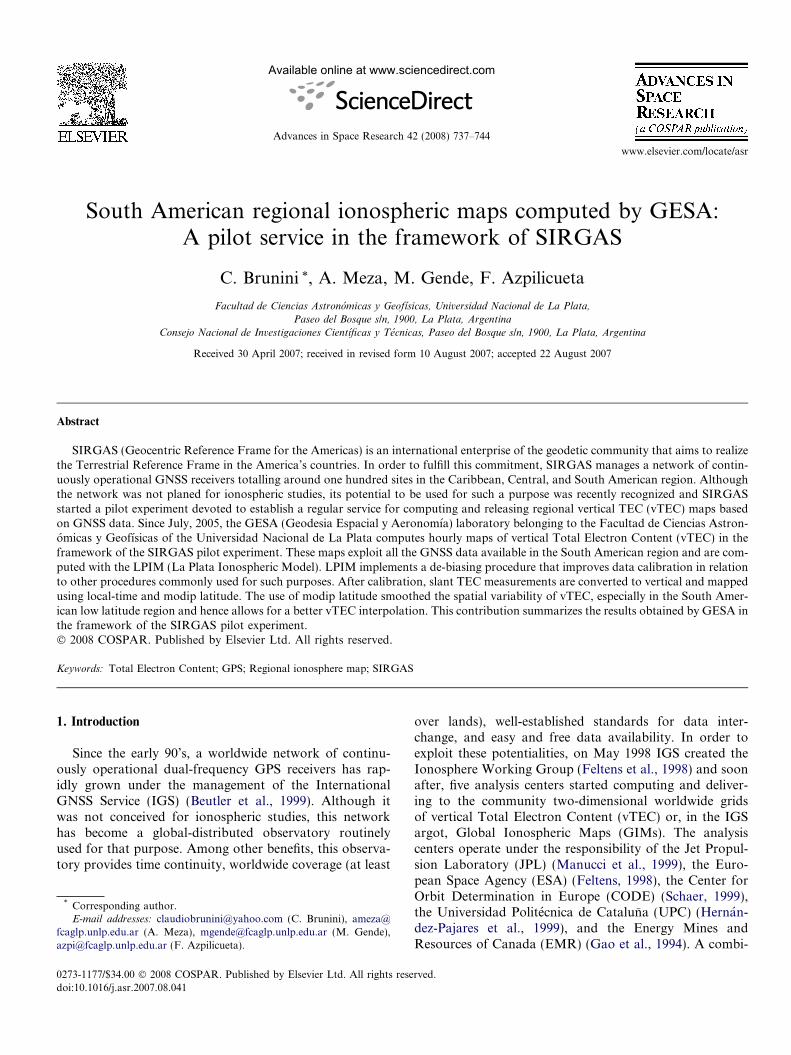
Fig. 1. Distribution of the SIRGAS stations used to compute theionospheric maps (squares: stations belonging to the global IGS network;circles: regional stations belonging to national organizations).

bal stations plus several regional stations managed bynational organizations. Although the large gap aroundthe Amazonian region, this network provides the best datacoverage currently available in South America. Fig. 1shows the distribution of the SIRGAS stations that weare currently using to compute the ionospheric maps.

A WGI action plan for the coming years was discussedduring the SIRGAS meeting, held in December 2004, inAguascalientes, Mexico. The general consensus was todrive WGI efforts toward the consolidation of the GPS net-work as the cornerstone for the reference frame mainte-nance. In addition, SIRGAS entrusted to WGI themission to promote new scientific researches that diversifythe applications of the SIRGAS observations. Followingthis mandate, WGI promoted a ‘‘call for participation”

in a pilot experiment devoted to establish a regular serviceto compute and deliver South American regional iono-spheric maps of vTEC (hereafter called ‘‘ionosphericmaps” for short) based on (but not exclusively) SIRGASobservations. The call for participation encouragedresearches aimed to improve the performances of the cur-rently available GPS-based vTEC models in South Ameri-can region. One of the outstanding goals of the service is toimprove the reliability of the ionospheric correction forGNSS applications. In particular, it aims to contribute tothe ‘‘Solucion de Aumentacion para el Caribe, Centro ySudamerica” (Augmentation Solution for the Caribbean,Central, and South America) project (http://www.rlasaccsa.com), promoted by the International Civil Aviation Orga-nization to extend the SBAS (Satellite Based AugmentationService) coverage to the region (Martınez, 2005).

Since July 2005, GESA (Geodesia Espacial y Aero-nomıa) laboratory belonging to the Facultad de CienciasAstronomicas y Geofısicas of the Universidad Nacionalde La Plata computes hourly ionospheric maps in theframework of the SIRGAS pilot experiment. These iono-spheric maps exploit all the GPS data available in theSouth American region and are computed using the La Pla-ta Ionospheric Model (LPIM). This contribution summa-rizes the results achieved until now, focusing on the maincharacteristics of the LPIM approach, i.e.: GPS data cali-bration and vTEC interpolation. The paper is organizedas follow: Section 2 provides a short description of theLPIM. Section 3 presents the problems that the so-called‘‘levelling carrier-to-code” procedure (often used to reducethe effects of carrier-phase ambiguities from the GPSobservations) causes in the calibration of the GPS slantTEC (sTEC); and shows how these problems are overcomeby the calibration procedure implemented in LPIM. Sec-tion 4 discusses the interpolation problem that arises fromthe need to create a regular data grid from the scatteredobservations in order to map the vTEC in the desiredregion; it shows that the use of the modip latitude insteadof geomagnetic produces an smoother representation ofthe vTEC and allows for a better interpolation, especiallyin the South American low latitude region. Finally, Section5 remarks the outstanding points of the paper.

C. Brunini et al. / Advances in Space Research 42 (2008) 737–744 739

2. Brief description of LPIM

LPIM implements ionospheric maps computation inthree stages: (i) pre-processing; (ii) calibration; and (iii)interpolation. This section provides a brief overview aboutthe general process performed by LPIM; the interest readeris referred to (Brunini et al., 2004a,b) for details. Stages (ii)and (iii) are described with more details in Sections 3 and 4.The main task performed by the pre-processing stage is thecomputation of the ionospheric observable from dual-fre-quency carrier-phase GPS observations, which is obtainedbased on the fact that the range-delay that the ionosphereproduces in the GPS measurements is proportional to thesTEC along the satellite–receiver line-of-sight and inverselyproportional to the square of the signal frequency. Hence,subtraction of simultaneous observations at different fre-quencies leads to an observable in which all frequency-independent effects disappear but the ionospheric and anyother frequency-dependent effects remain present:

LI ;arc ¼ sTECþ BR þ BS þ Carc þ eL; ð1Þ

where LI,arc is the carrier-phase ionospheric observable –the sub-indices arc refers to every continuous arc ofcarrier-phase observations, which is defined as a group ofconsecutive observations along which carrier-phase ambi-guities do not change–; BR and BS are the so-called satelliteand receiver inter-frequency biases (IFB) for carrier-phaseobservations; Carc is the bias produced by carrier-phaseambiguities in the ionospheric observable; and eL is theeffect of noise and multi-path. All terms of Eq. (1) areexpressed in Total Electron Content units (TECu), being1 TECu equivalent to 1016 electrons per square meters.

Dual-frequency P-code observations lead to an analo-gous ionospheric observable:

P I ¼ sTECþ bR þ bS þ eP ; ð2Þ

where the meaning of the terms is analogous to Eq. (1) withthe following distinctions: different satellite and receiverIFBs (bR and bS instead of BR and BS); there is not anyambiguity term; and the effect of noise and multi-path,eP, is around 100 time greater.

The calibration module of LPIM relays on the thin-shelland the mapping function approximations (Davies andHartmann, 1997). Based on those approximations, Eq.(1) is written in the following way:

LI ;arc ¼ secðz0Þ � vTEC þ carc þ eL; ð3Þ

where sec(z0) is the mapping function, z0 being the zenithdistance of the satellite as seen from the point where thesignal crosses the thin-shell (the so-called piercing point)that, in the case of LPIM, is located 450 km above theEarth’s surface; vTEC � cos (z0) � sTEC, is the equivalentvTEC at the piercing point; and carc � BR + BS + Carc, isa calibration constant that encompasses, all together, recei-ver and satellite IFBs and the ambiguity term. The calibra-tion, i.e. the estimation of carc for every continuous arc, isperformed independently for every observing receiver in

the network. To accomplish this task, the equivalent vTECis approximated by a bilinear expansion dependent on thepiercing point coordinates:

vTEC � aðtÞ þ bðtÞ � ðkI � k0Þ � cosðlIÞ þ cðtÞ � ðlI � l0Þ;ð4Þ

where t is the Universal Time of the observation, kI and lI

the geographic longitude and the modip latitude of thepiercing point and k0 and l0 the geographic longitudeand the modip latitude of the observing receiver (readersnot familiarized with modip latitude are referred to Section4). The dependence on time of the expansion coefficients isapproximated with ladder functions:

aðtÞ ¼ ai; for ti 6 t < ti þ dt; i ¼ 1; 2; . . . ; ð5Þ

where a represents anyone of the coefficient a, b, or c; anddt is the interval of validity of every planar approximation(5m in the case of LPIM).

Merging all together the observations gathered by areceiver in a given interval Dt (Dt� dt), and arrangingappropriately Eqs. (3)–(5), LPIM forms an overdeterminedlinear system of equation of observations that contains, asunknowns, the calibration constants for all observed con-tinuous arcs, carc (arc = 1,2, . . . ,narc), and the constantcoefficients of the planar fits, a1, . . . ,am,b1, . . . ,bm,c1, . . . cm

(m = Dt/dt). Since we are not interest on the coefficients,they are reduced from the system by means of a Gaussianelimination process and then, the system is solved by theLeast Square methods, hence estimating the narc calibrationconstants, carc. Finally, the observations are calibrated andthe equivalent vTEC are estimated from Eq. (3):

vTbEC � vTECþ eL

secðz0Þ ¼LI ;arc � carc

secðz0Þ : ð6Þ

In order to ensure calibration of complete arcs, LPIMprocesses, in any run, 36h of data from �6h to 30h UT, butretains the vTbEC values for the interval from 0h to 24h UT.

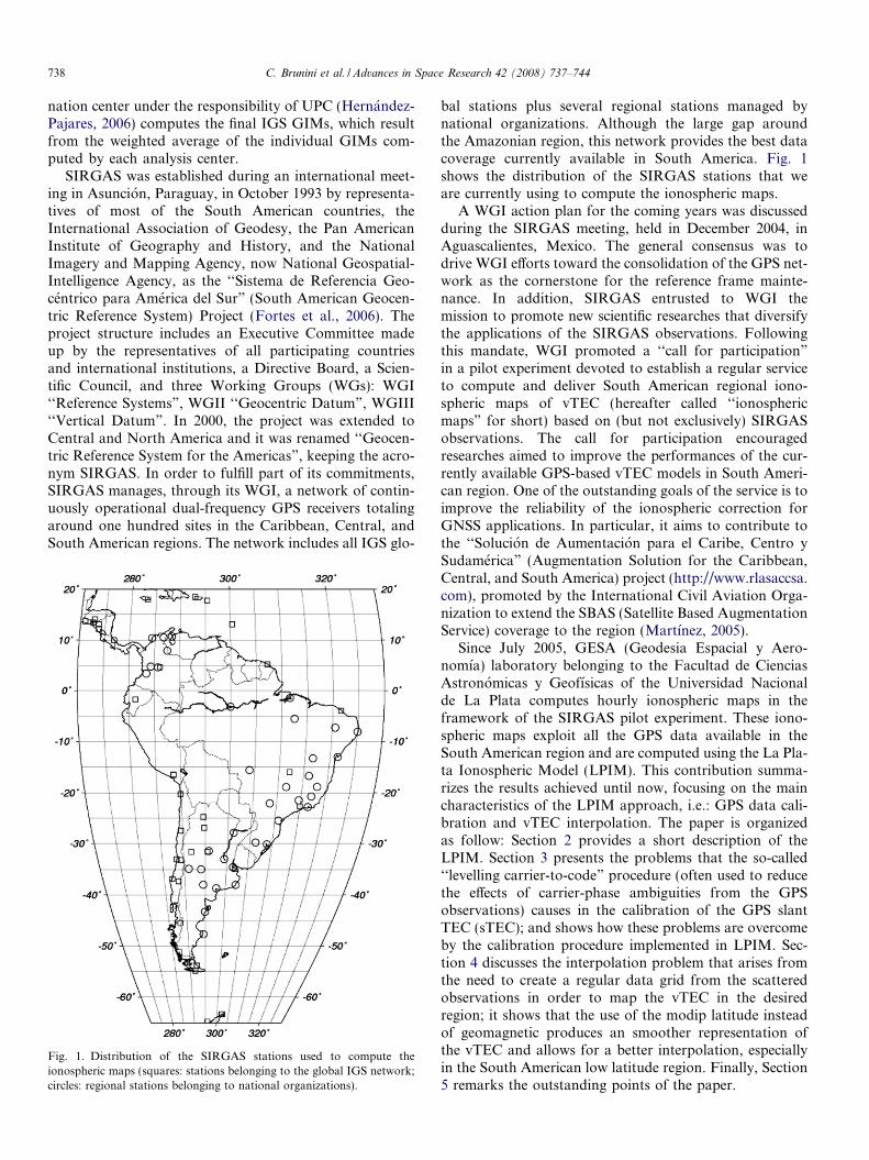
The interpolation module of LPIM starts from theequivalent vTEC given by Eqs. (1)–(6) for all receivers inthe network. Those values are binned into UT intervalsof 1h and then, a set of coefficients of a spherical harmonicexpansion up to degree and order 15 are estimated by theLeast Squares method, for every interval. The expansionis expressed in terms of the geographic longitude and themodip latitude of the piercing point. After the coefficientsare estimated, they are used to compute a regular grid ofvTEC every 1 h. Fig. 2 shows a typical ionospheric mapfor quiet conditions computed with LPIM. Twenty fourmaps per days are available since July 2005 at http://cplat.fcaglp.unlp.edu.ar, as part of the ionospheric prod-ucts delivered by the GESA service in the framework ofthe SIRGAS pilot experiment.

To close this section we would like to remark that twodifferent mathematical representations of the vTEC havebeen used: one is the bilinear expansion given by Eqs. (4)and (5), which is used for a single-site representation in

Fig. 2. Typical South American regional ionospheric map of vTEC forquiet ionospheric conditions (August 23, 2005, 0h–1h UT) computed withLPIM in the framework of the SIRGAS pilot experiment; vTEC valuesare in TECu.

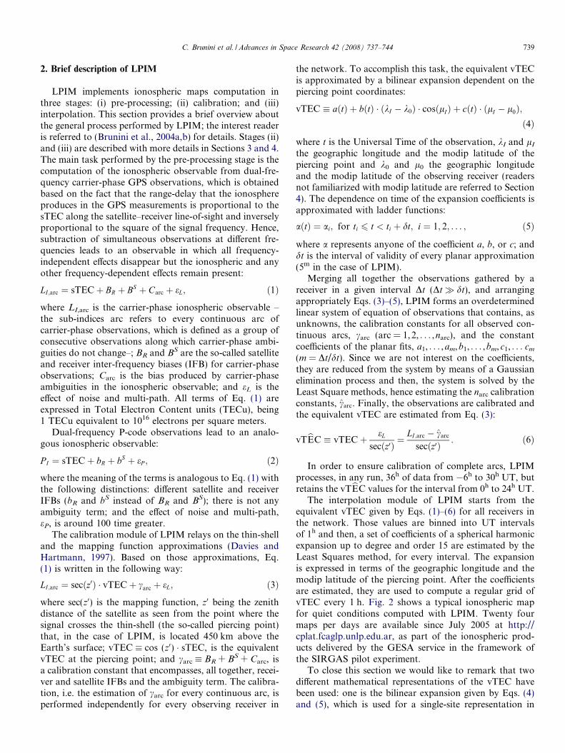
Fig. 3. Differences of the levelled carrier-phase ionospheric observable inTECu from two nearby GPS receivers (stations WTZA and WTZJ,Wetzel, Germany) for five satellites along four consecutive days.

740 C. Brunini et al. / Advances in Space Research 42 (2008) 737–744

the calibration stage, and the other is the spherical har-monic expansion, which is used for regional representationin the interpolation stage.

3. TEC calibration

The so-called ‘‘levelling carrier-to-code” (or simply ‘‘lev-elling”) is a widely used procedure to reduce the ambiguityterm, Carc, from the carrier-phase ionospheric observablegiven by Eq. (1). It relays on the fact that, even if the P-code ionospheric observable is much more contaminatedby noise and multi-path than the carrier-phase one, Eq.(2) shows that it is not affected by the ambiguity term. IfEqs. (1) and (2) are subtracted, and all the differences forevery continuous arc are averaged, results:

hLI ;arc � P Iiarc ¼ Carc þ BR � bR þ BS � bS � heP iarc; ð7Þwhere the symbol h�iarc indicates the average for of all datain the continuous arc; noise and multi-path on carrier-phase observations have been neglected in Eq. (7). Then,subtracting Eq. (7) from Eq. (1), the ambiguity term is re-duced from the carrier-phase ionospheric observable:

eLI;arc � LI ;arc � hLI;arc � P Iiarc

¼ sTECþ bR þ bS þ heP iarc þ eL; ð8Þ

where eLI;arc is the levelled ionospheric observable. Eq. (8)shows that, after the levelling process: (i) the carrier-phase

IFBs are replaced by the corresponding P-code IFBs (oftencalled differential code biases, DCBs); and (ii) the levelledionospheric observable may be affected by a levelling error,hePiarc, due to the P-code noise and multi-path that maynot average to zero in a continuous arc.

A very simple experiment to asses the magnitude of thelevelling error may be performed with data from two GPSreceivers, A and B, separated one from another by fewmeters, so that the sTEC can be considered equal for bothreceivers. From Eq. (8) follows that the differences DeLI ;arc

of the levelled ionospheric observable from the same satel-lite collected simultaneously by both receivers:

DeLI;arc � eLI;arc;A � eLI ;arc;B

¼ bRA � bRB þ heP iarc;A � heP iarc;B þ eLA � eLB; ð9Þ

should be equal to a constant that does not depend on theobserved satellite but on the difference of the receiversDCBs, DbR � bRA � bRB. It is expected that the databelonging to different arcs deviate from DbR by the combi-nation of the levelling errors of the same arc observed bythe two receivers, DhePiarc � hePiarc,A � hePiarc,B. Smalldeviations, DeL � eLA � eLB, are also expected due to car-rier-phase noise and multi-path. Carrying out this experi-ment with several pairs of nearby GPS receiversbelonging to the IGS network, and also from some dedi-cated experiment performed by ourselves, we found level-ling errors due to P-code multi-path that ranged from 1.4to 5.3 TECu in a way that strongly depends on the recei-ver/antenna configuration (Ciraolo et al., 2007). Just toillustrate the problem, Fig. 3 shows differences of the lev-elled ionospheric observable computed with observationsgathered by two nearby GPS receivers. In order to makethe figure readable, we have depicted the results for a fewsatellites and days, but the general behaviour observed inthis figure, i.e. a large spread between the results belonging

C. Brunini et al. / Advances in Space Research 42 (2008) 737–744 741

to different arcs, is present for all satellites and for otherdays and, also, for other pairs or nearby receivers.

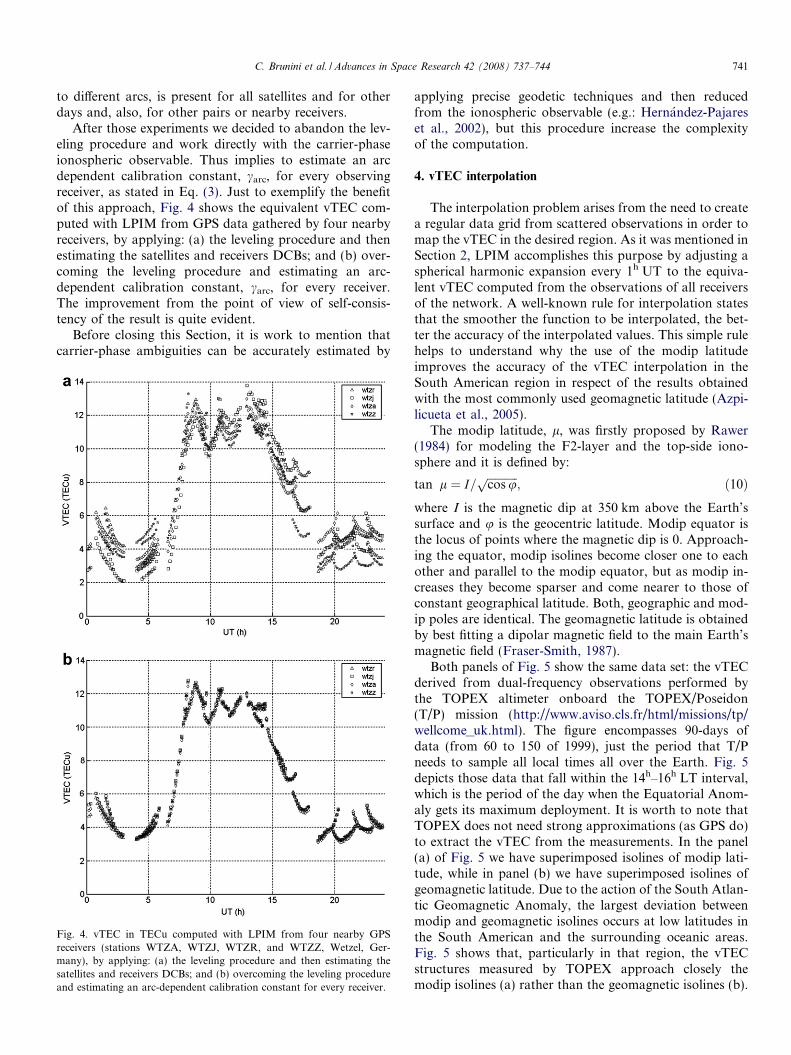
After those experiments we decided to abandon the lev-eling procedure and work directly with the carrier-phaseionospheric observable. Thus implies to estimate an arcdependent calibration constant, carc, for every observingreceiver, as stated in Eq. (3). Just to exemplify the benefitof this approach, Fig. 4 shows the equivalent vTEC com-puted with LPIM from GPS data gathered by four nearbyreceivers, by applying: (a) the leveling procedure and thenestimating the satellites and receivers DCBs; and (b) over-coming the leveling procedure and estimating an arc-dependent calibration constant, carc, for every receiver.The improvement from the point of view of self-consis-tency of the result is quite evident.

Before closing this Section, it is work to mention thatcarrier-phase ambiguities can be accurately estimated by

Fig. 4. vTEC in TECu computed with LPIM from four nearby GPSreceivers (stations WTZA, WTZJ, WTZR, and WTZZ, Wetzel, Ger-many), by applying: (a) the leveling procedure and then estimating thesatellites and receivers DCBs; and (b) overcoming the leveling procedureand estimating an arc-dependent calibration constant for every receiver.

applying precise geodetic techniques and then reducedfrom the ionospheric observable (e.g.: Hernandez-Pajareset al., 2002), but this procedure increase the complexityof the computation.

4. vTEC interpolation

The interpolation problem arises from the need to createa regular data grid from scattered observations in order tomap the vTEC in the desired region. As it was mentioned inSection 2, LPIM accomplishes this purpose by adjusting aspherical harmonic expansion every 1h UT to the equiva-lent vTEC computed from the observations of all receiversof the network. A well-known rule for interpolation statesthat the smoother the function to be interpolated, the bet-ter the accuracy of the interpolated values. This simple rulehelps to understand why the use of the modip latitudeimproves the accuracy of the vTEC interpolation in theSouth American region in respect of the results obtainedwith the most commonly used geomagnetic latitude (Azpi-licueta et al., 2005).

The modip latitude, l, was firstly proposed by Rawer(1984) for modeling the F2-layer and the top-side iono-sphere and it is defined by:

tan l ¼ I=ffiffiffiffiffiffiffiffiffiffifficos up

; ð10Þwhere I is the magnetic dip at 350 km above the Earth’ssurface and u is the geocentric latitude. Modip equator isthe locus of points where the magnetic dip is 0. Approach-ing the equator, modip isolines become closer one to eachother and parallel to the modip equator, but as modip in-creases they become sparser and come nearer to those ofconstant geographical latitude. Both, geographic and mod-ip poles are identical. The geomagnetic latitude is obtainedby best fitting a dipolar magnetic field to the main Earth’smagnetic field (Fraser-Smith, 1987).

Both panels of Fig. 5 show the same data set: the vTECderived from dual-frequency observations performed bythe TOPEX altimeter onboard the TOPEX/Poseidon(T/P) mission (http://www.aviso.cls.fr/html/missions/tp/wellcome_uk.html). The figure encompasses 90-days ofdata (from 60 to 150 of 1999), just the period that T/Pneeds to sample all local times all over the Earth. Fig. 5depicts those data that fall within the 14h–16h LT interval,which is the period of the day when the Equatorial Anom-aly gets its maximum deployment. It is worth to note thatTOPEX does not need strong approximations (as GPS do)to extract the vTEC from the measurements. In the panel(a) of Fig. 5 we have superimposed isolines of modip lati-tude, while in panel (b) we have superimposed isolines ofgeomagnetic latitude. Due to the action of the South Atlan-tic Geomagnetic Anomaly, the largest deviation betweenmodip and geomagnetic isolines occurs at low latitudes inthe South American and the surrounding oceanic areas.Fig. 5 shows that, particularly in that region, the vTECstructures measured by TOPEX approach closely themodip isolines (a) rather than the geomagnetic isolines (b).

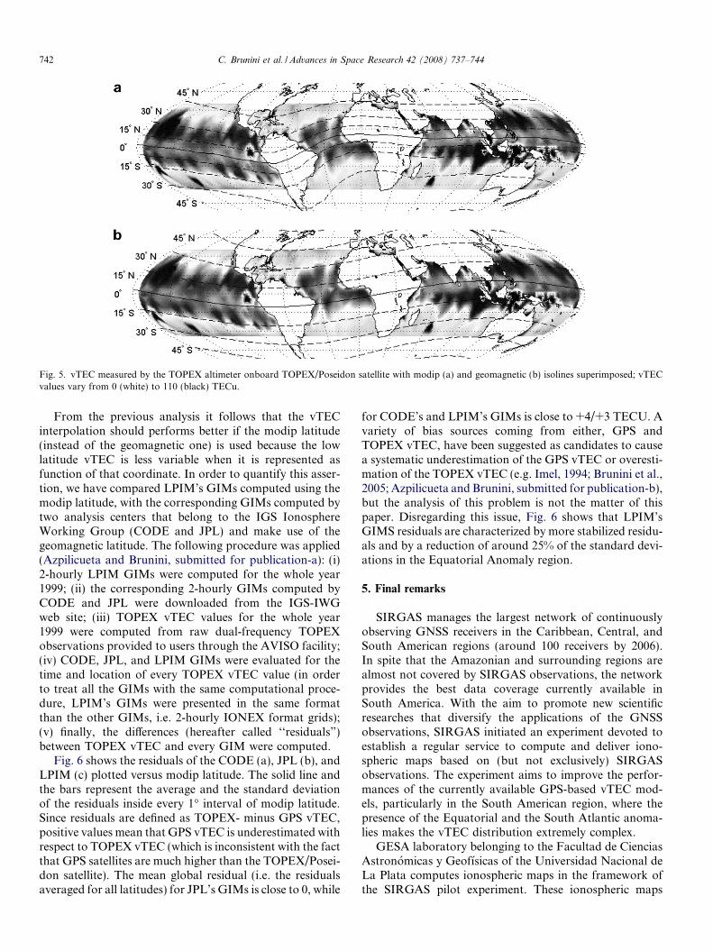
Fig. 5. vTEC measured by the TOPEX altimeter onboard TOPEX/Poseidon satellite with modip (a) and geomagnetic (b) isolines superimposed; vTECvalues vary from 0 (white) to 110 (black) TECu.

742 C. Brunini et al. / Advances in Space Research 42 (2008) 737–744

From the previous analysis it follows that the vTECinterpolation should performs better if the modip latitude(instead of the geomagnetic one) is used because the lowlatitude vTEC is less variable when it is represented asfunction of that coordinate. In order to quantify this asser-tion, we have compared LPIM’s GIMs computed using themodip latitude, with the corresponding GIMs computed bytwo analysis centers that belong to the IGS IonosphereWorking Group (CODE and JPL) and make use of thegeomagnetic latitude. The following procedure was applied(Azpilicueta and Brunini, submitted for publication-a): (i)2-hourly LPIM GIMs were computed for the whole year1999; (ii) the corresponding 2-hourly GIMs computed byCODE and JPL were downloaded from the IGS-IWGweb site; (iii) TOPEX vTEC values for the whole year1999 were computed from raw dual-frequency TOPEXobservations provided to users through the AVISO facility;(iv) CODE, JPL, and LPIM GIMs were evaluated for thetime and location of every TOPEX vTEC value (in orderto treat all the GIMs with the same computational proce-dure, LPIM’s GIMs were presented in the same formatthan the other GIMs, i.e. 2-hourly IONEX format grids);(v) finally, the differences (hereafter called ‘‘residuals”)between TOPEX vTEC and every GIM were computed.

Fig. 6 shows the residuals of the CODE (a), JPL (b), andLPIM (c) plotted versus modip latitude. The solid line andthe bars represent the average and the standard deviationof the residuals inside every 1� interval of modip latitude.Since residuals are defined as TOPEX- minus GPS vTEC,positive values mean that GPS vTEC is underestimated withrespect to TOPEX vTEC (which is inconsistent with the factthat GPS satellites are much higher than the TOPEX/Posei-don satellite). The mean global residual (i.e. the residualsaveraged for all latitudes) for JPL’s GIMs is close to 0, while

for CODE’s and LPIM’s GIMs is close to +4/+3 TECU. Avariety of bias sources coming from either, GPS andTOPEX vTEC, have been suggested as candidates to causea systematic underestimation of the GPS vTEC or overesti-mation of the TOPEX vTEC (e.g. Imel, 1994; Brunini et al.,2005; Azpilicueta and Brunini, submitted for publication-b),but the analysis of this problem is not the matter of thispaper. Disregarding this issue, Fig. 6 shows that LPIM’sGIMS residuals are characterized by more stabilized residu-als and by a reduction of around 25% of the standard devi-ations in the Equatorial Anomaly region.

5. Final remarks

SIRGAS manages the largest network of continuouslyobserving GNSS receivers in the Caribbean, Central, andSouth American regions (around 100 receivers by 2006).In spite that the Amazonian and surrounding regions arealmost not covered by SIRGAS observations, the networkprovides the best data coverage currently available inSouth America. With the aim to promote new scientificresearches that diversify the applications of the GNSSobservations, SIRGAS initiated an experiment devoted toestablish a regular service to compute and deliver iono-spheric maps based on (but not exclusively) SIRGASobservations. The experiment aims to improve the perfor-mances of the currently available GPS-based vTEC mod-els, particularly in the South American region, where thepresence of the Equatorial and the South Atlantic anoma-lies makes the vTEC distribution extremely complex.

GESA laboratory belonging to the Facultad de CienciasAstronomicas y Geofısicas of the Universidad Nacional deLa Plata computes ionospheric maps in the framework ofthe SIRGAS pilot experiment. These ionospheric maps

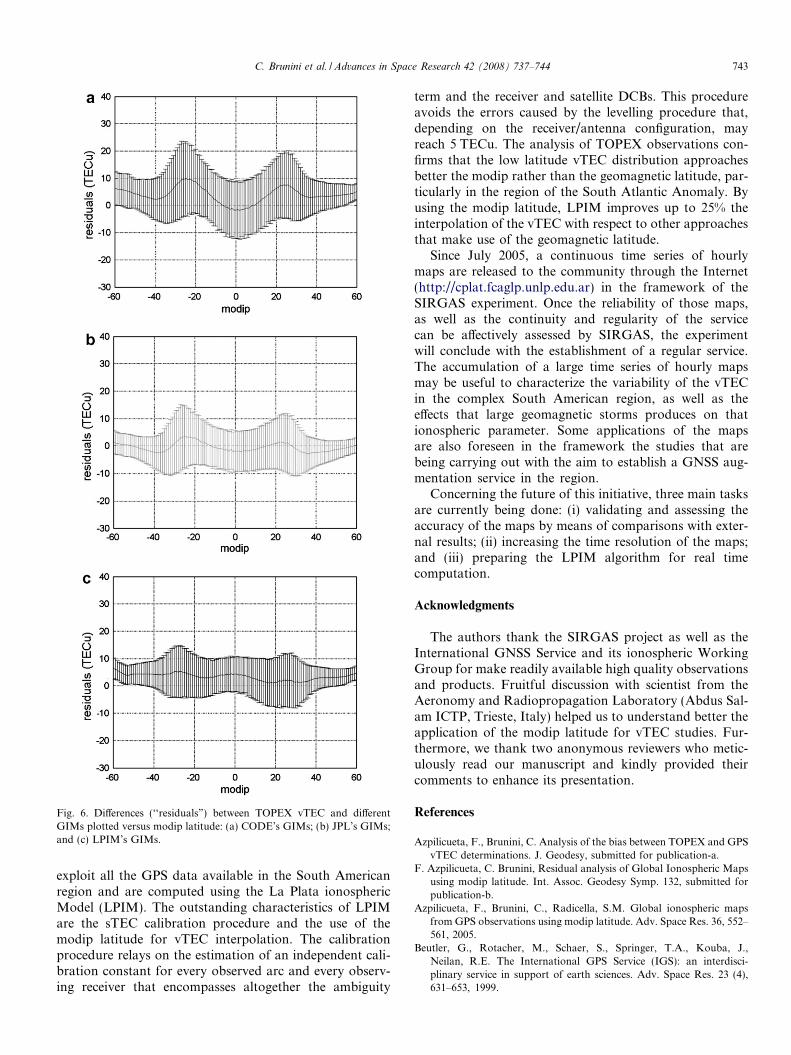
Fig. 6. Differences (‘‘residuals”) between TOPEX vTEC and differentGIMs plotted versus modip latitude: (a) CODE’s GIMs; (b) JPL’s GIMs;and (c) LPIM’s GIMs.

C. Brunini et al. / Advances in Space Research 42 (2008) 737–744 743

exploit all the GPS data available in the South Americanregion and are computed using the La Plata ionosphericModel (LPIM). The outstanding characteristics of LPIMare the sTEC calibration procedure and the use of themodip latitude for vTEC interpolation. The calibrationprocedure relays on the estimation of an independent cali-bration constant for every observed arc and every observ-ing receiver that encompasses altogether the ambiguity

term and the receiver and satellite DCBs. This procedureavoids the errors caused by the levelling procedure that,depending on the receiver/antenna configuration, mayreach 5 TECu. The analysis of TOPEX observations con-firms that the low latitude vTEC distribution approachesbetter the modip rather than the geomagnetic latitude, par-ticularly in the region of the South Atlantic Anomaly. Byusing the modip latitude, LPIM improves up to 25% theinterpolation of the vTEC with respect to other approachesthat make use of the geomagnetic latitude.

Since July 2005, a continuous time series of hourlymaps are released to the community through the Internet(http://cplat.fcaglp.unlp.edu.ar) in the framework of theSIRGAS experiment. Once the reliability of those maps,as well as the continuity and regularity of the servicecan be affectively assessed by SIRGAS, the experimentwill conclude with the establishment of a regular service.The accumulation of a large time series of hourly mapsmay be useful to characterize the variability of the vTECin the complex South American region, as well as theeffects that large geomagnetic storms produces on thationospheric parameter. Some applications of the mapsare also foreseen in the framework the studies that arebeing carrying out with the aim to establish a GNSS aug-mentation service in the region.

Concerning the future of this initiative, three main tasksare currently being done: (i) validating and assessing theaccuracy of the maps by means of comparisons with exter-nal results; (ii) increasing the time resolution of the maps;and (iii) preparing the LPIM algorithm for real timecomputation.

Acknowledgments

The authors thank the SIRGAS project as well as theInternational GNSS Service and its ionospheric WorkingGroup for make readily available high quality observationsand products. Fruitful discussion with scientist from theAeronomy and Radiopropagation Laboratory (Abdus Sal-am ICTP, Trieste, Italy) helped us to understand better theapplication of the modip latitude for vTEC studies. Fur-thermore, we thank two anonymous reviewers who metic-ulously read our manuscript and kindly provided theircomments to enhance its presentation.

References

Azpilicueta, F., Brunini, C. Analysis of the bias between TOPEX and GPSvTEC determinations. J. Geodesy, submitted for publication-a.

F. Azpilicueta, C. Brunini, Residual analysis of Global Ionospheric Mapsusing modip latitude. Int. Assoc. Geodesy Symp. 132, submitted forpublication-b.

Azpilicueta, F., Brunini, C., Radicella, S.M. Global ionospheric mapsfrom GPS observations using modip latitude. Adv. Space Res. 36, 552–561, 2005.

Beutler, G., Rotacher, M., Schaer, S., Springer, T.A., Kouba, J.,Neilan, R.E. The International GPS Service (IGS): an interdisci-plinary service in support of earth sciences. Adv. Space Res. 23 (4),631–653, 1999.

744 C. Brunini et al. / Advances in Space Research 42 (2008) 737–744

Brunini, C., Meza, A., Azpilicueta, F., Van Zele, M.A., Gende, M., Diaz,A. A new ionosphere monitoring technology based on GPS. Astro-phys. Space Sci. 290, 415–429, 2004a.

Brunini, C., Meza, A., Bosch, W. Spatial and temporal variability of theTEC bias between TOPEX and GPS. J. Geodesy 79 (4–5), 175–188,2005.

Brunini, C., Van Zele, M.A., Meza, A., Gende, M. Quiet and perturbedionospheric representation according to the electron content from GPSsignals. J. Geophys. Res. 108, doi:10.1029/2002JA009346, 2004b.

Ciraolo, L., Azpilicueta, F., Brunini, C., Meza, A., Radicela, S.M.Calibration errors on experimental slant total electron contentdetermined with GPS. J. Geodesy 81 (2), 111–120, doi:10.1007/s00190-006-0093-1, 2007.

Davies, K., Hartmann, G.K. Studying the ionosphere with the GlobalPositioning System. Radio Sci. 32 (4), 1695–1703, 1997.

Feltens, J. Chapman profile approach for 3-d global TEC representation.In: Proceedings of the 1998 IGS Analysis Centres Workshop Darms-tadt, pp. 285–297, 1998.

Feltens, J., Schaer, S. IGS Products for the ionosphere. In: Proceedings ofthe 1998 IGS Analysis Centres Workshop, Darmstadt, pp. 285–297,1998.

Fortes, L.P., Laurıa, E., Brunini, C., Amaya, W., Sanchez, L., Drewes,H., Seemuller, W. Current status and future developments of theSIRGAS project. Wissenschaftliche Arbeiten der FachrichtungGeodasie und Geoinformatik der Universitat Hannover 258, 59–70, 2006.

Fraser-Smith, A.C. Centered and eccentric geomagnetic dipoles and theirpoles 1600–1985. Rev. Geophys. 25 (1), 1–16, 1987.

Y. Gao, P. Heroux, J. Kouba. Estimation of GPS receiver and satellite L1/L2 signal delay biases using data from CACS. In: Proceedings of theKIS-94, Banff, pp. 109–117, 1994.

Hernandez-Pajares, M. Summary and current status of IGS IonosphereWG activities. IGS Workshop, Darmstadt, 2006.

Hernandez-Pajares, M., Juan, J.M., Sanz, J. New approaches in globalionospheric determination using ground GPS data. J. Atmos. Sol.-Terr.Phys. 61, 1237–1247, 1999.

Hernandez-Pajares, M., Juan, J.M., Sanz, J., Colombo, O.L. Improvingthe real-time ionospheric determination from GPS sites at very longdistances over the equator. J. Geophys. Res. 107 (A10), doi:10.1029/2001JA009203, 2002.

Imel, D. Evaluation of the TOPEX/ POSEIDON dual-frequency iono-sphere correction. J. Geophys. Res. 99 (C12), 24,895–24,906, 1994.

Manucci, A.J., Iijima, B.A., Lindqwister, U.J., Pi, X., Sparks, L., Wilson,B.D. GPS and ionosphere. URSI Reviews of Radio Science. JetPropulsion Laboratory, Pasadena, 1999.

Martınez, D. La cooperacion tecnica de la OACI en los sistemas GNSS/SBAS en las regiones CAR/SAM. Seminario Taller Regional sobreSistemas de Navegacion Satelitaria Global, Bogota (in Spanish), 2005.

Rawer, K. (Ed.). Encyclopedia of Physics. Geophysics III, Part VII.Springer-Verlag, pp. 89–391, 1984.

Schaer, S. Mapping and Predicting the Earth’s Ionosphere Using theGlobal Positioning System. Ph.D. thesis, Bern University, 1999.