NASA/CR–2020–220509 Sonic Booms in Atmospheric Turbulence (SonicBAT): The Influence of Turbulence on Shaped Sonic Booms Kevin A. Bradley, Christopher M. Hobbs, and Clifton B. Wilmer Wyle, Arlington, Virginia Victor W. Sparrow and Trevor A. Stout The Pennsylvania State University, University Park, Pennsylvania John M. Morgenstern Lockheed Martin, Palmdale, California Kenneth H. Underwood Technical & Business Systems, Valencia, California Domenic J. Maglieri Eagle Aeronautics, Inc., Newport News, Virginia Robert A. Cowart and Matthew T. Collmar Gulfstream Aerospace Corporation, Savannah, Georgia Hao Shen The Boeing Company, St. Louis, Missouri Philippe Blanc-Benon Laboratory of Fluid Mechanics and Acoustics, France

Welcome message from author
This document is posted to help you gain knowledge. Please leave a comment to let me know what you think about it! Share it to your friends and learn new things together.
Transcript

NASA/CR–2020–220509
Sonic Booms in Atmospheric Turbulence
(SonicBAT): The Influence of Turbulence on
Shaped Sonic Booms Kevin A. Bradley, Christopher M. Hobbs, and Clifton B. Wilmer Wyle, Arlington, Virginia Victor W. Sparrow and Trevor A. Stout The Pennsylvania State University, University Park, Pennsylvania John M. Morgenstern Lockheed Martin, Palmdale, California Kenneth H. Underwood Technical & Business Systems, Valencia, California Domenic J. Maglieri Eagle Aeronautics, Inc., Newport News, Virginia Robert A. Cowart and Matthew T. Collmar Gulfstream Aerospace Corporation, Savannah, Georgia Hao Shen The Boeing Company, St. Louis, Missouri Philippe Blanc-Benon Laboratory of Fluid Mechanics and Acoustics, France

NASA STI Program ... in Profile
Since its founding, NASA has been dedicated
to the advancement of aeronautics and space
science. The NASA scientific and technical
information (STI) program plays a key part in
helping NASA maintain this important role.
The NASA STI program operates under the
auspices of the Agency Chief Information
Officer. It collects, organizes, provides for
archiving, and disseminates NASA’s STI. The
NASA STI program provides access to the NTRS
Registered and its public interface, the NASA
Technical Reports Server, thus providing one of
the largest collections of aeronautical and space
science STI in the world. Results are published in
both non-NASA channels and by NASA in the
NASA STI Report Series, which includes the
following report types:
TECHNICAL PUBLICATION. Reports of
completed research or a major significant
phase of research that present the results of
NASA Programs and include extensive data
or theoretical analysis. Includes compila-
tions of significant scientific and technical
data and information deemed to be of
continuing reference value. NASA counter-
part of peer-reviewed formal professional
papers but has less stringent limitations on
manuscript length and extent of graphic
presentations.
TECHNICAL MEMORANDUM.
Scientific and technical findings that are
preliminary or of specialized interest,
e.g., quick release reports, working
papers, and bibliographies that contain
minimal annotation. Does not contain
extensive analysis.
CONTRACTOR REPORT. Scientific and
technical findings by NASA-sponsored
contractors and grantees.
CONFERENCE PUBLICATION.
Collected papers from scientific and
technical conferences, symposia, seminars,
or other meetings sponsored or
co-sponsored by NASA.
SPECIAL PUBLICATION. Scientific,
technical, or historical information from
NASA programs, projects, and missions,
often concerned with subjects having
substantial public interest.
TECHNICAL TRANSLATION.
English-language translations of foreign
scientific and technical material pertinent to
NASA’s mission.
Specialized services also include organizing
and publishing research results, distributing
specialized research announcements and feeds,
providing information desk and personal search
support, and enabling data exchange services.
For more information about the NASA STI
program, see the following:
Access the NASA STI program home page
at http://www.sti.nasa.gov
E-mail your question to [email protected]
Phone the NASA STI Information Desk at
757-864-9658
Write to:
NASA STI Information Desk
Mail Stop 148
NASA Langley Research Center
Hampton, VA 23681-2199

NASA/CR–2020–220509
Sonic Booms in Atmospheric Turbulence
(SonicBAT): The Influence of Turbulence on
Shaped Sonic Booms Kevin A. Bradley, Christopher M. Hobbs, and Clifton B. Wilmer Wyle, Arlington, Virginia Victor W. Sparrow and Trevor A. Stout The Pennsylvania State University, University Park, Pennsylvania John M. Morgenstern Lockheed Martin, Palmdale, California Kenneth H. Underwood Technical & Business Systems, Valencia, California Domenic J. Maglieri Eagle Aeronautics, Inc., Newport News, Virginia Robert A. Cowart and Matthew T. Collmar Gulfstream Aerospace Corporation, Savannah, Georgia Hao Shen The Boeing Company, St. Louis, Missouri Philippe Blanc-Benon Laboratory of Fluid Mechanics and Acoustics, France
National Aeronautics and
Space Administration
Armstrong Flight Research Center Prepared for Armstrong Flight Research Center
Edwards, California 93523-0273 under Contract NND15AA05C

ACKNOWLEDGMENTS
The Project Team would like to acknowledge Ed Haering of NASA Armstrong Flight Research Center,
Dr. Alexandra Loubeau of NASA Langley Research Center, Dr. Victor Sparrow of Penn State
University, and the late Dr. Kenneth Plotkin, former Wyle Chief Scientist, for laying the foundation of
the SonicBAT project and we dedicate this project to Kenneth Plotkin. The Project Team acknowledges
the excellent work of NASA Armstrong Flight Research Center for their support in planning the
research flight tests and conducting the precision flight operations required for this project to be a
success. We thank all of the collaborators on this project from The Japan Aerospace Exploration
Agency and the three participating NASA centers, Armstrong Flight Research Center, Langley Research
Center, and Kennedy Space Center, many of whom supported this project with their own resources.
Special thanks goes to John Graves and the other representatives of Kennedy Space Center who not
only made the second SonicBAT experiment possible, but through their excellent support and
unmatched hospitality helped to make this a great project and one to remember.
This report is available in electronic form at
https://ntrs.nasa.gov/search.jsp

SonicBAT Final Report Page | v
TABLE OF CONTENTS
SECTIONS
ACKNOWLEDGMENTS .............................................................................................................................. iv
EXECUTIVE SUMMARY ........................................................................................................................... xix
ACRONYMS .................................................................................................................................................. xxii
1.0 INTRODUCTION ................................................................................................................................. 1
1.1 Sonic Boom Propagation in the Atmosphere ............................................................................ 2
1.1.1 Atmospheric Distortion of N-Wave Sonic Boom ........................................................ 4
1.1.2 Statistical Variation............................................................................................................. 5
1.1.3 Motivation to Understand Turbulence Distortion of Shaped Sonic Boom.............. 5
1.2 Program Objectives ........................................................................................................................ 6
2.0 ATMOSPHERIC TURBULENCE OVERVIEW ............................................................................ 7
2.1 Atmospheric Turbulence Research and Modeling Background .............................................. 7
2.2 Atmospheric Layers and Properties ............................................................................................. 8
2.2.1 Stratosphere ........................................................................................................................ 8
2.2.2 Troposphere ........................................................................................................................ 8
2.2.3 Atmospheric Boundary Layer .......................................................................................... 9
2.2.4 Ground Measurement Height for Best Turbulence Measurements ......................... 11
2.3 Modeling the Atmospheric Boundary Layer ............................................................................ 12
2.3.1 Random Fourier Modes .................................................................................................. 12
2.3.2 Modeling Turbulence Distribution ................................................................................ 13
3.0 NUMERICAL TURBULENCE MODELING ............................................................................... 16
3.1 Introduction ................................................................................................................................... 16
3.2 Propagation Model ....................................................................................................................... 17
3.3 Atmospheric Turbulence Model ................................................................................................ 19
3.4 Numerical Algorithm ................................................................................................................... 22
3.4.1 Parallelism .......................................................................................................................... 22
3.4.2 Algorithm Inputs and Outputs ...................................................................................... 24
3.5 Finite Impulse Pesponse (FIR) Filter Application................................................................... 25
3.5.1 Introduction ...................................................................................................................... 25
3.5.2 Algorithm Description .................................................................................................... 27
3.5.3 Mean and Standard Deviation FIR Filters ................................................................... 28
4.0 CLASSICAL TURBULENCE MODELING .................................................................................. 30
4.1 Classical Turbulence Modeling Background ............................................................................ 30
4.1.1 Initial Sonic Boom Predictions with Modified-Linear Theory ................................. 30
4.1.2 Crow Classical Scattering Theory .................................................................................. 32
SonicBAT Final Report Page | vi
4.1.3 Background: Burgers Molecular Relaxation for Shock Rise Time
Prediction .......................................................................................................................... 35
4.1.4 Background: Turbulence Applications of Classical Methods Since 2000 ............... 36
4.1.5 Classical Turbulence Modeling Background Summary .............................................. 39
4.2 Classical Turbulence Modeling Approaches Investigated ...................................................... 40
4.2.1 Homogeneous Versus Heterogeneous Turbulence .................................................... 40
4.2.2 User Defined Turbulent Envelope ................................................................................ 40
4.2.3 Advancing Classical Turbulence versus Numerical Methods ................................... 41
4.2.4 Modified-Linear Theory Turbulent Paraboloid ........................................................... 41
4.3 Implemented Classical Turbulence Modeling Approach ....................................................... 42
4.3.1 Atmospheric Modeling .................................................................................................... 42
4.3.2 Classical Propagation Modeling ..................................................................................... 44
4.3.3 Classical Ground Intersection and Signature Integration .......................................... 46
4.3.4 Classical Outputs .............................................................................................................. 46
4.3.5 Classical Method Summary ............................................................................................. 46
5.0 SONIC BOOM RESEARCH FLIGHT TESTS .............................................................................. 48
5.1 Objectives ...................................................................................................................................... 48
5.2 NASA Armstrong Flight Research Center Measurement Program ...................................... 48
5.2.1 Acoustics............................................................................................................................ 49
5.2.2 Meteorology ...................................................................................................................... 54
5.2.3 Aircraft Data ..................................................................................................................... 66
5.2.4 Data Acquired ................................................................................................................... 70
5.3 NASA Kennedy Space Center Measurement Program .......................................................... 82
5.3.1 Acoustics............................................................................................................................ 83
5.3.2 Meteorology ...................................................................................................................... 88
5.3.3 Aircraft Data ..................................................................................................................... 93
5.3.4 Data Acquired ................................................................................................................... 95
5.3.5 Meteorological Data ......................................................................................................... 98
5.3.6 Aircraft Tracking Data .................................................................................................. 101
5.4 Acoustic Data Products ............................................................................................................. 102
5.4.1 Acoustic Data Archive .................................................................................................. 102
5.4.2 AFRC and KSC Sonic Boom Measurements ............................................................ 104
5.4.3 Waveform Categories and Signature Classifications ................................................. 114
6.0 ATMOSPHERIC TURBULENCE MEASUREMENTS AND DATA ANALYSIS ............. 118
6.1 Overview ...................................................................................................................................... 118
6.1.1 Measuring Atmospheric Turbulence ........................................................................... 118
6.1.2 Calculating the Structure Parameters .......................................................................... 122
6.2 Meteorological Instrumentation ............................................................................................... 127
6.2.1 Test Site and Instrumentation Deployment ............................................................... 127
6.2.2 Ultrasonic Anemometers .............................................................................................. 128
6.2.3 SODAR ........................................................................................................................... 129
SonicBAT Final Report Page | vii
6.2.4 Eddy-Covariance Flux System ..................................................................................... 131
6.3 Turbulence Data Analysis.......................................................................................................... 135
6.3.1 Real Time Computation of 𝐶𝑇2 and 𝐶𝑣
2 Profiles ......................................................... 135
6.3.2 Post-Processing the Sonic Raw Data Stream to Compute 𝐶𝑇2 and 𝐶𝑣
2 ................... 135
6.4 Meteorological Data Products .................................................................................................. 136
6.4.1 Meteorological Data Archive........................................................................................ 136
7.0 MODEL VALIDATION OF THE NUMERIC AND CLASSICAL SONIC BOOM-
TURBULENCE RESEARCH SOFTWARE CODES .................................................................. 139
7.1 Validation of Numeric Sonic Boom-Turbulence Research Software Code ...................... 139
7.1.1 Introduction .................................................................................................................... 139
7.1.2 Validation Simulation Parameters ................................................................................ 139
7.1.3 Statistical Results ............................................................................................................ 141
7.1.4 Discussion ....................................................................................................................... 150
7.2 Validation of the Classical Sonic Boom-Turbulence Research Code ................................. 151
7.2.1 Classical Turbulence Code Functional Overview ..................................................... 151
7.2.2 Code Component Testing ............................................................................................. 152
7.2.3 Flight Test Database ...................................................................................................... 158
7.2.4 Results Summary ............................................................................................................ 162
8.0 STATISTICAL ANALYSIS AND UNCERTAINTY QUANTIFICATION OF THE
NUMERIC AND CLASSICAL SONIC BOOM-TURBULENCE RESEARCH
CODES ................................................................................................................................................... 163
8.1 Statistical Analysis and Uncertainty Quantification of The Numeric Sonic Boom-
Turbulence Research Software Code ....................................................................................... 163
8.1.1 Introduction .................................................................................................................... 163
8.1.2 Simulation Parameters ................................................................................................... 163
8.1.3 Results and Statistical Analysis ..................................................................................... 165
8.1.4 Uncertainty Quantification ........................................................................................... 171
8.2 Statistical Analysis and Uncertainty Quantification of the Classical Sonic Boom-
Turbulence Research Software Code ....................................................................................... 173
8.2.1 Flight Test Comparisons ............................................................................................... 173
8.2.2 Parametric Variations .................................................................................................... 175
9.0 LOW BOOM VEHICLE ANALYSIS (EFFECT OF ATMOSPHERIC
TURBULENCE ON LOW BOOM SIGNATURES) ................................................................... 179
9.1 Low Boom Vehicle Configuration Analysis – Numeric Model .......................................... 179
9.1.1 Introduction .................................................................................................................... 179
9.1.2 Numerical Methods ....................................................................................................... 179
9.1.3 Statistical Results ............................................................................................................ 181
9.1.4 Comparison with Full Numeric Simulation ............................................................... 187
9.1.5 Utility of Boom Shaping ............................................................................................... 191
9.2 Low Boom Vehicle Analysis – Classical Model ..................................................................... 192

SonicBAT Final Report Page | viii
9.2.1 N-wave Boom Source Comparison............................................................................. 192
9.2.2 Low Boom Vehicle Signatures ..................................................................................... 192
9.2.3 Parametric Variations of Turbulence for LM LBFD (versus section 8.2.2.2
N-Waves) ......................................................................................................................... 194
9.2.4 Turbulence Variations of Three Low Boom Shaped Signatures ............................ 197
9.2.5 Summary of Low Boom Vehicle Analysis – Classical Model .................................. 201
10.0 SONIC BOOM SOFTWARE UPDATE ....................................................................................... 202
10.1 PCBoom Software Update ........................................................................................................ 202
10.1.1 New Features and Run Options .................................................................................. 202
10.1.2 PCBoom Implementation of the KZK Filters .......................................................... 203
11.0 SUMMARY, RECOMMENDATIONS, AND CONCLUSIONS ............................................. 208
11.1 Research Flight Tests at NASA AFRC and KSC .................................................................. 208
11.2 Numeric Model Development and Validation ....................................................................... 209
11.3 Classical Model Development and Validation ....................................................................... 210
11.4 Analysis of Low Boom Shaped Signatures ............................................................................. 210
REFERENCES............................................................................................................................................... 212
FIGURES
Figure 1. The atmosphere layers and features concerning a supersonic aircraft’s primary sonic
boom. .......................................................................................................................................................... 2 Figure 2. Effect of atmosphere’s variation on sonic boom amplitude during propagation. ................... 3
Figure 3. Sonic booms measured under calm and turbulent conditions. ................................................... 4 Figure 4. On-track statistical variation of measured to predicted overpressure for supersonic
military aircraft. .......................................................................................................................................... 5 Figure 5. Refraction in the Troposphere bends sonic boom during propagation until it no
longer intersects the ground. The final intersection points of tangency on each side
define the edges of the sonic boom carpet, and a rapid drop to no sonic boom beyond
the edges. .................................................................................................................................................... 8 Figure 6. Ray refraction in the longitudinal direction during troposphere propagation. ......................... 9 Figure 7. The atmospheric boundary layer’s diurnal variations. ................................................................ 10 Figure 8. Atmospheric boundary sub-layers. ................................................................................................ 11 Figure 9. Description of a random Fourier mode implementation. ......................................................... 13 Figure 10. Measured profiles of CT
2 and Cv2 for both daytime (convective, left) and nighttime
(stable, right) conditions. ........................................................................................................................ 15 Figure 11. Example scalar turbulent field (left) and vector field (right) generated by
KZKFourier. The color indicates the magnitude of the turbulent fluctuations, with
arrows showing the wind eddy directions in the vector field. .......................................................... 22
SonicBAT Final Report Page | ix
Figure 12. Two-dimensional KZKFourier simulation process on a Broadwell node in the
Pleiades cluster. ........................................................................................................................................ 23 Figure 13. Example data from outputs of the KZKFourier engine: the full wavefront (top)
with superimposed sampled waveforms at three virtual mic locations (bottom). ......................... 25 Figure 14. FIR filter creation and application process overview. The end user’s application is
shown to the right of the dotted line in the right box. The circled star denotes the
convolution operator. ............................................................................................................................. 27 Figure 15. Mean, -std, and +std PLdB filters created using KZKFourier results with high
turbulence conditions. ............................................................................................................................ 29 Figure 16. Performance of +std filter in reproducing the turbulized waveform after
convolution with the clean signature (red). The turbulized waveform (blue) is well
approximated by the convolved waveform (yellow). Both the turbulized and clean
waveforms are from simulated results.................................................................................................. 29 Figure 17. Non-linear aging results in shock coalescence into an N-Wave shape. ................................. 31 Figure 18. Illustrates the bounding amplitudes (±) of distortions applied to an N-wave. .................... 32 Figure 19. Geometry of the paraboloid of dependence. ............................................................................. 33 Figure 20. Overpressure versus time recorded by a microphone about 50 Feet above the
ground. ...................................................................................................................................................... 33 Figure 21. Root-mean-square perturbations on a 200 ft N-wave. ............................................................. 34 Figure 22. Experimental data of shock rise time versus shock strength. ................................................. 35 Figure 23. von Karman turbulence spectra act more like real Kolmogorov turbulence spectra
than a Gaussian distribution. Three turbulent spectra: von Kármán,
Gaussian, and Kolmogorov. .................................................................................................... 36 Figure 24. von Karman spectra (top) showing the greater range of turbulence scales and
smaller minimum scale size compared to a Gaussian spectra (bottom). ........................................ 37 Figure 25. Cloud absorption analysis possible with classical methodology. ............................................ 38 Figure 26. Significance of the greater cloud effect. ...................................................................................... 39 Figure 27. By deriving Crow's scattering analysis for a finite rise time shock, the initial
singularity is eliminated (Plotkin and George, Fig. 5, p. 466) ........................................................... 40 Figure 28. Crossing and folding of waves leading to rounding and local focusing. ............................... 41 Figure 29. Random Fourier Modes vector modes have a random velocity direction and a
random direction of variation that is normal to the direction of the velocity. .............................. 43 Figure 30. TURBO vector modes have variations in both directions normal to the velocity. .............. 43 Figure 31. Rays start with constant separation (RAYSEP=2ft here) parallel and perpendicular
to the direction of flight and angled matching the isopemp angle of the original phi.................. 45 Figure 32. NASA AFRC area near Edwards Air Force Base. Red lines are boundaries of the
supersonic corridor. ................................................................................................................................ 49 Figure 33. Microphone array locations. ......................................................................................................... 49 Figure 34. TG-14 motorized glider with microphone mounted under wingtip. ..................................... 50 Figure 35. Microphones on ground boards at primary array. .................................................................... 50

SonicBAT Final Report Page | x
Figure 36. Primary array layout of microphones 1 through 16 and meteorological
instrumentation. ....................................................................................................................................... 51 Figure 37. Secondary array layout showing microphones 21 through 28 and weather station. ............ 51 Figure 38. Tertiary array layout showing microphones 31 through 38 and weather station. ................ 52 Figure 39. PXI chassis containing data acquisition hardware used at primary array for
AFRC test. ................................................................................................................................................ 52 Figure 40. Weather station (in the foreground) deployed at the primary array. Ultrasonic
anemometer on 10 m tower shown in background. .......................................................................... 55 Figure 41. Weather balloon used to measure the atmospheric profile. .................................................... 57 Figure 42. SODAR Model 2000 deployed at the primary array for the AFRC test. .............................. 62 Figure 43. SODAR Model 4000 deployed at primary array for AFRC test. ............................................ 63 Figure 44. Ultrasonic anemometer mounted on 10 m tower at primary array during
AFRC test. ................................................................................................................................................ 63 Figure 45. Tower used for mounting ultrasonic anemometer near primary array for
AFRC test. ................................................................................................................................................ 64 Figure 46. Ultrasonic anemometer mounted on the 44 m tower near the primary array for the
AFRC test. ................................................................................................................................................ 64 Figure 47. Recordings of BAT014 on primary array. Signatures overlaid on same plot with
channel 1 starting at left in blue through channel 16 at right in red. ............................................... 72 Figure 48. Recordings of BAT004 on primary array. Signatures overlaid on same plot with
channel 1 starting at left in blue through channel 16 at right in red. ............................................... 72 Figure 49. Recordings of BAT014 on secondary array on same time scale. Channels 21 – 28
are colored from blue to red. ................................................................................................................. 73 Figure 50. Recordings of BAT014 on tertiary array on same time scale. Channels 31 to 38
are colored from blue to red. ................................................................................................................. 73 Figure 51. Recordings of BAT014 at primary array..................................................................................... 74 Figure 52. Recordings of BAT014 at secondary array................................................................................. 75 Figure 53. Recordings of BAT014 at tertiary array. ..................................................................................... 75 Figure 54. Recording of BAT001 from TG-14 (CH000). Time is relative to beginning of
recording. .................................................................................................................................................. 76 Figure 55. Met data at secondary array on 19 July 2016 showing flight times. ....................................... 77 Figure 56. Skew-T Log P diagram of forecast for 18:00 UTC on 14 July 2016 at AFRC.
Solid, black line shown is temperature curve. Dashed, black line is dew point curve.
Wind barbs at right are scaled in knots. Only data below 17 km shown....................................... 78 Figure 57. Skew-T Log P diagram of GPSsonde launched at 17:30 UTC on 14 July 2016 at
AFRC. Solid, black line shown is temperature curve. Dashed, black line is dew point
curve. Wind barbs at right are scaled in knots. Only data below 17 km shown. .......................... 78 Figure 58. Graphical representation of SODAR data: wind hodograph (top) and backscatter
echo (bottom). ......................................................................................................................................... 79
SonicBAT Final Report Page | xi
Figure 59. Graphical representation of SODAR data (concluded): horizontal wind field (top)
and horizontal wind speed, direction, backscatter intensities, and vertical velocity
(bottom). ................................................................................................................................................... 80 Figure 60. Data acquired by the Metek anemometers and weather tower deployed at the
primary array for the AFRC test 14 July 2016. The validity of the 44 m Metek data is in
question due to interference from the tower. ..................................................................................... 81 Figure 61. Trajectory (upper, thin white line) and ground track (lower, thick white line) and
calculated footprint in relation to the microphone arrays at AFRC. Colored lines are
peak overpressure contours with black lines representing the footprint’s isopemps. .................. 82 Figure 62. NASA KSC area in Florida. ......................................................................................................... 82 Figure 63. Flight path orientation relative to study area. ............................................................................ 83 Figure 64. TG-14 motorized glider with microphone mounted under and forward of wingtip. ......... 84 Figure 65. Microphones on ground boards at secondary array. Positions 18, 19, 20, and 09
shown going away from the camera. .................................................................................................... 84 Figure 66. Primary array layout of positions 21 through 36 and 51 through 54.
Meteorological instrumentation locations also shown. ..................................................................... 85 Figure 67. Secondary array layout showing microphone positions and weather station. Inset
shows a zoom of the center of the array with finer spaced positions added for first
week of measurements. .......................................................................................................................... 86 Figure 68. IRGASON humidity flux sensor. ................................................................................................ 88 Figure 69. Weather station deployed at the secondary array. ..................................................................... 90 Figure 70. Primary array site and tower J6-0490A. Small hill in foreground was mini SODAR
location and GPSsonde launch point. .................................................................................................. 91 Figure 71. Balloon launch site with Model 4000 SODAR at right. ........................................................... 93 Figure 72. Recordings of KSC037 on secondary array. Signatures overlaid on same plot with
channel 1 starting at left in blue through channel 44 at right in red. ............................................... 97 Figure 73. Recordings of KSC018 on the secondary array. Signatures overlaid on same plot
with channel 1 starting at left in blue through channel 44 at right in red. The channels
17 through 20 are evident by the close-packed booms. .................................................................... 97 Figure 74. Met data at secondary array on 21 August 2017 showing flight times................................... 98 Figure 75. Skew-T Log P diagram of forecast for 14:00 UTC on 29 August 2017 at KSC.
Dashed, black line is the dew point. Solid, black line is the temperature. Windbarbs
scaled in knots. ......................................................................................................................................... 99 Figure 76. Skew-T Log P diagram of GPSsonde launched at 14:29 UTC on 29 August 2017
at KSC. Dashed, black line is the dew point. Solid, black line is the temperature.
Windbarbs scaled in knots. Problems with the balloon data occurred above 36,000 ft (~
10.9 km). ................................................................................................................................................... 99 Figure 77. Graphical representation of structure constant calculated from SODAR data. ................ 100 Figure 78. Structure constants from anemometers for 23 August 2017 along with a ground
weather station’s data. ........................................................................................................................... 101

SonicBAT Final Report Page | xii
Figure 79. Structure constants corrected for humidity on 23 August 2017 along with a
ground weather station’s data. ............................................................................................................. 101 Figure 80. Trajectory and calculated footprint at KSC. Microphone arrays shown by cluster
of numbers (01 and 21). Ground track of trajectory (lower, thick white line) connected
to trajectory (upper, thin white line) by drop lines every 10 trajectory points. Peak
overpressure contours represented by colored lines with isopemps shown as black lines. ....... 102 Figure 81 (a-b). Probability plots of peak overpressures measured at various lateral locations
during the SonicBAT flight test programs at AFRC and KSC. ..................................................... 106 Figure 82. Distribution of peak overpressures measured during the KSC and AFRC
campaigns as a function of lateral distance from aircraft’s ground track. The 6 nmi
distribution of KSC signatures has a vertical scale of 0 to 0.2 relative probability. .................... 108 Figure 83. Rise times for all the sonic booms recorded at the arrays during the AFRC
measurement campaign. ....................................................................................................................... 109 Figure 84. Rise times for all the sonic booms recorded at the arrays during the KSC
measurement campaign. ....................................................................................................................... 110 Figure 85. Rise times for all the sonic booms recorded at the arrays closest to being under
track for the AFRC and KSC measurement campaigns. ................................................................. 111 Figure 86. Probability plots of all data (AFRC & KSC), measured PL. ................................................. 112 Figure 87. Probability plots of all data (AFRC & KSC), measured PL divided by average PL. ......... 112 Figure 88. AFRC Primary and Secondary Array Boom levels (PLdB). .................................................. 113 Figure 89. KSC Primary and Secondary Array Boom Levels (PLdB). ................................................... 114 Figure 90. Sonic Boom Waveform Categories. .......................................................................................... 115 Figure 91. Idealized evolution of the atmospheric boundary layer (ABL) over the course of a
day over land and under clear skies and a stationary atmosphere. At sunrise, heating
from below sets to a mixed (or convective) boundary layer, while at sunset heat loss to
space terminates convection and creates a thin stable layer. .......................................................... 119 Figure 92. An example of surface layer winds over a 24-hour period showing the onset and
cessation of the ocean breeze at Cape Canaveral. ............................................................................ 122 Figure 93. Plot of temperature and dew point as a function of altitude on a Skew-T
thermodynamic diagram. The dew point profile is the red dashed line (left) and the
temperature profile is the solid red line (right). ................................................................................ 126 Figure 94. Time – Height of the atmospheric echo intensity from the vertical component. ............. 127 Figure 95. Meteorological measurement positions at KSC. ..................................................................... 127 Figure 96. 150 meter tower and mounting arms. ....................................................................................... 128 Figure 97. Simulated and measured metric standard deviations as a function of vector
turbulence RMS magnitude. Each point represents all data for a measured or simulated
pass at AFRC. ........................................................................................................................................ 143 Figure 98. Simulated and measured metric standard deviations as a function of propagation
distance through the boundary layer. Each point represents all data for a measured or
simulated pass at AFRC. ...................................................................................................................... 143

SonicBAT Final Report Page | xiii
Figure 99. Simulated and measured metric means as a function of vector turbulence RMS
magnitude. Each point represents all data for a measured or simulated pass at AFRC. ........... 144 Figure 100. Simulated and measured metric means as a function of propagation distance
through the boundary layer. Each point represents all data for a measured or simulated
pass at AFRC. ........................................................................................................................................ 144 Figure 101. Accuracy of simulated metric standard deviations in predicting measured values.
Values of zero are represented in black and indicate that the predicted statistic falls
within the 95% confidence interval of the measurement at AFRC. .............................................. 145 Figure 102. Accuracy of simulated metric means in predicting measured values. Values of
zero are represented in black and indicate that the predicted statistic falls within the
95% confidence interval of the measurement at AFRC. ................................................................. 145 Figure 103. Simulated and measured metric standard deviations as a function of vector
turbulence RMS magnitude. Each point represents all data for a measured or simulated
pass at KSC. ........................................................................................................................................... 146 Figure 104. Simulated and measured metric standard deviations as a function of propagation
distance through the boundary layer. Each point represents all data for a measured or
simulated pass at KSC. ......................................................................................................................... 146 Figure 105. Simulated and measured metric means as a function of vector turbulence RMS
magnitude. Each point represents all data for a measured or simulated pass at KSC. .............. 147 Figure 106. Simulated and measured metric means as a function of propagation distance
through the boundary layer. Each point represents all data for a measured or simulated
pass at KSC. ........................................................................................................................................... 147 Figure 107. Accuracy of simulated metric standard deviations in predicting measured values.
Values of zero are represented in black and indicate that the predicted statistic falls
within the 95% confidence interval of the measurement at KSC. ................................................. 148 Figure 108. Accuracy of simulated metric means in predicting measured values. Values of
zero are represented in black and indicate that the predicted statistic falls within the
95% confidence interval of the measurement at KSC. .................................................................... 148 Figure 109. Combined results from KZKFourier validation simulations for the AFRC
measurement. The y-axis shows the probability the data is above the value on the x-
axis. The simulated data are shown as solid lines, and the dashed lines are best fits to a
normal distribution. The measured data are shown as black circles. ........................................... 149 Figure 110. Combined results from KZKFourier validation simulations for the KSC
measurement. The y-axis shows the probability the data is above the value on the x-
axis. The simulated data are shown as solid lines, and the dashed lines are best fits to a
normal distribution. The measured data are shown as black circles. ........................................... 150 Figure 111. Convectiveness of atmosphere during supersonic passes at AFRC (left) and KSC
(right). Dotted, dot dashed, and dashed lines indicate approximate regions of weak,
moderate, and strong convectiveness, respectively. ......................................................................... 151

SonicBAT Final Report Page | xiv
Figure 112. Rays start with constant separation (RAYSEP=2ft here) parallel and
perpendicular to the direction of flight. ............................................................................................. 154 Figure 113. Increasing turbulent modes from 32 to 256 noticeably improves randomness. .............. 155 Figure 114. Smaller modes provide increased variations, but sizes less than 0.164 ft become
negligible. ................................................................................................................................................ 156 Figure 115. Default tri-tubes use blue-lines, option adds red-lines. ........................................................ 157 Figure 116. 100 prediction points plotted for each of 121 flight test passes showing peak
variations (plus zero errors at 89 and a non-turbulent focus at 71). .............................................. 159 Figure 117. The 100 signature classic TURBO solution per flight pass was used to predict
mean level changes due to turbulence. ............................................................................................... 160 Figure 118. AFRC Measured standard deviation is near predictions and follows the variation
trend. ....................................................................................................................................................... 161 Figure 119. KSC measured standard deviation is near predictions and follows the variation
trend. ....................................................................................................................................................... 161 Figure 120. TURBO correlates with measurements until focusing becomes too prevalent
(really high levels for pass 6 result from a strong focus that halts execution). ............................ 162 Figure 121. Examples of peaked and rounded ground signatures after propagating through
about 2.3 km of low turbulence (left) or high turbulence (right). .................................................. 166 Figure 122. Ground signature metric standard deviations from the production simulations
plotted against total propagation distance. ........................................................................................ 167 Figure 123. Ground signature metric means from the production simulations at 15% relative
humidity plotted against total propagation distance. Green lines indicate nominal
results without turbulence. ................................................................................................................... 168 Figure 124. Ground signature metric means from the production simulations at 60% relative
humidity plotted against total propagation distance. Green lines indicate nominal
results without turbulence. ................................................................................................................... 168 Figure 125. Combined PL results from KZKFourier production simulations, at 15%
humidity (left) and 60% humidity (right). The y-axis shows the probability the data is
above the value on the x-axis. The data are shown as solid lines, and the dashed lines
are best fits to a normal distribution. ................................................................................................. 170 Figure 126. Combined ISBAP results from KZKFourier production simulations, at 15%
humidity (left) and 60% humidity (right). The y-axis shows the probability the data is
above the value on the x-axis. The data are shown as solid lines, and the dashed lines
are best fits to a normal distribution. ................................................................................................. 170 Figure 127. Combined maximum overpressure results from KZKFourier production
simulations, at 15% humidity (left) and 60% humidity (right). The y-axis shows the
probability the data is above the value on the x-axis. The data are shown as solid lines,
and the dashed lines are best fits to a normal distribution.............................................................. 171 Figure 128. Simulated absorption curve in KZKFourier (blue dots, red circles) and the
analytical solution (black line) at 20% and 80% humidity. .............................................................. 172
SonicBAT Final Report Page | xv
Figure 129. AFRC flight test data plus two standard deviations fit within the prediction. ................. 174 Figure 130. KSC flight test data plus two standard deviations fit within the prediction. .................... 175 Figure 131. The TURBO code turbulence reduces average level mostly as a function of
atmospheric boundary layer height with a similar slope regardless of humidity, and only
a slightly lower slope with lower turbulence. .................................................................................... 177 Figure 132. The standard deviation of the data plotted in Figure 128, deviation increases in
magnitude with Increasing ABL height but at a decreasing rate at greater ABL height. ........... 178 Figure 133. Windowed and zero padded ground low boom signatures convolved with
turbulence FIR filters. ........................................................................................................................... 179 Figure 134. Example low boom signatures after convolution with –std and +std filters for
PL, low turbulence strength, about 2.3 km propagation distance, and 15% humidity.
These conditions are the same as for the N-wave results in Figure 121. ..................................... 180 Figure 135. Example low boom signatures after convolution with –std and +std filters for
PL, high turbulence strength, about 2.3 km propagation distance, and 15% humidity.
These conditions are the same as for the N-wave results in Figure 121. ..................................... 180 Figure 136. PL standard deviations for the BOEING shaped signature at low (left), medium
(middle), and high (right) turbulence conditions, and the KZKFourier production
simulation results for N-waves (green). Shaped signature metrics are estimated using
the FIR filter suite produced from the simulations. ......................................................................... 181 Figure 137. PL standard deviations for the LOCKHEED shaped signature at low (left),
medium (middle), and high (right) turbulence conditions, and the KZKFourier
production simulation results for N-waves (green). Shaped signature metrics are
estimated using the FIR filter suite produced from the simulations. ............................................ 181 Figure 138. PL standard deviations for the NASA shaped signature at low (left), medium
(middle), and high (right) turbulence conditions, and the KZKFourier production
simulation results for N-waves (green). Shaped signature metrics are estimated using
the FIR filter suite produced from the simulations. ......................................................................... 182 Figure 139. ISBAP standard deviations for the Boeing shaped signature at low (left), medium
(middle), and high (right) turbulence conditions, and the KZKFourier production
simulation results for N-waves (green). Shaped signature metrics are estimated using
the FIR filter suite produced from the simulations. ......................................................................... 183 Figure 140. ISBAP standard deviations for the LOCKHEED shaped signature at low (left),
medium (middle), and high (right) turbulence conditions, and the KZKFourier
production simulation results for N-waves (green). Shaped signature metrics are
estimated using the FIR filter suite produced from the simulations. ............................................ 183 Figure 141. ISBAP standard deviations for the NASA shaped signature at low (left), medium
(middle), and high (right) turbulence conditions, and the KZKFourier production
simulation results for N-waves (green). Shaped signature metrics are estimated using
the FIR filter suite produced from the simulations. ......................................................................... 184

SonicBAT Final Report Page | xvi
Figure 142. Peak overpressure standard deviations for the Boeing shaped signature at low
(left), medium (middle), and high (right) turbulence conditions, and the KZKFourier
production simulation results for N-waves (green). Shaped signature metrics are
estimated using the FIR filter suite produced from the simulations. ............................................ 184 Figure 143. Peak overpressure standard deviations for the LOCKHEED shaped signature at
low (left), medium (middle), and high (right) turbulence conditions, and the
KZKFourier production simulation results for N-waves (green). Shaped signature
metrics are estimated using the FIR filter suite produced from the simulations. ........................ 185 Figure 144. Peak overpressure standard deviations for the NASA shaped signature at low
(left), medium (middle), and high (right) turbulence conditions, and the KZKFourier
production simulation results for N-waves (green). Shaped signature metrics are
estimated using the FIR filter suite produced from the simulations. ............................................ 185 Figure 145. Mean metric values for the Boeing shaped signature at low (black), medium
(blue), and high (red) turbulence conditions. Shaped signature metrics are estimated
using the FIR filter suite produced from the simulations. .............................................................. 186 Figure 146. Mean metric values for the LOCKHEED shaped signature at low (black),
medium (blue), and high (red) turbulence conditions. Shaped signature metrics are
estimated using the FIR filter suite produced from the simulations. ............................................ 186 Figure 147. Mean metric values for the NASA shaped signature at low (black), medium
(blue), and high (red) turbulence conditions. Shaped signature metrics are estimated
using the FIR filter suite produced from the simulations. .............................................................. 187 Figure 148. Processed shaped signatures at boundary layer height which were input into
KZKFourier. The signatures show minimal change compared to those at the ground in
Figure 133. .............................................................................................................................................. 188 Figure 149. Metric probabilities with respect to the nominal (found from simulations without
turbulence) for the Boeing signature (solid black lines) and N-wave (solid green line)
after propagation through turbulence, and approximations from corresponding
turbulence FIR filters convolved with the Boeing signature (red dots). Dashed lines
indicate the normal best fits. The y-axis shows the probability the data is above the x-
axis value. ................................................................................................................................................ 189 Figure 150. Metric probabilities with respect to the nominal (found from simulations without
turbulence) for the LOCKHEED signature (solid black lines) and N-wave (solid green
line) after propagation through turbulence, and approximations from corresponding
turbulence FIR filters convolved with the LOCKHEED signature (red dots). Dashed
lines indicate the normal best fits. The y-axis shows the probability the data is above
the x-axis value. ..................................................................................................................................... 189 Figure 151. Metric probabilities with respect to the nominal (found from simulations without
turbulence) for the NASA signature (solid black lines) and N-wave (solid green line)
after propagation through turbulence, and approximations from corresponding
turbulence FIR filters convolved with the NASA signature (red dots). Dashed lines

SonicBAT Final Report Page | xvii
indicate the normal best fits. The y-axis shows the probability the data is above the x-
axis value. ................................................................................................................................................ 190 Figure 152. The three provided signatures at the ground (Burgers propagation with 1.9
ground reflection) are similar in overpressure, duration (except Boeing aft signature)
multi-shock ramp shape and level....................................................................................................... 193 Figure 153. Green lines predict 70% more ∆PLdB reduction in dry air for shaped signatures
than for N-waves (Figure 131). ........................................................................................................... 194 Figure 154. N-wave audible level in sones exhibits peak level in the 80 - 500 Hz range. ................... 195 Figure 155. Shaped boom audible levels in sones for Phis of 0, 10, 20, 30 and 40 degrees.
Undertrack (Phi0) peak level of 80 to 316 Hz reduces to 50 to 200 Hz by Phi of 40. ............... 196 Figure 156. The combined N2, O2 and classical absorption effect grow in magnitude below
200 Hz in dry air, resulting in more absorption of shaped booms, especially at higher
Phis. ......................................................................................................................................................... 196 Figure 157. Rapid deviation growth in the first 1,000 feet of ABL height is followed by
slower deviation growth with ABL height. Higher turbulence strength results in a
greater deviation magnitude. Dry air has slightly weaker deviations than humid air,
which was not evident for an N-wave................................................................................................ 197 Figure 158. Results for LM LBFD at conditions in Table 37 and 16072218.atm. ............................... 199 Figure 159. Results for Boeing signature at conditions in Table 37 and 16072218.atm. ..................... 200 Figure 160. Results for NASA signature at conditions in Table 37 and 16072218.atm....................... 200 Figure 161. PCBoom new features and run options. ................................................................................ 202 Figure 162. WCON signature window overlaid by turbulent parameters entry dialog. ....................... 204 Figure 163. FiltVIEW window showing the PCBoom signature and three signatures showing
the effects of turbulence. ...................................................................................................................... 205 Figure 164. Example of multiple instances of the FiltVIEW module showing turbulized
waveforms from different locations of the boom footprint. .......................................................... 206 Figure 165. Medium turbulence filter applied to example waveform. .................................................... 206 Figure 166. High turbulence filter applied to example waveform. .......................................................... 207
TABLES
Table 1. Symbols used in the KZK equation. .............................................................................................. 18 Table 2. KZKFourier I/O overview. ............................................................................................................ 24 Table 3. KZKFourier atmospheric and fluid input parameters. ................................................................ 24 Table 4. FIR filter creation algorithm parameters used with KZKFourier results. ................................ 28 Table 5. Microphone coordinates (ref. WGS 84 Ellipsoid). ....................................................................... 53 Table 6. Location of meteorological instrumentation. ................................................................................ 54 Table 7. Balloon launch schedule with boom arrival times on primary array of first pass for
each flight. ................................................................................................................................................ 56 Table 8. Air Data Calibration of upper air data GPSsonde. ....................................................................... 58
SonicBAT Final Report Page | xviii
Table 9. SODAR systems specifications. ...................................................................................................... 62 Table 10. Orientation of ultrasonic anemometers. ...................................................................................... 65 Table 11. Ultrasonic anemometer specifications. ........................................................................................ 65 Table 12. Average parameters for AFRC flights. ......................................................................................... 67 Table 13. Naming conventions for AFRC timing files. .............................................................................. 71 Table 14. KSC measurement microphone coordinates (ref. WGS 84 Ellipsoid). .................................. 87 Table 15. Location of meteorological instrumentation. .............................................................................. 89 Table 16. Balloon launch schedule with boom arrival times on secondary array of first pass
for each flight. Cells highlighted in yellow denote launches with questionable data. ................... 91 Table 17. Flight parameters at emission time. .............................................................................................. 94 Table 18. Naming conventions for KSC timing files. ................................................................................. 96 Table 19. Example of noise metrics computed. ......................................................................................... 103 Table 20. Example of boom signature characteristics. .............................................................................. 104 Table 21. AFRC sonic boom statistics. ....................................................................................................... 105 Table 22. KSC sonic boom statistics. .......................................................................................................... 105 Table 23. AFRC boom signature types........................................................................................................ 116 Table 24. KSC boom signature types. ......................................................................................................... 117 Table 25. IRGASON Specifications. ........................................................................................................... 132 Table 26. Atmospheric and turbulence products (KSC test). .................................................................. 137 Table 27. Additional turbulence products (KSC test). .............................................................................. 138 Table 28. KZKFourier parameters and ranges of values used in validation simulations. ................... 141 Table 29. Range of discretized parameter values used in KZKFourier production
simulations. ............................................................................................................................................. 164 Table 30. Atmospheric turbulence quantities used for each turbulence condition considered. ......... 164 Table 31. Parameter values used in KZKFourier production simulations. ........................................... 165 Table 32. Inherent relative errors in metric approximations using turbulence FIR filters from
KZKFourier production simulations. ................................................................................................ 172 Table 33. Parametric turbulence strengths, humidity levels and atmospheric boundary layer
heights, otherwise used with standard atmosphere conditions. ..................................................... 177 Table 34. Decrease in PL and ISBAP deviations between N-wave simulations and
approximations for shaped signatures, averaged across propagation distances. ......................... 182 Table 35. Parameter values used with the KZKFourier filter validation simulations. ......................... 188 Table 36. Error in metric approximations using mean, -std, and +std turbulence FIR filters
with the shaped signatures. .................................................................................................................. 191 Table 37. Parametric turbulence strengths and atmospheric boundary layer heights, otherwise
used a16072218z.atm. ........................................................................................................................... 198
SonicBAT Final Report Page | xix
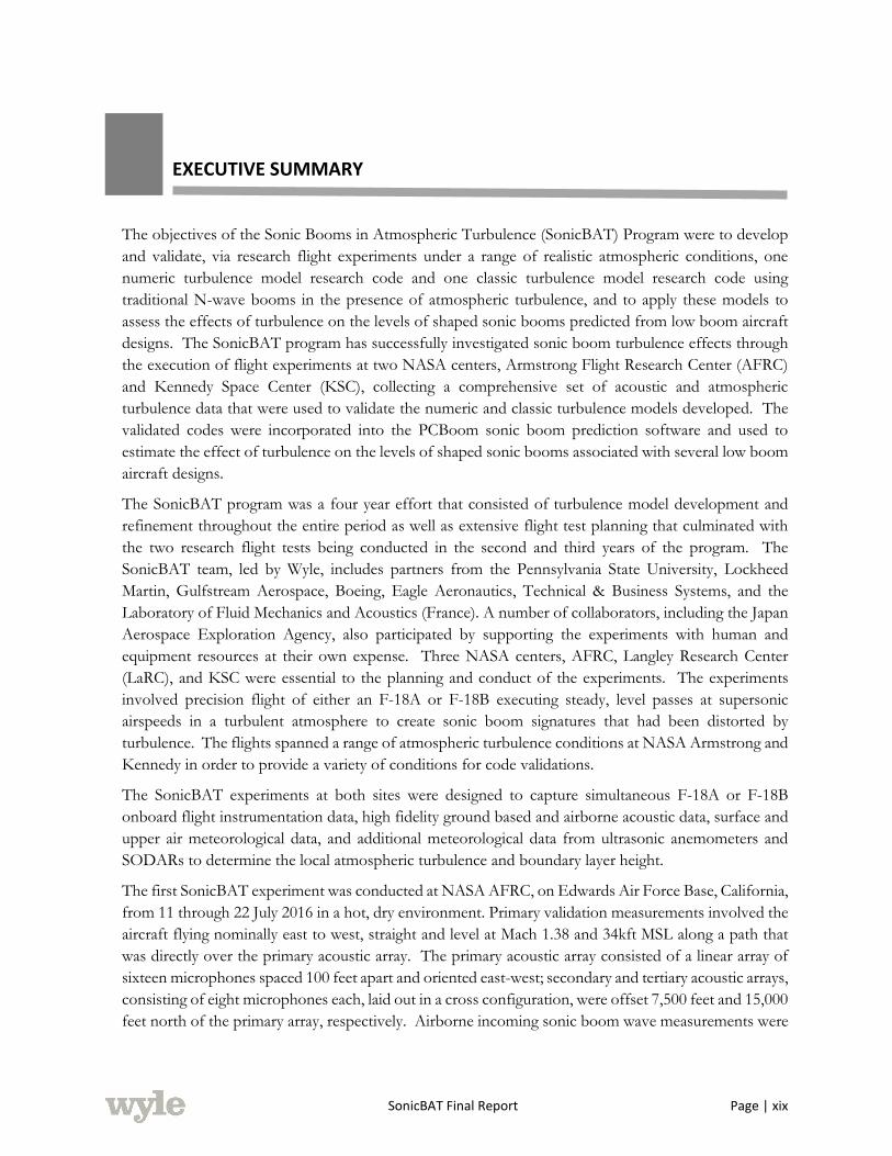
EXECUTIVE SUMMARY
The objectives of the Sonic Booms in Atmospheric Turbulence (SonicBAT) Program were to develop
and validate, via research flight experiments under a range of realistic atmospheric conditions, one
numeric turbulence model research code and one classic turbulence model research code using
traditional N-wave booms in the presence of atmospheric turbulence, and to apply these models to
assess the effects of turbulence on the levels of shaped sonic booms predicted from low boom aircraft
designs. The SonicBAT program has successfully investigated sonic boom turbulence effects through
the execution of flight experiments at two NASA centers, Armstrong Flight Research Center (AFRC)
and Kennedy Space Center (KSC), collecting a comprehensive set of acoustic and atmospheric
turbulence data that were used to validate the numeric and classic turbulence models developed. The
validated codes were incorporated into the PCBoom sonic boom prediction software and used to
estimate the effect of turbulence on the levels of shaped sonic booms associated with several low boom
aircraft designs.
The SonicBAT program was a four year effort that consisted of turbulence model development and
refinement throughout the entire period as well as extensive flight test planning that culminated with
the two research flight tests being conducted in the second and third years of the program. The
SonicBAT team, led by Wyle, includes partners from the Pennsylvania State University, Lockheed
Martin, Gulfstream Aerospace, Boeing, Eagle Aeronautics, Technical & Business Systems, and the
Laboratory of Fluid Mechanics and Acoustics (France). A number of collaborators, including the Japan
Aerospace Exploration Agency, also participated by supporting the experiments with human and
equipment resources at their own expense. Three NASA centers, AFRC, Langley Research Center
(LaRC), and KSC were essential to the planning and conduct of the experiments. The experiments
involved precision flight of either an F-18A or F-18B executing steady, level passes at supersonic
airspeeds in a turbulent atmosphere to create sonic boom signatures that had been distorted by
turbulence. The flights spanned a range of atmospheric turbulence conditions at NASA Armstrong and
Kennedy in order to provide a variety of conditions for code validations.
The SonicBAT experiments at both sites were designed to capture simultaneous F-18A or F-18B
onboard flight instrumentation data, high fidelity ground based and airborne acoustic data, surface and
upper air meteorological data, and additional meteorological data from ultrasonic anemometers and
SODARs to determine the local atmospheric turbulence and boundary layer height.
The first SonicBAT experiment was conducted at NASA AFRC, on Edwards Air Force Base, California,
from 11 through 22 July 2016 in a hot, dry environment. Primary validation measurements involved the
aircraft flying nominally east to west, straight and level at Mach 1.38 and 34kft MSL along a path that
was directly over the primary acoustic array. The primary acoustic array consisted of a linear array of
sixteen microphones spaced 100 feet apart and oriented east-west; secondary and tertiary acoustic arrays,
consisting of eight microphones each, laid out in a cross configuration, were offset 7,500 feet and 15,000
feet north of the primary array, respectively. Airborne incoming sonic boom wave measurements were
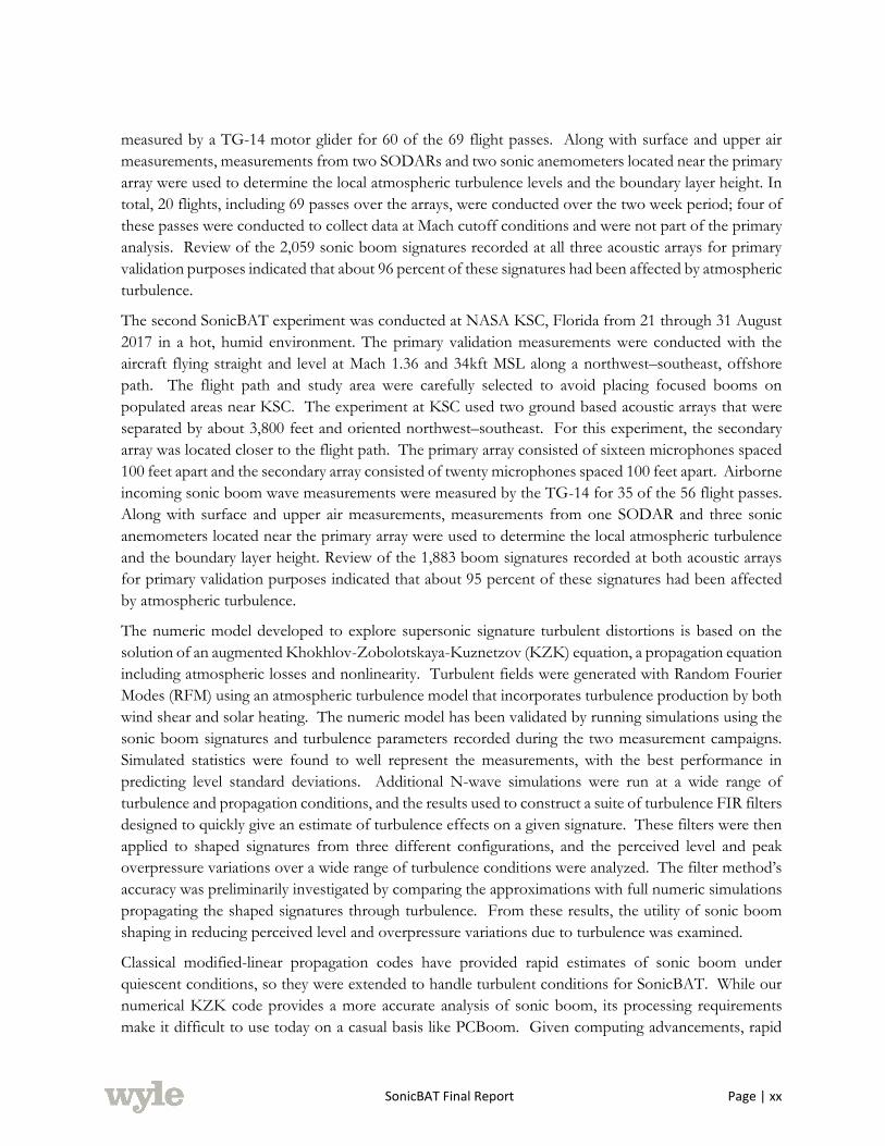
SonicBAT Final Report Page | xx
measured by a TG-14 motor glider for 60 of the 69 flight passes. Along with surface and upper air
measurements, measurements from two SODARs and two sonic anemometers located near the primary
array were used to determine the local atmospheric turbulence levels and the boundary layer height. In
total, 20 flights, including 69 passes over the arrays, were conducted over the two week period; four of
these passes were conducted to collect data at Mach cutoff conditions and were not part of the primary
analysis. Review of the 2,059 sonic boom signatures recorded at all three acoustic arrays for primary
validation purposes indicated that about 96 percent of these signatures had been affected by atmospheric
turbulence.
The second SonicBAT experiment was conducted at NASA KSC, Florida from 21 through 31 August
2017 in a hot, humid environment. The primary validation measurements were conducted with the
aircraft flying straight and level at Mach 1.36 and 34kft MSL along a northwest–southeast, offshore
path. The flight path and study area were carefully selected to avoid placing focused booms on
populated areas near KSC. The experiment at KSC used two ground based acoustic arrays that were
separated by about 3,800 feet and oriented northwest–southeast. For this experiment, the secondary
array was located closer to the flight path. The primary array consisted of sixteen microphones spaced
100 feet apart and the secondary array consisted of twenty microphones spaced 100 feet apart. Airborne
incoming sonic boom wave measurements were measured by the TG-14 for 35 of the 56 flight passes.
Along with surface and upper air measurements, measurements from one SODAR and three sonic
anemometers located near the primary array were used to determine the local atmospheric turbulence
and the boundary layer height. Review of the 1,883 boom signatures recorded at both acoustic arrays
for primary validation purposes indicated that about 95 percent of these signatures had been affected
by atmospheric turbulence.
The numeric model developed to explore supersonic signature turbulent distortions is based on the
solution of an augmented Khokhlov-Zobolotskaya-Kuznetzov (KZK) equation, a propagation equation
including atmospheric losses and nonlinearity. Turbulent fields were generated with Random Fourier
Modes (RFM) using an atmospheric turbulence model that incorporates turbulence production by both
wind shear and solar heating. The numeric model has been validated by running simulations using the
sonic boom signatures and turbulence parameters recorded during the two measurement campaigns.
Simulated statistics were found to well represent the measurements, with the best performance in
predicting level standard deviations. Additional N-wave simulations were run at a wide range of
turbulence and propagation conditions, and the results used to construct a suite of turbulence FIR filters
designed to quickly give an estimate of turbulence effects on a given signature. These filters were then
applied to shaped signatures from three different configurations, and the perceived level and peak
overpressure variations over a wide range of turbulence conditions were analyzed. The filter method’s
accuracy was preliminarily investigated by comparing the approximations with full numeric simulations
propagating the shaped signatures through turbulence. From these results, the utility of sonic boom
shaping in reducing perceived level and overpressure variations due to turbulence was examined.
Classical modified-linear propagation codes have provided rapid estimates of sonic boom under
quiescent conditions, so they were extended to handle turbulent conditions for SonicBAT. While our
numerical KZK code provides a more accurate analysis of sonic boom, its processing requirements
make it difficult to use today on a casual basis like PCBoom. Given computing advancements, rapid

SonicBAT Final Report Page | xxi
propagation of many rays through turbulence is possible in minutes on a typical PC. Our classical
“TURBO” code is a fully 3-D, linear acoustic propagation allowing turbulent temperature and gust
variation versus altitude along with up to 100 mean temperature and wind variations. This classical
turbulence code also works with Burgers methods to generate results that superimpose the separate (no
interactions) effects of non-linear aging, rounding, mean and turbulent atmospheric variations, and
easily runs inside the PCBoom interface. We acknowledge that more calibration is required to get the
best approximation of the numerical KZK code and rapid statistical results. The KZK code, FIR filters
and TURBO code generate the full range of high resolution predictions, representative signatures and
rapid statistics.
In summary, the SonicBAT program was a highly successful example of contractor team-NASA-partner
collaboration, with such notable accomplishments as:
• First time in 60 years of sonic boom measurements that the characteristics of the turbulence,
through which the boom signatures have travelled, have been measured along with the
signatures.
• One of the largest sonic boom data sets ever collected including 125 flight passes and over
4,000 sonic booms recorded, of which greater than ninety-five percent of the booms had
signatures that showed the effects of atmospheric turbulence.
• Development of meteorological measurement and analysis methods to characterize
atmospheric turbulence and the boundary layer height.
• Development and validation of two new sonic boom turbulence models which account for the
effects of atmospheric turbulence.
• Demonstrated the effects of turbulence on the levels of shaped sonic booms predicted from
low boom aircraft designs.
• Assessed the effects of turbulence using modern sonic boom metrics such as Steven’s Mark
VII Perceived Level (PL) instead of relying only upon maximum acoustic pressure (pmax).
• Excellent example of collaboration between three NASA centers, the contractor team, and
international partners.
SonicBAT Final Report Page | xxii
ACRONYMS
Acronym Definition
ABL Atmospheric Boundary Layer
ABLH Atmospheric Boundary Layer Height
ADC Air Data Calibration
AFRC Armstrong Flight Research Center
AGL Above Ground Level
ANSI American National Standards Institute
ASEL A-Weighted Sound Exposure Level
BSEL B-Weighted Sound Exposure Level
CFD Computational Fluid Dynamics
CSEL C-Weighted Sound Exposure Level
dBV Decibels Referenced to Voltage
DSEL D-Weighted Sound Exposure Level
ESEL E-Weighted Sound Exposure Level
CST Commercial Supersonic Technology
dB Decibel
FFT Fast Fourier Transform
FIR Finite Impulse Response
FLMAX Maximum Scale Length
FLMIN Minimum Scale Length
FSEL Unweighted Sound Exposure Level
GPS Global Positioning System
HZ Hertz
INS Inertial Navigation System
IRGASON Infrared-Gas Analyzer-Sonic
IRIG Inter-Range Instrumentation Group
ISBAP Indoor Sonic Boom Annoyance Predictor
JAXA Japan Aerospace Exploration Agency
KSC Kennedy Space Center
KZK Khokhlov-Zobolotskaya-Kuznetzov
KZKFourier Khokhlov-Zobolotskaya-Kuznetzov Fourier
LaRC Langley Research Center
LBFD Low Boom Flight Demonstrator
LCL Lifting Condensation Layer
LLZf Zwicker Loudness for Frontal Incidence
LLZd Zwicker Loudness for Diffuse Incidence
MOST Monin-Obukhov Similarity Theory
MPI Message Passing Interface
MSL Mean Sea Level
SonicBAT Final Report Page | xxiii
NASA National Aeronautics and Space Administration
NLMAX Number of Modes
NPE Nonlinear Progressive Wave Equation
OTT Over-The-Top
PC Personal Computer
PL Steven’s Mark VII Perceived Level
PLdB Perceived Decibel Level
PNL Kryter’s Perceived Noise Level
RAYSEP Ray Separation
RFM Random Fourier Modes
RH Relative Humidity
RMS Root-Mean-Square
SEL Sound Exposure Level
SODAR Sonic Detection And Ranging
SonicBAT Sonic Booms in Atmospheric Turbulence
SPM Seconds Past Midnight
TURBO Classic Turbulence Model
UTC Coordinated Universal Time

SonicBAT Final Report Page | 1
1.0
INTRODUCTION
The National Aeronautics and Space Administration (NASA) conducts supersonic vehicle research,
through its Commercial Supersonic Technology (CST) Project, aimed at eliminating the technical
barriers to commercial overland supersonic flight. This research includes developing new aircraft
technologies and designs that result in shaped, low-amplitude sonic boom signatures rather than the
historical unacceptable N-wave signature, improving predictive tools used for sonic boom assessment,
and increasing knowledge about sonic boom atmospheric effects – turbulence in particular, transmission
into structures, and human response.
NASA’s commitment to the goal of commercial overland supersonic flight requires accurate sonic boom
prediction tools that can be used in the near term to evaluate the Quiet Supersonic Transport or QueSST
aircraft design. QueSST is the initial design stage of NASA’s planned Low Boom Flight Demonstrator
(LBFD) experimental airplane that will be used to gauge community acceptance to overland supersonic
flights. Longer term, after the barrier to commercial overland supersonic flight has been lifted, accurate
sonic boom prediction tools will be needed for routine assessment of commercial supersonic flight
operations in the US and abroad.
Since the late 1950’s and early 1960’s it was found that the atmosphere through which the shock waves
from a supersonic transport propagate plays an important role in the sonic boom that is experienced at
the ground. Atmospheric pressure, temperature, density, and winds (the “macro” influences) and
turbulence, atmospheric absorption, and molecular relaxation (the “micro” influences) all come into
play. Over the years of making boom measurements it has been found that among all of these the one
that causes the most significant alterations to the sonic boom signature is turbulence, in particular, the
turbulence that is experienced in the lower layers of the atmosphere, the earth's boundary layer.
Prediction codes are in place to account for the atmospheric “macro” influences and a few of the
“micro” influences. A prediction code that accounts for turbulence was non existent. Part of the CST
Project is aimed at addressing this critical need and is the reason why NASA has conducted the Sonic
Booms in Atmospheric Turbulence (SonicBAT) Program. SonicBAT was designed to increase
knowledge of sonic boom atmospheric turbulence effects and improve prediction tool accuracy via the
development of 2-D and 3-D numeric turbulence models and a classic turbulence model. Two research
flight tests were conducted at NASA’s Armstrong Flight Research Center (AFRC) and Kennedy Space
Center (KSC) to record sonic booms in different geographic locations in a variety of atmospheric
conditions. The turbulence models developed on the program were validated, via flight test data, and
then were integrated with PCBoom, NASA’s general purpose sonic boom propagation software.
PCBoom and the turbulence models were then used to assess the effects of turbulence on the levels of
shaped sonic booms predicted from low boom aircraft designs.
The remainder of Section 1.0 includes a brief description of sonic boom propagation in the atmosphere
(Section 1.1) and the SonicBAT program objectives (Section 1.2). Section 2.0 provides an overview of
the atmosphere and turbulence modeling requirements. Section 3.0 presents the fundamentals of
numerical turbulence modeling including its background, atmospheric model inputs, numerical
propagation theory, and a representation of turbulence effects from numerical propagation. Section 4.0

SonicBAT Final Report Page | 2
presents the fundamentals of classical turbulence modeling including its background and basis in
classical scattering theory.
The two SonicBAT research flight tests at Armstrong Flight Research Center (2016) and Kennedy Space
center (2017) are described in Section 5.0. The Atmospheric turbulence measurements and data analysis
procedures employed during these flight tests are described in Section 6.0.
Section 7.0 presents the validation of the sonic boom turbulence research codes and Section 8.0 presents
a statistical analysis and uncertainty quantification of these codes.
Results of the low boom vehicle analysis performed with the new turbulence models are provided in
Section 9.0. Details of the integration of the turbulence models with PCBoom is provided in
Section 10.0. The project summary, recommendations, and conclusions are presented in Section 11.0.
1.1 SONIC BOOM PROPAGATION IN THE ATMOSPHERE
Sonic Boom pressure disturbances are created anytime a vehicle flies faster than the speed of sound.
Research into understanding sonic booms started before manned supersonic flight, but the levels of
sonic booms from manned supersonic vehicles flying over 14 km (45 kft) above the ground was not
anticipated from prior experience with shock waves, such as from: thunder (from lightning), buggy
whips, explosions and firearms. Much of the difference was eventually found to come from the way
sonic booms propagate from a vehicle through the atmosphere (Maglieri et al. 2014). Understanding
propagation was therefore actively researched as critical to the understanding and mitigation of
supersonic transport sonic boom.
Figure 1. The atmosphere layers and features concerning a supersonic aircraft’s primary sonic boom.
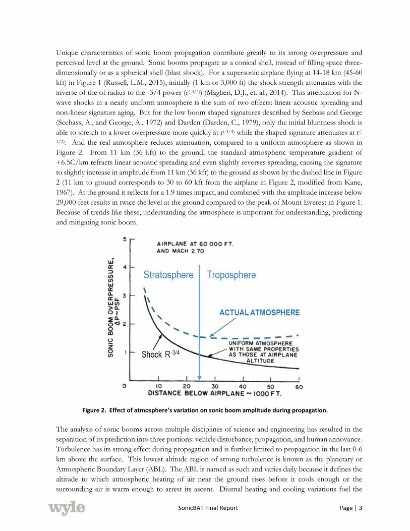
SonicBAT Final Report Page | 3
Unique characteristics of sonic boom propagation contribute greatly to its strong overpressure and
perceived level at the ground. Sonic booms propagate as a conical shell, instead of filling space three-
dimensionally or as a spherical shell (blast shock). For a supersonic airplane flying at 14-18 km (45-60
kft) in Figure 1 (Russell, L.M., 2015), initially (1 km or 3,000 ft) the shock strength attenuates with the
inverse of the of radius to the -3/4 power (r(-3/4)) (Maglieri, D.J., et. al., 2014). This attenuation for N-
wave shocks in a nearly uniform atmosphere is the sum of two effects: linear acoustic spreading and
non-linear signature aging. But for the low boom shaped signatures described by Seebass and George
(Seebass, A., and George, A., 1972) and Darden (Darden, C., 1979), only the initial bluntness shock is
able to stretch to a lower overpressure more quickly at r(-3/4) while the shaped signature attenuates at r(-
1/2). And the real atmosphere reduces attenuation, compared to a uniform atmosphere as shown in
Figure 2. From 11 km (36 kft) to the ground, the standard atmospheric temperature gradient of
+6.5C/km refracts linear acoustic spreading and even slightly reverses spreading, causing the signature
to slightly increase in amplitude from 11 km (36 kft) to the ground as shown by the dashed line in Figure
2 (11 km to ground corresponds to 30 to 60 kft from the airplane in Figure 2, modified from Kane,
1967). At the ground it reflects for a 1.9 times impact, and combined with the amplitude increase below
29,000 feet results in twice the level at the ground compared to the peak of Mount Everest in Figure 1.
Because of trends like these, understanding the atmosphere is important for understanding, predicting
and mitigating sonic boom.
Figure 2. Effect of atmosphere’s variation on sonic boom amplitude during propagation.
The analysis of sonic booms across multiple disciplines of science and engineering has resulted in the
separation of its prediction into three portions: vehicle disturbance, propagation, and human annoyance.
Turbulence has its strong effect during propagation and is further limited to propagation in the last 0-6
km above the surface. This lowest altitude region of strong turbulence is known as the planetary or
Atmospheric Boundary Layer (ABL). The ABL is named as such and varies daily because it defines the
altitude to which atmospheric heating of air near the ground rises before it cools enough or the
surrounding air is warm enough to arrest its ascent. Diurnal heating and cooling variations fuel the

SonicBAT Final Report Page | 4
turbulence here, and its gust and temperature variations follow known trends that can be measured,
modeled and predicted to a useful level of accuracy. Therefore turbulence effects are predicted by
calculating sonic boom propagation through a model of the ABL.
There have been many useful past flight test measurements of sonic booms in atmospheric turbulence
that enabled the SonicBAT program. However, none of those past flight test programs acquired the
mean and turbulent atmospheric measurements necessary for validation of codes that predict sonic
boom distortions in atmospheric turbulence. The SonicBAT research flight tests at AFRC and KSC
marks the first time in 60 years of boom measurements that the characteristics of the turbulence through
which the boom signatures have travelled have been measured along with the signatures.
1.1.1 ATMOSPHERIC DISTORTION OF N-WAVE SONIC BOOM
Sonic boom flight test measurements at the ground are always found to have distortions from their
expected N-wave shape (Pierce and Maglieri, 1972) and these distortions are associated with turbulence
in the atmospheric boundary layer (Maglieri et al. 1967). When flight tests are conducted under calm
atmospheric conditions (e.g., early morning with little or no wind), measured booms have insignificant
distortions and match the N-wave shape predicted by theory. When atmospheric conditions are not
calm (desert afternoons, with obvious thermal activity, or gusting surface winds) booms have a basic N-
wave shape, but they are distorted. This is illustrated in Figure 3 (Hilton et al. 1966). The turbulent-
condition booms have a fine scale distortion, which is strongest near the shock waves, and the shock
waves themselves are somewhat thicker. Theories have been set forth which appear to explain the
distortions (Crow 1969 and Pierce 1968) and shock thickening (Plotkin and George, 1972). These
theories require as inputs various atmospheric turbulence quantities. The specific turbulence quantities
required for the models developed on this program are described throughout this report.
Figure 3. Sonic booms measured under calm and turbulent conditions.
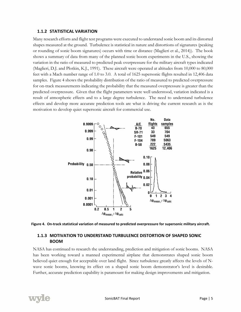
SonicBAT Final Report Page | 5
1.1.2 STATISTICAL VARIATION
Many research efforts and flight test programs were executed to understand sonic boom and its distorted
shapes measured at the ground. Turbulence is statistical in nature and distortions of signatures (peaking
or rounding of sonic boom signatures) occurs with time or distance (Maglieri et al., 2014)). The book
shows a summary of data from many of the planned sonic boom experiments in the U.S., showing the
variation in the ratio of measured to predicted peak overpressure for the military aircraft types indicated
(Maglieri, D.J. and Plotkin, K.J., 1991). These aircraft were operated at altitudes from 10,000 to 80,000
feet with a Mach number range of 1.0 to 3.0. A total of 1625 supersonic flights resulted in 12,406 data
samples. Figure 4 shows the probability distribution of the ratio of measured to predicted overpressure
for on-track measurements indicating the probability that the measured overpressure is greater than the
predicted overpressure. Given that the flight parameters were well understood, variation indicated is a
result of atmospheric effects and to a large degree turbulence. The need to understand turbulence
effects and develop more accurate prediction tools are what is driving the current research as is the
motivation to develop quiet supersonic aircraft for commercial use.
Figure 4. On-track statistical variation of measured to predicted overpressure for supersonic military aircraft.
1.1.3 MOTIVATION TO UNDERSTAND TURBULENCE DISTORTION OF SHAPED SONIC BOOM
NASA has continued to research the understanding, prediction and mitigation of sonic booms. NASA
has been working toward a manned experimental airplane that demonstrates shaped sonic boom
believed quiet enough for acceptable over land flight. Since turbulence greatly affects the levels of N-
wave sonic booms, knowing its effect on a shaped sonic boom demonstrator’s level is desirable.
Further, accurate prediction capability is paramount for making design improvements and mitigation.
SonicBAT Final Report Page | 6
1.2 PROGRAM OBJECTIVES
Supersonic aircraft with shaped, low boom signatures have the potential of finding community
acceptance to commercial supersonic flight. The objective of this research was to develop models that
estimate the effect of atmospheric turbulence on low boom signatures and their perceived level. To
accomplish this, research flight tests were conducted in a variety of atmospheres at two different
geographic locations to examine boom propagation effects over a range of turbulence conditions. Two
sonic boom turbulence models were developed including 2-D and 3-D versions of a numeric
propagation and turbulence model, and a classic, semianalytic propagation model. Practical
implementations of both of these models were incorporated into PCBoom, NASA’s sonic boom
prediction tool.
The first research flight test was conducted at Armstrong Flight Research Center in Edwards Air Force
Base, California to provide continuity with the vast majority of sonic boom flight tests that have been
conducted in that dry desert environment. The second research flight test was conducted at Kennedy
Space Center, Florida in a hot, humid environment to expand the range of climate conditions tested.
During both flight tests, atmospheric turbulence and sonic boom were measured simultaneously. Flight
test booms were all N-waves, but data was collected in sufficient detail to validate the sonic boom
turbulence models.
A numerical sonic boom turbulence model was developed using a Khokhlov-Zabolotskaya-Kuznetsov
(KZK) method. This numeric propagation model includes convection, multi-dimensional diffraction,
nonlinearity, and absorption effects. Turbulence is represented by a Fourier modes model. Both 2-D
and 3-D versions of the numeric model were developed. The 3-D version has been preliminarily tested
and is computationally expensive to run. Thus, the 2-D version was used to produce the results in this
report. Both versions are run using NASA’s Pleiades supercomputer which allows for massively parallel
computation. Using the numeric model, finite impulse response filters were developed for different
turbulence conditions; these filters represent the practical implementation of the numeric model in
PCBoom. A classic propagation model, based on scattering theory, was also developed for use in
PCBoom. Other required updates were made to PCBoom to permit processing of high resolution
signatures and to allow Burger’s evolved signatures to enter the turbulence models.

SonicBAT Final Report Page | 7
2.0
ATMOSPHERIC TURBULENCE OVERVIEW
Turbulent distortion is present in almost all sonic boom waveforms measured during the day. The
exception is very early in the morning immediately after the atmosphere has settled down throughout
the night. The distortion due to atmospheric turbulence has been seen in many field tests, resulting in
waveforms that are substantially different in shape and sonic character just a few hundred feet apart.
Predicting the effects of atmospheric turbulence on shaped sonic boom ground signatures, requires a
mathematical representation of the significant atmospheric effects. Understanding and modeling of the
atmosphere’s characteristics has been greatly developed in the past few decades primarily for weather
forecasting and aircraft simulations. Correspondingly, many instruments for atmospheric measurement
have been developed for satellites, aircraft and ground-based measurements. Since modeling and flight
test measurements of the Atmospheric Boundary Layer (ABL) are of greatest significance for sonic
boom distortions, this section will focus on applications in the ABL.
2.1 ATMOSPHERIC TURBULENCE RESEARCH AND MODELING BACKGROUND
In parallel with research and development of acoustical theories for sonic boom propagation,
fundamental research and theories were being developed on turbulence and atmospheric modeling for
aircraft and meteorology. In 1941 Kolmogorov (1941a and 1941b) and Obukhov (1941) postulated the
existence of a statistical theory of turbulence, which allows the computation of statistical and spectral
quantities suitable for ABL modeling. Obukhov further developed the application to atmospheric
turbulence and in 1962 published formulas for the scaling of turbulence within the ABL, which we now
call structure functions. With these structure functions, measurements of turbulence from a tower on
the ground can be used to characterize turbulence throughout the whole ABL.
Meteorologists worked throughout the 1970s and 1980s to improve computational modeling of the
atmosphere and its boundary layer with research measurements and instrumentation developments.
One notable experimental paper is the seminal work of Thomson, Coulter, and Warhaft (1978) where
they proved that a ground-based SODAR acoustic sounding device could remotely measure the
turbulent structure functions of the atmosphere just as well as a traditional hot-wire measurements made
by an aircraft passing through that atmosphere. Chapter 2 of the 1986 book of Stuart Bradley explains
the operation and signal processing used in SODARs and mini SODARs.
Subsequent work in the 1980s and 1990s solidified the ability of meteorologists to measure the structure
parameters indicating the strength of both thermal and kinetic atmospheric turbulence. A detailed
summary is captured in the review paper of Neff and Coulter from 1986. A briefer summary is given
in Coulter (1997).
The most recent work over the last 20 years has emphasized a model of the atmospheric boundary layer
that is altitude dependent, and included both shear and buoyancy forcing. Wilson described such a
model in 2000, although it was not applied specifically to sonic boom propagation. Additional
theoretical analysis of both homogeneous (altitude independent) and inhomogeneous (altitude
dependent) turbulence models are explained in Chapter 6 of the recent second edition of the book by
Vladimir Ostashev and Keith Wilson (2016).
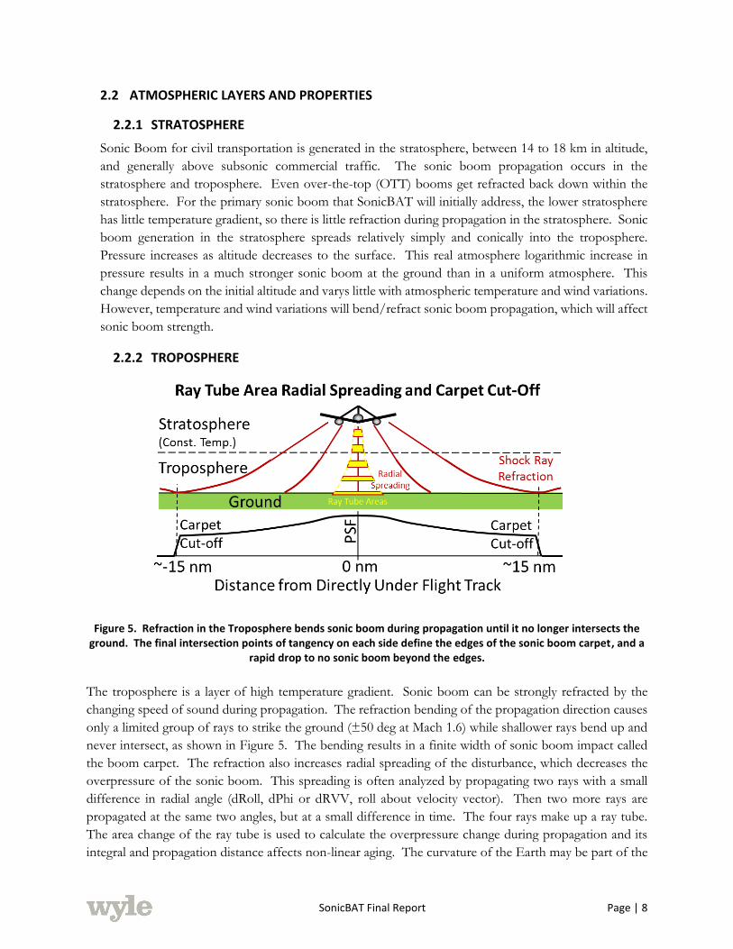
SonicBAT Final Report Page | 8
2.2 ATMOSPHERIC LAYERS AND PROPERTIES
2.2.1 STRATOSPHERE
Sonic Boom for civil transportation is generated in the stratosphere, between 14 to 18 km in altitude,
and generally above subsonic commercial traffic. The sonic boom propagation occurs in the
stratosphere and troposphere. Even over-the-top (OTT) booms get refracted back down within the
stratosphere. For the primary sonic boom that SonicBAT will initially address, the lower stratosphere
has little temperature gradient, so there is little refraction during propagation in the stratosphere. Sonic
boom generation in the stratosphere spreads relatively simply and conically into the troposphere.
Pressure increases as altitude decreases to the surface. This real atmosphere logarithmic increase in
pressure results in a much stronger sonic boom at the ground than in a uniform atmosphere. This
change depends on the initial altitude and varys little with atmospheric temperature and wind variations.
However, temperature and wind variations will bend/refract sonic boom propagation, which will affect
sonic boom strength.
2.2.2 TROPOSPHERE
Figure 5. Refraction in the Troposphere bends sonic boom during propagation until it no longer intersects the ground. The final intersection points of tangency on each side define the edges of the sonic boom carpet, and a
rapid drop to no sonic boom beyond the edges.
The troposphere is a layer of high temperature gradient. Sonic boom can be strongly refracted by the
changing speed of sound during propagation. The refraction bending of the propagation direction causes
only a limited group of rays to strike the ground (±50 deg at Mach 1.6) while shallower rays bend up and
never intersect, as shown in Figure 5. The bending results in a finite width of sonic boom impact called
the boom carpet. The refraction also increases radial spreading of the disturbance, which decreases the
overpressure of the sonic boom. This spreading is often analyzed by propagating two rays with a small
difference in radial angle (dRoll, dPhi or dRVV, roll about velocity vector). Then two more rays are
propagated at the same two angles, but at a small difference in time. The four rays make up a ray tube.
The area change of the ray tube is used to calculate the overpressure change during propagation and its
integral and propagation distance affects non-linear aging. The curvature of the Earth may be part of the
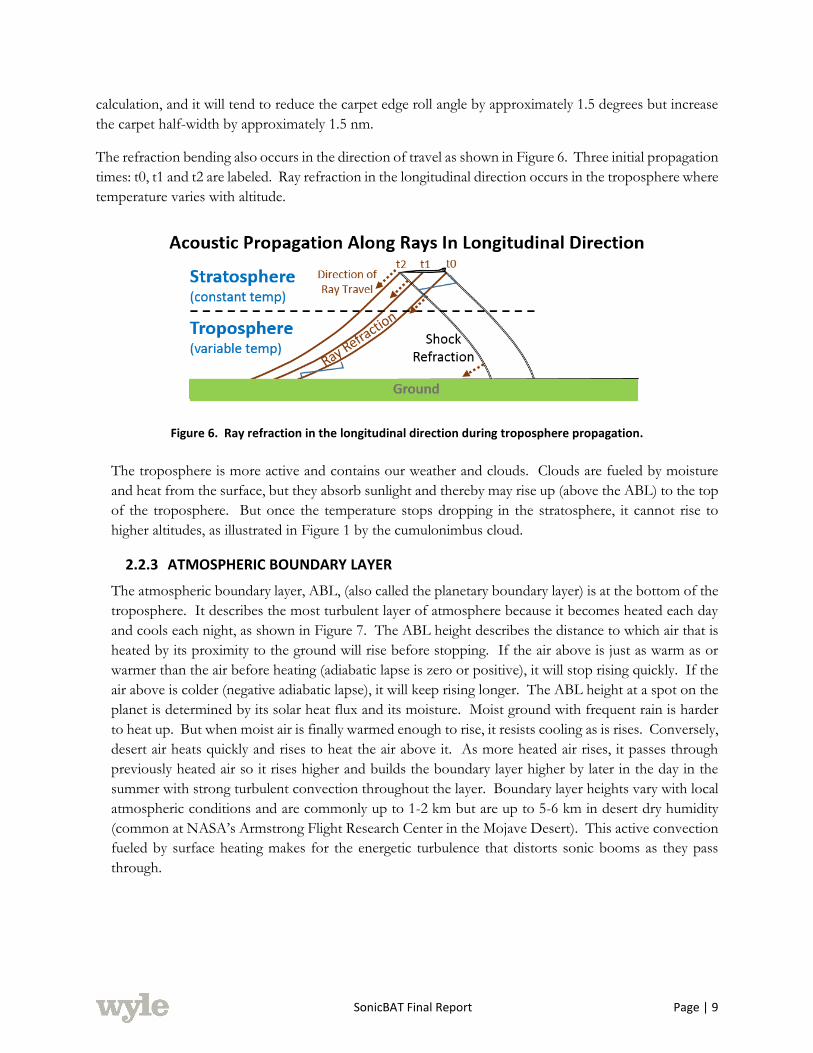
SonicBAT Final Report Page | 9
calculation, and it will tend to reduce the carpet edge roll angle by approximately 1.5 degrees but increase
the carpet half-width by approximately 1.5 nm.
The refraction bending also occurs in the direction of travel as shown in Figure 6. Three initial propagation
times: t0, t1 and t2 are labeled. Ray refraction in the longitudinal direction occurs in the troposphere where
temperature varies with altitude.
Figure 6. Ray refraction in the longitudinal direction during troposphere propagation.
The troposphere is more active and contains our weather and clouds. Clouds are fueled by moisture
and heat from the surface, but they absorb sunlight and thereby may rise up (above the ABL) to the top
of the troposphere. But once the temperature stops dropping in the stratosphere, it cannot rise to
higher altitudes, as illustrated in Figure 1 by the cumulonimbus cloud.
2.2.3 ATMOSPHERIC BOUNDARY LAYER
The atmospheric boundary layer, ABL, (also called the planetary boundary layer) is at the bottom of the
troposphere. It describes the most turbulent layer of atmosphere because it becomes heated each day
and cools each night, as shown in Figure 7. The ABL height describes the distance to which air that is
heated by its proximity to the ground will rise before stopping. If the air above is just as warm as or
warmer than the air before heating (adiabatic lapse is zero or positive), it will stop rising quickly. If the
air above is colder (negative adiabatic lapse), it will keep rising longer. The ABL height at a spot on the
planet is determined by its solar heat flux and its moisture. Moist ground with frequent rain is harder
to heat up. But when moist air is finally warmed enough to rise, it resists cooling as is rises. Conversely,
desert air heats quickly and rises to heat the air above it. As more heated air rises, it passes through
previously heated air so it rises higher and builds the boundary layer higher by later in the day in the
summer with strong turbulent convection throughout the layer. Boundary layer heights vary with local
atmospheric conditions and are commonly up to 1-2 km but are up to 5-6 km in desert dry humidity
(common at NASA’s Armstrong Flight Research Center in the Mojave Desert). This active convection
fueled by surface heating makes for the energetic turbulence that distorts sonic booms as they pass
through.

SonicBAT Final Report Page | 10
Figure 7. The atmospheric boundary layer’s diurnal variations.
Figure 7 illustrates the ABL for typical day/night conditions, over homogeneous terrain. There are
three distinct layers:
1. Surface Layer - The lowest part of the ABL is called the surface layer. The properties of the
ground and mechanical shear at the surface play a major role. Because much of our existence
is in the surface layer, it has been the most widely studied and is the best-understood region. A
now-classic scaling law developed by Monin and Obhukov (1954) has been well established in
this layer. The stability of this layer can be computed by this scaling law. Stability conditions
can also be estimated by simple rules, such as Turner class, which are based on simple
meteorological observations of surface wind, solar angle, and cloud cover.
The surface layer is characterized by vertical fluxes (momentum, heat, and moisture fluxes)
varying little with height, so it is often referred to as the constant stress layer. Panofsky and
Dutton (1984) argue that the surface layer can be defined to be the lowest 10 percent of the
mixing depth, on the grounds that fluxes are close enough to constant over this range, even if
they vary linearly over the full mixing depth.
It is common to see logarithmic wind and temperature profiles used to model surface layer
conditions. Logarithmic profiles correspond to neutral conditions, where heat flux is zero.
Under stable or unstable conditions, profiles are depicted by forms which are not strictly
logarithmic, although a logarithmic profile may be an adequate approximation. The region in
which logarithmic profiles are appropriate is sometimes referred to as the inertial layer.
2. Convective Mixed Layer - Here the mean gradients are usually smallest: the mean temperature
(adiabatic) and velocity are essentially constant with height, which would follow from this being
the layer with the strongest vertical convection. The upper limit of the mixed layer extends to
a height of approximately zi. Scaling laws for this region have been developed by Deardoff
(1972) and Wyngaard et al (1974). These scaling laws depend on vertical heat flux and the layer
height.

SonicBAT Final Report Page | 11
3. Inversion Layer - This region extends roughly between 0.8 zi to 1.2 zi as indicated in Figure 8.
Conditions in this region represent a transition between the mixed layer and the free
atmosphere.
Figure 8. Atmospheric boundary sub-layers.
Sonic boom distortions have been identified as coming from the inversion layer and mixed layer but
not strongly from the surface layer.
It has been stated that the surface layer has no impact on sonic boom distortions. This conclusion was
based upon a ray ground measurement, with distortion, that reflected and was remeasured on a tower
with microphones every 50 ft (Maglieri, et. al. p. 38 fig. 2.20, 2014). The tower measurement impacted
by the same ray as the ground measurement (based on the known shock angle from the temperature
and vehicle speed) had the same sonic boom distortion, indicating that the boom had not been further
distorted from the ground to the tower. Turbulence reduces near the surface in general, and z-velocity
winds are more strongly suppressed. Ideally, a model with a representative surface layer would quantify
this reduced importance and its dominant mechanism. Otherwise, not specifically modeling the surface
layer or ignoring its effect appear to be reasonable strategies.
2.2.4 GROUND MEASUREMENT HEIGHT FOR BEST TURBULENCE MEASUREMENTS
The inversion layer and mixing layer turbulence affects the surface layer turbulence in a predictable way.
So conversely, surface measurements provide good predictions of the turbulence in the layers above.
However, surface layer measurements are degraded by ground changes like clutter, man-made structures
or harsh geographic features (e.g., mountains, lake, or snow pack). Surface measurements are ideally
made far from such high-gradient features. Especially with clutter but also from low-gradient ground
interactions, there are wind shears near the ground where the direction of the wind changes. At the
node between the wind layers, measurements of turbulence are at their worst. The nodes occur less
frequently the higher you go, so the general rule is that higher is better. 10% of the ABL height is ideal,
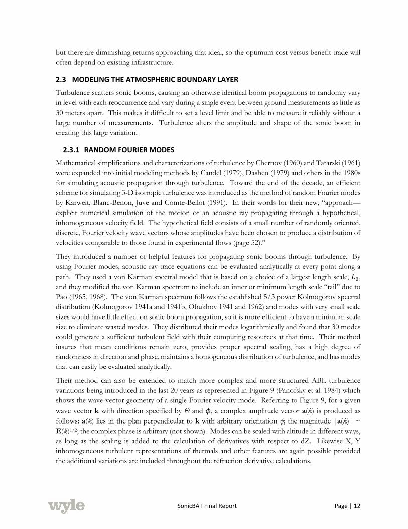
SonicBAT Final Report Page | 12
but there are diminishing returns approaching that ideal, so the optimum cost versus benefit trade will
often depend on existing infrastructure.
2.3 MODELING THE ATMOSPHERIC BOUNDARY LAYER
Turbulence scatters sonic booms, causing an otherwise identical boom propagations to randomly vary
in level with each reoccurrence and vary during a single event between ground measurements as little as
30 meters apart. This makes it difficult to set a level limit and be able to measure it reliably without a
large number of measurements. Turbulence alters the amplitude and shape of the sonic boom in
creating this large variation.
2.3.1 RANDOM FOURIER MODES
Mathematical simplifications and characterizations of turbulence by Chernov (1960) and Tatarski (1961)
were expanded into initial modeling methods by Candel (1979), Dashen (1979) and others in the 1980s
for simulating acoustic propagation through turbulence. Toward the end of the decade, an efficient
scheme for simulating 3-D isotropic turbulence was introduced as the method of random Fourier modes
by Karweit, Blanc-Benon, Juve and Comte-Bellot (1991). In their words for their new, “approach—
explicit numerical simulation of the motion of an acoustic ray propagating through a hypothetical,
inhomogeneous velocity field. The hypothetical field consists of a small number of randomly oriented,
discrete, Fourier velocity wave vectors whose amplitudes have been chosen to produce a distribution of
velocities comparable to those found in experimental flows (page 52).”
They introduced a number of helpful features for propagating sonic booms through turbulence. By
using Fourier modes, acoustic ray-trace equations can be evaluated analytically at every point along a
path. They used a von Karman spectral model that is based on a choice of a largest length scale, 𝐿0,
and they modified the von Karman spectrum to include an inner or minimum length scale “tail” due to
Pao (1965, 1968). The von Karman spectrum follows the established 5/3 power Kolmogorov spectral
distribution (Kolmogorov 1941a and 1941b, Obukhov 1941 and 1962) and modes with very small scale
sizes would have little effect on sonic boom propagation, so it is more efficient to have a minimum scale
size to eliminate wasted modes. They distributed their modes logarithmically and found that 30 modes
could generate a sufficient turbulent field with their computing resources at that time. Their method
insures that mean conditions remain zero, provides proper spectral scaling, has a high degree of
randomness in direction and phase, maintains a homogeneous distribution of turbulence, and has modes
that can easily be evaluated analytically.
Their method can also be extended to match more complex and more structured ABL turbulence
variations being introduced in the last 20 years as represented in Figure 9 (Panofsky et al. 1984) which
shows the wave-vector geometry of a single Fourier velocity mode. Referring to Figure 9, for a given
wave vector k with direction specified by Θ and ϕ, a complex amplitude vector a(k) is produced as
follows: a(k) lies in the plan perpendicular to k with arbitrary orientation ψ; the magnitude |a(k)| ~
E(k)1/2; the complex phase is arbitrary (not shown). Modes can be scaled with altitude in different ways,
as long as the scaling is added to the calculation of derivatives with respect to dZ. Likewise X, Y
inhomogeneous turbulent representations of thermals and other features are again possible provided
the additional variations are included throughout the refraction derivative calculations.
SonicBAT Final Report Page | 13
Figure 9. Description of a random Fourier mode implementation.
2.3.2 MODELING TURBULENCE DISTRIBUTION
The goal of the modeling in SonicBAT is to develop the capabilities so that NASA can assess the effects
of atmospheric turbulence on low-boom waveforms either by using a practical implementation of the
numeric model (Section 3.0) or the analytic classic model (Section 4.0). In this research the primary
effort is to develop both models to take a “clean” sonic boom waveform and incorporate turbulence.
Both of these models need to account for the strength of the turbulence, geometrical factors such as
the boundary layer thickness and the angle of incidence the sonic boom propagates through the
turbulence.
To provide proper inputs to both models, information about the atmosphere is required. In addition to
the non-turbulent, average conditions of wind, temperature, and humidity as a function of altitude, both
models require special information regarding the atmospheric turbulence. The part of the atmosphere
of most interest in SonicBAT is called the mixed layer (Section 2.2.3), and on a warm sunny day at KSC,
for example, the mixed layer could be 1 to 2 km in height.
In the mixed layer the parameters that are needed are:
𝑧𝑖 , the height of the mixed layer;
𝑙0 , the inner scale or smallest eddy size of the turbulence;
𝐿0 , the outer scale or largest eddy size of the turbulence;
𝐶𝑇2 , the temperature structure parameter for the thermal turbulence; and
𝐶𝑣2 , the velocity structure parameter for the kinetic turbulence.
The inner scale of the turbulence is indicated by the dissipation by viscosity (millimeters), and the outer
scale of the turbulence is indicated by the largest scales of the convection in the atmosphere (10s to
100s of meters). The temperature structure parameter and velocity structure parameter give an indication
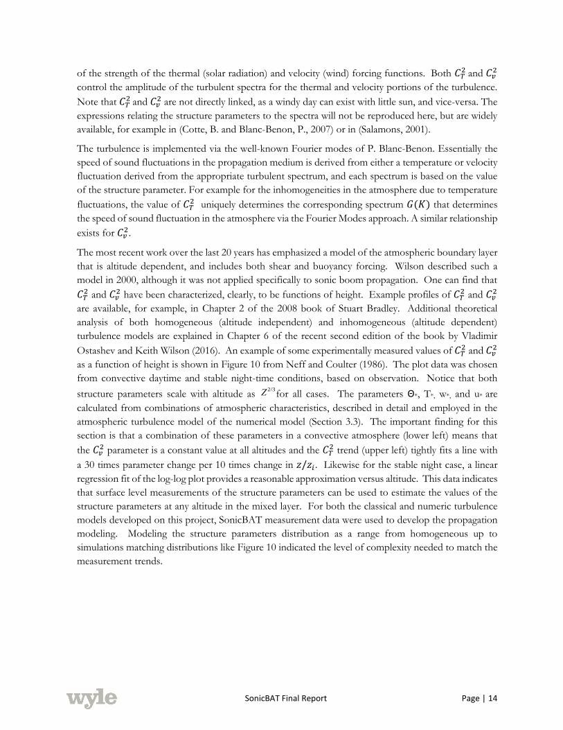
SonicBAT Final Report Page | 14
of the strength of the thermal (solar radiation) and velocity (wind) forcing functions. Both 𝐶𝑇2 and 𝐶𝑣
2
control the amplitude of the turbulent spectra for the thermal and velocity portions of the turbulence.
Note that 𝐶𝑇2 and 𝐶𝑣
2 are not directly linked, as a windy day can exist with little sun, and vice-versa. The
expressions relating the structure parameters to the spectra will not be reproduced here, but are widely
available, for example in (Cotte, B. and Blanc-Benon, P., 2007) or in (Salamons, 2001).
The turbulence is implemented via the well-known Fourier modes of P. Blanc-Benon. Essentially the
speed of sound fluctuations in the propagation medium is derived from either a temperature or velocity
fluctuation derived from the appropriate turbulent spectrum, and each spectrum is based on the value
of the structure parameter. For example for the inhomogeneities in the atmosphere due to temperature
fluctuations, the value of 𝐶𝑇2 uniquely determines the corresponding spectrum 𝐺(𝐾) that determines
the speed of sound fluctuation in the atmosphere via the Fourier Modes approach. A similar relationship
exists for 𝐶𝑣2.
The most recent work over the last 20 years has emphasized a model of the atmospheric boundary layer
that is altitude dependent, and includes both shear and buoyancy forcing. Wilson described such a
model in 2000, although it was not applied specifically to sonic boom propagation. One can find that
𝐶𝑇2 and 𝐶𝑣
2 have been characterized, clearly, to be functions of height. Example profiles of 𝐶𝑇2 and 𝐶𝑣
2
are available, for example, in Chapter 2 of the 2008 book of Stuart Bradley. Additional theoretical
analysis of both homogeneous (altitude independent) and inhomogeneous (altitude dependent)
turbulence models are explained in Chapter 6 of the recent second edition of the book by Vladimir
Ostashev and Keith Wilson (2016). An example of some experimentally measured values of 𝐶𝑇2 and 𝐶𝑣
2
as a function of height is shown in Figure 10 from Neff and Coulter (1986). The plot data was chosen
from convective daytime and stable night-time conditions, based on observation. Notice that both
structure parameters scale with altitude as Z2/3
for all cases. The parameters Θ*, T*, w*, and u* are
calculated from combinations of atmospheric characteristics, described in detail and employed in the
atmospheric turbulence model of the numerical model (Section 3.3). The important finding for this
section is that a combination of these parameters in a convective atmosphere (lower left) means that
the 𝐶𝑣2 parameter is a constant value at all altitudes and the 𝐶𝑇
2 trend (upper left) tightly fits a line with
a 30 times parameter change per 10 times change in 𝑧/𝑧𝑖 . Likewise for the stable night case, a linear
regression fit of the log-log plot provides a reasonable approximation versus altitude. This data indicates
that surface level measurements of the structure parameters can be used to estimate the values of the
structure parameters at any altitude in the mixed layer. For both the classical and numeric turbulence
models developed on this project, SonicBAT measurement data were used to develop the propagation
modeling. Modeling the structure parameters distribution as a range from homogeneous up to
simulations matching distributions like Figure 10 indicated the level of complexity needed to match the
measurement trends.

SonicBAT Final Report Page | 15
Figure 10. Measured profiles of 𝑪𝑻𝟐 and 𝑪𝑽
𝟐 for both daytime (convective, left) and nighttime (stable, right) conditions.
Further discussion of how the structure parameters 𝐶𝑇2 and 𝐶𝑣
2 and other turbulence parameters are
measured and applied in the models is made throughout this report. Sections 3.0 and 4.0 describe how
the turbulence parameters are implemented in the numeric and classic models, respectively. Sections
5.0 and 6.0 describe the atmospheric turbulence measurements and data analysis that were conducted,
as part of the two research flight tests, to yield the structure parameters for each test.

SonicBAT Final Report Page | 16
3.0
NUMERICAL TURBULENCE MODELING
3.1 INTRODUCTION
This section introduces the methods and algorithm, termed the KZKFourier engine, which were
developed to predict the atmospheric turbulence effects on sonic booms in the primary boom carpet.
Several methods already exist for predicting the geographical footprint of the signatures from supersonic
aircraft. Prediction programs such as PCBoom (Hobbs and Page, 2011) and sBOOM (Rallabhandi,
2011) use linear geometrical acoustics or ray-tracing to predict the amplitude and affected region, taking
the atmospheric temperature and wind profiles as inputs. To predict sonic boom waveforms including
nonlinear effects, PCBoom and sBOOM solve the Burgers’ propagation equation in conjunction with
ray-tracing. However, the atmospheric turbulence throughout the boundary layer, which may be up to
about 2 km in depth or more from the surface, is neglected.
Turbulence serves to randomly focus or defocus energy in the sonic boom wavefront, which can lead
to significant amplitude and level variations (Maglieri et al., 2014). Some ray-tracing models incorporate
turbulence effects and attempt to predict locations of caustics or energy focusing, but these methods
do not account for diffraction at the caustics which is important for high-amplitude N-waves in the
atmosphere (Karweit et al., 1991; Blanc-Benon et al., 2002; Averiyanov et al., 2011a). Inclusion of
turbulence effects to predict waveform distortions necessitates use of an equation more complex than
Burgers’. One such equation is the nonlinear Khokhlov-Zabolotskaya-Kuznetzov (KZK) propagation
equation, which has been used previously to study turbulence effects on N-wave sonic booms (Blanc-
Benon et al., 2002; Aver’yanov et al., 2006; Averiyanov et al., 2011a; Yuldashev et al., 2016).
The KZKFourier engine solves an augmented KZK equation to numerically model propagation of the
sonic boom wavefront. The KZK equation is a versatile model equation used in nonlinear applications
including shockwave propagation and for modeling ultrasonic transducers with biomedical applications
(Averkiou and Hamilton, 1997). Other nonlinear models have also been applied to sonic boom
propagation, including a time-domain solution of the nonlinear progressive wave equation (NPE)
(Locey, 2008), a combined time-domain and spectral approach called FLHOWARD (Luquet, 2016)
using a partially one-way equation, and a similar but one-way equation called HOWARD (Kanamori et
al., 2017). This KZK implementation is better-behaved at domain boundaries than the NPE solution
and the computation does not require the FFT’s used in FLHOWARD or HOWARD.
To generate random turbulent fields through which to model propagation, the KZKFourier engine
implements the Random Fourier Modes (RFM) method formulated for both temperature fluctuations
(Chevret et al., 1996) and wind fluctuations (Blanc-Benon et al., 2002). Doing so avoids the complexities
of an exhaustive fluid dynamics simulation over the entire planetary boundary layer. The RFM method
requires several atmospheric turbulence parameters as inputs, which are measured or inferred. The
KZKFourier engine uses sonic anemometer and balloon launch measurements of four turbulence
quantities together with the approximate turbulence model of Ostashev and Wilson (Wilson, 2000;
Ostashev and Wilson, 2015) to generate inputs for RFM. This atmospheric model is more appropriate
for a simulation involving wind fluctuations throughout the entire boundary layer than Monin-Obukhov
Similarity Theory (MOST), which previous studies have applied to simulations near the surface.

SonicBAT Final Report Page | 17
After many simulations through turbulence using the KZKFourier engine, linear FIR filters may be
generated which encapsulate the effect of turbulence. To approximate the effect of turbulence on a
given waveform, the waveform is simply convolved with the pre-computed filter, mitigating the need
for another computationally expensive set of numerical simulations. The filters are calculated similarly
to the method of Locey and Sparrow (Locey and Sparrow, 2007; Locey, 2008), using a matrix
deconvolution involving simulated waveforms after propagating through either a turbulent boundary
layer or a homogeneous atmosphere.
The propagation model, atmospheric turbulence model, and FIR filter application methodology are
described in greater detail in the following sections.
3.2 PROPAGATION MODEL
The present work focuses on simulations starting at the top of the atmospheric boundary layer, with an
initially planar waveform traveling through the turbulence to the ground. To use the KZK equation,
one assumes what is termed the parabolic approximation including the assumption that propagation is
primarily in one direction. In other words, the KZKFourier engine models only one wavefront or “ray”
at a time, the ray path must be straight, and bending of the ray due to the temperature profile in the
atmospheric boundary layer is neglected. Because the modeled propagation path is only within the
boundary layer, ray path curvature is negligible for most cases. In practice, the propagation angle is
arbitrarily chosen or approximated using ray-tracing results from another program. Propagation is
simulated along this angle and halted once the ground is reached.
The initial condition at the boundary layer height may be formed using an arbitrary choice of starting
wavefront. The KZKFourier engine is designed to take any starting waveform (e.g. a motor glider
measurement above the boundary layer) and “clone” it into a planar soundwave, which then distorts
randomly due to turbulence as it propagates towards the ground. The engine samples the modeled
wavefront at fixed transverse spatial locations. Upon reaching the ground, the waveforms that are
recorded by “virtual mics” at these ground locations may be extracted. No ground reflection is explicitly
modeled, but a reflection coefficient may be applied. For the present work, a reflection coefficient of
2.0 is always assumed, corresponding to a rigid ground. This coefficient, differing slightly from the
usual coefficient of 1.9, is chosen to more closely model reflection from a rigid surface.
The augmented KZK equation in two or three dimensions solved by KZKFourier is given by
𝜕𝑝
𝜕𝑧=
𝑐0
2∫ 𝛻⊥
2𝑝 𝑑𝜏′𝜏
−∞
+𝛿
2𝑐03
𝜕2𝑝
𝜕𝜏2+
𝛽𝑝
𝜌0𝑐03
𝜕𝑝
𝜕𝜏+
𝑐′
𝑐02
𝜕𝑝
𝜕𝜏+
𝒖𝑧
𝑐02
𝜕𝑝
𝜕𝜏−
1
𝑐0
(𝒖⊥ ∙ ∇⊥𝑝)
+ ∑𝑐𝜈
′
𝑐02 ∫
𝜕2𝑝
𝜕𝜏′2𝑒
−(𝜏−𝜏′)
𝑡𝜈 𝑑𝜏′𝜏
−∞𝜈
(1)
where the pressure waveform 𝑝(𝑧, 𝑦, 𝜏) is a function of the propagation direction coordinate 𝑧, the
transverse coordinate 𝑦 perpendicular to 𝑧, and the retarded time 𝜏; and the other quantities are given
in Table 1 below. The retarded time coordinate system follows the mean propagation of the wave, and
is defined as 𝜏 = 𝑡 − 𝑧/𝑐0 where 𝑡 is the usual time coordinate. In two dimensions, the transverse
Laplacian 𝛻⊥2 is equivalent to 𝜕2/𝜕𝑦2, and 𝒖⊥ ∙ ∇⊥𝑝 is equivalent to 𝒖𝑦𝜕𝑝/𝜕𝑦. From left to right, the
terms on the right-hand side of the equation describe the physical processes of diffraction,
thermoviscous absorption, nonlinearity, scalar (temperature fluctuations) turbulence, vector (wind
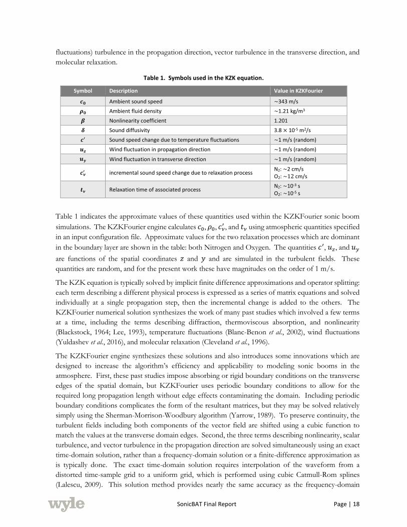
SonicBAT Final Report Page | 18
fluctuations) turbulence in the propagation direction, vector turbulence in the transverse direction, and
molecular relaxation.
Table 1. Symbols used in the KZK equation.
Symbol Description Value in KZKFourier
𝒄𝟎 Ambient sound speed ~343 m/s
𝝆𝟎 Ambient fluid density ~1.21 kg/m3
𝜷 Nonlinearity coefficient 1.201
𝜹 Sound diffusivity 3.8 × 10⁻⁵ m2/s
𝒄′ Sound speed change due to temperature fluctuations ~1 m/s (random)
𝒖𝒛 Wind fluctuation in propagation direction ~1 m/s (random)
𝒖𝒚 Wind fluctuation in transverse direction ~1 m/s (random)
𝒄𝝂′ incremental sound speed change due to relaxation process
N2: ~2 cm/s O2: ~12 cm/s
𝒕𝝂 Relaxation time of associated process N2: ~10-3 s O2: ~10-5 s
Table 1 indicates the approximate values of these quantities used within the KZKFourier sonic boom
simulations. The KZKFourier engine calculates 𝑐0, 𝜌0, 𝑐𝜈′ , and 𝑡𝜈 using atmospheric quantities specified
in an input configuration file. Approximate values for the two relaxation processes which are dominant
in the boundary layer are shown in the table: both Nitrogen and Oxygen. The quantities 𝑐′, 𝑢𝑧, and 𝑢𝑦
are functions of the spatial coordinates 𝑧 and 𝑦 and are simulated in the turbulent fields. These
quantities are random, and for the present work these have magnitudes on the order of 1 m/s.
The KZK equation is typically solved by implicit finite difference approximations and operator splitting:
each term describing a different physical process is expressed as a series of matrix equations and solved
individually at a single propagation step, then the incremental change is added to the others. The
KZKFourier numerical solution synthesizes the work of many past studies which involved a few terms
at a time, including the terms describing diffraction, thermoviscous absorption, and nonlinearity
(Blackstock, 1964; Lee, 1993), temperature fluctuations (Blanc-Benon et al., 2002), wind fluctuations
(Yuldashev et al., 2016), and molecular relaxation (Cleveland et al., 1996).
The KZKFourier engine synthesizes these solutions and also introduces some innovations which are
designed to increase the algorithm’s efficiency and applicability to modeling sonic booms in the
atmosphere. First, these past studies impose absorbing or rigid boundary conditions on the transverse
edges of the spatial domain, but KZKFourier uses periodic boundary conditions to allow for the
required long propagation length without edge effects contaminating the domain. Including periodic
boundary conditions complicates the form of the resultant matrices, but they may be solved relatively
simply using the Sherman-Morrison-Woodbury algorithm (Yarrow, 1989). To preserve continuity, the
turbulent fields including both components of the vector field are shifted using a cubic function to
match the values at the transverse domain edges. Second, the three terms describing nonlinearity, scalar
turbulence, and vector turbulence in the propagation direction are solved simultaneously using an exact
time-domain solution, rather than a frequency-domain solution or a finite-difference approximation as
is typically done. The exact time-domain solution requires interpolation of the waveform from a
distorted time-sample grid to a uniform grid, which is performed using cubic Catmull-Rom splines
(Lalescu, 2009). This solution method provides nearly the same accuracy as the frequency-domain
SonicBAT Final Report Page | 19
solution provided a high enough sampling rate, with much less computational expense. Finally, the
solution for the relaxation term has been altered to allow for numerical stability with a small step size in
the propagation direction.
In addition, the KZKFourier engine has been extended from the two-dimensional form (used
exclusively in the above studies due to memory and computational restraints) to three dimensions,
transforming the solution method for the refraction and wind fluctuation terms. The three-dimensional
algorithm attempts to parallelize and speed up as much as possible using the Message Passing Interface
(MPI) library and OpenMP parallel threading, but the computation is still extremely expensive. In
comparison, an extension to the FLHOWARD method described by Luquet called FLHOWARD3D
(2016) allows three-dimensional propagation, but the method uses an equation which is only partially
one-way and relies on spectral calculations which further increase the computational cost, making it
difficult to use a sampling rate high enough to resolve shocks. The two-dimensional KZKFourier
variant is used exclusively for the present results because of the unreasonable computational expense
that would be required to find statistical results at all the conditions of interest using the three-
dimensional algorithm.
3.3 ATMOSPHERIC TURBULENCE MODEL
An approximate atmospheric turbulence model is used in conjunction with the KZK-based propagation
code to simulate a random turbulent field throughout the domain. The fields are generated at runtime
via the Random Fourier Modes method of Blanc-Benon et al. (Chevret et al., 1996; Blanc-Benon et al.,
2002). This method creates frozen (i.e. time-invariant), isotropic fields and requires only the turbulent
energy spectrum as a function of wavenumber for the calculation. The fields are computed by sampling
the energy spectra and adding wavenumber components together with amplitudes prescribed by the
spectra and with uniformly randomized direction and phase. For scalar turbulence, 800 modes are
summed in this way, and 8000 modes for vector turbulence. Modes are logarithmically spaced in
wavenumber from about 1.0 × 10⁻⁵ m-1 to 3.1 × 10⁴ m-1, depending on the boundary layer height.
The three-dimensional von Karman energy spectrum is chosen to approximate energy spectra of real
atmospheric turbulence. To construct the spectra of both scalar and vector turbulence, the KZKFourier
engine uses the methods of Wilson and Ostashev (Wilson, 2000; Ostashev and Wilson, 2015), which
provide modified von Karman spectra as functions of the outer length scale of turbulence and the
variance of a single velocity component or the temperature. These parameters are derived using
measured or assumed atmospheric turbulence quantities.
For scalar turbulence, the variance 𝜎𝑇 and outer length scale 𝐿𝑇 suitable for the von Karman model are
given by Eqs. (6.50) and (6.51) in Ostashev and Wilson (Ostashev and Wilson, 2015):
𝜎𝑇
2(ℎ)
𝑇∗2
=4.0
[1 + 10(−ℎ/𝐿𝑚𝑜)]2/3
(2)
𝐿𝑇(𝑧)
ℎ= 2.0
1 + 7.0(−ℎ/𝐿𝑚𝑜)
1 + 10(−ℎ/𝐿𝑚𝑜) (3)
SonicBAT Final Report Page | 20
where ℎ is the height, 𝑇∗ is the surface-layer temperature scale, and 𝐿𝑚𝑜 is the Monin-Obukhov length
scale defined as,
𝐿𝑚𝑜 = −𝑧𝑖𝑢∗
3
𝜅𝑤∗3, (4)
where 𝑧𝑖 is the boundary layer height and 𝜅 = 0.4 is the von Karman’s constant. The quantity 𝑇∗ may
be calculated using measurements from a sonic anemometer.
For vector turbulence in the atmosphere, turbulence production due to wind shear and also buoyancy
production due to solar heating of the ground may be important. In convective conditions, such as a
clear, sunny day, buoyancy production may dominate in much of the boundary layer. The KZKFourier
engine models both sources of vector turbulence. The two sets of quantities corresponding to both
shear and buoyancy turbulence production are given in both Wilson (Wilson, 2000) and in Ostashev
and Wilson (Ostashev and Wilson, 2015):
𝜎𝑠2 = 3.0𝑢∗
2, 𝐿𝑠 = 1.8ℎ, (5)
𝜎𝑏2 = 0.35𝑤∗
2, 𝐿𝑏 = 0.23𝑧𝑖, (6)
where the subscript s denotes the quantity corresponding to shear production and b for buoyancy
production, and the quantities 𝑧𝑖 , 𝑢∗, and 𝑤∗ are the capping inversion height, the friction velocity, and
the mixed-layer velocity scale, respectively. The quantities 𝑢∗ and 𝑤∗ may be calculated using
measurements from a sonic anemometer and knowledge of the height 𝑧𝑖 , which can be found from
balloon launch data. The boundary layer height is found by determining the height at which a rising
parcel of air starts to experience negative buoyancy. This height is characterized by a rapid increase in
temperature, or more precisely, the virtual potential temperature. A straightforward way to combine
the theories for both buoyancy and shear production is to add the corresponding von Karman energy
spectra. The combined variance of vector turbulence is given by the relation,
𝜎vector2 = 3.0𝑢∗
2 + 0.35𝑤∗2 (7)
Although the KZKFourier engine does not explicity use the structure constants 𝐶𝑇2 and 𝐶𝑣
2 in its
calculations, these may be found by the relations
𝐶𝑇2 =
3Γ (56)
𝜋12
𝜎𝑇2
𝐿0
23
and 𝐶𝑣2 =
3Γ (56)
𝜋12
𝜎vector2
𝐿0
23
(8)
where Γ is the Gamma function and Γ(5/6) ≈ 1.1288. Note that the outer length scale 𝐿0 used in
Eq. (8) may be specific to either velocity or temperature fluctuations.
Many of these quantities vary with height, so the von Karman spectra vary as well. The procedure for
generating the turbulent fields is:
1. For the current simulation height (the simulation starts at 𝑧𝑖), calculate 𝜎𝑇2, 𝜎𝑠
2, 𝜎𝑏2, 𝐿𝑇, 𝐿𝑠, and
𝐿𝑏 using either measured atmospheric quantities or simulated quantities,
SonicBAT Final Report Page | 21
2. Calculate the von Karman spectrum for scalar turbulence and the two spectra for vector
turbulence; add the vector turbulence spectra together, and
3. Compute the turbulent fields at this height using the Random Fourier Modes method.
These steps are repeated as the simulated sonic boom propagates down towards the ground.
The equations for 𝜎𝑠2 and 𝜎𝑏
2 are valid close to the surface and up to about 0.9𝑧𝑖 depending on the
convective strength in the atmosphere; thus, by extending the turbulent fields in the simulation up to 𝑧𝑖
the simulation may be making nonphysical assumptions about behavior near the capping inversion
height. This error decreases in a highly-convective atmosphere, where buoyancy production dominates.
In addition, the simulation makes the approximation that the turbulent fields immediately fall to zero
magnitude above 𝑧𝑖 .
An example of the scalar and vector turbulent fields generated by KZKFourier is shown in Figure 11.
At lower heights, the outer length scales of the turbulence eddies in both fields decreases as predicted
by the approximate turbulence theory, although in Figure 11 this phenomenon is more easily seen in
the scalar turbulent field. The variance of the scalar turbulence is notably higher closer to the ground,
decreasing precipitously with height. The variance of the vector field is modeled as approximately
constant throughout the boundary layer, meaning an ensemble average of many random vector fields
would equal this variance at all heights. In Figure 11, energetic vector turbulence eddies are seen
throughout the modeled boundary layer as a consequence of the constant variance. Within the
KZKFourier algorithm, the scalar and vector turbulent fields are superimposed and sampled at each
propagation step.
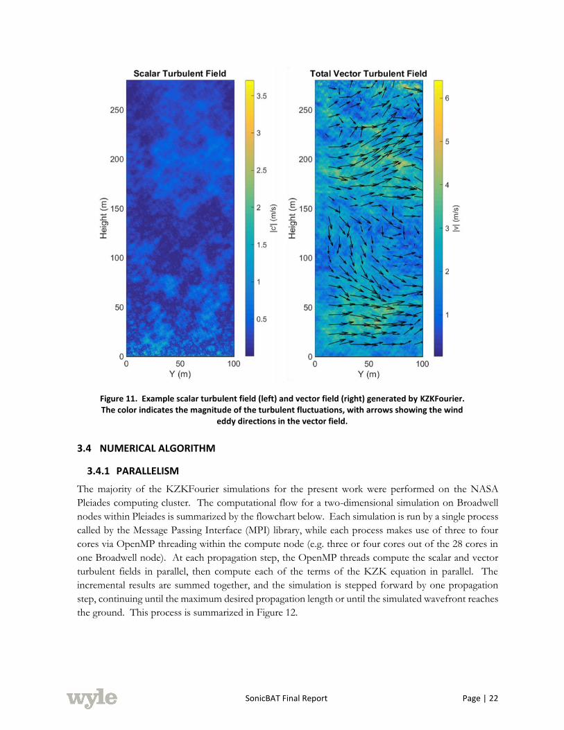
SonicBAT Final Report Page | 22
Figure 11. Example scalar turbulent field (left) and vector field (right) generated by KZKFourier. The color indicates the magnitude of the turbulent fluctuations, with arrows showing the wind
eddy directions in the vector field.
3.4 NUMERICAL ALGORITHM
3.4.1 PARALLELISM
The majority of the KZKFourier simulations for the present work were performed on the NASA
Pleiades computing cluster. The computational flow for a two-dimensional simulation on Broadwell
nodes within Pleiades is summarized by the flowchart below. Each simulation is run by a single process
called by the Message Passing Interface (MPI) library, while each process makes use of three to four
cores via OpenMP threading within the compute node (e.g. three or four cores out of the 28 cores in
one Broadwell node). At each propagation step, the OpenMP threads compute the scalar and vector
turbulent fields in parallel, then compute each of the terms of the KZK equation in parallel. The
incremental results are summed together, and the simulation is stepped forward by one propagation
step, continuing until the maximum desired propagation length or until the simulated wavefront reaches
the ground. This process is summarized in Figure 12.
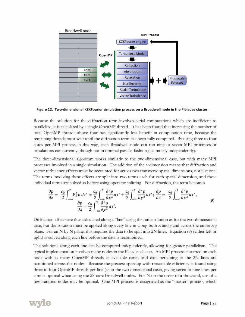
SonicBAT Final Report Page | 23
Figure 12. Two-dimensional KZKFourier simulation process on a Broadwell node in the Pleiades cluster.
Because the solution for the diffraction term involves serial computations which are inefficient to
parallelize, it is calculated by a single OpenMP thread. It has been found that increasing the number of
total OpenMP threads above four has significantly less benefit in computation time, because the
remaining threads must wait until the diffraction term has been fully computed. By using three to four
cores per MPI process in this way, each Broadwell node can run nine or seven MPI processes or
simulations concurrently, though not in optimal parallel fashion (i.e. mostly independently).
The three-dimensional algorithm works similarly to the two-dimensional case, but with many MPI
processes involved in a single simulation. The addition of the x dimension means that diffraction and
vector turbulence effects must be accounted for across two transverse spatial dimensions, not just one.
The terms involving these effects are split into two terms each for each spatial dimension, and these
individual terms are solved as before using operator splitting. For diffraction, the term becomes
𝜕𝑝
𝜕𝑧=
𝑐0
2∫ 𝛻⊥
2𝑝 𝑑𝜏′𝜏
−∞
≈𝑐0
2∫
𝜕2𝑝
𝜕𝑥2𝑑𝜏′
𝜏
−∞
+𝑐0
2∫
𝜕2𝑝
𝜕𝑦2𝑑𝜏′
𝜏
−∞
; 𝜕𝑝
𝜕𝑧=
𝑐0
2∫
𝜕2𝑝
𝜕𝑥2𝑑𝜏′
𝜏
−∞
,
𝜕𝑝
𝜕𝑧=
𝑐0
2∫
𝜕2𝑝
𝜕𝑦2𝑑𝜏′
𝜏
−∞
.
(9)
Diffraction effects are thus calculated along a “line” using the same solution as for the two-dimensional
case, but the solution must be applied along every line in along both x and y and across the entire x-y
plane. For an N by N plane, this requires the data to be split into 2N lines. Equation (9) (either left or
right) is solved along each line before the data is recombined.
The solutions along each line can be computed independently, allowing for greater parallelism. The
typical implementation involves many nodes in the Pleiades cluster. An MPI process is started on each
node with as many OpenMP threads as available cores, and data pertaining to the 2N lines are
partitioned across the nodes. Because the greatest speedup with reasonable efficiency is found using
three to four OpenMP threads per line (as in the two-dimensional case), giving seven to nine lines per
core is optimal when using the 28-core Broadwell nodes. For N on the order of a thousand, use of a
few hundred nodes may be optimal. One MPI process is designated as the “master” process, which
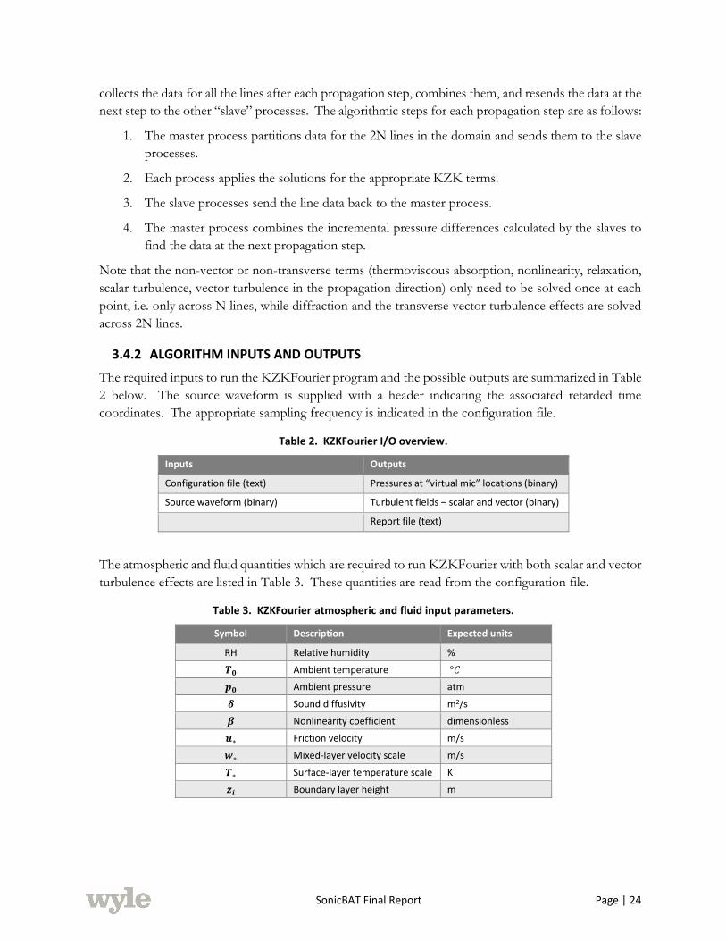
SonicBAT Final Report Page | 24
collects the data for all the lines after each propagation step, combines them, and resends the data at the
next step to the other “slave” processes. The algorithmic steps for each propagation step are as follows:
1. The master process partitions data for the 2N lines in the domain and sends them to the slave
processes.
2. Each process applies the solutions for the appropriate KZK terms.
3. The slave processes send the line data back to the master process.
4. The master process combines the incremental pressure differences calculated by the slaves to
find the data at the next propagation step.
Note that the non-vector or non-transverse terms (thermoviscous absorption, nonlinearity, relaxation,
scalar turbulence, vector turbulence in the propagation direction) only need to be solved once at each
point, i.e. only across N lines, while diffraction and the transverse vector turbulence effects are solved
across 2N lines.
3.4.2 ALGORITHM INPUTS AND OUTPUTS
The required inputs to run the KZKFourier program and the possible outputs are summarized in Table
2 below. The source waveform is supplied with a header indicating the associated retarded time
coordinates. The appropriate sampling frequency is indicated in the configuration file.
Table 2. KZKFourier I/O overview.
Inputs Outputs
Configuration file (text) Pressures at “virtual mic” locations (binary)
Source waveform (binary) Turbulent fields – scalar and vector (binary)
Report file (text)
The atmospheric and fluid quantities which are required to run KZKFourier with both scalar and vector
turbulence effects are listed in Table 3. These quantities are read from the configuration file.
Table 3. KZKFourier atmospheric and fluid input parameters.
Symbol Description Expected units
RH Relative humidity %
𝑻𝟎 Ambient temperature °𝐶
𝒑𝟎 Ambient pressure atm
𝜹 Sound diffusivity m2/s
𝜷 Nonlinearity coefficient dimensionless
𝒖∗ Friction velocity m/s
𝒘∗ Mixed-layer velocity scale m/s
𝑻∗ Surface-layer temperature scale K
𝒛𝒊 Boundary layer height m
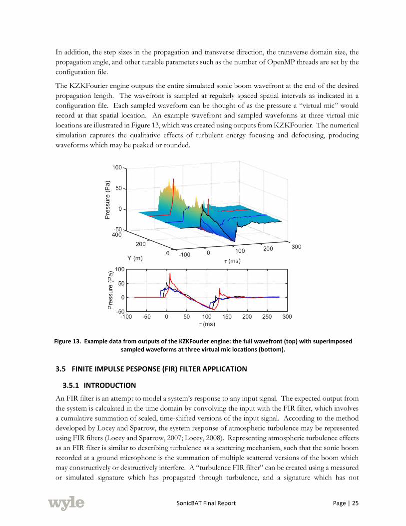
SonicBAT Final Report Page | 25
In addition, the step sizes in the propagation and transverse direction, the transverse domain size, the
propagation angle, and other tunable parameters such as the number of OpenMP threads are set by the
configuration file.
The KZKFourier engine outputs the entire simulated sonic boom wavefront at the end of the desired
propagation length. The wavefront is sampled at regularly spaced spatial intervals as indicated in a
configuration file. Each sampled waveform can be thought of as the pressure a “virtual mic” would
record at that spatial location. An example wavefront and sampled waveforms at three virtual mic
locations are illustrated in Figure 13, which was created using outputs from KZKFourier. The numerical
simulation captures the qualitative effects of turbulent energy focusing and defocusing, producing
waveforms which may be peaked or rounded.
Figure 13. Example data from outputs of the KZKFourier engine: the full wavefront (top) with superimposed sampled waveforms at three virtual mic locations (bottom).
3.5 FINITE IMPULSE PESPONSE (FIR) FILTER APPLICATION
3.5.1 INTRODUCTION
An FIR filter is an attempt to model a system’s response to any input signal. The expected output from
the system is calculated in the time domain by convolving the input with the FIR filter, which involves
a cumulative summation of scaled, time-shifted versions of the input signal. According to the method
developed by Locey and Sparrow, the system response of atmospheric turbulence may be represented
using FIR filters (Locey and Sparrow, 2007; Locey, 2008). Representing atmospheric turbulence effects
as an FIR filter is similar to describing turbulence as a scattering mechanism, such that the sonic boom
recorded at a ground microphone is the summation of multiple scattered versions of the boom which
may constructively or destructively interfere. A “turbulence FIR filter” can be created using a measured
or simulated signature which has propagated through turbulence, and a signature which has not

SonicBAT Final Report Page | 26
encountered turbulence or which propagated through still air. For example, using a recorded boom
with a front shock and an additional pressure spike near the front may produce an FIR filter with a jump
in coefficient amplitudes, much like the impulse response of a room with an echo. Because turbulence
is random, different turbulence FIR filters may have distinct characteristics.
FIR filters are inherently linear, because the filter coefficients do not change with the amplitude of the
input. Thus, using FIR filters to describe atmospheric turbulence requires the assumption that the
effects of nonlinearity and turbulence can be accounted for separately, and that the second-order effect
of the two combined may be neglected. This approximation is helped by the fact that, for a regular
cruising altitude, the majority of cumulative nonlinear effects occurs before the signature reaches the
planetary boundary layer and usually the boundary layer depth is relatively small.
To illustrate the assumption, let us designate the effect on a given waveform of travelling through the
atmospheric boundary layer in functional form as 𝑓𝑁,𝑇, where the subscripts 𝑁 and 𝑇 refer to nonlinear
effects and turbulence effects, respectively. For simplicity, other effects such as absorption are not
listed. The assumption inherent in FIR filter construction is that 𝑓𝑁,𝑇 ≈ 𝑓𝑇𝑓𝑁. The function 𝑓𝑁, which
operates first, represents propagation through still air, or any nonlinear propagation simulation that
provides “clean” (distortion free) waveforms at the ground. The function 𝑓𝑇 is approximated by a
turbulence FIR filter. To represent turbulent distortions, then, a simulated ground waveform may be
convolved with the turbulence FIR filter to “add in” the effect of turbulence.
The flow diagram in Figure 14 summarizes this process. The box on the left of the diagram illustrates
that a full numerical simulation including turbulence, or application of 𝑓𝑁,𝑇, would be necessary to find
a “turbulized” waveform given a starting waveform. Instead, through application of the approximation
that 𝑓𝑁,𝑇 ≈ 𝑓𝑇𝑓𝑁, the process in the box on the right side may be performed. The section to the left of
the dotted line is performed beforehand, and involves N-wave signature propagation simulations with
and without turbulence, and a matrix deconvolution to create the FIR filters. The number of FIR filters
created may be up to the total number of simulated, turbulized waveforms. This computation is detailed
in the next subsection. On the right of the dotted line, the diagram illustrates how an end user simulates
or measures a clean waveform, then convolves the waveform with the different FIR filters to create a
set of turbulized waveforms. The circled star denotes the convolution operator. Each waveform then
represents a possible measurement at the ground with turbulence.
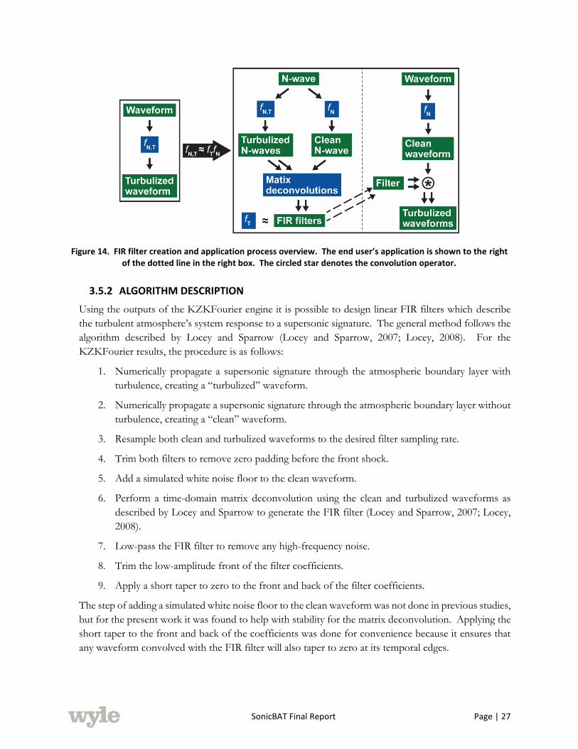
SonicBAT Final Report Page | 27
Figure 14. FIR filter creation and application process overview. The end user’s application is shown to the right of the dotted line in the right box. The circled star denotes the convolution operator.
3.5.2 ALGORITHM DESCRIPTION
Using the outputs of the KZKFourier engine it is possible to design linear FIR filters which describe
the turbulent atmosphere’s system response to a supersonic signature. The general method follows the
algorithm described by Locey and Sparrow (Locey and Sparrow, 2007; Locey, 2008). For the
KZKFourier results, the procedure is as follows:
1. Numerically propagate a supersonic signature through the atmospheric boundary layer with
turbulence, creating a “turbulized” waveform.
2. Numerically propagate a supersonic signature through the atmospheric boundary layer without
turbulence, creating a “clean” waveform.
3. Resample both clean and turbulized waveforms to the desired filter sampling rate.
4. Trim both filters to remove zero padding before the front shock.
5. Add a simulated white noise floor to the clean waveform.
6. Perform a time-domain matrix deconvolution using the clean and turbulized waveforms as
described by Locey and Sparrow to generate the FIR filter (Locey and Sparrow, 2007; Locey,
2008).
7. Low-pass the FIR filter to remove any high-frequency noise.
8. Trim the low-amplitude front of the filter coefficients.
9. Apply a short taper to zero to the front and back of the filter coefficients.
The step of adding a simulated white noise floor to the clean waveform was not done in previous studies,
but for the present work it was found to help with stability for the matrix deconvolution. Applying the
short taper to the front and back of the coefficients was done for convenience because it ensures that
any waveform convolved with the FIR filter will also taper to zero at its temporal edges.

SonicBAT Final Report Page | 28
The algorithm’s parameters used for this purpose with the KZKFourier results are listed in Table 4.
The length of 62.5 ms is somewhat longer than the 50 ms-long filters used by Locey and Sparrow. This
length is more than enough for accurate reproduction of turbulent effects on shocks.
Table 4. FIR filter creation algorithm parameters used with KZKFourier results.
Parameter Value
Sampling rate 51.2 kHz
Length 62.5 ms
Low-pass 10-dB down cutoff frequency 10 kHz
Taper length 2.5 ms
Simulated white noise floor RMS magnitude 0.02 Pa
3.5.3 MEAN AND STANDARD DEVIATION FIR FILTERS
To aid in the integration and use of turbulence FIR filters in the PCBoom program, a new
approximation was made that, for a particular set of atmospheric parameters, three FIR filters can be
chosen which represent the “mean”, “mean minus standard deviation” (-std), and “mean plus standard
deviation” (+std) effect of turbulence with respect to a particular metric. Here, the mean and standard
deviation refer to the metric’s statistical values for the total population of turbulized waveforms with
respect to the particular atmospheric parameters. The intent is to produce waveforms after convolution
which have these corresponding metric values. By carefully selecting these three filters, metric means
and standard deviations can be approximated without necessitating convolution with the thousands of
FIR filters that could be created. The following procedure is used to create the appropriate filters:
1. Perform many propagation simulations through the atmospheric boundary layer with random
realizations of turbulence.
2. Calculate a desired metric for each output turbulized waveform.
3. Compute the mean and standard deviation of the metric distribution.
4. Select the waveforms with metric values closest to the mean, and mean plus or minus one
standard deviation.
5. Perform one propagation simulation without turbulence to create a clean waveform.
6. Perform steps 3 through 9 in Section 3.5.2 with the three selected waveforms and the clean
waveform to produce the mean, -std, and +std turbulence FIR filters.
This procedure was used to create filters from the KZKFourier results detailed in Section 8.0, to provide
a quick representation of turbulence effects for a wide range of atmospheric parameters. After their
creation, the filters may be applied to any waveform, e.g. the low boom configurations in Section 9.0.
The accuracy of these three filters applied to shaped booms is also preliminarily investigated in
Section 9.0.
Example mean, -std, and +std FIR filters created using results from a condition with significant
turbulence and in reference to perceived level (PL) are shown in Figure 15. Figure 16 shows the ability
of the +std filter in recreating the turbulized waveform after convolution with the clean waveform. It
is seen that the convolved waveform without turbulence well approximates the waveform with

SonicBAT Final Report Page | 29
turbulence. The shock structure is faithfully reproduced, but the performance decreases after about 60
ms behind the front shock. This decrease in performance is due to the limited length of the FIR filter,
which is 62.5 ms long. Despite this, the perceived level is accurately represented: the convolved
waveform has a PL value of 101.6 dB, and the turbulized waveform has a value of 101.7 dB. The
accuracy of the FIR filters in reproducing N-wave levels is further examined in Section 8.0.
Figure 15. Mean, -std, and +std PLdB filters created using KZKFourier results with high turbulence conditions.
Figure 16. Performance of +std filter in reproducing the turbulized waveform after convolution with the clean signature (red). The turbulized waveform (blue) is well approximated by the convolved waveform (yellow).
Both the turbulized and clean waveforms are from simulated results.
SonicBAT Final Report Page | 30
4.0
CLASSICAL TURBULENCE MODELING
This section describes the background, approach and implementation of classical modeling for sonic
boom propagation through atmospheric turbulence. The first Section 4.1, describes the modified-linear
theory and Burgers code modeling concepts that are utilized for classical turbulence modeling. The
exact form of this model was not pre-defined, so this development did investigate a range of approaches.
Alternative approaches are described in Section 4.2 and the final method in Section 4.3. The objective
was to create a model that could predict the effect of atmospheric turbulence on sonic boom, with a
particular interest in how turbulence affects shaped sonic boom signatures (non N-wave) that are
expected to be much quieter. Such shaped sonic boom signatures are being utilized by NASA’s low
boom flight demonstrator (LBFD) program.
Classical sonic boom modeling provides accurate predictions of ground sonic boom using a
combination of linear acoustic ray tracing and non-linear aging. To predict level, shock rounding is also
important which is a function of atmospheric absorption and relaxation shock rounding and a function
of shock scattering in atmospheric turbulence. Burgers methods are named for the equation they solve
to add the effects of absorption and molecular relaxation to classical sonic boom modeling. Turbulence
scattering has been more difficult to analyze. A description of the theory of the selected approach, its
atmospheric turbulence modeling, propagation implementation and output are provided in this section.
Section 7.2 has classical method validation results and comparisons with measurements. Section 8.2
adds parametric trends with statistical and uncertainty analysis of results. Section 9.2 provides classical
model results for shaped signatures representative of low boom vehicles.
4.1 CLASSICAL TURBULENCE MODELING BACKGROUND
4.1.1 INITIAL SONIC BOOM PREDICTIONS WITH MODIFIED-LINEAR THEORY
Classical sonic boom prediction methods (codes like sBOOM, PCBoom, Thomas, ARAP, Carlson-
Middleton, etc. based on Whitham-Walkden theory (Whitham, G.B., 1956 and Walkden, F., 1958)
combine linear acoustic refraction (for bending due to temperature and wind gradients with altitude)
with a non-linear signature aging, to provide accurate prediction of sonic boom under calm atmospheric
conditions. Non-linear modeling predicts signature aging and shock coalescence, necessary to predict
signature evolution into the N-waves of ground measurements. Modified linear theory acoustic
predictions produce N-waves at the ground with instantaneous pressure jumps representing shocks. In
measurements, shocks may have 1 to 20 milliseconds of rounding that result in wide variations in level
from the same shock overpressure (Maglieri, D.J. and Parrott, 1963). Eventually, shock rounding was
attributed to two causes: (1) thermoviscous absorption and molecular relaxations and (2) scattering from
atmospheric boundary layer (ABL) turbulence.

SonicBAT Final Report Page | 31
Whitham’s early work on the flow disturbances from supersonic projectiles (Whitham, G.B., 1952) led
to his theory for propagation of weak shock waves (Whitham, G.B., 1956). The landmark Whitham
theory presented a method for converting the area distribution of an axisymmetric body into an F-
function, which was the non-dimensional (with distance) delta pressure over ambient pressure
disturbance (Δp/p) from the body that is heard as sonic boom at the ground. The far-field effect of lift
was worked out by Walkden (Walkden, F., 1958) using a dipole representation that varied as a cosine
variation with roll angle about the vehicle, which was a good approximation. So the sonic boom
calculation theory is more accurately termed the Whitham-Walkden theory than the often used Whitham
alone. A technique for reducing supersonic wave drag, called area ruling, used cross-sectional area
calculations for wave drag and wave drag minimization. Computer programs written for area ruling by
Harris (Harris, R., 1966) and others were connected through the Whitham-Walkden F-function to sonic
boom calculations.
The Rankine-Hugoniot relations for non-linear aging of a Δp/p disturbance to the ground was applied
by Middleton and Carlson, (Middleton, W.D., and Carlson, H.W., 1965) Hayes, (Hayes, W.D. et al.,
1969) Thomas (Thomas, C.L., 1972) and others and punched onto cards for programming and
execution by mainframe computers. Linear acoustic ray tracing was used to determine sound refraction
through the temperature changes in the atmosphere. Ray tracing four rays close together provided a
tube, where the change in the tube’s area at the ground was inversely proportional to the sonic booms
change in amplitude. With the addition of the non-linear aging, an accurate ground sonic boom
signature was predicted. Understanding this non-linear effect, Figure 17, which they termed signature
aging, was very key for understanding sonic boom, its level and means of reducing its level.
Figure 17. Non-linear aging results in shock coalescence into an N-Wave shape.
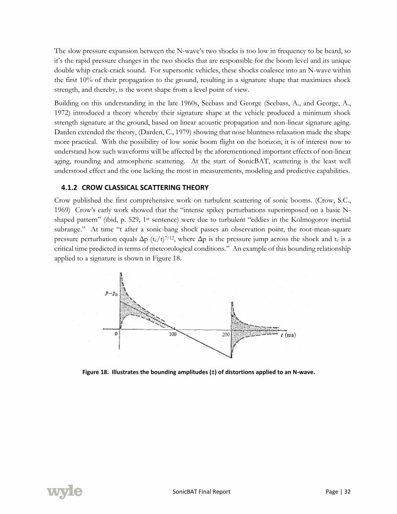
SonicBAT Final Report Page | 32
The slow pressure expansion between the N-wave’s two shocks is too low in frequency to be heard, so
it’s the rapid pressure changes in the two shocks that are responsible for the boom level and its unique
double whip crack-crack sound. For supersonic vehicles, these shocks coalesce into an N-wave within
the first 10% of their propagation to the ground, resulting in a signature shape that maximizes shock
strength, and thereby, is the worst shape from a level point of view.
Building on this understanding in the late 1960s, Seebass and George (Seebass, A., and George, A.,
1972) introduced a theory whereby their signature shape at the vehicle produced a minimum shock
strength signature at the ground, based on linear acoustic propagation and non-linear signature aging.
Darden extended the theory, (Darden, C., 1979) showing that nose bluntness relaxation made the shape
more practical. With the possibility of low sonic boom flight on the horizon, it is of interest now to
understand how such waveforms will be affected by the aforementioned important effects of non-linear
aging, rounding and atmospheric scattering. At the start of SonicBAT, scattering is the least well
understood effect and the one lacking the most in measurements, modeling and predictive capabilities.
4.1.2 CROW CLASSICAL SCATTERING THEORY
Crow published the first comprehensive work on turbulent scattering of sonic booms. (Crow, S.C.,
1969) Crow’s early work showed that the “intense spikey perturbations superimposed on a basic N-
shaped pattern” (ibid, p. 529, 1st sentence) were due to turbulent “eddies in the Kolmogorov inertial
subrange.” At time “t after a sonic-bang shock passes an observation point, the root-mean-square
pressure perturbation equals Δp (tc/t)7/12, where Δp is the pressure jump across the shock and tc is a
critical time predicted in terms of meteorological conditions.” An example of this bounding relationship
applied to a signature is shown in Figure 18.
Figure 18. Illustrates the bounding amplitudes (±) of distortions applied to an N-wave.

SonicBAT Final Report Page | 33
This result and its uncommon 7/12 power dependence was determined by assuming that scattering
happens at points of turbulence during propagation and that shocks propagate at a constant speed.
Consequentially, distortion at an observation point is found by a surface integral over a paraboloid of
dependence, whose focus is the observation point and whose directrix is the shock, Figure 19.
Figure 19. Geometry of the paraboloid of dependence.
The classic turbulence scatter theory of Crow is recognized as representative because it explains five
curious attributes of turbulence [paraphrased here as]: (1) perturbations are random and change
completely as the N-wave passes from point to point along the ground (even less than 100 feet apart),
(2) perturbations are comparable in amplitude to a shock immediately preceding it, but decrease rapidly
with greater distance behind the shock, (3) a strong peaked wave’s peak always occurs at or immediately
following a shock, (4) perturbations associated with the leading shock are always exactly the same as
perturbations associated with the trailing shock, (5) a microphone located 50 feet above the ground
recorded an N-wave and a superimposed N-wave (delayed in time correctly for the extra propagation
distance of a ground reflected signature), and the turbulence distortions of the front and aft shocks
match, as shown in Figure 20, but the direct and ground reflected turbulence distortions are very
different (the rays traveled paths more than 50 feet apart.)
Figure 20. Overpressure versus time recorded by a microphone about 50 Feet above the ground.
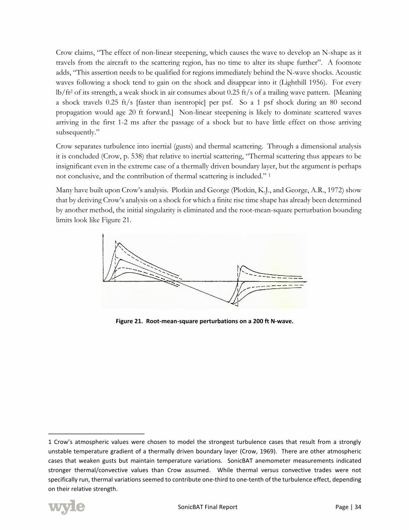
SonicBAT Final Report Page | 34
Crow claims, “The effect of non-linear steepening, which causes the wave to develop an N-shape as it
travels from the aircraft to the scattering region, has no time to alter its shape further”. A footnote
adds, “This assertion needs to be qualified for regions immediately behind the N-wave shocks. Acoustic
waves following a shock tend to gain on the shock and disappear into it (Lighthill 1956). For every
lb/ft2 of its strength, a weak shock in air consumes about 0.25 ft/s of a trailing wave pattern. [Meaning
a shock travels 0.25 ft/s [faster than isentropic] per psf. So a 1 psf shock during an 80 second
propagation would age 20 ft forward.] Non-linear steepening is likely to dominate scattered waves
arriving in the first 1-2 ms after the passage of a shock but to have little effect on those arriving
subsequently.”
Crow separates turbulence into inertial (gusts) and thermal scattering. Through a dimensional analysis
it is concluded (Crow, p. 538) that relative to inertial scattering, “Thermal scattering thus appears to be
insignificant even in the extreme case of a thermally driven boundary layer, but the argument is perhaps
not conclusive, and the contribution of thermal scattering is included.” 1
Many have built upon Crow’s analysis. Plotkin and George (Plotkin, K.J., and George, A.R., 1972) show
that by deriving Crow’s analysis on a shock for which a finite rise time shape has already been determined
by another method, the initial singularity is eliminated and the root-mean-square perturbation bounding
limits look like Figure 21.
Figure 21. Root-mean-square perturbations on a 200 ft N-wave.
1 Crow’s atmospheric values were chosen to model the strongest turbulence cases that result from a strongly
unstable temperature gradient of a thermally driven boundary layer (Crow, 1969). There are other atmospheric
cases that weaken gusts but maintain temperature variations. SonicBAT anemometer measurements indicated
stronger thermal/convective values than Crow assumed. While thermal versus convective trades were not
specifically run, thermal variations seemed to contribute one-third to one-tenth of the turbulence effect, depending
on their relative strength.
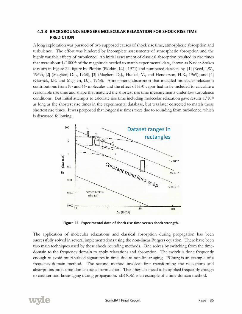
SonicBAT Final Report Page | 35
4.1.3 BACKGROUND: BURGERS MOLECULAR RELAXATION FOR SHOCK RISE TIME PREDICTION
A long exploration was pursued of two supposed causes of shock rise time, atmospheric absorption and
turbulence. The effort was hindered by incomplete assessments of atmospheric absorption and the
highly variable effects of turbulence. An initial assessment of classical absorption resulted in rise times
that were about 1/1000th of the magnitude needed to match experimental data, shown as Navier-Stokes
(dry air) in Figure 22; figure by Plotkin (Plotkin, K.J., 1971) and numbered datasets by [1] (Reed, J.W.,
1969), [2] (Maglieri, D.J., 1968), [3] (Maglieri, D.J., Huckel, V., and Henderson, H.R., 1969), and [4]
(Garrick, I.E. and Maglieri, D.J., 1968). Atmospheric absorption that included molecular relaxation
contributions from N2 and O2 molecules and the effect of H20 vapor had to be included to calculate a
reasonable rise time and shape that matched the shortest rise time measurements under low turbulence
conditions. But initial attempts to calculate rise time including molecular relaxation gave results 1/10th
as long as the shortest rise times in the experimental database, but was later corrected to match those
shortest rise times. It was proposed that longer rise times were due to rounding from turbulence, which
is discussed following.
Figure 22. Experimental data of shock rise time versus shock strength.
The application of molecular relaxations and classical absorption during propagation has been
successfully solved in several implementations using the non-linear Burgers equation. There have been
two main techniques used by these shock rounding methods. One solves by switching from the time-
domain to the frequency domain to apply relaxations and absorption. The switch is done frequently
enough to avoid multi-valued signatures in time, due to non-linear aging. PCburg is an example of a
frequency-domain method. The second method involves first transforming the relaxations and
absorptions into a time-domain based formulation. Then they also need to be applied frequently enough
to counter non-linear aging during propagation. sBOOM is an example of a time-domain method.

SonicBAT Final Report Page | 36
4.1.4 BACKGROUND: TURBULENCE APPLICATIONS OF CLASSICAL METHODS SINCE 2000
Turbulent applications of classical methods have extended the theory and applications in new ways.
Generally these applications have leveraged the large increases in available computing power.
Computing power increases have enabled new ways of using existing techniques that were not practical
previously. The classical formulation of linear geometrical acoustics is well established. Acoustic rays
are traced through each turbulent field desired. The turbulent field definition has evolved over time. It
is always considered to be invariant (frozen) throughout its transit by a sonic boom. The turbulent field
definition has evolved with time and increasing computational capabilities. Works from 2002 and 2008
were limited to 2-D fields with Fourier distributions of energy spectra based on both Gaussian and von
Karman distributions. More recent works with numerical methods and classical ray tracing are using 3-
D fields and von Karman distributions (which follows a Kolmogorov distribution up to the maximum
𝐿0 scale size), which are more representative of real turbulence as shown by the spectra comparison in
Figure 23 (Luquet, D., 2016), and the resulting turbulent flow field difference is illustrated in Figure 24
(Luquet, D., 2016.) The larger scale range is especially apparent in the smaller turbulent structures of
the von Karman distribution.
Figure 23. von Karman turbulence spectra act more like real Kolmogorov turbulence spectra than a Gaussian distribution. Three turbulent spectra: von Kármán,
Gaussian, and Kolmogorov.
Recent publications of ray tracing analyses tend to be done with more rays, smaller time steps, etc. due
to the faster computing available. Today, linear acoustic tracing of hundreds of rays can be done in
seconds on even a single processor with codes like PCBoom. Adding Burgers non-linear rounding to
the propagation increases calculation time (about 4 orders-of-magnitude) to 4 minutes per ray.
However, running with small step sizes and many points until a tightly converged answer is reached can
take hours instead of minutes. So execution time and convergence efficiency are important when adding
absorption to ray tracings for statistical results on cases like turbulence. Atmospheric modeling always
uses a single homogeneous turbulence layer (homogenous turbulence means that the turbulent mode
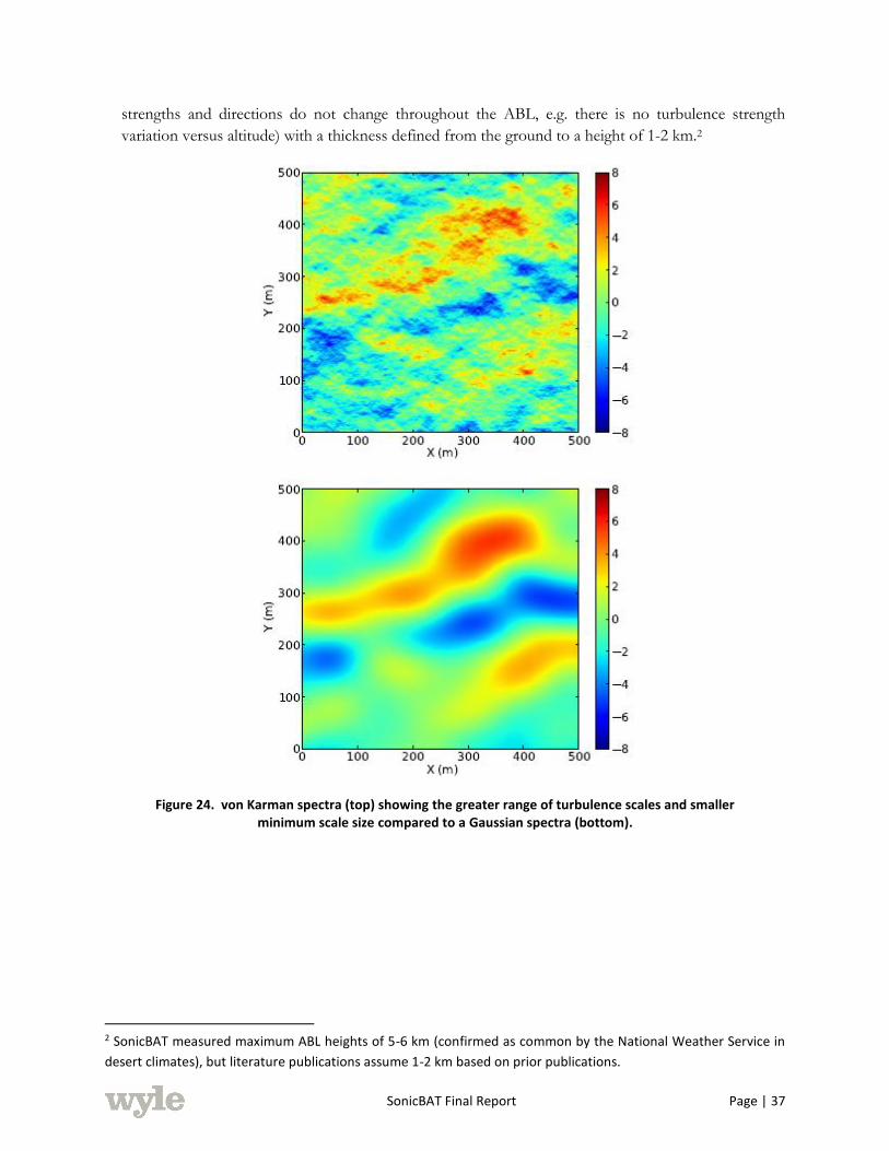
SonicBAT Final Report Page | 37
strengths and directions do not change throughout the ABL, e.g. there is no turbulence strength
variation versus altitude) with a thickness defined from the ground to a height of 1-2 km.2
Figure 24. von Karman spectra (top) showing the greater range of turbulence scales and smaller minimum scale size compared to a Gaussian spectra (bottom).
2 SonicBAT measured maximum ABL heights of 5-6 km (confirmed as common by the National Weather Service in
desert climates), but literature publications assume 1-2 km based on prior publications.

SonicBAT Final Report Page | 38
4.1.4.1 BACKGROUND: CLASSICAL METHOD POTENTIAL FOR SHADOW ZONE PREDICTION
An additional ray tracing application has been developed for shadow zone sonic boom (Lam, Y.W.,
2009.) While this capability is not implemented in the classical method, the existing methodology could
be extended to generate similar predictions. A shortcoming of linear acoustic ray tracing has been its
inability to determine sonic boom diffraction and scattering into shadow zones, like just beyond the
edge of the carpet or for flight barely below the Mach cutoff speed. Evanescent waves diffracted into
such a region have reduced high frequency content and attenuate in amplitude more quickly with
distance than sonic booms, so their noise may start -20 PLdB or more quieter and attenuate another -
20 PLdB in less than half a kilometer. In a turbulent atmosphere, significant sound energy can be
scattered into shadow zones. A ray tracing model was modified analytically into a scattered ray model.
Rays are first diffracted from a shadow boundary (at primary carpet edges and at cut-off Mach boundary)
determined by geometrical ray paths. The diffracted rays are then scattered by turbulence on their way
to the receiver. This turbulence scattered ray model is shown to have good accuracy against calculations
based on the parabolic equation and against previously published measured data. It was found that the
agreement is good both with and without turbulence, at a distance up to 2 km from the shadow
boundary.
4.1.4.2 BACKGROUND: CLASSICAL METHOD POTENTIAL FOR PROPAGATION THROUGH CLOUDS
Figure 25. Cloud absorption analysis possible with classical methodology.
The SonicBAT program did not address sonic boom propagation through clouds and tried to reduce
measurements of sonic boom propagation through clouds. (Pictures of the sky were taken during the
KSC measurements to document cloud cover.) Likewise, propagation prediction through clouds was
not implemented in the classical method and is not part of PCBoom. But a cloud propagation method
could be easily integrated like the sBOOM code that has been integrated for Burgers propagation. An
analysis of propagation through clouds (Baudoin, M., Coulouvrat, F. and Thomas, J.L., 2006) was
updated (Baudoin, M., Coulouvrat, F. and Thomas, J.L., 2011). The earlier work says, “as clouds cover
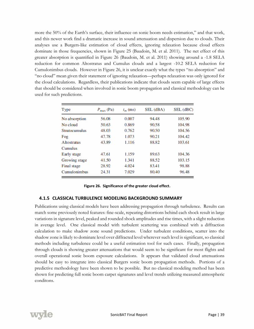
SonicBAT Final Report Page | 39
more the 50% of the Earth’s surface, their influence on sonic boom needs estimation,” and that work,
and this newer work find a dramatic increase in sound attenuation and dispersion due to clouds. Their
analyses use a Burgers-like estimation of cloud effects, ignoring relaxation because cloud effects
dominate in those frequencies, shown in Figure 25 (Baudoin, M. et al. 2011). The net effect of this
greater absorption is quantified in Figure 26 (Baudoin, M. et al. 2011) showing around a -1.8 SELA
reduction for common Altostratus and Cumulus clouds and a largest -10.2 SELA reduction for
Cumulonimbus clouds. However in Figure 26, it is unclear exactly what the types “no absorption” and
“no cloud” mean given their statement of ignoring relaxation—perhaps relaxation was only ignored for
the cloud calculations. Regardless, their publications indicate that clouds seem capable of large effects
that should be considered when involved in sonic boom propagation and classical methodology can be
used for such predictions.
Figure 26. Significance of the greater cloud effect.
4.1.5 CLASSICAL TURBULENCE MODELING BACKGROUND SUMMARY
Publications using classical models have been addressing propagation through turbulence. Results can
match some previously noted features: fine-scale, repeating distortions behind each shock result in large
variations in signature level, peaked and rounded shock amplitudes and rise times, with a slight reduction
in average level. One classical model with turbulent scattering was combined with a diffraction
calculation to make shadow zone sound predictions. Under turbulent conditions, scatter into the
shadow zone is likely to dominate level over diffracted level wherever such level is significant, so classical
methods including turbulence could be a useful estimation tool for such cases. Finally, propagation
through clouds is showing greater attenuations that would seem to be significant for most flights and
overall operational sonic boom exposure calculations. It appears that validated cloud attenuations
should be easy to integrate into classical Burgers sonic boom propagation methods. Portions of a
predictive methodology have been shown to be possible. But no classical modeling method has been
shown for predicting full sonic boom carpet signatures and level trends utilizing measured atmospheric
conditons.
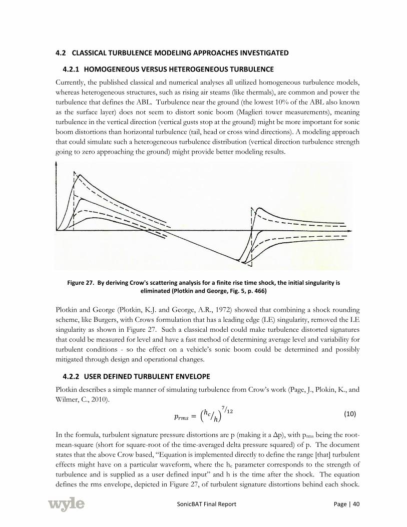
SonicBAT Final Report Page | 40
4.2 CLASSICAL TURBULENCE MODELING APPROACHES INVESTIGATED
4.2.1 HOMOGENEOUS VERSUS HETEROGENEOUS TURBULENCE
Currently, the published classical and numerical analyses all utilized homogeneous turbulence models,
whereas heterogeneous structures, such as rising air steams (like thermals), are common and power the
turbulence that defines the ABL. Turbulence near the ground (the lowest 10% of the ABL also known
as the surface layer) does not seem to distort sonic boom (Maglieri tower measurements), meaning
turbulence in the vertical direction (vertical gusts stop at the ground) might be more important for sonic
boom distortions than horizontal turbulence (tail, head or cross wind directions). A modeling approach
that could simulate such a heterogeneous turbulence distribution (vertical direction turbulence strength
going to zero approaching the ground) might provide better modeling results.
Figure 27. By deriving Crow's scattering analysis for a finite rise time shock, the initial singularity is eliminated (Plotkin and George, Fig. 5, p. 466)
Plotkin and George (Plotkin, K.J. and George, A.R., 1972) showed that combining a shock rounding
scheme, like Burgers, with Crows formulation that has a leading edge (LE) singularity, removed the LE
singularity as shown in Figure 27. Such a classical model could make turbulence distorted signatures
that could be measured for level and have a fast method of determining average level and variability for
turbulent conditions - so the effect on a vehicle’s sonic boom could be determined and possibly
mitigated through design and operational changes.
4.2.2 USER DEFINED TURBULENT ENVELOPE
Plotkin describes a simple manner of simulating turbulence from Crow’s work (Page, J., Plokin, K., and
Wilmer, C., 2010).
𝑝𝑟𝑚𝑠 = (ℎ𝑐
ℎ⁄ )
712⁄
(10)
In the formula, turbulent signature pressure distortions are p (making it a Δp), with prms being the root-
mean-square (short for square-root of the time-averaged delta pressure squared) of p. The document
states that the above Crow based, “Equation is implemented directly to define the range [that] turbulent
effects might have on a particular waveform, where the hc parameter corresponds to the strength of
turbulence and is supplied as a user defined input” and h is the time after the shock. The equation
defines the rms envelope, depicted in Figure 27, of turbulent signature distortions behind each shock.

SonicBAT Final Report Page | 41
Results from the Numerical KZK code and the SonicBAT flight test database could be used to correlate
the hc parameter with atmospheric turbulence measurements. Such work would have needed the KZK
and flight testing to be completed first, so scheduling the work for completion before the end of the
program would be difficult. But mostly, such a method would do little to advance modeling of the
important processes in a simplified, but sufficiently accurate, model that leverages advances in
computing. Since classical turbulence is based upon Crow’s work, advancing classical turbulence
modeling by building upon Crow’s work seemed like a promising approach.
4.2.3 ADVANCING CLASSICAL TURBULENCE VERSUS NUMERICAL METHODS
One approach would be to perform a modified-linear or Burgers theory propagation through a
simulation of turbulence. Such a method is a simplified numerical propagation method. A step up from
the modified-linear theory already used for useful predictions of sonic boom through temperature
variations and winds, without turbulence. At the other end of the spectrum, our KZK numerical
method does fully non-linear propagation, plus absorption rounding, plus refraction/diffraction and
their interactions. PCBoom approximates focal zone diffraction effects by scaling a Gill-Seebass
diffraction solution into useful estimates of focused signatures. Numerical analyses and work by Pierce
& Maglieri and Pierce (Figure 28) visualized that crossing and folding of waves leads to local focusing
that causes peaked and rounded waveforms, depending on positioning. So turbulent refraction is clearly
important, while diffraction and interactions may also be important. We can get confirmation of
important results from full numerical simulations, but they are too cumbersome and computationally
expensive to be used as casually as PCBoom. A simplified tool would be complementary. Ideally, such
a tool could run exact flight conditions, including balloon mean winds, temp and humidity and
turbulence measurements.
Figure 28. Crossing and folding of waves leading to rounding and local focusing.
4.2.4 MODIFIED-LINEAR THEORY TURBULENT PARABOLOID
With the advantage of PC computing capability in the year 2015, simulations of Crow’s work were
carried out with modified-linear acoustic theory. Atmospheric turbulence was simulated by random
Fourier modes of homogeneous turbulence following a von Karman implementation of a Kolmogorov
spectral distribution (described in more detail in Section 4.3). The domain size of the problem was
chosen by selecting a time limit for resolving turbulent distortions behind each shock. The time limit
SonicBAT Final Report Page | 42
selected the size of a (Crow’s) paraboloid domain from which distortions could originate. When running
simulations, it was repeatedly apparent that the domain was far greater than the distance from which
folded and crossed wavefronts were coming. The paraboloid ray tubes that hit a point on the ground
would be a very small portion of the paraboloid and they could arrive with greater time delay than the
specified duration limit of the paraboloid. The reason is apparent in the multi-folded wavefront of
Figure 28 and from plotting the ray propagation paths through turbulence. The rays are not “singly
perturbed” during propagation. The biggest perturbations come from the longest modes which are
spread over long distances instead of being concentrated into small discrete turbules. Numerical flow
visualizations from Penn State, JAXA and others show that turbulent distortions rise, fall and change
throughout propagation.
This paraboloid implementation in early versions of the classical method, required many thousands of
propagations for every output signature point calculated. This was slow to develop, test and run due to
run times of hours. To get usable results, the “shotgun” of ray intersections had to do more than hit
the desired ground location, it needed to hit close enough to the center to miss edge spreading. Edge
spreading reduces the overall amplitude calculated by superposition. A more efficient use of ray
propagation calculations was needed.
4.3 IMPLEMENTED CLASSICAL TURBULENCE MODELING APPROACH
4.3.1 ATMOSPHERIC MODELING
The atmospheric modeling of the final code, named TURBO, has typical features found in other codes,
with some implementation differences. The program is formulated in Cartesian coordinates. Like
others, it uses frozen Fourier modes of different lengths and random directions to model the turbulence
with a von Karman implementation of a Kolmogorov distribution and Log spacing of mode lengths. In
the method of Random Fourier Modes of Blanc-Benon et al. (Chevret et al., 1996; Blanc-Benon et al.,
2002) the vector modes have a random velocity direction and a random direction of variation that is
normal to the direction of the velocity in Figure 29. Shock rays are most bent by a mode when traveling
in the direction of the variation, which is normal to the mode velocity. If traveling normal to the velocity
but not in the direction of the variation, the mode becomes effectively longer (and thereby weaker in
gradient) until its effective mode length becomes infinite (and zero in gradient strength) when the ray is
traveling normal to the variation and velocity, the direction of no variation shown in Figure 29. In
TURBO every velocity mode has variations in both directions normal to the velocity, Figure 30. Mode
velocities vary in a 2-D square lattice in an alternating checker pattern. Gradients are created in two
dimensions by each mode, each with their own random phase and normal to the random direction of
the mode velocity.
Since there are 2 directions of variation, there is the possibility to vary the turbulence strength 50/50%
in each direction or with a random strength in each direction from 50/50% to 25/75%. This allows an
easy implementation of another degree of randomness. The turbulence strength can vary the same
(50%/50%, by using an input file variable named IRAND equal to either= 0 or 1) in both directions or
it can be randomly apportioned (from 25%/75% to 75%/25% by using IRAND equal to either 2 or 3)
with different strength variations. Even IRAND values of 0 or 2 cause the phase origin of all Z-direction
modes to be located at the top of the ABLH, making the onset of turbulence continuous with the
atmosphere above the ABL, while odd IRAND values provide a random Z phase for each mode like
the random X and Y phase in all cases. Testing seemed to favor using a randomly apportioned (IRAND

SonicBAT Final Report Page | 43
2 or 3) turbulence variation while even and odd IRAND values did not seem to make a noticeable
difference.
Figure 29. Random Fourier Modes vector modes have a random velocity direction and a random direction of variation that is normal to the direction of the velocity.
Figure 30. TURBO vector modes have variations in both directions normal to the velocity.
The model generation is based on several input turbulence parameters, namely: minimum scale length
(FLMIN), maximum scale length (FLMAX) and the number of modes NLMAX, spaced in constant
logarithmic steps. Plus, there is an optional parameter, NLMAXMORE, to allow the representation of
larger scales than FLMAX (L0 commonly), the mode of maximum strength by definition. Modes from

SonicBAT Final Report Page | 44
NLMAX+1 to NLMAXMORE can be significant but have diminishing strength according to the von
Karman spectrum equations of Cotte and Blanc-Benon. Structure parameters CT2 and CV
2 are input for
the strength of the turbulence at two altitudes (chosen for initial testing, but could be expanded) allowing
a Log variation in turbulence strength versus altitude.
This use of component breakdown of the turbulence distribution and strength was intended to provide
more accurate mode length representation (because of variation in 2-dimensions, instead of only one)
and to help with execution speed by reducing use of transcendental function calculations (more in
section 7.2.2.1). No comparisons have been made with other turbulence modeling computational
schemes. The implementation seems to work efficiently and code loops were written to be amenable
to future parallel execution.
4.3.2 CLASSICAL PROPAGATION MODELING
The integrated forms of the Fourier modes are used to get average turning gradients and displacements
over the chosen time step. The scheme will accurately calculate non-turbulent propagation to the
ground with step sizes as large as 10 seconds. But turbulent propagation is much more demanding,
requiring step sizes of 0.1 to 0.01 seconds. While many calculate only turning of rays, since it is much
more important over large distances, TURBO currently calculates both ray turning and displacement.
Propagation steps are calculated as circular arcs from integration of the Fourier gradents. While more
computationally expensive, it also allows mean wind displacements and turning to be assessed at the
same time. The turbulent displacement calculations can be easily disabled for future testing of whether
the accuracy improvement is worth the speed loss. The code also checks the convergence on every step
and iterates based on an error estimate multiplied by height, since ray turning accuracy at larger distances
has a much larger effect on final position. These iterations may not provide efficient accuracy
improvements, so future optimization studies could investigate their value versus smaller step sizes. All
program features were initially arranged for greatest accuracy with opportunities for future speed
improvement. The whole propagation scheme was programmed with future implementation of parallel
processing in mind, though none is implemented.
For each signature azimuth, PHI, where a turbulent assessment is requested, a PCBoom input file or
<arg1>.age file is read to get the mean atmospheric conditions of temperature, X-winds and Y-winds
as a function of altitude above sea level (from any PCBoom atmospheric input format, such as a balloon
file). PCBoom output is read for mean atmosphere ground intercept location, time and signature
information, and for ray starting location, vector direction and time at the top of the ABL. The classical
turbulence propagation must handle temperature and X, Y, Z winds and all their cross-derivatives in 3-
D, so there are many more evaluations than PCBoom’s Temp, X and Y derivatives only in the Z
direction. And the turbulent gradients are stronger and faster changing than mean conditions, excepting
strong wind sheers. Mean variations are calculated and simply added with turbulent variations in
summation, making their accommodation inexpensive. Propagation validation checks began with a
simple Mach cut-off case from 36,000 ft in a standard atmosphere without turbulence. TURBO
matches PCBoom’s trajectories and ground intersection location within feet from near-tangent ray-
ground intersection angles at Mach 1.154 using step sizes of up to 10 seconds. This is an especially
sensitive comparison because very small differences in the propagation ∂w gradient calculation lead to
large ground intersection changes.
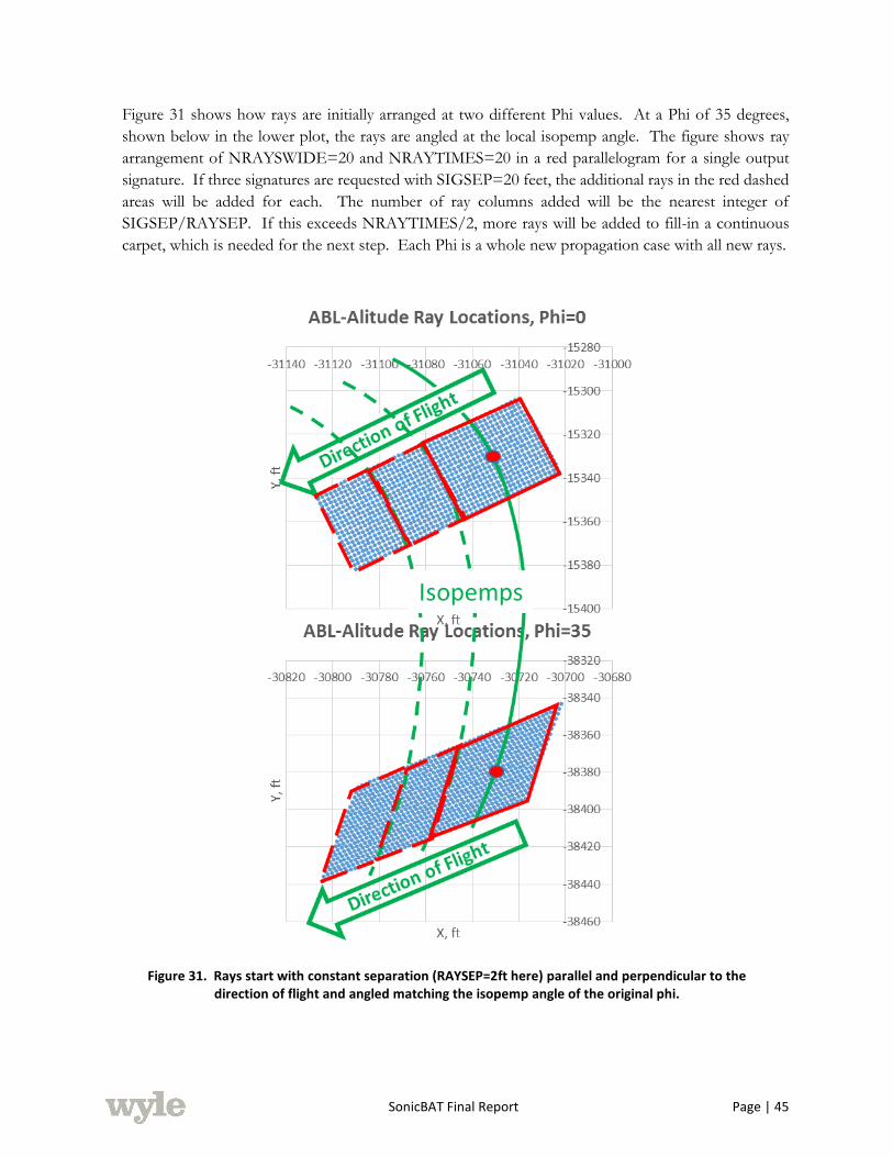
SonicBAT Final Report Page | 45
Figure 31 shows how rays are initially arranged at two different Phi values. At a Phi of 35 degrees,
shown below in the lower plot, the rays are angled at the local isopemp angle. The figure shows ray
arrangement of NRAYSWIDE=20 and NRAYTIMES=20 in a red parallelogram for a single output
signature. If three signatures are requested with SIGSEP=20 feet, the additional rays in the red dashed
areas will be added for each. The number of ray columns added will be the nearest integer of
SIGSEP/RAYSEP. If this exceeds NRAYTIMES/2, more rays will be added to fill-in a continuous
carpet, which is needed for the next step. Each Phi is a whole new propagation case with all new rays.
Figure 31. Rays start with constant separation (RAYSEP=2ft here) parallel and perpendicular to the direction of flight and angled matching the isopemp angle of the original phi.
SonicBAT Final Report Page | 46
4.3.3 CLASSICAL GROUND INTERSECTION AND SIGNATURE INTEGRATION
Ray propagation continues until the Z of the ground is crossed or a generous time step limit is reached.
The exact ray-ground intersection is then calculated between the last two steps. After all ray
propagations are complete, each ray tube is checked for intersections with all the NSIGTIMES
requested at this Phi. A key feature of the final code is ray carpet repeating. The rays are initially
arranged as parallelograms because duplicate ray carpets will be assumed to exist in all directions around
the one calculated. If a ray propagates beyond the left boundary of the current carpet, its effect will be
simulated by effectively duplicating the calculated carpet to the right of itself and now calculating the
effect of the ray that went beyond the left boundary. If turbulence redirects the whole ray carpet to
miss the requested signature points, the calculated carpet will be duplicated enough times until it falls
onto the requested signature points. Ray tubes stretched very wide or long will intersect the same
signature location more than once if they stretch across more than one carpet width and/or length.
With this logic, a many times greater fraction of the ray propagations get used and signature locations
are not missed due to turbulence redirection and ground intersection relocation.
At the ground, ray tubes are cut into triangles when resolving intersections to increase resolution and
better resolve quadrilaterals that get folded over upon themselves. Triangle cuts are done between the
closer corners, before turbulence (shown in Section 7.2.2.3, Figure 115, as blue lines). There is also an
option for cutting the triangles both ways and averaging the results (KTri = 2 instead of 1). More
application descriptions are provided in Section 7.2.2.3.
4.3.4 CLASSICAL OUTPUTS
Signature output is provided at any PHI interpolated from the input data provided from PCBoom and
sBOOM. PCBoom provides ray directional information at the top of the ABL and zero-turbulence
ground intersection location, timing, amplitude and aging at the ground, required to set-up the turbulent
simulation. Individual turbulence distorted signatures are calculated from the superposition of rays in
space and time. Ray tubes are initially arranged in regular parallelograms for ease in distinguishing
between time steps and phi steps. For superposition, they are cut into triangles for greater resolution
per ray calculation, along the corners that were closer before turbulence. Triangles can also be cut in
both directions (corners 1-3 and 2-4) with the result averaged, for testing of whether it provides better
resolution.
Multiple output time instances (like a ground microphone array) are easily requested (NSIGTIMES) to
explicitly calculate statistical variations from a large number of signatures in a more efficient manner.
The multiple signatures at each PHI can be resolved from fewer grid cells. Another possibility is to use
the whole grid of rays to provide statistical data even more efficiently. While untried and unproven,
there are indications from the program output that this could work accurately with a couple orders-of-
magnitude greater efficiency.
4.3.5 CLASSICAL METHOD SUMMARY
A classical method for propagation through turbulence was developed by performing many ray
propagations through a simulation of atmospheric turbulence. The code intends to perform simplified
propagations with near full computational accuracy in a much shorter run time. Already the code
calculates propagations through a von Karman distribution of turbulence with a possible variation in
turbulence strength with height and full mean atmospheric temperature and winds. Prediction

SonicBAT Final Report Page | 47
comparisons with flight test (Sections 7.2 and 8.2) indicate that the code is at least partially modeling
the important physics needed for predicting turbulence effects and trends. Predictions of low boom
shaped signatures (Section 9.2) have identified reduced shaped signature levels in dry air (relative to N-
waves) and indicate that shaping interacts with turbulence. Since different shaped signatures perform
differently in turbulence, there may be possible improved shapes and optimizations that result in quieter
signatures. There are also some results that need further review and results that indicate possible ways
to improve the code’s efficiency and accuracy.
SonicBAT Final Report Page | 48
5.0
SONIC BOOM RESEARCH FLIGHT TESTS
This section documents the research flight tests conducted at NASA’s Armstrong Flight Research
Center and Kennedy Space Center to collect acoustic and meteorological measurements as part of the
SonicBAT project. Described are the objectives of the data collection efforts followed by the specifics
of each measurement campaign. This section concludes with a descriptive examples of the data
acquired.
5.1 OBJECTIVES
The objective of the SonicBAT research program is to validate, via flight test measurements, models for
sonic boom signatures propagating through a turbulent atmosphere. This experiment required precision
flight of an F-18 to create sonic booms at known locations and times. The maneuvers were designed
to be replicated at the different measurement locations. The objective was to measure boom
propagation through a hot, dry atmosphere, and a hot, wet atmosphere.
The research flight tests were designed to capture concurrent F-18 onboard flight data instrumentation,
high fidelity air and ground-based acoustic data and surface and upper air meteorological measurements.
At AFRC the primary acoustic instrumentation array was located so that it would be in line with the
flight track. This was done so that it would receive sound that emanated from underneath the aircraft.
Secondary and tertiary arrays were deployed in order to measure booms that propagated through more
atmosphere. At KSC the flight operations were over the Atlantic Ocean, near the Florida coast, on a
nominal heading of approximately 164 degrees. Two measurement arrays were deployed with the
primary array more laterally displaced from the flight track than the secondary array. The atmospheric
profile recorded during the KSC flights was used to position the aircraft’s flight track as close to the
arrays as possible without placing the nearby villages on the Florida mainland inside the sonic boom
footprint as determined by PCBoom. The flight parameters for both measurement campaigns were
made so that the angle of elevation of the sound ray at the microphones was at least 20 degrees. This
was done to minimize grazing ground effects.
5.2 NASA ARMSTRONG FLIGHT RESEARCH CENTER MEASUREMENT PROGRAM
The first field campaign for the SonicBAT project occurred at and around NASA AFRC. Located on
Edwards Air Force Base property, the northern portion of the NASA AFRC property shown in Figure
32 is on the edge of Rogers Dry Lake and was ideal for measurement of sonic booms propagating
through a hot, dry atmosphere. Three types of data were acquired during the measurements that
occurred 11 – 22 July 2016: acoustic data from three microphone arrays on the ground and a
microphone attached to a TG-14 motorized sailplane; meteorological data from GPSsonde balloon
launches, weather towers on the ground, and two ultrasonic anemometers mounted on 10 m and 44 m
towers; and aircraft data from the F-18 and TG-14. This section details the measurements and data
acquired.

SonicBAT Final Report Page | 49
Figure 32. NASA AFRC area near Edwards Air Force Base. Red lines are boundaries of the supersonic corridor.
5.2.1 ACOUSTICS
Three arrays of microphones were deployed as well as a microphone on the motorized sailplane. The
motorized sailplane was a TG-14 and operated by NASA Armstrong pilots. The plan was for the
sailplane to position itself in such a way as to intersect the sound rays traveling from the F-18 to the
primary array. The arrays were deployed on the North end of NASA AFRC and beyond on Edwards’
property as shown in Figure 33.
Figure 33. Microphone array locations.
The TG-14 was equipped with a microphone mounted on its wingtip as shown in Figure 34.
Throughout this report, acoustic recordings are referred to by the measurement campaign and
microphone number. Recordings made by the TG-14’s microphone are referred to as channel 0 where
channel is synonymous with position. For the measurements made at NASA AFRC (this campaign)
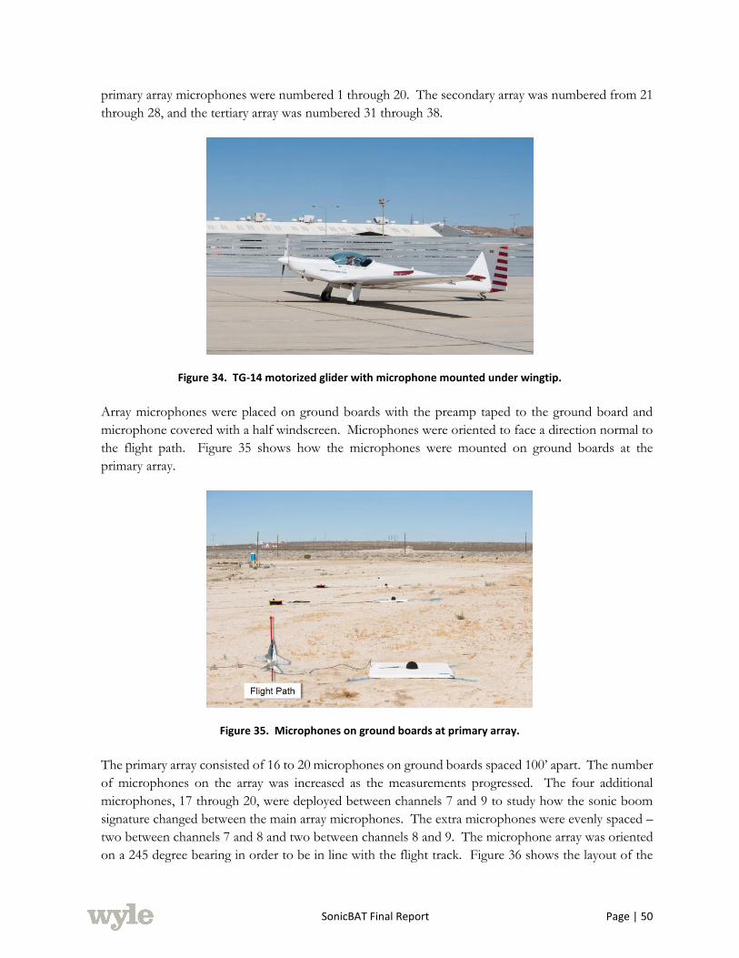
SonicBAT Final Report Page | 50
primary array microphones were numbered 1 through 20. The secondary array was numbered from 21
through 28, and the tertiary array was numbered 31 through 38.
Figure 34. TG-14 motorized glider with microphone mounted under wingtip.
Array microphones were placed on ground boards with the preamp taped to the ground board and
microphone covered with a half windscreen. Microphones were oriented to face a direction normal to
the flight path. Figure 35 shows how the microphones were mounted on ground boards at the
primary array.
Figure 35. Microphones on ground boards at primary array.
The primary array consisted of 16 to 20 microphones on ground boards spaced 100’ apart. The number
of microphones on the array was increased as the measurements progressed. The four additional
microphones, 17 through 20, were deployed between channels 7 and 9 to study how the sonic boom
signature changed between the main array microphones. The extra microphones were evenly spaced –
two between channels 7 and 8 and two between channels 8 and 9. The microphone array was oriented
on a 245 degree bearing in order to be in line with the flight track. Figure 36 shows the layout of the
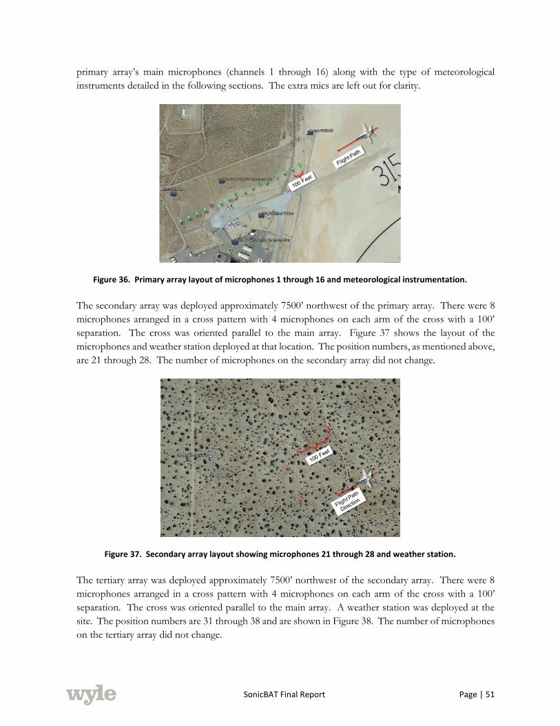
SonicBAT Final Report Page | 51
primary array’s main microphones (channels 1 through 16) along with the type of meteorological
instruments detailed in the following sections. The extra mics are left out for clarity.
Figure 36. Primary array layout of microphones 1 through 16 and meteorological instrumentation.
The secondary array was deployed approximately 7500’ northwest of the primary array. There were 8
microphones arranged in a cross pattern with 4 microphones on each arm of the cross with a 100’
separation. The cross was oriented parallel to the main array. Figure 37 shows the layout of the
microphones and weather station deployed at that location. The position numbers, as mentioned above,
are 21 through 28. The number of microphones on the secondary array did not change.
Figure 37. Secondary array layout showing microphones 21 through 28 and weather station.
The tertiary array was deployed approximately 7500’ northwest of the secondary array. There were 8
microphones arranged in a cross pattern with 4 microphones on each arm of the cross with a 100’
separation. The cross was oriented parallel to the main array. A weather station was deployed at the
site. The position numbers are 31 through 38 and are shown in Figure 38. The number of microphones
on the tertiary array did not change.

SonicBAT Final Report Page | 52
Figure 38. Tertiary array layout showing microphones 31 through 38 and weather station.
Numerous equipment was used to conduct this measurement. These are listed in the digital archive
prepared to store the acoustic and meteorological data for the research flight tests. All microphones
were 1/2" diameter, infrasonic microphones. Their type is detailed in the aforementioned archive along
with all serial numbers and connections. The different data recorders used by the organizations all had
24-bit A/D resolution; however, different recorders had different sampling rates. The data recorder in
the TG-14 motorized glider sampled the microphone signal at 65536 samples per second; whereas, all
other data records utilized a sample rate of 51200 samples per second. The data recorder used at the
primary array is based on equipment sold by National Instruments. The unit was based on hardware in
the PXI chassis shown in Figure 39. The coordinates of all array microphones are listed in Table 5.
Figure 39. PXI chassis containing data acquisition hardware used at primary array for AFRC test.
The timing of data recordings was accomplished in one of two ways: recording an IRIG-B time code
was done on the TG-14 and at the primary array; the time at the beginning of each recording on the
secondary and tertiary arrays was captured from a GPS unit attached to the data recorder. The first
allowed for determining the time throughout the recording by analyzing the IRIG-B signal while the

SonicBAT Final Report Page | 53
second used the sampling rate along with the start time of the recording to calculate the time of each
sample in the file. The log file on the recordings indicates when data drop outs occurred.
Table 5. Microphone coordinates (ref. WGS 84 Ellipsoid).
CH NUMBER Latitude (N) Longitude (W) Ellipsoid Ht. (ft)
TG-14
CH000 VARIABLE VARIABLE VARIABLE
PRIMARY ARRAY
CH001 34 57 36.96479 117 52 51.19354 2168
CH002 34 57 36.54674 117 52 52.28522 2170
CH003 34 57 36.12634 117 52 53.37561 2170
CH004 34 57 35.71209 117 52 54.46701 2170
CH005 34 57 35.29177 117 52 55.55494 2170
CH006 34 57 34.87407 117 52 56.64168 2171
CH007 34 57 34.45293 117 52 57.73170 2172
CH008 34 57 34.03667 117 52 58.81967 2172
CH009 34 57 33.61871 117 52 59.91124 2172
CH010 34 57 33.20112 117 53 00.99547 2172
CH011 34 57 32.78411 117-53 02.08995 2173
CH012 34 57 32.36700 117 53 03.17669 2176
CH013 34 57 31.94706 117 53 04.26537 2176
CH014 34 57 31.52753 117 53 05.35400 2177
CH015 34 57 31.11149 117 53 06.44354 2178
CH016 34 57 30.69033 117 53 07.53504 2180
CH017 34 57 34.18277 117 52 58.45079 2171
CH018 34 57 33.89788 117 52 59.18060 2172
CH019 34 57 34.31772 117 52 58.09305 2172
CH020 34 57 33.76265 117 52 59.54141 2172
SECONDARY ARRAY
CH021 34 58 33.47972 117 53 52.80564 2278
CH022 34 58 33.06398 117 53 53.89994 2283
CH023 34 58 32.64624 117 53 54.98224 2286
CH024 34 58 32.22929 117 53 56.07446 2285
CH025 34 58 31.51368 117 53 53.67689 2277
CH026 34 58 32.40816 117 53 54.18281 2281
CH027 34 58 33.30424 117 53 54.68964 2286
CH028 34 58 34.20294 117 53 55.20012 2284
TERTIARY ARRAY
CH031 34 59 44.78848 117 54 15.04280 2251
CH032 34 59 44.35768 117 54 16.16188 2252
CH033 34 59 43.91580 117 54 17.29996 2252
CH034 34 59 43.50785 117 54 18.36419 2253
CH035 34 59 42.79466 117 54 15.96304 2251
CH036 34 59 43.68704 117 54 16.44908 2251
CH037 34 59 44.58609 117 54 16.97494 2252
CH038 34 59 45.48287 117 54 17.47403 2252
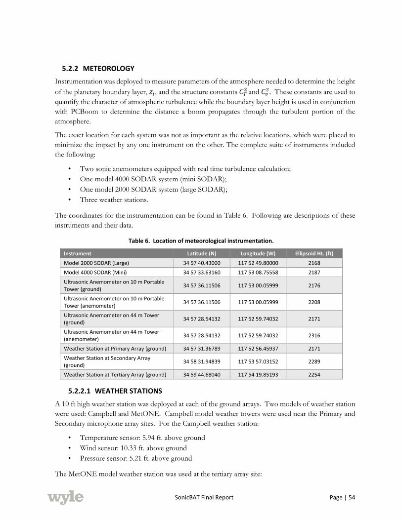
SonicBAT Final Report Page | 54
5.2.2 METEOROLOGY
Instrumentation was deployed to measure parameters of the atmosphere needed to determine the height
of the planetary boundary layer, 𝑧𝑖 , and the structure constants 𝐶𝑇2 and 𝐶𝑣
2. These constants are used to
quantify the character of atmospheric turbulence while the boundary layer height is used in conjunction
with PCBoom to determine the distance a boom propagates through the turbulent portion of the
atmosphere.
The exact location for each system was not as important as the relative locations, which were placed to
minimize the impact by any one instrument on the other. The complete suite of instruments included
the following:
• Two sonic anemometers equipped with real time turbulence calculation;
• One model 4000 SODAR system (mini SODAR);
• One model 2000 SODAR system (large SODAR);
• Three weather stations.
The coordinates for the instrumentation can be found in Table 6. Following are descriptions of these
instruments and their data.
Table 6. Location of meteorological instrumentation.
Instrument Latitude (N) Longitude (W) Ellipsoid Ht. (ft)
Model 2000 SODAR (Large) 34 57 40.43000 117 52 49.80000 2168
Model 4000 SODAR (Mini) 34 57 33.63160 117 53 08.75558 2187
Ultrasonic Anemometer on 10 m Portable Tower (ground)
34 57 36.11506 117 53 00.05999 2176
Ultrasonic Anemometer on 10 m Portable Tower (anemometer)
34 57 36.11506 117 53 00.05999 2208
Ultrasonic Anemometer on 44 m Tower (ground)
34 57 28.54132 117 52 59.74032 2171
Ultrasonic Anemometer on 44 m Tower (anemometer)
34 57 28.54132 117 52 59.74032 2316
Weather Station at Primary Array (ground) 34 57 31.36789 117 52 56.45937 2171
Weather Station at Secondary Array (ground)
34 58 31.94839 117 53 57.03152 2289
Weather Station at Tertiary Array (ground) 34 59 44.68040 117 54 19.85193 2254
5.2.2.1 WEATHER STATIONS
A 10 ft high weather station was deployed at each of the ground arrays. Two models of weather station
were used: Campbell and MetONE. Campbell model weather towers were used near the Primary and
Secondary microphone array sites. For the Campbell weather station:
• Temperature sensor: 5.94 ft. above ground
• Wind sensor: 10.33 ft. above ground
• Pressure sensor: 5.21 ft. above ground
The MetONE model weather station was used at the tertiary array site:

SonicBAT Final Report Page | 55
• Temperature sensor: 5.94 ft. above ground
• Wind sensor: 10.33 ft. above ground
• Pressure sensor: 3.83 ft. above ground
NASA AFRC weather tower data is given in Microsoft Excel format. It includes the following
parameters in column format:
• Time, UTC
• Wind direction, degrees true
• Wind speed, knots
• Air temperature, degrees F
• Relative humidity, %
• Pressure, millibars
Each excel file has three tabs corresponding to the weather towers near the primary, secondary and
tertiary sites. Data from the NASA weather towers covers 3-15, and 18-22 July 2016. The station at
the primary array is shown in Figure 40. These weather stations collect data two times per second.
Figure 40. Weather station (in the foreground) deployed at the primary array. Ultrasonic anemometer on 10 m tower shown in background.
Weather tower data from the Earth Networks WeatherBug Edwards, CA EDDFR site is provided. Data
is in comma separated value (CSV) format for July 11-23, 2016 (Earth Networks, 2015). Note that the
wind direction in WeatherBug data is given in degrees magnetic North.
5.2.2.2 GPSsonde
Atmospheric profiles were measured with GPSsondes using weather balloons carrying an
instrumentation package as shown in Figure 41. Balloons were launched within an hour of each flight
of the F-18. Days which had more than one flight had either three or four balloon launches. The times
of the balloons launched can be found in Table 7 along with the boom arrival times on the primary
array for the first pass of each flight. The tail number of the F-18 flown for each flight is also noted in
the table. The balloon data was post processed for use in PCBoom. Also available for the AFRC test
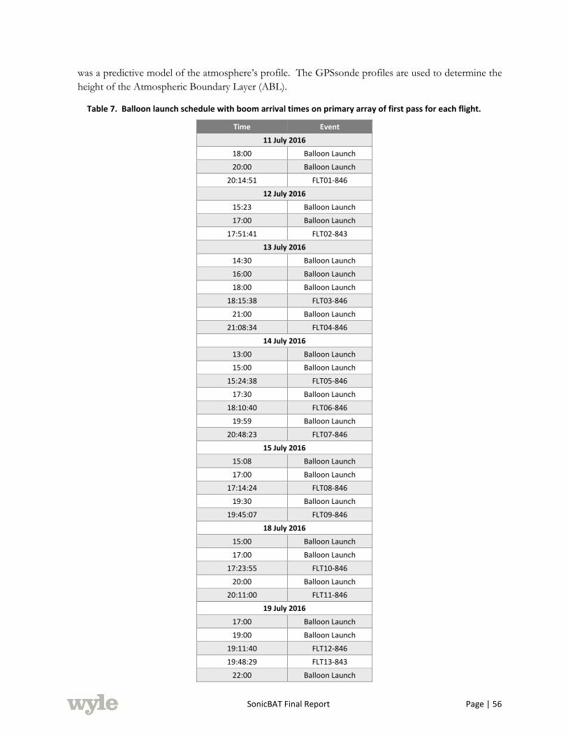
SonicBAT Final Report Page | 56
was a predictive model of the atmosphere’s profile. The GPSsonde profiles are used to determine the
height of the Atmospheric Boundary Layer (ABL).
Table 7. Balloon launch schedule with boom arrival times on primary array of first pass for each flight.
Time Event
11 July 2016
18:00 Balloon Launch
20:00 Balloon Launch
20:14:51 FLT01-846
12 July 2016
15:23 Balloon Launch
17:00 Balloon Launch
17:51:41 FLT02-843
13 July 2016
14:30 Balloon Launch
16:00 Balloon Launch
18:00 Balloon Launch
18:15:38 FLT03-846
21:00 Balloon Launch
21:08:34 FLT04-846
14 July 2016
13:00 Balloon Launch
15:00 Balloon Launch
15:24:38 FLT05-846
17:30 Balloon Launch
18:10:40 FLT06-846
19:59 Balloon Launch
20:48:23 FLT07-846
15 July 2016
15:08 Balloon Launch
17:00 Balloon Launch
17:14:24 FLT08-846
19:30 Balloon Launch
19:45:07 FLT09-846
18 July 2016
15:00 Balloon Launch
17:00 Balloon Launch
17:23:55 FLT10-846
20:00 Balloon Launch
20:11:00 FLT11-846
19 July 2016
17:00 Balloon Launch
19:00 Balloon Launch
19:11:40 FLT12-846
19:48:29 FLT13-843
22:00 Balloon Launch
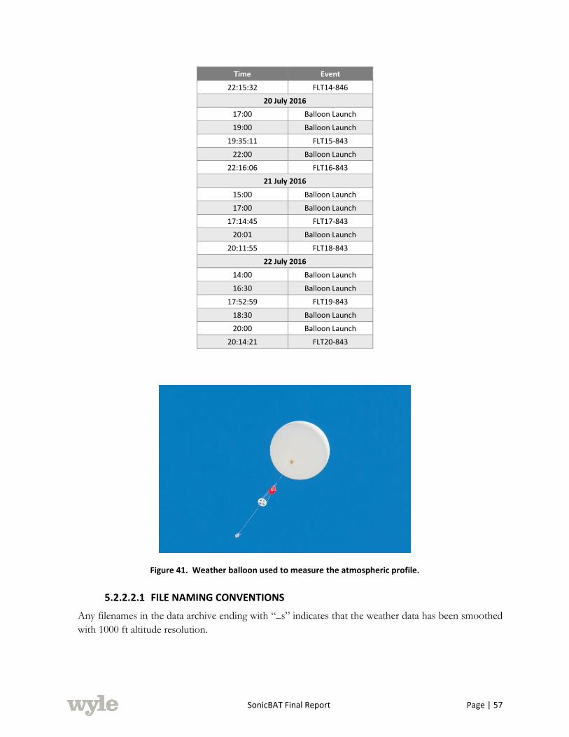
SonicBAT Final Report Page | 57
Time Event
22:15:32 FLT14-846
20 July 2016
17:00 Balloon Launch
19:00 Balloon Launch
19:35:11 FLT15-843
22:00 Balloon Launch
22:16:06 FLT16-843
21 July 2016
15:00 Balloon Launch
17:00 Balloon Launch
17:14:45 FLT17-843
20:01 Balloon Launch
20:11:55 FLT18-843
22 July 2016
14:00 Balloon Launch
16:30 Balloon Launch
17:52:59 FLT19-843
18:30 Balloon Launch
20:00 Balloon Launch
20:14:21 FLT20-843
Figure 41. Weather balloon used to measure the atmospheric profile.
5.2.2.2.1 FILE NAMING CONVENTIONS
Any filenames in the data archive ending with “_s” indicates that the weather data has been smoothed
with 1000 ft altitude resolution.

SonicBAT Final Report Page | 58
5.2.2.2.2 .DAT FORMAT
The post-processed meteorological profile data is a NASA AFRC Air Data Calibration (ADC) file. It
is nominally formatted and named as:
LLL_mmmddyy_hhmmZ_ADC.dat
LLL: Location, text string
• Typically “EDW” (Edwards, CA) for SonicBAT dataset
mmm: month, text string (ex. JUL)
dd: day of month, integer
yy: last two digits of year, integer
hh: hour, integer
mm: minute, integer
Z: Time zone, text string
• Typically “Z” (Zulu/UTC) for SonicBAT data set
For example, “EDW_JUL1116_1400Z_ADC.dat” refers to post-processed data from Edwards, CA on
July 11, 2016 at 1400Z. Each file is a nine-column atmospheric weather profile.
Row 1: Column header
Rows 2 – N:
Column 1: Geometric altitude, feet
Column 2: Pressure altitude, feet
Column 3: Temperature, degrees-Celsius
Column 4: Wind speed, knots
Column 5: Wind direction-from, degrees true
Column 6: Lateral Pressure gradient, feet/nautical mile
Column 7: Lateral Pressure gradient direction, degrees true
Column 8: Relative humidity, percentage
Column 9: Absolute humidity, gram/cubic-meter
A review of the balloon launches with respect to Air Data Calibration (ADC) can be found in Table 8.
Table 8. Air Data Calibration of upper air data GPSsonde.
Balloon Launch Time (UTC)
Analysis
11 July 2016
1800Z Initial heights at all levels appear low based on semi diurnal pressure behavior. Uncertainties of about 10 meters are observed from 19000 to 40000 feet.
2000Z Initial heights are much more aligned with semidiurnal features. Uncertainty of no more than 8 meters looks to be the rule.
Summary: No issues with winds and temperature: Winds are consistent with synoptic features and each balloon. Temperatures also fit well within synoptic pattern and each balloon. This is the case at all levels for both balloons.
12 July 2016
1523Z Heights fit both semi diurnal and synoptic structure with uncertainties of about 5 meters.
1700Z Heights fit both semi diurnal and synoptic structure with uncertainties of about 5 meters.

SonicBAT Final Report Page | 59
Balloon Launch Time (UTC)
Analysis
Summary Winds and temperatures fit very well to the synoptic structure and to the other balloon. Temps fit to within 0.3 degrees. Winds are well behaved, within 3 kt of the pattern and the other balloons.
13 July 2016
1430Z Initial heights are aligned with synoptic and semidiurnal features. Uncertainties of heights are no more than 7 meters at any altitude.
1600Z Initial heights are aligned with semidiurnal features. Worse case uncertainties of no more than 7 meters are observed at the highest altitude of 40000 ft.
1800Z Initial heights are aligned with semidiurnal features. Worse case uncertainties of no more than 5 meters are observed at any level.
2100Z Heights are upwards of 20 meters high of synoptic and semi diurnal balance. A pattern is developing where by the 20z balloons and later don't fit the synoptic and semi diurnal features.
Summary: None
14 July 2016
1300Z Heights fit both semi diurnal and synoptic structure.
1500Z Heights fit both semi diurnal and synoptic structure but the heights are slightly low by about 5 meters.
1730Z Heights look ok as compared to semi diurnal and synoptic structure. A slight deviation begins about 32000 ft. However, the heights uncertainties are only about 8 meters.
1959Z As with other late afternoon balloons, heights range from slightly above to significantly above the synoptic and semi diurnal structure. Uncertainties range from 7 meters at 25000 ft to nearly 20 meters at 40000 ft.
Summary
Winds and temperatures all fit within the semi diurnal and synoptic patterns. Temperatures appear to have a significant change after 15Z. At most levels, except at 40000 ft, a temperatures rise from 0.5 to 1.0 deg C is observed and then the temperatures remain constant to within a few tenths after. Winds are light and show a slight decrease in speed of about 5 to 10 kts over the seven-hour flight test period from 13-20Z.
15 July 2016
1508Z Heights fit both semi diurnal and synoptic structure with uncertainties of 5 meters.
1700Z Heights fit both semi diurnal and synoptic structure with uncertainties of 5 meters.
1930Z Most heights fit both the semi diurnal and synoptic structures. There is some uncertainties between 20000 and 35000 ft of about 10 meters.
Summary Winds and temperatures are very well behaved during this day. Winds are very light for this time of year. As a result of the very light winds wind directions are not organized and the directions can vary by 60 deg or more from balloon to balloon.
18 July 2016
1500Z Heights fit both semi diurnal and synoptic structure.
1700Z Heights are slightly high as compared to semi diurnal and synoptic structure at several altitude levels. Uncertainties range between 10 and 25 meters, 20000 and 35000 ft, respectively.
2000Z Heights are consistently higher than the semi diurnal and synoptic structure by 20 meters at all levels.
Summary
Winds are very consistent for this day. The wind speeds vary by only 3 kts over the course of the three balloons with directions behaving similar. Temperatures over the three balloons fluctuate more on this day than any other day. While not as I would like to see they vary between 0.4 and 1.0 degrees.
19 July 2016
1700Z Heights align well with semi diurnal and synoptic features with uncertainties in height of about 5 meters.
1900Z Heights agree fairly well to both synoptic and semi diurnal features. With uncertainties ranging about 9 meters high.

SonicBAT Final Report Page | 60
Balloon Launch Time (UTC)
Analysis
2200Z Heights are high as compared to the synoptic and semi diurnal features. Uncertainties are in the 20-25 meters range. Same issue with other later balloon with height not fitting the patterns.
Summary
Winds and temperatures all agree very well with synoptic features and each other. Temperature pattern shows a slight warming trend below 33000 feet and no change above that. Winds are unusually light at all levels with the strongest winds at the lowest levels below 24000 feet. As a result, the wind directions vary greatly as one would expect with light winds. Six kts is the largest separation of any two balloons.
20 July 2016
1700Z Heights fit both semi diurnal and synoptic structure with uncertainties of 5 meters.
1900Z Heights are a little high but fit both semi diurnal and synoptic structure with uncertainties of 6-10 meters.
2200Z As per the norm, the afternoon balloon heights are significantly higher than the semi and synoptic features. Uncertainties with theses heights range from 10 to 20 meters.
Summary
Winds for this day fit well with synoptic features and are very light. With speeds so light directions are not uniform. With the lightest winds, the direction is observed to vary by 60 degrees from balloon to balloon. The temperatures fit fairly well to the synoptic feature but there is some fluctuation from balloon to balloon. Uncertainties of the temperatures range from 0.3 to 1.4 deg C.
21 July 2016
1500Z Heights fit both semi diurnal and synoptic structure with uncertainties of 5 meters.
1700Z Heights fit both semi diurnal and synoptic structure with uncertainties of 5 meters.
2000Z As per what is becoming the norm with the late afternoon balloons, the heights are higher than the synoptic or semi diurnal features by as much as 10-25 meters.
Summary
Winds and temperatures both fit well into the synoptic pattern. Winds are generally light but consistent from one balloon to the next. As a result there is some variability in direction. Temperatures vary very little by no more than by 0.7 and this at one level. In most cases the difference is only 0.1 to 0.4 deg C.
22 July 2016
1400Z Heights fit both semi diurnal and synoptic structure but are slightly low by about 5 meters.
1630Z Heights fit both semi diurnal and synoptic structure with uncertainties of about 5 meters.
1830Z Heights are slightly higher than the semi diurnal and synoptic structure
2000Z Heights are significantly higher than both the semi diurnal and synoptic structure. Again, this balloon, like many other day 20Z balloons, is higher by 20 meters.
Summary
Winds and temperatures both fit well into the synoptic pattern. Temperatures and winds are observed to decrease and warm over the day and each balloon shows this change above 25000 ft. The temperature cooling observed is as much as 1.3 degrees while the winds are so light that the greatest decrease is 8 kts.
5.2.2.2.3 .ATM FORMAT
The .ATM file format is designed to work with PCBoom6 (Wyle) software. It refers to the
“BALLOON” atmospheric input type (Page et al., 2010). It is nominally formatted and named as such:
syymmddhhz.atm
s: source of data, text string
• For SonicBAT the three data types are:
• b: Raw meteorological profile data from GPS Radiosonde weather balloons
• m: Predicted, model meteorological profile data
• a: ADC post-processed data (Section 2.1) that has been reformatted

SonicBAT Final Report Page | 61
yy: last two digits of year, integer
mm: month of year, integer
dd: day of month, integer
hh: hour, integer
z: Time zone, text string
• Typically “z” (Zulu/UTC) for SonicBAT data set
For example, “b16071114z.atm” refers to radiosonde weather balloon data on July 11, 2016 at 1400Z.
Each file is a 14-column atmospheric weather profile.
Rows 1 – 5: Descriptions
Row 6: {blank}
Rows 7 – 8: Column headers
Row 9: {blank}
Rows 10 – N:
Column 01: Altitude, mean sea level, feet
Column 02: Wind direction-from, degrees true
Column 03: Wind speed, knots
Column 04: Wind shear, per second
Column 05: Temperature, degrees-Celsius
Column 06: Dew point, degrees-Celsius
Column 07: Pressure, millibars
Column 08: Relative humidity, percentage
Column 09: Absolute humidity, gram/cubic-meter
Column 10: Density, gram/cubic-meter
Column 11: Index of refraction, refractivity
Column 12: Speed of sound, knots
Column 13: Vapor pressure, millibars
Column 14: Precipital depth, millimeters
Note, all data parameters may not exist for all data sources
5.2.2.2.4 MODEL DATA
Predicted, model meteorological profile data might include additional information after the time zone.
After the time zone there may be a two-digit hour indicating the forecast time interval, followed by the
text “forecast”, before the “.atm” file extension. For example, “m16071114z08forecast.atm” refers to
modeled data for July 11, 2016 at 1400Z, which was predicted 08 hours in advance.
5.2.2.3 SODAR
NASA owns two Doppler SODAR systems (a model 2000 and a model 4000) originally manufactured
by AeroVironment, Inc. Doppler SODAR systems are acoustic based technologies that operate on the
principle that atmospheric propagating sound waves interact with local atmospheric turbulence to
produce an echo that can be monitored for intensity and frequency content. The intensity changes are
directly related to the level of turbulence and the frequency changes are due to radial motion relative to
the SODAR sensor. When three wind components are measured, this information can produce
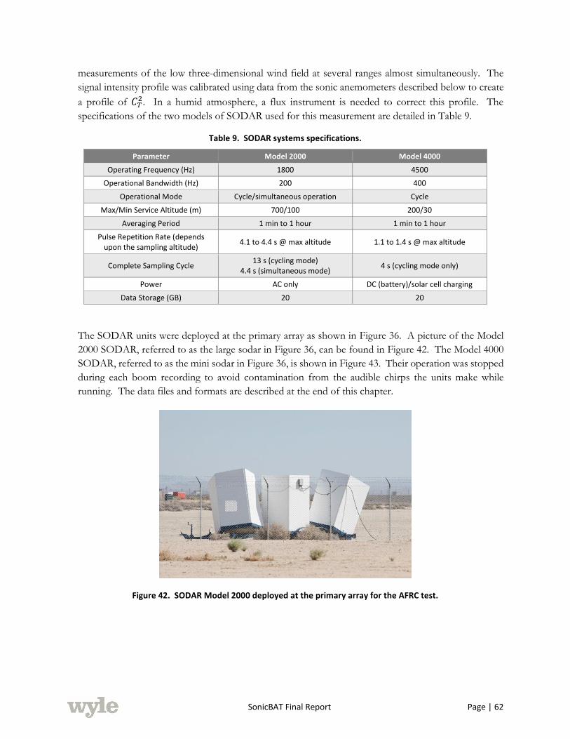
SonicBAT Final Report Page | 62
measurements of the low three-dimensional wind field at several ranges almost simultaneously. The
signal intensity profile was calibrated using data from the sonic anemometers described below to create
a profile of 𝐶𝑇2. In a humid atmosphere, a flux instrument is needed to correct this profile. The
specifications of the two models of SODAR used for this measurement are detailed in Table 9.
Table 9. SODAR systems specifications.
Parameter Model 2000 Model 4000
Operating Frequency (Hz) 1800 4500
Operational Bandwidth (Hz) 200 400
Operational Mode Cycle/simultaneous operation Cycle
Max/Min Service Altitude (m) 700/100 200/30
Averaging Period 1 min to 1 hour 1 min to 1 hour
Pulse Repetition Rate (depends upon the sampling altitude)
4.1 to 4.4 s @ max altitude 1.1 to 1.4 s @ max altitude
Complete Sampling Cycle 13 s (cycling mode)
4.4 s (simultaneous mode) 4 s (cycling mode only)
Power AC only DC (battery)/solar cell charging
Data Storage (GB) 20 20
The SODAR units were deployed at the primary array as shown in Figure 36. A picture of the Model
2000 SODAR, referred to as the large sodar in Figure 36, can be found in Figure 42. The Model 4000
SODAR, referred to as the mini sodar in Figure 36, is shown in Figure 43. Their operation was stopped
during each boom recording to avoid contamination from the audible chirps the units make while
running. The data files and formats are described at the end of this chapter.
Figure 42. SODAR Model 2000 deployed at the primary array for the AFRC test.

SonicBAT Final Report Page | 63
Figure 43. SODAR Model 4000 deployed at primary array for AFRC test.
5.2.2.4 ULTRASONIC ANEMOMETERS
Two anemometers were used to measure the atmospheric structural constants 𝐶𝑇2 and 𝐶𝑣
2 at two heights.
The first was mounted on a portable 10 m tower shown in the background of Figure 40. A close up of
the unit mounted on top of the portable tower is shown in Figure 44. The other unit was mounted atop
a fixed tower, 44 m in height, located near the primary array. The tower is shown in Figure 45 with the
mounted unit shown in Figure 46.
Figure 44. Ultrasonic anemometer mounted on 10 m tower at primary array during AFRC test.

SonicBAT Final Report Page | 64
Figure 45. Tower used for mounting ultrasonic anemometer near primary array for AFRC test.
Figure 46. Ultrasonic anemometer mounted on the 44 m tower near the primary array for the AFRC test.
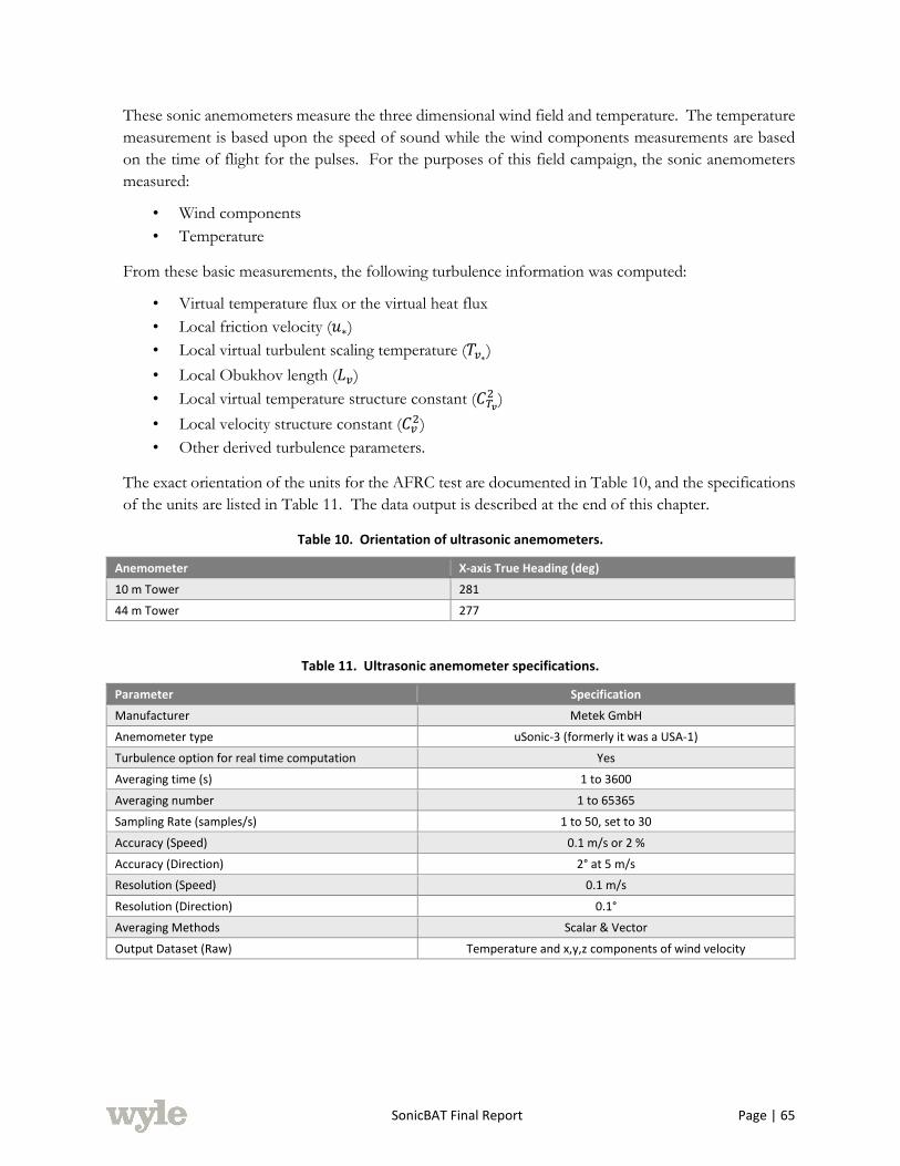
SonicBAT Final Report Page | 65
These sonic anemometers measure the three dimensional wind field and temperature. The temperature
measurement is based upon the speed of sound while the wind components measurements are based
on the time of flight for the pulses. For the purposes of this field campaign, the sonic anemometers
measured:
• Wind components
• Temperature
From these basic measurements, the following turbulence information was computed:
• Virtual temperature flux or the virtual heat flux
• Local friction velocity (𝑢∗)
• Local virtual turbulent scaling temperature (𝑇𝑣∗)
• Local Obukhov length (𝐿𝑣)
• Local virtual temperature structure constant (𝐶𝑇𝑣
2 )
• Local velocity structure constant (𝐶𝑣2)
• Other derived turbulence parameters.
The exact orientation of the units for the AFRC test are documented in Table 10, and the specifications
of the units are listed in Table 11. The data output is described at the end of this chapter.
Table 10. Orientation of ultrasonic anemometers.
Anemometer X-axis True Heading (deg)
10 m Tower 281
44 m Tower 277
Table 11. Ultrasonic anemometer specifications.
Parameter Specification
Manufacturer Metek GmbH
Anemometer type uSonic-3 (formerly it was a USA-1)
Turbulence option for real time computation Yes
Averaging time (s) 1 to 3600
Averaging number 1 to 65365
Sampling Rate (samples/s) 1 to 50, set to 30
Accuracy (Speed) 0.1 m/s or 2 %
Accuracy (Direction) 2° at 5 m/s
Resolution (Speed) 0.1 m/s
Resolution (Direction) 0.1°
Averaging Methods Scalar & Vector
Output Dataset (Raw) Temperature and x,y,z components of wind velocity

SonicBAT Final Report Page | 66
The data file naming convention follows the format
Anzzmyyyy_mm_dd_hh_mm_ssSch1
where,
zz: Approximate height above ground, meters, integer
yyyy: year, integer
mm: month, integer
dd: day of month, integer
hh: hour, integer
mm: minute, integer
ss: seconds, integer
*Date/time values correspond to first data point of file.
Example: An10m2016_07_05_20_45_19Sch1
Each file is ASCII with lines of data in format:
yyyy:m:d:sssssssss
x= 0.0 y= 0.00 z= 0.00 T= 0.00
where,
yyyy – year
m – month
d – day
sssssssss – time of week, milliseconds
x – x-velocity, m/s
y – y-velocity, m/s
z – z-velocity, m/s
T – temperature, degrees Celsius
• Times given in the data are integer seconds times 1000, and repeat about (but not always) 30
times before the next integer second.
• The time needs 17 seconds subtracted to give UTC time for AFRC (18 seconds for the KSC
measurements described below).
Additionally, with the turbulence data output option enabled, the unit outputs its calculation of the
parameters used for characterizing turbulence every 10 minutes. For this project, the turbulence
variables used were calculated from the raw data stream. The format of this section of the file can be
found in the anemometer instruction manual (Metek GmbH, 2014).
5.2.3 AIRCRAFT DATA
Two types of aircraft were used for the AFRC test: an F-18 jet aircraft and a TG-14 motorized sailplane.
Two different models of F-18 were used: an F-18B with tail number 846 and an F-18A with tail number
843. The F-18 used for each flight is noted in Table 7. The TG-14 flew for all but flights 19 and 20.
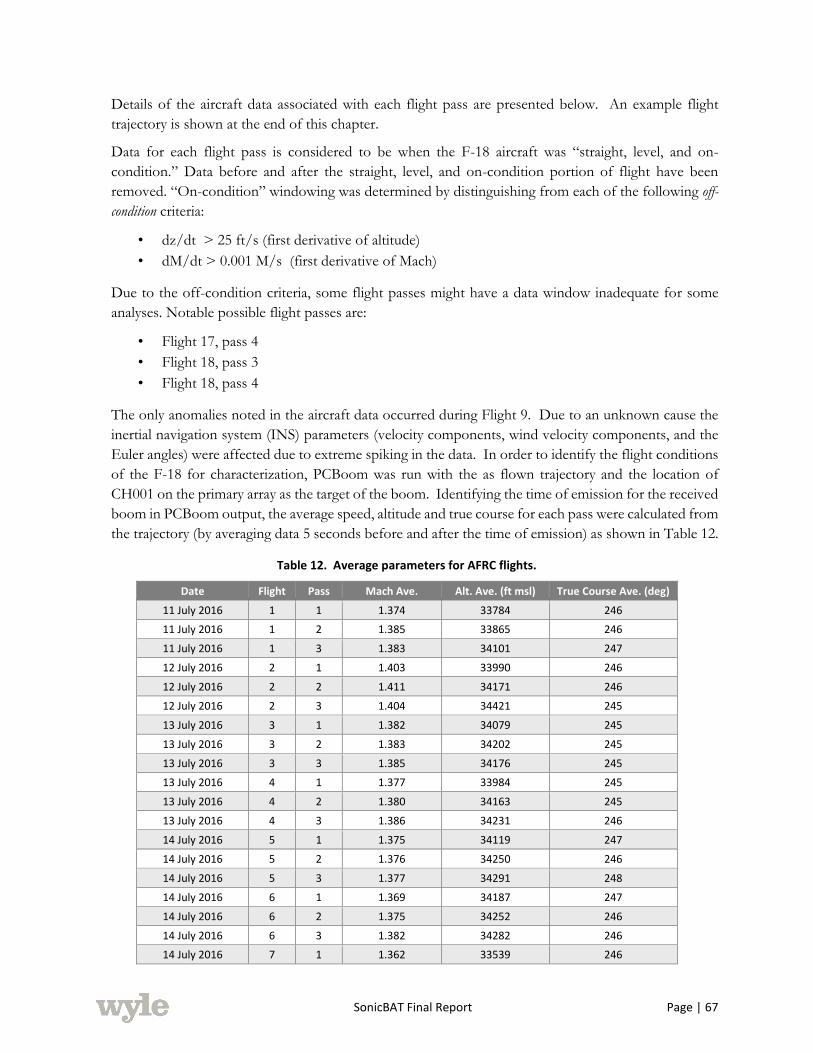
SonicBAT Final Report Page | 67
Details of the aircraft data associated with each flight pass are presented below. An example flight
trajectory is shown at the end of this chapter.
Data for each flight pass is considered to be when the F-18 aircraft was “straight, level, and on-
condition.” Data before and after the straight, level, and on-condition portion of flight have been
removed. “On-condition” windowing was determined by distinguishing from each of the following off-
condition criteria:
• dz/dt > 25 ft/s (first derivative of altitude)
• dM/dt > 0.001 M/s (first derivative of Mach)
Due to the off-condition criteria, some flight passes might have a data window inadequate for some
analyses. Notable possible flight passes are:
• Flight 17, pass 4
• Flight 18, pass 3
• Flight 18, pass 4
The only anomalies noted in the aircraft data occurred during Flight 9. Due to an unknown cause the
inertial navigation system (INS) parameters (velocity components, wind velocity components, and the
Euler angles) were affected due to extreme spiking in the data. In order to identify the flight conditions
of the F-18 for characterization, PCBoom was run with the as flown trajectory and the location of
CH001 on the primary array as the target of the boom. Identifying the time of emission for the received
boom in PCBoom output, the average speed, altitude and true course for each pass were calculated from
the trajectory (by averaging data 5 seconds before and after the time of emission) as shown in Table 12.
Table 12. Average parameters for AFRC flights.
Date Flight Pass Mach Ave. Alt. Ave. (ft msl) True Course Ave. (deg)
11 July 2016 1 1 1.374 33784 246
11 July 2016 1 2 1.385 33865 246
11 July 2016 1 3 1.383 34101 247
12 July 2016 2 1 1.403 33990 246
12 July 2016 2 2 1.411 34171 246
12 July 2016 2 3 1.404 34421 245
13 July 2016 3 1 1.382 34079 245
13 July 2016 3 2 1.383 34202 245
13 July 2016 3 3 1.385 34176 245
13 July 2016 4 1 1.377 33984 245
13 July 2016 4 2 1.380 34163 245
13 July 2016 4 3 1.386 34231 246
14 July 2016 5 1 1.375 34119 247
14 July 2016 5 2 1.376 34250 246
14 July 2016 5 3 1.377 34291 248
14 July 2016 6 1 1.369 34187 247
14 July 2016 6 2 1.375 34252 246
14 July 2016 6 3 1.382 34282 246
14 July 2016 7 1 1.362 33539 246
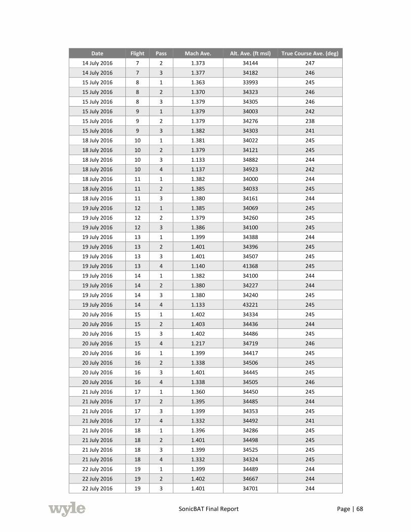
SonicBAT Final Report Page | 68
Date Flight Pass Mach Ave. Alt. Ave. (ft msl) True Course Ave. (deg)
14 July 2016 7 2 1.373 34144 247
14 July 2016 7 3 1.377 34182 246
15 July 2016 8 1 1.363 33993 245
15 July 2016 8 2 1.370 34323 246
15 July 2016 8 3 1.379 34305 246
15 July 2016 9 1 1.379 34003 242
15 July 2016 9 2 1.379 34276 238
15 July 2016 9 3 1.382 34303 241
18 July 2016 10 1 1.381 34022 245
18 July 2016 10 2 1.379 34121 245
18 July 2016 10 3 1.133 34882 244
18 July 2016 10 4 1.137 34923 242
18 July 2016 11 1 1.382 34000 244
18 July 2016 11 2 1.385 34033 245
18 July 2016 11 3 1.380 34161 244
19 July 2016 12 1 1.385 34069 245
19 July 2016 12 2 1.379 34260 245
19 July 2016 12 3 1.386 34100 245
19 July 2016 13 1 1.399 34388 244
19 July 2016 13 2 1.401 34396 245
19 July 2016 13 3 1.401 34507 245
19 July 2016 13 4 1.140 41368 245
19 July 2016 14 1 1.382 34100 244
19 July 2016 14 2 1.380 34227 244
19 July 2016 14 3 1.380 34240 245
19 July 2016 14 4 1.133 43221 245
20 July 2016 15 1 1.402 34334 245
20 July 2016 15 2 1.403 34436 244
20 July 2016 15 3 1.402 34486 245
20 July 2016 15 4 1.217 34719 246
20 July 2016 16 1 1.399 34417 245
20 July 2016 16 2 1.338 34506 245
20 July 2016 16 3 1.401 34445 245
20 July 2016 16 4 1.338 34505 246
21 July 2016 17 1 1.360 34450 245
21 July 2016 17 2 1.395 34485 244
21 July 2016 17 3 1.399 34353 245
21 July 2016 17 4 1.332 34492 241
21 July 2016 18 1 1.396 34286 245
21 July 2016 18 2 1.401 34498 245
21 July 2016 18 3 1.399 34525 245
21 July 2016 18 4 1.332 34324 245
22 July 2016 19 1 1.399 34489 244
22 July 2016 19 2 1.402 34667 244
22 July 2016 19 3 1.401 34701 244
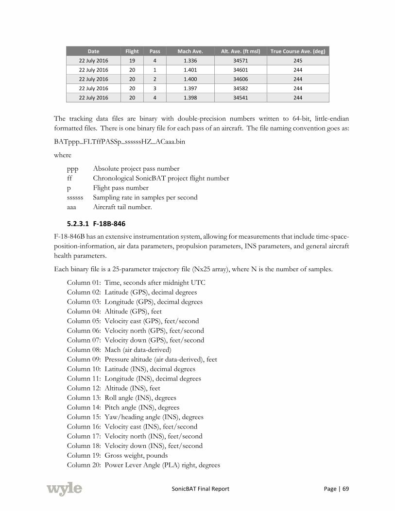
SonicBAT Final Report Page | 69
Date Flight Pass Mach Ave. Alt. Ave. (ft msl) True Course Ave. (deg)
22 July 2016 19 4 1.336 34571 245
22 July 2016 20 1 1.401 34601 244
22 July 2016 20 2 1.400 34606 244
22 July 2016 20 3 1.397 34582 244
22 July 2016 20 4 1.398 34541 244
The tracking data files are binary with double-precision numbers written to 64-bit, little-endian
formatted files. There is one binary file for each pass of an aircraft. The file naming convention goes as:
BATppp_FLTffPASSp_ssssssHZ_ACaaa.bin
where
ppp Absolute project pass number
ff Chronological SonicBAT project flight number
p Flight pass number
ssssss Sampling rate in samples per second
aaa Aircraft tail number.
5.2.3.1 F-18B-846
F-18-846B has an extensive instrumentation system, allowing for measurements that include time-space-
position-information, air data parameters, propulsion parameters, INS parameters, and general aircraft
health parameters.
Each binary file is a 25-parameter trajectory file (Nx25 array), where N is the number of samples.
Column 01: Time, seconds after midnight UTC
Column 02: Latitude (GPS), decimal degrees
Column 03: Longitude (GPS), decimal degrees
Column 04: Altitude (GPS), feet
Column 05: Velocity east (GPS), feet/second
Column 06: Velocity north (GPS), feet/second
Column 07: Velocity down (GPS), feet/second
Column 08: Mach (air data-derived)
Column 09: Pressure altitude (air data-derived), feet
Column 10: Latitude (INS), decimal degrees
Column 11: Longitude (INS), decimal degrees
Column 12: Altitude (INS), feet
Column 13: Roll angle (INS), degrees
Column 14: Pitch angle (INS), degrees
Column 15: Yaw/heading angle (INS), degrees
Column 16: Velocity east (INS), feet/second
Column 17: Velocity north (INS), feet/second
Column 18: Velocity down (INS), feet/second
Column 19: Gross weight, pounds
Column 20: Power Lever Angle (PLA) right, degrees
SonicBAT Final Report Page | 70
Column 21: Power Lever Angle (PLA) left, degrees
Column 22: Wind speed aloft east, knots
Column 23: Wind speed aloft north, knots
Column 24: Wind speed aloft vertical, knots
Column 25: Ambient air temperature, degrees-Rankin
5.2.3.2 F-18A-843 AND TG-14-856
F-18A-843 and TG-14-856 are only capable of measuring time-space-position-information data.
Each file is a 9-parameter trajectory file. The file is an Nx9 array, where N is the number of samples.
Column 01: Time, seconds after midnight UTC
Column 02: Latitude (GPS), decimal degrees
Column 03: Longitude (GPS), decimal degrees
Column 04: Altitude (GPS), feet
Column 05: Velocity east (GPS), feet/second
Column 06: Velocity north (GPS), feet/second
Column 07: Velocity down (GPS), feet/second
Column 08: Mach (derived from GPS and atmospheric data)
Column 09: Pressure altitude (derived from GPS and atmospheric data), feet
5.2.4 DATA ACQUIRED
This section will provide examples of the data acquired from deployed instrumentation at AFRC as well
as some details about the data itself. The measurement data for all flight tests was delivered on a hard
drive. All specifications and details of the data are contained on the hard drive. The information here
highlights aspects of the data germane to the raw data recordings at AFRC. Further chapters in this
report will address aspects of processing the data.
5.2.4.1 MICROPHONE DATA
The microphone data presented in the electronic archive are either binary files containing the calibrated
microphone signatures recorded during an aircraft pass or files with information about the equipment
used and its location. All physical details about the microphone array can be found in the Excel file
named SonicBAT_NASAAFRC_Measurements_July2016_Positions_ALLBooms. The same format is
used for the KSC test where KSC will replace AFRC in the Excel file and BAT in the microphone data
file names as described below. A sheet in the file labeled Positions details the equipment used at each
location on all arrays along with location coordinates and equipment models and serial numbers. There
is a sheet labeled Booms with the arrival times of booms for each array. Field logs from the various
organizations have been scanned and included with the archive. No attempt at editing them has been
made.
Apart from the time discussed below, all acoustic data in the archive are named with the flight number
of the aircraft and the pass number during that flight during which the data was recorded and include
the sampling rate of the data along with the position number the data came from. The acoustic data
files are in pounds per square foot and are stored as single-precision numbers in little-endian formatted
files. An example file name for the AFRC measurements is:
BATppp_FLTffPASSp_ssssssHZ_CHnnn.bin
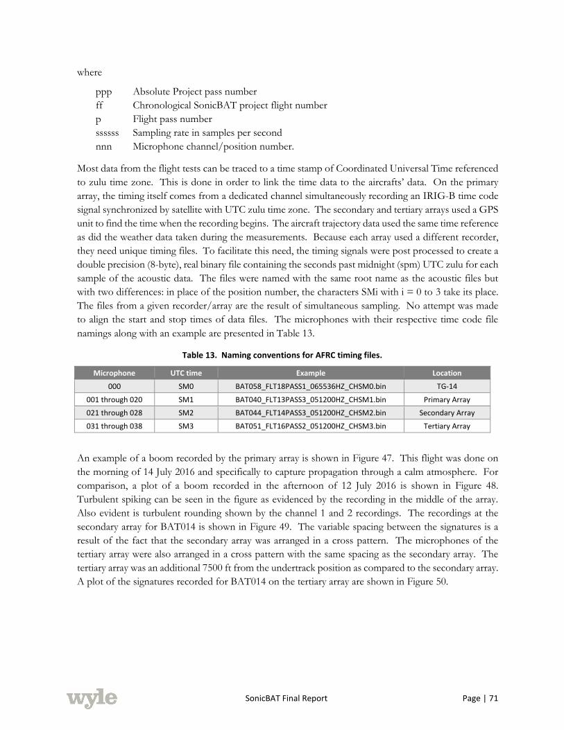
SonicBAT Final Report Page | 71
where
ppp Absolute Project pass number
ff Chronological SonicBAT project flight number
p Flight pass number
ssssss Sampling rate in samples per second
nnn Microphone channel/position number.
Most data from the flight tests can be traced to a time stamp of Coordinated Universal Time referenced
to zulu time zone. This is done in order to link the time data to the aircrafts’ data. On the primary
array, the timing itself comes from a dedicated channel simultaneously recording an IRIG-B time code
signal synchronized by satellite with UTC zulu time zone. The secondary and tertiary arrays used a GPS
unit to find the time when the recording begins. The aircraft trajectory data used the same time reference
as did the weather data taken during the measurements. Because each array used a different recorder,
they need unique timing files. To facilitate this need, the timing signals were post processed to create a
double precision (8-byte), real binary file containing the seconds past midnight (spm) UTC zulu for each
sample of the acoustic data. The files were named with the same root name as the acoustic files but
with two differences: in place of the position number, the characters SMi with i = 0 to 3 take its place.
The files from a given recorder/array are the result of simultaneous sampling. No attempt was made
to align the start and stop times of data files. The microphones with their respective time code file
namings along with an example are presented in Table 13.
Table 13. Naming conventions for AFRC timing files.
Microphone UTC time Example Location
000 SM0 BAT058_FLT18PASS1_065536HZ_CHSM0.bin TG-14
001 through 020 SM1 BAT040_FLT13PASS3_051200HZ_CHSM1.bin Primary Array
021 through 028 SM2 BAT044_FLT14PASS3_051200HZ_CHSM2.bin Secondary Array
031 through 038 SM3 BAT051_FLT16PASS2_051200HZ_CHSM3.bin Tertiary Array
An example of a boom recorded by the primary array is shown in Figure 47. This flight was done on
the morning of 14 July 2016 and specifically to capture propagation through a calm atmosphere. For
comparison, a plot of a boom recorded in the afternoon of 12 July 2016 is shown in Figure 48.
Turbulent spiking can be seen in the figure as evidenced by the recording in the middle of the array.
Also evident is turbulent rounding shown by the channel 1 and 2 recordings. The recordings at the
secondary array for BAT014 is shown in Figure 49. The variable spacing between the signatures is a
result of the fact that the secondary array was arranged in a cross pattern. The microphones of the
tertiary array were also arranged in a cross pattern with the same spacing as the secondary array. The
tertiary array was an additional 7500 ft from the undertrack position as compared to the secondary array.
A plot of the signatures recorded for BAT014 on the tertiary array are shown in Figure 50.
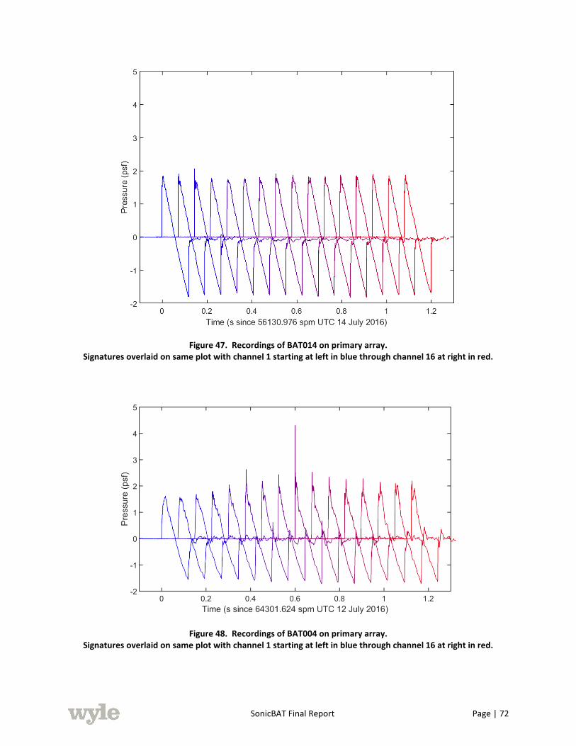
SonicBAT Final Report Page | 72
Figure 47. Recordings of BAT014 on primary array. Signatures overlaid on same plot with channel 1 starting at left in blue through channel 16 at right in red.
Figure 48. Recordings of BAT004 on primary array. Signatures overlaid on same plot with channel 1 starting at left in blue through channel 16 at right in red.
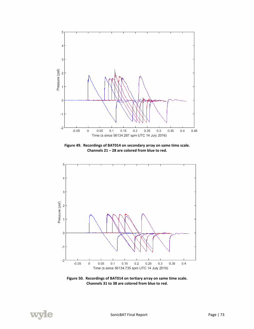
SonicBAT Final Report Page | 73
Figure 49. Recordings of BAT014 on secondary array on same time scale. Channels 21 – 28 are colored from blue to red.
Figure 50. Recordings of BAT014 on tertiary array on same time scale. Channels 31 to 38 are colored from blue to red.
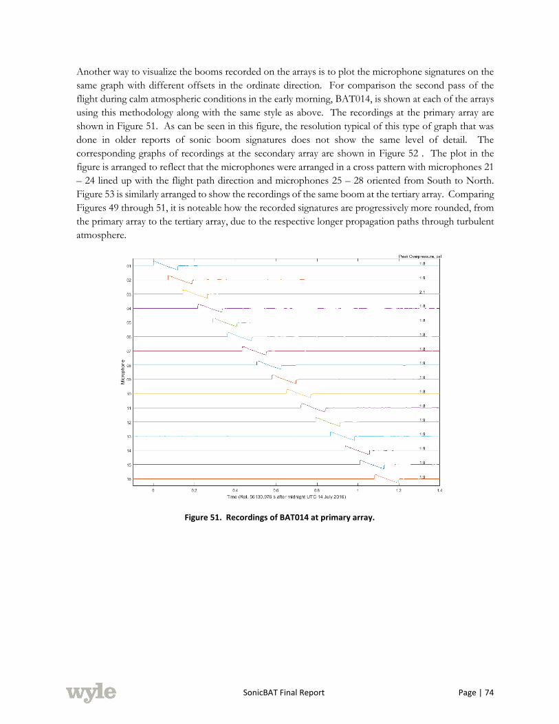
SonicBAT Final Report Page | 74
Another way to visualize the booms recorded on the arrays is to plot the microphone signatures on the
same graph with different offsets in the ordinate direction. For comparison the second pass of the
flight during calm atmospheric conditions in the early morning, BAT014, is shown at each of the arrays
using this methodology along with the same style as above. The recordings at the primary array are
shown in Figure 51. As can be seen in this figure, the resolution typical of this type of graph that was
done in older reports of sonic boom signatures does not show the same level of detail. The
corresponding graphs of recordings at the secondary array are shown in Figure 52 . The plot in the
figure is arranged to reflect that the microphones were arranged in a cross pattern with microphones 21
– 24 lined up with the flight path direction and microphones 25 – 28 oriented from South to North.
Figure 53 is similarly arranged to show the recordings of the same boom at the tertiary array. Comparing
Figures 49 through 51, it is noteable how the recorded signatures are progressively more rounded, from
the primary array to the tertiary array, due to the respective longer propagation paths through turbulent
atmosphere.
Figure 51. Recordings of BAT014 at primary array.
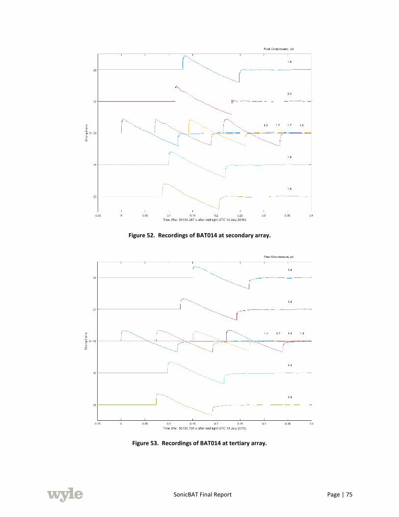
SonicBAT Final Report Page | 75
Figure 52. Recordings of BAT014 at secondary array.
Figure 53. Recordings of BAT014 at tertiary array.
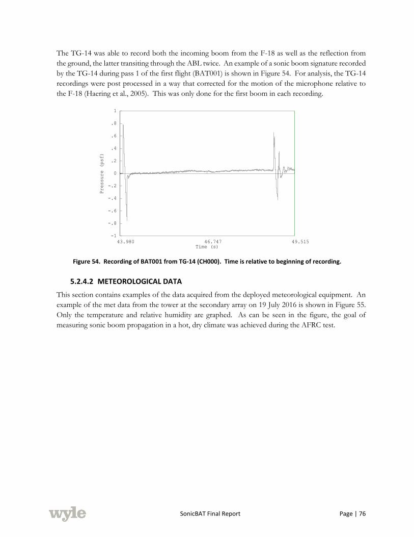
SonicBAT Final Report Page | 76
The TG-14 was able to record both the incoming boom from the F-18 as well as the reflection from
the ground, the latter transiting through the ABL twice. An example of a sonic boom signature recorded
by the TG-14 during pass 1 of the first flight (BAT001) is shown in Figure 54. For analysis, the TG-14
recordings were post processed in a way that corrected for the motion of the microphone relative to
the F-18 (Haering et al., 2005). This was only done for the first boom in each recording.
Figure 54. Recording of BAT001 from TG-14 (CH000). Time is relative to beginning of recording.
5.2.4.2 METEOROLOGICAL DATA
This section contains examples of the data acquired from the deployed meteorological equipment. An
example of the met data from the tower at the secondary array on 19 July 2016 is shown in Figure 55.
Only the temperature and relative humidity are graphed. As can be seen in the figure, the goal of
measuring sonic boom propagation in a hot, dry climate was achieved during the AFRC test.
43.980 46.747 49.515
-1
-.8
-.6
-.4
-.2
0
.2
.4
.6
.8
1
Time (s)
Pressure (psf)
M:\SonicBAT_NASAAFRC_DATA_DELIVERED_August2016\SonicBAT_NASA_AFRC_AllBooms\raw_TG14\BAT001_FLT01PASS1_065536HZ_CH000.binM:\SonicBAT_NASAAFRC_DATA_DELIVERED_August2016\SonicBAT_NASA_AFRC_AllBooms\raw_TG14\BAT001_FLT01PASS1_065536HZ_CH000.binM:\SonicBAT_NASAAFRC_DATA_DELIVERED_August2016\SonicBAT_NASA_AFRC_AllBooms\raw_TG14\BAT001_FLT01PASS1_065536HZ_CH000.bin
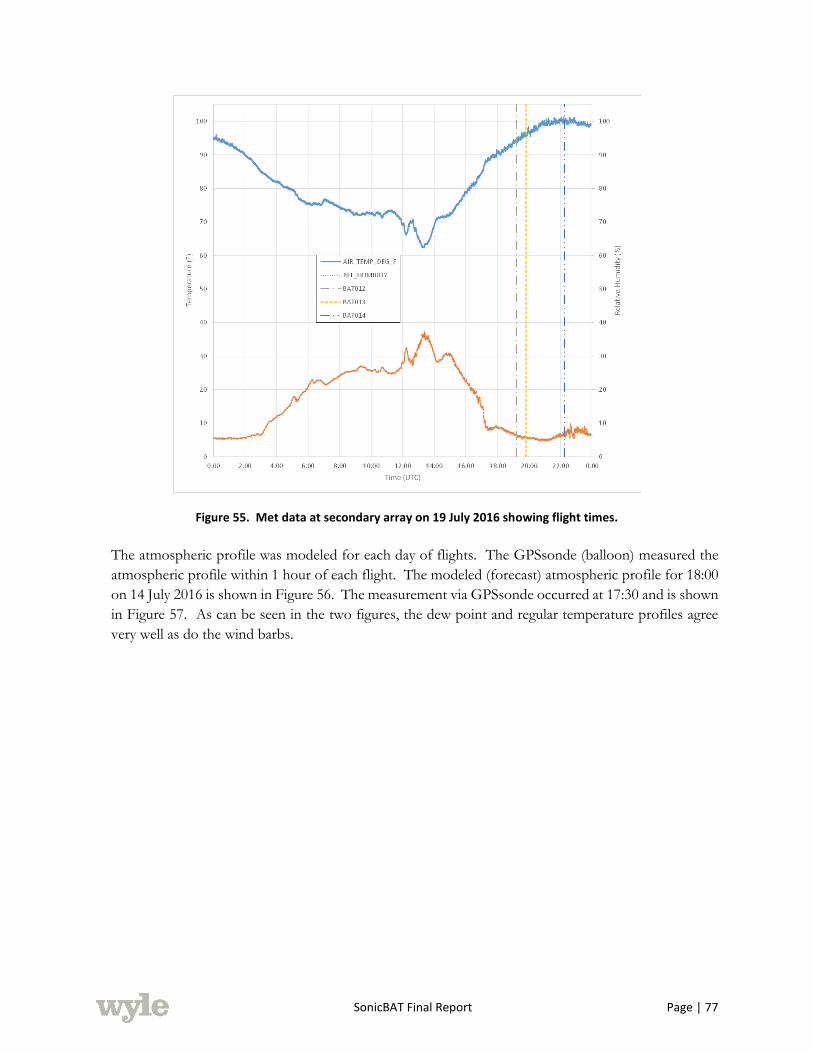
SonicBAT Final Report Page | 77
Figure 55. Met data at secondary array on 19 July 2016 showing flight times.
The atmospheric profile was modeled for each day of flights. The GPSsonde (balloon) measured the
atmospheric profile within 1 hour of each flight. The modeled (forecast) atmospheric profile for 18:00
on 14 July 2016 is shown in Figure 56. The measurement via GPSsonde occurred at 17:30 and is shown
in Figure 57. As can be seen in the two figures, the dew point and regular temperature profiles agree
very well as do the wind barbs.

SonicBAT Final Report Page | 78
Figure 56. Skew-T Log P diagram of forecast for 18:00 UTC on 14 July 2016 at AFRC. Solid, black line shown is temperature curve. Dashed, black line is dew point curve. Wind barbs at right are scaled in knots.
Only data below 17 km shown.
Figure 57. Skew-T Log P diagram of GPSsonde launched at 17:30 UTC on 14 July 2016 at AFRC. Solid, black line shown is temperature curve. Dashed, black line is dew point curve. Wind barbs at right are scaled in knots.
Only data below 17 km shown.
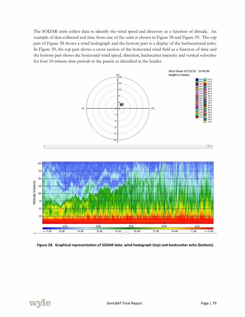
SonicBAT Final Report Page | 79
The SODAR units collect data to identify the wind speed and directory as a function of altitude. An
example of data collected real time from one of the units is shown in Figure 58 and Figure 59. The top
part of Figure 58 shows a wind hodograph and the bottom part is a display of the backscattered echo.
In Figure 59, the top part shows a cross-section of the horizontal wind field as a function of time and
the bottom part shows the horizontal wind speed, direction, backscatter intensity and vertical velocities
for four 10-minute time periods in the panels as identified in the header.
Figure 58. Graphical representation of SODAR data: wind hodograph (top) and backscatter echo (bottom).

SonicBAT Final Report Page | 80
(b) Horizontal wind field (top) and horizontal wind speed, direction, backscatter intensities, and vertical velocity (bottom)
Figure 59. Graphical representation of SODAR data (concluded): horizontal wind field (top) and horizontal wind speed, direction, backscatter intensities, and vertical velocity (bottom).
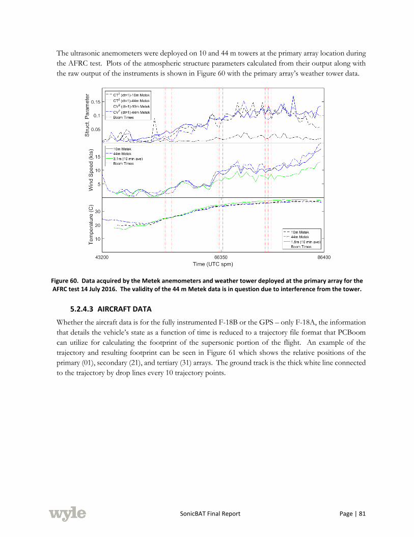
SonicBAT Final Report Page | 81
The ultrasonic anemometers were deployed on 10 and 44 m towers at the primary array location during
the AFRC test. Plots of the atmospheric structure parameters calculated from their output along with
the raw output of the instruments is shown in Figure 60 with the primary array’s weather tower data.
Figure 60. Data acquired by the Metek anemometers and weather tower deployed at the primary array for the AFRC test 14 July 2016. The validity of the 44 m Metek data is in question due to interference from the tower.
5.2.4.3 AIRCRAFT DATA
Whether the aircraft data is for the fully instrumented F-18B or the GPS – only F-18A, the information
that details the vehicle’s state as a function of time is reduced to a trajectory file format that PCBoom
can utilize for calculating the footprint of the supersonic portion of the flight. An example of the
trajectory and resulting footprint can be seen in Figure 61 which shows the relative positions of the
primary (01), secondary (21), and tertiary (31) arrays. The ground track is the thick white line connected
to the trajectory by drop lines every 10 trajectory points.

SonicBAT Final Report Page | 82
Figure 61. Trajectory (upper, thin white line) and ground track (lower, thick white line) and calculated footprint in relation to the microphone arrays at AFRC. Colored lines are peak overpressure contours with black lines
representing the footprint’s isopemps.
5.3 NASA KENNEDY SPACE CENTER MEASUREMENT PROGRAM
The second field campaign for the SonicBAT project occurred at NASA Kennedy Space Center (KSC).
Located in Florida, the portion of the NASA KSC property used for the study is shown in Figure 62.
Historical data shows that the climate at KSC during August would be ideal for measurement of sonic
booms propagating through a hot, wet atmosphere. Three types of data were acquired during the
measurements that occurred 21 – 31 August 2017: acoustic data from two microphone arrays on the
ground and a microphone attached to a TG-14 motorized sailplane; meteorological data from
GPSsonde balloon launches, weather towers on the ground, and two ultrasonic anemometers and a
humidity flux sensor mounted on a 150 m tower; and aircraft data from F-18s and a TG-14. This section
details the measurements and data acquired.
Figure 62. NASA KSC area in Florida.
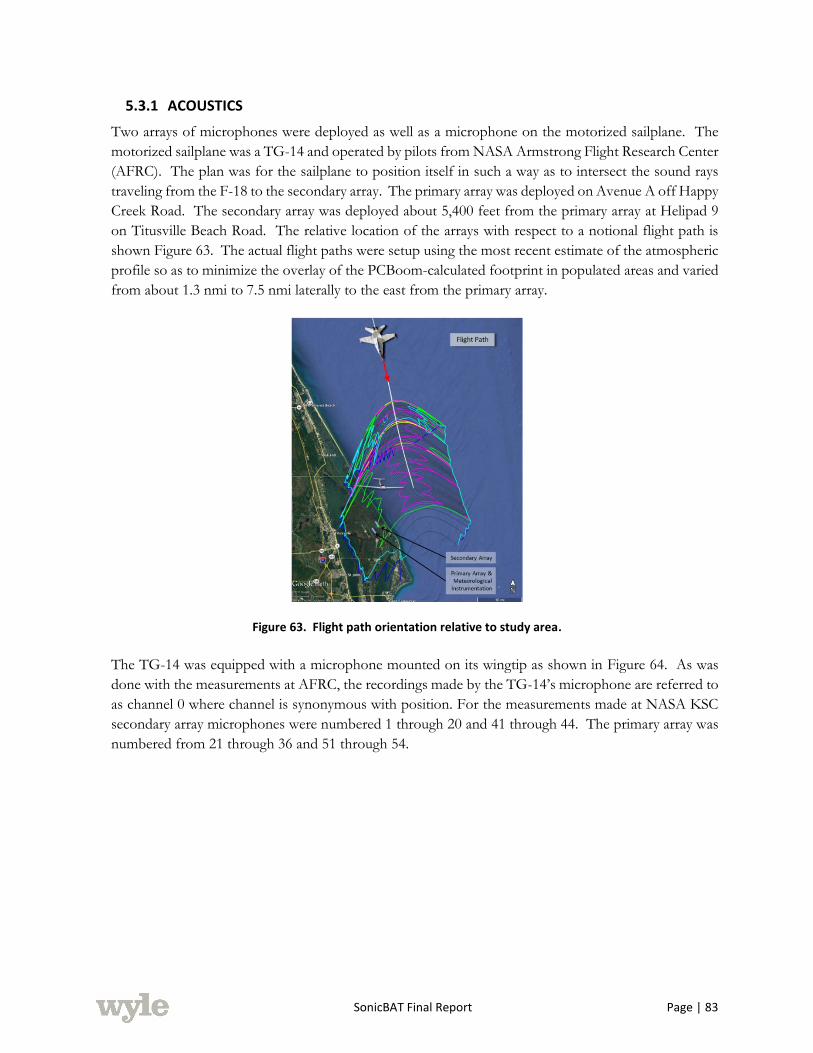
SonicBAT Final Report Page | 83
5.3.1 ACOUSTICS
Two arrays of microphones were deployed as well as a microphone on the motorized sailplane. The
motorized sailplane was a TG-14 and operated by pilots from NASA Armstrong Flight Research Center
(AFRC). The plan was for the sailplane to position itself in such a way as to intersect the sound rays
traveling from the F-18 to the secondary array. The primary array was deployed on Avenue A off Happy
Creek Road. The secondary array was deployed about 5,400 feet from the primary array at Helipad 9
on Titusville Beach Road. The relative location of the arrays with respect to a notional flight path is
shown Figure 63. The actual flight paths were setup using the most recent estimate of the atmospheric
profile so as to minimize the overlay of the PCBoom-calculated footprint in populated areas and varied
from about 1.3 nmi to 7.5 nmi laterally to the east from the primary array.
Figure 63. Flight path orientation relative to study area.
The TG-14 was equipped with a microphone mounted on its wingtip as shown in Figure 64. As was
done with the measurements at AFRC, the recordings made by the TG-14’s microphone are referred to
as channel 0 where channel is synonymous with position. For the measurements made at NASA KSC
secondary array microphones were numbered 1 through 20 and 41 through 44. The primary array was
numbered from 21 through 36 and 51 through 54.

SonicBAT Final Report Page | 84
Figure 64. TG-14 motorized glider with microphone mounted under and forward of wingtip.
Array microphones were placed on ground boards with the preamp taped to the ground board and
microphone covered with a half windscreen. Microphones were oriented to face east based on an
estimate of the incoming ray in PCBoom coming from the North for a typical atmospheric profile.
Figure 65 shows the microphones mounted on ground boards at the secondary array.
Figure 65. Microphones on ground boards at secondary array. Positions 18, 19, 20, and 09 shown going away from the camera.
The primary array consisted of 16 microphones on ground boards spaced 100’ apart. The number of
microphones on the array was decreased as the measurements progressed due to equipment failure that
resulted from fine dust contamination. Originally specified as positions 21 through 36, the latter 8
microphone stations were taken down and four new mic positions were deployed to the Northwest of
the array line and labeled as positions 51 through 54. This configuration began on 26 August and
remained throughout the remainder of the measurements. Figure 66 shows the layout of the primary

SonicBAT Final Report Page | 85
array’s main microphones (channels 21 through 36 and 51 through 54) along with the location of
meteorological instruments detailed in the following sections.
Figure 66. Primary array layout of positions 21 through 36 and 51 through 54. Meteorological instrumentation locations also shown.

SonicBAT Final Report Page | 86
The secondary array was deployed on Titusville Beach Road at Helipad 9. There were 20 microphones
with a 100’ separation on the road. They are numbered as positions 1 through 16 tended by Wyle and
positions 41 through 44 tended by the Japan Aerospace Exploration Agency (JAXA). Wyle also
deployed four microphones with a 20’ spacing between positions 08 and 09 for the first week of the
measurements, positions 17 through 20. Figure 67 shows the layout of the microphones and weather
station deployed at that location.
Figure 67. Secondary array layout showing microphone positions and weather station. Inset shows a zoom of the center of the array with finer spaced positions added for first week of measurements.
Much of the same equipment used for the AFRC measurements was used at KSC. The primary array
at KSC was deployed by Gulfstream. One difference between primary and secondary arrays at KSC
was that the primary array utilized a WiFi system to connect each of four recorders with a base station;
whereas, the secondary array had all microphones directly connected to one recorder at its base. As
with AFRC, all microphones were 1/2" diameter, infrasonic microphones. Their type is detailed in the
aforementioned digital archive along with all serial numbers and connections. Similar to the AFRC test,
the different data recorders used by the organizations all had 24-bit A/D resolution but a different
sampling rate was used by the TG-14 motorized glider. The data recorder in the TG-14 motorized
glider sampled the microphone signal at 65536 samples per second; whereas, all other data records
utilized a sample rate of 51200 samples per second. The coordinates of all array microphones are listed
in Table 14.

SonicBAT Final Report Page | 87
The timing of data recordings was accomplished in one of two ways: recording an IRIG-B time code
was done on the TG-14 and at the secondary array; the time at the beginning of each recording on the
primary array was captured from a GPS unit attached to the data recorder. The first allowed for
determining the time throughout the recording by analyzing the IRIG-B signal while the second used
the sampling rate along with the start time of the recording to calculate the time of each sample in the
file. The log file on the recordings indicates when data drop outs occurred.
Table 14. KSC measurement microphone coordinates (ref. WGS 84 Ellipsoid).
CH NUMBER Latitude (N) Longitude (W) Ellipsoid Ht. (ft)
TG-14
CH000 VARIABLE VARIABLE VARIABLE
PRIMARY ARRAY
CH001 28 38 29.92390 80 38 51.08488 -94
CH002 28 38 29.29937 80 38 50.21166 -94
CH003 28 38 28.67819 80 38 49.34507 -94
CH004 28 38 28.05614 80 38 48.47481 -94
CH005 28 38 27.43752 80 38 47.60742 -94
CH006 28 38 26.81688 80 38 46.73878 -94
CH007 28 38 26.19606 80 38 45.86902 -94
CH008 28 38 25.57711 80 38 45.00318 -94
CH009 28 38 24.95172 80 38 44.13173 -94
CH010 28 38 24.33382 80 38 43.27608 -94
CH011 28 38 23.71145 80 38 42.40736 -95
CH012 28 38 23.08717 80 38 41.54326 -94
CH013 28 38 22.46545 80 38 40.67846 -94
CH014 28 38 21.84218 80 38 39.80752 -94
CH015 28 38 21.21924 80 38 38.93992 -94
CH016 28 38 20.59612 80 38 38.06846 -94
CH017 28 38 25.45213 80 38 44.82902 -94
CH018 28 38 25.32710 80 38 44.65482 -94
CH019 28 38 25.20211 80 38 44.48065 -94
CH020 28 38 25.07712 80 38 44.30645 -94
CH041 28 38 19.97530 80 38 37.19856 -94
CH042 28 38 19.35070 80 38 36.32711 -94
CH043 28 38 18.73171 80 38 35.45922 -94
CH044 28 38 18.10996 80 38 34.58460 -94
SECONDARY ARRAY
CH021 28 37 42.25992 80 39 20.75615 -90
CH022 28 37 41.62974 80 39 19.88945 -91
CH023 28 37 40.99254 80 39 19.04893 -91
CH024 28 37 40.35617 80 39 18.19965 -91
CH025 28 37 39.71277 80 39 17.35019 -91
CH026 28 37 39.10002 80 39 16.47345 -91
CH027 28 37 38.44781 80 39 15.63324 -91
CH028 28 37 37.78663 80 39 14.77050 -91
CH029 28 37 37.09100 80 39 13.84030 -92
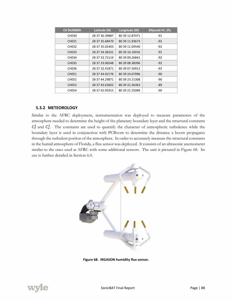
SonicBAT Final Report Page | 88
CH NUMBER Latitude (N) Longitude (W) Ellipsoid Ht. (ft)
CH030 28 37 36.39887 80 39 12.87471 -91
CH031 28 37 35.68470 80 39 11.93673 -92
CH032 28 37 35.02403 80 39 11.04540 -92
CH033 28 37 34.38161 80 39 10.16916 -92
CH034 28 37 33.72119 80 39 09.26841 -92
CH035 28 37 33.06548 80 39 08.38396 -92
CH036 28 37 32.41871 80 39 07.50912 -93
CH051 28 37 44.92176 80 39 24.07996 -90
CH052 28 37 44.29871 80 39 23.21308 -90
CH053 28 37 43.63602 80 39 22.36363 -89
CH054 28 37 42.95915 80 39 21.55089 -90
5.3.2 METEOROLOGY
Similar to the AFRC deployment, instrumentation was deployed to measure parameters of the
atmosphere needed to determine the height of the planetary boundary layer and the structural constants
𝐶𝑇2 and 𝐶𝑣
2. The constants are used to quantify the character of atmospheric turbulence while the
boundary layer is used in conjunction with PCBoom to determine the distance a boom propagates
through the turbulent portion of the atmosphere. In order to accurately measure the structural constants
in the humid atmosphere of Florida, a flux sensor was deployed. It consists of an ultrasonic anemometer
similar to the ones used at AFRC with some additional sensors. The unit is pictured in Figure 68. Its
use is further detailed in Section 6.0.
Figure 68. IRGASON humidity flux sensor.
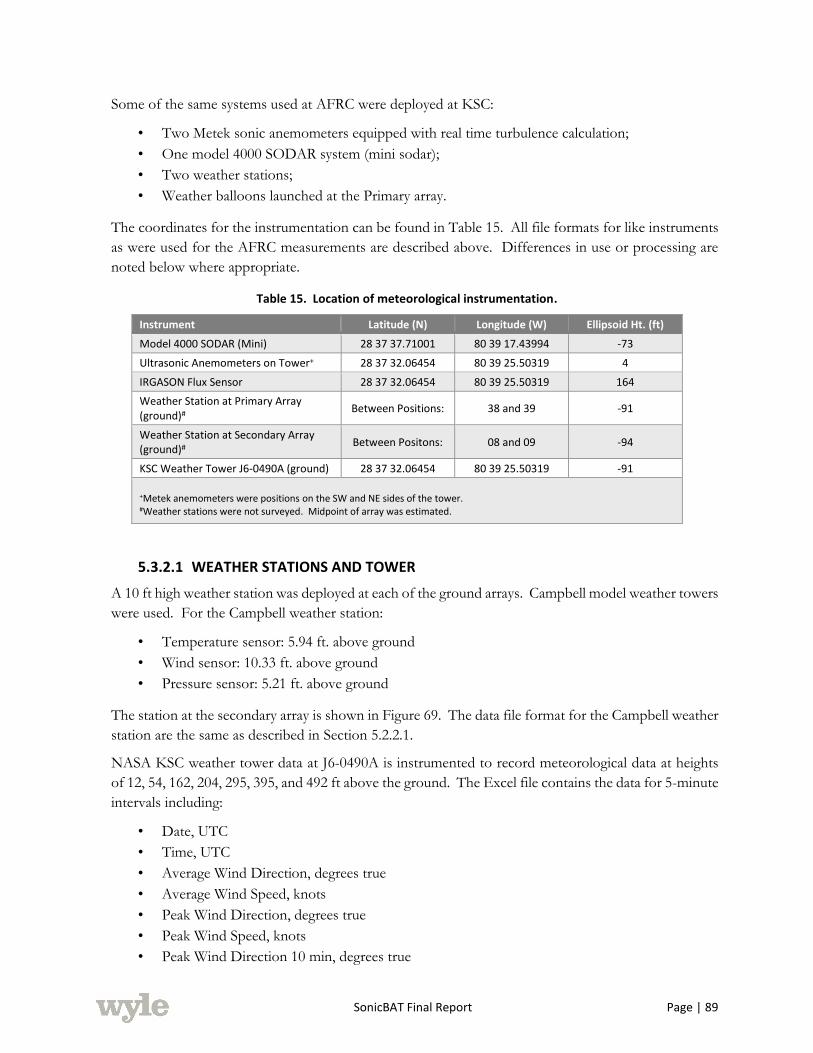
SonicBAT Final Report Page | 89
Some of the same systems used at AFRC were deployed at KSC:
• Two Metek sonic anemometers equipped with real time turbulence calculation;
• One model 4000 SODAR system (mini sodar);
• Two weather stations;
• Weather balloons launched at the Primary array.
The coordinates for the instrumentation can be found in Table 15. All file formats for like instruments
as were used for the AFRC measurements are described above. Differences in use or processing are
noted below where appropriate.
Table 15. Location of meteorological instrumentation.
Instrument Latitude (N) Longitude (W) Ellipsoid Ht. (ft)
Model 4000 SODAR (Mini) 28 37 37.71001 80 39 17.43994 -73
Ultrasonic Anemometers on Tower+ 28 37 32.06454 80 39 25.50319 4
IRGASON Flux Sensor 28 37 32.06454 80 39 25.50319 164
Weather Station at Primary Array (ground)# Between Positions: 38 and 39 -91
Weather Station at Secondary Array (ground)# Between Positons: 08 and 09 -94
KSC Weather Tower J6-0490A (ground) 28 37 32.06454 80 39 25.50319 -91
+Metek anemometers were positions on the SW and NE sides of the tower. #Weather stations were not surveyed. Midpoint of array was estimated.
5.3.2.1 WEATHER STATIONS AND TOWER
A 10 ft high weather station was deployed at each of the ground arrays. Campbell model weather towers
were used. For the Campbell weather station:
• Temperature sensor: 5.94 ft. above ground
• Wind sensor: 10.33 ft. above ground
• Pressure sensor: 5.21 ft. above ground
The station at the secondary array is shown in Figure 69. The data file format for the Campbell weather
station are the same as described in Section 5.2.2.1.
NASA KSC weather tower data at J6-0490A is instrumented to record meteorological data at heights
of 12, 54, 162, 204, 295, 395, and 492 ft above the ground. The Excel file contains the data for 5-minute
intervals including:
• Date, UTC
• Time, UTC
• Average Wind Direction, degrees true
• Average Wind Speed, knots
• Peak Wind Direction, degrees true
• Peak Wind Speed, knots
• Peak Wind Direction 10 min, degrees true

SonicBAT Final Report Page | 90
• Peak Wind Speed 10 min, knots
• Temperature, Fahrenheit
• Dew Point, Fahrenheit
• Relative humidity, %
Temperature, Dew Point and Relative Humidity are only recorded at the 54, 204, and 492 ft heights.
The information is in one tab of the Excel file and sequentially ordered.
Figure 69. Weather station deployed at the secondary array.
5.3.2.2 GPSsonde
Atmospheric profiles were measured with GPSsonde using weather balloons carrying the same type of
instrumentation package used at AFRC as shown in Figure 41. Balloons were launched within an hour
of each flight of the F-18 from the small hill in the foreground of Figure 70 where the mini SODAR
was located. The times of the balloon launches can be found in Table 16 along with the boom arrival
times on the secondary array for the first pass of each flight. The tail number of the F-18 flown for
each flight is also noted in the table. The balloon data was post processed for use in PCBoom. The
post processing involved smoothing the data and outputting the profile at 1000 ft intervals. Also
available for the KSC test was a predictive model of the atmosphere’s profile.

SonicBAT Final Report Page | 91
Figure 70. Primary array site and tower J6-0490A. Small hill in foreground was mini SODAR location and GPSsonde launch point.
Table 16. Balloon launch schedule with boom arrival times on secondary array of first pass for each flight. Cells highlighted in yellow denote launches with questionable data.
Time Event
21 August 2017
12:44 Balloon Launch
12:59:16 FLT01-846
15:32 Balloon Launch
15:45:23 FLT02-846
22 August 2017
14:43 Balloon Launch
15:12:26 FLT03-846
15:52 Balloon Launch
16:10:10 FLT04-843
17:56 Balloon Launch
18:26:17 FLT05-846
23 August 2017
15:32 Balloon Launch
16:26:17 FLT06-846
16:58 Balloon Launch
17:06:08 FLT07-843
17:32 Balloon Launch

SonicBAT Final Report Page | 92
Time Event
18:48 Balloon Launch
19:16:13 FLT08-846
19:49 Balloon Launch
19:54:27 FLT09-843
25 August 2017
18:52 Balloon Launch
19:24:19 FLT10-846
20:59 Balloon Launch
21:18:27 FLT11-843
26 August 2017
17:36 Balloon Launch
18:13:11 FLT12-846
28 August 2017
16:45 Balloon Launch
17:04:11 FLT13-846
29 August 2017
11:39 Balloon Launch
12:04:43 FLT14-846
14:27 Balloon Launch
15:12:20 FLT15-843
15:51 Balloon Launch
15:57:56 FLT16-846
30 August 2017
16:36 Balloon Launch
17:15:52 FLT17-843
19:50 Balloon Launch
20:11:16 FLT18-843
31 August 2017
16:32 Balloon Launch
17:14:18 FLT19-843
20:15 Balloon Launch
21:07:18 FLT20-843

SonicBAT Final Report Page | 93
5.3.2.3 SODAR
Only the model 4000 SODAR unit was deployed for the KSC measurements. It was located on the
small hill where balloons were launched as shown in Figures 67 and 68. The specifications of the two
models of SODAR used for this measurement are detailed in Table 9. File formats for the data in are
detailed in the archive.
Figure 71. Balloon launch site with Model 4000 SODAR at right.
5.3.2.4 ULTRASONIC ANEMOMETERS
The same two ultrasonic anemometers deployed at AFRC were used at KSC to measure the atmospheric
structural constants 𝐶𝑇2 and 𝐶𝑣
2. They were deployed at the same height on opposite sides of J6-0490A.
This is the tall tower shown in Figure 70. At 500 feet tall, the tower and adjacent roads made for an
ideal location for the primary array and meteorological measurements. No photographs were taken of
the installed units. A description of their capabilities can be found in Section 5.2.2.4 along with their
specifications in Table 11 and file naming convention. The data output and processing is described
below. The orientation of the anemometers was not surveyed, as this was not needed for determining
the atmospheric parameters.
5.3.3 AIRCRAFT DATA
The same aircraft that were used for the AFRC measurements were used at KSC: two F-18 jet aircraft
and a TG-14 motorized sailplane. Two different models of F-18 were used: an F-18B with tail number
846 and an F-18A with tail number 843. The F-18 used for each flight is noted in Table 16. The TG-
14 began measurements for flight 06 and flew for the rest of the flights except 10, 11, and 13. The F-
18B (tail no. 846) was disabled by a bird strike and did not fly for these measurements after 29 August
2017; thus, the F-18 with tail no. 843 flew for flights 17 through 20. Details of the data files for each
aircraft are presented in Section 5.2.3. An example flight trajectory is shown at the end of this chapter.
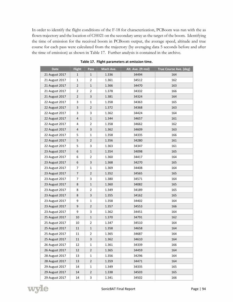
SonicBAT Final Report Page | 94
In order to identify the flight conditions of the F-18 for characterization, PCBoom was run with the as
flown trajectory and the location of CH021 on the secondary array as the target of the boom. Identifying
the time of emission for the received boom in PCBoom output, the average speed, altitude and true
course for each pass were calculated from the trajectory (by averaging data 5 seconds before and after
the time of emission) as shown in Table 17. Further analysis is contained in the archive.
Table 17. Flight parameters at emission time.
Date Flight Pass Mach Ave. Alt. Ave. (ft msl) True Course Ave. (deg)
21 August 2017 1 1 1.336 34494 164
21 August 2017 1 2 1.361 34512 162
21 August 2017 2 1 1.366 34470 163
21 August 2017 2 2 1.378 34332 166
21 August 2017 2 3 1.381 34324 164
22 August 2017 3 1 1.358 34363 165
22 August 2017 3 2 1.372 34368 163
22 August 2017 3 3 1.362 34424 164
22 August 2017 4 1 1.344 34657 161
22 August 2017 4 2 1.358 34662 162
22 August 2017 4 3 1.362 34609 163
22 August 2017 5 1 1.358 34335 166
22 August 2017 5 2 1.356 34280 161
22 August 2017 5 3 1.363 34347 161
23 August 2017 6 1 1.354 34098 165
23 August 2017 6 2 1.360 34417 164
23 August 2017 6 3 1.368 34270 165
23 August 2017 7 1 1.369 34408 164
23 August 2017 7 2 1.352 34565 165
23 August 2017 7 3 1.380 34571 164
23 August 2017 8 1 1.360 34082 165
23 August 2017 8 2 1.349 34189 165
23 August 2017 8 3 1.355 34162 165
23 August 2017 9 1 1.358 34402 164
23 August 2017 9 2 1.357 34553 166
23 August 2017 9 3 1.362 34451 164
25 August 2017 10 1 1.370 34791 162
25 August 2017 10 2 1.347 34510 164
25 August 2017 11 1 1.358 34658 164
25 August 2017 11 2 1.365 34687 164
25 August 2017 11 3 1.362 34610 164
26 August 2017 12 1 1.361 34339 166
26 August 2017 12 2 1.365 34459 164
28 August 2017 13 1 1.356 34296 164
28 August 2017 13 2 1.359 34471 164
29 August 2017 14 1 1.349 34335 165
29 August 2017 14 2 1.338 34503 165
29 August 2017 14 3 1.341 34502 166
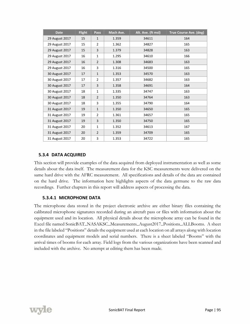
SonicBAT Final Report Page | 95
Date Flight Pass Mach Ave. Alt. Ave. (ft msl) True Course Ave. (deg)
29 August 2017 15 1 1.359 34611 164
29 August 2017 15 2 1.362 34827 165
29 August 2017 15 3 1.379 34828 163
29 August 2017 16 1 1.295 34610 166
29 August 2017 16 2 1.308 34683 163
29 August 2017 16 3 1.316 34500 165
30 August 2017 17 1 1.353 34570 163
30 August 2017 17 2 1.357 34682 163
30 August 2017 17 3 1.358 34691 164
30 August 2017 18 1 1.335 34747 163
30 August 2017 18 2 1.350 34764 163
30 August 2017 18 3 1.355 34790 164
31 August 2017 19 1 1.350 34650 165
31 August 2017 19 2 1.361 34657 165
31 August 2017 19 3 1.350 34750 165
31 August 2017 20 1 1.352 34613 167
31 August 2017 20 2 1.359 34709 165
31 August 2017 20 3 1.353 34722 165
5.3.4 DATA ACQUIRED
This section will provide examples of the data acquired from deployed instrumentation as well as some
details about the data itself. The measurement data for the KSC measurements were delivered on the
same hard drive with the AFRC measurement. All specifications and details of the data are contained
on the hard drive. The information here highlights aspects of the data germane to the raw data
recordings. Further chapters in this report will address aspects of processing the data.
5.3.4.1 MICROPHONE DATA
The microphone data stored in the project electronic archive are either binary files containing the
calibrated microphone signatures recorded during an aircraft pass or files with information about the
equipment used and its location. All physical details about the microphone array can be found in the
Excel file named SonicBAT_NASAKSC_Measurements_August2017_Positions_ALLBooms. A sheet
in the file labeled “Positions” details the equipment used at each location on all arrays along with location
coordinates and equipment models and serial numbers. There is a sheet labeled “Booms” with the
arrival times of booms for each array. Field logs from the various organizations have been scanned and
included with the archive. No attempt at editing them has been made.
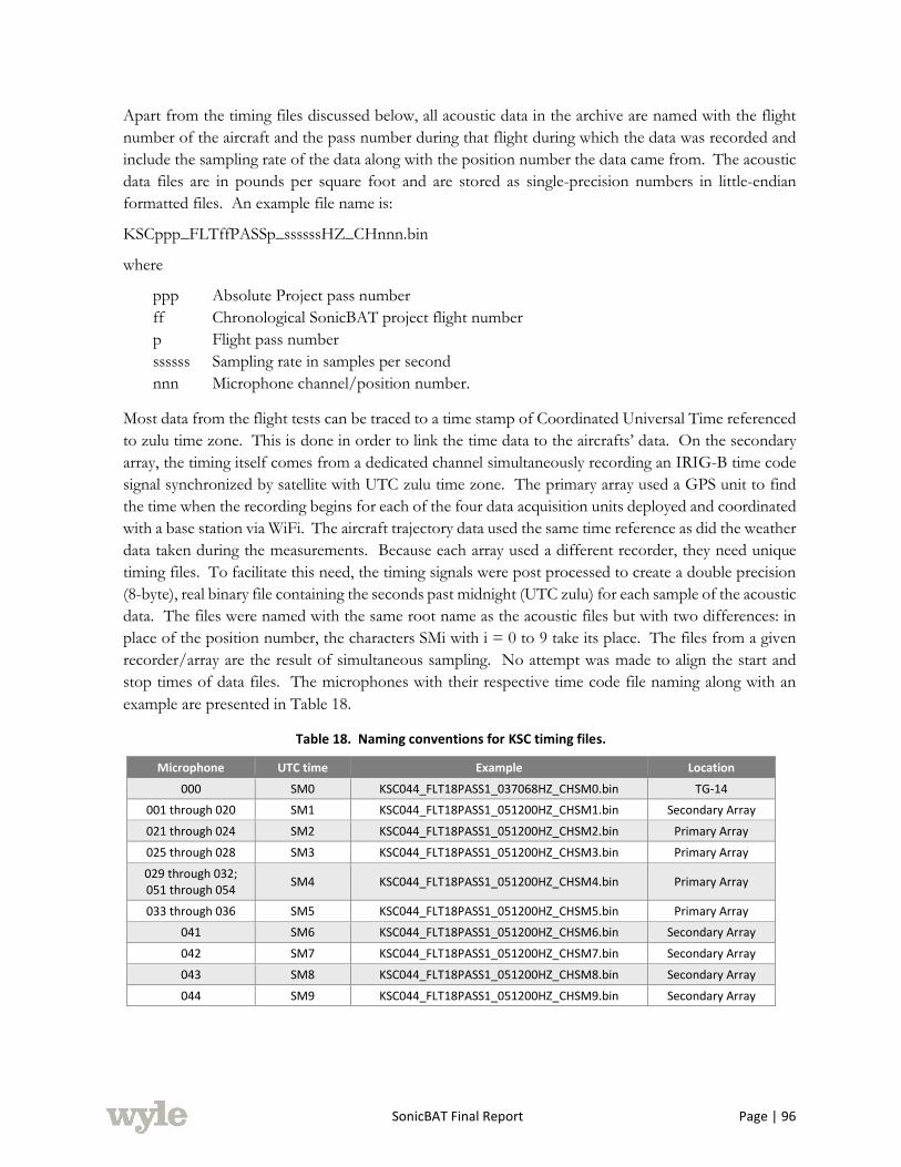
SonicBAT Final Report Page | 96
Apart from the timing files discussed below, all acoustic data in the archive are named with the flight
number of the aircraft and the pass number during that flight during which the data was recorded and
include the sampling rate of the data along with the position number the data came from. The acoustic
data files are in pounds per square foot and are stored as single-precision numbers in little-endian
formatted files. An example file name is:
KSCppp_FLTffPASSp_ssssssHZ_CHnnn.bin
where
ppp Absolute Project pass number
ff Chronological SonicBAT project flight number
p Flight pass number
ssssss Sampling rate in samples per second
nnn Microphone channel/position number.
Most data from the flight tests can be traced to a time stamp of Coordinated Universal Time referenced
to zulu time zone. This is done in order to link the time data to the aircrafts’ data. On the secondary
array, the timing itself comes from a dedicated channel simultaneously recording an IRIG-B time code
signal synchronized by satellite with UTC zulu time zone. The primary array used a GPS unit to find
the time when the recording begins for each of the four data acquisition units deployed and coordinated
with a base station via WiFi. The aircraft trajectory data used the same time reference as did the weather
data taken during the measurements. Because each array used a different recorder, they need unique
timing files. To facilitate this need, the timing signals were post processed to create a double precision
(8-byte), real binary file containing the seconds past midnight (UTC zulu) for each sample of the acoustic
data. The files were named with the same root name as the acoustic files but with two differences: in
place of the position number, the characters SMi with i = 0 to 9 take its place. The files from a given
recorder/array are the result of simultaneous sampling. No attempt was made to align the start and
stop times of data files. The microphones with their respective time code file naming along with an
example are presented in Table 18.
Table 18. Naming conventions for KSC timing files.
Microphone UTC time Example Location
000 SM0 KSC044_FLT18PASS1_037068HZ_CHSM0.bin TG-14
001 through 020 SM1 KSC044_FLT18PASS1_051200HZ_CHSM1.bin Secondary Array
021 through 024 SM2 KSC044_FLT18PASS1_051200HZ_CHSM2.bin Primary Array
025 through 028 SM3 KSC044_FLT18PASS1_051200HZ_CHSM3.bin Primary Array
029 through 032; 051 through 054 SM4 KSC044_FLT18PASS1_051200HZ_CHSM4.bin Primary Array
033 through 036 SM5 KSC044_FLT18PASS1_051200HZ_CHSM5.bin Primary Array
041 SM6 KSC044_FLT18PASS1_051200HZ_CHSM6.bin Secondary Array
042 SM7 KSC044_FLT18PASS1_051200HZ_CHSM7.bin Secondary Array
043 SM8 KSC044_FLT18PASS1_051200HZ_CHSM8.bin Secondary Array
044 SM9 KSC044_FLT18PASS1_051200HZ_CHSM9.bin Secondary Array
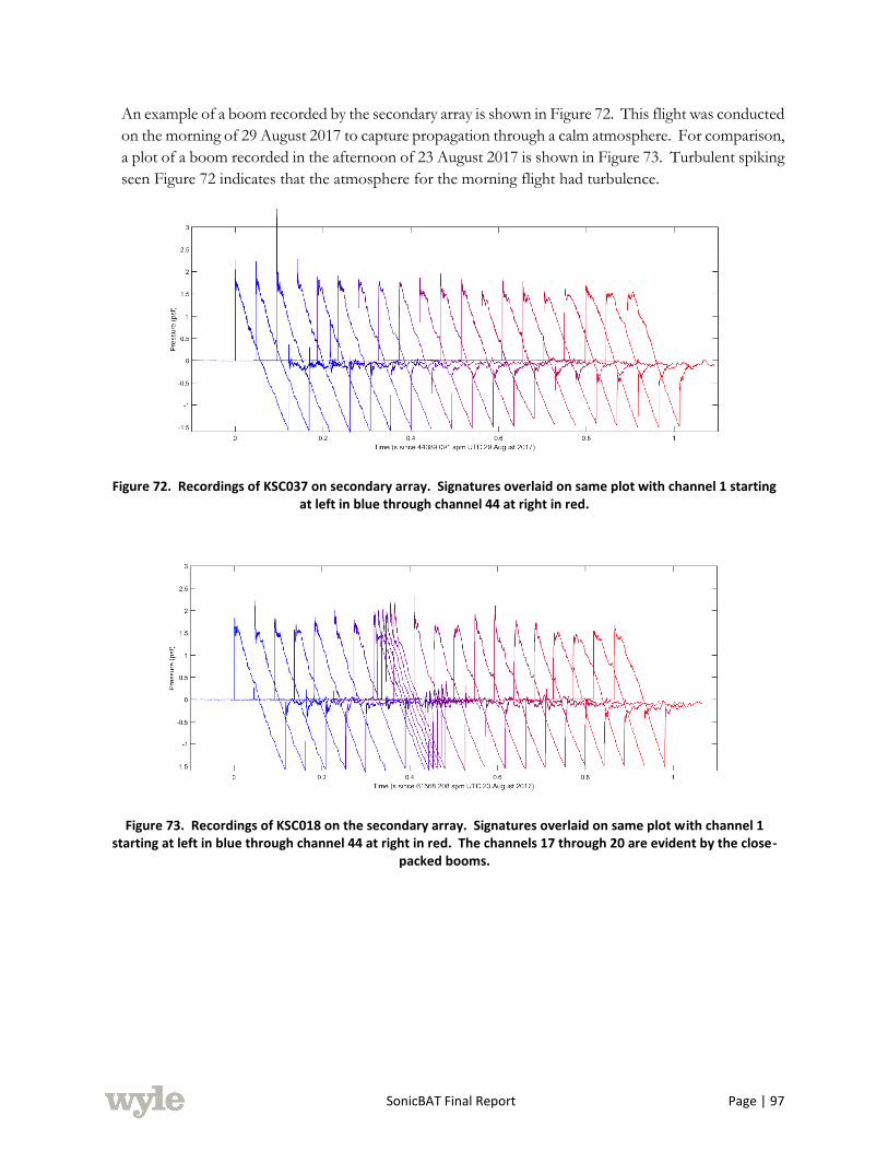
SonicBAT Final Report Page | 97
An example of a boom recorded by the secondary array is shown in Figure 72. This flight was conducted
on the morning of 29 August 2017 to capture propagation through a calm atmosphere. For comparison,
a plot of a boom recorded in the afternoon of 23 August 2017 is shown in Figure 73. Turbulent spiking
seen Figure 72 indicates that the atmosphere for the morning flight had turbulence.
Figure 72. Recordings of KSC037 on secondary array. Signatures overlaid on same plot with channel 1 starting at left in blue through channel 44 at right in red.
Figure 73. Recordings of KSC018 on the secondary array. Signatures overlaid on same plot with channel 1 starting at left in blue through channel 44 at right in red. The channels 17 through 20 are evident by the close-
packed booms.

SonicBAT Final Report Page | 98
5.3.5 METEOROLOGICAL DATA
This section contains examples of the data acquired from the deployed meteorological equipment. An
example of the met data from the tower at the secondary array on 21 August 2017 is shown in Figure
74. Only the temperature and relative humidity are graphed. As can be seen in the figure, the goal of
measuring sonic boom propagation in a hot, wet climate was achieved during the KSC test.
Figure 74. Met data at secondary array on 21 August 2017 showing flight times.
The atmospheric profile was modeled for each day of flights. The GPSsonde (balloon) measured the
atmospheric profile within 1 hour of each flight. The modeled (forecast) atmospheric profile for 14:00
on 29 August 2017 is shown in Figure 75. The measurement via GPSsonde occurred at 14:27 and is
shown in Figure 76. As can be seen in the two figures, the wind profiles agree well as shown by the
wind barbs. Problems with the measured dew point values in this data set occurred above 36,000 ft.
Since the modeling in PCBoom for the steady state portion of the trajectory was done for when the
aircraft was below that altitude, this does not affect these modeling results.

SonicBAT Final Report Page | 99
Figure 75. Skew-T Log P diagram of forecast for 14:00 UTC on 29 August 2017 at KSC. Dashed, black line is the dew point. Solid, black line is the temperature. Windbarbs scaled in knots.
Figure 76. Skew-T Log P diagram of GPSsonde launched at 14:29 UTC on 29 August 2017 at KSC. Dashed, black line is the dew point. Solid, black line is the temperature. Windbarbs scaled in knots.
Problems with the balloon data occurred above 36,000 ft (~ 10.9 km).
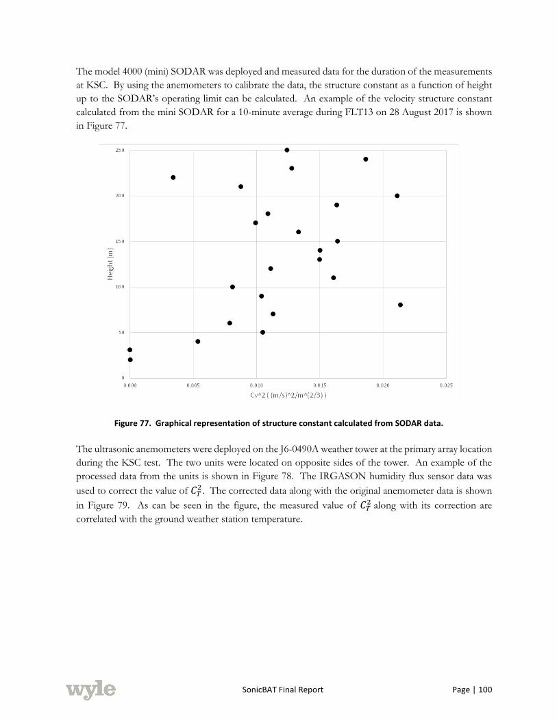
SonicBAT Final Report Page | 100
The model 4000 (mini) SODAR was deployed and measured data for the duration of the measurements
at KSC. By using the anemometers to calibrate the data, the structure constant as a function of height
up to the SODAR’s operating limit can be calculated. An example of the velocity structure constant
calculated from the mini SODAR for a 10-minute average during FLT13 on 28 August 2017 is shown
in Figure 77.
Figure 77. Graphical representation of structure constant calculated from SODAR data.
The ultrasonic anemometers were deployed on the J6-0490A weather tower at the primary array location
during the KSC test. The two units were located on opposite sides of the tower. An example of the
processed data from the units is shown in Figure 78. The IRGASON humidity flux sensor data was
used to correct the value of 𝐶𝑇2. The corrected data along with the original anemometer data is shown
in Figure 79. As can be seen in the figure, the measured value of 𝐶𝑇2 along with its correction are
correlated with the ground weather station temperature.

SonicBAT Final Report Page | 101
Figure 78. Structure constants from anemometers for 23 August 2017 along with a ground weather station’s data.
Figure 79. Structure constants corrected for humidity on 23 August 2017 along with a ground weather station’s data.
5.3.6 AIRCRAFT TRACKING DATA
Whether the aircraft data is for the fully instrumented F-18B or the GPS – only F-18A, the information
that details the vehicle’s flight condition and position as a function of time is reduced to a trajectory file
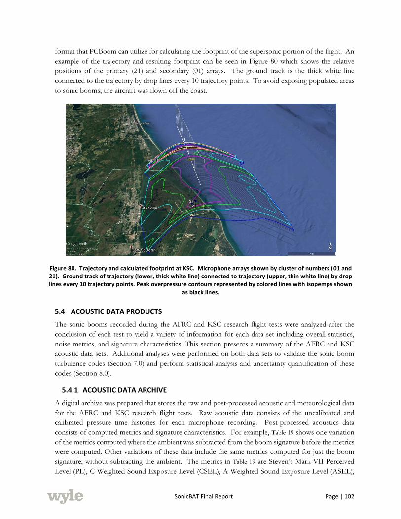
SonicBAT Final Report Page | 102
format that PCBoom can utilize for calculating the footprint of the supersonic portion of the flight. An
example of the trajectory and resulting footprint can be seen in Figure 80 which shows the relative
positions of the primary (21) and secondary (01) arrays. The ground track is the thick white line
connected to the trajectory by drop lines every 10 trajectory points. To avoid exposing populated areas
to sonic booms, the aircraft was flown off the coast.
Figure 80. Trajectory and calculated footprint at KSC. Microphone arrays shown by cluster of numbers (01 and 21). Ground track of trajectory (lower, thick white line) connected to trajectory (upper, thin white line) by drop lines every 10 trajectory points. Peak overpressure contours represented by colored lines with isopemps shown
as black lines.
5.4 ACOUSTIC DATA PRODUCTS
The sonic booms recorded during the AFRC and KSC research flight tests were analyzed after the
conclusion of each test to yield a variety of information for each data set including overall statistics,
noise metrics, and signature characteristics. This section presents a summary of the AFRC and KSC
acoustic data sets. Additional analyses were performed on both data sets to validate the sonic boom
turbulence codes (Section 7.0) and perform statistical analysis and uncertainty quantification of these
codes (Section 8.0).
5.4.1 ACOUSTIC DATA ARCHIVE
A digital archive was prepared that stores the raw and post-processed acoustic and meteorological data
for the AFRC and KSC research flight tests. Raw acoustic data consists of the uncalibrated and
calibrated pressure time histories for each microphone recording. Post-processed acoustics data
consists of computed metrics and signature characteristics. For example, Table 19 shows one variation
of the metrics computed where the ambient was subtracted from the boom signature before the metrics
were computed. Other variations of these data include the same metrics computed for just the boom
signature, without subtracting the ambient. The metrics in Table 19 are Steven’s Mark VII Perceived
Level (PL), C-Weighted Sound Exposure Level (CSEL), A-Weighted Sound Exposure Level (ASEL),

SonicBAT Final Report Page | 103
Unweighted Sound Exposure Level (FSEL), Zwicker loudness for frontal incidence (LLZf), Zwicker
loudness for diffuse incidence (LLZd), Kryter’s Perceived Noise Level (PNL), B-Weighted Sound
Exposure Level (BSEL), D-Weighted Sound Exposure Level (DSEL), E-Weighted Sound Exposure
Level (ESEL), and Indoor Sonic Boom Annoyance Prediction Level (ISBAP).
Table 19. Example of noise metrics computed.
File Name
Boom Minus Ambient - 650 ms Window
PL (dB)
CSEL (dB)
ASEL (dB)
FSEL (dB)
LLZf (Phons)
LLZd (Phons)
PNL (dB)
BSEL (dB)
DSEL (dB)
ESEL (dB)
ISBAP (dB)
BAT01_FLT1PASS1_CH001 103.1 108.5 86.7 119.1 112.5 112.9 110.4 98.1 97.9 94.2 112.3
BAT01_FLT1PASS1_CH002 106.8 107.7 92.5 118.7 115.0 115.5 114.1 99.8 99.7 97.9 113.2
BAT01_FLT1PASS1_CH003 107.2 107.0 93.4 118.7 116.0 116.6 114.8 99.8 100.0 98.3 113.0
BAT01_FLT1PASS1_CH004 102.9 106.3 88.1 118.5 111.7 112.1 110.4 97.0 97.0 94.4 110.5
BAT01_FLT1PASS1_CH005 103.6 106.9 88.7 119.0 114.0 114.3 111.3 96.9 97.4 94.4 111.3
BAT01_FLT1PASS1_CH006 101.5 106.7 86.5 119.1 110.4 111.0 108.5 96.2 96.4 93.1 110.0
BAT01_FLT1PASS1_CH007 104.7 106.7 91.1 119.0 112.8 113.5 111.9 98.5 98.5 96.6 111.3
BAT01_FLT1PASS1_CH008 101.7 106.2 86.7 119.0 109.6 110.1 109.1 96.6 96.6 93.8 109.8
BAT01_FLT1PASS1_CH009 99.4 105.5 84.0 119.2 108.5 109.0 107.0 94.6 95.1 91.1 108.5
BAT01_FLT1PASS1_CH010 97.9 105.2 81.6 119.1 107.0 107.4 105.3 93.5 94.3 89.7 107.8
BAT01_FLT1PASS1_CH011 98.9 105.4 83.5 119.2 108.4 109.0 106.2 94.0 94.6 90.4 108.1
BAT01_FLT1PASS1_CH012 98.2 106.0 82.9 119.0 108.9 109.3 106.6 94.0 94.7 90.3 107.9
BAT01_FLT1PASS1_CH013 99.0 106.5 83.1 118.7 109.7 110.1 107.4 95.0 95.2 90.9 108.8
BAT01_FLT1PASS1_CH015 103.8 107.0 88.4 118.6 112.5 112.9 111.4 98.3 97.9 95.2 111.7
BAT01_FLT1PASS1_CH016 104.9 106.8 90.6 118.5 113.5 114.1 112.5 99.2 98.8 96.7 111.7
An example of the signature characteristics data computed is shown in Table 20 including the signature
period (time from beginning of boom’s front shock to the negative peak), signature positive duration
(time from boom’s front shock to when expansion portion of signature becomes negative), impulse
(numerical integration of positive duration portion of signature), 10%-90% rise time (time difference
between points on front shock of boom equal to 10% and 90% of the peak overpressure), DC bias 200
(RMS values of signal using 200 ms of record ending 3 ms before front shock), positive and negative
peak pressures (maximum and minimum value of boom record), and waveform category. Waveform
category represents a manual classification, by pattern recognition, of the boom signature into one of
ten categories of waveforms including different types of N-waves, peaked waves, spiked waves, and
rounded waves (as described in section 5.4.3). These categories indicate how a boom signature was
distorted by turbulence, as it propagated through the ABL to the ground where it was recorded.
Comparisons of the AFRC and KSC sonic boom rise times and waveform categories are discussed
further in this section.
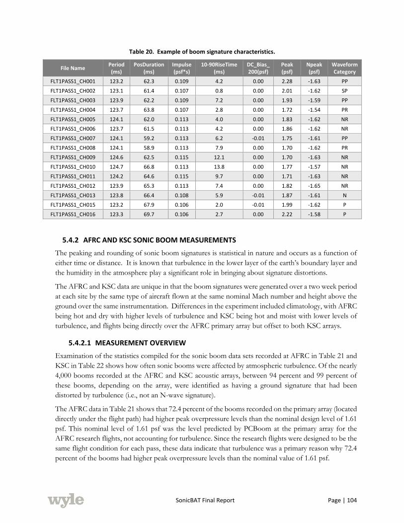
SonicBAT Final Report Page | 104
Table 20. Example of boom signature characteristics.
File Name Period (ms)
PosDuration (ms)
Impulse (psf*s)
10-90RiseTime (ms)
DC_Bias_ 200(psf)
Peak (psf)
Npeak (psf)
Waveform Category
FLT1PASS1_CH001 123.2 62.3 0.109 4.2 0.00 2.28 -1.63 PP
FLT1PASS1_CH002 123.1 61.4 0.107 0.8 0.00 2.01 -1.62 SP
FLT1PASS1_CH003 123.9 62.2 0.109 7.2 0.00 1.93 -1.59 PP
FLT1PASS1_CH004 123.7 63.8 0.107 2.8 0.00 1.72 -1.54 PR
FLT1PASS1_CH005 124.1 62.0 0.113 4.0 0.00 1.83 -1.62 NR
FLT1PASS1_CH006 123.7 61.5 0.113 4.2 0.00 1.86 -1.62 NR
FLT1PASS1_CH007 124.1 59.2 0.113 6.2 -0.01 1.75 -1.61 PP
FLT1PASS1_CH008 124.1 58.9 0.113 7.9 0.00 1.70 -1.62 PR
FLT1PASS1_CH009 124.6 62.5 0.115 12.1 0.00 1.70 -1.63 NR
FLT1PASS1_CH010 124.7 66.8 0.113 13.8 0.00 1.77 -1.57 NR
FLT1PASS1_CH011 124.2 64.6 0.115 9.7 0.00 1.71 -1.63 NR
FLT1PASS1_CH012 123.9 65.3 0.113 7.4 0.00 1.82 -1.65 NR
FLT1PASS1_CH013 123.8 66.4 0.108 5.9 -0.01 1.87 -1.61 N
FLT1PASS1_CH015 123.2 67.9 0.106 2.0 -0.01 1.99 -1.62 P
FLT1PASS1_CH016 123.3 69.7 0.106 2.7 0.00 2.22 -1.58 P
5.4.2 AFRC AND KSC SONIC BOOM MEASUREMENTS
The peaking and rounding of sonic boom signatures is statistical in nature and occurs as a function of
either time or distance. It is known that turbulence in the lower layer of the earth’s boundary layer and
the humidity in the atmosphere play a significant role in bringing about signature distortions.
The AFRC and KSC data are unique in that the boom signatures were generated over a two week period
at each site by the same type of aircraft flown at the same nominal Mach number and height above the
ground over the same instrumentation. Differences in the experiment included climatology, with AFRC
being hot and dry with higher levels of turbulence and KSC being hot and moist with lower levels of
turbulence, and flights being directly over the AFRC primary array but offset to both KSC arrays.
5.4.2.1 MEASUREMENT OVERVIEW
Examination of the statistics compiled for the sonic boom data sets recorded at AFRC in Table 21 and
KSC in Table 22 shows how often sonic booms were affected by atmospheric turbulence. Of the nearly
4,000 booms recorded at the AFRC and KSC acoustic arrays, between 94 percent and 99 percent of
these booms, depending on the array, were identified as having a ground signature that had been
distorted by turbulence (i.e., not an N-wave signature).
The AFRC data in Table 21 shows that 72.4 percent of the booms recorded on the primary array (located
directly under the flight path) had higher peak overpressure levels than the nominal design level of 1.61
psf. This nominal level of 1.61 psf was the level predicted by PCBoom at the primary array for the
AFRC research flights, not accounting for turbulence. Since the research flights were designed to be the
same flight condition for each pass, these data indicate that turbulence was a primary reason why 72.4
percent of the booms had higher peak overpressure levels than the nominal value of 1.61 psf.

SonicBAT Final Report Page | 105
Table 21. AFRC sonic boom statistics.
AFRC Boom Characteristics Primary Array Secondary Array Tertiary Array
Count % Count % Count %
PCBoom Avg computed boom level (psf) 1.61 1.56 1.48
PCBoom STD computed boom levels (psf) 0.06 0.08 0.07
Total number of measured booms 1034 100.0 518 100.0 507 100.0
Booms with N-wave signature 49 4.7 19 3.7 7 1.4
Booms with turbulized signature 985 95.3 499 96.3 500 98.6
Booms <= 1.61 peak psf 285 27.6
Booms > 1.61 peak psf 749 72.4
Booms <= 1.56 peak psf 178 34.4
Booms > 1.56 peak psf 340 65.6
Booms <= 1.48 peak psf 192 37.9
Booms > 1.48 peak psf 315 62.1
Metric Stats Value Value Value
Min peak psf 0.87 0.91 0.69
Max peak psf 6.10 5.31 4.29
Avg peak psf 1.95 1.78 1.69
STD peak psf 0.60 0.53 0.52
Min PLdB 91.1 90.7 89.8
Max PLdB 117.2 115.8 115.5
Avg PLdB 103.1 101.3 100.3
STD PLdB 4.41 4.13 4.48
Table 22. KSC sonic boom statistics.
KSC Boom Characteristics Primary Array Secondary Array
Count % Count %
PCBoom Avg computed boom level (psf) 1.35 1.50
PCBoom STD computed boom levels (psf) 0.29 0.28
Total number of measured booms 777 100.0 1106 100.0
Booms with N-wave signature 20 2.6 66 6.0
Booms with turbulized signature 757 97.4 1040 94.0
Booms <= 1.35 peak psf 249 32.0
Booms > 1.35 peak psf 528 68.0
Booms <= 1.50 peak psf 305 27.6
Booms > 1.50 peak psf 801 72.4
Metric Stats Value Value
Min peak psf 0.65 0.84
Max peak psf 5.26 4.72
Avg peak psf 1.59 1.75
STD peak psf 0.47 0.44
Min PLdB 78.9 90.5
Max PLdB 118.6 118.8
Avg PLdB 102.6 105.1
STD PLdB 4.78 4.17

SonicBAT Final Report Page | 106
The maximum peak psf recorded on the AFRC primary array for all clean recordings was 6.1 psf. There
was one instance where a boom exceeded the dynamic range of the recorder at a level of 7.02 psf;
judging from the rise time of this clipped recording, the actual peak was several psf higher. The
secondary array data from the AFRC test indicates that 65.6 percent of the recorded booms had higher
peak overpressure levels than the nominal value of 1.56 psf (nominal value at the secondary array is
somewhat lower than 1.61 psf due to the greater propagation distance).
Similarly, the KSC data in Table 22 shows that 68 percent of the booms recorded on the primary array
had higher peak overpressure levels than the nominal design level of 1.35 psf and 72.4 percent of the
booms recorded on the secondary array had higher peak overpressure levels than the nominal design
level of 1.5 psf. Note that the secondary array at KSC was located closer to the flight path than the
primary array and the flight path was 0.4 to 6.5 nmi offset from the secondary array, such that the
nominal peak levels varied with flight path offset, part of the total variation. The standard deviation of
the computed Perceived Level, PLdB, for the AFRC primary and secondary arrays is 4.41 dB and 4.13
dB, respectively. The standard deviation of PLdB for the KSC primary and secondary arrays is 4.78 dB
and 4.17 dB, respectively.
5.4.2.2 PROBABILITY PLOTS OF OVERPRESSURES DP
The manner of plotting in Figure 81 is not intended to imply the type of distribution which would best
describe the data. Although a log-normal distribution, of the type shown in Figure 4 , may be suggested,
no one type of distribution has been looked at so as to give a satisfactory fit for these data over the
entire range of the data.
Figure 81 (a-b). Probability plots of peak overpressures measured at various lateral locations during the SonicBAT flight test programs at AFRC and KSC.

SonicBAT Final Report Page | 107
Looking first to the probability of equaling or exceeding a given value of overpressure for both AFRC
and KSC and the three lateral locations, as shown in Figure 81a, a number of observations can be made.
First, more variability was experienced during the AFRC flight tests than at KSC. This was expected
because of the more frequent and higher levels of turbulence and lower humidity’s associated with arid
climates. Second, the increase in variability as overpressure increases were anticipated based on past
observations but because of the more intense turbulence encountered the variability is considerably
greater. However, as overpressures decrease, especially at the lower values, the data was expected to
fall off rather than showing a tendency to increase. Third, it was expected that the variability would
increase with increasing lateral displacement from the ground track. A look at the dashed lines on the
figure show this is not the case. Although the lateral distances at which the measurements were made
are not that large, one would not expect more signature variability (and resulting overpressure). Then
and again the turbulence encountered at those locations could have been more intense.
Another view of the variability in signature overpressure is to look at the probability of equaling or
exceeding a given value of the ratio of measured overpressure to the median value. This set of curves,
presented in Figure 81b, results from taking the data of Figure 81a and dividing by the overpressure
associated with the 50% probability value. Aside from a collapsing of the data from the three lateral
locations into a single curve the messages stated earlier are still evident.
As mentioned earlier in these discussions, presenting the results of Figure 81b on log-log coordinates
and dividing the measured overpressures by the predicted overpressure for flight in a standard
atmosphere with no wind will allow for a one to one comparison to the results shown on Figure 4 of
this report.
5.4.2.3 HISTOGRAMS OF MEASURED OVERPRESSURES
Another view of the variability in boom signature overpressure can be had by plotting histograms shown
in Figure 82. Addressing the AFRC results shown in the figure it can be seen that the largest variability
occurs at the on track location with the least variability occurring at the 1.2 nmi location. The greatest
number of events occur at the overpressures of about 1.8 psf, 1.7 psf, and 1.6 psf at the 0 nmi, 1.2 nmi,
and 2.4 nmi lateral locations, respectively. These values are higher for all three locations than the
predicted, no-turbulence levels of 1.61 psf, 1.56 psf, and 1.48 psf.
Examination of the KSC results shown in Figure 82 show less variability in the measured overpressures
than that observed at AFRC at the 0 – 2 nmi lateral locations and at the 2.4 – 4 nmi lateral locations.
The greatest number of events for the KSC data occurred at overpressures of about 1.7 psf, 1.7 psf, and
1.5 psf at the 0 – 2 nmi, 2.4 – 4 nmi, and 6 nmi lateral locations, respectively. Note that the plot in
Figure 82 showing the KSC 6 nmi lateral location has a vertical scale of 0 to 0.2 relative probability
whereas all of the other plots have a vertical scale of 0 to 0.1 relative probability.
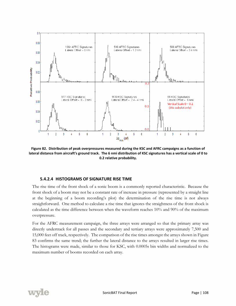
SonicBAT Final Report Page | 108
Figure 82. Distribution of peak overpressures measured during the KSC and AFRC campaigns as a function of lateral distance from aircraft’s ground track. The 6 nmi distribution of KSC signatures has a vertical scale of 0 to
0.2 relative probability.
5.4.2.4 HISTOGRAMS OF SIGNATURE RISE TIME
The rise time of the front shock of a sonic boom is a commonly reported characteristic. Because the
front shock of a boom may not be a constant rate of increase in pressure (represented by a straight line
at the beginning of a boom recording’s plot) the determination of the rise time is not always
straightforward. One method to calculate a rise time that ignores the straightness of the front shock is
calculated as the time difference between when the waveform reaches 10% and 90% of the maximum
overpressure.
For the AFRC measurement campaign, the three arrays were arranged so that the primary array was
directly undertrack for all passes and the secondary and tertiary arrays were approximately 7,500 and
15,000 feet off track, respectively. The comparison of the rise times amongst the arrays shown in Figure
83 confirms the same trend; the further the lateral distance to the arrays resulted in larger rise times.
The histograms were made, similar to those for KSC, with 0.0005s bin widths and normalized to the
maximum number of booms recorded on each array.
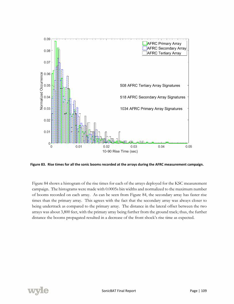
SonicBAT Final Report Page | 109
Figure 83. Rise times for all the sonic booms recorded at the arrays during the AFRC measurement campaign.
Figure 84 shows a histogram of the rise times for each of the arrays deployed for the KSC measurement
campaign. The histograms were made with 0.0005s bin widths and normalized to the maximum number
of booms recorded on each array. As can be seen from Figure 84, the secondary array has faster rise
times than the primary array. This agrees with the fact that the secondary array was always closer to
being undertrack as compared to the primary array. The distance in the lateral offset between the two
arrays was about 3,800 feet, with the primary array being further from the ground track; thus, the further
distance the booms propagated resulted in a decrease of the front shock’s rise time as expected.
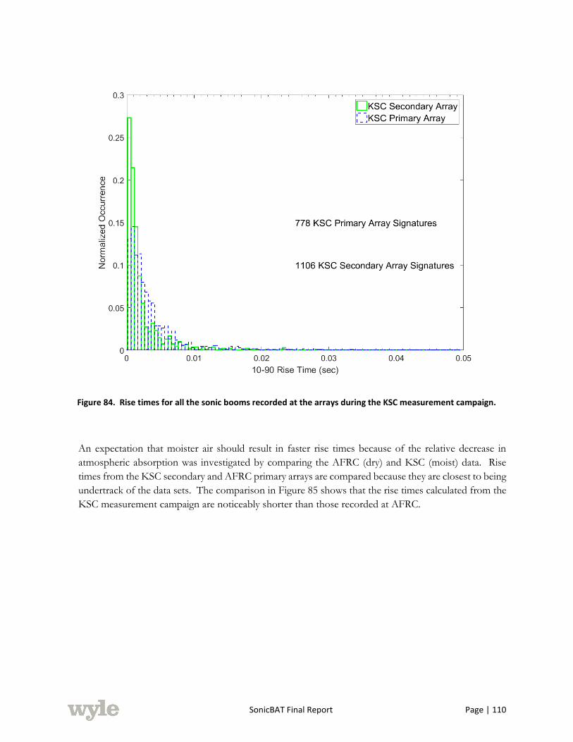
SonicBAT Final Report Page | 110
Figure 84. Rise times for all the sonic booms recorded at the arrays during the KSC measurement campaign.
An expectation that moister air should result in faster rise times because of the relative decrease in
atmospheric absorption was investigated by comparing the AFRC (dry) and KSC (moist) data. Rise
times from the KSC secondary and AFRC primary arrays are compared because they are closest to being
undertrack of the data sets. The comparison in Figure 85 shows that the rise times calculated from the
KSC measurement campaign are noticeably shorter than those recorded at AFRC.

SonicBAT Final Report Page | 111
Figure 85. Rise times for all the sonic booms recorded at the arrays closest to being under track for the AFRC and KSC measurement campaigns.
5.4.2.5 PROBABILITY PLOTS OF PERCEIVED LEVEL (PLDB)
The plots in Figure 86 and Figure 87 show a summary of all measured sonic boom data at AFRC and
KSC. Figure 86 shows the probability distribution of measured perceived level; this plot indicates, for
example, that fifty percent of the measured perceived levels on the AFRC tertiary array exceed 100
PLdB. Figure 87 shows the probability distribution of the ratio of measured perceived level (PLdB) to
average perceived level on each array indicating the probability that the measured perceived level is
greater than the average perceived level. Variation of the data in both figures is largely a result of
atmospheric effects and to a substantial degree turbulence. Of note is how closely distributed are these
acoustic data sets from the different measurement arrays, given that measurements from each array
include different effects of turbulence due either to local climate, time of day, or sonic boom
propagation path length differences. The notable outlying data in both plots, representing a single flight
pass recorded at the KSC primary array, were measured during highly overcast conditions which likely
attenuated the noise during propagation. It was indicated in the field notes that the noise heard at the
ground arrays for this flight pass was distinctly muffled.
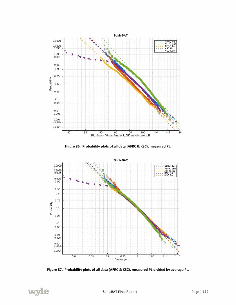
SonicBAT Final Report Page | 112
Figure 86. Probability plots of all data (AFRC & KSC), measured PL.
Figure 87. Probability plots of all data (AFRC & KSC), measured PL divided by average PL.
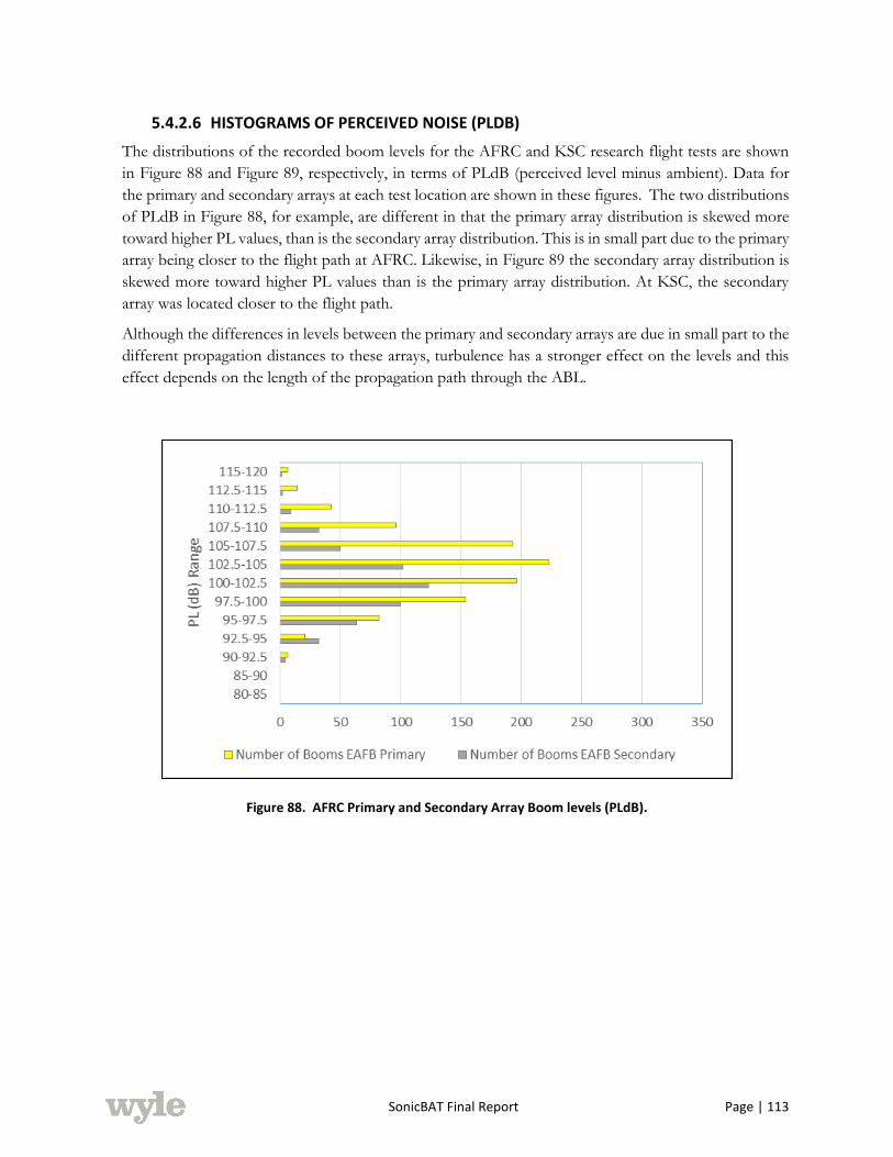
SonicBAT Final Report Page | 113
5.4.2.6 HISTOGRAMS OF PERCEIVED NOISE (PLDB)
The distributions of the recorded boom levels for the AFRC and KSC research flight tests are shown
in Figure 88 and Figure 89, respectively, in terms of PLdB (perceived level minus ambient). Data for
the primary and secondary arrays at each test location are shown in these figures. The two distributions
of PLdB in Figure 88, for example, are different in that the primary array distribution is skewed more
toward higher PL values, than is the secondary array distribution. This is in small part due to the primary
array being closer to the flight path at AFRC. Likewise, in Figure 89 the secondary array distribution is
skewed more toward higher PL values than is the primary array distribution. At KSC, the secondary
array was located closer to the flight path.
Although the differences in levels between the primary and secondary arrays are due in small part to the
different propagation distances to these arrays, turbulence has a stronger effect on the levels and this
effect depends on the length of the propagation path through the ABL.
Figure 88. AFRC Primary and Secondary Array Boom levels (PLdB).
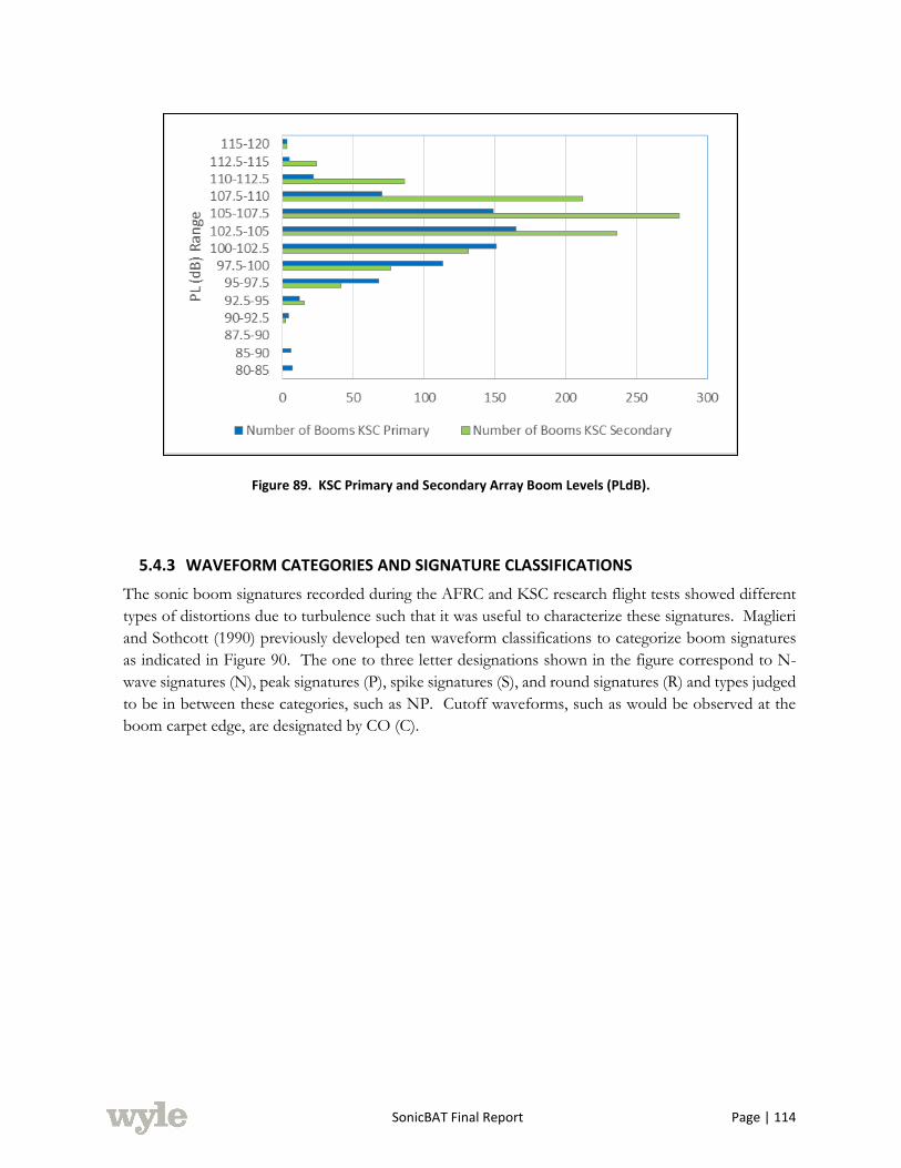
SonicBAT Final Report Page | 114
Figure 89. KSC Primary and Secondary Array Boom Levels (PLdB).
5.4.3 WAVEFORM CATEGORIES AND SIGNATURE CLASSIFICATIONS
The sonic boom signatures recorded during the AFRC and KSC research flight tests showed different
types of distortions due to turbulence such that it was useful to characterize these signatures. Maglieri
and Sothcott (1990) previously developed ten waveform classifications to categorize boom signatures
as indicated in Figure 90. The one to three letter designations shown in the figure correspond to N-
wave signatures (N), peak signatures (P), spike signatures (S), and round signatures (R) and types judged
to be in between these categories, such as NP. Cutoff waveforms, such as would be observed at the
boom carpet edge, are designated by CO (C).
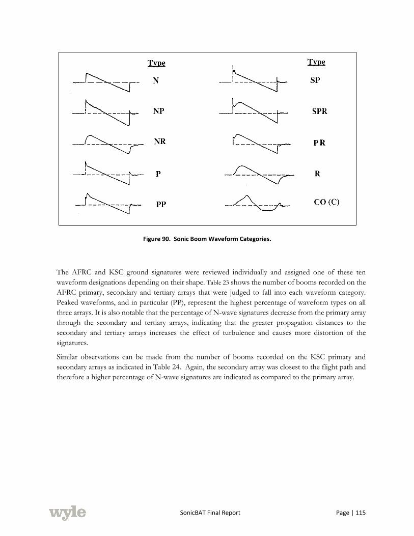
SonicBAT Final Report Page | 115
Figure 90. Sonic Boom Waveform Categories.
The AFRC and KSC ground signatures were reviewed individually and assigned one of these ten
waveform designations depending on their shape. Table 23 shows the number of booms recorded on the
AFRC primary, secondary and tertiary arrays that were judged to fall into each waveform category.
Peaked waveforms, and in particular (PP), represent the highest percentage of waveform types on all
three arrays. It is also notable that the percentage of N-wave signatures decrease from the primary array
through the secondary and tertiary arrays, indicating that the greater propagation distances to the
secondary and tertiary arrays increases the effect of turbulence and causes more distortion of the
signatures.
Similar observations can be made from the number of booms recorded on the KSC primary and
secondary arrays as indicated in Table 24. Again, the secondary array was closest to the flight path and
therefore a higher percentage of N-wave signatures are indicated as compared to the primary array.
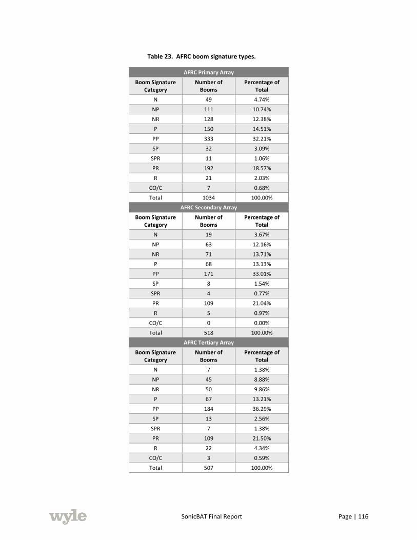
SonicBAT Final Report Page | 116
Table 23. AFRC boom signature types.
AFRC Primary Array
Boom Signature Category
Number of Booms
Percentage of Total
N 49 4.74%
NP 111 10.74%
NR 128 12.38%
P 150 14.51%
PP 333 32.21%
SP 32 3.09%
SPR 11 1.06%
PR 192 18.57%
R 21 2.03%
CO/C 7 0.68%
Total 1034 100.00%
AFRC Secondary Array
Boom Signature Category
Number of Booms
Percentage of Total
N 19 3.67%
NP 63 12.16%
NR 71 13.71%
P 68 13.13%
PP 171 33.01%
SP 8 1.54%
SPR 4 0.77%
PR 109 21.04%
R 5 0.97%
CO/C 0 0.00%
Total 518 100.00%
AFRC Tertiary Array
Boom Signature Category
Number of Booms
Percentage of Total
N 7 1.38%
NP 45 8.88%
NR 50 9.86%
P 67 13.21%
PP 184 36.29%
SP 13 2.56%
SPR 7 1.38%
PR 109 21.50%
R 22 4.34%
CO/C 3 0.59%
Total 507 100.00%
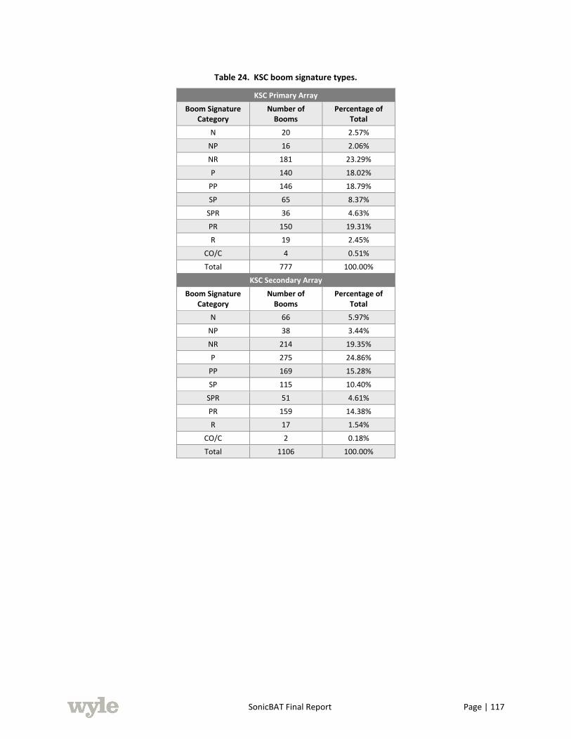
SonicBAT Final Report Page | 117
Table 24. KSC boom signature types.
KSC Primary Array
Boom Signature Category
Number of Booms
Percentage of Total
N 20 2.57%
NP 16 2.06%
NR 181 23.29%
P 140 18.02%
PP 146 18.79%
SP 65 8.37%
SPR 36 4.63%
PR 150 19.31%
R 19 2.45%
CO/C 4 0.51%
Total 777 100.00%
KSC Secondary Array
Boom Signature Category
Number of Booms
Percentage of Total
N 66 5.97%
NP 38 3.44%
NR 214 19.35%
P 275 24.86%
PP 169 15.28%
SP 115 10.40%
SPR 51 4.61%
PR 159 14.38%
R 17 1.54%
CO/C 2 0.18%
Total 1106 100.00%

SonicBAT Final Report Page | 118
6.0
ATMOSPHERIC TURBULENCE MEASUREMENTS AND DATA ANALYSIS
6.1 OVERVIEW
Sound waves propagating through the earth’s atmosphere are continuously scattered through its
interaction with small scale fluctuations of temperature, moisture and velocity. These variations are
observed at sizes within the inertial subrange of atmospheric turbulence. The inertial subrange of
turbulence is identified as that region of variations characterized by the cascade of energy from larger
structures (size depends upon the local atmospheric stability) to sizes associated with the viscous
dissipation of that energy. The actual length scale for this inertial subrange varies because it is dependent
upon the local atmospheric stability.
This section identifies the measurements needed to quantify the structure constants and the local
atmospheric boundary layer height. Whereas Section 2.2 included an overview of the different layers of
the atmosphere, including the atmospheric boundary layer, this section provides additional details of
the atmospheric boundary layer required to define the structure constants and discuss their variation
with increasing height within the boundary layer.
The meteorological measurement and data analysis procedures defined in this section represent the
general case, which includes modification of the temperature structure constant, 𝐶𝑇2, due to the effect
of moisture. These procedures were applied during the KSC test and measurement campaign, which
occurred in a humid environment. Accordingly, the methods described in this section refer to the KSC
test. The AFRC test utilized the same set of meteorological measurement and data analysis procedures
that are reported in this section for the KSC test; except, because of the dry environment conditions
experienced during the AFRC test, the correction to 𝐶𝑇2 to account for moisture fluctuations was
not done. The assumptions of stationarity and homogeneity for the turbulence field was made for both
the AFRC and KSC tests, which are valid assumptions in open fields but not in urban settings.
6.1.1 MEASURING ATMOSPHERIC TURBULENCE
The Atmospheric Boundary Layer (ABL) is that region of the atmosphere adjacent to the earth’s surface
that continuously responds to the diurnal heating and cooling of the earth’s surface. The three
dimensional wind flow within this region also continually responds to the height and type variations of
the earth’s surface. The atmosphere above the ABL is identified as the “free atmosphere” in that the
wind flow patterns, temperature and moisture fields are assumed to be independent of the earth’s
surface.

SonicBAT Final Report Page | 119
Figure 91. Idealized evolution of the atmospheric boundary layer (ABL) over the course of a day over land and under clear skies and a stationary atmosphere. At sunrise, heating from below sets to a mixed (or convective)
boundary layer, while at sunset heat loss to space terminates convection and creates a thin stable layer.
Figure 91 is a graphical presentation of the diurnally driven atmospheric boundary layers for a stationary
and horizontally homogeneous atmosphere. Day and night periods are indicated. The convective
boundary layer, also referred to as the mixed layer, is driven by the heating of the earth’s surface by
incident solar radiation.
In Figure 91, the early morning stable atmosphere transitions to a convectively driven atmosphere in
response to the onset of solar radiation after sunrise. The heating of the ground initiates and sustains
the thermal mixing processes which erodes the surface based inversion and results in the growth of the
inversion height. These processes mix the upper altitude winds so that the momentum is transferred
downward increasing the wind speeds near the ground and reducing the upper altitude wind. This mixed
boundary layer continues to grow until the early afternoon when the solar radiation begins to decrease.
These thermally driven processes enhance the small scale temperature and velocity fluctuations
increasing the magnitude of the temperature and velocity structure constants as reflected in the
measurements by both the sonic anemometer and the mini SODAR. Furthermore, these mixing
processes and the evolution of the boundary layer may be observable on the continuous display of the
SODAR receive intensity or intensity plot display and in the wind profile as measured by the mini
SODAR or other wind profiling instruments.
After the solar radiation has reached its maximum (generally in the early afternoon), the turbulence
intensities (especially as reflected in the magnitude of the temperature structure constant) decrease until
sunset after which the radiative cooling of the earth’s surface results in the development of a stable
boundary layer. Turbulence levels are both (a) much lower in magnitude and (b) intermittent in space
and time during stable or evening boundary layers. The low turbulence condition persists until the next
sunrise when the thermal evolution process repeats (in the absence of frontal passage or other non-

SonicBAT Final Report Page | 120
stationary atmospheric processes). This “lid” to the mixed layer is the capping inversion. It is this
inversion layer that is related to turbulence length sizes within the mixed layer.
For this study, the focus is on the turbulence within the convective surface layer or mixed layer. The
surface layer is shallow and below the mixed layer. It is the region of the lower atmosphere adjacent to
the surface and is characterized with wind shear and nearly constant momentum, heat and moisture
fluxes. In reality, these fluxes decrease with increasing altitude by 10% in the surface layer. The
atmospheric layer above the surface layer is defined as the mixed layer.
In the mixed layer, the surface fluxes of heat, moisture and momentum are assumed to linearly decrease
with increasing altitude and reach zero near the top of the mixed layer. The mixed layer is identified in
at least one of the following ways: (1) the height at which clouds begin to form or the lifting
condensation level (LCL), (2) the height at which there is an abrupt change in the wind speed or direction
(increased wind shear), (3) the height at which there is abrupt increase in potential temperature or (4)
the height at which there is an abrupt decrease in the moisture content of the atmosphere as reflected
in the dew point temperature. At the mixing height in the absence of condensational warming, the
positive buoyancy force driving the ascending air parcels upward becomes negative or a downward force
restricting their further upward movement. While condensation in some of the parcels will result with
the formation of clouds and further upward movement, this condensation warming results in motions
not considered as part of the mixing layer process. The result of the convective mixing process (absent
any non-stationary condition such as a frontal passage) is that the wind speed, temperature and moisture
fields are fairly uniform up to the altitude of about 70% of the mixing height (often denoted by 𝑧𝑖).
Above this altitude and extending to the top of the mixed layer is a region of increasing downward flux
of temperature (related to the heat flux). This region is also characterized by a decreasing moisture flux
with a corresponding decrease in the downward flux of momentum (Stull, 1988). The maximum
downward virtual temperature flux (downward virtual heat flux) is defined as the mixing layer height,
𝑧𝑖 . In the mixed layer model, the mixing height is assumed to be in the middle of the inversion layer as
shown in Figure 91. Turbulence within the mixed boundary layer is characterized by surface fluxes of
momentum, heat and moisture along with the appropriate length scale (𝑧𝑖).
Within the surface layer, the turbulence is characterized by the surface flux of momentum, the virtual
heat flux (𝐻𝑣) and the corresponding Monin-Obukhov length scale, 𝐿𝑣, defined below:
𝐿𝑣 = − 𝜌𝐶𝑝𝑇𝑣𝑢∗
3
𝑘𝑔𝐻𝑣 (11)
where 𝑢∗ is the surface friction velocity (m/s), 𝑇𝑣 is the temperature (K), 𝑘 is the Von Karman constant
(approximately 0.35), 𝑔 is the gravitational acceleration constant (9.8 m/s2), 𝜌 is the density of air, 𝐶𝑝 is
the specific heat of air at constant pressure and 𝐻𝑣 is the surface virtual heat flux (w/m2). The Monin-
Obukhov length is used to separate the predominantly mechanically driven turbulence (at altitudes
below 𝐿𝑣) from predominantly convectively driven turbulence (at altitudes greater than 𝐿𝑣). In a mixed
boundary layer, the magnitude of 𝐿𝑣 is small (often less than 30 meters). The Monin-Obukhov length
scale was computed for each flight during the AFRC and KSC field campaigns.
SonicBAT Final Report Page | 121
6.1.1.1 THE IMPACT OF THE ATLANTIC OCEAN ON THE MIXED LAYER
The main difference between the sonic boom measurements at Edwards AFB in 2016 and Cape
Canaveral in 2017 is the influence that the Atlantic Ocean has on the mixed layer due to the ocean
breeze effect. The strength (as measured by the ocean breeze winds) of the ocean on the East coast in
the vicinity of Cape Canaveral are not expected to be as strong as the ocean breezes on the West coast
because the temperature difference between the ocean and the land (the driving mechanism of the ocean
breeze) is not as great on the East coast compared to the West coast.
The ocean breeze is a thermally driven mesoscale circulation occurring in coastal regions primarily
during the warm season, when the daytime land temperature is most likely greater than the temperature
of the adjacent water. The ocean breeze forms when the temperature difference between the land and
sea is large enough to overcome any forcing by the large-scale wind field. After sunrise, the land heats
more rapidly than the nearby ocean. This heating produces a shallow thermal low over the land. Since
the air over the adjacent water remains relatively cool, a shallow thermal high forms over the water.
When there is a sufficient horizontal temperature gradient between the land and water, the ocean breeze
forms and moves toward the shore. Ocean breeze related wind speeds increase during the day reaching
a peak near the time of maximum heating or the time of greatest temperature difference between land
and ocean (Figure 92); at 15 UTC (11 EDT) the wind direction shifts from westerly (off shore) to
easterly with an associated increase in wind speed. After sunset, land temperatures decrease, and the
horizontal temperature gradient between the land and water diminishes. As a result, the ocean breeze
circulation ends, and the large-scale flow dominates the wind field. If the land temperature decreases to
become sufficiently cooler than the water temperature (which cools much more slowly), a reverse of the
ocean breeze, called a land breeze, will develop. Since the land-ocean temperature gradient during the
evening is not as great as during the day, land-ocean circulations are weaker than their daytime
counterpoint (Cetola, 1997).
As discussed previously, the intensity and penetration of the ocean breeze is a function of the horizontal
temperature differential, larger-scale weather influences, and time of year. For example, on the US west
coast sea surface temperatures are significantly cooler than in Florida generating stronger ocean breeze
which are often reinforced by synoptic-scale winds which also tend to blow onshore or from the West.
An ocean breeze front is associated with increased convective activity. In Florida, the increased
convective activity is enhanced by the convergence of ocean breezes that form on both coasts. Often
this leaves a bank of clouds inland with associated afternoon rain showers and thunderstorms
characteristic of central Florida weather conditions in the summer afternoon.
The height or vertical extent of the onshore flow defines the marine layer. The marine layer is
distinguished by uniformly saturated air and a consistent wind field. The marine layer depth typically
increases as it moves inland, being heated by the land surface, until no longer distinguishable.
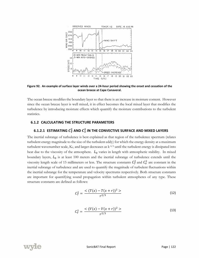
SonicBAT Final Report Page | 122
Figure 92. An example of surface layer winds over a 24-hour period showing the onset and cessation of the ocean breeze at Cape Canaveral.
The ocean breeze modifies the boundary layer so that there is an increase in moisture content. However
since the ocean breeze layer is well mixed, it in effect becomes the local mixed layer that modifies the
turbulence by introducing moisture effects which quantify the moisture contributions to the turbulent
statistics.
6.1.2 CALCULATING THE STRUCTURE PARAMETERS
6.1.2.1 ESTIMATING 𝑪𝑻𝟐 AND 𝑪𝒗
𝟐 IN THE CONVECTIVE SURFACE AND MIXED LAYERS
The inertial subrange of turbulence is best explained as that region of the turbulence spectrum (relates
turbulent energy magnitude to the size of the turbulent eddy) for which the energy density at a maximum
turbulent wavenumber scale, K0, and larger decreases as k-5/3 until the turbulent energy is dissipated into
heat due to the viscosity of the atmosphere. 𝐿0 varies in length with atmospheric stability. In mixed
boundary layers, 𝐿0 is at least 100 meters and the inertial subrange of turbulence extends until the
viscosity length scale of 15 millimeters or less. The structure constants 𝐶𝑇2 and 𝐶𝑣
2 are constant in the
inertial subrange of turbulence and are used to quantify the magnitude of turbulent fluctuations within
the inertial subrange for the temperature and velocity spectrums respectively. Both structure constants
are important for quantifying sound propagation within turbulent atmospheres of any type. These
structure constants are defined as follows:
𝐶𝑇2 =
< (𝑇(𝑥) − 𝑇(𝑥 + 𝑟))2 >
𝑟2 3⁄ (12)
𝐶𝑣2 =
< (𝑉(𝑥) − 𝑉(𝑥 + 𝑟))2 >
𝑟2 3⁄ (13)

SonicBAT Final Report Page | 123
The following mixed layer scaling quantities are used to generalize mixed layer turbulence statistics
(Panofsky and Dutton, 1984):
Velocity scale, 𝑊∗ = (𝑔𝐻𝑧𝑖 𝜌𝐶𝑝𝑇)⁄ 1 3⁄ (14)
Temperature scale, ∗ = 𝐻 𝜌𝐶𝑝𝑊∗⁄ (15)
Local inversion height, 𝑧𝑖 (16)
where 𝑔 is the acceleration of gravity (m/s2), 𝐻 is the surface heat flux (W/m2), 𝜌 is the air density
(kg/m3), 𝐶𝑝 is the heat capacity of air at constant pressure (J/kgK), 𝑧𝑖 is the local inversion height (m),
𝑇 is the surface temperature in (⁰K), 𝑊∗ is the mixed layer velocity scaling statistic (m/s) and 𝜃∗ is the
mixed layer temperature scaling statistic (⁰K).
Applying these scaling quantities to 𝐶𝑇2 and 𝐶𝑣
2 yields the following universal relationships for their
altitude above ground level (AGL) dependence within the mixed layer. The mixed layer scaling
relationship for the temperature structure constant is:
𝐶𝑇
2(𝑧)𝑧𝑖2 3⁄
𝜃∗2
=
[ 2.66 (𝑧 𝑧𝑖⁄ )
−4 3⁄
𝑧 < 0.5𝑧𝑖
6.72 0.5𝑧𝑖 < 𝑧 < 0.7𝑧𝑖
19.72 (𝑧 𝑧𝑖⁄ )3 .7𝑧𝑖 < 𝑧 < 𝑧𝑖
(17)
and the corresponding relationship for the velocity structure constant is:
𝐶𝑣
2(𝑧)𝑧𝑖2 3⁄
𝑊∗2
= 1.3 + 0.043 (𝑧 𝑧𝑖⁄ )−2 3⁄
𝑧 < 𝑧𝑖 (18)
The power of these relationships is that the magnitude of the structure constants can be accurately
determined by knowing the surface heat flux and the local inversion height for mixed layers. These
structure constant formulations are not valid for other types of boundary layers (such as stable or
transitional surface layers) as they are not as well verified as these relationships.
6.1.2.2 MODIFICATION OF THE STRUCTURE CONSTANTS DUE TO EFFECT OF MOISTURE
In the presence of a moist boundary layer such as the mixed layer associated with an ocean breeze, the
impact of moisture fluctuations modifies the temperature measurements using devices for which the
speed of sound is important. Later in this section, the discussion turns to two instruments that utilize
sound as the basis for their measurements. The speed of sound, 𝑐𝑎, in a moist atmosphere is defined as
𝑐𝑎 = 20.05(𝑇𝑣)1 2⁄ (19)

SonicBAT Final Report Page | 124
where 𝑇𝑣 is defined as the virtual temperature. The virtual temperature is defined as that temperature
at which dry air would need to be to make its density the same as moist air with a given vapor density.
When using the virtual temperature the ideal gas equations for dry air is applicable if the air temperature
is replaced by the virtual temperature of the air.
The virtual temperature is defined as:
𝑇𝑣 = 𝑇(1 + .608𝑞) (20)
where 𝑞 is the mixing ratio which is defined as the ratio of the actual water vapor to the mass of the dry
air in the same air volume. By substituting 𝑇𝑣 for 𝑇 in equation (12), the virtual temperature structure
constant is:
𝐶𝑇𝑣2 =
< (𝑇𝑣(𝑥) − 𝑇𝑣(𝑥 + 𝑟))2 >
𝑟2 3⁄ (21)
The relationship between 𝐶𝑇2and 𝐶𝑇𝑣
2 utilizes the Bowen ratio, 𝛽, and the covariance of the moisture
and temperature fluctuations denoted by 𝑅𝑞𝑇. The Bowen ratio is defined as the ratio of the heat flux
to the moisture flux as:
𝛽 =𝐻
𝐸=
𝐶𝑝 < 𝑤′𝑇′ >
< 𝑤′𝑞′ > (22)
where 𝜆 is the latent heat of evaporation of water, < 𝑤’𝑇’ > is the covariance of the vertical velocity
fluctuation with the temperature fluctuation and < 𝑤’𝑞’ > is the covariance of the vertical velocity
fluctuations with the mixing ratio fluctuations.
Using these definitions and expanding the relationship for 𝐶𝑇𝑣
2 we find that
𝐶𝑇𝑣
2 = 𝐶𝑇2(1 + 𝑅𝑞𝑇2𝐶 𝛽⁄ + 𝐶2/𝛽2) = 𝐶𝑇
2𝛼𝑎2 (23)
where C = 0.059 for the atmospheric boundary layer and 𝛼𝑎2 is defined as the quantity in parenthesis in
equation (23). The term 𝛼𝑎2 is considered to be a correction to 𝐶𝑇
2 for the moisture fluctuations present
in a moist boundary layer. For small values of 𝛽, the correction to 𝐶𝑇2 can become quite large. For this
project, the scaling relationships presented in equation (17) were used to extrapolate 𝐶𝑇2 to altitudes
above the instrument heights. This means that the data from the sonic anemometer and the SODAR
must be modified using the relationship in equation (23) to produce 𝐶𝑇2 magnitudes instead of 𝐶𝑇𝑣
2 .
The Bowen ratio and the 𝑅𝑞𝑇 covariance was determined using the flux measurement system described
later in this section.
Finally, the computation of the surface scaling parameters 𝑇∗ and 𝑊∗ requires that the sensible
temperature flux be determined from the virtual temperature flux. The sonic anemometers measure the
virtual temperature, 𝑇𝑣 and then compute the virtual temperature flux using the vertical velocity
measurements from the sonic anemometers. The correction formula is:
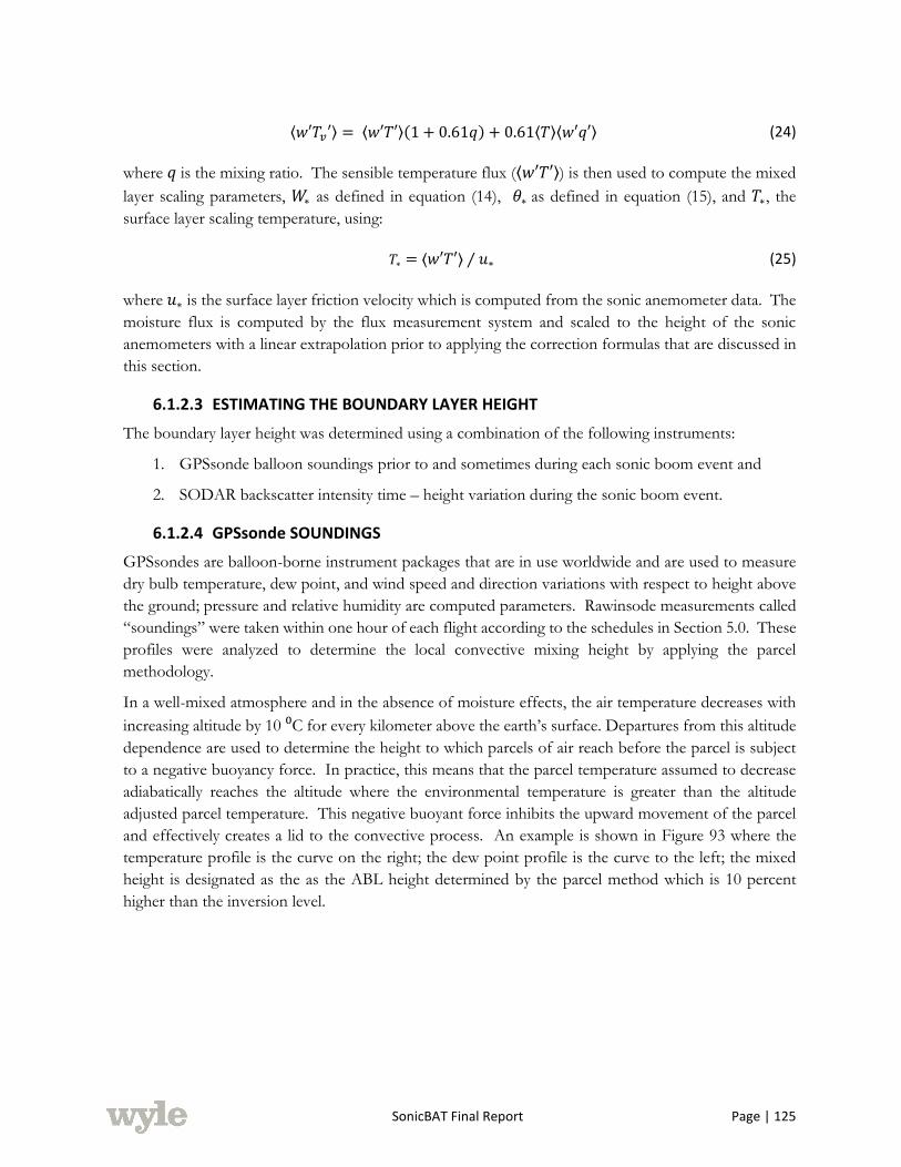
SonicBAT Final Report Page | 125
⟨𝑤′𝑇𝑣′⟩ = ⟨𝑤′𝑇′⟩(1 + 0.61𝑞) + 0.61⟨𝑇⟩⟨𝑤′𝑞′⟩ (24)
where 𝑞 is the mixing ratio. The sensible temperature flux (⟨𝑤′𝑇′⟩) is then used to compute the mixed
layer scaling parameters, 𝑊∗ as defined in equation (14), 𝜃∗ as defined in equation (15), and 𝑇∗, the
surface layer scaling temperature, using:
𝑇∗ = ⟨𝑤′𝑇′⟩ ⁄ 𝑢∗ (25)
where 𝑢∗ is the surface layer friction velocity which is computed from the sonic anemometer data. The
moisture flux is computed by the flux measurement system and scaled to the height of the sonic
anemometers with a linear extrapolation prior to applying the correction formulas that are discussed in
this section.
6.1.2.3 ESTIMATING THE BOUNDARY LAYER HEIGHT
The boundary layer height was determined using a combination of the following instruments:
1. GPSsonde balloon soundings prior to and sometimes during each sonic boom event and
2. SODAR backscatter intensity time – height variation during the sonic boom event.
6.1.2.4 GPSsonde SOUNDINGS
GPSsondes are balloon-borne instrument packages that are in use worldwide and are used to measure
dry bulb temperature, dew point, and wind speed and direction variations with respect to height above
the ground; pressure and relative humidity are computed parameters. Rawinsode measurements called
“soundings” were taken within one hour of each flight according to the schedules in Section 5.0. These
profiles were analyzed to determine the local convective mixing height by applying the parcel
methodology.
In a well-mixed atmosphere and in the absence of moisture effects, the air temperature decreases with
increasing altitude by 10 ⁰C for every kilometer above the earth’s surface. Departures from this altitude
dependence are used to determine the height to which parcels of air reach before the parcel is subject
to a negative buoyancy force. In practice, this means that the parcel temperature assumed to decrease
adiabatically reaches the altitude where the environmental temperature is greater than the altitude
adjusted parcel temperature. This negative buoyant force inhibits the upward movement of the parcel
and effectively creates a lid to the convective process. An example is shown in Figure 93 where the
temperature profile is the curve on the right; the dew point profile is the curve to the left; the mixed
height is designated as the as the ABL height determined by the parcel method which is 10 percent
higher than the inversion level.

SonicBAT Final Report Page | 126
Figure 93. Plot of temperature and dew point as a function of altitude on a Skew-T thermodynamic diagram. The dew point profile is the red dashed line (left) and the temperature profile is the solid red line (right).
6.1.2.5 mini SODAR MEASUREMENTS
Focusing now on the mini SODAR instrument, the back scatter intensity or echo intensity plots
(hereafter called the intensity plot) associated with the SODAR are the consequence of the interaction
of the sound pulse emitted by the SODAR interacting with atmospheric turbulence. This interaction is
a continuous process that results in a continuous echo that is recorded by the mini SODAR instrument.
An example of these intensity plots is shown in Figure 94. The intensity plot is a two dimensional plot
of the height variation of the scattered signal intensity presented as color encoded echo magnitude (in
dBV) as a function of the local time of day increasing from left to right.
In this figure, the upper limit for the measurements is 400 meters as shown on the vertical axis. The
mixing height as defined by the intensity gradient (dark green to green) which increases in altitude from
225 meters at 6:45 AM (left side of the figure) to 325 meters just after 10:00 AM. If the mixing height
is below the maximum sampling altitude for the SODAR instrument, it should be displayed graphically
in a manner similar to that shown in Figure 94.
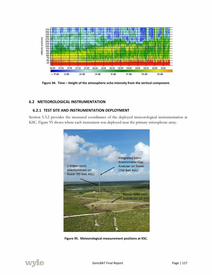
SonicBAT Final Report Page | 127
Figure 94. Time – Height of the atmospheric echo intensity from the vertical component.
6.2 METEOROLOGICAL INSTRUMENTATION
6.2.1 TEST SITE AND INSTRUMENTATION DEPLOYMENT
Section 5.3.2 provides the measured coordinates of the deployed meteorological instrumentation at
KSC. Figure 95 shows where each instrument was deployed near the primary microphone array.
Figure 95. Meteorological measurement positions at KSC.

SonicBAT Final Report Page | 128
The exact location for each system is not as important as the relative locations which are placed to
minimize the impact by any one instrument on the other. The complete suite of instruments includes:
1. One integrated sonic anemometer/gas analyzer system (moisture flux sensor);
2. Two sonic anemometers equipped with real time turbulence calculation;
3. One model 4000 SODAR system;
4. Two meteorological towers (measuring temperature, pressure and relative humidity).
As mentioned previously, the moisture flux sensor was added for the KSC test and was not deployed
during the AFRC test.
6.2.2 ULTRASONIC ANEMOMETERS
This project utilized two sonic anemometers to measure the mixed layer scaling parameters (except for
the local mixing height) and the reference structure constants. The sonic anemometers were
manufactured by Metek GmbH. Their specifications are described in Section 5.2.2.4, Table 11. The
data from these sonics (serial data stream) were time-tagged and recorded using a data acquisition
package supplied by NASA Armstrong.
6.2.2.1 FIELD SETUP, CALIBRATION AND OPERATION
During the KSC flight test and measurements campaign, the two Metek sonic anemometers were
deployed on mounting arms on the 150-meter tall tower (Figure 96) at a height of 29.03 meters (95.24
feet). Care was taken to mount and orient each anemometer sensor into the seasonal or monthly average
prevailing wind flow to minimize tower influences and obstructions on the measurements. A bubble
level was used to ensure proper sensor leveling at the time of installation.
Figure 96. 150 meter tower and mounting arms.

SonicBAT Final Report Page | 129
The sonic anemometers were calibrated by Metek GmbH as part of a firmware upgrade that was
performed in April 2016. The main purpose of the firmware upgrade was to update the processing
algorithms to utilize a right hand coordinate reference frame for its computations, to update the
computations to more recent algorithms and to extend the data processing to include the temperature
structure constant.
6.2.2.2 DATA DESCRIPTION AND COLLECTION PROCEDURES
The output from the sonic anemometers is a serial data stream. There is no data storage on the
anemometers so an external data logger was required to record and timestamp the serial data stream.
The basic data format consists of a date time stamp and the three wind components (X, Y, Z) and
temperature as measured by the sonic anemometer. The data packet for each sample is date, time, X,
Y, Z, and T.
6.2.3 SODAR
6.2.3.1 INSTRUMENT SPECIFICATIONS
NASA owns two Doppler SODAR systems (a model 2000 and model 4000 originally manufactured by
AeroVironment, Inc.) Their specifications are described in Section 5.2.2.3, Table 9. Doppler SODAR
systems are acoustic based instruments that operate on the principle that propagating sound waves in
the atmosphere interact with local atmospheric turbulence to produce an echo. This echo is continuous
and is monitored for its intensity and frequency content. The intensity changes are directly related to
the level of thermal turbulence (𝐶𝑇2) and the frequency changes are due to radial motion relative the
SODAR sensor. When three wind components are measured, this information can produce
measurements of the three dimensional wind field at several ranges almost simultaneously.
The SODAR instruments measure the interaction of a directed, high intensity sound pulse with
atmospheric turbulence through the turbulence induced acoustic refractive index fluctuations that
scatter the sound energy. The strength of the scattered acoustic echo is quantified by the acoustic
scattering cross-section which is defined as the sound power scattered into a specific direction per unit
area per unit solid angle. The equation for the backscattering (i.e. acoustic energy scattered back to the
source antenna by turbulence) cross section σ is:
𝜎(𝑧) = 0.0039𝐾1 3⁄ 𝐶𝑇𝑣
2 (𝑧)/𝑇𝑣2 (26)
where 𝐾 is the acoustic wavenumber and 𝑇𝑣 is the virtual temperature and 𝐶𝑇𝑣
2 (𝑧) is the value of the
temperature structure constant at the altitude 𝑧 (AGL).
The relationship between the emitted sound pulse, 𝑃0, and the received signal, 𝑃𝑅(𝑧), due to the
atmospheric echo is:
𝑃𝑅(𝑧) = 𝑃0(𝐴𝐺 𝑧2⁄ )𝐿𝑣𝜎(𝑧)𝑒−2𝛼𝑧 (27)
SonicBAT Final Report Page | 130
𝐴 is the effective cross-sectional area of the antenna, 𝐺 is the gain of the antenna (computed based on
-3 dB power points), 𝐿𝑣 is the length of the acoustic pulse in space (speed of sound times the pulse
length in time divided by 2), 𝛼 is the path averaged attenuation of the sound energy due to energy
exchange with the N2, O2 and H2O molecules and viscous dissipation of sound energy, 𝜎(𝑧), the
backscattering cross-section for sound (as defined in equation (26)) and 𝑧 is the altitude (AGL) of the
measurement based on the delay time after the pulse is emitted.
6.2.3.2 CALIBRATION PROCEDURE
By measuring 𝐶𝑇2(𝑧) at a fixed altitude 𝑧1, the actual power of the received signal corrected for 𝑧𝑖
2𝑒2𝛼𝑧𝑖
is directly related to the backscattering cross-section 𝜎 and consequently to 𝐶𝑇2(𝑧) as follows:
𝑧𝑖2𝑒2𝛼𝑧𝑖𝑃𝑅(𝑧) = 𝑃0𝐴𝐺𝐿𝑣(0.0039𝑘1 3⁄
𝐶𝑇𝑣
2 (𝑧) 𝑇𝑣2
⁄ ) (28)
The product 𝑃0𝐴𝐺𝐿𝑣 is defined as the system function 𝑆0. It is considered to be a constant when the
same antenna (related to both 𝐴 and 𝐺), the output power level 𝑃0, the frequency as reflected in the
wave number and the pulse length in space (𝐿𝑣) are held constant during the field campaign.
With a measurement of 𝐶𝑇2(z1), correcting for the spherical spread of the sound and the attenuation of
sound and solving for 𝐶𝑇2(z1), a “calibration” is established. The left side of the equal sign in equation
(28) is plotted in real-time as the intensity plot time – height presentation of the right side of equation
(28). This is scaled in terms of the received voltage level as a function of height presented as decibels.
A sample of the intensity plot is shown in Figure 94.
Using equation (28), the relationship displayed in the intensity plot is:
𝑧𝑖2𝑒2𝛼𝑧𝑖𝑃𝑅(𝑧) =< 𝐶𝐹 > 𝐶𝑇𝑣
2 (𝑧𝑖) (29)
< 𝐶𝐹 > is the “sample average” calibration factor that was produced from a series of inter-comparison
measurements taken with the 𝐶𝑇𝑣
2 (𝑧𝑖) available from the sonic anemometers on the 150 meter tower.
Because the < 𝐶𝐹 > is a result of measurements with widely varying signal level due to turbulent
process and changing atmospheric conditions, this factor must be developed through several repeated
inter-comparisons to establish and converge on the actual calibration factor. It is feasible that the <
𝐶𝐹 > itself could be a diurnal function of atmospheric stability and atmospheric properties such as
temperature and relative humidity.
The SODAR directly senses an echo which is directly related to the virtual temperature structure
constant, 𝐶𝑇𝑣
2 (𝑧). A “calibrated” SODAR is one for which the < 𝐶𝐹 > and its statistics (mean and
standard deviation) are determined.
In a convective atmosphere, the variation of 𝐶𝑇2 with increasing altitude is one of the strongest
relationships in atmospheric turbulence. This relationship is:
𝐶𝑇2(𝑧) = 2.5(𝑔 𝑇⁄ )−2 3⁄ 𝑄0𝑧
−4 3⁄ (30)
SonicBAT Final Report Page | 131
𝑄0 is the surface temperature flux or < 𝑤’𝑇’ >. 𝐶𝑇2 is directly related to the surface heat flux. The
variation of 𝐶𝑇2(𝑧) with altitude was verified with the SODAR and formed the basis for verification of
the < 𝐶𝐹 > discussed previously.
For the measurement of 𝐶𝑣2, the differencing method described in the sonic anemometer section below
was applied to the vertical and horizontal velocity raw SODAR data fields.
6.2.3.3 FIELD SETUP, CALIBRATION AND OPERATION
The model 4000 SODAR system was operated from the top of the 18-foot hill located near the NW
end of the primary microphone array. The location of the SODAR system with respect to the sonic
anemometers and 150 meter tower is shown in Figure 95. The model 2000 SODAR was used at NASA
Armstrong during the SonicBAT AFRC test but was not used at Cape Canaveral.
The model 4000 is battery powered and equipped with a solar charging package. Communication with
the model 4000 was through a cellular modem connection during the measurement campaign. Data
was stored on the local hard disk drive and on a removable USB drive.
The model 4000 SODAR system was operated by NASA Armstrong continuously during the test
period, except during the sonic booms when it was turned off. One laptop computer equipped with
the SodarView software package was required for operation.
6.2.3.4 DATA DESCRIPTION
Data produced by the model 4000 SODAR system included the following measurements stored in an
ASCII table:
• Sampling altitude (meters)
• Horizontal wind speed (m/s)
• Horizontal wind direction (degrees with respect to True North)
• Vertical velocity (m/s)
• Intensity of the atmospheric echo from the vertical antenna or beam.
• Standard deviation of the vertical velocity
In addition the real time intensity plot display was available to track the inversion height when it was in
range of the SODAR system.
6.2.4 EDDY-COVARIANCE FLUX SYSTEM
A Campbell Scientific Infrared-Gas Analyzer-Sonic (IRGASON) sensor was operated for remote eddy-
covariance (flux) measurements within the mixed layer. The IRGASON is an in-situ, open path,
infrared absorption gas analyzer integrated and synchronized with a three-dimensional sonic
anemometer. The gas analyzer provides measurements of absolute densities of carbon dioxide and
water vapor, while the sonic anemometer measures orthogonal wind components. Using the above
integrated measurements along with sonic air temperature, ambient air temperature and barometric
pressure the carbon dioxide, water vapor and heat fluxes using the eddy-covariance method can be
computed.
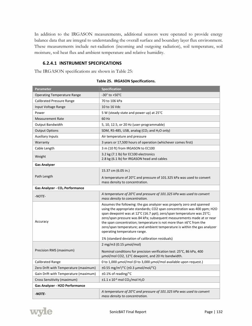
SonicBAT Final Report Page | 132
In addition to the IRGASON measurements, additional sensors were operated to provide energy
balance data that are integral to understanding the overall surface and boundary layer flux environment.
These measurements include net-radiation (incoming and outgoing radiation), soil temperature, soil
moisture, soil heat flux and ambient temperature and relative humidity.
6.2.4.1 INSTRUMENT SPECIFICATIONS
The IRGASON specifications are shown in Table 25:
Table 25. IRGASON Specifications.
Parameter Specification
Operating Temperature Range -30° to +50°C
Calibrated Pressure Range 70 to 106 kPa
Input Voltage Range 10 to 16 Vdc
Power 5 W (steady state and power up) at 25°C
Measurement Rate 60 Hz
Output Bandwidth 5, 10, 12.5, or 20 Hz (user-programmable)
Output Options SDM, RS-485, USB, analog (CO2 and H2O only)
Auxiliary Inputs Air temperature and pressure
Warranty 3 years or 17,500 hours of operation (whichever comes first)
Cable Length 3 m (10 ft) from IRGASON to EC100
Weight 3.2 kg (7.1 lb) for EC100 electronics 2.8 kg (6.1 lb) for IRGASON head and cables
Gas Analyzer
Path Length
15.37 cm (6.05 in.)
A temperature of 20°C and pressure of 101.325 kPa was used to convert mass density to concentration.
Gas Analyzer - CO2 Performance
-NOTE- A temperature of 20°C and pressure of 101.325 kPa was used to convert mass density to concentration.
Accuracy
Assumes the following: the gas analyzer was properly zero and spanned using the appropriate standards; CO2 span concentration was 400 ppm; H2O span dewpoint was at 12°C (16.7 ppt); zero/span temperature was 25°C; zero/span pressure was 84 kPa; subsequent measurements made at or near the span concentration; temperature is not more than ±6°C from the zero/span temperature; and ambient temperature is within the gas analyzer operating temperature range.
1% (standard deviation of calibration residuals)
Precision RMS (maximum)
2 mg/m3 (0.15 μmol/mol)
Nominal conditions for precision verification test: 25°C, 86 kPa, 400 μmol/mol CO2, 12°C dewpoint, and 20 Hz bandwidth.
Calibrated Range 0 to 1,000 μmol/mol (0 to 3,000 μmol/mol available upon request.)
Zero Drift with Temperature (maximum) ±0.55 mg/m3/°C (±0.3 μmol/mol/°C)
Gain Drift with Temperature (maximum) ±0.1% of reading/°C
Cross Sensitivity (maximum) ±1.1 x 10⁻⁴ mol CO2/mol H2O
Gas Analyzer - H2O Performance
-NOTE- A temperature of 20°C and pressure of 101.325 kPa was used to convert mass density to concentration.
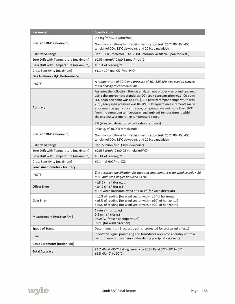
SonicBAT Final Report Page | 133
Parameter Specification
Precision RMS (maximum)
0.2 mg/m3 (0.15 μmol/mol)
Nominal conditions for precision verification test: 25°C, 86 kPa, 400 μmol/mol CO2, 12°C dewpoint, and 20 Hz bandwidth.
Calibrated Range 0 to 1,000 μmol/mol (0 to 3,000 μmol/mol available upon request.)
Zero Drift with Temperature (maximum) ±0.55 mg/m3/°C (±0.3 μmol/mol/°C)
Gain Drift with Temperature (maximum) ±0.1% of reading/°C
Cross Sensitivity (maximum) ±1.1 x 10⁻⁴ mol CO2/mol H2O
Gas Analyzer - H2O Performance
-NOTE- A temperature of 20°C and pressure of 101.325 kPa was used to convert mass density to concentration.
Accuracy
Assumes the following: the gas analyzer was properly zero and spanned using the appropriate standards; CO2 span concentration was 400 ppm; H2O span dewpoint was at 12°C (16.7 ppt); zero/span temperature was 25°C; zero/span pressure was 84 kPa; subsequent measurements made at or near the span concentration; temperature is not more than ±6°C from the zero/span temperature; and ambient temperature is within the gas analyzer operating temperature range.
2% (standard deviation of calibration residuals)
Precision RMS (maximum)
0.004 g/m3 (0.006 mmol/mol)
Nominal conditions for precision verification test: 25°C, 86 kPa, 400 μmol/mol CO2, 12°C dewpoint, and 20 Hz bandwidth.
Calibrated Range 0 to 72 mmol/mol (38°C dewpoint)
Zero Drift with Temperature (maximum) ±0.037 g/m3/°C (±0.05 mmol/mol/°C)
Gain Drift with Temperature (maximum) ±0.3% of reading/°C
Cross Sensitivity (maximum) ±0.1 mol H2O/mol CO2
Sonic Anemometer - Accuracy
-NOTE- The accuracy specification for the sonic anemometer is for wind speeds < 30 m s-1 and wind angles between ±170°.
Offset Error < ±8.0 cm s-1 (for ux, uy) < ±4.0 cm s-1 (for uz) ±0.7° while horizontal wind at 1 m s-1 (for wind direction)
Gain Error < ±2% of reading (for wind vector within ±5° of horizontal) < ±3% of reading (for wind vector within ±10° of horizontal) < ±6% of reading (for wind vector within ±20° of horizontal)
Measurement Precision RMS
1 mm s-1 (for ux, uy) 0.5 mm s-1 (for uz) 0.025°C (for sonic temperature) 0.6°C (for wind direction)
Speed of Sound Determined from 3 acoustic paths (corrected for crosswind effects)
Rain Innovative signal processing and transducer wicks considerably improve performance of the anemometer during precipitation events.
Basic Barometer (option -BB)
Total Accuracy ±3.7 kPa at -30°C, falling linearly to ±1.5 kPa at 0°C (-30° to 0°C) ±1.5 kPa (0° to 50°C)

SonicBAT Final Report Page | 134
6.2.4.2 FIELD SETUP, CALIBRATION AND OPERATION
During the KSC flight test and measurement campaign, the IRGASON flux system was deployed on
the 150-meter tall tower similar to that of the Metek ultrasonic anemometers but it was installed at a
height of 77.5 meters (254 feet) as shown in Figure 95. Care was taken to mount and orient the
IRGASON sensor into the seasonal or monthly average prevailing wind flow to minimize tower
influences and obstructions on the measurements. A bubble level located on the sensor mounting
hardware was used to ensure proper sensor leveling at the time of installation.
The flux system was wired to and operated using a Campbell Scientific CR6 series data logger. The CR6
data logger was used to store raw and averaged data tables using a pre-configured CR6 eddy-covariance
program developed by Campbell Scientific and was used for the processing and calculations of measured
flux and energy balance data, the storage of diagnostic and correction parameters and system and sensor
coefficients.
A field calibration of the IRGASON and associated peripheral sensors was not necessary during the
KSC measurement campaign as these sensors were delivered from Campbell Scientific calibrated and
tested, assuming no damage to the sensor geometry during shipping or a faulty sensor transducer.
Calibration test equipment (zero-and-span test shroud and zero air system) to verify the IRGASON’s
gas analyzer baseline response was available for use if sensor anomalies were observed during the field
program. Additional calibration equipment (not procured) would have been necessary to verify the
CO2 and H2O span response.
6.2.4.3 DATA COLLECTION PROCEDURES
IRGASON data was stored internally within the CR6 data logger and included the use of an onboard
micro SD card for automated data backup. A cellular modem was connected to the CR6 data logger
for routine scheduled remote polling of data tables initiated from the T&B System’s office in Valencia,
CA. These data tables were stored on a data management server hosted by T&B Systems. Time-series
data was displayed using Vista Data Vision (VDV) software and was routinely reviewed for consistency
and reasonableness. All data were recorded and timestamped using Coordinated Universal Time (UTC).
6.2.4.4 DATA DESCRIPTION
The primary purpose for using the IRGASON system during the KSC flight test and measurement
campaign, was to collect a dataset suitable for determining sensible and latent heat flux environments
during the flight tests. The integrated three-dimensional sonic anemometer was also used to measure
data similar to that produced by the Metek ultrasonic anemometers.
The IRGASON output included the following data in ASCII format (40 Hz raw and 10-minute averaged
data) via the CR6 data logger:
• Ux (m/s)
• Uy (m/s)
• Uz (m/s)
• Sonic Temperature (°C)
• Sonic Diagnostic
• CO2 Density (mg/m3)

SonicBAT Final Report Page | 135
• H2O Density (g/m3)
• Gas Analyzer Diagnostic
• Ambient Temperature (°C)
• Atmospheric Pressure (kPa)
• CO2 Signal Strength
• H2O Signal Strength
• Source Temperature (°C)
Data outputs from the peripheral energy balance sensors were also included in the data tables.
Additional CR6 programming instruction outputs, not shown above, were compiled to compute
atmospheric stability and flux parameters, standard deviation of measurements, processes for the
correction of data for frequency, coordinate rotation and lag. Near real-time steady state testing and
“grading” of measurements was collected to ensure data quality and validity.
A precipitation gauge was installed and integrated into the IRGASON’s data set to denote periods of
precipitation that contaminate measurements within the IRGASON’s open path length. Precipitation
data was used in determining the quality of data during precipitation events.
6.3 TURBULENCE DATA ANALYSIS
6.3.1 REAL TIME COMPUTATION OF 𝑪𝑻𝟐 AND 𝑪𝒗
𝟐 PROFILES
The sonic anemometers directly report 𝐶𝑇2 for the fixed averaging interval of 10 minutes. In addition
the raw data (as described in paragraph 6.2.2.2) from the sonic anemometers are also used to compute
both 𝐶𝑇2 and 𝐶𝑣
2 at arbitrary averaging times.
Using data from the sonic anemometers, the SODAR systems were calibrated to profile 𝐶𝑇2 and 𝐶𝑣
2.
This calibration required that the sonic anemometers and the SODAR systems be operated continuously
for several days prior to the field program.
6.3.2 POST-PROCESSING THE SONIC RAW DATA STREAM TO COMPUTE 𝑪𝑻𝟐 AND 𝑪𝒗
𝟐
A windows-based application was developed and verified to compute the structure constants and the
relevant mixed layer scaling parameters using the raw sonic anemometer data (see Section 6.2.2.2).
The surface heat flux, 𝐻, is computed by both the sonic anemometer (fixed intervals of 10 minutes) and
the windows application (user selected averaging interval). The heat flux in the turbulence parameter
output data string is designated as hf and its units are watts m-2. Sigma–w is designated in the same data
string as zsig.
The post processing of the raw sonic data to produce the structure constants used a two time interval
technique based on the following formula for 𝐶𝑇2. The two time lags Δt1 and Δt2 are selected based
upon conversations with Metek GmbH and subsequent verification tests. The first time lag Δt1 is
equivalent to time shift of one sample. For the sonic anemometers operating in the on-line turbulence
computation mode, the sampling rate is 30 Hz or 30 samples per second. Accordingly Δt1 = 1/30
seconds and is a fixed delay in the post processing program. The second time delay is selected so that
the equivalent length scale which is equal to average wind speed times Δt2 is also within the inertial
subrange scale length or wavenumber. This is also fixed in the post-processing program to a delay equal

SonicBAT Final Report Page | 136
to 1 sec or 30 samples with respect to the raw sonic anemometer data set. Using these sample delays
and equation (12), the 𝐶𝑇2 computations were verified to produce the same values as the Metek in-line
turbulence computation firmware.
The following equation for 𝐶𝑇𝑣
2 is the auto-covariance version of equation (12):
𝐶𝑇𝑣
2 =2(< 𝑇𝑣(𝑡)𝑇𝑣(𝑡 + ∆𝑡1) > −< 𝑇𝑣(𝑡)𝑇𝑣(𝑡 + ∆𝑡2) >)
< 𝑢 >2/3 ((∆𝑡2)2/3 − ((∆𝑡1)
2/3)) (31)
Where < 𝑢 > is the average wind speed during the entire sampling period, Δt1 and Δt2 are two different
sampling time intervals.
Correspondingly, the auto-covariance version of equation (13) for 𝐶𝑣2 is:
𝐶𝑣2 =
2(< 𝑉(𝑡)𝑉(𝑡 + ∆𝑡1) > −< 𝑉(𝑡)𝑉(𝑡 + ∆𝑡2) >)
< 𝑢 >2/3 ((∆𝑡2)2/3 − ((∆𝑡1)
2/3)) (32)
Where < 𝑢 > is the average wind speed during the entire sampling period, Δt1 and Δt2 are two different
sampling time intervals.
The averaging operator <> in equations (31) and (32) signifies that the corresponding auto-covariance
is computed using the specified time delay and averaged over the user selected time period such as the
campaign averaging time of 10 minutes. The averaging period for the post processing period is arbitrary
as needed by the analyst but must not be less than 1 minute for stable results. In addition the average
wind speed used in equations (31) and (32) is the scalar average wind speed over the same averaging
interval as the auto-covariance computation averaging time.
6.4 METEOROLOGICAL DATA PRODUCTS
The meteorological data recorded during the AFRC and KSC research flight tests were analyzed after
the conclusion of each test, using the procedures described in Section 6.3, to yield turbulence parameters
for each flight, including the structure constants and boundary layer height. This section presents a
summary of the KSC atmospheric turbulence data set to show an example of the data products
computed for both flight tests. Additional analyses were performed using these data sets to validate the
sonic boom turbulence codes (Section 7.0) and perform statistical analysis and uncertainty quantification
of these codes (Section 8.0).
6.4.1 METEOROLOGICAL DATA ARCHIVE
The digital archive described in Section 5.4.1 includes both raw and post-processed acoustic and
meteorological data for the AFRC and KSC research flight tests. Raw meteorological data consists of
the data recorded by the ground weather stations and tower weather station at KSC (Section 6.2.1),
ultrasonic anemometers (Section 6.2.2.2), SODARs (Section 6.2.3.4), Eddy-Covariance Flux System
(Section 6.2.4.4), and GPSsonde soundings (Section 6.1.2.4). Post-processed turbulence data consists
of what can be considered intermediate products and final products that specify the atmospheric
turbulence conditions associated with each flight; for our purposes, final products are those used as
inputs in either the numeric or classic turbulence models. For example, Table 26 shows for each flight
at KSC a mix of average macro atmospheric data, including wind speed and direction and ambient

SonicBAT Final Report Page | 137
temperature (𝑇), along with intermediate turbulence products such as the latent heat flux (Hl), sensible
heat flux (H), and vertical velocity (W). Final turbulence products include the surface friction velocity
(𝑢∗) and surface temperature scale (𝑇∗). Table 26 shows the remainder of the KSC turbulence data set
consisting of final products.
Table 26. Atmospheric and turbulence products (KSC test).
Flight No.
Latent Heat
Flux, Hl
(w/m2)
Sensible Heat
Flux, H
(w/m2)
Wind Speed (m/s)
Wind Direction
(deg)
Vertical Velocity, W
(m/s)
Surface Friction
Velocity, 𝒖∗ (m/s)
Surface Temp.
Scale, 𝑻∗ (K)
Ambient Temp.,
𝑻 (deg C)
1 81.85 30.82 4.7 20.1 -0.351 0.37543 0.06961 26.6
2 338.59 188.37 5.6 31.3 -0.368 0.52886 0.29822 27.5
3 406.23 159.36 4.3 359.8 -0.282 0.43180 0.28745 27.0
4 220.59 111.08 3.0 340.4 -0.088 0.32363 0.27722 27.2
5 580.42 213.47 4.3 315.2 -0.137 0.38699 0.47283 27.5
6 429.88 276.50 2.8 324.4 0.150 0.39353 0.59450 27.2
7 867.57 222.67 3.9 343.8 -0.224 0.41453 0.47169 27.0
8 640.62 195.07 4.8 341.0 -0.171 0.40945 0.39741 27.2
9 599.47 220.28 4.6 348.4 -0.058 0.55039 0.33610 27.2
10 408.38 127.43 6.2 80.6 -0.226 0.63474 0.16858 27.4
11 124.91 48.16 6.3 69.0 -0.286 0.49011 0.07674 25.5
12 362.27 117.47 5.6 52.4 -0.297 0.46756 0.19519 26.8
13 285.81 59.67 7.4 132.0 -0.233 0.64301 0.07234 26.7
14* 40.13 -5.87 5.7 223.4 -0.136 0.34017 0.01605 24.2
15 418.16 109.27 4.9 139.8 -0.129 0.51845 0.15555 27.2
16 344.59 89.51 4.6 147.3 -0.313 0.45592 0.16426 27.7
17 305.47 230.85 2.7 350.4 0.036 0.31448 0.65702 27.3
18 426.47 147.03 3.7 30.5 -0.147 0.33544 0.34817 27.8
19 681.22 239.70 4.4 59.0 -0.086 0.45234 0.50427 28.5
20 260.99 13.30 5.3 58.6 -0.282 0.34498 0.03345 27.8
* Parameters for flight 14 were derived from the flux system only without scaling.
Included in Table 27 for each KSC flight are turbulence level (L=low, M=medium, or H=high), a
classification made in the field and supported by the mixed layer stability parameter, mixed layer scaling
velocity (𝑤∗), local inversion height or mixing height (𝑧𝑖), structure parameters 𝐶𝑇2 and 𝐶𝑣
2 determined
from sonic anemometer Metek 2A, Monin-Obukhov length (𝐿𝑣), and the ratios of the local inversion
height to the Monin-Obukhov length (𝑧𝑖/𝐿𝑣) and the height above ground to the Monin-Obukhov
length (𝑧/𝐿𝑣). Note that mixing height values were rounded to the nearest 100 feet, which generated
several repeat values including 1,000 feet (304.9 meters in Table 27).

SonicBAT Final Report Page | 138
Table 27. Additional turbulence products (KSC test).
Flight No.
Turbulence Level
Mixed Layer Scaling
Velocity, 𝒘∗ (m/s2)
Mixing
Height, 𝒛𝒊 (m)
𝑪𝑻𝟐
(K2/m 2/3) 𝑪𝒗
𝟐 (m4/3/s-2)
Monin-Obukhov
Length, 𝑳𝒗 (m)
𝒛𝒊/𝑳𝒗 𝒛/𝑳𝒗
1 L 0.7197 457.3 0.00200 0.07658 -13.7492 -33.26 -2.129
2 M 1.3971 548.8 0.01778 0.12960 -6.5847 -83.34 -4.445
3 M 1.2411 487.8 0.01182 0.07840 -4.4682 -109.17 -6.551
4 M 1.1815 609.8 0.01616 0.06880 -2.6168 -233.01 -11.185
5 H 1.1932 304.9 0.02866 0.09972 -2.2244 -137.06 -13.159
6 H 1.5060 457.3 0.03928 0.10039 -1.8044 -253.44 -16.221
7 H 1.2174 304.9 0.02232 0.09407 -2.5111 -121.41 -11.656
8 H 1.3426 457.3 0.02829 0.11296 -2.9251 -156.34 -10.007
9 H 1.4256 487.8 0.02818 0.11395 -6.2419 -78.15 -4.689
10 M 1.3197 701.2 0.00887 0.16934 -16.6807 -42.04 -1.755
11 L 0.6946 304.9 0.00210 0.09952 -20.3218 -15.00 -1.440
12 M 0.9342 640.2 0.01311 0.09309 -7.6415 -83.78 -3.830
13 L 0.7543 823.2 0.00281 0.20613 -38.9751 -21.12 -0.751
14 L 0.3694 280.0 0.00136 0.05335 -44.4673 -6.30 -0.658
15 M 1.0958 457.3 0.01048 0.13873 -10.6123 -43.09 -2.758
16 M 1.1389 609.8 0.00815 0.15051 -8.9332 -68.26 -3.277
17 H 1.4438 487.8 0.02559 0.09367 -1.0464 -466.18 -27.973
18 M 0.9439 228.7 0.01800 0.07364 -2.2926 -99.74 -12.767
19 H 1.7873 823.2 0.01998 0.08713 -2.9538 -278.68 -9.909
20 L 0.4691 411.6 0.00424 0.04981 -25.2575 -16.30 -1.159
The final turbulence products of the AFRC and KSC flight tests were used in the numeric and classic
turbulence models for the validation studies (Section 7.0) and the statistics and uncertainty quantification
studies (Section 8.0).

SonicBAT Final Report Page | 139
7.0
MODEL VALIDATION OF THE NUMERIC AND CLASSICAL SONIC BOOM-TURBULENCE RESEARCH SOFTWARE CODES
7.1 VALIDATION OF NUMERIC SONIC BOOM-TURBULENCE RESEARCH SOFTWARE CODE
7.1.1 INTRODUCTION
To validate the KZKFourier numeric propagation and turbulence model, data from supersonic
overflight measurements at NASA’s Armstrong Flight Research Center (AFRC) and Kennedy Space
Center (KSC) are compared with outputs from numerical simulations. The simulation parameters are
chosen to approximate the actual sonic boom propagation geometry and the turbulent field parameters
in situ. Because of the randomness of turbulence and the difficulty of instantaneously measuring the
entire turbulent field, only statistical comparisons may be made between the simulation outputs and the
measurements. In addition, the task is made more difficult because atmospheric turbulence is constantly
evolving, such that turbulence parameters can change within a time period on the order of minutes.
Thus, statistical comparisons are made on a pass-by-pass basis. In particular, the means and standard
deviations of the Perceived Level (PL), maximum overpressure (sometimes shortened here to “pMax”),
and the Indoor Sonic Boom Annoyance Predictor (ISBAP) calculated using simulated outputs and
measurements along the primary arrays at both sites are compared. The PL and ISBAP are of particular
interest because they correlate with human response to sonic boom noise. The degree to which
simulated sonic boom statistics fall within the confidence bounds of the measured statistics and the
degree to which trends in the data are reproduced indicates the utility of this method and the
KZKFourier engine in predicting turbulence effects on sonic booms.
Passes for which turbulence data are not available are excluded from this analysis. In addition, two
passes from the KSC measurements are excluded because of abnormally low levels, possibly due to off-
condition flight or cloud cover. In total, 60 passes with 957 measured signatures at AFRC and 48 passes
with 680 measured signatures at KSC are considered.
7.1.2 VALIDATION SIMULATION PARAMETERS
Configuration of the KZKFourier validation simulations makes use of several sources of data, including
motor glider, weather tower, sonic anemometer, and balloon launch measurements. For passes where
the supersonic signature measured above the boundary layer by the motor glider was provided, this
signature is processed to provide the starting waveform for the KZKFourier engine. Where the glider
did not measure the signature, a glider measurement during similar atmospheric conditions is assumed.
The pressure waveform is trimmed around the signature, any DC offset is subtracted, some zero
padding is added to the left and right edges, and the signature is upsampled to the simulation sample
rate. The zero padding is necessary when simulating long propagation distances, because advection can
shift the time waveform towards the temporal domain edges. For sonic boom signatures about 140 ms
long, the starting waveforms with padding used in KZKFourier ranged from about 280 ms to 590 ms.
For very long propagation lengths and long input waveforms, the transverse domain length 𝑦max used
in the KZKFourier simulation is reduced to limit the simulation run time to below 120 hours, the limit
in the Pleiades “long” queue. In these cases, the number of KZKFourier realizations is increased to

SonicBAT Final Report Page | 140
compensate for the smaller domain. It was found in preliminary investigations that decreasing the
transverse domain size somewhat does not appreciably change the simulated sonic boom statistics. For
these simulations, the lower limit for transverse domain reduction was chosen to be 𝑦max = 140 m,
while most have domain lengths of 350 m. The transverse step size Δ𝑦 is held constant at 0.5 m,
meaning each simulation produces between 281 and 701 simulated ground waveforms.
Due to approximations inherent in the KZK-based propagation code, the simulated propagation angle
must remain constant within the simulation. The angle is approximated by performing a PCBoom
simulation and following the ray which strikes the ground close to the center of the primary microphone
array. The approximate angle is found using the ray’s interpolated coordinates at the boundary layer
height (where the KZKFourier simulation begins) and at the ground. The boundary layer height is
inferred from the balloon launch data, and these data are also used as inputs for PCBoom’s ray-tracing.
The approximate angle between the motor glider height and the boundary layer height is also calculated
from the PCBoom simulation, and used with an intermediate simulation without turbulence from the
motor glider position to the top of the boundary layer. This step is meant to account for absorption
and nonlinearity in this propagation length, which may be greater than a kilometer. The simulated
waveform at the top of the boundary layer is then used as the starting waveform for KZKFourier. Any
amplitude change predicted by PCBoom from the motor glider height to the ground is neglected. For
the AFRC measurements, this amplitude change is within about two percent, and for the KSC
measurements, the change is usually within about eight percent.
As an additional approximation, several atmospheric parameters are assumed to be constant throughout
the boundary layer, including ambient temperature, ambient density, and relative humidity. These
quantities are found from the weather tower data.
The friction velocity, 𝑢∗, the mixed-layer velocity scale, 𝑤∗, and the surface-layer temperature scale, 𝑇∗,
are computed from the sonic anemometer measurements, using ten-minute averages including the mark
time of the pass. Computation of 𝑤∗ uses heat flux measurements from the sonic anemometer and the
boundary layer height, and both 𝑤∗ and 𝑇∗ are corrected to account for moisture flux in the humid KSC
environment.
The simulation parameters, including ranges where applicable, are summarized in Table 28 below. The
lower bound on the number of realizations was chosen based on preliminary investigations which found
the simulated sonic boom metrics stabilized before about that number.

SonicBAT Final Report Page | 141
Table 28. KZKFourier parameters and ranges of values used in validation simulations.
Parameter Values for AFRC Values for KSC
𝒖∗ 0.05 – 0.76 m/s 0.20 – 0.63 m/s
𝒘∗ 0.58 – 3.51 m/s 0.61 – 1.73 m/s
𝑻∗ 0.05 – 1.82 K 0.04 – 0.67 K
𝒁𝒊 201.3 – 3583.4 m 228.6 – 823.0 m
Elevation angle 25.0 – 38.3° 13.3 – 34.0°
RH 4.5 – 23.1 % 34.0 – 85.0 %
𝑻𝟎 24.3 – 39.6 °C 27.3 – 31.1 °𝐶
𝒑𝟎 0.920 – 0.925 atm 0.997 – 1.008 atm
Signature length 320 – 590 ms 280 – 340 ms
Number of realizations 27 – 45 27
𝒚𝐦𝐚𝐱 140 – 350 m 350 m
𝚫𝒚 (transverse) 0.5 m 0.5 m
𝚫𝒛 (propagation) 0.05 m 0.05 m
Sampling rate 200 kHz 200 kHz
7.1.3 STATISTICAL RESULTS
After the KZKFourier validation simulations are complete, output waveforms at the ground are
multiplied by a reflection coefficient of 2.0, and metrics for each waveform are computed. A 2500-
sample Hanning window was applied to the right edge of the simulated waveforms prior to calculating
PL (and ISBAP) because the waveforms drop sharply to zero at the simulated domain edge. The
simulated metric distribution corresponding to a measurement pass includes all the metrics from the 27
or more random realizations, culminating in about 18000 simulated ground signatures per pass. From
this, the metric mean and standard deviations (𝜎) are computed and compared to the measured statistics.
Results for the simulations and measurements at AFRC are shown in Figure 97 through Figure 102.
Figure 97 and Figure 98 illustrate the effect of turbulence strength and propagation length through
turbulence on the metric standard deviations. For Figure 97, the root-mean-square (RMS) wind
turbulence strength is chosen as a descriptor because generally vector turbulence effects tend to
dominate the effect of temperature fluctuations in the atmosphere. The RMS magnitude of the
fluctuation in meters per second is calculated using the friction velocity and mixed-layer velocity scale
according to the formula (Wilson, 2000)
𝜎vector = (3.0 𝑢∗2 + 0.35 𝑤∗
2)1/2 (33)
The propagation distance through turbulence is found geometrically using the boundary layer height
and the approximate ray angle found from the PCBoom simulation corresponding to a pass.
Interestingly, the metric standard deviations show noticeable and similar trends with respect to both
turbulence strength and propagation distance. For the simulated results, the highest standard deviations
occur close to about 1.0 to 1.5 m/s turbulence strengths and between 2 and 4 km propagation distances.
SonicBAT Final Report Page | 142
Outside of these ranges, the standard deviations smoothly fall off. This general trend is less apparent
in the measured data because of randomness with fewer data points.
These observations with respect to propagation distance are likely explained by turbulence effect
saturation on the peak pressure and rise time distributions which has been observed in previous studies
(Lipkens and Blackstock, 1998; Averiyanov et al., 2011b; Yuldashev et al., 2017). Yuldashev et al. found
that as the wavefront propagates forward, both the peak pressure standard deviation and the standard
deviation of the front shock steepness tend to increase and reach a maximum at certain propagation
distances depending on the amplitude of the wave. The standard deviations then decrease with further
propagation. Assuming that the standard deviation of the shock steepness correlates with the rise time
deviation, the rise times behave similarly. Lipkens and Blackstock, and Averiyanov et al., found that the
shock rise time standard deviations increase with propagation distance and the rate of increase decreases
with distance. These authors’ findings also agree with Yuldashev et al. in that the peak pressure standard
deviation tends to increase to a saturation point, then decrease with further propagation.
These combined effects on peak pressures and rise times are in line with the experimental and simulated
turbulence effects on the maximum overpressure deviations and on PL and ISBAP shown in Figure 97
and Figure 98. PL and ISBAP are affected by both amplitude and rise times because the shock rise time
changes the overall frequency content. As the peak pressure and rise time standard deviations increase
to a saturation point the PL and ISBAP increase; they then decrease above this point. From these data
we may deduce that saturation occurs at about 2.5 km of propagation distance. This conclusion may
be specific to the sonic boom amplitudes and rise times experienced at AFRC.
It is more difficult to explain the standard deviation trends with respect to turbulence strength in Figure
97. Averiyanov et al. also studied the effect of turbulence RMS velocities on rise time distributions at a
fixed propagation distance, showing that the distribution tends to spread out with increasing turbulence
strength such that the maximum rise time increases with turbulence strength (Averiyanov et al., 2011b).
The authors also found that the rise time standard deviations tend to increase with propagation distance,
and moreso with increasing turbulence strength. At AFRC, however, the conditions which had the
highest turbulence strengths also had very long propagation distances, making separation of the effect
of turbulence strength more difficult. An analysis at distinct turbulence levels is performed on different,
simulated data in Section 8.0.
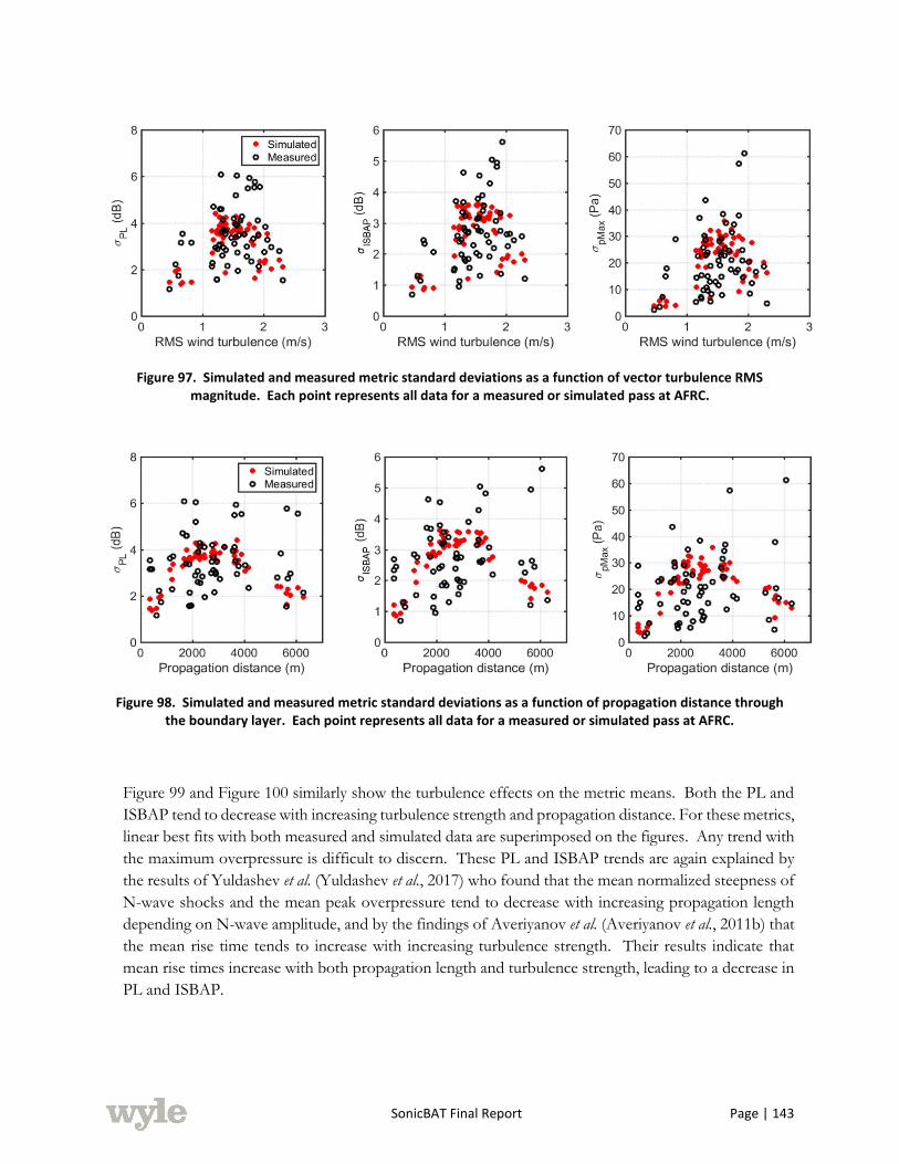
SonicBAT Final Report Page | 143
Figure 97. Simulated and measured metric standard deviations as a function of vector turbulence RMS magnitude. Each point represents all data for a measured or simulated pass at AFRC.
Figure 98. Simulated and measured metric standard deviations as a function of propagation distance through the boundary layer. Each point represents all data for a measured or simulated pass at AFRC.
Figure 99 and Figure 100 similarly show the turbulence effects on the metric means. Both the PL and
ISBAP tend to decrease with increasing turbulence strength and propagation distance. For these metrics,
linear best fits with both measured and simulated data are superimposed on the figures. Any trend with
the maximum overpressure is difficult to discern. These PL and ISBAP trends are again explained by
the results of Yuldashev et al. (Yuldashev et al., 2017) who found that the mean normalized steepness of
N-wave shocks and the mean peak overpressure tend to decrease with increasing propagation length
depending on N-wave amplitude, and by the findings of Averiyanov et al. (Averiyanov et al., 2011b) that
the mean rise time tends to increase with increasing turbulence strength. Their results indicate that
mean rise times increase with both propagation length and turbulence strength, leading to a decrease in
PL and ISBAP.
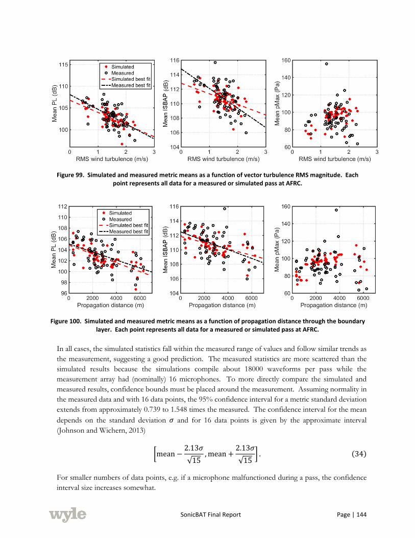
SonicBAT Final Report Page | 144
Figure 99. Simulated and measured metric means as a function of vector turbulence RMS magnitude. Each point represents all data for a measured or simulated pass at AFRC.
Figure 100. Simulated and measured metric means as a function of propagation distance through the boundary layer. Each point represents all data for a measured or simulated pass at AFRC.
In all cases, the simulated statistics fall within the measured range of values and follow similar trends as
the measurement, suggesting a good prediction. The measured statistics are more scattered than the
simulated results because the simulations compile about 18000 waveforms per pass while the
measurement array had (nominally) 16 microphones. To more directly compare the simulated and
measured results, confidence bounds must be placed around the measurement. Assuming normality in
the measured data and with 16 data points, the 95% confidence interval for a metric standard deviation
extends from approximately 0.739 to 1.548 times the measured. The confidence interval for the mean
depends on the standard deviation 𝜎 and for 16 data points is given by the approximate interval
(Johnson and Wichern, 2013)
[mean −2.13𝜎
√15,mean +
2.13𝜎
√15] . (34)
For smaller numbers of data points, e.g. if a microphone malfunctioned during a pass, the confidence
interval size increases somewhat.

SonicBAT Final Report Page | 145
The histograms in Figure 101 and Figure 102 indicate how many simulated predictions on a pass-by-
pass basis fall outside of the 95% confidence interval for a metric statistic. Predictions which fall within
the interval have values of zero in these histograms. In all cases except for the mean maximum
overpressures, the majority of predictions for the 60 passes fall within the interval, indicating an accurate
fit. For the standard deviations, all but one prediction fall within 2 PLdB of the confidence intervals,
and all but two are within 2 dB of the intervals for ISBAP. Predictions for maximum overpressure
deviations which fall outside the intervals show the highest relative error, within about 30 Pa. For the
mean statistics, the PL and ISBAP predictions are all within 5 dB of the measured intervals, which is
low relative to the measured mean values on the order of 100 dB. The maximum overpressure mean
predictions are within about 40 Pa, which is a higher relative error.
Figure 101. Accuracy of simulated metric standard deviations in predicting measured values. Values of zero are represented in black and indicate that the predicted statistic falls within the 95% confidence interval of the
measurement at AFRC.
Figure 102. Accuracy of simulated metric means in predicting measured values. Values of zero are represented in black and indicate that the predicted statistic falls within the 95% confidence interval of the measurement
at AFRC.
The same analysis for data from the KSC measurements and associated simulations is illustrated in Figure
103 through Figure 108. The range of RMS turbulence strengths at KSC was between about 0.6 and 1.5
m/s and the propagation distances were below 2 km, while the strengths at AFRC were between about
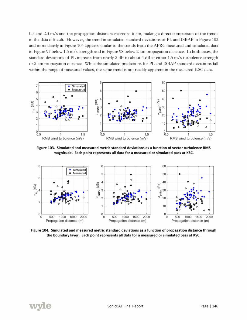
SonicBAT Final Report Page | 146
0.5 and 2.3 m/s and the propagation distances exceeded 6 km, making a direct comparison of the trends
in the data difficult. However, the trend in simulated standard deviations of PL and ISBAP in Figure 103
and more clearly in Figure 104 appears similar to the trends from the AFRC measured and simulated data
in Figure 97 below 1.5 m/s strength and in Figure 98 below 2 km propagation distance. In both cases, the
standard deviations of PL increase from nearly 2 dB to about 4 dB at either 1.5 m/s turbulence strength
or 2 km propagation distance. While the simulated predictions for PL and ISBAP standard deviations fall
within the range of measured values, the same trend is not readily apparent in the measured KSC data.
Figure 103. Simulated and measured metric standard deviations as a function of vector turbulence RMS magnitude. Each point represents all data for a measured or simulated pass at KSC.
Figure 104. Simulated and measured metric standard deviations as a function of propagation distance through the boundary layer. Each point represents all data for a measured or simulated pass at KSC.
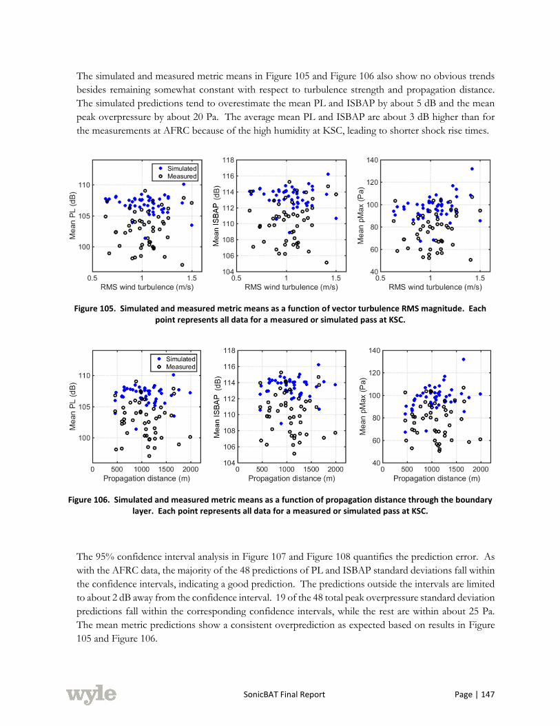
SonicBAT Final Report Page | 147
The simulated and measured metric means in Figure 105 and Figure 106 also show no obvious trends
besides remaining somewhat constant with respect to turbulence strength and propagation distance.
The simulated predictions tend to overestimate the mean PL and ISBAP by about 5 dB and the mean
peak overpressure by about 20 Pa. The average mean PL and ISBAP are about 3 dB higher than for
the measurements at AFRC because of the high humidity at KSC, leading to shorter shock rise times.
Figure 105. Simulated and measured metric means as a function of vector turbulence RMS magnitude. Each point represents all data for a measured or simulated pass at KSC.
Figure 106. Simulated and measured metric means as a function of propagation distance through the boundary layer. Each point represents all data for a measured or simulated pass at KSC.
The 95% confidence interval analysis in Figure 107 and Figure 108 quantifies the prediction error. As
with the AFRC data, the majority of the 48 predictions of PL and ISBAP standard deviations fall within
the confidence intervals, indicating a good prediction. The predictions outside the intervals are limited
to about 2 dB away from the confidence interval. 19 of the 48 total peak overpressure standard deviation
predictions fall within the corresponding confidence intervals, while the rest are within about 25 Pa.
The mean metric predictions show a consistent overprediction as expected based on results in Figure
105 and Figure 106.

SonicBAT Final Report Page | 148
Figure 107. Accuracy of simulated metric standard deviations in predicting measured values. Values of zero are represented in black and indicate that the predicted statistic falls within the 95% confidence interval of the
measurement at KSC.
Figure 108. Accuracy of simulated metric means in predicting measured values. Values of zero are represented in black and indicate that the predicted statistic falls within the 95% confidence interval of the measurement
at KSC.
The performance of the numeric model in reproducing the two measured datasets is further illustrated
in Figure 109 and Figure 110, combining all the validation simulation results for one dataset and the
corresponding measurements into single probability distributions. The simulated distributions in Figure
109 closely follow the measurements for the vast majority of probabilities. Both the PL and ISBAP
metric distributions are very normal, and follow the normal best fit represented by dashed lines. While
the measurement deviates somewhat from the normal fit at extreme probabilities, it is possible that with
more data the measured PL and ISBAP data would collapse further onto the normal line. This aggregate
result gives credence to the characterization of PL and ISBAP distributions for a given turbulence
condition as normal, so that the metric at any probability may be calculated with knowledge of the
corresponding standard deviation. However, both the measured and simulated data tend to curve away
from the normal at very low PL values (above about 99%).
The overall maximum overpressure distribution is well matched by the simulated data, and both do not
follow a normal distribution at high amplitudes (below about 10%). The measurement deviates

SonicBAT Final Report Page | 149
somewhat from the simulation at high pressures below about 1%, but again it is possible that with more
data the measured maximum overpressures could collapse onto the same trend.
The distributions shown in Figure 110 clearly illustrate the tendency of the numeric model to overpredict
the metric means, as indicated by the histograms in Figure 108. As with the AFRC measurement, the
distributions for PL and ISBAP are very normal, while the high-magnitude maximum overpressures
curve away from a normal fit at low probabilities. The simulated and measured data both exhibit these
same trends, although the distributions are visually separated because of the numeric model
overpredictions. In addition, the slopes of the measured PL and ISBAP distributions are somewhat
shallower than for the simulated data, indicating that the overall standard deviation may be
underpredicted. It should be noted that these figures combine data for all passes together, so that it is
impossible to determine from this representation which passes might have underpredicted PL or ISBAP
deviations. The pass-by-pass analysis in Figure 107 points out that while some standard deviations were
underpredicted (and a few overpredicted), the majority of predictions fell within the measurement
confidence interval.
Figure 109. Combined results from KZKFourier validation simulations for the AFRC measurement. The y-axis shows the probability the data is above the value on the x-axis. The simulated data are shown as solid lines, and
the dashed lines are best fits to a normal distribution. The measured data are shown as black circles.
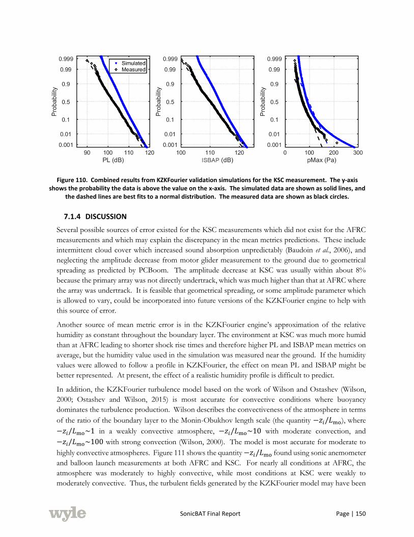
SonicBAT Final Report Page | 150
Figure 110. Combined results from KZKFourier validation simulations for the KSC measurement. The y-axis shows the probability the data is above the value on the x-axis. The simulated data are shown as solid lines, and
the dashed lines are best fits to a normal distribution. The measured data are shown as black circles.
7.1.4 DISCUSSION
Several possible sources of error existed for the KSC measurements which did not exist for the AFRC
measurements and which may explain the discrepancy in the mean metrics predictions. These include
intermittent cloud cover which increased sound absorption unpredictably (Baudoin et al., 2006), and
neglecting the amplitude decrease from motor glider measurement to the ground due to geometrical
spreading as predicted by PCBoom. The amplitude decrease at KSC was usually within about 8%
because the primary array was not directly undertrack, which was much higher than that at AFRC where
the array was undertrack. It is feasible that geometrical spreading, or some amplitude parameter which
is allowed to vary, could be incorporated into future versions of the KZKFourier engine to help with
this source of error.
Another source of mean metric error is in the KZKFourier engine’s approximation of the relative
humidity as constant throughout the boundary layer. The environment at KSC was much more humid
than at AFRC leading to shorter shock rise times and therefore higher PL and ISBAP mean metrics on
average, but the humidity value used in the simulation was measured near the ground. If the humidity
values were allowed to follow a profile in KZKFourier, the effect on mean PL and ISBAP might be
better represented. At present, the effect of a realistic humidity profile is difficult to predict.
In addition, the KZKFourier turbulence model based on the work of Wilson and Ostashev (Wilson,
2000; Ostashev and Wilson, 2015) is most accurate for convective conditions where buoyancy
dominates the turbulence production. Wilson describes the convectiveness of the atmosphere in terms
of the ratio of the boundary layer to the Monin-Obukhov length scale (the quantity −𝑧𝑖/𝐿mo), where
−𝑧𝑖/𝐿mo~1 in a weakly convective atmosphere, −𝑧𝑖/𝐿mo~10 with moderate convection, and
−𝑧𝑖/𝐿mo~100 with strong convection (Wilson, 2000). The model is most accurate for moderate to
highly convective atmospheres. Figure 111 shows the quantity −𝑧𝑖/𝐿mo found using sonic anemometer
and balloon launch measurements at both AFRC and KSC. For nearly all conditions at AFRC, the
atmosphere was moderately to highly convective, while most conditions at KSC were weakly to
moderately convective. Thus, the turbulent fields generated by the KZKFourier model may have been

SonicBAT Final Report Page | 151
inaccurate for some passes at KSC. To account for this source of error, a future version of the
KZKFourier engine might use a different atmospheric model for cases with weak convection.
Figure 111. Convectiveness of atmosphere during supersonic passes at AFRC (left) and KSC (right). Dotted, dot dashed, and dashed lines indicate approximate regions of weak, moderate, and strong
convectiveness, respectively.
For the AFRC and KSC environments, the KZKFourier engine predictions of standard deviations for
both PL and ISBAP are shown to be the most accurate. In all cases, the predicted PL and ISBAP
deviations fall within the overall ranges of measured values, and the majority are within 95% confidence
intervals of the measured values. This good agreement suggests that KZKFourier can well represent
the sonic boom level deviations even in varied atmospheric conditions. The majority of predicted
maximum overpressure deviations also fall within the confidence intervals for the AFRC data; however,
only about half of those for the KSC data are within the bounds. The mean metric predictions also
perform well and closely follow the trends in the measurements in moderately to highly convective
conditions with no cloud cover, such as at AFRC.
7.2 VALIDATION OF THE CLASSICAL SONIC BOOM-TURBULENCE RESEARCH CODE
7.2.1 CLASSICAL TURBULENCE CODE FUNCTIONAL OVERVIEW
The classical code, named TURBO, bases its results on a re-propagation through turbulence and mean
atmospheric conditions to capture: variations in amplitude and focusing from refraction plus rounding
and distortions from scattered multipath arrival times. Propagation path and propagation timing both
affect the turbulent signature results. The code begins with ground results from either modified-linear
theory or Burgers predictions of ground sonic boom carpet signatures propagated through mean
atmospheric conditions. It reads ray starting conditions (X, Y, Z, their unit vectors and time) from
PCBoom output at the top of the ABL, but does not read signatures from this height. The signatures
are read from ground solutions (PCBoom or sBOOM), along with their intersection X, Y, Z and time.
Mean atmospheric temperatures and winds are read from the PCBoom input <arg1>.dat file or from
the output <arg1>.age file along with the ABL/ground amplitude and aging ratios. For the milliseconds
of propagation difference between zero turbulence and turbulent multipath arrival times, non-linear

SonicBAT Final Report Page | 152
aging differences can be neglected, so the code saves computational time by not repeating non-linear
signature aging calculations. (If found to be important later, they could be accurately estimated from
the aging ratio read from the <arg1>.age file.) The atmospheric modeling is similar to full numerical
solutions, utilizing Fourier modes of turbulence pointing in random directions and distributed in length
and strength according to a von Karman implementation of a Kolmogorov frequency distribution. The
non-linear aging of focus peaks may also be particularly important for post-focus decay rate. This is a
simplified method that handles many parameters in 3-D by using simplifications, as opposed to more
rigorous numerical methods with fewer simplifications that may be more limited in the number of
variations they can handle and their speed, hardware requirements and ease of use.
Ray propagation dominates execution time and depends on the propagation and atmospheric
parameters chosen, so determining their best values is paramount to efficiency. Many studies were run
with earlier versions of the TURBO code that revealed a lot of ray propagation calculations were not
contributing to results. Solutions to those inefficiency problems were invented, which required adding
substantial new code to rearrange the propagation starting conditions and particularly the calculation of
intersections at the ground. The revised methodology is about 20 times more efficient than the originally
envisioned code. Because of its dynamic development, testing of the methodology continues to yield
further refinements to its efficiency and accuracy.
7.2.2 CODE COMPONENT TESTING
Testing of the classical method was initially performed on the individual execution steps: atmospheric
modeling, ray propagation, ray tube intersection determination and signature summation.
7.2.2.1 ATMOSPHERIC MODELING
The atmospheric modeling of the final code, named TURBO, has typical features found in other codes,
with some implementation differences. The program is formulated in Cartesian coordinates. Like
others, it uses frozen Fourier modes of different lengths and random directions to model the turbulence
with a von Karman implementation of a Kolmogorov distribution and Log spacing of mode lengths.
In TURBO every velocity mode has variations in both directions normal to the velocity (section 4.3.1,
Figure 30). Mode velocities vary in a 2-D square lattice in an alternating checker pattern. Gradients are
created in two dimensions by each mode, each with their own random phase and normal to the random
direction of the mode velocity.
Since there are 2 directions of variation, there is the possibility to vary the turbulence strength 50/50%
in each direction or with a random strength in each direction from 50/50% to 25/75%. This allows for
easy implementation of another degree of randomness. The turbulence strength can vary the same
(50%/50%, by using an input file variable named IRAND equal to either= 0 or 1) in both directions or
it can be randomly apportioned (from 25%/75% to 75%/25% by using IRAND equal to either 2 or 3)
with different strength variations. Even IRAND values of 0 or 2 cause the phase origin of all Z-direction
modes to be located at the top of the ABLH, making the onset of turbulence continuous with the
atmosphere above the ABL, while odd IRAND values provide a random Z phase for each mode like
the random X and Y phase in all cases. Testing seemed to favor using a randomly apportioned (IRAND
2 or 3) turbulence variation while even and odd IRAND values did not seem to make a noticeable
difference. Also, each mode’s random direction is broken down into components in X, Y and Z
directions to speed calculations particularly with regard to resolving turbulence strength variations as a

SonicBAT Final Report Page | 153
function of Z and resolving combined effects with the mean atmospheric property variations as a
function of Z.
The model generation is based on several input turbulence parameters, namely: minimum scale length
(FLMIN), maximum scale length (FLMAX) and the number of modes NLMAX, spaced in constant
logarithmic steps. Plus, there is an optional parameter, NLMAXMORE, to allow the representation of
larger scales than FLMAX (𝐿0 commonly), the mode of maximum strength by definition. Modes from
NLMAX+1 to NLMAXMORE can be significant but have diminishing strength according to the von
Karman spectrum equations of Cotte and Blanc-Benon. Structure parameters CT2 and CV
2 are input for
the strength of the turbulence at two altitudes (chosen for initial testing, but could be expanded) allowing
a Log variation in turbulence strength versus altitude.
This use of component breakdown of the turbulence distribution and strength was intended to provide
more accurate mode length representation (because of variation in 2-dimensions, instead of only one)
and to help with execution speed by reducing use of transcendental function calculations. With the ray
direction vector defined as u, with v defined as always level and left of u, and with w defined as
perpendicular to u and upward, resolving kinetic turbulence gradients is reduced to 6-∂w pitch effectors
(turbulent mode strengths in directions Tx(Y), Tx(Z), Ty(X), Ty(Z), Tz(X), Tz(Y)) and 4-∂v yaw
effectors (Tx(Y), Ty(X), Tz(X), Tz(Y), a horizontal v is not effected by turbulence T_(Z) gradients). No
comparisons have been made with other turbulence modeling computational schemes. The
implementation seems to work efficiently and code loops were written to be amenable to future parallel
execution.
7.2.2.2 RAY PROPAGATION
Ray Propagation is affected by turbulent temperature and gust variations as well as mean temperature
and wind distributions. The first ray propagation test was performed without turbulence using standard
atmosphere mean conditions and a propagation from 11km (36089 ft) at Mach 1.154, just above the
cutoff Mach. Results matched PCBoom ground intersection locations within several feet using step
sizes up to 10 seconds in duration. Using a balloon measured mean atmosphere with many altitudes of
temperature and wind variations, condition changes will occur at altitudes that do not exactly match the
time steps. TURBO subdivides time steps, individually for each ray, to coincide with condition break
altitudes (done automatically) to maintain highest accuracy. Adding strong turbulence requires a step
size reduction to 0.0005 seconds to be within several feet of the converged solution. Convergence error
seems to increase in proportion to step size while execution time increases in inverse proportion. Every
foot reduction in convergence error costs more and more to achieve, so the most suitable step size for
accuracy and efficiency was investigated. Because the repeating scheme can determine intersections
from coarser results and the figure of merit is level in dB, a step size of 0.02 seconds was found to
provide adequate results in the available time.
As mentioned above, ground ray intersection location plots were found to illustrate information about
the atmosphere and propagation modeling parameters. To help with their interpretation, Figure 112
shows TURBO starting ray locations at the top of the ABL before propagation (altitude 5761 ft, AFRC
flight 3 pass 2) for both Phi equals 0 and 35 degrees (proximity exaggerated as indicated by the scale).
The rays are swept in width at the angle of the isopemp at their Phi, then repeated in time in the direction
of flight.

SonicBAT Final Report Page | 154
Figure 112. Rays start with constant separation (RAYSEP=2ft here) parallel and perpendicular to the direction of flight.
The following plots began shaped as, Phi=0 in Figure 112, a 20 wide by 50 long grid of squares with 2
feet of separation. Based on results like Figure 113, the number of turbulent modes was determined to
be 128 to 256 to achieve good randomness. At lower numbers, modal patterns become increasingly
apparent. But, increasing randomness with additional modes, increases computational time
proportionally. Conversely, randomly (instead of equally) distributing the strength of turbulence
between the two axes of each plane (by specifying IRAND = 2 or 3) increased randomness a little
without any increase in computational time.
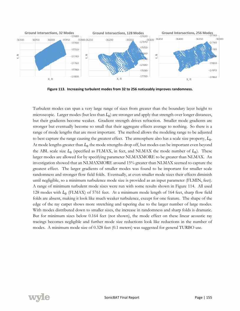
SonicBAT Final Report Page | 155
Figure 113. Increasing turbulent modes from 32 to 256 noticeably improves randomness.
Turbulent modes can span a very large range of sizes from greater than the boundary layer height to
microscopic. Larger modes (but less than 𝐿0) are stronger and apply that strength over longer distances,
but their gradients become weaker. Gradient strength drives refraction. Smaller mode gradients are
stronger but eventually become so small that their aggregate effects average to nothing. So there is a
range of mode lengths that are most important. The method allows the modeling range to be adjusted
to best capture the range causing the greatest effect. The atmosphere also has a scale size property, 𝐿0.
At mode lengths greater than 𝐿0 the mode strengths drop off, but modes can be important even beyond
the ABL scale size 𝐿0 (specified as FLMAX, in feet, and NLMAX the mode number of 𝐿0). These
larger modes are allowed for by specifying parameter NLMAXMORE to be greater than NLMAX. An
investigation showed that an NLMAXMORE around 15% greater than NLMAX seemed to capture the
greatest effect. The larger gradients of smaller modes was found to be important for smaller scale
randomness and stronger flow field folds. Eventually, at even smaller mode sizes their effects diminish
until negligible, so a minimum turbulence mode size is provided as an input parameter (FLMIN, feet).
A range of minimum turbulent mode sizes were run with some results shown in Figure 114. All used
128 modes with 𝐿0 (FLMAX) of 5761 feet. At a minimum mode length of 164 feet, sharp flow field
folds are absent, making it look like much weaker turbulence, except for one feature. The shape of the
edge of the ray carpet shows more stretching and tapering due to the larger number of large modes.
With modes distributed down to smaller sizes, the increase in randomness and sharp folds is dramatic.
But for minimum sizes below 0.164 feet (not shown), the mode effect on these linear acoustic ray
tracings becomes negligible and further mode size reductions look like reductions in the number of
modes. A minimum mode size of 0.328 feet (0.1 meters) was suggested for general TURBO use.

SonicBAT Final Report Page | 156
Figure 114. Smaller modes provide increased variations, but sizes less than 0.164 ft become negligible.
7.2.2.3 RAY-TUBE INTERSECTION DETERMINATION
Changes to the tube intersection calculation methodology and the repeating technique result in a 20
times improvement in code efficiency. The efficiency improvement comes from being able to reduce
the size of the ray lattice by 20 times and still reliably achieve intersections and sufficiently random
results. Previously the lattice would have to be large enough that its center would not degrade in
amplitude due to scatter, making the carpet equal 2 times the maximum scatter distance. Additionally,
the center of the carpet would move randomly for every atmosphere variation and miss the requested
signature location. Using the repeating technique, a small lattice simulates a much larger lattice by
duplicating the calculated lattice ahead, behind, to the sides and diagonally, as many times as necessary,
to capture all of the scatter that could intersect the desired ground point—even finding multiple
intersections with highly spread ray tubes if encountered. Robustly finding every intersection and
accurately calculating their normal area and intersection time, is required for the proper operation of
this method. This methodology does an efficient job of minimizing the comparisons needed to find
the intersections, but its complexity led to a lot of time spent debugging. The final method determines
intersections around 2 orders of magnitude faster than the ray propagation calculations, so its
complexity does not increase run times (which are dominated by propagation). (MOOUT is the MOre-
OUTput [or not] input variable that allows the output and execution efficiency to be matched to the

SonicBAT Final Report Page | 157
users needs. Generally 3+ values are for debugging.) The variable output provides a lot of information
about the intersections calculations at values of MOOUT ≥ 3, so conversely calculations are much faster
at MOOUT ≤ 2.
The intersection calculation has two options that were tested. The first option was the use of repeating
or not. The efficiency of repeating was shown to be such an improvement that all other analyses were
done with it enabled. However, the option remains for turning it off if additional testing is desired at
some future time.
The other intersection option calculates triangular tube intersections by cutting the quadrilaterals twice,
with a different pair of opposite rays, then dividing the amplitude of the signature summation by two.
Quadrilateral (regular parallelograms without turbulence) ray tubes are cut into triangular tubes, referred
to as tri-tubes, when resolving tube intersections. This improves resolution and is more reliable to
resolve because it avoids holes from folded quadrilaterals. By default, the triangle cut is switched
between different rays at negative Phis and positive Phis, like the blue-lines in Figure 115. The figure
shows curved green isopemp lines, two solid and one dashed. Additional green lines are drawn in the
direction of flight and their intersections with the green isopemp lines describes how ray starting
locations are organized by TURBO (Figure 115 shows flight heading green lines at phis of 30, 27, 24,
21 and 3, 0, -3, -6, -9, -12 degrees for illustration, typical TURBO dPhi spacing is much smaller, like
~0.002 deg). By default, the code connects the opposite corner ray-pair that is closer, before turbulence
distortions, which makes the triangular tubes more regular in shape.
Figure 115. Default tri-tubes use blue-lines, option adds red-lines.
A parameter option (KTri=2) causes each quadrilateral to be cut twice using the other, opposite corner
ray-pair, like the red-lines of the top quadrilaterals in Figure 115. This option resolves the triangles
redundantly as 2 sets of triangles that are superimposed, not 4 smaller triangles with an additional
interpolated center ray. When the superimposed signatures are summed, the result is divided by two to
get the correct amplitude. The additional calculation adds negligible execution time. It also seems to
make little difference. Future testing with many instances for statistical results may be required to
discern if this option provides any improvement.
SonicBAT Final Report Page | 158
7.2.2.4 SIGNATURE SUMMATION
The signature summation step sums one or more ground signatures together, one for each tri-tube
intersection found. First the tri-tube’s area ratio relative to PCBoom’s non-turbulent calculation is used
to adjust the signature amplitude contributed by this tube. Second, this scaled signature is shifted in
time to match the tri-tube intersection time. Then all intersections are interpolated to a common time
scale (defined by HzOUT, currently 2,000 Hz) and summed into a single signature. The summation
can either use a PCBoom discontinuous modified-linear theory signature or a Burgers rounded signature
from a sBOOM run. PCBoom will generate the sBOOM inputs if the “SBOOM” keyword is specified
on the line following the RAYTRACING keyword. The sBOOM run following PCBoom will use the
temperature, X-wind, Y-wind and humidity profiles defined for PCBoom in its *.dat input file, whether
they are input directly or called from weather balloon files, etc.
7.2.3 FLIGHT TEST DATABASE
A flight test measurement database was obtained specifically for this program and included turbulence
and other weather measurements. Flight passes 1-65 were performed at NASA AFRC in Edwards CA,
at the west end of the Mojave Desert during very dry conditions. The month of July (2016), was chosen
for it’s typically strong turbulence strengths and many flight days with high turbulence were recorded.
Flight passes 66-121 were performed over NASA’s Kennedy Space Center, by the ocean, with each
day’s temperature reducing the humidity about 30% from the night’s saturated value, during August
2017. This month was also selected to maximize turbulence strengths at this location, but turbulence
for flight days were generally below high turbulence levels and the peak values were substantially lower
than at AFRC. (Further described and quantified in section 8.2.2.1 and Table 30.) Flight times each
day (excepting a few for differentiation) were chosen to capture strongest turbulence.
The Figure 116 below represents 12,100 prediction points for the 121 flight pass conditions. Some
generalizations can be seen that follow from the general testing conditions. AFRC passes 1-65 have
generally more variation than KSC passes 66-121, which follows from stronger measured turbulence
values and a thicker ABL in the desert. Predictions for the KSC passes have a slightly lower range of
level variation (not necessarily an indicator of mean or median). Measurement variation ranges are a bit
smaller and more consistent at KSC, perhaps from lower turbulence. However, the average level is
more variable from pass to pass, which may be indicative of off-track measurements and trajectory
variations. The prediction plot below, Figure 116, shows the most extreme values well but tells less
about the distribution. For example, there is a focus predicted by PCBoom for pass 71, resulting in the
high TURBO level, but a close examination of the prediction output reveals that TURBO predicts a
significant reduction in the average level of the peak due to turbulence. Also there is a peak for pass 71
due to a predicted focus and low values at pass 89 due to a number of zero level errors. The pass 71
predicted focus indicated a need to more accurately determine which trajectory data actually produced
sonic boom at the ground measurement locations. All trajectory times were updated and the focus went
away and the zero error was fixed. These are common examples of the many analysis examinations
performed, errors found, fixes implemented and analysis reruns completed. Analyses were executed in
parallel (6 to 20 code instances run simultaneously).

SonicBAT Final Report Page | 159
Figure 116. 100 prediction points plotted for each of 121 flight test passes showing peak variations (plus zero errors at 89 and a non-turbulent focus at 71).
TURBO performs its turbulent propagation using its turbulence modeling combined with the mean
atmospheric temperature gradients and winds. Testing at AFRC was done with the primary
measurement array directly under the flight track. At KSC due to airspace restrictions and trying to be
a good neighbor to Titusville, Florida, the F-18s were flown over the ocean with its sonic boom
footprint confined to the cape. This resulted in Phi angles of 10 to 40 degrees (the edge of the carpet).
The N-wave boom amplitude drops like a cosine to about half at the edge. In addition, trajectory
variations in heading have no effect on the boom under track but become significant off-track. In
summary, it was expected that KSC sonic boom would be 1 to 5 PLdB quieter due to off-track distance,
louder by about 2 PLdB due to less rounded signatures in higher humidity, less variability due to weaker
turbulence, but possibly more variability from trajectory changes measured off-track and occasionally
near the cut-off Mach.
7.2.3.1 ARMSTRONG FLIGHT RESEARCH CENTER DATABASE
The AFRC database contained ground measurements along a primary array of 16 microphones spaced
100 feet apart in a line in the direction of flight. This provides sufficient separation to measure different
turbulent distortions while keeping the flight conditions nearly the same. For model validation, a
TURBO analysis was run for all 65 supersonic passes using:
• balloon measured mean atmospheric conditions and ABL height,
• anemometer measurements for determination of the structure parameters 𝐶𝑇2 and 𝐶𝑣
2,
• GPS flight trajectories.
Ground measurements were taken along the flight path with a line of 16 microphones 100 feet apart, as
described for the primary array in Section 5.2.1 and Figure 36. TURBO was run for all 65 passes at near
Mach 1.4. For every pass 100 signatures were calculated in a line using a rectangle of starting rays 40
wide by 1030 long (41200 total rays, 80262 tri-tubes) spaced in squares with 1 ft of corner ray separation
in a constant ABL height plane.
Predictions were compared with ground measurements to assess the predicted levels versus
measurements. The predicted and measured means are within a few dB of each other, as shown in

SonicBAT Final Report Page | 160
Figure 117. The turbulent variations from the Burgers trend do slightly improve matching, and there is
still a couple dB of prediction variation in the average from 100 signatures. Using the GPS trajectory
and mean weather conditions improves non-turbulent matching.
Figure 117. The 100 signature classic TURBO solution per flight pass was used to predict mean level changes due to turbulence.
While turbulence does affect the mean, it is expected to have a stronger effect on variations. Figure 118
and Figure 119 compare standard deviations at AFRC and KSC, respectively. The AFRC deviations
range from 2 to 6 PLdB while the KSC generally range from 2 to 4 with a few 5’s, except for one pass
with a 6 and 23 PLdB standard deviation. Trajectory data indicates a possibility for threshold Mach
effects. The measurements are believed to be accurate data. Using arrays of 16-20 microphones, the
measurements are a bit sparse for defining an accurate variation range. Running more predictions is
more economical for determining means and deviations. Comparisons are only expected to be close
with possible trend similarities. The figures show they are close, and furthermore, they have similar
magnitude variation trends, and overall the predicted deviations are high in both cases. The AFRC
deviations are generally close except that passes 34-49 are particularly over predicted. The KSC
deviations are generally close except for 11 predictions that spike above the others without any
noticeable pattern. These differences indicate likely opportunities for code improvement. Since the
KSC secondary array was only 3 degrees lower in Phi (the ray roll angle) than the primary array, it was
plotted with the predictions for the primary array (but secondary array conditions were collected if
secondary array predictions are ever desired). However, these differences may change because there are
still many parameters in the code that need testing to determine their best settings and many code
improvements are still being made. Matching variation trends provides confidence that important
processes are being modeled, and is important for the code’s intended application to low sonic boom
signatures.

SonicBAT Final Report Page | 161
Figure 118. AFRC Measured standard deviation is near predictions and follows the variation trend.
Figure 119. KSC measured standard deviation is near predictions and follows the variation trend.

SonicBAT Final Report Page | 162
7.2.3.2 KENNEDY SPACE CENTER FLIGHT TEST DATABASE
As described in Section 7.2.3 and illustrated in Figure 120, KSC cases tend to have stronger sensitivity
to trajectory variations, due to measurements being off-track and due to flight speeds and headwinds
which sometimes were close to the cutoff Mach. Trajectory variations cause stronger effects in the
outer carpet than under track and when closer to the cutoff Mach, so the effect is compounded but the
total is only 2 PLdB. Course changes affect boom at the edge while they don’t affect undertrack, and
the lower ray inclination angles magnify many trajectory, wind and temperature variations as well as
turbulence. Figure 120 shows that TURBO correlates well in general with the measurements; one
instance of high levels are shown for pass 6, resulting from a strong focus that halts program execution.
In spite of the above mentioned problems, good results are achieved, as shown in Figure 120, and in
the next chapter.
Figure 120. TURBO correlates with measurements until focusing becomes too prevalent (really high levels for pass 6 result from a strong focus that halts execution).
7.2.4 RESULTS SUMMARY
This validation shows that the TURBO code provides assessments of turbulence that correlate with
flight test measured results, which is likely to further improve with additional experience running the
method. Standard deviation predictions show even more matching with the measurement deviation
trends though overall values are generally overpredicted. TURBO is able to assess full flight conditions
of mean temperature and mean wind distributions with superimposed turbulence. The code has a
flexible implementation that allows for further development and refinement.

SonicBAT Final Report Page | 163
8.0
STATISTICAL ANALYSIS AND UNCERTAINTY QUANTIFICATION OF THE NUMERIC AND CLASSICAL SONIC BOOM-TURBULENCE RESEARCH CODES
8.1 STATISTICAL ANALYSIS AND UNCERTAINTY QUANTIFICATION OF THE NUMERIC SONIC BOOM-TURBULENCE RESEARCH SOFTWARE CODE
8.1.1 INTRODUCTION
To better understand the effect of turbulence and atmospheric parameters on sonic boom metrics,
multiple KZKFourier simulations at 96 different conditions varying these parameters were performed.
The code was run on the NASA Pleiades supercomputing cluster. The resultant database provides
insight into the effect of turbulence on N-waves across a wide range of possible atmospheric conditions.
For each of the 96 conditions, mean, -std, and +std turbulence FIR filters with respect to several metrics
(see Section 3.5) were created according to the FIR filter method developed by Locey and Sparrow
(Locey and Sparrow, 2007; Locey, 2008). The utility of the filters is that they can be convolved with
any given supersonic signature to approximate these metrics under the corresponding turbulent
conditions. These filters are applied to multiple low boom configurations in Section 9.0. The method
for choosing the 96 conditions and the associated simulation parameters are discussed in Section 8.1.2.
Results from the simulations including analysis of the effect of individual parameters are discussed in
Section 8.1.3, and in Section 8.1.4 some general uncertainty inherent in the KZKFourier algorithm and
in the turbulence FIR filter creation process is discussed.
8.1.2 SIMULATION PARAMETERS
Four general parameters including turbulence strength, boundary layer height, propagation angle, and
humidity were varied at discrete values to make up the space of simulated conditions under investigation.
The importance of turbulence strength and propagation distance on turbulized signature metrics is well
documented in the literature (Lipkens and Blackstock, 1998; Averiyanov et al., 2011b; Yuldashev et al.,
2013; Yuldashev et al., 2017). For the present work, the effect of propagation distance is broken up into
two different parameters, boundary layer height and ray propagation angle, because the turbulent fields
in KZKFourier (see Section 3.3) use height-dependent turbulence length scales according to the theory
of Wilson and Ostashev (Wilson, 2000; Ostashev and Wilson, 2015). It would be possible for two
conditions with similar propagation lengths to have different simulated atmospheric turbulence
conditions because of differing ray angles and boundary layer heights. To determine if such a situation
would appreciably change sonic boom metrics, the two parameters are considered independently.
Humidity is also considered because it greatly affects relaxation, which determines the shock structure
of sonic booms (Hammerton, 2001). Conditions with high humidity generally have less associated
relaxation absorption, which decreases the time a shock takes to reach peak pressure relative to low
humidity conditions (Loubeau, 2006).
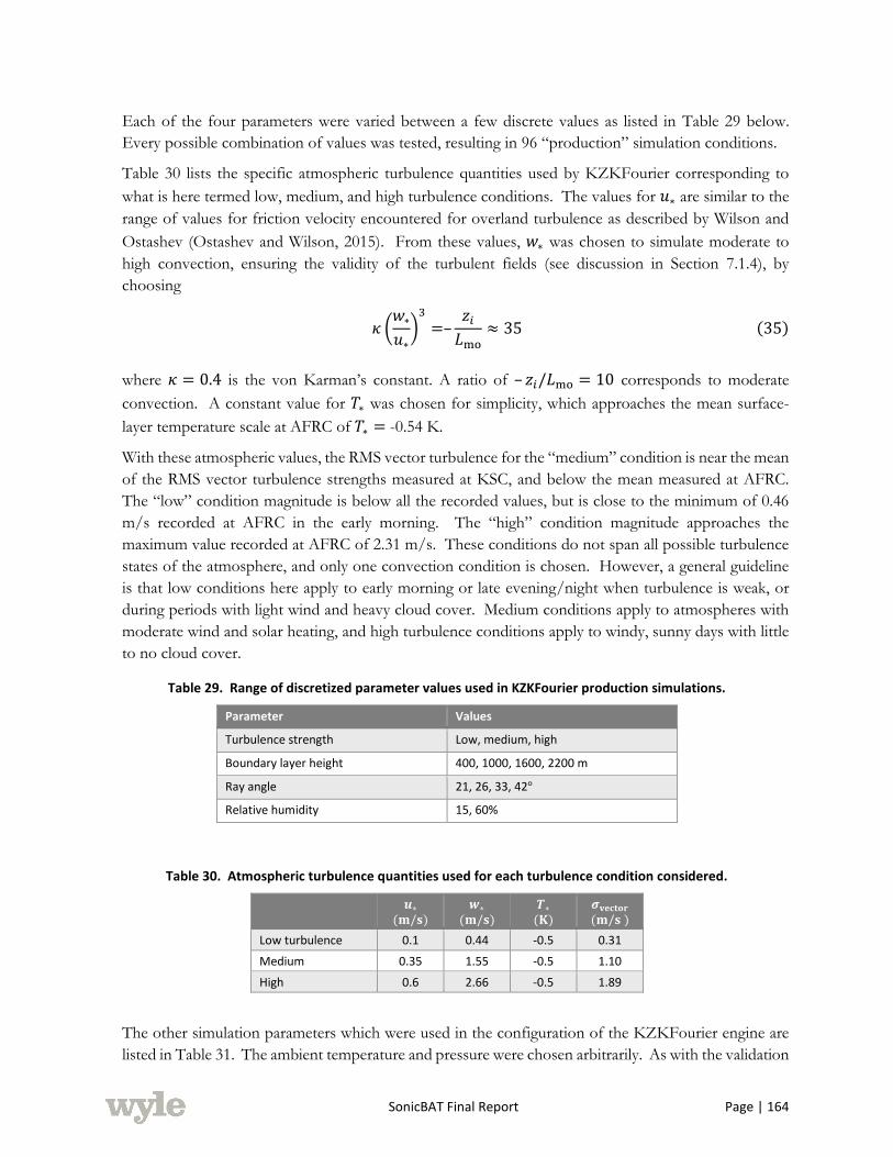
SonicBAT Final Report Page | 164
Each of the four parameters were varied between a few discrete values as listed in Table 29 below.
Every possible combination of values was tested, resulting in 96 “production” simulation conditions.
Table 30 lists the specific atmospheric turbulence quantities used by KZKFourier corresponding to
what is here termed low, medium, and high turbulence conditions. The values for 𝑢∗ are similar to the
range of values for friction velocity encountered for overland turbulence as described by Wilson and
Ostashev (Ostashev and Wilson, 2015). From these values, 𝑤∗ was chosen to simulate moderate to
high convection, ensuring the validity of the turbulent fields (see discussion in Section 7.1.4), by
choosing
𝜅 (𝑤∗
𝑢∗)
3
=–𝑧𝑖
𝐿mo
≈ 35 (35)
where 𝜅 = 0.4 is the von Karman’s constant. A ratio of – 𝑧𝑖/𝐿mo = 10 corresponds to moderate
convection. A constant value for 𝑇∗ was chosen for simplicity, which approaches the mean surface-
layer temperature scale at AFRC of 𝑇∗ = -0.54 K.
With these atmospheric values, the RMS vector turbulence for the “medium” condition is near the mean
of the RMS vector turbulence strengths measured at KSC, and below the mean measured at AFRC.
The “low” condition magnitude is below all the recorded values, but is close to the minimum of 0.46
m/s recorded at AFRC in the early morning. The “high” condition magnitude approaches the
maximum value recorded at AFRC of 2.31 m/s. These conditions do not span all possible turbulence
states of the atmosphere, and only one convection condition is chosen. However, a general guideline
is that low conditions here apply to early morning or late evening/night when turbulence is weak, or
during periods with light wind and heavy cloud cover. Medium conditions apply to atmospheres with
moderate wind and solar heating, and high turbulence conditions apply to windy, sunny days with little
to no cloud cover.
Table 29. Range of discretized parameter values used in KZKFourier production simulations.
Parameter Values
Turbulence strength Low, medium, high
Boundary layer height 400, 1000, 1600, 2200 m
Ray angle 21, 26, 33, 42°
Relative humidity 15, 60%
Table 30. Atmospheric turbulence quantities used for each turbulence condition considered.
𝒖∗
(𝐦/𝐬) 𝒘∗
(𝐦/𝐬) 𝑻∗ (𝐊)
𝝈𝐯𝐞𝐜𝐭𝐨𝐫 (𝐦/𝐬 )
Low turbulence 0.1 0.44 -0.5 0.31
Medium 0.35 1.55 -0.5 1.10
High 0.6 2.66 -0.5 1.89
The other simulation parameters which were used in the configuration of the KZKFourier engine are
listed in Table 31. The ambient temperature and pressure were chosen arbitrarily. As with the validation

SonicBAT Final Report Page | 165
simulations in Section 7.1.2, the transverse size 𝑦max was reduced from 350 m for long propagation
lengths and the number of realizations was increased to compensate. The input waveform was chosen
from one of the motor glider recordings taken at AFRC. The signature was propagated through 1 km
of homogeneous atmosphere, using the production simulation’s ambient atmospheric parameters,
before the full simulation with turbulence. The signature length varies because zero padding was
necessary for long propagation lengths through the boundary layer.
Table 31. Parameter values used in KZKFourier production simulations.
Parameter Values for Production Simulations
𝑻𝟎 22.0 °C
𝒑𝟎 1.0 atm
Signature Length 280 – 580 ms
Number of Realizations 27 – 45
𝒚𝐦𝐚𝐱 150 – 350 m
𝚫𝒚 (Transverse) 0.5 m
𝚫𝒛 (Propagation) 0.05 m
Sampling Rate 200 kHz
8.1.3 RESULTS AND STATISTICAL ANALYSIS
Multiple realizations of KZKFourier were performed at each of the 96 distinct conditions found from
varying the four atmospheric turbulence parameters in Table 29. The simulated waveforms at the
ground capture the qualitative effects of turbulence and clearly show differences between turbulence
conditions. As with the validation simulations in Section 7.0, about 18000 waveforms were produced
at each condition. For illustration, waveforms from two conditions which exhibit peaking and rounding
from turbulent distortions are shown in Figure 121. These waveforms had the lowest and highest
maximum overpressures in a particular realization. The two conditions for these waveforms differ only
by turbulence strength and the other parameters are the same with about 2.3 km of propagation distance
through the boundary layer at 15% humidity. The peaked waveform at high turbulence contains much
higher amplitude distortions beyond the shock compared to the low turbulence case, and the rounded
waveform at high turbulence has a much longer rise time. The prevalence of longer rise times with
higher turbulence magnitude has been discussed in the literature (Averiyanov et al., 2011b).
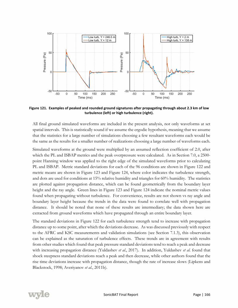
SonicBAT Final Report Page | 166
Figure 121. Examples of peaked and rounded ground signatures after propagating through about 2.3 km of low turbulence (left) or high turbulence (right).
All final ground simulated waveforms are included in the present analysis, not only waveforms at set
spatial intervals. This is statistically sound if we assume the ergodic hypothesis, meaning that we assume
that the statistics for a large number of simulations choosing a few resultant waveforms each would be
the same as the results for a smaller number of realizations choosing a large number of waveforms each.
Simulated waveforms at the ground were multiplied by an assumed reflection coefficient of 2.0, after
which the PL and ISBAP metrics and the peak overpressure were calculated. As in Section 7.0, a 2500-
point Hanning window was applied to the right edge of the simulated waveforms prior to calculating
PL and ISBAP. Metric standard deviations for each of the 96 conditions are shown in Figure 122 and
metric means are shown in Figure 123 and Figure 124, where color indicates the turbulence strength,
and dots are used for conditions at 15% relative humidity and triangles for 60% humidity. The statistics
are plotted against propagation distance, which can be found geometrically from the boundary layer
height and the ray angle. Green lines in Figure 123 and Figure 124 indicate the nominal metric values
found when propagating without turbulence. For convenience, results are not shown vs ray angle and
boundary layer height because the trends in the data were found to correlate well with propagation
distance. It should be noted that none of these results are intermediary; the data shown here are
extracted from ground waveforms which have propagated through an entire boundary layer.
The standard deviations in Figure 122 for each turbulence strength tend to increase with propagation
distance up to some point, after which the deviations decrease. As was discussed previously with respect
to the AFRC and KSC measurements and validation simulations (see Section 7.1.3), this observation
can be explained as the saturation of turbulence effects. These trends are in agreement with results
from other studies which found that peak pressure standard deviations tend to reach a peak and decrease
with increasing propagation distance (Yuldashev et al., 2017). In addition, Yuldashev et al. found that
shock steepness standard deviations reach a peak and then decrease, while other authors found that the
rise time deviations increase with propagation distance, though the rate of increase slows (Lipkens and
Blackstock, 1998; Averiyanov et al., 2011b).

SonicBAT Final Report Page | 167
Figure 122. Ground signature metric standard deviations from the production simulations plotted against total propagation distance.
The results in Figure 122 also show a dependence on turbulence strength for the distance to the standard
deviation turning point. The turning point for maximum overpressure deviations occurs at about 4.5
km propagation length for low turbulence strength, and near 3 km for medium and high strengths. The
turning point for PL and ISBAP deviations follows a similar trend with higher turbulence strengths
decreasing the distance to the turning point. For low, medium, and high turbulence conditions, the
turning points for PL and ISBAP are at about 5 km, 4 km, and 3 km, respectively.
The standard deviations for maximum overpressure tend to follow the expected ordering with respect
to turbulence strength. At low turbulence, the deviations are lower than at medium, and at high
turbulence conditions the deviations are highest. Interestingly, at above 2 km propagation distance and
above 3.5 km distance, respectively, the PL and ISBAP deviations for medium strength conditions
overtake those for high strength. In addition, the deviations for low turbulence conditions overtakes
those for high conditions after about 4 to 4.5 km for PL. These observations seem to contradict the
increase in rise time deviations with turbulence strength as shown by Averiyanov et al. (Averiyanov et
al., 2011b), although the authors may not have propagated far enough to find the behavior seen here.
One possible explanation is that with increasing propagation distance, the effects of atmospheric
absorption become more profound. The deviations then decrease as the high frequency content in the
signatures is reduced.
Interestingly, the ISBAP deviations in Figure 122 are generally lower than for PL by up to about 0.5 dB.
This difference occurs despite the fact that the ISBAP metric is strictly larger in value than PL, as
evidenced by the metric means in Figure 123 and Figure 124.
For most of the data in Figure 122 for PL and ISBAP deviations, conditions with a relative humidity of
60% tend to follow closely with results at 15% humidity, although the average effect is a slight increase
in metric deviations at 60%. This increase is more pronounced in the maximum overpressure
deviations, with disparities on the order of 10 Pa between humidities at medium and high turbulence
conditions.
As stated above, the overall trends in the data correlate well with propagation distance, though the actual
parameters varied in the simulations were boundary layer height and ray angle. The largest change in
PL and ISBAP deviations in Figure 122 between close propagation lengths occurs at distances of about

SonicBAT Final Report Page | 168
2.8 and 2.9 km, which correspond to boundary layer heights and angles of 1 km at 21 degrees, and 1.6
km at 42 degrees, respectively. The change is due to the use of height-dependent turbulence length
scales in KZKFourier. For these results with one choice of convective strength, this effect is shown to
be usually minor and trends generally follow the overall propagation distance.
Figure 123. Ground signature metric means from the production simulations at 15% relative humidity plotted against total propagation distance. Green lines indicate nominal results without turbulence.
Figure 124. Ground signature metric means from the production simulations at 60% relative humidity plotted against total propagation distance. Green lines indicate nominal results without turbulence.

SonicBAT Final Report Page | 169
The metric means in Figure 123 tend to follow with the expectation that mean rise time increases with
increasing propagation length through turbulence (Yuldashev et al., 2017), leading to a decrease in PL
and ISBAP. However, for conditions at 60% humidity in Figure 124, this rate of decrease is lessened,
and in the case of low turbulence, the mean PL and ISBAP actually increase with distance. This is likely
due to the cumulative effect of high humidity, which causes less absorption due to relaxation than at
low humidity. This cumulative effect is evident in the increasing nominal PL and ISBAP as a function
of propagation distance (green lines in the figures). The signature used for all the KZKFourier
production simulations came from motor glider measurements in the arid environment at AFRC, so
these conditions show the effect of a supersonic signature leaving dry air and propagating through
humid air near the ground. This is not a wholly nonphysical simulation, as humidity can vary throughout
the atmospheric profile.
At both relative humidities, the mean PL and ISBAP are both lowered by turbulence as indicated by
comparison with the nominal results without turbulence. This mean decrease becomes more significant
with increasing turbulence strength and with longer propagation distance. At high turbulence conditions
and at the farthest propagation distance considered here, turbulence decreases the mean PL by about 4-
5 dB and the ISBAP by about 2-3 dB. The mean peak pressures show the opposite trend, where
increasing turbulence strength and propagation distance tend to increase the mean.
Collected results for all the production simulations are shown in Figure 125 through Figure 127. Each
figure contains about 1.7 million data points, where the y-axis shows the empirical probability of the
metric being above the corresponding x-axis value. The dashed lines show the probabilities from the
best normal fits to the data. For PL and ISBAP, the normal fit closely approximates the data above 5-
10% up to 90-95% probabilities, or the vast majority of the data. In contrast, the normal fits perform
poorly for the maximum overpressures which have high magnitude outliers at low probabilities. In
general, the distribution of maximum overpressures for turbulized N-waves tends to skew towards high
pressures, and is better fit by a generalized gamma distribution or similar (Averiyanov et al., 2011b).
The results for these figures have been split by humidity because the primary effect of the higher
humidity is to raise the PL and the ISBAP by about 2 dB at all probabilities. However, the maximum
overpressure probability curves show slightly higher steepness at higher humidity. This is in line with
the results in Figure 122, where the higher humidity tended to increase the maximum overpressure
standard deviations, with a slight increase for PL and ISBAP.

SonicBAT Final Report Page | 170
Figure 125. Combined PL results from KZKFourier production simulations, at 15% humidity (left) and 60% humidity (right). The y-axis shows the probability the data is above the value on the x-axis. The data are shown
as solid lines, and the dashed lines are best fits to a normal distribution.
Figure 126. Combined ISBAP results from KZKFourier production simulations, at 15% humidity (left) and 60% humidity (right). The y-axis shows the probability the data is above the value on the x-axis. The data are shown
as solid lines, and the dashed lines are best fits to a normal distribution.
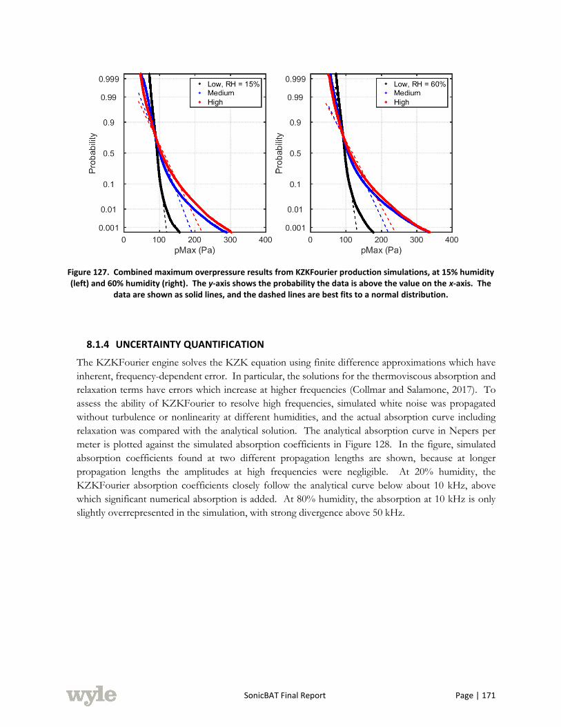
SonicBAT Final Report Page | 171
Figure 127. Combined maximum overpressure results from KZKFourier production simulations, at 15% humidity (left) and 60% humidity (right). The y-axis shows the probability the data is above the value on the x-axis. The
data are shown as solid lines, and the dashed lines are best fits to a normal distribution.
8.1.4 UNCERTAINTY QUANTIFICATION
The KZKFourier engine solves the KZK equation using finite difference approximations which have
inherent, frequency-dependent error. In particular, the solutions for the thermoviscous absorption and
relaxation terms have errors which increase at higher frequencies (Collmar and Salamone, 2017). To
assess the ability of KZKFourier to resolve high frequencies, simulated white noise was propagated
without turbulence or nonlinearity at different humidities, and the actual absorption curve including
relaxation was compared with the analytical solution. The analytical absorption curve in Nepers per
meter is plotted against the simulated absorption coefficients in Figure 128. In the figure, simulated
absorption coefficients found at two different propagation lengths are shown, because at longer
propagation lengths the amplitudes at high frequencies were negligible. At 20% humidity, the
KZKFourier absorption coefficients closely follow the analytical curve below about 10 kHz, above
which significant numerical absorption is added. At 80% humidity, the absorption at 10 kHz is only
slightly overrepresented in the simulation, with strong divergence above 50 kHz.

SonicBAT Final Report Page | 172
Figure 128. Simulated absorption curve in KZKFourier (blue dots, red circles) and the analytical solution (black line) at 20% and 80% humidity.
Even with a 200 kHz sampling rate, simulated frequencies above 10 kHz are not well represented by
KZKFourier at some humidities. Because of this, a 10 kHz low pass cut-off frequency was selected for
use with the turbulence FIR filters (see the algorithm description in Section 3.5.2).
The FIR filter creation process also has some inherent error because the filters produced are
approximate and are limited in length or number of filter coefficients. The filters are designed to closely
approximate the turbulized waveform when convolved with the clean waveform used to create them,
so this error can be assessed by performing the convolution and comparing the approximation with the
turbulized signature (e.g. Figure 16). The average relative error in terms of several metrics are shown in
Table 32, where the average is performed across the 96 production simulation conditions. The metric
standard deviations are approximated by subtracting results from the –std and +std filters and dividing
by two. Relative errors in standard deviation are with respect to the simulated standard deviation value.
In general, the standard deviation errors are within 5%, but are larger than the mean errors which are
within 1%. The filters for frequency-based metrics such as PL and ISBAP perform better than the
filters for the maximum overpressure. Table 32 averages across the 96 conditions, but in general the
approximation error increases for conditions with higher propagation distance.
The small mean error values in Table 32 are generally indicative of the validity of the FIR filter approach
for the production run simulations. These errors are in reference to convolution of the filters with N-
waves. The filters are used with shaped signatures in Section 9.0, including a preliminary validation of
the ability of the filters to accurately represent turbulence effects on shaped signatures.
Table 32. Inherent relative errors in metric approximations using turbulence FIR filters from KZKFourier production simulations.
PL (dB) ISBAP (dB)
pMax (Pa)
SELa (dB)
SELb (dB)
SELc (dB)
SELe (dB)
𝝈 error (rel. %) 3.08 3.46 4.54 3.40 2.22 3.04 3.57
Mean error (rel. %) 0.18 0.14 0.82 0.22 0.14 0.08 0.21
SonicBAT Final Report Page | 173
8.2 STATISTICAL ANALYSIS AND UNCERTAINTY QUANTIFICATION OF THE CLASSICAL SONIC BOOM-TURBULENCE RESEARCH SOFTWARE CODE
Before reading about turbulence trends for this Classical method, understand that TURBO analysis
results were improving rapidly at the end of the program and are likely improve further with more
development and experience with the code. Testing of the methodology continues to yield further
refinements to its efficiency and accuracy.
Modified linear theory methods predict sonic boom refraction through an atmosphere with winds
parallel to the ground (X and Y directions) with altitude (Z) variations and depending on temperature
with altitude (Z) variations. Burgers equation was added for atmospheric absorption rounding of shock
discontinuities depending on humidity with altitude (Z) variations. The rounding from absorption
calculations results in shock rise times of a few milliseconds, which matches the shortest rise times
measured under calm atmospheric conditions. But rise times under calm atmospheric conditions can
be up to 3 times longer and rise times over 10 times longer are found under turbulent conditions. These
longer rise times and other fine structure (Section 1.0, Figure 3) distortions were determined to be caused
by propagation through atmospheric turbulence. The purpose of the Classical model is to predict
turbulence effects on levels particularly for quiet shaped sonic booms. If trends can be accurately
predicted, the fast speed of the method makes it usable in an optimization framework, possibly to
quickly evaluate different shaped boom aircraft designs under turbulent conditions.
The Classic turbulence methodology builds upon the modified-linear theory used for calm atmosphere
sonic boom prediction. Section 4.0 describes that the TURBO code re-propagates the sonic boom
through (generally 300 to 6,000 feet above ground level but can be up to 18,000 feet in extremely dry
climates) the atmospheric boundary layer (ABL), with random turbulence superimposed upon the mean
temperature and winds. Four phenomena are involved in sonic boom propagation: refraction, non-
linear aging, absorption and diffraction. The first three are employed in Burgers propagation, i.e.
PCburg and sBOOM. Diffraction became necessary for focused sonic boom prediction. Turbulent
distortions result in part from post-focus scattering and propagation. Diffraction modeling is part of
the numerical method of Sections 3.0, 7.1 and 8.1. Results from that method can be used as an
additional benchmark for this code.
8.2.1 FLIGHT TEST COMPARISONS
In Section 7.2, the Classic turbulence code was validated first by individual execution steps and then in
comparison with flight test measurements, based on the magnitude of mean level and level standard
deviation. Figure 129 shows first (by legend order) a black line of the analysis preceding the addition of
turbulence to analyses. The TURBO prediction mean is blue with an upper and lower dotted boundary
in blue located 2 standard deviations from the prediction mean. Red circles mark the flight test
measurements along with their upper and lower dotted boundary located 2 standard deviations from
their measured mean levels. Clearly the measurement fits neatly inside, which is good; but does seem
to indicate that the TURBO modeling parameters may be over-predicting the variation range. The
prediction variation seems to over shoot more in the 30 to 50 range of passes, which may provide a clue
to reducing the difference. A good starting point for this modeling. Parameter testing to date has
generally indicated that smaller time steps, more turbulent modes, etc. improve the simulation accuracy.
Unfortunately, they also multiply the hours already required to run the simulation (121 runs, of 100 or

SonicBAT Final Report Page | 174
more signatures, of 10K to 100K ray propagations for each flight database parameter variation). In
addition, some execution streamlining is likely to be able to improve speed and help all other testing.
Figure 129. AFRC flight test data plus two standard deviations fit within the prediction.
Like with AFRC, the KSC predictions and measurements match well, as shown in Figure 130, and KSC
analysis has less over-prediction of the variation range. Since the secondary array was only 3 degrees
lower in Phi (ray roll angle), its measurements are also shown (primary is red circles, secondary is red
squares), and there are red dotted measurement standard deviations for both arrays which indicate no
clear difference between the nearby measurements. Some other features of note are a spike on KSC
pass #6 (flight 203 pass 1) where PCBoom is predicting a 4 psf focused sonic boom. However, the
carpet varies strongly over short distances for this pass, so small variations in the mean atmosphere
along the propagation path versus the weather balloon data can result in completely missing the focus.
For example, changing the trajectory time source by just a second will eliminate it at the measurement
location. Also, the very quiet data measured at pass 28 was sometimes predicted by PCBoom at a
particular trajectory second (or by a change in the PCBoom output interpolation scheme used by
TURBO). At KSC the margin between the cutoff Mach and the flight Mach is often diminished by
headwinds and high flight and ground temperature. In combination with off-track Phis, the effect of
any trajectory accelerations are relatively multiplied by 2 to 4 times. So we may need to look at
predictions around the vicinity of ground measurements to determine if a match is likely. And it
demonstrates that all these other parameters interact with turbulence effects. This classical method can
and does seem to be at least partially predicting such interactions.

SonicBAT Final Report Page | 175
Figure 130. KSC flight test data plus two standard deviations fit within the prediction.
8.2.2 PARAMETRIC VARIATIONS
8.2.2.1 MODELING PARAMETRIC VARIATIONS
Many modeling resolution parametric variations were run during the development of TURBO to
determine the best values for predictions. Since similar codes and parameters have not been disclosed
in literature publications, the choice of parameter variations was often trial and error. Some guidance
was applied from only slightly similar numerical methods, but was helpful or at least reaffirming in
several cases. The main parameters studied were: number, length range and strength distribution of
random turbulent modes; number of rays and their separation, propagation step size, signature spacing
when running multiple signatures at the same time and paraboloid size. As fixes, changes and
enhancements were applied to the code, best values have shifted and parameters have been removed or
added. Many low resolution trials produced poor and misleading results that were eventually discovered
to be corrected by running at higher resolutions and longer execution times. Recent code changes and
rapid output improvements suggest that modeling parameter rechecks are advisable.
Code results improved greatly for measurement comparisons and turbulence parameter trends. Initial
results were discouraging in comparison with the Numerical Model results. Improved results emerged
during the last couple months of SonicBAT, so assessments changed rapidly. With additional
refinement, the Classical Model may be able to provide useful turbulent prediction trends and signature
assessments in minutes (similar to Burgers methodology). Such rapid capabilities support design
assessment, optimization and refinement during steady, Mach cutoff, accelerating and maneuvering
flight.
SonicBAT Final Report Page | 176
For method refinement, many parameter values that produce better accuracy also increase execution
time, so suitable trade-offs had to be determined. Long execution times have been a constant
impediment to development, so further optimization of the code remains a high priority along with
continued testing for accuracy and robustness.
8.2.2.2 PARAMETRIC VARIATIONS OF TURBULENCE FOR F-18 N-WAVES
For this trend analysis, three turbulence strengths, two humidity profiles and 5 ABL heights were run
to investigate the current status of the code predicted trend results based on turbulence. Turbulence is
broken into three levels, low, medium and high, and 2 relative humidity (RH) levels, High and low.
High humidity is represented by the ANSI S1.26 humidity definition, which is 60% at sea level and 80%
at 22,000 feet. While the S1.26 distribution is not 100% RH, level changes little until RH becomes very
low, so humidity levels from 40% to 100% tend to be within 0.2 PLdB of the S1.26 distribution level.
The dry RH was chosen at 15% for this study. An RH of 15% is quieter by an average of 3 PLdB versus
the S1.26 distribution. (In Section 9.0, shaped low boom signatures are found to have more sensitivity
to humidity, averaging 5 PLdB difference between 15% and S1.26 humidity.) Level differences from
humidity become larger at extremely dry RH levels, but it is difficult to find humidity levels throughout
a dry ABL of lower than 10% (found once during 2 weeks of testing over Edwards Dry Lake with 1-3
balloon launches per day, and at a much higher temperature than standard day so the absolute humidity
was higher.
Humidity also has a strong effect on turbulent temperature variations (𝐶𝑇2) and ABL height, so some
same values and some different values are used at the two different RH levels. Dry air heats more easily,
so 𝐶𝑇2 variations averaged about 3 times stronger at AFRC than KSC, but 𝐶𝑣
2 variations were similar.
Keeping the 3:1 AFRC to KSC 𝐶𝑇2 ratio in mind, the rest is discussed in terms of AFRC. For the low
turbulence values, gusts can be present when the sun is down making 𝐶𝑇2 values zero, so zero 𝐶𝑇
2 is used
with the lowest turbulence level of 0.05 𝐶𝑣2. The highest turbulence approached 0.10 𝐶𝑇
2 and 0.25 𝐶𝑣2
(typically 2-5pm in daylight time), so these were used for high turbulence. Medium turbulence at AFRC
was chosen as 0.06/0.10, which was a common pair of values around mid-morning. All turbulence
values are shown in Table 33 below.
ABL heights at KSC remained below 3,000 feet with partial cloud cover and 100% RH every night
during August 2017. Short rain storms sometimes occurred around 2pm, and generally reduce
turbulence thereafter. The weather at AFRC in July 2016 was sunny with desert dry relative humidity
averaging 10-30% RH and ground temps in the mid-100 degrees F at the peak of the day. ABL Heights
over 14,000 feet were measured and local heights reach up to 18,000 feet under the most extreme
conditions; hence, different, overlapping ABL heights were chosen for the two RH levels, as shown in
the Table 33 of turbulence strengths (3), humidity levels (2) and a final column of ABL Heights (7), for
a total of 42 turbulent prediction conditions and 2 baseline conditions without turbulence.
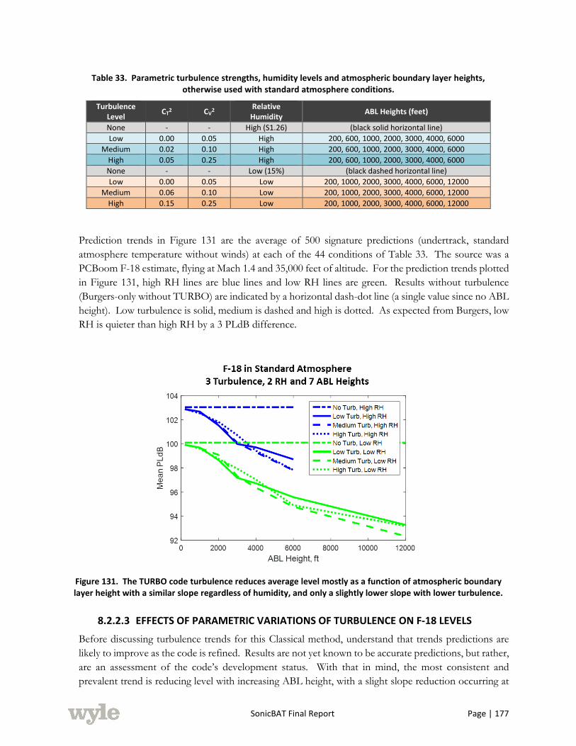
SonicBAT Final Report Page | 177
Table 33. Parametric turbulence strengths, humidity levels and atmospheric boundary layer heights, otherwise used with standard atmosphere conditions.
Turbulence Level
CT2 CV
2 Relative
Humidity ABL Heights (feet)
None - - High (S1.26) (black solid horizontal line)
Low 0.00 0.05 High 200, 600, 1000, 2000, 3000, 4000, 6000
Medium 0.02 0.10 High 200, 600, 1000, 2000, 3000, 4000, 6000
High 0.05 0.25 High 200, 600, 1000, 2000, 3000, 4000, 6000
None - - Low (15%) (black dashed horizontal line)
Low 0.00 0.05 Low 200, 1000, 2000, 3000, 4000, 6000, 12000
Medium 0.06 0.10 Low 200, 1000, 2000, 3000, 4000, 6000, 12000
High 0.15 0.25 Low 200, 1000, 2000, 3000, 4000, 6000, 12000
Prediction trends in Figure 131 are the average of 500 signature predictions (undertrack, standard
atmosphere temperature without winds) at each of the 44 conditions of Table 33. The source was a
PCBoom F-18 estimate, flying at Mach 1.4 and 35,000 feet of altitude. For the prediction trends plotted
in Figure 131, high RH lines are blue lines and low RH lines are green. Results without turbulence
(Burgers-only without TURBO) are indicated by a horizontal dash-dot line (a single value since no ABL
height). Low turbulence is solid, medium is dashed and high is dotted. As expected from Burgers, low
RH is quieter than high RH by a 3 PLdB difference.
Figure 131. The TURBO code turbulence reduces average level mostly as a function of atmospheric boundary layer height with a similar slope regardless of humidity, and only a slightly lower slope with lower turbulence.
8.2.2.3 EFFECTS OF PARAMETRIC VARIATIONS OF TURBULENCE ON F-18 LEVELS
Before discussing turbulence trends for this Classical method, understand that trends predictions are
likely to improve as the code is refined. Results are not yet known to be accurate predictions, but rather,
are an assessment of the code’s development status. With that in mind, the most consistent and
prevalent trend is reducing level with increasing ABL height, with a slight slope reduction occurring at
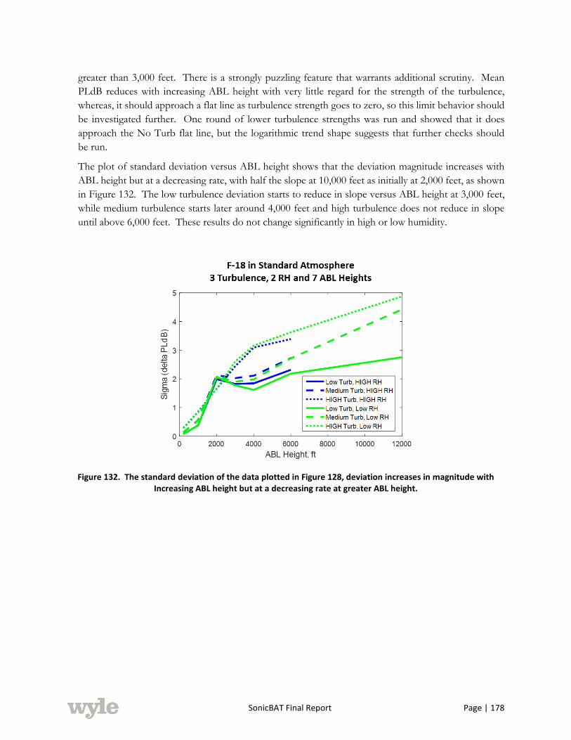
SonicBAT Final Report Page | 178
greater than 3,000 feet. There is a strongly puzzling feature that warrants additional scrutiny. Mean
PLdB reduces with increasing ABL height with very little regard for the strength of the turbulence,
whereas, it should approach a flat line as turbulence strength goes to zero, so this limit behavior should
be investigated further. One round of lower turbulence strengths was run and showed that it does
approach the No Turb flat line, but the logarithmic trend shape suggests that further checks should
be run.
The plot of standard deviation versus ABL height shows that the deviation magnitude increases with
ABL height but at a decreasing rate, with half the slope at 10,000 feet as initially at 2,000 feet, as shown
in Figure 132. The low turbulence deviation starts to reduce in slope versus ABL height at 3,000 feet,
while medium turbulence starts later around 4,000 feet and high turbulence does not reduce in slope
until above 6,000 feet. These results do not change significantly in high or low humidity.
Figure 132. The standard deviation of the data plotted in Figure 128, deviation increases in magnitude with Increasing ABL height but at a decreasing rate at greater ABL height.
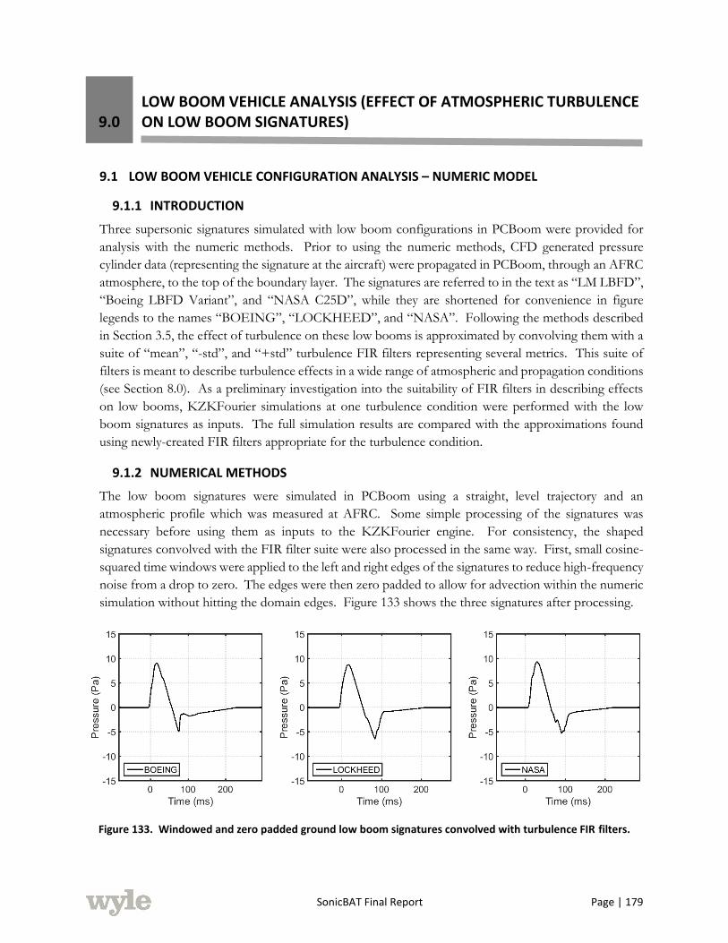
SonicBAT Final Report Page | 179
9.0
LOW BOOM VEHICLE ANALYSIS (EFFECT OF ATMOSPHERIC TURBULENCE ON LOW BOOM SIGNATURES)
9.1 LOW BOOM VEHICLE CONFIGURATION ANALYSIS – NUMERIC MODEL
9.1.1 INTRODUCTION
Three supersonic signatures simulated with low boom configurations in PCBoom were provided for
analysis with the numeric methods. Prior to using the numeric methods, CFD generated pressure
cylinder data (representing the signature at the aircraft) were propagated in PCBoom, through an AFRC
atmosphere, to the top of the boundary layer. The signatures are referred to in the text as “LM LBFD”,
“Boeing LBFD Variant”, and “NASA C25D”, while they are shortened for convenience in figure
legends to the names “BOEING”, “LOCKHEED”, and “NASA”. Following the methods described
in Section 3.5, the effect of turbulence on these low booms is approximated by convolving them with a
suite of “mean”, “-std”, and “+std” turbulence FIR filters representing several metrics. This suite of
filters is meant to describe turbulence effects in a wide range of atmospheric and propagation conditions
(see Section 8.0). As a preliminary investigation into the suitability of FIR filters in describing effects
on low booms, KZKFourier simulations at one turbulence condition were performed with the low
boom signatures as inputs. The full simulation results are compared with the approximations found
using newly-created FIR filters appropriate for the turbulence condition.
9.1.2 NUMERICAL METHODS
The low boom signatures were simulated in PCBoom using a straight, level trajectory and an
atmospheric profile which was measured at AFRC. Some simple processing of the signatures was
necessary before using them as inputs to the KZKFourier engine. For consistency, the shaped
signatures convolved with the FIR filter suite were also processed in the same way. First, small cosine-
squared time windows were applied to the left and right edges of the signatures to reduce high-frequency
noise from a drop to zero. The edges were then zero padded to allow for advection within the numeric
simulation without hitting the domain edges. Figure 133 shows the three signatures after processing.
Figure 133. Windowed and zero padded ground low boom signatures convolved with turbulence FIR filters.
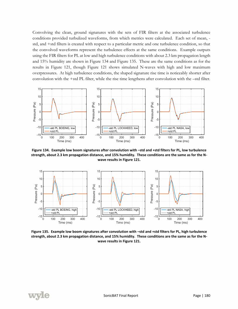
SonicBAT Final Report Page | 180
Convolving the clean, ground signatures with the sets of FIR filters at the associated turbulence
conditions provided turbulized waveforms, from which metrics were calculated. Each set of mean, -
std, and +std filters is created with respect to a particular metric and one turbulence condition, so that
the convolved waveforms represent the turbulence effects at the same conditions. Example outputs
using the FIR filters for PL at low and high turbulence conditions with about 2.3 km propagation length
and 15% humidity are shown in Figure 134 and Figure 135. These are the same conditions as for the
results in Figure 121, though Figure 121 shows simulated N-waves with high and low maximum
overpressures. At high turbulence conditions, the shaped signature rise time is noticeably shorter after
convolution with the +std PL filter, while the rise time lengthens after convolution with the –std filter.
Figure 134. Example low boom signatures after convolution with –std and +std filters for PL, low turbulence strength, about 2.3 km propagation distance, and 15% humidity. These conditions are the same as for the N-
wave results in Figure 121.
Figure 135. Example low boom signatures after convolution with –std and +std filters for PL, high turbulence strength, about 2.3 km propagation distance, and 15% humidity. These conditions are the same as for the N-
wave results in Figure 121.
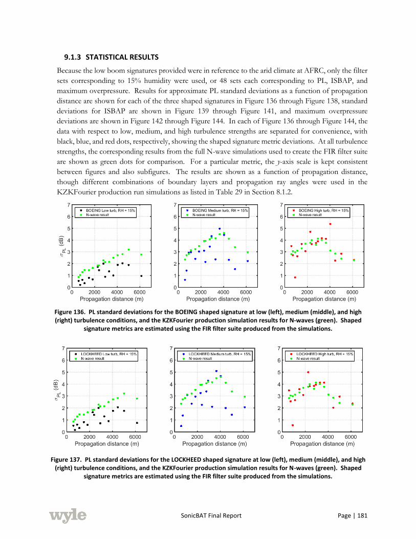
SonicBAT Final Report Page | 181
9.1.3 STATISTICAL RESULTS
Because the low boom signatures provided were in reference to the arid climate at AFRC, only the filter
sets corresponding to 15% humidity were used, or 48 sets each corresponding to PL, ISBAP, and
maximum overpressure. Results for approximate PL standard deviations as a function of propagation
distance are shown for each of the three shaped signatures in Figure 136 through Figure 138, standard
deviations for ISBAP are shown in Figure 139 through Figure 141, and maximum overpressure
deviations are shown in Figure 142 through Figure 144. In each of Figure 136 through Figure 144, the
data with respect to low, medium, and high turbulence strengths are separated for convenience, with
black, blue, and red dots, respectively, showing the shaped signature metric deviations. At all turbulence
strengths, the corresponding results from the full N-wave simulations used to create the FIR filter suite
are shown as green dots for comparison. For a particular metric, the y-axis scale is kept consistent
between figures and also subfigures. The results are shown as a function of propagation distance,
though different combinations of boundary layers and propagation ray angles were used in the
KZKFourier production run simulations as listed in Table 29 in Section 8.1.2.
Figure 136. PL standard deviations for the BOEING shaped signature at low (left), medium (middle), and high (right) turbulence conditions, and the KZKFourier production simulation results for N-waves (green). Shaped
signature metrics are estimated using the FIR filter suite produced from the simulations.
Figure 137. PL standard deviations for the LOCKHEED shaped signature at low (left), medium (middle), and high (right) turbulence conditions, and the KZKFourier production simulation results for N-waves (green). Shaped
signature metrics are estimated using the FIR filter suite produced from the simulations.
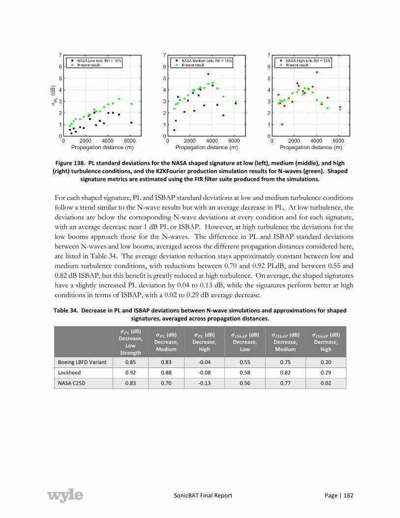
SonicBAT Final Report Page | 182
Figure 138. PL standard deviations for the NASA shaped signature at low (left), medium (middle), and high (right) turbulence conditions, and the KZKFourier production simulation results for N-waves (green). Shaped
signature metrics are estimated using the FIR filter suite produced from the simulations.
For each shaped signature, PL and ISBAP standard deviations at low and medium turbulence conditions
follow a trend similar to the N-wave results but with an average decrease in PL. At low turbulence, the
deviations are below the corresponding N-wave deviations at every condition and for each signature,
with an average decrease near 1 dB PL or ISBAP. However, at high turbulence the deviations for the
low booms approach those for the N-waves. The difference in PL and ISBAP standard deviations
between N-waves and low booms, averaged across the different propagation distances considered here,
are listed in Table 34. The average deviation reduction stays approximately constant between low and
medium turbulence conditions, with reductions between 0.70 and 0.92 PLdB, and between 0.55 and
0.82 dB ISBAP, but this benefit is greatly reduced at high turbulence. On average, the shaped signatures
have a slightly increased PL deviation by 0.04 to 0.13 dB, while the signatures perform better at high
conditions in terms of ISBAP, with a 0.02 to 0.29 dB average decrease.
Table 34. Decrease in PL and ISBAP deviations between N-wave simulations and approximations for shaped signatures, averaged across propagation distances.
𝝈𝑷𝑳 (dB) Decrease,
Low Strength
𝝈𝑷𝑳 (dB) Decrease, Medium
𝝈𝑷𝑳 (dB) Decrease,
High
𝝈𝑰𝑺𝒃𝑨𝑷 (dB) Decrease,
Low
𝝈𝑰𝑺𝒃𝑨𝑷 (dB) Decrease, Medium
𝝈𝑰𝑺𝒃𝑨𝑷 (dB) Decrease,
High
Boeing LBFD Variant 0.85 0.83 -0.04 0.55 0.75 0.20
Lockheed 0.92 0.88 -0.08 0.58 0.82 0.29
NASA C25D 0.83 0.70 -0.13 0.56 0.77 0.02
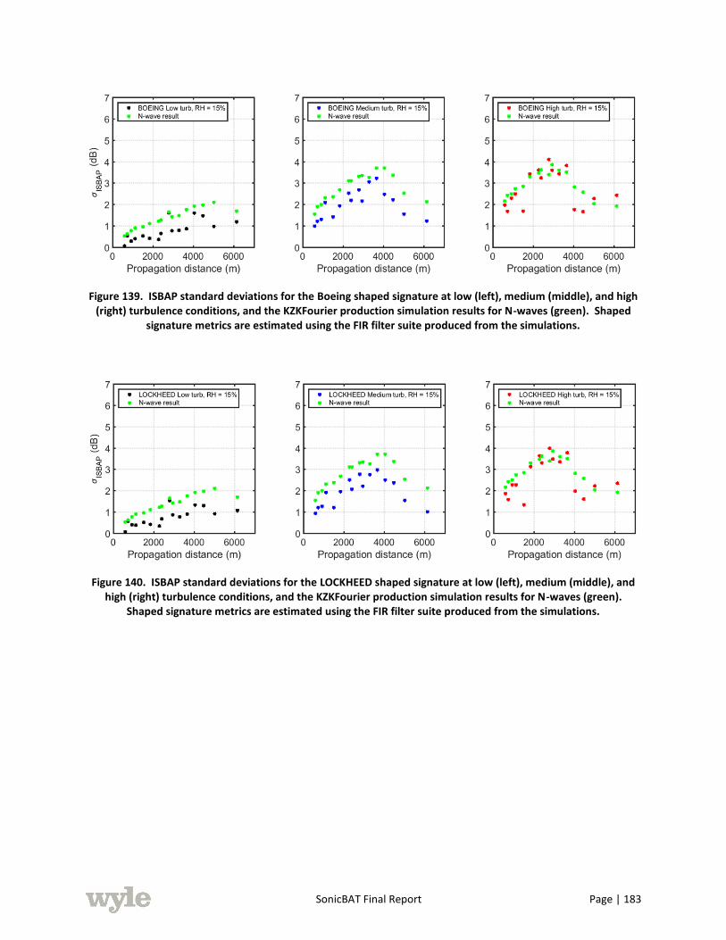
SonicBAT Final Report Page | 183
Figure 139. ISBAP standard deviations for the Boeing shaped signature at low (left), medium (middle), and high (right) turbulence conditions, and the KZKFourier production simulation results for N-waves (green). Shaped
signature metrics are estimated using the FIR filter suite produced from the simulations.
Figure 140. ISBAP standard deviations for the LOCKHEED shaped signature at low (left), medium (middle), and high (right) turbulence conditions, and the KZKFourier production simulation results for N-waves (green).
Shaped signature metrics are estimated using the FIR filter suite produced from the simulations.
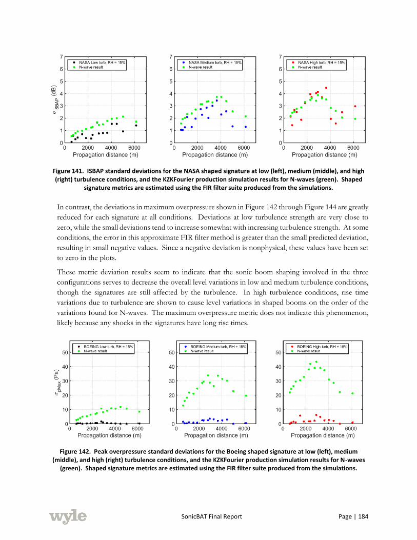
SonicBAT Final Report Page | 184
Figure 141. ISBAP standard deviations for the NASA shaped signature at low (left), medium (middle), and high (right) turbulence conditions, and the KZKFourier production simulation results for N-waves (green). Shaped
signature metrics are estimated using the FIR filter suite produced from the simulations.
In contrast, the deviations in maximum overpressure shown in Figure 142 through Figure 144 are greatly
reduced for each signature at all conditions. Deviations at low turbulence strength are very close to
zero, while the small deviations tend to increase somewhat with increasing turbulence strength. At some
conditions, the error in this approximate FIR filter method is greater than the small predicted deviation,
resulting in small negative values. Since a negative deviation is nonphysical, these values have been set
to zero in the plots.
These metric deviation results seem to indicate that the sonic boom shaping involved in the three
configurations serves to decrease the overall level variations in low and medium turbulence conditions,
though the signatures are still affected by the turbulence. In high turbulence conditions, rise time
variations due to turbulence are shown to cause level variations in shaped booms on the order of the
variations found for N-waves. The maximum overpressure metric does not indicate this phenomenon,
likely because any shocks in the signatures have long rise times.
Figure 142. Peak overpressure standard deviations for the Boeing shaped signature at low (left), medium (middle), and high (right) turbulence conditions, and the KZKFourier production simulation results for N-waves
(green). Shaped signature metrics are estimated using the FIR filter suite produced from the simulations.

SonicBAT Final Report Page | 185
Figure 143. Peak overpressure standard deviations for the LOCKHEED shaped signature at low (left), medium (middle), and high (right) turbulence conditions, and the KZKFourier production simulation results for N-waves
(green). Shaped signature metrics are estimated using the FIR filter suite produced from the simulations.
Figure 144. Peak overpressure standard deviations for the NASA shaped signature at low (left), medium (middle), and high (right) turbulence conditions, and the KZKFourier production simulation results for N-waves
(green). Shaped signature metrics are estimated using the FIR filter suite produced from the simulations.
The approximate metric means as a function of propagation distance are shown in Figure 145 through
Figure 147, where each figure shows results for one shaped signature and low, medium, and high
turbulence conditions are superimposed. The metric value of the ground signature used in the FIR filter
convolutions is also shown as a flat green line. For ease of comparison, the scales of the y-axes have
been modified to match those for the N-wave metric means in Figure 123 and Figure 124 in Section
8.1.3. In general, the mean PL and ISBAP tend to decrease somewhat due to propagation through
turbulence at medium and high conditions, though this decrease is insignificant at low conditions. The
greatest reductions generally occur for high turbulence; the PL is reduced at most by about 3-4 dB, and
the ISBAP by about 3 dB. The mean maximum overpressure tends to stay nearly constant at all
turbulence strengths and propagation distances, with a slight increase for most conditions.

SonicBAT Final Report Page | 186
Figure 145. Mean metric values for the Boeing shaped signature at low (black), medium (blue), and high (red) turbulence conditions. Shaped signature metrics are estimated using the FIR filter suite produced from
the simulations.
Figure 146. Mean metric values for the LOCKHEED shaped signature at low (black), medium (blue), and high (red) turbulence conditions. Shaped signature metrics are estimated using the FIR filter suite produced from
the simulations.

SonicBAT Final Report Page | 187
Figure 147. Mean metric values for the NASA shaped signature at low (black), medium (blue), and high (red) turbulence conditions. Shaped signature metrics are estimated using the FIR filter suite produced from
the simulations.
In Figure 136 through Figure 144, the standard deviation data trends for the shaped signatures with
respect to propagation distance do not collapse as cleanly as for the N-wave simulations in Section 8.0.
The additional scatter may exist because the propagation for these conditions was at different ray angles
through the boundary layer. At least some scatter is expected because of the approximations inherent
in the FIR filter process and its application as discussed in Section 8.1.4. The validity of the FIR filter
application is preliminarily investigated in the proceeding Section.
9.1.4 COMPARISON WITH FULL NUMERIC SIMULATION
Several full KZKFourier simulations were performed to give an analytical benchmark for the effect of
turbulence on low boom signatures, against which the approximations found using turbulence FIR
filters are compared. The numeric simulations were successfully performed with shaped signatures,
showing the effect of turbulence on the signatures. The FIR filters were created using outputs from
this simulation. For input to KZKFourier, the three shaped signatures were output by PCBoom
simulations at a boundary layer height of about 1 km. The signatures were then processed as described
in Section 9.1.2, with an additional step of upsampling to a 200 kHz sampling rate. This rate was chosen
to best resolve any possible shocks due to energy focusing, and was the same rate used with the N-wave
simulations in Section 8.0. The signatures as input into KZKFourier are shown in Figure 148, which
show minimal change from the signatures at the ground used in Section 9.1.2. The other configuration
parameters for the simulation were chosen from one of the validation simulations in Section 7.0,
corresponding to the same pass with the atmospheric profile used in PCBoom to create the shaped
signatures. The flight altitudes in PCBoom were chosen to be on design and differed between the three
signatures, leading to somewhat different ray angles through the boundary layer. The parameters are
listed in Table 35, where the elevation angles listed are in the order: Boeing LBFD Variant,
LOCKHEED, NASA C25D.

SonicBAT Final Report Page | 188
Table 35. Parameter values used with the KZKFourier filter validation simulations.
Parameter Value(s)
𝒖∗ 0.66 m/s
𝒘∗ 1.76 m/s
𝑻∗ -0.25 K
𝒁𝒊 1027 m
Elevation Angles (B) 32.9°, (LM) 29.6°, (N) 39.9°
RH 9.7 %
𝑻𝟎 35.8 °C
𝒑𝟎 0.924 atm
Signature Length 250 – 1230 ms
Number of Realizations 27 – 35
𝒚𝐦𝐚𝐱 200 – 350 m
𝚫𝒚 (Transverse) 0.5 m
𝚫𝒛 (Propagation) 0.05 m
Sampling Rate 200 kHz
Figure 148. Processed shaped signatures at boundary layer height which were input into KZKFourier. The signatures show minimal change compared to those at the ground in Figure 133.
The simulations were performed using the shaped signatures and also the N-wave from the same
validation simulation as inputs to best compare the turbulence effects on the different booms. The N-
wave simulations were run at the same elevation angles as with the three shaped signatures. Additionally,
simulations without turbulence were performed with the same other parameters. The PL, ISBAP, and
maximum overpressure from these clean simulations are designated the “nominal” metric values for
these signatures at the ground. The clean simulations were necessary in order to compare the effect of
turbulence on N-waves and shaped signatures in terms of metrics with respect to the nominal.
Figure 149 through Figure 151 show the resultant metric probabilities with respect to the nominal for
both shaped signatures and N-waves at the ground. As in other sections, the PL and ISBAP were
calculated after applying a 2500-point Hanning window to the right edge of the simulated waveforms.
The dB value for the nominal PL and ISBAP are subtracted from the calculated metrics, while the
maximum overpressures are divided by the nominal maximum overpressure. Dashed lines indicate the
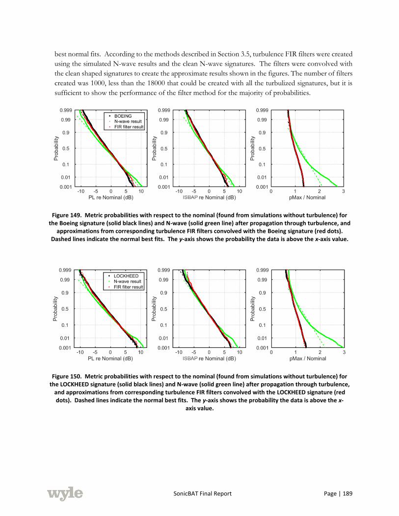
SonicBAT Final Report Page | 189
best normal fits. According to the methods described in Section 3.5, turbulence FIR filters were created
using the simulated N-wave results and the clean N-wave signatures. The filters were convolved with
the clean shaped signatures to create the approximate results shown in the figures. The number of filters
created was 1000, less than the 18000 that could be created with all the turbulized signatures, but it is
sufficient to show the performance of the filter method for the majority of probabilities.
Figure 149. Metric probabilities with respect to the nominal (found from simulations without turbulence) for the Boeing signature (solid black lines) and N-wave (solid green line) after propagation through turbulence, and
approximations from corresponding turbulence FIR filters convolved with the Boeing signature (red dots). Dashed lines indicate the normal best fits. The y-axis shows the probability the data is above the x-axis value.
Figure 150. Metric probabilities with respect to the nominal (found from simulations without turbulence) for the LOCKHEED signature (solid black lines) and N-wave (solid green line) after propagation through turbulence,
and approximations from corresponding turbulence FIR filters convolved with the LOCKHEED signature (red dots). Dashed lines indicate the normal best fits. The y-axis shows the probability the data is above the x-
axis value.

SonicBAT Final Report Page | 190
Figure 151. Metric probabilities with respect to the nominal (found from simulations without turbulence) for the NASA signature (solid black lines) and N-wave (solid green line) after propagation through turbulence, and
approximations from corresponding turbulence FIR filters convolved with the NASA signature (red dots). Dashed lines indicate the normal best fits. The y-axis shows the probability the data is above the x-axis value.
For all three signatures, the effect of turbulence on the PL and ISBAP metrics are similar to the
turbulized N-wave results, though the black lines have slightly higher slopes indicating slightly smaller
standard deviations. The metrics closely fall onto the dashed lines indicating a good fit to a normal
distribution. For all the signatures, the median PL and ISBAP falls below the nominal by about 2 dB,
showing the persistence of the shaped boom level reduction through turbulence as predicted by
previous tests with shaped aircraft (Morgenstern et al., 2005).
As stated above, the simulation parameters followed those used in one of the validation simulations,
which had turbulence strength approaching the “high” turbulence conditions in the production
simulations described in Section 8.0. The RMS wind turbulence here was 1.55 m/s, while the
corresponding value for the “high” turbulence condition is 1.89 m/s. Thus, the result that the shaped
signature PL and ISBAP distributions are similar to those for the N-waves agrees with the standard
deviation approximations at high turbulence conditions shown in Figure 136 through Figure 141.
Interestingly, the maximum overpressures for the shaped signatures in Figure 149 through Figure 151
do not follow the same trend as the N-wave overpressures. The distributions for the shaped signatures
are fairly normal with a small standard deviation and are generally much lower in magnitude than for
the N-waves, only converging to the N-wave results when heavily rounded at above 95% probabilities.
The median maximum overpressures for the shaped signatures are at or just below the nominal,
indicating that spiked and rounded shaped signatures have approximately the same probability of
occurring. In contrast, the median N-wave overpressure is greater than the nominal, so spiked N-wave
signatures are more likely to occur and have greater relative magnitudes.
In all cases for PL and ISBAP, the metric approximations using the turbulence FIR filters closely follow
the benchmark simulated results for the shaped signatures. Despite only 1000 filters being used, the
agreement is within about 1 dB for probabilities between 5% and 95%, the vast majority of the data.
The FIR filters perform well for all probabilities in predicting the maximum overpressures.
The N-wave results were also used to create mean, -std, and +std filters for the PL, ISBAP, and
maximum overpressure metrics according to the method described in Section 3.5. This method is
designed to give a quick estimation of turbulence effects by calculating metrics using only three
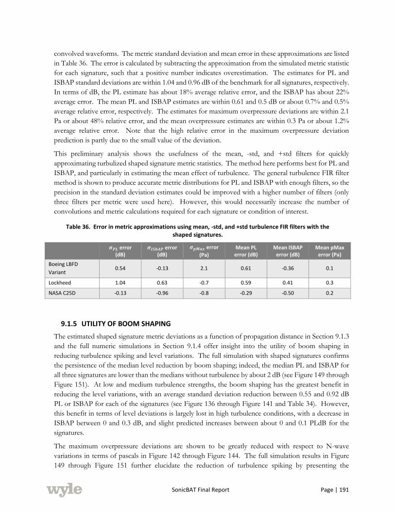
SonicBAT Final Report Page | 191
convolved waveforms. The metric standard deviation and mean error in these approximations are listed
in Table 36. The error is calculated by subtracting the approximation from the simulated metric statistic
for each signature, such that a positive number indicates overestimation. The estimates for PL and
ISBAP standard deviations are within 1.04 and 0.96 dB of the benchmark for all signatures, respectively.
In terms of dB, the PL estimate has about 18% average relative error, and the ISBAP has about 22%
average error. The mean PL and ISBAP estimates are within 0.61 and 0.5 dB or about 0.7% and 0.5%
average relative error, respectively. The estimates for maximum overpressure deviations are within 2.1
Pa or about 48% relative error, and the mean overpressure estimates are within 0.3 Pa or about 1.2%
average relative error. Note that the high relative error in the maximum overpressure deviation
prediction is partly due to the small value of the deviation.
This preliminary analysis shows the usefulness of the mean, -std, and +std filters for quickly
approximating turbulized shaped signature metric statistics. The method here performs best for PL and
ISBAP, and particularly in estimating the mean effect of turbulence. The general turbulence FIR filter
method is shown to produce accurate metric distributions for PL and ISBAP with enough filters, so the
precision in the standard deviation estimates could be improved with a higher number of filters (only
three filters per metric were used here). However, this would necessarily increase the number of
convolutions and metric calculations required for each signature or condition of interest.
Table 36. Error in metric approximations using mean, -std, and +std turbulence FIR filters with the shaped signatures.
𝝈𝑷𝑳 error
(dB) 𝝈𝑰𝑺𝒃𝑨𝑷 error
(dB)
𝝈𝒑𝑴𝒂𝒙 error
(Pa)
Mean PL error (dB)
Mean ISBAP error (dB)
Mean pMax error (Pa)
Boeing LBFD
Variant 0.54 -0.13 2.1 0.61 -0.36 0.1
Lockheed 1.04 0.63 -0.7 0.59 0.41 0.3
NASA C25D -0.13 -0.96 -0.8 -0.29 -0.50 0.2
9.1.5 UTILITY OF BOOM SHAPING
The estimated shaped signature metric deviations as a function of propagation distance in Section 9.1.3
and the full numeric simulations in Section 9.1.4 offer insight into the utility of boom shaping in
reducing turbulence spiking and level variations. The full simulation with shaped signatures confirms
the persistence of the median level reduction by boom shaping; indeed, the median PL and ISBAP for
all three signatures are lower than the medians without turbulence by about 2 dB (see Figure 149 through
Figure 151). At low and medium turbulence strengths, the boom shaping has the greatest benefit in
reducing the level variations, with an average standard deviation reduction between 0.55 and 0.92 dB
PL or ISBAP for each of the signatures (see Figure 136 through Figure 141 and Table 34). However,
this benefit in terms of level deviations is largely lost in high turbulence conditions, with a decrease in
ISBAP between 0 and 0.3 dB, and slight predicted increases between about 0 and 0.1 PLdB for the
signatures.
The maximum overpressure deviations are shown to be greatly reduced with respect to N-wave
variations in terms of pascals in Figure 142 through Figure 144. The full simulation results in Figure
149 through Figure 151 further elucidate the reduction of turbulence spiking by presenting the
SonicBAT Final Report Page | 192
maximum overpressure probabilities divided by the nominal without turbulence. With respect to the
nominal overpressure, all three probability curves for the shaped signatures fall to the left of the N-wave
results for nearly all probabilities, meaning that the signatures exhibit less spiking than the N-waves.
The median overpressure for the shaped signatures is at or just below the nominal, indicating that
rounded and spiked shaped signatures occur with approximately equal probability. The N-waves have
a much greater chance of spiking. In addition, the spiked shaped signatures have much lower relative
amplitudes compared with the N-waves. These results indicate that the relatively long rise times in the
shaped signatures once they enter the turbulent boundary layer greatly reduce the signature spiking in
turbulence.
9.2 LOW BOOM VEHICLE ANALYSIS – CLASSICAL MODEL
9.2.1 N-WAVE BOOM SOURCE COMPARISON
The TURBO classical model predictions, shown in the preceding Sections 7.2 and 8.2, were based upon
a PCBoom generated 4-point symmetrical N-wave starting signature. These N-wave analyses are
compared with low boom analyses in this section, so it is important to understand N-wave differences.
PCBoom’s N-wave routine (Carlson, 1978) is scaled to match the volume and lift of a vehicle and has
been validated as accurately matching ground measurements. This simplified signature source is
sufficient for a vehicle signature which becomes an N-wave within a few thousand feet from the vehicle
and remains that shape to the ground. For an N-wave signature only the magnitude of the shocks and
the slope of their rise (a.k.a. rise time), and to a lesser degree the duration, are needed to accurately
determine its non-turbulent spectral characteristics. Predicting non-turbulent N-wave levels can be
done accurately by scaling an N-wave source.
9.2.2 LOW BOOM VEHICLE SIGNATURES
In contrast, the shaped waveforms of a low boom vehicle require hundreds of points for an accurate
starting signature definition. Furthermore, low boom signatures have a different initial shape back near
the vehicle, before steepening from non-linear aging. The initial signature at the vehicle is shaped to
utilize aging during its propagation to evolve into its quietest shape at the ground, based on a backward
propagation theory developed by Seebass and George (1972), and refined and automated in a computer
code by Darden (1979). Shaping sonic boom by their theory is the only practical approach discovered
for reducing level by the 25 to 30 PLdB believed necessary for acceptable flight over land. In TURBO
analyses, signature evolution is affected by turbulence strength, atmospheric boundary layer (ABL)
height and humidity. Parametric results were produced from varying these three parameters with values
used in Section 8.2.2.2 for the F-18’s N-wave signature.
The first SonicBAT low boom test case presented here was contributed by Lockheed Martin (LM) and
is representative of a 94 foot long, highly slender, low boom flight demonstrator (LBFD) vehicle, similar
to the one LM is developing for NASA to gather human response data for quiet shaped sonic booms.
Therefore this signature is designated LM LBFD and its ground overpressure versus time is shown in
Figure 152 with a blue line. The other two low boom signatures contributed by Boeing and NASA have
nearly the same attributes and level, supporting our belief that all three are representative examples of
using shaped boom technology to achieve low boom levels. Boeing called their signature the Boeing
LBFD Variant, the red line in Figure 152. NASA called their signature NASA C25D, the green line in
Figure 152. All three signatures have similar front signatures between 0.35 to 0.37 psf peak overpressure

SonicBAT Final Report Page | 193
and 57 to 62 msec in front duration. The first ~0.11 psf of the front of the LM LBFD and Boeing
LBFD Variant signatures is their rounded front shock strength. Following the 0.11 psf rise, the slope
reduces due to being a combination of isentropic compression and smaller rounded shocks that blend
together. This allows the front signature to be as quiet to our hearing as an N-wave of 0.11 psf peak
overpressure (based on consistent methodology). Shaped signatures are much quieter than N-waves
with the same peak overpressure, for example, the LM LBFD and NASA C25D are equivalent to a 0.11
psf N-wave and average -31 PLdB relative to the F-18 N-wave and the Boeing LBFD Variant signature
is a close -27 PLdB. The Boeing LBFD Variant’s aft signature negative impulse is much weaker than
the other two signatures, but its aft recompression slope (at 120 msec in Figure 152) is much steeper,
indicating it is a single shock. The Boeing LBFD Variant signature’s stronger aft shock and another
secondary shock (at 48-54 msec in Figure 152) result in 4 PLdB more audible frequency levels in the
160-400 Hz range, but actually slightly lower levels at lower, less audible frequencies. So except as
quantified, the similar shaping of these three signatures results in a similar spectral content, a.k.a. similar
levels versus frequency.
Figure 152. The three provided signatures at the ground (Burgers propagation with 1.9 ground reflection) are similar in overpressure, duration (except Boeing aft signature) multi-shock ramp shape and level.
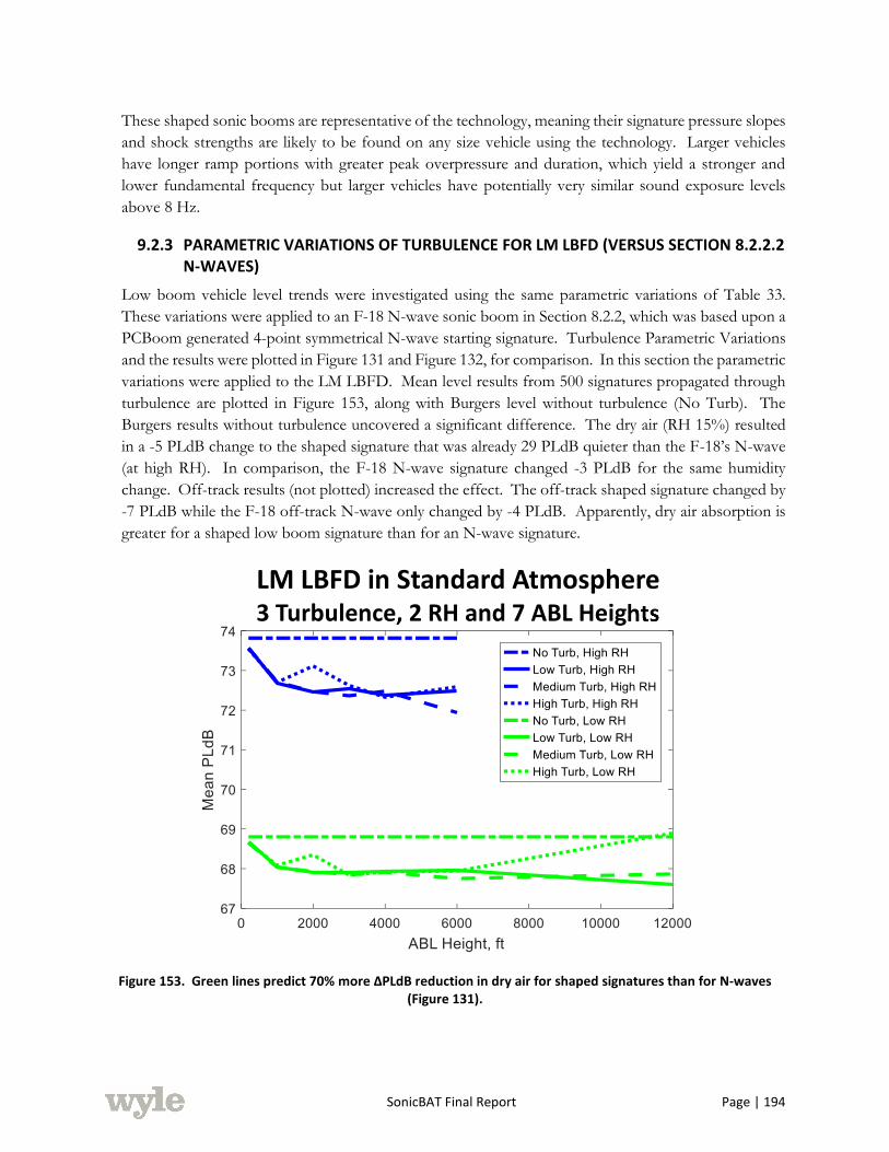
SonicBAT Final Report Page | 194
These shaped sonic booms are representative of the technology, meaning their signature pressure slopes
and shock strengths are likely to be found on any size vehicle using the technology. Larger vehicles
have longer ramp portions with greater peak overpressure and duration, which yield a stronger and
lower fundamental frequency but larger vehicles have potentially very similar sound exposure levels
above 8 Hz.
9.2.3 PARAMETRIC VARIATIONS OF TURBULENCE FOR LM LBFD (VERSUS SECTION 8.2.2.2 N-WAVES)
Low boom vehicle level trends were investigated using the same parametric variations of Table 33.
These variations were applied to an F-18 N-wave sonic boom in Section 8.2.2, which was based upon a
PCBoom generated 4-point symmetrical N-wave starting signature. Turbulence Parametric Variations
and the results were plotted in Figure 131 and Figure 132, for comparison. In this section the parametric
variations were applied to the LM LBFD. Mean level results from 500 signatures propagated through
turbulence are plotted in Figure 153, along with Burgers level without turbulence (No Turb). The
Burgers results without turbulence uncovered a significant difference. The dry air (RH 15%) resulted
in a -5 PLdB change to the shaped signature that was already 29 PLdB quieter than the F-18’s N-wave
(at high RH). In comparison, the F-18 N-wave signature changed -3 PLdB for the same humidity
change. Off-track results (not plotted) increased the effect. The off-track shaped signature changed by
-7 PLdB while the F-18 off-track N-wave only changed by -4 PLdB. Apparently, dry air absorption is
greater for a shaped low boom signature than for an N-wave signature.
Figure 153. Green lines predict 70% more ∆PLdB reduction in dry air for shaped signatures than for N-waves (Figure 131).
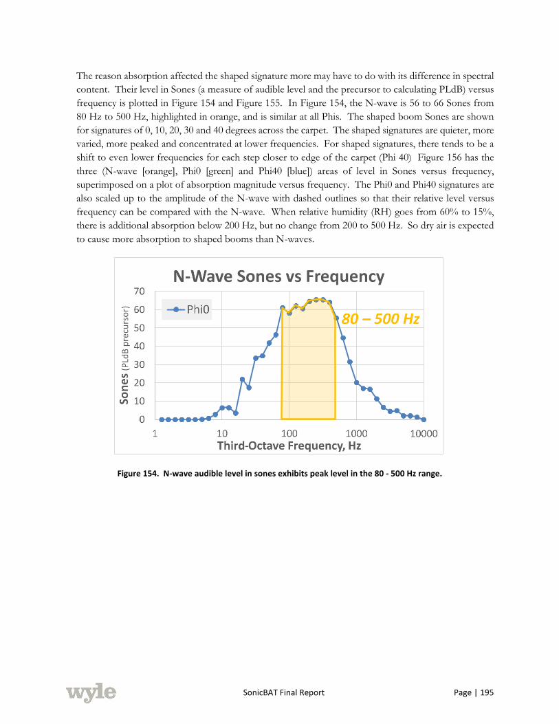
SonicBAT Final Report Page | 195
The reason absorption affected the shaped signature more may have to do with its difference in spectral
content. Their level in Sones (a measure of audible level and the precursor to calculating PLdB) versus
frequency is plotted in Figure 154 and Figure 155. In Figure 154, the N-wave is 56 to 66 Sones from
80 Hz to 500 Hz, highlighted in orange, and is similar at all Phis. The shaped boom Sones are shown
for signatures of 0, 10, 20, 30 and 40 degrees across the carpet. The shaped signatures are quieter, more
varied, more peaked and concentrated at lower frequencies. For shaped signatures, there tends to be a
shift to even lower frequencies for each step closer to edge of the carpet (Phi 40) Figure 156 has the
three (N-wave [orange], Phi0 [green] and Phi40 [blue]) areas of level in Sones versus frequency,
superimposed on a plot of absorption magnitude versus frequency. The Phi0 and Phi40 signatures are
also scaled up to the amplitude of the N-wave with dashed outlines so that their relative level versus
frequency can be compared with the N-wave. When relative humidity (RH) goes from 60% to 15%,
there is additional absorption below 200 Hz, but no change from 200 to 500 Hz. So dry air is expected
to cause more absorption to shaped booms than N-waves.
Figure 154. N-wave audible level in sones exhibits peak level in the 80 - 500 Hz range.
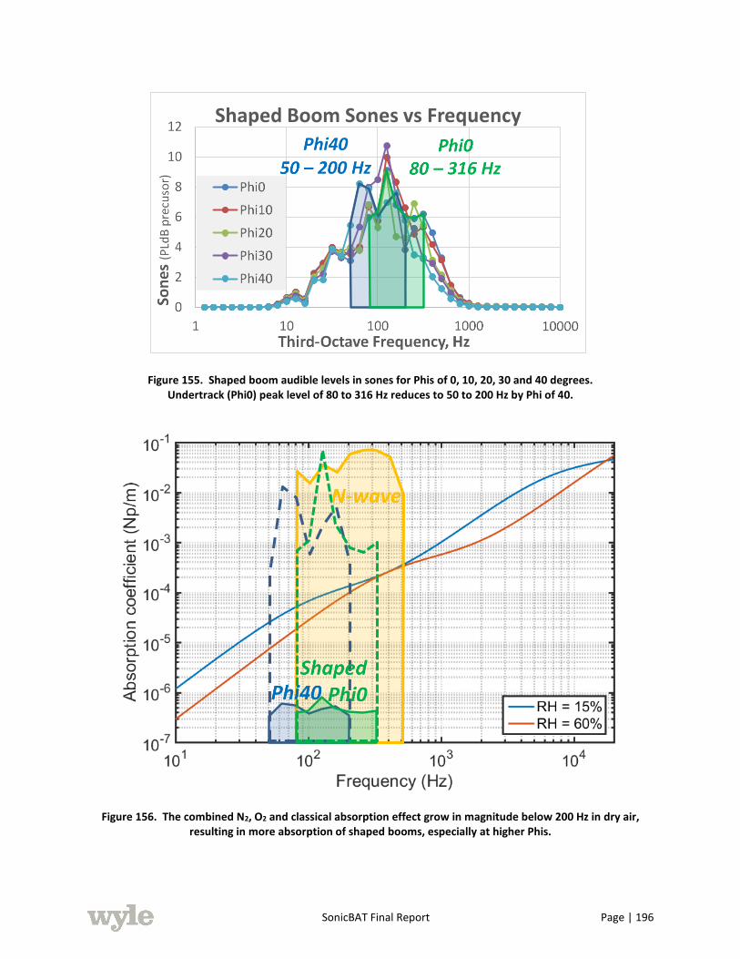
SonicBAT Final Report Page | 196
Figure 155. Shaped boom audible levels in sones for Phis of 0, 10, 20, 30 and 40 degrees. Undertrack (Phi0) peak level of 80 to 316 Hz reduces to 50 to 200 Hz by Phi of 40.
Figure 156. The combined N2, O2 and classical absorption effect grow in magnitude below 200 Hz in dry air, resulting in more absorption of shaped booms, especially at higher Phis.
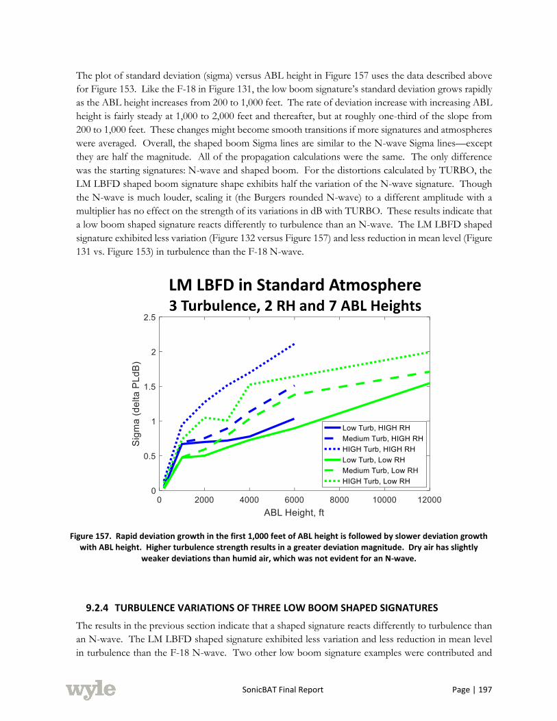
SonicBAT Final Report Page | 197
The plot of standard deviation (sigma) versus ABL height in Figure 157 uses the data described above
for Figure 153. Like the F-18 in Figure 131, the low boom signature’s standard deviation grows rapidly
as the ABL height increases from 200 to 1,000 feet. The rate of deviation increase with increasing ABL
height is fairly steady at 1,000 to 2,000 feet and thereafter, but at roughly one-third of the slope from
200 to 1,000 feet. These changes might become smooth transitions if more signatures and atmospheres
were averaged. Overall, the shaped boom Sigma lines are similar to the N-wave Sigma lines—except
they are half the magnitude. All of the propagation calculations were the same. The only difference
was the starting signatures: N-wave and shaped boom. For the distortions calculated by TURBO, the
LM LBFD shaped boom signature shape exhibits half the variation of the N-wave signature. Though
the N-wave is much louder, scaling it (the Burgers rounded N-wave) to a different amplitude with a
multiplier has no effect on the strength of its variations in dB with TURBO. These results indicate that
a low boom shaped signature reacts differently to turbulence than an N-wave. The LM LBFD shaped
signature exhibited less variation (Figure 132 versus Figure 157) and less reduction in mean level (Figure
131 vs. Figure 153) in turbulence than the F-18 N-wave.
Figure 157. Rapid deviation growth in the first 1,000 feet of ABL height is followed by slower deviation growth with ABL height. Higher turbulence strength results in a greater deviation magnitude. Dry air has slightly
weaker deviations than humid air, which was not evident for an N-wave.
9.2.4 TURBULENCE VARIATIONS OF THREE LOW BOOM SHAPED SIGNATURES
The results in the previous section indicate that a shaped signature reacts differently to turbulence than
an N-wave. The LM LBFD shaped signature exhibited less variation and less reduction in mean level
in turbulence than the F-18 N-wave. Two other low boom signature examples were contributed and

SonicBAT Final Report Page | 198
designated Boeing LBFD Variant and NASA C25D. They were not formatted and available in time for
running the same propagation examples used for the LM LBFD and F-18 N-wave signatures in the
previous section. Instead, all three low boom signatures were re-analyzed consistently using the AFRC
balloon mean atmosphere measurements of July 22, 1800 GMT hours (11:00 am PDT, designated
a16072218z_s.atm in the SonicBAT file labeling system) at the previous dry air turbulent strength
variations and ABL heights, shown in Table 37. This measured atmosphere’s humidity averages 16%
in the last 8,000 feet but at +20 degrees C (resulting in more absolute humidity), so expecting results
~+0.5 PLdB louder and otherwise similar to the previous 15% RH everywhere. The other main
differences between a16072218z and a standard day are a larger flight-to-ground temperature difference
and winds. The temperature reaches the standard lower stratosphere temperature of -56.5 degrees C
just above 41,000 feet but is -68.3 degrees C (-11.8 degrees C cooler) at 55,000 feet. The ground
temperature is 36.2 C versus the standard value of 15 C, for a total temperature degree difference of
104.5 C versus the standard difference of 71.5 C. Winds stay below 20 knots but switch from generally
out of the West to out of the South-East above 52,000 feet. Analyses used the mean and standard
deviation of 500 signature predictions for each turbulence strength and ABL height.
Table 37. Parametric turbulence strengths and atmospheric boundary layer heights, otherwise used a16072218z.atm.
Turbulence Level
CT2 CV
2 ABL Heights (feet)
None - - (magenta dash-dot horizontal line)
Low 0.00 0.05 200, 1000, 2000, 3000, 4000, 6000, 12000
Medium 0.06 0.10 200, 1000, 2000, 3000, 4000, 6000, 12000
High 0.15 0.25 200, 1000, 2000, 3000, 4000, 6000, 12000
The TURBO code does not separate the propagation calculations from the signature integration, so the
code had to be fully rerun for each case which required 260 minutes each. Since signature integration
is only about 1% of that time, future work could enable propagation saving and skip straight to
integration for fast signature comparisons or optimization of turbulent signatures.
9.2.4.1 CLASSICAL MODEL ANALYSIS OF LM LBFD
The atmospheric conditions used in Figure 158 are similar to the conditions used for the green lines in
Figure 153, excepting a larger flight-to-ground temperature difference and winds. The ground level
without turbulence is 69.3 PLdB. This is +1/2 PLdB louder than the Figure 153 no turbulence value,
which makes them reasonably comparable. However, the LM LBFD was rerun for the following three
signature comparisons using the exact same atmosphere so the results would be exactly comparable.
This different signature source was used because it was the only format in which all three low boom
signatures were provided.
The mean level of the LM LBFD signature (left plot of Figure 158) does not follow a consistent trend
versus atmospheric boundary layer height (ABLH) or versus turbulence strength. This inconsistency
might be caused by an error. Whether an error or not, it might diminish with a larger number of
predictions. However, sonic boom level can be very inconsistent in its variations. When secondary
shocks get closer together or further apart level changes are very non-linear as a function of separation
and change in sign. So the inconsistencies will need to be investigated further.
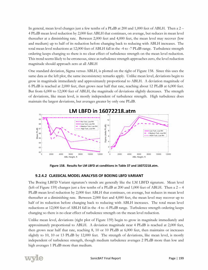
SonicBAT Final Report Page | 199
In general, mean level changes just a few tenths of a PLdB at 200 and 1,000 feet of ABLH. Then a 2 –
4 PLdB mean level reduction by 2,000 feet ABLH that continues, on average, but reduces in mean level
thereafter at a diminishing rate. Between 2,000 feet and 4,000 feet, the mean level may recover (low
and medium) up to half of its reduction before changing back to reducing with ABLH increases. The
total mean level reductions at 12,000 feet of ABLH fall in the -4 to -7 PLdB range. Turbulence strength
ordering keeps changing so there is no clear effect of turbulence strength on the mean level reduction.
This trend seems likely to be erroneous, since as turbulence strength approaches zero, the level reduction
magnitude should approach zero at all ABLH
One standard deviation, Sigma versus ABLH, is plotted on the right of Figure 158. Since this uses the
same data as the left plot, the same inconsistency remarks apply. Unlike mean level, deviations begin to
grow in magnitude immediately and approximately proportional to ABLH. A deviation magnitude of
6 PLdB is reached at 2,000 feet, then grows near half that rate, reaching about 12 PLdB at 6,000 feet.
But from 6,000 to 12,000 feet of ABLH, the magnitude of deviations slightly decreases. The strength
of deviations, like mean level, is mostly independent of turbulence strength. High turbulence does
maintain the largest deviations, but averages greater by only one PLdB.
Figure 158. Results for LM LBFD at conditions in Table 37 and 16072218.atm.
9.2.4.2 CLASSICAL MODEL ANALYSIS OF BOEING LBFD VARIANT
The Boeing LBFD Variant signature’s trends are generally like the LM LBFD signature. Mean level
(left of Figure 159) changes just a few tenths of a PLdB at 200 and 1,000 feet of ABLH. Then a 2 – 4
PLdB mean level reduction by 2,000 feet ABLH that continues, on average, but reduces in mean level
thereafter at a diminishing rate. Between 2,000 feet and 4,000 feet, the mean level may recover up to
half of its reduction before changing back to reducing with ABLH increases. The total mean level
reductions at 12,000 feet of ABLH fall in the -4 to -6 PLdB range. Turbulence strength ordering keeps
changing so there is no clear effect of turbulence strength on the mean level reduction.
Unlike mean level, deviations (right plot of Figure 159) begin to grow in magnitude immediately and
approximately proportional to ABLH. A deviation magnitude near 4 PLdB is reached at 2,000 feet,
then grows near half that rate, reaching 8, 10 or 10 PLdB at 6,000 feet, then maintains or increases
slightly to 10, 10 or 13 PLdB by 12,000 feet. The strength of deviations, like mean level, is mostly
independent of turbulence strength, though medium turbulence averages 2 PLdB more than low and
high averages 1 PLdB more than medium.
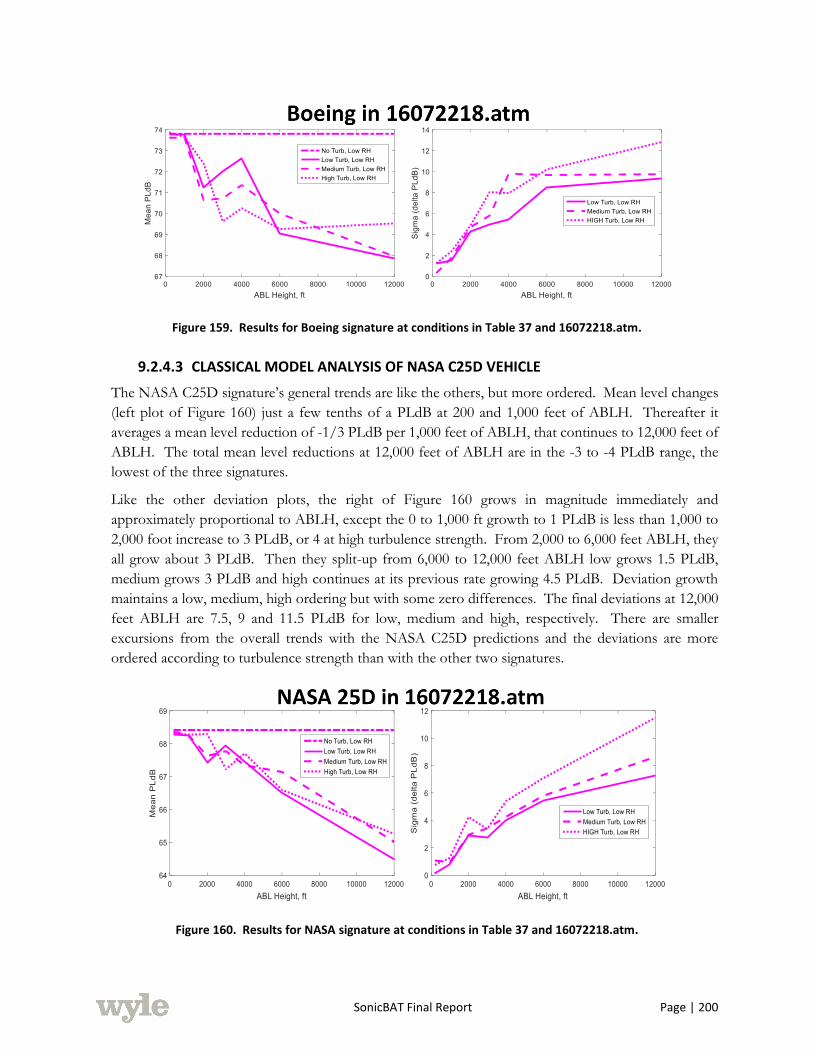
SonicBAT Final Report Page | 200
Figure 159. Results for Boeing signature at conditions in Table 37 and 16072218.atm.
9.2.4.3 CLASSICAL MODEL ANALYSIS OF NASA C25D VEHICLE
The NASA C25D signature’s general trends are like the others, but more ordered. Mean level changes
(left plot of Figure 160) just a few tenths of a PLdB at 200 and 1,000 feet of ABLH. Thereafter it
averages a mean level reduction of -1/3 PLdB per 1,000 feet of ABLH, that continues to 12,000 feet of
ABLH. The total mean level reductions at 12,000 feet of ABLH are in the -3 to -4 PLdB range, the
lowest of the three signatures.
Like the other deviation plots, the right of Figure 160 grows in magnitude immediately and
approximately proportional to ABLH, except the 0 to 1,000 ft growth to 1 PLdB is less than 1,000 to
2,000 foot increase to 3 PLdB, or 4 at high turbulence strength. From 2,000 to 6,000 feet ABLH, they
all grow about 3 PLdB. Then they split-up from 6,000 to 12,000 feet ABLH low grows 1.5 PLdB,
medium grows 3 PLdB and high continues at its previous rate growing 4.5 PLdB. Deviation growth
maintains a low, medium, high ordering but with some zero differences. The final deviations at 12,000
feet ABLH are 7.5, 9 and 11.5 PLdB for low, medium and high, respectively. There are smaller
excursions from the overall trends with the NASA C25D predictions and the deviations are more
ordered according to turbulence strength than with the other two signatures.
Figure 160. Results for NASA signature at conditions in Table 37 and 16072218.atm.

SonicBAT Final Report Page | 201
9.2.5 SUMMARY OF LOW BOOM VEHICLE ANALYSIS – CLASSICAL MODEL
The three low boom vehicle signatures, provided for SonicBAT analysis, all employed a ramp shaped
signature, a.k.a. minimum shock as described by Seebass and George (Seebass, A., and George, A., 1972)
and Darden (Darden, C., 1979), with multiple weak secondary shocks that were mostly rounded into
the ramp shape by atmospheric absorption. The shaped signatures were found to be -26 to -30 PLdB
quieter that the F-18’s N-wave signature. In addition to similar quietness, they have very similar front
shaping and 2 have similar aft shaping. The third signature, the Boeing LBFD Variant, had reduced aft
signature negative impulse but a stronger aft shock strength, producing a little more audible frequency
level but some lower infrasonic sound exposure level, but no differences in results were linked to these
signature differences for these cases.
In comparisons with N-wave results, shaped signatures resulted in some significant differences. When
going from the standard S1.26 relative humidity (RH) profile (averaging 65% RH near the ground) to
dry air of 15% RH, N-waves get quieter by -3 PLdB undertrack and -4 PLdB toward the edge of the
carpet. Shaped signatures get quieter by -5 PLdB undertrack and -7 PLdB toward the edge of the carpet.
This difference appears to be due to greater absorption at the lower frequencies that dominate shaped
signature levels. In analyses with turbulence, results indicated that a low boom shaped signature reacts
differently to turbulence than an N-wave. TURBO indicated that the LM LBFD shaped signature
exhibited less variation and less reduction in mean level in turbulence than the F-18 N-wave. These
results should not yet be relied upon as accurate, but the indication that a low boom shaped signature
reacts differently to turbulence warrants additional scrutiny and cross-checking with our Numerical
method to validate the results or make refinements to the code, so it can produce accurate results for a
low boom signature’s behavior in turbulence.
The analyses of the three low boom shaped signatures resulted in similar results with significant
variations. Identification of signature characteristics responsible for favorable results is not
recommended until the method’s accuracy is specifically validated for such work. However the result
that different signature shapes are affected differently by turbulence, indicates that signature shaping
may be able to improve propagation through turbulence.

SonicBAT Final Report Page | 202
10.0
SONIC BOOM SOFTWARE UPDATE
10.1 PCBOOM SOFTWARE UPDATE
The numeric and classic turbulence models developed on this project were incorporated into the
PCBoom software tool, along with several other updates, creating PCBoom version 7.0.0. Section
10.1.1 presents an overview of the new PCBoom updates and resulting run options. The practical
implementation of the numeric model in PCBoom was accomplished by incorporating finite impulse
response (FIR) filters generated by the KZK model (Section 3.0). Instructions for applying the FIR
filters is provided in Section 10.1.2.
10.1.1 NEW FEATURES AND RUN OPTIONS
A high-level summary of PCBoom’s new features and run options is shown in Figure 161.
Figure 161. PCBoom new features and run options.
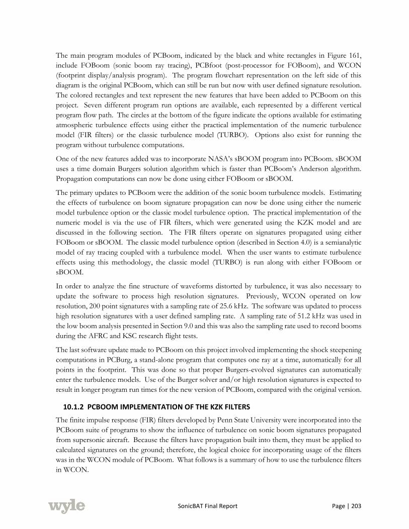
SonicBAT Final Report Page | 203
The main program modules of PCBoom, indicated by the black and white rectangles in Figure 161,
include FOBoom (sonic boom ray tracing), PCBfoot (post-processor for FOBoom), and WCON
(footprint display/analysis program). The program flowchart representation on the left side of this
diagram is the original PCBoom, which can still be run but now with user defined signature resolution.
The colored rectangles and text represent the new features that have been added to PCBoom on this
project. Seven different program run options are available, each represented by a different vertical
program flow path. The circles at the bottom of the figure indicate the options available for estimating
atmospheric turbulence effects using either the practical implementation of the numeric turbulence
model (FIR filters) or the classic turbulence model (TURBO). Options also exist for running the
program without turbulence computations.
One of the new features added was to incorporate NASA’s sBOOM program into PCBoom. sBOOM
uses a time domain Burgers solution algorithm which is faster than PCBoom’s Anderson algorithm.
Propagation computations can now be done using either FOBoom or sBOOM.
The primary updates to PCBoom were the addition of the sonic boom turbulence models. Estimating
the effects of turbulence on boom signature propagation can now be done using either the numeric
model turbulence option or the classic model turbulence option. The practical implementation of the
numeric model is via the use of FIR filters, which were generated using the KZK model and are
discussed in the following section. The FIR filters operate on signatures propagated using either
FOBoom or sBOOM. The classic model turbulence option (described in Section 4.0) is a semianalytic
model of ray tracing coupled with a turbulence model. When the user wants to estimate turbulence
effects using this methodology, the classic model (TURBO) is run along with either FOBoom or
sBOOM.
In order to analyze the fine structure of waveforms distorted by turbulence, it was also necessary to
update the software to process high resolution signatures. Previously, WCON operated on low
resolution, 200 point signatures with a sampling rate of 25.6 kHz. The software was updated to process
high resolution signatures with a user defined sampling rate. A sampling rate of 51.2 kHz was used in
the low boom analysis presented in Section 9.0 and this was also the sampling rate used to record booms
during the AFRC and KSC research flight tests.
The last software update made to PCBoom on this project involved implementing the shock steepening
computations in PCBurg, a stand-alone program that computes one ray at a time, automatically for all
points in the footprint. This was done so that proper Burgers-evolved signatures can automatically
enter the turbulence models. Use of the Burger solver and/or high resolution signatures is expected to
result in longer program run times for the new version of PCBoom, compared with the original version.
10.1.2 PCBOOM IMPLEMENTATION OF THE KZK FILTERS
The finite impulse response (FIR) filters developed by Penn State University were incorporated into the
PCBoom suite of programs to show the influence of turbulence on sonic boom signatures propagated
from supersonic aircraft. Because the filters have propagation built into them, they must be applied to
calculated signatures on the ground; therefore, the logical choice for incorporating usage of the filters
was in the WCON module of PCBoom. What follows is a summary of how to use the turbulence filters
in WCON.

SonicBAT Final Report Page | 204
Using the filters in WCON begins with the display of a signature. One way to display a boom signature
in WCON is to place the cursor somewhere inside the displayed boom footprint and pressing the ‘r’
key. Pressing the ‘r’ key changes the display to show the calculated boom signature for the cursor’s
location. In order to apply the filters to the displayed boom signature, the user must press the ‘k’ key.
This will open a dialog box for entering the atmospheric conditions as shown in Figure 162.
Figure 162. WCON signature window overlaid by turbulent parameters entry dialog.
The program will select the appropriate filter set to be applied to the signature in the WCON window
based upon the height of the boundary layer (in feet above ground level), the relative humidity (in
percent at the ground), the turbulence strength (low, medium or high), and the elevation angle of the
acoustic ray at the location in degrees. All but the last of these parameters must be entered into the
dialog box by the user. The elevation angle is computed by PCBoom and already available to the
turbulent filter selector; elevation angle is also shown in the header of the signature display. After
entering the atmospheric parameters and pressing the OK button, the user is shown a window with the
results of applying the appropriate filters to the sonic boom signature. This window is presented by an
independent program unit called FiltVIEW that is launched by WCON. An example display window
of FiltVIEW is shown in Figure 163. The header of the graph in the window shows the geometric
parameters of the boom ray and the atmospheric parameters entered by the user.
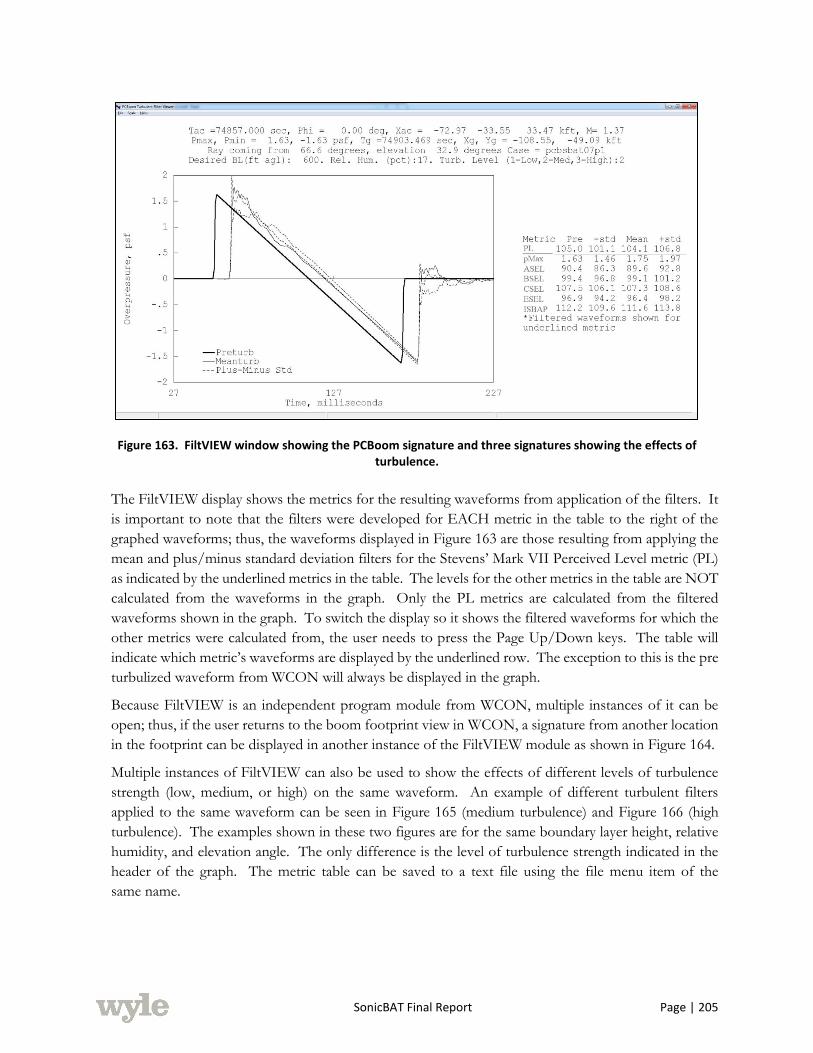
SonicBAT Final Report Page | 205
Figure 163. FiltVIEW window showing the PCBoom signature and three signatures showing the effects of turbulence.
The FiltVIEW display shows the metrics for the resulting waveforms from application of the filters. It
is important to note that the filters were developed for EACH metric in the table to the right of the
graphed waveforms; thus, the waveforms displayed in Figure 163 are those resulting from applying the
mean and plus/minus standard deviation filters for the Stevens’ Mark VII Perceived Level metric (PL)
as indicated by the underlined metrics in the table. The levels for the other metrics in the table are NOT
calculated from the waveforms in the graph. Only the PL metrics are calculated from the filtered
waveforms shown in the graph. To switch the display so it shows the filtered waveforms for which the
other metrics were calculated from, the user needs to press the Page Up/Down keys. The table will
indicate which metric’s waveforms are displayed by the underlined row. The exception to this is the pre
turbulized waveform from WCON will always be displayed in the graph.
Because FiltVIEW is an independent program module from WCON, multiple instances of it can be
open; thus, if the user returns to the boom footprint view in WCON, a signature from another location
in the footprint can be displayed in another instance of the FiltVIEW module as shown in Figure 164.
Multiple instances of FiltVIEW can also be used to show the effects of different levels of turbulence
strength (low, medium, or high) on the same waveform. An example of different turbulent filters
applied to the same waveform can be seen in Figure 165 (medium turbulence) and Figure 166 (high
turbulence). The examples shown in these two figures are for the same boundary layer height, relative
humidity, and elevation angle. The only difference is the level of turbulence strength indicated in the
header of the graph. The metric table can be saved to a text file using the file menu item of the
same name.
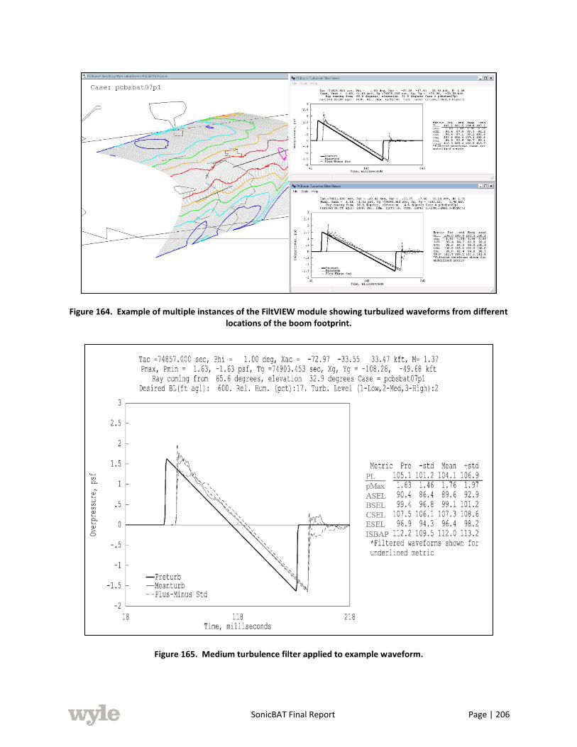
SonicBAT Final Report Page | 206
Figure 164. Example of multiple instances of the FiltVIEW module showing turbulized waveforms from different locations of the boom footprint.
Figure 165. Medium turbulence filter applied to example waveform.
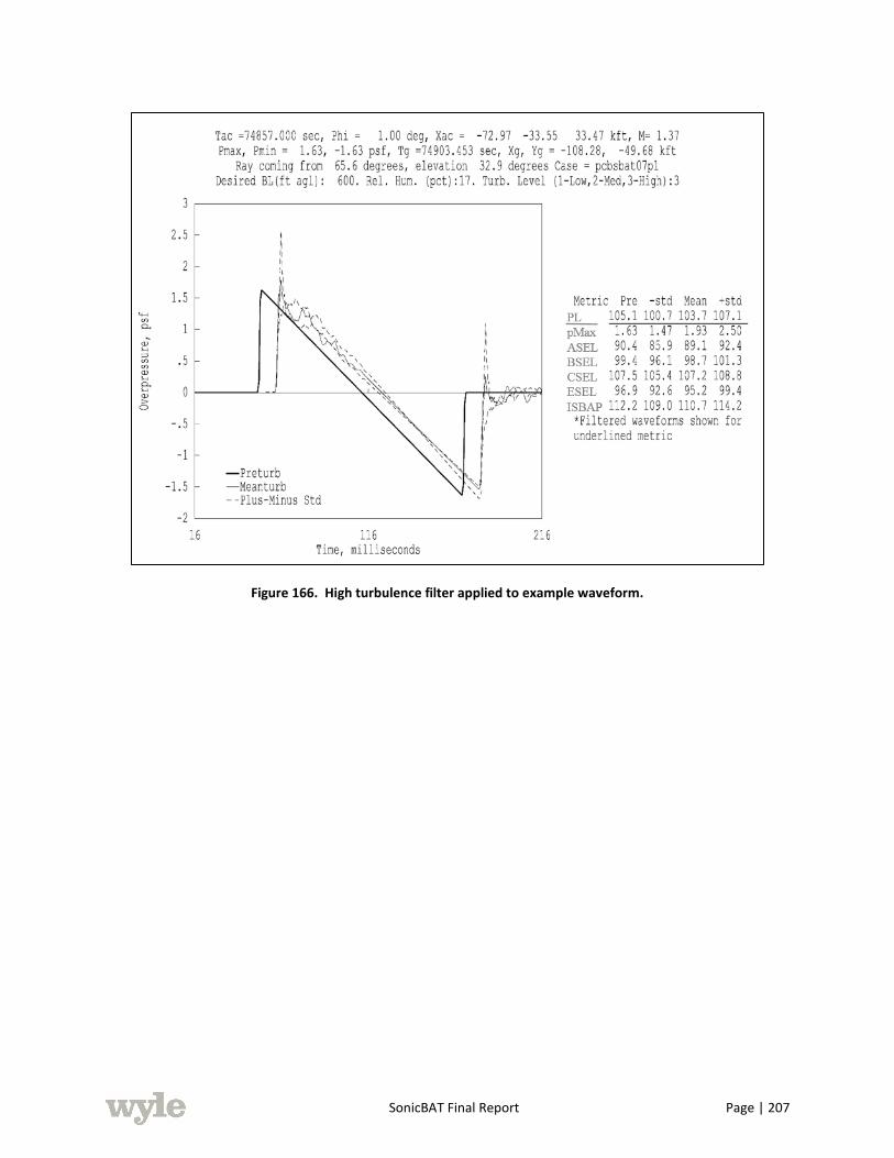
SonicBAT Final Report Page | 207
Figure 166. High turbulence filter applied to example waveform.

SonicBAT Final Report Page | 208
11.0
SUMMARY, RECOMMENDATIONS, AND CONCLUSIONS
The Sonic Booms in Atmospheric Turbulence Program was conducted to advance the understanding
of atmospheric turbulence effects on sonic boom propagation. Objectives of the program were to
design and conduct two supersonic research flight experiments under a variety of atmospheric
conditions, develop and validate one numeric turbulence model research code and one classic
turbulence model research code using measured acoustic and turbulence data from the flight
experiments, and apply the validated codes to estimate the effects of turbulence on the shaped signatures
from several low boom aircraft designs.
11.1 RESEARCH FLIGHT TESTS AT NASA AFRC AND KSC
The SonicBAT experiments at NASA AFRC and KSC were conducted in hot/dry and hot/humid
environments, respectively. Data collected during both experiments included simultaneous F-18A or F-
18B onboard flight instrumentation data, high fidelity ground based and airborne acoustic data, surface
and upper air meteorological data, and additional meteorological data from ultrasonic anemometers and
SODARS to determine the local atmospheric turbulence and boundary layer height.
The first SonicBAT experiment was conducted at NASA AFRC, on Edwards Air Force Base, California,
from 11 through 22 July 2016 in a hot, dry environment. Primary validation measurements involved the
F-18’s flying nominally east-west, straight and level at Mach 1.38 and 34kft MSL along a path that was
directly over the primary acoustic array. Airborne acoustic data were measured by the TG-14 motor
glider at an altitude just above the estimated boundary layer height to record the F-18 boom signature
just before it propagated into the boundary layer. The primary acoustic array was comprised of sixteen
microphones spaced 100 feet apart; secondary and tertiary acoustic arrays, consisting of eight
microphones each, laid out 100 feet apart and in a cross configuration, were offset 7,500 feet and 15,000
feet north of the primary array, respectively. In total, 20 flights and 69 passes were conducted over the
arrays during the two week period; airborne incoming sonic boom wave measurements were measured
by the TG-14 for 60 of the 69 flight passes. Along with surface and upper air measurements,
measurements from two SODARS and two sonic anemometers located near the primary array were
used to determine the local atmospheric turbulence levels and the boundary layer height. Review of the
2,059 sonic boom signatures recorded at all three acoustic arrays for primary validation purposes
indicated that about 96 percent of these signatures had been affected by atmospheric turbulence.
The second SonicBAT experiment was conducted at NASA KSC, Florida from 21 through 31 August
2017 in a hot, humid environment. The primary validation measurements were conducted with the
aircraft flying straight and level at Mach 1.36 and 34kft MSL along a northwest–southeast, offshore path
that was laterally offset from the primary and secondary microphone arrays. The experiment at KSC
used two ground based acoustic arrays with the secondary array being located closer to the flight path.
The primary array consisted of sixteen microphones spaced 100 feet apart and the secondary array
consisted of twenty microphones spaced 100 feet apart; both arrays were linear and nominally oriented
northwest–southeast. In total, 20 flights and 56 passes were conducted over the arrays during the two
week period; airborne incoming sonic boom wave measurements were measured by the TG-14 for 35
of the 56 flight passes. Review of the 1,883 boom signatures recorded at both acoustic arrays for primary
SonicBAT Final Report Page | 209
validation purposes indicated that about 95 percent of these signatures had been affected by atmospheric
turbulence. Due to the higher humidity at KSC, boom rise times calculated from the KSC
measurements are noticeably shorter than rise times calculated from the AFRC measurements.
Meteorological measurements were taken near the primary array at the surface, at a number of heights
on the 150 meter tower (including 12, 54, 132, 162, 204, 257, 295, 382, 394, 457, and 492 feet), and from
upper air soundings to determine the macro influences of the atmosphere including pressure,
temperature, humidity, and winds. Measurements were also taken near the primary array using one
SODAR and three sonic anemometers to determine the micro influences of the atmosphere including
turbulence; one anemometer was integrated with a moisture flux sensor specifically to provide a
humidity correction to certain turbulence quantities including the temperature structure constant.
Software was developed to post-process raw data from the anemometers to provide the turbulence
quantities of interest. The boundary layer height was determined using information from GPSsonde
balloon soundings and SODAR backscatter intensity time-height plots. The turbulence quantities and
boundary layer height were prepared as inputs to the numeric and classic turbulence models.
11.2 NUMERIC MODEL DEVELOPMENT AND VALIDATION
To numerically model supersonic signature turbulent distortions, the KZKFourier propagation code,
based on the solution of an augmented Khokhlov-Zobolotskaya-Kuznetzov (KZK) equation, has been
described including an approximate atmospheric turbulence model that incorporates measured or
simulated turbulence parameters. The code has been validated against data from the field measurement
campaigns using as inputs the signatures recorded at the motor glider and the parameters measured by
the sonic anemometers and balloon launches. The majority of PL, ISBAP, and maximum overpressure
deviation predictions fell within the confidence intervals around the measured values for both
campaigns, with the best performance in predicting PL and ISBAP standard deviations. The code’s
predictions including metric means and deviations were most accurate at AFRC, likely because the
primary array at KSC was not undertrack and because the turbulence model is best suited to moderate
and highly convective atmospheres. During some passes at KSC, the atmosphere was only weakly
convective. Additionally, boom level reduction due to clouds is not accounted for in the numeric model.
The full KZKFourier code was run on the NASA Pleiades supercomputer cluster at 96 different
turbulence and propagation conditions with multiple realizations at each condition. For these
production runs, an N-wave from the AFRC campaign was used as input, and “low”, “medium”, and
“high” turbulence strength conditions were considered. The results show trends in metric standard
deviations and means with respect to propagation distance and turbulence strength. In general, the PL,
ISBAP, and maximum overpressure standard deviations tend to increase with propagation up to about
3-5 km of propagation distance depending on turbulence strength, beyond which the deviations
decrease. This trend in maximum overpressure deviation follows with the turbulence saturation effects
which have been described by previous studies. The PL and ISBAP deviations are affected by pressure
amplitudes and rise times, which are affected by turbulence and atmospheric absorption. Additional
investigation into the simulated rise times may offer more insight into the PL and ISBAP trends. The
PL and ISBAP means after propagation through turbulence are all lower than the nominal case without
turbulence. Additionally, increasing turbulence strength and propagation distance are shown to further
decrease the mean PL and ISBAP. In contrast, the maximum overpressure means are higher than the
nominal after propagation through turbulence.

SonicBAT Final Report Page | 210
Results from the KZKFourier production runs were then used to create mean, -std, and +std turbulence
FIR filters designed to give a quick estimation of turbulence effects on a given waveform with respect
to several metrics. The error inherent in the approximate filter creation process was determined to be
below 5% on average for predicting metric standard deviations, and below 1% for metric mean
estimation.
Recommendations for future work with the KZKFourier model include:
• Additional investigation into the simulated rise times in Section 8.0 may offer more insight into
the PL and ISBAP trends with respect to propagation distance through turbulence.
• Three-dimensional numeric simulations at a few select conditions may qualify the use of two-
dimensional simulations to predict turbulence effects.
11.3 CLASSICAL MODEL DEVELOPMENT AND VALIDATION
A classical model for propagation through turbulence was developed with the long range potential for
fully accurate sonic boom predictions through real atmospheric conditions and runs quickly from a
desktop PC. The code already includes:
• Fully 3-D propagation including mean temperature and winds profiles run with turbulence
• Complex atmospheric modeling capability
• Connected to the PCBoom suite of tools, including sBOOM Burgers propagation
Areas for method improvement were identified including:
• Usability improvements from additional run experience and validation case updates, bug fixes,
integration with PCBoom suite of tools, and continuing documentation updates
• Speed enhancements through improved signature integration techniques, propagation loop
streamlining, parallel propagation loop execution and improved Burgers execution speed
• Enhanced capabilities and accuracy through improved diffraction modeling,
accelerating/maneuvering flight capability, cloud absorption prediction and shadow-zone
predictions beyond carpet and Mach cutoff predictions
11.4 ANALYSIS OF LOW BOOM SHAPED SIGNATURES
To estimate the effect of turbulence on low boom signatures, from analyses using the numeric model,
the FIR filters were convolved with three shaped supersonic signatures provided from PCBoom
simulations, giving estimates for metric means and deviations for a wide range of conditions. The results
indicate that boom shaping provides the best benefit in reducing PL and ISBAP deviations at low and
medium turbulence strengths, but at high turbulence conditions the variations for shaped signatures
approach those for N-waves. This observation was confirmed by full KZKFourier simulations
propagating the shaped signatures through turbulence with strength approaching the “high” condition
used in the production runs. The simulated shaped signature PL and ISBAP probability curves with
respect to the nominal, non-turbulized signatures follow the N-wave results. The median simulated PL
and ISBAP fall below the nominal values, showing that the level reduction from boom shaping persists
through atmospheric turbulence in an average sense.
The shaped signature numeric simulations were also used as a benchmark to test the accuracy of the
FIR filter method when applied to shaped signatures. Using a large number of filters, the PL and ISBAP

SonicBAT Final Report Page | 211
approximations accurately reproduce the probability curve to within 1 dB for 5% to 95% probabilites.
Thus, the general application of turbulence FIR filters to estimate shaped signature level variation is
validated. The filters also performs well in estimating the maximum overpressure curve at all
probabilities. The method of using mean, -std, and +std filters to quickly estimate metric statistics was
also compared with the benchmark, finding about 18% average relative error for approximate PL
deviations and 22% average error for ISBAP deviations, with a large relative error for maximum
overpressure deviations due to the very small value of the overpressure deviations. The mean metric
estimates had less error at less than 0.7% average error for PL and ISBAP means and 1.2% average
error for maximum overpressure means. The precision of the mean, -std, and +std filter method could
be improved by including more filters, though this would necessarily involve more convolutions and
metric computations for each signature and condition of interest.
Both the shaped signature numeric simulations and the FIR filter method suggest that the shaped
signatures spike less than N-waves, in terms of pascals and also with respect to the nominal peak
overpressure of each signature. For the KZKFourier simulations approaching high turbulence
conditions, the probabilities of shaped signatures either spiking or rounding were approximately equal,
while N-waves were shown to have a much higher probability of spiking. Results suggest that the
relatively long rise times in the shaped signatures once they enter the turbulent boundary layer serve to
reduce both the magnitude of spiking and the chance of occurrence.
Recommendations for future work with the numeric model and shaped signatures include additional
KZKFourier simulations at low and medium turbulence conditions to validate the predictions made
using FIR filters. Full simulations may illustrate the utility of boom shaping by more precisely
quantifying the predicted PL and ISBAP deviation reductions at low and medium turbulence.
Analyses of the low boom shaped signatures using the classical model yielded two primary results when
compared with the same analysis for N-waves: dry air is expected to cause more absorption to shaped
booms than N-waves and shaped booms react differently to turbulence than do N-waves. Concerning
absorption, when going from the standard S1.26 relative humidity (RH) profile (averaging 65% RH near
the ground) to dry air of 15% RH, N-waves get quieter by -3 PLdB undertrack and -4 PLdB toward the
edge of the carpet. Shaped signatures get quieter by -5 PLdB undertrack and -7 PLdB toward the edge
of the carpet. This difference appears to be due to greater absorption at the lower frequencies that
dominate shaped signature levels. Results of the classical model turbulence analyses indicate that the
LM LBFD shaped signature exhibited less variation and less reduction in mean level than the F-18 N-
wave.
Comparing the classical and numeric model results, there is considerable similarity and some difference
between them. Both the classical and numeric models provide similar trends of a reduction in mean
loudness, due to turbulence, for N-waves and shaped signatures. The classical means change by 0 to -
6 PLdB-avg while the numeric means change by +1 to -4 PLdB-avg. Classical model loudness
deviations are predominately larger than numeric model loudness deviations and increase at higher
turbulence strength.
SonicBAT Final Report Page | 212
REFERENCES
Averiyanov, M., Blanc-Benon, P., Cleveland, R. O., and Khokhlova, V. (2011a). “Nonlinear and
diffraction effects in propagation of N-waves in randomly inhomogeneous moving media,” The Journal
of the Acoustical Society of America 129, 1760-1772, April 2011.
Averiyanov, M., Ollivier, S., Khokhlova, V., and Blanc-Benon, P. (2011b). “Random focusing of
nonlinear acoustic N-waves in fully developed turbulence: Laboratory scale experiment,” The Journal
of the Acoustical Society of America 130, 3595-3607, December 2011.
Averkiou, M. A., and Hamilton, M. F. (1997). “Nonlinear distortion of short pulses radiated by plane
and focused circular pistons,” The Journal of the Acoustical Society of America 102, 2539-2548,
November 1997.
Aver’yanov, M., Khokhlova, V., Sapozhnikov, O., Blanc-Benon, P., and Cleveland, R. (2006). “Parabolic
equation for nonlinear acoustic wave propagation in inhomogeneous moving media,” Acoustical
Physics 52, 623-632, December 2006.
Baudoin, M.; Coulouvrat, F. and Thomas, J.L. (2011); “Sound, infrasound, and sonic boom absorption
by Atmospheric Clouds.” Journal of Acoustical Society of Am., v130 #3P, Figure 8, p. 1150, Sep. 2011.
Baudoin, M., Coulouvrat, F., Thomas, J. L., Atchley, A. A., Sparrow, V. W., and Keolian, R. M. (2006).
“Absorption of sonic boom by clouds,” in AIP Conference Proceedings (AIP), pp. 619-622, May 2006.
Blackstock, D. T. (1964). “On plane, spherical, and cylindrical sound waves of finite amplitude in lossless
fluids,” The Journal of the Acoustical Society of America 36, 217-219, January 1964.
Blanc-Benon, P., Lipkens, B., Dallois, L., Hamilton, M. F., and Blackstock, D. T. (2002). “Propagation
of finite amplitude sound through turbulence: Modeling with geometrical acoustics and the parabolic
approximation,” The Journal of the Acoustical Society of America 111, 487-498, January 2002.
Bradley, S. (2008). Atmospheric Acoustic Remote Sensing, (CRC Press, 2008).
Candel,S. (1979). “Numerical solutions of wave scattering problems in the parabolic approximation,” J.
Fluid Mech. 90, 465-507, 1979.
Carlson, H.W. (1978). “Simplified Sonic Boom Prediction,” NASA Technical Paper 1122, 1978.
Cetola, J. D. (1997). A Climatology of the Sea Breeze at Cape Canaveral, Florida. Florida State
University (1997).
Coulter, R. (1997). “Turbulence variables derived from sodar data,” in Acoustic Remote Sensing
Applications, S. Singal, Ed., Narosa Publishing House, New Delhi, India, 1997.
Cotte, B. and Ph. Blanc-Benon (2007). “Estimates of the relevant turbulent scales for acoustic
propagation in an upward refracting atmosphere,” Acta Acustica United with Acustica, 93 944-958
(2007)

SonicBAT Final Report Page | 213
Chernov, L. (1960). Wave Propagation in a Random Medium, Dover, New York, 1960.
Chevret, P., Blanc‐Benon, P., and Juvé, D. (1996). “A numerical model for sound propagation through
a turbulent atmosphere near the ground,” The Journal of the Acoustical Society of America 100, 3587-
3599, December 1996.
Cleveland, R. O., Hamilton, M. F., and Blackstock, D. T. (1996). “Time‐domain modeling of finite‐
amplitude sound in relaxing fluids,” The Journal of the Acoustical Society of America 99, 3312-3318,
June 1996.
Collmar, M. T., and Salamone, J. A. (2017). “Evaluation of finite difference approximations of
absorption and dispersion implemented in sonic boom propagation model equations,” in The Journal
of the Acoustical Society of America, pp. 3730-3730, May 2017.
Crow, S.C. (1969). “Distortion of Sonic Bangs by Atmospheric Turbulence,” printed in Great Britain,
J. Fluid Mechanics, vol. 37, part 3, pp. 529-563, 1969.
Darden, C. (1979). “Sonic Boom Minimization with Nose Bluntness Relaxation,” NASA TP-1348, 1979.
Dashen R. (1979). “Path integrals for waves in random media,” J. Math. Phys. 20, 894-920, 1979.
Deardoff, J. (1972). “Parameterization of the Planetary Boundary Layer for Use in General Circulation
Models,” Mon. Weather Rev., 100, 93-106, 1972.
“Earth Networks Data Archive Historical Surface Observations,” EN.DQ.Wx.WI1a, November 3,
2015.
Garratt, J.R. (1992). The Atmospheric Boundary Layer, Cambridge University Press, Pp. 316, ISBN
0521380529, 1992.
Garrick, I. E. and Maglieri, D. J. (1968). “A Summary of Results on Sonic-Boom Pressure-Signature
Variations Associated With Atmospheric Conditions,” NASA TN D-4588, 1968.
Haering, E., Murray, J., Purifoy, D., Graham, D., Meredith, K., Ashburn, C., and Stucky, M. (2005).
‘Airborne Shaped Sonic Boom Demonstration Pressure Measurements with Computation Fluid
Dynamic Comparisons,’ American Institute of Aeronautics and Astronautics, 43rd AIAA Aerospace
Sciences Meeting and Exhibit, Aerospace Sciences Meetings, Reno, NV, January, 2005.
Hammerton, P. (2001). “Effect of molecular relaxation on the propagation of sonic booms through a
stratified atmosphere,” Wave motion 33, 359-377, April 2001.
Harris, R. (1966). “A Numerical Technique for Analysis of Wave Drag at Lifting Conditions,” NASA
TN-D3586, 1966
Hayes, W.D., Haefeli, R.C., and Kulsrud, H.E. (1969). “Sonic Boom Propagation in a Stratified
Atmosphere, With Computer Program”, NASA CR-1299, April 1969.
Hilton, D., Huckel, V., and Maglieri, D. (1966). “Sonic Boom Measurements During Bomber Training
Operation in the Chicago Area,” NASA TN-D2655, 1966.
SonicBAT Final Report Page | 214
Hobbs, C., and Page, J. (2011). “PCBoom Model Prediction Comparisons with Flight Test Measurement
Data,” AIAA 2011-1277, 49th AIAA Aerospace Sciences Meeting including the New Horizons Forum
and Aerospace Exposition, January 2011.
Johnson, R., and Wichern, D. (2013). Applied Multivariate Statistical Analysis: Sixth Edition, Pearson
Education, Inc., 2013.
Kanamori, M., Takahashi, T., Naka, Y., Makino, Y., Takahashi, H., and Ishikawa, H. (2017). “Numerical
Evauation of Effect of Atmospheric Turbulence on Sonic Boom Observed in D-SEND#2 Flight Test,”
AIAA 2017-0278, 55th AIAA Aerospace Sciences Meeting, January 2017.
Kane, E. (1967). “Sonic Boom Research.” NASA SP-147, Proceedings of the Conference on Generation
and Propagation of Sonic Booms held at Princeton University; Seebass, A.R. ed., p. 51, Fig. 2, April 12,
1967.
Kaimal, J.C. and Finnigan, J.J. (1994). Atmospheric Boundary Layer Flows: Their Structure and
Measurement, Oxford University Press, 1994.
Karweit, M., Blanc‐Benon, P., Juvé, D., and Comte‐Bellot, G. (1991). “Simulation of the propagation
of an acoustic wave through a turbulent velocity field: A study of phase variance,” The Journal of the
Acoustical Society of America 89, 52-62, Januray 1991.
Kolmogorov, A.N. (1941). “Dissipation of energy under locally isotropic turbulence,” Dokl. Akad.
Nauk SSSR 32, 16–18, 1941a.
Kolmogorov, A.N. (1941). “The local structure of turbulence in incompressible viscous fluid for very
large Reynolds number,” Dokl. Akad. Nauk SSSR 30, 9–13, 1941b.
Lalescu, C. C. (2009). “Two hierarchies of spline interpolations. Practical algorithms for multivariate
higher order splines,” arXiv preprint arXiv:0905.3564, May 2009.
Lee, Y.-S. (1993). “Numerical solution of the KZK equation for pulsed finite amplitude sound beams
in thermoviscous fluids,” (Ph.D. dissertation, The University of Texas at Austin), December 1993.
Lipkens, B., and Blackstock, D. T. (1998). “Model experiment to study sonic boom propagation through
turbulence. Part II. Effect of turbulence intensity and propagation distance through turbulence,” The
Journal of the Acoustical Society of America 104, 1301-1309, September 1998.
Locey, L. L. (2008). “Sonic boom postprocessing functions to simulate atmospheric turbulence effects,”
(Ph.D. dissertation, The Pennsylvania State University), August 2008.
Locey, L. L., and Sparrow, V. W. (2007). “Modeling atmospheric turbulence as a filter for sonic boom
propagation,” Noise Control Engineering Journal 55, 495-503, November 2007.
Loubeau, A. (2006). “Nonlinear propagation of high-frequency energy from blast waves as it pertains
to bat hearing,” (Ph.D. dissertation, The Pennsylvania State University), December 2006.
Luquet, D. (2016). “3D simulation of acoustical shock waves propagation through a turbulent
atmosphere. Application to sonic boom,” (Ph.D. dissertation, Université Pierre et Marie Curie-Paris
VI), September 2016.

SonicBAT Final Report Page | 215
Maglieri, D. J., Bobbitt, P. J., Plotkin, K. J., Shepherd, K. P., Coen, P. G., and Richwine, D. M. (2014).
“Sonic Boom: Six Decades of Research,” NASA/SP-2014-622, December 2014.
Maglieri, D.J., Henderson, H.R., Massey, S.J., Stansbery, E.G. (2011). “A Compilation of Space Shuttle
Sonic Boom Measurements,” NASA/CR-2011-217-080, pp. 64, April 2011.
Maglieri, Domenic J. and Plotkin, Kenneth, J. (1991). Sonic Boom, Chapter 10: Aeroacoustics of Flight
Vehicles, Theory and Practice. NASA RP 1258, Vol. 1 and WDRC TR 80-3052, Aug. 1991.
Maglieri, D.J. and Sothcott, V.E. (1990). “Summary of Sonic Boom Rise Times Observed During FAA
Community Response Studies Over a 6-Month Period in the Oklahoma City Area,” NASA Contractor
Report 4277, pp. 64, April 1990.
Maglieri, D.J., Huckel, V., and Henderson, H.R. (1969) “Variability in Sonic-Boom Signatures Measured
Along an 8000-Foot Linear Array,” NASA TN D-5040, February 1969.
Maglieri, D.J. (1968) “Sonic Boom Ground Pressure Measurements for Flights at Altitudes in Excess
of 70,000 Feet and at Mach Numbers up to 3.0,” NASA SP-180, May 1968.
Maglieri, D. (1967). “Sonic Boom Flight Research – Some Effects of Airplane Operation and the
Atmosphere on Sonic Boom Signatures,” Sonic Boom Research, Seebass, A (Ed.), NASA SP-147, April
1967.
Maglieri, D.J. and Parrott, T. (1963). “Atmospheric effects on sonic-boom pressure signatures,” Sound:
Its uses and control 2 (4) 11-14 (1963).
Metek GmbH, Ultrasonic Anemometer uSonic-3 Scientific, Release Version: U.56c-1, 07-31-2014.
Middleton, W.D., and Carlson, H.W. (1965). “A Numerical Method for Calculating Near-Field Sonic-
Boom Pressure Signatures,” NASA TN D-3082, November 1965.
Monin, A. and Obhukov, A. (1954). “Basic Laws of Turbulent Mixing in the Ground Layer of the
Atmosphere,” Trans. Geophys. Inst. Akad., Nauk USSR 151, 163-187, 1954.
Morgenstern, J., Arslan, A., Lyman, V., and Vadyak, J. (2005). “F-5 Shaped Sonic Boom Demonstrator's
Persistence of Boom Shaping Reduction through Turbulence,” AIAA 2005-12, 43rd AIAA Aerospace
Sciences Meeting and Exhibit, January 2005.
Neff, W. and Couler, R. (1986). “Acoustic Remote Sensing,” in Probing the Atmospheric Boundary
layer, D. Lenschow, Ed. (American Meteorology Society, Boston, MA, 1986).
Obukhov, A.M. (1962). “Some specific features of atmospheric turbulence,” J. Fluid Mech. 13, 77–81,
1962.
Obukhov, A.M. (1941). “On the distribution of energy in the spectrum of turbulent flow,” Dokl. Akad.
Nauk SSSR 32, 19, 1941.
Ostashev, V. E., and Wilson, D. K. (2015). Acoustics in moving inhomogeneous media (CRC Press,
Boca Raton), September 2015.
Page, J.A., Plotkin, K.J., and Wilmer, C. (2010). “PCBoom Version 6.6 Technical Reference and User
Manual, “Wyle Laboratories, Inc. Rev. 01-21 December 2010.

SonicBAT Final Report Page | 216
Panofsky, H. and Dutton, J. (1984). Atmospheric Turbulence, (Models and Methods for Engineering
Applications) John Wiley & Sons, 1984.
Pao, Y. H. (1968). “Transfer of turbulent energy and scalar quantities at large wavenumbers,” Phys.
Fluids 11, 137I -1372, 1968.
Pao, Y. H. (1965). “Structure of turbulent velocity and scalar fields at large wavenumbers,” Phys. Fluids
8, 1063-1075, 1965.
Pierce, A. and Maglieri, D. (1972). “Effects of Atmospheric Irregularities on Sonic Boom Propagation,”
JASA, 51 (2), 702-721, 1972.
Pierce, A. (1968). “Spikes on Sonic Boom Pressure Waveforms,” JASA, 44(4), 1052-1061, 1968.
Plotkin, K.J. (1971). “The Effect of Atmospheric Inhomogeneities on the Sonic Boom,” (Ph.D.
dissertation, Cornell University), 1971.
Plotkin, K.J. and George, A.R. (1972). “Propagation of Weak Shock Waves through Turbulence,”
printed in Great Britain, J. Fluid Mech., vol. 54, part 3, pp. 449-467, 1972.
Rallabhandi, S. K. (2011). “Advanced sonic boom prediction using the augmented Burgers equation,”
Journal of Aircraft 48, 1245-1253, July 2011.
Reed, J.W. (1969). “Distribution of Airblast Amplitudes in the Ozonosphere Sound Rings,” Sandia
Laboratories Final Report SC-M-69-33, 1969.
Russell, L.M. (2015). Nature, 525(7568): 194-195, 2015.
Salamons, E. (2001). Computational Atmospheric Acoustics (Kluwer Academic, 2001)
Seebass, A. and George, A. (1972). “Sonic Boom Minimization,” The Journal of the Acoustical Society
of America 51, 686, 1972;
Stull, R.B. (1988). An introduction to Boundary Layer Meteorology, Kluwer Academic Publishers, 1988.
Tatarski, V. (1961). Wave Propagation in a Turbulent Medium, Dover, New York, 1961.
Thomas, C.L. (1972). “Extrapolation of Sonic Boom Pressure Signatures by the Waveform Parameter
Method,” NASA TN D-6832, June 1972.
Thomson, D.; Coulter, R. and Warhaft, Z. (1978). “Simultaneous measurements of turbulence in the
lower atmosphere using sodar and aircraft,” J. Appl. Meteorology 17 723 – 734, 1978.
Walkden, F. (1958). “The Shock Pattern of a Wing-Body Combination, Far From the Flight Path”,
Aeronautical Quarterly, IX(2), 164-194, 1958.
Wilson, D. K. (2000). “A turbulence spectral model for sound propagation in the atmosphere that
incorporates shear and buoyancy forcings,” The Journal of the Acoustical Society of America 108, 2021-
2038, November 2000.
Whitham, G.B. (1956). “On the Propagation of Weak Shock Waves”, J.Fluid Mech., 1, 290-318, 1956.

SonicBAT Final Report Page | 217
Whitham, G.B. (1952). “The Flow Pattern of a Supersonic Projectile”, Communications on Pure and
Applied Mathematics, 5, pp. 301-348, 1952.
Wyngaard, J. Cote, O., and Rao, K. (1974). “Modeling the Atmospheric Boundary Layer, “in Turbulent
Diffusion in Environmental Pollution, Frenkiel, F. and Munn, R. (Eds.), Advances in Geophysics, Vol.
18A, Academic Press, New York, 1974.
Yarrow, M. (1989). “Solving periodic block tridiagonal systems using the Sherman-Morrison-Woodbury
formula,” AIAA Paper 1989-1946, 9th Computational Fluid Dynamics Conference, 188-196, January
1989.
Yuldashev, P. V., Ollivier, S., Karzova, M. M., Khokhlova, V. A., and Blanc-Benon, P. (2017). “Statistics
of peak overpressure and shock steepness for linear and nonlinear N-wave propagation in a kinematic
turbulence,” The Journal of the Acoustical Society of America 142, 3402-3415, December 2017.
Yuldashev, P. V., Ollivier, S., Khokhlova, V. A., and Blanc-Benon, P. (2013). “Statistical properties of
nonlinear N-wave propagating in thermal or kinematic turbulence,” in Proceedings of Meetings on
Acoustics ICA2013 (ASA), p. 045074, June 2013.
Yuldashev, P. V., Ollivier, S., Khokhlova, V. A., and Blanc-Benon, P. (2016). “Steepening and smearing
of shock front of nonlinear N-wave propagating in a turbulent layer,” AIAA 2016-3012, 22nd
AIAA/CEAS Aeroacoustics Conference, May 2016.
Related Documents