Some wavelet-based analyses of Markov chain databrill/Papers/markov.pdf · Insbesondere scheint die Methode nuKtzlich zu sein, um abrupte oder stetige AGnderungenin derStrukturvon

*Corresponding author. Tel.: #1-510-642-2781; fax: #1-510-642-7892.

E-mail address: [email protected] (D.R. Brillinger).

Signal Processing 80 (2000) 1607}1627

Some wavelet-based analyses of Markov chain data

D.R. Brillinger!,*, P.A. Morettin", R.A. Irizarry#, C. Chiann"

!Statistics Department, University of California, Berkeley, CA 94720, USA

"Statistics Department, University of SaJ o Paulo, SP 05315-970, Brazil

#Biostatistics Department, Johns Hopkins University, Baltimore, MD 21205, USA

Received 19 April 1999; received in revised form 21 December 1999

Abstract

This work considers signals whose values are discrete states. It proceeds by expressing the transition probabilities of

a nonstationary Markov chain by means of models involving wavelet expansions and then, given part of a realization

of such a process, proceeds to estimate the coe$cients of the expansion and the probabilities themselves. Through choice

of the number of and which wavelet terms to include, the approach provides a #exible method for handling discrete-

valued signals in the nonstationary case. In particular, the method appears useful for detecting abrupt or steady changes

in the structure of Markov chains and the order of the chains. The method is illustrated by means of data sets concerning

music, rainfall and sleep. In the examples both direct and improved estimates are computed. The models include

explanatory variables in each case. The approach is implemented by means of statistical programs for "tting generalized

linear models. The Markov assumption and the presence of nonstationarity are assessed both by change of deviance and

graphically via periodogram plots of residuals. ( 2000 Elsevier Science B.V. All rights reserved.

Zusammenfassung

Diese Arbeit betrachtet Signale, deren Werte diskrete ZustaK nde sind. Sie faK hrt fort, indem die UG bergangswahrschein-

lichkeiten einer nichtstationaK ren Markov-Kette anhand von Modellen, die Wavelet-Entwicklungen beinhalten, ausged-

ruK ckt werden, und macht dann damit weiter, die Koe$zienten der Entwicklung und der Wahrscheinlichkeiten selbst zu

schaK tzen, wobei ein Teil einer Realisierung eines solchen Prozesses gegeben sei. Durch die Wahl, wieviel und welche der

Wavelet-Terme zu beruK cksichtigen sind, liefert diese Vorgehensweise eine #exible Methode, um wertdiskrete Signale im

nichtstationaK rem Fall zu behandeln. Insbesondere scheint die Methode nuK tzlich zu sein, um abrupte oder stetige

AG nderungen in der Struktur von Markov-Ketten und die Ordnung der Ketten zu entdecken. Die Methode wird anhand

von Musik-, Regen- und Schlafdaten veranschaulicht. In den Beispielen werden sowohl direkte als auch verbesserte

SchaK tzungen berechnet. Die Modelle beinhalten in allen FaK llen erklaK rende Variablen. Die Methode wird mit Hilfe von

statistischen Programmen zur Anpassung verallgemeinerter linearer Modell implementiert. Die Markov-Annahme und

die Gegenwart der NichtstationaritaK t werden sowohl durch die AG nderung der Abweichung als auch graphisch durch

Periodogrammdarstellungen der Residuen bewertet. ( 2000 Elsevier Science B.V. All rights reserved.

Re2 sume2

Ce travail considere les signaux dont les valeurs sont des eH tats discrets. Il procede en exprimant les probabiliteH s de

transition d'une cham(ne de Markov non stationnaire au moyen de modeles impliquant des expansions en ondelettes et

0165-1684/00/$ - see front matter ( 2000 Elsevier Science B.V. All rights reserved.

PII: S 0 1 6 5 - 1 6 8 4 ( 0 0 ) 0 0 0 9 7 - 9

ensuite, eH tant donneH une partie de la reH alisation d'un tel processus, procede a l'estimation des coe$cients de l'expansion et

des probabiliteH s elles-me(mes. Par le choix du nombre et des coe$cients a inclure, l'approche fournit une meH thode #exible

pour manipuler des signaux a valeurs discretes dans un cas non stationnaire. En particulier, le modele se reH vele utile pour

deH tecter des changements abrupts et reH guliers dans des cham(nes de Markov et l'ordre des cham(nes. La meH thode est illustreH e

au moyen des ensembles de donneH es concernant la musique, la chute de pluie et le sommeil. Dans les exemples nous

calculons a la fois les estimateurs directs et ameH lioreH s. L'approche est impleHmenteH e au moyen de programmes statistiques

pour l'ajustement de modeles lineH aires geH neH raliseH s. La supposition de Markov et de non stationnariteH est eH valueH e a la fois

par un changement de deH viation et de fac7 on graphique via des courbes de peH riodogrammes des reH sidus. ( 2000 Elsevier

Science B.V. All rights reserved.

Keywords: Wavelets; Transition probabilities; Nonstationary processes; Markov chains; Improved estimates

This work presents empirical analyses of non-

stationary Markov chain models, based on wavelet

expansions, for signals taken from musicology,

meteorology and sleep research, respectively.

A basic goal is looking for time-varying chara-

cteristics of the various series, such as trend and/or

changing (seasonal) e!ects. The work proceeds

from an initial analysis of the transition probabilit-

ies into the coe$cients of a wavelet expansion. This

is followed by an estimation of the coe$cients and

a synthesis to obtain estimates of the transition

probabilities themselves. The "tted characteristics

may be used to assess stationarity, e.g. detecting

points of change amongst other things. Through

choice of the number of and just which wavelet

terms to include in the linear predictor the

approach provides a #exible method for handling

signals of discrete-state-valued observations

amongst other possibilities.

The work may be viewed as involving a nonlin-

ear model within a linear model setup. Speci"cally

transition probabilities, Pab

(t), of movement from

state a to state b are expressed as functions of

a linear predictor in t, by means of wavelet expan-

sions and link functions. Generalized linear model

methodology and computing programs are em-

ployed in the empirical analyses.

Markov processes, in particular Markov chains,

have long been basic to signal processing. One can

mention their use in cryptology, coding, networks,

speech, control, image processing for example.

In the last decade wavelets have also become basic

to many areas of signal processing. Since wave-

lets provide economical expansions for a wide

class of functions, this implies for example that

they provide good compression of signals and

images.

In this work Markov chains and wavelet tech-

niques are married together to deal with non-

stationary processes. These two "elds have been

joined together before, e.g. by Crouse and Baraniuk

[15] which concerns hidden Markov modes, but

the present work concerns discrete-valued pro-

cesses and has a di!erent intent.

The next section provides pertinent basic back-

ground on Markov chains, wavelets, the model and

its analysis. Section 3 describes the data sets, Sec-

tion 4 presents the results of the analyses and the

paper ends with some general discussion.

1. Background

1.1. The Markov chain case

The concern is signals that take on a discrete set

of values. A homogeneous or stationary Markov

chain with A states is a random process, >(t), tak-

ing on values in the set M1,2,2,AN, such that the

conditional probabilities of taking on values at the

next time step, given the whole history of the pro-

cess, depend solely on the present value. Speci"-

cally,

ProbM>(t#1)"bD>(t)"a,>(t!1)"a~1

,

>(t!2)"a~2

,2N

"ProbM>(t#1)"bD>(t)"aN"Pab

(1)

for b, a, a~1

, a~2

,23M1,2, AN and t"1, 2,2 .

The circumstance (1) is called the Markov property

1608 D.R. Brillinger et al. / Signal Processing 80 (2000) 1607}1627

and also appears in the dynamic equation of the

state space model, so common in signal processing

today.

The matrix P"[Pab

] is called the transition

probability matrix. It, with a set of initial condi-

tions ProbM>(t)"aN"Pa, determines the process

in the sense that probabilities of sample realizations

M>(0),>(1),>(2),2,>(¹!1)N may be set down.

Results have been developed concerning "rst pas-

sage times, limiting behavior, communicating

states, etc. by various authors, e.g. Feller [22] and

Dynkin [20]. Applications may be found in [1,2].

If the probabilities Pa

and Pab

depend on the

particular time point, the chain is nonstationary

and Pab

(t) will denote the conditional probability of

being in state b at time t, given that the process was

in state a at time t!1 while Pa(t) will denote the

marginal probability of being in state a at time t.

It will be supposed that the state of the process

has been observed at the ¹ successive times,

t"1,2,2, ¹.

In many cases a set of parameters, reduced from

the full set MPa(t),P

ab(t)N, is required, particularly if

A is not small and the amount of data is limited.

The approach adopted here is to employ a linear

parameterization of some function of the P's, e.g. to

write

logitMPab

(t)N"+j,k

babjk

tjk

(t) (2)

with the b's unknown parameters to be estimated

and the t's given functions (here use of

logitMnN"log(n/(1!n) provides a simple manner

to ensure that the probability stays between 0 and

1). At the next step this expression is substituted

into a likelihood function such as (3) below and the

b's estimated by maximizing the likelihood. There

may be a further step of shrinkage of the coe$cient

estimates, that is replacement of an estimate bK by

a value closer to 0 in an attempt to improve the

estimate. In expansion (2), in this work, t's are the

functions of some wavelet basis as discussed below.

In de"ning the likelihood function it is conve-

nient to replace the process >(t), t"0,1,2,2 by

a vector-valued process X(t)"[Xa(t)] where

Xa(t)"1 if >(t)"a and X

a(t)"0 otherwise.

It satis"es +Xa(t)"1 and P

ab(t)"ProbMX

b(t)"

1DXa(t!1)"1N. Also one sets P

a"

ProbMXa(0)"1N.

Let Xab

(t)"1, if the process is in state a at time

t!1 and in state b at time t, and Xab

(t)"0 other-

wise. Given the data and parametric forms for

Pa(t),P

ab(t) the likelihood is now

CA<a/1

PXa (0)a DC

T<t/1

A<a/1

A<b/1

Pab

(t)Xab (t)D (3)

viewed as a function of the parameters. In the case

that A"2 things may be simpli"ed. Write

n1(t)"P

11(t), n

2(t)"P

22(t), then P

12(t)"1!

n1(t), P

21(t)"1!n

2(t) and the likelihood is

PX1 (0)1

PX2 (0)2

T<t/1

Mn1(t)X11 (t)[1!n

1(t)]X12 (t)n

2(t)X22 (t)

][1!n2(t)]X21 (t)N. (4)

In a variety of cases, e.g. ¹ large, the "rst two terms,

may be neglected. This will be done in the results

presented. The estimation criterion then becomes

T<t/1

Mn1(t)X11 (t)[1!n

1(t)]X1 (t~1)~X11 (t)n

2(t)X22 (t)

][1!n2(t)]X2 (t~1)~X22 (t)N (5)

as a function of the unknown parameters. When

consideration below turns to estimation, it is useful

to note that this has the form of a likelihood based

on independent Bernoullis, that is random

variables taking on the values 0,1 with some prob-

ability n. In consequence, the log of the criterion is

the sum of a term in n1(t) and one in n

2(t) each

corresponding to a binomial distribution. Standard

statistical packages, allowing generalized linear

model "tting of Binomials, may now be employed

to compute estimates of the b's of (2).

A variety of properties of maximum-likelihood

estimates have been developed for Markov chains

in the large sample case. For example, Billingsley

[3] developed consistency and asymptotic normal-

ity results for a stationary "nite-dimensional para-

meter Markov chain. Foutz and Srivastava [23]

and Ogata [35] derived the large sample distribu-

tion of the maximum-likelihood estimate in the

stationary ergodic case. Bishop et al. [5] suggested

D.R. Brillinger et al. / Signal Processing 80 (2000) 1607}1627 1609

some methods for assessing empirically whether

a Markov chain is stationary. Fahrmeir and Srivas-

tava [21] indicated how nonstationary Markov

chain models might be included within the general-

ized linear modelling methodology. Details of this

are provided below. Coe and Stern [14] presented

empirical analyses involving nonstationary

Markov chain models. McCullagh and Nelder [31,

Section 8.4.3], discussed the Coe and Stern work.

Consideration now turns to the wavelet meth-

odology basic to the model being studied.

1.2. Wavelets

Wavelets are contemporary approximation

tools, alternative to existing basis systems such as

sines and cosines, Walsh functions, etc.

The basic fact about wavelets is that they are

localized in time (and space), contrary to what

happens with the trigonometric functions used in

Fourier analysis. This behavior makes wavelets

ideal for the analysis of nonstationary signals,

particularly those with transients or singularities.

Fourier bases are localized in frequency but not in

time; small changes in some of the observations

may induce substantial changes in almost all the

components of a Fourier expansion, a fact that

does not hold for basic wavelet expansions and can

be a real disadvantage.

In elementary wavelet analysis there are two

basic functions, the scaling function (or father

wavelet) / and the wavelet t. Here / is a solution of

the two-scale di!erence equation

/(t)"J2+k|Z

hk/(2t!k) (6)

and normalized via :/(t) dt"1, while t is de"ned

by

t(t)"J2+k|Z

(!1)kh1~k

/(2t!k). (7)

Here Z is the set of all integers and the hk's are "lter

coe$cients which can be chosen in such a way

that one has wavelets with desirable proper-

ties. De"ning /lk(t)"2l@2/(2lt!k) and t

jk(t)"

2j@2t(2jt!k), for example the system M/lk(t)N

k|ZX

Mtjk

(t)Njwl_k|Z

forms an orthonormal basis for the

space of square integrable functions on the real line

¸2(R), under some additional conditions on the

"lter coe$cients. Accordingly, any f3¸2(R) can be

expanded as

f (t)"+k|Z

alk/lk

(t)# +jwl

+k|Z

bjk

tjk

(t), (8)

where l is the `coarsea level of the approximation

and the wavelet coe$cients are given by

alk"P f (t)/lk

(t) dt, bjk

"P f (t)tjk

(t) dt, (9)

following the orthonormality. On occasion nonor-

thogonal functions are used and one speaks of

frame analysis.

In practice for each wavelet analysis, empirical

versions of the wavelet coe$cients are de"ned. For

example, they can be de"ned as least-squares esti-

mates, say a( lk ,bK jk , that is, minimizers of

n+t/1Cf(t)!

2J~1+k/0

alk/lk

(t)!J~1+j/l

2j~1+k/0

bjk

tjk

(t)D2(10)

with J appropriately chosen. In this work nonlinear

smoothing (thresholding or shrinkage) rules are

applied to the coe$cients bKj,k

to obtain improved

estimators.

Several issues are of interest here:

(i) the choice of the wavelet basis,

(ii) the choice of a shrinkage policy,

(iii) the estimation of the scale parameter (noise

level).

A brief discussion of these follows. For further

details see for example [10}13,30,33].

(i) Concerning the choice of the wavelet basis,

some possibilities are the Haar functions and the

compactly supported wavelet bases of Daubechies

[16]. Other examples are the Morlet and Mexican

hat wavelets, which generate frames under speci"c

conditions. For these wavelets equations (6)}(8) no

longer hold and the coe$cients in (9) are obtained

using a dual frame. See [16] for details on frames.

The problem and the form of the signal to be

analyzed may suggest a particular basis. In the

examples to be presented here, the Haar expansion

will be used, having in mind its simplicity of inter-

pretation and its ability to detect abrupt temporal


changes. The Haar expansion is based on the choi-

ces

/(t)"1, 0)t(1, (11)

t(t)"G1, 0)t(1

2,

!1, 12)t(1.

(12)

Expansion (8) is then, more simply

f (t)"a00

#J~1+j/0

2j~1+k/0

bjk

tjk

(t) (13)

for some J. It may be remarked that in this case the

"tted values simply correspond to assuming the

function is constant at the coarsest resolution

employed.

(ii) By shrinkage is meant the replacement of an

estimated coe$cient, bKjk

, by a shrunken value

bK Hjk

"w(bKjk

/sjk

)bKjk

, for some function w(.) such that

w(u)+1 for large DuD and +0 for small DuD, and with

sjk

an estimated standard error of bKjk

. The function

w(.) is meant to dampen down the variability of

bKjk

and not to introduce too much bias. The esti-

mated function will be, in the Haar case,

fKH(t)"a(00

#+j

+k

bK Hjk

tjk

(t). (14)

Various criteria have been suggested for the

choice of w(.). For example Blow and Crick [6],

using a mean-squared error criterion, were led to

the function

w(u)"Jp2 CI0A

u2

2 B#I1A

u2

2 BDe~u2@2 (15)

with the Ij

Bessel functions. Tukey [37] suggested

the use of

w(u)"(1!1/u2)`

, (16)

which weights to zero any terms with DbKjk

D less than

its standard error and smoothly downweights lar-

ger values. This is the w( ) ) used in the examples

presented below.

Donoho and Johnstone [17}19], motivated by

considerations of risk, work with functions of

the form djn(bK

jk), with j

nPR as nPR, e.g.

jn"s

jkJ2 log n. Here s

jkis the estimated standard

deviation of bKjk

. Other forms of shrinkage rules

might be used to improve estimates, as the Sure

Shrink [18] and a cross-validation procedure [34].

See [33] for further suggestions. It remains to be

learned when these various choices are particularly

appropriate and for which practical situations.

In practice, ranges of values of j, k in (2) need to

be selected. Here the various j, k terms will have

varying weights, as a result of employing shrinkage,

and in a sense this alleviates the problem of choice

of range for j, k.

(iii) In the case of (15) or (16), sjk

, an estimate of

the standard deviation of bKjk

, is needed. For a sig-

nal plus stationary noise model, Brillinger [8] bases

such estimates on an estimate of the power spec-

trum of the errors. In the present examples output

from a standard generalized linear model program

may be used. Details are given below.

The present work will consider principally a logit

for the probabilities and a wavelet-based regression

function, as in (2). Of course functions other than

the logit may be used, see McCullagh and Nelder

[31].

In practice in the de"nitions the time period of

observation will be shrunk to the unit interval by

working in terms of the variate t/¹.

1.3. The model and its implementation

Given a stretch of data from a two-state Markov

chain, with transition probabilities Pab

(t), in the

empirical examples presented the estimation cri-

terion (5) will be used. What is further needed is

a speci"c model for the na(t), a"1,2.

Fahrmeir and Kaufmann [21] and Kaufmann

[29] present a maximum-likelihood approach for

statistical inference concerning categorical-valued

time signals possessing certain forms of Markov

structure. Their model allows the inclusion of ex-

planatory variables. These authors develop consist-

ency and asymptotic normality properties of the

estimates amongst other things. The model may be

written as

ProbMXa(t)"1 D X(t!1), X(t!2),2N"h

a(Z(t)qb)

for a"1,2,A!1, where X(t)"[Xa(t)],

h :RA~1PRA~1, is one-to-one, and Z(t) is a func-

tion of past observations and "xed explanatories

and b is a vector of unknown parameters. In this

case, it will include the wavelet coe$cients (see


Eq. (19) below). Higher-order Markov chains may

be included by inserting interaction terms such as

Xa(t!1)X

b(t!2) into the linear predictor, Z(t)qb.

To be speci"c, consider the two-state (A"2) and

Haar wavelets case. Model (2) may be written as

ProbM>(t)"aD>(t!1)"aN

"na(t)"hGaa#

Ja

+j/0

2j~1+k/0

bajk

tjk

(t)H, (17)

where a"1,2 with h for example the inverse of the

logit transform as in (2). This model falls within the

framework of the Fahrmeir}Kaufmann work de"n-

ing Xa(t)"1 if>(t)"a and X

a(t)"0 otherwise for

a"1,2, A!1. Assuming that the preceding

model is correct and that Ja

is "nite, the results of

Fahrmeir and Kaufmann show that the usual max-

imum-likelihood large sample standard error for-

mulae are appropriate asymptotically.

The sajk

, i.e. the standard error estimates for the

bKajk

, will be required in the formation of shrunken

estimates. They are typically part of the output of

maximum-likelihood programs. These values (and

estimated covariances) may be used to estimate the

variances of derived estimates, e.g. of the transition

probabilities of the Markov model. This is what has

been done in the examples presented below.

In [7,8] it is proposed to estimate the un-

certainty of a shrunken wavelet estimate of a

mean function by acting as if the weights,

w(sajk

/bKajk

) are constant, really more nearly con-

stant in the sense that the major variability comes

from the bKajk

. This is what has been done in the

examples presented below. It is also acted as if the

Ja

were constant.

It is crucial to assess the goodness of "t of models

employed as, for example, the Markov assumption

is basic for the development. The nonstationarity

described by wavelet expansions leads to a general-

ized linear model, so techniques proposed for that

case may be employed. These include: deviance

analysis and various types of residual analysis. In

particular, since temporal dependence is a principal

basic concern, an examination of the periodogram

of the residuals may prove insightful in considering

alternatives of stationary dependence.

Further details of the computations and de"ni-

tions are given in the appendix.

2. The data sets

Consideration now turns to applying the above

modelling procedure to some observed signals of

interest.

2.1. Music

Markov processes have been used in "nding

structure in music, see for example [36,26,28]. For

example musicologists have tried to model melo-

dies as kth order Markov chains. These methods

have generally failed to capture the essence of melo-

dies for two reasons. Firstly, they miss the global

structure of the music and secondly, they assume

stationarity, a characteristic that melodies de"nite-

ly do not seem to possess.

In [27] a stochastic composition is created using

a "ve-state Markov model (big jump up, small

jump up, no jump, small jump down, big jump

down) to generate the intervals between notes of

the melody. A 5]5 transition probability matrix,

estimated from simple melodies, is used. It was

noticed that, although the melody sounded "ne for

small stretches of time, it lacked direction and

seemed repetitive. Use of a nonstationary transition

probability matrix may `improvea such stochastic

compositions. In this work, as a preliminary study,

a simple two-state (jump, no jump) model will be

employed. A jump occurring at time t is related to

a note starting at that time. This representation is

then equivalent to the rhythm of the melody.

Stretches with many consecutive notes can be refer-

red to as an intense part of the melody.

The example to be considered involves the "rst

128 measures of the rhythm of the soprano line of

J.S. Bach's un"nished fugue, Contrapunctus XIV

from Die Kunst der Fuge. To begin, it is necessary

to put such data into the form considered in the

paper. To this end temporal subdivisions of

a measure are set up. The smallest has been called

a tatum [4]. In this particular fugue the smallest

subdivision of the beat is a 16th note (a note of

one-sixteenth the duration of a measure). However,

16th notes are used only as embellishments so to be

able to study the structure of the piece in terms of

the intense parts, a tatum will be de"ned to be an

eighth-note and a two-state time series will be


Fig. 1. Times of the beginnings of notes for the Soprano line in Bach's un"nished fugue for measures 80}111. The value 2 corresponds to

a new note starting.

de"ned via

>(t)"G2 if the beginning of a note

occurs in tatum t,

1 no new note in tatum t.

(18)

There are then ¹"1024 observations in total.

Fig. 1 presents some data from towards the end of

the piece. The event of a new note starting corres-

ponds to the level 2. One notices, for example,

a number of stretches of constant level.

Questions that might be addressed here include:

can wavelet analysis usefully describe nonstationar-

ity present? Does temporal dependency exist be-

yond the modeled nonstationary Markov?

Brillinger and Irizarry [9] and Irizarry [27]

contain more details on the quanti"cation and

statistical analysis of music.

2.2. Snoqualmie Falls rain

For the present work Peter Guttorp provided

daily data concerning whether or not at least 0.01 in

of rain had occurred at Snoqualmie Falls,

Washington, for each day for the period 1963 to

1977. He had analyzed the January data [24] and

in particular "t two-state stationary Markov chains

of orders 1 and 2. Guttorp restricted consideration

to January values in order to obtain realizations of

an approximately stationary process. In the present

work all the days and months are studied.

The data for the year 1963 is graphed in

Fig. 2 with >"1 when no rain and >"2 when

rain. One sees stretches of both wet and dry in

winter and summer as was to be anticipated.

Questions of interest include: Is the seasonal,

that is annual changing e!ect? Are there changes in

the signal structure?

2.3. Sleep research

Mallo et al. [32] investigated the sleep}awake

behavior of a boy from the age of "ve weeks to four

years. The procedure consisted of recording waking

and sleep states via direct observation by the

mother or eventually by a maid. When carried out


Fig. 2. The rain data. Value 2 corresponds to a day with rain and 1 to a day with none.

the measurements were done at intervals of 10 min.

The values 2 and 1 were assigned to the sleep and

awake states, respectively. In the present work only

the data for the age of "ve to six weeks, are studied.

There are ¹"2016 values. Fig. 3 shows the plot of

a segment of the data. Once again stretches of

constancy may be noted with the child asleep and

awake for approximately equal lengths of time.

Examination of the data, for example by periodo-

gram analysis, shows a period of 24 h as might have

been anticipated.

Questions of interest include: Is a simple Markov

process an acceptable model? Is the 24 h periodicity

changing in character?

3. Results of 5tting the Markov models

3.1. The music data

Fig. 1 provided a segment of some baroque mu-

sic data. To create the data each measure was

divided into eight tatums. In most of western music

tatums are given names within the measure. In this

case, tatums 1,3,5, and 7 are called beats 1,2,3, and

4, respectively. Beats 1 and 3 are called strong beats

and beats 2 and 4 are called weak beats. The re-

maining tatums (2,4,6, and 8), the tatums between

beats, are called subdivisions of the beat. In

baroque music it is common to have notes starting

on the beat, rather than the subdivisions of the

beat. Furthermore it is usually more likely to have

a note start on a strong beat rather than a weak

beat. The terms ca4

xa4

(t),2 in the model below

are `beata explanatories inserted to handle

these phenomena. Speci"cally de"ne the indicator

variables

xa4

(t)"1 when tmod4"1,

xa8

(t)"1 when tmod4"3,

xa4$

(t)"1 when tmod 4"0 or 2

with s referring to strong, w referring to weak and

sd to subdivision of the beat. The variate values are


Fig. 3. The sleep data. The value 2 corresponds to the child being asleep, 1 to awake.

0 otherwise. The model is now the following:

na(t)"hG

Ja

+j/1

2j~1+k/0

bajk

tjk

(t)#ca4

xa4

(t)

#ca8

xa8

(t)#ca4$

xa4$

(t)H, (19)

where a"1,2 with h the inverse of the logit trans-

form and with J1,J

2"3.

Fig. 4 is based on the data of measures 95 and 96

of the piece and provides the transition probabili-

ties as estimated by substituting the maximum-

likelihood estimates of the b, c into (19). For

example PK11

(t) gives the probability of the process

remaining in state 1 at the next time point, while

PK12

(t) estimates the probability of moving from

state 1 to 2. The estimates for measures 80}95 will

be the same as for measure 95 because they have the

same Z's associated with them (All Haar expan-

sions will be constant in that interval). Similarly

96}111 will have the same estimated transitions as

96. For this reason in Fig. 4 it is only necessary to

show 95 and 96, as opposed to 80}111. Showing the

whole stretch would not be successful because of

the substantial variation. In the plot S refers to

a strong beat and W to a weak one. The Fig.

5 provides the wavelet part of the linear predictor.

This "gure is useful for examining the non-

stationarity of the data as in particular it includes

marginal $2 s.e. limits about the beat level. In the

present case, as was anticipated from the context,

there is evidence of nonstationary transition prob-

abilities. At the same time various values are within,

or nearly within the $2 s.e. limits, suggesting that

improved estimates might be obtained via shrink-

age.

Fig. 6 is the same as the previous "gure, but with

the shrunken estimates. The "gure has narrowed,

but stretches remain outside the $2 s.e. limits.

Using the shrunken estimate and the beat factor,

estimates of the transition probabilities may be

constructed. However, the di!erence between

the maximum-likelihood estimates of the `beata

factors, c(14

"1.779, c(18

"2.176, c(14$

"0.864, c(24

"

!1.041, c(28

"!0.020, c(24$

"2.129 makes the

transition probability estimates highly variable


Fig. 4. Estimated transition probabilities for the music data using the data from measures 95 and 96. S refers to a strong beat and W to

a weak one.

Fig. 5. Fitted values of the linear predictor, excluding the beat explanatories, for the music data. Marginal $2 s.e. limits are included.


Fig. 6. The shrunken linear predictors, excluding the beat explanatories, for the music data and marginal $2 s.e. limits.

Table 1

Deviances resulting from "tting the stationary, then the model

with beats and then the model with wavelets (19) to the music

data

ANODEV table

Source Deviance DF

Music state 1

Stationary model 492.1 364

Adding beat 377.6 362

Wavelet model 348.4 355

Music state 2

Stationary model 697.0 658

Adding beat 664.6 656


within each measure, as seen in Fig. 4. For this

reason it is not practical to plot estimates of the

transition probabilities for all measures. To ap-

preciate the non-stationarity suggested by the esti-

mates, plots of the linear predictor about the beat

levels are provided. Now, for example, the "tted

model can be used to generate and listen to further

music of this type.

The overall "t of model (21) is now assessed in

two fashions: via the "nal deviances and via the

periodograms of the residuals. These two are dis-

cussed in the appendix. The results are given for

both states 1 and 2 in the analysis of deviance

(ANODEV) Table 1 and in Fig. 7, respectively. The

"nal deviances are 348.4 and 617.4 with degrees of

freedom 355 and 649. Neither provides evidence for

lack of "t, the former on the basis of the compari-

son of the "nal deviance to its degrees of freedom

(DF) and the latter on the basis of the approximate

constancy of the periodogram as a function of fre-

quency. For state 1 the change of deviance in mov-

ing from the stationary to the beat model is 114.5

with 2 degrees of freedom and in moving to the

wavelet model the change is 29.2 with 7 degrees of

freedom. Consistent with Fig. 5, one has evidence of

nonstationarity. There is corresponding evidence in

the case of state 2. The deviances necessarily de-

crease as more parameters are added to the model.

The second way overall "t is assessed in this

work is via the periodogram of the deviance resid-

uals. This statistic is sensitive to a variety of types of

stationary temporal dependence and is crucial for

examining the Markov assumption. For example


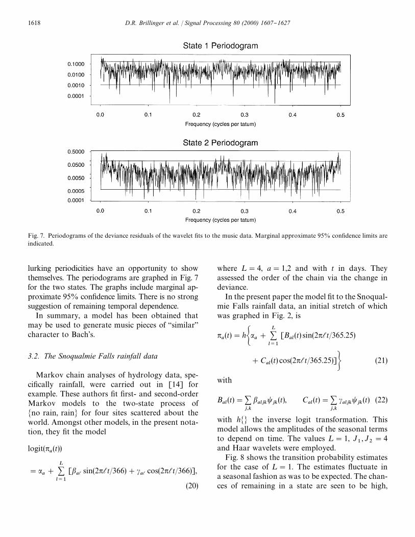
Fig. 7. Periodograms of the deviance residuals of the wavelet "ts to the music data. Marginal approximate 95% con"dence limits are

indicated.

lurking periodicities have an opportunity to show

themselves. The periodograms are graphed in Fig. 7

for the two states. The graphs include marginal ap-

proximate 95% con"dence limits. There is no strong

suggestion of remaining temporal dependence.

In summary, a model has been obtained that

may be used to generate music pieces of `similara

character to Bach's.

3.2. The Snoqualmie Falls rainfall data

Markov chain analyses of hydrology data, spe-

ci"cally rainfall, were carried out in [14] for

example. These authors "t "rst- and second-order

Markov models to the two-state process of

Mno rain, rainN for four sites scattered about the

world. Amongst other models, in the present nota-

tion, they "t the model

logit(pa(t))

"aa#

L+l/1

[bal

sin(2plt/366)#cal

cos(2plt/366)],

(20)

where ¸"4, a"1,2 and with t in days. They

assessed the order of the chain via the change in

deviance.

In the present paper the model "t to the Snoqual-

mie Falls rainfall data, an initial stretch of which

was graphed in Fig. 2, is

pa(t)"hGaa

#L+l/1

[Bal(t) sin(2plt/365.25)

#Cal(t) cos(2plt/365.25)]H (21)

with

Bal(t)"+

j,k

baljk

tjk

(t), Cal(t)"+

j,k

caljk

tjk

(t) (22)

with hMN the inverse logit transformation. This

model allows the amplitudes of the seasonal terms

to depend on time. The values ¸"1, J1, J

2"4

and Haar wavelets were employed.

Fig. 8 shows the transition probability estimates

for the case of ¸"1. The estimates #uctuate in

a seasonal fashion as was to be expected. The chan-

ces of remaining in a state are seen to be high,


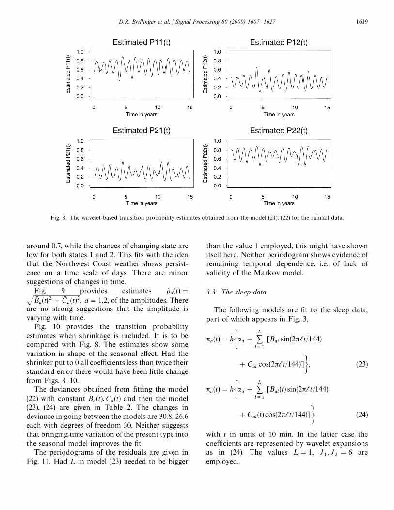
Fig. 8. The wavelet-based transition probability estimates obtained from the model (21), (22) for the rainfall data.

around 0.7, while the chances of changing state are

low for both states 1 and 2. This "ts with the idea

that the Northwest Coast weather shows persist-

ence on a time scale of days. There are minor

suggestions of changes in time.

Fig. 9 provides estimates o(a(t)"

JBKa(t)2#CK

a(t)2, a"1,2, of the amplitudes. There

are no strong suggestions that the amplitude is

varying with time.

Fig. 10 provides the transition probability

estimates when shrinkage is included. It is to be

compared with Fig. 8. The estimates show some

variation in shape of the seasonal e!ect. Had the

shrinker put to 0 all coe$cients less than twice their

standard error there would have been little change

from Figs. 8}10.

The deviances obtained from "tting the model

(22) with constant Ba(t),C

a(t) and then the model

(23), (24) are given in Table 2. The changes in

deviance in going between the models are 30.8, 26.6

each with degrees of freedom 30. Neither suggests

that bringing time variation of the present type into

the seasonal model improves the "t.

The periodograms of the residuals are given in

Fig. 11. Had ¸ in model (23) needed to be bigger

than the value 1 employed, this might have shown

itself here. Neither periodogram shows evidence of

remaining temporal dependence, i.e. of lack of

validity of the Markov model.

3.3. The sleep data

The following models are "t to the sleep data,

part of which appears in Fig. 3,

pa(t)"hGaa

#L+l/1

[Bal

sin(2plt/144)

#Cal

cos(2plt/144)]H, (23)

pa(t)"hGaa

#L+l/1

[Bal(t) sin(2plt/144)

#Cal(t) cos(2plt/144)]H (24)

with t in units of 10 min. In the latter case the

coe$cients are represented by wavelet expansions

as in (24). The values ¸"1, J1,J

2"6 are

employed.


Fig. 9. Wavelet-based estimates of the amplitude oa(t)"JB

a(t)2#C

a(t)2 of the model (23), (24) for the rainfall data. Marginal $2 s.e.

limits are included.

Fig. 10. The result of "tting the model (21), (22) and then applying shrinkage for the rainfall data.


Table 2

Deviances resulting from "tting the constant seasonal model

and the model (21), (22) to the rainfall data

ANODEV table

Source Deviance DF

Rain state 1

Constant coe$cient model 3001.6 2606


Rain state 2



Fig. 11. The periodogram of the deviance residuals for the rainfall data. Marginal approximate 95% con"dence intervals are indicated.

Fig. 12 provides the estimated transition prob-

abilities based directly on the maximum-likelihood

estimates of model (24), (26). The 24 h period of the

"tted probabilities is clear. Also it is apparent that

the child tends to remain asleep or awake with high

probabilities. Fig. 13 presents the wavelet-based

estimates of time-varying amplitudes of the sine

and cosine terms, oa(t)"JB

a(t)2#C

a(t)2. No

evidence of substantial nonstationarity appears.

Fig. 14 provides the results of shrinking the

estimates towards the constant coe$cient estimates

after "tting the time varying amplitude model. The

results are of more regular appearance.

The deviances found are listed in Table 3. The

changes in deviance involved in moving from the

constant coe$cient to the time-varying model are

24.8 and 18.5, respectively, each with 30 degrees of

freedom. Neither provides any evidence for the

necessity of inclusion of time varying coe$cients,

Ba,C

a. Nor do the periodograms of Fig. 15 suggest

remaining temporal dependence or that ¸ in

the model should be increased from the value 1

employed.

4. Discussion

In the work practical experience has been gained

with wavelet-based models and shrinkage estimates

for Markov chain data. In particular a variety of

departures from stationarity have had an oppor-

tunity to show themselves. The Markov assump-

tion is basic to the analysis. The reasonableness

of this has been con"rmed by examining the


Fig. 12. Wavelet-based transition probability estimates obtained for the period 24 h sleep model.

Fig. 13. Wavelet-based estimates of the amplitudes, oa(t), of the period 24 components of the sleep data. Marginal $2 s.e. limits are

included.


Fig. 14. The results of "tting the model (24) to the sleep data and then applying shrinkage.

Fig. 15. Periodograms of the residuals of the "t of the sleep model. Also included are marginal approximate 95% con"dence limits.


Fig. 16. The results of employing the sombrero function in estimating the transition probabilities for the main data.

Fig. 17. The estimated amplitudes for the linear predictor when the sombrero function is employed.

periodogram of residuals appropriate to the binary

nature of the data.

The initial estimates computed were maximum

likelihood, but in an attempt to improve upon them

marginal shrinkage has been employed. Covariates

were included in the analyses with no di$culty.

Haar wavelets were employed, because of simpli-

city of interpretation and to search for abrupt


Table 3

Deviances obtained when modeling the sleep data

ANODEV table

Source Deviance DF

Sleep state 1



Sleep state 2



changes. We have examined the e!ect of employing

smoother families of orthonormal wavelets and of

nonorthogonal regular functions. In particular,

"gures similar to Fig. 8 were obtained for the rain-

fall data using the S8 (symmlet) wavelet (which

generates a compactly supported orthonormal sys-

tem) and the Mexican hat (which generates

a nonorthogonal system). Apart from the fact that

the "gures become smooth, there are no changes in

conclusions. (See Figs. 16 and 17.)

The examples presented are all for the case of

a process with two states, but extensions to the

higher-order case are immediate. Extensions to

chain-type processes remembering further back in

time have also been also indicated.

Acknowledgements

We thank Peter Guttorp for providing the

Snoqualmie Falls data and Luiz Menna-Barreto

for providing the sleep data. The work was sup-

ported in part by the NSF Grants DMS-9625774

and INT-9600251, the CNPq Grant 910011/96-6

and the FAPESP Grant 97/11631-7.

Appendix

The computations needed in the work may be

carried out via programs such as Splus or Glim,

developed for generalized linear models and in par-

ticular for the binomial case.

The estimates of the coe$cients are obtained by

maximizing criterion (5) having taken the function

h( ) ) of (19) to be

h(g)"exp(g)/(1#exp(g)),

i.e. the inverse logit. This type of estimate falls into

the category of the so-called generalized linear

model, see McCullagh and Nelder [32], Hastie and

Pregibon [25], Venables and Ripley [38]. This

model provides extensions of many of the basic

concepts of regression analysis. An important ex-

tension is of residual to deviance residual.

In the present setup there are deviance residuals

for states 1 and 2. The former is given by

dt"J2 sgnA

X11

(t)

X1(t)

!n(1(t)BCX11

(t) logX

11(t)

X1(t)n(

1(t)

#(X1(t)!X

11(t)) logA

X1(t)!X

11(t)

X1(t)(1!n(

1(t))BD

1@2.

Here log(0) is taken to be zero and n(1(t) is the

"tted value of the probability under the model.

State 2 residual deviances, et, are given by a similar

formula. The "nal deviance is given by

T+t/1

(d2t#e2

t).

The use of these quantities is in assessing the "t of

the model.

There is empirical evidence to suggest that the

"nal deviance has a distribution that is approxim-

ately s2 (chi-square) with ¹!p DF, where p is the

number of parameters estimated. Further likeli-

hood ratio theory indicates that changes of devi-

ance will be approximately s2 with DF the number

of null parameters added to the model.

Continuing, if the model is "tting well the values

d1, d

2,2, d

Tshould be approximately indepen-

dent. The alternative is some form of temporal

dependence. An e!ective way of picking up tem-

poral dependence is examining the periodogram.

The deviance residual periodogram is given by the

modulus squared Fourier transforms

1

2p¹ KT+t/1

dte~*jtK

2,

1

2p¹ KT+t/1

ete~*jtK

2.

In the case of (approximate) independence the ex-

pected values of these will be constant in frequency

j and the distributions s2 with 2 DF. This last may


be used to set approximate con"dence intervals in

the "gures. Examples are given in Section 3.

The estimates may be computed using the func-

tion glm( ) from Splus. For the binomial case, glm( )

takes data in the form of a two column matrix in

which a 1 in the "rst column and 0 in the second

denotes a success and a 0 in the "rst column and

1 in the second denotes a failure. In the case

of estimating, say n1(t), one sees from Eq. (5)

that X11

(t)"1 will be considered a success and

X12

(t)"1 will be considered a failure. However,

X21

(t)"1 and X22

(t)"1 are neither a success nor

a failure. The function glm( ) can handle this type of

situation by having 0 in both columns in the row

corresponding to time t. A problem arises when too

many such negligible rows occur. If, for example

one is using the function

tjk

(t)"G1, t

0)t(t

1,

!1, t1)t(t

2

and the rows corresponding to either times

t0

through t1, or t

1through t

2are negligible, then

the corresponding coe$cient b1jk

is not estimable.

Splus resolves this circumstance by assigning Not

Available (NA) to the estimate of b1jk

. This presents

a problem at the shrinkage step. In the examples

presented to resolve this problem wavelet terms

corresponding to NA estimates are removed from

the regression matrix and the glm( ) "t reinitiated.

References

[1] J.R. Benjamin, C.A. Cornell, Probability, Statistics and

Decision for Civil Engineers, McGraw-Hill, New York,

1970.

[2] A.T. Bharucha-Reid, Elements of the Theory of Markov

Processes and Their Applications, McGraw-Hill, New

York, 1960.

[3] P. Billingsley, Statistical Inference for Markov Processes,

University of Chicago Press, Chicago, 1961.

[4] J. Bilmes, Timing is of the essence, Masters Thesis, MIT,

1993.

[5] Y.M. Bishop, S.E. Fienberg, P.W. Holland, Discrete Multi-

variate Analysis, MIT Press, Cambridge, MA, 1975.

[6] D.M. Blow, F.H.C. Crick, The treatment of errors in the

isomorphous replacement method, Acta Crystalogr. 12

(1959) 794}802.

[7] D.R. Brillinger, Some river wavelets, Environmetrics

5 (1994) 211}220.

[8] D.R. Brillinger, Some uses of cumulants in wavelet analy-

sis, J. Nonparametr. Statist. 6 (1996) 93}114.

[9] D.R. Brillinger, R.A. Irizarry, An investigation of the sec-

ond- and higher-order spectra of music, Signal Process. 39

(1998) 161}179.

[10] A.G. Bruce, H.-Y. Gao, S# Wavelets: User's Manual,

StatSci, Seattle, WA, 1994.

[11] A.G. Bruce, H.-Y. Gao, Understanding waveshrink:

variance and bias estimation, Biometrika 83 (1996)

727}745.

[12] C. Chiann, Wavelet analysis in time series, Ph.D. Thesis,

University of Sa8 o Paulo, 1997 (in Portuguese).

[13] C. Chiann, P.A. Morettin, A wavelet analysis for time

series, J. Nonparametr. Statist. 10 (1998) 1}46.

[14] R. Coe, R.D. Stern, Fitting models to daily rainfall data, J.

Appl. Meteorol. 21 (1982) 1024}1031.

[15] M.S. Crouse, R.G. Baraniuk, Contextual hidden Markov

models for wavelet-domain signal processing, Proceedings

of the 31st Asilomar Conference on Signals, Systems and

Computers, IEEE Computer Society, 1998.

[16] I. Daubechies, Ten Lectures on Wavelets, SIAM, Philadel-

phia, 1992.

[17] D.L. Donoho, I.M. Johnstone, Ideal spatial adaptation by

wavelet shrinkage, Biometrika 81 (1994) 425}455.

[18] D.L. Donoho, I.M. Johnstone, Adapting to unknown

smoothness via wavelet shrinkage, J. Amer. Statist. Assoc.

90 (1995) 1200}1224.

[19] D.L. Donoho, I.M. Johnstone, Minimax estimation via

wavelet shrinkage, Ann. Statist. 26 (1998) 879}921.

[20] E.B. Dynkin, Markov Processes, Springer, Berlin, 1965.

[21] L. Fahrmeir, H. Kaufmann, Regression models for non-

stationary categorical time series, J. Time Ser. Anal.

8 (1987) 147}160.

[22] W. Feller, An Introduction to Probability Theory and Its

Applications, Wiley, New York, 1957.

[23] R.V. Foutz, R.C. Srivastava, Statistical inference for Mar-

kov processes when the model is incorrect, Adv. Appl.

Probab. 11 (1979) 737}749.

[24] P. Guttorp, Stochastic Modelling of Scienti"c Data, Chap-

man & Hall, London, 1995.

[25] T.J. Hastie, D. Pregibon, Generalized linear models, in:

J.M. Chambers, T.J. Hastie (Eds.), Statistical Models in S,

Wadsworth, Paci"c Grove, 1992, pp. 195}247.

[26] L. Hiller, L. Isaacson, Experimental Music, McGraw-Hill,

New York, 1959.

[27] R. Irizarry, Statistics and music: "tting a local harmonic

model to musical sound signals, Ph.D. Thesis, University

of California, Berkeley, 1998.

[28] K. Jones, Compositional applications of stochastic pro-

cesses, Comput. Music J. 5 (1981) 381}396.

[29] H. Kaufman, Regression models for nonstationary cat-

egorical time series: asymptotic estimation theory, Ann.

Statist. 15 (1987) 79}98.

[30] S. Mallat, A Wavelet Tour of Signal Processing, Academic

Press, San Diego, 1998.

[31] P. McCullagh, J.A. Nelder, Generalized Linear Models,

2nd Edition, Chapman & Hall, London, 1989.


[32] L. Mello, A. Isola, F. Louzada, L. Menna-Barreto, A four-

year follow-up study of the sleep-wake cycle of an infant,

Biol. Rhythm Res. 27 (1996) 291}298.

[33] P.A. Morettin, Wavelets in statistics, Reviews of the Insti-

tute of Mathematics and Statistics, University of Sa8 oPaulo, Vol. 3, 1997, pp. 211}272.

[34] G.P. Nason, Wavelet function estimation using cross-

validation, in: A. Antoniadis, G. Oppenheim (Eds.),

Wavelets and Statistics, Springer, New York, 1993, pp.

261}280.

[35] Y. Ogata, Maximum likelihood estimates of incorrect

Markov models for time series and the derivation of AIC,

J. Appl. Probab. 17 (1980) 59}72.

[36] R. Pinkerton, Information theory and melody, Sci. Amer.

194 (1956) 77}84.

[37] J.W. Tukey, Introduction to the dilemmas and di$culties

of regression, Report, Statistics Department, Princeton

University, 1979.

[38] W.N. Venables, B.D. Ripley, Modern Applied Statistics

with SPLUS, 2nd Edition, Springer, New York, 1997.


Some wavelet-based analyses of Markov chain databrill/Papers/markov.pdf · Insbesondere scheint die Methode nuKtzlich zu sein, um abrupte oder stetige AGnderungenin derStrukturvon

Documents