Some Useful Distributions. Binomial Distribution k=0:20; y=binopdf(k,20,0.5); stem(k,y) Bernoulli1720 k=0:20; y=binocdf(k,20,0.5); stairs(k,y) grid on.

Some Useful Distributions

Binomial Distribution

k=0:20;

y=binopdf(k,20,0.5);

stem(k,y)

( ) (1 ) , 0,1,...,k n knp k p p k n

k-

æö÷ç ÷= - =ç ÷ç ÷çè ø

2 (1 )np np pm s= = -

20 0.5n p= =

Bernoulli 1720

k=0:20;

y=binocdf(k,20,0.5);

stairs(k,y)

grid on

Binomial Distribution

function y=mybinomial(n,p)

for k=0:n

y(k+1)=factorial(n)/(factorial(k)*factorial(n-k))*p^k*(1-p)^(n-k)

end

k=0:20;

y=mybinomial(20,0.5);

stem(k,y)

k=0:20;

y=binopdf(k,20,0.1);

stem(k,y)

20 0.5n p= = 20 0.1n p= =

Geometric Distribution

k=0:20;

y=geopdf(k,0.5);

stem(k,y)

1( ) (1 ) , 1,2,...kp k p p k-= - =

22

1 1 p

p pm s

-= =

0.5p=

k=0:20;

y=geocdf(k,0.5);

stairs(k,y)

axis([0 20 0 1])

( ) (1 ) , 0,1,2,...kp k p p k= - =

Warning: Matlab assumes

Geometric Distribution

k=1:20;

y=mygeometric(20,0.5);

stem(k,y)

k=1:20;

y=mygeometric(20,0.1);

stem(k,y)

function y=mygeometric(n,p)

for k=1:n

y(k)=(1-p)^(k-1)*p;

end

0.5p= 0.1p=

Poisson Distribution

k=0:20;

y=poisspdf(k,5);

stem(k,y)

( ) , 0,1,...!

k

p k e kk

ll -= =

2m l s l= =

k=0:20;

y=poisscdf(k,5);

stem(k,y)

grid on

5l =

Poisson 1837

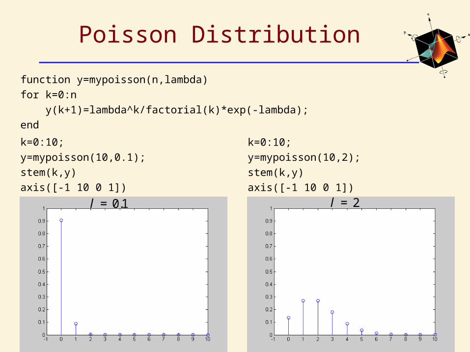
Poisson Distribution

k=0:10;

y=mypoisson(10,0.1);

stem(k,y)

axis([-1 10 0 1])

function y=mypoisson(n,lambda)

for k=0:n

y(k+1)=lambda^k/factorial(k)*exp(-lambda);

end

0.1l =

k=0:10;

y=mypoisson(10,2);

stem(k,y)

axis([-1 10 0 1])

2l =

Uniform Distribution

1( ) ,f x a x b

b a= £ £

-2

2 ( )

2 12

a b b am s

+ -= =

x=0:0.1:8;

y=unifpdf(x,2,6);

plot(x,y)

axis([0 8 0 0.5])

x=0:0.1:8;

y=unifcdf(x,2,6);

plot(x,y)

axis([0 8 0 2])

Normal Distribution

Gauss 18202

2

( )

21

( ) ,2

x

f x e xm

s

ps

--

= - ¥ < <¥

x=0:0.1:20;

y=normpdf(x,10,2);

plot(x,y)

2( , )N ms

x=0:0.1:20;

y=normcdf(x,10,2);

plot(x,y)

(10,4)N

Warning: Matlab uses ( , )N ms

Normal Distribution

x=-6:0.1:6;

y1=mynormal(x,0,1);

y2=mynormal(x,0,4);

plot(x,y1,x,y2,'r');

legend('N(0,1)','N(0,4)')

function y=mynormal(x,mu,sigma2)

y=1/sqrt(2*pi*sigma2)*exp(-(x-mu).^2/(2*sigma2));

Exponential Distribution

( ) , 0xf x e xll -= £ <¥

22

1 1m s

l l= =

2l =

x=0:0.1:5;

y=exppdf(x,1/2);

plot(x,y)

Warning: Matlab assumes1

( ) , 0f x e xcl

l

-= £ <¥

x=0:0.1:5;

y=expcdf(x,1/2);

plot(x,y)

Exponential Distribution

function y=myexp(x,lambda)

y=lambda*exp(-lambda*x);

x=0:0.1:10;

y1=myexp(x,2);

y2=myexp(x,0.5);

plot(x,y1,x,y2,'r')

legend('lampda=2','lambda=0.5')

Rayleigh Distribution

2

222

( ) , 0xx

f x e xs

s

-= ³

2 222 2

p pm s s s

æ ö÷ç= = - ÷ç ÷÷çè ø

x=0:0.1:10;

y1=raylpdf(x,1);

y2=raylpdf(x,2);

plot(x,y1,x,y2,'r')

legend('sigma=1','sigma=2')

Poisson Approximation to Binomial

n=100;

p=0.1;

lambda=10;

k=0:n;

y1=mybinomial(n,p);

y2=mypoisson(n,lambda);

stem(k,y1)

hold on

stem(k,y2,’r’)

1 1n p np l=? =

(1 )!

kk n knp p e

k kll- -

æö÷ç ÷ -ç ÷ç ÷çè ø;

Normal Approximation to Binomial

2( )

2 (1 )1[ ] (1 )

2 (1 )

k npk n k np pn

P X k p p ek np pp

--

- -æö÷ç ÷= = -ç ÷ç ÷çè ø -

;

DeMoivre – Laplace Theorem 1730

(1 )

X npZ

np p

-=

-If X is a binomial RV is approximately a

standard normal RV

A better approximation

2

1

2 11 2[ ] (1 )

(1 ) (1 )

kk n k

k k

n k np k npP k X k p p

k np p np p-

=

æ ö æ öæö - -÷ ÷ç ç÷ç ÷ ÷ç ç÷£ £ = - F - Fç ÷ ÷÷ ç çç ÷ ÷÷ç ÷ ÷ç çç çè ø - -è ø è øå ;

2 11 2

0.5 0.5[ ]

(1 ) (1 )

k np k npP k X k

np p np p

æ ö æ ö+ - - -÷ ÷ç ç÷ ÷ç ç£ £ F - F÷ ÷ç ç÷ ÷÷ ÷ç çç ç- -è ø è ø;

Normal Approximation to Binomial

10

0.5

n

p

=

=

30

0.5

n

p

=

=

function normbin(n,p)

clf

y1=mybinomial(n,p);

k=0:n;

bar(k,y1,1,'w')

hold on

x=0:0.1:n;

y2=mynormal(x,n*p,n*p*(1-p));

plot(x,y2,'r')

Central Limit Theorem

function k=clt(n) % Central Limit Theorem for sum of dies

m=(1+6)/2; % mean (a+b)/2

s=sqrt(35/12); % standart deviation sqrt(((b-a+1)^2-1)/12)

for i=1:n

x(i,:)=floor(6*rand(1,10000)+1);

end

for i=1:length(x(1,:)) % sum of n dies

y(i)=sum(x(:,i));

z(i)=(sum(x(:,i))-n*m)/(s*sqrt(n));

end

subplot(2,1,1)

hist(y,100)

title('unormalized')

subplot(2,1,2)

hist(z,100)

title('normalized')

Central Limit Theorem

1n=

2n=

3.52

a bm

+= =

22 ( 1) 1

2.9212

b as

- + -= =

1

n

ii

unormalized X=

=å

1

n

ii

X nnormalized

n

m

s=

-=å

Central Limit Theorem

10n=

5n=