HAL Id: tel-01223251 https://tel.archives-ouvertes.fr/tel-01223251 Submitted on 2 Nov 2015 HAL is a multi-disciplinary open access archive for the deposit and dissemination of sci- entific research documents, whether they are pub- lished or not. The documents may come from teaching and research institutions in France or abroad, or from public or private research centers. L’archive ouverte pluridisciplinaire HAL, est destinée au dépôt et à la diffusion de documents scientifiques de niveau recherche, publiés ou non, émanant des établissements d’enseignement et de recherche français ou étrangers, des laboratoires publics ou privés. Some results on backward equations and stochastic partial differential equations with singularities Lambert Piozin To cite this version: Lambert Piozin. Some results on backward equations and stochastic partial differential equations with singularities. Analysis of PDEs [math.AP]. Université du Maine, 2015. English. NNT : 2015LEMA1004. tel-01223251

Welcome message from author
This document is posted to help you gain knowledge. Please leave a comment to let me know what you think about it! Share it to your friends and learn new things together.
Transcript
HAL Id: tel-01223251https://tel.archives-ouvertes.fr/tel-01223251
Submitted on 2 Nov 2015
HAL is a multi-disciplinary open accessarchive for the deposit and dissemination of sci-entific research documents, whether they are pub-lished or not. The documents may come fromteaching and research institutions in France orabroad, or from public or private research centers.
L’archive ouverte pluridisciplinaire HAL, estdestinée au dépôt et à la diffusion de documentsscientifiques de niveau recherche, publiés ou non,émanant des établissements d’enseignement et derecherche français ou étrangers, des laboratoirespublics ou privés.
Some results on backward equations and stochasticpartial differential equations with singularities
Lambert Piozin
To cite this version:Lambert Piozin. Some results on backward equations and stochastic partial differential equationswith singularities. Analysis of PDEs [math.AP]. Université du Maine, 2015. English. NNT :2015LEMA1004. tel-01223251
UNIVERSITÉ DU MAINE - LE MANS
ECOLE DOCTORALE: STIMSCIENCES, TECHNOLOGIES DE l’INFORMATION
ET MATHEMATIQUES
THESEpour obtenir le titre de
Docteur de l’université du Maine
Specialité : Mathématiques appliquées
Soutenue par
Lambert Piozin
Quelques résultats sur les équationsrétrogrades et équations aux dérivées
partielles stochastiques avecsingularités.
Directeur de Thèse: Anis Matoussi
Co-directeur de Thèse: Alexandre Popier
preparée à l’université du Maine
Jury:
Directeur: Anis Matoussi - Université du MaineCo-directeur: Alexandre Popier - Université du Maine
Rapporteurs: Philippe Briand - Université de SavoieBruno Saussereau - Université de Besançon
Examinateurs: Romuald Elie - Université Paris-Est Marne-la-ValléeSaïd Hamadène - Université du Maine

i
Remerciements
Je voudrais remercier ici toutes les personnes qui ont su de quelque manière que ce soit m’aider,m’encourager ou m’influencer positivement dans l’accomplissement de cette thèse.
Je tiens donc à remercier chaleureusement Anis Matoussi et Alexandre Popier, pour avoird’abord réussi tant bien que mal à supporter mon caractère si singulier (maudits INTJ!). Maisaussi et surtout pour leurs inombrables conseils, leur écoute attentionnée et leur patience quasiinépuisable à mon égard. C’est une chance unique d’avoir pu travailler à leurs côtés et uneexpérience profondément enrichissante.
Je suis très sincèrement honoré que Philippe Briand et Bruno Saussereau aient accepté d’êtrerapporteurs, je les en remercie vivement. Je suis très reconnaissant également à l’encontre de Ro-muald Elie et Saïd Hamadène pour avoir bien voulu participer à ce jury en tant qu’examinateurs.
Mes remerciements vont également à l’ensemble de l’équipe du Laboratoire Manceau deMathématiques pour leur accueil. Pour avoir enseigné à leur côtés et disposé de leurs précieuxconseils, je tiens à citer: Ivan Suarez, Alexandre Brouste, Samir Ben Hariz, Sylvain Maugeaiset Gérard Leloup. Je voudrais aussi témoigner ma sympathie à l’égard de mes collègues debureau, doctorants et anciens doctorants: Ali, Achref, Fanny, Maroua, Samvel, Anastasiia,Rym, Arij, Wissal, Lin, Xuzhe, Rui, Chunhao. Pour leur aide quant à l’organisation au quoti-dien de la vie du laboratoire et pour leur sympathie, je remercie Brigitte Bougard et Irène Croset.
Je souhaite remercier infiniment ces enseignants de l’université Paris Dauphine qui réalisent untravail pédagogique d’une qualité inouïe. Pour leurs sympathie, leur patience et pour avoir étéune réelle source de motivation et d’inspiration pour moi ainsi que pour bien d’autres, je tiens àciter: Olivier Glass, Massimiliano Gubinelli, Nicolas Forcadel, Filippo Santambrogio, GuillaumeCarlier, Anne-Marie Boussion, Bruno Bouchard, Romuald Elie, Imen Ben Tahar, Rémi Rhodes,Cyril Imbert, Eric Séré, Bruno Nazaret, Jimmy Lamboley, Joseph Lehec, et Guillaume Legendre.
Je voudrais exprimer toute ma sympathie pour les divers doctorants et anciens doctorantsrencontrés au cours des différents séminaires et colloques, pour leur intelligence, leur gentillesseet leur convivialité, je pense entre autres à: Dylan Possamaï, Nabil Kazi-Tani, Chao Zhou,Sébastien Choukroun, Romain Bompis, Guillaume Royer et Julien Grepat. Je tiens en particulierà témoigner de ma profonde gratitude envers Dylan et Chao, travailler à leurs côtés fut un réelplaisir.
Enfin pour leur soutien constant et leur capacité à me faire oublier n’importe quel tracas duquotidien, je remercie ma famille ainsi que mes amis: Thomas S., Edouard, Quentin, MatthieuA., Yann, Julien, Laurent, Matthieu G., Florian, Thomas M. pour ne citer que les plus proches.

ii
Résumé
Cette thèse est consacrée à l’étude de quelques problèmes dans le domaine des équations dif-férentielles stochastiques rétrogrades (EDSR), et leurs applications aux équations aux dérivéespartielles (EDP) et à la finance.
Les deux premiers chapitres sont dédiés aux EDSR avec condition terminale singulière. Cetype d’équations a été introduit par Popier dans [83], et pose le problème de l’existence desolutions d’EDSR lorsque la condition terminale peut prendre la valeur +∞ sur un ensemblede mesure non négligeable. Dans le premier chapitre, nous introduisons la notion d’équationdifférentielle doublement stochastique rétrograde (EDDSR) avec condition terminale singulière.Un premier travail consistera à étudier les EDDSR avec générateur monotone. Nous obtenonsensuite un résultat d’existence par un schéma d’approximation en considérant une troncaturede la condition terminale. On peut vérifier assez aisément que le processus limite construit ainsisatisfait la dynamique qui nous intéresse, et possède les bonnes propriétés d’intégration sur desintervalles du type [0, T − δ]. En revanche la continuité en T est plus problématique, et estobtenue par deux méthodes différentes selon les valeurs de q. La dernière partie de ce chapitrevise à établir le lien avec les équations aux dérivées partielles stochastiques (EDPS), en utilisantl’approche de type solution faible développée par Bally, Matoussi in [6].
Le second chapitre est dédié aux EDSR avec condition terminale singulière et sauts. Comme dansle chapitre précédent la partie délicate sera de prouver la continuité en T . Nous formulons desconditions suffisantes sur les sauts de la diffusion afin d’obtenir cette dernière. Une section est en-suite vouée à établir le lien entre solution minimale de l’EDSR et équations intégro-différentielles.
Enfin un dernier chapitre est consacré aux équations différentielles stochastiques rétrogradesdu second ordre (2EDSR) doublement réfléchies. Nous avons cherché à établir l’existence etl’unicité de telles équations en suivant une approche identique à celle développée dans [89] et[90] par Soner, Touzi et Zhang. Pour ce faire, il nous a fallu dans un premier temps nousconcentrer sur le problème de réflexion par barrière supérieure des 2EDSR. Ce travail se situedans la continuité du papier [66], où Matoussi, Possamaï et Zhou considèrent le problèmede la réflexion par barrière inférieure. Contrairement aux EDSR classiques, le caractère nonlinéaire propre aux 2EDSR rend le problème de réflexion non symétrique. Nous traitons ceproblème essentiellement sous l’hypothèse que la barrière supérieure est une semi-martingaledont le processus à variation finie admet une décomposition de Jordan. Nous avons ensuitecombiné ces résultats à ceux développés dans [66] afin de donner une définition et un cadre aux2EDSR doublement réfléchies. L’unicité est établie comme conséquence directe d’une propriétéde représentation. L’existence est obtenue en utilisant les espaces shiftés, et les distributionsde probabilité conditionnelles régulières. Enfin une partie application aux jeux de Dynkin etoptions Israéliennes sous incertitude est traitée dans la dernière section.
Mots-clés: équations différentielles stochastiques rétrogrades du second ordre, analyse stochas-tique quasi-sûre, jeux de Dynkin sous incertitude, équations différentielles doublement stochas-tiques rétrogrades, condition terminale singulière, équations aux dérivées partielles stochastiques,solutions de viscosité, équations différentielles stochastiques rétrogrades avec sauts, équationsintégro-différentielles.

iii
Abstract
This thesis is devoted to the study of some problems in the field of backward stochastic differen-tial equations (BSDE), and their applications to partial differential equations (PDE) and finance.
The two first chapters are dedicated to BSDE with singular terminal conditions. This kind ofequations has been introduced by Popier in [83], and put forward the problem of existence ofBSDE solutions when the terminal condition is allowed to take the value +∞ on a non-negligibleset. In the first chapter, we introduce the notion of backward doubly stochastic differentialequations (BDSDE) with singular terminal condition. A first work consists in studying thecase of BDSDE with monotone generator. We then obtain existing result by an approximatingscheme built considering a truncation of the terminal condition. We can easily verify thatthe limit process obtained satisfy the dynamic we are interested in, and possess the goodintegrability properties on all intervals of type [0, T − δ]. On the other hand continuity in T ismore problematic and is proved with two different methods according to q values. The last partof this chapter aim to establish the link with stochastic partial differential equations (SPDE),using a weak solution approach developed by Bally, Matoussi in [6].
The second chapter is devoted to the BSDEs with singular terminal conditions and jumps.As in the previous chapter the tricky part will be to prove continuity in T . We formulatesufficient conditions on the jumps in order to obtain it. A section is then dedicated to establisha link between a minimal solution of our BSDE and partial integro-differential equations (PIDE).
A last chapter is dedicated to doubly reflected second order backward stochastic differentialequations (2DRBSDE). We have been looking to establish existence and uniqueness for suchequations by following a similar approach developed by Soner, Touzi and Zhang in [89], [90]. Inorder to obtain this, we had to focus first on the upper reflection problem for 2BSDEs. This workis the continuity of [66], where Matoussi, Possamaï and Zhou considered the lower reflectionproblem. Unlike classical BSDEs, the non-linearity nature of 2BSDE make this problem nonsymmetrical. We treat this problem essentially under the hypothesis that the upper barrier isa semi-martingale whose finite variation process admits a Jordan decomposition. We combinedthen these results to those obtained in [66] to give a definition and a wellposedness context to2DRBSDE. Uniqueness is established as a straight consequence of a representation property.Existence is obtained using shifted spaces, and regular conditional probability distributions. Alast part is then consecrated to the link with some Dynkin games and Israeli options underuncertainty.
Keywords: second order backward stochastic differential equations, quasi-sure stochastic anal-ysis, Dynkin games with uncertainty, backward doubly stochastic differential equations, singu-lar terminal conditions, stochastic partial differential equations, viscosity solutions, backwardstochastic differential equations with jumps, partial-integral differential equations.

Contents
1 Introduction 11.1 BSDEs with singular terminal condition, SPDEs and PIDEs . . . . . . . . . . . . 2
1.1.1 BDSDEs and SPDEs . . . . . . . . . . . . . . . . . . . . . . . . . . . . . . 21.1.2 BSDEs with jumps and PIDEs . . . . . . . . . . . . . . . . . . . . . . . . 31.1.3 BSDEs with singular terminal condition . . . . . . . . . . . . . . . . . . . 31.1.4 Motivation, formulation of the problem . . . . . . . . . . . . . . . . . . . . 51.1.5 Contributions to BDSDEs . . . . . . . . . . . . . . . . . . . . . . . . . . . 71.1.6 Contributions to BSDEs with jumps . . . . . . . . . . . . . . . . . . . . . 111.1.7 Perspectives . . . . . . . . . . . . . . . . . . . . . . . . . . . . . . . . . . . 14
1.2 2DBSDEs and related game options . . . . . . . . . . . . . . . . . . . . . . . . . 151.2.1 RBSDEs, DRBSDEs and applications . . . . . . . . . . . . . . . . . . . . 151.2.2 2BSDEs . . . . . . . . . . . . . . . . . . . . . . . . . . . . . . . . . . . . . 161.2.3 Motivation . . . . . . . . . . . . . . . . . . . . . . . . . . . . . . . . . . . 171.2.4 Main results . . . . . . . . . . . . . . . . . . . . . . . . . . . . . . . . . . . 18
2 SPDE with singular terminal condition 272.1 Setting and main results . . . . . . . . . . . . . . . . . . . . . . . . . . . . . . . . 292.2 Monotone BDSDE . . . . . . . . . . . . . . . . . . . . . . . . . . . . . . . . . . . 33
2.2.1 Case with f(t, y, z) = f(t, y) and g(t, y, z) = gt . . . . . . . . . . . . . . . 332.2.2 General case . . . . . . . . . . . . . . . . . . . . . . . . . . . . . . . . . . 382.2.3 Extension, comparison result . . . . . . . . . . . . . . . . . . . . . . . . . 40
2.3 Singular terminal condition, construction of a minimal solution . . . . . . . . . . 412.3.1 Approximation . . . . . . . . . . . . . . . . . . . . . . . . . . . . . . . . . 412.3.2 Existence of a limit at time T . . . . . . . . . . . . . . . . . . . . . . . . . 462.3.3 Minimal solution . . . . . . . . . . . . . . . . . . . . . . . . . . . . . . . . 49
2.4 Limit at time T by localization technic . . . . . . . . . . . . . . . . . . . . . . . . 512.4.1 Proof of (2.4.31) if q > 2 . . . . . . . . . . . . . . . . . . . . . . . . . . . . 532.4.2 Proof of (2.4.31) if q ≤ 2 . . . . . . . . . . . . . . . . . . . . . . . . . . . . 55
2.5 Link with SPDE’s . . . . . . . . . . . . . . . . . . . . . . . . . . . . . . . . . . . 59
3 BSDE with jumps and PIDE with singular terminal condition 653.1 Introduction . . . . . . . . . . . . . . . . . . . . . . . . . . . . . . . . . . . . . . . 653.2 Setting, construction of the minimal solution . . . . . . . . . . . . . . . . . . . . 663.3 Behaviour of Y at time T . . . . . . . . . . . . . . . . . . . . . . . . . . . . . . . 73
3.3.1 Existence of the limit . . . . . . . . . . . . . . . . . . . . . . . . . . . . . 733.3.2 Continuity at time T for q > 2 . . . . . . . . . . . . . . . . . . . . . . . . 75
3.4 Link with PIDE . . . . . . . . . . . . . . . . . . . . . . . . . . . . . . . . . . . . . 813.4.1 Existence of a viscosity solution with singular data . . . . . . . . . . . . . 833.4.2 Minimal solution . . . . . . . . . . . . . . . . . . . . . . . . . . . . . . . . 873.4.3 Regularity of the minimal solution . . . . . . . . . . . . . . . . . . . . . . 90
vi Contents
4 Second-order BSDEs with general reflection and game options under uncer-tainty 934.1 Introduction . . . . . . . . . . . . . . . . . . . . . . . . . . . . . . . . . . . . . . . 934.2 Definitions and Notations . . . . . . . . . . . . . . . . . . . . . . . . . . . . . . . 94
4.2.1 The stochastic framework . . . . . . . . . . . . . . . . . . . . . . . . . . . 944.2.2 Generator and measures . . . . . . . . . . . . . . . . . . . . . . . . . . . . 954.2.3 Quasi-sure norms and spaces . . . . . . . . . . . . . . . . . . . . . . . . . 964.2.4 Obstacles and definition . . . . . . . . . . . . . . . . . . . . . . . . . . . . 974.2.5 DRBSDEs as a special case of 2DRBSDEs . . . . . . . . . . . . . . . . . . 100
4.3 Uniqueness, estimates and representations . . . . . . . . . . . . . . . . . . . . . . 1004.3.1 A representation inspired by stochastic control . . . . . . . . . . . . . . . 1004.3.2 A priori estimates . . . . . . . . . . . . . . . . . . . . . . . . . . . . . . . 1014.3.3 Some properties of the solution . . . . . . . . . . . . . . . . . . . . . . . . 106
4.4 A constructive proof of existence . . . . . . . . . . . . . . . . . . . . . . . . . . . 1104.4.1 Shifted spaces . . . . . . . . . . . . . . . . . . . . . . . . . . . . . . . . . . 1104.4.2 A first existence result when ξ is in UCb(Ω) . . . . . . . . . . . . . . . . 1114.4.3 Main result . . . . . . . . . . . . . . . . . . . . . . . . . . . . . . . . . . . 115
4.5 Applications: Israeli options and Dynkin games . . . . . . . . . . . . . . . . . . . 1164.5.1 Game options . . . . . . . . . . . . . . . . . . . . . . . . . . . . . . . . . . 1164.5.2 A first step towards Dynkin games under uncertainty . . . . . . . . . . . . 118
4.6 Appendix: Doubly reflected g-supersolution and martingales . . . . . . . . . . . . 1204.6.1 Definitions and first properties . . . . . . . . . . . . . . . . . . . . . . . . 1214.6.2 Doob-Meyer decomposition . . . . . . . . . . . . . . . . . . . . . . . . . . 1234.6.3 Time regularity of doubly reflected g-supermartingales . . . . . . . . . . . 127
Bibliography 129
Chapter 1
Introduction
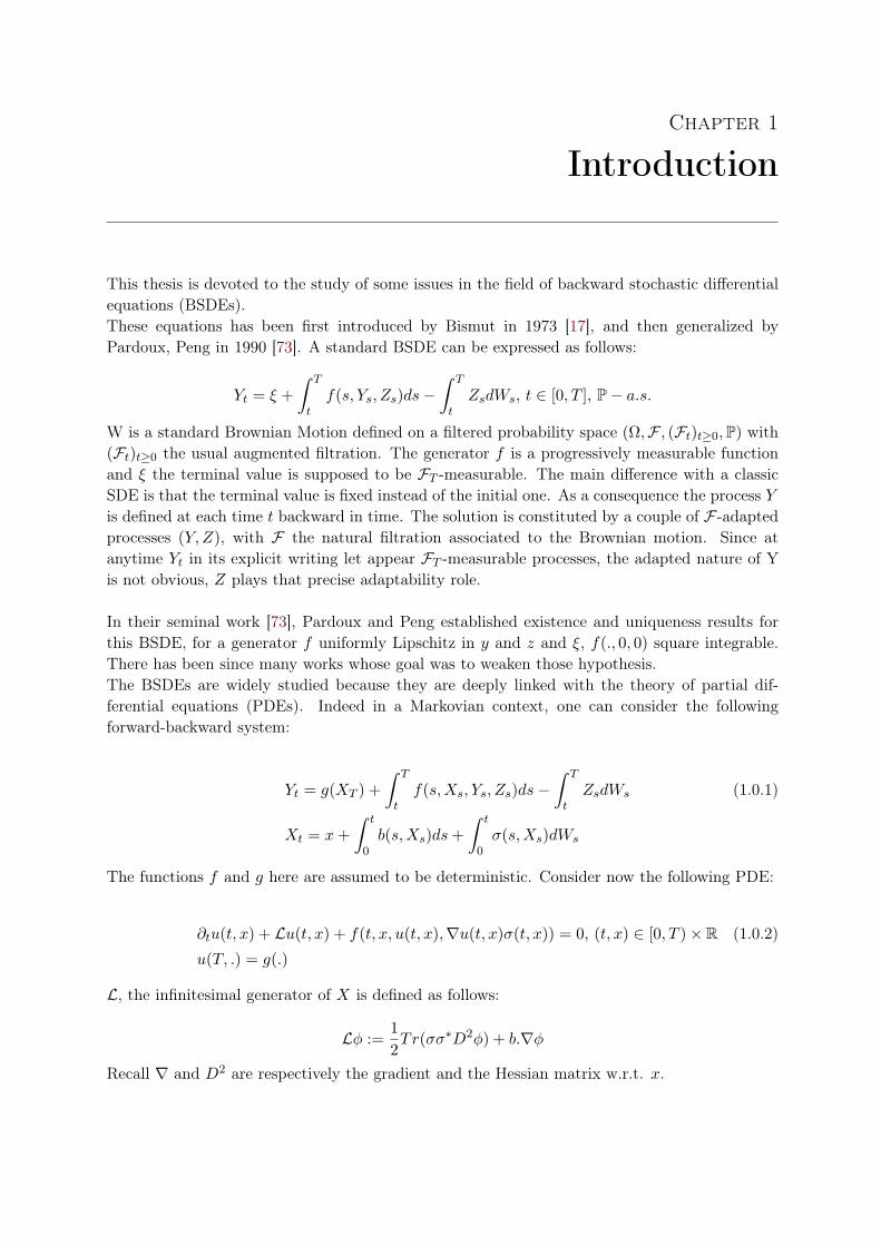
This thesis is devoted to the study of some issues in the field of backward stochastic differentialequations (BSDEs).These equations has been first introduced by Bismut in 1973 [17], and then generalized byPardoux, Peng in 1990 [73]. A standard BSDE can be expressed as follows:
Yt = ξ +∫ T
tf(s, Ys, Zs)ds−
∫ T
tZsdWs, t ∈ [0, T ], P− a.s.
W is a standard Brownian Motion defined on a filtered probability space (Ω,F , (Ft)t≥0,P) with(Ft)t≥0 the usual augmented filtration. The generator f is a progressively measurable functionand ξ the terminal value is supposed to be FT -measurable. The main difference with a classicSDE is that the terminal value is fixed instead of the initial one. As a consequence the process Yis defined at each time t backward in time. The solution is constituted by a couple of F-adaptedprocesses (Y, Z), with F the natural filtration associated to the Brownian motion. Since atanytime Yt in its explicit writing let appear FT -measurable processes, the adapted nature of Yis not obvious, Z plays that precise adaptability role.
In their seminal work [73], Pardoux and Peng established existence and uniqueness results forthis BSDE, for a generator f uniformly Lipschitz in y and z and ξ, f(., 0, 0) square integrable.There has been since many works whose goal was to weaken those hypothesis.The BSDEs are widely studied because they are deeply linked with the theory of partial dif-ferential equations (PDEs). Indeed in a Markovian context, one can consider the followingforward-backward system:
Yt = g(XT ) +∫ T
tf(s,Xs, Ys, Zs)ds−
∫ T
tZsdWs (1.0.1)
Xt = x+∫ t
0b(s,Xs)ds+
∫ t
0σ(s,Xs)dWs
The functions f and g here are assumed to be deterministic. Consider now the following PDE:
∂tu(t, x) + Lu(t, x) + f(t, x, u(t, x),∇u(t, x)σ(t, x)) = 0, (t, x) ∈ [0, T )× R (1.0.2)
u(T, .) = g(.)
L, the infinitesimal generator of X is defined as follows:
Lφ :=12Tr(σσ∗D2φ) + b.∇φ
Recall ∇ and D2 are respectively the gradient and the Hessian matrix w.r.t. x.
2 Chapter 1. Introduction
Then a simple application of Itô formula shows that if u is a strong solution to the PDE1.0.2, then (Yt, Zt) := (u(t,Xt),∇u(t,Xt)σ(t,Xt)) provides a solution to the BSDE 1.0.1. Thisprobabilistic representation of the PDE allows one, finally to use probabilistic methods toget numerical simulations of PDE solutions. Note that through this representation we get aconstraint on the class of PDE associated to a classical BSDE: one can only get this link withquasi-linear PDE. These equations appear naturally in many problems in finance, for a morecomplete overview regarding BSDEs and their applications, we refer the reader to the books[28], [34], [63] and [76].
This thesis will be structured as follows: the two first chapters are devoted to singular terminalcondition BSDEs, once in a doubly stochastic framework and then considering BSDEs withjumps. A third chapter is dedicated to the issue of doubly reflected 2BSDEs.
1.1 BSDEs with singular terminal condition, SPDEs and PIDEs
1.1.1 BDSDEs and SPDEs
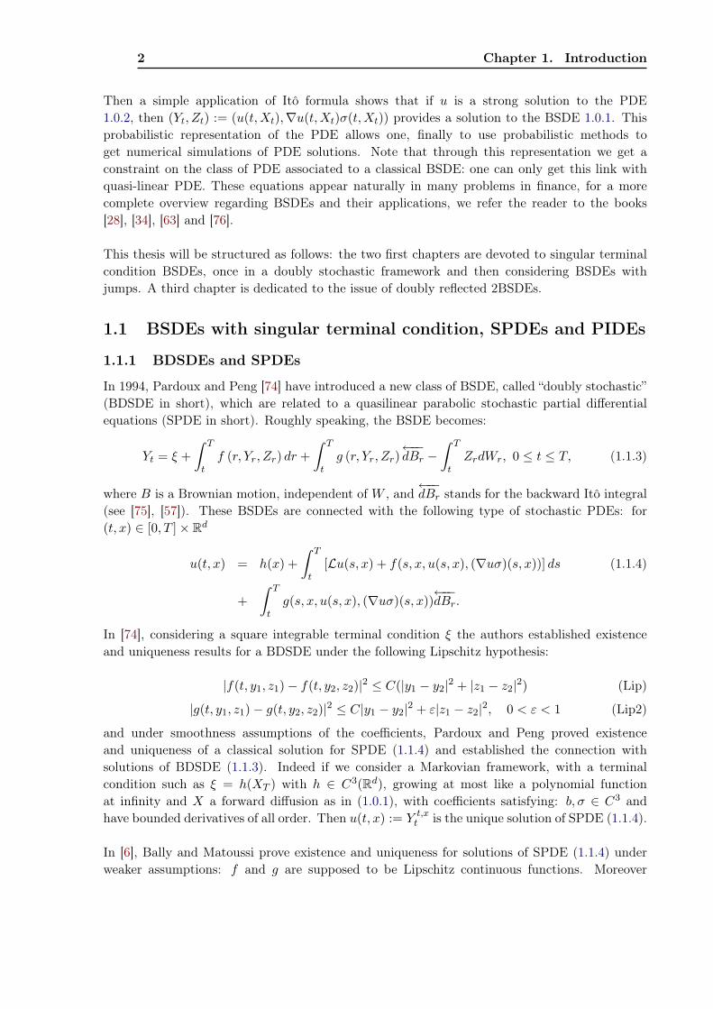
In 1994, Pardoux and Peng [74] have introduced a new class of BSDE, called “doubly stochastic”(BDSDE in short), which are related to a quasilinear parabolic stochastic partial differentialequations (SPDE in short). Roughly speaking, the BSDE becomes:
Yt = ξ +∫ T
tf (r, Yr, Zr) dr +
∫ T
tg (r, Yr, Zr)
←−−dBr −
∫ T
tZrdWr, 0 ≤ t ≤ T, (1.1.3)
where B is a Brownian motion, independent of W , and←−−dBr stands for the backward Itô integral
(see [75], [57]). These BSDEs are connected with the following type of stochastic PDEs: for(t, x) ∈ [0, T ]× Rd
u(t, x) = h(x) +∫ T
t[Lu(s, x) + f(s, x, u(s, x), (∇uσ)(s, x))] ds (1.1.4)
+∫ T
tg(s, x, u(s, x), (∇uσ)(s, x))
←−−dBr.
In [74], considering a square integrable terminal condition ξ the authors established existenceand uniqueness results for a BDSDE under the following Lipschitz hypothesis:
|f(t, y1, z1)− f(t, y2, z2)|2 ≤ C(|y1 − y2|2 + |z1 − z2|2) (Lip)
|g(t, y1, z1)− g(t, y2, z2)|2 ≤ C|y1 − y2|2 + ε|z1 − z2|2, 0 < ε < 1 (Lip2)
and under smoothness assumptions of the coefficients, Pardoux and Peng proved existenceand uniqueness of a classical solution for SPDE (1.1.4) and established the connection withsolutions of BDSDE (1.1.3). Indeed if we consider a Markovian framework, with a terminalcondition such as ξ = h(XT ) with h ∈ C3(Rd), growing at most like a polynomial functionat infinity and X a forward diffusion as in (1.0.1), with coefficients satisfying: b, σ ∈ C3 andhave bounded derivatives of all order. Then u(t, x) := Y t,x
t is the unique solution of SPDE (1.1.4).
In [6], Bally and Matoussi prove existence and uniqueness for solutions of SPDE (1.1.4) underweaker assumptions: f and g are supposed to be Lipschitz continuous functions. Moreover
1.1. BSDEs with singular terminal condition, SPDEs and PIDEs 3
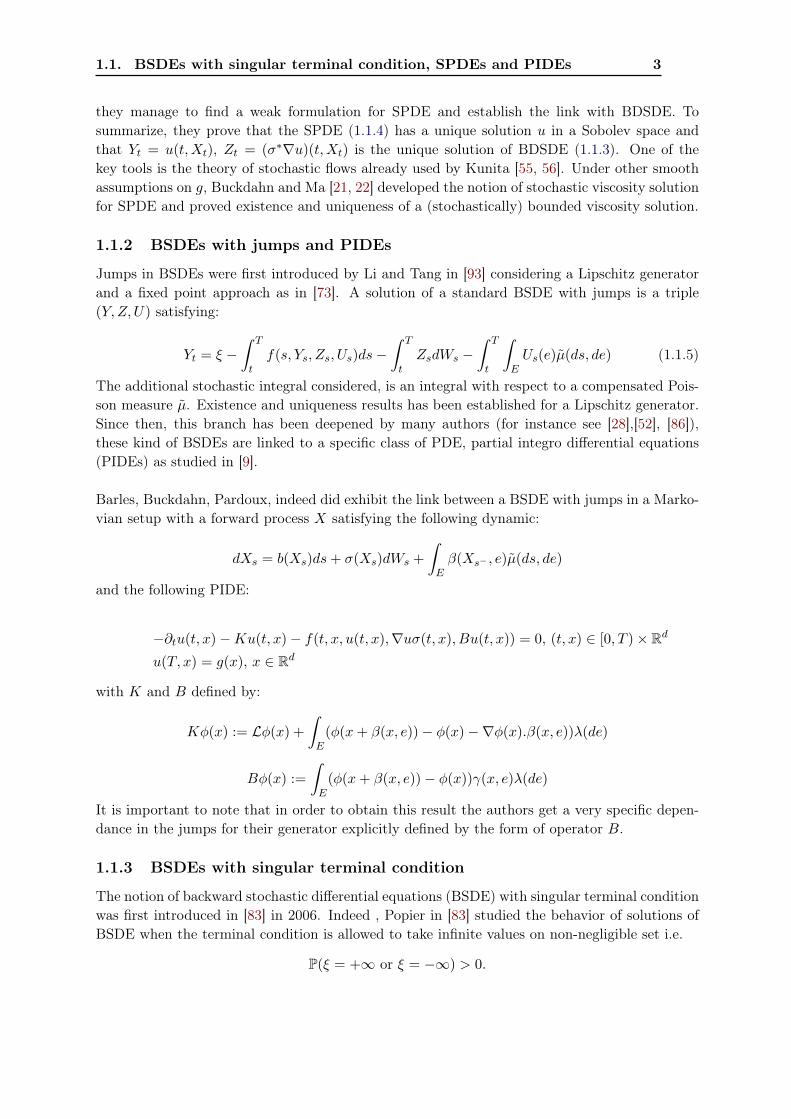
they manage to find a weak formulation for SPDE and establish the link with BDSDE. Tosummarize, they prove that the SPDE (1.1.4) has a unique solution u in a Sobolev space andthat Yt = u(t,Xt), Zt = (σ∗∇u)(t,Xt) is the unique solution of BDSDE (1.1.3). One of thekey tools is the theory of stochastic flows already used by Kunita [55, 56]. Under other smoothassumptions on g, Buckdahn and Ma [21, 22] developed the notion of stochastic viscosity solutionfor SPDE and proved existence and uniqueness of a (stochastically) bounded viscosity solution.
1.1.2 BSDEs with jumps and PIDEs
Jumps in BSDEs were first introduced by Li and Tang in [93] considering a Lipschitz generatorand a fixed point approach as in [73]. A solution of a standard BSDE with jumps is a triple(Y, Z, U) satisfying:
Yt = ξ −∫ T
tf(s, Ys, Zs, Us)ds−
∫ T
tZsdWs −
∫ T
t
∫EUs(e)µ(ds, de) (1.1.5)
The additional stochastic integral considered, is an integral with respect to a compensated Pois-son measure µ. Existence and uniqueness results has been established for a Lipschitz generator.Since then, this branch has been deepened by many authors (for instance see [28],[52], [86]),these kind of BSDEs are linked to a specific class of PDE, partial integro differential equations(PIDEs) as studied in [9].
Barles, Buckdahn, Pardoux, indeed did exhibit the link between a BSDE with jumps in a Marko-vian setup with a forward process X satisfying the following dynamic:
dXs = b(Xs)ds+ σ(Xs)dWs +∫
Eβ(Xs− , e)µ(ds, de)
and the following PIDE:
−∂tu(t, x)−Ku(t, x)− f(t, x, u(t, x),∇uσ(t, x), Bu(t, x)) = 0, (t, x) ∈ [0, T )× Rd
u(T, x) = g(x), x ∈ Rd
with K and B defined by:
Kφ(x) := Lφ(x) +∫
E(φ(x+ β(x, e))− φ(x)−∇φ(x).β(x, e))λ(de)
Bφ(x) :=∫
E(φ(x+ β(x, e))− φ(x))γ(x, e)λ(de)
It is important to note that in order to obtain this result the authors get a very specific depen-dance in the jumps for their generator explicitly defined by the form of operator B.
1.1.3 BSDEs with singular terminal condition
The notion of backward stochastic differential equations (BSDE) with singular terminal conditionwas first introduced in [83] in 2006. Indeed , Popier in [83] studied the behavior of solutions ofBSDE when the terminal condition is allowed to take infinite values on non-negligible set i.e.
P(ξ = +∞ or ξ = −∞) > 0.
4 Chapter 1. Introduction
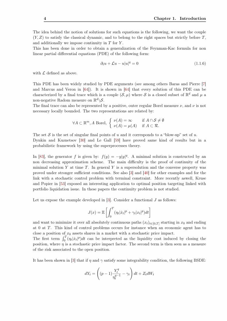
The idea behind the notion of solutions for such equations is the following, we want the couple(Y, Z) to satisfy the classical dynamic, and to belong to the right spaces but strictly before T ,and additionally we impose continuity in T for Y .This has been done in order to obtain a generalization of the Feynman-Kac formula for nonlinear partial differential equations (PDE) of the following form:
∂tu+ Lu− u|u|q = 0 (1.1.6)
with L defined as above.
This PDE has been widely studied by PDE arguments (see among others Baras and Pierre [7]and Marcus and Veron in [64]). It is shown in [64] that every solution of this PDE can becharacterized by a final trace which is a couple (S, µ) where S is a closed subset of Rd and µ anon-negative Radom measure on Rd\S.The final trace can also be represented by a positive, outer regular Borel measure ν, and ν is notnecessary locally bounded. The two representations are related by:
∀A ⊂ Rm, A Borel,ν(A) =∞ if A ∩ S 6= ∅ν(A) = µ(A) if A ⊂ R.
The set S is the set of singular final points of u and it corresponds to a “blow-up” set of u.Dynkin and Kuznetsov [30] and Le Gall [59] have proved same kind of results but in aprobabilistic framework by using the superprocesses theory.
In [83], the generator f is given by: f(y) = −y|y|q. A minimal solution is constructed by annon decreasing approximation scheme. The main difficulty is the proof of continuity of theminimal solution Y at time T . In general Y is a supersolution and the converse property wasproved under stronger sufficient conditions. See also [3] and [40] for other examples and for thelink with a stochastic control problem with terminal constraint. More recently aswell, Kruseand Popier in [53] exposed an interesting application to optimal position targeting linked withportfolio liquidation issue. In these papers the continuity problem is not studied.
Let us expose the example developed in [3]. Consider a functional J as follows:
J(x) = E[∫ T
0(ηt|xt|p + γt|xt|p)dt
]and want to minimize it over all absolutely continuous paths (xt)t∈[0,T ] starting in x0 and endingat 0 at T . This kind of control problems occurs for instance when an economic agent has toclose a position of x0 assets shares in a market with a stochastic price impact.The first term
∫ T0 (ηt|xt|p)dt can be interpreted as the liquidity cost induced by closing the
position, where η is a stochastic price impact factor. The second term is then seen as a measureof the risk associated to the open position.
It has been shown in [3] that if η and γ satisfy some integrability condition, the following BSDE:
dYt =
((p− 1)
Y qt
ηq−1t
− γt
)dt+ ZtdWt
1.1. BSDEs with singular terminal condition, SPDEs and PIDEs 5
where q is the conjugate of p, with the singular terminal condition:
limt→T
Yt =∞
has a minimal solution. Moreover Y provides an optimal control given by:
x∗t = x0e−
∫ t0 (Ys
ηs)q−1ds
and the value function is given by: J(x∗) = |x0|Y0.
1.1.4 Motivation, formulation of the problem
In the chapter 2 our aim is twofold, first we prove existence and uniqueness of the solution ofa BDSDE with monotone generator f , then we extend the results of [83] to BDSDE in orderto obtain a solution for a SPDE with singular terminal condition h. To our best knowlegde theclosest result concerning our first issue is in Aman [2]. Nevertheless we think that there is a lackin this paper (proof 4.2). Indeed for monotone BSDE (g = 0) the existence of a solution relieson the solvability of the BSDE:
Yt = ξ +∫ T
tf (r, Yr) dr −
∫ T
tZrdWr, 0 ≤ t ≤ T.
See among other the proof of Theorem 2.2 and Proposition 2.4 in [72]. To obtain a solution forthis BSDE, the main trick is to truncate the coefficients with suitable truncation functions inorder to have a bounded solution Y (see Proposition 2.2 in [18]). This can not be done for ageneral BDSDE. Indeed take for example (ξ = f = 0 and g = 1):
Yt =∫ T
t
←−−dBr −
∫ T
tZrdWr = BT −Bt, 0 ≤ t ≤ T,
with Z = 0. Thus in order to prove existence of a solution for (1.1.3), one can not directly followthe scheme of [72]. The first part of this chapter is devoted to the existence of a solution fora monotone BDSDE (see Section 2.2) in the space E2 (see definition in the next section). Torealize this project we will restrict the class of functions f : they should satisfy a polynomialgrowth condition (as in [18]). Until now we do not know how to extend this to general growthcondition as in [72] or [19].The second goal of this work is to extend the results of [83] to the doubly stochastic framework.We will consider the generator f(y) = −y|y|q with q ∈ R∗+ and a real FW
T -measurable and nonnegative random variable ξ such that:
P(ξ = +∞) > 0. (1.1.7)
And we want to find a solution to the following BDSDE:
Yt = ξ −∫ T
tYs|Ys|qds+
∫ T
tg(s, Ys, Zs)
←−−dBs −
∫ T
tZsdWs. (1.1.8)
The scheme to construct a solution is almost the same as in [83]. Let us emphasize one of maintechnical difficulties. If g = 0, we can use the conditional expectation w.r.t. Ft to withdraw themartingale part. If g 6= 0, this trick is useless and we have to be very careful when we want
6 Chapter 1. Introduction
almost sure property of the solution. This BDSDE is connected with the stochastic PDE withterminal condition h: for any 0 ≤ t ≤ T
u(t, x) = h(x) +∫ T
t(Lu(s, x)− u(s, x)|u(s, x)|q) ds
+∫ T
tg(s, u(s, x), σ(s, x)∇u(s, x))
←−−dBs. (1.1.9)
If h is a smooth function we could use the result of Pardoux and Peng [74]. But here we willassume that S = h = +∞ is a closed non empty set and thus we will precise the notion ofsolution for (1.1.9) in this case. Roughly speaking we will show that there is a minimal solutionu in the sense that u belongs to a Sobolev space and is a weak solution of the SPDE on anyinterval [0, T − δ], δ > 0 and satisfies the terminal condition: u(t, x) goes to h(x) also in a weaksense as t goes to T .
In Chapter 3 we would like to provide existence and unicity results for the following BSDE:
Yt = ξ −∫ T
tYs|Ys|qds−
∫ T
tZsdWs −
∫ T
t
∫EUs(e)µ(ds, de) (1.1.10)
where the terminal condition ξ satisfies
P(ξ = +∞) > 0. (1.1.11)
It is already established that such a BSDE has a unique solution when the terminal condition ξbelongs to Lp(Ω,FT ,P), p > 1 (see among others [9], [28], [52] or [93]). We would like to extendthis result when the terminal condition is singular, i.e. verifies (1.1.11). More precisely in [53](see Theorem 17 below) it is proved that the BSDE (1.1.10) with singular terminal condition hasa minimal super-solution (Y, Z, U) such that
lim inft→T
Yt ≥ ξ.
Since a priori estimates are not hard to establish, to obtain our existence results, we essentiallywant to find sufficient conditions to have a.s.
limt→T
Yt = ξ. (1.1.12)
This problem was studied in [83] when there is no jump. In the Markovian framework andfor q > 2, Equality (1.1.12) was proved. Here we will follow the same idea. But we needother technical assumptions on the jumps of the solution X of the forward SDE and the setS = ξ = +∞.The second part is devoted to the study of the related partial integro differential equation (PIDEin short): for any x ∈ Rd, u(T, x) = g(x) and for any (t, x) ∈ [0, T [×Rd
∂
∂tu(t, x) + Lu(t, x) + I(t, x, u)− u(t, x)|u(t, x)|q = 0 (1.1.13)
where L is given above and I is a integro-differential operator:
I(t, x, φ) =∫
E[φ(x+ h(t, x, e))− φ(x)− (∇φ)(x)h(t, x, e)]λ(de).

1.1. BSDEs with singular terminal condition, SPDEs and PIDEs 7
If there is no jump, in [83] the following link is established between the solution Y t,x of the BSDE(1.1.10) and the viscosity solution u of the PIDE (1.1.13):
u(t, x) = Y t,xt
This relation is also obtained in [9] in the case where there are jumps and if the terminal functiong is of linear growth. Moreover several papers have studied the existence and the uniqueness ofthe solution of such PIDE (see among others [1], [10], [13] or [48]).To our best knowledges the study of (1.1.13) in the jump case and with a singularity at time T iscompletely new. Singularity means that the set g = +∞ is non empty. There is no probabilisticrepresentation of such PIDE using superprocesses. Hence the second aim of the chapter is toprove that this minimal solution Y is the probabilistic representation of the minimal positiveviscosity solution u of the PIDE. Moreover we will show that the sufficient conditions for (1.1.12)are also sufficient to ensure “continuity at time T ” of u.
1.1.5 Contributions to BDSDEs
Let us now precise our notations. W and B are independent Brownian motions defined on aprobability space (Ω,F ,P) with values in Rk and Rm. Let N denote the class of P-null sets ofF . For each t ∈ [0, T ], we define
Ft = FWt ∨ FB
t,T
where for any process η, Fηs,t = σ ηr − ηs; s ≤ r ≤ t ∨ N , Fη
t = Fη0,t. As in [74] we define the
following filtration (Gt, t ∈ [0, T ]) by:
Gt = FWt ∨ FB
0,T .
ξ is a FWT -measurable and Rd-valued random variable.
We define by Hp(0, T ; Rn) the set of (classes of dP × dt a.e. equal) n dimensional jointly mea-surable random processes (Xt, t ≥ 0) which satisty:
1. E(∫ T
0|Xt|2dt
)p/2
< +∞
2. Xt is Gt-measurable for a.e. t ∈ [0, T ].
We denote similarly by Sp(0, T ; Rn) the set of continuous n dimensional random processes whichsatisfy:
1. E
(sup
t∈[0,T ]|Xt|p
)< +∞
2. Xt is Gt-measurable for any t ∈ [0, T ].
Bp(0, T ) is the product Sp(0, T ; Rd)×Hp(0, T ; Rd×k). (Y, Z) ∈ Ep(0, T ) if (Y, Z) ∈ Bp(0, T ) and Yt
and Zt are Ft-measurable. Finally Cp,q([0, T ] × Rd; R) denotes the space of R-valued functionsdefined on [0, T ] × Rd which are p-times continuously differentiable in t ∈ [0, T ] and q-timescontinuously differentiable in x ∈ Rd. Cp,q
b ([0, T ]×Rd; R) is the subspace of Cp,q([0, T ]×Rd; R)in which all functions have uniformly bounded partial derivatives; and Cp,q
c ([0, T ] × Rd; R) thesubspace of Cp,q([0, T ]× Rd; R) in which the functions have a compact support w.r.t. x ∈ Rd.
8 Chapter 1. Introduction
Now we precise our assumptions on f and g. The functions f and g are defined on[0, T ] × Ω × Rd × Rd×k with values respectively in Rd and Rd×m. Moreover we consider thefollowing assumptions.
Assumptions (A).
• The function y 7→ f(t, y, z) is continuous and there exists a constant µ such that for any(t, y, y′, z) a.s.
〈y − y′, f(t, y, z)− f(t, y′, z)〉 ≤ µ|y − y′|2. (A1)
• There exists Kf such that for any (t, y, z, z′) a.s.
|f(t, y, z)− f(t, y, z′)|2 ≤ Kf |z − z′|2. (A2)
• There exists Cf ≥ 0 and p > 1 such that
|f(t, y, z)− f(t, 0, z)| ≤ Cf (1 + |y|p). (A3)
• There exists a constant Kg ≥ 0 and 0 < ε < 1 such that for any (t, y, y′, z, z′) a.s.
|g(t, y, z)− g(t, y′, z′)|2 ≤ Kg|y − y′|2 + ε|z − z′|2. (A4)
• Finally for any (t, y, z), f(t, y, z) and g(t, y, z) are Ft-measurable with
E∫ T
0
(|f(t, 0, 0)|2 + |g(t, 0, 0)|2
)dt < +∞. (A5)
Remember that from [74] if f also satisfies: there exists Kf such that for any (t, y, y′, z) a.s.
|f(t, y, z)− f(t, y′, z)| ≤ Kf |y − y′| (1.1.14)
then there exists a unique solution (Y, Z) ∈ E2(0, T ) to the BDSDE (1.1.3). Note that (1.1.14)implies that
|f(t, y, z)− f(t, 0, z)| ≤ Kf |y|,
thus the growth assumption (A3) on f is satisfied with p = 1.We emphasize the fact that the assumptions (A2), (A4) are exactly (Lip),(Lip2) from [74] thusare somewhat standard when dealing with the doubly stochastic framework.In Section 2.2 we will prove the following result.
Theorem 1. Under Assumptions (A) and if the terminal condition ξ satisfies
E(|ξ|2) < +∞, (1.1.15)
the BDSDE (1.1.3) has a unique solution (Y, Z) ∈ E2(0, T ).
Using the paper of Aman [2], this result can be extended to the Lp case: for p ∈ (1, 2)
E∫ T
0(|f(t, 0, 0)|p + |g(t, 0, 0)|p) dt+ E(|ξ|p) < +∞.
1.1. BSDEs with singular terminal condition, SPDEs and PIDEs 9
There exists a unique solution in Ep(0, T ).The next sections are devoted to the singular case. The generator f will be supposed to bedeterministic and given by: f(y) = −y|y|q for some q > 0. The aim is to prove existence of asolution for BDSDE (1.1.8) when the non negative random variable ξ satisfies (1.1.7). A possibleextension of the notion of solution for a BDSDE with singular terminal condition could be thefollowing (see Definition 1 in [83]).
Definition 1 (Solution of the BDSDE (1.1.8)). Let q > 0 and ξ a FWT -measurable non negative
random variable satisfying condition (1.1.7). We say that the process (Y, Z) is a solution of theBDSDE (1.1.8) if (Y, Z) is such that (Yt, Zt) is Ft-measurable and:
(D1) for all 0 ≤ s ≤ t < T : Ys = Yt −∫ t
sYr|Yr|qdr +
∫ t
sg(r, Yr, Zr)
←−−dBr −
∫ t
sZrdWr;
(D2) for all t ∈ [0, T [, E(
sup0≤s≤t
|Ys|2 +∫ t
0‖Zr‖2dr
)< +∞;
(D3) P-a.s. limt→T
Yt = ξ.
A solution is said non negative if a.s. for any t ∈ [0, T ], Yt ≥ 0.
In order to define a wellposedness theory for DBSDE with singular terminal condition, we followthe idea initiated in [83], but we’ll have to deal with the backward integral term which intervenein a non-trivial way in some situations.
To obtain an a priori estimate of the solution we will assume that g(t, y, 0) = 0 for any (t, y)a.s. This condition will ensure that our solutions will be non negative and bounded on any timeinterval [0, T − δ] with δ > 0. Without this hypothesis, integrability of the solution would bemore challenging. In Section 2.3, we will prove the following result.
Theorem 2. There exists a process (Y, Z) satisfying Conditions (D1) and (D2) of Definition 8and such that Y has a limit at time T with
limt→T
Yt ≥ ξ.
Moreover this solution is minimal: if (Y , Z) is a non negative solution of (1.1.8), then a.s. forany t, Yt ≥ Yt.
It means in particular that Yt has a left limit at time T .In general we are not able to prove that (D3) holds. As in [83], we give sufficient conditions forcontinuity and we prove it in the Markovian framework. Hence the first hypothesis on ξ is thefollowing:
ξ = h(XT ), (H1)
where h is a function defined on Rd with values in R+ such that the set of singularity S =h = +∞ is closed; and where XT is the value at t = T of a diffusion process or more preciselythe solution of a stochastic differential equation (in short SDE):
Xt = x+∫ t
0b(r,Xr)dr +
∫ t
0σ(r,Xr)dWr, for t ∈ [0, T ]. (1.1.16)
10 Chapter 1. Introduction
We will always assume that b and σ are defined on [0, T ] × Rd, with values respectively in Rd
and Rd×k, are measurable w.r.t. the Borelian σ-algebras, and that there exists a constant K > 0s.t. for all t ∈ [0, T ] and for all (x, y) ∈ Rd × Rd:
1. Lipschitz condition:
|b(t, x)− b(t, y)|+ ‖σ(t, x)− σ(t, y)‖ ≤ K|x− y|; (L)
2. Growth condition:
|b(t, x)| ≤ K(1 + |x|) and ‖σ(t, x)‖ ≤ K(1 + |x|). (G)
It is well known that under the previous assumptions, Equation (1.1.16) has a unique strongsolution X.We denote R = Rd \ S. The second hypothesis on ξ is: for all compact set K ⊂ R = Rd \h = +∞
h(XT )1K(XT ) ∈ L1 (Ω,FT ,P; R) . (H2)
Unfortunately the above assumptions are not sufficient to prove continuity if q ≤ 2. Thus weadd the following conditions in order to use Malliavin calculus and to prove Equality (2.4.41).
1. The functions σ and b are bounded: there exists a constant K s.t.
∀(t, x) ∈ [0, T ]× Rd, |b(t, x)|+ ‖σ(t, x)‖ ≤ K. (B)
2. The second derivatives of σσ∗ belongs to L∞:
∂2σσ∗
∂xi∂xj∈ L∞([0, T ]× Rd). (D)
3. σσ∗ is uniformly elliptic, i.e. there exists λ > 0 s.t. for all (t, x) ∈ [0, T ]× Rd:
∀y ∈ Rd, σσ∗(t, x)y.y ≥ λ|y|2. (E)
4. h is continuous from Rd to R+ and:
∀M ≥ 0, h is a Lipschitz function on the set OM = |h| ≤M . (H3)
Theorem 3. Under Assumptions (H1), (H2) and (L) and if
• either q > 2 and (G);
• or (B), (D), (E) and (H3);
the minimal non negative solution (Y, Z) of (1.1.8) satisfies (D3): a.s.
limt→T
Yt = ξ.
1.1. BSDEs with singular terminal condition, SPDEs and PIDEs 11
Note that these conditions are identical to [83], nevertheless none of the proofs of this resultcould be adapted directly to our doubly stochastic context. Moreover it seems surprising to usthat we do not get additional hypothesis on g by introducing a doubly stochastic framework,other than (Lip), (Lip2) from [74].Finally in section 2.5, we show that this minimal solution (Y, Z) of (1.1.8) is connected to theminimal weak solution u of the SPDE (1.1.9). More precisely Xt,x is the solution of the SDE(1.1.16) with initial condition x at time t and (Y t,x, Zt,x) is the minimal solution of the BDSDE(1.1.8) with singular terminal condition ξ = h(Xt,x
T ).Let us define the space H(0, T ) as in [6]. We take the following weight function ρ : Rd → R: forκ > d
ρ(x) =1
(1 + |x|)κ. (1.1.17)
The constant κ will be fixed later. H(0, T ) is the set of the random fields u(t, x); 0 ≤ t ≤ T, x ∈Rd such that u(t, x) is FB
t,T -measurable for each (t, x), u and σ∗∇u belong to L2((0, T ) × Ω ×Rd; ds⊗ dP⊗ ρ(x)dx). On H(0, T ) we consider the following norm
‖u‖22 = E∫ T
0
∫Rd
(|u(s, x)|2 + |(σ∗∇u)(s, x)|2
)ρ(x)dx.
Theorem 4. The random field u defined by u(t, x) = Y t,xt belongs to H(0, T − δ) for any δ > 0
and is a weak solution of the SPDE (1.1.9) on [0, T − δ] × Rd. At time T , u satisfies a.s.lim inft→T u(t, x) ≥ h(x).Moreover under the same assumptions of Theorem 3, for any function φ ∈ C∞c (Rd) with supportincluded in R, then
limt→T
E(∫
Rd
u(t, x)φ(x)dx)
=∫
Rd
h(x)φ(x)dx.
Finally u is the minimal non negative solution of (1.1.9).
In order to prove this result, we proceeded in a few steps. First we noticed that (1.1.9) withterminal function h ∧ n has an unique weak solution un thanks to [6] and this solution coincidewith the solution of the forward-backward system in the following sense: Y n,t,x
s = un(s,Xt,xs ) ,
Zn,t,xs = (σ∗∇un)(s,Xt,x
s ). We define then u as the limit of the random fields un. Then it iseasy to deduce an upper bound for u on [0, T − δ], and by dominated convergence we get that usatisfies the two first properties of a weak solution. And since we have good a priori estimateswe can obtain that u satisfies the last property by a monotone convergence.The last point: limt→T E
(∫Rd u(t, x)φ(x)dx
)=∫
Rd h(x)φ(x)dx is obtained by proving inequali-ties in both ways and standard arguments.
1.1.6 Contributions to BSDEs with jumps
Our setting is the same as in [9]. In the following we will consider W = (Wt)t∈R+ the standardBrownian Motion on Rk, µ a Poisson random measure on R+ × E with compensator dtλ(de).Here E := R`\0, E its Borel field and we assume that we have a stochastic basis (Ω,F ,P) andthe filtration (Ft, t ≥ 0) is generated by the two independent processes W and µ and we assumethat F0 contains all P-null elements of F . We will denote µ is the compensated measure: forany A ∈ E such that λ(A) < +∞, then µ([0, t]×A) = µ([0, t]×A)− tλ(A) is a martingale. λ is
12 Chapter 1. Introduction
assumed to be a σ-finite measure on (E, E) satisfying∫E(1 ∧ |e|2)λ(de) < +∞.
In this chapter for a given T ≥ 0, we denote:
• P: the predictable σ-field on Ω× [0, T ] and
P = P ⊗ E
• On Ω = Ω × [0, T ] × E, a function that is P-measurable, is called predictable. Gloc(µ) isthe set of P-measurable functions ψ on Ω such that for any t ≥ 0 a.s.∫ t
0
∫E(|ψs(e)|2 ∧ |ψs(e)|)λ(de) < +∞.
• D (resp. D(0, T )): the set of all progressively measurable càdlàg processes on R+ (resp.on [0, T ]).
• Sp(0, T ) is the space of all processes X ∈ D(0, T ) such that
E
(sup
t∈[0,T ]|Xt|p
)< +∞.
For simplicity, X∗ = supt∈[0,T ] |Xt|.
• Hp(0, T ) is the subspace of all processes X ∈ D(0, T ) such that
E
[(∫ T
0|Xt|2dt
)p/2]< +∞.
• Lpµ(0, T ) = Lp
µ(Ω× (0, T )× E): the set of processes ψ ∈ Gloc(µ) such that
E
[(∫ T
0
∫E|ψs(e)|2λ(de)ds
)p/2]< +∞.
• Lpλ = Lp(E, λ; Rd): the set of measurable functions ψ : E → Rd such that
‖ψ‖pLp
λ=∫
E|ψ(e)|pλ(de) < +∞.
• Bpµ(0, T ) = Sp(0, T )×Hp(0, T )× Lp
µ(0, T ).
Definition 2. Let q > 0 and ξ a Ft-measurable non negative random variable such that P(ξ =∞) > 0. We say (Y, Z, U) is a solution of (1.1.10) with singular terminal condition ξ if
• (Y, Z, U) belongs to B2(0, t) for any t < T .

1.1. BSDEs with singular terminal condition, SPDEs and PIDEs 13
• for all 0 ≤ s ≤ t < T :
Ys = Yt −∫ t
sYr|Yr|qdr −
∫ t
sZrdWr −
∫ t
s
∫EUs(e)µ(ds, de).
• Y is continuous at T : a.s.limt→T
Yt = ξ.
If we consider the same approximating scheme as in [53], we define Y the limit process of Y n
where Y n satisfies the BSDE with jumps associated to the data (ξ ∧ n,U). Then we can obtainthis proposition.
Proposition 1. The process Y can be written as follows:
Yt =(q(T − t) + EFt
[1ξq
]− φt
)−1/q
where φ is a non negative supermartingale. As a consequence, the process Y has a left limit inT .
We suppose now our terminal condition is of the form: ξ = g(XT ). The function g is defined onRd with values in R+ ∪ +∞ and we denote
S := x ∈ Rd s.t. g(x) =∞
the set of singularity points for the terminal condition induced by g. This set S is supposed tobe closed. We also denoted by Γ the boundary of S. The process X is the solution of a SDEwith jumps:
Xt = X0 +∫ t
0b(s,Xs)ds+
∫ t
0σ(s,Xs)dWs +
∫ t
0
∫Eh(s,Xs− , e)µ(de, ds). (1.1.18)
The coefficients b : Ω×[0, T ]×Rd → Rd, σ : Ω×[0, T ]×Rd → Rd×k and h : Ω×[0, T ]×Rd×E → Rd
satisfy
Assumptions (B):
1. b, σ and h are jointly continuous w.r.t. (t, x) and Lipschitz continuous w.r.t. x uniformlyin t, e or ω, i.e. there exists a constant C such that for any (ω, t, e) ∈ Ω × [0, T ] × E, forany x and y in Rd: a.s.
|b(t, x)− b(t, y)|+ |σ(t, x)− σ(t, y)| ≤ C|x− y| (L)
and ∫E|h(t, x, e)− h(t, y, e)|2λ(de) ≤ C|x− y|. (B2)
2. b, σ and h growth at most linearly:
|b(t, x)|+ |σ(t, x)| ≤ C(1 + |x|). (G)
14 Chapter 1. Introduction
3. h is bounded w.r.t. t and x and there exists a constant Ch such that a.s.
|h(t, x, e)| ≤ Ch(1 ∧ |e|). (B4)
Now the second hypothesis on ξ is: for all compact set K ⊂ Rd \ S
g(XT )1K(XT ) ∈ L1 (Ω,FT ,P) . (1.1.19)
Assumption (C):
• The boundary ∂S = Γ is compact and of class C2.
• For any x ∈ S, any s ∈ [0, T ] and λ-a.s.
x+ h(s, x, e) ∈ S.
Furthermore there exists a constant κ > 0 such that if x ∈ Γ, then for any s ∈ [0, T ],d(x+ h(s, x, e),Γ) ≥ κ, λ-a.s.
Theorem 5. Under Assumptions (B) and (C), Y is continuous at T.
To have more regularity on u we add some conditions on the coefficients.
1. σ and b are bounded: there exists a constant C s.t.
∀(t, x) ∈ [0, T ]× Rd, |b(t, x)|+ ‖σ(t, x)‖ ≤ C; (B)
2. σσ∗ is uniformly elliptic, i.e. there exists λ > 0 s.t. for all (t, x) ∈ [0, T ]× Rd:
∀y ∈ Rd, σσ∗(t, x)y.y ≥ λ|y|2. (E)
Definition 3 (Viscosity solution with singular data). A function u is a viscosity solution of(1.1.13) with terminal data g if u is a viscosity solution on [0, T [×Rd and satisfies:
lim(t,x)→(T,x0)
u(t, x) = g(x0). (1.1.20)
Theorem 6. The function u is the minimal viscosity solution of (1.1.13) with terminal data g.
1.1.7 Perspectives
In the singular terminal condition framework, we assume the generator to be known and explicitas:
f(ω, t, y, z) := −y|y|q
This allows us when the terminal condition is deterministic to obtain the following solution toour BSDE (which becomes an ODE):
yCt = (q(T − t) +
1C
)−1q , Z ≡ 0
1.2. 2DBSDEs and related game options 15
Then by comparison theorem we easily get majorations for our processes Y n, Y nt ≤ yn
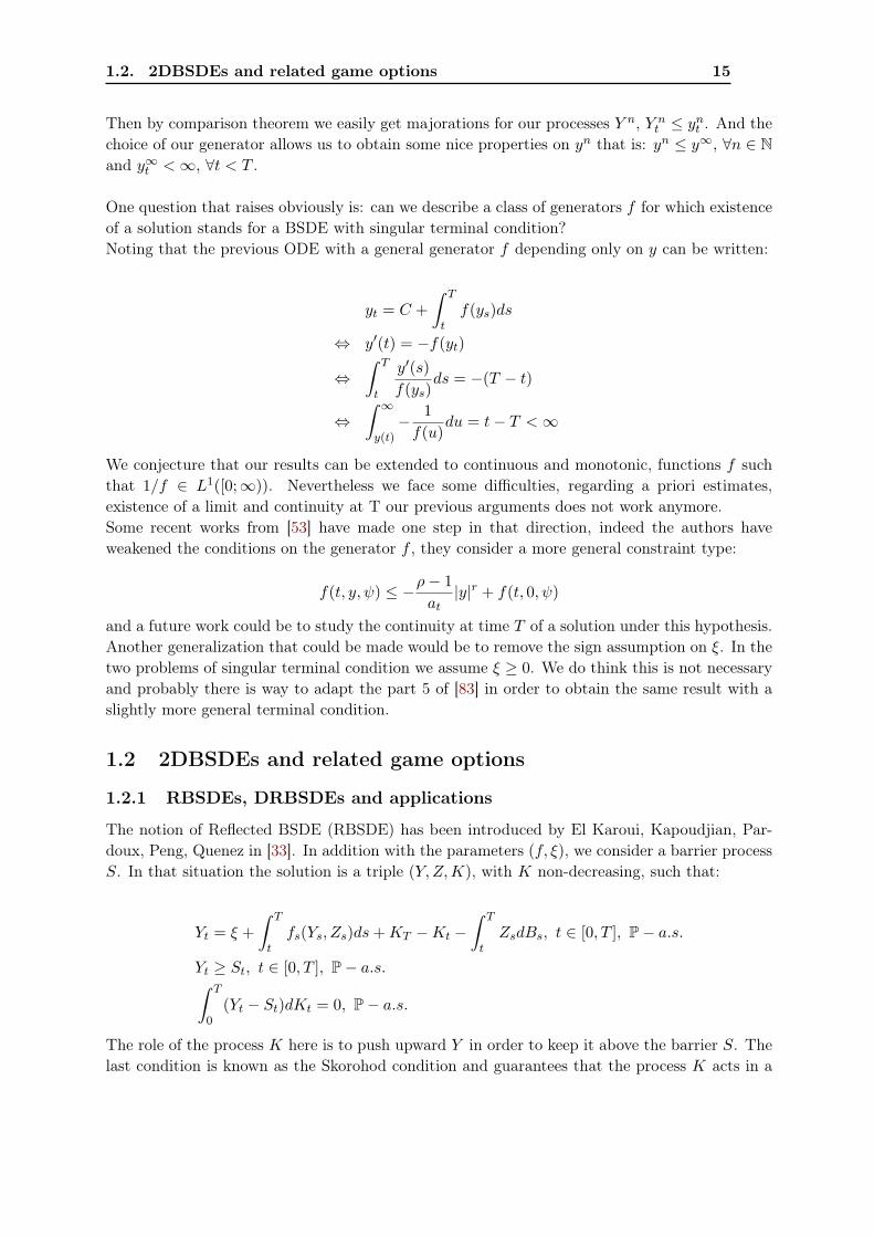
t . And thechoice of our generator allows us to obtain some nice properties on yn that is: yn ≤ y∞, ∀n ∈ Nand y∞t <∞, ∀t < T .
One question that raises obviously is: can we describe a class of generators f for which existenceof a solution stands for a BSDE with singular terminal condition?Noting that the previous ODE with a general generator f depending only on y can be written:
yt = C +∫ T
tf(ys)ds
⇔ y′(t) = −f(yt)
⇔∫ T
t
y′(s)f(ys)
ds = −(T − t)
⇔∫ ∞
y(t)− 1f(u)
du = t− T <∞
We conjecture that our results can be extended to continuous and monotonic, functions f suchthat 1/f ∈ L1([0;∞)). Nevertheless we face some difficulties, regarding a priori estimates,existence of a limit and continuity at T our previous arguments does not work anymore.Some recent works from [53] have made one step in that direction, indeed the authors haveweakened the conditions on the generator f , they consider a more general constraint type:
f(t, y, ψ) ≤ −ρ− 1at|y|r + f(t, 0, ψ)
and a future work could be to study the continuity at time T of a solution under this hypothesis.Another generalization that could be made would be to remove the sign assumption on ξ. In thetwo problems of singular terminal condition we assume ξ ≥ 0. We do think this is not necessaryand probably there is way to adapt the part 5 of [83] in order to obtain the same result with aslightly more general terminal condition.
1.2 2DBSDEs and related game options
1.2.1 RBSDEs, DRBSDEs and applications
The notion of Reflected BSDE (RBSDE) has been introduced by El Karoui, Kapoudjian, Par-doux, Peng, Quenez in [33]. In addition with the parameters (f, ξ), we consider a barrier processS. In that situation the solution is a triple (Y, Z,K), with K non-decreasing, such that:
Yt = ξ +∫ T
tfs(Ys, Zs)ds+KT −Kt −
∫ T
tZsdBs, t ∈ [0, T ], P− a.s.
Yt ≥ St, t ∈ [0, T ], P− a.s.∫ T
0(Yt − St)dKt = 0, P− a.s.
The role of the process K here is to push upward Y in order to keep it above the barrier S. Thelast condition is known as the Skorohod condition and guarantees that the process K acts in a
16 Chapter 1. Introduction
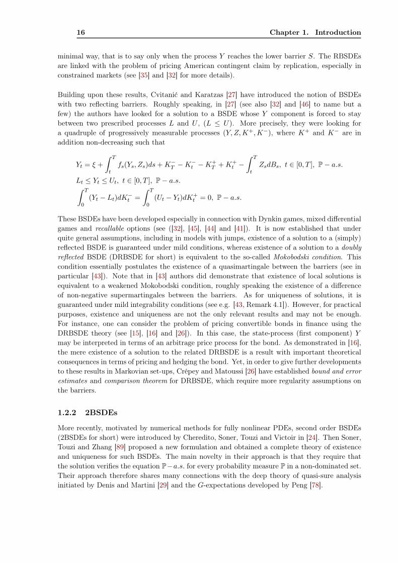
minimal way, that is to say only when the process Y reaches the lower barrier S. The RBSDEsare linked with the problem of pricing American contingent claim by replication, especially inconstrained markets (see [35] and [32] for more details).
Building upon these results, Cvitanić and Karatzas [27] have introduced the notion of BSDEswith two reflecting barriers. Roughly speaking, in [27] (see also [32] and [46] to name but afew) the authors have looked for a solution to a BSDE whose Y component is forced to staybetween two prescribed processes L and U , (L ≤ U). More precisely, they were looking fora quadruple of progressively measurable processes (Y, Z,K+,K−), where K+ and K− are inaddition non-decreasing such that
Yt = ξ +∫ T
tfs(Ys, Zs)ds+K−
T −K−t −K
+T +K+
t −∫ T
tZsdBs, t ∈ [0, T ], P− a.s.
Lt ≤ Yt ≤ Ut, t ∈ [0, T ], P− a.s.∫ T
0(Yt − Lt)dK−
t =∫ T
0(Ut − Yt)dK+
t = 0, P− a.s.
These BSDEs have been developed especially in connection with Dynkin games, mixed differentialgames and recallable options (see ([32], [45], [44] and [41]). It is now established that underquite general assumptions, including in models with jumps, existence of a solution to a (simply)reflected BSDE is guaranteed under mild conditions, whereas existence of a solution to a doublyreflected BSDE (DRBSDE for short) is equivalent to the so-called Mokobodski condition. Thiscondition essentially postulates the existence of a quasimartingale between the barriers (see inparticular [43]). Note that in [43] authors did demonstrate that existence of local solutions isequivalent to a weakened Mokobodski condition, roughly speaking the existence of a differenceof non-negative supermartingales between the barriers. As for uniqueness of solutions, it isguaranteed under mild integrability conditions (see e.g. [43, Remark 4.1]). However, for practicalpurposes, existence and uniqueness are not the only relevant results and may not be enough.For instance, one can consider the problem of pricing convertible bonds in finance using theDRBSDE theory (see [15], [16] and [26]). In this case, the state-process (first component) Ymay be interpreted in terms of an arbitrage price process for the bond. As demonstrated in [16],the mere existence of a solution to the related DRBSDE is a result with important theoreticalconsequences in terms of pricing and hedging the bond. Yet, in order to give further developmentsto these results in Markovian set-ups, Crépey and Matoussi [26] have established bound and errorestimates and comparison theorem for DRBSDE, which require more regularity assumptions onthe barriers.
1.2.2 2BSDEs
More recently, motivated by numerical methods for fully nonlinear PDEs, second order BSDEs(2BSDEs for short) were introduced by Cheredito, Soner, Touzi and Victoir in [24]. Then Soner,Touzi and Zhang [89] proposed a new formulation and obtained a complete theory of existenceand uniqueness for such BSDEs. The main novelty in their approach is that they require thatthe solution verifies the equation P−a.s. for every probability measure P in a non-dominated set.Their approach therefore shares many connections with the deep theory of quasi-sure analysisinitiated by Denis and Martini [29] and the G-expectations developed by Peng [78].
1.2. 2DBSDEs and related game options 17
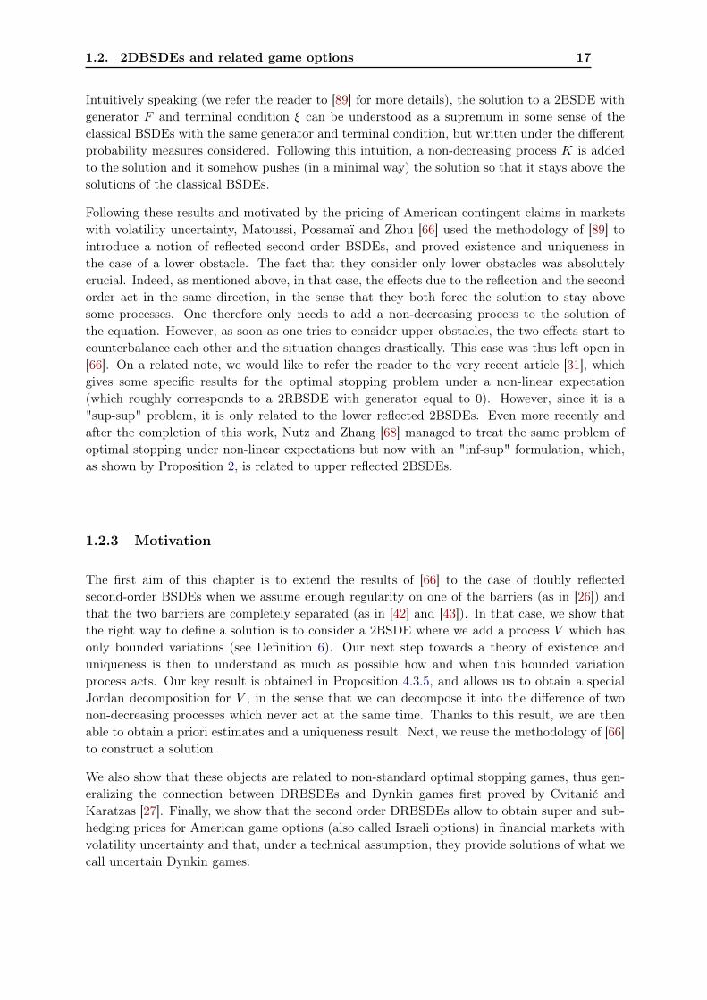
Intuitively speaking (we refer the reader to [89] for more details), the solution to a 2BSDE withgenerator F and terminal condition ξ can be understood as a supremum in some sense of theclassical BSDEs with the same generator and terminal condition, but written under the differentprobability measures considered. Following this intuition, a non-decreasing process K is addedto the solution and it somehow pushes (in a minimal way) the solution so that it stays above thesolutions of the classical BSDEs.
Following these results and motivated by the pricing of American contingent claims in marketswith volatility uncertainty, Matoussi, Possamaï and Zhou [66] used the methodology of [89] tointroduce a notion of reflected second order BSDEs, and proved existence and uniqueness inthe case of a lower obstacle. The fact that they consider only lower obstacles was absolutelycrucial. Indeed, as mentioned above, in that case, the effects due to the reflection and the secondorder act in the same direction, in the sense that they both force the solution to stay abovesome processes. One therefore only needs to add a non-decreasing process to the solution ofthe equation. However, as soon as one tries to consider upper obstacles, the two effects start tocounterbalance each other and the situation changes drastically. This case was thus left open in[66]. On a related note, we would like to refer the reader to the very recent article [31], whichgives some specific results for the optimal stopping problem under a non-linear expectation(which roughly corresponds to a 2RBSDE with generator equal to 0). However, since it is a"sup-sup" problem, it is only related to the lower reflected 2BSDEs. Even more recently andafter the completion of this work, Nutz and Zhang [68] managed to treat the same problem ofoptimal stopping under non-linear expectations but now with an "inf-sup" formulation, which,as shown by Proposition 2, is related to upper reflected 2BSDEs.
1.2.3 Motivation
The first aim of this chapter is to extend the results of [66] to the case of doubly reflectedsecond-order BSDEs when we assume enough regularity on one of the barriers (as in [26]) andthat the two barriers are completely separated (as in [42] and [43]). In that case, we show thatthe right way to define a solution is to consider a 2BSDE where we add a process V which hasonly bounded variations (see Definition 6). Our next step towards a theory of existence anduniqueness is then to understand as much as possible how and when this bounded variationprocess acts. Our key result is obtained in Proposition 4.3.5, and allows us to obtain a specialJordan decomposition for V , in the sense that we can decompose it into the difference of twonon-decreasing processes which never act at the same time. Thanks to this result, we are thenable to obtain a priori estimates and a uniqueness result. Next, we reuse the methodology of [66]to construct a solution.
We also show that these objects are related to non-standard optimal stopping games, thus gen-eralizing the connection between DRBSDEs and Dynkin games first proved by Cvitanić andKaratzas [27]. Finally, we show that the second order DRBSDEs allow to obtain super and sub-hedging prices for American game options (also called Israeli options) in financial markets withvolatility uncertainty and that, under a technical assumption, they provide solutions of what wecall uncertain Dynkin games.
18 Chapter 1. Introduction
1.2.4 Main results
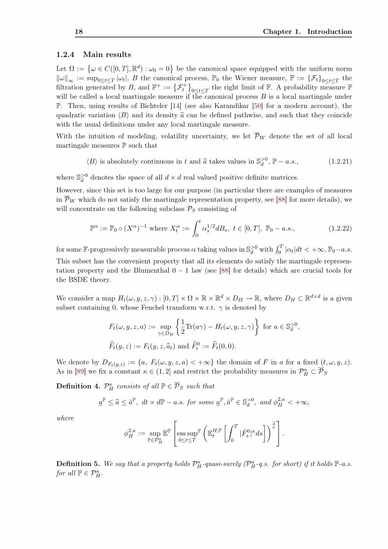
Let Ω :=ω ∈ C([0, T ],Rd) : ω0 = 0
be the canonical space equipped with the uniform norm
‖ω‖∞ := sup0≤t≤T |ωt|, B the canonical process, P0 the Wiener measure, F := Ft0≤t≤T thefiltration generated by B, and F+ :=
F+
t
0≤t≤T
the right limit of F. A probability measure Pwill be called a local martingale measure if the canonical process B is a local martingale underP. Then, using results of Bichteler [14] (see also Karandikar [50] for a modern account), thequadratic variation 〈B〉 and its density a can be defined pathwise, and such that they coincidewith the usual definitions under any local martingale measure.
With the intuition of modeling, volatility uncertainty, we let PW denote the set of all localmartingale measures P such that
〈B〉 is absolutely continuous in t and a takes values in S>0d , P− a.s., (1.2.21)
where S>0d denotes the space of all d× d real valued positive definite matrices.
However, since this set is too large for our purpose (in particular there are examples of measuresin PW which do not satisfy the martingale representation property, see [88] for more details), wewill concentrate on the following subclass PS consisting of
Pα := P0 (Xα)−1 where Xαt :=
∫ t
0α1/2
s dBs, t ∈ [0, T ], P0 − a.s., (1.2.22)
for some F-progressively measurable process α taking values in S>0d with
∫ T0 |αt|dt < +∞, P0−a.s.
This subset has the convenient property that all its elements do satisfy the martingale represen-tation property and the Blumenthal 0 − 1 law (see [88] for details) which are crucial tools forthe BSDE theory.
We consider a map Ht(ω, y, z, γ) : [0, T ]× Ω× R× Rd ×DH → R, where DH ⊂ Rd×d is a givensubset containing 0, whose Fenchel transform w.r.t. γ is denoted by
Ft(ω, y, z, a) := supγ∈DH
12Tr(aγ)−Ht(ω, y, z, γ)
for a ∈ S>0
d ,
Ft(y, z) := Ft(y, z, at) and F 0t := Ft(0, 0).
We denote by DFt(y,z) := a, Ft(ω, y, z, a) < +∞ the domain of F in a for a fixed (t, ω, y, z).As in [89] we fix a constant κ ∈ (1, 2] and restrict the probability measures in Pκ
H ⊂ PS
Definition 4. PκH consists of all P ∈ PS such that
aP ≤ a ≤ aP, dt× dP− a.s. for some aP, aP ∈ S>0d , and φ2,κ
H < +∞,
where
φ2,κH := sup
P∈PκH
EP
ess sup0≤t≤T
P(
EH,Pt
[∫ T
0|F 0
s |κds]) 2
κ
.Definition 5. We say that a property holds Pκ
H-quasi-surely (PκH-q.s. for short) if it holds P-a.s.
for all P ∈ PκH .

1.2. 2DBSDEs and related game options 19
We now state the main assumptions on the function F which will be our main interest in thesequel
Assumption (D):
(i) The domain DFt(y,z) = DFt is independent of (ω, y, z).
(ii) For fixed (y, z, a), F is F-progressively measurable in DFt .
(iii) We have the following uniform Lipschitz-type property in y and z
∀(y, y′, z, z′, t, a, ω),∣∣Ft(ω, y, z, a)− Ft(ω, y′, z′, a)
∣∣ ≤ C (∣∣y − y′∣∣+ ∣∣∣a1/2(z − z′
)∣∣∣) .(iv) F is uniformly continuous in ω for the || · ||∞ norm.
(v) PκH is not empty.
The following spaces and the corresponding norms will be used throughout the chapter. Withthe exception of the space Lp,κ
H , they all are immediate extensions of the usual spaces to thequasi-sure setting.
For p ≥ 1, Lp,κH denotes the space of all FT -measurable scalar r.v. ξ with
‖ξ‖pLp,κ
H:= sup
P∈PκH
EP [|ξ|p] < +∞.
Hp,κH denotes the space of all F+-progressively measurable Rd-valued processes Z with
‖Z‖pHp,κH
:= supP∈Pκ
H
EP
[(∫ T
0|a1/2
t Zt|2dt) p
2
]< +∞.
Dp,κH denotes the space of all F+-progressively measurable R-valued processes Y with
PκH − q.s. càdlàg paths, and ‖Y ‖pDp,κ
H:= sup
P∈PκH
EP
[sup
0≤t≤T|Yt|p
]< +∞,
where càdlàg is the french acronym for "right-continuous with left-limits".
Ip,κH denotes the space of all F+-progressively measurable R-valued processes K null at 0 with
PκH − q.s., càdlàg and non-decreasing paths, and ‖K‖pIp,κ
H:= sup
P∈PκH
EP [(KT )p] < +∞.
Vp,κH denotes the space of all F+-progressively measurable R-valued processes V null at 0 with
paths which are PκH − q.s. càdlàg and of bounded variation, and such that
‖V ‖pVp,κH
:= supP∈Pκ
H
EP [(Var0,T(V))p] < +∞.
For each ξ ∈ L1,κH , P ∈ Pκ
H and t ∈ [0, T ] denote
EH,Pt [ξ] := ess supP
P′∈PκH(t+,P)
EP′t [ξ] where Pκ
H(t+,P) :=
P′ ∈ Pκ
H : P′= P on F+
t
.

20 Chapter 1. Introduction
Here EPt [ξ] := EP[ξ|Ft]. Then we define for each p ≥ κ,
Lp,κH :=
ξ ∈ Lp,κ
H : ‖ξ‖Lp,κH
< +∞
where ‖ξ‖pLp,κH
:= supP∈Pκ
H
EP
[ess sup0≤t≤T
P(EH,P
t [|ξ|κ]) p
κ
].
We denote by UCb(Ω) the collection of all bounded and uniformly continuous maps ξ : Ω → Rwith respect to the ‖·‖∞-norm, and we let
Lp,κH := the closure of UCb(Ω) under the norm ‖·‖Lp,κ
H, for every 1 ≤ κ ≤ p.
Finally, for every P ∈ PκH , and for any p ≥ 1, Lp(P), Hp(P), Dp(P), Ip(P) and Vp(P) will denote
the corresponding usual spaces when there is only one measure P.
First, we consider a process S which will play the role of the upper obstacle. We will alwaysassume that S verifies the following properties
Assumption (E):
(i) S is F-progressively measurable and càdlàg.
(ii) S is uniformly continuous in ω in the sense that for all t
|St(ω)− St(ω)| ≤ ρ (‖ω − ω‖t) , ∀ (ω, ω) ∈ Ω2,
for some modulus of continuity ρ and where we define ‖ω‖t := sup0≤s≤t
|ω(s)|.
(iii) S is a semimartingale for every P ∈ PκH , with the decomposition
St = S0 +∫ t
0PsdBs +AP
t , P− a.s., for all P ∈ PκH , (1.2.23)
where the AP are bounded variation processes with Jordan decomposition AP,+−AP,− and
ζ2,κH := sup
P∈PκH
(EP
[ess supP
0≤t≤TEH,P
t
[(∫ T
t
∣∣∣a1/2s Ps
∣∣∣2 ds)κ/2
+(AP,+
T
)κ]])2
< +∞.
(iv) S satisfies the following integrability condition
ψ2,κH := sup
P∈PκH
EP
ess sup0≤t≤T
P
(EH,P
t
[sup
0≤s≤T|Ss|κ
]) 2κ
< +∞.
Next, we also consider a lower obstacle L which will be assumed to verify
Assumption (F):
(i) L is a F-progressively measurable càdlàg process.

1.2. 2DBSDEs and related game options 21
(ii) L is uniformly continuous in ω in the sense that for all t and for some modulus of continuityρ
|Lt(ω)− Lt(ω)| ≤ ρ (‖ω − ω‖t) , ∀ (ω, ω) ∈ Ω2.
(iii) For all t ∈ [0, T ], we have
Lt < St and Lt− < St− , PκH − q.s.
(iv) We have the following integrability condition
ϕ2,κH := sup
P∈PκH
EP
ess sup0≤t≤T
P
(EH,P
t
[(sup
0≤s≤T(Ls)
+
)κ]) 2κ
< +∞. (1.2.24)
We shall consider the following second order doubly reflected BSDE (2DRBSDE for short) withupper obstacle S and lower obstacle L
Yt = ξ +∫ T
tFs(Ys, Zs)ds−
∫ T
tZsdBs + VT − Vt, 0 ≤ t ≤ T, Pκ
H − q.s. (1.2.25)
In order to give the definition of the 2DRBSDE, we first need to introduce the correspondingstandard doubly reflected BSDEs. Hence, for any P ∈ Pκ
H , F-stopping time τ , and Fτ -measurablerandom variable ξ ∈ L2(P), let
(yP, zP, kP,+, kP,−) := (yP(τ, ξ), zP(τ, ξ), kP,+(τ, ξ), kP,−(τ, ξ)),
denote the unique solution to the following standard DRBSDE with upper obstacle S and lowerobstacle L (existence and uniqueness have been proved under these assumptions in [26] amongothers)
yPt = ξ +
∫ τt Fs(yP
s , zPs )ds−
∫ τt z
Ps dBs + kP,−
τ − kP,−t − kP,+
τ + kP,+t , 0 ≤ t ≤ τ, P− a.s.
Lt ≤ yPt ≤ St, P− a.s.∫ t
0
(yP
s− − Ls−)dkP,−
s =∫ t0
(Ss− − yP
s−
)dkP,+
s = 0, P− a.s., ∀t ∈ [0, T ].(1.2.26)
Everything is now ready for the
Definition 6. We say (Y, Z) ∈ D2,κH ×H2,κ
H is a solution to the 2DRBSDE (1.2.25) if
• YT = ξ, PκH − q.s.
• ∀P ∈ PκH , the process V P defined below has paths of bounded variation P− a.s.
V Pt := Y0 − Yt −
∫ t
0Fs(Ys, Zs)ds+
∫ t
0ZsdBs, 0 ≤ t ≤ T, P− a.s. (1.2.27)
22 Chapter 1. Introduction
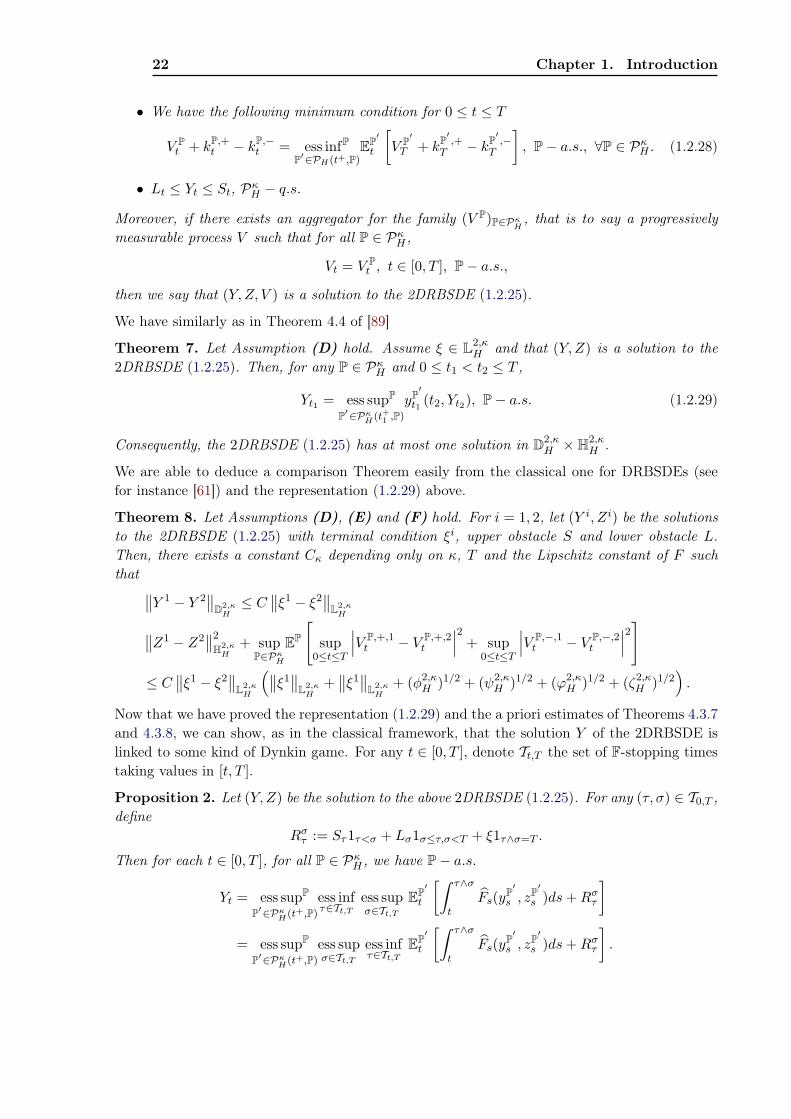
• We have the following minimum condition for 0 ≤ t ≤ T
V Pt + kP,+
t − kP,−t = ess infP
P′∈PH(t+,P)EP′
t
[V P′
T + kP′ ,+T − kP′ ,−
T
], P− a.s., ∀P ∈ Pκ
H . (1.2.28)
• Lt ≤ Yt ≤ St, PκH − q.s.
Moreover, if there exists an aggregator for the family (V P)P∈PκH, that is to say a progressively
measurable process V such that for all P ∈ PκH ,
Vt = V Pt , t ∈ [0, T ], P− a.s.,
then we say that (Y, Z, V ) is a solution to the 2DRBSDE (1.2.25).
We have similarly as in Theorem 4.4 of [89]
Theorem 7. Let Assumption (D) hold. Assume ξ ∈ L2,κH and that (Y, Z) is a solution to the
2DRBSDE (1.2.25). Then, for any P ∈ PκH and 0 ≤ t1 < t2 ≤ T ,
Yt1 = ess supP
P′∈PκH(t+1 ,P)
yP′t1 (t2, Yt2), P− a.s. (1.2.29)
Consequently, the 2DRBSDE (1.2.25) has at most one solution in D2,κH ×H2,κ
H .
We are able to deduce a comparison Theorem easily from the classical one for DRBSDEs (seefor instance [61]) and the representation (1.2.29) above.
Theorem 8. Let Assumptions (D), (E) and (F) hold. For i = 1, 2, let (Y i, Zi) be the solutionsto the 2DRBSDE (1.2.25) with terminal condition ξi, upper obstacle S and lower obstacle L.Then, there exists a constant Cκ depending only on κ, T and the Lipschitz constant of F suchthat ∥∥Y 1 − Y 2
∥∥D2,κ
H≤ C
∥∥ξ1 − ξ2∥∥L2,κH∥∥Z1 − Z2
∥∥2
H2,κH
+ supP∈Pκ
H
EP
[sup
0≤t≤T
∣∣∣V P,+,1t − V P,+,2
t
∣∣∣2 + sup0≤t≤T
∣∣∣V P,−,1t − V P,−,2
t
∣∣∣2]≤ C
∥∥ξ1 − ξ2∥∥L2,κH
(∥∥ξ1∥∥L2,κH
+∥∥ξ1∥∥L2,κ
H+ (φ2,κ
H )1/2 + (ψ2,κH )1/2 + (ϕ2,κ
H )1/2 + (ζ2,κH )1/2
).
Now that we have proved the representation (1.2.29) and the a priori estimates of Theorems 4.3.7and 4.3.8, we can show, as in the classical framework, that the solution Y of the 2DRBSDE islinked to some kind of Dynkin game. For any t ∈ [0, T ], denote Tt,T the set of F-stopping timestaking values in [t, T ].
Proposition 2. Let (Y, Z) be the solution to the above 2DRBSDE (1.2.25). For any (τ, σ) ∈ T0,T ,define
Rστ := Sτ1τ<σ + Lσ1σ≤τ,σ<T + ξ1τ∧σ=T .
Then for each t ∈ [0, T ], for all P ∈ PκH , we have P− a.s.
Yt = ess supP
P′∈PκH(t+,P)
ess infτ∈Tt,T
ess supσ∈Tt,T
EP′t
[∫ τ∧σ
tFs(yP′
s , zP′s )ds+Rσ
τ
]= ess supP
P′∈PκH(t+,P)
ess supσ∈Tt,T
ess infτ∈Tt,T
EP′t
[∫ τ∧σ
tFs(yP′
s , zP′s )ds+Rσ
τ
].
1.2. 2DBSDEs and related game options 23
Moreover, for any γ ∈ [0, 1], we have P− a.s.
Yt = ess infτ∈Tt,T
ess supσ∈Tt,T
EPt
[∫ τ∧σ
tFs(Ys, Zs)ds+KP,γ
τ∧σ −KP,γt +Rσ
τ
]= ess sup
σ∈Tt,T
ess infτ∈Tt,T
EPt
[∫ τ∧σ
tFs(Ys, Zs)ds+KP,γ
τ∧σ −KP,γt +Rσ
τ
],
where
KP,γt := γ
∫ t
01yP
s−<Ss−
dV Ps + (1− γ)
∫ t
01Ys−>Ls−
dV Ps .
Furthermore, for any P ∈ PκH , the following stopping times are ε-optimal
τ ε,Pt := inf
s ≥ t, yP
s ≥ Ss − ε, P− a.s.
and σεt := inf s ≥ t, Ys ≤ Ls + ε, Pκ
H − q.s. .
Then, if we have more information on the obstacle S and its decomposition (1.2.23), we can givea more explicit representation for the processes V P, just as in the classical case (see Proposition4.2 in [35]).
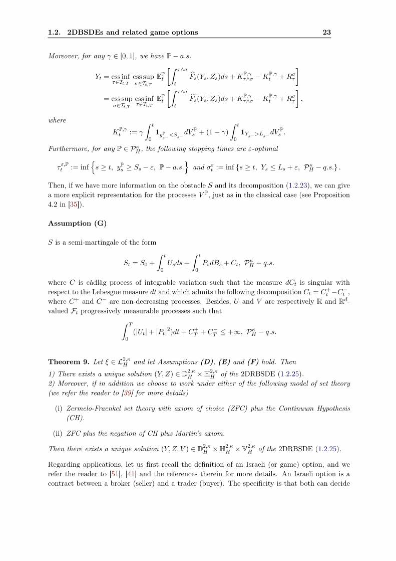
Assumption (G)
S is a semi-martingale of the form
St = S0 +∫ t
0Usds+
∫ t
0PsdBs + Ct, Pκ
H − q.s.
where C is càdlàg process of integrable variation such that the measure dCt is singular withrespect to the Lebesgue measure dt and which admits the following decomposition Ct = C+
t −C−t ,
where C+ and C− are non-decreasing processes. Besides, U and V are respectively R and Rd-valued Ft progressively measurable processes such that∫ T
0(|Ut|+ |Pt|2)dt+ C+
T + C−T ≤ +∞, PκH − q.s.
Theorem 9. Let ξ ∈ L2,κH and let Assumptions (D), (E) and (F) hold. Then
1) There exists a unique solution (Y, Z) ∈ D2,κH ×H2,κ
H of the 2DRBSDE (1.2.25).2) Moreover, if in addition we choose to work under either of the following model of set theory(we refer the reader to [39] for more details)
(i) Zermelo-Fraenkel set theory with axiom of choice (ZFC) plus the Continuum Hypothesis(CH).
(ii) ZFC plus the negation of CH plus Martin’s axiom.
Then there exists a unique solution (Y, Z, V ) ∈ D2,κH ×H2,κ
H × V2,κH of the 2DRBSDE (1.2.25).
Regarding applications, let us first recall the definition of an Israeli (or game) option, and werefer the reader to [51], [41] and the references therein for more details. An Israeli option is acontract between a broker (seller) and a trader (buyer). The specificity is that both can decide
24 Chapter 1. Introduction
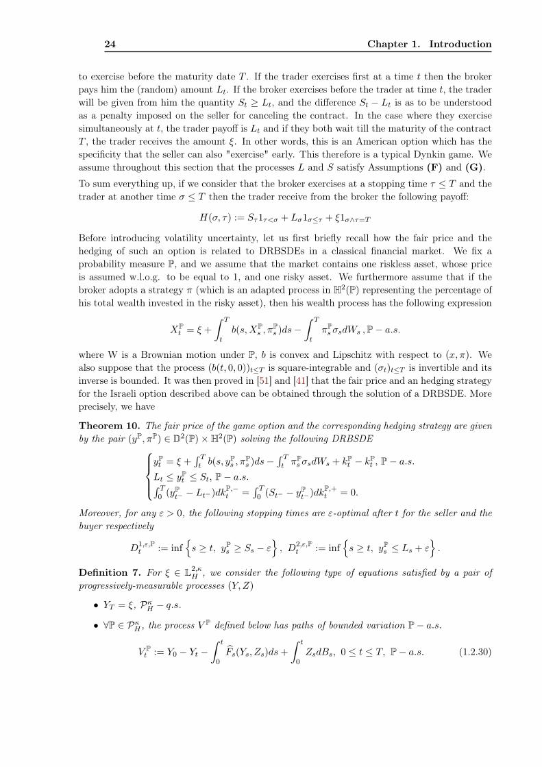
to exercise before the maturity date T . If the trader exercises first at a time t then the brokerpays him the (random) amount Lt. If the broker exercises before the trader at time t, the traderwill be given from him the quantity St ≥ Lt, and the difference St − Lt is as to be understoodas a penalty imposed on the seller for canceling the contract. In the case where they exercisesimultaneously at t, the trader payoff is Lt and if they both wait till the maturity of the contractT , the trader receives the amount ξ. In other words, this is an American option which has thespecificity that the seller can also "exercise" early. This therefore is a typical Dynkin game. Weassume throughout this section that the processes L and S satisfy Assumptions (F) and (G).
To sum everything up, if we consider that the broker exercises at a stopping time τ ≤ T and thetrader at another time σ ≤ T then the trader receive from the broker the following payoff:
H(σ, τ) := Sτ1τ<σ + Lσ1σ≤τ + ξ1σ∧τ=T
Before introducing volatility uncertainty, let us first briefly recall how the fair price and thehedging of such an option is related to DRBSDEs in a classical financial market. We fix aprobability measure P, and we assume that the market contains one riskless asset, whose priceis assumed w.l.o.g. to be equal to 1, and one risky asset. We furthermore assume that if thebroker adopts a strategy π (which is an adapted process in H2(P) representing the percentage ofhis total wealth invested in the risky asset), then his wealth process has the following expression
XPt = ξ +
∫ T
tb(s,XP
s , πPs )ds−
∫ T
tπP
sσsdWs ,P− a.s.
where W is a Brownian motion under P, b is convex and Lipschitz with respect to (x, π). Wealso suppose that the process (b(t, 0, 0))t≤T is square-integrable and (σt)t≤T is invertible and itsinverse is bounded. It was then proved in [51] and [41] that the fair price and an hedging strategyfor the Israeli option described above can be obtained through the solution of a DRBSDE. Moreprecisely, we have
Theorem 10. The fair price of the game option and the corresponding hedging strategy are givenby the pair (yP, πP) ∈ D2(P)×H2(P) solving the following DRBSDE
yPt = ξ +
∫ Tt b(s, yP
s , πPs )ds−
∫ Tt πP
sσsdWs + kPt − kP
t , P− a.s.Lt ≤ yP
t ≤ St, P− a.s.∫ T0 (yP
t− − Lt−)dkP,−t =
∫ T0 (St− − yP
t−)dkP,+t = 0.
Moreover, for any ε > 0, the following stopping times are ε-optimal after t for the seller and thebuyer respectively
D1,ε,Pt := inf
s ≥ t, yP
s ≥ Ss − ε, D2,ε,P
t := infs ≥ t, yP
s ≤ Ls + ε.
Definition 7. For ξ ∈ L2,κH , we consider the following type of equations satisfied by a pair of
progressively-measurable processes (Y, Z)
• YT = ξ, PκH − q.s.
• ∀P ∈ PκH , the process V P defined below has paths of bounded variation P− a.s.
V Pt := Y0 − Yt −
∫ t
0Fs(Ys, Zs)ds+
∫ t
0ZsdBs, 0 ≤ t ≤ T, P− a.s. (1.2.30)
1.2. 2DBSDEs and related game options 25
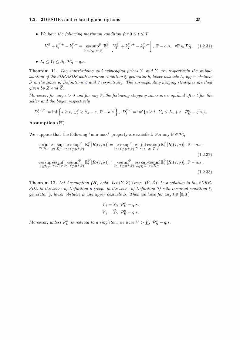
• We have the following maximum condition for 0 ≤ t ≤ T
V Pt + kP,+
t − kP,−t = ess supP
P′∈PH(t+,P)
EP′t
[V P′
T + kP′ ,+T − kP′ ,−
T
], P− a.s., ∀P ∈ Pκ
H . (1.2.31)
• Lt ≤ Yt ≤ St, PκH − q.s.
Theorem 11. The superhedging and subhedging prices Y and Y are respectively the uniquesolution of the 2DRBSDE with terminal condition ξ, generator b, lower obstacle L, upper obstacleS in the sense of Definitions 6 and 7 respectively. The corresponding hedging strategies are thengiven by Z and Z.
Moreover, for any ε > 0 and for any P, the following stopping times are ε-optimal after t for theseller and the buyer respectively
D1,ε,Pt := inf
s ≥ t, yP
s ≥ Ss − ε, P− a.s., D2,ε
t := inf s ≥ t, Ys ≤ Ls + ε, PκH − q.s. .
Assumption (H)
We suppose that the following "min-max" property are satisfied. For any P ∈ PκH
ess infτ∈Tt,T
ess supσ∈Tt,T
ess supP
P′∈PκH(t+,P)
EP′t [Rt(τ, σ)] = ess supP
P′∈PκH(t+,P)
ess infτ∈Tt,T
ess supσ∈Tt,T
EP′t [Rt(τ, σ)], P− a.s.
(1.2.32)
ess supσ∈Tt,T
ess infτ∈Tt,T
ess infPP′∈Pκ
H(t+,P)EP′
t [Rt(τ, σ)] = ess infPP′∈Pκ
H(t+,P)ess supσ∈Tt,T
ess infτ∈Tt,T
EP′t [Rt(τ, σ)], P− a.s.
(1.2.33)
Theorem 12. Let Assumption (H) hold. Let (Y, Z) (resp. (Y , Z)) be a solution to the 2DRB-SDE in the sense of Definition 6 (resp. in the sense of Definition 7) with terminal condition ξ,generator g, lower obstacle L and upper obstacle S. Then we have for any t ∈ [0, T ]
V t = Yt, PκH − q.s.
V t = Yt, PκH − q.s.
Moreover, unless PκH is reduced to a singleton, we have V > V , Pκ
H − q.s.

Chapter 2
SPDE with singular terminal condition
Contents2.1 Setting and main results . . . . . . . . . . . . . . . . . . . . . . . . . . . . 29
2.2 Monotone BDSDE . . . . . . . . . . . . . . . . . . . . . . . . . . . . . . . . 33
2.2.1 Case with f(t, y, z) = f(t, y) and g(t, y, z) = gt . . . . . . . . . . . . . . . . 33
2.2.2 General case . . . . . . . . . . . . . . . . . . . . . . . . . . . . . . . . . . . 38
2.2.3 Extension, comparison result . . . . . . . . . . . . . . . . . . . . . . . . . . 40
2.3 Singular terminal condition, construction of a minimal solution . . . . 41
2.3.1 Approximation . . . . . . . . . . . . . . . . . . . . . . . . . . . . . . . . . . 41
2.3.2 Existence of a limit at time T . . . . . . . . . . . . . . . . . . . . . . . . . . 46
2.3.3 Minimal solution . . . . . . . . . . . . . . . . . . . . . . . . . . . . . . . . . 49
2.4 Limit at time T by localization technic . . . . . . . . . . . . . . . . . . . 51
2.4.1 Proof of (2.4.31) if q > 2 . . . . . . . . . . . . . . . . . . . . . . . . . . . . . 53
2.4.2 Proof of (2.4.31) if q ≤ 2 . . . . . . . . . . . . . . . . . . . . . . . . . . . . . 55
2.5 Link with SPDE’s . . . . . . . . . . . . . . . . . . . . . . . . . . . . . . . . 59
Introduction
We recall that a BDSDE is written as:
Yt = ξ +∫ T
tf (r, Yr, Zr) dr +
∫ T
tg (r, Yr, Zr)
←−−dBr −
∫ T
tZrdWr, 0 ≤ t ≤ T, (2.0.1)
where B is a Brownian motion, independent of W , and←−−dBr is the backward Itô integral. These
BSDE are connected with the following type of stochastic PDE: for (t, x) ∈ [0, T ]× Rd
u(t, x) = h(x) +∫ T
t[Lu(s, x) + f(s, x, u(s, x), (∇uσ)(s, x))] ds (2.0.2)
+∫ T
tg(s, x, u(s, x), (∇uσ)(s, x))
←−−dBr.
The main goal of this chapter is to extend the results of [83] to BDSDE and to obtain a solutionfor a SPDE with singular terminal condition h. But before we have to prove existence anduniqueness of the solution of a BDSDE with monotone generator f . To our best knowlegde theclosest result on this topic is in Aman [2]. Nevertheless we think that there is a lack in this
28 Chapter 2. SPDE with singular terminal condition
paper (proof 4.2). Indeed for monotone BSDE (g = 0) the existence of a solution relies on thesolvability of the BSDE:
Yt = ξ +∫ T
tf (r, Yr) dr −
∫ T
tZrdWr, 0 ≤ t ≤ T.
See among other the proof of Theorem 2.2 and Proposition 2.4 in [72]. To obtain a solution forthis BSDE, the main trick is to truncate the coefficients with suitable truncation functions inorder to have a bounded solution Y (see Proposition 2.2 in [18]). This can not be done for ageneral BDSDE. Indeed take for example (ξ = f = 0 and g = 1):
Yt =∫ T
t
←−−dBr −
∫ T
tZrdWr = BT −Bt, 0 ≤ t ≤ T,
with Z = 0. Thus in order to prove existence of a solution for (2.0.1), one can not directly followthe scheme of [72]. The first part of this paper is devoted to the existence of a solution for amonotone BDSDE (see Section 2.2) in the space E2. To realize this project we will restrict theclass of functions f : they should satisfy a polynomial growth condition (as in [18]). Until nowwe do not know how to extend this to general growth condition as in [72] or [19].The second goal of this work is to extend the results of [83] to the doubly stochastic framework.We will consider the generator f(y) = −y|y|q with q ∈ R∗+ and a real FW
T -measurable and nonnegative random variable ξ such that:
P(ξ = +∞) > 0. (2.0.3)
And we want to find a solution to the following BDSDE:
Yt = ξ −∫ T
tYs|Ys|qds+
∫ T
tg(s, Ys, Zs)
←−−dBs −
∫ T
tZsdWs. (2.0.4)
The scheme to construct a solution is almost the same as in [83]. Let us emphasize one of maintechnical difficulties. If g = 0, we can use the conditional expectation w.r.t. Ft to withdraw themartingale part. If g 6= 0, this trick is useless and we have to be very careful when we wantalmost sure property of the solution. This BDSDE is connected with the stochastic PDE withterminal condition h: for any 0 ≤ t ≤ T
u(t, x) = h(x) +∫ T
t(Lu(s, x)− u(s, x)|u(s, x)|q) ds
+∫ T
tg(s, u(s, x), σ(s, x)∇u(s, x))
←−−dBs. (2.0.5)
If h is a smooth function we could use the result of Pardoux and Peng [74]. But here we willassume that S = h = +∞ is a closed non empty set and thus we will precise the notion ofsolution for (2.0.5) in this case. Roughly speaking we will show that there is a minimal solutionu in the sense that u belongs to a Sobolev space and is a weak solution of the SPDE on anyinterval [0, T − δ], δ > 0 and satisfies the terminal condition: u(t, x) goes to h(x) also in a weaksense as t goes to T .The chapter is decomposed as follows. In the first section, we give the mathematical setting andour main contributions. In the next section, we study the existence and uniqueness of a class ofmonotone BDSDE. In Section 2.3 we construct a (super)solution for the BDSDE with singularterminal condition. In Section 2.4 we prove continuity at time T for this solution under sufficientconditions. Finally in the last part, we connect BDSDE and SPDE with a singularity at time T .
2.1. Setting and main results 29
2.1 Setting and main results
Let us now precise our notations. W and B are independent Brownian motions defined on aprobability space (Ω,F ,P) with values in Rk and Rm. Let N denote the class of P-null sets ofF . For each t ∈ [0, T ], we define
Ft = FWt ∨ FB
t,T
where for any process η, Fηs,t = σ ηr − ηs; s ≤ r ≤ t ∨ N , Fη
t = Fη0,t. As in [74] we define the
following filtration (Gt, t ∈ [0, T ]) by:
Gt = FWt ∨ FB
0,T .
ξ is a FWT -measurable and Rd-valued random variable.
We define by Hp(0, T ; Rn) the set of (classes of dP × dt a.e. equal) n dimensional jointly mea-surable random processes (Xt, t ≥ 0) which satisty:
1. E(∫ T
0|Xt|2dt
)p/2
< +∞
2. Xt is Gt-measurable for a.e. t ∈ [0, T ].
We denote similarly by Sp(0, T ; Rn) the set of continuous n dimensional random processes whichsatisfy:
1. E
(sup
t∈[0,T ]|Xt|p
)< +∞
2. Xt is Gt-measurable for any t ∈ [0, T ].
Bp(0, T ) is the product Sp(0, T ; Rd)×Hp(0, T ; Rd×k). (Y, Z) ∈ Ep(0, T ) if (Y, Z) ∈ Bp(0, T ) and Yt
and Zt are Ft-measurable. Finally Cp,q([0, T ] × Rd; R) denotes the space of R-valued functionsdefined on [0, T ] × Rd which are p-times continuously differentiable in t ∈ [0, T ] and q-timescontinuously differentiable in x ∈ Rd. Cp,q
b ([0, T ]×Rd; R) is the subspace of Cp,q([0, T ]×Rd; R)in which all functions have uniformly bounded partial derivatives; and Cp,q
c ([0, T ] × Rd; R) thesubspace of Cp,q([0, T ]× Rd; R) in which the functions have a compact support w.r.t. x ∈ Rd.Now we precise our assumptions on f and g. The functions f and g are defined on[0, T ] × Ω × Rd × Rd×k with values respectively in Rd and Rd×m. Moreover we consider thefollowing
Assumptions (A):
• The function y 7→ f(t, y, z) is continuous and there exists a constant µ such that for any(t, y, y′, z) a.s.
〈y − y′, f(t, y, z)− f(t, y′, z)〉 ≤ µ|y − y′|2. (A1)
• There exists Kf such that for any (t, y, z, z′) a.s.
|f(t, y, z)− f(t, y, z′)|2 ≤ Kf |z − z′|2. (A2)
• There exists Cf ≥ 0 and p > 1 such that
|f(t, y, z)− f(t, 0, z)| ≤ Cf (1 + |y|p). (A3)
30 Chapter 2. SPDE with singular terminal condition
• There exists a constant Kg ≥ 0 and 0 < ε < 1 such that for any (t, y, y′, z, z′) a.s.
|g(t, y, z)− g(t, y′, z′)|2 ≤ Kg|y − y′|2 + ε|z − z′|2. (A4)
• Finally for any (t, y, z), f(t, y, z) and g(t, y, z) are Ft measurable with
E∫ T
0
(|f(t, 0, 0)|2 + |g(t, 0, 0)|2
)dt < +∞. (A5)
Remember that from [74] if f also satisfies: there exists Kf such that for any (t, y, y′, z) a.s.
|f(t, y, z)− f(t, y′, z)| ≤ Kf |y − y′| (2.1.6)
then there exists a unique solution (Y, Z) ∈ E2(0, T ) to the BDSDE (2.0.1). Note that (2.1.6)implies that
|f(t, y, z)− f(t, 0, z)| ≤ Kf |y|,
thus the growth assumption (A3) on f is satisfied with p = 1.In Section 2.2 we will prove the following result.
Theorem 13. Under Assumptions (A) and if the terminal condition ξ satisfies
E(|ξ|2) < +∞, (2.1.7)
the BDSDE (2.0.1) has a unique solution (Y, Z) ∈ E2(0, T ).
Using the paper of Aman [2], this result can be extended to the Lp case: for p ∈ (1, 2)
E∫ T
0(|f(t, 0, 0)|p + |g(t, 0, 0)|p) dt+ E(|ξ|p) < +∞.
There exists a unique solution in Ep(0, T ).The next sections are devoted to the singular case. The generator f will be supposed to bedeterministic and given by: f(y) = −y|y|q for some q > 0. The aim is to prove existence of asolution for BDSDE (2.0.4) when the non negative random variable ξ satisfies (2.0.3). A possibleextension of the notion of solution for a BDSDE with singular terminal condition could be thefollowing (see Definition 1 in [83]).
Definition 8 (Solution of the BDSDE (2.0.4)). Let q > 0 and ξ a FWT -measurable non negative
random variable satisfying condition (2.0.3). We say that the process (Y, Z) is a solution of theBDSDE (2.0.4) if (Y, Z) is such that (Yt, Zt) is Ft-measurable and:
(D1) for all 0 ≤ s ≤ t < T : Ys = Yt −∫ t
sYr|Yr|qdr +
∫ t
sg(r, Yr, Zr)
←−−dBr −
∫ t
sZrdWr;
(D2) for all t ∈ [0, T [, E(
sup0≤s≤t
|Ys|2 +∫ t
0‖Zr‖2dr
)< +∞;
(D3) P-a.s. limt→T
Yt = ξ.
A solution is said non negative if a.s. for any t ∈ [0, T ], Yt ≥ 0.

2.1. Setting and main results 31
To obtain an a priori estimate of the solution we will assume that g(t, y, 0) = 0 for any (t, y)a.s. This condition will ensure that our solutions will be non negative and bounded on any timeinterval [0, T − δ] with δ > 0. Without this hypothesis, integrability of the solution would bemore challenging. In Section 2.3, we will prove the following result.
Theorem 14. There exists a process (Y, Z) satisfying Conditions (D1) and (D2) of Definition8 and such that Y has a limit at time T with
limt→T
Yt ≥ ξ.
Moreover this solution is minimal: if (Y , Z) is a non negative solution of (2.0.4), then a.s. forany t, Yt ≥ Yt.
It means in particular that Yt has a left limit at time T .In general we are not able to prove that (D3) holds. As in [83], we give sufficient conditions forcontinuity and we prove it in the Markovian framework. Hence the first hypothesis on ξ is thefollowing:
ξ = h(XT ), (H1)
where h is a function defined on Rd with values in R+ such that the set of singularity S =h = +∞ is closed; and where XT is the value at t = T of a diffusion process or more preciselythe solution of a stochastic differential equation (in short SDE):
Xt = x+∫ t
0b(r,Xr)dr +
∫ t
0σ(r,Xr)dWr, for t ∈ [0, T ]. (2.1.8)
We will always assume that b and σ are defined on [0, T ] × Rd, with values respectively in Rd
and Rd×k, are measurable w.r.t. the Borelian σ-algebras, and that there exists a constant K > 0s.t. for all t ∈ [0, T ] and for all (x, y) ∈ Rd × Rd:
1. Lipschitz condition:
|b(t, x)− b(t, y)|+ ‖σ(t, x)− σ(t, y)‖ ≤ K|x− y|; (L)
2. Growth condition:
|b(t, x)| ≤ K(1 + |x|) and ‖σ(t, x)‖ ≤ K(1 + |x|). (G)
It is well known that under the previous assumptions, Equation (2.1.8) has a unique strongsolution X.We denote R = Rd \ S. The second hypothesis on ξ is: for all compact set K ⊂ R = Rd \h = +∞
h(XT )1K(XT ) ∈ L1 (Ω,FT ,P; R) . (H2)
Unfortunately the above assumptions are not sufficient to prove continuity if q ≤ 2. Thus weadd the following conditions in order to use Malliavin calculus and to prove Equality (2.4.41).
1. The functions σ and b are bounded: there exists a constant K s.t.
∀(t, x) ∈ [0, T ]× Rd, |b(t, x)|+ ‖σ(t, x)‖ ≤ K. (B)
32 Chapter 2. SPDE with singular terminal condition
2. The second derivatives of σσ∗ belongs to L∞:
∂2σσ∗
∂xi∂xj∈ L∞([0, T ]× Rd). (D)
3. σσ∗ is uniformly elliptic, i.e. there exists λ > 0 s.t. for all (t, x) ∈ [0, T ]× Rd:
∀y ∈ Rd, σσ∗(t, x)y.y ≥ λ|y|2. (E)
4. h is continuous from Rd to R+ and:
∀M ≥ 0, h is a Lipschitz function on the set OM = |h| ≤M . (H3)
Theorem 15. Under assumptions (H1), (H2) and (L) and if
• either q > 2 and (G);
• or (B), (D), (E) and (H3);
the minimal non negative solution (Y, Z) of (2.0.4) satisfies (D3): a.s.
limt→T
Yt = ξ.
Finally in section 2.5, we show that this minimal solution (Y, Z) of (2.0.4) is connected to theminimal weak solution u of the SPDE (2.0.5). More precisely Xt,x is the solution of the SDE(2.1.8) with initial condition x at time t and (Y t,x, Zt,x) is the minimal solution of the BDSDE(2.0.4) with singular terminal condition ξ = h(Xt,x
T ).Let us define the space H(0, T ) as in [6]. We take the following weight function ρ : Rd → R: forκ > d
ρ(x) =1
(1 + |x|)κ. (2.1.9)
The constant κ will be fixed later. H(0, T ) is the set of the random fields u(t, x); 0 ≤ t ≤ T, x ∈Rd such that u(t, x) is FB
t,T -measurable for each (t, x), u and σ∗∇u belong to L2((0, T ) × Ω ×Rd; ds⊗ dP⊗ ρ(x)dx). On H(0, T ) we consider the following norm
‖u‖22 = E∫ T
0
∫Rd
(|u(s, x)|2 + |(σ∗∇u)(s, x)|2
)ρ(x)dx.
Theorem 16. The random field u defined by u(t, x) = Y t,xt belongs to H(0, T − δ) for any
δ > 0 and is a weak solution of the SPDE (2.0.5) on [0, T − δ]× Rd. At time T , u satisfies a.s.lim inft→T u(t, x) ≥ h(x).Moreover under the same assumptions of Theorem 15, for any function φ ∈ C∞c (Rd) with supportincluded in R, then
limt→T
E(∫
Rd
u(t, x)φ(x)dx)
=∫
Rd
h(x)φ(x)dx.
Finally u is the minimal non negative solution of (2.0.5).
The almost sure continuity of u at time T is still an open question. In [83], this property is provedusing viscosity solution arguments (relaxation of the boundary condition). Here we cannot dothe same trick. This point will be investigated in further publications.In the continuation, unimportant constants will be denoted by C.

2.2. Monotone BDSDE 33
2.2 Monotone BDSDE
As mentioned in the introduction and in the previous section, our first contribution is the exten-sion of the result of Pardoux and Peng [74] with monotone condition (A1). We begin with theparticular case where f does not depend on z and g is a given random field.
2.2.1 Case with f(t, y, z) = f(t, y) and g(t, y, z) = gt
In this special case assume that there exists a solution to the BDSDE:
Yt = ξ +∫ T
tf (r, Yr) dr +
∫ T
tgr←−−dBr −
∫ T
tZrdWr, 0 ≤ t ≤ T. (2.2.10)
Then we have
Yt +∫ t
0gr←−−dBr = ξ +
∫ T
0gr←−−dBr +
∫ T
tf (r, Yr) dr −
∫ T
tZrdWr, 0 ≤ t ≤ T.
Let us define:
Ut = Yt +∫ t
0gr←−−dBr, ζ = ξ +
∫ T
0gr←−−dBr,
and
φ(t, y) = f
(t, y −
∫ t
0gr←−−dBr
).
Then (U,Z) satisfies:
Ut = ζ +∫ T
tφ (r, Ur) dr −
∫ T
tZrdWr, 0 ≤ t ≤ T. (2.2.11)
The terminal condition ζ is GT -measurable and the generator φ satisfies the following assump-tions.
1. φ is continuous w.r.t. y and (A1) is true with the same constant µ.
2. From (A3), there exists p > 1 such that
|φ(t, y)| ≤ h(t) + Cφ(1 + |y|p). (2.2.12)
where Cφ = Cf2p−1 and
h(t) = |f(t, 0)|+ 2p−1
∣∣∣∣∫ t
0gr←−−dBr
∣∣∣∣p .On the solution (U,Z) we impose the following measurability constraints:
(M1). The process (U,Z) is adapted to the filtration (Gt, t ≥ 0).
(M2). The random variable Ut −∫ t0 gr←−−dBr is Ft-measurable for any 0 ≤ t ≤ T .
34 Chapter 2. SPDE with singular terminal condition
Let us assume the boundedness hypothesis on ξ, g and f(t, 0): there exists a constant γ > 0such that a.s. for any t ≥ 0,
|ξ|+ |f(t, 0)|+ |gt| ≤ γ. (2.2.13)
Hence for any q > 1
E[|ζ|q +
(∫ T
0|h(t)|qdt
)]< +∞.
From [18] or [72] there exists a unique solution (U,Z) ∈ B2(0, T ) to the BSDE (2.2.11) such that(M1) holds and
E
[sup
t∈[0,T ]|Ut|2 +
(∫ T
0|Zr|2dr
)]< +∞.
Theorem 3.6 in [18] also gives that
E
[sup
t∈[0,T ]|Ut|2p +
(∫ T
0|Zr|2dr
)p]< +∞.
But we cannot derive directly from this result that (M2) is satisfied, that is Ut −∫ t0 gr←−−dBr is Ft-
measurable for any 0 ≤ t ≤ T . Therefore we follow the proof of Proposition 3.5 in [18] to provethe existence and uniqueness of the solution (U,Z) with the desired measurability conditions.
Proposition 3. Under Assumptions (A1), (A2), (A3) and (2.2.13), there exists a unique solu-tion (U,Z) ∈ B2(0, T ) to the BSDE (2.2.11), such that (M1) and (M2) hold.
Proof. As written before, we sketch the proof of Proposition 3.5 in [18]. The details can befound in [18] and we just emphasize the main differences. For any n ≥ 1, we define the followingfunction:
φn(t, y) =
φ(t, y) if h(t) ≤ n,n
|h(t)|φ(t, y) if h(t) > n.
This function is continuous w.r.t. y and (A1) still holds. Moreover
|φn(t, y)| ≤ (|h(t)| ∧ n) + Cφ(1 + |y|p).
Then as in [18], we defineφn(t, .) = ρn ∗ (Θq(n)+1(φn(t, .))),
where
• q(n) = de1/2(n+ 2Cφ)√
1 + T 2e+ 1, where dre stands for the integer part of r;
• Θn is a smooth function with values in [0, 1] such that Θn(u) = 1 if |u| ≤ n, Θn(u) = 0 if|u| ≥ n+ 1;
• ρn(u) = nkρ(nu) with ρ a C∞ non negative function with support equal to the unit balland such that
∫ρ(u)du = 1.
Since ζ is in Lq(Ω) (for any q > 2p) there exists a unique solution (Un, V n) ∈ Bq(0, T ) to theBSDE (see Theorem 4.2 in [19] or Theorem 5.1 in [36]):
Unt = ζ +
∫ T
tφn (r, Un
r ) dr −∫ T
tV n
r dWr, 0 ≤ t ≤ T. (2.2.14)

2.2. Monotone BDSDE 35
Moreover for some constant Kp independent of n
E
[sup
t∈[0,T ]|Un
t |2p +(∫ T
0|V n
r |2dr)p]≤ KpE
[|ζ|2p +
(∫ T
0(|h(r)|+ 2Cφ)dr
)2p].
We have a strong convergence of the sequence (Un, V n) to (U,Z):
limn→+∞
E
[sup
t∈[0,T ]|Un
t − Ut|2 +(∫ T
0|V n
r − Zr|2dr)]
= 0.
And (U,Z) is the solution of BSDE (2.2.11) satisfying condition (M1) and (U,Z) ∈ B2p(0, T ).Now let us come to the measurability condition (M2). Recall that
φ(t, y) = f
(t, y −
∫ t
0gr←−−dBr
),
h(t) = |f(t, 0)|+ 2p−1
∣∣∣∣∫ t
0gr←−−dBr
∣∣∣∣p ,and the process f(t, .) is Ft-measurable. Hence for any y and t
φn(t, y +∫ t
0gr←−−dBr) = ρn ∗ (Θq(n)+1(φn(t, .)))(y +
∫ t
0gr←−−dBr)
=∫ρn(z)Θq(n)+1
(φn
(t, y − z +
∫ t
0gr←−−dBr
))dz.
Now
φn
(t, x+
∫ t
0gr←−−dBr
)=
n
h(t) ∨ nf(t, x) =
n
h(t)1h(t)≥n ∨ nf(t, x),
Thus φn(t, y +∫ t0 gr←−−dBr) is measurable w.r.t. the σ-algebra Ft ∨ σ(h(t)1h(t)≥n). Let us denote
Hn = σ(h(t)1h(t)≥n, 0 ≤ t ≤ T ).
φn(t, y +∫ t0 gr←−−dBr) is measurable w.r.t. the σ-algebra Fn
t = Ft ∨Hn.If we define
Y nt = Un
t −∫ t
0gr←−−dBr,
then
Y nt = ξ +
∫ T
tgr←−Br +
∫ T
tφn
(r, Y n
r +∫ r
0gs←−Bs
)dr −
∫ T
tV n
r dWr, 0 ≤ t ≤ T.
We claim that Y nt is measurable w.r.t. Ft ∨ Hn. Indeed let us recall that (Un, V n), solution of
(2.2.14), is obtained via a fixed-point theorem. We define the map Ψ : B2(0, T ) → B2(0, T ) by:(U, V ) = Ψ(u, v) with
Ut = ζ +∫ T
tφn (r, ur) dr −
∫ T
tVrdWr, 0 ≤ t ≤ T.
By classical arguments (see the details in [36], Theorem 2.1), Ψ is a contraction on B2(0, T ) (undersuitable norms) and (Un, V n) is the fixed point of Ψ. Set (Un,m, V n,m) for any m ∈ N as follows:
36 Chapter 2. SPDE with singular terminal condition
for any t, (Un,0t , V n,0
t ) = (∫ t0 gs←−Bs, 0) and for any m ≥ 1, (Un,m, V n,m) = Ψ(Un,m−1, V n,m−1).
This sequence converges in B2(0, T ) to (Un, V n). Therefore Y n is the limit in S2(0, T ) of Y n,m
defined by: Y n,0t = 0 and
Y n,mt = ξ +
∫ T
tgr←−Br +
∫ T
tφn
(r, Y n,m−1
r +∫ r
0gs←−Bs
)dr −
∫ T
tV n,m
r dWr, 0 ≤ t ≤ T.
Now Y n,0t is trivially Ft measurable and
Y n,mt = E
[ξ +
∫ T
tgr←−Br
∣∣∣∣Gt
]+ E
[∫ T
tφn
(r, Y n,m−1
r +∫ r
0gs←−Bs
)dr
∣∣∣∣Gt
]= E
[ξ +
∫ T
tgr←−Br
∣∣∣∣Gt
]+ E
[Θ∣∣Gt
].
From [74] we know that the first term on the right hand side is Ft measurable. Assume thatY n,m−1
t is Ft ∨Hn measurable. Since the same holds for φn
(t, y +
∫ t0 gs←−Bs
), Θ depends only on
FWT ∨FB
t,T ∨Hn. Thus there is no independence between FBt and Ft ∨ σ(Θ), but Y n,m
t dependson FB
t only through Hn. Hence Y n,mt is Ft ∨ Hn measurable. Passing through the limit, we
obtain the desired measurability condition on Y n.Now for any m ∈ N, the sequence (Y n
t , n ≥ m) depends on the σ-algebra
Ft ∨Hm = Ft ∨
∨n≥m
Hn
.
Passing through the limit, we obtain that the limit Yt depends only on Ft ∨H∞ = Ft ∨⋂
m∈NHm.
The next lemma shows that H∞ ⊂ F0. We deduce that Yt is Ft-measurable, which achieves theproof.
Lemma 1. The σ-algebra H∞ is trivial: for every A ∈ H∞, A or Ac = Ω \A is negligible.
Proof. Recall that f and g are supposed to be bounded by a constant γ and
h(t) = |f(t, 0)|+ 2p−1
∣∣∣∣∫ t
0gr←−−dBr
∣∣∣∣p .Thus for any n
P
(sup
t∈[0,T ]h(t) ≥ n
)≤ P
(sup
t∈[0,T ]
∣∣∣∣∫ t
0gr←−−dBr
∣∣∣∣p ≥ 21−p(n− γ)
).
The Burkholder-Davis-Gundy inequality shows that
E
(sup
t∈[0,T ]
∣∣∣∣∫ t
0gr←−−dBr
∣∣∣∣p)≤ Cpγ
pT p/2.
And by Markov inequality for n > γ
P
(sup
t∈[0,T ]
∣∣∣∣∫ t
0gr←−−dBr
∣∣∣∣p ≥ 21−p(n− γ)
)≤ Cpγ
pT p/2
21−p(n− γ).

2.2. Monotone BDSDE 37
Note ζ = supt∈[0,T ] h(t). Now if A ∈ Hn, then we have two cases: either the set ζ < n isincluded either in A or in Ac. And if n ≥ m, then ζ < m ⊂ ζ < n. Hence if A is in
∨n≥m
Hn,
then ζ < m ⊂ A or A ∩ ζ < m = ∅. And thus P(A) ∧ P(Ac) ≤ C/(m − γ) for any m > γ.Finally if A ∈ H∞ =
⋂m∈N
∨n≥m
Hn, then P(A) = 0 or P(A) = 1.
From the previous lemma, if we define
Yt = Ut −∫ t
0gr←−−dBr
we obtain a solution (Y, Z) to the BDSDE:
Yt = ξ +∫ T
tf (r, Yr) dr +
∫ T
tgr←−−dBr −
∫ T
tZrdWr, 0 ≤ t ≤ T.
From the boundedness assumption on g, we have:
E
[sup
t∈[0,T ]|Yt|2 +
(∫ T
0|Zr|2dr
)]< +∞.
From the previous proof Yt is Ft-measurable. Then using the same argument as in [74], theprocess Zt is also Ft-measurable. In other words (Y, Z) ∈ E2(0, T ).Now we only assume that
E[|ξ|2 +
∫ T
0(|f(t, 0)|2 + |gt|2)dt
]< +∞.
For any n ∈ N∗ define Θn by
Θn(y) =
y if |y| ≤ n,ny
|y|if |y| > n,
and ξn = Θn(ξ), gnt = Θn(gt) and fn(t, y) = f(t, y) − f(t, 0) + Θn(f(t, 0)). Thus for a fixed n,
there exists a solution (Y n, Zn) to the BDSDE (2.2.10) with ξn, fn and gn instead of ξ, f and g:
Y nt = ξn +
∫ T
tfn (r, Y n
r ) dr +∫ T
tgnr
←−−dBr −
∫ T
tZn
r dWr, 0 ≤ t ≤ T.
Define for any n and m
∆ξ = ξm − ξn, ∆f(t, y) = fm(t, y)− fn(t, y), ∆gt = gmt − gn
t ,
and∆Yt = Y m
t − Y nt , ∆Zt = Zm
t − Znt .
From the Itô formula with α = 2µ+ 1, we have:
eαt|∆Yt|2 +∫ T
teαr|∆Zr|2dr = eαT |∆ξ|2 + 2
∫ T
teαs∆Ys(fm(s, Y m
s )− fn(s, Y ns ))ds
−∫ T
tαeαs|∆Ys|2ds− 2
∫ T
teαs∆Ys∆ZsdWs − 2
∫ T
teαs∆Ys∆gs
←−−dBs
+∫ T
teαs|∆gs|2ds.
38 Chapter 2. SPDE with singular terminal condition
From assumption (A1) on f and 2|ab| ≤ a2 + b2, we obtain:
eαt|∆Yt|2 +∫ T
teαr|∆Zr|2dr ≤ eαT |∆ξ|2 +
∫ T
teαs|∆f(s, 0)|2ds
−2∫ T
teαs∆Ys∆ZsdWs − 2
∫ T
teαs∆Ys∆gs
←−−dBs +
∫ T
teαs|∆gs|2ds.
Using BDG inequality we deduce that there exists a constant C depending on α and T such that
E
[sup
t∈[0,T ]|∆Yt|2 +
∫ T
0|∆Zr|2dr
]≤ CE
[|∆ξ|2 +
∫ T
0|∆f(s, 0)|2ds+
∫ T
0|∆gs|2ds
].
Therefore (Y n, Zn) is a Cauchy sequence which converges to (Y, Z) and the limit process (Y, Z) ∈E2(0, T ) satisfies the BDSDE (2.2.10).
Remark 1. Can we assume a weaker growth condition on f ? Suppose that there exists a nondecreasing function ψ : R+ → R+ such that
|f(t, y)| ≤ |f(t, 0)|+ ψ(|y|).
Using the same transformation, we have to control:
|φ(t, y)| = |f(t, y +∫ t
0gr←−−dBr)| ≤ |f(t, 0)|+ ψ(|y +
∫ t
0gr←−−dBr|).
If it is possible to find two functions ψ1 and ψ2 such that ψ(y + z) ≤ ψ1(y) + ψ2(z) and ifψ2(|
∫ t0 gr←−−dBr|) belongs to L2(Ω) for any bounded process gt, it may be possible to obtain a solution
with the desired properties to the BDSDE (2.0.1).Until now we did not succeed to obtain an example which is not controlled by (A3) for some plarge enough.
2.2.2 General case
The general case can be deduced from the previous one by a fixed-point argument. Let usconstruct the following sequence: (Y 0, Z0) = (0, 0) and for n ∈ N and any 0 ≤ t ≤ T
Y n+1t = ξ +
∫ T
tf(r, Y n+1
r , Znr
)dr +
∫ T
tg (r, Y n
r , Znr )←−−dBr −
∫ T
tZn+1
r dWr. (2.2.15)
Indeed if
E
[sup
t∈[0,T ]|Y n
t |2 +(∫ T
0|Zn
r |2dr)]
< +∞
then from (A4) and (A5), the process gnr = g (r, Y n
r , Znr ) satisfies
E∫ T
0|gn
r |2dr < +∞.
Moreover the process fn(r, 0) = f(r, 0, Znr ) verifies
E∫ T
0|f(r, 0, Zn
r )|2ds ≤ K2fE∫ T
0|Zn
r |2dr + E∫ T
0|f(r, 0, 0)|2dr < +∞.
2.2. Monotone BDSDE 39
The previous section shows that (Y n+1, Zn+1) exists and satisfies (2.2.15) with
E
[sup
t∈[0,T ]|Y n+1
t |2 +(∫ T
0|Zn+1
r |2dr)]
< +∞.
Hence the sequence of processes (Y n, Zn) is well defined.Now as before define for any n and m
∆Y nt = Y n+1
t − Y nt , ∆Zn
t = Zn+1t − Zn
t , ∆gnt = g(t, Y n+1
t , Zn+1t )− g(t, Y n
t , Znt ).
From the Itô formula with α > 0, we have:
eαt|∆Y nt |2 +
∫ T
teαr|∆Zn
r |2dr = 2∫ T
teαs∆Y n
s (f(s, Y n+1s , Zn
s )− f(s, Y ns , Z
n−1s ))ds
−∫ T
tαeαs|∆Y n
s |2ds− 2∫ T
teαs∆Y n
s ∆Zns dWs − 2
∫ T
teαs∆Y n
s ∆gn−1s
←−−dBs
+∫ T
teαs|∆gn−1
s |2ds.
Using the Lipschitz assumption on g, we have
|∆gn−1s |2 ≤ Kg|∆Y n−1
s |2 + ε|∆Zn−1s |2.
And∆Y n
s (f(s, Y n+1s , Zn
s )− f(s, Y ns , Z
n−1s )) ≤ µ|∆Y n
s |2 +√Kf |∆Y n
s ||∆Zn−1s |.
Thus
eαt|∆Y nt |2 +
∫ T
teαr|∆Zn
r |2dr ≤ (2µ− α)∫ T
teαs|∆Y n
s |2ds (2.2.16)
+2√Kf
∫ T
teαs|∆Y n
s ||∆Zn−1s |ds− 2
∫ T
teαs∆Y n
s ∆Zns dWs
−2∫ T
teαs∆Y n
s ∆gn−1s
←−−dBs +Kg
∫ T
teαs|∆Y n−1
s |2ds+ ε
∫ T
teαs|∆Zn−1
s |2ds.
Using the inequality ab ≤ ηa2 + 1η b
2, we have
2√Kf
∫ T
teαs|∆Y n
s ||∆Zn−1s |ds ≤ ηKf
∫ T
teαs|∆Y n
s |2ds+1η
∫ T
t|∆Zn−1
s |ds.
Therefore taking the expectation in (2.2.16) we deduce that
Eeαt|∆Y nt |2 + E
∫ T
teαr|∆Zn
r |2dr ≤ (2µ+ ηKf − α)E∫ T
teαs|∆Y n
s |2ds
+(
1η
+ ε
)E∫ T
teαs|∆Zn−1
s |ds+KgE∫ T
teαs|∆Y n−1
s |2ds.
Take t = 0, η = 21−ε and α = 2µ+ 2Kf
1−ε + 2Kg
1+ε such that
E∫ T
0eαr|∆Zn
r |2dr +2Kg
1 + εE∫ T
0eαs|∆Y n
s |2ds (2.2.17)
≤(
1 + ε
2
)E∫ T
0eαs|∆Zn−1
s |ds+(
1 + ε
2
)E∫ T
0
2Kg
1 + εeαs|∆Y n−1
s |2ds.
40 Chapter 2. SPDE with singular terminal condition
Since (1+ ε)/2 < 1, the sequence (Y n, Zn) is a Cauchy sequence in L2((0, T )×Ω) and convergesto some process (Y, Z). Moreover by the BDG inequality we also obtain:
E supt∈[0,T ]
∣∣∣∣∫ T
teαs∆Y n
s ∆Zns dWs
∣∣∣∣ ≤ 4E(∫ T
0e2αs|∆Y n
s |2|∆Zns |2ds
)1/2
≤ 14
E
(sup
t∈[0,T ]eαt|∆Y n
t |2)
+ 64E∫ T
0eαs|∆Zn
s |2ds,
and
E supt∈[0,T ]
∣∣∣∣∫ T
teαs∆Y n
s ∆gn−1s
←−−dBs
∣∣∣∣ ≤ 4E(∫ T
0e2αs|∆Y n
s |2|∆gn−1s |2ds
)1/2
≤ 14
E
(sup
t∈[0,T ]eαt|∆Y n
t |2)
+ 32E∫ T
0eαs|∆gn−1
s |2ds
≤ 14
E
(sup
t∈[0,T ]eαt|∆Y n
t |2)
+ 32KgE∫ T
0eαs|∆Y n−1
s |2ds+ 32εE∫ T
0eαs|∆Zn−1
s |2ds.
Coming back to (2.2.16) and using (2.2.17) we have for some constant C
E supt∈[0,T ]
eαt|∆Y nt |2 ≤ CE
∫ T
0eαr|∆Zn−1
r |2dr + CE∫ T
0eαs|∆Y n−1
s |2ds.
We deduce also the convergence of Y n to Y under this strong topology. Therefore (Y, Z) satisfiesthe general BDSDE:
Yt = ξ +∫ T
tf (r, Yr, Zr) dr +
∫ T
tg (r, Yr, Zr)
←−−dBr −
∫ T
tZrdWr, 0 ≤ t ≤ T.
Hence we have proved Theorem 13.
2.2.3 Extension, comparison result
The extension of Lp solutions, p ∈ (1, 2), is done in Aman [2] (see also Theorem 1.4 in [74] forp > 2). We just want here to recall the comparison principle for BDSDE (see [87], [62] or [37]on this topic). We will widely use the result in the next sections.
Proposition 4. Assume that BDSDE (2.0.1) with data (f1, g, ξ1) and (f2, g, ξ2) have solutions(Y 1, Z1) and (Y 2, Z2) in E2(0, T ), respectively. The coefficient g satisfies (A4). If ξ1 ≤ ξ2, a.s.,and f1 satisfies Assumptions (A1) and (A2), for all t ∈ [0, T ], f1(t, Y 2
t , Z2t ) ≤ f2(t, Y 2
t , Z2t ), a.s.
(resp. f2 satisfies (A1) and (A2), for all t ∈ [0, T ], f1(t, Y 1t , Z
1t ) ≤ f2(t, Y 1
t , Z1t ), a.s.), then we
have Y 1t ≤ Y 2
t , a.s., for all t ∈ [0, T ].
Proof. The proof is almost the same as Lemma 3.1 in [62]. We define
(Yt, Zt) = (Y 1t − Y 2
t , Z1t − Z2
t ), ξ = ξ1 − ξ2,
then (Yt, Zt) satisfies the following BDSDE: for all t ∈ [0, T ],
Yt = ξ +∫ T
t
[f1(r, Y 1
r , Z1r
)− f2
(r, Y 2
r , Z2r
)]dr
+∫ T
t
[g(r, Y 1
r , Z1r
)− g
(r, Y 2
r , Z2r
)]←−−dBr −
∫ T
tZrdWr.

2.3. Singular terminal condition, construction of a minimal solution 41
We apply Itô’s formula to (Y +t )2:
(Y +t )2 +
∫ T
t1Yr>0|Zr|2dr ≤ (ξ+)2 + 2
∫ T
tY +
r
[f1(r, Y 1
r , Z1r
)− f2
(r, Y 2
r , Z2r
)]dr
+2∫ T
tY +
r
[g(r, Y 1
r , Z1r
)− g
(r, Y 2
r , Z2r
)]←−−dBr
−2∫ T
tY +
r ZrdWr +∫ T
t1Yr>0|g(r, Y
1r , Z
1r )− g(r, Y 2
r , Z2r )|2dr.
Now from (A1) and (A2)
Y +r
[f1(r, Y 1
r , Z1r
)− f2
(r, Y 2
r , Z2r
)]= Y +
r
[f1(r, Y 1
r , Z1r
)− f1
(r, Y 2
r , Z2r
)]+ Y +
r
[f1(r, Y 2
r , Z2r
)− f2
(r, Y 2
r , Z2r
)]≤ µ(Y +
r )2 +Kf Y+r |Zr|.
The rest of the proof is exactly the same as in [62]. Using Gronwall’s Lemma, we deduce thatE(Y +
t )2 = 0 for any t ∈ [0, T ].
2.3 Singular terminal condition, construction of a minimal solu-tion
From now on we assume that the terminal condition ξ satisfies the property (2.0.3):
P(ξ ≥ 0) = 1 and P(ξ = +∞) > 0.
For q > 0, let us consider the function f : R→ R, defined by f(y) = −y|y|q. f is continuous andmonotone, i.e. satisfies Condition (A1) with µ = 0: for all (y, y′) ∈ R2:
(y − y′)(f(y)− f(y′)) ≤ 0.
Condition (A3) is also satisfied with p = q+1. We also consider a function g : [0, T ]×Ω×R×Rd →R and we assume that Condition (A4) holds.
2.3.1 Approximation
For every n ∈ N∗, we introduce ξn = ξ ∧ n. ξn belongs to L2 (Ω,FT ,P; R). We apply Theorem13 with ξn as the final data, and we build a sequence of random processes (Y n, Zn) ∈ E2(0, T )which satisfy (2.0.4).From Proposition 4, if n ≤ m, 0 ≤ ξn ≤ ξm ≤ m, which implies for all t in [0, T ], a.s.,
Ξ0t ≤ Y n
t ≤ Y mt ≤ Ξm
t . (2.3.18)
Here Ξk is the first component of the unique solution (Ξk,Θk) in E2(0, T ) of (2.0.4) with adeterministic terminal condition k. In order to have explicit and useful bound on Y m we willassume that g(t, y, 0) = 0 for any (t, y) a.s. In this case for m ≥ 1,
Ξ0t = 0, Ξm
t =
(1
q(T − t) + 1mq
) 1q
.
42 Chapter 2. SPDE with singular terminal condition
We define the progressively measurable R-valued process Y , as the increasing limit of the sequence(Y n
t )n≥1:∀t ∈ [0, T ], Yt = lim
n→+∞Y n
t . (2.3.19)
Then we obtain
∀0 ≤ t ≤ T, 0 ≤ Yt ≤(
1q(T − t)
) 1q
. (2.3.20)
In particular Y is finite on the interval [0, T [ and bounded on [0, T − δ] for all δ > 0.Here we will prove the first part of Theorem 14, that is (Y, Z) satisfies properties (D1) and (D2)of the definition 8. Moreover we will obtain that there exists a constant κ, depending on g, s.t.for all t ∈ [0, T [,
E∫ t
0‖Zr‖2dr ≤
κ
(q(T − t))2q
, (2.3.21)
Proof. Let δ > 0 and s ∈ [0, T − δ]. For all 0 ≤ t ≤ s, Itô’s formula leads to the equality:
|Y nt − Y m
t |2 +∫ s
t‖Zn
r − Zmr ‖2dr = |Y n
s − Y ms |2 − 2
∫ s
t(Y n
r − Y mr )(Zn
r − Zmr )dWr
+2∫ s
t(Y n
r − Y mr ) (f(Y n
r )− f(Y mr )) dr
+2∫ s
t(Y n
r − Y mr )(g(r, Y n
r , Znr )− g(r, Y m
r , Zmr ))←−−dBr
+∫ s
t|g(r, Y n
r , Znr )− g(r, Y m
r , Zmr )|2dr
≤ |Y ns − Y m
s |2 +K
∫ s
t|Y n
r − Y mr |2dr + ε
∫ s
t|Zn
r − Zmr |2dr
−2∫ s
t(Y n
r − Y mr )(Zn
r − Zmr )dWr
+2∫ s
t(Y n
r − Y mr )(g(r, Y n
r , Znr )− g(r, Y m
r , Zmr ))←−−dBr
from the monotonicity of f (Inequality (A1)) and the Lipschtiz property of g (Inequality (A4)).From the properties (A4) and since (Y, Z) ∈ E2, we have:
E(∫ s
t(Y n
r − Y mr )(Zn
r − Zmr )dWr
)= 0,
E(∫ s
t(Y n
r − Y mr )(g(r, Y n
r , Znr )− g(r, Y m
r , Zmr ))←−−dBr
)= 0.
From the Burkholder-Davis-Gundy inequality, we deduce the existence of a universal constantC with:
E(
sup0≤t≤s
|Y nt − Y m
t |2 +∫ s
0‖Zn
r − Zmr ‖2dr
)≤ C E
(|Y n
s − Y ms |2
). (2.3.22)
From the estimate (2.3.20), for s ≤ T − δ, Y ns ≤ 1
(qδ)1/q and Ys ≤ 1(qδ)1/q . Since Y n
s converges toYs a.s., the dominated convergence theorem and the previous inequality (2.3.22) imply:
2.3. Singular terminal condition, construction of a minimal solution 43
1. for all δ > 0, (Zn)n≥1 is a Cauchy sequence in L2(Ω × [0, T − δ]; Rd), and converges toZ ∈ L2(Ω× [0, T − δ]; Rd),
2. (Y n)n≥1 converges to Y uniformly in mean-square on the interval [0, T − δ], in particularY is continuous on [0, T ),
3. (Y, Z) satisfies Equation (2.0.4) on [0, T ).
Since Yt is smaller than 1/(q(T − t))1/q by (2.3.20), and since Z ∈ L2(Ω× [0, T −δ]; Rd), applyingthe Itô formula to |Y |2, with s < T and 0 ≤ t ≤ s, we obtain:
|Yt|2 +∫ s
t‖Zr‖2dr = |Ys|2 − 2
∫ s
tYrZrdWr + 2
∫ s
tYrf(Yr)dr
+2∫ s
tYrg(r, Yr, Zr)
←−−dBr +
∫ s
t|g(r, Yr, Zr)|2dr
≤ 1
(q(T − s))2q
− 2∫ s
tYrZrdWr + 2
∫ s
tYrg(r, Yr, Zr)
←−−dBr
+K∫ s
t|Yr|2dr + ε
∫ s
t|Zr|2dr,
again thanks to Inequalities (A1) and (A4). From (2.3.20), since Z ∈ L2([0, s]× Ω), we have:
E∫ s
tYrZrdWr = E
∫ s
tYrg(r, Yr, Zr)
←−−dBr = 0.
Therefore, we deduce that there exists a constant κ depending on T , K and ε such that :
E∫ s
0‖Zr‖2dr ≤
κ
(q(T − s))2q
.
Remark that if g is equal to zero, κ is equal to one. And in general
κ =1
1− ε(1 +KT ).
We want to establish the following statement which completes Inequality (2.3.21).
Proposition 5. The next inequality is a sharper estimation on Z:
E∫ T
0(T − s)2/q‖Zs‖2ds ≤
8 +KT
1− ε
(1q
)2/q
. (2.3.23)
The constants K and ε are given by the assumption (A4).
Proof. First suppose there exists a constant α > 0 such that P-a.s. ξ ≥ α. In this case, bycomparison, for all integer n and all t ∈ [0, T ]:
Y nt ≥
(1
qT + 1/αq
)1/q
> 0.
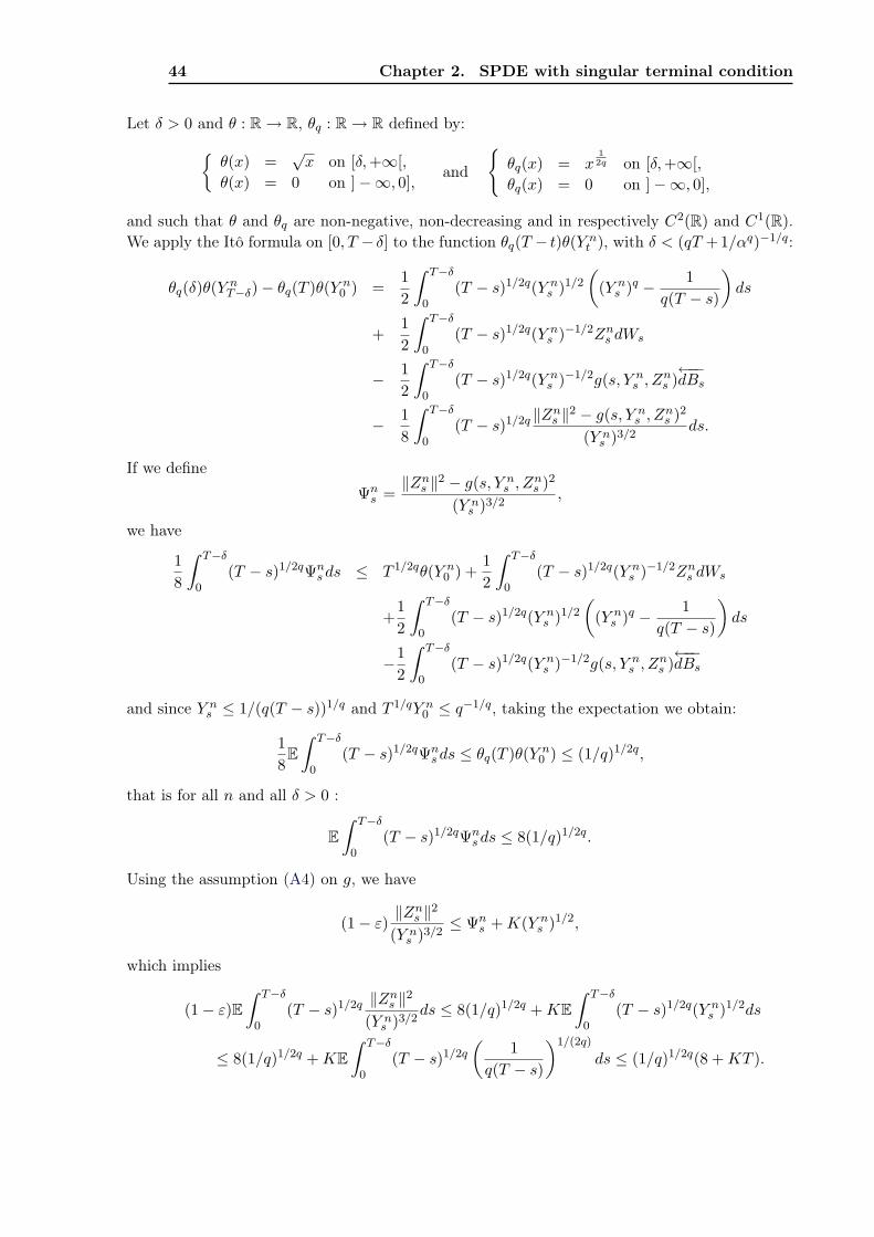
44 Chapter 2. SPDE with singular terminal condition
Let δ > 0 and θ : R→ R, θq : R→ R defined by:θ(x) =
√x on [δ,+∞[,
θ(x) = 0 on ]−∞, 0],and
θq(x) = x
12q on [δ,+∞[,
θq(x) = 0 on ]−∞, 0],
and such that θ and θq are non-negative, non-decreasing and in respectively C2(R) and C1(R).We apply the Itô formula on [0, T − δ] to the function θq(T − t)θ(Y n
t ), with δ < (qT +1/αq)−1/q:
θq(δ)θ(Y nT−δ)− θq(T )θ(Y n
0 ) =12
∫ T−δ
0(T − s)1/2q(Y n
s )1/2
((Y n
s )q − 1q(T − s)
)ds
+12
∫ T−δ
0(T − s)1/2q(Y n
s )−1/2Zns dWs
− 12
∫ T−δ
0(T − s)1/2q(Y n
s )−1/2g(s, Y ns , Z
ns )←−−dBs
− 18
∫ T−δ
0(T − s)1/2q ‖Zn
s ‖2 − g(s, Y ns , Z
ns )2
(Y ns )3/2
ds.
If we define
Ψns =‖Zn
s ‖2 − g(s, Y ns , Z
ns )2
(Y ns )3/2
,
we have
18
∫ T−δ
0(T − s)1/2qΨn
s ds ≤ T 1/2qθ(Y n0 ) +
12
∫ T−δ
0(T − s)1/2q(Y n
s )−1/2Zns dWs
+12
∫ T−δ
0(T − s)1/2q(Y n
s )1/2
((Y n
s )q − 1q(T − s)
)ds
−12
∫ T−δ
0(T − s)1/2q(Y n
s )−1/2g(s, Y ns , Z
ns )←−−dBs
and since Y ns ≤ 1/(q(T − s))1/q and T 1/qY n
0 ≤ q−1/q, taking the expectation we obtain:
18
E∫ T−δ
0(T − s)1/2qΨn
s ds ≤ θq(T )θ(Y n0 ) ≤ (1/q)1/2q,
that is for all n and all δ > 0 :
E∫ T−δ
0(T − s)1/2qΨn
s ds ≤ 8(1/q)1/2q.
Using the assumption (A4) on g, we have
(1− ε) ‖Zns ‖2
(Y ns )3/2
≤ Ψns +K(Y n
s )1/2,
which implies
(1− ε)E∫ T−δ
0(T − s)1/2q ‖Zn
s ‖2
(Y ns )3/2
ds ≤ 8(1/q)1/2q +KE∫ T−δ
0(T − s)1/2q(Y n
s )1/2ds
≤ 8(1/q)1/2q +KE∫ T−δ
0(T − s)1/2q
(1
q(T − s)
)1/(2q)
ds ≤ (1/q)1/2q(8 +KT ).

2.3. Singular terminal condition, construction of a minimal solution 45
Now, since 1/Y ns ≥ (q(T − s))1/q, letting δ → 0 and with the Fatou lemma, we deduce that
E∫ T
0(T − s)2/q‖Zs‖2ds ≤
8 +KT
1− ε(1/q)2/q.
Now we come back to the case ξ ≥ 0. We can not apply the Itô formula because we do not haveany positive lower bound for Y n. We will approach Y n in the following way. We define for n ≥ 1and m ≥ 1, ξn,m by:
ξn,m = (ξ ∧ n) ∨ 1m.
This random variable is in L2 and is greater or equal to 1/m a.s. The BSDE (2.0.4), with ξn,m
as terminal condition, has a unique solution (Y n,m, Zn,m). It is immediate that if m ≤ m′ andn ≤ n′ then:
Y n,m′ ≤ Y n′,m.
As for the sequence Y n, we can define Y m as the limit when n grows to +∞ of Y n,m. This limitY m is greater than Y = limn→+∞ Y n. But for any m and n, for t ∈ [0, T ]:∣∣∣Y n,m
t − Y nt
∣∣∣2 = |ξn,m − ξn|2 − 2∫ T
t
[Y n,m
r − Y nr
] [(Y n,m
r
)q+1− (Y n
r )q+1
]dr
−2∫ T
t
[Y n,m
r − Y nr
] [Zn,m
r − Znr
]dWr −
∫ T
t
[Zn,m
r − Znr
]2dr
+2∫ T
t
[Y n,m
r − Y nr
] [g(r, Y n,m
r , Zn,mr )− g(r, Y n
r , Znr )]←−−dBr
+∫ T
t
[g(r, Y n,m
r , Zn,mr )− g(r, Y n
r , Znr )]2dr
≤ |ξn,m − ξn|2 − 2∫ T
t
[Y n,m
r − Y nr
] [Zn,m
r − Znr
]dWr
+2∫ T
t
[Y n,m
r − Y nr
] [g(r, Y n,m
r , Zn,mr )− g(r, Y n
r , Znr )]←−−dBr
−(1− ε)∫ T
t
[Zn,m
r − Znr
]2dr + (1 +K)
∫ T
t
[Y n,m
r − Y nr
]2dr (2.3.24)
and taking the expectation:
E∣∣∣Y n,m
t − Y nt
∣∣∣2 ≤ E |ξn,m − ξn|2 + (1 +K)∫ T
tE[Y n,m
r − Y nr
]2dr.
Gronwall lemma shows that for any t ∈ [0, T ]:
E∣∣∣Y n,m
t − Y nt
∣∣∣2 ≤ e(1+K)T E |ξn,m − ξn|2 ≤ e(1+K)T 1m2
. (2.3.25)
To conclude we fix δ > 0 and we apply the Itô formula to the process (T − .)2/q∣∣∣Y n,m − Y n
∣∣∣2.This leads to the inequality:
(1− ε)E∫ T−δ
0(T − r)2/q
∥∥∥Zn,mr − Zn
r
∥∥∥2dr ≤ 2
qE∫ T−δ
0(T − s)(2/q)−1
∣∣∣Y n,ms − Y n
s
∣∣∣2 ds+(δ)2/qE
∣∣∣Y n,mT−δ − Y
nT−δ
∣∣∣2+KE
∫ T−δ
0(T − r)2/q
(Y n,m
r − Y nr
)2dr.

46 Chapter 2. SPDE with singular terminal condition
Let δ go to 0 in the previous inequality. We can do that because (T − .)(2/q)−1 is integrable onthe interval [0, T ] and because of (2.3.25). Finally we have
(1− ε)E∫ T
0(T − r)2/q
∥∥∥Zn,mr − Zn
r
∥∥∥2dr ≤ e(1+K)T
m2
[2q
∫ T
0(T − s)(2/q)−1ds+K
∫ T
0(T − s)(2/q)ds
]=
T 2/qe(1+K)T
m2
(1 +
KT
1 + 2/q
).
Therefore, for all η > 0 :
E∫ T
0(T − r)2/q ‖Zn
r ‖2 dr ≤ (1 + η)E
∫ T
0(T − r)2/q
∥∥∥Zn,mr
∥∥∥2dr
+ (1 +1η)E∫ T
0(T − r)2/q
∥∥∥Zn,mr − Zn
r
∥∥∥2dr
≤ (1 + η)8 +KT
1− ε(1/q)2/q + (1 +
1η)T 2/qe(1+K)T
m2(1− ε)
(1 +
KT
1 + 2/q
).
We have applied the previous result to Zn,m. Now we let first m go to +∞ and then η go to 0,we have:
E∫ T
0(T − r)2/q ‖Zn
r ‖2 dr ≤ 8 +KT
1− ε(1/q)2/q.
The result follows by letting finally n go to ∞ and this achieves the proof of the proposition.
2.3.2 Existence of a limit at time T
From now, the process Y is continuous on [0, T [ and we define YT = ξ. The main difficulty willbe to prove the continuity at time T . It is easy to show that:
ξ ≤ lim inft→T
Yt. (2.3.26)
Indeed, for all n ≥ 1 and all t ∈ [0, T ], Y nt ≤ Yt, therefore:
ξ ∧ n = lim inft→T
Y nt ≤ lim inf
t→TYt.
Thus, Y is lower semi-continuous on [0, T ] (this is clear since Y is the supremum of continuousfunctions). But now we will show that Y has a limit on the left at time T . We will distinguich thecase when ξ is greater than a positive constant from the case ξ non-negative. This will completethe proof of Theorem 14.
2.3.2.1 The case ξ bounded away from zero.
We can show that Y has a limit on the left at T by using Itô’s formula applied to the process1/(Y n)q. Suppose there exists a real α > 0 such that ξ ≥ α > 0, P-a.s. Then from Proposition4 (and since g(t, y, 0) = 0), for every n ∈ N∗ and every 0 ≤ t ≤ T :
n ≥ Y nt ≥
(1
q(T − t) + 1/αq
)1/q
≥(
1qT + 1/αq
)1/q
> 0.
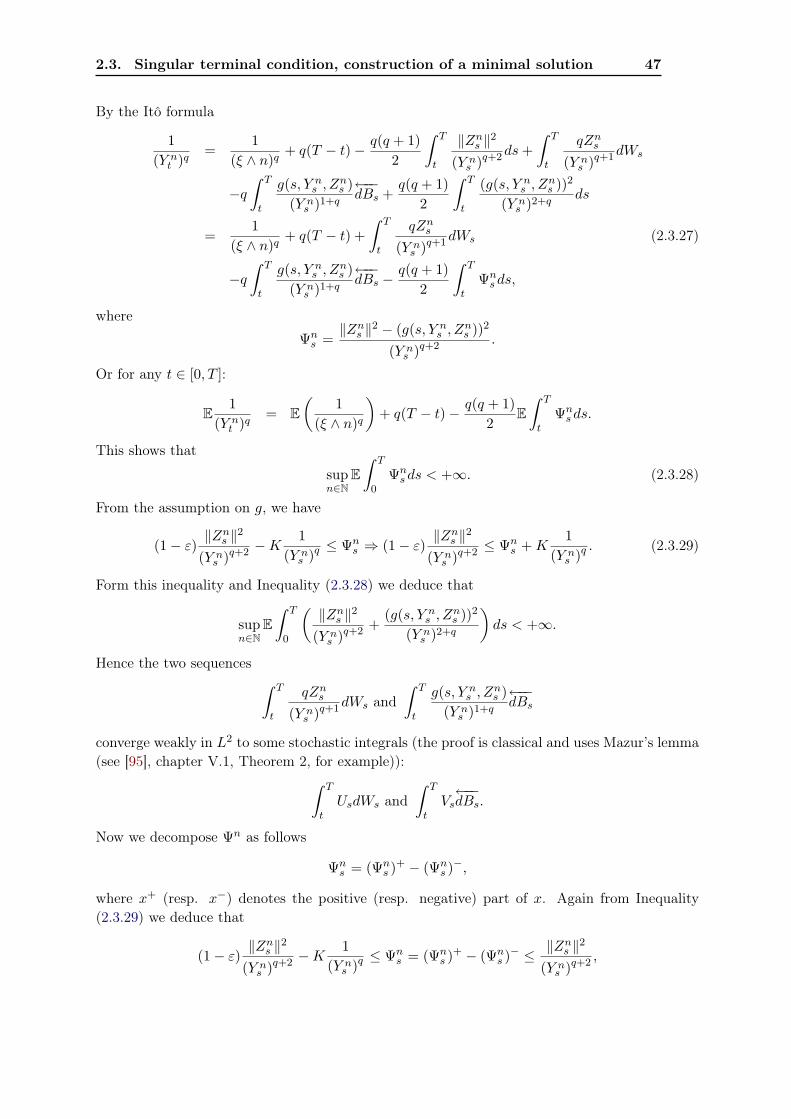
2.3. Singular terminal condition, construction of a minimal solution 47
By the Itô formula
1(Y n
t )q=
1(ξ ∧ n)q
+ q(T − t)− q(q + 1)2
∫ T
t
‖Zns ‖2
(Y ns )q+2ds+
∫ T
t
qZns
(Y ns )q+1dWs
−q∫ T
t
g(s, Y ns , Z
ns )
(Y ns )1+q
←−−dBs +
q(q + 1)2
∫ T
t
(g(s, Y ns , Z
ns ))2
(Y ns )2+q
ds
=1
(ξ ∧ n)q+ q(T − t) +
∫ T
t
qZns
(Y ns )q+1dWs (2.3.27)
−q∫ T
t
g(s, Y ns , Z
ns )
(Y ns )1+q
←−−dBs −
q(q + 1)2
∫ T
tΨn
s ds,
where
Ψns =‖Zn
s ‖2 − (g(s, Y ns , Z
ns ))2
(Y ns )q+2 .
Or for any t ∈ [0, T ]:
E1
(Y nt )q
= E(
1(ξ ∧ n)q
)+ q(T − t)− q(q + 1)
2E∫ T
tΨn
s ds.
This shows that
supn∈N
E∫ T
0Ψn
s ds < +∞. (2.3.28)
From the assumption on g, we have
(1− ε) ‖Zns ‖2
(Y ns )q+2 −K
1(Y n
s )q ≤ Ψns ⇒ (1− ε) ‖Z
ns ‖2
(Y ns )q+2 ≤ Ψn
s +K1
(Y ns )q . (2.3.29)
Form this inequality and Inequality (2.3.28) we deduce that
supn∈N
E∫ T
0
(‖Zn
s ‖2
(Y ns )q+2 +
(g(s, Y ns , Z
ns ))2
(Y ns )2+q
)ds < +∞.
Hence the two sequences ∫ T
t
qZns
(Y ns )q+1dWs and
∫ T
t
g(s, Y ns , Z
ns )
(Y ns )1+q
←−−dBs
converge weakly in L2 to some stochastic integrals (the proof is classical and uses Mazur’s lemma(see [95], chapter V.1, Theorem 2, for example)):∫ T
tUsdWs and
∫ T
tVs←−−dBs.
Now we decompose Ψn as follows
Ψns = (Ψn
s )+ − (Ψns )−,
where x+ (resp. x−) denotes the positive (resp. negative) part of x. Again from Inequality(2.3.29) we deduce that
(1− ε) ‖Zns ‖2
(Y ns )q+2 −K
1(Y n
s )q ≤ Ψns = (Ψn
s )+ − (Ψns )− ≤ ‖Zn
s ‖2
(Y ns )q+2 ,

48 Chapter 2. SPDE with singular terminal condition
and therefore
0 ≤ (Ψns )− ≤ K 1
(Y ns )q ≤ K(qT +
1αq
).
Therefore for any t ∈ [0, T ]:
0 ≤ q(q + 1)2
∫ T
t(Ψn
s )−ds ≤ q(q + 1)2
K(qT +1αq
)(T − t). (2.3.30)
If we define
Γt = lim infn→+∞
q(q + 1)2
EGt
∫ T
t(Ψn
s )−ds,
we obtain that Γ is a non negative bounded process. Since (Ψn)− is non negative, it is straight-forward that Γ is a supermartingale. Moreover the dominated convergence theorem proves thatΓ is a continuous process such that: lim
t→TΓt = 0.
Coming back to(2.3.27) and taking the conditional expectation, we have
q(q + 1)2
EGt
∫ T
tΨn
s ds = EGt
(1
(ξ ∧ n)q
)− 1
(Y nt )q
+ q(T − t)
+qEGt
∫ T
t
g(s, Y ns , Z
ns )
(Y ns )1+q
←−−dBs,
and the right hand side converges weakly in L2. Therefore if we define
Θt = lim supn→+∞
q(q + 1)2
EGt
∫ T
t(Ψn
s )+ds,
taking the weak limit, we obtain
Θt − Γt = EGt
(1ξq
)− 1
(Yt)q+ q(T − t) + qEGt
∫ T
tVs←−−dBs.
We can remark that (Θt)0≤t<T is a non-negative supermartingale and for any t ∈ [0, T ]:
1(Yt)q
= q(T − t) + EGt
(1ξq
)−Θt + Γt + qEGt
∫ T
tVs←−−dBs.
Θ being a right-continuous non-negative supermartingale, the limit of Θt as t goes to T existsP-a.s. and this limit ΘT− is finite P-a.s. The same holds for the backward Itô integral with limitMT = 0. The L1-bounded martingale EGt
(1ξq
)converges a.s. to 1/ξq, as t goes to T , then the
limit of Yt as t→ T exists and is equal to:
limt→T, t<T
Yt =1
( 1ξq −ΘT−)1/q
.
If we were able to prove that ΘT− is zero a.s., we would have shown that YT = ξ.
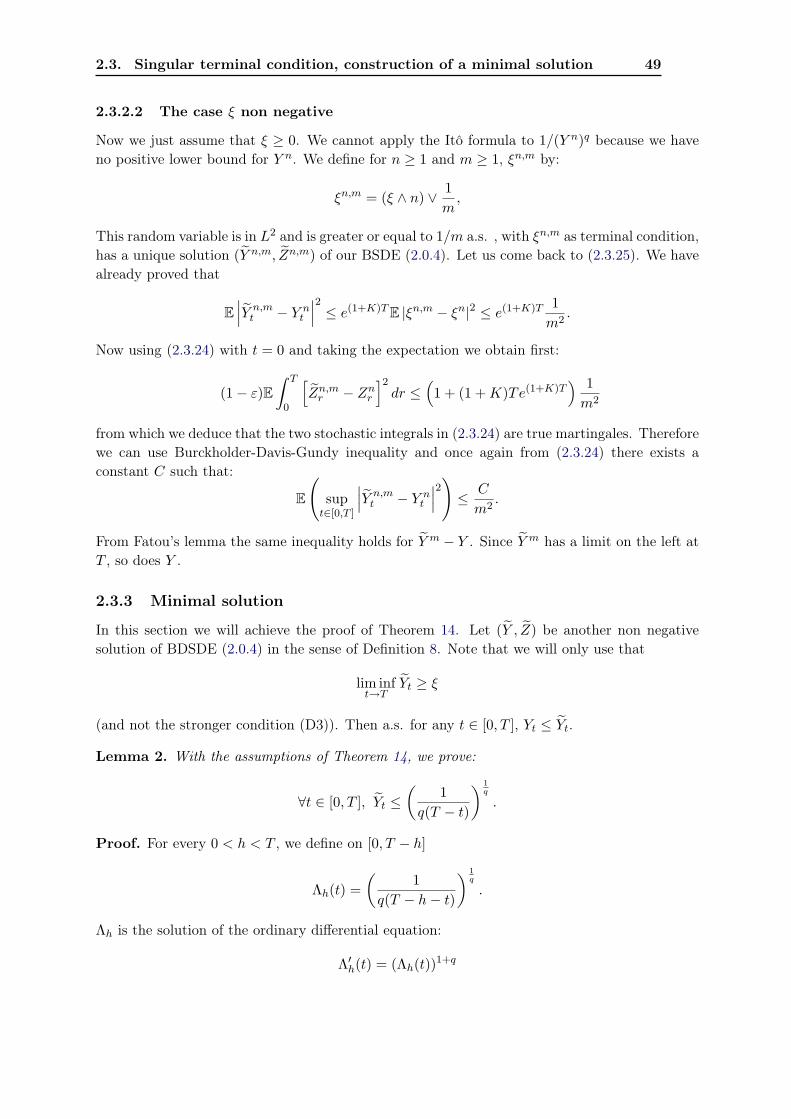
2.3. Singular terminal condition, construction of a minimal solution 49
2.3.2.2 The case ξ non negative
Now we just assume that ξ ≥ 0. We cannot apply the Itô formula to 1/(Y n)q because we haveno positive lower bound for Y n. We define for n ≥ 1 and m ≥ 1, ξn,m by:
ξn,m = (ξ ∧ n) ∨ 1m,
This random variable is in L2 and is greater or equal to 1/m a.s. , with ξn,m as terminal condition,has a unique solution (Y n,m, Zn,m) of our BSDE (2.0.4). Let us come back to (2.3.25). We havealready proved that
E∣∣∣Y n,m
t − Y nt
∣∣∣2 ≤ e(1+K)T E |ξn,m − ξn|2 ≤ e(1+K)T 1m2
.
Now using (2.3.24) with t = 0 and taking the expectation we obtain first:
(1− ε)E∫ T
0
[Zn,m
r − Znr
]2dr ≤
(1 + (1 +K)Te(1+K)T
) 1m2
from which we deduce that the two stochastic integrals in (2.3.24) are true martingales. Thereforewe can use Burckholder-Davis-Gundy inequality and once again from (2.3.24) there exists aconstant C such that:
E
(sup
t∈[0,T ]
∣∣∣Y n,mt − Y n
t
∣∣∣2) ≤ C
m2.
From Fatou’s lemma the same inequality holds for Y m − Y . Since Y m has a limit on the left atT , so does Y .
2.3.3 Minimal solution
In this section we will achieve the proof of Theorem 14. Let (Y , Z) be another non negativesolution of BDSDE (2.0.4) in the sense of Definition 8. Note that we will only use that
lim inft→T
Yt ≥ ξ
(and not the stronger condition (D3)). Then a.s. for any t ∈ [0, T ], Yt ≤ Yt.
Lemma 2. With the assumptions of Theorem 14, we prove:
∀t ∈ [0, T ], Yt ≤(
1q(T − t)
) 1q
.
Proof. For every 0 < h < T , we define on [0, T − h]
Λh(t) =(
1q(T − h− t)
) 1q
.
Λh is the solution of the ordinary differential equation:
Λ′h(t) = (Λh(t))1+q
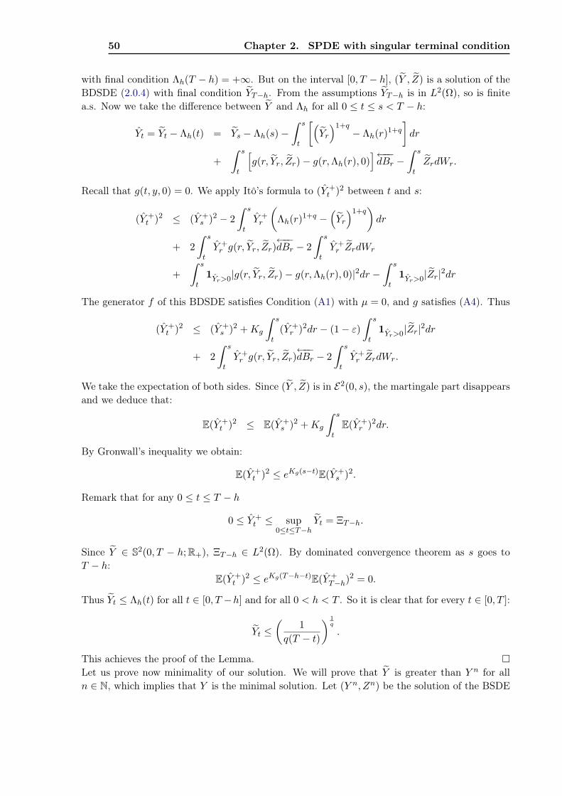
50 Chapter 2. SPDE with singular terminal condition
with final condition Λh(T − h) = +∞. But on the interval [0, T − h], (Y , Z) is a solution of theBDSDE (2.0.4) with final condition YT−h. From the assumptions YT−h is in L2(Ω), so is finitea.s. Now we take the difference between Y and Λh for all 0 ≤ t ≤ s < T − h:
Yt = Yt − Λh(t) = Ys − Λh(s)−∫ s
t
[(Yr
)1+q− Λh(r)1+q
]dr
+∫ s
t
[g(r, Yr, Zr)− g(r,Λh(r), 0)
]←−−dBr −
∫ s
tZrdWr.
Recall that g(t, y, 0) = 0. We apply Itô’s formula to (Y +t )2 between t and s:
(Y +t )2 ≤ (Y +
s )2 − 2∫ s
tY +
r
(Λh(r)1+q −
(Yr
)1+q)dr
+ 2∫ s
tY +
r g(r, Yr, Zr)←−−dBr − 2
∫ s
tY +
r ZrdWr
+∫ s
t1Yr>0|g(r, Yr, Zr)− g(r,Λh(r), 0)|2dr −
∫ s
t1Yr>0|Zr|2dr
The generator f of this BDSDE satisfies Condition (A1) with µ = 0, and g satisfies (A4). Thus
(Y +t )2 ≤ (Y +
s )2 +Kg
∫ s
t(Y +
r )2dr − (1− ε)∫ s
t1Yr>0|Zr|2dr
+ 2∫ s
tY +
r g(r, Yr, Zr)←−−dBr − 2
∫ s
tY +
r ZrdWr.
We take the expectation of both sides. Since (Y , Z) is in E2(0, s), the martingale part disappearsand we deduce that:
E(Y +t )2 ≤ E(Y +
s )2 +Kg
∫ s
tE(Y +
r )2dr.
By Gronwall’s inequality we obtain:
E(Y +t )2 ≤ eKg(s−t)E(Y +
s )2.
Remark that for any 0 ≤ t ≤ T − h
0 ≤ Y +t ≤ sup
0≤t≤T−hYt = ΞT−h.
Since Y ∈ S2(0, T − h; R+), ΞT−h ∈ L2(Ω). By dominated convergence theorem as s goes toT − h:
E(Y +t )2 ≤ eKg(T−h−t)E(Y +
T−h)2 = 0.
Thus Yt ≤ Λh(t) for all t ∈ [0, T −h] and for all 0 < h < T . So it is clear that for every t ∈ [0, T ]:
Yt ≤(
1q(T − t)
) 1q
.
This achieves the proof of the Lemma. Let us prove now minimality of our solution. We will prove that Y is greater than Y n for alln ∈ N, which implies that Y is the minimal solution. Let (Y n, Zn) be the solution of the BSDE

2.4. Limit at time T by localization technic 51
(2.0.4) with ξ ∧ n as terminal condition. By comparison with the solution of the same BSDEwith the deterministic terminal data n:
Y nt ≤
(1
q(T − t) + 1/nq
)1/q
≤ n.
Between the instants 0 ≤ t ≤ s < T :
Yt = Y nt − Yt =
(Y n
s − Ys
)−∫ s
t
((Yr)1+q − (Y n
r )1+q)dr −
∫ s
t
(Zn
r − Zr
)dWr
+∫ s
t
[g(r, Y n
r , Znr )− g(r, Yr, Zr)
]←−−dBr.
Once again we apply Itô’s formula to (Y +t )2:
(Y +t )2 ≤ (Y +
s )2 − 2∫ s
tY +
r
((Y n
r )1+q − (Yr)1+q)dr
+ 2∫ s
tY +
r
[g(r, Y n
r , Znr )− g(r, Yr, Zr)
]←−−dBr − 2
∫ s
tY +
r ZrdWr
+∫ s
t1Yr>0|g(r, Y
nr , Z
nr )− g(r, Yr, Zr)|2dr −
∫ s
t1Yr>0|Zr|2dr
and we deduce thatE(Y +
t )2 ≤ eKg(s−t)E(Y +s )2.
Since 0 ≤ Y +t ≤ Y n
t ≤ n, by dominated convergence theorem, we can take the limit as s goes toT and we obtain that E(Y +
t )2 = 0.
2.4 Limit at time T by localization technic
From now, the process Y is continuous on [0, T [ and we define YT = ξ. The main difficulty willbe to prove the continuity at time T . We have already proved that
lim inft→T
Yt = limt→T
Yt
and remarked that Y is lower semi-continuous on [0, T ]:
ξ ≤ lim inft→T
Yt.
In this paragraph we prove that the inequality in (2.3.26) is in fact an equality, i.e.
ξ = lim inft→T
Yt.
Note that the only remaining problem is on the set R = ξ < +∞.From now on, the conditions of Theorem 15 hold. In particular the terminal condition ξ is equalto h(XT ), where h is a function defined on Rd with values in R+. We denote by S = h = +∞the closed set of singularity and R its complement. In order to prove continuity at time T , we
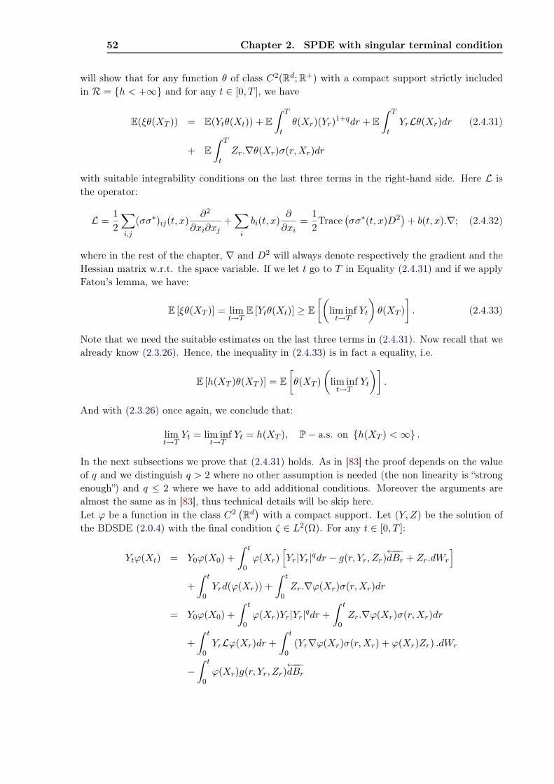
52 Chapter 2. SPDE with singular terminal condition
will show that for any function θ of class C2(Rd; R+) with a compact support strictly includedin R = h < +∞ and for any t ∈ [0, T ], we have
E(ξθ(XT )) = E(Ytθ(Xt)) + E∫ T
tθ(Xr)(Yr)1+qdr + E
∫ T
tYrLθ(Xr)dr (2.4.31)
+ E∫ T
tZr.∇θ(Xr)σ(r,Xr)dr
with suitable integrability conditions on the last three terms in the right-hand side. Here L isthe operator:
L =12
∑i,j
(σσ∗)ij(t, x)∂2
∂xi∂xj+∑
i
bi(t, x)∂
∂xi=
12Trace
(σσ∗(t, x)D2
)+ b(t, x).∇; (2.4.32)
where in the rest of the chapter, ∇ and D2 will always denote respectively the gradient and theHessian matrix w.r.t. the space variable. If we let t go to T in Equality (2.4.31) and if we applyFatou’s lemma, we have:
E [ξθ(XT )] = limt→T
E [Ytθ(Xt)] ≥ E[(
lim inft→T
Yt
)θ(XT )
]. (2.4.33)
Note that we need the suitable estimates on the last three terms in (2.4.31). Now recall that wealready know (2.3.26). Hence, the inequality in (2.4.33) is in fact a equality, i.e.
E [h(XT )θ(XT )] = E[θ(XT )
(lim inf
t→TYt
)].
And with (2.3.26) once again, we conclude that:
limt→T
Yt = lim inft→T
Yt = h(XT ), P− a.s. on h(XT ) <∞ .
In the next subsections we prove that (2.4.31) holds. As in [83] the proof depends on the valueof q and we distinguish q > 2 where no other assumption is needed (the non linearity is “strongenough”) and q ≤ 2 where we have to add additional conditions. Moreover the arguments arealmost the same as in [83], thus technical details will be skip here.Let ϕ be a function in the class C2
(Rd)
with a compact support. Let (Y, Z) be the solution ofthe BDSDE (2.0.4) with the final condition ζ ∈ L2(Ω). For any t ∈ [0, T ]:
Ytϕ(Xt) = Y0ϕ(X0) +∫ t
0ϕ(Xr)
[Yr|Yr|qdr − g(r, Yr, Zr)
←−−dBr + Zr.dWr
]+∫ t
0Yrd(ϕ(Xr)) +
∫ t
0Zr.∇ϕ(Xr)σ(r,Xr)dr
= Y0ϕ(X0) +∫ t
0ϕ(Xr)Yr|Yr|qdr +
∫ t
0Zr.∇ϕ(Xr)σ(r,Xr)dr
+∫ t
0YrLϕ(Xr)dr +
∫ t
0(Yr∇ϕ(Xr)σ(r,Xr) + ϕ(Xr)Zr) .dWr
−∫ t
0ϕ(Xr)g(r, Yr, Zr)
←−−dBr

2.4. Limit at time T by localization technic 53
where L is the operator defined by (2.4.32). Taking the expectation:
E(Ytϕ(Xt)) = E(Y0ϕ(X0)) + E∫ t
0ϕ(Xr)Yr|Yr|qdr (2.4.34)
+E∫ t
0Zr.∇ϕ(Xr)σ(r,Xr)dr + E
∫ t
0YrLϕ(Xr)dr.
Note that the generator g does not appear in this expression. Hence no extra assumption willbe added in the case q > 2.Let U be a bounded open set with a regular boundary and such that the compact set U isincluded in R. We denote by Φ = ΦU a function which is supposed to belong to C2(Rd; R+) andsuch that Φ is equal to zero on Rd \ U , is positive on U . Let α be a real number such that
α > 2(1 + 1/q).
For n ∈ N, let (Y n, Zn) be the solution of the BSDE (2.0.4) with the final condition (h∧n)(XT ).The equality (2.4.34) with t = T becomes:
E(Y nT Φα(XT )) = E(Y n
0 Φα(X0)) + E∫ T
0Zn
r .∇(Φα)(Xr)σ(r,Xr)dr
+ E∫ T
0Φα(Xr)(Y n
r )1+qdr + E∫ T
0Y n
r L(Φα)(Xr)dr. (2.4.35)
Lemma 3. Let p be such that1p
+1
1 + q= 1.
ThenΦ−α(p−1) |L(Φα)|p ∈ L∞([0, T ]× Rd).
Lemma 3 and Hölder inequality show that there exists a constant C such that
∀n ∈ N, E∫ T
0|Y n
r L(Φα)(Xr)| dr ≤ C[E∫ T
0Φα(Xr)(Y n
r )1+qdr
]1/(1+q)
. (2.4.36)
We distinguish the case q > 2 and q ≤ 2 in order to control the term containing Z in (2.4.35).
2.4.1 Proof of (2.4.31) if q > 2
Proposition 5 and the Cauchy-Schwarz inequality prove immediatly the following result.
Lemma 4 (Case q > 2). If q > 2, then there exists a constant C = C(q,Φ, α, σ) such that forall n ∈ N:
E∫ T
0|Zn
r .∇(Φα)(Xr)σ(r,Xr)| dr ≤ C. (2.4.37)
Lemmata 3 and 4 and Equality (2.4.35) imply the next result.
Lemma 5. The sequence Φα(X)(Y n)1+q is a bounded sequence in L1(Ω × [0, T ]) and with theFatou lemma, Y 1+qΦα(X) belongs to L1(Ω× [0, T ]):
E∫ T
0Y 1+q
r Φα(Xr)dr < +∞.
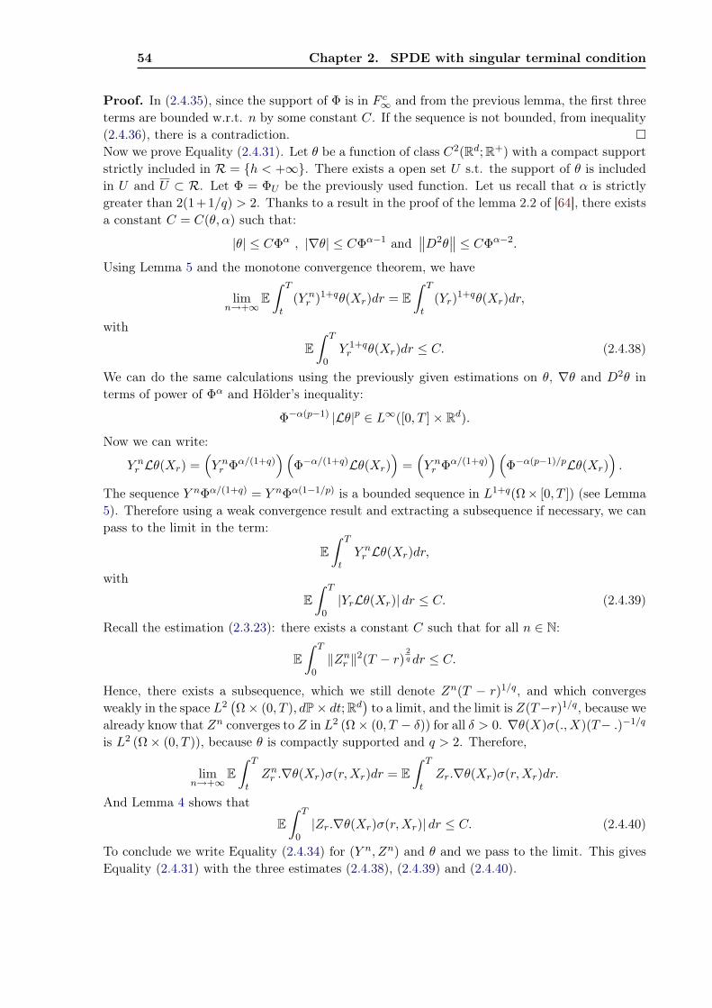
54 Chapter 2. SPDE with singular terminal condition
Proof. In (2.4.35), since the support of Φ is in F c∞ and from the previous lemma, the first three
terms are bounded w.r.t. n by some constant C. If the sequence is not bounded, from inequality(2.4.36), there is a contradiction. Now we prove Equality (2.4.31). Let θ be a function of class C2(Rd; R+) with a compact supportstrictly included in R = h < +∞. There exists a open set U s.t. the support of θ is includedin U and U ⊂ R. Let Φ = ΦU be the previously used function. Let us recall that α is strictlygreater than 2(1+1/q) > 2. Thanks to a result in the proof of the lemma 2.2 of [64], there existsa constant C = C(θ, α) such that:
|θ| ≤ CΦα , |∇θ| ≤ CΦα−1 and∥∥D2θ
∥∥ ≤ CΦα−2.
Using Lemma 5 and the monotone convergence theorem, we have
limn→+∞
E∫ T
t(Y n
r )1+qθ(Xr)dr = E∫ T
t(Yr)1+qθ(Xr)dr,
with
E∫ T
0Y 1+q
r θ(Xr)dr ≤ C. (2.4.38)
We can do the same calculations using the previously given estimations on θ, ∇θ and D2θ interms of power of Φα and Hölder’s inequality:
Φ−α(p−1) |Lθ|p ∈ L∞([0, T ]× Rd).
Now we can write:
Y nr Lθ(Xr) =
(Y n
r Φα/(1+q))(
Φ−α/(1+q)Lθ(Xr))
=(Y n
r Φα/(1+q))(
Φ−α(p−1)/pLθ(Xr)).
The sequence Y nΦα/(1+q) = Y nΦα(1−1/p) is a bounded sequence in L1+q(Ω× [0, T ]) (see Lemma5). Therefore using a weak convergence result and extracting a subsequence if necessary, we canpass to the limit in the term:
E∫ T
tY n
r Lθ(Xr)dr,
with
E∫ T
0|YrLθ(Xr)| dr ≤ C. (2.4.39)
Recall the estimation (2.3.23): there exists a constant C such that for all n ∈ N:
E∫ T
0‖Zn
r ‖2(T − r)2q dr ≤ C.
Hence, there exists a subsequence, which we still denote Zn(T − r)1/q, and which convergesweakly in the space L2
(Ω× (0, T ), dP× dt; Rd
)to a limit, and the limit is Z(T−r)1/q, because we
already know that Zn converges to Z in L2 (Ω× (0, T − δ)) for all δ > 0. ∇θ(X)σ(., X)(T− .)−1/q
is L2 (Ω× (0, T )), because θ is compactly supported and q > 2. Therefore,
limn→+∞
E∫ T
tZn
r .∇θ(Xr)σ(r,Xr)dr = E∫ T
tZr.∇θ(Xr)σ(r,Xr)dr.
And Lemma 4 shows that
E∫ T
0|Zr.∇θ(Xr)σ(r,Xr)| dr ≤ C. (2.4.40)
To conclude we write Equality (2.4.34) for (Y n, Zn) and θ and we pass to the limit. This givesEquality (2.4.31) with the three estimates (2.4.38), (2.4.39) and (2.4.40).

2.4. Limit at time T by localization technic 55
2.4.2 Proof of (2.4.31) if q ≤ 2
If we just assume q > 0, Lemma 4 does not hold anymore. In other words our previous controlon the term containing Z in (2.4.31) fails. But if we are able to prove that there exists a functionψ such that for 0 < t ≤ T :
E∫ T
tZn
r .∇θ(Xr)σ(r,Xr)dr = E∫ T
tY n
r ψ(r,Xr)dr, (2.4.41)
then we apply again the Hölder inequality in order to control
E∫ T
tY n
r ψ(r,Xr)dr by E∫ T
t(Y n
r )1+qΦα(Xr)dr.
Note that we will add the following condition on g. From now on g is a measurable func-tion defined on [0, T ] × Rd × R × Rk such that the Lipschitz property (A4) holds and for any(t, x, x′, y, z) ∈ [0, T ]× (Rd)2 × R× Rm
|g(t, x, y, z)− g(t, x′, y, z)| ≤ Kg|x− x′|. (A6)
First we will prove the next result. In fact it is a quite straightforward modification of Proposition2.3 in [74] or Proposition 4.2 in [5]. Let us denote by B2(0, T ; D1,2) the set of processes (Y, Z)such that Y ∈ S2([0, T ]), Z ∈ H2(0, T ) and Yt and Zt belong to D1,2 with
E[∫ T
0(|Yt|2 + ‖Zt‖2)dt+
∫ T
0
∫ T
0(|DsYt|2 + ‖DsZt‖2)dtds
]< +∞.
Lemma 6. Assume that (Y, Z) is solution of the BSDE (2.0.4) with terminal condition ξ =h(XT ):
Yt = h(XT )−∫ T
tYs|Ys|qds+
∫ T
tg(s,Xs, Ys, Zs)
←−−dBs −
∫ T
tZsdWs
where h is a bounded Lipschitz function on Rd, g satisfies the previous Lipschitz condition andXs ∈ D1,2 for every s ∈ [0, T ].
1. Then (Y, Z) ∈ B2(0, T ; D1,2) and for all 1 ≤ i ≤ d,Di
sYs, 0 ≤ s ≤ T
is a version of(Zs)i, 0 ≤ s ≤ T. (Zs)i denotes the i-th component of Zs. Here, Di
sYs has the followingsense:
DisYs = lim
r→sr<s
DirYs.
2. There exist two random fields u and v such that:
Yt = u(t,Xt) and Zt = v(t,Xt)
and for any (t, x) ∈ [0, T ]× Rm, u(t, x) and v(t, x) are FBt,T -measurable.
Proof. We just sketch the proof. The technical arguments can be found in [5] or [36]. It isknown (see e.g. proof of Theorem 1.1 in [74]) that the solution (Y, Z) of the previous BSDE isobtained by passing to the limit in the following iteration scheme:
(Y 0, Z0) = (0, 0)

56 Chapter 2. SPDE with singular terminal condition
Y m+1t = h(XT )−
∫ T
tY m
s |Y ms |qds+
∫ T
tg(s,Xs, Y
ms , Zm
s )←−−dBs −
∫ T
tZm+1
s dWs.
Our goal here is to show by induction that for all m ∈ N (Y m, Zm) ∈ B2(0, T ; D1,2) and that(Y m, Zm) converges in L2([0, T ],D1,2 × D1,2) to (Y, Z).It is clear that this is true at step 0 since constants are Malliavin differentiable. Let us supposenow that (Y m, Zm) ∈ B2(0, T ; D1,2). By Proposition 1.2.4 in [67] we know that h(XT ) ∈ D1,2
and g(s,Xs, Yms , Zm
s ) ∈ D1,2, since h and g are supposed Lipschitz continuous and XT , Y ms
and Zms are in D1,2. With Lemma 4.2 in [5] we obtain that
∫ Tt g(s,Xs, Y
ms , Zm
s )d←−B s ∈ D1,2.
Moreover, since h is bounded, Y m is also bounded (see (2.3.18)) and x 7→ x|x|q ∈ C1(R).Therefore Y m
t |Y mt |q ∈ D1,2. Then following the arguments of section 7.1 in [5], we obtain that
(Y m+1, Zm+1) ∈ B2(0, T ; D1,2) with DsYm+1t = DsZ
m+1t = 0 for 0 ≤ t ≤ s ≤ T and for
0 ≤ s ≤ t ≤ T
DsYm+1t = Hx
T (DsXT )− (q + 1)∫ T
t|Y m
u |qDsYmu du
+∫ T
t[Gx,m
u DsXu +Gy,mu DsY
mu +Gz,m
u DsZmu ] d←−B u −
∫ T
tDsZ
m+1u dWu
where HxT , resp. Gx,m
u , Gy,mu and Gz,m
u are four bounded random variables with Hx (resp. Gxu,
Gyu and Gz
u) is FWT (resp. Fu) measurable. The bound depends only on the Lipschitz constant of
h and g. Using the same arguments as in [5] we can prove that Gx,m, Gy,m and Gz,m converge tobounded processes and (Y m, Zm) converges in L2([0, T ],D1,2×D1,2) to (Y, Z). Now for 0 < s < t
DsYt = Zs + (q + 1)∫ t
s|Yu|qDsYudu
−∫ t
s[Gx
uDsXu +GyuDsYu +Gz
uDsZu] d←−B u +
∫ t
sDsZudWu.
We then pass to the limit as s goes to t to obtain the desired result.For the second part, we will show that there exists two random fields um and vm, such that forany (t, x) ∈ [0, T ]× Rm, um(t, x) and vm(t, x) are FB
t,T -measurable and
Y mt = um(t,Xt) and Zm
t = vm(t,Xt).
It is clear that this is true at step 0 by taking u0 = v0 = 0. Let us suppose now that there existstwo functions satisfying the measurability as stated in the proposition such that at step m ourprocesses verify:
Y mt = um(t,Xt) and Zm
t = vm(t,Xt).
We can write then:
Y m+1t = h(XT )−
∫ T
tum(s,Xs)|um(s,Xs)|qds
+∫ T
tg(s,Xs, u
m(s,Xs), vm(s,Xs))d←−B s −
∫ T
tZm+1
s dWs
We take the expectation with respect to Gt, which leads to:
Y m+1t = EGt
[h(XT )−
∫ T
tum(s,Xs)|um(s,Xs)|qds
+∫ T
tg(s,Xs, u
m(s,Xs), vm(s,Xs))d←−B s
].
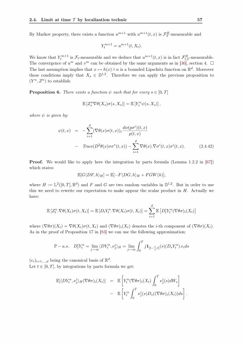
2.4. Limit at time T by localization technic 57
By Markov property, there exists a function um+1 with um+1(t, x) is FBT -measurable and
Y m+1t = um+1(t,Xt).
We know that Y m+1t is Ft-measurable and we deduce that um+1(t, x) is in fact FB
t,T -measurable.The convergence of um and vm can be obtained by the same arguments as in [36], section 4.
The last assumption implies that x 7→ h(x)∧n is a bounded Lipschitz function on Rd. Moreoverthese conditions imply that Xs ∈ D1,2. Therefore we can apply the previous proposition to(Y n, Zn) to establish:
Proposition 6. There exists a function ψ such that for every s ∈ [0, T ]
E [Zns∇θ(Xs)σ(s,Xs)] = E [Y n
s ψ(s,Xs)] ,
where ψ is given by:
ψ(t, x) = −d∑
i=1
(∇θ(x)σ(t, x))idiv(pσi)(t, x)
p(t, x)
− Trace(D2θ(x)σσ∗(t, x))−d∑
i=1
∇θ(x).∇σi(t, x)σi(t, x). (2.4.42)
Proof. We would like to apply here the integration by parts formula (Lemma 1.2.2 in [67])which states:
E[G〈DF, h〉H ] = E[−F 〈DG,h〉H + FGW (h)],
where H := L2([0, T ],Rd) and F and G are two random variables in D1,2. But in order to usethis we need to rewrite our expectation to make appear the scalar product in H. Actually wehave:
E [Znt .∇θ(Xt)σ(t,Xt)] = E [DtY
nt .∇θ(Xt)σ(t,Xt)] =
d∑i=1
E[Di
tYnt (∇θσ)i(Xt)
]where (∇θσ)(Xt) = ∇θ(Xt)σ(t,Xt) and (∇θσ)i(Xt) denotes the i-th component of (∇θσ)(Xt).As in the proof of Proposition 17 in [83] we can use the following approximation:
P− a.s. DitY
nt = lim
j→∞〈DY n
t , νij〉H = lim
j→∞
∫ T
0j1[t− 1
j,t[(s)(DsY
nt ).eids
(ei)i=1,...,d being the canonical basis of Rd.Let t ∈ [0, T ], by integrations by parts formula we get:
E[〈DY nt , ν
ij〉H(∇θσ)i(Xt)] = E
[Y n
t (∇θσ)i(Xt)∫ T
0νi
j(s)dWs
]− E
[Y n
t
∫ T
0νi
j(s)Ds((∇θσ)i(Xt))ds].
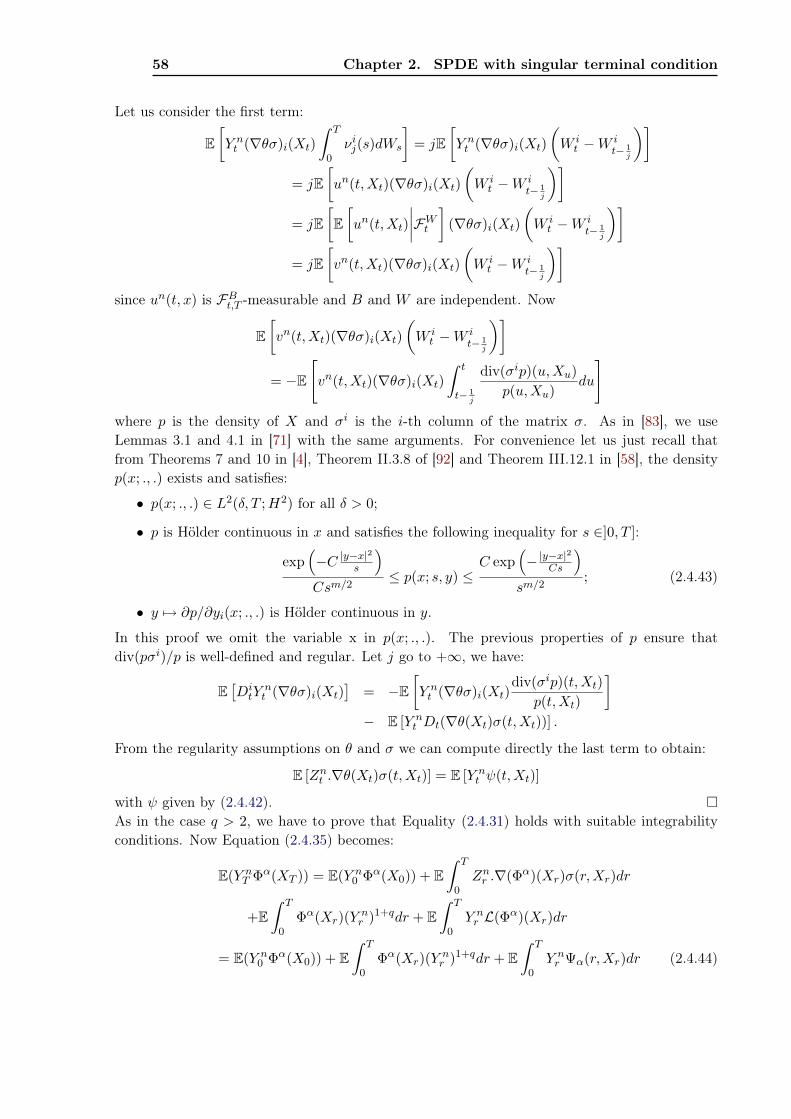
58 Chapter 2. SPDE with singular terminal condition
Let us consider the first term:
E[Y n
t (∇θσ)i(Xt)∫ T
0νi
j(s)dWs
]= jE
[Y n
t (∇θσ)i(Xt)(W i
t −W it− 1
j
)]= jE
[un(t,Xt)(∇θσ)i(Xt)
(W i
t −W it− 1
j
)]= jE
[E[un(t,Xt)
∣∣∣∣FWt
](∇θσ)i(Xt)
(W i
t −W it− 1
j
)]= jE
[vn(t,Xt)(∇θσ)i(Xt)
(W i
t −W it− 1
j
)]since un(t, x) is FB
t,T -measurable and B and W are independent. Now
E[vn(t,Xt)(∇θσ)i(Xt)
(W i
t −W it− 1
j
)]= −E
[vn(t,Xt)(∇θσ)i(Xt)
∫ t
t− 1j
div(σip)(u,Xu)p(u,Xu)
du
]where p is the density of X and σi is the i-th column of the matrix σ. As in [83], we useLemmas 3.1 and 4.1 in [71] with the same arguments. For convenience let us just recall thatfrom Theorems 7 and 10 in [4], Theorem II.3.8 of [92] and Theorem III.12.1 in [58], the densityp(x; ., .) exists and satisfies:
• p(x; ., .) ∈ L2(δ, T ;H2) for all δ > 0;
• p is Hölder continuous in x and satisfies the following inequality for s ∈]0, T ]:
exp(−C |y−x|2
s
)Csm/2
≤ p(x; s, y) ≤C exp
(− |y−x|2
Cs
)sm/2
; (2.4.43)
• y 7→ ∂p/∂yi(x; ., .) is Hölder continuous in y.
In this proof we omit the variable x in p(x; ., .). The previous properties of p ensure thatdiv(pσi)/p is well-defined and regular. Let j go to +∞, we have:
E[Di
tYnt (∇θσ)i(Xt)
]= −E
[Y n
t (∇θσ)i(Xt)div(σip)(t,Xt)
p(t,Xt)
]− E [Y n
t Dt(∇θ(Xt)σ(t,Xt))] .
From the regularity assumptions on θ and σ we can compute directly the last term to obtain:
E [Znt .∇θ(Xt)σ(t,Xt)] = E [Y n
t ψ(t,Xt)]
with ψ given by (2.4.42). As in the case q > 2, we have to prove that Equality (2.4.31) holds with suitable integrabilityconditions. Now Equation (2.4.35) becomes:
E(Y nT Φα(XT )) = E(Y n
0 Φα(X0)) + E∫ T
0Zn
r .∇(Φα)(Xr)σ(r,Xr)dr
+E∫ T
0Φα(Xr)(Y n
r )1+qdr + E∫ T
0Y n
r L(Φα)(Xr)dr
= E(Y n0 Φα(X0)) + E
∫ T
0Φα(Xr)(Y n
r )1+qdr + E∫ T
0Y n
r Ψα(r,Xr)dr (2.4.44)
2.5. Link with SPDE’s 59
with Ψα the following function: for t ∈]0, T ] and x ∈ Rd
Ψα(t, x) = ∇(Φα)(x).b(t, x)− 12Trace(D2(Φα)(x)σσ∗(t, x))
−d∑
i=1
((∇(Φα)(x)σ(t, x))i
div(p(t, x)σi(t, x))p(t, x)
)
−d∑
i=1
(∇(Φα)(x).[∇σi(t, x)σi(t, x)]
).
In [83] it is proved that for a fixed ε > 0 and p = 1 + 1/q:
Φ−α(p−1) |Ψα|p ∈ L∞([ε, T ]× Rd).
If it is true, then the last term in (2.4.45) satisfies:
E∫ T
t|Y n
r Ψα(r,Xr)| dr ≤ C(
E∫ T
tΦα(Xr)(Y n
r )1+qdr
) 11+q
and the end of the proof will be the same as in the case q > 2.
2.5 Link with SPDE’s
In the introduction, we have said that there is a connection between doubly stochastic backwardSDE whose terminal data is a function of the value at time T of a solution of a SDE (or forward-backward system), and solutions of a large class of semilinear parabolic stochastic PDE. Let usprecise this connection in our case.To begin with, we modify the equation (2.1.8). For all (t, x) ∈ [0, T ]×Rd, we denote by Xt,x thesolution of the following SDE:
Xt,xs = x+
∫ s
tb(r,Xt,x
r )dr +∫ s
tσ(r,Xt,x
r )dWr, for s ∈ [t, T ], (2.5.45)
and Xt,xs = x for s ∈ [0, t]. We enforce the assumptions on b and σ: we assume that b (resp. σ)
is a C2 (resp. C3) function whose partial derivatives of order less than 2 (resp. 3) are bounded.Therefore b and σ satisfy the assumptions (L)-(G). We consider the following doubly stochasticBSDE for t ≤ s ≤ T :
Y t,xs = h(Xt,x
T )−∫ T
sY t,x
r |Y t,xr |qdr +
∫ T
sg(r,Xt,x
r , Y t,xr , Zt,x
r )←−−dBr −
∫ T
sZt,x
r dWr, (2.5.46)
where h is a function defined on Rd with values in R. The two equations (2.5.45) and (2.5.46)are called a forward-backward system. This system is connected with the stochastic PDE (2.0.5)with terminal condition h.More precisely for any n ∈ N∗, let (Y n,t,x, Zn,t,x) be the solution of the BDSDE (2.5.46) withterminal condition h(Xt,x
T ) ∧ n. We know that
0 ≤ Y n,t,xs ≤
(1
q(T − s) + 1nq
) 1q
≤ n.
60 Chapter 2. SPDE with singular terminal condition
And the generator y 7→ −y|y|q is Lipschitz continuous on the interval [−n, n]. Moreover if weassume Assumption (H3), then h ∧ n is a Lipschitz and bounded function on Rd. Hence h ∧ nbelongs to L2(Rd, ρ(x)dx) = L2
ρ(Rd). Recall that ρ is defined by (2.1.9) and here we just needthat κ > d. Since we have imposed that g(t, x, y, 0) = 0, now the all conditions in [6] are satisfied.
Proposition 7 (Theorem 3.1 in [6]). There exists a unique weak solution un ∈ H(0, T ) of theSPDE (2.0.5) with terminal function h ∧ n. Moreover un(t, x) = Y n,t,x
t and
Y n,t,xs = un(s,Xt,x
s ), Zn,t,xs = (σ∗∇un)(s,Xt,x
s ).
The space H(0, T ) is defined in Section 2.1. The random field un is a weak solution of (2.0.5) ,which means:
1. For some δ > 0sups≤T
E[||un(s, .)||1+δ
L2ρ(Rd)
]<∞. (WS1)
Since un is bounded by n a.s. it is true for any δ > 0.
2. For every test-function φ ∈ C∞(Rd), dt⊗ dP a.e.
lims↑t
∫Rd
un(s, x)φ(x)dx =∫
Rd
un(t, x)φ(x)dx. (WS2)
3. Finally un satisfies for every function Ψ ∈ C1,∞c ([0, T ]× Rd)∫ T
t
∫Rd
un(s, x)∂sΨ(s, x)dxds+∫
Rd
un(t, x)Ψ(t, x)dx−∫
Rd
(h(x) ∧ n)Ψ(T, x)dx(2.5.47)
−12
∫ T
t
∫Rd
(σ∗∇un)(s, x)(σ∗∇Ψ)(s, x)dxds
−∫ T
t
∫Rd
un(s, x)div((b− A
)Ψ)
(s, x)dxds
= −∫ T
t
∫Rd
Ψ(s, x)un(s, x)|un(s, x)|qdxds
+∫ T
t
∫Rd
Ψ(s, x)g(s, x, un(s, x), σ∗∇un(s, x))dx←−−dBs.
C1,∞c ([0, T ]×Rd) is the set of functions ψ : [0, T ]×Rd → R such that ψ has a compact support
w.r.t. x ∈ Rd and
Ai =12
d∑k=1
∂(σσ∗)k,i
∂xk.
Remember that we have defined a process (Y t,x, Zt,x) solution in the sense of the Definition 8 ofthe backward doubly stochastic differential equation (2.5.46) with singular terminal condition h(see Theorem 14 and the beginning of the section 2.4 on continuity at time T ). The process Yis obtained as the increasing limit of the processes Y n:
Y t,xs = lim
n→+∞Y n,t,x
s a.s..
2.5. Link with SPDE’s 61
Therefore we can define the following random field u as follows:
u(t, x) = Y t,xt = lim
n→+∞Y n,t,x
t = limn→+∞
un(t, x).
Our aim is to prove Theorem 16, that is, u is also a weak solution of (2.0.5) with the singularterminal condition h. For any n we have a.s.
0 ≤ Y n,t,xs ≤
(1
q(T − s) + 1nq
) 1q
≤(
1q(T − s)
) 1q
.
In particular for any (t, x)
0 ≤ un(t, x) ≤(
1q(T − t)
) 1q
and hence u satisfies the same estimate. Thus u is bounded on [0, t] × Rd and in L2ρ(Rd). By
dominated convergence theorem, for any δ > 0, u satisfies (WS1) and (WS2) for any 0 ≤ s ≤t ≤ T − δ.Moreover we have Zn,t,x
s = (σ∗∇un)(s,Xt,xs ) and from the proof on Theorem 14 we know that the
sequence of processes (Zn,t,xs , s ≥ t) converges in L2((0, T − δ)×Ω) for any δ > 0 to Zt,x. Hence
the sequence un converges in H(0, t) to u. From Proposition 5 we have the a priori estimate(2.3.23):
E∫ T
0(T − s)2/q‖Zn,t,x
s ‖2ds ≤ 8 +KT
1− ε
(1q
)2/q
(as usual Zn,t,xs = 0 if s < t). Therefore we deduce
E∫ T
0(T − s)2/q‖(σ∗∇un)(s,Xt,x
s )‖2ds ≤ 8 +KT
1− ε
(1q
)2/q
.
We multiply each side by ρ(x), we integrate w.r.t. x and we use Proposition 5.1 in [6] to have:
E∫
Rd
∫ T
0(T − s)2/q‖(σ∗∇un)(s, x)‖2ρ(x)dxds ≤ C
where the constant C does not depend on n. With the Fatou lemma we have the same inequalityfor u.
E∫
Rd
∫ t
0(T − s)2/q‖(σ∗∇u)(s, x)‖2ρ(x)dxds <∞.
Now for every function Ψ ∈ C1,∞c ([0, T ] × Rd), un satisfies (2.5.47), therefore for every 0 ≤ r ≤
t < T , un satisfies also:∫ t
r
∫Rd
un(s, x)∂sΨ(s, x)dxds+∫
Rd
un(r, x)Ψ(r, x)dx−∫
Rd
un(t, x)Ψ(t, x)dx(2.5.48)
−12
∫ t
r
∫Rd
(σ∗∇un)(s, x)(σ∗∇Ψ)(s, x)dxds
−∫ t
r
∫Rd
un(s, x)div((b− A
)Ψ)
(s, x)dxds
= −∫ t
r
∫Rd
Ψ(s, x)un(s, x)|un(s, x)|qdxds
+∫ t
r
∫Rd
Ψ(s, x)g(s, x, un(s, x), σ∗∇un(s, x))dx←−−dBs.
62 Chapter 2. SPDE with singular terminal condition
But using monotone convergence theorem or the convergence of un to u in H(0, t), we can passto the limit as n goes to +∞ in (2.5.48) and we obtain that u is a weak solution of (2.0.5) on[0, T − δ]× Rd for any δ > 0.The only trouble concerns the behavior of u near T . Since un satisfies (2.5.47) for any n, and bythe integrability or regularity assumptions on un, b and σ, we have
limt→T
∫Rd
un(t, x)ψ(x)dx =∫
Rd
(h(x) ∧ n)ψ(x)dx
for any function ψ ∈ C∞c (Rd). Therefore by monotonicity
lim inft↑T
∫Rd
u(t, x)ψ(x)dx ≥ lim inft↑T
∫Rd
un(t, x)ψ(x)dx =∫
Rd
(h(x) ∧ n)ψ(x)dx
for any n. Hence a.s.
lim inft↑T
∫Rd
u(t, x)ψ(x)dx ≥∫
Rd
h(x)ψ(x)dx.
Our aim is to prove the converse inequality with the lim sup. In the second section we haveproved Equation (2.4.31) with suitable integrability condition on all terms:
E(h(Xt,xT )θ(Xt,x
T )) = E(u(t, x)θ(x)) + E∫ T
tθ(Xt,x
r )(Y t,xr )1+qdr
+ E∫ T
tY t,x
r Lθ(Xt,xr )dr + E
∫ T
tZt,x
r .∇θ(Xt,xr )σ(r,Xt,x
r )dr
for any smooth functions θ such that its compact support is strictly included in R = h < +∞.If we integrate this w.r.t. dx (no weight function ρ is needed here since θ is of compact support)and we let t go to T we obtain:
limt→T
∫Rd
E(h(Xt,xT )θ(Xt,x
T ))dx = limt→T
∫Rd
E(u(t, x)θ(x))dx.
By dominated convergence theorem this gives:
limt→T
E(∫
Rd
u(t, x)θ(x)dx)
=∫
Rd
h(x)θ(x)dx
for any function θ ∈ C2c (Rd) with supp(θ) ∩ S = ∅.
Note that Fatou’s lemma implies that
E(
lim inft→T
∫Rd
u(t, x)θ(x)dx)≤∫
Rd
h(x)θ(x)dx
and thus we obtain that a.e. on Ω× Rd
lim inft→T
u(t, x) = h(x).
Remark 2. If g does not depend of Z (or on ∇u), and if g ∈ C0,2,3b ([0, T ] × Rd × R; Rd), then
from [21], un is a stochastically bounded viscosity solution of the SPDE (2.0.5) on [0, T ] × Rd
and u is also a stochastically bounded viscosity solution of the SPDE (2.0.5) on [0, T − δ] × Rd
for any δ > 0.

2.5. Link with SPDE’s 63
Now let u be a non negative weak solution of (2.0.5) on [0, T − δ]× Rd for any δ > 0. It meansthat for any δ > 0, u ∈ H(0, T − δ) and u satisfies (WS1) and (WS2) and (2.5.48) on [0, T − δ].Moreover we assume that lim inft→T u(t, x) ≥ h(x) a.e. on Ω × Rd. We follow the proof ofuniqueness for Theorem 3.1 in [6]. We define
Y t,.s = u(s,Xt,.
s ), Zt,.s = (σ∗∇u)(s,Xt,.
s ).
Then by the same arguments as in [6], (Y t,xs , Zt,x
s ) solves the BDSDE (2.0.4) on any interval[0, T − δ]. Moreover a.s.
lim infs→T
Y t,xs ≥ h(Xt,x
T ) = ξ.
By Lemma 2 and the proof of minimality of the solution of the BDSDE (Theorem 14), we deducethat for every n, a.s.
Y t,x,ns ≤ Y t,x
s ≤(
1q(T − s)
)1/q
.
Thus u(t, x) ≤ u(t, x) a.e. on Ω× [0, T ]×Rd. And u is the minimal weak solution of the SPDE(2.0.5) with singular terminal condition.

Chapter 3
BSDE with jumps and PIDE withsingular terminal condition
Contents3.1 Introduction . . . . . . . . . . . . . . . . . . . . . . . . . . . . . . . . . . . 65
3.2 Setting, construction of the minimal solution . . . . . . . . . . . . . . . . 66
3.3 Behaviour of Y at time T . . . . . . . . . . . . . . . . . . . . . . . . . . . . 73
3.3.1 Existence of the limit . . . . . . . . . . . . . . . . . . . . . . . . . . . . . . 73
3.3.2 Continuity at time T for q > 2 . . . . . . . . . . . . . . . . . . . . . . . . . 75
3.4 Link with PIDE . . . . . . . . . . . . . . . . . . . . . . . . . . . . . . . . . 81
3.4.1 Existence of a viscosity solution with singular data . . . . . . . . . . . . . . 83
3.4.2 Minimal solution . . . . . . . . . . . . . . . . . . . . . . . . . . . . . . . . . 87
3.4.3 Regularity of the minimal solution . . . . . . . . . . . . . . . . . . . . . . . 90
3.1 Introduction
In this chapter we would like to provide existence results for the following BSDE:
Yt = ξ −∫ T
tYs|Ys|qds−
∫ T
tZsdWs −
∫ T
t
∫EUs(e)µ(ds, de) (3.1.1)
where the terminal condition ξ satisfies
P(ξ = +∞) > 0. (3.1.2)
The first aim is the following. We want to find sufficient conditions to have a.s.
limt→T
Yt = ξ. (3.1.3)
This problem was studied in [83] when there is no jump. In the Markovian framework and forq > 2, Equality (3.1.3) was proved. Here we will follow the same idea. But we need other technicalassumptions on the jumps of the solution X of the forward SDE and the set S = ξ = +∞.The second part is devoted to the study of the related partial integro differential equation (PIDEin short): for any x ∈ Rd, u(T, x) = g(x) and for any (t, x) ∈ [0, T [×Rd
∂
∂tu(t, x) + Lu(t, x) + I(t, x, u)− u(t, x)|u(t, x)|q = 0 (3.1.4)
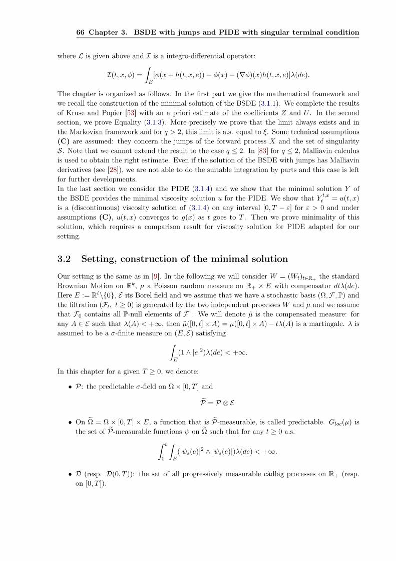
66 Chapter 3. BSDE with jumps and PIDE with singular terminal condition
where L is given above and I is a integro-differential operator:
I(t, x, φ) =∫
E[φ(x+ h(t, x, e))− φ(x)− (∇φ)(x)h(t, x, e)]λ(de).
The chapter is organized as follows. In the first part we give the mathematical framework andwe recall the construction of the minimal solution of the BSDE (3.1.1). We complete the resultsof Kruse and Popier [53] with an a priori estimate of the coefficients Z and U . In the secondsection, we prove Equality (3.1.3). More precisely we prove that the limit always exists and inthe Markovian framework and for q > 2, this limit is a.s. equal to ξ. Some technical assumptions(C) are assumed: they concern the jumps of the forward process X and the set of singularityS. Note that we cannot extend the result to the case q ≤ 2. In [83] for q ≤ 2, Malliavin calculusis used to obtain the right estimate. Even if the solution of the BSDE with jumps has Malliavinderivatives (see [28]), we are not able to do the suitable integration by parts and this case is leftfor further developments.In the last section we consider the PIDE (3.1.4) and we show that the minimal solution Y ofthe BSDE provides the minimal viscosity solution u for the PIDE. We show that Y t,x
t = u(t, x)is a (discontinuous) viscosity solution of (3.1.4) on any interval [0, T − ε] for ε > 0 and underassumptions (C), u(t, x) converges to g(x) as t goes to T . Then we prove minimality of thissolution, which requires a comparison result for viscosity solution for PIDE adapted for oursetting.
3.2 Setting, construction of the minimal solution
Our setting is the same as in [9]. In the following we will consider W = (Wt)t∈R+ the standardBrownian Motion on Rk, µ a Poisson random measure on R+ × E with compensator dtλ(de).Here E := R`\0, E its Borel field and we assume that we have a stochastic basis (Ω,F ,P) andthe filtration (Ft, t ≥ 0) is generated by the two independent processes W and µ and we assumethat F0 contains all P-null elements of F . We will denote µ is the compensated measure: forany A ∈ E such that λ(A) < +∞, then µ([0, t]×A) = µ([0, t]×A)− tλ(A) is a martingale. λ isassumed to be a σ-finite measure on (E, E) satisfying∫
E(1 ∧ |e|2)λ(de) < +∞.
In this chapter for a given T ≥ 0, we denote:
• P: the predictable σ-field on Ω× [0, T ] and
P = P ⊗ E
• On Ω = Ω × [0, T ] × E, a function that is P-measurable, is called predictable. Gloc(µ) isthe set of P-measurable functions ψ on Ω such that for any t ≥ 0 a.s.∫ t
0
∫E(|ψs(e)|2 ∧ |ψs(e)|)λ(de) < +∞.
• D (resp. D(0, T )): the set of all progressively measurable càdlàg processes on R+ (resp.on [0, T ]).

3.2. Setting, construction of the minimal solution 67
We refer to [49] (see also [12]) for details on random measures and stochastic integrals. Now todefine the solution of our BSDE, let us introduce the following spaces for p ≥ 1.
• Sp(0, T ) is the space of all processes X ∈ D(0, T ) such that
E
(sup
t∈[0,T ]|Xt|p
)< +∞.
For simplicity, X∗ = supt∈[0,T ] |Xt|.
• Hp(0, T ) is the subspace of all processes X ∈ D(0, T ) such that
E
[(∫ T
0|Xt|2dt
)p/2]< +∞.
• Lpµ(0, T ) = Lp
µ(Ω× (0, T )× E): the set of processes ψ ∈ Gloc(µ) such that
E
[(∫ T
0
∫E|ψs(e)|2λ(de)ds
)p/2]< +∞.
• Lpλ = Lp(E, λ; Rd): the set of measurable functions ψ : E → Rd such that
‖ψ‖pLp
λ=∫
E|ψ(e)|pλ(de) < +∞.
• Bpµ(0, T ) = Sp(0, T )×Hp(0, T )× Lp
µ(0, T ).
In [53], the following result is proved.
Theorem 17 (and Definition). Let q > 0 and ξ a Ft-measurable non negative random variablesuch that P(ξ =∞) > 0. There exists a process (Y, Z, U) such that
• (Y, Z, U) belongs to S2(0, t) for any t < T .
• for all 0 ≤ s ≤ t < T :
Ys = Yt −∫ t
sYr|Yr|qdr −
∫ t
sZrdWr −
∫ t
s
∫EUs(e)µ(ds, de).
• (Y, Z, U) is a super-solution in the sense that: a.s.
lim inft→T
Yt ≥ ξ.
Any process (Y , Z, U) satisfying the previous three items is called super-solution of the BSDE(3.1.1) with singular terminal condition ξ.

68 Chapter 3. BSDE with jumps and PIDE with singular terminal condition
By construction, Yt ≥ 0 a.s. and it is the minimal one: if (Y , Z, U) is another non negativesuper-solution, then a.s. Yt ≥ Yt.In this section we sketch the construction of the minimal solution and we give an a priori estimateof the martingale part (Z,U) of the solution. Indeed we have already seen that if ξ belongs toL2(Ω,FT ,P) we have existence and uniqueness results for such BSDE’s according to [28] or [52].The approach in [53] is then to approximate our BSDE by considering a terminal condition ofthe form ξn := ξ ∧ n and observe asymptotic behaviour.Let us consider the following process:
Y nt = ξ ∧ n−
∫ T
tY n
s |Y ns |qds−
∫ T
tZn
s dWs −∫ T
t
∫EUn
s (e)µ(ds, de)
where (Y n, Zn, Un) is solution of the BSDE. Moreover using comparison argument (see [85] or[52]) we can obtain for n ≤ m:
0 ≤ Y nt ≤ Y m
t ≤
(1
q(T − t) + 1mq
)1/q
≤(
1q(T − t)
)1/q
This allows us to define Y as the increasing limit of the sequence (Y nt )n≥1:
∀ t ∈ [0, T ], Yt := limn→∞
Y nt .
The next lemma shows that the sequences of processes Zn and Un also converge.
Lemma 7. There exists a constant C such that for any m, n and 0 ≤ t ≤ s < T :
E[
sup0≤t≤s
|Y nt − Y m
t |2 +∫ s
0‖Zn
r − Zmr ‖2dr +
∫ s
0
∫E|Un
r (e)− Umr (e)|2λ(de)dr
](3.2.5)
≤ CE[|Y n
s − Y ms |2
].
Proof. From the Itô formula with φ(y) = y2 we deduce for t ≤ s < T :
|Y nt − Y m
t |2 +∫ s
t‖Zn
r − Zmr ‖2dr +
∫ s
t
∫E|Un
r (e)− Umr (e)|2λ(de)dr =
|Y ns − Y m
s |2 + 2∫ s
t|Y n
r − Y mr |[(Y n
r )q+1 − (Y mr )q+1]dr
−2∫ s
t(Y n
r − Y mr )(Zn
r − Zmr )dWr −
∫ s
t
∫E|Y n
r − Y mr |2 − |Y n
r− − Ymr− |
2µ(dr, de).
Then from the monotonicity of y 7→ yq+1,
|Y nt − Y m
t |2 +∫ s
t‖Zn
r − Zmr ‖2dr +
∫ s
t
∫E|Un
r (e)− Umr (e)|2λ(de)dr (3.2.6)
≤ |Y ns − Y m
s |2 − 2∫ s
t(Y n
r − Y mr )(Zn
r − Zmr )dWr
−∫ s
t
∫E
(|Y n
r − Y mr |2 − |Y n
r− − Ymr− |
2)µ(dr, de)
From (3.2.6) we get directly:
E[∫ s
0‖Zn
r − Zmr ‖2dr +
∫ s
0
∫E|Un
r (e)− Umr (e)|2λ(de)dr
]≤ E
[|Y n
s − Y ms |2
](3.2.7)
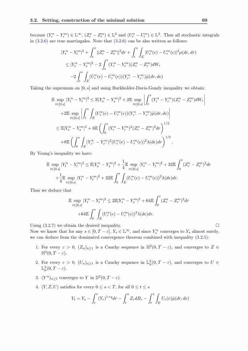
3.2. Setting, construction of the minimal solution 69
because (Y nr − Y m
r ) ∈ L∞, (Znr − Zm
r ) ∈ L2 and (Unr − Um
r ) ∈ L2. Thus all stochastic integralsin (3.2.6) are true martingales. Note that (3.2.6) can be also written as follows:
|Y nt − Y m
t |2 +∫ s
t‖Zn
r − Zmr ‖2dr +
∫ s
t
∫E|Un
r (e)− Umr (e)|2µ(de, dr)
≤ |Y ns − Y m
s |2 − 2∫ s
t(Y n
r − Y mr )(Zn
r − Zmr )dWr
−2∫ s
t
∫E(Un
r (e)− Umr (e))(Y n
r− − Ymr−)µ(dr, de)
Taking the supremum on [0, s] and using Burkholder-Davis-Gundy inequality we obtain:
E supt∈[0,s]
|Y nt − Y m
t |2 ≤ E|Y ns − Y m
s |2 + 2E supt∈[0,s]
∣∣∣∣∫ s
t(Y n
r − Y mr )(Zn
r − Zmr )dWr
∣∣∣∣+2E sup
t∈[0,s]
∣∣∣∣∫ s
t
∫E(Un
r (e)− Umr (e))(Y n
r− − Ymr−)µ(dr, de)
∣∣∣∣≤ E|Y n
s − Y ms |2 + 8E
(∫ s
0(Y n
r − Y mr )2(Zn
r − Zmr )2dr
)1/2
+8E(∫ s
0
∫E(Y n
r− − Ymr−)2(Un
r (e)− Umr (e))2λ(de)dr
)1/2
.
By Young’s inequality we have:
E supt∈[0,s]
|Y nt − Y m
t |2 ≤ E|Y ns − Y m
s |2 +14
E supt∈[0,s]
|Y nt − Y m
t |2 + 32E∫ s
0(Zn
r − Zmr )2dr
+14
E supt∈[0,s]
|Y nt − Y m
t |2 + 32E∫ s
0
∫E(Un
r (e)− Umr (e))2λ(de)dr.
Thus we deduce that
E supt∈[0,s]
|Y nt − Y m
t |2 ≤ 2E|Y ns − Y m
s |2 + 64E∫ s
0(Zn
r − Zmr )2dr
+64E∫ s
0
∫E(Un
r (e)− Umr (e))2λ(de)dr.
Using (3.2.7) we obtain the desired inequality. Now we know that for any s ∈ [0, T − ε], Ys ∈ L∞, and since Y n
s converges to Ys almost surely,we can deduce from the dominated convergence theorem combined with inequality (3.2.5):
1. For every ε > 0, (Zn)n≥1 is a Cauchy sequence in H2(0, T − ε), and converges to Z ∈H2(0, T − ε).
2. For every ε > 0, (Un)n≥1 is a Cauchy sequence in L2µ(0, T − ε), and converges to U ∈
L2µ(0, T − ε).
3. (Y n)n≥1 converges to Y in D2(0, T − ε).
4. (Y, Z, U) satisfies for every 0 ≤ s < T , for all 0 ≤ t ≤ s
Yt = Ys −∫ s
t(Yr)1+qdr −
∫ s
tZrdBr −
∫ s
t
∫EUr(e)µ(dr, de)

70 Chapter 3. BSDE with jumps and PIDE with singular terminal condition
Recall that on Y we have the following estimate:
0 ≤ Yt ≤(
1q(T − t)
)1/q
.
The previous proof shows that
E[∫ t
0‖Zs‖2ds+
∫ t
0
∫E|Us(e)|2λ(de)ds
]≤(
1q(T − t)
)2/q
.
Now let us prove some sharper estimates on Z and U .
Proposition 8. The process (Z,U) satisfies:
E[∫ T
0(T − s)2/q
(‖Zs‖2 +
∫E|Us(e)|2λ(de)
)ds
]≤ 16
(1q
)2/q
.
Proof. The proof is almost the same as in [83], Proposition 10. First suppose there exists aconstant α > 0 such that P-a.s. ξ ≥ α. In this case, by comparison, for all integer n and allt ∈ [0, T ]:
Y nt ≥
(1
qT + 1/αq
)1/q
> 0.
Let δ > 0 and θ : R→ R, θq : R→ R defined by:θ(x) =
√x on [δ,+∞[,
θ(x) = 0 on ]−∞, 0],and
θq(x) = x
12q on [δ,+∞[,
θq(x) = 0 on ]−∞, 0],
and such that θ and θq are non-negative, non-decreasing and in respectively C2(R) and C1(R).We apply the Itô formula on [0, T − δ] to the function θq(T − t)θ(Y n
t ), with δ < (qT +1/αq)−1/q:
θq(δ)θ(Y nT−δ)− θq(T )θ(Y n
0 ) =12q
∫ T−δ
0(T − s)1/2q−1(Y n
s )1/2ds
+12
∫ T−δ
0(T − s)1/2q(Y n
s )−1/2dY ns −
18
∫ T−δ
0(T − s)1/2q(Y n
s )3/2(Zns )2ds
+∫ T−δ
0(T − s)1/2q
∫E
[(Y n
s )1/2 − (Y ns−)1/2 − 1
2(Y n
s−)−1/2Uns (e)
]µ(ds, de)
We deduce:
18
E[∫ T−δ
0(T − s)1/2q(Y n
s )−3/2(Zns )2ds
]− E
[∫ T−δ
0
∫E(T − s)1/2q
((Y n
s )1/2 − (Y ns−)1/2 − 1
2(Y n
s−)−1/2Uns (e)
)µ(ds, de)
]= E
[θq(T )θ(Y n
0 )− θq(δ)θ(Y nT−δ)
]+
12
E[∫ T−δ
0(T − s)1/2q(Y n
s )1/2
((Y n
s )q − 1q(T − s)
)ds
]≤ E [θq(T )θ(Y n
0 )] ≤(
1q
)1/2q

3.2. Setting, construction of the minimal solution 71
Therefore
E[∫ T−δ
0(T − s)1/2q(Y n
s )−3/2(Zns )2ds
]≤ 8
(1q
)1/2q
.
We have also
E[∫ T−δ
0(T − s)1/2q(Y n
s )−3/2(Zns )2ds
]≥ q3/2qE
[∫ T−δ
0(T − s)2/q(Zn
s )2ds].
So if we combine those two inequalities we get:
E[∫ T−δ
0(T − s)2/q(Zn
s )2ds]≤ 8
(1q
)2/q
.
We can conclude to get the first part of our proposition by letting δ → 0 and using Fatou’sLemma.We now want to prove the second part. We already know:
−E[∫ T−δ
0
∫E(T − s)1/2q
((Y n
s )1/2 − (Y ns−)1/2 − 1
2(Y n
s−)−1/2Uns (e)
)µ(ds, de)
]≤(
1q
)1/2q
.
Let Y n,αs := Y n
s− + αUns (e). We have:
(Y ns )1/2 − (Y n
s−)1/2 − 12(Y n
s−)−1/2Uns (e) =
∫ 1
0|Un
s (e)|2(−14)(Y n,α
s )−3/2(1− α)dα.
One can easily check that: Y n,αs ≤ Y n
s− ∨ Yns ≤ ( 1
q(T−s))1/q. So we can deduce now:
14
E[∫ T−δ
0
∫E
∫ 1
0q3/2q(T − s)2/q(1− α)|Un
s (e)|2dαµ(ds, de)]≤(
1q
)1/2q
and so:
E[∫ T−δ
0
∫E(T − s)2/q|Un
s (e)|2µ(ds, de)]≤ 8
(1q
)2/q
.
Now we come back to the case ξ ≥ 0. We can not apply the Itô formula because we do not haveany positive lower bound for Y n. We will approach Y n in the following way. We define for n ≥ 1and m ≥ 1, ξn,m by:
ξn,m = (ξ ∧ n) ∨ 1m.
This random variable is in L2 and is greater or equal to 1/m a.s. The BSDE (3.1.1), with ξn,m
as terminal condition, has a unique solution (Y n,m, Zn,m, Un,m). It is immediate that if m ≤ m′
and n ≤ n′ then:
Y n,m′ ≤ Y n′,m.

72 Chapter 3. BSDE with jumps and PIDE with singular terminal condition
As for the sequence Y n, we can define Y m as the limit when n grows to +∞ of Y n,m. This limitY m is greater than Y = limn→+∞ Y n. But for any m and n, for t ∈ [0, T ]:∣∣∣Y n,m
t − Y nt
∣∣∣2 = |ξn,m − ξn|2 − 2∫ T
t
[Y n,m
r − Y nr
] [(Y n,m
r
)q+1− (Y n
r )q+1
]dr
−2∫ T
t
[Y n,m
r − Y nr
] [Zn,m
r − Znr
]dWr −
∫ T
t
[Zn,m
r − Znr
]2dr
−∫ T
t
∫E|Un,m
r (e)− Unr (e)|2λ(de)dr
−∫ T
t
∫E
(|Y n,m
r − Y nr |2 − |Y
n,mr− − Y n
r− |2)µ(dr, de).
≤ |ξn,m − ξn|2 − 2∫ T
t
[Y n,m
r − Y nr
] [Zn,m
r − Znr
]dWr
−∫ T
t
∫E
(|Y n,m
r − Y nr |2 − |Y
n,mr− − Y n
r− |2)µ(dr, de).
and taking the expectation:
E∣∣∣Y n,m
t − Y nt
∣∣∣2 ≤ E |ξn,m − ξn|2 ≤ 1m2
. (3.2.8)
To conclude we fix δ > 0 and we apply the Itô formula to the process (T − .)2/q∣∣∣Y n,m − Y n
∣∣∣2.This leads to the inequality:
E∫ T−δ
0(T − r)2/q
(∣∣∣Zn,mr − Zn
r
∣∣∣2 +∫
E
∣∣∣Un,mr (e)− Un
r (e)∣∣∣2) dr
≤ 2q
E∫ T−δ
0(T − s)(2/q)−1
∣∣∣Y n,ms − Y n
s
∣∣∣2 ds+ (δ)2/qE∣∣∣Y n,m
T−δ − YnT−δ
∣∣∣2 .Let δ go to 0 in the previous inequality. We can do that because (T − .)(2/q)−1 is integrable onthe interval [0, T ] and because of (3.2.8). Finally we have
E∫ T−δ
0(T − r)2/q
(∣∣∣Zn,mr − Zn
r
∣∣∣2 +∫
E
∣∣∣Un,mr (e)− Un
r (e)∣∣∣2) dr
≤ 1m2
[2q
∫ T
0(T − s)(2/q)−1ds
]=T 2/q
m2.
Therefore, for all η > 0 :
E∫ T−δ
0(T − r)2/q
(|Zn
r |2 +
∫E|Un
r (e)|2)dr
≤ (1 + η)E∫ T
0(T − r)2/q
(∣∣∣Zn,mr
∣∣∣2 +∫
E
∣∣∣Un,mr (e)
∣∣∣2) dr+ (1 +
1η)E∫ T
0(T − r)2/q
(∣∣∣Zn,mr − Zn
r
∣∣∣2 +∫
E
∣∣∣Un,mr (e)− Un
r (e)∣∣∣2) dr
≤ (1 + η)16(1/q)2/q + (1 +1η)T 2/q
m2.

3.3. Behaviour of Y at time T 73
We have applied the previous result to Zn,m and Un,m. Now we let first m go to +∞ and thenη go to 0, we have:
E∫ T
0(T − r)2/q
(|Zn
r |2 +
∫E|Un
r (e)|2)dr ≤ 16(1/q)2/q.
The result follows by letting finally n go to ∞ and this achieves the proof of the proposition.
Let use recall the minimality of this solution.
Proposition 9 (Minimal solution). The solution (Y, Z, U) obtained by approximation is minimal.If (Y , Z, U) is another non negative super-solution, then for all t ∈ [0, T ], P-a.s. Yt ≥ Yt.Moreover
Yt ≤(
1q(T − t)
)1/q
.
Proof. See [53] (or Section 3 in [83]).
3.3 Behaviour of Y at time T
Let us remark that a.s.ξ ∧ n = lim inf
t→TY n
t ≤ lim inft→T
Yt,
and thus we immediately haveξ ≤ lim inf
t→TYt.
Our main problem is to prove that ξ = limt→T
Yt. In this section we will prove that the limit alwaysexists and then we will prove that the limit is ξ under some sufficient conditions.
3.3.1 Existence of the limit
We proceed as in [83] (see here for more details). To begin with we suppose that ξ ≥ α > 0. Let(Y n, Zn, Un) be the solution of the BSDE (3.1.1) with terminal condition ξ ∧ n, and (Y, Z, U) isthe limit of (Y n, Zn, Un). By comparison we have a.s.
Yt ≥ Y nt ≥
(1
q(T − t) + 1αq
)1/q
≥
(1
qT + 1αq
)1/q
> 0.
Proposition 10. The process Y can be written as follows:
Yt =(q(T − t) + EFt
[1ξq
]− φt
)−1/q
where φ is a non negative supermartingale.
Proof. First, by Itô’s formula we obtain:
(Y nt )−q = (ξ ∧ n)−q + q(T − t) + q
∫ T
t
Zns
(Y ns−)q+1
dWs + q
∫ T
t
∫E
Uns (e)
(Y ns−)q+1
µ(de, ds)
− q(q + 1)2
∫ T
t
‖Zns ‖2
(Y ns−)q+2
ds−∫ T
t
∫E
[(Y n
s )−q − (Y ns−)−q + q(Y n
s−)−q−1Uns (e)
]µ(ds, de).

74 Chapter 3. BSDE with jumps and PIDE with singular terminal condition
Since Y nt is bounded from below by some positive constant we can apply Itô’s formula. Then
taking condition expectation with respect to Ft we get:
(Y nt )−q = EFt [(ξ ∧ n)−q] + q(T − t)− q(q + 1)
2EFt
[∫ T
t
‖Zns ‖2
(Y ns−)q+2
ds
]
− EFt
[∫ T
t
∫E
[(Y n
s )−q − (Y ns−)−q + q(Y n
s−)−q−1Uns (e)
]µ(ds, de)
].
We will denote from now on:
φnt =
q(q + 1)2
EFt
[∫ T
t
‖Zns ‖2
(Y ns−)q+2
ds
]
+EFt
[∫ T
t
∫E
[(Y n
s )−q − (Y ns−)−q + q(Y n
s−)−q−1Uns (e)
]µ(ds, de)
].
We estimate now the following difference for m ≥ n:
0 ≤ (Y nt )−q − (Y m
t )−q = EFt[(ξ ∧ n)−q − (ξ ∧m)−q
]− (φn
t − φmt ).
And so we obtain:
|φnt − φm
t | ≤ EFt[(ξ ∧ n)−q − (ξ ∧m)−q
]∨[(Y n
t )−q − (Y mt )−q
].
Since the sequences: (EFt [(ξ ∧ n)−q])n≥1 and ((Y nt )−q)n≥1 converge a.s. and in L1, we deduce
(φnt )n≥1 converge a.s. and in L1 to some φt. So by passing to the limit, one can write:
Y −qt = EFt [ξ−q] + q(T − t)− φt
On the other hand it is easy to verify that φ is a non negative càdlàg bounded supermartingale:
0 ≤ φt ≤ EFt [ξ−q].
This achieves the proof. So we can deduce the existence of the following limit:
φT− := limtT
φt
And so YT− exists and is equal to:
YT− := limtT
Yt =(
1ξq− φT−
)−1/q
Now we handle the case were ξ is only supposed to be bounded away from zero. We will considerin that situation the following terminal condition:
ξn,m := (ξ ∧ n) ∨ 1m.
As before we will denote the associated solution of our BSDE by (Y n,m, Zn,m, Un,m). We easilyobtain that a.s.
0 ≤ Y n,mt − Y n
t ≤1m

3.3. Behaviour of Y at time T 75
and thus a.s.sup
t∈[0,T ]
∣∣∣Y n,mt − Y n
t
∣∣∣ ≤ 1m.
Let n go to +∞ to deduce:
supt∈[0,T ]
∣∣∣Y mt − Yt
∣∣∣ ≤ 1m.
Since Y m has a limit on the left at T , so does Y .Now let us precise the behaviour of Y in a neighbourhood of T .
Lemma 8. For 0 ≤ t < T , P-a.s.
Yt ≥ EFt
( 1q(T − t) + 1
ξq
)1/q .
The right hand side is obtained through the following operation: first, we solve the ordinarydifferential equation y′ = y1+q with ξ as terminal condition, then we project this solution on theσ-algebra Ft.Proof. See proof of Lemma 11 in [83].
Proposition 11. On the set ξ =∞, a.s.
limtT
(T − t)1/qYt =(
1q
)1/q
Proof. See proof of Proposition 13 in [83]. Note that if ξ = +∞ a.s. we have proved that there is a unique solution (Y, Z, U) to the BSDE(3.1.1) given by Yt = (q(T − t))−1/q, Zt = Ut = 0.
3.3.2 Continuity at time T for q > 2
In order to prove that the limit at time T of Yt is equal to ξ, i.e.
limt→T
Yt = ξ,
we follow the same procedure as in [83] and we work in the Markovian setting. We suppose nowour terminal condition is of the form: ξ = g(XT ). The function g is defined on Rd with valuesin R+ ∪ +∞ and we denote
S := x ∈ Rd s.t. g(x) =∞
the set of singularity points for the terminal condition induced by g. This set S is supposed tobe closed. We also denoted by Γ the boundary of S. The process X is the solution of a SDEwith jumps:
Xt = X0 +∫ t
0b(s,Xs)ds+
∫ t
0σ(s,Xs)dWs +
∫ t
0
∫Eh(s,Xs− , e)µ(de, ds). (3.3.9)
The coefficients b : Ω×[0, T ]×Rd → Rd, σ : Ω×[0, T ]×Rd → Rd×k and h : Ω×[0, T ]×Rd×E → Rd
satisfy
Assumptions (B):
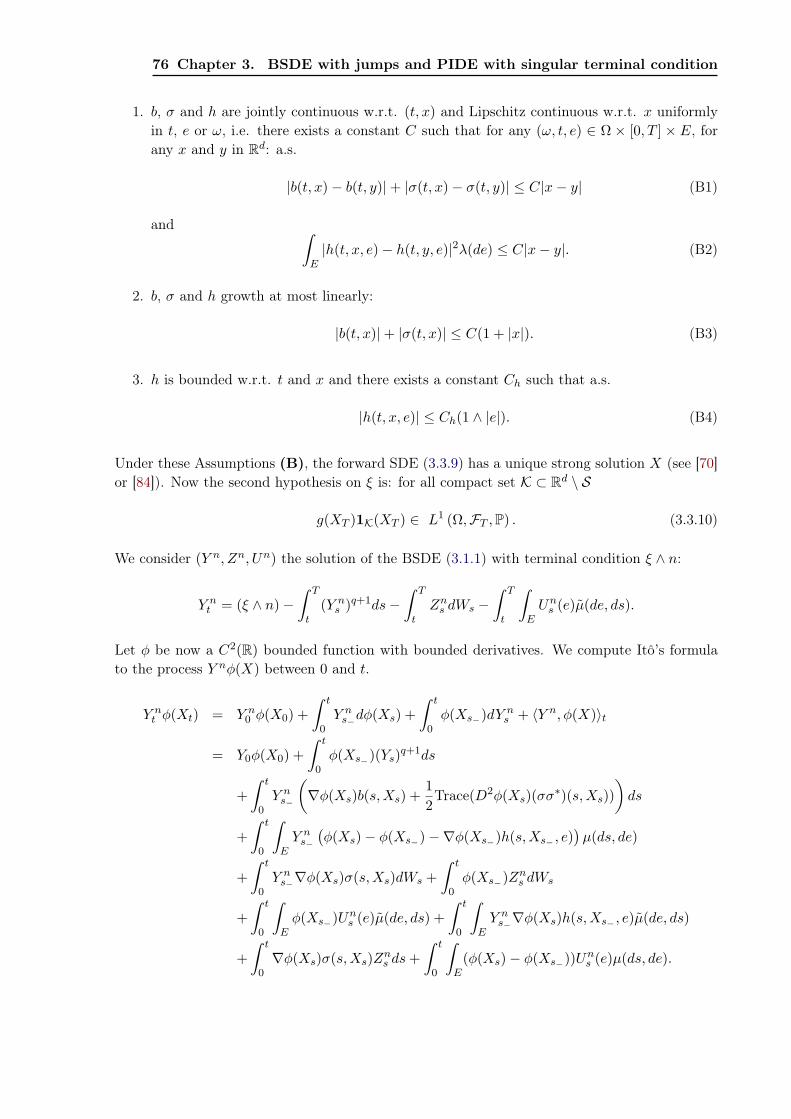
76 Chapter 3. BSDE with jumps and PIDE with singular terminal condition
1. b, σ and h are jointly continuous w.r.t. (t, x) and Lipschitz continuous w.r.t. x uniformlyin t, e or ω, i.e. there exists a constant C such that for any (ω, t, e) ∈ Ω × [0, T ] × E, forany x and y in Rd: a.s.
|b(t, x)− b(t, y)|+ |σ(t, x)− σ(t, y)| ≤ C|x− y| (B1)
and ∫E|h(t, x, e)− h(t, y, e)|2λ(de) ≤ C|x− y|. (B2)
2. b, σ and h growth at most linearly:
|b(t, x)|+ |σ(t, x)| ≤ C(1 + |x|). (B3)
3. h is bounded w.r.t. t and x and there exists a constant Ch such that a.s.
|h(t, x, e)| ≤ Ch(1 ∧ |e|). (B4)
Under these Assumptions (B), the forward SDE (3.3.9) has a unique strong solution X (see [70]or [84]). Now the second hypothesis on ξ is: for all compact set K ⊂ Rd \ S
g(XT )1K(XT ) ∈ L1 (Ω,FT ,P) . (3.3.10)
We consider (Y n, Zn, Un) the solution of the BSDE (3.1.1) with terminal condition ξ ∧ n:
Y nt = (ξ ∧ n)−
∫ T
t(Y n
s )q+1ds−∫ T
tZn
s dWs −∫ T
t
∫EUn
s (e)µ(de, ds).
Let φ be now a C2(R) bounded function with bounded derivatives. We compute Itô’s formulato the process Y nφ(X) between 0 and t.
Y nt φ(Xt) = Y n
0 φ(X0) +∫ t
0Y n
s−dφ(Xs) +∫ t
0φ(Xs−)dY n
s + 〈Y n, φ(X)〉t
= Y0φ(X0) +∫ t
0φ(Xs−)(Ys)q+1ds
+∫ t
0Y n
s−
(∇φ(Xs)b(s,Xs) +
12Trace(D2φ(Xs)(σσ∗)(s,Xs))
)ds
+∫ t
0
∫EY n
s−
(φ(Xs)− φ(Xs−)−∇φ(Xs−)h(s,Xs− , e)
)µ(ds, de)
+∫ t
0Y n
s−∇φ(Xs)σ(s,Xs)dWs +∫ t
0φ(Xs−)Zn
s dWs
+∫ t
0
∫Eφ(Xs−)Un
s (e)µ(de, ds) +∫ t
0
∫EY n
s−∇φ(Xs)h(s,Xs− , e)µ(de, ds)
+∫ t
0∇φ(Xs)σ(s,Xs)Zn
s ds+∫ t
0
∫E(φ(Xs)− φ(Xs−))Un
s (e)µ(ds, de).

3.3. Behaviour of Y at time T 77
Since (Zn, Un) and X are in H2(0, T ), and since φ and the derivatives of φ are supposed to bebounded, we can take the expectation of these terms:
E[Y nt φ(Xt)] = E[Y n
0 φ(X0)] + E[∫ t
0φ(Xs−)(Y n
s )q+1ds
](3.3.11)
+E[∫ t
0Y n
s−
(∇φ(Xs)b(s,Xs) +
12Trace(D2φ(Xs)σ2(s,Xs))
)ds
]+E
[∫ t
0
∫EY n
s−
(φ(Xs)− φ(Xs−)−∇φ(Xs−)h(s,Xs− , e)
)λ(de)ds
]+E
[∫ t
0∇φ(Xs)σ(s,Xs)Zn
s ds
]+ E
[∫ t
0
∫E(φ(Xs)− φ(Xs−))Un
s (e)λ(de)ds].
Recall the main idea of [83]. First we prove that we can pass to the limit on n in (3.3.11) andthat the limits have suitable integrability conditions on [0, T ] × Ω. Secondly we write (3.3.11)between t and T and we pass to the limit when t goes to T .Now we choose φ such that the support of φ is included in R = Sc. From the assumptions on g,we have for any n:
E(Y nT φ(XT )) ≤ E(g(XT )φ(XT )) < +∞.
Moreover
E(Y n0 φ(X0)) ≤
1(qT )1/q
E(φ(X0)) < +∞.
We use Proposition 8 and Hölder inequality to obtain:
E[∫ T
0|∇φ(Xs)σ(s,Xs)Zn
s |ds]≤[E∫ T
0(T − s)2/q|Zn
s |2ds]1/2
[E∫ T
0
|∇φ(Xs)σ(s,Xs)|2
(T − s)2/qds
]1/2
≤ 16(
1q
)2/q [E∫ T
0
|∇φ(Xs)σ(s,Xs)|2
(T − s)2/qds
]1/2
< +∞ (3.3.12)
since q > 2, since ∇φ is supposed to be bounded, σ grows linearly and X ∈ H2(0, T ). The sameestimate holds for Un:
E[∫ T
0
∫E|(φ(Xs)− φ(Xs−))Un
s (e)|λ(de)ds]
≤ 16(
1q
)2/q [E∫ T
0
∫E
|(φ(Xs− + h(s,Xs− , e))− φ(Xs−))|2
(T − s)2/qλ(de)ds
]1/2
< +∞(3.3.13)
Now we deal with the term:
E[∫ T
0Y n
s−L(φ)(s,Xs)ds]
= E[∫ T
0Y n
s−
(∇φ(Xs)b(s,Xs) +
12Trace(D2φ(Xs)σ2(s,Xs))
)ds
].
78 Chapter 3. BSDE with jumps and PIDE with singular terminal condition
As in [83] we consider test functions φ of the form ψα. Thus with Hölder inequality we obtain:
E[∫ T
0|Y n
s−L(ψα)(s,Xs)|ds]≤[E∫ T
0ψα(Xs)(Y n
s )q+1ds
]1/(q+1)
×[E∫ T
0ψ−α/q(Xs)|L(ψα)(s,Xs)|(q+1)/qds
]q/(q+1)
,
and there exists a constant C depending only on ψ, α, σ and b such that
|L(ψα)| ≤ Cψα−2.
Thus for α > 2(q + 1)/q
E∫ T
0ψ−α/q(Xs)|L(ψα)(s,Xs)|(q+1)/qds ≤ CE
∫ T
0ψ−α/q+(α−2)(q+1)/q(Xs)ds < +∞.
Then
E[∫ T
0|Y n
s−L(ψα)(s,Xs)|ds]≤ C
[E∫ T
0ψα(Xs)(Y n
s )q+1ds
]1/(q+1)
. (3.3.14)
Therefore the main difference with [83] comes from the term
E[∫ t
0
∫EY n
s−
(φ(Xs)− φ(Xs−)−∇φ(Xs−)h(s,Xs− , e)
)λ(de)ds
]. (3.3.15)
In order to control this term, we have to add some extra assumptions on the jumps of X and S.
Assumption (C):
• The boundary ∂S = Γ is compact and of class C2.
• For any x ∈ S, any s ∈ [0, T ] and λ-a.s.
x+ h(s, x, e) ∈ S.
Furthermore there exists a constant κ > 0 such that if x ∈ Γ, then for any s ∈ [0, T ],d(x+ h(s, x, e),Γ) ≥ κ, λ-a.s.
These assumptions mean in particular that if Xs− ∈ S, then Xs ∈ S a.s. Moreover if Xs− belongsto the boundary of S, and if there is a jump at time s, then Xs is in the interior of S.Since Γ is compact and of class C2, then there exists a constant µ0 > 0 such that if Γ(µ0) :=x ∈ Rd : d(x,Γ) < µ0, then for every y ∈ Γ(µ0), there exists a unique z ∈ Γ such thatd(y,Γ) = ‖y − z‖. Moreover we can define the exterior unit normal −→n (y) for any y ∈ Γ. Inthe following we will consider the following choice of test functions. For any 0 < µ ≤ µ0, letθ ∈ C∞(Rd) such that θ(x) ∈ [0, 1], θ(x) > 0 if x 6∈ Γ(µ/2), and
θ(x) =
0 on Γ(µ/2)1 on Γ(µ)c.
Now let consider φ defined as follow:
φ(x) =
0 on Sθ(x) on Sc = R. (3.3.16)
Therefore φ ∈ C∞b (Rd) (all derivatives exist and are bounded) and the support of φ is includedin R = Sc.

3.3. Behaviour of Y at time T 79
Lemma 9. Under the above assumptions, let us choose µ1 < µ0 such that (1 +Kh)µ1 < κ (Kh
is the Lipschitz constant of h w.r.t. x). We have for any 0 < µ < µ1:
φ(Xs−) = 0⇒ φ(Xs) = 0.
Moreoverφ(Xs)φ(Xs−)
= φ(Xs)1Γ(µ)c(Xs−).
Proof. We consider the case where Xs− /∈ supp(φ), that is φ(Xs−) = 0. Thus Xs− is inS ∪ Γ(µ/2).
1. If Xs− ∈ S, then Xs ∈ S, hence φ(Xs) = 0.
2. Let z ∈ Sc∩Γ(µ/2) and x ∈ Γ such that d(z,S) = ‖z−x‖. Let us prove that z+h(s, z, e) ∈S by contradiction. Assume that z + h(s, z, e) /∈ S and consider the following convexcombination:
zt := (1− t)(z + h(s, z, e)) + t(x+ h(s, x, e)).
Now since h is Lipschitz continuous w.r.t. x:
‖zt − (x+ h(s, x, e))‖ = (1− t)‖z + h(s, z, e)− x− h(s, x, e)‖
≤ (1− t)(1 +Kh)‖z − x‖ ≤ (1− t)(1 +Kh)µ2
≤ (1 +Kh)µ2
< κ.
Since x ∈ Γ, x + h(s, x, e) ∈ S. But z + h(s, z, e) /∈ S. Thus by continuity there existst0 ∈ (0, 1) such that
zt0 := (1− t0)(z + h(s, z, e)) + t0(x+ h(s, x, e)) ∈ Γ.
Thus we have obtained x ∈ Γ and zt0 ∈ Γ such that
‖zt0 − (x+ h(s, x, e))‖ < κ⇒ d(x+ h(x, s, e),Γ) < κ.
This leads to a contradiction. So we deduce z + h(s, z, e) ∈ S.
Hence if Xs− ∈ Sc ∩ Γ(µ/2), Xs ∈ S and φ(Xs) = 0.
Now consider the quotient
φ(Xs)φ(Xs−)
=φ(Xs)φ(Xs−)
1supp(φ)(Xs−).
The first part of the proof shows that for any µ < µ1, we have:
φ(Xs)φ(Xs−)
= φ(Xs)1Γ(µ)c(Xs−).
Indeed if Xs− is in supp(φ) ∩ Γ(µ), then Xs ∈ S, and thus the quotient is null.
80 Chapter 3. BSDE with jumps and PIDE with singular terminal condition
Now we can deal with the term given by (3.3.15). Let us take α > 2(q + 1)/q and by Hölderinequality we obtain:
E[∫ t
0
∫EY n
s−
∣∣φα(Xs)− φα(Xs−)−∇(φα)(Xs−)h(s,Xs− , e)∣∣λ(de)ds
]≤[E∫ t
0φα(Xs−)(Y n
s )q+1ds
] 1q+1
×
E∫ t
0
∫E
∣∣φα(Xs)− φα(Xs−)−∇(φα)(Xs−)h(s,Xs− , e)∣∣ q+1
q
φ(Xs−)α/qλ(de)ds.
q
q+1
The last integral is controlled by:
∣∣φα(Xs)− φα(Xs−)−∇(φα)(Xs−)h(s,Xs− , e)∣∣ q+1
q
φ(Xs−)α/q
≤ Cqφα(Xs)
(φ(Xs)φ(Xs−)
)α/q
+ Cqφα(Xs−)
+Cqφα−(q+1)/q(Xs−)|∇φ(Xs−)h(s,Xs− , e)|.
But with Lemma 9 we obtain:
∣∣φα(Xs)− φα(Xs−)−∇(φα)(Xs−)h(s,Xs− , e)∣∣ q+1
q
φ(Xs−)α/q
≤ Cq
[φ
αq+1q (Xs)1Γ(µ)c(Xs−) + φα(Xs−) + φ
α− q+1q (Xs−)|∇φ(Xs−)h(s,Xs− , e)|
].
From the assumption on φ and since α > 2 q+1q , there exists a constant C independent on n such
that:
E[∫ T
0
∫EY n
s−
∣∣φα(Xs)− φα(Xs−)−∇(φα)(Xs−)h(s,Xs− , e)∣∣λ(de)ds
](3.3.17)
≤ C[E∫ T
0φα(Xs−)(Y n
s )q+1ds
] 1q+1
.
Let us summarize what we obtained. For any µ small enough, any function φ defined by (3.3.16),and any α > 2(q + 1)/q, from (3.3.11) and using (3.3.12), (3.3.13), (3.3.14), (3.3.17) we deducethat there exists a constant C independent of n such that
E∫ T
0φα(Xs−)(Y n
s )q+1ds ≤ C < +∞. (3.3.18)
Moreover all these estimates show that we can pass to the limit in (3.3.11) (using monotone

3.4. Link with PIDE 81
convergence theorem or dominated convergence theorem) and we have:
E[ξφα(XT )] = E[Ytφα(Xt)] + E
[∫ T
tφα(Xs−)(Ys)q+1ds
](3.3.19)
+E[∫ T
tYs−L(φα)(s,Xs)ds
]+E
[∫ T
t
∫EYs−
(φα(Xs)− φα(Xs−)−∇(φα)(Xs−)h(s,Xs− , e)
)λ(de)ds
]+E
[∫ T
t∇(φα)(Xs)σ(s,Xs)Zsds
]+ E
[∫ T
t
∫E(φα(Xs)− φα(Xs−))Us(e)λ(de)ds
].
Estimate (3.3.18) also holds with Y , and once again from (3.3.12), (3.3.13), (3.3.14) and(3.3.17),we can let t go to T in (3.3.19) in order to have:
E[(lim inf
t→TYt)φα(XT )
]≤ lim
t→TE[Ytφ
α(Xt)] = E[ξφα(XT )].
Recall that the function φα is equal to one on R ∩ Γ(µ)c, that lim inft→T Yt ≥ ξ a.s. and thatthe limit of Yt exists. This last inequality shows that in fact a.s.
limt→T
Yt = ξ.
This achieves the proof of the continuity of Y at time T .
3.4 Link with PIDE
Let us now consider the partial integro-differential equation (3.1.4). The functions b, σ and h
satisfy Assumptions (B) and (C). Moreover Πg will denoted the space of functions φ : [0, T ] ×Rd → Rd of polynomial growth, i.e. for some non negative constants p and C
∀(t, x) ∈ [0, T ]× Rd, |φ(t, x)| ≤ C(1 + |x|p).
To simplify the notation, we will denote F the following function on [0, T ]×Rd×R×Rd×Sd×R:
F (t, x, u, p,X, c) = pb(t, x) +12Trace(X(σσ∗)(t, x)) + c− u|u|q.
Sd is the set of symmetric matrices of size d× d.For a locally bounded function u in [0, T ]×Rd, we define its upper (resp. lower) semicontinuousenvelope u∗ (resp. u∗) by:
u∗(t, x) = lim sup(s,y)→(t,x)
u(s, y) (resp. u∗(t, x) = lim inf(s,y)→(t,x)
u(s, y)).
For such equation (3.1.4) we introduce the notion of viscosity solution as in [1] (see also Definition3.1 in [9] or Definitions 1 and 2 in [10]). Since we do not assume the continuity of the involvedfunction u, we adapt the definition of discontinuous viscosity solution (see Definition 4.1 and 5.1in [48]).
Definition 9. A locally bounded function u is
82 Chapter 3. BSDE with jumps and PIDE with singular terminal condition
1. a viscosity subsolution of (3.1.4) if it is upper semicontinuous on [0, T )× Rd and if
u(T, x) ≤ g(x), x ∈ Rd,
and if for any φ ∈ C2([0, T ] × Rd) wherever (t, x) ∈ [0, T [×Rd is a global maximum pointof u− φ,
− ∂
∂tφ(t, x)− Lφ(t, x)− Iφ(t, x) + u(t, x)|u(t, x)|q ≤ 0.
2. a viscosity supersolution of (3.1.4) if it is lower semicontinuous on [0, T )× Rd and if
u(T, x) ≥ g(x), x ∈ Rd,
and if for any φ ∈ C2([0, T ] × Rd) wherever (t, x) ∈ [0, T [×Rd is a global minimum pointof u− φ,
− ∂
∂tφ(t, x)− Lφ(t, x)− Iφ(t, x) + u(t, x)|u(t, x)|q ≥ 0.
3. a viscosity solution of (3.1.4) if its upper envelope u∗ is a subsolution and if its lowerenvelope u∗ is a supersolution of (3.1.4).
This definition is equivalent to Definition 4.1 in [48]. Note that if a comparison principle holdsfor (3.1.4), then u∗ = u∗ and thus a viscosity solution is a continuous function. We can also giveanother definition like Definition 5.1 in [48]. For any δ > 0, the operator I will be split in twoparts:
I1,δ(t, x, φ) =∫|e|≤δ
[φ(x+ h(t, x, e))− φ(x)− (∇φ)(x)h(t, x, e)]λ(de)
I2,δ(t, x, p, φ) =∫|e|>δ
[φ(x+ h(t, x, e))− φ(x)− ph(t, x, e)]λ(de).
Definition 10. A locally bounded and upper (resp. lower) semicontinuous function u is a vis-cosity sub (resp. super) solution of (3.1.4) if
u(T, x) ≤ g(x) (resp. u(T, x) ≤ g(x)), x ∈ Rd,
and if for any δ > 0, for any φ ∈ C2([0, T ]×Rd) wherever (t, x) ∈ [0, T [×Rd is a global maximum(resp. minimum) point of u− φ on [0, T ]×B(x,Rδ),
− ∂
∂tφ(t, x)− Lφ(t, x)− I1,δ(t, x, φ)− I2,δ(t, x,∇φ, u) + u(t, x)|u(t, x)|q ≤ 0 (resp. ≥ 0).
We refer to Remark 3.2 and Lemma 3.3 in [9], to condition (NLT), Proposition 1 and Section2.2 in [10] and to Appendix in [48] for the discussion (and the proof) on the equivalence betweendefinitions 9 and 10. The value of Rδ will depend on the function h. If h is bounded by Ch, asin [48], Rδ = Chδ.
3.4. Link with PIDE 83
3.4.1 Existence of a viscosity solution with singular data
Now we introduce a function g : Rd → R+ = R+ ∪ +∞ such that for any n ∈ N, x 7→ gn(x) =g(x) ∧ n is on Rd. We define for t ≤ s ≤ T and x ∈ Rd
Xt,x = x+∫ s
tb(u,Xt,x
u−)du+∫ s
tσ(u,Xt,x
u )dWu +∫ s
t
∫Eh(u,Xt,x
u− , e)µ(ds, de),
and (Y n,t,x, Zn,t,x, Un,t,x) the solution of BSDE (3.1.1) with terminal condition ξ∧n = g(Xt,xT )∧n:
for t ≤ s ≤ T
Y n,t,xs = (ξ ∧ n)−
∫ T
sY n,t,x
u |Y n,t,xu |qdu−
∫ T
sZn,t,x
u dWu −∫ T
s
∫EUn,t,x
u (e)µ(du, de).
From Theorem 3.4 and Theorem 3.5 in [9], the function un(t, x) = Y n,t,xt , (t, x) ∈ [0, T ]× Rd, is
the unique bounded viscosity solution of (3.1.4) with terminal condition gn. Indeed the generatorjust depends on y. Even if it is not Lipschitz continuous w.r.t. y, since Y n,t,x is bounded by n,we can replace in the BSDE (3.1.1) our generator by f with f(y) = −y|y|q if |y| ≤ n + 1, andf(y) = −(n+ 1)qy if |y| > n+ 1.Now in the previous sections, we have proved that for any t ≤ s ≤ T
limn→+∞
Y n,t,xs = Y t,x
s
with
Y t,xs ≤
(1
q(T − s)
)1/q
.
Therefore the sequence un(t, x) converges to u(t, x) with
0 ≤ u(t, x) ≤(
1q(T − t)
)1/q
. (3.4.20)
Since un is a continuous function, the function u is lower semi-continuous on [0, T ] × Rd andsatisfies for all x0 ∈ Rd:
lim inf(t,x)→(T,x0)
u(t, x) ≥ g(x0).
Definition 11 (Viscosity solution with singular data). A function u is a viscosity solution of(3.1.4) with terminal data g if v is a viscosity solution on [0, T [×Rd and satisfies:
lim(t,x)→(T,x0)
u(t, x) = g(x0). (3.4.21)
Theorem 18. The function u is a viscosity solution of (3.1.4) with terminal data g.
The main tool is the half-relaxed upper- and lower-limit of the sequence of functions un, i.e.
u(t, x) = lim supn→+∞
(t′,x′)→(t,x)
un(t′, x′) and u(t, x) = lim infn→+∞
(t′,x′)→(t,x)
un(t′, x′).
In our case, u = u ≤ u = u∗ because the sequence un is non decreasing and un is continuousfor all n ∈ N∗. Note that u∗ also satisfies estimate (3.4.20).
84 Chapter 3. BSDE with jumps and PIDE with singular terminal condition
Lemma 10. The function u is a viscosity solution of (3.1.4) on [0, T [×Rd.
Proof. First u = u∗ = u is lower semi-continuous on [0, T [×Rd. From the estimate (3.4.20), forall δ > 0, n ∈ N∗ and all (t, x) ∈ [0, T − δ]× Rd,
un(t, x) ≤ u(t, x) ≤(
1qδ
)1/q
.
Since un is a supersolution of the PIDE (3.1.4), passing to the limit with a stability result (seethe proof of Theorem 4.1 in [48] or the results in [1], [10] or [13]), we can obtain that u is asupersolution of (3.1.4) on [0, T [×Rd.For convenience of the reader, let us give the main ideas (for details see the proof of Theorem 4.1in [48]). Let (t, x) ∈ [0, T [×Rd and let φ be a function which belongs to C1,2([0, T ] × Rd) ∩ Πg
such that u− φ has a strict global minimum in (t, x) on [0, T ]×Rd and we assume w.l.o.g. thatu(t, x) = φ(t, x). Now let δ > 0 and (tn, xn) be the global minimum of un−φ on [0, T ]×B(x,Rδ).Rδ is a positive number such that Rδ tends to zero when δ → 0. As in [48], one can prove that
limn
(tn, xn) = (t, x), limnun(tn, xn) = u(t, x).
The bound (3.4.20) is crucial here. Now since un is a viscosity supersolution, by Definition 10,
− ∂
∂tφ(tn, xn)− Lφ(tn, xn)− I1,δ(tn, xn, φ)− I2,δ(tn, xn,∇φ, un) (3.4.22)
+un(tn, xn)|un(tn, xn)|q ≥ 0.
By continuity of φ and h, we can pass to the limit as n goes to ∞:
limn→+∞
[− ∂
∂tφ(tn, xn)− Lφ(tn, xn)
]= − ∂
∂tφ(t, x)− Lφ(t, x)
andlim
n→+∞I1,δ(tn, xn, φ) = I1,δ(t, x, φ).
Moreoverlim
n→+∞un(tn, xn)|un(tn, xn)|q = u(t, x)|u(t, x)|q.
Finally since u− φ ≥ 0
I2,δ(tn, xn,∇φ, un)
=∫|e|>δ
[un(tn, xn + h(tn, xn, e))− un(tn, xn)−∇φ(tn, xn)h(tn, xn, e)]λ(de)
≥∫|e|>δ
[φ(tn, xn + h(tn, xn, e))− un(tn, xn)−∇φ(tn, xn)h(tn, xn, e)]λ(de)
and by Fatou’s lemma
lim infn→+∞
I2,δ(tn, xn,∇φ, un) ≥ I2,δ(t, x,∇φ, φ).
Passing to the limit in (3.4.22) we obtain:
− ∂
∂tφ(t, x)− Lφ(t, x)− I1,δ(t, x, φ) ≥ I2,δ(t, x,∇φ, φ)− u(t, x)|u(t, x)|q.
3.4. Link with PIDE 85
Thus u is a supersolution of (3.1.4) on [0, T [×Rd.By the same argument we can show that u∗ is a subsolution on [0, T [×Rd. Let (t, x) ∈ [0, T )×Rd
and φ ∈ C1,2([0, T ]×Rd)∩Πg such that u∗−φ has a strict global maximum at (t, x) on [0, T ]×Rd
with u∗(t, x) = φ(t, x). As in [48] there exists a subsequence nk such that
• (tnk, xnk
) is the global maximum of unk − φ on [0, T ]×B(x,Rδ);
• as k goes to ∞, (tnk, xnk
) −→ (t, x) and unk(tnk, xnk
) −→ u∗(t, x).
Now for k large, since unk is a subsolution, we have again by Definition 10,
− ∂
∂tφ(tnk
, xnk)− Lφ(tnk
, xnk)− I1,δ(tnk
, xnk, φ)− I2,δ(tnk
, xnk,∇φ, unk) (3.4.23)
+unk(tnk, xnk
)|unk(tnk, xnk
)|q ≤ 0.
Again since u ≤ φ, we have
I2,δ(tn, xn,∇φ, un)
=∫|e|>δ
[un(tn, xn + h(tn, xn, e))− un(tn, xn)−∇φ(tn, xn)h(tn, xn, e)]λ(de)
≤∫|e|>δ
[φ(tn, xn + h(tn, xn, e))− un(tn, xn)−∇φ(tn, xn)h(tn, xn, e)]λ(de)
and by continuity, Lebesgue’s theorem and since u(t, x) = φ(t, x)
− ∂
∂tφ(t, x)− Lφ(t, x)− I1,δ(t, x, φ) ≤ I2,δ(t, x,∇φ, φ)− u∗(t, x)|u∗(t, x)|q.
Thus u∗ is a subsolution on [0, T [×Rd. As in the case of the BSDE (3.1.1), the main difficulty is to show that
lim sup(t,x)→(T,x0)
u(t, x) ≤ g(x0) = u(T, x0).
We will prove that u∗ is locally bounded on a neighbourhood of T on the set g < +∞. Then,we deduce u∗ is a subsolution with relaxed terminal condition and we apply this to demonstratethat u∗(T, x) ≤ g(x) if x ∈ g < +∞, which shows the wanted inequality on u.
Lemma 11. Assumptions (B) and (C) hold. For any U ⊂ R = g < +∞ with a compactsupport, u∗ is a subsolution with relaxed terminal condition:
−∂u∗
∂t− Lu∗ − Iu∗ + u∗|u∗|q = 0, in [0, T [×U ;
min[−∂u
∗
∂t− Lu∗ − Iu∗ + u∗|u∗|q; u∗ − g
]≤ 0, in T × U.
Proof.We make the same calculation as in the proof of the continuity of Y at T . Let φ be defined by(3.3.16). We will prove that unφ is uniformly bounded on [0, T ] × Rd. On [0, T − δ] × Rd thebound (3.4.20) gives immediately the result. It remains to treat the problem on a neighbourhoodof T .

86 Chapter 3. BSDE with jumps and PIDE with singular terminal condition
We write the equality (3.3.11) between t and T , for x ∈ Rd;
un(t, x)φ(x) = E[Y n,t,xT φ(Xt,x
T )]− E[∫ T
tφ(Xt,x
s− )(Y n,t,xs )q+1ds
]−E
∫ T
tY n,t,x
s−
[Lφ(s,Xt,x
s ) + Iφ(s,Xt,xs− )]ds
−E[∫ T
t∇φ(Xt,x
s )σ(s,Xt,xs )Zn,t,x
s ds
]− E
[∫ T
t
∫E(φ(Xt,x
s )− φ(Xt,xs− ))Un,t,x
s (e)λ(de)ds].
The last term is controlled by:
E[∫ T
0
∫E|(φ(Xt,x
s )− φ(Xt,xs− ))Un,t,x
s (e)|λ(de)ds]
≤ 16(
1q
)2/q [E∫ T
0
∫E
|(φ(Xs− + h(s,Xs− , e))− φ(Xs−))|2
(T − s)2/qλ(de)ds
]1/2
≤ C = C(q, φ).
Moreover ∣∣∣∣E∫ T
tZn,t,x
r .∇φ(Xt,xr )σ(r,Xt,x
r )dr∣∣∣∣
≤ 16(
1q
)2/q(
E∫ T
t
‖∇φ(Xt,xr )σ(r,Xt,x
r )‖2
(T − r)2/qdr
)1/2
≤ C = C(q, φ).
Here, we use the fact that q > 2, θ is bounded, and the condition (B1).Thus, we have:
E∫ T
tφ(Xt,x
r )(Y n,t,xr )1+qdr + E
∫ T
tY t,x,n
r
[Lφ(Xt,x
r ) + Iφ(s,Xt,xr− )]dr
≤ E(Y n,t,xT φ(Xt,x
T ))− E∫ T
tZn,t,x
r .∇φ(Xt,xr )σ(r,Xt,x
r )dr
−E∫ T
t
∫E(φ(Xt,x
s )− φ(Xt,xs− ))Un,t,x
s (e)λ(de)ds
The right hand side is bounded by the supremum of gφ and 2C. In the left hand side, thesecond term is controlled by the first one raised to a power strictly smaller than 1 using Hölder’sinequality (see (3.3.14) and (3.3.17)). Therefore, there exists a constant C independent of n, tand x:
E∫ T
tφ(Xt,x
r )(Y t,x,nr )1+qdr ≤ C.
We deduce that:un(t, x)φ(x) ≤ C = C(T, g, φ, q).
Hence for any 0 < µ < µ1, if U = R∩ Γ(µ)c, un is uniformly bounded on [0, T ]× U w.r.t. to n.Therefore, u∗ is bounded on [0, T ] × U . We know that un is a subsolution of the PIDE (3.1.4)restricted to [0, T ]× U , i.e.
−∂un
∂t(t, x)− Lun(t, x) + un(t, x)|un(t, x)|q = 0, (t, x) ∈ [0, T [×U ;
un(T, x) = (g ∧ n)(x), x ∈ U.
3.4. Link with PIDE 87
From Lemma 10, u∗ is a subsolution of the PIDE (3.1.4) on [0, T [×U .The behaviour at time T is a adaptation of Theorem 4.1 in [8] (see also section 4.4.5 in [8]).Since g is continuous,
g(x) = g(x) = lim supn→+∞x′→x
(g ∧ n)(x′).
Now assume that for φ ∈ C1,2([0, T ] × Rd) ∩ Πg such that u∗ − φ has a strict global maximumon [0, T ] × U at (T, x) and suppose that u∗(T, x) > g(x). There exists a subsequence nk suchthat (tnk
, xnk) is the global maximum of unk − φ on [0, T ] × B(x,Rδ) and as k goes to ∞,
(tnk, xnk
) −→ (T, x) and unk(tnk, xnk
) −→ u∗(T, x). This implies in particular that tnk< T for
any k large enough. If not, then up to a subsequence (still denoted nk),
u∗(t, x) = lim supk
unk(tnk, xnk
) = lim supk
unk(T, xnk) = lim sup
k(g ∧ nk)(xnk
) ≤ g(x).
Since unk is a subsolution, we still have (3.4.23) and passing though the limit we obtain
− ∂
∂tφ(T, x)− Lφ(T, x)− I1,δ(T, x, φ) ≤ I2,δ(T, x,∇φ, φ)− u∗(T, x)|u∗(T, x)|q.
Thus u∗ is a subsolution on [0, T ]× U . Now Theorem 4.7 in [8] (with straightforward modifications) shows that u∗ ≤ g in T × U . Inother words for any x0 ∈ R,
lim sup(t,x)→(T,x0)
u(t, x) ≤ g(x0).
With Inequality (3.4.21), we obtain the desired behaviour of u near terminal time T . Thisachieves the proof of Theorem 18. The next proposition precises the behaviour of the solution uon a neighbourhood of T .
Proposition 12. The previously defined solution u satisfies for all x in the interior of g = +∞:
limt→T
[q(T − t)]1/q u(t, x) = 1.
Proof. See the proof of Proposition 22 in [83].
3.4.2 Minimal solution
The aim here is to prove minimality of the viscosity solution obtained by approximation amongall non negative viscosity solutions (Theorem 18). We compare a viscosity solution v (in thesense of Definition 11) with un, for all integer n: for all (t, x) ∈ [0, T ] × Rd, un(t, x) ≤ v∗(t, x).We deduce that u ≤ v∗ ≤ v. Recall that g : Rd → R+ is continuous, which implies thatg ∧ n : Rd → R+ is continuous.
Proposition 13. un ≤ v∗, where v is a non negative viscosity solution of the PDE (3.1.4).
Proof. This result seems to be a direct consequence of a well-known maximum principle forviscosity solutions (see [8] or [25] when I = 0, [9], [10] or [48] in general). But to the best ofour knowledge, this principle was not proved for solutions which can take the value +∞. Thus,following the proof of Proposition 4.1 in [48] or Theorem 3 in [10], we just give here the mainpoints.

88 Chapter 3. BSDE with jumps and PIDE with singular terminal condition
The beginning of the proof is exactly the same as the proof of Proposition 23 in [83]. We fixε > 0 and n ≥ 1 and we define un,ε(t, x) = un(t, x) − ε
t . We will prove that un,ε ≤ v∗ for everyε, hence we deduce un ≤ v∗.We suppose that there exists (s, z) ∈ [0, T ]×Rm such that un,ε(s, z)−v∗(s, z) ≥ ν > 0 and we willfind a contradiction. First of all, it is clear that s is not equal to 0 or T , because un,ε(0, z) = −∞and v∗(T, z) ≥ g(z) (by definition of a supersolution).un,ε and −v∗ are bounded from above on [0, T ]×Rm respectively by n and 0. Thus, for (α, β) ∈(R∗)2, if we define:
m(t, x, y) = un,ε(t, x)− v∗(t, y)−α
2|x− y|2 − β
(|x|2 + |y|2
),
m has a supremum µα,β on [0, T ]×Rm×Rm and the penalization terms assure that the supremumis attained at a point (t, x, y) = (tα,β, xα,β, yα,β). By classical arguments we prove that if β issufficiently small
ν/2 ≤ µα,β, |x|2 + |y|2 ≤ n
βand |x− y|2 ≤ 2n
α. (3.4.24)
Moreover for α large enough, the time t satisfies 0 < t < T (see [83] for the details).For α large enough, we can apply Jensen-Ishii’s Lemma for non local operator established byBarles and Imbert (Lemma 1 and Corollary 2 in [10]) with un,ε subsolution, v∗ supersolution andφ(x, y) = α
2 |x− y|2 + β
(|x|2 + |y|2
)at the point (t, x, y). For any δ > 0 there exists γ > 0 and
(a, p,X), (b, q, Y ) such that
• a = b, p = ∇xφ(x, y) = α(x− y) + 2βx, q = −∇yφ(x, y) = −α(y − x)− 2βy
• X and Y are symmetric matrices of size d× d such that(X 00 −Y
)≤ α
(I −I−I I
)+ 2β
(I 00 I
)+ oγ(1)
•
−a− F (t, x, un,ε(t, x), p,X, I1,δ(t, x, φγ(., y)) + I2,δ(t, x, p, un,ε(t, x))) ≤ − ε
T 2
−b− F (t, y, v∗(t, y), q, Y, I1,δ(t, y,−φγ(x, .)) + I2,δ(t, y, q, v∗(t, y))) ≥ 0.
The result holds for any 0 < γ < γ and the value γ > 0 depends on the coefficients of the PIDE.The function φγ is defined in the same way as in [10]. Proposition 3 in [10] shows that we canreplace φγ in I1,δ by φ up to some oγ(1). We substract the two previous inequalities:
ε
T 2+ oγ(1) ≤ F (t, x, un,ε(t, x), p,X, I1,δ(t, x, φ(., y)) + I2,δ(t, x, p, un,ε(t, x))) (3.4.25)
−F (t, y, v∗(t, y), q, Y, I1,δ(t, y,−φ(x, .)) + I2,δ(t, y, q, v∗(t, y))).
Let us separate the local terms with the non local ones. For the first ones we have:
12Trace
(σσ∗(t, x)X
)− 1
2Trace
(σσ∗(t, y)Y
)+(b(t, x)− b(t, y)
).α(x− y) + 2β
(b(t, x).x+ b(t, y).y
)−un,ε(t, x)1+q + v∗(t, y)1+q.

3.4. Link with PIDE 89
As in [83] we prove that there exists a constant K independent of α and β such that:(b(t, x)− b(t, y)
).α(x− y) + 2β
(b(t, x).x+ b(t, y).y
)(3.4.26)
≤ αK|x− y|2 + 2βK(1 + |x|2 + |y|2),
and
Trace(σσ∗(t, x)X
)− Trace
(σσ∗(t, y)Y
)≤ Kα|x− y|2 +Kβ(1 + |x|2 + |y|2). (3.4.27)
Moreoverv∗(t, y) ≤ un,ε(t, x). (3.4.28)
Now we deal with the non local terms. First we control
I2,δ(t, x, p, un,ε(t, x))− I2,δ(t, y, q, v∗(t, y))
=∫|e|>δ
[un,ε(x+ h(t, x, e))− un,ε(t, x)− ph(t, x, e)]λ(de)
−∫|e|>δ
[v∗(y + h(t, y, e))− v∗(t, y)− qh(t, y, e)]λ(de)
We use the following inequality:
un,ε(x+ h(t, x, e))− v∗(y + h(t, y, e)) ≤ m(t, x, y)
+α
2|x+ h(t, x, e)− y − h(t, y, e)|2 + β
(|x+ h(t, x, e)|2 + |y + h(t, y, e)|2
)≤ m(t, x, y) +
α
2|x− y|2 + β
(|x|2 + |y|2
)+α
2|h(t, x, e)− h(t, y, e)|2 + β
(|h(t, x, e)|2 + |h(t, y, e)|2
)+α(x− y)(h(t, x, e)− h(t, y, e)) + 2β
(xh(t, x, e) + yh(t, y, e)
)= un,ε(t, x)− v∗(t, y) + ph(t, x, e)− qh(t, y, e)
+α
2|h(t, x, e)− h(t, y, e)|2 + β
(|h(t, x, e)|2 + |h(t, y, e)|2
).
Therefore by Assumption (C) on h, there exists K independent of α and β such that:
I2,δ(t, x, p, un,ε(t, x))− I2,δ(t, y, q, v∗(t, y)) ≤ K(α
2|x− y|2 + β
). (3.4.29)
Now
I1,δ(t, x, φ(., y))− I1,δ(t, x,−φ(x, .)) (3.4.30)
=∫|e|≤δ
[φ(x+ h(t, x, e), y)− φ(x, y)− (∇xφ)(x, y)h(t, x, e)]λ(de)
−∫|e|≤δ
[−φ(x, y + h(t, y, e)) + φ(x, y) + (∇yφ)(x, y)h(t, y, e)]λ(de)
=(α
2+ β
)∫|e|≤δ
(|h(t, x, e)|2 + |h(t, y, e)|2
)λ(de)
≤ 2K2(α
2+ β
)∫|e|≤δ
(1 ∧ |e|2)λ(de),
90 Chapter 3. BSDE with jumps and PIDE with singular terminal condition
by Assumption (B4).Finally plugging (3.4.26), (3.4.27), (3.4.28), (3.4.29) and (3.4.30) in (3.4.25) we obtain:
ε
T 2+ oγ(1) ≤ K
(α|x− y|2 + β(1 + |x|2 + |y|2)
)+(α
2+ β
)oδ(1), (3.4.31)
where C is a constant independent of α and β. We let γ and δ go to zero and since
limα→+∞
limβ→0
α
2|x− y|2 + β
(|x|2 + |y|2
)= 0,
the inequality (3.4.31) leads to a contradiction taking β sufficiently small and α sufficiently large.Hence un,ε ≤ v∗ and it is true for every ε > 0, so the result is proved.
Note that if in Definition 11 we add the condition that u is bounded on [0, T − δ]× Rd for anyδ > 0, then we can prove that
• u(t) ≤ (q(T − t))−1/q.
• If g ≡ +∞, then there is a unique viscosity solution u.
3.4.3 Regularity of the minimal solution
The function u is the minimal non negative viscosity solution of the PDE (3.1.4). We knowthat u is finite on [0, T [×Rd (see (3.4.20)). For δ > 0, u is bounded on [0, T − δ] × Rd by aconstant which depends only on δ. To have more regularity on u we add some conditions on thecoefficients.
1. σ and b are bounded: there exists a constant C s.t.
∀(t, x) ∈ [0, T ]× Rd, |b(t, x)|+ ‖σ(t, x)‖ ≤ C; (A5)
2. σσ∗ is uniformly elliptic, i.e. there exists λ > 0 s.t. for all (t, x) ∈ [0, T ]× Rd:
∀y ∈ Rd, σσ∗(t, x)y.y ≥ λ|y|2. (A6)
Proposition 14. If λ is finite and if the coefficients of the operator L satisfy Conditions (A)and (A5) and (A6), and are Hölder-continuous in time, then u is continuous on [0, T ]×Rd, andfor all δ > 0:
u ∈ C1,2([0, T − δ]× Rd; R+). (3.4.32)
Proof. The proof of Proposition 13 shows that there is a unique bounded and continuousviscosity solution of the Cauchy problem:
∂tv + Lv + I(v)− v|v|q = 0, on [0, T − δ]× Rd,
v(T − δ, x) = φ(x) on Rd (3.4.33)
where φ is supposed bounded and continuous on Rd.Moreover, the Cauchy problem (3.4.33) has a classical solution for every bounded and continuousfunction φ (see Lemma 12 below).
3.4. Link with PIDE 91
Recall that un is jointly continuous in (t, x) and on [0, T − δ]× Rd, un is bounded by:
0 ≤ un(t, x) ≤(
1qδ
)1/q
.
Thus, the problem (3.4.33) with condition φ = un(T−δ, .) has a bounded classical solution. Sinceevery classical solution is a viscosity solution and since un is the unique bounded and continuousviscosity solution of (3.4.33), we deduce that:
∀δ > 0, un ∈ C1,2([0, T − δ[×Rd; R+).
From the construction of the classical solution un, we also know that the sequence un is locallybounded in Cα,1+α([0, T −δ/2]×Rd). The bound is given by the L∞ norm of un which is smallerthan (T − δ/4)−1/q. Therefore u is continuous on [T − δ/2]×Rd and if we consider the problem(3.4.33) with continuous terminal data u(T − δ, .), with the same argument as for un, we obtainthat u is a classical solution, i.e. u ∈ C1,2([0, T − δ]× Rd; R+).In particular, u is continuous on [0, T [×Rd. And the terminal condition on u in Theorem 18shows that u is continuous at time T .
Lemma 12. For every bounded and continuous function φ, the Cauchy problem (3.4.33) has aclassical bounded solution v.
Proof. We will use the scheme done in [83] (Proposition 24) and in Pham [80] (Proposition 5.3).For a given continuous and bounded function φ, the problem (3.4.33) has a unique bounded andcontinuous viscosity solution v (just apply Theorem 3.4 and Theorem 3.5 in [9]). We considerthe following Cauchy problem: on [0, T − δ]× Rd
∂tu+ Lu = fv, (3.4.34)
with
• L a differential operator:
Lφ =12Trace(D2φσσ∗(t, x)) + b(t, x)∇φ,
andb(t, x) = b(t, x)−
∫Eh(t, x, e)λ(de).
• fv is the following function:
fv(t, x) = v(t, x)|v(t, x)|q −∫
E[v(x+ h(t, x, e))− v(x)]λ(de).
First note that v is also the unique bounded viscosity solution of (3.4.34). Moreover the as-sumptions (B4) and (A5) imply that since λ is finite and v is bounded, the drift term b and thefunction fv are also bounded.Using the result of Veretennikov [94], Theorem 3.1, the problem (3.4.34) has a unique solutionu in the class C([0, T − δ]× Rd; R+) ∩
⋂p>1
W 1,2p,loc([0, T − δ[×Rd). Now we define three processes
for all s ≥ t:X
t,xs = x+
∫ s
tb(u,Xt,x
u )du+∫ s
tσ(u,Xt,x
u )dBu,
92 Chapter 3. BSDE with jumps and PIDE with singular terminal condition
andY
t,xs = u(s,Xt,x
s ), and Zt,xs = ∇u(s,Xt,x
s )σ(s,Xt,xs ).
We can apply the Itô formula to the function u (see [54], section 2.10). We have for all s ≥ t:
Yt,xs = Y
t,xT−δ −
∫ T−δ
sfv(r,X
t,xr )dr −
∫ T−δ
sZ
t,xr dBr.
Since fv is bounded, it is well known (see [72]) that the function (t, x) 7→ Yt,xt is a continuous
and bounded viscosity solution of (3.4.34). Therefore u = v and thus the viscosity solution v
belongs to⋂
p>1W1,2p,loc([0, T − δ[×Rd).
Hence for all α < 1, v belongs to the space Hβ,1+β (the set of functions which are β-Hölder-continuous in time and 1 + β-Hölder-continuous in space), and the Hölder norm of v dependsjust on the L∞ bound of v. Thus fv is also Hölder continuous, and from the existence result of[58] (see section IV, theorems 5.1 and 10.1), v is a classical solution of (3.4.34) and of (3.4.33).

Chapter 4
Second-order BSDEs with generalreflection and game options under
uncertainty
Contents4.1 Introduction . . . . . . . . . . . . . . . . . . . . . . . . . . . . . . . . . . . 934.2 Definitions and Notations . . . . . . . . . . . . . . . . . . . . . . . . . . . 94
4.2.1 The stochastic framework . . . . . . . . . . . . . . . . . . . . . . . . . . . . 944.2.2 Generator and measures . . . . . . . . . . . . . . . . . . . . . . . . . . . . . 954.2.3 Quasi-sure norms and spaces . . . . . . . . . . . . . . . . . . . . . . . . . . 964.2.4 Obstacles and definition . . . . . . . . . . . . . . . . . . . . . . . . . . . . . 974.2.5 DRBSDEs as a special case of 2DRBSDEs . . . . . . . . . . . . . . . . . . . 100
4.3 Uniqueness, estimates and representations . . . . . . . . . . . . . . . . . 1004.3.1 A representation inspired by stochastic control . . . . . . . . . . . . . . . . 1004.3.2 A priori estimates . . . . . . . . . . . . . . . . . . . . . . . . . . . . . . . . 1014.3.3 Some properties of the solution . . . . . . . . . . . . . . . . . . . . . . . . . 106
4.4 A constructive proof of existence . . . . . . . . . . . . . . . . . . . . . . . 1104.4.1 Shifted spaces . . . . . . . . . . . . . . . . . . . . . . . . . . . . . . . . . . . 1104.4.2 A first existence result when ξ is in UCb(Ω) . . . . . . . . . . . . . . . . . 1114.4.3 Main result . . . . . . . . . . . . . . . . . . . . . . . . . . . . . . . . . . . . 115
4.5 Applications: Israeli options and Dynkin games . . . . . . . . . . . . . . 1164.5.1 Game options . . . . . . . . . . . . . . . . . . . . . . . . . . . . . . . . . . . 1164.5.2 A first step towards Dynkin games under uncertainty . . . . . . . . . . . . 118
4.6 Appendix: Doubly reflected g-supersolution and martingales . . . . . . 1204.6.1 Definitions and first properties . . . . . . . . . . . . . . . . . . . . . . . . . 1214.6.2 Doob-Meyer decomposition . . . . . . . . . . . . . . . . . . . . . . . . . . . 1234.6.3 Time regularity of doubly reflected g-supermartingales . . . . . . . . . . . . 127
4.1 Introduction
The first aim of this chapter is to extend the results of [66] to the case of doubly reflectedsecond-order BSDEs when we assume enough regularity on one of the barriers (as in [26]) andthat the two barriers are completely separated (as in [42] and [43]). In that case, we show that
94Chapter 4. Second-order BSDEs with general reflection and game options
under uncertainty
the right way to define a solution is to consider a 2BSDE where we add a process V which hasonly bounded variations (see Definition 4.2.8). Our next step towards a theory of existence anduniqueness is then to understand as much as possible how and when this bounded variationprocess acts. Our key result is obtained in Proposition 4.3.5, and allows us to obtain a specialJordan decomposition for V , in the sense that we can decompose it into the difference of twonon-decreasing processes which never act at the same time. Thanks to this result, we are thenable to obtain a priori estimates and a uniqueness result. Next, we reuse the methodology of [66]to construct a solution.
We also show that these objects are related to non-standard optimal stopping games, thus gen-eralizing the connection between DRBSDEs and Dynkin games first proved by Cvitanić andKaratzas [27]. Finally, we show that the second order DRBSDEs allow to obtain super and sub-hedging prices for American game options (also called Israeli options) in financial markets withvolatility uncertainty and that, under a technical assumption, they provide solutions of what wecall uncertain Dynkin games.
The chapter is organized as follows. After recalling some notations and definitions, in Section 4.2,we treat the problem of uniqueness in Section 4.3. Section 4.4 is then devoted to the pathwiseconstruction of a solution, thus solving the existence problem. Finally, we investigate in Section4.5 the aforementioned game theoretical and financial applications. The Appendix is devoted tosome technical results used throughout the chapter.
4.2 Definitions and Notations
4.2.1 The stochastic framework
Let Ω :=ω ∈ C([0, T ],Rd) : ω0 = 0
be the canonical space equipped with the uniform norm
‖ω‖∞ := sup0≤t≤T |ωt|, B the canonical process, P0 the Wiener measure, F := Ft0≤t≤T thefiltration generated by B, and F+ :=
F+
t
0≤t≤T
the right limit of F. A probability measure Pwill be called a local martingale measure if the canonical process B is a local martingale underP. Then, using results of Bichteler [14] (see also Karandikar [50] for a modern account), thequadratic variation 〈B〉 and its density a can be defined pathwise, and such that they coincidewith the usual definitions under any local martingale measure.
With the intuition of modeling, volatility uncertainty, we let PW denote the set of all localmartingale measures P such that
〈B〉 is absolutely continuous in t and a takes values in S>0d , P− a.s., (4.2.1)
where S>0d denotes the space of all d× d real valued positive definite matrices.
However, since this set is too large for our purpose (in particular there are examples of measuresin PW which do not satisfy the martingale representation property, see [88] for more details), wewill concentrate on the following subclass PS consisting of
Pα := P0 (Xα)−1 where Xαt :=
∫ t
0α1/2
s dBs, t ∈ [0, T ], P0 − a.s., (4.2.2)
for some F-progressively measurable process α taking values in S>0d with
∫ T0 |αt|dt < +∞, P0−a.s.
4.2. Definitions and Notations 95
This subset has the convenient property that all its elements do satisfy the martingale represen-tation property and the Blumenthal 0−1 law (see [88] for details) which are crucial tools for theBSDE theory.
4.2.2 Generator and measures
We consider a map Ht(ω, y, z, γ) : [0, T ]× Ω× R× Rd ×DH → R, where DH ⊂ Rd×d is a givensubset containing 0, whose Fenchel transform w.r.t. γ is denoted by
Ft(ω, y, z, a) := supγ∈DH
12Tr(aγ)−Ht(ω, y, z, γ)
for a ∈ S>0
d ,
Ft(y, z) := Ft(y, z, at) and F 0t := Ft(0, 0).
We denote by DFt(y,z) := a, Ft(ω, y, z, a) < +∞ the domain of F in a for a fixed (t, ω, y, z).As in [89] we fix a constant κ ∈ (1, 2] and restrict the probability measures in Pκ
H ⊂ PS
Definition 4.2.1. PκH consists of all P ∈ PS such that
aP ≤ a ≤ aP, dt× dP− a.s. for some aP, aP ∈ S>0d , and φ2,κ
H < +∞,
where
φ2,κH := sup
P∈PκH
EP
ess sup0≤t≤T
P(
EH,Pt
[∫ T
0|F 0
s |κds]) 2
κ
.Definition 4.2.2. We say that a property holds Pκ
H-quasi-surely (PκH-q.s. for short) if it holds
P-a.s. for all P ∈ PκH .
We now state the main assumptions on the function F which will be our main interest in thesequel
Assumptions (D):
(i) The domain DFt(y,z) = DFt is independent of (ω, y, z).
(ii) For fixed (y, z, a), F is F-progressively measurable in DFt .
(iii) We have the following uniform Lipschitz-type property in y and z
∀(y, y′, z, z′, t, a, ω),∣∣Ft(ω, y, z, a)− Ft(ω, y′, z′, a)
∣∣ ≤ C (∣∣y − y′∣∣+ ∣∣∣a1/2(z − z′
)∣∣∣) .(iv) F is uniformly continuous in ω for the || · ||∞ norm.
(v) PκH is not empty.
Remark 4.2.3. Assumptions (ii), (iii) are completely standard in the BSDE literature sincethe paper [73]. Similarly, (i) was already present in the first paper on 2BSDEs in a quasi-sureformulation [89] and is linked to the fact that one does not know how to treat coupled second-orderFBSDEs. The last hypothesis (iv) is also proper to the second order framework, and allows usto not only give a pathwise construction for the solution to the 2RBSDE, but to recover the veryimportant dynamic programming property. We refer the reader to Section 4.4 for more details.
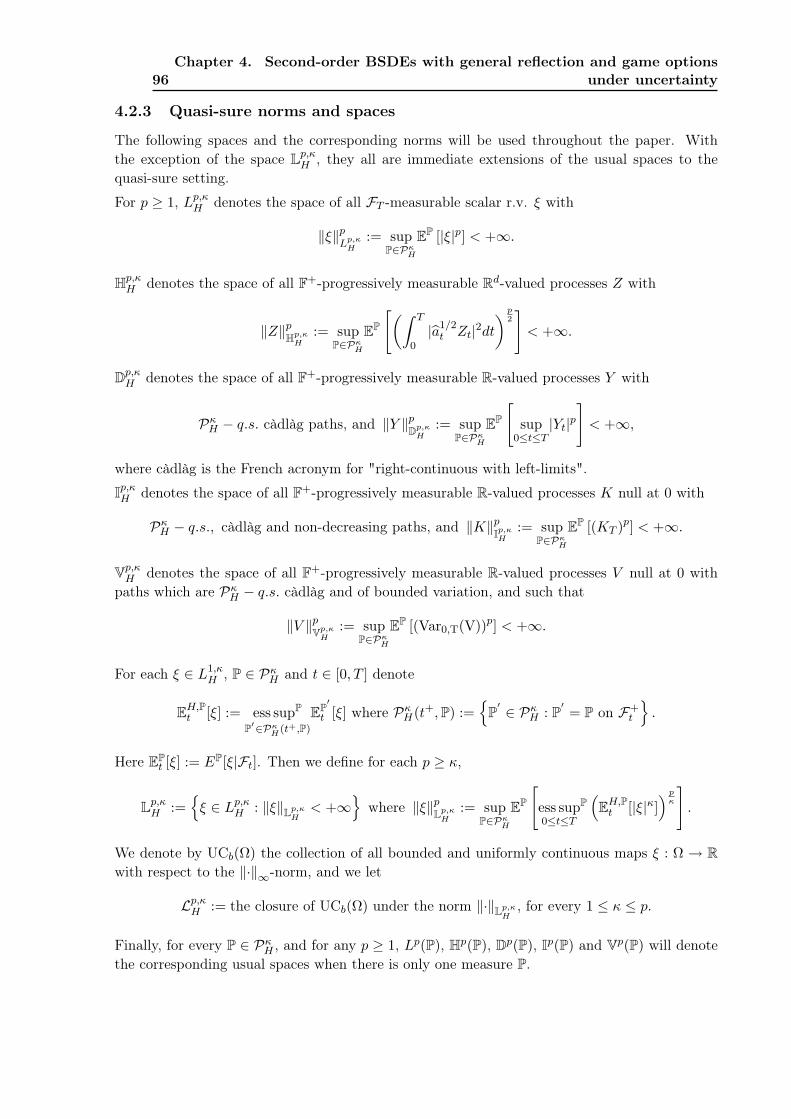
96Chapter 4. Second-order BSDEs with general reflection and game options
under uncertainty
4.2.3 Quasi-sure norms and spaces
The following spaces and the corresponding norms will be used throughout the paper. Withthe exception of the space Lp,κ
H , they all are immediate extensions of the usual spaces to thequasi-sure setting.
For p ≥ 1, Lp,κH denotes the space of all FT -measurable scalar r.v. ξ with
‖ξ‖pLp,κ
H:= sup
P∈PκH
EP [|ξ|p] < +∞.
Hp,κH denotes the space of all F+-progressively measurable Rd-valued processes Z with
‖Z‖pHp,κH
:= supP∈Pκ
H
EP
[(∫ T
0|a1/2
t Zt|2dt) p
2
]< +∞.
Dp,κH denotes the space of all F+-progressively measurable R-valued processes Y with
PκH − q.s. càdlàg paths, and ‖Y ‖pDp,κ
H:= sup
P∈PκH
EP
[sup
0≤t≤T|Yt|p
]< +∞,
where càdlàg is the French acronym for "right-continuous with left-limits".
Ip,κH denotes the space of all F+-progressively measurable R-valued processes K null at 0 with
PκH − q.s., càdlàg and non-decreasing paths, and ‖K‖pIp,κ
H:= sup
P∈PκH
EP [(KT )p] < +∞.
Vp,κH denotes the space of all F+-progressively measurable R-valued processes V null at 0 with
paths which are PκH − q.s. càdlàg and of bounded variation, and such that
‖V ‖pVp,κH
:= supP∈Pκ
H
EP [(Var0,T(V))p] < +∞.
For each ξ ∈ L1,κH , P ∈ Pκ
H and t ∈ [0, T ] denote
EH,Pt [ξ] := ess supP
P′∈PκH(t+,P)
EP′t [ξ] where Pκ
H(t+,P) :=
P′ ∈ Pκ
H : P′= P on F+
t
.
Here EPt [ξ] := EP[ξ|Ft]. Then we define for each p ≥ κ,
Lp,κH :=
ξ ∈ Lp,κ
H : ‖ξ‖Lp,κH
< +∞
where ‖ξ‖pLp,κH
:= supP∈Pκ
H
EP
[ess sup0≤t≤T
P(EH,P
t [|ξ|κ]) p
κ
].
We denote by UCb(Ω) the collection of all bounded and uniformly continuous maps ξ : Ω → Rwith respect to the ‖·‖∞-norm, and we let
Lp,κH := the closure of UCb(Ω) under the norm ‖·‖Lp,κ
H, for every 1 ≤ κ ≤ p.
Finally, for every P ∈ PκH , and for any p ≥ 1, Lp(P), Hp(P), Dp(P), Ip(P) and Vp(P) will denote
the corresponding usual spaces when there is only one measure P.
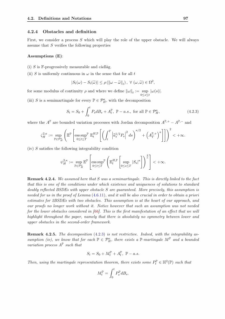
4.2. Definitions and Notations 97
4.2.4 Obstacles and definition
First, we consider a process S which will play the role of the upper obstacle. We will alwaysassume that S verifies the following properties
Assumptions (E):
(i) S is F-progressively measurable and càdlàg.
(ii) S is uniformly continuous in ω in the sense that for all t
|St(ω)− St(ω)| ≤ ρ (‖ω − ω‖t) , ∀ (ω, ω) ∈ Ω2,
for some modulus of continuity ρ and where we define ‖ω‖t := sup0≤s≤t
|ω(s)|.
(iii) S is a semimartingale for every P ∈ PκH , with the decomposition
St = S0 +∫ t
0PsdBs +AP
t , P− a.s., for all P ∈ PκH , (4.2.3)
where the AP are bounded variation processes with Jordan decomposition AP,+ −AP,− and
ζ2,κH := sup
P∈PκH
(EP
[ess supP
0≤t≤TEH,P
t
[(∫ T
t
∣∣∣a1/2s Ps
∣∣∣2 ds)κ/2
+(AP,+
T
)κ]])2
< +∞.
(iv) S satisfies the following integrability condition
ψ2,κH := sup
P∈PκH
EP
ess sup0≤t≤T
P
(EH,P
t
[sup
0≤s≤T|Ss|κ
]) 2κ
< +∞.
Remark 4.2.4. We assumed here that S was a semimartingale. This is directly linked to the factthat this is one of the conditions under which existence and uniqueness of solutions to standarddoubly reflected BSDEs with upper obstacle S are guaranteed. More precisely, this assumption isneeded for us in the proof of Lemma (4.6.11), and it will be also crucial in order to obtain a prioriestimates for 2BSDEs with two obstacles. This assumption is at the heart of our approach, andour proofs no longer work without it. Notice however that such an assumption was not neededfor the lower obstacles considered in [66]. This is the first manifestation of an effect that we willhighlight throughout the paper, namely that there is absolutely no symmetry between lower andupper obstacles in the second-order framework.
Remark 4.2.5. The decomposition (4.2.3) is not restrictive. Indeed, with the integrability as-sumption (iv), we know that for each P ∈ Pκ
H , there exists a P-martingale MP and a boundedvariation process AP such that
St = S0 +MPt +AP
t , P− a.s.
Then, using the martingale representation theorem, there exists some P Pt ∈ H2(P) such that
MPt =
∫ t
0P P
s dBs.
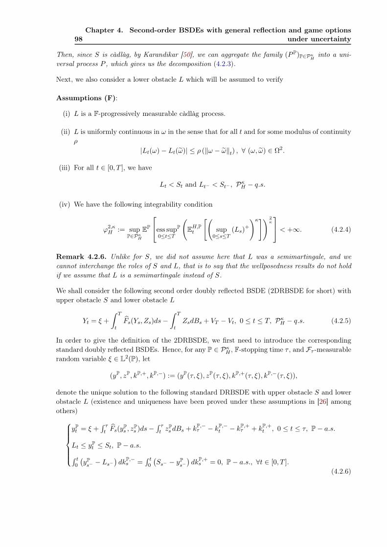
98Chapter 4. Second-order BSDEs with general reflection and game options
under uncertainty
Then, since S is càdlàg, by Karandikar [50], we can aggregate the family (P P)P∈PκH
into a uni-versal process P , which gives us the decomposition (4.2.3).
Next, we also consider a lower obstacle L which will be assumed to verify
Assumptions (F):
(i) L is a F-progressively measurable càdlàg process.
(ii) L is uniformly continuous in ω in the sense that for all t and for some modulus of continuityρ
|Lt(ω)− Lt(ω)| ≤ ρ (‖ω − ω‖t) , ∀ (ω, ω) ∈ Ω2.
(iii) For all t ∈ [0, T ], we have
Lt < St and Lt− < St− , PκH − q.s.
(iv) We have the following integrability condition
ϕ2,κH := sup
P∈PκH
EP
ess sup0≤t≤T
P
(EH,P
t
[(sup
0≤s≤T(Ls)
+
)κ]) 2κ
< +∞. (4.2.4)
Remark 4.2.6. Unlike for S, we did not assume here that L was a semimartingale, and wecannot interchange the roles of S and L, that is to say that the wellposedness results do not holdif we assume that L is a semimartingale instead of S.
We shall consider the following second order doubly reflected BSDE (2DRBSDE for short) withupper obstacle S and lower obstacle L
Yt = ξ +∫ T
tFs(Ys, Zs)ds−
∫ T
tZsdBs + VT − Vt, 0 ≤ t ≤ T, Pκ
H − q.s. (4.2.5)
In order to give the definition of the 2DRBSDE, we first need to introduce the correspondingstandard doubly reflected BSDEs. Hence, for any P ∈ Pκ
H , F-stopping time τ , and Fτ -measurablerandom variable ξ ∈ L2(P), let
(yP, zP, kP,+, kP,−) := (yP(τ, ξ), zP(τ, ξ), kP,+(τ, ξ), kP,−(τ, ξ)),
denote the unique solution to the following standard DRBSDE with upper obstacle S and lowerobstacle L (existence and uniqueness have been proved under these assumptions in [26] amongothers)
yPt = ξ +
∫ τt Fs(yP
s , zPs )ds−
∫ τt z
Ps dBs + kP,−
τ − kP,−t − kP,+
τ + kP,+t , 0 ≤ t ≤ τ, P− a.s.
Lt ≤ yPt ≤ St, P− a.s.∫ t
0
(yP
s− − Ls−)dkP,−
s =∫ t0
(Ss− − yP
s−
)dkP,+
s = 0, P− a.s., ∀t ∈ [0, T ].(4.2.6)
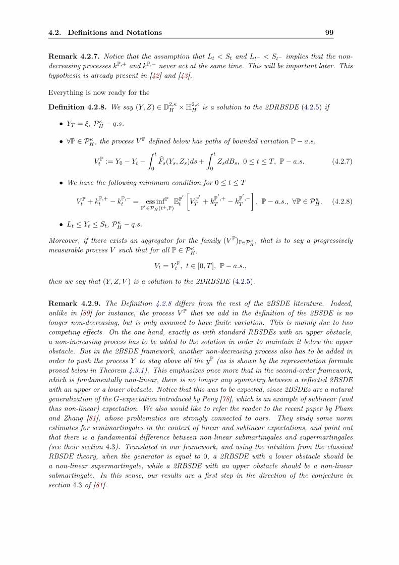
4.2. Definitions and Notations 99
Remark 4.2.7. Notice that the assumption that Lt < St and Lt− < St− implies that the non-decreasing processes kP,+ and kP,− never act at the same time. This will be important later. Thishypothesis is already present in [42] and [43].
Everything is now ready for the
Definition 4.2.8. We say (Y, Z) ∈ D2,κH ×H2,κ
H is a solution to the 2DRBSDE (4.2.5) if
• YT = ξ, PκH − q.s.
• ∀P ∈ PκH , the process V P defined below has paths of bounded variation P− a.s.
V Pt := Y0 − Yt −
∫ t
0Fs(Ys, Zs)ds+
∫ t
0ZsdBs, 0 ≤ t ≤ T, P− a.s. (4.2.7)
• We have the following minimum condition for 0 ≤ t ≤ T
V Pt + kP,+
t − kP,−t = ess infP
P′∈PH(t+,P)EP′
t
[V P′
T + kP′ ,+T − kP′ ,−
T
], P− a.s., ∀P ∈ Pκ
H . (4.2.8)
• Lt ≤ Yt ≤ St, PκH − q.s.
Moreover, if there exists an aggregator for the family (V P)P∈PκH, that is to say a progressively
measurable process V such that for all P ∈ PκH ,
Vt = V Pt , t ∈ [0, T ], P− a.s.,
then we say that (Y, Z, V ) is a solution to the 2DRBSDE (4.2.5).
Remark 4.2.9. The Definition 4.2.8 differs from the rest of the 2BSDE literature. Indeed,unlike in [89] for instance, the process V P that we add in the definition of the 2BSDE is nolonger non-decreasing, but is only assumed to have finite variation. This is mainly due to twocompeting effects. On the one hand, exactly as with standard RBSDEs with an upper obstacle,a non-increasing process has to be added to the solution in order to maintain it below the upperobstacle. But in the 2BSDE framework, another non-decreasing process also has to be added inorder to push the process Y to stay above all the yP (as is shown by the representation formulaproved below in Theorem 4.3.1). This emphasizes once more that in the second-order framework,which is fundamentally non-linear, there is no longer any symmetry between a reflected 2BSDEwith an upper or a lower obstacle. Notice that this was to be expected, since 2BSDEs are a naturalgeneralization of the G-expectation introduced by Peng [78], which is an example of sublinear (andthus non-linear) expectation. We also would like to refer the reader to the recent paper by Phamand Zhang [81], whose problematics are strongly connected to ours. They study some normestimates for semimartingales in the context of linear and sublinear expectations, and point outthat there is a fundamental difference between non-linear submartingales and supermartingales(see their section 4.3). Translated in our framework, and using the intuition from the classicalRBSDE theory, when the generator is equal to 0, a 2RBSDE with a lower obstacle should bea non-linear supermartingale, while a 2RBSDE with an upper obstacle should be a non-linearsubmartingale. In this sense, our results are a first step in the direction of the conjecture insection 4.3 of [81].
100Chapter 4. Second-order BSDEs with general reflection and game options
under uncertainty
4.2.5 DRBSDEs as a special case of 2DRBSDEs
In this subsection, we show how we can recover the usual theory. If H is linear in γ, that is tosay
Ht(y, z, γ) :=12Tr[a0
tγ]− ft(y, z),
where a0 : [0, T ] × Ω → S>0d is F-progressively measurable and has uniform upper and lower
bounds, then as in [89], we no longer need to assume any uniform continuity in ω in this case.Besides, the domain of F is restricted to a0 and we have
Ft(y, z) = ft(y, z).
If we further assume that there exists some P ∈ PS such that a and a0 coincide P − a.s. andEP[∫ T
0 |ft(0, 0)|2 dt]< +∞, then Pκ
H = P.
Then, we know that V P + kP,+t − kP,−
t is a P-martingale with finite variation. Since P satisfy themartingale representation property, this martingale is also continuous, and therefore it is null.Thus we have
0 = kP,+t − kP,−
t + V P, P− a.s.,
and the 2DRBSDE is equivalent to a standard DRBSDE. In particular, we see that V P nowbecomes a finite variation process which decreases only when Yt− = St− and increases only whenYt− = Lt− . This implies that V P satisfies the usual Skorohod conditions. We would like toemphasize this fact here, since it will be useful later on to have a deeper understanding of thestructure of the processes
V P
P∈PκH
.
4.3 Uniqueness, estimates and representations
4.3.1 A representation inspired by stochastic control
We have similarly as in Theorem 4.4 of [89]
Theorem 4.3.1. Let Assumption (D) hold. Assume ξ ∈ L2,κH and that (Y, Z) is a solution to
the 2DRBSDE (4.2.5). Then, for any P ∈ PκH and 0 ≤ t1 < t2 ≤ T ,
Yt1 = ess supP
P′∈PκH(t+1 ,P)
yP′t1 (t2, Yt2), P− a.s. (4.3.9)
Consequently, the 2DRBSDE (4.2.5) has at most one solution in D2,κH ×H2,κ
H .
Proof. The proof is exactly the same as the proof of Theorem 3.1 in [66], so we will onlysketch it. First, from the minimal condition (4.2.8), we deduce that for any P ∈ Pκ
H , the processV P + kP,+ − kP,− is a P-submartingale. By the Doob-Meyer decomposition and the martingalerepresentation property, its martingale part is continuous with finite variation and therefore null.Hence V P + kP,+ − kP,− is a non-decreasing process. Then, the inequality
Yt1 ≥ ess supP
P′∈PκH(t+1 ,P)
yP′t1 (t2, Yt2), P− a.s.,
is a simple consequence of a classical comparison Theorem. The reverse inequality is then ob-tained by standard linearization techniques using the Lipschitz properties of F , see [66] for thedetails.
4.3. Uniqueness, estimates and representations 101
Remark 4.3.2. Let us now justify the minimum condition (4.2.8). Assume for the sake of claritythat the generator F is equal to 0. By the above Theorem, we know that if there exists a solutionto the 2DRBSDE (4.2.5), then the process Y has to satisfy the representation (4.3.9). Therefore,we have a natural candidate for a possible solution of the 2DRBSDE. Now, assume that we couldconstruct such a process Y satisfying the representation (4.3.9) and which has the decomposition(4.2.5). Then, taking conditional expectations in Y − yP, we end up with exactly the minimumcondition (4.2.8).
Finally, the following comparison Theorem follows easily from the classical one for DRBSDEs(see for instance [61]) and the representation (4.3.9).
Theorem 4.3.3. Let (Y, Z) and (Y ′, Z ′) (resp. (yP, zP, k+,P, k−,P) and (y′P, z′P, k′+,P, k′−,P))be the solutions of the 2DRBSDEs (resp. DRBSDEs) with terminal conditions ξ and ξ
′ , upperobstacles S and S′, lower obstacles L and L′ and generators F and F ′ respectively. Assume thatthey both verify Assumptions (D), that Pκ
H ⊂ PκH′
and that we have PκH − q.s.
ξ ≤ ξ′ , Ft(y′Pt , z′Pt ) ≤ F ′t (y′Pt , z′Pt ), Lt ≤ L
′t and St ≥ S
′t.
Then Y ≤ Y ′, PκH − q.s.
Remark 4.3.4. Unlike in the classical framework, even if the upper obstacles S and S′ and thelower obstacles L and L′ are identical, we cannot compare the processes V P and V ′P. This is dueto the fact that these processes are not assumed to satisfy a Skorohod-type condition. This pointwas already mentioned in [66].
4.3.2 A priori estimates
We will now try to obtain a priori estimates for the 2DRBSDEs. We emphasize immediatelythat the fact that the process V P are only of finite variation makes the task a lot more difficultthan in [66]. Indeed, we are now in a case which shares some similarities with standard doublyreflected BSDEs for which it is known that a priori estimates cannot be obtained without someregularity assumptions on the obstacles (for instance if one of them is a semimartingale). Weassumed here that S was a semimartingale, a property which will be at the heart of our proofs.Nonetheless, even before this, we need to understand the fine structure of the processes V P. Thisis the object of the following proposition.
Proposition 4.3.5. Let Assumption (D) hold. Assume ξ ∈ L2,κH and (Y, Z) ∈ D2,κ
H × H2,κH
is a solution to the 2DRBSDE (4.2.5). Let(yP, zP, k+,P, k−,P)
P∈Pκ
Hbe the solutions of the
corresponding DRBSDEs (4.2.6). Then we have the following results for all t ∈ [0, T ] and for allP ∈ Pκ
H
(i) V P,+t :=
∫ t0 1yP
s−<Ss−
dV Ps is a non-decreasing process, P− a.s.
(ii) V P,−t :=
∫ t0 1yP
s−=Ss−
dV Ps = −kP,+
t , P− a.s., and is therefore a non-increasing process.
Proof.
Let us fix a given P ∈ PκH .
(i) Let τ1 and τ2 be two F-stopping times such that for all t ∈ [τ1, τ2), yPt− < St− , P− a.s.
102Chapter 4. Second-order BSDEs with general reflection and game options
under uncertainty
Then, we know from the usual Skorohod condition that the process kP,+ does not increasebetween τ1 and τ2. Now, we remind the reader that we showed in the proof of Theorem 4.3.1,that the process V P + k+,P − k−,P is always non-decreasing. This necessarily implies that V P
must be non-decreasing between τ1 and τ2. Hence the first result.
(ii) Let now τ1 and τ2 be two F-stopping times such that for all t ∈ [τ1, τ2), yPt− = St− , P− a.s.
First, since the two obstacles are separated, we necessarily have yPt− > Lt− , P − a.s. for every
t ∈ [τ1, τ2), which in turn implies that kP,− does not increase. Next, by the representationformula (4.3.9), we necessarily have Yt− ≥ yP
t− , P − a.s. for all t. Moreover, since we also haveYt ≤ St by definition, this implies, since all the processes here are càdlàg, that we must have
Yt− = yPt− = St− , t ∈ [τ1, τ2), P− a.s.
Using the fact that Y and yP solve respectively a 2BSDE and a BSDE, we also have P− a.s.
St− + ∆Yt = Yt = Yu +∫ u
tFs(Ys, Zs)ds−
∫ u
tZsdBs + V P
u − V Pt , τ1 ≤ t ≤ u < τ2
St− + ∆yPt = yP
t = yPu +
∫ u
tFs(yP
s , zPs )ds−
∫ u
tzPs dBs − kP,+
u + kP,+t , τ1 ≤ t ≤ u < τ2.
Identifying the martingale parts above, we obtain that Zs = zPs , ds× P− a.e. Then, identifying
the finite variation parts, we have
Yu −∆Yt +∫ u
tFs(Ys, Zs)ds+ V P
u − V Pt = yP
u −∆yPt +
∫ u
tFs(yP
s , zPs )ds− kP,+
u + kP,+t .
(4.3.10)
Now, we clearly have ∫ u
tFs(Ys, Zs)ds =
∫ u
tFs(yP
s , zPs )ds,
since Zs = zPs , dt×P−a.e. and Ys− = yP
s− = Ss− for all s ∈ [t, u]. Moreover, since Ys− = yPs− = Ss−
for all s ∈ [t, u] and since all the processes are càdlàg, the jumps of Y and yP are equal to thejumps of S. Therefore, (4.3.10) can be rewritten
V Pu − V P
t = −kP,+u + kP,+
t ,
which is the desired result.
The above Proposition is crucial for us. Indeed, we have actually shown that
V Pt = V P,+
t − kP,+t , P− a.s.,
where V P,+ and kP,+ are two non-decreasing processes which never act at the same time. Hence,we have obtained a Jordan decomposition for V P. Moreover, we can easily obtain a prioriestimates for kP,+ by using the fact that it is part of the solution of the DRBSDE (4.2.6). Noticethat these estimates hold only because we assumed that the corresponding upper obstacle S wasa semimartingale. This is this decomposition which will allow us to obtain the estimates.
Remark 4.3.6. The above result is enough for us to obtain the desired a priori estimates.However, we can go further into the structure of the bounded variation processes V P. Indeed,arguing as in Proposition 3.2 in [66], we could also show that
1Yt−=Lt−dV P
t = 1Yt−=Lt−dkP,−
t .
4.3. Uniqueness, estimates and representations 103
Notice however that we, a priori, cannot say anything about V P when Lt− = yPt− < Yt− , even
though we showed that it could be known explicitly when St− = yPt− . This emphasizes once more
the fact that the upper and the lower obstacle in our context do not play a symmetric role.
We can now prove the following theorem.
Theorem 4.3.7. Let Assumptions (D), (E) and (F) hold. Assume ξ ∈ L2,κH and (Y, Z) ∈
D2,κH ×H2,κ
H is a solution to the 2DRBSDE (4.2.5). Let(yP, zP, kP,+, kP,−)
P∈Pκ
Hbe the solutions
of the corresponding DRBSDEs (4.2.6). Then, there exists a constant Cκ depending only on κ,T and the Lipschitz constant of F such that
‖Y ‖2D2,κH
+ ‖Z‖2H2,κH
+ supP∈Pκ
H
∥∥∥yP∥∥∥2
D2(P)+∥∥∥zP∥∥∥2
H2(P)+ EP
[Var0,T
(V P)2
+(kP,+
T
)2+(kP,−
T
)2]
≤ Cκ
(‖ξ‖2L2,κ
H+ φ2,κ
H + ψ2,κH + ϕ2,κ
H + ζ2,κH
)Proof. First of all, since we assumed that S was a semimartingale, we can argue as in [26] toobtain that
dkP,+t ≤ F+
t (St, Pt)dt+ dAP,+t ≤ C
(∣∣∣F 0t
∣∣∣+ |St|+∣∣∣a1/2
t Pt
∣∣∣) dt+ dAP,+t .
Hence,
EPt
[(kP,+
T
)κ]≤ CκEP
t
[∫ T
t
∣∣∣F 0s
∣∣∣κ ds+(∫ T
t|a
12s Ps|2ds
)κ/2
+ supt≤s≤T
|Ss|κ +(AP,+
T
)κ]
≤ Cκ
((ζ2,κH
)1/2+ EP
t
[∫ T
t
∣∣∣F 0s
∣∣∣κ ds+ supt≤s≤T
|Ss|κ])
.
Let us now define
ξ := ξ − kP,+T , yP = yP − kP,+, Ft(y, z) := Ft
(y + kP,+
t , z).
Then, it is easy to see that (yP, zP, kP,+) is the solution of the lower reflected BSDE with terminalcondition ξ, generator F and obstacle L− kP,+. We can then once again apply Lemma 2 in [47]to obtain that there exists a constant Cκ depending only on κ, T and the Lipschitz constant ofF , such that for all P∣∣∣yP
t
∣∣∣ ≤ CκEPt
[∣∣∣ξ∣∣∣κ +∫ T
t
∣∣∣F 0s
∣∣∣κ ds+ supt≤s≤T
((Ls − kP,+
s
)+)κ]
≤ CκEPt
[|ξ|κ +
∫ T
t
∣∣∣F 0s
∣∣∣κ ds+ supt≤s≤T
(L+
s
)κ +(kP,+
T
)κ]
≤ Cκ
((ζ2,κH
)1/2+ EP
t
[|ξ|κ +
∫ T
t
∣∣∣F 0s
∣∣∣κ ds+ supt≤s≤T
|Ss|κ + supt≤s≤T
(L+
s
)κ]). (4.3.11)
This immediately provides the estimate for yP. Now by definition of the norms, we obtain from(4.3.11) and the representation formula (4.3.9) that
‖Y ‖2D2,κH≤ Cκ
(‖ξ‖2L2,κ
H+ φ2,κ
H + ψ2,κH + ϕ2,κ
H + ζ2,κH
). (4.3.12)
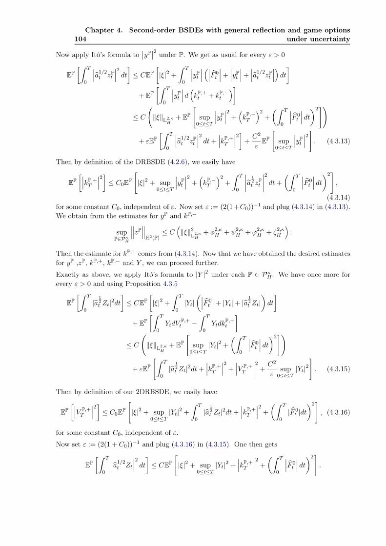
104Chapter 4. Second-order BSDEs with general reflection and game options
under uncertainty
Now apply Itô’s formula to∣∣yP∣∣2 under P. We get as usual for every ε > 0
EP[∫ T
0
∣∣∣a1/2t zP
t
∣∣∣2 dt] ≤ CEP[|ξ|2 +
∫ T
0
∣∣∣yPt
∣∣∣ (∣∣∣F 0t
∣∣∣+ ∣∣∣yPt
∣∣∣+ ∣∣∣a1/2t zP
t
∣∣∣) dt]+ EP
[∫ T
0
∣∣∣yPt
∣∣∣ d(kP,+t + kP,−
t
)]≤ C
(‖ξ‖L2,κ
H+ EP
[sup
0≤t≤T
∣∣∣yPt
∣∣∣2 +(kP,−
T
)2+(∫ T
0
∣∣∣F 0t
∣∣∣ dt)2])
+ εEP[∫ T
0
∣∣∣a1/2t zP
t
∣∣∣2 dt+∣∣∣kP,+
T
∣∣∣2]+C2
εEP
[sup
0≤t≤T
∣∣∣yPt
∣∣∣2] . (4.3.13)
Then by definition of the DRBSDE (4.2.6), we easily have
EP[∣∣∣kP,+
T
∣∣∣2] ≤ C0EP
[|ξ|2 + sup
0≤t≤T
∣∣∣yPt
∣∣∣2 +(kP,−
T
)2+∫ T
0
∣∣∣∣a 12t z
Pt
∣∣∣∣2 dt+(∫ T
0
∣∣∣F 0t
∣∣∣ dt)2],
(4.3.14)for some constant C0, independent of ε. Now set ε := (2(1+C0))−1 and plug (4.3.14) in (4.3.13).We obtain from the estimates for yP and kP,−
supP∈Pκ
H
∥∥∥zP∥∥∥
H2(P)≤ C
(‖ξ‖2L2,κ
H+ φ2,κ
H + ψ2,κH + ϕ2,κ
H + ζ2,κH
).
Then the estimate for kP,+ comes from (4.3.14). Now that we have obtained the desired estimatesfor yP ,zP, kP,+, kP,− and Y , we can proceed further.
Exactly as above, we apply Itô’s formula to |Y |2 under each P ∈ PκH . We have once more for
every ε > 0 and using Proposition 4.3.5
EP[∫ T
0|a
12t Zt|2dt
]≤ CEP
[|ξ|2 +
∫ T
0|Yt|
(∣∣∣F 0t
∣∣∣+ |Yt|+ |a12t Zt|
)dt
]+ EP
[∫ T
0YtdV
P,+t −
∫ T
0Ytdk
P,+t
]≤ C
(‖ξ‖L2,κ
H+ EP
[sup
0≤t≤T|Yt|2 +
(∫ T
0
∣∣∣F 0t
∣∣∣ dt)2])
+ εEP
[∫ T
0|a
12t Zt|2dt+
∣∣∣kP,+T
∣∣∣2 +∣∣∣V P,+
T
∣∣∣2 +C2
εsup
0≤t≤T|Yt|2
]. (4.3.15)
Then by definition of our 2DRBSDE, we easily have
EP[∣∣∣V P,+
T
∣∣∣2] ≤ C0EP
[|ξ|2 + sup
0≤t≤T|Yt|2 +
∫ T
0|a
12t Zt|2dt+
∣∣∣kP,+T
∣∣∣2 +(∫ T
0|F 0
t |dt)2], (4.3.16)
for some constant C0, independent of ε.
Now set ε := (2(1 + C0))−1 and plug (4.3.16) in (4.3.15). One then gets
EP[∫ T
0
∣∣∣a1/2t Zt
∣∣∣2 dt] ≤ CEP
[|ξ|2 + sup
0≤t≤T|Yt|2 +
∣∣∣kP,+T
∣∣∣2 +(∫ T
0
∣∣∣F 0t
∣∣∣ dt)2].
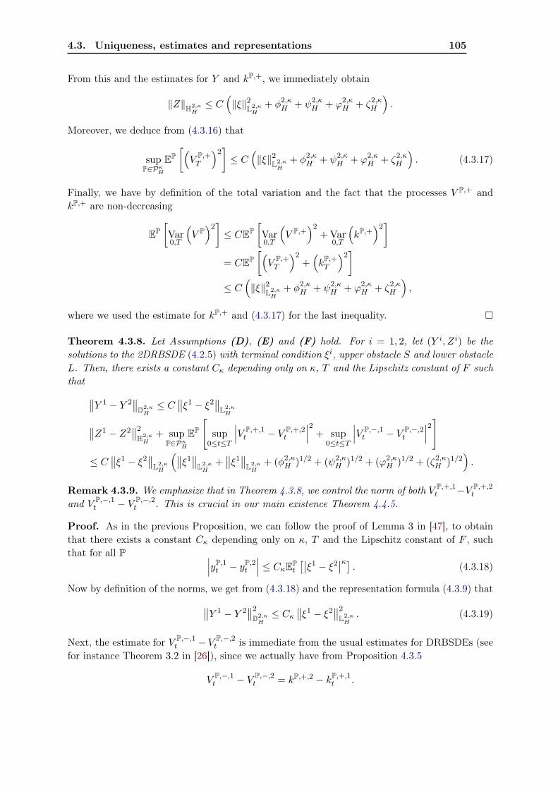
4.3. Uniqueness, estimates and representations 105
From this and the estimates for Y and kP,+, we immediately obtain
‖Z‖H2,κH≤ C
(‖ξ‖2L2,κ
H+ φ2,κ
H + ψ2,κH + ϕ2,κ
H + ζ2,κH
).
Moreover, we deduce from (4.3.16) that
supP∈Pκ
H
EP[(V P,+
T
)2]≤ C
(‖ξ‖2L2,κ
H+ φ2,κ
H + ψ2,κH + ϕ2,κ
H + ζ2,κH
). (4.3.17)
Finally, we have by definition of the total variation and the fact that the processes V P,+ andkP,+ are non-decreasing
EP[Var0,T
(V P)2]≤ CEP
[Var0,T
(V P,+
)2+ Var
0,T
(kP,+
)2]
= CEP[(V P,+
T
)2+(kP,+
T
)2]
≤ C(‖ξ‖2L2,κ
H+ φ2,κ
H + ψ2,κH + ϕ2,κ
H + ζ2,κH
),
where we used the estimate for kP,+ and (4.3.17) for the last inequality.
Theorem 4.3.8. Let Assumptions (D), (E) and (F) hold. For i = 1, 2, let (Y i, Zi) be thesolutions to the 2DRBSDE (4.2.5) with terminal condition ξi, upper obstacle S and lower obstacleL. Then, there exists a constant Cκ depending only on κ, T and the Lipschitz constant of F suchthat ∥∥Y 1 − Y 2
∥∥D2,κ
H≤ C
∥∥ξ1 − ξ2∥∥L2,κH∥∥Z1 − Z2
∥∥2
H2,κH
+ supP∈Pκ
H
EP
[sup
0≤t≤T
∣∣∣V P,+,1t − V P,+,2
t
∣∣∣2 + sup0≤t≤T
∣∣∣V P,−,1t − V P,−,2
t
∣∣∣2]≤ C
∥∥ξ1 − ξ2∥∥L2,κH
(∥∥ξ1∥∥L2,κH
+∥∥ξ1∥∥L2,κ
H+ (φ2,κ
H )1/2 + (ψ2,κH )1/2 + (ϕ2,κ
H )1/2 + (ζ2,κH )1/2
).
Remark 4.3.9. We emphasize that in Theorem 4.3.8, we control the norm of both V P,+,1t −V P,+,2
t
and V P,−,1t − V P,−,2
t . This is crucial in our main existence Theorem 4.4.5.
Proof. As in the previous Proposition, we can follow the proof of Lemma 3 in [47], to obtainthat there exists a constant Cκ depending only on κ, T and the Lipschitz constant of F , suchthat for all P ∣∣∣yP,1
t − yP,2t
∣∣∣ ≤ CκEPt
[∣∣ξ1 − ξ2∣∣κ] . (4.3.18)
Now by definition of the norms, we get from (4.3.18) and the representation formula (4.3.9) that∥∥Y 1 − Y 2∥∥2
D2,κH≤ Cκ
∥∥ξ1 − ξ2∥∥2
L2,κH. (4.3.19)
Next, the estimate for V P,−,1t − V P,−,2
t is immediate from the usual estimates for DRBSDEs (seefor instance Theorem 3.2 in [26]), since we actually have from Proposition 4.3.5
V P,−,1t − V P,−,2
t = kP,+,2 − kP,+,1t .
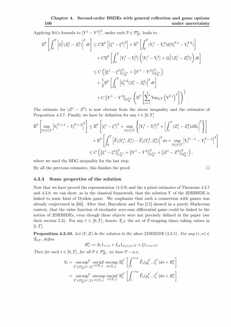
106Chapter 4. Second-order BSDEs with general reflection and game options
under uncertainty
Applying Itô’s formula to∣∣Y 1 − Y 2
∣∣2, under each P ∈ PκH , leads to
EP
[∫ T
0
∣∣∣∣a 12t (Z1
t − Z2t )∣∣∣∣2 dt
]≤ CEP
[∣∣ξ1 − ξ2∣∣2]+ EP[∫ T
0(Y 1
t − Y 2t )d(V P,1
t − V P,2t )
]+ CEP
[∫ T
0
∣∣Y 1t − Y 2
t
∣∣ (∣∣Y 1t − Y 2
t
∣∣+ |a 12t (Z1
t − Z2t )|)dt
]
≤ C(∥∥ξ1 − ξ2∥∥2
L2,κH
+∥∥Y 1 − Y 2
∥∥2
D2,κH
)+
12
EP[∫ T
0
∣∣∣a1/2t (Z1
t − Z2t )∣∣∣2 dt]
+ C∥∥Y 1 − Y 2
∥∥D2,κ
H
(EP
[2∑
i=1
Var0,T
(VP,i
)2]) 1
2
.
The estimate for (Z1 − Z2) is now obvious from the above inequality and the estimates ofProposition 4.3.7. Finally, we have by definition for any t ∈ [0, T ]
EP
[sup
0≤t≤T
∣∣∣V P,+,1t − V P,+,2
t
∣∣∣2] ≤ EP
[∣∣ξ1 − ξ2∣∣2 + sup0≤t≤T
∣∣Y 1t − Y 2
t
∣∣2 +∣∣∣∣∫ T
t(Z1
s − Z2s )dBs
∣∣∣∣2]
+ EP
[∫ T
0
∣∣∣Fs(Y 1s , Z
1s )− Fs(Y 2
s , Z2s )∣∣∣2 ds+ sup
0≤t≤T
∣∣∣V P,−,1t − V P,−,2
t
∣∣∣2]≤ C
(∥∥ξ1 − ξ2∥∥2
L2,κH
+∥∥Y 1 − Y 2
∥∥2
D2,κH
+∥∥Z1 − Z2
∥∥2
H2,κH
),
where we used the BDG inequality for the last step.
By all the previous estimates, this finishes the proof.
4.3.3 Some properties of the solution
Now that we have proved the representation (4.3.9) and the a priori estimates of Theorems 4.3.7and 4.3.8, we can show, as in the classical framework, that the solution Y of the 2DRBSDE islinked to some kind of Dynkin game. We emphasize that such a connection with games wasalready conjectured in [66]. After that, Bayraktar and Yao [11] showed in a purely Markoviancontext, that the value function of stochastic zero-sum differential game could be linked to thenotion of 2DRBSDEs, even though these objects were not precisely defined in the paper (seetheir section 5.2). For any t ∈ [0, T ], denote Tt,T the set of F-stopping times taking values in[t, T ].
Proposition 4.3.10. Let (Y, Z) be the solution to the above 2DRBSDE (4.2.5). For any (τ, σ) ∈T0,T , define
Rστ := Sτ1τ<σ + Lσ1σ≤τ,σ<T + ξ1τ∧σ=T .
Then for each t ∈ [0, T ], for all P ∈ PκH , we have P− a.s.
Yt = ess supP
P′∈PκH(t+,P)
ess infτ∈Tt,T
ess supσ∈Tt,T
EP′t
[∫ τ∧σ
tFs(yP′
s , zP′s )ds+Rσ
τ
]= ess supP
P′∈PκH(t+,P)
ess supσ∈Tt,T
ess infτ∈Tt,T
EP′t
[∫ τ∧σ
tFs(yP′
s , zP′s )ds+Rσ
τ
].
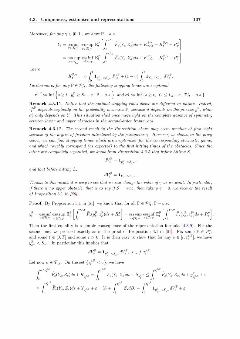
4.3. Uniqueness, estimates and representations 107
Moreover, for any γ ∈ [0, 1], we have P− a.s.
Yt = ess infτ∈Tt,T
ess supσ∈Tt,T
EPt
[∫ τ∧σ
tFs(Ys, Zs)ds+KP,γ
τ∧σ −KP,γt +Rσ
τ
]= ess sup
σ∈Tt,T
ess infτ∈Tt,T
EPt
[∫ τ∧σ
tFs(Ys, Zs)ds+KP,γ
τ∧σ −KP,γt +Rσ
τ
],
where
KP,γt := γ
∫ t
01yP
s−<Ss−
dV Ps + (1− γ)
∫ t
01Ys−>Ls−
dV Ps .
Furthermore, for any P ∈ PκH , the following stopping times are ε-optimal
τ ε,Pt := inf
s ≥ t, yP
s ≥ Ss − ε, P− a.s.
and σεt := inf s ≥ t, Ys ≤ Ls + ε, Pκ
H − q.s. .
Remark 4.3.11. Notice that the optimal stopping rules above are different in nature. Indeed,τ ε,Pt depends explicitly on the probability measures P, because it depends on the process yP, whileσε
t only depends on Y . This situation shed once more light on the complete absence of symmetrybetween lower and upper obstacles in the second-order framework
Remark 4.3.12. The second result in the Proposition above may seem peculiar at first sightbecause of the degree of freedom introduced by the parameter γ. However, as shown in the proofbelow, we can find stopping times which are ε-optimizer for the corresponding stochastic game,and which roughly correspond (as expected) to the first hitting times of the obstacles. Since thelatter are completely separated, we know from Proposition 4.3.5 that before hitting S,
dV Pt = 1yP
t−<St−
,
and that before hitting L,dV P
t = 1Yt−>Lt−.
Thanks to this result, it is easy to see that we can change the value of γ as we want. In particular,if there is no upper obstacle, that is to say if S = +∞, then taking γ = 0, we recover the resultof Proposition 3.1 in [66].
Proof. By Proposition 3.1 in [61], we know that for all P ∈ PκH , P− a.s.
yPt = ess inf
τ∈Tt,T
ess supσ∈Tt,T
EPt
[∫ τ∧σ
tFs(yP
s , zPs )ds+Rσ
τ
]= ess sup
σ∈Tt,T
ess infτ∈Tt,T
EPt
[∫ τ∧σ
tFs(yP
s , zPs )ds+Rσ
τ
].
Then the first equality is a simple consequence of the representation formula (4.3.9). For thesecond one, we proceed exactly as in the proof of Proposition 3.1 in [61]. Fix some P ∈ Pκ
H
and some t ∈ [0, T ] and some ε > 0. It is then easy to show that for any s ∈ [t, τ ε,Pt ], we have
yPs− < Ss− . In particular this implies that
dV Ps = 1yP
s−<Ss−
dV Ps , s ∈ [t, τ ε,P
t ].
Let now σ ∈ Tt,T . On the set τ ε,Pt < σ, we have∫ σ∧τε,P
t
tFs(Ys, Zs)ds+Rσ
τε,Pt
=∫ τε,P
t
tFs(Ys, Zs)ds+ S
τε,Pt≤∫ τε,P
t
tFs(Ys, Zs)ds+ yP
τε,Pt
+ ε
≤∫ τε,P
t
tFs(Ys, Zs)ds+ Y
τε,Pt
+ ε = Yt +∫ τε,P
t
tZsdBs −
∫ τε,Pt
t1yP
s−<Ss−
dV Ps + ε.
108Chapter 4. Second-order BSDEs with general reflection and game options
under uncertainty
Then, notice that the process (1yPs−
<Ss−−1Ys−>Ls−
)dV Ps is non-decreasing. Therefore, we deduce
∫ σ∧τε,Pt
tFs(Ys, Zs)ds+Rσ
τε,Pt
≤ Yt +∫ τε,P
t
tZsdBs −
∫ τε,Pt
t1yP
s−<Ss−
dV Ps
+ (1− γ)∫ τε,P
t
t
(1yP
s−<Ss−
− 1Ys−>Ls−
)dV P
s + ε
= Yt +∫ τε,P
t
tZsdBs − (Kγ
τP,εt
−Kγt ) + ε.
Similarly on the set τ ε,Pt ≥ σ, we have
∫ σ∧τε,Pt
tFs(Ys, Zs)ds+Rσ
τε,Pt
≤∫ σ
tFs(Ys, Zs)ds+ ξ1σ=T + Yσ1σ<T
= Yt +∫ σ
tZsdBs −
∫ σ
t1yP
s−<Ss−
dV Ps ≤ Yt +
∫ σ
tZsdBs − (Kγ
σ −Kγt ).
With these two inequalities, we therefore have
EPt
[∫ σ∧τε,Pt
tFs(Ys, Zs)ds+Rσ
τε,Pt
+Kγ
σ∧τP,εt
−Kγt
]− ε ≤ Yt, P− a.s. (4.3.20)
We can prove similarly that for any τ ∈ Tt,T
EPt
[∫ σε,Pt ∧τ
tFs(Ys, Zs)ds+R
σε,Pt
τ +Kγ
σP,εt ∧τ
−Kγt
]+ ε ≥ Yt, P− a.s. (4.3.21)
Then, we can use Lemma 5.3 of [61] to finish the proof.
Then, if we have more information on the obstacle S and its decomposition (4.2.3), we can givea more explicit representation for the processes V P, just as in the classical case (see Proposition4.2 in [35]).
Assumptions (G):S is a semi-martingale of the form
St = S0 +∫ t
0Usds+
∫ t
0PsdBs + Ct, Pκ
H − q.s.
where C is càdlàg process of integrable variation such that the measure dCt is singular withrespect to the Lebesgue measure dt and which admits the following decomposition Ct = C+
t −C−t ,
where C+ and C− are non-decreasing processes. Besides, U and V are respectively R and Rd-valued Ft progressively measurable processes such that∫ T
0(|Ut|+ |Pt|2)dt+ C+
T + C−T ≤ +∞, PκH − q.s.
4.3. Uniqueness, estimates and representations 109
Proposition 4.3.13. Let Assumptions (D), (E), (G) and (F) hold. Let (Y, Z) be the solutionto the 2DRBSDE (4.2.5), then for all P ∈ Pκ
H
Zt = Pt, dt× P− a.s. on the set Yt− = St− , (4.3.22)
and there exists a progressively measurable process (αPt )0≤t≤T such that 0 ≤ α ≤ 1 and
−1yPt−
=St−dV P
t = αPt 1yP
t−=St−
([Ft(St, Pt) + Ut
]+dt+ dC+
t
).
Proof. First, for all P ∈ PκH , the following holds P− a.s.
St − Yt = S0 − Y0 +∫ t
0
(Fs(Ys, Zs) + Us
)ds−
∫ t
0(Zs − Ps)dBs + V P
t + C+t − C
−t .
Now if we denote Lt the local time at 0 of St − Yt, then by Itô-Tanaka formula under P
(St − Yt)+ = (S0 − Y0)+ +∫ t
01Ys−<Ss−
(Fs(Ys, Zs) + Us
)ds−
∫ t
01Ys−<Ss−
(Zs − Ps)dBs
+∫ t
01Ys−<Ss−
d(V Pt + C+
t − C−t ) +
12Lt
+∑
0≤s≤t
(Ss − Ys)+ − (Ss− − Ys−)+ − 1Ys−<Ss−∆(Ss − Ys).
However, we have (St − Yt)+ = St − Yt, hence by identification of the martingale part
1Yt−=St−(Zt − Pt)dBt = 0, Pκ
H − q.s.,
from which the first statement is clear. Identifying the finite variation part, we obtain
1Ys−=Ss−
(Fs(Ys, Zs) + Us
)ds+ 1Ys−=Ss−
d(V Ps + C+
s − C−s )
=12Ls +
((Ss − Ys)+ − (Ss− − Ys−)+ − 1Ys−<Ss−
∆(Ss − Ys)).
By Proposition 4.3.5, we know that 1yPs−
=Ss−dV P
s is a non-increasing process, while 1yPs−
<Ss−dV P
s
is a non-decreasing process. Furthermore, we have
1Ys−=Ss−dV P
s = 1yPs−
=Ss−dV P
s + 1yPs−
<Ys−=Ss−dV P
s .
Since we also know that the jump part, L and C− are non-decreasing processes, we obtain
−1yPs−
=Ss−dV P
s ≤ 1yPs−
=Ss−
((Fs(Ys, Zs) + Us
)ds+ dC+
s
)+ 1yP
s−<Ys−=Ss−
((Fs(Ys, Zs) + Us
)ds+ dC+
s + dV Ps
).
Since, 1yPs−
=Ss−dV P
s and 1yPs−
<Ys−=Ss−
((Fs(Ys, Zs) + Us
)ds+ dC+
s + dV Ps
)never act at the
same time by definition, the second statement follows easily.
Remark 4.3.14. If we assume also that L is a semimartingale, then we can obtain exactly thesame type of results as in Corollary 3.1 in [66], using the exact same arguments.
110Chapter 4. Second-order BSDEs with general reflection and game options
under uncertainty
4.4 A constructive proof of existence
We have shown in Theorem 4.3.1 that if a solution exists, it will necessarily verify the represen-tation (4.2.8). This gives us a natural candidate for the solution as a supremum of solutions tostandard DRBSDEs. However, since those DRBSDEs are all defined on the support of mutuallysingular probability measures, it seems difficult to define such a supremum, because of the prob-lems raised by the negligible sets. In order to overcome this, Soner, Touzi and Zhang proposedin [89] a pathwise construction of the solution to a 2BSDE. Let us describe briefly their strategy.
The first step is to define pathwise the solution to a standard BSDE. For simplicity, let usconsider first a BSDE with a generator equal to 0. Then, we know that the solution is given bythe conditional expectation of the terminal condition. In order to define this solution pathwise,we can use the so-called regular conditional probability distribution (r.p.c.d. for short) of Stroockand Varadhan [91]. In the general case, the idea is similar and consists on defining BSDEs on ashifted canonical space.
Finally, we have to prove measurability and regularity of the candidate solution thus obtained,and the decomposition (4.2.5) is obtained through a non-linear Doob-Meyer decomposition. Ouraim in this section is to extend this approach in the presence of obstacles. We emphasize thatmost of the proofs are now standard, and we will therefore only sketch them, insisting particularlyon the new difficulties appearing in the present setting.
4.4.1 Shifted spaces
For the convenience of the reader, we recall below some of the notations introduced in [89].
• For 0 ≤ t ≤ T , denote by Ωt :=ω ∈ C
([t, T ],Rd
), w(t) = 0
the shifted canonical space, Bt
the shifted canonical process, Pt0 the shifted Wiener measure and Ft the filtration generated by
Bt.
• For 0 ≤ s ≤ t ≤ T and ω ∈ Ωs, define the shifted path ωt ∈ Ωt
ωtr := ωr − ωt, ∀r ∈ [t, T ].
• For 0 ≤ s ≤ t ≤ T and ω ∈ Ωs, ω ∈ Ωt define the concatenation path ω ⊗t ω ∈ Ωs by
(ω ⊗t ω)(r) := ωr1[s,t)(r) + (ωt + ωr)1[t,T ](r), ∀r ∈ [s, T ].
• For 0 ≤ s ≤ t ≤ T and a FsT -measurable random variable ξ on Ωs, for each ω ∈ Ωs, define the
shifted F tT -measurable random variable ξt,ω on Ωt by
ξt,ω(ω) := ξ(ω ⊗t ω), ∀ω ∈ Ωt.
Similarly, for an Fs-progressively measurable process X on [s, T ] and (t, ω) ∈ [s, T ] × Ωs, theshifted process
Xt,ω
r , r ∈ [t, T ]
is Ft-progressively measurable.
• For a F-stopping time τ , the r.c.p.d of P (denoted Pωτ ) is a probability measure on FT such
thatEP
τ [ξ](ω) = EPωτ [ξ], for P− a.e. ω.
4.4. A constructive proof of existence 111
It also induces naturally a probability measure Pτ,ω (that we also call the r.c.p.d. of P) on Fτ(ω)T
which in particular satisfies that for every bounded and FT -measurable random variable ξ
EPωτ [ξ] = EPτ,ω
[ξτ,ω] .
• We define similarly as in Section 4.2 the set PtS , by restricting to the shifted canonical space
Ωt, and its subset PtH .
• Finally, we define the "shifted" generator
F t,ωs (ω, y, z) := Fs(ω ⊗t ω, y, z, a
ts(ω)), ∀(s, ω) ∈ [t, T ]× Ωt.
Notice that thanks to Lemma 4.1 in [90], this generator coincides for P-a.e. ω with the shiftedgenerator as defined above, that is to say Fs(ω⊗t ω, y, z, as(ω⊗t ω)). The advantage of the chosen"shifted" generator is that it inherits the uniform continuity in ω under the L∞ norm of F .
4.4.2 A first existence result when ξ is in UCb(Ω)
Let us define for all ω ∈ Ω, Λ∗ (ω) := sup0≤s≤t
Λs (ω) , where
Λ2t (ω) := sup
P∈PtH
EP
[∣∣ξt,ω∣∣2 +
∫ T
t|F t,ω
s (0, 0)|2ds+ supt≤s≤T
∣∣St,ωs
∣∣2 + supt≤s≤T
((Lt,ω
s )+)2]
.
By Assumption (F), we can check directly that
Λt (ω) <∞ for all (t, ω) ∈ [0, T ]× Ω. (4.4.23)
To prove existence, we define the following value process Xt pathwise
Xt(ω) := supP∈Pt
H
YP,t,ωt (T, ξ) , for all (t, ω) ∈ [0, T ]× Ω, (4.4.24)
where, for any (t1, ω) ∈ [0, T ] × Ω, P ∈ Pt1H , t2 ∈ [t1, T ], and any Ft2-measurable η ∈ L2 (P),
we denote YP,t1,ωt1
(t2, η) := yP,t1,ωt1
, where(yP,t1,ω, zP,t1,ω, kP,+,t1,ω, kP,−,t1,ω
)is the solution of the
following DRBSDE with upper obstacle St1,ω and lower obstacle Lt1,ω on the shifted space Ωt1
under P
yP,t1,ωs = ηt1,ω +
∫ t2
sF t1,ω
r
(yP,t1,ω
r , zP,t1,ωr
)dr −
∫ t2
szP,t1,ωr dBt1
r − kP,+,t1,ωt2
+ kP,+,t1,ωs
+ kP,−,t1,ωt2
− kP,−,t1,ωs , P− a.s. (4.4.25)
Lt1,ωt ≤ yP,t1,ω
t ≤ St1,ωt , P− a.s.∫ t2
t1
(St1,ω
s− − yP,t1,ωs−
)dkP,+,t1,ω
s =∫ t2
t1
(yP,t1,ω
s− − Lt1,ωs−
)dkP,−,t1,ω
s = 0, P− a.s. (4.4.26)
Notice that since we assumed that S was a P-semimartingale for all P ∈ PκH , then for all
(t, ω) ∈ [0, T ] × Ω, St,ω is also a P-semimartingale for all P ∈ Pt,κH . Furthermore, we have the
decomposition
St,ωs = St,ω
t +∫ s
tP t,ω
u dBtu +AP,t,ω
s , P− a.s., for all P ∈ Pt,κH , (4.4.27)
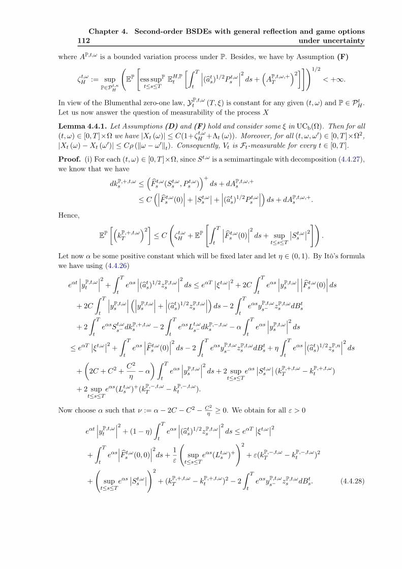
112Chapter 4. Second-order BSDEs with general reflection and game options
under uncertainty
where AP,t,ω is a bounded variation process under P. Besides, we have by Assumption (F)
ζt,ωH := sup
P∈Pt,κH
(EP
[ess supP
t≤s≤TEH,P
t
[∫ T
t
∣∣∣(ats)
1/2P t,ωs
∣∣∣2 ds+(AP,t,ω,+
T
)2]])1/2
< +∞.
In view of the Blumenthal zero-one law, YP,t,ωt (T, ξ) is constant for any given (t, ω) and P ∈ Pt
H .Let us now answer the question of measurability of the process X
Lemma 4.4.1. Let Assumptions (D) and (F) hold and consider some ξ in UCb(Ω). Then for all(t, ω) ∈ [0, T ]×Ω we have |Xt (ω)| ≤ C(1+ζt,ω
H +Λt (ω)). Moreover, for all (t, ω, ω′) ∈ [0, T ]×Ω2,|Xt (ω)−Xt (ω′)| ≤ Cρ (‖ω − ω′‖t). Consequently, Vt is Ft-measurable for every t ∈ [0, T ].
Proof. (i) For each (t, ω) ∈ [0, T ]×Ω, since St,ω is a semimartingale with decomposition (4.4.27),we know that we have
dkP,+,t,ωs ≤
(F t,ω
s (St,ωs , P t,ω
s ))+
ds+ dAP,t,ω,+s
≤ C(∣∣∣F t,ω
s (0)∣∣∣+ ∣∣St,ω
s
∣∣+ ∣∣∣(ats)
1/2P t,ωs
∣∣∣) ds+ dAP,t,ω,+s .
Hence,
EP[(kP,+,t,ω
T
)2]≤ C
(ζt,ωH + EP
[∫ T
t
∣∣∣F t,ωs (0)
∣∣∣2 ds+ supt≤s≤T
∣∣St,ωs
∣∣2]) .Let now α be some positive constant which will be fixed later and let η ∈ (0, 1). By Itô’s formulawe have using (4.4.26)
eαt∣∣∣yP,t,ω
t
∣∣∣2 +∫ T
teαs∣∣∣(at
s)1/2zP,t,ω
s
∣∣∣2 ds ≤ eαT∣∣ξt,ω
∣∣2 + 2C∫ T
teαs∣∣∣yP,t,ω
s
∣∣∣ ∣∣∣F t,ωs (0)
∣∣∣ ds+ 2C
∫ T
t
∣∣∣yP,t,ωs
∣∣∣ (∣∣∣yP,t,ωs
∣∣∣+ ∣∣∣(ats)
1/2zP,t,ωs
∣∣∣) ds− 2∫ T
teαsyP,t,ω
s− zP,t,ωs dBt
s
+ 2∫ T
teαsSt,ω
s− dkP,+,t,ωs − 2
∫ T
teαsLt,ω
s− dkP,−,t,ωs − α
∫ T
teαs∣∣∣yP,t,ω
s
∣∣∣2 ds≤ eαT
∣∣ξt,ω∣∣2 +
∫ T
teαs∣∣∣F t,ω
s (0)∣∣∣2 ds− 2
∫ T
teαsyP,t,ω
s− zP,t,ωs dBt
s + η
∫ T
teαs∣∣∣(at
s)1/2zP,n
s
∣∣∣2 ds+(
2C + C2 +C2
η− α
)∫ T
teαs∣∣∣yP,t,ω
s
∣∣∣2 ds+ 2 supt≤s≤T
eαs∣∣St,ω
s
∣∣ (kP,+,t,ωT − kP,+,t,ω
t )
+ 2 supt≤s≤T
eαs(Lt,ωs )+(kP,−,t,ω
T − kP,−,t,ωt ).
Now choose α such that ν := α− 2C − C2 − C2
η ≥ 0. We obtain for all ε > 0
eαt∣∣∣yP,t,ω
t
∣∣∣2 + (1− η)∫ T
teαs∣∣∣(at
s)1/2zP,t,ω
s
∣∣∣2 ds ≤ eαT∣∣ξt,ω
∣∣2+∫ T
teαs∣∣∣F t,ω
s (0, 0)∣∣∣2ds+
1ε
(sup
t≤s≤Teαs(Lt,ω
s )+)2
+ ε(kP,−,t,ωT − kP,−,t,ω
t )2
+
(sup
t≤s≤Teαs∣∣St,ω
s
∣∣)2
+ (kP,+,t,ωT − kP,+,t,ω
t )2 − 2∫ T
teαsyP,t,ω
s− zP,t,ωs dBt
s. (4.4.28)

4.4. A constructive proof of existence 113
Taking expectation and using (4.4.28) yields with η small enough
∣∣∣yP,t,ωt
∣∣∣2 + EP[∫ T
t|(at
s)12 zP,t,ω
s |2ds]≤ C
(Λ2
t (ω) +(ζt,ωH
)2)
+ εEP[(kP,−,t,ω
T − kP,−,t,ωt )2
].
Now by definition, we also have for some constant C0 independent of ε
EP[(kP,−,t,ω
T − kP,−,t,ωt )2
]≤ C0
(Λ2
t (ω) +(ζt,ωH
)2+ EP
[∫ T
t
∣∣∣yP,t,ωs
∣∣∣2 ds])+ C0EP
[∫ T
t
∣∣∣(ats)
1/2zP,t,ωs
∣∣∣2 ds] .Choosing ε = 1
2C0, Gronwall inequality then implies |yP,t,ω
t |2 ≤ C(1 + Λt(ω)). The result thenfollows by arbitrariness of P.
(ii) The proof is exactly the same as above, except that one has to use uniform continuity inω of ξt,ω, F t,ω, St,ω and Lt,ω. Indeed, for each (t, ω) ∈ [0, T ] × Ω and P ∈ Pt,κ
H , let α be somepositive constant which will be fixed later and let η ∈ (0, 1). By Itô’s formula we have, since Fis uniformly Lipschitz
eαt∣∣∣yP,t,ω
t − yP,t,ω′
t
∣∣∣2 +∫ T
teαs∣∣∣(at
s)1/2(zP,t,ω
s − zP,t,ω′s )
∣∣∣2 ds ≤ eαT∣∣∣ξt,ω − ξt,ω′
∣∣∣2+ 2C
∫ T
teαs∣∣∣yP,t,ω
s − yP,t,ω′s
∣∣∣ (∣∣∣yP,t,ωs − yP,t,ω′
s
∣∣∣+ ∣∣∣(ats)
12 (zP,t,ω
s − zP,t,ω′s )
∣∣∣) ds+ 2C
∫ T
teαs∣∣∣yP,t,ω
s − yP,t,ω′s
∣∣∣ ∣∣∣F t,ωs (yP,t,ω
s , zP,t,ωs )− F t,ω′
s (yP,t,ωs , zP,t,ω
s )∣∣∣ ds
+ 2∫ T
teαs(yP,t,ω
s− − yP,t,ω′
s− )d(kP,−,t,ω
s − kP,−,t,ω′s − kP,+,t,ω
s + kP,+,t,ω′s
)− α
∫ T
teαs∣∣∣yP,t,ω
s − yP,t,ω′s
∣∣∣2 ds− 2∫ T
teαs(yP,t,ω
s− − yP,t,ω′
s− )(zP,t,ωs − zP,t,ω′
s )dBts
≤ eαT∣∣∣ξt,ω − ξt,ω′
∣∣∣2 +∫ T
teαs∣∣∣F t,ω
s (yP,t,ωs , zP,t,ω
s )− F t,ω′s (yP,t,ω
s , zP,t,ωs )
∣∣∣2 ds+(2C+C2+C2
η−α) ∫ T
teαs∣∣∣yP,t,ω
s − yP,t,ω′s
∣∣∣2 ds+ η
∫ T
teαs∣∣∣(at
s)12 (zP,t,ω
s − zP,t,ω′s )
∣∣∣2 ds− 2
∫ T
teαs(yP,t,ω
s− − yP,t,ω′
s− )(zP,t,ωs − zP,t,ω′
s )dBts
+ 2∫ T
teαs(yP,t,ω
s− − yP,t,ω′
s− )d(kP,−,t,ω
s − kP,−,t,ω′s − kP,+,t,ω
s + kP,+,t,ω′s
).
By the Skorohod condition (4.4.26), we also have∫ T
teαs(yP,t,ω
s− − yP,t,ω′
s− )d(kP,−,t,ω
s − kP,−,t,ω′s − kP,+,t,ω
s + kP,+,t,ω′s
)≤∫ T
teαs(Lt,ω
s− − Lt,ω′
s− )d(kP,−,t,ωs − kP,−,t,ω′
s )−∫ T
teαs(St,ω
s− − St,ω′
s− )d(kP,+,t,ωs − kP,+,t,ω′
s ).
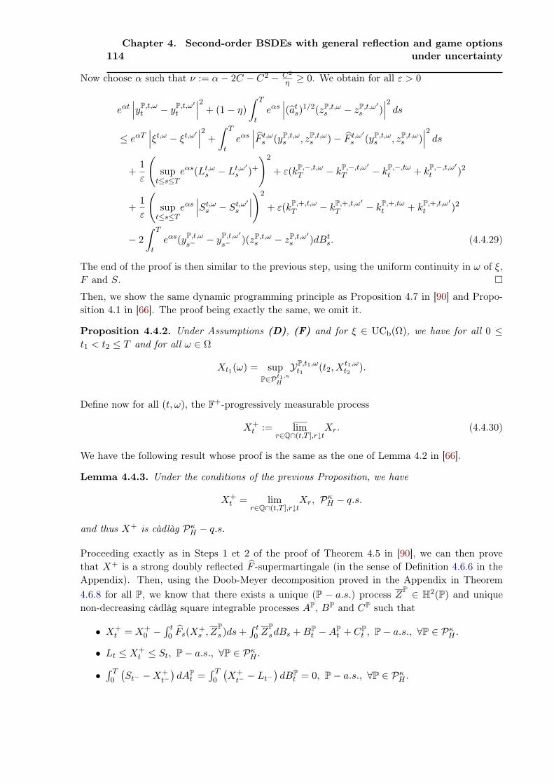
114Chapter 4. Second-order BSDEs with general reflection and game options
under uncertainty
Now choose α such that ν := α− 2C − C2 − C2
η ≥ 0. We obtain for all ε > 0
eαt∣∣∣yP,t,ω
t − yP,t,ω′
t
∣∣∣2 + (1− η)∫ T
teαs∣∣∣(at
s)1/2(zP,t,ω
s − zP,t,ω′s )
∣∣∣2 ds≤ eαT
∣∣∣ξt,ω − ξt,ω′∣∣∣2 +
∫ T
teαs∣∣∣F t,ω
s (yP,t,ωs , zP,t,ω
s )− F t,ω′s (yP,t,ω
s , zP,t,ωs )
∣∣∣2 ds+
1ε
(sup
t≤s≤Teαs(Lt,ω
s − Lt,ω′s )+
)2
+ ε(kP,−,t,ωT − kP,−,t,ω′
T − kP,−,tωt + kP,−,t,ω′
t )2
+1ε
(sup
t≤s≤Teαs∣∣∣St,ω
s − St,ω′s
∣∣∣)2
+ ε(kP,+,t,ωT − kP,+,t,ω′
T − kP,+,tωt + kP,+,t,ω′
t )2
− 2∫ T
teαs(yP,t,ω
s− − yP,t,ω′
s− )(zP,t,ωs − zP,t,ω′
s )dBts. (4.4.29)
The end of the proof is then similar to the previous step, using the uniform continuity in ω of ξ,F and S.
Then, we show the same dynamic programming principle as Proposition 4.7 in [90] and Propo-sition 4.1 in [66]. The proof being exactly the same, we omit it.
Proposition 4.4.2. Under Assumptions (D), (F) and for ξ ∈ UCb(Ω), we have for all 0 ≤t1 < t2 ≤ T and for all ω ∈ Ω
Xt1(ω) = supP∈Pt1,κ
H
YP,t1,ωt1
(t2, Xt1,ωt2
).
Define now for all (t, ω), the F+-progressively measurable process
X+t := lim
r∈Q∩(t,T ],r↓tXr. (4.4.30)
We have the following result whose proof is the same as the one of Lemma 4.2 in [66].
Lemma 4.4.3. Under the conditions of the previous Proposition, we have
X+t = lim
r∈Q∩(t,T ],r↓tXr, Pκ
H − q.s.
and thus X+ is càdlàg PκH − q.s.
Proceeding exactly as in Steps 1 et 2 of the proof of Theorem 4.5 in [90], we can then provethat X+ is a strong doubly reflected F -supermartingale (in the sense of Definition 4.6.6 in theAppendix). Then, using the Doob-Meyer decomposition proved in the Appendix in Theorem4.6.8 for all P, we know that there exists a unique (P − a.s.) process ZP ∈ H2(P) and uniquenon-decreasing càdlàg square integrable processes AP, BP and CP such that
• X+t = X+
0 −∫ t0 Fs(X+
s , ZPs )ds+
∫ t0 Z
PsdBs +BP
t −APt + CP
t , P− a.s., ∀P ∈ PκH .
• Lt ≤ X+t ≤ St, P− a.s., ∀P ∈ Pκ
H .
•∫ T0
(St− −X+
t−
)dAP
t =∫ T0
(X+
t− − Lt−)dBP
t = 0, P− a.s., ∀P ∈ PκH .

4.4. A constructive proof of existence 115
We then define V P := AP −BP −CP. By Karandikar [50], since X+ is a càdlàg semimartingale,we can define a universal process Z which aggregates the family
Z
P,P ∈ Pκ
H
.
We next prove the representation (4.3.9) for X and X+.
Proposition 4.4.4. Assume that ξ ∈ UCb(Ω) and that Assumptions (D) and (F) hold. Thenwe have
Xt = ess supP
P′∈PκH(t,P)
YP′t (T, ξ) and X+
t = ess supP
P′∈PκH(t+,P)
YP′t (T, ξ), P− a.s., ∀P ∈ Pκ
H .
Proof. The proof for the representations is the same as the proof of proposition 4.10 in [90],since we also have a stability result for RBSDEs under our assumptions.
Finally, we have to check that the minimum condition (4.2.8) holds. However, this can be doneexactly as in [66], so we refer the reader to that proof.
4.4.3 Main result
We are now in position to state the main result of this section
Theorem 4.4.5. Let ξ ∈ L2,κH and let Assumptions (D), (E) and (F) hold. Then
1) There exists a unique solution (Y, Z) ∈ D2,κH ×H2,κ
H of the 2DRBSDE (4.2.5).2) Moreover, if in addition we choose to work under either of the following model of set theory(we refer the reader to [39] for more details)
(i) Zermelo-Fraenkel set theory with axiom of choice (ZFC) plus the Continuum Hypothesis(CH).
(ii) ZFC plus the negation of CH plus Martin’s axiom.
Then there exists a unique solution (Y, Z, V ) ∈ D2,κH ×H2,κ
H × V2,κH of the 2DRBSDE (4.2.5).
Proof. The proof of the existence part follows the lines of the proof of Theorem 4.7 in [89], usingthe estimates of Theorem 4.3.8, so we only insist on the points which do not come directly fromthe proofs mentioned above. The idea is to approximate the terminal condition ξ by a sequence(ξn)n≥0 ⊂ UCb(Ω). Then, we use the estimates of Theorem 4.3.8 to pass to the limit as in theproof of Theorem 4.6 in [89]. The main point in this context is that for each n, if we considerthe Jordan decomposition of V P,n into the non-decreasing process V P,+,n and the non-increasingprocess V P,−,n, then the estimates of Theorem 4.3.8 ensure that these processes converge to someV P,+ and V P,−, which are respectively non-decreasing and non-increasing. Hence we are surethat the limit V P has indeed bounded variation.
Concerning the fact that we can aggregate the family(V P)
P∈PκH
, it can be deduced as follows.First, if ξ ∈ UCb(Ω), we know, using the same notations as above that the solution verifies
X+t = X+
0 −∫ t
0Fs(X+
s , Zs)ds+∫ t
0ZsdBs −KP
t , P− a.s., ∀P ∈ PκH .
Now, we know from (4.4.30) that X+ is defined pathwise, and so is the Lebesgue integral∫ t
0Fs(X+
s , Zs)ds.
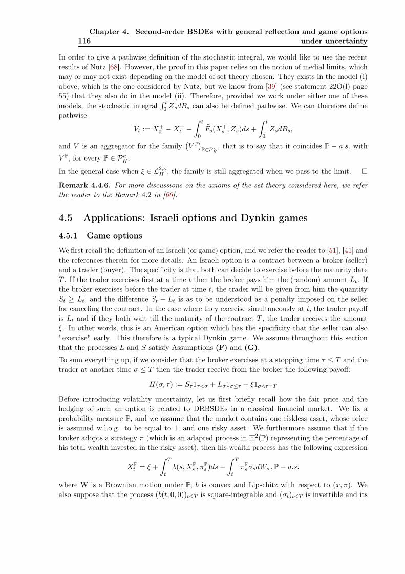
116Chapter 4. Second-order BSDEs with general reflection and game options
under uncertainty
In order to give a pathwise definition of the stochastic integral, we would like to use the recentresults of Nutz [68]. However, the proof in this paper relies on the notion of medial limits, whichmay or may not exist depending on the model of set theory chosen. They exists in the model (i)above, which is the one considered by Nutz, but we know from [39] (see statement 22O(l) page55) that they also do in the model (ii). Therefore, provided we work under either one of thesemodels, the stochastic integral
∫ t0 ZsdBs can also be defined pathwise. We can therefore define
pathwise
Vt := X+0 −X
+t −
∫ t
0Fs(X+
s , Zs)ds+∫ t
0ZsdBs,
and V is an aggregator for the family(V P)
P∈PκH
, that is to say that it coincides P − a.s. with
V P, for every P ∈ PκH .
In the general case when ξ ∈ L2,κH , the family is still aggregated when we pass to the limit.
Remark 4.4.6. For more discussions on the axioms of the set theory considered here, we referthe reader to the Remark 4.2 in [66].
4.5 Applications: Israeli options and Dynkin games
4.5.1 Game options
We first recall the definition of an Israeli (or game) option, and we refer the reader to [51], [41] andthe references therein for more details. An Israeli option is a contract between a broker (seller)and a trader (buyer). The specificity is that both can decide to exercise before the maturity dateT . If the trader exercises first at a time t then the broker pays him the (random) amount Lt. Ifthe broker exercises before the trader at time t, the trader will be given from him the quantitySt ≥ Lt, and the difference St − Lt is as to be understood as a penalty imposed on the sellerfor canceling the contract. In the case where they exercise simultaneously at t, the trader payoffis Lt and if they both wait till the maturity of the contract T , the trader receives the amountξ. In other words, this is an American option which has the specificity that the seller can also"exercise" early. This therefore is a typical Dynkin game. We assume throughout this sectionthat the processes L and S satisfy Assumptions (F) and (G).
To sum everything up, if we consider that the broker exercises at a stopping time τ ≤ T and thetrader at another time σ ≤ T then the trader receive from the broker the following payoff:
H(σ, τ) := Sτ1τ<σ + Lσ1σ≤τ + ξ1σ∧τ=T
Before introducing volatility uncertainty, let us first briefly recall how the fair price and thehedging of such an option is related to DRBSDEs in a classical financial market. We fix aprobability measure P, and we assume that the market contains one riskless asset, whose priceis assumed w.l.o.g. to be equal to 1, and one risky asset. We furthermore assume that if thebroker adopts a strategy π (which is an adapted process in H2(P) representing the percentage ofhis total wealth invested in the risky asset), then his wealth process has the following expression
XPt = ξ +
∫ T
tb(s,XP
s , πPs )ds−
∫ T
tπP
sσsdWs ,P− a.s.
where W is a Brownian motion under P, b is convex and Lipschitz with respect to (x, π). Wealso suppose that the process (b(t, 0, 0))t≤T is square-integrable and (σt)t≤T is invertible and its

4.5. Applications: Israeli options and Dynkin games 117
inverse is bounded. It was then proved in [51] and [41] that the fair price and an hedging strategyfor the Israeli option described above can be obtained through the solution of a DRBSDE. Moreprecisely, we have
Theorem 4.5.1. The fair price of the game option and the corresponding hedging strategy aregiven by the pair (yP, πP) ∈ D2(P)×H2(P) solving the following DRBSDE
yPt = ξ +
∫ Tt b(s, yP
s , πPs )ds−
∫ Tt πP
sσsdWs + kPt − kP
t , P− a.s.Lt ≤ yP
t ≤ St, P− a.s.∫ T0 (yP
t− − Lt−)dkP,−t =
∫ T0 (St− − yP
t−)dkP,+t = 0.
Moreover, for any ε > 0, the following stopping times are ε-optimal after t for the seller and thebuyer respectively
D1,ε,Pt := inf
s ≥ t, yP
s ≥ Ss − ε, D2,ε,P
t := infs ≥ t, yP
s ≤ Ls + ε.
Let us now extend this result to the uncertain volatility framework. We still consider a financialmarket with two assets and assume now that the wealth process has the following dynamic whenthe chosen strategy is π
Xt = ξ +∫ T
tb(s,Xs, πs)ds−
∫ T
tπsdBs, Pκ
H − q.s.,
where B is the canonical process and b is assumed to satisfy Assumptions (D), and where ξbelongs to L2,κ
H . Then, following the ideas of [66], it is natural to consider as a superhedgingprice for the option the quantity
Yt = ess supP
P′∈PκH(t+,P)
yP′t .
Indeed, this amount is greater than the price at time t of the the same Israeli option under anyprobability measure. Hence, if the seller receives this amount, he should always be able to hedgehis position. We emphasize however that we are not able to guarantee that this price is optimalin the sense that it is the lowest value for which we can find a super-replicating strategy. Thisinteresting question is left for future research.
Symmetrically, if the seller charges less than the following quantity for the option at time t,
Yt := ess infP′∈Pκ
H(t+,P)
PyP′t ,
then it will be clearly impossible for him to find a hedge. Y appears then as a subhedging price.
Hence, we have obtained a whole interval of prices, given by [Yt, Yt], which we can formallythink as arbitrage free, even though a precise definition of this notion in an uncertain market isoutside the scope of this paper. These two quantities can be linked to the notion of second-order2DRBSDEs. Indeed, this is immediate for Y , and for Y , we need to introduce a "symmetric"definition for the 2DRBSDEs.
Definition 4.5.2. For ξ ∈ L2,κH , we consider the following type of equations satisfied by a pair
of progressively-measurable processes (Y, Z)
• YT = ξ, PκH − q.s.
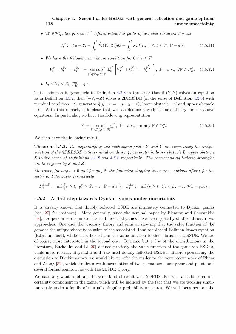
118Chapter 4. Second-order BSDEs with general reflection and game options
under uncertainty
• ∀P ∈ PκH , the process V P defined below has paths of bounded variation P− a.s.
V Pt := Y0 − Yt −
∫ t
0Fs(Ys, Zs)ds+
∫ t
0ZsdBs, 0 ≤ t ≤ T, P− a.s. (4.5.31)
• We have the following maximum condition for 0 ≤ t ≤ T
V Pt + kP,+
t − kP,−t = ess supP
P′∈PH(t+,P)
EP′t
[V P′
T + kP′ ,+T − kP′ ,−
T
], P− a.s., ∀P ∈ Pκ
H . (4.5.32)
• Lt ≤ Yt ≤ St, PκH − q.s.
This Definition is symmetric to Definition 4.2.8 in the sense that if (Y, Z) solves an equationas in Definition 4.5.2, then (−Y,−Z) solves a 2DRBSDE (in the sense of Definition 4.2.8) withterminal condition −ξ, generator g(y, z) := −g(−y,−z), lower obstacle −S and upper obstacle−L. With this remark, it is clear that we can deduce a wellposedness theory for the aboveequations. In particular, we have the following representation
Yt = ess infP′∈Pκ
H(t+,P)yP′
t , P− a.s., for any P ∈ PκH . (4.5.33)
We then have the following result.
Theorem 4.5.3. The superhedging and subhedging prices Y and Y are respectively the uniquesolution of the 2DRBSDE with terminal condition ξ, generator b, lower obstacle L, upper obstacleS in the sense of Definitions 4.2.8 and 4.5.2 respectively. The corresponding hedging strategiesare then given by Z and Z.
Moreover, for any ε > 0 and for any P, the following stopping times are ε-optimal after t for theseller and the buyer respectively
D1,ε,Pt := inf
s ≥ t, yP
s ≥ Ss − ε, P− a.s., D2,ε
t := inf s ≥ t, Ys ≤ Ls + ε, PκH − q.s. .
4.5.2 A first step towards Dynkin games under uncertainty
It is already known that doubly reflected BSDE are intimately connected to Dynkin games(see [27] for instance). More generally, since the seminal paper by Fleming and Souganidis[38], two person zero-sum stochastic differential games have been typically studied through twoapproaches. One uses the viscosity theory and aims at showing that the value function of thegame is the unique viscosity solution of the associated Hamilton-Jacobi-Bellman-Isaacs equation(HJBI in short), while the other relates the value function to the solution of a BSDE. We areof course more interested in the second one. To name but a few of the contributions in theliterature, Buckdahn and Li [20] defined precisely the value function of the game via BSDEs,while more recently Bayraktar and Yao used doubly reflected BSDEs. Before specializing thediscussion to Dynkin games, we would like to refer the reader to the very recent work of Phamand Zhang [82], which studies a weak formulation of two person zero-sum game and points outseveral formal connections with the 2BSDE theory.
We naturally want to obtain the same kind of result with 2DRBSDEs, with an additional un-certainty component in the game, which will be induced by the fact that we are working simul-taneously under a family of mutually singular probability measures. We will focus here on the
4.5. Applications: Israeli options and Dynkin games 119
construction of a game whose upper and lower values can be expressed as a solution of 2DRB-SDE. We insist that we prove only that a given solution to a 2DRBSDE provides a solution to thecorresponding Dynkin game described below. However, we are not able, as in [27], to constructthe solution of the 2DRBSDE directly from the solution of the Dynkin game. Moreover, we alsoface a difficult technical problem related to Assumption (H), which prevents our result to becomprehensive.
Let us now describe what we mean precisely by a Dynkin game with uncertainty. Two playersP1 and P2 are facing each other in a game. A strategy of a player consists in picking a stoppingtime. Let us say that P1 chooses τ ∈ T0,T and P2 chooses σ ∈ T0,T . Then the game stipulatesthat P1 will pay to P2 the following random payoff
Rt(τ, σ) :=∫ τ∧σ
tgsds+ Sτ1τ<σ + Lσ1σ≤τ,σ<T + ξ1τ∧σ=T ,
where g, S and L are F-progressively measurable processes satisfying Assumptions (D), (G) and(F). In particular, the upper obstacle S is a semimartingale.
Then naturally, P1 will try to minimize the expected amount that he will have to pay, but takinginto account the fact that both P2 and the "Nature" (which we interpret as a third player,represented by the uncertainty that the player has with respect to the underlying probabilitymeasure) can play against him. Symmetrically, P2 will try to maximize his expected returns,considering that both P1 and the Nature are antagonist players. This leads us to introduce thefollowing upper and lower values of the robust Dynkin game
V t := ess infτ∈Tt,T
ess supσ∈Tt,T
ess supP
P′∈PκH(t+,P)
EP′t [Rt(τ, σ)], P− a.s.
V t := ess supσ∈Tt,T
ess infτ∈Tt,T
ess infPP′∈Pκ
H(t+,P)EP′
t [Rt(τ, σ)], P− a.s.
Remark 4.5.4. In order to be completely rigorous, we should have made the dependence inP of the two functions above explicit, because it is not clear that an aggregator exists a priori.Nonetheless, we will prove in this section, that they both correspond to the solution of 2DRBSDE,and therefore that the aggregator indeed exists. Therefore, for the sake of clarity, we will alwaysomit this dependence.
V is the maximal amount that P1 will agree to pay in order to take part in the game. Sym-metrically, V is the minimal amount that P2 must receive in order to accept to take part to thegame. Unlike in the classical setting without uncertainty, for which there is only one value onwhich the 2 players can agree, in our context there is generally a whole interval of admissiblevalues for the game. Indeed, we have the following easy result
Lemma 4.5.5. We have for t ∈ [0, T ]
V t ≥ V t, PκH − q.s.
Therefore the admissible values for the game are the interval [V t, V t].
Proof. Let t ∈ [0, T ], P ∈ PκH and P′ ∈ Pκ
H(t+,P). For any (τ, σ) ∈ Tt,T × Tt,T , we have clearly
ess supP
P′∈PκH(t+,P)
EP′t [Rt(τ, σ)] ≥ ess inf
τ∈Tt,T
ess infPP′∈Pκ
H(t+,P)EP′
t [Rt(τ, σ)], P− a.s.
120Chapter 4. Second-order BSDEs with general reflection and game options
under uncertainty
Then we can take the essential supremum with respect to σ on both sides of the inequality, andthe result follows.
Now, in order to link the solution of the above robust Dynkin game to 2DRBSDEs, we willneed to assume a min-max property which is closely related to the usual Isaacs condition for theclassical Dynkin games. Given the length of the paper, we will not try to verify this assumption.Nonetheless, we emphasize that a related result was indeed proved in [65] in the context of arobust utility maximization problem. Even more in the spirit of our paper, Nutz and Zhang [69]also showed such a result (at least at time t = 0 and under sufficient regularity assumptions, seetheir Theorem 3.4) when there is only one player. We are convinced that their results could begeneralized to our framework and leave this interesting problem to future research.
Assumption (H):
We suppose that the following "min-max" property are satisfied. For any P ∈ PκH
ess infτ∈Tt,T
ess supσ∈Tt,T
ess supP
P′∈PκH(t+,P)
EP′t [Rt(τ, σ)] = ess supP
P′∈PκH(t+,P)
ess infτ∈Tt,T
ess supσ∈Tt,T
EP′t [Rt(τ, σ)], P− a.s.
(4.5.34)
ess supσ∈Tt,T
ess infτ∈Tt,T
ess infPP′∈Pκ
H(t+,P)EP′
t [Rt(τ, σ)] = ess infPP′∈Pκ
H(t+,P)ess supσ∈Tt,T
ess infτ∈Tt,T
EP′t [Rt(τ, σ)], P− a.s.
(4.5.35)
It is clear from Proposition 4.3.10 that the right-hand side of (4.5.34) can be expressed as thesolution of 2DRBSDE with terminal condition ξ, generator g, lower obstacle L and upper obstacleS. We deduce immediately the following result.
Theorem 4.5.6. Let Assumption (H) hold. Let (Y, Z) (resp. (Y , Z)) be a solution to the2DRBSDE in the sense of Definition 4.2.8 (resp. in the sense of Definition 4.5.2) with terminalcondition ξ, generator g, lower obstacle L and upper obstacle S. Then we have for any t ∈ [0, T ]
V t = Yt, PκH − q.s.
V t = Yt, PκH − q.s.
Moreover, unless PκH is reduced to a singleton, we have V > V , Pκ
H − q.s.
Proof. The two equalities are obvious. Moreover, if for each P ∈ PκH , we let yP be the solution
of the DRBSDE with terminal condition ξ, generator g, lower obstacle L and upper obstacle S,we have by (4.5.33)
V t = ess supP′∈Pκ
H(t+,P)
yP′t , P− a.s., and V t = ess inf
P′∈PκH(t+,P)
yP′t , P− a.s.,
which implies the last result.
4.6 Appendix: Doubly reflected g-supersolution and martingales
In this section, we extend some of the results of [77] and [66] concerning g-supersolution of BSDEsand RBSDEs to the case of DRBSDEs. Let us note that many of the results below are obtained
4.6. Appendix: Doubly reflected g-supersolution and martingales 121
using similar ideas as in [77] and [66], but we still provide most of them since, to the best of ourknowledge, they do not appear anywhere else in the literature. Moreover, we emphasize that weonly provide the results and definitions for the doubly reflected case, because the correspondingones for the upper reflected case can be deduced easily. In the following, we fix a probabilitymeasure P
4.6.1 Definitions and first properties
Let us be given the following objects
• A function gs(ω, y, z), F-progressively measurable for fixed y and z, uniformly Lipschitz in(y, z) and such that EP
[∫ T0 |gs(0, 0)|2 ds
]< +∞.
• A terminal condition ξ which is FT -measurable and in L2(P).
• Càdlàg processes V , S, L in I2(P) such that S and L satisfy Assumptions (E) and (F) (in
particular S is a semimartingale with the decomposition (4.2.3)), and with EP
[sup
0≤t≤T|Vt|2
]<
+∞.
We study the problem of finding (y, z, k+, k−) ∈ D2(P)×H2(P)× I2(P)× I2(P) such that
yt = ξ +∫ T
tgs(ys, zs)ds−
∫ T
tzsdWs + k−T − k
−t − k
+T + k+
t + VT − Vt, P− a.s.
Lt ≤ yt ≤ St, P− a.s.∫ T
0(Ss− − ys−) dk+
s =∫ T
0(ys− − Ls−) dk−s = 0, P− a.s. (4.6.36)
We first have a result of existence and uniqueness.
Proposition 4.6.1. Under the above hypotheses, there is a unique solution (y, z, k+, k−) ∈D2(P)×H2(P)× I2(P)× I2(P) to the doubly reflected BSDE (4.6.36).
Proof. Consider the following penalized RBSDE with lower obstacle L, whose existence anduniqueness are ensured by the results of Lepeltier and Xu [60]
ynt = ξ +
∫ T
tgs(yn
s , zns )ds−
∫ T
tzns dWs + kn,−
T − kn,−t − kn,+
T + kn,+t + VT − Vt,
where kn,+t := n
∫ t0 (Ss−yn
s )−ds. Then, define ynt := yn
t +Vt, ξ := ξ+VT , znt := zn
t , kn,±t := kn,±
t ,gt(y, z) := gt(y − V, z) and Lt := Lt + Vt. Then
ynt = ξ +
∫ T
tgs(yn
s , zns )ds−
∫ T
tzns dWs + kn,−
T − kn,−t − kn,+
T + kn,+t .
Since we know by Lepeltier and Xu [61], that the above penalization procedure converges to asolution of the corresponding RBSDE, existence and uniqueness are then simple generalization.
We also have a comparison theorem in this context
122Chapter 4. Second-order BSDEs with general reflection and game options
under uncertainty
Proposition 4.6.2. Let ξ1 and ξ2 ∈ L2(P), V i, i = 1, 2 be two adapted, càdlàg processes andgis(ω, y, z) two functions, which verify the above assumptions. Let (yi, zi, ki,+, ki,−) ∈ D2(P) ×
H2(P)× I2(P)× I2(P), i = 1, 2 be the solutions of the following DRBSDEs with upper obstacle Si
and lower obstacle Li
yit = ξi +
∫ T
tgis(y
is, z
is)ds−
∫ T
tzisdWs + ki,−
T − ki,−t − ki,+
T + ki,+t + V i
T − V it , P− a.s., i = 1, 2,
respectively. If it holds P− a.s. that ξ1 ≥ ξ2, V 1 − V 2 is non-decreasing, S1 ≤ S2, L1 ≥ L2 andg1s(y
1s , z
1s ) ≥ g2
s(y1s , z
1s ), then we have for all t ∈ [0, T ]
Y 1t ≥ Y 2
t , P− a.s.
Besides, if S1 = S2 (resp. L1 = L2), then we also have dk1,+ ≥ dk2,+ (resp. dk1,− ≤ dk2,−).
Proof. The first part is classical, whereas the second one comes from the fact that the penal-ization procedure converges in this framework, as seen previously. Indeed, with the notations ofthe proof of Proposition 4.6.1, we have in the sense of weak limits
ki,+t = lim
n→+∞n
∫ t
0
(Ss − yn,i
s
)−ds.
Moreover, using the classical comparison Theorem for RBSDEs with the same lower obstacle,we know that yn,1 ≥ yn,2 and dkn,1,−
t ≤ dkn,2,−t . This implies that dkn,1,+
t ≥ dkn,2,+t . Passing to
the limit yields the result.
Of course, all the above still holds if τ is replaced by some bounded stopping time τ. FollowingPeng’s original ideas, we now define a notion of doubly reflected g-(super)solutions.
Definition 4.6.3. If y is a solution of a DRBSDE of the form (4.6.36), then we call y a doublyreflected g-supersolution on [0, τ ]. If V = 0 on [0, τ ], then we call y a doubly reflected g-solution.
We have the following proposition concerning the uniqueness of a decomposition of the form(4.6.36). Notice that unlike in the lower reflected case considered in [66], the processes V , k+
and k− are not necessarily unique.
Proposition 4.6.4. Given y a g-supersolution on [0, τ ], there is a unique z ∈ H2(P) and a uniquecouple (k+, k−, V ) ∈ (I2(P))3 (in the sense that V −k++k− is unique), such that (y, z, k+, k−, V )satisfy (4.6.36).
Proof. If both (y, z, k+, k−, V ) and (y, z1, k+,1, k−,1, V 1) satisfy (4.6.36), then applying Itô’sformula to (yt − yt)2 gives immediately that z = z1 and thus V − k+ + k− = V 1 − k+,1 + k−,1,P− a.s.
Remark 4.6.5. We emphasize once more that the situation here is fundamentally different from[66], where reflected g-supersolution were defined for lower reflected BSDEs. In our case, insteadof having to deal with the sum of two non-decreasing processes, we actually have to add anothernon-increasing process. This will raise some difficulties later on, notably when we will prove anon-linear Doob-Meyer decomposition.
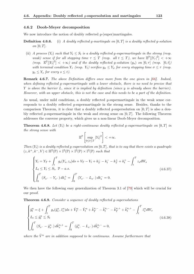
4.6. Appendix: Doubly reflected g-supersolution and martingales 123
4.6.2 Doob-Meyer decomposition
We now introduce the notion of doubly reflected g-(super)martingales.
Definition 4.6.6. (i) A doubly reflected g-martingale on [0, T ] is a doubly reflected g-solutionon [0, T ].
(ii) A process (Yt) such that Yt ≤ St is a doubly reflected g-supermartingale in the strong (resp.weak) sense if for all stopping time τ ≤ T (resp. all t ≤ T ), we have EP[|Yτ |2] < +∞(resp. EP[|Yt|2] < +∞) and if the doubly reflected g-solution (ys) on [0, τ ] (resp. [0, t])with terminal condition Yτ (resp. Yt) verifies yσ ≤ Yσ for every stopping time σ ≤ τ (resp.ys ≤ Ys for every s ≤ t).
Remark 4.6.7. The above Definition differs once more from the one given in [66]. Indeed,when defining reflected g-supermartingale with a lower obstacle, there is no need to precise thatY is above the barrier L, since it is implied by definition (since y is already above the barrier).However, with an upper obstacle, this is not the case and this needs to be a part of the definition.
As usual, under mild conditions, a doubly reflected g-supermartingale in the weak sense cor-responds to a doubly reflected g-supermartingale in the strong sense. Besides, thanks to thecomparison Theorem, it is clear that a doubly reflected g-supersolution on [0, T ] is also a dou-bly reflected g-supermartingale in the weak and strong sense on [0, T ]. The following Theoremaddresses the converse property, which gives us a non-linear Doob-Meyer decomposition.
Theorem 4.6.8. Let (Yt) be a right-continuous doubly reflected g-supermartingale on [0, T ] inthe strong sense with
EP
[sup
0≤t≤T|Yt|2
]< +∞.
Then (Yt) is a doubly reflected g-supersolution on [0, T ], that is to say that there exists a quadruple(z, k+, k−, V ) ∈ H2(P)× I2(P)× I2(P)× I2(P) such that
Yt = YT +∫ T
tgs(Ys, zs)ds+ VT − Vt + k−T − k
−t − k
+T + k+
t −∫ T
tzsdWs
Lt ≤ Yt ≤ St, P− a.s.∫ T
0(Ss− − Ys−) dk+
s =∫ T
0(Ys− − Ls−) dk−s = 0.
(4.6.37)
We then have the following easy generalization of Theorem 3.1 of [79] which will be crucial forour proof.
Theorem 4.6.9. Consider a sequence of doubly reflected g-supersolutions
ynt = ξ +
∫ T
tgs(yn
s , zns )ds+ V n
T − V nt + kn,−
T − kn,−t − kn,+
T + kn,+t −
∫ T
tzns dWs
Lt ≤ ynt ≤ St∫ T
0(Ss− − yn
s−) dkn,+s =
∫ T
0(yn
s− − Ls−) dkn,−s = 0,
(4.6.38)
where the V n are in addition supposed to be continuous. Assume furthermore that
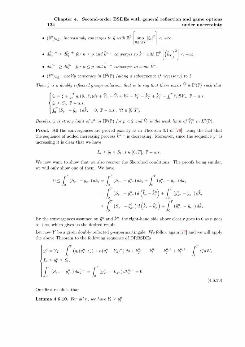
124Chapter 4. Second-order BSDEs with general reflection and game options
under uncertainty
• (yn)n≥0 increasingly converges to y with EP
[sup
0≤t≤T|yt|2
]< +∞.
• dkn,+t ≤ dkp,+
t for n ≤ p and kn,+ converges to k+ with EP[(k+
T
)2]< +∞.
• dkn,−t ≥ dkp,−
t for n ≤ p and kn,− converges to some k−.
• (zn)n≥0 weakly converges in H2(P) (along a subsequence if necessary) to z.
Then y is a doubly reflected g-supersolution, that is to say that there exists V ∈ I2(P) such thatyt = ξ +
∫ Tt gs(ys, zs)ds+ VT − Vt + k−T − k
−t − k
+T + k+
t −∫ Tt zsdWs, P− a.s.
yt ≤ St, P− a.s.∫ T0 (Ss− − ys−) dks = 0, P− a.s., ∀t ∈ [0, T ],
Besides, z is strong limit of zn in Hp(P) for p < 2 and Vt is the weak limit of V nt in L2(P).
Proof. All the convergences are proved exactly as in Theorem 3.1 of [79], using the fact thatthe sequence of added increasing process kn,− is decreasing. Moreover, since the sequence yn isincreasing it is clear that we have
Lt ≤ yt ≤ St, t ∈ [0, T ], P− a.s.
We now want to show that we also recover the Skorohod conditions. The proofs being similar,we will only show one of them. We have
0 ≤∫ T
0(Ss− − ys−) dks =
∫ T
0(Ss− − yn
s−) dks +∫ T
0(yn
s− − ys−) dks
=∫ T
0(Ss− − yn
s−) d(ks − kn
s
)+∫ T
0(yn
s− − ys−) dks
≤∫ T
0
(Ss− − y0
s−)d(ks − kn
s
)+∫ T
0(yn
s− − ys−) dks.
By the convergences assumed on yn and kn, the right-hand side above clearly goes to 0 as n goesto +∞, which gives us the desired result.
Let now Y be a given doubly reflected g-supermartingale. We follow again [77] and we will applythe above Theorem to the following sequence of DRBSDEs
ynt = YT +
∫ T
t
(gs(yn
s , zns ) + n(yn
s − Ys)−)ds+ kn,−
T − kn,−t − kn,+
T + kn,+t −
∫ T
tzns dWs,
Lt ≤ ynt ≤ St,∫ T
0(Ss− − yn
s−) dkn,+s =
∫ T
0(yn
s− − Ls−) dkn,−s = 0.
(4.6.39)
Our first result is that
Lemma 4.6.10. For all n, we have Yt ≥ ynt .

4.6. Appendix: Doubly reflected g-supersolution and martingales 125
Proof. The proof is exactly the same as the proof of Lemma 3.4 in [77], so we omit it.
We will now prove some estimates which will allow us to apply Theorem 4.6.9.
Lemma 4.6.11. There exists a constant C > 0 independent of n such that the processes definedin (4.6.39) verify
EP
[sup
0≤t≤T|yn
t |2 +
∫ T
0|zn
s |2 ds+ (V n
T )2 + (kn,+T )2 + (kn,−
T )2]≤ C.
Proof. First of all, let us define (y, z, k+, k−) the unique solution of the DRBSDE with terminalcondition YT , generator g, upper obstacle S and lower obstacle L (once again, existence anduniqueness are ensured by the results of [26] or [61]). By the comparison Theorem 4.6.2, it isclear that we have for all n ≥ 0
ynt ≥ yt, t ∈ [0, T ], P− a.s.
Consider now (y, z, k+, k−) the unique solution of the doubly reflected BSDE with terminalcondition YT , generator g, upper obstacle S and lower obstacle Y , that is to say
yt = YT +∫ T
tgs(ys, zs)ds+ k−T − k
−t − k
+T + k+
t −∫ T
tzsdWs,
Yt ≤ yt ≤ St,∫ T
0(Ss− − ys−) dk+
s =∫ T
0(ys− − Ys−) dk−s = 0.
(4.6.40)
Notice that since the upper obstacle S is a semimartingale satisfying
EP
[sup
0≤t≤T
((St)
−)2] < +∞,
we know from the results of Crépey and Matoussi [26] (see Theorem 3.2 and Proposition 5.2)that the above doubly reflected BSDE has indeed a unique solution and that we have for someconstant C > 0
EP[(k+
T
)2]≤ C.
Moreover, it is clear that since ys ≥ Ys, we also have
yt = YT +∫ T
tgs(ys, zs)ds+ n
∫ T
t(ys − Ys)−ds+ k−T − k
−t − k
+T + k+
t −∫ T
tzsdWs. (4.6.41)
Notice also that since Y is a doubly reflected g-supermartingale, we have y ≥ L. Thus we canuse now the comparison Theorem of Proposition 4.6.2 for doubly reflected BSDEs with the sameupper obstacles. We deduce that
ynt ≤ yt, and dkn,+
t ≤ dk+t .
Hence, this implies immediately that for some constant C independent of n
EP
[sup
0≤t≤T|yn
t |2 +
(kn,+
T
)2]≤ EP
[sup
0≤t≤T|yt|2 + sup
0≤t≤T|yt|2 +
(k+
T
)2]≤ C. (4.6.42)
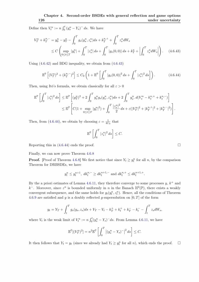
126Chapter 4. Second-order BSDEs with general reflection and game options
under uncertainty
Define then V nt := n
∫ t0 (yn
s − Ys)− ds. We have
V nT + kn,−
T = yn0 − yn
T −∫ T
0gs(yn
s , zns )ds+ kn,+
T +∫ T
0zns dWs
≤ C
(sup
0≤t≤T|yn
t |+∫ T
0|zn
s | ds+∫ T
0|gs(0, 0)| ds+ kn
T +∣∣∣∣∫ T
0zns dWs
∣∣∣∣). (4.6.43)
Using (4.6.42) and BDG inequality, we obtain from (4.6.43)
EP[(V n
T )2 + (kn,−T )2
]≤ C0
(1 + EP
[∫ T
0|gs(0, 0)|2 ds+
∫ T
0|zn
s |2 ds
]). (4.6.44)
Then, using Itô’s formula, we obtain classically for all ε > 0
EP[∫ T
0|zn
s |2 ds
]≤ EP
[(yn
T )2 + 2∫ T
0yn
s gs(yns , z
ns )ds+ 2
∫ T
0yn
s−d(Vns − kn,+
s + kn,−s )
]≤ EP
[C(1 + sup
0≤t≤T|yn
t |2) +
∫ T
0
|zns |
2
2ds+ ε(|V n
T |2 + |kn,+T |2 + |kn,−
T |2)
].
Then, from (4.6.44), we obtain by choosing ε = 14C0
that
EP[∫ T
0|zn
s |2 ds
]≤ C.
Reporting this in (4.6.44) ends the proof.
Finally, we can now prove Theorem 4.6.8
Proof. [Proof of Theorem 4.6.8] We first notice that since Yt ≥ ynt for all n, by the comparison
Theorem for DRBSDEs, we have
ynt ≤ yn+1
t , dkn,−t ≥ dkn+1,−
t and dkn,+t ≤ dkn+1,+
t .
By the a priori estimates of Lemma 4.6.11, they therefore converge to some processes y, k+ andk−. Moreover, since zn is bounded uniformly in n in the Banach H2(P), there exists a weaklyconvergent subsequence, and the same holds for gt(yn
t , znt ). Hence, all the conditions of Theorem
4.6.9 are satisfied and y is a doubly reflected g-supersolution on [0, T ] of the form
yt = YT +∫ T
tgs(ys, zs)ds+ VT − Vt − k+
T + k+t + k−T − k
−t −
∫ T
tzsdWs,
where Vt is the weak limit of V nt := n
∫ t0 (yn
s − Ys)−ds. From Lemma 4.6.11, we have
EP[(V nT )2] = n2EP
[∫ T
0
∣∣(yns − Ys)−
∣∣2 ds] ≤ C.It then follows that Yt = yt (since we already had Yt ≥ yn
t for all n), which ends the proof.

4.6. Appendix: Doubly reflected g-supersolution and martingales 127
4.6.3 Time regularity of doubly reflected g-supermartingales
In this section we prove a downcrossing inequality for doubly reflected g-supermartingales inthe spirit of the one proved in [23]. We use the same notations as in the classical theory ofg-martingales (see [23] and [77] for instance).
Theorem 4.6.12. Assume that g(0, 0) = 0. Let (Yt) be a positive reflected g-supermartingale inthe weak sense and let 0 = t0 < t1 < ... < ti = T be a subdivision of [0, T ]. Let 0 ≤ a < b, thenthere exists C > 0 such that Db
a[Y, n], the number of downcrossings of [a, b] byYtj
, verifies
E−µ[Dba[Y, n]] ≤ C
b− aEµ[Y0 ∧ b],
where µ is the Lipschitz constant of g.
Proof. Consider for all i = 0..n the following DRBSDEs with upper obstacle S and lowerobstacle L on [0, ti]
yit = Yti −
∫ T
t(µ∣∣yi
s
∣∣+ µ∣∣zi
s
∣∣)ds+ ki,−ti− ki,−
t − ki,+ti
+ ki,+t −
∫ ti
tzisdWs P− a.s.
Lt ≤ yit ≤ St, P− a.s.∫ ti
0
(yi
s− − Ls−)dki,−
s =∫ ti
0
(Ss− − yi
s−)dki,+
s = 0, P− a.s.
By the comparison theorem of Proposition 4.6.2, we know that we have for all i, yit ≥ yi
t fort ∈ [0, ti], where (yi, zi, ki) is the unique solution of the RBSDE on [0, ti] with the same generatorand terminal condition as above and upper obstacle S, that is to say
yit = Yti −
∫ Tt (µ
∣∣yis
∣∣+ µ∣∣zi
s
∣∣)ds− kiti + ki
t −∫ tit zi
sdWs P− a.s.
yit ≤ St, P− a.s.∫ ti0
(Ss− − yi
s−
)dki
s = 0, P− a.s.
We define ais := −µ sgn(zi
s)1tj−1<s≤tj and as :=∑n
i=0 ais. Let Qa be the probability measure
defined bydQa
dP= E
(∫ T
0asdWs
).
We then have easily that yit ≥ 0 since Yti ≥ 0. We next define yi := yi− ki, Y i := Y − ki. Then,
(yi, zi) solves the following BSDE on [0, ti]
yit = Y i
ti −∫ ti
tµ(yi
s + kis
)+ µ
∣∣zis
∣∣ ds− ∫ ti
tzisdWs.
It is then easy to solve this BSDE to obtain
yit = EQa
t
[e−µ(ti−t)Y i
ti − µ∫ ti
te−µ(s−t)ki
sds
].

128Chapter 4. Second-order BSDEs with general reflection and game options
under uncertainty
Define now the following càdlàg process kt :=∑n
i=i kit1ti−1≤t<ti and Y := Y −k. We clearly have
for t = ti−1
yiti−1
= EQa
ti−1
[e−µ(ti−ti−1)Yti − µ
∫ ti
ti−1
e−µ(s−ti−1)ksds
].
Now, since Y is a doubly reflected g-supermartingale (and thus also a doubly reflected g−µ-supermartingale where g−µ
s (y, z) := −µ(|y| + |z|) by a simple application of the comparisontheorem), we have
yi ≤ yi − ki ≤ Y .
Hence, we have obtained
EQa
ti−1
[e−µ(ti−ti−1)Yti − µ
∫ ti
ti−1
e−µ(s−ti−1)ksds
]≤ Yti−1 .
This actually implies that the process X := (Xti)0≤i≤n where
Xti := e−µti Yti − µ∫ ti
0e−µsksds,
is a Qa-supermartingale. Then we can finish the proof exactly as in the proof of Theorem 6 in[23].

Bibliography
[1] O. Alvarez and A. Tourin. Viscosity solutions of nonlinear integro-differential equations.Ann. Inst. H. Poincaré Anal. Non Linéaire, 13(3):293–317, 1996. (Cited on pages 7, 81and 84.)
[2] A. Aman. Lp-solutions of backward doubly stochastic differential equations. Stoch. Dyn.,12(3):1150025, 19, 2012. (Cited on pages 5, 8, 27, 30 and 40.)
[3] S. Ankirchner, M. Jeanblanc, and T. Kruse. BSDEs with Singular Terminal Condition anda Control Problem with Constraints. SIAM J. Control Optim., 52(2):893–913, 2014. (Citedon page 4.)
[4] D. G. Aronson. Non-negative solutions of linear parabolic equations. Ann. Scuola Norm.Sup. Pisa (3), 22:607–694, 1968. (Cited on page 58.)
[5] A. Bachouch, M. Anis Ben Lasmar, A. Matoussi, and M. Mnif. Numerical scheme for asemilinear Stochastic PDEs via Backward Doubly Stochastic Differential Equations. ArXive-prints, 2013. (Cited on pages 55 and 56.)
[6] V. Bally and A. Matoussi. Weak solutions of stochastic PDEs and backward doubly stochas-tic differential equations. Journal of Theoretical Probability, 14:125–164, 2001. (Cited onpages ii, iii, 2, 11, 32, 60, 61 and 63.)
[7] P. Baras and M. Pierre. Problèmes paraboliques semi-linéaires avec données mesures. Ap-plicable Anal., 18(1-2):111–149, 1984. (Cited on page 4.)
[8] G. Barles. Solutions de viscosité des équations de Hamilton-Jacobi, volume 17 of Mathéma-tiques & Applications (Berlin) [Mathematics & Applications]. Springer-Verlag, Paris, 1994.(Cited on page 87.)
[9] G. Barles, R. Buckdahn, and É. Pardoux. Backward stochastic differential equations andintegral-partial differential equations. Stochastics Stochastics Rep., 60(1-2):57–83, 1997.(Cited on pages 3, 6, 7, 11, 66, 81, 82, 83, 87 and 91.)
[10] G. Barles and C. Imbert. Second-order elliptic integro-differential equations: viscosity so-lutions’ theory revisited. Ann. Inst. H. Poincaré Anal. Non Linéaire, 25(3):567–585, 2008.(Cited on pages 7, 81, 82, 84, 87 and 88.)
[11] E. Bayraktar and S. Yao. On Zero-Sum Stochastic Differential Games. ArXiv e-prints,December 2011. (Cited on page 106.)
[12] D. Becherer. Bounded solutions to backward SDE’s with jumps for utility optimization andindifference hedging. Ann. Appl. Probab., 16(4):2027–2054, 2006. (Cited on page 67.)
[13] I. Bensaoud and A. Sayah. Stability results for Hamilton-Jacobi equations with integro-differential terms and discontinuous Hamiltonians. Arch. Math. (Basel), 79(5):392–395,2002. (Cited on pages 7 and 84.)

130 Bibliography
[14] K. Bichteler. Stochastic integration and lp-theory of semimartingales. Ann. Probab., 9(1):49–89, 02 1981. (Cited on pages 18 and 94.)
[15] T. Bielecki, S. Crepey, M. Jeanblanc, and M. Rutkowski. Arbitrage pricing of defaultablegame options with applications to convertible bonds. Quantitative Finance, 8(8):795–810,2008. (Cited on page 16.)
[16] T. Bielecki, S. Crepey, M. Jeanblanc, and M. Rutkowski. Defaultable options in a markovianintensity model of credit risk. MATHEMATICAL FINANCE, 18:493–518, 2008. (Cited onpage 16.)
[17] J.M. Bismut. Conjugate convex functions in optimal stochastic control. Journal of Mathe-matical Analysis and Applications, 44(2):384 – 404, 1973. (Cited on page 1.)
[18] P. Briand and R. Carmona. BSDEs with polynomial growth generators. J. Appl. Math.Stochastic Anal., 13(3):207–238, 2000. (Cited on pages 5, 28 and 34.)
[19] P. Briand, B. Delyon, Y. Hu, E. Pardoux, and L. Stoica. Lp solutions of backward stochasticdifferential equations. Stochastic Process. Appl., 108(1):109–129, 2003. (Cited on pages 5,28 and 34.)
[20] R. Buckdahn and J. Li. Stochastic differential games and viscosity solutions of hamilton-jacobi-bellman-isaacs equations. SIAM Journal on Control and Optimization, 47(1):444–475,2008. (Cited on page 118.)
[21] R. Buckdahn and J. Ma. Stochastic viscosity solutions for nonlinear stochastic partialdifferential equations. I. Stochastic Process. Appl., 93(2):181–204, 2001. (Cited on pages 3and 62.)
[22] R. Buckdahn and J. Ma. Stochastic viscosity solutions for nonlinear stochastic partialdifferential equations. II. Stochastic Process. Appl., 93(2):205–228, 2001. (Cited on page 3.)
[23] Z. Chen and S. Peng. A general downcrossing inequality for g-martingales. Statistics andProbability Letters, 46(2):169 – 175, 2000. (Cited on pages 127 and 128.)
[24] P. Cheridito, M. Soner, N. Touzi, and N. Victoir. Second-order backward stochastic differ-ential equations and fully nonlinear parabolic pdes. Communications on Pure and AppliedMathematics, 60(7):1081–1110, 2007. (Cited on page 16.)
[25] M. G. Crandall, H. Ishii, and P.-L. Lions. User’s guide to viscosity solutions of second orderpartial differential equations. Bull. Amer. Math. Soc. (N.S.), 27(1):1–67, 1992. (Cited onpage 87.)
[26] S. Crepey and A. Matoussi. Reflected and doubly reflected bsdes with jumps: A priori esti-mates and comparison. Ann. Appl. Probab., 18(5):2041–2069, 10 2008. (Cited on pages 16,17, 21, 93, 98, 103, 105 and 125.)
[27] J. Cvitanic and I. Karatzas. Backward stochastic differential equations with reflection anddynkin games. Ann. Probab., 24(4):2024–2056, 10 1996. (Cited on pages 16, 17, 94, 118and 119.)
Bibliography 131
[28] Ł. Delong. (Cited on pages 2, 3, 6, 66 and 68.)
[29] L. Denis and C. Martini. A theoretical framework for the pricing of contingent claims inthe presence of model uncertainty. Ann. Appl. Probab., 16(2):827–852, 05 2006. (Cited onpage 16.)
[30] E. B. Dynkin and S. E. Kuznetsov. Nonlinear parabolic P.D.E. and additive functionals ofsuperdiffusions. Ann. Probab., 25(2):662–701, 1997. (Cited on page 4.)
[31] I. Ekren, N. Touzi, and J. Zhang. Optimal Stopping under Nonlinear Expectation. ArXive-prints, September 2012. (Cited on page 17.)
[32] N. El Karoui, S. Hamadene, and A. Matoussi. Backward stochastic differential equationsand applications. Springer-Verlag, 2008. (Cited on page 16.)
[33] N. El Karoui, C. Kapoudjian, E. Pardoux, S. Peng, and M. C. Quenez. Reflected solutionsof backward sde’s, and related obstacle problems for pde’s. Ann. Probab., 25(2):702–737, 041997. (Cited on page 15.)
[34] N. El Karoui and L. Mazliak. Backward stochastic differential equations, volume 364. CRCPress, 1997. (Cited on page 2.)
[35] N. El Karoui, E. Pardoux, and M.C. Quenez. Reflected backward sdes and american op-tions. In L. C. G. Rogers and D. Talay, editors, Numerical Methods in Finance, pages215–231. Cambridge University Press, 1997. Cambridge Books Online. (Cited on pages 16,23 and 108.)
[36] N. El Karoui, S.G. Peng, and M.C. Quenez. Backward stochastic differential equations infinance. Math. Finance, 7(1):1–71, 1997. (Cited on pages 34, 35, 55 and 57.)
[37] M. El Otmani and N. Mrhardy. Converse comparison theorems for backward doubly stochas-tic differential equations. Commun. Stoch. Anal, 3(3):433–441, 2009. (Cited on page 40.)
[38] W. Fleming and P. Souganidis. On the existence of value functions of two-player, zero-sumstochastic differential games. Indiana Univ. Math. J., 38:293–314, 1989. (Cited on page 118.)
[39] D. H. Fremlin. Consequences of Martin’s Axiom. Cambridge University Press, 1984. Cam-bridge Books Online. (Cited on pages 23, 115 and 116.)
[40] P. Graewe, U. Horst, and J. Qiu. A Non-Markovian Liquidation Problem and BackwardSPDEs with Singular Terminal Conditions. ArXiv e-prints, 2013. (Cited on page 4.)
[41] S. Hamadene. Mixed zero-sum stochastic differential game and american game options.SIAM Journal on Control and Optimization, 45(2):496–518, 2006. (Cited on pages 16, 23,24, 116 and 117.)
[42] S. Hamadene and M. Hassani. Bsdes with two reflecting barriers: the general result. Prob-ability Theory and Related Fields, 132(2):237–264, 2005. (Cited on pages 17, 93 and 99.)
[43] S. Hamadene and M. Hassani. Bsdes with two reflecting barriers driven by a brownian anda poisson noise and related dynkin game. Electron. J. Probab, 11:121–145, 2006. (Cited onpages 16, 17, 93 and 99.)

132 Bibliography
[44] S. Hamadene and J.P. Lepeltier. Backward equations, stochastic control and zero-sumstochastic differential games. Stochastics: An International Journal of Probability andStochastic Processes, 54(3-4):221–231, 1995. (Cited on page 16.)
[45] S. Hamadene and J.P. Lepeltier. Zero-sum stochastic differential games and backward equa-tions. Systems and Control Letters, 24(4):259 – 263, 1995. (Cited on page 16.)
[46] S. Hamadene, J.P. Lepeltier, and A. Matoussi. Double barrier backward sdes with continuouscoefficient. Pitman Research Notes in Mathematics Series, pages 161–176, 1997. (Cited onpage 16.)
[47] S. Hamadene and A. Popier. Lp-solutions for reflected backward stochastic differentialequations. Stochastics and Dynamics, 12(02), 2012. (Cited on pages 103 and 105.)
[48] S. Hamadène and X. Zhao. Systems of Integro-PDEs with Interconnected Obstacles andMulti-Modes Switching Problem Driven by L\’evy Process. ArXiv e-prints, August 2014.(Cited on pages 7, 81, 82, 84, 85 and 87.)
[49] J. Jacod and A. N. Shiryaev. Limit theorems for stochastic processes, volume 288 ofGrundlehren der Mathematischen Wissenschaften [Fundamental Principles of MathematicalSciences]. Springer-Verlag, Berlin, second edition, 2003. (Cited on page 67.)
[50] R. L Karandikar. On pathwise stochastic integration. Stochastic Processes and their appli-cations, 57(1):11–18, 1995. (Cited on pages 18, 94, 98 and 115.)
[51] Y. Kifer. Dynkin’s games and israeli options. ISRN Probability and Statistics, 2013, 2013.(Cited on pages 23, 24, 116 and 117.)
[52] T. Kruse and A. Popier. BSDEs with jumps in a general filtration. ArXiv e-prints, December2014. (Cited on pages 3, 6 and 68.)
[53] T. Kruse and A. Popier. Minimal supersolutions for BSDEs with singular terminal conditionand application to optimal position targeting. ArXiv e-prints, April 2015. (Cited on pages 4,6, 13, 15, 66, 67, 68 and 73.)
[54] N. V. Krylov. Controlled diffusion processes, volume 14 of Applications of Mathematics.Springer-Verlag, New York-Berlin, 1980. Translated from the Russian by A. B. Aries. (Citedon page 92.)
[55] H. Kunita. Generalized solutions of a stochastic partial differential equation. J. Theoret.Probab., 7(2):279–308, 1994. (Cited on page 3.)
[56] H. Kunita. Stochastic flows acting on Schwartz distributions. J. Theoret. Probab., 7(2):247–278, 1994. (Cited on page 3.)
[57] H. Kunita. Stochastic flows and stochastic differential equations, volume 24. Cambridgeuniversity press, 1997. (Cited on page 2.)
[58] O. A. Ladyženskaja, V. A. Solonnikov, and N. N. Ural’ceva. Linear and quasilinear equationsof parabolic type. Translated from the Russian by S. Smith. Translations of MathematicalMonographs, Vol. 23. American Mathematical Society, Providence, R.I., 1968. (Cited onpages 58 and 92.)
Bibliography 133
[59] J.-F. Le Gall. A probabilistic approach to the trace at the boundary for solutions of asemilinear parabolic partial differential equation. J. Appl. Math. Stochastic Anal., 9(4):399–414, 1996. (Cited on page 4.)
[60] J.P. Lepeltier and M. Xu. Penalization method for reflected backward stochastic differentialequations with one rcll barrier. Statistics & probability letters, 75(1):58–66, 2005. (Cited onpage 121.)
[61] J.P. Lepeltier and M. Xu. Reflected backward stochastic differential equations with two rcllbarriers. ESAIM: Probability and Statistics, 11:3–22, 2007. (Cited on pages 22, 101, 107,108, 121 and 125.)
[62] Q. Lin and Z. Wu. A comparison theorem and uniqueness theorem of backward doublystochastic differential equations. Acta Math. Appl. Sin. Engl. Ser., 27(2):223–232, 2011.(Cited on pages 40 and 41.)
[63] J. Ma and J. Yong. Forward-backward stochastic differential equations and their applications.Number 1702. Springer Science & Business Media, 1999. (Cited on page 2.)
[64] M. Marcus and L. Véron. Initial trace of positive solutions of some nonlinear parabolicequations. Comm. Partial Differential Equations, 24(7-8):1445–1499, 1999. (Cited on pages 4and 54.)
[65] A. Matoussi, D. Possamai, and C. Zhou. Robust utility maximization in nondominatedmodels with 2bsde: the uncertain volatility model. Mathematical Finance, 2013. (Cited onpage 120.)
[66] A. Matoussi, D. Possamai, and C. Zhou. Second order reflected backward stochastic differ-ential equations. Ann. Appl. Probab., 23(6):2420–2457, 12 2013. (Cited on pages ii, iii, 17,93, 94, 97, 100, 101, 102, 106, 107, 109, 114, 115, 116, 117, 120, 121, 122 and 123.)
[67] D. Nualart. The Malliavin calculus and related topics. Probability and its Applications(New York). Springer-Verlag, New York, 1995. (Cited on pages 56 and 57.)
[68] M. Nutz. Pathwise construction of stochastic integrals. Electron. Commun. Probab,17(24):1–7, 2012. (Cited on pages 17 and 116.)
[69] M. Nutz and J. Zhang. Optimal stopping under adverse nonlinear expectation and relatedgames. arXiv preprint arXiv:1212.2140, 2012. (Cited on page 120.)
[70] B. Øksendal and A. Sulem. Applied stochastic control of jump diffusions. Universitext.Springer, Berlin, second edition, 2007. (Cited on page 76.)
[71] É. Pardoux. Grossissement d’une filtration et retournement du temps d’une diffusion. InSéminaire de Probabilités, XX, 1984/85, volume 1204 of Lecture Notes in Math., pages48–55. Springer, Berlin, 1986. (Cited on page 58.)
[72] É. Pardoux. BSDEs, weak convergence and homogenization of semilinear PDEs. In Nonlin-ear analysis, differential equations and control (Montreal, QC, 1998), volume 528 of NATOSci. Ser. C Math. Phys. Sci., pages 503–549. Kluwer Acad. Publ., Dordrecht, 1999. (Citedon pages 5, 28, 34 and 92.)

134 Bibliography
[73] E. Pardoux and S. Peng. Adapted solution of a backward stochastic differential equation.Systems & Control Letters, 14(1):55–61, 1990. (Cited on pages 1, 3 and 95.)
[74] É. Pardoux and S. Peng. Backward doubly stochastic differential equations and systems ofquasilinear SPDEs. Probab. Theory Related Fields, 98(2):209–227, 1994. (Cited on pages 2,6, 7, 8, 11, 28, 29, 30, 33, 36, 37, 40 and 55.)
[75] E. Pardoux and P. Protter. Two-sided stochastic integral and calculus. Probab. Theor. Rel.Fields, pages 15–50, 1987. (Cited on page 2.)
[76] E. Pardoux and A. Rascanu. Stochastic Differential Equations, Backward SDEs, PartialDifferential Equations, volume 69 of Stochastic Modelling and Applied Probability. Springer-Verlag, 2014. (Cited on page 2.)
[77] S. Peng. Monotonic limit theorem of bsde and nonlinear decomposition theorem of doob-meyer’s type. Probability theory and related fields, 113(4):473–499, 1999. (Cited on pages 120,121, 124, 125 and 127.)
[78] S. Peng. Nonlinear expectations and stochastic calculus under uncertainty. arXiv preprintarXiv:1002.4546, 2010. (Cited on pages 16 and 99.)
[79] S. Peng and M. Xu. The smallest g-supermartingale and reflected bsde with single anddouble l2 obstacles. In Annales de l’Institut Henri Poincare (B) Probability and Statistics,volume 41, pages 605–630. Elsevier, 2005. (Cited on pages 123 and 124.)
[80] H. Pham. Optimal stopping of controlled jump diffusion processes: a viscosity solutionapproach. J. Math. Systems Estim. Control, 8(1):27 pp. (electronic), 1998. (Cited onpage 91.)
[81] T. Pham and J. Zhang. Some norm estimates for semimartingales. arXiv preprintarXiv:1107.4020, 2011. (Cited on page 99.)
[82] T. Pham and J. Zhang. Two Person Zero-sum Game in Weak Formulation and Path De-pendent Bellman-Isaacs Equation. ArXiv e-prints, September 2012. (Cited on page 118.)
[83] A. Popier. Backward stochastic differential equations with singular terminal condition.Stochastic Process. Appl., 116(12):2014–2056, 2006. (Cited on pages ii, iii, 3, 4, 5, 6, 7, 9,11, 15, 27, 28, 30, 31, 32, 52, 57, 58, 59, 65, 66, 70, 73, 75, 77, 78, 87, 88, 89 and 91.)
[84] P.E. Protter. Stochastic integration and differential equations, volume 21 of Applicationsof Mathematics (New York). Springer-Verlag, Berlin, second edition, 2004. StochasticModelling and Applied Probability. (Cited on page 76.)
[85] M.-C. Quenez and A. Sulem. BSDEs with jumps, optimization and applications to dynamicrisk measures. Stochastic Process. Appl., 123(8):3328–3357, 2013. (Cited on page 68.)
[86] M. Royer. Backward stochastic differential equations with jumps and related non-linearexpectations. Stochastic Processes and their Applications, 116(10):1358 – 1376, 2006. (Citedon page 3.)
[87] Y. Shi, Y. Gu, and K. Liu. Comparison theorems of backward doubly stochastic differentialequations and applications. Stoch. Anal. Appl., 23(1):97–110, 2005. (Cited on page 40.)

Bibliography 135
[88] M. Soner, N. Touzi, and J. Zhang. Quasi-sure stochastic analysis through aggregation.Electron. J. Probab, 16(2):1844–1879, 2011. (Cited on pages 18, 94 and 95.)
[89] M. Soner, N. Touzi, and J. Zhang. Wellposedness of second order backward sdes. ProbabilityTheory and Related Fields, 153(1-2):149–190, 2012. (Cited on pages ii, iii, 16, 17, 18, 22,95, 99, 100, 110 and 115.)
[90] M. Soner, N. Touzi, and J. Zhang. Dual formulation of second order target problems. TheAnnals of Applied Probability, 23(1):308–347, 2013. (Cited on pages ii, iii, 111, 114 and 115.)
[91] D. Stroock and S. Varadhan. Multidimensional diffussion processes, volume 233. Springer,1979. (Cited on page 110.)
[92] D. W. Stroock. Diffusion semigroups corresponding to uniformly elliptic divergence formoperators. In Séminaire de Probabilités, XXII, volume 1321 of Lecture Notes in Math., pages316–347. Springer, Berlin, 1988. (Cited on page 58.)
[93] S.J. Tang and X.J. Li. Necessary conditions for optimal control of stochastic systems withrandom jumps. SIAM J. Control Optim., 32(5):1447–1475, 1994. (Cited on pages 3 and 6.)
[94] A. Yu. Veretennikov. Parabolic equations and Itô’s stochastic equations with coefficientsdiscontinuous in the time variable. Mathematical Notes, 31(4):278–283, 1982. (Cited onpage 91.)
[95] K. Yosida. Functional analysis, volume 123 of grundlehren der mathematischen wis-senschaften [fundamental principles of mathematical sciences]. Springer-Verlag, Berlin,,56:100, 1980. (Cited on page 47.)
Related Documents