Some quantitative versions of Ratner’s mixing estimates

arX

iv:1

312.

1161

v1 [

mat

h.D

S]

4 D

ec 2

013

SOME QUANTITATIVE VERSIONS OF RATNER’S MIXINGESTIMATES

CARLOS MATHEUS

ABSTRACT. We give explicit versions for some of Ratner’s estimates onthe decay of matrix coefficients ofSL(2,R)-representations.

CONTENTS

1. Introduction 1Acknowledgments 22. Preliminaries and main statements 33. Some preparatory estimates 64. Decay of matrix coefficients ofSL(2,R)-representations 95. Proof of Theorems 1 and 2 16References 18

1. INTRODUCTION

The study of topological and ergodic features of geodesic and horocycleflows is a classical subject in Dynamical Systems with applications in otherfields of Mathematics. For example, the topological features of horocycleflows were used by G. Margulis [M] to establish the Oppenheim conjecturein Number Theory, and, more recently, the ergodic properties (namely, ex-ponential mixing) of geodesic flows on hyperbolic manifoldswere success-fully applied by J. Kahn and V. Markovic in their work [KM] on essentialimmersed hyperbolic surfaces inside closed hyperbolic3-manifolds.

On the other hand, given the nature of the usual topological and ergodic-theoretical results, it is not surprising that most applications of geodesic andhorocycle flows to other areas arequalitativein the sense that some asymp-totic behavior is assured but no rate of convergence is provided. Of course,

Date: December 4, 2013.2000Mathematics Subject Classification.Primary: 37D40 (Dynamical systems of geo-

metric origin and hyperbolicity); Secondary: 37A25 (Ergodicity, mixing, rates of mixing),06B15 (Representation theory).

Key words and phrases.Geodesic flows, hyperbolic surfaces, Ratner’s estimates ofrateof mixing, quantitative versions of Ratner’s mixing estimates.

1

2 CARLOS MATHEUS

while qualitative information normally suffices in most applications, some-times this is not the case in certain fields (such as Number Theory). Hence,it is not rare thatquantitativeversions of qualitative dynamical results arenecessary. In particular, this provides part of the motivation behind certainquantitative versions of equidistribution results such asthe recent theoremof M. Einsiedler, G. Margulis and A. Venkatesh [EMV].

In this note, we will discuss some quantitative versions of M. Ratner’sestimates of the rate of mixing of geodesic flows [R]. In fact,it was knownamong experts that all quantities in M. Ratner’s article [R]could be ren-dered explicit. Thus, in some sense, her original paper was already pro-viding quantitative information about geodesic flows. In particular, we donot claim originality in the present note. On the other hand, theauthor isnot aware of accessible references in the literature where explicit versionsof Ratner’s estimates are discussed. Hence, he believes that this note mightbe helpful in certain applications of Ratner’s mixing estimates. Indeed, thisnote was originally written as part of a paper by G. Schmithüsen and theauthor [MS] where quantitative versions of Ratner’s results were used toexhibit explicit rational points in the moduli spaces of Abelian differen-tials generating Teichmüller curves with complementary series. Ultimatelythe quantitative Ratner estimates were replaced by applications of Cheeger-Buser inequalities in the [MS] paper, so the present author made the noteabout the quantitative Ratner estimates publicly available on his weblog[Ma]. A year later, the author was contacted by Han Li who communicatedthat the discussion in the informal notes [Ma] were also naturally relatedto a forthcoming paper [LM] by Han Li and Gregory Margulis (where theystudy the3-dimensional Markov spectrum and they largely improve a re-cent result of A. Mohammadi [Mo]). For these reasons, in order to makethese estimates more accessible for future work of others, the author hasformalized the results on quantitative Ratner estimates inthis note.

Let us now briefly describe the organization of this note. In the nextsection, we recall some elementary aspects of the representation theory ofSL(2,R), and we state quantitative versions of some results in [R], cf. The-orems 1 and 2 (and also Corollary 2.1 below). Then, in the two subsequentsections, we follow closely the arguments in [R] to render all implied con-stants in Lemma 2.2 in Ratner’s article [R] as explicitly as possible, and,in particular, we will summarize our conclusions in Lemma 4.1 below. Fi-nally, in the last section, we apply Lemma 4.1 and Ratner’s arguments in[R] to complete the proof of Theorems 1 and 2.

Acknowledgments. The author is thankful to the anonymous referee, IdrisAssani and Kimberly Presser for their immense help in improving previousversions of this note. The author was partially supported bythe Balzan

EXPLICIT RATNER’S ESTIMATES 3

project of Jacob Palis and by the French ANR grant “GeoDyM” (ANR-11-BS01-0004).

2. PRELIMINARIES AND MAIN STATEMENTS

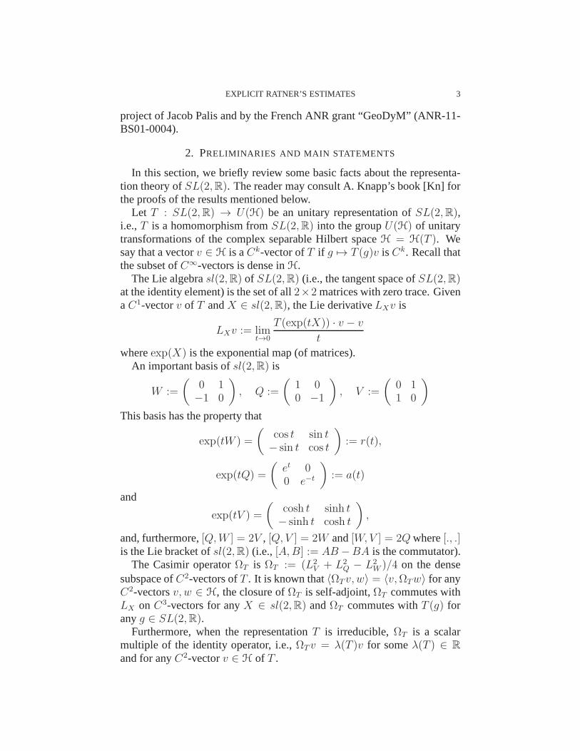
In this section, we briefly review some basic facts about the representa-tion theory ofSL(2,R). The reader may consult A. Knapp’s book [Kn] forthe proofs of the results mentioned below.

Let T : SL(2,R) → U(H) be an unitary representation ofSL(2,R),i.e.,T is a homomorphism fromSL(2,R) into the groupU(H) of unitarytransformations of the complex separable Hilbert spaceH = H(T ). Wesay that a vectorv ∈ H is aCk-vector ofT if g 7→ T (g)v isCk. Recall thatthe subset ofC∞-vectors is dense inH.

The Lie algebrasl(2,R) of SL(2,R) (i.e., the tangent space ofSL(2,R)at the identity element) is the set of all2×2 matrices with zero trace. GivenaC1-vectorv of T andX ∈ sl(2,R), the Lie derivativeLXv is

LXv := limt→0

T (exp(tX)) · v − v

t

whereexp(X) is the exponential map (of matrices).An important basis ofsl(2,R) is

W :=

(

0 1−1 0

)

, Q :=

(

1 00 −1

)

, V :=

(

0 11 0

)

This basis has the property that

exp(tW ) =

(

cos t sin t− sin t cos t

)

:= r(t),

exp(tQ) =

(

et 00 e−t

)

:= a(t)

and

exp(tV ) =

(

cosh t sinh t− sinh t cosh t

)

,

and, furthermore,[Q,W ] = 2V , [Q, V ] = 2W and[W,V ] = 2Q where[., .]is the Lie bracket ofsl(2,R) (i.e., [A,B] := AB −BA is the commutator).

The Casimir operatorΩT is ΩT := (L2V + L2

Q − L2W )/4 on the dense

subspace ofC2-vectors ofT . It is known that〈ΩTv, w〉 = 〈v,ΩTw〉 for anyC2-vectorsv, w ∈ H, the closure ofΩT is self-adjoint,ΩT commutes withLX on C3-vectors for anyX ∈ sl(2,R) andΩT commutes withT (g) foranyg ∈ SL(2,R).

Furthermore, when the representationT is irreducible,ΩT is a scalarmultiple of the identity operator, i.e.,ΩT v = λ(T )v for someλ(T ) ∈ R

and for anyC2-vectorv ∈ H of T .

4 CARLOS MATHEUS

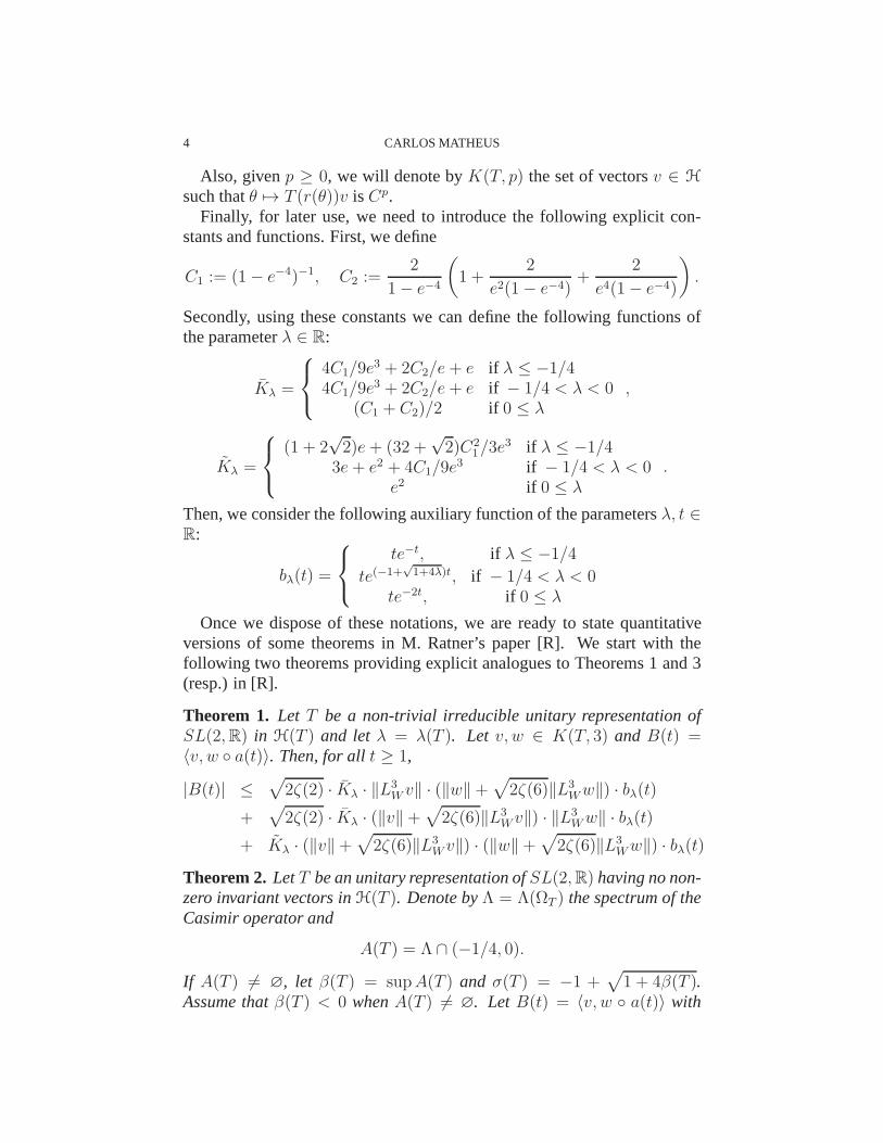
Also, givenp ≥ 0, we will denote byK(T, p) the set of vectorsv ∈ H

such thatθ 7→ T (r(θ))v isCp.Finally, for later use, we need to introduce the following explicit con-

stants and functions. First, we define

C1 := (1− e−4)−1, C2 :=2

1− e−4

(

1 +2

e2(1− e−4)+

2

e4(1− e−4)

)

.

Secondly, using these constants we can define the following functions ofthe parameterλ ∈ R:

Kλ =

4C1/9e3 + 2C2/e+ e if λ ≤ −1/4

4C1/9e3 + 2C2/e+ e if − 1/4 < λ < 0

(C1 + C2)/2 if 0 ≤ λ,

Kλ =

(1 + 2√2)e+ (32 +

√2)C2

1/3e3 if λ ≤ −1/4

3e+ e2 + 4C1/9e3 if − 1/4 < λ < 0

e2 if 0 ≤ λ.

Then, we consider the following auxiliary function of the parametersλ, t ∈R:

bλ(t) =

te−t, if λ ≤ −1/4

te(−1+√1+4λ)t, if − 1/4 < λ < 0

te−2t, if 0 ≤ λ

Once we dispose of these notations, we are ready to state quantitativeversions of some theorems in M. Ratner’s paper [R]. We start with thefollowing two theorems providing explicit analogues to Theorems 1 and 3(resp.) in [R].

Theorem 1. Let T be a non-trivial irreducible unitary representation ofSL(2,R) in H(T ) and letλ = λ(T ). Let v, w ∈ K(T, 3) andB(t) =〈v, w a(t)〉. Then, for allt ≥ 1,

|B(t)| ≤√

2ζ(2) · Kλ · ‖L3W v‖ · (‖w‖+

√

2ζ(6)‖L3Ww‖) · bλ(t)

+√

2ζ(2) · Kλ · (‖v‖+√

2ζ(6)‖L3Wv‖) · ‖L3

Ww‖ · bλ(t)+ Kλ · (‖v‖+

√

2ζ(6)‖L3Wv‖) · (‖w‖+

√

2ζ(6)‖L3Ww‖) · bλ(t)

Theorem 2. LetT be an unitary representation ofSL(2,R) having no non-zero invariant vectors inH(T ). Denote byΛ = Λ(ΩT ) the spectrum of theCasimir operator and

A(T ) = Λ ∩ (−1/4, 0).

If A(T ) 6= ∅, let β(T ) = supA(T ) and σ(T ) = −1 +√

1 + 4β(T ).Assume thatβ(T ) < 0 whenA(T ) 6= ∅. Let B(t) = 〈v, w a(t)〉 with

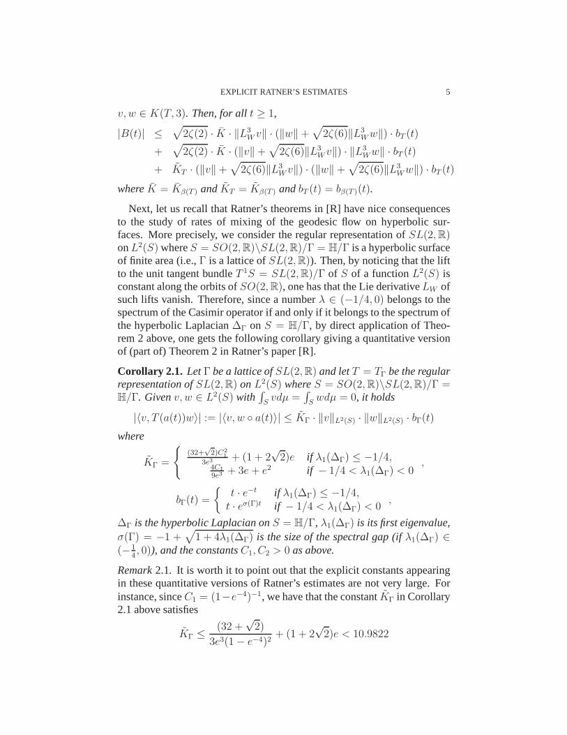
EXPLICIT RATNER’S ESTIMATES 5

v, w ∈ K(T, 3). Then, for allt ≥ 1,

|B(t)| ≤√

2ζ(2) · K · ‖L3W v‖ · (‖w‖+

√

2ζ(6)‖L3Ww‖) · bT (t)

+√

2ζ(2) · K · (‖v‖+√

2ζ(6)‖L3Wv‖) · ‖L3

Ww‖ · bT (t)+ KT · (‖v‖+

√

2ζ(6)‖L3W v‖) · (‖w‖+

√

2ζ(6)‖L3Ww‖) · bT (t)

whereK = Kβ(T ) andKT = Kβ(T ) andbT (t) = bβ(T )(t).

Next, let us recall that Ratner’s theorems in [R] have nice consequencesto the study of rates of mixing of the geodesic flow on hyperbolic sur-faces. More precisely, we consider the regular representation of SL(2,R)onL2(S) whereS = SO(2,R)\SL(2,R)/Γ = H/Γ is a hyperbolic surfaceof finite area (i.e.,Γ is a lattice ofSL(2,R)). Then, by noticing that the liftto the unit tangent bundleT 1S = SL(2,R)/Γ of S of a functionL2(S) isconstant along the orbits ofSO(2,R), one has that the Lie derivativeLW ofsuch lifts vanish. Therefore, since a numberλ ∈ (−1/4, 0) belongs to thespectrum of the Casimir operator if and only if it belongs to the spectrum ofthe hyperbolic Laplacian∆Γ on S = H/Γ, by direct application of Theo-rem 2 above, one gets the following corollary giving a quantitative versionof (part of) Theorem 2 in Ratner’s paper [R].

Corollary 2.1. LetΓ be a lattice ofSL(2,R) and letT = TΓ be the regularrepresentation ofSL(2,R) onL2(S) whereS = SO(2,R)\SL(2,R)/Γ =H/Γ. Givenv, w ∈ L2(S) with

∫

Svdµ =

∫

Swdµ = 0, it holds

|〈v, T (a(t))w〉| := |〈v, w a(t)〉| ≤ KΓ · ‖v‖L2(S) · ‖w‖L2(S) · bΓ(t)where

KΓ =

(32+√2)C2

1

3e3+ (1 + 2

√2)e if λ1(∆Γ) ≤ −1/4,

4C1

9e3+ 3e+ e2 if − 1/4 < λ1(∆Γ) < 0

,

bΓ(t) =

t · e−t if λ1(∆Γ) ≤ −1/4,t · eσ(Γ)t if − 1/4 < λ1(∆Γ) < 0

,

∆Γ is the hyperbolic Laplacian onS = H/Γ, λ1(∆Γ) is its first eigenvalue,σ(Γ) = −1 +

√

1 + 4λ1(∆Γ) is the size of the spectral gap (ifλ1(∆Γ) ∈(−1

4, 0)), and the constantsC1, C2 > 0 as above.

Remark2.1. It is worth it to point out that the explicit constants appearingin these quantitative versions of Ratner’s estimates are not very large. Forinstance, sinceC1 = (1−e−4)−1, we have that the constantKΓ in Corollary2.1 above satisfies

KΓ ≤ (32 +√2)

3e3(1− e−4)2+ (1 + 2

√2)e < 10.9822

6 CARLOS MATHEUS

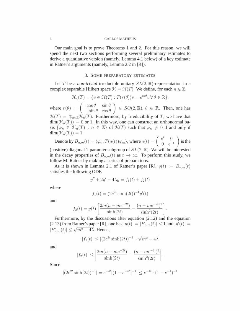
Our main goal is to prove Theorems 1 and 2. For this reason, we willspend the next two sections performing several preliminaryestimates toderive a quantitative version (namely, Lemma 4.1 below) of akey estimatein Ratner’s arguments (namely, Lemma 2.2 in [R]).

3. SOME PREPARATORY ESTIMATES

Let T be anon-trivial irreducible unitarySL(2,R)-representation in acomplex separable Hilbert spaceH = H(T ). We define, for eachn ∈ Z,

Hn(T ) = v ∈ H(T ) : T (r(θ))v = einθv ∀ θ ∈ R.

wherer(θ) =

(

cos θ sin θ− sin θ cos θ

)

∈ SO(2,R), θ ∈ R. Then, one has

H(T ) = ⊕n∈ZHn(T ). Furthermore, by irreducibility ofT , we have thatdim(Hn(T )) = 0 or 1. In this way, one can construct an orthonormal ba-sis ϕn ∈ Hn(T ) : n ∈ Z of H(T ) such thatϕn 6= 0 if and only ifdim(Hn(T )) = 1.

Denote byBn,m(t) = 〈ϕn, T (a(t))ϕm〉, wherea(t) =

(

et 00 e−t

)

is the

(positive) diagonal 1-paramter subgroup ofSL(2,R). We will be interestedin the decay properties ofBn,m(t) as t → ∞. To perform this study, wefollow M. Ratner by making a series of preparations.

As it is shown in Lemma 2.1 of Ratner’s paper [R],y(t) := Bn,m(t)satisfies the following ODE

y′′ + 2y′ − 4λy = f1(t) + f2(t)

wheref1(t) = (2e2t sinh(2t))−1y′(t)

and

f2(t) = y(t)

[

2m(n−me−2t)

sinh(2t)− (n−me−2t)2

sinh2(2t)

]

.

Furthermore, by the discussions after equation (2.12) and the equation(2.13) from Ratner’s paper [R], one has|y(t)| = |Bn,m(t)| ≤ 1 and|y′(t)| =|B′

n,m(t)| ≤√m2 − 4λ. Hence,

|f1(t)| ≤ |(2e2t sinh(2t))−1| ·√m2 − 4λ

and

|f2(t)| ≤∣

∣

∣

∣

2m(n−me−2t)

sinh(2t)− (n−me−2t)2

sinh2(2t)

∣

∣

∣

∣

.

Since

|(2e2t sinh(2t))−1| = e−4t|(1− e−4t)−1| ≤ e−4t · (1− e−4)−1

EXPLICIT RATNER’S ESTIMATES 7

for everyt ≥ 1, we obtain that the constantC1 appearing in equation (2.14)of Ratner’s paper [R] is

(3.1) C1 = (1− e−4)−1,

i.e.,

(3.2) |f1(t)| ≤ C1

√m2 − 4λ · e−4t

with C1 as above.Similarly, 2m(n−me−2t)

sinh(2t)− (n−me−2t)2

sinh2(2t)= 1

sinh(2t)[2m(n−me−2t)− (n−me−2t)2

sinh(2t)],

so that|f2(t)| ≤∣

∣

∣

2m(n−me−2t)sinh(2t)

− (n−me−2t)2

sinh2(2t)

∣

∣

∣is bounded by the quantity

2(1−e−4)

e−2t[2m(n − me−2t) − (n−me−2t)2

sinh(2t)] for every t ≥ 1. On the other

hand, this last quantity is bounded by

2C1e−2t[

|2mn|+ 2e−2m2 + 2e−2C1n2 + 2e−4C1|2mn|+ 2e−6C1m

2]

.

Because|2mn| ≤ m2 + n2 and2e−2 + 2C1e−6 = 2C1e

−2 (sinceC1 =1/(1− e−4)), we see that

|f2(t)| ≤ 2C1

e2t

[(

1 +2

e2+

2C1

e4+

2C1

e6

)

m2 +

(

1 +2C1

e2+

2C1

e4

)

n2

]

= 2C1e−2t(1 + 2C1e

−2 + 2C1e−4)(m2 + n2).

In other words, the constantC2 appearing in equation (2.14) of Ratner’spaper [R] is

(3.3) C2 =2

1− e−4

(

1 +2

e2(1− e−4)+

2

e4(1− e−4)

)

,

i.e.,

(3.4) |f2(t)| ≤ C2(m2 + n2)e−2t

with C2 as above.Next, we observe that the constantC1 in equation (2.16) of Ratner’s paper

[R] is slightly different that what she refers to asC1 in equation (2.14).Indeed, by denoting the roots of the characteristic equationx2+2x−4λ = 0of the ODE satisfied byy(t) := Bn,m(t) by r1 := r1(λ) := −1 +

√1 + 4λ

andr2 := r2(λ) := −1−√1 + 4λ, the fact that|f1(t)| ≤ C1e

−4t√m2 − 4λ

implies that∣

∣

∣

∣

∫ ∞

t

e−r1sf1(s)ds

∣

∣

∣

∣

≤ C1

√m2 − 4λ

∫ ∞

t

e(−Re(r1)−4)sds

≤ C1

3

√m2 − 4λ · e−3t(3.5)

8 CARLOS MATHEUS

because Re(r1) + 2 ≥ 1. However, the constantC2 in Ratner’s paper [R] isthe same for both (2.16) and (2.14):

∣

∣

∣

∣

∫ ∞

t

e−r1sf2(s)ds

∣

∣

∣

∣

≤ C2(m2 + n2)

∫ ∞

t

e(−Re(r1)−2)sds

≤ C2(m2 + n2)e−t(3.6)

because Re(r1) + 2 ≥ 1.Concluding our series of preparations, we recall the definitions of the

following two functions

A1(t) :=

∫ t

1

e(r1−r2)s

(∫ ∞

s

e−r1uf1(u) du

)

ds

and

A2(t) :=

∫ t

1

e(r1−r2)s

(∫ ∞

s

e−r1uf2(u) du

)

ds

introduced after equation (2.18) of Ratner’s paper [R]. These functionsappear naturally in our context because the ODE verified byy(t) = Bn,m(t)can be rewritten as(D − r1)(D − r2)y = f1(t) + f2(t) := f(t) whereDis the differentiation operator (with respect tot). Thus, since(D − r1)y =er1tD(e−r1ty), we haveer1tD(e−r1t(D − r2)y) = f(t) and, hence,

e(r2−r1)tD(e−r2ty) = −∫ ∞

t

e−r1sf(s) ds+ P1

whereP1 is a constant. In particular, we can write

(3.7) y(t) = −e−t

∫ t

1

(∫ ∞

s

eu f(u) du

)

ds+ P1te−t + P2e

−t

if r1 = r2, and

y(t) = er2tA(t) + er2t[

P1

∫ t

1

e(r1−r2)s ds+ P2

]

= er2tA(t) +P1

2√1 + 4λ

er1t +

(

P2 −e2

√1+4λP1

2√1 + 4λ

)

er2t(3.8)

if r1 6= r2, whereA(t) := A1(t) + A2(t). Moreover, by using these equa-tions, and the fact thaty(t) = Bn,m(t) → 0 ast → ∞ (a consequence ofthe non-triviality ofT , that is, it has no invariantT -invariant vectors), wecan deduce that

(3.9) P1 =

∫ ∞

1

e−r1sf(s) ds− r2e−r1y(1) + e−r1y′(1)

and

(3.10) P2 = y(1)e−r2

EXPLICIT RATNER’S ESTIMATES 9

Finally, from the estimates (3.2), (3.4) above, and the facts Re(r1) −Re(r2) ≥ 0 and Re(r1) + 2 ≥ 1, we can estimate:

|er2tA1(t)|(3.11)

= |er2t∫ t

1

e(r1−r2)s

∫ ∞

s

e−r1uf1(u)du ds|

≤ C1

√m2 − 4λ etRe(r2)

∫ t

1

e(Re(r1)−Re(r2))s

∫ ∞

s

e(−Re(r1)−4)udu ds

≤ C1

3

√m2 − 4λ etRe(r2)e(Re(r1)−Re(r2))t

∫ t

1

e(−Re(r1)−4)sds

≤ C1

9e3

√m2 − 4λ etRe(r1)

and

|er2tA2(t)|(3.12)

= |er2t∫ t

1

e(r1−r2)s

∫ ∞

s

e−r1uf2(u)du ds|

≤ C2(m2 + n2)etRe(r2)

∫ t

1

e(Re(r1)−Re(r2))s

∫ ∞

s

e(−Re(r1)−2)udu ds

≤ C2(m2 + n2)etRe(r1)

∫ t

1

e(−Re(r1)−2)sds

≤ C2

e(m2 + n2)etRe(r1)

Thus, we can take

(3.13) C1 = C1/9e3 and C2 = C2/e

in equations (2.19) and (2.20) of Ratner’s paper [R].After these preparations, we are ready to pass to the next section, where

we render more explicitly the constants appearing in Lemma 2.2 of Ratner’spaper [R] about the speed of decay of the matrix coefficientsBn,m(t) ast → ∞.

4. DECAY OF MATRIX COEFFICIENTS OFSL(2,R)-REPRESENTATIONS

By following closely the proof of Lemma 2.2 of Ratner’s paper[R], weshow the following explicit variant of it:

Lemma 4.1. For t ≥ 1, n,m ∈ Z,

|Bn,m(t)| ≤ (Kλ(m2 + n2) + Kλ) · bλ(t),

where

• bλ(t) = te−t if λ ≤ −1/4;

10 CARLOS MATHEUS

• bλ(t) = ter1t if −1/4 < λ < 0;• bλ(t) = te−2t if 0 ≤ λ;

and

Kλ =

4C1/9e3 + 2C2/e+ e if λ ≤ −1/4

4C1/9e3 + 2C2/e+ e if − 1/4 < λ < 0

(C1 + C2)/2 if 0 ≤ λ,

Kλ =

(1 + 2√2)e+ (32 +

√2)C2

1/3e3 if λ ≤ −1/4

3e+ e2 + 4C1/9e3 if − 1/4 < λ < 0

e2 if 0 ≤ λ.

with the constantsC1 andC2 given by(3.1)and (3.3)above.

Remark4.1. In Ratner’s article [R], the functionbλ(t) is slightly differentfrom the one above (whenλ < 0): indeed, in this paper,

bλ(t) =

minte−t, e−t(1 +√

1/|1 + 4λ|) if λ ≤ −1/4,

minter1t, er1t√

1/|1 + 4λ| if − 1/4 < λ < 0.

In particular, this allows us to gain over the factor oft (in front of the ex-ponential functionse−t, er1t) whenλ is not close to−1/4 at the cost ofpermitting larger constants. However, since we had in mind the idea of get-ting uniform constants regardless ofλ and the factor oft does not seem verysubstantial, we decided to neglect this issue by sticking tothe functionbλ(t)as defined in Lemma 4.1 above.

Proof. We begin with the caseλ = −1/4, i.e.,r1 = r2 = −1. From (3.7),we know that

y(t) = −e−t

∫ t

1

(∫ ∞

s

euf(u)du

)

ds+ P1te−t + P2e

−t.

Since, by definition,f(t) = f1(t) + f2(t), we can apply (3.2), (3.4) aboveto obtain

|y(t)| ≤ C1

√m2 + 1 · e−t

∫ t

1

∫ ∞

s

e−3udu ds

+ C2(m2 + n2)e−t

∫ t

1

∫ ∞

s

e−udu ds

+ |P1|te−t + |P2|e−t.

On the other hand, using that|y(1)| ≤ 1, |y′(1)| ≤√m2 − 4λ, the equa-

tions (3.5), (3.6), (3.9), (3.10) above, and the fact thatr1 = r2 = −1 in the

EXPLICIT RATNER’S ESTIMATES 11

present case, we get

|y(t)| ≤ C1

9e3

√m2 + 1 · e−t +

C2

e(m2 + n2)e−t

+ te−t

[

C1

3e3

√m2 + 1 +

C2

e(m2 + n2) + e+ e

√m2 + 1

]

+ e · e−t

Since√m2 + 1 ≤ |m|+ 1 ≤ m2 + n2 + 1 ande−t ≤ te−t (becauset ≥ 1),

we conclude that

(4.1) |y(t)| ≤ te−t[

K[λ=−1/4](m2 + n2) + K[λ=−1/4]

]

where

K[λ=−1/4] =4C1

9e3+

2C2

e+ e

and

K[λ=−1/4] =4C1

9e3+ 3e

Next, we notice that, whenr1 6= r2, by (3.8), and (3.11), (3.12) above,

|y(t)| ≤ C1

9e3

√m2 − 4λ · etRe(r1) +

C2

e(m2 + n2) · etRe(r1)(4.2)

+ |P1| · tetRe(r1) + |P2| · etRe(r2)

If −1/2 ≤ λ < −1/4, we have that Re(r1) = Re(r2) = −1, |r2| ≤√2

and√m2 − 4λ ≤

√m2 + 2 ≤ m2 + n2 +

√2, so that (3.9), (3.10) and the

equations (3.5), (3.6) and (4.2) above imply

|P1| ≤C1

3e3(m2 + n2 +

√2) +

C2

e(m2 + n2) +

√2 · e+ e(m2 + n2 +

√2),

|P2| ≤ e

and,a fortiori,

|y(t)| ≤(

C1

9e3+

C2

e

)

(m2 + n2)te−t +

√2C1

9e3te−t + (|P1|+ |P2|)te−t

≤ te−t(

K[−1/2≤λ<−1/4](m2 + n2) + K[−1/2≤λ<−1/4]

)

(4.3)

where

K[−1/2≤λ<−1/4] =4C1

9e3+

2C2

e+ e

and

K[−1/2≤λ<−1/4] =4√2C1

9e3+ (1 + 2

√2)e.

If −1/4 < λ < 0, we have that0 <√1 + 4λ < 1, so that Re(r1) =

r1 = −1+√1 + 4λ ∈ (−1, 0), Re(r2) = r2 = −1−

√1 + 4λ ∈ (−2,−1),

12 CARLOS MATHEUS

|r2| = 1 +√1 + 4λ ∈ (1, 2) and

√m2 − 4λ ≤

√m2 + 1 ≤ m2 + n2 + 1.

Putting this into (3.9), (3.10), and the equations (3.5), (3.6), and (4.2) above,we get

|P1| ≤C1

3e3(m2 + n2 + 1) +

C2

e(m2 + n2) + 2e+ e(m2 + n2 + 1),

|P2| ≤ e2,

and

|y(t)| ≤(

C1

9e3+

C2

e

)

(m2 + n2)tetr1 +C1

9e3tetr1 + (|P1|+ |P2|)tetr1

≤ tetr1(K[−1/4<λ<0](m2 + n2) + K[−1/4<λ<0])(4.4)

where

K[−1/4<λ<0] =4C1

9e3+

2C2

e+ e

and

K[−1/4<λ<0] =4C1

9e3+ 3e+ e2.

Now we pass to the caseλ < −1/2. In this situation,√m2 − 4λ is not

bounded, so we can’t controler2tA1(t) by using (3.11). So, we follow thearguments in page 281 of Ratner’s paper [R]. Recall that

A1(t) =

∫ t

1

e(r1−r2)s

(∫ ∞

s

e−r1uf1(u) du

)

ds

and

I(s) :=

∫ ∞

s

e−r1uf1(u)du = 2

∫ ∞

s

e(−r1−2)u y′(u)

sinh(2u)du.

DefineJ(s) :=∫∞u

y′(v)/ sinh(2v) dv. By integration by parts,J(u) =y(u)

sinh(2u)+ 2

∫∞u

y(v) cosh(2v)

sinh2(2v)dv,

I(s) = 2

[

e(−r1−2)sJ(s) + (r1 + 2)

∫ ∞

s

e(−r1−2)uJ(u) du

]

andA1(t) = 2(F1(t) + F2(t)), where

F1(t) =

∫ t

1

e(−r2−2)sJ(s) ds

and

F2(t) = (r1 + 2)

∫ t

1

e(r1−r2)s

(∫ ∞

s

e(−r1−2)uJ(u) du

)

ds.

EXPLICIT RATNER’S ESTIMATES 13

It follows that

|J(u)| ≤ 2

(1− e−4)e−2u + 2

(1 + e−4)

(1− e−4)

∫ ∞

u

dv

sinh(2v)

≤ 2

(1− e−4)e−2u + 2

(1 + e−4)

(1− e−4)2e−2u

≤ Q1 · e−2u

whereQ1 = 4/(1 − e−4)2 = 4C21 . That is, we can takeQ1 = 4C2

1 in theequation (2.22) of Ratner’s paper [R]. Also, since Re(r2) = −1, we get

|er2tF1(t)| =∣

∣

∣

∣

er2t∫ t

1

e−(r2+2)sJ(s)ds

∣

∣

∣

∣

≤ Q1e−t

∫ t

1

e−3sds ≤ Q2e−t

with Q2 = 4C21/3e

3, that is, this constantQ2 works in equation (2.24) ofRatner’s paper [R]. Finally, by integrating by parts,

er2tF2(t) =er2t(r1 + 2)

r1 − r2

(

[

e(r1−r2)s

∫ ∞

s

e(−r1−2)uJ(u) du

]t

1

+ F1(t)

)

On the other hand, sinceλ < −1/2, one has∣

∣

∣

r1+2r1−r2

∣

∣

∣=∣

∣

∣

1+√1+4λ

2√1+4λ

∣

∣

∣≤ 1. By

combining these facts, we see that

|er2tF2(t)| ≤2Q1

3e3e−t +Q2e

−t = Q3e−t

whereQ3 = Q1/e3.

Thus, using these estimates to controler2tA1(t) and the estimate (3.12)above to controler2tA2(t), we obtain

|er2tA(t)| ≤ |er2tA1(t)|+ |er2tA2(t)|≤ 2|er2tF1(t)|+ 2|er2tF2(t)|+ |er2tA2(t)|

≤ 2(Q2 +Q3)e−t +

C2

e(m2 + n2)e−t

= (Q+ Q(m2 + n2))e−t

whereQ = 2(Q2 +Q3) = 32C21/3e

3 andQ = C2 = C2/e.The second step in the analysis for the caseλ < −1/2 is the control

of the quantities|P1/2√1 + 4λ| and |P2 − e2

√1+4λP1/2

√1 + 4λ|. Since

r1 = −1 + i√

|1 + 4λ|, r2 = −1 − i√

|1 + 4λ| and|y(1)| ≤ 1, |y′(1)| ≤

14 CARLOS MATHEUS

√m2 − 4λ, we can estimate the first quantity as follows:∣

∣

∣

∣

P1

2√1 + 4λ

∣

∣

∣

∣

≤ 1

2√

|1 + 4λ|

(∣

∣

∣

∣

∫ ∞

1

e−r1sf1(s)ds

∣

∣

∣

∣

+

∣

∣

∣

∣

∫ ∞

1

e−r1sf2(s)ds

∣

∣

∣

∣

)

+1

2√

|1 + 4λ|(

|r2e−r1y(1)|+ |e−r1y′(1)|)

≤ 1

2√

|1 + 4λ|

(

C1

3e3

√m2 − 4λ+

C2

e(m2 + n2)

)

+1

2√

|1 + 4λ|

(

√

1 + |1 + 4λ| · e +√m2 − 4λ · e

)

=1

2√

|1 + 4λ|

(

C1

3e3

√

m2 + |1 + 4λ|+ 1 +C2

e(m2 + n2)

)

+e

2√

|1 + 4λ|

(

√

1 + |1 + 4λ|+√

m2 + |1 + 4λ|+ 1)

≤ 1

2√

|1 + 4λ|

(

C1

3e3+

C2

e+ e

)

(m2 + n2)

+

√

1 + |1 + 4λ|2√

|1 + 4λ|

(

C1

3e3+ 2e

)

≤ 1

2

(

C1

3e3+

C2

e+ e

)

(m2 + n2) +1√2

(

C1

3e3+ 2e

)

.

Here, we used thatλ < −1/2 (so that|1+4λ| > 1) and√

(1 + x)/x <√2

wheneverx > 1. Similarly, we can estimate the second quantity as follows:∣

∣

∣

∣

∣

P2 −e2

√1+4λ

2√1 + 4λ

P1

∣

∣

∣

∣

∣

≤ |P2|+∣

∣

∣

∣

P1

2√1 + 4λ

∣

∣

∣

∣

≤ Q1(m2 + n2) + Q1,

whereQ1 =12

(

C1

3e3+ C2

e+ e)

andQ1 =1√2

(

C1

3e3+ 2e

)

+ e. Inserting these

estimates above into (3.8), we deduce that

|y(t)| ≤ |er2tA(t)|+∣

∣

∣

∣

P1

2√1 + 4λ

∣

∣

∣

∣

· |er1t|+∣

∣

∣

∣

∣

P2 −e2

√1+4λ

2√1 + 4λ

P1

∣

∣

∣

∣

∣

· |er2t|

≤(

(Q+ 2Q1)(m2 + n2) + (Q + 2Q1 − e)

)

e−t

=(

K[λ<−1/2](m2 + n2) + K[λ<−1/2])

)

e−t(4.5)

where

K[λ<−1/2] =C1

3e3+

2C2

e+ e

EXPLICIT RATNER’S ESTIMATES 15

and

K[λ<−1/2] =(32 +

√2)C2

1

3e3+ (1 + 2

√2)e.

Finally, we consider the caseλ ≥ 0. We begin by estimating|er2tA2(t)|and er2tA1(t): using (3.2), (3.4) above andr1 = −1 +

√1 + 4λ ≥ 0,

r2 = −1 −√1 + 4λ ≤ −2, we obtain

|er2tA2(t)| ≤ C2(m2 + n2)er2t

∫ t

1

e(r1−r2)s

∫ ∞

s

e−r1ue−2udu ds

≤ C2

2(m2 + n2)er2t

∫ t

1

e(−r2−2)sds

≤ C2

2(m2 + n2)te−2t

and

|er2tA1(t)| ≤ C1

2

√m2 − 4λer2t

∫ t

1

e−(r2+2)sds ≤ C1

2|m|te−2t

≤ C1

2(m2 + n2)te−2t.

Thus,

|er2tA(t)| ≤ |er2tA1(t)|+ |er2tA2(t)| ≤C1 + C2

2(m2 + n2)te−2t,

so that we can takeC = (C1 + C2)/2 andC = 0 in the equation (2.28) ofRatner’s paper [R].

Next, we observe thaty(t) → 0 whent → ∞ andr1 ≥ 0 imply P1 = 0and

y(t) = er2tA(t) + y(1)e−r2er2t.

Therefore, from the previous discussion andr2 + 2 ≤ 0, it follows that

|y(t)| ≤ C1 + C2

2(m2 + n2)te−2t + e−r2e(r2+2)te−2t

≤ (K[λ≥0](m2 + n2) + K[λ≥0])te

−2t(4.6)

where

K[λ≥0] =C1 + C2

2and

K[λ≥0] = e2

At this stage, from (4.1), (4.3), (4.4), (4.5), (4.6) above,we see that theproof of the desired lemma is complete.

16 CARLOS MATHEUS

In next (and final) section, we apply Lemma 4.1 to derive explicit vari-ants of Theorems 1 and 3 of Ratner’s paper [R]. To do so, we recallsome notation already introduced in Section 2. We denote byr(θ) =(

cos θ sin θ− sin θ cos θ

)

∈ SO(2,R), θ ∈ R. Given an unitarySL(2,R)-

representationT , we denote byK(T, 3) the set of vectorsv ∈ H(T ) suchthat θ 7→ T (r(θ))v is C3. Finally, if the mapθ 7→ T (r(θ))v is C1, wedenote by

LW v := limθ→0

T (r(θ))v − v

θ

the Lie derivative ofv along the direction ofW =

(

0 1−1 0

)

of the infin-

itesimal generator of the rotation groupSO(2,R) = r(θ) : θ ∈ R.In particular, in the case of an irreducible unitarySL(2,R)-representation

T , sinceT (r(θ))ϕn = einθϕn whenϕn ∈ Hn(T ), we have that

LWϕn = inϕn

for everyn ∈ Z.

5. PROOF OFTHEOREMS1 AND 2

In this short section, we indicate how Lemma 4.1 can be used toproveTheorems 1 and 2 (whose respective statements are recalled below).

Theorem 3. Let T be a non-trivial irreducible unitary representation ofSL(2,R) in H(T ) and letλ = λ(T ). Let v, w ∈ K(T, 3) andB(t) =〈v, w a(t)〉. Then, for allt ≥ 1,

|B(t)| ≤√

2ζ(2) · Kλ · ‖L3W v‖ · (‖w‖+

√

2ζ(6)‖L3Ww‖) · bλ(t)

+√

2ζ(2) · Kλ · (‖v‖+√

2ζ(6)‖L3Wv‖) · ‖L3

Ww‖ · bλ(t)+ Kλ · (‖v‖+

√

2ζ(6)‖L3Wv‖) · (‖w‖+

√

2ζ(6)‖L3Ww‖) · bλ(t)

whereKλ, Kλ andbλ(t) are as in Lemma4.1.

Proof. Following the proof of Theorem 1 of Ratner’s paper [R] (at page283), we write

v =∑

n∈Zcnϕn, w =

∑

n∈Zdnϕn

with cn = 〈v, ϕn〉, dn = 〈w, ϕn〉 (andϕn ∈ Hn(T ), n ∈ Z) as in page 276of this paper. We have

B(t) =∑

n,m∈ZcndmBn,m(t)

EXPLICIT RATNER’S ESTIMATES 17

so that

|B(t)| ≤ bλ(t)∑

n,m∈Z|cn| · |dm| · (Kλ(m

2 + n2) + Kλ)

by Lemma 4.1.On the other hand, sinceL3

Wϕn = −in3ϕn for all n ∈ Z, we know that

∑

n∈Z|cn| ≤ |c0|+

∑

n∈Z−0n6|cn|2

1

2

∑

n∈Z−0

1

n6

1

2

≤ ‖v‖+√

2ζ(6) · ‖L3W v‖,

∑

m∈Z|dm| ≤ |d0|+

∑

m∈Z−0m6|dm|2

1

2

∑

m∈Z−0

1

m6

1

2

≤ ‖w‖+√

2ζ(6) · ‖L3Ww‖,

∑

n∈Z|cn| · n2 ≤

∑

n∈Z−0n6|cn|2

1

2

∑

n∈Z−0

1

n2

1

2

≤√

2ζ(2) · ‖L3Wv‖,

and

∑

m∈Z|dm| ·m2 ≤

∑

m∈Z−0m6|dm|2

1

2

∑

m∈Z−0

1

m2

1

2

≤√

2ζ(2) · ‖L3Ww‖,

The desired result follows.

Theorem 4. LetT be an unitary representation ofSL(2,R) having no non-zero invariant vectors inH(T ). Write Λ = Λ(ΩT ) the spectrum of theCasimir operator and

A(T ) = Λ ∩ (−1/4, 0).

If A(T ) 6= ∅, let β(T ) = supA(T ) and σ(T ) = −1 +√

1 + 4β(T ).Assume thatβ(T ) < 0 whenA(T ) 6= ∅. Let B(t) = 〈v, w a(t)〉 withv, w ∈ K(T, 3). Then, for allt ≥ 1,

|B(t)| ≤√

2ζ(2) · K · ‖L3W v‖ · (‖w‖+

√

2ζ(6)‖L3Ww‖) · bT (t)

+√

2ζ(2) · K · (‖v‖+√

2ζ(6)‖L3Wv‖) · ‖L3

Ww‖ · bT (t)+ KT · (‖v‖+

√

2ζ(6)‖L3W v‖) · (‖w‖+

√

2ζ(6)‖L3Ww‖) · bT (t)

18 CARLOS MATHEUS

whereK = 4C1

9e3+ 2C2

e+ e,

KT =

(32+√2)C2

1

3e3+ (1 + 2

√2)e if A(T ) = ∅,

4C1

9e3+ 3e+ e2 if A(T ) 6= ∅

,

bT (t) =

t · e−t if A(T ) = ∅,t · eσ(T )t if A(T ) 6= ∅

Proof. This is an immediate consequence of Theorem 3 and the argumentsfrom pages 285–286 of Ratner’s paper [R].

REFERENCES

[EMV] M. Einsiedler, G. Margulis and A. Venkatesh,Effective equidistribution for closedorbits of semisimple groups on homogeneous spaces, Invent. Math.,177 (2009), 137–212.

[KM] J. Kahn and V. Markovic,Immersing almost geodesic surfaces in a closed hyper-bolic three manifold, Annals of Math.,175 (2012), no. 3, 1127–1190.

[Kn] A. W. Knapp, Representation theory of semisimple groups. An overview based onexamples, Princeton Mathematical Series, 36. Princeton UniversityPress, Princeton,NJ, 1986.

[LM] H. Li and G. Margulis,Effective discreteness of the3-dimensional Markov spectrum,in preparation.

[M] G. Margulis,Discrete subgroups and ergodic theory. Number theory, trace formulasand discrete groups (Oslo, 1987), 377–398, Academic Press,Boston, MA, 1989.

[Ma] C. Matheus,Explicit constants in Ratner’s estimates on rates of mixingof geodesicflows of hyperbolic surfaces, post at the mathematical blog “Disquisitiones Mathe-maticae” (http://matheuscmss.wordpress.com/).

[MS] C. Matheus and G. Schmithüsen,Explicit Teichmüller curves with complementaryseries, to appear in Bulletin de la SMF.

[Mo] A. Mohammadi,A special case of effective equidistribution with explicitconstants,Ergodic Theory Dynam. Systems,32 (2012), no. 1, 237–247.

[R] M. Ratner, The rate of mixing for geodesic and horocycle flows, Ergodic TheoryDynam. Systems,7 (1987), 267–288.

CARLOS MATHEUS: UNIVERSITÉ PARIS 13, SORBONNEPARIS CITÉ, LAGA, CNRS(UMR 7539), F-93430, VILLETANEUSE, FRANCE.

E-mail address: [email protected].