Some new test functions for global optimization and ...

Munich Personal RePEc Archive

Some new test functions for global

optimization and performance of

repulsive particle swarm method

Mishra, Sudhanshu

North-Eastern Hill University, Shillong (India)

23 August 2006

Online at https://mpra.ub.uni-muenchen.de/2718/

MPRA Paper No. 2718, posted 13 Apr 2007 UTC

Some New Test Functions for Global Optimization

and Performance of Repulsive Particle Swarm Method

SK Mishra

Dept. of Economics North-Eastern Hill University

Shillong (India)

I. Introduction: In this paper we introduce some new multi-modal test functions to assess the performance of global optimization methods. These functions have been selected partly because several of them are aesthetically appealing and partly because a few of them are really difficult to optimize. We also propose to optimize some important benchmark functions already in vogue. Each function has been graphically presented to appreciate its geometrical appearance. To optimize these functions we have used the Repulsive Particle Swarm (RPS) method, with wider local search abilities and randomized neighbourhood topology.

II. The Particle Swarm Method of Global Optimization: This method is an instance of successful application of the philosophy of Simon’s bounded rationality and decentralized decision-making to solve the global optimization problems (Simon, 1982; Bauer, 2002; Fleischer, 2005). As it is well known, the problems of the existence of global order, its integrity, stability, efficiency, etc. have been long standing. The laws of development of institutions have been sought in this order. Newton, Hobbes, Adam Smith and Locke visualized the global system arising out of individual actions. In particular, Adam smith (1759) postulated the role of invisible hand in establishing the harmony that led to the said global order. The neo-classical economists applied the tools of equilibrium analysis to show how this grand synthesis and order is established while each individual is selfish. The postulate of perfect competition was felt to be a necessary one in demonstrating that. Yet, Alfred Marshall limited himself to partial equilibrium analysis and, thus, indirectly allowed for the role of invisible hand (while general equilibrium economists hoped that the establishment of order can be explained by their approach). Thorstein Veblen (1899) never believed in the mechanistic view and pleaded for economics as an evolutionary science. F. A. Hayek (1944) believed in a similar philosophy and believed that locally optimal decisions give rise to the global order and efficiency. Later, Herbert Simon (1982) postulated the ‘bounded rationality’ hypothesis and argued that the hypothesis of perfect competition is not necessary for explaining the emergent harmony and order at the global level. Elsewhere, I. Prigogine (1984) demonstrated how the global ‘order’ emerges from chaos at the local level.

It is observed that a swarm of birds or insects or a school of fish searches for food, protection, etc. in a very typical manner (Sumper, 2006). If one of the members of the swarm sees a desirable path to go, the rest of the swarm will follow quickly. Every member of the swarm searches for the best in its locality - learns from its own experience. Additionally, each member learns from the others, typically from the best performer among them. The Particle Swarm method of optimization mimics this behaviour (see Wikipedia: http://en.wikipedia.org/wiki/Particle_swarm_optimization). Every individual of the swarm is considered as a particle in a multidimensional space that has a position and a velocity. These particles fly through hyperspace and remember the

2

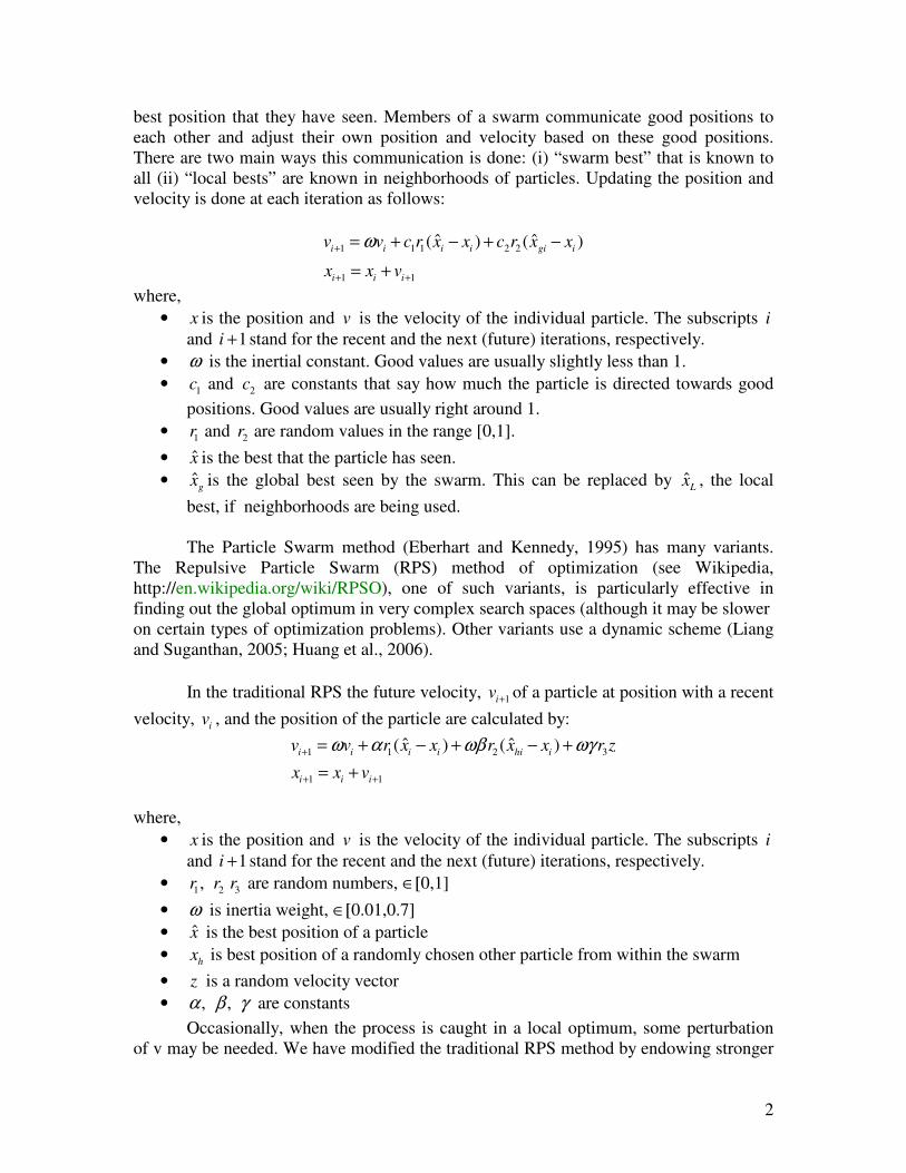
best position that they have seen. Members of a swarm communicate good positions to each other and adjust their own position and velocity based on these good positions. There are two main ways this communication is done: (i) “swarm best” that is known to all (ii) “local bests” are known in neighborhoods of particles. Updating the position and velocity is done at each iteration as follows:

1 1 1 2 2

1 1

ˆ ˆ( ) ( )i i i i gi i

i i i

v v c r x x c r x x

x x v

ω+

+ +

= + − + −

= +

where,

• x is the position and v is the velocity of the individual particle. The subscripts i and 1i + stand for the recent and the next (future) iterations, respectively.

• ω is the inertial constant. Good values are usually slightly less than 1.

• 1c and 2c are constants that say how much the particle is directed towards good

positions. Good values are usually right around 1.

• 1r and 2r are random values in the range [0,1].

• x̂ is the best that the particle has seen.

• ˆg

x is the global best seen by the swarm. This can be replaced by ˆL

x , the local

best, if neighborhoods are being used.

The Particle Swarm method (Eberhart and Kennedy, 1995) has many variants. The Repulsive Particle Swarm (RPS) method of optimization (see Wikipedia, http://en.wikipedia.org/wiki/RPSO), one of such variants, is particularly effective in finding out the global optimum in very complex search spaces (although it may be slower on certain types of optimization problems). Other variants use a dynamic scheme (Liang and Suganthan, 2005; Huang et al., 2006).

In the traditional RPS the future velocity, 1iv + of a particle at position with a recent

velocity, i

v , and the position of the particle are calculated by:

1 1 2 3

1 1

ˆ ˆ( ) ( )i i i i hi i

i i i

v v r x x r x x r z

x x v

ω α ωβ ωγ+

+ +

= + − + − +

= +

where,

• x is the position and v is the velocity of the individual particle. The subscripts i

and 1i + stand for the recent and the next (future) iterations, respectively.

• 1 2 3,r r r are random numbers, ∈[0,1]

• ω is inertia weight, ∈[0.01,0.7]

• x̂ is the best position of a particle

• h

x is best position of a randomly chosen other particle from within the swarm

• z is a random velocity vector

• , ,α β γ are constants

Occasionally, when the process is caught in a local optimum, some perturbation of v may be needed. We have modified the traditional RPS method by endowing stronger

3

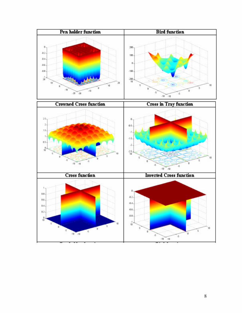
(wider) local search ability to each particle and the neighbourhood topology to each particle is randomized. III. The New Test Functions: We used RPS method for a fairly large number of established test problems (Mishra, 2006 (c) reports about 30 benchmark functions). Here we introduce the new functions and the results obtained by the RPS program (appended). These new functions are as follows. 1. Test tube holder function (a): This multi-modal function is defined as follows. We

obtain * 10.8723x −� in the domain [ 10, 10], 1, 2i

x i∈ − = . 2 21 2|cos(( ) / 200)|

1 2( ) 4 sin( ) cos( )e x xf x x x

+= − .

2. Test tube holder function (b): This multi-modal function is defined as follows. We

obtain * 10.8723x −� in the domain 1 2[ 9.5, 9.4], [ 10.9, 10.9]x x∈ − ∈ − . 2 21 2|cos(( ) / 200)|

1 2( ) 4 sin( ) cos( )e x xf x x x

+= − .

3. Holder table function: This ‘tabular holder’ function has multiple local minima with

four global minima at *( ) 26.92f x � . This function is given as: 2 2 0.51 2|1 [( ) ]/ |

1 2( ) cos( )cos( )e x xf x x x

π− += −

4. Carrom table function: This function has multiple local minima with four global

minima at *( ) 24.1568155f x � in the search domain [ 10, 10], 1, 2i

x i∈ − = . This

function is given as:

{ }2 2 0.51 2

2|1 [( ) ]/ |

1 2( ) cos( ) cos( ) e / 30x xf x x x

π− +� �= − � ��

5. Cross in tray function: This function has multiple local minima with the global

minima at *( ) 2.06261218f x −� in the search domain [ 10, 10], 1, 2i

x i∈ − = . This

function is given as: 2 2 0.51 2

0.1100 [( ) ]/

1 2( ) 0.0001 sin( )sin( ) 1x x

f x x x eπ− +� �

= − +� ��

6. Crowned cross function: This function is the negative form of the cross in tray

function. It has *( ) 0f x � in the search domain [ 10, 10], 1, 2i

x i∈ − = . It is a difficult

function to optimize. The minimal value obtained by us is approximately 0.1. This function is given as:

2 2 0.51 2

0.1100 [( ) ]/

1 2( ) 0.0001 sin( )sin( ) 1x x

f x x x eπ− +� �

= +� ��

7. Cross function: This is a multi-modal function with *( ) 0f x � . It is given as

4

2 2 0.51 2

0.1100 [( ) ]/

1 2( ) sin( )sin( ) 1x x

f x x x eπ

−− +� �

= +� ��

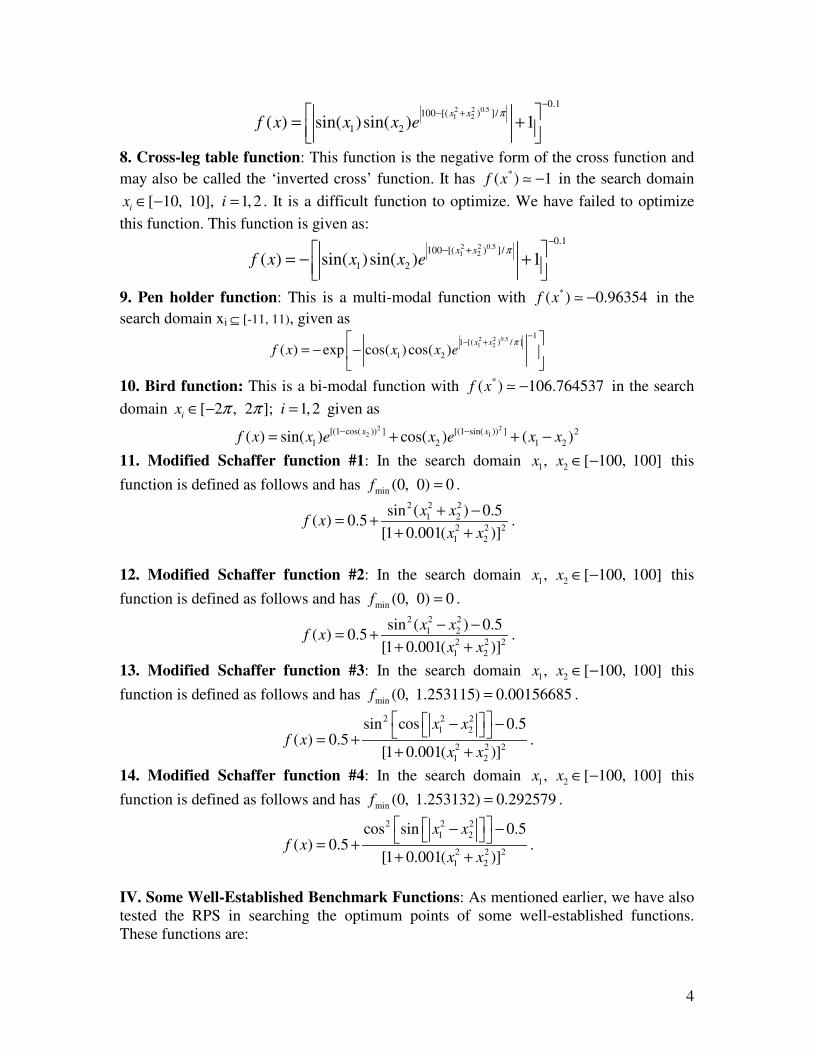
8. Cross-leg table function: This function is the negative form of the cross function and

may also be called the ‘inverted cross’ function. It has *( ) 1f x −� in the search domain

[ 10, 10], 1, 2i

x i∈ − = . It is a difficult function to optimize. We have failed to optimize

this function. This function is given as:

2 2 0.51 2

0.1100 [( ) ]/

1 2( ) sin( )sin( ) 1x x

f x x x eπ

−− +� �

= − +� ��

9. Pen holder function: This is a multi-modal function with *( ) 0.96354f x −� in the

search domain xi ⊆ [-11, 11), given as 2 2 0.51 2

11 [( ) / ]

1 2( ) exp cos( ) cos( )x x

f x x x eπ

−− +� �

= − −� ��

10. Bird function: This is a bi-modal function with *( ) 106.764537f x −� in the search

domain [ 2 , 2 ]; 1,2i

x iπ π∈ − = given as 2 2

2 1[(1 cos( )) ] [(1 sin( )) ] 2

1 2 1 2( ) sin( ) cos( ) ( )x xf x x e x e x x

− −= + + −

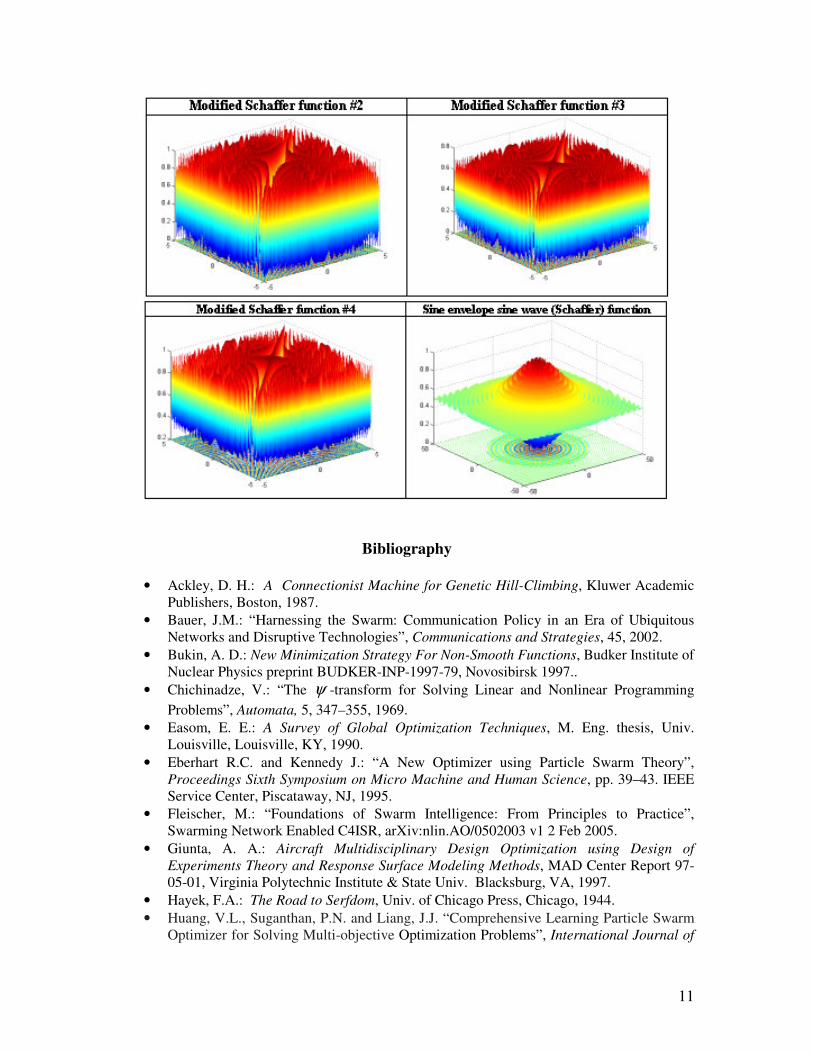
11. Modified Schaffer function #1: In the search domain 1 2, [ 100, 100]x x ∈ − this

function is defined as follows and has min (0, 0) 0f = . 2 2 2

1 2

2 2 2

1 2

sin ( ) 0.5( ) 0.5

[1 0.001( )]

x xf x

x x

+ −= +

+ +.


function is defined as follows and has min (0, 0) 0f = . 2 2 2

1 2

2 2 2

1 2

sin ( ) 0.5( ) 0.5

[1 0.001( )]

x xf x

x x

− −= +

+ +.


function is defined as follows and has min (0, 1.253115) 0.00156685f = .

2 2 2

1 2

2 2 2

1 2

sin cos 0.5( ) 0.5

[1 0.001( )]

x xf x

x x

� �� − −� �� = ++ +

.


function is defined as follows and has min (0, 1.253132) 0.292579f = .

2 2 2

1 2

2 2 2

1 2

cos sin 0.5( ) 0.5

[1 0.001( )]

x xf x

x x

� �� − −� �� = ++ +

.

IV. Some Well-Established Benchmark Functions: As mentioned earlier, we have also tested the RPS in searching the optimum points of some well-established functions. These functions are:

5

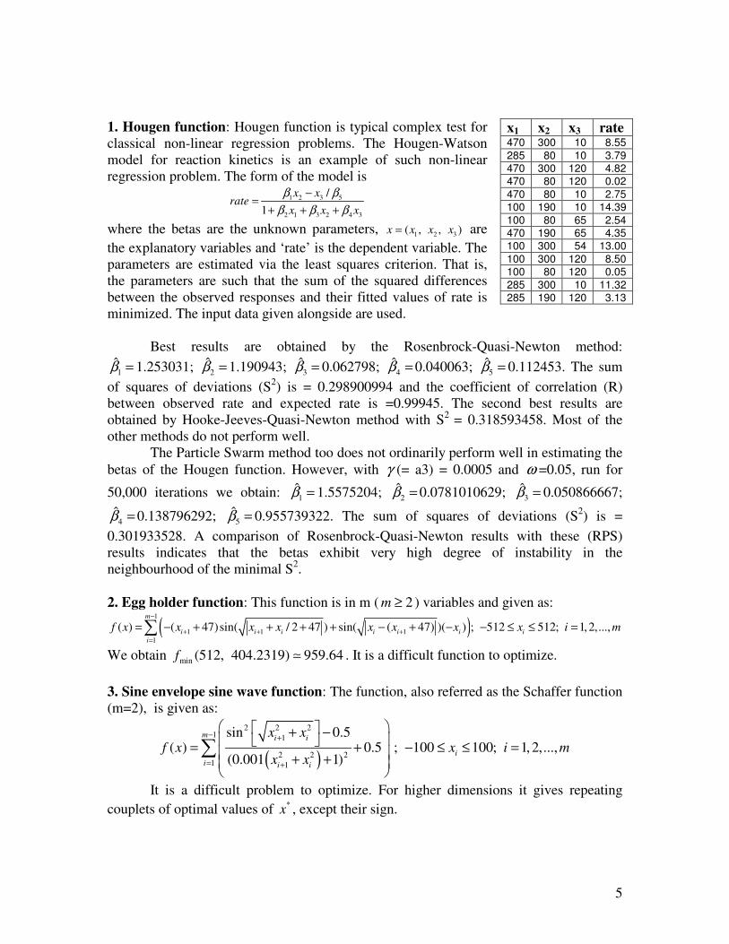
1. Hougen function: Hougen function is typical complex test for classical non-linear regression problems. The Hougen-Watson model for reaction kinetics is an example of such non-linear regression problem. The form of the model is

1 2 3 5

2 1 3 2 4 3

/

1

x xrate

x x x

β β

β β β

−=

+ + +

where the betas are the unknown parameters, 1 2 3( , , )x x x x= are

the explanatory variables and ‘rate’ is the dependent variable. The parameters are estimated via the least squares criterion. That is, the parameters are such that the sum of the squared differences between the observed responses and their fitted values of rate is minimized. The input data given alongside are used.

x1 x2 x3 rate 470 300 10 8.55

285 80 10 3.79

470 300 120 4.82

470 80 120 0.02

470 80 10 2.75

100 190 10 14.39

100 80 65 2.54

470 190 65 4.35

100 300 54 13.00

100 300 120 8.50

100 80 120 0.05

285 300 10 11.32

285 190 120 3.13

Best results are obtained by the Rosenbrock-Quasi-Newton method:

1β̂ = 1.253031; 2β̂ = 1.190943; 3β̂ = 0.062798; 4β̂ = 0.040063; 5β̂ = 0.112453. The sum

of squares of deviations (S2) is = 0.298900994 and the coefficient of correlation (R) between observed rate and expected rate is =0.99945. The second best results are obtained by Hooke-Jeeves-Quasi-Newton method with S2 = 0.318593458. Most of the other methods do not perform well.

The Particle Swarm method too does not ordinarily perform well in estimating the betas of the Hougen function. However, with γ (= a3) = 0.0005 and ω =0.05, run for

50,000 iterations we obtain: 1β̂ = 1.5575204; 2β̂ = 0.0781010629; 3β̂ = 0.050866667;

4β̂ = 0.138796292; 5β̂ = 0.955739322. The sum of squares of deviations (S2) is =

0.301933528. A comparison of Rosenbrock-Quasi-Newton results with these (RPS) results indicates that the betas exhibit very high degree of instability in the neighbourhood of the minimal S2.

2. Egg holder function: This function is in m ( 2m ≥ ) variables and given as:

( )1

1 1 1

1

( ) ( 47)sin( / 2 47 ) sin( ( 47) )( ) ; 512 512; 1,2,...,m

i i i i i i i

i

f x x x x x x x x i m−

+ + +=

= − + + + + − + − − ≤ ≤ =�

We obtain min (512, 404.2319) 959.64f � . It is a difficult function to optimize.

3. Sine envelope sine wave function: The function, also referred as the Schaffer function (m=2), is given as:

( )

2 2 21 1

2 2 21 1

sin 0.5( ) 0.5 ; 100 100; 1, 2,...,

(0.001 1)

m i i

i

i i i

x xf x x i m

x x

− +

= +

� � �+ − �� = + − ≤ ≤ = �+ + ��

�

It is a difficult problem to optimize. For higher dimensions it gives repeating

couplets of optimal values of *x , except their sign.

6

4. Chichinadze function: In the search domain 1 2, [ 30, 30]x x ∈ − this function is

defined as follows and has min (5.90133, 0.5) 43.3159f = − . 2

20.5( 0.5)2 0.5

1 1 1 1( ) 12 11 10cos( / 2) 8sin(5 ) (1/ 5) xf x x x x x eπ π − −= − + + + −

5. McCormick function: In the search domain 1 2[ 1.5, 4], [ 3, 4]x x∈ − ∈ − this function

is defined as follows and has min ( 0.54719, 1.54719) 1.9133f − − = − . 2

1 2 1 2 1 2( ) sin( ) ( ) 1.5 2.5 1f x x x x x x x= + + − − + + .

6. Levy function (#13): In the search domain 1 2, [ 10, 10]x x ∈ − this function is defined

as follows and has min (1, 1) 0f = . 2 2 2 2 2

1 1 2 2 2( ) sin (3 ) ( 1) [1 sin (3 )] ( 1) [1 sin (2 )]f x x x x x xπ π π= + − + + − + .

7. Three-humps camel back function: In the search domain 1 2, [ 5, 5]x x ∈ − this

function is defined as follows and has min (0, 0) 0f = . 2 4 6 2

1 1 1 1 2 2( ) 2 1.05 / 6f x x x x x x x= − + + + .

8. Zettle function: In the search domain 1 2, [ 5, 5]x x ∈ − this function is defined as

follows and has min ( 0.0299, 0) 0.003791f − = − . 2 2 2

1 2 1 1( ) ( 2 ) 0.25f x x x x x= + − +

9. Styblinski-Tang function: In the search domain 1 2, [ 5, 5]x x ∈ − this function is

defined as follows and has min ( 2.903534, 2.903534) 78.332f − − −� . 2

4 2

1

1( ) ( 16 5 )

2i i i

i

f x x x x=

= − +� .

10. Bukin functions: Bukin functions are almost fractal (with fine seesaw edges) in the surroundings of their minimal points. Due to this property, they are extremely difficult to optimize by any method of global (or local) optimization. In the search domain

1 2[ 15, 5], [ 3, 3]x x∈ − − ∈ − these functions are defined as follows. 2

4 2 1100 0.01 10f x x= + + ; min ( 10, 0) 0f − =

2

6 2 1 1( ) 100 0.01 0.01 10f x x x x= − + + ; min ( 10, 1) 0f − =

11. Leon function: In the search domain 1 2, [ 1.2, 1.2]x x ∈ − this function is defined as

follows and has min (1, 1) 0f = . 2 2 2

2 1 1( ) 100( ) (1 )f x x x x= − + −

12. Giunta function: In the search domain 1 2, [ 1, 1]x x ∈ − this function is defined as

follows and has min (0.45834282, 0.45834282) 0.0602472184f � . 2 16 16 1 162

15 15 50 151( ) 0.6 [sin( 1) sin ( 1) sin(4( 1))]

i i iif x x x x

== + − + − + −� .

We have obtained fmin (0.4673199, 0.4673183) = 0.06447.

13. Schaffer function: In the search domain 1 2, [ 100, 100]x x ∈ − this function is defined

as follows and has min (0, 0) 0f = .

7

2 2 2

1 2

2 2 2

1 2

sin 0.5( ) 0.5

[1 0.001( )]

x xf x

x x

� �+ −� �= +

+ +.

V. FORTRAN Program of RPS: We append a program of the Repulsive Particle Swarm method. The program has run successfully and optimized most of the functions. However, the crowned cross function and the cross-legged table functions have failed the program. VI. Conclusion: Our program of the RPS method has succeeded in optimizing most of the established functions and the newly introduced functions. The functions (namely - Giunta, Bukin, cross-legged table, crowned cross and Hougen functions in particular) that have failed the RPS program miserably may be attractive to other methods such as Simulated Annealing, Genetic algorithms and tunneling methods. Improved versions of Particle Swarm method also may be tested.

8

9

Some Well-established Benchmark Functions

10

11

Bibliography

• Ackley, D. H.: A Connectionist Machine for Genetic Hill-Climbing, Kluwer Academic Publishers, Boston, 1987.

• Bauer, J.M.: “Harnessing the Swarm: Communication Policy in an Era of Ubiquitous Networks and Disruptive Technologies”, Communications and Strategies, 45, 2002.

• Bukin, A. D.: New Minimization Strategy For Non-Smooth Functions, Budker Institute of Nuclear Physics preprint BUDKER-INP-1997-79, Novosibirsk 1997..

• Chichinadze, V.: “The ψ -transform for Solving Linear and Nonlinear Programming

Problems”, Automata, 5, 347–355, 1969.

• Easom, E. E.: A Survey of Global Optimization Techniques, M. Eng. thesis, Univ. Louisville, Louisville, KY, 1990.

• Eberhart R.C. and Kennedy J.: “A New Optimizer using Particle Swarm Theory”, Proceedings Sixth Symposium on Micro Machine and Human Science, pp. 39–43. IEEE Service Center, Piscataway, NJ, 1995.

• Fleischer, M.: “Foundations of Swarm Intelligence: From Principles to Practice”, Swarming Network Enabled C4ISR, arXiv:nlin.AO/0502003 v1 2 Feb 2005.

• Giunta, A. A.: Aircraft Multidisciplinary Design Optimization using Design of

Experiments Theory and Response Surface Modeling Methods, MAD Center Report 97-05-01, Virginia Polytechnic Institute & State Univ. Blacksburg, VA, 1997.

• Hayek, F.A.: The Road to Serfdom, Univ. of Chicago Press, Chicago, 1944.

• Huang, V.L., Suganthan, P.N. and Liang, J.J. “Comprehensive Learning Particle Swarm Optimizer for Solving Multi-objective Optimization Problems”, International Journal of

12

Intelligent Systems, 21, pp.209–226 (Wiley Periodicals, Inc. Published online in Wiley InterScience www.interscience.wiley.com) , 2006

• Jung, B.S. and Karney, B.W.: “Benchmark Tests of Evolutionary Computational Algorithms”, Environmental Informatics Archives (International Society for Environmental Information Sciences), 2, pp. 731-742, 2004.

• Kuester, J.L. and Mize, J.H.: Optimization Techniques with Fortran, McGraw-Hill Book Co. New York, 1973.

• Liang, J.J. and Suganthan, P.N. “Dynamic Multi-Swarm Particle Swarm Optimizer”, International Swarm Intelligence Symposium, IEEE # 0-7803-8916-6/05/$20.00. pp. 124-129, 2005.

• Madsen, K. and Zilinskas, J.: Testing Branch-and-Bound Methods for Global

Optimization, IMM technical report 05, Technical University of Denmark, 2000.

• Mishra, S.K.: “Least Squares Fitting of Chacón-Gielis Curves by the Particle Swarm Method of Optimization”, Social Science Research Network (SSRN), Working Papers Series, http://ssrn.com/abstract=917762 , 2006 (b).

• Mishra, S.K.: “Performance of Repulsive Particle Swarm Method in Global Optimization of Some Important Test Functions: A Fortran Program” , Social Science Research

Network (SSRN), Working Papers Series, http://ssrn.com/abstract=924339 , 2006 (c).

• Mishra, S.K.: “Some Experiments on Fitting of Gielis Curves by Simulated Annealing and Particle Swarm Methods of Global Optimization”, Social Science Research Network

(SSRN): http://ssrn.com/abstract=913667, Working Papers Series, 2006 (a).

• Nagendra, S.: Catalogue of Test Problems for Optimization Algorithm Verification, Technical Report 97-CRD-110, General Electric Company, 1997.

• Parsopoulos, K.E. and Vrahatis, M.N., “Recent Approaches to Global Optimization Problems Through Particle Swarm Optimization”, Natural Computing, 1 (2-3), pp. 235- 306, 2002.

• Prigogine, I. and Strengers, I.: Order Out of Chaos: Man’s New Dialogue with Nature, Bantam Books, Inc. NY, 1984.

• Schwefel, H.P.: Numerical Optimization of Computer Models, Wiley & Sons, Chichester, 1981.

• Silagadge, Z.K.: “Finding Two-Dimensional Peaks”, Working Paper, Budkar Insttute of Nuclear Physics, Novosibirsk, Russia, arXive:physics/0402085 V3 11 Mar 2004.

• Simon, H.A.: Models of Bounded Rationality, Cambridge Univ. Press, Cambridge, MA, 1982.

• Smith, A.: The Theory of the Moral Sentiments, The Adam Smith Institute (2001 e-version), 1759.

• Styblinski, M. and Tang, T.: “Experiments in Nonconvex Optimization: Stochastic Approximation with Function Smoothing and Simulated Annealing”, Neural Networks, 3, 467-483, 1990.

• Sumper, D.J.T.: “The Principles of Collective Animal Behaviour”, Phil. Trans. R. Soc. B. 361, pp. 5-22, 2006.

• Veblen, T.B.: The Theory of the Leisure Class, The New American library, NY. (Reprint, 1953), 1899.

• Whitley, D., Mathias, K., Rana, S. and Dzubera, J.: “Evaluating Evolutionary Algorithms”, Artificial Intelligence, 85, 245-276, 1996.

Author’s Contact: [email protected]

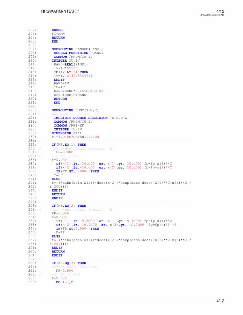
RPSWARM-NTEST.f 1/128/29/2006 6:38:42 AM

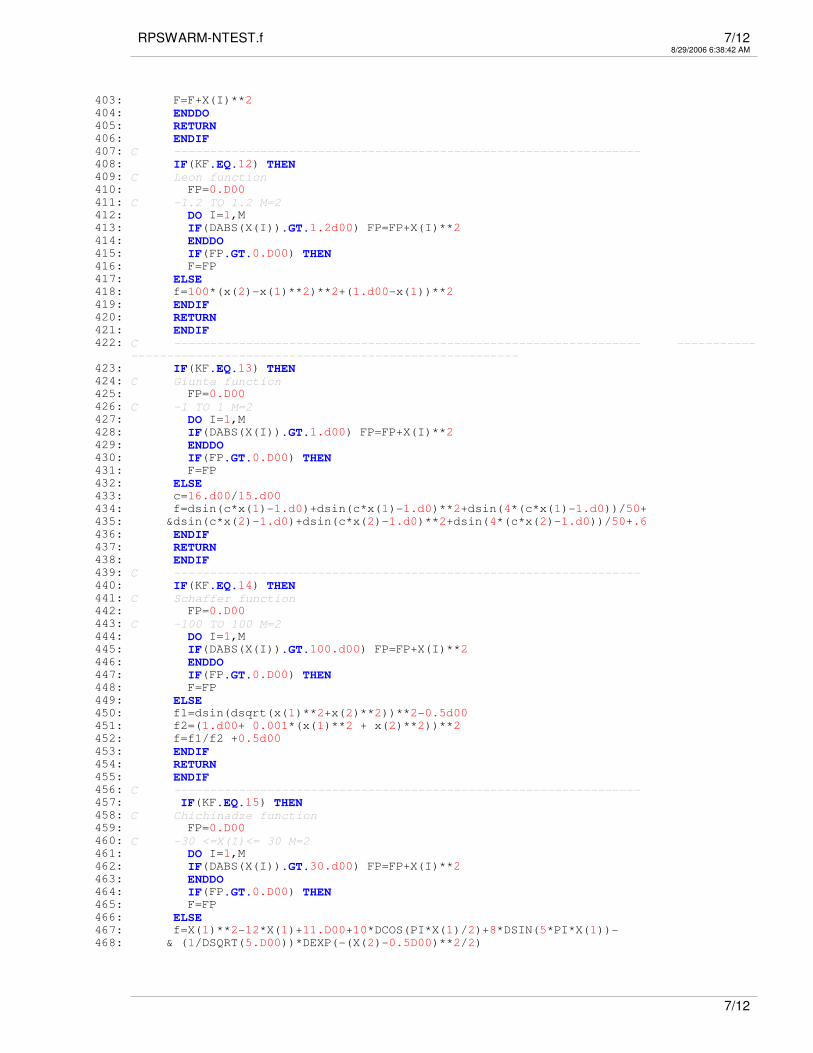
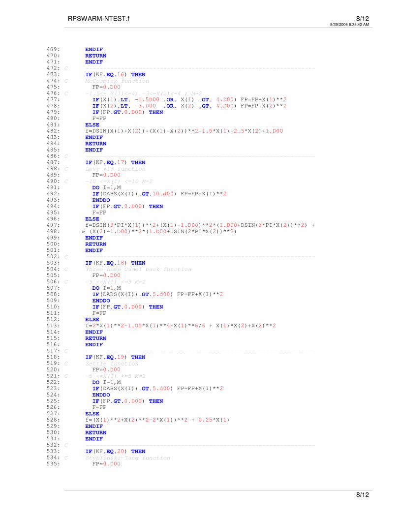
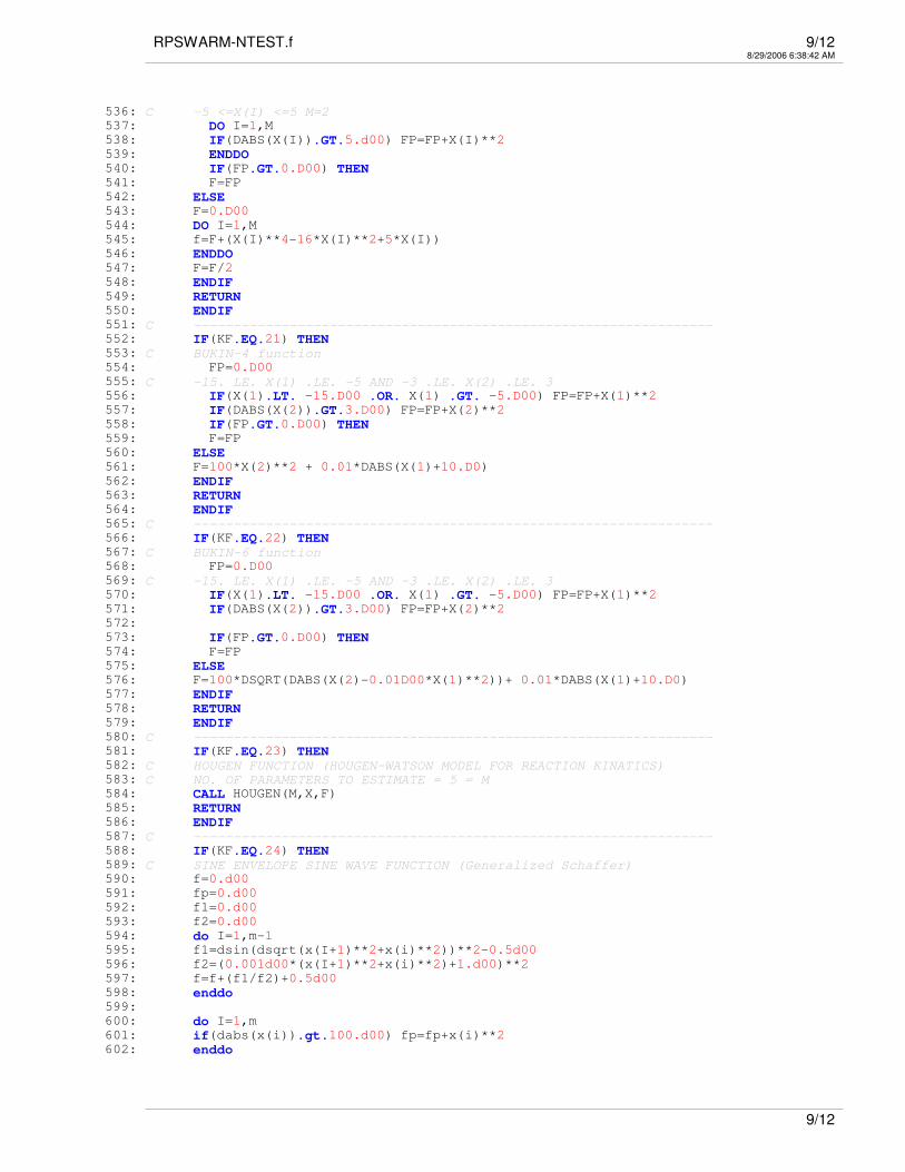
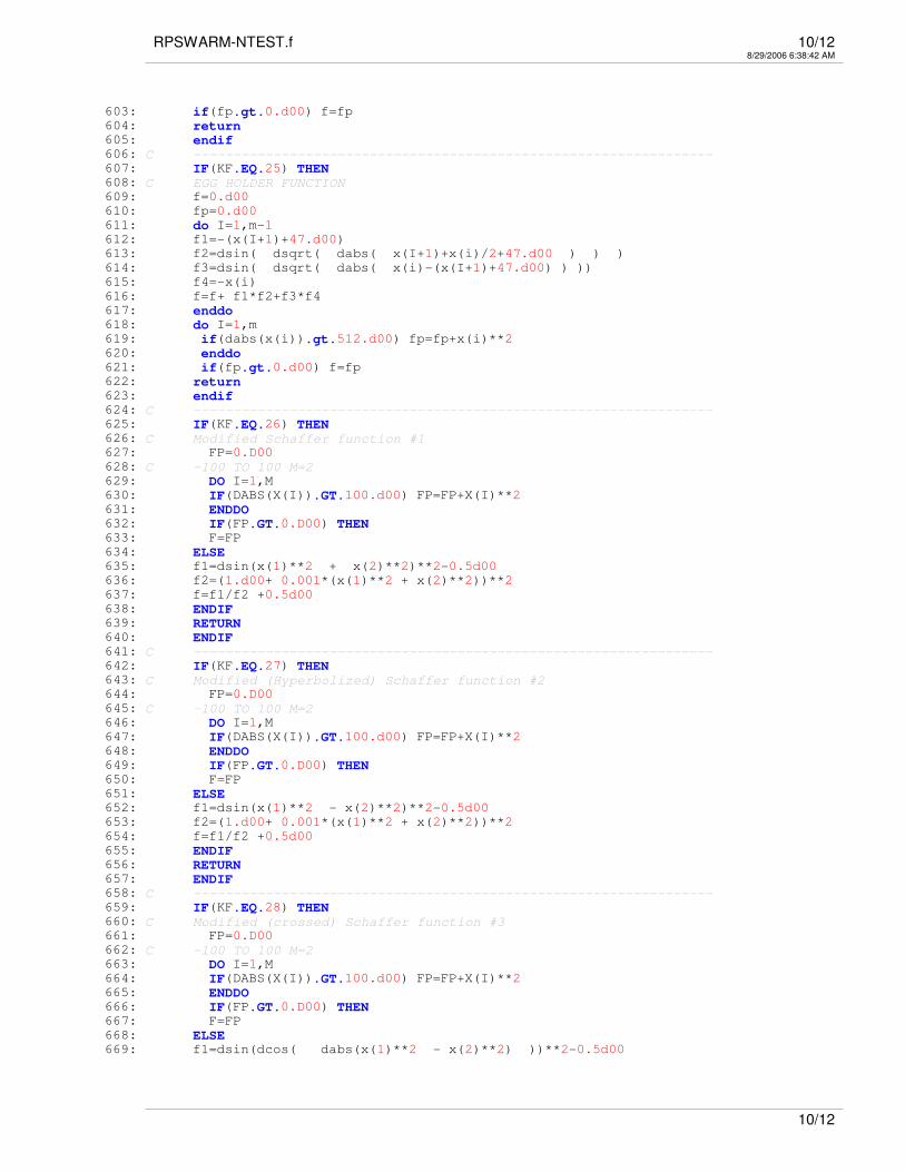
1: C PROGRAM TO FIND GLOBAL MINIMUM BY REPULSIVE PARTICLE SWARM METHOD2: C WRITTEN BY SK MISHRA, DEPT. OF ECONOMICS, NEHU, SHILLONG (INDIA)3: PARAMETER (N=50 ,NN=25 , MX=100, NSTEP=21, ITRN=5000)

4: C N = POPULATION SIZE. IN MOST OF THE CASES N=30 IS OK. ITS VALUE5: C MAY BE INCREASED TO 50 ALSO. THE PARAMETER NN IS THE SIZE OF6: C RANDOMLY CHOSEN NEIGHBOURS. 15 TO 25 (BUT SUFFICIENTLY LESS THAN7: C N) IS A GOOD CHOICE. MX IS THE MAXIMAL SIZE OF DECISION VARIABLES.8: C IN F(X1, X2,...,XM) M SHOULD BE LESS THAN OR EQUAL TO MX. ITRN IS9: C THE NO. OF ITERATIONS. IT MAY DEPEND ON THE PROBLEM. 200 TO 50010: C ITERATIONS MAY BE GOOD ENOUGH. BUT FOR FUNCTIONS LIKE ROSENBROCK11: C OR GRIEWANK OF LARGE SIZE (SAY M=20) IT IS NEEDED THAT ITRN IS12: C LARGE, SAY 5000 OR 10000.13: C THE SUBROUTINE FUNC( ) DEFINES THE FUNCTION TO BE OPTIMIZED.14:

15: IMPLICIT DOUBLE PRECISION (A-H,O-Z)

16: COMMON /RNDM/IU,IV

17: COMMON /KFF/KF

18: INTEGER IU,IV

19: DIMENSION X(N,MX),V(N,MX),A(MX),VI(MX),TIT(50)

20: DIMENSION XX(N,MX),F(N),R(3),V1(MX),V2(MX),V3(MX),V4(MX),BST(MX)

21: CHARACTER *70 TIT

22: C A1 A2 AND A3 ARE CONSTANTS AND W IS THE INERTIA WEIGHT.23: C OCCASIONALLY, TINKERING WITH THESE VALUES, ESPECIALLY A3, MAY BE24: C NEEDED.25: DATA A1,A2,A3,W /.5D00,.5D00,.0005D00,.5D00/

26: WRITE(*,*)'----------------------------------------------------'

27: DATA TIT(1)/'KF=1 TEST TUBE HOLDER FUNCTION(A) 2-VARIABLES M=2'/

28: DATA TIT(2)/'KF=2 TEST TUBE HOLDER FUNCTION(B) 2-VARIABLES M=2'/

29: DATA TIT(3)/'KF=3 HOLDER TABLE FUNCTION 2-VARIABLES M=2'/

30: DATA TIT(4)/'KF=4 CARROM TABLE FUNCTION 2-VARIABLES M=2'/

31: DATA TIT(5)/'KF=5 CROSS IN TRAY FUNCTION 2-VARIABLES M=2'/

32: DATA TIT(6)/'KF=6 CROWNED CROSS FUNCTION 2-VARIABLES M=2'/

33: DATA TIT(7)/'KF=7 CROSS FUNCTION 2-VARIABLES M=2'/

34: DATA TIT(8)/'KF=8 CROSS-LEGGED TABLE FUNCTION 2-VARIABLES M=2'/

35: DATA TIT(9)/'KF=9 PEN HOLDER FUNCTION 2-VARIABLES M=2'/

36: DATA TIT(10)/'KF=10 BIRD FUNCTION 2-VARIABLES M=2'/

37:

38: DATA TIT(11)/'KF=11 DE JONG SPHERE FUNCTION M-VARIABLE M=?'/

39: DATA TIT(12)/'KF=12 LEON FUNCTION 2-VARIABLE M=2'/

40: DATA TIT(13)/'KF=13 GIUNTA FUNCTION 2-VARIABLE M=2'/

41: DATA TIT(14)/'KF=14 SCHAFFER FUNCTION 2-VARIABLE M=2'/

42: DATA TIT(15)/'KF=15 CHICHINADZE FUNCTION 2-VARIABLE M=2'/

43: DATA TIT(16)/'KF=16 MCCORMICK FUNCTION 2-VARIABLE M=2'/

44: DATA TIT(17)/'KF=17 LEVY # 13 FUNCTION 2-VARIABLE M=2'/

45: DATA TIT(18)/'KF=18 3-HUMP CAMEL BACK FUNCTION 2-VARIABLE M=2'/

46: DATA TIT(19)/'KF=19 ZETTLE FUNCTION 2-VARIABLE M=2'/

47: DATA TIT(20)/'KF=20 STYBLINSKI-TANG FUNCTION 2-VARIABLE M=2'/

48:

49: DATA TIT(21)/'KF=21 BUKIN-4 FUNCTION 2-VARIABLE M=2'/

50: DATA TIT(22)/'KF=22 BUKIN-6 FUNCTION 2-VARIABLE M=2'/

51: DATA TIT(23)/'KF=23 HOUGEN REGRESSION FUNCTION 5-VARIABLE M=5'/

52: DATA TIT(24)/'KF=24 SINE ENVELOPE SINE WAVE FUNCTION M=? '/

53: DATA TIT(25)/'KF=25 EGG-HOLDER FUNCTION M=?'/

54: DATA TIT(26)/'KF=26 MODIFIED SCHAFFER FUNCTION #1 2-VARIABLE M=2'/




58: DATA TIT(30)/'KF=30 QUARTIC(+NOISE) FUNCTION M-VARIABLE M=?'/

59:

60: DO I=1,30

61: WRITE(*,*)TIT(I)

62: ENDDO63: WRITE(*,*)'----------------------------------------------------'

64: WRITE(*,*)'CHOOSE KF AND SPECIFY M'

65: READ(*,*) KF,M

66: DSIGN=1.D00

67: LCOUNT=0

1/12


68: WRITE(*,*)'4-DIGITS SEED FOR RANDOM NUMBER GENERATION'

69: READ(*,*) IU

70: DATA ZERO,ONE,FMIN /0.0D00,1.0D00,1.0E30/

71: C GENERATE N-SIZE POPULATION OF M-TUPLE PARAMETERS X(I,J) RANDOMLY72: DO I=1,N

73: DO J=1,M

74: CALL RANDOM(RAND)

75: X(I,J)=(RAND-0.5D00)*10

76:

77: C WE GENERATE RANDOM(-5,5). HERE MULTIPLIER IS 10. TINKERING IN SOME78: C CASES MAY BE NEEDED79: ENDDO80: F(I)=1.0E30

81: ENDDO82: C INITIALISE VELOCITIES V(I) FOR EACH INDIVIDUAL IN THE POPULATION83: DO I=1,N

84: DO J=1,M


86: V(I,J)=(RAND-.5D+00)

87: C V(I,J)=RAND88: ENDDO89: ENDDO90: ZZZ=1.0E+30

91: ICOUNT=0

92: DO 100 ITER=1,ITRN

93:

94: C LET EACH INDIVIDUAL SEARCH FOR THE BEST IN ITS NEIGHBOURHOOD95: DO I=1,N

96: DO J=1,M

97: A(J)=X(I,J)

98: VI(J)=V(I,J)

99: ENDDO100: CALL LSRCH(A,M,VI,NSTEP,FI)

101: IF(FI.LT.F(I)) THEN102: F(I)=FI

103: DO IN=1,M

104: BST(IN)=A(IN)

105: ENDDO106: C F(I) CONTAINS THE LOCAL BEST VALUE OF FUNCTION FOR ITH INDIVIDUAL107: C AND XX(I,J) IS THE M-TUPLE VALUE OF X ASSOCIATED WITH THE LOCAL BEST F(I)108: DO J=1,M

109: XX(I,J)=A(J)

110: ENDDO111: ENDIF112: ENDDO113:

114: C NOW LET EVERY INDIVIDUAL RANDOMLY COSULT NN(<<N) COLLEAGUES AND115: C FIND THE BEST AMONG THEM116:

117: DO I=1,N

118: C CHOOSE NN COLLEAGUES RANDOMLY AND FIND THE BEST AMONG THEM119: BEST=1.0E30

120: DO II=1,NN


122: NF=INT(RAND*N)+1

123: IF(BEST.GT.F(NF)) THEN124: BEST=F(NF)

125: NFBEST=NF

126: ENDIF127: ENDDO128: C IN THE LIGHT OF HIS OWN AND HIS BEST COLLEAGUES EXPERIENCE, THE129: C INDIVIDUAL I WILL MODIFY HIS MOVE AS PER THE FOLLOWING CRITERION130: C FIRST, ADJUSTMENT BASED ON ONES OWN EXPERIENCE131: C AND OWN BEST EXPERIENCE IN THE PAST (XX(I))132: DO J=1,M


134: V1(J)=A1*RAND*(XX(I,J)-X(I,J))

2/12


135: C THEN BASED ON THE OTHER COLLEAGUES BEST EXPERIENCE WITH WEIGHT W136: C HERE W IS CALLED AN INERTIA WEIGHT 0.01< W < 0.7137: C A2 IS THE CONSTANT NEAR BUT LESS THAN UNITY138: CALL RANDOM(RAND)

139: V2(J)=V(I,J)

140: IF(F(NFBEST).LT.F(I)) THEN141: V2(J)=A2*W*RAND*(XX(NFBEST,J)-X(I,J))

142: ENDIF143: C THEN SOME RANDOMNESS AND A CONSTANT A3 CLOSE TO BUT LESS THAN UNITY144: CALL RANDOM(RAND)

145: RND1=RAND


147: V3(J)=A3*RAND*W*RND1

148: C V3(J)=A3*RAND*W149: C THEN ON PAST VELOCITY WITH INERTIA WEIGHT W150: V4(J)=W*V(I,J)

151: C FINALLY A SUM OF THEM152: V(I,J)= V1(J)+V2(J)+V3(J)+V4(J)

153: ENDDO154: ENDDO155: C CHANGE X156: DO I=1,N

157: DO J=1,M

158: X(I,J)=X(I,J)+V(I,J)

159: ENDDO160: ENDDO161:

162: DO I=1,N

163: IF(F(I).LT.FMIN) THEN164: FMIN=F(I)

165: II=I

166: DO J=1,M

167: BST(J)=XX(II,J)

168: ENDDO169: ENDIF170: ENDDO171: Z=FMIN

172: IF(LCOUNT.EQ.100) THEN173:

174: LCOUNT=0

175: WRITE(*,*)'OPTIMAL SOLUTION UPTO THIS'

176: WRITE(*,*)'X = ',(BST(J),J=1,M),' MIN F = ',FMIN

177: ENDIF178: 999 FORMAT(5F15.6)

179: LCOUNT=LCOUNT+1

180: 100 CONTINUE181: WRITE(*,*)'OVER:',TIT(KF)

182: END183:

184: SUBROUTINE LSRCH(A,M,VI,NSTEP,FI)

185: IMPLICIT DOUBLE PRECISION (A-H,O-Z)

186: COMMON /KFF/KF


188: INTEGER IU,IV

189: DIMENSION A(*),B(100),VI(*)

190: AMN=1.0E30

191: DO J=1,NSTEP

192: DO JJ=1,M

193: B(JJ)=A(JJ)+(J-NSTEP/2-1)*VI(JJ)

194: ENDDO195: CALL FUNC(B,M,FI)

196: IF(FI.LT.AMN) THEN197: AMN=FI

198: DO JJ=1,M

199: A(JJ)=B(JJ)

200: ENDDO201: ENDIF

3/12


202: ENDDO203: FI=AMN

204: RETURN205: END206:

207: SUBROUTINE RANDOM(RAND1)

208: DOUBLE PRECISION RAND1


210: INTEGER IU,IV

211: RAND=REAL(RAND1)

212: IV=IU*65539

213: IF(IV.LT.0) THEN214: IV=IV+2147483647+1

215: ENDIF216: RAND=IV

217: IU=IV

218: RAND=RAND*0.4656613E-09

219: RAND1=DBLE(RAND)

220: RETURN221: END222:

223: SUBROUTINE FUNC(X,M,F)

224: C New Test Functions225: IMPLICIT DOUBLE PRECISION (A-H,O-Z)


227: COMMON /KFF/KF

228: INTEGER IU,IV

229: DIMENSION X(*)

230: PI=4.D+00*DATAN(1.D+00)

231: C -----------------------------------------------------------------232: IF(KF.EQ.1) THEN233: C Test-tube holder function (A)234: FP=0.D00

235: C -10 TO 10 M=2236: F=0.D00

237: if(x(1).lt.-10.d00 .or. x(1).gt. 10.d00) fp=fp+x(1)**2

238: if(x(2).lt.-10.d00 .or. x(2).gt. 10.d00) fp=fp+x(1)**2

239: IF(FP.GT.0.D00) THEN240: f=FP

241: ELSE242: f=-4*dabs(dsin(X(1))*dcos(x(2))*dexp(dabs(dcos((X(1)**2+x(2)**2)/

243: & 200))))

244: ENDIF245: RETURN246: ENDIF247: C -----------------------------------------------------------------248: IF(KF.EQ.2) THEN249: C Test-tube holder function (B)250: FP=0.D00

251: F=0.D00

252: if(x(1).lt.-9.5d00 .or. x(1).gt. 9.4d00) fp=fp+x(1)**2

253: if(x(2).lt.-10.9d00 .or. x(2).gt. 10.9d00) fp=fp+x(1)**2

254: IF(FP.GT.0.D00) THEN255: F=FP

256: ELSE257: f=-4*dabs(dsin(X(1))*dcos(x(2))*dexp(dabs(dcos((X(1)**2+x(2)**2)/

258: & 200))))

259: ENDIF260: RETURN261: ENDIF262: C -----------------------------------------------------------------263: IF(KF.EQ.3) THEN264: C Holder table function265: FP=0.D00

266: C -10 TO 10 M=2267: F=0.D00

268: DO I=1,M

4/12


269: IF( DABS(X(I)).GT.10.D00) FP=FP+X(I)**2

270: ENDDO271: IF(FP.GT.0.D00) THEN272: F=FP

273: ELSE274: f=-dabs(dcos(X(1))*dcos(x(2))*dexp(dabs(1.d00-(dsqrt(X(1)**2+

275: & x(2)**2)/pi))))

276: ENDIF277: RETURN278: ENDIF279: C -----------------------------------------------------------------280: IF(KF.EQ.4) THEN281: C Carrom table function282: FP=0.D00

283: C -10 TO 10 M=2284: F=0.D00

285: DO I=1,M

286: IF( DABS(X(I)).GT.10.D00) FP=FP+X(I)**2


290: ELSE291: f=-1.d00/30*(dcos(X(1))*dcos(x(2))*dexp(dabs(1.d00-

292: & (dsqrt(X(1)**2 + x(2)**2)/pi))))**2

293: ENDIF294: RETURN295: ENDIF296: C -----------------------------------------------------------------297: IF(KF.EQ.5) THEN298: FP=0.D00

299: C Cross in tray function300: C -10 TO 10 M=2301: F=0.D00

302: DO I=1,M

303: IF( DABS(X(I)).GT.10.d00) FP=FP+X(I)**2


307: ELSE308: f=-0.0001d00*(dabs(dsin(X(1))*dsin(x(2))*dexp(dabs(100.d00-(dsqrt

309: & (X(1)**2+x(2)**2)/pi))))+1.d00)**(.1)


316: C Crowned Cross function317: C -10 TO 10 M=2318: F=0.D00

319: DO I=1,M

320: IF( DABS(X(I)).GT.10.d00) FP=FP+dexp(dabs(X(I)))


324: ELSE325: f=0.0001d00*(dabs(dsin(X(1))*dsin(x(2))*dexp(dabs(100.d00-

326: & (dsqrt(X(1)**2+x(2)**2)/pi))))+1.d00)**(.1)


333: C Cross function334: C -10 TO 10 M=2335: F=0.D00

5/12


336: DO I=1,M

337:



342: ELSE343: f=(dabs(dsin(X(1))*dsin(x(2))*dexp(dabs(100.d00-(dsqrt

344: & (X(1)**2+x(2)**2)/pi))))+1.d00)**(-.1)


351: C Cross-legged table function352: C -10 TO 10 M=2353: F=0.D00

354: DO I=1,M

355:



360: ELSE361: f=-(dabs(dsin(X(1))*dsin(x(2))*dexp(dabs(100.d00-(dsqrt

362: & (X(1)**2+x(2)**2)/pi))))+1.d00)**(-.1)

363: ENDIF364: RETURN365: ENDIF366: C -----------------------------------------------------------------367: IF(KF.EQ.9) THEN368: C Pen holder function369: FP=0.D00

370: C -11 TO 11 M=2371: DO I=1,M

372: IF(DABS(X(I)).GT.11.D00) FP=FP+X(I)**2


376: ELSE377: f=-Dexp(-(Dabs(Dcos(X(1))*Dcos(X(2))*Dexp(Dabs(1.D0-(Dsqrt

378: & (X(1)**2+X(2)**2)/pi))))**(-1)))

379: ENDIF380: RETURN381: ENDIF382: C -----------------------------------------------------------------383: IF(KF.EQ.10) THEN384: C Bird function385: FP=0.D00

386: C -2Pi TO 2Pi M=2387: DO I=1,M

388: IF(DABS(X(I)).GT.2*pi) FP=FP+X(I)**2


392: ELSE393: f=(dsin(x(1))*dexp((1.d00-dcos(x(2)))**2) +

394: & dcos(x(2))*dexp((1.d00-dsin(x(1)))**2))+(x(1)-x(2))**2

395: ENDIF396: RETURN397: ENDIF398: C -----------------------------------------------------------------399: IF(KF.EQ.11) THEN400: C DE JONG SPHERE function401: F=0.D00

402: DO I=1,M

6/12


403: F=F+X(I)**2

404: ENDDO405: RETURN406: ENDIF407: C -----------------------------------------------------------------408: IF(KF.EQ.12) THEN409: C Leon function410: FP=0.D00

411: C -1.2 TO 1.2 M=2412: DO I=1,M

413: IF(DABS(X(I)).GT.1.2d00) FP=FP+X(I)**2


417: ELSE418: f=100*(x(2)-x(1)**2)**2+(1.d00-x(1))**2

419: ENDIF420: RETURN421: ENDIF422: C ----------------------------------------------------------------- -----------

------------------------------------------------------423: IF(KF.EQ.13) THEN424: C Giunta function425: FP=0.D00

426: C -1 TO 1 M=2427: DO I=1,M

428: IF(DABS(X(I)).GT.1.d00) FP=FP+X(I)**2


432: ELSE433: c=16.d00/15.d00

434: f=dsin(c*x(1)-1.d0)+dsin(c*x(1)-1.d0)**2+dsin(4*(c*x(1)-1.d0))/50+

435: &dsin(c*x(2)-1.d0)+dsin(c*x(2)-1.d0)**2+dsin(4*(c*x(2)-1.d0))/50+.6

436: ENDIF437: RETURN438: ENDIF439: C -----------------------------------------------------------------440: IF(KF.EQ.14) THEN441: C Schaffer function442: FP=0.D00

443: C -100 TO 100 M=2444: DO I=1,M



449: ELSE450: f1=dsin(dsqrt(x(1)**2+x(2)**2))**2-0.5d00

451: f2=(1.d00+ 0.001*(x(1)**2 + x(2)**2))**2

452: f=f1/f2 +0.5d00

453: ENDIF454: RETURN455: ENDIF456: C -----------------------------------------------------------------457: IF(KF.EQ.15) THEN458: C Chichinadze function459: FP=0.D00

460: C -30 <=X(I)<= 30 M=2461: DO I=1,M



466: ELSE467: f=X(1)**2-12*X(1)+11.D00+10*DCOS(PI*X(1)/2)+8*DSIN(5*PI*X(1))-

468: & (1/DSQRT(5.D00))*DEXP(-(X(2)-0.5D00)**2/2)

7/12


469: ENDIF470: RETURN471: ENDIF472: C -----------------------------------------------------------------473: IF(KF.EQ.16) THEN474: C McCormick function475: FP=0.D00

476: C -1.5<= X(1)<=4; -3<=X(2)<=4 ; M=2477: IF(X(1).LT. -1.5D00 .OR. X(1) .GT. 4.D00) FP=FP+X(1)**2

478: IF(X(2).LT. -3.D00 .OR. X(2) .GT. 4.D00) FP=FP+X(2)**2


481: ELSE482: f=DSIN(X(1)+X(2))+(X(1)-X(2))**2-1.5*X(1)+2.5*X(2)+1.D00

483: ENDIF484: RETURN485: ENDIF486: C -----------------------------------------------------------------487: IF(KF.EQ.17) THEN488: C Levy #13 function489: FP=0.D00

490: C -10 <=X(I) <=10 M=2491: DO I=1,M



496: ELSE497: f=DSIN(3*PI*X(1))**2+(X(1)-1.D00)**2*(1.D00+DSIN(3*PI*X(2))**2) +

498: & (X(2)-1.D00)**2*(1.D00+DSIN(2*PI*X(2))**2)

499: ENDIF500: RETURN501: ENDIF502: C -----------------------------------------------------------------503: IF(KF.EQ.18) THEN504: C Three-hump Camel back function505: FP=0.D00

506: C -5 <=X(I) <=5 M=2507: DO I=1,M



512: ELSE513: f=2*X(1)**2-1.05*X(1)**4+X(1)**6/6 + X(1)*X(2)+X(2)**2

514: ENDIF515: RETURN516: ENDIF517: C -----------------------------------------------------------------518: IF(KF.EQ.19) THEN519: C Zettle function520: FP=0.D00

521: C -5 <=X(I) <=5 M=2522: DO I=1,M



527: ELSE528: f=(X(1)**2+X(2)**2-2*X(1))**2 + 0.25*X(1)

529: ENDIF530: RETURN531: ENDIF532: C -----------------------------------------------------------------533: IF(KF.EQ.20) THEN534: C Styblinski-Tang function535: FP=0.D00

8/12


536: C -5 <=X(I) <=5 M=2537: DO I=1,M



542: ELSE543: F=0.D00

544: DO I=1,M

545: f=F+(X(I)**4-16*X(I)**2+5*X(I))

546: ENDDO547: F=F/2

548: ENDIF549: RETURN550: ENDIF551: C -----------------------------------------------------------------552: IF(KF.EQ.21) THEN553: C BUKIN-4 function554: FP=0.D00

555: C -15. LE. X(1) .LE. -5 AND -3 .LE. X(2) .LE. 3556: IF(X(1).LT. -15.D00 .OR. X(1) .GT. -5.D00) FP=FP+X(1)**2

557: IF(DABS(X(2)).GT.3.D00) FP=FP+X(2)**2


560: ELSE561: F=100*X(2)**2 + 0.01*DABS(X(1)+10.D0)

562: ENDIF563: RETURN564: ENDIF565: C -----------------------------------------------------------------566: IF(KF.EQ.22) THEN567: C BUKIN-6 function568: FP=0.D00

569: C -15. LE. X(1) .LE. -5 AND -3 .LE. X(2) .LE. 3570: IF(X(1).LT. -15.D00 .OR. X(1) .GT. -5.D00) FP=FP+X(1)**2

571: IF(DABS(X(2)).GT.3.D00) FP=FP+X(2)**2

572:


575: ELSE576: F=100*DSQRT(DABS(X(2)-0.01D00*X(1)**2))+ 0.01*DABS(X(1)+10.D0)

577: ENDIF578: RETURN579: ENDIF580: C -----------------------------------------------------------------581: IF(KF.EQ.23) THEN582: C HOUGEN FUNCTION (HOUGEN-WATSON MODEL FOR REACTION KINATICS)583: C NO. OF PARAMETERS TO ESTIMATE = 5 = M584: CALL HOUGEN(M,X,F)

585: RETURN586: ENDIF587: C -----------------------------------------------------------------588: IF(KF.EQ.24) THEN589: C SINE ENVELOPE SINE WAVE FUNCTION (Generalized Schaffer)590: f=0.d00

591: fp=0.d00

592: f1=0.d00

593: f2=0.d00

594: do I=1,m-1

595: f1=dsin(dsqrt(x(I+1)**2+x(i)**2))**2-0.5d00

596: f2=(0.001d00*(x(I+1)**2+x(i)**2)+1.d00)**2

597: f=f+(f1/f2)+0.5d00

598: enddo599:

600: do I=1,m

601: if(dabs(x(i)).gt.100.d00) fp=fp+x(i)**2

602: enddo

9/12


603: if(fp.gt.0.d00) f=fp

604: return605: endif606: C -----------------------------------------------------------------607: IF(KF.EQ.25) THEN608: C EGG HOLDER FUNCTION609: f=0.d00

610: fp=0.d00

611: do I=1,m-1

612: f1=-(x(I+1)+47.d00)

613: f2=dsin( dsqrt( dabs( x(I+1)+x(i)/2+47.d00 ) ) )

614: f3=dsin( dsqrt( dabs( x(i)-(x(I+1)+47.d00) ) ))

615: f4=-x(i)

616: f=f+ f1*f2+f3*f4

617: enddo618: do I=1,m

619: if(dabs(x(i)).gt.512.d00) fp=fp+x(i)**2

620: enddo621: if(fp.gt.0.d00) f=fp

622: return623: endif624: C -----------------------------------------------------------------625: IF(KF.EQ.26) THEN626: C Modified Schaffer function #1627: FP=0.D00

628: C -100 TO 100 M=2629: DO I=1,M



634: ELSE635: f1=dsin(x(1)**2 + x(2)**2)**2-0.5d00

636: f2=(1.d00+ 0.001*(x(1)**2 + x(2)**2))**2

637: f=f1/f2 +0.5d00

638: ENDIF639: RETURN640: ENDIF641: C -----------------------------------------------------------------642: IF(KF.EQ.27) THEN643: C Modified (Hyperbolized) Schaffer function #2644: FP=0.D00

645: C -100 TO 100 M=2646: DO I=1,M



651: ELSE652: f1=dsin(x(1)**2 - x(2)**2)**2-0.5d00

653: f2=(1.d00+ 0.001*(x(1)**2 + x(2)**2))**2

654: f=f1/f2 +0.5d00

655: ENDIF656: RETURN657: ENDIF658: C -----------------------------------------------------------------659: IF(KF.EQ.28) THEN660: C Modified (crossed) Schaffer function #3661: FP=0.D00

662: C -100 TO 100 M=2663: DO I=1,M



668: ELSE669: f1=dsin(dcos( dabs(x(1)**2 - x(2)**2) ))**2-0.5d00

10/12


670: f2=(1.d00+ 0.001*(x(1)**2 + x(2)**2))**2

671: f=f1/f2 +0.5d00

672: ENDIF673: RETURN674: ENDIF675: C -----------------------------------------------------------------676: IF(KF.EQ.29) THEN677: C Modified (crossed) Schaffer function #4678: FP=0.D00

679: C -100 TO 100 M=2680: DO I=1,M



685: ELSE686: f1=dcos(dsin( dabs(x(1)**2 - x(2)**2) ))**2-0.5d00

687: f2=(1.d00+ 0.001*(x(1)**2 + x(2)**2))**2

688: f=f1/f2 +0.5d00

689: ENDIF690: RETURN691: ENDIF692: C -----------------------------------------------------------------693: IF(KF.EQ.30) THEN694: C Quartic function with noise695: f=0.d00

696: FP=0.D00

697: DO I=1,M

698: IF(DABS(X(I)).GT.4.28D00) FP=FP+DEXP(DABS(X(I)))

699: ENDDO700: IF(FP.NE.0.D00) THEN701: F=FP

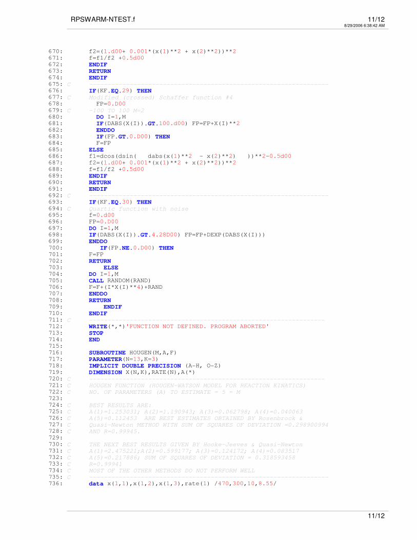
702: RETURN703: ELSE704: DO I=1,M


706: F=F+(I*X(I)**4)+RAND

707: ENDDO708: RETURN709: ENDIF710: ENDIF711: C ----------------------------------------------------------------712: WRITE(*,*)'FUNCTION NOT DEFINED. PROGRAM ABORTED'

713: STOP714: END715:

716: SUBROUTINE HOUGEN(M,A,F)

717: PARAMETER(N=13,K=3)

718: IMPLICIT DOUBLE PRECISION (A-H, O-Z)

719: DIMENSION X(N,K),RATE(N),A(*)

720: C ----------------------------------------------------------------721: C HOUGEN FUNCTION (HOUGEN-WATSON MODEL FOR REACTION KINATICS)722: C NO. OF PARAMETERS (A) TO ESTIMATE = 5 = M723:

724: C BEST RESULTS ARE:725: C A(1)=1.253031; A(2)=1.190943; A(3)=0.062798; A(4)=0.040063726: C A(5)=0.112453 ARE BEST ESTIMATES OBTAINED BY Rosenbrock &727: C Quasi-Newton METHOD WITH SUM OF SQUARES OF DEVIATION =0.298900994728: C AND R=0.99945.729:

730: C THE NEXT BEST RESULTS GIVEN BY Hooke-Jeeves & Quasi-Newton731: C A(1)=2.475221;A(2)=0.599177; A(3)=0.124172; A(4)=0.083517732: C A(5)=0.217886; SUM OF SQUARES OF DEVIATION = 0.318593458733: C R=0.99941734: C MOST OF THE OTHER METHODS DO NOT PERFORM WELL735: C -----------------------------------------------------------------736: data x(1,1),x(1,2),x(1,3),rate(1) /470,300,10,8.55/

11/12


737: data x(2,1),x(2,2),x(2,3),rate(2) /285,80,10,3.79/

738: data x(3,1),x(3,2),x(3,3),rate(3) /470,300,120,4.82/

739: data x(4,1),x(4,2),x(4,3),rate(4) /470,80,120,0.02/

740: data x(5,1),x(5,2),x(5,3),rate(5) /470,80,10,2.75/

741: data x(6,1),x(6,2),x(6,3),rate(6) /100,190,10,14.39/

742: data x(7,1),x(7,2),x(7,3),rate(7) /100,80,65,2.54/

743: data x(8,1),x(8,2),x(8,3),rate(8) /470,190,65,4.35/

744: data x(9,1),x(9,2),x(9,3),rate(9) /100,300,54,13/

745: data x(10,1),x(10,2),x(10,3),rate(10) /100,300,120,8.5/

746: data x(11,1),x(11,2),x(11,3),rate(11) /100,80,120,0.05/

747: data x(12,1),x(12,2),x(12,3),rate(12) /285,300,10,11.32/

748: data x(13,1),x(13,2),x(13,3),rate(13) /285,190,120,3.13/

749: C WRITE(*,1)((X(I,J),J=1,K),RATE(I),I=1,N)750: C 1 FORMAT(4F8.2)751:

752: F=0.D00

753: fp=0.d00

754: DO I=1,N

755: D=1.D00

756: DO J=1,K

757: D=D+A(J+1)*X(I,J)

758: ENDDO759: FX=(A(1)*X(I,2)-X(I,3)/A(M))/D

760: C FX=(A(1)*X(I,2)-X(I,3)/A(5))/(1.D00+A(2)*X(I,1)+A(3)*X(I,2)+761: C A(4)*X(I,3))762: F=F+(RATE(I)-FX)**2

763: ENDDO764: do j=1,m

765: if(dabs(a(j)).gt.5.d00) fp=fp+dexp(dabs(a(j)))

766: enddo767: if(fp.gt.0.d00) f=fp

768: RETURN769: END

12/12

Some new test functions for global optimization and ...

Documents