Some kanban-controlled manufacturing systems: a first stability analysis

kanban: 12/15/'94Some kanban{controlled manufacturing systems:a �rst stability analysisThomas I. SeidmanDepartment of Mathematics and StatisticsUniversity of Maryland Baltimore CountyBaltimore, MD 21228, USA(410)-455-2438e-mail: [email protected] de Matem�atica e EstatisticaUniversidade de S~ao PauloCarlos Humes Jr.Departamento de Ciencia de Computa�c~aoUniversidade de S~ao PauloS~ao Paulo, SP, Brasile-mail: [email protected]: The blockage/starvation patterns of known instability examples suggestusing local demand information | which is precisely what is provided by the widelyadvocated kanban approach to ow control in manufacturing systems. Therefore, wehave re-analyzed for stability the examples described in the 1990 Kumar{Seidman paperwhen modi�ed by introducing kanban control. It is found that this does not ensurestability and, in fact, some surprising new instability phenomena arise.Key Words: manufacturing systems, instability, kanbans, decentralized, schedulingcontrol.1

1. IntroductionThe stability of various decentralized scheduling policies for manufacturing systemshas been explored in numerous papers [10], [6], [8], [3], [9], [5], [12], [7], [11], [1]. Wenote that all of these analyses (except [12]) have concerned themselves with what wemay call ow-driven systems in which the scheduling of each machine is dependent onlyon the contents of the product bu�ers and such locally available information as mightbe carried by this product ow. In observing that the ow blockages occurring in knowninstability examples [6], [11], [1] might be alleviated by informing a supplier of impending`starvation', one is led to conjecture a likelihood of greater stability for demand-drivensystems, with dual ows of product and of controlling orders.This conjecture is somewhat strengthened by the popularity of one such approach,the kanban, as a scheduling control mechanism. We note that kanban systems have beenwidely advocated and widely implemented although, to the best of our knowledge, therehas been no mathematically rigorous analysis of their stability properties.Thus we are led to test the e�cacy of the kanban structure as a possible stabilizingcontrol mechanism speci�cally against the challenge posed by the context of CAF policieswithin which were found the �rst two known instability examples for ow-driven systems.The results of our investigation turn out to be interesting and somewhat unanticipated:they surprised us.� For the �rst example from [6] one �nds that the kanban structure has little e�ecton the instability mechanism: as for the ow-driven case analyzed in [6] and forthe identical parameter range1 one develops a pattern of mutual blockage whichrepeats on an ever-increasing scale. What is new, here, is a threshhold e�ect2 forthe initiation of this pattern, with the threshhold increasing when the number ofkanbans for the links, i.e., the speci�ed reserve supply levels, would be increased.� For the second example from [6], involving a single re-entrant line, one obtains withkanban operation a threshhold e�ect again and also a new instability criterion:� + �� > 1 with � < 1. Here, although one does not always have stability, moreof the parameter space now corresponds to the stable range; compare (3.1). Since� depends on a ratio of kanban speci�cations, we have the surprising fact thatincreasing the reserve supply level for some link may actually have the e�ect ofdestabilizing the system as a whole. Further, for this example we see a previouslyunobserved instability mechanism in which operation is essentially time-periodic,except for a single unboundedly growing demand bu�er, rather than repeating onan increasing scale.� Finally, noting that it had been shown [10] that CAF policies are always stable foracyclic ow-driven systems, we attempted to obtain the corresponding result using1This is taken in tems of the \slow" processing times �; � | which in [6] determined the stabil-ity/instability according as � + � < 1 or > 1 when one normalizes to have unit demand rates.2This corresponds, roughly, to a protective indi�erence to operational uctuations and limited bursti-ness of the input ow | here, demand rather than product arrivals. We have indicated this brie y |and suggest that this may explain why, with on-line tuning, instability is not observed in practice |but in this paper we have not attempted any formal analysis or proof of this e�ect.2

the kanban structure | and, instead, obtained our Example C, demonstrating thepossibility of instability in this setting as well.2. Kanban systems: formulation and notationWe are considering a model for ow in a manufacturing system which, in manyrespects, follows the formulation of [10], etc. Thus, we have a �nite set of tasks, indexedby i, with each task assigned to a machine Mm; we write m(i) for the machine index massociated with the task i and correspondingly write i 2 Mm, identifying the machinewith the set of its assigned tasks. Further, each task i is associated with a product streamPp corresponding to a material ow of (items of) some product indexed by p = p(i).We assume a �xed (pre-speci�ed) sequencing of tasks within each product stream so theset Pp has a linear order (i1; : : : ; iJ). We write i� and i+ for the predecessor and thesuccessor (within Pp) of a task i, where this is meaningful, and denote by i�(p) and i�(p)the initial and terminal tasks, respectively.It may be possible to index the machines in such a way that one always has m(i+) �m(i). In this case we call the system geometry acyclic; if there is no such ordering of themachines (as is the case for our Examples A and B), we call the geometry non-acyclicor re-entrant. [For our examples we index the tasks so i� = i � 1, etc., but this isinessential.]The standard paradigm of queueing theory, followed in [10], etc., presumes a se-quence of arrivals at the initial task of each product stream with the system `pushed' bythe incoming ow to maintain production. Our present paradigm is to reverse this soprocessing will only be done `as ordered' | i.e., we presume a sequence of orders arriv-ing to the terminal task of each product stream and view ourselves as processing orderswhich are transmitted in the product stream geometry in the direction opposite to ourtask sequencing and which `pull' the concommittant ow and processing of product. Tospecify the operation of the manufacturing system it is now necessary to specify boththe protocol for transmitting orders within the system and also the scheduling protocolfor processing products at each machine when there may be competing tasks.While this `pull' framework provides attractive alternatives to the `push systems'analyzed in [10], etc., it is clear that the analysis is now complicated by the necessity toprovide two sets of protocols and to track two ows through the system: of orders andof products. We note also that the double ow can be expected to blur the distinctionbetween acyclic geometries (which will no longer possess the inductive causality theyhave for `push' systems) and non-acyclic geometries.In general, for pull systems, one will have for each task both a `demand bu�er'of as-yet-unful�lled orders and a bu�er of product available for processing. For presentpurposes we make no further di�erentiation (e.g., as to `urgency') and it will be su�cientfor our analysis to note only the levels of these bu�ers; thus, ki(t) will denote the numberof orders awaiting (at time t) processing for task i, while xi(t) will denote the `supplylevel' of available product there.The kanban mechanism is a standard protocol for transmitting orders: it assumesspeci�cation3 of a reserve supply level Ki so that orders (kanbans) are transmitted from3Physically, one thinks of a �xed number Ki of `tokens' (or `order cards', to take a somewhat more3

i to i� as xi(t) drops below Ki. One might have some initial stock above the reservesupply level which would be utilized without replacement but, after that, one alwayshas the identity xi(t) + ki�(t) � Ki(2.1)(where we ignore any transit times for product or kanbans). This identity is to hold forall tasks which have internal suppliers, i.e., which are not the initial tasks for productstreams. For an initial task, we will suppose that product is always available as needed| e�ectively, that xi�(p)(t) � 1, although we do not count this as `work-in-process'(WIP). For a terminal task, the demand bu�er does not consist of internally issuedkanbans but of external demand and, without any equivalent of (2.1), we writeki�(p)(t) =: zp(t):(2.2)We denote by Xi(t) the total (cumulative) number of items of product processed at taski by time t and, similarly, we denote by Zp(t) the total number of orders received ati�(p) by time t, including any unful�lled demand present in the system at the initialtime. Then, for t > s, simple bookkeeping givesXi�(t)�Xi�(s) = [Xi(t)�Xi(s)] + [xi(t)� xi(s)]:(2.3)for each intermediate task i or, equivalently for the task i+ in view of (2.1),[ki(t)� ki(s)] + [Xi(t)�Xi(s)] = Xi+(t)�Xi+(s)(2.4)For terminal tasks we have, instead,[zp(t)� zp(s)] + [Xi�(p)(t)�Xi�(p)(s)] = [Zp(t)� Zp(s)]:(2.5)In general, a processing protocol (scheduling policy) will schedule the activity of eachmachineMm in terms of the values of fki; xi : i 2 Mmg. For our present purposes, wewill be considering scheduling policies in which a single task can be enabled at any time.We then distinguish three types of possible states !m(t) :Ai (task i is enabled and active)Ii (task i is enabled but inactive: the machine is `waiting')S i0i (task i is `becoming enabled' in transition from the prior enabled task i0)literal translation of the Japanese word `kanban') which would be attached to the stock of product ati when this is at its desired reserve level. When an item of this stock is utilized, the attached token isremoved from the product item and transmitted as an order to the `supplier' (predecessor) i�, to bereturned attached to the replacement item when that order is ful�lled to resupply the reserve. See, e.g.,Chapter 13 of [2] for a more detailed description; our model is there called a `one card' kanban system.An alternative interpretation occurs in the Queueing Theory literature as a discipline `with blocking':there one may assume that the supply bu�er for task i has capacity Ki and that the prior server is`blocked' (from task i�) if this bu�er is already full. One easily sees that this is precisely equivalent tothe kanban mechanism for this link. 4

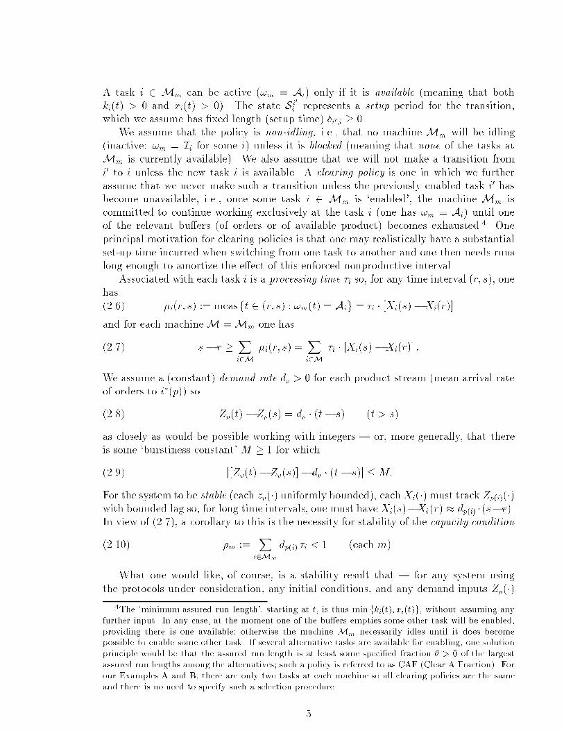
A task i 2 Mm can be active (!m = Ai) only if it is available (meaning that bothki(t) > 0 and xi(t) > 0). The state S i0i represents a setup period for the transition,which we assume has �xed length (setup time) �i0;i � 0.We assume that the policy is non-idling, i.e., that no machine Mm will be idling(inactive: !m = Ii for some i) unless it is blocked (meaning that none of the tasks atMm is currently available). We also assume that we will not make a transition fromi0 to i unless the new task i is available. A clearing policy is one in which we furtherassume that we never make such a transition unless the previously enabled task i0 hasbecome unavailable, i.e., once some task i 2 Mm is `enabled', the machine Mm iscommitted to continue working exclusively at the task i (one has !m = Ai) until oneof the relevant bu�ers (of orders or of available product) becomes exhausted.4 Oneprincipal motivation for clearing policies is that one may realistically have a substantialset-up time incurred when switching from one task to another and one then needs runslong enough to amortize the e�ect of this enforced nonproductive interval.Associated with each task i is a processing time �i so, for any time interval (r; s), onehas �i(r; s) := measft 2 (r; s) : !m(t) = Aig = �i � [Xi(s)�Xi(r)](2.6)and for each machineM =Mm one hass� r � Xi2M �i(r; s) = Xi2M �i � [Xi(s)�Xi(r)] :(2.7)We assume a (constant) demand rate dp > 0 for each product stream (mean arrival rateof orders to i�(p)) so Zp(t)� Zp(s) = dp � (t� s) (t > s)(2.8)as closely as would be possible working with integers | or, more generally, that thereis some `burstiness constant' M � 1 for whichj[Zp(t)� Zp(s)]� dp � (t� s)j �M:(2.9)For the system to be stable (each zp(�) uniformly bounded), eachXi(�) must track Zp(i)(�)with bounded lag so, for long time intervals, one must have Xi(s)�Xi(r) � dp(i) �(s�r).In view of (2.7), a corollary to this is the necessity for stability of the capacity condition�m := Xi2Mm dp(i) �i < 1 (each m).(2.10)What one would like, of course, is a stability result that | for any system usingthe protocols under consideration, any initial conditions, and any demand inputs Zp(�)4The `minimum assured run length', starting at t, is thus min fki(t); xi(t)g, without assuming anyfurther input. In any case, at the moment one of the bu�ers empties some other task will be enabled,providing there is one available; otherwise the machine Mm necessarily idles until it does becomepossible to enable some other task. If several alternative tasks are available for enabling, one solutionprinciple would be that the assured run length is at least some speci�ed fraction � > 0 of the largestassured run lengths among the alternatives; such a policy is referred to as CAF (Clear A Fraction). Forour Examples A and B, there are only two tasks at each machine so all clearing policies are the sameand there is no need to specify such a selection procedure.5

satisfying (2.9), subject to (2.10) | one would have each zp(�) bounded (uniformly intime t > 0). The point of this paper is that there are quite simple and `natural' systemsfor which this is false when using a kanban mechanism to transmit orders with a clearingpolicy to schedule production.3. Three examplesTo study the question of stability of systems operating with kanbans we shall startby analysing systems that have already been shown to be unstable under ow-drivenclearing policies. The earliest known examples were the two presented in [6]. Each-� ca a41 c32�� Example A � ca a41 c32 ���� Example Bexample is a system with two machines, each with two tasks. In each machine there is acomparatively slower task (indicated by an open dot in the �gure). In [6], it was shownthat, under unit input rates, instability was obtained if the processing times satis�ed an`instability condition' � + � > 1:(3.1)Those examples were themselves a response to the earlier general conjecture of stabilityof systems operating under CAF, presented in [10], where stability was proved for acyclicnetworks.For our present analysis | of systems under a clearing policy for production, much asin [6], and with order transmission now governed by a kanban mechanism| we assumethe geometries, the demand rates, and the processing times for tasks are �xed, the reservesupply levels (numbers of kanbans) for each link then chosen in some fashion. Thisspeci�es a well-de�ned dynamical system. We then assume that the initial conditions(from which we begin tracking the scenarios) may be imposed arbitrarily. To simplifythe exposition, we normalize to unit demand rates and assume negligible burstiness, i.e.,each dp = 1 and M = 1 in (2.9). For the �rst two examples we also neglect set-uptimes, taking each �i0;i = 0. In this case we can use a simpli�ed set of activity states: wewrite um = i rather than !m = Ai and write um = � when Mm is blocked; the vectoru = (u1; u2) then gives the complete activity state for the system as a whole.3:A. Two product streamsThe �rst example is a two product system with two machines, corresponding toExample A above. As in [6], we shall consider that \fast" tasks feed \slower" tasks, i.e.,given ��� = (�; �; "; �), we have �; " � �; � . The idea of reserve supply level applies onlyto tasks 2 and 4 and the corresponding numbers of available kanbans are respectivelyK2 and K4; to avoid some expositional complications, we assume that K2;K4 > 2.6

-� f41 fss 32k1[ x4 k3x2 ] ��z2 z1M1 M2Example AWe begin tracking this system at a moment t0 corresponding to the completion atM1 of a clearing run for task 4 due to exhaustion of the demand bu�er there, i.e.,z2(t0) = 0. As initial condition, we assume that we havex4 = K4; k3 = 0; for P2 and x2 = 0; k1 = K2 for P1(3:A.1)at t = t0 with `large' unful�lled demand z1(t0) = A. At this initial moment M2 isnecessarily idle (with task 2 starved for supplies and task 3 starved for demand), sothe control state has just become u(t0) = (1; �). The now-enabled operation of task 1,with its rapid processing time, means that supply is quickly provided to task 2, enablingu2 = 2 at time t0 + �.We are looking for a scenario in which the clearing run just initiated atM2 will endby exhaustion of the unful�lled demand z1. This run terminates at the time t0+ T andn new orders will have arrived for P1 by then: M2 will have processed A + n items,taking time T � � = � (A+ n) to make z1 = 0. To within an uncertainty of at most 1order (corresponding to the uncertain relation of the times t0 and t0+ �+T to the exactarrival times for the orders; compare (2.9) with d1 = 1, M = 1), we have n � T so, for�� � , one has T � A�=(1� � ):(3:A.2)Of course, to have such a scenario requires that the product bu�er at task 2 shouldnever become exhausted during this interval (x2 > 0) and we must determine conditionsensuring this. It should be emphasized that we make no claim that these conditions areactually necessary for instability, only that we will have shown an instability examplewhen they do hold.With task 1 enabled at M1 and � � � , it is clear that the clearing run at task 1ends long before t0 + T . Indeed, M1 will process (K2 + A + n) items in the interval[t0; t0+T ], taking total time �(K2+A+n) which will be much less than T�� = � (A+n)if, say, A > K2. Thus, since T will be large for A large, there must be (approximately)n arrivals at task 4 of orders for the P2 demand bu�er so task 4 will certainly becomeenabled. To ensure that the scenario does proceed as we are describing it, it is onlynecessary to ensure that task 4 never has a clearing run long enough for processing attask 2 to empty its reserve supply bu�er while task 1 is being temporarily blocked |i.e., since we necessarily have x2 = K2 at the beginning of such an `intermediate' run at7

task 4, we must ensure that �K2 � [run length] + �:(3:A.3)Since we are considering a period during which task 3 is blocked by task 2, the lengthof any run at task 4 is necessarily bounded by �K4; however, this bound is inadequate forour purpose without imposing undesirable conditions on the choices of K2;K4 in relationto �; � . Alternatively, the run length here can be bounded in terms of the length T1 ofthe preceding clearing run with u = (1; 2) which ends when the demand bu�er at task 1is exhausted. This will be longest for the �rst run at task 1, since that commences withk1 having its maximum value K2. M1 then processes the K2 items already (initially)ordered at task 1 but, meanwhile, new orders will have been received from M2 so thisrun corresponds to processing K2+n0 items, taking time T1 := �(K2+n0). This requires,of course, that n0 kanbans are received to task 1 from M2 so (n0 � 1) items must havebeen completed at task 2, taking time � (n0 � 1). Thus,� + � (n0 � 1) < �(K2 + n0) =: T1 � � + �n0i.e., n0 = j(K2 � 1) ����k ; T1 = � jK2������ k � �K2(3:A.4)Letting T2 be the time for which one then has u = (4; 2), we see that T2 = �n00 where n00is the number of orders arriving for P2 during the interval since task 4 was previouslycleared. To within an uncertainty of 1 order, we have n00 � T1 + T2 � (�K2 + T2)so T2 � [�=(1 � �)]�K2. Comparing this to the requirement (3:A.3), we see that |essentially independently of the size of K2 | we need � small enough to have�1� �� < �(3:A.5)to ensure that the scenario proceeds here as described.We now consider the situation at the time t1 = t0 + T when the demand bu�er attask 2 is �nally emptied. If A was initially large, making T proportionately large by(3:A.2), there will have been plenty of slack time at M1 to have not only kept x2 � K2but also to have, altogether, cleared the reserve supply at task 4 of its original K4items | necessarily unreplenished because task 3 has been blocked throughout. Asalready noted, the number of orders arriving for P2 during this period will also havebeen approximately the same n � T as for P1 so that the unful�lled demand is thenz2(t1) =: A0 = n�K4 � �1� � A�K2(3:A.6)by (3:A.2). At t1 the state will thus bex2 = K2; k1 = 0; for P1 and x4 = 0; k3 = K4 for P2(3:A.7)with z = (0; A0) and u = (�; 3).This state is, of course, essentially a `mirror image' of the initial state and, assumingA0 is large enough, essentially the same argumentmutatis mutandis shows that at a time8

t2 we will again complete a clearing run at task 4 with the state given again by (3:A.1)and now with z = (A00; 0) where, as in obtaining (3:A.6), we now havez1(t2) =: A00 � �1��A0 �K4� �A� h �1��K4 +K2iwith � := ��(1��)(1��):(3:A.8)To have z1(t2) > z1(t0), we must then require that � > 1 and that A is large enough5that (�� 1)A > � �1 � �K4 +K2� :(3:A.9)Note that �� 1 = (� + � � 1)=(1 � �)(1� � ) so� > 1 (giving instability) , � + � > 1:(3:A.10)Asymptotically, we may eventually ignore the constant term [�=(1��)]K4+K2 in (3:A.8)and see that each cycle repeats the same pattern with the unful�lled demand multipliedrepeatedly by the factor �. Of course, the cycle time is also scaled proportionately, sothe increase of unful�lled demand will be approximately linear in time: the long-timeaverage rate of increase of total WIP (z1+z2) uctuates boundedly | although withouta limit unless � = � > 1=2, in which case this is (2� 1=� ).We observe that (3:A.10) is precisely the instability condition (3.1) of [6]. There is,however, an interesting di�erence, which we term a threshhold e�ect. If, rather thantaking A large initially, we were to consider the system in operation subject to theburstiness condition (2.9), it is easy to see that a burst of demand permitted by (2.9)could also initiate the pattern described (if M is large enough) with the possibilitythat this might grow over some repetitions to the point where corresponding periods ofreduced demand, also permitted by (2.9), could no longer interrupt the pattern. To theextent that the burstiness of (2.9) is random, one might expect this to occur (eventually)with probability 1 if possible at all. This possibility is essentially equivalent to havingM larger than the minimal A described above, which increases with the Kj so, lookingat the converse, the instability cannot occur if K2;K4 are large enough in comparisonwith a given M . This is consistent with the viewpoint of seeing kanbans as a stabilizingdevice to insulate the system from the e�ect of sudden uctuations in demand.3:B. A single re-entrant lineWe next analyze stability under kanban control for the second example [6] under theassumption � + � < �;(3:B.1)which will be needed later to ensure that the scenario proceeds as described.5We could think of this analysis as beginning at t1 and some simple algebra shows that the corre-sponding condition (� � 1)A0 > � �1� � K2 +K4� :is precisely equivalent to (3:A.9). 9

� f41 fss 32�� k1[ x4 k2[ x3k3z x2 ] $%M1 M2Example BWe begin tracking this system also at a moment t0 corresponding to the completionat M1 of a clearing run for task 4 | now due to exhaustion of the product bu�er, i.e.,x4(t0) = 0. As initial condition, we assume that we have, then,k3 = K4; x4 = 0; k2 = K3; x3 = 0; k1 = K2; x2 = 0(3:B.2)with `large' unful�lled demand z(t0) = A.Note that at this initial momentM2 is necessarily idle (with both tasks starved forsupplies), so the control state is u(t0) = (1; �), but the now-enabled operation of task 1,with its rapid processing time, means that supply is quickly provided to task 2, enablingu2 = 2, which we take as characterizing the �rst phase of this scenario.Once task 1 is begun atM1, it will clear the demand indicated by the initial conditionk1(t0) = K2. Thus, noting that task 1 is assumed much faster than task 2, M2 will beadequately supplied to ensure that it will continue task 2 without interruption at leastuntil completing minfK2; x2(t0) = K3g items | and, indeed, since task 3 is blockedduring this and so cannot replenish the supply for task 4, M1 will continue to resupplythe product bu�er for task 2. Thus we continue to have u2 = 2 until the demand bu�erfor task 2 is cleared, ending this phase, precisely after M2 has processed K3 items. Wenote that at this point (time t = t1 = t0 + "+K3� ) we havek1 = 0; x2 = K2; k2 = 0; x3 = K3; k3 = K4; x4 = 0(3:B.3)and that the combined number of items x2 + x3 at t1 is just K2 +K3.The clearing of the demand bu�er for task 2 enables task 3 at M2 (i.e., u2 = 3)so, much as above, product is rapidly supplied for task 4, which then permits u1 = 4(at time t = t1 + �), which we take as characterizing the second phase of the scenario.One has, �rst, that K = minfK3;K4g items are processed at task 3 while the samenumber of kanbans are sent to the demand bu�er for the blocked task 2, after whichone has u2 = 2 while M2 clears at task 2 at the time t = t� = t1 + K� + ~K� byprocessing ~K = minfK; x2(t1) = K2g = minfK2;K3;K4g items without interruption.The condition (3:B.1) was imposed just to ensure that there is now still su�cient timefor task 3 to recommence and begin resupplying the product bu�er for task 4 beforeM1clears the stock of K supplied earlier; thus (3:B.1) ensures the uninterrupted continuationof task 4 at M1. Continued tracking along the same lines easily shows that one has10

u1 = 4 precisely until M1 has processed at task 4 a total of K2 + K3 items (i.e., onehas processed all of the items which were in the product bu�ers x2; x3 at time t1) sincetask 1 is necessarily blocked during this phase so no new product can be brought intothe system.The second phase then ends at the time t = t2 given byt2 = t1 + � + (K2 +K3)� = t0 + � + "+K3� + (K + 2 +K3)�;having processed, altogether, K2 + K3 items at task 4 to meet the initial unful�lleddemand. The `internal' state of the system is now again exacly as in (3:B.2), so | apartfrom the level z of the external demand bu�er | the same cycle will repeat exactlyso long as z remains positive. During each cycle one has (with unit demand rate) thearrival of new demand in the form of (approximately)[t2 � t0] = � + "+K3� + (K + 2 +K3)�new orders. Thus (to within this approximation and neglecting the comparatively smallquantities �; "), one hasz(t2)� z(t0) � (t2 � t0)� (K2 +K3)� (K2 +K3) h�� + K3K2+K3 ��� 1i :(3:B.4)This is positive precisely when one has� + �� > 1 � := 11 +K2=K3(3:B.5)and z then steadily increases with an average increase of1 � K2 +K3K3� + (K2 +K3)�per unit time.Note that this situation is rather di�erent from that of [6] | and from any previouslyknown example of instability | in that instability occurs with repetition on a �xed scale,rather than an exponentially increasing scale. Since one always has � < 1 in (3:B.5),this instability condition is favorably comparable to the instability condition (3.1) givenfor the `same' manufacturing system in [6] under ow-driven (`push') operation: thekanban mechanism helps, although it does not ensure stability. For �xed processingtimes satisfying (2.10) one can always obtain stability by making K2 large enough (for�xed K3). However, if � + � > 1, then increasing K3 su�ciently (for �xed K2) willactually make a stable situation unstable. Our earlier requirement of `large' initialunful�lled demand indicates that, as for Example A, the kanban mechanism provides athreshhold e�ect, insulating to some extent against occurrence of this instability.3:C. An `acyclic' instability exampleFor acyclic ow-driven systems, we know (cf., e.g., [5]) that: if each machine isgoverned by a `usable policy' (i.e., stable for inputs of bounded burstiness in the single-server context), then the system is stable globally. For demand-driven systems with11

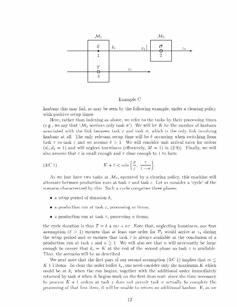
--f31" fs 2k1 x2 ] �� z2 z1M1 M2Example Ckanbans this may fail, as may be seen by the following example, under a clearing policywith positive setup times.Here, rather than indexing as above, we refer to the tasks by their processing times(e.g., we say that `M2 services only task �'). We will let K be the number of kanbansassociated with the link between task " and task �, which is the only link involvingkanbans at all. The only relevant setup time will be � occurring when switching fromtask � to task " and we assume � > 1. We will consider unit arrival rates for orders(d1; d2 = 1) and will neglect burstiness (e�ectively, M = 1) in (2.9)). Finally, we willalso assume that " is small enough and � close enough to 1 to haveK + 1 < min��" ; �1 � � � :(3:C.1)As we just have two tasks at M1, operated by a clearing policy, this machine willalternate between production runs at task � and task ". Let us consider a `cycle' of thescenario characterized by this. Such a cycle comprises three phases:� a setup period of duration �,� a production run at task ", processing m items,� a production run at task � , processing n items;the cycle duration is thus T = � +m"+ n� . Note that, neglecting burstiness, our �rstassumption (� > 1) ensures that at least one order for P1 would arrive at z1 duringthe setup period and so ensures that task � is always available at the conclusion of aproduction run at task " and n � 1. We will also see that n will necessarily be largeenough to ensure that k" = K at the end of the second phase so task " is available.Thus, the scenario will be as described.We next note that the �rst part of our second assumption (3:C.1) implies that m �K+1 items. To clear the order bu�er k", one need consider only the maximumK whichcould be at k" when the run begins, together with the additional order immediatelyreturned by task � when it begins work on the �rst item sent: since the time necessaryto process K + 1 orders at task " does not permit task � actually to complete theprocessing of that �rst item, it will be unable to return an additional kanban. If, as we12

now assume, the initial state of the cycle has k" = K, then we have precisely m = K+1and we will then have to show this state recurs at the next cycle.Since z2 = 0 both at the beginning and end of the cycle, n must be the numberof orders for P2 arriving at z2 during the cycle, i.e., n = T (to within the uncertaintyassociated with working with discrete items). With m = K + 1, this givesT = � + (K + 1)"+ T� so T = (K + 1)"+ �1 � � :The second part of the assumption (3:C.1) then ensures (as � > 1) that the durationn� � T� of the third phase is at least K + 1. Since � < 1, by (2.10), this means thereis certainly time during this for task � to empty its supply bu�er (at most K items) sowe will, indeed, have k" = K at the end of the cycle, i.e., as the initial state for the nextcycle as asserted.Since d1 = 1 the result we have obtained, that n� > K + 1, implies that we willhave at least K + 1 orders for P1 arriving at z1 during this phase and, with at least oneadditional order arriving during the setup period � > 1, there must be at least K + 2orders arriving during each cycle. On the other hand, only m = K + 1 items of P1are processed during the cycle so z1 must increase by at least one order per cycle: thisunful�lled demand increases unboundedly and the system is unstable.Reversing the arrows in the diagram here (so task � supplies product P1 to task ")merely interchanges the roles of orders and products in this product stream so the systemwould follow essentially the identical scenario as above: again, z1 must increase by atleast one order per cycle and this `reversed system' is also unstable.We have demonstrated instability for these `acyclic' settings | which could not havehappened for a ow-driven policy. On the other hand, it should be noted that simplytaking K large enough (for any �xed values of "; �; � ) to avoid (3:C.1) invalidates thescenario description here, presumably giving stability. A further comment is that it issomewhat inappropriate to think of this geometry as truly acyclic since the full `in uencegraph', giving the ows both for product and also for information (orders), will neverbe acyclic for any system involving a kanban-controlled link so the inductive `logic ofacyclicity' is inapplicable.We conclude this section by considering a single-machine, single-product system withtwo tasks (task � supplying product to task � ; necessarily, by (2.10), we must have� + � < 1) and setup delays ��; �� . In this case, the system will alternate clearing Korders at task � (taking time �� +K�) and processing the K items then in the supplybu�er at task � (taking time �� +K� ). Thus, K items pass through the system for eachsuch cycle which takes total time T = (�� + ��) +K(�+ � ) with an average of T ordersentering the system each cycle. If the setup delays are large enough and the reservesupply level K small enough that�� + ��K > 1 � (� + � );(3:C.2)then this system will also be unstable | with, of course, the simple remedy of increasingK enough to reverse (3:C.2). 13

References[1] M. Bramson, Instability of FIFO queueing networks, Ann. Appl. Prob., pp. 414-431,(1994).[2] J. Browne, J. Harhen, and J. Shivnan, Production Management Systems; a CIMperspective, Addison{Wesley, Reading, 1988.[3] C. J. Chase and P. J. Ramadge, On real time scheduling policies for exible man-ufacturing systems, IEEE Trans Autom. Control AC-37, pp. 491-496 (1992).[4] C. Chase, J. Serrano, and P. Ramadge, Periodicity and chaos from switched owsystems: Examples of the discrete control of continuous systems, IEEE Transactionson Automatic Control 38 1993, pp. 70{83.[5] C. Humes Jr., A regulator stabilization technique: Kumar-Seidman revisited, IEEETrans Autom. Control AC-39, pp. 191-196 (1994).[6] P.R. Kumar and T.I. Seidman, Dynamic instabilities and stabilization methods indistributed real time scheduling of manufacturing systems, IEEE Trans Autom. Con-trol 35, pp. 289{298 (1990) [see also, pp. 2028{2031 in Proc. 28th IEEE CDC, IEEE(1989)].[7] S. Lou, S. Sethi, and G. Sorger Analysis of a Class of Real-Time Multiproduct LotScheduling Policies, IEEE Trans Autom. Control AC-36, pp. 243-248 (1991).[8] S. H. Lu and P.R. Kumar, Distributed scheduling based on due dates and bu�erpriorities, IEEE Trans Autom. Control AC-36, pp. 1406-1416 (1991).[9] J.R. Perkins, C. Humes, and P.R. Kumar, Distributed control of exible manufac-turing systems: stability and performance, IEEE Trans Rob. and Automation 10,pp. 133-141 (1994).[10] J.R. Perkins and P.R. Kumar, Stable distributed real-time scheduling of exiblemanufacturing/ assembly/ disassembly systems, IEEE Trans Autom. Control AC-34, pp. 139{148 (1989).[11] T.I. Seidman, `First Come, First Served' can be unstable !, IEEE Trans. AC, (1994).[12] A. Sharifnia Stability and performance of distributed production control methodsbased on continuous ow models, pre-print, Boston Univ., (1993).14