Some insights regarding the optimal reorder period in periodic review inventory systems

Some insights regarding the optimal reorder period in periodic review inventory systems

Edward A. Silver Haskayne School of Business The University of Calgary 2500 University Dr. NW Calgary, Alberta CANADA T2N 1N4 Phone: (403) 220-6996 Fax: (403) 282-0095 e-mail: [email protected] David J. Robb1 Department of Information Systems and Operations Management The University of Auckland Private Bag 92019 Auckland NEW ZEALAND Phone: (64)(9)373-7599 ext.85990 Fax: (64)(9)373-7430 E-mail: [email protected]

Abstract2 The Periodic Review Inventory system is not only pervasive, but has an extensive literature

dealing with various aspects, from its theoretical underpinnings through to its performance.

However, the behaviour of the best review period with respect to basic inventory parameters

such as demand and supply variability appears to be poorly understood. This analysis

demonstrates and explains the somewhat counterintuitive results of how the best review

period, a key decision parameter, changes as various parameters are modified. We also show

that the cost function may be non-convex in the review period. Both Normal and Gamma

distributions for lead-time demand are considered. The findings should also be of use to

managers seeking improvement in inventory system performance.

Key Words

Inventory, Periodic Review, Stochastic Leadtimes, Normal Distribution, Gamma Distribution

1 Corresponding author 2 Acknowledgements. The research underlying this paper was supported by the Natural Sciences and

Engineering Research Council of Canada under Grant A1485. Part of the research was conducted

while the second author was on Research and Study Leave at the University of Calgary.

2

1. Introduction Treatment of inventory systems in which replenishments are conducted on a periodic basis

has been extensive, reflecting the ubiquitous nature of this method for controlling inventories.

Numerous complexities have been dealt with, including emergency replenishments (Bylka

2005), variable purchasing costs (Gavirneni 2004), and serially-correlated and inventory-

level-dependent demand (Urban 2005). However, despite the attention, the interaction of the

best review period (R*) with the basic parameters such as demand variability and leadtime

variability is not well understood. For example, many academics and practitioners, asked

what happens to the optimal review period when demand uncertainty increases, respond that

R* must always decrease. Others, perhaps more mathematically sophisticated, believe it

should always increase. However, the actual answer is “it depends” - on other parameters.

In this paper we demonstrate and explain these phenomena – initially observed in work

relating to date-terms trade credit (Robb and Silver 2004).

In our search for an explanation of this behaviour we discovered that while the expected total

relevant cost function is infinite at R=0 and R=∞, in between the tradeoff in the choice of R is

complex. The common argument that bigger R gives lower safety stock holding and shortage

costs doesn’t always hold true – the function may be non-convex. However, even when the

function is convex, demand and supply uncertainty may have opposite effects on the choice of

the best value of R.

Section 2 presents the model assumptions, notation, model, and decision rules. In Section 3

we describe a full factorial experiment utilised in our research. Section 4 demonstrates the

behaviour of the cost expression with respect to the review period, and Section 5 shows how

the optimal review period varies with incremental changes in basic parameters. We consider

both Normal and Gamma distributions to model leadtime demand.

2. Model Development In this section we describe the model environment, develop and discuss the behaviour of the

cost expression, and explain the methodology for selecting optimal decision parameters.

2.1 Model Environment We deal with the case of a single item with unit variable cost, c (see Table 1 for notation).

The inventory control system used is one that involves Periodic Review, and an Order-up-to

Level (R,S). Every R days the inventory is reviewed, and an order is placed (with a set-up

cost of A) to raise the inventory position to S. This order is available for consumption L (a

random variable) days following the review.

3

If (µD, σD) and (µL, σL) are the (mean, standard deviation) of daily demand and leadtime

(assumed to be independent of one another), respectively, then the mean and standard

deviation of the distribution of X (the demand during R+L, the “protection interval”) is given

(Silver, Pyke, and Peterson 1998) by ( )222)(,)(),( LDDLDLXX RR σµσµµµσµ +++= .

We model X with both Normal and Gamma distributions. The Normal distribution is often

employed by authors invoking the Central Limit Theorem as justification, and may indeed be

appropriate in some circumstances, e.g., when σL is very low (Tyworth and O'Neill 1997) and

when demand is normally distributed and/or (µL+R) is large. However, the appropriateness of

the Normal distribution, and the applicability of the CLT to a random sum of random

variables, are both questionable (Chopra, Reinhardt, and Dada 2004; Shore 2004), so

following Burgin (1975) we also test the Gamma distribution, which has particularly useful

properties including non-negativity, a wide variety of shapes (from the exponential

distribution to approximating a normal distribution), convenient tabulation, and availability in

software packages.

2.2 Cost Expression and Normalisation We assume that full-backordering occurs (i.e., no lost sales) with a charge of B2c per unit

short. We assume, however, that the average number of backorders is low enough to neglect

its effect on inventory holding costs.

The expected total relevant costs per unit time (in this case per day), being the sum of the

inventory holding costs in the deterministic model, the set-up costs, the safety stock carrying

costs and the expected shortage costs, are, ignoring the average backorder term:

∫∞

−+−++=S

xxD dxxfSxR

cBSrc

RARrcSRETRCPUT 000

2 )()()(2

),( µµ (1)

where A is the fixed cost component incurred with each replenishment, r is the inventory

carrying charge, and fx(x0) is the probability density function of X.

We can normalise (1) by dividing by the cost of holding one day’s worth of sales for one day,

µDcr, The managerial relevance of this is that the normalised costs are now in terms of “days

holding costs”. We also make the substitutions xx kS σµ += and rB /2=ρ (the number of

days of holding costs equivalent to the cost of a shortage of one unit), and eliminate A by

usingcrAw

Dµ2

= (w is the time-based EOQ in days, also known as the Wilson number) to

give the Normalised Expected Total Relevant Costs as

4

∫∞

+

+−+++==xx k

xxxDD

x

D

dxxfkxR

kR

wRcr

SRETRCPUTkRNETRCσµ

σµµρ

µσ

µ 000

2

)())((22

),(),( (2)

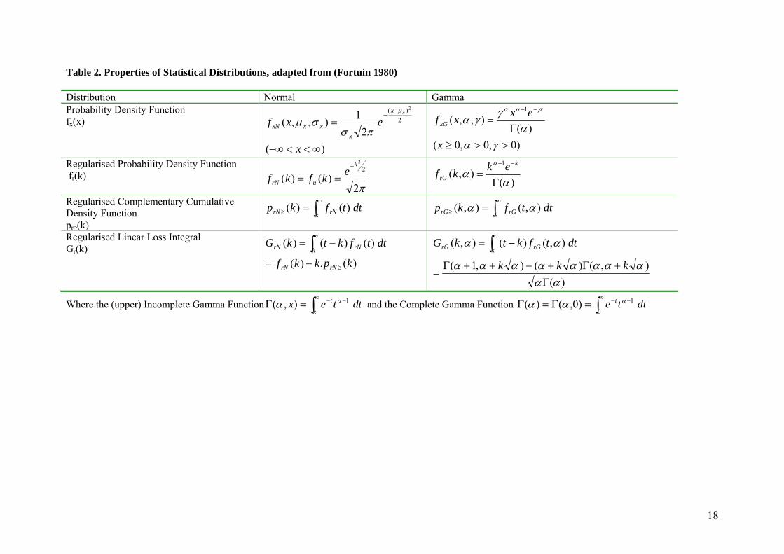
Now, for both Normal and Gamma distributed X it can be shown (Fortuin 1980)

that )()())(( 000 kGdxxfkx rxk

xxx

xx

σσµσµ

=+−∫∞

+

, where Gr(k) can be evaluated as in Table

2, and thus the last two terms in (2) may be combined into a single term, giving

D

xr kG

Rk

RwRkRNETRC

µσρ

⎟⎠⎞

⎜⎝⎛ +++= )(

22),(

2 (3)

Finally, we re-express the standard deviation of the demand during the protection interval (for

any distribution) in terms of the coefficient of variation of the demand DDDv µσ /= and

coefficient of variation of leadtime LLLv µσ /= , giving

2222

)()(22

),( LLDLr vvRkGR

kR

wRkRNETRC µµρ++⎟

⎠⎞

⎜⎝⎛ +++= (4)

2.3 Selection of Review Period and Order-up-to-Level While the first two terms of (4) are convex in R, the third may not be - we have observed

cases of the third term being non-convex, for both Normal and Gamma-distributed X. Indeed

the full expression for NETRC may be non-convex in R when X is Normally-distributed.

Also we have not been able to prove convexity of NETRC for Gamma-distributed X. Further

discussion on convexity is provided in Section 4.

With the potential non-convexity of NETRC, we employ a simultaneous approach to select

R* and S*, using a grid search to evaluate the optimal review period, R*. For each review

period considered, we evaluate S*(R) by calculating the critical fractile as follows:

Setting the derivative of ETRCPUT in (1) with respect to S,

⎥⎦

⎤⎢⎣

⎡−+=

∂∂

∫S

x dxxfR

cBrc

SSRETRCPUT

000

2 )(1),( equal to zero, one obtains

1

*

000 1)( PRdxxf

S

x =−=∫ ρ (5)

where P1 is the probability of no stockout in a replenishment cycle. This result applies for any

distribution of X.

5

For Normal X and making the substitution xx kS σµ ** += , (5) leads to

⎟⎟⎠

⎞⎜⎜⎝

⎛= −

≥ ρRpk rN

1* (6)

For Gamma X (see Table 2)

)()()(

010

00 αγ γαα

Γ==

−− x

xGxexxfxf , where 222

2

2

2

)()(

LLDL

L

x

x

vvRR

µµµ

σµ

α++

+== and 2

x

x

σµ

γ =

(equivalently γαµ =x ,

γασ =x , and

α1

=xv where vx is the coefficient of variation of

X).

Again making the substitutionγ

αγασµ *** kkS xx +=+= , and substituting 0xu γ= , (5)

becomes

1

*

0

*

0

1

1)()(

PRduufdueu k

sG

k u

=−==Γ ∫∫

++ −−

ρα

αααα α

(7)

Thus, for a given value of R, ETRCPUT (and NETRC) is minimised by using the safety

factor

ααρα

−⎟⎟⎠

⎞⎜⎜⎝

⎛= −

≥ ,1* 1 Rpk rG (9)

k* may be obtained using a reverse lookup (e.g., using

ααρα

−⎟⎟⎠

⎞⎜⎜⎝

⎛− 1,,11 RGAMMAINV in Microsoft ®Excel). Notice that k* depends upon

α, but not upon γ (the scale parameter of the Gamma distribution). Also note that α, which is

needed to invert the Gamma right-hand tail area in (8), only depends upon R, µL, vL, and vD,

and not upon µD.

Clearly the fractile for k*, in (6) and (8), can never exceed 1. We argue that many managers

would be reluctant to have even negative safety stock, and thus we prevent k* from going

negative, i.e., we set the minimum allowable safety factor as zero (Silver, Pyke, and Peterson

1998). This restriction does not affect the central findings of the paper.

Substituting (6) into (4), and using the identity concerning GrN(k) from Table 2, yields, for

Normal X,

6

22212

)(22

*),( LLDLrNrN vvRRpfRR

wRkRNETRC µµρ

ρ++⎟⎟

⎠

⎞⎜⎜⎝

⎛⎟⎟⎠

⎞⎜⎜⎝

⎛++= −

≥ (9)

Similarly, substituting (8) into (4) yields, for Gamma X,

22212

)(,,122

*),( LLDLrGrG vvRRpfRR

wRkRNETRC µµαααρα

ρ++⎟⎟

⎠

⎞⎜⎜⎝

⎛−⎟⎟

⎠

⎞⎜⎜⎝

⎛++= −

≥ (10)

3. Experimental Design Given the relatively complicated cost expression involving statistical functions, we employ a

factorial experiment to evaluate the conditions in which non-convexity occurs (in Section 4)

and the impact of key parameters on R* (in Section 5) under a wide variety of operating

conditions - reflecting both “average” conditions and extreme conditions of the five

parameters (w, ρ, µL, vL, and vD) in (4). We use a full factorial 35 experimental design, with

the five parameters and their levels selected as follows.

The Wilson number, w, is the EOQ, expressed as a time supply, for the deterministic problem

(i.e., σD=σL=0), and with convenient units of days. We are especially interested in how R*

may deviate from w. Based on our observations of industrial data, we set the lowest value of

w as 1 day, the median value at 15 days, and the highest value at 50 days.

The interpretation of ρ=B2/r is “the number of days holding costs that would be equivalent to

the cost of a shortage of one unit”. In terms of parameter values, consider the two

components. One could envisage B2 being a relatively small proportion of the cost of the

item, e.g., 5%, to a moderate value of 25%, up to perhaps losing the full value of the product,

e.g., 100% (more likely when a service failure generates substantial loss in goodwill). For the

holding cost, r, minimal values might be 5% per year (0.05/360 per day), with a mid-point of

25% per year (0.25/360 per day), and perhaps an extreme value of 75% per year (0.75/360).

(note that reports suggest that the depreciation component alone for computer equipment can

be as high as 2% per week (Kapuscinski et al. 2004)). Taking the extremes of both

combinations one could contemplate potential low, medium, and high values of ρ=B2/r of 24,

360, and 7200. However, combining two extremes can result in pathological conditions – for

example, it is highly unlikely that values as low as ρ=24 would occur in practice. Indeed,

products with very high r (e.g., PCs) are unlikely to have very low B2 (e.g. expediting costs

are likely to be high), or are unlikely to be stocked at all. Similarly, products with very low

holding costs (e.g., some plastics) are unlikely to have very high shortage costs. A more

realistic range then, still providing a good indication of the effect of a wide variety of

7

environmental conditions is ρ=100, 500, and 2000. For these values one may calculate

representative values of the probability of no stockout in a replenishment cycle (P1), e.g.,

setting R=w (i.e., without consideration of uncertainty), low, median, and high values

ofρwP −= 11 are ⎟

⎠⎞

⎜⎝⎛ −−−

200011,

500101,

100301 = (70%, 98%, 99.95%), respectively, i.e.,

reflecting a wide range of operating conditions.

For leadtimes, we consider means (µL) of 0.5, 10, and 30 days. Leadtime variability,

vL=σL/µL, ranges from extremes of almost deterministic, 0.05, up to 0.5, with a mid-point of

0.25. These figures are based on our observations of both domestic and international

leadtimes. For example, observations of vL for some two thousand shipments in the New

Zealand building industry average 0.30, with relatively little dependence on µL (i.e., σL tended

to increase linearly with µL).

Demand variability, vD=σD/µD (or, more properly, the coefficient of variation of the error in

the demand forecast) ranges from 0.1 to 10 with a mid-point of 2.5. These values may appear

high, but the time period considered is one day. The median coefficient of variation of

national monthly sales for more than 6000 products with positive annual sales in a major New

Zealand building products distributor is 1.58. If there were no autocorrelation in demand, this

would indicate a median value of vD of 8.6 (i.e., 1.58*√30). With positive autocorrelation the

actual values of vD would be somewhat lower. We conservatively use 2.5 as the mid-point.

Other empirical studies render similar ranges, e.g., Nahmias & Smith (1994) cite figures

which would convert to the range 0.55 to 7.07.

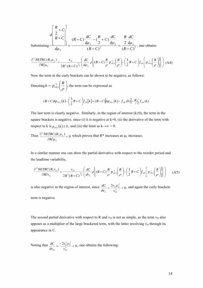
4. Behaviour of the Cost Expression as a Function of R In this section we demonstrate how and where the Expected Total Relevant Cost expression

may be non-convex for the case of Normal leadtime demand (X). We denote the first two

terms of (4) by R

wRE22

2

+= , and the last by 222)(*)(* LLDLr vvRkGR

kU µµρ++⎟

⎠⎞

⎜⎝⎛ += . E,

reflecting the cost curve for the deterministic EOQ case, is clearly convex in R. However, it

is not difficult to find cases where U, reflecting the incorporation of uncertainty, is non-

convex in R. Indeed we have proved that for k≥0 (the region of interest) U is either

decreasing in R, or has at most one local maximum (note that U is infinite at R=0 and it tends

to zero as R→∞). Moreover, cases exist in which the total expression NETRC=E+U is also

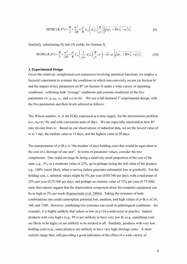
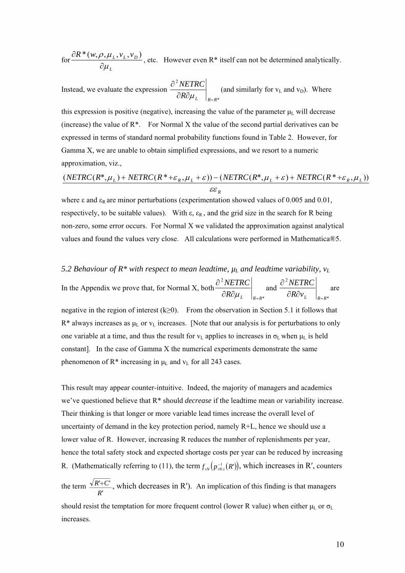
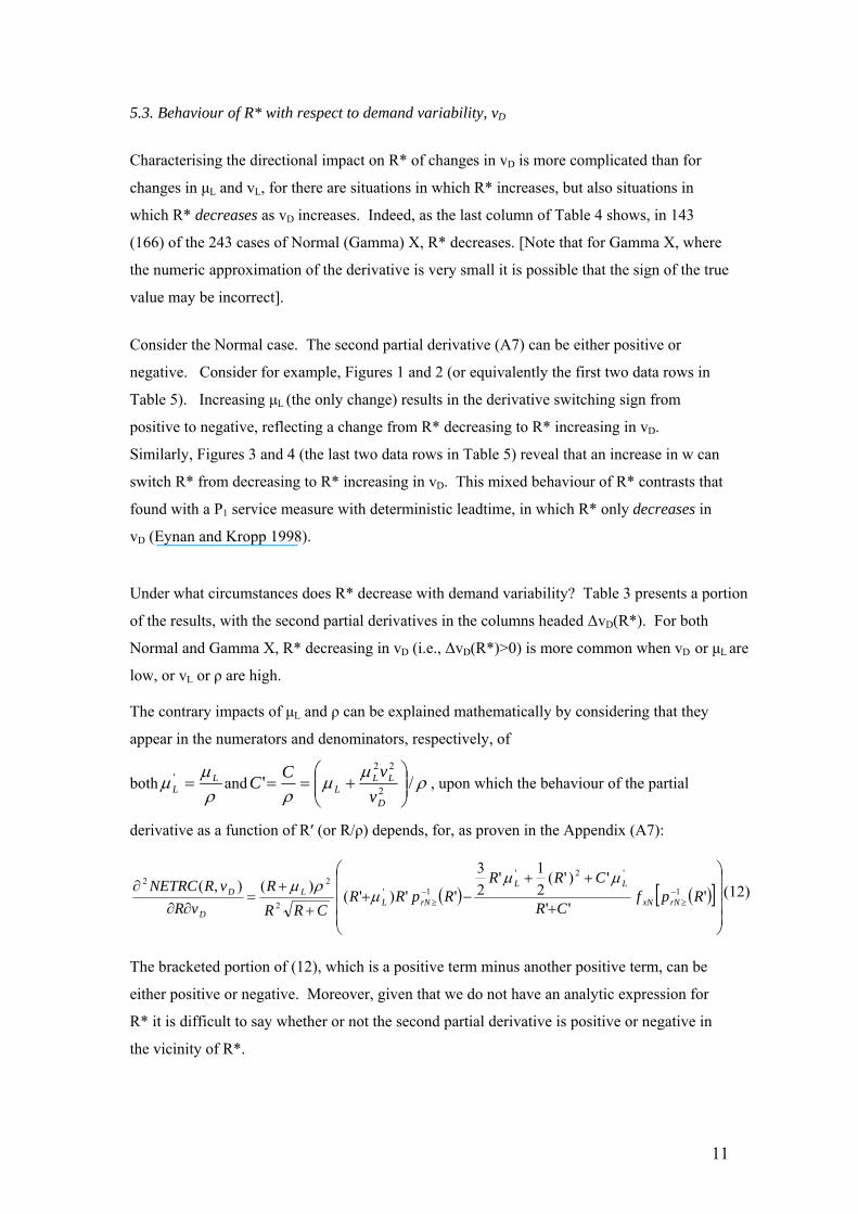
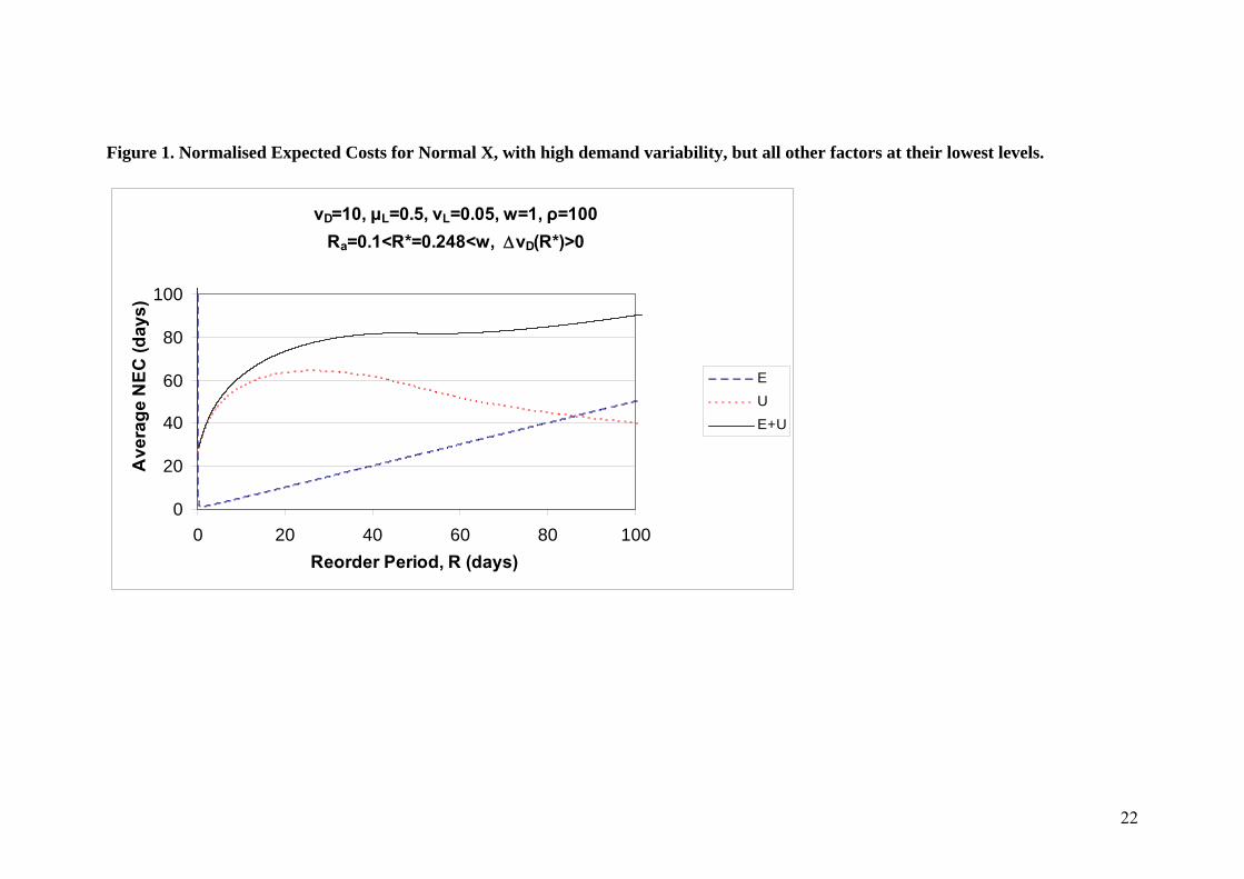
non-convex. Examples of this behaviour are illustrated in Figure 1 (with a local minimum at

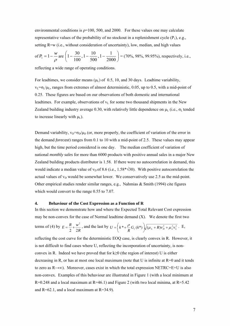
R=0.248 and a local maximum at R=46.1) and Figure 2 (with two local minima, at R=5.42

and R=62.1, and a local maximum at R=34.9).

8

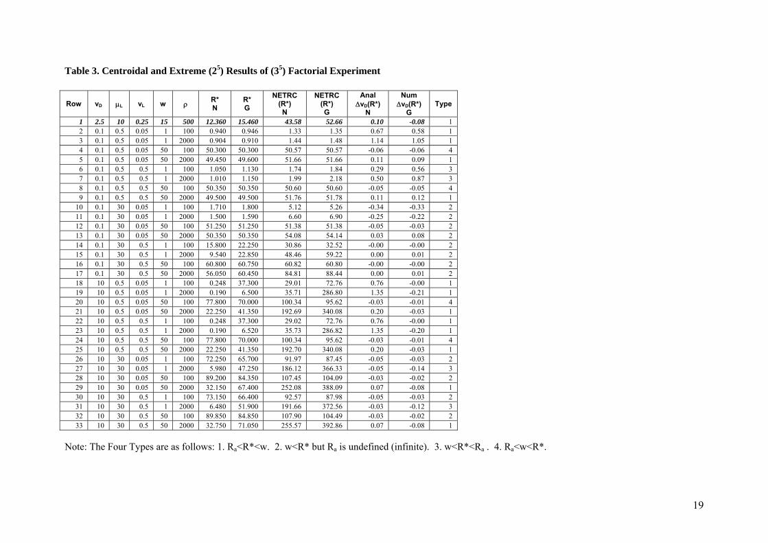
The full factorial experiment described in Section 3 was conducted. For each experimental

condition, R* was evaluated using a fine grid, from a low value of 0.06 to a high value of 115

days (all solutions were found within this range). The actual grid used was

0.06(0.002)1(0.01)5(0.02)20(0.05)115, i.e., involving 3521 evaluation points, with finer

resolution at lower values where the cost function generally changes more rapidly. Table 3

provides a partial listing of the results, for parameters in their centroidal position (row 1) and

the 25 extreme positions (e.g., row 2 has all the parameters at their low values and in row 3

only ρ is a its high value). Note that the last column, labelled “Type” will be explained later

in this section.

Among the 35 (243) experimental conditions NETRC has a local maximum in 9 instances.

These instances are (vD=10, µL=0.5, vL=(0.05, 0.25, 0.5), w=(1,15), ρ=100) and (vD=10,

µL=10, vL=(0.05, 0.25, 0.5), w=1, ρ=100). Note that none of these are included in the partial

experiments of Table 3. Local maxima are thus only observed when vD is high and ρ is low,

and never when µL is high or w is high. We have found no such cases of local maxima in

NETRC for Gamma X, although U itself may be non-convex.

Substituting ρRR =' and ρ

µµ

ρ/' 2

22

⎟⎟⎠

⎞⎜⎜⎝

⎛+==

D

LLL v

vCC into (9), one obtains

( )( ) ''''

)'( 1 CRRpfRv

ERNETRC rNrND ++= −

≥ (11)

With considerable separate experimentation we have found that ( )( )''

'' 1 RpfR

CRrNrN−

≥+

has a local maximum only when C′<0.085, i.e., when C′ is small enough. Without a

local maximum in U it is less likely that E+U is non-convex. Thus, small µL and vL

and large vD would tend to cause non-convexity. Large vD, which appears as a

multiplier in U, would tend to make U more important relative to E. The smaller w is,

the more important the non-convex U is relative to E, hence the more likely it is that

E+U is non-convex. In summary, non-convexity in NETRC(R) is more likely for low

µL, low vL, high vD, and low w (these results are validated by the experiments). The

behaviour with ρ is trickier as it appears in two places in U. However, we have been

able to show analytically that ρd

dUtends to be positive the lower ρ is, which again

agrees with experimental results regarding non-convexity.

9

Understandably, the non-convexity only appears at relatively high levels of uncertainty in X.

However, non-convexity can occur even with very little variability in the leadtime. This

suggests that one has to be careful in using solution methods based on convexity, e.g., Eynan

& Kropp (2004). Also, Rao (2003) as proven convexity for the case of deterministic

leadtime. Moreover, a recent paper shows convexity in the case of lost sales and no set-up

costs, when order crossover is allowed and inventory is charged at time of order arrival rather

than order placement (Janakiraman and Roundy 2004)

To provide more insight into the non-convexity we introduce the term Ra, the value of R that

minimises U (note: w minimises E). We may categorise cases as one of four Types (see the

first two rows of Table 4). Type 1 (the most common in our experiments) has Ra<R*<w.

Type 2, the second most common, has w<R* but Ra is undefined (infinite). Type 3 has

w<R*<Ra and Type 4 has Ra<w<R*. Note that is not possible for R* to exceed both w and Ra

(a related observation is that if w<Ra, then R* must be between w and Ra). Note also that

Ra<ρ/2, since one can prove analytically that 0' 5.0'

<=RdR

dU, i.e., the U function is always

decreasing as R′→0.5. Hence, if there is an earlier local minimum, there must be a local

maximum between the local minimum and R′=0.5.

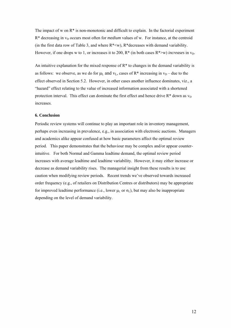
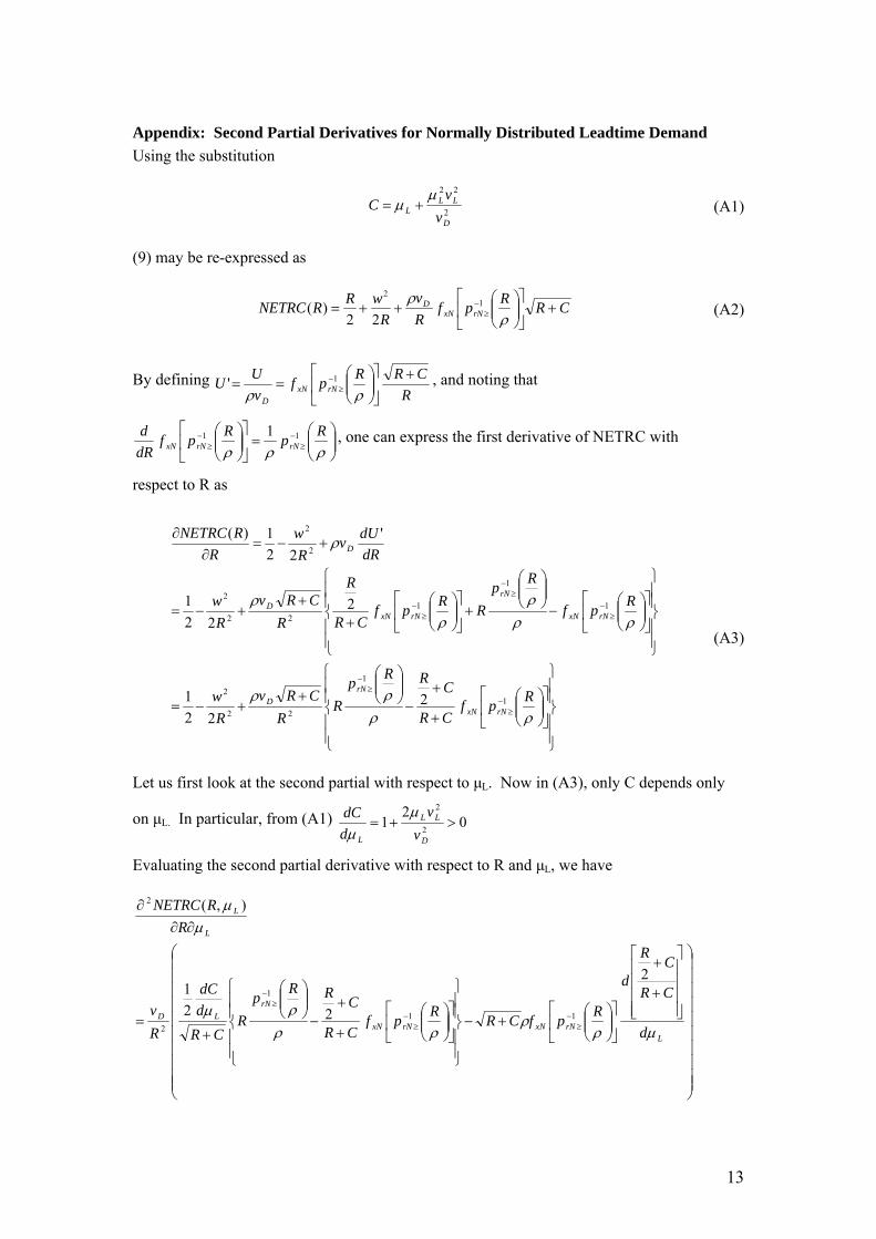
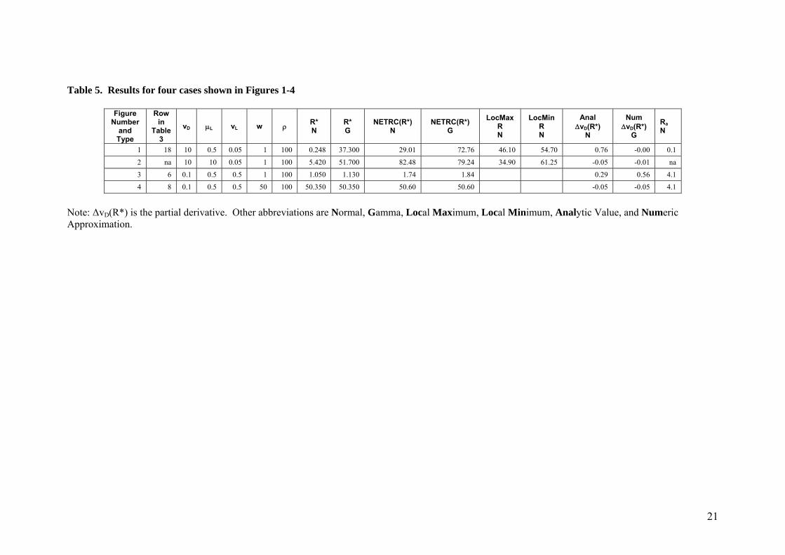
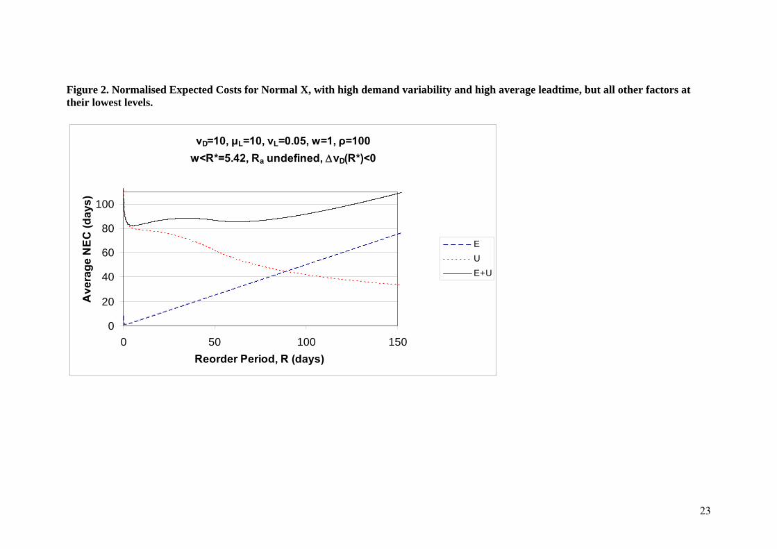
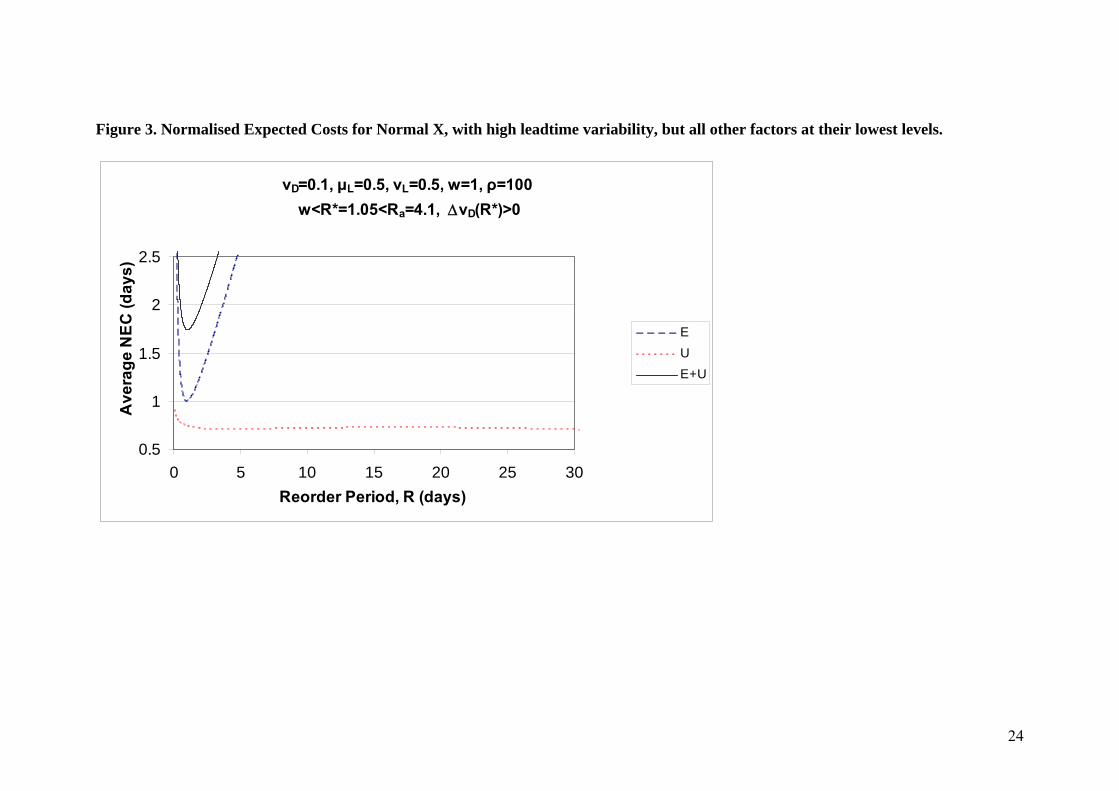
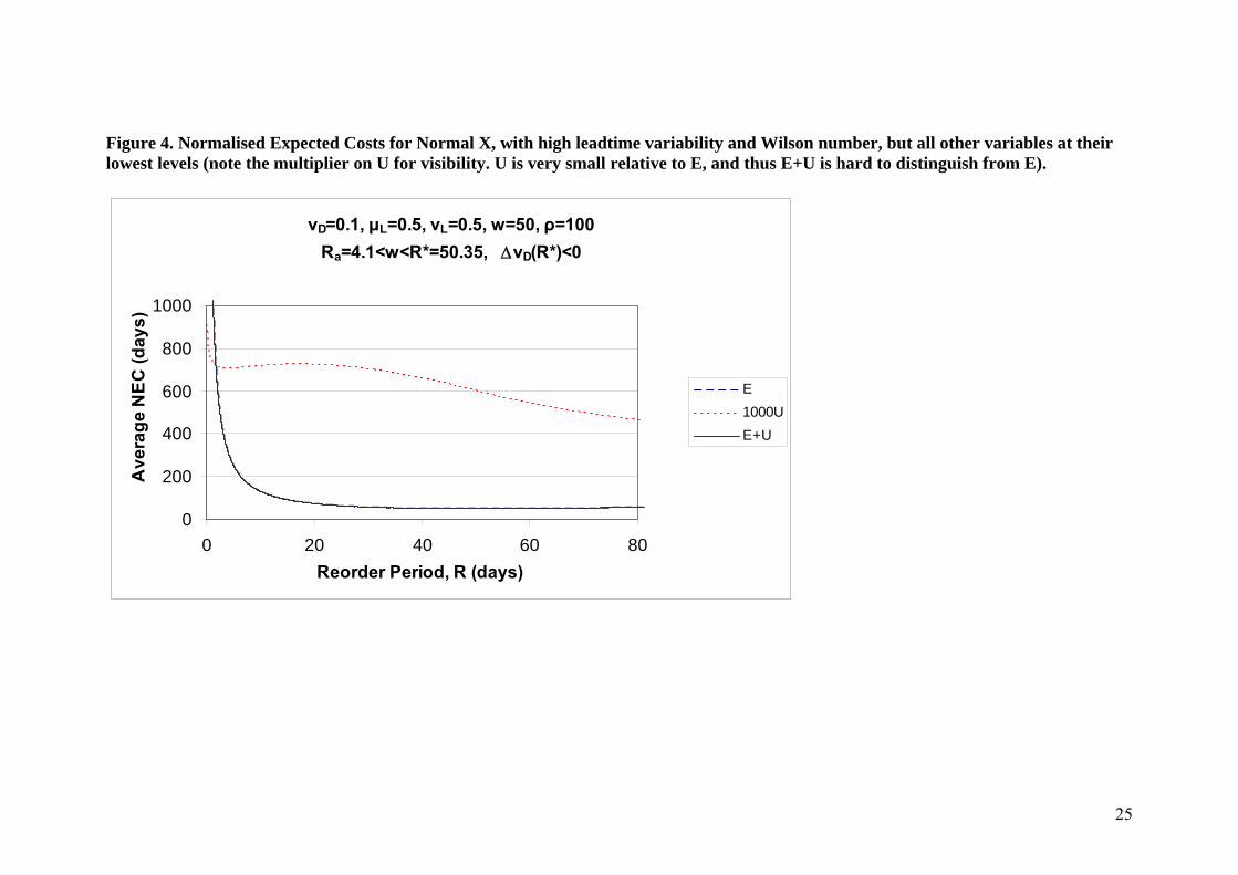
In Table 5 and in Figures 1 through 4 we present four cases, one from each of the types, from

the 35 conditions. Figure 1 shows (one of the 6 examples of) a Type 1 case with a local

maximum. Similarly, Figure 2 demonstrates (one of 3 examples of) a Type 2 case in which a

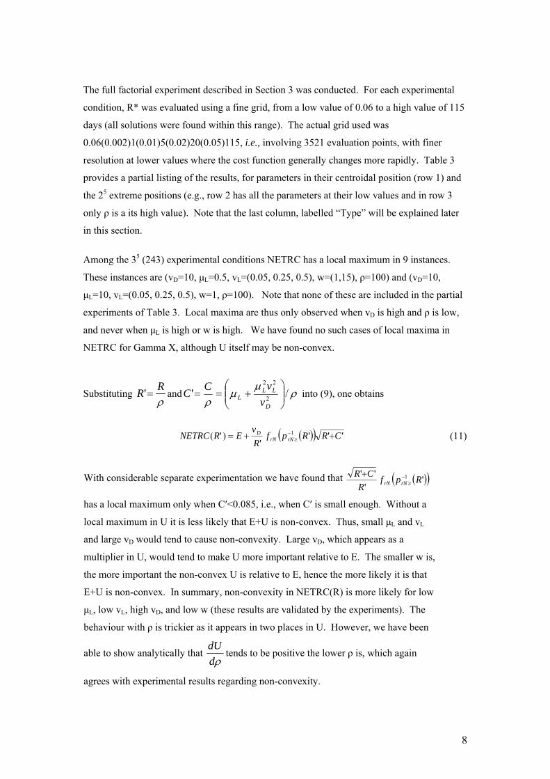
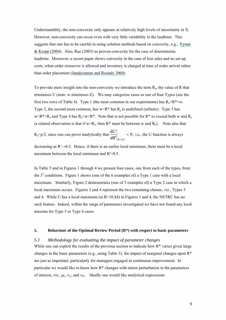
local maximum occurs. Figures 3 and 4 represent the two remaining classes, viz., Types 3

and 4. While U has a local maximum (at R=16.84) in Figures 3 and 4, the NETRC has no

such feature. Indeed, within the range of parameters investigated we have not found any local

maxima for Type 3 or Type 4 cases.

5. Behaviour of the Optimal Review Period (R*) with respect to basic parameters

5.1 Methodology for evaluating the impact of parameter changes While one can exploit the results of the previous section to indicate how R* varies given large

changes in the basic parameters (e.g., using Table 3), the impact of marginal changes upon R*

are just as important, particularly for managers engaged in continuous improvement. In

particular we would like to know how R* changes with minor perturbation in the parameters

of interest, viz., µL, vL, and vD. Ideally one would like analytical expressions

10

forL

DLL vvwRµµρ

∂∂ ),,,,(*

, etc. However even R* itself can not be determined analytically.

Instead, we evaluate the expression *

2

RRLRNETRC

=∂∂

∂µ

(and similarly for vL and vD). Where

this expression is positive (negative), increasing the value of the parameter µL will decrease

(increase) the value of R*. For Normal X the value of the second partial derivatives can be

expressed in terms of standard normal probability functions found in Table 2. However, for

Gamma X, we are unable to obtain simplified expressions, and we resort to a numeric

approximation, viz.,

R

LRLLRL RNETRCRNETRCRNETRCRNETRCεε

µεεµεµεµ )),*()*,(()),*()*,(( +++−+++

where ε and εR are minor perturbations (experimentation showed values of 0.005 and 0.01,

respectively, to be suitable values). With ε, εR , and the grid size in the search for R being

non-zero, some error occurs. For Normal X we validated the approximation against analytical

values and found the values very close. All calculations were performed in Mathematica®5.

5.2 Behaviour of R* with respect to mean leadtime, µL and leadtime variability, vL

In the Appendix we prove that, for Normal X, both*

2

RRLRNETRC

=∂∂

∂µ

and *

2

RRLvRNETRC

=∂∂

∂are

negative in the region of interest (k≥0). From the observation in Section 5.1 it follows that

R* always increases as µL or vL increases. [Note that our analysis is for perturbations to only

one variable at a time, and thus the result for vL applies to increases in σL when µL is held

constant]. In the case of Gamma X the numerical experiments demonstrate the same

phenomenon of R* increasing in µL and vL for all 243 cases.

This result may appear counter-intuitive. Indeed, the majority of managers and academics

we’ve questioned believe that R* should decrease if the leadtime mean or variability increase.

Their thinking is that longer or more variable lead times increase the overall level of

uncertainty of demand in the key protection period, namely R+L, hence we should use a

lower value of R. However, increasing R reduces the number of replenishments per year,

hence the total safety stock and expected shortage costs per year can be reduced by increasing

R. (Mathematically referring to (11), the term ( )( )'1 Rpf rNrN−

≥ , which increases in R′, counters

the term '

''R

CR + , which decreases in R′). An implication of this finding is that managers

should resist the temptation for more frequent control (lower R value) when either µL or σL

increases.

11

5.3. Behaviour of R* with respect to demand variability, vD

Characterising the directional impact on R* of changes in vD is more complicated than for

changes in µL and vL, for there are situations in which R* increases, but also situations in

which R* decreases as vD increases. Indeed, as the last column of Table 4 shows, in 143

(166) of the 243 cases of Normal (Gamma) X, R* decreases. [Note that for Gamma X, where

the numeric approximation of the derivative is very small it is possible that the sign of the true

value may be incorrect].

Consider the Normal case. The second partial derivative (A7) can be either positive or

negative. Consider for example, Figures 1 and 2 (or equivalently the first two data rows in

Table 5). Increasing µL (the only change) results in the derivative switching sign from

positive to negative, reflecting a change from R* decreasing to R* increasing in vD.

Similarly, Figures 3 and 4 (the last two data rows in Table 5) reveal that an increase in w can

switch R* from decreasing to R* increasing in vD. This mixed behaviour of R* contrasts that

found with a P1 service measure with deterministic leadtime, in which R* only decreases in

vD (Eynan and Kropp 1998).

Under what circumstances does R* decrease with demand variability? Table 3 presents a portion

of the results, with the second partial derivatives in the columns headed ∆vD(R*). For both

Normal and Gamma X, R* decreasing in vD (i.e., ∆vD(R*)>0) is more common when vD or µL are

low, or vL or ρ are high.

The contrary impacts of µL and ρ can be explained mathematically by considering that they

appear in the numerators and denominators, respectively, of

bothρ

µµ L

L =' and ρµ

µρ

/' 2

22

⎟⎟⎠

⎞⎜⎜⎝

⎛+==

D

LLL v

vCC , upon which the behaviour of the partial

derivative as a function of R′ (or R/ρ) depends, for, as proven in the Appendix (A7):

( ) ( )[ ]⎟⎟⎟⎟

⎠

⎞

⎜⎜⎜⎜

⎝

⎛

+

++−+

+

+=

∂∂∂ −

≥−

≥ '''

')'(21'

23

'')'()(),( 1

'2'

1'2

22

RpfCR

CRRRpRR

CRRR

vRvRNETRC

rNxN

LL

rNLL

D

Dµµ

µρµ (12)

The bracketed portion of (12), which is a positive term minus another positive term, can be

either positive or negative. Moreover, given that we do not have an analytic expression for

R* it is difficult to say whether or not the second partial derivative is positive or negative in

the vicinity of R*.

12

The impact of w on R* is non-monotonic and difficult to explain. In the factorial experiment

R* decreasing in vD occurs most often for medium values of w. For instance, at the centroid

(in the first data row of Table 3, and where R*<w), R*decreases with demand variability.

However, if one drops w to 1, or increases it to 200, R* (in both cases R*>w) increases in vD.

An intuitive explanation for the mixed response of R* to changes in the demand variability is

as follows: we observe, as we do for µL and vL, cases of R* increasing in vD – due to the

effect observed in Section 5.2. However, in other cases another influence dominates, viz., a

“hazard” effect relating to the value of increased information associated with a shortened

protection interval. This effect can dominate the first effect and hence drive R* down as vD

increases.

6. Conclusion

Periodic review systems will continue to play an important role in inventory management,

perhaps even increasing in prevalence, e.g., in association with electronic auctions. Managers

and academics alike appear confused at how basic parameters affect the optimal review

period. This paper demonstrates that the behaviour may be complex and/or appear counter-

intuitive. For both Normal and Gamma leadtime demand, the optimal review period

increases with average leadtime and leadtime variability. However, it may either increase or

decrease as demand variability rises. The managerial insight from these results is to use

caution when modifying review periods. Recent trends we’ve observed towards increased

order frequency (e.g., of retailers on Distribution Centres or distributors) may be appropriate

for improved leadtime performance (i.e., lower µL or σL), but may also be inappropriate

depending on the level of demand variability.

13

Appendix: Second Partial Derivatives for Normally Distributed Leadtime Demand Using the substitution

2

22

D

LLL v

vC

µµ += (A1)

(9) may be re-expressed as

CRRpfRv

RwRRNETRC rNxN

D +⎥⎦

⎤⎢⎣

⎡⎟⎟⎠

⎞⎜⎜⎝

⎛++= −

≥ ρρ 1

2

22)( (A2)

By defining R

CRRpfvUU rNxN

D

+⎥⎦

⎤⎢⎣

⎡⎟⎟⎠

⎞⎜⎜⎝

⎛== −

≥ ρρ1' , and noting that

⎟⎟⎠

⎞⎜⎜⎝

⎛=⎥

⎦

⎤⎢⎣

⎡⎟⎟⎠

⎞⎜⎜⎝

⎛ −≥

−≥ ρρρ

RpRpfdRd

rNrNxN11 1 , one can express the first derivative of NETRC with

respect to R as

⎪⎪⎭

⎪⎪⎬

⎫

⎪⎪⎩

⎪⎪⎨

⎧

⎥⎦

⎤⎢⎣

⎡⎟⎟⎠

⎞⎜⎜⎝

⎛+

+−

⎟⎟⎠

⎞⎜⎜⎝

⎛+

+−=

⎪⎪⎭

⎪⎪⎬

⎫

⎪⎪⎩

⎪⎪⎨

⎧

⎥⎦

⎤⎢⎣

⎡⎟⎟⎠

⎞⎜⎜⎝

⎛−

⎟⎟⎠

⎞⎜⎜⎝

⎛

+⎥⎦

⎤⎢⎣

⎡⎟⎟⎠

⎞⎜⎜⎝

⎛+

++−=

+−=∂

∂

−≥

−≥

−≥

−≥

−≥

ρρρρ

ρρρ

ρρ

ρ

RpfCR

CRRpR

RCRv

Rw

Rpf

RpRRpf

CR

R

RCRv

Rw

dRdUv

Rw

RRNETRC

rNxN

rND

rNxN

rN

rNxND

D

1

1

22

2

1

1

122

2

2

2

222

1

222

1

'22

1)(

(A3)

Let us first look at the second partial with respect to µL. Now in (A3), only C depends only

on µL. In particular, from (A1) 02

1 2

2

>+=D

LL

L vv

ddC µµ

Evaluating the second partial derivative with respect to R and µL, we have

⎟⎟⎟⎟⎟⎟⎟⎟⎟⎟

⎠

⎞

⎜⎜⎜⎜⎜⎜⎜⎜⎜⎜

⎝

⎛

⎥⎥⎥⎥

⎦

⎤

⎢⎢⎢⎢

⎣

⎡

+

+

⎥⎦

⎤⎢⎣

⎡⎟⎟⎠

⎞⎜⎜⎝

⎛+−

⎪⎪⎭

⎪⎪⎬

⎫

⎪⎪⎩

⎪⎪⎨

⎧

⎥⎦

⎤⎢⎣

⎡⎟⎟⎠

⎞⎜⎜⎝

⎛+

+−

⎟⎟⎠

⎞⎜⎜⎝

⎛

+=

∂∂∂

−≥

−≥

−≥

LrNxNrNxN

rNLD

L

L

d

CR

CR

d

RpfCRRpfCR

CRRpR

CRddC

Rv

RRNETRC

µρρ

ρρρµ

µµ

2

221

),(

11

1

2

2

14

Substituting 22 )(2

)(

)2

()(2

CRddCR

CRddCCR

ddCCR

d

CR

CR

d

LLL

L +=

+

+−+=

⎥⎥⎥⎥

⎦

⎤

⎢⎢⎢⎢

⎣

⎡

+

+

µµµµ

, one obtains

⎟⎟⎠

⎞⎜⎜⎝

⎛

⎪⎭

⎪⎬⎫

⎪⎩

⎪⎨⎧

⎥⎦

⎤⎢⎣

⎡⎟⎟⎠

⎞⎜⎜⎝

⎛⎟⎠⎞

⎜⎝⎛ +−⎟⎟

⎠

⎞⎜⎜⎝

⎛+

+=

∂∂∂ −

≥−

≥ ρρρρ

µµµ RpfCRRpRCR

ddC

CRR

vR

RNETRCrNxNrN

L

D

L

L 11

232

2

23)(

)(2

),( (A4)

Now the term in the curly brackets can be shown to be negative, as follows:

Denoting ⎟⎟⎠

⎞⎜⎜⎝

⎛= −

≥ ρRpk rN

1 , the term can be expressed as

( ) [ ] ( )[ ] )(2)()(23)( kfRkfkkpCRkfCRkkpCR xNxNrNxNrN −−+=⎟

⎠⎞

⎜⎝⎛ +−+ ≥≥

The last term is clearly negative. Similarly, in the region of interest (k≥0), the term in the

square brackets is negative, since (i) it is negative at k=0, (ii) the derivative of the term with

respect to k is ( ) 0≥≥ kprN , and (iii) the limit as k→∞ = 0.

Thus 0),(2

<∂∂

∂

L

L

RRNETRC

µµ which proves that R* increases as µL increases.

In a similar manner one can show the partial derivative with respect to the reorder period and

the leadtime variability,

⎟⎟⎠

⎞⎜⎜⎝

⎛

⎪⎭

⎪⎬⎫

⎪⎩

⎪⎨⎧

⎥⎦

⎤⎢⎣

⎡⎟⎟⎠

⎞⎜⎜⎝

⎛⎟⎠⎞

⎜⎝⎛ +−⎟⎟

⎠

⎞⎜⎜⎝

⎛+

+=

∂∂∂ −

≥−

≥ ρρρρ RpfCRRpRCR

dvdC

CRR

vvR

vRNETRCrNxNrN

L

D

L

L 11

232

2

23)(

)(2

),( (A5)

is also negative in the region of interest, since 02

2

2

>=D

LL

L vv

dvdC µ , and again the curly brackets

term is negative.

The second partial derivative with respect to R and vD is not as simple, as the term vD also

appears as a multiplier of the large bracketed term, with the latter involving vD through its

appearance in C.

Noting that 02

3

22

<−

=D

LL

D vv

dvdC µ , one obtains the following:

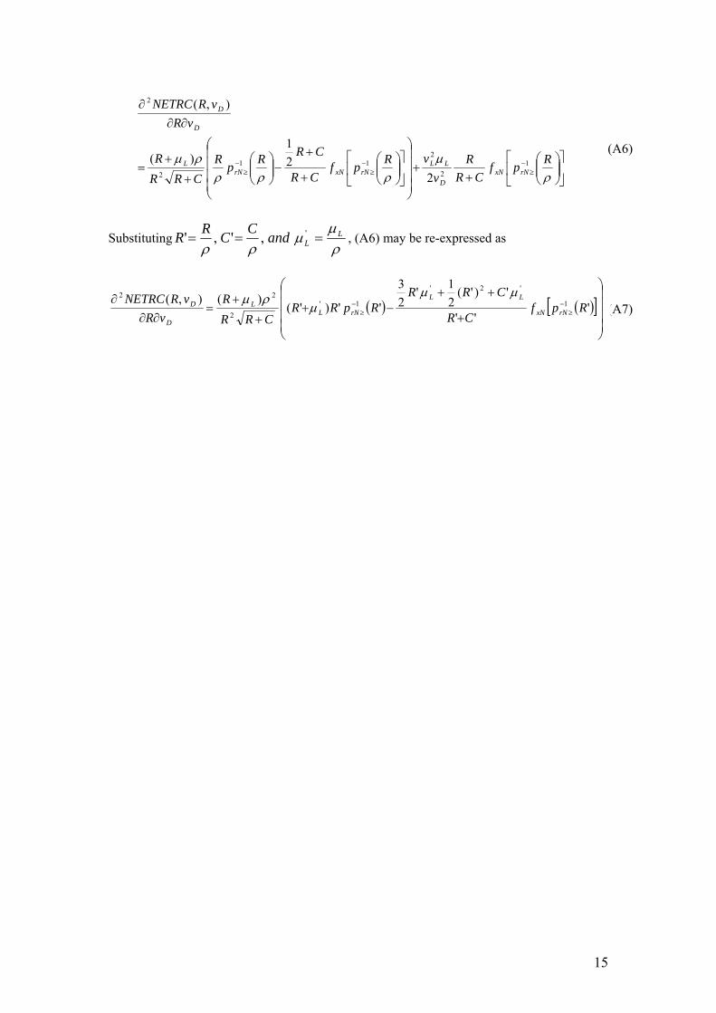
15

⎥⎦

⎤⎢⎣

⎡⎟⎟⎠

⎞⎜⎜⎝

⎛+

+⎟⎟⎟⎟

⎠

⎞

⎜⎜⎜⎜

⎝

⎛

⎥⎦

⎤⎢⎣

⎡⎟⎟⎠

⎞⎜⎜⎝

⎛+

+−⎟⎟

⎠

⎞⎜⎜⎝

⎛

+

+=

∂∂∂

−≥

−≥

−≥ ρ

µρρρ

ρµ RpfCR

Rv

vRpfCR

CRRpRCRR

R

vRvRNETRC

rNxND

LLrNxNrN

L

D

D

12

211

2

2

221

)(

),(

(A6)

Substitutingρ

µµ

ρρL

LandCCRR === ',',' , (A6) may be re-expressed as

( ) ( )[ ]⎟⎟⎟⎟

⎠

⎞

⎜⎜⎜⎜

⎝

⎛

+

++−+

+

+=

∂∂∂ −

≥−

≥ '''

')'(21'

23

'')'()(),( 1

'2'

1'2

22

RpfCR

CRRRpRR

CRRR

vRvRNETRC

rNxN

LL

rNLL

D

Dµµ

µρµ

(A7)

16

References

Burgin, T. A. 1975. The Gamma Distribution and Inventory Control. Operational Research Quarterly 26 (3):507-525.

Bylka, S. 2005. Turnpike policies for periodic review inventory model with emergency orders. International Journal of Production Economics 93-94:357-374.

Chopra, S, G Reinhardt, and M. Dada. 2004. The Effect of Lead Time Uncertainty on Safety Stocks. Decision Sciences 35 (1):1-24.

Eynan, A, and DH Kropp. 2004. Effective and Simple EOQ-Like Solutions for Stochastic Demand Periodic Review Systems.

Eynan, A., and D. H. Kropp. 1998. Periodic review and joint replenishment in stochastic demand environments. IIE Transactions 30 (11):1025-1033.

Fortuin, L. 1980. Five popular probability density functions: A comparison in the field of stock-control models. Journal of the Operational Research Society 31 (10):937-942.

Gavirneni, S. 2004. Periodic review inventory control with fluctuating purchasing costs. Operations Research Letters 32:374-379.

Janakiraman, G., and R. O. Roundy. 2004. Lost-Sales Problems with Stochastic Lead Times: Convexity Results for Base-Stock Policies. Operations Research 52 (5):795-803.

Kapuscinski, R, RQ Zhang, P Carbonneau, R Moore, and B Reeves. 2004. Inventory Decisions in Dell's Supply Chain. Interfaces 34 (3):191-205.

Nahmias, S., and S. A. Smith. 1994. Optimizing Inventory Levels in a Two-Echelon Retailer System with Partial Lost Sales. Management Science 40 (5):582-596.

Rao, US. 2003. Properties of the Periodic Review (R,T) Inventory Control Policy for Stationary,Stochastic Demand. Manufacturing & Service Operations Management 5 (1):37-53.

Robb, DJ, and EA Silver. 2004. Inventory Management under Date-terms Supplier Trade Credit with Stochastic Demand and Leadtime. In Haskayne School of Business Working Paper: The University of Calgary.

Shore, H. 2004. A general solution for the newsboy model with random order size and possibly a cutoff transaction size. Journal of the Operational Research Society 55 (11):1218-1228.

Silver, E. A., D. F. Pyke, and R. Peterson. 1998. Inventory Management and Production Planning and Scheduling. 3rd ed. New York: John Wiley & Sons.

Tyworth, J. E., and L. O'Neill. 1997. Robustness of the Normal Approximation of Lead-Time Demand in a Distribution Setting. Naval Research Logistics 44:165-186.

Urban, T. L. 2005. A periodic-review model with serially-correlated, inventory-level-dependent demand. International Journal of Production Economics 95 (3):287-295.

17

Table 1. Some Notation (note: $ may be replaced by any unit of currency) A $ Fixed cost component incurred with each replenishment B2 $/$ Fractional charge per unit short c $/unit Unit variable cost of an item

C Days 2

22

D

LLL v

vC

µµ +=

C′ - C′=C/ ρ D Units/day Demand per day, distributed with mean and standard deviation ),( DD σµ . k - Safety factor L Days Replenishment leadtime, distributed with mean and standard deviation ),( LL σµ . r $/$/day Inventory carrying charge R Days Reorder Period R′ - R/ρ Ra Days The local minimum of the normalised shortage and safety stock function (U) S Units Order-up-to Level, xx kS σµ += SS Units Safety Stock T Days The normalised set-up cost and cycle stock holding cost function U Days The normalised shortage cost and safety stock cost function vD - Demand variability, vD=σD/µD vL - Leadtime variability, vL=σL/µL

w Days The Economic Order Quantity expressed as a time period, also known as the Wilson number, crAw

Dµ2

=

X Units Demand during the “critical protection period”, R+L, distributed with mean and standard deviation ),( XX σµ . Coefficient of

variationx

xxv

µσ

=

ρ Days Shortage to Holding Cost ratio, ρ=B2/r (interpretation: number of days holding costs equivalent to the cost of running out of stock, B2) µL Days Leadtime mean µL′ - µL′/ ρ

18

Table 2. Properties of Statistical Distributions, adapted from (Fortuin 1980) Distribution Normal Gamma Probability Density Function fx(x)

)(2

1),,( 2)( 2

∞<<−∞

=−

−

x

exfxx

xxxxN

µ

πσσµ

)0,0,0(

)(),,(

1

>>≥Γ

=−−

γαα

γγαγαα

x

exxfx

xG

Regularised Probability Density Function fr(k)

π2)()(

22k

urNekfkf

−

== )(),(

1

αα

α

Γ=

−− k

rGekkf

Regularised Complementary Cumulative Density Function pr≥(k)

dttfkpk rNrN ∫∞

≥ = )()( dttfkpk rGrG ∫∞

≥ = ),(),( αα

Regularised Linear Loss Integral Gr(k)

)(.)(

)()()(

kpkkf

dttfktkG

rNrN

k rNrN

≥

∞

−=

−= ∫

)(),()(),1(

),()(),(

αααααααααα

αα

Γ+Γ+−++Γ

=

−= ∫∞

kkk

dttfktkGk rGrG

Where the (upper) Incomplete Gamma Function ∫∞ −−=Γx

t dttex 1),( αα and the Complete Gamma Function ∫∞ −−=Γ=Γ0

1)0,()( dtte t ααα

19

Table 3. Centroidal and Extreme (25) Results of (35) Factorial Experiment

Note: The Four Types are as follows: 1. Ra<R*<w. 2. w<R* but Ra is undefined (infinite). 3. w<R*<Ra . 4. Ra<w<R*.

Row vD µL vL w ρ R* N

R* G

NETRC (R*) N

NETRC (R*) G

Anal ∆vD(R*)

N

Num ∆vD(R*)

G Type

1 2.5 10 0.25 15 500 12.360 15.460 43.58 52.66 0.10 -0.08 1 2 0.1 0.5 0.05 1 100 0.940 0.946 1.33 1.35 0.67 0.58 1 3 0.1 0.5 0.05 1 2000 0.904 0.910 1.44 1.48 1.14 1.05 1 4 0.1 0.5 0.05 50 100 50.300 50.300 50.57 50.57 -0.06 -0.06 4 5 0.1 0.5 0.05 50 2000 49.450 49.600 51.66 51.66 0.11 0.09 1 6 0.1 0.5 0.5 1 100 1.050 1.130 1.74 1.84 0.29 0.56 3 7 0.1 0.5 0.5 1 2000 1.010 1.150 1.99 2.18 0.50 0.87 3 8 0.1 0.5 0.5 50 100 50.350 50.350 50.60 50.60 -0.05 -0.05 4 9 0.1 0.5 0.5 50 2000 49.500 49.500 51.76 51.78 0.11 0.12 1

10 0.1 30 0.05 1 100 1.710 1.800 5.12 5.26 -0.34 -0.33 2 11 0.1 30 0.05 1 2000 1.500 1.590 6.60 6.90 -0.25 -0.22 2 12 0.1 30 0.05 50 100 51.250 51.250 51.38 51.38 -0.05 -0.03 2 13 0.1 30 0.05 50 2000 50.350 50.350 54.08 54.14 0.03 0.08 2 14 0.1 30 0.5 1 100 15.800 22.250 30.86 32.52 -0.00 -0.00 2 15 0.1 30 0.5 1 2000 9.540 22.850 48.46 59.22 0.00 0.01 2 16 0.1 30 0.5 50 100 60.800 60.750 60.82 60.80 -0.00 -0.00 2 17 0.1 30 0.5 50 2000 56.050 60.450 84.81 88.44 0.00 0.01 2 18 10 0.5 0.05 1 100 0.248 37.300 29.01 72.76 0.76 -0.00 1 19 10 0.5 0.05 1 2000 0.190 6.500 35.71 286.80 1.35 -0.21 1 20 10 0.5 0.05 50 100 77.800 70.000 100.34 95.62 -0.03 -0.01 4 21 10 0.5 0.05 50 2000 22.250 41.350 192.69 340.08 0.20 -0.03 1 22 10 0.5 0.5 1 100 0.248 37.300 29.02 72.76 0.76 -0.00 1 23 10 0.5 0.5 1 2000 0.190 6.520 35.73 286.82 1.35 -0.20 1 24 10 0.5 0.5 50 100 77.800 70.000 100.34 95.62 -0.03 -0.01 4 25 10 0.5 0.5 50 2000 22.250 41.350 192.70 340.08 0.20 -0.03 1 26 10 30 0.05 1 100 72.250 65.700 91.97 87.45 -0.05 -0.03 2 27 10 30 0.05 1 2000 5.980 47.250 186.12 366.33 -0.05 -0.14 3 28 10 30 0.05 50 100 89.200 84.350 107.45 104.09 -0.03 -0.02 2 29 10 30 0.05 50 2000 32.150 67.400 252.08 388.09 0.07 -0.08 1 30 10 30 0.5 1 100 73.150 66.400 92.57 87.98 -0.05 -0.03 2 31 10 30 0.5 1 2000 6.480 51.900 191.66 372.56 -0.03 -0.12 3 32 10 30 0.5 50 100 89.850 84.850 107.90 104.49 -0.03 -0.02 2 33 10 30 0.5 50 2000 32.750 71.050 255.57 392.86 0.07 -0.08 1

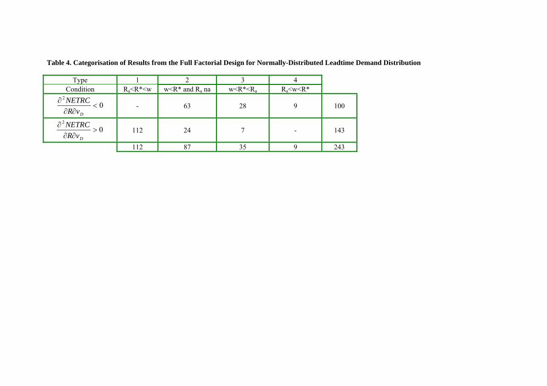
Table 4. Categorisation of Results from the Full Factorial Design for Normally-Distributed Leadtime Demand Distribution

Type 1 2 3 4 Condition Ra<R*<w w<R* and Ra na w<R*<Ra Ra<w<R*

02

<∂∂

∂

DvRNETRC

- 63 28 9 100

02

>∂∂

∂

DvRNETRC

112 24 7 - 143

112 87 35 9 243

21

Table 5. Results for four cases shown in Figures 1-4

Figure Number

and Type

Row in

Table 3

vD µL vL w ρ R* N

R* G

NETRC(R*) N

NETRC(R*) G

LocMax R N

LocMin R N

Anal ∆vD(R*)

N

Num ∆vD(R*)

G

Ra N

1 18 10 0.5 0.05 1 100 0.248 37.300 29.01 72.76 46.10 54.70 0.76 -0.00 0.1

2 na 10 10 0.05 1 100 5.420 51.700 82.48 79.24 34.90 61.25 -0.05 -0.01 na

3 6 0.1 0.5 0.5 1 100 1.050 1.130 1.74 1.84 0.29 0.56 4.1

4 8 0.1 0.5 0.5 50 100 50.350 50.350 50.60 50.60 -0.05 -0.05 4.1

Note: ∆vD(R*) is the partial derivative. Other abbreviations are Normal, Gamma, Local Maximum, Local Minimum, Analytic Value, and Numeric Approximation.

22

Figure 1. Normalised Expected Costs for Normal X, with high demand variability, but all other factors at their lowest levels.

vD=10, µL=0.5, vL=0.05, w=1, ρ=100Ra=0.1<R*=0.248<w, ∆vD(R*)>0

0

20

40

60

80

100

0 20 40 60 80 100Reorder Period, R (days)

Ave

rage

NEC

(day

s)

EUE+U

23

Figure 2. Normalised Expected Costs for Normal X, with high demand variability and high average leadtime, but all other factors at their lowest levels.

vD=10, µL=10, vL=0.05, w=1, ρ=100w<R*=5.42, Ra undefined, ∆vD(R*)<0

0

20

40

60

80

100

0 50 100 150Reorder Period, R (days)

Ave

rage

NE

C (d

ays)

EUE+U

24

Figure 3. Normalised Expected Costs for Normal X, with high leadtime variability, but all other factors at their lowest levels.

vD=0.1, µL=0.5, vL=0.5, w=1, ρ=100 w<R*=1.05<Ra=4.1, ∆vD(R*)>0

0.5

1

1.5

2

2.5

0 5 10 15 20 25 30Reorder Period, R (days)

Ave

rage

NE

C (d

ays)

EUE+U

25

Figure 4. Normalised Expected Costs for Normal X, with high leadtime variability and Wilson number, but all other variables at their lowest levels (note the multiplier on U for visibility. U is very small relative to E, and thus E+U is hard to distinguish from E).

vD=0.1, µL=0.5, vL=0.5, w=50, ρ=100Ra=4.1<w<R*=50.35, ∆vD(R*)<0

0

200

400

600

800

1000

0 20 40 60 80Reorder Period, R (days)

Ave

rage

NE

C (d

ays)

E1000UE+U