SOME ASPECTS OF USING FOURIER ANALYSIS TO … ASPECTS OF USING FOURIER ANALYSIS TO SUPPORT SURFACE MODELING ... Some other important characteristics of Fourier series-based surface

Pecora 16 “Global Priorities in Land Remote Sensing” October 23-27, 2005 * Sioux Falls, South Dakota

SOME ASPECTS OF USING FOURIER ANALYSIS TO SUPPORT SURFACE MODELING

Nora Csanyi¹

Charles K. Toth² Department of Civil and Environmental Engineering and Geodetic Science¹

Center for Mapping² The Ohio State University

1216 Kinnear Road, Columbus OH 43212-1154 [email protected]

ABSTRACT Using modern airborne and spaceborne sensors, terrain point observations are becoming available in a variety of formats with widely differing characteristics. The point distribution, accuracy and density can vary greatly, depending mostly on the sensor type and the data acquisition method used. Most of the data acquisition technologies deliver elevation data in irregular point distribution; therefore, the generation of DEM in regular grid structure requires interpolation. Various interpolation methods exist, and similarly, the surfaces to be modeled can have different characteristics and there is no single interpolation technique that is optimal for every situation. Fourier series technique is a powerful method to describe 1D/2D or N-dimensional periodic signals and can be used for surface modeling. However, the available formulae for calculating the Fourier series coefficients are based on evenly spaced input data, and thus it cannot be directly applied for surface approximations from irregularly spaced points. The proposed approach, therefore, aims to determine the coefficients in the case of irregular point distribution using least squares adjustment. Since Fourier series cannot model surface trends well, a polynomial extension has been added to model the surface trend, thus splitting the approximation task into two parts: global trend and local variation modeling. We introduced the idea earlier and this paper provides a performance analysis of the developed Fourier series-based surface modeling method. The proposed method is tested on LiDAR data in the case of different terrain characteristics, point distributions and point densities.

INTRODUCTION Surface modeling is essential for various applications; orthophoto productions, engineering design, floodplain mapping, telecommunication, etc. all require surface data with different level of detail and accuracy. There are currently three main technologies that deliver surface data with increased level of accuracy and detail. The traditional method has been photogrammetry using stereo image pairs. Recently, LIDAR technology has become the primary source of surface data while IfSAR is also an important source at


global scale. Surface data created by these technologies come with various point densities, point distributions and error characteristics. There are three commonly used data structures to store digital elevation data; Triangulated Irregular Networks (TINs), regular grid structure, and lines of equal elevation (contours). All representation methods have their advantages and disadvantages, depending on the terrain characteristics and the intended applications. Grid structure is the ultimate format for analysis purposes as it makes the comparison of different datasets very simple. In addition, most of the visualization tools and processing techniques are based on grid structure. Consequently, grid structure is the most common representation of terrain surface and is typically called DEM (Digital Elevation Model; DTM or DSM are also frequently used). Most of the data acquisition technologies deliver elevation data in irregular point distribution, and therefore, the generation of DEM in regular grid structure requires some kind of interpolation. Several interpolation methods exist for terrain approximation. Maune (2001) provides an overview of the most commonly used interpolation methods for terrain data. Each method has its advantages and disadvantages. Similarly, the surfaces to be modeled can have different characteristics and there is no single interpolation technique that is the best for every situation. Fourier series technique as a powerful method to describe 1D/2D signals has been widely used in several diverse applications and can be used for surface modeling. However, the available formulae for the calculation of the Fourier series coefficients are based on evenly spaced data and therefore cannot be directly applied for interpolation of irregularly spaced points. The proposed approach aims to determine the coefficients in the case of irregular point distribution using least squares adjustment. In the first section of the paper the method is discussed for both 1D, for modeling terrain profiles, and 2D, for modeling terrain surfaces, and some important characteristics of the model are also introduced. This is followed by an extensive performance analysis; the method is applied to model LiDAR profiles and LiDAR surfaces with various terrain characteristics, point densities and point distributions.

FOURIER SERIES FOR MODELING IRREGULARLY SPACED SURFACE DATA

1D case: Modeling Surface Profiles Periodic functions f(x) of period T can be expressed as an infinite sum of sine and cosine waves of the same period T:

(1)

∑∞

=⎟⎠⎞

⎜⎝⎛ ++

10

2sin2cosak

kk xT

kbxT

ka ππ


If the sum is calculated until finite n harmonics, the Fourier-series gives an approximation of the function. The bigger n, the better the approximation. If the continuous function is sampled at discrete locations, the calculation of the Fourier series coefficients is identical to the calculation of the discrete Fourier transform. Direct formulae are available to calculate the coefficients. However, these formulae are only valid for regular point distribution, therefore cannot be applied to irregularly sampled data such as for example LiDAR profiles. The proposed solution to determine the coefficients for irregular point distribution is to calculate the Fourier-series coefficients by least squares adjustment. Assuming that to approximate a profile that is sampled at m locations, the Fourier-series is calculated until the n-th harmonics, then for the best fit, the 2n+1 unknown coefficients can be calculated by least squares adjustment with the condition (Eq. (2)):

(2)

In the case of irregular point distribution, properly choosing the number of harmonics is crucial in order to get a good model of the profile. Choosing the proper number of harmonics and the fundamental wavelength of the series is discussed in detail at the 2D case but also valid for the 1D case. Figure 1 illustrates an important property of the Fourier series-based modeling. One period of a squarewave function is approximated by Fourier series calculated until the 5, 10, and 40 harmonics, respectively. The more harmonics are calculated, the better the approximation function fits to the original one, the series converges to the function, however, the errors near the discontinuity do not decrease. This phenomenon is called Gibb’s phenomenon. Gibb’s phenomenon appears whenever a discontinuity is approximated (Mesko, 1984). Near discontinuity the deviation of the Fourier series from the approximated functions remains different from zero, regardless the inclusion of more and more terms. With increasing harmonics, the oscillation squeezes into a narrower interval around the discontinuity, but their amplitudes do not decrease. Therefore the method is not adequate for modeling discontinuities. Some other important characteristics of Fourier series-based surface modeling are discussed in the 2D case but they are also valid for the 1D case, when modeling surface profiles or trajectories.

∑=

=⎟⎠⎞

⎜⎝⎛ −+++=

m

1i

2

10 min2sin...2cosM iini yxT

nbxT

aa ππ

( )( )∑=

=−m

iii yxy

1

2 min


The number of unknown Fourier coefficients can be calculated as: 4nm+2(n+m)+1, where n, m are the number of harmonics in x and y directions. Table 1 provides a few examples of the number of coefficients to be calculated for different number of Fourier harmonics when the harmonic numbers in the two coordinate directions are the same. Since the number of coefficients to be calculated is very large even for small number of harmonics, the Extended Gaussian algorithm can be used to solve for the coefficients to avoid the inversion of the huge normal matrix.

Number of harmonicsin both directions

Number of coefficients

1 7 2 25 3 49 4 81 5 121 6 169 7 225 8 289 9 361

10 441

Table 1. Number of coefficients in 2D case

Properly choosing the number of harmonics is crucial in order to model the surface well. When choosing the number of harmonics, the Shannon’s Sampling Theorem (Higgins, 1996) has to be considered. The Sampling Theorem states that if a continuous signal is sampled at least twice the frequency of the highest frequency in the signal then the signal can be completely reconstructed from the samples (Nyquist criterion). Therefore, the point density in x and y directions, in terms of defining the minimum sampling distance determines the maximum spatial frequency that can model the surface (whether it is adequate to properly describe the terrain is another question). Consequently, the maximum number of coefficients of the Fourier series in both x and y directions can be calculated. If more harmonics are calculated, the fit of the approximated surface could be very good at the measured points, but between the known points high waves will be produced due to the lack of constraints there. Thus, a trade-off has to be found to obtain a smooth enough surface and an acceptable fit at the known points. If the surface has a trend, this contradiction, however, cannot be resolved using only Fourier series interpolation itself. Therefore, as a refinement to the Fourier series interpolation, a polynomial extension has been introduced to model the surface trend, thus, splitting the approximation task into two parts, global trend and local variation modeling. More details can be found in (Csanyi et al., 2003). The proper order of the polynomial can be chosen considering the complexity of the trend in the data. Depending on the surface characteristics and the point distribution it is often advantageous to chose different number of Fourier harmonics for the two coordinate directions. A typical case when LiDAR data is modeled with significantly different point densities in the scan direction and flying direction. If the data is not oriented in the x-y


coordinate direction in such case, it is beneficial to align it before the Fourier series-based modeling. The fundamental wavelength is another important parameter to choose for the proposed surface modeling method. The fundamental wavelength is the highest wavelength (smallest frequency) used for modeling the surface. When choosing the fundamental wavelengths in x and y directions, one practical restriction is that it has to be at least the length of the data set in x and y directions, respectively, since the Fourier series approximation duplicates itself over the interval of the fundamental period. If the fundamental period is larger than the length of the data set then it can model trend in the data, however, the local variations won’t be modeled well, therefore it is advantageous to set it equal to the length of the data set since the trend is modeled by the polynomial part.

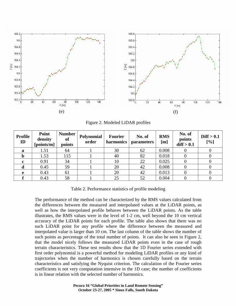
TEST RESULTS WITH LIDAR DATA The proposed method was tested on LiDAR data in both 1D, for modeling LiDAR profiles, and 2D, for modeling LiDAR surfaces with varying point densities, point distributions and terrain characteristics. Modeling LiDAR Profiles The test profiles shown in Figure 2 were selected from various LiDAR surveys with varying point densities; the LiDAR points are marked with red and the reconstructed profile is shown in green. The first two profiles, a and b, have relatively high point densities, profile c has lower, and profiles d, e, and f have low point densities. The profiles were selected such that they represent various terrain characteristics. Each profile has a main trend, which is modeled by a first order polynomial. Profiles a and b represent rough terrain, figures d and e represent smoother but characteristic terrain profile, figure c illustrates a terrain profile that is smooth but has sudden elevation change, and profile f shows moderately changing terrain with a peak. Please note that the scale of the figures varies. The main trend in each case was modeled by a first order polynomial while the local changes were modeled by a properly selected number of Fourier harmonics. The length of the selected profiles varies, and the fundamental wavelength of the Fourier series was chosen to be the length of the profile in each case. The number of Fourier harmonics was selected based on the surface characteristics and the number of LiDAR points. Obviously, perfect fit of the model to the LiDAR points could be obtained by calculating the series until the maximum number of harmonics that is possible depending on the number of LiDAR points. Due to the irregular point distribution in this case, however, the series would contain waves that have higher frequency than the highest frequency component that the sample can describe (Nyquist frequency), and therefore, it could result in wavy appearance of the profile between the LiDAR points. Therefore, the number of harmonics has to be chosen carefully keeping in mind the Sampling Theorem. Table 2 summarizes the numerical details of the profile approximations. The number of


harmonics was the largest for profiles a and b representing rough terrain, while for smoother terrain it was chosen to be smaller. The table also shows the point density and number of LiDAR points for each profile, and the root mean square error (RMS) of the fitted model.

(a)

(b)

(c)

(d)


(e)

(f)

Figure 2. Modeled LiDAR profiles

Profile ID

Point density

[points/m]

Number of

points

Polynomialorder

Fourier harmonics

No. of parameters

RMS [m]

No. of points

diff > 0.1

Diff > 0.1 [%]

a 1.51 64 1 30 62 0.008 0 0 b 1.53 115 1 40 82 0.018 0 0 c 0.91 34 1 10 22 0.025 0 0 d 0.45 59 1 20 42 0.008 0 0 e 0.43 61 1 20 42 0.013 0 0 f 0.43 58 1 25 52 0.004 0 0

Table 2. Performance statistics of profile modeling

The performance of the method can be characterized by the RMS values calculated from the differences between the measured and interpolated values at the LiDAR points, as well as how the interpolated profile behaves between the LiDAR points. As the table illustrates, the RMS values were in the level of 1-2 cm, well beyond the 10 cm vertical accuracy of the LiDAR points for each profile. The table also shows that there was no such LiDAR point for any profile where the difference between the measured and interpolated value is larger than 10 cm. The last column of the table shows the number of such points as percentage of the total number of points. It can also be seen in Figure 2, that the model nicely follows the measured LiDAR points even in the case of rough terrain characteristics. These test results show that the 1D Fourier series extended with first order polynomial is a powerful method for modeling LiDAR profiles or any kind of trajectories when the number of harmonics is chosen carefully based on the terrain characteristics and satisfying the Nyquist criterion. The calculation of the Fourier series coefficients is not very computation intensive in the 1D case; the number of coefficients is in linear relation with the selected number of harmonics.


Modeling LiDAR Surfaces To test the proposed Fourier series-based surface modeling method for modeling LiDAR surfaces, six areas were selected from different LiDAR surveys with varying point densities, point distributions and terrain characteristics. The size of the areas selected is between 30 m by 30 m and 50 m by 50 m and are shown in Figure 3 a-f. The LiDAR points are shown in red and the modeled surfaces are color coded and shaded based on elevation.

(a)

(b)

(c) (d)


(e)

(f)

Figure 3. Modeled LiDAR surfaces

The main trend of the surfaces was modeled by polynomial, properly choosing the polynomial order based on the complexity of the trend, and the local terrain variations were approximated by carefully chosen number of 2D Fourier harmonics. The fundamental frequencies in both x and y directions were chosen to be the length of the surface patch in x and y directions respectively. The number of Fourier harmonics in x and y coordinate directions were chosen based on the terrain characteristics and the LiDAR point distribution. Table 3 illustrates the chosen number of Fourier harmonics and polynomial order together with LiDAR point densities, the number of LiDAR points and the same statistics as in the 1D case before.

Fourier harmonics

Surface ID

Point density

[points/m2]

Number of

points

Polynomialorder

n m

No. of parameters

RMS [m]

No. of Points

diff > 0.1

Diff > 0.1 [%]

a 0.3 463 2 5 5 6+121 0.031 0 0 b 1.3 981 2 3 7 6+105 0.030 0 0 c 0.5 1185 2 7 7 6+225 0.032 2 0.17 d 0.5 484 3 4 7 10+135 0.035 4 0.83 e 3.5 3507 2 3 7 6+133 0.023 2 0.06 f 2.0 815 3 5 9 10+209 0.034 16 1.96

Table 3. Performance statistics of surface modeling

Surface a represents smoothly rolling terrain with a few small hills in it and has low point density, approximately equal in scan and flying direction, therefore equal number of Fourier harmonics were calculated in x and y coordinate directions. Figure 3b shows a surface with more significant elevation change and much higher point density in scan direction than in flying direction. To accommodate to this difference in point densities in


the two coordinate directions, much more harmonics were calculated in y direction than in x direction as shown in the table. This surface is a very good example of the advantage of the proposed surface modeling method since in contrast to other interpolation methods it produces a natural, smooth model of the terrain even in the direction of the low point density provided the number of harmonics is chosen properly. In cases when the point densities in the scan and flying directions are very different, it is important to orient the surface that it is oriented in x, y directions. The surface in Figure 3c has approximately equal point density in both scan and flying directions, and it represents rough, very hilly terrain; therefore, the same large numbers of harmonics were calculated in both coordinate directions, which together with a second order polynomial describe the surface well. Surface d represents terrain with sudden elevation change and has lower point density in flying direction than in scan direction; the order of the polynomial and the number of harmonics were chosen accordingly. Surface e represents a typical highway segment with very high LiDAR point density. To accommodate to the characteristics of the surface, much higher number of harmonics were selected to model the surface changes in the y direction (across the road) than in x direction (along the road). The proposed method is very efficient in representing surfaces such as this highway segment. Figure 3f represents a ditch with a small discontinuity (a LiDAR ground target in it). These types of surfaces are not well-modeled by the proposed method because of the small discontinuity represented by the LiDAR target in the ditch. In this case despite of the large number of harmonics calculated, there are a number of points around the discontinuity where the discrepancy between the measured and interpolated values is larger than 10 cm – this is caused by the mentioned Gibbs phenomenon. The other areas of the surface are well-modeled by the method. In summary, the RMS values are about 3 cm for all the surfaces shown here illustrating that the proposed Fourier series-based surface modeling method is a powerful method to model surfaces with varying terrain characteristics when the number of Fourier harmonics and the order of the polynomial is selected carefully considering both the terrain characteristics and the point densities in the two coordinate directions. However, the method is not well suited for modeling discontinuities in the surface.

CONCLUSIONS This paper analyzed the performance of the Fourier series for modeling irregularly spaced surface data. The traditional numerical procedure to calculate Fourier coefficients is based on regular point distribution and thus not suitable for irregularly distributed points. Therefore, the proposed solution calculates the coefficients by least squares adjustment. Tests have shown that because the Fourier series is calculated until finite harmonics, this representation has difficulty with modeling surface trends. To circumvent this problem, a polynomial extension has been added to the Fourier series thereby splitting the approximation task into two parts: global trend modeling by polynomial and modeling the local variations by Fourier series. The proper order of the polynomial can be chosen considering the complexity of the trend in the data, while the number of Fourier harmonics can be selected based on the terrain characteristics, the point density and


distribution, and considering the Nyquist criterion. Setting up rules to determine the optimal number of harmonics in different cases requires further investigation. The developed method was tested on LiDAR data in both 1D, for modeling LiDAR profiles, and 2D cases, for modeling LiDAR surfaces with different terrain characteristics, point densities and distributions. The RMS values were 1-2 cm in 1-dimensional cases and 2-3 cm in 2-dimensional cases, respectively. The method produced natural looking surfaces for terrains without any breaklines or other discontinuities, and works well for both regular and irregular point distribution, and unlike other methods, it produces natural looking surfaces even when the point densities in the two coordinate directions are significantly different. The interpolated surface is not constrained to the input data range – unsampled peaks and valleys can be represented to a certain extent. Furthermore, the method has the advantage that a few outliers do not disturb the interpolated surface; the surface maintains its natural shape in contrast to some other interpolation techniques. Based on the experiences, the method has proven to be a very accurate surface modeling technique for smaller areas. The size of the areas to be modeled can be chosen considering the terrain characteristics. In the case of smoothly rolling terrain the area can be larger, while surfaces with substantial undulations must be restricted to small areas. Obviously, any area size can be handled by segmenting it to smaller surface patches and merging the models after the interpolation. Near the edges the interpolated surfaces often have unnecessary waves due to the lack of constraint from one side, therefore, it is usually better to work with some overlap and cut around the boundaries. This method is not suited for modeling sharp, sudden changes and discontinuities like breaklines, buildings and other man-made objects.

REFERENCES Csanyi N., Paska E., Toth C., 2003. Comparison of Various Surface Modeling Methods,

ASPRS-MAPPS Conference, Charleston, SC, October 27-30, CD-ROM.

Davis, J. C., (1973), Statistics and Data Analysis in Geology, Wiley & Sons, Inc., New York.

Higgins, J.R. (1996). Sampling theory in Fourier and signal analysis: foundations, Oxford: Clarendon Press; New York: Oxford University Oxford Press.

Isaaks, E. H., Srivastava, R. M. (1989). An Introduction to Applied Geostatistics. Oxford University Press, New York, Oxford.

Maune, D. F. (2001). Digital Elevation Model Technologies and Applications: The DEM Users Manual, ASPRS, Bethesda, MD.

Mesko, A. (1984). Digital Filtering Applications in Geophysical Exploration for Oil, Pitman Publishing, London.

SOME ASPECTS OF USING FOURIER ANALYSIS TO … ASPECTS OF USING FOURIER ANALYSIS TO SUPPORT SURFACE MODELING ... Some other important characteristics of Fourier series-based surface

Documents