SOM dynamics and erosion in an agricultural test field

HESSD6, 1581–1619, 2009

SOM dynamics anderosion in an

agricultural test field

C. G. Wilson et al.

Title Page

Abstract Introduction

Conclusions References

Tables Figures

J I

J I

Back Close

Full Screen / Esc

Printer-friendly Version

Interactive Discussion

Hydrol. Earth Syst. Sci. Discuss., 6, 1581–1619, 2009www.hydrol-earth-syst-sci-discuss.net/6/1581/2009/© Author(s) 2009. This work is distributed underthe Creative Commons Attribution 3.0 License.

Hydrology andEarth System

SciencesDiscussions

Papers published in Hydrology and Earth System Sciences Discussions are underopen-access review for the journal Hydrology and Earth System Sciences

SOM dynamics and erosion in anagricultural test field of the Clear Creek,IA watershedC. G. Wilson, A. N. T. Papanicolaou, and O. Abaci

IIHR – Hydroscience & Engineering, The University of Iowa, 300 S. Riverside Dr., 100 SHL,Iowa City, IA 52242-1585, USA

Received: 1 February 2009 – Accepted: 3 February 2009 – Published: 4 March 2009

Correspondence to: A. N. T. Papanicolaou ([email protected])

Published by Copernicus Publications on behalf of the European Geosciences Union.

1581

http://www.hydrol-earth-syst-sci-discuss.net

http://www.hydrol-earth-syst-sci-discuss.net/6/1581/2009/hessd-6-1581-2009-print.pdf

http://www.hydrol-earth-syst-sci-discuss.net/6/1581/2009/hessd-6-1581-2009-discussion.html

http://creativecommons.org/licenses/by/3.0/

HESSD6, 1581–1619, 2009



C. G. Wilson et al.

Title Page



Tables Figures

J I

J I

Back Close

Full Screen / Esc



Abstract

To date, few studies have examined in detail the role of spatial variabilities of erosionon Soil Organic Matter (SOM). More specifically, the role of deposition is still poorlyunderstood. The nature of the research is novel because it combines dynamic modelsimulations using the Water Erosion Prediction Project (WEPP) and CENTURY SOM5

dynamics model to evaluate soil and SOM loss in an agricultural test field of the ClearCreek, IA watershed. In addition, numerical simulations were coupled with limited fieldinvestigations calibrating and verifying WEPP and CENTURY. The main task of thisstudy was to evaluate changes in SOM dynamics in a field using CENTURY and ac-counting for the interdependence of historical and current management practices, ero-10

sion (i.e., soil loss and deposition), and decomposition. Simulations were conductedunder three different erosion scenarios determined using WEPP to demonstrate theimportance of including deposition in studies of SOM dynamics: (1) assuming no ero-sion, (2) using an average erosion rate for the whole field, and (3) dividing the fieldinto an erosional upland and depositional floodplain. The total SOM concentrations15

produced by the segmented field simulation agreed best with the measured field val-ues. Simulated SOM concentrations values for the upland were 13% lower and valuesfor the floodplain were 16% higher than measured field values. The results of this in-vestigation compare well with the simulation results of other studies in terms of theeffects of deposition on SOM distributions and that more detailed erosion values lead20

to better performance of the model. Deposition decreased SOM loss from the field byaccounting for sequestration of carbon.

1 Introduction

The collection of organic by-products from the breakdown of plant and animal residuesin the pedosphere, which is referred to as Soil Organic Matter (SOM), strongly in-25

fluences several soil biogeochemical properties (e.g., aggregate stability and water-

1582





HESSD6, 1581–1619, 2009



C. G. Wilson et al.

Title Page



Tables Figures

J I

J I

Back Close

Full Screen / Esc



holding capacity) and processes, like infiltration/runoff (Lal, 2004). Thus, understand-ing the spatial distributions of SOM is integral to evaluate soil and water quality withinthe critical zone, which is comprised of components from the atmosphere, lithosphere,and biosphere interacting between the top of the canopy and the bottom of the aquifer(National Research Council, 2001; Chorover et al., 2007).5

Spatial distributions of SOM are quantified most simply through the following budget:

δSδt

= I − e − d (1)

where the concentration of SOM at a specific place and time (S) is the sum of in-puts from plant and animal residues (I) balanced by changes due to erosion (e) anddecomposition (d ). Soil erosion encompasses the four stages of detachment, trans-10

port, redistribution, and deposition (Lal, 2005), while decomposition is the biological orchemical breakdown of complex organic material into simpler products that results inthe release of CO2 (Brady and Weil, 2008).

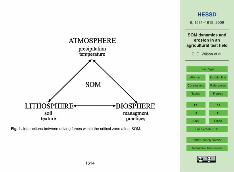
The constituents of Eq. (1) are controlled by interrelated driving forces within thecritical zone (Fig. 1). The relative influences of the individual controls differ depending15

on different land uses, landscape positions, and scales, at which they are studied.Moreover, many aspects of these interactions are grossly understudied, which inhibitsoverall understanding of the processes occurring in the critical zone (Chorover et al.,2007).

In the atmosphere, climate, namely temperature and precipitation, dictates primary20

productivity affecting both the residue quantity and quality, which is expressed as therelative ease of the residue to decompose (Duiker and Lal, 1999). Climate also af-fects the microbial activity driving the decomposition of the residue (Cole et al., 1993).Finally, precipitation intensity and duration determines raindrop impact and runoff, re-spectively, which are the triggering mechanisms for soil detachment and transport.25

Soil detachment results from the breakdown of soil aggregates, or complexes ofinorganic minerals and SOM. Within aggregates, SOM is physically protected fromdecomposing microbes. Thus, soil texture (i.e., clay content and aggregate size) can

1583





HESSD6, 1581–1619, 2009



C. G. Wilson et al.

Title Page



Tables Figures

J I

J I

Back Close

Full Screen / Esc



regulate decomposition (Bricklemyer et al., 2007), as well as influence soil erodibility(Gilley et al., 1993).

The degree of soil erosion results not only from the interplay between hydrologic forc-ings (i.e., raindrop impact and runoff) and soil biogeochemical properties (e.g., aggre-gate stability), but also the influences of anthropogenically applied management prac-5

tices (Dalzell et al., 2004; Papanicolaou and Abaci, 2008). In some instances, man-agement practices amplify erosion rates, while other management practices dampenthe impacts of the hydrologic forcings and soil characteristics on erosion. For example,it is widely accepted that conventional tillage in agricultural fields enhances erosion bydisassociating soil aggregates, decreasing soil strength, and facilitating particle mobil-10

ity under fluid forces (Williams, 1981). Reduced tillage practices have been shown tomaintain aggregate structure, thereby limiting grain particle entrainment by flow (Paus-tian et al., 2000).

Now, a strong relationship exists between erosion and SOM loss (Starr et al., 2000;Papanicolaou et al., 2009), so it follows that SOM concentrations are also strongly in-15

fluenced by the applied management practices. Previous studies have shown that theeffects of agricultural management practices (i.e., tillage) on SOM can vary consider-ably depending on the practice intensity (Duiker and Myers, 2005; Lal, 2005; Kennedyand Schillinger, 2006). For example, long-term conventional tillage reduces net pri-mary productivity, and ultimately the carbon input to the soil. However, tillage increases20

aeration and facilitates contact between residue and the decomposing microbes, thusstimulating microbial activity (Bot and Benites, 2005) and mineralization rates (Moor-man et al., 2004). Conversely, short-term conservation tillage preserves aggregatestability thereby protecting SOM, as well as improving soil tilth (Lal, 2005).

In addition to these observations, tillage-induced erosion has been shown to remove25

substantial amounts of SOM, especially immediately following conversion to cultivatedland (Starr et al., 2000; Manies et al., 2001). In fact, it has been estimated that approx-imately one-half of the topsoil (i.e., the highly organic O and A horizons) in Iowa waslost since settlement due to agriculture (Pimental et al., 1995).

1584





HESSD6, 1581–1619, 2009



C. G. Wilson et al.

Title Page



Tables Figures

J I

J I

Back Close

Full Screen / Esc



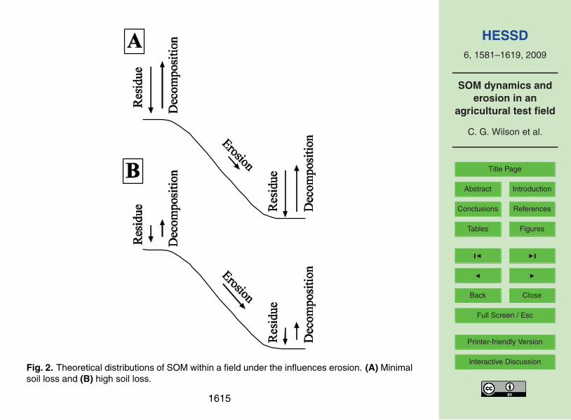
However, the exact relationship between SOM and erosion (i.e., soil loss and de-position) remains unclear. It can be deduced that on an undisturbed field or one withlittle topography, erosion would be minimal (Fig. 2a). Thus, SOM loss would primarilytake place through decomposition. Conversely, in agricultural fields with moderate tosevere slopes, erosion can play a more prominent role in SOM loss (Fig. 2b). Along5

the shoulder and back slope, soil loss would exceed deposition resulting in substantialSOM loss. On toe slopes and floodplains, deposition would dominate potentially lead-ing to sequestration of carbon (Gregorich et al., 1998), with as much as 0.6–1.5 Gt C/yrsequestered through burial (Stallard, 1998; Smith et al., 2001; Renwick et al., 2004).

Few studies have examined in detail the role of spatial variations of both soil loss10

and deposition on SOM (e.g., Polyakov and Lal, 2004), relative to studies focusing onclimate and texture controls (e.g., Cole et al., 1993; Bricklemyer et al., 2007). Mostof these efforts were limited by underestimating the importance of deposition on SOMdynamics (Gregorich et al., 1998), leading to potentially significant errors in SOM-estimation. For example, studies have linked models, which simulate SOM dynamics15

(e.g., CENTURY), with either lumped erosion models, such as the Universal Soil LossEquation (USLE), or coarse field erosion estimates (e.g. Monreal et al., 1997; Hardenet al., 1999; Manies et al., 2001; Pennock and Frick, 2001; Yadav and Malanson,2008). However, recent studies have shown that deposition of eroded material, whichis dependent on terrain, soil roughness, vegetative (or residue) cover, and runoff coef-20

ficients, can be a significant source of SOM (Mancilla, 2001; Pennock and Frick, 2001;Fox and Papanicolaou, 2007, 2008; Papanicolaou and Abaci, 2008). Hence depositionshould not be ignored, especially if an impact assessment of different managementpractices on soil erosion and SOM dynamics is needed.

In light of this apparent need to account for deposition, the main objective of this25

study was to better understand the spatial distributions of SOM as controlled by soilloss and deposition resulting from historical and current management strategies onSOM dynamics. SOM dynamics were modeled using the CENTURY SOM dynam-ics model, which accounted for the interdependence of management practices, soil

1585





HESSD6, 1581–1619, 2009



C. G. Wilson et al.

Title Page



Tables Figures

J I

J I

Back Close

Full Screen / Esc



loss/deposition, and decomposition for an agricultural test field in the Clear Creek, IAwatershed. Different scenarios of erosion, which included (1) no erosion, (2) an aver-age erosion rate for the whole field, and (3) individual rates for the erosional upland anddepositional floodplain, were determined using the Water Erosion Prediction Project(WEPP). These erosion rates were then implemented into CENTURY to determine C5

budgets for the test field. It was hypothesized that deposition would mute the overall Closs from the test field. Improving C budgets would provide better understanding of theglobal carbon cycle, as well as the biogeochemical processes occurring in the criticalzone.

2 Materials and methods10

2.1 CENTURY SOM dynamics model

The SOM dynamics of the test field were evaluated using the CENTURY Soil OrganicMatter model, version 4, which is currently the most used and tested version of themodel (Metherell et al., 1993). CENTURY simulates nutrient dynamics (carbon, nitro-gen, phosphorus, and sulfur) through plant-soil interactions for different ecosystems15

including grasslands, agricultural lands, and forests. The model’s primary use is as ananalysis tool for controls on SOM and productivity. SOM changes strongly reflect theintegration of ecosystem processes, environmental changes, and anthropogenic influ-ences. More detailed descriptions of the model can be found in Metherell et al. (1993)and Theregowda (2007).20

The CENTURY model is a synthesis of multiple sub-models (e.g., soil organicmatter/decomposition sub-model, water budget sub-model, and grassland/crop sub-model) with a management/events scheduling function that computes the fluxes of C,N, P, and S through the various compartments in the model.

The SOM sub-model is an important component of CENTURY. The sub-model ini-25

tially partitions crop residue and roots after harvest into either metabolic or structural

1586





HESSD6, 1581–1619, 2009



C. G. Wilson et al.

Title Page



Tables Figures

J I

J I

Back Close

Full Screen / Esc



carbon pools based on the lignin: nitrogen ratio of the residue (Metherell et al., 1993).Residue with higher lignin concentrations is partitioned to the structural pool, whileresidue with lower lignin concentrations is placed in the metabolic pool. As the residuedecomposes and is incorporated into the soil, the model differentiates the carbon intothree pools (active, slow, and passive) based on decomposition rates. The active pool5

consisting of microbes and their by-products (e.g., proteins, amino acids, sugars, andstarches), as well as low density SOM (termed as the light fraction; Cambardella andElliot, 1992) has short turnover times of 2 to 4 yr (Parton et al., 1988). This poolis strongly influenced by both climate and management practices (Bot and Benites,2005). The slow pool is comprised of mostly cellulose, hemi-cellulose, and SOM that10

is physically protected within soil aggregates. These products are more resistant todecomposition and have turnover times of 20 to 50 yr (Parton et al., 1988). The pas-sive pool contains lignin, which is chemically resistant to decomposition and has a longturnover time (800–1200 yr; Parton et al., 1988). All carbon flows linearly through theSOM sub-model, with rates proportional to the amounts of C in the different pools, until15

all carbon has been metabolized into CO2. Flows of N, P, and S are related to the Cflows through simple elemental ratios.

CENTURY simulates SOM dynamics of the different C pools using monthly timesteps in the surface horizon of the soil column. Multiple soil layers can be implementedinto CENTURY; however, SOM dynamics only occur in the surface horizon, identified20

as the active layer. The recommended depth of the active layer is 20 cm, but it shouldnot exceed 30 cm in CENTURY simulations.

2.2 Model simulations

In this study, SOM dynamics were simulated in a test field of the Clear Creek, IA water-shed for the entire period of cultivation for the field using CENTURY. SOM pools were25

allowed to reach steady state during an extended initialization period of 15 000 yr (theapproximate length time since the last glaciation of this area) before the implementationof agricultural practices. It is important to have an extended initialization period to allow

1587





HESSD6, 1581–1619, 2009



C. G. Wilson et al.

Title Page



Tables Figures

J I

J I

Back Close

Full Screen / Esc



default nutrient concentrations to reach equilibrium before implementing a disturbance,like conversion to agriculture (Manies et al., 2000 and 2001).

For initialization, default parameters and concentrations of C of grassland vegetation(i.e., bluegrass) were used, essentially simulating native prairie. Annual light grazingand a periodic burn every 15 years were included during the period (Ehrenreich and5

Aikman, 1963). The output values of this initialization period were used as initial valuesfor the subsequent cropped period.

Three different simulations of erosion for the cropped period were conducted in thisstudy that were based on different degrees of erosion (i.e., soil loss and deposition) andwere provided via previously calibrated/verified WEPP simulations (Papanicolaou and10

Abaci, 2008). The first simulation contained no erosion, while the second simulationused an average soil loss value for the whole test field. During the third simulation, thetest field was segmented into upland and floodplain components. The upland experi-enced only soil loss during the cropped period, according to WEPP. On the floodplain,WEPP simulations suggested both soil loss and deposition occurred; however, the15

floodplain was a net depositional area.

2.3 CENTURY inputs

Input data for CENTURY are distributed into twelve data files. These files contain in-formation regarding crops and trees, tillage, harvesting, grazing, irrigation, fertilizationand additional organic matter additions, fires, fixed parameters regarding decomposi-20

tion rates, and site specific parameters, which include climate and soil type. Each filecontains a certain subset of variables. Most of the internal parameters in CENTURYwere determined by calibrating the model to long-term soil decomposition experiments(1 to 5 yr) where different types of plant material were added to soils of different textures(Parton et al., 1987).25

Many of the input parameters used for this study were default values provided byCENTURY. However, certain site-specific parameters required user-defined values.These values, which are detailed below, include information regarding the soil tex-

1588





HESSD6, 1581–1619, 2009



C. G. Wilson et al.

Title Page



Tables Figures

J I

J I

Back Close

Full Screen / Esc



ture, climate, and applied management practices, as well as erosion (i.e., soil loss anddeposition).

2.3.1 Study site

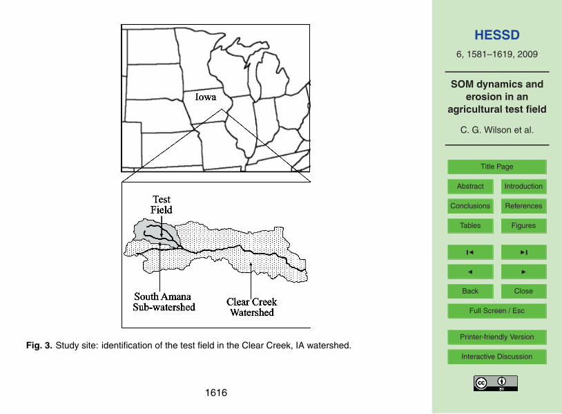
CENTURY simulations were conducted for a test field within the Clear Creek, IA wa-tershed (HUC-10: 0708020904). The watershed comprises approximately 270 km2 in5

east-central Iowa (Fig. 3) and drains to the Iowa River. Since settlement, nearly 80% ofthe watershed has been converted from a prairie and forested area to row-crop agricul-ture and pastures. Currently, the dominant rotation in the watershed is corn-soybeanand the two crops are in roughly equal proportions throughout the watershed. Althoughagriculture is still prominent in the watershed, Clear Creek is experiencing a marked10

increase in population.The test field is within a 26 km2, predominantly rural, headwater catchment of the

South Amana, IA area (Fig. 3). This catchment has two main sub-basins, both of whichcontain first order streams. Each stream length is approximately 6 river-km during thewet season. The outlet of the catchment is approximately 30 river-km above the Iowa15

River confluence.The catchment is the focal point of the Clear Creek Experiment Watershed, which is

an ideal natural laboratory for evaluating soil and water concerns due to an establishedinfrastructure maintained by the University of Iowa to monitor several environmen-tal parameters. In addition, an extensive geospatial, chemical, and eco-hydrological20

database exists, as well as a detailed history of land uses and management practicesfor the watershed (Papanicolaou and Abaci, 2008).

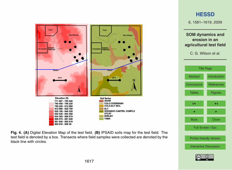
The test field (Fig. 4a) used in the computer simulations is a convex hillslope locatedin the southern part of the catchment. The elevation of the hillslope decreases 23.8 malong a slope length of 130 m yielding an average declination of 0.18. The predomi-25

nant soil series on the ridge and shoulder of the hillslope (Fig. 4b) is Tama (Fine-Silty,Mixed, Superactive, Mesic Typic Argiudoll). Soils of the Tama series are mollisols, orprairie-derived soils. They are well-drained and are formed from loess. The Colo-

1589





HESSD6, 1581–1619, 2009



C. G. Wilson et al.

Title Page



Tables Figures

J I

J I

Back Close

Full Screen / Esc



overwash soil series (Fine-Silty, Mixed, Superactive, Mesic Cumulic Endoaquoll) is atthe toe slope and floodplain. Soils of the Colo series are derived from alluvium andare poorly drained. Long cores (2 m) were collected using a truck mounted Giddingsprobe in the field to confirm soil series maps and identify important soil properties (Ta-ble 1; Papanicolaou et al., 2008). Samples were collected along transects at the ridge,5

shoulder, backslope, and floodplain of the test field and were analyzed for their organiccarbon content to provide a verification dataset for this study.

2.3.2 Climate

Decomposition is a prominent controlling factor of SOM dynamics and climatic con-ditions directly affect decomposition rates. Climatic variables are important inputs in10

CENTURY because decomposition is calculated as a single function of temperatureand precipitation (Metherell et al., 1993). Optimum levels of soil temperature andmoisture, which are influenced by air temperature and precipitation, exist that producemaximum decompositions rates. These rates will decrease as levels deviate from theoptimum values.15

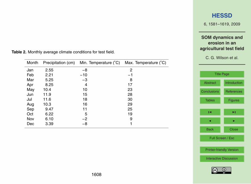
Observed climate data (Table 2) were obtained from the Iowa EnvironmentalMesonet, IEM, which collects environmental data from cooperating members with ob-serving networks. One such site was located less than 5 km from the test field.

These data were supplemented with estimates obtained via a stochastic weathergenerator, CLIGEN (Nicks, 1985). CLIGEN produces daily estimates of precipitation,20

temperature, dew point, wind, and solar radiation for a single geographic point, usingmonthly parameters (means, standard deviations, skewness, etc.) derived from thehistoric measurements.

CENTURY provides different options for climatic inputs. Monthly averages, whichwere varied based on variability and skewness statistics, were used during the ini-25

tialization period. Average values were assumed to be sufficient to establish base-level conditions for the simulations. Historical monthly averages were used during thecropped period because these values would provide better accuracy for the model.

1590





HESSD6, 1581–1619, 2009



C. G. Wilson et al.

Title Page



Tables Figures

J I

J I

Back Close

Full Screen / Esc



2.3.3 Test field management strategies

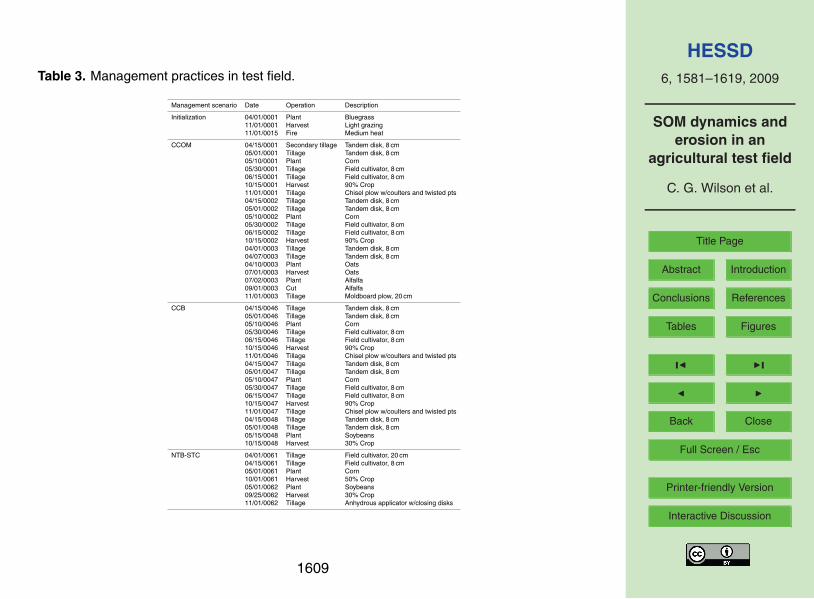
The test field was native prairie through 1930. Since then, three different land man-agement strategies have been utilized at the test field. Specific details regarding eachperiod were described in detail in Theregowda (2007) and are summarized herein (Ta-ble 3). The CENTURY and WEPP simulations were based on this established man-5

agement history.The first management period consisted of a 3-year Corn, Corn, Oat-Meadow

(CCOM) rotation, which lasted from 1931 through 1975. Corn was planted in thefirst two years followed by a year of oats with a winter cover crop of alfalfa. Con-ventional tillage was implemented during this period that utilized a tandem disk, field10

cultivator, and moldboard plow. Organic fertilizers were used until 1950 when inorganicfertilizers were then implemented. In 1976, the oat-meadow year in the rotation wasreplaced with soybean leaving a Corn-Corn-Bean (CCB) rotation. Management prac-tices were similar with the later part of the previous period, except the moldboard plowwas not used. The current management period began in 1991 and involves a two-year15

corn-soybean rotation using reduced tillage practices and applications of anhydrousammonia (STC-NTB).

2.3.4 Erosion

Along with decomposition, erosion significantly affects SOM within CENTURY; how-ever, the model does not directly calculate erosion. It must be supplied by the user as20

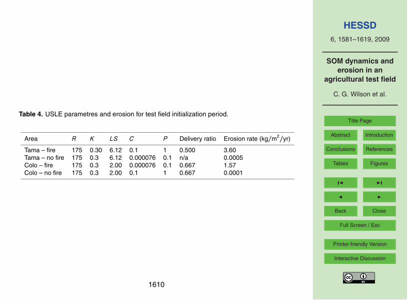
a monthly input.Soil loss during the initialization period was determined using the Universal Soil Loss

Equation (USLE). The USLE was a first attempt at developing a unified, widely appli-cable erosion model. It provides long-term average annual gross erosion rates. Themodel develops individual indices for the dominant factors controlling erosion: rain-25

fall erosivity (R), soil erodibility (K ), slope length (L), slope steepness (S), vegetativecover/management practices (C), and conservation measures (P ) (Wischmeier and

1591





HESSD6, 1581–1619, 2009



C. G. Wilson et al.

Title Page



Tables Figures

J I

J I

Back Close

Full Screen / Esc



Smith, 1965). The parameters of the USLE are empirically based on a large historicaldataset.

The USLE was chosen for the initialization period to simplify the monthly inputs. Soilloss rates were determined for both the erosional upland and depositional floodplain(Table 4). An individual soil loss rate was determined for the fire year, while another5

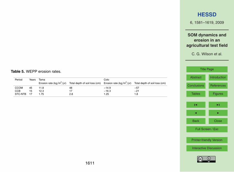
rate was used for the non-fire years.Soil loss/deposition rates during the simulation period were provided by WEPP (Ta-

ble 5). The advantage of this coupling of WEPP and CENTURY is that WEPP is a dis-tributed model for surface runoff, soil properties, and management practices (Flanaganand Nearing, 1995). WEPP’s strengths include being a physically-based model with10

a complete management practice database, which accounts for soil loss/deposition.Another advantage of using WEPP in this study was that baseline values of key modelparameters such as erosional strength and the effective hydraulic conductivity weremeasured in-situ prior to applying them to WEPP (Papanicolaou and Abaci, 2008).

The WEPP platform is an agglomeration of five sub-components: climate, topog-15

raphy, soil, management and watershed structure (Renschler and Flanagan, 2002).A comprehensive review of the model formulation is available in Flanagan and Nearing(1995) with a recent evaluation found in Laflen et al. (2004).

WEPP calculates rainfall excess (or runoff) by the Green-Ampt Mein-Larson infiltra-tion equation. The peak runoff rate is determined by kinematic wave overland flow20

routing, if the model is run for single storm events, or by simplified regression equa-tions based on the kinematic wave model, if the model is run in a continuous mode (aswas the case for this study).

Erosion is differentiated into rill and interrill components by WEPP. Interrill erosion isinitiated by soil detachment from raindrop impact and the sediment is carried to rills by25

overland flow. Rill erosion is considered a function of sediment detachment, the existingsediment load in the runoff, and sediment transport capacity (Flanagan and Nearing,1995). The driving sediment transport equation for rill erosion in WEPP includes the

1592





HESSD6, 1581–1619, 2009



C. G. Wilson et al.

Title Page



Tables Figures

J I

J I

Back Close

Full Screen / Esc



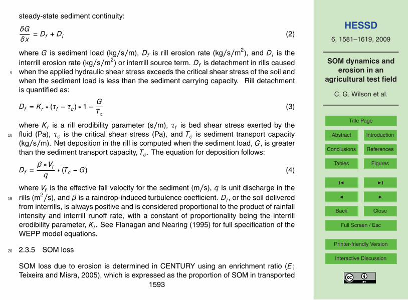
steady-state sediment continuity:

δGδx

= Df + Di (2)

where G is sediment load (kg/s/m), Df is rill erosion rate (kg/s/m2), and Di is theinterrill erosion rate (kg/s/m2) or interrill source term. Df is detachment in rills causedwhen the applied hydraulic shear stress exceeds the critical shear stress of the soil and5

when the sediment load is less than the sediment carrying capacity. Rill detachmentis quantified as:

Df = Kr ∗ (τf − τc) ∗ 1 − GTc

(3)

where Kr is a rill erodibility parameter (s/m), τf is bed shear stress exerted by thefluid (Pa), τc is the critical shear stress (Pa), and Tc is sediment transport capacity10

(kg/s/m). Net deposition in the rill is computed when the sediment load, G, is greaterthan the sediment transport capacity, Tc. The equation for deposition follows:

Df =β ∗ Vfq

∗ (Tc − G) (4)

where Vf is the effective fall velocity for the sediment (m/s), q is unit discharge in therills (m2/s), and β is a raindrop-induced turbulence coefficient. Di , or the soil delivered15

from interrills, is always positive and is considered proportional to the product of rainfallintensity and interrill runoff rate, with a constant of proportionality being the interrillerodibility parameter, Ki . See Flanagan and Nearing (1995) for full specification of theWEPP model equations.

2.3.5 SOM loss20

SOM loss due to erosion is determined in CENTURY using an enrichment ratio (E ;Teixeira and Misra, 2005), which is expressed as the proportion of SOM in transported

1593





HESSD6, 1581–1619, 2009



C. G. Wilson et al.

Title Page



Tables Figures

J I

J I

Back Close

Full Screen / Esc



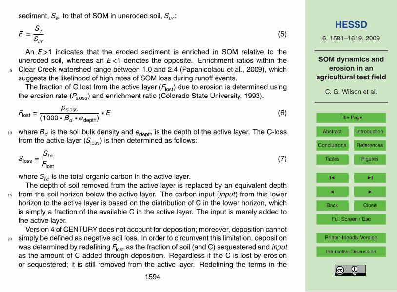
sediment, Se, to that of SOM in uneroded soil, Sur :

E =Se

Sur(5)

An E>1 indicates that the eroded sediment is enriched in SOM relative to theuneroded soil, whereas an E<1 denotes the opposite. Enrichment ratios within theClear Creek watershed range between 1.0 and 2.4 (Papanicolaou et al., 2009), which5

suggests the likelihood of high rates of SOM loss during runoff events.The fraction of C lost from the active layer (Flost) due to erosion is determined using

the erosion rate (Psloss) and enrichment ratio (Colorado State University, 1993).

Flost =psloss

(1000 ∗ Bd ∗ edepth)∗ E (6)

where Bd is the soil bulk density and edepth is the depth of the active layer. The C-loss10

from the active layer (Sloss) is then determined as follows:

Sloss =Stc

Flost(7)

where Stc is the total organic carbon in the active layer.The depth of soil removed from the active layer is replaced by an equivalent depth

from the soil horizon below the active layer. The carbon input (input) from this lower15

horizon to the active layer is based on the distribution of C in the lower horizon, whichis simply a fraction of the available C in the active layer. The input is merely added tothe active layer.

Version 4 of CENTURY does not account for deposition; moreover, deposition cannotsimply be defined as negative soil loss. In order to circumvent this limitation, deposition20

was determined by redefining Flost as the fraction of soil (and C) sequestered and inputas the amount of C added through deposition. Regardless if the C is lost by erosionor sequestered; it is still removed from the active layer. Redefining the terms in the

1594





HESSD6, 1581–1619, 2009



C. G. Wilson et al.

Title Page



Tables Figures

J I

J I

Back Close

Full Screen / Esc



erosion subroutine allowed for implementing the deposition rate as a positive valueand the proper functioning of the above equations.

As with soil loss, the initialization of the C pools of the added soil was important(Metherell et al., 1993). It was assumed that the deposited material was enriched inthe light fraction of SOM and depleted in C from the slow and passive pools. Actual5

values for the C pool distribution were determined during the calibration of the model.

2.4 Model calibration and verification

Calibration of CENTURY for the test field was conducted by adjusting specific sensitiveparameters within physical ranges, which were determined either via implicit/explicitmeasurements or based on values reported in the literature (e.g., Santhi et al., 2001).10

A set of governing factors, which represent the physical forcings, pedologic characteris-tics, and management practices within the watershed, was selected to provide indirectaccounting of the entire range of processes (Buol et al., 1997). Calibration of only themost sensitive parameters helped limit overparameterization.

Because of the limited number of governing factors determined during a sensitivity15

analysis, the model was manually calibrated by adjusting one parameter and keepingthe remaining parameters constant. Calibration continued until the simulated Stc ap-proached average values of cores collected in near proximity of the test field for theUS Department of Agriculture – Natural Resources Conservation Service Soil SurveyLaboratory. The chosen cores were described as pedons containing either the Tama or20

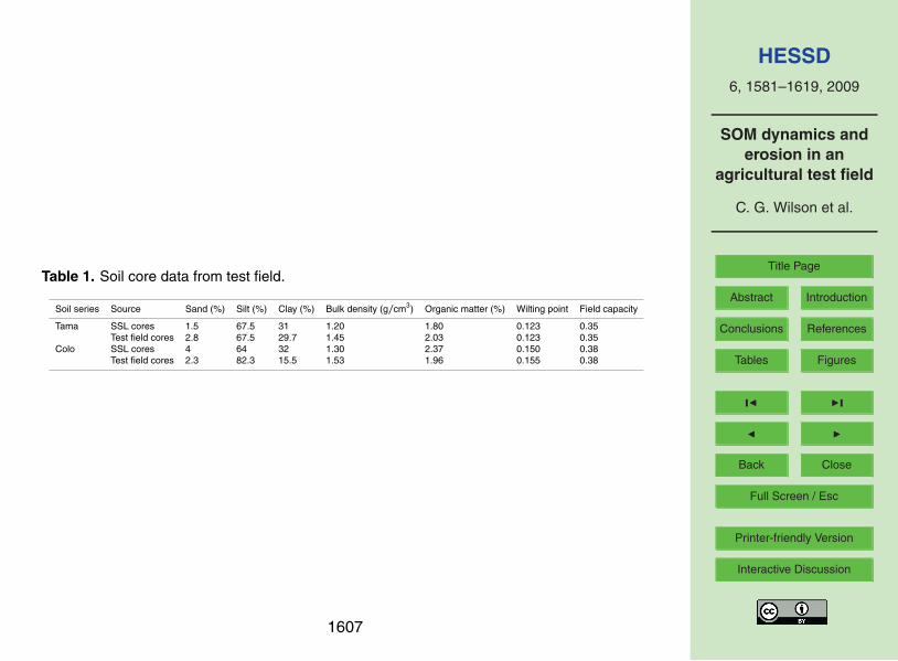
Colo soil series. Average particle size distributions and bulk densities for these cores(Table 1) were used in the calibration process with erosion rates and managementpractices from the test field. It was assumed that management practices and erosionrates were similar throughout the region.

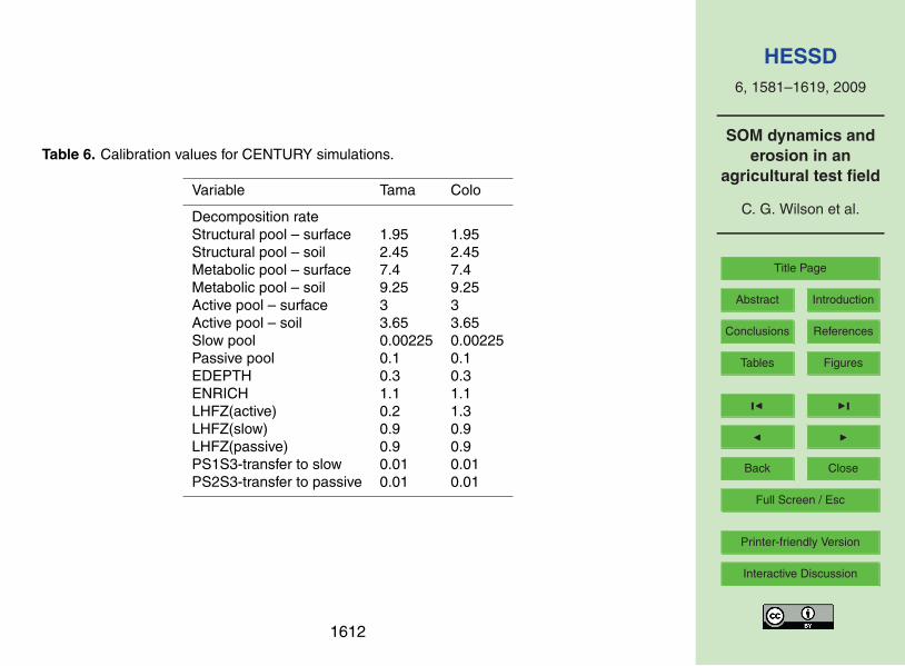
Factors considered in the calibration of CENTURY included erosion rates of the ini-25

tialization period, particle size, bulk density, enrichment ratios, decomposition rates,the flow rate of SOM to slow and passive pools, and the SOM distribution of eitherthe lower horizon or deposited sediment (Table 6). Predetermined ranges of these

1595





HESSD6, 1581–1619, 2009



C. G. Wilson et al.

Title Page



Tables Figures

J I

J I

Back Close

Full Screen / Esc



influential factors were evaluated to determine the appropriate values for the model.Verification of the model was conducted by implementing the particle size and bulk

densities of the cores collected within the test field into the calibrated model. Thesuccess of the verification was based on the accuracy of the model to predict the Stcof the samples collected on the transects in the test field.5

3 Results and discussion

The foci of this study were the changes in SOM dynamics resulting from shifts in differ-ent management practices and the effects of utilizing deposition rates in SOM evalu-ations. SOM results from CENTURY simulations that incorporated different scenariosof WEPP-determined soil loss/deposition rates for the test field are presented herein.10

The following levels of erosion were used in the study: (1) no erosion, (2) average soilloss rates for the whole test field, and (3) soil loss and deposition rates for the uplandand floodplain, respectively, of the test field. SOM results will primarily consist of to-tal SOM concentrations, Stc, which incorporate structural/metabolic C, as well as theactive, slow, and passive pools (Metherell et al., 1993).15

3.1 USLE & WEPP erosion rates

Erosion rates for the CENTURY initialization period were determined using the USLE tosimplify the monthly inputs for the lengthy period (Table 4). Erosion rates were minimalduring most of this period due to the high vegetative cover of the prairie grasses. Highererosion rates were experienced every 15th year of the initialization period due to the20

simulated burning of the test field.During the CENTURY simulations of the cropland period for the test field, soil

loss/deposition rates were determined using WEPP. WEPP provides physically basederosion values for different segments of the test field (i.e., upland and floodplain). In theupland, only soil loss occurred; however, in the floodplain both soil loss and deposition25

1596





HESSD6, 1581–1619, 2009



C. G. Wilson et al.

Title Page



Tables Figures

J I

J I

Back Close

Full Screen / Esc



were observed.During the CCOM and CCB periods, while conventional tillage practices were im-

plemented (i.e., tillage depth=20 cm), erosion rates in the upland were extremely high(Table 5). The erosion was slightly higher during the CCB period relative to the CCOMperiod even with the elimination of moldboard plow use. The benefits gained from5

foregoing the use of the moldboard plow were balanced by the negative effects of thedecreased residue quantities resulting from no longer planting the winter cover crop.Despite the high erosion, much of the eroded sediment was deposited on the floodplainbecause net deposition was observed on the floodplain of the field (Table 5).

The conservation tillage practices implemented at the test field in 1991 (i.e.,10

tillage depth=7.6 cm), resulted in a dramatic decrease in erosion rates of the upland(Table 5). Moreover, deposition on the floodplain also decreased. In fact, during theSTC-NTB period there was slight erosion on the floodplain (Table 5).

3.2 CENTURY initialization period

The initialization period for the CENTURY simulations established steady state concen-15

trations of SOM for the test field, which served as a baseline, from which to evaluatethe effects of introduced agricultural practices. Steady state conditions were reachedwhen organic matter accumulation from native grass residue equaled organic matterloss due to erosion and decomposition (Bot and Benites, 2005).

During the initialization period of the CENTURY simulations in this study, equilibrium20

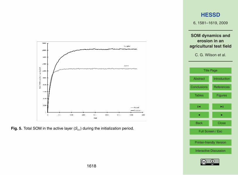
conditions were obtained relatively quickly (Fig. 5). Equilibrium concentrations of totalSOM for the upland and floodplain components of the test field were 12 600±87 g/m2

and 18 300±88 g/m2, respectively. SOM loss due to erosion was minimal during thisperiod with an accumulated SOM loss from the test field during the final 1000 years ofonly 10.2 g/m2/yr. Decomposition was the primary mechanism of SOM loss from the25

test field in this period, which averaged 415±42 g/m2/yr of CO2 lost through decom-position during equilibrium conditions.

Comparisons of SOM concentrations between the floodplain and the upland showed1597





HESSD6, 1581–1619, 2009



C. G. Wilson et al.

Title Page



Tables Figures

J I

J I

Back Close

Full Screen / Esc



that floodplain SOM concentrations approached higher values. Higher SOM values onthe floodplain resulted from lower erosion rates and excess moisture conditions existingon the floodplain, which can produce anaerobic conditions, due to poorly drained soilsand lower slopes. Excess water can cause stagnation and low aeration, which inhibitdecomposition of organic matter (Wells et al., 1997).5

Concentration trends during the initialization period of this study were similar toCENTURY-simulated SOM values for a test field in Western Iowa by Manies etal. (2001). SOM values at the end of the initialization period for this study were higherthan those in Manies et al. (2001); however, differences may be explained by moreintense grazing and a shorter interval between fires in Manies et al. (2001) leading10

to higher erosion rates than this study. The higher erosion rates would remove moreSOM from the simulated test site in the Manies et al. (2001) field leaving lower SOMconcentrations.

3.3 CENTURY cropland period

Simulations of the cropland period were conducted under three different erosion sce-15

narios to demonstrate the importance of including deposition in studies of SOM dynam-ics. Initially, the test field SOM dynamics were simulated without erosion to establishthe role of decomposition. The test field SOM dynamics were then simulated using av-erage soil loss values for the whole test field. Overall, the field has experienced a netloss of soil during the cropped period. The final simulation segmented the field into two20

components, an erosional upland and depositional floodplain. The upland componentwas spatially three times larger than the floodplain component, so all SOM values forthis simulation were weighted proportionately.

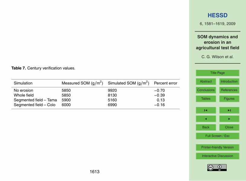
The final Stc values for each simulation were used for verification of the model cal-ibration (Table 7). Both the no erosion and whole field simulations produced higher25

Stc values than measured in the field. The total SOM concentrations produced by thesegmented simulation agreed well with the measured field values (Table 7). Simu-lated Stc values for the upland were 13% lower and values for the floodplain were 16%

1598





HESSD6, 1581–1619, 2009



C. G. Wilson et al.

Title Page



Tables Figures

J I

J I

Back Close

Full Screen / Esc



higher than measured field values. Thus, more detailed erosion values led to betterperformance of the model.

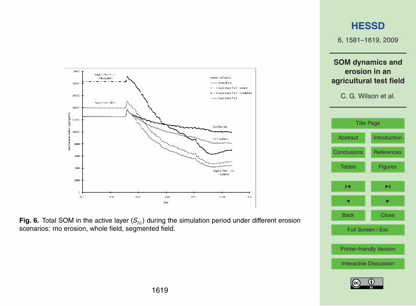
Despite the differences in accuracy when compared to field measurements, trends ofSOM for all three simulations were similar showing an initial increase in Stc immediatelyfollowing the conversion to agriculture due to incorporation of the prairie grass residue5

into the soil. A marked decrease was then observed in all three cases. This decreasewas more gradual for the no erosion and whole test field simulations than for the seg-mented field simulation (Fig. 6). Total SOM concentrations decreased 22%, 36%, and64% from the original concentration for the no erosion, whole field, and segmented fieldsimulations, respectively. Previous studies have also shown large decreases in SOM10

after the introduction of tillage (e.g., Manies et al., 2001; Conant et al., 2007). Despitethe large decreases in Stc for the segmented field simulation, a slight increase in to-tal SOM concentrations was observed during the during the most recent managementperiod, STC-NTB (Fig. 6), which was not seen in the other two simulations.

The primary mechanism for SOM loss during the cropland period was tillage-induced15

erosion and not decomposition as observed during the initialization period. Extensivetillage can break down soil aggregates reducing soil strength, which can increase ero-sion (Lal, 2005). In CENTURY, SOM loss and erosion are directly related (Parton et al.,1987; Metherell et al., 1993), and since the soil loss/deposition rates for the test fieldsubstantially increased due to tillage (over 2 orders of magnitude during the CCOM20

and CCB periods), the SOM loss was also considerably high. The majority of the SOMloss occurred during the first management period, which was attributed to the high soilloss and large store of available C from the incorporated prairie residue. Prairie residueprovided additional input of SOM, most probably in the slow (cellulosic) pool. Erosionallosses of SOM for the test field decreased after this high point through the remainder25

of the simulation period.Budgeting of the erosional losses of SOM during the whole field suggested that

8510 g/m2 of Stc were removed from the field during the cropped period, which is lessthan 13 300 g/m2 of Stc from the upland component of the segmented field simulation.

1599





HESSD6, 1581–1619, 2009



C. G. Wilson et al.

Title Page



Tables Figures

J I

J I

Back Close

Full Screen / Esc



This is when comparing the soil loss rates for these simulations. The lower soil lossrate of the whole field simulation also produced higher Stc values.

However, deposition muted the SOM loss due to erosion in the segmented simula-tion. The eroded soil and SOM in the uplands were retrained on the floodplain beforeleaving the field. Thus, on larger scales, less sediment was lost from the system.5

The floodplain component sequestered 6710 g/m2 of Stc yielding a net loss of only6561 g/m2 of Stc from the test field during the segmented simulation, which is 22%difference compared to the whole field simulation.

Moreover, existing sediment on the floodplain was buried, which inhibits its decom-position by limiting aeration and possibly inducing anaerobic conditions. Both these10

effects have implications regarding global carbon budgets (Polyakov and Lal, 2004).Even though deposition would inhibit decomposition of buried sediments, increased

decomposition in the active layer would result from deposition of the finer, highly or-ganic material from the upland. The deposited material would more easily decom-posed because it consists of the light fraction (LF). The LF organic-matter was defined15

originally by Greenland and Ford (1964) to be material having a density of <2.0 g/cm3

and composed of partially decomposed plant residue having a C/N ratio of <25 (Cam-bardella and Elliot, 1992). Moreover, mineralization would be eclipsed by higher waterholding capacities, which exist on the floodplain leading to higher CO2 emissions (Ma-nies et al., 2001). These findings agree with studies by Fox and Papanicolaou (200720

and 2008), which examined the movement of SOM in watersheds using stable Carbonand Nitrogen isotopes. Ignoring deposition in simulations of SOM dynamics during thisperiod would underestimate decomposition rates and CO2 emissions from the soil.

One question that arose from the trend of the floodplain SOM concentrations waswhy SOM concentrations declined, if deposition was occurring. This should result in25

a net addition of SOM. However, the decline resulted from a model limitation, whichwas mentioned above. It is important to note that CENTURY focuses on only theactive surface layer, whose depth is set by the user through the parameter, EDEPTH.As deposited sediments added depth to the active layer, the corresponding amount

1600





HESSD6, 1581–1619, 2009



C. G. Wilson et al.

Title Page



Tables Figures

J I

J I

Back Close

Full Screen / Esc



was removed from the bottom of the active layer to maintain the assigned depth, i.e.,buried SOM was removed from the active layer. The deposited material, which wascomprised of the light fraction, was different from the SOM material removed (morestable forms of SOM). These more stable forms were not replaced from above and theoverall SOM concentrations declined.5

4 Conclusions

The preservation of soil quality is of extreme relevance in the US Corn Belt where lo-cal economies are driven by agricultural production. Soil quality is difficult to measuredirectly because it is a function of several factors, like SOM. SOM content, which influ-ences other soil biogeochemical properties, provides a reliable surrogate measure of10

soil quality.SOM concentrations were strongly influenced by the applied management practices

to the test field, which controlled the erosion and deposition occurring at the site. Todate, few studies have examined in detail the role of spatial and temporal variations oferosion/ deposition on SOM, i.e., the role of deposition is still poorly understood. The15

main goal of this study was to evaluate the effects of historical and current managementstrategies on SOM dynamics (an indicator of soil quality) for an agricultural test fieldin the Clear Creek, IA watershed by accounting for the interdependence of manage-ment practices, soil loss/deposition, and decomposition. The nature of the research isnovel because it combines dynamic model simulations using WEPP and CENTURY to20

evaluate soil and SOM loss from the field.In this study, deposition was shown to mute the SOM loss due to erosion. The high

losses of soil and SOM in the uplands were entrained on the floodplain before leavingthe field. These effects have implications regarding global carbon budgets (Polyakovand Lal, 2004). Thus, it is important to accurately account for the roles of both erosion25

and deposition occurring in a field to provide reliable estimates of SOM loss.The present research was performed using CENTURY simulations that were limited

1601





HESSD6, 1581–1619, 2009



C. G. Wilson et al.

Title Page



Tables Figures

J I

J I

Back Close

Full Screen / Esc



to monthly predictions of SOM loss. This inherent limitation of the CENTURY modeldid not hinder understanding of the SOM dynamics resulting from different manage-ment practices. Changes in management practices occurred in periods longer thanthe monthly time step. Hence the model captured the effects of changing manage-ment practices on SOM dynamics. However, future studies that intend to capture daily5

changes in SOM due to different anthropogenic activities should consider the use dailyevent models like DAYCENT (Del Grosso et al., 2006).

Acknowledgements. The authors and PI Papanicolaou would like to acknowledge the studentand post doctoral support provided by the Iowa’s Multiscale Carbon and Nitrogen Studies (IM-CANS): Combining Remote and In-Situ Approaches in Agricultural Landscapes and the director10

of the program, Dr. William Byrd. In addition, the preliminary work by Ranjani Theregowda wasalso appreciated.

References

Brady, N. C. and Weil, R. R.: The Nature and Properties of Soil, 14th ed., Pearson-PrenticeHill, Upper Saddle River, NJ, 2008.15

Bricklemyer, R. S., Miller, P. R., Turk, P. J., Paustian, K., Keck, T., and Nielsen G. A.: Sensitivityof the Century model to scale related soil texture variability, Aust. J. Soil Sci., 71(3), 784–792,2007.

Bot, A. and Benites, J.: The importance of soil organic matter, Soils Bulletin 80, Food andAgriculture Organization of the United Nations (FAO), Rome, 2005.20

Buol, S. W., Hole, F. D., Mccracken, R. J., and Southard, R. J.: Soil Genesis and Classification,4th ed., Iowa State University Press, Ames, IA, 1997.

Cambardella, C. A. and Elliot, E. T.: Particulate soil organic-matter changes across a grasslandcultivation sequence, Soil Sci. Soc. Am. J., 56, 777–783, 1992.

Chorover, J., Kretzschmar, R., Garcia-Pichel, F., and Sparks, D. L.: Soil biogeochemical pro-25

cesses within the critical zone, Elements, 3, 321–326, 2007.Cole, C. V., Paustian, K., Elliott, E. T., Metherell, A. K. Ojima, D. S., and Parton W. J.: Analysis

of agroecosystem carbon pools, Water Air Soil Poll., 70, 357–371, 1993.Colorado State University: CENTURY source code, Version 4, Fort Collins, CO, 1993.

1602





HESSD6, 1581–1619, 2009



C. G. Wilson et al.

Title Page



Tables Figures

J I

J I

Back Close

Full Screen / Esc



Conant, R. T., Easter, M., Paustian, K., Swan, A., and Williams, S.: Impacts of periodic tillageon soil C stocks: A synthesis, Soil Till. Res., 95, 1–10, 2007.

Dalzell, B. J., Gowda, P. H., and Mulla, D. J.: Modeling sediment and Phosphorus losses in anagricultural watershed to meet TMDLs, J. Am. Water Resour. As., 40, 533–543, 2004.

Del Grosso, S. J., Parton, W. J., Mosier, A. R., Walsh, M. K., Ojima, D. S., and Thornton P. E.:5

DAYCENT national-scale simulations of Nitrous Oxide emissions from cropped soils in theUnited States, J. Environ. Qual., 35, 1451–1460, 2006.

Duiker, S. W. and Lal, R.: Crop residue and tillage effects on carbon sequestration in a Luvisolin central Ohio, Soil Till. Res., 52, 73–81, 1999.

Duiker, S. W. and Myers, J. C.: Better Soils with the No-Till System, Penn State College of10

Agricultural Sciences, University Park, PA, 2005.Ehrenreich, J. H. and Aikman, J. M.: An ecological study of the effect of certain management

practices on native prairie in Iowa, Ecol. Monogr., 33(2), 113–130, 1963.Flanagan, D. C. and Nearing M. A.: USDA – Water Erosion Prediction Project: Hillslope profile

and watershed model documentation, NSERL Report No. 10, West Lafayette, IN, 1995.15

Fox, J. F. and Papanicolaou, A. N.: The use of carbon and nitrogen isotopes to study watershederosion processes, J. Am. Water Resour. As., 43(4), 1047–1064, 2007.

Fox, J. F. and Papanicolaou, A. N.: An unmixing model to study watershed erosion processes,Adv. Water Resour., 31, 96–108, 2008.

Gilley, J. E., Elliot, W. J., Laflen, J. M., and Simanton J. R.: Critical shear stress and critical flow20

rates for initiation of rilling, J. Hydrol., 142, 251–271, 1993.Greenland, D. J. and Ford, G. W.: Separation of partially humified organic materials from soils

by ultrasonic dispersion, Trans. Int. Congr., Soil Sci., 8(3), 137–148, 1964.Gregorich, E. G., Greer, K. J., Anderson, D. W., and Liang, B. C.: Carbon distribution and

losses: erosion and deposition effects, Soil Till. Res., 47, 291–302, 1998.25

Harden, J. W., Sharpe, J. M., Parton, W. J., Ojima, D. S., Fries, T. L. Huntington, T. G., andDabney, S. M.: Dynamic replacement and loss of soil carbon on eroding cropland, GlobalBiogeochem. Cy., 13(4), 885–901, 1999.

Jacinthe, P.-A., Lal, R., Owens, L. B., and Hothem D. L.: Transport of labile carbon in runoff asaffected by land use and rainfall characteristics, Soil Till. Res., 77, 111–123, 2004.30

Kennedy, A. C. and Schillinger, W. F.: Soil quality and water intake in conventional-till vs. no-tillpaired farms in Washington’s Palouse Region, Soil Sci. Soc. Am. J., 70, 940–949, 2006.

Laflen, J. M., Flanagan, D. C., and Engel, B. A.: Soil erosion and sediment yield prediction

1603





HESSD6, 1581–1619, 2009



C. G. Wilson et al.

Title Page



Tables Figures

J I

J I

Back Close

Full Screen / Esc



accuracy using WEPP, J. Am. Water Resour. As., 40(2), 289–297, 2004.Lal, R.: Soil carbon sequestration to mitigate climate change, Geoderma, 123, 1–22, 2004.Lal, R.: Soil erosion and carbon dynamics, Soil Till. Res., 81, 137–142, 2005.Mancilla, G. A.: Prediction of Rill Density, Transport Capacity and Associated Soil Loss of

Different Tillage Systems under Winter Conditions, M.S. Thesis, College of Engineering and5

Architecture, Washington State University, Pullman, WA, 2001.Manies, K. L., Harden, J. W., Kramer, L., and Parton, W.: Parameterizing CENTURY to model

cultivated and noncultivated sites in the loess region of western Iowa, USGS Open-File Re-port 00-508, The United States Geological Survey, Reston, VA, USA, 2000.

Manies, K. L., Harden, J. W., Kramer, L., and Parton, W.: Carbon dynamics within agricultural10

and native sites in the loess region of western Iowa, Glob. Change Biol., 7, 545–555, 2001.Metherell, A. K., Harding, L. A., Cole, C. V., and Parton, W. J.: CENTURY soil organic matter

model environment. Technical documentation. Agroecosystem version 4.0, Technical ReportNo. 4, USDA-ARS Great Plains System Research Unit, Fort Collins, CO, 1993.

Monreal, C. M., Zentner, R. P., and Robertson. J. A.: An analysis of soil organic matter dynam-15

ics in relation to management, erosion and yield of wheat in long-term crop rotation plots,Can. J. Soil Sci., 77(4), 553–563, 1997.

Moorman, T. B., Cambardella, C. A., James, D. E., Karlen, D. L., and Kramer, L. A.: Quantifica-tion of tillage and landscape effects on soil carbon in small Iowa watersheds, Soil Till. Res.,78, 225–236, 2004.20

National Research Council: Basic Research Opportunities in Earth Science, National AcademyPress, Washington DC, 2001.

Nicks, A. D.: Generation of climate data, Proceedings of the Natural Resources Modeling Sym-posium, USDA-ASA ARS-30, 1985.

Papanicolaou, A. N. and Abaci, O.: Upland erosion modeling in a semi-humid environment via25

the Water Erosion Prediction Project. J. Irrig. Drain. E., 134(6), 796–806, 2008.Papanicolaou, A. N., Elhakeem, M., Wilson, C. G., Burras, C. L., and Oneal, B.: Observations of

soils at the hillslope scale in the Clear Creek watershed in Iowa, USA, Soil Survey Horizons,49, 83–86, 2008.

Papanicolaou, A. N., Wilson, C. G., Abaci, O., Elhakeem, M., and Skopec, M.: Soil quality in30

Clear Creek, IA: SOM loss and soil quality in the Clear Creek, IA Experimental Watershed,Journal of Iowa Academy of Science, In review, 2009.

Parton, W. J., Schimel, D. S., Cole, C. V., and Ojima. D. S.: Analysis of factors controlling soil

1604





HESSD6, 1581–1619, 2009



C. G. Wilson et al.

Title Page



Tables Figures

J I

J I

Back Close

Full Screen / Esc



organic matter levels in Great Plains grasslands, Soil Sci. Soc. Am. J., 51, 1173–1179, 1987.Parton, W. J., Stewart, J. W. B., and Cole, C. V.: Dynamics of C, N, P and S in grassland soils:

a model, Biogeochemistry, 5, 109–131, 1988.Paustian, K. H., Six, J., Elliott, E. T., and Hunt, H. W.: Management options for reducing CO2

emissions from agricultural soils, Biogeochemistry, 48, 147–163, 2000.5

Pennock, D. J. and Frick, A. H.: The role of field studies in landscape-scale applications ofprocess models: an example of soil redistribution and soil organic carbon modeling usingCENTURY, Soil Till. Res., 58, 183–191, 2001.

Pimental, D., Harvey, C., Resosudarm, P., Sinclair, K., Kurz, D., Mcnair, M., Crist, S., Shpritz,L., Fitton, L., Saffouri, R., and Blair, R.: Environmental and economic costs of soil erosion10

and conservation benefits, Science, 267(5201), 1117–1123, 1995.Polyakov, V. O. and Lal, R.: Modeling soil organic matter dynamics as affected by soil water

erosion, Environ. Int., 30, 547–556, 2004.Renschler, C. S. and Flanagan, D. C.: Implementing a process-based decision-support tool

for natural resource management the GeoWEPP example, in: Integrated Assessment and15

Decision Support, edited by: Rizzoli, A. E. and Jakeman, A. J., IEMSS 2002: Interl EnvironlModeling Software Soc., 24–27 June 2002, at University of Lugano, Switzerland, 3, 187–192,2002.

Renwick, W. H., Smith, S. V., Sleezer, R. O., and Buddemier, R. W.: Comments on managingsoil carbon, Science, 305, 1567–1573, 2004.20

Santhi, C., Arnold, J. G., Williams, J. R., Dugas, W. A., Srinivasan, R., and Hauck, L. M.:Validation of the SWAT model on a large river basin with point and nonpoint sources, J. Am.Water Resour. As., 37(5), 1169–1188, 2001.

Smith, S. V., Renwick, W. H., Buddemeier, R. W., and Crossland, C. J.: Budgets of soil ero-sion and deposition for sediments and sedimentary organic carbon across the conterminous25

United States, Global Biogeochem. Cy., 15, 697–707, 2001.Stallard, R. F.: Terrestrial sedimentation and carbon cycle: coupling weathering and erosion to

carbon burial, Global Biogeochem. Cy., 12, 231–257, 1998.Starr, G. C., Lal, R., Hothem, D. L., Owens, L. B., and Kimble, J.: Modeling soil carbon trans-

ported by water erosion processes, Land Degrad. Dev., 11, 83–91. 2000.30

Teixeira, P. C. and Misra, R. K.: Measurement and prediction of nitrogen loss by simulatederosion events on cultivated forest soils of contrasting structure, Soil Till. Res., 83, 204–217,2005.

1605





HESSD6, 1581–1619, 2009



C. G. Wilson et al.

Title Page



Tables Figures

J I

J I

Back Close

Full Screen / Esc



Theregowda, R. B.: A CENTURY simulation of Soil Organic Matter (SOM) in Clear Creek, Iowa.M. S. Thesis, Department of Civil and Environmental Engineering, The University of Iowa,Iowa City, IA, 2007.

Wells, K. L., Sims, J. L., and Smith, M. S.: Nitrogen in Kentucky soils, University of KentuckyCooperative Extension Service, Lexington, KY, 1997.5

Williams, J. R.: Soil erosion effects on soil productivity. J. Soil Water Conserv., 36, 82–90,1981.

Wischmeier, W. H. and Smith, D. D.: Predicting Rainfall-Erosion Losses from East of the RockyMountains: A Guide for Selection of Practices for Soil and Water Conservation, USDA Agri-cultural Handbook 282, Washington DC, The US Department of Agriculture, 1965.10

Yadav, V. and Malanson G.: Spatially explicit historical land use land cover and soil organictransformations in southern Illinois, Agr. Ecosyst. Environ., 123, 280–292, 2008.

1606





HESSD6, 1581–1619, 2009



C. G. Wilson et al.

Title Page



Tables Figures

J I

J I

Back Close

Full Screen / Esc



Table 1. Soil core data from test field.

Soil series Source Sand (%) Silt (%) Clay (%) Bulk density (g/cm3) Organic matter (%) Wilting point Field capacity

Tama SSL cores 1.5 67.5 31 1.20 1.80 0.123 0.35Test field cores 2.8 67.5 29.7 1.45 2.03 0.123 0.35

Colo SSL cores 4 64 32 1.30 2.37 0.150 0.38Test field cores 2.3 82.3 15.5 1.53 1.96 0.155 0.38

1607





HESSD6, 1581–1619, 2009



C. G. Wilson et al.

Title Page



Tables Figures

J I

J I

Back Close

Full Screen / Esc



Table 2. Monthly average climate conditions for test field.

Month Precipitation (cm) Min. Temperature (◦C) Max. Temperature (◦C)

Jan 2.55 −8 2Feb 2.21 −10 −1Mar 5.25 −3 8Apr 8.25 4 17May 10.4 10 23Jun 11.9 15 28Jul 11.6 18 30Aug 10.3 16 29Sep 9.47 11 25Oct 6.22 5 19Nov 6.10 −2 9Dec 3.39 −8 1

1608





HESSD6, 1581–1619, 2009



C. G. Wilson et al.

Title Page



Tables Figures

J I

J I

Back Close

Full Screen / Esc



Table 3. Management practices in test field.

Management scenario Date Operation Description

Initialization 04/01/0001 Plant Bluegrass11/01/0001 Harvest Light grazing11/01/0015 Fire Medium heat

CCOM 04/15/0001 Secondary tillage Tandem disk, 8 cm05/01/0001 Tillage Tandem disk, 8 cm05/10/0001 Plant Corn05/30/0001 Tillage Field cultivator, 8 cm06/15/0001 Tillage Field cultivator, 8 cm10/15/0001 Harvest 90% Crop11/01/0001 Tillage Chisel plow w/coulters and twisted pts04/15/0002 Tillage Tandem disk, 8 cm05/01/0002 Tillage Tandem disk, 8 cm05/10/0002 Plant Corn05/30/0002 Tillage Field cultivator, 8 cm06/15/0002 Tillage Field cultivator, 8 cm10/15/0002 Harvest 90% Crop04/01/0003 Tillage Tandem disk, 8 cm04/07/0003 Tillage Tandem disk, 8 cm04/10/0003 Plant Oats07/01/0003 Harvest Oats07/02/0003 Plant Alfalfa09/01/0003 Cut Alfalfa11/01/0003 Tillage Moldboard plow, 20 cm

CCB 04/15/0046 Tillage Tandem disk, 8 cm05/01/0046 Tillage Tandem disk, 8 cm05/10/0046 Plant Corn05/30/0046 Tillage Field cultivator, 8 cm06/15/0046 Tillage Field cultivator, 8 cm10/15/0046 Harvest 90% Crop11/01/0046 Tillage Chisel plow w/coulters and twisted pts04/15/0047 Tillage Tandem disk, 8 cm05/01/0047 Tillage Tandem disk, 8 cm05/10/0047 Plant Corn05/30/0047 Tillage Field cultivator, 8 cm06/15/0047 Tillage Field cultivator, 8 cm10/15/0047 Harvest 90% Crop11/01/0047 Tillage Chisel plow w/coulters and twisted pts04/15/0048 Tillage Tandem disk, 8 cm05/01/0048 Tillage Tandem disk, 8 cm05/15/0048 Plant Soybeans10/15/0048 Harvest 30% Crop

NTB-STC 04/01/0061 Tillage Field cultivator, 20 cm04/15/0061 Tillage Field cultivator, 8 cm05/01/0061 Plant Corn10/01/0061 Harvest 50% Crop05/01/0062 Plant Soybeans09/25/0062 Harvest 30% Crop11/01/0062 Tillage Anhydrous applicator w/closing disks

1609





HESSD6, 1581–1619, 2009



C. G. Wilson et al.

Title Page



Tables Figures

J I

J I

Back Close

Full Screen / Esc



Table 4. USLE parametres and erosion for test field initialization period.

Area R K LS C P Delivery ratio Erosion rate (kg/m2/yr)

Tama – fire 175 0.30 6.12 0.1 1 0.500 3.60Tama – no fire 175 0.3 6.12 0.000076 0.1 n/a 0.0005Colo – fire 175 0.3 2.00 0.000076 0.1 0.667 1.57Colo – no fire 175 0.3 2.00 0.1 1 0.667 0.0001

1610





HESSD6, 1581–1619, 2009



C. G. Wilson et al.

Title Page



Tables Figures

J I

J I

Back Close

Full Screen / Esc



Table 5. WEPP erosion rates.

Period Years Tama ColoErosion rate (kg/m2/yr) Total depth of soil loss (cm) Erosion rate (kg/m2/yr) Total depth of soil loss (cm)

CCOM 45 11.8 48 −14.9 −57CCB 15 12.3 17 −16.3 −21STC-NTB 17 1.75 2.8 1.25 1.8

1611





HESSD6, 1581–1619, 2009



C. G. Wilson et al.

Title Page



Tables Figures

J I

J I

Back Close

Full Screen / Esc



Table 6. Calibration values for CENTURY simulations.

Variable Tama Colo

Decomposition rateStructural pool – surface 1.95 1.95Structural pool – soil 2.45 2.45Metabolic pool – surface 7.4 7.4Metabolic pool – soil 9.25 9.25Active pool – surface 3 3Active pool – soil 3.65 3.65Slow pool 0.00225 0.00225Passive pool 0.1 0.1EDEPTH 0.3 0.3ENRICH 1.1 1.1LHFZ(active) 0.2 1.3LHFZ(slow) 0.9 0.9LHFZ(passive) 0.9 0.9PS1S3-transfer to slow 0.01 0.01PS2S3-transfer to passive 0.01 0.01

1612





HESSD6, 1581–1619, 2009



C. G. Wilson et al.

Title Page



Tables Figures

J I

J I

Back Close

Full Screen / Esc



Table 7. Century verification values.

Simulation Measured SOM (g/m2) Simulated SOM (g/m2) Percent error

No erosion 5850 9920 −0.70Whole field 5850 8130 −0.39Segmented field – Tama 5900 5160 0.13Segmented field – Colo 6000 6990 −0.16

1613





HESSD6, 1581–1619, 2009



C. G. Wilson et al.

Title Page



Tables Figures

J I

J I

Back Close

Full Screen / Esc



39

Fig. 1 1

2

3

4 Fig. 1. Interactions between driving forces within the critical zone affect SOM.

1614





HESSD6, 1581–1619, 2009



C. G. Wilson et al.

Title Page



Tables Figures

J I

J I

Back Close

Full Screen / Esc



40

Fig. 2 1

2

3

4 Fig. 2. Theoretical distributions of SOM within a field under the influences erosion. (A) Minimalsoil loss and (B) high soil loss.

1615





HESSD6, 1581–1619, 2009



C. G. Wilson et al.

Title Page



Tables Figures

J I

J I

Back Close

Full Screen / Esc


Interactive DiscussionFig. 3. Study site: identification of the test field in the Clear Creek, IA watershed.

1616





HESSD6, 1581–1619, 2009



C. G. Wilson et al.

Title Page



Tables Figures

J I

J I

Back Close

Full Screen / Esc



42

Fig. 4 1

2

3

4

5

6

7

8

9

10

11

12

13

14

15

16

17

Fig. 4. (A) Digital Elevation Map of the test field. (B) IPSAID soils map for the test field. Thetest field is denoted by a box. Transects where field samples were collected are denoted by theblack line with circles.

1617





HESSD6, 1581–1619, 2009



C. G. Wilson et al.

Title Page



Tables Figures

J I

J I

Back Close

Full Screen / Esc



43

Fig. 5 1

2

3 Fig. 5. Total SOM in the active layer (Stc) during the initialization period.

1618





HESSD6, 1581–1619, 2009



C. G. Wilson et al.

Title Page



Tables Figures

J I

J I

Back Close

Full Screen / Esc



44

Fig. 6 1

2

3 Fig. 6. Total SOM in the active layer (Stc) during the simulation period under different erosionscenarios: mo erosion, whole field, segmented field.

1619





SOM dynamics and erosion in an agricultural test field

Documents