Solving qualitative constraints involving landmarks

IJCAI-2011 Workshop 27

Benchmarks and Applicationsof Spatial Reasoning

Workshop Proceedings

Barcelona, SpainJuly 17, 2011

Workshop Co-Chairs

Jochen Renz (Australian National University - Canberra, AU)Anthony G. Cohn (University of Leeds, UK)Stefan Wolfl (University of Freiburg, DE)

Program Committee

Alia Abdelmoty (Cardiff University, UK)Marco Aiello (University of Groningen, NL)Mehul Bhatt (University of Bremen, DE)Jean-Francois Condotta (University of Artois, FR)Matt Duckham (University of Melbourne, AU)Antony Galton (University of Exeter, UK)Jason Jingshi Li (Ecole Polytechnique Federale de Lausanne, CH)Reinhard Moratz (University of Maine, Orono (ME), US)Bernhard Nebel (University of Freiburg, DE)Marco Ragni (University of Freiburg, DE)Christoph Schlieder (University of Bamberg, DE)Steven Schockaert (Ghent University, BE)Nico van de Weghe (Ghent University, BE)Jan-Oliver Wallgrun (University of Bremen, DE)

Contents

Jae Hee Lee and Diedrich Wolter:A new perspective on reasoning with qualitative spatial knowledge 3

Weiming Liu, Shengsheng Wang, and Sanjiang Li:Solving qualitative constraints involving landmarks 9

Muralikrishna Sridhar, Anthony G. Cohn, and David C. Hogg:Benchmarking qualitative spatial calculi for video activity analysis 15

Arne Kreutzmann and Diedrich Wolter:Physical puzzles – Challenging spatio-temporal configuration problems 21

Dominik Lucke, Till Mossakowski, and Reinhard Moratz:Streets to the Opra – Finding your destination with imprecise knowledge 25

Manolis Koubarakis, Kostis Kyzirakos, and Stavros Vassos:Challenges for qualitative spatial reasoning in linked geospatial data 33

Julien Hue, Mariette Serayet, Pierre Drap, Odile Papini, and Eric Wurbel:Underwater archaeological 3D surveys validation within the Removed Sets framework 39

Steven Schockaert:An application-oriented view on graded spatial relations 47

Weiming Liu and Sanjiang Li:On a semi-automatic method for generating composition tables 53

A new perspective on reasoning with qualitative spatial knowledge

Jae Hee Lee and Diedrich WolterSFB/TR 8 Spatial Cognition

Universitat BremenP.O. Box 330440 28334 Bremen, Germany

AbstractIn this paper we call for considering a paradigmshift in the reasoning methods that underly qualita-tive spatial representations. As alternatives to con-ventional methods we propose exploiting methodsfrom linear programming and real algebraic geom-etry. We argue that using mathematical theoriesof the spatial domain at hand might be the key toeffective reasoning methods, and thus to practicalapplications.

1 IntroductionQualitative spatial knowledge is ubiquitous in natural language.Thus, it is essential in human-computer interaction, which isan integral part of our everyday life where interaction withdigital equipments is omnipresent. In the field of artificialintelligence, reasoning with qualitative spatial knowledge hasbeen researched under the umbrella term Qualitative SpatialReasoning (QSR) [Cohn and Renz, 2008]. QSR pursues a rela-tion-algebraic approach that provides universal means to dealwith any type of qualitative spatial knowledge (e.g., topology,direction, distance). It has been assumed that the relation-alge-braic approach will allow for an efficient, effective, universalreasoning method. Despite its promising properties, however,the relation-algebraic approach suffers from its incomplete-ness for many representations of qualitative spatial knowledge.Furthermore, it is not capable of generating a model for givenconstraints, which is a desirable feature for many real-worldapplications.

In this paper we call for considering a paradigm shift in thereasoning methods that underly qualitative spatial represen-tations. As alternatives to conventional methods we proposeexploiting methods from linear programming and real alge-braic geometry. We argue that using mathematical theoriesof the spatial domain at hand might be the key to effectivereasoning methods, and thus to practical applications.

2 The Relation-Algebraic Approach and ItsLimitations

The building blocks of QSR are a spatial domain D, a finiteset R = {R1, R2, . . . , Rn} of binary relations on D whichpartitions D2, and a map ◦ : R × R → 2D, R1 ◦ R2 =

{y ∈ D |xR1y and yR2z }, which is called the composition.A prominent, simple example is the one-dimensional space(e.g., a queue) equipped with the relations before, behind,equal and the usual notion of composition, e.g., if Alice isbehind Bob and Bob is behind Charlie than Alice is behindCharlie (i.e., behind ◦ behind = behind).

For a given domain D (e.g., a queue), a partition R (e.g.,before, behind, equal), a composition ◦, a set of variables(e.g., Alice, Bob, Charlie), and a set of spatial constraints (e.g.,Alice is behind Bob, Bob is behind Charlie, Charlie is behindAlice), a common reasoning task is figuring out whether thereis an instantiation of the variables over the domain D, suchthat the given spatial constraints are consistent (the exampleis not consistent, as there is no instantiation for Alice, Boband Charlie that satisfies the constraints). For this reasoningproblem QSR employs the path-consistency method, whichis used for solving constraint satisfaction problems over finitedomains. Since the domain D of interest in QSR is usuallyinfinite as opposed to the domain of a finite CSP, partitionRand composition ◦ have to meet certain requirements, such thatthe path-consistency method is applicable to the constraints(See [Renz and Nebel, 2007] and [Renz and Ligozat, 2005] formore details). A triple (D,R, ◦) that meets those requirementsforms a non-associative algebra; it forms a relation algebra, ifit is additionally closed under composition [Ligozat, 2005].

We will call the reasoning approach that utilizes the path-consistency method the relation-algebraic approach. The maindeficiency of the relation-algebraic approach is that there is noguarantee for its completeness, i.e., the algorithm can fail toidentify all inconsistent scenarios. Accordingly, research hasbeen concentrated on finding out whether the consistency ofconstraints defined by a triple (D,R, ◦) can be decided withthe path-consistency method. The recent result showed thatspatial representations for directional information cannot bedecided by the path-consistency method in general [Wolter andLee, 2010]. Thus, we have to question the idea of keeping therelation-algebraic approach as a universal means, and shouldbe open to search for alternative methods for a sound andcomplete reasoning.

The relation-algebraic approach is also not capable of pro-viding models for the given input constraints. However, in realapplication domains (e.g., computer-aided design, geographicinformation systems) not only deciding the consistency of con-straints, but also determining the positions of spatial objects

3

satisfying those constraints is desired.In the next two sections we introduce a selection of quali-

tative spatial representations for directional information, andmethods for reasoning with those representations, which over-come the deficiencies of the relation-algebraic approach.

3 Representations for Qualitative SpatialKnowledge

If a set of spatial objects are represented by a finite numberof points in the Euclidian space—which is generally the casein many applications—then the qualitative spatial relationsbetween those objects can be described by a system of poly-nomial equations or inequalities. For example, we can modelpeople in a queue as points in R and represent “Alice is behindBob, Bob is behind Charlie, Charlie is behind Alice” with thesystem xA − xB > 0∧ xB − xC > 0∧ xC − xA > 0, wherexA, xB , xC ∈ R.

If we leave the one-dimensional Euclidian space R andmove to the two-dimensional Euclidian space R2, new con-straints emerge which were not existent in the one-dimensionalcase. An important new constraint in the two-dimensional caseis based on the relative positions of three points, i.e., whetherthe points are oriented in clockwise (CW) order, counterclock-wise (CCW) order, or collinear. Formally, such a constraintcan be expressed as a polynomial inequality or equation basedon three points p1=(x1, y1), p2=(x2, y2) and p3=(x3, y3)in the following way

x2y3 + x1y2 + x3y1 − y2x3 − y1x2 − y3x1 < 0 (CW)

x2y3 + x1y2 + x3y1 − y2x3 − y1x2 − y3x1 > 0 (CCW)

x2y3 + x1y2 + x3y1 − y2x3 − y1x2 − y3x1 = 0, (collin.)

where the polynomials on the lefthand side are obtained from

det

(1 x1 y11 x2 y21 x3 y3

), (1)

where det stands for determinant. The importance and ubiq-uity of this relationship of three points in a plane will be evi-dent in the next subsections, where we introduce a selection ofqualitative spatial representations for directional information.In each of the subsections we will show how a relation of eachspatial representation can be translated to a polynomial con-straint, which is based on the relative position of three pointspresented above.

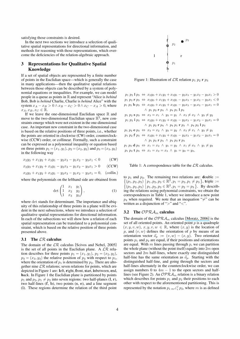
3.1 The LR calculusThe domain of the LR calculus [Scivos and Nebel, 2005]is the set of all points in the Euclidian plane. A LR rela-tion describes for three points p1 = (x1, y1), p2 = (x2, y2),p3 = (x3, y3) the relative position of p3 with respect to p1,where the orientation of p1 is determined by p2. There are alto-gether nine LR relations; seven relations for points, which aredepicted in Figure 1 are: left, right, front, start, inbetween, end,back. In Figure 1 the Euclidian plane is partitioned by pointsp1 and p2, p1 6= p2 into seven regions: two half-planes (l, r),two half-lines (f , b), two points (s, e), and a line segment(i). These regions determine the relation of the third point

Figure 1: Illustration of LR relation p1 p2 r p3

p1 p2 l p3 ⇔ x2y3 + x1y2 + x3y1 − y2x3 − y1x2 − y3x1 > 0

p1 p2 r p3 ⇔ x2y3 + x1y2 + x3y1 − y2x3 − y1x2 − y3x1 < 0

p1 p2 b p3 ⇔ x2y3 + x1y2 + x3y1 − y2x3 − y1x2 − y3x1 = 0

∧ p1 p2 r p4 ∧ p4 p1 l p3

p1 p2 s p3 ⇔ x3 = x1 ∧ y3 = y1 ∧ x3 6= x2 ∧ y3 6= y2

p1 p2 i p3 ⇔ x2y3 + x1y2 + x3y1 − y2x3 − y1x2 − y3x1 = 0

∧ p1 p2 r p4 ∧ p4 p1 r p3 ∧ p4 p2 l p3

p1 p2 e p3 ⇔ x3 = x2 ∧ y3 = y2 ∧ x3 6= x1 ∧ y3 6= y1

p1 p2 f p3 ⇔ x2y3 + x1y2 + x3y1 − y2x3 − y1x2 − y3x1 = 0

∧ p1 p2 r p4 ∧ p4 p2 r p3

p1 p2 d p3 ⇔ x1 = x2 ∧ y1 = y2 ∧ x1 6= x3 ∧ y1 6= y3

p1 p2 t p3 ⇔ x1 = x2 = x3 ∧ y1 = y2 = y3,

Table 1: A correspondence table for the LR calculus.

to p1 and p2. The remaining two relations are: double :={(p1, p2, p3)

∣∣ p1, p2, p3 ∈ R2, p1 = p2, p1 6= p3}

, triple :={(p1, p2, p3)

∣∣ p1, p2, p3 ∈ R2, p1 = p2 = p3}

. By describ-ing the relations using polynomial constraints, we obtain thecorrespondences in Table 1, where we introduce a new pointp4 when required. We note that an inequation “6=” can bewritten as a disjunction of “>” and “<”.

3.2 The OPRAm calculusThe domain of the OPRAm calculus [Moratz, 2006] is theset of all oriented points. An oriented point p is a quadruple(x, y, v, w), x, y, v, w ∈ R, where (x, y) is the location ofp, and (v, w) defines the orientation of p by means of anorientation vector ~op := (v, w) − (x, y). Two orientatedpoints p1 and p2 are equal, if their positions and orientationsare equal. With m lines passing through p, we can partitionthe whole plane (without the point itself) equally into 2m opensectors and 2m half-lines, where exactly one distinguishedhalf-line has the same orientation as ~op. Starting with thedistinguished half-line, and going through the sectors andhalf-lines alternately in the counterclockwise order, we canassign numbers 0 to 4m − 1 to the open sectors and half-lines (see Figure 2). An OPRAm relation is a binary relationwhich describes for points p1 and p2 their positions to eachother with respect to the aforementioned partitioning. This isrepresented by the notation p1 m∠ji p2, where m is as defined

4

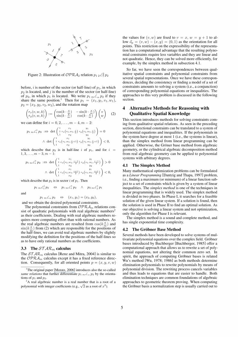
Figure 2: Illustration of OPRA2 relation p1 2∠27 p2

before, i is number of the sector (or half-line) of p1, in whichp2 is located, and j is the number of the sector (or half-line)of p2, in which p1 is located. We write p1 m∠= p2 if theyshare the same position.1 Then for p1 = (x1, y1, v1, w1),p2 = (x2, y2, v2, w2), and the rotation map(rx(v, w, k)ry(v, w, k)

):=

(cos(k · π

m) − sin(k · π

m)

sin(k · πm) cos(k · π

m)

)(vw

)(2)

we can define for i = 0, 2, . . . ,m− 4,m− 2:

p1 m∠∗i p2 :⇔ det

(1 x1 y11 rx(v1,w1,

i2 ) ry(v1,w1,

i2 )

1 x2 y2

)= 0

∧ det

(1 x1 y11 rx(v1,w1,

i2+1) ry(v1,w1,

i2+1)

1 x2 y2

)< 0,

which describe that p2 is in half-line i of p1, and for i =1, 3, . . . ,m− 3,m− 1:

p1 m∠∗i p2 :⇔ det

(1 x1 y1

1 rx(v1,w1,i−12 ) ry(v1,w1,

i−12 )

1 x2 y2

)> 0

∧ det

(1 x1 y1

1 rx(v1,w1,i+12 ) ry(v1,w1,

i+12 )

1 x2 y2

)< 0,

which describe that p2 is in sector i of p1. Then

p1 m∠ji p2 ⇔ p1 m∠∗i p2 ∧ p2 m∠∗

j p1

andp1 m∠= p2 ⇔ (x1, y1) = (x2, y2),

and we obtain the desired polynomial constraints.The polynomial constraints from OPRAm relations con-

sist of quadratic polynomials with real algebraic numbers2

as their coefficients. Dealing with real algebraic numbers re-quires more computing effort than with rational numbers. Asthe real algebraic numbers are resulted from cos(k πm ) andsin(k πm ) from (2) which are responsible for the positions ofthe half-lines, we can avoid real algebraic numbers by slightlymodifying the definition for the positions of the half-lines soas to have only rational numbers as the coefficients.

3.3 The ST ARm calculusThe ST ARm calculus [Renz and Mitra, 2004] is similar tothe OPRAm calculus except it has a fixed reference direc-tion. Consequently, for all oriented points p = (x, y, v, w)

1The original paper [Moratz, 2006] introduces also the so-calledsame relations that further differentiate p1 m∠= p2 by the orienta-tions of p1 and p2.

2A real algebraic number is a real number that is a root of apolynomial with integer coefficients (e.g.,

√2 as a root of x2).

the values for (v, w) are fixed to v = x, w = y + 1 to al-low ~op = (v, w) − (x, y) = (0, 1) as the orientation for allpoints. This restriction on the expressibility of the representa-tion has a computational advantage that the resulting polyno-mial constraints require less variables and they are linear andnot quadratic. Hence, they can be solved more efficiently, forexample, by the simplex method in subsection 4.1.

So far, we have seen the correspondences between qual-itative spatial constraints and polynomial constraints fromseveral spatial representations. Once we have these correspon-dences, deciding the consistency or finding a model of a set ofconstraints amounts to solving a system (i.e., a conjunction)of corresponding polynomial equations or inequalities. Theapproaches to this very problem is discussed in the followingsection.

4 Alternative Methods for Reasoning withQualitative Spatial Knowledge

This section introduces methods for solving constraints com-ing from qualitative spatial relations. As seen in the precedingsection, directional constraints can be translated to a system ofpolynomial equations and inequalities. If the polynomials inthe system have degree at most 1 (i.e., the systems is linear),than the simplex method from linear programming can beapplied. Otherwise, the Groner base method from algebraicgeometry, or the cylindrical algebraic decomposition methodfrom real algebraic geometry can be applied to polynomialsystems with arbitrary degrees.

4.1 The Simplex MethodMany mathematical optimization problems can be formulatedas a Linear Programming [Dantzig and Thapa, 1997] problem,i.e., finding a maximum (or minimum) of a linear function sub-ject to a set of constraints which is given by a system of linearinequalities. The simplex method is one of the techniques inlinear programming that is widely used. The simplex methodis divided in two phases. In Phase I, it searches for a feasiblesolution of the given linear system. If a solution is found, thenthe solution is used in Phase II to find an optimal solution. Asour objective is solving a linear system and not optimization,only the algorithm for Phase I is relevant.

The simplex method is a sound and complete method, andhas single exponential time complexity.

4.2 The Grobner Base MethodSeveral methods have been developed to solve systems of mul-tivariate polynomial equations over the complex field. Grobnerbases introduced by Buchberger [Buchberger, 1985] offer acomputational approach that allows us to rewrite a set of poly-nomial equations, not altering their common zero set. Inspirit, the approach of computing Grobner bases is relatedWu’s method [Wu, 1978; 1986] as both methods determineelimination polynomials to rewrite polynomials by means ofpolynomial division. The rewriting process cancels variablesand thus leads to equations that are easier to handle. Bothelimination techniques are common foundations of algebraicapproaches to geometric theorem proving. When computingthe Grobner basis a normalization step is usually carried out to

5

obtain the basis in normal form, called the reduced Grobnerbasis. This form exhibits a remarkable feature: when the ini-tial set of polynomials does not have a common solution, thenthe reduced Grobner basis is equal to {1}. This property sug-gests that Grobner basis enable a straight-forward approachto test the zero set for emptiness, but recall that polynomialequations can also involve complex roots. Henceforth, in caseswhere the reduced Grobner basis does not equal {1}, a com-mon solution is known to exist, but one still needs to checkwhether the common solution is real-valued. The approach offirst computing the Grobner basis and then further examiningexistence of real-valued solutions can handle problems arisingwhen analyzing constraint calculi [Wolter, to appear], e.g.,automatically computing the composition operation. However,this approach does not provide us with a complete decisionprocedure and it appears to be very difficult to turn it into aprovenly complete one.

4.3 Cylindrical Algebraic DecompositionThe Cylindrical Algebraic Decomposition (CAD) [Collins,1975; Arnon et al., 1984] overcomes the deficiencies of thetwo previously introduced methods; compared to the simplexmethod, CAD can handle any polynomial systems and is notlimited to linear systems, and where as the Grober base methodis not complete, CAD provides a complete algorithm.

Given a finite set of polynomials f1, . . . , fm in r variableswith coefficients from Q, the CAD algorithm computes a finitesubset S of Rr, such that

{(sgn(f1(s)), . . . , sgn(fn(s))) | s ∈ S } (3)= {(sgn(f1(x)), . . . , sgn(fr(x))) |x ∈ Rr } ,

where sgn is a real-valued function that returns the sign (i.e.,−1, 0, or 1) of its argument. Thus, solving a system of poly-nomial equations and inequalities having f1, . . . , fm on theleft-hand side of the system can be accomplished by evalu-ating f1, . . . , fm over the elements of S and checking theirsigns. Due to condition (3) this decision procedure is soundand complete. It also terminates as S is finite.

To generate the set of sample points S the CAD algo-rithm decomposes Rr, the domain of variables x1, . . . , xr,into finitely many subsets C1, . . . , CK of Rr, such that eachcell Ci is sign-invariant with respect to f1, . . . , fm, meaningthat the signs of f1, . . . , fm are constant when evaluated overCi. Set S is then obtained by calculating a sample point ineach of the cells C1, . . . , CK .

The complexity of CAD is doubly exponential in the numberr of the variables.

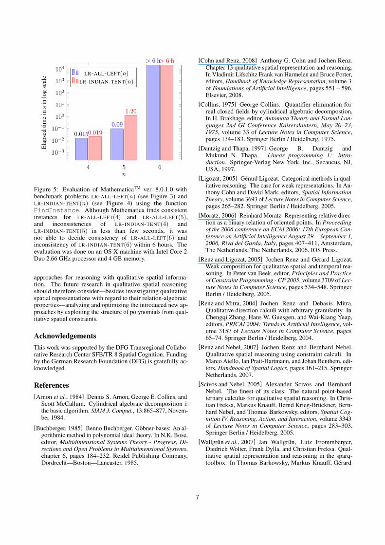
CAD is designed for general polynomial systems. As a con-sequence, it is not optimized for particular polynomial systemstranslated from qualitative spatial relations. For instance, thefact that most polynomial constraints coming from directionalrelations have their origins in the determinant expression in(1) is not deployed. This lack of integration results in thelow performance of the CAD algorithm when dealing withqualitative spatial constraints. We observe in the evaluation ofthe computer algebra system Mathematica3 in Figure 5 thatCAD is not able to deal with more than 5 objects efficiently.

3http://www.wolfram.com/mathematica

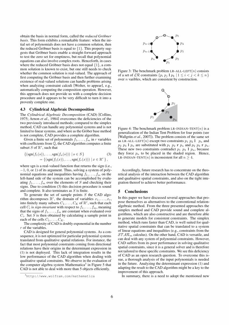
Figure 3: The benchmark problem LR-ALL-LEFT(n) consistsof a set of LR constraints {pi pj l pk | 1 ≤ i < j < k ≤ n}over n varibles, which are consistent by construction.

Figure 4: The benchmark problem LR-INDIAN-TENT(n) is ageneralization of the Indian Tent Problem for four points (see[Wallgrun et al., 2007]). The problem consists of the same setas LR-ALL-LEFT(n) except two constraints p1 p2 l pn andp2 p3 l pn are substituted with p1 p2 r pn and p2 p3 r pn.These new two constraints contradict p1 p3 l pn, becausethey force pn to be placed in the shaded region. Hence,LR-INDIAN-TENT(n) is inconsistent for all n ≥ 4.

Accordingly, future research has to concentrate on the theo-retical analysis of the interaction between the CAD algorithmand qualitative spatial constraints, and also on the tight inte-gration thereof to achieve better performance.

5 ConclusionsIn this paper we have discussed several approaches that pro-pose themselves as alternatives to the conventional relation-algebraic method. From the three presented approaches thesimplex method and CAD provide sound and complete al-gorithms, which are also constructive and are therefore ableto generate models for consistent constraints. The simplexmethod, which runs faster than CAD, is well suited for qual-itative spatial constraints that can be translated to a systemof linear equations and inequalities (e.g., constraints from theST ARm calculus). On the other hand, CAD is versatile, andcan deal with any system of polynomial constraints. However,CAD suffers from its poor performance in solving qualitativespatial constraints, since it is a general solver and is thereforenot tailored to these specific constraints. We see this deficiencyof CAD as an open research question. To overcome this is-sue, a thorough analysis of the input polynomials is neededin the future. Analyzing the determinant expression (1) andadapting the result to the CAD algorithm might be a key to theimprovement of this approach.

In summary, there is a need to adopt the mentioned new

6

4 5 6

10−3

10−2

10−1

100

101

102

103

104

0.015

0.09

> 6 h

0.019

1.20

> 6 h

n

Ela

psed

time

ins

inlo

gsc

ale LR-ALL-LEFT(n)

LR-INDIAN-TENT(n)

Figure 5: Evaluation of MathematicaTM ver. 8.0.1.0 withbenchmark problems LR-ALL-LEFT(n) (see Figure 3) andLR-INDIAN-TENT(n) (see Figure 4) using the functionFindInstance. Although Mathematica finds consistentinstances for LR-ALL-LEFT(4) and LR-ALL-LEFT(5),and inconsistencies of LR-INDIAN-TENT(4) andLR-INDIAN-TENT(5) in less than few seconds, it wasnot able to decide consistency of LR-ALL-LEFT(6) andinconsistency of LR-INDIAN-TENT(6) within 6 hours. Theevaluation was done on an OS X machine with Intel Core 2Duo 2.66 GHz processor and 4 GB memory.

approaches for reasoning with qualitative spatial informa-tion. The future research in qualitative spatial reasoningshould therefore consider—besides investigating qualitativespatial representations with regard to their relation-algebraicproperties—analyzing and optimizing the introduced new ap-proaches by exploiting the structure of polynomials from qual-itative spatial constraints.

AcknowledgementsThis work was supported by the DFG Transregional Collabo-rative Research Center SFB/TR 8 Spatial Cognition. Fundingby the German Research Foundation (DFG) is gratefully ac-knowledged.

References[Arnon et al., 1984] Dennis S. Arnon, George E. Collins, and

Scott McCallum. Cylindrical algebraic decomposition i:the basic algorithm. SIAM J. Comput., 13:865–877, Novem-ber 1984.

[Buchberger, 1985] Benno Buchberger. Gobner-bases: An al-gorithmic method in polynomial ideal theory. In N.K. Bose,editor, Multidimensional Systems Theory - Progress, Di-rections and Open Problems in Multidimensional Systems,chapter 6, pages 184–232. Reidel Publishing Company,Dordrecht—Boston—Lancaster, 1985.

[Cohn and Renz, 2008] Anthony G. Cohn and Jochen Renz.Chapter 13 qualitative spatial representation and reasoning.In Vladimir Lifschitz Frank van Harmelen and Bruce Porter,editors, Handbook of Knowledge Representation, volume 3of Foundations of Artificial Intelligence, pages 551 – 596.Elsevier, 2008.

[Collins, 1975] George Collins. Quantifier elimination forreal closed fields by cylindrical algebraic decompostion.In H. Brakhage, editor, Automata Theory and Formal Lan-guages 2nd GI Conference Kaiserslautern, May 20–23,1975, volume 33 of Lecture Notes in Computer Science,pages 134–183. Springer Berlin / Heidelberg, 1975.

[Dantzig and Thapa, 1997] George B. Dantzig andMukund N. Thapa. Linear programming 1: intro-duction. Springer-Verlag New York, Inc., Secaucus, NJ,USA, 1997.

[Ligozat, 2005] Gerard Ligozat. Categorical methods in qual-itative reasoning: The case for weak representations. In An-thony Cohn and David Mark, editors, Spatial InformationTheory, volume 3693 of Lecture Notes in Computer Science,pages 265–282. Springer Berlin / Heidelberg, 2005.

[Moratz, 2006] Reinhard Moratz. Representing relative direc-tion as a binary relation of oriented points. In Proceedingof the 2006 conference on ECAI 2006: 17th European Con-ference on Artificial Intelligence August 29 – September 1,2006, Riva del Garda, Italy, pages 407–411, Amsterdam,The Netherlands, The Netherlands, 2006. IOS Press.

[Renz and Ligozat, 2005] Jochen Renz and Gerard Ligozat.Weak composition for qualitative spatial and temporal rea-soning. In Peter van Beek, editor, Principles and Practiceof Constraint Programming - CP 2005, volume 3709 of Lec-ture Notes in Computer Science, pages 534–548. SpringerBerlin / Heidelberg, 2005.

[Renz and Mitra, 2004] Jochen Renz and Debasis Mitra.Qualitative direction calculi with arbitrary granularity. InChengqi Zhang, Hans W. Guesgen, and Wai-Kiang Yeap,editors, PRICAI 2004: Trends in Artificial Intelligence, vol-ume 3157 of Lecture Notes in Computer Science, pages65–74. Springer Berlin / Heidelberg, 2004.

[Renz and Nebel, 2007] Jochen Renz and Bernhard Nebel.Qualitative spatial reasoning using constraint calculi. InMarco Aiello, Ian Pratt-Hartmann, and Johan Benthem, edi-tors, Handbook of Spatial Logics, pages 161–215. SpringerNetherlands, 2007.

[Scivos and Nebel, 2005] Alexander Scivos and BernhardNebel. The finest of its class: The natural point-basedternary calculus for qualitative spatial reasoning. In Chris-tian Freksa, Markus Knauff, Bernd Krieg-Bruckner, Bern-hard Nebel, and Thomas Barkowsky, editors, Spatial Cog-nition IV. Reasoning, Action, and Interaction, volume 3343of Lecture Notes in Computer Science, pages 283–303.Springer Berlin / Heidelberg, 2005.

[Wallgrun et al., 2007] Jan Wallgrun, Lutz Frommberger,Diedrich Wolter, Frank Dylla, and Christian Freksa. Qual-itative spatial representation and reasoning in the sparq-toolbox. In Thomas Barkowsky, Markus Knauff, Gerard

7

Ligozat, and Daniel Montello, editors, Spatial CognitionV Reasoning, Action, Interaction, volume 4387 of LectureNotes in Computer Science, pages 39–58. Springer Berlin /Heidelberg, 2007.

[Wolter and Lee, 2010] D. Wolter and J.H. Lee. Qualitativereasoning with directional relations. Artificial Intelligence,174(18):1498 – 1507, 2010.

[Wolter, to appear] Diedrich Wolter. Analyzing qualitativespatio-temporal calculi using algebraic geometry. SpatialCognition and Computation, to appear.

[Wu, 1978] Wen-Tsun Wu. On the decision problem and themechanization of theorem proving in elementary geometry.Scientia Sinica, 21:157–179, 1978.

[Wu, 1986] Wen-Tsun Wu. Basic principles of mechanicaltheorem proving in elementary geometries. Journal ofAutomated Reasoning, 2:221–252, 1986.

8

Solving Qualitative Constraints Involving Landmarks ∗

Weiming Liu1, Shengsheng Wang2, Sanjiang Li11Centre for Quantum Computation and Intelligent Systems,

Faculty of Engineering and Information Technology, University of Technology Sydney, Australia2College of Computer Science and Technology, Jilin University, Changchun, China

AbstractConsistency checking plays a central role in quali-tative spatial and temporal reasoning. Given a setof variables V , and a set of constraints Γ takenfrom a qualitative calculus (e.g. the Interval Al-gebra (IA) or RCC-8), the aim is to decide if Γis consistent. The consistency problem has beeninvestigated extensively in the literature. Practi-cal applications e.g. urban planning often impose,in addition to those between undetermined entities(variables), constraints between determined entities(constants or landmarks) and variables. This paperintroduces this as a new class of qualitative con-straints satisfaction problems, and investigates itsconsistency in several well-known qualitative cal-culi, e.g. IA, RCC-5, and RCC-8. We show that theusual local consistency checking algorithm worksfor IA but fails in RCC-5 and RCC-8. We furthershow that, if the landmarks are represented as poly-gons, then the new consistency problem of RCC-5is tractable but that of RCC-8 is NP-complete.

1 IntroductionQualitative constraints are widely used in temporal and spa-tial reasoning. This is partially because they are close tothe way humans represent and reason about commonsenseknowledge. Moreover, qualitative constraints are easy tospecify and provide a flexible way to deal with incompleteknowledge.

Usually, these constraints are taken from a qualitative cal-culus, which is a set M of relations defined on an infiniteuniverse U of entities [6]. Well-known qualitative calculi in-clude the Interval Algebra [1], RCC-5 and RCC-8 [9], and thecardinal direction calculus (for point-like objects) [7].

A central problem of reasoning with a qualitative calcu-lus is the consistency problem. For a qualitative calculusMon U , an instance of the consistency problem over M is anetwork Γ of constraints like xαy, where x, y are variablestaken from a finite set V , and α is a relation inM. Consis-tency checking has applications in many areas, e.g. temporal

∗This work was partly supported by an ARC Future Fellowship(FT0990811).

or spatial query preprocessing, planning, natural language un-derstanding, etc. Moreover, several other reasoning problemse.g. the minimal label problem and the entailment problemcan be reduced in polynomially time to the consistency prob-lem.

The consistency problem has been studied extensively formany different qualitative calculi (cf. [2]). These worksalmost unanimously assume that the qualitative constraintsinvolve only unknown entities. In other words, the precise(geometric) information of every object is totally unknown.In practical applications, however, we often meet constraintsthat involve both known and unknown entities, i.e. constantsand variables.

For example, consider a class scheduling problem in a pri-mary school. In addition to constraints between unknown in-tervals (e.g. a Math class is followed by a Music class), wemay also impose constraints involving determined intervals(e.g. a P.E. class should be during afternoon).

Constraints involving known entities are especially com-mon in spatial reasoning tasks such as urban planning. Forexample, to find a best location for a landfill, we need to for-mulate constraints between the unknown landfill and signifi-cant landmarks, e.g. lake, university, hospital etc.

In this paper, we explicitly introduce landmarks (definedas known entities) into the definition of the consistency prob-lem, and call the consistency problem involving landmarksthe hybrid consistency problem. In comparison, we call theusual consistency problem (involving no landmarks) the pureconsistency problem.

In general, solving constraint networks involving land-marks is different from solving constraint networks involv-ing no landmarks. For example, consider the simple RCC-5algebra. It is a well-known result that a path-consistent con-straint network Γ is consistent when Γ involves no landmarks.But the following example shows that this fails to hold whenlandmarks are involved. Suppose a, b, c are the three regionsshown below. Let x be a spatial variable, which is required tobe a subset of a, b, c. This network is path-consistent, but in-consistent since the three landmarks have no common points.

The aim of this paper is to investigate how landmarks af-fect the consistency of constraint networks in several very im-portant qualitative calculi. The rest of this paper proceedsas follows. Section 2 introduces basic notions in qualitative

9

constraint solving and examples of qualitative calculi. Thenew consistency problem, as well as several basic results, isalso presented here. Assuming that all landmarks are rep-resented as polygons, Section 3 then provides a polynomialdecision procedure for the consistency of hybrid basic RCC-5 networks. Besides, if the network is consistent, a solution isconstructed in polynomial time; Section 4 shows that consis-tency problem for hybrid basic RCC-8 networks is NP-hard.The last section then concludes the paper.

2 Qualitative Calculi and The ConsistencyProblem

Most qualitative approaches to spatial and temporal knowl-edge representation and reasoning are based on qualitativecalculi. Suppose U is a universe of spatial or temporal enti-ties. Write Rel(U) for the algebra of binary relations on U . Aqualitative calculus on U is a sub-Boolean algebra of Rel(U)generated by a set B of jointly exhaustive and pairwise dis-joint (JEPD) relations on U . Relations in B are called basicrelations of the qualitative calculus.

We next recall the well-known Interval Algebra (IA) [1]and the two RCC algebras.Example 2.1 (Interval Algebra). Let U be the set of closedintervals on the real line. Thirteen binary relations betweentwo intervals x = [x−, x+] and y = [y−, y+] are defined bycomparing the order relations between the endpoints of x andy. These are the basic relations of IA.Example 2.2 (RCC-5 and RCC-8 Algebras1). Let U be theset of bounded regions in the real plane, where a region is anonempty regular set. The RCC-8 algebra is generated by theeight topological relations

DC,EC,PO,EQ,TPP,NTPP,TPP∼,NTPP∼, (1)

where DC,EC,PO,TPP and NTPP are defined in Ta-ble 1, EQ is the identity relation, and TPP∼ and NTPP∼

are the converses of TPP and NTPP, respectively, seeFig. 1 for illustraion. The RCC-5 algebra is the sub-algebraof RCC-8 generated by the five part-whole relations

DR,PO,EQ,PP,PP∼, (2)

where DR = DC ∪ EC, PP = TPP ∪ NTPP, andPP∼ = TPP∼ ∪NTPP∼.

A qualitative calculus provides a useful constraint lan-guage. Suppose M is a qualitative calculus defined on do-main U . Relations in M can be used to express constraints

1We note that the RCC algebras have interpretations in arbitrarytopological spaces. In this paper, we only consider the most impor-tant interpretation in the real plane.

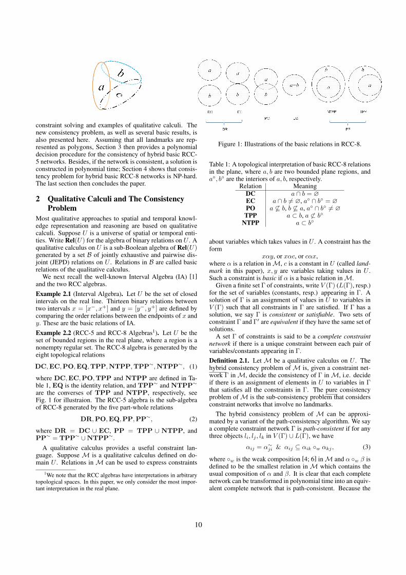
Figure 1: Illustrations of the basic relations in RCC-8.

Table 1: A topological interpretation of basic RCC-8 relationsin the plane, where a, b are two bounded plane regions, anda◦, b◦ are the interiors of a, b, respectively.

Relation MeaningDC a ∩ b = ∅EC a ∩ b 6= ∅, a◦ ∩ b◦ = ∅PO a 6⊆ b, b 6⊆ a, a◦ ∩ b◦ 6= ∅TPP a ⊂ b, a 6⊂ b◦

NTPP a ⊂ b◦

about variables which takes values in U . A constraint has theform

xαy, or xαc, or cαx,where α is a relation inM, c is a constant in U (called land-mark in this paper), x, y are variables taking values in U .Such a constraint is basic if α is a basic relation inM.

Given a finite set Γ of constraints, write V (Γ) (L(Γ), resp.)for the set of variables (constants, resp.) appearing in Γ. Asolution of Γ is an assignment of values in U to variables inV (Γ) such that all constraints in Γ are satisfied. If Γ has asolution, we say Γ is consistent or satisfiable. Two sets ofconstraint Γ and Γ′ are equivalent if they have the same set ofsolutions.

A set Γ of constraints is said to be a complete constraintnetwork if there is a unique constraint between each pair ofvariables/constants appearing in Γ.Definition 2.1. Let M be a qualitative calculus on U . Thehybrid consistency problem ofM is, given a constraint net-work Γ inM, decide the consistency of Γ inM, i.e. decideif there is an assignment of elements in U to variables in Γthat satisfies all the constraints in Γ. The pure consistencyproblem ofM is the sub-consistency problem that considersconstraint networks that involve no landmarks.

The hybrid consistency problem of M can be approxi-mated by a variant of the path-consistency algorithm. We saya complete constraint network Γ is path-consistent if for anythree objects li, lj , lk in V (Γ) ∪ L(Γ), we have

αij = α∼ji & αij ⊆ αik ◦w αkj , (3)

where ◦w is the weak composition [4; 6] inM and α ◦w β isdefined to be the smallest relation in M which contains theusual composition of α and β. It is clear that each completenetwork can be transformed in polynomial time into an equiv-alent complete network that is path-consistent. Because the

10

consistency problem is in general NP-hard, we do not expectthat a local consistency algorithm can solve the general con-sistency problem. However, it has been proved that the path-consistency algorithm suffices to decide the pure consistencyproblem for large fragments of some well-known qualitativecalculi, e.g. IA, RCC-5, and RCC-8 (cf. [2]). This showsthat, at least for these calculi, the pure consistency problemcan be solved by path-consistency algorithm and the back-tracking method.

The remainder of this paper will investigate the hybrid con-sistency problem for the above calculi. In the following dis-cussion, we assume Γ is a complete basic network that in-volves at least one landmark.

For IA, endpoints of the intervals in different solutions of acomplete basic constraint network respect the same ordering.This suggests that any partial solution of a consistent networkcan be extended to a complete solution.Proposition 2.1. Suppose Γ is a basic network of IA con-straints that involves landmarks and variables. Then Γ isconsistent iff it is path-consistent.

This result shows that, for IA, the hybrid consistency prob-lem can be solved in the same way as the pure consistencyproblem. Similar conclusion also holds for some other cal-culi, e.g. the Point Algebra, the Rectangle Algebra, and theCardinal Direction Calculus (for point-like objects) [7]. Thisproperty, however, does not hold in general. Take the RCC-5as example. If a basic network Γ involves no landmark, thenwe know Γ is consistent if it is path-consistent. If Γ involveslandmarks, we have seen in the introduction a path-consistentbut inconsistent basic RCC-5 network.

In the next two sections, we investigate how landmarks af-fect the consistency of RCC-5 and RCC-8 topological con-straints. We stress that, in this paper, we only consider thestandard (and the most important) interpretation of the RCClanguage in the real plane, as given in Example 2.2. Whenrestricting landmarks to polygons, we first show that the con-sistency of a hybrid basic RCC-5 network can still be decidedin polynomial time (Section 4), but the that of RCC-8 net-works is NP-hard.

3 The Hybrid Consistency Problem of RCC-5We begin with a short review of the realization algorithm forpure consistency problem of RCC-5 [5; 3]. Suppose Γ in-volves only spatial variables v1, v2, · · · , vn. We define a fi-nite set Xi of control points for each vi as follows:• Add a point Pi to Xi;• For any j > i, add a new point Pij to both Xi and Xj if

(viPOvj) ∈ Γ;• For any j, put all points in Xi into Xj if (viPPvj) ∈ Γ.

Take ε > 0 such that the distance between any two differ-ent points in

⋃ni=1Xi is greater than 2ε. Let B(P, ε) be the

closed disk with radius ε centred at P . By the choice of ε,different disks are disjoint. Let ai =

⋃{B(P, ε) : P ∈ Xi}.It is easy to check that the assignment is a solution of Γ, if Γis consistent.

Assume Γ is a basic RCC-5 network involving landmarksL = {l1, · · · , lm} in the real plane and variables V =

{v1, · · · , vn}. Write ∂L for the union of the boundaries ofthe landmarks. An equivalence relation∼L can be defined onthe plane as follows: For P,Q 6∈ ∂L,

P ∼L Q iff (∀1 ≤ j ≤ m)[P ∈ lj ↔ Q ∈ lj ] (4)

A block is defined as an equivalent class under ∼L. Be-cause∼L is defined only for points that are not on the bound-aries of the landmarks, it is easy to see that each block is anopen set. It is also clear that the complement of the union ofall landmarks (which are bounded) is the unique unboundedblock. We write B for the set of all blocks.

For each landmark li, we write I(li) for the set of blocksthat li contains, and write E(li) for the set of rest blocks, i.e.the blocks that are disjoint from li. That is,

I(li) = {b ∈ B : b ⊆ li}, (5)E(li) = {b ∈ B : b ∩ li = ∅}. (6)

It is easy to see that the interior (exterior, resp.) of li is exactlythe regularized union (i.e. the interior of its closure) of allblocks in I(li) (E(li),resp.). Moreover, each block is in eitherI(li) orE(li), but not both, i.e., I(li)∪E(li) = B and I(li)∩E(li) = ∅.

These constructions can be extended from landmarks tovariables as

I(vi) =⋃{I(lj) : ljPPvi}, (7)

E(vi) =⋃{I(lj) : ljDRvi} ∪

⋃{E(lj) : viPPlj}. (8)

Intuitively, I(vi) is the set of blocks that vi must contain,and E(vi) is the set of blocks that should be excluded fromvi.

The following proposition claims that no block can appearin both I(vi) and E(vi).Proposition 3.1. Suppose Γ is a basic RCC-5 constraintnetwork that involves at least one landmark. If Γ is path-consistent, then I(vi) ∩ E(vi) = ∅.

We have the following theorem.Theorem 3.1. Suppose Γ is a basic RCC-5 constraint net-work that involves at least one landmark. If Γ is consistent,then we have• For any vi ∈ V ,

E(vi) ( B. (9)

• For any vi ∈ V andw ∈ L∪V such that (viPOw) ∈ Γ,

E(vi) ∪ E(w) ( B, (10)E(vi) ∪ I(w) ( B, (11)I(vi) ∪ E(w) ( B. (12)

• For any vi ∈ V and lj ∈ L such that (viPPlj) ∈ Γ,

I(vi) ( I(lj). (13)

• For any vi ∈ V and lj ∈ L such that (ljPPvi) ∈ Γ,

E(vi) ( E(lj). (14)

• For any vi, vj ∈ V such that (viPPvj) ∈ Γ,

I(vi) ∪ E(vj) ( B. (15)

11

These conditions are also sufficient to determine the con-sistency of a path-consistent basic RCC-5 network. We showthis by devising a realization algorithm. The construction issimilar to that for the pure consistency problem. For each vi,we define a finite set Xi of control points as follows, wherefor clarity, we write

P (vi) = B− I(vi)− E(vi). (16)

• For each block b in P (vi), select a fresh point in b andadd the point into Xi.

• For any j > i with (viPOvj) ∈ Γ, select a fresh pointin some block b in P (vi)∩P (vj) (if it is not empty), andadd the point into Xi and Xj .

• For any j, put all points in Xj into Xi if (vjPPvi) ∈ Γ.

We note that the points selected from a block b for different vi,or in different steps, should be pairwise different. Recall thateach point in

⋃ni=1Xi is not at the boundary of any block. We

choose ε > 0 such that B(P, ε) does not intersect either theboundary of a block or another disk B(Q, ε). Furthermore,we can assume that ε is small enough such that the union ofall the disks B(P, ε) does not cover any block in B.

Let

ai =⋃{B(P, ε) : P ∈ Xi} ∪

⋃{lj : ljPPvi}. (17)

We claim that {a1, · · · , at} is a solution of Γ. To prove this,we need the following lemma.

Lemma 3.1. Let Γ be a path-consistent basic RCC-5 con-straint network that involves at least one landmark. SupposeB is the block set of Γ. Then, for each b ∈ B, we have

• b ∈ I(vi) iff b ⊆ ai.• If b ∈ E(vi) iff b ∩ ai = ∅.

• If b ∈ P (vi) iff b * ai and b ∩ ai 6= ∅.

Remark 3.1. Since {I(vi), E(vi), P (vi)} is a partition of theblocks in B, it is easy to see the conditions in Lemma 3.1 arealso sufficient. That is, for example, b ∈ I(vi) iff b ⊆ ai.

We next prove that {a1, · · · , at} is a solution of Γ.

Theorem 3.2. Suppose Γ is a complete basic RCC-5 networkinvolving landmarks L and variables V . Assume Γ is path-consistent and satisfies the conditions in Theorem 3.1. ThenΓ is consistent and {a1, · · · , at}, as constructed in (17), is asolution of Γ.

It is worth noting that the complexity of deciding the con-sistency of a hybrid basic RCC-5 network includes two parts,viz. the complexity of computing the blocks, and that ofchecking the conditions in Theorem 3.1. The latter part alonecan be completed in O(|B|n(n + m)) time, where |B| is thenumber of the blocks. In the worst situation, the numberof blocks may be up to 2m. This suggests that the deci-sion method described above is in general inefficient. Thefollowing theorem, however, asserts that this method is stillpolynomial in the size of the input instance, provided that thelandmarks are all represented as polygons.

Theorem 3.3. Suppose Γ is a basic RCC-5 constraint net-work, and V (Γ) = {v1, · · · , vn} and L(Γ) = {l1, · · · , lm}

are the set of variables and, respectively, the set of landmarksappearing in Γ. Assume each landmark li is represented by a(complex) polygon with less than k vertices. Then the consis-tency of Γ can be decided in O((m+ n)6k6) time.

4 The Hybrid Consistency Problem of RCC-8Suppose Γ is a complete basic RCC-8 network that involvesno landmarks. Then Γ is consistent if it is path-consistent [8;10]. Moreover, a solution can be constructed for each path-consistent basic network in cubic time [5; 3]. This sectionshows that, however, when considering polygons, it is NP-hard to determine if a complete basic RCC-8 network involv-ing landmarks has a solution. We achieve this by devising apolynomial reduction from 3-SAT.

In this section, for clarity, we use upper case lettersA,B,C(with indices) to denote landmarks, and use lower case lettersu, v, w (with indices) to denote spatial variables.

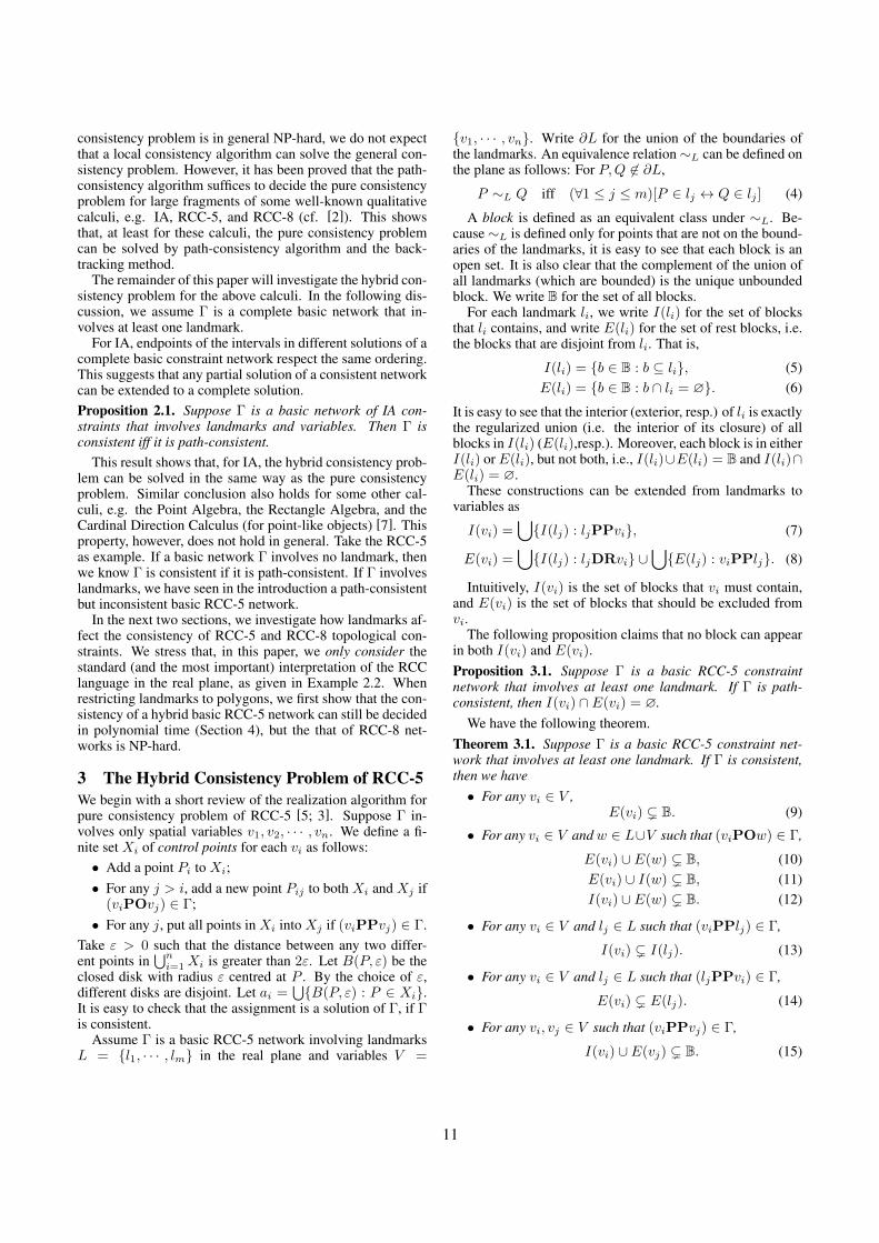
The NP-hardness stems from the fact that two externallyconnected polygons, say A,B, may have more than one tan-gential points. Assume v is a spatial variable that is requiredto be a tangentially proper part of A but externally connectedto B. Then it is undetermined at which tangential point(s) vand B should meet.

Precisely, consider the configuration shown in Fig. 2 (a),where A and B are two externally connected landmarks,meeting at two tangential points, say Q+ and Q−. Assume{u, v, w} are variables that are subject to the following con-straints

uTPPA, uECB,

vTPPB, vECA,wTPPB,wECA,

uECv, uDCw, vDCw.

It is easy to see that u andB are required to meet at eitherQ+

(a) (b) (c)

Figure 2: Two landmarks A,B that are externally connectedat two tangential points Q+ and Q−.

or Q−, but not both (cf Fig. 2(b,c)). The correspondence be-tween these two configurations and the two truth values (trueor false) of a propositional variable is exploited in the follow-ing reduction.

Let φ =∧mk=1 ϕk be a 3-SAT instance over propositional

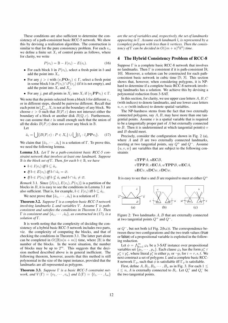
variables set {p1, · · · , pn}. Each clause ϕk has the form p∗r ∨p∗s ∨ p∗t , where literal p∗i is either pi or ¬pi for i = r, s, t. Wenext construct a set of polygons L and a complete basic RCC-8 network Γφ, such that φ is satisfiable iff Γφ is satisfiable.

First, define A,B1, B2, · · · , Bn as in Fig. 3. For each 1 ≤i ≤ n, A is externally connected to Bi. Let Q+

i and Q−i bethe two tangential points.

12

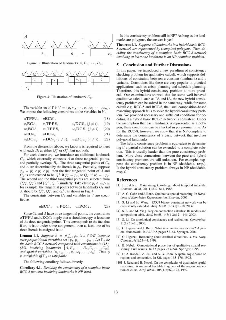
Figure 3: Illustration of landmarks A,B1, · · · , Bn.

Figure 4: Illustration of landmark Ck.

The variable set of Γ is V = {u, v1, · · · , vn, w1, · · · , wn}.We impose the following constraints to the variables in V .

uTPPA, uECBi, (18)viECA, viTPPBi, viDCBj (j 6= i), (19)wiECA, wiTPPBi, wiDCBj (j 6= i), (20)uECvi, uDCwi, (21)viDCwj , viDCvj (j 6= i), wiDCwj (j 6= i). (22)

From the discussion above, we know u is required to meetwith each Bi at either Q−i or Q+

i , but not both.For each clause ϕk, we introduce an additional landmark

Ck, which externally connects A at three tangential points,and partially overlaps Bi. The three tangential points of CkandA are determined by the literals in ϕk. Precisely, supposeϕk = p∗r ∨ p∗s ∨ p∗t , then the first tangential point of A andCk is constructed to be Q+

r if p∗r = pr, or Q−r if p∗r = ¬pr.The second and the third tangential points are selected from{Q+

s , Q−s } and {Q+

t , Q−t } similarly. Take clause pr∨¬ps∨pt

for example, the tangential points between landmarks Ck andA should be Q+

r , Q−s , and Q+t , as shown in Fig. 4.

The constraints between Ck and variables in V are speci-fied as

uECCk, viPOCk, wiPOCk. (23)

SinceCk andA have three tangential points, the constraintsuTPPA and uECCk imply that u should occupy at least oneof the three tangential points. This corresponds to the fact thatif ϕk is true under some assignment, then at least one of itsthree literals is assigned true.

Lemma 4.1. Suppose φ =∧mk=1 ϕk is a 3-SAT instance

over propositional variables set {p1, p2, · · · , pn}. Let Γφ bethe basic RCC-8 network composed with constraints in (18)-(23), involving landmarks {A,B1, · · · , Bn, C1, · · · , Cm}and spatial variables {u, v1, · · · , vn, w1, · · · , wn}. Then φis satisfiable iff Γφ is satisfiable.

The following corollary follows directly.

Corollary 4.1. Deciding the consistency of a complete basicRCC-8 network involving landmarks is NP-hard.

Is this consistency problem still in NP? As long as the land-marks are polygons, the answer is yes!Theorem 4.1. Suppose all landmarks in a hybrid basic RCC-8 network are represented by (complex) polygons. Then de-ciding the consistency of a complete basic RCC-8 networkinvolving at least one landmark is an NP-complete problem.

5 Conclusion and Further DiscussionsIn this paper, we introduced a new paradigm of consistencychecking problem for qualitative calculi, which supports def-initions of constraints between a constant (landmark) and avariable. Constraints like these are very popular in practicalapplications such as urban planning and schedule planning.Therefore, this hybrid consistency problem is more practi-cal. Our examinations showed that for some well-behavedqualitative calculi such as PA and IA, the new hybrid consis-tency problem can be solved in the same way; while for somecalculi e.g. RCC-5 and RCC-8, the usual composition-basedreasoning approach fails to solve the hybrid consistency prob-lem. We provided necessary and sufficient conditions for de-ciding if a hybrid basic RCC-5 network is consistent. Underthe assumption that each landmark is represented as a poly-gon, these conditions can be checked in polynomial time. Asfor the RCC-8, however, we show that it is NP-complete todetermine the consistency of a basic network that involvespolygonal landmarks.

The hybrid consistency problem is equivalent to determin-ing if a partial solution can be extended to a complete solu-tion. This is usually harder than the pure consistency prob-lem. More close connections between the pure and hybridconsistency problems are still unknown. For example, sup-pose the consistency problem is in NP (decidable, resp.).Is the hybrid consistency problem always in NP (decidable,resp.)?

References[1] J. F. Allen. Maintaining knowledge about temporal intervals.

Commun. ACM, 26(11):832–843, 1983.[2] A. G. Cohn and J. Renz. Qualitative spatial reasoning. In Hand-

book of Knowledge Representation. Elsevier, 2007.[3] S. Li and H. Wang. RCC8 binary constraint network can be

consistently extended. Artif. Intell., 170(1):1–18, 2006.[4] S. Li and M. Ying. Region connection calculus: Its models and

composition table. Artif. Intell., 145(1-2):121–146, 2003.[5] S. Li. On topological consistency and realization. Constraints,

11(1):31–51, 2006.[6] G. Ligozat and J. Renz. What is a qualitative calculus? A gen-

eral framework. In PRICAI, pages 53–64. Springer, 2004.[7] G. Ligozat. Reasoning about cardinal directions. J. Vis. Lang.

Comput., 9(1):23–44, 1998.[8] B. Nebel. Computational properties of qualitative spatial rea-

soning: First results. In KI, pages 233–244. Springer, 1995.[9] D. A. Randell, Z. Cui, and A. G. Cohn. A spatial logic based on

regions and connection. In KR, pages 165–176, 1992.[10] J. Renz and B. Nebel. On the complexity of qualitative spatial

reasoning: A maximal tractable fragment of the region connec-tion calculus. Artif. Intell., 108(1-2):69–123, 1999.

13

14

Benchmarking Qualitative Spatial Calculi for VideoActivity Analysis

Muralikrishna Sridhar, Anthony G Cohn and David C Hogg

University Of Leeds, UK,{krishna,agc,dch}@comp.leeds.ac.uk

Abstract. This paper presents a general way of addressing problems in videoactivity understanding using graph based relational learning. Video activities aredescribed using relational spatio-temporal graphs, that represent qualitative spatio-temporal relations between interacting objects. A wide range of spatio-temporalrelations are introduced, as being well suited for describing video activities. Then,a formulation is proposed, in which standard problems in video activity under-standing such as event detection, are naturally mapped to problems in graph basedrelational learning. Experiments on video understanding tasks, for a video datasetconsisting of common outdoor verbs, validate the significance of the proposedapproach.

1 Introduction

One of the goals of AI is to enable machines to observe human activities and understandthem. Many activities can be understood by an analysis of the interactions between ob-jects in space and time. The authors in [13][14] introduce a representation of interactionsbetween objects, using perceptually salient discretizations of space-time, in the form ofqualitative spatio-temporal relationships. Then, they apply relational learning to learnevent classes from this representation. This approach to understanding video activitiesusing a qualitative spatio-temporal representation and relational learning is an alternativeto much research on video activity analysis, which has largely focussed on a low-levelpixel based representations e.g. [17].

This paper expands the scope of this research in the following two ways. Firstly,building on previous work [14], that has restricted itself to just simple topological rela-tions, this work draws from a body of research in qualitative spatial relations [11][2], andproposes that these relations provide a natural way of representing video activities. Thisaspect is described in section 2. Secondly, this paper presents a general way of trans-lating standard problems in video activity analysis [9] to problems in relational graphlearning [4]1, by extending the application of a novel formulation proposed in [14]. Thisaspect is described in section 3. Sections 4 describes experimental analysis on real data.Section 5 concludes this chapter with pointers to future research.

1 While this paper concentrates on graph based relational learning for reasons given below, webelieve that this analysis can be carried over to logic based relational learning [7] [10].

15

2

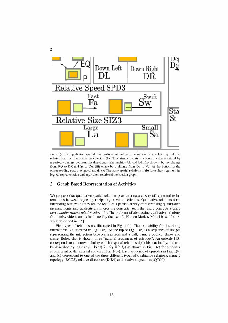
Fig. 1: (a) Five qualitative spatial relationships:(i)topology; (ii) direction; (iii) relative speed; (iv)relative size; (v) qualitative trajectories. (b) Three simple events: (i) bounce - characterized bya periodic change between the directional relationships UL and DL; (ii) throw - by the changefrom PO to DR and St to De; (iii) chase by a change from De to Pu. At the bottom is thecorresponding spatio-temporal graph. (c) The same spatial relations in (b) for a short segment, itslogical representation and equivalent relational interaction graph.

2 Graph Based Representation of Activities

We propose that qualitative spatial relations provide a natural way of representing in-teractions between objects participating in video activities. Qualitative relations forminteresting features as they are the result of a particular way of discretizing quantitativemeasurements into qualitatively interesting concepts, such that these concepts signifyperceptually salient relationships [3]. The problem of abstracting qualitative relationsfrom noisy video data, is facilitated by the use of a Hidden Markov Model based frame-work described in [15].

Five types of relations are illustrated in Fig. 1 (a). Their suitability for describinginteractions is illustrated in Fig. 1 (b). At the top of Fig. 1 (b) is a sequence of imagesrepresenting the interaction between a person and a ball, namely bounce, throw andchase. Below that is shown, three “parallel sequences of episodes”. An episode [13]corresponds to an interval, during which a spatial relationship holds maximally, and canbe described by logic (e.g. Holds(O1, O2,UR, I2) as shown in Fig. 1(c) for a shortersub-interval of the interval shown in Fig. 1(b)). Each sequence of episodes in Fig. 1(b)and (c) correspond to one of the three different types of qualitative relations, namelytopology (RCC5), relative directions (DIR4) and relative trajectories (QTC6).

16

3

An alternative to the above “sequence of episodes” based representation is to relatethe intervals corresponding to each pair of episodes, using Allen’s temporal relationships[1], e.g. Meets(I2, I3), as shown in Fig. 1(c). This leads to a fully relational representa-tion capturing many, if not all, qualitatively interesting temporal dependencies.

An alternative relational representation to logical predicates is to use interactiongraphs [14], as shown in Fig. 1(c). They are three layered graphs, in which the layer1 nodes are mapped to the interacting objects. Layer 2 nodes of the interaction graphrepresent the episodes between the respective pairs of tracks pointed to at layer 1 andare labelled with their respective maximal spatial relation as shown in Fig. 1(c). Thelayer 3 nodes of the activity graph are labelled with Allens temporal relations (e.g. m: meets, in Fig. 1(c)) between intervals corresponding to certain pairs [12] of layer 2nodes.

Interaction graphs are a computationally efficient alternative to logical predicates,as they avoid repetition of object and episode variables and also provide a well definedand computationally efficient comparison of interactions, by means of suitable simi-larity measure. This measure is defined using a kernel on a feature space obtained byexpressing a interaction graph in terms of a bag of sub-interaction subgraphs [14].

An activity graph is an interaction graph that captures the spatio-temporal relation-ships between all pairs of co-temporally observed objects that are involved in activitiesfor an extended duration. Note that the activity graph may also represent the spatio-temporal graph for activities in several unrelated videos for the same domain, and notnecessarily one single video.

3 Graph Based Relational Learning of Activities

The authors in [14] proposed a novel relational graph based learning formulation forvideo activity understanding, in the context of a specific unsupervised learning task. Inthe following, we use this formulation to describe a general way of translating standardproblems in video activity analysis to standard problems in relational graph learning.We show how it can be more generally applied, in order to address many of the standardvideo activity understanding tasks.

One of the key underlying hypotheses in research on video activity understanding[9] is that activities are composed of events of different types. Based on this hypothesis,tasks such as learning event class models, event classification, clustering and detectionare defined. In this work, we characterize events by a set of co-temporal tracklets (atracklet is a one-piece segment of a track). Events having similar spatio-temporal rela-tionships between their constituent tracklets tend to belong to the same event class. Theset of all event classes is called C. A set of events E is a “cover” of a set of tracks Tiff the union of all tracklets in E is isomorphic to T . In general there may be coinci-dental interactions between objects that that would not naturally be regarded as part ofany event in an event class 2. This notion of an event cover can be regarded as an globalexplanation of the activities in a video in terms of instances of event classes.

A set of tracks T can be abstractly represented using an activity graph A, as de-scribed above. An event corresponds to a subgraph of A, such that this subgraph is also

2 We ignore this complexity here but see [12], [14]. The final paper would contain details of howcoincidences can be incorporated into the learning algorithms. Here, there is no space to givefurther details here.

17

4

an interaction graph. An event cover in this formulation, thus becomes a set of interac-tion graphs, whose union isA. These interaction graphs are called event graphs3. Similarevent graphs tend to belong to the same event class. An event model is defined for theset of event classes C, according to which, each class is a probability distribution over afinite set of interaction graphs. Finally, observation noise is modelled by allowing multi-ple possible activity graphsA, for the same set of observed tracks T . This formalism hasbeen used to model the joint probability distribution of the above variables {C,G,A, T }as: P (C,G,A, T ) ≈ P (C)P (G|C)P (A|G, C)P (T |A)

We now apply this formulation to address the above video understanding tasks interms of relational graph learning. The task of learning an event model translates tolearning an event model for event classes C given A and a corresponding G. A MAPformulation of this problem is

C = argmaxC

P (C)P (G|C)

In this work, we learn a generative event model in the form of a simple mixture ofGaussians, in both supervised and unsupervised settings. In the unsupervised setting, weused a Bayesian Information Criterion to automatically determine the number of classes.More generally, techniques related to graph classification [5] [6] [8] and clustering [16],may be applied.

The video event detection task corresponds to the case, when given an event modelC, the goal is to detect the events, or more generally, learn a labelled cover G, where thelabels correspond to one of the event classes in C, that is:

G = argmaxG

P (G|C)P (A|G, C)

In this work, we form the cover G, by simply searching for subgraphs in the activitygraph that are most likely given the event model C. That is, we find those graphs g ∈ Gfor which the likelihood P (g|C), is above a threshold. We also simply assume a uniformdistribution P (A|G, C) for all possible event graph covers G.

In a more general unsupervised video understanding setting, the goal is to learn theunknowns: G, C and A, given only the observed tracks T , that is:

(C, G, A) = arg maxC,G,A

P (C)P (G|C)P (A|G, C)P (T |A)

A Markov Chain Monte Carlo (MCMC) procedure is used in [14] to find the MAP solu-tion. MCMC is used to efficiently search the space of possible activity graphs, possiblecovers of the activity graph and possible event models, in order to find the MAP solution.

4 Experiments

A real video dataset consisting of activities representing simple verbs such as throw (aball), catch etc is used to evaluate the proposed approach. The dataset consists of 36videos. Each video lasts for approximately 150–200 frames and contains one or more

3 In practical situations, with co-temporal events, there will be co-incidental interaction graphs,which are a part of A, but not a part of any event graph. We leave further details of this to thefull paper.

18

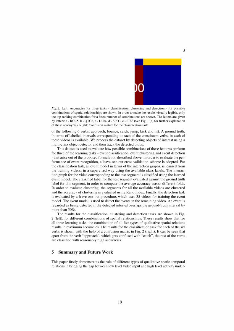
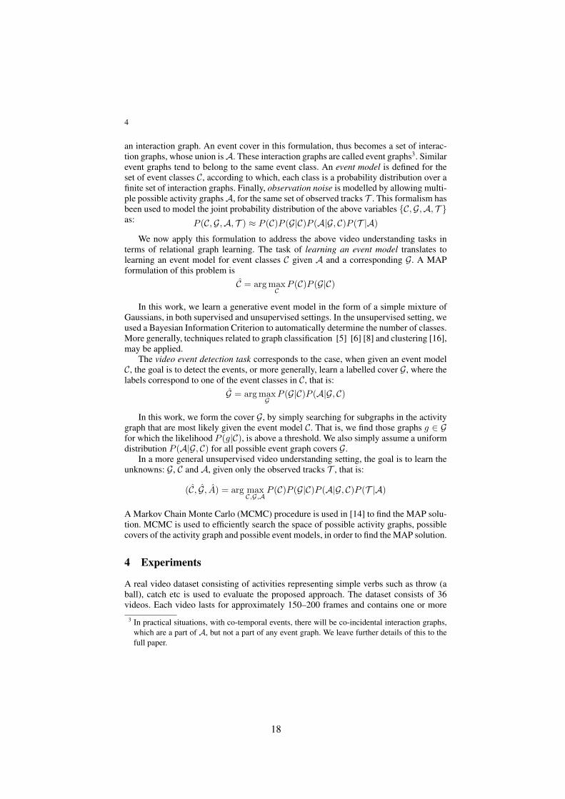
5

Fig. 2: Left: Accuracies for three tasks - classification, clustering and detection - for possiblecombinations of spatial relationships are shown. In order to make the results visually legible, onlythe top ranking combination for a fixed number of combinations are shown. The letters are givenby letters: a - RCC5, b - QTC6, c - DIR4, d - SPD3, e - SIZ3 (See Fig. 1 (a) for further explanationof these acronyms). Right: Confusion matrix for the classification task.

of the following 6 verbs: approach, bounce, catch, jump, kick and lift. A ground truth,in terms of labelled intervals corresponding to each of the constituent verbs, in each ofthese videos is available. We process the dataset by detecting objects of interest using amulti-class object detector and then track the detected blobs.

This dataset is used to evaluate how possible combinations of these features performfor three of the learning tasks - event classification, event clustering and event detection- that arise out of the proposed formulation described above. In order to evaluate the per-formance of event recognition, a leave-one out cross validation scheme is adopted. Forthe classification task, an event model in terms of the interaction graphs, is learned fromthe training videos, in a supervised way using the available class labels. The interac-tion graph for the video corresponding to the test segment is classified using the learnedevent model. The classified label for the test segment evaluated against the ground truthlabel for this segment, in order to compute the average accuracy across different folds.In order to evaluate clustering, the segments for all the available videos are clusteredand the accuracy of clustering is evaluated using Rand Index. Finally, the detection taskis evaluated by a leave one out procedure, which uses 35 videos for training the eventmodel. The event model is used to detect the events in the remaining video. An event isregarded as being detected if the detected interval overlaps the ground-truth interval bymore than 50%.

The results for the classification, clustering and detection tasks are shown in Fig.2 (left), for different combinations of spatial relationships. These results show that forall three learning tasks, the combination of all five types of qualitative spatial relationsresults in maximum accuracies. The results for the classification task for each of the sixverbs is shown with the help of a confusion matrix in Fig. 2 (right). It can be seen thatapart from the verb “approach”, which gets confused with “catch”, the rest of the verbsare classified with reasonably high accuracies.

5 Summary and Future Work

This paper firstly demonstrates the role of different types of qualitative spatio-temporalrelations in bridging the gap between low level video input and high level activity under-

19

6

standing has been demonstrated. One direction for future research is to investigate therole of other qualitative relations and their role in representing activities. Another inter-esting direction is to model human actions by considering relationships between bodyparts. These body parts could be obtained using part-based models.

Another contribution is that this paper presents a general way of addressing problemsin video activity understanding using graph based relational learning. In the future, itwould be interesting to extend this formalism to other tasks in activity understandingsuch as anomaly detection, scene description and gap filling.

References

1. Allen, J.: Maintaining knowledge about temporal intervals. Commun. ACM 26(11), 832–843(1983)

2. Cohn, A.G., Hazarika, S.M.: Qualitative spatial representation and reasoning: An overview.Fundamenta Informaticae (2001)

3. Cohn, A.G., Magee, D., Galata, A., Hogg, D.C., Hazarika, S.: Towards an architecture forcognitive vision using qualitative spatio-temporal representations and abduction. pp. 232–248(2003)

4. Cook, D.J., Holder, L.B.: Mining Graph Data. Wiley-Interscience (2007)5. Deshpande, M., Kuramochi, M., Wale, N., Karypis, G.: Frequent substructure-based ap-

proaches for classifying chemical compounds. IEEE Transactions on Knowledge and DataEngineering (TKDE) 17(8), 1036–1050 (2005)

6. Gartner, T., Flach, P.A., Wrobel, S.: On graph kernels: Hardness results and efficient alterna-tives. In: Proceedings of the Conference On Learning Theory (COLT). pp. 129–143 (2003)

7. Getoor, L., Taskar, B.: Introduction to Statistical Relational Learning (2007)8. Kudo, T., Maeda, E., Matsumoto, Y.: An application of boosting to graph classification. In:

Proceedings of Neural Information Processing Systems (NIPS) (2004)9. Lavee, G., Rivlin, E., Rudzsky, M.: Understanding video events: a survey of methods for

automatic interpretation of semantic occurrences in video. IEEE Transactions on Systems,Man, and Cybernetics pp. 489–504 (2009)

10. Raedt, L.D., Kersting, K.: Probabilistic inductive logic programming (2008)11. Randell, D.A., Cui, Z., Cohn, A.G.: A spatial logic based on regions and connection. In:

Proceedings of the Conference on Knowledge Representation and Reasoning (KR) (1992)12. Sridhar, M.: Unsupervised Learning of Event and Object Classes from Video. University Of

Leeds, http://www.comp.leeds.ac.uk/krishna/thesis.pdf13. Sridhar, M., Cohn, A.G., Hogg, D.C.: Learning functional object-categories from a relational

spatio-temporal representation. In: Proceedings of the European Conference on Artifical In-telligence (ECAI) (2008)

14. Sridhar, M., Cohn, A.G., Hogg, D.C.: Unsupervised learning of event classes from video. In:Proceedings of the AAAI Conference on Artificial Intelligence (AAAI) (2010)

15. Sridhar, M., Cohn, A.G., Hogg, D.C.: From video to RCC8: exploiting a distance based se-mantics to stabilise the interpretation of mereotopological relations. Proc. COSIT, In Press(2011)

16. Tsuda, K., Kurihara, K.: Graph mining with variational dirichlet process mixture models. In:Proceedings of SIAM International Conference on Data Mining (2008)

17. Wang, X., Ma, X., Grimson, E.: Unsupervised activity perception in crowded and compli-cated scenes using hierarchical Bayesian models. IEEE Transactions on Pattern Analysis andMachine Intelligence (TPAMI) (2009)

20

Physical Puzzles—Challenging Spatio-Temporal Configuration Problems

Arne Kreutzmann and Diedrich WolterSFB/TR 8 Spatial Cognition, University Bremen

AbstractThis paper serves to promote studying spatio-temporal configurations problems in physical do-mains, called physical puzzled for short. The kindof physical puzzles we consider involve simple ob-jects that are subject to the laws of mechanics, re-stricted to what is commonly considered to be ac-cessible by common sense knowledge. Our problemspecification involves several unknowns, creatinguncertainty which inhibits analytic construction ofsolutions. Instead, tests need to be carried out inorder to evaluate solution candidates. The objectiveis to find a solution whilst minimizing the numberof tests required.

1 IntroductionQualitative representations aim to capture human common-sense understanding and to enable efficient symbolic reasoningprocesses. Qualitative representations abstract from an overlydetailed domain by only distinguishing between an essentialset of meaningful concepts. Qualitative approaches are widelyacknowledged for their ability to abstract from uncertainty, forexample an uncertain measurement of a location can becomea certain notion of region membership. Naturally, differenttasks may call for different qualitative concepts to describe thestate of affairs. This task-dependency lead to the developmentof a wide range of qualitative representations of space andtime—see [Cohn and Renz, 2007] for an overview.

When benchmarking qualitative representation and reason-ing it appears natural to consider adequacy of representation aswell as effectiveness and efficiency of reasoning. Since quali-tative representations are meant to provide us with a formalmodel for common-sense reasoning, we argue for studyingproblems which are easy to solve for humans but hard for com-puters. To this end, we examine spatial configuration problemsin the physical domain, i.e., problems in which objects need tobe arranged in a certain way in order to achieve a specific goal(like making a ball hit a goal). As claimed by Bredeweg andStruss, “reasoning about, and solving problems in, the physicalworld is one of the most fundamental capabilities of humanintelligence and a fundamental subject for AI” [Bredewegand Struss, 2003]. Problem solving in a physical context canthus be considered a well-suited benchmark domain for AI.

The physical domain is also key to qualitative reasoning. AsWilliams and de Kleer put it, “[...] the heart of the qualitativereasoning enterprise is to develop computational theories ofthe core skills underlying engineers, scientists, and just plainfolks’s ability to hypothesize, test, predict, create, optimize,diagnose and debug physical mechanisms” [Williams and deKleer, 1991]. Solving puzzles has some tradition is AI re-search. Recently, Cabalar and Santos accounted puzzles asan well-suited test bed for their ability to present challengingproblems in small packages [Cabalar and Santos, 2011]. Weargue for studying physical puzzles that involve dynamics,in particular we consider the problem of configuring an en-vironment by arranging objects to make a ball bounce intoa pre-defined goal region. A similar kind of bouncing ballproblem also served as example to motivate the poverty con-jecture in qualitative reasoning [Forbus et al., 1991]. In thelight of today’s state of the art in qualitative spatial reasoning,Cohn and Renz take a more differentiated point of view [Cohnand Renz, 2007]. Therefore, we regard physical puzzles to bethe domain of choice for evaluating advances in qualitativereasoning.

2 The Physical Puzzle DomainOur proposal has been inspired by computer games that,among other difficulties, confront a player with tricky physicalproblems that involve spatio-temporal reasoning as well asreasoning about action and change. Two games exemplifythe genre of physical puzzles we propose to study: the gameDeflector published by Vortex Software in 1987 (see Figure 1for a screenshot of the Commodore 64 version) requires theplayer to arrange a set of rotatable mirrors in such a way asto make a laser beam hit balloons. Hitting all balloons (andthereby making them burst) clears a level. This kind of puzzleis a purely spatial one. Obstacles placed in the level makeit hard to foresee which mirror setup is required to point thelaser to a specific point in space. Whilst this problem can besolved purely using computational geometry, the state space istoo large to be enumerated by humans. Human players needto employ some means of heuristics and reasoning in orderto construct solutions. The second game, called Crazy Ma-chines developed by FAKT Software is similar but involves acomplex physical domain (see Figure 2 for a screenshot). Theobjective is to arrange objects in such a way that they exhibitcertain functionality (for instance, making a set of balloons

21

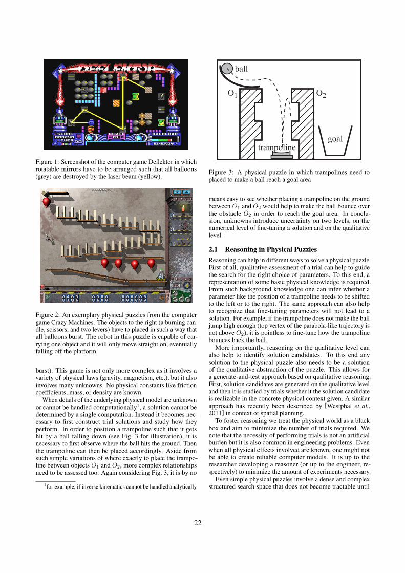
Figure 1: Screenshot of the computer game Deflektor in whichrotatable mirrors have to be arranged such that all balloons(grey) are destroyed by the laser beam (yellow).

Figure 2: An exemplary physical puzzles from the computergame Crazy Machines. The objects to the right (a burning can-dle, scissors, and two levers) have to placed in such a way thatall balloons burst. The robot in this puzzle is capable of car-rying one object and it will only move straight on, eventuallyfalling off the platform.

burst). This game is not only more complex as it involves avariety of physical laws (gravity, magnetism, etc.), but it alsoinvolves many unknowns. No physical constants like frictioncoefficients, mass, or density are known.

When details of the underlying physical model are unknownor cannot be handled computationally1, a solution cannot bedetermined by a single computation. Instead it becomes nec-essary to first construct trial solutions and study how theyperform. In order to position a trampoline such that it getshit by a ball falling down (see Fig. 3 for illustration), it isnecessary to first observe where the ball hits the ground. Thenthe trampoline can then be placed accordingly. Aside fromsuch simple variations of where exactly to place the trampo-line between objects O1 and O2, more complex relationshipsneed to be assessed too. Again considering Fig. 3, it is by no

1for example, if inverse kinematics cannot be handled analytically

goaltrampoline

ball

O1 O2

Figure 3: A physical puzzle in which trampolines need toplaced to make a ball reach a goal area

means easy to see whether placing a trampoline on the groundbetween O1 and O2 would help to make the ball bounce overthe obstacle O2 in order to reach the goal area. In conclu-sion, unknowns introduce uncertainty on two levels, on thenumerical level of fine-tuning a solution and on the qualitativelevel.

2.1 Reasoning in Physical PuzzlesReasoning can help in different ways to solve a physical puzzle.First of all, qualitative assessment of a trial can help to guidethe search for the right choice of parameters. To this end, arepresentation of some basic physical knowledge is required.From such background knowledge one can infer whether aparameter like the position of a trampoline needs to be shiftedto the left or to the right. The same approach can also helpto recognize that fine-tuning parameters will not lead to asolution. For example, if the trampoline does not make the balljump high enough (top vertex of the parabola-like trajectory isnot above O2), it is pointless to fine-tune how the trampolinebounces back the ball.

More importantly, reasoning on the qualitative level canalso help to identify solution candidates. To this end anysolution to the physical puzzle also needs to be a solutionof the qualitative abstraction of the puzzle. This allows fora generate-and-test approach based on qualitative reasoning.First, solution candidates are generated on the qualitative leveland then it is studied by trials whether it the solution candidateis realizable in the concrete physical context given. A similarapproach has recently been described by [Westphal et al.,2011] in context of spatial planning.

To foster reasoning we treat the physical world as a blackbox and aim to minimize the number of trials required. Wenote that the necessity of performing trials is not an artificialburden but it is also common in engineering problems. Evenwhen all physical effects involved are known, one might notbe able to create reliable computer models. It is up to theresearcher developing a reasoner (or up to the engineer, re-spectively) to minimize the amount of experiments necessary.

Even simple physical puzzles involve a dense and complexstructured search space that does not become tractable until

22

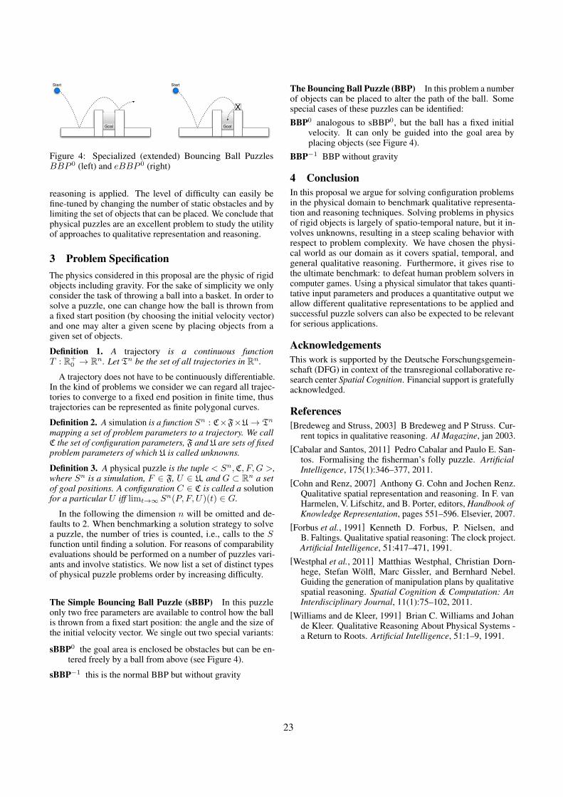
Start

Goal

X

Start

Goal

Figure 4: Specialized (extended) Bouncing Ball PuzzlesBBP 0 (left) and eBBP 0 (right)

reasoning is applied. The level of difficulty can easily befine-tuned by changing the number of static obstacles and bylimiting the set of objects that can be placed. We conclude thatphysical puzzles are an excellent problem to study the utilityof approaches to qualitative representation and reasoning.

3 Problem SpecificationThe physics considered in this proposal are the physic of rigidobjects including gravity. For the sake of simplicity we onlyconsider the task of throwing a ball into a basket. In order tosolve a puzzle, one can change how the ball is thrown froma fixed start position (by choosing the initial velocity vector)and one may alter a given scene by placing objects from agiven set of objects.

Definition 1. A trajectory is a continuous functionT : R+

0 → Rn. Let Tn be the set of all trajectories in Rn.

A trajectory does not have to be continuously differentiable.In the kind of problems we consider we can regard all trajec-tories to converge to a fixed end position in finite time, thustrajectories can be represented as finite polygonal curves.

Definition 2. A simulation is a function Sn : C×F×U→ Tn

mapping a set of problem parameters to a trajectory. We callC the set of configuration parameters, F and U are sets of fixedproblem parameters of which U is called unknowns.

Definition 3. A physical puzzle is the tuple < Sn,C, F,G >,where Sn is a simulation, F ∈ F, U ∈ U, and G ⊂ Rn a setof goal positions. A configuration C ∈ C is called a solutionfor a particular U iff limt→∞ Sn(P, F, U)(t) ∈ G.

In the following the dimension n will be omitted and de-faults to 2. When benchmarking a solution strategy to solvea puzzle, the number of tries is counted, i.e., calls to the Sfunction until finding a solution. For reasons of comparabilityevaluations should be performed on a number of puzzles vari-ants and involve statistics. We now list a set of distinct typesof physical puzzle problems order by increasing difficulty.

The Simple Bouncing Ball Puzzle (sBBP) In this puzzleonly two free parameters are available to control how the ballis thrown from a fixed start position: the angle and the size ofthe initial velocity vector. We single out two special variants:

sBBP0 the goal area is enclosed be obstacles but can be en-tered freely by a ball from above (see Figure 4).

sBBP−1 this is the normal BBP but without gravity

The Bouncing Ball Puzzle (BBP) In this problem a numberof objects can be placed to alter the path of the ball. Somespecial cases of these puzzles can be identified:BBP0 analogous to sBBP0, but the ball has a fixed initial

velocity. It can only be guided into the goal area byplacing objects (see Figure 4).

BBP−1 BBP without gravity

4 ConclusionIn this proposal we argue for solving configuration problemsin the physical domain to benchmark qualitative representa-tion and reasoning techniques. Solving problems in physicsof rigid objects is largely of spatio-temporal nature, but it in-volves unknowns, resulting in a steep scaling behavior withrespect to problem complexity. We have chosen the physi-cal world as our domain as it covers spatial, temporal, andgeneral qualitative reasoning. Furthermore, it gives rise tothe ultimate benchmark: to defeat human problem solvers incomputer games. Using a physical simulator that takes quanti-tative input parameters and produces a quantitative output weallow different qualitative representations to be applied andsuccessful puzzle solvers can also be expected to be relevantfor serious applications.

AcknowledgementsThis work is supported by the Deutsche Forschungsgemein-schaft (DFG) in context of the transregional collaborative re-search center Spatial Cognition. Financial support is gratefullyacknowledged.

References[Bredeweg and Struss, 2003] B Bredeweg and P Struss. Cur-

rent topics in qualitative reasoning. AI Magazine, jan 2003.[Cabalar and Santos, 2011] Pedro Cabalar and Paulo E. San-

tos. Formalising the fisherman’s folly puzzle. ArtificialIntelligence, 175(1):346–377, 2011.

[Cohn and Renz, 2007] Anthony G. Cohn and Jochen Renz.Qualitative spatial representation and reasoning. In F. vanHarmelen, V. Lifschitz, and B. Porter, editors, Handbook ofKnowledge Representation, pages 551–596. Elsevier, 2007.

[Forbus et al., 1991] Kenneth D. Forbus, P. Nielsen, andB. Faltings. Qualitative spatial reasoning: The clock project.Artificial Intelligence, 51:417–471, 1991.

[Westphal et al., 2011] Matthias Westphal, Christian Dorn-hege, Stefan Wolfl, Marc Gissler, and Bernhard Nebel.Guiding the generation of manipulation plans by qualitativespatial reasoning. Spatial Cognition & Computation: AnInterdisciplinary Journal, 11(1):75–102, 2011.

[Williams and de Kleer, 1991] Brian C. Williams and Johande Kleer. Qualitative Reasoning About Physical Systems -a Return to Roots. Artificial Intelligence, 51:1–9, 1991.

23

24

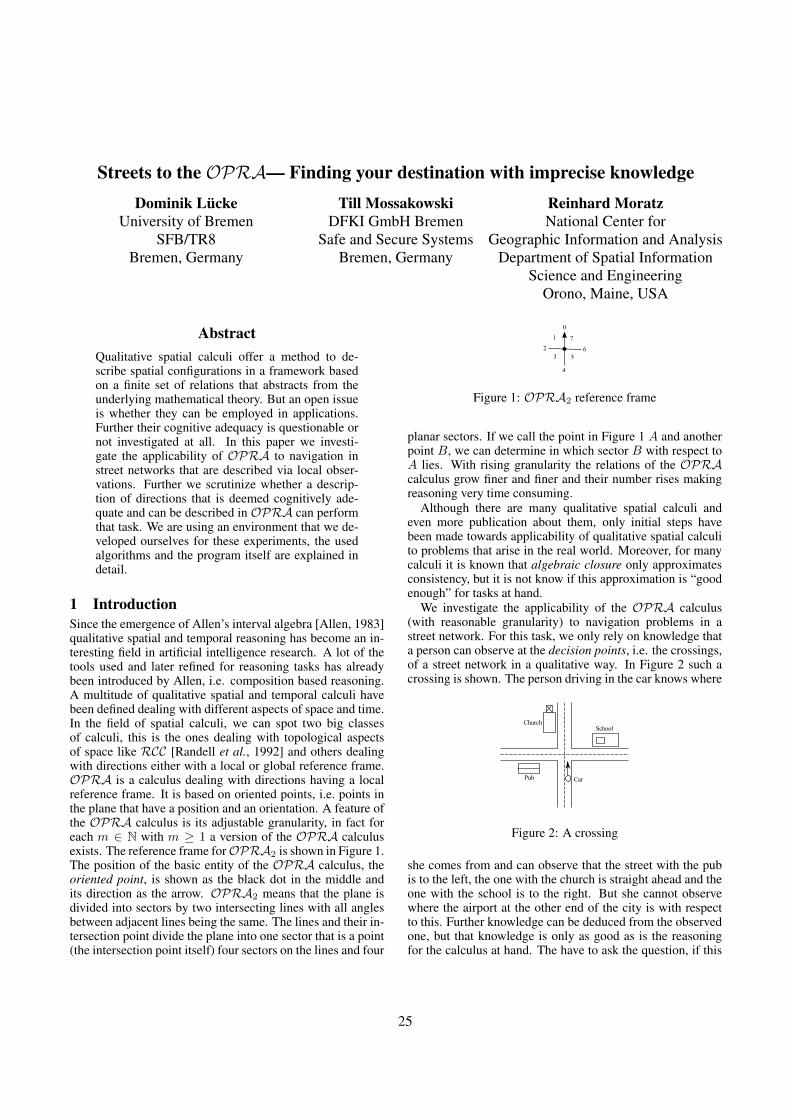
Streets to the OPRA— Finding your destination with imprecise knowledgeDominik Lücke

University of BremenSFB/TR8

Bremen, Germany

Till MossakowskiDFKI GmbH Bremen

Safe and Secure SystemsBremen, Germany

Reinhard MoratzNational Center for

Geographic Information and AnalysisDepartment of Spatial Information

Science and EngineeringOrono, Maine, USA

AbstractQualitative spatial calculi offer a method to de-scribe spatial configurations in a framework basedon a finite set of relations that abstracts from theunderlying mathematical theory. But an open issueis whether they can be employed in applications.Further their cognitive adequacy is questionable ornot investigated at all. In this paper we investi-gate the applicability of OPRA to navigation instreet networks that are described via local obser-vations. Further we scrutinize whether a descrip-tion of directions that is deemed cognitively ade-quate and can be described in OPRA can performthat task. We are using an environment that we de-veloped ourselves for these experiments, the usedalgorithms and the program itself are explained indetail.

1 IntroductionSince the emergence of Allen’s interval algebra [Allen, 1983]qualitative spatial and temporal reasoning has become an in-teresting field in artificial intelligence research. A lot of thetools used and later refined for reasoning tasks has alreadybeen introduced by Allen, i.e. composition based reasoning.A multitude of qualitative spatial and temporal calculi havebeen defined dealing with different aspects of space and time.In the field of spatial calculi, we can spot two big classesof calculi, this is the ones dealing with topological aspectsof space like RCC [Randell et al., 1992] and others dealingwith directions either with a local or global reference frame.OPRA is a calculus dealing with directions having a localreference frame. It is based on oriented points, i.e. points inthe plane that have a position and an orientation. A feature ofthe OPRA calculus is its adjustable granularity, in fact foreach m ∈ N with m ≥ 1 a version of the OPRA calculusexists. The reference frame forOPRA2 is shown in Figure 1.The position of the basic entity of the OPRA calculus, theoriented point, is shown as the black dot in the middle andits direction as the arrow. OPRA2 means that the plane isdivided into sectors by two intersecting lines with all anglesbetween adjacent lines being the same. The lines and their in-tersection point divide the plane into one sector that is a point(the intersection point itself) four sectors on the lines and four

Figure 1: OPRA2 reference frame

planar sectors. If we call the point in Figure 1 A and anotherpoint B, we can determine in which sector B with respect toA lies. With rising granularity the relations of the OPRAcalculus grow finer and finer and their number rises makingreasoning very time consuming.

Although there are many qualitative spatial calculi andeven more publication about them, only initial steps havebeen made towards applicability of qualitative spatial calculito problems that arise in the real world. Moreover, for manycalculi it is known that algebraic closure only approximatesconsistency, but it is not know if this approximation is “goodenough” for tasks at hand.

We investigate the applicability of the OPRA calculus(with reasonable granularity) to navigation problems in astreet network. For this task, we only rely on knowledge thata person can observe at the decision points, i.e. the crossings,of a street network in a qualitative way. In Figure 2 such acrossing is shown. The person driving in the car knows where

Figure 2: A crossing

she comes from and can observe that the street with the pubis to the left, the one with the church is straight ahead and theone with the school is to the right. But she cannot observewhere the airport at the other end of the city is with respectto this. Further knowledge can be deduced from the observedone, but that knowledge is only as good as is the reasoningfor the calculus at hand. The have to ask the question, if this

25

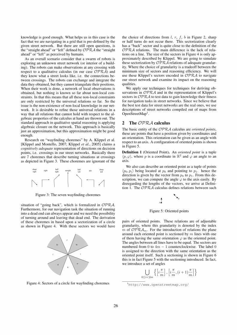
knowledge is good enough. What helps us in this case is thefact that we are navigating in a grid that is pre-defined by thegiven street network. But there are still open questions, isthe “straight ahead” or “left” defined byOPRA the “straightahead” or “left” as perceived by humans.

As an overall scenario consider that a swarm of robots isexploring an unknown street network (or interior of a build-ing). The robots can make observations at any crossing withrespect to a qualitative calculus (in our case OPRA) andthey know what a street looks like, i.e. the connections be-tween crossings. The robots can exchange and integrate thedata they obtained, but they cannot triangulate their positions.When their work is done, a network of local observations isobtained, but nothing is known so far about non-local con-straints. In that this means that all these non-local constraintsare only restricted by the universal relations so far. So theissue is the non-existence of non-local knowledge in our net-work. It is desirable to refine those universal relations in away that all relations that cannot hold with respect to the al-gebraic properties of the calculus at hand are thrown out. Thestandard approach in qualitative spatial reasoning is applyingalgebraic closure on the network. This approach is basicallyjust an approximation, but this approximation might be goodenough.

Research on “wayfinding choremes” by A. Klippel et al.[Klippel and Montello, 2007; Klippel et al., 2005] claims acognitively adequate representation of directions on decisionpoints, i.e. crossings in our street networks. Basically thereare 7 choremes that describe turning situations at crossingsas depicted in Figure 3. These choremes are ignorant of the

Figure 3: The seven wayfinding choremes

situation of “going back”, which is formalized in OPRA.Furthermore, for our navigation task the situation of runninginto a dead end can always appear and we need the possibilityof turning around and leaving that dead end. The derivationof these choremes in based upon a sectorization of a circleas shown in Figure 4. With these sectors we would have

Figure 4: Sectors of a circle for wayfinding choremes

the choice of directions from l, r, f , b in Figure 2, sharpor half turns do not occur there. This sectorization clearlyhas a “back” sector and is quite close to the definition of theOPRA relations. The main difference is the lack of rela-tions on a line. The size of the sectors in Figure 4 is only ap-proximately described by Klippel. We are going to simulatethese sectorization byOPRA relations of adequate granular-ity. Where the choice of granularity is a tradeoff between theminimum size of sectors and reasoning efficiency. We willuse these Klippel’s sectors encoded in OPRA to navigateour street network and examine its impact on the reasoningqualities.

We apply our techniques for techniques for deriving ob-servations in OPRA and in the representation of Klippel’ssectors in OPRA to test data to gain knowledge their fitnessfor navigation tasks in street networks. Since we believe thatthe best test data for street networks are the real ones, we usedescriptions of street networks compiled out of maps fromOpenStreetMap1.

2 The OPRA calculusThe basic entity of the OPRA calculus are oriented points,these are points that have a position given by coordinates andan orientation. This orientation can be given as an angle withrespect to an axis. A configuration of oriented points is shownin Figure 5.

Definition 1 (Oriented Point). An oriented point is a tuple〈p, ϕ〉, where p is a coordinate in R2 and ϕ an angle to anaxis.

We also can describe an oriented point as a tuple of points〈p0, pi〉 being located at p0 and pointing to p1. hence thedirection is given by the vector from p0 to p1. From this de-scription, we can compute the angle ϕ to the axis easily. Bydisregarding the lengths of the vectors, we arrive at Defini-tion 1. The OPRA calculus defines relations between such

Figure 5: Oriented points

pairs of oriented points. These relations are of adjustablegranularity, where this granularity is denoted by the indexm of OPRAm. For the introduction of relations the planearound each oriented point is sectioned by m lines with oneof them having the same orientation ϕ as the oriented point.The angles between all lines have to be equal. The sectors arenumbered from 0 to 4m − 1 counterclockwise. The label 0is assigned to the direction with the same orientation as theoriented point itself. Such a sectioning is shown in Figure 6this is in fact Figure 5 with the sectioning introduced. In fact,we introduce a set of angles

⋃

0≤i<2m

{[iπ

m

],[iπ

m, (i+ 1)

π

m

]}

1http://www.openstreetmap.org/

26

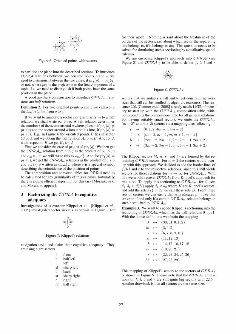
Figure 6: Oriented points with sectors

to partition the plane into the described sections. To introduceOPRA relations between two oriented points o and q, weneed to distinguish between the two cases, if pr1(o) = pr1(q)or not, where pr1 is the projection to the first component of atuple. I.e. we need to distinguish if both points have the sameposition in the plane.

A good auxiliary construction to introduce OPRAm rela-tions are half relations.Definition 2. For two oriented points o and q we call o B qthe half relation from o to q.

If we want to annotate a sector i or granularity m to a halfrelation, we shall write om Bi q. A half relation determinesthe number i of the sector around owhere q lies in if pr1(o) 6=pr1(q) and the sector around o into q points into, if pr1(o) =pr1(q). E.g. in Figure 6 the oriented points B lies in sector13 of A and we obtain the half relation A4 B13 B. And for Awith respect to B we get B4 B3 A.

First we consider the case of pr1(o) 6= pr1(q). We then getthe OPRAm relation from o to q as the product of om Bi q

and om Bj q, we will write this as om∠ji . And for pr1(o) =

pr1(q), we get theOPRAm relations as the product of o s qand om Bj q written as om∠j

sq, where s is a special symboldescribing the coincidence of the position of points.

The composition and converse tables for OPRA need tobe calculated for any granularity of this calculus, fortunatelythere is a quite efficient algorithm for this task [Mossakowskiand Moratz, to appear].

3 Factorizing the OPRA to cognitiveadequacy

Investigations of Alexander Klippel et al. [Klippel et al.,2005] investigated sector models as shown in Figure 7 for

Figure 7: Klippel’s relations

navigation tasks and claim their cognitive adequacy. Theyare using eight sectors

f fronthl half leftl leftsl sharp leftb backsr sharp rightr righthr half right

for their model. Nothing is said about the treatment of theborders of the sectors, i.e. about which sector the separatingline belongs to, if it belongs to any. This question needs to besolved for simulating such a sectioning by a qualitative spatialcalculus.

We are encoding Klippel’s approach into OPRA8 (seeFigure 8) and OPRA16 to be able to define f , b, l and r

Figure 8: OPRA8

sectors that are suitably small and to get constraint networksizes that still can be handled by algebraic reasoners. The rea-soner GQR [Gantner et al., 2008] already needs 14GB of mem-ory to start up with the OPRA16 composition table, with-out precaching the composition table for all general relations.For having suitably small sectors, we unite the OPRAm

(m ∈ 2n and n > 2) sectors via a mapping d as following.f 7→ {0, 1, 2, 4m− 1, 4m− 2}l 7→ {m− 2,m− 1,m,m+ 1,m+ 2}b 7→ {2m− 2, 2m− 1, 2m, 2m+ 1, 2m+ 2}r 7→ {3m− 2, 3m− 1, 3m, 3m+ 1, 3m+ 2}

The Klippel sectors hl, sl, sr and hr are formed by the re-maining OPRA sectors. For n = 2 the sectors would over-lap with this approach. We decided to add the border lines off , b l and r to the respective relations, since this still yieldssectors for these relations for m 7→ ∞ for OPRAm. Withthis we would recover OPRA2 from Klippel’s approach form 7→ ∞. To apply this sectioning to OPRAm, for all setsd1, d2 ∈ d(K) apply d1 × d2 where K are Klippel’s sectors,and add the sets {s} × d1 we call these sets D. From thesesets of sectors we can easily define predicates p1 . . . p8 thatare true if and only if a certain OPRAm relation belongs tosuch a set lifted to OPRAm.Example 3. We want to encode Klippel’s sectioning into thesectioning of OPRA8, which has the half relations 0 . . . 31.With the above definitions we obtain the mapping

f 7→ {30, 31, 0, 1, 2}hl 7→ {3, 4, 5}l 7→ {6, 7, 8, 9, 10}sl 7→ {11, 12, 13}b 7→ {14, 15, 16, 17, 18}sr 7→ {19, 20, 21}r 7→ {22, 23, 24, 25, 26}hr 7→ {27, 28, 29}

This mapping of Klippel’s sectors to the sectors of OPRA8

is shown in Figure 9. Please note that the OPRA8 emula-tions of f , l, b and r are still quite big sectors with 22.5◦.Another drawback is that all sectors are the same size.

27

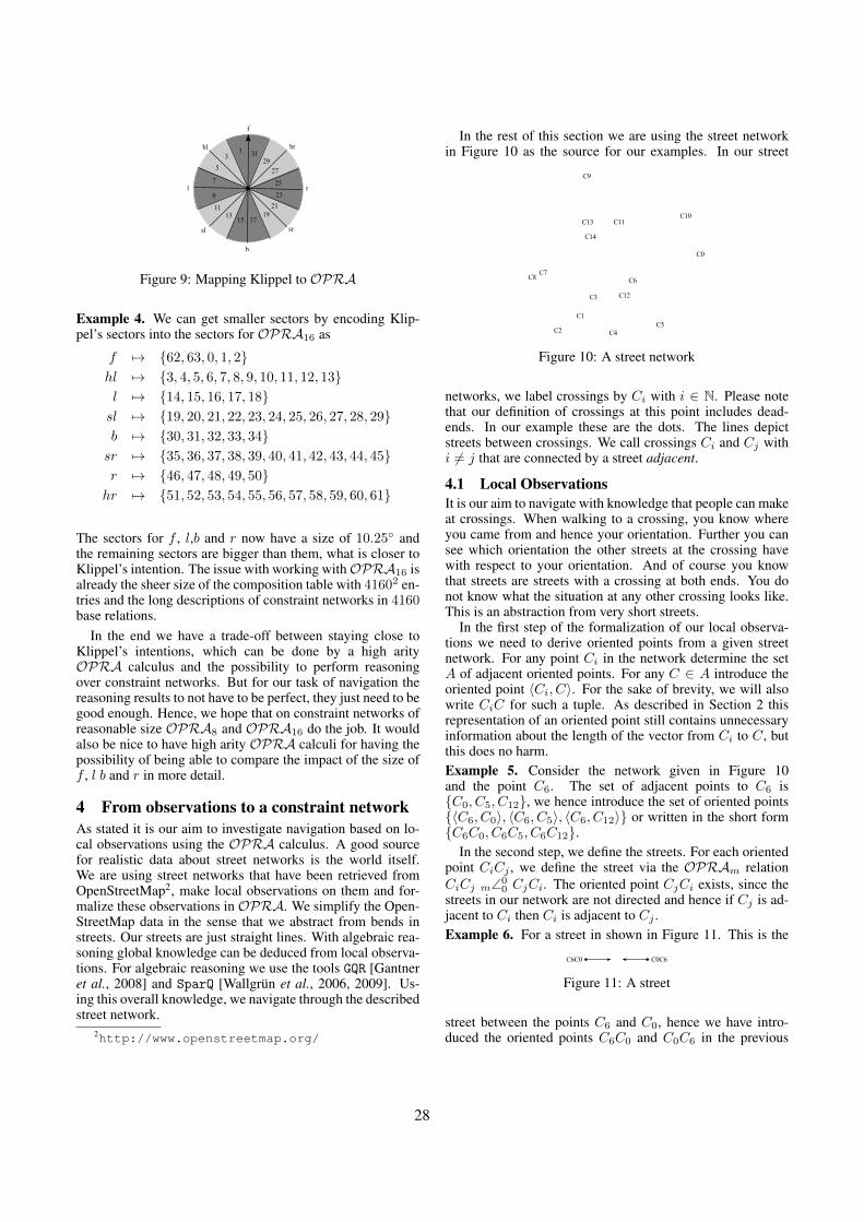
Figure 9: Mapping Klippel to OPRA

Example 4. We can get smaller sectors by encoding Klip-pel’s sectors into the sectors for OPRA16 as

f 7→ {62, 63, 0, 1, 2}hl 7→ {3, 4, 5, 6, 7, 8, 9, 10, 11, 12, 13}l 7→ {14, 15, 16, 17, 18}sl 7→ {19, 20, 21, 22, 23, 24, 25, 26, 27, 28, 29}b 7→ {30, 31, 32, 33, 34}sr 7→ {35, 36, 37, 38, 39, 40, 41, 42, 43, 44, 45}r 7→ {46, 47, 48, 49, 50}hr 7→ {51, 52, 53, 54, 55, 56, 57, 58, 59, 60, 61}

The sectors for f , l,b and r now have a size of 10.25◦ andthe remaining sectors are bigger than them, what is closer toKlippel’s intention. The issue with working withOPRA16 isalready the sheer size of the composition table with 41602 en-tries and the long descriptions of constraint networks in 4160base relations.

In the end we have a trade-off between staying close toKlippel’s intentions, which can be done by a high arityOPRA calculus and the possibility to perform reasoningover constraint networks. But for our task of navigation thereasoning results to not have to be perfect, they just need to begood enough. Hence, we hope that on constraint networks ofreasonable size OPRA8 and OPRA16 do the job. It wouldalso be nice to have high arity OPRA calculi for having thepossibility of being able to compare the impact of the size off , l b and r in more detail.

4 From observations to a constraint networkAs stated it is our aim to investigate navigation based on lo-cal observations using the OPRA calculus. A good sourcefor realistic data about street networks is the world itself.We are using street networks that have been retrieved fromOpenStreetMap2, make local observations on them and for-malize these observations in OPRA. We simplify the Open-StreetMap data in the sense that we abstract from bends instreets. Our streets are just straight lines. With algebraic rea-soning global knowledge can be deduced from local observa-tions. For algebraic reasoning we use the tools GQR [Gantneret al., 2008] and SparQ [Wallgrün et al., 2006, 2009]. Us-ing this overall knowledge, we navigate through the describedstreet network.

2http://www.openstreetmap.org/

In the rest of this section we are using the street networkin Figure 10 as the source for our examples. In our street

Figure 10: A street network

networks, we label crossings by Ci with i ∈ N. Please notethat our definition of crossings at this point includes dead-ends. In our example these are the dots. The lines depictstreets between crossings. We call crossings Ci and Cj withi 6= j that are connected by a street adjacent.

4.1 Local ObservationsIt is our aim to navigate with knowledge that people can makeat crossings. When walking to a crossing, you know whereyou came from and hence your orientation. Further you cansee which orientation the other streets at the crossing havewith respect to your orientation. And of course you knowthat streets are streets with a crossing at both ends. You donot know what the situation at any other crossing looks like.This is an abstraction from very short streets.

In the first step of the formalization of our local observa-tions we need to derive oriented points from a given streetnetwork. For any point Ci in the network determine the setA of adjacent oriented points. For any C ∈ A introduce theoriented point 〈Ci, C〉. For the sake of brevity, we will alsowrite CiC for such a tuple. As described in Section 2 thisrepresentation of an oriented point still contains unnecessaryinformation about the length of the vector from Ci to C, butthis does no harm.Example 5. Consider the network given in Figure 10and the point C6. The set of adjacent points to C6 is{C0, C5, C12}, we hence introduce the set of oriented points{〈C6, C0〉, 〈C6, C5〉, 〈C6, C12〉} or written in the short form{C6C0, C6C5, C6C12}.

In the second step, we define the streets. For each orientedpoint CiCj , we define the street via the OPRAm relationCiCj m∠0

0 CjCi. The oriented point CjCi exists, since thestreets in our network are not directed and hence if Cj is ad-jacent to Ci then Ci is adjacent to Cj .Example 6. For a street in shown in Figure 11. This is the

Figure 11: A street

street between the points C6 and C0, hence we have intro-duced the oriented points C6C0 and C0C6 in the previous

28

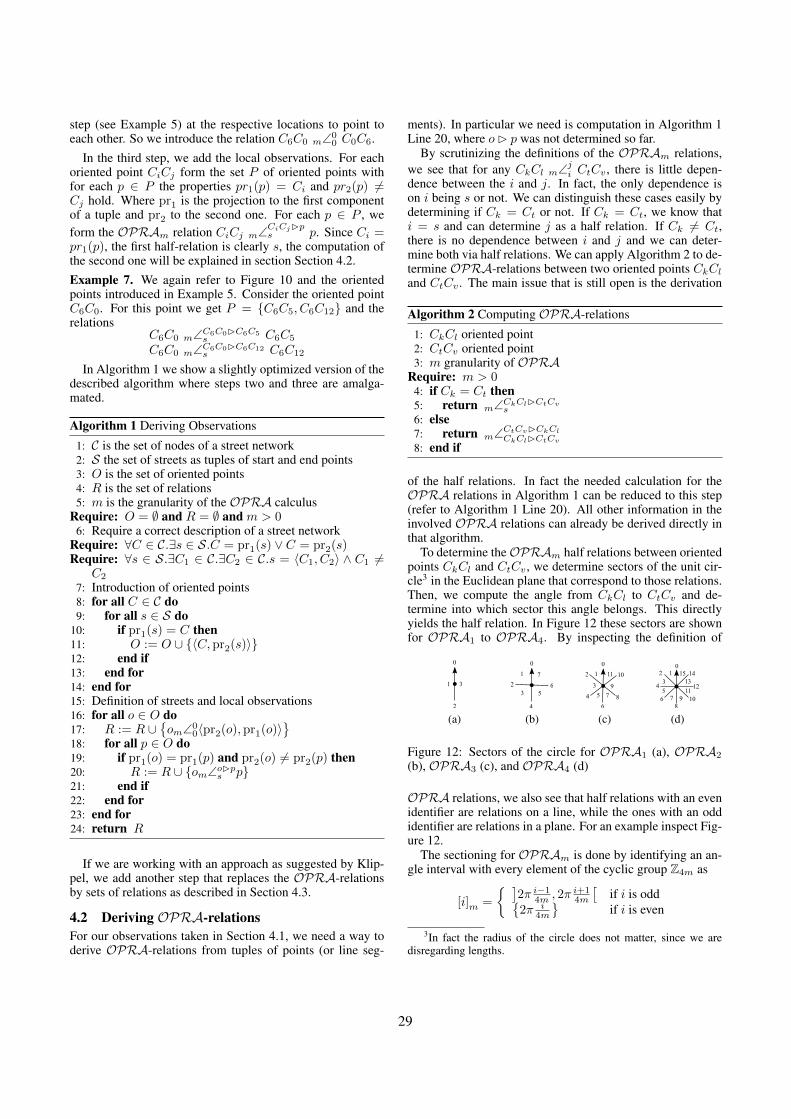
step (see Example 5) at the respective locations to point toeach other. So we introduce the relation C6C0 m∠0

0 C0C6.In the third step, we add the local observations. For each

oriented point CiCj form the set P of oriented points withfor each p ∈ P the properties pr1(p) = Ci and pr2(p) 6=Cj hold. Where pr1 is the projection to the first componentof a tuple and pr2 to the second one. For each p ∈ P , weform the OPRAm relation CiCj m∠CiCjBp

s p. Since Ci =pr1(p), the first half-relation is clearly s, the computation ofthe second one will be explained in section Section 4.2.Example 7. We again refer to Figure 10 and the orientedpoints introduced in Example 5. Consider the oriented pointC6C0. For this point we get P = {C6C5, C6C12} and therelations

C6C0 m∠C6C0BC6C5s C6C5

C6C0 m∠C6C0BC6C12s C6C12

In Algorithm 1 we show a slightly optimized version of thedescribed algorithm where steps two and three are amalga-mated.

Algorithm 1 Deriving Observations

1: C is the set of nodes of a street network2: S the set of streets as tuples of start and end points3: O is the set of oriented points4: R is the set of relations5: m is the granularity of the OPRA calculus

Require: O = ∅ and R = ∅ and m > 06: Require a correct description of a street network

Require: ∀C ∈ C.∃s ∈ S.C = pr1(s) ∨ C = pr2(s)Require: ∀s ∈ S.∃C1 ∈ C.∃C2 ∈ C.s = 〈C1, C2〉 ∧ C1 6=

C2

7: Introduction of oriented points8: for all C ∈ C do9: for all s ∈ S do

10: if pr1(s) = C then11: O := O ∪ {〈C,pr2(s)〉}12: end if13: end for14: end for15: Definition of streets and local observations16: for all o ∈ O do17: R := R ∪

{om∠0

0〈pr2(o),pr1(o)〉}

18: for all p ∈ O do19: if pr1(o) = pr1(p) and pr2(o) 6= pr2(p) then20: R := R ∪ {om∠oBp

s p}21: end if22: end for23: end for24: return R

If we are working with an approach as suggested by Klip-pel, we add another step that replaces the OPRA-relationsby sets of relations as described in Section 4.3.

4.2 Deriving OPRA-relationsFor our observations taken in Section 4.1, we need a way toderive OPRA-relations from tuples of points (or line seg-

ments). In particular we need is computation in Algorithm 1Line 20, where oB p was not determined so far.

By scrutinizing the definitions of the OPRAm relations,we see that for any CkCl m∠j

i CtCv , there is little depen-dence between the i and j. In fact, the only dependence ison i being s or not. We can distinguish these cases easily bydetermining if Ck = Ct or not. If Ck = Ct, we know thati = s and can determine j as a half relation. If Ck 6= Ct,there is no dependence between i and j and we can deter-mine both via half relations. We can apply Algorithm 2 to de-termine OPRA-relations between two oriented points CkCl

and CtCv . The main issue that is still open is the derivation

Algorithm 2 Computing OPRA-relations

1: CkCl oriented point2: CtCv oriented point3: m granularity of OPRA

Require: m > 04: if Ck = Ct then5: return m∠CkClBCtCv

s6: else7: return m∠CtCvBCkCl

CkClBCtCv

8: end if

of the half relations. In fact the needed calculation for theOPRA relations in Algorithm 1 can be reduced to this step(refer to Algorithm 1 Line 20). All other information in theinvolved OPRA relations can already be derived directly inthat algorithm.

To determine theOPRAm half relations between orientedpoints CkCl and CtCv , we determine sectors of the unit cir-cle3 in the Euclidean plane that correspond to those relations.Then, we compute the angle from CkCl to CtCv and de-termine into which sector this angle belongs. This directlyyields the half relation. In Figure 12 these sectors are shownfor OPRA1 to OPRA4. By inspecting the definition of

(a) (b) (c) (d)

Figure 12: Sectors of the circle for OPRA1 (a), OPRA2

(b), OPRA3 (c), and OPRA4 (d)

OPRA relations, we also see that half relations with an evenidentifier are relations on a line, while the ones with an oddidentifier are relations in a plane. For an example inspect Fig-ure 12.

The sectioning for OPRAm is done by identifying an an-gle interval with every element of the cyclic group Z4m as

[i]m =

{ ]2π i−1

4m , 2π i+14m

[if i is odd{

2π i4m

}if i is even

3In fact the radius of the circle does not matter, since we aredisregarding lengths.

29

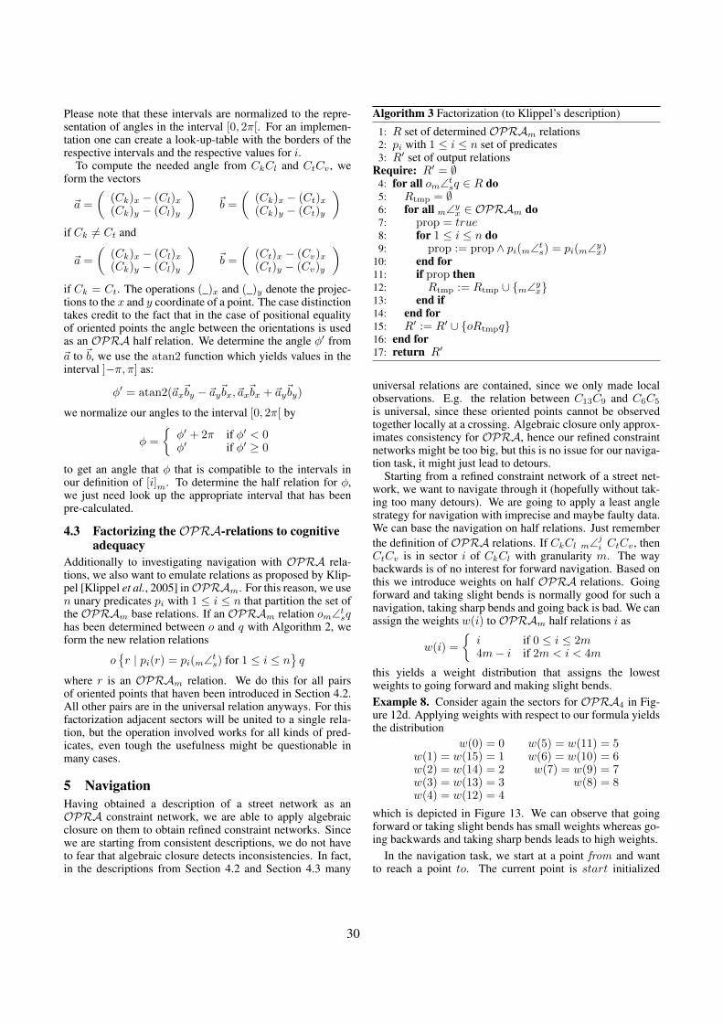
Please note that these intervals are normalized to the repre-sentation of angles in the interval [0, 2π[. For an implemen-tation one can create a look-up-table with the borders of therespective intervals and the respective values for i.

To compute the needed angle from CkCl and CtCv , weform the vectors

~a =

((Ck)x − (Cl)x(Ck)y − (Cl)y

)~b =

((Ck)x − (Ct)x(Ck)y − (Ct)y

)

if Ck 6= Ct and

~a =

((Ck)x − (Cl)x(Ck)y − (Cl)y

)~b =

((Ct)x − (Cv)x(Ct)y − (Cv)y

)

if Ck = Ct. The operations (_)x and (_)y denote the projec-tions to the x and y coordinate of a point. The case distinctiontakes credit to the fact that in the case of positional equalityof oriented points the angle between the orientations is usedas an OPRA half relation. We determine the angle φ′ from~a to ~b, we use the atan2 function which yields values in theinterval ]−π, π] as:

φ′ = atan2(~ax~by − ~ay~bx,~ax~bx + ~ay~by)

we normalize our angles to the interval [0, 2π[ by

φ =

{φ′ + 2π if φ′ < 0φ′ if φ′ ≥ 0

to get an angle that φ that is compatible to the intervals inour definition of [i]m. To determine the half relation for φ,we just need look up the appropriate interval that has beenpre-calculated.

4.3 Factorizing the OPRA-relations to cognitiveadequacy

Additionally to investigating navigation with OPRA rela-tions, we also want to emulate relations as proposed by Klip-pel [Klippel et al., 2005] inOPRAm. For this reason, we usen unary predicates pi with 1 ≤ i ≤ n that partition the set ofthe OPRAm base relations. If an OPRAm relation om∠t

sqhas been determined between o and q with Algorithm 2, weform the new relation relations

o{r | pi(r) = pi(m∠t

s) for 1 ≤ i ≤ n}q

where r is an OPRAm relation. We do this for all pairsof oriented points that haven been introduced in Section 4.2.All other pairs are in the universal relation anyways. For thisfactorization adjacent sectors will be united to a single rela-tion, but the operation involved works for all kinds of pred-icates, even tough the usefulness might be questionable inmany cases.

5 NavigationHaving obtained a description of a street network as anOPRA constraint network, we are able to apply algebraicclosure on them to obtain refined constraint networks. Sincewe are starting from consistent descriptions, we do not haveto fear that algebraic closure detects inconsistencies. In fact,in the descriptions from Section 4.2 and Section 4.3 many

Algorithm 3 Factorization (to Klippel’s description)

1: R set of determined OPRAm relations2: pi with 1 ≤ i ≤ n set of predicates3: R′ set of output relations

Require: R′ = ∅4: for all om∠t

sq ∈ R do5: Rtmp = ∅6: for all m∠y

x ∈ OPRAm do7: prop = true8: for 1 ≤ i ≤ n do9: prop := prop ∧ pi(m∠t

s) = pi(m∠yx)

10: end for11: if prop then12: Rtmp := Rtmp ∪ {m∠y

x}13: end if14: end for15: R′ := R′ ∪ {oRtmpq}16: end for17: return R′

universal relations are contained, since we only made localobservations. E.g. the relation between C13C9 and C6C5

is universal, since these oriented points cannot be observedtogether locally at a crossing. Algebraic closure only approx-imates consistency for OPRA, hence our refined constraintnetworks might be too big, but this is no issue for our naviga-tion task, it might just lead to detours.

Starting from a refined constraint network of a street net-work, we want to navigate through it (hopefully without tak-ing too many detours). We are going to apply a least anglestrategy for navigation with imprecise and maybe faulty data.We can base the navigation on half relations. Just rememberthe definition of OPRA relations. If CkCl m∠j

i CtCv , thenCtCv is in sector i of CkCl with granularity m. The waybackwards is of no interest for forward navigation. Based onthis we introduce weights on half OPRA relations. Goingforward and taking slight bends is normally good for such anavigation, taking sharp bends and going back is bad. We canassign the weights w(i) to OPRAm half relations i as

w(i) =

{i if 0 ≤ i ≤ 2m4m− i if 2m < i < 4m

this yields a weight distribution that assigns the lowestweights to going forward and making slight bends.Example 8. Consider again the sectors for OPRA4 in Fig-ure 12d. Applying weights with respect to our formula yieldsthe distribution

w(0) = 0 w(5) = w(11) = 5w(1) = w(15) = 1 w(6) = w(10) = 6w(2) = w(14) = 2 w(7) = w(9) = 7w(3) = w(13) = 3 w(8) = 8w(4) = w(12) = 4

which is depicted in Figure 13. We can observe that goingforward or taking slight bends has small weights whereas go-ing backwards and taking sharp bends leads to high weights.

In the navigation task, we start at a point from and wantto reach a point to. The current point is start initialized

30

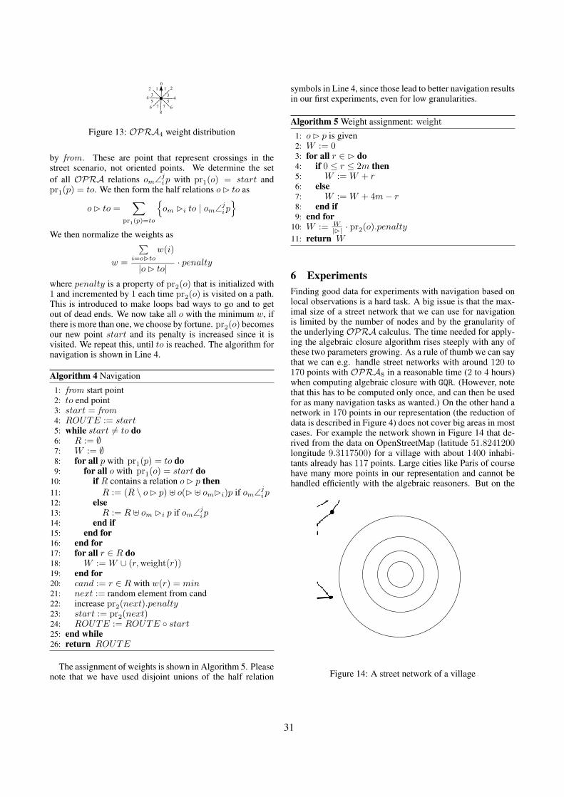
Figure 13: OPRA4 weight distribution

by from . These are point that represent crossings in thestreet scenario, not oriented points. We determine the setof all OPRA relations om∠j

ip with pr1(o) = start andpr1(p) = to. We then form the half relations oB to as

oB to =∑

pr1(p)=to

{om Bi to | om∠j

ip}

We then normalize the weights as

w =

∑i=oBto

w(i)

|oB to| · penalty

where penalty is a property of pr2(o) that is initialized with1 and incremented by 1 each time pr2(o) is visited on a path.This is introduced to make loops bad ways to go and to getout of dead ends. We now take all o with the minimum w, ifthere is more than one, we choose by fortune. pr2(o) becomesour new point start and its penalty is increased since it isvisited. We repeat this, until to is reached. The algorithm fornavigation is shown in Line 4.

Algorithm 4 Navigation

1: from start point2: to end point3: start = from4: ROUTE := start5: while start 6= to do6: R := ∅7: W := ∅8: for all p with pr1(p) = to do9: for all o with pr1(o) = start do

10: if R contains a relation oB p then11: R := (R \ oB p) ] o(B ] omBi)p if om∠j

ip12: else13: R := R ] om Bi p if om∠j

ip14: end if15: end for16: end for17: for all r ∈ R do18: W :=W ∪ (r,weight(r))19: end for20: cand := r ∈ R with w(r) = min21: next := random element from cand22: increase pr2(next).penalty23: start := pr2(next)24: ROUTE := ROUTE ◦ start25: end while26: return ROUTE

The assignment of weights is shown in Algorithm 5. Pleasenote that we have used disjoint unions of the half relation

symbols in Line 4, since those lead to better navigation resultsin our first experiments, even for low granularities.

Algorithm 5 Weight assignment: weight

1: oB p is given2: W := 03: for all r ∈ B do4: if 0 ≤ r ≤ 2m then5: W :=W + r6: else7: W :=W + 4m− r8: end if9: end for

10: W := W|B| · pr2(o).penalty

11: return W

6 ExperimentsFinding good data for experiments with navigation based onlocal observations is a hard task. A big issue is that the max-imal size of a street network that we can use for navigationis limited by the number of nodes and by the granularity ofthe underlying OPRA calculus. The time needed for apply-ing the algebraic closure algorithm rises steeply with any ofthese two parameters growing. As a rule of thumb we can saythat we can e.g. handle street networks with around 120 to170 points with OPRA8 in a reasonable time (2 to 4 hours)when computing algebraic closure with GQR. (However, notethat this has to be computed only once, and can then be usedfor as many navigation tasks as wanted.) On the other hand anetwork in 170 points in our representation (the reduction ofdata is described in Figure 4) does not cover big areas in mostcases. For example the network shown in Figure 14 that de-rived from the data on OpenStreetMap (latitude 51.8241200longitude 9.3117500) for a village with about 1400 inhabi-tants already has 117 points. Large cities like Paris of coursehave many more points in our representation and cannot behandled efficiently with the algebraic reasoners. But on the

Figure 14: A street network of a village

31

other hand, we want to observe navigations along paths ofvery differing lengths, including very long paths to be able tojudge the navigation properties of our networks based on lo-cal observations under very differing circumstances. For longpaths networks of a sufficiently big size are needed. Unfor-tunately this problem grows even bigger by the fact that thecloser we get to boundary of our street network the worse ourlocal observations and refinements will be. For a point in themiddle of a street network (as in the inner circle in Figure 14there are many points around it in all directions with observa-tions being made, putting this point into its place in a qualita-tive sense. In the middle circle the observations around a cer-tain point already get sparser and information about the pointsgets less certain, this gets worse in the outer circle. Outsideof the outer circle information about the points is very bad.In fact, it turned out, that navigating into the dead ends at theboundary of the map is very alluring, since their position withrespect to other points is not very restricted. For meaning-ful experiments about the navigation performance, the needstreet networks that are big enough to provide an area in thecenter for which enough information can be derived.

Our test data has hence to consist of street networks thatare small enough to be manageable with qualitative reasonersand that are big enough to yield enough information. For thefirst requirement networks in no more than 20 points wouldbe nice, for the second one the whole world, since then therewould be no boundary problem.

The results of our experiments are available athttp://www.informatik.uni-bremen.de/~till/fuerstenau_K8.html (for Klippel8) andhttp://www.informatik.uni-bremen.de/~till/fuerstenau_O8.html (for OPRA8). Wehave made 66 navigation experiments. The average pathlength was 16.0 (using OPRA8 factorized due to Klippel’ssectorization of the circle) and 16.2 (using OPRA8) withour algorithm based on local observations, while that ofa shortest path (using the complete map) was 13.2, andthat of a uniform shortest path (counting all way lengthsas 1) was 11.0. The average length of a random walkwas 718.0. As expected, the standard deviation of ouralgorithm is significantly higher than that of shortest paths:

Klippel8 OPRA8 shortestpath

uniformshortestpath

randomwalk

mean 16.0 16.2 13.2 11.0 718.0standarddeviation

9.3 9.3 5.1 3.5 519.9

However, our algorithm still performs quite well whencompared with shortest paths.

ConclusionOur experiments show that navigation based on local obser-vations of an agent performs fairly well when compared withshortest paths computed using global map knowledge, andorders of magnitude better than randowm walk.

When making the experiments, we quickly reached thelimits of the standard qualitative spatial reasoning tools. The

constraint networks generated by our algorithms thus couldbeen seen as a challenge for (further) improving performaceof these tools.

Further experiments should be done with different testdata. Particularly interesting would be street networks of di-verse style. It is e.g. interesting to use layouts of planned andgrown cities and villages. Further gyratory traffics (e.g. atPlace-Charles-de-Gaulle) of increased interest. With a largerset of experiments, the approach could be used to systemati-cally evaluate street networks with respect to their local nav-igation quality, and study which features of street networksinfluence this quality.

ReferencesJ. F. Allen. Maintaining knowledge about temporal intervals.

Communications of the ACM, pages 832–843, 1983.Z. Gantner, M. Westphal, and S. Wölfl. GQR - A Fast Rea-

soner for Binary Qualitative Constraint Calculi. In Proc. ofthe AAAI-08 Workshop on Spatial and Temporal Reason-ing, 2008.

Alexander Klippel and Daniel R. Montello. Linguistic andnonlinguistic turn direction concepts. In Stephan Winter,Matt Duckham, Lars Kulik, and Benjamin Kuipers, edi-tors, Spatial Information Theory, 8th International Confer-ence, COSIT 2007, Melbourne, Australia, September 19-23, 2007, Proceedings, volume 4736 of Lecture Notes inComputer Science, pages 354–372. Springer, 2007.

A. Klippel, H. Tappe, L. Kulik, and P. U. Lee. Wayfind-ing choremes–a language for modeling conceptual routeknowledge. Journal of Visual Languages and Computing,16(4):311 – 329, 2005. Perception and ontologies in visual,virtual and geographic space.

T. Mossakowski and R. Moratz. Qualitative reasoning aboutrelative direction on adjustable levels of granularity. Jour-nal of Artificial Intelligence, to appear.

D. A. Randell, Z. Cui, and A. G. Cohn. A spatial logic basedon regions and connection. In Bernhard Nebel, CharlesRich, and William Swartout, editors, Proc. of KR-92, pages165–176. Morgan Kaufmann, 1992.

J. O. Wallgrün, L. Frommberger, D. Wolter, F. Dylla, andC. Freksa. Qualitative Spatial Representation and Reason-ing in the SparQ-Toolbox. In T. Barkowsky, M. Knauff,G. Ligozat, and D. R. Montello, editors, Spatial Cognition,volume 4387 of Lecture Notes in Comput. Sci., pages 39–58. Springer, 2006.

J. O. Wallgrün, L. Frommberger, F. Dylla, and D. Wolter.SparQ User Manual V0.7. User manual, University of Bre-men, January 2009.

32

Challenges for Qualitative Spatial Reasoning in Linked Geospatial Data

Manolis Koubarakis and Kostis Kyzirakos and Manos Karpathiotakis andCharalampos Nikolaou and Michael Sioutis and Stavros Vassos

Dept. of Informatics and Telecommunications, National and Kapodistrian University of AthensDimitrios Michail

Dept. of Informatics and Telematics, Harokopio University of AthensThemistoklis Herekakis and Charalampos Kontoes and Ioannis Papoutsis

Inst. for Space Applications and Remote Sensing, National Observatory of Athens{koubarak,kkyzir,mk,charnik,sioutis,stavrosv}@di.uoa.gr

{therekak,kontoes,ipapoutsis}@space.noa.gr{michail}@hua.gr

Abstract

Linked geospatial data has recently received atten-tion, as researchers and practitioners have startedtapping the wealth of geospatial information avail-able on the Web. We discuss some core researchproblems that arise when querying linked geospa-tial data, and explain why these are relevant for thequalitative spatial reasoning community. The prob-lems are presented in the context of our recent workon the models stRDF and stSPARQL and their ex-tensions with indefinite geospatial information.

1 IntroductionLinked data is a new research area which studies how one canmake RDF data available on the Web, and interconnect it withother data with the aim of increasing its value for everybody[Bizer et al., 2009]. The resulting “Web of data” has recentlystarted being populated with geospatial data. A representa-tive example of such efforts is LinkedGeoData1 where Open-StreetMap data are made available as RDF and queried usingthe declarative query language SPARQL [Auer et al., 2009].With the recent emphasis on open government data, some ofit encoded already in RDF2, portals such as LinkedGeoDatademonstrate that the development of useful Web applicationsmight be just a few SPARQL queries away.

We have recently developed stSPARQL, an extension ofthe query language SPARQL for querying linked geospa-tial data [Koubarakis and Kyzirakos, 2010]3. stSPARQL hasbeen fully implemented and it is currently being used to query

1http://linkedgeodata.org/2http://data.gov.uk/linked-data/3The paper [Koubarakis and Kyzirakos, 2010] presents the lan-

guage stSPARQL that also enables the querying of valid times oftriples. Here, we omit time and discuss only the geospatial subset ofstSPARQL.

linked data describing sensors in the context of project Sem-sorGrid4Env4 [Kyzirakos et al., 2010] and linked earth obser-vation (EO) data in the context of project TELEIOS5.

In the context of TELEIOS we are developing a Virtual Ob-servatory infrastructure for EO data. One of the applicationsof TELEIOS is fire monitoring and management led by theNational Observatory of Athens (NOA). This application fo-cuses on the development of techniques for real time hotspotand active fire front detection, and burnt area mapping. Tech-nological solutions to both of these cases require the integra-tion of multiple, heterogeneous data sources, some of themavailable on the Web, with data of varying quality and vary-ing temporal and spatial scales.

In this paper we show how well-known approaches to qual-itative spatial representation and reasoning [Renz and Nebel,2007] can be used to represent and query linked geospatialdata using RDF and stSPARQL. Thus, we propose linkedgeospatial data as an interesting application area of qualita-tive spatial reasoning techniques, and discuss open problemsthat might be of interest to the qualitative spatial reasoningcommunity. In particular, we address the problem of repre-senting and querying indefinite geospatial information, anddiscuss the approach we adopt in TELEIOS.

The organization of the paper is as follows. Section 2 in-troduces the kinds of linked geospatial data that we need torepresent in the NOA application of TELEIOS, shows how torepresent it in stRDF, and presents some typical stSPARQLqueries. Then, Section 3 shows how the introduction of qual-itative spatial information in the stRDF data model enablesus to deal with the NOA application more accurately. Thesame section introduces the new model stRDFi which al-lows qualitative spatial information to be expressed in RDFand gives examples of interesting queries in the new model.In Section 4 we proceed to discuss some open problems inthe stRDFi framework that require new contributions by the

4http://www.semsorgrid4env.eu/5http://www.earthobservatory.eu/

33

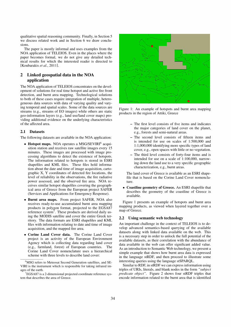
qualitative spatial reasoning community. Finally, in Section 5we discuss related work and in Section 6 we draw conclu-sions.

The paper is mostly informal and uses examples from theNOA application of TELEIOS. Even in the places where thepaper becomes formal, we do not give any detailed tech-nical results for which the interested reader is directed to[Koubarakis et al., 2011].

2 Linked geospatial data in the NOAapplication

The NOA application of TELEIOS concentrates on the devel-opment of solutions for real time hotspot and active fire frontdetection, and burnt area mapping. Technological solutionsto both of these cases require integration of multiple, hetero-geneous data sources with data of varying quality and vary-ing temporal and spatial scales. Some of the data sources arestreams (e.g., streams of EO images) while others are staticgeo-information layers (e.g., land use/land cover maps) pro-viding additional evidence on the underlying characteristicsof the affected area.

2.1 DatasetsThe following datasets are available in the NOA application:

• Hotspot maps. NOA operates a MSG/SEVIRI6 acqui-sition station and receives raw satellite images every 15minutes. These images are processed with image pro-cessing algorithms to detect the existence of hotspots.The information related to hotspots is stored in ESRIshapefiles and KML files. These files hold informa-tion about the date and time of image acquisition, carto-graphic X, Y coordinates of detected fire locations, thelevel of reliability in the observations, the fire radiativepower assessed, and the observed fire area. NOA re-ceives similar hotspot shapefiles covering the geograph-ical area of Greece from the European project SAFER(Services and Applications for Emergency Response).

• Burnt area maps. From project SAFER, NOA alsoreceives ready-to-use accumulated burnt area mappingproducts in polygon format, projected to the EGSA87reference system7. These products are derived daily us-ing the MODIS satellite and cover the entire Greek ter-ritory. The data formats are ESRI shapefiles and KMLfiles with information relating to date and time of imageacquisition, and the mapped fire area.

• Corine Land Cover data. The Corine Land Coverproject is an activity of the European EnvironmentAgency which is collecting data regarding land cover(e.g., farmland, forest) of European countries. TheCorine Land Cover nomenclature uses a hierarchicalscheme with three levels to describe land cover:

6MSG refers to Meteosat Second Generation satellites, and SE-VIRI is the instrument which is responsible for taking infrared im-ages of the earth.

7EGSA87 is a 2-dimensional projected coordinate reference sys-tem that describes the area of Greece.

Figure 1: An example of hotspots and burnt area mappingproducts in the region of Attiki, Greece

– The first level consists of five items and indicatesthe major categories of land cover on the planet,e.g., forests and semi-natural areas.

– The second level consists of fifteen items andis intended for use on scales of 1:500,000 and1:1,000,000 identifying more specific types of landcover, e.g., open spaces with little or no vegetation.

– The third level consists of forty-four items and isintended for use on a scale of 1:100,000, narrow-ing down the land use to a very specific geographiccharacterization, e.g., burnt areas.

The land cover of Greece is available as an ESRI shape-file that is based on the Corine Land Cover nomencla-ture.

• Coastline geometry of Greece. An ESRI shapefile thatdescribes the geometry of the coastline of Greece isavailable.

Figure 1 presents an example of hotspots and burnt areamapping products, as viewed when layered together over amap of Greece.

2.2 Using semantic web technologyAn important challenge in the context of TELEIOS is to de-velop advanced semantics-based querying of the availabledatasets along with linked data available on the web. Thisis a necessary step in order to unlock the full potential of theavailable datasets, as their correlation with the abundance ofdata available in the web can offer significant added value.As an introduction to Semantic Web technology, we present asimple example that shows how burnt area data is expressedin the language stRDF, and then proceed to illustrate someinteresting queries using the language stSPARQL.

Similar to RDF, in stRDF we can express information usingtriples of URIs, literals, and blank nodes in the form “subjectpredicate object”. Figure 2 shows four stRDF triples thatencode information related to the burnt area that is identified

34

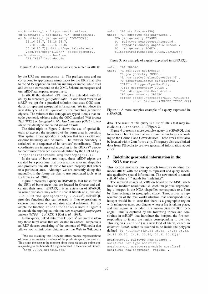
ex:BurntArea_1 rdf:type noa:BurntArea.ex:BurntArea_1 noa:hasID "1"ˆˆxsd:decimal.ex:BurntArea_1 geo:geometry "POLYGON((

38.16 23.7, 38.18 23.7,38.18 23.8, 38.16 23.8,38.16 23.7));<http://spatialreference.org/ref/epsg/4121/>"ˆˆstrdf:geometry.

ex:BurntArea_1 noa:hasArea"23.7636"ˆˆxsd:double.

Figure 2: An example of a burnt area represented in stRDF

by the URI ex:BurntArea_1. The prefixes noa and excorrespond to appropriate namespaces for the URIs that referto the NOA application and our running example, while xsdand strdf correspond to the XML Schema namespace andour stRDF namespace, respectively.

In stRDF the standard RDF model is extended with theability to represent geospatial data. In our latest version ofstRDF we opt for a practical solution that uses OGC stan-dards to represent geospatial information. We introduce thenew data type strdf:geometry for modeling geometricobjects. The values of this datatype are typed literals that en-code geometric objects using the OGC standard Well-knownText (WKT) or Geographic Markup Language (GML). Liter-als of this datatype are called spatial literals.

The third triple in Figure 2 shows the use of spatial lit-erals to express the geometry of the burnt area in question.This spatial literal specifies a polygon that has exactly oneexterior boundary and no holes. The exterior boundary isserialized as a sequence of its vertices’ coordinates. Thesecoordinates are interpreted according to the GGRS87 geode-tic coordinate reference system identified by the URI http://spatialreference.org/ref/epsg/4121/.

In the case of burnt area maps, these stRDF triples arecreated by a procedure that processes the relevant shapefilesand produces one stRDF triple for each property that refersto a particular area. Although we are currently doing thismanually, in the future we plan to use automated tools as in[Blazquez et al., 2010].

Figure 3 presents a query in stSPARQL that looks for allthe URIs of burnt areas that are located in Greece and cal-culates their area. stSPARQL is an extension of SPARQLin which variables may refer to spatial literals (e.g., variable?BAGEO in ?BA geo:geometry ?BAGEO8). stSPARQLprovides functions that can be used in filter expressions toexpress qualitative or quantitative spatial relations. For ex-ample the function strdf:Contains is used in Figure 3to encode the topological relation non-tangential proper partinverse (NTPP−1) of RCC-8 [Cui et al., 1993].

In this query, linked data from DBpedia9 are used to iden-tify those burnt areas that are located in Greece. DBpedia isan RDF dataset consisting of the contents of Wikipedia thatallows you to link other data sets on the Web to Wikipedia

8We are assuming that DBpedia offers precise representationsof country geometries as values of the predicate geo:geometry.This is not the case at the moment since these values are points cor-responding to the bounds of a region located in the center of Greece.

9http://www.dbpedia.org/

select ?BA strdf:Area(?BA)where {?BA rdf:type noa:BurntArea .

?BA geo:geometry ?BAGEO .?C rdf:type noa:GeographicBound .?C dbpedia:Country dbpedia:Greece .?C geo:geometry ?CGEO .filter(strdf:Contains(?CGEO,?BAGEO))}

Figure 3: An example of a query expressed in stSPARQL

select ?BA ?BAGEOwhere {?R rdf:type noa:Region .

?R geo:geometry ?RGEO .?R noa:hasCorineLandCoverUse ?F .?F rdfs:subClassOf clc:Forests .?CITY rdf:type dbpedia:City .?CITY geo:geometry ?CGEO .?BA rdf:type noa:BurntArea .?BA geo:geometry ?BAGEO .filter(strdf:Intersect(?RGEO,?BAGEO)&&

strdf:Distance(?BAGEO,?CGEO)<2)}

Figure 4: A more complex example of a query expressed instSPARQL

data. The result of this query is a list of URIs that may in-clude ex:BurntArea_1 of Figure 2.

Figure 4 presents a more complex query in stSPARQL thatlooks for all burnt areas that were classified as forests accord-ing to the Corine Land Cover dataset. These areas must alsobe located within 2km from a city. This query also uses linkeddata from DBpedia to retrieve geospatial information aboutcities.

3 Indefinite geospatial information in theNOA use case

This section motivates our approach towards extending themodel stRDF with the ability to represent and query indefi-nite qualitative spatial information. The new model is namedstRDFi where “i” stands for “indefinite”.

The infrared imager SEVIRI on board of the MSG satel-lites has medium resolution, i.e., each image pixel represent-ing a hotspot in the NOA shapefiles corresponds to a 3kmby 3km rectangle in geographic space. Thus, a precise rep-resentation of the real world situation that corresponds to ahotspot would be to state that there is a geographic regionwith unknown exact coordinates where a fire is taking place,and that region is included in a known 3km by 3km rect-angle. This is captured by the following triples and con-straints in stRDFi that introduce the hotspot, the fire cor-responding to it and the region corresponding to the fire.This region ( region1) is a new kind of literal, called anunknown literal, which is asserted to be inside the polygondefined by "POLYGON((24.81 35.32, 24.84 35.33,24.84 35.30, 24.81 35.30, 24.81 35.32))".

noa:hotspot1 rdf:type noa:Hotspot .noa:fire1 rdf:type noa:Fire .noa:hotspot1 noa:correspondsTo noa:fire1 .noa:fire1 noa:occuredIn _region1 .

35

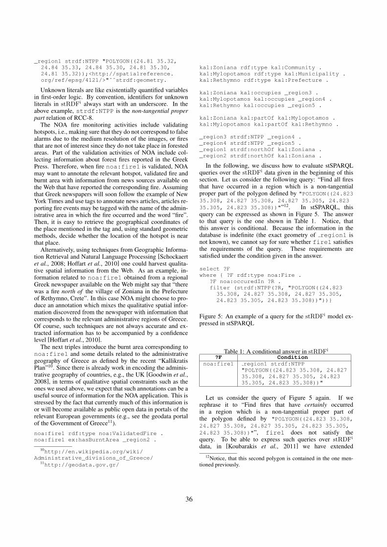
_region1 strdf:NTPP "POLYGON((24.81 35.32,24.84 35.33, 24.84 35.30, 24.81 35.30,24.81 35.32));<http://spatialreference.org/ref/epsg/4121/>"ˆˆstrdf:geometry.

Unknown literals are like existentially quantified variablesin first-order logic. By convention, identifiers for unknownliterals in stRDFi always start with an underscore. In theabove example, strdf:NTPP is the non-tangential properpart relation of RCC-8.

The NOA fire monitoring activities include validatinghotspots, i.e., making sure that they do not correspond to falsealarms due to the medium resolution of the images, or firesthat are not of interest since they do not take place in forestedareas. Part of the validation activities of NOA include col-lecting information about forest fires reported in the GreekPress. Therefore, when fire noa:fire1 is validated, NOAmay want to annotate the relevant hotspot, validated fire andburnt area with information from news sources available onthe Web that have reported the corresponding fire. Assumingthat Greek newspapers will soon follow the example of NewYork Times and use tags to annotate news articles, articles re-porting fire events may be tagged with the name of the admin-istrative area in which the fire occurred and the word “fire”.Then, it is easy to retrieve the geographical coordinates ofthe place mentioned in the tag and, using standard geometricmethods, decide whether the location of the hotspot is nearthat place.

Alternatively, using techniques from Geographic Informa-tion Retrieval and Natural Language Processing [Schockaertet al., 2008; Hoffart et al., 2010] one could harvest qualita-tive spatial information from the Web. As an example, in-formation related to noa:fire1 obtained from a regionalGreek newspaper available on the Web might say that “therewas a fire north of the village of Zoniana in the Prefectureof Rethymno, Crete”. In this case NOA might choose to pro-duce an annotation which mixes the qualitative spatial infor-mation discovered from the newspaper with information thatcorresponds to the relevant administrative regions of Greece.Of course, such techniques are not always accurate and ex-tracted information has to be accompanied by a confidencelevel [Hoffart et al., 2010].

The next triples introduce the burnt area corresponding tonoa:fire1 and some details related to the administrativegeography of Greece as defined by the recent “KallikratisPlan”10. Since there is already work in encoding the adminis-trative geography of countries, e.g., the UK [Goodwin et al.,2008], in terms of qualitative spatial constraints such as theones we used above, we expect that such annotations can be auseful source of information for the NOA application. This isstressed by the fact that currently much of this information isor will become available as public open data in portals of therelevant European governments (e.g., see the geodata portalof the Government of Greece11).

noa:fire1 rdf:type noa:ValidatedFire .noa:fire1 ex:hasBurntArea _region2 .

10http://en.wikipedia.org/wiki/Administrative_divisions_of_Greece/

11http://geodata.gov.gr/

kal:Zoniana rdf:type kal:Community .kal:Mylopotamos rdf:type kal:Municipality .kal:Rethymno rdf:type kal:Prefecture .

kal:Zoniana kal:occupies _region3 .kal:Mylopotamos kal:occupies _region4 .kal:Rethymno kal:occupies _region5 .

kal:Zoniana kal:partOf kal:Mylopotamos .kal:Mylopotamos kal:partOf kal:Rethymno .

_region3 strdf:NTPP _region4 ._region4 strdf:NTPP _region5 ._region1 strdf:northOf kal:Zoniana ._region2 strdf:northOf kal:Zoniana .

In the following, we discuss how to evaluate stSPARQLqueries over the stRDFi data given in the beginning of thissection. Let us consider the following query: “Find all firesthat have occurred in a region which is a non-tangentialproper part of the polygon defined by "POLYGON((24.82335.308, 24.827 35.308, 24.827 35.305, 24.82335.305, 24.823 35.308))"”12. In stSPARQL, thisquery can be expressed as shown in Figure 5. The answerto that query is the one shown in Table 1. Notice, thatthis answer is conditional. Because the information in thedatabase is indefinite (the exact geometry of region1 isnot known), we cannot say for sure whether fire1 satisfiesthe requirements of the query. These requirements aresatisfied under the condition given in the answer.

select ?Fwhere { ?F rdf:type noa:Fire .

?F noa:occuredIn ?R .filter (strdf:NTPP(?R, "POLYGON((24.82335.308, 24.827 35.308, 24.827 35.305,24.823 35.305, 24.823 35.308))"))}

Figure 5: An example of a query for the stRDFi model ex-pressed in stSPARQL

Table 1: A conditional answer in stRDFi

?F Conditionnoa:fire1 region1 strdf:NTPP

"POLYGON((24.823 35.308, 24.82735.308, 24.827 35.305, 24.82335.305, 24.823 35.308))"

Let us consider the query of Figure 5 again. If werephrase it to “Find fires that have certainly occurredin a region which is a non-tangential proper part ofthe polygon defined by "POLYGON((24.823 35.308,24.827 35.308, 24.827 35.305, 24.823 35.305,24.823 35.308))"”, fire1 does not satisfy thequery. To be able to express such queries over stRDFi

data, in [Koubarakis et al., 2011] we have extended12Notice, that this second polygon is contained in the one men-

tioned previously.

36

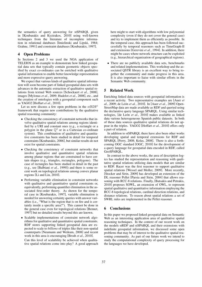
the semantics of query answering for stSPARQL givenin [Koubarakis and Kyzirakos, 2010] using well-knowntechniques from the literature of incomplete informa-tion in relational databases [Imielinski and Lipski, 1984;Grahne, 1991] and constraint databases [Koubarakis, 1997].

4 Open ProblemsIn Sections 2 and 3 we used the NOA application ofTELEIOS as an example to demonstrate how linked geospa-tial data sets that typically contain geometric objects spec-ified by exact co-ordinates can be enriched with qualitativespatial information to enable better knowledge representationand more expressive query answering.

We expect that various kinds of qualitative spatial informa-tion will soon become part of linked geospatial data sets withadvances in the automatic extraction of qualitative spatial re-lations from textual Web sources [Schockaert et al., 2008],images [Mylonas et al., 2009; Hudelot et al., 2008], etc., andthe creation of ontologies with a geospatial component suchas YAGO2 [Hoffart et al., 2010].

Let us now discuss a few open problems in the stRDFi

framework that require new contributions by the qualitativespatial reasoning community:• Checking the consistency of constraint networks that in-

volve qualitative spatial relations among regions identi-fied by a URI and constant ones (e.g., a rectangle or apolygon in the plane Q2 or in a Cartesian co-ordinatesystem). This combination of qualitative and quantita-tive constraints has been studied in detail for temporalconstraints [Koubarakis, 2006], but similar results do notexist for spatial constraints.• Checking the consistency of constraint networks that

involve qualitative and quantitative spatial relationsamong planar regions that are constrained to have cer-tain shapes (e.g., triangles, rectangles, polygons). Thecase of rectangles has been studied in detail in the past(e.g., see [Balbiani et al., 1999]) and there is some re-cent work on topological relations among convex planarregions [Li and Liu, 2010].• Performing variable elimination in constraint networks

with qualitative and quantitative spatial constraints or,equivalently, performing quantifier elimination in the as-sociated first-order theory. As shown for the tempo-ral case in [Koubarakis, 1997], variable elimination isneeded for answering certainty queries with answer vari-ables (i.e., “What is the region that is on fire and is cer-tainly inside a specific area?”). This cannot be done inthe general case even for topological relations [Bennet,1997] but no detailed results beyond this are known.• Scalable implementations of constraint network algo-

rithms for qualitative and quantitative spatial constraints.RDF stores supporting linked geospatial data are ex-pected to scale to billions of triples like their non-spatialcounterparts [Neumann and Weikum, 2008] and recentwork in this area is encouraging [Brodt et al., 2010].Can this level of scalability be achieved when qualita-tive spatial relations come into play? A good approach

here might to start with algorithms with low polynomialcomplexity (even if they do not cover the general case)and try to implement them as efficiently as possible. Inthe temporal case, this approach has been followed suc-cessfully by temporal reasoners such as TimeGraph-IIand extensions [Gerevini et al., 1994]. In addition, theremight be cases where network structure can be exploited(e.g., hierarchical organization of geographical regions).

• There are no publicly available data sets, benchmarksand related implementations. This workshop and the as-sociated QSTR library is an excellent way to bring to-gether the community and make progress in this area.It is also important to liaise with similar efforts in theSemantic Web community.

5 Related WorkEnriching linked data sources with geospatial information isa recent activity. Two representative examples are [Auer etal., 2009; de Leon et al., 2010]. In [Auer et al., 2009] Open-StreetMap data are made available as RDF and queried usingthe declarative query language SPARQL. Using similar tech-nologies, [de Leon et al., 2010] makes available as linkeddata various heterogeneous Spanish public datasets. In bothof these data sources qualitative spatial relations do not ap-pear in the triples. YAGO2 [Hoffart et al., 2010] offers onlya part-of relation.

In addition to stSPARQL there have also been other worksdeveloping spatial and temporal extensions for RDF andSPARQL [Perry, 2008; Kolas, 2008]. There is also a forth-coming OGC standard [OGC, 2010] for the development ofa query language for geospatial data encoded in RDF, calledGeoSPARQL.

In contrast to the above works, the area of description log-ics has studied the representation and reasoning with quali-tative spatial relations utilizing data models that are similarto RDF. Racer was the first reasoner to support qualitativespatial relations [Wessel and Moller, 2009]. More recently,[Stocker and Sirin, 2009] has developed an extension of theDL reasoner Pellet [Parsia and Sirin, 2004] that allows rea-soning with RCC-8 relations. Finally, [Batsakis and Petrakis,2010] proposes SOWL, an extension of OWL, to representspatial qualitative and quantitative information employing theRCC-8 topological relations, cardinal direction relations, anddistance relations. To reason about spatial relations a set ofSWRL rules are implemented in the Pellet reasoner.

6 ConclusionsIn this paper we proposed linked geospatial data on SemanticWeb as an interesting application area of qualitative spatialreasoning techniques. In the context of our recent work onthe models stRDF and stSPARQL and their extensions withindefinite geospatial information, we discussed some openproblems that may be of interest to the qualitative spatial rea-soning community. As part of our future work we intend tostudy the computational complexity of query processing forthe languages we have developed.

37

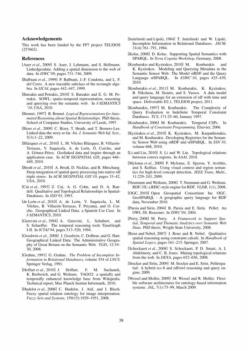
AcknowledgementsThis work has been funded by the FP7 project TELEIOS(257662).

References[Auer et al., 2009] S. Auer, J. Lehmann, and S. Hellmann.

Linkedgeodata: Adding a spatial dimension to the web ofdata. In ISWC’09, pages 731–746, 2009.

[Balbiani et al., 1999] P. Balbiani, J.-F. Condotta, and L. F.del Cerro. A new tractable subclass of the rectangle alge-bra. In IJCAI, pages 442–447, 1999.

[Batsakis and Petrakis, 2010] S. Batsakis and E. G. M. Pe-trakis. SOWL: spatio-temporal representation, reasoningand querying over the semantic web. In I-SEMANTICS’10, USA, 2010.

[Bennet, 1997] B. Bennet. Logical Representations for Auto-mated Reasoning about Spatial Relationships. PhD thesis,School of Computer Studies, University of Leeds, 1997.

[Bizer et al., 2009] C. Bizer, T. Heath, and T. Berners-Lee.Linked data-the story so far. Int. J. Semantic Web Inf. Syst.,5(3):1–22, 2009.

[Blazquez et al., 2010] L. M. Vilches Blazquez, B. Villazon-Terrazas, V. Saquicela, A. de Leon, O. Corcho, andA. Gomez-Perez. Geolinked data and inspire through anapplication case. In ACM SIGSPATIAL GIS, pages 446–449, 2010.

[Brodt et al., 2010] A. Brodt, D. Nicklas, and B. Mitschang.Deep integration of spatial query processing into native rdftriple stores. In ACM SIGSPATIAL GIS’10, pages 33–42,USA, 2010.

[Cui et al., 1993] Z. Cui, A. G. Cohn, and D. A. Ran-dell. Qualitative and Topological Relationships in Spatial-Databases. In SSD’93, 1993.

[de Leon et al., 2010] A. de Leon, V. Saquicela, L. M.Vilches, B. Villazon-Terrazas, F. Priyatna, and O. Cor-cho. Geographical Linked Data: a Spanish Use Case. InI-SEMANTICS, 2010.

[Gerevini et al., 1994] A. Gerevini, L. Schubert, andS. Schaeffer. The temporal reasoning tools TimeGraphI-II. In ICTAI’94, pages 513–520, 1994.

[Goodwin et al., 2008] J. Goodwin, C. Dolbear, and G. Hart.Geographical Linked Data: The Administrative Geogra-phy of Great Britain on the Semantic Web. TGIS, 12:19–30, 2008.

[Grahne, 1991] G. Grahne. The Problem of Incomplete In-formation in Relational Databases, volume 554 of LNCS.Springer Verlag, 1991.

[Hoffart et al., 2010] J. Hoffart, F. M. Suchanek,K. Berberich, and G. Weikum. YAGO2: a spatially andtemporally enhanced knowledge base from Wikipedia.Technical report, Max Planck Institut Informatik, 2010.

[Hudelot et al., 2008] C. Hudelot, J. Atif, and I. Bloch.Fuzzy spatial relation ontology for image interpretation.Fuzzy Sets and Systems, 159(15):1929–1951, 2008.

[Imielinski and Lipski, 1984] T. Imielinski and W. Lipski.Incomplete Information in Relational Databases. JACM,31(4):761–791, 1984.

[Kolas, 2008] D. Kolas. Supporting Spatial Semantics withSPARQL. In Terra Cognita Workshop, Germany, 2008.

[Koubarakis and Kyzirakos, 2010] M. Koubarakis andK. Kyzirakos. Modeling and Querying Metadata in theSemantic Sensor Web: The Model stRDF and the QueryLanguage stSPARQL. In ESWC’10, pages 425–439,2010.

[Koubarakis et al., 2011] M. Koubarakis, K. Kyzirakos,B. Nikolaou, M. Sioutis, and S. Vassos. A data modeland query language for an extension of rdf with time andspace. Deliverable D2.1, TELEIOS project, 2011.

[Koubarakis, 1997] M. Koubarakis. The Complexity ofQuery Evaluation in Indefinite Temporal ConstraintDatabases. TCS, 171:25–60, January 1997.

[Koubarakis, 2006] M. Koubarakis. Temporal CSPs. InHandbook of Constraint Programming. Elsevier, 2006.

[Kyzirakos et al., 2010] K. Kyzirakos, M. Karpathiotakis,and M. Koubarakis. Developing Registries for the Seman-tic Sensor Web using stRDF and stSPARQL. In SSN’10,volume 668, 2010.

[Li and Liu, 2010] S. Li and W. Liu. Topological relationsbetween convex regions. In AAAI, 2010.

[Mylonas et al., 2009] P. Mylonas, E. Spyrou, Y. Avrithis,and S. Kollias. Using visual context and region seman-tics for high-level concept detection. IEEE Trans. Multi.,11:229–243, 2009.

[Neumann and Weikum, 2008] T. Neumann and G. Weikum.RDF-3X: a RISC-style engine for RDF. VLDB, 1(1), 2008.

[OGC, 2010] Open Geospatial Consortium Inc OGC.GeoSPARQL - A geographic query language for RDFdata, November 2010.

[Parsia and Sirin, 2004] B. Parsia and E. Sirin. Pellet: AnOWL DL Reasoner. In ISWC’04, 2004.

[Perry, 2008] M. Perry. A Framework to Support Spa-tial, Temporal and Thematic Analytics over Semantic WebData. PhD thesis, Wright State University, 2008.

[Renz and Nebel, 2007] J. Renz and B. Nebel. Qualitativespatial reasoning using constraint calculi. In Handbook ofSpatial Logics, pages 161–215. Springer, 2007.

[Schockaert et al., 2008] S. Schockaert, P. D. Smart, A. I.Abdelmoty, and C. B. Jones. Mining topological relationsfrom the web. In DEXA, pages 652–656, 2008.

[Stocker and Sirin, 2009] M. Stocker and E. Sirin. Pelletspa-tial: A hybrid rcc-8 and rdf/owl reasoning and query en-gine, 2009.

[Wessel and Moller, 2009] M. Wessel and R. Moller. Flexi-ble software architectures for ontology-based informationsystems. JAL, 7(1):75–99, March 2009.

38

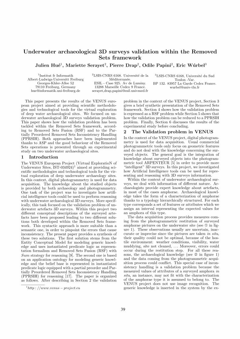
Underwater archaeological 3D surveys validation within the RemovedSets framework

Julien Hue1, Mariette Serayet2, Pierre Drap2, Odile Papini2, Eric Wurbel3

1Institut fr InformatikAlbert-Ludwigs-Universitt Freiburg

Georges-Khler-Allee 5279110 Freiburg, Germany

[email protected]

2LSIS-CNRS 6168. Universite de laMediterranee.

ESIL - Case 925. Av de Luminy.13288 Marseille Cedex 9 France.

serayet,drap,[email protected]

3LSIS-CNRS 6168, Universite du SudToulon -Var.

BP 132. 83957 La Garde Cedex [email protected]

This paper presents the results of the VENUS euro-pean project aimed at providing scientific methodolo-gies and technological tools for the virtual explorationof deep water archaeological sites. We focused on un-derwater archaeological 3D surveys validation problem.This paper shows how the validation problem has beentackled within the Removed Sets framework, accord-ing to Removed Sets Fusion (RSF) and to the Par-tially Preordered Removed Sets Inconsistency Handling(PPRSIH). Both approaches have been implementedthanks to ASP and the good behaviour of the RemovedSets operations is presented through an experimentalstudy on two underwater archaeological sites.

1 Introduction

The VENUS European Project (Virtual ExploratioN ofUnderwater Sites, IST-034924)1 aimed at providing sci-entific methodologies and technological tools for the vir-tual exploration of deep underwater archaeology sites.In this context, digital photogrammetry is used for dataacquisition. The knowledge about the studied objectsis provided by both archaeology and photogrammetry.One task of the project was to investigate how artifi-cial intelligence tools could be used to perform reasoningwith underwater archaeological 3D surveys. More specif-ically, this task focused on the validation problem of un-derwater artefacts 3D surveys. Within this project twodifferent conceptual descriptions of the surveyed arte-facts have been proposed leading to two different solu-tions both developed within the Removed Sets frame-work. This syntactic approach is more suitable than asemantic one, in order to pinpoint the errors that causeinconsistency. The present paper provides a synthesis ofthese two solutions. The first solution stems from theEntity Conceptual Model for modeling generic knowl-edge and uses instantiated predicate logic as represen-tation formalism and Removed Sets Fusion (RSF) withSum strategy for reasoning [9]. The second one is basedon an application ontology for modeling generic knowl-edge and the belief base is represented in instantiatedpredicate logic equipped with a partial preorder and Par-tially Preordered Removed Sets Inconsistency Handling(PPRSIH) for reasoning [17]. The paper is organizedas follows. After describing in Section 2 the validation

1http : //www.venus− project.eu

problem in the context of the VENUS project, Section 3gives a brief synthetic presentation of the Removed Setsframework. Section 4 shows how the validation problemis expressed as a RSF problem while Section 5 shows thathow the validation problem can be reduced to a PPRSIHproblem. Finally, Section 6 discusses the results of theexperimental study before concluding.

2 The Validation problem in VENUSIn the context of the VENUS project, digital photogram-metry is used for data acquisition. Usual commercialphotogrammetric tools only focus on geometric featuresand do not deal with the knowledge concerning the sur-veyed objects. The general goal is the integration ofknowledge about surveyed objects into the photogram-metric tool ARPENTEUR [5] in order to provide more“intelligent” 3D surveys. In this project, we investigatedhow Artificial Intelligence tools can be used for repre-senting and reasoning with 3D surveys information.

Within the context of underwater archaeological sur-veys, we deal with information of different nature. Ar-chaeologists provide expert knowledge about artefacts,in most of the cases amphorae. Archaeological knowl-edge takes the form of a characterization of amphoraethanks to a typology hierarchically structured. For eachtype corresponds a set of features or attributes which weassign an interval representing the expected values foran amphora of this type.

The data acquisition process provides measures com-ing from the photogrammetric restitution of surveyedamphorae pictures on the underwater site (see À in fig-ure 1). These observations usually are uncertain, inac-curate or imprecise since the pictures are taken in situ,their quality could not be optimal, because of the hos-tile environment: weather conditions, visibility, watermuddying, site not cleaned, . . . Moreover, errors couldoccur during the restitution step. For all these rea-sons, the archaeological knowledge (see Á in figure 1)and the data coming from the photogrammetric acqui-sition process could conflict. This special case of incon-sistency handling is a validation problem because themeasured values of attributes of a surveyed amphora insitu, an instance, may not fit with the characterizationof the amphorae type it is assumed to belong to. TheVENUS project does not use image recognition. Thegeneric knowledge is inserted in the system by the ex-

39

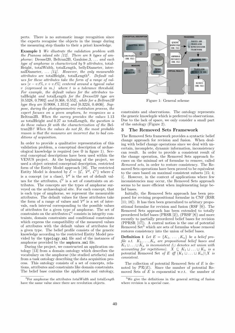
perts. There is no automatic image recognition sincethe experts recognise the objects in the image duringthe measuring step thanks to their a priori knowledge.

Example 1 We illustrate the validation problem withthe Pianosa island site [12]. There are 8 types of am-phorae: Dressel20, Beltran2B, Gauloise 3, . . . and eachtype of amphorae is characterized by 9 attributes, total-Height, totalWidth, totalLength, bellyDiameter, inter-nalDiameter, . . . [14]. However, the only measurableattributes are totalHeight, totalLength2. Default val-ues for these attributes take the form of a range of val-ues [v − v.t%, v + v.t%] centered around a typical valuev (expressed in m.) where t is a tolerance threshold.For example, the default values for the attributes to-talHeight and totalLength for the Dressel20 type are[0.5328, 0.7992] and [0.368, 0.552], while for a Beltran2Btype they are [0.9008, 1.3512] and [0.3224, 0.4836]. Sup-pose, during the photogrammetric restitution process, theexpert focuses on a given amphora, he recognizes as aBeltran2B. When the survey provides the values 1.13as totalHeight and 0.27 as totalLength, the question isdo these values fit with the characterization of the Bel-tran2B? When the values do not fit, the most probablereason is that the measures are incorrect due to bad con-ditions of acquisition.

In order to provide a qualitative representation of thisvalidation problem, a conceptual description of archae-ological knowledge is required (see Á in figure 1). Sev-eral conceptual descriptions have been used within theVENUS project. At the beginning of the project, weused a object oriented conceptual description, restrictedform of the Entity Model approach [16]. The restrictedEntity Model is denoted by E = {C, Vd, CI} where Cis a concept (or a class), Vd is the set of default val-ues for the attributes, CI is a set of constraints on at-tributes. The concepts are the types of amphorae sur-veyed on the archaeological site. For each concept, thatis each type of amphorae, we represent the measurableattributes. The default values for these attributes takethe form of a range of values and Vd is a set of inter-vals, each interval corresponding to the possible valuesof attributes for a given type of amphorae. The set ofconstraints on the attributes CI consists in integrity con-traints, domain constraints and conditional constraintswhich express the compatibility of the measured valuesof attributes with the default values of attributes fora given type. The belief profile consists of the genericknowledge according to the restricted Entity Model pro-vided by the typology.xml file and of the instances ofamphorae provided by the amphora.xml file.

During the project, we constructed an application on-tology [13] from a domain ontology which describes thevocabulary on the amphorae (the studied artefacts) andfrom a task ontology describing the data acquisition pro-cess. This ontology consists of a set of concepts, rela-tions, attributes and constraints like domain constraints.The belief base contains the application and ontology,

2For amphorae the attributes totalWidth and totalLengthhave the same value since there are revolution objects.

CONCEPTUAL DESCRIPTION

MEASURE

DATA

VIRTUAL REALITY

REASONING

CONCEPTUAL MODEL

IMPORTEXPORT

AMPHORAE(INSTANCES)(XML FILE)

MEASURE(ARPENTEUR)

GENERICKNOWLEDGE(XML FILE)

PARSER ANDTRANSLATOR

TO REPRESENTATIONFRAMEWORK

REASONING TOOL

TRANSLATOR(RESULTS TO XML)

RESULTS(XML FILE)

CONSTRAINTS(XML FILE)

①

②

Figure 1: General scheme

constraints and observations. The ontology representsthe generic knowlegde which is preferred to observations.Due to the lack of space, we only consider a small partof the ontology (Figure 2).

3 The Removed Sets Framework

The Removed Sets framework provides a syntactic beliefchange approach for revision and fusion. When deal-ing with belief change operations since we deal with un-certain, incomplete, dynamic information, inconsistencycan result. In order to provide a consistent result ofthe change operation, the Removed Sets approach fo-cuses on the minimal set of formulae to remove, calledRemoved sets, in order to restore consistency. The Re-moved Sets operations have been proved to be equivalentto the ones based on maximal consistent subsets [15; 4;1]. However, in the context of applications where fewinconsistencies may occur, the Removed Sets approachseems to be more efficient when implementing large be-lief bases.

Initially, the Removed Sets approach has been pro-posed for revising propositional formulae in CNF (RSR[11; 18]). It has then been generalized to arbitary propo-sitional formulae for revision and fusion (RSF [9]). TheRemoved Sets approach has been extended to totallypreordered belief bases (PRSR [2]), (PRSF [8]) and morerecently to partially preordered belief bases for revision(PPRSR [17]). A central notion is the one of potentialRemoved Set3 which are sets of formulas whose removalrestores consistency into the union of belief bases.

Definition 1 Let E = {K1, . . . ,Kn} be a belief pro-file s.t. K1, . . . ,Kn are propositional belief bases andK1 t . . . tKn is inconsistent (t denotes set union withaccounting for repetitions). X ⊆ K1 t . . . t Kn is apotential Removed Set of E iff (K1 t . . . t Kn)\X isconsistent.

The collection of potential Removed Sets of E is de-noted by PR(E). Since the number of potential Re-moved Sets of E is exponential w.r.t. the number of

3We give the definitions in the general setting of fusionwhere revision is a special case.

40

formulae, we only consider the minimal potential Re-moved Sets w.r.t. set inclusion. Moreover belief changeoperations or strategies are formalized in terms of totalor partial preorders on potential Removed Sets minimalw.r.t. set inclusion. This strategies can be sorted in twofamilies: majority operators (e.g. Card, Sum) whichfollows the point of view of the majority of the beliefbases in E and egalitarist operators (e.g. Max,GMax)which tries to satisfy best all the belief bases in E.

3.1 Removed Sets FusionFor Removed Sets Fusion, the fusion strategies (Card,Sum, Max, GMax)[9] are formalized thanks to a totalpreorder over PR(E). Let X and Y be two potentialRemoved Sets, for each strategy P a total preorder ≤P

over the potential Removed Sets is defined. X ≤P Ymeans that X is preferred to Y according to the strategyP . We define <P as the strict total preorder associatedto ≤P (i.e. X <P Y if and only if X ≤P Y and Y 6≤P

X).

Definition 2 Let E = {K1, . . . ,Kn} be a belief profilesuch that K1t. . .tKn is inconsistent. X ⊆ K1t. . .tKn

is a Removed Set of E according to the strategy P ifand only if i) X is a potential Removed Set of E; ii)@X ′ ∈ PR(E) such that X ′ ⊂ X; iii) @X ′ ∈ PR(E)such that X ′ <P X.

The collection of Removed Sets of E according to thestrategy P is denoted by RP (E). The Removed SetsFusion operation is defined by:

Definition 3 Let E = {K1, . . . ,Kn} such that K1 t. . .tKn is inconsistent. The merging operation is definedby: ∆RSF

P (E) =⋃

X∈RP (E){(K1 t . . . tKn)\X}.

3.2 Partially Preordered Removed SetsInconsistency Handling

Let K be a finite set of arbitrary formulae and �K bea partial preorder on K .=K denotes the equivalence re-lation �K corresponding to �K i.e. a =K b iff (a �K

b) ∧ (b �K a). Restoring the consistency of a partiallypreordered belief bases involves the definition of a partialpreorder on subsets of formulae, called comparators [3;19]. Several ways have been proposed for defining a pref-erence relation on subsets of formulae of K, from a par-tial preorder �K . In the VENUS project, we focus onthe lexicographic preference [19] which extends the lexi-cographic preorder initially defined for totally preorderedbelief bases to partially preordered belief bases. The be-lief base K is partitionned into K = E1t. . .tEn (n ≥ 1)where each subset Ei represents an equivalence class ofK w.r.t. =K . A preference relation between the equiva-lence classes Ei’s, denoted by ≺s is defined by Ei ≺s Ej

iff ∃ϕ ∈ Ei, ∃ϕ′ ∈ Ej such that ϕ ≺K ϕ′. This partitioncan be viewed as a generalization of the idea of strati-fication defined for totally preordered belief bases. Werephrase the lexicographic preference defined in [19] asfollows:

Definition 4 Let K = E1 t . . . t En be a finite setof arbitrary formulae partitioned into equivalence classaccording to =K . Let �K be a partial preorder on

K = E1 t . . . tEn, Y ⊆ K and X ⊆ K. Y is said to belexicographically preferred to X, denoted by Y EM X, iff∀i, 1 ≤ i ≤ n: if |Ei ∩ Y | > |Ei ∩X| then ∃j, 1 ≤ j ≤ nsuch that |Ej ∩X| > |Ej ∩ Y | and Ej ≺s Ei.

Let PR(K) be the set of potential removed sets. Amongthem, we want to prefer the potential removed sets whichallow us to remove the formulae that are not preferredaccording to �K . Therefore we generalize the notion ofRemoved Sets to subsets of partially preordered formu-lae. We denote by RM(K) the set of removed sets ofK.

Definition 5 Let K be an inconsistent belief baseequipped with a partial preorder �K . R ⊆ K is a re-moved set of K iff i) R is a potential removed set; ii)@R′ ∈ RM(K) such that R′ ⊂ R; iii) @R′ ∈ RM(K) suchthat R′ CM R.

Definition 6 Let K be an inconsistent belief baseequipped with a partial perorder �K . The consistencyrestoration operation is defined by

∆∆(K) =⋃

X∈RM(K)

{K\X}.

3.3 ASP implementation

In order to implement belief change operations withinthe Removed sets framework, we translate the beliefchange problem into a logic program with answer setsemantics. This method proceeds in two stages. Thefirst stage consists in the translation of E into a logicprogram ΠE and we have shown that the answer sets ofΠE correspond to the potential removed sets of E [9].

Let E be a belief profile4. Each propositional variablea occuring in E is represented by an ASP atom a ∈ Ain ΠE . The set of all positive, (resp. negative) literals ofΠE is denoted by V +, (resp. V −). The set of rule atomsrepresenting formulae is defined by R+ = {rf | f ∈ E}and FO(rf ) represents the formula of E correspondingto rf in ΠE , namely ∀rf ∈ R+, FO(rf ) = f . This trans-lation requires the introduction of intermediary atomsrepresenting subformulae. We denote by ρjf the inter-

mediary atom representing f j which is a subformula off ∈ E. The first part of the construction has two steps:

1. We introduce rules in order to build a one-to-onecorrespondence between answer sets of ΠE and in-terpretations of V +. For each atom, a ∈ V + tworules are introduced: a ← not a′ and a′ ← not awhere a′ ∈ V − is the negative atom correspondingto a.

2. We introduce rules in order to exclude the answersets S corresponding to interpretations which arenot models of (E\F ) with F = {f | rf ∈ S}. Ac-cording to the syntax of f , the following rules areintroduced: (i) If f =def a then rf ← not a is in-troduced; (ii) If f =def ¬f1 then rf ← not ρf1

is introduced; (iii) If f =def f1 ∨ . . . ∨ fm then

4In case of inconsistency handling the profile E is reducedto a belief base K.

41

rf ← ρf1 , . . . , ρfm is introduced; (iv) If f =def

f1∧. . .∧fm then it is necessary to introduce severalrules: ∀1 ≤ j ≤ m, rf ← ρfj .

This stage is common to any belief change operationwhile the next one depends on the chosen belief changeoperation.

In case of fusion the second stage provides, accordingto selected strategy P , another set of rules that leads tothe program ΠP

E and we have shown [9] that the answersets of ΠP

E correspond to the removed sets of E for astrategy P . In the validation problem since we have tominimize the number of formulae to remove, thereforethe number of formulae occuring in a removed set, weselect the Sum strategy. This strategy is expressed bythe minimize{} statement and the new logic progamΠSum

E = ΠE ∪minimize{rf | rf ∈ R+} is such that theanswer sets of ΠSum

E which are provided by the CLASPsolver [7] correspond to the removed sets of ∆RSF

Sum(E)[9].

In case of partially Preordered Removed Sets Incon-sistency Handling the CLASP solver [7] gives the answersets of ΠE . We then construct a partial preorder betweenthem using the lexicographic comparator EM. We haveshown in [17] that the preferred answer sets accordingto EM correspond to the removed sets of E. We used ajava program to partially preorder the answer sets to ob-tain the preferred answer sets. Since the lexicographiccomparator satisfies the monotony property [19], it issufficient to compare the answer sets which are minimalaccording to the inclusion. Moreover, the determinationof the minimal answer sets according to this partial pre-order does not increase the computationnal cost, sincethis cost is insignificant compared to the cost of answersets computation by CLASP.

4 The validation problem wihin RSFIn order to represent the validation problem within theRSF framework and to implement it with ASP, we rep-resented this problem with instantiated predicate logic.The belief profile consists of two belief bases. The firstone stems from the restricted Entity Model conceptualdescription and represents the generic knowledge. We in-troduce the predicates type(x, y) and cmp(z, y, x) wherex is an amphora, y is a type of amphorae and z is anattribute. type(x, y) expresses that an amphora x be-longs to a type y and cmp(z, y, x) expresses that an at-tribute z of an amphora x of type y has a value com-patible with the possible values for the type y, as spec-ified in 2. The domain constraints specify that an am-phora must have one and only one type. For n typesof amphorae, for each amphora there is one disjunctiontype(x, y1)∨ . . .∨ type(x, yn) and n(n− 1)/2 mutual ex-clusion formulae ¬type(x, yi) ∨ ¬type(x, yj). The con-ditional constraints specify the compatibility of the at-tributes values with respect to the type. For each am-phora x, for each attribute z and for each type y, thereis a formula type(x, y) → cmp(z, y, x). Let m be thenumber of attributes, the incompatibility of type speci-fies that for each amphora and each type there is a for-mula ¬cmp(z1, y, x)∧. . .∧¬cmp(zm, y, x)→ ¬type(x, y).

The second belief base represents the instances of am-phorae: the type the observed amphora belongs to(namely type(x, y)) and the compatible attributes withthe type (namely cmp(z, y, x)). We illustrate the RSFapproach with the example 1.

Example 2 We limit ourselves to only two types ofamphorae Beltran2B and Dressel20, respectively de-noted by B2B and D20 thereafter, and to the sur-vey of one observed amphora (denoted by 4 hereafter).Two attributes are used: totalHeight (denoted by tH)and totalLength (denoted by tL). The first belief baseis automatically generated from the typology.xml fileand K1 = {¬type(4, B2B) ∨ ¬type(4, D20), type(4, B2B) ∨type(4, D20), type(4, D20) → cmp(tH,D20, 4), type(4, D20)→ cmp(tL,D20, 4), type(4, B2B) → cmp(tH, B2B, 4),type(4, B2B) → cmp(tL, B2B, 4), ¬cmp(tH,B2B, 4) ∧¬cmp(tL, B2B, 4) → ¬type(4, B2B), ¬cmp(tH,D20, 4) ∧¬cmp(tL,D20, 4) → ¬type(4, D20) }. The second beliefbase corresponding to the observed amphora is automat-ically generated from typology.xml and amphora.xml filesand K2 = {type(4, B2B), cmp(tH,B2B, 4)}. The opera-tion ∆RSF

Sum,>(E) where E = {K1,K2} is translated into

ΠSumE as follows:

cmp(tH,B2B, 4).1 {type(4, d20), type(4, B2B)} 1.← n type(4, d20), type(4, d20).← n type(4, B2B), type(4, B2B).r(x0)← not type(4, B2B).r(x1)← type(4, d20), not cmp(tH, d20, 4).r(x2)← type(4, d20), not cmp(tL, d20, 4).r(x3)← type(4, B2B), not cmp(tH,B2B, 4).r(x4)← type(4, B2B), not cmp(tL,B2B, 4).r(x5)← type(4, d20), not cmp(tH, d20, 4), not cmp(tL, d20, 4).r(x6)← type(4, B2B), not cmp(tH,B2B, 4), not cmp(tL,B2B, 4).n type(4, B2B)← r(x0).n cmp(tH, d20, 4)← r(x1).n cmp(tL, d2, 4)← r(x2).n cmp(tH,B2B, 4)← r(x3).n cmp(tL,B2B, 4)← r(x4).minimize {r(x0), r(x1), r(x2), r(x3), r(x4)r(x5), r(x6)} .

Note that the ASP translation uses some shortcutscompared to the translation scheme depicted in section3.3. Thanks to the cardinality literals by recent ASPsolvers, the unique type constraint is reduced to a sin-gle rule 1 {type(4, d20), type(4, B2B)} 1. Also, the gen-eration of the rule corresponding to type(4, B2B) andthe mutual exclusion between this atom and its classicalnegation are compacted into a single rule.

The only answer set of the above pro-gram is {cmp(tH,B2B, 4), type(4, B2B), r(x4),n cmp(tL,B2B, 4)} which corresponds to the removedset {type(4, B2B) → cmp(tL,B2B, 4)} that pinpointsa bad measure for the total length attribute under thehypothesis of an amphora of type Beltran2B.

5 The validation problem withinPPRSIH

The conceptual description in this approach is repre-sented in terms of an application ontology and an extractis illustrated in Figure 2.

42

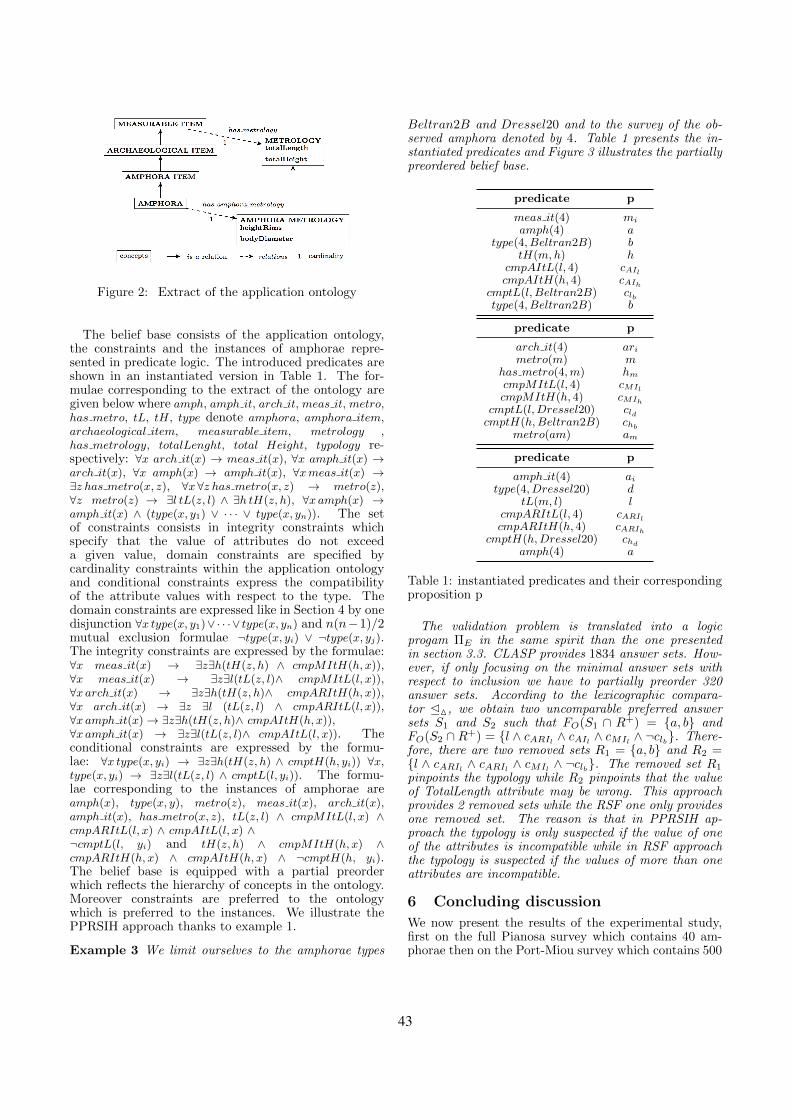
Figure 2: Extract of the application ontology

The belief base consists of the application ontology,the constraints and the instances of amphorae repre-sented in predicate logic. The introduced predicates areshown in an instantiated version in Table 1. The for-mulae corresponding to the extract of the ontology aregiven below where amph, amph it, arch it, meas it, metro,has metro, tL, tH, type denote amphora, amphora item,archaeological item, measurable item, metrology ,has metrology, totalLenght, total Height, typology re-spectively: ∀x arch it(x) → meas it(x), ∀x amph it(x) →arch it(x), ∀x amph(x) → amph it(x), ∀xmeas it(x) →∃z has metro(x, z), ∀x∀z has metro(x, z) → metro(z),∀z metro(z) → ∃l tL(z, l) ∧ ∃h tH(z, h), ∀x amph(x) →amph it(x) ∧ (type(x, y1) ∨ · · · ∨ type(x, yn)). The setof constraints consists in integrity constraints whichspecify that the value of attributes do not exceeda given value, domain constraints are specified bycardinality constraints within the application ontologyand conditional constraints express the compatibilityof the attribute values with respect to the type. Thedomain constraints are expressed like in Section 4 by onedisjunction ∀x type(x, y1)∨· · ·∨ type(x, yn) and n(n−1)/2mutual exclusion formulae ¬type(x, yi) ∨ ¬type(x, yj).The integrity constraints are expressed by the formulae:∀x meas it(x) → ∃z∃h(tH(z, h) ∧ cmpMItH(h, x)),∀x meas it(x) → ∃z∃l(tL(z, l)∧ cmpMItL(l, x)),∀x arch it(x) → ∃z∃h(tH(z, h)∧ cmpARItH(h, x)),∀x arch it(x) → ∃z ∃l (tL(z, l) ∧ cmpARItL(l, x)),∀x amph it(x)→ ∃z∃h(tH(z, h)∧ cmpAItH(h, x)),∀x amph it(x) → ∃z∃l(tL(z, l)∧ cmpAItL(l, x)). Theconditional constraints are expressed by the formu-lae: ∀x type(x, yi) → ∃z∃h(tH(z, h) ∧ cmptH(h, yi)) ∀x,type(x, yi) → ∃z∃l(tL(z, l) ∧ cmptL(l, yi)). The formu-lae corresponding to the instances of amphorae areamph(x), type(x, y), metro(z), meas it(x), arch it(x),amph it(x), has metro(x, z), tL(z, l) ∧ cmpMItL(l, x) ∧cmpARItL(l, x) ∧ cmpAItL(l, x) ∧¬cmptL(l, yi) and tH(z, h) ∧ cmpMItH(h, x) ∧cmpARItH(h, x) ∧ cmpAItH(h, x) ∧ ¬cmptH(h, yi).The belief base is equipped with a partial preorderwhich reflects the hierarchy of concepts in the ontology.Moreover constraints are preferred to the ontologywhich is preferred to the instances. We illustrate thePPRSIH approach thanks to example 1.

Example 3 We limit ourselves to the amphorae types

Beltran2B and Dressel20 and to the survey of the ob-served amphora denoted by 4. Table 1 presents the in-stantiated predicates and Figure 3 illustrates the partiallypreordered belief base.

predicate p

meas it(4) mi

amph(4) atype(4, Beltran2B) b

tH(m,h) hcmpAItL(l, 4) cAIlcmpAItH(h, 4) cAIh

cmptL(l, Beltran2B) clbtype(4, Beltran2B) b

predicate p

arch it(4) arimetro(m) m

has metro(4,m) hm

cmpMItL(l, 4) cMIlcmpMItH(h, 4) cMIh

cmptL(l,Dressel20) cldcmptH(h,Beltran2B) chb

metro(am) am

predicate p

amph it(4) ai

type(4, Dressel20) dtL(m, l) l

cmpARItL(l, 4) cARIlcmpARItH(h, 4) cARIh

cmptH(h,Dressel20) chd

amph(4) a

Table 1: instantiated predicates and their correspondingproposition p

The validation problem is translated into a logicprogam ΠE in the same spirit than the one presentedin section 3.3. CLASP provides 1834 answer sets. How-ever, if only focusing on the minimal answer sets withrespect to inclusion we have to partially preorder 320answer sets. According to the lexicographic compara-tor EM, we obtain two uncomparable preferred answersets S1 and S2 such that FO(S1 ∩ R+) = {a, b} andFO(S2 ∩ R+) = {l ∧ cARIl ∧ cAIl ∧ cMIl ∧ ¬clb}. There-fore, there are two removed sets R1 = {a, b} and R2 ={l ∧ cARIl ∧ cARIl ∧ cMIl ∧ ¬clb}. The removed set R1

pinpoints the typology while R2 pinpoints that the valueof TotalLength attribute may be wrong. This approachprovides 2 removed sets while the RSF one only providesone removed set. The reason is that in PPRSIH ap-proach the typology is only suspected if the value of oneof the attributes is incompatible while in RSF approachthe typology is suspected if the values of more than oneattributes are incompatible.

6 Concluding discussion

We now present the results of the experimental study,first on the full Pianosa survey which contains 40 am-phorae then on the Port-Miou survey which contains 500

43

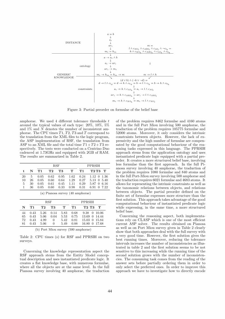
a = b↓ai

INSTANCE ↓ari m =↓ l ∧ cMIl

∧ cARIl∧ cAIl

∧ ¬clb =mi = hm h ∧ cMIh

∧ cARIh∧ cAIh

∧ chb↓

a→ ai ∧ b↓

ai → ari ↓ontology ↓

ari → mi

↓GENERIC mi → hm = hm → m m→ l ∧ h

KNOWLEDGE ↘ ↙(d ∨ b) ∧ (¬b ∨ ¬d) =

d→ l ∧ cld = d→ h ∧ chd= b→ l ∧ clb = b→ h ∧ chb↓

constraints ai → h ∧ cAIh= ai → l ∧ cAIl↓

ari → h ∧ cARIh= ari → l ∧ cARIl↓

mi → h ∧ cMIh= mi → l ∧ cMIl

Figure 3: Partial preorder on formulae of the belief base

amphorae. We used 4 different tolerance thresholds taround the typical values of each type: 20%, 10%, 5%and 1% and N denotes the number of inconsistent am-phorae. The CPU times T1, T2, T3 and T correspond tothe translation from the XML files to the logic program,the ASP implementation of RSF, the translation fromASP to an XML file and the total time T1 +T2 +T3 re-spectively. The tests were conducted on a Centrino Duocadenced at 1.73GHz and equipped with 2GB of RAM.The results are summarized in Table 2.

RSF PPRSIH

t N T1 T2 T3 T T1 T2T3 T

20 5 0.05 0.62 0.95 1.62 0.24 1.12 0 1.3610 26 0.05 0.60 0.64 1.29 0.27 5.13 0 5.405 30 0.05 0.61 0.45 1.11 0.29 5.87 0 6.161 36 0.05 0.60 0.33 0.98 0.31 6.91 0 7.22

(a) Pianosa survey (40 amphorae)

RSF PPRSIH

N T1 T2 T3 T T1 T2 T3 T

44 0.43 5.26 0.14 5.83 0.68 9.38 0 10.0665 0.43 5.06 0.04 5.53 0.75 13.69 0 14.4472 0.43 4.99 0 5.42 0.81 15.03 0 15.8481 0.43 5.06 0 5.49 0.88 16.80 0 17.68

(b) Port Miou survey (500 amphorae)

Table 2: CPU times (s) for RSF and PPRSIH on twosurveys.

Concerning the knowledge representation aspect theRSF approach stems from the Entity Model concep-tual description and uses instantiated predicate logic. Itcreates a flat knowledge base, with numerous formulae,where all the objects are at the same level. In the fullPianosa survey involving 40 amphorae, the traduction

of the problem requires 8462 formulae and 4160 atomsand in the full Port Miou involving 500 amphorae, thetraduction of the problem requires 105775 formulae and52000 atoms. Moreover, it only considers the intrinsicconstraints between objects. However, the lack of ex-pressivity and the high number of formulae are compen-sated by the good computational behaviour of the rea-soning tasks expressed in this language. The PPRSIHapproach stems from the application ontology and usesinstantiated predicate logic equipped with a partial pre-order. It creates a more structured belief base, involvingless formulae than the first approach. In the full Pi-anosa survey involving 40 amphorae, the traduction ofthe problem requires 1080 formulae and 840 atoms andin the full Port-Miou survey involving 500 amphorae andthe traduction requires 6021 formulae and 4683 atoms. Itallows for representing the intrinsic constraints as well asthe taxonomic relations between objects, and relationsbetween objects. The partial preorder defined on thefinite set of formulae expresses more structure than thefirst solution. This approach takes advantage of the goodcomputational behaviour of instantiated predicate logicwhile expressing, in the same time, a more structuredbelief base.

Concerning the reasoning aspect, both implementa-tions rely on CLASP which is one of the most efficientcurrent ASP solver. The results obtained on Pianosaas well as on Port Miou survey given in Table 2 clearlyshow that both approaches deal with the full survey witha very good time. However, the first solution gives thebest running times. Moreover, reducing the toleranceintervals increases the number of inconsistencies as illus-trated in table 2 and the first solution seems to be notsensitive to this increasing while the running time of thesecond solution grows with the number of inconsisten-cies. The consuming task comes from the reading of theanswer sets before partially ordering them in order toonly select the preferred ones. In order to improve thisapproach we have to investigate how to directly encode

44

the partial preorder on answer sets within the logic pro-gram. Another direction to follow in order to reach atrade-off between representation and reasoning could beto represent the validation problem in Description Logic,since the generic knowledge in expressed in terms of on-tology. However, we have to study which low complexityDescription Logic could be suitable. Moreover, we haveto study to which extent the approach combining De-scription logic and ASP [6] could be used for implemen-tation as well as the extended ASP solver to first orderlogic[10].

7 AcknowledgementsWork partially supported by the European Community un-der project VENUS (Contract IST-034924) of the ”Informa-tion Society Technologies (IST) program of the 6th FP forRTD”. The authors are solely responsible for the content ofthis paper. It does not represent the opinion of the EuropeanCommunity, and the European Community is not responsiblefor any use that might be made of data appearing therein.

References[1] C. Baral, S. Kraus, J. Minker, and V. S. Subrahmanian.

Combining knowledge bases consisting of first order the-ories. In Proc. of ISMIS, pages 92–101, 1991.

[2] S. Benferhat, Jonathan Ben-Naim, Odile Papini, andEric Wurbel. An answer set programming encoding ofprioritized removed sets revision: application to gis. Ap-plied Intelligence, 32(1):60–87, 2010.

[3] S. Benferhat, S. Lagrue, and O. Papini. Revision of par-tially ordered information : Axiomatization, semanticsand iteration. In Proc. of IJCAI’05, pages 376–381, Ed-inburgh, 2005.

[4] G. Brewka. Preferred sutheories: an extended logicalframework for default reasoning. In Proc. of IJCAI’89,pages 1043–1048, 1989.

[5] P. Drap and P. Grussenmeyer. A digital photogrammet-ric workstation on the web. Journal of Photogrammetryand Remote Sensing, 55(1):48–58, 2000.

[6] T. Eiter, G. Ianni, T. Lukasiewicz, R. Schindlauer, andH. Tompits. Combining answer set programming withdescription logics for the semantic web. Artificial Intel-ligence, 172(12-13):1495–1539, 2008.

[7] M. Gebser, B. Kaufmann, A. Neumann, and T. Schaub.clasp: A conflict-driven answer set solver. In Proc. ofLPNMR’07, pages 260–265. Springer, 2007.

[8] J. Hue, O. Papini, and E. Wurbel. Implementing prior-itized merging with asp. In Proc. of IPMU, volume 80of CCIS, pages 138–147. Springer, 2010.

[9] J. Hue, E. Wurbel, and O. Papini. Removed sets fusion:Performing off the shelf. In Proc. of ECAI’08, pages94–98, 2008.

[10] C. Lefevre and P. Nicolas. A first order forward chainingapproach for answer set computing. logic programmingand nonmonotonic reasoning. In Proc. of LPNMR’09,pages 196–208. Springer, 2009.

[11] O. Papini. A complete revision function in proposition-nal calculus. In B. Neumann, editor, Proc. of ECAI’92,pages 339–343. John Wiley and Sons. Ltd, 1992.

[12] O. Papini. D3.1 archaeological activities and knowledgeanalysis. Technical report, Delivrable, VENUS project.http://www.venus-project.eu, january 2007.

[13] O. Papini, O. Cure, P. Drap, B. Fertil, J. Hue,D. Roussel, M. Serayet, J. Seinturier, and E. Wurbel.http://www.venus project.eu. D3.6 reasoning with ar-chaeological ontologies. technical report and prototypeof software for the reversible fusion operations. Techni-cal report, Delivrable, VENUS project, july 2009.

[14] O. Papini, E. Wurbel, R. Jeansoulin, O. Cure, P. Drap,M. Serayet, J. Hue, J. Seinturier, and L. Long. D3.4representation of archaeological ontologies 1. Technicalreport, Delivrable, VENUS project. http://www.venus-project.eu, July 2008.

[15] N. Rescher and R. Manor. On inference from inconsis-tent premises. Theory and Decision, 1:179–219, 1970.

[16] J. Seinturier. Fusion de connaissances: Applications auxreleves photogrammetriques de fouilles archeologiquessous-marines. PhD thesis, Universite du Sud ToulonVar, 2007.

[17] M. Serayet, P. Drap, and O. Papini. Extending removedsets revision to partially preordered belief bases. Inter-national Journal of Approximate Reasoning, 52(1):110–126, 2011.

[18] E. Wurbel, O. Papini, and R. Jeansoulin. Revision: anapplication in the framework of gis. In Proc. of KR’00,pages 505–516, Breckenridge, Colorado, USA, 2000.

[19] S. Yahi, S. Benferhat, S. Lagrue, M. Serayet, and O. Pa-pini. A lexicographic inference for partially preorderedbelief bases. In Proc. of KR’08, pages 507–516, 2008.

45

46

An application-oriented view on graded spatial relations

Steven Schockaert∗Department of Applied Mathematics and Computer Science,

Ghent University, Gent, [email protected]

AbstractApproaches for modeling graded spatial relationsabound in the literature on image processing and ongeographic information systems. In contrast, fewproposals have addressed the use of degrees in ap-plication contexts where inference plays a centralrole. We argue that the use of degrees is nonethelessnatural in such contexts, and may enhance the ap-plication potential of qualitative spatial reasoningin domains where relations between vague regionsneed to be expressed, as well as domains where therobustness of spatial relations w.r.t. small changesin the underlying configurations is important. Inparticular, we discuss the interpretation of degrees,contrasting fuzzy regions with formal accounts ofspatial vagueness based on supervaluation seman-tics. We also touch upon the problem of acquiring(fuzzy) spatial relations from the web in an auto-mated way.

1 IntroductionThe field of qualitative spatial representation and reasoning(QSR) deals with symbolic representations of spatial con-figurations [4], modeling for instance how two regions aretopologically related [17] (e.g. whether some geographic re-gion overlaps with another) or what the relative position isof a point w.r.t. a vector [29] (e.g. the relative position of alandmark w.r.t. a moving subject). Typically, approaches toQSR are based on a small number of jointly exhaustive andpairwise disjoint (JEPD) relations. In the well-known RegionConnection Calculus (RCC [17]), for instance, the topologi-cal relationship of two regions is always one of the so-calledRCC8 relations: DC (disconnected), EC (externally con-nected), PO (partially overlapping), EQ (equal), TPP (tangen-tial proper part), NTPP (non-tangential proper part), TPP−1(inverse of TPP), or NTPP−1 (inverse of NTPP).

Despite the elegance and conceptual simplicity of suchframeworks, the way they discretize a continuum of possi-ble spatial configurations sometimes leads to unintuitive be-havior. When spatial relations are derived from images, forinstance, one pixel can make the difference between EC and

∗Postdoctoral fellow of the Research Foundation – Flanders.

DC, and, even worse, whether an EC or DC relation is foundmay depend on the resolution of the image. Along similarlines, when most of some region a is contained in a region b,it may be more natural to think of a as being a part of b than tothink of a and b as partially overlapping regions. In geogra-phy, the situation is further complicated by the fact that manytoponyms cannot be characterized by precise boundaries (e.g.downtown Barcelona). It may be difficult to assess the spatialrelationship between two vague regions (e.g. Northern Spainand Central Catalonia), as different views on the delineationof these regions may correspond to different spatial relations.

Many approaches address this kind of problems by assum-ing spatial relations to be graded (or fuzzy). Then it becomespossible to say that Northern Spain and Central Catalonia areoverlapping to some degree, while Central Catalonia is alsoconsidered to be a part of Northern Spain to some degree.How these graded relations are defined depends on the appli-cation. In this respect, it is useful to note that applications ofQSR can roughly be divided in two classes. In a first class ofapplications, qualitative spatial relations are used to interfacebetween a known quantitative description of a scene and natu-ral language (e.g. to describe a route or to query a geographicinformation system), or more generally, to abstract away fromirrelevant details in quantitative representations (e.g. to rec-ognize types of events [9]). Fuzzy spatial relations have beenwidely studied in this kind of applications, both from the an-gle of image processing and understanding (e.g. [12; 11; 25;14]), and from the angle of geographic information systems(e.g. [18; 15; 21]). The main purpose of using degrees, here,is to induce a total ordering, e.g. to decide which among agiven number of situations best satisfies some query. For thisfirst class of applications, one of the main considerations isthat relations be cognitively meaningful, more than obeyingnice mathematical properties or being easy to compute.

The second class of applications uses qualitative descrip-tions of spatial scenes as a surrogate for quantitative descrip-tions, when the latter are not available or require a prohibitiveamount of computation. In such applications, symbolic rea-soning plays a key role to verify the integrity of qualita-tive descriptions (e.g. in geo-ontologies [26]) and to augmentavailable knowledge by explicitly deriving its logical conse-quences. In order to support inference, it is important thatspatial relations are defined in such a way that they satisfyimportant mathematical properties, related to transitivity, re-

47

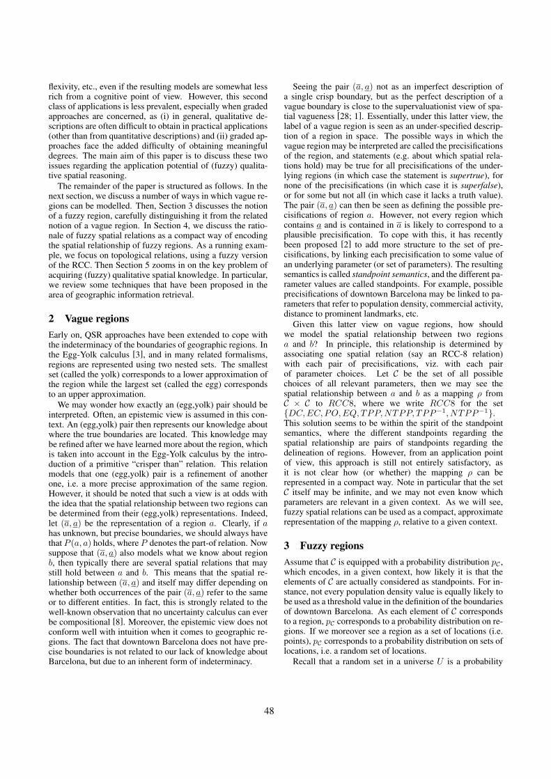
flexivity, etc., even if the resulting models are somewhat lessrich from a cognitive point of view. However, this secondclass of applications is less prevalent, especially when gradedapproaches are concerned, as (i) in general, qualitative de-scriptions are often difficult to obtain in practical applications(other than from quantitative descriptions) and (ii) graded ap-proaches face the added difficulty of obtaining meaningfuldegrees. The main aim of this paper is to discuss these twoissues regarding the application potential of (fuzzy) qualita-tive spatial reasoning.

The remainder of the paper is structured as follows. In thenext section, we discuss a number of ways in which vague re-gions can be modelled. Then, Section 3 discusses the notionof a fuzzy region, carefully distinguishing it from the relatednotion of a vague region. In Section 4, we discuss the ratio-nale of fuzzy spatial relations as a compact way of encodingthe spatial relationship of fuzzy regions. As a running exam-ple, we focus on topological relations, using a fuzzy versionof the RCC. Then Section 5 zooms in on the key problem ofacquiring (fuzzy) qualitative spatial knowledge. In particular,we review some techniques that have been proposed in thearea of geographic information retrieval.

2 Vague regionsEarly on, QSR approaches have been extended to cope withthe indeterminacy of the boundaries of geographic regions. Inthe Egg-Yolk calculus [3], and in many related formalisms,regions are represented using two nested sets. The smallestset (called the yolk) corresponds to a lower approximation ofthe region while the largest set (called the egg) correspondsto an upper approximation.

We may wonder how exactly an (egg,yolk) pair should beinterpreted. Often, an epistemic view is assumed in this con-text. An (egg,yolk) pair then represents our knowledge aboutwhere the true boundaries are located. This knowledge maybe refined after we have learned more about the region, whichis taken into account in the Egg-Yolk calculus by the intro-duction of a primitive “crisper than” relation. This relationmodels that one (egg,yolk) pair is a refinement of anotherone, i.e. a more precise approximation of the same region.However, it should be noted that such a view is at odds withthe idea that the spatial relationship between two regions canbe determined from their (egg,yolk) representations. Indeed,let (a, a) be the representation of a region a. Clearly, if ahas unknown, but precise boundaries, we should always havethat P (a, a) holds, where P denotes the part-of relation. Nowsuppose that (a, a) also models what we know about regionb, then typically there are several spatial relations that maystill hold between a and b. This means that the spatial re-lationship between (a, a) and itself may differ depending onwhether both occurrences of the pair (a, a) refer to the sameor to different entities. In fact, this is strongly related to thewell-known observation that no uncertainty calculus can everbe compositional [8]. Moreover, the epistemic view does notconform well with intuition when it comes to geographic re-gions. The fact that downtown Barcelona does not have pre-cise boundaries is not related to our lack of knowledge aboutBarcelona, but due to an inherent form of indeterminacy.

Seeing the pair (a, a) not as an imperfect description ofa single crisp boundary, but as the perfect description of avague boundary is close to the supervaluationist view of spa-tial vagueness [28; 1]. Essentially, under this latter view, thelabel of a vague region is seen as an under-specified descrip-tion of a region in space. The possible ways in which thevague region may be interpreted are called the precisificationsof the region, and statements (e.g. about which spatial rela-tions hold) may be true for all precisifications of the under-lying regions (in which case the statement is supertrue), fornone of the precisifications (in which case it is superfalse),or for some but not all (in which case it lacks a truth value).The pair (a, a) can then be seen as defining the possible pre-cisifications of region a. However, not every region whichcontains a and is contained in a is likely to correspond to aplausible precisification. To cope with this, it has recentlybeen proposed [2] to add more structure to the set of pre-cisifications, by linking each precisification to some value ofan underlying parameter (or set of parameters). The resultingsemantics is called standpoint semantics, and the different pa-rameter values are called standpoints. For example, possibleprecisifications of downtown Barcelona may be linked to pa-rameters that refer to population density, commercial activity,distance to prominent landmarks, etc.

Given this latter view on vague regions, how shouldwe model the spatial relationship between two regionsa and b? In principle, this relationship is determined byassociating one spatial relation (say an RCC-8 relation)with each pair of precisifications, viz. with each pairof parameter choices. Let C be the set of all possiblechoices of all relevant parameters, then we may see thespatial relationship between a and b as a mapping ρ fromC × C to RCC8, where we write RCC8 for the set{DC,EC,PO,EQ, TPP,NTPP, TPP−1, NTPP−1}.This solution seems to be within the spirit of the standpointsemantics, where the different standpoints regarding thespatial relationship are pairs of standpoints regarding thedelineation of regions. However, from an application pointof view, this approach is still not entirely satisfactory, asit is not clear how (or whether) the mapping ρ can berepresented in a compact way. Note in particular that the setC itself may be infinite, and we may not even know whichparameters are relevant in a given context. As we will see,fuzzy spatial relations can be used as a compact, approximaterepresentation of the mapping ρ, relative to a given context.

3 Fuzzy regionsAssume that C is equipped with a probability distribution pC ,which encodes, in a given context, how likely it is that theelements of C are actually considered as standpoints. For in-stance, not every population density value is equally likely tobe used as a threshold value in the definition of the boundariesof downtown Barcelona. As each element of C correspondsto a region, pC corresponds to a probability distribution on re-gions. If we moreover see a region as a set of locations (i.e.points), pC corresponds to a probability distribution on sets oflocations, i.e. a random set of locations.

Recall that a random set in a universe U is a probability

48

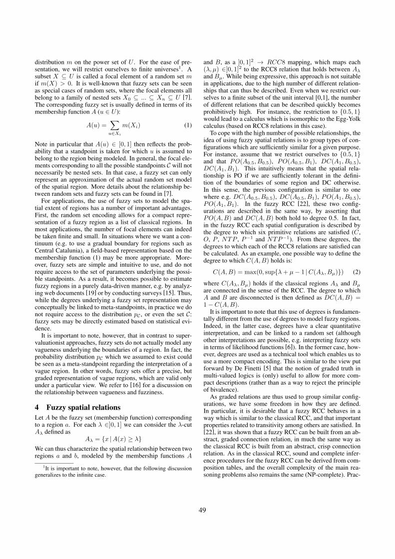
distribution m on the power set of U . For the ease of pre-sentation, we will restrict ourselves to finite universes1. Asubset X ⊆ U is called a focal element of a random set mif m(X) > 0. It is well-known that fuzzy sets can be seenas special cases of random sets, where the focal elements allbelong to a family of nested sets X0 ⊆ ... ⊆ Xn ⊆ U [7].The corresponding fuzzy set is usually defined in terms of itsmembership function A (u ∈ U ):

A(u) =∑

u∈Xi

m(Xi) (1)

Note in particular that A(u) ∈ [0, 1] then reflects the prob-ability that a standpoint is taken for which u is assumed tobelong to the region being modeled. In general, the focal ele-ments corresponding to all the possible standpoints C will notnecessarily be nested sets. In that case, a fuzzy set can onlyrepresent an approximation of the actual random set modelof the spatial region. More details about the relationship be-tween random sets and fuzzy sets can be found in [7].

For applications, the use of fuzzy sets to model the spa-tial extent of regions has a number of important advantages.First, the random set encoding allows for a compact repre-sentation of a fuzzy region as a list of classical regions. Inmost applications, the number of focal elements can indeedbe taken finite and small. In situations where we want a con-tinuum (e.g. to use a gradual boundary for regions such asCentral Catalunia), a field-based representation based on themembership function (1) may be more appropriate. More-over, fuzzy sets are simple and intuitive to use, and do notrequire access to the set of parameters underlying the possi-ble standpoints. As a result, it becomes possible to estimatefuzzy regions in a purely data-driven manner, e.g. by analyz-ing web documents [19] or by conducting surveys [15]. Thus,while the degrees underlying a fuzzy set representation mayconceptually be linked to meta-standpoints, in practice we donot require access to the distribution pC , or even the set C:fuzzy sets may be directly estimated based on statistical evi-dence.

It is important to note, however, that in contrast to super-valuationist approaches, fuzzy sets do not actually model anyvagueness underlying the boundaries of a region. In fact, theprobability distribution pC which we assumed to exist couldbe seen as a meta-standpoint regarding the interpretation of avague region. In other words, fuzzy sets offer a precise, butgraded representation of vague regions, which are valid onlyunder a particular view. We refer to [16] for a discussion onthe relationship between vagueness and fuzziness.

4 Fuzzy spatial relationsLet A be the fuzzy set (membership function) correspondingto a region a. For each λ ∈]0, 1] we can consider the λ-cutAλ defined as

Aλ = {x |A(x) ≥ λ}We can thus characterize the spatial relationship between tworegions a and b, modeled by the membership functions A

1It is important to note, however, that the following discussiongeneralizes to the infinite case.

and B, as a ]0, 1]2 → RCC8 mapping, which maps each(λ, µ) ∈]0, 1]2 to the RCC8 relation that holds between Aλand Bµ. While being expressive, this approach is not suitablein applications, due to the high number of different relation-ships that can thus be described. Even when we restrict our-selves to a finite subset of the unit interval [0,1], the numberof different relations that can be described quickly becomesprohibitively high. For instance, the restriction to {0.5, 1}would lead to a calculus which is isomorphic to the Egg-Yolkcalculus (based on RCC8 relations in this case).

To cope with the high number of possible relationships, theidea of using fuzzy spatial relations is to group types of con-figurations which are sufficiently similar for a given purpose.For instance, assume that we restrict ourselves to {0.5, 1}and that PO(A0.5, B0.5), PO(A0.5, B1), DC(A1, B0.5),DC(A1, B1). This intuitively means that the spatial rela-tionship is PO if we are sufficiently tolerant in the defini-tion of the boundaries of some region and DC otherwise.In this sense, the previous configuration is similar to onewhere e.g. DC(A0.5, B0.5), DC(A0.5, B1), PO(A1, B0.5),PO(A1, B1). In the fuzzy RCC [22], these two config-urations are described in the same way, by asserting thatPO(A,B) and DC(A,B) both hold to degree 0.5. In fact,in the fuzzy RCC each spatial configuration is described bythe degree to which six primitive relations are satisfied (C,O, P , NTP , P−1 and NTP−1). From these degrees, thedegrees to which each of the RCC8 relations are satisfied canbe calculated. As an example, one possible way to define thedegree to which C(A,B) holds is:

C(A,B) = max(0, sup{λ+ µ− 1 |C(Aλ, Bµ)}) (2)

where C(Aλ, Bµ) holds if the classical regions Aλ and Bµare connected in the sense of the RCC. The degree to whichA and B are disconnected is then defined as DC(A,B) =1− C(A,B).

It is important to note that this use of degrees is fundamen-tally different from the use of degrees to model fuzzy regions.Indeed, in the latter case, degrees have a clear quantitativeinterpretation, and can be linked to a random set (althoughother interpretations are possible, e.g. interpreting fuzzy setsin terms of likelihood functions [6]). In the former case, how-ever, degrees are used as a technical tool which enables us touse a more compact encoding. This is similar to the view putforward by De Finetti [5] that the notion of graded truth inmulti-valued logics is (only) useful to allow for more com-pact descriptions (rather than as a way to reject the principleof bivalence).

As graded relations are thus used to group similar config-urations, we have some freedom in how they are defined.In particular, it is desirable that a fuzzy RCC behaves in away which is similar to the classical RCC, and that importantproperties related to transitivity among others are satisfied. In[22], it was shown that a fuzzy RCC can be built from an ab-stract, graded connection relation, in much the same way asthe classical RCC is built from an abstract, crisp connectionrelation. As in the classical RCC, sound and complete infer-ence procedures for the fuzzy RCC can be derived from com-position tables, and the overall complexity of the main rea-soning problems also remains the same (NP-complete). Prac-

49

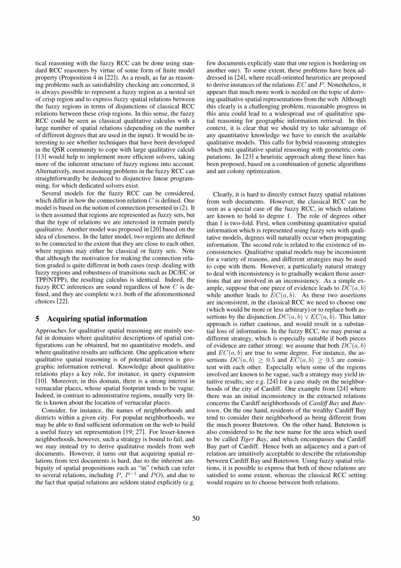
tical reasoning with the fuzzy RCC can be done using stan-dard RCC reasoners by virtue of some form of finite modelproperty (Proposition 4 in [22]). As a result, as far as reason-ing problems such as satisfiability checking are concerned, itis always possible to represent a fuzzy region as a nested setof crisp region and to express fuzzy spatial relations betweenthe fuzzy regions in terms of disjunctions of classical RCCrelations between these crisp regions. In this sense, the fuzzyRCC could be seen as classical qualitative calculus with alarge number of spatial relations (depending on the numberof different degrees that are used in the input). It would be in-teresting to see whether techniques that have been developedin the QSR community to cope with large qualitative calculi[13] would help to implement more efficient solvers, takingmore of the inherent structure of fuzzy regions into account.Alternatively, most reasoning problems in the fuzzy RCC canstraightforwardly be deduced to disjunctive linear program-ming, for which dedicated solvers exist.

Several models for the fuzzy RCC can be considered,which differ in how the connection relation C is defined. Onemodel is based on the notion of connection presented in (2). Itis then assumed that regions are represented as fuzzy sets, butthat the type of relations we are interested in remain purelyqualitative. Another model was proposed in [20] based on theidea of closeness. In the latter model, two regions are definedto be connected to the extent that they are close to each other,where regions may either be classical or fuzzy sets. Notethat although the motivation for making the connection rela-tion graded is quite different in both cases (resp. dealing withfuzzy regions and robustness of transitions such as DC/EC orTPP/NTPP), the resulting calculus is identical. Indeed, thefuzzy RCC inferences are sound regardless of how C is de-fined, and they are complete w.r.t. both of the aforementionedchoices [22].

5 Acquiring spatial informationApproaches for qualitative spatial reasoning are mainly use-ful in domains where qualitative descriptions of spatial con-figurations can be obtained, but no quantitative models, andwhere qualitative results are sufficient. One application wherequalitative spatial reasoning is of potential interest is geo-graphic information retrieval. Knowledge about qualitativerelations plays a key role, for instance, in query expansion[10]. Moreover, in this domain, there is a strong interest invernacular places, whose spatial footprint tends to be vague.Indeed, in contrast to administrative regions, usually very lit-tle is known about the location of vernacular places.

Consider, for instance, the names of neighborhoods anddistricts within a given city. For popular neighborhoods, wemay be able to find sufficient information on the web to builda useful fuzzy set representation [19; 27]. For lesser-knownneighborhoods, however, such a strategy is bound to fail, andwe may instead try to derive qualitative models from webdocuments. However, it turns out that acquiring spatial re-lations from text documents is hard, due to the inherent am-biguity of spatial propositions such as “in” (which can referto several relations, including P , P−1 and PO), and due tothe fact that spatial relations are seldom stated explicitly (e.g.

few documents explicitly state that one region is bordering onanother one). To some extent, these problems have been ad-dressed in [24], where recall-oriented heuristics are proposedto derive instances of the relationsEC and P . Nonetheless, itappears that much more work is needed on the topic of deriv-ing qualitative spatial representations from the web. Althoughthis clearly is a challenging problem, reasonable progress inthis area could lead to a widespread use of qualitative spa-tial reasoning for geographic information retrieval. In thiscontext, it is clear that we should try to take advantage ofany quantitative knowledge we have to enrich the availablequalitative models. This calls for hybrid reasoning strategieswhich mix qualitative spatial reasoning with geometric com-putations. In [23] a heuristic approach along these lines hasbeen proposed, based on a combination of genetic algorithmsand ant colony optimization.

Clearly, it is hard to directly extract fuzzy spatial relationsfrom web documents. However, the classical RCC can beseen as a special case of the fuzzy RCC, in which relationsare known to hold to degree 1. The role of degrees otherthan 1 is two-fold. First, when combining quantitative spatialinformation which is represented using fuzzy sets with quali-tative models, degrees will naturally occur when propagatinginformation. The second role is related to the existence of in-consistencies. Qualitative spatial models may be inconsistentfor a variety of reasons, and different strategies may be usedto cope with them. However, a particularly natural strategyto deal with inconsistency is to gradually weaken those asser-tions that are involved in an inconsistency. As a simple ex-ample, suppose that one piece of evidence leads to DC(a, b)while another leads to EC(a, b). As these two assertionsare inconsistent, in the classical RCC we need to choose one(which would be more or less arbitrary) or to replace both as-sertions by the disjunction DC(a, b) ∨ EC(a, b). This latterapproach is rather cautious, and would result in a substan-tial loss of information. In the fuzzy RCC, we may pursue adifferent strategy, which is especially suitable if both piecesof evidence are rather strong: we assume that both DC(a, b)and EC(a, b) are true to some degree. For instance, the as-sertions DC(a, b) ≥ 0.5 and EC(a, b) ≥ 0.5 are consis-tent with each other. Especially when some of the regionsinvolved are known to be vague, such a strategy may yield in-tuitive results; see e.g. [24] for a case study on the neighbor-hoods of the city of Cardiff. One example from [24] wherethere was an initial inconsistency in the extracted relationsconcerns the Cardiff neighborhoods of Cardiff Bay and Bute-town. On the one hand, residents of the wealthy Cardiff Baytend to consider their neighborhood as being different fromthe much poorer Butetown. On the other hand, Butetown isalso considered to be the new name for the area which usedto be called Tiger Bay, and which encompasses the CardiffBay part of Cardiff. Hence both an adjacency and a part-ofrelation are intuitively acceptable to describe the relationshipbetween Cardiff Bay and Butetown. Using fuzzy spatial rela-tions, it is possible to express that both of these relations aresatisfied to some extent, whereas the classical RCC settingwould require us to choose between both relations.

50

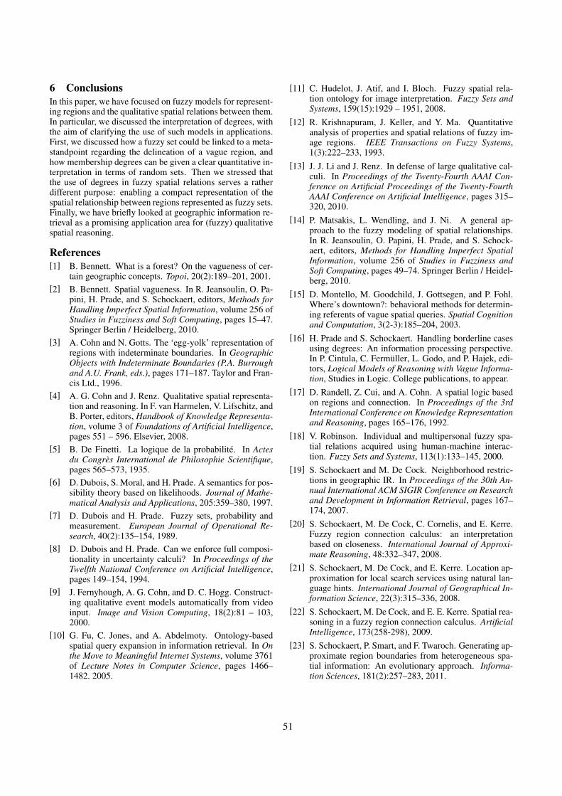
6 ConclusionsIn this paper, we have focused on fuzzy models for represent-ing regions and the qualitative spatial relations between them.In particular, we discussed the interpretation of degrees, withthe aim of clarifying the use of such models in applications.First, we discussed how a fuzzy set could be linked to a meta-standpoint regarding the delineation of a vague region, andhow membership degrees can be given a clear quantitative in-terpretation in terms of random sets. Then we stressed thatthe use of degrees in fuzzy spatial relations serves a ratherdifferent purpose: enabling a compact representation of thespatial relationship between regions represented as fuzzy sets.Finally, we have briefly looked at geographic information re-trieval as a promising application area for (fuzzy) qualitativespatial reasoning.

References[1] B. Bennett. What is a forest? On the vagueness of cer-

tain geographic concepts. Topoi, 20(2):189–201, 2001.[2] B. Bennett. Spatial vagueness. In R. Jeansoulin, O. Pa-

pini, H. Prade, and S. Schockaert, editors, Methods forHandling Imperfect Spatial Information, volume 256 ofStudies in Fuzziness and Soft Computing, pages 15–47.Springer Berlin / Heidelberg, 2010.

[3] A. Cohn and N. Gotts. The ‘egg-yolk’ representation ofregions with indeterminate boundaries. In GeographicObjects with Indeterminate Boundaries (P.A. Burroughand A.U. Frank, eds.), pages 171–187. Taylor and Fran-cis Ltd., 1996.

[4] A. G. Cohn and J. Renz. Qualitative spatial representa-tion and reasoning. In F. van Harmelen, V. Lifschitz, andB. Porter, editors, Handbook of Knowledge Representa-tion, volume 3 of Foundations of Artificial Intelligence,pages 551 – 596. Elsevier, 2008.

[5] B. De Finetti. La logique de la probabilite. In Actesdu Congres International de Philosophie Scientifique,pages 565–573, 1935.

[6] D. Dubois, S. Moral, and H. Prade. A semantics for pos-sibility theory based on likelihoods. Journal of Mathe-matical Analysis and Applications, 205:359–380, 1997.

[7] D. Dubois and H. Prade. Fuzzy sets, probability andmeasurement. European Journal of Operational Re-search, 40(2):135–154, 1989.

[8] D. Dubois and H. Prade. Can we enforce full composi-tionality in uncertainty calculi? In Proceedings of theTwelfth National Conference on Artificial Intelligence,pages 149–154, 1994.

[9] J. Fernyhough, A. G. Cohn, and D. C. Hogg. Construct-ing qualitative event models automatically from videoinput. Image and Vision Computing, 18(2):81 – 103,2000.

[10] G. Fu, C. Jones, and A. Abdelmoty. Ontology-basedspatial query expansion in information retrieval. In Onthe Move to Meaningful Internet Systems, volume 3761of Lecture Notes in Computer Science, pages 1466–1482. 2005.

[11] C. Hudelot, J. Atif, and I. Bloch. Fuzzy spatial rela-tion ontology for image interpretation. Fuzzy Sets andSystems, 159(15):1929 – 1951, 2008.

[12] R. Krishnapuram, J. Keller, and Y. Ma. Quantitativeanalysis of properties and spatial relations of fuzzy im-age regions. IEEE Transactions on Fuzzy Systems,1(3):222–233, 1993.

[13] J. J. Li and J. Renz. In defense of large qualitative cal-culi. In Proceedings of the Twenty-Fourth AAAI Con-ference on Artificial Proceedings of the Twenty-FourthAAAI Conference on Artificial Intelligence, pages 315–320, 2010.

[14] P. Matsakis, L. Wendling, and J. Ni. A general ap-proach to the fuzzy modeling of spatial relationships.In R. Jeansoulin, O. Papini, H. Prade, and S. Schock-aert, editors, Methods for Handling Imperfect SpatialInformation, volume 256 of Studies in Fuzziness andSoft Computing, pages 49–74. Springer Berlin / Heidel-berg, 2010.

[15] D. Montello, M. Goodchild, J. Gottsegen, and P. Fohl.Where’s downtown?: behavioral methods for determin-ing referents of vague spatial queries. Spatial Cognitionand Computation, 3(2-3):185–204, 2003.

[16] H. Prade and S. Schockaert. Handling borderline casesusing degrees: An information processing perspective.In P. Cintula, C. Fermuller, L. Godo, and P. Hajek, edi-tors, Logical Models of Reasoning with Vague Informa-tion, Studies in Logic. College publications, to appear.

[17] D. Randell, Z. Cui, and A. Cohn. A spatial logic basedon regions and connection. In Proceedings of the 3rdInternational Conference on Knowledge Representationand Reasoning, pages 165–176, 1992.

[18] V. Robinson. Individual and multipersonal fuzzy spa-tial relations acquired using human-machine interac-tion. Fuzzy Sets and Systems, 113(1):133–145, 2000.

[19] S. Schockaert and M. De Cock. Neighborhood restric-tions in geographic IR. In Proceedings of the 30th An-nual International ACM SIGIR Conference on Researchand Development in Information Retrieval, pages 167–174, 2007.

[20] S. Schockaert, M. De Cock, C. Cornelis, and E. Kerre.Fuzzy region connection calculus: an interpretationbased on closeness. International Journal of Approxi-mate Reasoning, 48:332–347, 2008.

[21] S. Schockaert, M. De Cock, and E. Kerre. Location ap-proximation for local search services using natural lan-guage hints. International Journal of Geographical In-formation Science, 22(3):315–336, 2008.

[22] S. Schockaert, M. De Cock, and E. E. Kerre. Spatial rea-soning in a fuzzy region connection calculus. ArtificialIntelligence, 173(258-298), 2009.

[23] S. Schockaert, P. Smart, and F. Twaroch. Generating ap-proximate region boundaries from heterogeneous spa-tial information: An evolutionary approach. Informa-tion Sciences, 181(2):257–283, 2011.

51

[24] S. Schockaert, P. D. Smart, A. I. Abdelmoty, and C. B.Jones. Mining topological relations from the web.In Proceedings of the 19th International Workshop onDatabase and Expert Systems Applications, pages 652–656, 2008.

[25] M. Skubic, P. Matsakis, G. Chronis, and J. Keller. Gen-erating multi-level linguistic spatial descriptions fromrange sensor readings using the histogram of forces. Au-tonomous Robots, 14(1):51–69, 2003.

[26] P. D. Smart, A. I. Abdelmoty, B. A. El-Geresy, andC. B. Jones. A framework for combining rules and geo-ontologies. In Proceedings of the First InternationalConference on Web Reasoning and Rule Systems, pages133–147, 2007.

[27] F. Twaroch, C. Jones, and A. Abdelmoty. Acquisitionof a vernacular gazetteer from web sources. In Proceed-ings of the first international workshop on Location andthe web, pages 61–64, 2008.

[28] A. Varzi. Vagueness in geography. Philosophy & Geog-raphy, 4(1):49–65, 2001.

[29] K. Zimmermann and C. Freksa. Qualitative spatial rea-soning using orientation, distance, and path knowledge.Applied Intelligence, 6(1):49–58, 1996.

52

On A Semi-Automatic Method for Generating Composition Tables ∗

Weiming Liu and Sanjiang LiCentre for Quantum Computation and Intelligent Systems, Faculty of Engineering and Information Technology,

University of Technology Sydney, Australia

Email: [email protected]

AbstractOriginating from Allen’s Interval Algebra,composition-based reasoning has been widelyacknowledged as the most popular reasoning tech-nique in qualitative spatial and temporal reasoning.Given a qualitative calculus (i.e. a relation model),the first thing we should do is to establish itscomposition table (CT). In the past three decades,such work is usually done manually. This isundesirable and error-prone, given that the calculusmay contain tens or hundreds of basic relations.Computing the correct CT has been identified byTony Cohn as a challenge for computer scientists in1995. This paper addresses this problem and intro-duces a semi-automatic method to compute the CTby randomly generating triples of elements. Forseveral important qualitative calculi, our methodcan establish the correct CT in a reasonable shorttime. This is illustrated by applications to theInterval Algebra, the Region Connection CalculusRCC-8, the INDU calculus, and the Oriented PointRelation Algebras. Our method can also be usedto generate CTs for customised qualitative calculidefined on restricted domains.

1 IntroductionSince Allen’s seminal work of Interval Algebra (IA) [1;2], qualitative calculi have been widely used to represent andreason about temporal and spatial knowledge. In the pastdecades, dozens of qualitative calculi have been proposed inthe artificial intelligence area “Qualitative Spatial & Tempo-ral Reasoning” and Geographic Information Science. ExceptIA, other well known binary qualitative calculi include thePoint Algebra [20], the Region Connection Calculi RCC-5and RCC-8 [17], the INDU calculus [16], the Oriented PointRelation Algebras OPRA [14], and the Cardinal DirectionCalculus (CDC) [10; 19; 13], etc.

Relations in each particular qualitative calculus are used torepresent temporal or spatial information at a certain gran-ularity. For example, The Netherlands is west of Germany,

∗A complete version of this paper is available via: http://arxiv.org/abs/1105.4224.This work was partly supportedby an ARC Future Fellowship (FT0990811).

The Alps partially overlaps Italy, I have today an appoint-ment with my doctor followed by a check-up.

Given a set of qualitative knowledge, new knowledge canbe derived by using constraint propagation. Consider an ex-ample in RCC-5. Given that The Alps partially overlapsItaly and Switzerland, and Italy is a proper part of the Eu-ropean Union (EU), and Switzerland is discrete from the EU,we may infer that The Alps partially overlaps the EU. Theabove inference can be obtained by using composition-basedreasoning. The composition-based reasoning technique hasbeen extensively used in qualitative spatial and temporal rea-soning, and, when combined with backtracking methods, hasbeen shown to be complete in determining the consistencyproblem for several important qualitative calculi, includingIA, Point Algebra, Rectangle Algebra, RCC-5, and RCC-8.Moreover, qualitative constraint solvers have been developedto facilitate composition-based reasoning [21; 22].

We here give a short introduction of the composition-basedreasoning technique. Suppose M is a qualitative calculus,and Γ = {viγijvj}ni,j=1 is a constraint network overM. Thecomposition-based reasoning technique uses a variant of thewell-known Path Consistency Algorithm,1 which applies thefollowing updating rule until the constraint network becomesstable or an empty relation appears:

γij ← γij ∩ γik ◦w γkj , (1)

where α ◦w β is the weak composition (cf. [11; 18]) of tworelations α, β inM, namely the smallest relation inMwhichcontains the usual composition of α and β. Although forOPRA and some other calculi the composition-based reason-ing is incomplete to decide the consistency problem, it re-mains a very efficient method to approximately solve the con-sistency problem.

The weak composition in a qualitative calculusM is deter-mined by its weak composition table (CT for short). Usually,the CT of M is obtained by manually checking the consis-tency of {xαy, yβz, xγz} for each triple of basic relations〈α, γ, β〉. When M contains dozens or even hundreds ofbasic relations, this consistency-based method is undesirableand error-prone. [7] first noticed this problem and identifiedit as a challenge for computer scientists.

1The notion of Path Consistency is usually defined for constraintson finite domains, and not always appropriate for general qualitativeconstraints, which are defined on infinite domains.

53

This problem remains a challenge today. We here considerseveral examples. The Interval Algebra and the RCC-8 al-gebra contain, respectively, 13 and 8 basic relations. TheirCTs were established manually. But if a calculus contains ahundred basic relations, we need to determine the consistencyof one million such basic networks. This is manually impos-sible. The OPRA calculi and the CDC are large qualitativespatial calculi that have drawn increasing interests. OPRAm

contains 4m×(4m+1) (i.e. 72, 156, 272 form = 2, 3, 4, re-spectively) basic relations [14], while the CDC contains 218basic relations [10]. Sometimes we need ingenious and spe-cial methods to establish CT for such a calculus. For theOPRA calculi, the algorithm presented in the original paper[14] contains gaps and errors. Later, [9] presented the secondalgorithm, which is quite lengthy and cumbersome. Anothersimple algorithm has also been proposed recently [15]. Giventhe huge number of basic relations of OPRAm, the validityof these algorithms need further verification. As for the CDC,[10] first studied the weak composition. Later, [19] noticederrors in Goyal’s method and gave a new algorithm to com-pute the weak composition. Unfortunately, in several cases,their algorithm does not generate the correct weak composi-tion (see [13]).

In this paper, we respond to this challenge and propose asemi-automatic approach to generate CT for general quali-tative calculi. In the remainder of this paper, we first recallbasic notions and results about qualitative calculi and weakcomposition tables in Section 2, and then apply our methodto IA, INDU, RCC-8, and OPRA1 and OPRA2 in Section3. Section 4 then concludes the paper.

2 PreliminariesIn this section we recall the notions of qualitative calculi andtheir weak composition tables. Interested readers may consulte.g. [12; 18] for more information.Definition 2.1. Suppose U is a universe of spatial or tempo-ral entities, and B is a set of jointly exhaustive and pairwisedisjoint (JEPD) binary relations on U . We call the Booleanalgebra generated by B a qualitative calculus, and call rela-tions in B the basic relations of this qualitative calculus.

We consider a simple example.Example 2.1 (Point Algebra). Suppose U = R. For twopoints a, b in U , we have either a < b, or a = b, or a > b. LetB = {<,=, >}. Then B is a JEPD set of relations on U . Wecall the Boolean Algebra generated by B the Point Algebra.

We next recall the central notion of weak composition.Definition 2.2. Suppose M is a qualitative calculus on U ,and B is the set of its basic relations. The weak compositionof two basic relations α and β inM, denoted as α ◦w β, isdefined as the smallest relation inM which contains α ◦ β,the usual composition of α and β.

Usually, a qualitative calculus has a finite set of relations.The weak composition operation ofM can be summarised inan n × n table, where n is the cardinality of B, and the cellspecified by α and β contains all basic relations γ in B suchthat γ ∩ α ◦ β 6= ∅. The CT of the Point Algebra is givenbelow.

◦ < = >< < < ∗= < = >> ∗ > >

Definition 2.3. Suppose M is a qualitative calculus on Uwith basic relation set B. For basic relations α, β, γ, we call〈α, γ, β〉 a composition triad, or c-triad, if γ ⊆ α ◦w β.

We can determine if a 3-tuple is a c-triad as follows.Proposition 2.1. A 3-tuple 〈α, γ, β〉 of basic relations inMis a c-triad iff γ ∩ α ◦ β 6= ∅, which is equivalent to sayingthat the basic constraint network

{xαy, yβz, xγz} (2)

is consistent, i.e. it has a solution in U .To compute the weak composition of α and β, one straight-

forward method is to find all basic relations γ such that〈α, γ, β〉 is a c-triad.

3 A General Method for Computing CTIn this section, we propose a general approach to compute thecomposition table of a qualitative calculus M with domainU and basic relation set B. The approach is based on theobservation that each triple of objects in U derives a validc-triad.Proposition 3.1. Suppose a, b, c are three objects in U . Then〈ρ(a, b), ρ(a, c), ρ(b, c)〉 is a c-triad, where ρ(x, y) is the ba-sic relation inM that relates x to y.

It is clear that six (different or not) c-triads can be generatedif we consider all permutations of a, b, c.

To compute the CT ofM, the idea is to choose randomlya triple of elements in U and then compute and record thec-triads related to these objects in a dynamic table. Con-tinuing in this way, we will get more and more c-triads un-til the dynamic table becomes stable after sufficient largeloops. The basic algorithm is given in Algorithm 1, whereD is a subdomain of U , Ψ decides when the procedure termi-nates, TRIAD records the number of c-triads obtained whenthe procedure terminates, and LASTFOUND records the timewhen the last triad is first recorded. For a calculus withunknown CT, the condition may be assigned with the formLOOP ≤ 1, 000, 000 (i.e., the algorithm loops one milliontimes), or LOOP ≤ LASTFOUND + 100, 000 (i.e., until nonew c-triad is found in the last one hundred thousand loops),or their conjunction. If the CT is known and we want todouble-check it, then the boundary condition could be set toTRIAD < N to save time, where N is the number of c-triadsof the calculus.

We make further explanations here.SupposeM is a qualitative calculus on U . Recall U is of-

ten an infinite set. We need first to decide a finite subdomainD of U , as computers only deal with numbers with finite pre-cision. Once D is chosen, we run the loop, say, one milliontimes. Therefore, one million instances of triples of elementsin D are generated. We then record all computed c-triads ina dynamic table. It is reasonable to claim that the table isstable if no new entry has been recorded after a long time

54

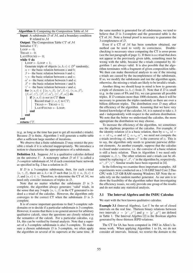
Algorithm 1: Computing the Composition Table ofMInput: A subdomain D ofM, and a boundary condition

Ψ related toMOutput: The Composition Table CT ofMInitialise CT ;LOOP ← 0;TRIAD ← 0;LASTFOUND ← 0;while Ψ do

LOOP ← LOOP + 1;Generate triple of objects (a, b, c) ∈ D3 randomly;α← the basic relation between a and b;β ← the basic relation between b and c;γ ← the basic relation between a and c;α′ ← the basic relation between b and a;β′ ← the basic relation between c and b;γ′ ← the basic relation between c and a;for 〈r, s, t〉 ∈ {〈α, γ, β〉, 〈α′, β, γ〉, 〈γ, α, β′〉,〈β, α′, γ′〉, 〈β′, γ′, α′〉, 〈γ′, β′, α〉} do

if 〈r, s, t〉 is not in CT thenRecord triad 〈r, s, t〉 to CT ;TRIAD ← TRIAD + 1;LASTFOUND ← LOOP;

endend

endreturn CT .

(e.g. as long as the time has past to get all recorded c-triads).Because D is finite, Algorithm 1 will generate a stable tableafter a sufficient large number of iterations.

We observe that a finite subdomain D may restrict the pos-sible c-triads if it is selected inappropriately. We introduce anotion to characterise the appropriateness of a subdomain.

Definition 3.1. SupposeM is a qualitative calculus definedon the universe U . A nonempty subset D of U is called a3-complete subdomain ofM if each consistent basic networkas specified in Eq. 2 has a solution in D.

If D is a 3-complete subdomain, then, for each c-triad〈α, γ, β〉, there are a, b, c in D such that (a, b) ∈ α, (b, c) ∈β, and (a, c) ∈ γ. Therefore, to determine the CT ofM, weneed only consider instances of triples in D.

Note that no matter whether the subdomain D is 3-complete, the algorithm always generates ‘valid’ triads, inthe sense that any 3-tuple 〈α, γ, β〉 in the CT generated is in-deed a c-triad of the calculus. However, the algorithm onlyconverges to the correct CT when the subdomain D is 3-complete.

It is of course important questions to find 3-complete sub-domains or to decide if a particular subdomain is 3-complete.However, it seems that there is no general answer for arbitraryqualitative calculi, since the questions are closely related tothe semantics of the calculi. For a particular calculus, e.g.IA, this can be verified by formal analysis. Note that a super-set of a 3-complete subdomain is also 3-complete. To makesure a chosen subdomain D is 3-complete, we often applythe algorithm on several of its supersets at the same time. If

the same number is generated for all subdomains, we tend tobelieve that D is 3-complete and the generated table is theCT ofM. Note a formal proof is necessary to guarantee the3-completeness of D.

Even if a CT of M has been somehow obtained, ourmethod can be used to verify its correctness. Double-checking is necessary since computing the CT is error-prone(see the last paragraph of page 1). If there is a c-triad that doesnot appear in the previously given table, something must bewrong with the table, because the c-triads computed by Al-gorithm 1 are always valid. It is also possible that the algo-rithm terminates with a fragment of given composition table.We then can make theoretical analysis to see if the missingc-triads are caused by the incompleteness of the subdomain.If so, we modify the subdomain and run the algorithm again,otherwise, the missing c-triads are likely to be invalid c-triads.

Another thing we should keep in mind is how to generatea triple of elements (a, b, c) from D. Note that if D is small(e.g. in the cases of PA and IA), we can generate all possibletriples. IfD contains more than 1000 elements, then it will benecessary to generate the triples randomly as there are over abillion different triples. The distribution over D may affectthe efficiency of the algorithm. Assuming that we have verylimited knowledge of the calculusM, it is natural to take a, band c independently with respect to the uniform distribution.We note that the better we understand the calculus, the moreappropriate the distribution we may choose.

To increase the efficiency of the algorithm, we sometimesuse the algebraic properties of the calculus. For example, ifthe identity relation id is a basic relation, then by α ◦w id =α = id ◦w α and id ⊆ α ◦w α∼, we need not compute thec-triads involving id, where α∼ is the converse of α. This isto say, the algorithm only needs to generate pairwise differ-ent elements. As another example, suppose that the calculusis closed under converse, i.e. the converse of a basic relationis still a basic relation. Then in Algorithm 1 we need onlycompute α, β, γ. The other relations and c-triads can be ob-tained by replacing α′, β′, γ′ in the algorithm by, respectively,α∼, β∼, γ∼. Similar results have been reported in [4].

In the following we examine three important examples. Allexperiments were conducted on a 3.16 GHZ Intel Core 2 DuoCPU with 3.25 GB RAM running Windows XP. Note the re-sults rely on the random number generator. As our aim is toshow the feasibility of the algorithm rather than investigatingthe efficiency issues, we only provide one group of the resultsand do not make any statistical analysis.

3.1 The Interval Algebra and the INDU CalculusWe start with the best known qualitative calculus.

Example 3.1 (Interval Algebra). Let U be the set of closedintervals on the real line. Thirteen binary relations betweentwo intervals x = [x−, x+] and y = [y−, y+] are definedin Table 1. The Interval Algebra [2] is the Boolean algebragenerated by these thirteen JEPD relations.

The CT for IA has been computed in 1983 in Allen’s fa-mous work. When applying Algorithm 1 to IA, we do notconsider all intervals. Instead, we restrict the domain to the

55

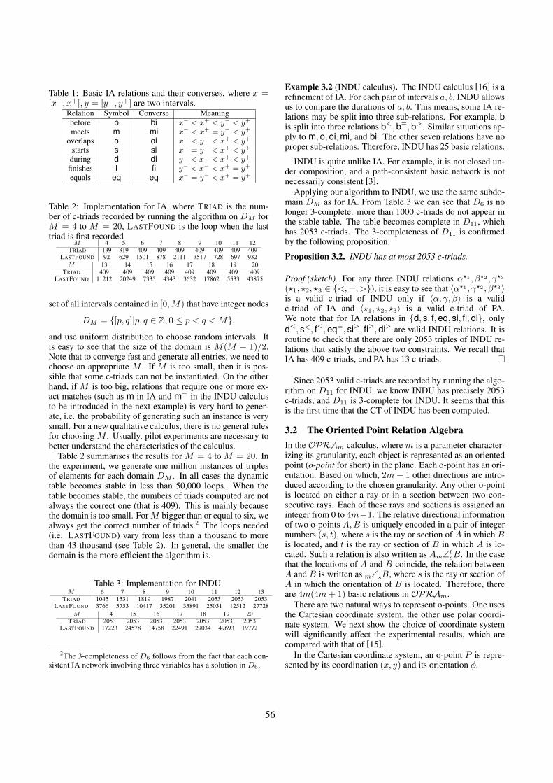
Table 1: Basic IA relations and their converses, where x =[x−, x+], y = [y−, y+] are two intervals.

Relation Symbol Converse Meaningbefore b bi x− < x+ < y− < y+

meets m mi x− < x+ = y− < y+

overlaps o oi x− < y− < x+ < y+

starts s si x− = y− < x+ < y+

during d di y− < x− < x+ < y+

finishes f fi y− < x− < x+ = y+

equals eq eq x− = y− < x+ = y+

Table 2: Implementation for IA, where TRIAD is the num-ber of c-triads recorded by running the algorithm on DM forM = 4 to M = 20, LASTFOUND is the loop when the lasttriad is first recorded

M 4 5 6 7 8 9 10 11 12TRIAD 139 319 409 409 409 409 409 409 409

LASTFOUND 92 629 1501 878 2111 3517 728 697 932M 13 14 15 16 17 18 19 20

TRIAD 409 409 409 409 409 409 409 409LASTFOUND 11212 20249 7335 4343 3632 17862 5533 43875

set of all intervals contained in [0,M) that have integer nodes

DM = {[p, q]|p, q ∈ Z, 0 ≤ p < q < M},and use uniform distribution to choose random intervals. Itis easy to see that the size of the domain is M(M − 1)/2.Note that to converge fast and generate all entries, we need tochoose an appropriate M . If M is too small, then it is pos-sible that some c-triads can not be instantiated. On the otherhand, if M is too big, relations that require one or more ex-act matches (such as m in IA and m= in the INDU calculusto be introduced in the next example) is very hard to gener-ate, i.e. the probability of generating such an instance is verysmall. For a new qualitative calculus, there is no general rulesfor choosing M . Usually, pilot experiments are necessary tobetter understand the characteristics of the calculus.

Table 2 summarises the results for M = 4 to M = 20. Inthe experiment, we generate one million instances of triplesof elements for each domain DM . In all cases the dynamictable becomes stable in less than 50,000 loops. When thetable becomes stable, the numbers of triads computed are notalways the correct one (that is 409). This is mainly becausethe domain is too small. ForM bigger than or equal to six, wealways get the correct number of triads.2 The loops needed(i.e. LASTFOUND) vary from less than a thousand to morethan 43 thousand (see Table 2). In general, the smaller thedomain is the more efficient the algorithm is.

Table 3: Implementation for INDUM 6 7 8 9 10 11 12 13

TRIAD 1045 1531 1819 1987 2041 2053 2053 2053LASTFOUND 3766 5753 10417 35201 35891 25031 12512 27728

M 14 15 16 17 18 19 20TRIAD 2053 2053 2053 2053 2053 2053 2053

LASTFOUND 17223 24578 14758 22491 29034 49693 19772

2The 3-completeness of D6 follows from the fact that each con-sistent IA network involving three variables has a solution in D6.

Example 3.2 (INDU calculus). The INDU calculus [16] is arefinement of IA. For each pair of intervals a, b, INDU allowsus to compare the durations of a, b. This means, some IA re-lations may be split into three sub-relations. For example, bis split into three relations b<,b=,b>. Similar situations ap-ply to m,o,oi,mi, and bi. The other seven relations have noproper sub-relations. Therefore, INDU has 25 basic relations.

INDU is quite unlike IA. For example, it is not closed un-der composition, and a path-consistent basic network is notnecessarily consistent [3].

Applying our algorithm to INDU, we use the same subdo-main DM as for IA. From Table 3 we can see that D6 is nolonger 3-complete: more than 1000 c-triads do not appear inthe stable table. The table becomes complete in D11, whichhas 2053 c-triads. The 3-completeness of D11 is confirmedby the following proposition.

Proposition 3.2. INDU has at most 2053 c-triads.

Proof (sketch). For any three INDU relations α?1 , β?2 , γ?3

(?1, ?2, ?3 ∈ {<,=, >}), it is easy to see that 〈α?1 , γ?2 , β?3〉is a valid c-triad of INDU only if 〈α, γ, β〉 is a validc-triad of IA and 〈?1, ?2, ?3〉 is a valid c-triad of PA.We note that for IA relations in {d, s, f,eq, si, fi,di}, onlyd<, s<, f<,eq=, si>, fi>,di> are valid INDU relations. It isroutine to check that there are only 2053 triples of INDU re-lations that satisfy the above two constraints. We recall thatIA has 409 c-triads, and PA has 13 c-triads.

Since 2053 valid c-triads are recorded by running the algo-rithm on D11 for INDU, we know INDU has precisely 2053c-triads, and D11 is 3-complete for INDU. It seems that thisis the first time that the CT of INDU has been computed.

3.2 The Oriented Point Relation AlgebraIn the OPRAm calculus, where m is a parameter character-izing its granularity, each object is represented as an orientedpoint (o-point for short) in the plane. Each o-point has an ori-entation. Based on which, 2m − 1 other directions are intro-duced according to the chosen granularity. Any other o-pointis located on either a ray or in a section between two con-secutive rays. Each of these rays and sections is assigned aninteger from 0 to 4m−1. The relative directional informationof two o-points A,B is uniquely encoded in a pair of integernumbers (s, t), where s is the ray or section of A in which Bis located, and t is the ray or section of B in which A is lo-cated. Such a relation is also written as Am∠t

sB. In the casethat the locations of A and B coincide, the relation betweenA and B is written as m∠sB, where s is the ray or section ofA in which the orientation of B is located. Therefore, thereare 4m(4m+ 1) basic relations in OPRAm.

There are two natural ways to represent o-points. One usesthe Cartesian coordinate system, the other use polar coordi-nate system. We next show the choice of coordinate systemwill significantly affect the experimental results, which arecompared with that of [15].

In the Cartesian coordinate system, an o-point P is repre-sented by its coordination (x, y) and its orientation φ.

56

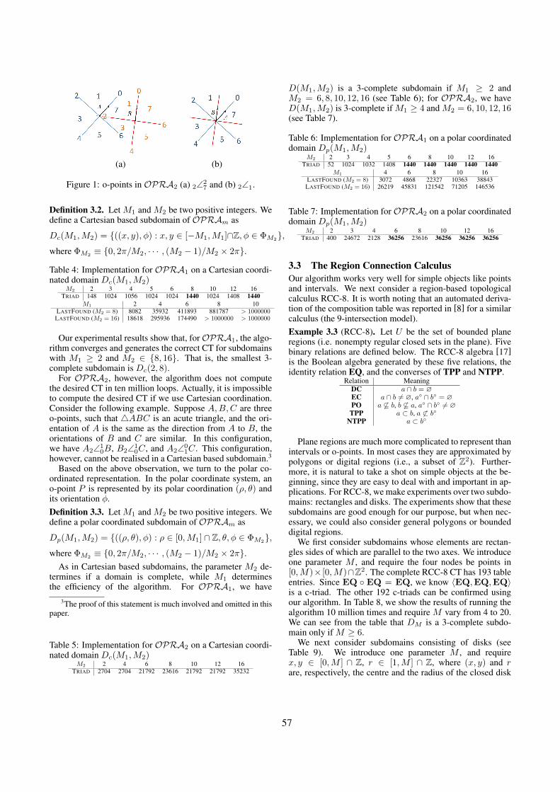
(a) (b)

Figure 1: o-points in OPRA2 (a) 2∠27 and (b) 2∠1.

Definition 3.2. Let M1 and M2 be two positive integers. Wedefine a Cartesian based subdomain of OPRAm as

Dc(M1,M2) = {((x, y), φ) : x, y ∈ [−M1,M1]∩Z, φ ∈ ΦM2},

where ΦM2 ≡ {0, 2π/M2, · · · , (M2 − 1)/M2 × 2π}.

Table 4: Implementation for OPRA1 on a Cartesian coordi-nated domain Dc(M1,M2)

M2 2 3 4 5 6 8 10 12 16TRIAD 148 1024 1056 1024 1024 1440 1024 1408 1440

M1 2 4 6 8 10LASTFOUND (M2 = 8) 8082 35932 411893 881787 > 1000000

LASTFOUND (M2 = 16) 18618 295936 174490 > 1000000 > 1000000

Our experimental results show that, forOPRA1, the algo-rithm converges and generates the correct CT for subdomainswith M1 ≥ 2 and M2 ∈ {8, 16}. That is, the smallest 3-complete subdomain is Dc(2, 8).

For OPRA2, however, the algorithm does not computethe desired CT in ten million loops. Actually, it is impossibleto compute the desired CT if we use Cartesian coordination.Consider the following example. Suppose A,B,C are threeo-points, such that 4ABC is an acute triangle, and the ori-entation of A is the same as the direction from A to B, theorientations of B and C are similar. In this configuration,we have A2∠1

0B, B2∠10C, and A2∠0

1C. This configuration,however, cannot be realised in a Cartesian based subdomain.3

Based on the above observation, we turn to the polar co-ordinated representation. In the polar coordinate system, ano-point P is represented by its polar coordination (ρ, θ) andits orientation φ.Definition 3.3. Let M1 and M2 be two positive integers. Wedefine a polar coordinated subdomain of OPRAm as

Dp(M1,M2) = {((ρ, θ), φ) : ρ ∈ [0,M1] ∩ Z, θ, φ ∈ ΦM2},where ΦM2

≡ {0, 2π/M2, · · · , (M2 − 1)/M2 × 2π}.As in Cartesian based subdomains, the parameter M2 de-

termines if a domain is complete, while M1 determinesthe efficiency of the algorithm. For OPRA1, we have

3The proof of this statement is much involved and omitted in thispaper.

Table 5: Implementation for OPRA2 on a Cartesian coordi-nated domain Dc(M1,M2)

M2 2 4 6 8 10 12 16TRIAD 2704 2704 21792 23616 21792 21792 35232

D(M1,M2) is a 3-complete subdomain if M1 ≥ 2 andM2 = 6, 8, 10, 12, 16 (see Table 6); for OPRA2, we haveD(M1,M2) is 3-complete if M1 ≥ 4 and M2 = 6, 10, 12, 16(see Table 7).

Table 6: Implementation for OPRA1 on a polar coordinateddomain Dp(M1,M2)

M2 2 3 4 5 6 8 10 12 16TRIAD 52 1024 1032 1408 1440 1440 1440 1440 1440

M1 4 6 8 10 16LASTFOUND (M2 = 8) 3072 4868 22327 10363 38843

LASTFOUND (M2 = 16) 26219 45831 121542 71205 146536

Table 7: Implementation for OPRA2 on a polar coordinateddomain Dp(M1,M2)

M2 2 3 4 6 8 10 12 16TRIAD 400 24672 2128 36256 23616 36256 36256 36256

3.3 The Region Connection CalculusOur algorithm works very well for simple objects like pointsand intervals. We next consider a region-based topologicalcalculus RCC-8. It is worth noting that an automated deriva-tion of the composition table was reported in [8] for a similarcalculus (the 9-intersection model).Example 3.3 (RCC-8). Let U be the set of bounded planeregions (i.e. nonempty regular closed sets in the plane). Fivebinary relations are defined below. The RCC-8 algebra [17]is the Boolean algebra generated by these five relations, theidentity relation EQ, and the converses of TPP and NTPP.

Relation MeaningDC a ∩ b = ∅EC a ∩ b 6= ∅, a◦ ∩ b◦ = ∅PO a 6⊆ b, b 6⊆ a, a◦ ∩ b◦ 6= ∅

TPP a ⊂ b, a 6⊂ b◦NTPP a ⊂ b◦

Plane regions are much more complicated to represent thanintervals or o-points. In most cases they are approximated bypolygons or digital regions (i.e., a subset of Z2). Further-more, it is natural to take a shot on simple objects at the be-ginning, since they are easy to deal with and important in ap-plications. For RCC-8, we make experiments over two subdo-mains: rectangles and disks. The experiments show that thesesubdomains are good enough for our purpose, but when nec-essary, we could also consider general polygons or boundeddigital regions.

We first consider subdomains whose elements are rectan-gles sides of which are parallel to the two axes. We introduceone parameter M , and require the four nodes be points in[0,M)× [0,M)∩Z2. The complete RCC-8 CT has 193 tableentries. Since EQ ◦ EQ = EQ, we know 〈EQ,EQ,EQ〉is a c-triad. The other 192 c-triads can be confirmed usingour algorithm. In Table 8, we show the results of running thealgorithm 10 million times and require M vary from 4 to 20.We can see from the table that DM is a 3-complete subdo-main only if M ≥ 6.

We next consider subdomains consisting of disks (seeTable 9). We introduce one parameter M , and requirex, y ∈ [0,M ] ∩ Z, r ∈ [1,M ] ∩ Z, where (x, y) and rare, respectively, the centre and the radius of the closed disk

57

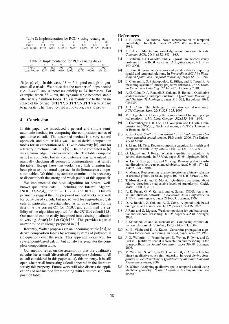
Table 8: Implementation for RCC-8 using rectanglesM 4 5 6 8 10 15 20

TRIAD 114 177 192 192 192 192 192LASTFOUND 14776 6513 2332646 56067 198255 261729 1521173

Table 9: Implementation for RCC-8 using disksM 4 5 6 8 10 15 20

TRIAD 188 192 192 192 192 192 192LASTFOUND 1759 8913 9489 25955 113757 942914 2961628

B((x, y), r)). In this case, M = 5 is good enough to gen-erate all c-triads. We notice that the number of loops needed(i.e. LASTFOUND) increases quickly as M increases. Forexample, when M = 20, the dynamic table becomes stableafter nearly 3 million loops. This is mainly due to that an in-stance of the c-triad 〈NTPP,NTPP,NTPP〉 is very hardto generate. The ‘hard’ c-triad is, however, easy to prove.

4 Conclusion

In this paper, we introduced a general and simple semi-automatic method for computing the composition tables ofqualitative calculi. The described method is a very naturalapproach, and similar idea was used to derive compositiontables for an elaboration of RCC with convexity [6], and fora ternary directional calculus [5]. The table computed in [6]was acknowledged there as incomplete. The table computedin [5] is complete, but its completeness was guaranteed bymanually checking all geometric configurations that satisfythe table. Except these two works, very little attention hasbeen given to this natural approach in the literature on compo-sition tables. We think a systematic examination is necessaryto discover both the strong and weak points of this approach.

We implemented the basic algorithm for several well-known qualitative calculi, including the Interval Algebra,INDU, OPRAm for m = 1 ∼ 4, and RCC-8. Our ex-periments suggest that the proposed method works very wellfor point-based calculi, but not so well for region-based cal-culi. In particular, we established, as far as we know, for thefirst time the correct CT for INDU, and confirmed the va-lidity of the algorithm reported for the OPRA calculi [15].Our method can be easily integrated into existing qualitativesolvers e.g. SparQ [21] or GQR [22]. This provides a partialanswer to the challenge proposed in [7].

Recently, Wolter proposes (in an upcoming article [23]) toderive composition tables by solving systems of polynomial(in)equations over the reals. This approach works well forseveral point-based calculi, but not always generates the com-plete composition table.

Our method relies on the assumption that the qualitativecalculus has a small ‘discretised’ 3-complete subdomain. Allcalculi considered in this paper satisfy this property. It is stillopen whether all interesting calculi appeared in the literaturesatisfy this property. Future work will also discuss the appli-cations of our method for reasoning with a customised com-position table.

References[1] J. F. Allen. An interval-based representation of temporal

knowledge. In IJCAI, pages 221–226. William Kaufmann,1981.

[2] J. F. Allen. Maintaining knowledge about temporal intervals.Commun. ACM, 26(11):832–843, 1983.

[3] P. Balbiani, J.-F. Condotta, and G. Ligozat. On the consistencyproblem for the INDU calculus. J. Applied Logic, 4(2):119–140, 2006.

[4] B. Bennett. Some observations and puzzles about composingspatial and temporal relations. In Proceedings ECAI-94 Work-shop on Spatial and Temporal Reasoning, pages 65–72, 1994.

[5] E. Clementini, S. Skiadopoulos, R. Billen, and F. Tarquini. Areasoning system of ternary projective relations. IEEE Trans.on Knowl. and Data Eng., 22:161–178, February 2010.

[6] A. G. Cohn, D. A. Randell, Z. Cui, and B. Bennett. Qualitativespatial reasoning and representation. In Qualitative Reasoningand Decision Technologies, pages 513–522, Barcelona, 1993.CIMNE.

[7] A. G. Cohn. The challenge of qualitative spatial reasoning.ACM Comput. Surv., 27(3):323–325, 1995.

[8] M. J. Egenhofer. Deriving the composition of binary topolog-ical relations. J. Vis. Lang. Comput., 5(2):133–149, 1994.

[9] L. Frommberger, J. H. Lee, J. O. Wallgrun, and F. Dylla. Com-position inOPRAm. Technical report, SFB/TR 8, Universityof Bremen, 2007.

[10] R. K. Goyal. Similarity assessment for cardinal directions be-tween extended spatial objects. PhD thesis, 2000. The Univer-sity of Maine.

[11] S. Li and M. Ying. Region connection calculus: Its models andcomposition table. Artif. Intell., 145(1-2):121–146, 2003.

[12] G. Ligozat and J. Renz. What is a qualitative calculus? Ageneral framework. In PRICAI, pages 53–64. Springer, 2004.

[13] W. Liu, X. Zhang, S. Li, and M. Ying. Reasoning about cardi-nal directions between extended objects. Artif. Intell., 174(12-13):951–983, 2010.

[14] R. Moratz. Representing relative direction as a binary relationof oriented points. In ECAI, pages 407–411. IOS Press, 2006.

[15] T. Mossakowski and R. Moratz. Qualitative reasoning aboutrelative direction on adjustable levels of granularity. CoRR,abs/1011.0098, 2010.

[16] A. K. Pujari, G. V. Kumari, and A. Sattar. INDU: An inter-val and duration network. In Australian Joint Conference onArtificial Intelligence, pages 291–303. Springer, 1999.

[17] D. A. Randell, Z. Cui, and A. G. Cohn. A spatial logic basedon regions and connection. In KR, pages 165–176, 1992.

[18] J. Renz and G. Ligozat. Weak composition for qualitative spa-tial and temporal reasoning. In CP, pages 534–548. Springer,2005.

[19] S. Skiadopoulos and M. Koubarakis. Composing cardinal di-rection relations. Artif. Intell., 152(2):143–171, 2004.

[20] M. B. Vilain and H. A. Kautz. Constraint propagation algo-rithms for temporal reasoning. In AAAI, pages 377–382, 1986.

[21] J. O. Wallgrun, L. Frommberger, D. Wolter, F. Dylla, and C.Freksa. Qualitative spatial representation and reasoning in thesparq-toolbox. In Spatial Cognition, pages 39–58. Springer,2006.

[22] M. Westphal, S. Wolfl, and Z. Gantner. GQR: A fast solver forbinary qualitative constraint networks. In AAAI Spring Sym-posium on Benchmarking of Qualitative Spatial and TemporalReasoning Systems, 2009.

[23] D. Wolter. Analyzing qualitative spatio-temporal calculi usingalgebraic geometry. Spatial Cognition & Computation. (toappear).

58