Takustraße 7 D-14195 Berlin-Dahlem Germany Konrad-Zuse-Zentrum f¨ ur Informationstechnik Berlin TOBIAS WEBER ,S EBASTIAN S AGER ,AMBROS GLEIXNER Solving Quadratic Programs to High Precision using Scaled Iterative Refinement This report has been published in Mathematical Programming Computation. Please cite as Tobias Weber, Sebastian Sager, Ambros Gleixner, Solving Quadratic Programs to High Precision using Scaled Iterative Refinement, Mathematical Programming Computation, 11:421–455, 2019, doi:10.1007/s12532-019-00154-6. ZIB Report 18-04 (March 2018)

Welcome message from author
This document is posted to help you gain knowledge. Please leave a comment to let me know what you think about it! Share it to your friends and learn new things together.
Transcript

Takustraße 7D-14195 Berlin-Dahlem
GermanyKonrad-Zuse-Zentrumfur Informationstechnik Berlin
TOBIAS WEBER, SEBASTIAN SAGER, AMBROS GLEIXNER
Solving Quadratic Programs to High Precisionusing Scaled Iterative Refinement
This report has been published in Mathematical Programming Computation. Please cite as Tobias Weber, Sebastian Sager, Ambros Gleixner, Solving QuadraticPrograms to High Precision using Scaled Iterative Refinement, Mathematical Programming Computation, 11:421–455, 2019, doi:10.1007/s12532-019-00154-6.
ZIB Report 18-04 (March 2018)

Herausgegeben vomKonrad-Zuse-Zentrum fur Informationstechnik BerlinTakustraße 7D-14195 Berlin-Dahlem
Telefon: 030-84185-0Telefax: 030-84185-125
e-mail: [email protected]: http://www.zib.de
ZIB-Report (Print) ISSN 1438-0064ZIB-Report (Internet) ISSN 2192-7782
Solving Quadratic Programs to High Precision
using Scaled Iterative Refinement
Tobias Weber1, Sebastian Sager1, Ambros Gleixner2
March 19, 2018
Abstract Quadratic optimization problems (QPs) are ubiquitous, and solution algo-rithms have matured to a reliable technology. However, the precision of solutions isusually limited due to the underlying floating-point operations. This may cause incon-veniences when solutions are used for rigorous reasoning. We contribute on three levelsto overcome this issue.
First, we present a novel refinement algorithm to solve QPs to arbitrary precision.It iteratively solves refined QPs, assuming a floating-point QP solver oracle. We provelinear convergence of residuals and primal errors. Second, we provide an efficient im-plementation, based on SoPlex and qpOASES that is publicly available in source code.Third, we give precise reference solutions for the Maros and Meszaros benchmark library.
Keywords Quadratic Programming · Iterative Refinement · Active Set · RationalCalculations
Mathematics Subject Classification 90C20 · 90-08 · 90C55
1 Introduction
Quadratic optimization problems (QPs) are optimization problems with a quadratic ob-jective function and linear constraints. They are of interest directly, e.g., in portfoliooptimization or support vector machines [1]. They also occur as subproblems in sequen-tial quadratic programming, mixed-integer quadratic programming, and nonlinear modelpredictive control. Efficient algorithms are usually of active set, interior point, or para-metric type. Examples of QP solvers are BQPD [5], CPLEX [2], Gurobi [11], qp solve [10],qpOASES [4], and QPOPT [7]. These QP solvers have matured to reliable tools and cansolve convex problems with many thousands, sometimes millions of variables. However,they calculate and check the solution of a QP in floating-point arithmetic. Thus, theclaimed precision may be violated and in extreme cases optimal solutions might not befound. This may cause inconveniences, especially when solutions are used for rigorousreasoning.
1Otto von Guericke University, Institute of Mathematical Optimization, Universitatsplatz 2, 02-204,39106 Magdeburg, Germany, { tobias. weber,sager}@ ovgu. de
2Zuse Institute Berlin, Department of Mathematical Optimization, Takustr. 7, 14195 Berlin, Ger-many, gleixner@ zib. de
This project has received funding from the European Research Council (ERC) under the EuropeanUnions Horizon 2020 research and innovation programme (grant agreement No 647573), from theDeutsche Forschungsgemeinschaft (DFG, German Research Foundation) – 314838170, GRK 2297MathCoRe, and from the German Federal Ministry of Education and Research as part of the ResearchCampus MODAL (BMBF grant number 05M14ZAM), all of which is gratefully acknowledged.
1
One possible approach is the application of interval arithmetic. It allows to includeuncertainties as lower and upper bounds on the modeling level, see [12] for a surveyfor the case of linear optimization. As a drawback, all internal calculations have to beperformed with interval arithmetic. Hence standard solvers can not be used any more,the computation times increase, and solutions may be very conservative.
We are only aware of one advanced algorithm that solves QPs exactly over the ratio-nal numbers. It is designed to tackle problems from computational geometry with a smallnumber of constraints or variables, [6]. Based on the classical QP simplex method [15], itreplaces critical calculations inside the QP solver by their rational counterparts. Heuris-tic decisions that do not affect the correctness of the algorithm are performed in fastfloating-point arithmetic.
In this paper we propose a novel algorithm that can use efficient floating-point QPsolvers as a black box. Our method is inspired by iterative refinement, a standardprocedure to improve the accuracy of an approximate solution for a system of linearequalities, [14]: The residual of the approximate solution is calculated, the linear systemis solved again with the residual as a right-hand side, and the new solution is used torefine the old solution, thus improving its accuracy. A generalization of this idea to thesolution of optimization problems needs to address several difficulties: most importantly,the presence of inequality constraints; the handling of optimality conditions; and thenumerical tolerances that floating-point solvers can return in practice.
For LPs this has first been developed in [9]. The approach refines primal-dual so-lutions of the Karush-Kuhn-Tucker (KKT) conditions and comprehends scaling andcalculations in rational arithmetic. We generalize further and discuss the specific issuesdue to the presence of a quadratic objective function. The fact that the general approachcarries over from LP to QP was remarked in [8]. Here we provide the details, providea general lemma showing how the residuals bound the primal and dual iterates, andanalyze the computational behavior of the algorithm based on an efficient implementa-tion that is made publicly available in source code and can be used freely for researchpurposes.
The paper is organized as follows. In Section 2 we define and discuss QPs and theirrefined and scaled counterparts. We give one illustrating and motivating example forscaling and refinement. In Section 3 we formulate an algorithm and prove its conver-gence properties. In Section 4 we consider performance issues and describe how ourimplementation based on SoPlex and qpOASES can be used to calculate solutions forQPs with arbitrary precision. In Section 5 we discuss run times and provide solutionsfor the Maros and Meszaros benchmark library, [13]. We conclude in Section 6 with adiscussion of the results and give directions for future research and applications of thealgorithm.
In the following we will use ‖ · ‖ for the maximum norm ‖ · ‖∞. The maximalentry of a vector maxi{vi} is written as max{v}. Inequalities a ≤ b for a, b ∈ Qn holdcomponentwise.
2 Refinement and Scaling of Quadratic Programs
In this section we collect some basic definitions and results that will be of use later on.We consider convex optimization problems of the following form.
Definition 1 (Quadratic optimization problem (QP)). Let a symmetric matrix Q ∈Qn×n, a matrix A ∈ Qm×n, and vectors c ∈ Qn, b ∈ Qm, l ∈ Qn be given. We considerthe quadratic optimization problem (QP)
minx
12x
TQx+ cTx
s.t. Ax = bx ≥ l
(P )
2

assuming that (P ) is feasible and bounded, and Q is positive semi-definite on the feasibleset. The rounded version of this convex rational data QP will be denoted as (P ).
A point x∗ ∈ Qn is a global optimum of (P ) if and only if it satisfies the Karush-Kuhn-Tucker (KKT) conditions, [3], i.e., if multipliers y∗ ∈ Qm exist such that
Ax∗ = b (1a)
x∗ ≥ l (1b)
AT y∗ ≤ Qx∗ + c (1c)
(Qx∗ + c−AT y∗)T (x∗ − l) = 0. (1d)
The pair (x∗, y∗) is then called KKT pair of (P ). Primal feasibility is given by (1a–1b),dual feasibility by (1c), and complementary slackness by (1d). Refinement of this systemof linear (in-)equalities is equivalent to the refinement of (P ).
Definition 2 (Refined QP). Let the QP (P ), scaling factors ∆P ,∆D ∈ Q+ and vectorsx∗ ∈ Qn, y∗ ∈ Qm be given. We define the refined QP as
minx
12x
T ∆D
∆PQx+ (∆D c)
Tx
s.t. Ax = ∆P b
x ≥ ∆P l,
(P∆)
where c = Qx∗ + c − AT y∗, b = b − Ax∗, and l = l − x∗. The rounded version of thisrefined and scaled rational data QP will be denoted as (P∆).
The following theorem is the basis for our theoretical and algorithmic approaches. Itis a generalization of iterative refinement for LP and was formulated and proven in [8,Theorem 5.2]. Again, primal feasibility refers to (1a–1b), dual feasibility to (1c), andcomplementary slackness to (1d).
Theorem 3 (QP Refinement). Let the QP (P ), scaling factors ∆P ,∆D ∈ Q+, vectorsx∗ ∈ Qn, y∗ ∈ Qm, and the refined QP (P∆) be given. Then for any x ∈ Rn, y ∈ Rmand tolerances εP , εD, εS ≥ 0:
1. x is primal feasible for (P∆) within an absolute tolerance εP if and only if x∗+ x∆P
is primal feasible for (P ) within εP /∆P .
2. y is dual feasible for (P∆) within an absolute tolerance εD if and only if y∗ + y∆D
is dual feasible for (P ) within εD/∆D.
3. x, y satisfy complementary slackness for (P∆) within an absolute tolerance εS ifand only if y∗ + y
∆D, x∗ + x
∆Psatisfy complementary slackness for (P ) within
εS/(∆P∆D).
For illustration, we investigate the following example.
Example 4 (QP Refinement). Consider the QP with two variables
minx
12 (x2
1 + x22) + x1 + (1 + 10−6)x2
s.t. x1 + x2 = 10−6
x1, x2 ≥ 0.
An approximate solution to a tolerance of 10−6 is x∗1 = x∗2 = 0 with dual multipliery∗ = 1. This solution is slightly primal and dual infeasible, but the solver can notrecognize this on this scale. The situation is depicted in Figure 1 on the left.
The point x∗ seems to be the optimal solution satisfying the equality constraintand the brown circle representing the level curve of the objective function indicates the
3
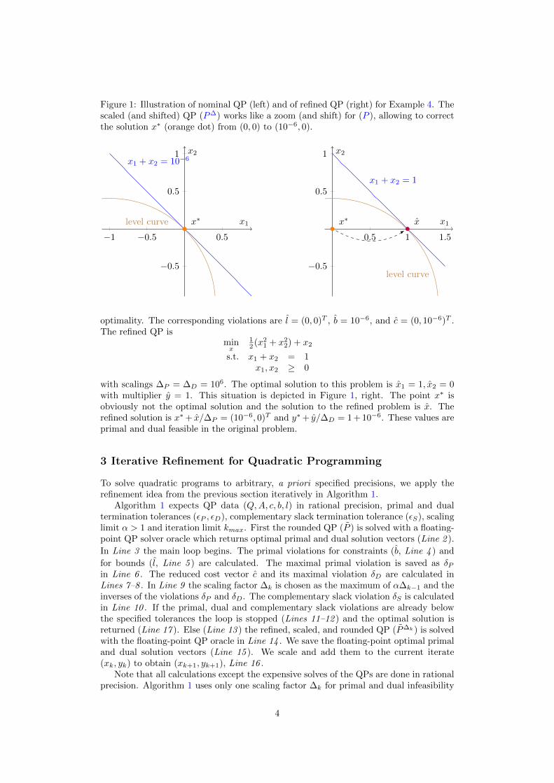
Figure 1: Illustration of nominal QP (left) and of refined QP (right) for Example 4. Thescaled (and shifted) QP (P∆) works like a zoom (and shift) for (P ), allowing to correctthe solution x∗ (orange dot) from (0, 0) to (10−6, 0).
−1 −0.5 0.5
−0.5
0.5
1x1 + x2 = 10−6
x∗level curve x1
x2
0.5 1 1.5
−0.5
0.5
1
x1 + x2 = 1
x∗ x
level curve
x1
x2
optimality. The corresponding violations are l = (0, 0)T , b = 10−6, and c = (0, 10−6)T .The refined QP is
minx
12 (x2
1 + x22) + x2
s.t. x1 + x2 = 1x1, x2 ≥ 0
with scalings ∆P = ∆D = 106. The optimal solution to this problem is x1 = 1, x2 = 0with multiplier y = 1. This situation is depicted in Figure 1, right. The point x∗ isobviously not the optimal solution and the solution to the refined problem is x. Therefined solution is x∗+ x/∆P = (10−6, 0)T and y∗+ y/∆D = 1 + 10−6. These values areprimal and dual feasible in the original problem.
3 Iterative Refinement for Quadratic Programming
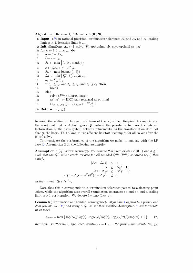
To solve quadratic programs to arbitrary, a priori specified precisions, we apply therefinement idea from the previous section iteratively in Algorithm 1.
Algorithm 1 expects QP data (Q,A, c, b, l) in rational precision, primal and dualtermination tolerances (εP , εD), complementary slack termination tolerance (εS), scalinglimit α > 1 and iteration limit kmax. First the rounded QP (P ) is solved with a floating-point QP solver oracle which returns optimal primal and dual solution vectors (Line 2 ).
In Line 3 the main loop begins. The primal violations for constraints (b, Line 4 ) and
for bounds (l, Line 5 ) are calculated. The maximal primal violation is saved as δPin Line 6 . The reduced cost vector c and its maximal violation δD are calculated inLines 7–8 . In Line 9 the scaling factor ∆k is chosen as the maximum of α∆k−1 and theinverses of the violations δP and δD. The complementary slack violation δS is calculatedin Line 10 . If the primal, dual and complementary slack violations are already belowthe specified tolerances the loop is stopped (Lines 11–12 ) and the optimal solution isreturned (Line 17 ). Else (Line 13 ) the refined, scaled, and rounded QP (P∆k) is solvedwith the floating-point QP oracle in Line 14 . We save the floating-point optimal primaland dual solution vectors (Line 15 ). We scale and add them to the current iterate(xk, yk) to obtain (xk+1, yk+1), Line 16 .
Note that all calculations except the expensive solves of the QPs are done in rationalprecision. Algorithm 1 uses only one scaling factor ∆k for primal and dual infeasibility
4
Algorithm 1 Iterative QP Refinement (IQPR)
1: Input: (P ) in rational precision, termination tolerances εP and εD and εS , scalinglimit α > 1, iteration limit kmax
2: Initialization: ∆0 ← 1, solve (P ) approximately, save optimal (x1, y1)3: for k ← 1, 2, ..., kmax do4: b← b−Axk5: l← l − xk6: δP ← max
{0, ‖b‖,max{l}
}7: c← Qxk + c−AT yk8: δD ← max {0,max{−c}}9: ∆k ← min
{δ−1P , δ−1
D , α∆k−1
}10: δS ←
∑i lici
11: if δP ≤ εP and δD ≤ εD and δS ≤ εS then12: break13: else14: solve (P∆k) approximately15: (x∗, y∗)← KKT pair returned as optimal
16: (xk+1, yk+1)← (xk, yk) + (x∗,y∗)∆k
17: Return: (xk, yk)
to avoid the scaling of the quadratic term of the objective. Keeping this matrix andthe constraint matrix A fixed gives QP solvers the possibility to reuse the internalfactorization of the basis system between refinements, as the transformation does notchange the basis. This allows to use efficient hotstart techniques for all solves after theinitial solve.
To investigate the performance of the algorithm we make, in analogy with the LPcase [9, Assumption 2.9], the following assumption.
Assumption 5 (QP solver accuracy). We assume that there exists ε ∈ [0, 1) and σ ≥ 0such that the QP solver oracle returns for all rounded QPs (P∆k) solutions (x, y) thatsatisfy
‖Ax−∆k b‖ ≤ ε
x ≥ ∆k l − 1εQx+ ∆k c ≥ AT y − 1ε
|(Qx+ ∆k c−AT y)T (x−∆k l)| ≤ σ
in the rational QPs (P∆k).
Note that this ε corresponds to a termination tolerance passed to a floating-pointsolver, while the algorithm uses overall termination tolerances εP and εD and a scalinglimit α > 1 per iteration. We denote ε = max{1/α, ε}.
Lemma 6 (Termination and residual convergence). Algorithm 1 applied to a primal anddual feasible QP (P ) and using a QP solver that satisfies Assumption 5 will terminatein at most
kmax = max { log(εP )/ log(ε), log(εD)/ log(ε), log(εS/σ)/(2 log(ε)) + 1 } (2)
iterations. Furthermore, after each iteration k = 1, 2, ... the primal-dual iterate (xk, yk)
5

and the scaling factor ∆k satisfy
∆k ≥ 1/εk (3a)
‖Axk − b‖ ≤ εk (3b)
xk − l ≥ −1εk (3c)
Qxk + c−AT yk ≥ −1εk (3d)
|(Qxk + c−AT yk)T (xk − l)| ≤ σε2(k−1). (3e)
Proof. We prove (3) by induction over k, starting with k = 1. As ε ≥ ε, the claims(3b–3e) follow directly from Assumption 5. Using Lines 6, 4–5 , and Assumption 5 weobtain
δP = max{
0, ‖b‖,max{l}}
= max{0, ‖Ax1 − b‖,max{l − x1}} ≤ ε
and with Lines 8,7 and Assumption 5
δD = max {0,max{−c}} = max{
0,max{Qx1 + c−AT y1}}≤ ε.
Thus from Line 9 we have
∆1 = min{δ−1P , δ−1
D , α∆0
}≥ min
{ε−1, ε−1, α
}≥ ε−1
and hence claim (3a) for the first iteration.Assuming (3) holds for k we know that δP,k, δD,k ≤ εk and ∆k ≥ 1/εk. With the
scaling factor ∆k using x∗ = xk and y∗ = yk we scale the QP (P ) as in Theorem 3and hand it to the QP solver. By Theorem 3 this scaled QP is still primal and dualfeasible and by Assumption 5 the solver hands back a solution (x, y) with tolerance ε ≤ ε.Therefore using Theorem 3 again the next refined iterate (xk+1, yk+1) has a tolerancein QP (P ) of ε/∆k ≤ εk+1, which proves (3b–3d).
With the same argument the solution (x, y) violates complementary slackness by σin the scaled QP (Assumption 5) and the refined iterate (xk+1, yk+1) violates comple-mentary slackness in QP (P ) by σ/∆2
k ≤ σε2k proving (3e).We have now δP,k+1, δD,k+1 ≤ εk+1. Also it holds that α∆k ≥ α/εk ≥ 1/εk+1. Line 9
of Algorithm 1 gives∆k+1 ≥ 1/εk+1,
proving (3a).Then (2) follows by assuming the slowest convergence rate of the primal, dual and
complementary violations and by comparing this with the termination condition inLine 11 of Algorithm 1
εk ≤ εP , εk ≤ εD, σε2(k−1) ≤ εS .
This is equivalent to (2).
The results show that even though we did not use the violation of the complemen-tary slackness to choose the scaling factor in Algorithm 1, the complementary slacknessviolation is bounded by the square of ε.
Remark 7 (Nonconvex QPs). Algorithm 1 can also be used to calculate high precisionKKT pairs of nonconvex QPs. If the black box QP solver hands back local solutions ofthe quality specified in Assumption 5 Lemma 6 holds as well for nonconvex QPs andAlgorithm 1 returns a high precision local solution.
However, assuming strict convexity, an even stronger result holds. Inspired by theresult for the equality-constrained QP [3, Proposition 2.12] we investigate how this right-hand side convergence of the KKT conditions is related to the primal-dual solution.
6

Lemma 8 (Primal and dual solution accuracy). Let QP (P ) be given and be strictlyconvex, the minimal and maximal eigenvalues of Q be λmin(Q) and λmax(Q), respectively,and the minimal nonzero singular value of A be σmin(A). Let the KKT conditions (1)hold for (x∗, y∗, z∗), i.e.,
Ax∗ = b (4a)
AT y∗ + z∗ = Qx∗ + c (4b)
z∗T (x∗ − l) = 0 (4c)
x∗ ≥ l (4d)
z∗ ≥ 0 (4e)
and the disturbed KKT conditions for disturbances e ∈ Qm, g, f, h ∈ Qn, and i ∈ Q holdfor (x, y, z), i.e.,
Ax = b+ e (5a)
AT y + z = Qx+ c+ g (5b)
zT (x− l) = i (5c)
x ≥ l + f (5d)
z ≥ h. (5e)
Denote
a :=λmax(Q)‖e‖2
2σmin(A)+ λmax(Q)λmin(Q)‖g‖2/2
d := λmax(Q)‖i− hT (x∗ − l)− z∗T f‖2.
Then‖AT (y − y∗) + (z − z∗)‖2 ≤ a+
√a2 + d (6)
and‖x− x∗‖2 ≤ λmin(Q)(a+
√a2 + d) + λmin(Q)‖g‖2 (7)
Proof. By (4a) and (5a) we have that A(x − x∗) = e and taking the Moore-Penrosepseudoinverse A+ of A we define δ = A+e with Aδ = e and ‖δ‖2 ≤ σmin(A)−1‖e‖2.Using this we can start to derive the dual bound by taking the difference of (4b) and(5b)
AT (y − y∗) + (z − z∗) = Q(x− x∗) + g. (8)
Multiplying from the left with Q−1(AT (y − y∗) + (z − z∗)) transposed gives
‖AT (y − y∗) + (z − z∗)‖2Q−1 = (AT (y − y∗) + (z − z∗))T ((x− x∗) +Q−1g).
= (AT (y − y∗) + (z − z∗))TQ−1g + (y − y∗)T A(x− x∗)︸ ︷︷ ︸Aδ
+(z − z∗)T (x− x∗).
= (AT (y − y∗) + (z − z∗))T (Q−1g + δ) + (z − z∗)T (x− x∗ − δ). (9)
The second term of (9) can be expressed as
(z − z∗)T (x− l − (x∗ − l)− δ) = zT (x− l)︸ ︷︷ ︸i
+ z∗T (x∗ − l)︸ ︷︷ ︸0
− zT (x∗ − l)︸ ︷︷ ︸≥hT (x∗−l)
− z∗T (x− l)︸ ︷︷ ︸≥z∗T f
(z − z∗)T (x− l − (x∗ − l)− δ) ≤ i− hT (x∗ − l)− z∗T f.
7
With this and (9) we bound from above the term ‖AT (y− y∗) + (z− z∗)‖2Q−1 = ∗ givingthe inequality
∗ ≤ (AT (y − y∗) + (z − z∗))T (Q−1g + δ) + i− hT (x∗ − l)− z∗T f.
Taking the norm on the right and reordering terms gives
‖Q‖−12 ‖AT (y − y∗) + (z − z∗)‖22 ≤ ‖AT (y − y∗) + (z − z∗)‖2‖Q−1g + δ‖2
+‖i− hT (x∗ − l)− z∗T f‖2.
This is a quadratic expression in ‖AT (y − y∗) + (z − z∗)‖2 = m
m2 −m‖Q−1g + δ‖2‖Q‖2 − ‖i− hT (x∗ − l)− z∗T f‖2‖Q‖2 ≤ 0.
It has two roots, but only one is greater than zero and bounds ‖AT (y−y∗)+(z−z∗)‖2(=m) from above
m ≤ ‖Q−1g + δ‖2‖Q‖2/2+√
(‖Q−1g + δ‖2‖Q‖2)2/4 + ‖i− hT (x∗ − l)− z∗T f‖2‖Q‖2.(10)
This can be expressed as
‖AT (y − y∗) + (z − z∗)‖2 ≤ a+√a2 + d (11)
where a and d are defined as above. This proves (6). To prove the primal bound wemultiply equation (8) from the left with Q−1
(x− x∗) = Q−1(AT (y − y∗) + (z − z∗)− g).
Taking norms gives the inequality
‖x− x∗‖2 ≤ ‖Q−1‖2‖AT (y − y∗) + (z − z∗)‖2 + ‖Q−1g‖2. (12)
Combining the dual bound (11) and (12) we get the final primal bound
‖x− x∗‖2 ≤ λmin(Q)(a+√a2 + d) + λmin(Q)‖g‖2
which proves (7).
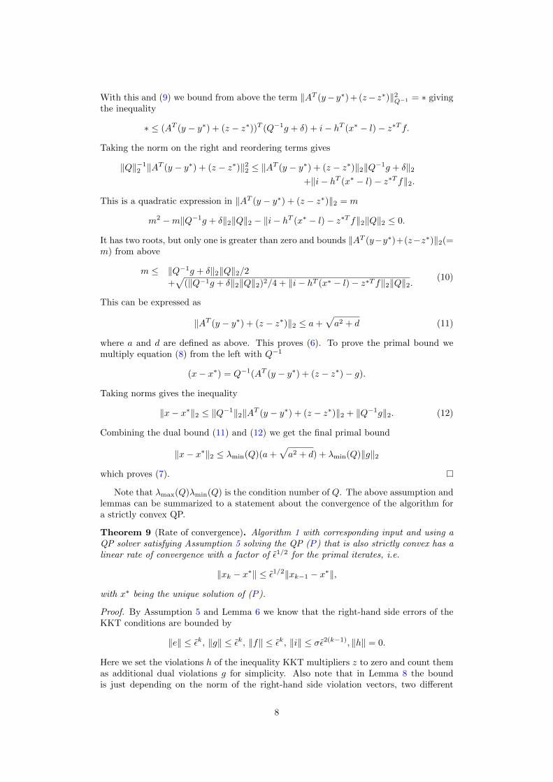
Note that λmax(Q)λmin(Q) is the condition number of Q. The above assumption andlemmas can be summarized to a statement about the convergence of the algorithm fora strictly convex QP.
Theorem 9 (Rate of convergence). Algorithm 1 with corresponding input and using aQP solver satisfying Assumption 5 solving the QP (P ) that is also strictly convex has alinear rate of convergence with a factor of ε1/2 for the primal iterates, i.e.
‖xk − x∗‖ ≤ ε1/2‖xk−1 − x∗‖,
with x∗ being the unique solution of (P ).
Proof. By Assumption 5 and Lemma 6 we know that the right-hand side errors of theKKT conditions are bounded by
‖e‖ ≤ εk, ‖g‖ ≤ εk, ‖f‖ ≤ εk, ‖i‖ ≤ σε2(k−1), ‖h‖ = 0.
Here we set the violations h of the inequality KKT multipliers z to zero and count themas additional dual violations g for simplicity. Also note that in Lemma 8 the boundis just depending on the norm of the right-hand side violation vectors, two different
8
violation vectors with the same norm give the same bound. Therefore we just considerthe norms. Combining the above with Lemma 8 we get
‖xk − x∗‖ ≤ c1εk +√c2εk + c3ε2k
for the primal iterate in iteration k with constants
c1 = λmin(Q)λmax(Q)(
( 1λmax(Q) + λmin(Q)
2 ) + 1(2σmin(A)
)c2 = λmax(Q)‖z∗‖c3 = (c1 − λmin(Q))2 + λmax(Q)σ/ε2.
Looking at the quotient
‖xk − x∗‖‖xk−1 − x∗‖
≤ c1εk +
√c2εk + c3ε2k
c1εk−1 +√c2εk−1 + c3ε2(k−1)
and seeing that
‖xk − x∗‖‖xk−1 − x∗‖
≤ εk/2(c1εk/2 +
√c2 + c3εk)
ε(k−1)/2(c1ε(k−1)/2 +√c2 + c3εk−1)
= ε1/2γk
with γk ≤ 1 proves the result.
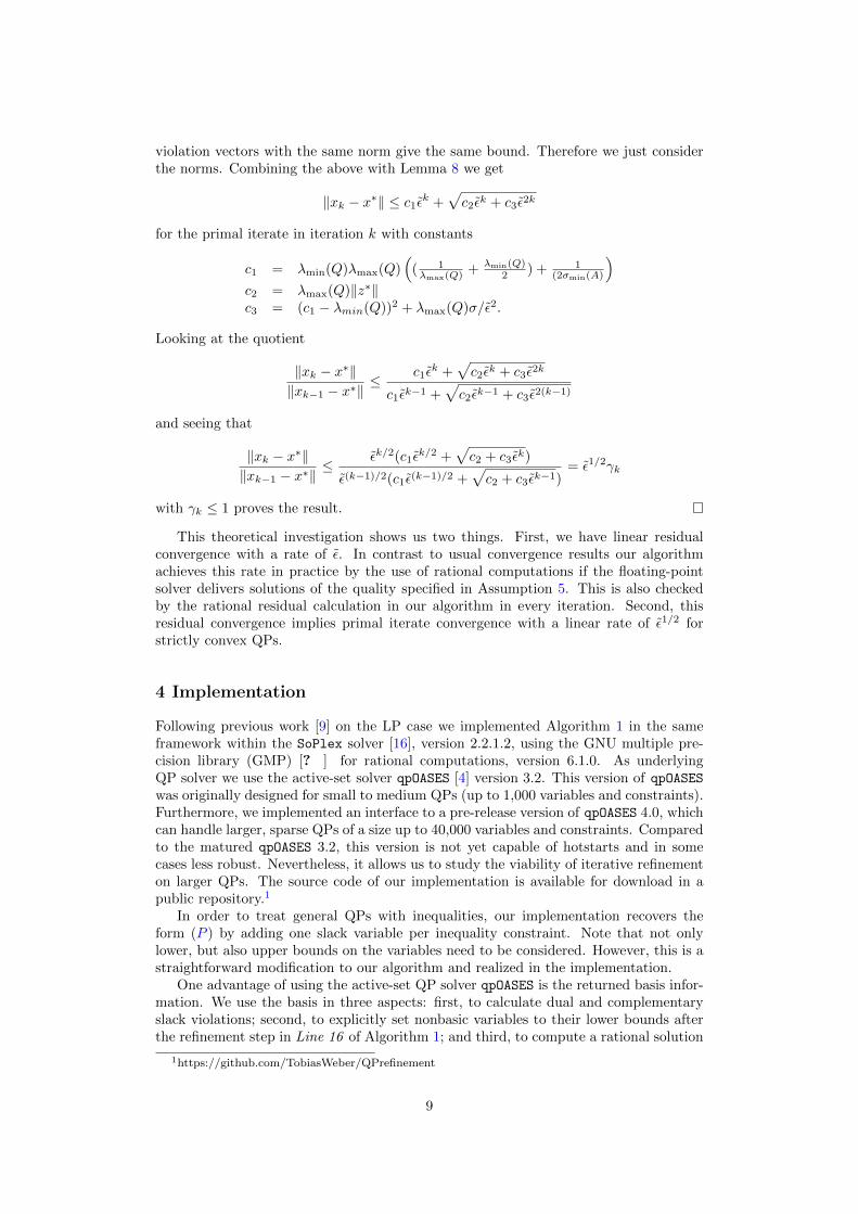
This theoretical investigation shows us two things. First, we have linear residualconvergence with a rate of ε. In contrast to usual convergence results our algorithmachieves this rate in practice by the use of rational computations if the floating-pointsolver delivers solutions of the quality specified in Assumption 5. This is also checkedby the rational residual calculation in our algorithm in every iteration. Second, thisresidual convergence implies primal iterate convergence with a linear rate of ε1/2 forstrictly convex QPs.
4 Implementation
Following previous work [9] on the LP case we implemented Algorithm 1 in the sameframework within the SoPlex solver [16], version 2.2.1.2, using the GNU multiple pre-cision library (GMP) [? ] for rational computations, version 6.1.0. As underlyingQP solver we use the active-set solver qpOASES [4] version 3.2. This version of qpOASESwas originally designed for small to medium QPs (up to 1,000 variables and constraints).Furthermore, we implemented an interface to a pre-release version of qpOASES 4.0, whichcan handle larger, sparse QPs of a size up to 40,000 variables and constraints. Comparedto the matured qpOASES 3.2, this version is not yet capable of hotstarts and in somecases less robust. Nevertheless, it allows us to study the viability of iterative refinementon larger QPs. The source code of our implementation is available for download in apublic repository.1
In order to treat general QPs with inequalities, our implementation recovers theform (P ) by adding one slack variable per inequality constraint. Note that not onlylower, but also upper bounds on the variables need to be considered. However, this is astraightforward modification to our algorithm and realized in the implementation.
One advantage of using the active-set QP solver qpOASES is the returned basis infor-mation. We use the basis in three aspects: first, to calculate dual and complementaryslack violations; second, to explicitly set nonbasic variables to their lower bounds afterthe refinement step in Line 16 of Algorithm 1; and third, to compute a rational solution
1https://github.com/TobiasWeber/QPrefinement
9
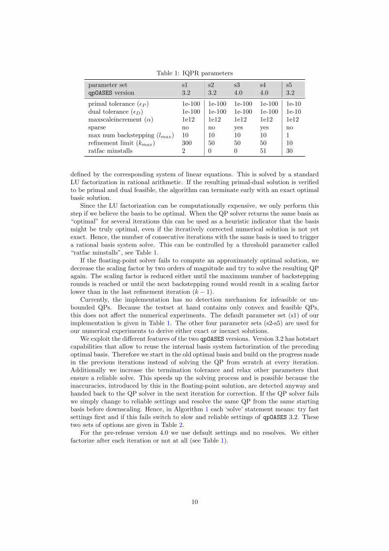
Table 1: IQPR parameters
parameter set s1 s2 s3 s4 s5qpOASES version 3.2 3.2 4.0 4.0 3.2
primal tolerance (εP ) 1e-100 1e-100 1e-100 1e-100 1e-10dual tolerance (εD) 1e-100 1e-100 1e-100 1e-100 1e-10maxscaleincrement (α) 1e12 1e12 1e12 1e12 1e12sparse no no yes yes nomax num backstepping (lmax) 10 10 10 10 1refinement limit (kmax) 300 50 50 50 10ratfac minstalls 2 0 0 51 30
defined by the corresponding system of linear equations. This is solved by a standardLU factorization in rational arithmetic. If the resulting primal-dual solution is verifiedto be primal and dual feasible, the algorithm can terminate early with an exact optimalbasic solution.
Since the LU factorization can be computationally expensive, we only perform thisstep if we believe the basis to be optimal. When the QP solver returns the same basis as“optimal” for several iterations this can be used as a heuristic indicator that the basismight be truly optimal, even if the iteratively corrected numerical solution is not yetexact. Hence, the number of consecutive iterations with the same basis is used to triggera rational basis system solve. This can be controlled by a threshold parameter called“ratfac minstalls”, see Table 1.
If the floating-point solver fails to compute an approximately optimal solution, wedecrease the scaling factor by two orders of magnitude and try to solve the resulting QPagain. The scaling factor is reduced either until the maximum number of backsteppingrounds is reached or until the next backstepping round would result in a scaling factorlower than in the last refinement iteration (k − 1).
Currently, the implementation has no detection mechanism for infeasible or un-bounded QPs. Because the testset at hand contains only convex and feasible QPs,this does not affect the numerical experiments. The default parameter set (s1) of ourimplementation is given in Table 1. The other four parameter sets (s2-s5) are used forour numerical experiments to derive either exact or inexact solutions.
We exploit the different features of the two qpOASES versions. Version 3.2 has hotstartcapabilities that allow to reuse the internal basis system factorization of the precedingoptimal basis. Therefore we start in the old optimal basis and build on the progress madein the previous iterations instead of solving the QP from scratch at every iteration.Additionally we increase the termination tolerance and relax other parameters thatensure a reliable solve. This speeds up the solving process and is possible because theinaccuracies, introduced by this in the floating-point solution, are detected anyway andhanded back to the QP solver in the next iteration for correction. If the QP solver failswe simply change to reliable settings and resolve the same QP from the same startingbasis before downscaling. Hence, in Algorithm 1 each ‘solve’ statement means: try fastsettings first and if this fails switch to slow and reliable settings of qpOASES 3.2. Thesetwo sets of options are given in Table 2.
For the pre-release version 4.0 we use default settings and no resolves. We eitherfactorize after each iteration or not at all (see Table 1).
10

Table 2: qpOASES options (version 3.2)
Option Fast Reliable
Standard settings set MPC ReliableNZCTests enabled enabled (default)DriftCorrection enabled enabled (default)Ramping enabled enabled (default)terminationTolerance 1e-3 1.1105e-9 (default)numRefinementSteps 0 (default) 10enableFullLITests 0 0
5 Numerical results
For the numerical experiments the standard testset of Maros and Meszaros [13] is used.It contains 138 convex QPs that feature between two and about 90,000 variables. Thenumber of constraints varies from one to about 180,000 and the number of nonzerosranges between two and about 550,000.
We perform two different experiments. The goal of the first experiment is to solveas many QPs from the testset as precisely as possible in order to analyze the iterativerefinement procedure computationally and to provide exact reference solutions for futureresearch on QP solvers. In the second experiment we want to compare qpOASES (version3.2, no QP refinement, one solve, default settings) to low accuracy refinement (lowtolerance of 1e-10 in Algorithm 1, using also qpOASES 3.2). This allows us to investigatewhether refinement could also be beneficial in cases that do not require extremely highaccuracy, but a strictly guaranteed solution tolerance in shortest possible runtime.
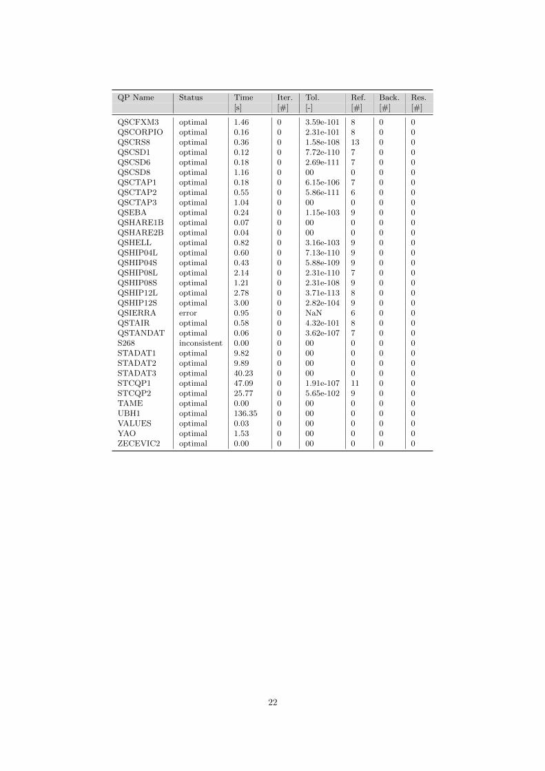
Experiment 1 We use the three different parameter sets (s2-s4) given in Table 1 tocalculate exact solutions. The first set (s2) contains a primal and dual terminationtolerance of 1e-100, enables rational factorization in every iteration, and allows for 50refinements and 10 backsteppings using a dense QP formulation with qpOASES version3.2. In contrast the other two sets (s3, s4) with qpOASES version 4.0 use a sparse QPformulation, either with factorization in every iteration or without factorization.
Table 3 states for each setting the number of instances which it solved exactly, forwhich tolerance 1e-100 was reached, and for which it failed to produce a high-precisionsolution. In total these three strategies could solve 91 out of the 138 QPs in the testsetexactly and 39 instances within tolerance 1e-100. For eight instances no high-precisionsolution was computed. These “virtual best” results stated in the fifth column considerfor each QP the result of the individual parameter sets that resulted in the smallestviolation. It should be emphasized that for each of the three parameter sets there existsat least one instance for which it produced the most accurate solution.
The last column reports the average number of nonzeros of the QPs in the three“virtual best” categories. This suggests that for problems with less nonzeros a higheraccuracy was reached. Furthermore, one sees that the entries in the second column (sets2) do not sum to 138 because with the dense QP formulation some of the problems donot return from the cluster due to memory limitations. Hence the set s2 fails in total on32 instances. For the parameter set s4 without rational factorization we see that one QPis solved by chance exactly while for all others the algorithm terminates with violationsgreater zero.
In order to solve the 197 (=33+45+118) QPs to high precision the algorithm neededon average 8.84 refinements. This confirms the linear convergence because we boundedthe increase of the scaling factor in each iteration by α = 1012 and terminate afterreaching a tolerance of 10−100. If qpOASES would consistently return solutions with an
11
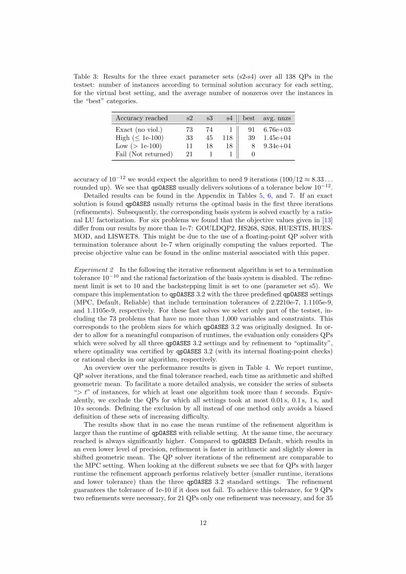
Table 3: Results for the three exact parameter sets (s2-s4) over all 138 QPs in thetestset: number of instances according to terminal solution accuracy for each setting,for the virtual best setting, and the average number of nonzeros over the instances inthe “best” categories.
Accuracy reached s2 s3 s4 best avg. nnzs
Exact (no viol.) 73 74 1 91 6.76e+03High (≤ 1e-100) 33 45 118 39 1.45e+04Low (> 1e-100) 11 18 18 8 9.34e+04Fail (Not returned) 21 1 1 0
accuracy of 10−12 we would expect the algorithm to need 9 iterations (100/12 ≈ 8.33 . . .rounded up). We see that qpOASES usually delivers solutions of a tolerance below 10−12.
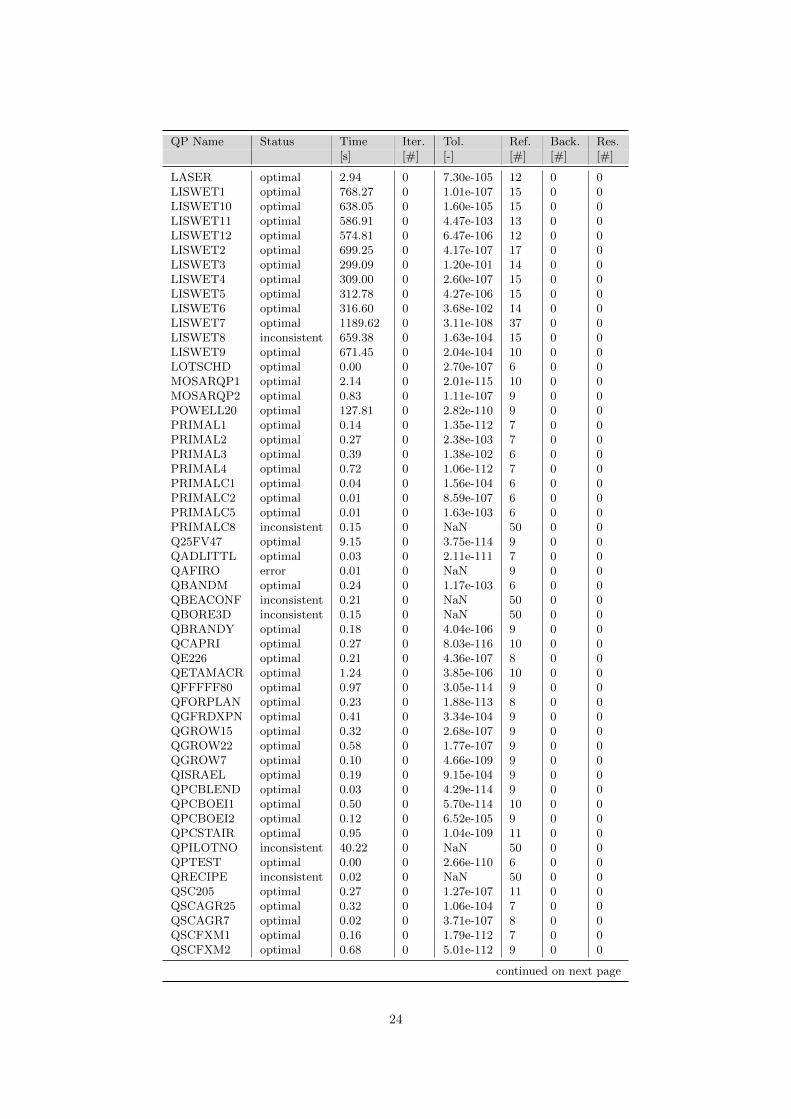
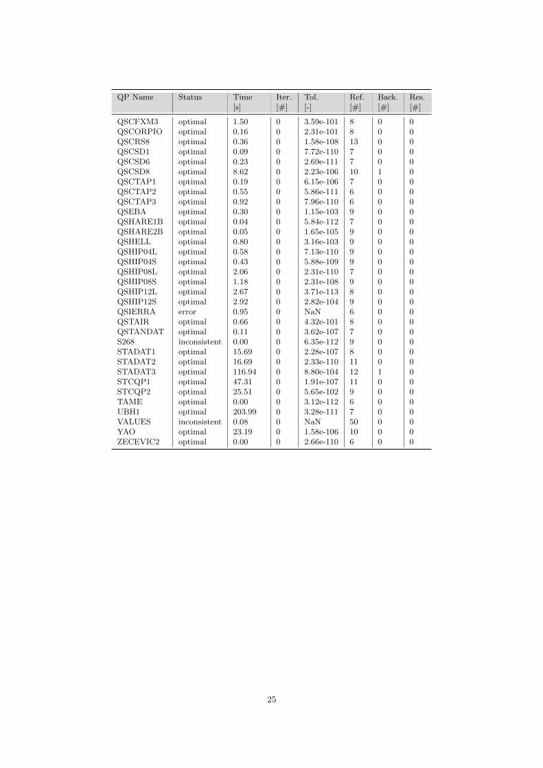
Detailed results can be found in the Appendix in Tables 5, 6, and 7. If an exactsolution is found qpOASES usually returns the optimal basis in the first three iterations(refinements). Subsequently, the corresponding basis system is solved exactly by a ratio-nal LU factorization. For six problems we found that the objective values given in [13]differ from our results by more than 1e-7: GOULDQP2, HS268, S268, HUESTIS, HUES-MOD, and LISWET8. This might be due to the use of a floating-point QP solver withtermination tolerance about 1e-7 when originally computing the values reported. Theprecise objective value can be found in the online material associated with this paper.
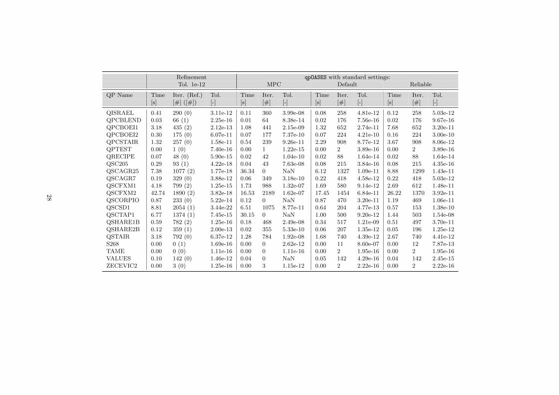
Experiment 2 In the following the iterative refinement algorithm is set to a terminationtolerance 10−10 and the rational factorization of the basis system is disabled. The refine-ment limit is set to 10 and the backstepping limit is set to one (parameter set s5). Wecompare this implementation to qpOASES 3.2 with the three predefined qpOASES settings(MPC, Default, Reliable) that include termination tolerances of 2.2210e-7, 1.1105e-9,and 1.1105e-9, respectively. For these fast solves we select only part of the testset, in-cluding the 73 problems that have no more than 1,000 variables and constraints. Thiscorresponds to the problem sizes for which qpOASES 3.2 was originally designed. In or-der to allow for a meaningful comparison of runtimes, the evaluation only considers QPswhich were solved by all three qpOASES 3.2 settings and by refinement to “optimality”,where optimality was certified by qpOASES 3.2 (with its internal floating-point checks)or rational checks in our algorithm, respectively.
An overview over the performance results is given in Table 4. We report runtime,QP solver iterations, and the final tolerance reached, each time as arithmetic and shiftedgeometric mean. To facilitate a more detailed analysis, we consider the series of subsets“> t” of instances, for which at least one algorithm took more than t seconds. Equiv-alently, we exclude the QPs for which all settings took at most 0.01 s, 0.1 s, 1 s, and10 s seconds. Defining the exclusion by all instead of one method only avoids a biaseddefinition of these sets of increasing difficulty.
The results show that in no case the mean runtime of the refinement algorithm islarger than the runtime of qpOASES with reliable setting. At the same time, the accuracyreached is always significantly higher. Compared to qpOASES Default, which results inan even lower level of precision, refinement is faster in arithmetic and slightly slower inshifted geometric mean. The QP solver iterations of the refinement are comparable tothe MPC setting. When looking at the different subsets we see that for QPs with largerruntime the refinement approach performs relatively better (smaller runtime, iterationsand lower tolerance) than the three qpOASES 3.2 standard settings. The refinementguarantees the tolerance of 1e-10 if it does not fail. To achieve this tolerance, for 9 QPstwo refinements were necessary, for 21 QPs only one refinement was necessary, and for 35
12

Table 4: Performance comparison for inexact solves (runtimes are in seconds).
IQPR s5 qpOASES with standard settings:Measure subset MPC Default Reliable
Time: arith. mean(% rat. time)
all 2.54 (0.16) 1.03 2.77 19.58> 0.01 3.25 (0.16) 1.32 3.55 25.08> 0.1 4.02 (0.12) 1.64 4.40 31.07> 1 5.66 (0.12) 2.31 6.27 44.60> 10 7.19 (0.11) 2.77 9.06 69.39
Time: shifted geo.mean, shift=0.01(% rat. time)
all 0.16 (1.68) 0.08 0.10 0.16> 0.01 0.36 (0.98) 0.15 0.20 0.36> 0.1 0.60 (0.54) 0.24 0.32 0.64> 1 0.94 (0.49) 0.43 0.67 1.66> 10 0.54 (1.00) 0.26 0.51 1.51
QP solver iterations:arith. mean
all 283.75 260.53 389.92 386.96> 0.01 362.16 332.44 496.91 493.09> 0.1 436.67 400.96 591.35 586.96> 1 520.91 479.38 765.59 761.56> 10 353.00 348.25 837.15 832.75
QP solver iterations:shifted geo. mean,shift=1
all 38.43 36.86 62.08 61.68> 0.01 85.18 80.86 113.98 112.72> 0.1 108.12 101.95 124.46 123.05> 1 105.41 100.22 144.20 142.88> 10 36.21 35.23 69.62 69.39
Tolerance:arith. mean
all 1.49e-12 1.29e-08 1.10e-08 2.28e-09> 0.01 1.91e-12 1.65e-08 1.40e-08 2.92e-09> 0.1 2.10e-12 2.03e-08 1.74e-08 3.62e-09> 1 8.89e-13 2.21e-08 2.48e-08 4.98e-09> 10 5.29e-14 1.42e-08 3.92e-08 7.32e-09
Tolcerance:shifted geo. mean,shift=1e-20
all 1.29e-16 2.14e-12 1.62e-15 4.34e-15> 0.01 8.71e-17 1.00e-11 4.91e-15 1.13e-14> 0.1 3.57e-17 8.45e-12 6.92e-15 2.10e-14> 1 1.94e-17 1.08e-12 2.44e-15 6.02e-15> 10 9.36e-19 6.86e-15 3.21e-16 2.45e-16
instances no refinement was necessary at all. The rational computation overhead statedin brackets after the runtime and is well below 2%. The details are shown in Table 8in the Appendix. Also note that due to exclusion of fails (which mainly occur with theqpOASES MPC settings) the summarized results have a slight bias towards qpOASES.
6 Conclusion
We presented a novel refinement algorithm and proved linear convergence of residualsand errors. Notably, this theoretical convergence result also carries over to our imple-mentation due to the use of exact rational calculations. We provided high-precisionsolutions for most of the QPs in the Maros and Meszaros testset, correcting inaccuraciesin optimal solution values reported in the literature. This is beneficial for future researchon QP solvers that are evaluated on this testset.
13
In a second experiment we saw that iterative refinement provides proven tolerancesolutions with smaller or equal computation times compared to qpOASES with “Reliable”solver settings. It can therefore be used as tool to increase the reliability and speed ofstandard floating-point QP solvers.
If optimal solutions are needed for rigorous reasoning or to make decisions in thereal world the algorithm presented is useful because it is able to fully ensure a specifiedtolerance. This tolerance then can be adapted to the necessity of the application athand. At the same time this comes with little overhead in rational computation time,which is important for practical applications.
Regarding algorithmic research and solver development, our framework also providesthe possibility to compare different floating-point QP solvers by looking at the numberof refinements needed with each solver to detect optimal bases or solutions of a specifiedtolerance as a measure for solver accuracy. Solver robustness can be checked preciselybecause violations are computed in rational precision. In the future, the implementationshould be extended for the detection of unbounded or infeasible QPs. Also one couldtry more general variable transformations, e.g. having a different scaling factor for eachvariable. As a concluding remark, we hope that the idea of checking numerical resultsof floating-point algorithms in exact or safe arithmetic will become a future trend whenapplying or analyzing numerical algorithms.
References
[1] K. P. Bennett and C. Campbell. Support vector machines: hype or hallelujah? AcmSigkdd Explorations Newsletter, 2(2):1–13, 2000.
[2] CPLEX, IBM ILOG. 12.7 user’s manual. URL https://www.ibm.com, 2016.
[3] Z. Dostal. Optimal Quadratic Programming Algorithms: With Applications to Varia-tional Inequalities. Springer Publishing Company, Incorporated, 1st edition, 2009. ISBN0387848053, 9780387848051.
[4] H. J. Ferreau, C. Kirches, A. Potschka, H. G. Bock, and M. Diehl. qpOASES: A parametricactive-set algorithm for quadratic programming. Mathematical Programming Computation,6(4):327–363, 2014.
[5] R. Fletcher and S. Leyffer. User manual for filtersqp. Numerical Analysis Report NA/181,Department of Mathematics, University of Dundee, Dundee, Scotland, 1998.
[6] B. Gartner and S. Schonherr. An efficient, exact, and generic quadratic programmingsolver for geometric optimization. In Proceedings of the sixteenth annual symposium onComputational geometry, pages 110–118. ACM, 2000.
[7] P. E. Gill, W. Murray, and M. A. Saunders. User’s guide for QPOPT 1.0: A Fortranpackage for quadratic programming. Technical report, 1995.
[8] A. M. Gleixner. Exact and fast algorithms for mixed-integer nonlinear programming. PhDthesis, Technische Universitat Berlin, 2015.
[9] A. M. Gleixner, D. E. Steffy, and K. Wolter. Improving the accuracy of linear programmingsolvers with iterative refinement. In ISSAC 2012. Proceedings of the 37th InternationalSymposium on Symbolic and Algebraic Computation, pages 187–194. ACM, 2012.
[10] D. Goldfarb and A. Idnani. Dual and primal-dual methods for solving strictly convexquadratic programs. In Numerical Analysis, pages 226–239. Springer, 1982.
[11] I. Gurobi Optimization. Gurobi optimizer reference manual. Technical Report Version 7.5,2017. URL URLhttp://www.gurobi.com.
[12] M. Hladık. Interval linear programming: A survey. Linear programming—new frontiers intheory and applications, pages 85–120, 2012.
[13] I. Maros and C. Meszaros. A repository of convex quadratic programming problems.Optimization Methods and Software, 11(1-4):671–681, 1999.
[14] J. H. Wilkinson. Rounding errors in algebraic processes. In IFIP Congress, pages 44–53,1959.
14

[15] P. Wolfe. The simplex method for quadratic programming. Econometrica: Journal of theEconometric Society, pages 382–398, 1959.
[16] R. Wunderling. Paralleler und Objektorientierter Simplex-Algorithmus. PhD thesis, Tech-nische Universitat Berlin, 1996.
15

Appendix
16
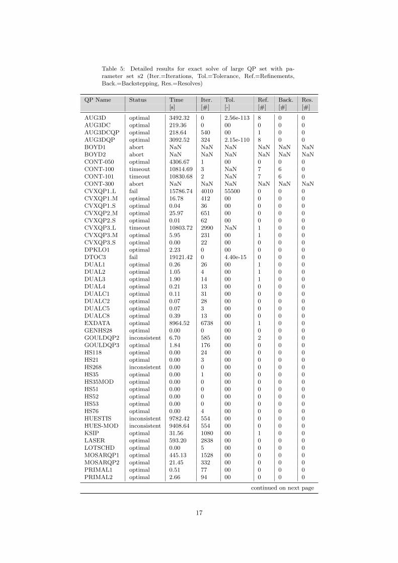
Table 5: Detailed results for exact solve of large QP set with pa-rameter set s2 (Iter.=Iterations, Tol.=Tolerance, Ref.=Refinements,Back.=Backstepping, Res.=Resolves)
QP Name Status Time Iter. Tol. Ref. Back. Res.[s] [#] [-] [#] [#] [#]
AUG3D optimal 3492.32 0 2.56e-113 8 0 0AUG3DC optimal 219.36 0 00 0 0 0AUG3DCQP optimal 218.64 540 00 1 0 0AUG3DQP optimal 3092.52 324 2.15e-110 8 0 0BOYD1 abort NaN NaN NaN NaN NaN NaNBOYD2 abort NaN NaN NaN NaN NaN NaNCONT-050 optimal 4306.67 1 00 0 0 0CONT-100 timeout 10814.69 3 NaN 7 6 0CONT-101 timeout 10830.68 2 NaN 7 6 0CONT-300 abort NaN NaN NaN NaN NaN NaNCVXQP1 L fail 15786.74 4010 55500 0 0 0CVXQP1 M optimal 16.78 412 00 0 0 0CVXQP1 S optimal 0.04 36 00 0 0 0CVXQP2 M optimal 25.97 651 00 0 0 0CVXQP2 S optimal 0.01 62 00 0 0 0CVXQP3 L timeout 10803.72 2990 NaN 1 0 0CVXQP3 M optimal 5.95 231 00 1 0 0CVXQP3 S optimal 0.00 22 00 0 0 0DPKLO1 optimal 2.23 0 00 0 0 0DTOC3 fail 19121.42 0 4.40e-15 0 0 0DUAL1 optimal 0.26 26 00 1 0 0DUAL2 optimal 1.05 4 00 1 0 0DUAL3 optimal 1.90 14 00 1 0 0DUAL4 optimal 0.21 13 00 0 0 0DUALC1 optimal 0.11 31 00 0 0 0DUALC2 optimal 0.07 28 00 0 0 0DUALC5 optimal 0.07 3 00 0 0 0DUALC8 optimal 0.39 13 00 0 0 0EXDATA optimal 8964.52 6738 00 1 0 0GENHS28 optimal 0.00 0 00 0 0 0GOULDQP2 inconsistent 6.70 585 00 2 0 0GOULDQP3 optimal 1.84 176 00 0 0 0HS118 optimal 0.00 24 00 0 0 0HS21 optimal 0.00 3 00 0 0 0HS268 inconsistent 0.00 0 00 0 0 0HS35 optimal 0.00 1 00 0 0 0HS35MOD optimal 0.00 0 00 0 0 0HS51 optimal 0.00 0 00 0 0 0HS52 optimal 0.00 0 00 0 0 0HS53 optimal 0.00 0 00 0 0 0HS76 optimal 0.00 4 00 0 0 0HUESTIS inconsistent 9782.42 554 00 0 0 0HUES-MOD inconsistent 9408.64 554 00 0 0 0KSIP optimal 31.56 1080 00 1 0 0LASER optimal 593.20 2838 00 0 0 0LOTSCHD optimal 0.00 5 00 0 0 0MOSARQP1 optimal 445.13 1528 00 0 0 0MOSARQP2 optimal 21.45 332 00 0 0 0PRIMAL1 optimal 0.51 77 00 0 0 0PRIMAL2 optimal 2.66 94 00 0 0 0
continued on next page
17

QP Name Status Time Iter. Tol. Ref. Back. Res.[s] [#] [-] [#] [#] [#]
PRIMAL3 optimal 4.37 117 00 0 0 0PRIMAL4 optimal 21.04 88 00 0 0 0PRIMALC1 optimal 0.11 234 00 0 0 0PRIMALC2 optimal 0.17 237 00 0 0 0PRIMALC5 optimal 0.23 288 00 0 0 0PRIMALC8 optimal 1.86 515 00 0 0 0Q25FV47 optimal 372.89 7362 00 0 0 0QADLITTL optimal 0.09 232 00 0 0 0QAFIRO optimal 0.00 30 6.15e-107 7 0 0QBANDM optimal 2.93 1164 00 0 0 0QBEACONF optimal 0.91 305 8.07e-110 9 0 0QBORE3D optimal 0.87 536 1.97e-111 9 0 0QBRANDY optimal 1.07 450 4.86e-108 8 0 0QCAPRI optimal 2.95 1051 1.76e-106 8 0 1QE226 optimal 4.66 1396 1.71e-101 8 0 0QETAMACR optimal 4.75 559 5.17e-102 9 0 0QFFFFF80 error 44.78 1079 NaN 9 3 5QFORPLAN optimal 2.20 1174 00 0 0 0QGFRDXPN optimal 29.31 1423 00 0 0 0QGROW15 optimal 8.11 632 2.54e-105 8 0 0QGROW22 optimal 32.92 944 2.86e-109 10 0 0QGROW7 optimal 0.83 298 7.99e-112 8 0 0QISRAEL optimal 0.38 290 00 0 0 0QPCBLEND optimal 0.06 66 00 1 0 0QPCBOEI1 optimal 3.64 435 00 1 0 0QPCBOEI2 optimal 0.23 175 00 0 0 0QPCSTAIR optimal 2.76 257 00 0 0 0QPILOTNO optimal 573.39 7442 1.99e-102 13 0 0QPTEST optimal 0.00 1 00 0 0 0QRECIPE optimal 0.07 48 9.74e-110 7 0 0QSC205 optimal 0.78 106 1.50e-107 8 0 0QSCAGR25 optimal 6.17 1076 00 0 0 0QSCAGR7 optimal 0.14 329 00 0 0 0QSCFXM1 optimal 8.05 801 1.13e-112 11 0 1QSCFXM2 optimal 81.35 1891 1.25e-108 10 0 0QSCFXM3 optimal 319.56 2510 1.77e-107 10 0 0QSCORPIO optimal 2.43 233 1.08e-101 7 0 0QSCRS8 optimal 49.19 2016 00 1 0 0QSCSD1 optimal 8.78 2054 00 1 0 0QSCSD6 optimal 106.56 6015 4.11e-101 9 0 0QSCSD8 optimal 1560.58 19564 2.22e-104 8 0 0QSCTAP1 optimal 11.22 1474 2.63e-103 8 0 0QSCTAP2 optimal 860.50 3862 6.58e-113 10 0 0QSCTAP3 optimal 2156.04 6964 2.49e-101 8 0 0QSEBA optimal 26.60 1677 00 0 0 0QSHARE1B optimal 0.51 782 00 1 0 0QSHARE2B optimal 0.19 359 00 1 0 0QSHELL optimal 119.14 3306 7.69e-109 9 0 1QSHIP04L optimal 398.29 4847 1.67e-106 8 0 0QSHIP04S optimal 130.24 2908 2.11e-107 8 0 1QSHIP08L optimal 3711.96 7911 3.68e-102 8 0 0QSHIP08S optimal 738.69 3997 1.86e-110 9 0 0QSHIP12L optimal 8386.98 9765 4.22e-109 8 0 1QSHIP12S optimal 1176.10 3821 2.30e-109 8 0 0
continued on next page
18

QP Name Status Time Iter. Tol. Ref. Back. Res.[s] [#] [-] [#] [#] [#]
QSIERRA error 996.02 6421 NaN 0 0 1QSTAIR optimal 13.43 1136 7.18e-111 9 1 2QSTANDAT optimal 26.45 1222 00 3 0 0S268 inconsistent 0.00 0 00 0 0 0STADAT1 optimal 8013.74 9995 00 0 0 0STADAT2 optimal 6437.65 6527 00 1 0 0STADAT3 timeout 18337.54 2144 NaN 0 0 1STCQP1 optimal 604.13 353 1.05e-103 7 0 0STCQP2 optimal 419.60 105 00 0 0 0TAME optimal 0.00 0 00 0 0 0VALUES optimal 0.10 143 00 2 0 1YAO optimal 659.58 2001 00 1 0 0ZECEVIC2 optimal 0.00 3 00 0 0 0
19

Table 6: Detailed results for exact solve of large QP set with pa-rameter set s3 (Iter.=Iterations, Tol.=Tolerance, Ref.=Refinements,Back.=Backstepping, Res.=Resolves)
QP Name Status Time Iter. Tol. Ref. Back. Res.[s] [#] [-] [#] [#] [#]
AUG2D timeout 10865.56 0 NaN 1 0 0AUG2DC timeout 10836.45 0 NaN 6 5 0AUG2DCQP optimal 155.71 0 1.47e-101 8 0 0AUG2DQP timeout 10801.84 0 NaN 6 5 0AUG3D error 7.60 0 NaN 1 0 0AUG3DC optimal 112.66 0 00 0 0 0AUG3DCQP optimal 19.50 0 00 0 0 0AUG3DQP optimal 7.62 0 00 0 0 0BOYD2 abort NaN NaN NaN NaN NaN NaNCONT-050 optimal 4224.16 0 00 0 0 0CONT-100 timeout 10806.77 0 NaN 7 6 0CONT-101 timeout 10809.28 0 NaN 7 6 0CONT-200 timeout 10802.04 0 NaN 7 6 0CONT-201 timeout 10801.56 0 NaN 7 6 0CONT-300 abort NaN NaN NaN NaN NaN NaNCVXQP1 L optimal 6641.26 0 1.90e-101 9 0 0CVXQP1 M optimal 8.02 0 00 0 0 0CVXQP1 S optimal 0.02 0 00 0 0 0CVXQP2 L timeout 11041.07 0 NaN 5 4 0CVXQP2 M optimal 19.13 0 00 0 0 0CVXQP2 S optimal 0.03 0 2.25e-110 7 0 0CVXQP3 L error 7587.33 0 NaN 6 1 0CVXQP3 M optimal 2.33 0 00 0 0 0CVXQP3 S reached 0.48 0 NaN 50 0 0DPKLO1 optimal 2.26 0 00 0 0 0DTOC3 optimal 2611.08 0 00 0 0 0DUAL1 optimal 0.15 0 00 0 0 0DUAL2 optimal 0.53 0 00 0 0 0DUAL3 optimal 0.78 0 00 0 0 0DUAL4 optimal 0.20 0 00 0 0 0DUALC1 optimal 0.07 0 00 0 0 0DUALC2 optimal 0.05 0 00 0 0 0DUALC5 optimal 0.08 0 00 0 0 0DUALC8 optimal 0.19 0 00 0 0 0EXDATA optimal 1407.82 0 00 0 0 0GENHS28 optimal 0.00 0 00 0 0 0GOULDQP2 inconsistent 0.24 0 1.50e-110 7 0 0GOULDQP3 optimal 0.11 0 00 0 0 0HS118 optimal 0.00 0 00 0 0 0HS21 optimal 0.00 0 00 0 0 0HS268 inconsistent 0.00 0 00 0 0 0HS35 optimal 0.00 0 00 0 0 0HS35MOD optimal 0.00 0 00 0 0 0HS51 optimal 0.00 0 3.14e-108 6 0 0HS52 optimal 0.00 0 00 0 0 0HS53 optimal 0.00 0 00 0 0 0HS76 optimal 0.00 0 00 0 0 0HUESTIS inconsistent 40.17 0 00 0 0 0HUES-MOD inconsistent 21.27 0 00 0 0 0KSIP optimal 2.38 0 00 0 0 0
continued on next page
20

QP Name Status Time Iter. Tol. Ref. Back. Res.[s] [#] [-] [#] [#] [#]
LASER optimal 41.47 0 00 0 0 0LISWET1 optimal 57.85 0 00 0 0 0LISWET10 optimal 645.20 0 1.60e-105 15 0 0LISWET11 optimal 54.26 0 00 0 0 0LISWET12 optimal 63.22 0 00 0 0 0LISWET2 optimal 704.57 0 4.17e-107 17 0 0LISWET3 optimal 306.45 0 1.20e-101 14 0 0LISWET4 optimal 317.64 0 2.60e-107 15 0 0LISWET5 optimal 324.42 0 4.27e-106 15 0 0LISWET6 optimal 325.27 0 3.68e-102 14 0 0LISWET7 optimal 54.87 0 00 0 0 0LISWET8 inconsistent 56.98 0 00 0 0 0LISWET9 optimal 64.09 0 00 0 0 0LOTSCHD optimal 0.00 0 00 0 0 0MOSARQP1 optimal 0.96 0 00 0 0 0MOSARQP2 optimal 0.52 0 00 0 0 0POWELL20 optimal 44.65 0 00 0 0 0PRIMAL1 optimal 0.20 0 00 0 0 0PRIMAL2 optimal 0.71 0 00 0 0 0PRIMAL3 optimal 1.45 0 00 0 0 0PRIMAL4 optimal 0.76 0 00 0 0 0PRIMALC1 optimal 0.01 0 00 0 0 0PRIMALC2 optimal 0.01 0 00 0 0 0PRIMALC5 optimal 0.01 0 00 0 0 0PRIMALC8 optimal 0.02 0 00 0 0 0Q25FV47 optimal 9.14 0 3.75e-114 9 0 0QADLITTL optimal 0.01 0 00 0 0 0QAFIRO optimal 0.00 0 00 0 0 0QBANDM optimal 0.20 0 1.17e-103 6 0 0QBEACONF inconsistent 0.16 0 NaN 50 0 0QBORE3D inconsistent 0.18 0 NaN 50 0 0QBRANDY optimal 0.18 0 4.04e-106 9 0 0QCAPRI optimal 0.11 0 00 0 0 0QE226 optimal 0.19 0 4.36e-107 8 0 0QETAMACR optimal 1.24 0 3.85e-106 10 0 0QFFFFF80 optimal 0.99 0 3.05e-114 9 0 0QFORPLAN optimal 0.23 0 1.88e-113 8 0 0QGFRDXPN optimal 0.45 0 3.34e-104 9 0 0QGROW15 optimal 0.37 0 00 0 0 0QGROW22 optimal 0.90 0 00 0 0 0QGROW7 optimal 0.22 0 00 0 0 0QISRAEL optimal 0.11 0 00 0 0 0QPCBLEND optimal 0.03 0 00 0 0 0QPCBOEI1 optimal 0.58 0 5.70e-114 10 0 0QPCBOEI2 optimal 0.10 0 00 0 0 0QPCSTAIR optimal 0.96 0 1.04e-109 11 0 0QPILOTNO inconsistent 40.49 0 NaN 50 0 0QPTEST optimal 0.00 0 00 0 0 0QRECIPE inconsistent 0.04 0 NaN 50 0 0QSC205 optimal 0.30 0 1.27e-107 11 0 0QSCAGR25 optimal 0.32 0 1.06e-104 7 0 0QSCAGR7 optimal 0.02 0 3.71e-107 8 0 0QSCFXM1 optimal 0.20 0 1.79e-112 7 0 0QSCFXM2 optimal 0.73 0 5.01e-112 9 0 0
continued on next page
21
QP Name Status Time Iter. Tol. Ref. Back. Res.[s] [#] [-] [#] [#] [#]
QSCFXM3 optimal 1.46 0 3.59e-101 8 0 0QSCORPIO optimal 0.16 0 2.31e-101 8 0 0QSCRS8 optimal 0.36 0 1.58e-108 13 0 0QSCSD1 optimal 0.12 0 7.72e-110 7 0 0QSCSD6 optimal 0.18 0 2.69e-111 7 0 0QSCSD8 optimal 1.16 0 00 0 0 0QSCTAP1 optimal 0.18 0 6.15e-106 7 0 0QSCTAP2 optimal 0.55 0 5.86e-111 6 0 0QSCTAP3 optimal 1.04 0 00 0 0 0QSEBA optimal 0.24 0 1.15e-103 9 0 0QSHARE1B optimal 0.07 0 00 0 0 0QSHARE2B optimal 0.04 0 00 0 0 0QSHELL optimal 0.82 0 3.16e-103 9 0 0QSHIP04L optimal 0.60 0 7.13e-110 9 0 0QSHIP04S optimal 0.43 0 5.88e-109 9 0 0QSHIP08L optimal 2.14 0 2.31e-110 7 0 0QSHIP08S optimal 1.21 0 2.31e-108 9 0 0QSHIP12L optimal 2.78 0 3.71e-113 8 0 0QSHIP12S optimal 3.00 0 2.82e-104 9 0 0QSIERRA error 0.95 0 NaN 6 0 0QSTAIR optimal 0.58 0 4.32e-101 8 0 0QSTANDAT optimal 0.06 0 3.62e-107 7 0 0S268 inconsistent 0.00 0 00 0 0 0STADAT1 optimal 9.82 0 00 0 0 0STADAT2 optimal 9.89 0 00 0 0 0STADAT3 optimal 40.23 0 00 0 0 0STCQP1 optimal 47.09 0 1.91e-107 11 0 0STCQP2 optimal 25.77 0 5.65e-102 9 0 0TAME optimal 0.00 0 00 0 0 0UBH1 optimal 136.35 0 00 0 0 0VALUES optimal 0.03 0 00 0 0 0YAO optimal 1.53 0 00 0 0 0ZECEVIC2 optimal 0.00 0 00 0 0 0
22
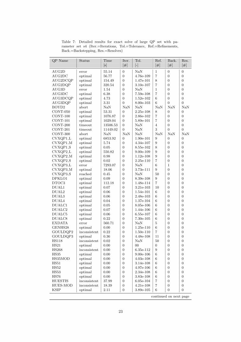
Table 7: Detailed results for exact solve of large QP set with pa-rameter set s4 (Iter.=Iterations, Tol.=Tolerance, Ref.=Refinements,Back.=Backstepping, Res.=Resolves)
QP Name Status Time Iter. Tol. Ref. Back. Res.[s] [#] [-] [#] [#] [#]
AUG2D error 55.14 0 NaN 1 0 0AUG2DC optimal 56.77 0 4.76e-109 7 0 0AUG2DCQP optimal 154.49 0 1.47e-101 8 0 0AUG2DQP optimal 320.54 0 3.10e-107 7 0 0AUG3D error 1.54 0 NaN 1 0 0AUG3DC optimal 6.38 0 7.59e-108 7 0 0AUG3DCQP optimal 4.73 0 1.52e-102 6 0 0AUG3DQP optimal 3.31 0 8.00e-103 6 0 0BOYD2 abort NaN NaN NaN NaN NaN NaNCONT-050 optimal 53.31 0 2.25e-108 8 0 0CONT-100 optimal 1076.87 0 2.86e-102 7 0 0CONT-101 optimal 1029.04 0 5.89e-101 7 0 0CONT-200 timeout 13506.53 0 NaN 4 0 0CONT-201 timeout 11449.02 0 NaN 3 0 0CONT-300 abort NaN NaN NaN NaN NaN NaNCVXQP1 L optimal 6853.92 0 1.90e-101 9 0 0CVXQP1 M optimal 5.74 0 4.34e-107 9 0 0CVXQP1 S optimal 0.05 0 8.55e-102 8 0 0CVXQP2 L optimal 550.82 0 9.00e-109 9 0 0CVXQP2 M optimal 0.98 0 1.12e-108 9 0 0CVXQP2 S optimal 0.02 0 2.25e-110 7 0 0CVXQP3 L error 7293.07 0 NaN 6 1 0CVXQP3 M optimal 18.06 0 3.73e-111 9 0 0CVXQP3 S reached 0.45 0 NaN 50 0 0DPKLO1 optimal 0.09 0 8.39e-108 9 0 0DTOC3 optimal 112.18 0 1.48e-114 7 0 0DUAL1 optimal 0.07 0 3.21e-103 10 0 0DUAL2 optimal 0.06 0 1.54e-101 6 0 0DUAL3 optimal 0.06 0 2.48e-103 6 0 0DUAL4 optimal 0.04 0 1.37e-104 6 0 0DUALC1 optimal 0.05 0 8.05e-106 6 0 0DUALC2 optimal 0.07 0 1.44e-106 6 0 0DUALC5 optimal 0.06 0 6.55e-107 6 0 0DUALC8 optimal 0.22 0 7.30e-105 6 0 0EXDATA error 560.71 0 NaN 5 0 0GENHS28 optimal 0.00 0 1.25e-110 6 0 0GOULDQP2 inconsistent 0.22 0 1.50e-110 7 0 0GOULDQP3 optimal 0.36 0 4.48e-108 11 0 0HS118 inconsistent 0.02 0 NaN 50 0 0HS21 optimal 0.00 0 00 0 0 0HS268 inconsistent 0.00 0 6.35e-112 9 0 0HS35 optimal 0.00 0 9.00e-106 6 0 0HS35MOD optimal 0.00 0 4.03e-108 6 0 0HS51 optimal 0.00 0 3.14e-108 6 0 0HS52 optimal 0.00 0 4.97e-106 6 0 0HS53 optimal 0.00 0 2.34e-108 6 0 0HS76 optimal 0.00 0 3.83e-108 6 0 0HUESTIS inconsistent 37.99 0 6.05e-104 7 0 0HUES-MOD inconsistent 18.39 0 4.21e-108 7 0 0KSIP optimal 2.11 0 3.89e-105 6 0 0
continued on next page
23
QP Name Status Time Iter. Tol. Ref. Back. Res.[s] [#] [-] [#] [#] [#]
LASER optimal 2.94 0 7.30e-105 12 0 0LISWET1 optimal 768.27 0 1.01e-107 15 0 0LISWET10 optimal 638.05 0 1.60e-105 15 0 0LISWET11 optimal 586.91 0 4.47e-103 13 0 0LISWET12 optimal 574.81 0 6.47e-106 12 0 0LISWET2 optimal 699.25 0 4.17e-107 17 0 0LISWET3 optimal 299.09 0 1.20e-101 14 0 0LISWET4 optimal 309.00 0 2.60e-107 15 0 0LISWET5 optimal 312.78 0 4.27e-106 15 0 0LISWET6 optimal 316.60 0 3.68e-102 14 0 0LISWET7 optimal 1189.62 0 3.11e-108 37 0 0LISWET8 inconsistent 659.38 0 1.63e-104 15 0 0LISWET9 optimal 671.45 0 2.04e-104 10 0 0LOTSCHD optimal 0.00 0 2.70e-107 6 0 0MOSARQP1 optimal 2.14 0 2.01e-115 10 0 0MOSARQP2 optimal 0.83 0 1.11e-107 9 0 0POWELL20 optimal 127.81 0 2.82e-110 9 0 0PRIMAL1 optimal 0.14 0 1.35e-112 7 0 0PRIMAL2 optimal 0.27 0 2.38e-103 7 0 0PRIMAL3 optimal 0.39 0 1.38e-102 6 0 0PRIMAL4 optimal 0.72 0 1.06e-112 7 0 0PRIMALC1 optimal 0.04 0 1.56e-104 6 0 0PRIMALC2 optimal 0.01 0 8.59e-107 6 0 0PRIMALC5 optimal 0.01 0 1.63e-103 6 0 0PRIMALC8 inconsistent 0.15 0 NaN 50 0 0Q25FV47 optimal 9.15 0 3.75e-114 9 0 0QADLITTL optimal 0.03 0 2.11e-111 7 0 0QAFIRO error 0.01 0 NaN 9 0 0QBANDM optimal 0.24 0 1.17e-103 6 0 0QBEACONF inconsistent 0.21 0 NaN 50 0 0QBORE3D inconsistent 0.15 0 NaN 50 0 0QBRANDY optimal 0.18 0 4.04e-106 9 0 0QCAPRI optimal 0.27 0 8.03e-116 10 0 0QE226 optimal 0.21 0 4.36e-107 8 0 0QETAMACR optimal 1.24 0 3.85e-106 10 0 0QFFFFF80 optimal 0.97 0 3.05e-114 9 0 0QFORPLAN optimal 0.23 0 1.88e-113 8 0 0QGFRDXPN optimal 0.41 0 3.34e-104 9 0 0QGROW15 optimal 0.32 0 2.68e-107 9 0 0QGROW22 optimal 0.58 0 1.77e-107 9 0 0QGROW7 optimal 0.10 0 4.66e-109 9 0 0QISRAEL optimal 0.19 0 9.15e-104 9 0 0QPCBLEND optimal 0.03 0 4.29e-114 9 0 0QPCBOEI1 optimal 0.50 0 5.70e-114 10 0 0QPCBOEI2 optimal 0.12 0 6.52e-105 9 0 0QPCSTAIR optimal 0.95 0 1.04e-109 11 0 0QPILOTNO inconsistent 40.22 0 NaN 50 0 0QPTEST optimal 0.00 0 2.66e-110 6 0 0QRECIPE inconsistent 0.02 0 NaN 50 0 0QSC205 optimal 0.27 0 1.27e-107 11 0 0QSCAGR25 optimal 0.32 0 1.06e-104 7 0 0QSCAGR7 optimal 0.02 0 3.71e-107 8 0 0QSCFXM1 optimal 0.16 0 1.79e-112 7 0 0QSCFXM2 optimal 0.68 0 5.01e-112 9 0 0
continued on next page
24
QP Name Status Time Iter. Tol. Ref. Back. Res.[s] [#] [-] [#] [#] [#]
QSCFXM3 optimal 1.50 0 3.59e-101 8 0 0QSCORPIO optimal 0.16 0 2.31e-101 8 0 0QSCRS8 optimal 0.36 0 1.58e-108 13 0 0QSCSD1 optimal 0.09 0 7.72e-110 7 0 0QSCSD6 optimal 0.23 0 2.69e-111 7 0 0QSCSD8 optimal 8.62 0 2.23e-106 10 1 0QSCTAP1 optimal 0.19 0 6.15e-106 7 0 0QSCTAP2 optimal 0.55 0 5.86e-111 6 0 0QSCTAP3 optimal 0.92 0 7.96e-110 6 0 0QSEBA optimal 0.30 0 1.15e-103 9 0 0QSHARE1B optimal 0.04 0 5.84e-112 7 0 0QSHARE2B optimal 0.05 0 1.65e-105 9 0 0QSHELL optimal 0.80 0 3.16e-103 9 0 0QSHIP04L optimal 0.58 0 7.13e-110 9 0 0QSHIP04S optimal 0.43 0 5.88e-109 9 0 0QSHIP08L optimal 2.06 0 2.31e-110 7 0 0QSHIP08S optimal 1.18 0 2.31e-108 9 0 0QSHIP12L optimal 2.67 0 3.71e-113 8 0 0QSHIP12S optimal 2.92 0 2.82e-104 9 0 0QSIERRA error 0.95 0 NaN 6 0 0QSTAIR optimal 0.66 0 4.32e-101 8 0 0QSTANDAT optimal 0.11 0 3.62e-107 7 0 0S268 inconsistent 0.00 0 6.35e-112 9 0 0STADAT1 optimal 15.69 0 2.28e-107 8 0 0STADAT2 optimal 16.69 0 2.33e-110 11 0 0STADAT3 optimal 116.94 0 8.80e-104 12 1 0STCQP1 optimal 47.31 0 1.91e-107 11 0 0STCQP2 optimal 25.51 0 5.65e-102 9 0 0TAME optimal 0.00 0 3.12e-112 6 0 0UBH1 optimal 203.99 0 3.28e-111 7 0 0VALUES inconsistent 0.08 0 NaN 50 0 0YAO optimal 23.19 0 1.58e-106 10 0 0ZECEVIC2 optimal 0.00 0 2.66e-110 6 0 0
25
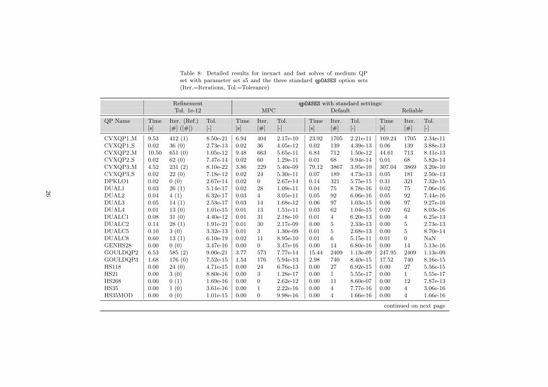
Table 8: Detailed results for inexact and fast solves of medium QPset with parameter set s5 and the three standard qpOASES option sets(Iter.=Iterations, Tol.=Tolerance)
Refinement qpOASES with standard settings:Tol. 1e-12 MPC Default Reliable
QP Name Time Iter. (Ref.) Tol. Time Iter. Tol. Time Iter. Tol. Time Iter. Tol.[s] [#] ([#]) [-] [s] [#] [-] [s] [#] [-] [s] [#] [-]
CVXQP1 M 9.53 412 (1) 8.50e-21 6.94 404 2.17e-10 23.92 1705 2.21e-11 169.24 1705 2.34e-11CVXQP1 S 0.02 36 (0) 2.73e-13 0.02 36 4.05e-12 0.02 139 4.39e-13 0.06 139 3.88e-13CVXQP2 M 10.50 651 (0) 1.05e-12 9.48 663 5.65e-11 6.84 712 1.50e-12 44.61 713 8.41e-13CVXQP2 S 0.02 62 (0) 7.47e-14 0.02 60 1.29e-11 0.01 68 9.94e-14 0.01 68 5.82e-14CVXQP3 M 4.52 231 (2) 8.10e-22 3.86 229 5.40e-09 79.12 3867 3.95e-10 307.04 3869 3.20e-10CVXQP3 S 0.02 22 (0) 7.18e-12 0.02 24 5.30e-11 0.07 189 4.73e-13 0.05 181 2.50e-13DPKLO1 0.02 0 (0) 2.67e-14 0.02 0 2.67e-14 0.14 321 5.75e-15 0.31 321 7.32e-15DUAL1 0.03 26 (1) 5.14e-17 0.02 28 1.09e-11 0.04 75 8.78e-16 0.02 75 7.06e-16DUAL2 0.04 4 (1) 6.32e-17 0.03 4 3.05e-11 0.05 92 6.06e-16 0.05 92 7.44e-16DUAL3 0.05 14 (1) 2.53e-17 0.03 14 1.68e-12 0.06 97 1.03e-15 0.06 97 9.27e-16DUAL4 0.01 13 (0) 1.01e-15 0.01 13 1.51e-11 0.03 62 1.04e-15 0.02 62 8.03e-16DUALC1 0.08 31 (0) 4.40e-12 0.01 31 2.18e-10 0.01 4 6.20e-13 0.00 4 6.25e-13DUALC2 0.14 28 (1) 1.91e-21 0.01 30 2.17e-09 0.00 5 2.33e-13 0.00 5 2.73e-13DUALC5 0.10 3 (0) 3.32e-13 0.01 3 1.30e-09 0.01 5 2.68e-13 0.00 5 8.70e-14DUALC8 0.60 13 (1) 6.10e-19 0.02 11 8.95e-10 0.01 6 5.15e-11 0.01 0 NaNGENHS28 0.00 0 (0) 3.47e-16 0.00 0 3.47e-16 0.00 14 6.80e-16 0.00 14 5.13e-16GOULDQP2 6.53 585 (2) 9.00e-21 3.77 573 7.77e-14 15.44 2409 1.13e-09 247.95 2409 1.13e-09GOULDQP3 1.68 176 (0) 7.52e-15 1.54 176 5.94e-13 2.98 740 8.40e-15 17.52 740 8.16e-15HS118 0.00 24 (0) 4.71e-15 0.00 24 6.76e-13 0.00 27 6.92e-15 0.00 27 5.56e-15HS21 0.00 3 (0) 8.80e-16 0.00 3 1.28e-17 0.00 1 5.55e-17 0.00 1 5.55e-17HS268 0.00 0 (1) 1.69e-16 0.00 0 2.62e-12 0.00 11 8.60e-07 0.00 12 7.87e-13HS35 0.00 1 (0) 3.61e-16 0.00 1 2.22e-16 0.00 4 7.77e-16 0.00 4 3.06e-16HS35MOD 0.00 0 (0) 1.01e-15 0.00 0 9.98e-16 0.00 4 1.66e-16 0.00 4 1.66e-16
continued on next page
26

Refinement qpOASES with standard settings:Tol. 1e-12 MPC Default Reliable
QP Name Time Iter. (Ref.) Tol. Time Iter. Tol. Time Iter. Tol. Time Iter. Tol.[s] [#] ([#]) [-] [s] [#] [-] [s] [#] [-] [s] [#] [-]
HS51 0.00 0 (0) 2.54e-16 0.00 0 2.54e-16 0.00 5 8.16e-15 0.00 5 8.16e-15HS52 0.00 0 (0) 1.22e-15 0.00 0 1.22e-15 0.00 10 2.29e-15 0.00 10 1.13e-15HS53 0.00 0 (0) 3.89e-16 0.00 0 3.89e-16 0.00 9 1.00e-15 0.00 9 8.30e-16HS76 0.00 4 (0) 3.16e-17 0.00 4 2.78e-16 0.00 4 6.36e-16 0.00 4 6.36e-16KSIP 24.26 1080 (1) 1.63e-18 0.15 1088 3.61e-15 0.21 1019 1.89e-16 0.20 1019 3.68e-17LOTSCHD 0.00 5 (0) 8.82e-15 0.00 5 5.30e-13 0.00 18 1.82e-14 0.00 18 2.27e-14MOSARQP2 18.25 332 (0) 1.18e-15 2.54 332 6.33e-13 8.99 1012 1.83e-15 317.07 1012 1.32e-15PRIMAL1 0.38 77 (0) 1.92e-16 0.17 75 1.76e-11 0.50 399 2.29e-16 6.14 399 1.05e-15PRIMAL2 3.49 94 (0) 8.16e-16 0.52 96 4.02e-11 3.04 742 1.45e-15 85.84 742 1.68e-15PRIMAL3 2.95 117 (0) 1.21e-15 0.69 101 4.77e-11 4.86 841 1.48e-15 134.65 841 1.83e-16PRIMALC1 0.17 234 (1) 2.69e-22 0.10 222 2.47e-09 0.02 27 6.50e-13 0.01 27 1.01e-12PRIMALC2 0.16 237 (1) 1.01e-22 0.11 237 6.00e-13 0.00 10 8.05e-16 0.00 10 1.66e-13PRIMALC5 0.27 288 (1) 7.11e-23 0.17 292 3.15e-10 0.03 23 2.50e-14 0.02 23 2.58e-14PRIMALC8 2.76 515 (1) 3.87e-17 0.70 519 2.34e-09 0.07 25 1.91e-14 0.05 26 4.08e-12QADLITTL 0.05 234 (1) 1.92e-17 0.03 189 5.93e-09 0.02 132 3.31e-13 0.02 124 1.39e-10QAFIRO 0.00 30 (0) 5.49e-15 0.00 29 8.37e-11 0.00 16 3.48e-15 0.00 16 3.48e-15QBANDM 2.85 1164 (0) 1.54e-13 1.59 870 1.61e-08 5.43 1512 2.23e-13 7.69 1512 9.62e-14QBEACONF 0.43 304 (2) 1.18e-18 0.24 302 2.44e-08 0.09 133 1.30e-11 0.09 133 1.31e-11QBORE3D 0.78 522 (1) 5.27e-13 0.25 155 NaN 0.30 221 4.61e-13 0.31 221 2.76e-11QBRANDY 0.56 444 (0) 4.69e-12 0.28 414 2.53e-08 0.85 854 2.43e-13 1.16 854 3.13e-13QCAPRI 2.69 1050 (1) 3.62e-19 1.06 1008 9.68e-08 0.64 457 4.83e-10 0.91 457 4.34e-10QE226 3.24 1393 (1) 1.07e-13 0.95 1431 2.59e-08 1.17 825 2.36e-14 2.07 813 3.78e-14QETAMACR 4.12 558 (2) 6.05e-16 2.15 493 2.14e-09 7.86 1354 2.30e-07 23.13 1354 2.30e-07QFFFFF80 19.05 1008 (1) 2.26e-13 7.76 1005 9.90e-08 20.85 2293 1.59e-11 73.22 1722 NaNQFORPLAN 2.21 1180 (1) 7.31e-22 1.53 1930 2.39e+06 1.28 796 8.03e-10 1.81 804 7.13e-10QGROW15 4.07 629 (1) 8.55e-18 2.66 531 1.04e-07 3.29 600 4.28e-09 4.17 589 6.40e-09QGROW22 15.30 934 (2) 1.52e-20 7.62 621 1.14e-07 10.71 888 3.69e-07 14.64 881 4.97e-08QGROW7 0.45 296 (1) 1.56e-19 0.28 266 5.07e-08 0.42 340 1.88e-09 0.45 298 3.22e-09
continued on next page
27
Refinement qpOASES with standard settings:Tol. 1e-12 MPC Default Reliable
QP Name Time Iter. (Ref.) Tol. Time Iter. Tol. Time Iter. Tol. Time Iter. Tol.[s] [#] ([#]) [-] [s] [#] [-] [s] [#] [-] [s] [#] [-]
QISRAEL 0.41 290 (0) 3.11e-12 0.11 360 3.99e-08 0.08 258 4.81e-12 0.12 258 5.03e-12QPCBLEND 0.03 66 (1) 2.25e-16 0.01 64 8.38e-14 0.02 176 7.56e-16 0.02 176 9.67e-16QPCBOEI1 3.18 435 (2) 2.12e-13 1.08 441 2.15e-09 1.32 652 2.74e-11 7.68 652 3.20e-11QPCBOEI2 0.30 175 (0) 6.07e-11 0.07 177 7.37e-10 0.07 224 4.21e-10 0.16 224 3.00e-10QPCSTAIR 1.32 257 (0) 1.58e-11 0.54 239 9.26e-11 2.29 908 8.77e-12 3.67 908 8.06e-12QPTEST 0.00 1 (0) 7.40e-16 0.00 1 1.22e-15 0.00 2 3.89e-16 0.00 2 3.89e-16QRECIPE 0.07 48 (0) 5.90e-15 0.02 42 1.04e-10 0.02 88 1.64e-14 0.02 88 1.64e-14QSC205 0.29 93 (1) 4.22e-18 0.04 43 7.63e-08 0.08 215 3.84e-16 0.08 215 4.35e-16QSCAGR25 7.38 1077 (2) 1.77e-18 36.34 0 NaN 6.12 1327 1.09e-11 8.88 1299 1.43e-11QSCAGR7 0.19 329 (0) 3.88e-12 0.06 349 3.18e-10 0.22 418 4.58e-12 0.22 418 5.03e-12QSCFXM1 4.18 799 (2) 1.25e-15 1.73 988 1.32e-07 1.69 580 9.14e-12 2.69 612 1.48e-11QSCFXM2 42.74 1890 (2) 3.82e-18 16.53 2189 1.62e-07 17.45 1454 6.84e-11 26.22 1370 3.92e-11QSCORPIO 0.87 233 (0) 5.22e-14 0.12 0 NaN 0.87 470 3.20e-11 1.19 469 1.06e-11QSCSD1 8.81 2054 (1) 3.44e-22 6.51 1075 8.77e-11 0.64 204 4.77e-13 0.57 153 1.38e-10QSCTAP1 6.77 1374 (1) 7.45e-15 30.15 0 NaN 1.00 500 9.20e-12 1.44 503 1.54e-08QSHARE1B 0.59 782 (2) 1.25e-16 0.18 468 2.49e-08 0.34 517 1.21e-09 0.51 497 3.70e-11QSHARE2B 0.12 359 (1) 2.00e-13 0.02 355 5.33e-10 0.06 207 1.35e-12 0.05 196 1.25e-12QSTAIR 3.18 792 (0) 6.37e-12 1.28 784 1.92e-08 1.68 740 4.39e-12 2.67 740 4.41e-12S268 0.00 0 (1) 1.69e-16 0.00 0 2.62e-12 0.00 11 8.60e-07 0.00 12 7.87e-13TAME 0.00 0 (0) 1.11e-16 0.00 0 1.11e-16 0.00 2 1.95e-16 0.00 2 1.95e-16VALUES 0.10 142 (0) 1.46e-12 0.04 0 NaN 0.05 142 4.29e-16 0.04 142 2.45e-15ZECEVIC2 0.00 3 (0) 1.25e-16 0.00 3 1.15e-12 0.00 2 2.22e-16 0.00 2 2.22e-16
28
Related Documents