Joakim Sundnes * Solving Ordinary Differential Equations in Python Nov 8, 2020 * Simula Research Laboratory and Department of Informatics, University of Oslo.

Welcome message from author
This document is posted to help you gain knowledge. Please leave a comment to let me know what you think about it! Share it to your friends and learn new things together.
Transcript
Joakim Sundnes∗
Solving Ordinary DifferentialEquations in Python
Nov 8, 2020
∗Simula Research Laboratory and Department of Informatics, University of Oslo.

Preface
These lecture notes are based on the book A Primer on Scientific Program-ming with Python by Hans Petter Langtangen1, and primarily cover topicsfrom Appendix A, C, and E. The notes are intended as a brief and gen-tle introduction to solving differential equations in Python, for use in thecourse Introduction to programming for scientific applications (IN1900) atthe University of Oslo. To read these notes one should have basic knowl-edge of Python and NumPy2, and it is also useful to have a fundamentalunderstanding of ordinary differential equations (ODEs).
The purpose of these notes is to provide a foundation for writing yourown ODE solvers in Python. One may ask why this is useful, since thereare already multiple such solvers available, for instance in the SciPy library.However, no single ODE solver is the best and most efficient tool for allpossible ODE problems, and the choice of solver should always based on thecharacteristics of the problem. To make such choices it is extremely useful toknow the strengths and weaknesses of the different solvers, and the best wayto learn this is to program your own collection of ODE solvers. Different ODEsolvers are also conveniently grouped into families and hierarchies of solvers,and provide an excellent example of how object oriented programming (OOP)can be used to maximize code reuse and minimize duplication.
Although the main purpose of these notes is to solve differential equations,the topic of the first chapter is difference equations. The motivation for thissomewhat unusual approach is that, from a programming perspective, dif-ference equations are easier to solve, and a natural step on the way towardssolving ODEs. The standard formulation of difference equations in mathe-matical textbooks is already in a "computer-friendly" form, and is very easyto translate into a Python program using for-loops and arrays. Furthermore,as we shall see in Chapter 2, applying a numerical method such as the For-
1Hans Petter Langtangen, A Primer on Scientific Programming with Python, 5thedition, Springer-Verlag, 2016.
2See for instance Joakim Sundnes, Introduction to Scientific Programming withPython, Springer-Verlag, 2020.
v
vi
ward Euler scheme to an ODE effectively turns the differential equation intoa difference equation. If we already know how to program difference equa-tions it is therefore very easy to solve an ODE, by simply adding one extrastep at the start of the process. However, although this structure provides anatural step-by-step introduction to ODE programming, it is entirely possi-ble to skip Chapter 1 completely and jump straight into the programming ofODE solvers in Chapter 2.
August 2020 Joakim Sundnes
Contents
Preface . . . . . . . . . . . . . . . . . . . . . . . . . . . . . . . . . . . . . . . . . . . . . . . . . . . . . . . v
1 Programming of difference equations . . . . . . . . . . . . . . . . . . . . . 11.1 Sequences and Difference Equations . . . . . . . . . . . . . . . . . . . . . . . 11.2 Systems of Difference Equations . . . . . . . . . . . . . . . . . . . . . . . . . . 61.3 More Examples of Difference Equations . . . . . . . . . . . . . . . . . . . 71.4 Taylor Series and Approximations . . . . . . . . . . . . . . . . . . . . . . . . 11
2 Solving ordinary differential equations . . . . . . . . . . . . . . . . . . . . 152.1 Creating a general-purpose ODE solver . . . . . . . . . . . . . . . . . . . . 152.2 The ODE solver implemented as a class . . . . . . . . . . . . . . . . . . . 202.3 Alternative ODE solvers . . . . . . . . . . . . . . . . . . . . . . . . . . . . . . . . . 232.4 A class hierarchy of ODE solvers . . . . . . . . . . . . . . . . . . . . . . . . . 26
3 Solving systems of ODEs . . . . . . . . . . . . . . . . . . . . . . . . . . . . . . . . . 313.1 An ODESolver class for systems of ODEs . . . . . . . . . . . . . . . . . . 32
4 Modeling infectious diseases . . . . . . . . . . . . . . . . . . . . . . . . . . . . . . 374.1 Derivation of the SIR model . . . . . . . . . . . . . . . . . . . . . . . . . . . . . 374.2 Extending the SIR model . . . . . . . . . . . . . . . . . . . . . . . . . . . . . . . . 424.3 A model of the Covid19 pandemic . . . . . . . . . . . . . . . . . . . . . . . . 44
vii

Chapter 1Programming of difference equations
Although the main focus of these notes is on solvers for differential equations,this first chapter is devoted to the closely related class of problems knownas difference equations. The main motivation for introducing this topic firstis that the mathematical formulation of difference equations is very easy totranslate into a computer program. When we move on to ODEs in the nextchapter, we shall see that such equations are typically solved by applyingsome numerical scheme to turn the differential equation into a differenceequation, which is then solved using the techniques presented in this chapter.
1.1 Sequences and Difference Equations
Sequences is a central topic in mathematics, which has important applicationsin numerical analysis and scientific computing. In the most general sense, asequence is simply a collection of numbers:
x0, x1, x2, . . . , xn, . . . .
For some sequences we can derive a formula that gives the the n-th numberxn as a function of n. For instance, all the odd numbers form a sequence
1,3,5,7, . . . ,
and for this sequence we can write a simple formula for the n-th term;
xn = 2n+1.
With this formula at hand, the complete sequence can be written on a com-pact form;
(xn)∞n=0, xn = 2n+1.
1
2 1 Programming of difference equations
Other examples of sequences include
1, 4, 9, 16, 25, . . . (xn)∞n=0, xn = n2,
1, 12 ,
13 ,
14 , . . . (xn)∞n=0, xn = 1
n+1 ,
1, 1, 2, 6, 24, . . . (xn)∞n=0, xn = n!,
1, 1+x, 1+x+ 12x
2, 1+x+ 12x
2 + 16x
3, . . . (xn)∞n=0, xn =n∑j=0
xj
j! .
These are all formulated as inifite sequences, which is common in mathemat-ics, but in real-life applications sequences are usually finite: (xn)Nn=0. Somefamiliar examples include the annual value of a loan or an investment.
In many cases it is impossible to derive an explicit formula for the entiresequence, and xn is instead given by a relation involving xn−1 and possiblyxn−2. Such equations are called difference equations, and they can be chal-lenging to solve with analytical methods, since in order to compute the n-thterm of a sequence we need to compute the entire sequence x0,x1, . . . ,xn−1.This can be very tedious to do by hand or using a calculator, but on a com-puter the equation is easy to solve with a for-loop. Combining sequences anddifference equations with programming therefore enables us to consider farmore interesting and useful cases.
A difference equation for computing interest. To start with a simpleexample, consider the problem of computing how an invested sum of moneygrows over time. In its simplest form, this problem can be written as puttingx0 money in a bank at year 0, with interest rate p percent per year. Whatis then the value after n years? You may recall from earlier in IN1900 (andfrom high school mathematics) that the solution to this problem is given bythe simple formula
xn = x0(1+p/100)n,
so there is really no need to formulate and solve the problem as a differenceequation. However, very simple generalizations, such as a non-constant in-terest rate, makes this formula difficult to apply, while a formulation basedon a difference equation will still be applicable. To formulate the problemas a difference equation, we use the fact that the amount xn at year n issimply the amount at year n− 1 plus the interest for year n− 1. This givesthe following relation between xn and xn−1:
xn = xn−1 + p
100xn−1.
In order to compute xn, we can now simply start with the known x0, andcompute x1,x2, . . . ,xn. The procedure involves repeating a simple calculationmany times, which is tedious to do by hand, but very well suited for a com-
1.1 Sequences and Difference Equations 3
puter. The complete program for solving this difference equation may looklike:
import numpy as npimport matplotlib.pyplot as pltx0 = 100 # initial amountp = 5 # interest rateN = 4 # number of yearsx = np.zeros(N+1)
x[0] = x0for n in range(1,N+1):
x[n] = x[n-1] + (p/100.0)*x[n-1]
plt.plot(x, ’ro’)plt.xlabel(’years’)plt.ylabel(’amount’)plt.show()
This code only involves tools that we have introduced earlier in the course.1The three lines starting with x[0] = x0 make up the core of the program.We here initialize the first element in our solution array with the known x0,and then step into the for-loop to compute the rest. The loop variable n runsfrom 1 to N(= 4), and the formula inside the loop computes x[n] from theknown x[n-1].
An alternative formulation of the for-loop would be
for n in range(N):x[n+1] = x[n] + (p/100.0)*x[n]
Here n runs from 0 to 3, and all the indices inside the loop have been in-creased by one so that the end result is the same. In this case it is easy toverify that the two loops give the same result, but mixing up the two formu-lations will easily lead to a loop that runs out of bounds (an IndexError)or a loop where some of the sequence elements are never computed. Suchmistakes are probably the most common type of programming error whensolving difference equations, and it is a good habit to always examine theloop formulation carefully. If an IndexError (or another suspected loop er-ror) occurs, a good debugging strategy is to look at the loop definition tofind the lower and upper value of the loop variable (here n), and insert bothby hand into the formulas inside the loop to check that they make sense. Asan example, consider the deliberately wrong code
for n in range(1,N+1):x[n+1] = x[n] + (p/100.0)*x[n]
1Notice that we pass a single array as argument to plt.plot, while in earlier exam-ples we sent two; representing the x- and y-coordinates of the points we wanted to plot.When only one array of numbers is sent to ’plot’, these are automatically interpreted asthe y-coordinates. The x-coordinates will simply be the indices of the array, in this casethe numbers from 0 to N .
4 1 Programming of difference equations
Assuming that the rest of the code is unchanged from the example above,the loop variable n will run from 1 to 4. If we first insert the lower bound n=1into the formula, we find that the first pass of the loop will try to computex[2] from x[1]. However, we have only initialized x[0], so x[1] is zero, andtherefore x[2] and all subsequent values will be set to zero. Furthermore,if we insert the upper bound n=4 we see that the formula will try to accessx[5], but this does not exist and we get an IndexError. Performing suchsimple analysis of a for-loop is often a good way to reveal the source of theerror and give an idea of how it can be fixed.
Solving a difference equation without using arrays. The programabove stored the sequence as an array, which is a convenient way to programthe solver and enables us to plot the entire sequence. However, if we are onlyinterested in the solution at a single point, i.e., xn, there is no need to storethe entire sequence. Since each xn only depends on the previous value xn−1,we only need to store the last two values in memory. A complete loop canlook like this:
x_old = x0for n in index_set[1:]:
x_new = x_old + (p/100.)*x_oldx_old = x_new # x_new becomes x_old at next step
print(’Final amount: ’, x_new)
For this simple case we can actually make the code even shorter, since x_oldis only used in a single line and we can just as well overwrite it once it hasbeen used:
x = x0 #x is here a single number, not arrayfor n in index_set[1:]:
x = x + (p/100.)*xprint(’Final amount: ’, x)
We see that these codes store just one or two numbers, and for each passthrough the loop we simply update these and overwrite the values we nolonger need. Although this approach is quite simple, and we obviously savesome memory since we do not store the complete array, programming with anarray x[n] is usually safer, and we are often interested in plotting the entiresequence. We will therefore mostly use arrays in the subsequent examples.
Extending the solver for the growth of money. Say we are interested inchanging our model for interest rate, to a model where the interest is addedevery day instead of every year. The interest rate per day is r= p/D if p is theannual interest rate and D is the number of days in a year. A common modelin business applies D = 360, but n counts exact (all) days. The differenceequation relating one day’s amount to the previous is the same as above
xn = xn−1 + r
100xn−1,
1.1 Sequences and Difference Equations 5
except that the yearly interest rate has been replaced by the daily (r). If weare interested in how much the money grows from a given date to another wealso need to find the number of days between those dates. This calculationcould of course be done by hand, but Python has a convenient module nameddatetime for this purpose. The following session illustrates how it can beused:
>>> import datetime>>> date1 = datetime.date(2017, 9, 29) # Sep 29, 2017>>> date2 = datetime.date(2018, 8, 4) # Aug 4, 2018>>> diff = date2 - date1>>> print(diff.days)309
Putting these tools together, a complete program for daily interest rates maylook like
import numpy as npimport matplotlib.pyplot as pltimport datetime
x0 = 100 # initial amountp = 5 # annual interest rater = p/360.0 # daily interest rate
date1 = datetime.date(2017, 9, 29)date2 = datetime.date(2018, 8, 4)diff = date2 - date1N = diff.daysindex_set = range(N+1)x = np.zeros(len(index_set))
x[0] = x0for n in index_set[1:]:
x[n] = x[n-1] + (r/100.0)*x[n-1]
plt.plot(index_set, x)plt.xlabel(’days’)plt.ylabel(’amount’)plt.show()
This program is slightly more sophisticated than the first one, but one maystill argue that solving this problem with a difference equation is unnecessarilycomplex, since we could just apply the well-known formula xn = x0(1+ r
100 )nto compute any xn we want. However, we know that interest rates changequite often, and the formula is only valid for a constant r. For the pro-gram based on solving the difference equation, on the other hand, only minorchanges are needed in the program to handle a varying interest rate. Thesimplest approach is to let p be an array of the same length as the number ofdays, and fill it with the correct interest rates for each day. The modificationsto the program above may look like this:
6 1 Programming of difference equations
p = np.zeros(len(index_set))# fill p[n] with correct values
r = p/360.0 # daily interest ratex = np.zeros(len(index_set))
x[0] = x0for n in index_set[1:]:
x[n] = x[n-1] + (r[n-1]/100.0)*x[n-1]
The only real difference from the previous example is that we initialize p asan array, and then r = p/360.0 becomes an array of the same length. In theformula inside the for-loop we then look up the correct value r[n-1] for eachiteration of the loop. Filling p with the correct values can be non-trivial, butmany cases can be handled quite easily. For instance, say the interest rate ispiecewise constant and increases from 4.0% to 5.0% on a given date. Codefor filling the array with values may then look like this
date0 = datetime.date(2017, 9, 29)date1 = datetime.date(2018, 2, 6)date2 = datetime.date(2018, 8, 4)Np = (date1-date0).daysN = (date2-date0).days
p = np.zeros(len(index_set))p[:Np] = 4.0p[Np:] = 5.0
1.2 Systems of Difference Equations
To consider a related example to the one above, assume that we have a fortuneF invested with an annual interest rate of p percent. Every year we plan toconsume an amount cn, where n counts years, and we want to compute ourfortune xn at year n. The problem can be formulated as a small extensionof the difference equation considered earlier. by reasoning that the fortuneat year n is equal to the fortune at year n− 1 plus the interest minus theamount we spent in year n−1. We have
xn = xn−1 + p
100xn−1− cn−1
In the simplest case cn is constant, but inflation demands cn to increase. Tosolve this problem, we assume that cn should grow with a rate of I percentper year, and in the first year we want to consume q percent of first year’sinterest. The extension of the difference equation above becomes
1.3 More Examples of Difference Equations 7
xn = xn−1 + p
100xn−1− cn−1,
cn = cn−1 + I
100cn−1.
with initial conditions x0 = F and c0 = (pF/100)(q/100) = pFq10000 . This is
a coupled system of two difference equations, but the programming is notmuch more difficult than for the single equation above. We simply create twoarrays x and c, initialize x[0] and c[0] to the given initial conditions, andthen update x[n] and c[n] inside the loop. A complete code may look like
import numpy as npimport matplotlib.pyplot as pltF = 1e7 # initial amountp = 5 # interest rateI = 3q = 75N = 40 # number of yearsindex_set = range(N+1)x = np.zeros(len(index_set))c = np.zeros_like(x)
x[0] = Fc[0] = q*p*F*1e-4
for n in index_set[1:]:x[n] = x[n-1] + (p/100.0)*x[n-1] - c[n-1]c[n] = c[n-1] + (I/100.0)*c[n-1]
plt.plot(index_set, x, ’ro’,label = ’Fortune’)plt.plot(index_set, c, ’go’, label = ’Yearly consume’)plt.xlabel(’years’)plt.ylabel(’amounts’)plt.legend()plt.show()
1.3 More Examples of Difference Equations
As noted above, sequences, series, and difference equations have countlessapplications in mathematics, science, and engineering. Here we present aselection of well known examples.
Fibonacci numbers as a difference equation. The sequence defined bythe difference equation
xn = xn−1 +xn−2, x0 = 1, x1 = 1.
8 1 Programming of difference equations
is called the Fibonacci numbers. It was originally derived for modeling ratpopulations, but it has a range of interesting mathematical properties andhas therefore attracted much attention from mathematicians. The equationfor the Fibonacci numbers differs from the previous ones, since xn dependson the two previous values (n− 1, n− 2), which makes this a second orderdifference equation. This classification is important for mathematical solutiontechniques, but in a program the difference between first and second orderequations is small. A complete code to solve the difference equation andgenerate the Fibonacci numbers can be written as
import sysfrom numpy import zeros
N = int(sys.argv[1])x = zeros(N+1, int)x[0] = 1x[1] = 1for n in range(2, N+1):
x[n] = x[n-1] + x[n-2]print(n, x[n])
Notice that in this case we need to initialize both x[0] and x[1] before start-ing the loop, since the update formula involves both x[n-1] and x[n-2].This is the main difference between this second order equation and the pro-grams for first order equations considered above. The Fibonacci numbersgrow quickly and running this program for large N will lead to problemswith overflow (try for instance N = 100). The NumPy int type supports upto 9223372036854775807, which is almost 1019, so this is very rarely a prob-lem in practical applications. We can fix the problem by avoiding NumPyarrays and instead use the standard Python int type, but we will not go intothese details here.
Logistic growth. If we return to the initial problem of calculating growth ofmoney in a bank, we can write the classical solution formula more compactlyas
xn = x0(1+p/100)n = x0Cn (= x0e
n lnC),
with C = (1+p/100). Since n counts years, this is an example of exponentialgrowth in time, with the general formula x= x0e
λt. Populations of humans,animals, and other organisms also exhibit the same type of growth whenthere are unlimited resources (space and food), and the model for expo-nential growth therefore has many applications in biology.2 However, mostenvironments can only support a finite number R of individuals, while in theexponential growth model the population will continue to grow indefinitely.
2The formula x = x0eλt is the solution of the differential equation dx/dt = λx, and
this formulation may be more familiar to some readers. As mentioned at the start ofthe chapter, differential equations and difference equations are closely related, and theserelations are discussed in more detail in Chapter 2.
1.3 More Examples of Difference Equations 9
How can we alter the equation to be a more realistic model for growing pop-ulations?
Initially, when resources are abundant, we want the growth to be expo-nential, i.e., to grow with a given rate r% per year according to the differenceequation introduced above:
xn = xn−1 +(r/100)xn−1.
To enforce the growth limit as xn→R, r must decay to zero as xn approachesR. The simplest variation of r(n) is linear:
r(n) = %(
1− xnR
)We observe that r(n)≈ % for small n, when xn�R, and r(n)→ 0 as n growsand xn→R. This formulation of the growth rate leads to the logistic growthmodel:
xn = xn−1 + %
100xn−1(
1− xn−1R
).
This is a nonlinear difference equation, while all the examples consideredabove were linear. The distinction between linear and non-linear equations isvery important for mathematical analysis of the equations, but it does notmake much difference when solving the equation in a program. To modifythe interest rate program above to describe logistic growth, we can simplyreplace the line
x[n] = x[n-1] + (p/100.0)*x[n-1]
by
x[n] = x[n-1] + (rho/100)*x[n-1]*(1 - x[n-1]/R)
A complete program may look like
import numpy as npimport matplotlib.pyplot as pltx0 = 100 # initial populationrho = 5 # growth rate in %R = 500 # max population (carrying capacity)N = 200 # number of years
index_set = range(N+1)x = np.zeros(len(index_set))
x[0] = x0for n in index_set[1:]:
x[n] = x[n-1] + (rho/100) *x[n-1]*(1 - x[n-1]/R)
plt.plot(index_set, x)plt.xlabel(’years’)plt.ylabel(’amount’)plt.show()
10 1 Programming of difference equations
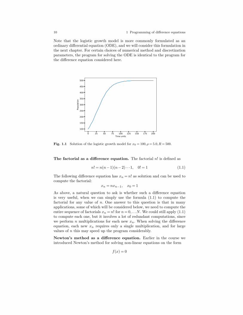
Note that the logistic growth model is more commonly formulated as anordinary differential equation (ODE), and we will consider this formulation inthe next chapter. For certain choices of numerical method and discretizationparameters, the program for solving the ODE is identical to the program forthe difference equation considered here.
0 25 50 75 100 125 150 175 200Time units
100
150
200
250
300
350
400
450
500Po
pula
tion
Fig. 1.1 Solution of the logistic growth model for x0 = 100,ρ= 5.0,R= 500.
The factorial as a difference equation. The factorial n! is defined as
n! = n(n−1)(n−2) · · ·1, 0! = 1 (1.1)
The following difference equation has xn = n! as solution and can be used tocompute the factorial:
xn = nxn−1, x0 = 1
As above, a natural question to ask is whether such a difference equationis very useful, when we can simply use the formula (1.1) to compute thefactorial for any value of n. One answer to this question is that in manyapplications, some of which will be considered below, we need to compute theentire sequence of factorials xn = n! for n= 0, . . .N . We could still apply (1.1)to compute each one, but it involves a lot of redundant computations, sincewe perform n multiplications for each new xn. When solving the differenceequation, each new xn requires only a single multiplication, and for largevalues of n this may speed up the program considerably.
Newton’s method as a difference equation. Earlier in the course weintroduced Newton’s method for solving non-linear equations on the form
f(x) = 0
1.4 Taylor Series and Approximations 11
Starting from some initial guess x0, Newton’s method gradually improves theapproximation by iterations
xn = xn−1−f(xn−1)f ′(xn−1) .
We may now recognize this as nonlinear first-order difference equation. Asn→∞, we hope that xn → xs, where xs is the solution to f(xs) = 0. Inpractice we solve the equation for n ≤ N , for some finite N , just as for thedifference equations considered earlier. But how do we choose N so that xNis sufficiently close to the true solution xs? Since we want to solve f(x) =0, the best approach is to solve the equation until f(x) ≤ ε, where ε is asmall tolerance. In practice, Newton’s method will usually converge ratherquickly, or not converge at all, so setting some upper bound on the numberof iterations is a good idea. A simple implementation of Newton’s method asa Python function may look like
def Newton(f, dfdx, x, epsilon=1.0E-7, max_n=100):n = 0while abs(f(x)) > epsilon and n <= max_n:
x = x - f(x)/dfdx(x)n += 1
return x, n, f(x)
The arguments to the function are Python functions f and dfdx implementingf(x) and its derivative. Both of these arguments are called inside the functionand must therefore be callable. The x argument is the initial guess for thesolution x, and the two optional arguments at the end are the tolerance andthe maximum number of iteration. Although the method is implemented asa while-loop rather than a for-loop, the main structure of the algorithm isexactly the same as for the other difference equations considered earlier.
1.4 Taylor Series and Approximations
One extremely important use of sequences and series is for approximatingother functions. For instance, commonly used functions such as sinx, lnx,and ex have been defined to have some desired mathematical properties, butwe need some kind of algorithm to evaluate the function values. A convenientapproach is to approximate sinx, etc. by polynomials, since they are easy tocalculate. It turns out that such approximations exist, for example this resultby Gregory from 1667:
sinx=∞∑k=0
(−1)k x2k+1
(2k+1)!
12 1 Programming of difference equations
and an even more amazing result discovered by Taylor in 1715:
f(x) =∞∑k=0
1k! (
dkf(0)dxk
)xk.
Here, the notation dkf(0)/dxk means the k-th derivative of f evaluated atx= 0. Taylor’s result means that for any function f(x), if we can compute thefunction value and its derivatives for x= 0, we can approximate the functionvalue at any x by evaluating a polynomial. For practical applications, wealways work with a truncated version of the Taylor series:
f(x)≈N∑k=0
1k! (
dkf(0)dxk
)xk. (1.2)
The approximation improves as N is increased, but the most popular choiceis actually N = 1, which gives a reasonable approximation close to x= 0 andhas been essential in developing physics and technology.
As an example, consider the Taylor approximation to the exponential func-tion. For this function we have that dkex/dxk = ex for all k, and e0 = 1, andinserting this into (1.2) yields
ex =∞∑k=0
xk
k!
≈N∑k=0
xk
k! .
Choosing, for instance, N = 1 and N = 4, we get
ex ≈ 1+x,
ex ≈ 1+x+ 12x
2 + 16x
3,
respectively. These approximations are obviously not very accurate for largex, but close to x= 0 they are sufficiently accurate for many applications. Bya shift of variables we can also make the Taylor polynomials accurate aroundany point x= a:
f(x)≈N∑k=0
1k! (
dk
dxkf(a))(x−a)k.
Taylor series formulated as a difference equation. We consider againthe Taylor series for ex around x= 0, given by
ex =∞∑k=0
xk
k! .
1.4 Taylor Series and Approximations 13
If we now define en as the approximation with n terms, i.e. for k= 0, . . . ,n−1,we have
en =n−1∑k=0
xk
k! =n−2∑k=0
xk
k! + xn−1
(n−1)! ,
and we can formulate the sum in en as the difference equation
en = en−1 + xn−1
(n−1)! , e0 = 0. (1.3)
We see that this difference equation involves (n− 1)!, and computing thecomplete factorial for every iteration involves a large number of redundantmultiplications. Above we introduced a difference equation for the factorial,and this idea can be utilized to formulate a more efficient computation of theTaylor polynomial. We have that
xn
n! = xn−1
(n−1)! ·x
n,
and if we let an = xn/n! it can be computed efficiently by solving
an = an−1x
n, a0 = 1.
Now we can formulate a system of two difference equations for the Taylorpolynomial, where we update each term via the an equation and sum theterms via the en equation:
en = en−1 +an−1, e0 = 0,
an = x
nan−1, a0 = 1.
Although we are here solving a system of two difference equations, the com-putation is far more efficient than solving the single equation in (1.3) directly,since we avoid the repeated multiplications involved in the factorial compu-tation.
A complete Python code for solving the difference equation and computethe Taylor approximation to the exponential function may look like
import numpy as np
x = 0.5 #approximate exp(x) for x = 0.5
N = 5index_set = range(N+1)a = np.zeros(len(index_set))e = np.zeros(len(index_set))a[0] = 1
14 1 Programming of difference equations
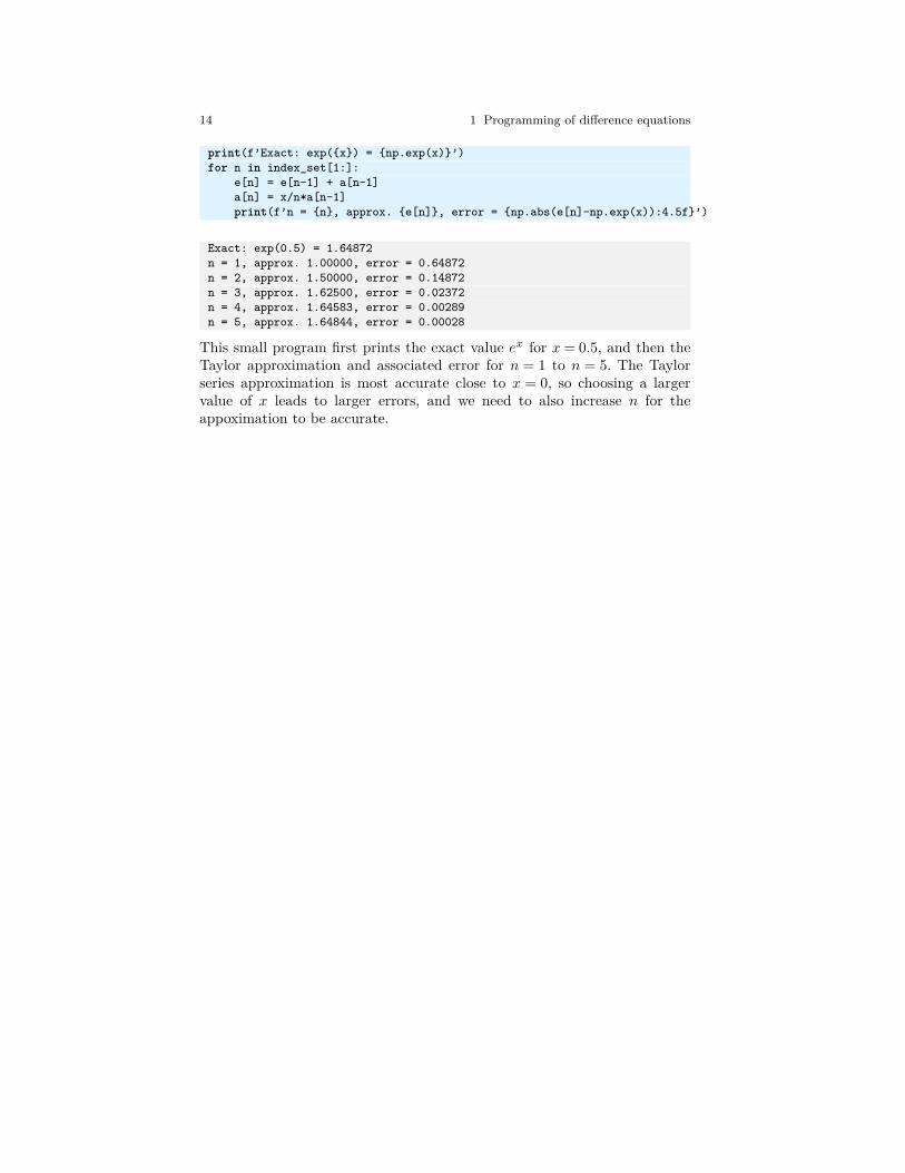
print(f’Exact: exp({x}) = {np.exp(x)}’)for n in index_set[1:]:
e[n] = e[n-1] + a[n-1]a[n] = x/n*a[n-1]print(f’n = {n}, approx. {e[n]}, error = {np.abs(e[n]-np.exp(x)):4.5f}’)
Exact: exp(0.5) = 1.64872n = 1, approx. 1.00000, error = 0.64872n = 2, approx. 1.50000, error = 0.14872n = 3, approx. 1.62500, error = 0.02372n = 4, approx. 1.64583, error = 0.00289n = 5, approx. 1.64844, error = 0.00028
This small program first prints the exact value ex for x = 0.5, and then theTaylor approximation and associated error for n = 1 to n = 5. The Taylorseries approximation is most accurate close to x = 0, so choosing a largervalue of x leads to larger errors, and we need to also increase n for theappoximation to be accurate.
Chapter 2Solving ordinary differentialequations
Ordinary differential equations (ODEs) are widely used in science and engi-neering, in particular for modeling dynamic processes. While simple ODEscan be solved with analytical methods, non-linear ODEs are generally notpossible to solve in this way, and we need to apply numerical methods. Inthis chapter we will see how we can program general numerical solvers thatcan be applied to any ODE. We will first consider scalar ODEs, i.e., ODEswith a single equation and a single unknown, and in Chapter 3 we will extendthe ideas to systems of coupled ODEs. Understanding the concepts of thischapter is useful not only for programming your own ODE solvers, but alsofor using a wide variety of general-purpose ODE solvers available both inPython and other programming languages.
2.1 Creating a general-purpose ODE solver
When solving ODEs analytically one will typically consider a specific ODE ora class of ODEs, and try to derive a formula for the solution. In this chapterwe want to implement numerical solvers that can be applied to any ODE,not restricted to a single example or a particular class of equations. For thispurpose, we need a general abstract notation for an arbitrary ODE. We willwrite the ODEs on the following form:
u′(t) = f(u(t), t), (2.1)
which means that the ODE is fully specified by the definition of the righthand side function f(u,t). Examples of this function may be:
15
16 2 Solving ordinary differential equations
f(u,t) = αu, exponential growth
f(u,t) = αu(
1− u
R
), logistic growth
f(u,t) =−b|u|u+g, falling body in a fluid
Notice that for generality we write all these right hand sides as functions ofboth u and t, although the mathematical formulations only involve u. It willbecome clear later why such a general formulation is useful. Our aim is now towrite functions and classes that take f as input, and solve the correspondingODE to produce u as output.
The Euler method turns an ODE into a difference equation. All thenumerical methods we will considered in this chapter are based on approxi-mating the derivatives in the equation u′ = f(u,t) by finite differences. Thisstep transforms the ODE into a difference equation, which can be solved withthe techniques presented in Chapter 1. To introduce the idea, assume thatwe have computed u at discrete time points t0, t1, . . . , tn. At time tn we havethe ODE
u′(tn) = f(u(tn), tn),
and we can now approximate u′(tn) by a forward finite difference;
u′(tn)≈ u(tn+1)−u(tn)∆t
.
Inserting this approximation into the ODE at t = tn yields the followingequation
u(tn+1)−u(tn)∆t
= f(u(tn), tn),
which we may recognize as a difference equation for computing u(tn+1) fromthe known value u(tn). We can rearrange the terms to obtain an explicitformula for u(tn+1):
u(tn+1) = u(tn)+∆tf(u(tn), tn).
This is known as the Forward Euler (FE) method, and is the simplest nu-merical method for solving and ODE. We can simplify the formula by usingthe notation for difference equations introduced in Chapter 1. If we let undenote the numerical approximation to the exact solution u(t) at t= tn, thedifference equation can be written as
un+1 = un+∆tf(un, tn). (2.2)
This is a regular difference equation which can be solved using arrays and afor-loop, just as we did for the other difference equations in Chapter 1. Westart from the known initial condition u0, and apply the formula repeatedlyto compute u1, u2, u3 and so forth.
2.1 Creating a general-purpose ODE solver 17
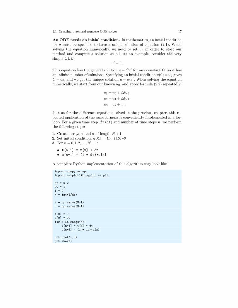
An ODE needs an initial condition. In mathematics, an initial conditionfor u must be specified to have a unique solution of equation (2.1). Whensolving the equation numerically, we need to set u0 in order to start ourmethod and compute a solution at all. As an example, consider the verysimple ODE
u′ = u.
This equation has the general solution u= Cet for any constant C, so it hasan infinite number of solutions. Specifying an initial condition u(0) = u0 givesC = u0, and we get the unique solution u= u0e
t. When solving the equationnumerically, we start from our known u0, and apply formula (2.2) repeatedly:
u1 = u0 +∆tu0,
u2 = u1 +∆tu1,
u3 = u2 + . . . .
Just as for the difference equations solved in the previous chapter, this re-peated application of the same formula is conveniently implemented in a for-loop. For a given time step ∆t (dt) and number of time steps n, we performthe following steps:
1. Create arrays t and u of length N +12. Set initial condition: u[0] = U0, t[0]=03. For n= 0,1,2, . . . ,N −1:
• t[n+1] = t[n] + dt• u[n+1] = (1 + dt)*u[n]
A complete Python implementation of this algorithm may look like
import numpy as npimport matplotlib.pyplot as plt
dt = 0.2U0 = 1T = 4N = int(T/dt)
t = np.zeros(N+1)u = np.zeros(N+1)
t[0] = 0u[0] = U0for n in range(N):
t[n+1] = t[n] + dtu[n+1] = (1 + dt)*u[n]
plt.plot(t,u)plt.show()
18 2 Solving ordinary differential equations
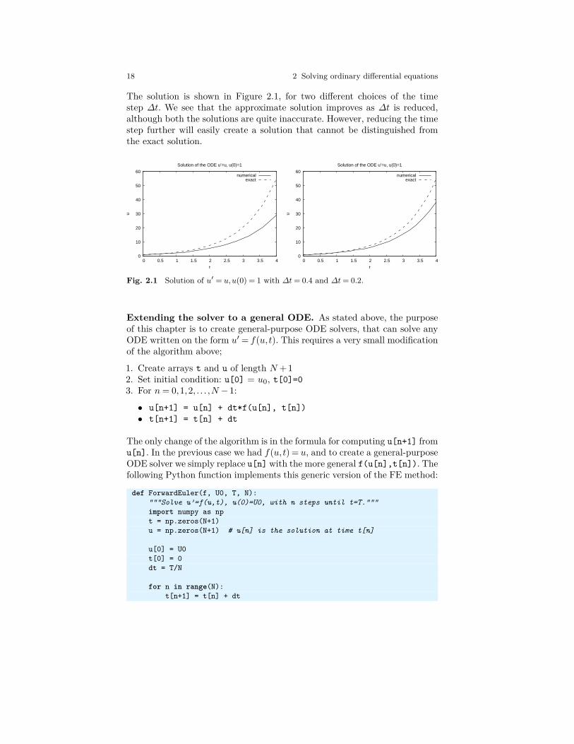
The solution is shown in Figure 2.1, for two different choices of the timestep ∆t. We see that the approximate solution improves as ∆t is reduced,although both the solutions are quite inaccurate. However, reducing the timestep further will easily create a solution that cannot be distinguished fromthe exact solution.
0
10
20
30
40
50
60
0 0.5 1 1.5 2 2.5 3 3.5 4
u
t
Solution of the ODE u’=u, u(0)=1
numericalexact
0
10
20
30
40
50
60
0 0.5 1 1.5 2 2.5 3 3.5 4
u
t
Solution of the ODE u’=u, u(0)=1
numericalexact
Fig. 2.1 Solution of u′ = u,u(0) = 1 with ∆t= 0.4 and ∆t= 0.2.
Extending the solver to a general ODE. As stated above, the purposeof this chapter is to create general-purpose ODE solvers, that can solve anyODE written on the form u′ = f(u,t). This requires a very small modificationof the algorithm above;
1. Create arrays t and u of length N +12. Set initial condition: u[0] = u0, t[0]=03. For n= 0,1,2, . . . ,N −1:
• u[n+1] = u[n] + dt*f(u[n], t[n])• t[n+1] = t[n] + dt
The only change of the algorithm is in the formula for computing u[n+1] fromu[n]. In the previous case we had f(u,t) = u, and to create a general-purposeODE solver we simply replace u[n] with the more general f(u[n],t[n]). Thefollowing Python function implements this generic version of the FE method:
def ForwardEuler(f, U0, T, N):"""Solve u’=f(u,t), u(0)=U0, with n steps until t=T."""import numpy as npt = np.zeros(N+1)u = np.zeros(N+1) # u[n] is the solution at time t[n]
u[0] = U0t[0] = 0dt = T/N
for n in range(N):t[n+1] = t[n] + dt
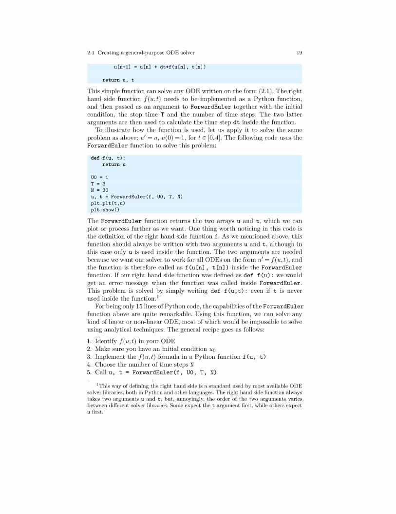
2.1 Creating a general-purpose ODE solver 19
u[n+1] = u[n] + dt*f(u[n], t[n])
return u, t
This simple function can solve any ODE written on the form (2.1). The righthand side function f(u,t) needs to be implemented as a Python function,and then passed as an argument to ForwardEuler together with the initialcondition, the stop time T and the number of time steps. The two latterarguments are then used to calculate the time step dt inside the function.
To illustrate how the function is used, let us apply it to solve the sameproblem as above; u′ = u, u(0) = 1, for t ∈ [0,4]. The following code uses theForwardEuler function to solve this problem:
def f(u, t):return u
U0 = 1T = 3N = 30u, t = ForwardEuler(f, U0, T, N)plt.plt(t,u)plt.show()
The ForwardEuler function returns the two arrays u and t, which we canplot or process further as we want. One thing worth noticing in this code isthe definition of the right hand side function f. As we mentioned above, thisfunction should always be written with two arguments u and t, although inthis case only u is used inside the function. The two arguments are neededbecause we want our solver to work for all ODEs on the form u′ = f(u,t), andthe function is therefore called as f(u[n], t[n]) inside the ForwardEulerfunction. If our right hand side function was defined as def f(u): we wouldget an error message when the function was called inside ForwardEuler.This problem is solved by simply writing def f(u,t): even if t is neverused inside the function.1
For being only 15 lines of Python code, the capabilities of the ForwardEulerfunction above are quite remarkable. Using this function, we can solve anykind of linear or non-linear ODE, most of which would be impossible to solveusing analytical techniques. The general recipe goes as follows:
1. Identify f(u,t) in your ODE2. Make sure you have an initial condition u03. Implement the f(u,t) formula in a Python function f(u, t)4. Choose the number of time steps N5. Call u, t = ForwardEuler(f, U0, T, N)
1This way of defining the right hand side is a standard used by most available ODEsolver libraries, both in Python and other languages. The right hand side function alwaystakes two arguments u and t, but, annoyingly, the order of the two arguments variesbetween different solver libraries. Some expect the t argument first, while others expectu first.
20 2 Solving ordinary differential equations
6. Plot the solution
It is worth mentioning that the FE method is the simplest of all ODE solvers,and many will argue that it is not very good. This is partly true, since thereare many other methods that are more accurate and more stable when appliedto challenging ODEs. We shall look at a few examples of such methods laterin this chapter. However, the FE method is quite suitable for solving mostODEs. If we are not happy with the accuracy we can simply reduce the timestep, and in most cases this will give the accuracy we need with a negligibleincrease in computing time.
2.2 The ODE solver implemented as a class
We can increase the flexibility of the ForwardEuler solver function by imple-menting it as a class. The usage of the class may for instance be as follows:
method = ForwardEuler_v1(f, U0=0.0, T=40, N=400)u, t = method.solve()plot(t, u)
The benefits of using a class instead of a function may not be obvious at thispoint, but it will become clear later. For now, let us just look at how such asolver class can be implemented:
• We need a constructor (__init__) which takes f, T, N, and U0 as argumentsand stores them as attributes.
• The time step ∆t and the sequences un, tn must be initalized and storedas attributes. These tasks are also natural to handle in the constructor.
• The class needs a solve-method, which implements the for-loop and re-turns the solution, similar to the ForwardEuler function considered earlier.
In addition to these methods, it may be convenient to implement the formulafor advancing the solution one step as a separate method advance. In thisway it becomes very easy to implement new numerical methods, since wetypically only need to change the advance method. A first version of thesolver class may look as follows:
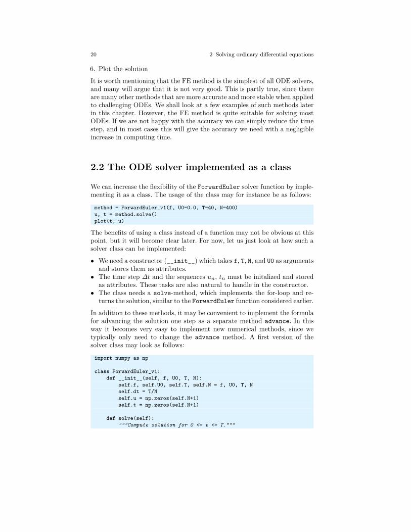
import numpy as np
class ForwardEuler_v1:def __init__(self, f, U0, T, N):
self.f, self.U0, self.T, self.N = f, U0, T, Nself.dt = T/Nself.u = np.zeros(self.N+1)self.t = np.zeros(self.N+1)
def solve(self):"""Compute solution for 0 <= t <= T."""
2.2 The ODE solver implemented as a class 21
self.u[0] = float(self.U0)
for n in range(self.N):self.n = nself.t[n+1] = self.t[n] + self.dtself.u[n+1] = self.advance()
return self.u, self.t
def advance(self):"""Advance the solution one time step."""# Create local variables to get rid of "self." in# the numerical formulau, dt, f, n, t = self.u, self.dt, self.f, self.n, self.t
unew = u[n] + dt*f(u[n], t[n])return unew
This class does essentially the same tasks as the ForwardEuler functionabove. The main advantage of the class implementation is the increased flex-ibility that comes with the advance method. As we shall see later, imple-menting a different numerical method typically only requires implementing anew version of this method, while all the other code can be left unchanged.
We can also use a class to hold the right-hand side f(u,t), which is par-ticularly convenient for functions with parameters. Consider for instance themodel for logistic growth;
u′(t) = αu(t)(
1− u(t)R
), u(0) = U0, t ∈ [0,40],
which is the ODE version of the difference equation considered in Chapter 1.The right hand side function has two parameters α and R, but if we want tosolve it using our ForwardEuler function or class, it must be implementedas a function of u and t only. As we have discussed earlier in the course, aclass with a call method provides a very flexible implementation of such afunction, since we can set the parameters as attributes in the constructor anduse them inside the __call__ method:
class Logistic:def __init__(self, alpha, R, U0):
self.alpha, self.R, self.U0 = alpha, float(R), U0
def __call__(self, u, t): # f(u,t)return self.alpha*u*(1 - u/self.R)
The main program for solving the logistic growth problem may now look like:
problem = Logistic(0.2, 1, 0.1)method = ForwardEuler_v1(problem,problem.U0,40,401)u, t = method.solve()plt.plot(t,u)plt.show()
22 2 Solving ordinary differential equations
0 5 10 15 20 25 30 35 40 45t
0.1
0.2
0.3
0.4
0.5
0.6
0.7
0.8
0.9
1.0
u
Logistic growth: alpha=0.2, R=1, dt=0.1
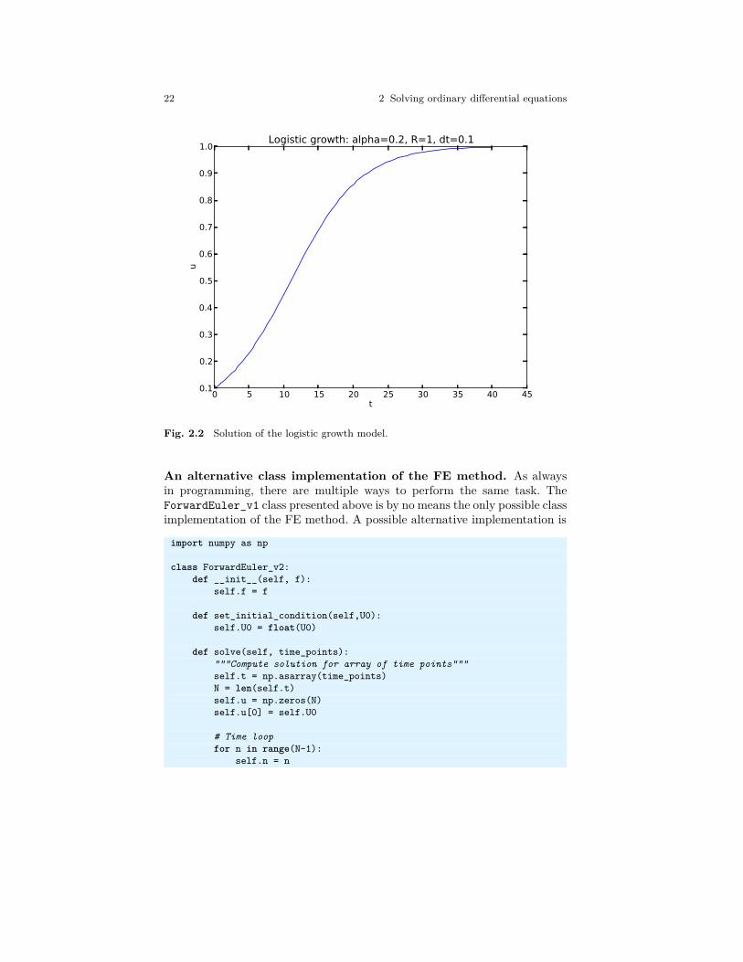
Fig. 2.2 Solution of the logistic growth model.
An alternative class implementation of the FE method. As alwaysin programming, there are multiple ways to perform the same task. TheForwardEuler_v1 class presented above is by no means the only possible classimplementation of the FE method. A possible alternative implementation is
import numpy as np
class ForwardEuler_v2:def __init__(self, f):
self.f = f
def set_initial_condition(self,U0):self.U0 = float(U0)
def solve(self, time_points):"""Compute solution for array of time points"""self.t = np.asarray(time_points)N = len(self.t)self.u = np.zeros(N)self.u[0] = self.U0
# Time loopfor n in range(N-1):
self.n = n
2.3 Alternative ODE solvers 23
self.u[n+1] = self.advance()return self.u, self.t
def advance(self):"""Advance the solution one time step."""# Create local variables to get rid of "self." in# the numerical formulau, f, n, t = self.u, self.f, self.n, self.t#dt is not necessarily constant:dt = t[n+1]-t[n]unew = u[n] + dt*f(u[n], t[n])return unew
This class is quite similar to the one above, but we have simplified the con-structor considerably, introduced a separate method for setting the initialcondition, and changed the solve method to take an array of time pointsas argument. The latter gives a bit more flexibility than the version inForwardEuler_v1, where the stop time and number of time points werepassed as arguments to the constructor and used to compute a (constant)time step dt. The ForwardEuler_v2 version does not require the time stepto be constant, and the method will work fine if we pass it a time_pointsarray with varying distance between the time points. This can be useful if weknow that the solution varies rapidly in some time intervals and more slowlyin others. However, in most cases we will use an evenly spaced array for thetime_points argument, for instance created using NumPy’s linspace, andin such cases there is not much difference between the two classes. To con-sider a concrete example, the solution of the same logistic growth problem asabove, using the new class, may look as follows:
problem = Logistic(0.2, 1, 0.1)time = np.linspace(0,40,401)
method = ForwardEuler_v2(problem)method.set_initial_condition(problem.U0)u, t = method.solve(time)
2.3 Alternative ODE solvers
As mentioned above, the FE method is not the most sophisticated ODEsolver, although it is sufficiently accurate for most of the applications wewill consider here. Many alternative methods exist, with better accuracy andstability than FE. One very popular class of ODE solvers is known as Runge-Kutta methods. The simplest example of a Runge-Kutta method is in factthe FE method;
un+1 = un+∆tf(un, tn),
24 2 Solving ordinary differential equations
which is an example of a one-stage, first-order, explicit Runge-Kutta method.The classification as a first-order methods means that the error in the ap-proximate solution produced by FE is proportional to ∆t. An alternativeformulation of the FE method is
k1 = f(un, tn),un+1 = un+∆t 1̨.
It can easily be verified that this is the same formula as above, and there isno real benefit from writing the formula in two lines rather than one. How-ever, the second formulation is more in line with how Runge-Kutta methodsare usually written, and it makes it easy to see the relation between theFE method and more advanced solvers. The intermediate value k1 is oftenreferred to as a stage derivative in the ODE literature.
We can easily improve the accuracy of the FE method to second order,i.e., error proportional to ∆t2, by taking one additional step:
k1 = f(un, tn),
k2 = f(un+ ∆t
2 k1, tn+ ∆t
2 ),
un+1 = un+∆tk2.
This method is known as the explicit midpoint method or the modified Eulermethod. The first step is identical to that of the FE method, but instead ofusing the stage derivate k1 to advance the solution to the next step, we useit to compute a new stage derivative k2, which is an approximation of thederivative of u at time tn+∆t/2. Finally, we use this midpoint derivative toadvance the the solution to tn+1.
An alternative second order method is Heun’s method, which is also re-ferred to as the explicit trapezoidal method:
k1 = f(un, tn), (2.3)k2 = f(un+∆tk1, tn+∆t), (2.4)
un+1 = un+∆t(k1/2+k2/2) (2.5)
This method also computes two stage derivatives k1 and k2, but from theformula for k2 we see that it approximates the derivative at tn+1 rather thanthe midpoint. The solution is advanced from tn to tn+1 using the mean valueof k1 and k2.
All Runge-Kutta methods follow the same recipe as the two second or-der methods considered above; we compute one or more intermediate values(stage derivatives), and then advance the solution using a combination ofthese stage derivatives. The accuracy of the method can be improved byadding more stages. A general RK method with s stages can be written as
2.3 Alternative ODE solvers 25
ki = f(tn+ ci∆t,yn+∆t
s∑j=1
aijkj), for i= 1, . . . ,s (2.6)
un+1 = u0 +∆t
s∑i=1
biki. (2.7)
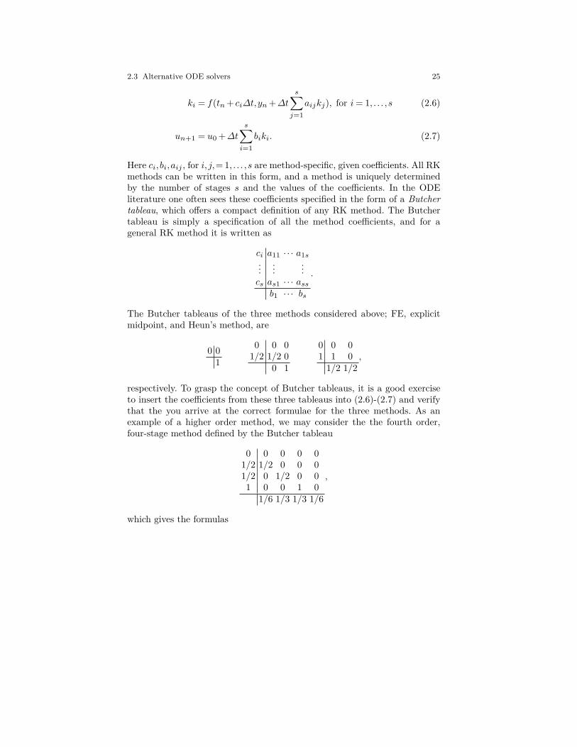
Here ci, bi,aij , for i, j,= 1, . . . ,s are method-specific, given coefficients. All RKmethods can be written in this form, and a method is uniquely determinedby the number of stages s and the values of the coefficients. In the ODEliterature one often sees these coefficients specified in the form of a Butchertableau, which offers a compact definition of any RK method. The Butchertableau is simply a specification of all the method coefficients, and for ageneral RK method it is written as
ci a11 · · · a1s...
......
cs as1 · · · assb1 · · · bs
.
The Butcher tableaus of the three methods considered above; FE, explicitmidpoint, and Heun’s method, are
0 01
0 0 01/2 1/2 0
0 1
0 0 01 1 0
1/2 1/2,
respectively. To grasp the concept of Butcher tableaus, it is a good exerciseto insert the coefficients from these three tableaus into (2.6)-(2.7) and verifythat the you arrive at the correct formulae for the three methods. As anexample of a higher order method, we may consider the the fourth order,four-stage method defined by the Butcher tableau
0 0 0 0 01/2 1/2 0 0 01/2 0 1/2 0 01 0 0 1 0
1/6 1/3 1/3 1/6
,
which gives the formulas
26 2 Solving ordinary differential equations
k1 = f(un, tn),
k2 = f(un+ 12k1, tn+ 1
2∆t),
k3 = f(un+ 12k2, tn+ 1
2∆t),
k4 = f(un+k3, tn+∆t),un+1 = un+ ∆t
6 (k1 +2k2 +2k3 +k4) .
All the RK methods we will consider in this course are explicit methods,which means that aij = 0 for j ≥ i. If we look closely at the formula in (2.6),we see that the expression for computing each stage derivative ki then onlyincludes previously computed stage derivatives, and all ki can be computedsequentially using explicit formulas. For implicit RK methods, on the otherhand, we we have aij 6= 0 for some j ≥ i, and we see in (2.6) that the formulafor computing ki will then include ki on the right hand side. We therefore needto solve equations to compute the stage derivatives, and for non-linear ODEsthese will be non-linear equations that are typically solved using Newton’smethod. This makes implicit RK methods more complex to implement andmore computationally expensive per time step, but they are also more stablethan explicit methods and perform much better for certain classes of ODEs.We will not consider implicit RK methods in this course.
2.4 A class hierarchy of ODE solvers
We now want to implement some of the Runge-Kutta methods as classes, sim-ilar to the FE classes introduced above. When inspecting the ForwardEuler_v2class, we quickly observe that most of the code is common to all ODE solvers,and not specific to the FE method. For instance, we always need to createan array for holding the solution, and the general solution method using afor-loop is always the same. In fact, the only difference between the differentmethods is how the solution is advanced from one step to the next. Recall-ing the ideas of Object-Oriented Programming, it becomes obvious that aclass hierarchy is very convenient for implementing such a collection of ODEsolvers. In this way we can collect all common code in a superclass, and relyon inheritance to avoid code duplication. The superclass can handle most ofthe more "administrative" steps of the ODE solver, such as
• Storing the solution un and the corresponding time levels tn, k= 0,1,2, . . . ,n• Storing the right-hand side function f(u,t)• Storing and applying initial condition• Running the loop over all time steps
We can introduce a superclass ODESolver to handle these parts, and imple-ment the method-specific details in sub-classes. It should now become quite
2.4 A class hierarchy of ODE solvers 27
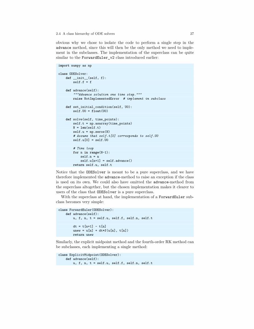
obvious why we chose to isolate the code to perform a single step in theadvance method, since this will then be the only method we need to imple-ment in the subclasses. The implementation of the superclass can be quitesimilar to the ForwardEuler_v2 class introduced earlier:
import numpy as np
class ODESolver:def __init__(self, f):
self.f = f
def advance(self):"""Advance solution one time step."""raise NotImplementedError # implement in subclass
def set_initial_condition(self, U0):self.U0 = float(U0)
def solve(self, time_points):self.t = np.asarray(time_points)N = len(self.t)self.u = np.zeros(N)# Assume that self.t[0] corresponds to self.U0self.u[0] = self.U0
# Time loopfor n in range(N-1):
self.n = nself.u[n+1] = self.advance()
return self.u, self.t
Notice that the ODESolver is meant to be a pure superclass, and we havetherefore implemented the advance-method to raise an exception if the classis used on its own. We could also have omitted the advance-method fromthe superclass altogether, but the chosen implementation makes it clearer tousers of the class that ODESolver is a pure superclass.
With the superclass at hand, the implementation of a ForwardEuler sub-class becomes very simple:
class ForwardEuler(ODESolver):def advance(self):
u, f, n, t = self.u, self.f, self.n, self.t
dt = t[n+1] - t[n]unew = u[n] + dt*f(u[n], t[n])return unew
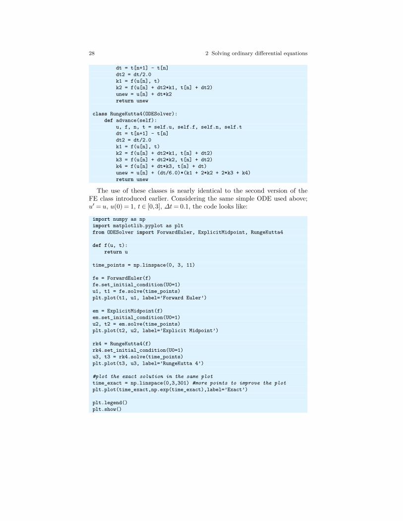
Similarly, the explicit midpoint method and the fourth-order RK method canbe subclasses, each implementing a single method:
class ExplicitMidpoint(ODESolver):def advance(self):
u, f, n, t = self.u, self.f, self.n, self.t
28 2 Solving ordinary differential equations
dt = t[n+1] - t[n]dt2 = dt/2.0k1 = f(u[n], t)k2 = f(u[n] + dt2*k1, t[n] + dt2)unew = u[n] + dt*k2return unew
class RungeKutta4(ODESolver):def advance(self):
u, f, n, t = self.u, self.f, self.n, self.tdt = t[n+1] - t[n]dt2 = dt/2.0k1 = f(u[n], t)k2 = f(u[n] + dt2*k1, t[n] + dt2)k3 = f(u[n] + dt2*k2, t[n] + dt2)k4 = f(u[n] + dt*k3, t[n] + dt)unew = u[n] + (dt/6.0)*(k1 + 2*k2 + 2*k3 + k4)return unew
The use of these classes is nearly identical to the second version of theFE class introduced earlier. Considering the same simple ODE used above;u′ = u, u(0) = 1, t ∈ [0,3], ∆t= 0.1, the code looks like:
import numpy as npimport matplotlib.pyplot as pltfrom ODESolver import ForwardEuler, ExplicitMidpoint, RungeKutta4
def f(u, t):return u
time_points = np.linspace(0, 3, 11)
fe = ForwardEuler(f)fe.set_initial_condition(U0=1)u1, t1 = fe.solve(time_points)plt.plot(t1, u1, label=’Forward Euler’)
em = ExplicitMidpoint(f)em.set_initial_condition(U0=1)u2, t2 = em.solve(time_points)plt.plot(t2, u2, label=’Explicit Midpoint’)
rk4 = RungeKutta4(f)rk4.set_initial_condition(U0=1)u3, t3 = rk4.solve(time_points)plt.plot(t3, u3, label=’RungeKutta 4’)
#plot the exact solution in the same plottime_exact = np.linspace(0,3,301) #more points to improve the plotplt.plot(time_exact,np.exp(time_exact),label=’Exact’)
plt.legend()plt.show()
2.4 A class hierarchy of ODE solvers 29
This code will solve the same equation using three different methods, andplot the solutions in the same window. Experimenting with different stepsizes should reveal the difference in accuracy between the two methods.

Chapter 3Solving systems of ODEs
So far we have only considered ODEs with a single solution component, oftencalled scalar ODEs. Many interesting processes can be described by systems ofODEs, i.e., multiple ODEs where the right hand side of one equation dependson the solution of the others. Such equation systems are also referred to asvector ODEs. One simple example is
u′ = v, u(0) = 1v′ =−u, v(0) = 0.
The solution of this system is u= cos t,v = sin t, which can easily be verifiedby insterting the solution into the equations and initial conditions. For moregeneral cases, it is usually even more difficult to find analytical solutionsof ODE systems than of scalar ODEs, and numerical methods are usuallyrequired. In this chapter we will extend the solvers introduced in Chapter 2to be able to solve systems of ODEs. We shall see that such an extensionrequires relatively small modifications of the code.
We want to develop general software that can be applied to any vectorODE or scalar ODE, and for this purpose it is useful to introduce generalmathematical notation. We have n unknowns
u(0)(t),u(1)(t), . . . ,u(n−1)(t)
in a system of n ODEs:
d
dtu(0) = f (0)(u(0),u(1), . . . ,u(n−1), t),
d
dtu(1) = f (1)(u(0),u(1), . . . ,u(n−1), t),
... =...
d
dtu(n−1) = f (n−1)(u(0),u(1), . . . ,u(n−1), t).
31
32 3 Solving systems of ODEs
To simplify the notation (and later the implementation), we collect both thesolutions u(i)(t) and right-hand side functions f (i) in vectors;
u= (u(0),u(1), . . . ,u(n−1)),
andf = (f (0),f (1), . . . ,f (n−1)).
Note that f is now a vector-valued function. It takes n+ 1 input arguments(t and the n components of u) and returns a vector of n values. The ODEsystem can now be written
u′ = f(u,t), u(0) = u0
where u and f are vectors and u0 is a vector of initial conditions. We see thatwe use exactly the same notation as for scalar ODEs, and whether we solvea scalar or system of ODEs is determined by how we define f and the initialcondition u0. This general notation is completely standard in text books onODEs, and we can easily make the Python implementation just as general.
3.1 An ODESolver class for systems of ODEs
The ODESolver class above was written for a scalar ODE. We now want tomake it work for a system u′ = f , u(0) = U0, where u, f and U0 are vectors(arrays). To identify how the code needs to be changed, let us start with thesimplest method. Applying the forward Euler method to a system of ODEsyields an update formula that looks exactly as for the scalar case, but whereall the terms are vectors:
uk+1︸ ︷︷ ︸vector
= uk︸︷︷︸vector
+∆t f(uk, tk)︸ ︷︷ ︸vector
.
We could also write this formula in terms of the individual components, asin
u(i)k+1 = u
(i)k +∆tf (i)(uk, tk), for i= 0, . . . ,n−1,
but the compact vector notation is much easier to read. Fortunately, the waywe write the vector version of the formula is also how NumPy arrays are usedin calculations. The Python code for the formula above may therefore lookidential to the version for scalar ODEs;
u[k+1] = u[k] + dt*f(u[k], t)
3.1 An ODESolver class for systems of ODEs 33
with the important difference that both u[k] and u[k+1] are now arrays.1Since these are arrays, the solution u must be a two-dimensional array, andu[k],u[k+1], etc. are the rows of this array. The function f expects an arrayas its first argument, and must return a one-dimensional array, containing allthe right-hand sides f (0), . . . ,f (n−1). To get a better feel for how these arrayslook and how they are used, we may compare the array holding the solutionof a scalar ODE to that of a system of two ODEs. For the scalar equation,both t and u are one-dimensional NumPy arrays, and indexing into u givesus numbers, representing the solution at each time step:
t = [0. 0.4 0.8 1.2 (...) ]
u = [ 1.0 1.4 1.96 2.744 (...)]
u[0] = 1.0u[1] = 1.4
(...)
In the case of a system of two ODEs, t is still a one-dimensional array,but the solution array u is now two-dimensional, with one column for eachsolution component. Indexing into it yields one-dimensional arrays of lengthtwo, which are the two solution components at each time step:
u = [[1.0 0.8][1.4 1.1] [1.9 2.7] (...)]
u[0] = [1.0 0.8]u[1] = [1.4 1.1]
(...)
The similarity of the generic notation for vector and scalar ODEs, and theconvenient algebra of NumPy arrays, indicate that the solver implementationfor scalar and system ODEs can also be very similar. This is indeed true, andthe ODESolver class from the previous chapter can be made to work for ODEsystems by a few minor modifactions:
• Ensure that f(u,t) always returns an array.• Inspect U0 to see if it is a single number or a list/array/tuple and make
the u either a one-dimensional or two-dimensional array
If these two items are handled and initialized correctly, the rest of the codefrom Chapter 2 will in fact work with no modifications. The extended super-class implementation may look like:
class ODESolver:def __init__(self, f):
1This compact notation requires that the solution vector u is represented by a NumPyarray. We could also, in principle, use lists to hold the solution components, but theresulting code would need to loop over the components and be far less elegant andreadable.
34 3 Solving systems of ODEs
# Wrap user’s f in a new function that always# converts list/tuple to array (or let array be array)self.f = lambda u, t: np.asarray(f(u, t), float)
def set_initial_condition(self, U0):if isinstance(U0, (float,int)): # scalar ODE
self.neq = 1 # no of equationsU0 = float(U0)
else: # system of ODEsU0 = np.asarray(U0)self.neq = U0.size # no of equations
self.U0 = U0
def solve(self, time_points):self.t = np.asarray(time_points)N = len(self.t)if self.neq == 1: # scalar ODEs
self.u = np.zeros(N)else: # systems of ODEs
self.u = np.zeros((N,self.neq))
# Assume that self.t[0] corresponds to self.U0self.u[0] = self.U0
# Time loopfor n in range(N-1):
self.n = nself.u[n+1] = self.advance()
return self.u, self.t
It is worth commenting on some parts of this code. First, the constructorlooks almost identical to the scalar case, but we use a lambda function andnp.asarray to convert any f that returns a list or tuple to a function re-turning a NumPy array. This modification is not strictly needed, since wecould just assume that the user implements f to return an array, but itmakes the class more robust and flexible. We have also included tests in theset_initial_condition method, to check if U0 is a single number (float)or a NumPy array, and define the attribute self.neq to hold the numberof equations. The final modification is found in the method solve, wherethe self.neq attribute is inspected and u is initialized to a one- or two-dimensional array of the correct size. The actual for-loop, as well as theimplementation of the advance method in the subclasses, can be left un-changed.
Example: ODE model for throwing a ball. To demonstrate the use ofthe extended ODESolver hierarchy, let us derive and solve a system of ODEsdescribing the trajectory of a ball. We first define x(t),y(t) to be the positionof the ball, vx and vy the velocity components, and ax,ay the accelerationcomponents. From the definition of velocity and acceleration, we have vx =dx/dt,vy = dy/dt,ax = dvx/dt, and ay = dvy/dt. If we neglect air resistancethere are no forces acting on the ball in the x-direction, so from Newton’s
3.1 An ODESolver class for systems of ODEs 35
second law we have ax = 0. In the y-direction the acceleration must be equalto the acceleration of gravity, which yields ay =−g. In terms of the velocities,we have
ax = 0 ⇒ dvxdt
= 0,
ay =−g ⇒dvydt
=−g ,
and the complete ODE system can be written as
dx
dt= vx, (3.1)
dvxdt
= 0, (3.2)
dy
dt= vy, (3.3)
dvydt
=−g. (3.4)
To solve the system we need to define initial conditions for all four unknowns,i.e., we need to know the initial position and velocity of the ball.
A closer inspection of the system (3.1)-(3.4) will reveal that although thisis a coupled system of ODEs, the coupling is in fact quite weak and thesystem is easy to solve analytically. There is essentially a one-way couplingbetween equations (3.2) and (3.1), the same between (3.4) and (3.3), and noother coupling between the equations. We can easily solve (3.2) to concludethat vx is a constant, and inserting a constant on the right hand side of (3.1)yields that x must be a linear function of t. Similarly, we can solve (3.4) tofind that vy is a linear function, and then insert this into (3.3) to find thaty is a quadratic function of t. The functions x(t) and y(t) will contain fourunknown coefficients that must be determined from the initial conditions.
Although the analytical solution is available, we want to use the ODESolverclass hierarchy presented above to solve this system. The first step is then toimplement the right hand side as a Python function:
def f(u, t):x, vx, y, vy = ug = 9.81return [vx, 0, vy, -g]
We see that the function here returns a list, but this will automatically beconverted to an array by the solver class’ constructor, as mentioned above.The main program is not very different from the examples of the previouschapter, except that we need to define an initial condition with four compo-nents:
from ODESolver import ForwardEulerimport numpy as np
36 3 Solving systems of ODEs
import matplotlib.pyplot as plt
# Initial condition, start at the origin:x = 0; y = 0# velocity magnitude and angle:v0 = 5; theta = 80*np.pi/180vx = v0*np.cos(theta); vy = v0*np.sin(theta)
U0 = [x, vx, y, vy]
solver= ForwardEuler(f)solver.set_initial_condition(U0)time_points = np.linspace(0, 1.0, 101)u, t = solver.solve(time_points)# u is an array of [x,vx,y,vy] arrays, plot y vs x:x = u[:,0]; y = u[:,2]
plt.plot(x, y)plt.show()
Notice that since u is a two-dimensional array, we use array slicing to extractand plot the individual components. A call like plt.plot(t,u) will also work,but it will plot all the solution components in the same window, which forthis particular model is not very useful. A very useful exercise is to extendthis code to plot the analytical solution of the system in the same windowas the numerical solution. The system can be solved as outlined above, andthe unknown coefficients in the solution formulas can be determined from thegiven initial conditions. With the chosen number of time steps there will be avisible difference between the numerical solution and the analytical solution,but this can easily be removed by reducing the time step or choosing a moreaccurate solver.
Chapter 4Modeling infectious diseases
In this chapter we will look at a particular family of ODE systems thatdescribe the spread of infectious diseases. Athough the spread of infectionsis a very complex physical and biological process, we shall see that it can bemodeled with fairly simple systems of ODEs, which we can solve using thetools from the previous chapters.
4.1 Derivation of the SIR model
In order to derive a model we need to make a number of simplifying assump-tions. The most important one is that we do not consider individuals, justpopulations. The population is assumed to be perfectly mixed in a confinedarea, which means that we do not consider spatial transport of the disease,just temporal evolution. The first model we will derive is very simple, but weshall see that it can easily be extended to models that are used world-wideby health authorities to predict the spread of diseases such as Covid19, flu,ebola, HIV, etc.
In the first version of the model we will keep track of three categories ofpeople:
• S: susceptibles - who can get the disease• I: infected - who have developed the disease and can infect susceptibles• R: recovered - who have recovered and become immune
We represent these as mathematical quantities S(t), I(t), R(t), which repre-sent the number of people in each category. The goal is now to derive a set ofequations for S(t), I(t), R(t), and then solve these equations to predict thespread of the disease.
To derive the model equations, we first consider the dynamics in a timeinterval ∆t, and our goal is to derive mathematical expressions for how manypeople that move between the three categories in this time interval. The key
37
38 4 Modeling infectious diseases
part of the model is the description of how people move from S to I, i.e., howsusceptible individuals get the infection from those already infected. Infec-tious diseases are (mainly) transferred by direct interactions between people,so we need mathematical descriptions of the number of interactions betweensusceptible and infected individuals. We make the following assumptions:• An individual in the S category interacts with an approximately constant
number of people each day, so the number of interactions in a time interval∆t is proportional to ∆t.
• The probability of one of these interactions being with an infected personis proportional to the ratio of infected individuals to the total population,i.e., to I/N , with N = S+ I+R.
Based on these assumptions, the probability that a single susceptible persongets infected is proportional to ∆tI/N . The total number of infections canbe written as βSI/N , for some constant β. The infection of new individualsrepresents a reduction in S and a corresponding gain in I: , so we have
S(t+∆t) = S(t)−∆tβS(t)I(t)N
,
I(t+∆t) = I(t)+∆tβS(t)I(t)N
.
These two equations represent the key component of all the models consideredin this chapter. More advanced models are typically derived by adding morecategories and more transitions between them, but the individual transitionsare very similar to the ones presented here.
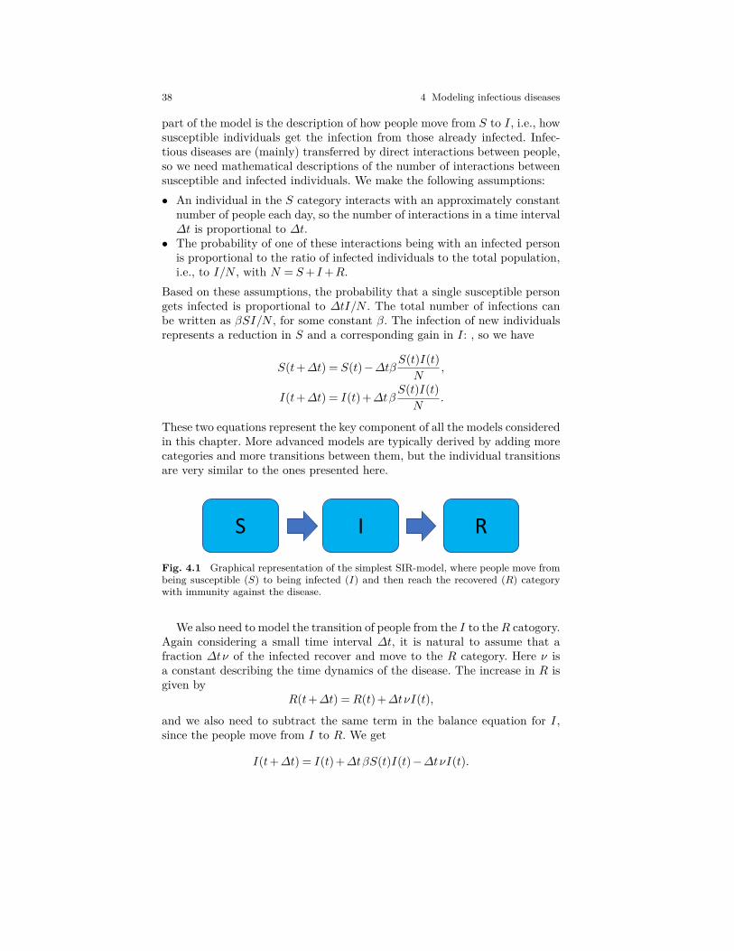
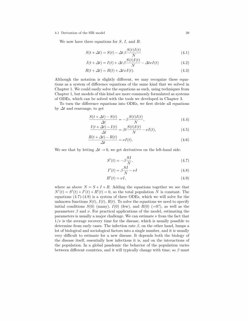
S RIFig. 4.1 Graphical representation of the simplest SIR-model, where people move frombeing susceptible (S) to being infected (I) and then reach the recovered (R) categorywith immunity against the disease.
We also need to model the transition of people from the I to theR catogory.Again considering a small time interval ∆t, it is natural to assume that afraction ∆tν of the infected recover and move to the R category. Here ν isa constant describing the time dynamics of the disease. The increase in R isgiven by
R(t+∆t) =R(t)+∆tνI(t),
and we also need to subtract the same term in the balance equation for I,since the people move from I to R. We get
I(t+∆t) = I(t)+∆tβS(t)I(t)−∆tνI(t).
4.1 Derivation of the SIR model 39
We now have three equations for S, I, and R:
S(t+∆t) = S(t)−∆tβS(t)I(t)N
(4.1)
I(t+∆t) = I(t)+∆tβS(t)I(t)N
−∆tνI(t) (4.2)
R(t+∆t) =R(t)+∆tνI(t). (4.3)
Although the notation is slightly different, we may recognize these equa-tions as a system of difference equations of the same kind that we solved inChapter 1. We could easily solve the equations as such, using techniques fromChapter 1, but models of this kind are more commonly formulated as systemsof ODEs, which can be solved with the tools we developed in Chapter 3.
To turn the difference equations into ODEs, we first divide all equationsby ∆t and rearrange, to get
S(t+∆t)−S(t)∆t
=−βS(t)I(t)N
, (4.4)
I(t+∆t)− I(t)∆t
= βtS(t)I(t)N
−νI(t), (4.5)
R(t+∆t)−R(t)∆t
= νI(t). (4.6)
We see that by letting ∆t→ 0, we get derivatives on the left-hand side:
S′(t) =−βSIN, (4.7)
I ′(t) = βSI
N−νI (4.8)
R′(t) = νI, (4.9)
where as above N = S+ I +R. Adding the equations together we see thatN ′(t) = S′(t) + I ′(t) +R′(t) = 0, so the total population N is constant. Theequations (4.7)-(4.9) is a system of three ODEs, which we will solve for theunknown functions S(t), I(t), R(t). To solve the equations we need to specifyinitial conditions S(0) (many), I(0) (few), and R(0) (=0?), as well as theparameters β and ν. For practical applications of the model, estimating theparameters is usually a major challenge. We can estimate ν from the fact that1/ν is the average recovery time for the disease, which is usually possible todetermine from early cases. The infection rate β, on the other hand, lumps alot of biological and sociological factors into a single number, and it is usuallyvery difficult to estimate for a new disease. It depends both the biology ofthe disease itself, essentially how infectious it is, and on the interactions ofthe population. In a global pandemic the behavior of the population variesbetween different countries, and it will typically change with time, so β must
40 4 Modeling infectious diseases
usually be adapted to different regions and different phases of the diseaseoutbreak.1
Although the system (4.7)-(4.9) looks quite simple, analytical solutionscannot easily be derived. For particular applications it is common to makesimplifications that allow simple analytical solutions. For instance, whenstudying the early phase of an epidemic one is mostly interested in the Icategory, and since the number of infected cases in this phase is low com-pared with the entire population we may assume that S is approximatelyconstant and equal to N . Inserting S ≈N turns (4.8) into a simple equationdescribing exponential growth, with solution
I(t) = I0e(β−ν). (4.10)
Such an approximate formula may be very useful, in particular for estimatingthe parameters of the model. In the early phase of an epidemic the numberof infected people typically follows an exponential curve, and we can fit theparameters of the model so that (4.10) fits the observed dynamics. However,if we want to describe the full dynamics of the epidemic we need to solve thecomplete system of ODEs, and in this case numerical solvers are needed.
Solving the SIR model with the ODESystem class hierarchy. We couldof course implement a numerical solution of the SIR equations directly, forinstance by applying the forward Euler method to (4.7)-(4.9), which willsimply give us back the original difference equations in (4.4)-(4.6). However,since the ODE solver tools we developed in Chapter 3 are completely gen-eral, they can easily be used to solve the SIR model. To solve the systemusing the fourth-order RK method of the ODESolver hierarchy, the Pythonimplementation may look as follows:
from ODESolver import RungeKutta4import numpy as npimport matplotlib.pyplot as plt
def SIR_model(u,t):beta = 1.0nu = 1/7.0S, I, R = u[0], u[1], u[2]N = S+I+RdS = -beta*S*I/NdI = beta*S*I/N - nu*IdR = nu*Ireturn [dS,dI,dR]
S0 = 1000
1A simpler version of the SIR model is also quite common, where the disease trans-mission term is not scaled with N . Eq. (4.8) then reads S′ = −βSI, and (4.8) is modifiedsimilarly. Since N is constant the two models are equivalent, but the version in (4.7)-(4.9) is more common in real-world applications and gives a closer relation between βand key epidemic parameters.
4.1 Derivation of the SIR model 41
I0 = 1R0 = 0
solver= RungeKutta4(SIR_model)solver.set_initial_condition([S0,I0,R0])time_points = np.linspace(0, 100, 101)u, t = solver.solve(time_points)S = u[:,0]; I = u[:,1]; R = u[:,2]
plt.plot(t,S,t,I,t,R)plt.show()
A class implementation of the SIR model. As noted above, estimatingthe parameters in the model is often challenging. In fact, the most importantapplication of models of this kind is to predict the dynamics of new diseases,for instance the global Covid19 pandemic. Accurate predictions of the numberof disease cases can be extremely important in planning the response tothe epidemic, but the challenge is that for a new disease all the parametersare largely unknown. Although there are ways to estimate the parametersfrom the early disease dynamics, the estimates will contain a large degree ofuncertainty, and a common strategy is then to run the model for multipleparameters to get an idea of what disease outbreak scenarios to expect. Wecan easily run the code above for multiple values of beta and nu, but it isinconvenient that both parameters are hardcoded as local variables in theSIR_model function, so we need to edit the code for each new parametervalue we want. As we have seen earlier, it is much better to represent sucha parameterized function as a class, where the parameters can be set in theconstructor and the function itself is implemented in a __call__ method. Aclass for the SIR model could look like:
class SIR:def __init__(self, beta, nu):
self.beta = betaself.nu = nu
def __call__(self,u,t):S, I, R = u[0], u[1], u[2]N = S+I+RdS = -self.beta*S*I/NdI = self.beta*S*I/N - self.nu*IdR = self.nu*Ireturn [dS,dI,dR]
The use of the class is very similar to the use of the SIR_model functionabove. We need to create an instance of the class with given values of betaand nu, and then this instance can be passed to the ODE solver just as anyregular Python function.
42 4 Modeling infectious diseases
4.2 Extending the SIR model
The SIR model itself is rarely used for predictive simulations of real-worlddiseases, but various extensions of the model are used to a large extent.Many such extensions have been derived, in order to best fit the dynamicsof different infectious diseases. We will here consider a few such extensions,which are all based on the building blocks of the simple SIR model.
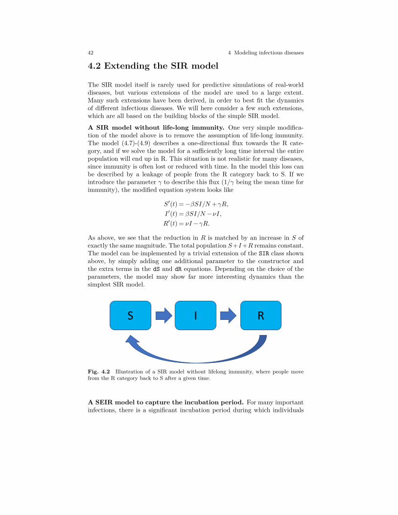
A SIR model without life-long immunity. One very simple modifica-tion of the model above is to remove the assumption of life-long immunity.The model (4.7)-(4.9) describes a one-directional flux towards the R cate-gory, and if we solve the model for a sufficiently long time interval the entirepopulation will end up in R. This situation is not realistic for many diseases,since immunity is often lost or reduced with time. In the model this loss canbe described by a leakage of people from the R category back to S. If weintroduce the parameter γ to describe this flux (1/γ being the mean time forimmunity), the modified equation system looks like
S′(t) =−βSI/N +γR,
I ′(t) = βSI/N −νI,R′(t) = νI−γR.
As above, we see that the reduction in R is matched by an increase in S ofexactly the same magnitude. The total population S+I+R remains constant.The model can be implemented by a trivial extension of the SIR class shownabove, by simply adding one additional parameter to the constructor andthe extra terms in the dS and dR equations. Depending on the choice of theparameters, the model may show far more interesting dynamics than thesimplest SIR model.
S RI
Fig. 4.2 Illustration of a SIR model without lifelong immunity, where people movefrom the R category back to S after a given time.
A SEIR model to capture the incubation period. For many importantinfections, there is a significant incubation period during which individuals
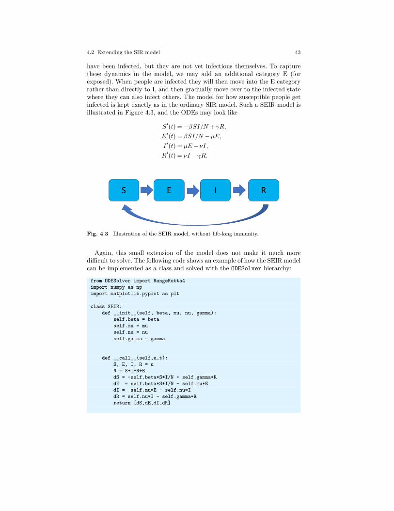
4.2 Extending the SIR model 43
have been infected, but they are not yet infectious themselves. To capturethese dynamics in the model, we may add an additional category E (forexposed). When people are infected they will then move into the E categoryrather than directly to I, and then gradually move over to the infected statewhere they can also infect others. The model for how susceptible people getinfected is kept exactly as in the ordinary SIR model. Such a SEIR model isillustrated in Figure 4.3, and the ODEs may look like
S′(t) =−βSI/N +γR,
E′(t) = βSI/N −µE,I ′(t) = µE−νI,R′(t) = νI−γR.
S RIE
Fig. 4.3 Illustration of the SEIR model, without life-long immunity.
Again, this small extension of the model does not make it much moredifficult to solve. The following code shows an example of how the SEIR modelcan be implemented as a class and solved with the ODESolver hierarchy:
from ODESolver import RungeKutta4import numpy as npimport matplotlib.pyplot as plt
class SEIR:def __init__(self, beta, mu, nu, gamma):
self.beta = betaself.mu = muself.nu = nuself.gamma = gamma
def __call__(self,u,t):S, E, I, R = uN = S+I+R+EdS = -self.beta*S*I/N + self.gamma*RdE = self.beta*S*I/N - self.mu*EdI = self.mu*E - self.nu*IdR = self.nu*I - self.gamma*Rreturn [dS,dE,dI,dR]
44 4 Modeling infectious diseases
S0 = 1000E0 = 0I0 = 1R0 = 0model = SEIR(beta=1.0, mu=1.0/5,nu=1.0/7,gamma=1.0/50)
solver= RungeKutta4(model)solver.set_initial_condition([S0,E0,I0,R0])time_points = np.linspace(0, 100, 101)u, t = solver.solve(time_points)S = u[:,0]; E = u[:,1]; I = u[:,2]; R = u[:,3]
plt.plot(t,S,t,E,t,I,t,R)plt.show()
4.3 A model of the Covid19 pandemic
The models considered above can typically be adapted to describe more com-plex disease behavior by adding more categories of people and possibly moreinteractions between the different categories. We will now consider an exten-sion of the SEIR model above into a model that has been used by Norwegianhealth authorities to predict the spread of the 2020 Covid19 pandemic. Wewill here derive the model as a system of ODEs, just like the models consid-ered above, while the real model that is used to provide Covid19 predictionsfor health authorities is a stochastic model.2 A stochastic model is some-what more flexible than the deterministic ODE version, and can more easilyincorporate dynamics such as model parameters that vary with time afterinfection. For instance, the infectiousness (β) should typically follow a bell-shaped curve that increases gradually after infection, reaches a peak aftera few days, and is then reduced. Such behavior is easier to incorporate ina stochastic model than in the deterministic ODE model considered here,which essentially assumes a constant β for everyone in the I category. How-ever, the overall structure and dynamics of the two model types are exactlythe same, and for certain choices of the model parameters the stochastic anddeterministic models become equivalent.
To describe Covid19, the SEIR model introduced above is modified toincorporate two important disease characteristics:
• A certain number of people infected with Covid19 have no symptoms.These asymptomatic people can still infect other, but with a lower infec-tiousness than the symptomatic group, and they need to be treated as aseparate category.
2See https://github.com/folkehelseinstituttet/spread
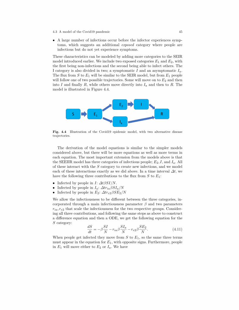
4.3 A model of the Covid19 pandemic 45
• A large number of infections occur before the infector experiences symp-toms, which suggests an additional exposed category where people areinfectious but do not yet experience symptoms.
These characteristics can be modeled by adding more categories to the SEIRmodel introduced earlier. We include two exposed categories E1 and E2, withthe first being non-infectious and the second being able to infect others. TheI category is also divided in two; a symptomatic I and an asymptomatic Ia.The flux from S to E1 will be similar to the SEIR model, but from E1 peoplewill follow one of two possible trajectories. Some will move on to E2 and theninto I and finally R, while others move directly into Ia and then to R. Themodel is illustrated in Figure 4.4.
S R
I
E1
E2
Ia
Fig. 4.4 Illustration of the Covid19 epidemic model, with two alternative diseasetrajectories.
The derivation of the model equations is similar to the simpler modelsconsidered above, but there will be more equations as well as more terms ineach equation. The most important extension from the models above is thatthe SEEIIR model has three categories of infectious people; E2, I, and Ia. Allof these interact with the S category to create new infections, and we modeleach of these interactions exactly as we did above. In a time interval ∆t, wehave the following three contributions to the flux from S to E1:
• Infected by people in I: ∆tβSI/N .• Infected by people in Ia: ∆triaβSIa/N• Infected by people in E2: ∆tre2βSE2/N
We allow the infectiousness to be different between the three categories, in-corporated through a main infectiousness parameter β and two parametersria, re2 that scale the infectiousness for the two respective groups. Consider-ing all three contributions, and following the same steps as above to constructa difference equation and then a ODE, we get the following equation for theS category:
dS
dt=−βSI
N− riaβ
SIaN− re2β
SE2N
. (4.11)
When people get infected they move from S to E1, so the same three termsmust appear in the equation for E1, with opposite signs. Furthermore, peoplein E1 will move either to E2 or Ia. We have
46 4 Modeling infectious diseases
dE1dt
= βSI
N+ riaβ
SIaN
+ re2βSE2N−λ1(1−pa)E1−λ1paE1
= βSI
N+ riaβ
SIaN
+ re2βSE2N−λ1E1.
Here, pa is a parameter describing the proportion of infected people that neverdevelop symptoms, while 1/λ1 is the mean duration of the non-infectiousincubation period. The term λ1(1− pa)E1 represents people moving to E2,and λ1paE1 are people moving to Ia. In the equation for E1 we can combinethese two fluxes into a single term, but they must be considered separatelyin the equations for E2 and Ia.
The E2 category will get an influx of people from E1, and an outflux ofpeople moving on to the infected I category, while I gets an influx from E2and an outflux to R. The ODEs for these two categories become
dE2dt
= λ1(1−pa)E1−λ2E2,
dI
t= λ2E2−µI,
where 1/λ2 and 1/µ are the mean durations of the E2 and I phases, respec-tively.
The model for the asymptomatic disease trajectory is somewhat simpler,with Ia receiving an influx from E1 and losing people directly to R. We have
dIadt
= λ1paE1−µIa,
where we have assumed that the duration of the Ia period is the same as forI, i.e. 1/µ. Finally, the dynamics of the recovered category are governed by
dR
dt= µI+µIa.
Notice that we do not consider flow from the R category back to S, so wehave effectively assumed life-long immunity. This assumption is probablynot correct for Covid19, but since the duration of immunity is still largelyunknown, and we are mostly interested in the early epidemic spread, weneglect the loss of immunity.
To summarize, the complete ODE system of the SEEIIR model can bewritten as
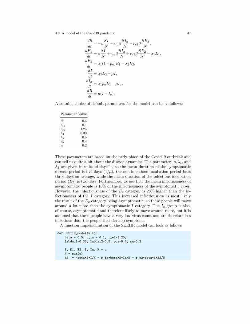
4.3 A model of the Covid19 pandemic 47
dS
dt=−βSI
N− riaβ
SIaN− re2β
SE2N
,
dE1dt
= βSI
N+ riaβ
SIaN
+ re2βSE2N−λ1E1,
dE2dt
= λ1(1−pa)E1−λ2E2,
dI
dt= λ2E2−µI,
dIadt
= λ1paE1−µIa,
dR
dt= µ(I+ Ia).
A suitable choice of default parameters for the model can be as follows:
Parameter Value
β 0.5ria 0.1re2 1.25λ1 0.33λ2 0.5pa 0.4µ 0.2
These parameters are based on the early phase of the Covid19 outbreak andcan tell us quite a bit about the disease dynamics. The parameters µ,λ1, andλ2 are given in units of days−1, so the mean duration of the symptomaticdisease period is five days (1/µ), the non-infectious incubation period laststhree days on average, while the mean duration of the infectious incubationperiod (E2) is two days. Furthermore, we see that the mean infectiousness ofasymptomatic people is 10% of the infectiousness of the symptomatic cases.However, the infectiousness of the E2 category is 25% higher than the in-fectiousness of the I category. This increased infectiousness is most likelythe result of the E2 category being asymptomatic, so these people will movearound a lot more than the symptomatic I category. The Ia group is also,of course, asymptomatic and therefore likely to move around more, but it isassumed that these people have a very low virus count and are therefore lessinfectious than the people that develop symptoms.
A function implementation of the SEEIIR model can look as follows
def SEEIIR_model(u,t):beta = 0.5; r_ia = 0.1; r_e2=1.25;lmbda_1=0.33; lmbda_2=0.5; p_a=0.4; mu=0.2;
S, E1, E2, I, Ia, R = uN = sum(u)dS = -beta*S*I/N - r_ia*beta*S*Ia/N - r_e2*beta*S*E2/N
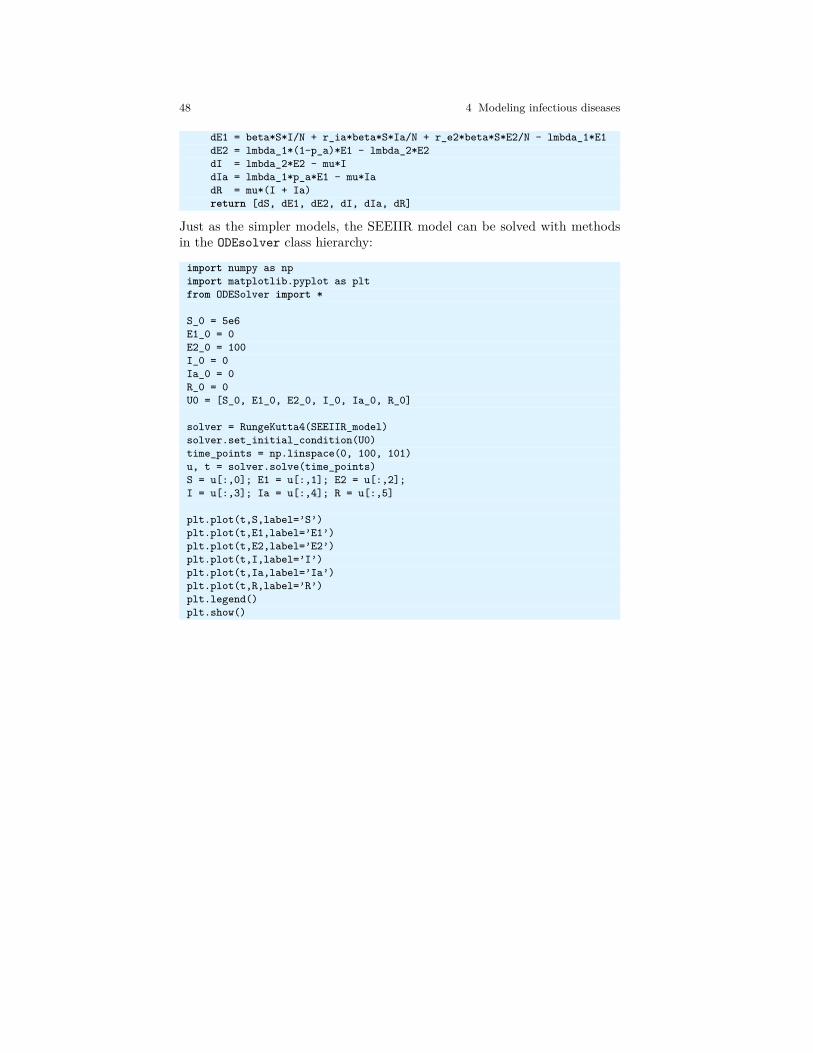
48 4 Modeling infectious diseases
dE1 = beta*S*I/N + r_ia*beta*S*Ia/N + r_e2*beta*S*E2/N - lmbda_1*E1dE2 = lmbda_1*(1-p_a)*E1 - lmbda_2*E2dI = lmbda_2*E2 - mu*IdIa = lmbda_1*p_a*E1 - mu*IadR = mu*(I + Ia)return [dS, dE1, dE2, dI, dIa, dR]
Just as the simpler models, the SEEIIR model can be solved with methodsin the ODEsolver class hierarchy:
import numpy as npimport matplotlib.pyplot as pltfrom ODESolver import *
S_0 = 5e6E1_0 = 0E2_0 = 100I_0 = 0Ia_0 = 0R_0 = 0U0 = [S_0, E1_0, E2_0, I_0, Ia_0, R_0]
solver = RungeKutta4(SEEIIR_model)solver.set_initial_condition(U0)time_points = np.linspace(0, 100, 101)u, t = solver.solve(time_points)S = u[:,0]; E1 = u[:,1]; E2 = u[:,2];I = u[:,3]; Ia = u[:,4]; R = u[:,5]
plt.plot(t,S,label=’S’)plt.plot(t,E1,label=’E1’)plt.plot(t,E2,label=’E2’)plt.plot(t,I,label=’I’)plt.plot(t,Ia,label=’Ia’)plt.plot(t,R,label=’R’)plt.legend()plt.show()
Related Documents


