European Society of Computational Methods in Sciences and Engineering (ESCMSE) Journal of Numerical Analysis, Industrial and Applied Mathematics (JNAIAM) vol. 1, no. 1, 2007, pp. 1-30 ISSN 1790–8140 Solving Differential-Algebraic Equations by Taylor Series (III): the DAETS Code Nedialko S. Nedialkov 1 Department of Computing and Software, McMaster University, Hamilton, Ontario, L8S 4L7, Canada John D. Pryce 2 Department of Information Systems, Cranfield University, RMCS Shrivenham, Swindon SN6 8LA, UK Received —; accepted in revised form — Abstract: The authors have developed a Taylor series method for solving numerically an initial-value problem differential-algebraic equation (DAE) that can be of high index, high order, nonlinear, and fully implicit, see BIT 45:561–592, 2005 and BIT 41:364-394, 2001. Numerical results have shown this method to be efficient and very accurate, and particularly suitable for problems that are of too high an index for present DAE solvers. This paper outlines this theory and describes the design, implementation, usage and per- formance of DAETS, a DAE solver based on this theory and written in C++. c 2007 European Society of Computational Methods in Sciences and Engineering Keywords: Differential-algebraic equations (DAEs), structural analysis, Taylor series, au- tomatic differentiation Mathematics Subject Classification: 34A09, 65L80, 65L05, 41A58 1 Introduction 1.1 What DAETS does and the tools it uses This paper describes the structure and use of a code DAETS (D ifferential A lgebraic E quations by T aylor S eries) that solves initial value problems for differential algebraic equation systems (DAEs) for state variables x j (t),j =1,...,n, of the general form f i ( t, the x j and derivatives of them ) = 0, i =1,...,n, (1) by expanding the solution in a Taylor series (TS) at each integration step. The f i can be arbitrary expressions built from the x j and t using +, −, ×, ÷, other analytic standard functions, and the 1 Corresponding author. E-mail: [email protected] 2 E-mail: [email protected]

Welcome message from author
This document is posted to help you gain knowledge. Please leave a comment to let me know what you think about it! Share it to your friends and learn new things together.
Transcript
European Society of Computational Methodsin Sciences and Engineering (ESCMSE)
Journal of Numerical Analysis,Industrial and Applied Mathematics
(JNAIAM)vol. 1, no. 1, 2007, pp. 1-30
ISSN 1790–8140
Solving Differential-Algebraic Equations byTaylor Series (III): the DAETS Code
Nedialko S. Nedialkov 1
Department of Computing and Software,McMaster University, Hamilton, Ontario,
L8S 4L7, Canada
John D. Pryce 2
Department of Information Systems,Cranfield University, RMCS Shrivenham,
Swindon SN6 8LA, UK
Received —; accepted in revised form —
Abstract: The authors have developed a Taylor series method for solving numericallyan initial-value problem differential-algebraic equation (DAE) that can be of high index,high order, nonlinear, and fully implicit, see BIT 45:561–592, 2005 and BIT 41:364-394,2001. Numerical results have shown this method to be efficient and very accurate, andparticularly suitable for problems that are of too high an index for present DAE solvers.This paper outlines this theory and describes the design, implementation, usage and per-formance of DAETS, a DAE solver based on this theory and written in C++.
c© 2007 European Society of Computational Methods in Sciences and Engineering
Keywords: Differential-algebraic equations (DAEs), structural analysis, Taylor series, au-tomatic differentiation
Mathematics Subject Classification: 34A09, 65L80, 65L05, 41A58
1 Introduction
1.1 What DAETS does and the tools it uses
This paper describes the structure and use of a code DAETS (Differential Algebraic Equations byTaylor Series) that solves initial value problems for differential algebraic equation systems (DAEs)for state variables xj(t), j = 1, . . . , n, of the general form
fi( t, the xj and derivatives of them ) = 0, i = 1, . . . , n, (1)
by expanding the solution in a Taylor series (TS) at each integration step. The fi can be arbitraryexpressions built from the xj and t using +,−,×,÷, other analytic standard functions, and the
1Corresponding author. E-mail: [email protected]: [email protected]

2 N. S. Nedialkov and J. D. Pryce
differentiation operator dp/dtp. They can be nonlinear and fully implicit in the variables andderivatives. An equation such as
(x′′1 )
2
(c2 + (x′1)
2)3 + t2 cosx2 = 0 (2)
can be encoded directly into DAETS. Derivatives need not actually be present, so DAETS cansolve continuation problems f(t,x) = 0, taking t as the continuation parameter. It has handleddifficult problems of this kind, as reported below.
A common measure of the numerical difficulty of a DAE is its differentiation index νd, thenumber of times the fi must be differentiated (w.r.t. t) to obtain equations that can be solved toform an ODE system for the xj . An index of 3 and above is normally considered hard. DAETS isnot inherently affected by high index, for reasons explained later. Below, we report results on upto index-47 DAEs.
One of the hardest parts of DAE solution can be finding an initial consistent point. This canbe seen as a minimization problem, and DAETS gives this task to a proven optimization packageIPOPT [25], which has proved robust and effective.
Stiff behaviour can be present for DAEs, as for ODEs. DAETS handles moderate stiffness well,but is unsuitable for highly stiff problems.
DAETS is written in C++. Apart from IPOPT, it makes use of Stauning’s automatic differen-tiation (AD) package FADBAD++ [24] and the C version of Volgenant’s LAP [10] code for LinearAssignment Problems.
The rest of this introduction takes a software developer’s viewpoint. Subsection 1.2 reviewstheoretical approaches to DAEs based on derivatives of equations, as is that of DAETS; anddescribes the origins of the software architecture of DAETS. Subsection 1.3 gives a broad overviewof the numerical method, and discusses the impact it has on the architecture and the user interface.
The remainder of the paper is laid out as follows. Section 2 outlines the structural analysis(SA) theory on which the numerical method is based. Section 3 describes the main componentsof the algorithm. Section 4 discusses the most important components of the code’s class structure— both the user-visible and the internal parts. Section 5 describes and discusses the performanceof the code on a variety of problems. Section 6 gives examples of coding up a function defining aDAE system, and a main program to solve the problem with DAETS. Section 7 summarises ourexperience with DAETS and describes some outstanding problems and planned enhancements.
1.2 Background
Many problems of importance in science and industry are modelled as DAEs. Examples fromapplications are in, for instance, the Test Set for Initial Value Solvers [13], which contains problemsfrom electronic circuits, mechanical systems and chemical processing. Adding detail to a model,such as accounting for the internal behaviour of actuating motors in a robot arm, often increasesthe DAE index.
For a traditional solver, the problem is typically written as a first-order ODE x′ = f(t,x) orfirst-order DAE M(t,x)x′ = f(t,x), where M is a singular matrix. The code only sees a “blackbox” routine that computes the value of f or M or (for stiff problems) Jacobian information atgiven inputs (t,x). It has long been known in various theoretical frameworks that a DAE can beseen as an ODE on a manifold and can be accurately solved as such, provided one “knows” how tomanipulate derivatives of the defining functions. This underlies the jet space approach [22] basedon differential geometry, Campbell’s derivative array theory [3] and more practical approaches ofindex reduction [1, 12]. DAETS is based on Pryce’s structural analysis [21], which has this samebasic approach and is itself an extension of the method of Pantelides [17].
c© 2007 European Society of Computational Methods in Sciences and Engineering (ESCMSE)

Solving DAEs by Taylor Series (III): DAETS 3
The software architecture of DAETS is derived from that of Nedialkov’s VNODE code [14]mainly written during his PhD project at the University of Toronto. VNODE finds validated
solutions (that is, enclosures of the solutions) of ordinary differential equation (ODE) initial valueproblems, using interval arithmetic. More important than the interval aspect is that VNODE isan object-oriented implementation of a general design for ODE solvers due to Hull and Enright[9]. This design separates parts of the algorithm into modules, such as the stepping formula, errorestimation, step size choice, output to the user, etc., in a way that makes it easy to change thealgorithm for one part with minimal impact on the others.
DAETS and VNODE have in common parts of the implementation as well as of the design:for instance they both use FADBAD++ to do AD, and VNODE has an optional stepping modulethat uses TS. However DAETS handles the implicit system (1) while VNODE handles an explicitODE system x′ = f(t,x), which makes a large difference to the details of how the two codesuse FADBAD++ and how they generate Taylor coefficients (TCs). Some significant parts of theDAETS algorithm have no counterpart in the Hull–Enright design.
1.3 The method and how it affects the design
We describe in broad terms the numerical method based on Pryce’s structural analysis (SA) [20, 21],and discuss how its features affect the design of the code, especially the user interface. In thissubsection, “software” means our (or another) DAE solver, as opposed to the infrastructure toolsbelow it or an application on top of it.
The numerical method. Starting with code for the functions fi in (1), an SA-based method usesautomatic differentiation (AD) to evaluate suitable derivatives dr/dtr of the fi. By equating theseto zero at a given t = t, it solves implicitly for derivatives, or equivalently TCs, of the solutioncomponents xj(t) at t.
The AD can be handled in many ways, depending on language features and on the tools oneconsiders efficient and convenient. We use Ole Stauning’s popular AD tool, FADBAD++, whichuses C++ templates and operator overloading to compute derivatives. There is evidence thatother tools may give somewhat faster code, e.g. ADOL-C [5], but we have found FADBAD++ isconvenient for the software writer, allows a straightforward user interface, and has to date causedno problems with installing the software.
As illustrated in (2), differentiation d/dt can be used anywhere in the expressions defining theDAE. To enable this, Stauning modified FADBAD++ to make d/dt a “first-class” operator (nameddiff), like the arithmetic operations and standard functions. Also, to make over/underflow lesslikely in computing coefficients ar of a Taylor expansion a(t∗ + h) =
∑r arh
r, DAETS computesthe terms arh
r directly. This is neatly done by an implicit change of independent variable from tto s where t = t∗ + sh. This needed creating our version of the d/dt operator (named Diff) insideDAETS, so FADBAD++ is not changed.
Various numerical methods can be based on SA. “Solving implicitly” can in effect reduce theDAE to an ODE system — numerically implementing the definition of the differentiation index— and a standard method such as Runge–Kutta or BDF can be applied to the result. Methodsof this kind are starting to be studied. We have chosen the approach in Pryce’s original papers,using the AD to evaluate the TS to some order. The resulting method is generally not as efficientas standard DAE solvers on problems they can solve, but becomes increasingly efficient at highaccuracies and is relatively simple to code.
In the SA one computes the n×n signature matrix, and 2n integers, the offsets of the variablesand of the equations. These prescribe the overall process for computing TCs, as well as how toform the System Jacobian J (4) that is central to the theory and the numerical method.
c© 2007 European Society of Computational Methods in Sciences and Engineering (ESCMSE)

4 N. S. Nedialkov and J. D. Pryce
The TCs are used with an appropriate stepsize to find a truncated TS approximation of thesolution, which is then projected to satisfy the constraints of the DAE. The process is repeated oneach integration step in a standard time-stepping manner. Error estimation and step size selectionare like that in Taylor codes for ODEs, but the offsets complicate the details.
If J is nonsingular at a consistent point, see Subsection 2.3, the SA has succeeded and the DAEis solvable in a neighborhood of this point. Although SA applies to a wide range of DAEs, there areproblems on which it fails: when J is singular at a point at which the DAE is solvable. Typicallythis happens when the equations (1) are “not sparse enough” to reveal the underlying structure ofthe system. Examples are discussed in [15, 20, 21].
An SA-based method derives a structural index νs, which is the same as the index found bythe method of Pantelides [17] for DAEs to which that method applies. It is shown by Reißig,Martinson and Barton [23] that νs can be arbitrarily greater than νd; but in [21, Subsection 5.3],that provided the SA succeeds — that is, J is nonsingular — νs can never be less than νd, andin [15] that overestimating νs causes, at worst, mild inefficiency in the solution process. Moreoverthe method is robust in the sense that it can always detect (up to roundoff) when J is singular,and therefore indicate that the SA fails: see [15, Algorithm 6.1].
Effect on the user interface. C++ code for the functions fi in (1) looks much as for a standardODE solver for y′ = f(t,y). However, the active variables must be declared of a templated type,instantiated at compile time with several different actual types. One type is used for the numericalAD, another to compute the signature matrix, and so on. This imposes some restrictions on theallowed expressions. Also, the differentiation operator Diff(·,q) denoting dq/dtq can be appliedto any active item. The latter are the inputs x[j] denoting xj , the outputs f[i] denoting fi , andany code variables or expressions on the computational path between these.
When the SA method succeeds, it provides the user with much useful information about thestructure of the DAE. We provide a way for the calling program to print out the signature matrix,offsets and related data after the SA has been done.
In fact the user needs to know SA data in order to use an SA-based method effectively. Thereason is that the offsets determine the shape of the set of initial values that must be given to thesolver (fixed values, or free, guessed, values). For traditional ODE or DAE solvers the initial valuesare flat vectors: here they form an irregular array as in (17) on page 12.
Hence coding the calling program for an unfamiliar DAE tends to be a two-stage process. First,give the function code to DAETS and make it print a description of the structure. Setting initialvalues can then be coded correctly, though it may need thought about their physical meaning inorder to get a sensible choice of fixed and free values.
The fact that analysis precedes numerical solution affects the user interface. First, it is whythe interface makes two (main) classes available. One, DAEsolution, holds the irregular arrayof xj-and-derivatives at a given t, plus related data. The other, DAEsolver, knows among otherthings the result of the structural analysis. Its integrate method can be applied to differentDAEsolution objects, thus one can compute many solution paths without re-doing the SA.
Second, each stage has its own kind of error. The SA can find there is no transversal (Sub-section 2.1) of finite value, indicating an ill-formulated problem. Or it can appear that the SAsucceeded, but the resulting Jacobian matrix J is always singular, indicating that the SA was un-able to reveal the true structure of the DAE. Or DAETS may find a nonsingular J but be unableto find a consistent point. Or it may find a consistent point and start along the solution path, butgrind to a halt for some reason.
The two-way flow of information in preparing the problem for solution gives DAETS somefeatures of a Problem Solving Environment. We do not offer an interactive GUI yet, but thiswould be useful. There is a contrasting requirement, however. The software may be needed as an
c© 2007 European Society of Computational Methods in Sciences and Engineering (ESCMSE)

Solving DAEs by Taylor Series (III): DAETS 5
“engine”, to solve a DAE of known structure as part of a larger application. For such use, it mustsuppress printing and return any error diagnostics by a flag (or similar) that is handled by thecalling program. DAETS can be used in such a silent mode as well as in a verbose one.
2 Theory
2.1 Pryce’s Structural analysis of DAEs
We present as much of Pryce’s structural analysis [21] as is needed for this paper.The following definitions are needed. A transversal T of an n × n matrix (σij) is a set of
n positions in the matrix with one entry in each row and each column. That is, T is a set{(1, j1), (2, j2), . . . , (n, jn)} where (j1, . . . , jn) are a permutation of (1, . . . , n). The value of T isVal T =
∑(i,j)∈T σij .
Given a DAE in the form of (1), we perform the following steps.
1. Form the n× n signature matrix Σ = (σij), where
σij =
order of the derivative to which the jth variable xj occurs inthe ith equation fi; or
−∞ if xj does not occur in fi.
2. Find a highest value transversal (HVT), which is a transversal T that makes ValT as large aspossible. The value of a HVT is also, by definition, the value of the signature matrix, writtenValΣ.
The value of any transversal, and of Σ, is either an integer or −∞. The DAE is structurally
regular if Val Σ is finite: that is, if there exists at least one transversal all of whose σij arefinite. Otherwise the DAE is structurally ill-posed — there is probably some error in problemformulation.
3. Find n-dimensional integer vectors c and d, with all ci ≥ 0, that satisfy
dj − ci ≥ σij for all i, j = 1, . . . , n and (3)
dj − ci = σij for all (i, j) ∈ T . (4)
By [21, Lemma 3.3], if a transversal T and vectors c,d are found such that (3) and (4) hold,then necessarily T is a HVT. Summing (4) over T gives an alternative formula for Val Σ:
n∑
j=1
dj −
n∑
i=1
ci = ValT = Val Σ.
From this follows that for any c and d, if (3, 4) hold for some HVT, then (4) holds for anyHVT.
c and d are the offsets. They are never unique. It is a little more efficient, but not necessary,to choose the canonical offsets, which are smallest in the sense of a ≤ b if ai ≤ bi for each i.
4. Form the n× n System Jacobian matrix
J =∂(f
(c1)1 , . . . , f
(cn)n
)
∂(x
(d1)1 , . . . , x
(dn)n
) . (5)
c© 2007 European Society of Computational Methods in Sciences and Engineering (ESCMSE)
6 N. S. Nedialkov and J. D. Pryce
By results in [21], (5) has the equivalent reformulations:
Jij =∂fi
∂x(dj−ci)j
=
∂fi
∂x(σij)j
if dj − ci = σij and
0 otherwise.
(6)
5. Seek values for the xj and for appropriate derivatives, consistent with the DAE in the senseof Subsection 2.3, and at which J is nonsingular. If such values are found, they define a pointthrough which there is locally a unique solution of the DAE. In this case we say the method“succeeds”.
Step 2 is a Linear Assignment Problem (LAP), a form of a linear programming problem for whichgood software exists [10]. Step 3 defines its dual. The two formulae for Val Σ instance the factthat primal and dual have the same optimal value.
When the method succeeds:
• Val Σ equals the number of degrees of freedom (DOF) of the DAE, that is the number ofindependent initial conditions required.
• An upper bound for the differentiation index νd is given by the Taylor index
νT = maxi
ci +
{1 if some dj is zero,0 otherwise.
(7)
In many cases, νT = νd.
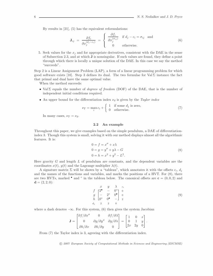
2.2 An example
Throughout this paper, we give examples based on the simple pendulum, a DAE of differentiation-index 3. Though this system is small, solving it with our method displays almost all the algorithmicfeatures. It is:
0 = f = x′′ + xλ
0 = g = y′′ + yλ−G
0 = h = x2 + y2 − L2.
(8)
Here gravity G and length L of pendulum are constants, and the dependent variables are thecoordinates x(t), y(t) and the Lagrange multiplier λ(t).
A signature matrix Σ will be shown by a “tableau”, which annotates it with the offsets ci, dj
and the names of the functions and variables, and marks the positions of a HVT. For (8), thereare two HVTs, marked • and ◦ in the tableau below. The canonical offsets are c = (0, 0, 2) andd = (2, 2, 0):
x y λ ci[ ]f 2• − 0◦ 0
g − 2◦ 0• 0
h 0◦ 0• − 2
dj 2 2 0
(9)
where a dash denotes −∞. For this system, (6) then gives the system Jacobian
J =
∂f/∂x′′ 0 ∂f/∂λ
0 ∂g/∂y′′ ∂g/∂λ
∂h/∂x ∂h/∂y 0
=
1 0 x0 1 y2x 2y 0
.
From (7) the Taylor index is 3, agreeing with the differentiation index.
c© 2007 European Society of Computational Methods in Sciences and Engineering (ESCMSE)

Solving DAEs by Taylor Series (III): DAETS 7
2.3 Consistent points and quasi-linearity
The offsets specify what data is needed to define a consistent point, and what consistent means.Namely, the data comprise a point
X =(x1, x
′1, . . . , x
(d1−1)1 ; x2, x
′2, . . . , x
(d2−1)2 ; . . . ; xn, x′
n, . . . , x(dn−1)n
)(10)
and it is consistent iff it satisfies the set of equations
F =(f1, f
′1, . . . , f
(c1−1)1 ; f2, f
′2, . . . , f
(c2−1)2 ; . . . ; fn, f ′
n, . . . , f (cn−1)n
)= 0. (11)
An xj whose dj is zero (it must have σij = 0 for all i and thus is a “purely algebraic variable”)does not appear in the vector X. Similarly, an fi with ci = 0 does not appear in F.
f ′i means dfi/dt treating the variables and their derivatives as (unknown) functions of t, for
instance if f1 = x′′1 − x1x3 then f ′
1 = x′′′1 − x′
1x3 − x1x′3; similarly for higher derivatives.
A convenient notation for such “irregular vectors” is as follows. If J is a set of indices (j, r)
where 1 ≤ j ≤ n and r ≥ 0, let xJ denote the set of derivatives x(r)j for (j, r) ∈ J , regarded as a
vector. Use the notation J≤k [resp. J<k] to mean the set of (j, r) satisfying 0 ≤ r ≤ k + dj [resp.
0 ≤ r < k + dj ]. For a similar set of indices I, let fI denote the derivatives f(r)i for (i, r) ∈ I, and
let I≤k [resp. I<k] mean the set of (i, r) satisfying 0 ≤ r ≤ k + ci [resp. 0 ≤ r < k + ci].Then (10, 11) can be written
fI<0(xJ<0
) = 0. (12)
There is an amendment to the above definition of X and F. DAETS checks whether the nextderivatives after those in (10), namely x
(dj)j , j = 1, . . . , n, occur in a jointly linear way in the fi.
If they do, we call the DAE quasi-linear, by analogy with a similar notion in PDE theory.
If the DAE is not quasi-linear, these next derivatives x(dj)j are included in X and corresponding
derivatives of the fi, namely f(ci)i = 0, i = 1, . . . , n, are included in the equations (11) that define
a consistent point. That is, (12) changes to
fI≤0
(xJ≤0
)= 0. (13)
If we denote
α =
{−1 if the DAE is quasi-linear and
0 otherwise,
then we write (12) and (13) as
fI≤α
(xJ≤α
)= 0.
For example, in the Pendulum system (8), the relevant derivatives x(dj)j are x′′, y′′ and λ. Their
occurrence is jointly linear, so (8) is quasi-linear. It would still be so were, say, f changed tox′′x + xλ or to x′′y′ + xλ, but not if it were changed to x′′y′′ + xλ, or to x′′λ + xλ.
In the original quasi-linear case the equations (12) for a consistent point are
Solve h, h′ = 0 for x, x′, y, y′.
When not quasi-linear they become
Solve f, g, h, h′, h′′ = 0 for x, x′, x′′, y, y′, y′′, λ.
c© 2007 European Society of Computational Methods in Sciences and Engineering (ESCMSE)

8 N. S. Nedialkov and J. D. Pryce
The reason for going from (12) to (13) is as follows. Consider a particular independent variablevalue t. Let a set of values X in (10) be consistent with some solution of the DAE at t. Thenif the DAE is quasi-linear that solution is unique. If it is not quasi-linear, there may be severalsolutions consistent with these values; however, augmenting X with the next level of derivativesrestores uniqueness.
This affects how the user sets initial conditions. These are usually only guesses of consistentvalues, which the code corrects by a root-finding process. When the DAE is not quasi-linear, goodguesses of the extra derivatives make it more likely that the code finds the consistent point —hence the solution — that was intended.
An example is the use of DAETS to do arc-length continuation (see Subsection 5.6). Here t isarc-length from an initial point x0 along a path x(t) in some R
m. There is inherent non-uniqueness:from x0 you can traverse the path in either direction. In this case the required extra derivatives,at a consistent point, are the unit tangent x′
0 in the desired direction. That is, the augmented Xis the pair (x0,x
′0). A good guess of x′
0 will make the code start off in the right direction.
3 Algorithm overview
We present the stepping algorithm in DAETS and then elaborate on various points of this algo-rithm, including order and stepsize selection.
3.1 The stepping algorithm
Initial state: We have an initial t value and
• TS expansion of order p• Initial solution guess at t comprising xJ≤α
• No predicted next step• User-supplied point tend
Standard state: We have a current interval [tprev, tcur], of nonzero length, and
• p as above• Complete TS xprev,J≤p
at tprev
• htrial = predicted next step• Essential part, xcur,J≤α
of (accepted) solution at tcur
• Error estimate e of above accepted solution; necessarily ‖e‖ ≤ tol• User-supplied point tend, assumed to be “in front of” tprev, that is
(tend − tprev)(tcur − tprev) ≥ 0 ; note tend = tprev is allowed
Algorithm 3.1 (Stepping algorithm)while tend is not in [tprev, tcur]
// Take a stepdo
if htrial too small return htoosmallttrial ← tprev + htrial
// Compute scaled TCs to required order p:xcur,J≤p
← ComputeTCs(tcur, xcur,J≤α, step = htrial, order = p)
// Unprojected Taylor series solution and error estimate:[xTS,J≤α
, ets] ← SumTS(tcur, xcur,J≤p, step = htrial, order = p)
// Projected Taylor series solution on to the constraints:xtrial,J≤α
← Project(xTS,J≤α)
c© 2007 European Society of Computational Methods in Sciences and Engineering (ESCMSE)

Solving DAEs by Taylor Series (III): DAETS 9
if (Projection failure) return badprojfailure// Summary error estimate:e ← ‖ets‖+ ‖xtrial,J≤α
− xTS,J≤α‖
tol ← atol + ‖xtrial‖ × rtolhtrial ← new predicted value based on e, tol, p
while e > tol
// Now accept the step:tprev ← tcur, tcur ← ttrialxprev,J≤p
← xcur,J≤p, xcur,J≤α
← xtrial,J≤α
if (one-step mode) return onesteppingend while
// Now tend is inside [tprev, tcur], compute solution at tend:xend,J≤α
← SumTS(tprev, xprev, step = tend − tprev, order = p)Project it// We assume the error in this is acceptablereturn this projected solution
3.2 About the main loop
We speak of “DAETS” doing the things described below; mostly, they are features of the integratemethod of the DAEsolver class.
3.2.1 Output points.
As with most solvers, we do not want closely spaced output points tend to cause inefficiencyby reducing the step size. A good way to do this is for the solver to create a (usually piecewisepolynomial) u(t) approximating the solution to sufficient order, and evaluate this at output points.DAETS does not yet do this, see Section 7. Instead, after stepping to ti, DAETS remembers theTS expansion at ti−1. If tend is between these two points it evaluates the TS with a step tend−ti−1,and projects the result to give the output value. Since the error test has already passed with thelarger step hi = ti− ti−1, no error check is done. This handles any number of output points withina step reasonably efficiently, though not quite as well as having a u(t).
3.2.2 Changing direction.
One may have a sequence of tend’s that are not in monotone order, e.g. during the root-findinginvolved in event location. If they are all in the current interval between ti−1 and ti, the mechanismin the last paragraph handles them with no problem. If however tend lies outside this interval, onthe ti−1 side, the integration must change direction. The stored TS at ti−1 is re-used, with a stepsize obtained from stored data, to step to a “new ti” in the reverse direction. Further steps aretaken as necessary till the new tend is passed, and output produced as in the last paragraph.
3.2.3 One-step mode.
When called in one-step mode, DAETS returns at the end of each step, as well as at an outputpoint. This can be used to produce output for graphing; it is also necessary for event location,which at present is not provided within DAETS and must be coded in the calling program.
c© 2007 European Society of Computational Methods in Sciences and Engineering (ESCMSE)
10 N. S. Nedialkov and J. D. Pryce
3.2.4 Finding an initial consistent point
At each step, the algorithm projects a trial solution point onto the consistent manifoldM to givethe accepted point. On steps after the first, the step size selection process aims to make the trialpoint close to M, so a simple projection method suffices. The first step is different in two ways.First, the task is of finding a consistent point, given an initial guess that may be very far fromM.This is recognized as one of the challenging problems in solving nonlinear DAEs. The code treatsthis as a minimisation problem and gives it to the optimisation package IPOPT.
Second, the initial guess is part of the user interface. It makes sense to split its componentsinto fixed values, which the user “decides” and wants to keep as is, and free values — “just guesses”that the minimisation process is free to change.
Let the set of values to be found, xJ≤α, be regarded as a flat vector x = (y, z) where y and z
denote fixed and free components respectively. Let the equations by whichM is defined, fI≤α= 0,
be denoted f = 0. Let the fixed and free user-supplied values be y∗ and z∗ respectively. ThenIPOPT is given the following (generally nonlinear) least-squares problem:
min(y,z)
‖z− z∗‖22
subject to f(y, z) = 0,
and y = y∗.
(14)
Currently the unweighted 2-norm is used; we intend to provide the option of a weighted 2-norm‖v‖2 =
∑i wi|vi|
2 in the future.
3.2.5 Order and stepsize selection
Currently, DAETS uses constant order during an integration, where either DAETS selects a valuefor the order or the user can set a value for it. If the user has not specified such, a value is selectedby [11]
p = ⌈−0.5 ln(tol) + 1⌉, (15)
where tol is either the default tolerance of 10−12 in DAETS or a user-specified value. (Currentlya maximum value for the order of the TS is set to 200 at compile time, but this can be easilychanged to another value.)
The error in an approximate Taylor series solution is estimated as that in the computed ap-proximation to xJ≤α
. Consider the TS expansion of xj to order p + dj at a point t. With stepsizeh, DAETS computes scaled TCs at t + h:
xj,k ≈x
(k)j (t)
k!hk for k = 0, 1, . . . , p + dj .
Then it computes approximations x(k)j to x
(k)j at t + h for all k = 0, . . . , dj + α:
x(k)j =
p+dj−1∑
i=k
i(i− 1) · · · (i− k + 1)
hk· xj,i + rj,k,
where α is as above, and
rj,k =(p + dj)(p + dj − 1) · · · (p + dj − k + 1)
hk· xj,p+dj
.
c© 2007 European Society of Computational Methods in Sciences and Engineering (ESCMSE)
Solving DAEs by Taylor Series (III): DAETS 11
If we denote by r the vector with components rj,k for all j = 1, . . . , n and all k = 0, . . . dj + α, weestimate the error in the TS solution by
ets = ‖r‖.
We select a trial stepsize, after an accepted or rejected step, by
htrial = h
(0.25 · tol
e
)p−α
, (16)
where e is computed as in Algorithm 3.1:
e = ‖ets‖+ ‖xtrial,J≤α− xTS,J≤α
‖.
In the error estimations, DAETS uses the max norm.The initial stepsize is currently selected as in (16) with h = 1, but in the future we shall
incorporate a better strategy that avoids possible overflows/underflows in the TC computation onthe first step.
4 The structure of DAETS
DAETS is implemented as a collection of C++ classes. This section describes the classes, first thoseneeded by the user and then the internal ones. Only a few methods and attributes are mentioned:for more information see the User Guide [19].
4.1 User-visible architecture
The calling program uses two classes DAEsolver and DAEsolution; optionally, a “cut-down” ver-sion of DAEsolution called DAEpoint; and an enumerated type DAEexitflag that signals integra-tion success or failure.
The reason for having DAEsolver and DAEsolution is as follows. An ODE/DAE integrationcan be viewed as moving a point along a path x(t) in some R
m. It is highly desirable to storeinternal state data — current step size, Jacobian, etc. — in a separate place that “belongs” tothe given path. Without this, for instance, it is hard to follow two or more paths in parallel bycalling the integrator on each, alternately. For codes written in non-OO languages this storage istypically a work array passed to the integrator. Here, these two classes achieve the separation.
A DAEsolver object Solver implements the integration process. It contains the needed knowl-edge about the DAE itself such as the function code and the offsets. It also contains policy dataabout the integration, such as the Taylor series order, the accuracy tolerance and type of error test(absolute, relative or mixed), and whether the integration is done in one-step mode.
A DAEsolution object X implements the moving point. This includes the numerical values ofits components and the current value of t; also data describing the current state of the solution:are we at an initial guess, a point on the path from which we can integrate further, or a pointwhere an error prevents further progress?
The allocation of attributes between the DAEsolver and DAEsolution classes is to some extentarbitrary and makes some operations more convenient than others. To use one Solver to advancetwo solutions with different initial conditions, using the same order and tolerance, is easy. To usethe same initial conditions but different tolerances, for instance, is possible but less convenient.We could have made the tolerance part of X rather than part of Solver, but this felt less natural.
This design supports various protective interlocks. A newly created X has its first entry flagset true, indicating that it is expected to be an inconsistent point. Its t, and each component of its
c© 2007 European Society of Computational Methods in Sciences and Engineering (ESCMSE)
12 N. S. Nedialkov and J. D. Pryce
x, is flagged as “uninitialized”, and integrate will not accept it until all these values are set. Atsubsequent consistent points first entry becomes false and can only be reset by an explicit callto setFirstEntry(). When it is false, trying to alter the x or t values in X is an error. Similarly,once integration of X has failed, say with “step size too small”, re-calling the integrator raises anerror unless one has reset first entry. Such protections are difficult in a traditional code thatuses a work array.
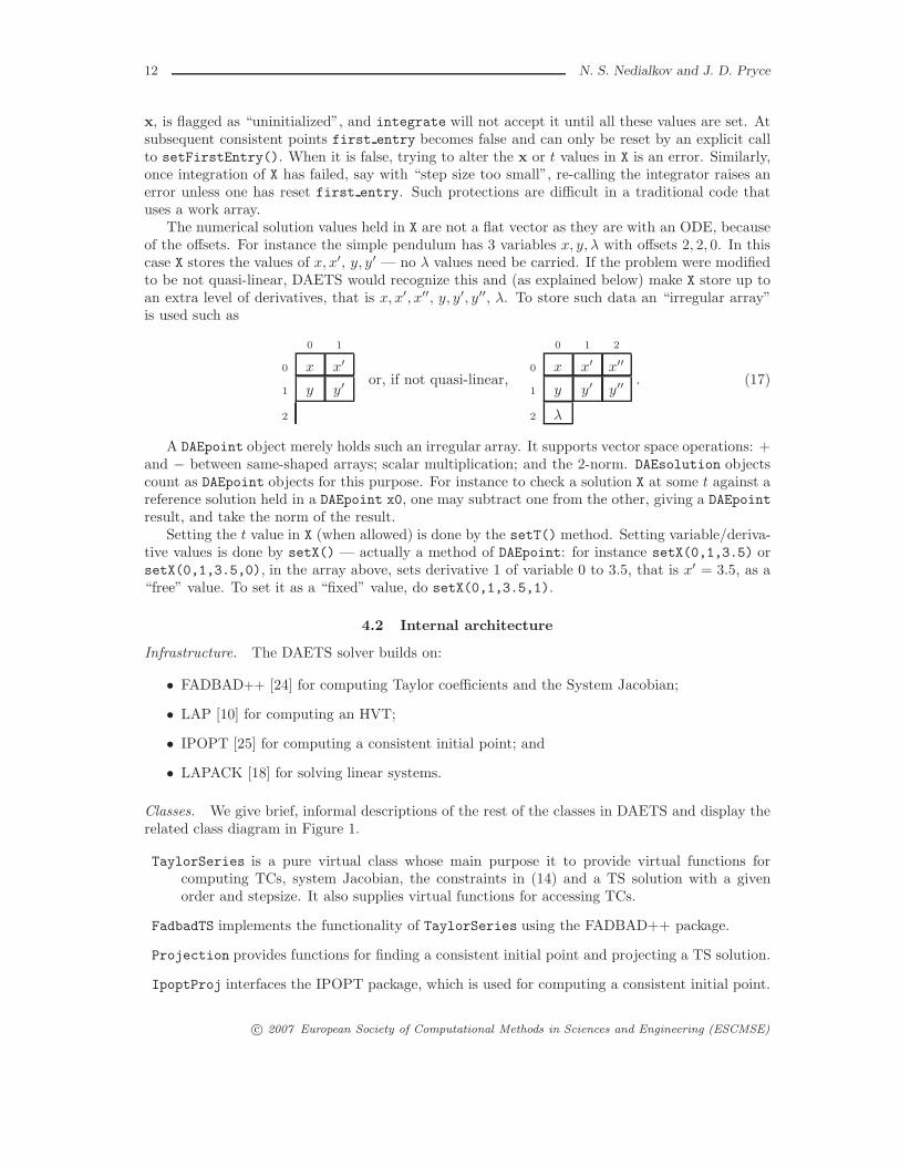
The numerical solution values held in X are not a flat vector as they are with an ODE, becauseof the offsets. For instance the simple pendulum has 3 variables x, y, λ with offsets 2, 2, 0. In thiscase X stores the values of x, x′, y, y′ — no λ values need be carried. If the problem were modifiedto be not quasi-linear, DAETS would recognize this and (as explained below) make X store up toan extra level of derivatives, that is x, x′, x′′, y, y′, y′′, λ. To store such data an “irregular array”is used such as
0 1
0 x x′
1 y y′
2
or, if not quasi-linear,
0 1 2
0 x x′ x′′
1 y y′ y′′
2 λ
. (17)
A DAEpoint object merely holds such an irregular array. It supports vector space operations: +and − between same-shaped arrays; scalar multiplication; and the 2-norm. DAEsolution objectscount as DAEpoint objects for this purpose. For instance to check a solution X at some t against areference solution held in a DAEpoint x0, one may subtract one from the other, giving a DAEpoint
result, and take the norm of the result.Setting the t value in X (when allowed) is done by the setT() method. Setting variable/deriva-
tive values is done by setX() — actually a method of DAEpoint: for instance setX(0,1,3.5) orsetX(0,1,3.5,0), in the array above, sets derivative 1 of variable 0 to 3.5, that is x′ = 3.5, as a“free” value. To set it as a “fixed” value, do setX(0,1,3.5,1).
4.2 Internal architecture
Infrastructure. The DAETS solver builds on:
• FADBAD++ [24] for computing Taylor coefficients and the System Jacobian;
• LAP [10] for computing an HVT;
• IPOPT [25] for computing a consistent initial point; and
• LAPACK [18] for solving linear systems.
Classes. We give brief, informal descriptions of the rest of the classes in DAETS and display therelated class diagram in Figure 1.
TaylorSeries is a pure virtual class whose main purpose it to provide virtual functions forcomputing TCs, system Jacobian, the constraints in (14) and a TS solution with a givenorder and stepsize. It also supplies virtual functions for accessing TCs.
FadbadTS implements the functionality of TaylorSeries using the FADBAD++ package.
Projection provides functions for finding a consistent initial point and projecting a TS solution.
IpoptProj interfaces the IPOPT package, which is used for computing a consistent initial point.
c© 2007 European Society of Computational Methods in Sciences and Engineering (ESCMSE)

Solving DAEs by Taylor Series (III): DAETS 13
TaylorSeries
FadbadTS
Constants
ErrorEst
IpoptProj
Parameters
Projection
SigmaVector
SigmaMatrix
Offsets
Stats
PointComponent
DAEpoint
DAEsolution
DAEsolver
IpoptFuncs
Figure 1: DAETS class diagram. The arrows with the triangle denote inheritance; a “normal”arrow from class A to class B means A uses B.
IpoptFuncs provides the functions needed by IPOPT in (14): for evaluating the objective, itsgradient, the constraints and the Jacobian of the constraints on each stage.
SigmaVector overloads the arithmetic operations and standard functions, including the Diff
operator, for “sigma vectors”; see also [15].
SigmaMatrix provides functions for computing the signature matrix of a DAE and determining ifthe problem is quasi-linear. These computations are performed by propagating SigmaVector
objects through the code list of the DAE.
Offsets provides functions for computing the offsets of the problem, using its signature matrix.
Constants stores various constants, such as default values for order, tolerance, etc. needed duringintegration.
Parameters encapsulates various parameters that can be set before integration, such as order,tolerance, smallest allowed stepsize, etc.
ErrorEst estimates the error in a TS soluion.
PointComponent describes an entry in a DAEpoint object: a PointComponent object contains itsnumerical value, and says whether it is fixed or free and whether it is initialized.
Stats collects various statistics during an integration, such as CPU time, number of steps, per-centage rejected steps, etc.
c© 2007 European Society of Computational Methods in Sciences and Engineering (ESCMSE)

14 N. S. Nedialkov and J. D. Pryce
4.3 Help for the user
This subsection lists features in the code and documentation that go beyond what is traditionalfor an ODE solver.
The theory of signature matrix and offsets is given in some detail in the User Guide [19] becauseit is fairly new and will be unfamiliar to most potential users.
The signature tableau, on the lines of that for the Pendulum example shown in (9), offers muchinsight into the structure of a DAE, so there is a method printOffsets() that displays it.
To use DAETS, a user must understand that the needed initial values to be fixed or guessedform an irregular array, see above. The User Guide explains this in detail, and also the code offershelp: if the correct set of derivatives has not been initialized on first entry to integrate, a messageis printed indicating just what this set is.
There is a method to display a requested set of variable and derivative values of a DAEsolution
point — again, useful because of its irregular shape.
More familiarly, there are methods to display statistics about the integration (accepted/rejectedsteps etc.); and to explain the meaning of a DAEexitflag value.
5 Numerical results
Subsection 5.1 shows that DAETS is very accurate on four standard test problems from [13].Subsection 5.2 examines the efficiency of DAETS on these problems and compares it with theefficiency of DASSL [2] and RADAU [7]. Subsection 5.3 investigates the performance of DAETSon high-index DAEs, where we solve up to index-47 DAEs. Subsection 5.4 studies the efficiencyof DAETS on the heat equation discretized by the method of lines and formulated as an index-1DAE. Subsection 5.5 illustrates how the total number of steps behaves as the order of the methodincreases. Finally, Subsection 5.6 shows that DAETS can solve a pure algebraic system usingcontinuation and formulated as an implicit DAE of index 1.
The computations are performed on a Mac Pro having two dual-core Intel Xeon, 2.66 GHzprocessors (four cores in total), 2GB main memory and 4MB L2 cache per processor. DAETS iscompiled with the gcc compiler version 4.0.1 with an optimization flag -O2; RADAU and DASSLare compiled with g77 version 3.4.2 and optimization flag -O2.
The timing results are reported in seconds.
5.1 Accuracy
We study the accuracy of the computed solutions by DAETS on four test problems from [13]: caraxis, an index-3 DAE consisting of 8 differential and 2 algebraic equations; transistor amplifier, anindex-1 DAE consisting of 8 differential equations; chemical Akzo Nobel, an index-1 DAE consistingof 5 differential and 1 algebraic equations; and HIRES, an ODE consisting of 8 equations. (Exceptthe chemical Azko Nobel problem, the rest are classified as stiff in [13].)
Let the set of computed values (with a given tolerance) for xJ≤αbe regarded as a flat vector
x, and let a reference solution for xJ≤αbe regarded as a flat vector xref. If e is the vector with ith
component (xi − xref,i)/xref,i, we estimate number of signicant correct digits, scd, in x as in [13]:
scd = − log10(‖e‖∞).
We integrate these problems with DAETS using a mixed relative–absolute error control withtolerances tol = 10−4, 10−5, . . . , 10−14. We determine scd using the reference solutions given in[13] and reference solutions computed by DAETS with tol = 10−16. We also compute scd with
c© 2007 European Society of Computational Methods in Sciences and Engineering (ESCMSE)
Solving DAEs by Taylor Series (III): DAETS 15
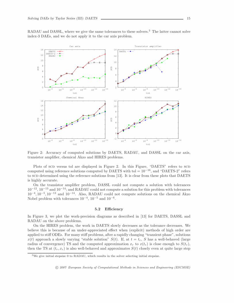
RADAU and DASSL, where we give the same tolerances to these solvers.3 The latter cannot solveindex-3 DAEs, and we do not apply it to the car axis problem.
0
2
4
6
8
10
12
14
10-1410-1210-1010-810-610-4
SCD
tol
Car axis
DAETSDAETS-2RADAU
2
4
6
8
10
12
14
10-1410-1210-1010-810-610-4
SCD
tol
Transistor amplifier
DASSL
-2
0
2
4
6
8
10
12
10-1410-1210-1010-810-610-4
SCD
tol
HIRES
0
2
4
6
8
10
12
14
16
10-1410-1210-1010-810-610-4
SCD
tol
Chemical Akzo
Figure 2: Accuracy of computed solutions by DAETS, RADAU, and DASSL on the car axis,transistor amplifier, chemical Akzo and HIRES problems.
Plots of scd versus tol are displayed in Figure 2. In this Figure, “DAETS” refers to scd
computed using reference solutions computed by DAETS with tol = 10−16, and “DAETS-2” refersto scd determined using the reference solutions from [13]. It is clear from these plots that DAETSis highly accurate.
On the transistor amplifier problem, DASSL could not compute a solution with tolerances10−12, 10−13 and 10−14; and RADAU could not compute a solution for this problem with tolerances10−4, 10−5, 10−13 and 10−14. Also, RADAU could not compute solutions on the chemical AkzoNobel problem with tolerances 10−4, 10−5 and 10−6.
5.2 Efficiency
In Figure 3, we plot the work-precision diagrams as described in [13] for DAETS, DASSL andRADAU on the above problems.
On the HIRES problem, the work in DAETS slowly decreases as the tolerance decreases. Webelieve this is because of an under-appreciated effect when (explicit) methods of high order areapplied to stiff ODEs. For many stiff problems, after a rapidly changing “transient phase”, solutionsx(t) approach a slowly varying “stable solution” S(t). If, at t = tr, S has a well-behaved (largeradius of convergence) TS and the computed approximation xr to x(tr) is close enough to S(tr),then the TS at (tr, xr) is also well-behaved and approximates S(t) closely even at quite large step
3We give initial stepsize 0 to RADAU, which results in the solver selecting initial stepsize.
c© 2007 European Society of Computational Methods in Sciences and Engineering (ESCMSE)

16 N. S. Nedialkov and J. D. Pryce
10-3
10-2
10-1
100
0 2 4 6 8 10 12 14
CPU time
SCD
Car axis
DAETSRADAU
10-2
10-1
100
101
102
2 4 6 8 10 12 14
CPU time
SCD
Transistor amplifier
DASSL
10-3
10-2
10-1
100
101
-2 0 2 4 6 8 10 12
CPU time
SCD
HIRES
10-3
10-2
10-1
0 2 4 6 8 10 12 14 16
CPU time
SCD
Chemical Akzo
Figure 3: Efficiency of DAETS, RADAU, and DASSL on the car axis, transistor amplifier, chemicalAkzo and HIRES problems.
sizes. Thus the local error is small enough not to “re-awaken” transients, and this good behaviourcontinues at subsequent steps. The higher the order, the stronger is this effect.
We do not yet understand the phenomenon well. It will not apply to all stiff systems; and itprobably depends on our step size control algorithm being sufficiently cautious to keep well withinthe stability region.
Generally, our solver is not as efficient as standard DAE solvers on problems (and tolerances)for which these solvers perform well. The strength of DAETS is in solving high-index problems,which standard solvers cannot tackle, and in computing accurate solutions at stringent tolerances;cf. Figures 2 and 3.
5.3 High-index DAEs
We consider the DAE problem consisting of P pendula:
0 = x′′1 + λ1x1
0 = y′′1 + λ1y1 −G
0 = x21 + y2
1 − L2
and
0 = x′′i + λixi
0 = y′′i + λiyi −G
0 = x2i + y2
i − (L + cλi−1)2,
(i = 2, 3, . . . , P ), (18)
where G, L and c are given constants. Here, the first pendulum is undriven, and pendulum (i− 1)exerts a driving effect on pendulum i, for i = 2, . . . , P . The system (18) is of size 3P and index2P + 1.
c© 2007 European Society of Computational Methods in Sciences and Engineering (ESCMSE)
Solving DAEs by Taylor Series (III): DAETS 17
Our solver requires initial conditions for
x(d)i , y
(d)i for all i = 1, . . . , P and for all d = 0, . . . , 2(P − i + 1); and
λ(d)i for all i = 1, . . . , P − 1 and for all d = 0, . . . , 2(P − i + 1)− 1.
(19)
That is, the earlier pendula in the sequence require more initial conditions. In the numericalexperiments that follow, we set G = 9.8, L = 3.4 and c = 0.1.
-5-4-3-2-1 0 1 2 3 4 5
0 10 20 30 40 50 60
x7, tol = 5*10-9
-5-4-3-2-1 0 1 2 3 4 5
0 10 20 30 40 50 60
y7, tol = 5*10-9
-200 0
200 400 600 800 1000 1200 1400 1600
0 10 20 30 40 50 60
λ7, tol = 5*10-9
-5-4-3-2-1 0 1 2 3 4 5
0 10 20 30 40 50 60
x7, tol = 10-9
-5-4-3-2-1 0 1 2 3 4 5
0 10 20 30 40 50 60
y7, tol = 10-9
-40-30-20-10 0 10 20 30 40 50 60
0 10 20 30 40 50 60
λ7, tol = 10-9
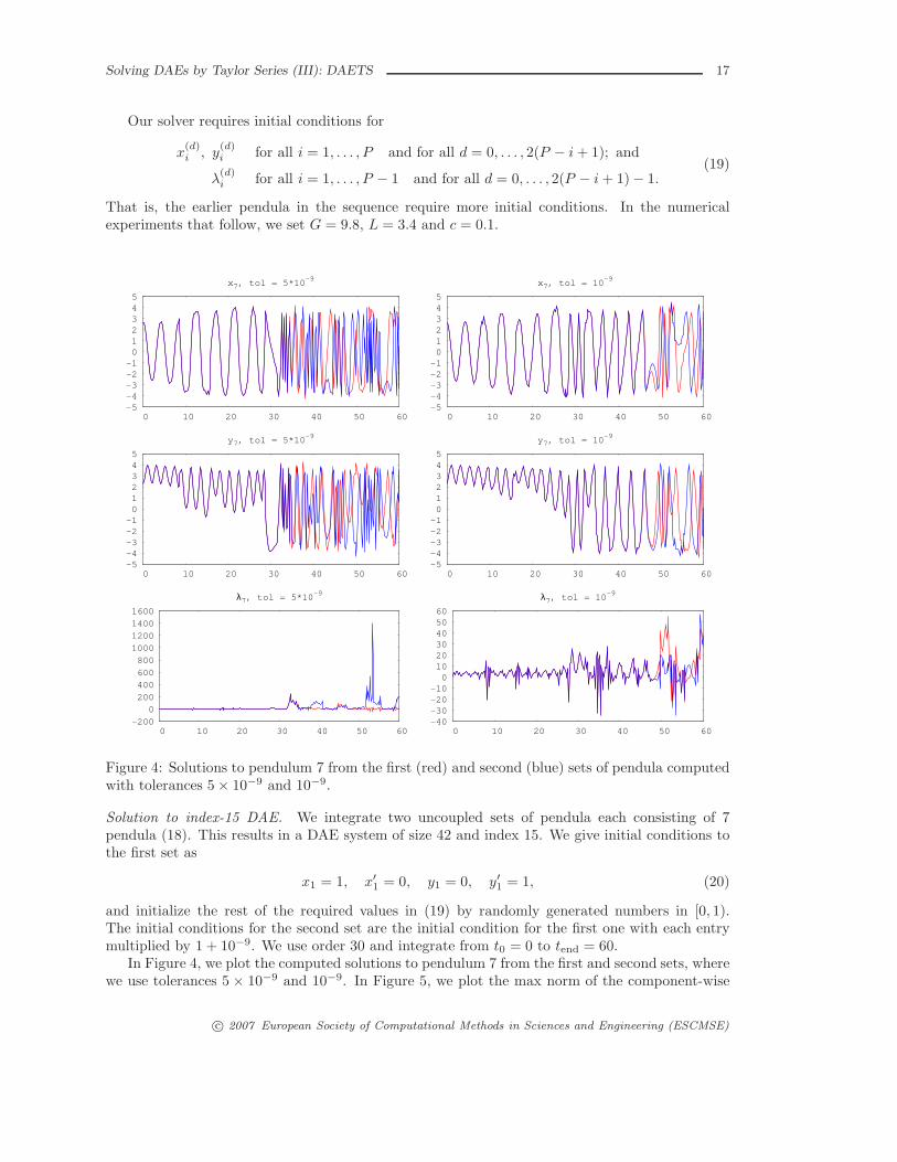
Figure 4: Solutions to pendulum 7 from the first (red) and second (blue) sets of pendula computedwith tolerances 5× 10⁻⁹ and 10−9.
Solution to index-15 DAE. We integrate two uncoupled sets of pendula each consisting of 7pendula (18). This results in a DAE system of size 42 and index 15. We give initial conditions tothe first set as
x1 = 1, x′1 = 0, y1 = 0, y′
1 = 1, (20)
and initialize the rest of the required values in (19) by randomly generated numbers in [0, 1).The initial conditions for the second set are the initial condition for the first one with each entrymultiplied by 1 + 10−9. We use order 30 and integrate from t0 = 0 to tend = 60.
In Figure 4, we plot the computed solutions to pendulum 7 from the first and second sets, wherewe use tolerances 5 × 10⁻⁹ and 10−9. In Figure 5, we plot the max norm of the component-wise
c© 2007 European Society of Computational Methods in Sciences and Engineering (ESCMSE)
18 N. S. Nedialkov and J. D. Pryce
10-10
10-8
10-6
10-4
10-2
100
102
104
0 10 20 30 40 50 60
norm of solution difference
t
tol = 5*10-9
10-10
10-8
10-6
10-4
10-2
100
102
0 10 20 30 40 50 60
norm of solution difference
t
tol = 10-9
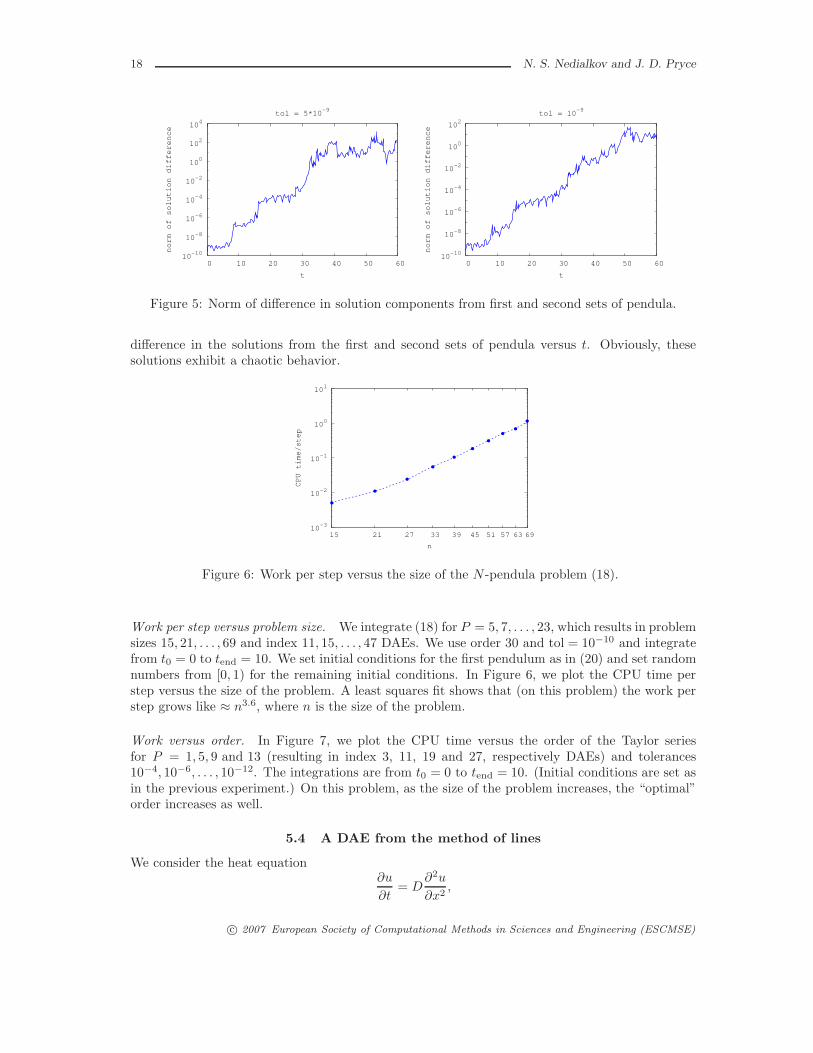
Figure 5: Norm of difference in solution components from first and second sets of pendula.
difference in the solutions from the first and second sets of pendula versus t. Obviously, thesesolutions exhibit a chaotic behavior.
10-3
10-2
10-1
100
101
69 63 57 51 45 39 33 27 21 15
CPU time/step
n
Figure 6: Work per step versus the size of the N -pendula problem (18).
Work per step versus problem size. We integrate (18) for P = 5, 7, . . . , 23, which results in problemsizes 15, 21, . . . , 69 and index 11, 15, . . . , 47 DAEs. We use order 30 and tol = 10−10 and integratefrom t0 = 0 to tend = 10. We set initial conditions for the first pendulum as in (20) and set randomnumbers from [0, 1) for the remaining initial conditions. In Figure 6, we plot the CPU time perstep versus the size of the problem. A least squares fit shows that (on this problem) the work perstep grows like ≈ n3.6, where n is the size of the problem.
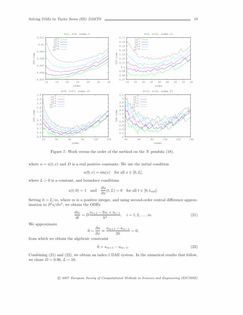
Work versus order. In Figure 7, we plot the CPU time versus the order of the Taylor seriesfor P = 1, 5, 9 and 13 (resulting in index 3, 11, 19 and 27, respectively DAEs) and tolerances10−4, 10−6, . . . , 10−12. The integrations are from t0 = 0 to tend = 10. (Initial conditions are set asin the previous experiment.) On this problem, as the size of the problem increases, the “optimal”order increases as well.
5.4 A DAE from the method of lines
We consider the heat equation∂u
∂t= D
∂2u
∂x2,
c© 2007 European Society of Computational Methods in Sciences and Engineering (ESCMSE)
Solving DAEs by Taylor Series (III): DAETS 19
0.005
0.006
0.007
0.008
0.009
0.01
0.011
10 15 20 25 30 35 40
CPU time
order
P=1, n=3, index 3
10-4
10-6
10-8
10-10
10-12
0.07
0.08
0.09
0.1
0.11
0.12
0.13
0.14
0.15
0.16
0.17
20 25 30 35 40 45 50 55 60
CPU time
order
P=5, n=15, index 11
10-4
10-6
10-8
10-10
10-12
0.5
0.6
0.7
0.8
0.9
1
1.1
1.2
1.3
1.4
1.5
20 40 60 80 100 120
CPU time
order
P=9, n=27, index 19
10-4
10-6
10-8
10-10
10-12
2
2.2
2.4
2.6
2.8
3
3.2
3.4
3.6
3.8
4
4.2
40 60 80 100 120 140
CPU time
order
P=13, n=39, index 27
10-4
10-6
10-8
10-10
10-12
Figure 7: Work versus the order of the method on the N pendula (18).
where u = u(t, x) and D is a real positive constants. We use the initial condition
u(0, x) = sin(x) for all x ∈ [0, L],
where L > 0 is a constant, and boundary conditions
u(t, 0) = 1 and∂u
∂x(t, L) = 0 for all t ∈ [0, tend].
Setting h = L/m, where m is a positive integer, and using second-order central difference approx-imation to ∂2u/∂x2, we obtain the ODEs
dui
dt= D
ui+1 − 2ui + ui−1
h2, i = 1, 2, . . . , m. (21)
We approximate
0 =∂u
∂x≈
um+1 − um−1
2h= 0,
from which we obtain the algebraic constraint
0 = um+1 − um−1. (22)
Combining (21) and (22), we obtain an index-1 DAE system. In the numerical results that follow,we chose D = 0.96, L = 10.
c© 2007 European Society of Computational Methods in Sciences and Engineering (ESCMSE)

20 N. S. Nedialkov and J. D. Pryce
10-3
10-2
10-1
200 160 120 80 60 40 20
CPU time/step
n
Figure 8: Work per step versus the size of the discretized heat equation.
-40
-30
-20
-10
0
10
20
30
40
-35 -30 -25 -20 -15 -10 -5 0 5
Figure 9: Stability regions of the Taylorseries method for orders p =5, 10, 15,. . . , 90. They are very nearly semicir-cles with radius r given by r ≈ 0.375p+1.352. The lobes near the y axis seemto get smaller with p but actually havea periodic pattern.
Work per step versus problem size. In Figure 8, weplot the CPU time per step versus the size of the prob-lem when integrating (21–22) with the above initial andboundary conditions. We use order 30 and tol = 10−10
and integrate from t0 = 0 to tend = 5. A least squares fitshows that this work grow like ≈ n2.1.
The reason DAETS is more efficient on this problemthan on the pendula problem from the previous subsec-tion is the amount of automatic differentiation involved.Here, we have a linear problem, and to compute p coef-ficients we require O(p) work, while to compute TCs fora nonlinear problem, we require O(p2) work.
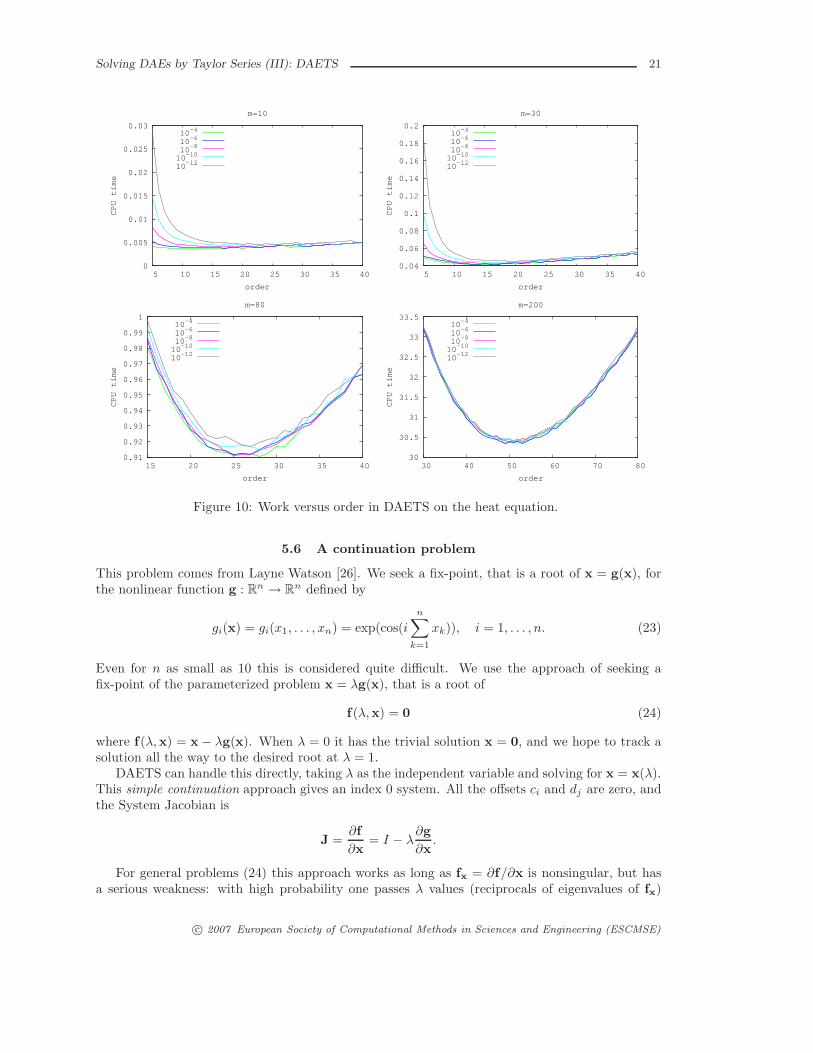
Work versus order. In Figure 10, we show the work ver-sus order for tolerances tol = 10−4, 10−6, . . . , 10−12 whenintegrating (21–22) with the above initial and boundaryconditions from t0 = 0 to tend = 10. As the discretizationin x becomes finer, the problem becomes stiffer, whichresults in increasing the “optimal” order as m increases,due to the Taylor method’s stability region increasingwith order, see Figure 9.
5.5 Number of steps versus order
We illustrate how the total number of integration stepsbehaves as the order of the integration increases. In Fig-ure 11, we plot number of steps versus the order of themethod when integrating the car axis, HIRES, the pen-dula problem with 5 and 13 pendula, and the discretizedheat equation with m = 30 and m = 300. As expected,when the order increases, this number goes down due to the smaller truncation error and extendedstability region of the Taylor series method.
The behavior of the number of steps on the HIRES problem seems unusual: DAETS takes moresteps as the tolerance becomes more relaxed from 10−12 to 10−4. A possible explanation is alongthe lines of Subsection 5.2.
c© 2007 European Society of Computational Methods in Sciences and Engineering (ESCMSE)
Solving DAEs by Taylor Series (III): DAETS 21
0
0.005
0.01
0.015
0.02
0.025
0.03
5 10 15 20 25 30 35 40
CPU time
order
m=10
10-4
10-6
10-8
10-10
10-12
0.04
0.06
0.08
0.1
0.12
0.14
0.16
0.18
0.2
5 10 15 20 25 30 35 40
CPU time
order
m=30
10-4
10-6
10-8
10-10
10-12
0.91
0.92
0.93
0.94
0.95
0.96
0.97
0.98
0.99
1
15 20 25 30 35 40
CPU time
order
m=80
10-4
10-6
10-8
10-10
10-12
30
30.5
31
31.5
32
32.5
33
33.5
30 40 50 60 70 80
CPU time
order
m=200
10-4
10-6
10-8
10-10
10-12
Figure 10: Work versus order in DAETS on the heat equation.
5.6 A continuation problem
This problem comes from Layne Watson [26]. We seek a fix-point, that is a root of x = g(x), forthe nonlinear function g : R
n → Rn defined by
gi(x) = gi(x1, . . . , xn) = exp(cos(i
n∑
k=1
xk)), i = 1, . . . , n. (23)
Even for n as small as 10 this is considered quite difficult. We use the approach of seeking afix-point of the parameterized problem x = λg(x), that is a root of
f(λ,x) = 0 (24)
where f(λ,x) = x− λg(x). When λ = 0 it has the trivial solution x = 0, and we hope to track asolution all the way to the desired root at λ = 1.
DAETS can handle this directly, taking λ as the independent variable and solving for x = x(λ).This simple continuation approach gives an index 0 system. All the offsets ci and dj are zero, andthe System Jacobian is
J =∂f
∂x= I − λ
∂g
∂x.
For general problems (24) this approach works as long as fx = ∂f/∂x is nonsingular, but hasa serious weakness: with high probability one passes λ values (reciprocals of eigenvalues of fx)
c© 2007 European Society of Computational Methods in Sciences and Engineering (ESCMSE)

22 N. S. Nedialkov and J. D. Pryce
0
50
100
150
200
250
300
350
400
450
500
10 20 30 40 50 60 70 80 90 100
number steps
order
Car axis
10-4
10-6
10-8
10-10
10-12
1000
2000
3000
4000
5000
6000
7000
8000
10 20 30 40 50 60 70 80 90 100
number steps
order
HIRES
10-4
10-6
10-8
10-10
10-12
0
50
100
150
200
250
20 40 60 80 100 120 140
number steps
order
5 pendula
10-4
10-6
10-8
10-10
10-12
0
50
100
150
200
250
300
350
400
450
20 40 60 80 100 120 140number steps
order
13 pendula
10-4
10-6
10-8
10-10
10-12
0
50
100
150
200
250
300
350
400
10 20 30 40 50 60 70 80
number steps
order
Discretized heat equation, m=30
10-4
10-6
10-8
10-10
10-12
1000
2000
3000
4000
5000
6000
7000
8000
9000
10000
10 20 30 40 50 60 70 80
number steps
order
Discretized heat equation, m=300
10-4
10-6
10-8
10-10
10-12
Figure 11: Plots of number of steps versus the order of the method.
where fx becomes singular, even though the n × (n+1) matrix [fλ, fx] retains full rank n. Theseare turning points, at which dx/dλ becomes infinite. For (23), simple continuation only works forn = 1 and 2.
A powerful alternative is to treat λ, x1, . . . , xn as all on the same footing instead of viewing λas special, and to use arc-length continuation. The system (24) may be rewritten as n equationsin n+1 unknowns:
f(y) = 0 (25)
where y = (λ; x). As long as fy is of full row rank there is a (unique except for direction) solutionpath through any point in R
n+1 satisfying (25), tangential to the 1-dimensional null space of fy.Generically, i.e. for a “randomly chosen problem”, this is true everywhere along the path. Invent
c© 2007 European Society of Computational Methods in Sciences and Engineering (ESCMSE)
Solving DAEs by Taylor Series (III): DAETS 23
x1, x10
λ
x1x10x1x10
0
0.5
1
1.5
2
2.5
0 0.2 0.4 0.6 0.8 1 1.2
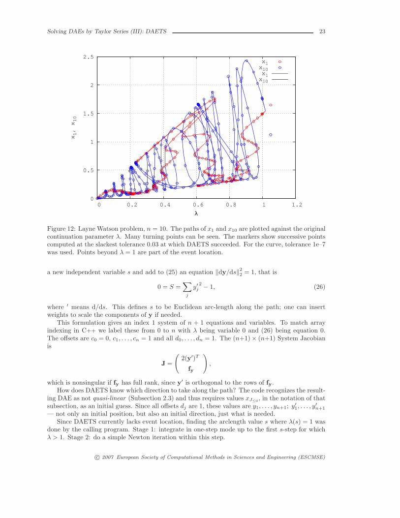
Figure 12: Layne Watson problem, n = 10. The paths of x1 and x10 are plotted against the originalcontinuation parameter λ. Many turning points can be seen. The markers show successive pointscomputed at the slackest tolerance 0.03 at which DAETS succeeded. For the curve, tolerance 1e–7was used. Points beyond λ = 1 are part of the event location.
a new independent variable s and add to (25) an equation ‖dy/ds‖22 = 1, that is
0 = S =∑
j
y′j
2− 1, (26)
where ′ means d/ds. This defines s to be Euclidean arc-length along the path; one can insertweights to scale the components of y if needed.
This formulation gives an index 1 system of n + 1 equations and variables. To match arrayindexing in C++ we label these from 0 to n with λ being variable 0 and (26) being equation 0.The offsets are c0 = 0, c1, . . . , cn = 1 and all d0, . . . , dn = 1. The (n+1)× (n+1) System Jacobianis
J =
(2(y′)T
fy
),
which is nonsingular if fy has full rank, since y′ is orthogonal to the rows of fy.How does DAETS know which direction to take along the path? The code recognizes the result-
ing DAE as not quasi-linear (Subsection 2.3) and thus requires values xJ≤0, in the notation of that
subsection, as an initial guess. Since all offsets dj are 1, these values are y1, . . . , yn+1; y′1, . . . , y
′n+1
— not only an initial position, but also an initial direction, just what is needed.Since DAETS currently lacks event location, finding the arclength value s where λ(s) = 1 was
done by the calling program. Stage 1: integrate in one-step mode up to the first s-step for whichλ > 1. Stage 2: do a simple Newton iteration within this step.
c© 2007 European Society of Computational Methods in Sciences and Engineering (ESCMSE)
24 N. S. Nedialkov and J. D. Pryce
A larger tolerance τ1 was used for stage 1 since the aim is to follow the path quickly; a smallertolerance τ2 = 10−10 was used for the final Newton iteration. As n increased τ1 had to be madesmaller, else a projection failure occurred somewhere on the path. Taking τ1 = 10−8 worked tofind a solution for all n we tried, though τ1 = 0.03 worked for n = 10.
Figure 12 shows, for n = 10, the graphs of two components x1 and x10 against λ. The valuesat λ = 1 are
s 8.7504e+01 λ 1.0000000e+00x1 1.4919137e+00 x2 5.0666536e−01x3 3.8904338e−01 x4 9.2731714e−01x5 2.4198068e+00 x6 2.1869661e+00x7 7.7291816e−01 x8 3.7209292e−01x9 5.8659232e−01 x10 1.7538403e+00
Many turning points are visible. The path in the full (λ, x1, . . . , xn) space is quite convoluted andgets rapidly more so as n increases. The arc length traversed as λ goes from 0 to 1 increases fromabout 87 for n = 10 to over 44,000 for n = 130, the largest value we tried.
6 Examples of DAETS code
In Subsection 6.1, we present a DAETS program for integrating (18). In Subsection 6.2, we showthe function for evaluating the Layne Watson problem from Subsection 5.6; we omit the programfor generating the numerical results in this Subsection. A comprehensive description of using thecode is in the DAETS User Guide [19].
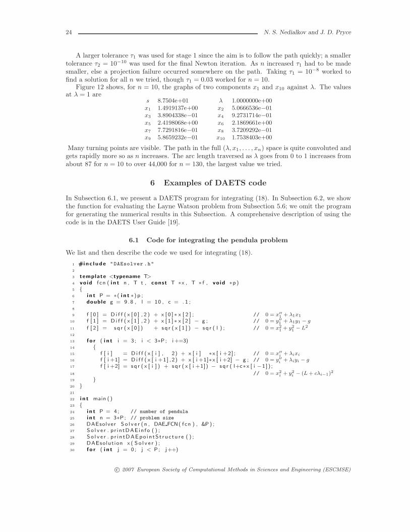
6.1 Code for integrating the pendula problem
We list and then describe the code we used for integrating (18).
1 #in c l u d e "DAEsolver .h"
2
3 template <typename T>
4 vo id f cn ( i n t n , T t , const T ∗x , T ∗ f , vo id ∗p )5 {6 i n t P = ∗( i n t ∗) p ;7 double g = 9 . 8 , l = 10 , c = . 1 ;8
9 f [ 0 ] = D i f f ( x [ 0 ] , 2 ) + x [ 0 ] ∗ x [ 2 ] ; // 0 = x′′
1+ λ1x1
10 f [ 1 ] = D i f f ( x [ 1 ] , 2 ) + x [ 1 ] ∗ x [ 2 ] − g ; // 0 = y′′
1+ λ1y1 − g
11 f [ 2 ] = sq r ( x [ 0 ] ) + sq r ( x [ 1 ] ) − s q r ( l ) ; // 0 = x2
1+ y2
1− L2
12
13 f o r ( i n t i = 3 ; i < 3∗P ; i +=3)14 {15 f [ i ] = D i f f ( x [ i ] , 2) + x [ i ] ∗x [ i +2] ; // 0 = x′′
i+ λixi
16 f [ i +1] = D i f f ( x [ i +1] ,2) + x [ i +1]∗x [ i +2] − g ; // 0 = y′′
i+ λiyi − g
17 f [ i +2] = sq r ( x [ i ] ) + sq r ( x [ i +1]) − s q r ( l+c∗x [ i −1 ] ) ;
18 // 0 = x2
i+ y2
i− (L + cλi−1)
2
19 }20 }21
22 i n t main ( )23 {24 i n t P = 4 ; // number of pendula
25 i n t n = 3∗P ; // problem size
26 DAEsolver S o l v e r (n , DAE FCN( f cn ) , &P ) ;27 So l v e r . p r i n tDAEin f o ( ) ;28 So l v e r . p r i n tDAEpo i n tS t r u c tu r e ( ) ;29 DAEsolut ion x ( S o l v e r ) ;30 f o r ( i n t j = 0 ; j < P ; j++)
c© 2007 European Society of Computational Methods in Sciences and Engineering (ESCMSE)

Solving DAEs by Taylor Series (III): DAETS 25
31 {32 i n t d = 2∗(P−j ) ;33 f o r ( i n t i = 0 ; i < d ; i++)34 {35 x . setX (3∗ j , i , drand48 ( ) ) ;36 x . setX (3∗ j +1, i , drand48 ( ) ) ;37 }38 f o r ( i n t i = 0 ; i < d−2; i++)39 x . setX (3∗ j +2, i , drand48 ( ) ) ;40 }41 double t0 = 0 , tend = 20 ;42 x . setT ( t0 ) ;43 DAEex i t f l ag e x i t f l a g ;44 So l v e r . i n t e g r a t e ( x , tend , e x i t f l a g ) ;45 i f ( e x i t f l a g != s u c c e s s )46 p r i n tDAEe x i t f l a g ( e x i t f l a g ) ;47 e l s e
48 {49 cout << "\t t = " << x . getT ( ) << end l ;50 f o r ( i n t i = 0 ; i < n ; i++)51 cout << "\t x(" << i << ") = " << x ( i , 0 ) << end l ;52 x . p r i n t S t a t s ( ) ;53 }54 r e t u r n 0 ;55 }
The interface to DAETS is in the file DAEsolver.h. First, a template function for evaluating theDAE must be coded, lines 3–20. The paramers to this function are:
n : size of the problem;
t : time variable;
x : pointer to an array for storing the input variables;
f : pointer to an array for storing the residual;
p : void pointer for passing additional data to this function.
Here, the Diff operator performs the differentiation of a variable.Then, we write a main program. First a solver is created, line 26, where we pass the size of
the problem, the function fcn (DAE FCN is a pre-defined macro), and as an optional parameter,the number of pendula. After a solver is created, we print information about the DAE and thevariables and their derivatives that need to be initialized, lines 27 and 28, respectively; see also theoutput of this program below.
A DAEsolution object is created, line 29, and initial values are set in lines 30–40; a value for thetime variable is set in line 42. The integration is performed by the call to the integrate functionin line 44. If the exitflag is success, the DAEsolution object x contains solution values at tend;otherwise, x contains solution values at the reached t between t0 and tend.
The value of the reached t is printed in line 49, and values for xi, i = 1, . . . , n, are printed inlines 50–51. Finally, statistics about the integration are printed in line 52.
The resulting output for the case of P = 4 pendula is
DAEsize..................12index ................9
LINEAR
Initial values must be given for:variable derivatives
c© 2007 European Society of Computational Methods in Sciences and Engineering (ESCMSE)
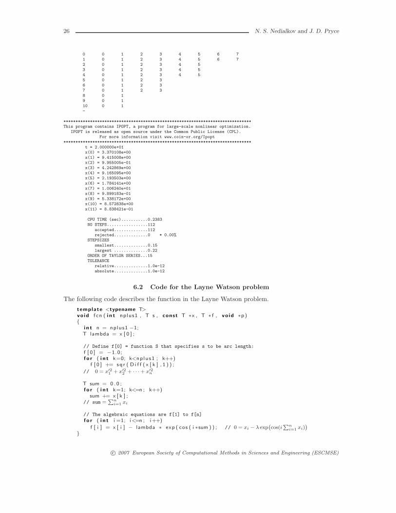
26 N. S. Nedialkov and J. D. Pryce
0 0 1 2 3 4 5 6 7
1 0 1 2 3 4 5 6 72 0 1 2 3 4 5
3 0 1 2 3 4 54 0 1 2 3 4 55 0 1 2 3
6 0 1 2 37 0 1 2 3
8 0 19 0 1
10 0 1-
******************************************************************************This program contains IPOPT, a program for large-scale nonlinear optimization.
IPOPT is released as open source under the Common Public License (CPL).For more information visit www.coin-or.org/Ipopt
******************************************************************************
t = 2.000000e+01x(0) = 3.370108e+00
x(1) = 9.415008e+00x(2) = 9.955005e-01
x(3) = 4.242869e+00x(4) = 9.165095e+00x(5) = 2.193503e+00
x(6) = 1.784141e+00x(7) = 1.006240e+01
x(8) = 9.899183e-01x(9) = 5.338172e+00x(10) = 8.572838e+00
x(11) = 8.838421e-01
CPU TIME (sec)...........0.2383NO STEPS.................112
accepted..............112rejected..............0 * 0.00%
STEPSIZES
smallest..............0.15largest ..............0.22
ORDER OF TAYLOR SERIES...15TOLERANCE
relative..............1.0e-12
absolute..............1.0e-12
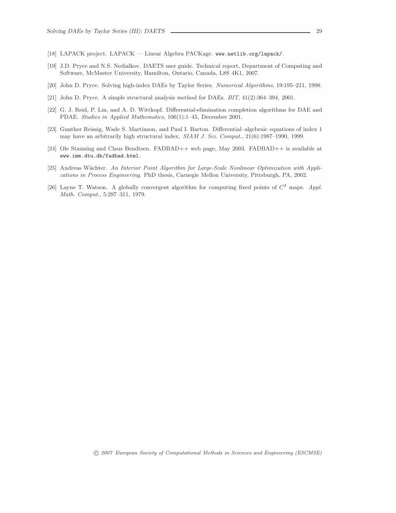
6.2 Code for the Layne Watson problem
The following code describes the function in the Layne Watson problem.
template <typename T>
vo id f cn ( i n t nplus1 , T s , const T ∗x , T ∗ f , vo id ∗p ){
i n t n = nplus1 −1;T lambda = x [ 0 ] ;
// Define f[0] = function S that specifies s to be arc length:
f [ 0 ] = −1.0;f o r ( i n t k=0; k<np lus1 ; k++)
f [ 0 ] += sq r ( D i f f ( x [ k ] , 1 ) ) ;
// 0 = x′2
1+ x′2
2+ · · · + x′2
n
T sum = 0 . 0 ;f o r ( i n t k=1; k<=n ; k++)
sum += x [ k ] ;// sum =
P
n
i=1xi
// The algebraic equations are f[1] to f[n]
f o r ( i n t i =1; i<=n ; i++)
f [ i ] = x [ i ] − lambda ∗ exp ( cos ( i ∗sum ) ) ; // 0 = xi − λ exp`
cos(iP
n
i=1xi)
´
}
c© 2007 European Society of Computational Methods in Sciences and Engineering (ESCMSE)

Solving DAEs by Taylor Series (III): DAETS 27
7 Conclusions
Comparisons and challenges.
DAETS is a DAE solver based on Pryce’s structural analysis (SA) and the use of automaticdifferentiation to expand the solution in Taylor series. It has shown itself robust in our experiments.It has as good accuracy-to-tolerance proportionality as do the codes DASSL and RADAU wecompare it with, and far better on the index 3 car axis problem (Subsection 5.1). It is especiallyefficient at high accuracies (Subsection 5.2). Its symbolic understanding of the structure of the DAEenables it to handle high index problems (Subsection 5.3), as well as purely algebraic continuationproblems (Subsection 5.6) and explicit or implicit ODEs.
The results of the SA can be printed out, which is a help to understanding an unfamiliar DAE.A method to find an initial consistent point is built in to DAETS, by contrast to most solvers.
DAETS copes well with moderately stiff problems (Subsection 5.4) because of the increasing(though bounded) stability regions of Taylor methods as the order increases.
DAETS cannot handle very large problems, very stiff problems, and problems where SA getsthe structure wrong. These pose three rather different challenges:
Large problems. The difficulty is mainly practical: the memory requirement of high-orderTS methods and the computational work associated with AD. One can improve this by usingsparse linear algebra; and by having fewer long vectors active at once while computing Taylorcoefficients. This suggests memory management based on a frontal analysis of the computationalgraph. However, probably no-one wants to solve very large problems to the great accuracy that isthe main advantage of Taylor methods
Stiff problems. There is a real need to develop SA-based methods with suitable stability. Anatural extension of our approach would be to adapt Hermite-Obreschkoff methods to DAEs: theyare a sort of Taylor series from both ends of the interval at once, and for ODEs a very effectivealternative to Taylor methods with the extra advantage of handling stiffness [6, 16]. It looks aninteresting task in numerical analysis to devise the formulae and data structures to achieve this.
Wrong structural analysis. This event is rare in our experience, but likely to become commonas SA-based methods are applied more widely. They pose another interesting and difficult task,more in computer science than in numerical analysis. In all the cases we have seen, it is possibleto make SA get the right answer by rearranging the DAE, manually, in an equivalent form butwith “better sparsity”. What are the principles and methods involved, and can they be at leastpartially automated?
Future developments.
In the short term the following enhancements to DAETS are planned.
We aim to include event location. Namely, given a set of real event functions g, . . . , gm of thevariables and derivatives, check if any gr has changed sign over an integration step. Then locateits zero accurately.
We aim to move to defect-based error estimation following the methods of Enright [8]. Anapproximate solution u(t) over the whole interval is constructed. The defect is the residual onsubstituting u into the DAE.
Although the error control of DAETS has proved robust in our tests, it is less well founded ontheory than are other parts of the code, and there is evidence that it can be over-cautious. Theoryindicates that defect estimation gives a more unambiguous foundation to error control for DAEsthan does local error estimation.
Finally, we aim to combine this with stepsize control based on estimation of the radius of
convergence following the algorithm of Chang and Corliss [4].
c© 2007 European Society of Computational Methods in Sciences and Engineering (ESCMSE)

28 N. S. Nedialkov and J. D. Pryce
References
[1] Uri M. Ascher, Hongsheng Chin, and Sebastian Reich. Stabilization of DAEs and invariantmanifolds. Numerische Mathematik, 67(2):131–149, 1994.
[2] K. Brenan, S. Campbell, and L. Petzold. Numerical Solution of Initial-Value Problems in
Differential-Algebraic Equations. SIAM, Philadelphia, second edition, 1996.
[3] S. L. Campbell and C. W. Gear. The index of general nonlinear DAEs. Numerische Mathe-
matik, 72:173–196, 1995.
[4] Y. F. Chang and George F. Corliss. ATOMFT: Solving ODEs and DAEs using Taylor series.Comp. Math. Appl., 28:209–233, 1994.
[5] Andreas Griewank, David Juedes, and Jean Utke. ADOL-C, a package for the automaticdifferentiation of algorithms written in C/C++. ACM Trans. Math. Software, 22(2):131–167,June 1996.
[6] E. Hairer, S. P. Nørsett, and G. Wanner. Solving Ordinary Differential Equations I. Nonstiff
Problems. Springer-Verlag, second edition, 1991.
[7] E. Hairer and G. Wanner. Solving Ordinary Differential Equations II. Stiff and Differential–
Algebraic Problems. Springer Verlag, Berlin, 1991.
[8] P. M. Hanson and Wayne H. Enright. Controlling the defect in existing variable-order Adamscodes for initial-value problems. ACM Trans. Math. Soft., 9:71–97, March 1983.
[9] T. E. Hull and W. H. Enright. A structure for programs that solve ordinary differentialequations. Technical Report 66, Department of Computer Science, University of Toronto,May 1974.
[10] R. Jonker and A. Volgenant. A shortest augmenting path algorithm for dense and sparselinear assignment problems. Computing, 38:325–340, 1987. The assignment code is availableat www.magiclogic.com/assignment.html.
[11] A. Jorba and M. Zou. A software package for the numerical integration of ODEs by means of high-order Taylor methods. Technical Report , Department of Mathematics, University of Texas at Austin,TX 78712-1082, USA, 2001.
[12] Sven Erik Mattsson and Gustaf Soderlind. Index reduction in differential-algebraic equations usingdummy derivatives. SIAM J. Sci. Comput., 14(3):677–692, 1993.
[13] F. Mazzia and F Iavernaro. Test set for initial value problem solvers. Technical Report 40, Departmentof Mathematics, University of Bari, Italy, 2003. http://pitagora.dm.uniba.it/~testset/.
[14] N. S. Nedialkov and K. R. Jackson. The design and implementation of a validated object-orientedsolver for IVPs for ODEs. Technical Report 6, Software Quality Research Laboratory, Departmentof Computing and Software, McMaster University, Hamilton, Canada, L8S 4K1, 2002.
[15] N. S. Nedialkov and J. D. Pryce. Solving differential-algebraic equations by Taylor series (I): Com-puting Taylor coefficients. BIT, 45:561–591, 2005.
[16] Nedialko Stoyanov Nedialkov. Computing Rigorous Bounds on the Solution of an Initial Value Problem
for an Ordinary Differential Equation. PhD thesis, Department of Computer Science, University ofToronto, Toronto, Canada, M5S 3G4, February 1999.
[17] C. C. Pantelides. The consistent initialization of differential-algebraic systems. SIAM. J. Sci. Stat.
Comput., 9:213–231, 1988.
c© 2007 European Society of Computational Methods in Sciences and Engineering (ESCMSE)
Solving DAEs by Taylor Series (III): DAETS 29
[18] LAPACK project. LAPACK — Linear Algebra PACKage. www.netlib.org/lapack/.
[19] J.D. Pryce and N.S. Nedialkov. DAETS user guide. Technical report, Department of Computing andSoftware, McMaster University, Hamilton, Ontario, Canada, L8S 4K1, 2007.
[20] John D. Pryce. Solving high-index DAEs by Taylor Series. Numerical Algorithms, 19:195–211, 1998.
[21] John D. Pryce. A simple structural analysis method for DAEs. BIT, 41(2):364–394, 2001.
[22] G. J. Reid, P. Lin, and A. D. Wittkopf. Differential-elimination completion algorithms for DAE andPDAE. Studies in Applied Mathematics, 106(1):1–45, December 2001.
[23] Gunther Reissig, Wade S. Martinson, and Paul I. Barton. Differential–algebraic equations of index 1may have an arbitrarily high structural index. SIAM J. Sci. Comput., 21(6):1987–1990, 1999.
[24] Ole Stauning and Claus Bendtsen. FADBAD++ web page, May 2003. FADBAD++ is available atwww.imm.dtu.dk/fadbad.html.
[25] Andreas Wachter. An Interior Point Algorithm for Large-Scale Nonlinear Optimization with Appli-
cations in Process Engineering. PhD thesis, Carnegie Mellon University, Pittsburgh, PA, 2002.
[26] Layne T. Watson. A globally convergent algorithm for computing fixed points of C2 maps. Appl.
Math. Comput., 5:297–311, 1979.
c© 2007 European Society of Computational Methods in Sciences and Engineering (ESCMSE)
Related Documents


![arXivarXiv:1705.03794v2 [math.DS] 29 Aug 2017 Noname manuscript No. (will be inserted by the editor) Global Hopf bifurcation for differential-algebraic equations with …](https://static.cupdf.com/doc/110x72/5fa7c72d811ff4788b058af0/arxiv-arxiv170503794v2-mathds-29-aug-2017-noname-manuscript-no-will-be-inserted.jpg)


![arXiv:1807.05946v4 [math.AG] 28 Jan 2020 · algebraic, differential, and arithmetic geometry coincide: Brody hyperbolicity (no entire holomor-phic curves), arithmetically hyperbolicity](https://static.cupdf.com/doc/110x72/5fb96b90782a89050a02e48d/arxiv180705946v4-mathag-28-jan-2020-algebraic-diierential-and-arithmetic.jpg)


