Solver Linear Problem Solving MAN 327 2.0 Micro-computers & Their Applications.

Solver

Linear Problem Solving

MAN 327 2.0 Micro-computers & Their Applications

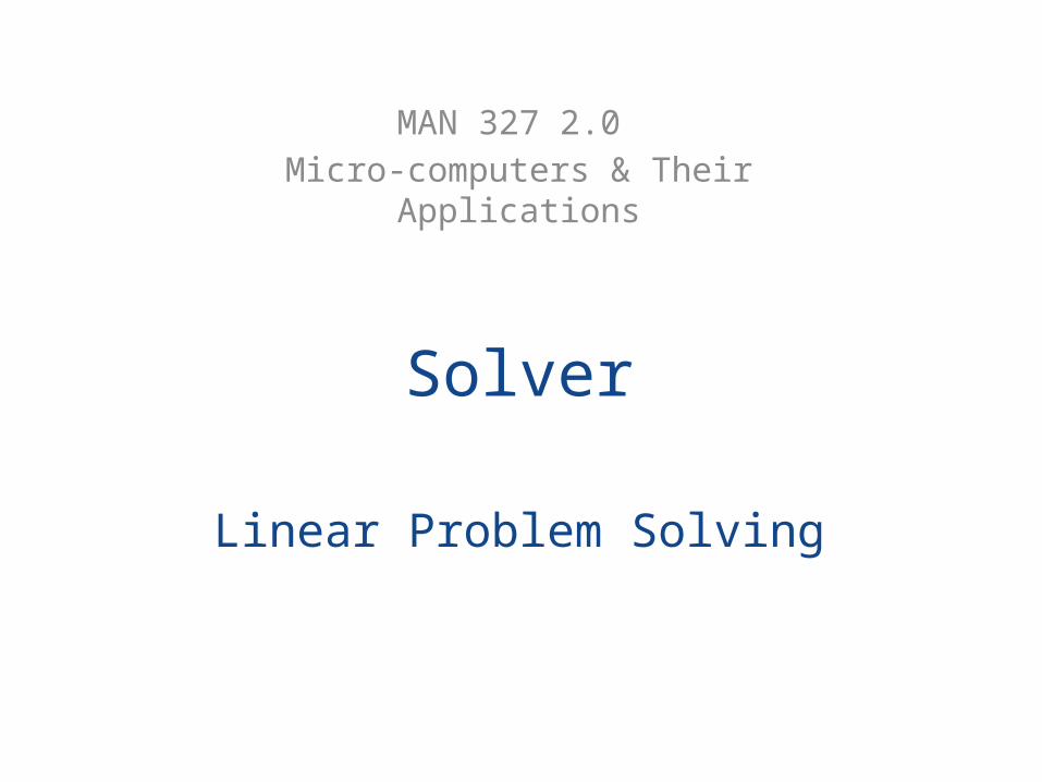
Installing Solver for Use

• File Options Add-ins Solver-ins

• Data Analysis Solver

What is Linear Programming?

• A Linear Programming model seeks to maximize or minimize a linear function, subject to a set of linear constraints.

4

Introduction to Linear Programming

• The Importance of Linear Programming– Many real world problems lend themselves to linear programming modeling. – Many real world problems can be approximated by linear

models.– There are well-known successful applications in:

• Manufacturing• Marketing• Finance (investment)• Advertising• Agriculture

Setting up a Linear Problem

• The Objective Function• The Decision Variables (optimal values will be

calculated by Solver)• The Constraints

– Relationships ( >, <, =)– Values

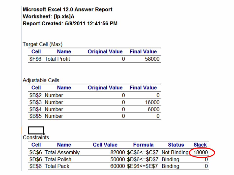
Output

• The Answer Report• The Sensitivity Report

9

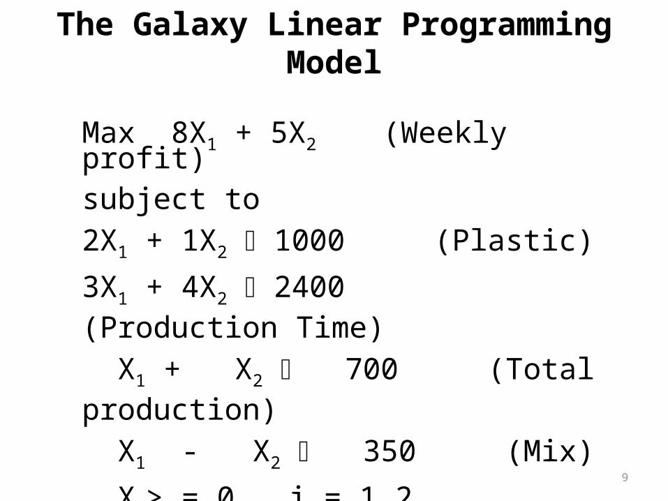
Max 8X1 + 5X2 (Weekly profit)subject to2X1 + 1X2 £ 1000 (Plastic)

3X1 + 4X2 £ 2400 (Production Time)

X1 + X2 £ 700 (Total production)

X1 - X2 £ 350 (Mix)

Xj> = 0, j = 1,2 (Nonnegativity)

The Galaxy Linear Programming Model

10

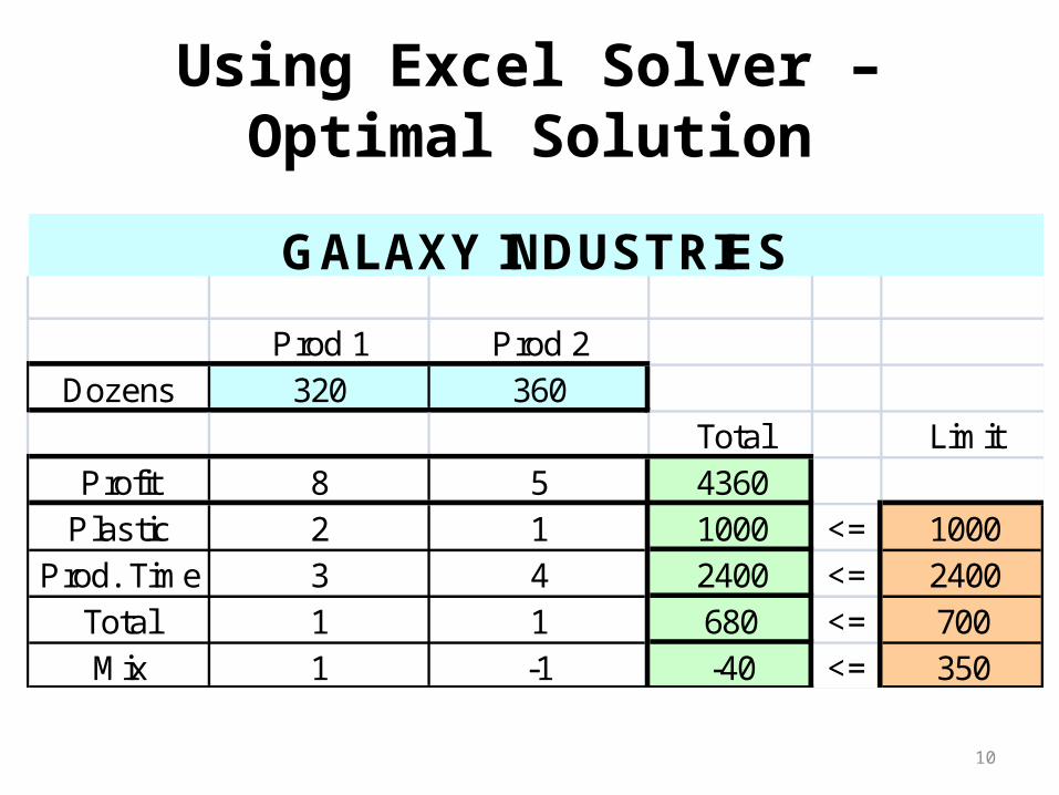
Prod 1 Prod 2Dozens 320 360

Total LimitProfit 8 5 4360

Plastic 2 1 1000 <= 1000Prod. Time 3 4 2400 <= 2400

Total 1 1 680 <= 700Mix 1 -1 -40 <= 350

GALAXY INDUSTRIES

Using Excel Solver – Optimal Solution

11

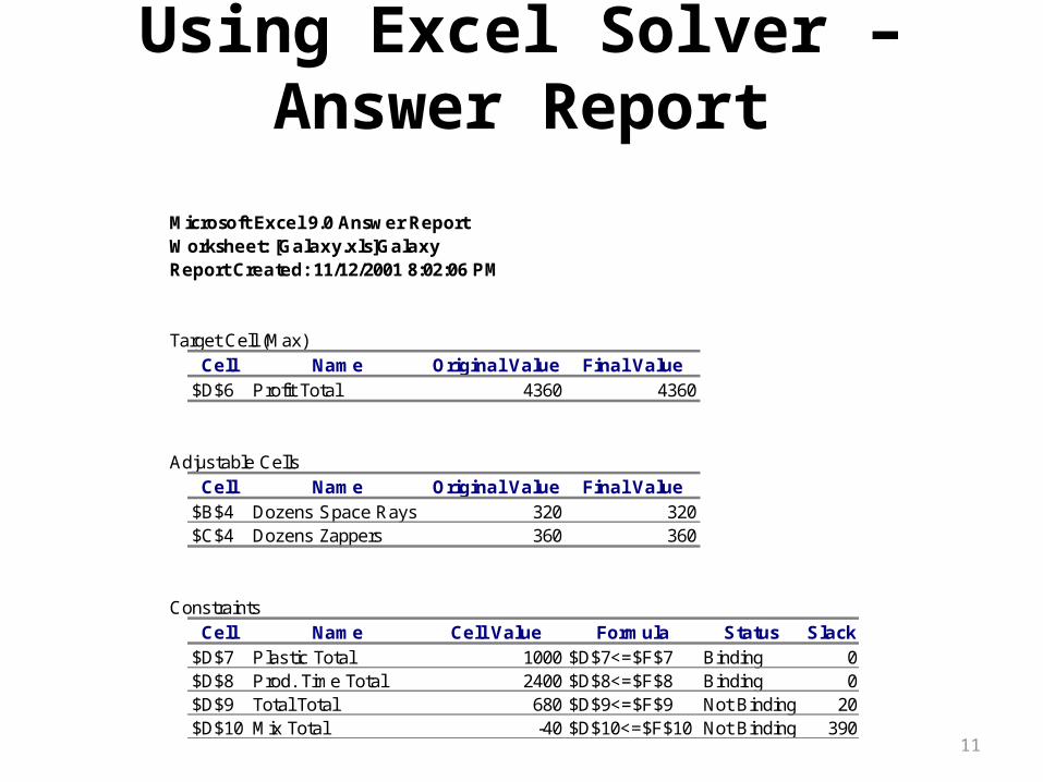
Using Excel Solver –Answer Report

Microsoft Excel 9.0 Answer ReportWorksheet: [Galaxy.xls]GalaxyReport Created: 11/12/2001 8:02:06 PM

Target Cell (Max)Cell Name Original Value Final Value

$D$6 Profit Total 4360 4360

Adjustable CellsCell Name Original Value Final Value

$B$4 Dozens Space Rays 320 320$C$4 Dozens Zappers 360 360

ConstraintsCell Name Cell Value Formula Status Slack

$D$7 Plastic Total 1000 $D$7<=$F$7 Binding 0$D$8 Prod. Time Total 2400 $D$8<=$F$8 Binding 0$D$9 Total Total 680 $D$9<=$F$9 Not Binding 20$D$10 Mix Total -40 $D$10<=$F$10 Not Binding 390

12

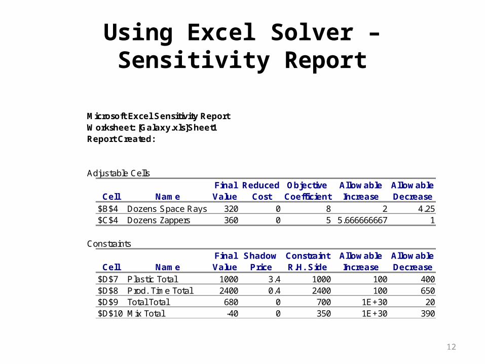
Using Excel Solver –Sensitivity Report

Microsoft Excel Sensitivity ReportWorksheet: [Galaxy.xls]Sheet1Report Created:

Adjustable CellsFinal Reduced Objective Allowable Allowable

Cell Name Value Cost Coefficient Increase Decrease$B$4 Dozens Space Rays 320 0 8 2 4.25$C$4 Dozens Zappers 360 0 5 5.666666667 1

ConstraintsFinal Shadow Constraint Allowable Allowable

Cell Name Value Price R.H. Side Increase Decrease$D$7 Plastic Total 1000 3.4 1000 100 400$D$8 Prod. Time Total 2400 0.4 2400 100 650$D$9 Total Total 680 0 700 1E+30 20$D$10 Mix Total -40 0 350 1E+30 390

13

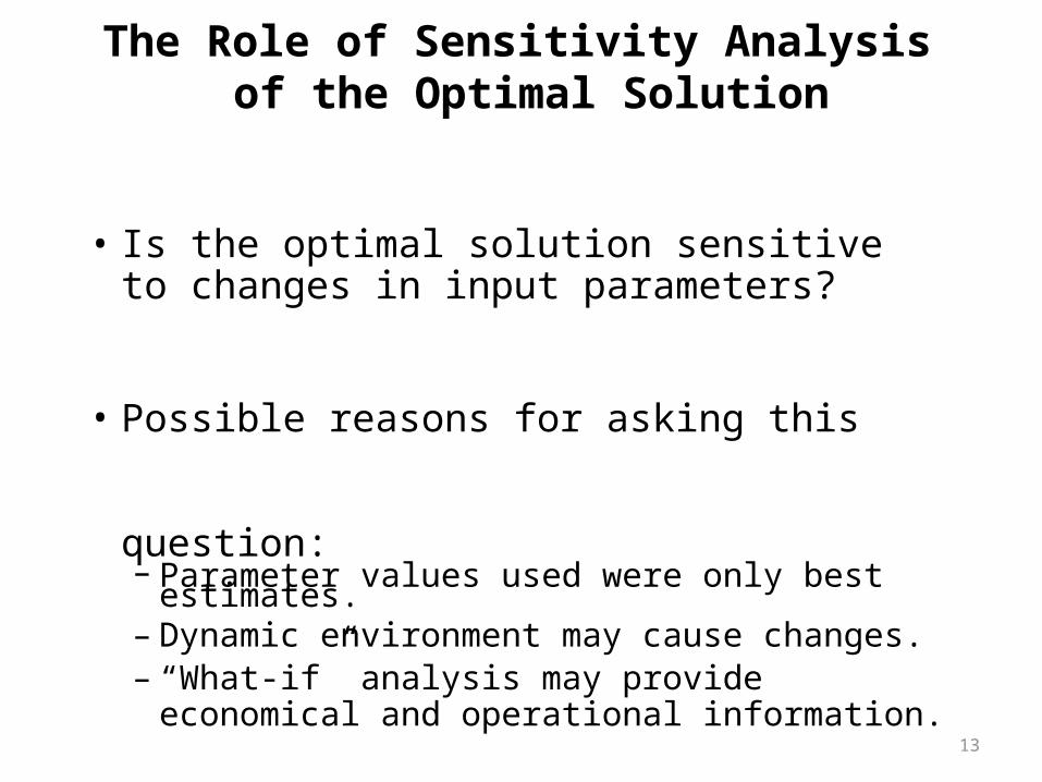
The Role of Sensitivity Analysis of the Optimal Solution

• Is the optimal solution sensitive to changes in input parameters?

• Possible reasons for asking this question:– Parameter values used were only best estimates.– Dynamic environment may cause changes.– “What-if” analysis may provide economical

and operational information.

14

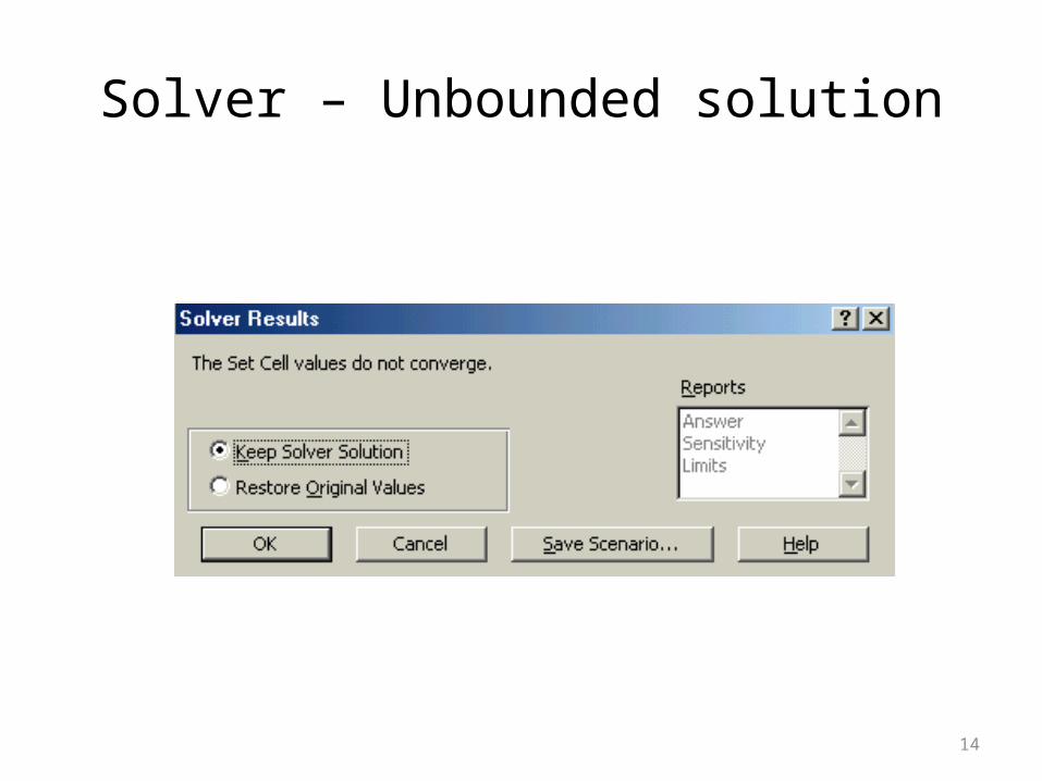
Solver – Unbounded solution

15

• Solver does not alert the user to the existence of alternate optimal solutions.

• Many times alternate optimal solutions exist when the allowable increase or allowable decrease is equal to zero.

• In these cases, we can find alternate optimal solutions using Solver by the following procedure:

Solver – An Alternate Optimal Solution

16

• Observe that for some variable Xj the Allowable increase = 0, orAllowable decrease = 0.

• Add a constraint of the form:Objective function = Current optimal value.

• If Allowable increase = 0, change the objective to Maximize Xj

• If Allowable decrease = 0, change the objective to Minimize Xj

Solver – An Alternate Optimal Solution

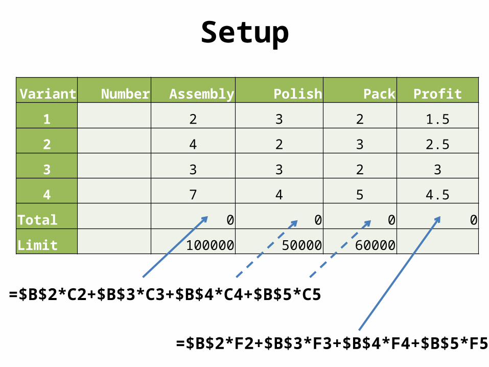
Setup

Variant Number Assembly Polish Pack Profit

1 2 3 2 1.5

2 4 2 3 2.5

3 3 3 2 3

4 7 4 5 4.5

Total 0 0 0 0

Limit 100000 50000 60000

=$B$2*C2+$B$3*C3+$B$4*C4+$B$5*C5

=$B$2*F2+$B$3*F3+$B$4*F4+$B$5*F5

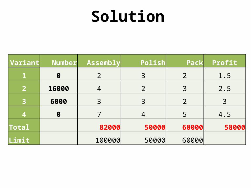
Solution

Variant Number Assembly Polish Pack Profit

1 0 2 3 2 1.5

2 16000 4 2 3 2.5

3 6000 3 3 2 3

4 0 7 4 5 4.5

Total 82000 50000 60000 58000

Limit 100000 50000 60000

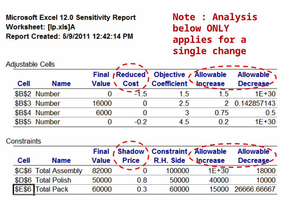
Note : Analysis below ONLY applies for a single change

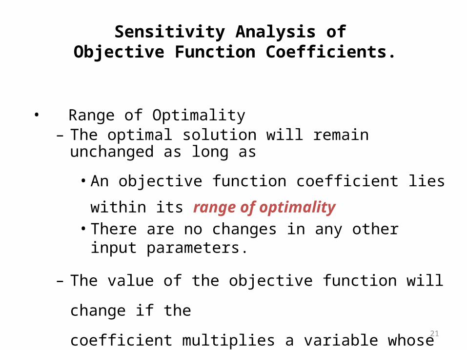
21

• Range of Optimality– The optimal solution will remain unchanged as long as

• An objective function coefficient lies within its range of

optimality • There are no changes in any other input parameters.

– The value of the objective function will change if the

coefficient multiplies a variable whose value is nonzero.

Sensitivity Analysis of Objective Function Coefficients.

What they mean ?

• Changing the objective function coefficient for a variable

• Optimal LP solution will remain unchanged– Decision to produce 16000 of variant 2 and 6000

of variant 3 remains optimal even if the profit per unit on variant 2 is not actually 2.5. It lies in the range 2.3571 ( 2.5 - 0.1429 ) to 4.50 ( 2.5 + 2).

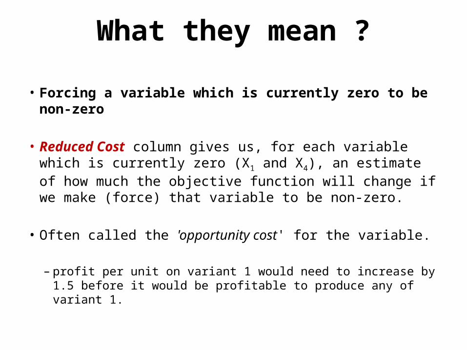
What they mean ?

• Forcing a variable which is currently zero to be non-zero

• Reduced Cost column gives us, for each variable which is currently zero (X1 and X4), an estimate of how much the objective function will change if we make (force) that variable to be non-zero.

• Often called the 'opportunity cost' for the variable.

– profit per unit on variant 1 would need to increase by 1.5 before it would be profitable to produce any of variant 1.

24

Shadow Prices

• Assuming there are no other changes to the input parameters, the change to the objective function value per unit increase to a right hand side of a constraint is called the “Shadow Price”

What they mean ?

• Changing the right-hand side of a constraint

• Shadow Price tells us exactly how much the objective function will change if we change the right-hand side of the corresponding constraint within the limits given in the Allowable Increase/Decrease columns

• Often called the 'marginal value' or 'dual value' for that constraint.

– For the polish constraint, the objective function change will be exactly 0.80.

26

• In sensitivity analysis of right-hand sides of constraints we are interested in the following questions:– Keeping all other factors the same, how much

would the optimal value of the objective function (for example, the profit) change if the right-hand side of a constraint changed by one unit?

– For how many additional or fewer units will this per unit change be valid?

Sensitivity Analysis of Right-Hand Side Values

27

• Any change to the right hand side of a binding constraint will change the optimal solution.

• Any change to the right-hand side of a non-binding constraint that is less than its slack or surplus, will cause no change in the optimal solution.

Sensitivity Analysis of Right-Hand Side Values

• To decide whether the objective function will go up or down use: – constraint more (less) restrictive after change in right-hand side

implies objective function worse (better) – if objective is maximise (minimise) then worse means down (up),

better means up (down)

• Hence – if you had an extra 100 hours to which operation would you assign it? – if you had to take 50 hours away from polishing or packing which one

would you choose? – what would the new objective function value be in these two cases?

Minimizing Problem

• Nutritional facts of foods (per 100 g)Bread (500cal) – P 10 g, F 30g, C 60g, Rice (800cal) - P 10 g, F 10g, C 80g, Dahl (700cal) - P 70 g, F 10g, C 20g, Egg (1100cal) - P 80 g, F 15g, C 5g,

• Suppose we need to minimize our calories (2000cal), while keeping the minimum level of nutritionals.

Protein – 300 cal(75g) Fat – 600 cal(67g) Carbohydrate – 1100 cal(275g)

Solver Help

• www.solver.com.