SOLUTIONS TO THE FINAL - PART 1 MATH 150 – FALL 2016 – KUNIYUKI PART 1: 135 POINTS, PART 2: 115 POINTS, TOTAL: 250 POINTS No notes, books, or calculators allowed. 135 points: 45 problems, 3 pts. each. You do not have to algebraically simplify or box in your answers, unless you are instructed to. Fill in all blanks after “ = ” signs. DERIVATIVES (66 POINTS TOTAL) D x x 2 ( ) = 2 x 2 −1 D x x 3 cos x () ⎡ ⎣ ⎤ ⎦ = D x x 3 ( ) ⎡ ⎣ ⎤ ⎦ ⋅ cos x () ⎡ ⎣ ⎤ ⎦ + x 3 ⎡ ⎣ ⎤ ⎦ ⋅ D x cos x () ⎡ ⎣ ⎤ ⎦ ( ) by Product Rule ( ) = 3x 2 ⎡ ⎣ ⎤ ⎦ cos x () ⎡ ⎣ ⎤ ⎦ + x 3 ⎡ ⎣ ⎤ ⎦ − sin x () ⎡ ⎣ ⎤ ⎦ = 3x 2 cos x () − x 3 sin x () , or x 2 3cos x () − x sin x () ⎡ ⎣ ⎤ ⎦ D x x 7 2 x − 5 ⎛ ⎝ ⎜ ⎞ ⎠ ⎟ = 2 x − 5 ⎡ ⎣ ⎤ ⎦ ⋅ D x x 7 ( ) ⎡ ⎣ ⎤ ⎦ − x 7 ⎡ ⎣ ⎤ ⎦ ⋅ D x 2 x − 5 ( ) ⎡ ⎣ ⎤ ⎦ 2 x − 5 ( ) 2 by Quotient Rule ( ) = 2 x − 5 ⎡ ⎣ ⎤ ⎦ ⋅ 7 x 6 ⎡ ⎣ ⎤ ⎦ − x 7 ⎡ ⎣ ⎤ ⎦ ⋅ 2 ⎡ ⎣ ⎤ ⎦ 2 x − 5 ( ) 2 , or 12 x 7 − 35x 6 2 x − 5 ( ) 2 , or x 6 12 x − 35 ( ) 2 x − 5 ( ) 2 D x e x + 4 ( ) 6 ⎡ ⎣ ⎢ ⎤ ⎦ ⎥ = 6 e x + 4 ( ) 5 ⎡ ⎣ ⎢ ⎤ ⎦ ⎥ ⋅ D x e x + 4 ( ) ⎡ ⎣ ⎤ ⎦ = 6 e x + 4 ( ) 5 ⎡ ⎣ ⎢ ⎤ ⎦ ⎥ ⋅ e x ⎡ ⎣ ⎤ ⎦ = 6e x e x + 4 ( ) 5 by Gen. Power Rule ( ) D x tan x () ⎡ ⎣ ⎤ ⎦ = sec 2 x () D x cot x () ⎡ ⎣ ⎤ ⎦ = − csc 2 x () D x sec x () ⎡ ⎣ ⎤ ⎦ = sec x () tan x () D x csc x () ⎡ ⎣ ⎤ ⎦ = − csc x () cot x () D x sin 4 x + 7 ( ) ⎡ ⎣ ⎤ ⎦ = cos 4 x + 7 ( ) ⎡ ⎣ ⎤ ⎦ ⋅ D x 4 x + 7 ( ) ⎡ ⎣ ⎤ ⎦ = cos 4 x + 7 ( ) ⎡ ⎣ ⎤ ⎦ ⋅ 4 ⎡ ⎣ ⎤ ⎦ = 4cos 4 x + 7 ( ) by Gen. Trig Rule ( ) D x e 1 3 x ⎛ ⎝ ⎜ ⎞ ⎠ ⎟ = e 1 3 x ⎡ ⎣ ⎢ ⎤ ⎦ ⎥ ⋅ D x 1 3 x ⎛ ⎝ ⎜ ⎞ ⎠ ⎟ ⎡ ⎣ ⎢ ⎤ ⎦ ⎥ = e 1 3 x ⎡ ⎣ ⎢ ⎤ ⎦ ⎥ ⋅ 1 3 ⎡ ⎣ ⎢ ⎤ ⎦ ⎥ = 1 3 e 1 3 x

Welcome message from author
This document is posted to help you gain knowledge. Please leave a comment to let me know what you think about it! Share it to your friends and learn new things together.
Transcript

SOLUTIONS TO THE FINAL - PART 1 MATH 150 – FALL 2016 – KUNIYUKI
PART 1: 135 POINTS, PART 2: 115 POINTS, TOTAL: 250 POINTS
No notes, books, or calculators allowed.
135 points: 45 problems, 3 pts. each. You do not have to algebraically simplify or box in your answers, unless you are instructed to. Fill in all blanks after “= ” signs.
DERIVATIVES (66 POINTS TOTAL)
Dx x 2( ) = 2x 2 −1
Dx x3 cos x( )⎡⎣ ⎤⎦ = Dx x3( )⎡⎣
⎤⎦ ⋅ cos x( )⎡⎣ ⎤⎦ + x3⎡⎣ ⎤⎦ ⋅ Dx cos x( )⎡⎣ ⎤⎦( ) by Product Rule( )
= 3x2⎡⎣ ⎤⎦ cos x( )⎡⎣ ⎤⎦ + x3⎡⎣ ⎤⎦ −sin x( )⎡⎣ ⎤⎦= 3x2 cos x( )− x3 sin x( ), or x2 3cos x( )− xsin x( )⎡⎣ ⎤⎦
Dx
x7
2x −5⎛⎝⎜
⎞⎠⎟=
2x −5⎡⎣ ⎤⎦ ⋅ Dx x7( )⎡⎣
⎤⎦ − x7⎡⎣ ⎤⎦ ⋅ Dx 2x −5( )⎡⎣ ⎤⎦2x −5( )2 by Quotient Rule( )
=2x −5⎡⎣ ⎤⎦ ⋅ 7x6⎡⎣ ⎤⎦ − x7⎡⎣ ⎤⎦ ⋅ 2⎡⎣ ⎤⎦
2x −5( )2 , or12x7 − 35x6
2x −5( )2 , orx6 12x − 35( )
2x −5( )2
Dx ex + 4( )6⎡⎣⎢
⎤⎦⎥= 6 ex + 4( )5⎡
⎣⎢⎤⎦⎥⋅ Dx ex + 4( )⎡⎣
⎤⎦ = 6 ex + 4( )5⎡
⎣⎢⎤⎦⎥⋅ ex⎡⎣ ⎤⎦
= 6ex ex + 4( )5by Gen. Power Rule( )
Dx tan x( )⎡⎣ ⎤⎦ = sec2 x( )
Dx cot x( )⎡⎣ ⎤⎦ = −csc2 x( )
Dx sec x( )⎡⎣ ⎤⎦ = sec x( ) tan x( )
Dx csc x( )⎡⎣ ⎤⎦ = −csc x( )cot x( )
Dx sin 4x + 7( )⎡⎣ ⎤⎦ = cos 4x + 7( )⎡⎣ ⎤⎦ ⋅ Dx 4x + 7( )⎡⎣ ⎤⎦ = cos 4x + 7( )⎡⎣ ⎤⎦ ⋅ 4⎡⎣ ⎤⎦= 4cos 4x + 7( ) by Gen. Trig Rule( )
Dx e
13
x⎛
⎝⎜⎞
⎠⎟= e
13
x⎡
⎣⎢
⎤
⎦⎥ ⋅ Dx
13
x⎛⎝⎜
⎞⎠⎟
⎡
⎣⎢
⎤
⎦⎥ = e
13
x⎡
⎣⎢
⎤
⎦⎥ ⋅
13⎡
⎣⎢
⎤
⎦⎥ = 1
3e
13
x

MORE!
Dx 5x( ) = 5x ln 5( )
Dx 10x3( ) = 10x3
ln 10( )⎡⎣
⎤⎦ ⋅ Dx x3( )⎡⎣
⎤⎦ = 10x3
ln 10( )⎡⎣
⎤⎦ ⋅ 3x2⎡⎣ ⎤⎦ = 3x2 ⋅10x3
ln 10( )
Dx ln 7x2 +1( )⎡
⎣⎤⎦ =
17x2 +1⎡
⎣⎢
⎤
⎦⎥ ⋅ Dx 7x2 +1( )⎡⎣
⎤⎦ = 1
7x2 +1⎡
⎣⎢
⎤
⎦⎥ ⋅ 14x⎡⎣ ⎤⎦ = 14x
7x2 +1
Dx log9 x( )⎡⎣ ⎤⎦ =
Dx
ln x( )ln 9( )
⎡
⎣⎢⎢
⎤
⎦⎥⎥= 1
ln 9( )⎡
⎣⎢⎢
⎤
⎦⎥⎥⋅ Dx ln x( )⎡⎣ ⎤⎦( ) = 1
ln 9( )⎡
⎣⎢⎢
⎤
⎦⎥⎥⋅ 1
x⎡
⎣⎢
⎤
⎦⎥ = 1
x ln 9( )
Dx sin−1 x( )⎡⎣ ⎤⎦ =
1
1− x2
Dx cos−1 x( )⎡⎣ ⎤⎦ =
�
− 1
1− x2
Dx tan−1 x( )⎡⎣ ⎤⎦ =
�
11+ x2
Dx sec−1 x( )⎡⎣ ⎤⎦ =
1
x x2 −1 (Assume the usual range for sec−1 x( ) in our class.)
Dx tan−1 7x( )⎡⎣ ⎤⎦ =1
1+ 7x( )2
⎡
⎣⎢⎢
⎤
⎦⎥⎥⋅ Dx 7x( )⎡⎣ ⎤⎦ = 1
1+ 7x( )2
⎡
⎣⎢⎢
⎤
⎦⎥⎥⋅ 7⎡⎣ ⎤⎦ = 7
1+ 49x2
Dx sinh x( )⎡⎣ ⎤⎦ = cosh x( )
Dx cosh x( )⎡⎣ ⎤⎦ = sinh x( )
Dx sech x( )⎡⎣ ⎤⎦ = −sech x( ) tanh x( )

INDEFINITE INTEGRALS (42 POINTS TOTAL)
x9 dx∫ = x10
10+ C
1x
dx∫ = ln x +C
e −7 x dx∫ = e −7 x
−7+ C = − e −7 x
7+ C, or C − 1
7e7 x
6x dx∫ = 6x
ln 6( ) + C
sin x( ) dx∫ = −cos x( ) +C
tan x( ) dx∫ = − ln cos x( ) +C, or ln sec x( ) +C
cot x( ) dx∫ = ln sin x( ) +C
sec x( ) dx∫ = ln sec x( ) + tan x( ) +C
csc x( ) dx∫ = ln csc x( )− cot x( ) +C, or − ln csc x( ) + cot x( ) +C
cos 3x( ) dx∫ = 1
3sin 3x( ) +C
sec2 x( ) dx∫ = tan x( ) +C
136+ x2 dx∫ = 1
6tan−1 x
6⎛⎝⎜
⎞⎠⎟+C
1
36− x2dx∫ = sin−1 x
6⎛⎝⎜
⎞⎠⎟+C
cosh x( ) dx∫ = sinh x( ) +C
WARNING: YOU'VE BEEN DEALING WITH INDEFINITE INTEGRALS. DID YOU FORGET SOMETHING? (+ C)

INVERSE TRIGONOMETRIC FUNCTIONS (6 POINTS TOTAL)
•
lim
x→∞tan−1 x( ) = π
2 (Drawing a graph may help.)
• If f x( ) = sin−1 x( ) , what is the range of f in interval form (the form with
parentheses and/or brackets)? Range f( ) = − π
2, π
2⎡
⎣⎢
⎤
⎦⎥ .
HYPERBOLIC FUNCTIONS (6 POINTS TOTAL)
• The definition of (as given in class) is: sinh x( ) =
ex − e− x
2
• Complete the following identity: cosh2 x( )− sinh2 x( ) = 1
(We mentioned this identity in class.) TRIGONOMETRIC IDENTITIES (15 POINTS TOTAL)
Complete each of the following identities, based on the type of identity given.
• tan2 x( ) +1= sec2 x( ) (Pythagorean Identity) • cos − x( ) = cos x( ) (Even/Odd Identity)
• sin 2x( ) = 2sin x( )cos x( ) (Double-Angle Identity) • cos 2x( ) = cos2 x( )− sin2 x( ), or 1− 2sin2 x( ), or 2cos2 x( )−1
(Double-Angle Identity) (For
cos 2x( ) , I gave you three versions; you may pick any one.)
• sin2 x( ) = 1− cos 2x( )
2 (Power-Reducing Identity)
sinh x( )
SOLUTIONS TO THE FINAL - PART 2 MATH 150 – FALL 2016 – KUNIYUKI
PART 1: 135 POINTS, PART 2: 115 POINTS, TOTAL: 250 POINTS
A scientific calculator and an appropriate sheet of notes are allowed on this final part.
1) Find the following limits. Each answer will be a real number,
�
∞,
�
−∞ , or DNE (Does Not Exist). Write ∞ or −∞ when appropriate. If a limit does not exist, and ∞ and −∞ are inappropriate, write “DNE.” Box in your final answers. (14 points total)
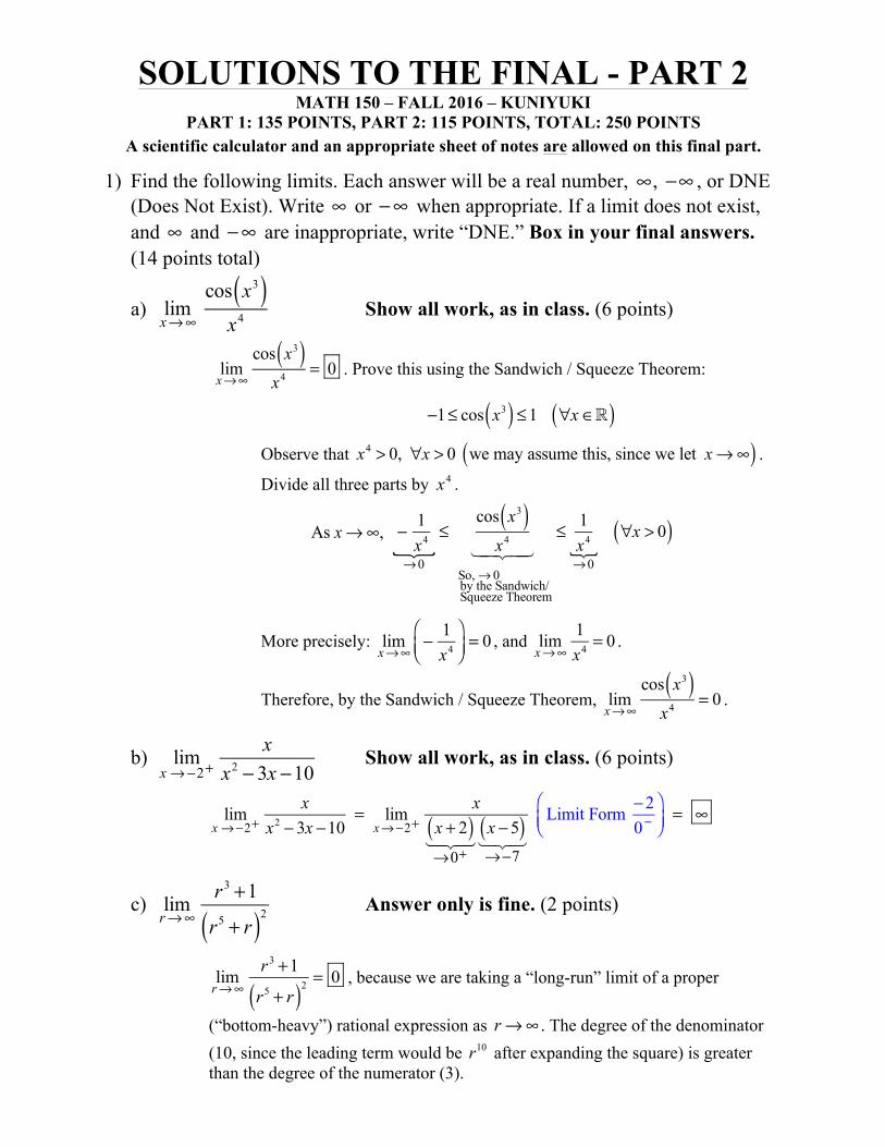
a) lim
x→∞
cos x3( )x4 Show all work, as in class. (6 points)
lim
x→∞
cos x3( )x4 = 0 . Prove this using the Sandwich / Squeeze Theorem:
−1≤ cos x3( ) ≤1 ∀x ∈( )
Observe that x4 > 0, ∀x > 0 we may assume this, since we let x →∞( ) .
Divide all three parts by x4 .
As x →∞,
− 1x4
→0
≤cos x3( )
x4
So, → 0 by the Sandwich/ Squeeze Theorem
≤ 1
x4
→0
∀x > 0( )
More precisely: lim
x→∞− 1
x4
⎛⎝⎜
⎞⎠⎟= 0 , and
lim
x→∞
1x4 = 0 .
Therefore, by the Sandwich / Squeeze Theorem, lim
x→∞
cos x3( )x4 = 0 .
b)
limx →−2+
xx2 − 3x −10
Show all work, as in class. (6 points)
limx →−2+
xx2 − 3x −10
= limx→−2+
xx + 2( )→0+
x −5( )→−7
Limit Form −20−
⎛⎝⎜
⎞⎠⎟= ∞
c)
limr→∞
r3 +1
r5 + r( )2
Answer only is fine. (2 points)
limr→∞
r3 +1
r5 + r( )2 = 0 , because we are taking a “long-run” limit of a proper
(“bottom-heavy”) rational expression as r →∞ . The degree of the denominator (10, since the leading term would be r10 after expanding the square) is greater than the degree of the numerator (3).

2) Let f x( ) = x + 4, x ≠ 3
9, x = 3⎧⎨⎩
. Classify the discontinuity at x = 3. Box in one:
(2 points)
Infinite discontinuity Jump discontinuity Removable discontinuity
limx→3
f x( ) = limx→3
x + 4( ) = 3+ 4 = 7 ≠ 9 , which is f 3( ) . (The limit value and the
function value exist but are unequal.) If f 3( ) were 7, then f would be continuous at 3.
3) Use the limit definition of the derivative to prove that Dx 5x2 − x + 7( ) = 10x −1,
∀x ∈ . Do not use derivative short cuts we have used in class. (10 points)
Let f x( ) = 5x2 − x + 7 .
′f x( ) = limh→0
f x + h( )− f x( )h
= limh→0
5 x + h( )2− x + h( ) + 7⎡
⎣⎢⎤⎦⎥ − 5x2 − x + 7⎡⎣ ⎤⎦
h
= limh→0
5 x2 + 2xh+ h2( )− x − h+ 7⎡⎣
⎤⎦ − 5x2 − x + 7⎡⎣ ⎤⎦
h
= limh→0
5x2 +10xh+5h2 − x − h +7 −5x2 + x −7h
= limh→0
10xh+5h2 − hh
= limh→0
h1( )
10x +5h−1( )h1( )
= limh→0
10x +5h−1( )
= 10x +5 0( )−1 = 10x −1. Q.E.D.( )
4) Let f x( ) = log4 x( ) . Consider the graph of y = f x( ) in the usual xy-plane. Find a Point-Slope Form of the equation of the tangent line to the graph at the point where x = 16 . Give exact values; you do not have to approximate. (8 points)
f 16( ) = log4 16( ) = 2 , so the point of interest is 16, 2( ) .
Find ′f 16( ) , the slope m of the tangent line to the graph at that point.
′f x( ) = Dx log4 x( )⎡⎣ ⎤⎦ = Dx
ln x( )ln 4( )
⎡
⎣⎢⎢
⎤
⎦⎥⎥
Change-of-Base Property of Logarithms( )
= 1ln 4( )
⎡
⎣⎢⎢
⎤
⎦⎥⎥⋅ Dx ln x( )⎡⎣ ⎤⎦( ) = 1
ln 4( )⎡
⎣⎢⎢
⎤
⎦⎥⎥⋅ 1
x⎡
⎣⎢
⎤
⎦⎥ = 1
x ln 4( ) ⇒
′f 16( ) = 116ln 4( ) , or
1ln 416( ) This is our desired slope, m.( )
Find a Point-Slope Form of the equation of the tangent line.
y − y1 = m x − x1( ) ⇒ y − 2 = 116ln 4( ) x −16( )

5) Assume that x and y are differentiable functions of t. Evaluate Dt exy( ) when
x = 3, y = 5 , dxdt
= 2 , and dydt
= −4 . (8 points)
Dt exy( ) = exy⎡⎣ ⎤⎦ ⋅ Dt xy( )⎡⎣ ⎤⎦ = exy⎡⎣ ⎤⎦ ⋅dxdt
⋅ y + x ⋅ dydt
⎡
⎣⎢
⎤
⎦⎥ by the Product Rule( )
= e 3( ) 5( )⎡⎣
⎤⎦ ⋅ 2( ) 5( ) + 3( ) −4( )⎡⎣ ⎤⎦ = e15⎡⎣ ⎤⎦ ⋅ 10−12⎡⎣ ⎤⎦ = e15⎡⎣ ⎤⎦ ⋅ −2⎡⎣ ⎤⎦ = −2e15
6) Let f x( ) = x3 − 2x2 − 4x +1. (14 points total)
a) Find the two critical numbers of f .
′f x( ) = 3x2 − 4x − 4 = 3x + 2( ) x − 2( ) , which is never undefined (“DNE”) but
is 0 at x = −
23
and x = 2 . These numbers are in Dom f( ) , which is , so the
critical numbers are: − 2
3 and 2 .
Note: We could use the Quadratic Formula (QF) with a = 3 , b = −4 , and c = −4 .
x = −b± b2 − 4ac2a
=− −4( ) ± −4( )2
− 4 3( ) −4( )2 3( ) = 4 ± 16+ 48
2 3( ) = 4 ± 646
= 4 ±86
= 2 ± 43
⇒
x = 2+ 43
= 63
= 2 or x = 2− 43
= −23
= − 23
b) Consider the graph of y = f x( ) , although you do not have to draw it. Use the First Derivative Test to classify the point at x = 2 as a local maximum point, a local minimum point, or neither.
�
f is continuous on , so the First Derivative Test (1st DT) should apply wherever we have critical numbers (CNs). Both
�
f and
�
′ f are continuous on , so use just the CNs as “fenceposts” on the real number line where ′f could change sign.
(not needed) − 2 / 3 Test x = 0 2 Test x = 3
�
′ f sign (see below) 0
�
− 0 +
�
f Classify point at CN (1st DT) L.Min.
Pt.
′f x( ) = 3x + 2( ) x − 2( )′f 0( ) = +( ) −( ) = −
′f 3( ) = +( ) +( ) = +
or Evaluate ′f at 0 and 3 directly.
Also, the graph of y = ′f x( ) is an upward-opening parabola with two distinct
x-intercepts at − 2
3, 0
⎛⎝⎜
⎞⎠⎟
and 2, 0( ) . The multiplicities of the zeros of ′f are both
odd (1), so signs alternate in our “windows.” Answer: Local Minimum Point

c) Use the Second Derivative Test to classify the point at the other critical number as a local maximum point or a local minimum point.
′f −
23
⎛⎝⎜
⎞⎠⎟= 0 , so we may apply the Second Derivative Test for
x = − 2
3.
′f x( ) = 3x2 − 4x − 4 ⇒
′′f x( ) = 6x − 4 ⇒
′′f − 23
⎛⎝⎜
⎞⎠⎟= 6 − 2
3⎛⎝⎜
⎞⎠⎟− 4 = −8 ⇒ ′′f − 2
3⎛⎝⎜
⎞⎠⎟< 0
Therefore, the point at x = −
23
is a Local Maximum Point .
Think: Concave down (∩ ) “at” (actually, on a neighborhood of) x = −
23
.
7) Evaluate the following integrals. (20 points total)
a)
e x
xdx
9
16
∫ . Give an exact answer. (10 points)
Let u = x or x1/2 ⇒
du = 12
x−1/2 dx ⇒ du = 1
2 xdx ⇒ Can use:
1
xdx = 2 du
⎛⎝⎜
⎞⎠⎟
Method 1 (Change the limits of integration.)
x = 9 ⇒ u = 9 = 3 ⇒ u = 3
x = 16 ⇒ u = 16 = 4 ⇒ u = 4
e x
xdx
9
16
∫ = 2e x
2 xdx
9
16
∫ by Compensation( ) = 2 e x ⋅ 1
2 xdx
9
16
∫
= 2 eu du3
4
∫ = 2 eu⎡⎣ ⎤⎦ 3
4= 2 e4 − e3( ), or 2e3 e−1( )
Method 2 (Work out the corresponding indefinite integral first.)
e x
xdx∫ = 2
e x
2 x∫ dx by Compensation( ) = 2 e x ⋅ 1
2 x∫ dx
= 2 eu du∫ = 2eu +C = 2e x +C
Now, apply the FTC directly using our antiderivative (where C = 0 ).
e x
xdx
9
16
∫ = 2e x⎡⎣
⎤⎦ 9
16= 2 e x⎡
⎣⎤⎦ 9
16= 2 e 16⎡
⎣⎤⎦ − e 9⎡
⎣⎤⎦( )
= 2 e4 − e3( ), or 2e3 e−1( )
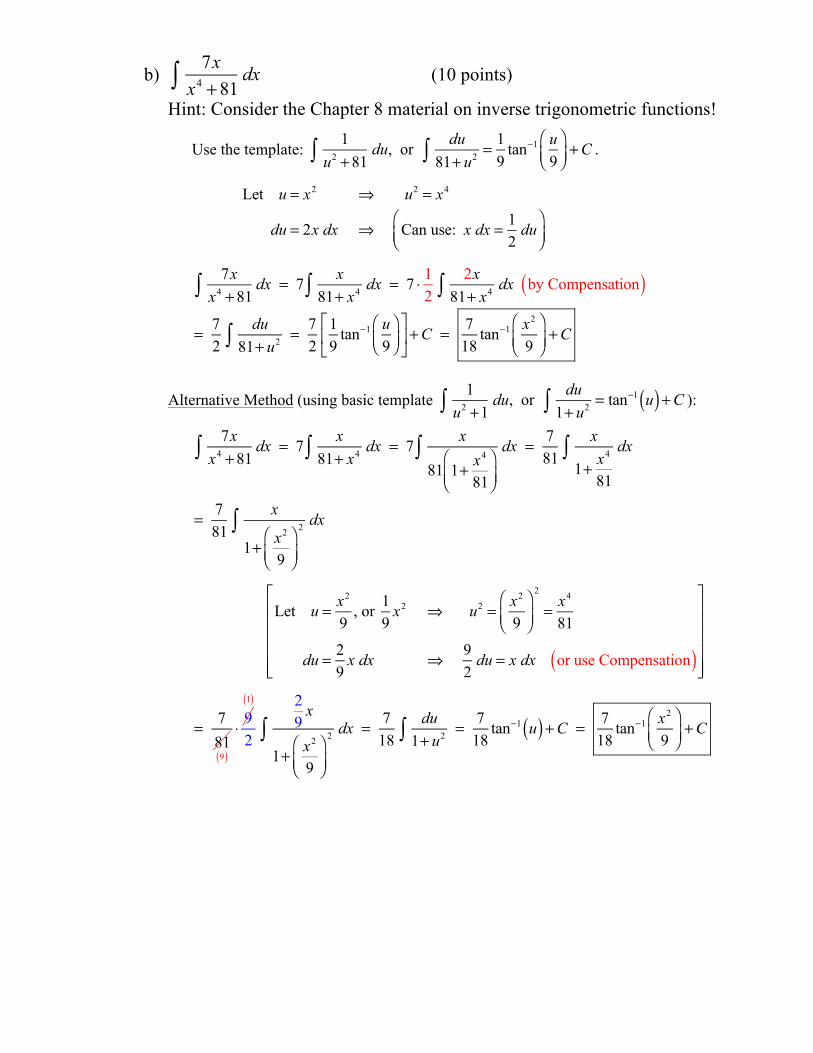
b)
7xx4 +81
dx∫ (10 points)
Hint: Consider the Chapter 8 material on inverse trigonometric functions!
Use the template:
1u2 +81
du∫ , or du
81+ u2∫ = 19
tan−1 u9
⎛⎝⎜
⎞⎠⎟+C .
Let u = x2 ⇒ u2 = x4
du = 2x dx ⇒ Can use: x dx = 12
du⎛⎝⎜
⎞⎠⎟
7xx4 +81
dx∫ = 7x
81+ x4 dx∫ = 7 ⋅ 12
2x81+ x4 dx∫ by Compensation( )
= 72
du81+ u2∫ = 7
219
tan−1 u9
⎛⎝⎜
⎞⎠⎟
⎡
⎣⎢
⎤
⎦⎥ +C = 7
18tan−1 x2
9⎛⎝⎜
⎞⎠⎟+C
Alternative Method (using basic template
1u2 +1
du∫ , or du
1+ u2∫ = tan−1 u( ) +C ):
7xx4 +81
dx∫ = 7 x81+ x4 dx∫ = 7 x
81 1+ x4
81⎛⎝⎜
⎞⎠⎟
dx∫ = 781
x
1+ x4
81
dx∫
= 781
x
1+ x2
9⎛⎝⎜
⎞⎠⎟
2 dx∫
Let u = x2
9, or
19
x2 ⇒ u2 = x2
9⎛⎝⎜
⎞⎠⎟
2
= x4
81
du = 29
x dx ⇒ 92
du = x dx or use Compensation( )
⎡
⎣
⎢⎢⎢⎢⎢
⎤
⎦
⎥⎥⎥⎥⎥
= 781
9( )
⋅ 91( )
2
29
x
1+ x2
9⎛⎝⎜
⎞⎠⎟
2 dx∫ = 718
du1+ u2∫ = 7
18tan−1 u( ) +C = 7
18tan−1 x2
9⎛⎝⎜
⎞⎠⎟+C

8) The velocity function for a particle moving along a coordinate line for t > 0( )
is given by v t( ) = 1
t4− t , where t is time measured in seconds and velocity is
given in meters per second. The particle’s position is measured in meters. Find
�
s t( ), the corresponding position function [rule], if s 1( ) = 2 (meters). (9 points)
v t( )∫ dt = 1t4 − t
⎛⎝⎜
⎞⎠⎟
dt∫ = t−4 − t1/2( ) dt∫ ⇒
s t( ) = t−3
−3− t3/2
3 / 2+C = − 1
3t3 −23
t3/2 +C
Find C.
We know: s 1( ) = 2 (meters).
s 1( ) = − 1
3 1( )3 −23
1( )3/2+C
2 = − 13− 2
3+C
2 = −1+CC = 3 ⇒
s t( ) = − 13t3 −
23
t3/2 + 3, or 3− 13t3 −
23
t t , or 9t3 −1− 2t4 t( )
3t3 ,
or 9t3 −1− 2t9/2
3t3 (in meters)
9) The region R is bounded by the x-axis, the y-axis, and the graphs of y = cos x( ) and
x = π
4 in the usual xy-plane. Sketch and shade in the region R. Find the
volume of the solid generated by revolving R about the x-axis. Evaluate your integral completely. Give an exact answer in simplest form with appropriate units. Distances and lengths are measured in meters. Hint: Use a Power-Reducing Identity. (18 points)
Let f x( ) = cos x( ) . Then, f is nonnegative and continuous on the x-interval
0, π4
⎡
⎣⎢
⎤
⎦⎥ .

The region R and the equation y = cos x( ) suggest a “dx scan” and the Disk Method.
V, the volume of the solid, is given by:
V = π radius( )2dx
0
π /4
∫ = π cos x( )⎡⎣ ⎤⎦2
dx0
π /4
∫ = π cos2 x( ) dx0
π /4
∫= π
1+ cos 2x( )20
π /4
∫ by a Power-Reducing Identity( ) = π2
1+ cos 2x( )⎡⎣ ⎤⎦ dx0
π /4
∫
= π2
x + 12
sin 2x( )⎡
⎣⎢
⎤
⎦⎥
0
π /4
by "Guess-and-check," or using u = 2x( )
= π2
π4+ 1
2sin 2 ⋅ π
4⎛⎝⎜
⎞⎠⎟
⎡
⎣⎢
⎤
⎦⎥ − 0 + 1
2sin 2 ⋅0( )⎡
⎣⎢
⎤
⎦⎥
⎛
⎝⎜⎞
⎠⎟
= π2
π4+ 1
2sin
π2
⎛⎝⎜
⎞⎠⎟
⎡
⎣⎢
⎤
⎦⎥ − 0 + 1
2sin 0( )⎡
⎣⎢
⎤
⎦⎥
⎛
⎝⎜⎞
⎠⎟
= π2
π4+ 1
21( )⎡
⎣⎢
⎤
⎦⎥ − 0⎡⎣ ⎤⎦
⎛⎝⎜
⎞⎠⎟= π
2π4+ 1
2⎛⎝⎜
⎞⎠⎟= π
2π + 2
4⎛⎝⎜
⎞⎠⎟=
π π + 2( )8
m3
10) Rewrite tan sin−1 x
5⎛⎝⎜
⎞⎠⎟
⎛⎝⎜
⎞⎠⎟
as an algebraic expression in x, where 0 < x < 5 .
(7 points)
Let θ = sin−1 x
5⎛⎝⎜
⎞⎠⎟
θ acute( ) ⇒ sin θ( ) = x5
ß found by the Pythagorean Theorem
tan θ( ) = opp.
adj.= x
25− x2
Note: Rationalizing the denominator is usually unnecessary if the radicand involved is variable.
11) Find Dr sin−1 sinh r( )( )⎡
⎣⎤⎦ . (5 points)
Use the template: Dr sin−1 u( )⎡⎣ ⎤⎦ =
1
1− u2⋅ Dr u( )⎡⎣ ⎤⎦ .
Dr sin−1 sinh r( )( )⎡⎣
⎤⎦ = 1
1− sinh2 r( )⎡
⎣
⎢⎢
⎤
⎦
⎥⎥⋅ Dr sinh r( )( )⎡⎣
⎤⎦ = 1
1− sinh2 r( )⎡
⎣
⎢⎢
⎤
⎦
⎥⎥⋅ cosh r( )⎡⎣ ⎤⎦
=cosh r( )
1− sinh2 r( ). Note: 1− sinh2 r( ) is not equivalent to cosh2 r( ), but 1+ sinh2 r( ) is.
Related Documents