Solutions to Exercises - eit.lth.se

Solutions to Exercises

Digital Signal Processing

Exercise Problems and Solutions

Mikael Swartling, Nedelko Grbic, and Bengt Mandersson

Seyedezahra Chamideh, Navya Sri Garigapati, Johan Isaksson,

Guoda Tian, and Jan Eric Larsson

Spring 2021

Department of Electrical and Information TechnologyLund University

Introduction

Solution 1.2

A signal is periodic if there is anN so that cos(ω(n+N )) = cos(ωn) for all n. N is the fundamental period ifω = 2π kN

where k and N are integers that should lack common factors.

a) cos(0.01π(n +N )) = cos(0.01πn) for this to be true, 0.01πN = 2πk and Nk = 200. So x(n) is periodic and its

period is N = 200.

b) Periodic, N = 7.

c) Periodic, N = 2.

d) sin(3n) = sin(3(n+N )) about 3N = 2πp and p integer. Then N cannot be integers so sin(3n) is not periodic.

e) Periodic, N = 10.

Solution 1.5

a) See c).

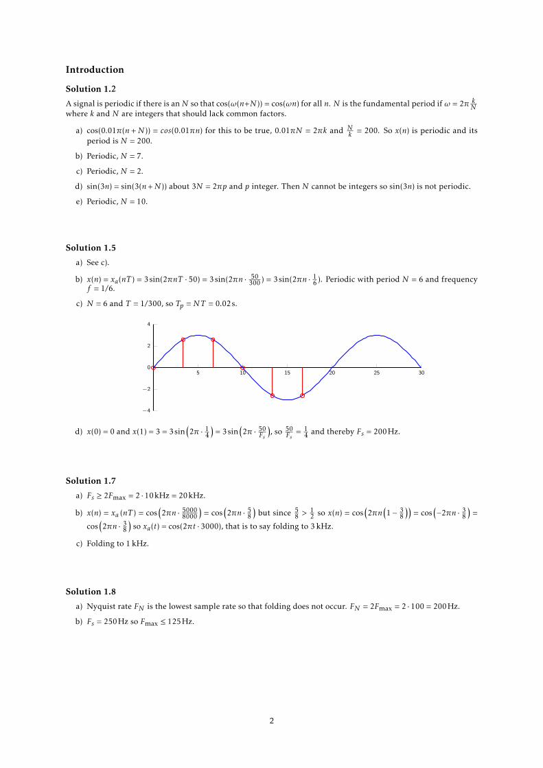
b) x(n) = xa(nT ) = 3sin(2πnT · 50) = 3sin(2πn · 50300 ) = 3sin(2πn · 1

6 ). Periodic with period N = 6 and frequencyf = 1/6.

c) N = 6 and T = 1/300, so Tp =NT = 0.02s.

5 10 15 20 25 30

−4

−2

0

2

4

d) x(0) = 0 and x(1) = 3 = 3sin(2π · 1

4

)= 3sin

(2π · 50

Fs

), so 50

Fs= 1

4 and thereby Fs = 200Hz.

Solution 1.7

a) Fs ≥ 2Fmax = 2 · 10kHz = 20kHz.

b) x(n) = xa (nT ) = cos(2πn · 5000

8000

)= cos

(2πn · 5

8

)but since 5

8 >12 so x(n) = cos

(2πn

(1− 3

8

))= cos

(−2πn · 3

8

)=

cos(2πn · 3

8

)so xa(t) = cos(2πt · 3000), that is to say folding to 3 kHz.

c) Folding to 1 kHz.

Solution 1.8

a) Nyquist rate FN is the lowest sample rate so that folding does not occur. FN = 2Fmax = 2 · 100 = 200Hz.

b) Fs = 250Hz so Fmax ≤ 125Hz.

2

Solution 1.11

The analog signal is:

xa(t) = 3cos(2πt · 50) + 2sin(2πt · 125) (1)

Sample with Fs = 200Hz.

x(n) = xa(n · 1

200

)(2)

= 3cos(2πn · 50

200

)+ 2sin

(2πn · 125

200

)(3)

= 3cos(2πn · 1

4

)+ 2sin

(2πn · 5

8

)(4)

= 3cos(2πn · 1

4

)+ 2sin

(−2πn · 3

8

)(5)

Reconstruct with Frek = 1000Hz.

ya(t) = 3cos(2πt · 1000

4

)+ 2sin

(−2πt · 3 · 1000

8

)(6)

= 3cos(2πt · 250)− 2sin(2πt · 375) (7)

MATLAB-code illustrating the example:

>> t = (0:10000 -1)/1000;>> x = 3*sin (100*pi*t)+2* sin (250*pi*t);>> y = x(1:5: end);>> subplot (2,1,1); plot(t(1:100) ,x(1:100));>> subplot (2,1,2); plot(t(1:100) ,y(1:100));

Then listen to the signals:

>> soundsc(x, 1000);>> soundsc(y, 1000);

Solution 1.13

The number of levels is L = xmax−xmin∆

+ 1 and the number of bits are b = log2L.

a) b = 7

b) b = 10

Solution 1.14

Bitrate = numberof bitsXsamplingf requency = nFs, so rate = 20Hz · 8bitar = 160bitar/s. Fmax = Fs2 = 10Hz.

∆ = DynamicRange2n−1 = 1/255V.

Solution E1.1

Simulation in Matlab.

3

Solution N1.1

Euler’s formulae:

cos(2πn) =12ej2πn +

12e−j2πn (8)

sin(2πn) =12jej2πn − 1

2je−j2πn (9)

The derivative of cos(2πn) is as follows:

ddn

cos(2πn) =ddn

(12ej2πn +

12e−j2πn) (10)

=12

(j2π)ej2πn +12

(−j2π)e−j2πn (11)

= (−2π)(−j2ej2πn +

j

2e−j2πn) (12)

= (−2π)(12jej2πn − 1

2je−j2πn) (13)

= (−2π)sin(2πn) (14)

(15)

The derivative of sin(2πn) is as follows:

ddn

sin(2πn) =ddn

(12jej2πn − 1

2je−j2πn) (16)

=12j

(j2π)ej2πn − 12

(−j2π)e−j2πn (17)

= (2π)(12ej2πn +

12e−j2πn) (18)

= (2π)cos(2πn) (19)

(20)

Solution N1.2

See the formulas for the sum of a geometric series from Lecture 1 slides.

a)∑Nn=0 2n = 1−2N+1

1−2 = −1 + 2N+1

b)∑∞n=0 0.5n = 1

1−0.5 = 2

Solution N1.3

The Nyquist rate(NR) is twice the maximum signal frequency available in the signal.

a) fmax = 75Hz,NR = 150Hz.

b) fmax = 200Hz,NR = 400Hz.

c) x(t) = 3sin(100πt)cos(250πt) = 32 (sin(350πt)− sin(150πt)). so,fmax = 175Hz,NR = 350Hz.

4

Solution N1.4

a) x(n) = nu(n) = 1δ(n− 1) + 2δ(n− 2) + 3δ(n− 3) + 4δ(n− 4) + ... =∑∞k=1 kδ(n− k).

b) x(n) = u(n+ 1) = δ(n+ 1) + δ(n) + δ(n− 1) + δ(n− 2) + .. =∑∞k=−1 δ(n− k)

c) x(n) = u(n− 1) = δ(n− 1) + δ(n− 2) + δ(n− 3) + .. =∑∞k=1 δ(n− k)

Solution N1.5

A causal signal means that the signal is zero before n=0.

a) x(n) = u(n+ 1), is non zero before n = 0 so it is noncausal.

b) x(n) = u(n− 1), is zero before n = 0 so it is causal.

Solution N1.6

a) x(n+ 1) = {1,2,1,−3,5,8}, and the corresponding values of n = {−1,0,1,2,3,4}

b) x(n− 1) = {1,2,1,−3,5,8}, and the corresponding values of n = {1,2,3,4,5,6}

c) x(2n) = {1,1,5}, interpolation, and the corresponding values of n = {0,1,2}

d) x(0.5n) = {1,2,1,−3,5,8}, and the corresponding values of n = {0,2,4,6,8,10}.

Solution N1.7

Hint: For the signal to be an energy signal, the energy should be finite and the power should be zero. If theenergy is infinite and the power is zero then it is a power signal.

Suggestion: The signals with decaying amplitude are energy signals and signals having constant amplitude arepower signals. The signals whose amplitude increases are neither energy nor power signals.

a) x(n) = u(n),n ≥ 0

Energy of the signal, E =∑∞n=0 | u(n) |2=

∑N−1n=0 (1)2 =∞.

Power of the signal,P = limN→∞1N

∑N−1n=0 | u(n) |2= limN→∞

1N

∑N−1n=0 (1)2 = limN→∞

NN = 1.

Hence it is a power signal.

b) x(n) = nu(n),n ≥ 0

Energy of the signal, E =∑∞n=0 | nu(n) |2=

∑∞n=0n

2 =∞.

Power of the signal,P = limN→∞1N

∑N−1n=0 | nu(n) |2= limN→∞

12+22+...(N−1)2

N =∞.

It is neither an energy nor a power signal.

c) x(n) = (0.5)nu(n)

Energy of the signal, E =∑∞n=0 | (0.5)n |2=

∑∞n=0(0.25)n = 1

1−0.25 = 43 .

Power of the signal,P = limN→∞1N

∑N−1n=0 | (0.5)nu(n) |2= limN→∞

1N

∑N−1n=0 (0.25)n = limN→∞

1N

1−o.25N+1

1−0.25 =0.

Hence it is an energy signal.

5

Solution N1.8

Even signal if x(−n) = x(n), odd signal if x(−n) = −x(n).

a) sin(−n) = 12j e−jn − 1

2j ejn = −( 1

2j ejn − 1

2j e−jn) = −sin(n), hence odd signal.

b) cos(−n) = 12 e−jn + 1

2 ejn = 1

2 ejn + 1

2 e− = cos(n), hence even signal.

c) cot(−n) = cos(−n)sin(−n) = cos(n)

−sin(n) = −cot(n), hence odd signal.

Solution N1.9

Linearity: Linear systems should satisfy homogeneity(if y(n) = f (x(n)) then ay(n) = af (x(n))) and additivity prop-erty (if y1(n) = f (x1(n)),y2(n) = f (x2(n)) then y1(n) + y2(n) = f (x1(n) + x2(n)).

Time Invariance: If y(n) = f (x(n)) then y(n−D) = f (x(n−D)).

a) Linearity check:

Homogeneity: For the input ax1(n), output is y1(n) = ax1(n− 1) so y(n) = ay1(n). Hence satisfied.

Additive:y1(n) = x1(n−1),y2(n) = x2(n−1). For the input,x1(n)+x2(n),output is y(n) = x1(n−1)+x2(n−1) =y1(n) + y2(n). The additive property is satisfied.

Hence it is linear.

Time invariance check:

y(n) = x(n−1) and y(n−D) = x(n−1−D). Let us delay the input by D. Now the output is y(n) = x(n−1−D),which is the same as y(n−D), hence time invariant.

b) Linearity check:

Homogeneity: for the input ax1(n), the output is y1(n) = ax1(n2) so y(n) = ay1(n). Hence satisfied.

Additive:y1(n) = x1(n2),y2(n) = x2(n2). For the input,x1(n) + x2(n),output is y(n) = x1(n2) + x2(n2) =y1(n) + y2(n). The additive property is satisfied.

Hence linear.

Time invariance check:

y(n) = x(n2) and y(n−D) = x(n2 −D). Let us delay the input by D. Now the output is y(n) = x((n−D)2),which is not the same as y(n−D), hence not time invariant.

c) Linearity check:

Homogeneity: For the input ax1(n), output is y1(n) = a2x1(n)2 so y(n) , ay1(n). Hence not satisfied.

Additive:y1(n) = x1(n)2,y2(n) = x2(n)2. For the input,x1(n) + x2(n),output is y(n) = (x1(n) + x2(n))2 ,y1(n) + y2(n). The additive property is not satisfied.

Hence not linear. Even if one of the properties are not satisfied, it will be non-linear.

Time invariance check:

y(n) = x(n)2 and y(n −D) = x(n −D)2. Let us delay the input by D. Now the output is y(n) = x(n −D)2,which is the same as y(n−D), hence time invariant.

Solution N1.10

The analog signal is xa(t) = 3cos(500πt) + 2sin(1000πt).

a) The maximum signal frequency component Fmax = 500Hz, so the Nyquist rate is 1000Hz. The samplingfrequency should be at least higher than the Nyquist rate for ideal reconstruction.

6

b) For Fs = 400Hz,

x(n) = 3cos(2πn250400

) + 2sin(2πn500400

) (21)

= 3cos(2πn58

) + 2sin(2πn54

) (22)

= 3cos(2πn38

) + 2sin(2πn14

) (23)

now reconstructing with Fs = 400Hz

x(t) = 3cos(2πn38

400) + 2sin(2πn14

400) (24)

= 3cos(300πt) + 2sin(200πt) (25)

Here the sampling frequency is very low compared to the Nyquist rate, so the signal cannot be recoveredafter sampling.For Fs = 600Hz,

x(n) = 3cos(2πn250600

) + 2sin(2πn500600

) (26)

= 3cos(2πn5

12) + 2sin(2πn

56

) (27)

= 3cos(2πn5

12)− 2sin(2πn

16

) (28)

(29)

Now reconstructing with Fs = 600Hz,

x(t) = 3cos(2πt5

12600)− 2sin(2πt

16

600) (30)

= 3cos(500πt)− 2sin(200πt) (31)

(32)

Now reconstructing with Fs = 600Hz,. As the frequency signal is higher than the Nyquist rate of 250 Hz onlythis signal is recovered.For Fs = 1100Hz

x(n) = 3cos(2πn250

1100) + 2sin(2πn

5001100

) (33)

= 3cos(2πn5

22) + 2sin(2πn

511

) (34)

Now reconstructing with F=1100Hz

x(t) = 3cos(2πt5

221100) + 2sin(2πt

511

1100) (35)

= 3cos(500πt) + 2sin(10000πt) (36)

(37)

All frequency components are recovered as the sampling frequency is higher than the Nyquist rate.

Impulse Response and Convolution, Chapter 2

Solution 2.1

a)

7

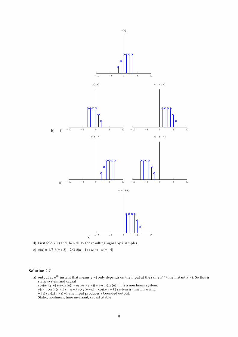
−10 −5 0 5 10

x(n)

b) i) −10 −5 0 5 10

x(−n)

−10 −5 0 5 10

x(−n+ 4)

ii) −10 −5 0 5 10

x(n− 4)

−10 −5 0 5 10

x(−n− 4)

c) −10 −5 0 5 10

x(−n+ 4)

d) First fold x(n) and then delay the resulting signal by k samples.

e) x(n) = 1/3 δ(n+ 2) + 2/3 δ(n+ 1) +u(n)−u(n− 4)

Solution 2.7

a) output at nth instant that means y(n) only depends on the input at the same nth time instant x(n). So this isstatic system and causalcos(a1x1(n) + a2x2(n)) , a1cos(x1(n)) + a2cos(x2(n)). it is a non linear system.y(i) = cos(x(i)) if i = n− k so y(n− k) = cos(x(n− k) system is time invariant.−1 ≤ cos(x(n)) ≤ +1 any input produces a bounded output.Static, nonlinear, time invariant, causal ,stable

8

b) Here output at nth instant depends on input at kth instant, where k = −∞, ...,n − 1,n,n+ 1 . output dependson present input as well as past and future inputs..So the system is dynamic.

y1(n) =n+1∑k=−∞

x1(k) y2(n) =n+1∑k=−∞

x2(k) x(n) = a1x1(n) + a2x2(n)

y(n) =n+1∑k=−∞

(a1x1(k) + a2x2(k)) =n+1∑k=−∞

a1x1(k) +n+1∑k=−∞

a2x2(k)

= a1

n+1∑k=−∞

x1(k) + a2

n+1∑k=−∞

x2(k) = a1y1(n) + a2y2(n)

system is linear.

y(n− i) =n−i+1∑k=−∞

x(k) =n+1∑k∗=−∞

x(k∗ − i)

=n+1∑k=−∞

x(k − i)

system is time invariantoutput at time n depends on the input at t n+ 1 time (future) . So system is noncausal.suppose x(n) = a where ≤ a ≤∞ so x(n) is bounded we have y(n) =

∑n+1k=−∞ a→∞ is unstable

Dynamic, Linear, time invariant, non causal, unstable.

c) output at n that means y(n) depends on the input at the same nth time instant x(n). So this is static systemand causal

y1(n) = x1(n)cos(ω0n) y2(n) = x2(n)cos(ω0n) x(n) = a1x1(n) + a2x2(n)

y(n) = x(n)cos(ω0n) = (a1x1(n) + a2x2(n))cos(ω0n)

= a1x1(n)cos(ω0n) + a2x2(n)cos(ω0n) = a1y1(n) + a2y2(n)

system is linear.suppose the system input is x(n− i) so the output is y∗(n) = x(n− i)cos(ω0n) , y(n− i)suppose that x(n) is bounded since we know that cos(ω0n) is bounded so y(n) is bounded. system is stable.

Static, linear, time variant, causal ,stable

e) output at time n only depends on the input at the same nth time instant x(n). So this is static system andcausalsuppose x1(n) = 2.3 and x2(n) = 2.8, so y1(n) = tran(x1(n)) = 2 and y2(n) = tran(x2(n)) = 2 . y1(n) + y2(n) = 4 ,trun(x1(n) + x1(n)) = 5 nonlinear systemif x(n) is bounded the integer part of x(n) is bounded, BIBO stable

Static, nonlinear, time invariant, causal ,stable

h) output at time n only depends on the input at the same nth time instant x(n). So this is static system andcausalsuppose xd (n) = x(n−k)→ yd (n) = xd (n)u(n) = x(n−k)u(n) now delay the output by k, y(n−k) = x(n−k)u(n−k)as we see yd (n) , y(n− k) system is time variant.if x(n) is bounded y(n) = x(n) where n > 0 is bounded, BIBO stable

Static, linear, time variant, causal ,stable

j) Dynamic, Linear, time variant, non causal, stable. suppose xd (n) = x(n− k)→ yd (n) = xd (2n) = x(2n− k) nowdelay the output by k, y(n− k) = x(2n− 2k) as we see yd (n) , y(n− k) system is time variant.

9

n) Static, linear, time invariant, causal ,stable

Solution 2.13

a) ∑n

y(n) =∑n

∑k

h(n− k)x(k) =∑k

x(k)∑n

h(n− k) =∑k

x(k)∑l

h(l) (38)

b) (1) Sufficient: Suppose that∑n |h(n)| = Mh < ∞. Then apply with limited input signal,

∑n |x(n)| ≤ Mx <

∞,by using the fundamental properties of absolute values (Multiplicativity ,Subadditivity)

∣∣∣y(k)∣∣∣ =

∣∣∣∣∣∣∣∞∑

n=−∞h(n)x(k −n)

∣∣∣∣∣∣∣ ≤∞∑

n=−∞|h(n)| · |x(k −n)| ≤Mh ·Mx <∞ (39)

Shows that, the system is BIBO stable.

(2) Necessary: Assume that∑n |h(n)| =∞. Form the input signal

x(n) ={h∗(−n)/ |h(−n)| h(−n) , 0,0 h(−n) = 0.

(40)

x(n) is limited for |x(n)| ≤ 1. We get

y(0) =∞∑

n=−∞h(n)x(−n) =

∞∑n=−∞

h(n)h∗(n)|h(n)|

=∞∑

n=−∞

|h(n)|2

|h(n)|=∞∑

n=−∞|h(n)| =∞, (41)

that is, a limited input signal provides an unlimited output and the system is not BIBO stable. Thus, ifthe system is BIBO -stable,

∑n |h(n)| <∞must be BIBO-stable.

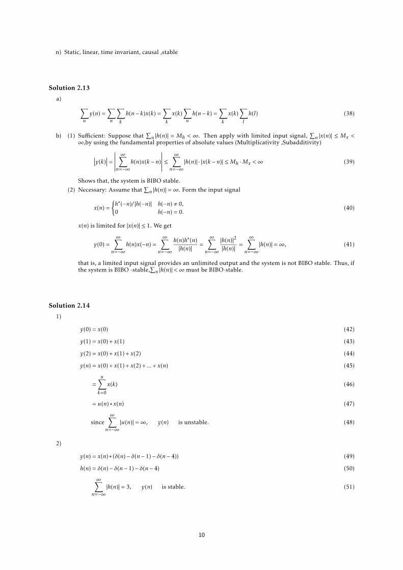
Solution 2.14

1)

y(0) = x(0) (42)

y(1) = x(0) + x(1) (43)

y(2) = x(0) + x(1) + x(2) (44)

y(n) = x(0) + x(1) + x(2) + ... + x(n) (45)

=n∑k=0

x(k) (46)

= u(n) ∗ x(n) (47)

since∞∑

n=−∞|u(n)| =∞, y(n) is unstable. (48)

2)

y(n) = x(n) ∗ (δ(n)− δ(n− 1)− δ(n− 4)) (49)

h(n) = δ(n)− δ(n− 1)− δ(n− 4) (50)

∞∑n=−∞

|h(n)| = 3, y(n) is stable. (51)

10

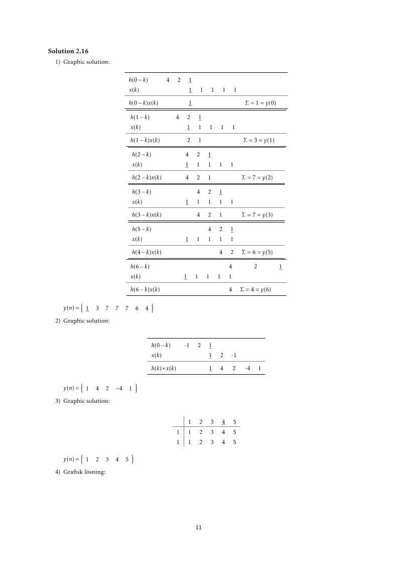
Solution 2.16

1) Graphic solution:

h(0− k) 4 2 1

x(k) 1 1 1 1 1

h(0− k)x(k) 1 Σ = 1 = y(0)

h(1− k) 4 2 1

x(k) 1 1 1 1 1

h(1− k)x(k) 2 1 Σ = 3 = y(1)

h(2− k) 4 2 1

x(k) 1 1 1 1 1

h(2− k)x(k) 4 2 1 Σ = 7 = y(2)

h(3− k) 4 2 1

x(k) 1 1 1 1 1

h(3− k)x(k) 4 2 1 Σ = 7 = y(3)

h(5− k) 4 2 1

x(k) 1 1 1 1 1

h(4− k)x(k) 4 2 Σ = 6 = y(5)

h(6− k) 4 2 1

x(k) 1 1 1 1 1

h(6− k)x(k) 4 Σ = 4 = y(6)

y(n) ={

1 3 7 7 7 6 4}

2) Graphic solution:

h(0− k) -1 2 1

x(k) 1 2 -1

h(k) ∗ x(k) 1 4 2 -4 1

y(n) ={

1 4 2 −4 1}

3) Graphic solution:

1 2 3 4 5

1 1 2 3 4 5

1 1 2 3 4 5

y(n) ={

1 2 3 4 5}

4) Grafisk lösning:

11

1 -2 -3 4

1 1 -2 -3 4

1 1 -2 -3 4

0 0 0 0 0

1 1 -2 -3 4

1 1 -2 -3 4

Summera antidiagonalerna,

y(n) ={

1 −1 −5 2 3 −5 1 4}, (52)

∑n

y(n) = 0 =∑k

x(k)∑l

h(l) = 0 · 4 (53)

(5) Formel-lösning:

y(n) =∞∑

k=−∞

(12

)ku(k)

(14

)n−ku(n− k) (54)

=∞∑k=0

(12

)k (14

)n−ku(n− k) (55)

=n∑k=0

(12

)k (14

)n−k(56)

=(1

4

)n n∑k=0

2k (57)

=(1

4

)n 1− 2n+1

1− 2n ≥ 0 (58)

=[2 ·

(12

)n−(1

4

)n]u(n) (59)

∑n

y(n) =83

=∑k

x(k)∑l

h(l) = 2 · 43

(60)

Solution 2.17

a)

6 5 4 3 2 1 0 0

1 6 5 4 3 2 1 0 0

1 6 5 4 3 2 1 0 0

1 6 5 4 3 2 1 0 0

1 6 5 4 3 2 1 0 0

y(n) ={

6 11 15 18 14 10 6 3 1}

b)

6 5 4 3 2 1 0 0

1 6 5 4 3 2 1 0 0

1 6 5 4 3 2 1 0 0

1 6 5 4 3 2 1 0 0

1 6 5 4 3 2 1 0 0

y(n) ={

6 11 15 18 14 10 6 3 1}

12

c) y(n) ={

1 2 2 2 1}

d) y(n) ={

1 2 2 2 1}

Solution 2.21

a) Om a , b:

y(n) =∞∑

k=−∞bku(k)an−ku(n− k) (61)

= ann∑k=0

(ba

)k(62)

= an1−

(ba

)n+1

1− ba(63)

=an+1 − bn+1

a− bn ≥ 0 (64)

Om a = b:

y(n) = ann∑k=0

1k = an · (n+ 1) n ≥ 0 (65)

b) y(n) ={

1 1 −1 0 0 3 3 2 1}

Solution 2.35

a) Parallel and serial connection:

h(n) = h1(n) ∗ [h2(n)− h3(n) ∗ h4(n)] (66)

b)

h3(n) ∗ h4(n) = (n− 1) ·u(n− 2) (67)

h2(n)− h3(n) ∗ h4(n) = δ(n) + 2u(n− 1) (68)

h(n) =12δ(n) +

54δ(n− 1) + 2δ(n− 2) +

52u(n− 3) (69)

c) Falta med en komponent av x(n) i taget.

h(n) ∗ δ(n+ 2) 12

54 2 5

252

52

52

52

52 . . .

h(n) ∗ 3δ(n− 1) 0 0 0 32

154 6 15

2152

152 . . .

h(n) ∗ (−4δ(n− 3)) 0 0 0 0 0 -2 -5 -8 -10 -10∑ 12

54 2 4 25

4132 5 2 0 0

The output signal becomes

y(n) ={

12

54 2 4 25

4132 5 2

}(70)

13

d)

h(n) =12δ(n) +

54δ(n− 1) + 2δ(n− 2) +

52u(n− 3) (71)

∞∑n=−∞

|h(n)| =12

+54

+52

∞∑n=0

1 =∞ system is unstable (72)

Solution 2.61

• For rxx(l):

rxx(l) =∑n

x(n)x(n− l) =n0+N∑n=n0−N

x(n− l) =n0+N∑

n=n0−N+l

1 = 2N − l + 1 l ≥ 0 (73)

rxx(l) =∑n

x(n)x(n− l) =n0+N∑n=n0−N

x(n− l) =n0+N+l∑n=n0−N

1 = 2N + l + 1 l ≤ 0 (74)

rxx(l) = 2N − |l|+ 1 (75)

• For rxy (l):

y(n) = x(n+n0) (76)

rxy (l) =∑n

x(n)y(n− l) =∑n

x(n)x(n+n0 − l) (77)

Lös grafiskt, dvs

rxy (l) = rxx(l −n0) (78)

Solution 2.62

a) rxx(l) = x(n) ∗ x(−n)x(n) =

{1 2 1 1

}and x(−n) =

{1 1 2 1

}rxx(l) =

{1 3 5 7 5 3 1

}b) ryy (l) = y(n) ∗ y(−n)

y(n) ={

1 1 2 1}

and y(−n) ={

1 2 1 1}

ryy (l) ={

1 3 5 7 5 3 1}

Solution 2.64

x(n) = s(n) + r1s(n− k1) + r2s(n− k2) (79)

rxx(l) =∑n

x(n)x(n− l) = (80)

=∑n

[s(n) + r1s(n− k1) + r2s(n− k2)] · [s(n− l) + r1s(n− k1 − l) + r2s(n− k2 − l)] (81)

= rss(l) + r1rss(l + k1) + r2rss(l + k2) (82)

+ r1rss(l − k1) + r21 rss(l) + r1r2rss(l + k2 − k1) (83)

+ r2rss(l − k2) + r1r2rss(l + k1 − k2) + r22 rss(l) (84)

14

Låt r1� 1 och r2� 1:

rxx(l) ≈ rss(l) + r1rss(l + k1) + r2rss(l + k2) + r1rss(l − k1) + r2rss(l − k2) (85)

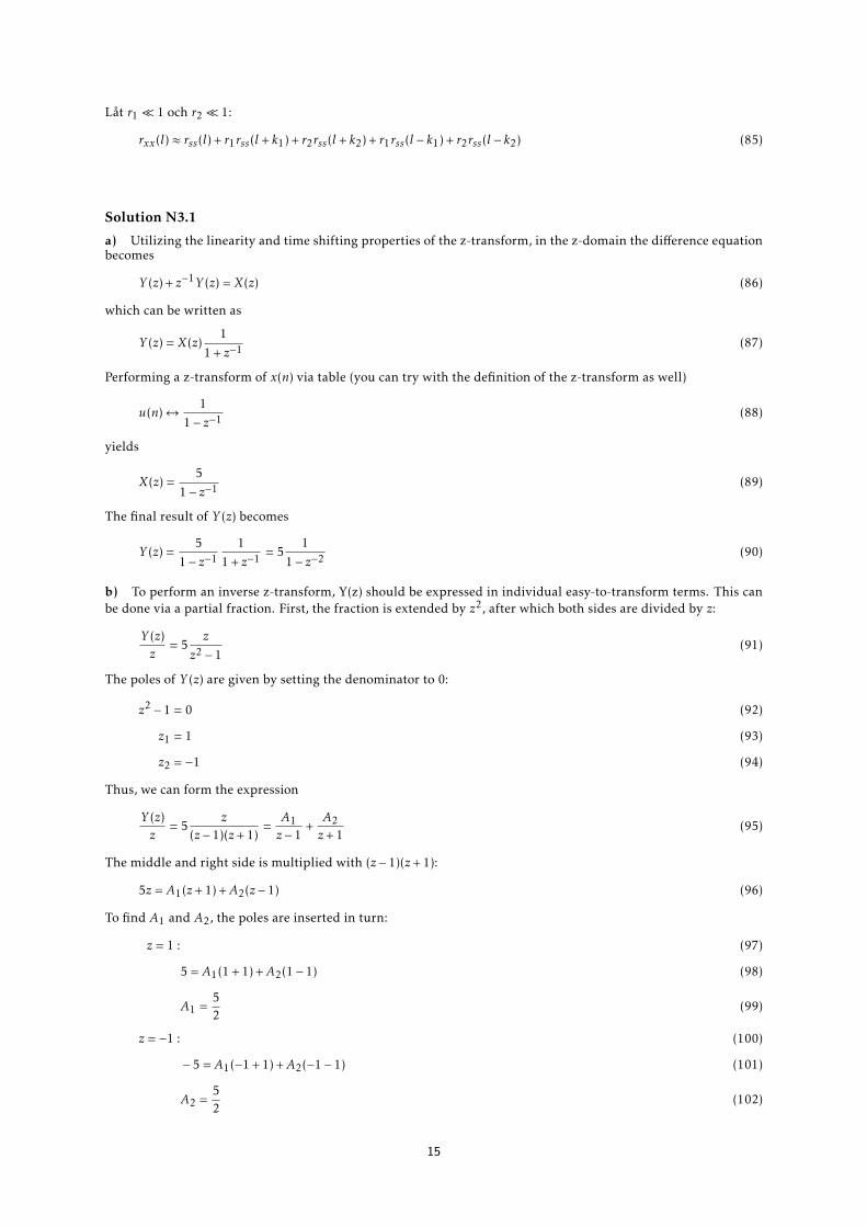
Solution N3.1

a) Utilizing the linearity and time shifting properties of the z-transform, in the z-domain the difference equationbecomes

Y (z) + z−1Y (z) = X(z) (86)

which can be written as

Y (z) = X(z)1

1 + z−1 (87)

Performing a z-transform of x(n) via table (you can try with the definition of the z-transform as well)

u(n)↔ 11− z−1 (88)

yields

X(z) =5

1− z−1 (89)

The final result of Y (z) becomes

Y (z) =5

1− z−11

1 + z−1 = 51

1− z−2 (90)

b) To perform an inverse z-transform, Y(z) should be expressed in individual easy-to-transform terms. This canbe done via a partial fraction. First, the fraction is extended by z2, after which both sides are divided by z:

Y (z)z

= 5z

z2 − 1(91)

The poles of Y (z) are given by setting the denominator to 0:

z2 − 1 = 0 (92)

z1 = 1 (93)

z2 = −1 (94)

Thus, we can form the expression

Y (z)z

= 5z

(z − 1)(z+ 1)=A1z − 1

+A2z+ 1

(95)

The middle and right side is multiplied with (z − 1)(z+ 1):

5z = A1(z+ 1) +A2(z − 1) (96)

To find A1 and A2, the poles are inserted in turn:

z = 1 : (97)

5 = A1(1 + 1) +A2(1− 1) (98)

A1 =52

(99)

z = −1 : (100)

− 5 = A1(−1 + 1) +A2(−1− 1) (101)

A2 =52

(102)

15

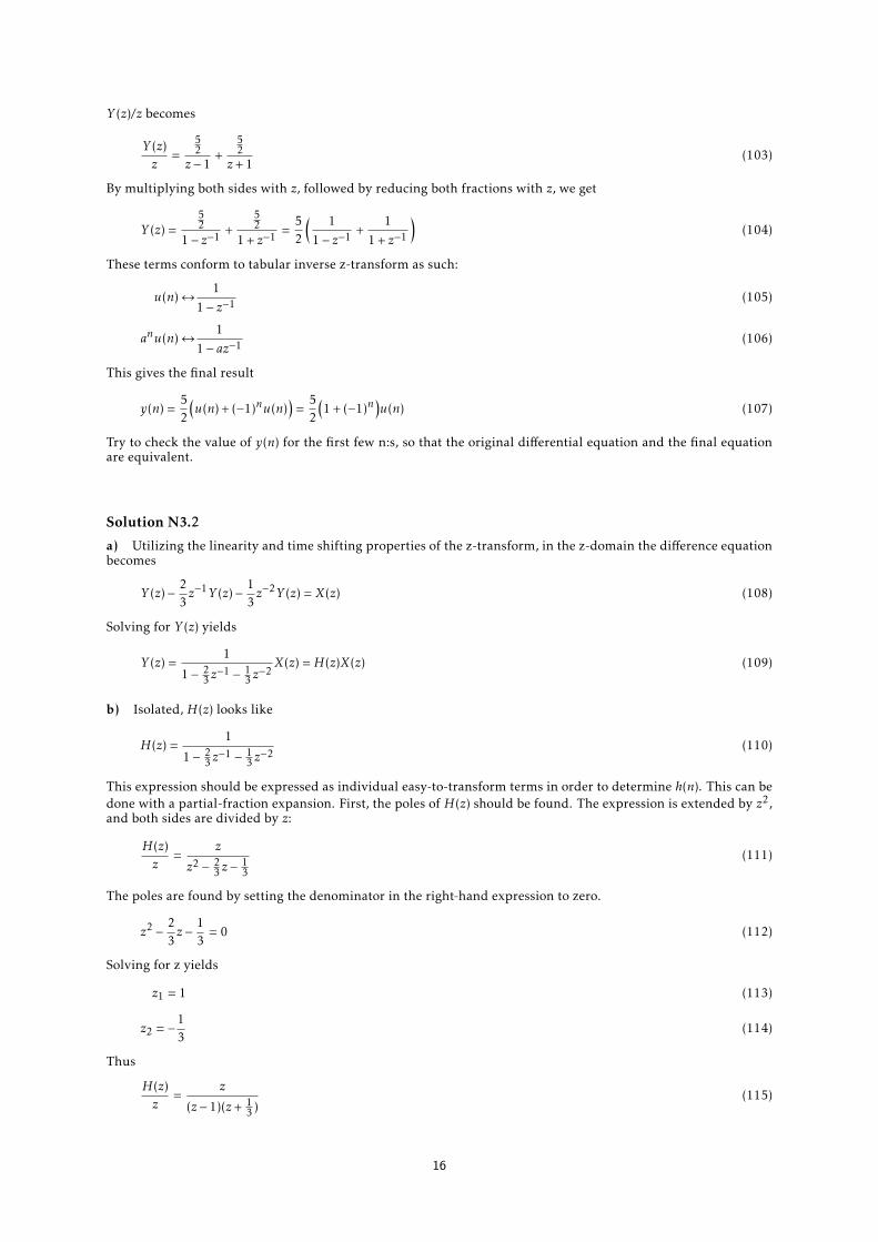
Y (z)/z becomes

Y (z)z

=52

z − 1+

52

z+ 1(103)

By multiplying both sides with z, followed by reducing both fractions with z, we get

Y (z) =52

1− z−1 +52

1 + z−1 =52

( 11− z−1 +

11 + z−1

)(104)

These terms conform to tabular inverse z-transform as such:

u(n)↔ 11− z−1 (105)

anu(n)↔ 11− az−1 (106)

This gives the final result

y(n) =52

(u(n) + (−1)nu(n)

)=

52

(1 + (−1)n

)u(n) (107)

Try to check the value of y(n) for the first few n:s, so that the original differential equation and the final equationare equivalent.

Solution N3.2

a) Utilizing the linearity and time shifting properties of the z-transform, in the z-domain the difference equationbecomes

Y (z)− 23z−1Y (z)− 1

3z−2Y (z) = X(z) (108)

Solving for Y (z) yields

Y (z) =1

1− 23 z−1 − 1

3 z−2X(z) =H(z)X(z) (109)

b) Isolated, H(z) looks like

H(z) =1

1− 23 z−1 − 1

3 z−2

(110)

This expression should be expressed as individual easy-to-transform terms in order to determine h(n). This can bedone with a partial-fraction expansion. First, the poles of H(z) should be found. The expression is extended by z2,and both sides are divided by z:

H(z)z

=z

z2 − 23 z −

13

(111)

The poles are found by setting the denominator in the right-hand expression to zero.

z2 − 23z − 1

3= 0 (112)

Solving for z yields

z1 = 1 (113)

z2 = −13

(114)

Thus

H(z)z

=z

(z − 1)(z+ 13 )

(115)

16

Which should be expressed in the form of

H(z)z

=z

(z − 1)(z+ 13 )

=A1z − 1

+A2

z+ 13

(116)

Multiplying both sides with the denominator of the middle yields

z = A1(z+13

) +A2(z − 1) (117)

Inserting the pole values readily produces A1 and A2:

z = 1 : 1 = A1(1 +13

) +A2(1− 1) (118)

A1 =34

(119)

z = −13

: − 13

= A1(−13

+13

) +A2(−13− 1) (120)

A2 =14

(121)

Having A1 and A2, we move back to the partial-fraction expression

H(z)z

=A1z − 1

+A2

z+ 13

(122)

To achieve a transformable form, both sides are first multiplied with z, both fractions are reduced by z, and lastlyA1 and A2 are moved in front of their respective terms:

H(z) = A11

1− z−1 +A21

1 + 13 z−1

(123)

Due to the linearity of the z-transform, the right-hand terms can be transformed individually. Both correspond tothe table transformation:

u(n)↔ 11− z−1 (124)

anu(n)↔ 11− az−1 (125)

Thus

h(n) = A1u(n) +A2

(13

)nu(n) (126)

Inserting A1 and A2 and a slight restructuring yields the final result:

h(n) =(

34

+14

(13

)n )u(n) (127)

Solution 3.1

a) The z-transform is defined as

X(z) ≡∞∑

n=−∞x(n)z−n (128)

The signal is finite, starting at n = −5 and ending at n = 2. The z-transform can thus be written as

X(z) =2∑

n=−5

x(n)z−n (129)

Compute all individual terms:

n −5 −4 −3 −2 −1 0 1 2

x(n) 3 0 0 0 0 6 1 −4

x(n)z−n 3z5 0 0 0 0 6z0 = 6 z−1 −4z−2

(130)

Add the terms together to produce the final result:

X(z) = 3z5 + 6 + z−1 +−4z−2 (131)

17

b) Utilizing a step function, the signal can be expressed as

x(n) = (12

)nu(n− 5) (132)

Plugging this into the z-transform definition yields

X(z) =∞∑n=5

(12

)nz−n (133)

Simplifying it gives

X(z) =∞∑n=5

(12z−1)n (134)

(The original signal description can also be plugged into the definition, case by case, yielding the same: X(z) =4∑

n=−∞0nz−n +

∞∑n=5

( 12 )nz−n =

∞∑n=5

( 12 z−1)n)

As the signal has no upper bound, the individual terms cannot be manually added together. However, due to thegeometrical fraction ( 1

2 z−1)n, it is recognized as a geometric sum. Additionally, since the fraction is between −1

and 1, it converges.Writing out the terms gives

X(z) = (12z−1)5 + (

12z−1)6 + (

12z−1)7 + ... (135)

A geometric sum can be solved by finding a similar geometric sum – with an identical fraction but a differentstarting term – and then reducing the original sum with the latter sum. Finding such a sum can be done by simplymultiplying the original sum with its geometrical fraction, as such:

X(z)(12z−1) = (

12z−1)6 + (

12z−1)7 + (

12z−1)8 + ... (136)

Then, taking the difference, gives

X(z)−X(z)(12z−1) = (

12z−1)5 (137)

as all other terms cancel each other out (which works due to that the fraction approaches zero as n moves to infinity,if it were a finite signal the very last term of the second sum would remain as well).Breaking out X(z) gives the final result:

X(z) =( 1

2 z−1)5

1− 12 z−1

(138)

Solution 3.2

a) Since the z-transform enjoys the linearity property, the terms of x(n) can be transformed separately. Expandingx(n) gives

x(n) = u(n) +nu(n) (139)

Via table:

u(n)↔ 11− z−1 (140)

and

nanu(n)↔ az−1

(1− az−1)2(141)

The z-transform can thus be written as:

X(z) =1

1− z−1 +z−1

(1− z−1)2(142)

18

(For a non-formulaic transformation, the first term can readily be transformed using the geometric sum methodused in 3.1b; how to transform the second term is shown in example 2.7 in the book.)Simplifying the expression gives the z-transform result:

X(z) =1

(1− z−1)2(143)

To retrieve the poles and zeros, the denominator is first expanded, as such

X(z) =1

1− 2z−1 + z−2 (144)

Then, the expression is extended according to the polynomial order:

X(z) =z2

z2 − 2z+ 1(145)

Set the numerator and denominator to zero, to obtain the zeros and poles, respectively:

z2 = 0⇒ There are two zeros at z = 0 (146)

z2 − 2z+ 1 = 0⇒ There are two poles at z = 1 (147)

c) Simplifying x(n) gives

x(n) = (−12

)nu(n) (148)

Via table:

anu(n)↔ 11− az−1 (149)

The z-transform becomes:

X(z) =1

1 + 12 z−1

(150)

Again, extend the expression to procure the poles and zeros:

X(z) =z

z+ 12

(151)

Setting the numerator and denominator to zero, gives that there is a zero at z = 0 and a pole at z = −12

f) In order to perform a formulaic z-transform of x(n) the phase shift is removed using the trigonometric formula

cos(α + β) = cosα cosβ − sinα sinβ (152)

x(n) becomes

x(n) = Arn(cos(ω0n)cosφ− sin(ω0n)sinφ)u(n) (153)

= A(rn cos(ω0n)u(n)cosφ− rn sin(ω0n)u(n)sinφ) (154)

The cos- and sin-term are transformed individually per the formulas:

an cos(ω0n)u(n)↔ 1− az−1 cosω01− 2az−1 cosω0 − a2z−2 (155)

an sin(ω0n)u(n)↔ az−1 sinω01− 2az−1 cosω0 − a2z−2 (156)

X(z) then becomes (A, cosφ and sinφ are carried through unchanged):

X(z) = A(1− rz−1 cosω0)cosφ− rz−1 sinω0 sinφ

1− 2rz−1 cosω0 + r2z−2 (157)

To find the zeros and poles, the expression is extended with z2

X(z) = A(z2 − rzcosω0)cosφ− rz sinω0 sinφ

z2 − 2rzcosω0 + r2(158)

19

The numerator is set to zero to find the zeros:

0 = (z2 − rzcosω0)cosφ− rz sinω0 sinφ (159)

= z((z − r cosω0)cosφ− r sinω0 sinφ

)(160)

= z(zcosφ− r(cosω0 cosφ− sinω0 sinφ)

)(161)

The trigonometric formula used earlier can be used again in reverse on the second term:

z(zcosφ− r cos(ω0 +φ)

)= 0 (162)

Zeros are at z = 0 and z = r cos(ω0+φ)cosφ

The denominator is set to zero to find the poles:

0 = z2 − 2rzcosω0 + r2 (163)

= z2 − rz(ejω0 + e−jω0 ) + r2 (164)

= (z − rejω0 )(z − re−jω0 ) (165)

Poles are at z = re±jω0

h) Plug x(n) into the z-transform definition:

X(z) =9∑n=0

(12

)nz−n (166)

Simplify as a geometric sum to get the final z-transform:

X(z) =1−

(12 z−1

)10

1− 12 z−1

=1−

(12

)10z−10

1− 12 z−1

(167)

Extend with z10 to find zeros and poles:

X(z) =z10 −

(12

)10

z10 − 12 z

9(168)

Set numerator to zero to get zeros:

0 = z10 −(1

2

)10(169)

Zeros are at z = 12 ej2πk/10, for k = 0...9

Set denominator to zero to get poles:

0 = z10 − 12z9 (170)

= z9(z − 12

) (171)

There are 9 poles at z = 0 and 1 pole at z = 12 . Note however that the zero of z = 1

2 and the pole of z = 12 cancel each

other out. Thus, zeros are at z = 12 ej2πk/10, for k = 1...9 and 9 poles are at z = 0.

Solution 3.8

a) That a signal output is the sum of all previous inputs of the signal, can be expressed as a convolution of thesignal with a unit step:

y(n) =n∑

k=−∞x(k) =

∞∑k=−∞

x(k)u(n− k) = x(n) ∗u(n) (172)

20

Thus, by using the convolution property of the z-transform, we get

Y (z) = X(z)U (z) (173)

Since

u(n)↔ 11− z−1 (174)

the final result is

Y (z) = X(z)1

1− z−1 (175)

b) Convolve u(n) ∗u(n)

u(n) ∗u(n) =∞∑

k=−∞u(k)u(n− k) (176)

Since

u(k) = 0 k < 0 (177)

u(n− k) = 0 n < k (178)

We get

u(n) ∗u(n) =n∑k=0

u(k)u(n− k) =n∑k=0

1 (179)

Which is equal to x(n) = (n+ 1)u(n).Using the convolution property of the z-transform we have

Y (z) =U (z)U (z) (180)

Since

u(n)↔ 11− z−1 (181)

the z-transform becomes

Y (z) =1

1− z−11

1− z−1 (182)

=1

1− 2z−1 + z−2 (183)

Solution 3.9

Given a pole or a zero at z = rejω1 , it has its complex-conjugate paired pole or zero at z = re−jω1 .Scaling in the z-domain via table:

anx(n)↔ X(a−1z) (184)

gives that the new poles or zeros are given by

ze−jω0 = rejω1 and ze−jω0 = re−jω1 (185)

Solving for z gives

z = rejω1ejω0 = rej(ω1+ω0) and z = re−jω1ejω0 = rej(−ω1+ω0) (186)

The poles or zeros thus are not complex-conjugate pairs anymore.

21

Solution 3.14

a) X(z) is a proper rational transform and a partial-fraction can be determined as-is. First it is multiplied withz2.

X(z) =z2 + 3z

z2 + 3z+ 2(187)

This is followed by dividing both sides with z (this helps due to that the individual fraction terms later will have amaximum power of z; thus it will aid in making the terms conform to the z-transform formulas) :

X(z)z

=z+ 3

z2 + 3z+ 2(188)

Next the poles are found by setting the denominator to zero:

0 = z2 + 3z+ 2 (189)

which gives p1 = −1 and p2 = −2. The transform is written as:

X(z)z

=z+ 3

z2 + 3z+ 2=

z+ 3(z+ 1)(z+ 2)

=A1z+ 1

+A2z+ 2

(190)

A1 and A2 can be found by first multiplying with the denominator (z+ 1)(z+ 2)

z+ 3 = A1(z+ 2) +A2(z+ 1) (191)

A1 and A2 are then found by setting z as the poles in turn, thus eliminating either A1 or A2:

z = p1 = −1 : (192)

− 1 + 3 = A1(−1 + 2) +A2(−1 + 1) (193)

A1 = 2 (194)

z = p2 = −2 : (195)

− 2 + 3 = A1(−2 + 2) +A2(−2 + 1) (196)

A2 = −1 (197)

Inserting A1 and A2 in the transform yields

X(z)z

=2

z+ 1+−1z+ 2

(198)

Multiply both sides with z1

X(z) =2zz+ 1

+−zz+ 2

(199)

Extend the right terms with z−1

X(z) =2

1 + z−1 +−1

1 + 2z−1 (200)

These terms can readily be inverse z-transformed individually. Via table:

anu(n)↔ 11− az−1 (201)

Thus

x(n) = 2(−1)nu(n)− (−2)nu(n) (202)

b) X(z) is a proper rational transform and so a partial-fraction can be produced. The fraction is extended by z2,and both sides are divided by z:

X(z)z

=z

z2 − z+ 0.5(203)

The right-hand denominator is set to zero to find the poles:

z2 − z+ 0.5 = 0 (204)

z =12± j 1

2(205)

22

(note that the poles are complex-conjugate). Thus we have

X(z)z

=z

z2 − z+ 0.5=

z

(z − ( 12 + j 1

2 ))(z − ( 12 − j

12 ))

(206)

A partial-fraction is sought as

z

(z − ( 12 + j 1

2 ))(z − ( 12 − j

12 ))

=A1

z − ( 12 + j 1

2 )+

A2

z − ( 12 − j

12 )

(207)

In order to find A1 and A2, both sides are first multiplied with (z − ( 12 + j 1

2 ))(z − ( 12 − j

12 ))

z = A1

(z −

(12− j 1

2

))+A2

(z −

(12

+ j12

))= A1

(z − 1

2+ j

12

)+A2

(z − 1

2− j 1

2

)(208)

Then, the pole-values are inserted individually:

z =12

+ j12

: (209)

12

+ j12

= A1

(12

+ j12− 1

2+ j

12

)+A2

(12

+ j12− 1

2− j 1

2

)(210)

A1 =12 + j 1

2j

=12− j 1

2(211)

z =12− j 1

2: (212)

12− j 1

2= A1

(12− j 1

2− 1

2+ j

12

)+A2

(12− j 1

2− 1

2− j 1

2

)(213)

A2 =12 − j

12

j=

12

+ j12

(214)

(In general, it holds that a complex-conjugate pair of poles p1 = p∗2 will result in complex-conjugate coefficientsA1 = A∗2). We now have that

X(z)z

=12 − j

12

z − ( 12 + j 1

2 )+

12 + j 1

2

z − ( 12 − j

12 )

(215)

Multiplying both sides with z, followed by reducing the fractions with z, yields

X(z) =12 − j

12

1− ( 12 + j 1

2 )z−1+

12 + j 1

2

1− ( 12 − j

12 )z−1

(216)

Inverse z-transforming according to

anu(n)↔ 11− az−1 (217)

yields

y(n) =(1

2− j 1

2

)(12

+ j12

)nu(n) +

(12

+ j12

)(12− j 1

2

)nu(n) (218)

=[(1

2− j 1

2

)(12

+ j12

)n+(1

2+ j

12

)(12− j 1

2

)n]u(n) (219)

It is assumed that x(n) is real, and so the complex terms should be reducible to real ones. First they are expressedin polar form:

y(n) =[

1√

2e−jπ/4

(1√

2ejπ/4

)n+

1√

2ejπ/4

(1√

2e−jπ/4

)n]u(n) (220)

Then, the expression is rearranged to isolate the imaginary parts:

y(n) =1√

2

(1√

2

)n (e−jπ/4ejnπ/4 + ejπ/4e−jnπ/4

)u(n) (221)

=1√

2

(1√

2

)n (ej(n−1)π/4 + e−j(n−1)π/4

)u(n) (222)

23

According to Euler:

cosφ =ejφ + e−jφ

2(223)

Thus

y(n) =1√

2

(1√

2

)n2cos

((n− 1)

π4

)u(n) (224)

=(

1√

2

)n−1cos

((n− 1)

π4

)u(n) (225)

c)

X(z) =z−6 + z−7

1− z−1 (226)

By inspection it is seen that the denominator already conforms to the formulaic z-transform

u(n)↔ 11− z−1 (227)

Thus, the fraction is split according to the individual terms of the numerator:

X(z) =z−6 + z−7

1− z−1 =z−6

1− z−1 +z−7

1− z−1 (228)

By using the z-transform formula above, and taking into account the time-shifting property of the z-transform,x(n) becomes

x(n) = u(n− 6) +u(n− 7) (229)

In general, improper rational transform (the numerator is a same or higher order polynomial than the denominator)such as this X(z) can always be expressed as a polynomial added with a proper rational transform (which then canbe expressed as a partial fraction, and then can be inverse z-transformed, along with the polynomial). Such a formcan be reached using a long division, as follows:

−z−6 −2z−5 −2z−4 −2z−3 −2z−2 −2z−1 −2

−z−1 + 1)

z−7 +z−6

− z−7 −z−6

2z−6

− 2z−6 −2z−5

2z−5

− 2z−5 −2z−4

2z−4

− 2z−4 −2z−3

2z−3

− 2z−3 −2z−2

2z−2

− 2z−2 −2z−1

2z−1

− 2z−1 −2

2

(230)

Resulting in

X(z) = −2− 2z−1 − 2z−2 − 2z−3 − 2z−4 − 2z−5 − z−6 + 21

1− z−1 (231)

(Note the form of a polynomial and a proper rational transform). These are readily inverse z-transformed as:

x(n) = −2δ(n)− 2δ(n− 1)− 2δ(n− 2)− 2δ(n− 3)− 2δ(n− 4)− 2δ(n− 5)− δ(n− 6) + 2u(n) (232)

Or in the form of samples

x(n) = {0,0,0,0,0,0,1,2,2,2, ...} (233)

Which can be expressed as:

x(n) = u(n− 6) +u(n− 7) (234)

24

d) The transform is improper and an easy modification that would help is hard to discern. Thus we perform along division:

2

z−2 + 1(

2z−2 +1

− 2z−2 +2

−1

(235)

Thus

X(z) = 2− 11 + z−2 (236)

The rightmost term is now a proper rational and transform a partial-fraction expansion will be helpful. The rootsof the denominator should be found and first we expand the fraction with z−2, and remove a z to the front of theexpression.

11 + z−2 =

z2

z2 + 1= z

z

z2 + 1(237)

The roots of the denominator are z = ±j, and we have

zz

z2 + 1= z

z(z+ j)(z − j)

(238)

The fraction (excluding the prior z) should be expanded as such:

z(z − j)(z+ j)

=A1z − j

+A2z+ j

(239)

Multiplying with the left-hand side denominator yields

z = A1(z+ j) +A2(z − j) (240)

Inserting the roots individually:

z = j : (241)

j = A1(j + j) +A2(j − j) (242)

A1 =12

(243)

z = −j : (244)

− j = A1(−j + j) +A2(−j − j) (245)

A2 =12

(246)

X(z) becomes

X(z) = 2− z 1

2z − j

+12z+ j

(247)

Inserting the prior z and reducing both fractions with z produce

X(z) = 2− 12

11− jz−1 −

12

11 + jz−1 (248)

Via table:

δ(n)↔ 1 (249)

anu(n)↔ 11− az−1 (250)

x(n) becomes

x(n) = 2δ(n)− 12

(j)nu(n)− 12

(−j)nu(n) (251)

25

Isolating the complex terms and writing them in polar form:

x(n) = 2δ(n)− 12

(ejnπ/2 − e−jnπ/2

)u(n) (252)

According to Euler:

cosφ =ejφ + e−jφ

2(253)

Thus

x(n) = 2δ(n)− 12

(2cos(n

π2

))u(n) = 2δ(n)− cos(n

π2

)u(n) (254)

g) The rational transform is improper and there is no easily discernible simple solution. A long division isutilized until the remainder forms a proper rational transform (numerator polynom is of a lower order than thedenominator polynom):

14

4z−2 + 4z−1 + 1(

z−2 +2z−1 +1

− z−2 +z−1 + 14

z−1 + 34

(255)

Thus

X(z) =14

+34 + z−1

1 + 4z−1 + 4z−2 =14

+34

1 + 4z−1 + 4z−2 +z−1

1 + 4z−1 + 4z−2 (256)

The fractions could individually be partial-fraction expanded as usual, however the denominator polynoms havedouble zeros (which, if not seen initially, becomes apparent when starting the partial-fraction expansion). I.e.

X(z) =14

+34

(1 + 2z−1)2+

z−1

(1 + 2z−1)2(257)

All the terms should be modifiable to fit the formulaic transformations

δ(n)↔ 1 (258)

nanu(n)↔ z−1

(1− az−1)2(259)

as such:

X(z) =14

+−38z

−2z−1

(1− (−2)z−1)2+−1

2−2z−1

(1− (−2)z−1)2(260)

Taking into account time scaling, this gives

x(n) =14δ(n) +

(−3

8

)(n+ 1)(−2)(n+1)u(n+ 1) +

(−1

2

)n(−2)nu(n) (261)

=14δ(n) +

34

(n+ 1)(−2)nu(n+ 1) +n(−2)n−1u(n) (262)

which is a valid transformation. However, it can be simplified significantly. We start by trying to make the unitstep functions alike. Investigating for n = −1, shows

x(0) = 0 + 0 + 0 = 0 (263)

Which should be the case of a causal signal. It also follows that

34

(n+ 1)(−2)nu(n+ 1) =34

(n+ 1)(−2)nu(n) (264)

Investigating for n = 0, further shows that

x(0) =14

+34

+ 0 = 1 (265)

26

Thus,

34

(n+ 1)(−2)nu(n) =34δ(n) +

34

(n+ 1)(−2)nu(n− 1), (266)

and n(−2)n−1u(n) = n(−2)n−1u(n− 1) (267)

We then have that

x(n) = δ(n) +(3

4(n+ 1)(−2)n +n(−2)n−1

)u(n− 1) (268)

Simplify to final result:

x(n) = δ(n) +(3

4(n+ 1)(−2)n +n(−2)n−1

)u(n− 1) (269)

= δ(n) +(3

4(n+ 1)(−2)n +n(−2)n(−2)n

)u(n− 1) (270)

= δ(n) + (−2)n(3

4(n+ 1)− n

2

)u(n− 1) (271)

= δ(n) + (n+ 3)(−2)n−2u(n− 1) (272)

Solution 3.16

a) As a convolution in the time domain becomes a simple multiplication in the z-domain, it is advantageous toperform it there. First the individual signals are z-transformed. First they are modified to fit a formulaic transform.x1(n) becomes

x1(n) =(1

4

)nu(n− 1) =

(14

)n−1+1u(n− 1) =

14

(14

)n−1u(n− 1) (273)

Which fits with

anu(n)↔ 11− az−1 (274)

if simple scaling and a time shift of z−1 is used. Meanwhile, x2(n) can be written as

x2(n) =(1 +

(12

)n)u(n) = u(n) +

(12

)nu(n) (275)

Which works directly with

u(n)↔ 11− z−1 (276)

and anu(n)↔ 11− az−1 (277)

Thus,

X1(z) =14 z−1

1− 14 z−1

, (278)

and X2(z) =1

1− z−1 +1

1− 12 z−1

(279)

Our sought signal x(n) = x1(n) ∗ x2(n)↔ X(z) = X1(z)X2(z).

X(z) =14 z−1

1− 14 z−1

11− z−1 +

1

1− 12 z−1

(280)

This should be expressed in readily inverse z-transformable terms. First, the multiplication is performed

X(z) =14 z−1

(1− 14 z−1)(1− z−1)

+14 z−1

(1− 14 z−1)(1− 1

2 z−1)

(281)

27

These terms are individually partial-fraction expanded:

Xa(z) =14 z−1

(1− 14 z−1)(1−z−1)

Xb(z) =14 z−1

(1− 14 z−1)(1− 1

2 z−1)

Xa(z) = z14

(z− 14 )(z−1)

Xb(z) = z14

(z− 14 )(z− 1

2 )Xa(z)z =

14

(z− 14 )(z−1)

= A1z− 1

4+ A2z−1

Xb(z)z =

14

(z− 14 )(z− 1

2 )= B1z− 1

4+ B2z− 1

214 = A1(z − 1) +A2(z − 1

4 ) 14 = B1(z − 1

2 ) +B2(z − 14 )

z = 1 : A2 = 13 z = 1

2 : B2 = 1

z = 14 : A1 = −1

3 z = 14 : B1 = −1

Xa(z) = z(− 1

3z− 1

4+

13z−1

)Xb(z) = z

(−1z− 1

4+ 1z− 1

2

)(282)

X(z) can thus be expressed as

X(z) = Xa(z) +Xb(z) = z

−13

z − 14

+13

z − 1

+ z

−1

z − 14

+1

z − 12

(283)

=−1

3

1− 14 z−1

+13

1− z−1 +−1

1− 14 z−1

+1

1− 12 z−1

(284)

(285)

Which is inverse z-transformable according to

u(n)↔ 11− z−1 (286)

and anu(n)↔ 11− az−1 (287)

giving

x(n) = −13

(14

)nu(n) +

13u(n)−

(14

)nu(n) +

(12

)nu(n) (288)

=(−1

3

(14

)n+

13−(1

4

)n+(1

2

)n)u(n) (289)

=(

13− 1

3

(14

)n−1+(1

2

)n)u(n) (290)

and since

n = 0 1 2 3 4 5 ...

x(n) = 0 0.5 0.5 0.4375 0.39.. 0.36.. ...(291)

the signal can be expressed as

x(n) =(

13− 1

3

(14

)n−1+(1

2

)n)u(n− 1) (292)

c) The signals are directly transformable according to

anu(n)↔ 11− az−1 , and (293)

cos(ω0n)u(n)↔ 1− z−1 cos(ω0)1− 2z−1 cos(ω0) + z−2 (294)

X1(z) and X2(z) become

X1(z) =1

1− 0.5z−1 (295)

X2(z) =1− z−1 cos(π)

1− 2z−1 cos(π) + z−2 =1 + z−1

1 + 2z−1 + z−2 (296)

28

Multiplication in the z-domain is equivalent to convolution in the time domain:

X(z) = X1(z)X2(z) =1

1− 0.5z−11 + z−1

1 + 2z−1 + z−2 (297)

=1 + z−1

(1− 0.5z−1)(1 + 2z−1 + z−2)(298)

By finding the roots of the second denominator polynomial, we factorize and get

X(z) =1 + z−1

(1− 0.5z−1)(1 + z−1)2(299)

One zero and one node cancel each other out:

X(z) =1

(1− 0.5z−1)(1 + z−1)(300)

Partial-fraction expansion is performed as

X(z) =z2

(z − 0.5)(z+ 1)(301)

X(z)z

=z

(z − 0.5)(z+ 1)=

A1(z − 0.5)

+A2

(z+ 1)(302)

z = A1(z+ 1) +A2(z − 0.5) (303)

z = −1 : A2 =23

(304)

z = 0.5 : A1 =13

(305)

X(z) becomes

X(z)z

=A1

(z − 0.5)+

A2(z+ 1)

(306)

X(z) =A1

(1− 0.5z−1)+

A2(1 + z−1)

(307)

These terms are transformable according to:

anu(n)↔ 11− az−1 (308)

Resulting in

x(n) = A1

(12

)nu(n) +A2 (−1)nu(n) (309)

=(A1

(12

)n+A2 (−1)n

)u(n) (310)

Inserting the coefficient values:

=(

13

(12

)n+

23

(−1)n)u(n) (311)

Which can be written as

=(

13

(12

)n+

23

cos(πn))u(n) (312)

29

Solution 3.35

a) yzs(n) = h ∗ x(n) when the system is at rest, that is,

y(−`) = 0 ` = 1 . . .N (313)

Yzs(z) =H(z) ·X(z) =1

1− 13 z−1·

1− 14 z−1

1− 12 z−1 + 1

4 z−2

(314)

=

A

1− 13 z−1

+B+Cz−1

1− 12 z−1 + 1

4 z−2

(315)

=A− 1

2Az−1 + 1

4Az−2 +B+Cz−1 − 1

3Bz−1 − 1

3Cz−2(

1− 13 z−1

)(1− 1

2 z−1 + 1

4 z−2

) (316)

Identification of coefficients gives

A+B = 1

−12A− 1

3B+C = −1

4

14A− 1

3C = 0

⇒

A =17

B =67

C =3

28

(317)

Yzs(z) =1/7

1− 1/3 z−1 +6/7 + 3/28 z−1

(1− 1/2 z−1 + 1/4 z−2)(318)

=1/7

1− 1/3 z−1 +67· 1 + 1/8 z−1

1− 1/2 z−1 + 1/4 z−2 (319)

=17· 1

1− 1/3 z−1 +67· 1− 1/4 z−1

1− 1/2 z−1 + 1/4 z−2 +3√

37·

√3/4 z−1

1− 1/2 z−1 + 1/4 z−2 (320)

Yzs(z)z -1−→ yzs(n) =

[17

(13

)n+

67

(12

)ncos

(nπ3

)+

3√

37

(12

)nsin

(nπ3

)]u(n) (321)

d)

y(n) =12· x(n)− 1

2· x(n− 1)

x(n) = 10cos(π

2n)u(n)

⇒ yzs(n) = 5cos(π

2n)u(n)− 5cos

(π2

(n− 1))u(n− 1) (322)

Solution 3.40

A causal LTI system

x(n) =(1

2

)nu(n)− 1

4

(12

)n−1·u(n− 1) (323)

y(n) =(1

3

)n·u(n) (324)

a) Causal in, causal out: initial value = 0.

X(z) =1

1− 12 z−1−

14 z−1

1− 12 z−1

=1− 1

4 z−1

1− 12 z−1

(325)

30

Y (z) =1

1− 13 z−1

(326)

H(z) =Y (z)X(z)

=1

1− 13 z−1·

1− 12 z−1

1− 14 z−1

= (327)

=1− 1

2 z−1

1− 712 z−1 + 1

12 z−2

=−2

1− 13 z−1

+3

1− 14 z−1

(328)

H(z)z -1−→ h(n) =

[−2

(13

)n+ 3

(14

)n]·u(n) (329)

b) y(n)− 712y(n− 1) + 1

12y(n− 2) = x(n)− 12x(n− 1)

c) Realization:

x(n) + + y(n)

z−1

+

z−1

v(n)

712 − 1

2

− 112

d)

|poles| < 1

h(n) causal

⇒ stable (330)

Solution 3.49

b)

Y +(z)− 1.5[z−1Y +(z) + 1

]+ 0.5

[z−2Y +(z) + z−1

]= 0 (331)

Y +(z)− 1.5z−1Y +(z) + 0.5z−2Y +(z) = 1.5− 0.5z−1 (332)

Y +(z) =1.5− 0.5z−1

1− 1.5z−1 + 0.5z−2 =2

1− z−1 +−1/2

1− 1/2 z−1 (333)

Y +(z)z -1−→ yzi (n) =

(2− 1

2

(12

)n)·u(n) (334)

c)

Y +(z) =12Y +(z)z−1 +

12y(−1) +

1

1− 13 z−1

(335)

Y +(z) =12z−1Y +(z) +

12

+1

1− 13 z−1

(336)

Y +(z) =1

2(1− 1

2 z−1

) +1(

1− 13 z−1

)(1− 1

2 z−1

) (337)

=1− 1

3 z−1 + 2

2(1− 1

2 z−1

)(1− 1

3 z−1

) =7/2

1− 12 z−1

+−2

1− 13 z−1

(338)

31

Y +(z)z -1−→ y(n) =

72

(12

)n·u(n)− 2

(13

)n·u(n) (339)

d)

Y +(z) =14Y +(z)z−2 +

14z−1y(−1) +

14y(−2) +

11− z−1 (340)

Y +(z) =14z−2Y +(z) +

14

+1

1− z−1 (341)

Y +(z) =1

4(1− 1

4 z−2

) +1(

1− z−1)(

1− 14 z−2

) (342)

=1− z−1 + 4

4(1− 1

4 z−2

)(1− z−1

) (343)

=−3/8

1− 12 z−1

+7/24

1 + 12 z−1

+4/3

1− z−1 (344)

Y +(z)z -1−→ y(n) = −3

8

(12

)n·u(n) +

724

(−1

2

)n·u(n) +

43·u(n) (345)

Solution E3.1

A-III, B-I, C-II

The longer the distance from a pole to the unit circle, the more damped the impulse response will be. A doublepole on the unit circle gives an unstable system, which is the reason that poles should never be allowed on the unitcircle, even if the system is not explicitly unstable. An input signal pole at the same location will give an unlimitedoutput signal.

Solution E3.2

a)

x(n) = 3sin(π

2n)u(n)

z−→ X(z) = 3z−1

1 + z−2 (346)

y(n) = −12y(n− 1) +

15x(n− 1) där y(−1) =

13

(347)

Y +(z) = −12z−1

[Y +(z) + y(−1) · z

]+

15z−1X(z) (348)

Y +(z) =−1

6

1 + 12 z−1

+35 z−2(

1 + 12 z−1

)(1 + z−2)

(349)

=−1

6

1 + 12 z−1

+35z−1

25

1 + 2z−1

1 + z−2 −25

1

1 + 12 z−1

(350)

y(n) = −16

(−1

2

)nu(n) +

625

[cos

(π2

(n− 1))

+ 2sin(π

2(n− 1)

)−(−1

2

)n−1]u(n− 1) (351)

b) y(n) = 0, that is, a zero at ω0 = 2πf0.

T (z) = b0 + b1z−1 + b2z

−2 = 2(1 + z−1 + z−2

)= 0 (352)

z1,2 =−1± j

√3

2= e±j2π 1/3 gives f0 =

13

(353)

32

c) A pole on the unit circle at f1.

N (z) = 1 + a1z−1 + a2z

−2 = 1− z−1 + z−2 = 0 (354)

z1,2 =1± j√

32

= e±j2π 1/6 gives f1 =16

(355)

Solution E3.3

y(n)− y(n− 1) +3

16y(n− 2) = x(n) (356)

Y (z)(1− z−1 +

316z−2

)= X(z) (357)

Y (z) =1(

1− 14 z−1

)(1− 3

4 z−1

) ·X(z) (358)

Poles:

p1,2 ={

1/43/4

(359)

Y (z) =1(

1− 14 z−1

)(1− 3

4 z−1

) ·X(z) (360)

Let x(n) = x1(n) + x2(n) where

x1(n) =(1

2

)nu(n) (361)

x2(n) = sin(2π

14n)

(362)

X1(z) =1

1− 12 z−1⇒ Y1(z) =

12

1− 14 z−1

+92

1− 34 z−1− 4

1− 12 z−1

(363)

H(ω = 2π

14

)=

1

1− e−j2π 14 + 3

16 e−j2 π4 2=

11316 + j

= 0.776e−j0.888 (364)

y(n) =(

12

(14

)n+

92

(34

)n− 4

(12

)n)·u(n) + 0.776sin

(2π

14n− 0.888

)(365)

Solution E3.4

H(z) =1

1− z−1 + 0.5z−2 (366)

Poles: p1,2 = 1√2

e±j π4

a)

yzi (n) = −(

1√

2

)n [cos(

π4n) + sin(

π4n)

]u(n) (367)

33

b)

yzs(n) = z−1 ·H(z) ·X(z) (368)

= z−1[

0.5z−1 − (1− 0.5z−1)1− z−1 + 0.5z−2 +

21− z−1

](369)

=(

1√

2

)n·(sin

π4n− cos

π4n)·u(n) + 2u(n) (370)

c)

ytr =(

1√

2

)n−1cos

(π4n+

3π4

)+(

1√

2

)n· sin

π4n− cos

π4n (371)

= −(1√

2)n2cos

π4n, n ≥ 0. (372)

d)

yss = 2u(n) (373)

Solution E3.5

y(n)− 14y(n− 1) = x(n) (374)

Y (z)(1− 1

4z−1

)= X(z) where p =

14

(375)

H(z) =1

1− 14 z−1

⇒ H(ω) =1

1− 14 e−jω

(376)

For n < 0:

H(2π

14

)=

1

1− 14 e−j2π 1

4

=1

1 + 14 j

=4√

17e−jarctan 1

4 = 0.97e−j0.24 (377)

y(n) = 0.97sin(2π

14n− 0.24

)⇒ y(−1) = − 4

√17· 4√

17= −16

17= 0.94 (378)

For n ≥ 0:

Y +(n) =1

1− 1/4 z−1 ·14y(−1) = −1

4· 1

1− 1/4 z−1 ⇒ y(n) = − 417

(14

)n·u(n) (379)

Fourier Transform, LTI Systems, and Sampling, Chapters 4, 5, and 6

Solution N4.1

Here the input signal can be divided as two parts, the sinusoid part and the unit step part. Since the given systemis shown as the LTI system, we can consider this two parts separately. In other words, the response to each partshould be calculated separately and combined together later.The input signal can be divided as:

x(n) = x1(n) + x2(n); x1(n) = u(n− 1) x2(n) = sin(2π14n+

π4

)

Then the output signal can be represented as

y(n) = y1(n) + y2(n) (380)

34

where y1(n) represents the response of input x1(n) while y2(n) represents x2(n). Regarding to y1(n), we can calculateit by the z transform

y1(n) = Z−1(X1(z)H(z)

)= Z−1

[ z−1

(1− 0.5z−1)(1 + 0.5z−1)

]= Z−1

[ 11− 0.5z−1 −

11 + 0.5z−1

]= (0.5)nu(n)− (−0.5)nu(n)

(381)

Regarding to the y2(n), we can leverage the frequency response of the system. Since the input signal is sinusoid,the amplitude and phase response can be calculated directly.The frequency response of the system can be calculated as:

H(ejw) =1− e−jω

(1− 0.5e−jω)(1 + 0.5e−jω)(382)

when w = π2 , we can calculate the system response as:

H(ejw)|w= π2

=1− e−j

π2

(1− 0.5e−jπ2 )(1 + 0.5e−j

π2 )

= 0.8 + j0.8 = 1.1314∠π4

(383)

Therefore, the second part of the output signal y2(n) can be represented as

y2(n) = 1.1314 sin(2π14n+

π2

) (384)

Finally the output signal is

y(n) = y1(n) + y2(n) = (0.5)nu(n)− (−0.5)nu(n) + 1.1314 sin(2π14n+

π2

) (385)

Solution N4.2

By applying similar method, we divide the input signal as:

x(n) = x1(n) + x2(n); x1(n) = 0.5n−1u(n− 1) x2(n) = sin(2π13n)

Then the output signal can be represented as

y(n) = y1(n) + y2(n) (386)

where y1(n) represents the response of input x1(n) while y2(n) represents x2(n). Regarding to y1(n), we can calculateit by the z transform

y1(n) = Z−1(X1(z)H(z)

)= Z−1

[ z−1

1− 0.5z−11− 0.5z−1

1− z−1

]= Z−1

[ z−1

1− z−1

]= u(n− 1)

(387)

The frequency response of the system can be calculated as:

H(ejw) =1− 0.5e−jω

1− e−jω(388)

when w = 2π3 , we can calculate the system response as:

H(ejw)|w= 2π3

=1− 0.5e−j

2π3

1− e−j2π3

= 0.75− j0.1443 = 0.7638∠−0.19 (389)

35

Therefore, the second part of the output signal y2(n) can be represented as

y2(n) = 0.7638 sin(2π13n− 0.19) (390)

Finally the output signal is

y(n) = y1(n) + y2(n) = u(n− 1) + 0.7638 sin(2π13n− 0.19) (391)

Solution 4.8

a) This part can be solved by using the geometry sum, but we need to analyze this problem by two cases sinceej2πk/N = 1 when k = 0,±N ,±2N , · · · = `N , ` ∈ Z.

N−1∑n=0

e jπkn/N =

1− e j2πk/N ·N

1− e j2πk/N= 0 for k , 0,±N ,±2N , . . .

N−1∑n=0

e j2π`Nn/N =N−1∑n=0

1 =N for k = 0,±N ,±2N , · · · = `N , ` ∈ Z

(392)

b) Here note that when k is fixed, the signal regarding to n can be plotted on the complex plane because each nwill result in a complex number.

n = 0

n = 1n = 2

n = 3

n = 4 n = 5

k = 1

n = 0,3

n = 1,4

n = 2,5

k = 2

n = 0,2, 4n = 1,3, 5

k = 3

n = 0,3

n = 2,5

n = 1,4

k = 4

n = 0

n = 5n = 4

n = 3

n = 2 n = 1

k = 5

n = 0,1, 2, 3, 4, 5

k = 6

36

c) Here we need to be aware that the harnomic signal can be represented by ej(2π/N )`n, where l = mk andm = 2,3, ...N , then by using the geometric sum, we can get:

N1+N−1∑n=N1

e j(2π/N )kn · e−j(2π/N )`n =N1+N−1∑n=N1

e j(2π/N )(k−`)n ={N k − ` = 0,±N ,±2N0 otherwise

(393)

N1+N−1∑n=N1

e j(2π/N )(k−`)n ={N k = ` (ty sk(n) = sk+N (n))0 otherwise

(394)

Solution 4.9

a)

X(ω) =∞∑

n=−∞(u(n)−u(n− 6))e−jωn (395)

=5∑n=0

e−jωn =1− e−jω6

1− e−jω=e−jw3(ejω3 − e−jω3)

e−jω2 (ejω2 − e−jω2 )

(396)

=sin(3ω)

sin(ω2

) · e−j 5ω2 (397)

b) Let p = −n, then x(n) = x(−p) = 2−pu(p), then we can leverage the z transform, such as

Z {x(−p)} = 1

1− 12 z−1

Z {x(p)} = X(1z

) =1

1− 12 z

(398)

Then we utilize the relationship between the z transform and discrete fourier transform z = ejw, we can geteasily

X(ω) =1

1− 12 e jω

(399)

c) We first write the original signal as x(n) = (0.25)−4(0.25)n+4u(n+ 4), then we can use the z transform so that:

X(z) = 2561

1− 0.25z−1 z4 (400)

Then we use the same technology, we can get:

X(ω) =256e j4ω

1− 14 e−jω

(401)

d)

X(ω) =∞∑

n=−∞(αn sinω0n) ·u(n) · e−jωn (402)

=∞∑n=0

αne jω0n −αne−jω0n

2j· e−jωn (403)

=1

2j(1−αe jω0 e−jω)− 1

2j(1−αe−jω0e−jω)(404)

=1−αe−jω0 e−jω − 1 +αe jω0 e−jω

2j(1−αe−jω0 e−jω −αe jω0 e−jω +α2e−j2ω)(405)

=α sinω0e−jω

1− 2α cosω0e−jω +α2e−j2ω(406)

Observe that one alternative way for achieving the result is to calculate the z transform and get the resultimmediately.

37

g)

X(ω) =n=2∑n=−2

x(n)ejωn (407)

= −2e−j2ω − e−jω + ejω + 2ej2ω (408)

= −2j(sinω+ 2sin2ω) (409)

Solution 4.10

a)

x(n) =1

2π

∫ π

−πX(ω)e jωndω =

12π

∫ π

−πX(ω)cos(ωn) + jX(ω)sin(ωn)dω (410)

=[j∫ π

−πX(ω)sin(ωn)dω = 0 observe that X(ω) is even function and sin(ωn) is odd function

](411)

=2

2π

∫ π

ω0

1 · cos(ωn)dω =1π

[sin(ωn)n

]πω0

(412)

=sin(πn)πn

− sin(ω0n)πn

= δ(n)− sin(ω0n)πn

(413)

b)

X(ω) = cos2ω =12

+12· cos2ω (414)

=12

+14· e jω2 +

14· e−jω2 (415)

=∞∑

n=−∞x(n)e−jωn only the terms with n = 0,−2,2 exist (416)

x(n) =12δ(n) +

14δ(n+ 2) +

14δ(n− 2) (417)

Solution 4.12

c) Multiplication with e jωcn in the time domain gives a shift ωc in the frequency domain.

Let XL(ω) be an idela low pass filter with a cutoff frequency W/2 and amplitude 2.

xL(n) =1

2π

∫ W/2

−W/22e jωndω = 2 ·

sin(W2 n)

πn

2cosωcn = e jωcn + e−jωcn

⇒F {xL(n) · 2cosωcn} = X(ω) (418)

This means

x(n) = 4 ·sin

(W2 n

)πn

· cosωcn (419)

38

Solution 4.14

a) This is the sum of all the signals, since we can get from the definition that X(ω) =∑x(n)e−iωn, the result is

therefore X(0) = −1.

b) This one I do not think it can completely avoid calculation, we can discuss this later, the result isargX(ω) = π [X(ω) real and negative for all ω]

c) Here since x(n) = 12π

∫ π

−πX(ω)ejωndω by definition, then let n = 0. Because we have already known the value

x(0), it is easy to get the result:∫ π

−πX(ω)dω = −6π

d) By definition X(π) =∑+∞n=0 x(n)ejωn = x(0)− x(1) + x(2)− x(−1) + x(−2). Then we can get result as: X(π) = −9

e)∫ π

−π|X(ω)|2 dω = 2π

∑n

|x(n)|2 = 38π [seeP arseval′sf ormula]

Solution 5.2

a)

WR(ω) =∞∑

n=−∞wR(n)e−jωn (420)

=M∑n=0

e−jωn =1− e−jω(M+1)

1− e−jω(421)

=e−jω(M+1)/2

e−jω/2·

(e jω(M+1)/2 − e−jω(M+1)/2

)e jω/2 − e−jω/2

(422)

= e−jωM/2 ·sinω (M+1)

2sin ω

2(423)

−0.5 −0.4 −0.3 −0.2 −0.1 0 0.1 0.2 0.3 0.4 0.5

5

10

15

20

M = 5

−0.5 −0.4 −0.3 −0.2 −0.1 0 0.1 0.2 0.3 0.4 0.5

5

10

15

20

M = 10

39

−0.5 −0.4 −0.3 −0.2 −0.1 0 0.1 0.2 0.3 0.4 0.5

5

10

15

20

M = 20

b)

wT (n) = wR(n) ∗wR(n− 1) (424)

where

wR(n) ={

1 n = 0 . . . M2 − 10 f.ö.

(425)

Then by using the result of (a) part, we can replace M in (32) by M2 − 1, we can get the frequency spectrum

WR(ω) as:

WR(ω) = e−jω(M2 −1)/2 sinωM4

sin(ω2 )(426)

WT (ω) =WR(ω) ·WR(ω) e−jω = e−jωM2

sin2ωM4sin2 ω

2(427)

Solution 5.17

a) According to the block diagram, the collection of formulas

y(n) = x(n)− 2cosω0x(n− 1) + x(n− 2) (428)

By using the definition of the impulse response, if we input a delta function to the system, the output gives

h(n) = δ(n)− 2cosω0δ(n− 1) + δ(n− 2) (429)

b) Applying standard DTFT, we can get

H(ω) = 1− 2cosω0e−jω + e−j2ω (430)

= e−j2ω(e j2ω − 2cosω0e jω + 1

)(431)

= e−j2ω[ej2ω − (ejω0 + e−jω0 )ejω + 1

](432)

=

(e jω − e jω0

)(e jω − e−jω0

)e j2ω

(433)

|H(ω)| =∣∣∣e jω − e jω0

∣∣∣ · ∣∣∣e jω − e−jω0∣∣∣ = V1(ω)V2(ω) (434)

φ(ω) = arg[1− 2cosω0e−jω + e−j2ω

](435)

= arg(e−jω

(ejω + e−jω − 2cosω0

))(436)

= arg[2e−jω(cosω − cosω0)

]=

{−ω ω < ω0−ω −π ω > ω0

(437)

40

−0.5 −0.4 −0.3 −0.2 −0.1 0 0.1 0.2 0.3 0.4 0.5

1

2

3

ω0 = π3

c)

x(n) = 3cos(π

3n+

π6

)−∞ < n <∞ (438)

Here keep in mind that the system response to sinosoid signals can be shown as the phase shift and the thescaling of the amplitude, which can be calculated from the transfer function.

y(n) = 3 ·∣∣∣∣∣H (π

3

)∣∣∣∣∣ · cos(π

3n+

π6

+φ(π

3

))−∞ < n <∞ (439)

ω0 =π2⇒

∣∣∣∣∣H (π3

)∣∣∣∣∣ =∣∣∣∣1 + e j2 π/3

∣∣∣∣ =

√(1− 1

2

)2+(√

32

)2

= 1 (440)

φ(π

3

)= −π

3⇒ y(n) = 3cos

(π3n− π

6

)−∞ < n <∞ (441)

Solution 5.25

Plot |X(f )|with MATLAB. Here keep in mind that the response will be boosted when the digital frequency is closedto poles and attenuated when the digital frequency is closed to zeros.

−0.5 −0.4 −0.3 −0.2 −0.1 0 0.1 0.2 0.3 0.4 0.5

2

4

Pole zero 1

−0.5 −0.4 −0.3 −0.2 −0.1 0 0.1 0.2 0.3 0.4 0.5

2

4

Pole zero 2

41

−0.5 −0.4 −0.3 −0.2 −0.1 0 0.1 0.2 0.3 0.4 0.5

0.5

1

1.5

2

Pole zero 3

−0.5 −0.4 −0.3 −0.2 −0.1 0 0.1 0.2 0.3 0.4 0.5

2

4

6

8

10

Pole zero 4

Solution 5.26

Here one way to design the transfer function for the system can be shown as:

W (z) =(z − e−j

π4 )(z − ej

π4 )

z2

= (1− e−jπ4 z−1)(1− ej

π4 z−1)

= 1−√

2z−1 + z−2

(442)

ω0 =π4⇒ h(n) =

{1 −

√2 1

}(443)

x(n) ={

0 1√2

1 1√2

0 − 1√2−1 − 1√

2. . .

}(444)

For example, a graphical convolution gives

y(n) ={

0 1√2

0 0 0 . . .}

(445)

As the input signal starts in n = 0, there is a transient in the output signal.

Solution 5.35

I think here I want to suggest a better solution, which is easier to understand.The transfer function can be shown as

W (z) = G(z − e−j

3π4 )(z − ej

3π4 )

(z − 12 )2

(446)

Since W (0) =W (ejω)|ω=0 = 1, G = 14(2+

√2)

42

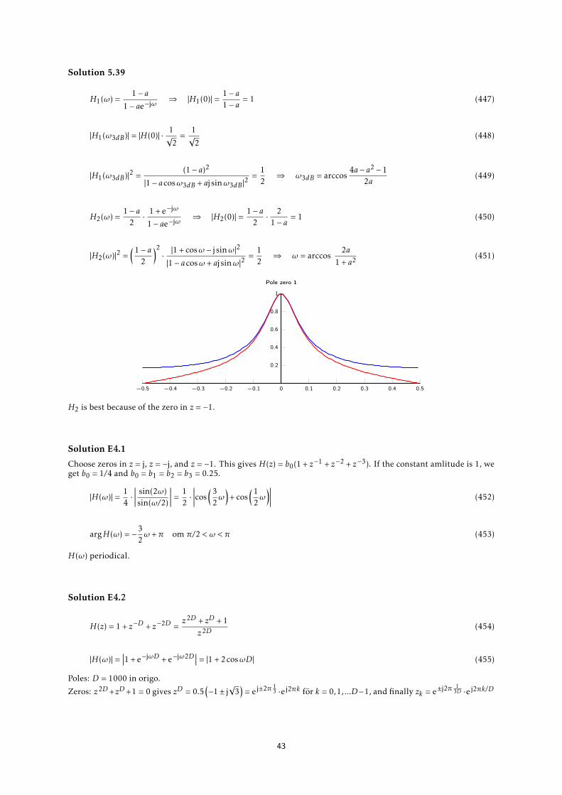
Solution 5.39

H1(ω) =1− a

1− ae−jω⇒ |H1(0)| =

1− a1− a

= 1 (447)

|H1(ω3dB)| = |H(0)| ·1√

2=

1√

2(448)

|H1(ω3dB)|2 =(1− a)2

|1− acosω3dB + aj sinω3dB|2=

12⇒ ω3dB = arccos

4a− a2 − 12a

(449)

H2(ω) =1− a

2· 1 + e−jω

1− ae−jω⇒ |H2(0)| =

1− a2· 2

1− a= 1 (450)

|H2(ω)|2 =(1− a

2

)2· |

1 + cosω − j sinω|2

|1− acosω+ aj sinω|2=

12⇒ ω = arccos

2a1 + a2 (451)

−0.5 −0.4 −0.3 −0.2 −0.1 0 0.1 0.2 0.3 0.4 0.5

0.2

0.4

0.6

0.8

1

Pole zero 1

H2 is best because of the zero in z = −1.

Solution E4.1

Choose zeros in z = j, z = −j, and z = −1. This gives H(z) = b0(1 + z−1 + z−2 + z−3). If the constant amlitude is 1, weget b0 = 1/4 and b0 = b1 = b2 = b3 = 0.25.

|H(ω)| =14·∣∣∣∣∣ sin(2ω)sin(ω/2)

∣∣∣∣∣ =12·∣∣∣∣∣cos

(32ω)

+ cos(1

2ω)∣∣∣∣∣ (452)

argH(ω) = −32ω+π om π/2 < ω < π (453)

H(ω) periodical.

Solution E4.2

H(z) = 1 + z−D + z−2D =z2D + zD + 1

z2D (454)

|H(ω)| =∣∣∣1 + e−jωD + e−jω2D

∣∣∣ = |1 + 2cosωD | (455)

Poles: D = 1000 in origo.

Zeros: z2D+zD+1 = 0 gives zD = 0.5(−1± j

√3)

= e j±2π 13 ·e j2πk för k = 0,1, ...D−1, and finally zk = e±j2π 1

3D ·e j2πk/D

43

Solution E4.3

a) y(n) = x(n) + 0.9x(n−D) gives h(n) = δ(n) + 0.9δ(n−D)

b) H(z) = 1 + 0.9z−D = zD+0.9ZD

with D = 500 gives 500 poles in origo. Zeros:

z500 = −0.9 = 0.9e j2πk+jπ (456)

zk = 0.91/500e j2πk/500+jπ/500 for k = 0,1,2, ...,499 (on a circle). (457)

Solution E4.4

|H(f )| =∣∣∣∣∣ sin4ωsinω/2

∣∣∣∣∣ (458)

Multiplication with cos(2πn/8) moves the spectrum ±1/8. H(f ) blocks all frequencies except f = 0 (draw thespectra). This gives y(t) = 4cos(2π1000t)

Solution N4.3

a) 50 Hz in the time domain represents a frequency of 5044100 ∗ 2π = 2π

882 rad in the z-domain. A notch filter can bedescribed as such:

H(z) =(1− ejωz−1)(1− e−jωz−1)

(1− rejωz−1)(1− re−jωz−1)(459)

Where ω is the frequency to be suppressed, and r is the radius of the poles. Thus our filter can be written as

H(z) =(1− ej

2π882 z−1)(1− e−j

2π882 z−1)

(1− 0.9ej2π882 z−1)(1− 0.9e−j

2π882 z−1)

(460)

b) 300044100 ∗ 2π = 2π

14.7 rad. The new notch filter then becomes:

Hn(z) =(1− ej

2π14.7 z−1)(1− e−j

2π14.7 z−1)

(1− 0.9ej2π

14.7 z−1)(1− 0.9e−j2π

14.7 z−1)(461)

Adding a filter to an existing filter is equivalent with multiplying them in the z-domain. The new filter becomes

H(z) =(1− ej

2π882 z−1)(1− e−j

2π882 z−1)

(1− 0.9ej2π882 z−1)(1− 0.9e−j

2π882 z−1)

· (1− ej2π

14.7 z−1)(1− e−j2π

14.7 z−1)

(1− 0.9ej2π

14.7 z−1)(1− 0.9e−j2π

14.7 z−1)(462)

Sampling

Solution E4.5

Observe that this problem shows the importance of applying antialiasing filter before sampling especially whenwe work with the signal has infinite frequency spectrum range, such as this signal.

a)

xa(t) = e−10tu(t) (463)

By using the standard analog fourier transform definition, we can show that the spectrum is:

Xa(F) =∫ ∞

0e−(10+j2πF)tdt =

e−(10+j2πF)t

−(10 + j2πF)

∞0

(464)

=1

10 + j2πF(465)

|Xa(F)|2 =1

102 + (2πF)2(466)

44

b) If we use a antialiasing filter observe that all of the frequency above 50Hz should be blocked, observe thatwe should calculate the energy at both negative frequency and positive frequency side, since the energy atnegative frequency part still contributes the total signal energy according to pasaval theorem. Therefore, theblocked energy can be calculated as:

Es =∫ −50

−∞|Xa(F)|2 dF +

∫ ∞50|Xa(F)|2 dF (467)

= 2∫ ∞

50

1102 + (2πF)2

dF (468)

= 2 · 110 · 2π

[arctan2π

F10

]∞50

(469)

=1

10π

[π2− 1.539

](470)

Total energy:

Etot =∫ +∞

−∞|Xa(F)|2 dF =

110π

· π2⇒ the blocked fraction is

π2 − 1.539

π2

≈ 2% (471)

c) Without filter: After sampling we can get the signal,

ya(nTs) = e−10nTsu(n) (472)

Applying standard DTFT to signal ya(n), we can get the spectrum Y (f ) as:

|Y (f )| =

∣∣∣∣∣∣∣∞∑n=0

e−10n/100e−j2πf n

∣∣∣∣∣∣∣ =∣∣∣∣∣ 1

1− e−0.1e−j2πf

∣∣∣∣∣ (473)

=1√

(1− e−0.1 cos(2πf )2) + (e−0.1)2 sin2 2πf=

1√1.8187− 1.8096cos2πf

(474)

With filter: Observe that here since the frequency components above 50Hz are removed, the formula (1.16)See course book page 399) holds, therefore:∣∣∣Y (f )

∣∣∣ = Fs |Xa(F)| = Fs ·1√

100 + (2πf Fs)2=

1√0.01 + (2πf )2

. (475)

∣∣∣Y (f )∣∣∣ |Y (f )|

f = 0 10 10.5

f = 0.25 0.64 0.74

f = 0.5 0.32 0.53

Solution E4.6

This problem gives the insight of viewing the sampling process at frequency domain. It is important to understandthe relationship between analog frequency, sampling frequency and digital frequency.

First since the input signal has frequency component at F0 = 600Hz, the spectrum can be plotted by Fig 1. Aftersampling, since here Fs > 2 ∗ F0, therefore all the analog frequency components above Fs

2 = 500Hz (below -500Hz)

will be folded back with the centre of Fs2 = 500Hz, which plots figure 2.

Then the signal multiplies (−1)n, which is equivalent to multiply x1(n) = cos(πn), according to the modulationproperty (formula on Course book Page 296), the frequency spectrum is shifted and then we can get Fig 3.Then the signal is upsampled by a factor of 2, which means that the spectrum is compressed with a factor of 2.Observe that the spectrum outside the range [-0.5 0.5] is visible after this compression, which generates Fig 4.The final step we construct the signal with constructing frequency Fs = 1000Hz, which generates Fig 5.

45

−1,500 −1,000 −500 0 500 1,000 1,500

0.2

0.4

0.6

0.8

1

Fig.1 Spectrum for the signal xa(t)

−1.5 −1 −0.5 0 0.5 1 1.5

0.2

0.4

0.6

0.8

1

Fig.2 Spectrum for the signal x(n)

−1.5 −1 −0.5 0 0.5 1 1.5

0.2

0.4

0.6

0.8

1

Fig 3 Spectrum for the signal z(n) after modulation

−1.5 −1 −0.5 0 0.5 1 1.5

0.2

0.4

0.6

0.8

1

Fig 4 Spectrum for the signal y(n) after upsampling

−3,000 −2,000 −1,000 0 1,000 2,000 3,000

0.2

0.4

0.6

0.8

1

Fig 5 Spectrum for the signal ya(t) after reconstruction

Then our signal expression can be written as ya(t) = cos(2π100t) + cos(2π900t).

46

Solution 7.1

If x(n) is real |X(ω)| is an even function, and arg(X(ω)) is an odd function. X(ω) is always a periodical functionwith the period 2π. This is true even when X(ω) is sampled to X(k) and the period for discrete signal X(k) is N = 8(eight-point DFT) This means that when

X(k) = X∗(N − k) (476)

X(0) = 0.25 (477)

X(1) = 0.125− j0.3018 (478)

X(2) = 0 (479)

X(3) = 0.125− j0.0518 (480)

X(4) = 0 (481)

we have

X(5) = X∗(3) = 0.125 + j0.0518 (482)

X(6) = X∗(2) = 0 (483)

X(7) = X∗(1) = 0.125 + j0.3018 (484)

Solution 7.2

a) x(n) = x1 � x2 =∑N−1k=0 x1(k)x2(n− k modN )where N = 8

y(0) = x1(0) · x2(0) + x1(1) · x2(N − 1) + x1(2) · x2(N − 2) + x1(3) · x2(N − 3) + x1(4) · x2(N − 4)+ (485)

+ x1(5) · x2(N − 5) + x1(6) · x2(N − 6) + x1(7) · x2(N − 7) = 1.25 (486)

y(1) = x1(0) · x2(1) + x1(1) · x2(0) + x1(2) · x2(N − 1) + x1(3) · x2(N − 2) + x1(4) · x2(N − 3)+ (487)

+ x1(5) · x2(N − 4) + x1(6) · x2(N − 5) + x1(7) · x2(N − 6) = 2.55 (488)

y(2) = x1(0) · x2(2) + x1(1) · x2(1) + x1(2) · x2(0) + x1(3) · x2(N − 1) + x1(4) · x2(N − 2)+ (489)

+ x1(5) · x2(N − 3) + x1(6) · x2(N − 4) + x1(7) · x2(N − 5) = 2.55 (490)

y(3) = x1(0) · x2(3) + x1(1) · x2(2) + x1(2) · x2(1) + x1(3) · x2(0) + x1(4) · x2(N − 1)+ (491)

+ x1(5) · x2(N − 2) + x1(6) · x2(N − 3) + x1(7) · x2(N − 4) = 1.25 (492)

y(4) = x1(0) · x2(4) + x1(1) · x2(3) + x1(2) · x2(2) + x1(3) · x2(1) + x1(4) · x2(0)+ (493)

+ x1(5) · x2(N − 1) + x1(6) · x2(N − 2) + x1(7) · x2(N − 3) = 0.25 (494)

y(5) = x1(0) · x2(5) + x1(1) · x2(4) + x1(2) · x2(3) + x1(3) · x2(2) + x1(4) · x2(1)+ (495)

+ x1(5) · x2(0) + x1(6) · x2(N − 1) + x1(7) · x2(N − 2) = −1.06 (496)

y(6) = x1(0) · x2(6) + x1(1) · x2(5) + x1(2) · x2(4) + x1(3) · x2(3) + x1(4) · x2(2)+ (497)

+ x1(5) · x2(1) + x1(6) · x2(0) + x1(7) · x2(N − 1) = −1.06 (498)

y(7) = x1(0) · x2(7) + x1(1) · x2(6) + x1(2) · x2(5) + x1(3) · x2(4) + x1(4) · x2(3)+ (499)

+ x1(5) · x2(2) + x1(6) · x2(1) + x1(7) · x2(0) = 0.25 (500)

(501)

y(n) ={

1.25 2.55 2.55 1.25 0.25 −1.06 −1.06 0.25}.

47

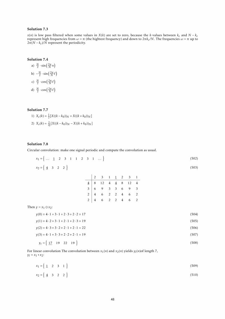
Solution 7.3

x(n) is low pass filtered when some values in X(k) are set to zero, because the k-values between kc and N − kcrepresent high frequencies from ω = π (the hightest frequency) and down to 2πkc/N . The frequencies ω = π up to2π(N − kc)/N represent the periodicity.

Solution 7.4

a) N2 · sin

(2πN n

)b) −N2 · sin

(2πN `

)c) N

2 · cos(

2πN `

)d) N

2 · cos(

2πN `

)

Solution 7.7

1) Xc(k) = 12 [X((k − k0))N +X((k + k0))N ]

2) Xs(k) = 12j [X((k − k0))N −X((k + k0))N ]

Solution 7.8

Circular convolution: make one signal periodic and compute the convolution as usual.

x1 ={. . . 1 2 3 1 1 2 3 1 . . .

}(502)

x2 ={

4 3 2 2}

(503)

2 3 1 1 2 3 1

4 8 12 4 4 8 12 4

3 6 9 3 3 6 9 3

2 4 6 2 2 4 6 2

2 4 6 2 2 4 6 2

Then y = x1 � x2:

y(0) = 4 · 1 + 3 · 1 + 2 · 3 + 2 · 2 = 17 (504)

y(1) = 4 · 2 + 3 · 1 + 2 · 1 + 2 · 3 = 19 (505)

y(2) = 4 · 3 + 3 · 2 + 2 · 1 + 2 · 1 = 22 (506)

y(3) = 4 · 1 + 3 · 3 + 2 · 2 + 2 · 1 = 19 (507)

yc ={

17 19 22 19}

(508)

For linear convolution The convolution between x1(n) and x2(n) yields yl (n)of length 7,yl = x1 ∗ x2:

x1 ={

1 2 3 1}

(509)

x2 ={

4 3 2 2}

(510)

48

1 2 3 1

4 4 8 12 4

3 3 6 9 3

2 2 4 6 2

2 2 4 6 2

y(0) = 4 (511)

y(1) = 4 · 2 + 3 · 1 = 11 (512)

y(2) = 4 · 3 + 3 · 2 + 2 · 1 = 20 (513)

y(3) = 4 · 1 + 3 · 3 + 2 · 2 + 2 · 1 = 19 (514)

y(4) = 3 · 1 + 2 · 3 + 2 · 2 = 13 (515)

y(5) = 2 · 1 + 2 · 3 = 8 (516)

y(6) = 2 · 1 = 2 (517)

yl ={

4 11 20 19 13 8 2}

(518)

The linear convolution is related to the circular convolution.

yc ={

17 19 22 19}

(519)

yl ={

4 11 20 19 13 8 2}

(520)

yc ={yl (0) + yl (4) yl (1) + yl (5) yl (2) + yl (6) yl (3) + yl (7)

}(521)

Solution 7.9

x1(n) ={

1 2 3 1}

(522)

x2(n) ={

4 3 2 2}

(523)

x3(n) = x1(n)� x2(n) (524)

X(k) = DFT {xn} =3∑n=0

xne−j2πnk/4 k = 0 . . .3 (525)

X1(0) = 7 X2(0) = 11 (526)

X1(1) = −2− j X2(1) = 2− j (527)

X1(2) = 1 X2(2) = 1 (528)

X1(3) = X∗1(1) = −2 + j X2(3) = X∗2(1) = 2 + j (529)

X3(k) = X1(k)X2(k) (530)

X3(0) = 77 (531)

X3(1) = −5 (532)

X3(2) = 1 (533)

X3(3) = −5 (534)

49

x(n) = IDFT {X(k)} =14

3∑k=0

X(k)e j2πnk/4 n = 0 . . .3 (535)

x3(0) = 17 (536)

x3(1) = 19 (537)

x3(2) = 22 (538)

x3(3) = 19 (539)

Solution 7.10

x(n) = cos(

2πk0nN

)0 ≤ n ≤N − 1 (540)

Ex =N−1∑n=0

|x(n)|2 =N−1∑n=0

cos2(

2πk0N

n

)=N−1∑n=0

1 + cos(

4πk0N n

)2

(541)

(542)

For k0 = i∗N2 where i = 0,1,2, . . .:

cos(

4πk0N

n

)= cos(2πi.n) = 1 (543)

Ex =N (544)

(545)

Otherwise:

Ex =N−1∑n=0

12

+N−1∑n=0

cos(

4πk0N n

)2

(546)

=N2

+12

N−1∑n=0

cos(

4πk0N

n

)(547)

=N2

+12

N−1∑n=0

e j4πk0n/N + e−j4πk0n/N

2(548)

=N2

+14

(N−1∑n=0

e j4πk0n/N +N−1∑n=0

e−j4πk0n/N ) (549)

=N2

+14·

1− e j4πk0N/N

1− e j4πk0/N︸ ︷︷ ︸=0

+1− e−j4πk0N/N

1− e−j4πk0/N︸ ︷︷ ︸=0

=N2

(550)

Ex =N2

+14·

1− e j4πkN/N

1− e j4πk/N︸ ︷︷ ︸=0

+1− e−j4πkN/N

1− e−j4πk/N︸ ︷︷ ︸=0

=N2

(551)

50

Solution 7.11

X (k) for k = 0 . . .7 is given.

x1(n) = x(n− 5 mod 8)

x2(n) = x(n− 2 mod 8)⇒

X1(k) = X(k)e−j2π· k8 ·5

X2(k) = X(k)e−j2π· k8 ·2(552)

Solution 7.18

Y (k) =H(f ) where f = kN .

Solution 7.23

X(k) =N−1∑n=0

x(n)e−j2πkn/N k = 0,1. . . .N − 1

a) X(k) =N−1∑n=0

δ(n)e−j2πkn/N = e−j2πk×0N = 1

b) X(k) =N−1∑n=0

δ(n−n0)e−j2πkn/N = e−j2πkn0/N k = 0, . . . ,N − 1

c)

X(k) =N−1∑n=0

ane−j2πkn/N (553)

=N−1∑n=0

(ae−j2πk/N )n (554)

=1− (a)N e−j2πkN/N

1− ae−j2πk/Nk = 1, . . . ,N − 1 (555)

=1− aN

1− ae−j2πk/N(556)

d)

x(n) ={

1 0 ≤ n ≤ N2 − 1

0 N2 ≤ n ≤N − 1

N even (557)

X(k) =N/2−1∑n=0

e−j2πkn/N = {k , 0} (558)

=1− e−j2πk N/2·N

1− e−j2πk/N=

1− e−j2πk/2

1− e−j2πk/N= (559)

=1− (−1)k

1− e−j2πk/Nk = 1, . . . ,N − 1 (560)

X(0) =N2

(561)

51

e) x(n) = e j 2πN k0n ⇒ X(k) =N · δ(k − k0)

X(k) =N−1∑n=0

(e j2πk0n/N × e−j2πkn/N ) = (562)

=N−1∑n=0

e j2π(k0−k)n/N = {k , k0} (563)

=1− e−j2π(k−k0)·N/N

1− e−j2π(k−k0)/N=

1− e−j2π(k−k0)

1− e−j2π(k−k0)/N= (564)

=1− (1)(k−k0)

1− e−j2π(k−k0)/N= 0 k , k0 (565)

X(k0) =N (566)

X(k) =Nδ(k − k0) (567)

f) x(n) = cos(

2πk0N n

)= e j2πk0n/N+e−j2πk0n/N

2

e j 2πN k0n ⇒ N · δ(k − k0) (568)

e−j 2πN k0n ⇒ N · δ(k − (N − k0)) (569)

X(k) =N2

(δ(k − k0) + δ(k − (N − k0))) (570)

g) x(n) = sin(

2πk0N n

)= e j2πk0n/N−e−j2πk0n/N

2j

e j 2πN k0n ⇒ N · δ(k − k0) (571)

e−j 2πN k0n ⇒ N · δ(k − (N − k0)) (572)

X(k) =N2j

(δ(k − k0)− δ(k − (N − k0))) (573)

h) Given that N is even

x(n) ={

1 n even0 n odd

(574)

=12

(1 + (−1)n) =12

(e j2π(0)n/N + e j2π(N2 )n/N ) (575)

e j 2πN 0n ⇒ N · δ(k) (576)

e−j 2πN

N2 n ⇒ N · δ(k − N

2) (577)

X(k) =N2

(δ(k) + δ

(k − N

2

))(578)

Solution 7.24

X(k) = 1 + 2e−j πk/2 + 3e−jπk + e−j 3πk/2 ={

7 −2− j 1 −2 + j}

(579)

52

Solution 7.25

a)

x(n) ={

1 2 3 2 1 0}

(580)

X(ω) =∞∑

n=−∞x(n)e−jωn = e j2ω + 2e jω + 3 + 2e−jω + e−j2ω = (581)

= 3 + 4cosω+ 2cos2ω (582)

b)

v(n) ={

3 2 1 0 1 2}

(583)

VDFT (k) =5∑n=0

v(n)e−j2π k6 n (584)

= 3 + 2e−j π3 k + e−j 2π3 k + e−j 4π

3 k + 2e−j 5π3 k (585)

c) VDFT (k) = 3 + 4cos π3 k + 2cos 2π3 k for k = 0 . . .5. That is, VDFT (k) = X(ωk) where ωk = 2π k6 för k = 0 . . .5.

Solution N5.0

The length of the h(n) is M=3, Let us take L=3 then the lenght of the smaller x(n) would be N= M+L-1=5. So x(n)will be divided into the smaller sequences to perform convolution in a faster and easy way as shown below.

x(n) 3 1 -1 4 5 7 6 2 1 0 3 4 0 0

x1(n) 3 1 -1 0 0 0 0 0 0 0 0 0 0 0

x2(n) 0 0 0 4 5 7 0 0 0 0 0 0 0 0

x3(n) 0 0 0 0 0 0 6 2 1 0 0 0 0 0

x4(n) 0 0 0 0 0 0 0 0 0 0 3 4 0 0

x1(n) = [3,1,−1,0,0],h(n) = [1,2,0] and y1(n) is given by

3 0 0 −1 1

1 3 0 0 −1

−1 1 3 0 0

0 −1 1 3 0

0 0 −1 1 3

1

2

0

0

0

=

3

7

1

−2

0

x2(n) = [4,5,7,0,0],h(n) = [1,2,0] and y2(n) is given by

4 0 0 7 3

5 4 0 0 7

7 5 4 0 0

0 7 5 4 0

0 0 7 5 4

1

2

0

0

0

=

4

13

17

14

0

x3(n) = [6,2,1,0,0],h(n) = [1,2,0] and y3(n) is given by

6 0 0 1 2

2 6 0 0 1

1 2 6 0 0

0 1 2 6 0

0 0 1 2 6

1

2

0

0

0

=

6

10

5

2

0

53

x4(n) = [0,3,4,0,0],h(n) = [1,2,0] and y4(n) is given by

0 0 0 4 3

3 0 0 0 4

4 3 0 0 0

0 4 3 0 0

0 0 4 3 0

1

2

0

0

0

=

0

3

10

8

0

and finally y(n) = y1(n)+y2(n)+y3(n)+y4(n) is given by

n 0 1 2 3 4 5 6 7 8 9 10 11 12 13

y1(n) 3 7 1 -2 0 0 0 0 0 0 0 0 0 0

y2(n) 0 0 0 4 13 17 14 0 0 0 0 0 0 0

y3(n) 0 0 0 0 0 0 6 10 5 2 0 0 0 0

y4(n) 0 0 0 0 0 0 0 0 0 0 3 10 8 0

y(n) 3 7 1 2 13 17 20 10 5 2 3 10 8 0

Solution N5.1

The length of the h(n) is M=4, Let us take L=4 then the length of the smaller x(n) would be N= M+L-1=7. So x(n)will be divided into the smaller sequences to perform convolution in a faster and easy way as shown below.

x(n) 1 1 -1 -5 3 0 1 3 -1 0 0 0 0 0 0

x1(n) 1 1 -1 -5 0 0 0 0 0 0 0 0 0 0 0

x2(n) 0 0 0 0 3 0 1 3 0 0 0 0 0 0 0

x3(n) 0 0 0 0 0 0 0 0 -1 0 0 0 0 0 0

x1(n) = [1,1,−1,−5,0,0,0],h(n) = [0,−1,2,4] and y4(n) is given by

1 0 0 0 −5 −1 1

1 1 0 0 0 −5 −1

−1 1 1 0 0 0 −5

−5 −1 1 1 0 0 0

0 −5 −1 1 1 0 0

0 0 −5 −1 1 1 0

0 0 0 −5 −1 1 1

0

−1

2

4

0

0

0

=

0

−1

1

7

7

−14

−20

x2(n) = [3,0,1,3,0,0,0],h(n) = [0,−1,2,4] and y4(n) is given by

3 0 0 0 3 1 0

0 3 0 0 0 3 1

1 0 3 0 0 0 3

3 1 0 3 0 0 0

0 3 1 0 3 0 0

0 0 3 1 0 3 0

0 0 0 3 1 0 3

0

−1

2

4

0

0

0

=

0

−3

6

11

−1

10

12

54

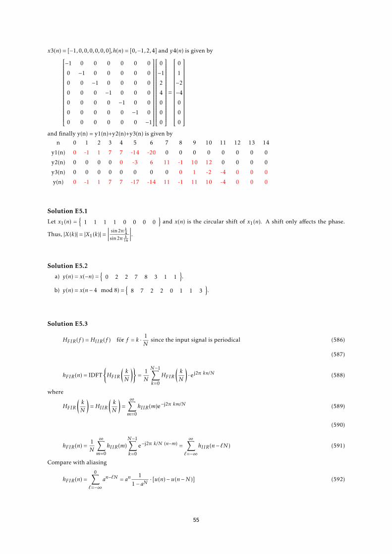
x3(n) = [−1,0,0,0,0,0,0],h(n) = [0,−1,2,4] and y4(n) is given by

−1 0 0 0 0 0 0

0 −1 0 0 0 0 0

0 0 −1 0 0 0 0

0 0 0 −1 0 0 0

0 0 0 0 −1 0 0

0 0 0 0 0 −1 0

0 0 0 0 0 0 −1

0

−1

2

4

0

0

0

=

0

1

−2

−4

0

0

0

and finally y(n) = y1(n)+y2(n)+y3(n) is given by

n 0 1 2 3 4 5 6 7 8 9 10 11 12 13 14

y1(n) 0 -1 1 7 7 -14 -20 0 0 0 0 0 0 0 0

y2(n) 0 0 0 0 0 -3 6 11 -1 10 12 0 0 0 0

y3(n) 0 0 0 0 0 0 0 0 0 1 -2 -4 0 0 0

y(n) 0 -1 1 7 7 -17 -14 11 -1 11 10 -4 0 0 0

Solution E5.1

Let x1(n) ={

1 1 1 1 0 0 0 0}

and x(n) is the circular shift of x1(n). A shift only affects the phase.

Thus, |X(k)| = |X1(k)| =∣∣∣∣∣ sin2π k4sin2π k

16

∣∣∣∣∣.

Solution E5.2

a) y(n) = x(−n) ={

0 2 2 7 8 3 1 1}.

b) y(n) = x(n− 4 mod 8) ={

8 7 2 2 0 1 1 3}.

Solution E5.3

HFIR(f ) =HIIR(f ) för f = k · 1N

since the input signal is periodical (586)

(587)

hFIR(n) = IDFT{HFIR

(kN

)}=

1N

N−1∑k=0

HFIR

(kN

)· e j2π kn/N (588)

where

HFIR

(kN

)=HIIR

(kN

)=∞∑m=0

hIIR(m)e−j2π km/N (589)

(590)

hFIR(n) =1N

∞∑m=0

hIIR(m)N−1∑k=0

e−j2π k/N (n−m) =∞∑

`=−∞hIIR(n− `N ) (591)

Compare with aliasing

hFIR(n) =0∑

`=−∞an−`N = an

11− aN

· [u(n)−u(n−N )] (592)

55

Solution E5.4

f0 = ±138 +n · 400 ={

138 262 . . .}.

Solution E5.5

1-C, 2-F, 3-G, 4-H.

Solution E5.6

a)

H(f ) =14

+14

e−j2πf +14

e−j2π2f +14

e−j2π3f (593)

(594)

H(k) =14

+14

e−j2πk/N +14

e−j2π2k/N +14

e−j2π3k/N + 0 + 0 + . . .+ 0 (595)

for k = 0 . . .N − 1. H(k) are samples of H(f ) in the points f = kN , k = 0 . . .N − 1.

b) H(0) = 1, H(1) = 0, H(2) = 0, and H(3) = 0. hp(n) = 14 for all values of n.

0 0.1 0.2 0.3 0.4 0.5 0.6 0.7 0.8 0.9 1

0.2

0.4

0.6

0.8

1

Solution E5.7

Y (k/N ) = X(k/N )

Solution E5.8

a) y(n) = δ(n) + 2 δ(n− 1) + 1.5 δ(n− 2) + 0.5 δ(n− 3)

b) See above.

c) M = 4; generally M = P +Q−1 where P is the length of the impulse response and Q is the length of the inputsignal.

Solution E5.9

yp(n) =L∑l=0

bl for n = 0 . . .N − 1 (596)

56

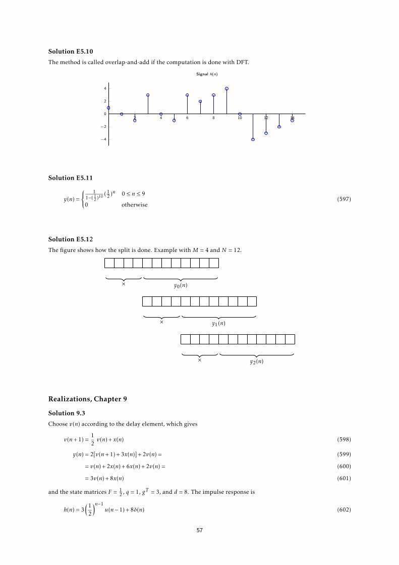
Solution E5.10

The method is called overlap-and-add if the computation is done with DFT.

2 4 6 8 10 12 14

−4

−2

0

2

4

Signal h(n)

Solution E5.11

y(n) =

11−( 1

2 )10 ( 12 )n 0 ≤ n ≤ 9

0 otherwise(597)

Solution E5.12

The figure shows how the split is done. Example with M = 4 and N = 12.

× y0(n)

× y1(n)

× y2(n)

Realizations, Chapter 9

Solution 9.3

Choose v(n) according to the delay element, which gives

v(n+ 1) =12v(n) + x(n) (598)

y(n) = 2[v(n+ 1) + 3x(n)] + 2v(n) = (599)

= v(n) + 2x(n) + 6x(n) + 2v(n) = (600)

= 3v(n) + 8x(n) (601)

and the state matrices F = 12 , q = 1, gT = 3, and d = 8. The impulse response is

h(n) = 3(1

2

)n−1u(n− 1) + 8δ(n) (602)

57

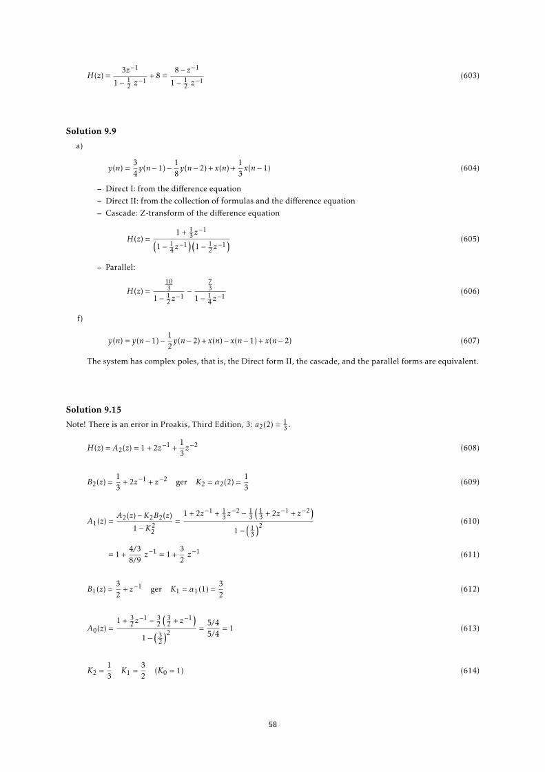
H(z) =3z−1

1− 12 z−1

+ 8 =8− z−1

1− 12 z−1

(603)

Solution 9.9

a)

y(n) =34y(n− 1)− 1

8y(n− 2) + x(n) +

13x(n− 1) (604)

– Direct I: from the difference equation

– Direct II: from the collection of formulas and the difference equation

– Cascade: Z-transform of the difference equation

H(z) =1 + 1

3 z−1(

1− 14 z−1

)(1− 1

2 z−1

) (605)

– Parallel:

H(z) =103

1− 12 z−1−

73

1− 14 z−1

(606)

f)

y(n) = y(n− 1)− 12y(n− 2) + x(n)− x(n− 1) + x(n− 2) (607)

The system has complex poles, that is, the Direct form II, the cascade, and the parallel forms are equivalent.

Solution 9.15

Note! There is an error in Proakis, Third Edition, 3: a2(2) = 13 .

H(z) = A2(z) = 1 + 2z−1 +13z−2 (608)

B2(z) =13

+ 2z−1 + z−2 ger K2 = α2(2) =13

(609)

A1(z) =A2(z)−K2B2(z)

1−K22

=1 + 2z−1 + 1

3 z−2 − 1

3

(13 + 2z−1 + z−2

)1−

(13

)2 (610)

= 1 +4/38/9

z−1 = 1 +32z−1 (611)

B1(z) =32

+ z−1 ger K1 = α1(1) =32

(612)

A0(z) =1 + 3

2 z−1 − 3

2

(32 + z−1

)1−

(32

)2 =5/45/4

= 1 (613)

K2 =13

K1 =32

(K0 = 1) (614)

58

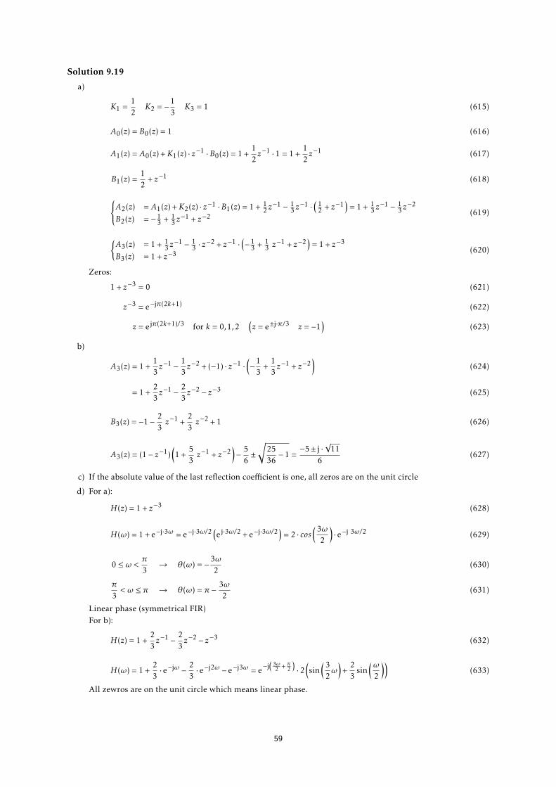
Solution 9.19

a)

K1 =12

K2 = −13

K3 = 1 (615)

A0(z) = B0(z) = 1 (616)

A1(z) = A0(z) +K1(z) · z−1 ·B0(z) = 1 +12z−1 · 1 = 1 +

12z−1 (617)

B1(z) =12

+ z−1 (618)

A2(z) = A1(z) +K2(z) · z−1 ·B1(z) = 1 + 12 z−1 − 1

3 z−1 ·

(12 + z−1

)= 1 + 1

3 z−1 − 1

3 z−2

B2(z) = −13 + 1

3 z−1 + z−2 (619)

A3(z) = 1 + 13 z−1 − 1

3 · z−2 + z−1 ·

(−1

3 + 13 z−1 + z−2

)= 1 + z−3

B3(z) = 1 + z−3 (620)

Zeros:

1 + z−3 = 0 (621)

z−3 = e−jπ(2k+1) (622)

z = e jπ(2k+1)/3 for k = 0,1,2(z = e±j·π/3 z = −1

)(623)

b)

A3(z) = 1 +13z−1 − 1

3z−2 + (−1) · z−1 ·

(−1

3+

13z−1 + z−2

)(624)

= 1 +23z−1 − 2

3z−2 − z−3 (625)

B3(z) = −1− 23z−1 +

23z−2 + 1 (626)

A3(z) = (1− z−1)(1 +

53z−1 + z−2

)− 5

6±√

2536− 1 =

−5± j ·√

116

(627)

c) If the absolute value of the last reflection coefficient is one, all zeros are on the unit circle

d) For a):

H(z) = 1 + z−3 (628)

H(ω) = 1 + e−j·3ω = e−j·3ω/2 (e j·3ω/2 + e−j·3ω/2) = 2 · cos

(3ω2

)· e−j 3ω/2 (629)

0 ≤ω < π3→ θ(ω) = −3ω

2(630)

π3< ω ≤ π → θ(ω) = π − 3ω

2(631)

Linear phase (symmetrical FIR)For b):

H(z) = 1 +23z−1 − 2

3z−2 − z−3 (632)

H(ω) = 1 +23· e−jω − 2

3· e−j2ω − e−j3ω = e−j

(3ω2 + π

2

)· 2

(sin

(32ω)

+23

sin(ω

2

))(633)

All zewros are on the unit circle which means linear phase.

59

Examples of Filter Design

Solution E8.1

a) From the realization, y(n) becomes

y(n) = x(n) + x(n− 1) + x(n− 2) + x(n− 3) (634)

Performing the z-transform yields

Y (z) = X(z) + z−1X(z) + z−2X(z) + z−3X(z) = (1 + z−1 + z−2 + z−3)X(z) (635)

H(z) = 1 + z−1 + z−2 + z−3 =z3 + z2 + z+ 1

z3 (636)

The three poles then are readily recognizable as

p1,2,3 = 0 (637)

To find the zeros, one zero can be guessed as

z1 = −1 (638)

The others can then be found by a long division using this zero:

z2 +1

z+ 1)

z3 +z2 +z +1

− z3 z2

z +1

− z +1

0

(639)

Thus

H(z) =z3 + z2 + z+ 1

z3 =(z+ 1)(z2 + 1)

z3 (640)

And the zeroes are

z1 = −1 z2,3 = ±j (641)

b) + d) The magnitude of the system response is asked for, thus the Fourier transform of h(n) should be used.

H(z) = 1 + z−1 + z−2 + z−3 (642)

H(f )[=H(z = ej2πf )

]= 1 + e−j2πf + e−j2π·2f + e−j2π·3f [rewrite to conform with Euler] (643)

= e−j2π·3/2f(ej2π·3/2f + ej2π·1/2f + e−j2π·1/2f + e−j2π·3/2f

)(644)

= e−j2π·3/2f(ej2π·1/2f + e−j2π·1/2f + ej2π·3/2f + e−j2π·3/2f

)(645)

= 2e−j2π·3/2f(cos2π · 1

2f + cos2π · 3

2f)

(646)

The magnitude becomes

|H(f )| = 2∣∣∣∣∣cos2π · 1

2f + cos2π · 3

2f

∣∣∣∣∣ (647)

With this form it is easy to see for instance that |H(0)| = 4. However, seeing where for instance |H(f )| = 0 is trickier.Another form which might make it easier can be found via geometric sum:

H(f ) = 1 + e−j2πf + e−j2π·2f + e−j2π·3f =3∑n=0

e−j2π·nf (648)

(649)

60

Which can be plugged into the geometric sum formula, however the result can easily be shown as follows:

H(f ) =3∑n=0

e−j2π·nf (650)

= 1 + e−j2πf + e−j2π·2f + e−j2π·3f (651)

e−j2πf ∗H(f ) = e−j2πf + e−j2π·2f + e−j2π·3f + e−j2π·4f (652)

H(f )− e−j2πf ∗H(f ) = 1− e−j2π·4f (653)

H(f )(1− e−j2πf ) = 1− e−j2π·4f (654)

H(f ) =1− e−j2π·4f

1− e−j2πf[rewrite to conform with Euler] (655)

=e−j2π·2f (ej2π·2f − e−j2π·2f )

e−j2π·1/2f (ej2π·1/2f − e−j2π·1/2f )=

2je−j2π·2f sin2π · 2f2je−j2π·1/2f sin2π · 1

2 f(656)

= e−j2π·3/2fsin2π · 2fsin2π · 1

2 f(657)

|H(f )| =

∣∣∣∣∣∣∣ sin2π · 2fsin2π · 1

2 f

∣∣∣∣∣∣∣ (658)

(659)

Thus |H(f )| = 0 at f = ±14 ,±1

2 .Plotting (any version of) |H(f )| yields:

|H(f )|

−0.5 −0.4 −0.3 −0.2 −0.1 0.1 0.2 0.3 0.4 0.5

1

2

3

4

c)The phase function is given by ∠H(f ):

∠H(f ) = ∠e−j2π·3/2fsin2π · 2fsin2π · 1

2 f= ∠e−j2π·3/2f + ∠

sin2π · 2fsin2π · 1

2 f= −2π · 3/2f + ∠

sin2π · 2fsin2π · 1

2 f(660)

[note that real positive values have argument 0 and real negative values argument π] (661)

=

−2π · 3/2f −π, −1

2 < f < −14

−2π · 3/2f , −14 < f <

14

−2π · 3/2f +π, 14 < f <

12

,−12< f <

12

(662)

∠H(f )

−0.5 −0.4 −0.3 −0.2 −0.1 0.1 0.2 0.3 0.4 0.5

−π

π

61

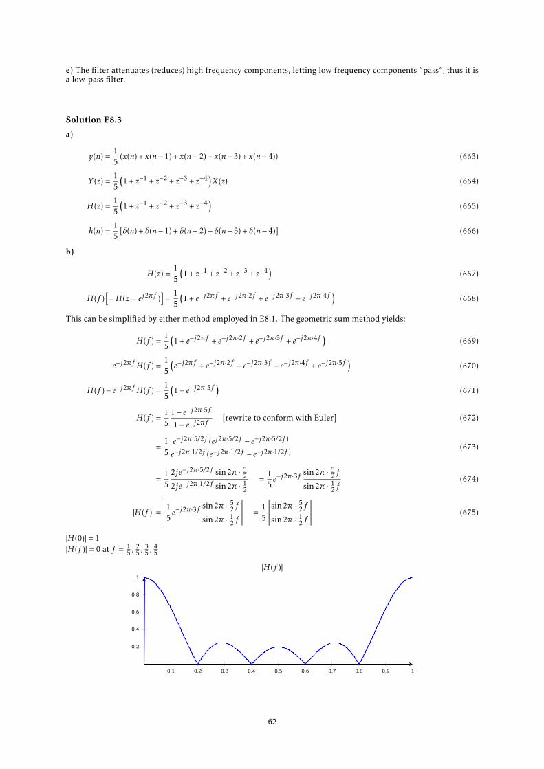
e) The filter attenuates (reduces) high frequency components, letting low frequency components “pass”, thus it isa low-pass filter.

Solution E8.3

a)

y(n) =15

(x(n) + x(n− 1) + x(n− 2) + x(n− 3) + x(n− 4)) (663)

Y (z) =15

(1 + z−1 + z−2 + z−3 + z−4

)X(z) (664)

H(z) =15

(1 + z−1 + z−2 + z−3 + z−4

)(665)

h(n) =15

[δ(n) + δ(n− 1) + δ(n− 2) + δ(n− 3) + δ(n− 4)] (666)

b)

H(z) =15

(1 + z−1 + z−2 + z−3 + z−4

)(667)

H(f )[=H(z = ej2πf )

]=

15

(1 + e−j2πf + e−j2π·2f + e−j2π·3f + e−j2π·4f

)(668)

This can be simplified by either method employed in E8.1. The geometric sum method yields:

H(f ) =15

(1 + e−j2πf + e−j2π·2f + e−j2π·3f + e−j2π·4f

)(669)

e−j2πf H(f ) =15

(e−j2πf + e−j2π·2f + e−j2π·3f + e−j2π·4f + e−j2π·5f

)(670)

H(f )− e−j2πf H(f ) =15

(1− e−j2π·5f

)(671)

H(f ) =15

1− e−j2π·5f

1− e−j2πf[rewrite to conform with Euler] (672)

=15e−j2π·5/2f (ej2π·5/2f − e−j2π·5/2f )

e−j2π·1/2f (e−j2π·1/2f − e−j2π·1/2f )(673)

=15

2je−j2π·5/2f sin2π · 52

2je−j2π·1/2f sin2π · 12

=15e−j2π·3f

sin2π · 52 f

sin2π · 12 f

(674)

|H(f )| =

∣∣∣∣∣∣∣15 e−j2π·3f sin2π · 52 f

sin2π · 12 f

∣∣∣∣∣∣∣ =15

∣∣∣∣∣∣∣ sin2π · 52 f

sin2π · 12 f

∣∣∣∣∣∣∣ (675)

|H(0)| = 1|H(f )| = 0 at f = 1

5 , 25 , 3

5 , 45

|H(f )|

0.1 0.2 0.3 0.4 0.5 0.6 0.7 0.8 0.9 1

0.2

0.4

0.6

0.8

1

62

Solution E8.4

Try a first order FIR filter:

H(z) = b0 + b1z−1 (676)

H(ω)[=H(z = ejω)

]= b0 + b1e

−jω (677)

We know that H(ω)|f =π/2 = e jπ/3, thus

H(ω)|f =π/2 = b0 + b1e−jπ/2 = ejπ/3 (678)

b0 − jb1 =12

+ j

√3

2[noting that b0 is real and b1 imaginary allows the identification:] (679)

b0 =12

b1 = −√

32

(680)

The filter thus is given by H(z) = 12 −√

32 z−1.

Solution E8.5

Since we should have linear phase, H(z) must be 1. an FIR filter, and 2. have a symmetric or antisymmetricimpulse response h(n). Further, since h(n) should be real, all complex zeros must have a conjugate pair. Giventhat H(ω = 2/5) = H(ω = −2/5) = 0, we can begin building our filter as (note that the resulting h(n) would becomesymmetrical):

H1(z) = (1− e−j2π2/5z−1)(1− ej2π2/5z−1) (681)

The specification states that |H(f = 0)| = 1. Evaluation at f = 0 yields

|H1(f = 0)| = 1 =∣∣∣∣(1− e−j2π2/5e−j2π∗0)(1− ej2π2/5e−j2π∗0)

∣∣∣∣ =∣∣∣∣(1− e−j2π2/5)(1− ej2π2/5)

∣∣∣∣ (682)

=∣∣∣∣2je−j2π1/5 sin2π1/5 ∗ −2jej2π1/5 sin2π1/5

∣∣∣∣ = 4sin2 2π1/5 (683)

As the equality does not hold, H1(z) must be appended with a gain, g1 = 14sin2 2π1/5

, which would yield:

H2(z) = g1(1− e−j2π2/5z−1)(1− ej2π2/5z−1) =1

4sin2 2π1/5(1− e−j2π2/5z−1)(1− ej2π2/5z−1) (684)

However, the specification further states that |H(f = 1/5)| = 1, and evaluation at f = 1/5 yields

H2(z) = 1 =∣∣∣∣∣ 1

4sin2 2π1/5(1− e−j2π1/5e−j2π2/5)(1− ej2π2/5e−j2π1/5)

∣∣∣∣∣ = 0.618... (685)

Thus, we instead will add more zeros to satisfy the specifications. We try to remove the gain add a conjugate pairof zeros with radius r and phase α:

H3(z) = (1− e−j2π2/5z−1)(1− ej2π2/5z−1)(1− re−j2παz−1)(1− rej2παz−1) (686)

= (1− ej2π2/5z−1 − e−j2π2/5z−1 + z−2)(1− rej2παz−1 − re−j2παz−1 + r2z−2) (687)

= (1− 2cos2π2/5 z−1 + z−2)(1− 2r cos2πα z−1 + r2z−2) (688)

[c1 = 2cos2π2/5, cα = 2cos2πα] (689)

= (1− c1z−1 + z−2)(1− rcαz−1 + r2z−2) (690)

= 1− rcαz−1 + r2z−2 − c1z−1 + rc1cαz−2 − r2c1z−3 + z−2 − rcαz−3 + r2z−4 (691)

= 1− (rcα + c1)z−1 + (r2 + rc1cα + 1)z−2 − (r2c1 + rcα)z−3 + r2z−4 (692)

However, for any r , 1, h(n) lose symmetry, and thus we set r = 1. However, since we probably (as we have seen)need two variables to fulfill both |H(f = 0)| = |H(f = 1/5)| = 1, we also reintroduce a gain g2. We have:

H4(z) = g2(1− e−j2π2/5z−1)(1− ej2π2/5z−1)(1− e−j2παz−1)(1− ej2παz−1) (693)

= g2(1− (cα + c1)z−1 + (2 + c1cα)z−2 − (c1 + cα)z−3 + z−4) (694)

63

In order to find suitable r and α we first utilize |H(f = 0)| = 1:

|H4(f = 0)| = 1 = |g2(1− (cα + c1) + (2 + c1cα)− (c1 + cα) + 1)| (695)

1 = |g2 ∗ (4− cα(2− c1)− 2c1)| (696)

case1 case21g2

= 4− cα(2− c1)− 2c1 − 1g2

= 4− cα(2− c1)− 2c1

cα = −1g2−4+2c1

(2−c1) cα = −− 1g2−4+2c1

(2−c1)

(697)

Next, |H(f = 1/5)| = 1 is utilized:

|H4(f = 1/5)| = 1 =∣∣∣∣g2(1− e−j2π2/5e−j2π1/5)(1− ej2π2/5e−j2π1/5)(1− e−j2παe−j2π1/5)(1− ej2παe−j2π1/5)

∣∣∣∣(698)

=∣∣∣∣g2(1− (cα + c1)e−j2π1/5 + (2 + c1cα)e−j2π2/5 − (c1 + cα)e−j2π3/5 + e−j2π4/5)

∣∣∣∣ (699)

=∣∣∣∣g2e−j2π2/5(ej2π2/5 − (cα + c1)ej2π1/5 + (2 + c1cα)− (c1 + cα)e−j2π1/5 + e−j2π2/5)

∣∣∣∣ (700)

=∣∣∣∣g2e−j2π2/5(2cos2π2/5 − 2(cα + c1)cos2π1/5 + 2 + c1cα)

∣∣∣∣ (701)

= |g2(2cos2π2/5 − 2(cα + c1)cos2π1/5 + 2 + c1cα)| (702)

[c1 = 2cos2π2/5, c2 = 2cos2π1/5] (703)

= |g2(c1 − (cα + c1)c2 + 2 + c1cα)| = |g2(c1 − cαc2 − c1c2 + 2 + c1cα)| (704)

= |g2(c1 + cα(−c2 + c1)− c1c2 + 2)|

insert case 1 above cα = −1g2− 4 + 2c1

(2− c1)

(705)

=∣∣∣∣∣g2c1 −

1− 4g2 + 2c1g2(2− c1)

(−c2 + c1)− c1c2g2 + 2g2

∣∣∣∣∣ (706)

=∣∣∣∣∣ 12− c1

(g2c1(2− c1)− (1− 4g2 + 2c1g2)(−c2 + c1)− c1c2g2(2− c1) + 2g2(2− c1))∣∣∣∣∣ (707)

=∣∣∣∣∣ 12− c1

(g2c1(2− c1)− (−c2 + c1) + 4g2(−c2 + c1)− 2c1g2(−c2 + c1)− c1c2g2(2− c1) + 2g2(2− c1))∣∣∣∣∣

(708)

=∣∣∣∣∣ 12− c1

(g2(c1(2− c1) + 4(−c2 + c1)− 2c1(−c2 + c1)− c1c2(2− c1) + 2(2− c1)) + c2 − c1))∣∣∣∣∣ (709)

=∣∣∣∣∣g2

12− c1

(c1(2− c1) + 4(−c2 + c1)− 2c1(−c2 + c1)− c1c2(2− c1) + 2(2− c1)) +1

2− c1(c2 − c1)

∣∣∣∣∣(710)

=∣∣∣∣∣g2−4c2 + c1(4− 3c1 + c1c2) + 4

2− c1+c2 − c12− c1

∣∣∣∣∣ (711)

case1.1 case1.2

g2 = 2−c2−4c2+c1(4−3c1+c1c2)+4 g2 = −2+2c1−c2

−4c2+c1(4−3c1+c1c2)+4

(712)

for cα = −− 1g2− 4 + 2c1

(2− c1), we instead get

(713)

case2.1 case2.2

g2 = 2−2c1+c2−4c2+c1(4−3c1+c1c2)+4 g2 = −2+c2

−4c2+c1(4−3c1+c1c2)+4

(714)

We can thus write the final filter H4 as:

H4(z) = g2(1− (cα + c1)z−1 + (2 + c1cα)z−2 − (c1 + cα)z−3 + z−4) (715)

64

For any case:

case1.1 case1.2 case2.1 case2.2

g2 = −0.1236 0.5236 −0.5236 0.1236

cα = 4.2361 1.4721 1.4721 4.2361

(716)

Choosing for instance g2 = 0.5236 and cα = 1.4721 (yielding a real angle α) gives a valid filter

H4(z) = 0.5236 + 0.0764z−1 − 0.2z−2 + 0.0764z−3 + 0.5236z−4 (717)

Solution E8.7

An FIR filter with linear phase and 50 dB damping means a Hamming window. −6 dB at f = f1 = 0.1 measn that at−50 dB and f = 0.15 we get (0.15− 0.1) ·M = 1.62

M =1.620.05

= 32.4 ⇒ M = 33 (718)

h(n) =

2 · f1 sinc(2f1(n− 16)) ·[0.54 + 0.46cos 2π(n−16)

32

]0 ≤ n ≤ 32

0 f.ö.(719)

Solution E8.8{HdB(0.2) = −3dB gives (0.2− fc) ·M = −0.40HdB(0.25) = −40dB gives (0.25− fc) ·M = 1.49

(720)

M =1.49 + 0.400.25− 0.20

= 37.8 ⇒ M = 39 (odd) (721)

{fc = 0.2 + 0.40

39 = 0.2103fc = 0.25− 1.49

39 = 0.2118(722)

Choose fc = 0.2103, but any fc in the interval 0.2103 ≤ fc ≤ 0.2118 works.

bn =[h(n) = h(n− 19) = hd (n− 19)wH (n− 19)

](723)

=sin(2π · 0.2103(n− 19))

π(n− 19)·(0.54 + 0.46cos

2π(n− 19)38

)(724)

for n = 0, . . . ,38.

+ + . . . + y(n)

x(n) z−1 z−1 . . . z−1

b0 b1 b2 b38

Solution E8.9

From the Hamming window diagram:{−0.4 = −(0.16− fc)M1.49 = −(0.10− fc)M

⇒{M = 33fc = 0.1479

(725)

65

wH (n) = 0.54 + 0.46cos2πn32

(726)

hd (n) = δ(n)− 2fc sinc(2fcn) (727)

h(n) = hd (n− 16) wH (n− 16) 0 ≤ n ≤ 32 (728)

Solution E8.10

Start from an ideal band pass filter:

hd (n) = 4fc sinc(2fcn) · cos(2πf0n) (729)

Truncate hd (n) using wH (n). A Hamming works becaise we only need 40 dB dampning.

wH (n) ={

0.54 + 0.46cos 2πnM−1 −M−1

2 ≤ n ≤ M−12

0 f.ö.(730)

Write

h(n) = hd (n) ·wH (n) (731)

Translate h(n) until it becomes causal:

h(n) = h(n− M − 1

2

)(732)

WE also need to compute M, f0, and f1. First we look at the left side. The collection of formulas gives{−(0.05− (f0 − f1))M = 1.49 (−40dB) (1)−(0.10− (f0 − f1))M = −0.4 (−3dB) (2)

⇒ 0.05 ·M = 1.89 ⇒ M = 37.8 (733)

Then we look at the right side:{(0.25− (f0 + f1))M = −0.4 (−3dB) (3)(0.275− (f0 + f1))M = 0.91 (−20dB) (4)

⇒ 0.025 ·M = 1.31 ⇒ M = 52.4 (734)

To fulfill the demand at both sides, we need M > max(37.8, 52.4): choose M = 53. Theer is also the deamdns thatat the freqeuncies 0.10 and 0.25 the damping should be 3 dB, whcih measdn that when we solve for f0 and f1 wemust use Equations (2) and (3). The M value to be used is M = 53, in both equations{

ekv (2) ⇒ (0.10− (f0 − f1)) · 53 = 0.4ekv (3) ⇒ (0.25− (f0 + f1)) · 53 = −0.4

⇒{f0 = 0.175f1 = 0.0825

(735)

Thus:

hd (n) = 0.3302 · sinc(0.1652n) · cos(2π · 0.175n) (736)

wH (n) ={

0.54 + 0.46cos 2πn52 −26 ≤ n ≤ 26

0 otherwise(737)

and

h(n) = hd (n− 26) ·wH (n− 26) (738)

=

[0.3302 · sinc(0.1652(n− 26)) · cos(2π · 0.175(n− 26))]×[0.54 + 0.46cos 2π(n−26)

52

]0 ≤ n ≤ 52

0 otherwise(739)

66

Solution E8.11

The center frequency is f0 = 0.2096, fc = 0.1233, and M = 41 (from the expression). This is used in

(f1 − (f0 + fc))M = −0.4 → f1 = 0.3231 (740)

for the right side (low pass) and in

−(f2 − (f0 − fc))M = −0.4 → f2 = 0.0960 (741)

for the left side (high pass). The bandwidth is ∆f = f1 − f2 = 0.2270.

Solution E8.12

H(z) shoudl have linear phase. Let H2(z) = a+ bz−1 + cz−2 since first order is not enough. Calcuating H(f ) we getlinear phase if

a = cr2 (742)

b − 2ar cos(θ) = br2 − 2cr cos(θ) (743)

Combined with the demand on the stationary amplification this gives

H2(z) = r2 − 2r cos(θ)z−1 + z−2 (744)

H(z) is order 4 and has a symmetrical impulse response. This gives arg(H(f )) = −4πf .

Solution E8.13

Sampling with 10 MHz gives aliasing. The overtoneds appear in 4 MHz to 5 MHz and the disturbances appear in0 MHz to 1 MHz. This gives a band pass filter with the following demands.

0 0.5

0

0.1 0.25 0.3 0.4

−3

−40

A Hamming window gives L = 19, f0 = 0.275, and f1 = 0.0461. The impulse response is

h(n) =(0.54 + 0.46cos

(2π(n− 9)

18

))· 4f1 sinc(2f1(n− 9))cos(2πf0(n− 9)) 0 ≤ n ≤ 18 (745)

67