Solutions of Selected Problems from Probability Essentials, Second Edition Solutions to selected problems of Chapter 2 2.1 Let’s first prove by induction that #(2 Ωn )=2 n if Ω = {x 1 ,...,x n }. For n =1 it is clear that #(2 Ω 1 ) = #({∅, {x 1 }}) = 2. Suppose #(2 Ω n-1 )=2 n-1 . Observe that 2 Ωn = {{x n }∪ A, A ∈ 2 Ω n-1 }∪ 2 Ω n-1 } hence #(2 Ωn ) = 2#(2 Ω n-1 )=2 n . This proves finiteness. To show that 2 Ω is a σ-algebra we check: 1. ∅⊂ Ω hence ∅∈ 2 Ω . 2. If A ∈ 2 Ω then A ⊂ Ω and A c ⊂ Ω hence A c ∈ 2 Ω . 3. Let (A n ) n≥1 be a sequence of subsets of Ω. Then ∞ n=1 A n is also a subset of Ω hence in 2 Ω . Therefore 2 Ω is a σ-algebra. 2.2 We check if H = ∩ α∈A G α has the three properties of a σ-algebra: 1. ∅∈G α ∀α ∈ A hence ∅∈∩ α∈A G α . 2. If B ∈∩ α∈A G α then B ∈G α ∀α ∈ A. This implies that B c ∈G α ∀α ∈ A since each G α is a σ-algebra. So B c ∈∩ α∈A G α . 3. Let (A n ) n≥1 be a sequence in H. Since each A n ∈G α , ∞ n=1 A n is in G α since G α is a σ-algebra for each α ∈ A. Hence ∞ n=1 A n ∈∩ α∈A G α . Therefore H = ∩ α∈A G α is a σ-algebra. 2.3 a. Let x ∈ (∪ ∞ n=1 A n ) c . Then x ∈ A c n for all n, hence x ∈∩ ∞ n=1 A c n . So (∪ ∞ n=1 A n ) c ⊂ ∩ ∞ n=1 A c n . Similarly if x ∈∩ ∞ n=1 A c n then x ∈ A c n for any n hence x ∈ (∪ ∞ n=1 A n ) c . So (∪ ∞ n=1 A n ) c = ∩ ∞ n=1 A c n . b. By part-a ∩ ∞ n=1 A n =(∪ ∞ n=1 A c n ) c , hence (∩ ∞ n=1 A n ) c = ∪ ∞ n=1 A c n . 2.4 lim inf n→∞ A n = ∪ ∞ n=1 B n where B n = ∩ m≥n A m ∈A∀n since A is closed under taking countable intersections. Therefore lim inf n→∞ A n ∈A since A is closed under taking countable unions. By De Morgan’s Law it is easy to see that lim sup A n = (lim inf n→∞ A c n ) c , hence lim sup n→∞ A n ∈ A since lim inf n→∞ A c n ∈A and A is closed under taking complements. Note that x ∈ lim inf n→∞ A n ⇒∃n * s.t x ∈∩ m≥n * A m ⇒ x ∈∩ m≥n A m ∀n ⇒ x ∈ lim sup n→∞ A n . Therefore lim inf n→∞ A n ⊂ lim sup n→∞ A n . 2.8 Let L = {B ⊂ R : f -1 (B) ∈ B}. It is easy to check that L is a σ-algebra. Since f is continuous f -1 (B) is open (hence Borel) if B is open. Therefore L contains the open sets which implies L⊃B since B is generated by the open sets of R. This proves that f -1 (B) ∈B if B ∈B and that A = {A ⊂ R : ∃B ∈B with A = f -1 (B) ∈ B} ⊂ B. 1

Welcome message from author
This document is posted to help you gain knowledge. Please leave a comment to let me know what you think about it! Share it to your friends and learn new things together.
Transcript

Solutions of Selected Problems from ProbabilityEssentials, Second Edition
Solutions to selected problems of Chapter 2
2.1 Let’s first prove by induction that #(2Ωn) = 2n if Ω = x1, . . . , xn. For n = 1it is clear that #(2Ω1) = #(∅, x1) = 2. Suppose #(2Ωn−1) = 2n−1. Observe that2Ωn = xn ∪ A, A ∈ 2Ωn−1 ∪ 2Ωn−1 hence #(2Ωn) = 2#(2Ωn−1) = 2n. This provesfiniteness. To show that 2Ω is a σ-algebra we check:
1. ∅ ⊂ Ω hence ∅ ∈ 2Ω.2. If A ∈ 2Ω then A ⊂ Ω and Ac ⊂ Ω hence Ac ∈ 2Ω.3. Let (An)n≥1 be a sequence of subsets of Ω. Then
⋃∞n=1 An is also a subset of Ω hence
in 2Ω.Therefore 2Ω is a σ-algebra.
2.2 We check if H = ∩α∈AGα has the three properties of a σ-algebra:1. ∅ ∈ Gα ∀α ∈ A hence ∅ ∈ ∩α∈AGα.2. If B ∈ ∩α∈AGα then B ∈ Gα ∀α ∈ A. This implies that Bc ∈ Gα ∀α ∈ A since each
Gα is a σ-algebra. So Bc ∈ ∩α∈AGα.3. Let (An)n≥1 be a sequence in H. Since each An ∈ Gα,
⋃∞n=1 An is in Gα since Gα is a
σ-algebra for each α ∈ A. Hence⋃∞
n=1 An ∈ ∩α∈AGα.Therefore H = ∩α∈AGα is a σ-algebra.
2.3 a. Let x ∈ (∪∞n=1An)c. Then x ∈ Acn for all n, hence x ∈ ∩∞n=1A
cn. So (∪∞n=1An)c ⊂
∩∞n=1Acn. Similarly if x ∈ ∩∞n=1A
cn then x ∈ Ac
n for any n hence x ∈ (∪∞n=1An)c. So(∪∞n=1An)c = ∩∞n=1A
cn.
b. By part-a ∩∞n=1An = (∪∞n=1Acn)c, hence (∩∞n=1An)c = ∪∞n=1A
cn.
2.4 lim infn→∞ An = ∪∞n=1Bn where Bn = ∩m≥nAm ∈ A ∀n since A is closed under takingcountable intersections. Therefore lim infn→∞ An ∈ A since A is closed under takingcountable unions.
By De Morgan’s Law it is easy to see that lim sup An = (lim infn→∞ Acn)c, hence lim supn→∞ An ∈
A since lim infn→∞ Acn ∈ A and A is closed under taking complements.
Note that x ∈ lim infn→∞ An ⇒ ∃n∗ s.t x ∈ ∩m≥n∗Am ⇒ x ∈ ∩m≥nAm∀n ⇒ x ∈lim supn→∞ An. Therefore lim infn→∞ An ⊂ lim supn→∞ An.
2.8 Let L = B ⊂ R : f−1(B) ∈ B. It is easy to check that L is a σ-algebra. Since fis continuous f−1(B) is open (hence Borel) if B is open. Therefore L contains the opensets which implies L ⊃ B since B is generated by the open sets of R. This proves thatf−1(B) ∈ B if B ∈ B and that A = A ⊂ R : ∃B ∈ B with A = f−1(B) ∈ B ⊂ B.
1

Solutions to selected problems of Chapter 3
3.7 a. Since P (B) > 0 P (.|B) defines a probability measure on A, therefore by Theorem2.4 limn→∞ P (An|B) = P (A|B).
b. We have that A ∩ Bn → A ∩ B since 1A∩Bn(w) = 1A(w)1Bn(w) → 1A(w)1B(w).Hence P (A ∩Bn) → P (A ∩B). Also P (Bn) → P (B). Hence
P (A|Bn) =P (A ∩Bn)
P (Bn)→ P (A ∩B)
P (B)= P (A|B).
c.
P (An|Bn) =P (An ∩Bn)
P (Bn)→ P (A ∩B)
P (B)= P (A|B)
since An ∩Bn → A ∩B and Bn → B.
3.11 Let B = x1, x2, . . . , xb and R = y1, y2, . . . , yr be the sets of b blue balls and rred balls respectively. Let B′ = xb+1, xb+2, . . . , xb+d and R′ = yr+1, yr+2, . . . , yr+d bethe sets of d-new blue balls and d-new red balls respectively. Then we can write down thesample space Ω as
Ω = (a, b) : (a ∈ B and b ∈ B ∪B′ ∪R) or (a ∈ R and b ∈ R ∪R′ ∪B).
Clearly card(Ω) = b(b + d + r) + r(b + d + r) = (b + r)(b + d + r). Now we can define aprobability measure P on 2Ω by
P (A) =card(A)
card(Ω).
a. Let
A = second ball drawn is blue= (a, b) : a ∈ B, b ∈ B ∪B′ ∪ (a, b) : a ∈ R, b ∈ B
card(A) = b(b + d) + rb = b(b + d + r), hence P (A) = bb+r
.b. Let
B = first ball drawn is blue= (a, b) ∈ Ω : a ∈ B
Observe A ∩B = (a, b) : a ∈ B, b ∈ B ∪B′ and card(A ∩B) = b(b + d). Hence
P (B|A) =P (A ∩B)
P (A)=
card(A ∩B)
card(A)=
b + d
b + d + r.
2

3.17 We will use the inequality 1−x > e−x for x > 0, which is obtained by taking Taylor’sexpansion of e−x around 0.
P ((A1 ∪ . . . ∪ An)c) = P (Ac1 ∩ . . . ∩ Ac
n)
= (1− P (A1)) . . . (1− P (An))
≤ exp(−P (A1)) . . . exp(−P (An)) = exp(−n∑
i=1
P (Ai))
3

Solutions to selected problems of Chapter 4
4.1 Observe that
P (k successes) =
(n2
)λ
n
k (1− λ
n
)n−k
= Canb1,n . . . bk,ndn
where
C =λk
k!an = (1− λ
n)n bj,n =
n− j + 1
ndn = (1− λ
n)−k
It is clear that bj,n → 1 ∀j and dn → 1 as n →∞. Observe that
log((1− λ
n)n) = n(
λ
n− λ2
n2
1
ξ2) for some ξ ∈ (1− λ
n, 1)
by Taylor series expansion of log(x) around 1. It follows that an → e−λ as n → ∞ andthat
|Error| = |en log(1−λn
) − e−λ| ≥ |n log(1− λ
n)− λ| = n
λ2
n2
1
ξ2≥ λp
Hence in order to have a good approximation we need n large and p small as well as λ tobe of moderate size.
4
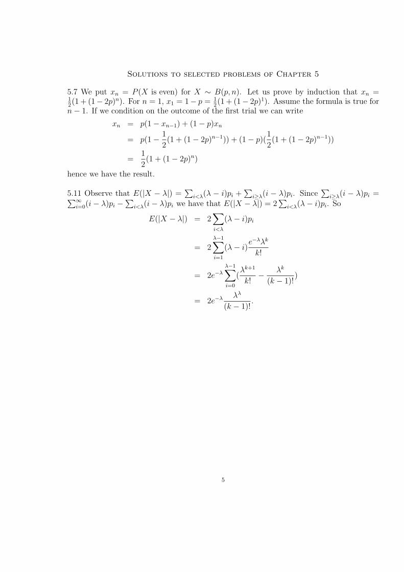
Solutions to selected problems of Chapter 5
5.7 We put xn = P (X is even) for X ∼ B(p, n). Let us prove by induction that xn =12(1 + (1− 2p)n). For n = 1, x1 = 1− p = 1
2(1 + (1− 2p)1). Assume the formula is true for
n− 1. If we condition on the outcome of the first trial we can write
xn = p(1− xn−1) + (1− p)xn
= p(1− 1
2(1 + (1− 2p)n−1)) + (1− p)(
1
2(1 + (1− 2p)n−1))
=1
2(1 + (1− 2p)n)
hence we have the result.
5.11 Observe that E(|X − λ|) =∑
i<λ(λ − i)pi +∑
i≥λ(i − λ)pi. Since∑
i≥λ(i − λ)pi =∑∞i=0(i− λ)pi −
∑i<λ(i− λ)pi we have that E(|X − λ|) = 2
∑i<λ(λ− i)pi. So
E(|X − λ|) = 2∑i<λ
(λ− i)pi
= 2λ−1∑i=1
(λ− i)e−λλk
k!
= 2e−λ
λ−1∑i=0
(λk+1
k!− λk
(k − 1)!)
= 2e−λ λλ
(k − 1)!.
5
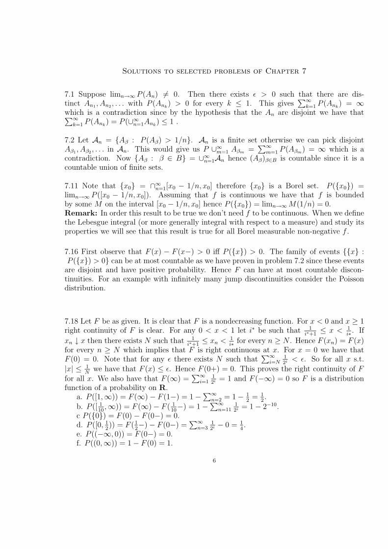
Solutions to selected problems of Chapter 7
7.1 Suppose limn→∞ P (An) 6= 0. Then there exists ε > 0 such that there are dis-tinct An1 , An2 , . . . with P (Ank
) > 0 for every k ≤ 1. This gives∑∞
k=1 P (Ank) = ∞
which is a contradiction since by the hypothesis that the An are disjoint we have that∑∞k=1 P (Ank
) = P (∪∞n=1Ank) ≤ 1 .
7.2 Let An = Aβ : P (Aβ) > 1/n. An is a finite set otherwise we can pick disjointAβ1 , Aβ2 , . . . in An. This would give us P ∪∞m=1 Aβm =
∑∞m=1 P (Aβm) = ∞ which is a
contradiction. Now Aβ : β ∈ B = ∪∞n=1An hence (Aβ)β∈B is countable since it is acountable union of finite sets.
7.11 Note that x0 = ∩∞n=1[x0 − 1/n, x0] therefore x0 is a Borel set. P (x0) =limn→∞ P ([x0 − 1/n, x0]). Assuming that f is continuous we have that f is boundedby some M on the interval [x0 − 1/n, x0] hence P (x0) = limn→∞ M(1/n) = 0.Remark: In order this result to be true we don’t need f to be continuous. When we definethe Lebesgue integral (or more generally integral with respect to a measure) and study itsproperties we will see that this result is true for all Borel measurable non-negative f .
7.16 First observe that F (x) − F (x−) > 0 iff P (x) > 0. The family of events x :P (x) > 0 can be at most countable as we have proven in problem 7.2 since these events
are disjoint and have positive probability. Hence F can have at most countable discon-tinuities. For an example with infinitely many jump discontinuities consider the Poissondistribution.
7.18 Let F be as given. It is clear that F is a nondecreasing function. For x < 0 and x ≥ 1right continuity of F is clear. For any 0 < x < 1 let i∗ be such that 1
i∗+1≤ x < 1
i∗ . If
xn ↓ x then there exists N such that 1i∗+1
≤ xn < 1i∗ for every n ≥ N . Hence F (xn) = F (x)
for every n ≥ N which implies that F is right continuous at x. For x = 0 we have thatF (0) = 0. Note that for any ε there exists N such that
∑∞i=N
12i < ε. So for all x s.t.
|x| ≤ 1N
we have that F (x) ≤ ε. Hence F (0+) = 0. This proves the right continuity of F
for all x. We also have that F (∞) =∑∞
i=112i = 1 and F (−∞) = 0 so F is a distribution
function of a probability on R.a. P ([1,∞)) = F (∞)− F (1−) = 1−
∑∞n=2 = 1− 1
2= 1
2.
b. P ([ 110
,∞)) = F (∞)− F ( 110−) = 1−
∑∞n=11
12i = 1− 2−10.
c P (0) = F (0)− F (0−) = 0.d. P ([0, 1
2)) = F (1
2−)− F (0−) =
∑∞n=3
12i − 0 = 1
4.
e. P ((−∞, 0)) = F (0−) = 0.f. P ((0,∞)) = 1− F (0) = 1.
6

7

Solutions to selected problems of Chapter 9
9.1 It is clear by the definition of F that X−1(B) ∈ F for every B ∈ B. So X is measurablefrom (Ω,F) to (R,B).
9.2 Since X is both F and G measurable for any B ∈ B, P (X ∈ B) = P (X ∈ B)P (X ∈B) = 0 or 1. Without loss of generality we can assume that there exists a closed intervalI such that P (I) = 1. Let Λn = tn0 , . . . tnln be a partition of I such that Λn ⊂ Λn+1 andsupk tnk − tnk−1 → 0. For each n there exists k∗(n) such that P (X ∈ [tnk∗ , t
nk∗+1]) = 1 and
[tnk∗(n+1, tnk∗(n+1)+1] ⊂ [tnk∗(n), t
nk∗(n)+1]. Now an = tnk∗(n) and bn = tnk∗(n) + 1 are both Cauchy
sequences with a common limit c. So 1 = limn→∞ P (X ∈ (tnk∗ , tnk∗+1]) = P (X = c).
9.3 X−1(A) = (Y −1(A) ∩ (Y −1(A) ∩X−1(A)c)c)∪(X−1(A) ∩ Y −1(A)c). Observe that bothY −1(A)∩ (X−1(A))c and X−1(A)∩Y −1(A)c are null sets and therefore measurable. Henceif Y −1(A) ∈ A′ then X−1(A) ∈ A′. In other words if Y is A′ measurable so is X.
9.4 Since X is integrable, for any ε > 0 there exists M such that∫|X|1X>MdP < ε by
the dominated convergence theorem. Note that
E[X1An ] = E[X1An1X>M] + E[X1An1X≤M]
≤ E[|X|1X≤M] + MP (An)
Since P (An) → 0, there exists N such that P (An) ≤ εM
for every n ≥ N . ThereforeE[X1An ] ≤ ε + ε ∀n ≥ N , i.e. limn→∞ E[X1An ] = 0.
9.5 It is clear that 0 ≤ Q(A) ≤ 1 and Q(Ω) = 1 since X is nonnegative and E[X] = 1. LetA1, A2, . . . be disjoint. Then
Q(∪∞n=1An) = E[X1∪∞n=1An ] = E[∑n=1
X1An ] =∞∑
n=1
E[X1An ]
where the last equality follows from the monotone convergence theorem. Hence Q(∪∞n=1An) =∑∞n=1 Q(An). Therefore Q is a probability measure.
9.6 If P (A) = 0 then X1A = 0 a.s. Hence Q(A) = E[X1A] = 0. Now assume P is theuniform distribution on [0, 1]. Let X(x) = 21[0,1/2](x). Corresponding measure Q assignszero measure to (1/2, 1], however P ((1/2, 1]) = 1/2 6= 0.
9.7 Let’s prove this first for simple functions, i.e. let Y be of the form
Y =n∑
i=1
ci1Ai
8

for disjoint A1, . . . , An. Then
EQ[Y ] =n∑
i=1
ciQ(Ai) =n∑
i=1
ciE[X1Ai] = EP [XY ]
For non-negative Y we take a sequence of simple functions Yn ↑ Y . Then
EQ[Y ] = limn→∞
EQ[Yn] = limn→∞
EP [XYn] = EP [XY ]
where the last equality follows from the monotone convergence theorem. For general Y ∈ L1(Q) we have that EQ[Y ] = EQ[Y +]− EQ[Y −] = EP [(XY )+]− EQ[(XY )−] = EP [XY ].
9.8 a. Note that 1X
X = 1 a.s. since P (X > 0) = 1. By problem 9.7 EQ[ 1X
] = EP [ 1X
X] = 1.
So 1X
is Q-integrable.
b. R : A → R, R(A) = EQ[ 1X1A] is a probability measure since 1
Xis non-negative and
EQ[ 1X
] = 1. Also R(A) = EQ[ 1X1A] = EP [ 1
XX1A] = P (A). So R = P .
9.9 Since P (A) = EQ[ 1X1A] we have that Q(A) = 0 ⇒ P (A) = 0. Now combining the
results of the previous problems we can easily observe that Q(A) = 0 ⇔ P (A) = 0 iffP (X > 0) = 1.
9.17. Let
g(x) =((x− µ)b + σ)2
σ2(1 + b2)2.
Observe that X ≥ µ + bσ ∈ g(X) ≥ 1. So
P (X ≥ µ + bσ) ≤ P (g(X) ≥ 1) ≤ E[g(X)]
1
where the last inequality follows from Markov’s inequality. Since E[g(X)] = σ2(1+b2)σ2(1+b2)2
we
get that
P (X ≥ µ + bσ) ≤ 1
1 + b2.
9.19
xP (X > x) ≤ E[X1X > x]
=
∫ ∞
x
z√2π
e−z2
2 dz
=e−
x2
2
√2π
Hence
P (X > x) ≤ e−x2
2
x√
2π9

.
9.21 h(t+s) = P (X > t+s) = P (X > t+s, X > s) = P (X > t+s|X > s)P (X >
s) = h(t)h(s) for all t, s > 0. Note that this gives h( 1n) = h(1)
1n and h(m
n) = h(1)
mn . So
for all rational r we have that h(r) = exp (log(h(1))r). Since h is right continuous thisgives h(x) = exp(log(h(1))x) for all x > 0. Hence X has exponential distribution withparameter − log h(1).
10
Solutions to selected problems of Chapter 10
10.5 Let P be the uniform distribution on [−1/2, 1/2]. Let X(x) = 1[−1/4,1/4] and Y (x) =1[−1/4,1/4]c . It is clear that XY = 0 hence E[XY ] = 0. It is also true that E[X] = 0. SoE[XY ] = E[X]E[Y ] however it is clear that X and Y are not independent.
10.6 a. P (min(X, Y ) > i) = P (X > i)P (Y > i) = 12i
12i = 1
4i . So P (min(X, Y ) ≤ i) =
1− P (min(X,Y ) > i) = 1− 14i .
b. P (X = Y ) =∑∞
i=1 P (X = i)P (Y = i) =∑∞
i=112i
12i = 1
1− 1
4i− 1 = 1
3.
c. P (Y > X) =∑∞
i=1 P (Y > i)P (X = i) =∑∞
i=112i
12i = 1
3.
d. P (X divides Y ) =∑∞
i=1
∑∞k=1
12i
12ki =
∑∞i=1
12i
12i−1
.
e. P (X ≥ kY ) =∑∞
i=1 P (X ≥ ki)P (Y = i) =∑∞
i=112i
12ki−1
= 22k+1−1
.
11

Solutions to selected problems of Chapter 11
11.11. Since PX > 0 = 1 we have that PY < 1 = 1. So FY (y) = 1 for y ≥ 1. AlsoPY ≤ 0 = 0 hence FY (y) = 0 for y ≤ 0. For 0 < y < 1 PY > y = PX < 1−y
y =
FX(1−yy
). So
FY (y) = 1−∫ 1−y
y
0
fX(x)dx = 1−∫ y
0
−1
z2fX(
1− z
z)dz
by change of variables. Hence
fY (y) =
0 −∞ < y ≤ 01y2 fX(1−y
y) 0 < y ≤ 1
0 1 ≤ y < ∞
11.15 Let G(u) = infx : F (x) ≥ u. We would like to show u : G(u) > y = u :F (Y ) < u. Let u be such that G(u) > y. Then F (y) < u by definition of G. Henceu : G(u) > y ⊂ u : F (Y ) < u. Now let u be such that F (y) < u. Then y < x for any xsuch that F (x) ≥ u by monotonicity of F . Now by right continuity and the monotonicity ofF we have that F (G(u)) = infF (x)≥u F (x) ≥ u. Then by the previous statement y < G(u).So u : G(u) > y = u : F (Y ) < u. Now PG(U) > y = PU > F (y) = 1− F (y) soG(U) has the desired distribution. Remark:We only assumed the right continuityof F .
12

Solutions to selected problems of Chapter 12
12.6 Let Z = ( 1σY
)Y − (ρXY
σX)X. Then σ2
Z = ( 1σ2
Y)σ2
Y − (ρ2
XY
σ2X
)σ2X − 2( ρXY
σXσY)Cov(X, Y ) =
1− ρ2XY . Note that ρXY = ∓1 implies σ2
Z = 0 which implies Z = c a.s. for some constantc. In this case X = σX
σY ρXY(Y − c) hence X is an affine function of Y .
12.11 Consider the mapping g(x, y) = (√
x2 + y2, arctan(xy)). Let S0 = (x, y) : y = 0,
S1 = (x, y) : y > 0, S2 = (x, y) : y < 0. Note that ∪2i=0Si = R2 and m2(S0) = 0.
Also for i = 1, 2 g : Si → R2 is injective and continuously differentiable. Correspondinginverses are given by g−1
1 (z, w) = (z sin w, z cos w) and g−12 (z, w) = (z sin w,−z cos w). In
both cases we have that |Jg−1i
(z, w)| = z hence by Corollary 12.1 the density of (Z,W ) is
given by
fZ,W (z, w) = (1
2πσ2e−z2
2σ z +1
2πσ2e−z2
2σ z)1(−π2, π2)(w)1(0,∞)(z)
=1
π1(−π
2, π2)(w) ∗ z
σ2e−z2
2σ 1(0,∞)(z)
as desired.
12.12 Let P be the set of all permutations of 1, . . . , n. For any π ∈ P let Xπ be thecorresponding permutation of X, i.e. Xπ
k = Xπk. Observe that
P (Xπ1 ≤ x1, . . . , X
πn ≤ xn) = F (x1) . . . F (Xn)
hence the law of Xπ and X coincide on a πsystem generating Bn therefore they are equal.Now let Ω0 = (x1, . . . , xn) ∈ Rn : x1 < x2 < . . . < xn. Since Xi are i.i.d and havecontinuous distribution PX(Ω0) = 1. Observe that
PY1 ≤ y1, . . . , Yn ≤ yn = P (∪π∈PXπ1 ≤ y1, . . . , X
πn ≤ yn ∩ Ω0)
Note that Xπ1 ≤ y1, . . . , X
πn ≤ yn ∩ Ω0, π ∈ P are disjoint and P (Ω0 = 1) hence
PY1 ≤ y1, . . . , Yn ≤ yn =∑π∈P
PXπ1 ≤ y1, . . . , X
πn ≤ yn
= n!F (y1) . . . F (yn)
for y1 ≤ . . . ≤ yn. Hence
fY (y1, . . . , yn) =
n!f(y1) . . . f(yn) y1 ≤ . . . ≤ yn
0 otherwise
13

Solutions to selected problems of Chapter 14
14.7 ϕX(u) is real valued iff ϕX(u) = ϕX(u) = ϕ−X(u). By uniqueness theorem ϕX(u) =ϕ−X(u) iff FX = F−X . Hence ϕX(u) is real valued iff FX = F−X .
14.9 We use induction. It is clear that the statement is true for n = 1. Put Yn =∑ni=1 Xi and assume that E[(Yn)3] =
∑ni=1 E[(Xi)
3]. Note that this implies d3
dx3 ϕYn(0) =
−i∑n
i=1 E[(Xi)3]. Now E[(Yn+1)
3] = E[(Xn+1 + Yn)3] = −i d3
dx3 (ϕXn+1ϕYn)(0) by indepen-dence of Xn+1 and Yn. Note that
d3
dx3ϕXn+1ϕYn(0) =
d3
dx3ϕXn+1(0)ϕYn(0)
+ 3d2
dx2ϕXn+1(0)
d
dxϕYn(0) + 3
d
dxϕXn+1(0)
d2
dx2ϕYn(0)
+ ϕXn+1(0)d3
dx3ϕYn(0)
=d3
dx3ϕXn+1(0) +
d3
dx3ϕYn(0)
= −i
(E[(Xn+1)
3] +n∑
i=1
E[(Xi)3]
)where we used the fact that d
dxϕXn+1(0) = iE(Xn+1) = 0 and d
dxϕYn(0) = iE(Yn) = 0. So
E[(Yn+1)3] =
∑n+1i=1 E[(Xi)
3] hence the induction is complete.
14.10 It is clear that 0 ≤ ν(A) ≤ 1 since
0 ≤n∑
j=1
λjµj(A) ≤n∑
j=1
λj = 1.
Also for Ai disjoint
ν(∪∞i=1Ai) =n∑
j=1
λjµj(∪∞i=1Ai)
=n∑
j=1
λj
∞∑i=1
µj(Ai)
=∞∑i=1
n∑j=1
λjµj(Ai)
=∞∑i=1
ν(Ai)
14

Hence ν is countably additive therefore it is a probability mesure. Note that∫
1Adν(dx) =∑nj=1 λj
∫1A(x)dµj(dx) by definition of ν. Now by linearity and monotone convergence
theorem for a non-negative Borel function f we have that∫
f(x)ν(dx) =∑n
j=1 λj
∫f(x)dµj(dx).
Extending this to integrable f we have that ν(u) =∫
eiuxν(dx) =∑n
j=1 λj
∫eiuxdµj(dx) =∑n
j=1 λjµj(u).
14.11 Let ν be the double exponential distribution, µ1 be the distribution of Y and µ2 bethe distribution of −Y where Y is an exponential r.v. with parameter λ = 1. Then wehave that ν(A) = 1
2
∫A∩(0,∞)
e−xdx + 12
∫A∩(−∞,0)
exdx = 12µ1(A) + 1
2µ2(A). By the previous
exercise we have that ν(u) = 12µ1(u) + 1
2µ2(u) = 1
2( 1
1−iu+ 1
1+iu) = 1
1+u2 .
14.15. Note that EXn = (−i)n dn
dxn ϕX(0). Since X ∼ N(0, 1) ϕX(s) = e−s2/2. Note that
we can get the derivatives of any order of e−s2/2 at 0 simply by taking Taylor’s expansionof ex:
e−s2/2 =∞∑i=0
(−s2/2)n
n!
=∞∑i=0
1
2n!
(−i)2n(2n)!
2nn!s2n
hence EXn = (−i)n dn
dxn ϕX(0) = 0 for n odd. For n = 2k EX2k = (−i)2k d2k
dx2k ϕX(0) =
(−i)2k (−i)2k(2k)!2kk!
= (2k)!2kk!
as desired.
15

Solutions to selected problems of Chapter 15
15.1 a. Ex = 1n
∑ni=1 EXi = µ.
b. Since X1, . . . , Xn are independent Var(x) = 1n2
∑ni=1 VarXi = σ2
n.
c. Note that S2 = 1n
∑ni=1(Xi)
2 − x2. Hence E(S2) = 1n
∑ni=1(σ
2 + µ2)− (σ2
n+ µ2) =
n−1n
σ2.
15.17 Note that ϕY (u) =∏α
i=1 ϕXi(u) = ( β
β−iu)α which is the characteristic function
of Gamma(α,β) random variable. Hence by uniqueness of characteristic function Y isGamma(α,β).
16

Solutions to selected problems of Chapter 16
16.3 P (Y ≤ y) = P (X ≤ y ∩ Z = 1) + P (−X ≤ y ∩ Z = −1) = 12Φ(y) +
12Φ(−y) = Φ(y) since Z and X are independent and Φ(y) is symmetric. So Y is normal.
Note that P (X + Y = 0) = 12
hence X + Y can not be normal. So (X, Y ) is not Gaussianeven though both X and Y are normal.
16.4 Observe that
Q = σXσY
[ σX
σYρ
ρ σY
σX
]So det(Q) = σXσY (1− ρ2). So det(Q) = 0 iff ρ = ∓1. By Corollary 16.2 the joint densityof (X,Y ) exists iff −1 < ρ < 1. (By Cauchy-Schwartz we know that −1 ≤ ρ ≤ 1). Notethat
Q−1 =1
σXσY (1− ρ2)
σY
σX−ρ
−ρ σX
σY
Substituting this in formula 16.5 we get that
f(X,Y )(x, y) =1
2πσXσY (1− ρ2)exp
−1
2(1− ρ2)
((x− µX
σX
)2
− 2ρ(x− µX)(y − µY )
σXσY
+
(y − µY
σY
)2)
.
16.6 By Theorem 16.2 there exists a multivariate normal r.v. Y with E(Y ) = 0 and adiagonal covariance matrix Λ s.t. X − µ = AY where A is an orthogonal matrix. SinceQ = AΛA∗ and det(Q) > 0 the diagonal entries of Λ are strictly positive hence we candefine B = Λ−1/2A∗. Now the covariance matrix Q of B(X − µ) is given by
Q = Λ−1/2A∗AΛA∗AΛ−1/2
= I
So B(X − µ) is standard normal.
16.17 We know that as in Exercise 16.6 if B = Λ−1/2A∗ where A is the orthogonal matrix s.t.Q = AΛA∗ then B(X−µ) is standard normal. Note that this gives (X−µ)∗Q−1(X−µ) =(X − µ)∗B∗B(X − µ) which has chi-square distribution with n degrees of freedom.
17

Solutions to selected problems of Chapter 17
17.1 Let n(m) and j(m) be such that Ym = n(m)1/pZn(m),j(m). This gives that P (|Ym| >0) = 1
n(m)→ 0 as m → ∞. So Ym converges to 0 in probability. However E[|Ym|p] =
E[n(m)Zn(m),j(m)] = 1 for all m. So Ym does not converge to 0 in Lp.
17.2 Let Xn = 1/n. It is clear that Xn converge to 0 in probability. If f(x) = 10(x) thenwe have that P (|f(Xn) − f(0)| > ε) = 1 for every ε ≥ 1, so f(Xn) does not converge tof(0) in probability.
17.3 First observe that E(Sn) =∑n
i=1 E(Xn) = 0 and that Var(Sn) =∑n
i=1 Var(Xn) = nsince E(Xn) = 0 and Var(Xn) = E(X2
n) = 1. By Chebyshev’s inequality P (|Sn
n| ≥ ε) =
P (|Sn| ≥ nε) ≤ Var(Sn)n2ε2
= nn2ε2
→ 0 as n →∞. Hence Sn
nconverges to 0 in probability.
17.4 Note that Chebyshev’s inequality gives P (|Sn2
n2 | ≥ ε) ≤ 1n2ε2
. Since∑∞
i=11
n2ε2< ∞ by
Borel Cantelli Theorem P (lim supn|Sn2
n2 | ≥ ε) = 0. Let Ω0 =(∪∞m=1 lim supn|
Sn2
n2 | ≥ 1m)c
.
Then P (Ω0) = 1. Now let’s pick w ∈ Ω0. For any ε there exists m s.t. 1m≤ ε and
w ∈ (lim supn|Sn2
n2 | ≥ 1m)c. Hence there are finitely many n s.t. |Sn2
n2 | ≥ 1m
which implies
that there exists N(w) s.t. |Sn2
n2 | ≤ 1m
for every n ≥ N(w). HenceSn2 (w)
n2 → 0. SinceP (Ω0) = 1 we have almost sure convergence.
17.12 Y < ∞ a.s. which follows by Exercise 17.11 since Xn < ∞ and X < ∞ a.s. LetZ = 1
c1
1+Y. Observe that Z > 0 a.s. and EP (Z) = 1. Therefore as in Exercise 9.8
Q(A) = EP (Z1A) defines a probability measure and EQ(|Xn − X|) = EP (Z|Xn − X|).Note that Z|Xn − X| ≤ 1 a.s. and Xn → X a.s. by hypothesis, hence by dominatedconvergence theorem EQ(|Xn−X|) = EP (Z|Xn−X|) → 0, i.e. Xn tends to X in L1 withrespect to Q.
17.14 First observe that |E(X2n)−E(X2)| ≤ E(|X2
n−X2|). Since |X2n−X2| ≤ (Xn−X)2 +
2|X||Xn − X| we get that |E(X2n) − E(X2)| ≤ E((Xn − X)2) + 2E(|X||Xn − X|). Note
that first term goes to 0 since Xn tends to X in L2. Applying Cauchy Schwarz inequalityto the second term we get E(|X||Xn − X|) ≤
√E(X2)E(|Xn −X|2), hence the second
term also goes to 0 as n →∞. Now we can conclude E(X2n) → E(X2).
17.15 For any ε > 0 P (|X| ≤ c+ε) ≥ P (|Xn| ≤ c, |Xn−X| ≤ ε) → 1 as n →∞. HenceP (|X| ≤ c + ε) = 1. Since X ≤ c = ∩∞m=1X ≤ c + 1
m we get that PX ≤ c = 1.
Now we have that E(|Xn − X|) = E(|Xn − X|1|Xn−X|≤ε) + E(|Xn − X|1|Xn−X|>ε) ≤ε + 2c(P|Xn − X| > ε), hence choosing n large we can make E(|Xn − X|) arbitrarilysmall, so Xn tends to X in L1.
18

Solutions to selected problems of Chapter 18
18.8 Note that ϕYn(u) = Πni=1ϕXi
(un) = Πn
i=1e− |u|
n = e−|u|, hence Yn is also Cauchy withα = 0 and β = 1 which is independent of n, hence trivially Yn converges in distributionto a Cauchy distributed r.v. with α = 0 and β = 1. However Yn does not converge toany r.v. in probability. To see this, suppose there exists Y s.t. P (|Yn − Y | > ε) → 0.Note that P (|Yn − Ym| > ε) ≤ P (|Yn − Y | > ε
2) + P (|Ym − Y | > ε
2). If we let m = 2n,
|Yn − Ym| = 12| 1n
∑ni=1 Xi − 1
n
∑2ni=n+1 Xi| which is equal in distribution to 1
2|U −W | where
U and W are independent Cauchy r.v.’s with α = 0 and β = 1. Hence P (|Yn − Ym| > ε2)
does not depend on n and does not converge to 0 if we let m = 2n and n →∞ which is acontradiction since we assumed the right hand side converges to 0.
18.16 Define fm as the following sequence of functions:
fm(x) =
x2 if |x| ≤ N − 1
m(N − 1
m)x− (N − 1
m)N if x ≥ N − 1
m−(N − 1
m)x + (N − 1
m)N if x ≤ −N + 1
m0 otherwise
Note that each fm is continuous and bounded. Also fm(x) ↑ 1(−N,N)(x)x2 for every x ∈ R.Hence ∫ N
−N
x2F (dx) = limm→∞
∫ ∞
−∞fm(x)F (dx)
by monotone convergence theorem. Now∫ ∞
−∞fm(x)F (dx) = lim
n→∞
∫ ∞
−∞fm(x)Fn(dx)
by weak convergence. Since∫∞−∞ fm(x)Fn(dx) ≤
∫ N
−Nx2Fn(dx) it follows that∫ N
−N
x2F (dx) ≤ limm→∞
lim supn→∞
∫ N
−N
x2Fn(dx) = lim supn→∞
∫ N
−N
x2Fn(dx)
as desired.
18.17 Following the hint, suppose there exists a continuity point y of F such that
limn→∞
Fn(y) 6= F (y)
Then there exist ε > 0 and a subsequence (nk)k≥1 s.t. Fnk(y) − F (y) < −ε for all k, or
Fnk(y)− F (y) > ε for all k. Suppose Fnk
(y)− F (y) < −ε for all k, observe that for x ≤ y,Fnk
(x)− F (x) ≤ Fnk(y)− F (x) = Fnk
(y)− F (y) + (F (y)− F (x)) < −ε + (F (y)− F (x)).Since f is continuous at y there exists an interval [y1, y) s.t. |(F (y) − F (x))| < ε
2, hence
Fnk(x) − F (x) < − ε
2for all x ∈ [y1, y). Now suppose Fnk
(y) − F (y) > ε, then for x ≥ y,Fnk
(x) − F (x) ≥ Fnk(y) − F (x) = Fnk
(y) − F (y) + (F (y) − F (x)) > ε + (F (y) − F (x)).19

Now we can find an interval (y, y1] s.t. |(F (y)−F (x))| < ε2
which gives Fnk(x)−F (x) > ε
2
for all x ∈ (y, y1]. Note that both cases would yield∫ ∞
−infty
|Fnk(x)− F (x)|rdx > |y1 − y| ε
2
which is a contradiction to the assumption
limn→∞
∫ ∞
−infty
|Fn(x)− F (x)|rdx = 0.
Therefore Xn converges to X in distribution.
20

Solutions to selected problems of Chapter 19
19.1 Note that ϕXn(u) = eiuµn−u2σ2
n2 → eiuµ−u2σ2
2 . By Levy’s continuity theorem it followsthat Xn ⇒ X where X is N(µ, σ2).
19.3 Note that ϕXn+Yn(u) = ϕXn(u)ϕYn(u) → ϕX(u)ϕY (u) = ϕX+Y (u). Therefore Xn +Yn ⇒ X + Y
21

Solutions to selected problems of Chapter 20
20.1 a. First observe that E(S2n) =
∑ni=1
∑nj=1 E(XiXj) =
∑ni=1 X2
i since E(XiXj) = 0
for i 6= j. Now P ( |Sn|n≥ ε) ≤ E(S2
n)ε2n2 =
nE(X2i )
ε2n2 ≤ cnε2
as desired.
b. From part (a) it is clear that 1nSn converges to 0 in probability. Also E(( 1
nSn)2) =
E(X2i
n→ 0 since E(X2
i ) ≤ ∞, so 1nSn converges to 0 in L2 as well.
20.5 Note that Zn ⇒ Z implies that ϕZn(u) → ϕZ(u) uniformly on compact subset of R.(See Remark 19.1). For any u, we can pick n > N s.t. u√
n< M , supx∈[−M,M ] |ϕZn(x) −
ϕZ(x)| < ε and |varphiZ( u√n)− ϕZ(0)| < ε. This gives us
|ϕZn(u√n
)− ϕZ(0)| = |ϕZn(u√n
)− ϕZ(u√n
)|+ |ϕZ(u√n
)− ϕZ(0)| ≤ 2ε
So ϕZn√n(u) = ϕZn( u√
n) converges to ϕZ(0) = 1 for every u. Therefore Zn√
n⇒ 0 by continuity
theorem. We also have by the strong law of large numbers that Zn√n→ E(Xj) − ν. This
implies E(Xj)− ν = 0, hence the assertion follows by strong law of large numbers.
22

http://www.springer.com/978-3-540-43871-7
Related Documents


![Essentials Fabrication Quality Plan Sample · 2018-03-09 · Pat [Pick the date] Essentials Fabrication Quality Plan Sample. Selected pages not a complete plan. Includes Standards](https://static.cupdf.com/doc/110x72/5ea6ded88e4b24047a0d13bd/essentials-fabrication-quality-plan-sample-2018-03-09-pat-pick-the-date-essentials.jpg)