SOLUTIONS MANUAL FOR ADVANCED ENGINEERING MATHEMATICS 1ST EDITION TURYN SOLUTIONS SOLUTIONS MANUAL FOR ADVANCED ENGINEERING MATHEMATICS 1ST EDITION TURYN

Welcome message from author
This document is posted to help you gain knowledge. Please leave a comment to let me know what you think about it! Share it to your friends and learn new things together.
Transcript

SOLUTIONS MANUAL FOR ADVANCED ENGINEERING MATHEMATICS 1ST EDITION TURYN
SOLUTIONS
SOLUTIONS MANUAL FOR ADVANCED ENGINEERING MATHEMATICS 1ST EDITION TURYN
page 1
Chapter Two
Section 2.1.6
2.1.6.1. 0 =
∣∣∣∣ −2− λ 71 4− λ
∣∣∣∣ = (−2− λ)(4− λ)− 7 = λ2 − 2λ− 15 = (λ− 5)(λ+ 3)
⇒ eigenvalues are λ1 = −3, λ2 = 5
[A− λ1I | 0 ] =
[1 7 | 01 7 | 0
]∼[
1© 7 | 00 0 | 0
], after −R1 +R2 → R2
⇒ v1 = c1
[−7
1
], for any constant c1 6= 0, are the eigenvectors corresponding to eigenvalue λ1 = −3.
[A− λ2I | 0 ] =
[−7 7 | 0
1 −1 | 0
]∼[
1© −1 | 00 0 | 0
], after − 1
7R1 → R1, −R1 +R2 → R2
⇒ v2 = c1
[11
], for any constant c1 6= 0, are the eigenvectors corresponding to eigenvalue λ2 = 5.
2.1.6.2. 0 =
∣∣∣∣ 1− λ 23 2− λ
∣∣∣∣ = (1− λ)(2− λ)− 6 = λ2 − 3λ− 4 = (λ− 4)(λ+ 1)
⇒ eigenvalues are λ1 = −1, λ2 = 4
[A− λ1I | 0 ] =
[2 2 | 03 3 | 0
]∼[
1© 1 | 00 0 | 0
], after 1
2R1 → R1, -3R1 +R2 → R2
⇒ v1 = c1
[−1
1
], for any constant c1 6= 0, are the eigenvectors corresponding to eigenvalue λ1 = −1.
[A− λ2I | 0 ] =
[−3 2 | 0
3 −2 | 0
]∼[
1© − 23| 0
0 0 | 0
], after R1 +R2 → R2, − 1
3R1 → R1
⇒ v2 = c1
[23
1
], for any constant c1 6= 0, are the eigenvectors corresponding to eigenvalue λ2 = 4.
2.1.6.3. 0 =
∣∣∣∣ −1− λ 41 1− λ
∣∣∣∣ = (−1− λ)(1− λ)− 4 = λ2 − 5
⇒ eigenvalues are λ1 =√
5, λ2 = −√
5
[A− λ1I | 0 ] =
[−1−
√5 4 | 0
1 1−√
5 | 0
]∼[
1© 1−√
5 | 00 0 | 0
], after R1 ↔ R2, (1 +
√5)R1 +R2 → R2
⇒ v1=c1
[−1 +
√5
1
], for any constant c1 6= 0, are the eigenvectors corresponding to eigenvalue λ1 =
√5.
[A− λ2I | 0 ] =
[−1 +
√5 4 | 0
1 1 +√
5 | 0
]∼[
1© 1 +√
5 | 00 0 | 0
], after R1 ↔ R2, (1−
√5)R1 +R2 → R2
⇒ v2=c1
[−1−
√5
1
], for any const. c1 6= 0, are the eigenvectors corresponding to eigenvalue λ2 = −
√5.
2.1.6.4. 0 =
∣∣∣∣ −2− λ −51 0− λ
∣∣∣∣ = (−2− λ)(−λ)− (−5) = λ2 + 2λ+ 5
⇒ eigenvalues are λ1 = −1 + i2, λ2 = −1− i2. Because the eigenvalues are not real and are a complex conjugatepair, we only need to calculate one eigenvector:
[A− λ1I | 0 ] =
[−1− i2 −5 | 0
1 1− i2 | 0
]∼[
1© 1− i2 | 00 0 | 0
], after R1 ↔ R2, (1 + i2)R1 +R2 → R2
⇒ v1 = c1
[−1 + i2
1
], for any constant c1 6= 0, are the eigenvectors corresponding to eigenvalue λ1 = −1 + i2.
The eigenvectors corresponding to λ2 = −1− i2 are v2 = v̄1 = c1
[−1− i2
1
], for any constant c1 6= 0.
c©Larry Turyn, January 2, 2014
SOLUTIONS MANUAL FOR ADVANCED ENGINEERING MATHEMATICS 1ST EDITION TURYN

page 2
2.1.6.5. We are given three distinct eigenvalues, so the only eigenvalues are λ1 = 0, λ2 = 2, λ3 = 4. All we need to dois to find the eigenvectors.
[A− λ1I | 0 ] =
1 1 2 | 0−1 3 2 | 0
1 1 2 | 0
∼
−R1 +R2 → R2
R1 +R3 → R3
1 1 2 | 00 4 4 | 00 0 0 | 0
∼
14R2 → R2
−R2 +R1 → R1
1© 0 1 | 00 1© 1 | 00 0 0 | 0
⇒ v1 = c1
−1−1
1
, for any constant c1 6= 0, are the eigenvectors corresponding to eigenvalue λ1 = 0.
[A− λ2I | 0 ] =
−1 1 2 | 0−1 1 2 | 0
1 1 0 | 0
∼
−R1 → R1
R1 +R2 → R2
−R1 +R3 → R3
1 −1 −2 | 00 0 0 | 00 2 2 | 0
∼
R2 ↔ R312R2 → R2
R2 +R1 → R1
1© 0 −1 | 00 1© 1 | 00 0 0 | 0
⇒ v2 = c1
1−1
1
, for any constant c1 6= 0, are the eigenvectors corresponding to eigenvalue λ2 = 2.
[A− λ3I | 0 ] =
−3 1 2 | 0−1 −1 2 | 0
1 1 −2 | 0
∼
R1 ↔ R3
R1 +R2 → R2
3R1 +R3 → R3
1 1 −2 | 00 0 0 | 00 4 −4 | 0
∼
R2 ↔ R314R2 → R2
−R2 +R1 → R1
1© 0 −1 | 00 1© −1 | 00 0 0 | 0
⇒ v3 = c1
111
, for any constant c1 6= 0, are the eigenvectors corresponding to eigenvalue λ3 = 4.
2.1.6.6. By expanding along the second row, we calculate
0 =
∣∣∣∣∣∣1− λ −3 6
0 −2− λ 02 0 −λ
∣∣∣∣∣∣ = (−2− λ) ·∣∣∣∣ 1− λ 6
2 −λ
∣∣∣∣ = (−2− λ)((1− λ)(−λ)− 12
)= (−2− λ)
(λ2 − λ− 12
)= (−2− λ)(λ− 4)(λ+ 3),
so the eigenvalues are λ1 = −3, λ2 = −2, λ3 = 4.
[A− λ1I | 0 ] =
4 −3 6 | 00 1 0 | 02 0 3 | 0
∼
− 12R1 +R3 → R3
14R1 → R1
1 −0.75 32| 0
0 1 0 | 00 1.5 0 | 0
∼
34R2 +R1 → R1
− 32R2 +R3 → R3
1© 0 32| 0
0 1© 0 | 00 0 0 | 0
⇒ v1 = c1
− 32
01
, for any constant c1 6= 0, are the eigenvectors corresponding to eigenvalue λ1 = −3.
[A−λ2I | 0 ] =
3 −3 6 | 00 0 0 | 02 0 2 | 0
∼
13R1 → R1
−2R1 +R3 → R3
R2 ↔ R3
1 −1 2 | 00 2 −2 | 00 0 0 | 0
∼
12R2 → R2
R2 +R1 → R1
1© 0 1 | 00 1© −1 | 00 0 0 | 0
c©Larry Turyn, January 2, 2014
SOLUTIONS MANUAL FOR ADVANCED ENGINEERING MATHEMATICS 1ST EDITION TURYN

page 3
⇒ v2 = c1
−111
, for any constant c1 6= 0, are the eigenvectors corresponding to eigenvalue λ2 = −2.
[A−λ3I | 0 ] =
−3 −3 6 | 00 −6 0 | 02 0 −4 | 0
∼
− 13R1 → R1
−2R1 +R3 → R3
1 1 −2 | 00 −6 0 | 00 −2 0 | 0
∼
− 16R2 → R2
−R2 +R1 → R1
2R2 +R3 → R3
1© 0 −2 | 00 1© 0 | 00 0 0 | 0
⇒ v3 = c1
201
, for any constant c1 6= 0, are the eigenvectors corresponding to eigenvalue λ3 = 4.
2.1.6.7. By expanding along the first row, we calculate
0 =
∣∣∣∣∣∣−3− λ 0 0
4 −4− λ −3−1 1 −λ
∣∣∣∣∣∣ = (−3− λ) ·∣∣∣∣ −4− λ −3
1 −λ
∣∣∣∣ = (−3− λ)((−4− λ)(−λ) + 3
)= (−3− λ)
(λ2 + 4λ+ 3
)= (−3− λ)(λ+ 3)(λ+ 1),
so the eigenvalues are λ1 = λ2 = −3, λ3 = −1.
[A− λ1I | 0 ] =
0 0 0 | 04 −1 −3 | 0−1 1 3 | 0
∼
R1 ↔ R3
−R1 → R1
−4R1 +R2 → R2
1 −1 −3 | 00 3 9 | 00 0 0 | 0
∼
13R2 → R2
R2 +R1 → R1
1© 0 0 | 00 1© 3 | 00 0 0 | 0
⇒ v1 = c1
0−3
1
, for any constant c1 6= 0, are the only eigenvectors corresponding to eigenvalue λ1 = −3.
So, λ = −3 is a defective eigenvalue.
Because λ2 = λ1, we get no further eigenvectors corresponding to eigenvalue λ2.
[A− λ3I | 0 ] =
−2 0 0 | 04 −3 −3 | 0−1 1 1 | 0
∼
− 12R1 → R1
−4R1 +R2 → R2
R1 +R3 → R3
1 0 0 | 00 −3 −3 | 00 1 1 | 0
∼
− 13R2 → R2
−R2 +R3 → R3
2R2 +R3 → R3
1© 0 0 | 00 1© 1 | 00 0 0 | 0
⇒ v3 = c1
0−1
1
, for any constant c1 6= 0, are the eigenvectors corresponding to eigenvalue λ3 = −1.
2.1.6.8. Using the criss-cross method,
0 =
∣∣∣∣∣∣6− λ 1 4−4 1− λ −4−1 −1 −λ
∣∣∣∣∣∣= (6−λ)(1−λ)(−λ)+4+16−(−4(1−λ)+4λ+4(6−λ)
)= −λ(6−λ)(1−λ)+��20−��20−4λ
= −λ(
(6− λ)(1− λ) + 4)
= −λ(λ2 − 7λ+ 10
)= −λ(λ− 2)(λ− 5),
so the eigenvalues are λ1 = 0, λ2 = 2, λ3 = 5.
c©Larry Turyn, January 2, 2014
SOLUTIONS MANUAL FOR ADVANCED ENGINEERING MATHEMATICS 1ST EDITION TURYN

page 4
[A−λ1I | 0 ] =
6 1 4 | 0−4 1 −4 | 0−1 −1 0 | 0
∼
R1 ↔ R3
−R1 → R1
4R1 +R2 → R2
−6R1 +R2 → R2
1 1 0 | 00 5 −4 | 00 −5 4 | 0
∼
R2 +R3 → R315R2 → R2
−R2 +R1 → R1
1© 0 0.8 | 00 1© −0.8 | 00 0 0 | 0
⇒ v1 = c1
−0.80.8
1
, for any constant c1 6= 0, are the eigenvectors corresponding to eigenvalue λ1 = 0.
[A− λ2I | 0 ] =
4 1 4 | 0−4 −1 −4 | 0−1 −1 −2 | 0
∼
R2 +R1 → R1
R1 ↔ R3
−R1 → R1
4R1 +R2 → R2
1 1 2 | 00 3 4 | 00 0 0 | 0
∼
13R2 → R2
−R2 +R1 → R1
1© 0 2/3 | 00 1© 4/3 | 00 0 0 | 0
⇒ v2 = c1
−2/3−4/3
1
, for any constant c1 6= 0, are the only eigenvectors corresponding to eigenvalue λ2 = 2.
[A− λ3I | 0 ] =
1 1 4 | 0−4 −4 −4 | 0−1 −1 −5 | 0
∼
4R1 +R2 → R2
R1 +R3 → R3
1 1 4 | 00 0 12 | 00 0 −1 | 0
∼
112R2 → R2
R2 +R3 → R3
−4R2 +R1 → R1
1© 1 0 | 00 0 1© | 00 0 0 | 0
⇒ v3 = c1
−110
, for any constant c1 6= 0, are the only eigenvectors corresponding to eigenvalue λ3 = 5.
2.1.6.9. By expanding along the first row, we calculate
0=
∣∣∣∣∣∣1− λ 0 0
2 3− λ 1−1 2 5− λ
∣∣∣∣∣∣=(1− λ)
∣∣∣∣ 3− λ 12 5− λ
∣∣∣∣= (1− λ)(
(3− λ)(5− λ)− 2)
= (1− λ)(λ2 − 8λ+ 13),
so the eigenvalues are λ1 = 1, λ2 = 4 +√
3, λ3 = 4−√
3.
[A− λ1I | 0 ] =
0 0 0 | 02 2 1 | 0−1 2 4 | 0
∼
R1 ↔ R3
−R1 → R1
−2R1 +R2 → R2
1 −2 −4 | 00 6 9 | 00 0 0 | 0
∼
16R2 → R2
2R2 +R1 → R1
1© 0 −1 | 00 1© 3
2| 0
0 0 0 | 0
⇒ v1 = c1
1− 3
2
1
, for any constant c1 6= 0, are the eigenvectors corresponding to eigenvalue λ1 = 1.
c©Larry Turyn, January 2, 2014
SOLUTIONS MANUAL FOR ADVANCED ENGINEERING MATHEMATICS 1ST EDITION TURYN
page 5
[A− λ2I | 0 ] =
−3−√
3 0 0 | 0
2 −1−√
3 1 | 0
−1 2 1−√
3 | 0
∼
R1 ↔ R3
−R1 → R1
−2R1 +R2 → R2
(3 +√
3)R1 +R3 → R3
1 −2 −1 +√
3 | 0
0 3−√
3 3− 2√
3 | 0
0 −2(3 +√
3) 2√
3 | 0
.
Note that3− 2
√3
3−√
3=
3− 2√
3
3−√
3· 3 +
√3
3 +√
3= ... =
1−√
3
2. So,
[A− λ2I | 0 ] ∼
(3−√
3)−1R2 → R2
2R2 +R1 → R1
2(3 +√
3)R2 +R3 → R3
1© 0 0 | 0
0 1© 1−√3
2| 0
0 0 0 | 0
⇒ v2 = c1
0−1+
√3
2
1
, for any const. c1 6= 0, are the eigenvectors corresponding to eigenvalue λ2 = 4 +√
3.
[A− λ3I | 0 ] =
−3 +√
3 0 0 | 0
2 −1 +√
3 1 | 0
−1 2 1 +√
3 | 0
∼
R1 ↔ R3
−R1 → R1
−2R1 +R2 → R2
(3−√
3)R1 +R3 → R3
1 −2 −1−√
3 | 0
0 3 +√
3 3 + 2√
3 | 0
0 −2(3−√
3) −2√
3 | 0
.
Note that3 + 2
√3
3 +√
3=
3 + 2√
3
3 +√
3· 3−
√3
3−√
3= ... =
1 +√
3
2. So,
[A− λ3I | 0 ] ∼
(3−√
3)−1R2 → R2
2R2 +R1 → R1
2(3−√
3)R2 +R3 → R3
1© 0 0 | 0
0 1© 1+√3
2| 0
0 0 0 | 0
⇒ v3 = c1
0−1−
√3
2
1
, for any const. c1 6= 0, are the eigenvectors corresponding to eigenvalue λ3 = 4−√
3.
2.1.6.10. Using the determinant of an upper triangular matrix,
0 = |A− λI | =
∣∣∣∣∣∣a− λ b 0
0 a− λ b0 0 c− λ
∣∣∣∣∣∣ = (a− λ)(a− λ)(c− λ),
so the distinct eigenvalues of A are µ1 = a and µ2 = c. Using the given information that b 6= 0,
[A− µ1I | 0 ] =
0 b 0 | 00 0 b | 00 0 c− a | 0
∼
b−1R1 → R1
b−1R2 → R2
−(c− a)R2 +R3 → R3
0 1© 0 | 00 0 1© | 00 0 0 | 0
⇒ x1 = c1 is the only free variable and x2 = x3 = 0.
c©Larry Turyn, January 2, 2014
SOLUTIONS MANUAL FOR ADVANCED ENGINEERING MATHEMATICS 1ST EDITION TURYN
page 6
⇒ v1 = c1
100
, for any constant c1 6= 0, are the only eigenvectors corresponding to eigenvalue µ1 = a.
So, µ1 = a is a deficient eigenvalue.Using the given information that a 6= c,
[A− µ2I | 0 ] =
a− c b 0 | 00 a− c b | 00 0 0 | 0
∼
(a− c)−1R1 → R1
(a− c)−1R2 → R2
−bR2 +R1 → R1
1© 0 −b2/(a− c) | 00 1© b/(a− c) | 00 0 0 | 0
⇒ x3 = c1 is the only free variable and x1 = x2 = 0
⇒ v2=c1
b2/(a− c)−b/(a− c)
1
, for any const. c1 6= 0, are the only eigenvectors corresponding to eigenvalue µ2 = c.
2.1.6.11. Ax = λBx, that is, (A− λB)x = 0, has a non-trivial solution for x if, and only if,
0 = |A− λB | =
∣∣∣∣∣∣ −1 0 5
2 1 43 −2 3
− λ 0 0 0
0 1 00 0 1
∣∣∣∣∣∣ =
∣∣∣∣∣∣−1 0 5
2 1− λ 43 −2 3− λ
∣∣∣∣∣∣= (−1) ·
∣∣∣∣ 1− λ 4−2 3− λ
∣∣∣∣+ 5 ·∣∣∣∣ 2 1− λ
3 −2
∣∣∣∣ = −((1− λ)(3− λ) + 8
)+ 5(− 4− 3(1− λ)
),
= −λ2 + 4λ− 11− 35 + 15λ = −(λ2 − 19λ+ 46).
by expanding along the first row. So, the only such values are λ =19±
√177
2.
2.1.6.12. v ,
241
being an eigenvector of A =
4 −1 22 1 4−1 0 5
leads us to calculate
Av =
4 −1 22 1 4−1 0 5
241
=
6123
= 3
241
,hence λ = 3 is an eigenvalue of A. This enables us to factor the characteristic polynomial:
−λ3 + 10λ2 − 33λ+ 36 = P(λ) = (3− λ)(λ2 − 7λ+ 12) = (3− λ)(3− λ)(4− λ).
So, 3 and 4 are all of the eigenvalues of A.
2.1.6.13.
2−1
1
being an eigenvector of A =
4 0 10−5 −6 −5
5 0 −1
leads us to calculate
Av =
4 0 10−5 −6 −5
5 0 −1
2−1
1
=
18−9
9
= 9
2−1
1
⇒ λ = 9 is an eigenvalue of A
−101
being an eigenvector of A =
4 0 10−5 −6 −5
5 0 −1
leads us to calculate
Av =
4 0 10−5 −6 −5
5 0 −1
−101
=
60−6
= −6
−101
⇒ λ = −6 is an eigenvalue of A
c©Larry Turyn, January 2, 2014
SOLUTIONS MANUAL FOR ADVANCED ENGINEERING MATHEMATICS 1ST EDITION TURYN
page 7
010
being an eigenvector of A =
4 0 10−5 −6 −5
5 0 −1
leads us to calculate
Av =
4 0 10−5 −6 −5
5 0 −1
010
=
0−6
0
= −6
010
⇒ λ = −6 is an eigenvalue of A
Denote the eigenvalues we found by µ1 = 9 and µ2 = −6. Are there any other eigenvalues of A?
The latter two eigenvectors form a linearly independent set
−1
01
, 0
10
, so the nullity of(A− (−6)I
), that is, the geometric multiplicity, is m2 ≥ 2. This implies that α2, the algebraic multiplicity of −6, is
at least two.α1, the algebraic multiplicity of 9, is at least one. By Theorem 2.3(a) in Section 2.1, α1 +α2 ≤ 3 But α1 ≥ 1 and
α2 ≥ 2, so α1 + α2 ≥ 3. It follows that α1 + α2 = 3 and the only eigenvalues of A are 9 and −6.Because α2 ≥ 2, α1 ≥ 1, and α1+α2 = 3, we conclude that α1 = 1 and α2 = 2. Becausem2 ≥ 2 andm2 ≤ α2 = 2,
we conclude that m2 = 2.Also, α1 = 1 and 1 ≤ m1 ≤ α1 imply m1 = 1.To summarize, the only eigenvalues of A are µ1 = 9, with algebraic multiplicity α1 = 1 and geometric multiplicity
m1 = 1, and eigenvalue µ2 = −6, with algebraic multiplicity α2 = 2 and geometric multiplicity m2 = 2.
2.1.6.14. By expanding along the third column,
0 = |A− λI | =
∣∣∣∣∣∣−3− 5
√2− λ −4
√2 0
4√
2 −3 + 5√
2− λ 00 0 3− λ
∣∣∣∣∣∣ = (3− λ)
∣∣∣∣ −3− 5√
2− λ −4√
2
4√
2 −3 + 5√
2− λ
∣∣∣∣= (3− λ)
((−3− 5
√2− λ)(−3 + 5
√2− λ) + 32
)= (3− λ)
(λ2 + 6λ− 9
),
so the eigenvalues of A are λ1 = 3, λ2 = −3 + 3√
2, and λ3 = −3− 3√
2.
[A− λ1I | 0 ]=
−6− 5√
2 −4√
2 0 | 0
4√
2 −6 + 5√
2 0 | 00 0 0 | 0
∼
R1 ↔ R2
(4√
2)−1R1 → R1
(6 + 5√
2)R1 +R2 → R2
− 9√2
4R2 +R1 → R1
1© 0 0 | 00 1© 0 | 00 0 0 | 0
⇒ x3 = c1 is the only free variable and x1 = x2 = 0
⇒ v1=c1
001
, for any const. c1 6= 0, are the eigenvectors corresponding to eigenvalue λ1 = 3.
[A− λ2I | 0 ]=
−8√
2 −4√
2 0 | 0
4√
2 2√
2 0 | 0
0 0 6− 3√
2 | 0
∼
R1 ↔ R2
(4√
2)−1R1 → R1
8√
2R1 +R2 → R2
(6− 3√
2)−1R3 → R3
1© 12
0 | 00 0 0 | 00 0 1© | 0
⇒ x2 = c1 is the only free variable and x3 = 0
⇒ v2=c1
− 12
10
, for any const. c1 6= 0, are the eigenvectors corresponding to eigenvalue λ2 = −3 + 3√
2.
[A− λ3I | 0 ]=
−2√
2 −4√
2 0 | 0
4√
2 8√
2 0 | 0
0 0 6 + 3√
2 | 0
∼
R1 ↔ R2
(4√
2)−1R1 → R1
2√
2R1 +R2 → R2
(6 + 3√
2)−1R3 → R3
1© 2 0 | 00 0 0 | 00 0 1© | 0
c©Larry Turyn, January 2, 2014
SOLUTIONS MANUAL FOR ADVANCED ENGINEERING MATHEMATICS 1ST EDITION TURYN
page 8
⇒ x2 = c1 is the only free variable and x3 = 0
⇒ v3=c1
−210
, for any const. c1 6= 0, are the eigenvectors corresponding to eigenvalue λ3 = −3− 3√
2.
2.1.6.15. (a) Can Ax = λ1x and x 6= 0, as well as Ax = λ2x, if λ1 6= λ2? No, two unequal eigenvalues cannot havethe same eigenvector because then we would have
λ1x = Ax = λ2x and x 6= 0,
henceλ1x = λ2x and x 6= 0,
hence(λ1 − λ2)x = λ1x− λ2x = 0 and x 6= 0.
If the vector x 6= 0 and the vector (λ1 − λ2)x = 0, then we must have that the scalar (λ1 − λ2) = 0, contradictingthe assumption that λ1 and λ2 are unequal. [Why “must have?” Because x 6= 0, at least one of its entries, say xj ,must be nonzero. If (λ1 − λ2) 6= 0, then the j-th entry in (λ1 − λ2)x would be (λ1 − λ2)xj 6= 0, so (λ1 − λ2)x wouldbe a nonzero vector, contradicting (λ1 − λ2)x = 0.](b) Yes, a nonzero vector x be an eigenvector for two unequal eigenvalues λ1 and λ2 corresponding to two differentmatrices A and B, respectively.
Ex: A =
[1 00 0
]and B =
[5 00 0
]both have x =
[10
]as an eigenvector corresponding to A’s eigenvalue
λ1 = 1 and B’s eigenvalue λ2 = 5, respectively.
2.1.6.16. λ is an eigenvalue of A so there exists a vector x 6= 0 with Ax = λx.(a) This implies Bx = (2In −A)x = 2Inx−Ax = 2x− λx = (2− λ)x. Because C = B−1, this implies
x = Inx = CBx = C(2− λ)x = B−1(2− λ)x = (2− λ)B−1x.
Because λ 6= 2, we can divide both sides by (2− λ) to get (2− λ)−1x = B−1x. Because x 6= 0, by the definitionsof eigenvalue and eigenvector this implies x is an eigenvector of B−1 corresponding to eigenvalue γ , (2− λ)−1.(b) No, γ, an eigenvalue of C, cannot equal to 1
2. Why not? Because if B−1y = Cy = 1
2y for some y 6= 0, then
y = B(B−1y
)= B
(1
2y)
=1
2By =
1
2(2In −A)y =
1
2(2y −Ay) = y − 1
2Ay.
Subtracting y from both sides would give 0 = − 12Ay. Because y 6= 0, this would imply 0 is an eigenvalue of A,
contradicting the given information that A is invertible. So, no, 12cannot be an eigenvalue of C.
2.1.6.17. (a) Because C = A + B and x is an eigenvector for both A and B, corresponding to eigenvalues λ and β,respectively, x 6= 0 and
Cx = (A+B)x = Ax +Bx = λx + βx = (λ+ β)x,
which implies γ , λ+ β is an eigenvalue of C with corresponding eigenvector x.(b) If, in addition, C = A2, then λ2x = A2x = Cx = (λ+ β)x, hence
(λ2 − (λ+ β)
)x = 0. Because x 6= 0, it follows
thatλ2 − λ− β = 0.
This quadratic equation for λ only has solutions λ =1±√
1 + 4β
2. So it follows that either λ =
1
2
(1 +
√1 + 4β
)or
λ =1
2
(1−
√1 + 4β
).
2.1.6.18. Because x is an eigenvector for both A and B, corresponding to eigenvalues λ and β, respectively, x 6= 0and
ABx = A(Bx) = A(βx) = β Ax = β(λx) = (βλ)x,
which implies βλ is an eigenvalue of AB with corresponding eigenvector x.
c©Larry Turyn, January 2, 2014
SOLUTIONS MANUAL FOR ADVANCED ENGINEERING MATHEMATICS 1ST EDITION TURYN
page 9
2.1.6.19. Let x(1) and x(2) be two distinct solutions of Ax = b. Then Ax(1) = b and Ax(2) = b, so A(x(1) − x(2)
)=
Ax(1) −Ax(2) = b− b = 0.(a) So, x , x(1)−x(2) is a nonzero solution of Ax = 0. By definition, λ = 0 is an eigenvalue of A with correspondingeigenvector x.(b) The assumption that b = 0 is actually irrelevant. By part (a), Ax = 0 has a nonzero solution x. Linearity impliesthat Ax = 0 would have infinitely many solutions, namely cx for all scalars c.
2.1.6.20. By (2.2) in Section 2.1, |A− λI | = P(λ) = (λ1 − λ)(λ2 − λ) · · · (λn − λ). Substitute λ = 0 to get
|A− 0 · I | = P(0) = (λ1 − 0)(λ2 − 0) · · · (λn − 0), that is, |A | = λ1 · λ2 · · ·λn.
2.1.6.21. The n distinct eigenvalues of A must each have algebraic multiplicity of one, by Theorem 2.3(a) in Section2.1. It follows that each of the geometric multiplicities must be one, by Theorem 2.3(c) in Section 2.1.
Because
0 = |A− λI | =
∣∣∣∣∣∣∣∣∣∣∣∣
a11 − λ a12 . . . a1n0 a22 − λ a2n. . . .. . . .. . . .0 0 . . . ann − λ
∣∣∣∣∣∣∣∣∣∣∣∣= (a11 − λ)(a22 − λ) · · · (ann − λ),
the eigenvalues of A are a11, a22, ..., ann.To find the eigenvectors, note that the fact that the ajj are distinct implies a22 − a11 6= 0, so
[A− a11I |0 ] =
0 a12 . . . a1n | 00 a22 − a11 a2n | 0. 0 . . | 0. . . . | 0. . . . | 00 0 . . . ann − a11 | 0
∼
1a22−a11
R2 → R2
...1
ann−a11Rn → Rn
0 a12 a1n | 00 1 . . . a2n | 0. 0 1 . | 0. . . . | 0. . . . | 00 0 . . . 1 | 0
.
We see that e(1) = [ 1 0 ... 0 ]T is an eigenvector corresponding to eigenvalue a11.Similarly,
[A− a22I |0 ] =
a11 − a22 a12 . . . a1n | 0
0 0 a2n | 0. 0 . . | 0. . . . | 0. . . . | 00 0 . . . ann − a22 | 0
∼
1a11−a22
Rn...
1ann−a22
Rn → Rn
1 a12 . . . a1n | 00 0 a2n | 0. 0 . . | 0. . . . | 0. . . . | 00 0 . . . 1 | 0
.
We see that e(2) = [ 1 0 ... 0 ]T is an eigenvector corresponding to eigenvalue a22.We see in that for an upper triangular matrix whose diagonal entries are distinct, the eigenvalues are the diagonal
entries a11, a22, ..., ann and the corresponding eigenvectors are e(1), e(2),..., e(n), respectively.
2.1.6.22. A2x(1) = A(− 3x(2)
)= −3Ax(2) = −3 · 2x(1), hence A2x(1) = −6x(1). Similarly, A2x(2) = A
(2x(1)
)=
2Ax(1) = 2 · (−3)x(2), hence A2x(2) = −6x(2).(a) So, A2 has eigenvalue −6 with corresponding eigenvectors x(1) and x(2).(b) {x(1),x(2)} is linearly independent, so A2’s eigenvalue (−6) has geometric multiplicity being at least two. ByTheorem 2.3(b) in Section 2.1, α, the algebraic multiplicity of A2’s eigenvalue (−6) is at least two. This impliesthat (−6 − λ)α is a factor of the characteristic polynomial PA2(λ), hence (−6 − λ)2 is a factor of the characteristicpolynomial PA2(λ).
c©Larry Turyn, January 2, 2014
SOLUTIONS MANUAL FOR ADVANCED ENGINEERING MATHEMATICS 1ST EDITION TURYN

page 10
(c) Ex: A =
[0 −32 0
], x(1) =
[01
], and x(2) =
[10
]satisfy the hypotheses of this problem. Note that A2 = −6I2
in this example in R2.
2.1.6.23. (a) If (I−A−1) were not invertible, then there would be an x 6= 0 with (I−A−1)x = 0, hence x−A−1x = 0,hence x = A−1x, hence Ax = AA−1x = Ix = x, hence λ = 1 would be an eigenvalue of A, contradicting the giveninformation. So, (I −A−1) is invertible.
Alternatively, we can calculate | (A− I) | = |A(I −A−1) | = |A | · | (I −A−1) |, and use the given information...
(b) Using Theorem 1.23(c) in Section 1.5, A−1(I −A−1)−1 =((I −A−1)A
)−1=(I A−A−1A
)−1= (A− I)−1.
(c) Using Theorem 1.23(c) in Section 1.5, (I −A−1)−1A−1 =(A(I −A−1)
)−1=(AI −AA−1
)−1= (A− I)−1.
2.1.6.24. We are given that x 6= 0 and Ax = λx, as well as B = CTAC. For any vector y we calculate
(?)(B − λCTC
)y = By − λCTCy = CTACy − λCTCy = CT (A− λI)Cy.
Because C is invertible, we can choose y so that Cy = x, namely let y , C−1x.So, (?) implies
(??)(B − λCTC
)y = CT (A− λI)Cy = CT (A− λI)x = CT (Ax− λIx) = CT (λx− λx) = CT0 = 0.
Now, y 6= 0, because Cy = x. (If, instead, y = 0 then 0 = C0 = Cy = x, which would contradict the giveninformation that x 6= 0.)
Together, y 6= 0 and (??)(B − λCTC
)y = 0 imply that zero is an eigenvalue of
(B − λCTC
). By Theorem
1.30 in Section 1.6, |B − λCTC | = 0.(b) In the work of part (a) we found that y , C−1x satisfies
(B − λCTC
)y = 0.
2.1.6.25. (a) We are given that x 6= 0, which implies y , Bx 6= 0. Why? Because, if not, then 0 = B−10 = B−1y =B−1Bx = x, which would contradict x 6= 0.(b) We were given that AB = BA and that x is an eigenvector of A corresponding to eigenvalue λ. It follows that
A(Bx)
= (AB)x = (BA)x = B(Ax)
= B(λx)
= λ(Bx).
y , Bx 6= 0 satisfies Ay = λy, hence by definition y is an eigenvector of A corresponding to eigenvalue λ.(c) Suppose, in addition to all of the above assumptions, A’s eigenvalue λ has geometric multiplicity equal to one.Then the additional facts that both Bx and x are nonzero and eigenvectors of A corresponding to eigenvalue λ implythat {Bx,x} is linearly dependent. It follows from Theorem 1.35 in Section 1.7 that either x can be written as alinear combination of Bx or Bx can be written as a linear combination of x. Because both x and Bx are nonzero,in either case it follows that Bx = µx, for some scalar µ. So, x is an eigenvector of B.
2.1.6.26. 0 =
∣∣∣∣∣∣−1− λ 1 0
0 −1− λ 10 0 −1− λ
∣∣∣∣∣∣ = (−1− λ)(−1− λ)(−1− λ) ⇒ eigenvalues are λ1 = λ2 = λ3 = −1.
So, the only distinct eigenvalue of A is µ1 = −1, which has algebraic multiplicity α1 = 3.
[A− µ1I | 0 ]=
0 1© 0 | 00 0 1© | 00 0 0 | 0
is already in RREF ⇒ x1 = x2 = 0 and the only free variable is x3 = c1
⇒ v1=c1
100
, for any const. c1 6= 0, are the only eigenvectors corresponding to eigenvalue µ1 = −1.
So, eigenvalue µ1 = −1 has geometric multiplicity m1 = 1.
2.1.6.27. (a) A is invertible if, and only if, |A| 6= 0. Because |A| = |A− 0 · I | = P(0), we see that A is invertible if,and only if, P(0) 6= 0, which is true if and only if 0 is not an eigenvalue of A.(b) If every eigenvalue of A is greater than 2, then P(λ) 6= 0 for all λ ≤ 2. In particular, |A− 1 · I | = P(1) 6= 0, so(A− I) is invertible. It follows that (I −A) = −(A− I) is invertible.
c©Larry Turyn, January 2, 2014
SOLUTIONS MANUAL FOR ADVANCED ENGINEERING MATHEMATICS 1ST EDITION TURYN
page 11
(c) By the result of part (a), because 0 is not an eigenvalue of A, it follows that A is invertible. Because everyeigenvalue of A is greater than 2, there is no nonzero vector x for which Ax = 1 ·x. It follows that there is no nonzerovector for which x = Ix = A−1Ax = A−1x. It follows that (A−1 − I) is invertible, hence (I −A−1) = −(A−1 − I) isinvertible.
2.1.6.28. Ex: A =
[0 10 0
]is an upper triangular matrix, so µ1 = 0 is its only eigenvalue.
[A− µ1I | 0 ] =
[0 1© | 00 0 | 0
]is already in RREF ⇒ the only eigenvectors are v1=c1
[10
], for any const. c1 6= 0.
AT =
[0 01 0
]is a lower triangular matrix, so β1 = 0 is its only eigenvalue.
[AT − β1I | 0 ] =
[0 0 | 01 0 | 0
]∼
R1 ↔ R2
[1© 0 | 00 0 | 0
], which is in RREF
⇒ the only eigenvectors are u1=d1
[01
], for any const. d1 6= 0.
No eigenvector of A is an eigenvector of AT , and, vice-versa, no eigenvector of AT is an eigenvector of A.We needed to have A 6= AT , because if A = AT then of course eigenvectors of A will be eigenvectors of AT and
vice-versa.
2.1.6.29. (a) (A− λB)x = 0 has a non-trivial solution for x if, and only if,
0 = |A− λB | =∣∣∣∣ [ 0 1
0 0
]− λ
[1 −11 1
] ∣∣∣∣ =
∣∣∣∣ −λ 1 + λ−λ −λ
∣∣∣∣ = −λ(−λ) + λ(1 + λ) = λ(2λ+ 1),
if and only if λ1 = 0 or λ2 = − 12.
(b) For generalized eigenvalue λ1 = 0, [A− λ1B | 0 ] =
[0 1© | 00 0 | 0
]is already in RREF.
⇒ w1=c1
[10
], for any const. c1 6= 0, are the eigenvectors corresponding to generalized eigenvalue λ1 = 0.
[A− λ2B | 0 ] =
12
12| 0|
12
12| 0
∼ [ 1© 1 | 00 0 | 0
], after −R1 +R2 → R2, 2R1 → R1
⇒ w2=c1
[−1
1
], for any const. c1 6= 0, are the eigenvectors corresponding to generalized eigenvalue λ2=− 1
2.
2.1.6.32. Problem 2.1.6.25 suggests that any example we look for should try to have AB 6= BA. Also, if 0 is aneigenvalue of B than any corresponding eigenvector of B will automatically be an eigenvector of AB.
Ex: A =
[1 20 1
]and B =
[0 13 2
]give AB =
[6 53 2
].
First, find the eigenvalues of B: 0 = |B − λI | =∣∣∣∣ −λ 1
3 2− λ
∣∣∣∣ = λ2 − 2λ− 3 = (λ− 3)(λ+ 1), so the eigenvalues
are λ1 = −1 and λ2 = 3.
To find the eigenvectors of B: [B − λ1I | 0 ] =
[1 1 | 03 3 | 0
]∼[
1© 1 | 00 0 | 0
], after −3R1 +R2 → R2.
⇒ v1 = c1
[−1
1
], for any const. c1 6= 0, are the eigenvectors corresponding to eigenvalue λ1 = −1.
[B − λ2I | 0 ] =
[−3 1 | 0
3 −1 | 0
]∼[
1© − 13| 0
0 0 | 0
], after R1 +R2 → R2, − 1
3R1 → R1.
⇒ v2 = c1
[13
1
], for any const. c1 6= 0, are the eigenvectors corresponding to eigenvalue λ2 = 3.
c©Larry Turyn, January 2, 2014
SOLUTIONS MANUAL FOR ADVANCED ENGINEERING MATHEMATICS 1ST EDITION TURYN

page 12
We calculate
(AB)
[−1
1
]=
[6 53 2
] [−1
1
]=
[−1−1
]6= γ
[−1
1
]for any scalar γ, because we can’t have both −1 = γ(−1) and −1 = γ · 1. Also,
(AB)
[13
1
]=
[6 53 2
] [13
1
]=
[83
]6= γ
[13
1
]for any scalar γ, because we can’t have both 8 = γ · 1
3and 3 = γ · 1.
So, no eigenvector of B is also an eigenvector of AB.
c©Larry Turyn, January 2, 2014
SOLUTIONS MANUAL FOR ADVANCED ENGINEERING MATHEMATICS 1ST EDITION TURYN

page 13
Section 2.2.3
2.2.3.1. 0 =
∣∣∣∣ 5− λ −13 1− λ
∣∣∣∣ = (5− λ)(1− λ) + 3 = λ2 − 6λ+ 8 = (λ− 2)(λ− 4)
⇒ eigenvalues λ1 = 4, λ2 = 2.
[A− λ1I | 0 ] =
[1 −1 | 03 −3 | 0
]∼[
1© −1 | 00 0 | 0
], after −3R1 +R2 → R2.
⇒ p(1) =
[11
]is an eigenvector corr. to eigenvalue λ1 = 4
[A− λ2I | 0 ] =
[3 −1 | 03 −1 | 0
]∼[
1© − 13| 0
0 0 | 0
], after −R1 +R2 → R2, 1
3R1 → R1.
⇒ p(2) =
[13
]is an eigenvector corr. to eigenvalue λ2 = 2
The matrix P = [p(1) pp p
(2) ] =
[1 11 3
]should diagonalize A.
2.2.3.2. 0 =
∣∣∣∣ 5− λ −2−2 2− λ
∣∣∣∣ = (5− λ)(2− λ)− 4 = λ2 − 7λ+ 6 = (λ− 1)(λ− 6)
⇒ eigenvalues λ1 = 6, λ2 = 1.
[A− λ1I | 0 ] =
[−1 −2 | 0−2 −4 | 0
]∼[
1© 2 | 00 0 | 0
], after −R1 → R1, 2R1 +R2 → R2.
⇒ p(1) =
[−2
1
]is an eigenvector corr. to eigenvalue λ1 = 6
[A− λ2I | 0 ] =
[4 −2 | 0−2 1 | 0
]∼[
1© − 12| 0
0 0 | 0
], after 1
2R1 +R2 → R2, 1
4R1 → R1.
⇒ p(2) =
[12
]is an eigenvector corr. to eigenvalue λ2 = 1
The matrix P = [p(1) pp p
(2) ] =
[−2 1
1 2
]should diagonalize A.
2.2.3.3. 0 =
∣∣∣∣ 2− λ 0−1 −1− λ
∣∣∣∣ = (2− λ)(−1− λ)− 0 = (2− λ)(−1− λ)
⇒ eigenvalues λ1 = 2, λ2 = −1.
[A− λ1I | 0 ] =
[0 0 | 0−1 −3 | 0
]∼[
1© 3 | 00 0 | 0
], after R1 ↔ R2, −R1 → R1.
⇒ p(1) =
[−3
1
]is an eigenvector corr. to eigenvalue λ1 = 6
[A− λ2I | 0 ] =
[3 0 | 0−1 0 | 0
]∼[
1© 0 | 00 0 | 0
], after 1
3R1 → R1, R1 +R2 → R1.
⇒ p(2) =
[01
]is an eigenvector corr. to eigenvalue λ2 = −1
The matrix P = [p(1) pp p
(2) ] =
[−3 0
1 1
]should diagonalize A.
2.2.3.4. 0 =
∣∣∣∣ −3− λ√
3
−√
3 1− λ
∣∣∣∣ = (−3− λ)(1− λ) + 3 = λ2 + 2λ = λ(λ+ 2)
⇒ eigenvalues λ1 = 0, λ2 = −2.
[A− λ1I | 0 ] =
[−3
√3 | 0
−√
3 1 | 0
]∼[
1© − 1√3| 0
0 0 | 0
], after − 1
3R1 → R1,
√3R1 +R2 → R2.
c©Larry Turyn, January 2, 2014
SOLUTIONS MANUAL FOR ADVANCED ENGINEERING MATHEMATICS 1ST EDITION TURYN
page 14
⇒ p(1) =
[1√3
]is an eigenvector corr. to eigenvalue λ1 = 0
[A− λ2I | 0 ] =
[−1
√3 | 0
−√
3 3 | 0
]∼[
1© −√
3 | 00 0 | 0
], after −R1 → R1,
√3R1 +R2 → R2.
⇒ p(2) =
[ √31
]is an eigenvector corr. to eigenvalue λ2 = −2
The matrix P = [p(1) pp p
(2) ] =
[1√
3√3 1
]should diagonalize A.
2.2.3.5. 0 =
∣∣∣∣ −2− λ√
2
−√
2 2− λ
∣∣∣∣ = (−2− λ)(2− λ) + 2 = λ2 + λ = λ2 − 2
⇒ eigenvalues λ1 =√
2, λ2 = −√
2.
[A− λ1I | 0 ] =
[−2−
√2
√2 | 0
−√
2 2−√
2 | 0
]∼[
1© 1−√
2 | 00 0 | 0
], after R1 ↔ R2, − 1√
2R1 → R1, (2 +
√2)R1 +
R2 → R2.
⇒ p(1) =
[−1 +
√21
]is an eigenvector corr. to eigenvalue λ1 =
√2
[A−λ2I | 0 ] =
[−2 +
√2
√2 | 0
−√
2 2 +√
2 | 0
]∼[
1© −1−√
2 | 00 0 | 0
], after R1 ↔ R2, − 1√
2R1 → R1, (2−
√2)R1 +
R2 → R2.
⇒ p(2) =
[1 +√
21
]is an eigenvector corr. to eigenvalue λ2 = −
√2
The matrix P = [p(1) pp p
(2) ] =
[−1 +
√2 1 +
√2
1 1
]should diagonalize A.
2.2.3.6. Expanding along the second row,
0 =
∣∣∣∣∣∣−3− λ −1 2
0 −2− λ 0−1 −1 −λ
∣∣∣∣∣∣ = (−2− λ)
∣∣∣∣ −3− λ 2−1 −λ
∣∣∣∣ = (−2− λ)(λ2 + 3λ+ 2) = (−2− λ)(λ+ 2)(λ+ 1),
so the eigenvalues are λ1 = λ2 = −2 and λ3 = −1.
[A− λ1I | 0 ] =
−1 −1 2 | 00 0 0 | 0−1 −1 2 | 0
∼
−R1 +R3 → R3
−R1 → R1
1© 1 −2 | 00 0 0 | 00 0 0 | 0
⇒ x2 = c1 and x3 = c2 are free variables and v1 =
−c1 + 2c2c1c2
= c1
−110
+ c2
201
, for anyconstants c1, c2 with |c1|+ |c2| > 0, are the eigenvectors corresponding to eigenvalue λ1 = λ2 = −2.
⇒ p(1) =
−110
, p(2) =
201
are eigenvectors that span the eigenspace Eλ=−2.
[A− λ3I | 0 ] =
−2 −1 2 | 00 −1 0 | 0−1 −1 1 | 0
∼
R1 ↔ R3
−R1 → R1
2R1 +R3 → R3
1© 1 −1 | 00 −1 0 | 00 1 0 | 0
∼
−R2 → R2
−R2 +R3 → R3
−R2 +R1 → R1
1© 0 −1 | 00 1© 0 | 00 0 0 | 0
⇒ x3 = c1 is the only free variable and v3 =
c10c1
= c1
101
, for any constant c1 6= 0, are the eigenvectors
corresponding to eigenvalue λ3 = −1.
c©Larry Turyn, January 2, 2014
SOLUTIONS MANUAL FOR ADVANCED ENGINEERING MATHEMATICS 1ST EDITION TURYN
page 15
The matrix P = [p(1) pp p
(2) pp p
(3) ] =
−1 2 11 0 00 1 1
should diagonalize A.
2.2.3.7. 0 =
∣∣∣∣∣∣6− λ 7 7−7 −8− λ −77 7 6− λ
∣∣∣∣∣∣ =
R2 +R3 → R3
∣∣∣∣∣∣6− λ 7 7−7 −8− λ −70 −1− λ −1− λ
∣∣∣∣∣∣
=
R3 ← (−1− λ)R3
(−1− λ)
∣∣∣∣∣∣6− λ 7 7−7 −8− λ −70 1 1
∣∣∣∣∣∣ = (−1− λ)
(−∣∣∣∣ 6− λ 7−7 −7
∣∣∣∣+
∣∣∣∣ 6− λ 7−7 −8− λ
∣∣∣∣ )
= (−1−λ)(
7(6−λ)−��49 + (6−λ)(−8−λ) +��49)
= (−1−λ)(6−λ)(7− 8−λ) = (−1−λ)2(6−λ) so the eigenvaluesare λ1 = λ2 = −1 and λ3 = 6.
[A− λ1I | 0 ] =
7 7 7 | 0−7 −7 −7 | 0
7 7 7 | 0
∼
R1 +R2 → R2
−R1 +R3 → R3
7−1R1 → R1
1© 1 1 | 00 0 0 | 00 0 0 | 0
⇒ x2 = c1 and x3 = c2 are free variables and v1 =
−c1 − c2c1c2
= c1
−110
+ c2
−101
, for anyconstants c1, c2 with |c1|+ |c2| > 0, are the eigenvectors corresponding to eigenvalue λ1 = λ2 = −1.
⇒ p(1) =
−110
, p(2) =
−101
are eigenvectors that span the eigenspace Eλ=−1.
[A− λ3I | 0 ]=
0 7 7 | 0−7 −14 −7 | 0
7 7 0 | 0
∼
R1 ↔ R3
R1 +R2 → R2
7−1R1 → R1
1© 1 0 | 00 −7 −7 | 00 7 7 | 0
∼
R2 +R3 → R3
(−7)−1R2 → R2
−R2 +R1 → R1
1© 0 −1 | 00 1© 1 | 00 0 0 | 0
⇒ x3 = c1 is the only free variable and v3 =
c1−c1c1
= c1
1−1
1
, for any constant c1 6= 0, are the eigenvectors
corresponding to eigenvalue λ3 = 6.
The matrix P = [p(1) pp p
(2) pp p
(3) ] =
−1 −1 11 0 −10 1 1
should diagonalize A.
2.2.3.8. It turns out that we can do the problem in a straight forward way without the given information that 6 isan eigenvalue. Expanding along the third row,
0 =
∣∣∣∣∣∣1− λ 5 −10
5 1− λ −100 0 −4− λ
∣∣∣∣∣∣ = (−4− λ)
∣∣∣∣ 1− λ 55 1− λ
∣∣∣∣ = (−4− λ)(
(1− λ)(1− λ)− 25)
= (−4− λ)(λ2 − 2λ− 24) = (−4− λ)(λ− 6)(λ+ 4)
⇒ eigenvalues are λ1 = λ2 = −4, λ3 = 6.
[A− λ1I | 0 ] =
5 5 −10 | 05 5 −10 | 00 0 0 | 0
∼
−R1 +R2 → R2
5−1R1 → R1
1© 1 −2 | 00 0 0 | 00 0 0 | 0
c©Larry Turyn, January 2, 2014
SOLUTIONS MANUAL FOR ADVANCED ENGINEERING MATHEMATICS 1ST EDITION TURYN
page 16
⇒ x2 = c1 and x3 = c2 are free variables and v1 =
−c1 + 2c2c1c2
= c1
−110
+ c2
201
, for anyconstants c1, c2 with |c1|+ |c2| > 0, are the eigenvectors corresponding to eigenvalue λ1 = λ2 = −4.
⇒ p(1) =
−110
, p(2) =
201
are eigenvectors that span the eigenspace Eλ=−4.
[A− λ3I | 0 ]=
−5 5 −10 | 05 −5 −10 | 00 0 −10 | 0
∼
R1 +R2 → R2
(−5)−1R1 → R1
(−20)−1R2 → R2
1© −1 2 | 00 0 1 | 00 0 −10 | 0
∼
10R2 +R3 → R3
−2R2 +R1 → R1
1© −1 0 | 00 0 1©| 00 0 0 | 0
⇒ x3 = 0 and x2 = c1 is the only free variable and v3 =
c1c10
= c1
110
, for any constant c1 6= 0, are the
eigenvectors corresponding to eigenvalue λ3 = 6.
The matrix P = [p(1) pp p
(2) pp p
(3) ] =
−1 2 11 0 10 1 0
should diagonalize A.
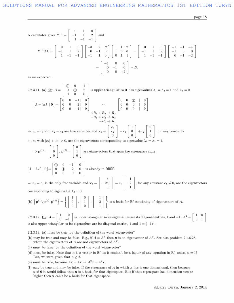
A calculator gives P−1 = 12
−1 1 20 0 21 1 −2
and
P−1AP =1
2
−1 1 20 0 21 1 −2
1 5 −105 1 −100 0 −4
−1 2 11 0 10 1 0
=1
2
−1 1 20 0 21 1 −2
4 −8 6−4 0 6
0 −4 0
=
1
2
−8 0 00 −8 00 0 12
=
−4 0 00 −4 00 0 6
= D,
as we expected.
2.2.3.9. It turns out that we can do the problem in a straight forward way without the given information that −1and 3 are eigenvalues. Expanding along the third row,
0 =
∣∣∣∣∣∣3− λ 0 −12
4 −1− λ −120 0 −1− λ
∣∣∣∣∣∣ = (−1− λ)
∣∣∣∣ 3− λ 04 −1− λ
∣∣∣∣ = (−1− λ)(3− λ)(−1− λ)
⇒ eigenvalues are λ1 = λ2 = −1, λ3 = 3.
[A− λ1I | 0 ] =
4 0 −12 | 04 0 −12 | 00 0 0 | 0
∼
−R1 +R2 → R2
4−1R1 → R1
1© 0 −3 | 00 0 0 | 00 0 0 | 0
⇒ x2 = c1 and x3 = c2 are free variables and v1 =
3c2c1c2
= c1
010
+ c2
301
, for anyconstants c1, c2 with |c1|+ |c2| > 0, are the eigenvectors corresponding to eigenvalue λ1 = λ2 = −1.
⇒ p(1) =
010
, p(2) =
301
are eigenvectors that span the eigenspace Eλ=−1.
[A− λ3I | 0 ]=
0 0 −12 | 04 −4 −12 | 00 0 −4 | 0
∼
R1 ↔ R2
4−1R1 → R1
1© −1 −3 | 00 0 −12 | 00 0 −4 | 0
∼
(−12)−1R2 → R3
3R2 +R1 → R1
4R2 +R3 → R3
1© −1 0 | 00 0 1©| 00 0 0 | 0
c©Larry Turyn, January 2, 2014
SOLUTIONS MANUAL FOR ADVANCED ENGINEERING MATHEMATICS 1ST EDITION TURYN
page 17
⇒ x3 = 0 and x2 = c1 is the only free variable and v3 =
c1c10
= c1
110
, for any constant c1 6= 0, are the
eigenvectors corresponding to eigenvalue λ3 = 3.
The matrix P = [p(1) pp p
(2) pp p
(3) ] =
0 3 11 0 10 1 0
should diagonalize A.
A calculator gives P−1 =
−1 1 30 0 11 0 −3
and
P−1AP =
−1 1 30 0 11 0 −3
3 0 −124 −1 −120 0 −1
0 3 11 0 10 1 0
=
−1 1 30 0 11 0 −3
0 −3 3−1 0 3
0 −1 0
=
−1 0 00 −1 00 0 3
= D,
as we expected.
2.2.3.10. It turns out that we can do the problem in a straight forward way without the given information that −1is an eigenvalue. Expanding along the second row,
0 =
∣∣∣∣∣∣−3− λ 2 2
0 −1− λ 0−1 1 −λ
∣∣∣∣∣∣ = (−1− λ)
∣∣∣∣ −3− λ 2−1 −λ
∣∣∣∣ = (−1− λ)(
(−3− λ)(−λ) + 2)
= (−1− λ)(λ2 + 3λ+ 2) = (−1− λ)(λ+ 1)(λ+ 2)
⇒ eigenvalues are λ1 = λ2 = −1, λ3 = −2.
[A− λ1I | 0 ] =
−2 2 2 | 00 0 0 | 0−1 1 1 | 0
∼
− 12R1 → R1
R1 +R2 → R2
1© −1 −1 | 00 0 0 | 00 0 0 | 0
⇒ x2 = c1 and x3 = c2 are free variables and v1 =
c1 + c2c1c2
= c1
110
+ c2
101
, for anyconstants c1, c2 with |c1|+ |c2| > 0, are the eigenvectors corresponding to eigenvalue λ1 = λ2 = −1.
⇒ p(1) =
110
, p(2) =
101
are eigenvectors that span the eigenspace Eλ=−1.
[A− λ3I | 0 ]=
−1 2 2 | 00 1 0 | 0−1 1 2 | 0
∼
−2R2 +R1 → R1
−R2 +R3 → R3
−R1 +R3 → R3
−R1 → R1
1© 0 −2 | 00 1© 0 | 00 0 0 | 0
⇒ x2 = 0 and x3 = c1 is the only free variable and v3 =
2c10c1
= c1
201
, for any constant c1 6= 0, are the
eigenvectors corresponding to eigenvalue λ3 = −2.
The matrix P = [p(1) pp p
(2) pp p
(3) ] =
1 1 21 0 00 1 1
should diagonalize A.
c©Larry Turyn, January 2, 2014
SOLUTIONS MANUAL FOR ADVANCED ENGINEERING MATHEMATICS 1ST EDITION TURYN
page 18
A calculator gives P−1 =
0 1 0−1 1 2
1 −1 −1
and
P−1AP =
0 1 0−1 1 2
1 −1 −1
−3 2 20 −1 0−1 1 0
1 1 21 0 00 1 1
=
0 1 0−1 1 2
1 −1 −1
−1 −1 −4−1 0 0
0 −1 −2
=
−1 0 00 −1 00 0 −2
= D,
as we expected.
2.2.3.11. (a) Ex: A =
1© 0 −10 1© 20 0 0
is upper triangular so it has eigenvalues λ1 = λ2 = 1 and λ3 = 0.
[A− λ1I | 0 ] =
0 0 −1 | 00 0 2 | 00 0 −1 | 0
∼
2R1 +R2 → R2
−R1 +R3 → R3
−R1 → R1
0 0 1© | 00 0 0 | 00 0 0 | 0
⇒ x1 = c1 and x2 = c2 are free variables and v1 =
c1c20
= c1
100
+ c2
010
, for any constants
c1, c2 with |c1|+ |c2| > 0, are the eigenvectors corresponding to eigenvalue λ1 = λ2 = 1.
⇒ p(1) =
100
, p(2) =
010
are eigenvectors that span the eigenspace Eλ=1.
[A− λ3I | 0 ]=
1© 0 −1 | 00 1© 2 | 00 0 0 | 0
is already in RREF.
⇒ x3 = c1 is the only free variable and v3 =
c1−2c1c1
= c1
1−2
1
, for any constant c1 6= 0, are the eigenvectors
corresponding to eigenvalue λ3 = 0.
(b){p(1),p(2),p(3)
}=
1
00
, 0
10
, 1−2
1
is a basis for R3 consisting of eigenvectors of A.
2.2.3.12. Ex: A =
[1 00 −1
]is upper triangular so its eigenvalues are its diagonal entries, 1 and −1. A2 =
[1 00 1
]is also upper triangular so its eigenvalues are its diagonal entries, 1 and 1 = (−1)2.
2.2.3.13. (a) must be true, by the definition of the word “eigenvector”(b) may be true and may be false. E.g., if A = AT then x is an eigenvector of AT . See also problem 2.1.6.28,
where the eigenvectors of A are not eigenvectors of AT .(c) must be false, by the definition of the word “eigenvector”(d) must be false. Note that x is a vector in Rn so it couldn’t be a factor of any equation in Rn unless n = 1!
But, we were given that n ≥ 2.(e) must be true, because Ax = λx ⇒ A2x = λ2x
(f) may be true and may be false. If the eigenspace of A in which x lies is one dimensional, then becausex 6= 0 it would follow that x is a basis for that eigenspace. But if that eigenspace has dimension two orhigher then x can’t be a basis for that eigenspace.
c©Larry Turyn, January 2, 2014
SOLUTIONS MANUAL FOR ADVANCED ENGINEERING MATHEMATICS 1ST EDITION TURYN
page 19
(g) may be true and may be false. Because B is similar to A there is an invertible matrix P with B = P−1AP .If Ax = λx and x 6= 0, then Bx = P−1APx. If Px = βx and β 6= 0, then P−1x = β−1x and
Bx = P−1APx = P−1Aβx = P−1λβx = λβP−1x = λββ−1x = λx,
so x would be an eigenvector of B, too. But, on the other hand, if Px is not an eigenvector of A then xis not an eigenvector of B, by Theorem 2.11 in Section 2.2.
2.2.3.14. A =
[29 18−50 −31
]. Suppose there were an invertible matrix P that diagonalizes A, so that D = P−1AP .
By Theorem 2.11 in Section 2.2, the eigenvalues of D must be the eigenvalues of A. But in Example 2.16 in Section2.2, we saw that the only eigenvalue of A is λ = −1. Because D is diagonal, its diagonal entries are its eigenvalues.
Putting together what we know so far, we must have D =
[−1 0
0 −1
].
Let P =
[a bc d
]. We have
[29a+ 18c 29b+ 18d−50a− 31c −50b− 31d
]=
[29 18−50 −31
] [a bc d
]= AP = PD =
[a bc d
] [−1 0
0 −1
]=
[−a −b−c −d
].
It follows that 29a+ 18c = −a, hence c = − 53a, and also 29b+ 18d = −b, hence d = − 5
3b. So, the invertible matrix
P has
0 6= |P | =∣∣∣∣ a bc d
∣∣∣∣ =
∣∣∣∣ a b− 5
3a − 5
3b
∣∣∣∣ = a(− 5
3b)− b(− 5
3a)
= 0,
giving a contradiction. So, no, there is no invertible matrix P that diagonalizes the matrix A of Example 2.16 inSection 2.2.
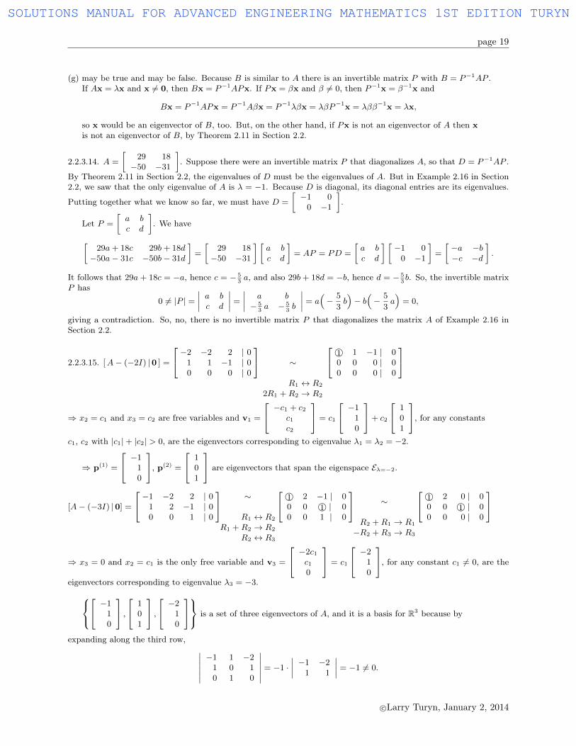
2.2.3.15. [A− (−2I) |0 ] =
−2 −2 2 | 01 1 −1 | 00 0 0 | 0
∼
R1 ↔ R2
2R1 +R2 → R2
1© 1 −1 | 00 0 0 | 00 0 0 | 0
⇒ x2 = c1 and x3 = c2 are free variables and v1 =
−c1 + c2c1c2
= c1
−110
+ c2
101
, for any constants
c1, c2 with |c1|+ |c2| > 0, are the eigenvectors corresponding to eigenvalue λ1 = λ2 = −2.
⇒ p(1) =
−110
, p(2) =
101
are eigenvectors that span the eigenspace Eλ=−2.
[A− (−3I) |0] =
−1 −2 2 | 01 2 −1 | 00 0 1 | 0
∼
R1 ↔ R2
R1 +R2 → R2
R2 ↔ R3
1© 2 −1 | 00 0 1© | 00 0 1 | 0
∼
R2 +R1 → R1
−R2 +R3 → R3
1© 2 0 | 00 0 1© | 00 0 0 | 0
⇒ x3 = 0 and x2 = c1 is the only free variable and v3 =
−2c1c10
= c1
−210
, for any constant c1 6= 0, are the
eigenvectors corresponding to eigenvalue λ3 = −3. −1
10
, 1
01
, −2
10
is a set of three eigenvectors of A, and it is a basis for R3 because by
expanding along the third row, ∣∣∣∣∣∣−1 1 −2
1 0 10 1 0
∣∣∣∣∣∣ = −1 ·∣∣∣∣ −1 −2
1 1
∣∣∣∣ = −1 6= 0.
c©Larry Turyn, January 2, 2014
SOLUTIONS MANUAL FOR ADVANCED ENGINEERING MATHEMATICS 1ST EDITION TURYN

page 20
2.2.3.16. (a) B = P−1AP ⇒ |B| = |P−1AP | = |P−1| |A| |P | = 1
|P | |A| |P | = |A|
(b) No, the converse is not true. Ex: A =
[1 00 1
]and B =
[2 00 0.5
]both have determinant equal to one. But
A cannot be similar to B because the eigenvalues of A are 1 and 1 while the eigenvalues of B are 2 and 0.5. (Similarmatrices must have the same eigenvalues.)
2.2.3.17. Because n = 3, the geometric multiplicity of A’s eigenvalue µ1 = 2 is m1 = n− rank(A− 2I3) = 3− 2 = 1and the geometric multiplicity of A’s eigenvalue µ2 = 3 is m2 = n−rank(A−3I3) = 3−1 = 2. Because m1 +m2 = n,it follows that the corresponding algebraic multiplicities are α1 = 1 and α2 = 2.
To finish the work, we have a choice of two different methods:Method I: The algebraic multiplicities imply both that the eigenvalues of A are 2, 3, 3, counting multiplicity, andthat the characteristic polynomial of A is P(λ) = (2 − λ)(3 − λ)2. Using the result of problem 2.1.6.20, or arguingdirectly from P(λ), we conclude that |A| = λ1λ2λ3 = 2 · 3 · 3 = 18.
Method II: The geometric multiplicities of the eigenvalues of A add up to 3, which equals n, so A is diagonalizablewith A being similar to D = diag(2, 3, 3). By the result of problem 2.2.3.16(a), |A| = |D| = 2 · 3 · 3 = 18.
2.2.3.18. [A− (−1)I) |0 ] ∼
1 −2 3 5 | 00 0 1 4 | 00 0 0 0 | 00 0 0 0 | 0
∼
−3R2 +R1 → R1
1© −2 0 −7 | 00 0 1© 4 | 00 0 0 0 | 00 0 0 0 | 0
⇒ x2 = c1 and x4 = c2 are free variables and v1 =
2c1 + 7c2
c1−4c2c2
= c1
2100
+ c2
70−4
1
, for any constants
c1, c2 with |c1|+ |c2| > 0, are the eigenvectors corresponding to eigenvalue µ = −1.
⇒ eigenspace Eµ=−1 has basis
2100
,
70−4
1
.
2.2.3.19. S2 = S · S = (P diag(√λ1, ...,
√λn) P−1)(P diag(
√λ1, ...,
√λn) P−1)
= P diag(√λ1, ...,
√λn) (P−1P ) diag(
√λ1, ...,
√λn) P−1
= P diag(√λ1, ...,
√λn) (I) diag(
√λ1, ...,
√λn) P−1
= P (diag(√λ1, ...,
√λn) · diag(
√λ1, ...,
√λn) P−1 = P (diag
((√λ1
)2, ...,
(√λn)2)
P−1
= Pdiag(λ1, ..., λn
)P−1 = A.
2.2.3.20. Yes. B = P−1AP ⇒ PB = (PP−1)AP = (I)AP = AP⇒ PBP−1 = (PB)P−1 = (AP )P−1 = A(PP−1) = A(I) = A.
2.2.3.21. Use the two given eigenvectors to form the matrix P = [p(1) pp p
(2) ] =
[−5 4
1 1
]that diagonalizes A. For
example, if A is similar to the diagonal matrix D =
[9 00 27
], then the result of problem 2.2.3.20 gives
A = PDP−1 =
[−5 4
1 1
] [9 00 27
] [−5 4
1 1
]−1
=
[−5 4
1 1
] [9 00 27
](1
−9
[1 −4−1 −5
])
=
[−5 4
1 1
] [−1 0
0 −3
] [1 −4−1 −5
]=
[−5 4
1 1
] [−1 4
3 15
]=
[17 402 19
].
c©Larry Turyn, January 2, 2014
SOLUTIONS MANUAL FOR ADVANCED ENGINEERING MATHEMATICS 1ST EDITION TURYN

page 21
2.2.3.22. By expanding along the second row,
0 = |A− λI | =
∣∣∣∣∣∣2− λ 0 1
0 −5− λ 03 0 2− λ
∣∣∣∣∣∣ = (−5− λ)
∣∣∣∣ 2− λ 13 2− λ
∣∣∣∣ = (−5− λ)(
(2− λ)2 − 3)
⇒ the eigenvalues of A are λ1 = −5, λ2 = 2 +√
3, λ3 = 2−√
3.
[A− λ1I |0 ] =
7 0 1 | 00 0 0 | 03 0 7 | 0
∼
7−1R1 → R1
−3R1 +R3 → R3
R2 ↔ R3
1© 0 1/7 | 00 0 46/7 | 00 0 0 | 0
∼
746R2 → R2
− 17R2 +R1 → R1
1© 0 0 | 00 0 1© | 00 0 0 | 0
⇒ x1 = x3 = 0 and x2 = c1 is the only free variable and v1 =
0c10
= c1
010
, for any constant c1 6= 0, are the
eigenvectors corresponding to eigenvalue λ1 = −5.[A− λ2I |0 ]=
−√
3 0 1 | 0
0 −7−√
3 0 | 0
3 0 −√
3 | 0
∼
(−7−√
3)−1R2 → R2
(−√
3)−1R1 → R1
−3R1 +R3 → R3
1© 0 − 1√3| 0
0 1© 0 | 00 0 0 | 0
⇒ x2 = 0 and x3 = c1 is the only free variable and v2 =
1√3c1
0c1
= c1
1√3
01
, for any constant c1 6= 0, are the
eigenvectors corresponding to eigenvalue λ2 = 2 +√
3.
[A− λ3I |0 ]=
√
3 0 1 | 0
0 −7 +√
3 0 | 0
3 0√
3 | 0
∼
(−7 +√
3)−1R2 → R2
(√
3)−1R1 → R1
−3R1 +R3 → R3
1© 0 1√3| 0
0 1© 0 | 00 0 0 | 0
⇒ x2 = 0 and x3 = c1 is the only free variable and v3 =
− 1√3c1
0c1
= c1
− 1√3
01
, for any constant c1 6= 0, are
the eigenvectors corresponding to eigenvalue λ3 = 2−√
3.
(b) Because A has three distinct eigenvalues and n = 3, A has a set of eigenvectors that is a basis for R3, by Theorem2.7(c) in Section 2.2.
2.2.3.23. (a) A is 3× 3 and three eigenvalues, 2,−2,√
3 are given, so those are the only eigenvalues and the charac-teristic polynomial is PA(λ) = (2− λ)(−2− λ)(
√3− λ).
(b) We were given that Ax1 = 2x1, Ax2 = −2x2, and Ax3 =√
3x3. Because these are eigenvectors correspondingto distinct eigenvalues of A, {x1,x2,x3} is a linearly independent set.
It follows that A2x1 = 4x1, A2x2 = 4x2, and A2x3 = 3x3. So, x1, x2, and x3 are also eigenvectors of A2 andwe already know that {x1,x2,x3} is a linearly independent set. So, {x1,x2,x3} is a linearly independent set ofeigenvectors of A2.(c) Because {x1,x2,x3} is a linearly independent set of eigenvectors of A2 corresponding to eigenvalues 4, 4, and 3,respectively, it follows that the characteristic polynomial of A2 is PA2(λ) = (4− λ)(4− λ)(3− λ).
2.2.3.24. (a) Use (A− λ1I)(A− λ3I) · · · (A− λnI). How? Suppose 0 = c1x(1) + c2x
(2) + ...+ cnx(n). If we multiply
c©Larry Turyn, January 2, 2014
SOLUTIONS MANUAL FOR ADVANCED ENGINEERING MATHEMATICS 1ST EDITION TURYN
page 22
on the left by the matrix (A− λ1I)(A− λ3I) · · · (A− λnI), we have
0 = c1(A− λ1I)(A− λ3I) · · · (A− λnI)x(1) + c2(A− λ1I)(A− λ3I) · · · (A− λnI)x(2) + ...+
+cn(A− λ1I)(A− λ3I) · · · (A− λnI)x(n)
= c1(λ1 − λ1)(λ1 − λ3) · · · (λ1 − λn)x(1) + c2(λ2 − λ1)(λ2 − λ3) · · · (λ2 − λn)x(2) + ...+
+cn(λn − λ1)(λn − λ3) · · · (λn − λn)x(n)
= 0 + c2(λ2 − λ1)(λ2 − λ3) · · · (λ2 − λn)x(2) + 0 + ...+ 0.
Because the eigenvalues were assumed to be distinct, and x(2) 6= 0, it follows that c2 = 0.
(b) Use (A− λ1I)(A− λ2I) · · · (A− λn−1I). How? Suppose 0 = c1x(1) + c2x
(2) + ...+ cnx(n). If we multiply on the
left by the matrix (A− λ1I)(A− λ2I) · · · (A− λn−1I), we have
0 = c1(A− λ1I)(A− λ2I) · · · (A− λn−1I)x(1) + c2(A− λ1I)(A− λ2I) · · · (A− λn−1I)x(2) + ...+
+cn(A− λ1I)(A− λ2I) · · · (A− λn−1I)x(n)
= c1(λ1 − λ1)(λ1 − λ2) · · · (λ1 − λn−1)x(1) + c2(λ2 − λ1)(λ2 − λ2) · · · (λ2 − λn−1)x(2) + ...+
+cn(λn − λ1)(λn − λ2) · · · (λn − λn−1)x(n)
= 0 + ...+ 0 + cn(λn − λ1)(λn − λ2) · · · (λn − λn−1)x(n).
Because the eigenvalues were assumed to be distinct, and x(n) 6= 0, it follows that cn = 0.
2.2.3.25. Use multiplication on the left by (A− µ2I)(A− µ3I) · · · (A− µpI). Why? Suppose
0 = c1,1x1,1 + ...+ c1,m1x
1,m1 + c2,1x2,1 + ...+ c2,m2x
2,m2 + ...+ cp,1xp,1 + ...+ cp,mpx
p,mp .
If we multiply on the left by the matrix (A− µ2I)(A− µ3I) · · · (A− µpI), we have
0 = (A− µ2I)(A− µ3I) · · · (A− µpI)(c1,1x1,1 + ...+ c1,m1x
1,m1)+
+(A− µ2I)(A− µ3I) · · · (A− µpI)(c2,1x2,1 + ...+ c2,m2x
2,m2) + ...+
+(A− µ2I)(A− µ3I) · · · (A− µpI)(cp,1xp,1 + ...+ cp,mpx
p,mp)
= (µ1 − µ2) · · · (µ1 − µp)(c1,1x1,1 + ...+ c1,m1x1,m1) + (µ2 − µ2) · · · (µ2 − µp)(c2,1x2,1 + ...+ c2,m2x
2,m2)+
+...+ (µp − µ2) · · · (µp − µp)(cp,1xp,1 + ...+ cp,mpxp,mp)
= (µ1 − µ2) · · · (µ1 − µp)(c1,1x1,1 + ...+ c1,m1x1,m1) + 0 + ...+ 0
Because the µ1, ..., µp were assumed to be distinct, it follows that c1,1x1,1 + ...+ c1,m1x1,m1 = 0.
But, in Theorem 2.7(a) in Section 2.2 we also assumed that {x1,1, ..,x1,m1} is linearly independent. This impliesthat c1,1 = · · · = c1,m1 = 0.
2.2.3.26. No, R3 cannot have a basis of eigenvectors all of which have 0 in their first component, because a basis mustspan R3 but [ 1 0 0 ]T would not be in that span.
2.2.3.27. By expanding along the first column,
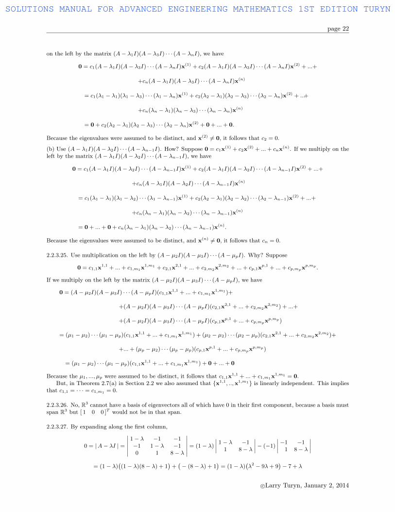
0 = |A− λI | =
∣∣∣∣∣∣1− λ −1 −1−1 1− λ −10 1 8− λ
∣∣∣∣∣∣ = (1− λ)
∣∣∣∣ 1− λ −11 8− λ
∣∣∣∣− (−1)
∣∣∣∣ −1 −11 8− λ
∣∣∣∣= (1− λ)
((1− λ)(8− λ) + 1
)+(− (8− λ) + 1
)= (1− λ)
(λ2 − 9λ+ 9
)− 7 + λ
c©Larry Turyn, January 2, 2014
SOLUTIONS MANUAL FOR ADVANCED ENGINEERING MATHEMATICS 1ST EDITION TURYN
page 23
= −λ3 + 10λ2 − 18λ+ 9− 7 + λ = −λ3 + 10λ2 − 17λ+ 2 , P(λ).
Standard advice for factoring polynomials suggests trying λ = ±1,±2. We find that P(1) = −6, P(−1) = 30,P(2) = 0. The latter implies 2 is an eigenvalue and enables factoring
P(λ) = (2− λ)(λ2 − 8λ+ 1).
The quadratic equation λ2 − 8λ+ 1 = 0 has solutions λ =8±√
60
2= 4±
√15.
Because there are three distinct eigenvalues, 2, 4 ±√
15, for this 3 × 3 matrix, theory in Section 2.2 guaranteesthat A has a set of three linearly independent eigenvectors.
c©Larry Turyn, January 2, 2014
SOLUTIONS MANUAL FOR ADVANCED ENGINEERING MATHEMATICS 1ST EDITION TURYN
page 24
Section 2.3.4
2.3.4.1. Denote a1 =
[11
]and a2 =
[20
]. To start the Gram-Schmidt process, let
v1, a1, r11, ||v1|| =√
2, q1= r−111 v1=
1√2
[11
].
Next, let
v2 , a2 − (a2 • q1)q1 =
[20
]−([
20
]• 1√
2
[11
])1√2
[11
]=
[20
]−(
2√2
)1√2
[11
]=
[1−1
],
r22 , ||v2|| =√
2, and
q2= r−122 v2=
1√2
[1−1
].
According to Theorem 2.16 in Section 2.3, the o.n. set{1√2
[11
],
1√2
[1−1
]}
has span equal to the span of the given set of vectors,{[
11
],
[20
]}.
2.3.4.2. Denote a1 =
101
, a2 =
011
, and a3 =
111
. To start the Gram-Schmidt process, let
v1, a1, r11, ||v1|| =√
2, q1= r−111 v1=
1√2
101
.Next, let
v2 , a2 − (a2 • q1)q1 =
011
− 0
11
• 1√2
101
1√2
101
=
011
− ( 1√2
)1√2
101
=1
2
−121
,r22 , ||v2|| =
√62, and
q2= r−122 v2=
1√6
−121
.Further, let
v3 , a3 − (a3 • q1)q1 − (a3 • q2)q2
=
111
− 1
11
• 1√2
101
1√2
101
− 1
11
• 1√6
−121
1√6
−121
=
111
− ( 2√2
)1√2
101
− ( 2√6
)1√6
−121
=1
3
11−1
,r33 , ||v3|| = 1√
3, and
q3= r−133 v3=
1√3
11−1
.According to Theorem 2.16 in Section 2.3, the o.n. set 1√
2
101
, 1√6
−121
, 1√3
11−1
c©Larry Turyn, January 2, 2014
SOLUTIONS MANUAL FOR ADVANCED ENGINEERING MATHEMATICS 1ST EDITION TURYN
page 25
has span equal to the span of the given set of vectors,
1
01
, 0
11
, 1
11
.
2.3.4.3. Denote a1 =
−120
, a2 =
21−1
, and a3 =
102
. To start the Gram-Schmidt process, let
v1, a1, r11, ||v1|| =√
5,
and
q1 = r−111 v1 =
1√5
−120
.Next, let
v2 , a2 − (a2 • q1)q1 =
21−1
− 2
1−1
• 1√5
−120
1√5
−120
=
21−1
− 0 · 1√5
−120
=
21−1
,r22 , ||v2|| =
√6, and
q2= r−122 v2=
1√6
21−1
.Further, let
v3 , a3 − (a3 • q1)q1 − (a3 • q2)q2
=
102
− 1
02
• 1√5
−120
1√5
−120
− 1
02
• 1√6
21−1
1√6
21−1
=
102
− (−1√5
)1√5
−120
− 0 · 1√6
21−1
=1
5
42
10
=2
5
215
,r33 , ||v3|| = 2
√305
, and
q3= r−133 v3=
1√30
215
.According to Theorem 2.16 in Section 2.3, the o.n. set 1√
5
−120
, 1√6
21−1
, 1√30
215
has span equal to the span of the given set of vectors,
−1
20
, 2
1−1
, 1
02
.
2.3.4.4. Denote a1 =
1−1
1
, a2 =
11−1
, and a3 =
−111
. To start the Gram-Schmidt process, let
v1, a1, r11, ||v1|| =√
3, q1= r−111 v1=
1√3
1−1
1
.Next, let
v2 , a2 − (a2 • q1)q1 =
11−1
− 1
1−1
• 1√3
1−1
1
1√3
1−1
1
c©Larry Turyn, January 2, 2014
SOLUTIONS MANUAL FOR ADVANCED ENGINEERING MATHEMATICS 1ST EDITION TURYN
page 26
=
11−1
− (−1√3
)1√3
1−1
1
=1
3
42−2
=2
3
21−1
,r22 , ||v2|| = 2
√6
3, and
q2= r−122 v2=
1√6
21−1
.Further, let
v3 , a3 − (a3 • q1)q1 − (a3 • q2)q2
=
−111
− −1
11
• 1√3
1−1
1
1√3
1−1
1
− −1
11
• 1√6
21−1
1√6
21−1
=
−111
− (−1√3
)1√3
1−1
1
− (−2√6
)1√6
21−1
=
011
,r33 , ||v3|| =
√2, and
q3= r−133 v3=
1√2
011
.According to Theorem 2.16 in Section 2.3, the o.n. set 1√
3
1−1
1
, 1√6
21−1
, 1√2
011
has span equal to the span of the given set of vectors,
1−1
1
, 1
1−1
, −1
11
.
2.3.4.5. Denote a1 =
[3−4
]and a2 =
[1√2
]. To start the Gram-Schmidt process, let
v1, a1, r11, ||v1|| = 5, q1= r−111 v1=
1
5
[3−4
].
Next, let
v2 , a2 − (a2 • q1)q1 =
[1√2
]−([
1√2
]• 1
5
[3−4
])1
5
[3−4
]=
[1√2
]−(
3− 4√
2
5
)1
5
[3−4
]
=1
25
[16 + 12
√2
12 + 9√
2
]=
4 + 3√
2
25
[43
],
r22 , ||v2|| = 4+3√2
5, and
q2= r−122 v2=
1
5
[43
].
According to Theorem 2.16 in Section 2.3, the o.n. set
S =
{1
5
[3−4
],
1
5
[43
]}
has span equal to the span of the given set of vectors,{[
3−4
],
[1√2
]}.
c©Larry Turyn, January 2, 2014
SOLUTIONS MANUAL FOR ADVANCED ENGINEERING MATHEMATICS 1ST EDITION TURYN

page 27
2.3.4.6. (a) We were given a1 =
211
, a2 =
110
, and a3 =
102
. To start the Gram-Schmidt process, let
v1, a1, r11, ||v1|| =√
6, q1= r−111 v1=
1√6
211
.Next, let
v2 , a2 − (a2 • q1)q1 =
110
− 1
10
• 1√6
211
1√6
211
=
110
− ( 3√6
)1√6
211
=1
2
01−1
,r22 , ||v2|| =
√22, and
q2= r−122 v2=
1√2
01−1
.Further, let
v3 , a3 − (a3 • q1)q1 − (a3 • q2)q2
=
102
− 1
02
• 1√6
211
1√6
211
− 1
02
• 1√2
01−1
1√2
01−1
=
102
− ( 4√6
)1√6
211
− (−2√2
)1√2
01−1
=1
3
−111
,r33 , ||v3|| =
√2, and
q3= r−133 v3=
1√3
−111
.According to Theorem 2.16 in Section 2.3, the o.n. set 1√
6
211
, 1√2
01−1
, 1√3
−111
has span equal to the span of the vectors, a1 =
211
, a2 =
110
, a3 =
102
.
(b) We were given w1 = a2 =
110
, w2 = a3 =
102
, and w3 = a1 =
211
. To start the Gram-Schmidt
process, let
V1, a1, R11, ||V1||=√
2, q1= R−111 V1=
1√2
110
.Next, let
V2 , w2 − (w2 • q1)q1 =
102
− 1
02
• 1√2
110
1√2
110
=
102
− ( 1√2
)1√2
110
=1
2
1−1
4
,R22 , ||V2|| =
√182
, and
q2= R−122 V2=
1√18
1−1
4
.
c©Larry Turyn, January 2, 2014
SOLUTIONS MANUAL FOR ADVANCED ENGINEERING MATHEMATICS 1ST EDITION TURYN
page 28
Further, letV3 , w3 − (w3 • q1)q1 − (w3 • q2)q2
=
211
− 2
11
• 1√2
110
1√2
110
− 2
11
• 1√18
1−1
4
1√18
1−1
4
=
211
− ( 3√2
)1√2
110
− ( 5√18
)1√18
1−1
4
=
1
18
4−4−2
,R33 , ||V3|| = 1
3, and
q3= R−133 V3=
1
6
4−4−2
=1
3
2−2−1
.According to Theorem 2.16 in Section 2.3, the o.n. set 1√
2
110
, 1√18
1−1
4
, 1
3
2−2−1
has span equal to the span of the vectors, w1 =
211
, w2 =
110
, w3 =
102
.The results of parts (a) and (b) show that the o.n. set that we get depends on the order in which we list the three
given vectors (whose span we wish to equal using the span of the vectors in the o.n. set).
2.3.4.7. Ex: G-S. on{[
10
],
[11
]}yields
{[10
],
[01
]}, while G-S. on
{[11
],
[10
]}yields
{1√2
[11
], 1√
2
[1−1
]}.
2.3.4.8. To start the Gram-Schmidt process, let
v1, a1, r11, ||v1|| = ||a1||, q1= r−111 v1.
Next, let
v2 , a2 − (a2 • q1)q1 = a2 − (a2 • r−111 a1)r−1
11 a1 = a2 − r−211 (a2 • a1)a1 = a2 − r−2
11 ·1
3· a1.
Sor22, ||v2|| =
∣∣∣∣∣∣∣∣a2 −1
3r−211 a1
∣∣∣∣∣∣∣∣and
q2 =1
r22
(a2 −
1
3||a1||2a1
).
We could go further and calculate that
r222, ||v2||2 =
∣∣∣∣∣∣∣∣a2 −1
3r−211 a1
∣∣∣∣∣∣∣∣2 =
⟨a2 −
1
3r−211 a1, a2 −
1
3r−211 a1
⟩= ||a2||2 −
2
3r−211 〈a2, a1〉+
∣∣∣∣∣∣∣∣13 r−211 a1
∣∣∣∣∣∣∣∣2= ||a2||2 −
2
3r−211 ·
1
3+(1
3r−211
)2||a1||2 = ||a2||2 −
2
9r−211 +
1
9r−411 · r
211 = ||a2||2 −
1
9r−211
that is,
r222 = ||a2||2 −1
9||a1||−2.
2.3.4.9. We calculate〈x,x + y − z〉 = 〈x,x〉+ 〈x,y〉 − 〈x, z〉 = ||x ||2 + 〈x,y〉 − 〈x, z〉,
c©Larry Turyn, January 2, 2014
SOLUTIONS MANUAL FOR ADVANCED ENGINEERING MATHEMATICS 1ST EDITION TURYN
page 29
〈y,y + z− x〉 = 〈y,y〉+ 〈y, z〉 − 〈y,x〉 = ||y ||2 + 〈y, z〉 − 〈y,x〉,and
〈z, z + x− y〉 = 〈z, z〉+ 〈z,x〉 − 〈z,y〉 = || z ||2 + 〈z,x〉 − 〈z,y〉.So,
〈x,x+y−z〉+ 〈y,y+z−x〉+ 〈z, z+x−y〉 = ||x ||2 +���〈x,y〉−���〈x, z〉+ ||y ||2 +���〈y, z〉−���〈y,x〉+ || z ||2 +���〈z,x〉−���〈z,y〉
= ||x ||2 + ||y ||2 + ||z||2.Yes,
〈x,x + y − z〉+ 〈y,y + z− x〉+ 〈z, z + x− y〉 = ||x ||2 + ||y ||2 + ||z||2
is true for all vectors x,y, z.
2.3.4.10. (i)(a) and (b) If n = 2 or n = 3, in fact for any n ≥ 1, the given data x ⊥ y and y ⊥ z imply
〈 (x + z),y〉 = 〈x,y〉+ 〈z,y〉 = 0 + 0 = 0,
so (x + z) ⊥ y.(ii) (a) If n = 2, then x ‖ z. Why?
First, will give an intuitive argument why this should be true, but to be honest this intuitive reasoning is not100% persuasive, as we will see later when discussing the case n = 3.
Note that x ⊥ y implies the angle between x and y is ±90◦, and y ⊥ z implies the angle between y and z is±90◦. Because the nonzero vectors x, y, and z are all in R2, the angle between x and z is −180◦, 0◦, or 180◦, thesum or the difference of the angle between x and y and the angle between y and z. Because the angle between x andz is an integer multiple of 180◦, we conclude that x ‖ z.
Here is completely persuasive reasoning : Because x ⊥ y and x, y are nonzero vectors in R2, the set of vectors{x,y} is a basis for R2. Why? From Theorem 1.43 in Section 1.7, it will suffice to explain why {x,y} is a linearlyindependent set of vectors in R2: Suppose 0 = αx + βy for some scalars α, β. Then x ⊥ y would imply
0 = 0 • x = αx • x + βy • x = α||x||2 + β · 0 = α||x||2,
hence α = 0 because x 6= 0. Similarly,
0 = 0 • y = αx • y + βy • y = α · 0 + β||y||2 = β||y||2,
hence β = 0 because y 6= 0. So, 0 = αx + βy implies α = β = 0. By definition, {x,y} is a linearly independent setof vectors in R2.
It follows that there exists constants c1, c2 such that
z = c1x + c2y.
It follows from x ⊥ y thatz • x = c1x • x + c2y • x = c1x • x + c2 · 0,
soz • x = c1x • x = c1||x||2.
Similarly, it follows from y ⊥ z that
z • y = c1x • y + c2y • y = c1 · 0 + c2y • y,
soz • y = c2||y||2.
It follows thatz =
z • x||x||2 x +
z • y||y||2 y.
But, z ⊥ y implies z • y = 0, soz =
z • x||x||2 x.
It follows that(?) ||z|| =
∣∣∣∣ z • x||x||2
∣∣∣∣ ||x|| = |z • x|||x||2 ||x|| =|z • x|||x|| .
c©Larry Turyn, January 2, 2014
SOLUTIONS MANUAL FOR ADVANCED ENGINEERING MATHEMATICS 1ST EDITION TURYN

page 30
But the Cauchy-Schwarz inequality implies|z • x| ≤ ||x|| ||z||,
with equality only if x ‖ z. This, combined with (?), implies
||z|| = |z • x|||x|| ≤||x|| ||z||||x|| = ||z||.
hence equality holds throughout. This implies that equality holds in the Cauchy-Schwarz inequality, hence x ‖ z.
(ii) (b) If n = 3, then it does not follow x ‖ z. Here’s an example: x = e(1), y = e(2), and z = e(3).So, why does the intuitive argument we gave for n = 2 not work for n = 3? I.e., why does the angle between x
and y being ±90◦ and the angle between y and z being ±90◦ not imply that the angle between x and z −180◦, 0◦,or 180◦, the sum or the difference of the angle between x and y and the angle between y and z.
Perhaps you can explain the error in the reasoning for n = 3. In any case, it points out why we have theresponsibility for explaining why something is true; we cannot “turn the tables” and claim that “something is trueuntil proven otherwise."
(iii)(a) and (b) If n = 2 or n = 3, x ⊥ (−y), because
x • (−y) = x • (−1 · y) = −1 · x • y = −1 · 0 = 0.
2.3.4.11. (a) To start the Gram-Schmidt process, let
v1, a1, r11, ||v1|| =√a1 • a1 =
√2,
andq1 = r−1
11 v1 =1√2a1.
Next, let
v2 , a2 − (a2 • q1)q1 = a2 −(a2 •
1√2a1
) 1√2a1 = a2 −
1
2(a2 • a1)a1 = a2 −
3
2a1.
So
r222,||v2||2=
∣∣∣∣∣∣∣∣a2 −3
2a1
∣∣∣∣∣∣∣∣2= ⟨a2 −3
2a1, a2 −
3
2a1
⟩= 〈a2, a2〉 − 3 〈a2, a1〉+
9
4〈a1, a1〉 = 5− 3 · 3 +
9
4· 2 =
1
2.
We haver22 =
1√2
and q2 = r−122 v2 =
√2(a2 −
3
2a1
).
Next,
v3 , a3 − (a3 • q1)q1 − (a3 • q2)q2 = a3 −(a3 •
1√2a1
) 1√2a1
−(a3 •√
2(a2 −
3
2a1
)) √2(a2 −
3
2a1
)=a3 −
1
2(a3 • a1)a1 − 2
((a3 • a2)− 3
2(a3 • a1)
)(a2 −
3
2a1
)= a3 −
1
2· 4a1 − 2
(6− 3
2· 4)(
a2 −3
2a1
)= a3 − 2a1.
So, {v1,v2,v3} is an orthogonal basis for R3, where v1 = a1, v2 = a2 − 32a1, and v3 = a3 − 2a1.
(b) Continuing with the Gram-Schmidt process,
r233 ,||v3||2 = ||a3 −2a1||2 = 〈a3 −2a1, a3 −2a1〉 = 〈a3, a3〉 − 4 〈a3, a1〉+ 4〈a1, a1〉 = 9− 4 · 4 + 4 · 2 = 1.
We haver33 = 1 and q3 = r−1
33 v3 = a3 − 2a1.
So, {q1,q2,q3} is an orthogonal basis for R3, where q1 = 1√2a1, q2 =
√2(a2 − 3
2a1), and q3 = a3 − 2a1.
2.3.4.12. ||x + y||2 + ||x− y||2
= 〈x + y, x + y〉+ 〈x− y, x− y〉 = 〈x, x〉+ 2〈x, y〉+ 〈y, y〉+ 〈x, x〉 − 2〈x, y〉+ 〈y, y〉 = 2(||x ||2 + ||y ||2).
c©Larry Turyn, January 2, 2014
SOLUTIONS MANUAL FOR ADVANCED ENGINEERING MATHEMATICS 1ST EDITION TURYN
page 31
2.3.4.13. For all x,y in Rn, we have
||x + y||2 = 〈x + y, x + y〉 = 〈x, x〉+ 2〈x, y〉+ 〈y, y〉,
so||x + y||2 = ||x||2 + 2〈x, y〉+ ||y||2.
It follows that ||x + y||2 = ||x||2 + ||y||2 if, and only if, 2〈x, y〉 = 0, that is, if and only if x ⊥ y.
2.3.4.14. For all scalars α and vectors x in Rn,
||αx||2 = || [αx1 ... αxn ] ||2 = (αx1)2 + ...+ (αxn)2 = α2x21 + ...+ α2x2n = α2(x21 + ...+ x2n) = |α|2 ||x ||2.
We can take the square root of both sides to get
||αx|| = |α| ||x ||,
because |α| ||x || ≥ 0.
2.3.4.15. We are given that an is a linear combination of {a1, ...,an−1}, hence an is in the Span{a1, ...,an} =Span{q1, ...,qn}. So, an is a linear combination of {q1, ...,qn−1}, that is, there exists scalars c1, ..., cn−1 such that
(?) an = c1q1 + ...+ cn−1qn−1.
Because {q1, ...,qn−1} is an o.n. set of vectors, cj = an • qj for j = 1, ..., n − 1. [This follows from taking the dotproduct of (?) with qj to get
an • qj = c1q1 • qj + ...+ cn−1qn−1 • qj = c1 · 0 + ...+ cj−1 · 0 + cj · 1 + cj+1 · 0 + ...+ cn · 0 = cj .]
It follows that
vn , an − (an • q1)q1 − ...− (an • qn−1)qn−1 = an − (c1q1 + ...+ cn−1qn−1) = an − an = 0.
It follows that we cannot construct qn from {a1, ...,an} and the Gram-Schmidt process fails at this step.
2.3.4.16. We are given that λ is real, Au = λu, and ||u|| = 1.(a) 〈u, Au〉 = 〈u, λu〉 = λ〈u,u〉 = λ||u||2 = λ · 1 = λ.(b) 〈u, A2u〉 = 〈u, λ2u〉 = λ2〈u,u〉 = λ2||u||2 = λ2 · 1 = λ2.(c) ||Au||2 = ( ||λu|| )2 = ( |λ| ||u|| )2 = |λ|2 ||u||2 = λ2 · 1 = λ2.
2.3.4.17. Assume q is a unit vector and define P , qqT . Then
P 2 = (qqT )(qqT ) = q(qTq)qT = q(||qT ||2)qT = q(1)qT = qqT = P
andPT = (qqT )T = (qT )TqT = qqT = P.
So, P satisfies the two properties of an orthogonal projection, that is, P is an orthogonal projection.
2.3.4.18. A = γ1P1 + γ2P2 = γ1q1qT1 + γ2q2q
T2 .
(a) We calculate
Aw = γ1(qT1 w)q1 + γ2(qT2 w)q2 = γ1qT1 (α1q1 + α2q2)q1 + γ2q
T2 (α1q1 + α2q2)q2
= γ1(α1 · 1 + α2 · 0
)q1 + γ2
(α1 · 0 + α2 · 1
)q2 = α1γ1q1 + α2γ2q2.
(b) If λ is an eigenvalue if, and only if, Aw = λw for some w 6= 0.We can try to find eigenvalues by using w in the form w = α1q1 +α2q2 for unspecified scalars α1, α2. Note that
because {q1,q2} is an o.n. set of vectors, the Pythagorean Theorem 2.15 in Section 2.3 implies that
||w||2 = ||α1q1 + α2q2||2 = ||α1q1||2 + ||α2q2||2 = |α1|2|q1||2 + |α2|2||q2||2 = α21 · 1 + α2
2 · 1.
So,||w||2 = α2
1 + α22.
c©Larry Turyn, January 2, 2014
SOLUTIONS MANUAL FOR ADVANCED ENGINEERING MATHEMATICS 1ST EDITION TURYN

page 32
The vector w = α1q1 + α2q2 will be nonzero as long as either α1 6= 0 or α2 6= 0.Using the result of part (a), we study the solutions of
α1γ1q1 + α2γ2q2 = Aw = λw = λ(α1q1 + α2q2)
that is,α1(γ1 − λ)q1 + α2(γ2 − λ)q2 = 0.
Using again the Pythagorean Theorem 2.15 in Section 2.3 implies that
0 = ||0||2 = ||α1(γ1 − λ)q1 + α2(γ2 − λ)q2||2 = ... =(α1(γ1 − λ)
)2+(α2(γ2 − λ)
)2.
So, we need both α1(γ1 − λ) = 0 and α2(γ2 − λ) = 0, as well as either α1 6= 0 or α2 6= 0.The solutions for λ are λ1 = γ1 and λ2 = γ2. Because we were given that m = 2, that is, A is a 2× 2 matrix, A
has at most two distinct eigenvalues. Because we were given that γ1 6= γ2, the only eigenvalues of A are γ1 and γ2.The eigenvectors of A corresponding to eigenvalue γ1 are w = α1q1, with α1 6= 0. The eigenvectors of A
corresponding to eigenvalue γ2 are w = α2q2, with α2 6= 0.
2.3.4.19. Define P , P1P2. We calculate
P 2 = (P1P2)(P1P2) = P1(P2P1)P2,
We were given that P1 and P2 are orthogonal projections and that P1P2 = P2P1, so
P 2 = P1(P2P1)P2 = P1(P1P2)P2 = P 21 P
22 = P1P2 = P.
Also,PT = (P1P2)T = PT2 P
T1 = P2P1 = P1P2 = P.
So, P satisfies the two properties of an orthogonal projection, that is, P is an orthogonal projection.
c©Larry Turyn, January 2, 2014
SOLUTIONS MANUAL FOR ADVANCED ENGINEERING MATHEMATICS 1ST EDITION TURYN

page 33
Section 2.4.3
2.4.3.1. Denote a1 =
12−1
, a2 =
1−1
0
, and a3 =
30−1
. To start the Gram-Schmidt process, let
v1, a1, r11, ||v1|| =√
2, q1= r−111 v1=
1√6
12−1
.Next, let
v2 , a2 − (a2 • q1)q1 =
1−1
0
− 1
−10
• 1√6
12−1
1√6
12−1
=
1−1
0
− (−1√6
)1√6
12−1
=1
6
7−4−1
,r22 , ||v2|| =
√666
, and
q2= r−122 v2=
1√66
7−4−1
.Further, let
v3 , a3 − (a3 • q1)q1 − (a3 • q2)q2
=
30−1
− 3
0−1
• 1√6
12−1
1√6
12−1
− 3
0−1
• 1√66
7−4−1
1√66
7−4−1
=
30−1
− ( 4√6
)1√6
12−1
− ( 22√66
)1√66
7−4−1
=
000
,In using the G.-S. process, we arrive at v3 = 0, which cannot be used to create the third orthonormal vector q3.
So, no, we cannot use the given set of vectors to construct an o.n. basis for R3 using the G.-S. process. Theunderlying cause of the G.-S. process’s failure is that the given set of three vectors is linearly dependent.
2.4.3.2. Examples:
Q1 =
[1 00 1
], Q2 =
[0 11 0
], and Q3 = 1√
2
[1 11 −1
]all are solutions for Q of the matrix equation QTQ = I2.
2.4.3.3. A is a real, orthogonal matrix exactly when I3 = ATA =
=
a 1/
√2 0
0 0 1
1/√
2 b 0
a 0 1/√
2
1/√
2 0 b
0 1 0
=
a2 + 1
20 (a+ b)/
√2
0 1 0
(a+ b)/√
2 0 b2 + 12
,
which is true if, and only if, a2 + 12
= 1, a+ b = 0, and b2 + 12
= 1.The first equation is satisfied if, and only if, a = ± 1√
2, in which case b = −a = −± 1√
2= ∓ 1√
2satisfies the third
equation.So, there are two solutions for a and b: (1) a = 1√
2and b = − 1√
2; (2) a = − 1√
2and b = 1√
2.
2.4.3.4. I made many attempts to pick a nice first column of Q having no zero entry and then using the method inthe Appendix to find the second, and then the third, columns of Q. Unfortunately, it always turned out that theproposed third column of Q had a zero entry!
So, I decided to try a completely different and more systematic method:
c©Larry Turyn, January 2, 2014
SOLUTIONS MANUAL FOR ADVANCED ENGINEERING MATHEMATICS 1ST EDITION TURYN
page 34
We can use the method in the Appendix, starting from a vector u1 which is to be the first column of Q and whichhas no zero entry. After many failed attempts to find all three columns of Q each having no zero entries, I decidedto try a first column with three different nonzero entries:
Let the first column of Q be
u1 =1√14
123
.Let’s try to find Q’s second and third columns, each in the form v = [v1 v2 v3]T , that are orthogonal to the firstcolumn:
0 = v • u1 =
v1v2v3
• 1√14
123
that is, v1 + 2v2 + 3v3 = 0. The augmented matrix is[
1© 2 3 | 0],
so the free variables are v2, v3 and whose solutions are
v =
−2v2 − 3v3v2v3
.One choice, v2 = a 6= 0 and v3 = b 6= 0 with 2a + 3b 6= 0, will give the second column of Q, and another choice,v2 = α 6= 0 and v3 = β 6= 0 with 2α+ 3β 6= 0, will give the third column of Q. For the columns of Q to be orthogonalwe will need
0 =
−2a− 3bab
• −2α− 3β
αβ
= (−2a− 3b)(−2α− 3β) + aα+ bβ = 4aα+ 6bα+ 6aβ + 9bβ + aα+ bβ
= 5aα+ 6bα+ 6aβ + 10bβ.
Let’s try a = 2 and b = −1, so we need
0 = 10α− 6α+ 12β − 10β = 4α+ 2β
and 2α+ 3β 6= 0. For example, α = 1 and β = −2 should work.This gives two vectors, one from a = 2 and b = −1,
v =
−12−1
,and another from one from α = 1 and β = −2,
w =
41−2
.All that is needed is to normalize the second and third columns of Q to get
Q =
1√14
− 1√6
4√21
2√14
2√6
1√21
3√14
− 1√6
− 2√21
2.4.3.5. Method 1 : We can use the method in the Appendix, starting from the given vector
u1 =1√14
123
c©Larry Turyn, January 2, 2014
SOLUTIONS MANUAL FOR ADVANCED ENGINEERING MATHEMATICS 1ST EDITION TURYN
page 35
which is to be the first column of Q.We will use the Gram-Schmidt process on the set of vectors {u1, e
(1), e(2), e(3)} to get an o.n. set of three vectors;we will stop the process after we have three vectors. Hopefully each of those vectors will have no zero entry; if not,we can try using the Gram-Schmidt process on a different set of vectors.
Let
v2 , e(1) − (e(1) • u1)u1 =
100
− 1
00
• 1√14
123
1√14
123
=
100
− ( 1√14
)1√14
123
=1
14
13−2−3
,r22 , ||v2|| =
√18214
, and
u2= r−122 v2=
1√182
13−2−3
.Further, let
v3 , e(2) − (e(2) • u1)u1 − (e(2) • u2)u2
=
010
− 0
10
• 1√14
123
1√14
123
− 0
10
• 1√182
13−2−3
1√182
13−2−3
=
010
− ( 2√14
)1√14
123
− ( −2√182
)1√182
13−2−3
=1
182
0126−84
=1
13
09−6
,r33 , ||v2|| =
√11713
, and
u3= r−133 v3=
1√117
09−6
.A desired orthogonal matrix is
Q =
1√14
13√182
0
2√14
− 2√182
9√117
3√14
− 3√182
− 6√117
.
Method 2 : It is easy to guess a column vector that is orthogonal to the first column of Q:
v2 =
−210
and then normalize it to get the second column of Q to be
u2 =1√5
−210
.After that, we can use the method of the Appendix to find a third column: Let
v3 , e(1) − (e(1) • u1)u1 − (e1) • u2)u2
=
100
− 1
00
• 1√14
123
1√14
123
− 1
00
• 1√5
−210
1√5
−210
c©Larry Turyn, January 2, 2014
SOLUTIONS MANUAL FOR ADVANCED ENGINEERING MATHEMATICS 1ST EDITION TURYN

page 36
=
100
− ( 1√14
)1√14
123
− (−2√5
)1√5
−210
=1
70
918−15
=3
70
36−5
,r33 , ||v2|| = 3
√70
70, and
u3= r−133 v3=
1√70
36−5
.A desired orthogonal matrix is
Q =
1√14
− 2√5
3√70
2√14
1√5
6√70
3√14
0 − 5√70
.We could multiply the last column by (−1) to get another orthogonal matrix,
Q = Q =
1√14
− 2√5
− 3√70
2√14
1√5
− 6√70
3√14
0 5√70
.
2.4.3.6. There is no real, 3× 3, orthogonal matrix that has exactly three zero entries.Because no column of an orthogonal matrix can be the zero vector, there are only two cases to consider: (1) each
column contains exactly one zero, or (2) one column contains two zeros.In case (1), if each column contains exactly one zero, then without loss of generality the matrix has the form
Q =
0 a bc 0 df g 0
,where none of a, b, c, d, f, g are zero. Then we would need
I = QTQ =
0 a bc 0 df g 0
0 c fa 0 gb d 0
,that is, 1 0 0
0 1 00 0 1
=
a2 + b2 bd agbd c2 + d2 cfag cf f2 + g2
We would need b = 0 or d = 0, hence Q would have more than three zeros, giving a contradiction.
In case (2), without loss of generality, one column of Q is [0 0 1]T = e(3), that is, the unit vector on the z−axis.The other two columns of Q are orthogonal to e(3) and thus are in the xy−plane. It follows that Q has at least fourzero entries, giving a contradiction.
2.4.3.7. We could start with the first column of Q being e(1), which has two zeros, but then we would have left exactlyone zero that we should have in the remaining two columns.
Instead, let’s try the first column of Q to be
u1 =1√2
110
.We will use the Gram-Schmidt process on the set of vectors {u1, e
(1), e(2), e(3)} to get an o.n. set of three vectors;we will stop the process after we have three vectors. Hopefully each of those vectors will have no zero entry; if not,we can try using the Gram-Schmidt process on a different set of vectors.
c©Larry Turyn, January 2, 2014
SOLUTIONS MANUAL FOR ADVANCED ENGINEERING MATHEMATICS 1ST EDITION TURYN
page 37
Let
v2 , e(1) − (e(1) •u1)u1 =
100
− 1
00
• 1√2
110
1√2
110
=
100
−( 1√2
)1√2
110
=1
2
1−1
0
,r22 , ||v2|| =
√22, and
u2= r−122 v2=
1√2
1−1
0
.Further, let
v3 , e(2) − (e(2) • u1)u1 − (e(2) • u2)u2
=
010
− 0
10
• 1√2
110
1√2
110
− 0
10
• 1√2
1−1
0
1√2
1−1
0
=
010
− ( 1√2
)1√2
110
− (−1√2
)1√2
1−1
0
=1
2
000
,which is a dead end.
So, let’s try yet again. Let a3 = e(3), and
v3 , a3 − (a3 • u1)u1 − (a3 • u2)u2
=
001
− 0
01
• 1√2
110
1√2
110
− 1
11
• 1√2
1−1
0
1√2
[1 − 1
0
]
=
001
− ( 0√2
)1√2
110
− ( 0√2
)1√2
1−1
0
=
001
e(3).
[We probably could have guessed the third column after looking at the first two columns! ]A desired orthogonal matrix is
Q =
1√2
1√2
0
1√2
− 1√2
0
0 0 1
,which has exactly four zeros.
Alternatively, it’s even easier to think geometrically to guess an example of Q, one of whose column vectors ise(3), along the z − axis, and whose other two column vectors are in the plane z = 0.
2.4.3.8. The columns of A are
A∗1 =
sinφ cos θsinφ sin θ
cosφ
, A∗2 =
− sin θcos θ
0
, and A∗3 =
cosφ cos θcosφ sin θ− sinφ
.We calculate
A∗1 •A∗2 = − sinφ cos θ sin θ + sinφ sin θ cos θ + cosφ · 0 = 0,
A∗1 •A∗3 = sinφ cos θ cosφ cos θ + sinφ sin θ sinφ sin θ − cosφ sinφ
= sinφ cosφ(sin2 θ + cos2 θ)− cosφ sinφ = sinφ cosφ · 1− cosφ sinφ = 0,
andA∗2 •A∗3 = − sin θ cosφ cos θ + cos θ sinφ sin θ − 0 · sinφ
= − sin θ cosφ cos θ + cos θ sinφ sin θ − 0 = 0.
c©Larry Turyn, January 2, 2014
SOLUTIONS MANUAL FOR ADVANCED ENGINEERING MATHEMATICS 1ST EDITION TURYN
page 38
So, the columns of A are an orthogonal set of vectors. using the Pythagorean identity, we also to calculate that
||A∗1||2 = (sinφ cos θ)2 + (sinφ sin θ)2 + (cosφ)2 = sin2 φ cos2 θ + sin2 φ sin2 θ + cos2 φ
= sin2 φ(cos2 θ + sin2 θ) + cos2 φ = sin2 φ · 1 + cos2 φ = 1,
||A∗2||2 = (− sin θ)2 + (cos θ)2 + (0)2 = sin2 θ + cos2 θ = 1,
and||A∗3||2 = cos2 φ cos2 θ + cos2 φ sin2 θ + sin2 φ = cos2 φ(cos2 θ + sin2 θ) + sin2 φ
= cos2 φ · 1 + sin2 φ = 1.
Because the columns of the real, square matrix A are an o.n. set, it follows that A is an orthogonal matrix.
2.4.3.9. Q1 and Q2 are both orthogonal matrices and Q , Q1Q2. Because Q1 and Q2 are both square, so is Q(otherwise Q doesn’t even exist.) We have
QTQ = (Q1Q2)T (Q1Q2) =(QT2 Q
T1
)(Q1Q2) = QT2 (QT1 Q1)Q2 = QT2 (I)Q2 = QT2 Q2 = I,
so, Q is an orthogonal matrix.
2.4.3.10. (a) If m = n, hence Q is square, then the set of n columns of Q are an o.n. set of vectors in Rn, hence theset of columns of Q are a basis for Rn and thus Q has rank(Q) = n.(b) Suppose n < m and Q = [q1 ... qn] is a real, m × n, matrix whose set of columns is an o.n. set. The latterimplies that each column of Q is a unit vector and is thus nonzero.
For all m×n matrices A, rank(A) ≤ min{m,n}. So, n < m implies rank(Q) ≤ n. To explain why rank(Q) = n,it will suffice to explain why we cannot have rank(Q) < n.
Suppose that rank(Q) < n. Then the nullity of Q is positive, so there exists a vector x = [x1 ... xn] for which
0 = Qx = [x1q1 + ...+ xnqn],
using Lemma 1.3 in Section 1.7, and x 6= 0. The latter implies that, without loss of generality, xn 6= 0, hence
qn = − 1
xn(x1q1 + ...+ xn−1qn−1).
Because qn 6= 0, at least one of x1, ..., xn−1 must be nonzero. Say that xj 6= 0. Then taking the inner product withqj and using the fact that {q1, ...,qn} is an o.n. set, we have
0 = qj • qn = − 1
xn(x1qj • q1 + ...+ xn−1qj • qn−1)
= − 1
xn(x1 · 0 + ...+ xj−1 · 0 + xj · 1 + xj+1 · 0 + ...+ xn−1 · 0) = − 1
xnxj ,
giving a contradiction with xj 6= 0. So, rank(Q) = n.(c) If m < n, then it is not possible for the set of columns of the m× n, real matrix Q to be an o.n. set. Why not?Method 1 : If the n columns of Q were an o.n. set in Rm, then by Theorem 2.20 in Section 2.4 the set of columns ofQ would be a linearly independent set. Using Lemma 1.3 in Section 1.7, it would follow that the only solution of
0 = Qx = x1q1 + ...+ xnqn,
is x = 0. Then ν(Q), the nullity of Q, would be zero, so Theorem 1.17 in Section 1.3 implies that
m=min{m,n}≤rank(Q)=n− ν(Q)=n− 0=n>m,
giving a contradiction.Method 2 : If the n columns of Q were an o.n. set in Rm, then the set of its first m columns, {q1, ...,qm}, would bean o.n. basis for Rm. By Corollary 2.6(a) in Section 2.4 and using orthonormality,
qm+1 = 〈qm+1,q1〉q1 + ...+ 〈qm+1,qm〉qm = 0 · q1 + ...+ 0 · qm = 0,
contradicting the assumption that qm+1 is a unit vector.
c©Larry Turyn, January 2, 2014
SOLUTIONS MANUAL FOR ADVANCED ENGINEERING MATHEMATICS 1ST EDITION TURYN

page 39
2.4.3.11. For all x,y,
〈Qx, Qy〉 = (Qx)T (Qy) = (xTQT )(Qy) = xT (QTQ)y = xT (I)y = 〈x,y〉.
2.4.3.12. (a) For all x, ||Qx ||2 = 〈Qx, Qx〉 = (Qx)TQx = xTQTQx = xT (QTQ)x = xT I x = xTx = ||x ||2. Then,take square root of both sides to get ||Qx || = ±||x ||. But, ||Qx || ≥ 0, so ||Qx || = ||x ||.(b) If x is a unit eigenvector of Q corresponding to λ, then 1 = ||x ||2 = ||Qx ||2 = ||λx||2 = (|λ| ||x ||)2 = |λ|2 ||x ||2 =|λ|2 · 12 = |λ|2. Because |λ|, the modulus of λ, is non-negative, taking the square root gives |λ| = 1.
2.4.3.13. Method 1 : Yes, because B is a real, orthogonal matrix and we have the result of Problem 2.4.3.12.Method 2 : Alternatively, we could explicitly calculate that for all x = [x1 x2 x3 ]T in R3,
||Bx||2 =
∣∣∣∣∣∣∣∣∣∣
∣∣∣∣∣∣∣∣∣∣
1√3x1 + 1√
2x2 + 1√
6x3
1√3x1 − 1√
2x2 + 1√
6x3
1√3x1 − 2√
6x3
∣∣∣∣∣∣∣∣∣∣
∣∣∣∣∣∣∣∣∣∣
2
=
(1√3x1 +
1√2x2 +
1√6x3
)2
+
(1√3x1 −
1√2x2 +
1√6x3
)2
+
(1√3x1 −
2√6x3
)2
=1
3x21 +
1
2x22 +
1
6x23 +
2√6x1x2 +
2√18x1x3 +
2√12x2x3
+1
3x21 +
1
2x22 +
1
6x23 −
2√6x1x2 +
2√18x1x3 −
2√12x2x3 +
1
3x21 +
4
6x23 −
4√18x1x3 +
2√12x2x3
= x21 + x22 + x23 = ||x||2.
2.4.3.14. Method 1 : Yes, because A is a real, orthogonal matrix and we have the result of Problem 2.4.3.12.Method 2 : Alternatively, we could explicitly calculate that for all x = [x1 x2 x3 ]T in R3,
||Ax||2 =
∣∣∣∣∣∣∣∣∣∣
∣∣∣∣∣∣∣∣∣∣
12x1 − 1
2x2 + 1√
2x3
1√2x1 + 1√
2x2
12x1 − 1
2x2 − 1√
2x3
∣∣∣∣∣∣∣∣∣∣
∣∣∣∣∣∣∣∣∣∣
2
=
(1
2x1 −
1
2x2 +
1√2x3
)2
+
(1√2x1 +
1√2x2
)2
+
(1
2x1 −
1
2x2 −
1√2x3
)2
=1
4x21 +
1
4x22 +
1
2x23 −
2
4x1x2 +
2
2√
2x1x3 −
2
2√
2x2x3 +
1
2x21 +
1
2x22 +
2
2x1x2
+1
4x21 +
1
4x22 +
1
2x23 −
2
4x1x2 −
2
2√
2x1x3 +
2
2√
2x2x3
= x21 + x22 + x23 = ||x||2.
2.4.3.15. Suppose x and y are any vectors in Rn and {q1, ...,qn} is an o.n. set in Rn. Then from (2.19)(a) in Section2.4,
x = 〈x,q1〉q1 + ...+ 〈x,qn〉qn,so
〈x,y〉 =⟨〈x,q1〉q1 + ...+ 〈x,qn〉qn,y
⟩= 〈x,q1〉〈q1,y〉+ ...+ 〈x,qn〉〈qn,y〉,
as we wanted to derive.
2.4.3.16. Q is real, and 1 = | I | = |QTQ| = |QT | |Q| = |Q| |Q| = |Q|2, so |Q| = ±1.
c©Larry Turyn, January 2, 2014
SOLUTIONS MANUAL FOR ADVANCED ENGINEERING MATHEMATICS 1ST EDITION TURYN
page 40
2.4.3.17. QT =(I − 2qqT
)T= IT − 2
(qT)T
qT = I − qTqT = Q and so QTQ = Q2 =(I − 2qqT
)2= I2 − 4qqT +(
2qqT)2
= I − 4qqT + 4(qqT
) (qqT
)= I − 4qqT + 4q
(qTq
)qT = I −���4qqT +�
��4qqT = I
2.4.3.18. Define P = q1qT1 + q2q
T2 and note that it is an orthogonal projection by Theorem 2.19 in Section 2.3.
So, P 2 = P and PT = P . It follows that A = I − 2P satisfies AT = (I − 2P )T = IT − 2PT = I − 2P = A andATA = (I − 2P )(I − 2P ) = 1− 2PI − 2IP + 4P 2 = 1−��2P −��2P +��4P = I.
2.4.3.19. As suggested by Corollary 2.5 in Section 2.4, begin by using Theorem 1.41 in Section 1.7 to construct abasis for Col(A): Row reduce
A =
[1 −12 1
]∼
−2R1 +R2 → R2
[1 −10 3
],
so the two columns of A are its pivot columns.Method 1 : It follows that the two columns of A are a basis for R2 and thus that Col(A) = R2. Geometrically, the
projection of R2 onto all of itself is the identity matrix, I2 =
[1 00 1
].
Method 2 : Use the Gram-Schmidt process: Let
v1, a1, r11, ||v1|| =√
5, q1= r−111 v1=
1√5
[12
].
Next, let
v2 , a2 − (a2 • q1)q1 =
[−1
1
]−([−1
1
]• 1√
5
[12
])1√5
[12
]=
[−1
1
]−(
1√5
)1√5
[12
]=
3
5
[−2
1
],
r22 , ||v2|| = 3√5
5, and
q2= r−122 v2=
1√5
[−2
1
].
Using Corollary 2.5 in Section 2.4, we have that the orthogonal projection onto Col(A) is given by
PA = q1qT1 + q2q
T2
=1√5
[12
]1√5
[1 2] +1√5
[−2
1
]1√5
[−2 1] =1
5
[1 22 4
]+
1
5
[4 −2−2 1
]=
[1 00 1
].
2.4.3.20. As suggested by Corollary 2.5 in Section 2.4, begin by using Theorem 1.41 in Section 1.7 to construct abasis for Col(A): Row reduce
A =
[1 −12 −2
]∼
−2R1 +R2 → R2
[1 −10 0
],
so the first column of A is its only pivot column.Use the Gram-Schmidt process: Let
v1, a1, r11, ||v1|| =√
5, q1= r−111 v1=
1√5
[12
].
Using Corollary 2.5 in Section 2.4, we have that the orthogonal projection onto Col(A) is given by
PA = q1qT1 =
1√5
[12
]1√5
[1 2] =1
5
[1 22 4
].
2.4.3.21. As suggested by Corollary 2.5 in Section 2.4, begin by using Theorem 1.41 in Section 1.7 to construct abasis for Col(A): Row reduce
A =
1 1 00 −1 12 0 2
∼
−2R1 +R3 → R3
1 1 00 −1 10 −2 2
, ∼
−2R2 +R3 → R3
1 1 00 −1 10 0 0
,
c©Larry Turyn, January 2, 2014
SOLUTIONS MANUAL FOR ADVANCED ENGINEERING MATHEMATICS 1ST EDITION TURYN
page 41
so the first two columns of A are its only pivot columns.Use the Gram-Schmidt process: Let
v1, a1, r11, ||v1||=√
5, q1= r−111 v1=
1√5
102
.Next, let
v2 , a2 − (a2 • q1)q1 =
1−1
0
− 1
−10
• 1√5
102
1√5
102
=
1−1
0
− ( 1√5
)1√5
102
=1
5
4−5−2
,r22 , ||v2|| =
√455
, and
q2= r−122 v2=
1√45
4−5−2
.Using Corollary 2.5 in Section 2.4, we have that the orthogonal projection onto Col(A) is given by
PA = q1qT1 + q2q
T2 =
1√5
102
1√5
[1 0 2] +1√45
4−5−2
1√45
[4 − 5 − 2]
=1
5
1 0 20 0 02 0 4
+1
45
16 −20 −8−20 25 10−8 10 4
. =1
45
25 −20 10−20 25 10
10 10 40
.2.4.3.22. Method 1 : Because there exists Q−1 = QT , the unique solution of Qx = b is
x = Q−1b = QTb =
qT1...qTn
b =
qT1 b...
qTnb
,using Theorem 1.11 in Section 1.2, that is,
x =
〈b,q1〉...
〈b,qn〉
=
n∑j=1
〈b, qj〉e(j).
Method 2 : Because there exists Q−1 = QT , Qx = b has exactly one solution.Define x = [x1 ... xn]. Using Lemma 1.3 in Section 1.7 and Corollary 2.6(a) in Section 2.4, Qx = b can be
rewritten as〈b,q1〉q1 + ...+ 〈b,qn〉qn= b=Qx=x1q1 + ...+ xnqn
so x1 = 〈b,q1〉, ..., xn = 〈b,qn〉. So, the only solution is
x =
x1...xn
=
〈b,q1〉...
〈b,qn〉
=
n∑j=1
〈b, qj〉e(j).
c©Larry Turyn, January 2, 2014
SOLUTIONS MANUAL FOR ADVANCED ENGINEERING MATHEMATICS 1ST EDITION TURYN

page 42
Section 2.5.2
2.5.2.1. The system is Ax = b, where A =
1 −11 20 1
and b =
012
. The normal equations are ATAx = ATb,
where
ATA =
[1 1 0−1 2 1
] 1 −11 20 1
=
[2 11 6
]is invertible. There is only one l.s.s.:
x = (ATA)−1ATb =1
11
[6 −1−1 2
] [1 1 0−1 2 1
] 012
=1
11
[6 −1−1 2
] [14
]=
1
11
[27
].
2.5.2.2. The system is Ax = b, where A =
1 23 45 −1
and b =
351
. The normal equations are ATAx = ATb,
where
ATA =
[1 3 52 4 −1
] 1 23 45 −1
=
[35 99 21
]is invertible. There is only one l.s.s.:
x = (ATA)−1ATb =1
654
[21 −9−9 35
] [1 3 52 4 −1
] 351
=1
654
[21 −9−9 35
] [2325
]=
1
654
[258668
]
=1
327
[129334
].
2.5.2.3. The system is Ax = b, where A =
4 −14 −32 −1
and b =
2−1
1
. The normal equations are ATAx = ATb,
where
ATA =
[4 4 2−1 −3 −1
] 4 −14 −32 −1
=
[36 −18−18 11
]is invertible. There is only one l.s.s.:
x = (ATA)−1ATb =1
72
[11 1818 36
] [4 4 2−1 −3 −1
] 2−1
1
=1
72
[11 1818 36
] [60
]=
1
12
[1118
].
2.5.2.4. The system is Ax = b, where A =
2 −12 −2−1 3
and b =
2−1
1
. The normal equations are ATAx = ATb,
where
ATA =
[2 2 −1−1 −2 3
] 2 −12 −2−1 3
=
[9 −9−9 14
]is invertible. There is only one l.s.s.:
x = (ATA)−1ATb =1
45
[14 99 9
] [2 2 −1−1 −2 3
] 2−1
1
=1
45
[14 99 9
] [13
]=
1
45
[4136
].
c©Larry Turyn, January 2, 2014
SOLUTIONS MANUAL FOR ADVANCED ENGINEERING MATHEMATICS 1ST EDITION TURYN
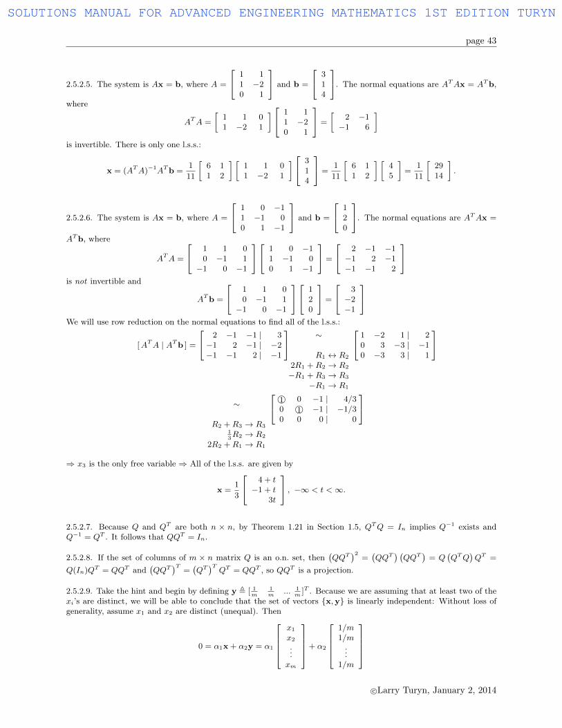
page 43
2.5.2.5. The system is Ax = b, where A =
1 11 −20 1
and b =
314
. The normal equations are ATAx = ATb,
where
ATA =
[1 1 01 −2 1
] 1 11 −20 1
=
[2 −1−1 6
]is invertible. There is only one l.s.s.:
x = (ATA)−1ATb =1
11
[6 11 2
] [1 1 01 −2 1
] 314
=1
11
[6 11 2
] [45
]=
1
11
[2914
].
2.5.2.6. The system is Ax = b, where A =
1 0 −11 −1 00 1 −1
and b =
120
. The normal equations are ATAx =
ATb, where
ATA =
1 1 00 −1 1−1 0 −1
1 0 −11 −1 00 1 −1
=
2 −1 −1−1 2 −1−1 −1 2
is not invertible and
ATb =
1 1 00 −1 1−1 0 −1
120
=
3−2−1
We will use row reduction on the normal equations to find all of the l.s.s.:
[ATA | ATb ] =
2 −1 −1 | 3−1 2 −1 | −2−1 −1 2 | −1
∼
R1 ↔ R2
2R1 +R2 → R2
−R1 +R3 → R3
−R1 → R1
1 −2 1 | 20 3 −3 | −10 −3 3 | 1
∼
R2 +R3 → R313R2 → R2
2R2 +R1 → R1
1© 0 −1 | 4/30 1© −1 | −1/30 0 0 | 0
⇒ x3 is the only free variable ⇒ All of the l.s.s. are given by
x =1
3
4 + t−1 + t
3t
, −∞ < t <∞.
2.5.2.7. Because Q and QT are both n × n, by Theorem 1.21 in Section 1.5, QTQ = In implies Q−1 exists andQ−1 = QT . It follows that QQT = In.
2.5.2.8. If the set of columns of m × n matrix Q is an o.n. set, then(QQT
)2=(QQT
) (QQT
)= Q
(QTQ
)QT =
Q(In)QT = QQT and(QQT
)T=(QT)TQT = QQT , so QQT is a projection.
2.5.2.9. Take the hint and begin by defining y , [ 1m
1m
... 1m
]T . Because we are assuming that at least two of thexi’s are distinct, we will be able to conclude that the set of vectors {x,y} is linearly independent: Without loss ofgenerality, assume x1 and x2 are distinct (unequal). Then
0 = α1x + α2y = α1
x1x2...xm
+ α2
1/m1/m...
1/m
c©Larry Turyn, January 2, 2014
SOLUTIONS MANUAL FOR ADVANCED ENGINEERING MATHEMATICS 1ST EDITION TURYN
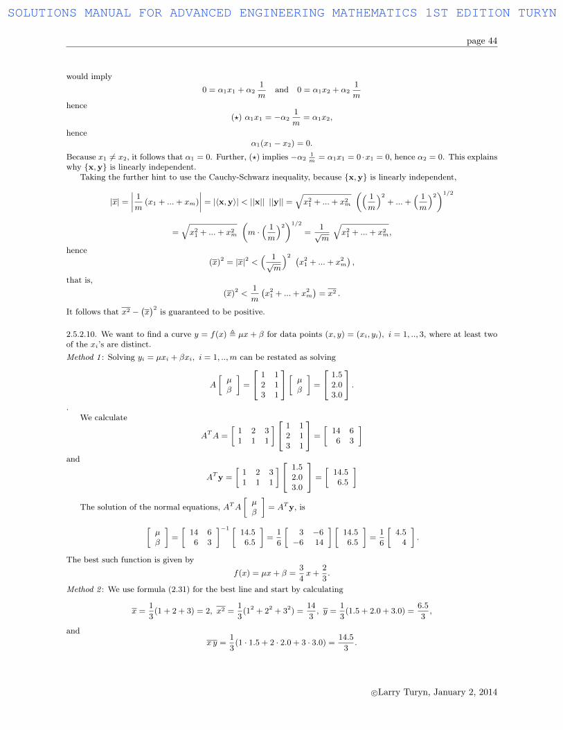
page 44
would imply
0 = α1x1 + α21
mand 0 = α1x2 + α2
1
mhence
(?) α1x1 = −α21
m= α1x2,
henceα1(x1 − x2) = 0.
Because x1 6= x2, it follows that α1 = 0. Further, (?) implies −α21m
= α1x1 = 0 ·x1 = 0, hence α2 = 0. This explainswhy {x,y} is linearly independent.
Taking the further hint to use the Cauchy-Schwarz inequality, because {x,y} is linearly independent,
|x| =∣∣∣∣ 1
m(x1 + ...+ xm)
∣∣∣∣ = |〈x,y〉| < ||x|| ||y|| =√x21 + ...+ x2m
(( 1
m
)2+ ...+
( 1
m
)2)1/2
=√x21 + ...+ x2m
(m ·
( 1
m
)2)1/2
=1√m
√x21 + ...+ x2m,
hence(x)2 = |x|2 <
( 1√m
)2 (x21 + ...+ x2m
),
that is,
(x)2 <1
m
(x21 + ...+ x2m
)= x2 .
It follows that x2 −(x)2 is guaranteed to be positive.
2.5.2.10. We want to find a curve y = f(x) , µx+ β for data points (x, y) = (xi, yi), i = 1, .., 3, where at least twoof the xi’s are distinct.Method 1 : Solving yi = µxi + βxi, i = 1, ..,m can be restated as solving
A
[µβ
]=
1 12 13 1
[ µβ
]=
1.52.03.0
..
We calculate
ATA =
[1 2 31 1 1
] 1 12 13 1
=
[14 66 3
]and
ATy =
[1 2 31 1 1
] 1.52.03.0
=
[14.56.5
]
The solution of the normal equations, ATA[µβ
]= ATy, is
[µβ
]=
[14 66 3
]−1 [14.56.5
]=
1
6
[3 −6−6 14
] [14.56.5
]=
1
6
[4.5
4
].
The best such function is given by
f(x) = µx+ β =3
4x+
2
3.
Method 2 : We use formula (2.31) for the best line and start by calculating
x =1
3(1 + 2 + 3) = 2, x2 =
1
3(12 + 22 + 32) =
14
3, y =
1
3(1.5 + 2.0 + 3.0) =
6.5
3,
andx y =
1
3(1 · 1.5 + 2 · 2.0 + 3 · 3.0) =
14.5
3.
c©Larry Turyn, January 2, 2014
SOLUTIONS MANUAL FOR ADVANCED ENGINEERING MATHEMATICS 1ST EDITION TURYN
page 45
So, the best line is
y =1
x2 −(x)2 ((xy − x y)x+ (−x xy + x2 y)
)y =
1143− 22
((14.5
3− 2 · 6.5
3
)x+
(− 2 · 14.5
3+
14
3· 6.5
3
)),
that is,
y =3
2
(1
2x+
4
9
)that is,
y =3
4x+
2
3
2.5.2.11. We want to find a curve y = f(x) , µx+ β for data points (x, y) = (xi, yi), i = 1, .., 3, where at least twoof the xi’s are distinct.Method 1 : Solving yi = µxi + βxi, i = 1, ..,m can be restated as solving
A
[µβ
]=
0.9 12.1 12.8 1
[ µβ
]=
1.02.03.0
..
We calculate
ATA =
[0.9 2.1 2.8
1 1 1
] 0.9 12.1 12.8 1
=
[13.06 5.8
5.8 3
]and
ATy =
[0.9 2.1 2.8
1 1 1
] 1.02.03.0
=
[13.56.0
]
The solution of the normal equations, ATA[µβ
]= ATy, is
[µβ
]=
[13.06 5.8
5.8 3
]−1 [13.56.0
]=
1
5.54
[3 −5.8
−5.8 13.06
] [13.56.0
]=
1
5.54
[5.70.06
].
The best such function is given by
f(x) = µx+ β ≈ 1.028880866x+ 0.0108303249.
Method 2 : We use formula (2.31) for the best line and start by calculating
x =1
3(0.9 + 2.1 + 2.8) =
5.8
3, x2 =
1
3(0.92 + 2.12 + 2.82) =
13.06
3, y =
1
3(1.0 + 2.0 + 3.0) = 2,
andx y =
1
3(0.9 · 1.0 + 2.1 · 2.0 + 2.8 · 3.0) =
13.5
3.
So, the best line is
y =1
x2 −(x)2 ((xy − x y)x+ (−x xy + x2 y)
)=
1
13.063−(
5.83
)2 ((13.5
3− 5.8
3· 2)x+
(− 5.8
3· 13.5
3+
13.06
3· 2))
that is,y ≈ 1.028880866x+ 0.01808303249.
2.5.2.12. We want to find a curve y = f(x) , µx+ β for data points (x, y) = (xi, yi), i = 1, .., 4, where at least twoof the xi’s are distinct.Method 1 : Solving yi = µxi + βxi, i = 1, ..,m can be restated as solving
A
[µβ
]=
0.6 10.7 11.3 11.8 1
[ µβ
]=
0.91.12.03.0
.
c©Larry Turyn, January 2, 2014
SOLUTIONS MANUAL FOR ADVANCED ENGINEERING MATHEMATICS 1ST EDITION TURYN

page 46
.We calculate
ATA =
[0.6 0.7 1.3 1.8
1 1 1 1
]0.6 10.7 11.3 11.8 1
=
[5.78 4.44.4 4
]
and
ATy =
[0.6 0.7 1.3 1.8
1 1 1 1
]0.91.12.03.0
=
[9.317.0
]
The solution of the normal equations, ATA[µβ
]= ATy, is
[µβ
]=
[5.78 4.44.4 4
]−1 [9.317.0
]=
1
3.76
[4 −4.4
−4.4 5.78
] [9.317.0
]=
1
3.76
[6.44−0.504
].
The best such function is given by
f(x) = µx+ β ≈ 1.712765957x− 0.1340425532.
Method 2 : We use formula (2.31) for the best line and start by calculating
x =1
4(0.6 + 0.7 + 1.3 + 1.8) = 1.1, x2 =
1
4(0.62 + 0.72 + 1.32 + 1.82) = 1.445, y =
1
4(0.9 + 1.1 + 2.0 + 3.0) = 1.75,
andx y =
1
4(0.6 · 0.9 + 0.7 · 1.1 + 1.3 · 2.0 + 1.8 · 3.0) = 2.3275.
So, the best line is
y =1
x2 −(x)2 ((xy − x y)x+ (−x xy + x2 y)
)=
1
1.445− (1.1)2
((2.3275− 1.1 · 1.75)x+ (−1.1 · 2.3275 + 1.445 · 1.75)
)that is,
y ≈ 1.712765957x− 0.1340425532.
2.5.2.13. Let xi and yi be the grades, on a 4 point scale, in Dynamics and Circuits, respectively, for the i−th student.We want to find a curve y = f(x) , µx+ β for data points (x, y) = (xi, yi), i = 1, .., 6, where at least two of the xi’sare distinct.Method 1 : Solving yi = µxi + βxi, i = 1, ..,m can be restated as solving
A
[µβ
]=
3 13.7 12.3 12.3 11 12.7 1
[µβ
]=
2.32.732.703.3
..
We calculate
ATA =
[3 3.7 2.3 2.3 1 2.71 1 1 1 1 1
]
3 13.7 12.3 12.3 11 12.7 1
=
[41.56 1515 6
]
c©Larry Turyn, January 2, 2014
SOLUTIONS MANUAL FOR ADVANCED ENGINEERING MATHEMATICS 1ST EDITION TURYN

page 47
and
ATy =
[3 3.7 2.3 2.3 1 2.71 1 1 1 1 1
]
2.32.732.703.3
=
[38.9114.0
]
The solution of the normal equations, ATA[µβ
]= ATy, is
[µβ
]=
[41.56 1515 6
]−1 [38.9114.0
]=
1
24.36
[6 −15−15 41.56
] [38.9114.0
]=
1
24.36
[23.46−1.81
].
The best such function is given by
f(x) = µx+ β ≈ 0.9630541872x− 0.0743021346.
(a) Students who receive a B−, that is, x = 2.7, in Dynamics, would get a grade of y = f(2.7) ≈ 0.9630541872 · 2.7−0.0743021346 ≈ 2.525944171, that is, about a B−, in Circuits.(b) Students who receive a B−, that is, y = 2.7, in Circuits, would get a grade of x in Dynamics, where 2.7 = y =f(x) ≈ 0.9630541872 · x − 0.0743021346, hence x = 0.9630541872−1(2.7 + 0.0743021346) ≈ 2.880733163, that is,between a B− and a B but closer to a B.Method 2 : We use formula (2.31) in Section 2.5 for the best line and start by calculating
x =1
6(3 + 3.7 + 2.3 + 2.3 + 1 + 2.7) = 2.5, x2 =
1
6(32 + 3.72 + 2.32 + 2.32 + 12 + 2.72) =
41.56
6,
y =1
6(2.3 + 2.7 + 3 + 2.7 + 0 + 3.3) =
14
6,
andx y =
1
6(3 · 2.3 + 3.7 · 2.7 + 2.3 · 3 + 2.3 · 2.7 + 1 · 0 + 2.7 · 3.3) =
38.91
6.
So, the best line is
y =1
x2 −(x)2 ((xy − x y)x+ (−x xy + x2 y)
)=
141.56
6− (2.5)2
((38.91
6− 2.5 · 14
6
)x+ (−2.5 · 38.91
6+
41.56
6· 14
6
))that is,
y ≈ 0.9630541872x− 0.0743021346.
2.5.2.14. We want to find a curve y = f(x) , αx + βx2 for data points (x, y) = (xi, yi), i = 1, ..,m, where at least
two of the xi’s are distinct. Trying to solve yi = αxi + βx2i , i = 1, ..,m can be restated as A[αβ
]= y, where
A =
x1 x21...
...xm x2m
, x =
[αβ
], and y =
y1...ym
..
We calculate
ATA =
[x1 . . . xmx21 . . . x2m
] x1 x21...
...xm x2m
=
x21 + ...+ x2m x31 + ...+ x3m
x31 + ...+ x3m x41 + ...+ x4m
and
ATy =
[x1 . . . xmx21 . . . x2m
] y1...ym
=
x1y1 + ...+ xmym
x21y1 + ...+ x2mym
c©Larry Turyn, January 2, 2014
SOLUTIONS MANUAL FOR ADVANCED ENGINEERING MATHEMATICS 1ST EDITION TURYN

page 48
The normal equations, ATAx = ATy, are
m∑i=1
x2i
m∑i=1
x3i
m∑i=1
x3i∑mi=1 x
4i
α
β
=
m∑i=1
xiyi
m∑i=1
x2i yi
.
Some averages commonly used in statistics and mechanics are defined by
x2 ,1
m
m∑i=1
x2i , x3 ,1
m
m∑i=1
x3i , x4 ,1
m
m∑i=1
x4i , xy ,1
m
m∑i=1
xiyi, and x2y ,1
m
m∑i=1
x2i yi.
The system is mx2 mx3
mx3 mx4
α
β
=
mxy
mx2y
.Divide both sides by m to see that this is
(?)
x2 x3
x3 x4
α
β
=
xy
x2y
.Case 1 : Assuming the matrix ATA is invertible, that is, assuming its determinant, x2 x4 −
(x3)2, is nonzero, the
l.s.s. is α
β
=(ATA
)−1
xy
x2y
=1
x2x4 −(x3)2 x4 −x3
−x3 x2
xy
x2y
.The best such function is given by
f(x) = αx+ βx2 =(x4 xy − x3 x2y)x+ (−x3 xy + x2 x2y)x2
x2 x4 −(x3)2 ,
in the case that x2 x4 6=(x3)2.
Case 2 : Assuming the matrix ATA is not invertible, that is, assuming its determinant, x2 x4 −(x3)2
= 0, then weknow there are infinitely many l.s.s. because we know there is always at least one l.s.s. It follows that we must beable to solve system (?) by row reduction to get
x2 x3 | xy|
x3 x4 | x2y
∼
1
x2R1 → R1
−x3R1 +R2 → R2
1 x3
x2| xy
x2
|0 0 | 0
,
hence α
β
=
−x3
x2t+ xy
x2
t
, −∞ < t <∞.
One such function is given by α = xy
x2, β = 0, that is, when t = 0, so
f(x) =xy
x2x,
in the case that x2 x4 =(x3)2.
2.5.2.15. Yes, there can be infinitely many solutions, depending upon the matrix ATA. For example, here’s amodification of Example 2.20 in Section 2.5: For the system 1 −1
−2 23 −3
x =
2−2
0
c©Larry Turyn, January 2, 2014
SOLUTIONS MANUAL FOR ADVANCED ENGINEERING MATHEMATICS 1ST EDITION TURYN
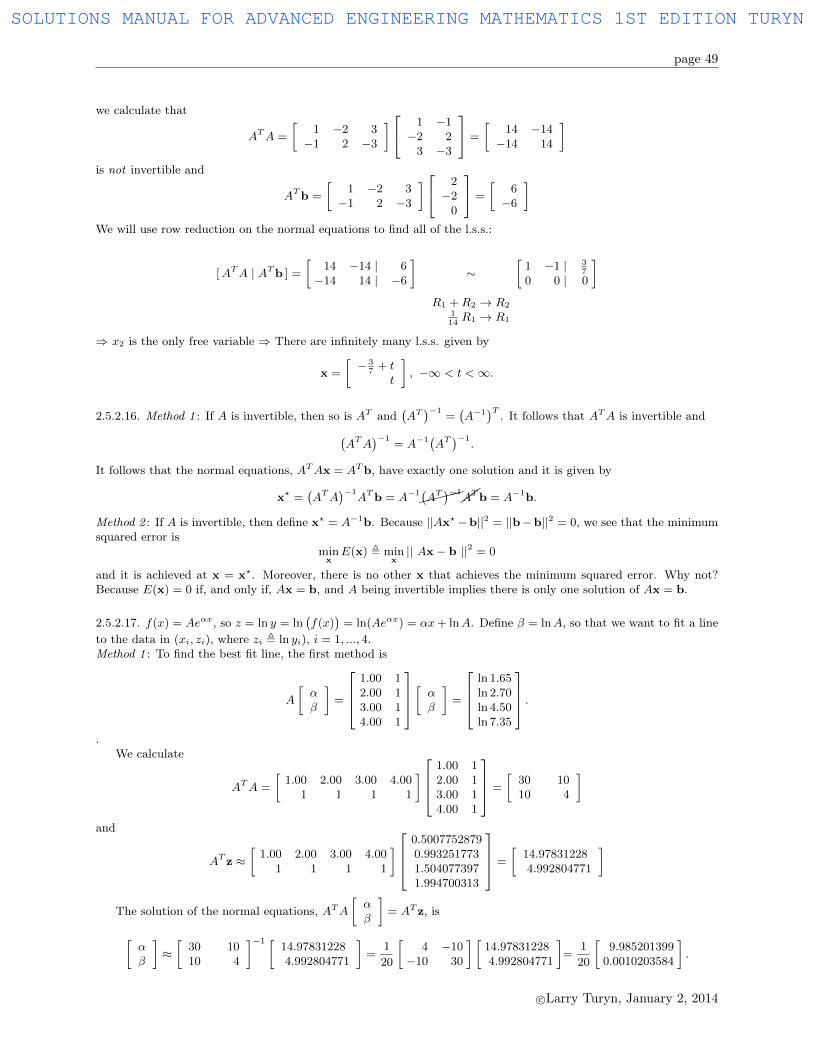
page 49
we calculate that
ATA =
[1 −2 3−1 2 −3
] 1 −1−2 2
3 −3
=
[14 −14−14 14
]is not invertible and
ATb =
[1 −2 3−1 2 −3
] 2−2
0
=
[6−6
]We will use row reduction on the normal equations to find all of the l.s.s.:
[ATA | ATb ] =
[14 −14 | 6−14 14 | −6
]∼
R1 +R2 → R2114R1 → R1
[1 −1 | 3
7
0 0 | 0
]
⇒ x2 is the only free variable ⇒ There are infinitely many l.s.s. given by
x =
[− 3
7+ tt
], −∞ < t <∞.
2.5.2.16. Method 1 : If A is invertible, then so is AT and(AT)−1
=(A−1
)T . It follows that ATA is invertible and(ATA
)−1= A−1(AT )−1
.
It follows that the normal equations, ATAx = ATb, have exactly one solution and it is given by
x? =(ATA
)−1ATb = A−1
����(AT)−1
��ATb = A−1b.
Method 2 : If A is invertible, then define x? = A−1b. Because ||Ax?−b||2 = ||b−b||2 = 0, we see that the minimumsquared error is
minxE(x) , min
x|| Ax− b ||2 = 0
and it is achieved at x = x?. Moreover, there is no other x that achieves the minimum squared error. Why not?Because E(x) = 0 if, and only if, Ax = b, and A being invertible implies there is only one solution of Ax = b.
2.5.2.17. f(x) = Aeαx, so z = ln y = ln(f(x)
)= ln(Aeαx) = αx+ lnA. Define β = lnA, so that we want to fit a line
to the data in (xi, zi), where zi , ln yi), i = 1, ..., 4.Method 1 : To find the best fit line, the first method is
A
[αβ
]=
1.00 12.00 13.00 14.00 1
[ αβ
]=
ln 1.65ln 2.70ln 4.50ln 7.35
..
We calculate
ATA =
[1.00 2.00 3.00 4.00
1 1 1 1
]1.00 12.00 13.00 14.00 1
=
[30 1010 4
]
and
AT z ≈[
1.00 2.00 3.00 4.001 1 1 1
]0.50077528790.9932517731.5040773971.994700313
=
[14.978312284.992804771
]
The solution of the normal equations, ATA[αβ
]= AT z, is
[αβ
]≈[
30 1010 4
]−1 [14.978312284.992804771
]=
1
20
[4 −10
−10 30
] [14.978312284.992804771
]=
1
20
[9.985201399
0.0010203584
].
c©Larry Turyn, January 2, 2014
SOLUTIONS MANUAL FOR ADVANCED ENGINEERING MATHEMATICS 1ST EDITION TURYN

page 50
The best linear function ln(f(x)
)is given by
ln f(x) = αx+ β ≈ 0.4992600699x+ 0.0000510179195.
Because β = lnA, we have A ≈ 1.000051019. The best fit is
y = Aeαx ≈ 1.000051019 e0.4992600699 x.
Method 2 : We use formula (2.31) for the best line and start by calculating
x =1
4(1.00 + 2.00 + 3.00 + 4.00) = 2.5, x2 =
1
4(1.002 + 2.002 + 3.002 + 4.002) = 7.5,
z=1
4(ln 1.65 + ln 2.70 + ln 4.50 + ln 7.35)≈1.248201193,
andx z =
1
4(1.00 · ln 1.65 + 2.00 · ln 2.70 + 3.00 · ln 4.50 + 4.00 · 7.35) ≈ 3.744578069
So, the best line is
z = ln f(x) =1
x2 −(x)2 ((xz − x z)x+ (−x xz + x2 z)
)=
1
7.5− (2.5)2
((3.744578069− 2.5 · 1.248201193)x+ (−2.5 · 3.744578069 + 7.5 · 1.248201193)
)that is,
z ≈ 0.4992600694x+ 0.00005101941936.
Because β = lnA, we have A ≈ 1.000051021. The best fit is
y = Aeαx ≈ 1.000051021 e0.4992600694 x.
c©Larry Turyn, January 2, 2014
SOLUTIONS MANUAL FOR ADVANCED ENGINEERING MATHEMATICS 1ST EDITION TURYN
page 51
Section 2.6.3
2.6.3.1. 0 =
∣∣∣∣ 1− λ 22 4− λ
∣∣∣∣ = (1− λ)(4− λ)− 4 = λ2 − 5λ = λ(λ− 5) ⇒ eigenvalues λ1 = 0, λ2 = 5.
[A− λ1I | 0 ] =
[1 2 | 02 4 | 0
]∼[
1© 2 | 00 0 | 0
], after −2R1 +R2 → R2.
⇒ p(1)=
[−2
1
]is an eigenvector corr. to eigenvalue λ1 = 0.
[A− λ2I | 0 ] =
[−4 2 | 0
2 −1 | 0
]∼[
1© − 12| 0
0 0 | 0
], after − 1
4R1→R1, −2R1+R2→R1.
⇒ p(2)=
[12
]is an eigenvector corr. to eigenvalue λ2 = 5.
The matrix P = [p(1) pp p
(2) ] =
[−2 1
1 2
]should diagonalize A.
To find a real, orthogonal matrix that diagonalizes A, all that we need to do is to normalize the columns because{p(1),p(2)} is already an orthogonal set. So, the real, orthogonal matrix
Q =1√5
[ p(1) pp p
(2) ] =1√5
[−2 1
1 2
]should diagonalize A.
2.6.3.2. 0 =
∣∣∣∣ −λ −√
3
−√
3 −λ
∣∣∣∣ = λ2 − 3 ⇒ eigenvalues λ1 = −√
3, λ2 =√
3.
[A− λ1I | 0 ] =
[ √3 −
√3 | 0
−√
3√
3 | 0
]∼[
1© −1 | 00 0 | 0
], after R1+R2→R2, 1√
3R1→R1.
⇒ p(1) =
[11
]is an eigenvector corr. to eigenvalue λ1 = −
√3.
[A− λ2I | 0 =
[−√
3 −√
3 | 0
−√
3 −√
3 | 0
]∼[
1© 1 | 00 0 | 0
], after −R1+R2→R2, − 1√
3R1→R1.
⇒ p(2) =
[−1
1
]is an eigenvector corr. to eigenvalue λ2 =
√3.
The matrix P = [p(1) pp p
(2) ] =
[1 −11 1
]should diagonalize A.
To find a real, orthogonal matrix that diagonalizes A, all that we need to do is to normalize the columns because{p(1),p(2)} is already an orthogonal set. So, the real, orthogonal matrix
Q =1√2
[ p(1) pp p
(2) ] =1√2
[1 −11 1
]should diagonalize A.
2.6.3.3. 0 =
∣∣∣∣∣∣−λ 1 0
1 −λ 00 0 2− λ
∣∣∣∣∣∣ = (2− λ)
∣∣∣∣ −λ 11 −λ
∣∣∣∣ = (2− λ)(λ2 − 1) ⇒ eigenvalues λ1 = −1, λ2 = 1, λ3 = 2.
[A− λ1I | 0 ] =
1 1 0 | 01 1 0 | 00 0 3 | 0
∼ 1© 1 0 | 0
0 0 1© | 00 0 0 | 0
, after −R1 +R2 → R2, 13R3 → R3, R2 ↔ R3.
⇒ p(1) =
−110
is an eigenvector corr. to eigenvalue λ1 = −1.
c©Larry Turyn, January 2, 2014
SOLUTIONS MANUAL FOR ADVANCED ENGINEERING MATHEMATICS 1ST EDITION TURYN
page 52
[A− λ2I | 0 ] =
−1 1 0 | 01 −1 0 | 00 0 1 | 0
∼ 1© −1 0 | 0
0 0 1© | 00 0 0 | 0
, after R1 +R2 → R2, −R1 → R1, R2 ↔ R3.
⇒ p(2) =
110
is an eigenvector corr. to eigenvalue λ2 = 1.
[A−λ3I | 0 ] =
−2 1 0 | 01 −2 0 | 00 0 0 | 0
∼ 1© 0 0 | 0
0 1© 0 | 00 0 0 | 0
, after − 12R1 → R1, −R1 +R2 → R2, − 2
3R2 → R2,
12R2 +R1 → R1.
⇒ p(3) =
001
is an eigenvector corr. to eigenvalue λ3 = 2.
The matrix P = [p(1) pp p
(2) pp p
(3) ] =
−1 1 01 1 00 0 1
should diagonalize A.
To find a real, orthogonal matrix that diagonalizes A, all that we need to do is to normalize the columns because{p(1),p(2),p(3)} is already an orthogonal set. So, the real, orthogonal matrix
Q=
[1√2p(1) p
p1√2p(2) p
p p(3)
]=
1√2
−1 1 01 1 0
0 0√
2
should diagonalize A.
2.6.3.4. 0 =
∣∣∣∣∣∣1− λ 0 −5
0 −2− λ 0−5 0 1− λ
∣∣∣∣∣∣ = (−2− λ)
∣∣∣∣ 1− λ −5−5 1− λ
∣∣∣∣ = (−2− λ)((1− λ)2 − 25
)= (−2− λ)
((1− λ)− 5
)((1− λ) + 5
)⇒ eigenvalues λ1 = −4, λ2 = −2, λ3 = 6.
[A− λ1I | 0 ] =
5 0 −5 | 00 2 0 | 0−5 0 5 | 0
∼ 1© 0 −1 | 0
0 1© 0 | 00 0 0 | 0
, after R1 +R3 → R3, 15R1 → R1, 1
2R2 → R2.
⇒ p(1) =
101
is an eigenvector corr. to eigenvalue λ1 = −4.
[A− λ2I | 0 ] =
3 0 −5 | 00 0 0 | 0−5 0 3 | 0
∼ 1© 0 0 | 0
0 0 1© | 00 0 0 | 0
, after 13R1 → R1, 5R1 +R3 → R3, − 3
16R3 → R3,
53R3 +R1 → R1, R2 ↔ R3.
⇒ p(2) =
010
is an eigenvector corr. to eigenvalue λ2 = −2.
[A−λ3I | 0 ] =
−5 0 −5 | 00 −8 0 | 0−5 0 −5 | 0
∼ 1© 0 1 | 0
0 1© 0 | 00 0 0 | 0
, after −R1+R3 → R3, − 15R1 → R1, − 1
8R2 → R2.
⇒ p(3) =
−101
is an eigenvector corr. to eigenvalue λ3 = 6.
The matrix P = [p(1) pp p
(2) pp p
(3) ] =
1 0 −10 1 01 0 1
should diagonalize A.
c©Larry Turyn, January 2, 2014
SOLUTIONS MANUAL FOR ADVANCED ENGINEERING MATHEMATICS 1ST EDITION TURYN

page 53
To find a real, orthogonal matrix that diagonalizes A, all that we need to do is to normalize the columns because{p(1),p(2),p(3)} is already an orthogonal set. So, the real, orthogonal matrix
Q=
[1√2p(1) p
p p(2) p
p1√2p(3)
]=
1√2
1 0 −1
0√
2 01 0 1
should diagonalize A.
2.6.3.5. 0 =
∣∣∣∣∣∣−2− λ 4 4
4 7− λ −54 −5 7− λ
∣∣∣∣∣∣ =
−R2 +R3 → R3
∣∣∣∣∣∣−2− λ 4 4
4 7− λ −50 −12 + λ 12− λ
∣∣∣∣∣∣=
R3 ← (12− λ)R3
(12− λ)
∣∣∣∣∣∣−2− λ 4 4
4 7− λ −50 −1 1
∣∣∣∣∣∣ =
C2 + C3 → C2
(12− λ)
∣∣∣∣∣∣−2− λ 8 4
4 2− λ −50 0 1
∣∣∣∣∣∣= (12− λ)
∣∣∣∣ −2− λ 84 2− λ
∣∣∣∣ = (12− λ)((−2− λ)(2− λ)− 32
)= (12− λ)(λ2 − 36)
⇒ eigenvalues λ1 = −6, λ2 = 6, λ3 = 12.
[A − λ1I | 0 ] =
4 4 4 | 04 13 −5 | 04 −5 13 | 0
∼ 1© 1 1 | 0
0 9 −9 | 00 −9 9 | 0
, after −R1 + R2 → R2, −R1 + R3 → R3,
14R1 → R1,
∼
1© 0 2 | 00 1© −1 | 00 0 0 | 0
,after R2 +R3 → R3, 1
9R2 → R2, −R2 +R1 → R1.
⇒ p(1) =
−211
is an eigenvector corr. to eigenvalue λ1 = −6.
[A − λ2I | 0 ] =
−8 4 4 | 04 1 −5 | 04 −5 1 | 0
∼ 1© − 1
2− 1
2| 0
0 3 −3 | 00 −3 3 | 0
, after 12R1 + R2 → R2, 1
2R1 + R3 → R3,
− 18R1 → R1,
∼
1© 0 −1 | 00 1© −1 | 00 0 0 | 0
,after R2 +R3 → R3, 1
3R2 → R2, 1
2R2 +R1 → R1.
⇒ p(2) =
111
is an eigenvector corr. to eigenvalue λ2 = 6.
[A − λ3I | 0 ] =
−14 4 4 | 04 −5 −5 | 04 −5 −5 | 0
∼ 1© − 5
4− 5
4| 0
−14 4 4 | 00 0 0 | 0
, after −R2 + R3 → R3, R1 ↔ R2,
14R1 → R1,
∼
1© −5/4 −5/4 | 00 −54/4 −54/4 | 00 0 0 | 0
,after 14R1 +R2 → R2,
∼
1© 0 0 | 00 1© 1 | 00 0 0 | 0
,c©Larry Turyn, January 2, 2014
SOLUTIONS MANUAL FOR ADVANCED ENGINEERING MATHEMATICS 1ST EDITION TURYN
page 54
after − 454R2 → R2, 5
4R2 +R1 → R1.
⇒ p(3)=
0−1
1
is an eigenvector corr. to eigenvalue λ3 = 12.
The matrix P = [p(1) pp p
(2) pp p
(3) ] =
−2 1 01 1 −11 1 1
should diagonalize A.
To find a real, orthogonal matrix that diagonalizes A, all that we need to do is to normalize the columns because{p(1),p(2),p(3)} is already an orthogonal set. So, the real, orthogonal matrix
Q=
[1√6p(1) p
p1√3p(2) p
p1√2p(3)
]=
1√6
−2√
2 0
1√
2 −√
3
1√
2√
3
should diagonalize A.
2.6.3.6. 0 =
∣∣∣∣∣∣1− λ −3 0−3 1− λ 00 0 −2− λ
∣∣∣∣∣∣ = (−2− λ)
∣∣∣∣ 1− λ −3−3 1− λ
∣∣∣∣= (−2− λ)
((1− λ)2 − 9
)= (−2− λ)
((1− λ)− 3
)((1− λ) + 3
)⇒ eigenvalues λ1 = λ2 = −2, λ3 = 4.
[A− λ1I | 0 ] =
3 −3 0 | 0−3 3 0 | 0
0 0 0 | 0
∼ 1© −1 0 | 0
0 0 0 | 00 0 0 | 0
, after R1 +R2 → R2, 13R1 → R1.
⇒ free variables are x2 = c1 and x3 = c2
⇒ v =
c1c1c2
= c1
110
+ c2
001
⇒ p(1) =
110
and p(2) =
001
are eigenvectors corr. to eigenvalue λ1 = λ2 = −2. As it happens, {p(1),p(2)} is
already an orthogonal set of eigenvectors, so there is no need to use the Gram-Schmidt process in this problem.
[A−λ3I | 0 ] =
−3 −3 0 | 0−3 −3 0 | 0
0 0 −6 | 0
∼ 1© 1 0 | 0
0 0 1© | 00 0 0 | 0
, after −R1+R2 → R2, − 13R1 → R1, − 1
6R3 → R3,
R2 ↔ R3.
⇒ p(3) =
−110
is an eigenvector corr. to eigenvalue λ3 = 4.
The matrix P = [p(1) pp p
(2) pp p
(3) ] =
1 −1 01 1 00 0 1
should diagonalize A.
To find a real, orthogonal matrix that diagonalizes A, all that we need to do is to normalize the columns because{p(1),p(2),p(3)} is already an orthogonal set. So, the real, orthogonal matrix
Q=
[1√2p(1) p
p1√2p(2) p
p p(3)
]=
1√2
1 −1 01 1 0
0 0√
2
should diagonalize A.
2.6.3.7. 0 =
∣∣∣∣∣∣−2− λ 0 0
0 3− λ −10 −1 3− λ
∣∣∣∣∣∣ = (−2− λ)
∣∣∣∣ 3− λ −1−1 3− λ
∣∣∣∣ = (−2− λ)((3− λ)2 − 1
)= (−2− λ)
((3− λ)− 1
)((3− λ) + 1
)c©Larry Turyn, January 2, 2014
SOLUTIONS MANUAL FOR ADVANCED ENGINEERING MATHEMATICS 1ST EDITION TURYN
page 55
⇒ eigenvalues λ1 = −2, λ2 = 2, λ3 = 4.
[A − λ1I | 0 ] =
0 0 0 | 00 5 −1 | 00 −1 5 | 0
∼ 0 1© 0 | 0
0 0 1© | 00 0 0 | 0
, after R1 ↔ R3, −R1 → R1, −5R1 + R2 → R2,
124R2 → R2, 5R2 +R1 → R1.
⇒ p(1) =
100
is an eigenvector corr. to eigenvalue λ1 = −2 .
[A− λ2I | 0 ] =
−4 0 0 | 00 1 −1 | 00 −1 1 | 0
∼ 1© 0 0 | 0
0 1© −1 | 00 0 0 | 0
, after − 14R1 → R1, R2 +R3 → R3.
⇒ p(2) =
011
is an eigenvector corr. to eigenvalue λ2 = 2 .
[A−λ3I | 0 ] =
−6 0 0 | 00 −1 −1 | 00 −1 −1 | 0
∼ 1© 0 0 | 0
0 1© 1 | 00 0 0 | 0
, after − 16R1 → R1, −R2 +R3 → R3, −R2 → R2.
⇒ p(3) =
0−1
1
is an eigenvector corr. to eigenvalue λ3 = 4.
The matrix P = [p(1) pp p
(2) pp p
(3) ] =
1 0 00 1 −10 1 1
should diagonalize A.
To find a real, orthogonal matrix that diagonalizes A, all that we need to do is to normalize the columns because{p(1),p(2),p(3)} is already an orthogonal set. So, the real, orthogonal matrix
Q=
[p(1) p
p1√2p(2) p
p1√2p(3)
]=
1√2
√2 0 00 1 −10 1 1
should diagonalize A.
2.6.3.8. 0 =
∣∣∣∣∣∣5− λ 3 0
3 5− λ 00 0 5− λ
∣∣∣∣∣∣ = (5− λ)
∣∣∣∣ 5− λ 33 5− λ
∣∣∣∣ = (5− λ)((5− λ)2 − 9
)= (5− λ)
((5− λ)− 3
)((5− λ) + 3
)⇒ eigenvalues λ1 = 2, λ2 = 5, λ3 = 8.
[A − λ1I | 0 ] =
3 3 0 | 03 3 0 | 00 0 3 | 0
∼ 1© 1 0 | 0
0 0 1© | 00 0 0 | 0
, after −R1 + R2 → R2, 13R1 → R1, R2 ↔ R3,
13R2 → R2.
⇒ p(1) =
−110
is an eigenvector corr. to eigenvalue λ1 = 2 .
[A− λ2I | 0 ] =
0 3 0 | 03 0 0 | 00 0 0 | 0
∼ 1© 0 0 | 0
0 1© 0 | 00 0 0 | 0
, after R2 ↔ R3, 13R1 → R1, 1
3R2 → R2.
⇒ p(2) =
001
is an eigenvector corr. to eigenvalue λ2 = 5 .
c©Larry Turyn, January 2, 2014
SOLUTIONS MANUAL FOR ADVANCED ENGINEERING MATHEMATICS 1ST EDITION TURYN
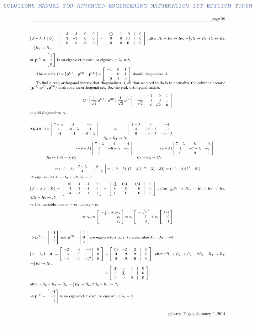
page 56
[A− λ3I | 0 ] =
−3 3 0 | 03 −3 0 | 00 0 −3 | 0
∼ 1© −1 0 | 0
0 0 1© | 00 0 0 | 0
, after R1 + R2 → R2, − 13R1 → R1, R2 ↔ R3,
− 13R2 → R2.
⇒ p(3) =
110
is an eigenvector corr. to eigenvalue λ3 = 8.
The matrix P = [p(1) pp p
(2) pp p
(3) ] =
−1 0 11 0 10 1 0
should diagonalize A.
To find a real, orthogonal matrix that diagonalizes A, all that we need to do is to normalize the columns because{p(1),p(2),p(3)} is already an orthogonal set. So, the real, orthogonal matrix
Q=
[1√2p(1) p
p p(2) p
p1√2p(3)
]=
1√2
−1 0 11 0 1
0√
2 0
should diagonalize A.
2.6.3.9. 0 =
∣∣∣∣∣∣7− λ 4 −4
4 −8− λ −1−4 −1 −8− λ
∣∣∣∣∣∣ =
R2 +R3 → R3
∣∣∣∣∣∣7− λ 4 −4
4 −8− λ −10 −9− λ −9− λ
∣∣∣∣∣∣=
R3 ← (−9− λ)R3
(−9− λ)
∣∣∣∣∣∣7− λ 4 −4
4 −8− λ −10 1 1
∣∣∣∣∣∣ =
C2 − C3 → C2
(9− λ)
∣∣∣∣∣∣7− λ 8 4
4 −7− λ −10 0 1
∣∣∣∣∣∣= (−9− λ)
∣∣∣∣ 7− λ 84 −7− λ
∣∣∣∣ = (−9− λ)((7− λ)(−7− λ)− 32
)= (−9− λ)(λ2 − 81)
⇒ eigenvalues λ1 = λ2 = −9, λ3 = 9.
[A − λ1I | 0 ] =
16 4 −4 | 04 1 −1 | 0−4 −1 1 | 0
∼ 1© 1/4 −1/4 | 0
0 0 0 | 00 0 0 | 0
, after 116R1 → R1, −4R1 + R2 → R2,
4R1 +R3 → R3.
⇒ free variables are x2 = c1 and x3 = c2
⇒ v1 =
− 14c1 + 1
4c2c1c2
= c1
−1/410
+ c2
1/401
⇒ p(1) =
−140
and p(2) =
104
are eigenvectors corr. to eigenvalue λ1 = λ2 = −9 .
[A − λ3I | 0 ] =
−2 4 −4 | 04 −17 −1 | 0−4 −1 −17 | 0
∼ 1© −2 2 | 0
0 −9 −9 | 00 −9 −9 | 0
, after 2R1 + R2 → R2, −2R1 + R3 → R3,
− 12R1 → R1,
∼
1© 0 4 | 00 1© 1 | 00 0 0 | 0
,after −R2 +R3 → R2, − 1
9R2 → R2, 2R2 +R1 → R1.
⇒ p(3) =
−4−1
1
is an eigenvector corr. to eigenvalue λ3 = 9.
c©Larry Turyn, January 2, 2014
SOLUTIONS MANUAL FOR ADVANCED ENGINEERING MATHEMATICS 1ST EDITION TURYN

page 57
The matrix P = [p(1) pp p
(2) pp p
(3) ] =
−1 1 −44 0 −10 4 1
should diagonalize A.
Next, we will find a real, orthogonal matrix that diagonalizes A. We will need to use the Gram-Schmidt processon {p(1),p(2)} because it is not an orthogonal set of eigenvectors corr. to eigenvalue λ1 = λ2 = −9.
To start the Gram-Schmidt process, let
v1, p(1), r11, ||v1|| =√
17,
and
q1= r−111 v1=
1√17
−140
.Next, let
v2 , p(2) − (p(2) • q1)q1 =
104
− 1
04
• 1√17
−140
1√17
−140
=
104
− ( −1√17
)1√17
−140
=4
17
41
17
r22 , ||v2|| = 4
√30617
, and
q2= r−122 v2=
1√306
41
17
.So, the real, orthogonal matrix
Q =
[q1
pp q2
pp
1√18
p(3)
]=
1√306
−√
18 4 −4√
17
4√
18 1 −√
17
0 17√
17
should diagonalize A.
2.6.3.10. Expanding the determinant along the first row, we find that the characteristic equation is
0 =
∣∣∣∣∣∣4− λ 2 −2
2 1− λ −1−2 −1 1− λ
∣∣∣∣∣∣ = (4− λ)
∣∣∣∣ 1− λ −1−1 1− λ
∣∣∣∣− (2)
∣∣∣∣ 2 −1−2 1− λ
∣∣∣∣+ (−2)
∣∣∣∣ 2 1− λ−2 −1
∣∣∣∣= (4− λ)(λ2 − 2λ)− 2(−2λ)− 2(−2λ) = −λ3 + 4λ2 + 2λ2 − 8λ+ 4λ+ 4λ = −λ3 + 6λ2 = −λ2(λ− 6)
⇒ eigenvalues λ1 = λ2 = 0, λ3 = 6.
[A − λ1I | 0 ] =
4 2 −2 | 02 1 −1 | 0−2 −1 1 | 0
∼ 1© 1/2 −1/2 | 0
0 0 0 | 00 0 0 | 0
, after 14R1 → R1, −2R1 + R2 → R2,
2R1 +R3 → R3.
⇒ free variables are x2 = c1 and x3 = c2
⇒ v =
− 12c1 + 1
2c2c1c2
= c1
−1/210
+ c2
1/201
⇒ p(1) =
−120
and p(2) =
102
are eigenvectors corr. to eigenvalue λ1 = λ2 = 0 .
c©Larry Turyn, January 2, 2014
SOLUTIONS MANUAL FOR ADVANCED ENGINEERING MATHEMATICS 1ST EDITION TURYN

page 58
[A − λ3I | 0 ] =
−2 2 −2 | 02 −5 −1 | 0−2 −1 −5 | 0
∼ 1© −1 1 | 0
0 −3 −3 | 00 −3 −3 | 0
, after − 12R1 → R1, −2R1 + R2 → R2,
2R1 +R3 → R3,
∼
1© 0 2 | 00 1© 1 | 00 0 0 | 0
,after −R2 +R3 → R2, − 1
3R2 → R2, R2 +R1 → R1.
⇒ p(3) =
−2−1
1
is an eigenvector corr. to eigenvalue λ3 = 6.
The matrix P = [p(1) pp p
(2) pp p
(3) ] =
−1 1 −22 0 −10 2 1
should diagonalize A.
Next, we will find a real, orthogonal matrix that diagonalizes A. We will need to use the Gram-Schmidt processon {p(1),p(2)} because it is not an orthogonal set of eigenvectors corr. to eigenvalue λ1 = λ2 = 0.
To start the Gram-Schmidt process, let
v1, p(1), r11, ||v1|| =√
5,
and
q1= r−111 v1=
1√5
−120
.Next, let
v2 , p(2) − (p(2) • q1)q1 =
102
− 1
02
• 1√5
−120
1√5
−120
=
102
− (−1√5
)1√5
−120
=2
5
215
r22 , ||v2|| = 2
√305
, and
q2= r−122 v2=
1√30
215
.So, the real, orthogonal matrix
Q =
[q1
pp q2
pp
1√6p(3)
]=
1√30
−√
6 2 −2√
5
2√
6 1 −√
5
0 5√
5
should diagonalize A.
2.6.3.11. For every vector x = [x1 . . . xn ]T in Cn,
xTx = x1x1 + · · ·+ xnxn = |x1|2 + · · ·+ |xn|2
is real.
2.6.3.12. Suppose A is a real, m× n matrix, ATA is invertible, m > n, and we define B = A(ATA)−1AT . Then
BT =(A(ATA)−1AT
)T=(AT)T (
(ATA)−1)TAT = A((ATA)T
)−1AT = A
(AT (AT )T
)−1AT
= A(ATA
)−1AT = B,
hence B is symmetric.
c©Larry Turyn, January 2, 2014
SOLUTIONS MANUAL FOR ADVANCED ENGINEERING MATHEMATICS 1ST EDITION TURYN

page 59
2.6.3.13. Suppose A is a real, m× n matrix, ATA is invertible, m > n, and we define B = A(ATA)−1AT . Then
B2 =(A(ATA)−1AT
)2=(A(ATA)−1AT
)(A(ATA)−1AT
)= A����
(ATA)−1
����(ATA
)(ATA)−1AT
= A(ATA
)−1AT = B,
hence B2 = B.
2.6.3.14. The spectral decomposition (2.34) gives A =∑ni=1 λiqiq
Ti . It follows that
A2 =
(n∑i=1
λiqiqTi
)(n∑j=1
λjqjqTj
)=
n∑i=1
n∑j=1
(λiqiq
Ti
)(λjqjq
Tj
)
=
n∑i=1
n∑j=1
λiλjqi(qTi qj)q
Tj =
n∑i=1
n∑j=1
λiλjqi ·{
1, i = j0, i 6= j
}· qTj =
n∑i=1
λ2iqiq
Ti ,
hence (2.38) is correct.
2.6.3.15. The spectral decomposition (2.34) gives A =∑ni=1 λiqiq
Ti and we define
√A ,
n∑i=1
√λi qiq
Ti .
We calculate that(√A)2
=
(n∑i=1
√λi qiq
Ti
)(n∑j=1
√λj qjq
Tj
)=
n∑i=1
n∑j=1
(√λi qiq
Ti
)(√λj qjq
Tj
)
=
n∑i=1
n∑j=1
√λi√λj qi(q
Ti qj)q
Tj =
n∑i=1
n∑j=1
√λi√λj qi ·
{1, i = j0, i 6= j
}· qTj
=
n∑i=1
(√λi)
2qiqTi ,=
n∑i=1
λiqiqTi = A,
hence (2.39) is correct.
2.6.3.16. Method 1 : For all x = [x1 x2 ]T in R2, we have
xTAx = [x1 x2 ]
[1 αα 1
] [x1x2
]= [x1 x2 ]
[x1 + αx2αx1 + x2
]= x21 + 2αx1x2 + x22 = (x1 + αx2)2 + (1− α2)x22.
It follows that(a) A is positive definite if, and only if, −1 < α < 1, that is, |α| < 1,and(b) A is positive semi-definite if, and only if, −1 ≤ α ≤ 1, that is, |α| ≤ 1.
Method 2 : 0 =
∣∣∣∣ 1− λ αα 1− λ
∣∣∣∣ = (1− λ)2 − α2,
⇒ the eigenvalues of A are λ = 1± α.By Theorem 2.25 in Section 2.10, it follows that
(a) A is positive definite if, and only if, −1 < α < 1, that is, |α| < 1,and(b) A is positive semi-definite if, and only if, −1 ≤ α ≤ 1, that is, |α| ≤ 1.
We could also establish positive definiteness using Theorem 2.31 in Section 2.6, after calculating that the principal
minors are A1 = det( [ 1 ] ) = 1 and A2 =
∣∣∣∣ 1 αα 1
∣∣∣∣ = 1− α2.
2.6.3.17. We define 〈x,y〉W , 〈Wx,y〉 , xT WTy and ||x ||W ,√〈x,x〉W , where W is a real, symmetric, positive
definite n× n matrix.
c©Larry Turyn, January 2, 2014
SOLUTIONS MANUAL FOR ADVANCED ENGINEERING MATHEMATICS 1ST EDITION TURYN
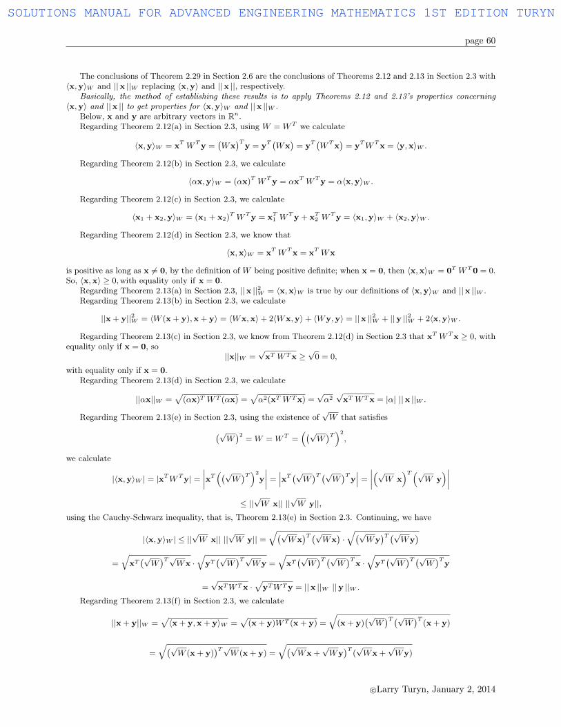
page 60
The conclusions of Theorem 2.29 in Section 2.6 are the conclusions of Theorems 2.12 and 2.13 in Section 2.3 with〈x,y〉W and ||x ||W replacing 〈x,y〉 and ||x ||, respectively.
Basically, the method of establishing these results is to apply Theorems 2.12 and 2.13’s properties concerning〈x,y〉 and ||x || to get properties for 〈x,y〉W and ||x ||W .
Below, x and y are arbitrary vectors in Rn.Regarding Theorem 2.12(a) in Section 2.3, using W = WT we calculate
〈x,y〉W = xT WTy =(Wx
)Ty = yT
(Wx
)= yT
(WTx
)= yTWTx = 〈y,x〉W .
Regarding Theorem 2.12(b) in Section 2.3, we calculate
〈αx,y〉W = (αx)T WTy = αxT WTy = α〈x,y〉W .
Regarding Theorem 2.12(c) in Section 2.3, we calculate
〈x1 + x2,y〉W = (x1 + x2)T WTy = xT1 WTy + xT2 W
Ty = 〈x1,y〉W + 〈x2,y〉W .
Regarding Theorem 2.12(d) in Section 2.3, we know that
〈x,x〉W = xT WTx = xT Wx
is positive as long as x 6= 0, by the definition of W being positive definite; when x = 0, then 〈x,x〉W = 0T WT0 = 0.So, 〈x,x〉 ≥ 0,with equality only if x = 0.
Regarding Theorem 2.13(a) in Section 2.3, ||x ||2W = 〈x,x〉W is true by our definitions of 〈x,y〉W and ||x ||W .Regarding Theorem 2.13(b) in Section 2.3, we calculate
||x + y||2W = 〈W (x + y),x + y〉 = 〈Wx,x〉+ 2〈Wx,y〉+ 〈Wy,y〉 = ||x ||2W + ||y ||2W + 2〈x,y〉W .
Regarding Theorem 2.13(c) in Section 2.3, we know from Theorem 2.12(d) in Section 2.3 that xT WTx ≥ 0, withequality only if x = 0, so
||x||W =√xT WTx ≥
√0 = 0,
with equality only if x = 0.Regarding Theorem 2.13(d) in Section 2.3, we calculate
||αx||W =√
(αx)T WT (αx) =√α2(xT WTx) =
√α2√xT WTx = |α| ||x ||W .
Regarding Theorem 2.13(e) in Section 2.3, using the existence of√W that satisfies(√
W)2
= W = WT =((√
W)T)2
,
we calculate
|〈x,y〉W | = |xTWTy| =∣∣∣∣xT((√W )T)2y∣∣∣∣ =
∣∣∣xT (√W )T (√W )Ty∣∣∣ =
∣∣∣∣(√W x)T(√
W y)∣∣∣∣
≤ ||√W x|| ||
√W y||,
using the Cauchy-Schwarz inequality, that is, Theorem 2.13(e) in Section 2.3. Continuing, we have
|〈x,y〉W | ≤ ||√W x|| ||
√W y|| =
√(√Wx
)T (√Wx
)·√(√
Wy)T (√
Wy)
=
√xT(√W)T√
Wx ·√
yT(√W)T√
Wy =
√xT(√W)T (√
W)T
x ·√
yT(√W)T (√
W)T
y
=√xTWTx ·
√yTWTy = ||x ||W ||y ||W .
Regarding Theorem 2.13(f) in Section 2.3, we calculate
||x + y||W =√〈x + y,x + y〉W =
√(x + y)WT (x + y) =
√(x + y)
(√W)T (√
W)T
(x + y)
=
√(√W (x + y)
)T√W (x + y) =
√(√Wx +
√Wy
)T(√Wx +
√Wy)
c©Larry Turyn, January 2, 2014
SOLUTIONS MANUAL FOR ADVANCED ENGINEERING MATHEMATICS 1ST EDITION TURYN
page 61
=∣∣∣∣∣∣√Wx +
√Wy
∣∣∣∣∣∣ ≤ ∣∣∣∣∣∣√Wx∣∣∣∣∣∣+
∣∣∣∣∣∣√Wy∣∣∣∣∣∣ ,
using Theorem 2.13(f) in Section 2.3. Continuing, we have
||x + y||W ≤∣∣∣∣∣∣√Wx
∣∣∣∣∣∣+∣∣∣∣∣∣√Wy
∣∣∣∣∣∣ =
√(√Wx
)T√Wx ·
√(√Wy
)T√Wy
=
√xT(√W)T√
Wx +
√yT(√W)T√
Wy =
√xT(√W)T (√
W)T
x +
√yT(√W)T (√
W)T
y
=√xTWTx +
√yTWTy = ||x ||W + ||y ||W .
2.6.3.19. Let W = diag(b−21 , ..., b−2
m ) = WT . Then the relative squared error is
m∑i=1
((Ax)i − bi
bi
)2
=
⟨(Ax)1−b1
b1...
(Ax)m−bmbm
,
(Ax)1−b1b1...
(Ax)m−bmbm
⟩
=
⟨(Ax)1−b1
b21...
(Ax)m−bmb2m
, (Ax)1 − b1
...(Ax)m − bm
⟩
=⟨diag(b−2
1 , ..., b−2m )(Ax− b), (Ax− b)
⟩= 〈W (Ax− b), (Ax− b)〉 = (Ax− b)TWT (Ax− b) = ||Ax− b||2W .
So, the problem of minimizing the relative squared error is a weighted least squares problem.
2.6.3.20. Define C ,√M −1K
√M −1, where both M and K are real, symmetric, and positive definite.
Because M is real, symmetric, and positive definite, so is√M , as defined in formula (2.39). It follows from
formula (2.37) that√M−1
is also real, symmetric, and positive definite.Because, in addition, K is real, symmetric, and positive definite, it follows that C is real, and
CT= (√M −1K
√M −1)T= (
√M −1)TKT (
√M −1)T = (
√M −1)TK(
√M −1)T= (
√M −1)K(
√M −1) = C,
so C is symmetric. Also, C is positive definite, because for all x 6= 0,
xTCx = xT√M −1K
√M −1x = xT (
√M −1)TK(
√M −1)x =
((√M −1)x
)TK(
(√M −1)Tx
)> 0,
because K is positive definite and (√M −1)x 6= 0. [The latter follows from the following reasoning: (
√M −1) is itself
invertible, so the only solution of (√M −1)x = 0 is x = 0, but we assumed that x 6= 0.]
2.6.3.21. Exs.: Q1 =
[1 00 1
], Q2 =
[0 −1−1 0
]
2.6.3.22. If λ is an eigenvalue of Q, then problem 2.4.3.12(b) yields |λ| = 1. But Q being real and symmetric impliesλ is real. The only real numbers whose absolute value is 1 are ±1.
c©Larry Turyn, January 2, 2014
SOLUTIONS MANUAL FOR ADVANCED ENGINEERING MATHEMATICS 1ST EDITION TURYN

page 62
Section 2.7.7
2.7.7.1. Use the Gram-Schmidt process on the columns of A: Let a1 =
110
and a2 =
011
. Then
v1, a1, r11, ||v1|| =√
2, q1= r−111 v1=
1√2
110
.Next, let
v2 , a2 − (a2 • q1)q1 =
011
− 0
11
• 1√2
110
1√2
110
=
011
− ( 1√2
)1√2
110
=1
2
−112
,r22 , ||v2|| =
√62, and
q2= r−122 v2=
1√6
−112
.We have
Q = [ q1pp q2 ] =
1√6
√3 −1√3 10 2
and, using r12 , a2 • q1,
R=
[r11 r120 r22
]=
[ √2√
2−1
0√62
]=
1√2
[2 1
0√
3
].
2.7.7.2. Use the Gram-Schmidt process on the columns of A: Let a1 =
1−1
10
and a2 =
0121
. Then
v1, a1, r11, ||v1||=√
3, q1= r−111 v1=
1√3
1−1
10
.Next, let
v2 , a2 − (a2 • q1)q1 =
0121
−
0121
• 1√3
1−1
10
1√
3
1−1
10
=
0121
− ( 1√3
)1√3
1−1
10
=1
3
−1
453
,r22 , ||v2|| =
√513
, and
q2= r−122 v2=
1√51
−1
453
.We have
Q = [ q1pp q2 ] =
1√51
√
17 −1
−√
17 4√17 50 3
and, using r12 , a2 • q1,
R =
[r11 r120 r22
]=
[ √3√
3−1
0√513
]=
1√3
[3 1
0√
17
].
c©Larry Turyn, January 2, 2014
SOLUTIONS MANUAL FOR ADVANCED ENGINEERING MATHEMATICS 1ST EDITION TURYN
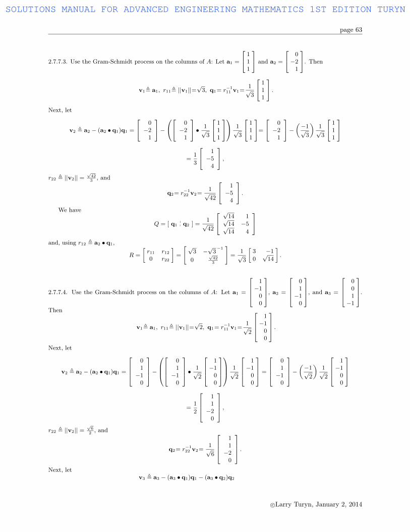
page 63
2.7.7.3. Use the Gram-Schmidt process on the columns of A: Let a1 =
111
and a2 =
0−2
1
. Then
v1, a1, r11, ||v1||=√
3, q1= r−111 v1=
1√3
111
.Next, let
v2 , a2 − (a2 • q1)q1 =
0−2
1
− 0
−21
• 1√3
111
1√3
111
=
0−2
1
− (−1√3
)1√3
111
=1
3
1−5
4
,r22 , ||v2|| =
√423
, and
q2= r−122 v2=
1√42
1−5
4
.We have
Q = [ q1pp q2 ] =
1√42
√
14 1√14 −5√14 4
and, using r12 , a2 • q1,
R =
[r11 r120 r22
]=
[ √3 −
√3−1
0√423
]=
1√3
[3 −1
0√
14
].
2.7.7.4. Use the Gram-Schmidt process on the columns of A: Let a1 =
1−1
00
, a2 =
01−1
0
, and a3 =
001−1
.Then
v1, a1, r11, ||v1||=√
2, q1= r−111 v1=
1√2
1−1
00
.Next, let
v2 , a2 − (a2 • q1)q1 =
01−1
0
−
01−1
0
• 1√2
1−1
00
1√
2
1−1
00
=
01−1
0
− (−1√2
)1√2
1−1
00
=1
2
11−2
0
,r22 , ||v2|| =
√62, and
q2= r−122 v2=
1√6
11−2
0
.Next, let
v3 , a3 − (a3 • q1)q1 − (a3 • q2)q2
c©Larry Turyn, January 2, 2014
SOLUTIONS MANUAL FOR ADVANCED ENGINEERING MATHEMATICS 1ST EDITION TURYN

page 64
=
001−1
−
001−1
• 1√2
1−1
00
1√
2
1−1
00
−
001−1
• 1√6
11−2
0
1√
6
11−2
0
.
=
001−1
− ( 0√2
)1√2
1−1
00
− (−2√6
)1√6
11−2
0
=1
3
111−3
,r22 , ||v2|| =
√123
, and
q2= r−122 v2=
1√12
111−3
.We have
Q = [ q1pp q2
pp q3 ] =
1√12
√
6√
2 1
−√
6√
2 1
0 −2√
2 10 0 −3
and, using r12 , a2 • q1, r13 , a3 • q1, and r23 , a3 • q2,
R =
r11 r12 r13
0 r22 r23
0 0 r33
=
√2 − 1√
20
0√
62− 2√
6
0 0√123
=
√2 − 1√
20
0√3√2− 2√
6
0 0 2√3
=1√6
2√
3 −√
3 0
0 3 −2
0 0 2√
2
.
2.7.7.5. We are given that A = [a1 . . . an], where {a1, . . . ,an} is an orthogonal set in Rm. It follows that{a1, . . . ,an} is linearly independent, so the Gram-Schmidt process can be used to find the QR factorization of A:
v1, a1, r11, ||v1||, q1= r−111 v1=
1
||a1||a1,
v2 , a2 − (a2 • q1)q1 = a2 − (a2 •1
||a1||a1)q1 = a2 − 0 · q1
hencev2 = a2, r22, ||v2||, q2= r−1
22 v2=1
||a2||a2,
...
vn , an − (an • q1)q1 − ...− (an • qn−1)qn−1 = an − 0 · q1 − ...−−0 · qn−1 = an,
rnn, ||vn||, qn= r−1nnvn=
1
||an||an.
So,
Q =
[1
||a1||a1
pp ...
pp
1
||an||an
]and
R = diag( ||a1||, ..., ||an|| ).
2.7.7.6. We are given that A = [a1 . . . an], where {a1, . . . ,an} is an o.n. set in Rm.Method 1 : Because the columns of A are already an o.n. set, the set {q1, . . . ,qn} = {a1, . . . ,an} will be the result ofthe Gram-Schmidt process. It follows that Q = A, and therefore R = In.Method 2 : It follows that {a1, . . . ,an} is linearly independent, so the Gram-Schmidt process can be used to find theQR factorization of A
v1, a1, r11, ||v1|| = 1, q1= r−111 v1=a1,
c©Larry Turyn, January 2, 2014
SOLUTIONS MANUAL FOR ADVANCED ENGINEERING MATHEMATICS 1ST EDITION TURYN
page 65
v2 , a2 − (a2 • q1)q1 = a2 − (a2 • a1)a1 = a2 − 0 · a1
hencev2 = a2, r22, ||v2|| = 1, q2= r−1
22 v2=a2,
...
vn , an − (an • a1)a1 − ...− (an • an−1)an−1 = an − 0 · a1 − ...−−0 · an−1 = an,
rnn, ||vn|| = 1, qn= r−1nnvn=an.
So,Q =
[a1
pp ...
pp an
]= A
andR = diag( 1, ..., 1 ) = In.
2.7.7.7. Because A is invertible it must be square, say n× n.Because A =
[a1
pp ...
pp an
]is a real, invertible, upper triangular matrix, it follows that {a1, . . . ,an} is linearly
independent. The Gram-Schmidt process can be used to find the QR factorization of A:
v1, a1 = a11e(1), r11, ||v1|| = |a11|,
andq1 = r−1
11 v1 =1
|a11|a1 = sgn(a11) e(1).
Next, a2 = a12e(1) + a22e
(2), so
v2 , a2 − (a2 • q1)q1= a2 −(sgn(a11)a12
)(sgn(a11) e(1)) = a2 −
(sgn(a11)
)2a12 e
(1) = a2 − a12 e(1)
hencev2 = a22e
(2), r22, ||v2|| = |a22|,and
q2 = r−122 v2 =
1
|a22|a22 e
(2) = sgn(a22) e(2).
...
an = a1ne(1) + ...+ anne
(n), so
vn , an − (an • q1)q1 − ...− (an • qn−1)qn−1
= an −(sgn(a11) a1n
)(sgn(a11) e(1))− ...−
(sgn(an−1,n−1) a12
)(sgn(an−1,n−1) e(n−1))
= ... = anne(n), rnn, ||vn|| = |ann|,
andqn = r−1
nnvn =1
|ann|ann e
(n) = sgn(ann) e(n).
So,Q =
[sgn(a11) e(1) p
p ...pp sgn(ann) e(n)
],
that is,Q = diag
(sgn(a11), ..., sgn(ann)
),
and
R=
|a11| a12sgn(a11) . . . a1nsgn(a11)
0 |a22| a2nsgn(a22). . .. . .. . .0 . . . |ann|
.
Note that the diagonal elements of R are ||vj || > 0, j = 1, ..., n.
c©Larry Turyn, January 2, 2014
SOLUTIONS MANUAL FOR ADVANCED ENGINEERING MATHEMATICS 1ST EDITION TURYN

page 66
2.7.7.8. The problem suggests that we start by looking for a matrix Q and a vector b for which QQTb 6= b. This isnot possible if m = n. Also, ultimately we will be dealing with a matrix A whose QR factorization is QR, and thisis possible only if m ≥ n. So, we should look for an example with m > n.
The matrix Q = 1√6
√
2 1√2 −2√2 1
has its two columns being an o.n. set of vectors in R3. We calculate
QQT =1√6
√
2 1√2 −2√2 1
1√6
[ √2√
2√
21 −2 1
]=
1
6
3 0 30 6 03 0 3
.We want to find a vector b = [ b1 b2 b3 ] with QQTb 6= b, that is,
0 6= (QQT − I)b =1
2
−b1 + b30
b1 − b3
,so any vector b with b1 6= b3 will do. For example, let us choose b = [ 1 0 0 ]
Ultimately, we will need x, the solution of Rx = QTb, to have Ax 6= b. Because A = QR and x = R−1QTb, wewould need to have
b 6= Ax = (QR)(R−1QTb) = QQTb.
So, let us choose a 2 × 2, real, invertible, upper triangular matrix R having r11 > 0 and r22 > 0, for example,
R = 1√2
[2 −1
0 2√
2
]. Then
A = QR =1√6
√
2 1√2 −2√2 1
1√2
[2 −1
0 2√
2
]=
1√12
2√
2√
2
2√
2 −5√
2
2√
2√
2
,that is,
A =1√6
2 12 −52 1
,and
x = R−1QTb =
[ √2 −1/
√2
0 2
]−11√6
[ √2√
2√
21 −2 1
] 100
=1√6· 1
2√
2
[2 1/
√2
0√
2
] [ √21
]
=1
4√
3
[5/√
2√2
],
that is,
x =1
4√
6
[52
].
We have
Ax =1√6
2 12 −52 1
1
4√
6
[52
]=
1
24
120
12
=
12
012
6= 1
00
= b,
even though Rx = QTb, as x was designed to satisfy.
2.7.7.9. Take the hint, and begin by using Rx = QTb to see that
Ax = Q(Rx) = Q(QTb) = (QQT )b.
Next, use b = Qc to see that
Ax = (QQT )(Qc) = Q(QTQ)c) = Q(I)c = Qc = b.
So, yes, x = R−1QTb is guaranteed to satisfy the original system, Ax = b, as long as b = Qc for some c and A = QRis the QR factorization of A.
c©Larry Turyn, January 2, 2014
SOLUTIONS MANUAL FOR ADVANCED ENGINEERING MATHEMATICS 1ST EDITION TURYN
page 67
2.7.7.10. We see that A = QR is the QR factorization with Q =
2/3 1/
√2
2/3 −1/√
2
1/3 0
and R =
6 −3
0√
2
. Then the
unique solution (and thus the unique l.s.s.) of the system Ax = b =
2−1
1
is given by
x = R−1QTb =
6 −3
0√
2
−1[2/3 2/3 1/3
1/√
2 −1/√
2 0
] 2−1
1
=1
6√
2
√2 3
0 6
1
3/√
2
=1
6√
2
11/√
2
18/√
2
=1
12
11
18
.
2.7.7.11. We see that A = QR is the QR factorization with Q =
2/3 1/
√5
2/3 0
−1/3 2/√
5
and R =
3 −3
0√
5
. Then the
unique solution (and thus the unique l.s.s.) of the system Ax = b =
2−1
1
is given by
x = R−1QTb =
3 −3
0√
5
−1 2/3 2/3 −1/3
1/√
5 0 2/√
5
2−1
1
=1
3√
5
√5 3
0 3
1/3
4/√
5
=1
3√
5
41/(3√
5)
12/√
5
=1
45
41
36
.
2.7.7.12. We see that A = UΣV T is the SVD factorization with
U = [u1 . . . u3 ] =
1/√
2 0 1/√
2
0 1 0
−1/√
2 0 1/√
2
,
Σ =
σ1 0 | 0
|0 σ2 | 0− − − | −0 0 | 0
=
3 0 0
0 2 0
0 0 0
,and
V T= [vT1 . . . vT3 ]T=
1 0 0
0 1/√
2 1/√
2
0 −1/√
2 1/√
2
.(a) Then then all l.s.s. of the system
Ax = b =
2−1
1
c©Larry Turyn, January 2, 2014
SOLUTIONS MANUAL FOR ADVANCED ENGINEERING MATHEMATICS 1ST EDITION TURYN

page 68
are given by (2.65) in Section 2.7, that is,
x =
2∑i=1
(σ−1i uTi b)vi +
3∑i=3
civi = x? +
3∑i=3
civi = (σ−11 uT1 b)v1 + (σ−1
2 uT2 b)v2 + c3v3,
where c3 is an arbitrary constant. So, in this problem, all of the l.s.s. are given by
x =
3−1[
1/√
2 0 − 1/√
2] 2−1
1
100
+
2−1[
0 1 0] 2−1
1
0
1/√
2
1/√
2
+ c3
0
−1/√
2
1/√
2
=1
3√
2
100
− 1
2
0
1/√
2
1/√
2
+ c3
0
−1/√
2
1/√
2
=1
6√
2
2−3− 6c3−3 + 6c3
,where c3 is an arbitrary constant.(b) Because {v1, ...,v3} is an o.n. set of vectors, the l.s.s of minimum norm is given by
x = x? =1
6√
2
2−3−3
.(c) The Moore-Penrose generalized inverse of A is given by (2.66), that is,
A+ =
2∑i=1
σ−1i viu
Ti = 3−1
100
[ 1/√
2 0 − 1/√
2]
+ 2−1
0
1/√
2
1/√
2
[ 0 1 0]
=1
3
1/√
2 0 −1/√
20 0 00 0 0
+1
2
0 0 0
0 1/√
2 0
0 1/√
2 0
=1
6√
2
2 0 −20 3 00 3 0
.2.7.7.13. We did not mention the case m < n before Theorem 2.36 in Section 2.7 because it is impossible for thecolumns of an m × n matrix to be linearly independent if there are more columns than rows in the matrix. This isbecause of Corollary 1.3 in Section 1.7.
2.7.7.14. Method 1 : Recall from problem 2.4.3.12(a) that “(multiplication by) an orthogonal matrix preserves lengthsof vectors,”that is, ||Qx || = ||x || for all x. So, for all x in Rn, hence for all Rx,
||Ax ||2 = ||Q(Rx) ||2 = ||Rx ||2.
Method 2 : For all x in Rn, ||Ax ||2 = 〈Ax, Ax〉 = (Ax)T (Ax) = xTATAx = xT (QR)TQRx = xTRT (QTQ)Rx =xTRTRx = (Rx)T (Rx) = ||Rx ||2
2.7.7.15. To start the Gram-Schmidt process, let
v1, a1, r11, ||v1|| =√a1 • a1 =
√2,
andq1= r−1
11 v1 =1√2a1.
Next, let
v2 , a2 − (a2 • q1)q1 = a2 −(a2 •
1√2a1
) 1√2a1 = a2 −
( 1√2a2 • a1
) 1√2a1 = a2 −
(− 1√
2
) 1√2a1
= a2 +1
2a1.
So
r222,||v2||2=
∣∣∣∣∣∣∣∣a2 +1
2a1
∣∣∣∣∣∣∣∣2= ⟨a2 +1
2a1, a2 +
1
2a1
⟩= 〈a2, a2〉+ 〈a2, a1〉+
1
4〈a1, a1〉 = 2 + (−1) +
1
4· 2 =
3
2.
c©Larry Turyn, January 2, 2014
SOLUTIONS MANUAL FOR ADVANCED ENGINEERING MATHEMATICS 1ST EDITION TURYN
page 69
We have
r22 =
√3
2=
√3√2
and
q2 = r−122 v2 =
√2√3
(a2 +
1
2a1
)=
2√6
(a2 +
1
2a1
).
The QR factorization is A = QR, where
Q =
[1√2a1
1√6
(a1 + 2a2
)]and R =
√
2 − 1√2
0√
32
.
2.7.7.16. We are given that the m×n matrix A = QR, where the columns of Q are an o.n. set and R is an invertible,upper triangular matrix. Suppose that b is any vector in Rm and x is any l.s.s. of Ax = b. Then x must satisfy thenormal equations
ATAx = ATb,
that is,(QR)TQRx = (QR)Tb,
that is,RTRx = RT (I)Rx = RT (QTQ)Rx = (QR)TQRx = RTQTb.
But R being invertible implies so is RT , so this implies
Rx = (RT )−1RTRx = (RT )−1RTQTb = QTb,
hencex = R−1Rx = R−1QTb.
So, there is exactly one l.s.s. and it is x = R−1QTb.
2.7.7.17. We calculate
B = ATA =
[1 −11 1
] [1 1−1 1
]=
[2 00 2
].
It is easy to see that the eigenvalues of B = 2I2 are λ1 = λ2 = 2 and the corresponding eigenvectors are v1 = e(1) =[1 0] and v2 = e(2) = [0 1], respectively. It follows that σ1 = σ2 =
√2, Σ = S = diag(
√2,√
2) =√
2I2, andV = [ e(1) e(2)] = I2.
Using this we see that
U1=AV1S−1=AI2
√2−1I2 =
1√2A =
1√2
[1 1−1 1
].
Because A is 2 × 2 and U1 is 2 × 2, U = U1, that is, we do not need to find additional columns in the orthogonalmatrix U .
To summarize, the SVD factorization is A = UΣV T , where U = 1√2
[1 1−1 1
], Σ =
[ √2 0
0√
2
], and V T = I2.
2.7.7.18. We calculate
B = ATA =
1 0 −50 −2 0−5 0 1
1 0 −50 −2 0−5 0 1
. =
26 0 −100 4 0
−10 0 26
.Next, find the eigenvalues of B:
0 =
∣∣∣∣∣∣26− µ 0 −10
0 4− µ 0−10 0 26− µ
∣∣∣∣∣∣ = (4− µ)
∣∣∣∣ 26− µ −10−10 26− µ
∣∣∣∣ = (4− µ)((26− µ)2 − 100
)= (4− µ)
((26− µ)− 10
))((26− µ) + 10
)The eigenvalues of B are µ1 = 36, µ2 = 16, µ3 = 4. Correspondingly, σ1 = 6, σ2 = 4, and σ3 = 2.
Next, find the eigenvectors of B corresponding to its eigenvalues:
c©Larry Turyn, January 2, 2014
SOLUTIONS MANUAL FOR ADVANCED ENGINEERING MATHEMATICS 1ST EDITION TURYN
page 70
[B − µ1I | 0 ] =
−10 0 −10 | 00 −32 0 | 0
−10 0 −10 | 0
∼ 1© 0 1 | 0
0 1© 0 | 00 0 0 | 0
, after −R1 + R3 → R3, − 110R1 → R1,
− 132R2 → R2.
⇒ p(1) =
−101
is an eigenvector corr. to B’s eigenvalue µ1 = 36.
⇒ v1 = 1√2
−101
is a normalized eigenvector corr. to B’s eigenvalue µ1 = 36.
[B − µ2I | 0 ] =
10 0 −10 | 00 −12 0 | 0
−10 0 10 | 0
∼ 1© 0 −1 | 0
0 1© 0 | 00 0 0 | 0
, after R1 + R3 → R3, 110R1 → R1,
− 112R2 → R2.
⇒ p(2) =
101
is an eigenvector corr. to B’s eigenvalue µ2 = 16.
⇒ v2 = 1√2
101
is a normalized eigenvector corr. to eigenvalue µ2 = 16.
[B − µ3I | 0 ] =
22 0 −10 | 00 0 0 | 0
−10 0 22 | 0
∼ 1© 0 0 | 0
0 0 1© | 00 0 0 | 0
, after 122R1 → R1, 10R1 +R2 → R2, R2 ↔ R3,
11192
R2 → R2, 511R2 +R1 → R1.
⇒ p(3) =
010
is an eigenvector corr. to B’s eigenvalue µ3 = 4.
⇒ v3 =
010
is a normalized eigenvector corr. to B’s eigenvalue µ3 = 4.
Because all of the σ’s are positive, we have
V = V1 = [v1 v2 v3] =
−1/√
2 1/√
2 00 0 1
1/√
2 1/√
2 0
.Because all of the σ’s are positive, we have Σ = S = diag(6, 4, 2). Using this we see that
U = AV Σ−1 =
1 0 −50 −2 0−5 0 1
1√2
−1 1 0
0 0√
21 1 0
16
0 00 1
40
0 0 12
=1√2
1 0 −50 −2 0−5 0 1
− 16
14
0
0 0√22
16
14
0
=1√2
−1 −1 0
0 0 −√
21 −1 0
.To summarize, the SVD factorization is A = UΣV T , where U = 1√
2
−1 −1 0
0 0 −√
21 −1 0
,Σ =
6 0 00 4 00 0 2
, and V T = 1√2
−1 0 11 0 1
0√
2 0
.
c©Larry Turyn, January 2, 2014
SOLUTIONS MANUAL FOR ADVANCED ENGINEERING MATHEMATICS 1ST EDITION TURYN
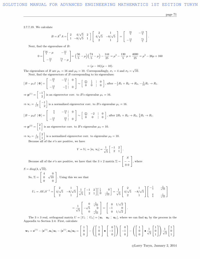
page 71
2.7.7.19. We calculate
B =ATA =
[2 4/
√5 2
1 −8/√
5 1
] 2 1
4/√
5 −8/√
52 1
=
565
− 125
− 125
745
.Next, find the eigenvalues of B:
0 =
565− µ − 12
5
− 125
745− µ
=(56
5− µ
)(74
5− µ
)− 144
25= µ2 − 130
5µ+
4000
25= µ2 − 26µ+ 160
= (µ− 16)(µ− 10).
The eigenvalues of B are µ1 = 16 and µ2 = 10. Correspondingly, σ1 = 4 and σ2 =√
10.Next, find the eigenvectors of B corresponding to its eigenvalues:
[B − µ1I | 0 ] =
− 245
− 125| 0|
− 125
− 65| 0
∼ [ 1© 12| 0
0 0 | 0
], after − 1
2R1 +R2 → R2, − 5
24R1 → R1.
⇒ p(1) =
[−1
2
]is an eigenvector corr. to B’s eigenvalue µ1 = 16.
⇒ v1 = 1√5
[−1
2
]is a normalized eigenvector corr. to B’s eigenvalue µ1 = 16.
[B − µ2I | 0 ] =
65
− 125| 0|
− 125
245| 0
∼ [ 1© −2 | 00 0 | 0
], after 2R1 +R2 → R2, 5
6R1 → R1.
⇒ p(2) =
[21
]is an eigenvector corr. to B’s eigenvalue µ2 = 10.
⇒ v2 = 1√5
[21
]is a normalized eigenvector corr. to eigenvalue µ2 = 10.
Because all of the σ’s are positive, we have
V = V1 = [v1 v2] =1√5
[−1 2
2 1
].
Because all of the σ’s are positive, we have that the 3× 2 matrix Σ =
S− −0 0
, whereS = diag(4,
√10).
So, Σ =
4 0
0√
100 0
. Using this we see that
U1 = AV1S−1 =
2 1
4/√
5 −8/√
52 1
1√5
[−1 2
2 1
][ 14
00 1√
10
]=
1√5
2 1
4/√
5 −8/√
52 1
− 14
2√10
24
1√10
=1√5
0 5√10
−√
5 00 5√
10
=
0 1/√
2−1 0
0 1/√
2
.The 3× 3 real, orthogonal matrix U = [U1
pp U2 ] = [u1 u2
pp u3 ], where we can find u3 by the process in the
Appendix to Section 2.4: First, calculate
w3 = e(1) − 〈e(1),u1〉u1 − 〈e(1),u2〉u2 =
100
− 1
00
• 0−1
0
0−1
0
− 1
00
• 1√2
101
1√2
101
c©Larry Turyn, January 2, 2014
SOLUTIONS MANUAL FOR ADVANCED ENGINEERING MATHEMATICS 1ST EDITION TURYN
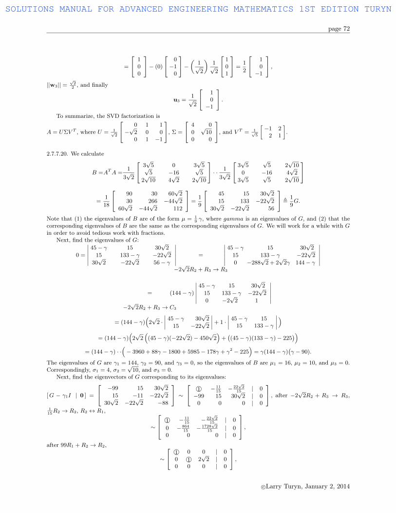
page 72
=
100
− (0)
0−1
0
− ( 1√2
)1√2
101
=1
2
10−1
,||w3|| =
√22, and finally
u3 =1√2
10−1
.To summarize, the SVD factorization is
A = UΣV T , where U = 1√2
0 1 1
−√
2 0 00 1 −1
, Σ =
4 0
0√
100 0
, and V T = 1√5
[−1 2
2 1
].
2.7.7.20. We calculate
B =ATA =1
3√
2
3√
5 0 3√
5√5 −16
√5
2√
10 4√
2 2√
10
· · 1
3√
2
3√
5√
5 2√
10
0 −16 4√
2
3√
5√
5 2√
10
=1
18
90 30 60√
2
30 266 −44√
2
60√
2 −44√
2 112
=1
9
45 15 30√
2
15 133 −22√
2
30√
2 −22√
2 56
,1
9G.
Note that (1) the eigenvalues of B are of the form µ = 19γ, where gamma is an eigenvalues of G, and (2) that the
corresponding eigenvalues of B are the same as the corresponding eigenvalues of G. We will work for a while with Gin order to avoid tedious work with fractions.
Next, find the eigenvalues of G:
0 =
∣∣∣∣∣∣45− γ 15 30
√2
15 133− γ −22√
2
30√
2 −22√
2 56− γ
∣∣∣∣∣∣ =
−2√
2R2 +R3 → R3
∣∣∣∣∣∣45− γ 15 30
√2
15 133− γ −22√
2
0 −288√
2 + 2√
2γ 144− γ
∣∣∣∣∣∣
=
−2√
2R2 +R3 → C3
(144− γ)
∣∣∣∣∣∣45− γ 15 30
√2
15 133− γ −22√
2
0 −2√
2 1
∣∣∣∣∣∣= (144− γ)
(2√
2 ·∣∣∣∣ 45− γ 30
√2
15 −22√
2
∣∣∣∣+ 1 ·∣∣∣∣ 45− γ 15
15 133− γ
∣∣∣∣ )= (144− γ)
(2√
2(
(45− γ)(−22√
2)− 450√
2)
+((45− γ)(133− γ)− 225
))= (144− γ) · ·
(− 3960 + 88γ − 1800 + 5985− 178γ + γ2 − 225
)= γ(144− γ)
(γ − 90).
The eigenvalues of G are γ1 = 144, γ2 = 90, and γ3 = 0, so the eigenvalues of B are µ1 = 16, µ2 = 10, and µ3 = 0.Correspondingly, σ1 = 4, σ2 =
√10, and σ3 = 0.
Next, find the eigenvectors of G corresponding to its eigenvalues:
[G − γ1I | 0 ] =
−99 15 30√
2
15 −11 −22√
2
30√
2 −22√
2 −88
∼ 1© − 11
15− 22
√2
15| 0
−99 15 30√
2 | 00 0 0 | 0
, after −2√
2R2 + R3 → R3,
115R2 → R2, R2 ↔ R1,
∼
1© − 1115
− 22√2
15| 0
0 − 86415
− 1728√2
15| 0
0 0 0 | 0
,after 99R1 +R2 → R2,
∼
1© 0 0 | 0
0 1© 2√
2 | 00 0 0 | 0
,
c©Larry Turyn, January 2, 2014
SOLUTIONS MANUAL FOR ADVANCED ENGINEERING MATHEMATICS 1ST EDITION TURYN
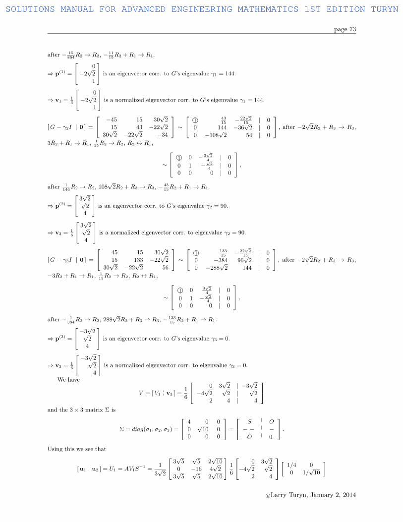
page 73
after − 15864
R2 → R2, − 1115R2 +R1 → R1.
⇒ p(1) =
0
−2√
21
is an eigenvector corr. to G’s eigenvalue γ1 = 144.
⇒ v1 = 13
0
−2√
21
is a normalized eigenvector corr. to G’s eigenvalue γ1 = 144.
[G − γ2I | 0 ] =
−45 15 30√
2
15 43 −22√
2
30√
2 −22√
2 −34
∼ 1© 43
15− 22
√2
15| 0
0 144 −36√
2 | 0
0 −108√
2 54 | 0
, after −2√
2R2 + R3 → R3,
3R2 +R1 → R1, 115R2 → R2, R2 ↔ R1,
∼
1© 0 − 3√2
4| 0
0 1 −√2
4| 0
0 0 0 | 0
,after 1
144R2 → R2, 108
√2R2 +R3 → R3, − 43
15R2 +R1 → R1.
⇒ p(2) =
3√
2√2
4
is an eigenvector corr. to G’s eigenvalue γ2 = 90.
⇒ v2 = 16
3√
2√2
4
is a normalized eigenvector corr. to eigenvalue γ2 = 90.
[G − γ3I | 0 ] =
45 15 30√
2
15 133 −22√
2
30√
2 −22√
2 56
∼ 1© 133
15− 22
√2
15| 0
0 −384 96√
2 | 0
0 −288√
2 144 | 0
, after −2√
2R2 + R3 → R3,
−3R2 +R1 → R1, 115R2 → R2, R2 ↔ R1,
∼
1© 0 3√2
4| 0
0 1 −√2
4| 0
0 0 0 | 0
,after − 1
384R2 → R2, 288
√2R2 +R3 → R3, − 133
15R2 +R1 → R1.
⇒ p(3) =
−3√
2√2
4
is an eigenvector corr. to G’s eigenvalue γ3 = 0.
⇒ v3 = 16
−3√
2√24
is a normalized eigenvector corr. to eigenvalue γ3 = 0.
We have
V = [V1pp v3 ] =
1
6
0 3√
2 | −3√
2
−4√
2√
2 |√
22 4 | 4
and the 3× 3 matrix Σ is
Σ = diag(σ1, σ2, σ3) =
4 0 0
0√
10 00 0 0
=
S | O
− − | −O | 0
.Using this we see that
[u1pp u2 ] = U1 = AV1S
−1 =1
3√
2
3√
5√
5 2√
10
0 −16 4√
2
3√
5√
5 2√
10
1
6
0 3√
2
−4√
2√
22 4
[ 1/4 0
0 1/√
10
]
c©Larry Turyn, January 2, 2014
SOLUTIONS MANUAL FOR ADVANCED ENGINEERING MATHEMATICS 1ST EDITION TURYN
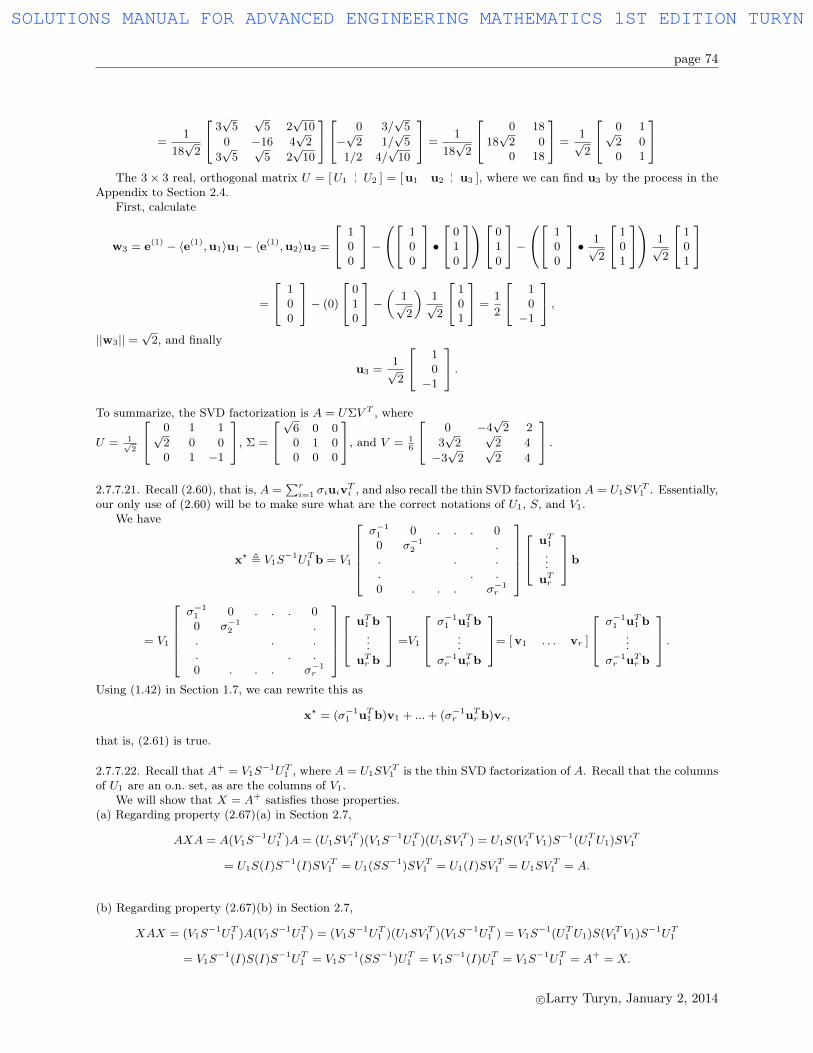
page 74
=1
18√
2
3√
5√
5 2√
10
0 −16 4√
2
3√
5√
5 2√
10
0 3/√
5
−√
2 1/√
5
1/2 4/√
10
=1
18√
2
0 18
18√
2 00 18
=1√2
0 1√2 00 1
The 3× 3 real, orthogonal matrix U = [U1
pp U2 ] = [u1 u2
pp u3 ], where we can find u3 by the process in the
Appendix to Section 2.4.First, calculate
w3 = e(1) − 〈e(1),u1〉u1 − 〈e(1),u2〉u2 =
100
− 1
00
• 0
10
010
− 1
00
• 1√2
101
1√2
101
=
100
− (0)
010
− ( 1√2
)1√2
101
=1
2
10−1
,||w3|| =
√2, and finally
u3 =1√2
10−1
.To summarize, the SVD factorization is A = UΣV T , where
U = 1√2
0 1 1√2 0 00 1 −1
, Σ =
√6 0 00 1 00 0 0
, and V = 16
0 −4√
2 2
3√
2√
2 4
−3√
2√
2 4
.2.7.7.21. Recall (2.60), that is, A =
∑ri=1 σiuiv
Ti , and also recall the thin SVD factorization A = U1SV
T1 . Essentially,
our only use of (2.60) will be to make sure what are the correct notations of U1, S, and V1.We have
x? , V1S−1UT1 b = V1
σ−11 0 . . . 00 σ−1
2 .. . .. . .0 . . . σ−1
r
uT1
...uTr
b
= V1
σ−11 0 . . . 00 σ−1
2 .. . .. . .0 . . . σ−1
r
uT1 b
...uTr b
=V1
σ−11 uT1 b
...σ−1r uTr b
= [v1 . . . vr ]
σ−11 uT1 b
...σ−1r uTr b
.Using (1.42) in Section 1.7, we can rewrite this as
x? = (σ−11 uT1 b)v1 + ...+ (σ−1
r uTr b)vr,
that is, (2.61) is true.
2.7.7.22. Recall that A+ = V1S−1UT1 , where A = U1SV
T1 is the thin SVD factorization of A. Recall that the columns
of U1 are an o.n. set, as are the columns of V1.We will show that X = A+ satisfies those properties.
(a) Regarding property (2.67)(a) in Section 2.7,
AXA = A(V1S−1UT1 )A = (U1SV
T1 )(V1S
−1UT1 )(U1SVT1 ) = U1S(V T1 V1)S−1(UT1 U1)SV T1
= U1S(I)S−1(I)SV T1 = U1(SS−1)SV T1 = U1(I)SV T1 = U1SVT1 = A.
(b) Regarding property (2.67)(b) in Section 2.7,
XAX = (V1S−1UT1 )A(V1S
−1UT1 ) = (V1S−1UT1 )(U1SV
T1 )(V1S
−1UT1 ) = V1S−1(UT1 U1)S(V T1 V1)S−1UT1
= V1S−1(I)S(I)S−1UT1 = V1S
−1(SS−1)UT1 = V1S−1(I)UT1 = V1S
−1UT1 = A+ = X.
c©Larry Turyn, January 2, 2014
SOLUTIONS MANUAL FOR ADVANCED ENGINEERING MATHEMATICS 1ST EDITION TURYN
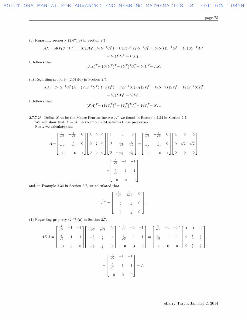
page 75
(c) Regarding property (2.67)(c) in Section 2.7,
AX = A(V1S−1UT1 ) = (U1SV
T1 )(V1S
−1UT1 ) = U1S(V T1 V1)S−1UT1 = U1S(I)S−1UT1 = U1(SS−1)UT1
= U1(I)UT1 = U1UT1 .
It follows that(AX)T=
(U1U
T1
)T=(UT1)TUT1 = U1U
T1 = AX.
(d) Regarding property (2.67)(d) in Section 2.7,
XA = (V1S−1UT1 )A = (V1S
−1UT1 )(U1SVT1 ) = V1S
−1(UT1 U1)SV T1 = V1S−1(I)SV T1 = V1(S−1S)V T1
= V1(I)V T1 = V1VT1 .
It follows that(XA)T=
(V1V
T1
)T=(V T1)TV T1 = V1V
T1 = XA.
2.7.7.23. Define X to be the Moore-Penrose inverse A+ we found in Example 2.34 in Section 2.7.We will show that X = A+ in Example 2.34 satisfies those properties.First, we calculate that
A =
1√2− 1√
20
1√2
1√2
0
0 0 1
3 0 0
0 2 0
0 0 0
1 0 0
0 1√2
1√2
0 − 1√2
1√2
=
1√2− 1√
20
1√2
1√2
0
0 0 1
3 0 0
0√
2√
2
0 0 0
=
3√2−1 −1
3√2
1 1
0 0 0
,and, in Example 2.34 in Section 2.7, we calculated that
A+ =
1
3√2
1
3√2
0
− 14
14
0
− 14
14
0
.
(1) Regarding property (2.67)(a) in Section 2.7,
AXA =
3√2−1 −1
3√2
1 1
0 0 0
1
3√2
1
3√2
0
− 14
14
0
− 14
14
0
3√2−1 −1
3√2
1 1
0 0 0
=
3√2−1 −1
3√2
1 1
0 0 0
1 0 0
0 12
12
0 12
12
=
3√2−1 −1
3√2
1 1
0 0 0
= A.
c©Larry Turyn, January 2, 2014
SOLUTIONS MANUAL FOR ADVANCED ENGINEERING MATHEMATICS 1ST EDITION TURYN
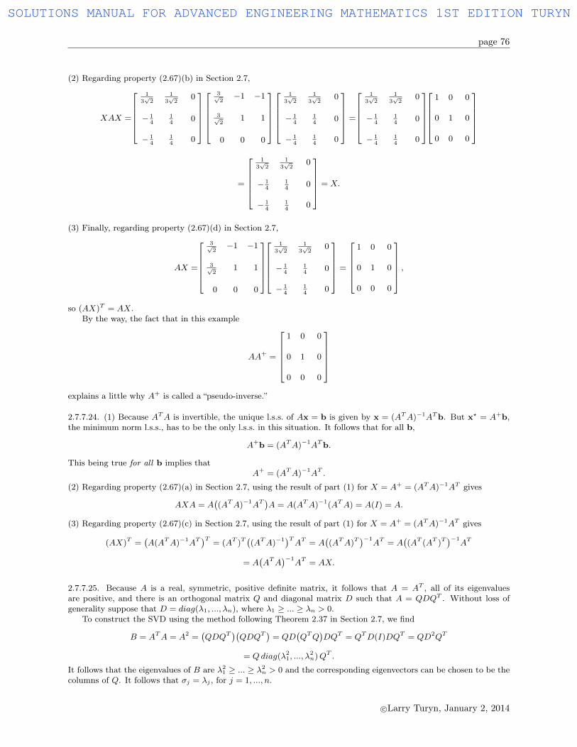
page 76
(2) Regarding property (2.67)(b) in Section 2.7,
XAX =
1
3√2
1
3√2
0
− 14
14
0
− 14
14
0
3√2−1 −1
3√2
1 1
0 0 0
1
3√2
1
3√2
0
− 14
14
0
− 14
14
0
=
1
3√2
1
3√2
0
− 14
14
0
− 14
14
0
1 0 0
0 1 0
0 0 0
=
1
3√2
1
3√2
0
− 14
14
0
− 14
14
0
= X.
(3) Finally, regarding property (2.67)(d) in Section 2.7,
AX =
3√2−1 −1
3√2
1 1
0 0 0
1
3√2
1
3√2
0
− 14
14
0
− 14
14
0
=
1 0 0
0 1 0
0 0 0
,
so (AX)T = AX.By the way, the fact that in this example
AA+ =
1 0 0
0 1 0
0 0 0
explains a little why A+ is called a “pseudo-inverse.”
2.7.7.24. (1) Because ATA is invertible, the unique l.s.s. of Ax = b is given by x = (ATA)−1ATb. But x? = A+b,the minimum norm l.s.s., has to be the only l.s.s. in this situation. It follows that for all b,
A+b = (ATA)−1ATb.
This being true for all b implies thatA+ = (ATA)−1AT .
(2) Regarding property (2.67)(a) in Section 2.7, using the result of part (1) for X = A+ = (ATA)−1AT gives
AXA = A((ATA)−1AT
)A = A(ATA)−1(ATA) = A(I) = A.
(3) Regarding property (2.67)(c) in Section 2.7, using the result of part (1) for X = A+ = (ATA)−1AT gives
(AX)T =(A(ATA)−1AT
)T= (AT )T
((ATA)−1)TAT = A
((ATA)T
)−1AT = A
((AT (AT )T
)−1AT
= A(ATA
)−1AT = AX.
2.7.7.25. Because A is a real, symmetric, positive definite matrix, it follows that A = AT , all of its eigenvaluesare positive, and there is an orthogonal matrix Q and diagonal matrix D such that A = QDQT . Without loss ofgenerality suppose that D = diag(λ1, ..., λn), where λ1 ≥ ... ≥ λn > 0.
To construct the SVD using the method following Theorem 2.37 in Section 2.7, we find
B = ATA = A2 =(QDQT
)(QDQT
)= QD
(QTQ
)DQT = QTD(I)DQT = QD2QT
= Qdiag(λ21, ..., λ
2n)QT .
It follows that the eigenvalues of B are λ21 ≥ ... ≥ λ2
n > 0 and the corresponding eigenvectors can be chosen to be thecolumns of Q. It follows that σj = λj , for j = 1, ..., n.
c©Larry Turyn, January 2, 2014
SOLUTIONS MANUAL FOR ADVANCED ENGINEERING MATHEMATICS 1ST EDITION TURYN

page 77
So, Σ = D and V = Q. It follows that
U = AV Σ−1 = (QDQT )QD−1 = QD(QTQ)D−1 = QD(I)D−1 = Q(DD−1) = Q.
To summarize, if A is a real, symmetric, positive definite matrix, then its SVD factorization is A = QDQT , thefactorization we found in Section 2.6.
2.7.7.26. Because A is a real, symmetric, matrix, it follows that A = AT , all of its eigenvalues are real, and there isan orthogonal matrix Q and diagonal matrix D such that A = QDQT , as in Section 2.6.
We assumed that the eigenvalues of A satisfy |λ1| ≥ |λ2| ≥ ... ≥ |λn| ≥ 0; without loss of generality, D =diag(λ1, ..., λn).
Assume that |λr| > 0 and that λj = 0 for j = r + 1, ..., n.To construct the SVD using the method following Theorem 2.37 in Section 2.7, we find
B = ATA = A2 =(QDQT
)(QDQT
)= QD
(QTQ
)DQT = QTD(I)DQT = QD2QT
= Qdiag(λ21, ..., λ
2n)QT .
It follows that the n eigenvalues of B are λ21 ≥ ... ≥ λ2
r > 0 = ... = 0 and the corresponding eigenvectors can bechosen to be the columns of Q. It follows that σj = |λj |, for j = 1, ..., n.
As usual for the SVD factorization, we let V1 =[v1
pp ...
pp vr
].
So, V = Q and
Σ =
S | O
− − | −O | O
= diag(|λ1|, ..., |λr|, 0, ..., 0).
It follows thatU1 = AV1S
−1 = (QDQT )V1S−1 = QD(QTV1)S−1,
that is,U1 = QD(QTV1)S−1.
We calculate that
QTV1 =
vT1...
vTn
[v1pp ...
pp vr
]=
vT1 v1 ... vT1 vr...
vTnv1 ... vTnvr
=
Ir− − −On−r,r
,hence
(QTV1)S−1 =
diag(|λ1|−1, ..., |λr|−1)− − − − − − −
On−r,r
.So,
U1 = QD(QTV1)S−1 = Q
diag(λ1, ..., λn)
diag(|λ1|−1, ..., |λr|−1)− − − − − − −
On−r,r
= Q
diag(sgn(λ1), ..., sgn(λr)
)− − − − − − −
On−r,r
=[v1
pp ...
pp vn
] diag(sgn(λ1), ..., sgn(λr))
− − − − − − −On−r,r
=[sgn(λ1)v1
pp ...
pp sgn(λr)vr
].
It is easy to find the rest of the columns of the orthogonal matrix U because {v1, ...,vn} being an o.n. set impliesthat {sgn(λ1)v1, ..., sgn(λr)vr,vr+1, ...,vn} is an o.n. set.
To summarize, if A is a real, symmetric matrix whose eigenvalues satisfy , then its SVD factorization is A = UΣV T ,where
U=[sgn(λ1)v1
pp ...
pp sgn(λr)vr
pp vr+1
pp · · · p
p vn], Σ = diag
(sgn(λ1), ..., sgn(λr), 0, . . . , 0
),
andV = Q =
[v1
pp ...
pp vn
].
c©Larry Turyn, January 2, 2014
SOLUTIONS MANUAL FOR ADVANCED ENGINEERING MATHEMATICS 1ST EDITION TURYN
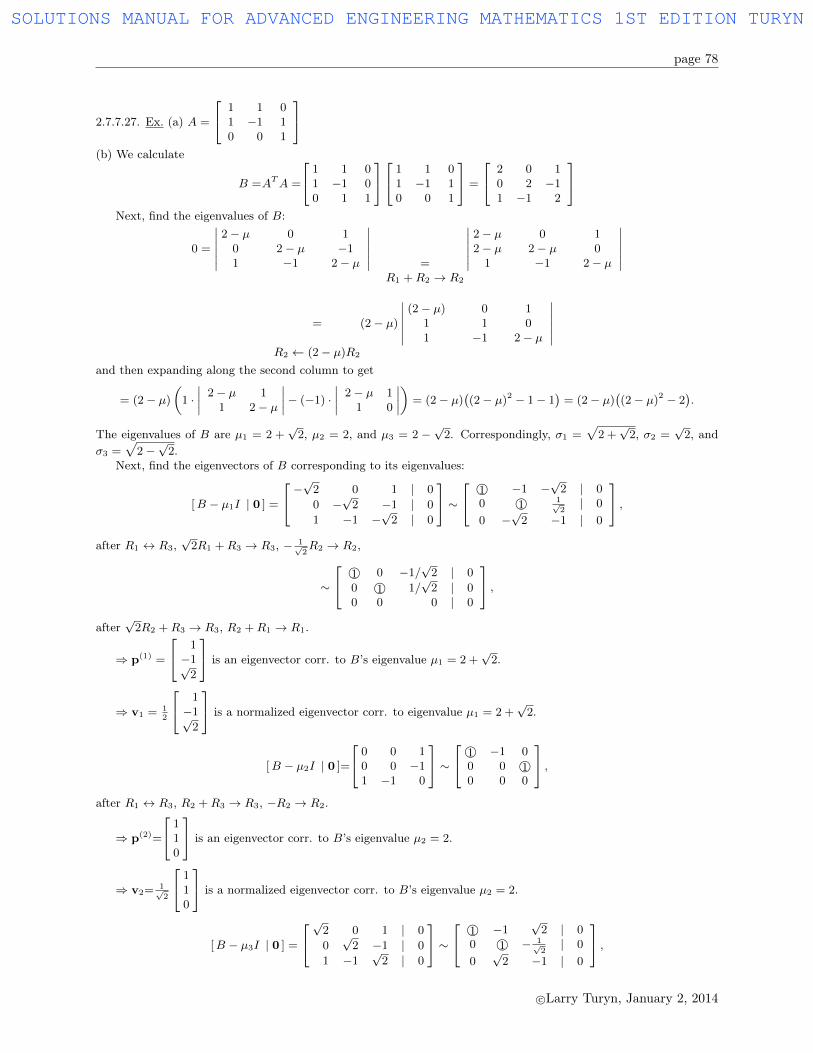
page 78
2.7.7.27. Ex. (a) A =
1 1 01 −1 10 0 1
(b) We calculate
B =ATA =
1 1 01 −1 00 1 1
1 1 01 −1 10 0 1
=
2 0 10 2 −11 −1 2
Next, find the eigenvalues of B:
0 =
∣∣∣∣∣∣2− µ 0 1
0 2− µ −11 −1 2− µ
∣∣∣∣∣∣ =R1 +R2 → R2
∣∣∣∣∣∣2− µ 0 12− µ 2− µ 0
1 −1 2− µ
∣∣∣∣∣∣
=
R2 ← (2− µ)R2
(2− µ)
∣∣∣∣∣∣(2− µ) 0 1
1 1 01 −1 2− µ
∣∣∣∣∣∣and then expanding along the second column to get
= (2− µ)
(1 ·∣∣∣∣ 2− µ 1
1 2− µ
∣∣∣∣− (−1) ·∣∣∣∣ 2− µ 1
1 0
∣∣∣∣) = (2− µ)((2− µ)2 − 1− 1
)= (2− µ)
((2− µ)2 − 2
).
The eigenvalues of B are µ1 = 2 +√
2, µ2 = 2, and µ3 = 2 −√
2. Correspondingly, σ1 =√
2 +√
2, σ2 =√
2, andσ3 =
√2−√
2.Next, find the eigenvectors of B corresponding to its eigenvalues:
[B − µ1I | 0 ] =
−√
2 0 1 | 0
0 −√
2 −1 | 0
1 −1 −√
2 | 0
∼ 1© −1 −
√2 | 0
0 1© 1√2| 0
0 −√
2 −1 | 0
,after R1 ↔ R3,
√2R1 +R3 → R3, − 1√
2R2 → R2,
∼
1© 0 −1/√
2 | 0
0 1© 1/√
2 | 00 0 0 | 0
,after
√2R2 +R3 → R3, R2 +R1 → R1.
⇒ p(1) =
1−1√
2
is an eigenvector corr. to B’s eigenvalue µ1 = 2 +√
2.
⇒ v1 = 12
1−1√
2
is a normalized eigenvector corr. to eigenvalue µ1 = 2 +√
2.
[B − µ2I | 0 ]=
0 0 10 0 −11 −1 0
∼ 1© −1 0
0 0 1©0 0 0
,after R1 ↔ R3, R2 +R3 → R3, −R2 → R2.
⇒ p(2)=
110
is an eigenvector corr. to B’s eigenvalue µ2 = 2.
⇒ v2= 1√2
110
is a normalized eigenvector corr. to B’s eigenvalue µ2 = 2.
[B − µ3I | 0 ] =
√
2 0 1 | 0
0√
2 −1 | 0
1 −1√
2 | 0
∼ 1© −1
√2 | 0
0 1© − 1√2| 0
0√
2 −1 | 0
,c©Larry Turyn, January 2, 2014
SOLUTIONS MANUAL FOR ADVANCED ENGINEERING MATHEMATICS 1ST EDITION TURYN

page 79
after R1 ↔ R3, −√
2R1 +R3 → R3, 1√2R2 → R2,
∼
1© 0 1/√
2 | 0
0 1© −1/√
2 | 00 0 0 | 0
,after −
√2R2 +R3 → R3, R2 +R1 → R1.
⇒ p(3) =
−11√2
is an eigenvector corr. to B’s eigenvalue µ3 = 2−√
2.
⇒ v3 = 12
−11√2
is a normalized eigenvector corr. to eigenvalue µ3 = 2−√
2.
Because all of the σ’s are positive, we have
V = V1 = [v1 ... v3] =1
2
1√
2 −1
−1√
2 1√2 0
√2
and
Σ = S = diag(
√2 +√
2,√
2,
√2−√
2) =
√
2 +√
2 0 0
0√
2 0
0 0√
2−√
2
.Using this we see that
U = U1 = AV Σ−1 =
1 1 01 −1 10 0 1
1
2
1√
2 −1
−1√
2 1√2 0
√2
1/
√2 +√
2 0 0
0 1/√
2 0
0 0 1/√
2−√
2
=1
2
0 2√
2 0
2 +√
2 0 −2 +√
2√2 0
√2
1/
√2 +√
2 0 0
0 1/√
2 0
0 0 1/√
2−√
2
=1
2
0 2 0√
2 +√
2 0 −√
2−√
2√2/√
2 +√
2 0√
2/√
2−√
2
.
To summarize, the SVD factorization is A = UΣV T , where
U =1
2
0 2 0√
2 +√
2 0 −√
2−√
2
√2/√
2 +√
2 0√
2/√
2−√
2
, Σ =
√2 +√
2 0 0
0 2 0
0 0√
2−√
2
,
and
V T =
1/2 −1/2 1/
√2
1/√
2 1/√
2 0
−1/2 1/2 1/√
2
.
2.7.7.28. A = QR implies QTA = (QTQ)R = (I)R = R, and this implies QTAQ = RQ, which shows that A isorthogonally similar to RQ.
c©Larry Turyn, January 2, 2014
SOLUTIONS MANUAL FOR ADVANCED ENGINEERING MATHEMATICS 1ST EDITION TURYN
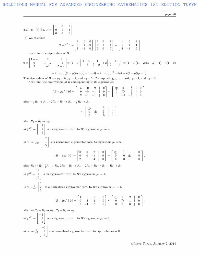
page 80
2.7.7.29. (a) Ex. A =
1 0 20 1 −10 0 0
(b) We calculate
B =ATA =
1 0 00 1 02 −1 0
1 0 20 1 −10 0 0
=
1 0 20 1 −12 −1 5
Next, find the eigenvalues of B:
0 =
∣∣∣∣∣∣1− µ 0 2
0 1− µ −12 −1 5− µ
∣∣∣∣∣∣= (1− µ)
∣∣∣∣ 1− µ −1−1 5− µ
∣∣∣∣+ 2
∣∣∣∣ 0 1− µ2 −1
∣∣∣∣= (1− µ)((1− µ)(5− µ)− 1
)− 4(1− µ)
= (1− µ)((1− µ)(5− µ)− 1− 4
)= (1− µ)(µ2 − 6µ) = µ(1− µ)(µ− 6).
The eigenvalues of B are µ1 = 6, µ2 = 1, and µ3 = 0. Correspondingly, σ1 =√
6, σ2 = 1, and σ3 = 0.Next, find the eigenvectors of B corresponding to its eigenvalues:
[B − µ1I | 0 ] =
−5 0 2 | 00 −5 −1 | 02 −1 −1 | 0
∼ 1© 0 − 2
5| 0
0 1© 15| 0
0 −1 − 15| 0
,after − 1
5R1 → R1, −2R1 +R3 → R3, − 1
5R2 → R2,
∼
1© 0 − 25| 0
0 1© 15| 0
0 0 0 | 0
,after R2 +R3 → R3.
⇒ p(1) =
2−1
5
is an eigenvector corr. to B’s eigenvalue µ1 = 6.
⇒ v1 = 1√30
2−1
5
is a normalized eigenvector corr. to eigenvalue µ1 = 6.
[B − µ2I | 0 ] =
0 0 2 | 00 0 −1 | 02 −1 4 | 0
∼ 1© − 1
20 | 0
0 0 1© | 00 0 0 | 0
,after R1 ↔ R3, 1
2R1 → R1, 2R2 +R3 → R3, −2R2 +R1 → R1, −R2 → R2.
⇒ p(2)=
120
is an eigenvector corr. to B’s eigenvalue µ2 = 1.
⇒ v2= 1√5
120
is a normalized eigenvector corr. to B’s eigenvalue µ2 = 1.
[B − µ3I | 0 ] =
1 0 2 | 00 1 −1 | 02 −1 5 | 0
∼ 1© 0 2 | 0
0 1© −1 | 00 0 0 | 0
,after −2R1 +R3 → R3, R2 +R3 → R3.
⇒ p(3) =
−211
is an eigenvector corr. to B’s eigenvalue µ3 = 0.
⇒ v3 = 1√6
−211
is a normalized eigenvector corr. to eigenvalue µ3 = 0.
c©Larry Turyn, January 2, 2014
SOLUTIONS MANUAL FOR ADVANCED ENGINEERING MATHEMATICS 1ST EDITION TURYN

page 81
V = [V1pp v3 ] =
1√30
2√
6 | −2√
5
−1 2√
6 |√
5
5 0 |√
5
and the 3× 3 matrix Σ is
Σ = diag(σ1, σ2, σ3) =
√6 0 00 1 00 0 0
=
S | O
− − | −O | 0
.Using this we see that
[u1pp u2 ] = U1 = AV1S
−1 =
1 0 20 1 −10 0 0
1√30
2√
6
−1 2√
65 0
[ 1/√
6 00 1
]
=1√30
1 0 20 1 −10 0 0
2/√
6√
6
−1/√
6 2√
6
5/√
6 0
=1
6√
5
1 0 20 1 −10 0 0
2 6−1 12
5 0
=
1
6√
5
12 6−6 12
0 0
=1√5
2 1−1 2
0 0
The 3× 3 real, orthogonal matrix U = [U1
pp U2 ] = [u1 u2
pp u3 ], where we can find u3 by the process in the
Appendix to Section 2.4.Because Span
({u1,u2}
)= Span
({e(1), e(2)}
), we should use e(3) instead of e(1).
First, calculatew3 = e(3) − 〈e(3),u1〉u1 − 〈e(3),u2〉u2
=
001
− 0
01
• 1√5
2−1
0
1√5
2−1
0
− 0
01
• 1√5
120
1√5
120
=
001
− (0)1√5
2−1
0
− (0)1√5
120
=
001
= e(3),
||w3|| = 1, and finally
u3 = e(3) =
001
.To summarize, the SVD factorization is A = UΣV T , where
U = 1√5
2 1 0−1 2 0
0 0√
5
, Σ =
√6 0 00 1 00 0 0
, and V T = 1√30
2 −1 5√6 2
√6 0
−2√
5√
5√
5
.
c©Larry Turyn, January 2, 2014
SOLUTIONS MANUAL FOR ADVANCED ENGINEERING MATHEMATICS 1ST EDITION TURYN
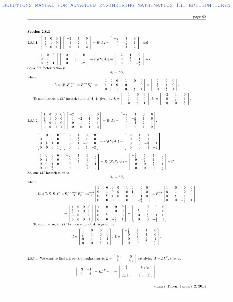
page 82
Section 2.8.3
2.8.3.1.
1 0 012
1 00 0 1
−2 1 01 −2 10 1 −2
= E1A3 =
−2 1 00 − 3
21
0 1 −2
, and 1 0 0
0 1 00 2
31
−2 1 00 − 3
21
0 1 −2
= E2(E1A3) =
−2 1 00 − 3
21
0 0 − 43
= U.
So, a LU factorization isA3 = LU,
where
L = (E2E1)−1 = E−11 E−1
2 =
1 0 0− 1
21 0
0 0 1
1 0 00 1 00 − 2
31
=
1 0 0− 1
21 0
0 − 23
1
.To summarize, a LU factorization of A3 is given by L =
1 0 0− 1
21 0
0 − 23
1
, U =
−2 1 00 − 3
21
0 0 − 43
.
2.8.3.2.
1 0 0 012
1 0 00 0 1 00 0 0 1
−2 1 0 0
1 −2 1 00 1 −2 10 0 1 −2
= E1A4 =
−2 1 0 0
0 − 32
1 00 1 −2 10 0 1 −2
,
1 0 0 00 1 0 00 2
31 0
0 0 0 1
−2 1 0 0
0 − 32
1 00 1 −2 00 0 1 −2
= E2(E1A4) =
−2 1 1 0
0 − 32
1 00 0 − 4
31
0 0 1 −2
1 0 0 00 1 0 00 0 1 00 0 3
41
−2 1 1 0
0 − 32
1 00 0 − 4
31
0 0 1 −2
= E3(E2E1A3) =
− 2
11 1 0
0 − 32
1 00 0 − 4
31
0 0 0 − 54
= U
So, one LU factorization isA4 = LU,
where
L=(E3E2E1)−1=E−11 E−1
2 E−13 =E−1
1
1 0 0 00 1 0 00 − 2
31 0
0 0 0 1
1 0 0 00 1 0 00 0 1 00 0 − 3
41
= E−11
1 0 0 00 1 0 00 − 2
31 0
0 0 − 34
1
=
1 0 0 012
1 0 00 0 1 00 0 0 1
1 0 0 00 1 0 00 − 2
31 0
0 0 − 34
1
=
1 0 0 0− 1
21 0 0
0 − 23
1 00 0 − 3
41
.To summarize, an LU factorization of A4 is given by
L=
1 0 0 012
1 0 00 − 2
31 1
0 0 − 34
1
, U=
− 2
11 1 0
0 − 32
1 00 0 − 4
31
0 0 0 − 54
.
2.8.3.4. We want to find a lower triangular matrix L =
[`11 0`21 `22
]satisfying A = LLT , that is,
[3 −1−1 3
]= LLT = ... =
`211 `11`21
`11`21 `221 + `222
.c©Larry Turyn, January 2, 2014
SOLUTIONS MANUAL FOR ADVANCED ENGINEERING MATHEMATICS 1ST EDITION TURYN
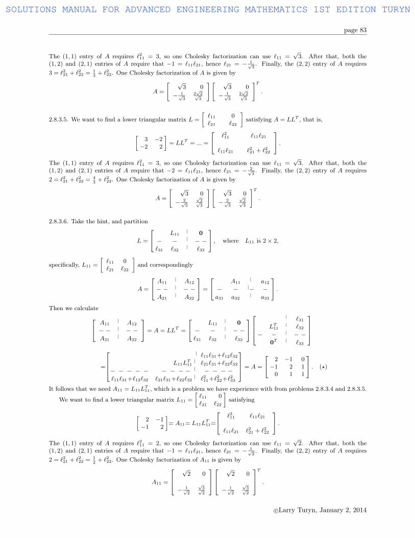
page 83
The (1, 1) entry of A requires `211 = 3, so one Cholesky factorization can use `11 =√
3. After that, both the(1, 2) and (2, 1) entries of A require that −1 = `11`21, hence `21 = − 1√
3. Finally, the (2, 2) entry of A requires
3 = `221 + `222 = 13
+ `222. One Cholesky factorization of A is given by
A =
[ √3 0
− 1√3
2√2√3
][ √3 0
− 1√3
2√2√3
]T.
2.8.3.5. We want to find a lower triangular matrix L =
[`11 0`21 `22
]satisfying A = LLT , that is,
[3 −2−2 2
]= LLT = ... =
`211 `11`21
`11`21 `221 + `222
.The (1, 1) entry of A requires `211 = 3, so one Cholesky factorization can use `11 =
√3. After that, both the
(1, 2) and (2, 1) entries of A require that −2 = `11`21, hence `21 = − 2√3. Finally, the (2, 2) entry of A requires
2 = `221 + `222 = 43
+ `222. One Cholesky factorization of A is given by
A =
[ √3 0
− 2√3
√2√3
][ √3 0
− 2√3
√2√3
]T.
2.8.3.6. Take the hint, and partition
L =
L11| 0
− − | − −`31 `32
| `33
, where L11 is 2× 2,
specifically, L11 =
[`11 0`21 `22
]and correspondingly
A =
A11| A12
− − | − −A21
| A22
=
A11| a12
− − |− −a31 a32
| a33
.Then we calculate A11
| A12
− − | − −A21
| A22
= A = LLT =
L11| 0
− − | − −`31 `32
| `33
| `31LT11
| `32− − | − −
0T | `33
=
| `11`31+`12`32
L11LT11| `21`31+`22`32
− − − − − − − − − | − − − −`11`31+`12`32 `21`31+`22`32
| `211+`222+`233
= A =
2 −1 0−1 2 1
0 1 1
. (?)
It follows that we need A11 = L11LT11, which is a problem we have experience with from problems 2.8.3.4 and 2.8.3.5.
We want to find a lower triangular matrix L11 =
[`11 0`21 `22
]satisfying
[2 −1−1 2
]= A11= L11L
T11=
`211 `11`21
`11`21 `221 + `222
.The (1, 1) entry of A requires `211 = 2, so one Cholesky factorization can use `11 =
√2. After that, both the
(1, 2) and (2, 1) entries of A require that −1 = `11`21, hence `21 = − 1√2. Finally, the (2, 2) entry of A requires
2 = `221 + `222 = 12
+ `222. One Cholesky factorization of A11 is given by
A11 =
√
2 0
− 1√2
√3√2
√
2 0
− 1√2
√3√2
T
.
c©Larry Turyn, January 2, 2014
SOLUTIONS MANUAL FOR ADVANCED ENGINEERING MATHEMATICS 1ST EDITION TURYN
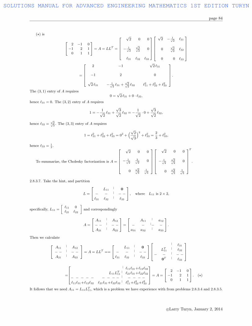
page 84
(?) is
2 −1 0−1 2 1
0 1 1
= A = LLT =
√
2 0 0
− 1√2
√3√2
0
`31 `32 `33
√2 − 1√
2`31
0√3√2
`32
0 0 `33
=
2 −1
√2 `31
−1 2 0
√2 `31 − 1√
2`31 +
√3√2`32 `211 + `222 + `233
.The (3, 1) entry of A requires
0 =√
2 `31 + 0 · `32,hence `31 = 0. The (3, 2) entry of A requires
1 = − 1√2`31 +
√3√2`32 = − 1√
2· 0 +
√3√2`32,
hence `32 =√2√3. The (3, 3) entry of A requires
1 = `231 + `222 + `233 = 02 +(√2√
3
)2+ `233 =
2
3+ `233,
hence `33 = 13.
To summarize, the Cholesky factorization is A =
√2 0 0
− 1√2
3√2
0
0√2√3
1√3
√2 0 0
− 1√2
√3√2
0
0√2√3
1√3
T
.
2.8.3.7. Take the hint, and partition
L =
L11| 0
− − | − −`31 `32
| `33
, where L11 is 2× 2,
specifically, L11 =
[`11 0`21 `22
]and correspondingly
A =
A11| A12
− − | − −A21
| A22
=
A11| a12
− − |− −a31 a32
| a33
.Then we calculate
A11| A12
− − | − −A21
| A22
= A = LLT ==
L11| 0
− − | − −`31 `32
| `33
| `31LT11
| `32− − | − −
0T | `33
=
| `11`31+`12`32
L11LT11| `21`31+`22`32
− − − − − − − − − | − − − −`11`31+`12`32 `21`31+`22`32
| `211+`222+`233
= A =
2 −1 0−1 2 1
0 1 1
. (?)
It follows that we need A11 = L11LT11, which is a problem we have experience with from problems 2.8.3.4 and 2.8.3.5.
c©Larry Turyn, January 2, 2014
SOLUTIONS MANUAL FOR ADVANCED ENGINEERING MATHEMATICS 1ST EDITION TURYN
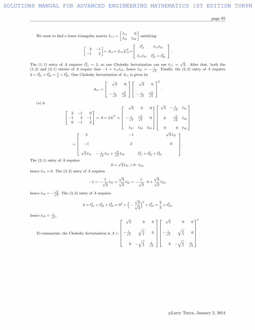
page 85
We want to find a lower triangular matrix L11 =
[`11 0`21 `22
]satisfying
[2 −1−1 2
]= A11= L11L
T11=
`211 `11`21
`11`21 `221 + `222
.The (1, 1) entry of A requires `211 = 2, so one Cholesky factorization can use `11 =
√2. After that, both the
(1, 2) and (2, 1) entries of A require that −1 = `11`21, hence `21 = − 1√2. Finally, the (2, 2) entry of A requires
2 = `221 + `222 = 12
+ `222. One Cholesky factorization of A11 is given by
A11 =
√
2 0
− 1√2
√3√2
√
2 0
− 1√2
√3√2
T
.
(?) is
2 −1 0−1 2 −1
0 −1 2
= A = LLT =
√
2 0 0
− 1√2
√3√2
0
`31 `32 `33
√2 − 1√
2`31
0√3√2
`32
0 0 `33
=
2 −1
√2 `31
−1 2 0
√2 `31 − 1√
2`31 +
√3√2`32 `211 + `222 + `233
.The (3, 1) entry of A requires
0 =√
2 `31 + 0 · `32,hence `31 = 0. The (3, 2) entry of A requires
−1 = − 1√2`31 +
√3√2`32 = − 1√
2· 0 +
√3√2`32,
hence `32 = −√
2√3. The (3, 3) entry of A requires
2 = `231 + `222 + `233 = 02 +(−√
2√3
)2+ `233 =
2
3+ `233,
hence `33 = 2√3.
To summarize, the Cholesky factorization is A =
√2 0 0
− 1√2
√32
0
0 −√
23
2√3
√2 0 0
− 1√2
√32
0
0 −√
23
2√3
T
c©Larry Turyn, January 2, 2014
SOLUTIONS MANUAL FOR ADVANCED ENGINEERING MATHEMATICS 1ST EDITION TURYN
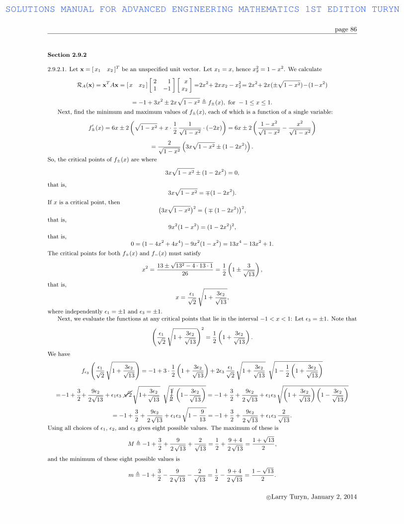
page 86
Section 2.9.2
2.9.2.1. Let x = [x1 x2 ]T be an unspecified unit vector. Let x1 = x, hence x22 = 1− x2. We calculate
RA(x) = xTAx = [x x2 ]
[2 11 −1
] [xx2
]=2x2+ 2xx2 − x22 = 2x2+ 2x(±
√1− x2)−(1−x2)
= −1 + 3x2 ± 2x√
1− x2 , f±(x), for − 1 ≤ x ≤ 1.
Next, find the minimum and maximum values of f±(x), each of which is a function of a single variable:
f ′±(x) = 6x± 2
(√1− x2 + x · 1
2
1√1− x2
· (−2x)
)= 6x± 2
(1− x2√1− x2
− x2√1− x2
)=
2√1− x2
(3x√
1− x2 ± (1− 2x2)).
So, the critical points of f±(x) are where
3x√
1− x2 ± (1− 2x2) = 0,
that is,3x√
1− x2 = ∓(1− 2x2).
If x is a critical point, then (3x√
1− x2)2
=(∓ (1− 2x2)
)2,
that is,9x2(1− x2) = (1− 2x2)2,
that is,0 = (1− 4x2 + 4x4)− 9x2(1− x2) = 13x4 − 13x2 + 1.
The critical points for both f+(x) and f−(x) must satisfy
x2 =13±
√132 − 4 · 13 · 1
26=
1
2
(1± 3√
13
),
that is,
x =ε1√
2
√1 +
3ε2√13,
where independently ε1 = ±1 and ε3 = ±1.Next, we evaluate the functions at any critical points that lie in the interval −1 < x < 1: Let ε3 = ±1. Note that(
ε1√2
√1 +
3ε2√13
)2
=1
2
(1 +
3ε2√13
).
We have
fε3
(ε1√
2
√1 +
3ε2√13
)= −1 + 3 · 1
2
(1 +
3ε2√13
)+ 2ε3
ε1√2
√1 +
3ε2√13
√1− 1
2
(1 +
3ε2√13
)
=−1 +3
2+
9ε2
2√
13+ ε1ε3 ��
√2
√1+
3ε2√13
√��12
(1− 3ε2√
13
)= −1 +
3
2+
9ε2
2√
13+ ε1ε3
√(1 +
3ε2√13
)(1− 3ε2√
13
)
= −1 +3
2+
9ε2
2√
13+ ε1ε3
√1− 9
13= −1 +
3
2+
9ε2
2√
13+ ε1ε3
2√13.
Using all choices of ε1, ε2, and ε3 gives eight possible values. The maximum of these is
M , −1 +3
2+
9
2√
13+
2√13
=1
2+
9 + 4
2√
13=
1 +√
13
2,
and the minimum of these eight possible values is
m , −1 +3
2− 9
2√
13− 2√
13=
1
2− 9 + 4
2√
13=
1−√
13
2.
c©Larry Turyn, January 2, 2014
SOLUTIONS MANUAL FOR ADVANCED ENGINEERING MATHEMATICS 1ST EDITION TURYN

page 87
We also need to evaluate the functions at the endpoints of the interval −1 ≤ x ≤ 1:
f+(±1) = −1 + 3(±1)2 + 2(±1)√
1− (±1)2 = 2
and similarly f−(±1) = 2.So, the Rayleigh quotient for this 2 × 2 real, symmetric matrix gives maximum eigenvalue being 1+
√13
2and
minimum eigenvalue being 1−√13
2.
By the way, Section 2.1’s usual way of finding the eigenvalues using the characteristic equation gives the resultthat the exact eigenvalues of A are 1±
√13
2.
2.9.2.2. Let x = [x1 x2 ]T be an unspecified unit vector. Let x1 = x, hence x22 = 1− x2. We calculate
RA(x) = xTAx = [x x2 ]
[1 33 4
] [xx2
]=x2+ 6xx2 + 4x22 = x2+ 6x(±
√1− x2)+4(1−x2)
= 4− 3x2 ± 6x√
1− x2 , f±(x), for − 1 ≤ x ≤ 1.
Next, find the minimum and maximum values of f±(x), each of which is a function of a single variable:
f ′±(x) = −6x± 6
(√1− x2 + x · 1
2
1√1− x2
· (−2x)
)= −6x± 6
(1− x2√1− x2
− x2√1− x2
)=
6√1− x2
(−x√
1− x2 ± (1− 2x2)).
So, the critical points of f±(x) are where
−x√
1− x2 ± (1− 2x2) = 0,
that is,x√
1− x2 = ±(1− 2x2).
If x is a critical point, then (x√
1− x2)2
=(± (1− 2x2)
)2,
that is,x2(1− x2) = (1− 2x2)2,
that is,0=(1−4x2+4x4)−x2(1−x2) = 5x4−5x2+1.
The critical points for both f+(x) and f−(x) must satisfy
x2 =5±√
52 − 4 · 5 · 110
=5±√
5
10=
1
2
(1± 1√
5
),
that is,
x =ε1√
2
√1 +
ε2√5,
where independently ε1 = ±1 and ε3 = ±1.Next, we evaluate the functions at any critical points that lie in the interval −1 < x < 1: Let ε3 = ±1. Note that(
ε1√2
√1 +
ε2√5
)2
=1
2
(1 +
ε2√5
).
We have
fε3
(ε1√
2
√1 +
ε2√5
)= 4− 3 · 1
2
(1 +
ε2√5
)+ 6ε3
ε1√2
√1 +
ε2√5
√1− 1
2
(1 +
ε2√5
)
=4− 3
2− 3ε2
2√
5+
6ε1ε3√2
√1+
ε2√5
√1
2
(1− ε2√
5
)
= 4− 3
2− 3ε2
2√
5+ 3ε1ε3
√(1 +
ε2√5
)(1− ε2√
5
)= 4− 3
2− 3ε2
2√
5+ 3ε1ε3
√1− 1
5
c©Larry Turyn, January 2, 2014
SOLUTIONS MANUAL FOR ADVANCED ENGINEERING MATHEMATICS 1ST EDITION TURYN

page 88
= 4− 3
2− 3ε2
2√
5+ 3ε1ε3
2√5
Using all choices of ε1, ε2, and ε3 gives eight possible values. The maximum of these is
M , 4− 3
2+
3
2√
5+
6√5
=5
2+
3 + 12
2√
5=
5 + 3√
5
2,
and the minimum of these eight possible values is
m , 4− 3
2− 3
2√
5− 6√
5=
5
2− 3 + 12
2√
5=
5− 3√
5
2.
We also need to evaluate the functions at the endpoints of the interval −1 ≤ x ≤ 1:
f+(±1) = 4− 3(±1)2 + 6(±1)√
1− (±1)2 = 1
and similarly f−(±1) = 1.So, the Rayleigh quotient for this 2 × 2 real, symmetric matrix gives maximum eigenvalue being 53+
√5
2and
minimum eigenvalue being 5−3√5
2.
By the way, Section 2.1’s usual way of finding the eigenvalues using the characteristic equation gives the resultthat the exact eigenvalues of A are 5±3
√5
2.
2.9.2.3. Let ||x|| = [x y z ]T be an unspecified nonzero vector. We calculate
RA(x) =xTAx
||x||2 =xTAx
x2 + y2 + z2=
1
x2 + y2 + z2· [x y z ]
2√
3 0√3 0 00 0 −1
xyz
=
2x2 + 2√
3xy − z2
x2 + y2 + z2, f(x, y, z)
MathematicaTMon f(x, y, z) over the unit cube, as in Example 2.37 in Section 2.9, gives maximum value of +3 andminimum value of −1.
2.9.2.4. Let ||x|| = [x y z ]T be an unspecified nonzero vector. We calculate
RA(x) =xTAx
||x||2 =xTAx
x2 + y2 + z2=
1
x2 + y2 + z2· [x y z ]
0 1 11 0 01 0 2
xyz
=
2xy + 2xz + 2z2
x2 + y2 + z2, f(x, y, z).
MathematicaTMon f(x, y, z) over the unit cube, as in Example 2.37 in Section 2.9, gives approximate maximum valueof +2.4811943040920146 and approximate minimum value of −1.1700864866260186.
2.9.2.5. x+ = [1 1 1 1 1]T and x− = [1 − 1 1 − 1 1]T give estimates RA(x+) = 4 ≈ λ1, the maximumeigenvalue of A, and for the minimum eigenvalue of A gives the estimate λ5 ≈ RA(x−) = − 4
5, after calculating
RA(x+) =1
||x+||2[1 1 1 1 1]
0 1 1 1 11 0 1 1 11 1 0 1 11 1 1 0 11 1 1 1 0
11111
=1
5[1 1 1 1 1]
02020
= 4
and
RA(x−) =1
||x−||2[1 − 1 1 − 1 1]
0 1 1 1 11 0 1 1 11 1 0 1 11 1 1 0 11 1 1 1 0
1−1
1−1
1
=1
5[1 − 1 1 − 1 1]
02020
= −4
5.
c©Larry Turyn, January 2, 2014
SOLUTIONS MANUAL FOR ADVANCED ENGINEERING MATHEMATICS 1ST EDITION TURYN
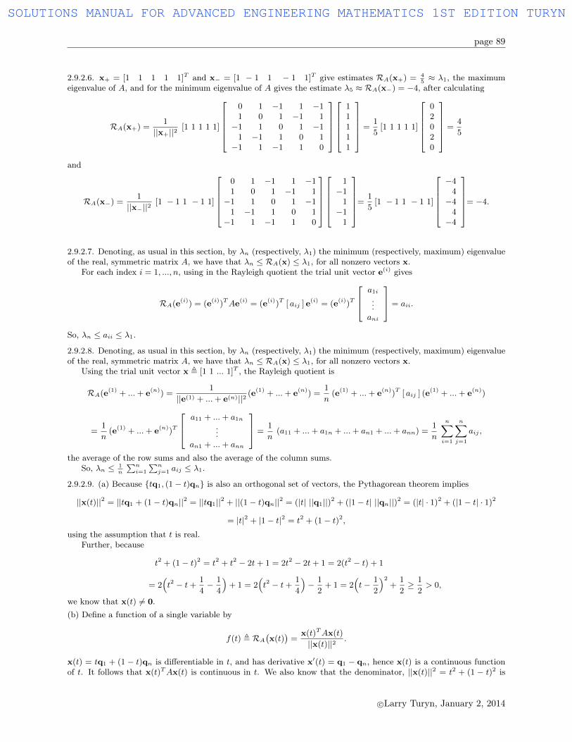
page 89
2.9.2.6. x+ = [1 1 1 1 1]T and x− = [1 − 1 1 − 1 1]T give estimates RA(x+) = 45≈ λ1, the maximum
eigenvalue of A, and for the minimum eigenvalue of A gives the estimate λ5 ≈ RA(x−) = −4, after calculating
RA(x+) =1
||x+||2[1 1 1 1 1]
0 1 −1 1 −11 0 1 −1 1−1 1 0 1 −1
1 −1 1 0 1−1 1 −1 1 0
11111
=1
5[1 1 1 1 1]
02020
=4
5
and
RA(x−) =1
||x−||2[1 − 1 1 − 1 1]
0 1 −1 1 −11 0 1 −1 1−1 1 0 1 −1
1 −1 1 0 1−1 1 −1 1 0
1−1
1−1
1
=1
5[1 − 1 1 − 1 1]
−4
4−4
4−4
= −4.
2.9.2.7. Denoting, as usual in this section, by λn (respectively, λ1) the minimum (respectively, maximum) eigenvalueof the real, symmetric matrix A, we have that λn ≤ RA(x) ≤ λ1, for all nonzero vectors x.
For each index i = 1, ..., n, using in the Rayleigh quotient the trial unit vector e(i) gives
RA(e(i)) = (e(i))TAe(i) = (e(i))T [ aij ] e(i) = (e(i))T
a1i...ani
= aii.
So, λn ≤ aii ≤ λ1.
2.9.2.8. Denoting, as usual in this section, by λn (respectively, λ1) the minimum (respectively, maximum) eigenvalueof the real, symmetric matrix A, we have that λn ≤ RA(x) ≤ λ1, for all nonzero vectors x.
Using the trial unit vector x , [1 1 ... 1]T , the Rayleigh quotient is
RA(e(1) + ...+ e(n)) =1
||e(1) + ...+ e(n)||2(e(1) + ...+ e(n)) =
1
n(e(1) + ...+ e(n))T [ aij ] (e(1) + ...+ e(n))
=1
n(e(1) + ...+ e(n))T
a11 + ...+ a1n...
an1 + ...+ ann
=1
n(a11 + ...+ a1n + ...+ an1 + ...+ ann) =
1
n
n∑i=1
n∑j=1
aij ,
the average of the row sums and also the average of the column sums.So, λn ≤ 1
n
∑ni=1
∑nj=1 aij ≤ λ1.
2.9.2.9. (a) Because {tq1, (1− t)qn} is also an orthogonal set of vectors, the Pythagorean theorem implies
||x(t)||2 = ||tq1 + (1− t)qn||2 = ||tq1||2 + ||(1− t)qn||2 = (|t| ||q1||)2 + (|1− t| ||qn||)2 = (|t| · 1)2 + (|1− t| · 1)2
= |t|2 + |1− t|2 = t2 + (1− t)2,using the assumption that t is real.
Further, because
t2 + (1− t)2 = t2 + t2 − 2t+ 1 = 2t2 − 2t+ 1 = 2(t2 − t) + 1
= 2(t2 − t+
1
4− 1
4
)+ 1 = 2
(t2 − t+
1
4
)− 1
2+ 1 = 2
(t− 1
2
)2+
1
2≥ 1
2> 0,
we know that x(t) 6= 0.(b) Define a function of a single variable by
f(t) , RA(x(t)
)=
x(t)TAx(t)
||x(t)||2 .
x(t) = tq1 + (1 − t)qn is differentiable in t, and has derivative x′(t) = q1 − qn, hence x(t) is a continuous functionof t. It follows that x(t)TAx(t) is continuous in t. We also know that the denominator, ||x(t)||2 = t2 + (1 − t)2 is
c©Larry Turyn, January 2, 2014
SOLUTIONS MANUAL FOR ADVANCED ENGINEERING MATHEMATICS 1ST EDITION TURYN

page 90
differentiable in t, hence is a continuous function of t. Finally, we know that the denominator is never zero. Puttingall of these results together imply that f(t) is a continuous function.(c) Because f(t) is continuous on the interval −1 ≤ t ≤ 1, the Intermediate Value Theorem applies. Because therange f( [−1, 1] ) contains both λn = f(0) and λ1 = f(1), every w between λn and λ1 must be in f( [−1, 1] ), that is,there is a tw such that f(tw) = w.
2.9.2.10. (a) Let µ1 and λ1 be the maximum eigenvalues of B and A, respectively. Let q1 be a unit eigenvector of Acorresponding to eigenvalue λ1. Then we calculate that
qT1 Bq1 = qT1 (A+ CTC)q1 = qT1 Aq1 + qT1 CTCq1 = qT1 Aq1 + (Cq1)T (Cq1) = RA(q1) + ||Cq1||2
≥ RA(q1) + 0 = RA(q1)
It follows thatµ1 ≥ RB(q1) = qT1 Bq1 ≥ RA(q1) = λ1.
So, the maximum eigenvalue of B is greater than or equal to the maximum eigenvalue of A.(b) Let λn and µn be the minimum eigenvalues of A and B, respectively. In the calculations of part (a), replace q1
by zn, a unit eigenvector of B corresponding to eigenvalue µn, to get
zTnAzn = zTn (B − CTC)zn = ... = RB(zn)− ||Czn||2.
Thenλn ≤ RA(zn) = zTnAzn = RB(zn)− ||Czn||2 ≤ RB(zn) = µn.
So, the minimum eigenvalue of B is greater than or equal to the minimum eigenvalue of A.
c©Larry Turyn, January 2, 2014
SOLUTIONS MANUAL FOR ADVANCED ENGINEERING MATHEMATICS 1ST EDITION TURYN
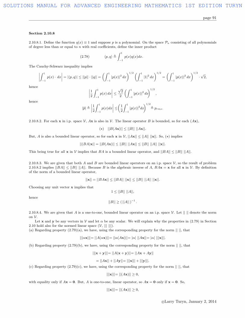
page 91
Section 2.10.8
2.10.8.1. Define the function q(x) ≡ 1 and suppose p is a polynomial. On the space Pn consisting of all polynomialsof degree less than or equal to n with real coefficients, define the inner product
(2.78) 〈p, q〉 ,ˆ 1
−1
p(x)q(x)dx.
The Cauchy-Schwarz inequality implies∣∣∣∣ˆ 1
−1
p(x) · dx∣∣∣∣ = |〈p, q〉| ≤ ||p|| · ||q|| =
(ˆ 1
−1
|p(x)|2 dx)1/2(ˆ 1
−1
|1|2 dx)1/2
=
(ˆ 1
−1
|p(x)|2 dx)1/2
·√
2,
hence ∣∣∣∣12ˆ 1
−1
p(x) dx
∣∣∣∣ ≤ √2
2
(ˆ 1
−1
|p(x)|2 dx)1/2
,
hence
|p| ,∣∣∣∣12ˆ 1
−1
p(x)dx
∣∣∣∣ ≤(1
2
ˆ 1
−1
|p(x)|2dx)1/2
, prms.
2.10.8.2. For each x in i.p. space V, Ax is also in V. The linear operator B is bounded, so for each (Ax),
(?) ||B(Ax)|| ≤ ||B|| ||Ax||.
But, A is also a bounded linear operator, so for each x in V, ||Ax|| ≤ ||A|| ||x||. So, (?) implies
||(BA)x|| = ||B(Ax)|| ≤ ||B|| ||Ax|| ≤ ||B|| ||A|| ||x||.
This being true for all x in V implies that BA is a bounded linear operator, and ||BA|| ≤ ||B|| ||A||.
2.10.8.3. We are given that both A and B are bounded linear operators on an i.p. space V, so the result of problem2.10.8.2 implies ||BA|| ≤ ||B|| ||A||. Because B is the algebraic inverse of A, BAx = x for all x in V. By definitionof the norm of a bounded linear operator,
||x|| = ||BAx|| ≤ ||BA|| ||x|| ≤ ||B|| ||A|| ||x||.
Choosing any unit vector x implies that1 ≤ ||B|| ||A||,
hence||B|| ≥ ( ||A|| )−1 .
2.10.8.4. We are given that A is a one-to-one, bounded linear operator on an i.p. space V. Let || || denote the normon V.
Let x and y be any vectors in V and let α be any scalar. We will explain why the properties in (2.79) in Section2.10 hold also for the normed linear space (V, ||| |||).(a) Regarding property (2.79)(a), we have, using the corresponding property for the norm || ||, that
|||αx|||= ||A(αx)||= ||α(Ax)||= |α| ||Ax||= |α| |||x|||.
(b) Regarding property (2.79)(b), we have, using the corresponding property for the norm || ||, that
|||x + y|||= ||A(x + y)||= ||Ax +Ay||
= ||Ax||+ ||Ay||= |||x|||+ |||y|||.(c) Regarding property (2.79)(c), we have, using the corresponding property for the norm || ||, that
|||x|||= ||(Ax)|| ≥ 0,
with equality only if Ax = 0. But, A is one-to-one, linear operator, so Ax = 0 only if x = 0. So,
|||x|||= ||(Ax)|| ≥ 0,
c©Larry Turyn, January 2, 2014
SOLUTIONS MANUAL FOR ADVANCED ENGINEERING MATHEMATICS 1ST EDITION TURYN
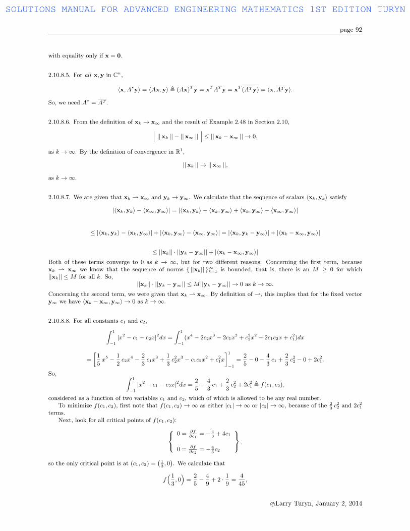
page 92
with equality only if x = 0.
2.10.8.5. For all x,y in Cn,
〈x, A∗y〉 = 〈Ax,y〉 , (Ax)Ty = xTATy = xT (ATy) = 〈x, ATy〉.
So, we need A∗ = AT .
2.10.8.6. From the definition of xk → x∞ and the result of Example 2.48 in Section 2.10,∣∣∣ ||xk || − ||x∞ || ∣∣∣ ≤ ||xk − x∞ || → 0,
as k →∞. By the definition of convergence in R1,
||xk || → ||x∞ ||,
as k →∞.
2.10.8.7. We are given that xk ⇀ x∞ and yk → y∞. We calculate that the sequence of scalars 〈xk,yk〉 satisfy
|〈xk,yk〉 − 〈x∞,y∞〉| = |〈xk,yk〉 − 〈xk,y∞〉+ 〈xk,y∞〉 − 〈x∞,y∞〉|
≤ |〈xk,yk〉 − 〈xk,y∞〉|+ |〈xk,y∞〉 − 〈x∞,y∞〉| = |〈xk,yk − y∞〉|+ |〈xk − x∞,y∞〉|
≤ ||xk|| · ||yk − y∞||+ |〈xk − x∞,y∞〉|Both of these terms converge to 0 as k → ∞, but for two different reasons: Concerning the first term, becausexk ⇀ x∞ we know that the sequence of norms { ||xk|| }∞k=1 is bounded, that is, there is an M ≥ 0 for which||xk|| ≤M for all k. So,
||xk|| · ||yk − y∞|| ≤M ||yk − y∞|| → 0 as k →∞.Concerning the second term, we were given that xk ⇀ x∞. By definition of ⇀, this implies that for the fixed vectory∞ we have 〈xk − x∞,y∞〉 → 0 as k →∞.
2.10.8.8. For all constants c1 and c2,ˆ 1
−1
|x2 − c1 − c2x|2dx =
ˆ 1
−1
(x4 − 2c2x3 − 2c1x
2 + c22x2 − 2c1c2x+ c21)dx
=
[1
5x5 − 1
2c2x
4 − 2
3c1x
3 +1
3c22x
3 − c1c2x2 + c21x
]1−1
=2
5− 0− 4
3c1 +
2
3c22 − 0 + 2c21.
So, ˆ 1
−1
|x2 − c1 − c2x|2dx =2
5− 4
3c1 +
2
3c22 + 2c21 , f(c1, c2),
considered as a function of two variables c1 and c2, which of which is allowed to be any real number.To minimize f(c1, c2), first note that f(c1, c2)→∞ as either |c1| → ∞ or |c2| → ∞, because of the 2
3c22 and 2c21
terms.Next, look for all critical points of f(c1, c2):
0 = ∂f∂c1
= − 43
+ 4c1
0 = ∂f∂c2
= − 43c2
,
so the only critical point is at (c1, c2) =(13, 0). We calculate that
f(1
3, 0)
=2
5− 4
9+ 2 · 1
9=
4
45,
c©Larry Turyn, January 2, 2014
SOLUTIONS MANUAL FOR ADVANCED ENGINEERING MATHEMATICS 1ST EDITION TURYN
page 93
so (c1, c2) =(13, 0)gives the minimum value of
ˆ 1
−1
|x2 − c1 − c2x|2dx.
2.10.8.9. For all x in V, using the triangle inequality we have
||Ax|| ,∣∣∣∣∣∣λ1〈x,u(1)〉u(1) + · · ·+ λn〈x,u(n)〉u(n)
∣∣∣∣∣∣ ≤ ∣∣∣∣∣∣λ1〈x,u(1)〉u(1)∣∣∣∣∣∣+ · · ·+
∣∣∣∣∣∣λn〈x,u(n)〉u(n)∣∣∣∣∣∣ ,
and then using (2.79)(a),
||Ax|| ≤ |λ1〈x,u(1)〉| · ||u(1)||+ · · ·+ |λn〈x,u(n)〉| · ||u(n)||,
and using the information that the u(j) are unit vectors,
||Ax|| ≤ |λ1〈x,u(1)〉|+ · · ·+ |λn〈x,u(n)〉| = |λ1| · |〈x,u(1)〉|+ · · ·+ |λn| · |〈x,u(n)〉|,
and then, using the Cauchy-Schwarz inequality,
||Ax|| ≤ |λ1| · ||x|| ||u(1)||+ · · ·+ |λn| · ||x|| ||u(n)||,
and again using the information that ||u(j)|| = 1,
||Ax|| ≤ |λ1| · ||x||+ · · ·+ |λn| · ||x||.
This being true for all x in V, it follows that A is bounded and ||A || ≤ |λ1|+ · · ·+ |λn|.To go further, we want to find the value of ||A||, not just an upper bound on ||A||. How?Add more unit vectors to the set {u1, ...,un} to get an o.n. basis, {u1, ...,un, ...}, for V. [We use the ellipsis ... to
indicate that there may be finitely many or infinitely many more vectors in the basis.]Then, no matter how many more vectors there are in the o.n. basis for V, we have
x =∑i=1
xiu(i),
where the notation∑i=1
indicates that the sum may have a finite or infinite number of terms, depending on the
dimension of V.We calculate using Parseval’s identity that
||x||2 =
∣∣∣∣∣∣∣∣∣∣∑i=1
xiu(i)
∣∣∣∣∣∣∣∣∣∣2
=∑i=1
|xi|2
and
Ax ,n∑j=1
λj〈x,u(j)〉u(j) =
n∑j=1
λj
⟨∑i=1
xiu(i),u(j)
⟩u(j).
Using orthogonality,
(?) Ax =
n∑j=1
λjxju(j).
Note that, even though x and ||x||2 may involve infinitely many terms, orthogonality made Ax be a finite sum.Again using Parseval’s identity,
||Ax||2=
∣∣∣∣∣∣∣∣∣∣n∑j=1
λjxju(j)
∣∣∣∣∣∣∣∣∣∣2
=
n∑j=1
|λjxj |2=
n∑j=1
|λj |2|xj |2.
But, we were given that |λ1| ≥ |λ2| ≥ ... ≥ |λn|, so
||Ax||2 ≤n∑j=1
|λ1|2|xj |2 = |λ1|2n∑j=1
|xj |2,
so,
||Ax||2 ≤ |λ1|2n∑i=1
|xi|2 = |λ1|2||x||2.
c©Larry Turyn, January 2, 2014
SOLUTIONS MANUAL FOR ADVANCED ENGINEERING MATHEMATICS 1ST EDITION TURYN

page 94
It follows that ||A|| ≤ |λ1|.But, in fact, choosing x = u(1) = 1 · u(1) + 0 · u(2) + ..., we have, from (?),
Ax = λ1u(1),
so||Ax||2 = |λ1|2 · 1 = |λ1|2 · ||u(1)||2 = |λ1|2 · ||x||2.
It follows that ||A|| ≥ |λ1. Combined with the previous result, we get
||A|| = |λ1|.
2.10.8.10. We will explain why every x in W⊥2 must be in W⊥1 , and thus explain why W⊥2 ⊆ W⊥1 .Choose any x in W⊥2 . By definition of the latter,
(?) x ⊥ w2 for every w2 in W2.
But, we were given that W1 ⊆ W2, that is, every vector w1 in W1 is also in W2. So, (?) app;lies to every w1 in W1,that is,
(?) x ⊥ w1 for every w1 in W1.
By definition, x is in W⊥1 , which is what we wanted to get.
2.10.8.11. For all x,y in H, ⟨x,(A−1)∗ y⟩ =
⟨A−1x,y
⟩.
Let w = A−1x and v = (A∗)−1y, hence Aw = x and A∗v = y. It follows that⟨x, (A∗)
−1y⟩
= 〈x,v〉 = 〈Aw,v〉 = 〈w, A∗v〉 =⟨w, A∗
((A∗)−1y
)⟩=⟨w,(A∗(A∗)−1)y⟩
= 〈w,y〉 =⟨A−1x,y
⟩=⟨x,(A−1)∗y⟩ .
To summarize, for all x,y in H, ⟨x, (A∗)
−1y⟩
=⟨x,(A−1)∗y⟩ .
It follows that(A∗)
−1=(A−1)∗.
2.10.8.12. First, we will explain why A is one-to-one: If Ax1 = Ax2, then 0 = ||0|| = ||A(x1−x2)|| ≥ α||x1−x2|| ≥ 0.It follows that 0 = α||x1 − x2||. Because α > 0, it follows that ||x1 − x2|| = 0, which implies x1 − x2 = 0, that is,x1 = x2. So, yes, A is one-to-one.
It follows that A has a linear, algebraic inverse A−1. For all x in H, x = A−1Ax, hence
||x|| = ||A(A−1x)|| ≥ α||A−1x||,
hence||A−1x|| ≤ 1
α||x||.
This being true for all x in H, it follows that A−1 is bounded and
||A−1|| ≤ 1
α.
2.10.8.13. For each x = [x1 . . . xn ] in Cn,
||Ax ||2 =
∣∣∣∣∣∣∣∣∣∣∣∣∣∣∑nk=1 a1kxk
...∑nk=1 ankxk
∣∣∣∣∣∣∣∣∣∣∣∣∣∣2
=∑j=1
∣∣∣∣∣n∑k=1
ajkxk
∣∣∣∣∣2
.
For each index j = 1, ..., n, let A∗j denote the j−th column of A. Then
n∑k=1
ajkxk = A∗j • x,
c©Larry Turyn, January 2, 2014
SOLUTIONS MANUAL FOR ADVANCED ENGINEERING MATHEMATICS 1ST EDITION TURYN

page 95
so the Cauchy-Schwarz inequality implies ∣∣∣∣∣n∑k=1
ajkxk
∣∣∣∣∣ ≤ ||A∗j || ||x||,hence ∣∣∣∣∣
n∑k=1
ajkxk
∣∣∣∣∣2
≤ |A∗j ||2 ||x||2 =
(n∑k=1
|ajk|2)||x||2.
It follows that
||Ax ||2 =∑j=1
∣∣∣∣∣n∑k=1
ajkxk
∣∣∣∣∣2
≤∑j=1
(n∑k=1
|ajk|2)||x||2,
hence
||Ax ||2 ≤ ||x||2 ·
(∑j=1
n∑k=1
|ajk|2).
This implies
||Ax || ≤ ||x|| ·
√√√√∑j=1
n∑k=1
|ajk|2.
Because this is true for all x in Cn, A is a bounded linear operator and
||A || ≤
√√√√ n∑j=1
n∑k=1
|ajk|2 , ||A ||F .
2.10.8.14. To start the Gram-Schmidt process, let
g1(x) ≡ f0(x),
r11 , ||g1|| =
√ˆ 1
0
|g1|2dx =
√ˆ 1
0
1dx = 1,
andq1(x)= r−1
11 g1(x) =1
1· g1(x) ≡ 1.
Next, let
g2(x) , f1(x)− 〈f1, q1〉q1(x) = x−(ˆ 1
0
x · 1 dx)
1 = x− 1
2,
r22 , ||g2|| =
√ˆ 1
0
|g2|2dx =
√ˆ 1
0
(x− 1
2
)2dx =
√ˆ 1
0
(x2 − x+
1
4
)dx =
√(1
3− 1
2+
1
4
)dx =
1√12
andq2(x)= r−1
11 g2(x) =√
12 ·(x− 1
2
).
Further, let
g3(x) , f2(x)− 〈f2, q1〉q1 − 〈f2, q2〉q2 = x2 −(ˆ 1
0
x2 · 1 dx)· 1−
(ˆ 1
0
x2 ·√
12 ·(x− 1
2
)dx
)√12(x− 1
2
)
= x2 − 1
3− 12
(ˆ 1
0
(x3 − 1
2x2)dx
)(x− 1
2
)= x2 − 1
3− 12 · 1
12
(x− 1
2
)= x2 − x+
1
6,
r33 , ||g3|| =
√ˆ 1
0
|g3|2dx =
√ˆ 1
0
(x2 − x+
1
6
)2dx =
√ˆ 1
0
(x4 − 2x3 +
4
3x2 − 1
3x+
1
36
)dx
=
√1
5− 1
2+
4
9− 1
6+
1
36=
√1
180=
√23
90=
1
3√
10,
c©Larry Turyn, January 2, 2014
SOLUTIONS MANUAL FOR ADVANCED ENGINEERING MATHEMATICS 1ST EDITION TURYN

page 96
andq3(x)= r−1
33 g3(x)= 3√
10(x2 − x+
1
6
)According to Theorem 2.16 in Section 2.3, the o.n. set{
1,√
12(x− 1
2
), 3√
10(x2 − x+
1
6
)}has span equals the span of the given set of vectors,
{1, x, x2
}.
c©Larry Turyn, January 2, 2014
SOLUTIONS MANUAL FOR ADVANCED ENGINEERING MATHEMATICS 1ST EDITION TURYN
Courtesy of CRC Press/Taylor & Francis Group
FIGURE 2.1 Geometry of eigenvectors.
002x001.eps
SOLUTIONS MANUAL FOR ADVANCED ENGINEERING MATHEMATICS 1ST EDITION TURYN

Courtesy of CRC Press/Taylor & Francis Group
FIGURE 2.2 Complex numbers.
002x002.eps
SOLUTIONS MANUAL FOR ADVANCED ENGINEERING MATHEMATICS 1ST EDITION TURYN
Courtesy of CRC Press/Taylor & Francis Group
FIGURE 2.3 Triangle inequality.
002x003.eps
SOLUTIONS MANUAL FOR ADVANCED ENGINEERING MATHEMATICS 1ST EDITION TURYN
Courtesy of CRC Press/Taylor & Francis Group
FIGURE 2.4 Angle between vectors.
002x004.eps
SOLUTIONS MANUAL FOR ADVANCED ENGINEERING MATHEMATICS 1ST EDITION TURYN
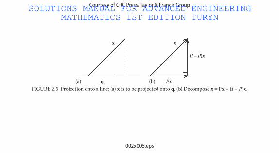
Courtesy of CRC Press/Taylor & Francis Group
FIGURE 2.5 Projection onto a line: (a) x is to be projected onto q, (b) Decompose x = Px + (I − P)x.
002x005.eps
SOLUTIONS MANUAL FOR ADVANCED ENGINEERING MATHEMATICS 1ST EDITION TURYN

Courtesy of CRC Press/Taylor & Francis Group
FIGURE 2.6 Projection onto a plane.
002x006.eps
SOLUTIONS MANUAL FOR ADVANCED ENGINEERING MATHEMATICS 1ST EDITION TURYN

Courtesy of CRC Press/Taylor & Francis Group
FIGURE 2.7 Least squares problems: Projection PA.
002x007.eps
SOLUTIONS MANUAL FOR ADVANCED ENGINEERING MATHEMATICS 1ST EDITION TURYN
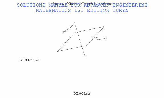
Courtesy of CRC Press/Taylor & Francis Group
FIGURE 2.8 W⊥.
002x008.eps
SOLUTIONS MANUAL FOR ADVANCED ENGINEERING MATHEMATICS 1ST EDITION TURYN
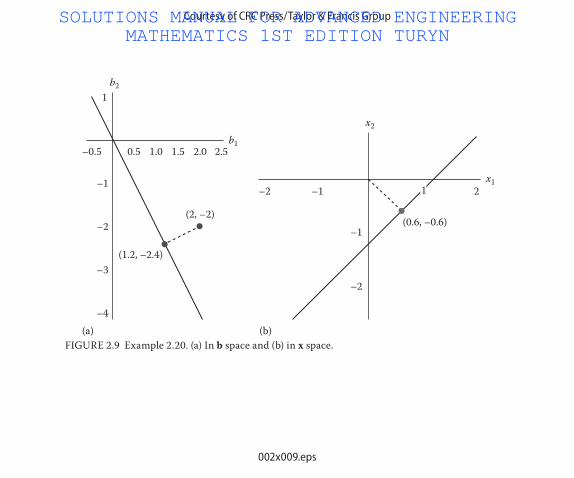
Courtesy of CRC Press/Taylor & Francis Group
FIGURE 2.9 Example 2.20. (a) In b space and (b) in x space.
002x009.eps
SOLUTIONS MANUAL FOR ADVANCED ENGINEERING MATHEMATICS 1ST EDITION TURYN

Courtesy of CRC Press/Taylor & Francis Group
FIGURE 2.10 Regression line for Example 2.21.
002x010.eps
SOLUTIONS MANUAL FOR ADVANCED ENGINEERING MATHEMATICS 1ST EDITION TURYN

Courtesy of CRC Press/Taylor & Francis Group
FIGURE 2.11 Example 2.28: Solid in parameter space.
002x011.eps
SOLUTIONS MANUAL FOR ADVANCED ENGINEERING MATHEMATICS 1ST EDITION TURYN
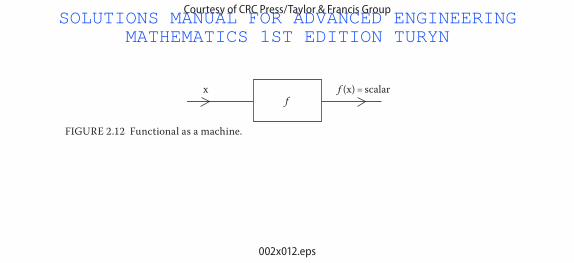
Courtesy of CRC Press/Taylor & Francis Group
FIGURE 2.12 Functional as a machine.
002x012.eps
SOLUTIONS MANUAL FOR ADVANCED ENGINEERING MATHEMATICS 1ST EDITION TURYN
Related Documents