This file and several accompanying files contain the solutions to the odd- numbered problems in the book Econometric Analysis of Cross Section and Panel Data, by Jeffrey M. Wooldridge, MIT Press, 2002. The empirical examples are solved using various versions of Stata, with some dating back to Stata 4.0. Partly out of laziness, but also because it is useful for students to see computer output, I have included Stata output in most cases rather than type tables. In some cases, I do more hand calculations than are needed in current versions of Stata. Currently, there are some missing solutions. I will update the solutions occasionally to fill in the missing solutions, and to make corrections. For some problems I have given answers beyond what I originally asked. Please report any mistakes or discrepencies you might come across by sending me e- mail at [email protected]. CHAPTER 2 E(yx ,x ) E(yx ,x ) 1 2 1 2 2.1. a. = + x and = +2 x + x . 1 4 2 2 3 2 4 1 x x 1 2 2 b. By definition, E(ux ,x ) = 0. Because x and xx are just functions 1 2 2 1 2 of (x ,x ), it does not matter whether we also condition on them: 1 2 2 E(ux ,x ,x ,xx ) = 0. 1 2 2 1 2 c. All we can say about Var(ux ,x ) is that it is nonnegative for all x 1 2 1 and x : E(ux ,x ) = 0 in no way restricts Var(ux ,x ). 2 1 2 1 2 2.3. a. y = + x + x + xx + u, where u has a zero mean given x 0 1 1 2 2 3 1 2 1 and x : E(ux ,x ) = 0. We can say nothing further about u. 2 1 2 b. E(yx ,x )/ x = + x . Because E(x ) = 0, = 1 2 1 1 3 2 2 1 1

Solutions Manual and Supplementary Materials for Eco No Metric Analysis of Cross Section and Panel Data
Jul 29, 2015
Welcome message from author
This document is posted to help you gain knowledge. Please leave a comment to let me know what you think about it! Share it to your friends and learn new things together.
Transcript
This file and several accompanying files contain the solutions to the odd-
numbered problems in the book Econometric Analysis of Cross Section and Panel
Data, by Jeffrey M. Wooldridge, MIT Press, 2002. The empirical examples are
solved using various versions of Stata, with some dating back to Stata 4.0.
Partly out of laziness, but also because it is useful for students to see
computer output, I have included Stata output in most cases rather than type
tables. In some cases, I do more hand calculations than are needed in current
versions of Stata.
Currently, there are some missing solutions. I will update the solutions
occasionally to fill in the missing solutions, and to make corrections. For
some problems I have given answers beyond what I originally asked. Please
report any mistakes or discrepencies you might come across by sending me e-
mail at [email protected].
CHAPTER 2
dE(y|x ,x ) dE(y|x ,x )1 2 1 22.1. a. ----------------------------------------------------- = b + b x and ----------------------------------------------------- = b + 2b x + b x .1 4 2 2 3 2 4 1dx dx1 2
2b. By definition, E(u|x ,x ) = 0. Because x and x x are just functions1 2 2 1 2
of (x ,x ), it does not matter whether we also condition on them:1 2
2E(u|x ,x ,x ,x x ) = 0.1 2 2 1 2
c. All we can say about Var(u|x ,x ) is that it is nonnegative for all x1 2 1
and x : E(u|x ,x ) = 0 in no way restricts Var(u|x ,x ).2 1 2 1 2
2.3. a. y = b + b x + b x + b x x + u, where u has a zero mean given x0 1 1 2 2 3 1 2 1
and x : E(u|x ,x ) = 0. We can say nothing further about u.2 1 2
b. dE(y|x ,x )/dx = b + b x . Because E(x ) = 0, b =1 2 1 1 3 2 2 1
1
E[dE(y|x ,x )/dx ]. Similarly, b = E[dE(y|x ,x )/dx ].1 2 1 2 1 2 2
c. If x and x are independent with zero mean then E(x x ) = E(x )E(x )1 2 1 2 1 2
2= 0. Further, the covariance between x x and x is E(x x Wx ) = E(x x ) =1 2 1 1 2 1 1 2
2E(x )E(x ) (by independence) = 0. A similar argument shows that the1 2
covariance between x x and x is zero. But then the linear projection of1 2 2
x x onto (1,x ,x ) is identically zero. Now just use the law of iterated1 2 1 2
projections (Property LP.5 in Appendix 2A):
L(y|1,x ,x ) = L(b + b x + b x + b x x |1,x ,x )1 2 0 1 1 2 2 3 1 2 1 2
= b + b x + b x + b L(x x |1,x ,x )0 1 1 2 2 3 1 2 1 2
= b + b x + b x .0 1 1 2 2
d. Equation (2.47) is more useful because it allows us to compute the
partial effects of x and x at any values of x and x . Under the1 2 1 2
assumptions we have made, the linear projection in (2.48) does have as its
slope coefficients on x and x the partial effects at the population average1 2
values of x and x -- zero in both cases -- but it does not allow us to1 2
obtain the partial effects at any other values of x and x . Incidentally,1 2
the main conclusions of this problem go through if we allow x and x to have1 2
any population means.
2.5. By definition, Var(u |x,z) = Var(y|x,z) and Var(u |x) = Var(y|x). By1 2
2 2assumption, these are constant and necessarily equal to s _ Var(u ) and s _1 1 2
2 2Var(u ), respectively. But then Property CV.4 implies that s > s . This2 2 1
simple conclusion means that, when error variances are constant, the error
variance falls as more explanatory variables are conditioned on.
2.7. Write the equation in error form as
2
y = g(x) + zB + u, E(u|x,z) = 0.
Take the expected value of this equation conditional only on x:
E(y|x) = g(x) + [E(z|x)]B,
and subtract this from the first equation to get
y - E(y|x) = [z - E(z|x)]B + u
~ ~ ~ ~or y = zB + u. Because z is a function of (x,z), E(u|z) = 0 (since E(u|x,z) =
~ ~ ~0), and so E(y|z) = zB. This basic result is fundamental in the literature on
estimating partial linear models. First, one estimates E(y|x) and E(z|x)
using very flexible methods, typically, so-called nonparametric methods.
~ ^ ~Then, after obtaining residuals of the form y _ y - E(y |x ) and z _ z - -i i i i i i
^ ~ ~E(z |x ), B is estimated from an OLS regression y on z , i = 1,...,N. Underi i i i
general conditions, this kind of nonparametric partialling-out procedure leads
-----to a rN-consistent, asymptotically normal estimator of B. See Robinson (1988)
and Powell (1994).
CHAPTER 3
3.1. To prove Lemma 3.1, we must show that for all e > 0, there exists b < 8e
and an integer N such that P[|x | > b ] < e, all N > N . We use thee N e ep
following fact: since x L a, for any e > 0 there exists an integer N suchN e
that P[|x - a| > 1] < e for all N > N . [The existence of N is implied byN e e
Definition 3.3(1).] But |x | = |x - a + a| < |x - a| + |a| (by the triangleN N N
inequality), and so |x | - |a| < |x - a|. It follows that P[|x | - |a| > 1]N N N
< P[|x - a| > 1]. Therefore, in Definition 3.3(3) we can take b _ |a| + 1N e
(irrespective of the value of e) and then the existence of N follows frome
Definition 3.3(1).
3
p3.3. This follows immediately from Lemma 3.1 because g(x ) L g(c).N
----- 2 ----- ----- 2 23.5. a. Since Var(y ) = s /N, Var[rN(y - m)] = N(s /N) = s .N N
----- ----- a 2 ----- ----- 2b. By the CLT, rN(y - m) ~ Normal(0,s ), and so Avar[rN(y - m)] = s .N N
----- ----- -----c. We Obtain Avar(y ) by dividing Avar[rN(y - m)] by N. Therefore,N N
----- 2 -----Avar(y ) = s /N. As expected, this coincides with the actual variance of y .N N
-----d. The asymptotic standard deviation of y is the square root of itsN
-----asymptotic variance, or s/rN.
-----e. To obtain the asymptotic standard error of y , we need a consistentN
2 ^2estimator of s. Typically, the unbiased estimator of s is used: s = (N -
N-1 ----- 2 ^1) S (y - y ) , and then s is the positive square root. The asymptotici N
i=1
----- ^ -----standard error of y is simply s/rN.N
3.7. a. For q > 0 the natural logarithim is a continuous function, and so
^ ^plim[log(q)] = log[plim(q)] = log(q) = g.
----- ^b. We use the delta method to find Avar[rN(g - g)]. In the scalar case,
^ ^ ----- ^ 2 ----- ^if g = g(q) then Avar[rN(g - g)] = [dg(q)/dq] Avar[rN(q - q)]. When g(q) =
----- ^log(q) -- which is, of course, continuously differentiable -- Avar[rN(g - g)]
2 ----- ^= (1/q) Avar[rN(q - q)].
^c. In the scalar case, the asymptotic standard error of g is generally
^ ^ ^ ^ ^ ^|dg(q)/dq|Wse(q). Therefore, for g(q) = log(q), se(g) = se(q)/q. When q = 4
^ ^ ^and se(q) = 2, g = log(4) ~ 1.39 and se(g) = 1/2.
^ ^d. The asymptotic t statistic for testing H : q = 1 is (q - 1)/se(q) =0
3/2 = 1.5.
e. Because g = log(q), the null of interest can also be stated as H : g =0
4
^0. The t statistic based on g is about 1.39/(.5) = 2.78. This leads to a
^very strong rejection of H , whereas the t statistic based on q is, at best,0
marginally significant. The lesson is that, using the Wald test, we can
change the outcome of hypotheses tests by using nonlinear transformations.
3.9. By the delta method,
----- ^ ----- ~Avar[rN(G - G)] = G(Q)V G(Q)’, Avar[rN(G - G)] = G(Q)V G(Q)’,1 2
where G(Q) = D g(Q) is Q * P. Therefore,q----- ~ ----- ^
Avar[rN(G - G)] - Avar[rN(G - G)] = G(Q)(V - V )G(Q)’.2 1
By assumption, V - V is positive semi-definite, and therefore G(Q)(V -2 1 2
V )G(Q)’ is p.s.d. This completes the proof.1
CHAPTER 4
4.1. a. Exponentiating equation (4.49) gives
wage = exp(b + b married + b educ + zG + u)0 1 2
= exp(u)exp(b + b married + b educ + zG).0 1 2
Therefore,
E(wage|x) = E[exp(u)|x]exp(b + b married + b educ + zG),0 1 2
where x denotes all explanatory variables. Now, if u and x are independent
then E[exp(u)|x] = E[exp(u)] = d , say. Therefore0
E(wage|x) = d exp(b + b married + b educ + zG).0 0 1 2
Now, finding the proportionate difference in this expectation at married = 1
and married = 0 (with all else equal) gives exp(b ) - 1; all other factors1
cancel out. Thus, the percentage difference is 100W[exp(b ) - 1].1
b. Since q = 100W[exp(b ) - 1] = g(b ), we need the derivative of g with1 1 1
5
^respect to b : dg/db = 100Wexp(b ). The asymptotic standard error of q1 1 1 1
^using the delta method is obtained as the absolute value of dg/db times1
^se(b ):1
^ ^ ^se(q ) = [100Wexp(b )]Wse(b ).1 1 1
c. We can evaluate the conditional expectation in part (a) at two levels
of education, say educ and educ , all else fixed. The proportionate change0 1
in expected wage from educ to educ is0 1
[exp(b educ ) - exp(b educ )]/exp(b educ )2 1 2 0 2 0
= exp[b (educ - educ )] - 1 = exp(b Deduc) - 1.2 1 0 2
^Using the same arguments in part (b), q = 100W[exp(b Deduc) - 1] and2 2
^ ^ ^se(q ) = 100W|Deduc|exp(b Deduc)se(b )2 2 2
^ ^d. For the estimated version of equation (4.29), b = .199, se(b ) =1 1
^ ^ ^ ^.039, b = .065, se(b ) = .006. Therefore, q = 22.01 and se(q ) = 4.76. For2 2 1 1
^ ^ ^q we set Deduc = 4. Then q = 29.7 and se(q ) = 3.11.2 2 2
4.3. a. Not in general. The conditional variance can always be written as
2 2 2Var(u|x) = E(u |x) - [E(u|x)] ; if E(u|x) $ 0, then E(u |x) $ Var(u|x).
b. It could be that E(x’u) = 0, in which case OLS is consistent, and
Var(u|x) is constant. But, generally, the usual standard errors would not be
valid unless E(u|x) = 0.
4.5. Write equation (4.50) as E(y|w) = wD, where w = (x,z). Since Var(y|w) =
2 ----- ^ 2 -1 ^s , it follows by Theorem 4.2 that Avar rN(D - D) is s [E(w’w)] ,where D =
^ ^(B’,g)’. Importantly, because E(x’z) = 0, E(w’w) is block diagonal, with
2upper block E(x’x) and lower block E(z ). Inverting E(w’w) and focusing on
the upper K * K block gives
6
----- ^ 2 -1Avar rN(B - B) = s [E(x’x)] .
----- ~Next, we need to find Avar rN(B - B). It is helpful to write y = xB + v
where v = gz + u and u _ y - E(y|x,z). Because E(x’z) = 0 and E(x’u) = 0,
2 2 2 2 2 2E(x’v) = 0. Further, E(v |x) = g E(z |x) + E(u |x) + 2gE(zu|x) = g E(z |x) +
2 2 2s , where we use E(zu|x,z) = zE(u|x,z) = 0 and E(u |x,z) = Var(y|x,z) = s .
2Unless E(z |x) is constant, the equation y = xB + v generally violates the
homoskedasticity assumption OLS.3. So, without further assumptions,
----- ~ -1 2 -1Avar rN(B - B) = [E(x’x)] E(v x’x)[E(x’x)] .
----- ~ ----- ^Now we can show Avar rN(B - B) - Avar rN(B - B) is positive semi-definite by
writing
----- ~ ----- ^Avar rN(B - B) - Avar rN(B - B)
-1 2 -1 2 -1= [E(x’x)] E(v x’x)[E(x’x)] - s [E(x’x)]
-1 2 -1 2 -1 -1= [E(x’x)] E(v x’x)[E(x’x)] - s [E(x’x)] E(x’x)[E(x’x)]
-1 2 2 -1= [E(x’x)] [E(v x’x) - s E(x’x)][E(x’x)] .
-1 2Because [E(x’x)] is positive definite, it suffices to show that E(v x’x) -
2 2s E(x’x) is p.s.d. To this end, let h(x) _ E(z |x). Then by the law of
2 2 2 2iterated expectations, E(v x’x) = E[E(v |x)x’x] = g E[h(x)x’x] + s E(x’x).
2 2 2Therefore, E(v x’x) - s E(x’x) = g E[h(x)x’x], which, when g $ 0, is actually
2 2a positive definite matrix except by fluke. In particular, if E(z |x) = E(z )
2= h > 0 (in which case y = xB + v satisfies the homoskedasticity assumption
2 2 2 2OLS.3), E(v x’x) - s E(x’x) = g h E(x’x), which is positive definite.
4.7. a. One important omitted factor in u is family income: students that
come from wealthier families tend to do better in school, other things equal.
Family income and PC ownership are positively correlated because the
probability of owning a PC increases with family income. Another factor in u
7
is quality of high school. This may also be correlated with PC: a student
who had more exposure with computers in high school may be more likely to own
a computer.
^b. b is likely to have an upward bias because of the positive3
correlation between u and PC, but it is not clear-cut because of the other
explanatory variables in the equation. If we write the linear projection
u = d + d hsGPA + d SAT + d PC + r0 1 2 3
then the bias is upward if d is greater than zero. This measures the partial3
correlation between u (say, family income) and PC, and it is likely to be
positive.
c. If data on family income can be collected then it can be included in
the equation. If family income is not available sometimes level of parents’
education is. Another possibility is to use average house value in each
student’s home zip code, as zip code is often part of school records. Proxies
for high school quality might be faculty-student ratios, expenditure per
student, average teacher salary, and so on.
4.9. a. Just subtract log(y ) from both sides:-1
Dlog(y) = b + xB + (a - 1)log(y ) + u.0 1 -1
Clearly, the intercept and slope estimates on x will be the same. The
coefficient on log(y ) changes.-1
b. For simplicity, let w = log(y), w = log(y ). Then the population-1 -1
slope coefficient in a simple regression is always a = Cov(w ,w)/Var(w ).1 -1 -1
But, by assumption, Var(w) = Var(w ), so we can write a =-1 1
Cov(w ,w)/(s s ), where s = sd(w ) and s = sd(w). But Corr(w ,w) =-1 w w w -1 w -1-1 -1
Cov(w ,w)/(s s ), and since a correlation coefficient is always between -1-1 w w-1
8
and 1, the result follows.
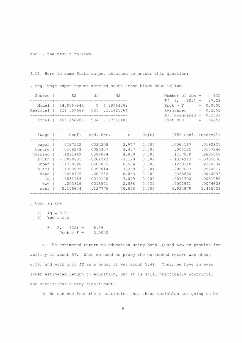
4.11. Here is some Stata output obtained to answer this question:
. reg lwage exper tenure married south urban black educ iq kww
Source | SS df MS Number of obs = 935
---------+------------------------------ F( 9, 925) = 37.28
Model | 44.0967944 9 4.89964382 Prob > F = 0.0000
Residual | 121.559489 925 .131415664 R-squared = 0.2662
---------+------------------------------ Adj R-squared = 0.2591
Total | 165.656283 934 .177362188 Root MSE = .36251
------------------------------------------------------------------------------
lwage | Coef. Std. Err. t P>|t| [95% Conf. Interval]
---------+--------------------------------------------------------------------
exper | .0127522 .0032308 3.947 0.000 .0064117 .0190927
tenure | .0109248 .0024457 4.467 0.000 .006125 .0157246
married | .1921449 .0389094 4.938 0.000 .1157839 .2685059
south | -.0820295 .0262222 -3.128 0.002 -.1334913 -.0305676
urban | .1758226 .0269095 6.534 0.000 .1230118 .2286334
black | -.1303995 .0399014 -3.268 0.001 -.2087073 -.0520917
educ | .0498375 .007262 6.863 0.000 .0355856 .0640893
iq | .0031183 .0010128 3.079 0.002 .0011306 .0051059
kww | .003826 .0018521 2.066 0.039 .0001911 .0074608
_cons | 5.175644 .127776 40.506 0.000 4.924879 5.426408
------------------------------------------------------------------------------
. test iq kww
( 1) iq = 0.0
( 2) kww = 0.0
F( 2, 925) = 8.59
Prob > F = 0.0002
a. The estimated return to education using both IQ and KWW as proxies for
ability is about 5%. When we used no proxy the estimated return was about
6.5%, and with only IQ as a proxy it was about 5.4%. Thus, we have an even
lower estimated return to education, but it is still practically nontrivial
and statistically very significant.
b. We can see from the t statistics that these variables are going to be
9
jointly significant. The F test verifies this, with p-value = .0002.
c. The wage differential between nonblacks and blacks does not disappear.
Blacks are estimated to earn about 13% less than nonblacks, holding all other
factors fixed.
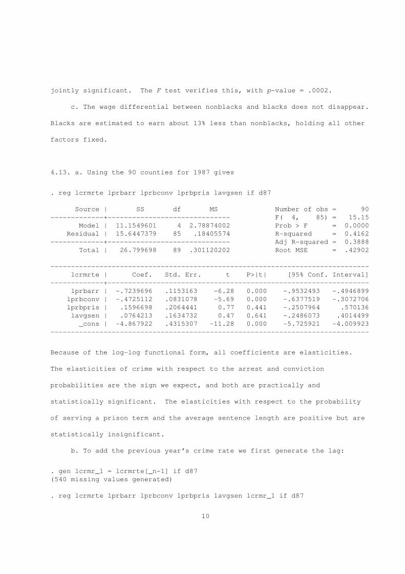
4.13. a. Using the 90 counties for 1987 gives
. reg lcrmrte lprbarr lprbconv lprbpris lavgsen if d87
Source | SS df MS Number of obs = 90
-------------+------------------------------ F( 4, 85) = 15.15
Model | 11.1549601 4 2.78874002 Prob > F = 0.0000
Residual | 15.6447379 85 .18405574 R-squared = 0.4162
-------------+------------------------------ Adj R-squared = 0.3888
Total | 26.799698 89 .301120202 Root MSE = .42902
------------------------------------------------------------------------------
lcrmrte | Coef. Std. Err. t P>|t| [95% Conf. Interval]
-------------+----------------------------------------------------------------
lprbarr | -.7239696 .1153163 -6.28 0.000 -.9532493 -.4946899
lprbconv | -.4725112 .0831078 -5.69 0.000 -.6377519 -.3072706
lprbpris | .1596698 .2064441 0.77 0.441 -.2507964 .570136
lavgsen | .0764213 .1634732 0.47 0.641 -.2486073 .4014499
_cons | -4.867922 .4315307 -11.28 0.000 -5.725921 -4.009923
------------------------------------------------------------------------------
Because of the log-log functional form, all coefficients are elasticities.
The elasticities of crime with respect to the arrest and conviction
probabilities are the sign we expect, and both are practically and
statistically significant. The elasticities with respect to the probability
of serving a prison term and the average sentence length are positive but are
statistically insignificant.
b. To add the previous year’s crime rate we first generate the lag:
. gen lcrmr_1 = lcrmrte[_n-1] if d87
(540 missing values generated)
. reg lcrmrte lprbarr lprbconv lprbpris lavgsen lcrmr_1 if d87
10
Source | SS df MS Number of obs = 90
-------------+------------------------------ F( 5, 84) = 113.90
Model | 23.3549731 5 4.67099462 Prob > F = 0.0000
Residual | 3.4447249 84 .04100863 R-squared = 0.8715
-------------+------------------------------ Adj R-squared = 0.8638
Total | 26.799698 89 .301120202 Root MSE = .20251
------------------------------------------------------------------------------
lcrmrte | Coef. Std. Err. t P>|t| [95% Conf. Interval]
-------------+----------------------------------------------------------------
lprbarr | -.1850424 .0627624 -2.95 0.004 -.3098523 -.0602325
lprbconv | -.0386768 .0465999 -0.83 0.409 -.1313457 .0539921
lprbpris | -.1266874 .0988505 -1.28 0.204 -.3232625 .0698876
lavgsen | -.1520228 .0782915 -1.94 0.056 -.3077141 .0036684
lcrmr_1 | .7798129 .0452114 17.25 0.000 .6899051 .8697208
_cons | -.7666256 .3130986 -2.45 0.016 -1.389257 -.1439946
------------------------------------------------------------------------------
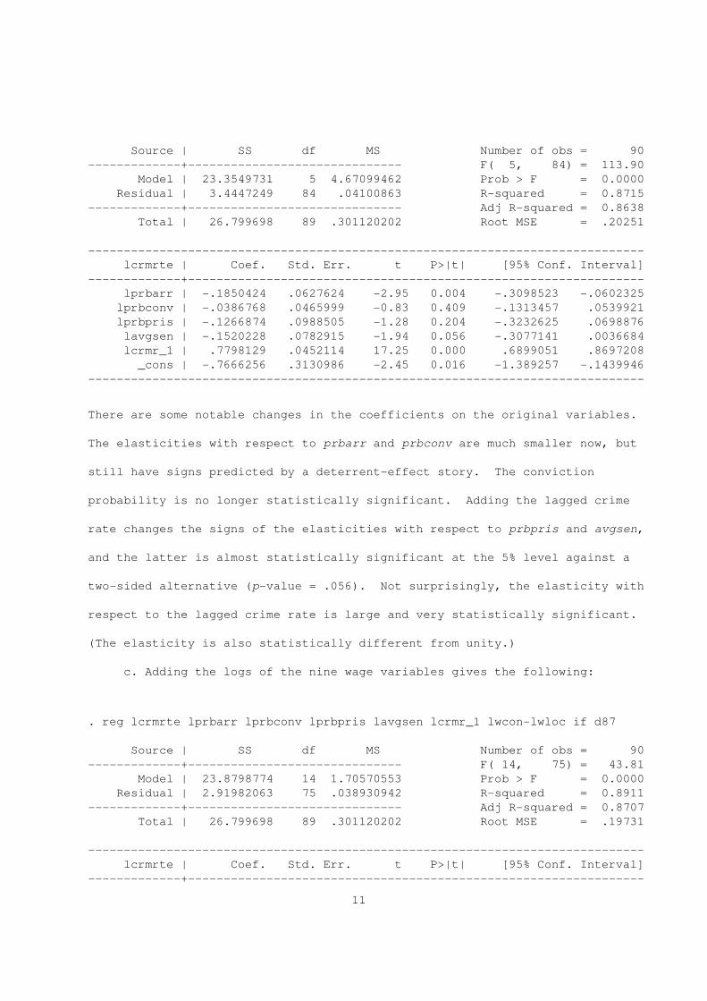
There are some notable changes in the coefficients on the original variables.
The elasticities with respect to prbarr and prbconv are much smaller now, but
still have signs predicted by a deterrent-effect story. The conviction
probability is no longer statistically significant. Adding the lagged crime
rate changes the signs of the elasticities with respect to prbpris and avgsen,
and the latter is almost statistically significant at the 5% level against a
two-sided alternative (p-value = .056). Not surprisingly, the elasticity with
respect to the lagged crime rate is large and very statistically significant.
(The elasticity is also statistically different from unity.)
c. Adding the logs of the nine wage variables gives the following:
. reg lcrmrte lprbarr lprbconv lprbpris lavgsen lcrmr_1 lwcon-lwloc if d87
Source | SS df MS Number of obs = 90
-------------+------------------------------ F( 14, 75) = 43.81
Model | 23.8798774 14 1.70570553 Prob > F = 0.0000
Residual | 2.91982063 75 .038930942 R-squared = 0.8911
-------------+------------------------------ Adj R-squared = 0.8707
Total | 26.799698 89 .301120202 Root MSE = .19731
------------------------------------------------------------------------------
lcrmrte | Coef. Std. Err. t P>|t| [95% Conf. Interval]
-------------+----------------------------------------------------------------
11
lprbarr | -.1725122 .0659533 -2.62 0.011 -.3038978 -.0411265
lprbconv | -.0683639 .049728 -1.37 0.173 -.1674273 .0306994
lprbpris | -.2155553 .1024014 -2.11 0.039 -.4195493 -.0115614
lavgsen | -.1960546 .0844647 -2.32 0.023 -.364317 -.0277923
lcrmr_1 | .7453414 .0530331 14.05 0.000 .6396942 .8509887
lwcon | -.2850008 .1775178 -1.61 0.113 -.6386344 .0686327
lwtuc | .0641312 .134327 0.48 0.634 -.2034619 .3317244
lwtrd | .253707 .2317449 1.09 0.277 -.2079524 .7153665
lwfir | -.0835258 .1964974 -0.43 0.672 -.4749687 .3079171
lwser | .1127542 .0847427 1.33 0.187 -.0560619 .2815703
lwmfg | .0987371 .1186099 0.83 0.408 -.1375459 .3350201
lwfed | .3361278 .2453134 1.37 0.175 -.1525615 .8248172
lwsta | .0395089 .2072112 0.19 0.849 -.3732769 .4522947
lwloc | -.0369855 .3291546 -0.11 0.911 -.6926951 .618724
_cons | -3.792525 1.957472 -1.94 0.056 -7.692009 .1069592
------------------------------------------------------------------------------
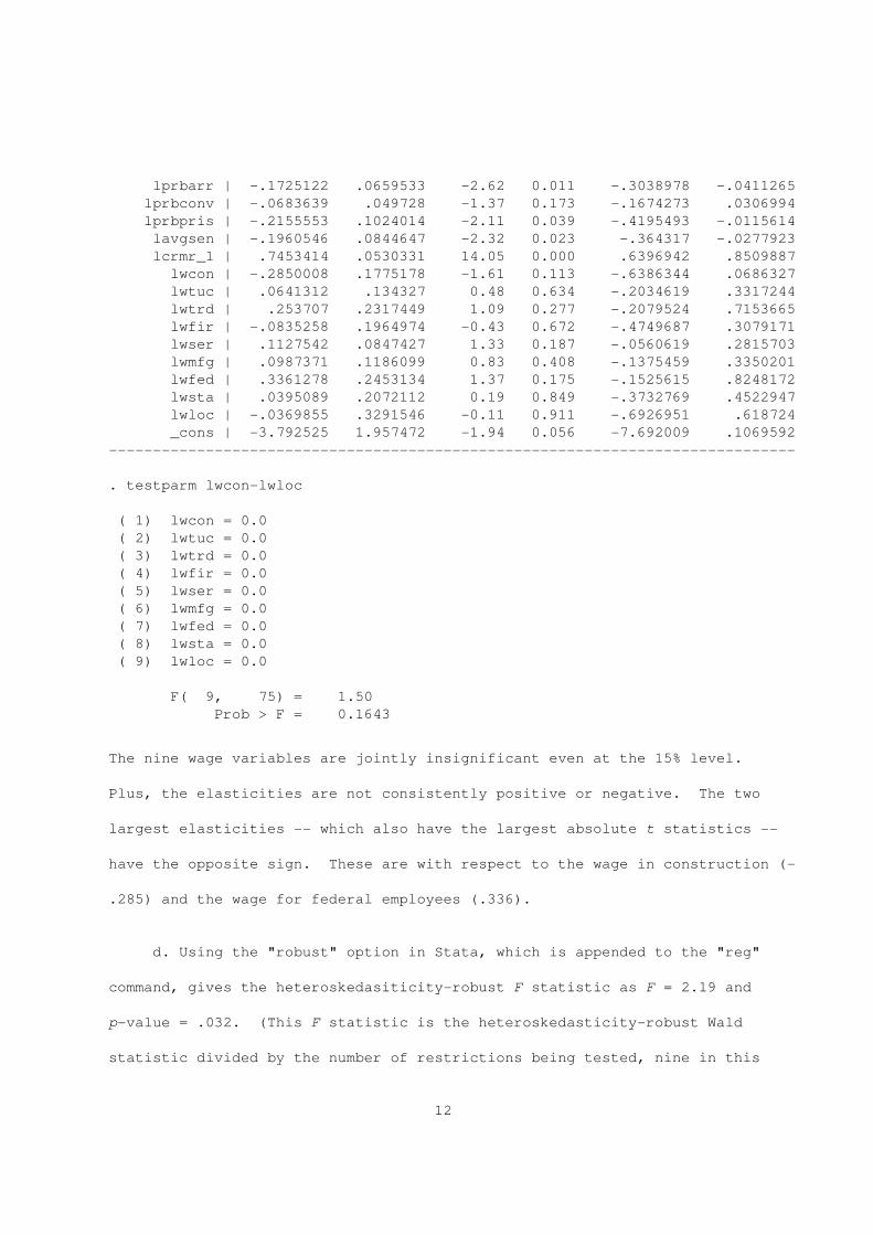
. testparm lwcon-lwloc
( 1) lwcon = 0.0
( 2) lwtuc = 0.0
( 3) lwtrd = 0.0
( 4) lwfir = 0.0
( 5) lwser = 0.0
( 6) lwmfg = 0.0
( 7) lwfed = 0.0
( 8) lwsta = 0.0
( 9) lwloc = 0.0
F( 9, 75) = 1.50
Prob > F = 0.1643
The nine wage variables are jointly insignificant even at the 15% level.
Plus, the elasticities are not consistently positive or negative. The two
largest elasticities -- which also have the largest absolute t statistics --
have the opposite sign. These are with respect to the wage in construction (-
.285) and the wage for federal employees (.336).
d. Using the "robust" option in Stata, which is appended to the "reg"
command, gives the heteroskedasiticity-robust F statistic as F = 2.19 and
p-value = .032. (This F statistic is the heteroskedasticity-robust Wald
statistic divided by the number of restrictions being tested, nine in this
12
example. The division by the number of restrictions turns the asymptotic chi-
square statistic into one that roughly has an F distribution.)
4.15. a. Because each x has finite second moment, Var(xB) < 8. Since Var(u)j
< 8, Cov(xB,u) is well-defined. But each x is uncorrelated with u, soj
2 2Cov(xB,u) = 0. Therefore, Var(y) = Var(xB) + Var(u), or s = Var(xB) + s .y u
b. This is nonsense when we view the x as random draws along with y .i i
2The statement "Var(u ) = s = Var(y ) for all i" assumes that the regressorsi i
are nonrandom (or B = 0, which is not a very interesting case). This is
another example of how the assumption of nonrandom regressors can lead to
counterintuitive conclusions. Suppose that an element of the error term, say
z, which is uncorrelated with each x , suddenly becomes observed. When we addj
z to the regressor list, the error changes, and so does the error variance.
(It gets smaller.) In the vast majority of economic applications, it makes no
sense to think we have access to the entire set of factors that one would ever
want to control for, so we should allow for error variances to change across
different models for the same response variable.
2 2c. Write R = 1 - SSR/SST = 1 - (SSR/N)/(SST/N). Therefore, plim(R ) = 1
2 2 2- plim[(SSR/N)/(SST/N)] = 1 - [plim(SSR/N)]/[plim(SST/N)] = 1 - s /s = r ,u y
2where we use the fact that SSR/N is a consistent estimator of s and SST/N isu
2a consistent estimator of s .y
d. The derivation in part (c) assumed nothing about Var(u|x). The
population R-squared depends on only the unconditional variances of u and y.
Therefore, regardless of the nature of heteroskedasticity in Var(u|x), the
usual R-squared consistently estimates the population R-squared. Neither
R-squared nor the adjusted R-squared has desirable finite-sample properties,
13
such as unbiasedness, so the only analysis we can do in any generality
involves asymptotics. The statement in the problem is simply wrong.
CHAPTER 5
^ ^ ^ ^5.1. Define x _ (z ,y ) and x _ v , and let B _ (B’,r )’ be OLS estimator1 1 2 2 2 1 1
^ ^ ^ ^from (5.52), where B = (D’,a )’. Using the hint, B can also be obtained by1 1 1 1
partitioned regression:
^ ¨(i) Regress x onto v and save the residuals, say x .1 2 1
¨(ii) Regress y onto x .1 1
^ ^But when we regress z onto v , the residuals are just z since v is1 2 1 2
N ^orthogonal in sample to z. (More precisely, S z’ v = 0.) Further, becausei1 i2
i=1
^ ^ ^ ^we can write y = y + v , where y and v are orthogonal in sample, the2 2 2 2 2
^residuals from regressing y onto v are simply the first stage fitted values,2 2
^ ^¨y . In other words, x = (z ,y ). But the 2SLS estimator of B is obtained2 1 1 2 1
^exactly from the OLS regression y on z , y .1 1 2
5.3. a. There may be unobserved health factors correlated with smoking
behavior that affect infant birth weight. For example, women who smoke during
pregnancy may, on average, drink more coffee or alcohol, or eat less
nutritious meals.
b. Basic economics says that packs should be negatively correlated with
cigarette price, although the correlation might be small (especially because
price is aggregated at the state level). At first glance it seems that
cigarette price should be exogenous in equation (5.54), but we must be a
little careful. One component of cigarette price is the state tax on
14
cigarettes. States that have lower taxes on cigarettes may also have lower
quality of health care, on average. Quality of health care is in u, and so
maybe cigarette price fails the exogeneity requirement for an IV.
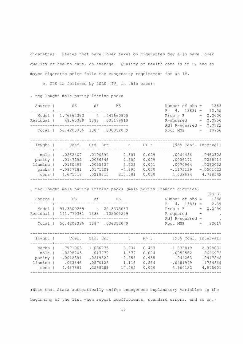
c. OLS is followed by 2SLS (IV, in this case):
. reg lbwght male parity lfaminc packs
Source | SS df MS Number of obs = 1388
---------+------------------------------ F( 4, 1383) = 12.55
Model | 1.76664363 4 .441660908 Prob > F = 0.0000
Residual | 48.65369 1383 .035179819 R-squared = 0.0350
---------+------------------------------ Adj R-squared = 0.0322
Total | 50.4203336 1387 .036352079 Root MSE = .18756
------------------------------------------------------------------------------
lbwght | Coef. Std. Err. t P>|t| [95% Conf. Interval]
---------+--------------------------------------------------------------------
male | .0262407 .0100894 2.601 0.009 .0064486 .0460328
parity | .0147292 .0056646 2.600 0.009 .0036171 .0258414
lfaminc | .0180498 .0055837 3.233 0.001 .0070964 .0290032
packs | -.0837281 .0171209 -4.890 0.000 -.1173139 -.0501423
_cons | 4.675618 .0218813 213.681 0.000 4.632694 4.718542
------------------------------------------------------------------------------
. reg lbwght male parity lfaminc packs (male parity lfaminc cigprice)
(2SLS)
Source | SS df MS Number of obs = 1388
---------+------------------------------ F( 4, 1383) = 2.39
Model | -91.3500269 4 -22.8375067 Prob > F = 0.0490
Residual | 141.770361 1383 .102509299 R-squared = .
---------+------------------------------ Adj R-squared = .
Total | 50.4203336 1387 .036352079 Root MSE = .32017
------------------------------------------------------------------------------
lbwght | Coef. Std. Err. t P>|t| [95% Conf. Interval]
---------+--------------------------------------------------------------------
packs | .7971063 1.086275 0.734 0.463 -1.333819 2.928031
male | .0298205 .017779 1.677 0.094 -.0050562 .0646972
parity | -.0012391 .0219322 -0.056 0.955 -.044263 .0417848
lfaminc | .063646 .0570128 1.116 0.264 -.0481949 .1754869
_cons | 4.467861 .2588289 17.262 0.000 3.960122 4.975601
------------------------------------------------------------------------------
(Note that Stata automatically shifts endogenous explanatory variables to the
beginning of the list when report coefficients, standard errors, and so on.)
15
The difference between OLS and IV in the estimated effect of packs on bwght is
huge. With the OLS estimate, one more pack of cigarettes is estimated to
reduce bwght by about 8.4%, and is statistically significant. The IV estimate
has the opposite sign, is huge in magnitude, and is not statistically
significant. The sign and size of the smoking effect are not realistic.
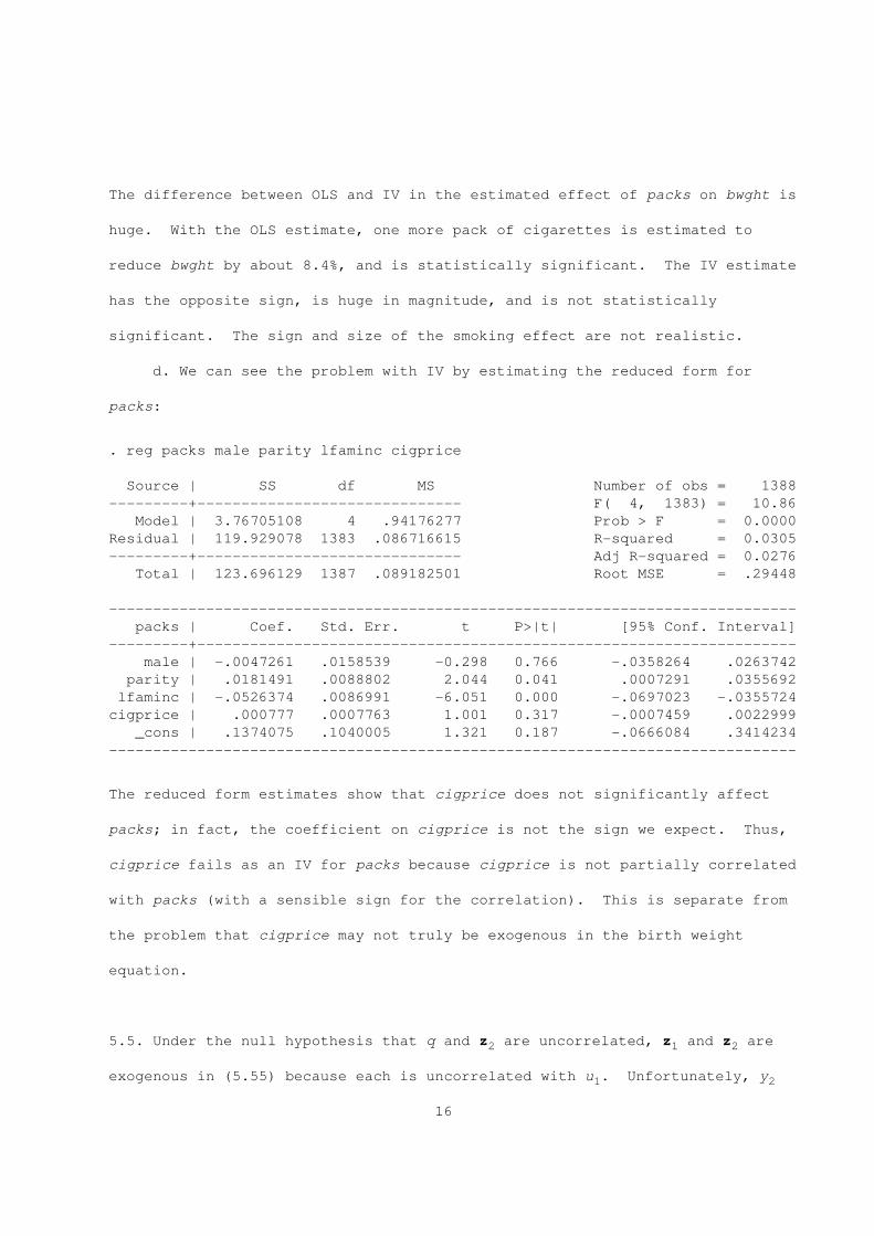
d. We can see the problem with IV by estimating the reduced form for
packs:
. reg packs male parity lfaminc cigprice
Source | SS df MS Number of obs = 1388
---------+------------------------------ F( 4, 1383) = 10.86
Model | 3.76705108 4 .94176277 Prob > F = 0.0000
Residual | 119.929078 1383 .086716615 R-squared = 0.0305
---------+------------------------------ Adj R-squared = 0.0276
Total | 123.696129 1387 .089182501 Root MSE = .29448
------------------------------------------------------------------------------
packs | Coef. Std. Err. t P>|t| [95% Conf. Interval]
---------+--------------------------------------------------------------------
male | -.0047261 .0158539 -0.298 0.766 -.0358264 .0263742
parity | .0181491 .0088802 2.044 0.041 .0007291 .0355692
lfaminc | -.0526374 .0086991 -6.051 0.000 -.0697023 -.0355724
cigprice | .000777 .0007763 1.001 0.317 -.0007459 .0022999
_cons | .1374075 .1040005 1.321 0.187 -.0666084 .3414234
------------------------------------------------------------------------------
The reduced form estimates show that cigprice does not significantly affect
packs; in fact, the coefficient on cigprice is not the sign we expect. Thus,
cigprice fails as an IV for packs because cigprice is not partially correlated
with packs (with a sensible sign for the correlation). This is separate from
the problem that cigprice may not truly be exogenous in the birth weight
equation.
5.5. Under the null hypothesis that q and z are uncorrelated, z and z are2 1 2
exogenous in (5.55) because each is uncorrelated with u . Unfortunately, y1 2
16
is correlated with u , and so the regression of y on z , y , z does not1 1 1 2 2
produce a consistent estimator of 0 on z even when E(z’q) = 0. We could find2 2
^that J from this regression is statistically different from zero even when q1
and z are uncorrelated -- in which case we would incorrectly conclude that z2 2
is not a valid IV candidate. Or, we might fail to reject H : J = 0 when z0 1 2
and q are correlated -- in which case we incorrectly conclude that the
elements in z are valid as instruments.2
The point of this exercise is that one cannot simply add instrumental
variable candidates in the structural equation and then test for significance
of these variables using OLS. This is the sense in which identification
cannot be tested. With a single endogenous variable, we must take a stand
that at least one element of z is uncorrelated with q.2
5.7. a. If we plug q = (1/d )q - (1/d )a into equation (5.45) we get1 1 1 1
y = b + b x + ... + b x + h q + v - h a , (5.56)0 1 1 K K 1 1 1 1
where h _ (1/d ). Now, since the z are redundant in (5.45), they are1 1 h
uncorrelated with the structural error, v (by definition of redundancy).
Further, we have assumed that the z are uncorrelated with a . Since each xh 1 j
is also uncorrelated with v - h a , we can estimate (5.56) by 2SLS using1 1
instruments (1,x ,...,x ,z ,z ,...,z ) to get consistent of the b and h .1 K 1 2 M j 1
Given all of the zero correlation assumptions, what we need for
identification is that at least one of the z appears in the reduced form forh
q . More formally, in the linear projection1
q = p + p x + ... + p x + p z + ... + p z + r ,1 0 1 1 K K K+1 1 K+M M 1
at least one of p , ..., p must be different from zero.K+1 K+M
b. We need family background variables to be redundant in the log(wage)
17
equation once ability (and other factors, such as educ and exper), have been
controlled for. The idea here is that family background may influence ability
but should have no partial effect on log(wage) once ability has been accounted
for. For the rank condition to hold, we need family background variables to
be correlated with the indicator, q , say IQ, once the x have been netted1 j
out. This is likely to be true if we think that family background and ability
are (partially) correlated.
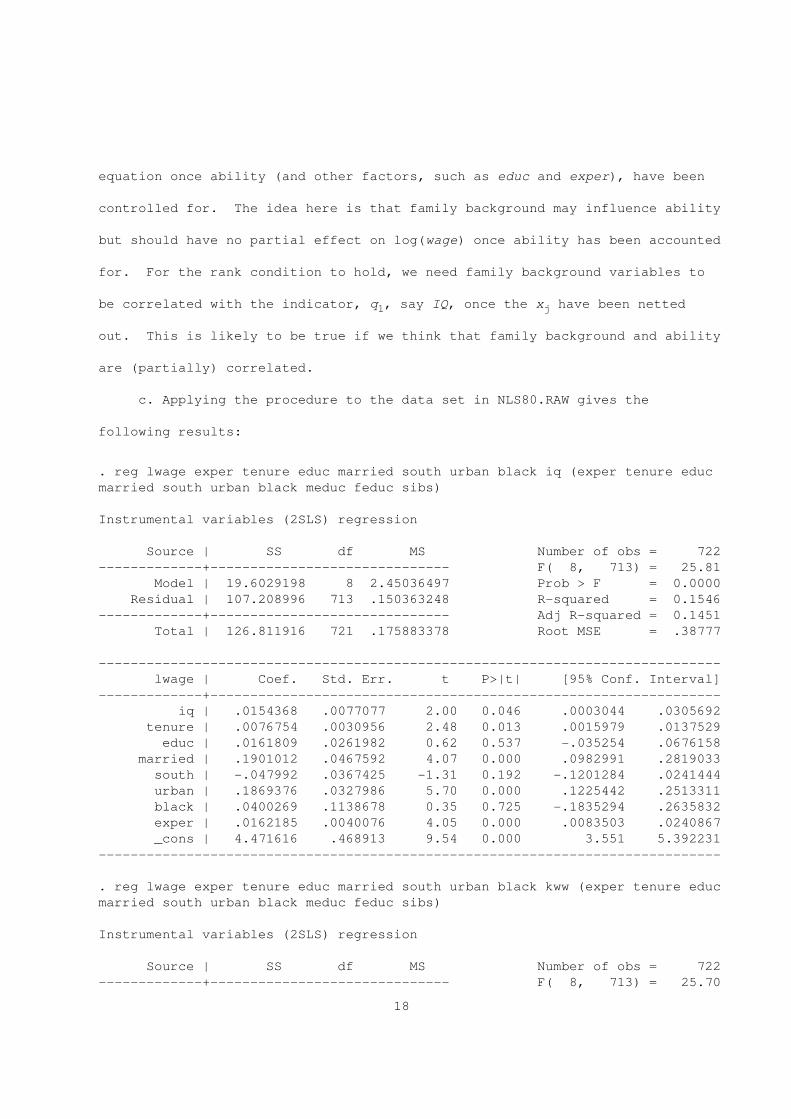
c. Applying the procedure to the data set in NLS80.RAW gives the
following results:
. reg lwage exper tenure educ married south urban black iq (exper tenure educ
married south urban black meduc feduc sibs)
Instrumental variables (2SLS) regression
Source | SS df MS Number of obs = 722
-------------+------------------------------ F( 8, 713) = 25.81
Model | 19.6029198 8 2.45036497 Prob > F = 0.0000
Residual | 107.208996 713 .150363248 R-squared = 0.1546
-------------+------------------------------ Adj R-squared = 0.1451
Total | 126.811916 721 .175883378 Root MSE = .38777
------------------------------------------------------------------------------
lwage | Coef. Std. Err. t P>|t| [95% Conf. Interval]
-------------+----------------------------------------------------------------
iq | .0154368 .0077077 2.00 0.046 .0003044 .0305692
tenure | .0076754 .0030956 2.48 0.013 .0015979 .0137529
educ | .0161809 .0261982 0.62 0.537 -.035254 .0676158
married | .1901012 .0467592 4.07 0.000 .0982991 .2819033
south | -.047992 .0367425 -1.31 0.192 -.1201284 .0241444
urban | .1869376 .0327986 5.70 0.000 .1225442 .2513311
black | .0400269 .1138678 0.35 0.725 -.1835294 .2635832
exper | .0162185 .0040076 4.05 0.000 .0083503 .0240867
_cons | 4.471616 .468913 9.54 0.000 3.551 5.392231
------------------------------------------------------------------------------
. reg lwage exper tenure educ married south urban black kww (exper tenure educ
married south urban black meduc feduc sibs)
Instrumental variables (2SLS) regression
Source | SS df MS Number of obs = 722
-------------+------------------------------ F( 8, 713) = 25.70
18
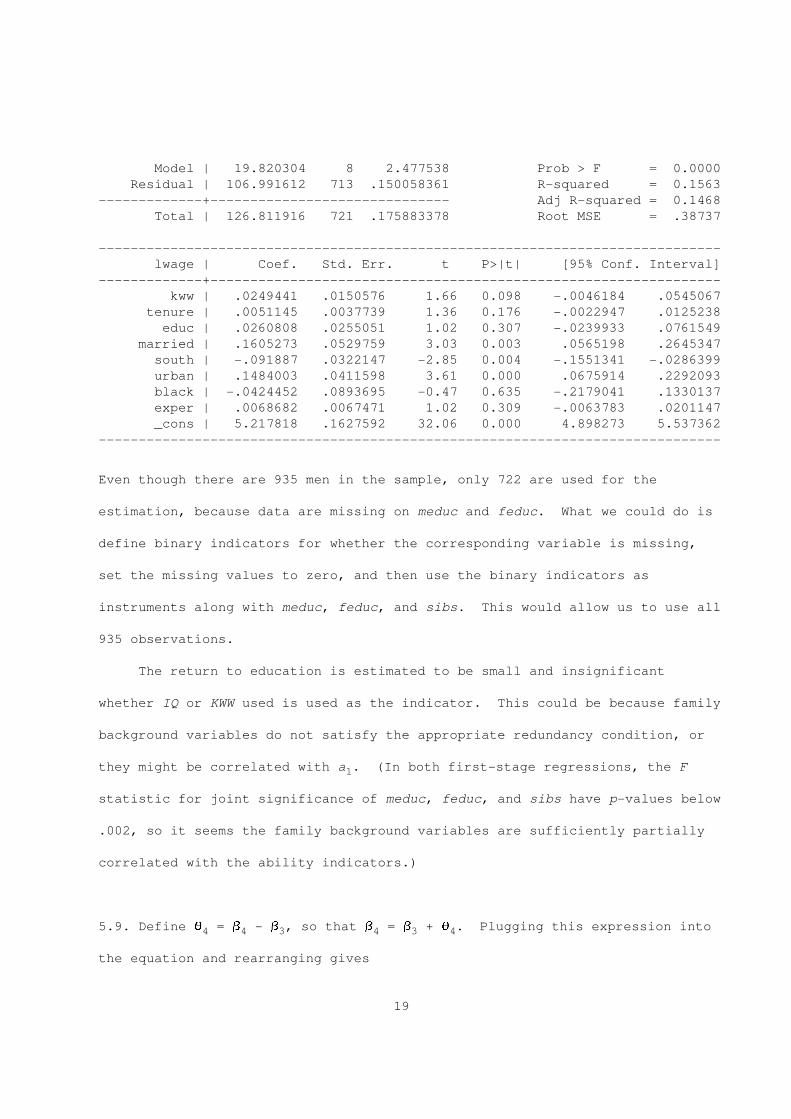
Model | 19.820304 8 2.477538 Prob > F = 0.0000
Residual | 106.991612 713 .150058361 R-squared = 0.1563
-------------+------------------------------ Adj R-squared = 0.1468
Total | 126.811916 721 .175883378 Root MSE = .38737
------------------------------------------------------------------------------
lwage | Coef. Std. Err. t P>|t| [95% Conf. Interval]
-------------+----------------------------------------------------------------
kww | .0249441 .0150576 1.66 0.098 -.0046184 .0545067
tenure | .0051145 .0037739 1.36 0.176 -.0022947 .0125238
educ | .0260808 .0255051 1.02 0.307 -.0239933 .0761549
married | .1605273 .0529759 3.03 0.003 .0565198 .2645347
south | -.091887 .0322147 -2.85 0.004 -.1551341 -.0286399
urban | .1484003 .0411598 3.61 0.000 .0675914 .2292093
black | -.0424452 .0893695 -0.47 0.635 -.2179041 .1330137
exper | .0068682 .0067471 1.02 0.309 -.0063783 .0201147
_cons | 5.217818 .1627592 32.06 0.000 4.898273 5.537362
------------------------------------------------------------------------------
Even though there are 935 men in the sample, only 722 are used for the
estimation, because data are missing on meduc and feduc. What we could do is
define binary indicators for whether the corresponding variable is missing,
set the missing values to zero, and then use the binary indicators as
instruments along with meduc, feduc, and sibs. This would allow us to use all
935 observations.
The return to education is estimated to be small and insignificant
whether IQ or KWW used is used as the indicator. This could be because family
background variables do not satisfy the appropriate redundancy condition, or
they might be correlated with a . (In both first-stage regressions, the F1
statistic for joint significance of meduc, feduc, and sibs have p-values below
.002, so it seems the family background variables are sufficiently partially
correlated with the ability indicators.)
5.9. Define q = b - b , so that b = b + q . Plugging this expression into4 4 3 4 3 4
the equation and rearranging gives
19
2log(wage) = b + b exper + b exper + b (twoyr + fouryr) + q fouryr + u0 1 2 3 4
2= b + b exper + b exper + b totcoll + q fouryr + u,0 1 2 3 4
where totcoll = twoyr + fouryr. Now, just estimate the latter equation by
22SLS using exper, exper , dist2yr and dist4yr as the full set of instruments.
^We can use the t statistic on q to test H : q = 0 against H : q > 0.4 0 4 1 4
05.11. Following the hint, let y be the linear projection of y on z , let a2 2 2 2
be the projection error, and assume that L is known. (The results on2
generated regressors in Section 6.1.1 show that the argument carries over to
0the case when L is estimated.) Plugging in y = y + a gives2 2 2 2
0y = z D + a y + a a + u .1 1 1 1 2 1 2 1
0Effectively, we regress y on z , y . The key consistency condition is that1 1 2
each explanatory is orthogonal to the composite error, a a + u . By1 2 1
0assumption, E(z’u ) = 0. Further, E(y a ) = 0 by construction. The problem1 2 2
is that E(z’a ) $ 0 necessarily because z was not included in the linear1 2 1
projection for y . Therefore, OLS will be inconsistent for all parameters in2
*general. Contrast this with 2SLS when y is the projection on z and z : y2 1 2 2
*= y + r = zP + r , where E(z’r ) = 0. The second step regression (assuming2 2 2 2 2
that P is known) is essentially2
*y = z D + a y + a r + u .1 1 1 1 2 1 2 1
*Now, r is uncorrelated with z, and so E(z’r ) = 0 and E(y r ) = 0. The2 1 2 2 2
lesson is that one must be very careful if manually carrying out 2SLS by
explicitly doing the first- and second-stage regressions.
5.13. a. In a simple regression model with a single IV, the IV estimate of the
N N^ & * & *_ _ _ _slope can be written as b = S (z - z)(y - y) / S (z - z)(x - x) =1 i i i i7 8 7 8i=1 i=1
20
N N& * & *_ _S z (y - y) / S z (x - x) . Now the numerator can be written asi i i i7 8 7 8i=1 i=1N N N& * ----- ----- ----- -----_ _S z (y - y) = S z y - S z y = N y - N y = N (y - y).i i i i i 1 1 1 1 17 8i=1 i=1 i=1
N
where N = S z is the number of observations in the sample with z = 1 and1 i ii=1
----- -----y is the average of the y over the observations with z = 1. Next, write y1 i i
----- ----- -----as a weighted average: y = (N /N)y + (N /N)y , where the notation should be0 0 1 1
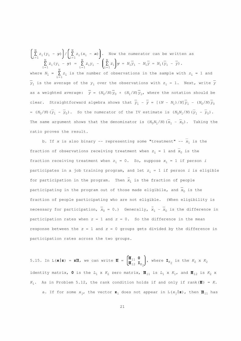
----- ----- ----- -----clear. Straightforward algebra shows that y - y = [(N - N )/N]y - (N /N)y1 1 1 0 0
----- ----- ----- -----= (N /N)(y - y ). So the numerator of the IV estimate is (N N /N)(y - y ).0 1 0 0 1 1 0
----- -----The same argument shows that the denominator is (N N /N)(x - x ). Taking the0 1 1 0
ratio proves the result.
-----b. If x is also binary -- representing some "treatment" -- x is the1
-----fraction of observations receiving treatment when z = 1 and x is thei 0
fraction receiving treatment when z = 0. So, suppose x = 1 if person ii i
participates in a job training program, and let z = 1 if person i is eligiblei
-for participation in the program. Then x is the fraction of people1
-----participating in the program out of those made eligibile, and x is the0
fraction of people participating who are not eligible. (When eligibility is
----- - -----necessary for participation, x = 0.) Generally, x - x is the difference in0 1 0
participation rates when z = 1 and z = 0. So the difference in the mean
response between the z = 1 and z = 0 groups gets divided by the difference in
participation rates across the two groups.
( )^ 0115.15. In L(x|z) = z^, we can write ^ = 2 2, where I is the K x KK 2 2^ I 212 K9 20
identity matrix, 0 is the L x K zero matrix, ^ is L x K , and ^ is K x1 2 11 1 1 12 2
K . As in Problem 5.12, the rank condition holds if and only if rank(^) = K.1
a. If for some x , the vector z does not appear in L(x |z), then ^ hasj 1 j 11
21
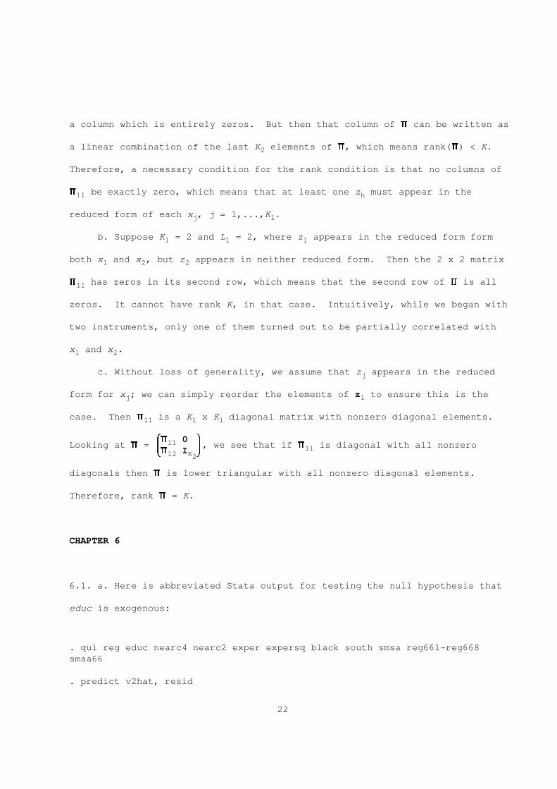
a column which is entirely zeros. But then that column of ^ can be written as
a linear combination of the last K elements of ^, which means rank(^) < K.2
Therefore, a necessary condition for the rank condition is that no columns of
^ be exactly zero, which means that at least one z must appear in the11 h
reduced form of each x , j = 1,...,K .j 1
b. Suppose K = 2 and L = 2, where z appears in the reduced form form1 1 1
both x and x , but z appears in neither reduced form. Then the 2 x 2 matrix1 2 2
^ has zeros in its second row, which means that the second row of ^ is all11
zeros. It cannot have rank K, in that case. Intuitively, while we began with
two instruments, only one of them turned out to be partially correlated with
x and x .1 2
c. Without loss of generality, we assume that z appears in the reducedj
form for x ; we can simply reorder the elements of z to ensure this is thej 1
case. Then ^ is a K x K diagonal matrix with nonzero diagonal elements.11 1 1
( )^ 011Looking at ^ = 2 2, we see that if ^ is diagonal with all nonzero11^ I12 K9 20
diagonals then ^ is lower triangular with all nonzero diagonal elements.
Therefore, rank ^ = K.
CHAPTER 6
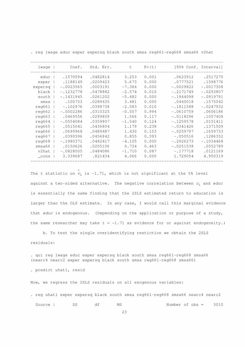
6.1. a. Here is abbreviated Stata output for testing the null hypothesis that
educ is exogenous:
. qui reg educ nearc4 nearc2 exper expersq black south smsa reg661-reg668
smsa66
. predict v2hat, resid
22
. reg lwage educ exper expersq black south smsa reg661-reg668 smsa66 v2hat
------------------------------------------------------------------------------
lwage | Coef. Std. Err. t P>|t| [95% Conf. Interval]
---------+--------------------------------------------------------------------
educ | .1570594 .0482814 3.253 0.001 .0623912 .2517275
exper | .1188149 .0209423 5.673 0.000 .0777521 .1598776
expersq | -.0023565 .0003191 -7.384 0.000 -.0029822 -.0017308
black | -.1232778 .0478882 -2.574 0.010 -.2171749 -.0293807
south | -.1431945 .0261202 -5.482 0.000 -.1944098 -.0919791
smsa | .100753 .0289435 3.481 0.000 .0440018 .1575042
reg661 | -.102976 .0398738 -2.583 0.010 -.1811588 -.0247932
reg662 | -.0002286 .0310325 -0.007 0.994 -.0610759 .0606186
reg663 | .0469556 .0299809 1.566 0.117 -.0118296 .1057408
reg664 | -.0554084 .0359807 -1.540 0.124 -.1259578 .0151411
reg665 | .0515041 .0436804 1.179 0.238 -.0341426 .1371509
reg666 | .0699968 .0489487 1.430 0.153 -.0259797 .1659733
reg667 | .0390596 .0456842 0.855 0.393 -.050516 .1286352
reg668 | -.1980371 .0482417 -4.105 0.000 -.2926273 -.1034468
smsa66 | .0150626 .0205106 0.734 0.463 -.0251538 .0552789
v2hat | -.0828005 .0484086 -1.710 0.087 -.177718 .0121169
_cons | 3.339687 .821434 4.066 0.000 1.729054 4.950319
------------------------------------------------------------------------------
^The t statistic on v is -1.71, which is not significant at the 5% level2
against a two-sided alternative. The negative correlation between u and educ1
is essentially the same finding that the 2SLS estimated return to education is
larger than the OLS estimate. In any case, I would call this marginal evidence
that educ is endogenous. (Depending on the application or purpose of a study,
the same researcher may take t = -1.71 as evidence for or against endogeneity.)
b. To test the single overidentifying restiction we obtain the 2SLS
residuals:
. qui reg lwage educ exper expersq black south smsa reg661-reg668 smsa66
(nearc4 nearc2 exper expersq black south smsa reg661-reg668 smsa66)
. predict uhat1, resid
Now, we regress the 2SLS residuals on all exogenous variables:
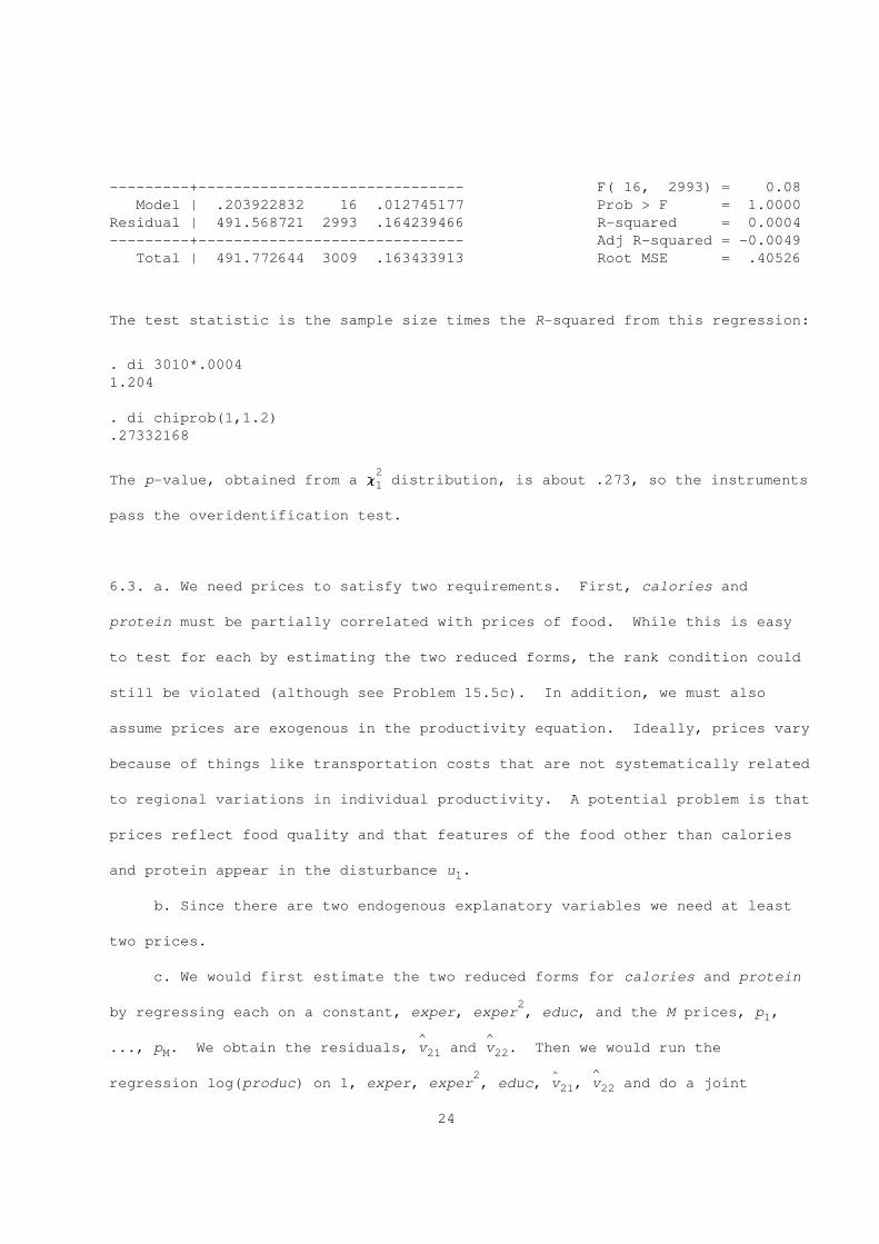
. reg uhat1 exper expersq black south smsa reg661-reg668 smsa66 nearc4 nearc2
Source | SS df MS Number of obs = 3010
23
---------+------------------------------ F( 16, 2993) = 0.08
Model | .203922832 16 .012745177 Prob > F = 1.0000
Residual | 491.568721 2993 .164239466 R-squared = 0.0004
---------+------------------------------ Adj R-squared = -0.0049
Total | 491.772644 3009 .163433913 Root MSE = .40526
The test statistic is the sample size times the R-squared from this regression:
. di 3010*.0004
1.204
. di chiprob(1,1.2)
.27332168
2The p-value, obtained from a c distribution, is about .273, so the instruments1
pass the overidentification test.
6.3. a. We need prices to satisfy two requirements. First, calories and
protein must be partially correlated with prices of food. While this is easy
to test for each by estimating the two reduced forms, the rank condition could
still be violated (although see Problem 15.5c). In addition, we must also
assume prices are exogenous in the productivity equation. Ideally, prices vary
because of things like transportation costs that are not systematically related
to regional variations in individual productivity. A potential problem is that
prices reflect food quality and that features of the food other than calories
and protein appear in the disturbance u .1
b. Since there are two endogenous explanatory variables we need at least
two prices.
c. We would first estimate the two reduced forms for calories and protein
2by regressing each on a constant, exper, exper , educ, and the M prices, p ,1
^ ^..., p . We obtain the residuals, v and v . Then we would run theM 21 22
2 ^ ^regression log(produc) on 1, exper, exper , educ, v , v and do a joint21 22
24
^ ^significance test on v and v . We could use a standard F test or use a21 22
heteroskedasticity-robust test.
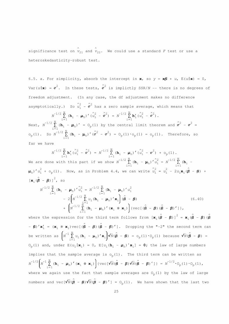
6.5. a. For simplicity, absorb the intercept in x, so y = xB + u, E(u|x) = 0,
2 ^2Var(u|x) = s . In these tests, s is implictly SSR/N -- there is no degrees of
freedom adjustment. (In any case, the df adjustment makes no difference
^2 ^2asymptotically.) So u - s has a zero sample average, which means thati
N N-1/2 ^2 ^2 -1/2 ^2 ^2N S (h - M )’(u - s ) = N S h’(u - s ).i h i i i
i=1 i=1N-1/2 ^2 2
Next, N S (h - M )’ = O (1) by the central limit theorem and s - s =i h pi=1
N-1/2 ^2 2o (1). So N S (h - M )’(s - s ) = O (1)Wo (1) = o (1). Therefore, sop i h p p p
i=1
far we have
N N-1/2 ^2 ^2 -1/2 ^2 2N S h’(u - s ) = N S (h - M )’(u - s ) + o (1).i i i h i p
i=1 i=1N N-1/2 ^2 -1/2
We are done with this part if we show N S (h - M )’u = N S (h -i h i ii=1 i=1
2 ^2 2 ^M )’u + o (1). Now, as in Problem 4.4, we can write u = u - 2u x (B - B) +h i p i i i i
^ 2[x (B - B)] , soi
N N-1/2 ^2 -1/2 2N S (h - M )’u = N S (h - M )’ui h i i h i
i=1 i=1N& -1/2 * ^
- 2 N S u (h - M )’x (B - B) (6.40)i i h i7 8i=1N& -1/2 * ^ ^
+ N S (h - M )’(x t x ) {vec[(B - B)(B - B)’]},i h i i7 8i=1
^ 2 ^ ^where the expression for the third term follows from [x (B - B)] = x (B - B)(Bi i
^ ^- B)’x’ = (x t x )vec[(B - B)(B - B)’]. Dropping the "-2" the second term cani i i
N& -1 * ----- ^ ----- ^be written as N S u (h - M )’x rN(B - B) = o (1)WO (1) because rN(B - B) =i i h i p p7 8i=1
O (1) and, under E(u |x ) = 0, E[u (h - M )’x ] = 0; the law of large numbersp i i i i h i
implies that the sample average is o (1). The third term can be written asp
N-1/2& -1 * ----- ^ ----- ^ -1/2N N S (h - M )’(x t x ) {vec[rN(B - B)rN(B - B)’]} = N WO (1)WO (1),i h i i p p7 8i=1
where we again use the fact that sample averages are O (1) by the law of largep
----- ^ ----- ^numbers and vec[rN(B - B)rN(B - B)’] = O (1). We have shown that the last twop
25
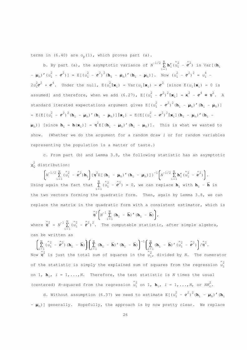
terms in (6.40) are o (1), which proves part (a).p
N-1/2 ^2 ^2b. By part (a), the asymptotic variance of N S h’(u - s ) is Var[(hi i i
i=1
2 2 2 2 2 2 2 2 4- M )’(u - s )] = E[(u - s ) (h - M )’(h - M )]. Now (u - s ) = u -h i i i h i h i i
2 2 4 2 22u s + s . Under the null, E(u |x ) = Var(u |x ) = s [since E(u |x ) = 0 isi i i i i i i
2 2 2 2 4 2assumed] and therefore, when we add (6.27), E[(u - s ) |x ] = k - s _ h . Ai i
2 2 2standard iterated expectations argument gives E[(u - s ) (h - M )’(h - M )]i i h i h
2 2 2 2 2 2= E{E[(u - s ) (h - M )’(h - M )]|x } = E{E[(u - s ) |x ](h - M )’(h -i i h i h i i i i h i
2M )} [since h = h(x )] = h E[(h - M )’(h - M )]. This is what we wanted toh i i i h i h
show. (Whether we do the argument for a random draw i or for random variables
representing the population is a matter of taste.)
c. From part (b) and Lemma 3.8, the following statistic has an asymptotic
2c distribution:Q
N N& -1/2 ^2 ^2 * 2 -1& -1/2 ^2 ^2 *N S (u - s )h {h E[(h - M )’(h - M )]} N S h’(u - s ) .i i i h i h i i7 8 7 8i=1 i=1
N ^2 ^2 -----Using again the fact that S (u - s ) = 0, we can replace h with h - h ini i i
i=1
the two vectors forming the quadratic form. Then, again by Lemma 3.8, we can
replace the matrix in the quadratic form with a consistent estimator, which is
N^2& -1 ----- ----- *h N S (h - h)’(h - h) ,i i7 8i=1N^2 -1 ^2 ^2 2
where h = N S (u - s ) . The computable statistic, after simple algebra,ii=1
can be written as
N N -1 N& ^2 ^2 ----- *& ----- ----- * & ----- ^2 ^2 * ^2S (u - s )(h - h) S (h - h)’(h - h) S (h - h)’(u - s ) /h .i i i i i i7 87 8 7 8i=1 i=1 i=1
^2 ^2Now h is just the total sum of squares in the u , divided by N. The numeratori
^2of the statistic is simply the explained sum of squares from the regression ui
on 1, h , i = 1,...,N. Therefore, the test statistic is N times the usuali
^2 2(centered) R-squared from the regression u on 1, h , i = 1,...,N, or NR .i i c
2 2 2d. Without assumption (6.37) we need to estimate E[(u - s ) (h - M )’(hi i h i
- M )] generally. Hopefully, the approach is by now pretty clear. We replaceh
26
the population expected value with the sample average and replace any unknown
2parameters -- B, s , and M in this case -- with their consistent estimatorsh
N& -1/2 ^2 ^2 *(under H ). So a generally consistent estimator of Avar N S h’(u - s )0 i i7 8i=1
is
N-1 ^2 ^2 2 ----- -----N S (u - s ) (h - h)’(h - h),i i i
i=1
and the test statistic robust to heterokurtosis can be written as
N N -1& ^2 ^2 ----- *& ^2 ^2 2 ----- ----- *S (u - s )(h - h) S (u - s ) (h - h)’(h - h)i i i i i7 87 8i=1 i=1N& ----- ^2 ^2 *W S (h - h)’(u - s ) ,i i7 8i=1
which is easily seen to be the explained sum of squares from the regression of
^2 ^2 -----1 on (u - s )(h - h), i = 1,...,N (without an intercept). Since the totali i
sum of squares, without demeaning, is N = (1 + 1 + ... + 1) (N times), the
statistic is equivalent to N - SSR , where SSR is the sum of squared0 0
residuals.
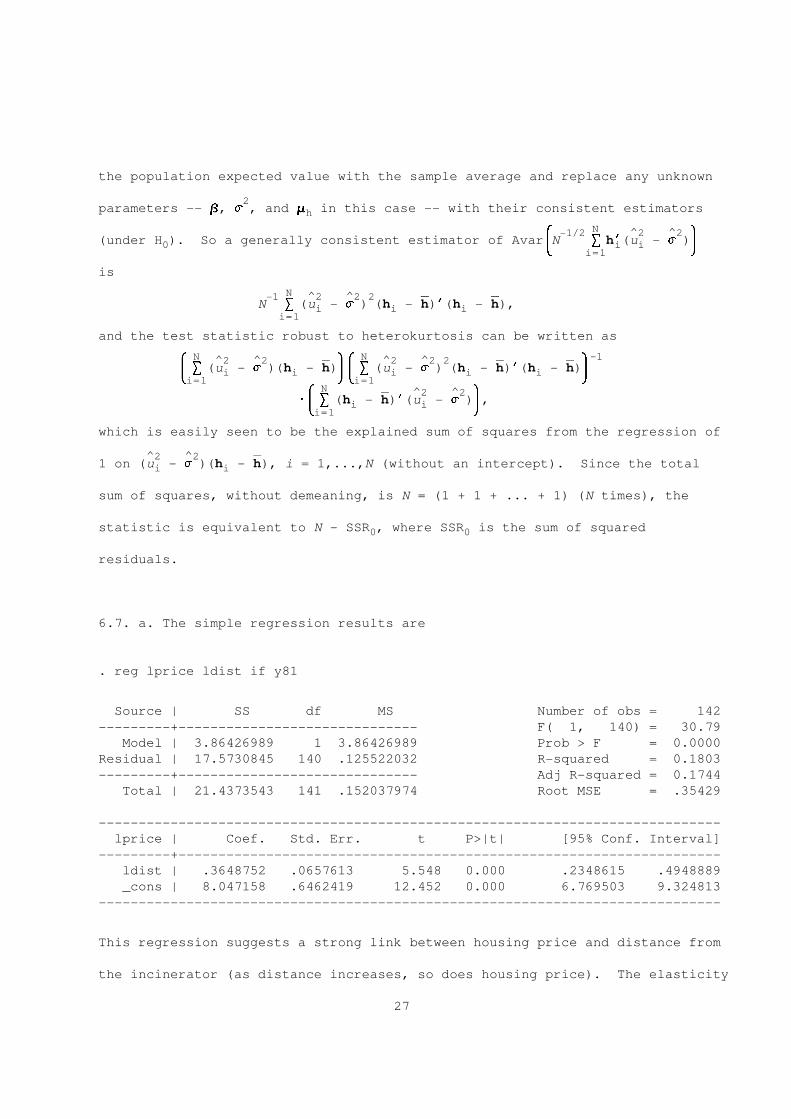
6.7. a. The simple regression results are
. reg lprice ldist if y81
Source | SS df MS Number of obs = 142
---------+------------------------------ F( 1, 140) = 30.79
Model | 3.86426989 1 3.86426989 Prob > F = 0.0000
Residual | 17.5730845 140 .125522032 R-squared = 0.1803
---------+------------------------------ Adj R-squared = 0.1744
Total | 21.4373543 141 .152037974 Root MSE = .35429
------------------------------------------------------------------------------
lprice | Coef. Std. Err. t P>|t| [95% Conf. Interval]
---------+--------------------------------------------------------------------
ldist | .3648752 .0657613 5.548 0.000 .2348615 .4948889
_cons | 8.047158 .6462419 12.452 0.000 6.769503 9.324813
------------------------------------------------------------------------------
This regression suggests a strong link between housing price and distance from
the incinerator (as distance increases, so does housing price). The elasticity
27
is .365 and the t statistic is 5.55. However, this is not a good causal
regression: the incinerator may have been put near homes with lower values to
begin with. If so, we would expect the positive relationship found in the
simple regression even if the new incinerator had no effect on housing prices.
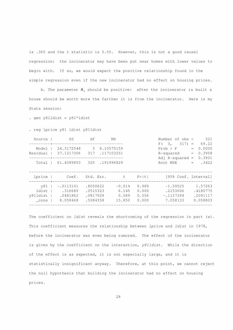
b. The parameter d should be positive: after the incinerator is built a3
house should be worth more the farther it is from the incinerator. Here is my
Stata session:
. gen y81ldist = y81*ldist
. reg lprice y81 ldist y81ldist
Source | SS df MS Number of obs = 321
---------+------------------------------ F( 3, 317) = 69.22
Model | 24.3172548 3 8.10575159 Prob > F = 0.0000
Residual | 37.1217306 317 .117103251 R-squared = 0.3958
---------+------------------------------ Adj R-squared = 0.3901
Total | 61.4389853 320 .191996829 Root MSE = .3422
------------------------------------------------------------------------------
lprice | Coef. Std. Err. t P>|t| [95% Conf. Interval]
---------+--------------------------------------------------------------------
y81 | -.0113101 .8050622 -0.014 0.989 -1.59525 1.57263
ldist | .316689 .0515323 6.145 0.000 .2153006 .4180775
y81ldist | .0481862 .0817929 0.589 0.556 -.1127394 .2091117
_cons | 8.058468 .5084358 15.850 0.000 7.058133 9.058803
------------------------------------------------------------------------------
The coefficient on ldist reveals the shortcoming of the regression in part (a).
This coefficient measures the relationship between lprice and ldist in 1978,
before the incinerator was even being rumored. The effect of the incinerator
is given by the coefficient on the interaction, y81ldist. While the direction
of the effect is as expected, it is not especially large, and it is
statistically insignificant anyway. Therefore, at this point, we cannot reject
the null hypothesis that building the incinerator had no effect on housing
prices.
28
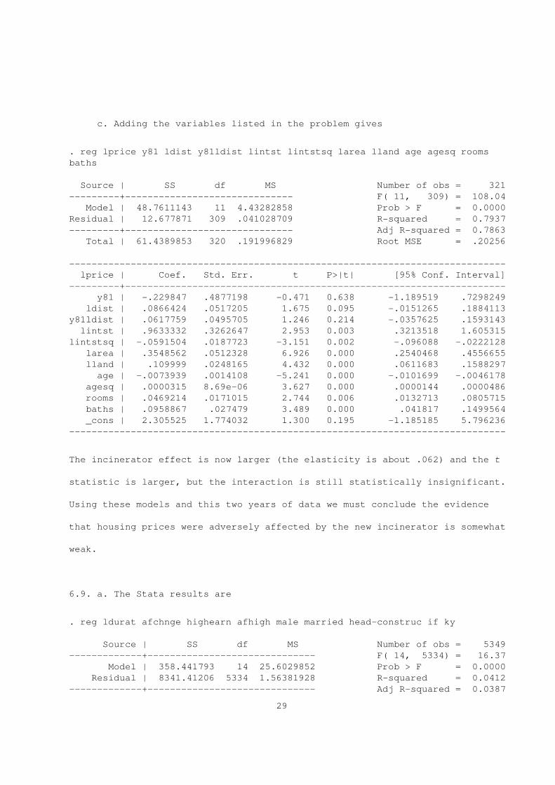
c. Adding the variables listed in the problem gives
. reg lprice y81 ldist y81ldist lintst lintstsq larea lland age agesq rooms
baths
Source | SS df MS Number of obs = 321
---------+------------------------------ F( 11, 309) = 108.04
Model | 48.7611143 11 4.43282858 Prob > F = 0.0000
Residual | 12.677871 309 .041028709 R-squared = 0.7937
---------+------------------------------ Adj R-squared = 0.7863
Total | 61.4389853 320 .191996829 Root MSE = .20256
------------------------------------------------------------------------------
lprice | Coef. Std. Err. t P>|t| [95% Conf. Interval]
---------+--------------------------------------------------------------------
y81 | -.229847 .4877198 -0.471 0.638 -1.189519 .7298249
ldist | .0866424 .0517205 1.675 0.095 -.0151265 .1884113
y81ldist | .0617759 .0495705 1.246 0.214 -.0357625 .1593143
lintst | .9633332 .3262647 2.953 0.003 .3213518 1.605315
lintstsq | -.0591504 .0187723 -3.151 0.002 -.096088 -.0222128
larea | .3548562 .0512328 6.926 0.000 .2540468 .4556655
lland | .109999 .0248165 4.432 0.000 .0611683 .1588297
age | -.0073939 .0014108 -5.241 0.000 -.0101699 -.0046178
agesq | .0000315 8.69e-06 3.627 0.000 .0000144 .0000486
rooms | .0469214 .0171015 2.744 0.006 .0132713 .0805715
baths | .0958867 .027479 3.489 0.000 .041817 .1499564
_cons | 2.305525 1.774032 1.300 0.195 -1.185185 5.796236
------------------------------------------------------------------------------
The incinerator effect is now larger (the elasticity is about .062) and the t
statistic is larger, but the interaction is still statistically insignificant.
Using these models and this two years of data we must conclude the evidence
that housing prices were adversely affected by the new incinerator is somewhat
weak.
6.9. a. The Stata results are
. reg ldurat afchnge highearn afhigh male married head-construc if ky
Source | SS df MS Number of obs = 5349
-------------+------------------------------ F( 14, 5334) = 16.37
Model | 358.441793 14 25.6029852 Prob > F = 0.0000
Residual | 8341.41206 5334 1.56381928 R-squared = 0.0412
-------------+------------------------------ Adj R-squared = 0.0387
29
Total | 8699.85385 5348 1.62674904 Root MSE = 1.2505
------------------------------------------------------------------------------
ldurat | Coef. Std. Err. t P>|t| [95% Conf. Interval]
-------------+----------------------------------------------------------------
afchnge | .0106274 .0449167 0.24 0.813 -.0774276 .0986824
highearn | .1757598 .0517462 3.40 0.001 .0743161 .2772035
afhigh | .2308768 .0695248 3.32 0.001 .0945798 .3671738
male | -.0979407 .0445498 -2.20 0.028 -.1852766 -.0106049
married | .1220995 .0391228 3.12 0.002 .0454027 .1987962
head | -.5139003 .1292776 -3.98 0.000 -.7673372 -.2604634
neck | .2699126 .1614899 1.67 0.095 -.0466737 .5864988
upextr | -.178539 .1011794 -1.76 0.078 -.376892 .0198141
trunk | .1264514 .1090163 1.16 0.246 -.0872651 .340168
lowback | -.0085967 .1015267 -0.08 0.933 -.2076305 .1904371
lowextr | -.1202911 .1023262 -1.18 0.240 -.3208922 .0803101
occdis | .2727118 .210769 1.29 0.196 -.1404816 .6859052
manuf | -.1606709 .0409038 -3.93 0.000 -.2408591 -.0804827
construc | .1101967 .0518063 2.13 0.033 .0086352 .2117581
_cons | 1.245922 .1061677 11.74 0.000 1.03779 1.454054
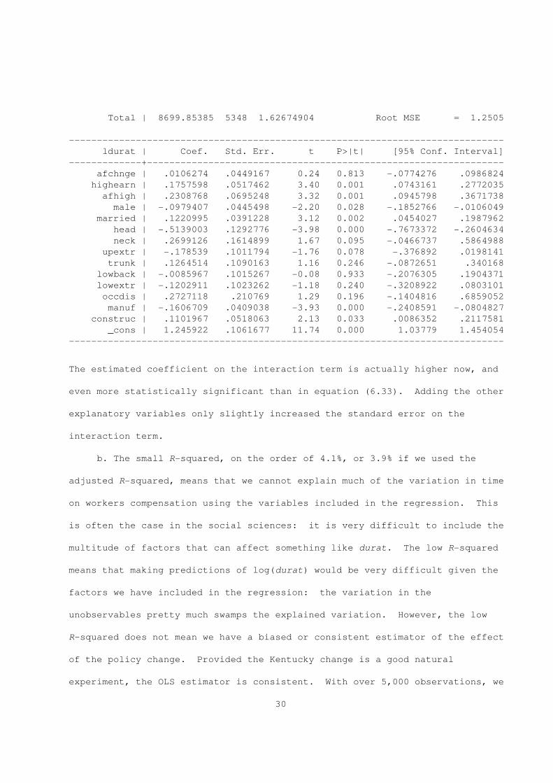
------------------------------------------------------------------------------
The estimated coefficient on the interaction term is actually higher now, and
even more statistically significant than in equation (6.33). Adding the other
explanatory variables only slightly increased the standard error on the
interaction term.
b. The small R-squared, on the order of 4.1%, or 3.9% if we used the
adjusted R-squared, means that we cannot explain much of the variation in time
on workers compensation using the variables included in the regression. This
is often the case in the social sciences: it is very difficult to include the
multitude of factors that can affect something like durat. The low R-squared
means that making predictions of log(durat) would be very difficult given the
factors we have included in the regression: the variation in the
unobservables pretty much swamps the explained variation. However, the low
R-squared does not mean we have a biased or consistent estimator of the effect
of the policy change. Provided the Kentucky change is a good natural
experiment, the OLS estimator is consistent. With over 5,000 observations, we
30
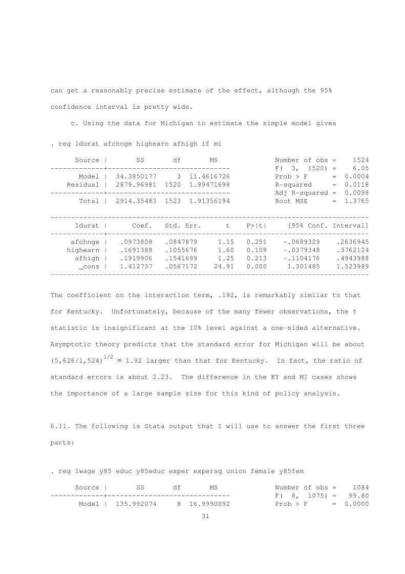
can get a reasonably precise estimate of the effect, although the 95%
confidence interval is pretty wide.
c. Using the data for Michigan to estimate the simple model gives
. reg ldurat afchnge highearn afhigh if mi
Source | SS df MS Number of obs = 1524
-------------+------------------------------ F( 3, 1520) = 6.05
Model | 34.3850177 3 11.4616726 Prob > F = 0.0004
Residual | 2879.96981 1520 1.89471698 R-squared = 0.0118
-------------+------------------------------ Adj R-squared = 0.0098
Total | 2914.35483 1523 1.91356194 Root MSE = 1.3765
------------------------------------------------------------------------------
ldurat | Coef. Std. Err. t P>|t| [95% Conf. Interval]
-------------+----------------------------------------------------------------
afchnge | .0973808 .0847879 1.15 0.251 -.0689329 .2636945
highearn | .1691388 .1055676 1.60 0.109 -.0379348 .3762124
afhigh | .1919906 .1541699 1.25 0.213 -.1104176 .4943988
_cons | 1.412737 .0567172 24.91 0.000 1.301485 1.523989
------------------------------------------------------------------------------
The coefficient on the interaction term, .192, is remarkably similar to that
for Kentucky. Unfortunately, because of the many fewer observations, the t
statistic is insignificant at the 10% level against a one-sided alternative.
Asymptotic theory predicts that the standard error for Michigan will be about
1/2(5,626/1,524) ~ 1.92 larger than that for Kentucky. In fact, the ratio of
standard errors is about 2.23. The difference in the KY and MI cases shows
the importance of a large sample size for this kind of policy analysis.
6.11. The following is Stata output that I will use to answer the first three
parts:
. reg lwage y85 educ y85educ exper expersq union female y85fem
Source | SS df MS Number of obs = 1084
-------------+------------------------------ F( 8, 1075) = 99.80
Model | 135.992074 8 16.9990092 Prob > F = 0.0000
31
Residual | 183.099094 1075 .170324738 R-squared = 0.4262
-------------+------------------------------ Adj R-squared = 0.4219
Total | 319.091167 1083 .29463635 Root MSE = .4127
------------------------------------------------------------------------------
lwage | Coef. Std. Err. t P>|t| [95% Conf. Interval]
-------------+----------------------------------------------------------------
y85 | .1178062 .1237817 0.95 0.341 -.125075 .3606874
educ | .0747209 .0066764 11.19 0.000 .0616206 .0878212
y85educ | .0184605 .0093542 1.97 0.049 .000106 .036815
exper | .0295843 .0035673 8.29 0.000 .0225846 .036584
expersq | -.0003994 .0000775 -5.15 0.000 -.0005516 -.0002473
union | .2021319 .0302945 6.67 0.000 .1426888 .2615749
female | -.3167086 .0366215 -8.65 0.000 -.3885663 -.244851
y85fem | .085052 .051309 1.66 0.098 -.0156251 .185729
_cons | .4589329 .0934485 4.91 0.000 .2755707 .642295
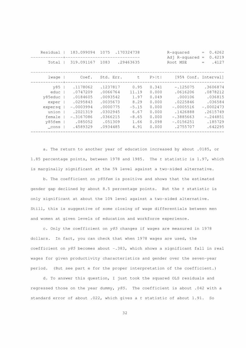
------------------------------------------------------------------------------
a. The return to another year of education increased by about .0185, or
1.85 percentage points, between 1978 and 1985. The t statistic is 1.97, which
is marginally significant at the 5% level against a two-sided alternative.
b. The coefficient on y85fem is positive and shows that the estimated
gender gap declined by about 8.5 percentage points. But the t statistic is
only significant at about the 10% level against a two-sided alternative.
Still, this is suggestive of some closing of wage differentials between men
and women at given levels of education and workforce experience.
c. Only the coefficient on y85 changes if wages are measured in 1978
dollars. In fact, you can check that when 1978 wages are used, the
coefficient on y85 becomes about -.383, which shows a significant fall in real
wages for given productivity characteristics and gender over the seven-year
period. (But see part e for the proper interpretation of the coefficient.)
d. To answer this question, I just took the squared OLS residuals and
regressed those on the year dummy, y85. The coefficient is about .042 with a
standard error of about .022, which gives a t statistic of about 1.91. So
32
there is some evidence that the variance of the unexplained part of log wages
(or log real wages) has increased over time.
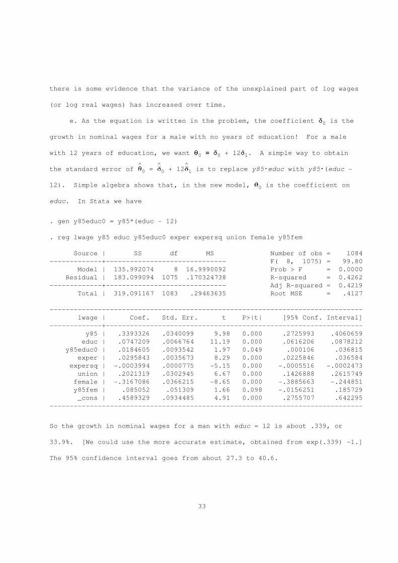
e. As the equation is written in the problem, the coefficient d is the0
growth in nominal wages for a male with no years of education! For a male
with 12 years of education, we want q _ d + 12d . A simple way to obtain0 0 1
^ ^ ^the standard error of q = d + 12d is to replace y85Weduc with y85W(educ -0 0 1
12). Simple algebra shows that, in the new model, q is the coefficient on0
educ. In Stata we have
. gen y85educ0 = y85*(educ - 12)
. reg lwage y85 educ y85educ0 exper expersq union female y85fem
Source | SS df MS Number of obs = 1084
-------------+------------------------------ F( 8, 1075) = 99.80
Model | 135.992074 8 16.9990092 Prob > F = 0.0000
Residual | 183.099094 1075 .170324738 R-squared = 0.4262
-------------+------------------------------ Adj R-squared = 0.4219
Total | 319.091167 1083 .29463635 Root MSE = .4127
------------------------------------------------------------------------------
lwage | Coef. Std. Err. t P>|t| [95% Conf. Interval]
-------------+----------------------------------------------------------------
y85 | .3393326 .0340099 9.98 0.000 .2725993 .4060659
educ | .0747209 .0066764 11.19 0.000 .0616206 .0878212
y85educ0 | .0184605 .0093542 1.97 0.049 .000106 .036815
exper | .0295843 .0035673 8.29 0.000 .0225846 .036584
expersq | -.0003994 .0000775 -5.15 0.000 -.0005516 -.0002473
union | .2021319 .0302945 6.67 0.000 .1426888 .2615749
female | -.3167086 .0366215 -8.65 0.000 -.3885663 -.244851
y85fem | .085052 .051309 1.66 0.098 -.0156251 .185729
_cons | .4589329 .0934485 4.91 0.000 .2755707 .642295
------------------------------------------------------------------------------
So the growth in nominal wages for a man with educ = 12 is about .339, or
33.9%. [We could use the more accurate estimate, obtained from exp(.339) -1.]
The 95% confidence interval goes from about 27.3 to 40.6.
33
CHAPTER 7
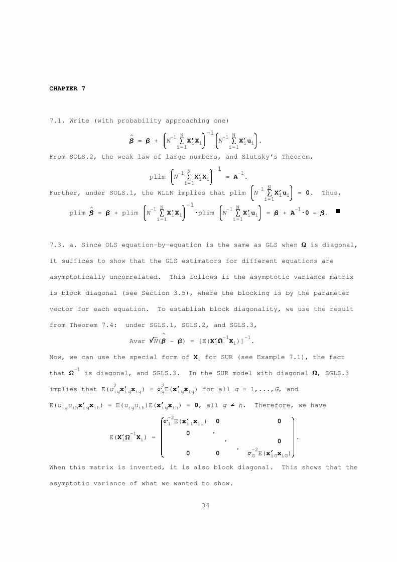
7.1. Write (with probability approaching one)
-1N N^ & -1 * & -1 *B = B + N S X’X N S X’u .i i i i7 8 7 8i=1 i=1
From SOLS.2, the weak law of large numbers, and Slutsky’s Theorem,
-1N& -1 * -1plim N S X’X = A .i i7 8i=1
N& -1 *Further, under SOLS.1, the WLLN implies that plim N S X’u = 0. Thus,i i7 8i=1
-1N N^ & -1 * & -1 * -1plim B = B + plim N S X’X Wplim N S X’u = B + A W0 = B. )i i i i7 8 7 8i=1 i=1
7.3. a. Since OLS equation-by-equation is the same as GLS when ) is diagonal,
it suffices to show that the GLS estimators for different equations are
asymptotically uncorrelated. This follows if the asymptotic variance matrix
is block diagonal (see Section 3.5), where the blocking is by the parameter
vector for each equation. To establish block diagonality, we use the result
from Theorem 7.4: under SGLS.1, SGLS.2, and SGLS.3,
^----- -1 -1Avar rN(B - B) = [E(X’) X )] .i i
Now, we can use the special form of X for SUR (see Example 7.1), the facti
-1that ) is diagonal, and SGLS.3. In the SUR model with diagonal ), SGLS.3
2 2implies that E(u x’ x ) = s E(x’ x ) for all g = 1,...,G, andig ig ig g ig ig
E(u u x’ x ) = E(u u )E(x’ x ) = 0, all g $ h. Therefore, we haveig ih ig ih ig ih ig ih
-2&s E(x’ x ) 0 0 *1 i1 i1
2 2-1 0 W
E(X’) X ) = 2 2.i i W 02 2W -27 0 0 s E(x’ x )8G iG iG
When this matrix is inverted, it is also block diagonal. This shows that the
asymptotic variance of what we wanted to show.
34
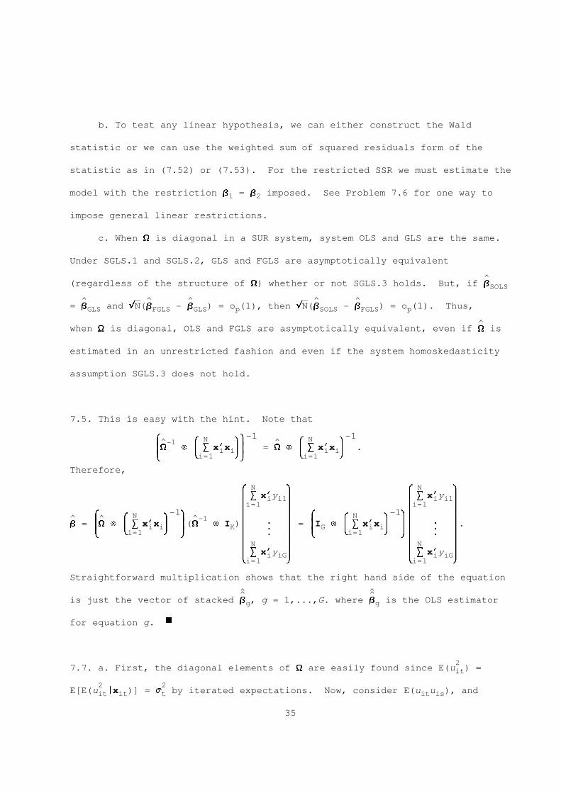
b. To test any linear hypothesis, we can either construct the Wald
statistic or we can use the weighted sum of squared residuals form of the
statistic as in (7.52) or (7.53). For the restricted SSR we must estimate the
model with the restriction B = B imposed. See Problem 7.6 for one way to1 2
impose general linear restrictions.
c. When ) is diagonal in a SUR system, system OLS and GLS are the same.
Under SGLS.1 and SGLS.2, GLS and FGLS are asymptotically equivalent
^(regardless of the structure of )) whether or not SGLS.3 holds. But, if BSOLS
^ ----- ^ ^ ----- ^ ^= B and rN(B - B ) = o (1), then rN(B - B ) = o (1). Thus,GLS FGLS GLS p SOLS FGLS p
^when ) is diagonal, OLS and FGLS are asymptotically equivalent, even if ) is
estimated in an unrestricted fashion and even if the system homoskedasticity
assumption SGLS.3 does not hold.
7.5. This is easy with the hint. Note that
-1 -1& N * N^-1 & * ^ & *2) t S x’x 2 = ) t S x’x .i i i i7 8 7 87 i=1 8 i=1
Therefore,
N N& * & *S x’y S x’yi i1 i i12 2 2 2i=1 i=1
-1 2 2 -1 2 2& N * & N *^ ^ & * ^-1 & *B = 2) t S x’x 2() t I )2 W 2 = 2I t S x’x 22 W 2.i i K G i i7 8 W 7 8 W7 i=1 8 7 i=1 82 W 2 2 W 2N N2 2 2 2S x’y S x’yi iG i iG7 8 7 8i=1 i=1
Straightforward multiplication shows that the right hand side of the equation
^ ^^ ^is just the vector of stacked B , g = 1,...,G. where B is the OLS estimatorg g
for equation g. )
27.7. a. First, the diagonal elements of ) are easily found since E(u ) =it
2 2E[E(u |x )] = s by iterated expectations. Now, consider E(u u ), andit it t it is
35
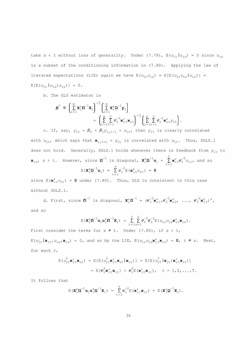
take s < t without loss of generality. Under (7.79), E(u |u ) = 0 since uit is is
is a subset of the conditioning information in (7.80). Applying the law of
iterated expectations (LIE) again we have E(u u ) = E[E(u u |u )] =it is it is is
E[E(u |u )u )] = 0.it is is
b. The GLS estimator is
-1N N* & -1 * & -1 *B _ S X’) X S X’) yi i i i7 8 7 8i=1 i=1
-1N T N T& -2 * & -2 *= S S s x’ x S S s x’ y .t it it t it it7 8 7 8i=1t=1 i=1t=1
c. If, say, y = b + b y + u , then y is clearly correlatedit 0 1 i,t-1 it it
with u , which says that x = y is correlated with u . Thus, SGLS.1it i,t+1 it it
does not hold. Generally, SGLS.1 holds whenever there is feedback from y toit
T-1 -1 -2x , s > t. However, since ) is diagonal, X’) u = S x’ s u , and sois i i it t it
t=1T-1 -2
E(X’) u ) = S s E(x’ u ) = 0i i t it itt=1
since E(x’ u ) = 0 under (7.80). Thus, GLS is consistent in this caseit it
without SGLS.1.
-1 -1 -2 -2 -2d. First, since ) is diagonal, X’) = (s x’ ,s x’ , ..., s x’ )’,i 1 i1 2 i2 T iT
and so
T T-1 -1 -2 -2E(X’) u u’) X ) = S S s s E(u u x’ x ).i i i i t s it is it is
t=1s=1
First consider the terms for s $ t. Under (7.80), if s < t,
E(u |x ,u ,x ) = 0, and so by the LIE, E(u u x’ x ) = 0, t $ s. Next,it it is is it is it is
for each t,
2 2 2E(u x’ x ) = E[E(u x’ x |x )] = E[E(u |x )x’ x )]it it it it it it it it it it it
2 2= E[s x’ x ] = s E(x’ x ), t = 1,2,...,T.t it it t it it
It follows that
T-1 -1 -2 -1E(X’) u u’) X ) = S s E(x’ x ) = E(X’) X ).i i i i t it it i i
t=1
36
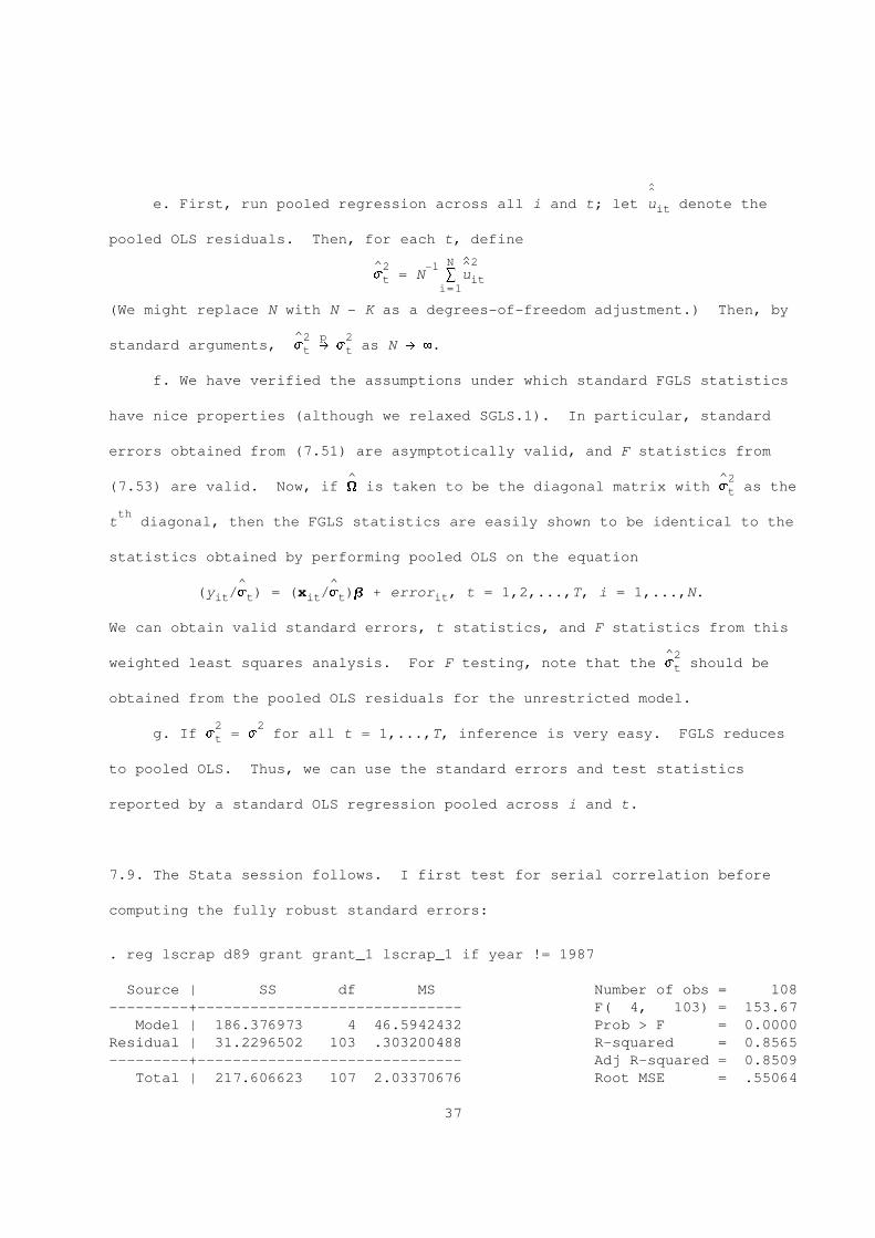
^
e. First, run pooled regression across all i and t; let u denote theit
pooled OLS residuals. Then, for each t, define
N ^2^2 -1 ^s = N S ut iti=1
(We might replace N with N - K as a degrees-of-freedom adjustment.) Then, by
^2 p 2standard arguments, s L s as N L 8.t t
f. We have verified the assumptions under which standard FGLS statistics
have nice properties (although we relaxed SGLS.1). In particular, standard
errors obtained from (7.51) are asymptotically valid, and F statistics from
^ ^2(7.53) are valid. Now, if ) is taken to be the diagonal matrix with s as thet
tht diagonal, then the FGLS statistics are easily shown to be identical to the
statistics obtained by performing pooled OLS on the equation
^ ^(y /s ) = (x /s )B + error , t = 1,2,...,T, i = 1,...,N.it t it t it
We can obtain valid standard errors, t statistics, and F statistics from this
^2weighted least squares analysis. For F testing, note that the s should bet
obtained from the pooled OLS residuals for the unrestricted model.
2 2g. If s = s for all t = 1,...,T, inference is very easy. FGLS reducest
to pooled OLS. Thus, we can use the standard errors and test statistics
reported by a standard OLS regression pooled across i and t.
7.9. The Stata session follows. I first test for serial correlation before
computing the fully robust standard errors:
. reg lscrap d89 grant grant_1 lscrap_1 if year != 1987
Source | SS df MS Number of obs = 108
---------+------------------------------ F( 4, 103) = 153.67
Model | 186.376973 4 46.5942432 Prob > F = 0.0000
Residual | 31.2296502 103 .303200488 R-squared = 0.8565
---------+------------------------------ Adj R-squared = 0.8509
Total | 217.606623 107 2.03370676 Root MSE = .55064
37
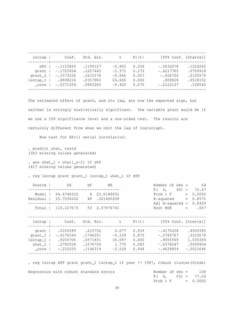
------------------------------------------------------------------------------
lscrap | Coef. Std. Err. t P>|t| [95% Conf. Interval]
---------+--------------------------------------------------------------------
d89 | -.1153893 .1199127 -0.962 0.338 -.3532078 .1224292
grant | -.1723924 .1257443 -1.371 0.173 -.4217765 .0769918
grant_1 | -.1073226 .1610378 -0.666 0.507 -.426703 .2120579
lscrap_1 | .8808216 .0357963 24.606 0.000 .809828 .9518152
_cons | -.0371354 .0883283 -0.420 0.675 -.2123137 .138043
------------------------------------------------------------------------------
The estimated effect of grant, and its lag, are now the expected sign, but
neither is strongly statistically significant. The variable grant would be if
we use a 10% significance level and a one-sided test. The results are
certainly different from when we omit the lag of log(scrap).
Now test for AR(1) serial correlation:
. predict uhat, resid
(363 missing values generated)
. gen uhat_1 = uhat[_n-1] if d89
(417 missing values generated)
. reg lscrap grant grant_1 lscrap_1 uhat_1 if d89
Source | SS df MS Number of obs = 54
---------+------------------------------ F( 4, 49) = 73.47
Model | 94.4746525 4 23.6186631 Prob > F = 0.0000
Residual | 15.7530202 49 .321490208 R-squared = 0.8571
---------+------------------------------ Adj R-squared = 0.8454
Total | 110.227673 53 2.07976741 Root MSE = .567
------------------------------------------------------------------------------
lscrap | Coef. Std. Err. t P>|t| [95% Conf. Interval]
---------+--------------------------------------------------------------------
grant | .0165089 .215732 0.077 0.939 -.4170208 .4500385
grant_1 | -.0276544 .1746251 -0.158 0.875 -.3785767 .3232679
lscrap_1 | .9204706 .0571831 16.097 0.000 .8055569 1.035384
uhat_1 | .2790328 .1576739 1.770 0.083 -.0378247 .5958904
_cons | -.232525 .1146314 -2.028 0.048 -.4628854 -.0021646
------------------------------------------------------------------------------
. reg lscrap d89 grant grant_1 lscrap_1 if year != 1987, robust cluster(fcode)
Regression with robust standard errors Number of obs = 108
F( 4, 53) = 77.24
Prob > F = 0.0000
38
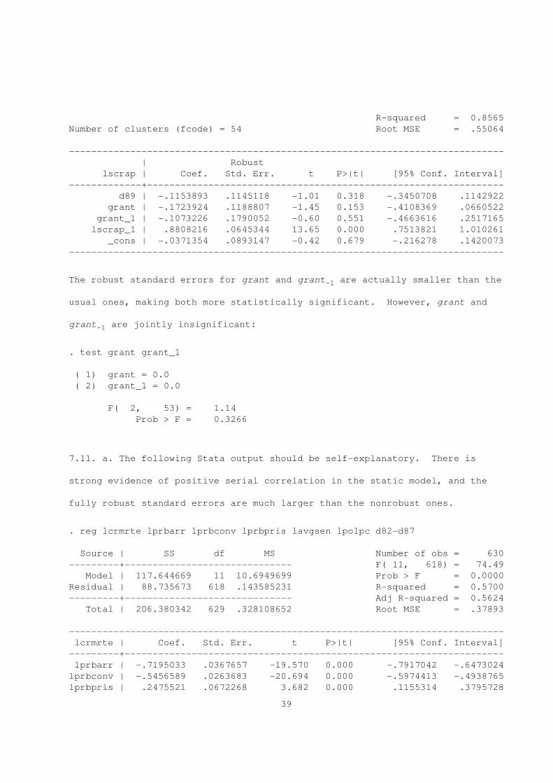
R-squared = 0.8565
Number of clusters (fcode) = 54 Root MSE = .55064
------------------------------------------------------------------------------
| Robust
lscrap | Coef. Std. Err. t P>|t| [95% Conf. Interval]
-------------+----------------------------------------------------------------
d89 | -.1153893 .1145118 -1.01 0.318 -.3450708 .1142922
grant | -.1723924 .1188807 -1.45 0.153 -.4108369 .0660522
grant_1 | -.1073226 .1790052 -0.60 0.551 -.4663616 .2517165
lscrap_1 | .8808216 .0645344 13.65 0.000 .7513821 1.010261
_cons | -.0371354 .0893147 -0.42 0.679 -.216278 .1420073
------------------------------------------------------------------------------
The robust standard errors for grant and grant are actually smaller than the-1
usual ones, making both more statistically significant. However, grant and
grant are jointly insignificant:-1
. test grant grant_1
( 1) grant = 0.0
( 2) grant_1 = 0.0
F( 2, 53) = 1.14
Prob > F = 0.3266
7.11. a. The following Stata output should be self-explanatory. There is
strong evidence of positive serial correlation in the static model, and the
fully robust standard errors are much larger than the nonrobust ones.
. reg lcrmrte lprbarr lprbconv lprbpris lavgsen lpolpc d82-d87
Source | SS df MS Number of obs = 630
---------+------------------------------ F( 11, 618) = 74.49
Model | 117.644669 11 10.6949699 Prob > F = 0.0000
Residual | 88.735673 618 .143585231 R-squared = 0.5700
---------+------------------------------ Adj R-squared = 0.5624
Total | 206.380342 629 .328108652 Root MSE = .37893
------------------------------------------------------------------------------
lcrmrte | Coef. Std. Err. t P>|t| [95% Conf. Interval]
---------+--------------------------------------------------------------------
lprbarr | -.7195033 .0367657 -19.570 0.000 -.7917042 -.6473024
lprbconv | -.5456589 .0263683 -20.694 0.000 -.5974413 -.4938765
lprbpris | .2475521 .0672268 3.682 0.000 .1155314 .3795728
39
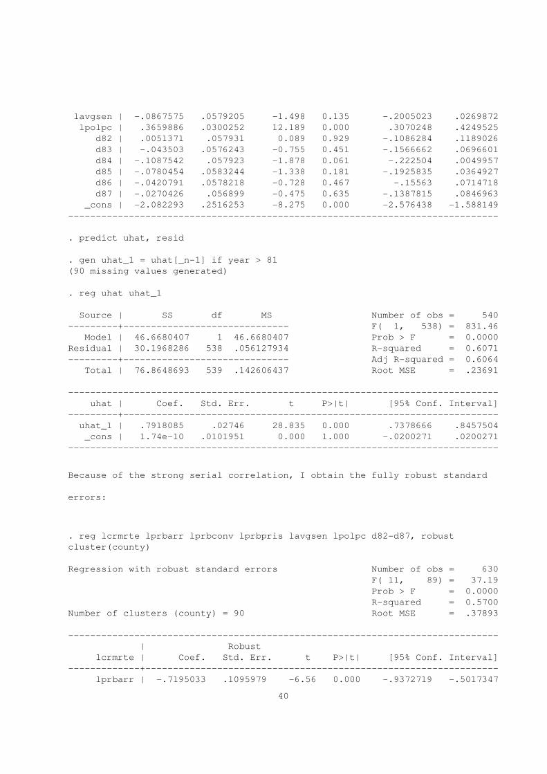
lavgsen | -.0867575 .0579205 -1.498 0.135 -.2005023 .0269872
lpolpc | .3659886 .0300252 12.189 0.000 .3070248 .4249525
d82 | .0051371 .057931 0.089 0.929 -.1086284 .1189026
d83 | -.043503 .0576243 -0.755 0.451 -.1566662 .0696601
d84 | -.1087542 .057923 -1.878 0.061 -.222504 .0049957
d85 | -.0780454 .0583244 -1.338 0.181 -.1925835 .0364927
d86 | -.0420791 .0578218 -0.728 0.467 -.15563 .0714718
d87 | -.0270426 .056899 -0.475 0.635 -.1387815 .0846963
_cons | -2.082293 .2516253 -8.275 0.000 -2.576438 -1.588149
------------------------------------------------------------------------------
. predict uhat, resid
. gen uhat_1 = uhat[_n-1] if year > 81
(90 missing values generated)
. reg uhat uhat_1
Source | SS df MS Number of obs = 540
---------+------------------------------ F( 1, 538) = 831.46
Model | 46.6680407 1 46.6680407 Prob > F = 0.0000
Residual | 30.1968286 538 .056127934 R-squared = 0.6071
---------+------------------------------ Adj R-squared = 0.6064
Total | 76.8648693 539 .142606437 Root MSE = .23691
------------------------------------------------------------------------------
uhat | Coef. Std. Err. t P>|t| [95% Conf. Interval]
---------+--------------------------------------------------------------------
uhat_1 | .7918085 .02746 28.835 0.000 .7378666 .8457504
_cons | 1.74e-10 .0101951 0.000 1.000 -.0200271 .0200271
------------------------------------------------------------------------------
Because of the strong serial correlation, I obtain the fully robust standard
errors:
. reg lcrmrte lprbarr lprbconv lprbpris lavgsen lpolpc d82-d87, robust
cluster(county)
Regression with robust standard errors Number of obs = 630
F( 11, 89) = 37.19
Prob > F = 0.0000
R-squared = 0.5700
Number of clusters (county) = 90 Root MSE = .37893
------------------------------------------------------------------------------
| Robust
lcrmrte | Coef. Std. Err. t P>|t| [95% Conf. Interval]
-------------+----------------------------------------------------------------
lprbarr | -.7195033 .1095979 -6.56 0.000 -.9372719 -.5017347
40
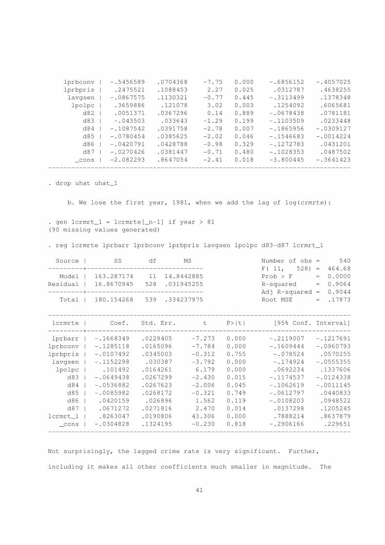
lprbconv | -.5456589 .0704368 -7.75 0.000 -.6856152 -.4057025
lprbpris | .2475521 .1088453 2.27 0.025 .0312787 .4638255
lavgsen | -.0867575 .1130321 -0.77 0.445 -.3113499 .1378348
lpolpc | .3659886 .121078 3.02 0.003 .1254092 .6065681
d82 | .0051371 .0367296 0.14 0.889 -.0678438 .0781181
d83 | -.043503 .033643 -1.29 0.199 -.1103509 .0233448
d84 | -.1087542 .0391758 -2.78 0.007 -.1865956 -.0309127
d85 | -.0780454 .0385625 -2.02 0.046 -.1546683 -.0014224
d86 | -.0420791 .0428788 -0.98 0.329 -.1272783 .0431201
d87 | -.0270426 .0381447 -0.71 0.480 -.1028353 .0487502
_cons | -2.082293 .8647054 -2.41 0.018 -3.800445 -.3641423
------------------------------------------------------------------------------
. drop uhat uhat_1
b. We lose the first year, 1981, when we add the lag of log(crmrte):
. gen lcrmrt_1 = lcrmrte[_n-1] if year > 81
(90 missing values generated)
. reg lcrmrte lprbarr lprbconv lprbpris lavgsen lpolpc d83-d87 lcrmrt_1
Source | SS df MS Number of obs = 540
---------+------------------------------ F( 11, 528) = 464.68
Model | 163.287174 11 14.8442885 Prob > F = 0.0000
Residual | 16.8670945 528 .031945255 R-squared = 0.9064
---------+------------------------------ Adj R-squared = 0.9044
Total | 180.154268 539 .334237975 Root MSE = .17873
------------------------------------------------------------------------------
lcrmrte | Coef. Std. Err. t P>|t| [95% Conf. Interval]
---------+--------------------------------------------------------------------
lprbarr | -.1668349 .0229405 -7.273 0.000 -.2119007 -.1217691
lprbconv | -.1285118 .0165096 -7.784 0.000 -.1609444 -.0960793
lprbpris | -.0107492 .0345003 -0.312 0.755 -.078524 .0570255
lavgsen | -.1152298 .030387 -3.792 0.000 -.174924 -.0555355
lpolpc | .101492 .0164261 6.179 0.000 .0692234 .1337606
d83 | -.0649438 .0267299 -2.430 0.015 -.1174537 -.0124338
d84 | -.0536882 .0267623 -2.006 0.045 -.1062619 -.0011145
d85 | -.0085982 .0268172 -0.321 0.749 -.0612797 .0440833
d86 | .0420159 .026896 1.562 0.119 -.0108203 .0948522
d87 | .0671272 .0271816 2.470 0.014 .0137298 .1205245
lcrmrt_1 | .8263047 .0190806 43.306 0.000 .7888214 .8637879
_cons | -.0304828 .1324195 -0.230 0.818 -.2906166 .229651
------------------------------------------------------------------------------
Not surprisingly, the lagged crime rate is very significant. Further,
including it makes all other coefficients much smaller in magnitude. The
41
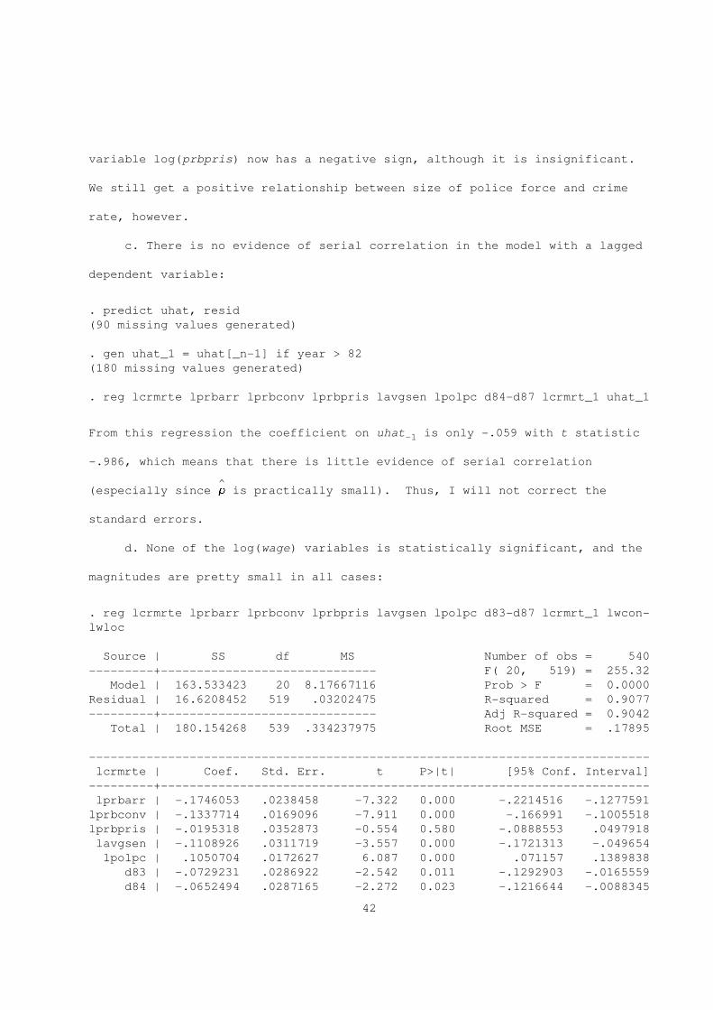
variable log(prbpris) now has a negative sign, although it is insignificant.
We still get a positive relationship between size of police force and crime
rate, however.
c. There is no evidence of serial correlation in the model with a lagged
dependent variable:
. predict uhat, resid
(90 missing values generated)
. gen uhat_1 = uhat[_n-1] if year > 82
(180 missing values generated)
. reg lcrmrte lprbarr lprbconv lprbpris lavgsen lpolpc d84-d87 lcrmrt_1 uhat_1
From this regression the coefficient on uhat is only -.059 with t statistic-1
-.986, which means that there is little evidence of serial correlation
^(especially since r is practically small). Thus, I will not correct the
standard errors.
d. None of the log(wage) variables is statistically significant, and the
magnitudes are pretty small in all cases:
. reg lcrmrte lprbarr lprbconv lprbpris lavgsen lpolpc d83-d87 lcrmrt_1 lwcon-
lwloc
Source | SS df MS Number of obs = 540
---------+------------------------------ F( 20, 519) = 255.32
Model | 163.533423 20 8.17667116 Prob > F = 0.0000
Residual | 16.6208452 519 .03202475 R-squared = 0.9077
---------+------------------------------ Adj R-squared = 0.9042
Total | 180.154268 539 .334237975 Root MSE = .17895
------------------------------------------------------------------------------
lcrmrte | Coef. Std. Err. t P>|t| [95% Conf. Interval]
---------+--------------------------------------------------------------------
lprbarr | -.1746053 .0238458 -7.322 0.000 -.2214516 -.1277591
lprbconv | -.1337714 .0169096 -7.911 0.000 -.166991 -.1005518
lprbpris | -.0195318 .0352873 -0.554 0.580 -.0888553 .0497918
lavgsen | -.1108926 .0311719 -3.557 0.000 -.1721313 -.049654
lpolpc | .1050704 .0172627 6.087 0.000 .071157 .1389838
d83 | -.0729231 .0286922 -2.542 0.011 -.1292903 -.0165559
d84 | -.0652494 .0287165 -2.272 0.023 -.1216644 -.0088345
42
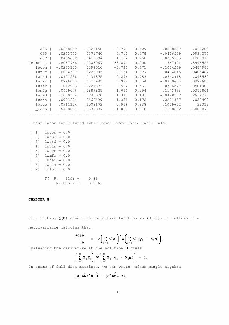
d85 | -.0258059 .0326156 -0.791 0.429 -.0898807 .038269
d86 | .0263763 .0371746 0.710 0.478 -.0466549 .0994076
d87 | .0465632 .0418004 1.114 0.266 -.0355555 .1286819
lcrmrt_1 | .8087768 .0208067 38.871 0.000 .767901 .8496525
lwcon | -.0283133 .0392516 -0.721 0.471 -.1054249 .0487983
lwtuc | -.0034567 .0223995 -0.154 0.877 -.0474615 .0405482
lwtrd | .0121236 .0439875 0.276 0.783 -.0742918 .098539
lwfir | .0296003 .0318995 0.928 0.354 -.0330676 .0922683
lwser | .012903 .0221872 0.582 0.561 -.0306847 .0564908
lwmfg | -.0409046 .0389325 -1.051 0.294 -.1173893 .0355801
lwfed | .1070534 .0798526 1.341 0.181 -.0498207 .2639275
lwsta | -.0903894 .0660699 -1.368 0.172 -.2201867 .039408
lwloc | .0961124 .1003172 0.958 0.338 -.1009652 .29319
_cons | -.6438061 .6335887 -1.016 0.310 -1.88852 .6009076
------------------------------------------------------------------------------
. test lwcon lwtuc lwtrd lwfir lwser lwmfg lwfed lwsta lwloc
( 1) lwcon = 0.0
( 2) lwtuc = 0.0
( 3) lwtrd = 0.0
( 4) lwfir = 0.0
( 5) lwser = 0.0
( 6) lwmfg = 0.0
( 7) lwfed = 0.0
( 8) lwsta = 0.0
( 9) lwloc = 0.0
F( 9, 519) = 0.85
Prob > F = 0.5663
CHAPTER 8
8.1. Letting Q(b) denote the objective function in (8.23), it follows from
multivariable calculus that
’dQ(b) N N& *’^& *------------------------------ = -2 S Z’X W S Z’(y - X b) .i i i i i7 8 7 8db i=1 i=1
^Evaluating the derivative at the solution B gives
N N& *’^& ^ *S Z’X W S Z’(y - X B) = 0.i i i i i7 8 7 8i=1 i=1
In terms of full data matrices, we can write, after simple algebra,
^ ^ ^(X’ZWZ’X)B = (X’ZWZ’Y).
43
^Solving for B gives (8.24).
8.3. First, we can always write x as its linear projection plus an error: x =
* * *x + e, where x = z^ and E(z’e) = 0. Therefore, E(z’x) = E(z’x ), which
verifies the first part of the hint. To verify the second step, let h _ h(z),
and write the linear projection as
L(y|z,h) = z^ + h^ ,1 2
where ^ is M * K and ^ is Q * K. Then we must show that ^ = 0. But, from1 2 2
the two-step projection theorem (see Property LP.7 in Chapter 2),
-1^ = [E(s’s)] E(s’r), where s _ h - L(h|z) and r _ x - L(x|z).2
Now, by the assumption that E(x|z) = L(x|z), r is also equal to x - E(x|z).
Therefore, E(r|z) = 0, and so r is uncorrelated with all functions of z. But
s is simply a function of z since h _ h(z). Therefore, E(s’r) = 0, and this
shows that ^ = 0.2
8.5. This follows directly from the hint. Straightforward matrix algebra
-1 -1shows that (C’* C) - (C’WC)(C’W*WC) (C’WC) can be written as
-1/2 -1 -1/2C’* [I - D(D’D) D’]* C,L
1/2where D _ * WC. Since this is a matrix quadratic form in the L * L
-1symmetric, idempotent matrix I - D(D’D) D’, it is necessarily itselfL
positive semi-definite.
N^ ^ ^8.7. When ) is diagonal and Z has the form in (8.15), S Z’)Z = Z’(I t ))Zi i i N
i=1Nth ^2& * ^2
is a block diagonal matrix with g block s S z’ z _ s Z’Z , where Zg ig ig g g g g7 8i=1
thdenotes the N * L matrix of instruments for the g equation. Further, Z’Xg
this block diagonal with g block Z’X . Using these facts, it is nowg g
44
straightforward to show that the 3SLS estimator consists of
-1 -1 -1[X’Z (Z’Z ) Z’X ] X’Z (Z’Z ) Z’Y stacked from g = 1,...,G. This is justg g g g g g g g g g g g
the system 2SLS estimator or, equivalently, 2SLS equation-by-equation.
8.9. The optimal instruments are given in Theorem 8.5, with G = 1:
* -1 2z = [w(z )] E(x |z ), w(z ) = E(u |z ).i i i i i i i
2 2 -2If E(u |z ) = s and E(x |z ) = z ^, the the optimal instruments are s z ^.i i i i i i
-2The constant multiple s clearly has no effect on the optimal IV estimator,
so the optimal instruments are z ^. These are the optimal IVs underlyingi
-----2SLS, except that ^ is replaced with its rN-consistent OLS estimator. The
^2SLS estimator has the same asymptotic variance whether ^ or ^ is used, and so
2SLS is asymptotically efficient.
2 2 -2If E(u|x) = 0 and E(u |x) = s then the optimal instruments are s E(x|x)
-2= s x, and this leads to the OLS estimator.
8.11. a. This is a simple application of Theorem 8.5 when G = 1. Without the
i subscript, x = (z ,y ) and so E(x |z) = [z ,E(y |z)]. Further, )(z) =1 1 2 1 1 2
2Var(u |z) = s . It follows that the optimal instruments are1 1
2 2(1/s )[z ,E(y |z)]. Dropping the division by s clearly does not affect the1 1 2 1
optimal instruments.
b. If y is binary then E(y |z) = P(y = 1|z) = F(z), and so the optimal2 2 2
IVs are [z ,F(z)].1
45

CHAPTER 9
9.1. a. No. What causal inference could one draw from this? We may be
interested in the tradeoff between wages and benefits, but then either of
these can be taken as the dependent variable and the analysis would be by OLS.
Of course, if we have omitted some important factors or have a measurement
error problem, OLS could be inconsistent for estimating the tradeoff. But it
is not a simultaneity problem.
b. Yes. We can certainly think of an exogenous change in law enforcement
expenditures causing a reduction in crime, and we are certainly interested in
such thought experiments. If we could do the appropriate experiment, where
expenditures are assigned randomly across cities, then we could estimate the
crime equation by OLS. (In fact, we could use a simple regression analysis.)
The simultaneous equations model recognizes that cities choose law enforcement
expenditures in part on what they expect the crime rate to be. An SEM is a
convenient way to allow expenditures to depend on unobservables (to the
econometrician) that affect crime.
c. No. These are both choice variables of the firm, and the parameters
in a two-equation system modeling one in terms of the other, and vice versa,
have no economic meaning. If we want to know how a change in the price of
foreign technology affects foreign technology (FT) purchases, why would we
want to hold fixed R&D spending? Clearly FT purchases and R&D spending are
simultaneously chosen, but we should use a SUR model where neither is an
explanatory variable in the other’s equation.
d. Yes. We we can certainly be interested in the causal effect of
alcohol consumption on productivity, and therefore wage. One’s hourly wage is
46

determined by the demand for skills; alcohol consumption is determined by
individual behavior.
e. No. These are choice variables by the same household. It makes no
sense to think about how exogenous changes in one would affect the other.
Further, suppose that we look at the effects of changes in local property tax
rates. We would not want to hold fixed family saving and then measure the
effect of changing property taxes on housing expenditures. When the property
tax changes, a family will generally adjust expenditure in all categories. A
SUR system with property tax as an explanatory variable seems to be the
appropriate model.
f. No. These are both chosen by the firm, presumably to maximize
profits. It makes no sense to hold advertising expenditures fixed while
looking at how other variables affect price markup.
9.3. a. We can apply part b of Problem 9.2. First, the only variable excluded
from the support equation is the variable mremarr; since the support equation
contains one endogenous variable, this equation is identified if and only if
d $ 0. This ensures that there is an exogenous variable shifting the21
mother’s reaction function that does not also shift the father’s reaction
function.
The visits equation is identified if and only if at least one of finc and
fremarr actually appears in the support equation; that is, we need d $ 0 or11
d $ 0.13
b. Each equation can be estimated by 2SLS using instruments 1, finc,
fremarr, dist, mremarr.
c. First, obtain the reduced form for visits:
47
visits = p + p finc + p fremarr + p dist + p mremarr + v .20 21 22 23 24 2
^Estimate this equation by OLS, and save the residuals, v . Then, run the OLS2
regression
^support on 1, visits, finc, fremarr, dist, v2
^and do a (heteroskedasticity-robust) t test that the coefficient on v is2
zero. If this test rejects we conclude that visits is in fact endogenous in
the support equation.
d. There is one overidentifying restriction in the visits equation,
assuming that d and d are both different from zero. Assuming11 12
homoskedasticity of u , the easiest way to test the overidentifying2
restriction is to first estimate the visits equation by 2SLS, as in part b.
^Let u be the 2SLS residuals. Then, run the auxiliary regression2
^u on 1, finc, fremarr, dist, mremarr;2
the sample size times the usual R-squared from this regression is distributed
2asymptotically as c under the null hypothesis that all instruments are1
exogenous.
^A heteroskedasticity-robust test is also easy to obtain. Let support
denote the fitted values from the reduced form regression for support. Next,
^regress finc (or fremarr) on support, mremarr, dist, and save the residuals,
^ ^ ^say r . Then, run the simple regression (without intercept) of 1 on u r ; N -1 2 1
2SSR from this regression is asymptotically c under H . (SSR is just the0 1 0 0
usual sum of squared residuals.)
9.5. a. Let B denote the 7 * 1 vector of parameters in the first equation1
with only the normalization restriction imposed:
B’ = (-1,g ,g ,d ,d ,d ,d ).1 12 13 11 12 13 14
48
The restrictions d = 0 and d + d = 1 are obtained by choosing12 13 14
&0 0 0 0 1 0 0*R = .1 71 0 0 0 0 1 18
Because R has two rows, and G - 1 = 2, the order condition is satisfied.1
Now, we need to check the rank condition. Letting B denote the 7 * 3 matrix
of all structural parameters with only the three normalizations,
straightforward matrix multiplication gives
& d d d *12 22 32
R B = 2 2.1 d + d - 1 d + d - g d + d - g13 14 23 24 21 33 34 317 8
By definition of the constraints on the first equation, the first column of
R B is zero. Next, we use the constraints in the remainder of the system to1
get the expression for R B with all information imposed. But g = 0, d =1 23 22
0, d = 0, d = 0, g = 0, and g = 0, and so R B becomes23 24 31 32 1
&0 0 d *32
R B = 2 2.1 0 -g d + d - g21 33 34 317 8
Identification requires g $ 0 and d $ 0.21 32
b. It is easy to see how to estimate the first equation under the given
assumptions. Set d = 1 - d and plug this into the equation. After simple14 13
algebra we get
y - z = g y + g y + d z + d (z - z ) + u .1 4 12 2 13 3 11 1 13 3 4 1
This equation can be estimated by 2SLS using instruments (z ,z ,z ,z ). Note1 2 3 4
that, if we just count instruments, there are just enough instruments to
estimate this equation.
9.7. a. Because alcohol and educ are endogenous in the first equation, we need
at least two elements in z and/or z that are not also in z . Ideally,(2) (3) (1)
49
we have at least one such element in z and at least one such element in(2)
z .(3)
b. Let z denote all nonredundant exogenous variables in the system. Then
use these as instruments in a 2SLS analysis.
c. The matrix of instruments for each i is
( )z 0 02 i 2
Z = 2 0 (z ,educ ) 2.i i i
2 20 0 zi9 0
d. z = z. That is, we should not make any exclusion restrictions in(3)
the reduced form for educ.
9.9. a. Here is my Stata output for the 3SLS estimation of (9.28) and (9.29):
. reg3 (hours lwage educ age kidslt6 kidsge6 nwifeinc) (lwage hours educ exper
expersq)
Three-stage least squares regression
----------------------------------------------------------------------
Equation Obs Parms RMSE "R-sq" chi2 P
----------------------------------------------------------------------
hours 428 6 1368.362 -2.1145 34.53608 0.0000
lwage 428 4 .6892584 0.0895 79.87188 0.0000
----------------------------------------------------------------------
------------------------------------------------------------------------------
| Coef. Std. Err. z P>|z| [95% Conf. Interval]
-------------+----------------------------------------------------------------
hours |
lwage | 1676.933 431.169 3.89 0.000 831.8577 2522.009
educ | -205.0267 51.84729 -3.95 0.000 -306.6455 -103.4078
age | -12.28121 8.261529 -1.49 0.137 -28.47351 3.911094
kidslt6 | -200.5673 134.2685 -1.49 0.135 -463.7287 62.59414
kidsge6 | -48.63986 35.95137 -1.35 0.176 -119.1032 21.82352
nwifeinc | .3678943 3.451518 0.11 0.915 -6.396957 7.132745
_cons | 2504.799 535.8919 4.67 0.000 1454.47 3555.128
-------------+----------------------------------------------------------------
lwage |
hours | .000201 .0002109 0.95 0.340 -.0002123 .0006143
educ | .1129699 .0151452 7.46 0.000 .0832858 .1426539
exper | .0208906 .0142782 1.46 0.143 -.0070942 .0488753
50
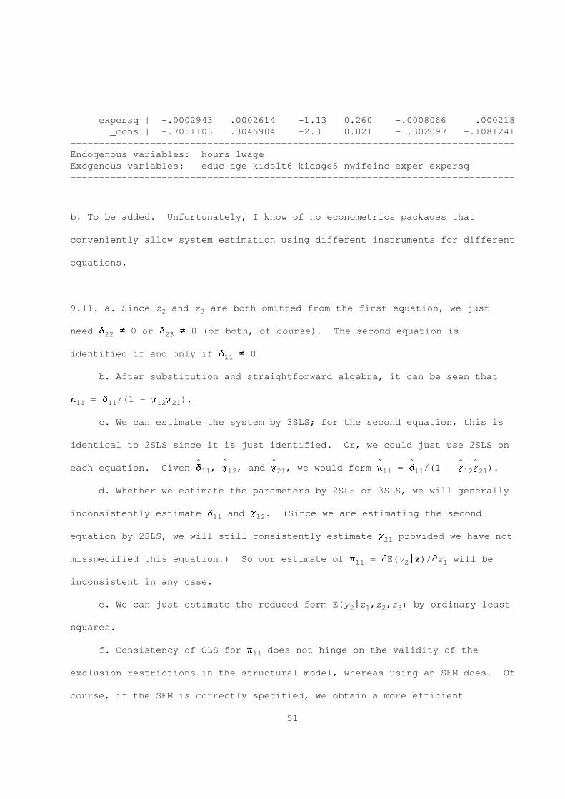
expersq | -.0002943 .0002614 -1.13 0.260 -.0008066 .000218
_cons | -.7051103 .3045904 -2.31 0.021 -1.302097 -.1081241
------------------------------------------------------------------------------
Endogenous variables: hours lwage
Exogenous variables: educ age kidslt6 kidsge6 nwifeinc exper expersq
------------------------------------------------------------------------------
b. To be added. Unfortunately, I know of no econometrics packages that
conveniently allow system estimation using different instruments for different
equations.
9.11. a. Since z and z are both omitted from the first equation, we just2 3
need d $ 0 or d $ 0 (or both, of course). The second equation is22 23
identified if and only if d $ 0.11
b. After substitution and straightforward algebra, it can be seen that
p = d /(1 - g g ).11 11 12 21
c. We can estimate the system by 3SLS; for the second equation, this is
identical to 2SLS since it is just identified. Or, we could just use 2SLS on
^ ^ ^ ^ ^ ^ ^each equation. Given d , g , and g , we would form p = d /(1 - g g ).11 12 21 11 11 12 21
d. Whether we estimate the parameters by 2SLS or 3SLS, we will generally
inconsistently estimate d and g . (Since we are estimating the second11 12
equation by 2SLS, we will still consistently estimate g provided we have not21
misspecified this equation.) So our estimate of p = dE(y |z)/dz will be11 2 1
inconsistent in any case.
e. We can just estimate the reduced form E(y |z ,z ,z ) by ordinary least2 1 2 3
squares.
f. Consistency of OLS for p does not hinge on the validity of the11
exclusion restrictions in the structural model, whereas using an SEM does. Of
course, if the SEM is correctly specified, we obtain a more efficient
51
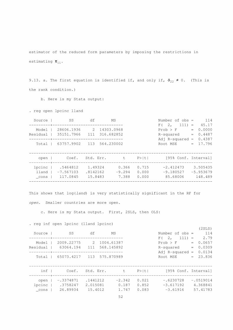
estimator of the reduced form parameters by imposing the restrictions in
estimating p .11
9.13. a. The first equation is identified if, and only if, d $ 0. (This is22
the rank condition.)
b. Here is my Stata output:
. reg open lpcinc lland
Source | SS df MS Number of obs = 114
---------+------------------------------ F( 2, 111) = 45.17
Model | 28606.1936 2 14303.0968 Prob > F = 0.0000
Residual | 35151.7966 111 316.682852 R-squared = 0.4487
---------+------------------------------ Adj R-squared = 0.4387
Total | 63757.9902 113 564.230002 Root MSE = 17.796
------------------------------------------------------------------------------
open | Coef. Std. Err. t P>|t| [95% Conf. Interval]
---------+--------------------------------------------------------------------
lpcinc | .5464812 1.49324 0.366 0.715 -2.412473 3.505435
lland | -7.567103 .8142162 -9.294 0.000 -9.180527 -5.953679
_cons | 117.0845 15.8483 7.388 0.000 85.68006 148.489
------------------------------------------------------------------------------
This shows that log(land) is very statistically significant in the RF for
open. Smaller countries are more open.
c. Here is my Stata output. First, 2SLS, then OLS:
. reg inf open lpcinc (lland lpcinc)
(2SLS)
Source | SS df MS Number of obs = 114
---------+------------------------------ F( 2, 111) = 2.79
Model | 2009.22775 2 1004.61387 Prob > F = 0.0657
Residual | 63064.194 111 568.145892 R-squared = 0.0309
---------+------------------------------ Adj R-squared = 0.0134
Total | 65073.4217 113 575.870989 Root MSE = 23.836
------------------------------------------------------------------------------
inf | Coef. Std. Err. t P>|t| [95% Conf. Interval]
---------+--------------------------------------------------------------------
open | -.3374871 .1441212 -2.342 0.021 -.6230728 -.0519014
lpcinc | .3758247 2.015081 0.187 0.852 -3.617192 4.368841
_cons | 26.89934 15.4012 1.747 0.083 -3.61916 57.41783
52
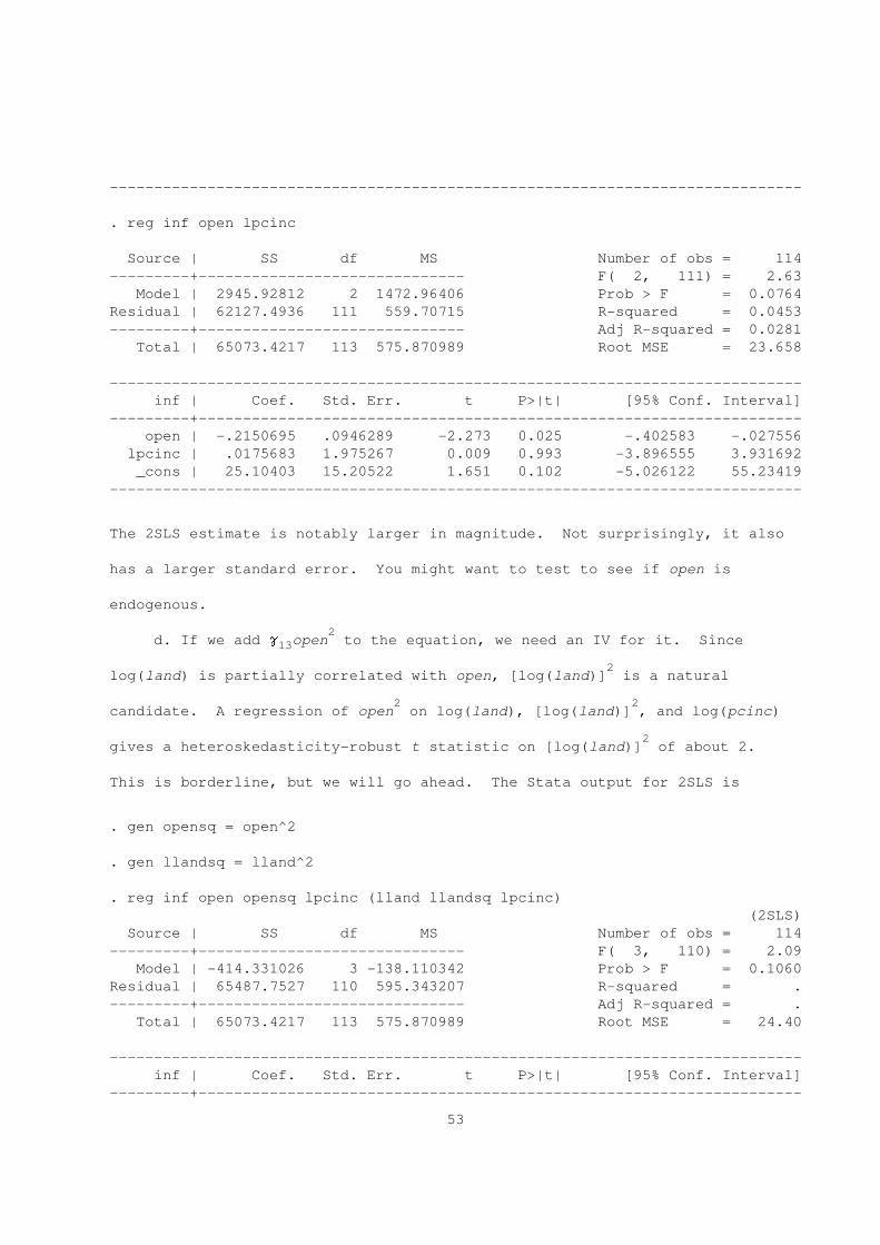
------------------------------------------------------------------------------
. reg inf open lpcinc
Source | SS df MS Number of obs = 114
---------+------------------------------ F( 2, 111) = 2.63
Model | 2945.92812 2 1472.96406 Prob > F = 0.0764
Residual | 62127.4936 111 559.70715 R-squared = 0.0453
---------+------------------------------ Adj R-squared = 0.0281
Total | 65073.4217 113 575.870989 Root MSE = 23.658
------------------------------------------------------------------------------
inf | Coef. Std. Err. t P>|t| [95% Conf. Interval]
---------+--------------------------------------------------------------------
open | -.2150695 .0946289 -2.273 0.025 -.402583 -.027556
lpcinc | .0175683 1.975267 0.009 0.993 -3.896555 3.931692
_cons | 25.10403 15.20522 1.651 0.102 -5.026122 55.23419
------------------------------------------------------------------------------
The 2SLS estimate is notably larger in magnitude. Not surprisingly, it also
has a larger standard error. You might want to test to see if open is
endogenous.
2d. If we add g open to the equation, we need an IV for it. Since13
2log(land) is partially correlated with open, [log(land)] is a natural
2 2candidate. A regression of open on log(land), [log(land)] , and log(pcinc)
2gives a heteroskedasticity-robust t statistic on [log(land)] of about 2.
This is borderline, but we will go ahead. The Stata output for 2SLS is
. gen opensq = open^2
. gen llandsq = lland^2
. reg inf open opensq lpcinc (lland llandsq lpcinc)
(2SLS)
Source | SS df MS Number of obs = 114
---------+------------------------------ F( 3, 110) = 2.09
Model | -414.331026 3 -138.110342 Prob > F = 0.1060
Residual | 65487.7527 110 595.343207 R-squared = .
---------+------------------------------ Adj R-squared = .
Total | 65073.4217 113 575.870989 Root MSE = 24.40
------------------------------------------------------------------------------
inf | Coef. Std. Err. t P>|t| [95% Conf. Interval]
---------+--------------------------------------------------------------------
53

open | -1.198637 .6205699 -1.932 0.056 -2.428461 .0311868
opensq | .0075781 .0049828 1.521 0.131 -.0022966 .0174527
lpcinc | .5066092 2.069134 0.245 0.807 -3.593929 4.607147
_cons | 43.17124 19.36141 2.230 0.028 4.801467 81.54102
------------------------------------------------------------------------------
The squared term indicates that the impact of open on inf diminishes; the
estimate would be significant at about the 6.5% level against a one-sided
alternative.
e. Here is the Stata output for implementing the method described in the
problem:
. reg open lpcinc lland
Source | SS df MS Number of obs = 114
-------------+------------------------------ F( 2, 111) = 45.17
Model | 28606.1936 2 14303.0968 Prob > F = 0.0000
Residual | 35151.7966 111 316.682852 R-squared = 0.4487
-------------+------------------------------ Adj R-squared = 0.4387
Total | 63757.9902 113 564.230002 Root MSE = 17.796
------------------------------------------------------------------------------
open | Coef. Std. Err. t P>|t| [95% Conf. Interval]
-------------+----------------------------------------------------------------
lpcinc | .5464812 1.49324 0.37 0.715 -2.412473 3.505435
lland | -7.567103 .8142162 -9.29 0.000 -9.180527 -5.953679
_cons | 117.0845 15.8483 7.39 0.000 85.68006 148.489
------------------------------------------------------------------------------
. predict openh
(option xb assumed; fitted values)
. gen openhsq = openh^2
. reg inf openh openhsq lpcinc
Source | SS df MS Number of obs = 114
-------------+------------------------------ F( 3, 110) = 2.24
Model | 3743.18411 3 1247.72804 Prob > F = 0.0879
Residual | 61330.2376 110 557.547615 R-squared = 0.0575
-------------+------------------------------ Adj R-squared = 0.0318
Total | 65073.4217 113 575.870989 Root MSE = 23.612
------------------------------------------------------------------------------
inf | Coef. Std. Err. t P>|t| [95% Conf. Interval]
-------------+----------------------------------------------------------------
54
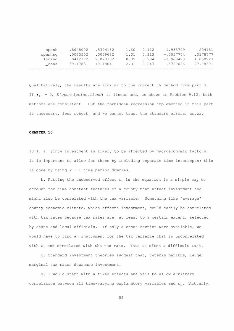
openh | -.8648092 .5394132 -1.60 0.112 -1.933799 .204181
openhsq | .0060502 .0059682 1.01 0.313 -.0057774 .0178777
lpcinc | .0412172 2.023302 0.02 0.984 -3.968493 4.050927
_cons | 39.17831 19.48041 2.01 0.047 .5727026 77.78391
------------------------------------------------------------------------------
Qualitatively, the results are similar to the correct IV method from part d.
If g = 0, E(open|lpcinc,lland) is linear and, as shown in Problem 9.12, both13
methods are consistent. But the forbidden regression implemented in this part
is uncessary, less robust, and we cannot trust the standard errors, anyway.
CHAPTER 10
10.1. a. Since investment is likely to be affected by macroeconomic factors,
it is important to allow for these by including separate time intercepts; this
is done by using T - 1 time period dummies.
b. Putting the unobserved effect c in the equation is a simple way toi
account for time-constant features of a county that affect investment and
might also be correlated with the tax variable. Something like "average"
county economic climate, which affects investment, could easily be correlated
with tax rates because tax rates are, at least to a certain extent, selected
by state and local officials. If only a cross section were available, we
would have to find an instrument for the tax variable that is uncorrelated
with c and correlated with the tax rate. This is often a difficult task.i
c. Standard investment theories suggest that, ceteris paribus, larger
marginal tax rates decrease investment.
d. I would start with a fixed effects analysis to allow arbitrary
correlation between all time-varying explanatory variables and c . (Actually,i
55

doing pooled OLS is a useful initial exercise; these results can be compared
with those from an FE analysis). Such an analysis assumes strict exogeneity
of z , tax , and disaster in the sense that these are uncorrelated withit it it
the errors u for all t and s.is
I have no strong intuition for the likely serial correlation properties
of the {u }. These might have little serial correlation because we haveit
allowed for c , in which case I would use standard fixed effects. However, iti
seems more likely that the u are positively autocorrelated, in which case Iit
might use first differencing instead. In either case, I would compute the
fully robust standard errors along with the usual ones. Remember, with first-
differencing it is easy to test whether the changes Du are seriallyit
uncorrelated.
e. If tax and disaster do not have lagged effects on investment, thenit it
the only possible violation of the strict exogeneity assumption is if future
values of these variables are correlated with u . It is safe to say thatit
this is not a worry for the disaster variable: presumably, future natural
disasters are not determined by past investment. On the other hand, state
officials might look at the levels of past investment in determining future
tax policy, especially if there is a target level of tax revenue the officials
are are trying to achieve. This could be similar to setting property tax
rates: sometimes property tax rates are set depending on recent housing
values, since a larger base means a smaller rate can achieve the same amount
of revenue. Given that we allow tax to be correlated with c , this mightit i
not be much of a problem. But it cannot be ruled out ahead of time.
----- ----- -----¨10.3. a. Let x = (x + x )/2, y = (y + y )/2, x = x - x ,i i1 i2 i i1 i2 i1 i1 i
56
-----¨ ¨ ¨x = x - x , and similarly for y and y . For T = 2 the fixed effectsi2 i2 i i1 i2
estimator can be written as
-1N N^ & * & *¨ ¨ ¨ ¨ ¨ ¨ ¨ ¨B = S (x’ x + x’ x ) S (x’ y + x’ y ) .FE i1 i1 i2 i2 i1 i1 i2 i27 8 7 8i=1 i=1
Now, by simple algebra,
x = (x - x )/2 = -Dx /2i1 i1 i2 i
x = (x - x )/2 = Dx /2i2 i2 i1 i
y = (y - y )/2 = -Dy /2i1 i1 i2 i
y = (y - y )/2 = Dy /2.i2 i2 i1 i
Therefore,
¨ ¨ ¨ ¨x’ x + x’ x = Dx’Dx /4 + Dx’Dx /4 = Dx’Dx /2i1 i1 i2 i2 i i i i i i
¨ ¨ ¨ ¨x’ y + x’ y = Dx’Dy /4 + Dx’Dy /4 = Dx’Dy /2,i1 i1 i2 i2 i i i i i i
and so
-1N N^ & * & *B = S Dx’Dx /2 S Dx’Dy /2FE i i i i7 8 7 8i=1 i=1
-1N N& * & * ^= S Dx’Dx S Dx’Dy = B .i i i i FD7 8 7 8i=1 i=1
^ ^ ^ ^¨ ¨ ¨ ¨b. Let u = y - x B and u = y - x B be the fixed effectsi1 i1 i1 FE i2 i2 i2 FE
^residuals for the two time periods for cross section observation i. Since BFE
^= B , and using the representations in (4.1’), we haveFD
^ ^ ^ ^u = -Dy /2 - (-Dx /2)B = -(Dy - Dx B )/2 _ -e /2i1 i i FD i i FD i
^ ^ ^ ^u = Dy /2 - (Dx /2)B = (Dy - Dx B )/2 _ e /2,i2 i i FD i i FD i
^ ^where e _ Dy - Dx B are the first difference residuals, i = 1,2,...,N.i i i FD
Therefore,
N N^2 ^2 ^2S (u + u ) = (1/2) S e .i1 i2 ii=1 i=1
This shows that the sum of squared residuals from the fixed effects regression
is exactly one have the sum of squared residuals from the first difference
regression. Since we know the variance estimate for fixed effects is the SSR
57
divided by N - K (when T = 2), and the variance estimate for first difference
is the SSR divided by N - K, the error variance from fixed effects is always
half the size as the error variance for first difference estimation, that is,
^2 ^2s = s /2 (contrary to what the problem asks you so show). What I wanted youu e
^ ^to show is that the variance matrix estimates of B and B are identical.FE FD
This is easy since the variance matrix estimate for fixed effects is
-1 -1 -1N N N^2& * ^2 & * ^2& *¨ ¨ ¨ ¨s S (x’ x + x’ x ) = (s /2) S Dx’Dx /2 = s S Dx’Dx ,u i1 i1 i2 i2 e i i e i i7 8 7 8 7 8i=1 i=1 i=1
which is the variance matrix estimator for first difference. Thus, the
standard errors, and in fact all other test statistics (F statistics) will be
numerically identical using the two approaches.
210.5. a. Write v v’ = c j j’ + u u’ + j (c u’) + (c u )j’. Under RE.1,i i i T T i i T i i i i T
E(u |x ,c ) = 0, which implies that E[(c u’)|x ) = 0 by interated expecations.i i i i i i
2 2Under RE.3a, E(u u’|x ,c ) = s I , which implies that E(u u’|x ) = s Ii i i i u T i i i u T
(again, by iterated expectations). Therefore,
2 2E(v v’|x ) = E(c |x )j j’ + E(u u’|x ) = h(x )j j’ + s I ,i i i i i T T i i i i T T u T
2where h(x ) _ Var(c |x ) = E(c |x ) (by RE.1b). This shows that thei i i i i
conditional variance matrix of v given x has the same covariance for all t $i i
2s, h(x ), and the same variance for all t, h(x ) + s . Therefore, while thei i u
variances and covariances depend on x in general, they do not depend on timei
separately.
-----b. The RE estimator is still consistent and rN-asymptotically normal
without assumption RE.3b, but the usual random effects variance estimator of
^B is no longer valid because E(v v’|x ) does not have the form (10.30)RE i i i
58
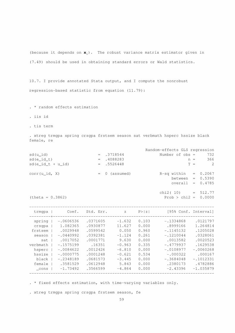
(because it depends on x ). The robust variance matrix estimator given ini
(7.49) should be used in obtaining standard errors or Wald statistics.
10.7. I provide annotated Stata output, and I compute the nonrobust
regression-based statistic from equation (11.79):
. * random effects estimation
. iis id
. tis term
. xtreg trmgpa spring crsgpa frstsem season sat verbmath hsperc hssize black
female, re
Random-effects GLS regression
sd(u_id) = .3718544 Number of obs = 732
sd(e_id_t) = .4088283 n = 366
sd(e_id_t + u_id) = .5526448 T = 2
corr(u_id, X) = 0 (assumed) R-sq within = 0.2067
between = 0.5390
overall = 0.4785
chi2( 10) = 512.77
(theta = 0.3862) Prob > chi2 = 0.0000
------------------------------------------------------------------------------
trmgpa | Coef. Std. Err. z P>|z| [95% Conf. Interval]
---------+--------------------------------------------------------------------
spring | -.0606536 .0371605 -1.632 0.103 -.1334868 .0121797
crsgpa | 1.082365 .0930877 11.627 0.000 .8999166 1.264814
frstsem | .0029948 .0599542 0.050 0.960 -.1145132 .1205028
season | -.0440992 .0392381 -1.124 0.261 -.1210044 .0328061
sat | .0017052 .0001771 9.630 0.000 .0013582 .0020523
verbmath | -.1575199 .16351 -0.963 0.335 -.4779937 .1629538
hsperc | -.0084622 .0012426 -6.810 0.000 -.0108977 -.0060268
hssize | -.0000775 .0001248 -0.621 0.534 -.000322 .000167
black | -.2348189 .0681573 -3.445 0.000 -.3684048 -.1012331
female | .3581529 .0612948 5.843 0.000 .2380173 .4782886
_cons | -1.73492 .3566599 -4.864 0.000 -2.43396 -1.035879
------------------------------------------------------------------------------
. * fixed effects estimation, with time-varying variables only.
. xtreg trmgpa spring crsgpa frstsem season, fe
59
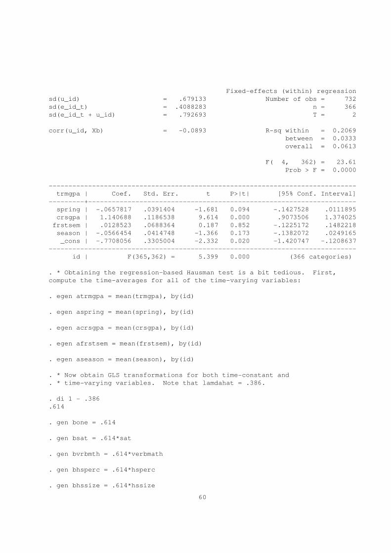
Fixed-effects (within) regression
sd(u_id) = .679133 Number of obs = 732
sd(e_id_t) = .4088283 n = 366
sd(e_id_t + u_id) = .792693 T = 2
corr(u_id, Xb) = -0.0893 R-sq within = 0.2069
between = 0.0333
overall = 0.0613
F( 4, 362) = 23.61
Prob > F = 0.0000
------------------------------------------------------------------------------
trmgpa | Coef. Std. Err. t P>|t| [95% Conf. Interval]
---------+--------------------------------------------------------------------
spring | -.0657817 .0391404 -1.681 0.094 -.1427528 .0111895
crsgpa | 1.140688 .1186538 9.614 0.000 .9073506 1.374025
frstsem | .0128523 .0688364 0.187 0.852 -.1225172 .1482218
season | -.0566454 .0414748 -1.366 0.173 -.1382072 .0249165
_cons | -.7708056 .3305004 -2.332 0.020 -1.420747 -.1208637
------------------------------------------------------------------------------
id | F(365,362) = 5.399 0.000 (366 categories)
. * Obtaining the regression-based Hausman test is a bit tedious. First,
compute the time-averages for all of the time-varying variables:
. egen atrmgpa = mean(trmgpa), by(id)
. egen aspring = mean(spring), by(id)
. egen acrsgpa = mean(crsgpa), by(id)
. egen afrstsem = mean(frstsem), by(id)
. egen aseason = mean(season), by(id)
. * Now obtain GLS transformations for both time-constant and
. * time-varying variables. Note that lamdahat = .386.
. di 1 - .386
.614
. gen bone = .614
. gen bsat = .614*sat
. gen bvrbmth = .614*verbmath
. gen bhsperc = .614*hsperc
. gen bhssize = .614*hssize
60
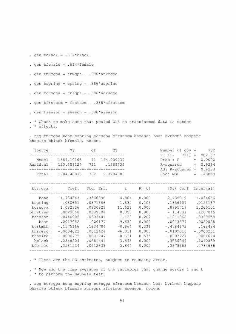
. gen bblack = .614*black
. gen bfemale = .614*female
. gen btrmgpa = trmgpa - .386*atrmgpa
. gen bspring = spring - .386*aspring
. gen bcrsgpa = crsgpa - .386*acrsgpa
. gen bfrstsem = frstsem - .386*afrstsem
. gen bseason = season - .386*aseason
. * Check to make sure that pooled OLS on transformed data is random
. * effects.
. reg btrmgpa bone bspring bcrsgpa bfrstsem bseason bsat bvrbmth bhsperc
bhssize bblack bfemale, nocons
Source | SS df MS Number of obs = 732
---------+------------------------------ F( 11, 721) = 862.67
Model | 1584.10163 11 144.009239 Prob > F = 0.0000
Residual | 120.359125 721 .1669336 R-squared = 0.9294
---------+------------------------------ Adj R-squared = 0.9283
Total | 1704.46076 732 2.3284983 Root MSE = .40858
------------------------------------------------------------------------------
btrmgpa | Coef. Std. Err. t P>|t| [95% Conf. Interval]
---------+--------------------------------------------------------------------
bone | -1.734843 .3566396 -4.864 0.000 -2.435019 -1.034666
bspring | -.060651 .0371666 -1.632 0.103 -.1336187 .0123167
bcrsgpa | 1.082336 .0930923 11.626 0.000 .8995719 1.265101
bfrstsem | .0029868 .0599604 0.050 0.960 -.114731 .1207046
bseason | -.0440905 .0392441 -1.123 0.262 -.1211368 .0329558
bsat | .0017052 .000177 9.632 0.000 .0013577 .0020528
bvrbmth | -.1575166 .1634784 -0.964 0.336 -.4784672 .163434
bhsperc | -.0084622 .0012424 -6.811 0.000 -.0109013 -.0060231
bhssize | -.0000775 .0001247 -0.621 0.535 -.0003224 .0001674
bblack | -.2348204 .0681441 -3.446 0.000 -.3686049 -.1010359
bfemale | .3581524 .0612839 5.844 0.000 .2378363 .4784686
------------------------------------------------------------------------------
. * These are the RE estimates, subject to rounding error.
. * Now add the time averages of the variables that change across i and t
. * to perform the Hausman test:
. reg btrmgpa bone bspring bcrsgpa bfrstsem bseason bsat bvrbmth bhsperc
bhssize bblack bfemale acrsgpa afrstsem aseason, nocons
61
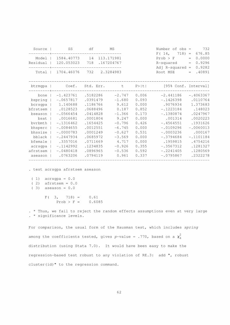
Source | SS df MS Number of obs = 732
---------+------------------------------ F( 14, 718) = 676.85
Model | 1584.40773 14 113.171981 Prob > F = 0.0000
Residual | 120.053023 718 .167204767 R-squared = 0.9296
---------+------------------------------ Adj R-squared = 0.9282
Total | 1704.46076 732 2.3284983 Root MSE = .40891
------------------------------------------------------------------------------
btrmgpa | Coef. Std. Err. t P>|t| [95% Conf. Interval]
---------+--------------------------------------------------------------------
bone | -1.423761 .5182286 -2.747 0.006 -2.441186 -.4063367
bspring | -.0657817 .0391479 -1.680 0.093 -.1426398 .0110764
bcrsgpa | 1.140688 .1186766 9.612 0.000 .9076934 1.373683
bfrstsem | .0128523 .0688496 0.187 0.852 -.1223184 .148023
bseason | -.0566454 .0414828 -1.366 0.173 -.1380874 .0247967
bsat | .0016681 .0001804 9.247 0.000 .001314 .0020223
bvrbmth | -.1316462 .1654425 -0.796 0.426 -.4564551 .1931626
bhsperc | -.0084655 .0012551 -6.745 0.000 -.0109296 -.0060013
bhssize | -.0000783 .0001249 -0.627 0.531 -.0003236 .000167
bblack | -.2447934 .0685972 -3.569 0.000 -.3794684 -.1101184
bfemale | .3357016 .0711669 4.717 0.000 .1959815 .4754216
acrsgpa | -.1142992 .1234835 -0.926 0.355 -.3567312 .1281327
afrstsem | -.0480418 .0896965 -0.536 0.592 -.2241405 .1280569
aseason | .0763206 .0794119 0.961 0.337 -.0795867 .2322278
------------------------------------------------------------------------------
. test acrsgpa afrstsem aseason
( 1) acrsgpa = 0.0
( 2) afrstsem = 0.0
( 3) aseason = 0.0
F( 3, 718) = 0.61
Prob > F = 0.6085
. * Thus, we fail to reject the random effects assumptions even at very large
. * significance levels.
For comparison, the usual form of the Hausman test, which includes spring
2among the coefficients tested, gives p-value = .770, based on a c4
distribution (using Stata 7.0). It would have been easy to make the
regression-based test robust to any violation of RE.3: add ", robust
cluster(id)" to the regression command.
62
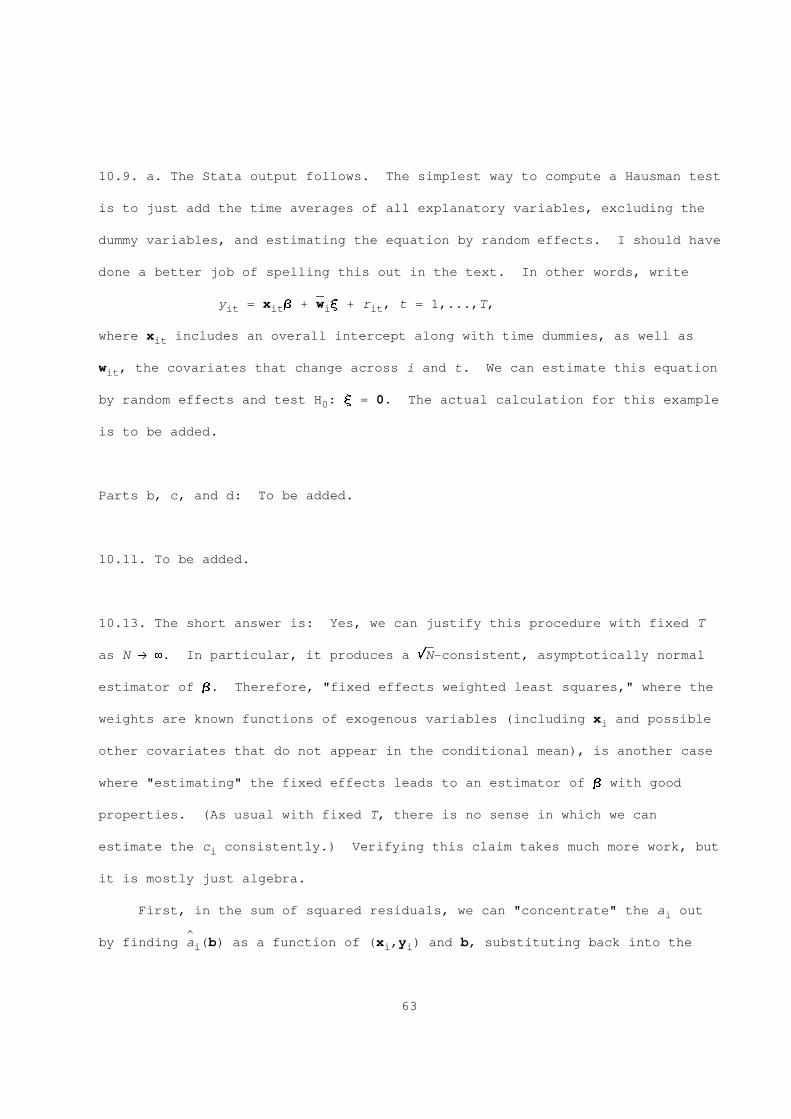
10.9. a. The Stata output follows. The simplest way to compute a Hausman test
is to just add the time averages of all explanatory variables, excluding the
dummy variables, and estimating the equation by random effects. I should have
done a better job of spelling this out in the text. In other words, write
-----y = x B + w X + r , t = 1,...,T,it it i it
where x includes an overall intercept along with time dummies, as well asit
w , the covariates that change across i and t. We can estimate this equationit
by random effects and test H : X = 0. The actual calculation for this example0
is to be added.
Parts b, c, and d: To be added.
10.11. To be added.
10.13. The short answer is: Yes, we can justify this procedure with fixed T
-----as N L 8. In particular, it produces a rN-consistent, asymptotically normal
estimator of B. Therefore, "fixed effects weighted least squares," where the
weights are known functions of exogenous variables (including x and possiblei
other covariates that do not appear in the conditional mean), is another case
where "estimating" the fixed effects leads to an estimator of B with good
properties. (As usual with fixed T, there is no sense in which we can
estimate the c consistently.) Verifying this claim takes much more work, buti
it is mostly just algebra.
First, in the sum of squared residuals, we can "concentrate" the a outi
^by finding a (b) as a function of (x ,y ) and b, substituting back into thei i i
63

sum of squared residuals, and then minimizing with respect to b only.
Straightforward algebra gives the first order conditions for each i as
T ^S (y - a - x b)/h = 0,it i it itt=1
which gives
T T^ & * & *a (b) = w S y /h - w S x /h bi i it it i it it7 8 7 8t=1 t=1
-----w -----w_ y - x b,i i
T T& * -----w & *where w _ 1/ S (1/h ) > 0 and y _ w S y /h , and a similari it i i it it7 8 7 8t=1 t=1
-----w -----w -----wdefinition holds for x . Note that y and x are simply weighted averages.i i i
-----w -----wIf h equals the same constant for all t, y and x are the usual timeit i i
averages.
^ ^Now we can plug each a (b) into the SSR to get the problem solved by B:i
N T -----w -----w 2min S S [(y - y ) - (x - x )b] /h .it i it i itK i=1t=1beR
-----wBut this is just a pooled weighted least squares regression of (y - y ) onit i
-----w ~ -----w -------------(x - x ) with weights 1/h . Equivalently, define y _ (y - y )/rh ,it i it it it i it
~ -----w ------------- ^x _ (x - x )/rh , all t = 1,...,T, i = 1,...,N. Then B can be expressedit it i it
in usual pooled OLS form:
N T -1 N T^ & ~ ~ * & ~ ~ *B = S S x’ x S S x’ y . (10.82)it it it it7 8 7 8i=1t=1 i=1t=1
-----wNote carefully how the initial y are weighted by 1/h to obtain y , butit it i
-------------where the usual 1/rh weighting shows up in the sum of squared residuals onit
the time-demeaned data (where the demeaming is a weighted average). Given
^(10.82), we can study the asymptotic (N L 8) properties of B. First, it is
T-----w -----w -----w -----w & *easy to show that y = x B + c + u , where u _ w S u /h . Subtractingi i i i i i it it7 8t=1
~ ~ ~this equation from y = x B + c + u for all t gives y = x B + u ,it it i it it it it
~ -----w ------------- ~where u _ (u - u )/rh . When we plug this in for y in (10.82) andit it i it it
divide by N in the appropriate places we get
64
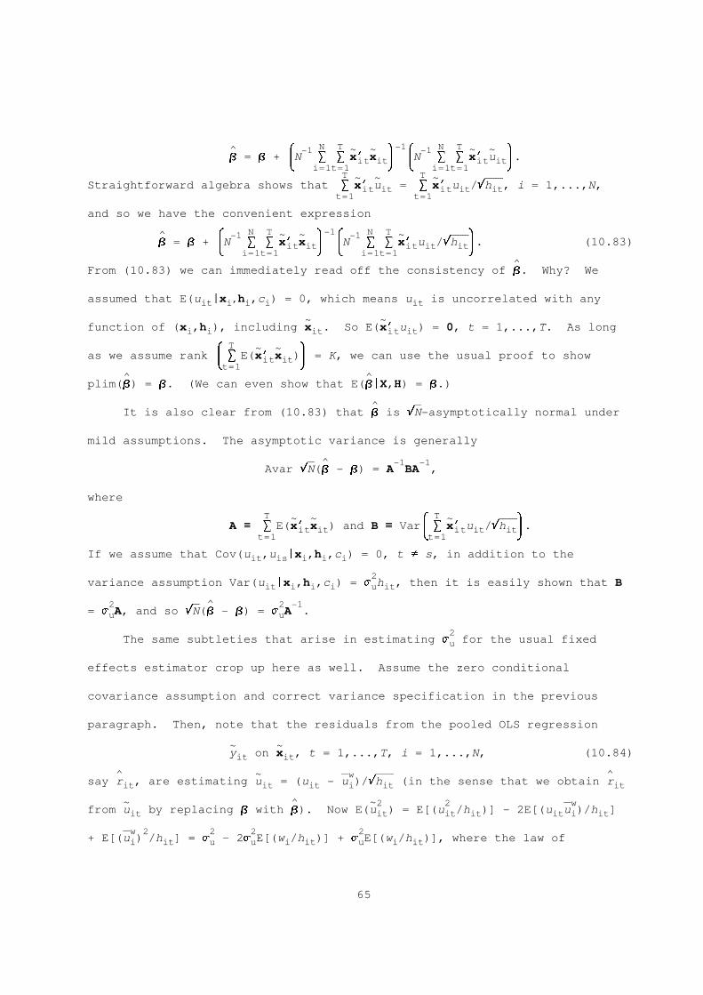
N T -1 N T^ & -1 ~ ~ * & -1 ~ ~ *B = B + N S S x’ x N S S x’ u .it it it it7 8 7 8i=1t=1 i=1t=1T T~ ~ ~ -------------
Straightforward algebra shows that S x’ u = S x’ u /rh , i = 1,...,N,it it it it itt=1 t=1
and so we have the convenient expression
N T -1 N T^ & -1 ~ ~ * & -1 ~ -------------*B = B + N S S x’ x N S S x’ u /rh . (10.83)it it it it it7 8 7 8i=1t=1 i=1t=1
^From (10.83) we can immediately read off the consistency of B. Why? We
assumed that E(u |x ,h ,c ) = 0, which means u is uncorrelated with anyit i i i it
~ ~function of (x ,h ), including x . So E(x’ u ) = 0, t = 1,...,T. As longi i it it it
T& ~ ~ *as we assume rank S E(x’ x ) = K, we can use the usual proof to showit it7 8t=1
^ ^plim(B) = B. (We can even show that E(B|X,H) = B.)
^ -----It is also clear from (10.83) that B is rN-asymptotically normal under
mild assumptions. The asymptotic variance is generally
----- ^ -1 -1Avar rN(B - B) = A BA ,
where
T T~ ~ & ~ -------------*A _ S E(x’ x ) and B _ Var S x’ u /rh .it it it it it7 8t=1 t=1
If we assume that Cov(u ,u |x ,h ,c ) = 0, t $ s, in addition to theit is i i i
2variance assumption Var(u |x ,h ,c ) = s h , then it is easily shown that Bit i i i u it
2 ----- ^ 2 -1= s A, and so rN(B - B) = s A .u u
2The same subtleties that arise in estimating s for the usual fixedu
effects estimator crop up here as well. Assume the zero conditional
covariance assumption and correct variance specification in the previous
paragraph. Then, note that the residuals from the pooled OLS regression
~ ~y on x , t = 1,...,T, i = 1,...,N, (10.84)it it
^ ~ -----w ------------- ^say r , are estimating u = (u - u )/rh (in the sense that we obtain rit it it i it it
~ ^ ~2 2 -----wfrom u by replacing B with B). Now E(u ) = E[(u /h )] - 2E[(u u )/h ]it it it it it i it
-----w 2 2 2 2+ E[(u ) /h ] = s - 2s E[(w /h )] + s E[(w /h )], where the law ofi it u u i it u i it
65
-----w 2 2iterated expectations is applied several times, and E[(u ) |x ,h ] = s w hasi i i u i
~2 2been used. Therefore, E(u ) = s [1 - E(w /h )], t = 1,...,T, and soit u i it
T ~2 2 T 2S E(u ) = s {T - E[w WS (1/h )]} = s (T - 1).it u i it ut=1t=1
This contains the usual result for the within transformation as a special
2case. A consistent estimator of s is SSR/[N(T - 1) - K], where SSR is theu
usual sum of squared residuals from (10.84), and the subtraction of K is
^optional. The estimator of Avar(B) is then
-1N T^2& ~ ~ *s S S x’ x .u it it7 8i=1t=1
If we want to allow serial correlation in the {u }, or allowit
2Var(u |x ,h ,c ) $ s h , then we can just apply the robust formula for theit i i i u it
pooled OLS regression (10.84).
CHAPTER 11
11.1. a. It is important to remember that, any time we put a variable in a
regression model (whether we are using cross section or panel data), we are
controlling for the effects of that variable on the dependent variable. The
whole point of regression analysis is that it allows the explanatory variables
to be correlated while estimating ceteris paribus effects. Thus, the
inclusion of y in the equation allows prog to be correlated withi,t-1 it
y , and also recognizes that, due to inertia, y is often stronglyi,t-1 it
related to y .i,t-1
An assumption that implies pooled OLS is consistent is
E(u |z ,x ,y ,prog ) = 0, all t,it i it i,t-1 it
66
which is implied by but is weaker than dynamic completeness. Without
additional assumptions, the pooled OLS standard errors and test statistics
need to be adjusted for heteroskedasticity and serial correlation (although
the later will not be present under dynamic completeness).
b. As we discussed in Section 7.8.2, this statement is incorrect.
Provided our interest is in E(y |z ,x ,y ,prog ), we do not care aboutit i it i,t-1 it
serial correlation in the implied errors, nor does serial correlation cause
inconsistency in the OLS estimators.
c. Such a model is the standard unobserved effects model:
y = x B + d prog + c + u , t=1,2,...,T.it it 1 it i it
We would probably assume that (x ,prog ) is strictly exogenous; the weakestit it
form of strict exogeneity is that (x ,prog ) is uncorrelated with u forit it is
all t and s. Then we could estimate the equation by fixed effects or first
differencing. If the u are serially uncorrelated, FE is preferred. Weit
could also do a GLS analysis after the fixed effects or first-differencing
transformations, but we should have a large N.
d. A model that incorporates features from parts a and c is
y = x B + d prog + r y + c + u , t = 1,...,T.it it 1 it 1 i,t-1 i it
Now, program participation can depend on unobserved city heterogeneity as well
as on lagged y (we assume that y is observed). Fixed effects and first-it i0
differencing are both inconsistent as N L 8 with fixed T.
Assuming that E(u |x ,prog ,y ,y ,...,y ) = 0, a consistentit i i i,t-1 i,t-2 i0
procedure is obtained by first differencing, to get
y = Dx B + d Dprog + r Dy + Du , t=2,...,T.it it 1 it 1 i,t-1 it
At time t and Dx , Dprog can be used as there own instruments, along withit it
y for j > 2. Either pooled 2SLS or a GMM procedure can be used. Underi,t-j
67
strict exogeneity, past and future values of x can also be used asit
instruments.
^11.3. Writing y = bx + c + u - br , the fixed effects estimator bit it i it it FE
can be written as
2N T N T& -1 ----- * & -1 ----- ----- ----- *b + N S S (x - x ) N S S (x - x )(u - u - b(r - r ) .it i it i it i it i7 8 7 8i=1t=1 i=1t=1
----- * -----* ----- *Now, x - x = (x - x ) + (r - r ). Then, because E(r |x ,c ) = 0 forit i it i it i it i i
* -----* -----all t, (x - x ) and (r - r ) are uncorrelated, and soit i it i
----- * -----* -----Var(x - x ) = Var(x - x ) + Var(r - r ), all t.it i it i it i
----- -----Similarly, under (11.30), (x - x ) and (u - u ) are uncorrelated for allit i it i
----- ----- * -----* ----- -----t. Now E[(x - x )(r - r )] = E[{(x - x ) + (r - r )}(r - r )] =it i it i it i it i it i
-----Var(r - r ). By the law of large numbers and the assumption of constantit i
variances across t,
N T T-1 ----- p ----- * -----* -----N S S (x - x ) L S Var(x - x ) = T[Var(x - x ) + Var(r - r )]it i it i it i it i
i=1t=1 t=1
and
N T-1 ----- ----- ----- p -----N S S (x - x )(u - u - b(r - r ) L -TbVar(r - r ).it i it i it i it i
i=1t=1
Therefore,
-----Var(r - r )it i^ & *
plim b = b - b ---------------------------------------------------------------------------------------------------------------------------------------------------------------FE 7 * ------* ----- 8[Var(x - x ) + Var(r - r )]it i it i
-----Var(r - r )it i& *
= b 1 - --------------------------------------------------------------------------------------------------------------------------------------------------------------- .7 * ------* ----- 8[Var(x - x ) + Var(r - r )]it i it i
11.5. a. E(v |z ,x ) = Z [E(a |z ,x ) - A] + E(u |z ,x ) = Z (A - A) + 0 = 0.i i i i i i i i i i i
Next, Var(v |z ,x ) = Z Var(a |z ,x )Z’ + Var(u |z ,x ) + Cov(a ,u |z ,x ) +i i i i i i i i i i i i i i i
Cov(u ,a |z ,x ) = Z Var(a |z ,x )Z’ + Var(u |z ,x ) because a and u arei i i i i i i i i i i i i i
uncorrelated, conditional on (z ,x ), by FE.1’ and the usual iteratedi i
68
2expectations argument. Therefore, Var(v |z ,x ) = Z *Z’ + s I under thei i i i i u T
assumptions given, which shows that the conditional variance depends on z .i
Unlike in the standard random effects model, there is conditional
heteroskedasticity.
b. If we use the usual RE analysis, we are applying FGLS to the equation
y = Z A + X B + v , where v = Z (a - A) + u . From part a, we know thati i i i i i i i
E(v |x ,z ) = 0, and so the usual RE estimator is consistent (as N L 8 fori i i
-----fixed T) and rN-asymptotically normal, provided the rank condition, Assumption
^RE.2, holds. (Remember, a feasible GLS analysis with any ) will be consistent
^provided ) converges in probability to a nonsingular matrix as N L 8. It need
^ ^not be the case that Var(v |x ,z ) = plim()), or even that Var(v ) = plim()).i i i i
From part a, we know that Var(v |x ,z ) depends on z unless we restricti i i i
almost all elements of * to be zero (all but those corresponding the the
constant in z ). Therefore, the usual random effects inference -- that is,it
based on the usual RE variance matrix estimator -- will be invalid.
c. We can easily make the RE analysis fully robust to an arbitrary
Var(v |x ,z ), as in equation (7.49). Naturally, we expand the set ofi i i
explanatory variables to (z ,x ), and we estimate A along with B.it it
11.7. When L = L/T for all t, we can rearrange (11.60) to gett
-----y = x B + x L + v , t = 1,2,...,T.it it i it
^ ^Let B (along with L) denote the pooled OLS estimator from this equation. By
standard results on partitioned regression [for example, Davidson and
^MacKinnon (1993, Section 1.4)], B can be obtained by the following two-step
procedure:
69
-----(i) Regress x on x across all t and i, and save the 1 * K vectors ofit i
^residuals, say r , t = 1,...,T, i = 1,...,N.it
^ ^ ^(ii) Regress y on r across all t and i. The OLS vector on r is B.it it it
^We want to show that B is the FE estimator. Given that the FE estimator can
----- ^be obtained by pooled OLS of y on (x - x ), it suffices to show that r =it it i it
-----x - x for all t and i. Butit i
N T -1 N T^ ----- & ----- ----- * & ----- *r = x - x S S x’x S S x’xit it i i i i it7 8 7 8i=1t=1 i=1t=1
N T N T N N T----- ----- ----- ----- ----- ----- ^ -----and S S x’x = S x’ S x = S Tx’x = S S x’x , and so r = x - x Ii it i it i i i i it it i K
i=1t=1 i=1 t=1 i=1 i=1t=1
-----= x - x . This completes the proof.it i
11.9. a. We can apply Problem 8.8.b, as we are applying pooled 2SLS to the
T& *¨ ¨time-demeaned equation: rank S E(z’ x ) = K. This clearly fails if xit it it7 8t=1
contains any time-constant explanatory variables (across all i, as usual).
T& *¨ ¨The condition rank S E(z’ z ) = L is also needed, and this rules out time-it it7 8t=1
constant instruments. But if the rank condition holds, we can always redefine
T¨ ¨z so that S E(z’ z ) has full rank.it it it
t=1
b. We can apply the results on GMM estimation in Chapter 8. In
-1¨ ¨ ¨ ¨particular, in equation (8.25), take C = E(Z’X ), W = [E(Z’Z )] , and * =i i i i
¨ ¨ ¨ ¨ ¨ " ¨E(Z’u u’Z ). A key point is that Z’u = (Q Z )’(Q u ) = Z’Q u = Z’u , wherei i i i i i T i T i i T i i i
Q is the T x T time-demeaning matrix defined in Chapter 10. Under (11.80),T
2¨E(u u’|Z ) = s I (by the usual iterated expectations argument), and so * =i i i u T
2¨ ¨ ¨ ¨E(Z’u u’Z ) = s E(Z’Z ). If we plug these choices of C, W, and * into (8.25)i i i i u i i
and simplify, we obtain
----- ^ 2 -1 -1¨ ¨ ¨ ¨ ¨ ¨Avar rN(B - B) = s {E(X’Z )[E(Z’Z )] E(Z’X )} .u i i i i i i
c. The argument is very similar to the case of the fixed effects
T 2 2 ^ ^¨ ¨ ¨estimator. First, S E(u ) = (T - 1)s , just as before. If u = y - x Bit u it it itt=1
70
are the pooled 2SLS residuals applied to the time-demeaned data, then [N(T -
N T-1 ^2 21)] S S u is a consistent estimator of s . Typically, N(T - 1) would beit u
i=1t=1
replaced by N(T - 1) - K as a degrees of freedom adjustment.
d. From Problem 5.1 (which is purely algebraic, and so applies
immediately to pooled 2SLS), the 2SLS estimator of all parameters in (11.81),
including B, can be obtained as follows: first run the regression x on d1 ,it i
^..., dN , z across all t and i, and obtain the residuals, say r ; second,i it it
^ ^ ^obtain c , ..., c , B from the pooled regression y on d1 , ..., dN , x ,1 N it i i it
^ ^ ^r . Now, by algebra of partial regression, B and the coefficient on r , sayit it
^D, from this last regression can be obtained by first partialling out the
dummy variables, d1 , ..., dN . As we know from Chapter 10, this partiallingi i
^ ^out is equivalent to time demeaning all variables. Therefore, B and D can be
^¨ ¨obtained from the pooled regression y on x , r , where we use the factit it it
^that the time average of r for each i is identically zero.it
Now consider the 2SLS estimator of B from (11.79). This is equivalent to
^¨ ¨first regressing x on z and saving the residuals, say s , and thenit it it
^¨ ¨running the OLS regression y on x , s . But, again by partial regressionit it it
^and the fact that regressing on d1 , ..., dN results in time demeaning, s =i i it
^r for all i and t. This proves that the 2SLS estimates of B from (11.79)it
and (11.81) are identical. (If some elements of x are included in z , asit it
^would usually be the case, some entries in r are identically zero for all tit
and i. But we can simply drop those without changing any other steps in the
argument.)
e. First, by writing down the first order condition for the 2SLS
^estimates from (11.81) (with dn as their own instruments, and x as the IVsi it
^ ----- ----- ^ ^for x ), it is easy to show that c = y - x B, where B is the IV estimatorit i i i
71
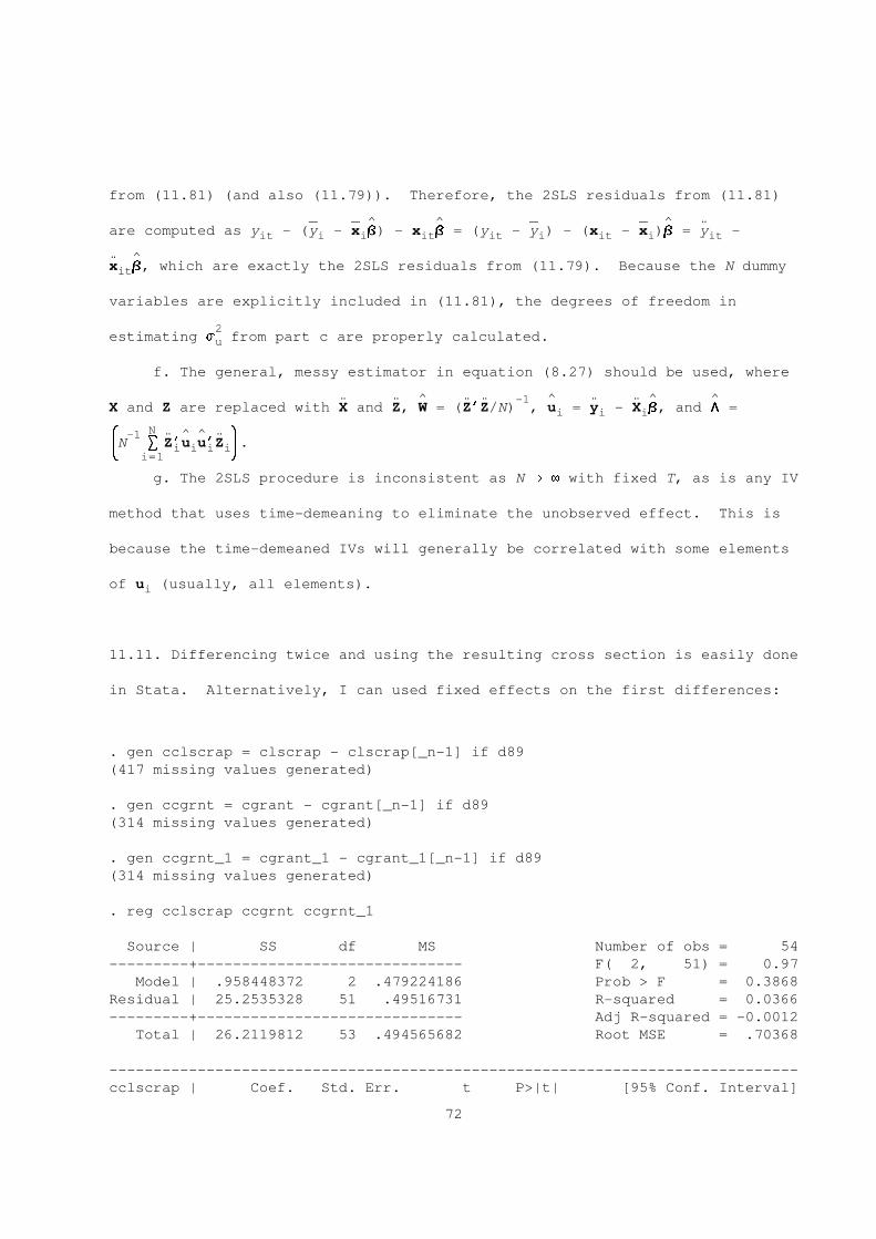
from (11.81) (and also (11.79)). Therefore, the 2SLS residuals from (11.81)
----- ----- ^ ^ ----- ----- ^ ¨are computed as y - (y - x B) - x B = (y - y ) - (x - x )B = y -it i i it it i it i it
^x B, which are exactly the 2SLS residuals from (11.79). Because the N dummyit
variables are explicitly included in (11.81), the degrees of freedom in
2estimating s from part c are properly calculated.u
f. The general, messy estimator in equation (8.27) should be used, where
^ -1 ^ ^ ^¨ ¨ ¨ ¨ ¨ ¨X and Z are replaced with X and Z, W = (Z’Z/N) , u = y - X B, and * =i i i
N& -1 ^ ^ *¨ ¨N S Z’u u’Z .i i i i7 8i=1
g. The 2SLS procedure is inconsistent as N L 8 with fixed T, as is any IV
method that uses time-demeaning to eliminate the unobserved effect. This is
because the time-demeaned IVs will generally be correlated with some elements
of u (usually, all elements).i
11.11. Differencing twice and using the resulting cross section is easily done
in Stata. Alternatively, I can used fixed effects on the first differences:
. gen cclscrap = clscrap - clscrap[_n-1] if d89
(417 missing values generated)
. gen ccgrnt = cgrant - cgrant[_n-1] if d89
(314 missing values generated)
. gen ccgrnt_1 = cgrant_1 - cgrant_1[_n-1] if d89
(314 missing values generated)
. reg cclscrap ccgrnt ccgrnt_1
Source | SS df MS Number of obs = 54
---------+------------------------------ F( 2, 51) = 0.97
Model | .958448372 2 .479224186 Prob > F = 0.3868
Residual | 25.2535328 51 .49516731 R-squared = 0.0366
---------+------------------------------ Adj R-squared = -0.0012
Total | 26.2119812 53 .494565682 Root MSE = .70368
------------------------------------------------------------------------------
cclscrap | Coef. Std. Err. t P>|t| [95% Conf. Interval]
72
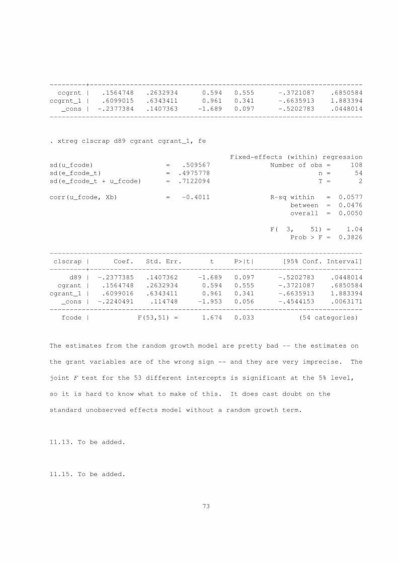
---------+--------------------------------------------------------------------
ccgrnt | .1564748 .2632934 0.594 0.555 -.3721087 .6850584
ccgrnt_1 | .6099015 .6343411 0.961 0.341 -.6635913 1.883394
_cons | -.2377384 .1407363 -1.689 0.097 -.5202783 .0448014
------------------------------------------------------------------------------
. xtreg clscrap d89 cgrant cgrant_1, fe
Fixed-effects (within) regression
sd(u_fcode) = .509567 Number of obs = 108
sd(e_fcode_t) = .4975778 n = 54
sd(e_fcode_t + u_fcode) = .7122094 T = 2
corr(u_fcode, Xb) = -0.4011 R-sq within = 0.0577
between = 0.0476
overall = 0.0050
F( 3, 51) = 1.04
Prob > F = 0.3826
------------------------------------------------------------------------------
clscrap | Coef. Std. Err. t P>|t| [95% Conf. Interval]
---------+--------------------------------------------------------------------
d89 | -.2377385 .1407362 -1.689 0.097 -.5202783 .0448014
cgrant | .1564748 .2632934 0.594 0.555 -.3721087 .6850584
cgrant_1 | .6099016 .6343411 0.961 0.341 -.6635913 1.883394
_cons | -.2240491 .114748 -1.953 0.056 -.4544153 .0063171
------------------------------------------------------------------------------
fcode | F(53,51) = 1.674 0.033 (54 categories)
The estimates from the random growth model are pretty bad -- the estimates on
the grant variables are of the wrong sign -- and they are very imprecise. The
joint F test for the 53 different intercepts is significant at the 5% level,
so it is hard to know what to make of this. It does cast doubt on the
standard unobserved effects model without a random growth term.
11.13. To be added.
11.15. To be added.
73

----- ^11.17. To obtain (11.55), we use (11.54) and the representation rN(B - B) =FE
-1 -1/2 N ¨A (N S X’u ) + o (1). Simple algebra and standard properties of O (1)i i p pi=1
and o (1) givep
N----- ^ -1/2 -1rN(A - A) = N S [(Z’Z ) Z’(y - X B) - A]i i i i ii=1
N& -1 -1 * ----- ^- N S (Z’Z ) Z’X rN(B - B)i i i i FE7 8i=1
N N-1/2 -1 -1/2 ¨= N S (s - A) - CA N S X’u + o (1)i i i pi=1 i=1
-1 -1where C _ E[(Z’Z ) Z’X ] and s _ (Z’Z ) Z’(y - X B). By definition, E(s )i i i i i i i i i i i
= A. By combining terms in the sum we have
N----- ^ -1/2 -1¨rN(A - A) = N S [(s - A) - CA X’u ] + o (1),i i i pi=1
which implies by the central limit theorem and the asymptotic equivalence
----- ^lemma that rN(A - A) is asymptotically normal with zero mean and variance
-1¨E(r r’), where r _ (s - A) - CA X’u . If we replace A, C, A, and B withi i i i i i
^their consistent estimators, we get exactly (11.55), sincethe u are the FEi
residuals.
74
CHAPTER 12
12.1. Take the conditional expectation of equation (12.4) with respect to x,
and use E(u|x) = 0:
2 2E{[y - m(x,Q)] |x] = E(u |x) + 2[m(x,Q ) - m(x,Q)]E(u|x)o
2+ E{[m(x,Q ) - m(x,Q)] |x}o
2 2= E(u |x) + 0 + [m(x,Q ) - m(x,Q)]o
2 2= E(u |x) + [m(x,Q ) - m(x,Q)] .o
Now, the first term does not depend on Q, and the second term is clearly
minimized at Q = Q (although not uniquely, in general).o
^ ^12.3. a. The approximate elasticity is dlog[E(y|z)]/dlog(z ) = d[q +1 1
^ ^ ^q log(z ) + q z ]/dlog(z ) = q .2 1 3 2 1 2
^ ^b. This is approximated by 100Wdlog[E(y|z)]/dz = 100Wq .2 3
^ ^ ^ ^ ^ 2 ^ ^c. Since dE(y|z)/dz = exp[q + q log(z ) + q z + q z ]W(q + 2q z ),2 1 2 1 3 2 4 2 3 4 2
* ^ ^the turning point is z = q /(-2q ).2 3 4
d. Since D m(x,Q) = exp(x Q + x Q )x, the gradient of the mean functionq 1 1 2 2
~ ~ ~ ~evaluated under the null is D m = exp(x Q )x _ m x , where Q is theq i i1 1 i i i 1
restricted NLS estimator. From (12.72), we can compute the usual LM
2 ~ ~ ~statistic as NR from the regression u on m x , m x , i = 1,...,N, whereu i i i1 i i2
~ ~ ~ ~u = y - m . For the robust test, we first regress m x on m x andi i i i i2 i i1
~obtain the 1 * K residuals, r . Then we compute the statistic as in2 i
regression (12.75).
12.5. We need the gradient of m(x ,Q) evaluated under the null hypothesis.i
2 3 2By the chain rule, D m(x,Q) = g[xB + d (xB) + d (xB) ]W[x + 2d (xB) +b 1 2 1
75
2 2 3 2 3 ~3d (xB) ], D m(x,Q) = g[xB + d (xB) + d (xB) ]W[(xB) ,(xB) ]. Let B denote2 d 1 2
~ ~the NLS estimator with d = d = 0 imposed. Then D m(x ,Q) = g(x B)x and1 2 b i i i
~ ~ ~ 2 ~ 3D m(x ,Q) = g(x B)[(x B) ,(x B) ]. Therefore, the usual LM statistic can bed i i i i
2 ~ ~ ~ ~ 2 ~ ~ 3obtained as NR from the regression u on g x , g W(x B) , g W(x B) , whereu i i i i i i i
~ ~g _ g(x B). If G(W) is the identity function, g(W) _ 1, and we get RESET.i i
12.7. a. For each i and g, define u _ y - m(x ,Q ), so that E(u |x ) =ig ig ig o ig i
0, g = 1,...,G. Further, let u be the G * 1 vector containing the u .i ig
^Then E(u u’|x ) = E(u u’) = ) . Let u be the vector of nonlinear leasti i i i i o i
squares residuals. That is, do NLS for each g, and collect the residuals.
Then, by standard arguments, a consistent estimator of ) iso
N^ -1 ^ ^^ ^) _ N S u u’i ii=1
^because each NLS estimator, Q is consistent for Q as N L 8.g og
b. This part involves several steps, and I will sketch how each one
goes. First, let G be the vector of distinct elements of ) -- the nuisance
parameters in the context of two-step M-estimation. Then, the score for
observation i is
-1s(w ,Q;G) = -D m(x ,Q)’) u (Q)i q i i
where, hopefully, the notation is clear. With this definition, we can verify
condition (12.37), even though the actual derivatives are complicated. Each
element of s(w ,Q;G) is a linear combination of u (Q). So D s (w ,Q ;G) is ai i g j i o
linear combination of u (Q ) _ u , where the linear combination is a functioni o i
of (x ,Q ,G). Since E(u |x ) = 0, E[D s (w ,Q ;G)|x ] = 0, and so itsi o i i g j i o i
unconditional expectation is zero, too. This shows that we do not have to
adjust for the first-stage estimation of ) . Alternatively, one can verifyo
the hint directly, which has the same consequence.
76
Next, we derive B _ E[s (Q ;G )s (Q ;G )’]:o i o o i o o
-1 -1E[s (Q ;G )s (Q ;G )’] = E[D m (Q )’) u u’) D m (Q )]i o o i o o q i o o i i o q i o
-1 -1= E{E[D m (Q )’) u u’) D m (Q )|x ]}q i o o i i o q i o i
-1 -1= E[D m (Q )’) E(u u’|x )) D m (Q )]q i o o i i i o q i o
-1 -1 -1= E[D m (Q )’) ) ) D m (Q )] = E[D m (Q )’) D m (Q )].q i o o o o q i o q i o o q i o
Next, we have to derive A _ E[H (Q ;G )], and show that B = A . Theo i o o o o
Hessian itself is complicated, but its expected value is not. The Jacobian
of s (Q;G) with respect to Q can be writteni
-1H (Q;G) = D m(x ,Q)’) D m(x ,Q) + [I t u (Q)’]F(x ,Q;G),i q i q i P i i
where F(x ,Q;G) is a GP * P matrix, where P is the total number ofi
-1parameters, that involves Jacobians of the rows of ) D m (Q) with respect toq i
Q. The key is that F(x ,Q;G) depends on x , not on y . So,i i i
-1E[H (Q ;G )|x ] = D m (Q )’) D m (Q ) + [I t E(u |x )’]F(x ,Q ;G )i o o i q i o o q i o P i i i o o
-1= D m (Q )’) D m (Q ).q i o o q i o
-1Now iterated expectations gives A = E[D m (Q )’) D m (Q )]. So, we haveo q i o o q i o
----- ^verified (12.37) and that A = B . Therefore, from Theorem 12.3, Avar rN(Q -o o
-1 -1 -1Q ) = A = {E[D m (Q )’) D m (Q )]} .o o q i o o q i o
c. As usual, we replace expectations with sample averages and unknown
^ ^parameters, and divide the result by N to get Avar(Q):
N -1^ ^ & -1 ^ ^-1 ^ *Avar(Q) = N S D m (Q)’) D m (Q) /Nq i q i7 8i=1
N -1& ^ ^-1 ^ *= S D m (Q)’) D m (Q) .q i q i7 8i=1
^The estimate ) can be based on the multivariate NLS residuals or can be
updated after the nonlinear SUR estimates have been obtained.
d. First, note that D m (Q ) is a block-diagonal matrix with blocksq i o
D m (Q ), a 1 * P matrix. (I implicityly assumed that there are noq ig og gg
cross-equation restrictions imposed in the nonlinear SUR estimation.) If )o
77
is block-diagonal, so is its inverse. Standard matrix multiplication shows
that
( )-2 o o2s D m ’D m 0 W W W 0 2o1 q i1 q i11 12 2
-1 0D m (Q )’) D m (Q ) = 2 2.q i o o q i o W2 W 2W -2 o o2 20 W W W 0 s D m ’D moG q iG q iGG G9 0----- ^
Taking expectations and inverting the result shows that Avar rN(Q - Q ) =g og
2 o o -1s [E(D m ’D m )] , g = 1,...,G. (Note also that the nonlinear SURog q ig q igg g
estimators are asymptotically uncorrelated across equations.) These
asymptotic variances are easily seen to be the same as those for nonlinear
least squares on each equation; see p. 360.
e. I cannot see a nonlinear analogue of Theorem 7.7. The first hint
given in Problem 7.5 does not extend readily to nonlinear models, even when
the same regressors appear in each equation. The key is that X is replacedi
with D m(x ,Q ). While this G * P matrix has a block-diagonal form, asq i o
described in part d, the blocks are not the same even when the same
regressors appear in each equation. In the linear case, D m (x ,Q ) = xq g i og ig
for all g. But, unless Q is the same in all equations -- a veryog
restrictive assumption -- D m (x ,Q ) varies across g. For example, ifq g i ogg
m (x ,Q ) = exp(x Q ) then D m (x ,Q ) = exp(x Q )x , and the gradientsg i og i og q g i og i og ig
differ across g.
12.9. a. We cannot say anything in general about Med(y|x), since Med(y|x) =
m(x,B ) + Med(u|x), and Med(u|x) could be a general function of x.o
b. If u and x are independent, then E(u|x) and Med(u|x) are both
constants, say a and d. Then E(y|x) - Med(y|x) = a - d, which does not
78
depend on x.
c. When u and x are independent, the partial effects of x on thej
conditional mean and conditional median are the same, and there is no
ambiguity about what is "the effect of x on y," at least when only the meanj
and median are in the running. Then, we could interpret large differences
between LAD and NLS as perhaps indicating an outlier problem. But it could
just be that u and x are not independent.
12.11. a. For consistency of the MNLS estimator, we need -- in addition to
the regularity conditions, which I will ignore -- the identification
condition. That is, B must uniquely minimize E[q(w ,B)] = E{[y -o i i
m(x ,B)]’[y - m(x ,B)]} = E({u + [m(x ,B ) - m(x ,B)]}’{u + [m(x ,B ) -i i i i i o i i i o
m(x ,B)]}) = E(u’u ) + 2E{[m(x ,B ) - m(x ,B)]’u } + E{[m(x ,B ) -i i i i o i i i o
m(x ,B)]’[m(x ,B ) - m(x ,B)]} = E(u u’) + E{[m(x ,B ) - m(x ,B)]’[m(x ,B ) -i i o i i i i o i i o
m(x ,B)]} because E(u |x ) = 0. Therefore, the identification assumption isi i i
that
E{[m(x ,B ) - m(x ,B)]’[m(x ,B ) - m(x ,B)]} > 0, B $ B .i o i i o i o
In a linear model, where m(x ,B) = X B for X a G * K matrix, the conditioni i i
is
(B - B)’E(X’X )(B - B) > 0, B $ B ,o i i o o
and this holds provided E(X’X ) is positive definite.i i
Provided m(x,W) is twice continuously differentiable, there are no
problems in applying Theorem 12.3. Generally, B = E[D m (B )’u u’D m (B )]o q i o i i q i o
and A = E[D m (B )’D m (B )]. These can be consistently estimated in theo q i o q i o
obvious way after obtain the MNLS estimators.
b. We can apply the results on two-step M-estimation. The key is that,
79
underl general regularity conditions,
N-1 ^ -1N S [y - m(x ,B)]’[W (D)] [y - m(x ,B)]/2,i i i i i
i=1
converges uniformly in probability to
-1E{[y - m(x ,B)]’[W(x ,D )] [y - m(x ,B)]}/2,i i i o i i
which is just to say that the usual consistency proof can be used provided we
verify identification. But we can use an argument very similar to the
unweighted case to show
-1 -1E{[y - m(x ,B)]’[W(x ,D )] [y - m(x ,B)]} = E{u’[W (D )] u }i i i o i i i i o i
-1+ E{[m(x ,B ) - m(x ,B)]’[W (D )] [m(x ,B ) - m(x ,B)]},i o i i o i o i
where E(u |x ) = 0 is used to show the cross-product term, 2E{[m(x ,B ) -i i i o
-1m(x ,B)]’[W (D )] u }, is zero (by iterated expectations, as always). Asi i o i
before, the first term does not depend on B and the second term is minimized
at B ; we would have to assume it is uniquely minimized.o
To get the asymptotic variance, we proceed as in Problem 12.7. First,
it can be shown that condition (12.37) holds. In particular, we can write
D s (B ;D ) = (I t u )’G(x ,B ;D ) for some function G(x ,B ;D ). Itd i o o P i i o o i o o
follows easily that E[D s (B ;D )|x ] = 0, which implies (12.37). This meansd i o o i
that, under E(y |x ) = m(x ,B ), we can ignore preliminary estimation of Di i i o o
-----provided we have a rN-consistent estimator.
To obtain the asymptotic variance when the conditional variance matrix
is correctly specified, that is, when Var(y |x ) = Var(u |x ) = W(x ,D ), wei i i i i o
can use an argument very similar to the nonlinear SUR case in Problem 12.7:
-1 -1E[s (B ;D )s (B ;D )’] = E[D m (B )’[W (D )] u u’[W (D )] D m (B )]i o o i o o b i o i o i i i o b i o
-1 -1= E{E[D m (B )’[W (D )] u u’[W (D )] D m (B )|x ]}b i o i o i i i o b i o i
-1 -1= E[D m (B )’[W (D )] E(u u’|x )[W (D )] D m (B )]b i o i o i i i i o b i o
-1= E{D m (B )’[W (D )] ]D m (B )}.b i o i o b i o
80
Now, the Hessian (with respect to B), evaluated at (B ,D ), can be written aso o
-1H (B ;D ) = D m(x ,B )’[W (D )] D m(x ,B ) + (I t u )’]F(x ,B ;D ),i o o b i o i o b i o P i i o o
for some complicated function F(x ,B ;D ) that depends only on x . Takingi o o i
expectations gives
-1A _ E[H (B ;D )] = E{D m(x ,B )’[W (D )] D m(x ,B )} = B .o i o o b i o i o b i o o
----- ^ -1Therefore, from the usual results on M-estimation, Avar rN(B - B ) = A , ando o
a consistent estimator of A iso
N^ -1 ^ ^ -1 ^A = N S D m(x ,B)’[W (D)] D m(x ,B).b i i b i
i=1
c. The consistency argument in part b did not use the fact that W(x,D)
is correctly specified for Var(y|x). Exactly the same derivation goes
through. But, of course, the asymptotic variance is affected because A $o
B , and the expression for B no longer holds. The estimator of A in part bo o o
still works, of course. To consistently estimate B we useo
N^ -1 ^ ^ -1^ ^ ^ -1 ^B = N S D m(x ,B)’[W (D)] u u’[W (D)] D m(x ,B).b i i i i i b i
i=1
----- ^ ^-1^^-1Now, we estimate Avar rN(B - B ) in the usual way: A BA .o
CHAPTER 13
13.1. No. We know that Q solveso
max E[log f(y |x ;Q)],i i
Qe$
where the expectation is over the joint distribution of (x ,y ). Therefore,i i
because exp(W) is an increasing function, Q also maximizes exp{E[logo
f(y |x ;Q)]} over $. The problem is that the expectation and the exponentiali i
function cannot be interchanged: E[f(y |x ;Q)] $ exp{E[log f(y |x ;Q)]}. Ini i i i
fact, Jensen’s inequality tells us that E[f(y |x ;Q)] > exp{E[logi i
81
f(y |x ;Q)]}.i i
13.3. Parts a and b essentially appear in Section 15.4.
g -113.5. a. Since s (F ) = [G(Q )’] s (Q ),i o o i o
g g -1 -1E[s (F )s (F )’|x ] = E{[G(Q )’] s (Q )s (Q )’[G(Q )] |x }i o i o i o i o i o o i
-1 -1= [G(Q )’] E[s (Q )s (Q )’|x ][G(Q )]o i o i o i o
-1 -1= [G(Q )’] A (Q )[G(Q )] .o i o o
~ ~b. In part b, we just replace Q with Q and F with F:o o
~g ~ -1 ~ ~ -1 ~ -1~ ~-1A = [G(Q)’] A (Q)[G(Q)] _ G’ A G .i i i
c. The expected Hessian form of the statistic is given in the second
~g ~gpart of equation (13.36), but where it is based initial on s and A :i i
N N -1 N& ~g*’& ~g* & ~g*LM = S s S A S sg i i i7 8 7 8 7 8i=1 i=1 i=1
N N -1 N& ~ -1~ *’& ~ -1~ ~-1* & ~ -1~ *= S G’ s S G’ A G S G’ si i i7 8 7 8 7 8i=1 i=1 i=1
N ’ N -1 N& ~ * ~-1~& ~ * ~ ~ -1& ~ *= S s G G S A G’G’ S si i i7 8 7 8 7 8i=1 i=1 i=1
N N -1 N& ~ *’& ~ * & ~ *= S s S A S s = LM.i i i7 8 7 8 7 8i=1 i=1 i=1
13.7. a. The joint density is simply g(y |y ,x;Q )Wh(y |x;Q ). The log-1 2 o 2 o
likelihood for observation i is
l (Q) _ log g(y |y ,x ;Q) + log h(y |x ;Q),i i1 i2 i i2 i
and we would use this in a standard MLE analysis (conditional on x ).i
b. First, we know that, for all (y ,x ), Q maximizes E[l (Q)|y ,x ].i2 i o i1 i2 i
Since r is a function of (y ,x ),i2 i2 i
E[r l (Q)|y ,x ] = r E[l (Q)|y ,x ];i2 i1 i2 i i2 i1 i2 i
since r > 1, Q maximizes E[r l (Q)|y ,x ] for all (y ,x ), andi2 o i2 i1 i2 i i2 i
therefore Q maximizes E[r l (Q)]. Similary, Q maximizes E[l (Q)], ando i2 i1 o i2
82
so it follows that Q maximizes r l (Q) + l (Q). For identification, weo i2 i1 i2
have to assume or verify uniqueness.
c. The score is
s (Q) = r s (Q) + s (Q),i i2 i1 i2
where s (Q) _ D l (Q)’ and s (Q) _ D l (Q)’. Therefore,i1 q i1 i2 q i2
E[s (Q )s (Q )’] = E[r s (Q )s (Q )’] + E[s (Q )s (Q )’]i o i o i2 i1 o i1 o i2 o i2 o
+ E[r s (Q )s (Q )’] + E[r s (Q )s (Q )’].i2 i1 o i2 o i2 i2 o i1 o
Now by the usual conditional MLE theory, E[s (Q )|y ,x ] = 0 and, since ri1 o i2 i i2
and s (Q) are functions of (y ,x ), it follows thati2 i2 i
E[r s (Q )s (Q )’|y ,x ] = 0, and so its transpose also has zeroi2 i1 o i2 o i2 i
conditional expectation. As usual, this implies zero unconditional
expectation. We have shown
E[s (Q )s (Q )’] = E[r s (Q )s (Q )’] + E[s (Q )s (Q )’].i o i o i2 i1 o i1 o i2 o i2 o
Now, by the unconditional information matrix equality for the density
h(y |x;Q), E[s (Q )s (Q )’] = -E[H (Q )], where H (Q) = D s (Q).2 i2 o i2 o i2 o i2 q i2
Further, byt the conditional IM equality for the density g(y |y ,x;Q),1 2
E[s (Q )s (Q )’|y ,x ] = -E[H (Q )|y ,x ], (13.70)i1 o i1 o i2 i i1 o i2 i
where H (Q) = D s (Q). Since r is a function of (y ,x ), we can put ri1 q i1 i2 i2 i i2
inside both expectations in (13.70). Then, by iterated expectatins,
E[r s (Q )s (Q )’] = -E[r H (Q )].i2 i1 o i1 o i2 i1 o
Combining all the pieces, we have shown that
E[s (Q )s (Q )’] = -E[r H (Q )] - E[H (Q )]i o i o i2 i1 o i2 o
= -{E[r D s (Q) + D s (Q)]i2 q i1 q i2
2= -E[D l (Q)] _ -E[H (Q)].q i i
So we have verified that an unconditional IM equality holds, which means we
----- ^ -1can estimate the asymptotic variance of rN(Q - Q ) by {-E[H (Q)]} .o i
83
----- ^d. From part c, one consistent estimator of rN(Q - Q ) iso
N-1 ^ ^N S (r H + H ),i2 i1 i2
i=1
where the notation should be obvious. But, as we discussed in Chapters 12
and 13, this estimator need not be positive definite. Instead, we can break
the problem into needed consistent estimators of -E[r H (Q )] andi2 i1 o
-E[H (Q )], for which we can use iterated expectations. Since, byi2 o
N-1 ^definition, A (Q ) _ -E[H (Q )|x ], N S A is consistent for -E[H (Q )]i2 o i2 o i i2 i2 o
i=1
by the usual iterated expectations argument. Similarly, since A (Q ) _i1 o
-E[H (Q )|y ,x ], and r is a function of (y ,x ), it follows thati1 o i2 i i2 i2 i
E[r A (Q )] = -E[r H (Q )]. This implies that, under general regularityi2 i1 o i2 i1 o
N-1 ^conditions, N S r A consistently estimates -E[r H (Q )]. Thisi2 i1 i2 i1 o
i=1
completes what we needed to show. Interestingly, even though we do not have
a true conditional maximum likelihood problem, we can still used the
conditional expectations of the hessians -- but conditioned on different sets
of variables, (y ,x ) in one case, and x in the other -- to consistentlyi2 i i
estimate the asymptotic variance of the partial MLE.
e. Bonus Question: Show that if we were able to use the entire random
sample, the result conditional MLE would be more efficient than the partial
MLE based on the selected sample.
Answer: We use a basic fact about positive definite matrices: if A and
B are P * P positive definite matrices, then A - B is p.s.d. if and only if
-1 -1B - A is positive definite. Now, as we showed in part d, the asymptotic
-1variance of the partial MLE is {E[r A (Q ) + A (Q )]} . If we could usei2 i1 o i2 o
the entire random sample for both terms, the asymptotic variance would be
-1 -1{E[A (Q ) + A (Q )]} . But {E[r A (Q ) + A (Q )]} - {E[A (Q ) +i1 o i2 o i2 i1 o i2 o i1 o
-1A (Q )]} is p.s.d. because E[A (Q ) + A (Q )] - E[r A (Q ) + A (Q )]i2 o i1 o i2 o i2 i1 o i2 o
84
= E[(1 - r )A (Q )] is p.s.d. (since A (Q ) is p.s.d. and 1 - r > 0.i2 i1 o i1 o i2
13.9. To be added.
13.11. To be added.
CHAPTER 14
14.1. a. The simplest way to estimate (14.35) is by 2SLS, using instruments
(x ,x ). Nonlinear functions of these can be added to the instrument list1 2
2 2-- these would generally improve efficiency if g $ 1. If E(u |x) = s ,2 2 2
2SLS using the given list of instruments is the efficient, single equation
GMM estimator. Otherwise, the optimal weighting matrix that allows
heteroskedasticity of unknown form should be used. Finally, one could try
to use the optimal instruments derived in section 14.5.3. Even under
homoskedasticity, these are difficult, if not impossible, to find
analytically if g $ 1.2
b. No. If g = 0, the parameter g does not appear in the model. Of1 2
course, if we knew g = 0, we would consistently estimate D by OLS.1 1
c. We can see this by obtaining E(y |x):1
g2E(y |x) = x D + g E(y |x) + E(u |x)1 1 1 1 2 1
g2= x D + g E(y |x).1 1 1 2
g g2 2Now, when g $ 1, E(y |x) $ [E(y |x)] , so we cannot write2 2 2
g2E(y |x) = x D + g (xD ) ;1 1 1 1 2
in fact, we cannot find E(y |x) without more assumptions. While the1
regression y on x consistently estimates D , the two-step NLS estimator of2 2 2
85
g^ 2y on x , (x D ) will not be consistent for D and g . (This is ani1 i1 i 2 1 2
example of a "forbidden regression.") When g = 1, the plug-in method works:2
it is just the usual 2SLS estimator.
*14.3. Let Z be the G * G matrix of optimal instruments in (14.63), wherei
we suppress its dependence on x . Let Z be a G * L matrix that is ai i
function of x and let % be the probability limit of the weighting matrix.i o
Then the asymptotic variance of the GMM estimator has the form (14.10) with
G = E[Z’R (x )]. So, in (14.54), take A _ G’% G and s(w ) _o i o i o o o i
*G’% Z’r(w ,Q ). The optimal score function is s (w ) _o o i i o i
-1R (x )’) (x ) r(w ,Q ). Now we can verify (14.57) with r = 1:o i o i i o
* -1E[s(w )s (w )’] = G’% E[Z’r(w ,Q )r(w ,Q )’) (x ) R (x )]i i o o i i o i o o i o i
-1= G’% E[Z’E{r(w ,Q )r(w ,Q )’|x }) (x ) R (x )]o o i i o i o i o i o i
-1= G’% E[Z’) (x )) (x ) R (x )] = G’% G = A.o o i o i o i o i o o o
14.5. We can write the unrestricted linear projection as
y = p + x P + v , t = 1,2,3,it t0 i t it
where P is 1 + 3K * 1, and then P is the 3 + 9K * 1 vector obtained byt
stacking the P . Let Q = (j,L’,L’,L’,B’)’. With the restrictions imposed ont 1 2 3
the P we havet
p = j, t = 1,2,3, P = [(L + B)’,L’,L’]’,t0 1 1 2 3
P = [L’,(L + B)’,L’]’, P = [L’,L’,(L + B)’]’.2 1 2 3 3 1 2 3
Therefore, we can write P = HQ for the (3 + 9K) * (1 + 4K) matrix H defined
by
86
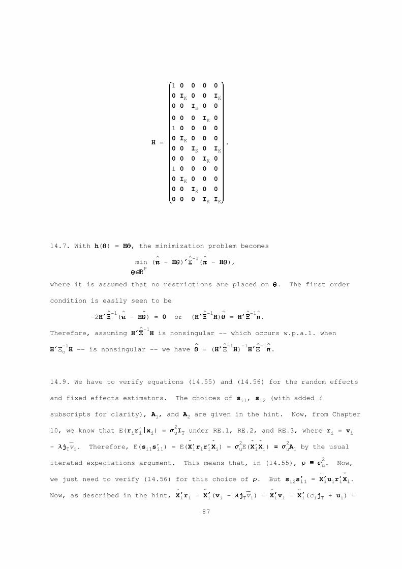
&1 0 0 0 0 *2 20 I 0 0 IK K2 20 0 I 0 0K2 2
20 0 0 I 0 2K
2 21 0 0 0 02 20 I 0 0 0KH = 2 2.0 0 I 0 I2 K K2
20 0 0 I 0 2K
2 21 0 0 0 02 20 I 0 0 0K2 20 0 I 0 02 K 2
70 0 0 I I 8K K
14.7. With h(Q) = HQ, the minimization problem becomes
^ ^-1 ^min (P - HQ)’% (P - HQ),
PQeR
where it is assumed that no restrictions are placed on Q. The first order
condition is easily seen to be
^-1 ^ ^ ^-1 ^ ^-1^-2H’% (P - HQ) = 0 or (H’% H)Q = H’% P.
^-1Therefore, assuming H’% H is nonsingular -- which occurs w.p.a.1. when
-1 ^ ^-1 -1 ^-1^H’% H -- is nonsingular -- we have Q = (H’% H) H’% P.o
14.9. We have to verify equations (14.55) and (14.56) for the random effects
and fixed effects estimators. The choices of s , s (with added ii1 i2
subscripts for clarity), A , and A are given in the hint. Now, from Chapter1 2
210, we know that E(r r’|x ) = s I under RE.1, RE.2, and RE.3, where r = vi i i u T i i
----- ˇ ˇ 2 ˇ ˇ 2- lj v . Therefore, E(s s’ ) = E(X’r r’X ) = s E(X’X ) _ s A by the usualT i i1 i1 i i i i u i i u 1
2iterated expectations argument. This means that, in (14.55), r _ s . Now,u
¨ ˇwe just need to verify (14.56) for this choice of r. But s s’ = X’u r’X .i2 i1 i i i i
¨ ¨ ----- ¨ ¨Now, as described in the hint, X’r = X’(v - lj v ) = X’v = X’(c j + u ) =i i i i T i i i i i T i
87
¨ ¨ ˇ ¨ ˇX’u . So s s’ = X’r r’X and therefore E(s s’ |x ) = X’E(r r’|x )X =i i i2 i1 i i i i i2 i1 i i i i i i
2¨ ˇ 2 ¨ ˇs X’X . It follows that E(s s’ ) = s E(X’X ). To finish off the proof,u i i i2 i1 u i i
¨ ˇ ¨ ----- ¨ ¨ ¨note that X’X = X’(X - lj x ) = X’X = X’X . This verifies (14.56) with ri i i i T i i i i i
2= s .u
88
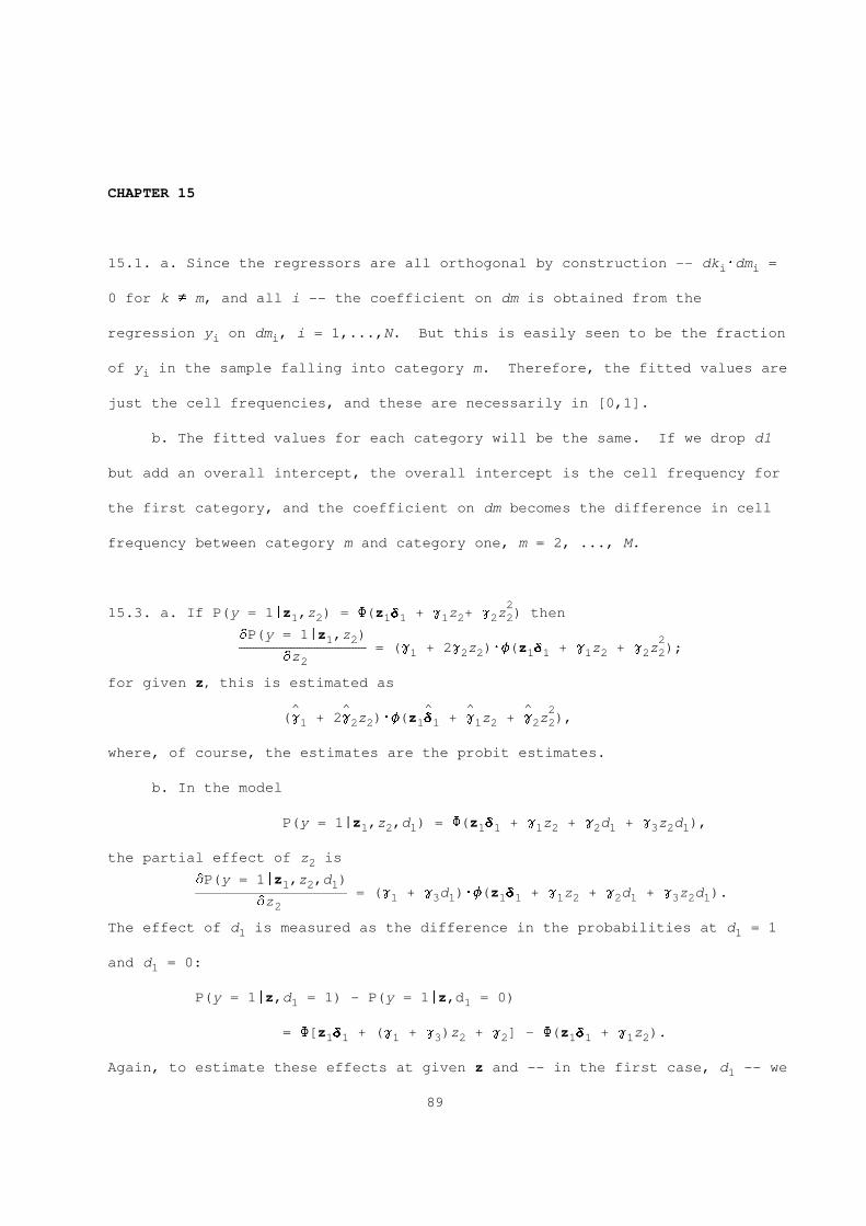
CHAPTER 15
15.1. a. Since the regressors are all orthogonal by construction -- dk Wdm =i i
0 for k $ m, and all i -- the coefficient on dm is obtained from the
regression y on dm , i = 1,...,N. But this is easily seen to be the fractioni i
of y in the sample falling into category m. Therefore, the fitted values arei
just the cell frequencies, and these are necessarily in [0,1].
b. The fitted values for each category will be the same. If we drop d1
but add an overall intercept, the overall intercept is the cell frequency for
the first category, and the coefficient on dm becomes the difference in cell
frequency between category m and category one, m = 2, ..., M.
215.3. a. If P(y = 1|z ,z ) = F(z D + g z + g z ) then1 2 1 1 1 2 2 2
dP(y = 1|z ,z )1 2 2------------------------------------------------------------------------- = (g + 2g z )Wf(z D + g z + g z );1 2 2 1 1 1 2 2 2dz2for given z, this is estimated as
^ ^ ^ ^ ^ 2(g + 2g z )Wf(z D + g z + g z ),1 2 2 1 1 1 2 2 2
where, of course, the estimates are the probit estimates.
b. In the model
P(y = 1|z ,z ,d ) = F(z D + g z + g d + g z d ),1 2 1 1 1 1 2 2 1 3 2 1
the partial effect of z is2
dP(y = 1|z ,z ,d )1 2 1--------------------------------------------------------------------------------------- = (g + g d )Wf(z D + g z + g d + g z d ).1 3 1 1 1 1 2 2 1 3 2 1dz2The effect of d is measured as the difference in the probabilities at d = 11 1
and d = 0:1
P(y = 1|z,d = 1) - P(y = 1|z,d = 0)1 1
= F[z D + (g + g )z + g ] - F(z D + g z ).1 1 1 3 2 2 1 1 1 2
Again, to estimate these effects at given z and -- in the first case, d -- we1
89
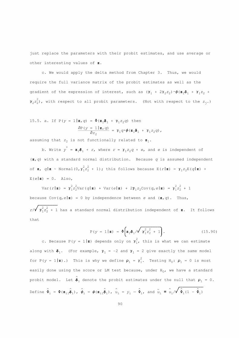
just replace the parameters with their probit estimates, and use average or
other interesting values of z.
c. We would apply the delta method from Chapter 3. Thus, we would
require the full variance matrix of the probit estimates as well as the
gradient of the expression of interest, such as (g + 2g z )Wf(z D + g z +1 2 2 1 1 1 2
2g z ), with respect to all probit parameters. (Not with respect to the z .)2 2 j
15.5. a. If P(y = 1|z,q) = F(z D + g z q) then1 1 1 2
dP(y = 1|z,q)----------------------------------------------------------------- = g qWf(z D + g z q),1 1 1 1 2dz2assuming that z is not functionally related to z .2 1
*b. Write y = z D + r, where r = g z q + e, and e is independent of1 1 1 2
(z,q) with a standard normal distribution. Because q is assumed independent
2 2of z, q|z ~ Normal(0,g z + 1); this follows because E(r|z) = g z E(q|z) +1 2 1 2
E(e|z) = 0. Also,
2 2 2 2Var(r|z) = g z Var(q|z) + Var(e|z) + 2g z Cov(q,e|z) = g z + 11 2 1 2 1 2
because Cov(q,e|z) = 0 by independence between e and (z,q). Thus,
5======================================2 2
r/r g z + 1 has a standard normal distribution independent of z. It follows1 2
that
5======================================& 2 2 *P(y = 1|z) = F z D /r g z + 1 . (15.90)1 1 1 27 8
2c. Because P(y = 1|z) depends only on g , this is what we can estimate1
along with D . (For example, g = -2 and g = 2 give exactly the same model1 1 1
2for P(y = 1|z).) This is why we define r = g . Testing H : r = 0 is most1 1 0 1
easily done using the score or LM test because, under H , we have a standard0
^probit model. Let D denote the probit estimates under the null that r = 0.1 1
5================================================^ ^ ^ ^ ^ ^ ~ ^ ^ ^
Define F = F(z D ), f = f(z D ), u = y ----- F , and u _ u /r F (1 - F )i i1 1 i i1 1 i i i i i i i
90
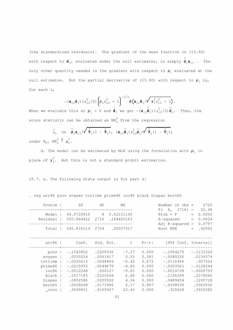
(the standardized residuals). The gradient of the mean function in (15.90)
^with respect to D , evaluated under the null estimates, is simply f z . The1 i i1
only other quantity needed is the gradient with respect to r evaluated at the1
null estimates. But the partial derivative of (15.90) with respect to r is,1
for each i,
-3/2 5==========================================2 & 2 * ( 2 2 )
-(z D )(z /2) r z + 1 f z D /r g z + 1 .i1 1 i2 1 i2 i1 1 1 i27 8 9 0^ ^ 2 ^
When we evaluate this at r = 0 and D we get -(z D )(z /2)f . Then, the1 1 i1 1 i2 i
2score statistic can be obtained as NR from the regressionu
5================================================ 5================================================~ ^ ^ ^ ^ 2 ^ ^ ^u on f z /r F (1 - F ), (z D )z f /r F (1 - F );i i i1 i i i1 1 i2 i i i
2 a 2under H , NR ~ c .0 u 1
d. The model can be estimated by MLE using the formulation with r in1
2place of g . But this is not a standard probit estimation.1
15.7. a. The following Stata output is for part a:
. reg arr86 pcnv avgsen tottime ptime86 inc86 black hispan born60
Source | SS df MS Number of obs = 2725
-------------+------------------------------ F( 8, 2716) = 30.48
Model | 44.9720916 8 5.62151145 Prob > F = 0.0000
Residual | 500.844422 2716 .184405163 R-squared = 0.0824
-------------+------------------------------ Adj R-squared = 0.0797
Total | 545.816514 2724 .20037317 Root MSE = .42942
------------------------------------------------------------------------------
arr86 | Coef. Std. Err. t P>|t| [95% Conf. Interval]
-------------+----------------------------------------------------------------
pcnv | -.1543802 .0209336 -7.37 0.000 -.1954275 -.1133329
avgsen | .0035024 .0063417 0.55 0.581 -.0089326 .0159374
tottime | -.0020613 .0048884 -0.42 0.673 -.0116466 .007524
ptime86 | -.0215953 .0044679 -4.83 0.000 -.0303561 -.0128344
inc86 | -.0012248 .000127 -9.65 0.000 -.0014738 -.0009759
black | .1617183 .0235044 6.88 0.000 .1156299 .2078066
hispan | .0892586 .0205592 4.34 0.000 .0489454 .1295718
born60 | .0028698 .0171986 0.17 0.867 -.0308539 .0365936
_cons | .3609831 .0160927 22.43 0.000 .329428 .3925382
91
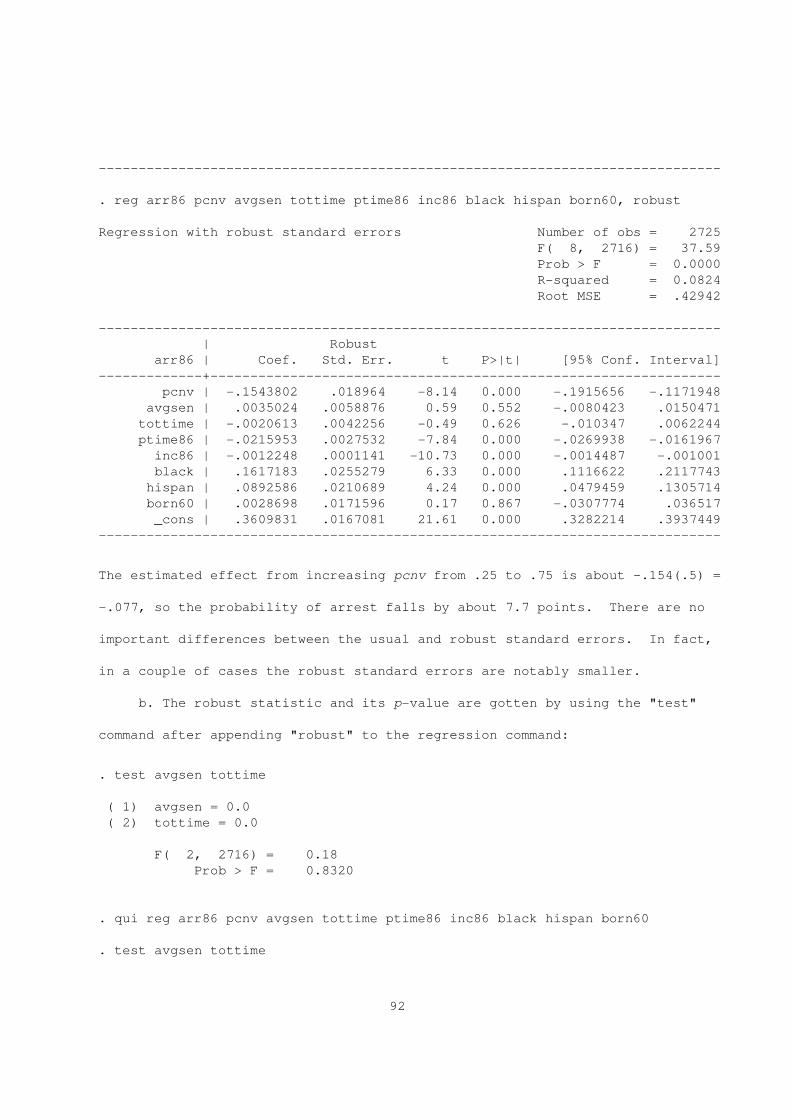
------------------------------------------------------------------------------
. reg arr86 pcnv avgsen tottime ptime86 inc86 black hispan born60, robust
Regression with robust standard errors Number of obs = 2725
F( 8, 2716) = 37.59
Prob > F = 0.0000
R-squared = 0.0824
Root MSE = .42942
------------------------------------------------------------------------------
| Robust
arr86 | Coef. Std. Err. t P>|t| [95% Conf. Interval]
-------------+----------------------------------------------------------------
pcnv | -.1543802 .018964 -8.14 0.000 -.1915656 -.1171948
avgsen | .0035024 .0058876 0.59 0.552 -.0080423 .0150471
tottime | -.0020613 .0042256 -0.49 0.626 -.010347 .0062244
ptime86 | -.0215953 .0027532 -7.84 0.000 -.0269938 -.0161967
inc86 | -.0012248 .0001141 -10.73 0.000 -.0014487 -.001001
black | .1617183 .0255279 6.33 0.000 .1116622 .2117743
hispan | .0892586 .0210689 4.24 0.000 .0479459 .1305714
born60 | .0028698 .0171596 0.17 0.867 -.0307774 .036517
_cons | .3609831 .0167081 21.61 0.000 .3282214 .3937449
------------------------------------------------------------------------------
The estimated effect from increasing pcnv from .25 to .75 is about -.154(.5) =
-.077, so the probability of arrest falls by about 7.7 points. There are no
important differences between the usual and robust standard errors. In fact,
in a couple of cases the robust standard errors are notably smaller.
b. The robust statistic and its p-value are gotten by using the "test"
command after appending "robust" to the regression command:
. test avgsen tottime
( 1) avgsen = 0.0
( 2) tottime = 0.0
F( 2, 2716) = 0.18
Prob > F = 0.8320
. qui reg arr86 pcnv avgsen tottime ptime86 inc86 black hispan born60
. test avgsen tottime
92
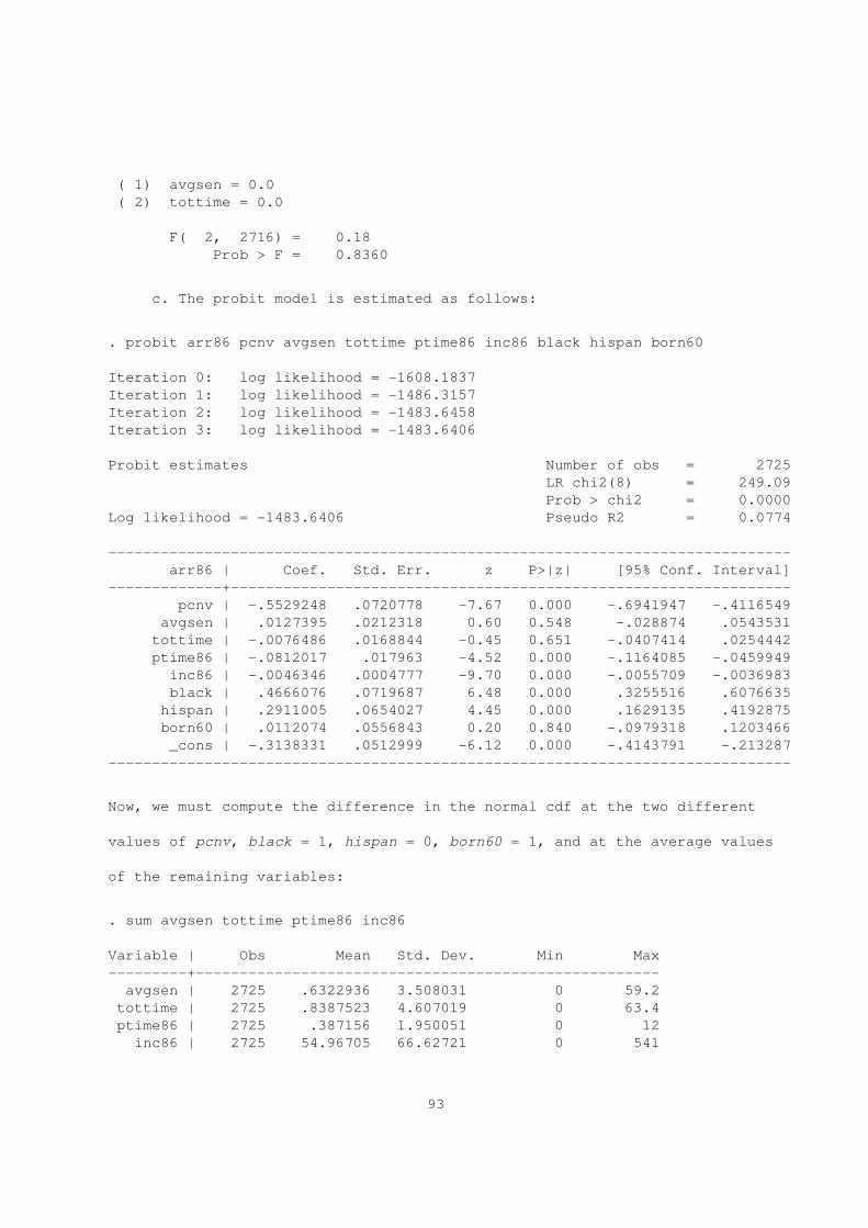
( 1) avgsen = 0.0
( 2) tottime = 0.0
F( 2, 2716) = 0.18
Prob > F = 0.8360
c. The probit model is estimated as follows:
. probit arr86 pcnv avgsen tottime ptime86 inc86 black hispan born60
Iteration 0: log likelihood = -1608.1837
Iteration 1: log likelihood = -1486.3157
Iteration 2: log likelihood = -1483.6458
Iteration 3: log likelihood = -1483.6406
Probit estimates Number of obs = 2725
LR chi2(8) = 249.09
Prob > chi2 = 0.0000
Log likelihood = -1483.6406 Pseudo R2 = 0.0774
------------------------------------------------------------------------------
arr86 | Coef. Std. Err. z P>|z| [95% Conf. Interval]
-------------+----------------------------------------------------------------
pcnv | -.5529248 .0720778 -7.67 0.000 -.6941947 -.4116549
avgsen | .0127395 .0212318 0.60 0.548 -.028874 .0543531
tottime | -.0076486 .0168844 -0.45 0.651 -.0407414 .0254442
ptime86 | -.0812017 .017963 -4.52 0.000 -.1164085 -.0459949
inc86 | -.0046346 .0004777 -9.70 0.000 -.0055709 -.0036983
black | .4666076 .0719687 6.48 0.000 .3255516 .6076635
hispan | .2911005 .0654027 4.45 0.000 .1629135 .4192875
born60 | .0112074 .0556843 0.20 0.840 -.0979318 .1203466
_cons | -.3138331 .0512999 -6.12 0.000 -.4143791 -.213287
------------------------------------------------------------------------------
Now, we must compute the difference in the normal cdf at the two different
values of pcnv, black = 1, hispan = 0, born60 = 1, and at the average values
of the remaining variables:
. sum avgsen tottime ptime86 inc86
Variable | Obs Mean Std. Dev. Min Max
---------+-----------------------------------------------------
avgsen | 2725 .6322936 3.508031 0 59.2
tottime | 2725 .8387523 4.607019 0 63.4
ptime86 | 2725 .387156 1.950051 0 12
inc86 | 2725 54.96705 66.62721 0 541
93
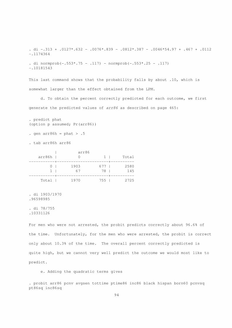
. di -.313 + .0127*.632 - .0076*.839 - .0812*.387 - .0046*54.97 + .467 + .0112
-.1174364
. di normprob(-.553*.75 - .117) - normprob(-.553*.25 - .117)
-.10181543
This last command shows that the probability falls by about .10, which is
somewhat larger than the effect obtained from the LPM.
d. To obtain the percent correctly predicted for each outcome, we first
generate the predicted values of arr86 as described on page 465:
. predict phat
(option p assumed; Pr(arr86))
. gen arr86h = phat > .5
. tab arr86h arr86
| arr86
arr86h | 0 1 | Total
-----------+----------------------+----------
0 | 1903 677 | 2580
1 | 67 78 | 145
-----------+----------------------+----------
Total | 1970 755 | 2725
. di 1903/1970
.96598985
. di 78/755
.10331126
For men who were not arrested, the probit predicts correctly about 96.6% of
the time. Unfortunately, for the men who were arrested, the probit is correct
only about 10.3% of the time. The overall percent correctly predicted is
quite high, but we cannot very well predict the outcome we would most like to
predict.
e. Adding the quadratic terms gives
. probit arr86 pcnv avgsen tottime ptime86 inc86 black hispan born60 pcnvsq
pt86sq inc86sq
94
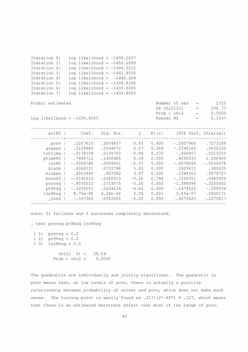
Iteration 0: log likelihood = -1608.1837
Iteration 1: log likelihood = -1452.2089
Iteration 2: log likelihood = -1444.3151
Iteration 3: log likelihood = -1441.8535
Iteration 4: log likelihood = -1440.268
Iteration 5: log likelihood = -1439.8166
Iteration 6: log likelihood = -1439.8005
Iteration 7: log likelihood = -1439.8005
Probit estimates Number of obs = 2725
LR chi2(11) = 336.77
Prob > chi2 = 0.0000
Log likelihood = -1439.8005 Pseudo R2 = 0.1047
------------------------------------------------------------------------------
arr86 | Coef. Std. Err. z P>|z| [95% Conf. Interval]
-------------+----------------------------------------------------------------
pcnv | .2167615 .2604937 0.83 0.405 -.2937968 .7273198
avgsen | .0139969 .0244972 0.57 0.568 -.0340166 .0620105
tottime | -.0178158 .0199703 -0.89 0.372 -.056957 .0213253
ptime86 | .7449712 .1438485 5.18 0.000 .4630333 1.026909
inc86 | -.0058786 .0009851 -5.97 0.000 -.0078094 -.0039478
black | .4368131 .0733798 5.95 0.000 .2929913 .580635
hispan | .2663945 .067082 3.97 0.000 .1349163 .3978727
born60 | -.0145223 .0566913 -0.26 0.798 -.1256351 .0965905
pcnvsq | -.8570512 .2714575 -3.16 0.002 -1.389098 -.3250042
pt86sq | -.1035031 .0224234 -4.62 0.000 -.1474522 -.059554
inc86sq | 8.75e-06 4.28e-06 2.04 0.041 3.63e-07 .0000171
_cons | -.337362 .0562665 -6.00 0.000 -.4476423 -.2270817
------------------------------------------------------------------------------
note: 51 failures and 0 successes completely determined.
. test pcnvsq pt86sq inc86sq
( 1) pcnvsq = 0.0
( 2) pt86sq = 0.0
( 3) inc86sq = 0.0
chi2( 3) = 38.54
Prob > chi2 = 0.0000
The quadratics are individually and jointly significant. The quadratic in
pcnv means that, at low levels of pcnv, there is actually a positive
relationship between probability of arrest and pcnv, which does not make much
sense. The turning point is easily found as .217/(2*.857) ~ .127, which means
that there is an estimated deterrent effect over most of the range of pcnv.
95
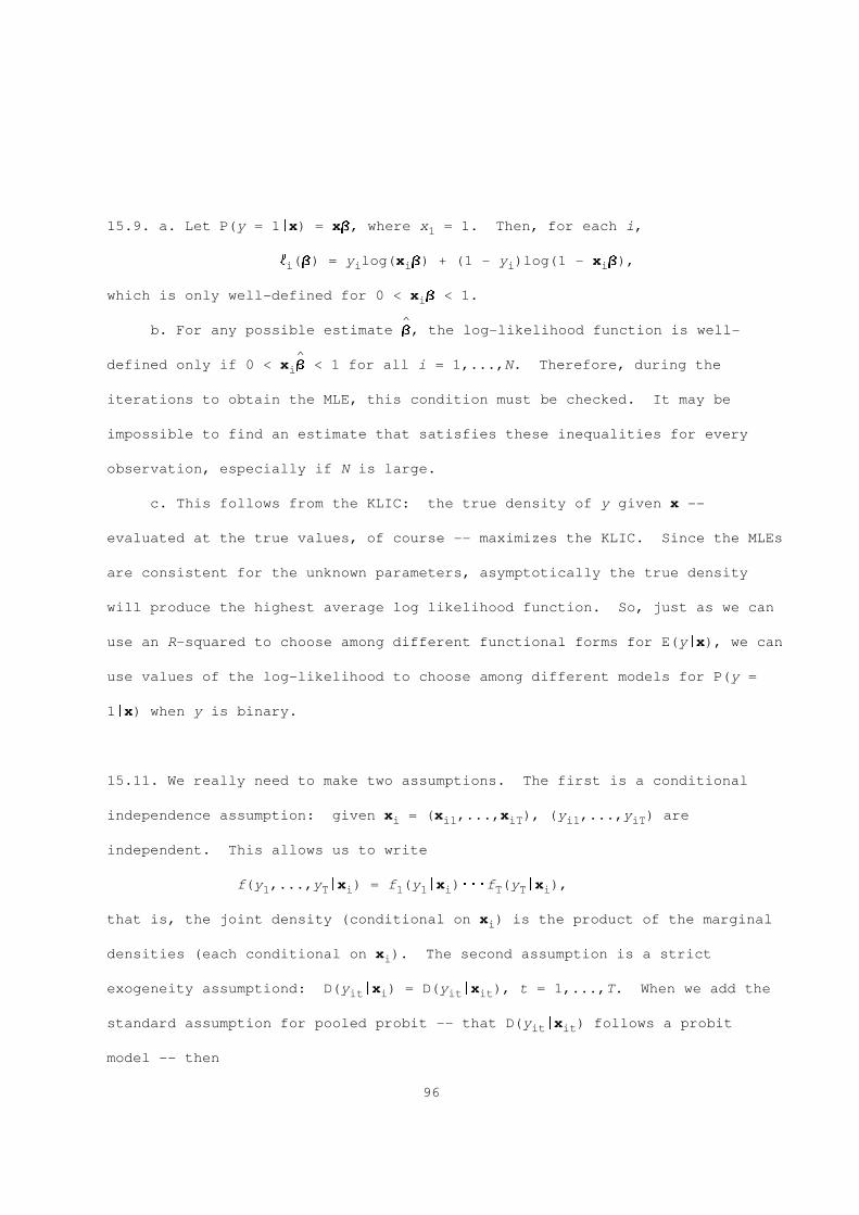
15.9. a. Let P(y = 1|x) = xB, where x = 1. Then, for each i,1
l (B) = y log(x B) + (1 - y )log(1 - x B),i i i i i
which is only well-defined for 0 < x B < 1.i
^b. For any possible estimate B, the log-likelihood function is well-
^defined only if 0 < x B < 1 for all i = 1,...,N. Therefore, during thei
iterations to obtain the MLE, this condition must be checked. It may be
impossible to find an estimate that satisfies these inequalities for every
observation, especially if N is large.
c. This follows from the KLIC: the true density of y given x --
evaluated at the true values, of course -- maximizes the KLIC. Since the MLEs
are consistent for the unknown parameters, asymptotically the true density
will produce the highest average log likelihood function. So, just as we can
use an R-squared to choose among different functional forms for E(y|x), we can
use values of the log-likelihood to choose among different models for P(y =
1|x) when y is binary.
15.11. We really need to make two assumptions. The first is a conditional
independence assumption: given x = (x ,...,x ), (y ,...,y ) arei i1 iT i1 iT
independent. This allows us to write
f(y ,...,y |x ) = f (y |x )WWWf (y |x ),1 T i 1 1 i T T i
that is, the joint density (conditional on x ) is the product of the marginali
densities (each conditional on x ). The second assumption is a stricti
exogeneity assumptiond: D(y |x ) = D(y |x ), t = 1,...,T. When we add theit i it it
standard assumption for pooled probit -- that D(y |x ) follows a probitit it
model -- then
96
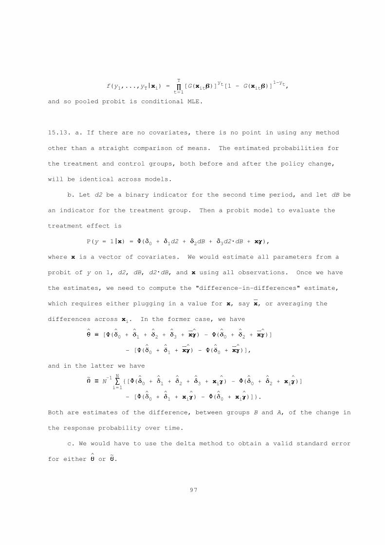
T y 1-yt tf(y ,...,y |x ) = p [G(x B)] [1 - G(x B)] ,1 T i it itt=1
and so pooled probit is conditional MLE.
15.13. a. If there are no covariates, there is no point in using any method
other than a straight comparison of means. The estimated probabilities for
the treatment and control groups, both before and after the policy change,
will be identical across models.
b. Let d2 be a binary indicator for the second time period, and let dB be
an indicator for the treatment group. Then a probit model to evaluate the
treatment effect is
P(y = 1|x) = F(d + d d2 + d dB + d d2WdB + xG),0 1 2 3
where x is a vector of covariates. We would estimate all parameters from a
probit of y on 1, d2, dB, d2WdB, and x using all observations. Once we have
the estimates, we need to compute the "difference-in-differences" estimate,
-----which requires either plugging in a value for x, say x, or averaging the
differences across x . In the former case, we havei
^ ^ ^ ^ ^ ------ ^ ^ ------q _ [F(d + d + d + d + xG) - F(d + d + xG)]0 1 2 3 0 2
^ ^ ------ ^ ------- [F(d + d + xG) - F(d + xG)],0 1 0
and in the latter we have
N~ -1 ^ ^ ^ ^ ^ ^ ^ ^q _ N S {[F(d + d + d + d + x G) - F(d + d + x G)]0 1 2 3 i 0 2 ii=1
^ ^ ^ ^ ^- [F(d + d + x G) - F(d + x G)]}.0 1 i 0 i
Both are estimates of the difference, between groups B and A, of the change in
the response probability over time.
c. We would have to use the delta method to obtain a valid standard error
^ ~for either q or q.
97
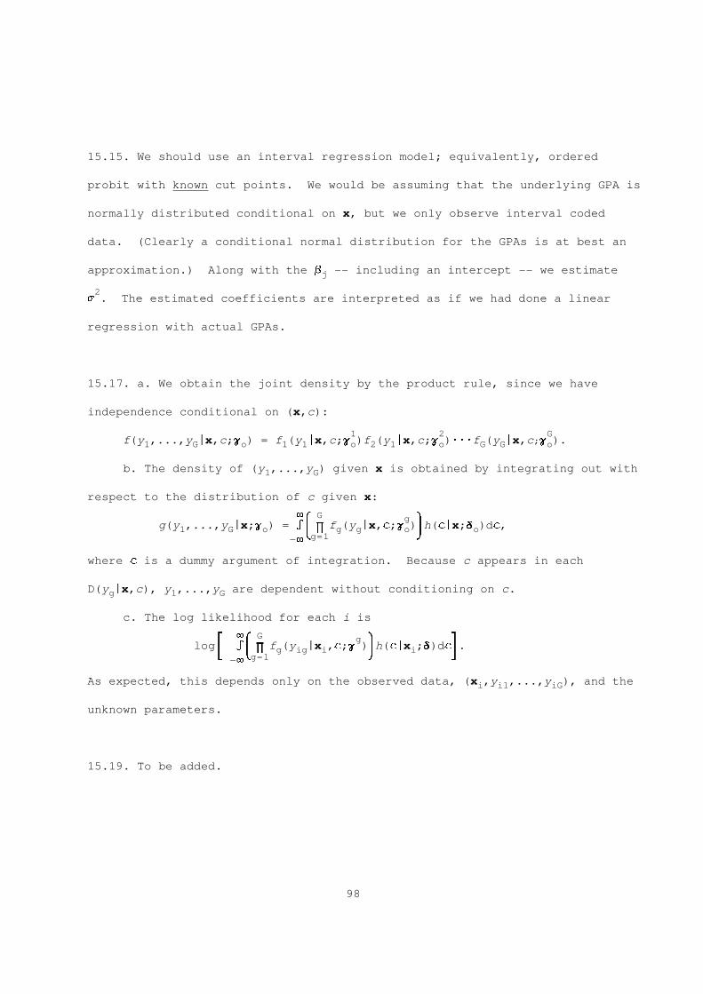
15.15. We should use an interval regression model; equivalently, ordered
probit with known cut points. We would be assuming that the underlying GPA is
normally distributed conditional on x, but we only observe interval coded
data. (Clearly a conditional normal distribution for the GPAs is at best an
approximation.) Along with the b -- including an intercept -- we estimatej
2s . The estimated coefficients are interpreted as if we had done a linear
regression with actual GPAs.
15.17. a. We obtain the joint density by the product rule, since we have
independence conditional on (x,c):
1 2 Gf(y ,...,y |x,c;G ) = f (y |x,c;G )f (y |x,c;G )WWWf (y |x,c;G ).1 G o 1 1 o 2 1 o G G o
b. The density of (y ,...,y ) given x is obtained by integrating out with1 G
respect to the distribution of c given x:
8 G& g *g(y ,...,y |x;G ) = i p f (y |x,c;G ) h(c|x;D )dc,1 G o g g o o7 8g=1-8
where c is a dummy argument of integration. Because c appears in each
D(y |x,c), y ,...,y are dependent without conditioning on c.g 1 G
c. The log likelihood for each i is
8 G# & g * $log i p f (y |x ,c;G ) h(c|x ;D)dc .g ig i i3 7 8 4g=1-8
As expected, this depends only on the observed data, (x ,y ,...,y ), and thei i1 iG
unknown parameters.
15.19. To be added.
98
CHAPTER 16
*16.1. a. P[log(t ) = log(c)|x ] = P[log(t ) > log(c)|x ]i i i i
= P[u > log(c) - x B|x ] = 1 - F{[log(c) - x B]/s}.i i i i
As c L 8, F{[log(c) - x B]/s} L 1, and so P[log(t ) = log(c)|x ] L 0 as c L 8.i i i
This simply says that, the longer we wait to censor, the less likely it is
that we observe a censored observation.
b. The density of y _ log(t ) (given x ) when t < c is the same as thei i i i
* * 2density of y _ log(t ), which is just Normal(x B,s ). This is because, for yi i i
*< log(c), P(y < y|x ) = P(y < y|x ). Thus, the density for y = log(t ) isi i i i i i
f(y|x ) = 1 - F{[log(c) - x B]/s}, y = log(c)i i
1f(y|x ) = -----f[(y - x B)/s], y < log(c).i is
2c. l (B,s ) = 1[y = log(c)]Wlog(1 - F{[log(c) - x B]/s})i i i
-1+ 1[y < log(c)]Wlog{s f[(y - x B)/s]}.i i i
d. To test H : B = 0, I would probably use the likelihood ratio0 2
statistic. This requires estimating the model with all variables, and then
the model without x . The LR statistic is LR = 2(L - L ). Under H , LR is2 ur r 0
2distributed asymptotically as c .K2
e. Since u is independent of (x ,c ), the density of y given (x ,c )i i i i i i
has the same form as the density of y given x above, except that c replacesi i i
c. The assumption that u is independent of c means that the decision toi i
censor an individual (or other economic unit) is not related to unobservables
*affecting t . Thus, in something like an unemployment duration equation,i
where u might contain unobserved ability, we do not wait longer to censori
people of lower ability. Note that c can be related to x . Thus, if xi i i
contains something like education, which is treated as exogenous, then the
99
censoring time can depend on education.
*16.3. a. P(y = a |x ) = P(y < a |x ) = P[(u /s) < (a - x B)/s]i 1 i i 1 i i 1 i
= F[(a - x B)/s].1 i
Similarly,
*P(y = a |x ) = P(y > a |x ) = P(x B + u > a |x )i 2 i i 2 i i i 2 i
= P[(u /s) > (a - x B)/s] = 1 - F[(a - x B)/s]i 2 i 2 i
= F[-(a - x B)/s].2 i
*Next, for a < y < a , P(y < y|x ) = P(y < y|x ) = F[(y - x B)/s]. Taking1 2 i i i i i
the derivative of this cdf with respect to y gives the pdf of y conditionali
on x for values of y strictly between a and a : (1/s)f[(y - x B)/s].i 1 2 i
* * * *b. Since y = y when a < y < a , E(y|x,a < y < a ) = E(y |x,a < y <1 2 1 2 1
* *a ). But y = xB + u, and a < y < a if and only if a - xB < u < a - xB.2 1 2 1 2
Therefore, using the hint,
* *E(y |x,a < y < a ) = xB + E(u|x,a - xB < u < a - xB)1 2 1 2
= xB + sE[(u/s)|x,(a - xB)/s < u/s < (a - xB)/s]1 2
= xB + s{f[(a - xB)/s]1
- f[(a - xB)/s]}/{F[(a - xB)/s] - F[(a - xB)/s]}2 2 1
= E(y|x,a < y < a ).1 2
Now, we can easily get E(y|x) by using the following:
E(y|x) = a P(y = a |x) + E(y|x,a < y < a )WP(a < y < a |x)1 1 1 2 1 2
+ a P(y = a |x)2 2 2
= a F[(a - xB)/s]1 1
+ E(y|x,a < y < a )W{F[(a - xB)/s] - F[(a - xB)/s]}1 2 2 1
+ a F[(xB - a )/s]2 2
= a F[(a - xB)/s]1 1
100
+ (xB)W{F[(a - xB)/s] - F[(a - xB)/s]} (16.57)2 1
+ s{f[(a - xB)/s] - f[(a - xB)/s]}1 2
+ a F[(xB - a )/s].2 2
* *c. From part b it is clear that E(y |x,a < y < a ) $ xB, and so it1 2
would be a fluke if OLS on the restricted sample consistently estimated B.
The linear regression of y on x using only those y such that a < y < ai i i 1 i 2
*consistently estimates the linear projection of y on x in the subpopulation
*for which a < y < a . Generally, there is no reason to think that this will1 2
have any simple relationship to the parameter vector B. [In some restrictive
cases, the regression on the restricted subsample could consistently estimate
B up to a common scale coefficient.]
d. We get the log-likelihood immediately from part a:
l (q) = 1[y = a ]log{F[(a - x B)/s]}i i 1 1 i
+ 1[y = a ]log{F[(x B - a )/s]}i 2 i 2
+ 1[a < y < a ]log{(1/s)f[(y - x B)/s]}.1 i 2 i i
Note how the indicator function selects out the appropriate density for each
of the three possible cases: at the left endpoint, at the right endpoint, or
strictly between the endpoints.
^ ^2e. After obtaining the maximum likelihood estimates B and s , just plug
these into the formulas in part b. The expressions can be evaluated at
interesting values of x.
f. We can show this by brute-force differentiation of equation (16.57).
As a shorthand, write f _ f[(a - xB)/s], f _ f[(a - xB)/s] = f[(xB -1 1 2 2
a )/s], F _ F[(a - x B)/s], and F _ F[(a - xB)/s]. Then2 1 1 i 2 2
dE(y|x)----------------------------------- = -(a /s)f b + (a /s)f b1 1 j 2 2 jdxj+ (F - F )b + [(xB/s)(f - f )]b2 1 j 1 2 j
101
+ {[(a - xB)/s]f }b - {[(a - xB)/s]f }b ,1 1 j 2 2 j
where the first two parts are the derivatives of the first and third terms,
respectively, in (16.57), and the last two lines are obtained from
differentiating the second term in E(y|x). Careful inspection shows that all
terms cancel except (F - F )b , which is the expression we wanted to be left2 1 j
with.
The scale factor is simply the probability that a standard normal random
variable falls in the interval [(a - xB)/s,(a - xB)/s], which is necessarily1 2
between zero and one.
g. The partial effects on E(y|x) are given in part f. These are
estimated as
^ ^ ^ ^ ^{F[(a - xB)/s] - F[(a - xB)/s]}b , (16.58)2 1 j
where the estimates are the MLEs. We could evaluate these partial effects
----- ^ ^ ^ ^at, say, x. Or, we could average {F[(a - x B)/s] - F[(a - x B)/s]} across2 i 1 i
^all i to obtain the average partial effect. In either case, the scaled bj
^can be compared to the g . Generally, we expectj
^ ^ ^g ~ rWb ,j j
^where 0 < r < 1 is the scale factor. Of course, this approximation need not
be very good in a partiular application, but it is often roughly true. It
^ ^does not make sense to directly compare the magnitude of b with that of g .j j
^ ^By the way, note that s appears in the partial effects along with the b ;j
^there is no sense in which s is "ancillary."
h. For data censoring where the censoring points might change with i,
the analysis is essentially the same but a and a are replaced with a and1 2 i1
a . Intepretating the results is even easier, since we act as if we werei2
able to do OLS on an uncensored sample.
102
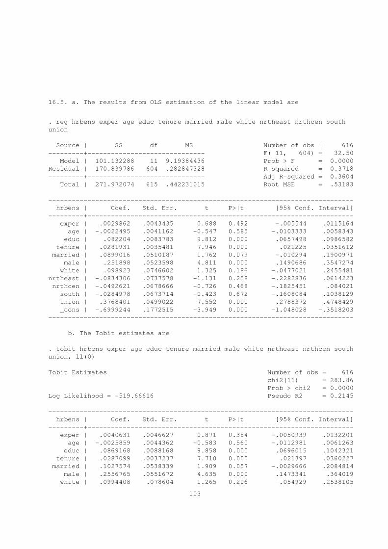
16.5. a. The results from OLS estimation of the linear model are
. reg hrbens exper age educ tenure married male white nrtheast nrthcen south
union
Source | SS df MS Number of obs = 616
---------+------------------------------ F( 11, 604) = 32.50
Model | 101.132288 11 9.19384436 Prob > F = 0.0000
Residual | 170.839786 604 .282847328 R-squared = 0.3718
---------+------------------------------ Adj R-squared = 0.3604
Total | 271.972074 615 .442231015 Root MSE = .53183
------------------------------------------------------------------------------
hrbens | Coef. Std. Err. t P>|t| [95% Conf. Interval]
---------+--------------------------------------------------------------------
exper | .0029862 .0043435 0.688 0.492 -.005544 .0115164
age | -.0022495 .0041162 -0.547 0.585 -.0103333 .0058343
educ | .082204 .0083783 9.812 0.000 .0657498 .0986582
tenure | .0281931 .0035481 7.946 0.000 .021225 .0351612
married | .0899016 .0510187 1.762 0.079 -.010294 .1900971
male | .251898 .0523598 4.811 0.000 .1490686 .3547274
white | .098923 .0746602 1.325 0.186 -.0477021 .2455481
nrtheast | -.0834306 .0737578 -1.131 0.258 -.2282836 .0614223
nrthcen | -.0492621 .0678666 -0.726 0.468 -.1825451 .084021
south | -.0284978 .0673714 -0.423 0.672 -.1608084 .1038129
union | .3768401 .0499022 7.552 0.000 .2788372 .4748429
_cons | -.6999244 .1772515 -3.949 0.000 -1.048028 -.3518203
------------------------------------------------------------------------------
b. The Tobit estimates are
. tobit hrbens exper age educ tenure married male white nrtheast nrthcen south
union, ll(0)
Tobit Estimates Number of obs = 616
chi2(11) = 283.86
Prob > chi2 = 0.0000
Log Likelihood = -519.66616 Pseudo R2 = 0.2145
------------------------------------------------------------------------------
hrbens | Coef. Std. Err. t P>|t| [95% Conf. Interval]
---------+--------------------------------------------------------------------
exper | .0040631 .0046627 0.871 0.384 -.0050939 .0132201
age | -.0025859 .0044362 -0.583 0.560 -.0112981 .0061263
educ | .0869168 .0088168 9.858 0.000 .0696015 .1042321
tenure | .0287099 .0037237 7.710 0.000 .021397 .0360227
married | .1027574 .0538339 1.909 0.057 -.0029666 .2084814
male | .2556765 .0551672 4.635 0.000 .1473341 .364019
white | .0994408 .078604 1.265 0.206 -.054929 .2538105
103
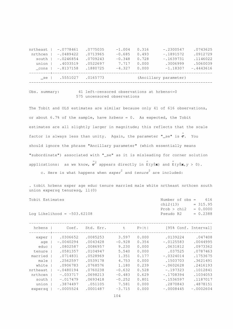
nrtheast | -.0778461 .0775035 -1.004 0.316 -.2300547 .0743625
nrthcen | -.0489422 .0713965 -0.685 0.493 -.1891572 .0912729
south | -.0246854 .0709243 -0.348 0.728 -.1639731 .1146022
union | .4033519 .0522697 7.717 0.000 .3006999 .5060039
_cons | -.8137158 .1880725 -4.327 0.000 -1.18307 -.4443616
---------+--------------------------------------------------------------------
_se | .5551027 .0165773 (Ancillary parameter)
------------------------------------------------------------------------------
Obs. summary: 41 left-censored observations at hrbens<=0
575 uncensored observations
The Tobit and OLS estimates are similar because only 41 of 616 observations,
or about 6.7% of the sample, have hrbens = 0. As expected, the Tobit
estimates are all slightly larger in magnitude; this reflects that the scale
^factor is always less than unity. Again, the parameter "_se" is s. You
should ignore the phrase "Ancillary parameter" (which essentially means
"subordinate") associated with "_se" as it is misleading for corner solution
^2 ^ ^applications: as we know, s appears directly in E(y|x) and E(y|x,y > 0).
2 2c. Here is what happens when exper and tenure are included:
. tobit hrbens exper age educ tenure married male white nrtheast nrthcen south
union expersq tenuresq, ll(0)
Tobit Estimates Number of obs = 616
chi2(13) = 315.95
Prob > chi2 = 0.0000
Log Likelihood = -503.62108 Pseudo R2 = 0.2388
------------------------------------------------------------------------------
hrbens | Coef. Std. Err. t P>|t| [95% Conf. Interval]
---------+--------------------------------------------------------------------
exper | .0306652 .0085253 3.597 0.000 .0139224 .047408
age | -.0040294 .0043428 -0.928 0.354 -.0125583 .0044995
educ | .0802587 .0086957 9.230 0.000 .0631812 .0973362
tenure | .0581357 .0104947 5.540 0.000 .037525 .0787463
married | .0714831 .0528969 1.351 0.177 -.0324014 .1753675
male | .2562597 .0539178 4.753 0.000 .1503703 .3621491
white | .0906783 .0768576 1.180 0.239 -.0602628 .2416193
nrtheast | -.0480194 .0760238 -0.632 0.528 -.197323 .1012841
nrthcen | -.033717 .0698213 -0.483 0.629 -.1708394 .1034053
south | -.017479 .0693418 -0.252 0.801 -.1536597 .1187017
union | .3874497 .051105 7.581 0.000 .2870843 .4878151
expersq | -.0005524 .0001487 -3.715 0.000 -.0008445 -.0002604
104
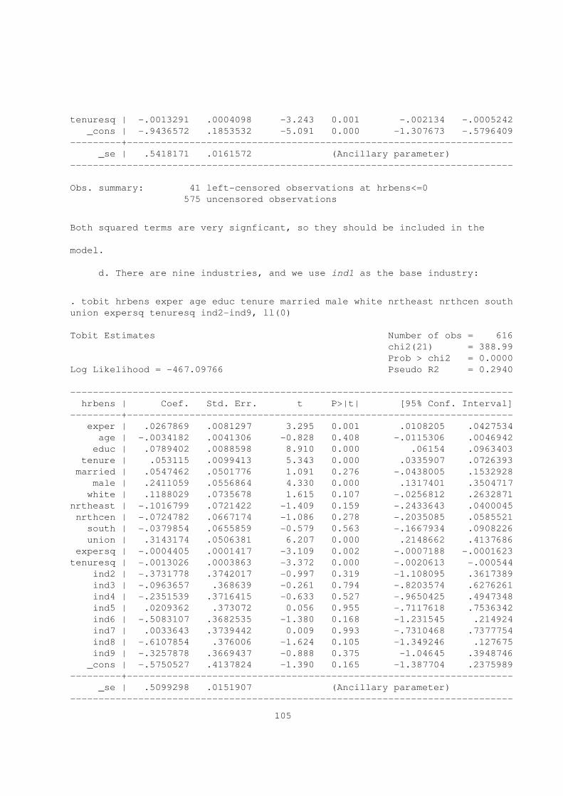
tenuresq | -.0013291 .0004098 -3.243 0.001 -.002134 -.0005242
_cons | -.9436572 .1853532 -5.091 0.000 -1.307673 -.5796409
---------+--------------------------------------------------------------------
_se | .5418171 .0161572 (Ancillary parameter)
------------------------------------------------------------------------------
Obs. summary: 41 left-censored observations at hrbens<=0
575 uncensored observations
Both squared terms are very signficant, so they should be included in the
model.
d. There are nine industries, and we use ind1 as the base industry:
. tobit hrbens exper age educ tenure married male white nrtheast nrthcen south
union expersq tenuresq ind2-ind9, ll(0)
Tobit Estimates Number of obs = 616
chi2(21) = 388.99
Prob > chi2 = 0.0000
Log Likelihood = -467.09766 Pseudo R2 = 0.2940
------------------------------------------------------------------------------
hrbens | Coef. Std. Err. t P>|t| [95% Conf. Interval]
---------+--------------------------------------------------------------------
exper | .0267869 .0081297 3.295 0.001 .0108205 .0427534
age | -.0034182 .0041306 -0.828 0.408 -.0115306 .0046942
educ | .0789402 .0088598 8.910 0.000 .06154 .0963403
tenure | .053115 .0099413 5.343 0.000 .0335907 .0726393
married | .0547462 .0501776 1.091 0.276 -.0438005 .1532928
male | .2411059 .0556864 4.330 0.000 .1317401 .3504717
white | .1188029 .0735678 1.615 0.107 -.0256812 .2632871
nrtheast | -.1016799 .0721422 -1.409 0.159 -.2433643 .0400045
nrthcen | -.0724782 .0667174 -1.086 0.278 -.2035085 .0585521
south | -.0379854 .0655859 -0.579 0.563 -.1667934 .0908226
union | .3143174 .0506381 6.207 0.000 .2148662 .4137686
expersq | -.0004405 .0001417 -3.109 0.002 -.0007188 -.0001623
tenuresq | -.0013026 .0003863 -3.372 0.000 -.0020613 -.000544
ind2 | -.3731778 .3742017 -0.997 0.319 -1.108095 .3617389
ind3 | -.0963657 .368639 -0.261 0.794 -.8203574 .6276261
ind4 | -.2351539 .3716415 -0.633 0.527 -.9650425 .4947348
ind5 | .0209362 .373072 0.056 0.955 -.7117618 .7536342
ind6 | -.5083107 .3682535 -1.380 0.168 -1.231545 .214924
ind7 | .0033643 .3739442 0.009 0.993 -.7310468 .7377754
ind8 | -.6107854 .376006 -1.624 0.105 -1.349246 .127675
ind9 | -.3257878 .3669437 -0.888 0.375 -1.04645 .3948746
_cons | -.5750527 .4137824 -1.390 0.165 -1.387704 .2375989
---------+--------------------------------------------------------------------
_se | .5099298 .0151907 (Ancillary parameter)
------------------------------------------------------------------------------
105
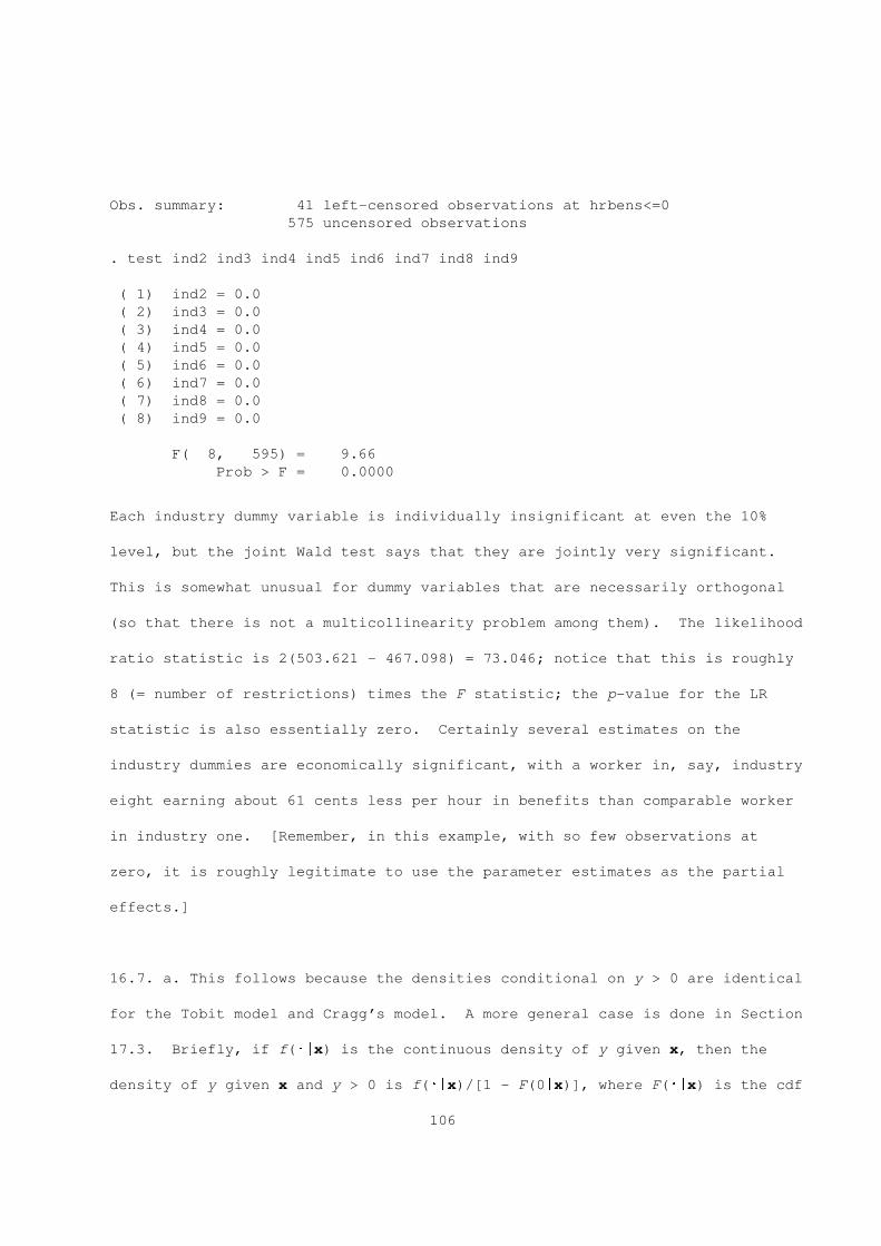
Obs. summary: 41 left-censored observations at hrbens<=0
575 uncensored observations
. test ind2 ind3 ind4 ind5 ind6 ind7 ind8 ind9
( 1) ind2 = 0.0
( 2) ind3 = 0.0
( 3) ind4 = 0.0
( 4) ind5 = 0.0
( 5) ind6 = 0.0
( 6) ind7 = 0.0
( 7) ind8 = 0.0
( 8) ind9 = 0.0
F( 8, 595) = 9.66
Prob > F = 0.0000
Each industry dummy variable is individually insignificant at even the 10%
level, but the joint Wald test says that they are jointly very significant.
This is somewhat unusual for dummy variables that are necessarily orthogonal
(so that there is not a multicollinearity problem among them). The likelihood
ratio statistic is 2(503.621 - 467.098) = 73.046; notice that this is roughly
8 (= number of restrictions) times the F statistic; the p-value for the LR
statistic is also essentially zero. Certainly several estimates on the
industry dummies are economically significant, with a worker in, say, industry
eight earning about 61 cents less per hour in benefits than comparable worker
in industry one. [Remember, in this example, with so few observations at
zero, it is roughly legitimate to use the parameter estimates as the partial
effects.]
16.7. a. This follows because the densities conditional on y > 0 are identical
for the Tobit model and Cragg’s model. A more general case is done in Section
17.3. Briefly, if f(W|x) is the continuous density of y given x, then the
density of y given x and y > 0 is f(W|x)/[1 - F(0|x)], where F(W|x) is the cdf
106

2of y given x. When f is the normal pdf with mean xB and variance s , we get
-1that f(y|x,y > 0) = {F(xB/s)} {f[(y - xB)/s]/s} for the Tobit model, and this
is exactly the density specified for Cragg’s model given y > 0.
b. From (6.8) we have
E(y|x) = F(xG)WE(y|x,y > 0) = F(xG)[xB + sl(xB/s)].
c. This follows very generally -- not just for Cragg’s model or the Tobit
model -- from (16.8):
log[E(y|x)] = log[P(y > 0|x)] + log[E(y|x,y > 0)].
If we take the partial derivative with respect to log(x ) we clearly get the1
sum of the elasticities.
16.9. a. A two-limit Tobit model, of the kind analyzed in Problem 16.3, is
appropriate, with a = 0, a = 10.1 2
b. The lower limit at zero is logically necessary considering the kind of
response: the smallest percentage of one’s income that can be invested in a
pension plan is zero. On the other hand, the upper limit of 10 is an
arbitrary corner imposed by law. One can imagine that some people at the
corner y = 10 would choose y > 10 if they could. So, we can think of an
underlying variable, which would be the percentage invested in the absense of
any restrictions. Then, there would be no upper bound required (since we
would not have to worry about 100 percent of income being invested in a
pension plan).
c. From Problem 16.3(b), with a = 0, we have1
E(y|x) = (xB)W{F[(a - xB)/s] - F(-xB/s)}2
+ s{f(xB/s) - f[(a - xB)/s]} + a F[(xB - a )/s].2 2 2
Taking the derivative of this function with respect to a gives2
107
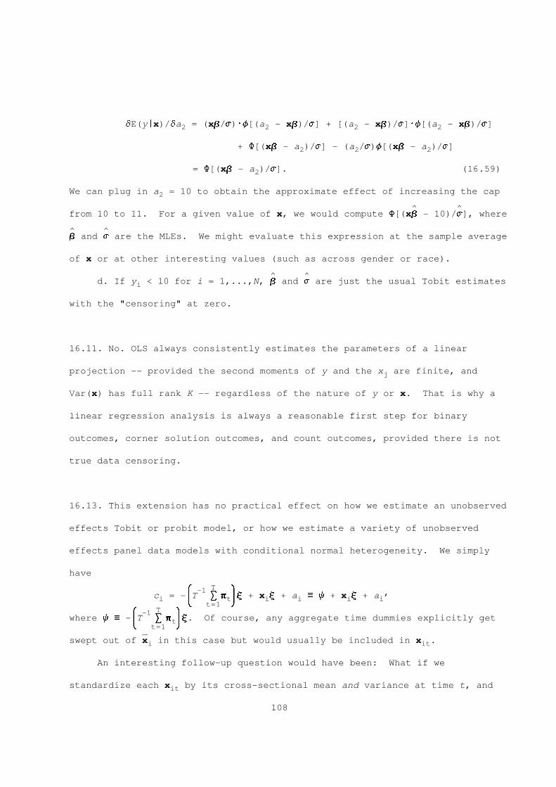
dE(y|x)/da = (xB/s)Wf[(a - xB)/s] + [(a - xB)/s]Wf[(a - xB)/s]2 2 2 2
+ F[(xB - a )/s] - (a /s)f[(xB - a )/s]2 2 2
= F[(xB - a )/s]. (16.59)2
We can plug in a = 10 to obtain the approximate effect of increasing the cap2
^ ^from 10 to 11. For a given value of x, we would compute F[(xB - 10)/s], where
^ ^B and s are the MLEs. We might evaluate this expression at the sample average
of x or at other interesting values (such as across gender or race).
^ ^d. If y < 10 for i = 1,...,N, B and s are just the usual Tobit estimatesi
with the "censoring" at zero.
16.11. No. OLS always consistently estimates the parameters of a linear
projection -- provided the second moments of y and the x are finite, andj
Var(x) has full rank K -- regardless of the nature of y or x. That is why a
linear regression analysis is always a reasonable first step for binary
outcomes, corner solution outcomes, and count outcomes, provided there is not
true data censoring.
16.13. This extension has no practical effect on how we estimate an unobserved
effects Tobit or probit model, or how we estimate a variety of unobserved
effects panel data models with conditional normal heterogeneity. We simply
have
T& -1 * ----- ----- ,c = - T S P X + x X + a _ j + x X + ai t i i i i7 8t=1T& -1 *
where j _ - T S P X. Of course, any aggregate time dummies explicitly gett7 8t=1
-----swept out of x in this case but would usually be included in x .i it
An interesting follow-up question would have been: What if we
standardize each x by its cross-sectional mean and variance at time t, andit
108

assume c is related to the mean and variance of the standardized vectors. Ini
-1/2other words, let z _ (x - P )) , t = 1,...,T, for each random draw iit it t t
----- 2from the population. Then, we might assume c |x ~ Normal(j + z X,s ) (where,i i i a
again, z would not contain aggregate time dummies). This is the kind ofit
scenario that is handled by Chamberlain’s more general assumption concerning
T
the relationship between c and x : c = j + S x L + a , where L =i i i ir r i rr=1
-1/2) X/T, t = 1,2,...,T. Alternatively, one could estimate estimate P and )r t t
for each t using the cross section observations {x : i = 1,2,...,N}. Theit
^ ^usual sample means and sample variance matrices, say P and ) , are consistentt t
----- ^-1/2 ^^and rN-asymptotically normal. Then, form z _ ) (x - P ), and proceedit t it t
with the usual Tobit (or probit) unobserved effects analysis that includes the
----- T-1^ ^time averages z = T S z . This is a rather simple two-step estimationi itt=1
^ ^method, but accounting for the sample variation in P and ) would bet t
^ ^cumbersome. It may be possible to use a much larger to obtain P and ) , int t
which case one might ignore the sampling error in the first-stage estimates.
16.15. To be added.
CHAPTER 17
17.1. If you are interested in the effects of things like age of the building
and neighborhood demographics on fire damage, given that a fire has occured,
then there is no problem. We simply need a random sample of buildings that
actually caught on fire. You might want to supplement this with an analysis
of the probability that buildings catch fire, given building and neighborhood
characteristics. But then a two-stage analysis is appropriate.
109
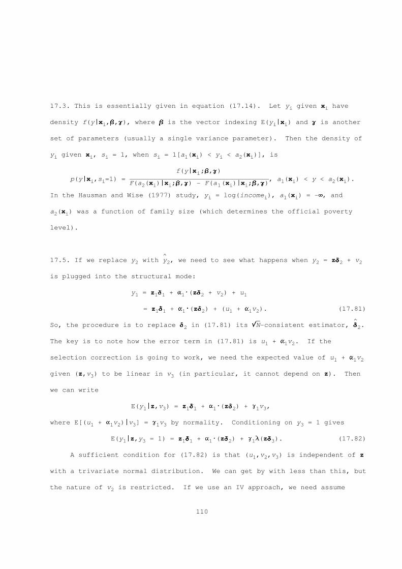
17.3. This is essentially given in equation (17.14). Let y given x havei i
density f(y|x ,B,G), where B is the vector indexing E(y |x ) and G is anotheri i i
set of parameters (usually a single variance parameter). Then the density of
y given x , s = 1, when s = 1[a (x ) < y < a (x )], isi i i i 1 i i 2 i
f(y|x ;B,G)i
p(y|x ,s =1) = ----------------------------------------------------------------------------------------------------------------------------------------------------------------------------, a (x ) < y < a (x ).i i 1 i 2 iF(a (x )|x ;B,G) - F(a (x )|x ;B,G)2 i i 1 i i
In the Hausman and Wise (1977) study, y = log(income ), a (x ) = -8, andi i 1 i
a (x ) was a function of family size (which determines the official poverty2 i
level).
^17.5. If we replace y with y , we need to see what happens when y = zD + v2 2 2 2 2
is plugged into the structural mode:
y = z D + a W(zD + v ) + u1 1 1 1 2 2 1
= z D + a W(zD ) + (u + a v ). (17.81)1 1 1 2 1 1 2
----- ^So, the procedure is to replace D in (17.81) its rN-consistent estimator, D .2 2
The key is to note how the error term in (17.81) is u + a v . If the1 1 2
selection correction is going to work, we need the expected value of u + a v1 1 2
given (z,v ) to be linear in v (in particular, it cannot depend on z). Then3 3
we can write
E(y |z,v ) = z D + a W(zD ) + g v ,1 3 1 1 1 2 1 3
where E[(u + a v )|v ] = g v by normality. Conditioning on y = 1 gives1 1 2 3 1 3 3
E(y |z,y = 1) = z D + a W(zD ) + g l(zD ). (17.82)1 3 1 1 1 2 1 3
A sufficient condition for (17.82) is that (u ,v ,v ) is independent of z1 2 3
with a trivariate normal distribution. We can get by with less than this, but
the nature of v is restricted. If we use an IV approach, we need assume2
110
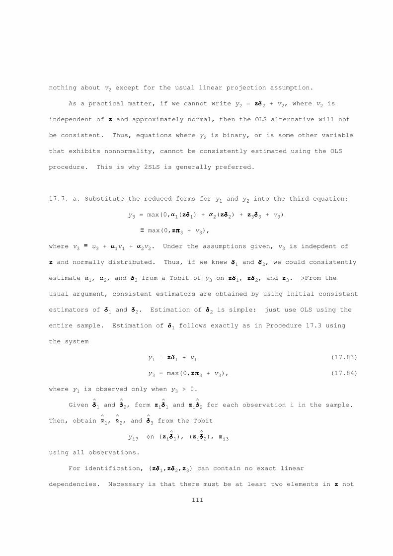
nothing about v except for the usual linear projection assumption.2
As a practical matter, if we cannot write y = zD + v , where v is2 2 2 2
independent of z and approximately normal, then the OLS alternative will not
be consistent. Thus, equations where y is binary, or is some other variable2
that exhibits nonnormality, cannot be consistently estimated using the OLS
procedure. This is why 2SLS is generally preferred.
17.7. a. Substitute the reduced forms for y and y into the third equation:1 2
y = max(0,a (zD ) + a (zD ) + z D + v )3 1 1 2 2 3 3 3
_ max(0,zP + v ),3 3
where v _ u + a v + a v . Under the assumptions given, v is indepdent of3 3 1 1 2 2 3
z and normally distributed. Thus, if we knew D and D , we could consistently1 2
estimate a , a , and D from a Tobit of y on zD , zD , and z . >From the1 2 3 3 1 2 3
usual argument, consistent estimators are obtained by using initial consistent
estimators of D and D . Estimation of D is simple: just use OLS using the1 2 2
entire sample. Estimation of D follows exactly as in Procedure 17.3 using1
the system
y = zD + v (17.83)1 1 1
y = max(0,zP + v ), (17.84)3 3 3
where y is observed only when y > 0.1 3
^ ^ ^ ^Given D and D , form z D and z D for each observation i in the sample.1 2 i 1 i 2
^ ^ ^Then, obtain a , a , and D from the Tobit1 2 3
^ ^y on (z D ), (z D ), zi3 i 1 i 2 i3
using all observations.
For identification, (zD ,zD ,z ) can contain no exact linear1 2 3
dependencies. Necessary is that there must be at least two elements in z not
111
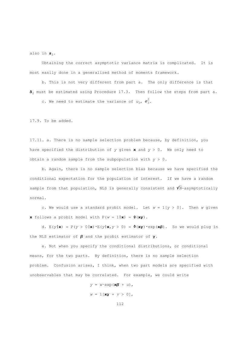
also in z .3
Obtaining the correct asymptotic variance matrix is complicated. It is
most easily done in a generalized method of moments framework.
b. This is not very different from part a. The only difference is that
D must be estimated using Procedure 17.3. Then follow the steps from part a.2
2c. We need to estimate the variance of u , s .3 3
17.9. To be added.
17.11. a. There is no sample selection problem because, by definition, you
have specified the distribution of y given x and y > 0. We only need to
obtain a random sample from the subpopulation with y > 0.
b. Again, there is no sample selection bias because we have specified the
conditional expectation for the population of interest. If we have a random
-----sample from that population, NLS is generally consistent and rN-asymptotically
normal.
c. We would use a standard probit model. Let w = 1[y > 0]. Then w given
x follows a probit model with P(w = 1|x) = F(xG).
d. E(y|x) = P(y > 0|x)WE(y|x,y > 0) = F(xG)Wexp(xB). So we would plug in
the NLS estimator of B and the probit estimator of G.
e. Not when you specify the conditional distributions, or conditional
means, for the two parts. By definition, there is no sample selection
problem. Confusion arises, I think, when two part models are specified with
unobservables that may be correlated. For example, we could write
y = wWexp(xB + u),
w = 1[xG + v > 0],
112
so that w = 0 6 y = 0. Assume that (u,v) is independent of x. Then, if u and
v are independent -- so that u is independent of (x,w) -- we have
E(y|x,w) = wWexp(xB)E[exp(u)|x,w] = wWexp(xB)E[exp(u)],
which implies the specification in part b (by setting w = 1, once we absorb
E[exp(u)] into the intercept). The interesting twist here is if u and v are
correlated. Given w = 1, we can write log(y) = xB + u. So
E[log(y)|x,w = 1] = xB + E(u|x,w = 1).
If we make the usual linearity assumption, E(u|v) = rv and assume a standard
normal distribution for v then we have the usual inverse Mills ratio added to
the linear model:
E[log(y)|x,w = 1] = xB + rl(xG).
A two-step strategy for estimating G and B is pretty clear. First, estimate a
^ ^probit of w on x to get G and l(x G). Then, using the y > 0 observations,i i i i
^ ^ ^run the regression log(y ) on x , l(x G) to obtain B, r. A standard ti i i
^statistic on r is a simple test of Cov(u,v) = 0.
This two-step procedure reveals a potential problem with the model that
allows u and v to be correlated: adding the inverse Mills ratio means that we
are adding a nonlinear function of x. In other words, identification of B
comes entirely from the nonlinearity of the IMR, which we warned about in this
chapter. Ideally, we would have a variable that affects P(w = 1|x) that can
be excluded from xB. In labor economics, where two-part models are used to
allow for fixed costs of entering the labor market, one would try to find a
variable that affects the fixed costs of being employed that does not affect
the choice of hours.
If we assume (u,v) is multivariate normal, with mean zero, then we can
use a full maximum likelihood procedure. While this would be a little less
113

robust, making full distributional assumptions has a subtle advantage: we can
then compute partial effects on E(y|x) and E(y|x,y > 0). Even with a full set
of assumptions, the partial effects are not straightforward to obtain. For
one,
E(y|x,y > 0) = exp(x,B)WE[exp(u)|x,w = 1)],
where E[exp(u)|x,w = 1)] can be obtained under joint normality. A similar
example is given in Section 19.5.2; see, particularly, equation (19.44).
Then, we can multiply this expectation by P(w = 1|x) = F(xG). The point is
that we cannot simply look at B to obtain partial effects of interest. This
is very different from the sample selection model.
17.13. a. We cannot use censored Tobit because that requires observing x when
whatever the value of y. Instead, we can use truncated Tobit: we use the
distribution of y given x and y > 0. Notice that our reason for using
truncated Tobit differs from the usual application. Usually, the underlying
variable y of interest has a conditional normal distribution in the
population. Here, y given x follows a standard Tobit model in the population
(for a corner solution outcome).
b. Provided x varies enough in the subpopulation where y > 0 such that b.
rank E(x’x|y > 0) = K, the parameters. In the case where an element of x is a
derived price, we need sufficient price variation for the population that
consumes some of the good. Given such variation, we can estimate E(y|x) =
F(xB/s)xB + sf(xB/s) because we have made the assumption that y given x
follows a Tobit in the full population.
114
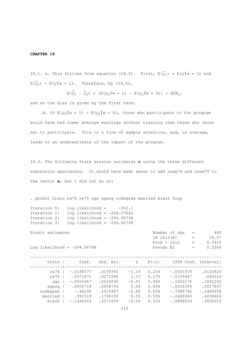
CHAPTER 18
-----18.1. a. This follows from equation (18.5). First, E(y ) = E(y|w = 1) and1
-----E(y ) = E(y|w = 1). Therefore, by (18.5),0
----- -----E(y - y ) = [E(y |w = 1) - E(y |w = 0)] + ATE ,1 0 0 0 1
and so the bias is given by the first term.
b. If E(y |w = 1) < E(y |w = 0), those who participate in the program0 0
would have had lower average earnings without training than those who chose
not to participate. This is a form of sample selection, and, on average,
leads to an underestimate of the impact of the program.
18.3. The following Stata session estimates a using the three different
regression approaches. It would have made sense to add unem74 and unem75 to
the vector x, but I did not do so:
. probit train re74 re75 age agesq nodegree married black hisp
Iteration 0: log likelihood = -302.1
Iteration 1: log likelihood = -294.07642
Iteration 2: log likelihood = -294.06748
Iteration 3: log likelihood = -294.06748
Probit estimates Number of obs = 445
LR chi2(8) = 16.07
Prob > chi2 = 0.0415
Log likelihood = -294.06748 Pseudo R2 = 0.0266
------------------------------------------------------------------------------
train | Coef. Std. Err. z P>|z| [95% Conf. Interval]
-------------+----------------------------------------------------------------
re74 | -.0189577 .0159392 -1.19 0.234 -.0501979 .0122825
re75 | .0371871 .0271086 1.37 0.170 -.0159447 .090319
age | -.0005467 .0534045 -0.01 0.992 -.1052176 .1041242
agesq | .0000719 .0008734 0.08 0.934 -.0016399 .0017837
nodegree | -.44195 .1515457 -2.92 0.004 -.7389742 -.1449258
married | .091519 .1726192 0.53 0.596 -.2468083 .4298464
black | -.1446253 .2271609 -0.64 0.524 -.5898524 .3006019
115
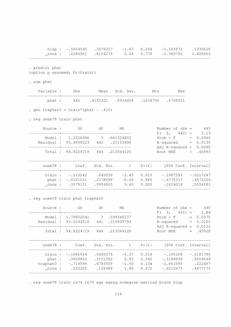
hisp | -.5004545 .3079227 -1.63 0.104 -1.103972 .1030629
_cons | .2284561 .8154273 0.28 0.779 -1.369752 1.826664
------------------------------------------------------------------------------
. predict phat
(option p assumed; Pr(train))
. sum phat
Variable | Obs Mean Std. Dev. Min Max
-------------+-----------------------------------------------------
phat | 445 .4155321 .0934459 .1638736 .6738951
. gen traphat0 = train*(phat - .416)
. reg unem78 train phat
Source | SS df MS Number of obs = 445
-------------+------------------------------ F( 2, 442) = 3.13
Model | 1.3226496 2 .661324802 Prob > F = 0.0449
Residual | 93.4998223 442 .21153806 R-squared = 0.0139
-------------+------------------------------ Adj R-squared = 0.0095
Total | 94.8224719 444 .213564126 Root MSE = .45993
------------------------------------------------------------------------------
unem78 | Coef. Std. Err. t P>|t| [95% Conf. Interval]
-------------+----------------------------------------------------------------
train | -.110242 .045039 -2.45 0.015 -.1987593 -.0217247
phat | -.0101531 .2378099 -0.04 0.966 -.4775317 .4572254
_cons | .3579151 .0994803 3.60 0.000 .1624018 .5534283
------------------------------------------------------------------------------
. reg unem78 train phat traphat0
Source | SS df MS Number of obs = 445
-------------+------------------------------ F( 3, 441) = 2.84
Model | 1.79802041 3 .599340137 Prob > F = 0.0375
Residual | 93.0244515 441 .210939799 R-squared = 0.0190
-------------+------------------------------ Adj R-squared = 0.0123
Total | 94.8224719 444 .213564126 Root MSE = .45928
------------------------------------------------------------------------------
unem78 | Coef. Std. Err. t P>|t| [95% Conf. Interval]
-------------+----------------------------------------------------------------
train | -.1066934 .0450374 -2.37 0.018 -.195208 -.0181789
phat | .3009852 .3151992 0.95 0.340 -.3184939 .9204644
traphat0 | -.719599 .4793509 -1.50 0.134 -1.661695 .222497
_cons | .233225 .129489 1.80 0.072 -.0212673 .4877173
------------------------------------------------------------------------------
. reg unem78 train re74 re75 age agesq nodegree married black hisp
116
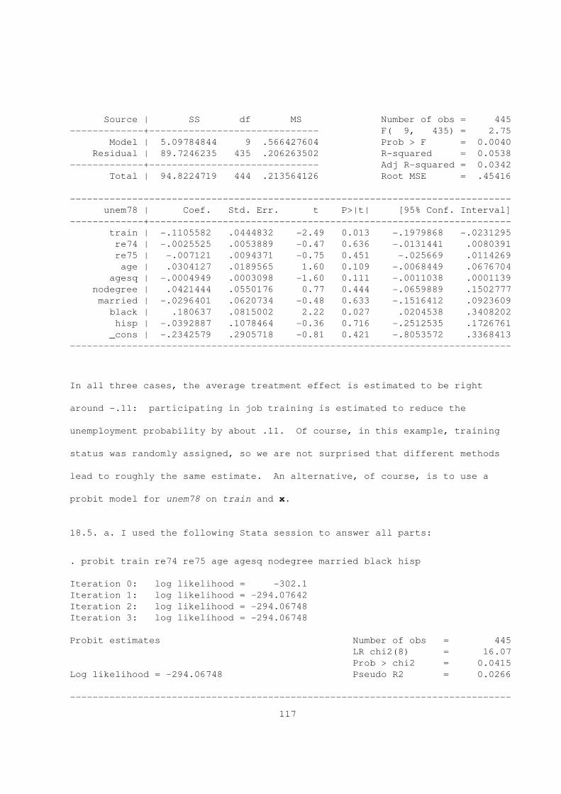
Source | SS df MS Number of obs = 445
-------------+------------------------------ F( 9, 435) = 2.75
Model | 5.09784844 9 .566427604 Prob > F = 0.0040
Residual | 89.7246235 435 .206263502 R-squared = 0.0538
-------------+------------------------------ Adj R-squared = 0.0342
Total | 94.8224719 444 .213564126 Root MSE = .45416
------------------------------------------------------------------------------
unem78 | Coef. Std. Err. t P>|t| [95% Conf. Interval]
-------------+----------------------------------------------------------------
train | -.1105582 .0444832 -2.49 0.013 -.1979868 -.0231295
re74 | -.0025525 .0053889 -0.47 0.636 -.0131441 .0080391
re75 | -.007121 .0094371 -0.75 0.451 -.025669 .0114269
age | .0304127 .0189565 1.60 0.109 -.0068449 .0676704
agesq | -.0004949 .0003098 -1.60 0.111 -.0011038 .0001139
nodegree | .0421444 .0550176 0.77 0.444 -.0659889 .1502777
married | -.0296401 .0620734 -0.48 0.633 -.1516412 .0923609
black | .180637 .0815002 2.22 0.027 .0204538 .3408202
hisp | -.0392887 .1078464 -0.36 0.716 -.2512535 .1726761
_cons | -.2342579 .2905718 -0.81 0.421 -.8053572 .3368413
------------------------------------------------------------------------------
In all three cases, the average treatment effect is estimated to be right
around -.11: participating in job training is estimated to reduce the
unemployment probability by about .11. Of course, in this example, training
status was randomly assigned, so we are not surprised that different methods
lead to roughly the same estimate. An alternative, of course, is to use a
probit model for unem78 on train and x.
18.5. a. I used the following Stata session to answer all parts:
. probit train re74 re75 age agesq nodegree married black hisp
Iteration 0: log likelihood = -302.1
Iteration 1: log likelihood = -294.07642
Iteration 2: log likelihood = -294.06748
Iteration 3: log likelihood = -294.06748
Probit estimates Number of obs = 445
LR chi2(8) = 16.07
Prob > chi2 = 0.0415
Log likelihood = -294.06748 Pseudo R2 = 0.0266
------------------------------------------------------------------------------
117
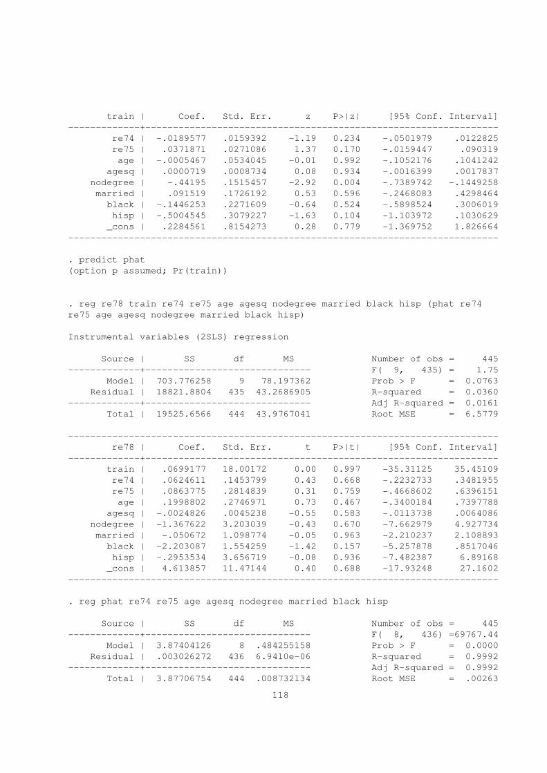
train | Coef. Std. Err. z P>|z| [95% Conf. Interval]
-------------+----------------------------------------------------------------
re74 | -.0189577 .0159392 -1.19 0.234 -.0501979 .0122825
re75 | .0371871 .0271086 1.37 0.170 -.0159447 .090319
age | -.0005467 .0534045 -0.01 0.992 -.1052176 .1041242
agesq | .0000719 .0008734 0.08 0.934 -.0016399 .0017837
nodegree | -.44195 .1515457 -2.92 0.004 -.7389742 -.1449258
married | .091519 .1726192 0.53 0.596 -.2468083 .4298464
black | -.1446253 .2271609 -0.64 0.524 -.5898524 .3006019
hisp | -.5004545 .3079227 -1.63 0.104 -1.103972 .1030629
_cons | .2284561 .8154273 0.28 0.779 -1.369752 1.826664
------------------------------------------------------------------------------
. predict phat
(option p assumed; Pr(train))
. reg re78 train re74 re75 age agesq nodegree married black hisp (phat re74
re75 age agesq nodegree married black hisp)
Instrumental variables (2SLS) regression
Source | SS df MS Number of obs = 445
-------------+------------------------------ F( 9, 435) = 1.75
Model | 703.776258 9 78.197362 Prob > F = 0.0763
Residual | 18821.8804 435 43.2686905 R-squared = 0.0360
-------------+------------------------------ Adj R-squared = 0.0161
Total | 19525.6566 444 43.9767041 Root MSE = 6.5779
------------------------------------------------------------------------------
re78 | Coef. Std. Err. t P>|t| [95% Conf. Interval]
-------------+----------------------------------------------------------------
train | .0699177 18.00172 0.00 0.997 -35.31125 35.45109
re74 | .0624611 .1453799 0.43 0.668 -.2232733 .3481955
re75 | .0863775 .2814839 0.31 0.759 -.4668602 .6396151
age | .1998802 .2746971 0.73 0.467 -.3400184 .7397788
agesq | -.0024826 .0045238 -0.55 0.583 -.0113738 .0064086
nodegree | -1.367622 3.203039 -0.43 0.670 -7.662979 4.927734
married | -.050672 1.098774 -0.05 0.963 -2.210237 2.108893
black | -2.203087 1.554259 -1.42 0.157 -5.257878 .8517046
hisp | -.2953534 3.656719 -0.08 0.936 -7.482387 6.89168
_cons | 4.613857 11.47144 0.40 0.688 -17.93248 27.1602
------------------------------------------------------------------------------
. reg phat re74 re75 age agesq nodegree married black hisp
Source | SS df MS Number of obs = 445
-------------+------------------------------ F( 8, 436) =69767.44
Model | 3.87404126 8 .484255158 Prob > F = 0.0000
Residual | .003026272 436 6.9410e-06 R-squared = 0.9992
-------------+------------------------------ Adj R-squared = 0.9992
Total | 3.87706754 444 .008732134 Root MSE = .00263
118

------------------------------------------------------------------------------
phat | Coef. Std. Err. t P>|t| [95% Conf. Interval]
-------------+----------------------------------------------------------------
re74 | -.0069301 .0000312 -222.04 0.000 -.0069914 -.0068687
re75 | .0139209 .0000546 254.82 0.000 .0138135 .0140283
age | -.0003207 .00011 -2.92 0.004 -.0005368 -.0001046
agesq | .0000293 1.80e-06 16.31 0.000 .0000258 .0000328
nodegree | -.1726018 .000316 -546.14 0.000 -.1732229 -.1719806
married | .0352802 .00036 98.01 0.000 .0345727 .0359877
black | -.0562315 .0004726 -118.99 0.000 -.0571603 -.0553027
hisp | -.1838453 .0006238 -294.71 0.000 -.1850713 -.1826192
_cons | .5907578 .0016786 351.93 0.000 .5874586 .594057
------------------------------------------------------------------------------
b. The IV estimate of a is very small -- .070, much smaller than when we
used either linear regression or the propensity score in a regression in
^Example 18.2. (When we do not instrument for train, a = 1.625, se = .640.)
The very large standard error (18.00) suggests severe collinearity among the
instruments.
^c. The collinearity suspected in part b is confirmed by regressing F oni
the x : the R-squared is .9992, which means there is virtually no separatei
^variation in F that cannot be explained by x .i i
d. This example illustrates why trying to achieve identification off of a
nonlinearity can be fraught with problems. Generally, it is not a good idea.
18.7. To be added.
18.9. a. We can start with equation (18.66),
y = h + xG + bw + wW(x - J)D + u + wWv + e,0
and, again, we will replace wWv with its expectation given (x,z) and an error.
But E(wWv|x,z) = E[E(wWv|x,z,v)|x,z] = E[E(w|x,z,v)Wv|x,z] = E[exp(p + xP +0 1
zP + p v)Wv|x,z] = xWexp(p + xP + zP ) where x = E[exp(p v)Wv], and we have2 3 0 1 2 3
119
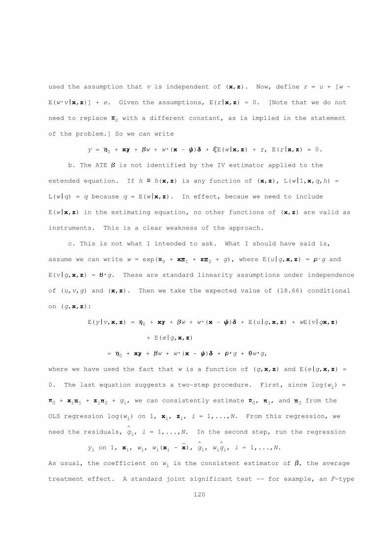
used the assumption that v is independent of (x,z). Now, define r = u + [w -
E(wWv|x,z)] + e. Given the assumptions, E(r|x,z) = 0. [Note that we do not
need to replace p with a different constant, as is implied in the statement0
of the problem.] So we can write
y = h + xG + bw + wW(x - J)D + xE(w|x,z) + r, E(r|x,z) = 0.0
b. The ATE b is not identified by the IV estimator applied to the
extended equation. If h _ h(x,z) is any function of (x,z), L(w|1,x,q,h) =
L(w|q) = q because q = E(w|x,z). In effect, becaue we need to include
E(w|x,z) in the estimating equation, no other functions of (x,z) are valid as
instruments. This is a clear weakness of the approach.
c. This is not what I intended to ask. What I should have said is,
assume we can write w = exp(p + xP + zP + g), where E(u|g,x,z) = rWg and0 1 2
E(v|g,x,z) = qWg. These are standard linearity assumptions under independence
of (u,v,g) and (x,z). Then we take the expected value of (18.66) conditional
on (g,x,z):
E(y|v,x,z) = h + xG + bw + wW(x - J)D + E(u|g,x,z) + wE(v|gx,z)0
+ E(e|g,x,z)
= h + xG + bw + wW(x - J)D + rWg + qwWg,0
where we have used the fact that w is a function of (g,x,z) and E(e|g,x,z) =
0. The last equation suggests a two-step procedure. First, since log(w ) =i
p + x P + z P + g , we can consistently estimate p , P , and P from the0 i 1 i 2 i 0 1 2
OLS regression log(w ) on 1, x , z , i = 1,...,N. From this regression, wei i i
^need the residuals, g , i = 1,...,N. In the second step, run the regressioni
----- ^ ^y on 1, x , w , w (x - x), g , w g , i = 1,...,N.i i i i i i i i
As usual, the coefficient on w is the consistent estimator of b, the averagei
treatment effect. A standard joint significant test -- for example, an F-type
120
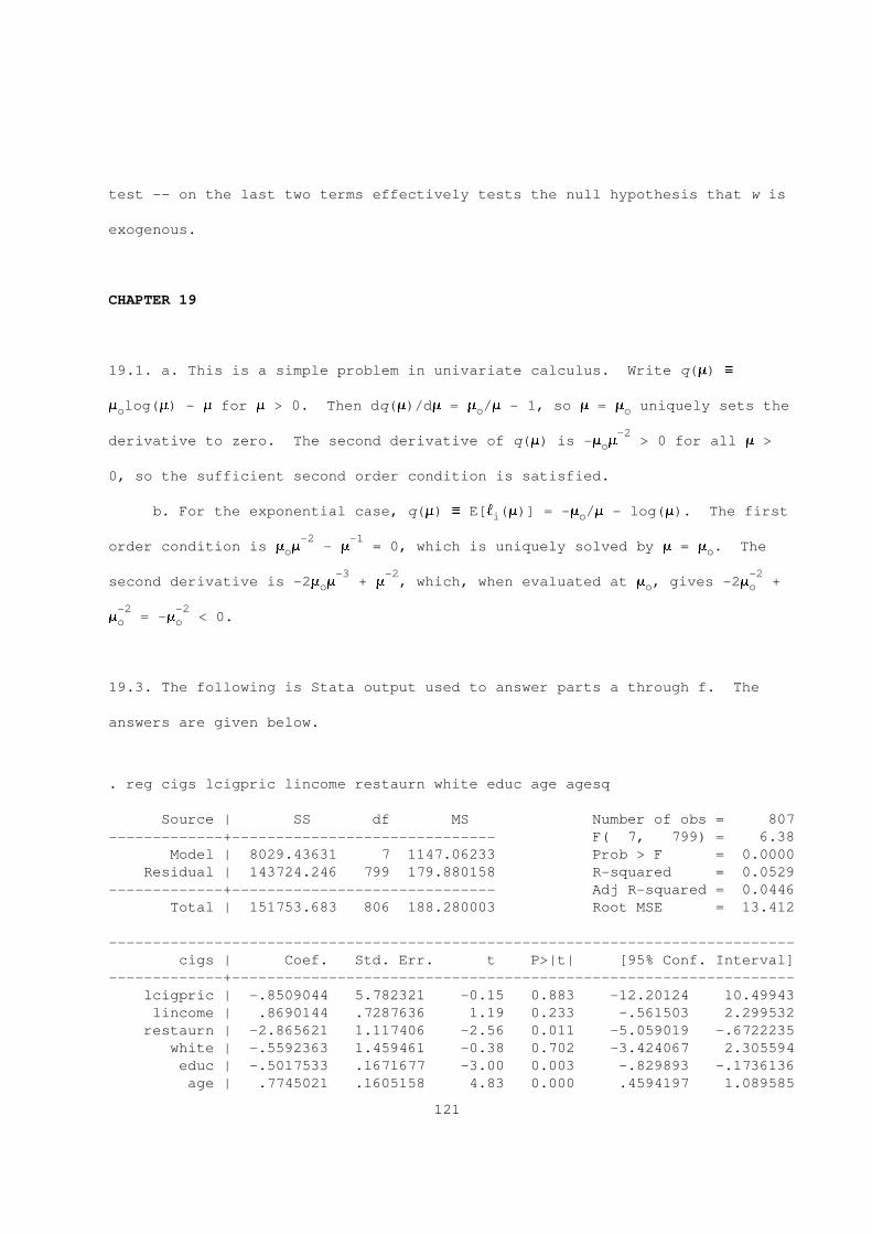
test -- on the last two terms effectively tests the null hypothesis that w is
exogenous.
CHAPTER 19
19.1. a. This is a simple problem in univariate calculus. Write q(m) _
m log(m) - m for m > 0. Then dq(m)/dm = m /m - 1, so m = m uniquely sets theo o o
-2derivative to zero. The second derivative of q(m) is -m m > 0 for all m >o
0, so the sufficient second order condition is satisfied.
b. For the exponential case, q(m) _ E[l (m)] = -m /m - log(m). The firsti o
-2 -1order condition is m m - m = 0, which is uniquely solved by m = m . Theo o
-3 -2 -2second derivative is -2m m + m , which, when evaluated at m , gives -2m +o o o
-2 -2m = -m < 0.o o
19.3. The following is Stata output used to answer parts a through f. The
answers are given below.
. reg cigs lcigpric lincome restaurn white educ age agesq
Source | SS df MS Number of obs = 807
-------------+------------------------------ F( 7, 799) = 6.38
Model | 8029.43631 7 1147.06233 Prob > F = 0.0000
Residual | 143724.246 799 179.880158 R-squared = 0.0529
-------------+------------------------------ Adj R-squared = 0.0446
Total | 151753.683 806 188.280003 Root MSE = 13.412
------------------------------------------------------------------------------
cigs | Coef. Std. Err. t P>|t| [95% Conf. Interval]
-------------+----------------------------------------------------------------
lcigpric | -.8509044 5.782321 -0.15 0.883 -12.20124 10.49943
lincome | .8690144 .7287636 1.19 0.233 -.561503 2.299532
restaurn | -2.865621 1.117406 -2.56 0.011 -5.059019 -.6722235
white | -.5592363 1.459461 -0.38 0.702 -3.424067 2.305594
educ | -.5017533 .1671677 -3.00 0.003 -.829893 -.1736136
age | .7745021 .1605158 4.83 0.000 .4594197 1.089585
121
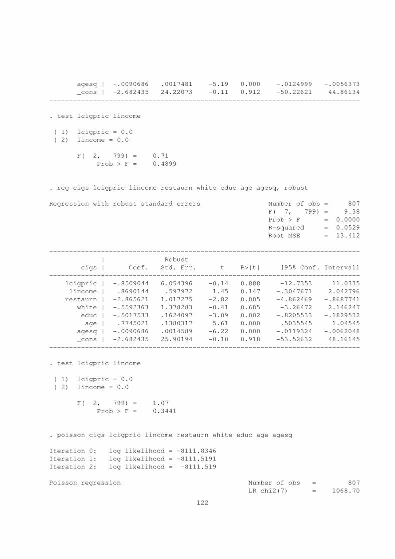
agesq | -.0090686 .0017481 -5.19 0.000 -.0124999 -.0056373
_cons | -2.682435 24.22073 -0.11 0.912 -50.22621 44.86134
------------------------------------------------------------------------------
. test lcigpric lincome
( 1) lcigpric = 0.0
( 2) lincome = 0.0
F( 2, 799) = 0.71
Prob > F = 0.4899
. reg cigs lcigpric lincome restaurn white educ age agesq, robust
Regression with robust standard errors Number of obs = 807
F( 7, 799) = 9.38
Prob > F = 0.0000
R-squared = 0.0529
Root MSE = 13.412
------------------------------------------------------------------------------
| Robust
cigs | Coef. Std. Err. t P>|t| [95% Conf. Interval]
-------------+----------------------------------------------------------------
lcigpric | -.8509044 6.054396 -0.14 0.888 -12.7353 11.0335
lincome | .8690144 .597972 1.45 0.147 -.3047671 2.042796
restaurn | -2.865621 1.017275 -2.82 0.005 -4.862469 -.8687741
white | -.5592363 1.378283 -0.41 0.685 -3.26472 2.146247
educ | -.5017533 .1624097 -3.09 0.002 -.8205533 -.1829532
age | .7745021 .1380317 5.61 0.000 .5035545 1.04545
agesq | -.0090686 .0014589 -6.22 0.000 -.0119324 -.0062048
_cons | -2.682435 25.90194 -0.10 0.918 -53.52632 48.16145
------------------------------------------------------------------------------
. test lcigpric lincome
( 1) lcigpric = 0.0
( 2) lincome = 0.0
F( 2, 799) = 1.07
Prob > F = 0.3441
. poisson cigs lcigpric lincome restaurn white educ age agesq
Iteration 0: log likelihood = -8111.8346
Iteration 1: log likelihood = -8111.5191
Iteration 2: log likelihood = -8111.519
Poisson regression Number of obs = 807
LR chi2(7) = 1068.70
122
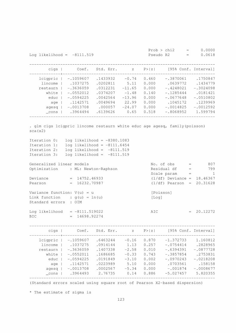
Prob > chi2 = 0.0000
Log likelihood = -8111.519 Pseudo R2 = 0.0618
------------------------------------------------------------------------------
cigs | Coef. Std. Err. z P>|z| [95% Conf. Interval]
-------------+----------------------------------------------------------------
lcigpric | -.1059607 .1433932 -0.74 0.460 -.3870061 .1750847
lincome | .1037275 .0202811 5.11 0.000 .0639772 .1434779
restaurn | -.3636059 .0312231 -11.65 0.000 -.4248021 -.3024098
white | -.0552012 .0374207 -1.48 0.140 -.1285444 .0181421
educ | -.0594225 .0042564 -13.96 0.000 -.0677648 -.0510802
age | .1142571 .0049694 22.99 0.000 .1045172 .1239969
agesq | -.0013708 .000057 -24.07 0.000 -.0014825 -.0012592
_cons | .3964494 .6139626 0.65 0.518 -.8068952 1.599794
------------------------------------------------------------------------------
. glm cigs lcigpric lincome restaurn white educ age agesq, family(poisson)
sca(x2)
Iteration 0: log likelihood = -8380.1083
Iteration 1: log likelihood = -8111.6454
Iteration 2: log likelihood = -8111.519
Iteration 3: log likelihood = -8111.519
Generalized linear models No. of obs = 807
Optimization : ML: Newton-Raphson Residual df = 799
Scale param = 1
Deviance = 14752.46933 (1/df) Deviance = 18.46367
Pearson = 16232.70987 (1/df) Pearson = 20.31628
Variance function: V(u) = u [Poisson]
Link function : g(u) = ln(u) [Log]
Standard errors : OIM
Log likelihood = -8111.519022 AIC = 20.12272
BIC = 14698.92274
------------------------------------------------------------------------------
cigs | Coef. Std. Err. z P>|z| [95% Conf. Interval]
-------------+----------------------------------------------------------------
lcigpric | -.1059607 .6463244 -0.16 0.870 -1.372733 1.160812
lincome | .1037275 .0914144 1.13 0.257 -.0754414 .2828965
restaurn | -.3636059 .1407338 -2.58 0.010 -.6394391 -.0877728
white | -.0552011 .1686685 -0.33 0.743 -.3857854 .2753831
educ | -.0594225 .0191849 -3.10 0.002 -.0970243 -.0218208
age | .1142571 .0223989 5.10 0.000 .0703561 .158158
agesq | -.0013708 .0002567 -5.34 0.000 -.001874 -.0008677
_cons | .3964493 2.76735 0.14 0.886 -5.027457 5.820355
------------------------------------------------------------------------------
(Standard errors scaled using square root of Pearson X2-based dispersion)
* The estimate of sigma is
123
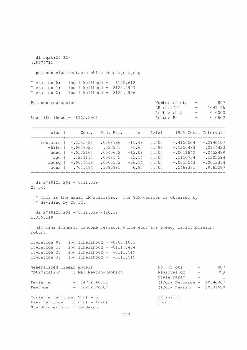
. di sqrt(20.32)
4.5077711
. poisson cigs restaurn white educ age agesq
Iteration 0: log likelihood = -8125.618
Iteration 1: log likelihood = -8125.2907
Iteration 2: log likelihood = -8125.2906
Poisson regression Number of obs = 807
LR chi2(5) = 1041.16
Prob > chi2 = 0.0000
Log likelihood = -8125.2906 Pseudo R2 = 0.0602
------------------------------------------------------------------------------
cigs | Coef. Std. Err. z P>|z| [95% Conf. Interval]
-------------+----------------------------------------------------------------
restaurn | -.3545336 .0308796 -11.48 0.000 -.4150564 -.2940107
white | -.0618025 .037371 -1.65 0.098 -.1350483 .0114433
educ | -.0532166 .0040652 -13.09 0.000 -.0611842 -.0452489
age | .1211174 .0048175 25.14 0.000 .1116754 .1305594
agesq | -.0014458 .0000553 -26.14 0.000 -.0015543 -.0013374
_cons | .7617484 .1095991 6.95 0.000 .5469381 .9765587
------------------------------------------------------------------------------
. di 2*(8125.291 - 8111.519)
27.544
. * This is the usual LR statistic. The GLM version is obtained by
. * dividing by 20.32:
. di 2*(8125.291 - 8111.519)/(20.32)
1.3555118
. glm cigs lcigpric lincome restaurn white educ age agesq, family(poisson)
robust
Iteration 0: log likelihood = -8380.1083
Iteration 1: log likelihood = -8111.6454
Iteration 2: log likelihood = -8111.519
Iteration 3: log likelihood = -8111.519
Generalized linear models No. of obs = 807
Optimization : ML: Newton-Raphson Residual df = 799
Scale param = 1
Deviance = 14752.46933 (1/df) Deviance = 18.46367
Pearson = 16232.70987 (1/df) Pearson = 20.31628
Variance function: V(u) = u [Poisson]
Link function : g(u) = ln(u) [Log]
Standard errors : Sandwich
124
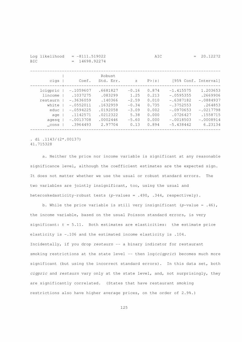
Log likelihood = -8111.519022 AIC = 20.12272
BIC = 14698.92274
------------------------------------------------------------------------------
| Robust
cigs | Coef. Std. Err. z P>|z| [95% Conf. Interval]
-------------+----------------------------------------------------------------
lcigpric | -.1059607 .6681827 -0.16 0.874 -1.415575 1.203653
lincome | .1037275 .083299 1.25 0.213 -.0595355 .2669906
restaurn | -.3636059 .140366 -2.59 0.010 -.6387182 -.0884937
white | -.0552011 .1632959 -0.34 0.735 -.3752553 .264853
educ | -.0594225 .0192058 -3.09 0.002 -.0970653 -.0217798
age | .1142571 .0212322 5.38 0.000 .0726427 .1558715
agesq | -.0013708 .0002446 -5.60 0.000 -.0018503 -.0008914
_cons | .3964493 2.97704 0.13 0.894 -5.438442 6.23134
------------------------------------------------------------------------------
. di .1143/(2*.00137)
41.715328
a. Neither the price nor income variable is significant at any reasonable
significance level, although the coefficient estimates are the expected sign.
It does not matter whether we use the usual or robust standard errors. The
two variables are jointly insignificant, too, using the usual and
heteroskedasticity-robust tests (p-values = .490, .344, respectively).
b. While the price variable is still very insignificant (p-value = .46),
the income variable, based on the usual Poisson standard errors, is very
significant: t = 5.11. Both estimates are elasticities: the estimate price
elasticity is -.106 and the estimated income elasticity is .104.
Incidentally, if you drop restaurn -- a binary indicator for restaurant
smoking restrictions at the state level -- then log(cigpric) becomes much more
significant (but using the incorrect standard errors). In this data set, both
cigpric and restaurn vary only at the state level, and, not surprisingly, they
are significantly correlated. (States that have restaurant smoking
restrictions also have higher average prices, on the order of 2.9%.)
125
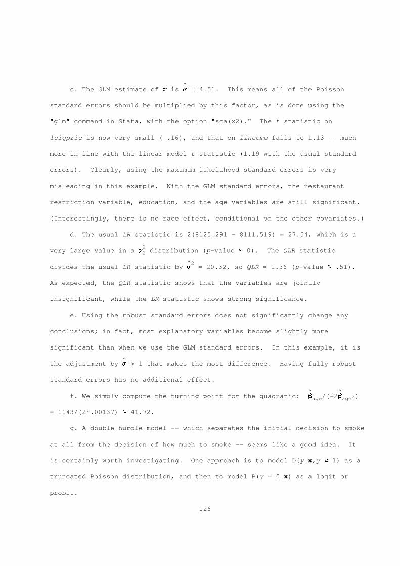
^c. The GLM estimate of s is s = 4.51. This means all of the Poisson
standard errors should be multiplied by this factor, as is done using the
"glm" command in Stata, with the option "sca(x2)." The t statistic on
lcigpric is now very small (-.16), and that on lincome falls to 1.13 -- much
more in line with the linear model t statistic (1.19 with the usual standard
errors). Clearly, using the maximum likelihood standard errors is very
misleading in this example. With the GLM standard errors, the restaurant
restriction variable, education, and the age variables are still significant.
(Interestingly, there is no race effect, conditional on the other covariates.)
d. The usual LR statistic is 2(8125.291 - 8111.519) = 27.54, which is a
2very large value in a c distribution (p-value ~ 0). The QLR statistic2
^2divides the usual LR statistic by s = 20.32, so QLR = 1.36 (p-value ~ .51).
As expected, the QLR statistic shows that the variables are jointly
insignificant, while the LR statistic shows strong significance.
e. Using the robust standard errors does not significantly change any
conclusions; in fact, most explanatory variables become slightly more
significant than when we use the GLM standard errors. In this example, it is
^the adjustment by s > 1 that makes the most difference. Having fully robust
standard errors has no additional effect.
^ ^f. We simply compute the turning point for the quadratic: b /(-2b 2)age age
= 1143/(2*.00137) ~ 41.72.
g. A double hurdle model -- which separates the initial decision to smoke
at all from the decision of how much to smoke -- seems like a good idea. It
is certainly worth investigating. One approach is to model D(y|x,y > 1) as a
truncated Poisson distribution, and then to model P(y = 0|x) as a logit or
probit.
126
19.5. a. We just use iterated expectations:
E(y |x ) = E[E(y |x ,c )|x ] = E(c |x )exp(x B)it i it i i i i i it
----- -----= exp(a + x G)exp(x B) = exp(a + x B + x G).i it it i
b. We are explicitly testing H : G = 0, but we are maintaining full0
independence of c and x under H . We have enough assumptions to derivei i 0
Var(y |x ), the T * T conditional variance matrix of y given x under H .i i i i 0
First,
Var(y |x ) = E[Var(y |x ,c )|x ] + Var[E(y |x ,c )|x ]it i it i i i it i i i
= E[c exp(x B)|x ] + Var[c exp(x B)|x ]i it i i it i
2 2= exp(a + x B) + t [exp(x B)] ,it it
2where t _ Var(c ) and we have used E(c |x ) = exp(a) under H . A similar,i i i 0
general expression holds for conditional covariances:
Cov(y ,y |x ) = E[Cov(y ,y |x ,c )|x ]it ir i it ir i i i
+ Cov[E(y |x ,c ),E(y |x ,c )|x ]it i i ir i i i
= 0 + Cov[c exp(x B),c exp(x B)|x ]i it i ir i
2= t exp(x B)exp(x B).it ir
2So, under H , Var(y |x ) depends on a, B, and t , all of which we can0 i i
estimate. It is natural to use a score test of H : G = 0. First, obtain0
~ ~ ~ ~~ ~ ~ ~consistent estimators a, B by, say, pooled Poisson QMLE. Let y = exp(a +it
~ ~ ~~ ~ ~ 2x B) and u = y - y . A consistent estimator of t can be obtained fromit it it it
a simple pooled regression, through the origin, of
~ ~ ~~2 ~ ~ 2u - y on [exp(x B)] , t = 1,...,T; i = 1,...,N.it it it
~2 2 2Call this estimator t . This works because, under H , E(u |x ) = E(u |x )0 it i it it
2 2= exp(a + x B) + t [exp(x B)] , where u _ y - E(y |x ). [We couldit it it it it it
2 2also use the many covariance terms in estimating t because t =
127
2 2E{[u /exp(x B)][u /exp(x B)]}, all t $ r.it it ir ir
Next, we construct the T * T weighting matrix for observation i, as in
~ ~Section 19.6.3; see also Problem 12.11. The matrix W (D) = W(x ,D) hasi i
~ ~~ ~2 ~ 2diagonal elements y + t [exp(x B)] , t = 1,...,T and off-diagonal elementsit it
~ ~~2 ~ ~ ~ ~t exp(x B)exp(x B), t $ r. Let a, B be the solutions toit ir
N ~ -1min (1/2) S [y - m(x ,a,B)]’[W (D)] [y - m(x ,a,B)],i i i i i
i=1a,Bth
where m(x ,a,B) has t element exp(a + x B). Since Var(y |x ) = W(x ,D),i it i i i
this is a MWNLS estimation problem with a correctly specified conditional
variance matrix. Therefore, as shown in Problem 12.1, the conditional
information matrix equality holds. To obtain the score test in the context
of MWNLS, we need the score of the comditional mean function, with respect to
all parameters, evaluated under H . Then, we can apply equation (12.69).0
Let Q _ (a,B’,G’)’ denote the full vector of conditional mean
parameters, where we want to test H : G = 0. The unrestricted conditional0
mean function, for each t, is
-----m (x ,Q) = exp(a + x B + x G).t i it i
Taking the gradient and evaluating it under H gives0
~ ~ ~ -----D m (x ,Q) = exp(a + x B)[1,x ,x ],q t i it it i
-----which would be 1 * (1 + 2K) without any redundancies in x . Usually, xi it
would contain year dummies or other aggregate effects, and these would be
----- ~dropped from x ; we do not make that explicit here. Let D M(x ,Q) denote thei q i
~T * (1 + 2K) matrix obtained from stacking the D m (x ,Q) from t = 1,...,T.q t i
~ ~ ~ ~Then the score function, evaluate at the null estimates Q _ (a,B’,G’)’, is
~ ~ ~ -1~s (Q) = -D M(x ,Q)’[W (D)] u ,i q i i i
~ ~ ~ ~where u is the T * 1 vector with elements u _ y - exp(a + x B). Thei it it it
128
estimated conditional Hessian, under H , is0
N~ -1 ~ ~ -1 ~A = N S D M(x ,Q)’[W (D)] D M(x ,Q),q i i q i
i=1
a (1 + 2K) * (1 + 2K) matrix. The score or LM statistic is therefore
N N -1& ~ ~ -1~ *’& ~ ~ -1 ~ *LM = S D M(x ,Q)’[W (D)] u S D M(x ,Q)’[W (D)] D M(x ,Q)q i i i q i i q i7 8 7 8i=1 i=1
N& ~ ~ -1~ *W S D M(x ,Q)’[W (D)] u .q i i i7 8i=1
a 2Under H , and the full set of maintained assumptions, LM ~ c . If only J < K0 K
-----elements of x are included, then the degrees of freedom gets reduced to J.i
In practice, we might want a robust form of the test that does not
require Var(y |x ) = W(x ,D) under H , where W(x ,D) is the matrix describedi i i 0 i
above. This variance matrix was derived under pretty restrictive
~assumptions. A fully robust form is given in equation (12.68), where s (Q)i
N~ ~ -1 ~ ~and A are as given above, and B = N S s (Q)s (Q)’. Since the restrictionsi i
i=1
~are written as G = 0, we take c(Q) = G, and so C = [0|I ], where the zeroK
matrix is K * (1 + K).
-----c. If we assume (19.60), (19.61) and c = a exp(a + x G) where a |x ~i i i i i
Gamma(d,d), then things are even easier -- at least if we have software that
estimates random effects Poisson models. Under these assumptions, we have
-----y |x ,a ~ Poisson[a exp(a + x B + x G)]it i i i it i
y , y are independent conditional on (x ,a ), t $ rit ir i i
a |x ~ Gamma(d,d).i i
In other words, the full set of random effects Poisson assumptions holds, but
-----where the mean function in the Poisson distribution is a exp(a + x B + x G).i it i
-----In practice, we just add the (nonredundant elements of) x in each timei
period, along with a constant and x , and carry out a random effects Poissonit
analysis. We can test H : G = 0 using the LR, Wald, or score approaches.0
Any of these wouldbe asymptotically efficient. But none is robust because we
129
have used a full distribution for y given x .i i
19.7. a. First, for each t, the density of y given (x = x, c = c) isit i i
ytf(y |x,c;B ) = exp[-cWm(x ,B )][cWm(x ,B )] /y !, y = 0,1,2,....t o t o t o t t
Multiplying these together gives the joint density of (y ,...,y ) given (xi1 iT i
= x, c = c). Taking the log, plugging in the observed data for observationi
i, and dropping the factorial term gives
T
S {-c m(x ,B) + y [log(c ) + log(m(x ,B))]}.i it it i itt=1
b. Taking the derivative of l (c ,B) with respect to c , setting thei i i
result to zero, and rerranging gives
T
(n /c ) = S m(x ,B).i i itt=1
Letting c (B) denote the solution as a function of B, we have c (B) =i i
T
n /M (B), where M (B) _ S m(x ,B). The second order sufficient conditioni i i itt=1
for a maximum is easily seen to hold.
c. Plugging the solution from part b into l (c ,B) givesi i
T
l [c (B),B] = -[n /M (B)]M (B) + S y {log[n /M (B)] + log[m(x ,B)]i i i i i it i i itt=1T
= -n + n log(n ) + S y {log[m(x ,B)/M (B)]i i i it it it=1
T
= S y log[p (x ,B)] + (n - 1)log(n ),it t i i it=1
because p (x ,B) = m(x ,B)/M (B) [see equation (19.66)].t i it i
N
d. From part c it follows that if we maximize S l (c ,B) with respect toi ii=1
(c ,...,c ) -- that is, we concentrate out these parameters -- we get exactly1 N
N N
S l [c (B),B]. But, except for the term S (n - 1)log(n ) -- which does noti i i ii=1 i=1
depend on B -- this is exactly the conditional log likelihood for the
conditional multinomial distribution obtained in Section 19.6.4. Therefore,
this is another case where treating the c as parameters to be estimated leadsi
-----us to a rN-consistent, asymptotically normal estimator of B .o
130
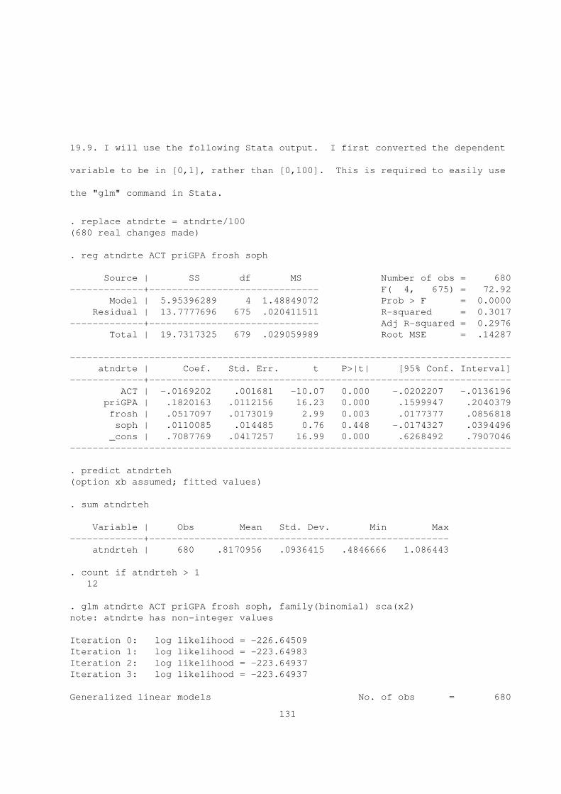
19.9. I will use the following Stata output. I first converted the dependent
variable to be in [0,1], rather than [0,100]. This is required to easily use
the "glm" command in Stata.
. replace atndrte = atndrte/100
(680 real changes made)
. reg atndrte ACT priGPA frosh soph
Source | SS df MS Number of obs = 680
-------------+------------------------------ F( 4, 675) = 72.92
Model | 5.95396289 4 1.48849072 Prob > F = 0.0000
Residual | 13.7777696 675 .020411511 R-squared = 0.3017
-------------+------------------------------ Adj R-squared = 0.2976
Total | 19.7317325 679 .029059989 Root MSE = .14287
------------------------------------------------------------------------------
atndrte | Coef. Std. Err. t P>|t| [95% Conf. Interval]
-------------+----------------------------------------------------------------
ACT | -.0169202 .001681 -10.07 0.000 -.0202207 -.0136196
priGPA | .1820163 .0112156 16.23 0.000 .1599947 .2040379
frosh | .0517097 .0173019 2.99 0.003 .0177377 .0856818
soph | .0110085 .014485 0.76 0.448 -.0174327 .0394496
_cons | .7087769 .0417257 16.99 0.000 .6268492 .7907046
------------------------------------------------------------------------------
. predict atndrteh
(option xb assumed; fitted values)
. sum atndrteh
Variable | Obs Mean Std. Dev. Min Max
-------------+-----------------------------------------------------
atndrteh | 680 .8170956 .0936415 .4846666 1.086443
. count if atndrteh > 1
12
. glm atndrte ACT priGPA frosh soph, family(binomial) sca(x2)
note: atndrte has non-integer values
Iteration 0: log likelihood = -226.64509
Iteration 1: log likelihood = -223.64983
Iteration 2: log likelihood = -223.64937
Iteration 3: log likelihood = -223.64937
Generalized linear models No. of obs = 680
131
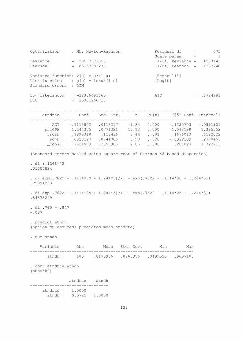
Optimization : ML: Newton-Raphson Residual df = 675
Scale param = 1
Deviance = 285.7371358 (1/df) Deviance = .4233143
Pearson = 85.57283238 (1/df) Pearson = .1267746
Variance function: V(u) = u*(1-u) [Bernoulli]
Link function : g(u) = ln(u/(1-u)) [Logit]
Standard errors : OIM
Log likelihood = -223.6493665 AIC = .6724981
BIC = 253.1266718
------------------------------------------------------------------------------
atndrte | Coef. Std. Err. z P>|z| [95% Conf. Interval]
-------------+----------------------------------------------------------------
ACT | -.1113802 .0113217 -9.84 0.000 -.1335703 -.0891901
priGPA | 1.244375 .0771321 16.13 0.000 1.093199 1.395552
frosh | .3899318 .113436 3.44 0.001 .1676013 .6122622
soph | .0928127 .0944066 0.98 0.326 -.0922209 .2778463
_cons | .7621699 .2859966 2.66 0.008 .201627 1.322713
------------------------------------------------------------------------------
(Standard errors scaled using square root of Pearson X2-based dispersion)
. di (.1268)^2
.01607824
. di exp(.7622 - .1114*30 + 1.244*3)/(1 + exp(.7622 - .1114*30 + 1.244*3))
.75991253
. di exp(.7622 - .1114*25 + 1.244*3)/(1 + exp(.7622 - .1114*25 + 1.244*3))
.84673249
. di .760 - .847
-.087
. predict atndh
(option mu assumed; predicted mean atndrte)
. sum atndh
Variable | Obs Mean Std. Dev. Min Max
-------------+-----------------------------------------------------
atndh | 680 .8170956 .0965356 .3499525 .9697185
. corr atndrte atndh
(obs=680)
| atndrte atndh
-------------+------------------
atndrte | 1.0000
atndh | 0.5725 1.0000
132
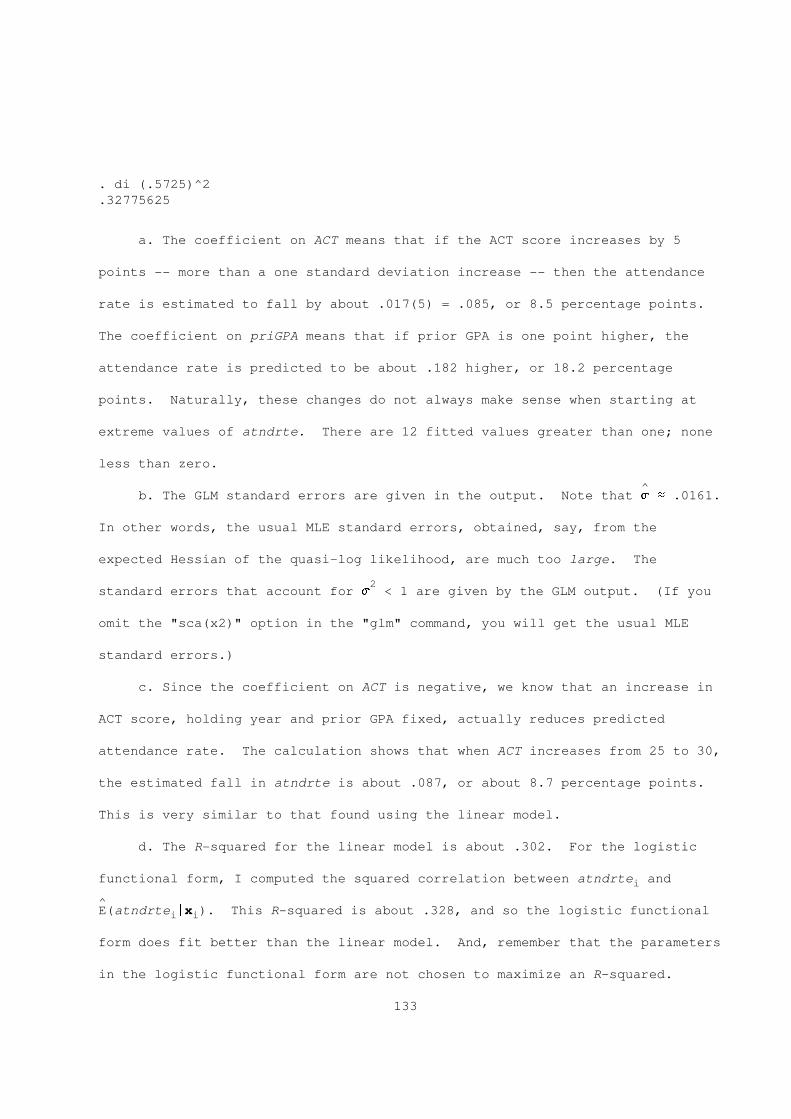
. di (.5725)^2
.32775625
a. The coefficient on ACT means that if the ACT score increases by 5
points -- more than a one standard deviation increase -- then the attendance
rate is estimated to fall by about .017(5) = .085, or 8.5 percentage points.
The coefficient on priGPA means that if prior GPA is one point higher, the
attendance rate is predicted to be about .182 higher, or 18.2 percentage
points. Naturally, these changes do not always make sense when starting at
extreme values of atndrte. There are 12 fitted values greater than one; none
less than zero.
^b. The GLM standard errors are given in the output. Note that s ~ .0161.
In other words, the usual MLE standard errors, obtained, say, from the
expected Hessian of the quasi-log likelihood, are much too large. The
2standard errors that account for s < 1 are given by the GLM output. (If you
omit the "sca(x2)" option in the "glm" command, you will get the usual MLE
standard errors.)
c. Since the coefficient on ACT is negative, we know that an increase in
ACT score, holding year and prior GPA fixed, actually reduces predicted
attendance rate. The calculation shows that when ACT increases from 25 to 30,
the estimated fall in atndrte is about .087, or about 8.7 percentage points.
This is very similar to that found using the linear model.
d. The R-squared for the linear model is about .302. For the logistic
functional form, I computed the squared correlation between atndrte andi
^E(atndrte |x ). This R-squared is about .328, and so the logistic functionali i
form does fit better than the linear model. And, remember that the parameters
in the logistic functional form are not chosen to maximize an R-squared.
133
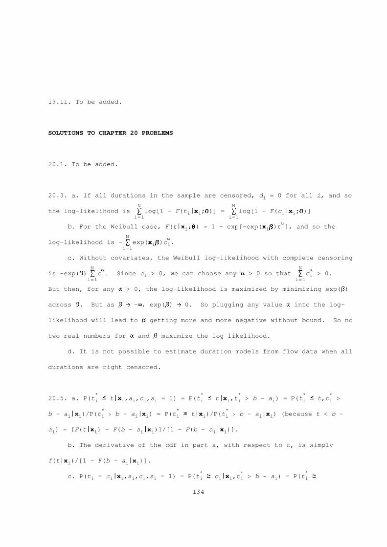
19.11. To be added.
SOLUTIONS TO CHAPTER 20 PROBLEMS
20.1. To be added.
20.3. a. If all durations in the sample are censored, d = 0 for all i, and soi
N N
the log-likelihood is S log[1 - F(t |x ;Q)] = S log[1 - F(c |x ;Q)]i i i ii=1 i=1
ab. For the Weibull case, F(t|x ;Q) = 1 - exp[-exp(x B)t ], and so thei i
N alog-likelihood is - S exp(x B)c .i i
i=1
c. Without covariates, the Weibull log-likelihood with complete censoring
N Na ais -exp(b) S c . Since c > 0, we can choose any a > 0 so that S c > 0.i i i
i=1 i=1
But then, for any a > 0, the log-likelihood is maximized by minimizing exp(b)
across b. But as b L -8, exp(b) L 0. So plugging any value a into the log-
likelihood will lead to b getting more and more negative without bound. So no
two real numbers for a and b maximize the log likelihood.
d. It is not possible to estimate duration models from flow data when all
durations are right censored.
* * * * *20.5. a. P(t < t|x ,a ,c ,s = 1) = P(t < t|x ,t > b - a ) = P(t < t,t >i i i i i i i i i i i
* * *b - a |x )/P(t > b - a |x ) = P(t < t|x )/P(t > b - a |x ) (because t < b -i i i i i i i i i i
a ) = [F(t|x ) - F(b - a |x )]/[1 - F(b - a |x )].i i i i i i
b. The derivative of the cdf in part a, with respect to t, is simply
f(t|x )/[1 - F(b - a |x )].i i i
* * *c. P(t = c |x ,a ,c ,s = 1) = P(t > c |x ,t > b - a ) = P(t >i i i i i i i i i i i i
134
*c |x )/P(t > b - a |x ) (because c > b - a ) = [1 - F(c |x )]/[1 - F(b -i i i i i i i i i
a |x )].i i
20.7. a. We suppress the parameters in the densities. First, by (20.22) and
*D(a |c ,x ) = D(a |x ), the density of (a ,t ) given (c ,x ) does not dependi i i i i i i i i
on c and is given by k(a|x )f(t|x ) for 0 < a < b and 0 < t < 8. This isi i i
also the conditional density of (a ,t ) given (c ,x ) when t < c , that is,i i i i i
the observation is uncensored. For t = c , the density is k(a|x )[1 -i i
F(c |x )], by the usual right censoring argument. Now, the probability ofi i
*observing the random draw (a ,c ,x ,t ), conditional on x , is P(t > b -i i i i i i
a ,x ), which is exactly (20.32). From the standard result for densities fori i
truncated distributions, the density of (a ,t ) given (c ,d ,x ) and s = 1 isi i i i i i
d (1 - d )i ik(a|x )[f(t|x )] [1 - F(c |x )] /P(s = 1|x ),i i i i i i
for all combinations (a,t) such that s = 1. Putting in the parameters andi
taking the log gives (20.56).
b. We have the usual tradeoff between robustness and efficiency. Using
the log likelihood (20.56) results in more efficient estimators provided we
have the two densities correctly specified; (20.30) requires us to only
specify f(W|x ).i
20.9. To be added.
135
Related Documents


