Solution of the elastic/visco-plastic constitutive equations: A finite volume approach

Solution of the elastic / visco-plastic constitutive equations: A finite volume approach

G. A. Taylor, C. Bailey and M. Cross

Centre for Numerical Modelling and Process Analysis, University of Greenwich, London, UK

A novel two dimensional finite volume (FV) approach to the solution of elastic / uisco-plastic solid mechanics problems is described. The numerical procedure is an extension of that developed by Fryer et al. for linear elastic materials and utilizes an unstructured mesh. The procedure is compared favorably with conventional finite element (FE) formulations with respect to both accuracy and CPU time. A number of test problems demonstrate the ability of the FV procedure to model a range of boundary constraints, in addition to mechanical and thermal loads. It might be argued from the work reported here that the FV approach shows the potential to be at least as effective as conventional FE formulations in representing nonlinear solid mechanics behavior.

Keywords: finite volume, visco-plastic, casting

1. Introduction

During the last 30 years a number of discretization techniques have evolved for the solution of differential equations describing a wide range of physical phenomena. The two families of methods that are most widely employed within the computational mechanics community are the finite element (FE) and the finite volume (FV) procedures. Historically the FE method evolved from the solid/structural mechanical analysis to handle both linear and nonlinear solid mechanics phenomena. Of course this method is also well established in the modelling of acoustics, heat transfer, fluid flow, and electromagnetism.’ The FV method evolved from early finite difference techniques essentially from the heat transfer community and has been extensively used for computational fluid dynamics (CFD) for a wide range of phenomena including combustion, free surface flows and multi-phase flo~s.~,~ The main reason for the popularity of the FV method for flow problems is its ability to conserve physical quantities at a local as well as a global level. Indeed, it may be argued that FV formulations for highly nonlinear problems, including free surface and multiphase flows, are potentially superior to their FE equivalents because of their local conservation properties. This feature is particularly beneficial in flow problems where there are nonsmooth sources to be accounted for. In essence with the FV procedure there is no artificial cre-

Address reprint requests to Prof. Mark Cross, University of Greenwich, Centre for Numerical Modelling and Process Analysis, Wellington Street,

Woolwich, London, SE18 6PF, U.K.

Received 23 March 1995; revised 26 April 1995; accepted 10 May 1995

Appl. Math. Modelling 1995, Vol. 19, December 0 1995 by Elsevier Science Inc. 655 Avenue of the Americas, New York, NY 10010

ation or destruction of a conserved variable as it is trans- ported from one control volume to the next.2,3 Errors that arise are due solely to a combination of the coarseness of the mesh and the approximations used to represent the way variables are assumed to change across mesh elements.

Recently, interest in developing FV methods in solid mechanics has been rekindled.4Ts A number of methods have used structured meshes and, unfortunately, although they have showed encouraging results for linear elastic problems, these procedures are problematic when applied to complex geometries for all the usual reasons. Alterna- tively, DemirdiiC et al. 6,7 have developed a cell-centered FV solution procedure that is applicable to structured and unstructured meshes. A FV procedure has been discussed by Ohate et al.’ on a generic way for unstructured meshes and Fryer et a1.9S’0 have developed and implemented a vertex-based FV solution procedure for solving linear elastic solid mechanics problems on an unstructured mesh using triangular and quadrilateral mesh elements. This solution procedure has been extended and compared with FE predictions in three dimensions2 against a number of benchmark problems which illustrate the robustness and the efficiency of the FV formulation. The procedure has been coupled with fluid flow and solidification algorithms to produce a multiphysics framework for the simulation of a metal casting process.“-r3

The objective of this paper is to extend the formulation of Fryer et al9 to incorporate the nonlinear material properties of elastic/visco-plasticity and demonstrate the performance of the developed FV procedure against typical FE formulations for a number of test cases. For reasons of clarity the analysis in this paper is restricted to two dimensions.

0307-904x/95/$10.00 SSDI 0307-904X(95)00093-Y

2. Elastic/ visco-plastic modelling approach

The combined phenomena of creep and plasticity may be modelled using a visco-plastic material law that can be expressed as a unified constitutive equation. The ultimate objective of this work is to develop a FV procedure that can cope with any kind of nonlinear material law. How- ever, the initial objective is to explore the extent to which an effective procedure could be developed for a common form of elastic/visco-plastic law. As such, a widely accepted modification of the elastic/visco-plastic model pro- posed by Perzyna l4 is utilized in the present work. The underlying assumption is that the viscous properties are only apparent after the material has yielded. For an elastic/visco- lastic material, the total strain is the sum of its elastic E($, visco-plastic cVP, and initial L$) multiaxial components:

E = &e) + .@P) + .(O (1)

The inelastic strain represents combined viscous and plastic effects, and the initial strain represents autogenous strains as produced by thermal expansion or transformation of the material. In Equation 1 all the strains are represented by vectors of the following form E = {E,, .sy,, E,~}~. The stress is dependent on the elastic strain,

U = DEce) (2)

where a = {a,, uYr aXy}’ is the stress vector, and D is the well known elasttctty matrix, which for a plane stress approximation reduces to

lu 0 E vl 0

D=-

I I

l-Y2 o o 1-v

2

where E and v are the Youngs modulus and Poissons ratio, respectively. The theory can also be applied without any loss of generality to plane strain and axisymmetric approximations. As the material has no viscous properties in the elastic region, the static yield criterion will not differ from that of the classical inviscid theory of plasticity,15 hence the limit criterion for yielding can be defined as a function of the stress components only, which is a modification of the original Perzyna model.14 From this theory we can introduce a generic scalar yield function of the form

F==(g) -Y (3)

such that F < 0 depicts the purely elastic region and, in this case, Y is the uniaxial yield stress. Y may also be a function of a hardening parameter, though strain hardening (and softening) are neglected in this instance and, there- fore, a constant yield stress is assumed for simplicity.

To develop this well-established theory, the general visco-plastic flow rule’6-‘8 is adopted

d &“P=_E”P=

dt (4)

in which a power law has been applied to the normalized

Elastic/visco-plastic constitutive equations: G. A. Taylor et al.

yield function 5, the concept of a plastic potential Q is employed as described by the classical theory of plasticity,15 and y is a fluidity parameter which can be dependent on state variables.

To ensure that visco-plastic flow only occurs after yielding we equate

if F<O

(t(G))=t(G) if FaO

In this case we only consider an associative law15, thus we are independent of hydrostatic pressure and are constrained by the equivalence of the yield function and the plastic potential, i.e.

Q=F

The von-Mises yield criterion is specifically utilized in Equation (3) to obtain the following yield function formulation,

F&““-Y=m-Y= 3

r -sijs,, - Y 2

where ~(~‘o is the von-Mises or effective stress and J; is the second invariant of the deviatoric stress tensor sij, which is defined below as

1 s II = mjj - &,?Trace( gij)

Hence, it may be shown quite simply that the visco-plastic strain rate is defined by the following specific flow rule, where the conditionals ( ) indicate that zero or the function value is returned depending on if the enclosed function is negative or not, respectively:

N 3

2,0S (5)

(In most cases N is simply taken as unity.) Completing the formulation of the constitutive equations the following relationship is obtained

(T = DE(e) = D[ E _ &P) _ &)I (6)

where the nonlinear dependency on stress is obviously indicated via the stress dependency of c(“~). This formulation has been used by a number of workers including Zienkiewicz et al.,16x19 where other yield surfaces, such as, Tresca, Mohr-Coulomb, etc., are described. These are applicable to both metals and other materials, such as con- cretes and soils. The formulation described here will apply generally to any yield surface, including nonassociative relationships. The materials in this formulation are assumed to be isotropic and homogeneous, though the theory can be extended to include anisotropic and heterogenous materials.

The theory is applicable for a quasistatic problem and it should be noted that if a steady-state solution is asymptoti- cally approached over a load increment, then the

Appl. Math. Modelling, 1995, Vol. 19, December 747

Elastidvisco-plastic constitutive equations: G. A. Taylor et al.

The displacements within any mesh element depend upon the local natural co-ordinates s and t according to

U(S, t) = &vi&=N+ (9) i= 1

Integration points where m is the total number of nodes associated with a mesh element and N, and +i are the shape functions and nodal displacements respectively.22x23

Integrating equation (7) over a control volume using the divergence theorem and substituting in equations (6) and (8) yields the following discretized governing equation

Figure 1. Vertex-based discretization.

elastic/visco-plastic method is equivalent to an acceler- ated solution technique for elastic/plastic problems, with a pseudo-time marching scheme.16~‘8

$ DLu.nd.4 =

s #DBc$. nd4 = /Fdu + $DE(~~) ’ n&I

: #DC(~) . ndA ’

s

s

3. Governing equations and discretization The general equation for static equilibrium at any point within the material, including internal body forces, can be described using tensor notation, by

aa 2 =F, axj (7)

where F, represents body forces in the i direction. Figure 1, depicts a two-dimensional domain meshed

with triangular and quadrilateral elements. For the FV procedure, the above equilibrium equations are integrated over control volumes. The location of the control volume within the meshed domain has led to a number of varia- tions of the FV method,” i.e. cell-centered, node-centered, etc. The control volumes in this analysis are generated by connecting the centers of the mesh elements to the mid- points of the respective faces, thus creating subcontrol volumes in each of the mesh elements. Combining all the subcontrol volumes from the mesh elements associated with a node creates a polyhedra type cell that surrounds each of the nodes representing the vertices of the mesh elements. The generation of control volumes in this manner is known as the node centered arrangement.” It is also the control volume structure that Baliga and Patankar” used in their CV-FE solution procedures for fluid flow and heat transfer.

where B = LN. The above surface integrals are approximated at the integration points located at the centers of the subcontrol volume faces. It should be noted that derivatives calculated at these faces will be the same for adjacent control volumes, leading to both the local and global conservation principle. Alternatively a finite element formulation can be performed based on the Galerkin procedure, where Gauss quadrature is employed to obtain the required volume integrals.2

The basic steps of a FV formulation are described below. In this case we adhere to a plane stress approximation though a full three-dimensional description is a straightforward extension of the formulation. The total strain can be expressed in terms of the elastic and visco- plastic strains:

1 E =- (T - XX E( XX UUJ + &$P’,p’

E I( YY = 2 UYY - ua,,)+ &g?)

& XY

=;(l+v)u-y+~~)

It is possible to formulate the following governing equation by employing the well known infinitesimal rela- tions for total strain and displacement:

&=Lu (8) where u = (u,uJr is the displacement vector representing displacements in the x and y directions, respectively, and L is a linear differential operator:

a - 0 ax

a L= 0 ay

a a

Here the initial strain is neglected to simplify the analysis without any loss of generality. The stress can now be obtained in terms of strain by a number of simple algebraic steps. The direct and shear stress components may be expressed as

ay ax

u =- xx 1:” E( i & xx - &Jy)

VE +-

l-v (%, + &yy + Ep 11

(T =- (VP) YY 1:” E( [

& YY - &YY 1

VE +-

l-v (5, + Eyy + Ep )I (T xy=

748 Appl. Math. Modelling, 1995, Vol. 19, December

Utilizing the governing equations previously derived and substituting in the above stress-strain and strain-displacement relationships, the following discretized equations can be obtained, where the modifications to the applied loads due to the visco-plastic corrections are included, i.e.

+@(g+J++4]=S,

&$[f(~+++ 1 f-

#[(

au au I - Ll s ay -+% i 11 ‘ny at4 =S,

where

S,= F,dV+ - / L’

u - _g(“P) . n, &

1-v == I

The derivatives in the above integrals can be approximated at the integration points on the surfaces, by the derivatives of equation (9) with respect to the local co-ordinate system. The global derivatives can then be obtained with a transformation using the related Jacobian in the normal manner.2

A system of equations for the discretized variable $ can be constructed via assembling contributions from all control volumes associated with a finite volume formulation and is given below in matrix notation where K is equivalent to the familiar stiffness matrix (a similar system of equations can be constructed from element contributions with a FE formulation), i.e.

G(4) =K(4)4-f-O (10) The load contributions generated by the visco-plastic strains modify the load vector f incrementally, resulting in an iterative solution technique.

4. Numerical procedure

The numerical process can be identified in some sense with the solution of a nonlinear first-order system of ordinary differential equations.24 A number of established solution techniques are available, but in this solution a fully explicit initial strain procedure’,16 is utilized. This technique is equivalent to a modified Newton-Raphson method and requires a Euler approximation for the time

integration to obtain a visco-plastic strain increment. The benefits of this procedure are relative simplicity and a reduction in computation due to the employment of a constant stiffness matrix. There are disadvantages to this procedure with regard to efficiency, accuracy, and stability, but in comparing FV with FE formulations, the procedure is practical. At each iteration the above system of equations is solved, using a conjugate gradient solver with diagonal scaling.25 For a specified elastic/visco-plastic problem, the total external load can be applied over one increment, as opposed to the usual incremental load appli- cations generally associated with non-linear deformation problems.16 In the following cases the external loads were applied over one increment. The numerical procedure is as follows: l Step 1: Assume known values of variables an, +n, cyp

and f, at time instant t,. Calculate the visco- plastic strain rate using equation 5:

. Step 2: Determine the approximate change in E(“~) and update t:

&+T) = n @‘)A t, t, + 1 = t,, + At,

l Step 3: Update the total visco-plastic strain at the cur -

rent instant in time:

E$P)I = #P) + A,(“P) n n

l Step 4: Update the load vector f:

f n+ 1 = p + $Dc~‘_“{ . n&l s

where p represents the applied loads. l Step 5: Calculate the associated displacement and stress:

4 n+ I =KPfn+1 CT n+ 1 = D( E,+, - &;+p)1)

= DB& + , - DC;‘+“;

0 Return to step 1 and repeat with the new values for the next time interval. The solution has converged if the Euclidian norm ratio of the effective visco-plastic strain rate is within tolerance, i.e.

II $“P) II ~ X 100 < Tolerance II $“P) )I

In implementing the algorithm, an approximation was employed for the stress and strain variables. As opposed to storing the variables at integration or Gauss points, the variables are stored only at mesh element centers, thus considerably reducing the storage required. This approach is obviously applicable to 3-noded constant strain triangular elements, where the quantities are invariant over the mesh element, but it is an approximation for 4-noded quadrilateral elements, where the quantities actually vary over a mesh element. This variation will become negligible for a suitably fine mesh, justifying the approximation.




Plane Stress

X

Perforation Diameter : 1Omm

t t t tC t t tD

200mm

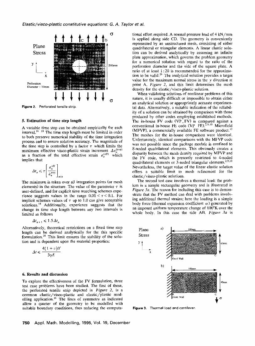
Figure 2. Perforated tensile strip.

5. Estimation of time step length

A variable time step can be obtained empirically for each interval.16-18 The time step length must be limited in order to both preserve numerical stability of the time integration process and to ensure solution accuracy. The magnitude of the time step is controlled by a factor 7 which limits the maximum effective visco-plastic strain increment A&ievp) as a fraction of the total effective strain &FfQ which implies that:

min

The minimum is taken over all integration points (or mesh elements) in the structure. The value of the parameter 7 is user-defined, and for explicit time marching schemes experience suggests values in the range 0.01 < T < 0.1. For implicit schemes values of T up to 1.0 can give acceptable solutions.” Additionally, experience suggests that the change in time step length between any two intervals is limited as follows

At/l+ 1 < lSAt,

Alternatively, theoretical restrictions on a fixed time step length can be derived analytically for the this specific formulation.24 This limit ensures the stability of the solution and is dependent upon the material properties:

At,< 4(1+ U)Y

3yE

6. Results and discussion

To explore the effectiveness of the FV formulation, three test case problems have been studied. The first of these, the perforated tensile strip depicted in Figure 2, is a common elastic/visco-plastic and elastic/plastic modelling application.16 The lines of symmetry as indicated allow a quarter of the geometry to be modelled with suitable boundary conditions, thus reducing the computa-

tional effort required. A normal pressure load of 4 kN/mm is applied along side CD. The geometry is conveniently represented by an unstructured mesh, consisting of either quadrilateral or triangular elements. A linear elastic solution can be derived analytically by assuming an infinite plate approximation, which governs the problem geometry for a numerical solution with regard to the ratio of the perforation diameter and the side of the square plate. A ratio of at least 1: 20 is recommended for the approximation to be valid.2” The analytical solution provides a target value for the maximum normal stress in the y direction at point A, Figure 2, and this limit determines the mesh density for the elastic/visco-plastic solution.

When validating solutions of nonlinear problems of this nature, it is usually difficult or impossible to obtain either an analytical solution or appropriately accurate experimental data. Alternatively, a suitable indication of the reliabil- ity of a solution can be obtained by comparison with those produced by other codes employing established methods. The in-house FV code (VP_FV) is corn

! ared against a

conventional in-house FE code (VP-FE). 19,” Microfield (MFVP), a commercially available FE software product.18 The meshes for the in-house comparison were identical. Unfortunately, identical comparisons with the MFVP code was not possible since the package module is confined to 8-noded quadrilateral elements. This obviously creates a disparity between the mesh density required by MFVP and the FV code, which is presently restricted to 4-noded quadrilateral elements or 3-noded triangular elements.2,9.‘0 Nevertheless, the target value of the linear elastic solution offers a suitable limit to mesh refinemknt for the elastic/visco-plastic solutions.

The second test case involves a thermal load; the problem is a simple rectangular geometry and is illustrated in Figure 3a. The reason for including this case is to demonstrate that the FV method can deal with problems involving additional thermal strains; here the loading is a simple body force (thermal expansion coefficient (Y) generated by an imposed uniform temperature change of 100°K over the whole body. In this case the side AB, Figure 3a is

Plane a) IOOmm

Stress

Yk

/ X

4Omm

IFixed Wall

b)

Figure 3. Thermal load and cantilever.


ElastWvisco-plastic constitutive equations: G. A. Taylor et al.

constrained, which will produce symmetric peaks of effective (equivalent) stress at the Points A and B. There is a line of symmetry as illustrated for this problem, but in this case the whole geometry was modelled as a test for robustness.

Finally, Figure 3b describes a cantilever problem that has the same geometry as the previous thermal load problem. This problem illustrates the flexibility of the FV procedure in modelling problems with a shear pressure load of 1 kN/mm, along side CD and a constrained side AB.

The results in Tables l-22 describe for each of the test cases over a number of yield stresses the variation of the

displacements at points close to or within the visco-plastic regions and the number of pseudo-time steps required for a converged solution. Changes in displacements are negligible when comparing the linear elastic solution to the nonlinear solutions at points far from the visco-plastic region. The tabulated infinite yield stress and zero pseudo- time step relates to the linear elastic solution. When comparing differing solution techniques with respect to displacements at nodes there is no difficulty when employing the same mesh, but when the meshes are different it is not always possible to obtain coincident nodes at specific points of interest. This is shown in Tables 1, 2 and 3, where the meshes differ considerably and it was only

Table 1. Perforation

Displacement component (mm) No. of pseudo-time steps

Yield stress VP_ FV MFVP VP_ FV MFVP

5500 + 0.3259 + 0.3398 143 144 6500 +0.3122 +0.3186 98 94 7500 + 0.3057 + 0.3099 68 71 Infinity + 0.2990 +0.3019 none none

VP FV mesh: 275 nodes, 240 4-noded quadrilaterals; MFVP mesh: 225 nodes, 64 8-noded quadrilaterals; Elastic maximum effective stress at Point A, Figure 1; VP_ FV: 9.952 kN/mm; MFIELD: 10.040 kN/mm. The material properties are the same for all cases and the tolerance was 1.0~10-~. ~=0.3;y=1x10-4s-‘;E=200kN/mm;~=1x10~4K-’. Variable pseudo-time stepping scheme: T= 0.01

Table 2. Thermal load

No. pseudo-time steps

Yield stress Y VP_ FV MFVP 2800 53 54

VP_FV mesh: 289 nodes, 256 4-node quadrilaterals; MFVP mesh: 225 nodes, 64 8-noded quadrilaterals; elastic maximum effective stress at Point 6, Figure 2; VP_FV: 3.637 kN/mm; VP-FE: 3.691 kN/ mm. The material properties are the same for all cases and the tolerance was 1.0 x 10-4. v=O.3; ~=lxlO-~ s-‘; E=200 kN/mm; a= 1 x 10e4 Km’. Variable pseudo-time stepping scheme: 7 = 0.01

Table 3. Cantilever

No. of pseudo-time steps

Yield stress Y VP_ FV MFVP

1100 100 74 1200 64 49 1300 45 35

VP_FV mesh: 289 nodes, 256 4-noded quads; MFVP mesh; 93 nodes, 24 8-noded quads; elastic maximum effective stress at point B, Figure 3; VP_ FV: 1.530 kN/mm; VP_ FE: 1.554 kN/mm. The material properties are the same for all cases and the tolerance was 1.0 x 10-4. v=O.3; y= 1 x 1O-4 s-‘; E=200 kN/mm; a = 1 x 10m4 K-‘. Variable pseudo-time stepping scheme: 7= 0.01



possible to obtain coincident nodes for the perforation problem at Point B, Figure 2, which is a geometry point close to the visco-plastic regions (Figures 12 and 13). This was not possible for the other two problems.

Since the Microfield software module” is restricted to a variable pseudo-time stepping scheme only, the same initial step size and empirical parameters are applied for comparisons with the FV and equivalent FE procedure as indicated in Tables 1, 2 and 3. For the variable step case, Tables 6 and 7 an initial step of unity was utilized, and

alternatively for the hybrid step case, Tables 8 and 9 an initial step equivalent to that calculated for the fixed step case Tables 4 and 5 was employed. The hybrid technique could be implemented using MFVP, but was not studied here.

The comparison between the solutions provided by the VP_FV code and MFVP are described in Tables 1, 2, and 3 and Figures 4-9. By inspection of the compared y component of displacements at point B, Figure 1 in Table 1, we immediately see the close agreement of the solutions

Table 4. Perforated tensile strip

Displacement No. of pseudo-time component (mm) steps

Yield stress Step size At VP_ FV VP- FE VP_ FV VP_ FE

5500 476.67 +0.3239 + 0.3258 52 58 6500 563.33 +0.3111 +0.3123 30 32 7500 650.00 + 0.3047 + 0.3058 21 21 Infinity Zero + 0.2990 + 0.2999 none none

Mesh: 275 nodes, 240 4-noded quadrilaterals; y displacement component at point B, Figure 1. Fixed pseudo-time stepping scheme. The yield stress y varies the step size as tabulated.

Table 5. Cantilever


Yield stress y Step size At VP- FV VP- FE VP_ FV VP_ FE

1100 95.33 -0.0213 - 0.0232 129 101 1200 104.00 -0.0158 -0.0172 29 29 1300 112.67 -0.0133 -0.0142 14 18 Infinity Zero -0.0101 - 0.0095 none none

Mesh: 289 nodes, 256 4-noded quadrilaterals; y displacement component near point B, Figure 3. Fixed pseudo-time stepping scheme. The yield stress y varies the step size as tabulated.


Displacement component (mm) No. pseudo-time steps

Yield stress VP- FV VP_ FE VP_ FV VP_ FE

5500 + 0.3259 + 0.3239 143 146 6500 + 0.3122 +0.3111 98 100 7500 + 0.3057 + 0.3046 68 69 Infinity + 0.2990 + 0.2999 none none

Mesh: 275 nodes, 240 4-noded quadrilaterals; y displacement components at point B, Figure 7. Variable pseudo-time stepping scheme: T= 0.01.

Table 7. Cantilever


Yield stress VP_ FV VP- FE VP- FV VP_ FE

1100 -0.0214 - 0.0233 100 101 1200 -0.0159 -0.0173 64 66 1300 -0.0133 -0.0143 45 48 Infinity -0.0101 - 0.0095 none none

Mesh: 289 nodes, 256 4-noded quadrilaterals; y displacement components near point B, Figure 3. Variable pseudo-time stepping scheme: T= 0.01.



Figure 4. Perforated tensile strip

of the perforated tensile strip problem. For the linear all test cases are depicted in Figures 4-9. The top two elastic solution, the difference is less than l%, and for the view ports of the figures illustrate agreement of effective nonlinear solution with a yield stress of 5,500 kN/mm the (equivalent) stress field contours, while the bottom two difference is just over 4%. The slightly larger difference in view ports are plots of nodal values of effective stress the nonlinear solution can be attributed to the different along the indicated lines. The values at the nodes are algorithms employed. The agreement of the solutions for largely dependent on the interpolation technique utilized to



Yield stress VP_ FV VP_ FE VP_ FV VP_ FE

5500 + 0.3238 + 0.3260 82 90 6500 +0.3111 +0.3124 50 56 7500 + 0.3047 + 0.3057 29 30 Infinity + 0.2990 + 0.2999 none none

Mesh: 275 nodes, 240 4-noded quadrilaterals; y displacement component at point B, Figure 1. Hybrid pseudo-time stepping scheme: T= 0.01. Fixed time step criterion is utilized initially, then switch to variable time step criterion.

Table 9. Cantilever


Yield stress VP_ FV VP_ FE VP- FV VP- FE

1100 -0.0215 - 0.0233 65 60 1200 -0.0159 -0.0173 27 30 1300 -0.0133 -0.0142 18 21 Infinity -0.0101 - 0.0095 none none

Mesh: 289 nodes, 256 4-noded quadrilaterals; y displacement component near point B, Figure 3. Hybrid pseudo-time stepping scheme: T= 0.01. Fixed time step criterion is utilized initially, then switch to variable time step criterion.


ElastWvisco-plastic constitutive equations: G. A. Taylor et al.

obtain values from the cell centers or Gauss points. In the also illustrated by the associated line plots of Figures 4-9

case of MFVP, the interpolation technique produced nodal and also Figures 10-14.

effective stress values well above the yield stress, even The instantaneous linear elastic solution of the final though the values at Gauss points were always below the problem provides effective stress gradients over the whole yield stress value, this is illustrated by the line plots for problem domain, whereas in the two previous test cases MFVP. The in-house FV and FE interpolation technique discussed the effective stress field was uniform over most does not produce nodal values above the yield stress, as is of the problem domain, with peaks at the described points.


Figure 6. Thermal load.



If we consider the results in the Tables 1, 2, and 3, it is problem, hence increasing the nonlinearity of the problem. immediately apparent that the number of pseudo-time steps This may illustrate the relative performance of the algo- to obtain a converged solution are quite similar for the first rithm implemented in VP _ FV and VP _ FE, against that of two test cases, but this is not true for the final test case. the alternative algorithm employed in MFVP.‘2~‘s This This may be attributed to the size of the visco-plastic point is supported firstly by the good agreement of the region, which is considerably larger for the final cantilever in-house codes which employ exactly the same linear

Figure 7. Thermal load.

Figure 8. Cantilever.



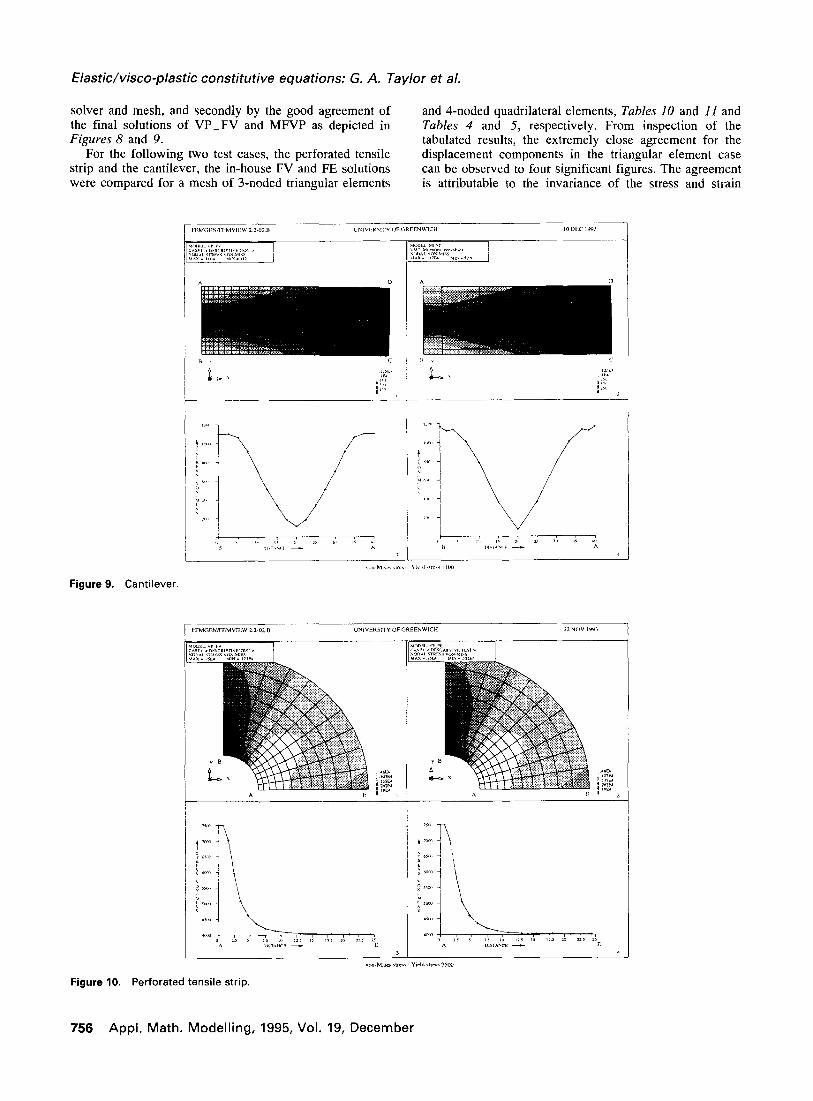
solver and mesh, and secondly by the good agreement of and 4-noded quadrilateral elements, Tables 10 and 11 and the final solutions of VP_FV and MFVP as depicted in Tables 4 and 5, respectively. From inspection of the Figures 8 and 9. tabulated results, the extremely close agreement for the

For the following two test cases, the perforated tensile displacement components in the triangular element case strip and the cantilever, the in-house FV and FE solutions can be observed to four significant figures. The agreement were compared for a mesh of 3-noded triangular elements is attributable to the invariance of the stress and strain

Figure 9. Cantilever.




variables over a triangular mesh element. The displace- case just under 9%. The discrepancy can be attributed to ment components in the quadrilateral element case are also the approximation of invariance for the quadrilateral ele- in close agreement but not to the same degree of accuracy. ments; the approximation may be affected differently by The difference in displacement components for the perfo- the particular integration technique employed in each rated tensile strip case is under 0.6% and for the cantilever method. The more significant disagreement for the can-





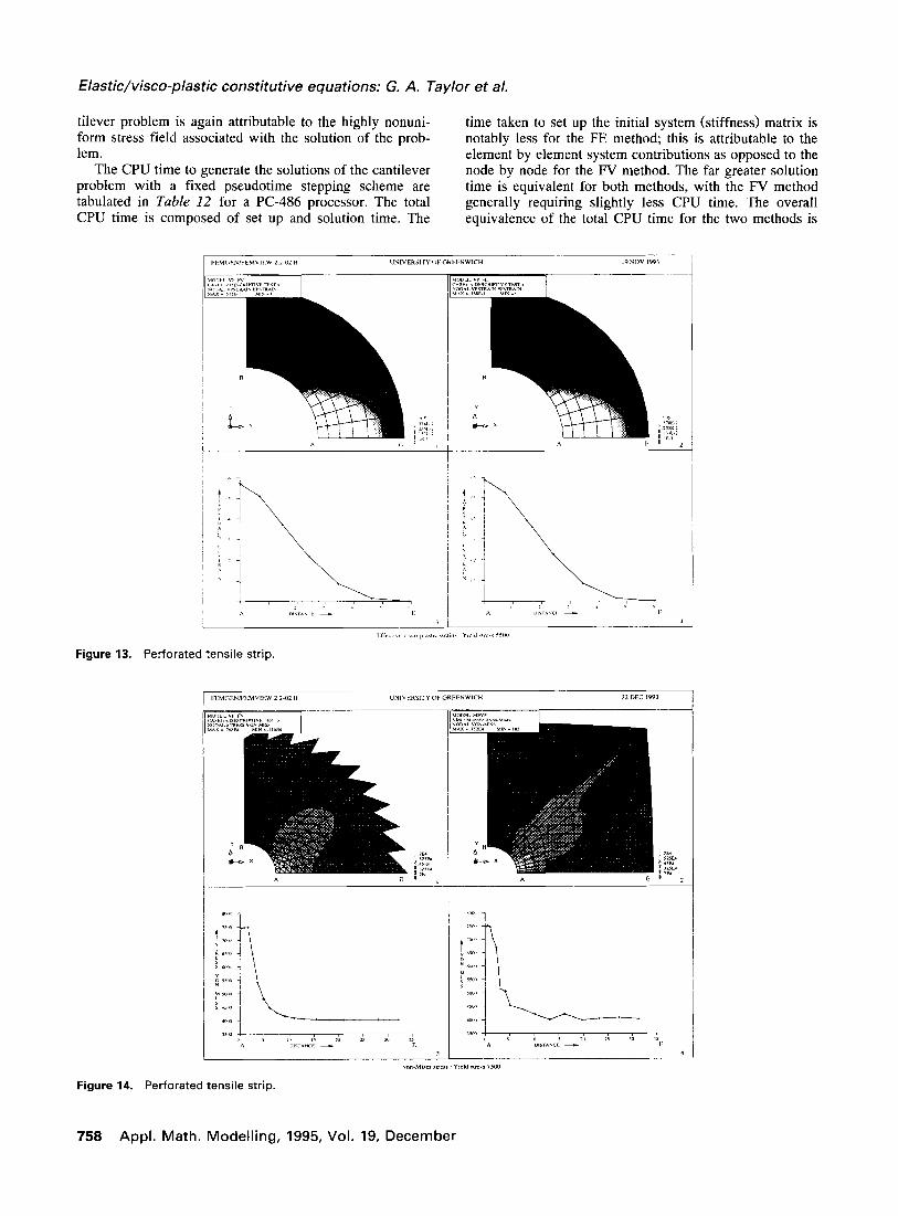
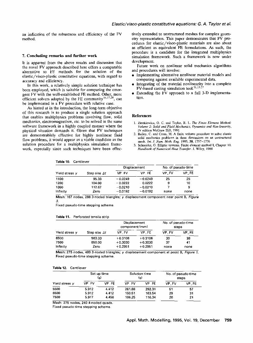
tilever problem is again attributable to the highly nonuni- time taken to set up the initial system (stiffness) matrix is form stress field associated with the solution of the prob- notably less for the FE method; this is attributable to the lem. element by element system contributions as opposed to the

The CPU time to generate the solutions of the cantilever node by node for the FV method. The far greater solution problem with a fixed pseudotime stepping scheme are time is equivalent for both methods, with the FV method tabulated in Table 12 for a PC-486 processor. The total generally requiring slightly less CPU time. The overall CPU time is composed of set up and solution time. The equivalence of the total CPU time for the two methods is


r




an indication of the robustness and efficiency of the FV method.

7. Concluding remarks and further work

It is apparent from the above results and discussion that the novel FV approach described here offers a comparable alternative to FE methods for the solution of the elastic/visco-plastic constitutive equations, with regard to accuracy and efficiency.

In this work, a relatively simple solution technique has been employed, which is suitable for comparing the emer- gent FV with the well-established FE method. Other, more efficient solvers adopted by the FE community’6~17*28, can be implemented in a FV procedure with relative ease.

As hinted at in the introduction, the long-term objective of this research is to produce a single solution approach that enables multiphysics problems involving flow, solid mechanics, electromagnetism, etc. to be solved in the same software framework in a highly coupled manner where the physical situation demands it. Given that FV techniques are demonstrablely effective for highly nonlinear fluid flow problems, it would appear as a viable candidate as the solution procedure for a multiphysics simulation framework, especially since such techniques have been effec-

Table 10. Cantilever

tively extended to unstructured meshes for complex geometry representation. This paper demonstrates that FV procedures for elastic/visco-plastic materials are also about as efficient as equivalent FE formulations. As such, the procedure is a candidate for the integrated multiphysics simulation framework. Such a framework is now under development.

Future work on nonlinear solid mechanics algorithms and procedures will involve:

Implementing alternative nonlinear material models and comparing against available experimental data. Integrating of the material nonlinearity into a complete FV-based casting simulation tool.“P’3* 7 Extending the FV approach to a full 3-D implementa- tion.

References

1. Zienkiewicz, 0. C. and Taylor, R. L. The Finite Element Method: Volume 2: Solid and Fluid Mechanics, Dynamics and Non-linearity, IV edition McGraw Hill, 1991

2. Bailey, C. and Cross, M. A finite volume procedure to solve elastic solid mechanics problems in three dimensions on an unstructured mesh. Int. J. Num. Meth. Eng. 1995, 38, 1757-1776

3. Schneider, G. Elliptic systems. Finite element method I, Chapter 10. Handbook of Numerical Heat Transfer. J. Wiley, 1988

Displacement No. of pseudo-time

Yield stress y Step size At VP_ FV VP_ FE VP_ FV VP_ FE

1100 95.33 - 0.0249 - 0.0249 25 25 1200 104.00 - 0.0222 - 0.0222 9 10 1300 112.67 -0.0210 -0.0210 7 9 Infinity Zero -0.0192 -0.0192 none none

Mesh: 167 nodes, 288 3-noded triangles; y displacement component near point B, Figure 3. Fixed pseudo-time stepping scheme.


Yield stress y Step size At


VP_ FV VP_ FE VP_ FV VP_ FE

6500 563.33 +0.3106 +0.3106 30 38 7500 650.00 + 0.3030 + 0.3030 37 41 Infinity Zero + 0.2951 + 0.2951 none none

Mesh: 275 nodes, 480 3-noded triangles; y displacement component at point B, Figure 7.

Fixed pseudo-time stepping scheme.

Table 12. Cantilever

Set up time Ls)

Yield stress y VP_ FV VP_ FE

Solution time (s)

VP_ FV VP- FE

No. of pseudo-time steps

VP_ FV VP_ FE

5500 5.912 4.412 6500 5.912 4.412 7500 5.917 4.450

Mesh: 275 nodes, 240 4-noded quads. Fixed pseudo-time stepping scheme.

261.88 292.31 51 57

150.51 163.54 29 31 106.25 116.34 20 21



4. Hattell, J., Hansen, P. N., and Hansen, L. F. Analysis of thermal induced stresses in die casting using a novel control volume FDM technique. Modelling Casting, Welding, Adu. Solid. Proc. 1993, VI, 582-592

5. Ng, S. F. and Benchariff, N. A finite difference program for the modelling of thick rectangular plates Comput. Struct. 1989, 33, 1011-1016

6. DemirdiiC, I. and MartinoviC, D. Finite volume method for thermo- elasto-plastic stress analysis. Comp. Meth. Appl. Mech. Eng. 1992, 109, 331-349

7. Demirdiic, 1. and Muzaferija, S. Finite volume method for stress analysis in complex domain. Int. .I. Num. Meth. Eng. 1994, 37, 3751-3766

8. Oiiate, E., Cerrera, M., and Zienkiewicz, 0. C. A finite volume format for structural mechanics. Int. Centre Num. Meth. Eng. 1992, 15, in press

9. Fryer, Y. D., Bailey, C., Cross, M. and Lai, C.-H. A control volume procedure for solving the elastic stress-strain equations on an unstructured mesh. Appl. Math. Modelling 1991, 15, 639-645

10. Fryer, Y. D. A control volume unstructured grid approach to the solution of the elastic stress-strain equations, Ph.D. Thesis, Univer- sity of Greenwich, 1993

11. Cross, M. Development of novel computational techniques for the next generation of software tools for casting simulation. Modelling Casting, Welding, Adv Solid. Proc. 1993, VI, 143-152

12. Cross, M., Bailey, C., Chow, P., and Pericleous, K. Towards an integrated control volume unstructured mesh code for the simulation of all the macroscopic processes involved in shape casting. Num. Meth. Industrial Forming Proc. 1992, 92, 787-792

13. Fryer, Y., Bailey, C., Cross, M., and Chow, P. Predicting macro- porosity in shape casting using an integrated control volume unstructured mesh framework. Model&g Casting, Welding Adu. Solid. Proc. 1993, VI, 143-152

14. Perzyna, P. Fundamental problems in viscoplasticity. Adu. Appl. Mech. 1966, 9, 243-377

15. Hill, R. The Mathematical Theory of Plasticiry. Oxford Science Publications, 1950

16. Zienkiewicz, 0. C. and Cormeau, I. C. Visco-plasticity, plasticity and creep in elastic solids, a unified numerical solution approach. Int. J. Num. Meth. Eng. 1974, 8, 821-845

17. Owen, D. R. J. and Hinton, E. Finite Elements in Plasticity. Piner- idge Press, Swansea, 1980

18. Elasto-viscoplastic Analysis of Plane and Axisymmetric Problems. User Manual, Microfield V2.30, Rockfield Software Ltd., The Inno- vation Centre, University College of Swansea, 1992

19. Majorana, C., Natali, A., Vitaliani, R. Analysis of three-dimensional prestressed concrete structures using a non-linear material model. Eng. Comput. 1990, 7, 157-166

20. Selim, V. A node centred finite volume approach: Bridge between finite differences and finite elements. Comp. Meth. Appl. Eng. 1993, 102, 107-138

21. Baliga, B. R. and Patankar, S. V. Elliptic systems: Finite element method Il. Handbook Num. Heat Transfer Chapter 11. J. Wiley, 1988

22. Chow, P. and Cross, M. An enthalpy control volume unstructured mesh (CV-UM) algorithm for solidification by conduction only. Int. .I. Num. Meth. 1992, 35, 1849-1870

23. Chow, P. Control volume unstructured mesh procedure for convec- tion diffusion solidification processes. Ph.D. Thesis, University of Greenwich, 1993

24. Cormeau, I. C. Numerical stability in quasi-static elasto/visco-plasticity. Int. .I. Num. Methods Eng. 1975, 9, 109-127

25. Jennings, A. Matrix Computation, J. Wiley, 1992 26. Fenner, R. T. Engineering Plasticity: Application of Numerical and

Analytical Techniques, Ellis Horwood, 1986 27. Thomas, B. G. Stress modelling of the casting process: An overview.

Modelling Casting, Welding, Adt,. Solid. Proc. 1993, VI, 519-534 28. Reed, M. B. Newton-like methods with limited storage, for the

solution of elasto-viscoplasticity problems. Inc. J. Num. Mefh. Eng. 1992, 35, 223-240


Solution of the elastic/visco-plastic constitutive equations: A finite volume approach

Documents