3 34 47 7 CHAPTER 11 COST-VOLUME-PROFIT ANALYSIS: A MANAGERIAL PLANNING TOOL QUESTIONS FOR WRITING AND DISCUSSION 1. CVP analysis allows managers to focus on selling prices, volume, costs, profits, and sales mix. Many different “what if” questions can be asked to assess the effect on profits of changes in key variables. 2. The units-sold approach defines sales vo- lume in terms of units of product and gives answers in these same terms. The sales- revenue approach defines sales volume in terms of revenues and provides answers in these same terms. 3. Break-even point is the level of sales activity where total revenues equal total costs, or where zero profits are earned. 4. At the break-even point, all fixed costs are covered. Above the break-even point, only variable costs need to be covered. Thus, contribution margin per unit is profit per unit, provided that the unit selling price is greater than the unit variable cost (which it must be for break-even to be achieved). 5. Profit = $7.00 × 5,000 = $35,000 6. Variable cost ratio = Variable costs/Sales. Contribution margin ratio = Contribution margin/Sales. Contribution margin ratio = 1 – Variable cost ratio. 7. Break-even revenues = $20,000/0.40 = $50,000 8. No. The increase in contribution is $9,000 (0.30 × $30,000), and the increase in adver- tising is $10,000. 9. Sales mix is the relative proportion sold of each product. For example, a sales mix of 3:2 means that three units of one product are sold for every two of the second product. 10. Packages of products, based on the ex- pected sales mix, are defined as a single product. Selling price and cost information for this package can then be used to carry out CVP analysis. 11. Package contribution margin: (2 × $10) + (1 × $5) = $25. Break-even point = $30,000/$25 = 1,200 packages, or 2,400 units of A and 1,200 units of B. 12. Profit = 0.60($200,000 – $100,000) = $60,000 13. A change in sales mix will change the con- tribution margin of the package (defined by the sales mix) and, thus, will change the units needed to break even. 14. Margin of safety is the sales activity in excess of that needed to break even. The higher the margin of safety, the lower the risk. 15. Operating leverage is the use of fixed costs to extract higher percentage changes in profits as sales activity changes. It is achieved by increasing fixed costs while lo- wering variable costs. Therefore, increased leverage implies increased risk, and vice versa. 16. Sensitivity analysis is a “what if” technique that examines the impact of changes in un- derlying assumptions on an answer. A com- pany can input data on selling prices, varia- ble costs, fixed costs, and sales mix and set up formulas to calculate break-even points and expected profits. Then, the data can be varied as desired to see what impact changes have on the expected profit. 17. By specifically including the costs that vary with nonunit drivers, the impact of changes in the nonunit drivers can be examined. In traditional CVP, all nonunit costs are lumped together as “fixed costs.” While the costs are fixed with respect to units, they vary with re- spect to other drivers. ABC analysis reminds us of the importance of these nonunit drivers and costs.

Welcome message from author
This document is posted to help you gain knowledge. Please leave a comment to let me know what you think about it! Share it to your friends and learn new things together.
Transcript

334477
CHAPTER 11 COST-VOLUME-PROFIT ANALYSIS: A MANAGERIAL PLANNING TOOL
QUESTIONS FOR WRITING AND DISCUSSION
1. CVP analysis allows managers to focus on selling prices, volume, costs, profits, and sales mix. Many different “what if” questions can be asked to assess the effect on profits of changes in key variables.
2. The units-sold approach defines sales vo-lume in terms of units of product and gives answers in these same terms. The sales-revenue approach defines sales volume in terms of revenues and provides answers in these same terms.
3. Break-even point is the level of sales activity where total revenues equal total costs, or where zero profits are earned.
4. At the break-even point, all fixed costs are covered. Above the break-even point, only variable costs need to be covered. Thus, contribution margin per unit is profit per unit, provided that the unit selling price is greater than the unit variable cost (which it must be for break-even to be achieved).
5. Profit = $7.00 × 5,000 = $35,000
6. Variable cost ratio = Variable costs/Sales. Contribution margin ratio = Contribution margin/Sales. Contribution margin ratio = 1 – Variable cost ratio.
7. Break-even revenues = $20,000/0.40 = $50,000
8. No. The increase in contribution is $9,000 (0.30 × $30,000), and the increase in adver-tising is $10,000.
9. Sales mix is the relative proportion sold of each product. For example, a sales mix of 3:2 means that three units of one product are sold for every two of the second product.
10. Packages of products, based on the ex-pected sales mix, are defined as a single product. Selling price and cost information for this package can then be used to carry out CVP analysis.
11. Package contribution margin: (2 × $10) + (1 × $5) = $25. Break-even point =
$30,000/$25 = 1,200 packages, or 2,400 units of A and 1,200 units of B.
12. Profit = 0.60($200,000 – $100,000) = $60,000
13. A change in sales mix will change the con-tribution margin of the package (defined by the sales mix) and, thus, will change the units needed to break even.
14. Margin of safety is the sales activity in excess of that needed to break even. The higher the margin of safety, the lower the risk.
15. Operating leverage is the use of fixed costs to extract higher percentage changes in profits as sales activity changes. It is achieved by increasing fixed costs while lo-wering variable costs. Therefore, increased leverage implies increased risk, and vice versa.
16. Sensitivity analysis is a “what if” technique that examines the impact of changes in un-derlying assumptions on an answer. A com-pany can input data on selling prices, varia-ble costs, fixed costs, and sales mix and set up formulas to calculate break-even points and expected profits. Then, the data can be varied as desired to see what impact changes have on the expected profit.
17. By specifically including the costs that vary with nonunit drivers, the impact of changes in the nonunit drivers can be examined. In traditional CVP, all nonunit costs are lumped together as “fixed costs.” While the costs are fixed with respect to units, they vary with re-spect to other drivers. ABC analysis reminds us of the importance of these nonunit drivers and costs.

334488
18. JIT simplifies the firm’s cost equation since more costs are classified as fixed (e.g., di-rect labor). Additionally, the batch-level vari-able is gone (in JIT, the batch is one unit). Thus, the cost equation for JIT includes fixed costs, unit variable cost times the number of units sold, and unit product-level cost times the number of products sold (or related cost
driver). JIT means that CVP analysis ap-proaches the standard analysis with fixed and unit-level costs only.

334499
EXERCISES
11–1
1. Direct materials $3.90 Direct labor 1.40 Variable overhead 2.10 Variable selling expenses 1.00 Variable cost per unit $ 8.40 2. Price $14.00 Variable cost per unit 8.40 Contribution margin per unit $5.60 3. Contribution margin ratio = $5.60/$14 = 0.40 or 40% 4. Variable cost ratio = $8.40/$14 = 0.60 or 60% 5. Total fixed cost = $44,000 + $47,280 = $91,280 6. Breakeven units = (Fixed cost)/Contribution margin = $91,280/$5.60 = 16,300

335500
11–2
1. Price $12.00 Less: Direct materials $1.90 Direct labor 2.85 Variable overhead 1.25 Variable selling expenses 2.00 8.00 Contribution margin per unit $4.00 2. Breakeven units = (Fixed cost)/Contribution margin = (44,000 + $37,900)/$4.00 = 20,475 3. Units for target = (44,000 + $37,900 + $9,000)/$4 = $90,900/$4 = 22,725 4. Sales (22,725 × $12) $ 272,700 Variable costs (22,725 × $8) 181,800 Contribution margin $ 90,900 Fixed costs 81,900 Operating income $ 9,000
Sales of 22,725 units does produce operating income of $9,000.
11–3
1. Units = Fixed cost/Contribution margin = $37,500/($8 – $5) = 12,500 2. Sales (12,500 × $8) $100,000 Variable costs (12,500 × $5) 62,500 Contribution margin $ 37,500 Fixed costs 37,500 Operating income $ 0 3. Units = (Target income + Fixed cost)/Contribution margin = ($37,500 + $9,900)/($8 – $5) = $47,400/$3 = 15,800

335511
11–4
1. Contribution margin per unit = $8 – $5 = $3 Contribution margin ratio = $3/$8 = 0.375, or 37.5% 2. Variable cost ratio = $75,000/$120,000 = 0.625, or 62.5% 3. Revenue = Fixed cost/Contribution margin ratio = $37,500/0.375 = $100,000 4. Revenue = (Target income + Fixed cost)/Contribution margin ratio = ($37,500 + $9,900)/0.375 = $126,400
11–5
1. Break-even units = Fixed costs/(Price – Variable cost) = $180,000/($3.20 – $2.40) = $180,000/$0.80 = 225,000 2. Units = ($180,000 + $12,600)/($3.20 – $2.40) = $192,600/$0.80 = 240,750 3. Unit variable cost = $2.40 Unit variable manufacturing cost = $2.40 – $0.32 = $2.08
The unit variable cost is used in cost-volume-profit analysis, since it includes all of the variable costs of the firm.

335522
11–6
1. Before-tax income = $25,200/(1 – 0.40) = $42,000
Units = ($180,000 + $42,000)/$0.80 = $222,000/$0.80 = 277,500 2. Before-tax income = $25,200/(1 – 0.30) = $36,000
Units = ($180,000 + $36,000)/$0.80 = $216,000/$0.80 = 270,000 3. Before-tax income = $25,200/(1 – 0.50) = $50,400
Units = ($180,000 + $50,400)/$0.80 = $230,400/$0.80 = 288,000
11–7
1. Contribution margin per unit = $15 – ($3.90 + $1.40 + $2.10 + $1.60) = $6 Contribution margin ratio = $6/$15 = 0.40 or 40% 2. Breakeven Revenue = Fixed cost/Contribution margin ratio = ($52,000 + $37,950)/0.40 = $224,875 3. Revenue = (Target income + Fixed cost)/Contribution margin ratio = ($52,000 + $37,950 + $18,000)/0.40 = $269,875 4. Breakeven units = $224,875/$15 = 14,992 (rounded) Or Breakeven units = $89,950/$6 = 14,992 (rounded) 5. Units for target income = $269,875/$15 = 17,992 (rounded) Or Units for target income = $107,950/$6 = 17,992 (rounded)

335533
11–8
1. Sales mix is 2:1 (Twice as many videos are sold as equipment sets.) 2. Variable Sales Product Price – Cost = CM × Mix = Total CM Videos $12 $4 $8 2 $16 Equipment sets 15 6 9 1 9 Total $25
Break-even packages = $70,000/$25 = 2,800
Break-even videos = 2 × 2,800 = 5,600 Break-even equipment sets = 1 × 2,800 = 2,800 3. Switzer Company Income Statement
For Last Year
Sales ........................................................................................... $ 195,000 Less: Variable costs ................................................................. 70,000 Contribution margin .................................................................. $ 125,000 Less: Fixed costs ...................................................................... 70,000 Operating income ................................................................ $ 55,000
Contribution margin ratio = $125,000/$195,000 = 0.641, or 64.1% Break-even sales revenue = $70,000/0.641 = $109,204

335544
11–9
1. Sales mix is 2:1:4 (Twice as many videos will be sold as equipment sets, and four times as many yoga mats will be sold as equipment sets.)
2. Variable Sales Product Price – Cost = CM × Mix = Total CM Videos $12 $ 4 $8 2 $16 Equipment sets 15 6 9 1 9 Yoga mats 18 13 5 4 20 Total $45
Break-even packages = $118,350/$45 = 2,630
Break-even videos = 2 × 2,630 = 5,260 Break-even equipment sets = 1 × 2,630 = 2,630 Break-even yoga mats = 4 × 2,630 = 10,520 3. Switzer Company Income Statement
For the Coming Year
Sales ........................................................................................... $555,000 Less: Variable costs ................................................................. 330,000 Contribution margin .................................................................. $225,000 Less: Fixed costs ...................................................................... 118,350 Operating income ................................................................ $106,650
Contribution margin ratio = $225,000/$555,000 = 0.4054, or 40.54% Break-even revenue = $118,350/0.4054 = $291,934
11–10
1. Variable cost per unit = $5.60 + $7.50 + $2.90 + $2.00 = $18 Breakeven units = $75,000/($24 – $18) = 12,500 Breakeven Revenue = $24 × 12,500 = $300,000 2. Margin of safety in sales dollars = ($24 × 14,000) – $300,000 = $36,000 3. Margin of safety in units = 14,000 units – 12,500 units = 1,500 units

335555
11–11
1.
$0
$5,000
$10,000
$15,000
$20,000
$25,000
$30,000
$35,000
0 500 1,000 1,500 2,000 2,500 3,000 3,500
Units Sold
Break-even point = 2,500 units; + line is total revenue and x line is total costs.

335566
11–11 Continued
2. a. Fixed costs increase by $5,000:
$0
$5,000
$10,000
$15,000
$20,000
$25,000
$30,000
$35,000
$40,000
0 500 1,000 1,500 2,000 2,500 3,000 3,500 4,000
Units Sold
Break-even point = 3,750 units

335577
11–11 Continued
b. Unit variable cost increases to $7:
$0
$10,000
$20,000
$30,000
$40,000
$50,000
0 500 1,000 1,500 2,000 2,500 3,000 3,500 4,000
Units Sold
Break-even point = 3,333 units
335588
11–11 Continued
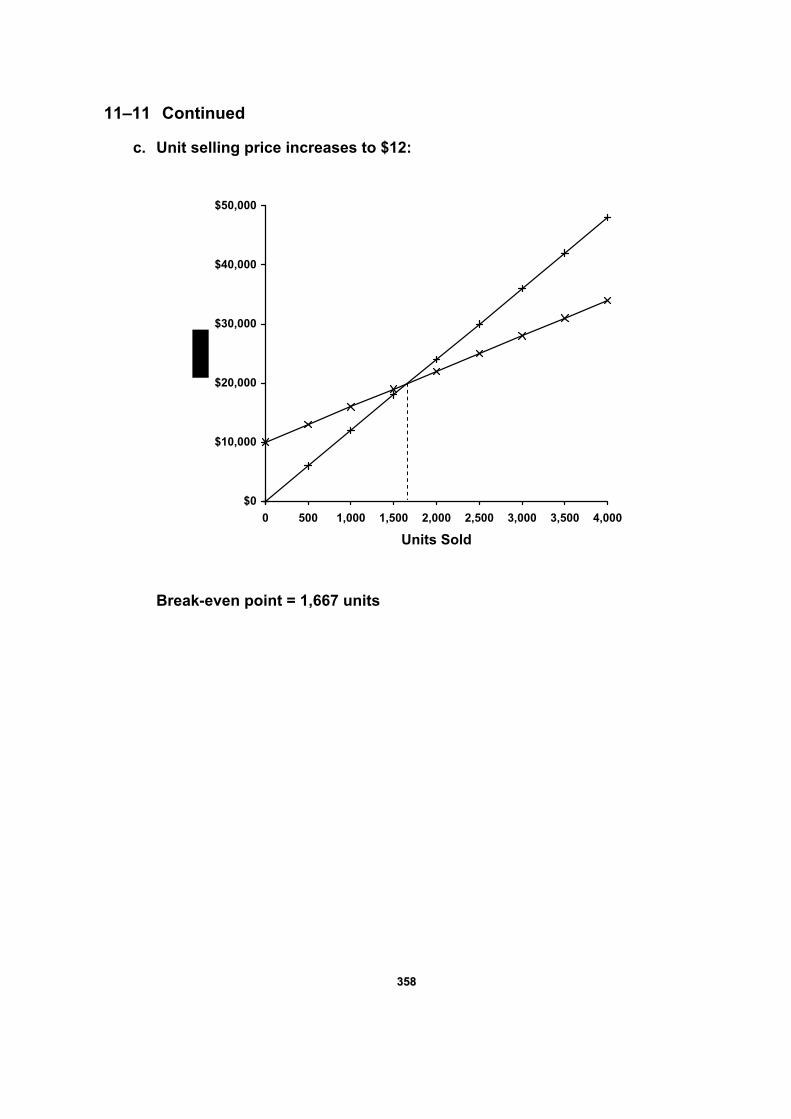
c. Unit selling price increases to $12:
$0
$10,000
$20,000
$30,000
$40,000
$50,000
0 500 1,000 1,500 2,000 2,500 3,000 3,500 4,000
Units Sold
Break-even point = 1,667 units

335599
11–11 Continued
d. Both fixed costs and unit variable cost increase:
$0
$10,000
$20,000
$30,000
$40,000
$50,000
$60,000
$70,000
0 1,000 2,000 3,000 4,000 5,000 6,000 7,000 8,000
Units Sold
Break-even point = 5,000 units

336600
11–11 Continued
3. Original data:
-$10,000
$0
$10,000
0 500 1,000 1,500 2,000 2,500 3,000 3,500 4,000
Break-even point = 2,500 units

336611
11–11 Continued
a. Fixed costs increase by $5,000:
-$15,000
$0
$15,000
0 500 1,000 1,500 2,000 2,500 3,000 3,500 4,000
Break-even point = 3,750 units

336622
11–11 Continued
b. Unit variable cost increases to $7:
-$10,000
$0
$10,000
0 500 1,000 1,500 2,000 2,500 3,000 3,500 4,000
Break-even point = 3,333 units

336633
11–11 Continued
c. Unit selling price increases to $12:
-$10,000
$0
$10,000
0 500 1,000 1,500 2,000 2,500 3,000 3,500 4,000
Break-even point = 1,667 units

336644
11–11 Concluded
d. Both fixed costs and unit variable cost increase:
-$15,000
$0
$15,000
0 1,000 2,000 3,000 4,000 5,000 6,000 7,000
Break-even point = 5,000 units 4. The first set of graphs is more informative since these graphs reveal how
costs change as sales volume changes.

336655
11–12
1. Darius: $100,000/$50,000 = 2 Xerxes: $300,000/$50,000 = 6 2. Darius Xerxes X = $50,000/(1 – 0.80) X = $250,000/(1 – 0.40) X = $50,000/0.20 X = $250,000/0.60 X = $250,000 X = $416,667
Xerxes must sell more than Darius to break even because it must cover $200,000 more in fixed costs (it is more highly leveraged).
3. Darius: 2 × 50% = 100% Xerxes: 6 × 50% = 300%
The percentage increase in profits for Xerxes is much higher than the in-crease for Darius because Xerxes has a higher degree of operating leverage (i.e., it has a larger amount of fixed costs in proportion to variable costs as compared to Darius). Once fixed costs are covered, additional revenue must cover only variable costs, and 60 percent of Xerxes revenue above break-even is profit, whereas only 20 percent of Darius revenue above break-even is profit.
11–13
1. Breakeven units = $10,350/($15 – $12) = 3,450 2. Breakeven sales dollars = $10,350/0.20 = $51,750 3. Margin of safety in units = 5,000 – 3,450 = 1,550 4. Margin of safety in sales dollars = $75,000 – $51,750 = $23,250

336666
11–14
1. Variable cost ratio = Variable costs/Sales = $399,900/$930,000 = 0.43, or 43%
Contribution margin ratio = (Sales – Variable costs)/Sales = ($930,000 – $399,900)/$930,000 = 0.57, or 57% 2. Break-even sales revenue = $307,800/0.57 = $540,000 3. Margin of safety = Sales – Break-even sales = $930,000 – $540,000 = $390,000 4. Contribution margin from increased sales = ($7,500)(0.57) = $4,275 Cost of advertising = $5,000
No, the advertising campaign is not a good idea, because the company’s op-erating income will decrease by $725 ($4,275 – $5,000).
11–15
1. Income = Revenue – Variable cost – Fixed cost 0 = 1,500P – $300(1,500) – $120,000 0 = 1,500P – $450,000 – $120,000 $570,000 = 1,500P P = $380 2. $160,000/($3.50 – Unit variable cost) = 128,000 units Unit variable cost = $2.25 3. Margin of safety = Actual units – Breakeven units 300 = 35,000 – breakeven units Breakeven units = 34,700 Breakeven units = Total Fixed Cost/(Price – Variable cost per unit) 34,700 = Total Fixed Cost/($40 – $30) Total Fixed Cost = $347,000

336677
11–16
1. Contribution margin per unit = $5.60 – $4.20* = $1.40
*Variable costs per unit: $0.70 + $0.35 + $1.85 + $0.34 + $0.76 + $0.20 = $4.20
Contribution margin ratio = $1.40/$5.60 = 0.25 = 25% 2. Break-even in units = ($32,300 + $12,500)/$1.40 = 32,000 boxes
Break-even in sales = 32,000 × $5.60 = $179,200 or = ($32,300 + $12,500)/0.25 = $179,200 3. Sales ($5.60 × 35,000) $ 196,000 Variable costs ($4.20 × 35,000) 147,000 Contribution margin $ 49,000 Fixed costs 44,800 Operating income $ 4,200 4. Margin of safety = $196,000 – $179,200 = $16,800 5. Break-even in units = 44,800/($6.20 – $4.20) = 22,400 boxes
New operating income = $6.20(31,500) – $4.20(31,500) – $44,800 = $195,300 – $132,300 – $44,800 = $18,200
Yes, operating income will increase by $14,000 ($18,200 – $4,200).

336688
11–17
1. Variable cost ratio = $126,000/$315,000 = 0.40 Contribution margin ratio = $189,000/$315,000 = 0.60 2. $46,000 × 0.60 = $27,600 3. Break-even revenue = $63,000/0.60 = $105,000 Margin of safety = $315,000 – $105,000 = $210,000 4. Revenue = ($63,000 + $90,000)/0.60 = $255,000 5. Before-tax income = $56,000/(1 – 0.30) = $80,000
Note: Tax rate = $37,800/$126,000 = 0.30
Revenue = ($63,000 + $80,000)/0.60 = $238,333
Sales ................................................................................ $ 238,333 Less: Variable expenses ($238,333 × 0.40) .................. 95,333 Contribution margin ....................................................... $ 143,000 Less: Fixed expenses .................................................... 63,000 Income before income taxes ......................................... $ 80,000 Income taxes ($80,000 × 0.30) ....................................... 24,000 Net income ................................................................ $ 56,000

336699
11–18
1. Contribution margin/unit = $410,000/100,000 = $4.10 Contribution margin ratio = $410,000/$650,000 = 0.6308 Break-even units = $295,200/$4.10 = 72,000 units
Break-even revenue = 72,000 × $6.50 = $468,000 or = $295,200/0.6308 = $467,977* *Difference due to rounding error in calculating the contribution margin ratio. 2. The break-even point decreases:
X = $295,200/(P – V) X = $295,200/($7.15 – $2.40) X = $295,200/$4.75 X = 62,147 units
Revenue = 62,147 × $7.15 = $444,351 3. The break-even point increases:
X = $295,200/($6.50 – $2.75) X = $295,200/$3.75 X = 78,720 units
Revenue = 78,720 × $6.50 = $511,680 4. Predictions of increases or decreases in the break-even point can be made
without computation for price changes or for variable cost changes. If both change, then the unit contribution margin must be known before and after to predict the effect on the break-even point. Simply giving the direction of the change for each individual component is not sufficient. For our example, the unit contribution changes from $4.10 to $4.40, so the break-even point in units will decrease.
Break-even units = $295,200/($7.15 – $2.75) = 67,091
Now, let’s look at the break-even point in revenues. We might expect that it, too, will decrease. However, that is not the case in this particular example. Here, the contribution margin ratio decreased from about 63 percent to just over 61.5 percent. As a result, the break-even point in revenues has gone up.
Break-even revenue = 67,091 × $7.15 = $479,701

337700
11–18 Concluded
5. The break-even point will increase because more units will need to be sold to
cover the additional fixed expenses.
Break-even units = $345,200/$4.10 = 84,195 units Revenue = $547,268

337711
PROBLEMS
11–19
1. Operating income = Revenue(1 – Variable cost ratio) – Fixed cost (0.20)Revenue = Revenue(1 – 0.40) – $24,000 (0.20)Revenue = (0.60)Revenue – $24,000 (0.40)Revenue = $24,000 Revenue = $60,000
Sales ................................................................................ $ 60,000 Variable expenses ($60,000 × 0.40) .............................. 24,000 Contribution margin ....................................................... $ 36,000 Fixed expenses .............................................................. 24,000 Operating income ..................................................... $ 12,000
$12,000 = $60,000 × 20% 2. If revenue of $60,000 produces a profit equal to 20 percent of sales and if the
price per unit is $10, then 6,000 units must be sold. Let X equal number of units, then:
Operating income = (Price – Variable cost) – Fixed cost 0.20($10)X = ($10 – $4)X – $24,000 $2X = $6X – $24,000 $4X = $24,000 X = 6,000 buckets
0.25($10)X = $6X – $24,000 $2.50X = $6X – $24,000 $3.50X = $24,000 X = 6,857 buckets
Sales (6,857 × $10) ......................................................... $68,570 Variable expenses (6,857 × $4) ..................................... 27,428 Contribution margin ....................................................... $41,142 Fixed expenses .............................................................. 24,000 Operating income ..................................................... $17,142
$17,142* = 0.25 × $68,570 as claimed
*Rounded down.
Note: Some may prefer to round up to 6,858 units. If this is done, the operat-ing income will be slightly different due to rounding.
337722
11–19 Concluded
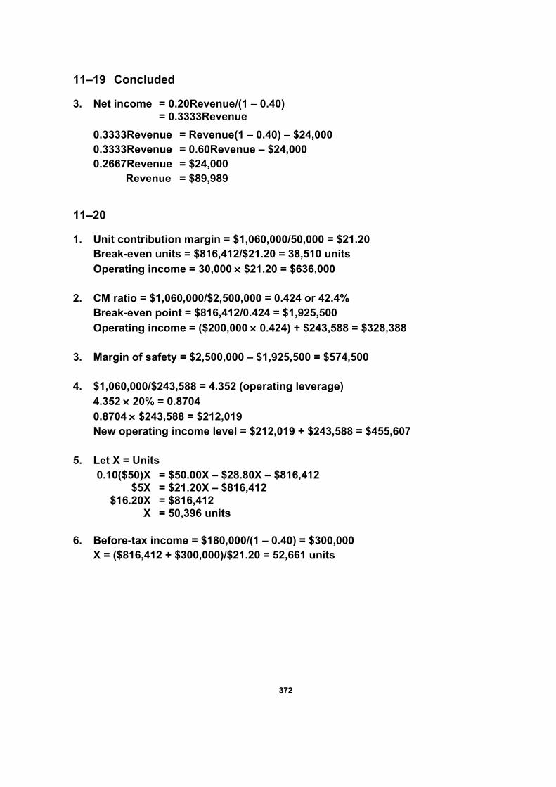
3. Net income = 0.20Revenue/(1 – 0.40) = 0.3333Revenue
0.3333Revenue = Revenue(1 – 0.40) – $24,000 0.3333Revenue = 0.60Revenue – $24,000 0.2667Revenue = $24,000 Revenue = $89,989
11–20
1. Unit contribution margin = $1,060,000/50,000 = $21.20 Break-even units = $816,412/$21.20 = 38,510 units Operating income = 30,000 × $21.20 = $636,000 2. CM ratio = $1,060,000/$2,500,000 = 0.424 or 42.4% Break-even point = $816,412/0.424 = $1,925,500 Operating income = ($200,000 × 0.424) + $243,588 = $328,388 3. Margin of safety = $2,500,000 – $1,925,500 = $574,500 4. $1,060,000/$243,588 = 4.352 (operating leverage) 4.352 × 20% = 0.8704 0.8704 × $243,588 = $212,019 New operating income level = $212,019 + $243,588 = $455,607 5. Let X = Units 0.10($50)X = $50.00X – $28.80X – $816,412 $5X = $21.20X – $816,412 $16.20X = $816,412 X = 50,396 units 6. Before-tax income = $180,000/(1 – 0.40) = $300,000 X = ($816,412 + $300,000)/$21.20 = 52,661 units

337733
11–21
1. Unit contribution margin = $825,000/110,000 = $7.50 Break-even point = $495,000/$7.50 = 66,000 units
CM ratio = $7.50/$25 = 0.30 Break-even point = $495,000/0.30 = $1,650,000 or = $25 × 66,000 = $1,650,000 2. Increased CM ($400,000 × 0.30) $ 120,000 Less: Increased advertising expense 40,000 Increased operating income $ 80,000 3. $315,000 × 0.30 = $94,500 4. Before-tax income = $360,000/(1 – 0.40) = $600,000 Units = ($495,000 + $600,000)/$7.50 = 146,000 5. Margin of safety = $2,750,000 – $1,650,000 = $1,100,000 or = 110,000 units – 66,000 units = 44,000 units 6. $825,000/$330,000 = 2.5 (operating leverage) 20% × 2.5 = 50% (profit increase)

337744
11–22
1. Sales mix:
Squares: $300,000/$30 = 10,000 units Circles: $2,500,000/$50 = 50,000 units
Sales Total Product P – V* = P – V × Mix = CM Squares $30 $10 $20 1 $ 20 Circles 50 10 40 5 200 Package $220
*$100,000/10,000 = $10 $500,000/50,000 = $10
Break-even packages = $1,628,000/$220 = 7,400 packages Break-even squares = 7,400 × 1 = 7,400 Break-even circles = 7,400 × 5 = 37,000 2. Contribution margin ratio = $2,200,000/$2,800,000 = 0.7857
0.10Revenue = 0.7857Revenue – $1,628,000 0.6857Revenue = $1,628,000 Revenue = $2,374,216 3. New mix: Sales Total Product P – V = P – V × Mix = CM Squares $30 $10 $20 3 $ 60 Circles 50 10 40 5 200 Package $260
Break-even packages = $1,628,000/$260 = 6,262 packages Break-even squares = 6,262 × 3 = 18,786 Break-even circles = 6,262 × 5 = 31,310
CM ratio = $260/$340* = 0.7647
*(3)($30) + (5)($50) = $340 revenue per package
0.10Revenue = 0.7647Revenue – $1,628,000 0.6647Revenue = $1,628,000 Revenue = $2,449,225

337755
11–22 Concluded
4. Increase in CM for squares (15,000 × $20) $ 300,000 Decrease in CM for circles (5,000 × $40) (200,000) Net increase in total contribution margin $ 100,000 Less: Additional fixed expenses 45,000 Increase in operating income $ 55,000
Gosnell would gain $55,000 by increasing advertising for the squares. This is a good strategy.
11–23
1. Variable Units in Package Product Price* – Cost = CM × Mix = CM Scientific $25 $12 $13 1 $13 Business 20 9 11 5 55 Total $68
*$500,000/20,000 = $25 $2,000,000/100,000 = $20
X = ($1,080,000 + $145,000)/$68 X = $1,225,000/$68 X = 18,015 packages
18,015 scientific calculators (1 × 18,015) 90,075 business calculators (5 × 18,015) 2. Revenue = $1,225,000/0.544* = $2,251,838
*($1,360,000/$2,500,000) = 0.544

337766
11–24
1. Currently:
Sales (830,000 × $0.36) $ 298,800 Variable expenses 224,100 Contribution margin $ 74,700 Fixed expenses 54,000 Operating income $ 20,700
New contribution margin = 1.5 × $74,700 = $112,050 $112,050 – promotional spending – $54,000 = 1.5 × $20,700 Promotional spending = $27,000 2. Here are two ways to calculate the answer to this question:
a. The per-unit contribution margin needs to be the same:
Let P* represent the new price and V* the new variable cost. (P – V) = (P* – V*) $0.36 – $0.27 = P* – $0.30 $0.09 = P* – $0.30 P* = $0.39 b. Old break-even point = $54,000/($0.36 – $0.27) = 600,000 New break-even point = $54,000/(P* – $0.30) = 600,000 P* = $0.39
The selling price should be increased by $0.03. 3. Projected contribution margin (700,000 × $0.13) $91,000 Present contribution margin 74,700 Increase in operating income $16,300
The decision was good because operating income increased by $16,300.
(New quantity × $0.13) – $54,000 = $20,700 New quantity = 574,615
Selling 574,615 units at the new price will maintain profit at $20,700.

337777
11–25
1. Contribution margin ratio = $487,548/$840,600 = 0.58 2. Revenue = $250,000/0.58 = $431,034 3. Operating income = CMR × Revenue – Total fixed cost 0.08R/(1 – 0.34) = 0.58R – $250,000 0.1212R = 0.58R – $250,000 0.4588R = $250,000 R = $544,900 4. $840,600 × 110% = $924,660 $353,052 × 110% = 388,357 $536,303
CMR = $536,303/$924,660 = 0.58
The contribution margin ratio remains at 0.58. 5. Additional variable expense = $840,600 × 0.03 = $25,218 New contribution margin = $487,548 – $25,218 = $462,330 New CM ratio = $462,330/$840,600 = 0.55
Break-even point = $250,000/0.55 = $454,545 The effect is to increase the break-even point. 6. Present contribution margin $ 487,548 Projected contribution margin ($920,600 × 0.55) 506,330 Increase in contribution margin/profit $ 18,782
Fitzgibbons should pay the commission because profit would increase by $18,782.

337788
11–26
1. One package, X, contains three Grade I and seven Grade II cabinets.
0.3X($3,400) + 0.7X($1,600) = $1,600,000 X = 748 packages
Grade I: 0.3 × 748 = 224 units Grade II: 0.7 × 748 = 524 units 2. Product P – V = P – V × Mix = Total CM Grade I $3,400 $2,686 $714 3 $2,142 Grade II 1,600 1,328 272 7 1,904 Package $4,046
Direct fixed costs—Grade I $ 95,000 Direct fixed costs—Grade II 95,000 Common fixed costs 35,000 Total fixed costs $ 225,000
$225,000/$4,046 = 56 packages Grade I: 3 × 56 = 168; Grade II: 7 × 56 = 392 3. Product P – V = P – V × Mix = Total CM Grade I $3,400 $2,444 $956 3 $2,868 Grade II 1,600 1,208 392 7 2,744 Package $5,612
Package CM = 3($3,400) + 7($1,600) Package CM = $21,400 $21,400X = $1,600,000 – $600,000 X = 47 packages remaining
141 Grade I (3 × 47) and 329 Grade II (7 × 47)
Additional contribution margin:
141($956 – $714) + 329($392 – $272) $73,602 Increase in fixed costs 44,000 Increase in operating income $29,602
Break-even: ($225,000 + $44,000)/$5,612 = 48 packages
144 Grade I (3 × 48) and 336 Grade II (7 × 48)

337799
11–26 Concluded
The new break-even point is a revised break-even for 2004. Total fixed costs must be reduced by the contribution margin already earned (through the first five months) to obtain the units that must be sold for the last seven months. These units are then be added to those sold during the first five months:
CM earned = $600,000 – (83* × $2,686) – (195* × $1,328) = $118,102
*224 – 141 = 83; 524 – 329 = 195
X = ($225,000 + $44,000 – $118,102)/$5,612 = 27 packages
In the first five months, 28 packages were sold (83/3 or 195/7). Thus, the re-vised break-even point is 55 packages (27 + 28)—in units, 165 of Grade I and 385 of Grade II.
4. Product P – V = P – V × Mix = Total CM Grade I $3,400 $2,686 $714 1 $714 Grade II 1,600 1,328 272 1 272 Package $986
New sales revenue $1,000,000 × 130% = $1,300,000
Package CM = $3,400 + $1,600 $5,000X = $1,300,000 X = 260 packages
Thus, 260 units of each cabinet will be sold during the rest of the year.
Effect on profits:
Change in contribution margin [$714(260 – 141) – $272(329 – 260)] $66,198 Increase in fixed costs [$70,000(7/12)] 40,833 Increase in operating income $25,365
X = F/(P – V) = $295,000/$986 = 299 packages (or 299 of each cabinet)
The break-even point for 2006 is computed as follows:
X = ($295,000 – $118,102)/$986 = $176,898/$986 = 179 packages (179 of each)
To this, add the units already sold, yielding the revised break-even point:
Grade I: 83 + 179 = 262 Grade II: 195 + 179 = 374

338800
11–27
1. R = F/(1 – VR) = $150,000/(1/3) = $450,000 2. Of total sales revenue, 60 percent is produced by floor lamps and 40 percent
by desk lamps.
$360,000/$30 = 12,000 units $240,000/$20 = 12,000 units
Thus, the sales mix is 1:1.
Product P – V* = P – V × Mix = Total CM Floor lamps $30.00 $20.00 $10.00 1 $10.00 Desk lamps 20.00 13.33 6.67 1 6.67 Package $16.67
X = F/(P – V) = $150,000/$16.67 = 8,999 packages
Floor lamps: 1 × 8,999 = 8,999 Desk lamps: 1 × 8,999 = 8,999 Note: packages have been rounded up to ensure attainment of breakeven. 3. Operating leverage = CM/Operating income = $200,000/$50,000 = 4.0
Percentage change in profits = 4.0 × 40% = 160%

338811
11–28
1. Break-even units = $300,000/$14* = 21,429
*$406,000/29,000 = $14
Break-even in dollars = 21,429 × $42** = $900,018 or = $300,000/(1/3) = $900,000
The difference is due to rounding error.
**$1,218,000/29,000 = $42 2. Margin of safety = $1,218,000 – $900,000 = $318,000 3. Sales $ 1,218,000 Variable costs (0.45 × $1,218,000) 548,100 Contribution margin $ 669,900 Fixed costs 550,000 Operating income $ 119,900
Break-even in units = $550,000/$23.10* = 23,810
Break-even in sales dollars = $550,000/0.55** = $1,000,000
*$669,900/29,000 = $23.10 **$669,900/$1,218,000 = 55%

338822
11–29
1. The annual break-even point in units at the Peoria plant is 73,500 units and at the Moline plant, 47,200 units, calculated as follows:
Unit contribution calculation:
Peoria Moline Selling price $150.00 $150.00 Less variable costs: Manufacturing (72.00) (88.00) Commission (7.50) (7.50) G&A (6.50) (6.50) Unit contribution $ 64.00 $ 48.00 Fixed costs calculation:
Total fixed costs = (Fixed manufacturing cost + Fixed G&A) × Production rate per day × Normal working days Peoria = [$30.00 + ($25.50 – $6.50)] × 400 × 240 = $4,704,000 Moline = [$15.00 + ($21.00 – $6.50)] × 320 × 240 = $2,265,600 Break-even calculation:
Break-even units = Fixed costs/Unit contribution Peoria = $4,704,000/$64 = 73,500 units Moline = $2,265,600/$48 = 47,200 units 2. The operating income that would result from the divisional production man-
ager’s plan to produce 96,000 units at each plant is $3,628,800. The normal capacity at the Peoria plant is 96,000 units (400 × 240); however, the normal capacity at the Moline plant is 76,800 units (320 × 240). Therefore, 19,200 units (96,000 – 76,800) will be manufactured at Moline at a reduced contribution margin of $40 per unit ($48 – $8).
Contribution per plant:
Peoria (96,000 × $64) $ 6,144,000 Moline (76,800 × $48) 3,686,400 Moline (19,200 × $40) 768,000 Total contribution $ 10,598,400 Less: Fixed costs 6,969,600 Operating income $ 3,628,800

338833
11–29 Concluded
3. If this plan is followed, 120,000 units will be produced at the Peoria plant and 72,000 units at the Moline plant.
Contribution per plant:
Peoria (96,000 × $64) $ 6,144,000 Peoria (24,000 × $61) 1,464,000 Moline (72,000 × $48) 3,456,000 Total contribution $ 11,064,000 Less: Fixed costs 6,969,600 Operating income $ 4,094,400

338844
11–30
1. Break-even dollars (in thousands) X = Variable cost of goods sold + Current fixed costs + Fixed cost of hiring + Commissions
X = 0.45aX + $6,120b + $1,890c + 0.1X + 0.05(X – $16,000) = 0.60X + $6,120 + $1,890 – $800 = $18,025 a$11,700/$26,000 = 45% bCurrent fixed costs (in thousands):
Fixed cost of goods sold $2,870 Fixed advertising expenses 750 Fixed administrative expenses 1,850 Fixed interest expenses 650 Total $6,120
cFixed cost of hiring (in thousands): Salespeople (8 × $80) $ 640 Travel and entertainment 600 Manager/secretary 150 Additional advertising 500 Total $1,890
2. Break-even formula set equal to net income (in thousands): 0.6(Sales – Var. COGS – Fixed costs – Commissions) = Net income 0.6(X – 0.45X – $6,120 – 0.23X) = $2,100 0.192X – $3,672 = $2,100 0.192X = $5,772 X = $30,063 3. The general assumptions underlying break-even analysis that limit its useful-
ness include the following: all costs can be divided into fixed and variable elements; variable costs vary proportionally to volume; and selling prices re-main unchanged.

338855
MANAGERIAL DECISION CASES
11–31
1. Break-even point = F/(P – V)
First process: $100,000/($30 – $10) = 5,000 cases Second process: $200,000/($30 – $6) = 8,333 cases 2. I = X(P – V) – F X($30 – $10) – $100,000 = X($30 – $6) – $200,000 $20X – $100,000 = $24X – $200,000 $100,000 = $4X X = 25,000
The manual process is more profitable if sales are less than 25,000 cases; the automated process is more profitable at a level greater than 25,000 cases. It is important for the manager to have a sales forecast to help in deciding which process should be chosen.
3. The divisional manager has the right to decide which process is better. Dan-
na is morally obligated to report the correct information to her superior. By al-tering the sales forecast, she unfairly and unethically influenced the decision-making process. Managers do have a moral obligation to assess the impact of their decisions on employees, and to be fair and honest with employees. However, Danna’s behavior is not justified by the fact that it helped a number of employees retain their employment. First, she had no right to make the de-cision. She does have the right to voice her concerns about the impact of au-tomation on employee well-being. In so doing, perhaps the divisional manag-er would come to the same conclusion even though the automated system appears to be more profitable. Second, the choice to select the manual sys-tem may not be the best for the employees anyway. The divisional manager may have more information, making the selection of the automated system the best alternative for all concerned, provided the sales volume justifies its selection. For example, the divisional manager may have plans to retrain and relocate the displaced workers in better jobs within the company. Third, her motivation for altering the forecast seems more driven by her friendship for Jerry Johnson than any legitimate concerns for the layoff of other employees. Danna should examine her reasoning carefully to assess the real reasons for her behavior. Perhaps in so doing, the conflict of interest that underlies her decision will become apparent.

338866
11–31 Concluded
4. Some standards that seem applicable are III-1 (conflict of interest), III-2 (re-frain from engaging in any conduct that would prejudice carrying out duties ethically), and IV-1 (communicate information fairly and objectively).
11–32
1. Number of seats sold (expected):
Seats sold = Number of performances × Capacity × Percent sold
Type of Seat A B C Dream 570 3,024 3,690 Petrushka 570 3,024 3,690 Nutcracker 2,280 15,120 19,680 Sleeping Beauty 1,140 6,048 7,380 Bugaku 570 3,024 3,690 5,130 30,240 38,130
Total revenues = ($35 × 5,130) + ($25 × 30,240) + ($15 × 38,130) = $179,550 + $756,000 + $571,950 = $1,507,500 Segmented revenues (Seat price × Total seats):
A B C Total Dream $19,950 $ 75,600 $ 55,350 $150,900 Petrushka 19,950 75,600 55,350 150,900 Nutcracker 79,800 378,000 295,200 753,000 Sleeping Beauty 39,900 151,200 110,700 301,800 Bugaku 19,950 75,600 55,350 150,900

338877
11–32 Continued
Segmented variable-costing income statement:
Dream Petrushka Nutcracker Sales $ 150,900 $150,900 $753,000 Variable costs 42,500 42,500 170,000 Contribution margin $ 108,400 $108,400 $583,000 Direct fixed costs 275,500 145,500 70,500 Segment margin $(167,100) $ (37,100) $512,500
Sleeping Beauty Bugaku Total Sales $ 301,800 $ 150,900 $ 1,507,500 Variable costs 85,000 42,500 382,500 Contribution margin $ 216,800 $ 108,400 $ 1,125,000 Direct fixed costs 345,000 155,500 992,000 Segment margin $(128,200) $ (47,100) $ 133,000 Common fixed costs 401,000 Operating (loss) $ (268,000)
2. Contribution margin per ballet performance:
Dream $108,400/5 = $21,680 Petrushka $108,400/5 = $21,680 Nutcracker $583,000/20 = $29,150 Sleeping Beauty $216,800/10 = $21,680 Bugaku $108,400/5 = $21,680 Segment break-even point:
X = F/(P – V) Dream $275,500/$21,680 = 13 Petrushka $145,500/$21,680 = 7 Nutcracker $70,500/$29,150 = 3 Sleeping Beauty $345,000/$21,680 = 16 Bugaku $155,500/$21,680 = 8

338888
11–32 Continued
3. Weighted contribution margin (package): Mix: 1:1:4:2:1
$21,680 + $21,680 + 4($29,150) + 2($21,680) + $21,680 = $225,000
X = F/(P – V)
X = ($992,000 + $401,000)/$225,000 = 6.19 or 7 (rounded up)
7 Dream, Petrushka, and Bugaku; 14 Sleeping Beauty; 28 Nutcracker
Provided the community will support the number of performances indicated in the break-even solution, I would alter the schedule to reflect the break-even mix.
4. Additional revenue per performance:
114 × $30 × 80% = $ 2,736 756 × $20 × 80% = 12,096 984 × $10 × 80% = 7,872 $ 22,704
Increase in revenues ($22,704 × 5) $113,520 Less: Variable costs ($8,300 × 5) 41,500 Increase in contribution margin $ 72,020
New mix 1:1:4:2:1:1
Contribution margin per matinee: $72,020/5 = $14,404
Adding the matinees will increase profits by $72,020.
New break-even point:
X = F/(P – V) = ($992,000 + $401,000)/($225,000 + $14,404) = $1,393,000/$239,404 = 5.82 packages, or 6 (rounded up) 6 Dream, Petrushka, Bugaku, and Nutcracker matinees 12 Sleeping Beauty 24 Nutcracker

338899
11–32 Concluded
5. Current total segment margin $ 133,000 Add: Additional contribution margin 72,020 Add: Grant 60,000 Projected segment margin $ 265,020 Less: Common fixed costs 401,000 Operating (loss) $ (135,980)
No, the company will not break even. This is a very thorny problem faced by ballet companies around the world. The standard response is to offer as many performances of The Nutcracker as possible. That action has already been taken here. Other actions that may help include possible increases in prices of the seats (particularly the A seats), offering additional performances of some of the other ballets, cutting administrative costs (they seem some-what high), and offering a less expensive ballet (direct costs of Sleeping Beauty are quite high).
RESEARCH ASSIGNMENT
11–33
Answers will vary.

339900
Related Documents


