Solute-strengthening in elastically anisotropic fcc alloys

HAL Id: hal-03068666https://hal.archives-ouvertes.fr/hal-03068666

Submitted on 15 Dec 2020

HAL is a multi-disciplinary open accessarchive for the deposit and dissemination of sci-entific research documents, whether they are pub-lished or not. The documents may come fromteaching and research institutions in France orabroad, or from public or private research centers.

L’archive ouverte pluridisciplinaire HAL, estdestinée au dépôt et à la diffusion de documentsscientifiques de niveau recherche, publiés ou non,émanant des établissements d’enseignement et derecherche français ou étrangers, des laboratoirespublics ou privés.

Solute-strengthening in elastically anisotropic fcc alloysShankha Nag, Céline Varvenne, William Curtin

To cite this version:Shankha Nag, Céline Varvenne, William Curtin. Solute-strengthening in elastically anisotropic fccalloys. Modelling and Simulation in Materials Science and Engineering, IOP Publishing, 2020, 28 (2),pp.025007. �10.1088/1361-651X/ab60e0�. �hal-03068666�

https://hal.archives-ouvertes.fr/hal-03068666

https://hal.archives-ouvertes.fr

Solute-strengthening in elastically anisotropic fcc alloys

Shankha Naga, Celine Varvenneb, William A. Curtina

aEcole polytechnique federale de Lausanne, SwitzerlandbAix-Marseille University, CNRS, CINaM, Marseille, France

Abstract

Dislocation motion through a random alloy is impeded by its interactions withthe compositional fluctuations intrinsic to the alloy, leading to strengthening. Arecent theory predicts the strengthening as a function of the solute-dislocation inter-action energies and composition. First-principles calculations of solute/dislocationinteraction energies are computationally expensive, motivating simplified models. Anelasticity model for the interaction reduces to the pressure field of the dislocationmultiplied by the solute misfit volume. Here, the elasticity model is formulated andevaluated for cubic anisotropy in fcc metals, and compared to a previous isotropicmodel. The prediction using the isotropic model with Voigt-averaged elastic con-stants is shown to represent the full anisotropic results within a few percent, andso is the recommended approach for studying anisotropic alloys. Application of theelasticity model using accessible experimentally-measured properties and/or first-principles-computed properties is then discussed so as to guide use of the model forestimating strengths of existing and newly proposed alloys.

Keywords:solute-strengthening, interaction energy, linear elasticity approximation, elasticmodulli averaging, Voigt averaging scheme

1. Introduction1

The strengthening of elemental metals by alloying has a long history. The un-2

derlying mechanism of strengthening [1, 10, 2] is the interaction of dislocations with3

either (i) the alloying elements as solutes in the lattice or (ii) the stable and/or4

metastable precipitates formed by the host elements and the alloying elements. So-5

lute strengthening due to the glide of dislocations through a field of substitutional6

solute atoms, whether the solutes are randomly distributed on the lattice sites or7

having preferential interactions leading to short-range-order, has seen a resurgence8

of interest in recent years due to the discovery of so-called High Entropy Alloys9

Preprint submitted to Modelling and Simulation in Materials Science and EngineeringAugust 4, 2019

Page 1 of 32 AUTHOR SUBMITTED MANUSCRIPT - MSMSE-104066

123456789101112131415161718192021222324252627282930313233343536373839404142434445464748495051525354555657585960

(HEAs) [25]. HEAs are multicomponent alloys (N=5 or more elements) in near-equal10

compositions but generally forming single fcc or bcc phases with no precipitation.11

While other systems may consist of multiple phases, and some HEAs may be unsta-12

ble to eventual precipitate formation, the existence of stable or metastable random13

phases with high atomic complexity is intriguing. Moreover, some of these HEA14

materials have impressive mechanical properties (strength, ductility, and/or fracture15

toughness) [11, 45].16

Scientific and technological interest in both dilute solute-strengthened alloys (Al-17

Mg, Mg-Y, Ni-Al, and many others) and the HEAs, which are essentially high-18

concentration solute-strengthened materials, has led to the development of a general19

theoretical model to predict solute strengthening in random alloys [21, 22, 42, 40].20

The full theory shows that the temperature- and strain-rate dependent flow strength21

stems from the intrinsic solute/dislocation interaction energies and the dislocation22

line tension [15, 16]. The solute/dislocation interaction energies are challenging to23

determine in real alloys, especially HEAs, due to the need for computational study24

of the dislocation core via first principles methods [31]. Experiments cannot provide25

this information directly either.26

To enable the use of experimental inputs and/or first-principles inputs, the full27

theory has been reduced to a simpler form through the use of linear elasticity the-28

ory to compute the solute/dislocation interaction energies [42]. The elasticity model29

for solute strengthening then relies on fundamental material and solute quantities:30

elastic constants Cij, dislocation Burgers vector b, stable and unstable stacking fault31

energies γssf and γusf , dislocation line tension Γ, and the solute misfit strain tensors32

εmisfitij in the alloy (or similarly the solute elastic dipoles). First-principles meth-33

ods can compute all of these quantities, even in the highly-complex HEAs [47]. On34

the other-hand, mechanical tests are often carried out on polycrystals, and supple-35

mented by TEM analyses, to obtain experimental values of properties like the average36

isotropic elastic constants, Burgers vector (and lattice constant a), and stacking fault37

width, from which γssf can be deduced. The solute misfit volumes ∆V = εmisfitii a3/438

for fcc alloys can be determined in principle from lattice constant measurements on39

alloys of varying composition. Thus, if the elasticity approximation is accurate then40

the theory can be used to rationalize existing experimental measurements and to pre-41

dict properties of new alloys via the use of first-principles computations on candidate42

alloys [37, 47].43

The elasticity theory of solute strengthening has only been examined within44

isotropic elasticity. Yet the elemental fcc metals exhibit a range of anisotropies,45

as characterized by the Zener anisotropy A = 2C44/ (C11 − C12) where C11, C12, and46

C44 are the three independent elastic constants in a cubic crystal, with A ∼ 1.2247

2

Page 2 of 32AUTHOR SUBMITTED MANUSCRIPT - MSMSE-104066

123456789101112131415161718192021222324252627282930313233343536373839404142434445464748495051525354555657585960

for Al, ∼ 2.57 for Ni, ∼ 3.21 for Cu, and ∼ 2.85 for Au [5]. Dilute alloys based48

on Ni, Cu, and Au should thus be treated within anisotropic elasticity, and many49

fcc HEA families (e.g. Co-Cr-Fe-Mn-Ni-Al, Rh-Ir-Pt-Pd-Au-Ag-Ni-Cu) are at least50

moderately anisotropic. The aim of this paper is therefore to provide general results51

for solute-strengthening in the anisotropic elastic model for fcc random alloys.52

The isotropic theory has a simple analytic form and experimental measurements53

may only provide averaged isotropic elastic constants. Therefore, we present results54

in terms of the difference in predictions between anisotropic and isotropic models. We55

show that both elasticity assumptions lead to qualitatively identical results, which en-56

ables the use of the isotropic model with a correction factor to account for estimated57

or anticipated anisotropy. Our results also allow for an understanding of whether the58

isotropic estimate is an underestimate or an overestimate, and to what approximate59

degree. Overall, predictions using the full anisotropic theory and isotropic theory60

using the Voigt averaged isotropic moduli are in very good agreement (within a few61

%) over a wide range of anistropy, 0.5 < A < 4.62

The remainder of the paper is organized as follows. Section 2 briefly reviews the63

current theory of solute-strengthening. Section 3 simplifies the theory using linear64

elasticity, for both anisotropic and isotropic models. In Section 4, predictions of65

isotropic and anisotropic models over a wide range of parametric dislocation core66

structures are compared. Section 5 discusses how to apply the theory with limited67

experimental or first-principles properties. Section 6 summarizes the paper.68

2. Theory of solute strengtening69

We consider random alloys, i.e. for an alloy containing n elements at concen-70

trations cn, the probability that a type-n solute occupies a particular lattice site is71

exactly cn, irrespective of surrounding atom-types. When an initially straight dis-72

location is introduced into such a random alloy, it spontaneously becomes wavy as73

it moves into regions where the local solute environment reduces the energy of the74

local dislocation segment. However, the wavy structure has an increased line length,75

and so there is an energy cost to becoming wavy. The dislocation thus takes on a76

wavy structure that minimizes its total energy, i.e. lowering of potential energy due77

to interactions with favorable solute environments and increase in elastic energy due78

to line tension. Each local segment of the dislocation is then in a local energy mini-79

mum, and motion of that segment (plastic flow) then requires stress-assisted thermal80

activation out of the local minimum and over the adjacent local maximum into the81

subsequent local minimum along the glide plane. The overall dislocation moves as the82

local segments advance via the thermally-activated process. This general framework83

was first postulated by Labusch [15, 16].84

3


123456789101112131415161718192021222324252627282930313233343536373839404142434445464748495051525354555657585960

Leyson et al. [21, 22] formalized the above description in a more quantitative85

way, in particular (i) by making connection with the atomistically-computed solute /86

dislocation interaction energies, and (ii) by considering a dislocation of total length L87

to become wavy with a wavelength 4ζ and amplitude w, constructing the total energy88

as a function of (ζ, w), and minimizing the total energy to obtain the characteristic89

length scales (ζc, wc). The elastic energy due to increased dislocation length can be90

expressed as91

∆Eel ≈ Γ

(w2

2ζ

)(L

2ζ

), (1)

when w � ζ, which is typically the case. The potential energy due to solute interac-92

tions with the dislocation starts from the fundamental interaction energy U(xi, yj)93

between a solute at in-plane position (xi, yj), and a straight dislocation aligned along94

z at the origin. For fcc metals, x and y are the < 110 > and < 111 > crystallo-95

graphic directions. In a specific solute environment, the change in potential energy96

of a segment as the dislocation glides a distance w from an initial starting point is97

∆Utot(ζ, w) =∑ij

nij [U(xi − w, yj)− U(xi, yj)] (2)

where nij is the number of solute atoms along the dislocation length ζ. In a random98

alloy, the average energy change is zero, and the dislocation segments seek favorable99

(energy-lowering) fluctuations that scale with the standard deviation of the potential100

energy change. The total potential energy of the wavy dislocation in the random alloy101

can be derived as [22],102

∆Ep = −(

ζ√3b

) 12

∆Ep(w) · L2ζ, (3)

where ∆Ep(w) =

[c∑ij

(U(xi − w, yj)− U(xi, yj))2

] 12

, (4)

is the characteristic energy fluctuation per unit length of dislocation and c is the103

concentration of the solute.104

Minimization of the total energy, ∆Etot = ∆Ep + ∆Eel, with respect to ζ isanalytic. The subsequent minimization with respect to w reduces to the solutionof d∆Ep(w)/dw = ∆Ep(w)/2w. Each individual segment at length ζc then lies ina minimum local energy well of depth −(ζc/

√3b))1/2∆Ep(wc) with a nearby energy

maximum at distance wc along the glide plane. The net barrier height, including the

4


123456789101112131415161718192021222324252627282930313233343536373839404142434445464748495051525354555657585960

reduction in elastic energy, leads to an energy barrier of

∆Eb = 1.22

(w2cΓ∆E2

p(wc)

b

) 13

. (5)

The energy barrier is reduced by an applied stress, which does work of −τbζcx on105

the dislocation as it glides over distance x. The zero-temperature yield stress τy0 is106

the stress needed to reduce the barrier to zero so that the dislocation moves with no107

thermal activation. This flow stress is given by108

τy0 =π

2

∆Ebbζc(wc)wc

= 1.01

(∆E4

p(wc)

Γb5w5c

) 13

. (6)

For stresses τ < τy0, the energy barrier is finite and the dislocation segments overcomethe barrier by thermal activation. The time required to overcome the barrier is thenrelated to the plastic strain rate. The finite-temperature and finite strain-rate flowstress τy(T, ε) is then derived as

τy(T, ε) = τy0

[1−

(kT

∆Eblnε0

ε

) 23

]; at low temperatures,

(7)

where ε0 = 104s−1, consistent with previous works [21, 42]. At stresses below≈ 0.5τy0109

waviness on multiple scales becomes important [17, 20] but this is not crucial for the110

present paper.111

From the skeleton review of the theory above, it is evident that the key parameters112

for solute strengthening are the energy barrier ∆Eb and zero-temperature flow stress113

τy0. These quantities are directly derived from the underlying solute/dislocation114

interaction energies U(xi, yj) and dislocation line tension Γ, and so the theory has115

no fitting parameters. The theory above has been outlined for the case of a dilute116

binary alloy (one type of solute in a host matrix) but the analysis can be generalized117

to arbitrary compositions and thus encompasses High Entropy Alloys and other non-118

dilute solid solution alloys [42, 40].119

3. Linear elasticity model120

The solute/dislocation interaction energies U(xi, yj) can be computed using inten-121

sive first-principles methods [21, 22, 40, 46] for dilute alloys. Atomistic simulations122

5


123456789101112131415161718192021222324252627282930313233343536373839404142434445464748495051525354555657585960

using semi-empirical potentials can be employed, but are rarely quantitative for real123

materials and so such simulations are best used to test the theory and any approx-124

imations to it. It is thus valuable to gain broad insight through the introduction of125

reasonable approximations that enable great simplification of the theory.126

3.1. Anisotropic elasticity for solute/dislocation interactions127

In linear elasticity, the solute/dislocation interaction energy is128

U(xi, yj) = p(xi, yj)∆V, (8)

where p(xi, yj) is the pressure field created at position (xi, yj) by the dislocation129

centered at the origin. The above expression is specific to substitutional solutes in130

cubic materials; the general form involves the contraction of the stress tensor and131

the solute misfit strain tensor [7, 8, 36, 37] and is straightforward. Note that solute132

interactions with the stacking fault of the dissociated fcc dislocation are neglected133

here. The pressure field of the dislocation depends on the dislocation core structure.134

The dislocation structure is characterized generally by the distribution of Burgers135

vector ∂b/∂x along the glide plane; we discuss analytical descriptions of the core136

structure later. The pressure field generated by the dislocation structure is then a137

function of the Burgers vector distribution and the elastic constants, and can be138

written in the form139

p(xi, yj) = C44 f(xi, yj,C11

C44

, A,∂b

∂x), (9)

where f is a dimensionless pressure field. f is obtained from the fundamental Strohsolution σStroh

ij for the components of the stress field created by an incremental Burg-ers vector db(x′) in an anisotropic material [33], followed by superposition of thefields due to all the increments of Burgers vector. Specifically, we can write

f(xi, yj) =1

C44

∫ ∞−∞

∂σStrohkk

∂b(xi − x′, yj)

∂b

∂x(x′)dx′. (10)

Substituting the above approximation for U(xi, yj) into all of the prior resultsleads to a decoupling of the solute misfit volume and the dislocation fields. The keyenergy quantity in Equation 4 becomes

∆Ep(w) = C44∆V c12

[∑ij

(f(xi − w, yj)− f(xi, yj))2

] 12

,

= C44∆V c12 g

(w,C11

C44

, A,∂b

∂x

). (11)

6


123456789101112131415161718192021222324252627282930313233343536373839404142434445464748495051525354555657585960

The minimization with respect to w to obtain wc involves only the dislocation-core-structure-dependent quantity g via the solution of dg/dw = g/2w. The final quan-tities controlling the flow stress versus temperature and strain rate reduce to theforms

∆Eb = 1.22 (wc g (wc))23

(cC2

44∆V 2Γ

b

) 13

, (12)

τy0 = 1.01

(g4 (wc)

wc5

) 13(c2C4

44∆V 4

Γb5

) 13

. (13)

For a given matrix material, the analysis is independent of the solute(s) added to140

create the alloy. The solute misfit volume and concentration only enter through141

multiplication after all minimizations have been carried out. In the elasticity theory,142

we can thus address the key features of solute strengthening as a function of the143

elastic properties of the material, the line tension, and the dislocation structure as144

represented through ∂b/∂x.145

For non-dilute alloys or HEAs with more than one type of solute, c∆V 2 is replaced146

with∑

n cn(∆V 2n + σ2

∆Vn) [42], where ∆Vn is the average misfit volume of solute n147

and σ∆Vn is its standard deviation due to local fluctuations in chemical occupation.148

Also, the elastic moduli entering the theory are those for the concentrated alloy at149

the given composition.150

3.2. Solute/dislocation interactions estimated with average isotropic elastic constants151

The theory can be reduced further under the assumption of isotropy in line with152

Ref. [42]. Introducing the average isotropic elastic constants µavg and νavg, the quan-153

tity g can be written as154

g

(w,C11

C44

, A,∂b

∂x

)=

(µavg

C44

)1 + νavg

1− νavg

giso

(w,∂b

∂x

). (14)

In this form, the contribution to solute-dislocation interaction energy from disloca-155

tion structure (giso) and elasticity are fully decoupled. All predictions scale with µavg156

and νavg. Here, we examine the three standard averaging schemes of Voigt, Reuss,157

and Hill [43, 30, 13]. For all three, the bulk modulus is158

Kavg =C11 + 2C12

3, (15)

7


123456789101112131415161718192021222324252627282930313233343536373839404142434445464748495051525354555657585960

while the shear moduli are given by

µVoigtavg =

C11 − C12 + 3C44

5, (16)

µReussavg =

5C44 (C11 − C12)

3C11 − 3C12 + 4C44

, (17)

µHillavg =

µVoigtavg + µReuss

avg

2. (18)

The average Poisson’s ratio νavg is then computed from µavg and Kavg as159

νavg =3Kavg − 2µavg

2 (3Kavg + µavg). (19)

The Voigt and Reuss results are polycrystalline upper and lower bounds, respectively.160

The intermediate Hill average was proposed because it tends to be closer to many161

experimental measurements of elastic constants in polycrystals than either of the162

bounds. Lastly, µavg/C44 and νavg are dimensionless functions of only C11/C44 and163

the anisotropy ratio A. Therefore, comparisons between isotropic and anisotropic164

elasticity depend only C11/C44, A, the slip density ∂b/∂x, and the chosen isotropic165

averaging scheme.166

3.3. Dislocation core structure parameterization167

The strengthening parameters depend on the dislocation structure as character-168

ized by ∂b/∂x. In fcc systems, the relevant a/2〈110〉 dislocations dissociate into two169

Shockley partial dislocations, bp,1 and bp,2, of a/6〈112〉 type. Following Varvenne170

et al. [42], we parameterize the dislocation core structure in terms of two Gaussian171

functions of width σ separated by the Shockley partial separation d. The classical172

analytical Peierls-Nabarro model yields a Lorentzian distribution [6], and atomistic173

simulations of the shear displacement across the glide plane show a slow decay sim-174

ilar to the Lorentzian function. However, the atomistic simulations give the total175

shear displacement, not solely the “plastic” displacement associated with the dis-176

tribution ∂b/∂x. The slow decay in atomistics is well-represented as arising from177

the elastic strain due to a Gaussian distribution of Burgers vector ∂b/∂x, as shown178

explicitly for atomistic models of Al, Cu, and Ni in Appendix A. The Burgers vector179

distribution is thus parameterized as180

∂b

∂x(x) =

1√2πσ2

(bp,1e−

(x+d/2)2

2σ2 + bp,2e−(x−d/2)2

2σ2

). (20)

8


123456789101112131415161718192021222324252627282930313233343536373839404142434445464748495051525354555657585960

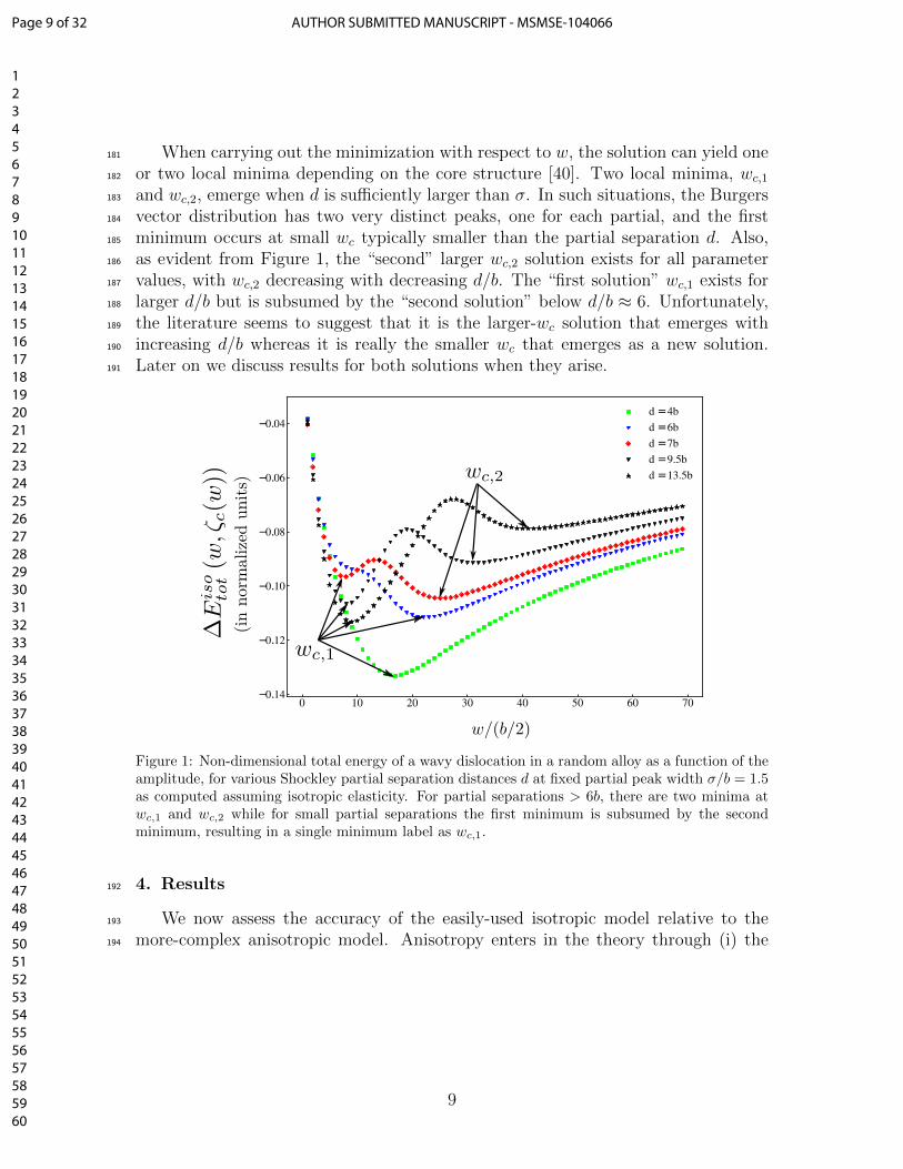
When carrying out the minimization with respect to w, the solution can yield one181

or two local minima depending on the core structure [40]. Two local minima, wc,1182

and wc,2, emerge when d is sufficiently larger than σ. In such situations, the Burgers183

vector distribution has two very distinct peaks, one for each partial, and the first184

minimum occurs at small wc typically smaller than the partial separation d. Also,185

as evident from Figure 1, the “second” larger wc,2 solution exists for all parameter186

values, with wc,2 decreasing with decreasing d/b. The “first solution” wc,1 exists for187

larger d/b but is subsumed by the “second solution” below d/b ≈ 6. Unfortunately,188

the literature seems to suggest that it is the larger-wc solution that emerges with189

increasing d/b whereas it is really the smaller wc that emerges as a new solution.190

Later on we discuss results for both solutions when they arise.191

0 10 20 30 40 50 60 70−0.14

−0.12

−0.10

−0.08

−0.06

−0.04d =4bd =6bd =7bd =9.5bd =13.5b

Figure 1: Non-dimensional total energy of a wavy dislocation in a random alloy as a function of theamplitude, for various Shockley partial separation distances d at fixed partial peak width σ/b = 1.5as computed assuming isotropic elasticity. For partial separations > 6b, there are two minima atwc,1 and wc,2 while for small partial separations the first minimum is subsumed by the secondminimum, resulting in a single minimum label as wc,1.

4. Results192

We now assess the accuracy of the easily-used isotropic model relative to the193

more-complex anisotropic model. Anisotropy enters in the theory through (i) the194

9


123456789101112131415161718192021222324252627282930313233343536373839404142434445464748495051525354555657585960

dislocation line tension, and (ii) the dislocation core structure quantity g. Both195

aspects are examined in the following.196

4.1. Line tension197

The line tension Γ enters the theory as Γ1/3 in ∆Eb and as Γ−1/3 in τy0 (Equa-198

tions 12 and 13), and hence results are weakly dependent on the precise value of199

Γ. However, the line tension scales with the elastic moduli, and so is in princi-200

ple a function of the anisotropy. For fcc alloys, the line tension is best related to201

the shear modulus in the < 111 > plane along the < 110 > direction, µ111/110 =202

(C11 − C12 + C44) /3 via the scaling relation Γ = αµ111/110b2. Values of α ∼ 1/16 −203

1/8 have been used, with the larger value found in several atomistic studies of bowed-204

out dislocations [35]. In the absence of the crystal anisotropic elastic constants,205

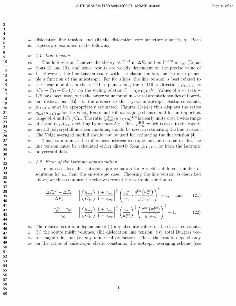
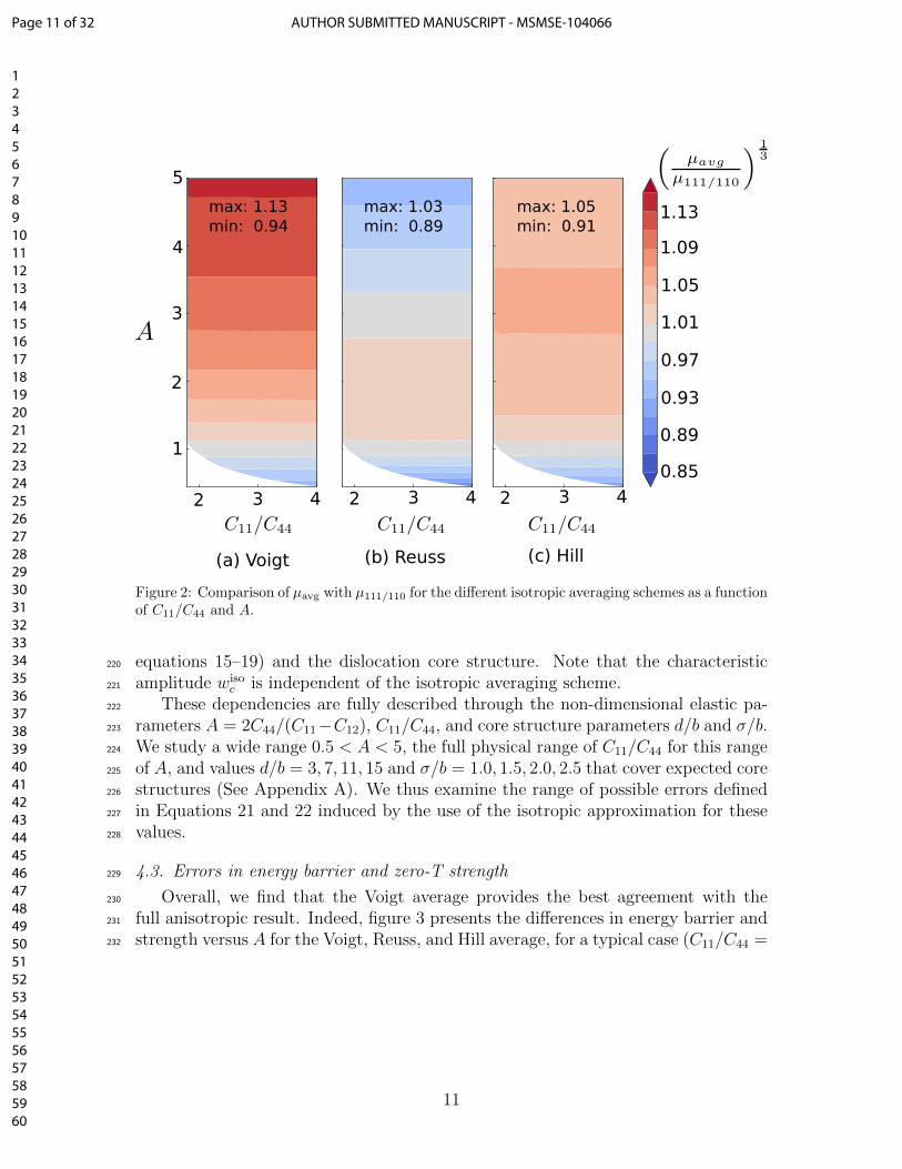
µ111/110 must be appropriately estimated. Figures 2(a)-(c) thus displays the ratios206

µavg/µ111/110 for the Voigt, Reuss and Hill averaging schemes, and for an important207

range of A and C11/C44. The ratio (µHillavg/µ111/110)1/3 is nearly unity over a wide range208

of A and C11/C44, deviating by at most 5%. Thus, µHillavg , which is close to the esperi-209

mental polycrystalline shear modulus, should be used in estimating the line tension.210

The Voigt averaged moduli should not be used for estimating the line tension [4].211

Thus, to minimize the differences between isotropic and anisotropic results, the212

line tension must be calculated either directly from µ111/110, or from the isotropic213

polycrystal data.214

4.2. Error of the isotropic approximation215

In no case does the isotropic approximation for g yield a different number ofsolutions for wc than the anisotropic case. Choosing the line tension as describedabove, we thus compute the relative error of the isotropic solution as

∆Eisob −∆Eb∆Eb

=

[(µavg

C44

)1 + νavg

1− νavg

] 23

(wisoc

wc·giso(wisoc

)g (wc)

) 23

− 1; and (21)

τ isoy0 − τy0

τy0

=

[(µavg

C44

)1 + νavg

1− νavg

] 43(wcwisoc

) 53

(giso(wisoc

)g (wc)

) 43

− 1. (22)

The relative error is independent of (i) any absolute values of the elastic constants,216

(ii) the solute misfit volumes, (iii) dislocation line tension, (iv) total Burgers vec-217

tor magnitude, and (v) any numerical prefactors. Thus, the results depend only218

on the ratios of anisotropic elastic constants, the isotropic averaging scheme (see219

10


123456789101112131415161718192021222324252627282930313233343536373839404142434445464748495051525354555657585960

2 3 4 2 3 4 2 3 4

(a) Voigt (b) Reuss (c) Hill

1

2

3

4

5

max: 1.13min: 0.94

max: 1.03min: 0.89

max: 1.05min: 0.91

1.13

1.09

1.05

1.01

0.97

0.93

0.89

0.85

Figure 2: Comparison of µavg with µ111/110 for the different isotropic averaging schemes as a functionof C11/C44 and A.

equations 15–19) and the dislocation core structure. Note that the characteristic220

amplitude wisoc is independent of the isotropic averaging scheme.221

These dependencies are fully described through the non-dimensional elastic pa-222

rameters A = 2C44/(C11−C12), C11/C44, and core structure parameters d/b and σ/b.223

We study a wide range 0.5 < A < 5, the full physical range of C11/C44 for this range224

of A, and values d/b = 3, 7, 11, 15 and σ/b = 1.0, 1.5, 2.0, 2.5 that cover expected core225

structures (See Appendix A). We thus examine the range of possible errors defined226

in Equations 21 and 22 induced by the use of the isotropic approximation for these227

values.228

4.3. Errors in energy barrier and zero-T strength229

Overall, we find that the Voigt average provides the best agreement with the230

full anisotropic result. Indeed, figure 3 presents the differences in energy barrier and231

strength versus A for the Voigt, Reuss, and Hill average, for a typical case (C11/C44 =232

11


123456789101112131415161718192021222324252627282930313233343536373839404142434445464748495051525354555657585960

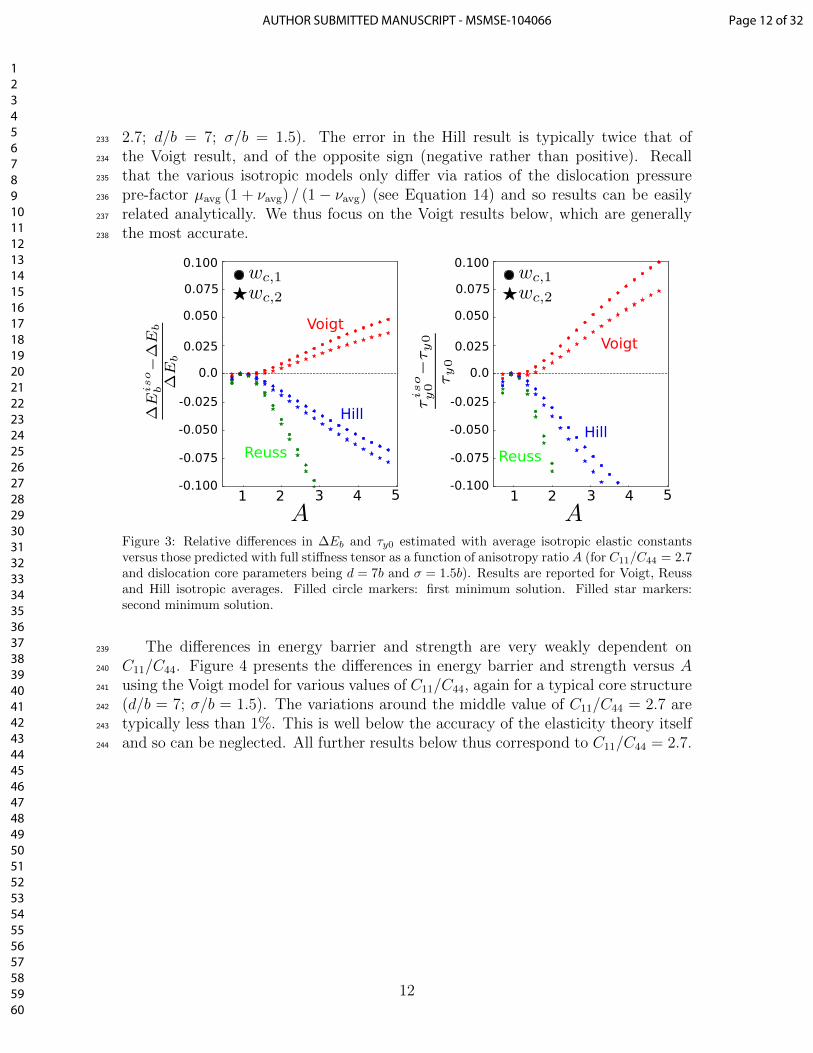
2.7; d/b = 7; σ/b = 1.5). The error in the Hill result is typically twice that of233

the Voigt result, and of the opposite sign (negative rather than positive). Recall234

that the various isotropic models only differ via ratios of the dislocation pressure235

pre-factor µavg (1 + νavg) / (1− νavg) (see Equation 14) and so results can be easily236

related analytically. We thus focus on the Voigt results below, which are generally237

the most accurate.238

Voigt

Reuss

Hill

Voigt

Reuss

Hill

1 2 3 4 5 1 2 3 4 5

0.100

0.075

0.050

0.025

0.0

-0.025

-0.050

-0.075

-0.100

0.100

0.075

0.050

0.025

0.0

-0.025

-0.050

-0.075

-0.100

Figure 3: Relative differences in ∆Eb and τy0 estimated with average isotropic elastic constantsversus those predicted with full stiffness tensor as a function of anisotropy ratio A (for C11/C44 = 2.7and dislocation core parameters being d = 7b and σ = 1.5b). Results are reported for Voigt, Reussand Hill isotropic averages. Filled circle markers: first minimum solution. Filled star markers:second minimum solution.

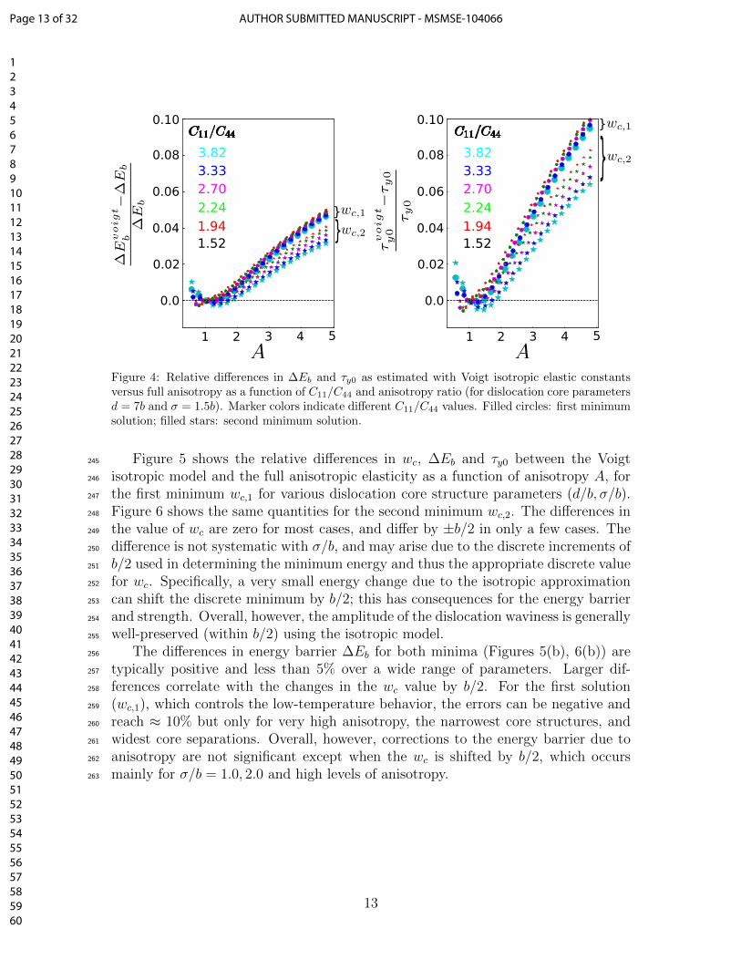
The differences in energy barrier and strength are very weakly dependent on239

C11/C44. Figure 4 presents the differences in energy barrier and strength versus A240

using the Voigt model for various values of C11/C44, again for a typical core structure241

(d/b = 7; σ/b = 1.5). The variations around the middle value of C11/C44 = 2.7 are242

typically less than 1%. This is well below the accuracy of the elasticity theory itself243

and so can be neglected. All further results below thus correspond to C11/C44 = 2.7.244

12


123456789101112131415161718192021222324252627282930313233343536373839404142434445464748495051525354555657585960

0.10

0.08

0.06

0.04

0.02

0.0

0.10

0.08

0.06

0.04

0.02

0.0

}

}

}}

1 2 3 4 5 1 2 3 4 5

3.823.332.70

2.241.941.52

3.823.332.70

2.241.941.52

Figure 4: Relative differences in ∆Eb and τy0 as estimated with Voigt isotropic elastic constantsversus full anisotropy as a function of C11/C44 and anisotropy ratio (for dislocation core parametersd = 7b and σ = 1.5b). Marker colors indicate different C11/C44 values. Filled circles: first minimumsolution; filled stars: second minimum solution.

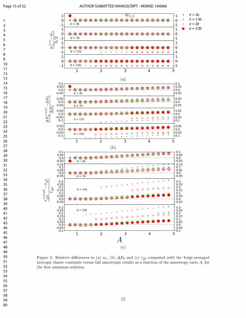
Figure 5 shows the relative differences in wc, ∆Eb and τy0 between the Voigt245

isotropic model and the full anisotropic elasticity as a function of anisotropy A, for246

the first minimum wc,1 for various dislocation core structure parameters (d/b, σ/b).247

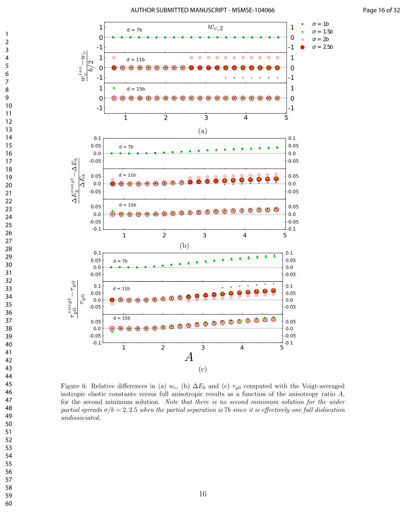
Figure 6 shows the same quantities for the second minimum wc,2. The differences in248

the value of wc are zero for most cases, and differ by ±b/2 in only a few cases. The249

difference is not systematic with σ/b, and may arise due to the discrete increments of250

b/2 used in determining the minimum energy and thus the appropriate discrete value251

for wc. Specifically, a very small energy change due to the isotropic approximation252

can shift the discrete minimum by b/2; this has consequences for the energy barrier253

and strength. Overall, however, the amplitude of the dislocation waviness is generally254

well-preserved (within b/2) using the isotropic model.255

The differences in energy barrier ∆Eb for both minima (Figures 5(b), 6(b)) are256

typically positive and less than 5% over a wide range of parameters. Larger dif-257

ferences correlate with the changes in the wc value by b/2. For the first solution258

(wc,1), which controls the low-temperature behavior, the errors can be negative and259

reach ≈ 10% but only for very high anisotropy, the narrowest core structures, and260

widest core separations. Overall, however, corrections to the energy barrier due to261

anisotropy are not significant except when the wc is shifted by b/2, which occurs262

mainly for σ/b = 1.0, 2.0 and high levels of anisotropy.263

13


123456789101112131415161718192021222324252627282930313233343536373839404142434445464748495051525354555657585960

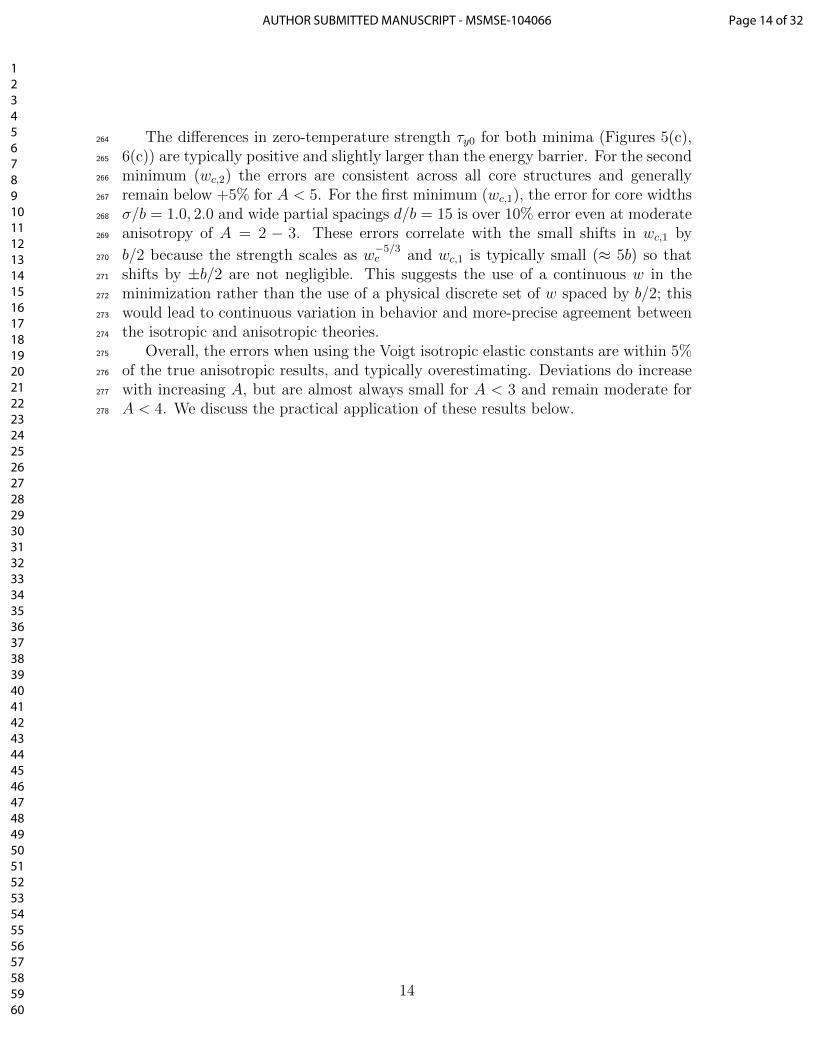
The differences in zero-temperature strength τy0 for both minima (Figures 5(c),264

6(c)) are typically positive and slightly larger than the energy barrier. For the second265

minimum (wc,2) the errors are consistent across all core structures and generally266

remain below +5% for A < 5. For the first minimum (wc,1), the error for core widths267

σ/b = 1.0, 2.0 and wide partial spacings d/b = 15 is over 10% error even at moderate268

anisotropy of A = 2 − 3. These errors correlate with the small shifts in wc,1 by269

b/2 because the strength scales as w−5/3c and wc,1 is typically small (≈ 5b) so that270

shifts by ±b/2 are not negligible. This suggests the use of a continuous w in the271

minimization rather than the use of a physical discrete set of w spaced by b/2; this272

would lead to continuous variation in behavior and more-precise agreement between273

the isotropic and anisotropic theories.274

Overall, the errors when using the Voigt isotropic elastic constants are within 5%275

of the true anisotropic results, and typically overestimating. Deviations do increase276

with increasing A, but are almost always small for A < 3 and remain moderate for277

A < 4. We discuss the practical application of these results below.278

14


123456789101112131415161718192021222324252627282930313233343536373839404142434445464748495051525354555657585960

10

-110

-110

-110

-1

10

-110

-110

-110

-1

1 2 3 4 5

σ = 1bσ = 1.5bσ = 2bσ = 2.5b

d = 3b

d = 7b

d = 11b

d = 15b

(a)0.1

0.0-0.05

0.05

0.0-0.05

0.05

0.0-0.05

0.05

0.0-0.05

0.05

-0.1

-0.1

0.1

0.0-0.05

0.05

0.0-0.05

0.05

0.0-0.05

0.05

0.0-0.05

0.05

-0.1

-0.1

1 2 3 4 5

d = 3b

d = 7b

d = 11b

d = 15b

(b)0.1

0.0-0.05

0.05

0.0-0.05

0.05

0.0-0.05

0.05

0.0-0.05

0.05

-0.1

0.10.15

0.10.150.2

0.250.3

0.10.150.2

0.250.3

0.1

0.0-0.05

0.05

0.0-0.05

0.05

0.0-0.05

0.05

0.0-0.05

0.05

-0.1

0.10.15

0.10.150.20.250.3

0.10.150.20.250.3

1 2 3 4 5

d = 3b

d = 7b

d = 11b

d = 15b

(c)

Figure 5: Relative differences in (a) wc, (b) ∆Eb and (c) τy0 computed with the Voigt-averagedisotropic elastic constants versus full anisotropic results as a function of the anisotropy ratio A, forthe first minimum solution.

15


123456789101112131415161718192021222324252627282930313233343536373839404142434445464748495051525354555657585960

σ = 1bσ = 1.5bσ = 2bσ = 2.5b

1

0

-1

1 2 3 4 5

1

0

-1

1

0

-1

1

0

-1

1

0

-1

1

0

-1

d = 7b

d = 11b

d = 15b

(a)0.1

0.0

-0.05

0.05

0.0

-0.05

0.05

0.0

-0.05

0.05

-0.1

1 2 3 4 5

d = 7b

d = 11b

d = 15b

0.1

0.0

-0.05

0.05

0.0

-0.05

0.05

0.0

-0.05

0.05

-0.1

(b)

1 2 3 4 5

0.1

0.0

-0.05

0.05

0.0

-0.05

0.05

0.0

-0.05

0.05

-0.1

d = 7b

d = 11b

d = 15b

0.1

0.1

0.0

-0.05

0.05

0.0

-0.05

0.05

0.0

-0.05

0.05

-0.1

0.1

(c)

Figure 6: Relative differences in (a) wc, (b) ∆Eb and (c) τy0 computed with the Voigt-averagedisotropic elastic constants versus full anisotropic results as a function of the anisotropy ratio A,for the second minimum solution. Note that there is no second minimum solution for the widerpartial spreads σ/b = 2, 2.5 when the partial separation is 7b since it is effectively one full dislocationundissociated.

16


123456789101112131415161718192021222324252627282930313233343536373839404142434445464748495051525354555657585960

5. Practical application of the theory279

We have shown that the difference between the Voigt isotropic model and the full280

anisotropic model are usually relatively small. The largest deviations arise when the281

isotropic model predicts a shift of b/2 in wc relative to the full anisotropic model,282

which occurs almost exclusively for σ/b = 1.0, 2.0 and can thus be identified. Other-283

wise, we consider the errors of 5% to be well within the uncertainty of the elasticity284

model, relative to the full theory, and the full theory itself involves approximations.285

Thus, the isotropic theory can be used and then corrected to approach the anisotropic286

result based on available understanding. Experiments do not usually yield the Voigt287

moduli nor the core structure (especially σ), and application of the model also re-288

quires the line tension Γ. In this section, we therefore first present a parametric study289

of the predictions of the isotropic theory and then address how we envision the use of290

the anisotropic elasticity theory in combination with experimental or first-principles291

inputs.292

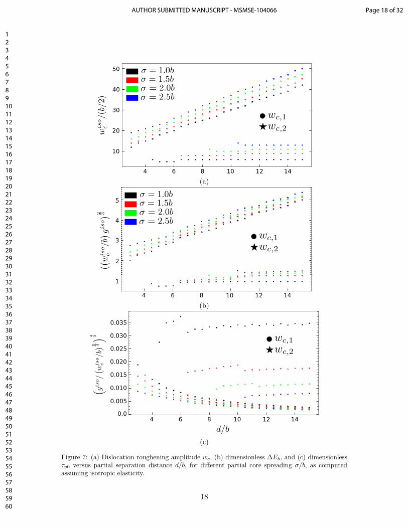
5.1. Normalized results for wc, ∆Eb and τy0 using isotropic elasticity293

We first present the isotropic results over the range of core structures. FromEqs. 12, 13 and 14, it is evident that the energy barrier and strength are functionsof wiso

c (d/b, σ/b) and giso(wc, d/b, σ/b), with

∆Eb ∝(wisoc g

iso)2/3

, (23)

τy0 ∝(giso/wiso

c

5/4)4/3

. (24)

Figures 7(b) and 7(c) show these normalized quantities over a wide range of294

(d/b, σ/b) with the two solutions for wc (where applicable). Figure 7(a) presents the295

wc,1 and wc,2, although these are not directly needed in practical application of the296

model.297

Figure 7(c) shows that the strength quantity is quite sensitive to the partial core298

width σ, especially for small σ. The quantity σ, while correlated through the Peierls-299

Nabarro model to the unstable stacking fault energy and elastic constants of the alloy300

[6], is not well established. The atomistic simulations in Appendix A, and previous301

analyses in Ref. [42], indicate that a range 1.5 < σ/b < 2.5 prevails across most302

materials. Subsequent applications of the model used the value σ/b = 1.5 across303

a wide range of materials with good success and we have seen above that the wc304

for this value of σ/b agrees with that obtained in the full anisotropic model; this is305

further discussed below.306

17


123456789101112131415161718192021222324252627282930313233343536373839404142434445464748495051525354555657585960

10

20

30

40

50

6 8 104 12 14

(a)

6 8 104 12 14

1

2

3

4

5

(b)

0.06 8 104 12 14

0.005

0.010

0.015

0.020

0.025

0.030

0.035

(c)

Figure 7: (a) Dislocation roughening amplitude wc, (b) dimensionless ∆Eb, and (c) dimensionlessτy0 versus partial separation distance d/b, for different partial core spreading σ/b, as computedassuming isotropic elasticity.

18


123456789101112131415161718192021222324252627282930313233343536373839404142434445464748495051525354555657585960

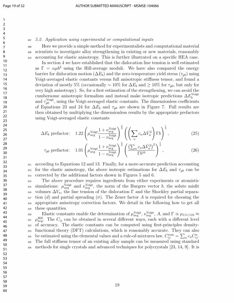
5.2. Application using experimental or computational inputs307

Here we provide a simple method for experimentalists and computational material308

scientists to investigate alloy strengthening in existing or new materials, reasonably309

accounting for elastic anisotropy. This is further illustrated on a specific HEA case.310

In section 4 we have established that the dislocation line tension is well estimatedas Γ = αµb2 using the Hill-average moduli. We have also compared the energybarrier for dislocation motion (∆Eb) and the zero-temperature yield stress (τy0) usingVoigt-averaged elastic constants versus full anisotropic stiffness tensor, and found adeviation of mostly 5% (occasionally ∼ 10% for ∆Eb and ≥ 10% for τy0, but only forvery high anisotropy). So, for a first estimation of the strengthening, we can avoid thecumbersome anisotropic formalism and instead make isotropic predictions ∆EVoigt

b

and τVoigty0 , using the Voigt-averaged elastic constants. The dimensionless coefficients

of Equations 23 and 24 for ∆Eb and τy0 are shown in Figure 7. Full results arethen obtained by multiplying the dimensionless results by the appropriate prefactorsusing Voigt-averaged elastic constants

∆Eb prefactor: 1.22

(µVoigt

avg

1 + νVoigtavg

1− νVoigtavg

) 23((∑

n

cn∆V 2n

)Γb

) 13

, (25)

τy0 prefactor: 1.01

(µVoigt

avg

1 + νVoigtavg

1− νVoigtavg

) 43((∑

n cn∆V 2n

)2

Γb10

) 13

, (26)

according to Equations 12 and 13. Finally, for a more-accurate prediction accounting311

for the elastic anisotropy, the above isotropic estimations for ∆Eb and τy0 can be312

corrected by the additional factors shown in Figures 5 and 6.313

The above procedure requires ingredients from either experiments or atomistic314

simulations: µVoigtavg and νVoigt

avg , the norm of the Burgers vector b, the solute misfit315

volumes ∆Vn, the line tension of the dislocation Γ and the Shockley partial separa-316

tion (d) and partial spreading (σ). The Zener factor A is required for choosing the317

appropriate anisotropy correction factors. We detail in the following how to get all318

these quantities.319

Elastic constants enable the determination of µVoigtavg , νVoigt

avg , A, and Γ ∝ µ111/110 ≈320

µHillavg . The Cij can be obtained in several different ways, each with a different level321

of accuracy. The elastic constants can be computed using first-principles density-322

functional theory (DFT) calculations, which is reasonably accurate. They can also323

be estimated using the elemental values and a rule-of-mixtures law, Cromij =

∑n cnC

nij.324

The full stiffness tensor of an existing alloy sample can be measured using standard325

methods for single crystals and advanced techniques for polycrystals [23, 14, 9]. It is326

19


123456789101112131415161718192021222324252627282930313233343536373839404142434445464748495051525354555657585960

more conventional, however, to measure only the average elastic moduli of equiaxed327

polycrystals, which are typically close to the Hill approximation [13]. Γ can thus328

be computed using the experimental isotropic shear modulus. The Voigt-averaged329

values can then be estimated by using the anisotropy A of the rule-of-mixtures Cromij330

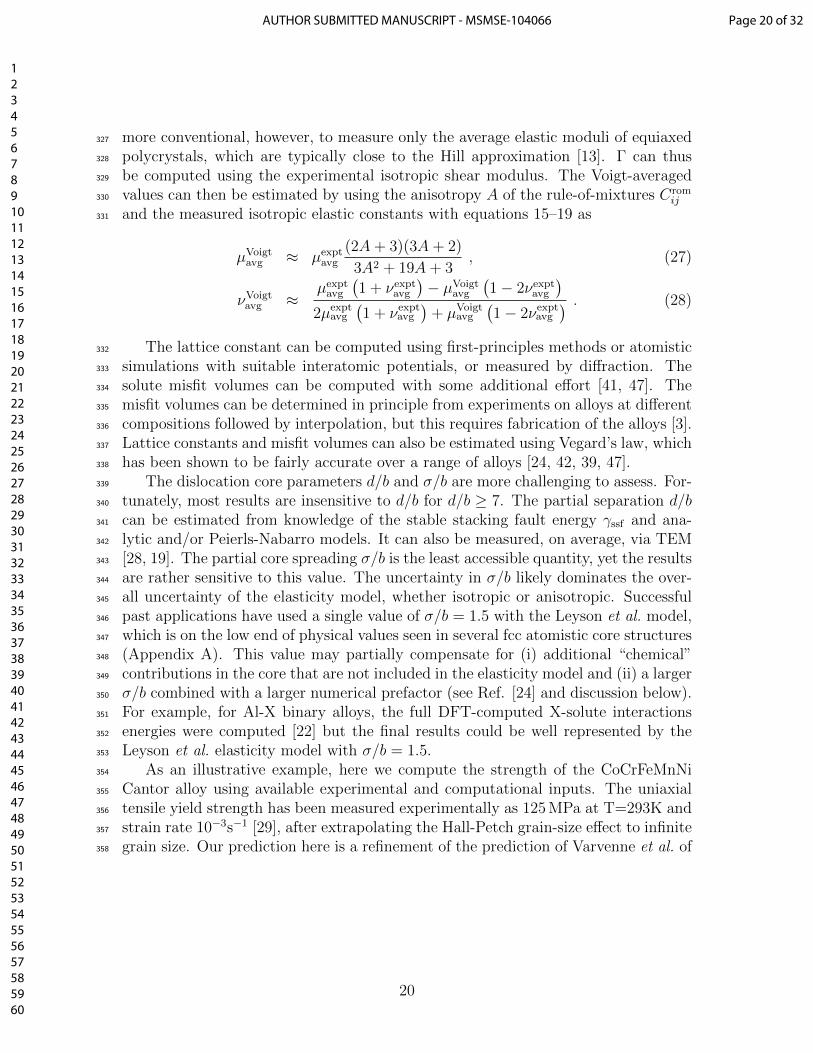
and the measured isotropic elastic constants with equations 15–19 as331

µVoigtavg ≈ µexpt

avg

(2A+ 3)(3A+ 2)

3A2 + 19A+ 3, (27)

νVoigtavg ≈

µexptavg

(1 + νexpt

avg

)− µVoigt

avg

(1− 2νexpt

avg

)2µexpt

avg

(1 + νexpt

avg

)+ µVoigt

avg

(1− 2νexpt

avg

) . (28)

The lattice constant can be computed using first-principles methods or atomistic332

simulations with suitable interatomic potentials, or measured by diffraction. The333

solute misfit volumes can be computed with some additional effort [41, 47]. The334

misfit volumes can be determined in principle from experiments on alloys at different335

compositions followed by interpolation, but this requires fabrication of the alloys [3].336

Lattice constants and misfit volumes can also be estimated using Vegard’s law, which337

has been shown to be fairly accurate over a range of alloys [24, 42, 39, 47].338

The dislocation core parameters d/b and σ/b are more challenging to assess. For-339

tunately, most results are insensitive to d/b for d/b ≥ 7. The partial separation d/b340

can be estimated from knowledge of the stable stacking fault energy γssf and ana-341

lytic and/or Peierls-Nabarro models. It can also be measured, on average, via TEM342

[28, 19]. The partial core spreading σ/b is the least accessible quantity, yet the results343

are rather sensitive to this value. The uncertainty in σ/b likely dominates the over-344

all uncertainty of the elasticity model, whether isotropic or anisotropic. Successful345

past applications have used a single value of σ/b = 1.5 with the Leyson et al. model,346

which is on the low end of physical values seen in several fcc atomistic core structures347

(Appendix A). This value may partially compensate for (i) additional “chemical”348

contributions in the core that are not included in the elasticity model and (ii) a larger349

σ/b combined with a larger numerical prefactor (see Ref. [24] and discussion below).350

For example, for Al-X binary alloys, the full DFT-computed X-solute interactions351

energies were computed [22] but the final results could be well represented by the352

Leyson et al. elasticity model with σ/b = 1.5.353

As an illustrative example, here we compute the strength of the CoCrFeMnNi354

Cantor alloy using available experimental and computational inputs. The uniaxial355

tensile yield strength has been measured experimentally as 125 MPa at T=293K and356

strain rate 10−3s−1 [29], after extrapolating the Hall-Petch grain-size effect to infinite357

grain size. Our prediction here is a refinement of the prediction of Varvenne et al. of358

20


123456789101112131415161718192021222324252627282930313233343536373839404142434445464748495051525354555657585960

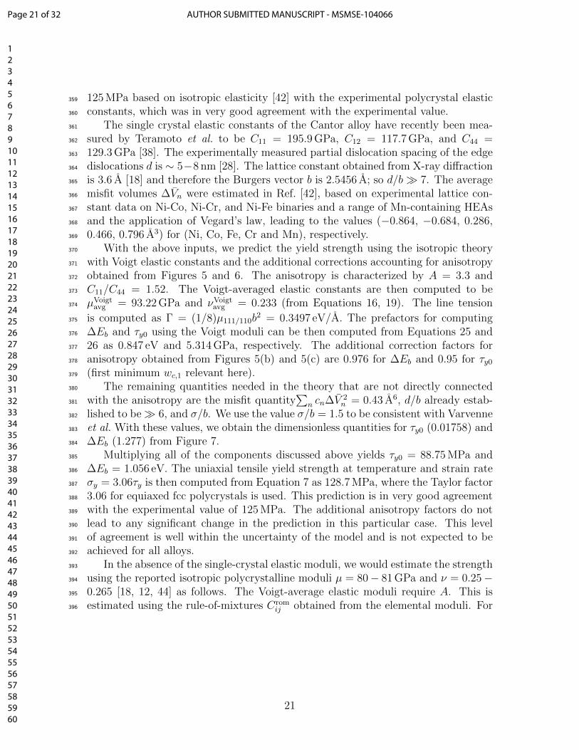
125 MPa based on isotropic elasticity [42] with the experimental polycrystal elastic359

constants, which was in very good agreement with the experimental value.360

The single crystal elastic constants of the Cantor alloy have recently been mea-361

sured by Teramoto et al. to be C11 = 195.9 GPa, C12 = 117.7 GPa, and C44 =362

129.3 GPa [38]. The experimentally measured partial dislocation spacing of the edge363

dislocations d is ∼ 5−8 nm [28]. The lattice constant obtained from X-ray diffraction364

is 3.6 A [18] and therefore the Burgers vector b is 2.5456 A; so d/b� 7. The average365

misfit volumes ∆Vn were estimated in Ref. [42], based on experimental lattice con-366

stant data on Ni-Co, Ni-Cr, and Ni-Fe binaries and a range of Mn-containing HEAs367

and the application of Vegard’s law, leading to the values (−0.864, −0.684, 0.286,368

0.466, 0.796 A3) for (Ni, Co, Fe, Cr and Mn), respectively.369

With the above inputs, we predict the yield strength using the isotropic theory370

with Voigt elastic constants and the additional corrections accounting for anisotropy371

obtained from Figures 5 and 6. The anisotropy is characterized by A = 3.3 and372

C11/C44 = 1.52. The Voigt-averaged elastic constants are then computed to be373

µVoigtavg = 93.22 GPa and νVoigt

avg = 0.233 (from Equations 16, 19). The line tension374

is computed as Γ = (1/8)µ111/110b2 = 0.3497 eV/A. The prefactors for computing375

∆Eb and τy0 using the Voigt moduli can be then computed from Equations 25 and376

26 as 0.847 eV and 5.314 GPa, respectively. The additional correction factors for377

anisotropy obtained from Figures 5(b) and 5(c) are 0.976 for ∆Eb and 0.95 for τy0378

(first minimum wc,1 relevant here).379

The remaining quantities needed in the theory that are not directly connected380

with the anisotropy are the misfit quantity∑

n cn∆V 2n = 0.43 A6, d/b already estab-381

lished to be� 6, and σ/b. We use the value σ/b = 1.5 to be consistent with Varvenne382

et al. With these values, we obtain the dimensionless quantities for τy0 (0.01758) and383

∆Eb (1.277) from Figure 7.384

Multiplying all of the components discussed above yields τy0 = 88.75 MPa and385

∆Eb = 1.056 eV. The uniaxial tensile yield strength at temperature and strain rate386

σy = 3.06τy is then computed from Equation 7 as 128.7 MPa, where the Taylor factor387

3.06 for equiaxed fcc polycrystals is used. This prediction is in very good agreement388

with the experimental value of 125 MPa. The additional anisotropy factors do not389

lead to any significant change in the prediction in this particular case. This level390

of agreement is well within the uncertainty of the model and is not expected to be391

achieved for all alloys.392

In the absence of the single-crystal elastic moduli, we would estimate the strength393

using the reported isotropic polycrystalline moduli µ = 80− 81 GPa and ν = 0.25−394

0.265 [18, 12, 44] as follows. The Voigt-average elastic moduli require A. This is395

estimated using the rule-of-mixtures Cromij obtained from the elemental moduli. For396

21


123456789101112131415161718192021222324252627282930313233343536373839404142434445464748495051525354555657585960

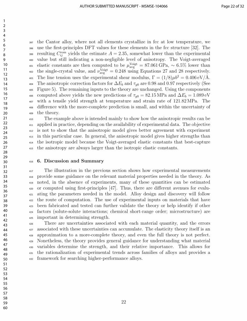
the Cantor alloy, where not all elements crystallize in fcc at low temperature, we397

use the first-principles DFT values for these elements in the fcc structure [32]. The398

resulting Cromij yields the estimate A = 2.35, somewhat lower than the experimental399

value but still indicating a non-negligible level of anisotropy. The Voigt-averaged400

elastic constants are then computed to be µVoigtavg = 87.061 GPa, ∼ 6.5% lower than401

the single-crystal value, and νVoigtavg = 0.248 using Equations 27 and 28 respectively.402

The line tension uses the experimental shear modulus, Γ = (1/8)µb2 = 0.406 eV/A.403

The anisotropic correction factors for ∆Eb and τy0 are 0.98 and 0.97 respectively (See404

Figure 5). The remaining inputs to the theory are unchanged. Using the components405

computed above yields the new predictions of τy0 = 82.15 MPa and ∆Eb = 1.089 eV406

with a tensile yield strength at temperature and strain rate of 121.82 MPa. The407

difference with the more-complete prediction is small, and within the uncertainty of408

the theory.409

The example above is intended mainly to show how the anisotropic results can be410

applied in practice, depending on the availability of experimental data. The objective411

is not to show that the anisotropic model gives better agreement with experiment412

in this particular case. In general, the anisotropic model gives higher strengths than413

the isotropic model because the Voigt-averaged elastic constants that best-capture414

the anisotropy are always larger than the isotropic elastic constants.415

6. Discussion and Summary416

The illustration in the previous section shows how experimental measurements417

provide some guidance on the relevant material properties needed in the theory. As418

noted, in the absence of experiments, many of these quantities can be estimated419

or computed using first-principles [47]. Thus, there are different avenues for evalu-420

ating the parameters needed in the model. Alloy design and discovery will follow421

the route of computation. The use of experimental inputs on materials that have422

been fabricated and tested can further validate the theory or help identify if other423

factors (solute-solute interactions; chemical short-range order; microstructure) are424

important in determining strength.425

There are uncertainties associated with each material quantity, and the errors426

associated with these uncertainties can accumulate. The elasticity theory itself is an427

approximation to a more-complete theory, and even the full theory is not perfect.428

Nonetheless, the theory provides general guidance for understanding what material429

variables determine the strength, and their relative importance. This allows for430

the rationalization of experimental trends across families of alloys and provides a431

framework for searching higher-performance alloys.432

22


123456789101112131415161718192021222324252627282930313233343536373839404142434445464748495051525354555657585960

The underlying theory of this complex process of a dislocation moving through a433

random alloy continues to evolve. In application to edge dislocations in bcc alloys,434

a new general stochastic analysis of the wavy dislocation configuration has been435

presented [24]. This analysis involves a more-detailed statistical analysis of the wavy436

dislocation structure via stochastic modeling of the structure segment-by-segment437

and including the full statistical distribution of possible segment energy changes due438

to the solute fluctuations. This analysis leads to additional numerical coefficients439

κ = 0.56 and β = 0.833 multiplying the line energy and potential energy terms440

appearing in Equation 5, respectively, and a change in the energy barrier by a factor441 √2/(√

2− 0.25) = 1.214. The same analysis applies to fcc alloys, and the net effects442

are a factor of√κ/β = 0.82 multiplying the line tension and the factor of 1.214443

for the energy barrier, which then also enters the zero-temperature strength. These444

effects change the numerical coefficients in Equations 5 and 6 from (1.22, 1.01) to445

(1.39, 1.31), respectively. Thus, the successful use of σ/b = 1.5, which is smaller446

than values seen in simulations (see Appendix A), together with the original Leyson447

model may reflect some cancellation of effects. For instance, using σ/b = 2.0 and448

the corresponding dimensionless coefficient for τy0 of ∼ 0.012 (see Figure 7(c)) with449

the revised prefactor of 1.31 gives a net factor of ∼ 0.016 which is nearly equal450

to that obtained using the present Leyson model with σ/b = 1.5 (dimensionless451

coefficient ∼ 0.017) and with the Leyson coefficient 1.01, giving a net factor ∼452

0.017. However, for overall consistency with the previous literature and successful453

quantitative application of the Leyson model, we advocate continued use of the454

original Leyson model coefficients. We also note that these coefficients do not enter455

into any difference between isotropic and anisotropic theories, and so do not affect456

the primary analyses of this paper.457

The theory is also currently being extended to include the effects of solute-solute458

interactions, while remaining in the random alloy limit. The anisotropic elasticity459

theory here will remain valuable because the solute-solute interactions can be in-460

corporated along with the elasticity contributions to solute/dislocation interactions.461

Thus, the theory will continue to improve by incorporating increasing, but realistic,462

complexity.463

In summary, we have shown that the predictions of a fully anisotropic elastic464

model for solute strengthening can be obtained using an isotropic elasticity model465

with the Voigt-averaged elastic constants for the dislocation field and the Hill-466

averaged elastic constants for the line tension. Additional small correction factors467

to match the anisotropic result precisely are also provided. The effects of anisotropy468

are not negligible — the use of the standard Hill estimate for the isotropic moduli469

in equations 21 and 22 leads to rather lower strength predictions for high anisotropy470

23


123456789101112131415161718192021222324252627282930313233343536373839404142434445464748495051525354555657585960

(A = 3 − 4). Since many HEAs to date have anisotropy in the range of A = 2 − 4,471

these corrections are valuable for making refined predictions. We have provided some472

guidelines on obtaining the data needed to make predictions. Results then follow us-473

ing the coefficients presented graphically here, which we hope assists with application474

of the theory. The elastic theory provides an approximate but firm and analytical475

foundation for understanding trends in solute strengthening. Since the composition476

space in multi-component random alloys is immense, and experimental searching477

through that entire space is not feasible, the present theory provides a framework for478

rapid probing of the entire space in the search for attractive compositions for desired479

performance.480

7. Acknowledgement481

We thank the European Research Council for funding this work through the482

project ERC/FP Project 339081 entitled “PreCoMet Predictive Computational Met-483

allurgy”.484

Appendix A. Slip density in fcc elements485

In elements having an fcc crystal structure of lattice parameter a, the prevailing486

a/2 < 110 > dislocations gliding on the {111} planes dissociate into two mixed487

a/6 < 112 >-type Shockley partial dislocations bp,1 and bp,2. The partials are488

separated by an intrinsic stable stacking fault of energy γssf . The separation distance489

is determined by a balance between the repulsive elastic force between the partials490

and the attractive configurational force due to the stacking fault.491

The cores of the Shockley partials are not delta-functions; the Burgers vector is492

spread along the glide plane over some range of atoms. The most widely-used model493

for describing the Burgers vector density of dislocation cores is the Peierls-Nabarro494

(P-N) model [6]. Under certain simplifications of the generalized stacking fault energy495

curve, the P-N model predicts a Lorentzian form of Burgers vector density as bπ

ζx2+ζ2

496

where ζ characterizes the width. Analysis shows that ζ ∼ 1/γusf where γusf is the497

unstable stacking fault energy. However, the computed values of ζ for partial cores498

are typically about 1/2 those observed in simulations of atomistic dislocation cores499

[34]. Here, we show that a Gaussian function provides a better description of the500

plastic displacements associated with the atomistic dislocation core structure.501

The Burgers vector distribution is the plastic slip distribution along the glide502

plane. The plastic slip is not the same as the total shear strain, due to the additional503

elastic shearing. In the centers of the partial cores of the dislocation, the elastic504

shearing is indeed small and the use of elasticity questionable. Away from the centers505

24


123456789101112131415161718192021222324252627282930313233343536373839404142434445464748495051525354555657585960

of the partial cores, the shear distribution is composed of both plastic and elastic506

contributions, and the elastic contributions stem from the elastic fields of the plastic507

slip distribution along the entire slip plane.508

We have examined the slip distribution of fully-relaxed atomistic edge dislocation509

cores for Al, Ni, and Cu as predicted by widely-used interatomic potentials [26, 27].510

Specifically, the core structure is created in the standard manner. In an initial511

cylindrical sample of fcc crystal of radius 100b with orientation x= (Burgers vector512

and glide direction {110}), y = (normal to the slip plane {111}), z = (dislocation513

line direction {112}), we impose the anisotropic displacement field corresponding to a514

Volterra edge dislocation lying along the z axis of the cylinder with the cut-plane for515

slip lying along the (x-y) slip plane in the region (x < 0, y = 0). The displacements516

of a thin annular region of atoms on the outer boundary of the cylinder are held fixed517

at the Volterra solution and all interior atoms are then relaxed to their equilibrium518

positions to create the dissociated dislocation. The displacement u(x) of every atom519

away from its initial fcc position is then measured. We focus on the atoms in the520

planes just above and just below the slip plane, and denote their positions by the521

coordinate xi along the glide plane direction. The difference in shear displacements522

across the slip plane is computed by finite differences in the discrete system as523

D∆u

Dx

∣∣∣∣(xi+xi+1)/2

=∆u(xi+1)−∆u(xi)

b/2. (A.1)

Figure A.8 shows the computed D∆ux/Dx and D∆uz/Dx from the atomistic cal-524

culations for the edge and screw components respectively of a edge full dislocation525

in Al, Ni and Cu.526

We are interested only in the plastic displacements, which are the discrete atom-527

istic counterparts of the slip density ∂b/∂x. We consider the measured shear strains528

D∆ux/(b/√

1.5) > 0.01 (corresponding to D∆ux/Dx > 0.016) to be dominated by529

the plastic displacements. We thus fit the measured D∆u/Dx in this region to a530

sum of two Gaussians (Equation 20) as531

D∆u

Dx≈ 1√

2πσ2

(bp,1e−

(x+d/2−xc)2

2σ2 + bp,2e−(x−d/2−xc)2

2σ2

). (A.2)

d/b is taken as the distance between the peaks in D∆ux/Dx and the average or532

center position xc of the full dislocation is taken as the middle of the peaks. σ/b is533

then the only fitting parameter, computed by a least-squares method, considering534

both components ∂bx∂x

and ∂bz∂x

. Figure A.8 shows the best-fit results using dislocations535

symbols ⊥⊥⊥ and the fitted value of σ/b is shown in each figure. The fits are gener-536

ally good, with root-mean-square error below ∼ 0.01. We note that fits to other537

25


123456789101112131415161718192021222324252627282930313233343536373839404142434445464748495051525354555657585960

types of functions, viz. logistic, Lorentzian, Gaussian-Lorentzian mixture, are not538

significantly better or worse in this region.539

26


123456789101112131415161718192021222324252627282930313233343536373839404142434445464748495051525354555657585960

0.00

0.02

0.04

0.06

0.08

0.10

0.12

−10 0 10−0.075

−0.050

−0.025

0.000

0.025

0.050

0.075

x/b

atomisticsPlastic part(Gaussian fit)

elastic+plastic

Gra

die

nt

of

Rela

tive d

isp

lace

men

t acr

oss

th

e s

lip p

lane

1% shear strain

Edge

Screw

(a) Al

0.00

0.02

0.04

0.06

0.08

−20 −10 0 10 20

−0.06

−0.04

−0.02

0.00

0.02

0.04

0.06


elastic+plastic

Gra

die

nt

of

Rela

tive d

isp

lace

men

t acr

oss

th

e s

lip p

lane

x/b

Edge

Screw

1% shear strain

(b) Cu

0.00

0.02

0.04

0.06

0.08

0.10

−20 −10 0 10 20

−0.075

−0.050

−0.025

0.000

0.025

0.050

0.075

1% shear strain


elastic+plastic

Edge

Screw

Gra

die

nt

of

Rela

tive d

ispla

cem

en

t acr

oss

th

e s

lip p

lane

x/b

(c) Ni

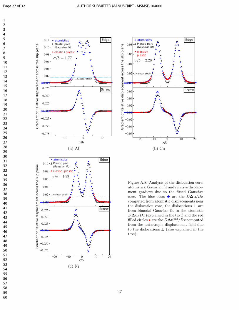
Figure A.8: Analysis of the dislocation core:atomistics, Gaussian fit and relative displace-ment gradient due to the fitted Gaussiancore. The blue stars F are the D∆u/Dxcomputed from atomistic displacements nearthe dislocation core, the dislocations ⊥⊥⊥ arefrom bimodal Gaussian fit to the atomisticD∆u/Dx (explained in the text) and the redfilled circles • are the D∆utot/Dx computedfrom the anisotropic displacement field dueto the dislocations ⊥⊥⊥ (also explained in thetext).

27


123456789101112131415161718192021222324252627282930313233343536373839404142434445464748495051525354555657585960

In the small shear strain region < 1%, Figure A.8 shows that the best-fit Gaussian540

plastic slip is significantly smaller than the total atomistic slip. This discrepancy541

may have tended to movitate the use of the Lorentzian function of the original PN542

model. However, in this regime, the total shear strains are dominated by the elastic543

shear strains caused by the Gaussian distribution of plastic slip. To demonstrate544

this, we compute the total anisotropic displacements utot(x) at every atomic site545

generated by the best-fit bimodal Gaussian Burgers vector distribution using the546

Stroh formalism and the superposition principle to obtain the elastic contribution,547

similar to Equation 10. The quantity D∆utot/Dx is then computed from utot using548

finite differences as above. Figure A.8 shows the total slip distribution (elastic plus549

plastic) in the region outside the cores, and the results closely match the full atomistic550

results. The two-Gaussian model thus captures both the underlying plastic slip551

distribution and the surrounding elastic shearing for dissociated fcc dislocations.552

Atomistically-computed dislocation core structures require either DFT or atom-553

istic interatomic potentials. DFT can be performed on elemental metals but alloy554

studies automatically include the response of the atoms to the random environment,555

preventing extraction of the underlying structure of the average alloy. In this case,556

computation of GPFE curves together with a double-Gaussian modeling of the dislo-557

cation core structure could be useful. Atomistic potentials are available for a number558

of elements, and some alloy systems, but with the usual caveats about accuracy rela-559

tive to the real materials. For alloys, the average-atom potential [41] can be created560

and used to examine the average core structure, but again relies on accuracy of the561

underlying potentials for the elemental constituents and their interactions. Typical562

values of σ are thus valuable. In Figure A.8, we find values 1.75 < σ/b < 2.25 for563

Al, Cu, and Ni. This range is consistent with the range 1.5 < σ/b < 2.5 obtained by564

Varvenne et al. [42] for Fe-Ni-Cr alloys. They then showed that σ/b = 1.5 provided565

good predictions for strength across a range of alloys, and this value was then used566

in subsequent work. While the solute strengthening does depend on σ/b, we thus567

remain consistent with previous work in suggesting the use of 1.5b in all fcc materials568

unless there is compelling evidence that a significantly different value should apply569

(see section 6).570

[1] Ali Argon. Strengthening Mechanisms in Crystal Plasticity. Oxford University571

Press, August 2007.572

[2] T. Balakrishna Bhat and V. S. Arunachalam. Strengthening mechanisms in573

alloys. Proceedings of the Indian Academy of Sciences Section C: Engineering574

Sciences, 3(4):275–296, December 1980.575

28


123456789101112131415161718192021222324252627282930313233343536373839404142434445464748495051525354555657585960

[3] J. Bandyopadhyaya and K. P. Gupta. Low temperature lattice parameter of576

nickel and some nickel-cobalt alloys and gruneisen parameter of nickel. Cryo-577

genics, 17(6):345–347, 1977.578

[4] D. M. Barnett, R. J. Asaro, S. D. Gavazza, D. J. Bacon, and R. O. Scattergood.579

The effects of elastic anisotropy on dislocation line tension in metals. J. Phys.580

F: Met. Phys., 2:854–864, 1972.581

[5] Allan Bower. Applied Mechanics of Solids. CRC Press, October 2009.582

[6] Vasily V. Bulatov and Wei Cai. Computer Simulations of Dislocations. Oxford583

series on materials modelling. Oxford University Press, 2006.584

[7] E. Clouet. The vacancy - edge dislocation interaction in FCC metals: a compar-585

ison between atomic simulations and elasticity theory. Acta Mater., 54:3543–586

3552, 2006.587

[8] Emmanuel Clouet, Sbastien Garruchet, Hoang Nguyen, Michel Perez, and Char-588

lotte S. Becquart. Dislocation interaction with C in α-Fe: A comparison between589

atomic simulations and elasticity theory. Acta Mater., 56:3450–3460, 2008.590

[9] X. Du and Ji-Cheng Zhao. Facile measurement of single-crystal elastic constants591

from polycrystalline samples. npj Computational Materials, 3(17), 2017.592

[10] H. Gleiter. Fundamentals of Strengthening Mechanisms. In Strength of Metals593

and Alloys (ICSMA 6), pages 1009–1024. Elsevier, 1982.594

[11] Bernd Gludovatz, Anton Hohenwarter, Dhiraj Catoor, Edwin H. Chang, Easo P.595

George, and Robert O. Ritchie. A fracture-resistant high-entropy alloy for cryo-596

genic applications. Science, 345(6201):1153–1158, 2014.597

[12] A. Haglund, M. Koehler, D. Catoor, E. P. George, and V. Keppens. Poly-598

crystalline elastic moduli of a high-entropy alloy at cryogenic temperatures.599

Intermetallics, 58:62–64, 2015.600

[13] R. Hill. The Elastic Behaviour of a Crystalline Aggregate. Proceedings of the601

Physical Society. Section A, 65(5):349–354, May 1952.602

[14] C. J. Howard and E. H. Kisi. Measurement of single-crystal elastic constants603

by neutron diffraction from polycrystals. Journal of Applied Crystallography,604

32(4):624–633, 1999.605

29


123456789101112131415161718192021222324252627282930313233343536373839404142434445464748495051525354555657585960

[15] R. Labusch. A Statistical Theory of Solid Solution Hardening. physica status606

solidi (b), 41(2):659–669, 1970.607

[16] R. Labusch. Statistische theorien der mischkristallhrtung. Acta Metall.,608

20(7):917 – 927, 1972.609

[17] R. Labusch. Cooperative effects in alloy hardening. Czech. J. Phys., 38(5):474–610

481, 1988.611

[18] G. Laplanche, P. Gadaud, O. Horst, F. Otto, G. Eggeler, and E. P. George.612

Temperature dependencies of the elastic moduli and thermal expansion coeffi-613

cient of an equiatomic, single-phase cocrfemnni high-entropy alloy. Journal of614

Alloys and Compounds, 623:348–353, 2015.615

[19] G. Laplanche, A. Kostka, C. Reinhart, J. Hunfeld, G. Eggeler, and E.P. George.616

Reasons for the superior mechanical properties of medium-entropy CrCoNi com-617

pared to high-entropy CrMnFeCoNi. Acta Materialia, 128:292–303, April 2017.618

[20] G. P. M. Leyson and W. A. Curtin. Solute strengthening at high temperatures.619

Modelling and Simulation in Materials Science and Engineering, 24(6):065005,620

August 2016.621

[21] Gerard Paul M. Leyson, William A. Curtin, Louis G. Hector, and Christopher F.622

Woodward. Quantitative prediction of solute strengthening in aluminium alloys.623

Nature Materials, 9(9):750–755, September 2010.624

[22] G.P.M. Leyson, L.G. Hector, and W.A. Curtin. Solute strengthening from first625

principles and application to aluminum alloys. Acta Materialia, 60(9):3873–626

3884, May 2012.627

[23] D. Y. Li and J. A. Szpunar. Determination of single crystals’ elastic constants628

from the measurement of ultrasonic velocity in the polycrystalline material. Acta629

Metallurgica et Materialia, 40(12):3277–3283, 1992.630

[24] F. Maresca and W. A. Curtin. Mechanistic origin of high retained strength in631

refractory bcc high entropy alloys up to 1900K. submitted.632

[25] D.B. Miracle and O.N. Senkov. A critical review of high entropy alloys and633

related concepts. Acta Materialia, 122:448–511, January 2017.634

[26] Y. Mishin, D. Farkas, M. J. Mehl, and D. A. Papaconstantopoulos. Interatomic635

potentials for monoatomic metals from experimental data and ab initio calcu-636

lations. Physical Review B, 59(5):3393–3407, February 1999.637

30


123456789101112131415161718192021222324252627282930313233343536373839404142434445464748495051525354555657585960

[27] Y. Mishin, M. J. Mehl, D. A. Papaconstantopoulos, A. F. Voter, and J. D. Kress.638

Structural stability and lattice defects in copper: Ab initio, tight-binding, and639

embedded-atom calculations. Physical Review B, 63(22), May 2001.640

[28] Norihiko L. Okamoto, Shu Fujimoto, Yuki Kambara, Marino Kawamura, Zheng-641

hao M. T. Chen, Hirotaka Matsunoshita, Katsushi Tanaka, Haruyuki Inui, and642

Easo P. George. Size effect, critical resolved shear stress, stacking fault en-643

ergy, and solid solution strengthening in the CrMnFeCoNi high-entropy alloy.644

Scientific Reports, 6:35863, October 2016.645

[29] F. Otto, A. Dlouhy, Ch. Somsen, H. Bei, G. Eggeler, and E. P. George. The646

influences of temperature and microstructure on the tensile properties of a CoCr-647

FeMnNi high-entropy alloy. Acta Materialia, 61(15):5743–5755, 2013.648

[30] A. Reuss. Berechnung der Fliegrenze von Mischkristallen auf Grund der Plas-649

tizittsbedingung fr Einkristalle . ZAMM - Zeitschrift fr Angewandte Mathematik650

und Mechanik, 9(1):49–58, 1929.651

[31] D. Rodney, L. Ventelon, E. Clouet, L. Pizzagalli, and F. Willaime. Ab initio652

modeling of dislocation core properties in metals and semiconductors. Acta653

Mater., 124:633 – 659, 2017.654

[32] S. L. Shang, A. Saengdeejing, Z. G. Mei, D. E. Kim, H. Zhang, S. Ganeshan,655

Y. Wang, and Z. K. Liu. First-principles calculations of pure elements: Equa-656

tions of state and elastic stiffness constants. Computational Materials Science,657

48:813–826, 2010.658

[33] A. N. Stroh. Dislocations and Cracks in Anisotropic Elasticity. Philosophical659

Magazine, 3(30):625–646, June 1958.660

[34] B. A. Szajewski, A. Hunter, D. J. Luscher, and I. J. Beyerlein. The influ-661

ence of anisotropy on the core structure of Shockley partial dislocations within662

FCC materials. Modelling and Simulation in Materials Science and Engineering,663

26(1):015010, 2018.664

[35] B. A. Szajewski, F. Pavia, and W. A. Curtin. Robust atomistic calculation665

of dislocation linetension. Modelling and Simulation in Materials Science and666

Engineering, 23, 2015.667

[36] A. Tehranchi, B. Yin, and W. A. Curtin. Softening and hardening of yield668

stress by hydrogen-solute interactions. Philosophical Magazine, 97(6):400–418,669

February 2017.670

31


123456789101112131415161718192021222324252627282930313233343536373839404142434445464748495051525354555657585960

[37] A. Tehranchi, B. Yin, and W. A. Curtin. Solute strengthening of basal slip in671

Mg alloys. Acta Materialia, 151:56–66, 2018.672

[38] Takeshi Teramoto, Kazuki Yamada, Ryo Ito, and Katsushi Tanaka. Monocrys-673

talline elastic constants and their temperature dependences for equiatomic CrM-674

nFeCoNi high-entropy alloy with the face-centered cubic structure. Journal of675

Alloys and Compounds, 777:1313–1318, 2019.676

[39] C. Varvenne and William A. Curtin. Predicting yield strengths of noble metal677

high entropy alloys. Scr. Mater., 142:92 – 95, 2018.678

[40] C. Varvenne, G.P.M. Leyson, M. Ghazisaeidi, and W.A. Curtin. Solute strength-679

ening in random alloys. Acta Materialia, 124:660–683, February 2017.680

[41] C. Varvenne, A. Luque, W. Nohring, and W. A. Curtin. Average-atom inter-681

atomic potential for random alloys. Physical Review B, 93(104201), 2016.682

[42] C. Varvenne, Aitor Luque, and William A. Curtin. Theory of strengthening in683

fcc high entropy alloys. Acta Materialia, 118:164–176, October 2016.684

[43] W. Voigt. Lehrbuch der Kristallphysik, (Leipzig Teubner) p 962. 1928.685

[44] Z. Wu, H. Bei, G. M. Pharr, and E. P. George. Temperature dependence of686

the mechanical properties of equiatomic solid solution alloys with face-centered687

cubic crystal structures. Acta Materialia, 81:428–441, 2014.688

[45] X. Yang, Y. Zhang, and P.K. Liaw. Microstructure and compressive properties689

of nbtivtaalx high entropy alloys. Procedia Engineering, 36:292 – 298, 2012.690

[46] J. A. Yasi, L. G. Jr. Hector, and D. R. Trinkle. First-principles data for solid-691

solution strengthening of magnesium: From geometry and chemistry to proper-692

ties. Acta Materialia, 58(17):5704–5713, 2010.693

[47] B. Yin and W. A. Curtin. First-principles-based prediction of yield strength694

in the RhIrPdPtNiCu high-entropy alloy. npj Computational Materials, 5(14),695

2019.696

32


123456789101112131415161718192021222324252627282930313233343536373839404142434445464748495051525354555657585960

Solute-strengthening in elastically anisotropic fcc alloys

Documents