Solusi Buku Fisika Kuantum Stephen G.

SOLUTIONS MANUAL

CHAPTER 1 1. The energy contained in a volume dV is

U(ν,T )dV = U (ν,T )r 2drsinθdθdϕ when the geometry is that shown in the figure. The energy from this source that emerges through a hole of area dA is

dE(ν,T ) = U (ν,T )dVdAcosθ

4πr 2

The total energy emitted is

.

dE(ν,T ) = dr dθ dϕU (ν,T )sinθ cosθdA4π0

2π

∫0

π /2

∫0

cΔ t

∫

=dA4π

2πcΔtU(ν,T ) dθ sinθ cosθ0

π / 2

∫

=14

cΔtdAU (ν,T )

By definition of the emissivity, this is equal to EΔtdA . Hence

E(ν,T ) =c4

U (ν,T )

2. We have

w(λ,T ) = U (ν,T ) | dν / dλ |= U (cλ

)cλ2 =

8πhcλ5

1ehc/λkT −1

This density will be maximal when dw(λ,T ) / dλ = 0. What we need is

d

dλ1

λ51

eA /λ −1⎛ ⎝

⎞ ⎠ = (−5

1λ6 −

1λ5

eA /λ

eA /λ −1(−

Aλ2 ))

1eA /λ −1

= 0

Where A = hc / kT . The above implies that with x = A / λ , we must have 5 − x = 5e−x A solution of this is x = 4.965 so that

λmaxT =hc

4.965k= 2.898 ×10−3 m

In example 1.1 we were given an estimate of the sun’s surface temperature as 6000 K. From this we get

λmaxsun =

28.98 ×10−4 mK6 ×103K

= 4.83 ×10−7 m = 483nm

3. The relationship is hν = K + W where K is the electron kinetic energy and W is the work function. Here

hν =hcλ

=(6.626 ×10−34 J .s)(3×108 m / s)

350 ×10−9 m= 5.68 ×10−19J = 3.55eV

With K = 1.60 eV, we get W = 1.95 eV 4. We use

hcλ1

−hcλ2

= K1 − K2

since W cancels. From ;this we get

h =1c

λ1λ2

λ2 − λ1

(K1 − K2) =

= (200 ×10−9 m)(258 ×10−9 m)(3×108 m / s)(58 ×10−9 m)

× (2.3− 0.9)eV × (1.60 ×10−19)J / eV

= 6.64 ×10−34 J .s

5. The maximum energy loss for the photon occurs in a head-on collision, with the photon scattered backwards. Let the incident photon energy be hν , and the backward-scattered photon energy be hν' . Let the energy of the recoiling proton be E. Then its recoil momentum is obtained from E = p2c 2 + m 2c 4 . The energy conservation equation reads hν + mc2 = hν '+E and the momentum conservation equation reads

hνc

= −hν 'c

+ p

that is hν = −hν '+ pc We get E + pc − mc2 = 2hν from which it follows that p2c2 + m2c4 = (2hν − pc + mc2)2 so that

pc =4h2ν2 + 4hνmc2

4hν + 2mc2

The energy loss for the photon is the kinetic energy of the proton K = E − mc2 . Now hν = 100 MeV and mc 2 = 938 MeV, so that pc = 182MeV and E − mc2 = K = 17.6MeV 6. Let hν be the incident photon energy, hν' the final photon energy and p the outgoing

electron momentum. Energy conservation reads hν + mc2 = hν '+ p2c2 + m2c4 We write the equation for momentum conservation, assuming that the initial photon moves in the x –direction and the final photon in the y-direction. When multiplied by c it read i(hν) = j(hν ') + (ipxc + jpyc) Hence pxc = hν; pyc = −hν ' . We use this to rewrite the energy conservation equation as follows:

(hν + mc 2 − hν ')2 = m 2c 4 + c 2(px

2 + py2) = m2c4 + (hν)2 + (hν ') 2

From this we get

hν'= hνmc2

hν + mc2

⎛ ⎝ ⎜ ⎞

⎠ ⎟

We may use this to calculate the kinetic energy of the electron

K = hν − hν '= hν 1−

mc2

hν + mc2

⎛ ⎝ ⎜ ⎞

⎠ ⎟ = hν

hνhν + mc2

=(100keV )2

100keV + 510keV=16.4keV

Also pc = i(100keV ) + j(−83.6keV) which gives the direction of the recoiling electron.

7. The photon energy is

hν =

hcλ

=(6.63×10−34 J.s)(3 ×108 m / s)

3×106 ×10−9 m= 6.63×10−17J

=6.63×10−17 J

1.60 ×10−19 J / eV= 4.14 ×10−4 MeV

The momentum conservation for collinear motion (the collision is head on for maximum energy loss), when squared, reads

hνc

⎛ ⎝

⎞ ⎠

2

+ p2 + 2hνc

⎛ ⎝

⎞ ⎠ pηi =

hν 'c

⎛ ⎝

⎞ ⎠

2

+ p'2 +2hν 'c

⎛ ⎝

⎞ ⎠ p'η f

Here ηi = ±1, with the upper sign corresponding to the photon and the electron moving in the same/opposite direction, and similarly for η f . When this is multiplied by c2 we get (hν)2 + (pc)2 + 2(hν) pcηi = (hν ')2 + ( p'c)2 + 2(hν ') p'cη f The square of the energy conservation equation, with E expressed in terms of momentum and mass reads (hν)2 + (pc)2 + m 2c 4 + 2Ehν = (hν ')2 + ( p'c)2 + m2c4 + 2E ' hν ' After we cancel the mass terms and subtracting, we get hν(E −η ipc) = hν '(E'−η f p'c) From this can calculate hν' and rewrite the energy conservation law in the form

E − E '= hνE − ηi pcE '−p'cη f

−1⎛

⎝ ⎜ ⎞

⎠ ⎟

The energy loss is largest if ηi = −1;η f = 1. Assuming that the final electron momentum is

not very close to zero, we can write E + pc = 2E and E'− p'c =(mc2 )2

2E' so that

E − E '= hν2E × 2E'(mc2 )2

⎛ ⎝ ⎜

⎞ ⎠ ⎟

It follows that 1E'

=1E

+16hν with everything expressed in MeV. This leads to

E’ =(100/1.64)=61 MeV and the energy loss is 39MeV. 8.We have λ’ = 0.035 x 10-10 m, to be inserted into

λ'−λ =h

mec(1− cos600) =

h2mec

=6.63 ×10−34 J.s

2 × (0.9 ×10−30kg)(3×108 m / s)= 1.23×10−12m

Therefore λ = λ’ = (3.50-1.23) x 10-12 m = 2.3 x 10-12 m. The energy of the X-ray photon is therefore

hν =hcλ

=(6.63×10−34 J .s)(3 ×108 m / s)

(2.3×10−12m)(1.6 ×10−19 J / eV )= 5.4 ×105eV

9. With the nucleus initially at rest, the recoil momentum of the nucleus must be equal and opposite to that of the emitted photon. We therefore have its magnitude given by p = hν / c , where hν = 6.2 MeV . The recoil energy is

E =p2

2M= hν

hν2Mc2 = (6.2MeV )

6.2MeV2 ×14 × (940MeV )

= 1.5 ×10−3 MeV

10. The formula λ = 2asinθ / n implies that λ / sinθ ≤ 2a / 3. Since λ = h/p this leads to p ≥ 3h / 2asinθ , which implies that the kinetic energy obeys

K =p2

2m≥

9h2

8ma2 sin2 θ

Thus the minimum energy for electrons is

K =9(6.63×10−34 J.s)2

8(0.9 ×10−30 kg)(0.32 ×10−9 m)2 (1.6 ×10−19 J / eV )= 3.35eV

For Helium atoms the mass is 4(1.67 ×10−27 kg) / (0.9 ×10−30kg) = 7.42 ×103 larger, so that

K =33.5eV

7.42 ×103 = 4.5 ×10−3 eV

11. We use K =p2

2m=

h2

2mλ2 with λ = 15 x 10-9 m to get

K =(6.63×10−34 J.s)2

2(0.9 ×10−30 kg)(15 ×10−9 m)2 (1.6 ×10−19 J / eV )= 6.78 ×10−3 eV

For λ = 0.5 nm, the wavelength is 30 times smaller, so that the energy is 900 times larger. Thus K =6.10 eV. 12. For a circular orbit of radius r, the circumference is 2πr. If n wavelengths λ are to fit into the orbit, we must have 2πr = nλ = nh/p. We therefore get the condition pr = nh / 2π = n which is just the condition that the angular momentum in a circular orbit is an integer in units of . 13. We have a = nλ / 2sinθ . For n = 1, λ= 0.5 x 10-10 m and θ= 5o . we get

a = 2.87 x 10-10 m. For n = 2, we require sinθ2 = 2 sinθ1. Since the angles are very small, θ2 = 2θ1. So that the angle is 10o.

14. The relation F = ma leads to mv 2/r = mωr that is, v = ωr. The angular momentum quantization condition is mvr = n , which leads to mωr2 = n . The total energy is therefore

E =

12

mv2 +12

mω 2r2 = mω2r 2 = n ω

The analog of the Rydberg formula is

ν(n → n') =

En − En '

h=

ω(n − n')h

= (n − n')ω2π

The frequency of radiation in the classical limit is just the frequency of rotation νcl = ω / 2π which agrees with the quantum frequency when n – n’ = 1. When the selection rule Δn = 1 is satisfied, then the classical and quantum frequencies are the same for all n.

15. With V(r) = V0 (r/a)k , the equation describing circular motion is

mv2

r=|

dVdr

|=1r

kV0ra

⎛ ⎝

⎞ ⎠

k

so that

v =kV0

mrk

⎛ ⎝

⎞ ⎠

k / 2

The angular momentum quantization condition mvr = n reads

ma2kV0ra

⎛ ⎝

⎞ ⎠

k +22

= n

We may use the result of this and the previous equation to calculate

E =

12

mv2 + V0ra

⎛ ⎝

⎞ ⎠

k

= (12

k +1)V0ra

⎛ ⎝

⎞ ⎠

k

= (12

k +1)V0n2 2

ma2kV0

⎡

⎣ ⎢

⎤

⎦ ⎥

kk+2

In the limit of k >>1, we get

E →

12

(kV0 )2

k +22

ma2

⎡

⎣ ⎢

⎤

⎦ ⎥

kk+ 2

(n2 )k

k +2 →2

2ma2 n2

Note that V0 drops out of the result. This makes sense if one looks at a picture of the potential in the limit of large k. For r< a the potential is effectively zero. For r > a it is effectively infinite, simulating a box with infinite walls. The presence of V0 is there to provide something with the dimensions of an energy. In the limit of the infinite box with the quantum condition there is no physical meaning to V0 and the energy scale is provided by 2 / 2ma 2 . 16. The condition L = n implies that

E =

n2 2

2I

In a transition from n1 to n2 the Bohr rule implies that the frequency of the radiation is given

ν12 =

E1 − E2

h=

2

2Ih(n1

2 − n22 ) =

4πI(n1

2 − n22 )

Let n1 = n2 + Δn. Then in the limit of large n we have (n1

2 − n22 ) → 2n2Δn , so

that

ν12 →

12π

n2

IΔn =

12π

LI

Δn

Classically the radiation frequency is the frequency of rotation which is ω = L/I , i.e.

νcl =ω2π

LI

We see that this is equal to ν12 when Δn = 1. 17. The energy gap between low-lying levels of rotational spectra is of the order of

2 / I = (1 / 2π )h / MR2 , where M is the reduced mass of the two nuclei, and R is their separation. (Equivalently we can take 2 x m(R/2)2 = MR2). Thus

hν =

hcλ

=1

2πh

MR2

This implies that

R =

λ2πMc

=λ

πmc=

(1.05 ×10−34 J.s)(10−3 m)π (1.67 ×10−27kg)(3×108 m / s)

= 26nm

CHAPTER 2 1. We have

ψ (x) = dkA(k)eikx

−∞

∞

∫ = dkN

k2 + α 2 eikx

−∞

∞

∫ = dkN

k2 + α 2 coskx−∞

∞

∫

because only the even part of eikx = coskx + i sinkx contributes to the integral. The integral can be looked up. It yields

ψ (x) = Nπα

e−α |x |

so that

|ψ (x) |2 =N 2π 2

α 2 e−2α |x|

If we look at |A(k)2 we see that this function drops to 1/4 of its peak value at k =± α.. We may therefore estimate the width to be Δk = 2α. The square of the wave function drops to about 1/3 of its value when x =±1/2α. This choice then gives us Δk Δx = 1. Somewhat different choices will give slightly different numbers, but in all cases the product of the widths is independent of α. 2. the definition of the group velocity is

vg =dωdk

=2πdν

2πd(1/ λ )=

dνd(1/ λ )

= −λ2 dνdλ

The relation between wavelength and frequency may be rewritten in the form

ν2 −ν02 =

c 2

λ2

so that

−λ2 dνdλ

=c 2

νλ= c 1− (ν0 /ν)2

3. We may use the formula for vg derived above for

ν =2πT

ρλ−3/2

to calculate

vg = −λ2 dνdλ

=32

2πTρλ

4. For deep gravity waves,

ν = g / 2πλ−1/2

from which we get, in exactly the same way vg =12

λg2π

.

5. With ω = k2/2m, β = /m and with the original width of the packet w(0) = √2α, we

have

w(t)w(0)

= 1+β 2t2

2α 2 = 1 +2t2

2m 2α 2 = 1 +2 2t2

m 2w4 (0)

(a) With t = 1 s, m = 0.9 x 10-30 kg and w(0) = 10-6 m, the calculation yields w(1) = 1.7 x

102 m With w(0) = 10-10 m, the calculation yields w(1) = 1.7 x 106 m. These are very large numbers. We can understand them by noting that the characteristic velocity associated with a particle spread over a range Δx is v = /mΔx and here m is very small. (b) For an object with mass 10-3 kg and w(0)= 10-2 m, we get

2 2t2

m2w4 (0)=

2(1.05 ×10−34 J.s)2 t2

(10−3 kg)2 × (10−2m)4 = 2.2 ×10−54

for t = 1. This is a totally negligible quantity so that w(t) = w(0). 6. For the 13.6 eV electron v /c = 1/137, so we may use the nonrelativistic expression

for the kinetic energy. We may therefore use the same formula as in problem 5, that is

w(t)w(0)

= 1+β 2t2

2α 2 = 1 +2t2

2m 2α 2 = 1 +2 2t2

m 2w4 (0)

We caclulate t for a distance of 104 km = 107 m, with speed (3 x 108m/137) to be 4.6 s. We are given that w(0) = 10-3 m. In that case

w(t) = (10−3 m) 1 +2(1.05 ×10−34 J.s)2 (4.6s)2

(0.9 ×10−30kg)2(10−3 m)4 = 7.5 ×10−2 m

For a 100 MeV electron E = pc to a very good approximation. This means that β = 0 and therefore the packet does not spread.

7. For any massless particle E = pc so that β= 0 and there is no spreading. 8. We have

φ( p) =12π

dxAe−μ |x|e−ipx/

−∞

∞

∫ =A2π

dxe(μ −ik )x

−∞

0

∫ + dxe−(μ +ik )x

0

∞

∫ =

A2π

1μ − ik

+1

μ + ik⎧ ⎨ ⎩

⎫ ⎬ ⎭

=A2π

2μμ 2 + k2

where k = p/ .

9. We want

dxA2

−∞

∞

∫ e−2μ|x | = A2 dxe2μx + dxe−2μx

0

∞

∫−∞

0

∫ = A2 1μ

=1

so that A = μ 10. Done in text. 11. Consider the Schrodinger equation with V(x) complex. We now have

∂ψ (x,t)

∂t=

i2m

∂ 2ψ (x,t)∂x 2 −

iV (x)ψ (x, t)

and

∂ψ *(x,t)

∂t= −

i2m

∂ 2ψ *(x,t)∂x 2 +

iV *(x)ψ (x, t)

Now

∂∂t

(ψ *ψ ) =∂ψ *

∂tψ +ψ *

∂ψ∂t

= (−i

2m∂ 2ψ *∂x 2 +

iV * (x)ψ*)ψ +ψ * (

i2m

∂ 2ψ (x,t)∂x2 −

iV (x)ψ (x,t))

= −i2m

(∂ 2ψ *∂x 2 ψ −ψ *

∂ 2ψ (x, t)∂x 2 ) +

i(V *−V )ψ *ψ

= −i2m

∂∂x

∂ψ *∂x

ψ −ψ *∂ψ∂x

⎧ ⎨ ⎩

⎫ ⎬ ⎭

+2ImV (x)

ψ *ψ

Consequently

∂∂t

dx |ψ (x,t) |2−∞

∞

∫ =2

dx(ImV (x)) |ψ (x, t) |2−∞

∞

∫

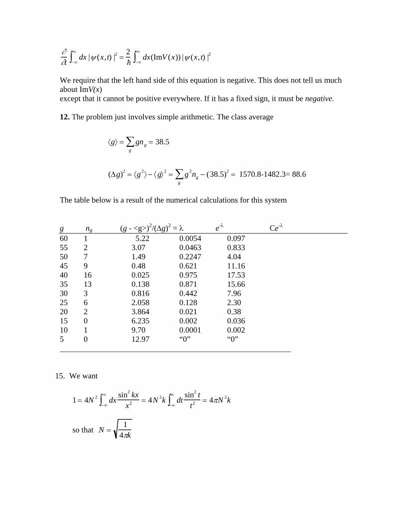
We require that the left hand side of this equation is negative. This does not tell us much about ImV(x) except that it cannot be positive everywhere. If it has a fixed sign, it must be negative. 12. The problem just involves simple arithmetic. The class average

⟨g⟩ = gngg∑ = 38.5

(Δg)2 = ⟨g2⟩ − ⟨g⟩ 2 = g2ngg∑ − (38.5)2 = 1570.8-1482.3= 88.6

The table below is a result of the numerical calculations for this system g ng (g - <g>)2/(Δg)2 = λ e-λ Ce-λ 60 1 5.22 0.0054 0.097 55 2 3.07 0.0463 0.833 50 7 1.49 0.2247 4.04 45 9 0.48 0.621 11.16 40 16 0.025 0.975 17.53 35 13 0.138 0.871 15.66 30 3 0.816 0.442 7.96 25 6 2.058 0.128 2.30 20 2 3.864 0.021 0.38 15 0 6.235 0.002 0.036 10 1 9.70 0.0001 0.002 5 0 12.97 “0” “0” __________________________________________________________

15. We want

1 = 4N 2 dxsin2 kx

x2−∞

∞

∫ = 4N 2k dtsin2 t

t2−∞

∞

∫ = 4πN 2k

so that N =1

4πk

16. We have

⟨xn ⟩ =απ

⎛ ⎝

⎞ ⎠

1/ 2

dxx n

−∞

∞

∫ e−αx 2

Note that this integral vanishes for n an odd integer, because the rest of the integrand is even. For n = 2m, an even integer, we have

⟨x2m ⟩ =απ

⎛ ⎝

⎞ ⎠

1/2

=απ

⎛ ⎝

⎞ ⎠

1/2

−d

dα⎛ ⎝

⎞ ⎠

m

dx−∞

∞

∫ e−αx 2

=απ

⎛ ⎝

⎞ ⎠

1/2

−d

dα⎛ ⎝

⎞ ⎠

m πα

⎛ ⎝

⎞ ⎠

1/ 2

For n = 1 as well as n = 17 this is zero, while for n = 2, that is, m = 1, this is 1

2α.

17. φ( p) =

12π

dxe− ipx/

−∞

∞

∫ απ

⎛ ⎝

⎞ ⎠

1/4

e−αx 2 /2

The integral is easily evaluated by rewriting the exponent in the form

−

α2

x 2 − ixp

= −α2

x +ipα

⎛ ⎝

⎞ ⎠

2

−p2

2 2α

A shift in the variable x allows us to state the value of the integral as and we end up with

φ( p) =

1π

πα

⎛ ⎝

⎞ ⎠

1/4

e− p2 / 2α 2

We have, for n even, i.e. n = 2m,

⟨p2m⟩ =1π

πα

⎛ ⎝

⎞ ⎠

1/ 2

dpp2me− p2 /α 2

−∞

∞

∫ =

=1

ππα

⎛ ⎝

⎞ ⎠

1/ 2

−d

dβ⎛ ⎝ ⎜

⎞ ⎠ ⎟

mπβ

⎛ ⎝ ⎜

⎞ ⎠ ⎟

1/2

where at the end we set β =

1α 2 . For odd powers the integral vanishes.

18. Specifically for m = 1 we have We have

(Δx)2 = ⟨x2 ⟩ = 12α

(Δp)2 = ⟨p2⟩ =α 2

2

so that ΔpΔx =

2. This is, in fact, the smallest value possible for the product of the

dispersions. 22. We have

dxψ *(x)xψ (x) =1

2π−∞

∞

∫ dxψ * (x)x dpφ( p)eipx/

−∞

∞

∫−∞

∞

∫

= 12π

dxψ * (x) dpφ(p)i−∞

∞

∫−∞

∞

∫ ∂∂p

eipx/ = dpφ * (p)i ∂φ(p)∂p−∞

∞

∫

In working this out we have shamelessly interchanged orders of integration. The justification of this is that the wave functions are expected to go to zero at infinity faster than any power of x , and this is also true of the momentum space wave functions, in their dependence on p.

CHAPTER 3. 1. The linear operators are (a), (b), (f) 2.We have

dx ' x 'ψ (x ') = λψ (x)−∞

x

∫

To solve this, we differentiate both sides with respect to x, and thus get

λdψ (x)

dx= xψ (x)

A solution of this is obtained by writing dψ /ψ = (1/ λ )xdx from which we can immediately state that ψ (x) = Ceλx 2 / 2 The existence of the integral that defines O6ψ(x) requires that λ < 0. 3, (a)

O2O6ψ (x) − O6O2ψ (x)

= xd

dxdx ' x 'ψ (x ') −

−∞

x

∫ dx ' x '2dψ (x ')

dx '−∞

x

∫

= x2ψ(x) − dx 'd

dx '−∞

x

∫ x '2 ψ(x ')( )+ 2 dx ' x 'ψ (x')−∞

x

∫= 2O6ψ (x)

Since this is true for every ψ(x) that vanishes rapidly enough at infinity, we conclude that [O2 , O6] = 2O6 (b)

O1O2ψ(x) − O2O1ψ (x)

= O1 xdψdx

⎛ ⎝

⎞ ⎠ − O2 x 3ψ( )= x 4 dψ

dx− x

ddx

x3ψ( )= −3x3ψ(x) = −3O1ψ (x)

so that [O1, O2] = -3O1

4. We need to calculate

⟨x2 ⟩ =2a

dxx 2 sin2 nπxa0

a

∫

With πx/a = u we have

⟨x2 ⟩ =2a

a3

π 3 duu2 sin2 nu =a2

π 30

π

∫ duu2

0

π

∫ (1− cos2nu)

The first integral is simple. For the second integral we use the fact that

duu2 cosαu = −

ddα

⎛ ⎝

⎞ ⎠ 0

π

∫2

ducosαu = −0

π

∫ ddα

⎛ ⎝

⎞ ⎠

2 sinαπα

At the end we set α = nπ. A little algebra leads to

⟨x2 ⟩ =a2

3−

a2

2π 2n2

For large n we therefore get Δx =a3

. Since ⟨p2⟩ =

2n2π 2

a2 , it follows that

Δp =

πna

, so that

ΔpΔx ≈

nπ3

The product of the uncertainties thus grows as n increases.

5. With En =

2π 2

2ma 2 n2 we can calculate

E2 − E1 = 3(1.05 ×10−34 J .s)2

2(0.9 ×10−30kg)(10−9 m)21

(1.6 ×10−19J / eV )= 0.115eV

We have ΔE =hcλ

so that λ =

2π cΔE

=2π (2.6 ×10−7 ev.m)

0.115eV=1.42 ×10−5m

where we have converted c from J.m units to eV.m units.

6. (a) Here we write

n2 =

2ma 2E2π 2 =

2(0.9 ×10−30kg)(2 ×10−2 m)2 (1.5eV )(1.6 ×10−19J / eV )(1.05 ×10−34 J .s)2π 2 = 1.59 ×1015

so that n = 4 x 107 . (b) We have

ΔE =2π 2

2ma2 2nΔn = (1.05 ×10−34 J.s)2π 2

2(0.9 ×10−30kg)(2 ×10−2 m)2 2(4 ×107) =1.2 ×10−26J

= 7.6 ×10−8eV

7. The longest wavelength corresponds to the lowest frequency. Since ΔE is

proportional to (n + 1)2 – n2 = 2n + 1, the lowest value corresponds to n = 1 (a state with n = 0 does not exist). We therefore have

h

cλ

= 32π 2

2ma2

If we assume that we are dealing with electrons of mass m = 0.9 x 10-30 kg, then

a2 =

3 πλ4mc

=3π (1.05 ×10−34 J.s)(4.5 ×10−7 m)

4(0.9 ×10−30kg)(3×108 m / s)= 4.1×10−19 m2

so that a = 6.4 x 10-10 m.

8. The solutions for a box of width a have energy eigenvalues En =

2π 2n2

2ma 2 with

n = 1,2,3,…The odd integer solutions correspond to solutions even under x → −x , while the even integer solutions correspond to solutions that are odd under reflection. These solutions vanish at x = 0, and it is these solutions that will satisfy the boundary conditions for the “half-well” under consideration. Thus the energy eigenvalues are given by En above with n even. 9. The general solution is

ψ (x, t) = Cn un (x)e− iE nt /

n =1

∞

∑

with the Cn defined by Cn = dxun

* (x)ψ (x,0)− a/ 2

a /2

∫

(a) It is clear that the wave function does not remain localized on the l.h.s. of the box at later times, since the special phase relationship that allows for a total interference for x > 0 no longer persists for t ≠ 0.

(b) With our wave function we have Cn =2a

dxun (x)−q /2

0

∫ .We may work this out by

using the solution of the box extending from x = 0 to x = a, since the shift has no physical consequences. We therefore have

Cn =2a

dx2a0

a/ 2

∫ sinnπxa

=2a

−a

nπcos

nπxa

⎡ ⎣

⎤ ⎦ 0

a /2

=2

nπ1− cos

nπ2

⎡ ⎣

⎤ ⎦

Therefore P1 =| C1 |2 =4

π 2 and P2 =| C2 |2 =1

π 2 | (1− (−1)) |2 =4π 2

10. (a) We use the solution of the above problem to get

Pn =| Cn |2 =4

n2π 2 fn

where fn = 1 for n = odd integer; fn = 0 for n = 4,8,12,…and fn = 4 for n = 2,6,10,… (b) We have

Pnn=1

∞

∑ =4π 2

1n2

odd∑ +

4π 2

4n2

n= 2,6,10,,,∑ =

8π 2

1n2 = 1

odd∑

Note. There is a typo in the statement of the problem. The sum should be restricted to odd integers. 11. We work this out by making use of an identity. The hint tells us that

(sin x)5 =12i

⎛ ⎝

⎞ ⎠

5

(eix − e−ix)5 =1

1612i

(e5ix − 5e3ix +10eix −10e− ix + 5e−3ix − e−5ix )

=116

(sin5x − 5sin 3x +10sin x)

Thus

ψ (x,0) = Aa2

116

u5 (x) − 5u3(x) +10u1(x)( )

(a) It follows that

ψ (x, t) = A

a2

116

u5 (x)e− iE 5t / − 5u3 (x)e−iE 3t / +10u1(x)e−iE1t /( )

(b) We can calculate A by noting that dx |ψ (x,0) |2 =1

0

a

∫ . This however is equivalent to the statement that the sum of the probabilities of finding any energy eigenvalue adds up to 1. Now we have

P5 =a2

A2 1256

;P3 =a2

A2 25256

;P1 =a2

A2 100256

so that

A2 =25663a

The probability of finding the state with energy E3 is 25/126.

12. The initial wave function vanishes for x ≤ -a and for x ≥ a. In the region in between it

is proportional to cosπx2a

, since this is the first nodeless trigonometric function that

vanishes at x = ± a. The normalization constant is obtained by requiring that

1 = N 2 dx cos2

− a

a

∫πx2a

= N 2 2aπ

⎛ ⎝

⎞ ⎠ ducos2 u = N 2a

−π / 2

π /2

∫

so that N =1a

. We next expand this in eigenstates of the infinite box potential with

boundaries at x = ± b. We write

1a

cosπx2a

= Cnn =1

∞

∑ un (x;b)

so that

Cn = dxun (x;b)ψ (x) = dx− a

a

∫− b

b

∫ un (x;b)1a

cosπx2a

In particular, after a little algebra, using cosu cosv=(1/2)[cos(u-v)+cos(u+v)], we get

C1 =

1ab

dx cosπx2b−a

a

∫ cosπx2a

=1ab

dx12−a

a

∫ cosπx(b − a)

2ab+ cos

πx(b + a)2ab

⎡ ⎣ ⎢

⎤ ⎦ ⎥

=4b ab

π(b2 − a2 )cos

πa2b

so that

P1 =| C1 |2 =16ab3

π 2 (b2 − a2)2 cos2 πa2b

The calculation of C2 is trivial. The reason is that while ψ(x) is an even function of x, u2(x) is an odd function of x, and the integral over an interval symmetric about x = 0 is zero. Hence P2 will be zero. 13. We first calculate

φ( p) = dx2a

sinnπx

a0

a

∫ eipx/

2π=

1i

14π a

dxeix (nπ /a + p / )

0

a

∫ − (n ↔ −n)⎛ ⎝

⎞ ⎠

=1

4π aeiap / (−1)n −1p / − nπ / a

−eiap / (−1)n −1p / + nπ / a

⎛ ⎝ ⎜

⎞ ⎠ ⎟

=1

4π a2nπ / a

(nπ / a)2 − (p / )2 (−1)n cos pa / −1+ i(−1)n sin pa /

From this we get

P( p) =| φ(p) |2=

2n2πa3

1− (−1)n cos pa /(nπ / a)2 − (p / )2[ ]2

The function P(p) does not go to infinity at p = nπ / a , but if definitely peaks there. If we write p / = nπ / a +ε , then the numerator becomes 1− cosaε ≈ a2ε 2 / 2 and the

denominator becomes (2nπε / a)2 , so that at the peak P

nπa

⎛ ⎝

⎞ ⎠ = a / 4π . The fact that the

peaking occurs at

p2

2m=

2π 2n2

2ma2

suggests agreement with the correspondence principle, since the kinetic energy of the particle is, as the r.h.s. of this equation shows, just the energy of a particle in the infinite box of width a. To confirm this, we need to show that the distribution is strongly peaked for large n. We do this by looking at the numerator, which vanishes when aε = π / 2, that is, when p / = nπ / a +π / 2a = (n +1 / 2)π / a . This implies that the width of the

distribution is Δp = π / 2a . Since the x-space wave function is localized to 0 ≤ x ≤ a we only know that Δx = a. The result ΔpΔx ≈ (π / 2) is consistent with the uncertainty principle. 14. We calculate

φ( p) = dxαπ

⎛ ⎝

⎞ ⎠ −∞

∞

∫1/4

e−αx 2 / 2 12π

e− ipx/

=απ

⎛ ⎝

⎞ ⎠

1/ 4 12π

⎛ ⎝

⎞ ⎠

1/2

dxe−α (x − ip/α )2

−∞

∞

∫ e− p 2 /2α 2

=1

πα 2

⎛ ⎝

⎞ ⎠

1/ 4

e− p2 / 2α 2

From this we find that the probability the momentum is in the range (p, p + dp) is

| φ( p) |2 dp =

1πα 2

⎛ ⎝

⎞ ⎠

1/ 2

e− p2 /α 2

To get the expectation value of the energy we need to calculate

⟨p2

2m⟩ =

12m

1πα 2

⎛ ⎝

⎞ ⎠

1/ 2

dpp2e− p2 /α 2

−∞

∞

∫

=1

2m1

πα 2

⎛ ⎝

⎞ ⎠

1/2 π2

(α 2 )3/ 2 =α 2

2m

An estimate on the basis of the uncertainty principle would use the fact that the “width” of the packet is1 / α . From this we estimate Δp ≈ / Δx = α , so that

E ≈

(Δp)2

2m=

α 2

2m

The exact agreement is fortuitous, since both the definition of the width and the numerical statement of the uncertainty relation are somewhat elastic.

15. We have

j(x) =2im

ψ * (x)dψ (x)

dx−

dψ *(x)dx

ψ (x)⎛ ⎝

⎞ ⎠

=2im

(A * e−ikx + B *eikx )(ikAeikx − ikBe−ikx ) − c.c)[ ]

=2im

[ik | A |2 −ik | B |2 +ikAB *e2ikx − ikA* Be −2ikx

− (−ik ) | A |2 −(ik) | B |2 −(−ik)A * Be −2ikx − ikAB *e2ikx ]

=k

m[| A |2 − | B |2 ]

This is a sum of a flux to the right associated with A eikx and a flux to the left associated with Be-ikx.. 16. Here

j(x) =2im

u(x)e− ikx(iku(x)eikx +du(x)

dxeikx) − c.c⎡

⎣ ⎤ ⎦

=2im

[(iku2 (x) + u(x)du(x)

dx) − c.c] =

km

u2 (x)

(c) Under the reflection x -x both x and p = −i

∂∂x

change sign, and since the

function consists of an odd power of x and/or p, it is an odd function of x. Now the eigenfunctions for a box symmetric about the x axis have a definite parity. So that

un (−x) = ±un (x). This implies that the integrand is antisymmetric under x - x. Since the integral is over an interval symmetric under this exchange, it is zero.

(d) We need to prove that

dx(Pψ (x))*ψ(x) =−∞

∞

∫ dxψ (x)* Pψ (x)−∞

∞

∫

The left hand side is equal to

dxψ *(−x)ψ (x) =−∞

∞

∫ dyψ * (y)ψ(−y)−∞

∞

∫ with a change of variables x -y , and this is equal to the right hand side. The eigenfunctions of P with eigenvalue +1 are functions for which u(x) = u(-x), while those with eigenvalue –1 satisfy v(x) = -v(-x). Now the scalar product is dxu *(x)v(x) = dyu *(−x)v(−x) = − dxu *(x)v(x)

−∞

∞

∫−∞

∞

∫−∞

∞

∫ so that dxu *(x)v(x) = 0

−∞

∞

∫ (e) A simple sketch of ψ(x) shows that it is a function symmetric about x = a/2. This means that the integral dxψ (x)un (x)

0

a

∫ will vanish for the un(x) which are odd under the reflection about this axis. This means that the integral vanishes for n = 2,4,6,…

CHAPTER 4. 1. The solution to the left side of the potential region is ψ (x) = Aeikx + Be−ikx . As shown in Problem 3-15, this corresponds to a flux

j(x) =

km

| A |2 − | B |2( )

The solution on the right side of the potential is ψ (x) = Ceikx + De−ikxx , and as above, the flux is

j(x) =

km

| C |2 − | D |2( )

Both fluxes are independent of x. Flux conservation implies that the two are equal, and this leads to the relationship | A |2 + | D |2=| B |2 + | C |2 If we now insert

C = S11A + S12DB = S21A + S22D

into the above relationship we get | A |2 + | D |2= (S21A + S22D)(S21

* A * +S22* D*) + (S11A + S12D)(S11

* A * +S12* D*)

Identifying the coefficients of |A|2 and |D|2, and setting the coefficient of AD* equal to zero yields

| S21 |2 + | S11 |2= 1

| S22 |2 + | S12 |2= 1S12S22

* + S11S12* = 0

Consider now the matrix

Str =S11 S21

S12 S22

⎛ ⎝ ⎜ ⎞

⎠ ⎟

The unitarity of this matrix implies that

S11 S21

S12 S22

⎛ ⎝ ⎜ ⎞

⎠ ⎟ S11

* S12*

S21* S22

*

⎛

⎝ ⎜ ⎞

⎠ ⎟ =

1 00 1

⎛ ⎝ ⎜ ⎞

⎠ ⎟

that is,

| S11 |2 + | S21 |2=| S12 |2 + | S22 |2 =1

S11S12* + S21S22

* = 0

These are just the conditions obtained above. They imply that the matrix Str is unitary, and therefore the matrix S is unitary. 2. We have solve the problem of finding R and T for this potential well in

the text.We take V0 < 0. We dealt with wave function of the form

eikx + Re−ikx x < −a

Teikx x > a

In the notation of Problem 4-1, we have found that if A = 1 and D = 0, then C = S11 = T and B = S21 = R.. To find the other elements of the S matrix we need to consider the same problem with A = 0 and D = 1. This can be solved explicitly by matching wave functions at the boundaries of the potential hole, but it is possible to take the solution that we have and reflect the “experiment” by the interchange x - x. We then find that S12 = R and S22 = T. We can easily check that

| S11 |2 + | S21 |2=| S12 |2 + | S22 |2 =| R |2 + | T |2= 1

Also S11S12

* + S21S22* = TR* +RT* = 2Re(TR*)

If we now look at the solutions for T and R in the text we see that the product of T and R* is of the form (-i) x (real number), so that its real part is zero. This confirms that the S matrix here is unitary. 3. Consider the wave functions on the left and on the right to have the

forms ψ L(x) = Ae ikx + Be− ikx

ψ R (x) = Ceikx + De−ikx

Now, let us make the change k - k and complex conjugate everything. Now the two wave functions read

ψ L(x)'= A *eikx + B *e− ikx

ψ R (x)'= C * eikx + D* e−ikx

Now complex conjugation and the transformation k - k changes the original relations to

C* = S11

* (−k)A * +S12* (−k)D*

B* = S21* (−k)A * +S22

* (−k)D*

On the other hand, we are now relating outgoing amplitudes C*, B* to ingoing amplitude A*, D*, so that the relations of problem 1 read

C* = S11(k)A * +S12(k)D*B* = S21(k)A * +S22(k)D*

This shows that S11(k) = S11

* (−k); S22(k) = S22* (−k); S12(k) = S21

* (−k) . These

result may be written in the matrix form S(k) = S+ (−k) . 4. (a) With the given flux, the wave coming in from x = −∞ , has the

form eikx , with unit amplitude. We now write the solutions in the various regions

x < b eikx + Re− ikx k 2 = 2mE / 2

−b < x < −a Aeκx + Be−κx κ 2 = 2m(V0 − E) / 2

−a < x < c Ceikx + De− ikx

c < x < d Meiqx + Ne−iqx q2 = 2m(E + V1) / 2

d < x Teikx

(b) We now have

x < 0 u(x) = 0

0 < x < a Asinkx k 2 = 2mE / 2

a < x < b Beκx + Ce−κx κ 2 = 2m(V0 − E ) / 2

b < x e−ikx + Reikx

The fact that there is total reflection at x = 0 implies that |R|2 = 1

5. The denominator in (4- ) has the form D = 2kq cos2qa − i(q2 + k2 )sin2qa With k = iκ this becomes D = i 2κqcos2qa − (q2 −κ 2 )sin2qa( ) The denominator vanishes when

tan2qa =2tanqa

1− tan2 qa=

2qκq2 −κ 2

This implies that

tanqa = −q2 −κ 2

2κq± 1 +

q2 −κ 2

2κq⎛ ⎝ ⎜

⎞ ⎠ ⎟

2

= −q2 −κ 2

2κq±

q2 +κ 2

2κq

This condition is identical with (4- ). The argument why this is so, is the following: When k = iκ the wave functio on the left has the form e−κx + R(iκ )eκx . The function e-κx blows up as x → −∞ and the wave function only make sense if this term is overpowered by the other term, that is when R(iκ ) = ∞ . We leave it to the student to check that the numerators are the same at k = iκ. 6. The solution is u(x) = Aeikx + Be-ikx x < b = Ceikx + De-ikx x > b The continuity condition at x = b leads to Aeikb + Be-ikb = Ceikb + De-ikb And the derivative condition is

(ikAeikb –ikBe-ikb) - (ikCeikb –ikDe-ikb)= (λ/a)( Aeikb + Be-ikb) With the notation Aeikb = α ; Be-ikb = β; Ceikb = γ; De-ikb = δ These equations read

α + β = γ + δ ik(α - β + γ - δ) = (λ/a)(α + β) We can use these equations to write (γ,β) in terms of (α,δ) as follows

γ =

2ika2ika − λ

α +λ

2ika − λδ

β =λ

2ika − λα +

2ika2ika − λ

δ

We can now rewrite these in terms of A,B,C,D and we get for the S matrix

S =

2ika2ika− λ

λ2ika − λ

e−2ikb

λ2ika − λ

e2ikb 2ika2ika− λ

⎛

⎝

⎜ ⎜

⎞

⎠

⎟ ⎟

Unitarity is easily established:

| S11 |2 + | S12 |2= 4k 2a2

4k2a2 + λ2 + λ2

4k2a2 + λ2 = 1

S11S12* + S12S22

* =2ika

2ika − λ⎛ ⎝

⎞ ⎠

λ−2ika− λ

e−2ikb⎛ ⎝

⎞ ⎠ +

λ2ika − λ

e−2ikb⎛ ⎝

⎞ ⎠

−2ika−2ika − λ

⎛ ⎝

⎞ ⎠ = 0

The matrix elements become infinite when 2ika =λ. In terms of κ= -ik, this condition becomes κ = -λ/2a = |λ|/2a. 7. The exponent in T = e-S is

S =2

dx 2m(V (x) − E)A

B

∫

=2

dx (2m(mω 2

2(x 2 −

x 3

a)) −

ω2A

B

∫

where A and B are turning points, that is, the points at which the quantity under the square root sign vanishes. We first simplify the expression by changing to dimensionless variables:

x = / mω y; η = a / / mω << 1

The integral becomes

2 dy y2 −ηy 3 −1y1

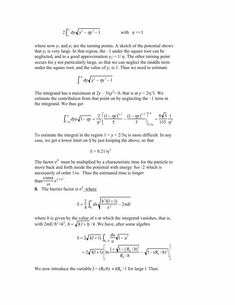
y2∫ with η <<1

where now y1 and y2 are the turning points. A sketch of the potential shows that y2 is very large. In that region, the –1 under the square root can be neglected, and to a good approximation y2 = 1/η. The other turning point occurs for y not particularly large, so that we can neglect the middle term under the square root, and the value of y1 is 1. Thus we need to estimate dy y2 −ηy 3 −1

1

1/η

∫ The integrand has a maximum at 2y – 3ηy2= 0, that is at y = 2η/3. We estimate the contribution from that point on by neglecting the –1 term in the integrand. We thus get

dyy 1−ηy2/ 3η

1/η

∫ =2

η2(1− ηy)5/ 2

5−

(1− ηy)3/ 2

3⎡

⎣ ⎢ ⎤

⎦ ⎥ 2/3η

1/η

=8 3135

1η2

To estimate the integral in the region 1 < y < 2/3η is more difficult. In any case, we get a lower limit on S by just keeping the above, so that S > 0.21/η2 The factor eS must be multiplied by a characteristic time for the particle to move back and forth inside the potential with energy ω / 2 which is necessarily of order 1/ω. Thus the estimated time is longer

thanconst.

ωe0.2/η 2

.

8. The barrier factor is eS where

S =

2dx

2l(l +1)x 2 − 2mE

R0

b

∫

where b is given by the value of x at which the integrand vanishes, that is, with 2mE/ 2 =k2, b = l(l +1) / k .We have, after some algebra

S = 2 l(l +1)duuR0 / b

1

∫ 1− u2

= 2 l(l +1) ln1+ 1− (R0 / b)2

R0 / b− 1− (R0 / b)2

⎡

⎣ ⎢ ⎢

⎤

⎦ ⎥ ⎥

We now introduce the variable f = (R0/b) ≈ kR0 / l for large l. Then

eS eS =1+ 1− f 2

f

⎡

⎣ ⎢

⎤

⎦ ⎥

2l

e−2l 1− f 2

≈e2

⎛ ⎝

⎞ ⎠

−2l

f −2l

for f << 1. This is to be multiplied by the time of traversal inside the box. The important factor is f-2l. It tells us that the lifetime is proportional to (kR0)-2l so that it grows as a power of l for small k. Equivalently we can say that the probability of decay falls as (kR0)2l. 9. The argument fails because the electron is not localized inside the

potential. In fact, for weak binding, the electron wave function extends over a region R = 1/α = 2mEB , which, for weak binding is much larger than a.

10. For a bound state, the solution for x > a must be of the

form u(x) = Ae −αx , where α = 2mEB / . Matching 1u

dudx

at x = a

yields −α = f (EB ). If f(E) is a constant, then we immediately know α.. Even if f(E) varies only slightly over the energy range that overlaps small positive E, we can determine the binding energy in terms of the reflection coefficient. For positive energies the wave function u(x) for x > a has the form e-ikx + R(k)eikx, and matching yields

f (E ) ≈ −α = −ik

e− ika − Re ika

e−ika + Re ika = −ik1− Re2ika

1 + Re2ika

so that

R = e−2ika k + iαk − iα

We see that |R|2 = 1. 11. Since the well is symmetric about x = 0, we need only match wave functions at x = b and a. We look at E < 0, so that we introduce and α2 = 2m|E|/ 2 and q2 = 2m(V0-|E|)/ 2 . We now write down Even solutions: u(x) = coshαx 0 < x < b = A sinqx + B cosqx b < x < a = C e-αx a < x

Matching 1

u(x)du(x)

dx at x = b and at x = a leads to the equations

α tanhαb = qAcosqb − BsinqbAsinqb + B cosqb

−α = q Acosqa − BsnqaAsinqa + B cosqa

From the first equation we get

BA

=qcosqb −α tanhαbsinqbqsinqb +α tanhαbcosqb

and from the second

BA

=qcosqa +α sinqaqsinqa −α cosqa

Equating these, cross-multiplying, we get after a little algebra q2 sinq(a − b) − αcosq(a − b) = α tanhαb[αsinq(a − b) + qcosq(a − b)] from which it immediately follows that

sinq(a − b)cosq(a − b)

=αq(tanhαb +1)q2 − α 2 tanhαb

Odd Solution Here the only difference is that the form for u(x) for 0 < x < b is sinhαx. The result of this is that we get the same expresion as above, with tanhαb replaced by cothαb. 11. (a) The condition that there are at most two bound states is equivalent

to stating that there is at most one odd bound state. The relevant figure is Fig. 4-8, and we ask for the condition that there be no intersection point with the tangent curve that starts up at 3π/2. This means that

λ − y2

y= 0

for y ≤ 3π/2. This translates into λ = y2 with y < 3π/2, i.e. λ < 9π2/4. (b) The condition that there be at most three bound states implies that there be at most two even bound states, and the relevant figure is 4-7. Here the conditon is that y < 2π so that λ < 4π2.

(c) We have y = π so that the second even bound state have zero binding energy. This means that λ = π2. What does this tell us about the first bound state? All we know is that y is a solution of Eq. (4-54) with λ = π2. Eq.(4-54) can be rewritten as follows:

tan2 y =1− cos2 y

cos2 y=

λ − y2

y2 =1− (y2 / λ )

(y 2 / λ)

so that the even condition is cos y = y / λ , and in the same way, the odd conditin is sin y = y / λ . Setting λ = π still leaves us with a transcendental equation. All we can say is that the binding energy f the even state will be larger than that of the odd one. 13.(a) As b 0, tanq(a-b) tanqa and the r.h.s. reduces to α/q. Thus we get, for the even solution

tanqa = α/q and, for the odd solution, tanqa = - q/α. These are just the single well conditions. (b) This part is more complicated. We introduce notation c = (a-b), which will be held fixed. We will also use the notation z = αb. We will also use the subscript “1” for the even solutions, and “2” for the odd solutions. For b large,

tanhz =

ez − e− z

ez + e−z =1− e−2z

1 + e−2z ≈1− 2e−2z

cothz ≈1 = 2e−2z

The eigenvalue condition for the even solution now reads

tanq1c =q1α1(1+1− 2e−2z1 )q1

2 −α12(1− 2e−2z1 )

≈2q1α1

q12 − α1

2 (1−q1

2 + α12

q12 − α1

2 e−2z1 )

The condition for the odd solution is obtained by just changing the sign of the e-2z term, so that

tanq2c =q2α2 (1+1 + 2e−2z2 )

q22α2

2(1 + 2e−2z2 )≈

2q2α 2

q22 −α 2

2 (1+q2

2 +α 22

q22 −α2

2 e−2z2 )

In both cases q2 + α2 = 2mV0/ 2 is fixed. The two eigenvalue conditions only differ in the e-2z terms, and the difference in the eigenvalues is therefore proportional to e-2z , where z here is some mean value between α1 b and α2b. This can be worked out in more detail, but this becomes an exercise in Taylor expansions with no new physical insights. 14. We write

⟨xdV (x)

dx⟩ = dxψ(x)x

dV (x)dx−∞

∞

∫ ψ (x)

= dxddx

ψ 2xV( )− 2ψdψdx

xV −ψ 2V⎡ ⎣ ⎢

⎤ ⎦ ⎥ −∞

∞

∫

The first term vanishes because ψ goes to zero rapidly. We next rewrite

−2 dxdψdx−∞

∞

∫ xVψ = −2 dxdψdx−∞

∞

∫ x(E +2

2md2

dx2 )ψ

= −E dxxdψ 2

dx−

2

2m−∞

∞

∫ dxxd

dxdψdx

⎛ ⎝

⎞ ⎠

2

−∞

∞

∫

Now

dxxdψ 2

dx−∞

∞

∫ = dxddx−∞

∞

∫ xψ 2( )− dxψ 2

−∞

∞

∫

The first term vanishes, and the second term is unity. We do the same with the second term, in which only the second integral

dxdψdx

⎛ ⎝

⎞ ⎠

2

−∞

∞

∫

remains. Putting all this together we get

⟨x

dVdx

⟩ + ⟨V ⟩ =2

2mdx

dψdx

⎛ ⎝

⎞ ⎠

2

+ E dxψ 2

−∞

∞

∫−∞

∞

∫ = ⟨p2

2m⟩ + E

so that

12

⟨xdVdx

⟩ = ⟨p2

2m⟩

CHAPTER 5. 1. We are given

dx(AΨ(x)) *Ψ(x) =−∞

∞

∫ dxΨ(x) * AΨ(x)−∞

∞

∫

Now let Ψ(x) = φ(x) + λψ (x) , where λ is an arbitrary complex number. Substitution into the above equation yields, on the l.h.s.

dx(Aφ(x) + λAψ (x)) *(φ(x) + λψ(x))−∞

∞

∫= dx (Aφ) *φ + λ (Aφ)*ψ + λ * (Aψ )*φ + | λ |2 (Aψ )*ψ[ ]

−∞

∞

∫

On the r.h.s. we get

dx(φ(x) + λψ (x)) *(Aφ(x) + λAψ(x))−∞

∞

∫= dx φ * Aφ + λ *ψ * Aφ + λφ * Aψ + | λ |2 ψ * Aψ[ ]

−∞

∞

∫

Because of the hermiticity of A, the first and fourth terms on each side are equal. For the rest, sine λ is an arbitrary complex number, the coefficients of λ and λ* are independent , and we may therefore identify these on the two sides of the equation. If we consider λ, for example, we get dx(Aφ(x)) *ψ (x) =

−∞

∞

∫ dxφ(x) * Aψ (x)−∞

∞

∫ the desired result. 2. We have A+ = A and B+ = B , therefore (A + B)+ = (A + B). Let us call (A + B) = X.

We have shown that X is hermitian. Consider now (X +)n = X+ X+ X+ …X+ = X X X …X = (X)n

which was to be proved. 3. We have

⟨A2⟩ = dxψ * (x)A2

−∞

∞

∫ ψ (x)

Now define Aψ(x) = φ(x). Then the above relation can be rewritten as

⟨A2⟩ = dxψ (x)Aφ(x) = dx

−∞

∞

∫−∞

∞

∫ (Aψ (x))*φ(x)

= dx−∞

∞

∫ (Aψ (x))* Aψ (x) ≥ 0

4. Let U = eiH = inH n

n!n= 0

∞

∑ . Then U + =(−i)n (H n )+

n!n= 0

∞

∑ =(−i)n (H n )

n!n =0

∞

∑ = e− iH , and thus

the hermitian conjugate of eiH is e-iH provided H = H+.. 5. We need to show that

eiHe−iH =in

n!n =0

∞

∑ H n (−i)m

m!m = o

∞

∑ H m = 1

Let us pick a particular coefficient in the series, say k = m + n and calculate its coefficient. We get, with m= k – n, the coefficient of Hk is

in

n!n= 0

k

∑ (−i) k−n

(k − n)!=

1k!

k!n!(k − n)!n =0

k

∑ in (−i) k−n

=1k!

(i − i)k = 0

Thus in the product only the m = n = 0 term remains, and this is equal to unity. 6. We write I(λ,λ*) = dx φ(x) + λψ (x)( )

−∞

∞

∫ * (φ(x) + λψ (x)) ≥ 0. The left hand side, in abbreviated notation can be written as

I(λ,λ*) = |φ |2∫ + λ * ψ *φ + λ φ *ψ + λλ * |ψ |2∫∫∫

Since λ and λ* are independent, he minimum value of this occurs when

∂I∂λ *

= ψ *φ + λ |ψ |2∫∫ = 0

∂I∂λ

= φ *ψ + λ * |ψ |2∫∫ = 0

When these values of λ and λ* are inserted in the expression for I(λ,λ*) we get

I(λ min,λ min* ) = |φ |2∫ −

φ *ψ ψ *φ∫∫|ψ |2∫

≥ 0

from which we get the Schwartz inequality.

7. We have UU+ = 1 and VV+ = 1. Now (UV)+ = V+U+ so that

(UV)(UV)+ = UVV+U+ = UU+ = 1

8. Let Uψ(x) = λψ(x), so that λ is an eigenvalue of U. Since U is unitary, U+U = 1. Now

dx−∞

∞

∫ (Uψ (x))*Uψ (x) = dxψ *(x)U +Uψ (x) =−∞

∞

∫= dxψ * (x)ψ (x) =1

−∞

∞

∫

On the other hand, using the eigenvalue equation, the integral may be written in the form dx

−∞

∞

∫ (Uψ (x))*Uψ (x) = λ *λ dxψ *(x)ψ (x) =| λ |2−∞

∞

∫ It follows that |λ|2 = 1, or equivalently λ = eia , with a real. 9. We write

dxφ(x) *φ(x) =−∞

∞

∫ dx−∞

∞

∫ (Uψ (x))*Uψ (x) = dxψ *(x)U +Uψ (x) =−∞

∞

∫= dxψ * (x)ψ (x) =1

−∞

∞

∫

10. We write, in abbreviated notation

va*∫ vb = (Uua∫ )*Uub = ua

*∫ U +Uub = ua*∫ ub = δ ab

11. (a) We are given A+ = A and B+ = B. We now calculate (i [A,B])+ = (iAB – iBA)+ = -i (AB)+ - (-i)(BA)+ = -i (B+A+) + i(A+B+) = -iBA + iAB = i[A,B] (b) [AB,C] = ABC-CAB = ABC – ACB + ACB – CAB = A(BC – CB) – (AC – CA)B

= A [B,C] – [A,C]B

(c) The Jacobi identity written out in detail is [A,[B,C]] + [B,[C,A]] + [C,[A,B]] =

A(BC – CB) – (BC – CB)A + B(CA – AC) – (CA - AC)B + C(AB – BA) – (AB – BA)C = ABC – ACB – BCA + CBA + BCA – BAC – CAB + ACB + CAB – CBA – ABC + BAC It is easy to see that the sum is zero. 12. We have eA B e-A = (1 + A + A2/2! + A3/3! + A4/4! +…)B (1 - A + A2/2! - A3/3! + A4/4! -…) Let us now take the term independent of A: it is B. The terms of first order in A are AB – BA = [A,B]. The terms of second order in A are A2B/2! – ABA + BA2/2! = (1/2!)(A2B – 2ABA + BA2) = (1/2!)(A(AB – BA) – (AB – BA)A) = (1/2!)A[A,B]-[A,B]A = (1/2!)[A,[A,B]] The terms of third order in A are A3B/3! – A2BA/2! + ABA2/2! – BA3. One can again rearrange these and show that this term is (1/3!)[A,[A,[A,B]]]. There is actually a neater way to do this. Consider F(λ) = eλABe−λA Then

dF(λ)

dλ= eλA ABe−λA − eλA BAe−λA = eλA[A,B]e−λA

Differentiating again we get

d2F(λ)

dλ2 = eλA[A,[A,B]]e−λA

and so on. We now use the Taylor expansion to calculate F(1) = eA B e-A.

F(1) = F (0) + F '(0) +12!

F ' '(0) +13!

F ' ' '(0) + ..,

= B+ [A,B] + 12!

[A,[A,B]] + 13!

[A,[A,[A,B]]] + ...

13. Consider the eigenvalue equation Hu = λu. Applying H to this equation we get

H2 u = λ 2u ; H3 u = λ3u and H4u = λ4u . We are given that H4 = 1, which means that H4 applied to any function yields 1. In particular this means that λ4 = 1. The solutions of this are λ = 1, -1, i, and –i. However, H is hermitian, so that the eigenvalues are real. Thus only λ = ± 1 are possible eigenvalues. If H is not hermitian, then all four eigenvalues are acceptable.

14. We have the equations

Bua(1) = b11ua

(1) + b12ua(2)

Bua(2) = b21ua

(1) + b22ua(2)

Let us now introduce functions (va

(1),va(2)) that satisfy the equations

Bva(1) = b1va

(1);Bva(2) = b2va

(2). We write, with simplified notation, v1 = α u1 + β u2 v2 = γ u1 + δ u2 The b1 - eigenvalue equation reads b1v1 = B ( α u1 + β u2) = α (b11 u1 + b12u2) + β (b21u1 + b22u2) We write the l.h.s. as b1(α u1 + β u2). We can now take the coefficients of u1 and u2 separately, and get the following equations α (b1 – b11) = βb21

β (b1 – b22) = αb12 The product of the two equations yields a quadratic equation for b1, whose solution is

b1 =b11 + b22

2±

(b11 − b22)2

4+ b12b21

We may choose the + sign for the b1 eigenvalue. An examination of the equation involving v2 leads to an identical equation, and we associate the – sign with the b2 eigenvalue. Once we know the eigenvalues, we can find the ratios α/β and γ/δ. These suffice, since the normalization condition implies that α2 + β2 = 1 and γ2 + δ2 = 1 15. The equations of motion for the expectation values are

ddt

⟨x⟩ =i

⟨[H ,x]⟩ =i

⟨[p2

2m, x]⟩ =

im

⟨ p[ p, x]⟩ = ⟨pm

⟩

ddt

⟨p⟩ =i

⟨[H, p]⟩ = −i

⟨[p,12

mω12x 2 +ω2x]⟩ = −mω1

2 ⟨x⟩ −ω2

16. We may combine the above equations to get

d2

dt2 ⟨x⟩ = −ω12⟨x⟩ −

ω2

m

The solution of this equation is obtained by introducing the variable

X = ⟨x⟩ +ω2

mω12

The equation for X reads d2X/dt2 = - ω1

2 X, whose solution is X = Acosω1 t + Bsinω1 t This gives us

⟨x⟩t = −ω2

mω12 + Acosω1t + B sinω1t

At t = 0

⟨x⟩0 = −

ω2

mω12 + A

⟨p⟩0 = m ddt

⟨x⟩t = 0 = mBω1

We can therefore write A and B in terms of the initial values of < x > and < p >,

⟨x⟩t = −ω2

mω12 + ⟨x⟩0 +

ω2

mω12

⎛ ⎝ ⎜

⎞ ⎠ ⎟ cosω1t +

⟨p⟩ 0

mω1sinω1t

17. We calculate as above, but we can equally well use Eq. (5-53) and (5-57), to get

ddt

⟨x⟩ =1m

⟨ p⟩

ddt

⟨p⟩ = −⟨∂V (x, t)

∂x⟩ = eE 0cosωt

Finally

ddt

⟨H ⟩ = ⟨∂H∂t

⟩ = eE0ω sinωt⟨x⟩

18. We can solve the second of the above equations to get

⟨p⟩ t =eE 0

ωsinωt + ⟨p⟩ t =0

This may be inserted into the first equation, and the result is

⟨x⟩t = −eE0

mω 2 (cosωt −1) +⟨ p⟩t = 0 t

m+ ⟨x⟩t = 0

CHAPTER 6 19. (a) We have

A|a> = a|a>

It follows that <a|A|a> = a<a|a> = a if the eigenstate of A corresponding to the eigenvalue a is normalized to unity. The complex conjugate of this equation is <a|A|a>* = <a|A+|a> = a* If A+ = A, then it follows that a = a*, so that a is real. 13. We have

⟨ψ | (AB)+ |ψ ⟩ = ⟨(AB)ψ |ψ ⟩ = ⟨Bψ | A+ |ψ ⟩ = ⟨ψ | B+A+ |ψ ⟩

This is true for every ψ, so that (AB)+ = B+A+ 2.

TrAB = ⟨n | AB | n⟩ = ⟨n | A1B | n⟩n∑

n∑

= ⟨n | A | m⟩⟨m | B | n⟩ =m∑

n∑ ⟨m | B | n⟩⟨n | A | m⟩

m∑

n∑

= ⟨m | B1A | m⟩ =m∑ ⟨m | BA | m⟩ =

m∑ TrBA

3. We start with the definition of |n> as

| n⟩ =1n!

(A+)n | 0⟩

We now take Eq. (6-47) from the text to see that

A | n⟩ =1n!

A(A+)n | 0⟩ =nn!

(A+ )n−1 | 0⟩ =n

(n −1)!(A+ )n −1 | 0⟩ = n | n −1⟩

4. Let f (A+) = Cnn=1

N

∑ (A+)n . We then use Eq. (6-47) to obtain

Af (A+) | 0⟩ = A Cnn=1

N

∑ (A+)n | 0⟩ = nCn (A+)n−1

n=1

N

∑ | 0⟩

=d

dA+ Cnn =1

N

∑ (A+)n | 0⟩ =df (A+)

dA+ | 0⟩

5. We use the fact that Eq. (6-36) leads to

x =2mω

(A + A+ )

p = i mω2

(A+ − A)

We can now calculate

⟨k | x | n⟩ =2mω

⟨k | A + A+ | n⟩ =2mω

n⟨k | n −1⟩ + k ⟨k −1 | n⟩( )

=2mω

nδk ,n−1 + n +1δ k ,n+1( )

which shows that k = n ± 1. 6. In exactly the same way we show that

⟨k | p | n⟩ = i

mω2

⟨k | A+ − A | n⟩ = imω

2( n +1δk ,n+1 − nδ k,n −1)

7. Let us now calculate

⟨k | px | n⟩ = ⟨k | p1x | n⟩ = ⟨k | p | q⟩⟨q | x | n⟩q∑

We may now use the results of problems 5 and 6. We get for the above

i2

( kq∑ δ k −1,q − k +1δk +1,q )( nδq ,n−1 + n +1δ q ,n+1)

=i2

( knδkn − (k +1)nδ k+1,n−1 + k(n +1)δ k −1,n +1 − (k +1)(n +1)δ k+1,n+1)

=i2

(−δ kn − (k +1)(k + 2)δ k +2,n + n(n + 2)δ k,n +2 )

To calculate ⟨k | xp | n⟩ we may proceed in exactly the same way. It is also possible to abbreviate the calculation by noting that since x and p are hermitian operators, it follows that

⟨k | xp | n⟩ = ⟨n | px | k⟩* so that the desired quantity is obtained from what we obtained before by interchanging k and n and complex-conjugating. The latter only changes the overall sign, so that we get

⟨k | xp | n⟩ = −

i2

(−δ kn − (n +1)(n + 2)δ k ,n+ 2 + (k +1)(k + 2)δ k +2,n)

8.The results of problem 7 immediately lead to ⟨k | xp − px | n⟩ = i δkn 9. This follows immediately from problems 5 and 6. 10. We again use

x =2mω

(A + A+ )

p = i mω2

(A+ − A)

to obtain the operator expression for

x 2 =2mω

(A + A+)(A + A+) =2mω

(A2 + 2A+ A + (A+)2 +1)

p2 = −mω

2(A+ − A)(A+ − A) = −

mω2

(A2 − 2A+A + (A+)2 −1)

where we have used [A,A+] = 1. The quadratic terms change the values of the eigenvalue integer by 2, so that they do not appear in the desired expressions. We get, very simply

⟨n | x 2 | n⟩ =2mω

(2n +1)

⟨n | p2 | n⟩ =mω

2(2n +1)

14. Given the results of problem 9, and of 10, we have

(Δx)2 =2mω

(2n +1)

(Δp)2 =mω2

(2n +1)

and therefore

ΔxΔp = (n +

12

)

15. The eigenstate in A|α> = α|α> may be written in the form

| α⟩ = f (A+) | 0⟩

It follows from the result of problem 4 that the eigenvalue equation reads

Af (A+) | 0⟩ =df (A+ )

dA+ | 0⟩ = αf (A+) | 0⟩

The solution of df (x) = α f(x) is f(x) = C eαx so that | α⟩ = CeαA +

| 0⟩ The constant C is determined by the normalization condition <α|α> = 1 This means that

1C2 = ⟨0 | eα *AeαA +

| 0⟩ =(α*)n

n!n =0

∞

∑ ⟨0 |d

dA+

⎛ ⎝

⎞ ⎠

n

eαA +

| 0⟩

=| α |2n

n!n =0

∞

∑ ⟨0 | eαA +

| 0⟩ =|α |2n

n!n= 0

∞

∑ = e |α |2

Consequently C = e−|α |2 /2 We may now expand the state as follows

| α⟩ = | n⟩⟨n |α⟩ = | n⟩⟨0 |

An

n!n∑

n∑ CeαA+

| 0⟩

= C | n⟩1n!n

∑ ⟨0 |d

dA+⎛ ⎝

⎞ ⎠

n

eαA +

| 0⟩ = Cα n

n!| n⟩

The probability that the state |α> contains n quanta is

Pn =| ⟨n | α⟩ |2= C2 | α |2n

n!=

(|α |2 )n

n!e−|α | 2

This is known as the Poisson distribution. Finally ⟨α | N |α⟩ = ⟨α | A+A | α⟩ = α *α =|α |2 13. The equations of motion read

dx( t)dt

=i[H, x(t)]=

i[p2(t)2m

,x(t)] =p(t)m

dp( t)dt

=i[mgx(t), p(t)] = −mg

This leads to the equation

d2x(t)

dt2 = −g

The general solution is

x(t) =12

gt2 +p(0)m

t + x(0)

14. We have, as always

dxdt

=pm

Also

dpdt

=i

[12

mω2 x2 + eξx, p]

=i 1

2mω 2x[x, p] +

12

mω 2[x, p]x + eξ[x, p]⎛ ⎝

⎞ ⎠

= −mω 2x − eξ

Differentiating the first equation with respect to t and rearranging leads to

d2xdt2 = −ω 2x −

eξm

= −ω2 (x +eξ

mω 2 )

The solution of this equation is

x +eξ

mω2 = Acosωt + B sinωt

= x(0) +eξ

mω 2⎛ ⎝

⎞ ⎠ cosωt +

p(0)mω

sinωt

We can now calculate the commutator [x(t1),x(t2)], which should vanish when t1 = t2. In this calculation it is only the commutator [p(0), x(0)] that plays a role. We have

[x( t1),x(t2)] = [x(0)cosωt1 +p(0)mω

sinωt1,x(0)cosωt2 +p(0)mω

sinωt2 ]

= i1

mω(cosωt1 sinωt2 − sinωt1 cosωt2

⎛ ⎝

⎞ ⎠ =

imω

sinω(t2 − t1)

16. We simplify the algebra by writing

mω2

= a;2mω

=1

2a

Then

n!π

mω⎛ ⎝

⎞ ⎠

1/ 4

un (x) = vn(x) = ax −1

2addx

⎛ ⎝

⎞ ⎠

n

e− a2x 2

Now with the notation y = ax we get

v1(y) = (y −12

ddy

)e−y 2= (y + y)e− y 2

= 2ye− y 2

v2(y) = (y −12

ddy

)(2ye −y 2

) = (2y 2 −1 + 2y2 )e−y 2

= (4 y2 −1)e−y 2

Next

v3(y) = (y −12

ddy

) (4 y2 −1)e−y 2[ ]= 4y 3 − y − 4y + y(4 y2 −1)( )e− y 2

= (8y 3 − 6y)e− y 2

The rest is substitution y =

mω2

x

17. We learned in problem 4 that

Af (A+) | 0⟩ =df (A+ )

dA+ | 0⟩

Iteration of this leads to

An f (A+ ) | 0⟩ =dn f (A+)

dA+ n | 0⟩

We use this to get

eλA f (A+) | 0⟩ =λn

n!n= 0

∞

∑ An f (A+) | 0⟩ =λn

n!n= 0

∞

∑ ddA+

⎛ ⎝

⎞ ⎠

n

f (A+) | 0⟩ = f (A+ + λ ) | 0⟩

18. We use the result of problem 16 to write

eλA f (A+)e−λA g(A+) | 0⟩ = eλA f (A+)g(A+ − λ) | 0⟩ = f (A+ + λ)g(A+) | 0⟩ Since this is true for any state of the form g(A+)|0> we have eλA f (A+)e−λA = f (A+ + λ ) In the above we used the first formula in the solution to 16, which depended on the fact that [A,A+] = 1. More generally we have the Baker-Hausdorff form, which we derive as follows: Define F(λ) = eλA A+e−λA Differentiation w.r.t. λ yields

dF(λ)

dλ= eλA AA+e−λA − eλA A+ Ae−λA = eλA [A,A+ ]e−λA ≡ eλAC1e

−λA

Iteration leads to

d2F(λ)dλ2 = eλA[A,[A,A+ ]]e−λA ≡ eλAC2e

−λA

.......dnF(λ )

dλn = eλA [A,[A,[A,[A, ....]]..]e−λA ≡ eλACne−λA

with A appearing n times in Cn. We may now use a Taylor expansion for

F(λ +σ ) =σ n

n!n =0

∞

∑ dn F(λ )dλn =

σ n

n!n =0

∞

∑ eλACne−λA

If we now set λ = 0 we get

F(σ ) =σ n

n!n =0

∞

∑ Cn

which translates into

eσA A+e−σA = A+ + σ[A, A+] +σ 2

2![A,[A, A+]] +

σ 3

3![A,[A,[A, A+ ]]] + ...

Note that if [A,A+] = 1 only the first two terms appear, so that eσA f (A+)e−σA = f (A+ + σ[A,A+]) = f (A+ + σ )

19. We follow the procedure outlined in the hint. We define F(λ) by

eλ(aA + bA + ) = eλaA F(λ) Differentiation w.r.t λ yields

(aA + bA+ )eλaA F(λ) = aAeλAF (λ ) + eλaA dF(λ )dλ

The first terms on each side cancel, and multiplication by e−λaA on the left yields

dF(λ)

dλ= e−λaA bA+eλaA F(λ ) = bA+ − λab[A,A+ ]F(λ )

When [A,A+] commutes with A. We can now integrate w.r.t. λ and after integration Set λ = 1. We then get F(1) = ebA + − ab[A ,A + ] /2 = ebA +

e−ab / 2

so that eaA + bA +

= eaAebA +

e−ab / 2 20. We can use the procedure of problem 17, but a simpler way is to take the hermitian

conjugate of the result. For a real function f and λ real, this reads e−λA+

f (A)eλA +

= f (A + λ )

Changing λ to -λ yields eλA +

f (A)e−λA +

= f (A − λ) The remaining steps that lead to eaA + bA +

= ebA +

eaA eab /2 are identical to the ones used in problem 18.

20. For the harmonic oscillator problem we have

x =

2mω(A + A+)

This means that eikx is of the form given in problem 19 with a = b = ik / 2mω This leads to eikx = eik / 2m ω A +

eik /2mω Ae− k 2 / 4mω Since A|0> = 0 and <0|A+ = 0, we get ⟨0 | eikx | 0⟩ = e− k 2 / 4mω 21. An alternative calculation, given that u0 (x) = (mω / π )1/ 4 e−mωx 2 /2 , is

mωπ

⎛ ⎝

⎞ ⎠

1/ 2

dxeikx

−∞

∞

∫ e−mωx 2

=mωπ

⎛ ⎝

⎞ ⎠

1/ 2

dxe−

m ω(x −

ik2mω

)2

−∞

∞

∫ e−

k 2

4 mω

The integral is a simple gaussian integral and

dy−∞

∞

∫ e−m ωy 2 / =π

mω which just

cancels the factor in front. Thus the two results agree.

CHAPTER 7

1. (a) The system under consideration has rotational degrees of freedom, allowing it to

rotate about two orthogonal axes perpendicular to the rigid rod connecting the two

masses. If we define the z axis as represented by the rod, then the Hamiltonian has the

form

H =Lx

2 + Ly

2

2I=L2 − Lz

2

2I

where I is the moment of inertia of the dumbbell.

(b) Since there are no rotations about the z axis, the eigenvalue of Lz is zero, so that the

eigenvalues of the Hamiltonian are

E =

2( +1)2I

with = 0,1,2,3,…

(c) To get the energy spectrum we need an expression for the moment of inertia. We use

the fact that

I = Mred a2

where the reduced mass is given by

M red =MC MN

MC + MN

=12 ×14

26Mnucleon = 6.46M nucleon

If we express the separation a in Angstroms, we get

I = 6.46 × (1.67 ×10−27kg)(10

−10m / A)

2aA

2 =1.08 ×10−46aA

2

The energy difference between the ground state and the first excited state is 22/ 2I

which leads to the numerical result

∆E =(1.05 ×10−34

J.s)2

1.08 ×10−46aA2kg.m 2 ×

1

(1.6×10−19 J / eV )=6.4 ×10−4

aA2 eV

2. We use the connection x

r= sinθ cosφ;

y

r= sinθ sinφ;

z

r= cosθ to write

Y1,1 = −3

8πe iφ sinθ = −

3

8π(

x + iy

r)

Y1,0 =3

4πcosθ =

3

4π(

z

r)

Y1,−1 = (−1)Y1,1* =

3

8πe−iφ

sinθ =3

8π(

x − iy

r)

Next we have

Y2,2 =15

32πe2iφ sin2θ =

15

32π(cos2φ + i sin2φ)sin2θ

=15

32π(cos

2φ − sin2φ + 2isinφ cosφ)sin2θ

=15

32πx2 − y2 + 2ixy

r2

Y2,1 = −15

8πe

iφsinθ cosθ = −

15

8π(x + iy)z

r2

and

Y2,0 =5

16π(3cos

2θ −1) =5

16π2z

2 − x2 − y

2

r2

We may use Eq. (7-46) to obtain the form for Y2,−1 and Y2,−2.

3. We use L± = Lx ± iLy to calculate Lx =1

2(L+ + L− ); Ly =

i

2(L− − L+ ) . We may now

proceed

⟨l,m1 |Lx | l,m2 ⟩ =1

2⟨l,m1 | L+ | l,m2 ⟩ +

1

2⟨l,m1 |L− | l,m2⟩

⟨l,m1 |Ly | l,m2 ⟩ =i

2⟨l,m1 | L− | l,m2 ⟩ −

i

2⟨l,m1 | L+ | l,m2 ⟩

and on the r.h.s. we insert

⟨l,m1 |L+ | l,m2⟩ = (l − m2)( l + m2 +1)δm1 ,m2 +1

⟨l,m1 |L− | l,m2⟩ = (l + m2 )(l − m2 +1)δm1 ,m2 −1

4. Again we use Lx =1

2(L+ + L− ); Ly =

i

2(L− − L+ ) to work out

Lx

2 =1

4(L+ + L− )(L+ + L−) =

=1

4(L+

2 + L−2 + L2 − Lz

2 + Lz + L2 − Lz

2 − Lz )

=1

4L+2 +

1

4L−2 +

1

2L2 −

1

2Lz2

We calculate

⟨l,m1 |L+2| l,m2⟩ = (l − m2)( l + m2 +1)⟨l,m1 |L+ | l,m2 +1⟩

= 2 (l − m2 )(l + m2 +1)( l− m2 −1)(l + m2 + 2( )1/2δm1,m 2 +2

and

⟨l,m1 |L−2| l,m2⟩ = ⟨l,m2 | L+

2| l,m1⟩ *

which is easily obtained from the preceding result by interchanging m1 and m2.

The remaining two terms yield

1

2⟨l,m1 | (L

2 − Lz

2) | l,m2⟩ =

2

2(l(l +1) − m2

2)δm1,m 2

The remaining calculation is simple, since

⟨l,m1 |Ly

2| l,m2 ⟩ = ⟨l,m1 |L

2 − Lz

2 − Lx

2| l,m2 ⟩

5. The Hamiltonian may be written as

H =

L2 − Lz

2

2I1+

Lz

2

2I3

whose eigenvalues are

2 l( l +1)

2I1+ m

2 1

2I3−

1

2I1

where –l ≤ m ≤ l.

(b) The plot is given on the right.

(c) The spectrum in the limit that I1 >> I3 is just

E =2

2I3m

2,

with m = 0,1,2,…l. The m = 0 eigenvalue is nondegenerate, while the other ones are

doubly degenerate (corresponding to the negative values of m).

6. We will use the lowering operator

L− = e−iφ(−

∂∂θ

+ icotθ∂∂φ

) acting on Y44. Since

we are not interested in the normalization, we will not carry the factor.

Y43 ∝ e−iφ (−∂∂θ

+ i cotθ∂∂φ

) e4iφ sin4 θ[ ]= e3iφ −4 sin3θ cosθ − 4 cotθ sin4θ = −8e3iφ sin3θ cosθ

Y42 ∝ e−iφ

(−∂∂θ

+ i cotθ∂∂φ

) e3 iφ

sin3θ cosθ[ ]

= e2iφ −3sin2θ cos 2θ + sin

4θ − 3sin2θ cos2θ =

= e2iφ −6sin2θ + 7sin

4 θ

Y41 ∝ e−iφ (−∂∂θ

+ icotθ∂∂φ

) e2iφ (−6sin2θ + 7sin4θ[ ]

= eiφ12sinθ cosθ − 28sin

3θ cosθ − 2 −6sinθ cosθ + 7sin3θ cosθ( )

= eiφ

24sinθ cosθ − 42sin3cosθ

Y40 ∝ e−iφ

(−∂∂θ

+ i cotθ∂∂φ

) eiφ(4sinθ − 7sin

3θ)cosθ[ ]

= (−4cosθ + 21sin2θ cosθ)cosθ + (4 sin

2θ − 7sin4 θ) − (4 cos

2θ − 7sin2θ cos2θ

= −8 + 40sin2θ − 35sin

4 θ

7. Consider the H given. The angular momentum eigenstates | ,m⟩ are eigenstates of the

Hamiltonian, and the eigenvalues are

E =2( +1)2I

+αm

with − ≤ m ≤ . Thus for every value of there will be (2 +1) states, no longer

degenerate.

8. We calculate

[x,Lx ] = [x, ypz − zpy] = 0

[y,Lx ] = [y, ypz − zpy] = z[py , y] = −iz

[z,Lx] = [z, ypz − zpy] = −y[ pz,z] = iy

[x,Ly ] = [x,zpx − xpz ] = −z[px,x] = iz

[y,Ly ] = [y,zpx − xpz ] = 0

[z,Ly] = [z,zpx − xpz ] = x[ pz,z] = −ix

The pattern is cyclical (x ,y) i z and so on, so that we expect (and can check) that

[x,Lz ] = −iy

[y,Lz ] = ix

[z,Lz ] = 0

9. We again expect a cyclical pattern. Let us start with

[px,Ly ] = [px,zpx − xpz ] = −[px, x]pz = ipz

and the rest follows automatically.

10. (a) The eigenvalues of Lz are known to be 2,1,0,-1,-2 in units of .

(b) We may write

(3 / 5)Lx − (4 / 5)Ly = n•L

where n is a unit vector, since nx

2 + ny

2 = (3 / 5)2 + (−4 / 5)

2 = 1. However, we may well

have chosen the n direction as our selected z direction, and the eigenvalues for this are

again 2,1,0,-1,-2.

(c) We may write

2Lx − 6Ly + 3Lz = 22 + 62 + 32 2

7Lx −

6

7Ly + 3Lz

= 7n•L

Where n is yet another unit vector. By the same argument we can immediately state that

the eigenvalues are 7m i.e. 14,7,0,-7,-14.

11. For our purposes, the only part that is relevant is

xy + yz + zx

r2 = sin2θ sinφ cosφ + (sinφ + cosφ)sinθ cosθ

=1

2sin2θ

e2iφ − e−2iφ

2i+ sinθ cosθ

e iφ − e− iφ

2i+

e iφ + e− iφ

2

Comparison with the table of Spherical Harmonics shows that all of these involve

combinations of = 2 functions. We can therefore immediately conclude that the

probability of finding = 0 is zero, and the probability of finding 62 iz one, since this

value corresponds to = 2 .A look at the table shows that

e2 iφ sin2θ =32π15

Y2,2; e−2iφ sin2θ =32π15

Y2,−2

e iφ sinθ cosθ = −8π15

Y2,1; e− iφ sinθ cosθ =8π15

Y2,−1

Thus

xy + yz + zx

r2 =

1

2sin2θ

e2iφ − e−2iφ

2i+ sinθ cosθ

e iφ − e−iφ

2i+

e iφ + e− iφ

2

=1

4i

32π15

Y2,2 −1

4i

32π15

Y2,−2 −−i +12

8π15

Y2,1 +i +12

8π15

Y2,−1

This is not normalized. The sum of the squares of the coefficients is

2π15

+2π15

+4π15

+4π15

=12π15

=4π5

, so that for normalization purposes we must multiply

by 5

4π. Thus the probability of finding m = 2 is the same as getting m = -2, and it is

P±2 =5

4π2π15

=1

6

Similarly P1 = P-1 , and since all the probabilities have add up to 1,

P±1 =1

3

12.Since the particles are identical, the wave function eimφ

must be unchanged under the

rotation φ φ + 2π/N. This means that m(2π/N ) = 2nπ, so that m = nN, with n =

0,±1,±2,±3,…

The energy is

E =

2m

2

2MR2 =2N

2

2MR2 n2

The gap between the ground state (n = 0) and the first excited state (n =1) is

∆E =2N

2

2MR2 → ∞ as N →∞

If the cylinder is nicked, then there is no such symmetry and m = 0,±1,±23,…and

∆E =

2

2MR2

CHAPTER 8 1. The solutions are of the form ψ n1n2n3

(x, y,z) = un1(x)un2

(y)un3(z)

where un (x) =2

asin

nπxa

,and so on. The eigenvalues are

E = En1

+ En2+ En3

=

2π 2

2ma2 (n1

2 + n2

2 + n3

2)

2. (a) The lowest energy state corresponds to the lowest values of the integers

n1,n2,n3, that is, 1,1,1)Thus

Eground =

2π 2

2ma2 × 3

In units of

2π 2

2ma 2 the energies are

1,1,1 3 nondegenerate)

1,1,2,(1,2,1,(2,1,1 6 (triple degeneracy)

1,2,2,2,1,2.2,2,1 9 (triple degeneracy)

3,1,1,1,3,1,1,1,3 11 (triple degeneracy)

2,2,2 12 (nondegenrate)

1,2,3,1,3,2,2,1,3,2,3,1,3,1,2,3,2,1 14 (6-fold degenerate)

2,2,3,2,3,2,3,2,217 (triple degenerate)

1,1,4,1,4,1,4,1,118 (triple degenerate)

1,3,3,3,1,3,3,3,1 19 (triple degenerate)

1,2,4,1,4,2,2,1,4,2,4,1,4,1,2,4,2,121 (6-fold degenerate)

3. The problem breaks up into three separate, here identical systems. We know that the

energy for a one-dimensional oscillator takes the values ω(n +1/ 2) , so that here the

energy eigenvalues are

E = ω(n1 + n2 + n3 + 3 /2)

The ground state energy correspons to the n values all zero. It is

3

2ω .

4. The energy eigenvalues in terms of ωwith the corresponding integers are

(0,0,0) 3/2 degeneracy 1

(0,0,1) etc 5/2 3

(0,1,1) (0,0,2) etc 7/2 6

(1,1,1),(0,0,3),(0,1,2) etc 9/2 10

(1,1,2),(0,0,4),(0,2,2),(0,1,3) 11/2 15

(0,0,5),(0,1,4),(0,2,3)(1,2,2)

(1,1,3) 13/2 21

(0,0,6),(0,1,5),(0,2,4),(0,3,3)

(1,1,4),(1,2,3),(2,2,2), 15/2 28

(0,0,7),(0,1,6),(0,2,5),(0,3,4)

(1,1,5),(1,2,4),(1,3,3),(2,2,3) 17/2 36

(0,0,8),(0,1,7),(0,2,6),(0,3,5)

(0,4,4),(1,1,6),(1,2,5),(1,3,4)

(2,2,4),(2,3,3) 19/2 45

(0,0,9),(0,1,8),(0,2,7),(0,3,6)

(0,4,5)(1,1,7),(1,2,6),(1,3,5)

(1,4,4),(2,2,5) (2,3,4),(3,3,3) 21/2 55

5. It follows from the relations x = ρcosφ,y = ρsinφ that

dx = dρcosφ − ρsinφdφ; dy = dρsinφ +ρcosφdφ

Solving this we get

dρ = cosφdx + sinφdy;ρdφ = −sinφdx + cosφdy

so that

∂∂x

=∂ρ∂x

∂∂ρ

+∂φ∂x

∂∂φ

= cosφ∂∂ρ

−sinφρ

∂∂φ

and

∂∂y

=∂ρ∂y

∂∂ρ

+∂φ∂y

∂∂φ

= sinφ∂∂ρ

+cosφρ

∂∂φ

We now need to work out

∂2

∂x2+

∂ 2

∂y 2=

(cosφ∂∂ρ

−sinφρ

∂∂φ

)(cosφ∂∂ρ

−sinφρ

∂∂φ

) + (sinφ∂∂ρ

+cosφρ

∂∂φ

)(sinφ∂∂ρ

+cosφρ

∂∂φ

)

A little algebra leads to the r.h.s. equal to

∂ 2

∂ρ2 +1

ρ2

∂ 2

∂φ2

The time-independent Schrodinger equation now reads

−

2

2m

∂2Ψ(ρ,φ)

∂ρ2 +1

ρ2

∂2Ψ(ρ,φ)

∂φ2

+V (ρ)Ψ(ρ,φ) = EΨ(ρ,φ)

The substitution of Ψ(ρ,φ) = R(ρ)Φ(φ) leads to two separate ordinary differential

equations. The equation for Φ(φ) , when supplemented by the condition that the solution

is unchanged when φ φ + 2π leads to

Φ(φ) =1

2πeimφ

m = 0,±1,±2,...

and the radial equation is then

d2R(ρ)

dρ2 −m

2

ρ2 R(ρ) +2mE

2 R(ρ) =

2mV (ρ)

2 R(ρ)

6. The relation between energy difference and wavelength is

2πc

λ=

1

2mredc

2α 21−

1

4

so that

λ =16π3

mecα2 1 +

me

M

where M is the mass of the second particle, bound to the electron. We need to evaluate

this for the three cases: M = mP; M =2mp and M = me. The numbers are

λ(in m) =1215.0226 ×10−10

(1 +me

M)

= 1215.68 for hydrogen

=1215.35 for deuterium

= 2430.45 for positronium

7. The ground state wave function of the electron in tritium (Z = 1) is

ψ100(r) =2

4π1

a0

3/ 2

e−r /a0

This is to be expanded in a complete set of eigenstates of the Z = 2 hydrogenlike atom,

and the probability that an energy measurement will yield the ground state energy of the

Z = 2 atom is the square of the scalar product

d3∫ r

2

4π1

a0

3/2

e−r /a0

2

4π2

2

a0

3/ 2

e−2r /a0

=8 2

a03

r2

0

∞

∫ dre−3r /a0 =8 2

a03

a0

3

3

2!=16 2

27

Thus the probability is P = 512

729

8. The equation reads

−∇2ψ + (−

E2 − m

2c

4

2c2 −

2ZαEc

1

r−

(Zα)2

r 2 )ψ (r) = 0

Compare this with the hydrogenlike atom case

−∇2ψ (r) +2mEB

2 −

2mZe2

4πε02

1

r

ψ (r) = 0

and recall that

−∇2 = −

d2

dr2 −2

r

d

dr+( +1)

r2

We may thus make a translation

E 2 −m 2c 4 → −2mc 2EB

−2ZαEc

→−2mZe

2

4πε02

( +1) − Z 2α 2 → ( +1)

Thus in the expression for the hydrogenlike atom energy eigenvalue

2mEB = −m

2Z

2e

2

4πε02

1

(nr + +1) 2

we replace by * , where * ( *+1) = ( +1) − (Zα )2, that is,

* = −1

2+ +

1

2

2

− (Zα)2

1/ 2

We also replace

mZe2

4πε0 by

ZαEc

and 2mEB by −E

2 −m2c

4

c2

We thus get

E2 = m

2c

41+

Z2α 2

(n r + *+1)2

−1

For (Zα) << 1 this leads to

E −mc2 = −

1

2mc

2(Zα)

2 1

(nr + *+1) 2

This differs from the nonrelativisric result only through the replacement of by * .

9. We use the fact that

⟨T ⟩nl −Ze

2

4πε0

⟨1

r⟩ nl = Enl = −

mc2(Zα)

2

2n2

Since

Ze2

4πε0

⟨1

r⟩nl =

Ze2

4πε0

Z

a0n2 =

Ze2

4πε0

2mcαn2 =

mc2Z

2α 2

n2

we get

⟨T ⟩nl =mc

2Z

2α 2

2n2 =1

2⟨V (r)⟩ nl

10. The expectation value of the energy is

Similarly

Finally

⟨E⟩ =4

6

2

E1 +3

6

2

E2 + −1

6

2

E2 +10

6

2

E2

= −mc 2α 2

2

16

36+

20

36

1

22

= −

mc 2α 2

2

21

36

⟨L2⟩ = 2 16

36× 0 +

20

36× 2

=

40

36

2

⟨Lz ⟩ = 16

36× 0 +

9

36×1+

1

36× 0 +

10

36× (−1)

= −1

36

11. We change notation from α to β to avoid confusion with the fine-structure constant

that appears in the hydrogen atom wave function. The probability is the square of the

integral

d3rβπ

∫

3/2

e−β 2r2/ 2 2

4πZ

a0

3/ 2

e− Zr/a0

=4

π 1/ 4

Zβa0

3/2

r2dr

0

∞

∫ e−β 2r2 / 2

e− Zr/ a0

=4

π 1/ 4

Zβa0

3/2

−2d

dβ 2

dr0

∞

∫ e−β 2r2 / 2e− Zr/ a0

The integral cannot be done in closed form, but it can be discussed for large and small

a0β .

12. It follows from ⟨d

dt(p•r)⟩ = 0 that ⟨[H,p•r]⟩ = 0

Now

[1

2mpi pi + V (r),x j p j ] =

1

m(−i)p2 + ix j

∂V∂x j

= −ip

2

m− r • ∇V(r)

As a consequence

⟨p2

m⟩ = ⟨r •∇V(r)⟩

If

V(r) = −Ze

2

4πε0r

then

⟨r • ∇V (r)⟩ = ⟨Ze

2

4πε0r⟩

so that

⟨T ⟩ =1

2⟨Ze

2

4πε0r⟩ = −

1

2V (r)⟩

13. The radial equation is

d2

dr2 +2

r

d

dr

R(r) +

2m

2 E −

1

2mω2

r2 −

l(l +1)2

2mr 2

R(r) = 0

With a change of variables to

ρ =mω

r and with E = λω / 2 this becomes

d

2

dρ2 +2

ρd

dρ

R(ρ) + λ − ρ2 −

l(l +1)

ρ2

R(ρ) = 0

We can easily check that the large ρ behavior is e−ρ 2 / 2

and the small ρ behavior is ρl.

The function H(ρ) defined by

R(ρ) = ρle

−ρ 2 / 2H (ρ)

obeys the equation

d

2H(ρ)dρ2 + 2

l +1

ρ− ρ

dH (ρ)

dρ+ (λ − 3− 2 l)H (ρ) = 0

Another change of variables to y = ρ2 yields

d

2H(y)

dy2 +l + 3 /2

y−1

dH (y)

dy+

λ − 2l − 3

4yH (y) = 0

This is the same as Eq. (8-27), if we make the replacement

2l → 2l + 3 /2

λ −1→λ − 2l − 3

4

This leads to the result that

λ = 4nr + 2l + 3

or, equivalently

E = ω(2nr + l + 3 /2)

While the solution is La

(b)(y) with a = nr and b = (2l + 3)/4

CHAPTER 9

1. With A+ =

0 0 0 0 0

1 0 0 0 0

0 2 0 0 0

0 0 3 0 0

0 0 0 4 0

we have

(A+)

2 =

0 0 0 0 0

1 0 0 0 0

0 2 0 0 0

0 0 3 0 0

0 0 0 4 0

0 0 0 0 0

1 0 0 0 0

0 2 0 0 0

0 0 3 0 0

0 0 0 4 0

=

0 0 0 0 0

0 0 0 0 0

2 0 0 0 0

0 6 0 0 0

0 0 12 0 0

It follows that

(A+)

3 =

0 0 0 0 0

1 0 0 0 0

0 2 0 0 0

0 0 3 0 0

0 0 0 4 0

0 0 0 0 0

0 0 0 0 0

2 0 0 0 0

0 6 0 0 0

0 0 12 0 0

=

0 0 0 0 0

0 0 0 0 0

0 0 0 0 0

3.2.1 0 0 0 0

0 4.3.2 0 0 0

The next step is obvious: In the 5 x 5 format, there is only one entry in the bottom left-

most corner, and it is 4.3.2.1.

2. [The reference should be to Eq. (6-36) instead of Eq. (6-4)

x =

2mω(A + A+

) =

2mω

0 1 0 0 0

1 0 2 0 0

0 2 0 3 0

0 0 3 0 4

0 0 0 4 0

from which it follows that

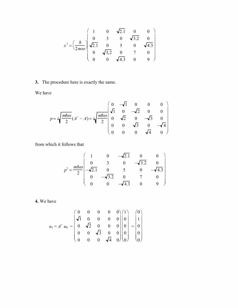
x2 =

2mω

1 0 2.1 0 0

0 3 0 3.2 0

2.1 0 5 0 4.3

0 3,2 0 7 0

0 0 4.3 0 9

3. The procedure here is exactly the same.

We have

p = imω

2(A

+ − A) = imω

2

0 − 1 0 0 0

1 0 − 2 0 0

0 2 0 − 3 0

0 0 3 0 − 4

0 0 0 4 0

from which it follows that

p2 =mω

2

1 0 − 2.1 0 0

0 3 0 − 3.2 0

− 2.1 0 5 0 − 4.3

0 − 3.2 0 7 0

0 0 − 4.3 0 9

4. We have

u1 = A+ u0 =

0 0 0 0 0

1 0 0 0 0

0 2 0 0 0

0 0 3 0 0

0 0 0 4 0

1

0

0

0

0

=

0

1

0

0

0

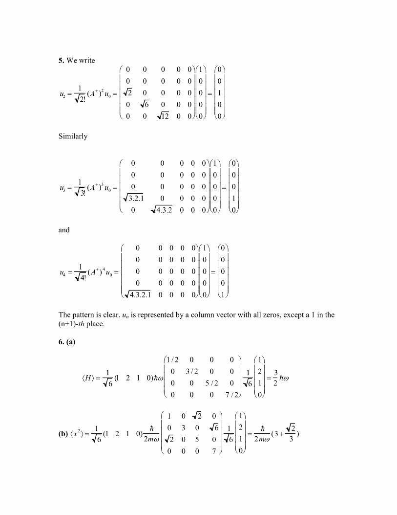
5. We write

u2 =1

2!(A

+)

2u0 =

0 0 0 0 0

0 0 0 0 0

2 0 0 0 0

0 6 0 0 0

0 0 12 0 0

1

0

0

0

0

=

0

0

1

0

0

Similarly

u3 =1

3!(A

+)

3u0 =

0 0 0 0 0

0 0 0 0 0

0 0 0 0 0

3.2.1 0 0 0 0

0 4.3.2 0 0 0

1

0

0

0

0

=

0

0

0

1

0

and

u4 =1

4!(A

+)

4u0 =

0 0 0 0 0

0 0 0 0 0

0 0 0 0 0

0 0 0 0 0

4.3.2.1 0 0 0 0

1

0

0

0

0

=

0

0

0

0

1

The pattern is clear. un is represented by a column vector with all zeros, except a 1 in the

(n+1)-th place.

6. (a)

⟨H ⟩ =1

6(1 2 1 0)ω

1 / 2 0 0 0

0 3 / 2 0 0

0 0 5 /2 0

0 0 0 7 / 2

1

6

1

2

1

0

=3

2ω

(b)

⟨x2 ⟩ =1

6(1 2 1 0)

2mω

1 0 2 0

0 3 0 6

2 0 5 0

0 0 0 7

1

6

1

2

1

0

=

2mω(3 +

2

3)

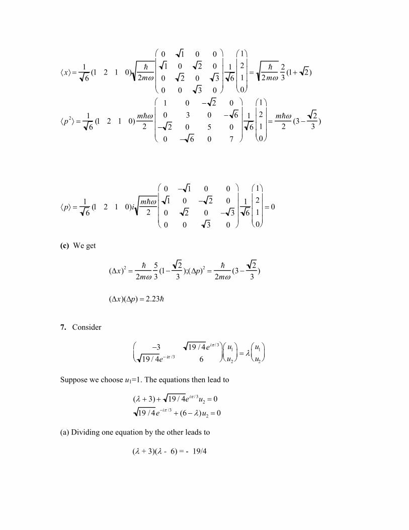
⟨x⟩ =1

6(1 2 1 0)

2mω

0 1 0 0

1 0 2 0

0 2 0 3

0 0 3 0

1

6

1

2

1

0

=

2mω2

3(1+ 2)

⟨p2⟩ =1

6(1 2 1 0)

mω2

1 0 − 2 0

0 3 0 − 6

− 2 0 5 0

0 − 6 0 7

1

6

1

2

1

0

=mω

2(3 −

2

3)

⟨p⟩ =1

6(1 2 1 0)i

mω2

0 − 1 0 0

1 0 − 2 0

0 2 0 − 3

0 0 3 0

1

6

1

2

1

0

= 0

(c) We get

(∆x)2 =

2mω5

3(1−

2

3);(∆p)2 =

2mω(3−

2

3)

(∆x)(∆p) = 2.23

7. Consider

−3 19 / 4e iπ / 3

19 / 4e− iπ /3 6

u1

u2

= λ

u1

u2

Suppose we choose u1=1. The equations then lead to

(λ + 3) + 19 / 4e iπ / 3u2 = 0

19 / 4e−iπ /3 + (6 − λ)u2 = 0

(a) Dividing one equation by the other leads to

(λ + 3)(λ - 6) = - 19/4

The roots of this equation are λ =- 7/2 and λ = 13/2. The values of u 2 corresponding to

the two eigenvalues are

u2 (−7 / 2) =1

19e−iπ /3

;u2(13 / 2) = − 19e−iπ /3

(b) The normalized eigenvectors are

1

20

19

−e−iπ / 3

;

1

20

eiπ /3

19

It is easy to see that these are orthogonal.

(c) The matrix that diagonalizes the original matrix is, according to Eq. (9-55)

U =1

20

1 − 19e iπ /3

19e− iπ / 3 1

It is easy to check that

U+AU =

13 /2 0

0 −7 / 2

8. We have, as a result of problem 7,

A =UAdiagU+

From this we get

eA =Ue

A diagU+ =U

e13/ 2

0

0 e−7/2

U

+

The rest is rather trivial matrix multiplication.

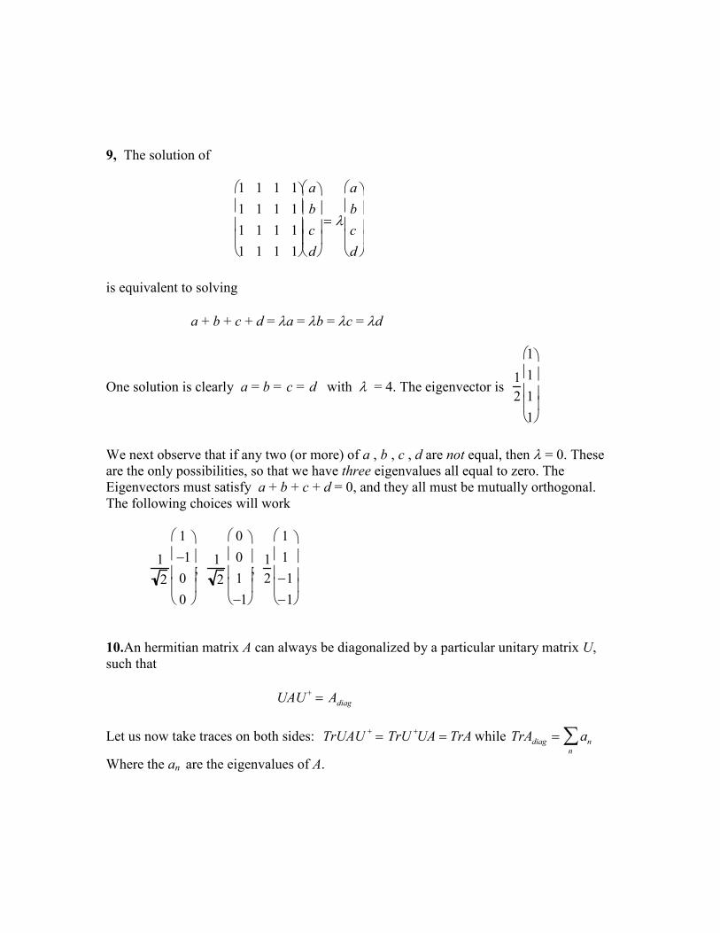
9, The solution of

1 1 1 1

1 1 1 1

1 1 1 1

1 1 1 1

a

b

c

d

= λ

a

b

c

d

is equivalent to solving

a + b + c + d = λa = λb = λc = λd

One solution is clearly a = b = c = d with λ = 4. The eigenvector is 1

2

1

1

1

1

We next observe that if any two (or more) of a , b , c , d are not equal, then λ = 0. These

are the only possibilities, so that we have three eigenvalues all equal to zero. The

Eigenvectors must satisfy a + b + c + d = 0, and they all must be mutually orthogonal.

The following choices will work

1

2

1

−1

0

0

;

1

2

0

0

1

−1

;

1

2

1

1

−1

−1

10.An hermitian matrix A can always be diagonalized by a particular unitary matrix U,

such that

UAU+ = Adiag

Let us now take traces on both sides: TrUAU+ = TrU +

UA = TrAwhile TrAdiag = ann

∑

Where the an are the eigenvalues of A.

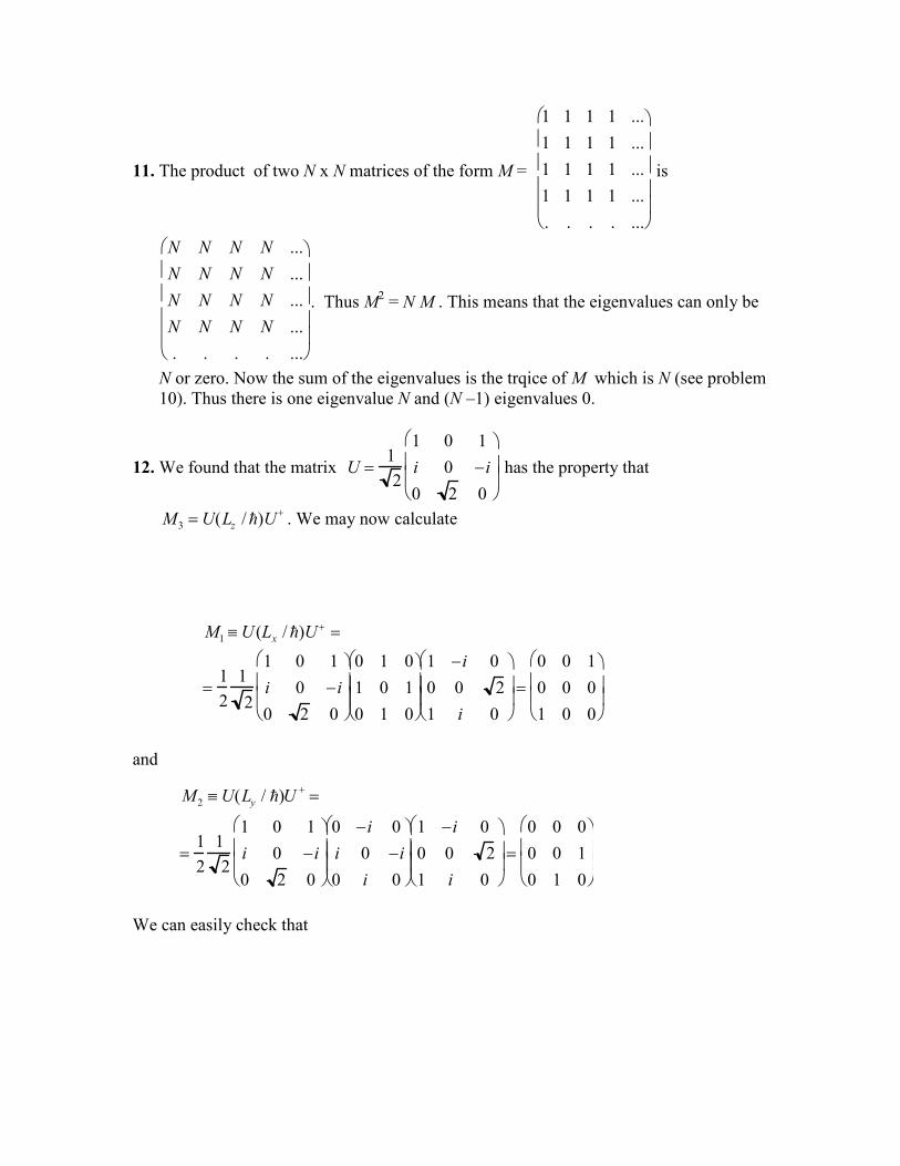
11. The product of two N x N matrices of the form M =

1 1 1 1 ...

1 1 1 1 ...

1 1 1 1 ...

1 1 1 1 ...

. . . . ...

is

N N N N ...

N N N N ...

N N N N ...

N N N N ...

. . . . ...

. Thus M2 = N M . This means that the eigenvalues can only be

N or zero. Now the sum of the eigenvalues is the trqice of M which is N (see problem

10). Thus there is one eigenvalue N and (N –1) eigenvalues 0.

12. We found that the matrix U =1

2

1 0 1

i 0 −i

0 2 0

has the property that

M3 =U(Lz /)U

+. We may now calculate

and

We can easily check that

M2 ≡U(Ly / )U+ =

=1

2

1

2

1 0 1

i 0 −i

0 2 0

0 −i 0

i 0 −i

0 i 0

1 −i 0

0 0 2

1 i 0

=

0 0 0

0 0 1

0 1 0

M1 ≡U (Lx /)U + =

=1

2

1

2

1 0 1

i 0 −i

0 2 0

0 1 0

1 0 1

0 1 0

1 −i 0

0 0 2

1 i 0

=

0 0 1

0 0 0

1 0 0

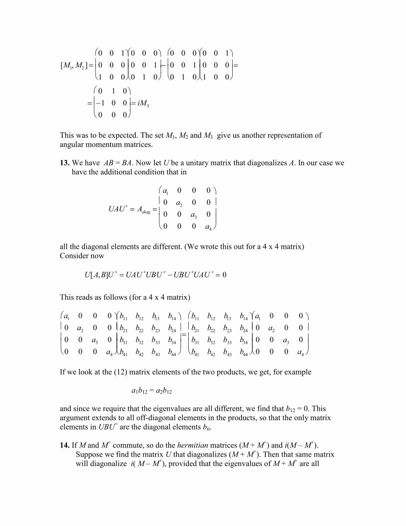
[M1,M2 ] =

0 0 1

0 0 0

1 0 0

0 0 0

0 0 1

0 1 0

−

0 0 0

0 0 1

0 1 0

0 0 1

0 0 0

1 0 0

=

=

0 1 0

−1 0 0

0 0 0

= iM3

This was to be expected. The set M1, M2 and M3 give us another representation of

angular momentum matrices.

13. We have AB = BA. Now let U be a unitary matrix that diagonalizes A. In our case we

have the additional condition that in

UAU+ = Adiag =

a1 0 0 0

0 a2 0 0

0 0 a3 0

0 0 0 a4

all the diagonal elements are different. (We wrote this out for a 4 x 4 matrix)

Consider now

U[A,B]U

+ =UAU +UBU

+ −UBU +UAU

+ = 0

This reads as follows (for a 4 x 4 matrix)

a1 0 0 0

0 a2 0 0

0 0 a3 0

0 0 0 a4

b11 b12 b13 b14

b21 b22 b23 b24

b31 b32 b33 b34

b41 b42 b43 b44

=

b11 b12 b13 b14

b21 b22 b23 b24

b31 b32 b33 b34

b41 b42 b43 b44

a1 0 0 0

0 a2 0 0

0 0 a3 0

0 0 0 a4

If we look at the (12) matrix elements of the two products, we get, for example

a1b12 = a2b12

and since we require that the eigenvalues are all different, we find that b12 = 0. This

argument extends to all off-diagonal elements in the products, so that the only matrix

elements in UBU= are the diagonal elements bii.

14. If M and M+ commute, so do the hermitian matrices (M + M

+) and i(M – M

+).

Suppose we find the matrix U that diagonalizes (M + M+). Then that same matrix

will diagonalize i( M – M+), provided that the eigenvalues of M + M

+ are all

different. This then shows that the same matrix U diagonalizes both M and M+

separately.

(The problem is not really solved, till we learn how to deal with the situation when

the eigenvalues of A in problem 13 are not all different).

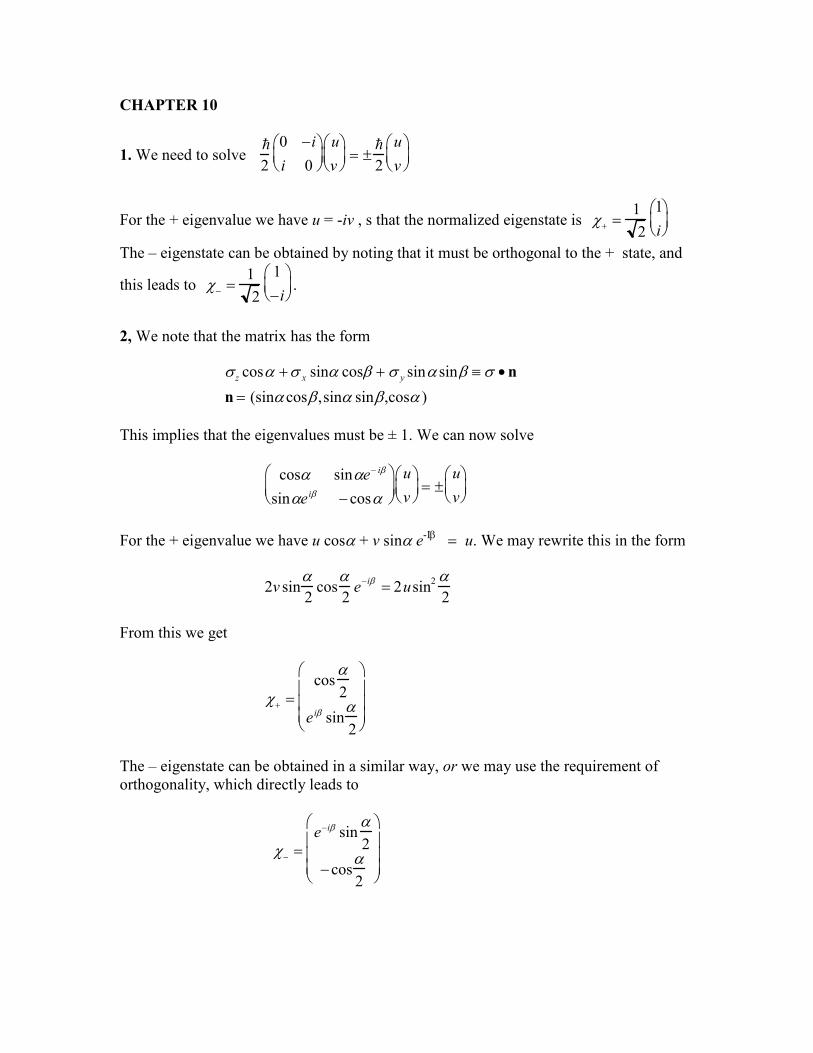
CHAPTER 10

1. We need to solve

2

0 −i

i 0

u

v

= ±

2

u

v

For the + eigenvalue we have u = -iv , s that the normalized eigenstate is χ+ =1

2

1

i

The – eigenstate can be obtained by noting that it must be orthogonal to the + state, and

this leads to χ− =1

2

1

−i

.

2, We note that the matrix has the form

σ z cosα +σ x sinα cosβ + σ y sinα sinβ ≡ σ •n

n = (sinαcosβ,sinα sinβ,cosα )

This implies that the eigenvalues must be ± 1. We can now solve

cosα sinαe− iβ

sinαe iβ −cosα

u

v

= ±

u

v

For the + eigenvalue we have u cosα + v sinα e-Iβ = u. We may rewrite this in the form

2v sinα2cos

α2e−iβ = 2usin2 α

2

From this we get

χ+ =cos

α2

e iβ sinα2

The – eigenstate can be obtained in a similar way, or we may use the requirement of

orthogonality, which directly leads to

χ− =e−iβ sin

α2

−cosα2

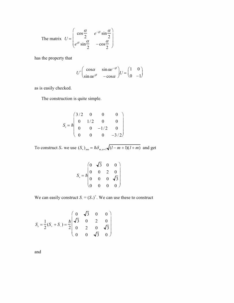
The matrix U =cos

α2

e−iβ sinα2

e iβ sinα2

−cosα2

has the property that

U+ cosα sinαe− iβ

sinαe iβ −cosα

U =

1 0

0 −1

as is easily checked.

The construction is quite simple.

Sz =

3 /2 0 0 0

0 1/ 2 0 0

0 0 −1/2 0

0 0 0 −3 / 2

To construct S+ we use (S+)mn = δm ,n+1 (l −m +1)( l +m) and get

S+ =

0 3 0 0

0 0 2 0

0 0 0 3

0 0 0 0

We can easily construct S- = (S+)+. We can use these to construct

Sx =1

2(S+ + S− ) =

2

0 3 0 0

3 0 2 0

0 2 0 3

0 0 3 0

and

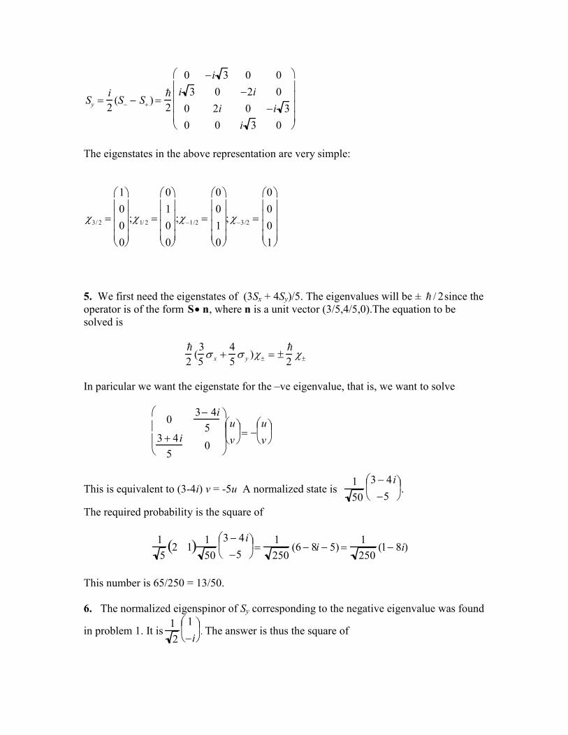
Sy =i

2(S− − S+ ) =

2

0 −i 3 0 0

i 3 0 −2i 0

0 2i 0 −i 3

0 0 i 3 0

The eigenstates in the above representation are very simple:

χ3/ 2 =

1

0

0

0

;χ1/ 2 =

0

1

0

0

;χ−1/2 =

0

0

1

0

;χ−3/2 =

0

0

0

1

5. We first need the eigenstates of (3Sx + 4Sy)/5. The eigenvalues will be ± / 2since the

operator is of the form S• n, where n is a unit vector (3/5,4/5,0).The equation to be solved is

2(3

5σ x +

4

5σ y )χ± = ±

2χ±

In paricular we want the eigenstate for the –ve eigenvalue, that is, we want to solve

03− 4i

53 + 4i5

0

u

v

= −

u

v

This is equivalent to (3-4i) v = -5u A normalized state is 1

50

3 − 4i

−5

.

The required probability is the square of

1

52 1( ) 1

50

3 − 4i

−5

=

1

250(6 − 8i − 5) =

1

250(1− 8i)

This number is 65/250 = 13/50.

6. The normalized eigenspinor of Sy corresponding to the negative eigenvalue was found

in problem 1. It is1

2

1

−i

. The answer is thus the square of

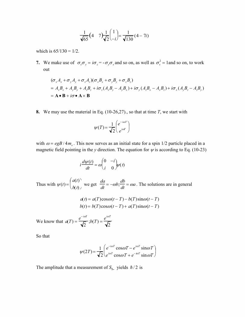
1

654 7( ) 1

2

1

−i

=

1

130(4 − 7i)

which is 65/130 = 1/2.

7. We make use of σxσ y = iσ z = -σyσ x and so on, as well as σx

2 = 1and so on, to work out

(σ xAx +σ yAy +σ zAz )(σ xBx +σ yBy +σ zBz )

= AxBx + AyBy + AzBz + iσ z (AxBy − AyBx ) + iσ y (AzBx − AxBz ) + iσ x (AyBz − AzBy )

= A •B + iσ •A × B

8. We may use the material in Eq. (10-26,27)., so that at time T, we start with

ψ (T ) =1

2

e− iωT

eiωT

with ω = egB / 4me . This now serves as an initial state for a spin 1/2 particle placed in a

magnetic field pointing in the y direction. The equation for ψ is according to Eq. (10-23)

idψ (t)

dt=ω

0 −i

i 0

ψ( t)

Thus with ψ (t) =a(t)

b( t)

we get

da

dt= −ωb;

db

dt=ωa . The solutions are in general

a( t) = a(T )cosω(t − T ) − b(T )sinω(t − T )b(t) = b(T )cosω(t − T ) + a(T )sinω(t − T )

We know that a(T ) =e− iωT

2;b(T ) =

eiωT

2

So that

ψ (2T ) =1

2

e−iωT

cosωT − e iωTsinωT

eiωT

cosωT + e− iωT sinωT

The amplitude that a measurement of Sx yields / 2 is

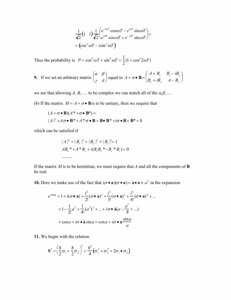
1

21 1( ) 1

2

e−iωT

cosωT − e iωTsinωT

eiωT

cosωT + e− iωT sinωT

=

= cos2ωT − isin2ωT( )

Thus the probability is P = cos4ωT + sin4ωT =

1

2(1 + cos22ωT )

9. If we set an arbitrary matrix α βγ δ

equal to A + σ • B =

A + Bz Bx − iBy

Bx + iBy A− Bz

we see that allowing A, Bx … to be complex we can match all of the α,β,….

(b) If the matrix M = A + σ • Bis to be unitary, then we require that

(A +σ •B)(A*+σ • B*) =

| A |2 +Aσ • B*+A*σ •B + B• B* +iσ •B × B* = 1

which can be satisfied if

| A |2 + | Bx |2 + |By |

2 + | Bz |2= 1

ABx * +A*Bx + i(ByBz *−By *Bz ) = 0

.........

If the matrix M is to be hermitian, we must require that A and all the components of B

be real.

10. Here we make use of the fact that (σ •a)(σ •a) = a •a ≡ a2 in the expansion

e iσ•a =1 + i(σ • a) +i2

2!(σ • a)2 +

i3

3!(σ • a)3 +

i4

4!(σ • a)4 + ...

=1−1

2!a

2 +1

4!(a

2)2 + ...+ iσ • ˆ a (a −

a3

3!+ ...)

= cosa + iσ • ˆ a sina = cosa + iσ •asina

a

11. We begin with the relation

S2 =

2σ1 +

2σ 2

2

=2

4σ1

2 +σ 2

2 + 2σ1 •σ 2( )

from which we obtain σ1 •σ 2 = 2S(S +1) − 3 . This = -3 for a singlet and +1 for a triplet state.

We now choose ˆ e to point in the z direction, so that the first term in S12 is equal to 3σ1zσ 2z .

(a) for a singlet state the two spins are always in opposite directions so that the

first term is –6 and the second is +3. Thus

S12Xsinglet = 0

(b) For a triplet the first term is +1 when Sz = 1 and Sz = -1 and –1 when Sz =0.

This means that S12 acting on a triplet state in the first case is 3-1= 2, and in

the second case it is –3-1= - 4. Thus

(S12 − 2)(S12 + 4)X triplet = 0

12. The potential may be written in the form

V(r) = V1(r) + V2(r)S12 + V3(r)[2S(S +1) − 3]

For a singlet state S12 has expectation value zero, so that

V(r) = V1(r) – 3V3(r)

For the triplet state S12 has a value that depends on the z component of the total spin.

What may be relevant

for a potential energy is an average, assuming that the two particles have equal

probability of being in any one of the three Sz states. In that case the average value of Sz is

(2+2-4)/3= 0

13. (a) It is clear that for the singlet state, ψ singlet =1

2(χ +

(1)χ −(2) − χ −

(1)χ +(2)) , if one of the

electrons is in the “up” state, the other must be in the “down” state.

(b). Suppose that we denote the eigenstates of Sy by ξ± . These are, as worked out in problem 1,

ξ+(1) =

1

2

1

i

;ξ−

(1) =1

2

1

−i

The spinors for particle (1) may be expanded in terms of the ξ± thus:

χ+ =1

0

=

1

2

1

2

1

i

+

1

2

1

−i

=

1

2ξ+ + ξ−( )

χ− =0

1

=

i

2

1

2

1

i

−

1

2

1

−i

=

i

2(ξ+ − ξ− )

Similarly, for particle (2), we want to expand the spinors in terms of the η± , the

eigenstates of Sx

η+(2) =

1

2

1

1

; η−

(2) =1

2

1

−1

thus

χ+ =1

0

=

1

2

1

2

1

1

+

1

2

1

−1

=

1

2η+ +η−( )

χ− =0

1

=

1

2

1

2

1

1

−

1

2

1

−1

=

1

2η+ −η−( )

We now pick out, in the expansion of the singlet wave function the coefficient of ξ+(1)η+

(2)

and take its absolute square.Some simple algebra shows that it is

|1

2

1

2

1− i2

|2=

1

4

9. The state is (cosα1χ+(1) + sinα1e

iβ1 χ−(1))(cosα2χ+

(2) + sinα2eiβ 2χ−

(2)) . We need to calculate

the scalar product of this with the three triplet wave functions of the two-electgron

system. It is easier to calculate the probability that the state is found in a singlet state,

and then subtract that from unity.

The calculation is simple

⟨1

2(χ+

(1)χ−(2) − χ −

(1)χ +(2)) | (cosα1χ+

(1) + sinα1eiβ1 χ−

(1))(cosα2χ+

(2) + sinα2eiβ2 χ−

(2))⟩

=1

2(cosα1 sinα2e

iβ2 − sinα1eiβ1 cosα2 )

The absolute square of this is the singlet probability. It is

Ps =1

2(cos

2α1 sin2α 2 + cos

2α2 sin2α1 + 2sinα1cosα1 sinα1cosα 2cos(β1 − cosβ2 ))

and

Pt = 1 - Ps

14. We use J = L +S so that J2 = L

2 + S

2 + 2L.S, from which we get

L •S =1

2J (J +1) − L(L +1) − 2[ ]

since S = 1. Note that we have taken the division by 2 into account. For J = L + 1 this

takes on the value L; for J = L, it takes on the value –1, and for J = L – 1 it is –L – 1.

We therefore find

J = L +1: V = V1 + LV2 + L2V3

J = L V = V1 − V2 +V3

J = L −1 V = V1 − (L +1)V2 + (L +1)2V3

CHAPTER 11

1. The first order contribution is

En

(1) = λ⟨n | x2 | n⟩ = λ

2mω

2

⟨n | (A + A+)(A + A

+) | n⟩

To calculate the matrix element ⟨n | A2 + AA+ + A

+A + (A+

)2|n⟩ we note that

A+|n⟩ = n +1 |n +1⟩ ; ⟨n | A = n +1⟨n +1 | so that (1) the first and last terms give

zero, and the second and third terms yield (n + 1) + (n – 1)=2n. Thus the first order shift

is

En

(1) = λ

mωn

The second order calculation is quite complicated. What is involved is the calculation of

En

(2) = λ2

2mω

2⟨n | (A + A

+)2| m⟩⟨m | (A + A

+)2|n⟩

ω(n − m)m≠n∑

This is manageable but quite messy. The suggestion is to write

H =p2

2m+1

2mω2

x2 + λx2

This is just a simple harmonic oscillator with frequency

ω* = ω 2 + 2λ /m = ω +λ

ωm−1

2

λ2

ω 3m2 + ...

Whose spectrum is

En = ω * (n +

1

2) = ω(n +

1

2) +

λωm

(n +1

2) −

λ2

2ω3m 2 (n +1

2) + ...

The extra factor of 1/2 that goes with each n is the zero-point energy. We are only

interested in the change in energy of a given state |n> and thus subtract the zero-point

energy to each order of λ. Note that the first order λ calculation is correct.

2. The eigenfunction of the rotator are the spherical harmonics. The first order energy

shift for l = 1 states is given by

∆E = ⟨1,m | E cosθ |1,m⟩ = E dφ sinθdθ cosθ |Y1.m |2

0

π

∫0

2π

∫

For m = ±1, this becomes

2πE sinθdθ cosθ3

8π

0

π

∫ sin2θ =

3E

4duu(1− u

2) = 0

−1

1

∫

The integral for m = 0 is also zero. This result should have been anticipated. The

eigenstates of L2 are also eigenstates of parity. The perturbation cosθ is odd under the

reflection r - r and therefore the expectation value of an odd operator will always be

zero. Since the perturbation represents the interaction with an electric field, our result

states that a symmetric rotator does not have a permanent electric dipole moment.

The second order shift is more complicated. What needs to be evaluated is

∆E (2) = E2 | ⟨1,m | cosθ |L,M⟩ |2

E1 − ELL ,M (L ≠1)∑

with EL =

2

2IL(L +1) . The calculation is simplified by the fact that only L = 0 and L = 2

terms contribute. This can easily be seen from the table of spherical harmonics. For L =1

we saw that the matrix element vanishes. For the higher values we see that

cosθY1,±1 ∝Y2,±1 and cosθY1,0 ∝ aY2,0 + bY0,0 . The orthogonality of the spherical harmonics

for different values of L takes care of the matter. Note that because of the φ integration, for m = ±1 only the L = 2 ,M = ± 1 term contributes, while for the m = 0 term, there will

be contributions from L = 0 and L = 2, M = 0. Some simple integrations lead to

∆Em=±1(2) = −

2IE2

2

1

15; ∆Em= 0

(2) = −2IE

2

2

1

60

3. To lowest order in V0 the shift is given by

∆E =2

L

2

V0

Ldxxsin

2

0

L

∫nπxL

=2V0

L2

L

π

2

duusin2 nu =V0

π 20

π

∫ duu(1− cos2nu) =1

20

π

∫ V0

The result that the energy shift is just the value of the perturbation at the mid-

point is perhaps not surprising, given that the square of the eigenfunctions do not,

on the average, favor one side of the potential over the other.

4. The matrix

E λ 0 0

λ E 0 0

0 0 2E σ0 0 σ 0

consists of two boxes which can be diagonalized

separately. The upper left hand box involves solving E λλ E

u

v

= η

u

v

The result is that the eigenvalues are η = E ± λ. The corresponding eigenstates are easily

worked out and are 1

2

1

±1

for the two cases.

For the lower left hand box we have to solve 2E σσ 0

a

b

= ξ

a

b

. Here we find that the

eigenvalues are ξ = E ± E2 + σ 2

. The corresponding eigenstates are

Nσ

−E ± E 2 + σ 2

respectively, with

1

N 2 = σ 2 + (−E ± E2 + σ 2

)2.

5. The change in potential energy is given by

V1 = −3e2

8πε0R3 R2 −

1

3r2

+e2

4πε0rr ≤ R

= 0 elsewhere

Thus

∆E = d3rψ nl

*(r)V1ψ nl (r) = r

2dr

0

R

∫∫ V1Rnl

2(r)

We may now calculate this for various states.

n = 1 ∆E10 = 4Z

a0

3

r2dr

0

R

∫ e−2Zr /a0 −

3e2

8πε0R3 R

2 −1

3r2

+

e2

4πε0r

With a change of variables to x = r/Za0 and with ρ = ZR/a0 this becomes

∆E10 = 4Ze

2

4πε0a0

x2dx −

3

2ρ+

x2

2ρ3 +1

x

0

ρ

∫ e−2x

Since x << 1 we may approximate e−2x ≈1− 2x , which simplifies the integrals. What

results is

∆E10 =Ze

2

4πε0a0

4

10ρ2 + ...

A similar calculation yields

∆E20 =1

2

Ze2

4πε0a0

x2dx(1− x)

2 −3

2ρ+

x2

2ρ3 +1

x

0

ρ

∫ e− x ≈

Ze2

4πε0a0

1

20ρ2 + ...

and

∆E21 =1

24

Ze2

4πε0a0

x2dxx

2 −3

2ρ+

x2

2ρ3 +1

x

0

ρ

∫ e−x ≈

Ze2

4πε0a0

1

1120ρ4 + ...

6. We need to calculate λ⟨0 | x4 | 0⟩ . One way of proceeding is to use the expression

x =

2mω(A + A

+)

Then

λ⟨0 | x4 | 0⟩ = λ

2mω

2

⟨0 | (A + A+)(A + A

+)(A + A

+)(A + A

+) | 0⟩

The matrix element is

⟨0 | (A + A+)(A + A+ )(A + A+ )(A + A+ ) | 0⟩ =

⟨0 | A+(A + A

+)(A + A

+)A

+| 0⟩ =

⟨1| (A + A+ )(A + A+ ) |1⟩ =

⟨0 |+ 2⟨2 |[ ]| 0⟩ + 2 | 2⟩[ ]= 3

Thus the energy shift is

∆E = 3λ

2mω

2

It is easy to see that the same result is obtained from

dx(λx 4)

mωπ

1/4

e−mωx 2 /2

−∞

∞

∫2

7. The first order perturbation shift is

∆En =2εb

dx0

b

∫ sinπxb

sinnπxb

2

=2επ

dusinu(sin nu)2

0

π

∫

=2επ

1+1

4n2 −1

8. It follows from [p, x] = −i that

−i = ⟨a | px − xp |a⟩ =

= ⟨a | p |n⟩⟨n | x |a⟩ − ⟨a | x |n⟩⟨n | p |a⟩n

∑

Now

⟨a | p |n⟩ = m⟨a |

dx

dt| n⟩ =

im

⟨a | Hx − xH | n⟩ =

im

(Ea − En )⟨a | x |n⟩

Consequently

⟨n | p | a⟩ = ⟨a | p |n⟩* = −

im

(Ea − En )⟨n | x |a⟩

Thus

−i =2im

n

∑ (Ea − En )⟨a | x | n⟩⟨n | x | a⟩

from which it follows that

(En − Ea )n

∑ | ⟨a | x | n⟩ |2=2

2m

9. For the harmonic oscillator, with |a> = |0>, we have

⟨n | x | 0⟩ =

2mω⟨n | A+

| 0⟩ =

2mωδn,1

This means that in the sum rule, the left hand side is

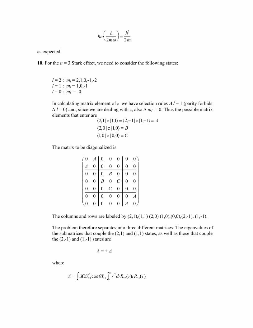
ω

2mω

=2

2m

as expected.

10. For the n = 3 Stark effect, we need to consider the following states:

l = 2 : ml = 2,1,0,-1,-2

l = 1 : ml = 1,0,-1

l = 0 : ml = 0

In calculating matrix element of z we have selection rules ∆ l = 1 (parity forbids ∆ l = 0) and, since we are dealing with z, also ∆ ml = 0. Thus the possible matrix

elements that enter are

⟨2,1| z |1,1⟩ = ⟨2,−1| z |1,−1⟩ ≡ A

⟨2,0 | z |1,0⟩ ≡ B

⟨1,0 | z | 0,0⟩ ≡ C

The matrix to be diagonalized is

0 A 0 0 0 0 0

A 0 0 0 0 0 0

0 0 0 B 0 0 0

0 0 B 0 C 0 0

0 0 0 C 0 0 0

0 0 0 0 0 0 A

0 0 0 0 0 A 0

The columns and rows are labeled by (2,1),(1,1) (2,0) (1,0),(0,0),(2,-1), (1,-1).

The problem therefore separates into three different matrices. The eigenvalues of

the submatrices that couple the (2,1) and (1,1) states, as well as those that couple

the (2,-1) and (1,-1) states are

λ = ± A where

A = dΩY21*∫ cosθY11 r

2drR32(r)rR31(r)0

∞

∫

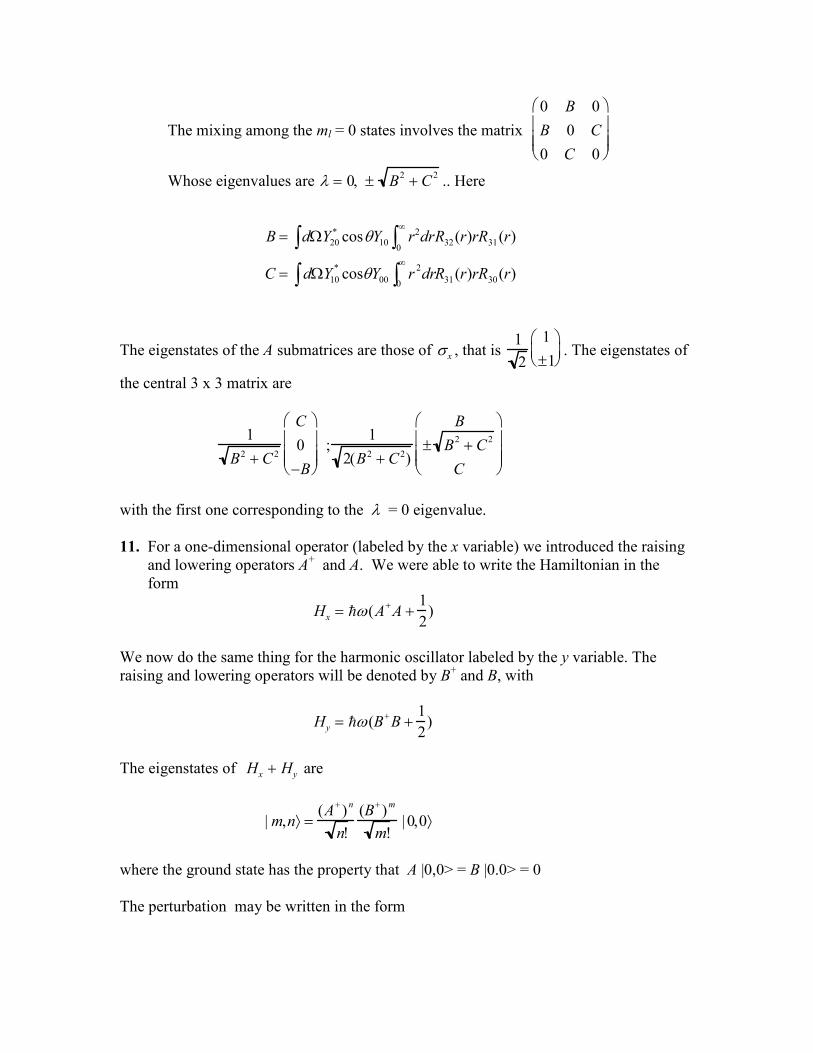
The mixing among the ml = 0 states involves the matrix

0 B 0

B 0 C

0 C 0

Whose eigenvalues are λ = 0, ± B2 + C

2.. Here

B = dΩY20* cosθY10∫ r2dr

0

∞

∫ R32(r)rR31(r)

C = dΩY10*cosθY00∫ r

2dr

0

∞

∫ R31(r)rR30(r)

The eigenstates of the A submatrices are those of σx , that is 1

2

1

±1

. The eigenstates of

the central 3 x 3 matrix are

1

B2 + C2

C

0

−B

;

1

2(B2 + C2)

B

± B2 + C

2

C

with the first one corresponding to the λ = 0 eigenvalue.

11. For a one-dimensional operator (labeled by the x variable) we introduced the raising

and lowering operators A+ and A. We were able to write the Hamiltonian in the

form

Hx = ω(A+

A +1

2)

We now do the same thing for the harmonic oscillator labeled by the y variable. The

raising and lowering operators will be denoted by B+ and B, with

Hy = ω(B+

B +1

2)

The eigenstates of Hx + Hy are

| m,n⟩ =(A

+)n

n!

(B+)m

m!| 0,0⟩

where the ground state has the property that A |0,0> = B |0.0> = 0

The perturbation may be written in the form

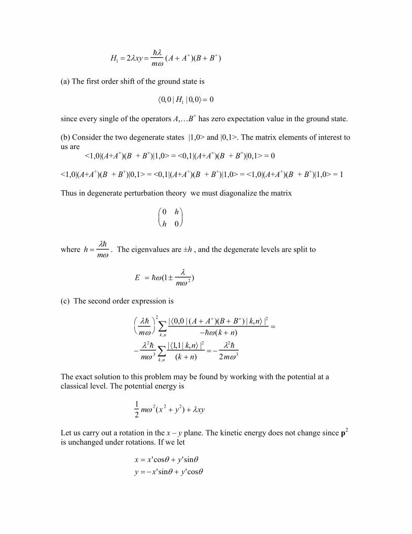
H1 = 2λxy =

λmω

(A + A+)(B + B

+)

(a) The first order shift of the ground state is

⟨0,0 | H1 | 0,0⟩ = 0

since every single of the operators A,…B+ has zero expectation value in the ground state.

(b) Consider the two degenerate states |1,0> and |0,1>. The matrix elements of interest to

us are

<1,0|(A+A+)(B + B

+)|1,0> = <0,1|(A+A

+)(B + B

+)|0,1> = 0

<1,0|(A+A+)(B + B

+)|0,1> = <0,1|(A+A

+)(B + B

+)|1,0> = <1,0|(A+A

+)(B + B

+)|1,0> = 1

Thus in degenerate perturbation theory we must diagonalize the matrix

0 h

h 0

where h =

λmω

. The eigenvalues are ±h , and the degenerate levels are split to

E = ω(1±

λmω 2 )

(c) The second order expression is

λmω

2| ⟨0,0 | (A + A+)(B + B+ ) | k,n⟩ |2

−ω(k + n)k ,n

∑ =

−λ2

mω 3

| ⟨1,1| k,n⟩ |2

(k + n)k ,n

∑ = −λ2

2mω3

The exact solution to this problem may be found by working with the potential at a

classical level. The potential energy is

1

2mω 2

(x2 + y

2) + λxy

Let us carry out a rotation in the x – y plane. The kinetic energy does not change since p2

is unchanged under rotations. If we let

x = x 'cosθ + y 'sinθy = −x 'sinθ + y 'cosθ

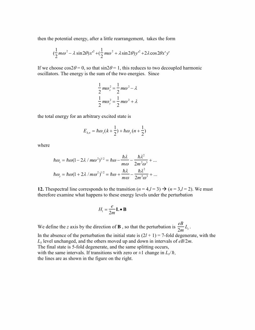
then the potential energy, after a little rearrangement, takes the form

(1

2mω 2 − λ sin2θ)x '2 +(

1

2mω 2 + λsin2θ)y '2 +2λcos2θx ' y'

If we choose cos2θ = 0, so that sin2θ = 1, this reduces to two decoupled harmonic oscillators. The energy is the sum of the two energies. Since

1

2mωx

2 =1

2mω 2 − λ

1

2mωy

2 =1

2mω 2 + λ

the total energy for an arbitrary excited state is

Ek,n = ωx(k +

1

2) + ωy (n +

1

2)

where

ωx = ω(1− 2λ / mω 2)1/ 2 = ω −λmω

−λ2

2m 2ω3+ ...

ωy = ω(1 + 2λ /mω2)1/2 = ω +

λmω

−λ2

2m 2ω3 + ...

12. Thespectral line corresponds to the transition (n = 4,l = 3) (n = 3,l = 2). We must

therefore examine what happens to these energy levels under the perturbation

H1 =e

2mL •B

We define the z axis by the direction of B , so that the perturbation is eB

2mLz .

In the absence of the perturbation the initial state is (2l + 1) = 7-fold degenerate, with the

Lz level unchanged, and the others moved up and down in intervals of eB/2m.

The final state is 5-fold degenerate, and the same splitting occurs,

with the same intervals. If transitions with zero or ±1 change in Lz/ ,

the lines are as shown in the figure on the right.

What will be the effect of a constant electric field parallel to B?

The additional perturbation is therefore

H2 = −eE0 • r = −eE0z

and we are only interested in what this does to the energy level

structure. The perturbation acts as in the Stark effect. The effect

of H1 is to mix up levels that are degenerate, corresponding

to a given ml value with different values of l. For example,

the l = 3, ml = 2 and the l = 2, ml = 2 degeneracy (for n = 4)will

be split. There will be a further breakdown of degeneracy.

13. The eigenstates of the unperturbed Hamiltonian are eigenstates of σ z . They are

1

0

corresponding to E = E0 and

0

1

corresponding to E = - E0.

The first order shifts are given by

1 0( )λα u

u * β

1

0

= λα

0 1( )λα u

u * β

0

1

= λβ

for the two energy levels.

The second order shift for the upper state involves summing over intermediate states that

differ from the initial state. Thus, for the upper state, the intermediate state is just the

lower one, and the energy denominator is E0 – (- E0) = 2E0. Thus the second order shift is

λ2

2E0

1 0( )α u

u * β

0

1

0 1( )

α u

u* β

1

0

=

λ2|u |

2

2E0

For the lower state we get

λ2

−2E0

0 1( )α u

u* β

1

0

1 0( )

α u

u * β

0

1

= −

λ2| u |

2

2E0

The exact eigenvalues can be obtained from

detE0 +α −ε u

u * −E0 + β −ε= 0

This leads to

ε = λα + β2

± (E0 − λα − β2

)2 + λ2

| u |2

= λα + β2

± (E0 − λα − β2

)(1+1

2

λ2 |u |2

E0

2 + ...

(b) Consider now

H =E0 u

v −E0

where we have dropped the α and β terms. The eigenvalues are easy to determine, and they are

ε = ± E0

2 + λ2uv

The eigenstates are written as a

b

and they satisfy

E0 u

v −E0

a

b

= ± E0

2 + λ2uv

a

b

For the upper state we find that the un-normalized eigenstate is

λu

E0

2 + λ2uv − E0

For the lower state it is

−λu

E0

2 + λ2uv + E0

The scalar product

−λ2| u |

2 + (E0

2 + λ2uv) − E0

2[ ]= λ2u(u* −v) ≠ 0

which shows that the eigenstates are not orthogonal unless v = u*.

CHAPTER 12.

1. With a potential of the form

V(r) =1

2mω2

r2

the perturbation reduces to

H1 =1

2m2c2 S• L

1

r

dV (r)

dr=

ω2

4mc2 (J

2 − L2 − S2)

=(ω) 2

4mc2 j( j +1) − l(l +1)− s(s +1)( )

where l is the orbital angular momentum, s is the spin of the particle in the well (e.g. 1/2

for an electron or a nucleon) and j is the total angular momentum. The possible values of

j are l + s, l + s – 1, l + s –2, …|l – s|.

The unperturbed energy spectrum is given by En r l

= ω(2n r + l +3

2). Each of the

levels characterized by l is (2l + 1)-fold degenerate, but there is an additional degeneracy,

not unlike that appearing in hydrogen. For example nr =2, l = 0. nr =1, l = 2 , nr = 0, l = 4

all have the same energy.

A picture of the levels and their spin-orbit splitting is given below.

2. The effects that enter into the energy levels corresponding to n = 2, are (I) the basic

Coulomb interaction, (ii) relativistic and spin-orbit effects, and (iii) the hyperfine

structure which we are instructed to ignore. Thus, in the absence of a magnetic field,

the levels under the influence of the Coulomb potential consist of 2n2 = 8 degenerate

levels. Two of the levels are associated with l = 0 (spin up and spin down) and six

levels with l = 0, corresponding to ml = 1,0,-1, spin up and spin down. The latter can

be rearranged into states characterized by J2, L

2 and Jz. There are two levels

characterized by j = l –1/2 = 1/2 and four levels with j = l + 1/2 = 3/2. These energies

are split by relativistic effects and spin-orbit coupling, as given in Eq. (12-16). We

ignore reduced mass effects (other than in the original Coulomb energies). We

therefore have

∆E = −1

2mec

2α 4 1

n3

1

j +1/ 2−

3

4n

= −1

2mec

2α 4 5

64

j =1 / 2

= −1

2mec

2α 4 1

64

j = 3 / 2

(b) The Zeeman splittings for a given j are

∆EB =eB

2me

m j

2

3

j =1 / 2

=eB

2me

m j

4

3

j = 3 / 2

Numerically 1

128mec

2α 4 ≈1.132×10−5eV , while for B = 2.5T

eB

2me

= 14.47×10−5eV ,

so under these circumstances the magnetic effects are a factor of 13 larger than the

relativistic effects. Under these circumstances one could neglect these and use Eq. (12-

26).

3. The unperturbed Hamiltonian is given by Eq. (12-34) and the magnetic field interacts

both with the spin of the electron and the spin of the proton. This leads to

H = A

S• I2 + a

Sz

+ b

Iz

Here

A =4

3α 4

mec2gP

me

MP

I•S2

a= 2eB

2me

b = −gP

eB

2M p

Let us now introduce the total spin F = S + I. It follows that

S• I2 =

1

222F(F +1) −

3

42 −

3

42

=1

4for F =1

= −3

4for F = 0

We next need to calculate the matrix elements of aSz + bI z for eigenstates of F2 and Fz .

These will be exactly like the spin triplet and spin singlet eigenstates. These are

⟨1,1| aSz + bI z |1,1⟩ = ⟨χ +ξ+ |aSz + bIz | χ+ξ+ ⟩ =1

2(a + b)

⟨1,0 | aSz + bI z |1,0⟩ =1

2

2

⟨χ +ξ− + χ−ξ+ | aSz + bI z | χ +ξ− + χ+ξ−⟩ = 0

⟨1,−1 |aSz + bIz |1,−1⟩ = ⟨χ −ξ− |aSz + bIz | χ−ξ− ⟩ = −1

2(a + b)

And for the singlet state (F = 0)

⟨1,0 | aSz + bI z | 0,0⟩ =1

2

2

⟨χ +ξ− + χ−ξ+ | aSz + bI z | χ +ξ− − χ +ξ−⟩ =1

2(a− b)

⟨0,0 | aSz + bI z | 0,0⟩ =1

2

2

⟨χ +ξ− − χ −ξ+ |aSz + bIz | χ+ξ− − χ+ξ−⟩ = 0

Thus the magnetic field introduces mixing between the |1,0> state and the |0.0> state.

We must therefore diagonalize the submatrix

A / 4 (a − b) / 2

(a− b) / 2 −3A / 4

=

−A / 4 0

0 −A / 4

+

A / 2 (a − b) / 2

(a− b) / 2 −A / 2

The second submatrix commutes with the first one. Its eigenvalues are easily determined

to be ± A2/ 4 + (a − b)

2/ 4 so that the overall eigenvalues are

−A / 4 ± A2/ 4 + (a − b)

2/ 4

Thus the spectrum consists of the following states:

F = 1, Fz = 1 E = A / 4 + (a + b) / 2

F =1, Fz = -1 E = A / 4 − (a + b) / 2

F = 1,0; Fz = 0 E = −A / 4 ± (A2/ 4 + (a− b)

2/ 4

We can now put in numbers.

For B = 10-4 T, the values, in units of 10

-6 eV are 1.451, 1.439, 0(10

-10), -2.89

For B = 1 T, the values in units of 10-6 eV are 57.21,-54.32, 54.29 and 7 x 10

-6.

4. According to Eq. (12-17) the energies of hydrogen-like states, including relativistic +

spin-orbit contributions is given by

En , j = −1

2

mec2(Zα) 2

(1+ me /M p )

1

n2 −1

2mec

2(Zα )4

1

n 3

1

j +1/ 2−

3

4n

The wavelength in a transition between two states is given by

λ =

2πc∆E

where ∆E is the change in energy in the transition. We now consider the transitions

n =3, j = 3/2 n = 1, j = 1/2 and n = 3 , j = 1/2 n = 1, j = 1/2.. The corresponding

energy differences (neglecting the reduced mass effect) is

(3,3/21,1/2) ∆E =1

2mec

2(Zα )2 (1−

1

9) +

1

2mec

2(Zα) 4

1

4(1−

1

27)

(3,1/21,1/2) 1

2mec

2(Zα)2(1−

1

9) +

1

2mec

2(Zα) 4

1

4(1−

3

27)

We can write these in the form

(3,3/21,1/2) ∆E0(1 +13

48(Zα )2 )

(3,1/21,1/2) ∆E0(1 +1

18(Zα) 2)

where

∆E0 =1

2mec

2(Zα )2

8

9

The corresponding wavelengths are

(3,3/21,1/2) λ0 (1−13

48(Zα )2 ) = 588.995 ×10−9m

(3,1/21,1/2) λ0 (1−1

18(Zα)2) = 589.592 ×10−9

m

We may use the two equations to calculate λ0 and Z. Dividing one equation by the other we get, after a little arithmetic Z = 11.5, which fits with the Z = 11 for Sodium.

(Note that if we take for λ0 the average of the two wavelengths, then , using

λ0 = 2πc / ∆E0 = 9π / 2mc(Zα )2 , we get a seemingly unreasonably small value of Z = 0.4! This is not surprising. The ionization potential for sodium is 5.1 eV instead of

Z2(13.6 eV), for reasons that will be discussed in Chapter 14)

4. The relativistic correction to the kinetic energy term is −1

2mc 2

p2

2m

2

. The energy

shift in the ground state is therefore

∆E = −1

2mc 2 ⟨0 |p2

2m

2

| 0⟩ = −1

2mc 2 ⟨0 | (H −1

2mω2

r2)2| 0⟩

To calculate < 0 | r2 | 0 > and < 0 | r

4 | 0 > we need the ground state wave function. We

know that for the one-dimensional oscillator it is

u0 (x) =mωπ

1/4

e−mωx 2 / 2

so that for the three dimensional oscillator it is

u0 (r) = u0(x)u0 (y)u0(z) =mωπ

3/ 4

e−mωr2 / 2

It follows that

⟨0 | r2 | 0⟩ = 4πr20

∞

∫ drmωπ

3/2

r2e−mωr2 / =

= 4πmωπ

3/ 2

mω

5/2

dyy4e−y 2

0

∞

∫

=3

2mω

We can also calculate

⟨0 | r4 | 0⟩ = 4πr 20

∞

∫ drmωπ

3/ 2

r4e−mωr2 / =

= 4πmωπ

3/ 2

mω

7/2

dyy6e− y 2

0

∞

∫

=15

4

mω

2

We made use of dzzn

0

∞

∫ e− z = Γ(n +1) = nΓ(n) and Γ(

1

2) = π

Thus

∆E = −1

2mc 2

3

2ω

2

−3

2ω

mω 2 3

2mω

+1

4m2ω 4 15

4

mω

2

= −15

32

(ω) 2

mc2

6. (a) With J = 1 and S = 1, the possible values of the orbital angular momentum, such

that j = L + S, L + S –1…|L – S| can only be L = 0,1,2. Thus the possible states are 3S1,

3P1,

3D1 . The parity of the deuteron is (-1)

L assuming that the intrinsic parities of

the proton and neutron are taken to be +1. Thus the S and D states have positive

parity and the P state has opposite parity. Given parity conservation, the only possible

admixture can be the 3D1 state.

(b)The interaction with a magnetic field consists of three contributions: the

interaction of the spins of the proton and neutron with the magnetic field, and the L.B

term, if L is not zero. We write

H = −M p •B −Mn •B −ML • B

where

M p =eg p

2MS p = (5.5792)

e

2M

S p

Mn =egn

2MSn = (−3.8206)

e

2M

Sn

ML =e

2M red

L

We take the neutron and proton masses equal (= M ) and the reduced mass of the two-

particle system for equal masses is M/2. For the 3S1 stgate, the last term does not

contribute.

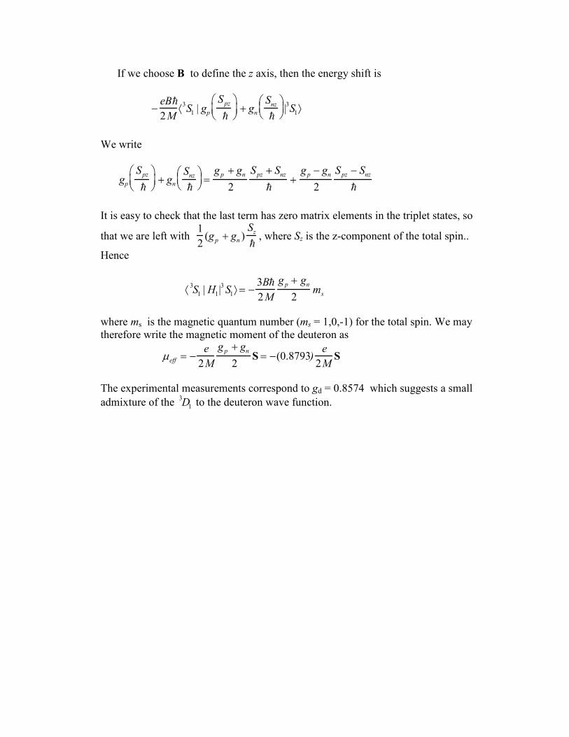
If we choose B to define the z axis, then the energy shift is

−eB

2M⟨3S1 | gp

S pz

+ gn

Snz

|3S1⟩

We write

gp

Spz

+ gn

Snz

=

gp + gn

2

Spz + Snz

+

gp − gn

2

Spz − Snz

It is easy to check that the last term has zero matrix elements in the triplet states, so

that we are left with

1

2(gp + gn )

Sz

, where Sz is the z-component of the total spin..

Hence

⟨ 3S1 |H1|

3S1⟩ = −

3B

2M

g p + gn

2ms

where ms is the magnetic quantum number (ms = 1,0,-1) for the total spin. We may

therefore write the magnetic moment of the deuteron as

µeff = −e

2M

gp + gn

2S = −(0.8793)

e

2MS

The experimental measurements correspond to gd = 0.8574 which suggests a small

admixture of the 3D1 to the deuteron wave function.

1

CHAPTER 13

1. (a) electron-proton system mr =me

1+me / M p

= (1− 5.45×10−4

)me

(b) electron-deuteron system mr =me

1+me / Md

= (1− 2.722 ×10−4

)me

(c) For two identical particles of mass m, we have mr =m

2

2. One way to see that P12 is hermitian, is to note that the eigenvalues ±1 are both real.

Another way is to consider

i, j

∑ dx1∫ dx2ψ ij

* (x1, x2)P12ψ ij (x1, x2 ) =

i, j

∑ dx1dx2∫ ψ ij

*(x1, x2)ψ ji(x2, x1) =

j,i

∑ dy1∫ dy2ψ ji

* (y2,y1)ψ ij(y1,y2) = dy1∫ dy2 (P12ψ ij(y1,y2)) *ψ ij (y1,y2 )j,i

∑

3. If the two electrons are in the same spin state, then the spatial wave function must be

antisymmetric. One of the electrons can be in the ground state, corresponding to n =

1, but the other must be in the next lowest energy state, corresponding to n = 2. The

wave function will be

ψ ground (x1, x2) =1

2u1(x1)u2(x2) − u2(x1)u1(x2)( )

4. The energy for the n-th level is En =

2π 2

2ma 2 n2 ≡ εn2

Only two electrons can go into a particular level, so that with N electrons, the lowest

N/2 levels must be filled. The energy thus is

E tot = 2εn2

n =1

N /2

∑ ≈ 2ε1

3

N

2

3

=εN 3

12

If N is odd, then the above is uncertain by a factor of εN 2 which differs from the

above by (12/N )ε, a small number if N is very large.

5. The problem is one of two electrons interacting with each other. The form of the

interaction is a square well potential. The reduction of the two-body problem to a

one-particle system is straightforward. With the notation

2

x = x1 − x2;X =x1 + x2

2;P = p1 + p2 , the wave function has the form

ψ (x1, x2) = eiPX

u(x) , where u(x) is a solution of

−

2

m

d2u(x)

dx 2 + V (x)u(x) = Eu(x)

Note that we have taken into account the fact that the reduced mass is m/2. The spatial

interchange of the two electrons corresponds to the exchange x -x .Let us denote the

lowest bound state wave function by u0(x) and the next lowest one by u1(x). We know

that the lowest state has even parity, that means, it is even under the above interchange,

while the next lowest state is odd under the interchange. Hence, for the two electrons in a

spin singlet state, the spatial symmetry must be even, and therefor the state is u0(x), while

for the spin triplet states, the spatial wave function is odd, that is, u1(x).

6. With P = p1 + p2; p =1

2( p1 − p2); X =

1

2(x1 + x2); x = x1 − x2 , the Hamiltonian

becomes

H =P

2

2M+

1

2Mω2

X2 +

p2

2µ+

1

2µω2

x2

with M = 2m the total mass of the system, and µ = m/2 the reduced mass. The energy

spectrum is the sum of the energies of the oscillator describing the motion of the center of

mass, and that describing the relative motion. Both are characterized by the same angular

frequency ω so that the energy is

E = ω(N +

1

2) + ω(n +

1

2) = ω(N + n +1) ≡ ω(ν +1)

The degeneracy is given by the number of ways the integer ν can be written as the sum of

two non-negative integers. Thus, for a given ν we can have

(N,n) = (ν,0),(ν −1,1),(ν − 2,2),...(1,ν −1).(0,ν)

so that the degeneracy is ν + 1.

Note that if we treat the system as two independent harmonic oscillators characterized by

the same frequency, then the energy takes the form

E = ω(n1 +

1

2) + ω(n2 +

1

2) = ω(n1 + n 2 +1) ≡ ω(ν +1)

which is the same result, as expected.

3

7. When the electrons are in the same spin state, the spatial two-electron wave function

must be antisymmetric under the interchange of the electrons. Since the two electrons

do not interact, the wave function will be a product of the form

1

2(un (x1)uk (x2) − uk(x1)un (x2))

with energy E = En + Ek =

2π 2

2ma2 (n2 + k

2) . The lowest state corresponds to n = 1,

k = 2, with n2 + k

2 = 5 . The first excited state would normally be the (2,2) state, but this

is not antisymmetric, so that we must choose (1,3) for the quantum numbers.

8. The antisymmetric wave function is of the form

Nπµ 2 e

−µ 2(x1 − a)2 /2e−µ 2 (x2 + a)2 / 2 − e−µ

2(x1 + a)2 /2e−µ 2 (x2 − a)2 / 2( )

= Nπµ2 e

−µ 2a

2

e−µ2(x1

2 + x22

)/ 2 e−µ2(x2 − x1 )a − e−µ

2(x1 − x2 )a( )

Let us introduce the center of mass variable X and the separation x by

x1 = X +x

2; x2 = X −

x

2

The wave function then becomes

ψ = 2Nπµ 2 e

−µ 2a2

e−µ 2X 2

e−µ 2x 2 / 4

sinhµ2ax

To normalize, we require

dX dx |ψ |2

−∞

∞

∫−∞

∞

∫ =1

Some algebra leads to the result that

Nπµ 2 =

1

2

1

1− e−2µ 2a2

The second factor is present because of the overlap. If we want this to be within 1 part in

a 1000 away from 1, then we require that e−2(µa )2 ≈1/ 500 , i.e. µa = 1.76, or a = 0.353

nm

R fi =4

π(Zα)

3 d2

a02

mc2

2∆Emc

2

.

.

4

9. Since

ψ = 2e−(µa)2

1− e−2(µa )2e−(µX )2

e−(µx )2 / 4

sinhµ2ax

the probability density for x is obtained by integrating the square of ψ over all X. This is

a simple Gaussian integral, and it leads to

P(x)dx =2e

−2(µa )2

1− e−2(µa)2

π2

1

µe−(µx )2 /2

sinh2(µ 2

ax)dx

It is obvious that

⟨X⟩ = dXXe−2(µX )2

= 0−∞

∞

∫

since the integrand os an odd function of X.

10. If we denote µx by y, then the relevant quantities in the plot are e−y 2 / 2

sinh22y and

e−y 2 / 2

sinh2(y / 2).

11. Suppose that the particles are bosons. Spin is irrelevant, and the wave function for the

two particles is symmetric. The changes are minimal. The wave function is

ψ = 2Nπµ 2 e

−µ 2a2

e−µ 2X 2

e−µ 2x 2 / 4

coshµ2xa

with

Nµ 2

π=

1

2

1

1+ e−2µ 2a 2

and

P(x) =2e

−2µ 2a2

1 + e−2µ 2a2

πµ 2

e−µ 2x 2 /2

cosh2(µ 2

ax)

The relevant form is now P(y) = e− y2 /2

cosh2κy which peaks at y = 0 and has extrema at

5

−y coshκy + 2κ sinhκy = 0 , that is, when

tanhκy = y / 2κ

which only happens if 2κ 2 > 1. Presumably, when the two centers are close together, then

the peak occurs in between; if they are far apart, there is a slight rise in the middle, but

most of the time the particles are around their centers at ± a.

12. The calculation is almost unchanged. The energy is given by

E = pc =

πcL

n1

2 + n 2

2 + n3

2

so that in Eq. (13-58)

R

2 = n1

2 + n 2

2 + n3

2 = (EF /cπ )2L

2

Thus

N =π3

EFL

πc

3

and

EF = πc3n

π

1/3

13. The number of triplets of positive integers n1,n2,n3 such that

n1

2 + n2

2 + n3

2 = R2 =

2mE

2π 2 L

2

is equal to the numbers of points that lie on an octant of a sphere of radius R, within a

thickness of ∆n = 1. We therefore need 1

84πR2

dR . To translate this into E we use

2RdR = (2mL2

/ 2π 2

)dE . Hence the degeneracy of states is

N(E)dE = 2 ×

1

84πR(RdR) = L

3 m 2m

3π 2 EdE

To get the electron density we had to multiply by 2 to take into account that there are two

electrons per state.

14. Since the photons are massless, and there are two photon states per energy state, this

problem is identical to problem 12. We thus get

6

n1

2 + n2

2 + n3

2 = R2 =

E

πc

2

L2

or R = EL /πc . Hence

N(E)dE =

1

84πR2

dE = L3 E

2

3c 3π 2 dE

15. The eigenfunctions for a particle in a box of sides L1,L2, L3 are of the form of a

product

u(x,y,z) =8

L1L2L3

sinn1πxL1

sinn2πyL2

sinn3πzL3

and the energy for a massless partticle, for which E = pc is

E = cπn1

2

L1

2 +n2

2

L2

2 +n3

2

L3

2 = cπn1

2 + n 2

2

a2 +n3

2

L2

Note that a << L . thus the low-lying states will have n1 = n2 = 1, with n3 ranging from 1

upwards. At some point the two levels n1 = 2, n2=1 and n1=1 and n2 = 2 will provide a

new “platform” upon which n3 = 1,2,3,… are stacked. With a = 1 nm and L = 103 nm, for

n1 = n2 = 1 the n3 values can go up to 103 before the new platform starts.

16. For nonrelativistic particles we have

E =

2

2m

n1

2 + n 2

2

a2 +n3

2

L2

17. We have

EF =

2π 2

2M

3n

π

2/ 3

where M is the nucleon mass, taken to be the same for protons and for neutrons, and

where n is the number density. Since there are Z protons in a volume 4π3

r03A , the number

densities for protons and neutrons are

np =3

4πr03

Z

A; n n =

3

4πr03

A− Z

A

7

Putting in numbers, we get

EFp = 65Z

A

2/ 3

MeV ; EFn = 65 1−Z

A

2/3

MeV

For A = 208, Z = 82 these numbers become EFp = 35MeV; EFn = 47MeV .

1

CHAPTER 14

1. The spin-part of the wave function is the triplet

ms = 1 χ +(1)χ +

(2)

ms = 01

2(χ +

(1)χ −(2) + χ −

(1)χ +(2)

)

ms = −1 χ−(1)χ−

(2)

This implies that the spatial part of the wave function must be antisymetric under the

interchange of the coordinates of the two particles. For the lowest energy state, one of the

electrons will be in an n = 1, l = 0 state. The other will be in an n = 2, l = 1, or l = 0 state.

The possible states are

1

2u100 (r1)u21m(r2 ) − u100 (r2)u21m (r1)( ) m = 1,0,−1

1

2u100 (r1)u200 (r2 ) − u100 (r2)u200 (r1)( )

Thus the total number of states with energy E2 + E1 is 3 x 4 = 12

2. For the triplet state, the first order perturbation energy shifts are given by

∆E21m = d 3r1∫∫ d3r2 |1

2u100 (r1)u21m(r2 ) − u100 (r2)u21m (r1)( )|2

e2

4πε0 |r1 − r2 |

∆E200 = d3r1∫∫ d

3r2 |

1

2u100(r1)u200 (r2) − u100 (r2)u200 (r1)( )|

2 e2

4πε0 |r1 − r2 |

The l = 1 energy shift uses tw-electron wave functions that have an orbital angular

momentum 1. There is no preferred direction in the problem, so that there cannot be any

dependence on the eigenvalue of Lz. Thus all three m values have the same energy. The l

= 0 energy shift uses different wave functions, and thus the degeneracy will be split.

Instead of a 12-fold degeneracy we will have a splitting into 9 + 3 states.

The simplification of the energy shift integrals reduces to the simplification of the

integrals in the second part of Eq. (14-29). The working out of this is messy, and we only

work out the l = 1 part.

The integrals d3r1∫∫ d

3r2 → r1

2dr10

∞

∫ r22dr20

∞

∫ dΩ1 dΩ2∫∫ and the angular parts only come

through the u210 wave function and through the 1/r12 term. We use Eqs. (14-26) – (14-29)

to get, for the direct integral

2

e2

4πε0

r12dr1

0

∞

∫ r22dr2

0

∞

∫ R10(r1)2R21(r2)

2

dΩ1∫ dΩ2∫1

4π

23

4πcosθ2

2

PL(cosθ12)r<L

r>L +1

L

∑

where θ12 is the angle between r1 and r2. We make use of an addition theorem which

reads

PL(cosθ12) = PL (cosθ1)PL (cosθ2)

+ 2(L − m)!

(L + m)!m=1

∑ PLm (cosθ1)PL

m(cosθ2)cosmφ2

r<L

r>L +1

Since the sum is over m = 1,2,3,…the integration over φ2 eliminates the sum, and for all

practical purposes we have

PLL

∑ (cosθ12)r<L

r>L +1 = PL

L

∑ (cosθ1)PL(cosθ2 )r<L

r>L +1

The integration over dΩ1 yields 4πδL0 and in our integral we are left with

dΩ2∫ (cosθ2)2 = 4π / 3. The net effect is to replace the sum by 1 / r> to be inserted into

the radial integral.

(b) For the exchange integral has the following changes have to be made: In the radial

integral,

R10(r1)2R21(r2)

2 → R10(r1)R21(r1)R10(r2 )R21(r2 )

In the angular integral

1

4π3

4π(cosθ2)

2 →3

(4π )2 cosθ1 cosθ2

In the azimuthal integration again the m ≠ 0 terms disappear, and in the rest there is a

product of two integrals of the form

dΩ3

4π∫ cosθPL (cosθ) =4π3

δL1

The net effect is that the sum is replaced by 1

3

r<r>

2 inserted into the radial integral.

For the l = 0 case the same procedure will work, leading to

3

e2

4πε0

r12dr10

∞

∫ r2

2dr20

∞

∫1

r>R10(r1)R20(r2 )[ ]R10(r1)R20(r2) − R10(r2)R20(r1)[ ]

The radial integrals are actually quite simple, but there are many terms and the

calculation is tedious, without teaching us anything about physics.

To estimate which of the(l = 0,l = 0) or the (l = 0, l = 1) antisymmetric

combinations has a lower energy we approach the problem physically. In the two-

electron wave function, one of the electrons is in the n = 1, l = 0 state. The other electron

is in an n = 2 state. Because of this, the wave function is pushed out somewhat. There is

nevertheless some probability that the electron can get close to the nucleus. This

probability is larger for the l = 0 state than for the l = 1 state. We thus expect that the state

in which both electrons have zero orbital angular momentum is the lower-lying state.

3. In the ground state of ortho-helium, both electroNs have zero orbital angular

momentum. Thus the only contributions to the magnetic moment come from the

electron spin. An electron interacts with the magnetic field according to

H = −ge

2me

s1 •B −ge

2me

s2 • B = −ge

2me

S• B

The value of g is 2, and thus coefficient of B takes on the values

−e

2me

m1 , where

m1 = 1,0,-1. 4. We assume that ψ is properly normalized, and is of the form

|ψ ⟩ =|ψ 0 ⟩ + ε | χ ⟩

The normalization condition implies that

⟨ψ |ψ ⟩ =1 = ⟨ψ 0 |ψ 0 ⟩ + ε* ⟨χ |ψ 0⟩ + ε⟨ψ 0 | χ⟩ +εε *⟨χ | χ ⟩

so that

ε * ⟨χ |ψ 0 ⟩ + ε⟨ψ 0 | χ⟩ +εε *⟨χ | χ ⟩ = 0

Now

⟨ψ | H |ψ ⟩ = ⟨ψ 0 + εχ | H |ψ 0 +εχ⟩

= E0 + ε* E0⟨χ |ψ 0⟩ +εE0⟨ψ 0 | χ⟩+ |ε |2 ⟨χ |H | χ⟩

= E0 + |ε |2 ⟨χ | H − E0 | χ⟩

4

where use has been made of the normalization condition.Thus the expectation value of H

differs from the exact value by terms of order |ε|2.

5. We need to calculate

E(α) =

4πr2dre−αr −

2

2m

d2

dr 2+

2

r

d

dr

+

1

2mω 2r2

e−αr

0

∞

∫

4πr 2dre−2αr

0

∞

∫

With a little algebra, and using dyyn

0

∞

∫ e−y = n!, we end up with

E(α) =

2α 2

2m+

3mω 2

2α 2

This takes its minimum value when dE(α ) / dα = 0 . This is easily worked out, and leads

to α2 = 3mω / . When this is substituted into E(α) we get

Emin = 3ω

The true ground state energy is bound to lie below this value. The true value is

3

2ω so

that our result is pretty good.

4. The Schrodinger equation for a bound state in an attractive potential, with l = 0 reads

−

2

2m

d2

dr 2 +2

r

d

dr

ψ (r)− |V0 | f (

r

r0)ψ (r) = −EBψ (r)

With the notation x = r/r0 , u0(x) = x ψ(x),

λ = 2m |V0 | r0

2/

2; α 2 = 2mEB r0

2/

2 this

becomes

d

2u0 (x)

dx 2 −α 2u0 (x) + λf (x)u0(x) = 0

Consider, now an arbitrary function w(x) which satisfies w(0)= 0 (like u0(0)) , and define

η[w] =

dxdw(x)

dx

2

+ α 2w

2(x)

0

∞

∫

dxf (x)w2 (x)0

∞

∫

5

We are asked to prove that if η = λ + δλ and w (x) = u0(x) + δ u(x) , then as δ u(x) 0,

δλ 0. We work to first order in δu(x) only. Then the right hand side of the above

equation, written in abbreviated form becomes

u0'2 +α 2

u0

2( )+ 2 u0 'δu' +α 2u0δu( )∫∫

f u0

2 + 2u0δu( )∫=

=u0 '2 +α 2u0

2( )∫fu0

2∫− 2

u0 'δu' +α 2u0δu( )∫fu0

2∫u0'

2 +α 2u02( )∫

fu02∫

In the above, the first term is just η[u0], and it is easy to show that this is just λ. The

same form appears in the second term. For the first factor in the second term we use

dx u0 'δu'( )∫ = dxd

dx∫ u0'δu( )− dxu0' 'δu∫

The first term on the right vanishes because the eigenfunction vanishes at infinity and

because δu(0) = 0. Thus the second term in the equation for η[w] becomes

2

fu02∫

δu −u0' ' +α 2u0 − λfu0[ ]∫

Thus η → λ as δu 0.

5. We want to minimize ⟨ψ | H |ψ ⟩ = ai

*

i, j

∑ H ija j subject to the condition that

⟨ψ |ψ ⟩ = ai

*

i

∑ ai =1 . The method of Lagrange multipliers instructs us to minimize

F(ai

*,ai) = ai

*

ij

∑ H ija j − λ ai

*

i

∑ ai

The condition is that ∂F /∂ai

* = 0 . The condition implies that

H ij

j

∑ a j = λai

Similarly ∂F /∂ai = 0 implies that

ai

*

i

∑ H ij = λa j

*

Thus the minimization condition yields solutions of an eigenvalue equation for H.

6

6. Consider the expectation value of H evaluated with the normalized trial wave

function

ψ (x) =βπ

1/ 2

e− β 2x 2 / 2

Then an evaluation of the expectation value of H yields, after some algebra,

E(β ) = dxψ *−∞

∞

∫ (x) −

2

2m

d2

dx 2+V (x)

ψ (x)

=βπ

dx

2

2m(β 2 − β 4

x2)e

− β 2x 2

−∞

∞

∫ +βπ

dxV (x)e− β 2x 2

−∞

∞

∫

=

2β 2

2m+

βπ

dxV (x)e−β 2x 2

−∞

∞

∫

The question is: can we find a value of β such that this is negative. If so, then the true

value of the ground state energy will necessarily be more negative. We are given the fact

that the potential is attractive, that is, V(x) is never positive. We write V(x) = - |V(x)| and

ask whether we can find a value of β such that

βπ

dx |V (x) |e−β 2x 2

−∞

∞

∫ >

2β 2

2m

For any given |V(x)| we can always find a square “barrier” that is contained in the positive

form of |V(x)|. If the height of that barrier is V0 and it extends from –a to +a , for

example, then the left side of the above equation is always larger than

L(β ) =βπ

V0 dxe−β 2x 2

−a

a

∫

Our question becomes: Can we find a β such that

4m

2 L(β) > β 2

It is clear that for small β such that β2a

2 << 1, the left hand side is approximated by

2aβπ

4mV0

2 . This is linear in β so that we can always find a β small enough so that the

left hand side is larger than the right hand side.

7. The data indicates a resonance corresponding to a wavelength of 20.61 nm. This

corresponds to an energy of

7

hc

λ=

2π (1.054 ×10−34

J.s)(3 ×108m / s)

(20.61×10−9m)(1.602 ×10−19J /eV )= 60.17eV

above the ground state. The ground state has energy – 78.98 eV, while the ground state of

He+

has a binding energy of a hydrogenlike atom with Z = 2, that is, 54.42 eV. This

means that the ionization energy of He is (78.98-54.42)eV = 24.55 eV above the ground

state. Thus when the (2s)(2p) state decays into He+ and an electron, the electron has an

energy of (60.17 – 24.55)eV = 35.62 eV. This translates into

v = 2E / m = 3.54 ×106m / s .

The first excited state of the He+

ion lies 54.42(1-1/4)=40.82 eV above the ground state of

He+ , and this

is above the (2s)(2p) state.

8. To calculate the minimum of

E(α1,α2, ...) =⟨ψ (α1,α2, ...) | H |ψ (α1,α 2,...)⟩

⟨ψ (α1,α 2,...) |ψ (α1,α2, ...)⟩

we set ∂E /∂αi = 0, i =1,2,3.... This implies that

⟨∂ψ∂αi

|H |ψ ⟩ + ⟨ψ |H |∂ψ∂αi

⟩

⟨ψ |ψ ⟩−

⟨ψ | H |ψ ⟩ ⟨∂ψ∂αi

|ψ ⟩ + ⟨ψ |∂ψ∂α i

⟩

⟨ψ |ψ ⟩ 2 = 0

This is equivalent to

⟨∂ψ∂αi

|H |ψ ⟩ + ⟨ψ |H |∂ψ∂αi

⟩ =

E(α1,α2, ..) ⟨∂ψ∂αi

|ψ ⟩ + ⟨ψ |∂ψ∂αi

⟩

Let us now assume that H depends on some parameter λ.. To calculate the minimum we

must choose our parameters αi to depend on λi. We may rewrite the starting equation by

emphasizing the dependence of everything on λ, as follows

E(λ )⟨ψ (λ) |ψ(λ )⟩ = ⟨ψ (λ) |H |ψ(λ )⟩

Let us now differentiate with respect to λ , noting that ∂

∂λ=

∂αi

∂λi

∑ ∂∂α i

We get

8

dE(λ)

dλ⟨ψ (λ ) |ψ (λ)⟩ + E(λ )

∂αi

∂λi

∑ ⟨∂ψ∂αi

|ψ (λ )⟩ + ⟨ψ (λ ) |∂ψ (λ)

∂αi

⟩

=

= ⟨ψ (λ ) |∂H∂λ

|ψ (λ)⟩ +∂αi

∂λi

∑ ⟨∂ψ∂α i

| H |ψ (λ )⟩ + ⟨ψ (λ) |H |∂ψ (λ)

∂αi

⟩

Since we have shown that

⟨∂ψ∂αi

|H |ψ ⟩ + ⟨ψ |H |∂ψ∂αi

⟩ =

E(α1,α2, ..) ⟨∂ψ∂αi

|ψ ⟩ + ⟨ψ |∂ψ∂αi

⟩

we obtain the result that

dE(λ)

dλ⟨ψ (λ ) |ψ (λ)⟩ = ⟨ψ (λ ) |

∂H∂λ

ψ (λ)⟩

With normalized trial wave functions we end up with

dE(λ)

dλ= ⟨ψ (α1,α2,..) |

∂H∂λ

|ψ (α1,α2,..)⟩

A comment: The Pauli theorem in Supplement 8-A has the same form, but it deals with

exact eigenvalues and exact wave functions. Here we find that the same form applies to

approximate values of the eigenvalue and eigenfunctions, provided that these are chosen

to depend on parameters α which minimize the expectation value of the Hamiltonian

(which does not depend on these parameters).

9. With the trial wave function

ψ (x) =βπ

1/ 2

e− β 2x 2 / 2

we can calculate

9

E(β ) =βπ

dxe −β 2x 2 /2

−∞

∞

∫ −

2

2m

d2

dx 2+ λx 4

e

−β 2x 2 /2

=βπ

dxe−β 2x 2

−∞

∞

∫

2

2m(β 2 − β 4

x2) + λx4

=

2β 2

2m+

3λ4β 4

We minimize this by setting ∂E /∂β = 0 , which leads to

β 2 =6mλ

2

1/3

. When this is

inserted into the expression for E, we get

Emin =

2

2m

2/3

(4λ)1/ 3 6

1/ 3

4+

3

4

1

62/ 3

= 1.083

2

2m

2/ 3

λ1/ 3

This is quite close to the exact value, for which the coefficient is 1.060

10. With the Hamiltonian

H =p

2

2m+ λx 4

we first choose (1/2m) as the parameter in the Feynman-Hellmann theorem. This leads to

⟨0 | p2

| 0⟩ =∂Emin

∂(1 /m)= 0.890(

4mλ )

1/3

If we choose λ as the parameter, then

⟨0 | x4

| 0⟩ =∂Emin

∂λ= 0.353

2

2mλ

2/3

11. We start from

E0 ≤⟨ψ |H |ψ ⟩

⟨ψ |ψ ⟩=

ai

*Hija j

ij

∑ai

*ai

i

∑

We now choose for the trial vector one in which all the entries are zero, except that at the

k-th position there is 1, so that ai = δ ik . This leads to

10

E0 ≤ H kk (k is not summed over)

We may choose k = 1,2,3,…Thus the lowest eigenvalue is always smaller than the the

smallest of the diagonal elements.

12. With the system’s center of mass at rest, the two-body problem reduces to a one-body

problem, whose Hamiltonian is

H =p

2

2µ+

1

2µω 2

r2

where µ is the reduced mass, whose value is m/2.

(a) The two particles are in an l = 0 state which means that the ground state wave

function only depends on r, which is symmetric under the interchange of the two particles

(Recall that r =| r1 − r2 |). Thus the electrons must be in a spin-singlet state, and the

ground state wave function is

ψ (r) = u0 (r)Xsinglet

where

u0 (r) = u0(x)u0 (y)u0(z) =µωπ

3/4

e− µωr2 / 2

(We use u0(x) from Eq. (6-55)).

(b) To proceed with this we actually have to know something about the solutions of the

simple harmonic oscillator in three dimensions. The solution of this was required by

Problem 13 in Chapter 8. We recall that the solutions are very similar to the hydrogen

atom problem. There are two quantum numbers, nr and l. Here l = 0, so that the first

excited singlet state must correspond to nr = 1. In the spin triplet state, the spin-wave

function is symmetric, so that the spatial wave function must be antisymmetric. This

is not possible with l = 0!

To actually obtain the wave function for the first excited singlet state, we look at the

equation for H(ρ), with H(ρ) of the form a + bρ2. Since

d

2H

dρ2 + 2(1

ρ− ρ)

dH

dρ+ 4H = 0

We get H (ρ)= 1-2ρ2/3 and the solution is

u1(r) = N (1−2

3ρ2

)e− ρ 2 /2

11

where

ρ =µω

1/2

r . The normalization constant is obtained from the requirement

that

N

2r

2

0

∞

∫ dr(1−2µω

3r

2)

2e

−µωr2 / = 1

so that

N2 =

6

πµω

3/2

(c) The energy shift to lowest order is

∆E = r2dr C

δ(r)

r 2

0

∞

∫ N2(1−

2µω3

r2)

2e

−µωr 2 / = CN2

13. The energy is given by

E =1

2Mredω

2(R − R0 )

2 +

2J (J +1)

2MredR2

If we treat the vibrational potential classically, then the lowest state of energy is

characterized by R = R0. The vibrational motion changes the separation of the nuclei in

the molecule. The new equilibrium point is given by R1 , which is determined by the

solution of

∂E∂R

R1

= 0 = Mredω2(R1 − R0) −

J(J +1)2

M redR1

3

Let R1 = R0 + ∆. Then to first order in ∆,

∆ =J(J +1)

2

Mred2 ω 2R0

3

If we now insert the new value of R1 into the energy equation, we find that only the

rotational energy is changed (since the vibrational part is proportional to ∆2). The

rotational energy is now

Erot =J(J +1)2

2MredR02(1 + 2∆ / R0)

=J(J +1)

2

2M redR02 − (J(J +1))

2 4

M red3 ω2R0

6

12

The sign of the second term is negative. The sign is dictated by the fact that the rotation

stretches the molecule and effectively increases its moment of inertia.

14. In the transition J = 1 J = 0 we have

∆E =

2

2M redR2 (2 − 0) =

2πcλ

so that

R2 =λ

2πc1

M red

=λ2πc

1

Mnucleon

1

12+

1

16

=

= (1.127 ×10−10 m)2

The internuclear separation is therefore 0.113 nm, and the momentu of inertia is

M redR2 = 1.45 ×10

−46kg.m

2

15. (a) The two nuclei are identical. Since the two-electron state is a spatially symmetric

spin 0 state, we can ignore the electrons in discussing the lowest energy states of the

molecule. In the ground state, the two protons will be in the symmetric L = 0 state, so

that they must be in a spin-antisymmetric S = 0 state.

For the spin-symmetric S = 1 state, the spatial wave function must be antisymmetric,

so that the lowest energy state will have L = 1.

(b) The lowest energy state that lies above the ground state of L = 0, and is also a

spin S = 0 state must have L = 2. Thus the change in energy in the transition is

∆E =

2

M pR2 2(2 +1) − 0( ) =

62

M pR2 =

2πcλs

We have used the fact that the reduced mass of the two-proton system is Mp/2.

For the S = 1 system, the state above the lowest L = 1 state is the L = 3 state, and here

∆E =

2

M pR2 3(3 +1) −1(1+1)( ) =

102

M pR2 =

2πcλt

The singlet and triplet wavelengths are easily calculated once we know R. Note that

these are not exactly the same, but can be looked up.

1

CHAPTER 15

1. With the perturbing potential given, we get

C(1s → 2 p) =

eE0

i⟨φ210 | z |φ100⟩ dte

iωt

0

∞

∫ e−γt

where ω = (E21 – E10). The integral yields 1 / (γ − iω) so that the absolute square of

C(1s2p) is

P(1s → 2 p) = e2E0

2 | ⟨φ210 | z |φ100 ⟩ |2

2(ω2 + γ 2 )

We may use | ⟨φ210 | z |φ100 ⟩ |2=

215

310 a0

2 to complete the calculation.

2. Here we need to calculate the absolute square of

1

idt

0

T

∫ eiω 21t sinωt ×

2

aλ dx

0

a

∫ sin2πx

a(x −

a

2)sin

πx

a

Let us first consider the time integral. We will assume that at t = 0 the system starts in the

ground state. The time integral then becomes

dte

iω 21 t

0

∞

∫ sinωt =1

2idte

i(ω 21 +ω )t

0

∞

∫ − ei(ω 21 −ω )t

=ω

ω 2 −ω21

2

We have used the fact that an finitely rapidly oscillating function is zero on the average.

In the special case that ω matches the transition frequency, one must deal with this

integral in a more delicate manner. We shall exclude this possibility.

The spatial integral involves

2

adx sin

2πx

a0

a

∫ sinπx

a(x −

a

2) =

1

acos

πx

a− cos

3πx

a

0

a

∫ (x −a

2)

=1

adx

d

dx

a

πsin

πx

a−

a

3πsin

3πx

a

(x −

a

2)

−

a

πsin

πx

a−

a

3πsin

3πx

a

0

a

∫

=1

a

a2

π 2 cosπx

a−

a2

9π 2 cos3πx

a

0

a

= −2a

π 2

8

9

The probability is therefore

2

P12 =λ

216a

9π 2

2 ω2

(ω212 −ω2) 2

(b) The transition from the n = 1 state to the n = 3 state is zero. The reason is that the

eigenfunctions for all the odd values of n are all symmetric about x = a/2, while the

potential (x – a/2) is antisymmetric about that axis, so that the integral vanishes. In fact,

quite generally all transition probabilities (even even) and (odd odd) vanish.

(c) The probability goes to zero as ω 0.

3. The only change occurs in the absolute square of the time integral. The relevant one is

dteiω 21 t

−∞

∞

∫ e− t 2 /τ 2

= πe−ω 2τ 2 / 4

which has to be squared.

When τ ∞ this vanishes, showing that the transition rate vanishes for a very slowly

varying perturbation.

4. The transition amplitude is

Cn→m =λi

⟨m |

2Mω(A + A+ ) | n⟩ dte iω (m−n )t

0

∞

∫ e−αt cosω1t

= −iλ 1

2Mωδm,n −1 n +δm,n +1 n +1( ) α − iω(m − n)

(α − iω(m − n))2 +ω12

(a) Transitions are only allowed for m = n ± 1.

(b) The absolute square of the amplitude is, taking into account that (m – n)2 = 1,

λ2

2Mω(nδm,n −1 + (n +1)δm ,n+1)

α 2 + ω2

(α 2 +ω12 − ω2 )2 + 4α 2ω2

When ω1 ω, nothing special happens, except that the probability appears to exceed

unity when α2 gets to be small enough. This is not possible physically, and what this

suggests is that when the external frequency ω 1 matches the oscillator frequency, we get

a resonance condition as α approaches zero. Under those circumstances first order

perturbation theory is not applicable.

When α 0, then we get a frequency dependence similar to that in problem 2.

5. The two particles have equal and opposite momenta, so that

3

E i = ( pc)2 + mi

2c

4

The integral becomes

1

(2π)6 dΩ p2dpδ Mc

2 − E1( p) − E2 (p)( )0

∞

∫∫

and it is only the second integral that is of interest to us. Let us change variables to

u = E1(p) + E2(p)

then

du =pc

2

E1

dp +pc

2

E2

dp = (E1 + E2 )pdp

E1E2

and the momentum integral is

p 2dpδ Mc 2 − E1( p) − E2( p)( )0

∞

∫ = pE1E2du

uc 2(m1 +m2 )c 2

∞

∫ δ(Mc2 − u)

= pE1E2

Mc4

To complete the expression we need to express p in terms of the masses.

We have

(m2c2 )2 + p2c2 = (Mc2 − (m1c

2)2 + p2c 2 )2

= (Mc 2) 2 − 2Mc 2E1( p) + (m1c2) 2 + p2c 2

This yields

E1(p) =(Mc

2)

2 + (m1c2)

2 − (m2c2)

2

2Mc2

and in the same way

E2( p) =(Mc

2)

2 + (m2c2)

2 − (m1c2)

2

2Mc 2

By squaring both sides of either of these we may find an expression for p2.

The result of a short algebraic manipulation yields

4

p2 =

c2

4M 2 (M − m1 − m2 )(M − m1 + m2)(M + m1 − m2 )(M + m1 + m2 )

6. The wave function of a system subject to the perturbing potential

λ V(t) = V f(t)

where f(0) = 0 and Limf (t) = 1

t→∞, with df(t)/dt << ω f(t), is given by

|ψ (t)⟩ = Cm (t)e−iEm

0 t /|

m

∑ φm ⟩

and to lowest order in V, we have

Cm( t) =

1

idt'e

iωt'

0

t

∫ f ( t')⟨φm | V |φ0 ⟩

where ω = (Em

0 − E0

0) / and at time t = 0 the system is in the ground state. The time

integral is

dt'eiωt '

0

t

∫ f (t') = dt '0

t

∫ f ( t')d

dt'

eiωt'

iω=

1

iωdt '

d

dt'(e

iωt '

0

t

∫ f ( t')) −1

iωdt'e

iωt'

0

t

∫ df ( t') / dt'

The second term is much smaller than the term we are trying to evaluate, so that we are

left with the first term. Using f(0) = 0 we are left with eiωt

/ iω, since for large times

f(t) = 1. When this is substituted into the expression for Cm(t) we get

Cm( t) = −e

iωt

(Em0 − E0

0)⟨φm | V |φ0⟩ m ≠ 0

Insertion of this into the expression for |ψ(t)> yields

|ψ (t)⟩ =|φ0 ⟩ + e− iE 0

0t / ⟨φm |V |φ0⟩E0

0 − Em0

m≠ 0

∑ |φm⟩

On the other hand the ground state wave function, to first order in V is

| w0⟩ =|φ0⟩ +⟨φn |V |φ0 ⟩

E00 − En

0n≠ 0

∑ |φn ⟩

It follows that

⟨w0 |ψ (t)⟩ = 1+ e− iE0

0t / ⟨φ0 |V |φm ⟩⟨φm |V |φ0 ⟩(E0

0 − Em0 )2

m≠0

∑

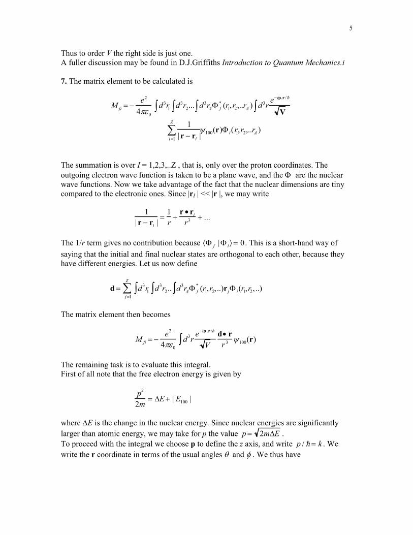
5

Thus to order V the right side is just one.

A fuller discussion may be found in D.J.Griffiths Introduction to Quantum Mechanics.i

7. The matrix element to be calculated is

M fi = −e2

4πε0

d 3r1∫ d3r2... d 3rAΦ f* (r1∫∫ ,r2, ..rA ) d 3r∫

e−ip.r /

V

1

|r − ri |i=1

Z

∑ ψ100(r)Φ i(r1,r2,..rA )

The summation is over I = 1,2,3,..Z , that is, only over the proton coordinates. The

outgoing electron wave function is taken to be a plane wave, and the Φ are the nuclear

wave functions. Now we take advantage of the fact that the nuclear dimensions are tiny

compared to the electronic ones. Since |rI | << |r |, we may write

1

|r − ri |=

1

r+r •ri

r3 + ...

The 1/r term gives no contribution because ⟨Φ f |Φ i⟩ = 0. This is a short-hand way of

saying that the initial and final nuclear states are orthogonal to each other, because they

have different energies. Let us now define

d = d3r1∫

j=1

Z

∑ d3r2∫ .. d

3rA∫ Φ f

*(r1,r2, ..)r jΦ i(r1,r2, ..)

The matrix element then becomes

M fi = −e

2

4πε0

d3r

e−ip .r /

V∫

d• rr 3 ψ100(r)

The remaining task is to evaluate this integral.

First of all note that the free electron energy is given by

p

2

2m= ∆E+ | E100 |

where ∆E is the change in the nuclear energy. Since nuclear energies are significantly

larger than atomic energy, we may take for p the value p = 2m∆E .

To proceed with the integral we choose p to define the z axis, and write p / = k . We

write the r coordinate in terms of the usual angles θ and φ . We thus have

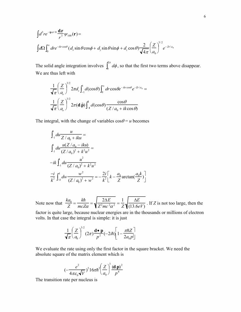
6

d3re

−ip.r / ∫d.r

r3 ψ100 (r) =

dΩ dre−ikr cosθ

0

∞

∫∫ (dx sinθ cosφ + dy sinθ sinφ + dz cosθ)2

4πZ

a0

3/ 2

e− Zr/ a0

The solid angle integration involves dφ0

2π

∫ , so that the first two terms above disappear.

We are thus left with

1

πZ

ao

3/2

2πdz d(cosθ) dr0

∞

∫ cosθe− ikr cosθ

−1

1

∫ e−Zr /a0 =

1

πZ

ao

3/2

2π (d.ˆ p ) d(cosθ)cosθ

(Z / a0 + ikcosθ)−1

1

∫

The integral, with the change of variables cosθ = u becomes

duu

Z / a0 + iku−1

1

∫ =

duu(Z /a0 − iku)

(Z / a0 )2 + k2u2=

−1

1

∫

−ik duu

2

(Z / a0)2 + k2u2−1

1

∫−i

k2 dw

w2

(Z / a0 )2 + w

2−k

k

∫ = −2i

k2 k −

a0

Zarctan(

a0k

Z)

Note now that

ka0

Z=

k

mcZα=

2∆E

Z 2mc 2α 2 =1

Z

∆E

(13.6eV ). If Z is not too large, then the

factor is quite large, because nuclear energies are in the thousands or millions of electron

volts. In that case the integral is simple: it is just

1

πZ

a0

3/2

(2π )d• pp2 (−2i) 1−

πZ2a0 p

We evaluate the rate using only the first factor in the square bracket. We need the

absolute square of the matrix element which is

(−e

2

4πε0 V)

216π2 Z

a0

3

(d.p)2

p4

The transition rate per nucleus is

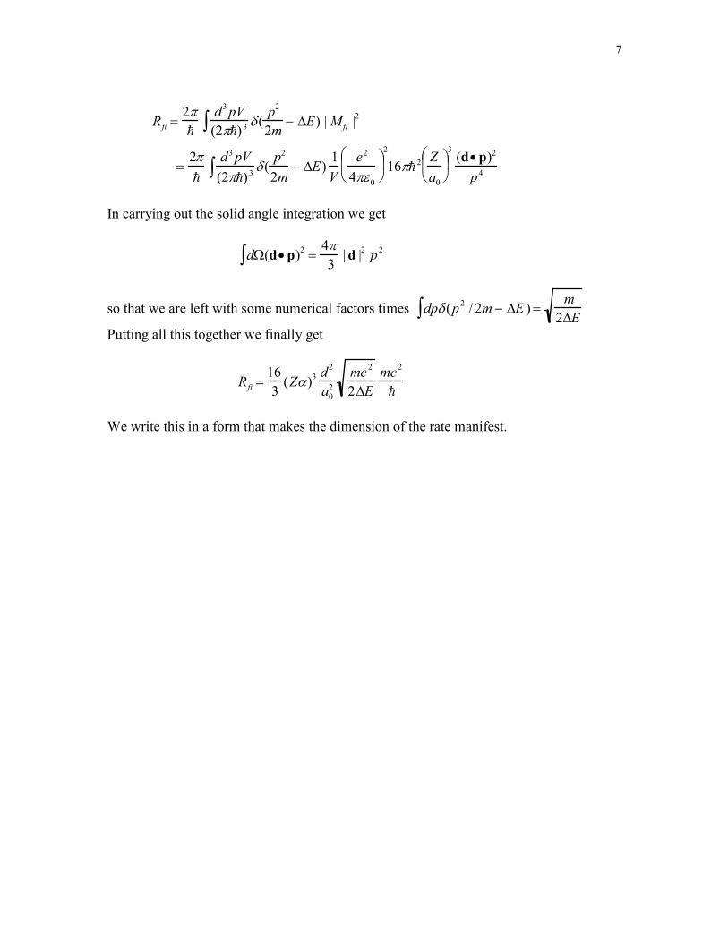
7

R fi =2π

d3pV

(2π) 3 δ(p

2

2m∫ − ∆E) | M fi |2

=2π

d3 pV

(2π) 3δ(

p2

2m∫ − ∆E)1

V

e2

4πε0

2

16π 2 Z

a0

3(d•p)2

p4

In carrying out the solid angle integration we get

dΩ(d•p)2∫ =

4π3

|d |2

p2

so that we are left with some numerical factors times dpδ(p2

/ 2m − ∆E ) =m

2∆E∫

Putting all this together we finally get

R fi =16

3(Zα)

3 d2

a02

mc2

2∆E

mc2

We write this in a form that makes the dimension of the rate manifest.

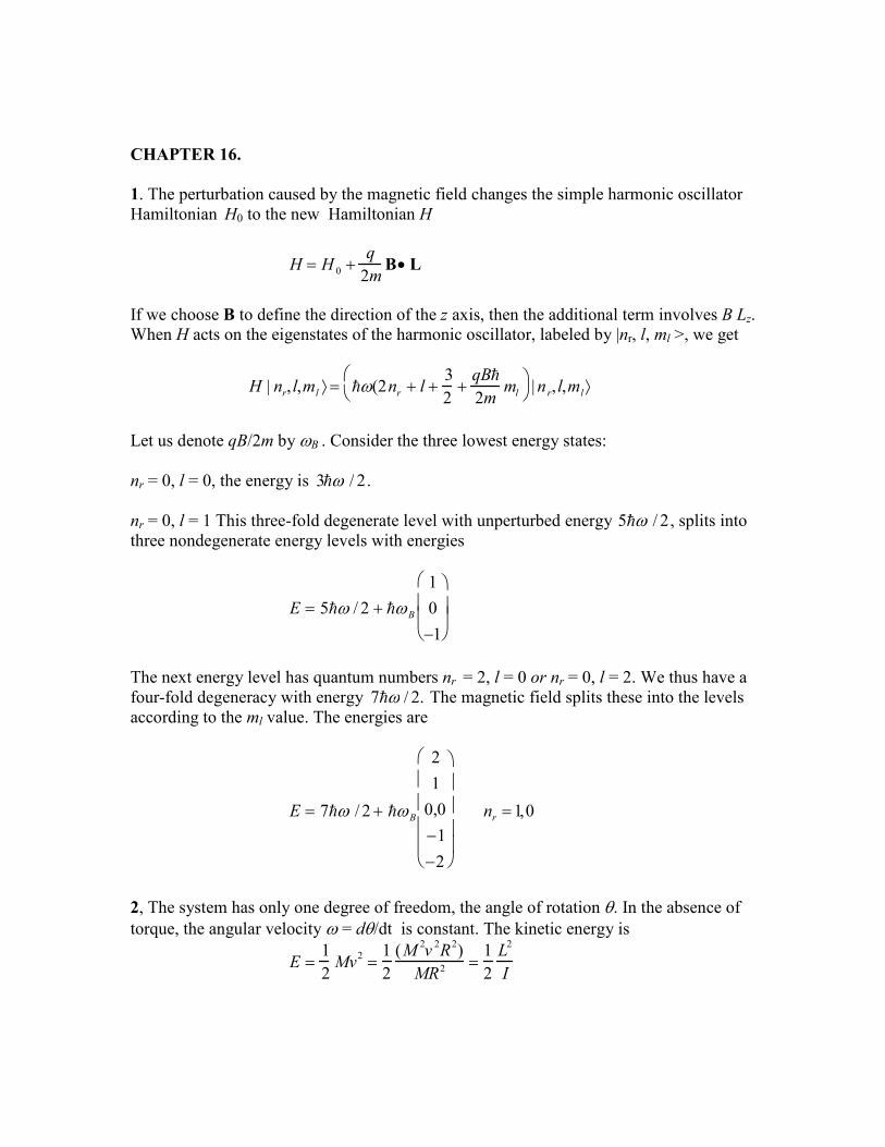
CHAPTER 16.

1. The perturbation caused by the magnetic field changes the simple harmonic oscillator

Hamiltonian H0 to the new Hamiltonian H

H = H 0 +q

2mB• L

If we choose B to define the direction of the z axis, then the additional term involves B Lz.

When H acts on the eigenstates of the harmonic oscillator, labeled by |nr, l, ml >, we get

H | nr, l,ml ⟩ = ω(2nr + l +

3

2+qB

2mml

|n r, l,ml⟩

Let us denote qB/2m by ωB . Consider the three lowest energy states:

nr = 0, l = 0, the energy is 3ω / 2 .

nr = 0, l = 1 This three-fold degenerate level with unperturbed energy 5ω / 2 , splits into

three nondegenerate energy levels with energies

E = 5ω / 2 + ωB

1

0

−1

The next energy level has quantum numbers nr = 2, l = 0 or nr = 0, l = 2. We thus have a

four-fold degeneracy with energy 7ω / 2. The magnetic field splits these into the levels

according to the ml value. The energies are

E = 7ω / 2 + ωB

2

1

0,0

−1

−2

nr =1,0

2, The system has only one degree of freedom, the angle of rotation θ. In the absence of

torque, the angular velocity ω = dθ/dt is constant. The kinetic energy is

E =1

2Mv

2 =1

2

(M2v

2R

2)

MR2 =1

2

L2

I

where L = MvR is the angular momentum, and I the moment of inertia. Extending this to

a quantum system implies the replacement of L2 by the corresponding operator. This

suggests that

H =L

2

2I

(b) The operator L can also be written as p x R.

When the system is placed in a constant magnetic field, we make the replacement

p→ p− qA = p− q(−1

2r ×B) = p +

q

2r × B

The operator r represents the position of the particle relative to the axis of rotation, and

this is equal to R. We may therefore write

L =R × p→R × (p +q

2R × B) = L +

q

2R(R•B) − R2

B( )

If we square this, and only keep terms linear in B , then it follows from (R.B) = 0, that

H =1

2IL

2 − qR2L• B( )= L

2

2I−

q

2ML •B =

L2

2I−qB

2MLz

The last step is taken because we choose the direction of B to define the z axis.

The energy eigenvalues are therefore

E =

2l(l +1)

2I−qB

2Mml

where ml = l,l −1,l − 2,...− l . Note that the lowest of the levels corresponds to ml = l.

3. In the absence of a magnetic field, the frequency for the transition n = 3 to n = 2 is

determined by

2πν =

1

2mc

2α 2 1

4−

1

9

so that

ν =

mc2α 2

4π5

36

The lines with ∆ml = ± 1 are shifted upward (and downward) relative to the ∆ml = 0

(unperturbed ) line. The amount of the shift is given by

h∆ν =

eB

2mc

so that

∆ν =eB

4πmc

Numerically ν = 0.4572 x 1015

Hz and with B = 1 T, ∆ν = 1.40 x 1010

Hz. Thus the

frequencies are ν and ν(1 ± ∆ν /ν) . Thus the wavelengths are c /ν and

(c /ν)(1∓ ∆ν /ν) . This leads to the three values λ = 655.713 nm, with the other lines

shifted down/up by 0.02 nm.

4. The Hamiltonian is

H =1

2mp− qA( )2 − qE• r

Let us choose E = (E, 0, 0 ) and B = ( 0, 0, B), but now we choose the gauge such that

A = (0, Bx, 0). This leads to

H =1

2mpx

2 + (py − qBx)2 + pz

2( )− qEx =

=1

2m( px

2 + py2 + pz

2 − 2qBpy x + q2B2x 2 − 2mqEx)

Let us now choose the eigenstate to be a simultaneous eigenstate of H, pz (with

eigenvalue zero) and py (with eigenvalue k ). Then the Hamiltonian takes the form

H =

2k

2

2m+

1

2mpx

2 +1

2mqBx − k −mE /B( )2 − 1

2mk + mE / B)

2( )

This is the Hamiltonian for a shifted harmonic oscillator with a constant energy added on.

We may write this in the form

H = −kE

B−mE

2

2B2 +1

2m

q2B

2

m2

x −

k − mE / B

qB

2

Thus the energy is

E = −

kE

B−mE

2

2B2 + qB

m

(n +

1

2)

with n = 0,1,2,3,…

5. We first need to express everything in cylindrical coordinates. Since we are dealing

with an infinite cylinder which we choose to be aligned with the z axis,, nothing depends

on z, and we only deal with the ρ and φ coordinates. We only need to consider the

Schrodinger equation in the region a≤ ρ ≤ b.

We start withH =1

2me

Πx

2 + Πy

2( ) where

Πx = −i∂∂x+ eAx; Πy = −i

∂∂y+ eAy

To write this in cylindrical coordinates we use Eq. (16-33) and the fact that for the

situation at hand

Ax = −sinϕ Aϕ ; Ay = cosϕ Aϕ; Aϕ =Φ

2πρ

where Φ is the magnetic flux in the interior region. When all of this is put together, the

equation Hψ (ρ,ϕ) = Eψ (ρ,ϕ)

takes the form

Eψ = −

2

2me

∂ 2ψ∂ρ2 +

1

ρ∂ψ∂ρ

+1

ρ2

∂2ψ∂ϕ 2

− 2ie

Φ2π

1

ρ2

∂ψ∂ϕ

+e

2

ρ2

Φ2π

2

ψ

To solve this, we use the separation of variables technique. Based on previous

experience, we write

ψ (ρ,ϕ) = f (ρ)eimϕ

The single-valuedness of the solution implies that m = 0,±1,±2,±3,…

With the notation k2 = 2meE /

2 the equation for f(ρ) becomes

−k 2f (ρ) =

d2f

dρ2 +1

ρdf

dρ− m +

eΦ2π

2

f

If we now introduce z = kρ and ν = m +

eΦ2π

the equation takes the form

d

2f (z)

dz2 +1

z

df (z)

dz+ 1−

ν 2

z2

f (z) = 0

This is Bessel’s equation. The most general solution has the form

f (ρ) = AJν (kρ) + BNν (kρ)

If we now impose the boundary conditions f (ka) = f (kb) = 0 we end up with

AJν (ka) + BNν (ka) = 0

and

AJν (kb) + BNν (kb) = 0

The two equations can only be satisfied if

Jν (ka)Nν (kb) − Jν (kb)Nν (ka) = 0

This is the eigenvalue equation, and the solution k clearly depends on the order ν of the

Bessel functions, that is, on the flux enclosed in the interior cylinder.

CHAPTER 17

1. We start with Eq. (17-19) . We define k as the z axis. This means that the

polarization vector, which is perpendicular to k has the general form

ε (λ ) = ˆ i cosϕ + ˆ j sinϕ This leads to

B = ∇ ×A = −i

2ε0ωVkˆ k × (ˆ i cosϕ + ˆ j sinϕ) = B0(

ˆ j cosϕ − ˆ i sinϕ)

We are now interested in

M = B0

gp − gn2

2X 0(σ y

( p ) −σ y

(n ))cosϕ − (σ x

( p) − σ x

(n))sinϕX1

m

The operators are of the form

σycosϕ −σ xsinϕ =0 −icosϕ

icosϕ 0

−

0 sinϕsinϕ 0

=

0 −ie− iϕ

ieiϕ

0

It is simple to work out the “bra” part of the scalar product

1

2χ +

( p)χ −(n) − χ −

( p)χ +(n)( ) 0 −ie −iϕ

ieiϕ

0

p

−0 −ie−iϕ

ieiϕ

0

n

with the help of

χ +0 −ie− iϕ

ieiϕ

0

= 1 0( ) 0 −ie−iϕ

ieiϕ

0

= 0 −ie−iϕ( )= −ie− iϕχ −

and

χ −0 −ie− iϕ

ieiϕ

0

= 0 1( ) 0 −ie−iϕ

ieiϕ

0

= ie

iϕ0( )= ieiϕχ +

This implies that the “bra” part is

1

2χ +

( p)χ −(n) − χ −

( p)χ +(n)( ) 0 −ie −iϕ

ieiϕ

0

p

−0 −ie−iϕ

ieiϕ

0

n

=

= − 2i(e−iϕχ −

( p)χ −(n) + e iϕχ +

( p )χ +(n )

)

= − 2i e−iϕX 1−1 + e iϕX 1

1( )

For the “ket” state we may choose X triplet = αX1

1 + βX1

0 +γX1

−1, and then the matrix

element is

M = −i 2B0

g p − gn2

2(eiϕα + e− iϕγ )

2. We are interested in finding out for what values of l, m, the matrix element

1

2⟨,m | (ε.p)(k.r) + (ε.r)(p.k) | 0,0⟩

does not vanish. We use the technique used in Eq. (17-22) to rewrite this in the form

1

2

ime

⟨,m | [H 0,ε.r]( k.r) + (ε.r)[H0,k.r] | 0.0⟩ =

ime2

⟨,m | H0 (ε.r)(k.r) − (ε.r)H 0(k.r) + (ε.r)H 0(k.r) − (ε.r)(k.r)H 0 | 0,0⟩ =

ime

2(E,m − E0,0)⟨,m | (ε.r)(k.r) | 0,0⟩

Let us now choose k to define the z axis, so that k = ( 0,0,k). Since εεεε is perpendicular to k

, we may choose it to be represented by εεεε = (cosα, sinα, 0). Then, with the usual polar

coordinates, we have

(ε.r)(k.r) = k(cosαsinθcosφ + sinαsinθsinφ)cosθ =

= ksinθcosθ cos(φ −α )

This is a linear combination of Y21(θ,φ) and Y2,−1(θ,φ) . Thus the angular integral is of

the form dΩYl ,m*Y2,±1∫ Y0,0 , and since Y0,0 is just a number, the integral is proportional to

δ ,2 .

There is also a selection rule that requires m = ± 1. This comes about because of our

choice of axes.

3. In the transition under consideration, the radial part of the transition rate is

unchanged. The only change has to do with the part of the matrix element that deals

with the dependence on the polarization of the photon emitted in the transition.

Eq. (17-44), for example shows that δm ,1 is multiplied by εx2 + εy

2 = 1− εz

2and this

factor carries some information about the direction of the photon momentum, even

though that does not appear explicitly in the matrix element. We proceed as follows:

The direction of the polarization of the initial atomic state defines the z axis. Let the

photon momentum direction be given by

ˆ d = ˆ i sinΘcosΦ + ˆ j sinΘsinΦ + ˆ k cosΘ

We may define two unit vectors perpendicular to this. For the first one we take ˆ d × ˆ k ,

which, after being divided by the sine of the angle between these two vectors, i.e. by

sinΘ , yields

ˆ ε 1 = − ˆ i sinΦ + ˆ j cosΦ

The other one is ˆ ε 2 = ˆ d × ˆ ε 1 (two vectors perpendicular to each other), which leads to

ˆ ε 2 = ˆ i cosΘcosΦ + ˆ j cosΘsinΦ − ˆ k sinΘ

In the coordinate system in which ˆ d represents the z axis, the ει vectors represent the

x and y axes, and since the photon polarization must lie in that new x – y plane, we

see that the polarization vector has the form

ε = cosχ ˆ ε 1 + sin χ ˆ ε 2

Thus

εz = ˆ k • ε = −sin χsinΘ ,

εx = ˆ i •ε = cos χ sinΦ + sin χcosΘcosΦ,

εy = ˆ j •ε = −cos χ cosΦ + sin χcosΘsinΦ

and

εx2 + εy

2 = 1−εz2 =1− sin

2 χ sin2Θ

Thus the final answer (using Eq. (17-44) is

dΓ =α2π

ω3

c2

215

310

1

2δm,1

1− sin

2 χ sin2Θ( )d(cosΘ)dΦ

The dependence on the polarization appears in the sin2 χ term.

4. First of all, we need to recognize what 2p 1s means for the harmonic oscillator

in three dimensions. The numbers “2” and “1” usually refer to the principal quantum

number, e.g n = nr + +1 for the hydrogen atom. Here the energy spectrum is

characterized by 2n r + +1 , and it is this combination that we call the principal quantum

number. Thus we take the 2p 1s transition to mean (n r = 0, =1) → (nr = 0, = 0) .

To solve this problem we recognized that nothing changes in the angular

integration that was done for the 2p 1s transition in hydrogen. The only change in the

matrix element involves the radial functions. In hydrogen we calculated

r3

0

∞

∫ R21(r)R10(r)dr

using the radial functions for hydrogen. Here the same integral appears, except that the

radial functions are those of the three-dimensional harmonic oscillator. Here, the properly

normalized eigenfunctions are

R10(r) =2

π 1/ 4

mω

3/ 2

e−mωr2 / 2

and

R21(r) =8

3

1/ 21

π1/4

mω

5/4

re−mωr2 / 2

Note that these functions appear in the solution to problem 8-13. Given these, the integral

that yields the matrix element is straightforward. We have

M =8

3

1/22

π 1/ 2

mω

2

drr4

0

∞

∫ e−mωr2 / =

=4

π1/2

2

3

1/ 2mω

2

mω

5/21

2dxx

3/2

0

∞

∫ e−x

=4

π1/2

2

3

1/ 2mω

2

mω

5/21

2

3π 1/ 2

4

The square of this is

3

2mω. We check that this has the dimensions of a (length)

2 as

required. To get the decay rate, we just take the hydrogen result and make the substitution

|M hydrogen |

2=2

15

39 a0

2 →|M |2=

3

2mω

This then leads to the rate

R =4

9αω3

c 2 |M |2=

2α3

ωmc2

ω

CHAPTER 19

1. We have

M fi =1

Vd

3re

−i∆.r∫ V (r)

If V(r) = V(r), that is, if the p9otential is central, we may work out the angular

integration as follows:

M fi =1

Vr

2V (r)

0

∞

∫ dr dφ sinθdθe−i∆r cosθ

0

π

∫0

2π

∫

with the choice of the vector ∆ as defining the z axis. The angular integration yields

dφ sinθdθe− i∆r cosθ = 2π d(cosθ)e−i∆r cosθ

−1

1

∫ =4π∆r0

π

∫0

2π

∫ sin∆r

so that

M fi =1

V

4π∆

rdrV (r)sin∆r0

∞

∫

Note that this is an even function of ∆ that is, it is a function of ∆2 = (p f − pi)

2/

2

2. For the gaussian potential

M fi =1

V

4πV0

∆rdr sin∆r

0

∞

∫ e−r 2 /a 2

Note that the integrand is an even function of r. We may therefore rewrite it as

rdr sin∆r0

∞

∫ e− r2 / a2

=1

2rdr sin∆r

−∞

∞

∫ e− r2 / a2

The integral on the right may be rewritten as

1

2rdr sin∆r

−∞

∞

∫ e− r2 / a2

=1

4 irdr e

−r 2 /a 2 +i∆r − c.c)( )−∞

∞

∫

Now

1

4irdr

−∞

∞

∫ e− r2 / a2 + i∆r =

1

i

∂∂∆

dr−∞

∞

∫ e− r2 / a2 + i∆r = −i

∂∂∆

a πe−a2∆2 /4 = i

∆a3 π2

e− a2∆2 / 4

Subtracting the complex conjugate and dividing by 4i gives

M fi =1

Va π( )3V0e

−a 2∆2 /4

The comparable matrix element for the Yukawa potential is

M fi =1

V

4π∆VYb dr

0

∞

∫ e− r/ b

sin∆r =1

V4πVY

b3

1+ b2∆2

We can easily check that the matrix elements and their derivatives with respect to ∆2 at

∆ = 0 will be equal if a = 2b and VY = 2 πV0 .

The differential cross section takes its simplest form if the scattering involves the same

particles in the final state as in the initial state. The differential cross section is

dσdΩ

=µ 2

4π 2

4 |U (∆) |2

where µ is the reduced mass and U(∆) = VM fi .

We are interested in the comparison

(dσ / dΩ)gauss

(dσ /dΩ)Yukawa=

e−2b2∆2

(1+ b2∆2 )−2 = (1+ X )2e−2X

where we have introduced the notation X = b2x

2. This ratio, as a function of X, starts out

at X = 0 with the value of 1, and zero slope, but then it drops rapidly, reaching less than

1% of its initial value when X = 4, that is, at ∆ = 2/b.

3. We use the hint to write

dσdΩ

=p

2

π2

dσd∆2 =

µ 2

4π 2

4 4πV0

b3

1+ b2∆2

2

The total cross section may be obtained by integrating this over ∆2 with the range given

by 0 ≤ ∆2 ≤ 4 p

2/

2, corresponding to the values of cosθ between –1 and + 1.. The

integral can actually be done analytically. With the notation k2 = p

2/

2 the integral is

d∆2

0

4k 2

∫1

(1 + b2∆2)2 =1

b2

dx

(1+ x)20

4 k 2b2

∫ =4k

2

1 + 4k 2b 2

This would immediately lead to the cross section if the particles were not identical. For

identical particles, there are symmetry problems caused by the Pauli Exclusion Principle

and the fact that the protons have spin 1/2. The matrix elements are not affected by the

spin because there is no spin-orbit coupling or any other spin dependence in the potential.

However:

In the spin triplet state, the spatial wave function of the proton is antisymmetric, while for

the spin singlet state, the spatial wave function is symmetric. This means that in the

original Born approximation we have

d3∫ re−ik '.r

∓ e ik '.r

2V (r)

e ik .r∓ e−ik .r

2=

d3rV (r)e−i(k '−k ).r∫ ∓ d 3rV (r)e− i(k +k' ). r∫

The first term has the familiar form

4πV0

b3

1+ b 2∆2 = 4πV0

b3

1 + 2b 2k2 (1− cosθ)

and the second term is obtained by changing cosθ to - cosθ.. Thus the cross section

involves

d(cosθ)1

1+ 2b2k2 − 2b 2k2 cosθ∓

1

1+ 2b 2k2 + 2b 2k2 cosθ

2

→ dz1

1 + a − az∓

1

1+ a + az

2

−1

1

∫−1

1

∫

=4

1+ 2a∓

2

a(1+ a)ln(1+ 2a)

where a = 2b2k

2.

Thus the total cross section is

σ =8πµ2

b6

4 V0

2 4

1+ 4k2b2

∓

1

k 2b 2(1 + 2k 2b2)ln(1+ 4k

2b

2)

The relation to the center of mass energy follows from E = p2

/ 2µ = 2k

2/ 2µ , so that

k

2 =2µE

2 =(1.67 ×10

−27kg)(100 ×1.6 ×10

−13J )

(1.054 ×10−34 J.s)2

With b = 1.2 x 10-1`5

m, we get (kb)2 = 3.5, so that σ = 4.3 x 10

-28 m

2 = 4.3 x 10

-24 cm

2 =

3.4 barns.

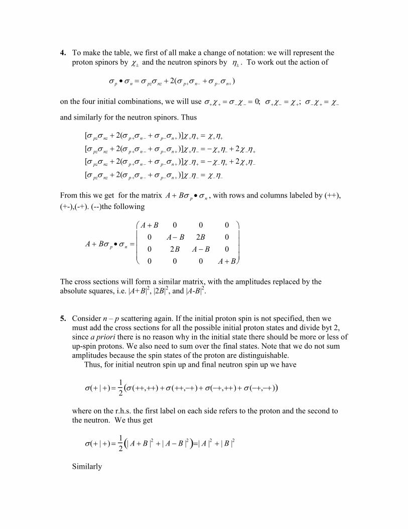
4. To make the table, we first of all make a change of notation: we will represent the

proton spinors by χ± and the neutron spinors by η± . To work out the action of

σ p •σ n = σ pzσ nz + 2(σ p+σ n− +σ p−σ n+ )

on the four initial combinations, we will use σ+χ + = σ −χ − = 0; σ +χ− = χ +; σ −χ + = χ−

and similarly for the neutron spinors. Thus

[σ pzσ nz + 2(σ p +σ n − + σ p−σn + )]χ +η+ = χ+η+

[σ pzσ nz + 2(σ p +σ n − + σ p−σn + )]χ +η− = −χ+η− + 2χ −η+

[σ pzσ nz + 2(σ p +σ n − + σ p−σn + )]χ −η+ = −χ−η+ + 2χ +η−

[σ pzσ nz + 2(σ p +σ n − + σ p−σn + )]χ −η− = χ−η−

From this we get for the matrix A + Bσ p •σ n , with rows and columns labeled by (++),

(+-),(-+). (--)the following

A + Bσ p •σ n =

A + B 0 0 0

0 A− B 2B 0

0 2B A − B 0

0 0 0 A + B

The cross sections will form a similar matrix, with the amplitudes replaced by the

absolute squares, i.e. |A+B|2, |2B|

2, and |A-B|

2.

5. Consider n – p scattering again. If the initial proton spin is not specified, then we

must add the cross sections for all the possible initial proton states and divide byt 2,

since a priori there is no reason why in the initial state there should be more or less of

up-spin protons. We also need to sum over the final states. Note that we do not sum

amplitudes because the spin states of the proton are distinguishable.

Thus, for initial neutron spin up and final neutron spin up we have

σ(+ | +) =1

2σ (++,++) +σ (++,−+) + σ(−+,++) + σ (−+,−+)( )

where on the r.h.s. the first label on each side refers to the proton and the second to

the neutron. We thus get

σ(+ | +) =1

2| A + B |

2 + | A − B |2( )=| A |

2 + | B |2

Similarly

σ(− |+) =1

2σ (+−,++) + σ (+−,−+) +σ (−−,++) +σ (−−,−+)( )

=1

2| 2B |2( )= 2 | B |2

Thus

P =| A |

2 + |B |2 −2 | B |

2

| A |2 + |B |2 +2 |B |2=

| A |2 − |B |

2

| A |2 +3 |B |2

6. For triplet triplet scattering we have (with the notation (S,Sz)

(1,1)(1,1) ⟨χ+η+ | χ+η+ ⟩ = A + B

(1,-1)(1,-1) ⟨χ−η− | χ−η− ⟩ = A + B

(1,0) (1,0) ⟨χ+η− + χ−η+

2|χ+η− + χ−η+

2⟩ =

1

2A− B + 2B + 2B + A− B( ) = A + B

(0,0)(0.0) ⟨χ+η− − χ −η+

2|χ +η− − χ−η+

2⟩ =

1

2A− B− 2B− 2B + A− B( ) = A − 3B

(0,0)(1,0) ⟨χ+η− − χ −η+

2|χ +η− + χ −η+

2⟩ =

1

2A − B + 2B− 2B− A + B( ) = 0

We can check this by noting that (in units of ,

A + Bσ p •σ n = A + 4Bs p • sn = A + 2B(S2 − s p2 − sn

2 )

= A + 2B S(S +1)−3

2

For S = 1 this is A + B, For S = 0, it is A – B , and since ⟨S = 1|S2 − 3 / 2 |S = 0⟩ = 0 by

orthogonality of the triplet to singlet states, we get the same result as above.

7. We have, with x = kr and cosθ = u,

I(x) = dug(u)e− iux−1

1

∫ = dug(u)i

x−1

1

∫d

dxe−iux

=i

xdu

d

du−1

1

∫ g(u)e− iux( )− i

xdu

dg

du

−1

1

∫ e− iux

The first term vanishes since g(±1)=0. We can proceed once more, and using the fact that

the derivatives of g(u) also vanish at u = ± 1, we find

I(x) =−ix

2

dud

2g

du2

−1

1

∫ e− ixu

and so on. We can always go beyond any pre-determined power of 1/x so that I(x) goes

to zero faster than any power of (1/x).

7. We proceed as in the photoelectric effect. There the rate, as given in Eq.(19-111) is

R =

2πV

dΩ∫mpe

(2π)3 |M fi |2

Here m is the electron mass, and pe is the momentum of the outgoing.electron.The factor

arose out of the phase space integral

dpp2∫ δ

p2

2m− Eγ

= d

p2

2m

∫ mpδ

p2

2m− Eγ

= mpe

with pe determined by the photon energy, as shown in the delta function. In the deuteron

photodisintegration process, the energy conservation is manifest in δp

2

M− Eγ + EB

.

The delta function differs in two respects: first, some of the photon energy goes into

dissociating the deuteron, which takes an energy EB ; second, in the final state two

particles of equal mass move in in equal and opposite directions, both with momentum of

magnitude p, so that the reduced mass Mred = M/2 appears. Thus the factor mpe will be

replaced by Mp/2, where the momentum of the particle is determined by the delta

function.

Next, we consider the matrix element. The final state is the same as given in Eq.

(19-114) with pe replaced by p , and with the hydrogen-like wave function replaced by

the deuteron ground state wave function. We thus have

dσdΩ

=2π

(VMp / 2)

(2π) 3

V

c

e

M

2

2ε0ωV1

V(ε •p) 2

d3re

i(k −p / )•rψ d (r)∫2

We need to determine the magnitude of the factor eik•r

. The integral is over the wave

function of the deuteron. If the ground state wave function behaves as e−αr

, then the

probability distribution goes as e−2αr

, and we may roughly take 1/2α as the “size” of the

deuteron. Note that α2 = MEB /

2. As far as k is concerned, it is given by

k =

pγ

=Eγ

c

Numerically we get, with EB =2.2 MeV, and Eγ = 10 MeV, k/2α = 0.11, which means

that we can neglect the oscillating factor. Thus in the matrix element we just need

d3re

ik•r∫ ψ d (r) . The wave function to be used is

ψ d (r) =N

4πe−α (r− r0 )

rr > r0

N is determined by the normalization condition

N

2

4π4πr2

r0

∞

∫ dre−2α (r− r0 )

r2 = 1

So that

N2 = 2α

The matrix element involves

N

4π4πk

rdrr0

∞

∫ sinkre−α (r− r0 )

r=

=N 4πk

dx0

∞

∫ sink(x + r0)e−αx

=N 4πk

dx sinkr0 Re(e−x (α − ik)( )

0

∞

∫ + coskr0 Im(e−x (α −ik )

))

=N 4πk

αα 2 + k 2 sin kr0 +

k

α 2 + k2 coskr0

The square of this is

4πN 2

k2 r02 αr0α 2r0

2 + k2r02 sin kr0 +

kr0α 2r0

2 + k 2r02 coskr0

2

It follows that

dσdΩ

= 2e

2

4πε0c

pr0Mω

(αr0)αr0

α 2r02 + k 2r0

2 sinkr0 +kr0

α 2r02 + k2r0

2 coskr0

2

We can easily check that this has the correct dimensions of an area.

For numerical work we note that αr0 = 0.52; kr0 = 0.26 EMeV and ω = EB +

p2

M.

9. The change in the calculation consists of replacing the hydrogen wave function

1

4π2Z

a0

3/2

e−Zr /a0

by

ψ (r) =N

4πsinqr

rr < r0

=N

4πe−κr

rr > r0

where the binding energy characteristic of the ground state of the electron determines κ

as follows

κ2 = 2me | EB | /

2 = (mecα /)2

with α = 1/137. The eigenvalue condition relates q to κ as follows:

qr0 cotqr0 = −κr0

where

` q

2 =2meV0

2 −κ 2

and V0 is the depth of the square well potential. The expression for the differential cross

section is obtained from Eq. (19-116) by dividing by 4(Z/a0)2 and replacing the wave

function in the matrix element by the one written out above,

dσdΩ

=2π

me pe(2π)3

1

c

e

me

2

2ε0ωpe

2

4π( ˆ ε .ˆ p ) 2

d3re

i(k −p e / ).rψ(r)∫2

We are interested in the energy-dependence of the cross section, under the assumptions

that the photon energy is much larger than the electron binding energy and that the

potential has a very short range. The energy conservation law states that under these

assumptions ω = pe2

/ 2me . The factor in front varies as pe3

/ω ∝ pe ∝ Eγ , and thus

we need to analyze the energy dependence of d

3re

i(k −p e / ).rψ (r)∫2

. The integral has the

form

d3re

iQ.r∫ ψ (r) =4πQ

rdr sinQrψ (r)0

∞

∫

where Q = k − pe / so that Q

2 = k 2 +pe

2

2 − 2

kpe

( ˆ k .ˆ p ) .

Now

2k

2/ pe

2 = 2ω 2/ pe

2c

2 = ωpe

2/ 2m

pe2c 2 =

ω2mec

2 . We are dealing with the

nonrelativistic regime, so that this ratio is much smaller than 1. We will therefore neglect

the k –dependence, and replace Q by pe/ . The integral thus becomes

4πQ

N

4πdrsinQr sinqr + drsinQre

−κr

r0

∞

∫0

r0

∫

The first integral is

1

2dr