Soluble Substrate Design Tool - CLU-IN

FINAL REPORT & USER’S GUIDE Development of a Design Tool for Planning Aqueous

Amendment Injection Systems Soluble Substrate Design Tool

ESTCP Project ER-200626

June 2012

Robert C. Borden Ki Young Cha North Carolina State University Thomas Simpkin CH2M HILL, Inc. M. Tony Lieberman Solutions-IES, Inc.

Standard Form 298 (Rev. 8/98)

REPORT DOCUMENTATION PAGE

Prescribed by ANSI Std. Z39.18

Form Approved OMB No. 0704-0188

The public reporting burden for this collection of information is estimated to average 1 hour per response, including the time for reviewing instructions, searching existing data sources, gathering and maintaining the data needed, and completing and reviewing the collection of information. Send comments regarding this burden estimate or any other aspect of this collection of information, including suggestions for reducing the burden, to the Department of Defense, Executive Services and Communications Directorate (0704-0188). Respondents should be aware that notwithstanding any other provision of law, no person shall be subject to any penalty for failing to comply with a collection of information if it does not display a currently valid OMB control number. PLEASE DO NOT RETURN YOUR FORM TO THE ABOVE ORGANIZATION. 1. REPORT DATE (DD-MM-YYYY) 2. REPORT TYPE 3. DATES COVERED (From - To)

4. TITLE AND SUBTITLE 5a. CONTRACT NUMBER

5b. GRANT NUMBER

5c. PROGRAM ELEMENT NUMBER

5d. PROJECT NUMBER

5e. TASK NUMBER

5f. WORK UNIT NUMBER

6. AUTHOR(S)

7. PERFORMING ORGANIZATION NAME(S) AND ADDRESS(ES) 8. PERFORMING ORGANIZATION REPORT NUMBER

9. SPONSORING/MONITORING AGENCY NAME(S) AND ADDRESS(ES) 10. SPONSOR/MONITOR'S ACRONYM(S)

11. SPONSOR/MONITOR'S REPORT NUMBER(S)

12. DISTRIBUTION/AVAILABILITY STATEMENT

13. SUPPLEMENTARY NOTES

14. ABSTRACT

15. SUBJECT TERMS

16. SECURITY CLASSIFICATION OF: a. REPORT b. ABSTRACT c. THIS PAGE

17. LIMITATION OF ABSTRACT

18. NUMBER OF PAGES

19a. NAME OF RESPONSIBLE PERSON

19b. TELEPHONE NUMBER (Include area code)

ii

This report was prepared for the Environmental Security Technology Certification Program (ESTCP) by North Carolina State University (NCSU) and representatives from ESTCP. In no event shall either the United States Government or NCSU have any responsibility or liability for any consequences of any use, misuse, inability to use, or reliance upon the information contained herein, nor does either warrant or otherwise represent in any way the accuracy, adequacy, efficacy, or applicability of the contents hereof. To discuss applications of this technology please contact: Dr. Robert C. Borden of North Carolina State University can be reached at 919-515-1625 or [email protected]

iii

EXECUTIVE SUMMARY Soluble substrate has been used at hundreds of sites to generate anaerobic conditions and enhance in situ anaerobic biodegradation / immobilization of chlorinated solvents, perchlorate, explosives, nitrate and chromium. Typically, the soluble substrate is diluted with water and then injected using a series of wells. In some cases, a pH buffer or other amendment may be included to further enhance biodegradation. The actual installation process has three main steps: (1) installation of temporary or permanent injection wells, (2) substrate preparation, and (3) substrate injection with water to distribute the soluble substrate throughout the treatment zone. Once injected, the soluble substrate is fermented molecular hydrogen (H2) and acetate by common subsurface microorganisms. This H2 and acetate are then used as electron donors for anaerobic biodegradation of the target pollutants. To be most effective, the soluble substrate should be brought into close contact with the contaminant to be treated. However, it can be difficult to uniformly distribute soluble substrate (or any other reagent) throughout a spatially heterogeneous aquifer since the soluble substrate will be preferentially transported through the higher permeability zones. A series of numerical model simulations were conducted to evaluate the effect of important design parameters on remediation system performance in spatially heterogeneous aquifers. Substrate transport and consumption by bacteria is represented by the standard form of the advection-dispersion equation with a first order decay term to simulate substrate consumption by bacteria. The model was used to examine the impact of different design variables on contact efficiency. Design variables examined included well spacing, amount of substrate and water, time between substrate reinjection, etc. Results of these simulations were used to develop relationships between these design variables (represented by dimensionless parameters) and contact efficiency. A simple spreadsheet based tool was developed to assist in the design of injection only systems for distributing soluble substrate. This tool allows users to quickly compare the relative costs and performance of different injection alternatives and identify a design that is best suited to their site specific conditions. The design process embodied in the spreadsheet based tool includes the following steps: (1) select injection well configuration and unit costs for well installation, injection, and substrate; (2) determine treatment zone dimension; (3) select trial injection well spacing, time period between substrate reinjection and injection pore volume; (4) estimate contact efficiency and capital and life-cycle costs. This process is then repeated until a final design is selected. Sensitivity analysis results generated using the design tool indicate that total cost to treat a site for 5-yr life cycle using soluble substrate are relatively insensitive to site conditions. Unit cost will be higher for smaller sites due to the proportionately higher fixed costs associated with planning, design, and permitting. In most case, costs increase with estimated steady state contact efficiency (CESS). The highest ratio of CESS to cost occurs for CESS in the range of 70% - 80%.

iv

ACKNOWLEDGEMENTS

We gratefully acknowledge the financial and technical support provided by the Environmental Technology Certification Program including the guidance provided by Andrea Leeson, Erica Becvar (the Contracting Officer’s Representative), and Hans Stroo (ESTCP reviewer).

v

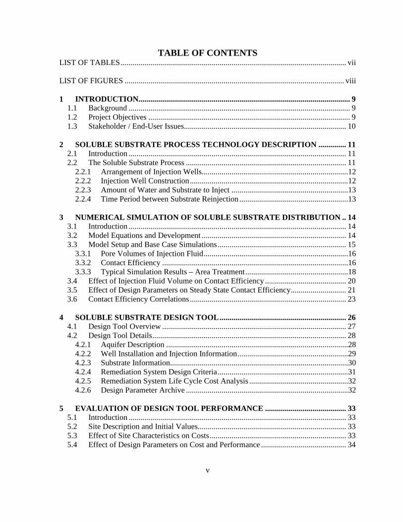
TABLE OF CONTENTS LIST OF TABLES .................................................................................................................. vii LIST OF FIGURES ............................................................................................................... viii 1 INTRODUCTION........................................................................................................... 9

1.1 Background ................................................................................................................ 9 1.2 Project Objectives ...................................................................................................... 9 1.3 Stakeholder / End-User Issues.................................................................................. 10

2 SOLUBLE SUBSTRATE PROCESS TECHNOLOGY DESCRIPTION .............. 11

2.1 Introduction .............................................................................................................. 11 2.2 The Soluble Substrate Process ................................................................................. 11

2.2.1 Arrangement of Injection Wells ..........................................................................12 2.2.2 Injection Well Construction ................................................................................12 2.2.3 Amount of Water and Substrate to Inject ...........................................................13 2.2.4 Time Period between Substrate Reinjection .......................................................13

3 NUMERICAL SIMULATION OF SOLUBLE SUBSTRATE DISTRIBUTION .. 14

3.1 Introduction .............................................................................................................. 14 3.2 Model Equations and Development ......................................................................... 14 3.3 Model Setup and Base Case Simulations ................................................................. 15

3.3.1 Pore Volumes of Injection Fluid .........................................................................16 3.3.2 Contact Efficiency ..............................................................................................16 3.3.3 Typical Simulation Results – Area Treatment ....................................................18

3.4 Effect of Injection Fluid Volume on Contact Efficiency ......................................... 20 3.5 Effect of Design Parameters on Steady State Contact Efficiency ............................ 21 3.6 Contact Efficiency Correlations ............................................................................... 23

4 SOLUBLE SUBSTRATE DESIGN TOOL ................................................................ 26

4.1 Design Tool Overview ............................................................................................. 27 4.2 Design Tool Details .................................................................................................. 28

4.2.1 Aquifer Description ............................................................................................28 4.2.2 Well Installation and Injection Information ........................................................29 4.2.3 Substrate Information..........................................................................................30 4.2.4 Remediation System Design Criteria ..................................................................31 4.2.5 Remediation System Life Cycle Cost Analysis ..................................................32 4.2.6 Design Parameter Archive ..................................................................................32

5 EVALUATION OF DESIGN TOOL PERFORMANCE ......................................... 33

5.1 Introduction .............................................................................................................. 33 5.2 Site Description and Initial Values........................................................................... 33 5.3 Effect of Site Characteristics on Costs ..................................................................... 33 5.4 Effect of Design Parameters on Cost and Performance ........................................... 34

vi

5.4.1 Effect of Time Period between Substrate Reinjection on Cost and Performance ........................................................................................................34

5.4.2 Effect of Injection Pore Volume on Cost and Performance ...............................35 5.4.3 Effect of Target Contact Efficiency on Cost.......................................................36

5.5 Summary .................................................................................................................. 38 6 REFERENCES .............................................................................................................. 39 7 POINTS OF CONTACT .............................................................................................. 40

vii

LIST OF TABLES Table 3.1 Contact Efficiency Regression Coefficients ..................................................... 23 Table 5.1 Summary of 5 year costs (NPV) for a range of site conditions ........................ 34

viii

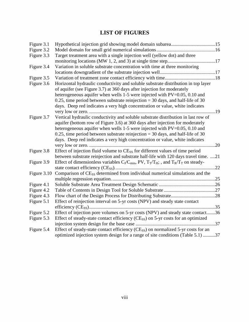
LIST OF FIGURES Figure 3.1 Hypothetical injection grid showing model domain subarea ....................................15 Figure 3.2 Model domain for small grid numerical simulations ................................................16 Figure 3.3 Target treatment area with a single injection well (yellow dot) and three

monitoring locations (MW 1, 2, and 3) at single time step.......................................17 Figure 3.4 Variation in soluble substrate concentration with time at three monitoring

locations downgradient of the substrate injection well .............................................17 Figure 3.5 Variation of treatment zone contact efficiency with time .........................................18 Figure 3.6 Horizontal hydraulic conductivity and soluble substrate distribution in top layer

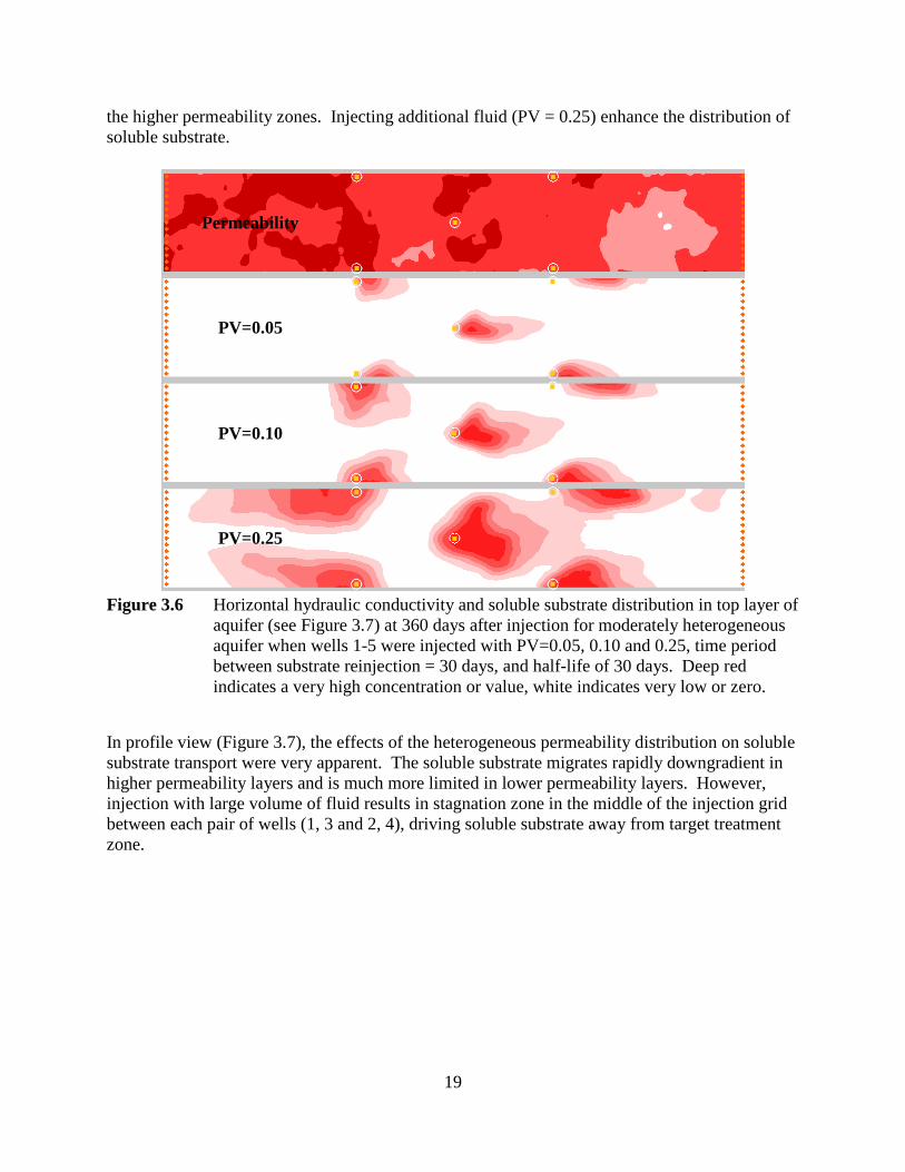
of aquifer (see Figure 3.7) at 360 days after injection for moderately heterogeneous aquifer when wells 1-5 were injected with PV=0.05, 0.10 and 0.25, time period between substrate reinjection = 30 days, and half-life of 30 days. Deep red indicates a very high concentration or value, white indicates very low or zero. .......................................................................................................19

Figure 3.7 Vertical hydraulic conductivity and soluble substrate distribution in last row of aquifer (bottom row of Figure 3.6) at 360 days after injection for moderately heterogeneous aquifer when wells 1-5 were injected with PV=0.05, 0.10 and 0.25, time period between substrate reinjection = 30 days, and half-life of 30 days. Deep red indicates a very high concentration or value, white indicates very low or zero. .......................................................................................................20

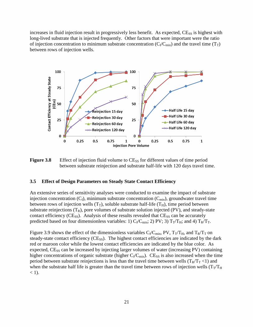
Figure 3.8 Effect of injection fluid volume to CESS for different values of time period between substrate reinjection and substrate half-life with 120 days travel time. ....21

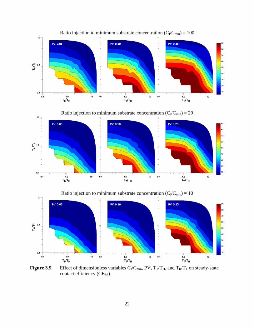
Figure 3.9 Effect of dimensionless variables CI/Cmin, PV, TT/TH; , and TR/TT on steady-state contact efficiency (CESS). .................................................................................22

Figure 3.10 Comparison of CESS determined from individual numerical simulations and the multiple regression equation. ....................................................................................25

Figure 4.1 Soluble Substrate Area Treatment Design Schematic ..............................................26 Figure 4.2 Table of Contents in Design Tool for Soluble Substrate ..........................................27 Figure 4.3 Flow chart of the Design Process for Distributing Substrate ....................................28 Figure 5.1 Effect of reinjection interval on 5-yr costs (NPV) and steady state contact

efficiency (CESS) .......................................................................................................35 Figure 5.2 Effect of injection pore volumes on 5-yr costs (NPV) and steady state contact .......36 Figure 5.3 Effect of steady-state contact efficiency (CESS) on 5-yr costs for an optimized

injection system design for the base case .................................................................37 Figure 5.4 Effect of steady-state contact efficiency (CESS) on normalized 5-yr costs for an

optimized injection system design for a range of site conditions (Table 5.1) ..........37

9

1 INTRODUCTION 1.1 Background Anaerobic bioremediation using soluble organic substrate can be an effective approach for in situ treatment of a variety of groundwater contaminants. However to be effective, the soluble substrate must come in close contact with the target contaminant. There are a variety of different approaches that can be used to distribute soluble substrate in the subsurface including: (a) injection only using grids of wells; and (b) recirculation using systems of injection and pumping wells. Both approaches have advantages and disadvantages with the ‘best’ approach dependent on site-specific conditions. For each approach, cost and effectiveness are a function of the well layout and injection sequence. Consequently, there will be an ‘optimum design’ that will include a specific arrangement of injection and extraction wells, injection volumes and rates, and amount of substrate. Existing guidance documents (AFCEE, 2004) provides general information on how the remediation process works and factors to consider when planning an injection system. However, these documents do not provide specific information on how to actually design an injection system to provide good amendment distribution at a reasonable cost. In recent years, a number of computer modeling packages have been developed that can be used to simulate dissolved substrate transport under reasonably realistic (i.e. heterogeneous) conditions. With these tools, users can evaluate alternative injection approaches and identify the ‘best’ design based on site-specific conditions including aquifer permeability and heterogeneity, contaminant distribution, site access limitations, drilling, labor and material costs, etc.

Unfortunately, these models are only rarely used. In most cases, remediation systems are designed by based on rules of thumb and prior experience. Sometimes this approach results in a good and efficient design. However, in some cases, designs are less effective than desired and more expensive than required. To reduce remediation system costs and improve effectiveness, tools are needed that allow engineers to quickly identify an efficient design for the specific conditions at their site without extensive site characterization and a high level of modeling expertise.

1.2 Project Objectives The overall objective of this project is to develop a tool to assist in the design of in situ bioremediation systems using soluble organic substrate. Specific objectives of this project are listed below.

1. Using currently available numerical models, examine the effects of site conditions (permeability, site heterogeneity, etc.) and design variables (location of wells, injection rates and volumes, amount of substrate, etc.) on distribution of dissolved organic carbon

10

throughout the target treatment zone. Develop simple relationships between substrate distribution efficiency and the amount of organic substrate and water injected.

2. Develop a simple, spreadsheet-based tool to assist in the design of soluble substrate

injection systems. This design tool will allow designers to evaluate the effect of different variables (well spacing, amount of substrate and water, time period between substrate reinjection, etc.) on remediation system cost and expected performance. Experienced users who have already compiled the input data for their site (permeability, target treatment zone dimensions, etc.) should be able to quickly develop and evaluate several alternative designs.

1.3 Stakeholder / End-User Issues The primary objective of this project is to develop a design tool that is easy to learn, simple to use, and widely applied. Educational materials will be developed to allow new users to download the required materials, and then complete a preliminary injection system design in a few hours. The design tool will be structured to allow easy use without extensive groundwater modeling experience. However, users will be expected to be familiar with basic fundamentals of groundwater flow, solute transport, and anaerobic bioremediation using soluble substrate. Once developed, the design tool and guidance document will be available for download from one or more websites.

11

2 SOLUBLE SUBSTRATE PROCESS TECHNOLOGY DESCRIPTION

2.1 Introduction This design tool is intended to assist with the design of injection systems for distributing soluble organic substrate to stimulate enhanced in situ bioremediation (EISB) of groundwater contaminants. The design tool is intended to assist users in selecting an appropriate injection well spacing, amount of substrate and water to inject, and time period between substrate reinjection. Prior to beginning use of the design tool, users should have already conducted a preliminary screening to determine if EISB using soluble substrate is appropriate for the conditions at their site. Users are expected to have a good understanding of EISB using soluble substrate prior to beginning use of the design tool. For information on EISB, users should first consult the following documents.

• “A Treatability Test for Evaluating the Potential Applicability of the Reductive Anaerobic Biological In Situ Treatment Technology to Remediate Chloroethenes” (Morse et al., 1998) (search for title at http://serdp-estcp.org/).

• “Principles and Practices of Enhanced Anaerobic Bioremediation of Chlorinated Solvents” (search for title at http://serdp-estcp.org/).

There are a wide variety of compounds that can be anaerobically bioremediated using soluble organic substrate including chlorinated ethenes, chlorinated ethanes, halomethanes, perchlorate, nitrate, certain metals, and explosives (RDX, HMX, etc.). For a few of these compounds (PCE, TCE, perchlorate, nitrate, etc.), the biodegradation pathways and microorganisms that carry out this process are relatively well understood and enhanced anaerobic biodegradation has been demonstrated in the field at multiple sites. However, there are many other compounds (chlorinated ethanes and methanes, freons, etc.) where the factors controlling contaminant biodegradation are much less well understood. In addition, substrate addition has the potential to inhibit biodegradation of petroleum hydrocarbons and related contaminants. If mixtures of chlorinated solvents, petroleum hydrocarbon, and/or solvent stabilizers (e.g., 1,4-dioxane) are present, other alternatives may need to be considered. 2.2 The Soluble Substrate Process In the soluble substrate process, a water soluble, fermentable organic substrate is diluted with water and distributed throughout the target treatment zone. The soluble substrate is fermented to molecular hydrogen (H2) and acetate by common subsurface microorganisms. This H2 and acetate are then used as an electron donor and carbon source for anaerobic biodegradation of the target pollutants. Since the soluble substrate is consumed within a few weeks or months of injection, additional material must be periodically reinjected to maintain treatment performance. Substrate reinjections typically continue for several years as contaminants in both the mobile and immobile portions of the aquifer are consumed.

http://serdp-estcp.org/

http://serdp-estcp.org/

12

The primary design variables that must be considered when planning a substrate injection project are:

(1) the spatial arrangement of the injection wells; (2) the type and physical construction of the injection wells; (3) the amount of substrate and water to inject; and (4) the time period between substrate reinjection.

Each of these variables has an important influence on both the cost and effectiveness of the injection project. 2.2.1 Arrangement of Injection Wells There are two general approaches used to distribute soluble substrate through the subsurface: (a) recirculation systems; and (b) injection only systems. Recirculation systems can be effective in distributing soluble substrate significant distances through the subsurface in certain situations, allowing the use of fewer injection wells. These systems are particularly useful where drilling costs are high or site access limitations restrict well installation. Recirculation systems can also be designed to minimize the physical displacement of contaminants by injection water. However, capital and operating costs of recirculation systems are can be higher due to the more complex equipment and piping requirements and higher operation and maintenance (O&M) costs. In many cases, the design of recirculation systems is more complicated and may require the use of a site specific groundwater model. Injection only systems are most useful when drilling and site access conditions allow installation of rows or grids of injection wells. Under these conditions, capital and O&M costs are often lower for injection only systems. The design of injection only systems can also be simplified by generating a ‘standard’ design for a small group of injection wells which is then replicated throughout the site. The design tool described in this document has been developed to assist users in the design of injection only systems for distributing soluble substrate using grids of injections wells to treat a source area. Once the treatment zone dimensions have been determined, the user must then select an injection well spacing. Selecting the best well spacing can be complicated. Increasing the separation between injection wells will reduce the number of wells, reducing drilling costs. However, a larger well spacing can also increase the time required for injection, increasing labor costs. It may also be more difficult to uniformly distribute the substrate throughout the treatment zone using fewer, widely spaced injection wells. In many cases, an intermediate well spacing results in the lowest total cost with reasonably good substrate distribution throughout the target treatment zone. The design tool allows users to easily evaluate the effect of different well spacings on substrate distribution and comparative costs. 2.2.2 Injection Well Construction

13

Soluble substrate can be injected through 1-inch direct-push wells or through 2-inch or 4-inch conventionally-drilled wells. In essentially all cases, permanent wells are used since additional substrate must be periodically reinjected to maintain performance. The selection of the most appropriate method for injection well installation depends on site-specific conditions including drilling costs, flow rate per well, and volume of fluid that must be injected. When the contamination extends over a significant vertical extent, it may be desirable to install several shorter screened wells to target specific intervals. This allows a known quantity of substrate to be injected in each interval. However, this also increases injection system cost and complexity. 2.2.3 Amount of Water and Substrate to Inject Soluble substrate is transported in the subsurface by flowing groundwater. Consequently, sufficient water must be injected to transport the substrate throughout the target treatment zone. The amount of substrate required is determined by the treatment zone volume, target substrate concentration, and rate of substrate depletion by biodegradation and downgradient migration with flowing groundwater. Substrate distribution in the aquifer can be enhanced by injecting more substrate and/or more water. However, injecting additional substrate increases material costs and potential for biofouling. Injecting additional water increases labor costs. 2.2.4 Time Period between Substrate Reinjection The amount of soluble substrate within the treatment zone will decline over time as substrate is transported downgradient by groundwater flow and is depleted by microbial activity. To maintain good performance, additional dissolved substrate must be reinjected and distributed throughout the target treatment zone. However, there is a significant labor cost associated with periodic reinjection.

14

3 NUMERICAL SIMULATION OF SOLUBLE SUBSTRATE DISTRIBUTION 3.1 Introduction In situ bioremediation process will be most effective when the soluble substrate is uniformly distributed throughout the treatment zone. Soluble substrate is often injected in a grid configuration to effectively treat contaminant source area. This grid consists of several rows of wells with multiple wells installed in each row. In some cases, the spacing between rows may be greater than spacing between well within a row. This configuration is used when the ambient groundwater flow is used to distribute the soluble substrate. Once the target treatment zone has been defined, the system designer should decide several important parameters such as well spacing, time period between substrate reinjection, concentration of soluble substrate to inject, and water injection volume, and time period between substrate reinjection. Each of these parameters will influence contact efficiency (defined below). However, there is essentially no available information on the effect of these important design parameters on contact efficiency. In this project, a series of numerical model simulations were conducted to evaluate the effect of important design parameters on remediation system performance. Model simulations were performed using the MODFLOW (Harbaugh et al., 2000) and MT3D (Zheng, 1990) within GMS (Aquaveo 2011). Degradation of soluble substrate was represented using first order irreversible kinetic reaction. 3.2 Model Equations and Development In this work, substrate transport and consumption by bacteria is represented by the standard form of the advection-dispersion equation with a first order decay term to simulate substrate consumption by bacteria.

( )C CD vC kCt x x x

∂ ∂ ∂ ∂∂ ∂ ∂ ∂

= − −

where: C: aqueous phase concentration (ML-3); t: time (T); x: distance (L); D: dispersion coefficient (L2T-1) v: pore water velocity (LT-1) k: effective first order decay rate (T-1) We have not simulated contaminant biodegradation. Instead, we assume that contaminant biodegradation will be enhanced when the concentration of the organic substrate is greater than a user defined minimum concentration (Cmin).

15

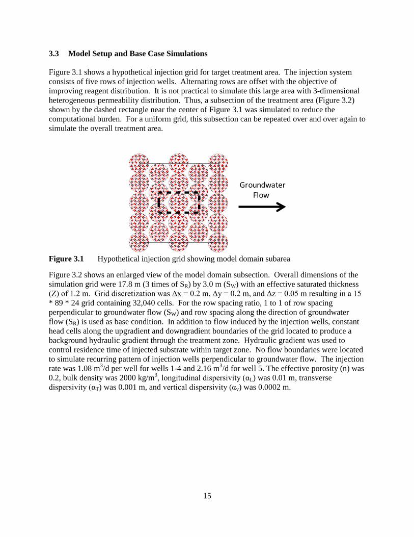
3.3 Model Setup and Base Case Simulations Figure 3.1 shows a hypothetical injection grid for target treatment area. The injection system consists of five rows of injection wells. Alternating rows are offset with the objective of improving reagent distribution. It is not practical to simulate this large area with 3-dimensional heterogeneous permeability distribution. Thus, a subsection of the treatment area (Figure 3.2) shown by the dashed rectangle near the center of Figure 3.1 was simulated to reduce the computational burden. For a uniform grid, this subsection can be repeated over and over again to simulate the overall treatment area.

Figure 3.1 Hypothetical injection grid showing model domain subarea

Figure 3.2 shows an enlarged view of the model domain subsection. Overall dimensions of the simulation grid were 17.8 m (3 times of SR) by 3.0 m (SW) with an effective saturated thickness (Z) of 1.2 m. Grid discretization was Δx = 0.2 m, Δy = 0.2 m, and Δz = 0.05 m resulting in a 15 * 89 * 24 grid containing 32,040 cells. For the row spacing ratio, 1 to 1 of row spacing perpendicular to groundwater flow (SW) and row spacing along the direction of groundwater flow (SR) is used as base condition. In addition to flow induced by the injection wells, constant head cells along the upgradient and downgradient boundaries of the grid located to produce a background hydraulic gradient through the treatment zone. Hydraulic gradient was used to control residence time of injected substrate within target zone. No flow boundaries were located to simulate recurring pattern of injection wells perpendicular to groundwater flow. The injection rate was 1.08 m3/d per well for wells 1-4 and 2.16 m3/d for well 5. The effective porosity (n) was 0.2, bulk density was 2000 kg/m3, longitudinal dispersivity (αL) was 0.01 m, transverse dispersivity (αT) was 0.001 m, and vertical dispersivity (αv) was 0.0002 m.

GroundwaterFlow

16

Figure 3.2 Model domain for small grid numerical simulations

All simulations have used a spatially heterogeneous 3-dimensional permeability distribution represented as a spatially correlated random field. The random field was generated using turning bands method (Tompson et al., 1989) with a horizontal correlation length of 2 m and a vertical correlation length of 0.2 m. The permeability distribution was designed to have 0.5 m/d of average hydraulic conductivity. The average groundwater velocity was varied from 0.2 to 0.013 m/d by altering the flow field boundary conditions. 3.3.1 Pore Volumes of Injection Fluid To allow easy comparison between different simulations, the volume of fluid injected were presented as the fraction of the total pore volumes of fluid in the target treatment zone where PV = Volume of water injected / (n SW SR Z) n is the total porosity and Z is the effective saturated thickness. 3.3.2 Contact Efficiency For good treatment, the soluble substrate should be distributed throughout the target treatment zone. This section describes the approach used to calculate contact efficiency from the numerical model simulation results. Figure 3.3 below shows a hypothetical treatment area with a single injection well (yellow dot) and three monitoring locations (MW 1, 2, and 3) at single moment in time. The dark red areas have high substrate concentrations, while the white areas have very low substrate concentrations.

17

Figure 3.3 Target treatment area with a single injection well (yellow dot) and three

monitoring locations (MW 1, 2, and 3) at single time step

Figure 3.4 shows the simulated substrate concentration versus time at the three monitoring wells (MW 1, 2 and 3). Substrate concentrations in MW 1 spike immediately after substrate injection, then decline with time due to downgradient transport, dilution, and first order decay. Since MW 1 is close to the injection well, the majority of the time, the substrate concentration is greater than the minimum required for effective treatment. However at MW 3, concentrations are frequently less than the minimum level required for effective treatment.

Figure 3.4 Variation in soluble substrate concentration with time at three monitoring

locations downgradient of the substrate injection well

In this work, effective treatment is assumed to occur when the substrate concentration is greater than a user defined minimum concentration (Cmin). In the Figure 3.4, the substrate concentration at MW 1 at 140 days is greater than the minimum required and MW 1 is counted as contacted. However at MW 3, the TOC concentration at 140 days is below the minimum concentration and

Minimum TOC Concentration

Time (Days)

Conc

entr

atio

n [m

g/L]

18

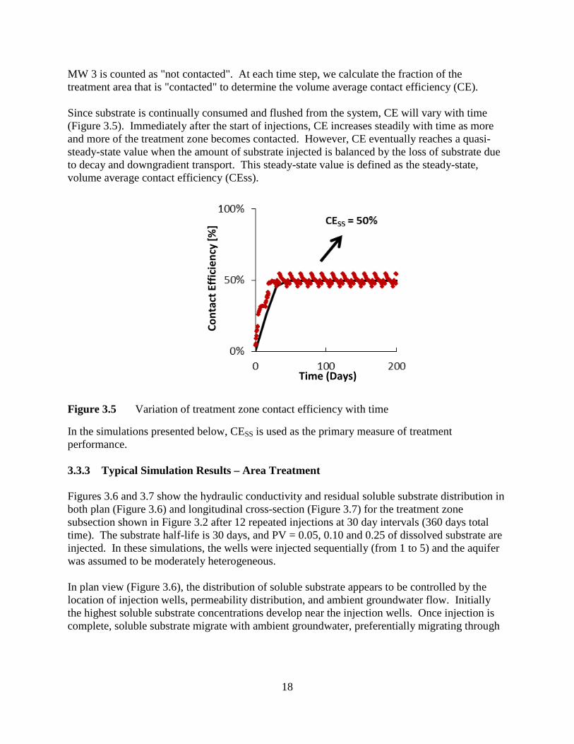
MW 3 is counted as "not contacted". At each time step, we calculate the fraction of the treatment area that is "contacted" to determine the volume average contact efficiency (CE). Since substrate is continually consumed and flushed from the system, CE will vary with time (Figure 3.5). Immediately after the start of injections, CE increases steadily with time as more and more of the treatment zone becomes contacted. However, CE eventually reaches a quasi-steady-state value when the amount of substrate injected is balanced by the loss of substrate due to decay and downgradient transport. This steady-state value is defined as the steady-state, volume average contact efficiency (CEss).

Figure 3.5 Variation of treatment zone contact efficiency with time

In the simulations presented below, CESS is used as the primary measure of treatment performance. 3.3.3 Typical Simulation Results – Area Treatment Figures 3.6 and 3.7 show the hydraulic conductivity and residual soluble substrate distribution in both plan (Figure 3.6) and longitudinal cross-section (Figure 3.7) for the treatment zone subsection shown in Figure 3.2 after 12 repeated injections at 30 day intervals (360 days total time). The substrate half-life is 30 days, and PV = 0.05, 0.10 and 0.25 of dissolved substrate are injected. In these simulations, the wells were injected sequentially (from 1 to 5) and the aquifer was assumed to be moderately heterogeneous. In plan view (Figure 3.6), the distribution of soluble substrate appears to be controlled by the location of injection wells, permeability distribution, and ambient groundwater flow. Initially the highest soluble substrate concentrations develop near the injection wells. Once injection is complete, soluble substrate migrate with ambient groundwater, preferentially migrating through

Time (Days)

Cont

act E

ffic

ienc

y [%

]

19

the higher permeability zones. Injecting additional fluid (PV = 0.25) enhance the distribution of soluble substrate.

Figure 3.6 Horizontal hydraulic conductivity and soluble substrate distribution in top layer of

aquifer (see Figure 3.7) at 360 days after injection for moderately heterogeneous aquifer when wells 1-5 were injected with PV=0.05, 0.10 and 0.25, time period between substrate reinjection = 30 days, and half-life of 30 days. Deep red indicates a very high concentration or value, white indicates very low or zero.

In profile view (Figure 3.7), the effects of the heterogeneous permeability distribution on soluble substrate transport were very apparent. The soluble substrate migrates rapidly downgradient in higher permeability layers and is much more limited in lower permeability layers. However, injection with large volume of fluid results in stagnation zone in the middle of the injection grid between each pair of wells (1, 3 and 2, 4), driving soluble substrate away from target treatment zone.

Permeability

PV=0.05

PV=0.25

PV=0.10

20

Figure 3.7 Vertical hydraulic conductivity and soluble substrate distribution in last row of

aquifer (bottom row of Figure 3.6) at 360 days after injection for moderately heterogeneous aquifer when wells 1-5 were injected with PV=0.05, 0.10 and 0.25, time period between substrate reinjection = 30 days, and half-life of 30 days. Deep red indicates a very high concentration or value, white indicates very low or zero.

The numerical model simulations indicate that soluble substrate can be effectively distributed throughout the target treatment zone. Under appropriate conditions (neutral pH, presence of appropriate microorganisms, etc.) this substrate will enhance contaminant biodegradation. However, significant portions of the model domain may not be contacted with soluble substrate and consequently, microbial activity may be limited, reducing contaminant destruction. In subsequent sections, results from series of sensitivity analyses are presented illustrating the effect of different design parameters on contact efficiency. This information can be used to generate improved designs with higher contact efficiencies. 3.4 Effect of Injection Fluid Volume on Contact Efficiency A series of simulations were conducted to examine the effect of injection fluid volume on contact efficiency for 3-D heterogeneity conditions. Figure 3.8 shows the effect of injection volume on CESS for different values of the time period between substrate reinjections (TR) and soluble substrate half-life (TH). All the curves follow the same trend, where increasing the injection volume initially results in a significant improvement in contact efficiency, then further

Permeability

PV=0.05

PV=0.25

PV=0.10

21

increases in fluid injection result in progressively less benefit. As expected, CESS is highest with long-lived substrate that is injected frequently. Other factors that were important were the ratio of injection concentration to minimum substrate concentration (CI/Cmin) and the travel time (TT) between rows of injection wells.

Figure 3.8 Effect of injection fluid volume to CESS for different values of time period between substrate reinjection and substrate half-life with 120 days travel time.

3.5 Effect of Design Parameters on Steady State Contact Efficiency An extensive series of sensitivity analyses were conducted to examine the impact of substrate injection concentration (CI), minimum substrate concentration (Cmin), groundwater travel time between rows of injection wells (TT), soluble substrate half-life (TH), time period between substrate reinjections (TR), pore volumes of substrate solution injected (PV), and steady-state contact efficiency (CESS). Analysis of these results revealed that CESS can be accurately predicted based on four dimensionless variables: 1) CI/Cmin; 2) PV; 3) TT/TH; and 4) TR/TT. Figure 3.9 shows the effect of the dimensionless variables CI/Cmin, PV, TT/TH, and TR/TT on steady-state contact efficiency (CESS). The highest contact efficiencies are indicated by the dark red or maroon color while the lowest contact efficiencies are indicated by the blue color. As expected, CESS can be increased by injecting larger volumes of water (increasing PV) containing higher concentrations of organic substrate (higher CI/Cmin). CESS is also increased when the time period between substrate reinjections is less than the travel time between wells (TR/TT <1) and when the substrate half life is greater than the travel time between rows of injection wells (TT/TH < 1).

22

Ratio injection to minimum substrate concentration (CI/Cmin) = 100



Figure 3.9 Effect of dimensionless variables CI/Cmin, PV, TT/TH, and TR/TT on steady-state

contact efficiency (CESS).

23

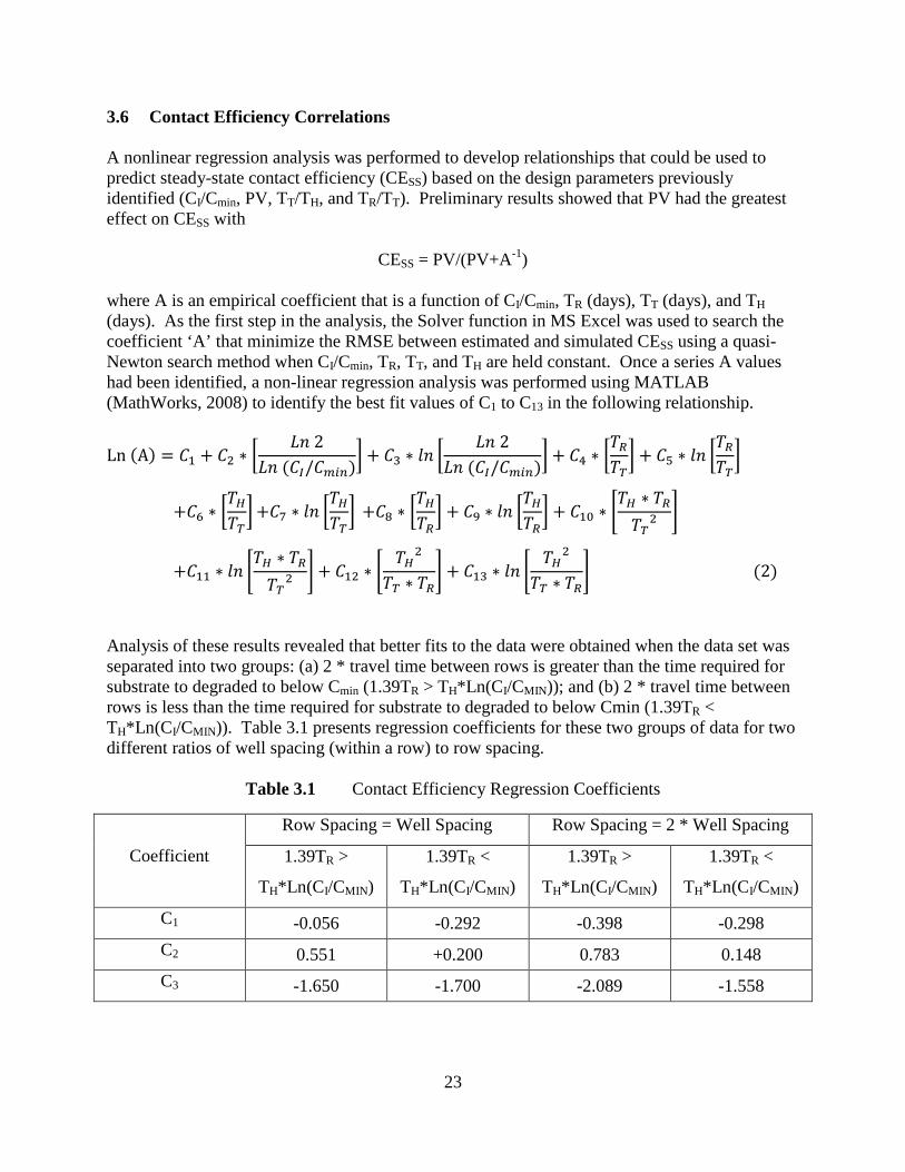
3.6 Contact Efficiency Correlations A nonlinear regression analysis was performed to develop relationships that could be used to predict steady-state contact efficiency (CESS) based on the design parameters previously identified (CI/Cmin, PV, TT/TH, and TR/TT). Preliminary results showed that PV had the greatest effect on CESS with

CESS = PV/(PV+A-1) where A is an empirical coefficient that is a function of CI/Cmin, TR (days), TT (days), and TH (days). As the first step in the analysis, the Solver function in MS Excel was used to search the coefficient ‘A’ that minimize the RMSE between estimated and simulated CESS using a quasi-Newton search method when CI/Cmin, TR, TT, and TH are held constant. Once a series A values had been identified, a non-linear regression analysis was performed using MATLAB (MathWorks, 2008) to identify the best fit values of C1 to C13 in the following relationship.

Ln (A) = 𝐶1 + 𝐶2 ∗ �𝐿𝑛 2

𝐿𝑛 (𝐶𝐼/𝐶𝑚𝑖𝑛)� + 𝐶3 ∗ 𝑙𝑛 �

𝐿𝑛 2𝐿𝑛 (𝐶𝐼/𝐶𝑚𝑖𝑛)

� + 𝐶4 ∗ �𝑇𝑅𝑇𝑇� + 𝐶5 ∗ 𝑙𝑛 �

𝑇𝑅𝑇𝑇�

+𝐶6 ∗ �𝑇𝐻𝑇𝑇�+𝐶7 ∗ 𝑙𝑛 �

𝑇𝐻𝑇𝑇� +𝐶8 ∗ �

𝑇𝐻𝑇𝑅� + 𝐶9 ∗ 𝑙𝑛 �

𝑇𝐻𝑇𝑅� + 𝐶10 ∗ �

𝑇𝐻 ∗ 𝑇𝑅𝑇𝑇2

�

+𝐶11 ∗ 𝑙𝑛 �𝑇𝐻 ∗ 𝑇𝑅𝑇𝑇2

� + 𝐶12 ∗ �𝑇𝐻2

𝑇𝑇 ∗ 𝑇𝑅� + 𝐶13 ∗ 𝑙𝑛 �

𝑇𝐻2

𝑇𝑇 ∗ 𝑇𝑅� (2)

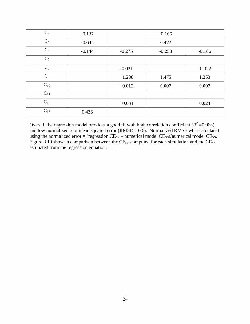
Analysis of these results revealed that better fits to the data were obtained when the data set was separated into two groups: (a) 2 * travel time between rows is greater than the time required for substrate to degraded to below Cmin (1.39TR > TH*Ln(CI/CMIN)); and (b) 2 * travel time between rows is less than the time required for substrate to degraded to below Cmin (1.39TR < TH*Ln(CI/CMIN)). Table 3.1 presents regression coefficients for these two groups of data for two different ratios of well spacing (within a row) to row spacing.

Table 3.1 Contact Efficiency Regression Coefficients

Coefficient

Row Spacing = Well Spacing Row Spacing = 2 * Well Spacing

1.39TR >

TH*Ln(CI/CMIN)

1.39TR <

TH*Ln(CI/CMIN)

1.39TR >

TH*Ln(CI/CMIN)

1.39TR <

TH*Ln(CI/CMIN)

C1 -0.056 -0.292 -0.398 -0.298 C2 0.551 +0.200 0.783 0.148 C3 -1.650 -1.700 -2.089 -1.558

24

C4 -0.137 -0.166 C5 -0.644 0.472 C6 -0.144 -0.275 -0.258 -0.186 C7 C8 -0.021 -0.022 C9 +1.288 1.475 1.253 C10 +0.012 0.007 0.007 C11 C12 +0.031 0.024 C13 0.435

Overall, the regression model provides a good fit with high correlation coefficient (R2 =0.968) and low normalized root mean squared error (RMSE = 0.6). Normalized RMSE what calculated using the normalized error = (regression CESS – numerical model CESS)/numerical model CESS. Figure 3.10 shows a comparison between the CESS computed for each simulation and the CESS estimated from the regression equation.

25

Figure 3.10 Comparison of CESS determined from individual numerical simulations and the

multiple regression equation.

26

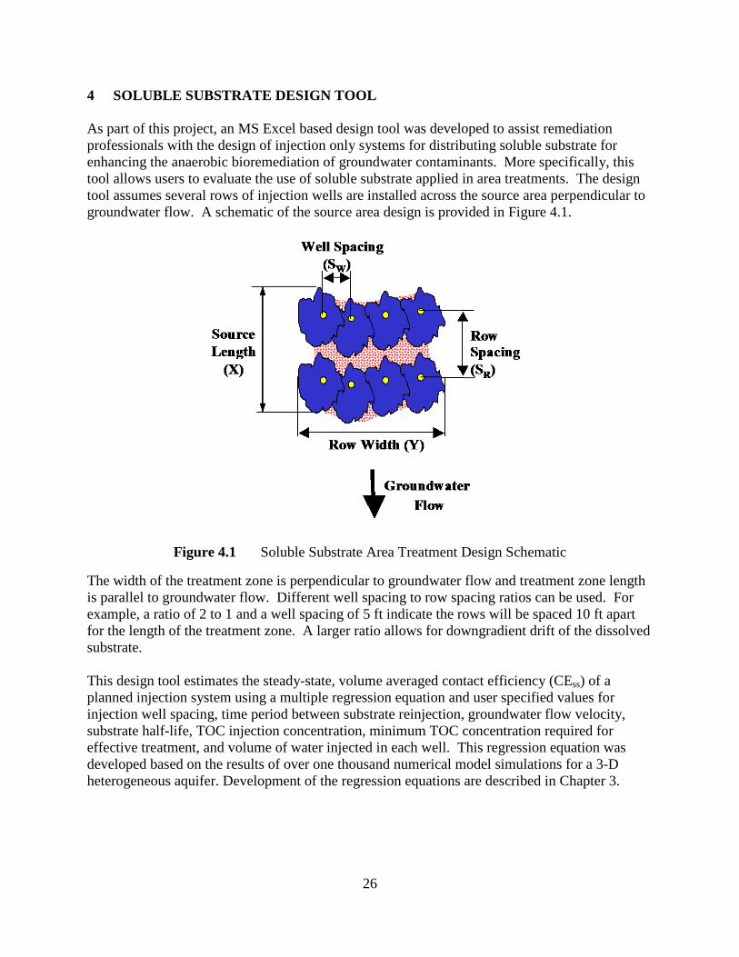
4 SOLUBLE SUBSTRATE DESIGN TOOL As part of this project, an MS Excel based design tool was developed to assist remediation professionals with the design of injection only systems for distributing soluble substrate for enhancing the anaerobic bioremediation of groundwater contaminants. More specifically, this tool allows users to evaluate the use of soluble substrate applied in area treatments. The design tool assumes several rows of injection wells are installed across the source area perpendicular to groundwater flow. A schematic of the source area design is provided in Figure 4.1.

Figure 4.1 Soluble Substrate Area Treatment Design Schematic

The width of the treatment zone is perpendicular to groundwater flow and treatment zone length is parallel to groundwater flow. Different well spacing to row spacing ratios can be used. For example, a ratio of 2 to 1 and a well spacing of 5 ft indicate the rows will be spaced 10 ft apart for the length of the treatment zone. A larger ratio allows for downgradient drift of the dissolved substrate. This design tool estimates the steady-state, volume averaged contact efficiency (CEss) of a planned injection system using a multiple regression equation and user specified values for injection well spacing, time period between substrate reinjection, groundwater flow velocity, substrate half-life, TOC injection concentration, minimum TOC concentration required for effective treatment, and volume of water injected in each well. This regression equation was developed based on the results of over one thousand numerical model simulations for a 3-D heterogeneous aquifer. Development of the regression equations are described in Chapter 3.

27

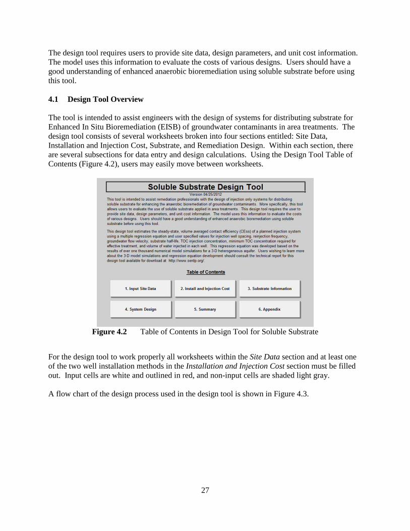
The design tool requires users to provide site data, design parameters, and unit cost information. The model uses this information to evaluate the costs of various designs. Users should have a good understanding of enhanced anaerobic bioremediation using soluble substrate before using this tool. 4.1 Design Tool Overview The tool is intended to assist engineers with the design of systems for distributing substrate for Enhanced In Situ Bioremediation (EISB) of groundwater contaminants in area treatments. The design tool consists of several worksheets broken into four sections entitled: Site Data, Installation and Injection Cost, Substrate, and Remediation Design. Within each section, there are several subsections for data entry and design calculations. Using the Design Tool Table of Contents (Figure 4.2), users may easily move between worksheets.

Figure 4.2 Table of Contents in Design Tool for Soluble Substrate

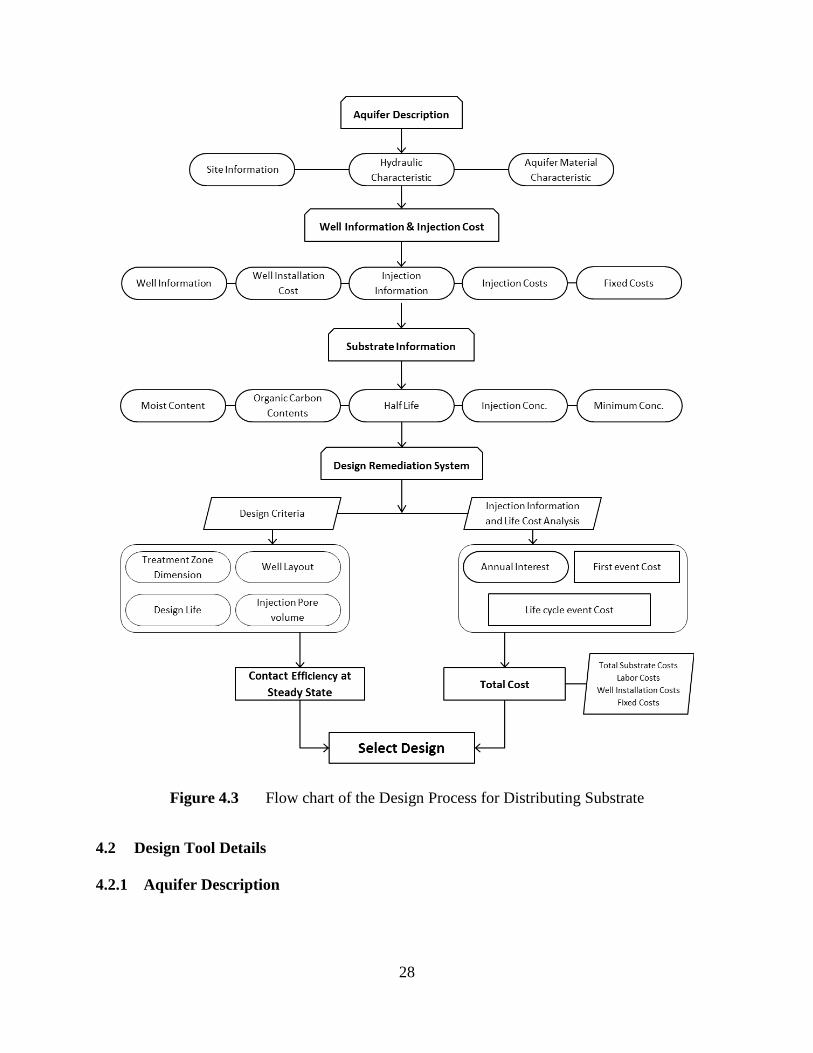
For the design tool to work properly all worksheets within the Site Data section and at least one of the two well installation methods in the Installation and Injection Cost section must be filled out. Input cells are white and outlined in red, and non-input cells are shaded light gray. A flow chart of the design process used in the design tool is shown in Figure 4.3.

28

Figure 4.3 Flow chart of the Design Process for Distributing Substrate

4.2 Design Tool Details 4.2.1 Aquifer Description

29

The first step in using the design tool is to enter information on the physical characteristics of the aquifer. The information will be used later to calculate injection volumes and costs.

• Name, Description, Location are used to identify and describe the project and are used again in the Design Parameter Archive page.

• Hydraulics Characteristics including depth to water table and depth to top and bottom of

injection zone hydraulic gradient, hydraulic conductivity, estimated total porosity, and seepage velocity: are used in estimating potential injection rates and in calculating injection fluid volumes. First three data are used to calculate the seepage velocity and groundwater flux through the treatment zone.

• Aquifer Material Characteristics including soil lithology and bulk density are included for

future reference (optional): This data are not used in the design tool, but is provided for future reference.

4.2.2 Well Installation and Injection Information Users enter information on the labor and materials required for installing temporary or permanent injection wells/points by either Direct Push Technology (DPT) or conventional drilling. Injection well/point installation is assumed to be by a subcontract driller with supervision by the prime contractor. Once the wells are installed, multiple wells are manifolded together for soluble substrate injection. Results of this analysis are summarized as: a) total fixed cost; b) cost per boring; and c) cost per gallon of fluid injected. Costs for monitoring well installation and sampling are not included in this design tool.

• Well screen and effective sand pack diameter are included for documentation and are used to estimate potential injection rates. The typical range of well screen diameter for DPT and conventional drilling is 0.75 to 1.25 inches and 1 to 2 inches, respectively. The effective diameter of sand pack for DPT and conventional drilling is typically 0.75 to 2 and 1 to 3.75 inches, respectively, depending on the installation method.

• Well installation costs are calculated from wells installed per day with unit cost per

drilling depth for conventional wells or daily costs for equipment and labor by DPT. Material costs and personnel costs are entered to compute the total cost per well. Per diem, vehicle rental, and lodging costs from are also included in the total cost per well.

• By clicking YES for “Do you want to use same cost and injection information for

Conventional Drilling as Direct Push Installation?”, the program will copy reducing data entry time. Once copied over, users can still change individual values.

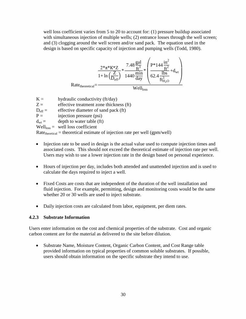
• Injection pressure and well loss coefficient are used along with hydraulic conductivity

and well construction information to estimate potential injection rates. Typically, the

30

well loss coefficient varies from 5 to 20 to account for: (1) pressure buildup associated with simultaneous injection of multiple wells; (2) entrance losses through the well screen; and (3) clogging around the well screen and/or sand pack. The equation used in the design is based on specific capacity of injection and pumping wells (Todd, 1980).

Ratetheoretical=

2*π*K*Z

1+ ln � ZDeff

�*

7.48 galft3

1440 minday

*

⎝

⎜⎛P*144 in2

ft2

62.4 lbsftH2O

3

+dwt

⎠

⎟⎞

Wellloss

K = hydraulic conductivity (ft/day) Z = effective treatment zone thickness (ft) Deff = effective diameter of sand pack (ft) P = injection pressure (psi) dwt = depth to water table (ft) Wellloss = well loss coefficient Ratetheortical = theoretical estimate of injection rate per well (gpm/well)

• Injection rate to be used in design is the actual value used to compute injection times and

associated costs. This should not exceed the theoretical estimate of injection rate per well. Users may wish to use a lower injection rate in the design based on personal experience.

• Hours of injection per day, includes both attended and unattended injection and is used to

calculate the days required to inject a well. • Fixed Costs are costs that are independent of the duration of the well installation and

fluid injection. For example, permitting, design and monitoring costs would be the same whether 20 or 30 wells are used to inject substrate.

• Daily injection costs are calculated from labor, equipment, per diem rates. 4.2.3 Substrate Information Users enter information on the cost and chemical properties of the substrate. Cost and organic carbon content are for the material as delivered to the site before dilution.

• Substrate Name, Moisture Content, Organic Carbon Content, and Cost Range table provided information on typical properties of common soluble substrates. If possible, users should obtain information on the specific substrate they intend to use.

31

• Substrate moisture content, organic carbon content, and TOC injection concentration used in design determine the total mass of soluble substrate injected. TOC injection concentration is total organic carbon content in soluble substrate (mass of soluble substrate * organic carbon content /total water volume.

• Cost per lb: Unit price of selected soluble substrate.

• Soluble substrate half life is used to represent soluble substrate consumption by

microorganism.

• Minimum Groundwater TOC Concentration required to for effective contaminant biodegradation. The ratio of injection to minimum TOC concentration is later used in estimating the steady state contact efficiency.

4.2.4 Remediation System Design Criteria Users enter information on the design criteria for installation of area treatments. These criteria are later used to determine material quantities and estimate costs for a different design alternatives. Well spacing, groundwater velocity, time period between substrate reinjection, and substrate characteristics (half-life, injection concentration, and minimum concentration) are used to estimate the time weighted average contact efficiency based on 3-D simulations for a medium heterogeneity aquifer.

• Drilling, injection, and substrate information are carried over from previous pages. Use should click on the button to select which well installation approach will be used. .

• Treatment width (perpendicular to groundwater flow), length (parallel to groundwater

flow), thickness (carried over from previous pages), and percentage of injection zone that transmits most flow are used to compute the effective volume of the treatment zone. The percent of the aquifer that transmits most flow should be estimated form boring logs and is used to account for the presence of low permeability layers that do not transmit water.

• Well spacing (perpendicular to groundwater flow) and row spacing (parallel to

groundwater flow) are used to determine the total number of wells based on the treatment zone dimensions.

• Design life (duration that TOC must be maintained in aquifer for enhanced

bioremediation) and reinjection interval (time between substrate reinjection) are used to calculate contact efficiency and life cycle costs.

• Pore volumes of substrate solution injected during each event is used to determine

contact efficiency, total amount of substrate, and labor costs for injection. Typically, between 0.05 and 0.25 pore volumes are injected with higher values resulting in higher

32

contact efficiencies. However, it can be difficult to inject large amounts of fluid into lower permeability aquifers, significantly increasing injection duration and costs.

• Estimated contact efficiency at steady state is estimated from the regression equations

developed in Chapter 3, and user specified values entered above. There is no absolute minimum contact efficiency required. Higher contact efficiencies should result in more rapid and effective treatment, but will also increase costs. Users are encouraged to evaluate a range of design parameters and their impact on both cost and contact efficiency and select a design that generates a higher contact efficiency per dollar expended.

4.2.5 Remediation System Life Cycle Cost Analysis This portion of the design tool summarizes information generated on previous worksheets and provides space for users to enter parameters used in the life cycle cost analysis.

• Planning, engineering, and permitting costs include any fixed costs associated with substrate injections (after the first injection is complete).

• Maximum number of wells to inject at one time is used to determine the total time for

substrate injection. Injecting multiple wells together reduces the total time it takes to complete injection resulting in a lower total cost. However, the number of wells to inject at once is usually limited by site logistical constrains (available water supply, hose and valve available, etc.). No more than 50% of the wells should be injected at one time to reduce interference between wells. If possible, wells injected simultaneously should be spaced far apart to reduce stagnation zones between the wells.

4.2.6 Design Parameter Archive This portion of the design tool summarizes information generated on previous worksheets and results of the cost analysis for different design alternatives. Graphs can be easily generated to allow comparison of the costs and contact efficiency associated with up to six different design alternatives. Alternatives can be eliminated or included in the graphs by clicking the clear or plot buttons. Users are encouraged to evaluate a range of design parameters and their impact on both cost and contact efficiency and select a design that generates a higher contact efficiency per dollar expended.

33

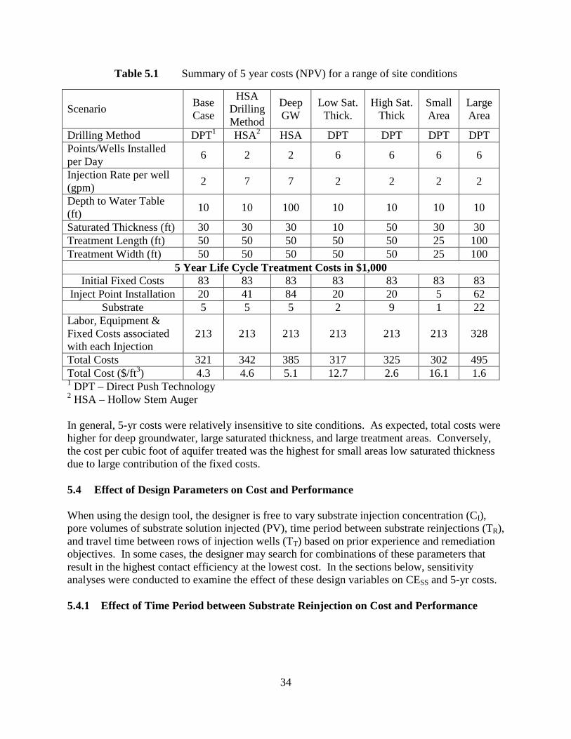
5 EVALUATION OF DESIGN TOOL PERFORMANCE 5.1 Introduction A series of sensitivity analyses with design tool were conducted to identify factors that had a major influence on costs and performance. In all analyses, results are presented as Net Present Value (NPV) assuming a 5-yr operating period. Results are compared to a base case condition intended to represent a typical site. 5.2 Site Description and Initial Values The base case site used in this analysis is a shallow aquifer is comprised of silty sand and gravel with a 75 ft x 75 ft source area. The water table aquifer extends from 10 to 40 ft below ground surface and has an average hydraulic conductivity (permeability or K) of 5.65 ft/day with a porosity of 25%, and seepage velocity of 33 ft/yr. 0.05 pore volumes of soluble substrate are reinjected once every 18 weeks for 5 years to enhance anaerobic biodegradation processes. The soluble substrate used in this analysis is assumed to be molasses (36% organic carbon) with a unit cost of $0.5/lb delivered and half life of 60 days. The injection concentration is assumed to be 5000 mg/L of TOC and the minimum TOC concentration for effective bioremediation is 50 mg/L. Injection wells are assumed to be installed 15 ft on center within a row with 15 ft between rows. For these conditions, the estimated CESS is approximately 46%. Two different well installation methods were evaluated – direct push technology (DPT) and hollow stem auger (HSA). The direct push wells are assumed to be 1 inch PVC installed at a total cost of $532 per well including all equipment. Total costs for installation of 2 inch PVC wells with sand pack by HSA are $2,585 per well. Injection rates were assumed to be 2 gpm for DPT wells and 7 gpm for HSA wells with up to 10 wells manifolded together to inject at one time. Total costs for injection were assumed to be $2,885/day including labor, equipment, vehicles, health and safety and per diem. The cost analysis assumed a 5 year operating period with an annual interest rate of 5.0%. Fixed costs for planning, design, permitting, mobilization, and equipment setup at the site are $83,070 for first injection event and $10,970 for each life-cycle event. 5.3 Effect of Site Characteristics on Costs A range of conditions were examined to evaluate the impact site characteristics on costs for a soluble substrate bioremediation system. Factors having a significant influence on costs for each site condition are summarized in Table 5.1. Unit costs were calculated as total cost of treatment divided by the cost per unit volume of the area treatment zone (width x length x saturated thickness).

34

Table 5.1 Summary of 5 year costs (NPV) for a range of site conditions

Scenario Base Case

HSA Drilling Method

Deep GW

Low Sat. Thick.

High Sat. Thick

Small Area

Large Area

Drilling Method DPT1 HSA2 HSA DPT DPT DPT DPT Points/Wells Installed per Day 6 2 2 6 6 6 6

Injection Rate per well (gpm) 2 7 7 2 2 2 2

Depth to Water Table (ft) 10 10 100 10 10 10 10

Saturated Thickness (ft) 30 30 30 10 50 30 30 Treatment Length (ft) 50 50 50 50 50 25 100 Treatment Width (ft) 50 50 50 50 50 25 100

5 Year Life Cycle Treatment Costs in $1,000 Initial Fixed Costs 83 83 83 83 83 83 83

Inject Point Installation 20 41 84 20 20 5 62 Substrate 5 5 5 2 9 1 22

Labor, Equipment & Fixed Costs associated with each Injection

213 213 213 213 213 213 328

Total Costs 321 342 385 317 325 302 495 Total Cost ($/ft3) 4.3 4.6 5.1 12.7 2.6 16.1 1.6 1 DPT – Direct Push Technology 2 HSA – Hollow Stem Auger In general, 5-yr costs were relatively insensitive to site conditions. As expected, total costs were higher for deep groundwater, large saturated thickness, and large treatment areas. Conversely, the cost per cubic foot of aquifer treated was the highest for small areas low saturated thickness due to large contribution of the fixed costs. 5.4 Effect of Design Parameters on Cost and Performance When using the design tool, the designer is free to vary substrate injection concentration (CI), pore volumes of substrate solution injected (PV), time period between substrate reinjections (TR), and travel time between rows of injection wells (TT) based on prior experience and remediation objectives. In some cases, the designer may search for combinations of these parameters that result in the highest contact efficiency at the lowest cost. In the sections below, sensitivity analyses were conducted to examine the effect of these design variables on CESS and 5-yr costs. 5.4.1 Effect of Time Period between Substrate Reinjection on Cost and Performance

35

Figure 5.1 presents the effect of time period between substrate reinjections on CESS and NPV costs over a 5-yr operating period for the base case site conditions. Initially, increasing the time between substrate injections results in a modest decline in CESS with a rapid decline in costs due to the decline in labor, substrate and fixed costs for each injection event. However for time between substrate reinjection greater than 15 weeks, CESS declines significantly, while the cost savings are minimal since total costs are dominated by the initial costs for planning, design, permitting and well installation. For the base case site conditions and a substrate half-life of 60 days, a time between substrate reinjection of 10 to 15 weeks results in the highest ratio of CESS to 5-yr costs. Note that this analysis does not consider the potential benefits of increasing CESS in reducing the project operating period.

Figure 5.1 Effect of time period between substrate reinjection on 5-yr costs (NPV) and

steady state contact efficiency (CESS)

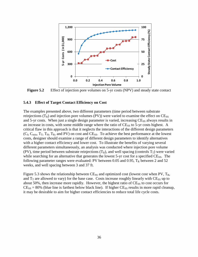
5.4.2 Effect of Injection Pore Volume on Cost and Performance Figure 5.2 shows the effect of increasing the pore volumes (PV) of substrate injected on CESS and NPV costs over a 5-yr operating period for the base case site conditions. Initially, increasing the PV of substrate injected results in a large increase in CESS. However, the benefits of increased CESS decline rapidly with increasing injection volumes. In contrast, increasing PV of substrate injected results in an almost linear increase in costs since injecting larger amounts of substrate solution increase the time and associated labor costs for each injection. For the base case site conditions, 0.1 to 0.2 PV of substrate injection results in the highest ratio of CESS to 5-yr costs, assuming project operating period is independent of CESS.

36

Figure 5.2 Effect of injection pore volumes on 5-yr costs (NPV) and steady state contact

5.4.3 Effect of Target Contact Efficiency on Cost The examples presented above, two different parameters (time period between substrate reinjections (TR) and injection pore volumes (PV)) were varied to examine the effect on CESS and 5-yr costs. When just a single design parameter is varied, increasing CESS always results in an increase in costs, with some middle range where the ratio of CESS to 5-yr costs highest. A critical flaw in this approach is that it neglects the interactions of the different design parameters (CI, Cmin, TT, TH, TR, and PV) on cost and CESS. To achieve the best performance at the lowest costs, designer should examine a range of different design parameters to identify alternatives with a higher contact efficiency and lower cost. To illustrate the benefits of varying several different parameters simultaneously, an analysis was conducted where injection pore volume (PV), time period between substrate reinjections (TR), and well spacing (controls TT) were varied while searching for an alternative that generates the lowest 5-yr cost for a specified CESS. The following parameter ranges were evaluated: PV between 0.05 and 0.95, TR between 2 and 52 weeks, and well spacing between 3 and 37 ft. Figure 5.3 shows the relationship between CESS and optimized cost (lowest cost when PV, TR, and TT are allowed to vary) for the base case. Costs increase roughly linearly with CESS up to about 50%, then increase more rapidly. However, the highest ratio of CESS to cost occurs for CESS = 80% (blue line is farthest below black line). If higher CESS results in more rapid cleanup, it may be desirable to aim for higher contact efficiencies to reduce total life cycle costs.

0

25

50

75

100

0

300

600

900

1,200

0.0 0.2 0.4 0.6 0.8 1.0

Stea

dy St

ate

Cont

act E

ffici

ency

(%)

5-yr

Cos

ts (

in $

1,00

0)

Injection Pore Volume

Cost

Contact Efficiency

37

Figure 5.3 Effect of steady-state contact efficiency (CESS) on 5-yr costs for an optimized

injection system design for the base case

Figure 5.4 shows the normalized 5-yr cost versus CESS for the different site conditions listed in Table 5.1. Normalized 5-yr cost is defined as the optimized 5-yr cost for that value of CESS divided by the optimized 5-yr cost for a 50% contact efficiency. The relationship between normalized 5-yr cost and contact efficiency follow a similar relationship with costs increasing more slowly than CESS up until around 70 -80% CESS when costs begin to increase rapidly.

Figure 5.4 Effect of steady-state contact efficiency (CESS) on normalized 5-yr costs for an

optimized injection system design for a range of site conditions (Table 5.1)

$0

$100

$200

$300

$400

$500

$600

0 20 40 60 80 100

5-yr

Cos

t (in

$1,

000)

Steady State Contact Efficiency (%)

0.0

0.5

1.0

1.5

2.0

0 10 20 30 40 50 60 70 80 90 100

Nor

mal

ized

5-yr

Cos

t

Steady State Contact Efficiency (%)

BaseHSA Drilling MethodDeep GroundwaterLow Saturation ThicknessHigh Saturation ThicknessSmall SiteLarge Site

38

5.5 Summary Total costs ($) to treat a site for 5-yr using soluble substrate is relatively insensitive to site conditions. Obviously, total costs will be higher for large and deep sites. Unit costs will be higher for smaller sites due to the proportionately higher fixed costs associated with planning, design, and permitting. Estimated steady state contact efficiency (CESS) can be increased by varying different design parameters including substrate injection concentration (CI), minimum substrate concentration (Cmin), groundwater travel time between rows of injection wells (TT), soluble substrate half-life (TH), time period between substrate reinjections (TR), and pore volumes of substrate solution injected (PV). In most cases, increasing CESS results in increasing costs. For many parameters, there is some middle range where the ratio of CESS to 5-yr costs highest. Optimized designs can be developed by simultaneously varying several different design parameters to generate alternatives that result in the lowest cost for a specified value of CESS. In many cases, the highest ratio of CESS to cost occurs for CESS in the range of 70% - 80%. If higher CESS results in more rapid cleanup, it may be desirable to aim for higher contact efficiencies to reduce total life cycle costs.

39

6 REFERENCES

Aquaveo, 2011. The Department of Defense Groundwater Modeling System, GMS v8.1. South Jordan Utah: Aquaveo.

AFCEE, NFESC, and ESTCP, 2004. Principles and Practices of Enhanced Anaerobic Bioremediation of Chlorinated Solvents, Prepared for Air Force Center for Environmental Excellence, TX, Naval Facilities Engineering Service Center, CA and Environmental Security Technology Certification Program, VA.

Harbaugh, A.W., Banta, E.R., Hill, M.C., and McDonald, M.G., 2000. “MODFLOW-2000, The U.S. Geological Survey Modular Ground-Water Model – User Guide to Modularization Concepts and the Groundwater Flow Process.” USGS.

Mathworks, 2008. MATLAB® Software, Version 7.12 (R2011a). Natick, Massachusetts: The Mathworks Inc.

Morse, J.J., Alleman, B.C., Gossett, J.M., Zinder, S.H., Fennell, D.E., Sewell, G.W., Vogel, C.M., 1998. A treatability test for evaluating the potential applicability of the reductive anaerobic biological in situ treatment technology (RABITT) to remediate chloroethenes. Environmental Technology Certification Program, Washington, DC.

Todd, K.T., 1980. Groundwater Hydrology, 2nd Edition. ISBN 0-471-87616-X, John Wiley & Sons, New York, NY.

Tompson, A.F.B., Aboudu, R. and Gelhar L.W., 1989. Implementation of the three-dimensional turning bands random field generator, Water Resources Research, 25(10), 2227-2243.

Zheng, C., 1990. MT3D, A modular three-dimensional transport model for simulation of advection, dispersion and chemical reactions of contaminants in groundwater systems, US Environmental Protection Agency.

40

7 POINTS OF CONTACT

POINT OF CONTACT

Name

ORGANIZATION Name

Address Phone/Fax/email Role in Project Robert C. Borden, P.E., Ph.D.

North Carolina State University Campus Box 7908 Raleigh, NC 27695

919-515-1625 919-515-7908 (fax) [email protected]

Principal Investigator

Thomas Simpkin, P.E., Ph.D.

CH2M HILL, Inc. 9193 South Jamaica St Englwood, CO 80112-5946


Co-Investigator

M. Tony Lieberman, R.S.M.

Solutions-IES, Inc. 3722 Benson Drive Raleigh, NC 27609


Co-Investigator

Erica Becvar HQ AFCEE/TDE Technology Transfer 3300 Sidney Brooks Brooks City-Base, TX 78235-5112


Contracting Officer’s Representative (COR)

Soluble Substrate Design Tool - CLU-IN

Documents