arXiv:1806.05188v1 [hep-th] 13 Jun 2018 Soliton Scattering in Noncommutative Spaces Masashi Hamanaka 1 and Hisataka Okabe 2 Graduate School of Mathematics, Nagoya University, Chikusa-ku, Nagoya, 464-8602, JAPAN Abstract We discuss exact multi-soliton solutions to integrable hierarchies on noncommutative space-times in diverse dimension. The solutions are represented by quasi-determinants in compact forms. We study soliton scattering processes in the asymptotic region where the configurations could be real-valued. We find that the asymptotic configurations in the soliton scatterings can be all the same as commutative ones, that is, the configuration of N -soliton solution has N isolated localized lump of energy and each solitary wave-packet lump preserves its shape and velocity in the scattering process. The phase shifts are also the same as commutative ones. As new results, we present multi-soliton solutions to noncommutative anti-self-dual Yang-Mills hierarchy and discuss 2-soliton scattering in detail. 1 E-mail: [email protected] 2 has worked at a company since April 2018

Welcome message from author
This document is posted to help you gain knowledge. Please leave a comment to let me know what you think about it! Share it to your friends and learn new things together.
Transcript
arX
iv:1
806.
0518
8v1
[he
p-th
] 1
3 Ju
n 20
18
Soliton Scattering in Noncommutative Spaces
Masashi Hamanaka1 and Hisataka Okabe2
Graduate School of Mathematics, Nagoya University,Chikusa-ku, Nagoya, 464-8602, JAPAN
Abstract
We discuss exact multi-soliton solutions to integrable hierarchies on noncommutativespace-times in diverse dimension. The solutions are represented by quasi-determinants incompact forms. We study soliton scattering processes in the asymptotic region where theconfigurations could be real-valued. We find that the asymptotic configurations in thesoliton scatterings can be all the same as commutative ones, that is, the configuration ofN -soliton solution has N isolated localized lump of energy and each solitary wave-packetlump preserves its shape and velocity in the scattering process. The phase shifts arealso the same as commutative ones. As new results, we present multi-soliton solutionsto noncommutative anti-self-dual Yang-Mills hierarchy and discuss 2-soliton scattering indetail.
1E-mail: [email protected] worked at a company since April 2018

1 Introduction
Noncommutative (NC) extension of integrable systems has attracted many researchers
in both mathematics and physics for long time. It would be a recent breakthrough that
exact multi-soliton solutions to the noncommutative KP hierarchy are constructed in
terms of quasi-determinants [11]. The quasideterminants are first introduced in 1991 by
Gelfand and Retakh [14] in the context of noncommutative generalization of theory of
determinants of matrices. It has been found that the quasideterminants play important
roles in construction of exact solutions to noncommutative integrable systems. (See e.g.
[10, 12, 15, 16, 17, 18, 19, 20, 21, 27, 28, 37, 48, 50] and references therein.) It is interesting
that quasideterminants simplify proofs in commutative theories.
For the last several years, extension of integrable systems to noncommutative space-
times has been studied intensively. This can be realized by using the star-product. From
now on,, the word “noncommutative” is assumed to refer to generalization to noncom-
mutative spaces, not to non-abelian and so on. For surveys on integrable systems in
noncommutative space-times, see e.g. [9, 22, 24, 31, 35, 41, 54].
N -soliton solutions are stable in the sense that the configuration has N localized lump
of energy where shape and velocity of each localized lump keep intact in the scattering
process. Existence of them closely relates to existence of infinite conserved quantities
or infinite dimensional symmetry. Hence it is worth studying the stability of the non-
commutative soliton dynamics. In the star-product formalism, space-time coordinates
and functions take c-number values and scattering dynamics can be clarified explicitly.
However, there are few studies on it [8, 39, 47].
In this paper, we study exact multi-soliton solutions to noncommutative integrable
hierarchies and the asymptotic behavior of them where the asymptotic configurations are
real-valued. We focus on the noncommutative Korteweg-de Vries (KdV), Kadomtsev-
Petviashvili (KP) and anti-self-dual Yang-Mills (ASDYM) equations in (1 + 1), (2 + 1)
and 4 dimension, respectively. We find that the asymptotic behavior in soliton scatter-
ings is all the same as commutative ones, that is, the N -soliton solution has N isolated
localized lump of energy and each wave-packet lump preserves its shape and velocity in
the scattering process. The phase shift is also the same as commutative one. The analysis
of 2-soliton scattering in the noncommutative ASDYM equation is new. Property of the
quasideterminants and the star products plays crucial roles.
This paper is organized as follows. In section 2, we give a brief introduction to non-
commutative field theory in the star-product formalism. In section 3, we make a brief
review of the quasi-determinants. In section 4, we define noncommutative integrable hier-
archy and construct exact multi-soliton solutions by using quasideterminants. Asymptotic
1

behaviors of noncommutative KdV and KP solitons are discussed in the star-product for-
malism [27]. In section 5, we define noncommutative ASDYM hierarchy and give exact
solutions to it in terms of quasideterminants. Asymptotic behavior of 2-soliton solutions
are discussed. This section gives new results.
2 Integrable Equations in Noncommutative Spaces
Noncommutative spaces are defined by the noncommutativity of the coordinates:
[xµ, xν ] = iθµν , (2.1)
where the constant θµν is called the noncommutative parameter. If the coordinates are
real, noncommutative parameters should be real because of hermicity of the coordinates.
We note that the noncommutative parameter θµν is anti-symmetric with respect to µ and
ν which implies that the rank of it is even. In (1+1)-dimension with the coordinate (t, x),
there is unique choice of noncommutativity : [x, t] = iθ which is space-time noncommu-
tativity. In (2 + 1)-dimension with the coordinate (t, x, y), there are essentially two kind
of choices of noncommutativity, that is, space-space noncommutativity: [x, y] = iθ and
space-time noncommutativity: [x, t] = iθ or [y, t] = iθ.
Noncommutative field theories are given by the replacement of ordinary products in
the commutative field theories with the star-products. The star-product is defined for
ordinary fields. On flat spaces, is it represented explicitly by
f ⋆ g(x) := exp
(i
2θµν∂(x1)
µ ∂(x2)ν
)f(x1)g(x2)
∣∣∣x1=x2=x
= f(x)g(x) +i
2θµν∂µf(x)∂νg(x) + O(θ2), (2.2)
where ∂(x)µ := ∂/∂xµ. This is known as the Moyal product [42]. The ordering of fields in
nonlinear terms are determined so that some structures such as gauge symmetries should
be preserved.
The star-product has associativity: f ⋆ (g ⋆ h) = (f ⋆ g) ⋆ h. It reduces to the
ordinary product in the commutative limit: θµν → 0. In this sense, the noncommu-
tative field theories are deformed theories from the commutative ones. The replace-
ment of the product makes the ordinary spatial coordinates “noncommutative,” that is,
[xµ, xν ]⋆ := xµ ⋆ xν − xν ⋆ xµ = iθµν .
We note that the fields themselves take c-number values and the differentiation and
the integration for them are the same as commutative ones.
Here is a gallery of noncommutative integrable equations. Time and spatial coordi-
nates are denoted by t and x, y, respectively.
2

• In (1 + 1) dimension:
– Noncommutative KdV equation
u =1
4u′′′ +
3
4(u′ ⋆ u+ u ⋆ u′) , (2.3)
where u := ∂f/∂t, u′ := ∂f/∂x, u′′ := ∂2f/∂x2 and so on. 2-soliton dynamics
is discussed [8].
– Noncommutative Boussinesq equation
3u+ u′′′′ + 2(u ⋆ u)′′ − 2[u, ∂−1x u]′⋆ = 0. (2.4)
– Noncommutative Non-Linear Schrodinger equation
iψ = ψ′′ − 2εψ ⋆ ψ ⋆ ψ. (2.5)
– Noncommutative modified KdV equation
v =1
4v′′′ −
3
4(v ⋆ v ⋆ v′ + v′ ⋆ v ⋆ v) . (2.6)
This is connected with the noncommutative KdV equation via the noncommu-
tative Miura map: u = v′ − v2 [8].
– Noncommutative Burgers equation
u = u′′ + 2u ⋆ u′ or u = u′′ − 2u′ ⋆ u. (2.7)
These can be linearized by the noncommutative Cole-Hopf transformations:
u = ψ−1 ⋆ ψ′ or u = −ψ′ ⋆ ψ−1, respectively. (See e.g. [30].) 2 shock-wave
dynamics is discussed [39].
• In (2 + 1) dimension:
– Noncommutative KP equation
ut =1
4uxxx +
3
4(ux ⋆ u+ u ⋆ ux) + ∂−1
x uyy − [u, ∂−1x uy]⋆. (2.8)
where the subscripts denote partial derivatives and ∂−1x f(x) =
∫ xdx′f(x′).
This reduces to the KdV equation in (1 + 1)-dimension by ∂y = 0 . 2-soliton
dynamics is discussed in detail [47].
3
– Noncommutative Zakharov system [26]
iψt = ψxy − εψ ⋆ ∂−1x ∂y(ψ ⋆ ψ) − ε∂−1
x ∂y(ψ ⋆ ψ) ⋆ ψ,
where ε = ±1. This reduces to the noncommutative Non-Linear Schrodinger
(NLS) equation in (1 + 1)-dimension by x = y .
– Noncommutative Bogoyavlenskii-Calogero-Schiff equation [55]
4ut = uxxy + 2 (u ⋆ u)y +(uy ⋆ ∂
−1x u+ ∂−1
x u ⋆ uy)
+ ∂−1x [u, ∂−1
x [u, ∂−1x uy]⋆]⋆.
This reduces to the noncommutative KdV equation by x = y .
– Noncommutative Davey-Stewartson equation [25]
{2iqt = (∂2x − ∂2y)q +R1 ⋆ q − q ⋆ R2,2irt = −(∂2x − ∂2y)r +R2 ⋆ r − r ⋆ R1,
where (∂x − i∂y)R1 = −(∂x + i∂y)(q ⋆ r), (∂x + i∂y)R2 = (∂x − i∂y)(r ⋆ q). This
reduces to the noncommutative NLS equation in (1 + 1)-dimension by ∂y = 0
and R1 = −q ⋆ r, Rs = r ⋆ q, q = ψ, r = ψ.
• In 4-dimension, there is an important integrable equation: noncommutative anti-
self-dual Yang-Mills (ASDYM) equation
F ⋆zw = 0, F ⋆
zw = 0, F ⋆zz + F ⋆
ww = 0, (2.9)
where z and w denote local coordinates of the 4-dimensional Euclidean plane C2,
and F ⋆µν := ∂µAν − ∂νAµ + [Aµ, Aν ]⋆ denotes the field strength. There are two
choices of rank 2 and 4 with respect to noncommutativity. We note that the non-
commutative ASDYM equation gives rise by reduction to various noncommutative
lower-dimensional integrable equations including all equations above except for non-
commutative Burgers equation. More examples are summarized in [25, 26], which
would be evidence for noncommutative version [29] of the Ward conjecture [58].
(See also [1, 40].)
3 Review of Quasi-determinants
In this section, we briefly review quasi-determinants introduced by Gelfand and Retakh
[14] and present a few properties of them which play important roles in the following
sections. The detailed discussion is seen in e.g. [13].
4
Quasi-determinants are not just a generalization of usual commutative determinants
but rather related to inverse matrices. From now on, we assume existence of the inverses
in any case.
Let A = (aij) be a N × N matrix and B = (bij) be the inverse matrix of A, that is,
A ⋆ B = B ⋆ A = 1. In this paper, all products of matrix elements are assumed to be
star-products.
Quasi-determinants of A are defined formally as the inverse of the elements ofB = A−1:
|A|ij := b−1ji . (3.1)
In the commutative limit, this reduces to
|A|ijθ→0−→ (−1)i+j detA
detAij, (3.2)
where Aij is the matrix obtained from A deleting the i-th row and the j-th column.
We can write down more explicit form of quasi-determinants. In order to see it, let us
recall the following formula for the inverse 2 × 2 block matrix:
[A BC d
]−1
=
[A−1 + A−1 ⋆ B ⋆ S−1 ⋆ C ⋆ A−1 −A−1 ⋆ B ⋆ S−1
−S−1 ⋆ C ⋆ A−1 S−1
],
where A is a square matrix and d is a single element and S := d − C ⋆ A−1 ⋆ B is called
the Schur complement. We note that any matrix can be decomposed as a 2×2 matrix by
block decomposition where one of the diagonal parts is 1×1. We note that by choosing an
appropriate partitioning, any element in the inverse of a square matrix can be expressed as
the inverse of the Schur complement. Hence quasi-determinants can be defined iteratively
by:
|A|ij = aij −∑
i′(6=i),j′(6=j)
aii′ ⋆ ((Aij)−1)i′j′ ⋆ aj′j
= aij −∑
i′(6=i),j′(6=j)
aii′ ⋆ (|Aij |j′i′)−1 ⋆ aj′j . (3.3)
It is convenient to represent the quasi-determinant as follows:
|A|ij =
a11 · · · a1j · · · a1n...
......
ai1 aij ain...
......
an1 · · · anj · · · ann
. (3.4)
5
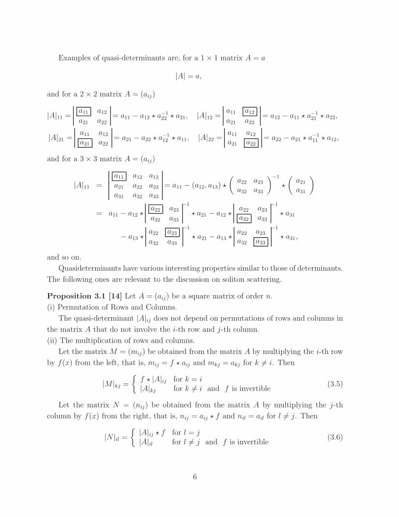
Examples of quasi-determinants are, for a 1 × 1 matrix A = a
|A| = a,
and for a 2 × 2 matrix A = (aij)
|A|11 =a11 a12a21 a22
= a11 − a12 ⋆ a−122 ⋆ a21, |A|12 =
a11 a12a21 a22
= a12 − a11 ⋆ a−121 ⋆ a22,
|A|21 =a11 a12a21 a22
= a21 − a22 ⋆ a−112 ⋆ a11, |A|22 =
a11 a12a21 a22
= a22 − a21 ⋆ a−111 ⋆ a12,
and for a 3 × 3 matrix A = (aij)
|A|11 =
a11 a12 a13a21 a22 a23a31 a32 a33
= a11 − (a12, a13) ⋆
(a22 a23a32 a33
)−1
⋆
(a21a31
)
= a11 − a12 ⋆a22 a23a32 a33
−1
⋆ a21 − a12 ⋆a22 a23a32 a33
−1
⋆ a31
− a13 ⋆a22 a23a32 a33
−1
⋆ a21 − a13 ⋆a22 a23a32 a33
−1
⋆ a31,
and so on.
Quasideterminants have various interesting properties similar to those of determinants.
The following ones are relevant to the discussion on soliton scattering.
Proposition 3.1 [14] Let A = (aij) be a square matrix of order n.
(i) Permutation of Rows and Columns.
The quasi-determinant |A|ij does not depend on permutations of rows and columns in
the matrix A that do not involve the i-th row and j-th column.
(ii) The multiplication of rows and columns.
Let the matrix M = (mij) be obtained from the matrix A by multiplying the i-th row
by f(x) from the left, that is, mij = f ⋆ aij and mkj = akj for k 6= i. Then
|M |kj =
{f ⋆ |A|ij for k = i|A|kj for k 6= i and f is invertible
(3.5)
Let the matrix N = (nij) be obtained from the matrix A by multiplying the j-th
column by f(x) from the right, that is, nij = aij ⋆ f and nil = ail for l 6= j. Then
|N |il =
{|A|ij ⋆ f for l = j|A|il for l 6= j and f is invertible
(3.6)
6

4 NC Integrable Hierarchy and Soliton Solutions
In this section, we give exact multi-soliton solutions to noncommutative integrable hierar-
chies in terms of quasi-determinants. In the commutative case, determinants of Wronski
matrices play crucial roles. In the noncommutative case, quasi-determinants give a better
formulation. We review foundation of the noncommutative KP hierarchy and the reduced
hierarchies, so called noncommutative Gelfand-Dickey (GD) hierarchies, and present the
exact multi-soliton solutions to them developed by Etingof, Gelfand and Retakh [11]. (See
also [18])
An N -th order pseudo-differential operator A is represented as follows
A = aN∂Nx + aN−1∂
N−1x + · · · + a0 + a−1∂
−1x + a−2∂
−2x + · · · , (4.1)
where ai is a function of x associated with noncommutative associative products (here,
the star products). When the coefficient of the highest order aN equals to 1, we call it
monic. Here we introduce the following symbols:
A≥r := ∂Nx + aN−1∂N−1x + · · · + ar∂
rx, (4.2)
A≤r := A−A≥r+1 = ar∂rx + ar−1∂
r−1x + · · · . (4.3)
The action of a differential operator ∂nx on a multiplicity operator f is formally defined
as the following generalized Leibniz rule:
∂nx · f :=∑
i≥0
(ni
)(∂ixf)∂n−i, (4.4)
where the binomial coefficient is given by(ni
):=
n(n− 1) · · · (n− i + 1)
i(i− 1) · · ·1. (4.5)
We note that the definition of the binomial coefficient (4.5) is applicable to the case of
negative n, which implies that the action of negative power of differential operators is
defined.
The composition of pseudo-differential operators is also well-defined and the total set of
pseudo-differential operators forms an operator algebra. For a monic pseudo-differential
operator A, there exist the unique inverse A−1 and the unique m-th root A1/m which
commute with A. (These proofs are all the same as commutative ones as far as the
commutative limit exists.) For more on pseudo-differential operators and Sato’s theory,
see e.g. [3, 4, 7, 34].
7

4.1 Noncommutative KP and KdV hierarchies
In order to define the noncommutative KP hierarchy, let us introduce a monic pseudo-
differential operator:
L = ∂x + u2∂−1x + u3∂
−2x + u4∂
−3x + · · · , (4.6)
where the coefficients uk (k = 2, 3, . . .) are functions of infinite coordinates ~x := (x1, x2, . . .)
with x1 ≡ x:
uk = uk(x1, x2, . . .). (4.7)
The noncommutativity is introduced into the coordinates (x1, x2, . . .) as Eq. (2.1) here.
In order to define the noncommutative KP hierarchy, let us introduce a differential
operator Bm as follows:
Bm := (L ⋆ · · · ⋆ L︸ ︷︷ ︸m times
)≥0 =: (Lm)≥0. (4.8)
The noncommutative KP hierarchy is defined as follows:
∂mL = [Bm, L]⋆ , m = 1, 2, . . . , (4.9)
where the action of ∂m := ∂/∂xm on the pseudo-differential operator L is defined by
∂mL := [∂m, L]⋆ or ∂m∂kx = 0. The KP hierarchy gives rise to a set of infinite differential
equations with respect to infinite kind of fields from the coefficients in Eq. (4.9) for a
fixed m. Hence it contains huge amount of differential (evolution) equations for all m.
The LHS of Eq. (4.9) becomes ∂muk which shows a kind of flow in the xm direction.
If we put the constraint (Ll)≤−1 = 0 or equivalently Ll = Bl (l = 2, 3, · · · ) on the non-
commutative KP hierarchy (4.9), we get a reduced noncommutative KP hierarchy which
is called the l-reduction of the noncommutative KP hierarchy, or the noncommutative
lKdV hierarchy, or the l-th noncommutative GD hierarchy. In particular, the 2-reduction
of noncommutative KP hierarchy is just the noncommutative KdV hierarchy. We can
easily show
∂uk∂xnl
= 0, (4.10)
for all n, k because ∂Ll/∂xnl = [Bnl, Ll] = [(Ll)n, Ll] = 0. This time, the constraint
Ll = Bl gives simple relationships which make it possible to represent infinite kind of
fields ul+1, ul+2, ul+3, . . . in terms of (l − 1) kind of fields u2, u3, . . . , ul. (cf. Appendix A
in [23].)
Let us see explicit examples.
8

• Noncommutative KP hierarchy
The coefficients of each powers of (pseudo-)differential operators in the noncom-
mutative KP hierarchy (4.9) yield a series of infinite noncommutative “evolution
equations,” that is, for m = 1
∂1−kx ) ∂1uk = u′k, k = 2, 3, . . . ⇒ x1 ≡ x, (4.11)
for m = 2
∂−1x ) ∂2u2 = u′′2 + 2u′3,
∂−2x ) ∂2u3 = u′′3 + 2u′4 + 2u2 ⋆ u
′2 + 2[u2, u3]⋆,
∂−3x ) ∂2u4 = u′′4 + 2u′5 + 4u3 ⋆ u
′2 − 2u2 ⋆ u
′′2 + 2[u2, u4]⋆,
∂−4x ) ∂2u5 = · · · , (4.12)
and for m = 3
∂−1x ) ∂3u2 = u′′′2 + 3u′′3 + 3u′4 + 3u′2 ⋆ u2 + 3u2 ⋆ u
′2,
∂−2x ) ∂3u3 = u′′′3 + 3u′′4 + 3u′5 + 6u2 ⋆ u
′3 + 3u′2 ⋆ u3 + 3u3 ⋆ u
′2 + 3[u2, u4]⋆,
∂−3x ) ∂3u4 = u′′′4 + 3u′′5 + 3u′6 + 3u′2 ⋆ u4 + 3u2 ⋆ u
′4 + 6u4 ⋆ u
′2
−3u2 ⋆ u′′3 − 3u3 ⋆ u
′′2 + 6u3 ⋆ u
′3 + 3[u2, u5]⋆ + 3[u3, u4]⋆,
∂−4x ) ∂3u5 = · · · . (4.13)
These contain the (2 + 1)-dimensional noncommutative KP equation (2.8) with
2u2 ≡ u, x2 ≡ y, x3 ≡ t and ∂−1x f(x) =
∫ xdx′f(x′). We note that infinite kind of
fields u3, u4, u5, . . . are represented in terms of one kind of field 2u2 ≡ u as is seen
in Eq. (4.12).
• Noncommutative KdV Hierarchy (2-reduction of the noncommutative KP hierarchy)
Putting the constraint L2 = B2 =: ∂2x +u on the noncommutative KP hierarchy, we
get the noncommutative KdV hierarchy. We note that the even-th flows are trivial.
The following noncommutative hierarchy
∂u
∂xm=[Bm, L
2]⋆, (4.14)
has neither positive nor negative power of (pseudo-)differential operators for the
same reason as commutative case and gives rise to the m-th KdV equation for each
m = 1, 3, 5, · · · . The noncommutative KdV hierarchy (4.14) coincides with the
(1 + 1)-dimensional noncommutative KdV equation for m = 3 with x3 ≡ t, (2.3)
9

and and with the (1 + 1)-dimensional 5-th noncommutative KdV equation [55] for
m = 5 with x5 ≡ t:
u =1
16u′′′′′ +
5
16(u ⋆ u′′′ + u′′′ ⋆ u) +
5
8(u′ ⋆ u′ + u ⋆ u ⋆ u)′. (4.15)
In this way, we can generate infinite set of the l-reduced noncommutative KP hierarchies.
Explicit examples are seen in e.g. [23]. (See also [5, 33, 38, 46, 56, 57].)
4.2 Multi-soliton Solutions to NC KP and KdV hierarchies
Now we construct multi-soliton solutions of the noncommutative KP hierarchy. Let us
introduce the following functions,
fs(~x) = eξ(~x;ks)⋆ + aseξ(~x;k′s)⋆ , where ξ(~x; k) = x1k + x2k
2 + x3k3 + · · · , (4.16)
where ks, k′s and as are constants. Star exponential functions are defined by
ef(x)⋆ := 1 +∞∑
n=1
1
n!f(x) ⋆ · · · ⋆ f(x)︸ ︷︷ ︸
n times
. (4.17)
An N -soliton solution to the noncommutative KP hierarchy (4.9) is given by [11],
L = ΦN ⋆ ∂xΦ−1N , (4.18)
where
ΦN ⋆ f = |W (f1, . . . , fN , f)|N+1,N+1,
=
f1 f2 · · · fN ff ′1 f ′
2 · · · f ′N f ′
......
. . ....
...
f(N−1)1 f
(N−1)2 · · · f
(N−1)N f (N−1)
f(N)1 f
(N)2 · · · f
(N)N f (N)
. (4.19)
The Wronski matrix W (f1, f2, · · · , fm) is given by
W (f1, f2, · · · , fm) :=
f1 f2 · · · fmf ′1 f ′
2 · · · f ′m
......
. . ....
f(m−1)1 f
(m−1)2 · · · f
(m−1)m
, (4.20)
where f1, f2, · · · , fm are functions of x and f ′ := ∂f/∂x, f ′′ := ∂2f/∂x2, f (m) :=
∂mf/∂xm and so on.
10

In the commutative limit, ΦN ⋆ f is reduced to
ΦN ⋆ f −→detW (f1, f2, . . . , fN , f)
detW (f1, f2, . . . , fN), (4.21)
which just coincides with the commutative N -soliton solution [7]. In this respect, quasi-
determinants are fit to this framework of the Wronskian solutions, however, give a new
formulation of it.
From Eq. (4.18), we have a more explicit form as
u2 = ∂x
(N∑
s=1
W ′s ⋆ W
−1s
), where Ws := |W (f1, . . . , fs)|ss. (4.22)
In the soliton solutions, The l-reduction condition (Ll)≤−1 = 0 or Ll = Bl is equivalent
to the constraint ks = ǫk′s (s = 1, 2, · · · , N), where ǫ is the l-th root of unity.
4.3 Asymptotic Behavior of the Exact Soliton Solutions
In this subsection, we discuss asymptotic behavior of the N -soliton solutions in asymptotic
region of infinitely past and future. In the star-product formalism, all coordinates are
regarded as c-number functions. We can as usual plot the configurations and interpret
the positions of localized wave packet lump, and read phase shifts. Here we restrict
ourselves to noncommutative KdV and KP equations (the third flow of the hierarchies)
with space-time noncommutativity [x, t]⋆ = iθ where (x, t) ≡ (x1, x3). Discussion to other
noncommutative hierarchies is similarly made [27].
First, let us comment on an important formula which is relevant to one-soliton solu-
tions. Let x, t be noncommutative space-time coordinates. Introducing new noncommu-
tative coordinates as z := x + vt, z := x− vt, we can easily find
f(z) ⋆ g(z) = f(z)g(z) (4.23)
because the star-product (2.2) is rewritten in terms of (z, z) as
f(z, z) ⋆ g(z, z) = eivθ(∂z1∂z2−∂z1∂z2)f(z1, z1)g(z2, z2)∣∣∣ z1 = z2 = z
z1 = z2 = z.
(4.24)
Hence noncommutative one soliton-solutions can be the same as commutative ones.
When f(x) is a linear function, the star exponential function ef(x)⋆ is tractable because
it satisfies
(eξ(~x;k)⋆ )−1 = e−ξ(~x;k)⋆ , (4.25)
∂xeξ(~x;k)⋆ = keξ(~x;k)⋆ . (4.26)
11

These formula play crucial roles in discussion on asymptotic behavior of the N -soliton
solutions.
4.3.1 Asymptotic behavior of noncommutative KdV solitons
First, let us discuss the asymptotic behavior of the N -soliton solutions to the noncom-
mutative KdV equation. The noncommutative KdV hierarchy is the 2-reduction of the
noncommutative KP hierarchy and realized by putting k′s = −ks on the N -soliton solu-
tions to the noncommutative KP hierarchy. Here the constants ks and as are non-zero
real numbers and as is positive. Because of the permutation property of the columns of
quasi-determinants in Proposition 3.1 (i), we can assume k1 < k2 < · · · < kN .
Let us discuss the soliton solutions to the noncommutative KdV equation where the
coordinates are specified as (x, t) ≡ (x1, x3). Let us define a new coordinate X := x+ k2I t
comoving with the I-th soliton and take t → ±∞ limit. We note that X is finite at any
time. Then, because of x+ k2st = x+ k2I t+ (k2s − k2I )t, either eks(x+k2s t)⋆ or e
−ks(x+k2st)⋆ goes
to zero for s 6= I. Hence the behavior of fs becomes at t→ +∞:
fs(~x) −→
ase−ks(x+k2st)⋆ s < I
ekI (x+k2
It)
⋆ + aIe−kI(x+k2
It)
⋆ s = I
eks(x+k2st)⋆ s > I,
(4.27)
and at t→ −∞:
fs(~x) −→
eks(x+k2st)⋆ s < I
ekI (x+k2
It)
⋆ + aIe−kI(x+k2
It)
⋆ s = I
ase−ks(x+k2st)⋆ s > I.
(4.28)
We note that the s-th (s 6= I) column is proportional to a single exponential function
e±ks(x+k2st)⋆ due to Eq. (4.26). Because of the multiplication property of columns of quasi-
determinants in Proposition 3.1 (ii), we can eliminate a common invertible factor from
the s-th column in |A|ij where s 6= j. (Note that this exponential function is actually
invertible as is shown in Eq. (4.25).) Hence the N -soliton solution becomes the following
simple form where only the I-th column is non-trivial, at t→ +∞:
ΦN ⋆ f →
1 · · · 1 eξ(~x;kI)⋆ + aIe
−ξ(~x;kI)⋆ 1 · · · 1 f
−k1 · · · −kI−1 kI(eξ(~x;kI)⋆ − aIe
−ξ(~x;kI)⋆ ) kI+1 · · · kN f ′
......
......
......
(−k1)N−1 · · · (−kI−1)
N−1 kN−1I (e
ξ(~x;kI)⋆ + (−1)N−1aIe
−ξ(~x;kI)⋆ ) kN−1
I+1 · · · kN−1N f (N−1)
(−k1)N · · · (kI−1)
N kNI (eξ(~x;kI)⋆ + (−1)NaIe
−ξ(~x;kI)⋆ ) kNI+1 · · · kNN f (N)
,
12
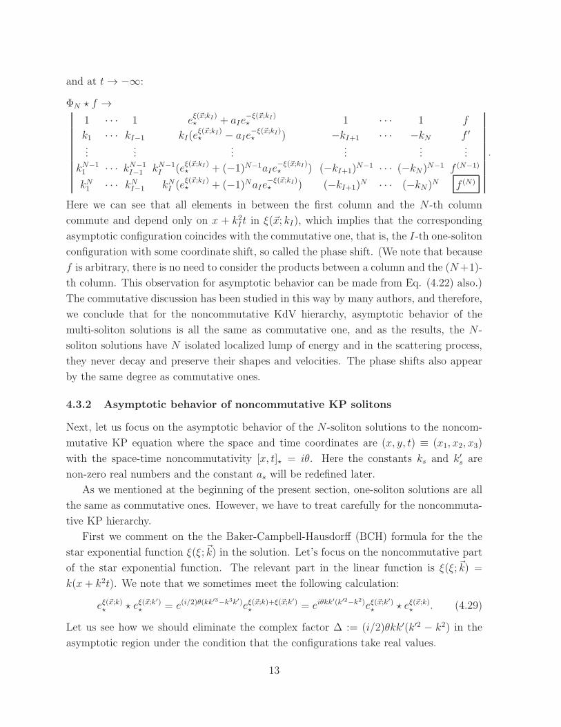
and at t→ −∞:
ΦN ⋆ f →
1 · · · 1 eξ(~x;kI)⋆ + aIe
−ξ(~x;kI)⋆ 1 · · · 1 f
k1 · · · kI−1 kI(eξ(~x;kI)⋆ − aIe
−ξ(~x;kI)⋆ ) −kI+1 · · · −kN f ′
......
......
......
kN−11 · · · kN−1
I−1 kN−1I (e
ξ(~x;kI)⋆ + (−1)N−1aIe
−ξ(~x;kI)⋆ ) (−kI+1)
N−1 · · · (−kN)N−1 f (N−1)
kN1 · · · kNI−1 kNI (eξ(~x;kI)⋆ + (−1)NaIe
−ξ(~x;kI)⋆ ) (−kI+1)
N · · · (−kN)N f (N)
.
Here we can see that all elements in between the first column and the N -th column
commute and depend only on x + k2I t in ξ(~x; kI), which implies that the corresponding
asymptotic configuration coincides with the commutative one, that is, the I-th one-soliton
configuration with some coordinate shift, so called the phase shift. (We note that because
f is arbitrary, there is no need to consider the products between a column and the (N+1)-
th column. This observation for asymptotic behavior can be made from Eq. (4.22) also.)
The commutative discussion has been studied in this way by many authors, and therefore,
we conclude that for the noncommutative KdV hierarchy, asymptotic behavior of the
multi-soliton solutions is all the same as commutative one, and as the results, the N -
soliton solutions have N isolated localized lump of energy and in the scattering process,
they never decay and preserve their shapes and velocities. The phase shifts also appear
by the same degree as commutative ones.
4.3.2 Asymptotic behavior of noncommutative KP solitons
Next, let us focus on the asymptotic behavior of the N -soliton solutions to the noncom-
mutative KP equation where the space and time coordinates are (x, y, t) ≡ (x1, x2, x3)
with the space-time noncommutativity [x, t]⋆ = iθ. Here the constants ks and k′s are
non-zero real numbers and the constant as will be redefined later.
As we mentioned at the beginning of the present section, one-soliton solutions are all
the same as commutative ones. However, we have to treat carefully for the noncommuta-
tive KP hierarchy.
First we comment on the the Baker-Campbell-Hausdorff (BCH) formula for the the
star exponential function ξ(ξ;~k) in the solution. Let’s focus on the noncommutative part
of the star exponential function. The relevant part in the linear function is ξ(ξ;~k) =
k(x + k2t). We note that we sometimes meet the following calculation:
eξ(~x;k)⋆ ⋆ eξ(~x;k′)
⋆ = e(i/2)θ(kk′3−k3k′)eξ(~x;k)+ξ(~x;k′)
⋆ = eiθkk′(k′2−k2)eξ(~x;k
′)⋆ ⋆ eξ(~x;k)⋆ . (4.29)
Let us see how we should eliminate the complex factor ∆ := (i/2)θkk′(k′2 − k2) in the
asymptotic region under the condition that the configurations take real values.
13

From Eq. (4.22), naive one-soliton solution can be expressed as follows:
u2 = ∂x
(∂x(eξ(~x;k)⋆ + aeξ(~x;k
′)⋆ ) ⋆ (eξ(~x;k)⋆ + aeξ(~x;k
′)⋆ )−1
)
= ∂x
((ki + ak′i∆eη(~x;k,k
′)⋆ ) ⋆ (1 + a∆eη(~x;k,k
′)⋆ )−1
), (4.30)
where η(~x; k, k′) := x(k′ − k) + y(k′2 − k2) + t(k′3 − k3). We note that the complex
factor ∆ cannot be absorbed by redefining a coordinate such as x → x + (k′ − k)−1∆
because the space-time coordinates are real.3 Instead of this, we redefine a positive real
constant a := a∆ in order to absorb the complex factor ∆ so that f1 = eξ(~x;k)⋆ +ae
ξ(~x;k′)⋆ =(
1 + aeη(~x;k,k′)⋆
)⋆ e
ξ(~x;k)⋆ . This avoids the coordinate shift by a complex number. The
configuration in asymptotic region is real.
This point becomes important for scattering process of the multi-soliton solutions. We
will soon see that the constants as in the N -soliton solution to the noncommutative KP
equation should be replaced with a positive real number as which satisfies as = as∆−1s
where ∆s := e(i/2)θksk′
s(k′2s −k2s).
Let us define new coordinates comoving with the I-th soliton as follows:
X := x + kIy + k2I t, Y := x + k′Iy + k′2I t, (4.31)
so that X, Y are finite in the asymptotic region. Then the function ξ(x, y, t; ks) can be
rewritten in terms of the new coordinates as ξ(X, Y, t; ks) = A(ks)X + B(ks)Y + C(ks)t
where A(ks), B(ks) and C(ks) are real constants depending on kI , k′I and ks. We can get
from Eq. (4.31)(xy
)=
1
k′I − kI
(k′IX − kIY + kIk
′I(k
′I − kI)t
−X + Y + (k2I − k′2I )t
), (4.32)
and find
ξ = x + ksy + kn−1s t =
k′I − ksk′I − kI
X +ks − kIk′I − kI
Y + (ks − kI)(ks − k′I)t.
Here we assume that C(ks) 6= C(k′s) which corresponds to pure soliton scatterings. (The
condition C(ks) = C(k′s) could lead to soliton resonances. For commutative discussion,
see e.g. [45], and [32] as well.)
Now let us take t → ±∞ limit, then, for the same reason as in the noncommutative
KdV equation, we can see that the asymptotic behavior of fs becomes:
fs(~x) −→
{Ase
ξ(~x;ks)⋆ s 6= I
eξ(~x;kI)⋆ + aIe
ξ(~x;k′I)
⋆ s = I(4.33)
3 In [39], similar observations are made of the noncommutative Burgers equation where the noncom-mutative parameter is not real but pure imaginary. This implies that the factor ∆ is real and can beabsorbed by a coordinate shift which affects the phase shift.
14

where As is some real constant whose value is 1 or as, and ks is a real constant taking a
value of ks or k′s. As in the case of the noncommutative KdV equation, the s-th (s 6= I)
column is proportional to a single exponential function and we can eliminate this factor
from the s-th column. Hence in the asymptotic region t → ±∞, the N -soliton solution
becomes the following simple form where only the I-th column is non-trivial:
ΦN ⋆ f →
1 · · · 1 eξ(~x;kI)⋆ + aIe
ξ(~x;k′I)
⋆ 1 · · · 1 f
k1 · · · kI−1 kIeξ(~x;kI)⋆ + aIk
′Ie
ξ(~x;k′I)
⋆ kI+1 · · · kN f ′
......
......
......
kN−11 · · · kN−1
I−1 kN−1I e
ξ(~x;kI)⋆ + aIk
′N−1I e
ξ(~x;k′I)
⋆ kN−1I+1 · · · kN−1
N f (N−1)
kN1 · · · kNI−1 kNI eξ(~x;kI)⋆ + aIk
′NI e
ξ(~x;k′I)
⋆ kNI+1 · · · kNN f (N)
=
1 · · · 1 1 + aIeη(~x;kI ,k
′
I)
⋆ 1 · · · 1 f
k1 · · · kI−1 kI + aIk′Ie
η(~x;kI ,k′
I)
⋆ kI+1 · · · kN f ′
......
......
......
kN−11 · · · kN−1
I−1 kN−1I + aIk
′N−1I e
η(~x;kI ,k′
I)
⋆ kN+1I+1 · · · kN−1
N f (N−1)
kN1 · · · kNI−1 kNI + aIk′NI e
η(~x;kI ,k′
I)
⋆ kNI+1 · · · kNN f (N)
.
Here we can see that all elements between the first column and the N -th column are
real and depend only on x(k′I − kI) + t(k′3I − k3I ) for noncommutative coordinates. This
implies that the corresponding asymptotic configuration coincides with the commutative
one. Hence, we can also conclude that for the noncommutative KP equation, asymptotic
behavior of the multi-soliton solutions is all the same as commutative one in the process
of pure soliton scatterings. As the results, the N -soliton solutions possess N isolated
localized lump of energy and in the pure scattering process, they never decay and preserve
their shapes and velocities of the localized solitary waves. This coincides with the result
on 2-soliton scattering studied by Paniak [47].
As is suggested by the stability of the N -soliton solution, there actually exist infinite
conserved densities of the noncommutative KP equation with space-time noncommuta-
tivity:
σn = coef−1Ln − 3θ ((coef−1L
n) ⋄ u′3 + (coef−2Ln) ⋄ u′2) , n = 1, 2, · · · (4.34)
where coef−lLn denotes the coefficient of ∂−l in Ln. (In particular, coef−1L
n is the residue
of Ln.) The product “⋄” is called the Strachan’s product [51] and defined by
f(x) ⋄ g(x) :=∞∑
p=0
(−1)p
(2p+ 1)!
(1
2θij∂
(x′)i ∂
(x′′)j
)2p
f(x′)g(x′′)∣∣∣x′=x′′=x
. (4.35)
15
This is a commutative and non-associative product. Conserved densities for one-soliton
configuration are not deformed in the noncommutative extension because one soliton
solutions can be always reduced to commutative ones
5 NC ASDYM Hierarchy and Soliton Solutions
Finally, we present noncommutative anti-self-dual Yang-Mills (ASDYM) equations in 4
dimension and its hierarchy generalization. Let (x0, x1, x2, · · · ; y0, y1, y2, · · · ) be complex
coordinates and define covariant derivatives Dxk:= ∂xk
+ Axk, Dyl := ∂yl + Ayl (k, l =
0, 1, 2, · · · ) where Axkand Ayl are n × n complex matrices. Noncommutativity is intro-
duced into the coordinates.
Let us consider the following linear systems:
Lk ⋆ ψ := (Dxk− ζDxk−1
) ⋆ ψ, (5.1)
Ml ⋆ ψ := (Dyl − ζDyl−1) ⋆ ψ, (5.2)
where ζ ∈ CP 1 is a spectral parameter which commutes with all spatial coordinates. The
compatibility condition of the linear systems is [Lk,Ml]⋆ = 0 for any k, l. This yields an
infinite systems of partial differential equations, which is called the noncommutative anti-
self-dual Yang-Mills hierarchy. By identification of x0 ≡ z, x1 ≡ w, y0 ≡ −w, y1 ≡ z, the
compatibility condition for k = l = 1 coincides with the noncommutative anti-self-dual
Yang-Mills equation (2.9). For the commutative anti-self-dual Yang-Mills hierarchies, see
e.g. [2, 40, 43, 52, 53].
The noncommutative anti-self-dual Yang-Mills hierarchy equations can be rewritten
as the following form:
∂yl(J−1 ⋆ ∂xk−1
J) − ∂xk(J−1 ⋆ ∂yl−1
J) = 0, (5.3)
where J is an n × n matrix. The equation (5.3) and the matrix J is called the noncom-
mutative Yang’s hierarchy equation and the Yang’s J-matrix, respectively. For k = l = 1,
this coincides with the noncommutative Yang’s equation.
Anti-self-dual gauge fields can be reproduced from the solution J to the equation (5.3)
by decomposition J = h−1 ⋆ h as
Ayl = −(∂ylh) ⋆ h−1, Axk= −(∂xk
h) ⋆ h−1, Axk−1= −(∂xk−1
h) ⋆ h−1, Ayl−1= −(∂yl−1
h) ⋆ h−1.
The proof is the same as the noncommutative anti-self-dual Yang-Mills equation. (See
e.g. [15].)
16

From now on, we focus on the n = 2 case. The J-matrix can be reparametrized
without loss of generality as follows:
J =
[p− r ⋆ q−1 ⋆ s −r ⋆ q−1
q−1 ⋆ s q−1
]. (5.4)
Exact solutions of the m-th Atiyah-Ward ansatz are represented in terms of quasideter-
minants (m = 0, 1, 2, · · · ):
pm =
ϕ0 ϕ−1 · · · ϕ−m
ϕ1 ϕ0 · · · ϕ1−m...
.... . .
...ϕm ϕm−1 · · · ϕ0
−1
, qm =
ϕ0 ϕ−1 · · · ϕ−m
ϕ1 ϕ0 · · · ϕ1−m...
.... . .
...ϕm ϕm−1 · · · ϕ0
−1
,
rm =
ϕ0 ϕ−1 · · · ϕ−m
ϕ1 ϕ0 · · · ϕ1−m...
.... . .
...ϕm ϕm−1 · · · ϕ0
−1
, sm =
ϕ0 ϕ−1 · · · ϕ−m
ϕ1 ϕ0 · · · ϕ1−m...
.... . .
...ϕm ϕm−1 · · · ϕ0
−1
. (5.5)
where the scalar functions ϕi(x; y) can be determined from a scalar function ϕ0 recursively
by the chasing relation:
∂ϕi
∂yl= −
∂ϕi+1
∂yl−1
,∂ϕi
∂xk= −
∂ϕi+1
∂xk−1
, −m ≤ i ≤ m− 1 (m ≥ 2). (5.6)
The scalar function ϕ0 is a solution to the linear equation (∂xk∂yk−1 − ∂yk∂xk−1)ϕ0 = 0.
5.1 Asymptotic behavior of noncommutative ASDYM solitons
Here let us discuss N soliton solutions to the anti-self-dual Yang-Mills hierarchy (5.3)
and asymptotic behaviors of the 2-soliton case. In order to discuss it, we have to pick a
specified coordinate up in order to identify it with time coordinate.
By the identification of xk−1 ≡ z = t1 − it2, xk ≡ w = t3 + it4, yl−1 ≡ −w = −t3 −
it4, yl ≡ z = t1 + it2 where tµ (µ = 1, 2, 3, 4) is a real coordinate, the linear equation
becomes the Laplace equation in 4-dimension:
∂2ϕ0(t) = 0, (5.7)
where ∂2 := ∂µ∂µ = ∂21 + ∂22 + ∂23 + ∂24 . The Yang’s equation (5.3) becomes
∂z(J−1 ⋆ ∂zJ) + ∂w(J−1 ⋆ ∂wJ) = 0. (5.8)
17
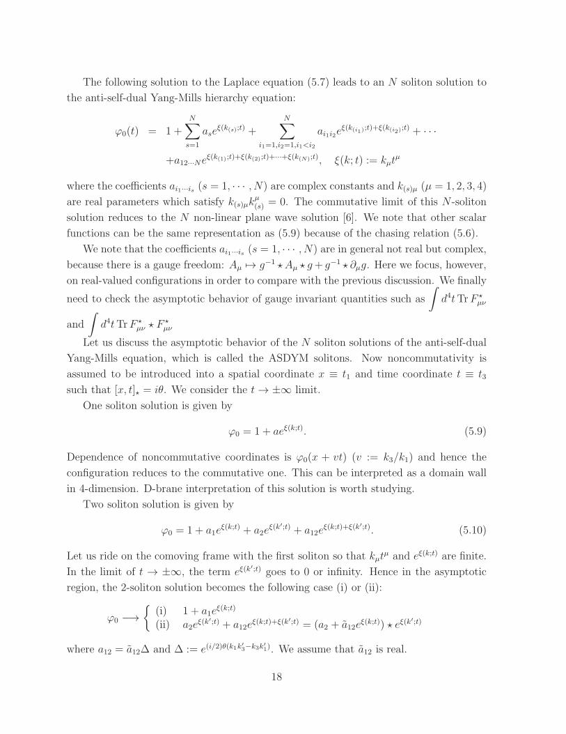
The following solution to the Laplace equation (5.7) leads to an N soliton solution to
the anti-self-dual Yang-Mills hierarchy equation:
ϕ0(t) = 1 +
N∑
s=1
aseξ(k(s);t) +
N∑
i1=1,i2=1,i1<i2
ai1i2eξ(k(i1);t)+ξ(k(i2);t) + · · ·
+a12···Neξ(k(1);t)+ξ(k(2);t)+···+ξ(k(N);t), ξ(k; t) := kµt
µ
where the coefficients ai1···is (s = 1, · · · , N) are complex constants and k(s)µ (µ = 1, 2, 3, 4)
are real parameters which satisfy k(s)µkµ(s) = 0. The commutative limit of this N -soliton
solution reduces to the N non-linear plane wave solution [6]. We note that other scalar
functions can be the same representation as (5.9) because of the chasing relation (5.6).
We note that the coefficients ai1···is (s = 1, · · · , N) are in general not real but complex,
because there is a gauge freedom: Aµ 7→ g−1 ⋆Aµ ⋆ g+ g−1 ⋆ ∂µg. Here we focus, however,
on real-valued configurations in order to compare with the previous discussion. We finally
need to check the asymptotic behavior of gauge invariant quantities such as
∫d4tTrF ⋆
µν
and
∫d4tTrF ⋆
µν ⋆ F⋆µν
Let us discuss the asymptotic behavior of the N soliton solutions of the anti-self-dual
Yang-Mills equation, which is called the ASDYM solitons. Now noncommutativity is
assumed to be introduced into a spatial coordinate x ≡ t1 and time coordinate t ≡ t3
such that [x, t]⋆ = iθ. We consider the t→ ±∞ limit.
One soliton solution is given by
ϕ0 = 1 + aeξ(k;t). (5.9)
Dependence of noncommutative coordinates is ϕ0(x + vt) (v := k3/k1) and hence the
configuration reduces to the commutative one. This can be interpreted as a domain wall
in 4-dimension. D-brane interpretation of this solution is worth studying.
Two soliton solution is given by
ϕ0 = 1 + a1eξ(k;t) + a2e
ξ(k′;t) + a12eξ(k;t)+ξ(k′;t). (5.10)
Let us ride on the comoving frame with the first soliton so that kµtµ and eξ(k;t) are finite.
In the limit of t → ±∞, the term eξ(k′;t) goes to 0 or infinity. Hence in the asymptotic
region, the 2-soliton solution becomes the following case (i) or (ii):
ϕ0 −→
{(i) 1 + a1e
ξ(k;t)
(ii) a2eξ(k′;t) + a12e
ξ(k;t)+ξ(k′;t) = (a2 + a12eξ(k;t)) ⋆ eξ(k
′;t)
where a12 = a12∆ and ∆ := e(i/2)θ(k1k′
3−k3k′1). We assume that a12 is real.
18

In the case of (i), we can find that ϕ0(t, x) = ϕ0(x + vt) and hence the configuration
coincides with commutative one. In the case of (ii), we have to proceed the calculation.
As is commented, other scalar functions in the Atiyah-Ward ansatz solution (5.5) have
the form: ϕi = bi + cieξ(k;t) + die
ξ(k′;t) + rieξ(k;t)+ξ(k′;t) where bi, ci, di, ri are constants, and
bi, ci, di are real. Asymptotic behavior of (ii) is ϕi −→ (ci + rieξ(k;t)) ⋆ eξ(k
′;t). where
ri = ri∆ so that ri is real.
Because of the multiplication property of columns of quasideterminants, the Atiyah-
Ward ansatz solution (5.5) have the common asymptotic form: p, q, r, s→ f(t+vx)⋆eξ(k′;t).
The gauge fields can be recovered from the matrices h and h as in (5.11). Let us
decompose the matrix J into h and h as follows:
J =
[p ⋆−r ⋆ q−1s −r ⋆ q−1
q−1 ⋆ s q−1
]=
[1 r0 q
]−1
⋆
[p 0s 1
]= h−1 ⋆ h.
The gauge fields are calculated as
Az =−(∂zh) ⋆ h−1=
[−(∂zp) ⋆ p
−1 0−(∂zs) ⋆ p
−1 0
], Aw =−(∂wh) ⋆ h−1 =
[−(∂wp) ⋆ p
−1 0−(∂ws) ⋆ p
−1 0
],
Az =−(∂zh) ⋆ h−1=
[0 −(∂zr) ⋆ q
−1
0 −(∂zq) ⋆ q−1
], Aw =−(∂wh) ⋆ h−1=
[0 −(∂wr) ⋆ q
−1
0 −(∂wq) ⋆ q−1
].
We can see that the common factor eξ(k′;t) in p, q, r, s is canceled out here, and the coor-
dinate dependence in the gauge fields becomes Aµ(t, x) = Aµ(x + vt). Note that there is
no difference between commutative case and noncommutative case in the derivation from
(5.11). We can therefore conclude the gauge invariant quantities consist of F ⋆µν are the
same as commutative ones.
Let us consider the comoving frame with the second soliton where k′µtµ and eξ(k
′;t)
are finite. In the limit of t → ±∞, the factor eξ(k;t) goes to (i) 0 or (ii) infinity. The
case (i) reduces to one-soliton configuration. The case (ii) leads to, in similar way, the
following asymptotic behaviors of the scalar functions: ϕi → eξ(k;t) ⋆ (a1 + a12eξ(k′;t)),
ϕi → eξ(k;t) ⋆(di+ rieξ(k′;t)), and p, q, r, s→ eξ(k;t) ⋆f(x+v′t). We note that the coefficients
a1, a12, di, ri are the same as those in case (i).) We can see that the common factor eξ(k;t)
appears in the gauge fields as Aµ(x, t) → eξ(k;t) ⋆ A(x + v′t) ⋆ e−ξ(k;t) This is essentially
gauge equivalent to A(x+ v′t) up to constants which do not contribute the field strength.
Hence the gauge invariant quantities consist of F ⋆µν are the same as commutative ones in
this case as well.
Therefore we can conclude that the asymptotic behavior of the 2-soliton solutions is
the same as commutative one [6] and as the results, the 2-soliton solutions has 2 isolated
localized lump of energy and in the scattering process, they never decay and preserve
their shapes and velocities of the localized solitary waves.
19

Higher-charge soliton scattering is worth studying. For this purpose, Wronskian-type
solutions [44] would be suitable. This will be reported elsewhere.
Acknowledgments
One of the authors would like to thank the organizers at the workshop on Physics and
Mathematics of Nonlinear Phenomena (PMNP2017): 50 years of IST in Gallipoli, Italy.
The work of MH was supported by Grant-in-Aid for Scientific Research (#16K05318).
References
[1] M. J. Ablowitz and P. A. Clarkson, Solitons, Nonlinear Evolution Equations andInverse Scattering (Cambridge UP, 1991) Chapter 6.5 [ISBN/0-521-38730-2].
[2] M. J. Ablowitz, S. Chakravarty and L. A. Takhtajan, Commun. Math. Phys. 158(1993) 289;
[3] O. Babelon, D. Bernard and M. Talon, Introduction to classical integrable systems,(Cambridge UP, 2003) [ISBN/0-521-82267-X].
[4] M. B laszak, Multi-Hamiltonian Theory of Dynamical Systems (Springer, 1998)[ISBN/3-540-64251-X].
[5] S. Carillo, M. Lo Schiavo and C. Schiebold, SIGMA 12, 087 (2016)
[6] H. J. de Vega, Commun. Math. Phys. 116, 659 (1988).
[7] L. A. Dickey, Soliton equations and Hamiltonian systems (2nd Ed.), Adv. Ser. Math.Phys. 26 (2003) 1 [ISBN/9812381732].
[8] A. Dimakis and F. Muller-Hoissen, Phys. Lett. A 278 (2000) 139 [hep-th/0007074].
[9] A. Dimakis and F. Muller-Hoissen, “Extension of Moyal-deformed hierarchies of soli-ton equations,” nlin.si/0408023.
[10] E. V. Doktorov and S. B. Leble, A Dressing Method in Mathematical Physics,(Springer, 2010).
[11] P. Etingof, I. Gelfand and V. Retakh, Math. Res. Lett. 4 (1997) 413 [q-alg/9701008].
[12] P. Etingof, I. Gelfand and V. Retakh, Math. Res. Lett. 5 (1998) 1 [q-alg/9707017].
[13] I. Gelfand, S. Gelfand, V. Retakh and R. Wilson, Adv. Math. 193 (2005) 56[math.QA/0208146].
[14] I. Gelfand and V. Retakh, Funct. Anal. Appl. 25 (1991) 91; Funct. Anal. Appl. 2(1992) 1.
20

[15] C. R. Gilson, M. Hamanaka and J. J. C. Nimmo, Glasgow Mathematical Journal51-A (2009) 83 [arXiv:0709.2069].
[16] C. R. Gilson, M. Hamanaka and J. J. C. Nimmo, Proc. Roy. Soc. Lond. A 465, 2613(2009) [arXiv:0812.1222].
[17] C. R. Gilson and S. R. Macfarlane, J. Phys. A 42 (2009) 235202 [arXiv:0901.4918].
[18] C. R. Gilson and J. J. C. Nimmo, J. Phys. A 40, 3839 (2007) [nlin.si/0701027].
[19] C. R. Gilson, J. J. C. Nimmo and Y. Ohta, J. Phys. A 40, 12607 (2007)[nlin.SI/0702020].
[20] C. R. Gilson, J. J. C. Nimmo and C. M. Sooman, J. Phys. A 41, 085202 (2008)[arXiv:0711.3733].
[21] B. Haider and M. Hassan, J. Phys. A 41, 255202 (2008) [arXiv:0912.1984 [hep-th]].
[22] M. Hamanaka, “Noncommutative solitons and D-branes,” Ph. D thesis (Universityof Tokyo, 2003) hep-th/0303256.
[23] M. Hamanaka, J. Math. Phys. 46 (2005) 052701 [hep-th/0311206].
[24] M. Hamanaka, “Noncommutative solitons and integrable systems,” hep-th/0504001.
[25] M. Hamanaka, Phys. Lett. B 625 (2005) 324 [hep-th/0507112].
[26] M. Hamanaka, Nucl. Phys. B 741 (2006) 368 [hep-th/0601209].
[27] M. Hamanaka, JHEP 0702 (2007) 094 [hep-th/0610006].
[28] M. Hamanaka, Phys. Scripta 89, 038006 (2014) [arXiv:1101.0005 [hep-th]].
[29] M. Hamanaka and K. Toda, Phys. Lett. A 316 (2003) 77 [hep-th/0211148].
[30] M. Hamanaka and K. Toda, J. Phys. A 36 (2003) 11981 [hep-th/0301213].
[31] M. Hamanaka and K. Toda, Proc. Inst. Math. NAS Ukraine (2004) 404[hep-th/0309265].
[32] Y. Kodama, KP Solitons and the Grassmannians, (Springer, 2017)
[33] B. G. Konopelchenko and W. Oevel, “Matrix Sato theory and integrable systems in2+1 dimensions,” in Nonlinear evolution equations and dynamical systems, editedby M. Bolti, L. Martina and F. Pempinelli (World Sci., 1992) 87.
[34] B. Kupershmidt, KP or mKP (AMS, 2000) [ISBN/0821814001].
[35] O. Lechtenfeld, “Noncommutative solitons,” [hep-th/0605034].
[36] K. M. Lee, JHEP 0408, 054 (2004) [hep-th/0405244].
21

[37] C. X. Li, J. J. C. Nimmo and K. M. Tamizhmani , Proc. Roy. Soc. Lond. A 465,1441 (2009), [arXiv:0809.3833].
[38] W. X. Ma, J. Math. Phys. 51, 073505 (2010).
[39] L. Martina and O. K. Pashaev, “Burgers’ equation in non-commutative space-time,”hep-th/0302055.
[40] L. J. Mason and N. M. Woodhouse, Integrability, Self-Duality, and Twistor Theory(Oxford UP, 1996) [ISBN/0-19-853498-1].
[41] L. Mazzanti, “Topics in noncommutative integrable theories and holographic brane-world cosmology,” Ph. D thesis, arXiv:0712.1116.
[42] J. E. Moyal, Proc. Cambridge Phil. Soc. 45 (1949) 99; H. J. Groenewold, Physica 12(1946) 405.
[43] Y. Nakamura, J. Math. Phys. 29, 244 (1988).
[44] J. J. C. Nimmo, C. R. Gilson and Y. Ohta, Theor. Math. Phys. 122, 239 (2000)[Teor. Mat. Fiz. 122, 284 (2000)].
[45] K. Ohkuma and M. Wadati, J. Phys. Soc. Jap. 52, 749 (1983).
[46] P. J. Olver and V. V. Sokolov, Commun. Math. Phys. 193 (1998) 245.
[47] L. Paniak, “Exact noncommutative KP and KdV multi-solitons,” hep-th/0105185.
[48] V. Retakh and V. Rubtsov, J. Phys. A 43, 505204 (2010) [arXiv:1007.4168].
[49] M. Sakakibara, J. Phys. A 37, L599 (2004). [nlin.si/0408002].
[50] M. Siddiq, U. Saleem and M. Hassan, Mod. Phys. Lett. A 23, 115 (2008).
[51] I. A. B. Strachan, J. Geom. Phys. 21 (1997) 255 [hep-th/9604142].
[52] K. Suzuki, “Explorations of a self-dual Yang-Mills hierarchy,” Diploma thesis (MaxPlanck Institute for Dynamics and Self-Organization, 2006).
[53] K. Takasaki, Commun. Math. Phys. 94, 35 (1984).
[54] L. Tamassia, “Noncommutative supersymmetric / integrable models and string the-ory,” Ph. D thesis, hep-th/0506064.
[55] K. Toda, “Extensions of soliton equations to non-commutative (2 + 1) dimensions,”Proceedings of workshop on Integrable Theories, Solitons and Duality, Sao Paulo,Brazil, 1-6 July 2002 [JHEP PRHEP-unesp2002/038].
[56] J. P. Wang, J. Math. Phys. 47 (2006) 113508.
[57] N. Wang and M. Wadati, J. Phys. Soc. Jap. 73 (2004) 1689.
[58] R. S. Ward, Phil. Trans. Roy. Soc. Lond. A 315 (1985) 451.
22
Related Documents