Solitons in optics - University of Ljubljanamafija.fmf.uni-lj.si/seminar/files/2010_2011/solitons.pdf · Seminar Solitons in optics Author: Dan Grahelj Mentor: prof. dr. Igor Poberaj

Seminar

Solitons in optics

Author: Dan GraheljMentor: prof. dr. Igor Poberaj

Ljubljana, november 2010

Abstract

Solitons are the solutions of certain nonlinear partial differential equa-tions, with interesting properties. Because of a balance between nonlinearand linear effects, the shape of soliton wave pulses does not change duringpropagation in a medium. In the following seminar, I present the generalproperties of solitons and the way these can be used in physical applica-tions. Focusing on optical solitons, both temporal and spatial solitons arepresented together with the physical effects that make them possible. Theadvantages and difficulties regarding soliton based optical communicationare explained. Furthermore, the potential future application of solitonsand soliton interactions for ultra fast optical logical devices is introduced.

Contents

1 Solitons 21.1 General properties . . . . . . . . . . . . . . . . . . . . . . . . . . 21.2 A brief history . . . . . . . . . . . . . . . . . . . . . . . . . . . . 3

2 Optical solitons 32.1 Temporal solitons . . . . . . . . . . . . . . . . . . . . . . . . . . . 4

2.1.1 Derivation of the nonlinear Schrodinger equation . . . . . 52.1.2 Soliton solutions . . . . . . . . . . . . . . . . . . . . . . . 62.1.3 Soliton stability . . . . . . . . . . . . . . . . . . . . . . . . 82.1.4 Fiber losses . . . . . . . . . . . . . . . . . . . . . . . . . . 82.1.5 Soliton amplification . . . . . . . . . . . . . . . . . . . . . 9

2.2 Spatial solitons . . . . . . . . . . . . . . . . . . . . . . . . . . . . 102.3 Spatio-temporal solitons . . . . . . . . . . . . . . . . . . . . . . . 122.4 Soliton interactions . . . . . . . . . . . . . . . . . . . . . . . . . . 132.5 Soliton logic gates . . . . . . . . . . . . . . . . . . . . . . . . . . 13

3 Conclusion 15

4 References 15

1

1 Solitons

1.1 General properties

Although it is hard to find a precise definition of a soliton, the term is usuallyassociated with any solution of a nonlinear equation which

1. Represents a wave of permanent form

2. Is also localized (though moving)

3. Can interact strongly with other solitons and retain its identity

[1] In other words, a soliton is a wave packet (a pulse) that maintains its shapewhile traveling at a constant speed. Solitons are caused by a cancellation of non-linear and dispersive effects in the medium. [2] Dispersion is the phenomenonin which the phase velocity of a wave depends on its frequency. [3] Every wavepacket can be thought of as consisting of plane waves of several different fre-quencies. Because of dispersion, waves with different frequencies will travel atdifferent velocities and the shape of the pulse will therefore change over time.It is important to point out that dispersion does not add any new frequencycomponents to the original specter of the pulse, it merely rearranges the phaserelations between the existing ones. On the other hand, nonlinear effects (suchas the Kerr effect in optics) may modify the phase shift across the pulse and thuscreate new frequency components in the specter of the pulse (in optics this effectis known as self-phase modulation). If the original pulse has the right shape,nonlinear effects may exactly cancel dispersion thus producing a pulse with aconstant shape: a soliton. [2] The third above mentioned property of solitons,the fact that they can interact strongly and continue almost as if there had beenno interaction at all, is what led N. J. Zabusky and M. D. Kruskal to coin thename soliton (in order to emphasise their particle-like behavior in collisions).[1] While many nonlinear dispersive partial differential equations yield solitonsolutions the most important ones (of those describing physical systems) are theKorteweg-de Vries equation (describing waves on shallow water surfaces) andthe nonlinear Schrodinger equation (describing waves on deep water surfacesand more importantly light waves in optical fibers). [1] Examples of observ-able soliton solutions include solitary water waves (on the surface or undersea- internal waves) and also atmospheric solitons such as Morning Glory clouds(vast linear roll clouds produced by pressure solitons travelling in a temperatureinversion) . [4]

Figure 1: Morning Glory clouds in Queensland, Australia - these vast linearclouds are the product of pressure soliton waves. [4]

2

1.2 A brief history

In 1834, John Scott Russel, a Scottish naval architect was conducting experi-ments to determine the most efficient design for canal boats. During his experi-ments he discovered a phenomenon that he described as the wave of translation.He described his discovery in an article called Report on waves [5] which repre-sents the first scientific account of solitons in history. The phenomenon was awater wave that formed in a narrow channel and displayed some strange prop-erties. For one, the wave was stable, it neither flattened out or steepened likenormal waves and Russel was able to follow it for a few kilometers. Furthermore,the wave would not merge with other waves, a small wave traveling faster wouldrather overtake a large slower one. [5] Through a series of measurements, Russelmanaged to determine an empirical formula for the velocity of such waves butwas unable to find the correct equation of motion. [2]

Figure 2: A modern recreation of Russel’s wave of translation - a soliton waterwave. [6]

In 1895 Diederik Korteweg and Gustav de Vries derived a nonlinear partialdifferential equation (today known as the Korteweg-de Vries equation) thatdescribes Russel’s solitary waves. Their work fell into obscurity until 1965 whenNorman Zabusky and Martin Kruskal published their numerical solutions ofthe KdV equation (and invented the term soliton). In 1973 Akira Hasegawawas the first to suggest that solitons could exist in optical fibers, due to abalance between self-phase modulation and anomalous dispersion. In 1988 LinnMollenauer and his team transmitted soliton pulses over 4000 kilometers using aphenomenon called the Raman effect (see chapter 2.1.5), to provide optical gainin the fiber. Only three years later, a Bell research team transmitted solitonserror-free at 2.5 gigabits per second over more than 14000 kilometers, usingerbium (rare earth) optical fiber amplifiers. [2]

2 Optical solitons

In optics, the term soliton is used to refer to any optical field that does notchange during propagation because of a balance between nonlinear and disper-sive effects in the medium. In both cases, the nonlinear part in equations is aconsequence of the Kerr effect in media. [7] The Kerr effect is a phenomenon

3

where an applied electrical field induces a change in the refractive index of amaterial. What distinguishes the Kerr effect from others of this kind (e.g. thePockels effect) is that the change in refractive index is directly proportional tothe square of the electric field (or in other words, directly proportional to theintensity). The refractive index is then described by the following equation:

n(I) = n+ n2I (2.1)

where I is the field intensity and n2 the the second-order nonlinear refractiveindex. [3]

There are two main kinds of optical solitons: spatial and temporal solitons.Temporal solitons were discovered first and are often simply referred to as soli-tons in optics. We talk about temporal solitons when the electromagnetic fieldis already spatially confined (e.g. in optical fibers) and the pulse shape (in time)will not change because the nonlinear effects balance dispersion. Spatial soli-tons on the other hand may occur when the electromagnetic field is not spatiallyconfined but the pulse shape in space does not change with propagation becauseof nonlinear effects (self-focusing) balancing out diffraction. [7]

2.1 Temporal solitons

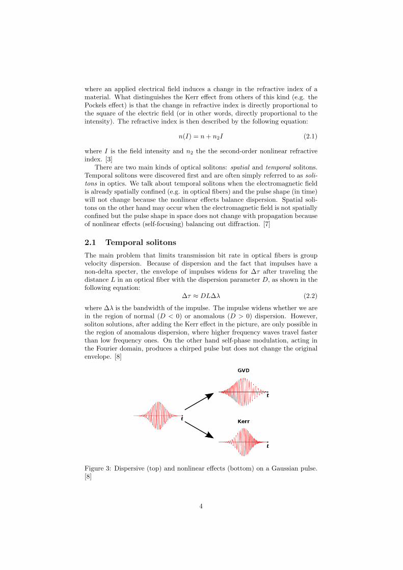
The main problem that limits transmission bit rate in optical fibers is groupvelocity dispersion. Because of dispersion and the fact that impulses have anon-delta specter, the envelope of impulses widens for ∆τ after traveling thedistance L in an optical fiber with the dispersion parameter D, as shown in thefollowing equation:

∆τ ≈ DL∆λ (2.2)

where ∆λ is the bandwidth of the impulse. The impulse widens whether we arein the region of normal (D < 0) or anomalous (D > 0) dispersion. However,soliton solutions, after adding the Kerr effect in the picture, are only possible inthe region of anomalous dispersion, where higher frequency waves travel fasterthan low frequency ones. On the other hand self-phase modulation, acting inthe Fourier domain, produces a chirped pulse but does not change the originalenvelope. [8]

Figure 3: Dispersive (top) and nonlinear effects (bottom) on a Gaussian pulse.[8]

4

2.1.1 Derivation of the nonlinear Schrodinger equation

An electric field propagating in a medium showing optical Kerr effect througha guiding structure (such as an optical fiber) that limits the power on the xyplane can be expressed in the following way:

E(r, t) = Amu(t, z)f(x, y)ei(k0z−w0t) (2.3)

where Am is the maximum amplitude of the field, u the envelope of the pulsenormalized to 1, f the shape of the pulse in the x, y plane, determined by theoptical fiber and k0 the angular wave number for propagation in the z direction.The scalar representation of the electric field is appropriate because of the smallbiefringence of optical fibers. [2] To obtain the wave equation for the slowlyvarying amplitude E(r, t), it is more convenient to work in the Fourier domain.

E(r, ω − ω0) =

∞∫−∞

E(r, t)e−i(w−w0)

Inserting (2.3) into the wave equation we obtain the Helmholtz equation wherethe refractive index depends on the frequency and also on the intensity:

∇2E + n2(w)k20E = 0 (2.5)

The phase change parameter β(w) = n(w)k0 can be described as:

β(w) = β0 + βl(w) + βnl = β0 + ∆β(w) (2.6)

[8] We assume that both dispersive and nonlinear effects are small (which is truein optical fibers [2]): |β0| � |∆β(w)|. It is therefore appropriate to approxi-mate the linear (dispersive) part with its Taylor expansion around some centralfrequency ω0:

β(w) = β0 + (ω − ω0)β1 +(ω − ω0)2

2β2 + βnl (2.7)

where βu = duβ(w)dωu . Inserting the electric field (2.3) into equation (2.5) we

obtain:

2iβ0∂u

∂z+ [β2(ω)− β2

0 ]u = 0 (2.8)

where we have neglected the second derivate of u because of the assumption

that u(z, ω) is a slowly varying function of z:∣∣∣∂2u∂z2

∣∣∣ � ∣∣β0 ∂u∂z ∣∣. This is known

as the slowly varying envelope approximation. Because of small dispersive andnonlinear effects we also make the following approximation:

β2(ω)− β20 ≈ 2β0∆β(ω) (2.9)

Transforming back into the time domain: ∆β(ω)⇐⇒ iβ1∂∂t −

β2

2∂2

∂t2 + βnl andexpressing the non linear component in terms of the amplitude of the field:

βnl = k0n2I = k0n2|E|22η0/n

= k0n2n|Am|22η0|u|2 (where η0 is the wave impedance of

empty space), we obtain:

i∂u

∂z+ iβ1

∂u

∂t− β2

2

∂2u

∂t2+

1

Lnl|u|2u = 0 (2.10)

5

Since we know that the pulse propagates in the direction of the z axis with thegroup velocity 1

β1, we make the substitution T = t−β1z, in order to follow only

the changing of the envelope of the pulse. Also, because we assume anomalousdispersion, we know that β2 < 0. The equation is now finally:

1

2

∂2u

∂τ2+ i

∂u

∂ζ+N2|u|2u = 0 (2.11)

[8] In this equation we introduce the so called soliton units, so that the equa-tion is in its general form. Equation (2.11) is the fundamental equation de-scribing temporal (and as we shall see also spatial) solitons. It is called thenonlinear Schrodinger equation 1. The variables in the equation are: τ = T

T0

where T0 is connected with the FWHM of the fundamental soliton solution(TFWHM = 2 ln(1 +

√2)T0 ≈ 1.763 T0), ζ = z

Ld, where Ld is a characteristic

length for effects of the dispersive term, connected with the dispersion coefficient(simmilar is Lnl, a characteristic length for nonlinear effects, connected with themaximum amplitude) and N2 = Ld

Lnl. It is easy to identify the dispersive (first)

and nonlinear (third) terms in the equation. [2] The physical meaning of theparameter N is the following:

1. if N � 1, then we can neglect the nonlinear part of the equation. Itmeans Ld � Lnl therefore the field will be affected by the linear effect(dispersion) much earlier than the nonlinear effect.

2. if N � 1, then the nonlinear effect will be more evident than dispersionand the pulse will spectrally broaden because of self-phase modulation.

3. if N ≈ 1, then the two effects balance each other and soliton solutions arepossible.

This of course holds when the length of the fiber2 L is L � Lnl and L � Ld,otherwise neither nonlinear nor dispersive effects will play a significant rolein pulse propagation. Normally, in the case when L < 50 km, nonlinear anddispersive effects may be neglected for pulses with T0 > 100 ps and P0 = |Am| <1 mW . However, Ld and Lnl become smaller as pulses become shorter and moreintense. For example, Ld and Lnl are ≈ 100 m for pulses with T0 ≈ 1 ps andP0 ≈ 1 W . For such optical pulses, both the dispersive and nonlinear effectsneed to be included if fiber length exceeds a few meters. [8]

2.1.2 Soliton solutions

ForN = 1 the solution of the equation is simple and is known as the fundamentalsolution:

u(τ, ζ) = sech(τ)eiζ/2 (2.12)

Since the phase term in the equation has no dependence on t, the soliton iscompletely nondispersive. That is, its shape does not change with z either inthe temporal domain or in the frequency domain. [2] For soliton solutions, Nmust be an integer and is said to be the order of the soliton.

1It is important to note that this equation got its name because of a simmilarity to the wellknown Schrodinger equation, but does not describe the evolution of quantum wave functions.[2]

2The described effects have almost no dependence on the other two dimensions of the fiber.[2]

6

Figure 4: Dispersion of a pulse of initial sech(T/τ) profile in a medium withoutnonlinear effects. The pulse FWHM broadens from 16.5 fs to 91.5 fs, aftertraveling the distance of 5 Z0 (confocal dispersive distances). [7]

Figure 5: Temporal soliton pulse of initial sech(T/τ) profile in a medium withboth dispersive and nonlinear effects. After propagating 5 Z0, the pulse positionand duration are the same. [7]

Higher order solitons3 change shape during propagation but in a periodic man-ner with the period ζ0 = π

2 . To give an example, the typical soliton period forpulses with T0 = 1 ps is about 80 m and scales as T 2

0 becoming 8 km whenT0 = 10 ps. Also, the maximum amplitude needed to produce higher ordersolitons scales as N2 compared to the one needed for the fundamental soliton.Since in higher order solitons, the maximum amplitude rises dramatically dur-ing the changing of the envelope in every soliton period, it is possible to obtainamplitudes which render some of the proposed approximations obsolete, or evensuch that may damage the medium. [8]

3Soliton solutions where N is an integer and N > 1. [8]

7

Figure 6: The intensity pulse shape of a third order (N = 3) soliton during onesoliton period. [8]

The evolution pattern of higher order solitons (as seen in Fig. 6) is the con-sequence of mutual dispersive and self-phase modulation effects. In the caseof a fundamental soliton, these effects balance each other so that neither pulseshape nor spectrum change during propagation. In higher order solitons, self-phase modulation dominates initially, but dispersion soon catches up leading toa periodic behavior. [8]

2.1.3 Soliton stability

The natural question to ask is what happens if the initial pulse shape and/ormaximum amplitude are not appropriate for a soliton solution. In other words,the scenario where N is not an integer. It has been shown that the pulseadjusts its shape and width as it propagates along the fiber and evolves intoa soliton. A part of the pulse energy is dispersed away in the process. Thispart is known as the continuum radiation. It separates from the soliton as ζincreases and its contribution to the soliton decays as ζ−

12 . For ζ � 1 the pulse

evolves asymptotically into a soliton whose order N is an integer closest to thelaunched value of N (of the initial pulse). This can be written as N = N + ε,where |ε| < 0.5. The initial pulse broadens for ε < 0 and narrows for ε > 0.For N ≤ 1

2 no solitons are formed. One may conclude that the exact shape ofthe input pulse used to launch a fundamental soliton is not critical. However, itis important to realize that, when input parameters deviate substantially fromtheir ideal values, a part of the pulse energy is invariably shed away in the formof dispersive waves as the pulse evolves to form a fundamental soliton. Suchdispersive waves are undesirable because they not only represent an energy lossbut can also affect the performance of soliton communication systems [8].

2.1.4 Fiber losses

Because solitons result from a balance between the nonlinear and dispersiveeffects, the pulse must maintain its maximum amplitude if it has to preserve itssoliton character. Fiber losses are detrimental simply because they reduce themaximum amplitude of solitons along the fiber length. As a result, the widthof a fundamental soliton also increases with propagation because of power loss.[8]

8

Figure 7: The broadening of pulse width with distance in a lossy fiber forthe fundamental soliton. The exponential (perturbative) law holds only forsmall distances. Also shown is the broadening without nonlinear effects (dashedcurve). [8]

If the peak power decreases exponentially P = P0e−αz = C|Am|2, the equation

1 = N2 =T 20 |Am|2n2nk0

2η0|β2| shows that in order to keep the soliton, the width T0must exponentially increase during propagation. This is true for small distanceswhere αz � 1 since after a substantial broadening of the pulse, the nonlineareffects become negligible and the pulse continues to broaden in a linear fashion(as shown in Fig. 7). Even though optical fibers have a relatively low linearloss (≈ 0.2 dB/km) this is a serious problem for temporal solitons propagatingin fibers for several kilometers [2].

2.1.5 Soliton amplification

To overcome the effect of fiber losses, solitons need to be amplified periodicallyso that their energy is restored to its initial value. Two different approaches havebeen used for soliton amplification: the so called lumped and distributed ampli-fication schemes. In the lumped scheme, an optical amplifier boosts the solitonenergy to its input level after the soliton has propagated a certain distance.The soliton then readjusts its parameters to their input values. However, italso sheds a part of its energy as dispersive waves (continuum radiation) duringthis adjustment phase. The dispersive part is undesirable and can accumulateto significant levels over a large number of amplification stages. This problemmay be solved by reducing the spacing La of amplifiers so that La � Ld. Forhigh bit-rates, requiring short solitons (T0 < 10 ps), Ld becomes very short thusmaking this method impractical. [8]

The distributed-amplification scheme uses stimulated emission for amplifi-cation: either stimulated Raman scattering or erbium-doped fibers. Ramanamplification is based on the stimulated Raman scattering (SRS) phenomenon,when a lower frequency input photon induces the inelastic scattering of a higher-frequency pump photon in an optical medium. As a result of this, anotherphoton is produced, with the same phase, frequency, polarization, and directionas the input one while the surplus energy of the pump photon is resonantlypassed to the vibrational states of the medium. For this method of amplifica-tion, a pump beam (up-shifted in frequency from the soliton carrier frequencyby nearly 13 THz) is injected periodically into the fiber. The up-shift in fre-quency determines which frequencies will be most amplified4 as shown in Fig.8. [8]

4Although the pulses are not monochromatic, their spectrum is nevertheless narrow enough,so that the Raman gain is roughly the same for all the represented frequencies. [8]

9

Figure 8: The Raman gain versus the frequency difference between input andpump photons. The figure demonstrates that frequencies down-shifted from thepump frequency for about 12 Thz will be maximally amplified. [8]

In the case of erbium-doped fibers, the fiber is doped with ≈ 0.1% by weight ofEr3+ ions which have a emission and absorption cross-sections in the wavelengthrange 1525 nm − 1565 nm. This range coincides with the typical soliton carrierwavelengths making erbium an ideal stimulated emission amplifier. As before,energy is provided by means of a pump beam injected periodically in the fiber.[2]

In both cases, optical gain is, in contrast to lumped amplification, distributedover the entire fiber length. As a result, solitons can be amplified while main-taining N ≈ 1, a feature that reduces the dispersive part almost entirely. [8]However, spontaneous Raman emissions from excited states also occur. Thesephotons have a random phase, polarization and direction, and represent a noisewith the spectrum approximately the same as the gain spectrum of the amplifier(e.g. for SRS Fig. 8). These photons may then be amplified by the process ofstimulated emission in the same way as input photons and are called ampli-fied spontaneous emission (ASE). ASE represents the main difficulty for long-distance optical communication with solitons. ASE photons randomly changethe soliton parameters and degrade the signal-to-noise ratio. The main problemhowever is that ASE noise also produces random variations of the solitons cen-tral frequency. Because of dispersion, the pulses start to travel with a changedvelocity, producing a jitter in pulse arriving times. This effect is known as theGordon-Haus effect. Since the timing deviations of the pulses accumulate moreand more with propagation, this is a seroius difficulty for ultra long haul com-munication. Regularly spaced optical filters, or simply amplifiers with limitedgain bandwidth are normally used to limit this effect. [2]

2.2 Spatial solitons

Spatial solitons result from the balance between linear diffraction and non-linearself-focusing. Self-focusing is possible in media with nonlinear effects (such asthe Kerr effect). Because of the dependence of the refractive index on theintensity (in other words on the pulse shape), the refractive index thus dependson the position in space. The phase change with propagation will therefore bedifferent for different parts of the pulse, thus creating an effect similar to thepropagation through a thin lens. The result is self-focusing and depends on theshape of the wavefront. [7]

10

Figure 9: The focusing of a thin lens - the phase change depends on the position.The intensity pulse shape in a material exhibiting the Kerr effect changes therefractive index of the medium so that it acts as a thin lens. [3]

Coupled with linear diffraction, spatial solitons are possible.

Figure 10: The combined effects of linear diffraction and self-focusing. [7]

It has been shown that spatial solitons are stable in one transverse dimension,meaning that the balance between diffraction and nonlinear effects prevent smallamplitude or phase perturbations from destroying the soliton. If a perturbationacts to widen the soliton, nonlinear self-focusing overpowers diffraction to restorebalance and vice versa. This is in perfect analogy with the temporal case wherenon-soliton initial pulses would evolve into solitons of the nearest order. For asystem confined in one spatial dimension, the electric field can be expressed inthe following way:

E(r, t) = Amu(x, z)f(y)ei(k0z−w0t) (2.13)

where as before Am is the maximum amplitude of the field, u the envelope of thepulse normalized to 1, f the shape of the pulse in the y plane, determined by thegeometry of the medium (a planar waveguide) and k0 the angular wave numberfor propagation in the z direction. The equation describing spatial solitons isthen the following:

1

2

∂2u

∂ξ2+ i

∂u

∂ζ+N2|u|2u = 0 (2.14)

This again is the nonlinear Schrodigner equation that governed the behaviourof temporal solitons5 (eq. 2.11), the only difference is that instead of a second

5For a detailed step by step derivation of the nonlinear Schrodinger equation for spatialsolitons see [7].

11

derivate of time, here is a second derivate of the transversal spatial dimension(since our pulse envelope is now u = u(x, z) 6= u(t)). The soliton units in thiscase are: ξ = x

X0, where X0 is connected with the FWHM of the fundamental

soliton solution (XFWHM = 2 ln(1 +√

2)X0 ≈ 1.763 X0), ζ = zLd

as before

and N2 = Ld

Lnlalso. [7] Spatial and temporal solitons are governed by the same

equation owing to the fact that the nonlinear Schrodigner equation describesall transmission lines with dispersive and nonlinear properties (under certainapproximations6), even outside the field of optics. [2] This means that solitonsolutions and their properties as described in chapters 2.1.2 and 2.1.3 are thesame for spatial solitons under the assumption of one confined spatial dimension(and the pulse envelope being a function of x and not t). In this case Ld = X0k0nstands for a characteristic diffraction length. [7]

2.3 Spatio-temporal solitons

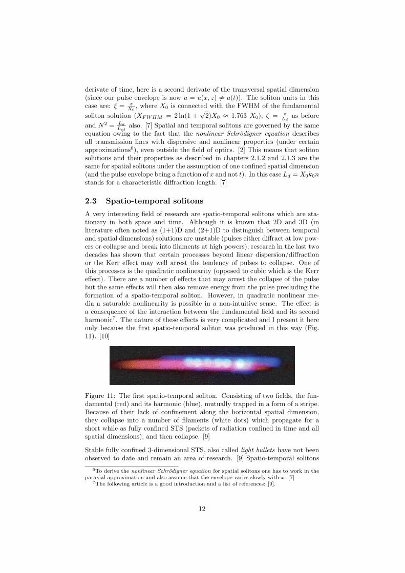
A very interesting field of research are spatio-temporal solitons which are sta-tionary in both space and time. Although it is known that 2D and 3D (inliterature often noted as (1+1)D and (2+1)D to distinguish between temporaland spatial dimensions) solutions are unstable (pulses either diffract at low pow-ers or collapse and break into filaments at high powers), research in the last twodecades has shown that certain processes beyond linear dispersion/diffractionor the Kerr effect may well arrest the tendency of pulses to collapse. One ofthis processes is the quadratic nonlinearity (opposed to cubic which is the Kerreffect). There are a number of effects that may arrest the collapse of the pulsebut the same effects will then also remove energy from the pulse precluding theformation of a spatio-temporal soliton. However, in quadratic nonlinear me-dia a saturable nonlinearity is possible in a non-intuitive sense. The effect isa consequence of the interaction between the fundamental field and its secondharmonic7. The nature of these effects is very complicated and I present it hereonly because the first spatio-temporal soliton was produced in this way (Fig.11). [10]

Figure 11: The first spatio-temporal soliton. Consisting of two fields, the fun-damental (red) and its harmonic (blue), mutually trapped in a form of a stripe.Because of their lack of confinement along the horizontal spatial dimension,they collapse into a number of filaments (white dots) which propagate for ashort while as fully confined STS (packets of radiation confined in time and allspatial dimensions), and then collapse. [9]

Stable fully confined 3-dimensional STS, also called light bullets have not beenobserved to date and remain an area of research. [9] Spatio-temporal solitons

6To derive the nonlinear Schrodigner equation for spatial solitons one has to work in theparaxial approximation and also assume that the envelope varies slowly with x. [7]

7The following article is a good introduction and a list of references: [9].

12

are a promising field because of their possible use in ultrafast optical logic gates.[7]

2.4 Soliton interactions

Soliton interactions8 have been known since the first treatment of the nonlin-ear Schrodinger equation. The motivation for the study came from the effectsof soliton interactions on the timing jitter in soliton communications systems.These interactions, which represent a difficulty for communications, can be use-ful for switching though. The most common interactions between solitons (Fig.12) are: collision, attraction/repulsion and trapping/dragging. [7]

Figure 12: An illustration of common soliton interaction geometries. The dashedlines indicate the soliton paths in the case of no interaction. [7]

If two same-polarized solitons interact, the interaction is phase-sensitive. Onthe other hand, the interaction of two orthogonally-polarized solitons is phase-insensitive. Typically, the collision between two same-polarized solitons pro-duces a spatial shift in the propagation of each soliton after collision. Sincethe interaction is a symmetric one, there is no net change in the propagationangle. The collision of two orthogonally-polarized solitons may on the otherhand result in a angle change. Two same-polarized and in phase solitons willattract each other while two solitons with a relative phase π will repel (for otherrelative phases, more complex behavior is expected). Trapping and draggingare interactions where in the beginning two solitons overlap, the former beingphase-sensitive and the latter phase-insensitive. [7]

2.5 Soliton logic gates

An optical logical device could be made if signals in the form of optical soli-tons could affect the propagation of another, potentially more energetic, solitoncalled the pump9, which is always present and is analogous to the power supplyin electronic logic gates. The pump soliton propagates through the logical gateto the output, providing the high state of the device, unless affected by the in-teraction with a signal soliton. When present, a signal soliton interacts with thepump, altering the propagation of the pump by inducing a spatial (or temporal)

8These interactions have of course nothing to do with the fundamental interactions, theyare merely interpretations of the solutions of the NLS equation. [7]

9This pump soliton has of course nothing to do with pump photons used in soliton ampli-fication.

13

shift, angle (or frequency) change, rotation of polarization, etc. Since displace-ment is more easily detected than other changes, only spatial shifts and anglechanges fall into the category of potential mechanisms. Furthermore, since thepump soliton continues to propagate without broadening after the interaction,angle changes result in arbitrarily large spatial shifts, dependent on the lengthof the gate (thus making angle changes more suitable than single spatial shifts).[7] Another issue is the nature of interaction. In a computing or switching sys-tem consisting of a large number of gates, a fixed relative phase may be difficultor even impossible to maintain, therefore it is essential to reduce or completelyeliminate phase-dependence of the interaction. This is possible to achieve if thetwo interacting solitons are orthogonally-polarized. [7]

Figure 13: The left hand plot shows the paths of two orthogonally-polarizedsolitons without interaction and the right hand plot their paths after the drag-ging interaction. The interaction changes the angles of both solitons (and thusthe final positions) enough that the threshold contrast of such a gate is > 1000[7]

Figure 14: Simulation (left) and observation (right) of spatio-temporal solitonformation in a Y-junction geometry. (a) and (b) show individual STS formationwith only the right- and left-going fields, respectively. (c) shows STS formationalong the center with both fields present. A detector placed at the center of theframe sees a signal only if both fields are launched - a logical AND operation.[11]

14

3 Conclusion

In this seminar I have presented the general properties of solitons as solutionsof certain nonlinear partial differential equations. Solitons may exist if thereis a balance between opposing linear and nonlinear effects. Their interestingand nonintuitive properties make them candidates for various applications inphysics. The canceling of dispersive broadening of pulses makes temporal soli-tons suitable for ultra long haul high bit rate optical communication. On theother hand, the particle-like behavior in interactions, makes possible the use ofsolitons for ultra fast optical logical devices.

4 References

[1] P. G. Drazin and R. S. Johnson (1989). Solitons: An introduction. Cam-bridge University Press, 2nd edition, ISBN 0521336554

[2] L. F. Mollenauer and J. P. Gordon (2006). Solitons in Optical Fibers:Fundamentals and Applications. Academic Press, 1st edition, ISBN012504190X

[3] E. Hecht (2001). Optics. Addison Wesley, 4th edition, ISBN 0805385665

[4] A. Menhofer et al. (1997). Morning-Glory disturbances and the environmentin which they propagate. Journal of the Atmospheric Sciences: Vol. 54, No.13 pp. 1712-1725

[5] J. S. Russell (1844). Report on waves. Fourteenth meeting of the BritishAssociation for the Advancement of Science.

[6] http://www.ma.hw.ac.uk/solitons/press.html (9.11.2010)

[7] Steve Blair (1998). Optical soliton based logic gates. PhDThesis, University of Colorado at Boulder. Available on:http://www.ece.utah.edu/ blair/P/dissert.pdf (9.11.2010)

[8] G. P. Agrawal (1995). Nonlinear fiber optics. Academic Press, 3rd edition.ISBN 0-12-045142-5

[9] F. Wise and P. di Trapani (2002). The hunt for light bullets. Optics andPhotonic News, February 2002 issue, p28 p51.

[10] X. Liu, L. Qian, and F. Wise (1999). Generation of optical spatiotemporalsolitons. Phys. Rev. Lett. 82, 4631.

[11] X. Liu, K. Beckwitt and F. Wise (2000). Noncollinear generation of opticalspatiotemporal solitons and application to ultrafast digital logic. Phys. Rev.E, 61, 5. doi:10.1103/PhysRevE.61.R4722.

15