Soliton-soliton Interaction with Parabolic Law Nonlinearity

J. of Electromagn. Waves and Appl., Vol. 20, No. 7, 927–939, 2006

SOLITON-SOLITON INTERACTION WITHPARABOLIC LAW NONLINEARITY

A. Biswas

Department of Applied Mathematics and Theoretical PhysicsDelaware State UniversityDover, DE 19901-2277, USA

S. Konar

Department of Applied PhysicsBirla Institute of TechnologyMesra, Ranchi-835215, India

E. Zerrad

Department of Physics and Pre-EngineeringDelaware State UniversityDover, DE 19901-2277, USA

Abstract—The intra-channel collision of optical solitons, withparabolic law non-linearity, is studied in this paper by the aid ofquasi-particle theory. The perturbation terms that are considered inthis paper are of Hamiltonian type. The suppression of soliton-solitoninteraction, in presence of these perturbation terms, is achieved. Thenumerical simulations support the quasi-particle theory.

1. INTRODUCTION

The theoretical possibility of existence of optical solitons in a dielectricdispersive fiber was first predicted by Hasegawa and Tappert [12]. Acouple of years later Mollenauer et al. [12] successfully performed thefamous experiment to verify this prediction. Important characteristicproperties of these solitons are that they posses a localized waveformwhich remains intact upon interaction with another soliton. Becauseof their remarkable robustness, they attracted enormous interest in

928 Biswas, Konar, and Zerrad

optical and telecommunication community. At present optical solitonsare regarded as the natural data bits for transmission and processingof information in future, and an important alternative for the nextgeneration of ultra high speed optical communication systems.

The fundamental mechanism of soliton formation namely thebalanced interplay of linear group velocity dispersion (GVD) andnonlinearity induced self-phase modulation (SPM) is well understood.In the pico second regime, the nonlinear evolution equation that takesinto account this interplay of GVD and SPM and which describes thedynamics of soliton is the well known nonlinear Schrodinger’s equation(NLSE). The NLSE, which is the ideal equation in an ideal Kerr media,is in its original form found to be completely integrable by the methodof Inverse Scattering Transform (IST) and tremendous success has beenachieved in the development of soliton theory in the framework of theNLSE model.

However, communication grade optical fibers or as a matter offact any optical transmitting medium does posses finite attenuationcoefficient, thus optical loss in inevitable and the pulse is oftendeteriorated by this loss. Therefore, optical amplifiers have to beemployed to compensate for this loss. When the gain bandwidth ofthe amplifier is comparable to the spectral width of the ultrashortoptical pulse, the frequency and intensity dependent gain must beconsidered. Another hindrance to the stable propagation in a practicalsystem is the noise induced Gordon-Hauss timing jitter. An importantaspect that has not been addressed with proper perspective is the factthat due to its nonsaturable nature, Kerr nonlinearity is inadequate todescribe the soliton dynamics in the ultrahigh bit rate transmission.For example, when transmission bit rate is very high, for solitonformation the peak power of the incident field accordingly becomevery large. On the other hand higher order nonlinearities may becomesignificant even at moderate intensities in certain materials such assemiconductor doped glass fibers. Under circumstances, as mentionedabove, non-Kerr law nonlinearities come into play changing essentiallythe physical features of optical soliton propagation. Therefore whenvery high bit rate transmission or transmission through materials withhigher nonlinear coefficients are considered, it is necessary to take intoaccount higher order nonlinearities. This problem can be addressed byincorporating the parabolic law nonlinearity in the NLSE.

It has been realized that the Gordon-Hauss timing jitter can bereduced by introducing bandpass filtering. Stabilazition of solitonpropagation with the aid of nonlinear gain or under combined operationof gain and saturable absorption was recommended by Kodama etal. [19–23]. Thus, in order to model these features in the soliton

Soliton-soliton interaction with parabolic law nonlinearity 929

dynamics, in a practical situation, the NLSE should be modified byincorporating additional terms. Thus the concept of control of solitonpropagation described by the NLSE with parabolic law nonlinearityis new and important developments in the application of solitons foroptical communication systems. Because the NLSE with parabolic lawis not integrable, perturbation methods or numerical techniques haveto be applied. Therefore, the control of soliton and interaction of twoneighboring solitons incorporating perturbation terms like nonlineargain, saturable amplification and filtering are going to be addressed inthis paper.

2. MATHEMATICAL MODEL

The propagation of pulses through an optical fiber in an opticalcommunication system, with parabolic law nonlinearity, is governed bythe Nonlinear Schrodinger’s Equation (NLSE) [4]. The dimensionlessform of the NLSE is given by

i∂q

∂Z+

12∂2q

∂T 2+

(|q|2 + ν|q|4

)q = 0 (1)

Here q is the normalized effective amplitude of the wave electric fieldwhile Z and T are the independent variables. Here Z represents thedistance along the fiber while T is the time and ν is a constant thataccounts for the strength of the parabolic law.

The particularly relevant solutions to (1) are called solitons. Inmost cases, the interest is confined to a single pulse described by the 1-soliton solution of the NLSE. However, in this paper, the effects of theperturbation terms in NLSE on two soliton interaction will be studied.It is necessary to launch the solitons close to each other for enhancingthe information carrying capacity of the fiber. If two solitons are placedclose to each other then it can lead to its mutual interaction thusproviding a very serious hindrance to the performance of the solitontransmission system. However, as elucidated in the previous section,the presence of appropriate perturbation terms the NLSE can leadto soliton control and suppression of this interaction. Therefore, inview of achieving soliton control and suppression of the interaction,the perturbed NLSE that is going to be studied in this paper is givenby

i∂q

∂Z+

12∂2q

∂T 2+

(|q|2 + ν|q|4

)q = iεR[q, q∗] (2)

where

R = λ∂

∂T

(|q|2q

)+ µq

∂

∂T

(|q|2

)− α

∂q

∂T− γ

∂3q

∂T 3− iσ

∂4q

∂T 4(3)


In fiber optics ε is called the relative width of the spectrum, thatarises due to quasi-monochromaticity, and is assumed that 0 < ε� 1.In (3), α is the frequency separation between the soliton carrierand the frequency at the peak of EDFA gain. Also, λ is the self-steepening coefficient for short pulses [3, 4, 11, 24] (typically ≤ 100femto seconds), µ is the higher order dispersion coefficient [11, 24] andγ is the coefficient of the third order dispersion [11, 18, 24]. Moreover,σ represents the coefficient of fourth order dispersion.

It is known that the NLSE, as given by (1), does not givecorrect prediction for pulse widths smaller than 1 picosecond. Forexample, in solid state solitary lasers, where pulses as short as 10femtoseconds are generated, the approximation breaks down. Thus,quasi-monochromaticity is no longer valid and higher order dispersionterms come in. If the group velocity dispersion is close to zero,one needs to consider the third order dispersion for performanceenhancement along trans-oceanic distances. Also, for short pulsewithin the spectral bandwidth of the signal so that the presence ofthe third order dispersion needs to be taken into consideration.

The quasi-particle theory (QPT) of soliton-soliton interaction(SSI) has been investigated [2, 3, 7, 8] and it is proved by virtue ofit that the interaction can be suppressed due to the BLA perturbationterms. Also it has been proved that the sliding frequency guiding filters[8, 9] leads to the suppression of the SSI. Here, by virtue of the QPT itwill be proved that the SSI can be suppressed due to the NLSE givenby (1) and also in presence of the perturbation terms in (2).

Equation (2) is not integrable by IST as it is not of Painleve type[1]. However, (2) supports solitary waves of the form [4, 18]

q(Z, T ) =η

[1 + a cosh{ζ(T − vZ − T0)}]12

ei{−κT+ωZ+σ0} (4)

where

ζ = η√

2 (5)κ = −v (6)

ω =η2

4− κ2

2(7)

a =√

1 +43νη2 (8)

Here η is the amplitude of the soliton, ζ is the width of the soliton,v is its velocity, κ is the soliton frequency and ω is the wave numberwhile T0 and σ0 are the center of the soliton and the center of thesoliton phase respectively. In this paper it will be assumed that ν > 0


although ν could be negative as well. In fact, it is to be noted that for(1) solitons exist for ν ∈ (−3/4A2,∞).

Also, the 2-soliton solution of the NLSE (1) takes the asymptoticform

q(Z, T ) =2∑

l=1

ηl

[1 + al cosh{ζl(T − vZ − Tl)}]12

ei(−κlT+ωlZ+σ0l) (9)

with

κl = −vl (10)

ζl = ηl

√2 (11)

ωl =η2

l − 2κ2l

4(12)

αl =√

1 +43νη2

l (13)

In the study of SSI, the initial pulse waveform is taken to be of theform

q(0, T ) =η1[

1 + a1 cosh{ζ1

(T − T0

2

)}] 12

eiφ1

+η2[

1 + a2 cosh{ζ2

(T +

T0

2

)}] 12

eiφ2 (14)

which represents the injection of 2-soliton like pulses into a fiber. HereT0 represents the initial separation of the solitons. We note that forT0 → ∞ (5) represents exact soliton solutions, but for T0 ∼ O(1) itdoes not represent an exact 2-soliton solution. Corresponding to theinput waveform given by (15) the case of in-phase injection of solitonswith unequal amplitudes will be studied. Thus, without any loss ofgenerality the choice η1 = η0, η2 = 1 and φ1 = φ2 = 0 is considered sothat (5) modifies to

q(0, T ) =η0[

1 +√

1 +43νη0 cosh

{η0

√2

(T − T0

2

)}] 12

+η0[

1 +√

1 +43ν cosh

{√2

(T +

T0

2

)}] 12

(15)


3. QUASI-PARTICLE THEORY

The QPT dates back to 1981 since the appearance of the paper byKarpman and Solov’ev [3]. We shall study the mathematical approachto the SSI using the QPT. Here we treat the solitons as particles. Iftwo pulses are separated and each of them is close to a soliton theycan be written as the linear superposition of two soliton like pulses [2]:

q(Z, T ) = q1(Z, T ) + q2(Z, T ) (16)

withql(Z, T ) =

Al

[1 + al cosh[Bl(T − Tl)]]12

e−iBl(T−Tl)+iδl (17)

where l = 1, 2 and Al, Bl, Tl and δl are functions of Z. We note thatAl and Bl do not represent the amplitude and the frequency of thefull wave form. However, they approach the amplitude and frequencyrespectively for large separation namely as ∆T = T1−T2 → ∞, we haveAl → ηl and Bl → κl. Since the waveform is assumed to remain in theform of two pulses, the method is called the quasi-particle approach.We shall first drive the equations for Al, Bl, Tl and δl using the solitonperturbation theory. Substituting (9) into (2) we get

i∂ql∂Z

+12∂2ql∂T 2

+(|ql|2 + ν|ql|4

)ql = iεR[ql, q∗l ] −

(q2l q

∗l

+ 2|ql|2ql)

−ν[q3l

(q∗l

)2+ 2|ql|2q2l q∗l + 3|ql|4ql + 3|ql|2q∗l q2l + 6|ql|2|ql|

2ql

](18)

where l = 1, 2 and l = 3 − l. Here, the separation

|q|2q+ν|q|4q =(|q1|2q1+q21q

∗2+2|q1|2q2

) (|q2|2q2+q22q

∗1 + 2|q2|2q1

)+ν

[|q1|4q1+q31 (q∗2)

2+2|q1|2q21q∗2+3|q1|4q2+3|q1|2q∗1q22+6|q1|2|q2|2q1]

+ν[|q2|4q2+q32 (q∗1)

2+2|q2|2q22q∗1+3|q2|4q1+3|q2|2q∗2q21+6|q1|2|q2|2q2]

(19)

was used based on the degree of overlapping. By the solitonperturbation theory [2] the evolution equations are

dAl

dZ= F

(l)1 (A,∆T,∆φ; ν) + εMl (20)

dBl

dZ= F

(l)2 (A,∆T,∆φ; ν) + εNl (21)


dTl

dZ= −Bl − F3(A,∆T,∆φ; ν) + εQl (22)

dδldZ

=A2

l

4+B2

l

2+ F4(A,∆T,∆φ; ν) + εPl (23)

where

Ml = k1(l)∫ ∞

−∞�

{R[ql, q∗l ]e

−iφl

} dτl

(1 + al cosh τl)12

dτl (24)

Nl = k2(l)∫ ∞

−∞

{R[ql, q∗l ]e

−iφl

} sinh τl(1 + al cosh τl)

12

dτl (25)

Ql = k3(l)∫ ∞

−∞�

{R[ql, q∗l ]e

−iφl

} τl

(1 + al cosh τl)12

dτl (26)

Pl = k4(l)∫ ∞

−∞

{R[ql, q∗l ]e

−iφl

} (1 − alτl sinh τl)

(1 + alτl cosh τl)12

dτl (27)

where kj(l), for j = 1, 2, 3, 4 are suitable functions of Al and Bl forl = 1, 2. Also, � and stands for the real and imaginary partsrespectively. The following notations are now used

R[ql, q∗l ] = R[ql, q∗l ] −(q2l q

∗l

+ 2|ql|2ql)

−ν[q3l

(q∗l

)2+ 2|ql|2q2l q∗l + 2|ql|4ql + 3|ql|2q∗l q2l + 6|ql|2|ql|

2ql

](28)

τl = Al(T − Tl) (29)φl = Bl(T − Tl) − δl (30)

∆φ = B∆T + ∆δ (31)∆T = T1 − T2 (32)∆δ = δ1 − δ2 (33)

A =12(A1 +A2) (34)

B =12(B1 +B2) (35)

∆A = A1 −A2 (36)∆B = B1 −B2 (37)

Moreover, it was assumed that

|∆A| � A (38)


|∆B| � 1 (39)A∆T � 1 (40)

|∆A|∆T � 1 (41)

From (12) to (15) we can now obtain

dA

dZ= εM (42)

dB

dZ= εN (43)

d(∆A)dZ

= F(1)1 (A,∆T,∆φ; ν) − F

(2)1 (A,∆T,∆φ; ν) + ε∆M (44)

d(∆B)dZ

= F(1)2 (A,∆T,∆φ; ν) − F

(2)2 (A,∆T,∆φ; ν) + ε∆N (45)

d(∆T )dZ

= −∆B + ε∆Q (46)

d(∆φ)dZ

=12A∆A+

∆T2

(F

(1)2 + F

(2)2

)+ εB∆Q+ ε∆P (47)

where

M =12(M1 +M2) (48)

N =12(N1 +N2) (49)

and ∆M, ∆N, ∆Q and ∆P are the variations ofM, N, Q and P whichare written as for example

∆M =∂M

∂A∆A+

∂M

∂B∆B (50)

assuming that they are functions of A and B only, which is, in fact,true for most of the cases of interest, otherwise, the equations for

T =12(T1 + T2) (51)

andφ =

12(φ1 + φ2) (52)

would have been necessary. In presence of the perturbation terms, asgiven by, (3), the dynamical system of the soliton parameters, by virtue


of soliton perturbation theory, are

dA

dZ= 0 (53)

dB

dZ= 0 (54)

dT0

dZ= −B − εα

E

2√

2A√a2 − 1

tan−1

√a− 1a+ 1

−ε√

22E

A3

(a2 − 1)32

(3λ+ 2µ)

√

a2 − 1 − 2 tan−1

√a− 1a+ 1

−3√

2εγA

E

(

a4A2

2+

2B2

√a2 − 1

)tan−1

√a−1a+1

− a2A2

4

√a2−1

(55)

where E is the energy of the soliton given by

E =∫ ∞

−∞|q|2dT =

2√

2A√a2 − 1

tan−1

√a− 1a+ 1

(56)

From (54)–(57) one can now conclude that

dA

dZ= 0 (57)

dB

dZ= 0 (58)

d(∆A)dZ

= F(1)1 (A,∆T,∆φ) − F

(2)1 (A,∆T,∆φ) (59)

d(∆B)dZ

= F(1)2 (A,∆T,∆φ) − F

(2)2 (A,∆T,∆φ) (60)

d(∆T )dZ

=dT1

dZ− dT2

dZ(61)

d(∆φ)dZ

=12A∆A (62)

Equation (61) can be rewritten as

d(∆T )dZ

= −∆B + εG(α, λ, ν, γ, σ)g{d(∆φ)dZ

}(63)


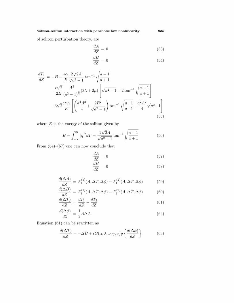
Figure 1. Parameters: ν = 0.5, ε = 0.1, α = 0.8, γ = −0.25, σ =0.05.

where G is the functional form that depends on the said parameters.For in-phase injection of solitons with unequal amplitudes,

A =12(A0 + 1) (64)

B = 0 (65)

∆A0 = A0 − 1 (66)∆B0 = 0 (67)∆T0 = T0 (68)∆φ0 = 0 (69)∆φ = ∆δ (70)

so that, one can obtain from (63), for ∆B = 0,

∆T = T0 + εG(α, λ, ν, γ, σ)h{d(∆φ)dZ

}(71)

wherehj(s) =

∫gj(s)ds (72)

for j = 1, 2. Thus,∆T = T0 +Q(ε) (73)


Now, T0 ∼ O(1) so that ∆T �→ 0 and thus the pulses do not collideduring the transmission. This will be observed in the numerical resultsin the next section.

4. NUMERICAL SIMULATIONS

In this section, the numerical simulations of the quasi-particle theoryfor the soliton-soliton interaction due to Hamiltonian perturbation withKerr law nonlinearity will be observed. In all cases, A0 is taken to beequal to 1.1 and ε was set to 0.1 while T0 = 9. The following numericalsimulation was observed for ν = 0.5, α = 0.8, γ = 0.25 and σ = 0.05while λ = µ = 0.

Since T0 ∼ O(1) so that ∆T �→ 0 and thus the pulses do notcollide during the transmission as seen in Figure 1 for these values ofthe perturbation parameters.

5. CONCLUSIONS

In this paper, the SSI of the NLSE, with parabolic law nonlinearityin presence of nonlinear gain, saturable amplifiers and filters areinvestigated. It is observed that the SSI can be suppressed in presenceof these perturbation terms for various values of the degree of nonlineargain. The QPT, due to these perturbation terms, was developed andthe analytical reasoning of the suppression of the SSI was formulated.

Thus, in the applied soliton community two solitons can beinjected into a single channel, close to one another and also suppresstheir mutual interaction so that performance enhancement can beachieved. This conclusion is based on numerical and analytical resultsdue to the quasi-particle theory of SSI.

ACKNOWLEDGMENT

The work of the first author is partially supported by the Departmentof Science and Technology (DST), Government of India, throughthe R&D grant SP/S2/L-21/99. Therefore, S. K. would like toacknowledge this support with thanks.

This research for the second author was fully supported by NSFGrant No: HRD-970668 and the support is thankfully appreciated.

REFERENCES

1. Ablowitz, M. J. and H. Segur, Solitons and the Inverse ScatteringTransform, SIAM Publishers, Philadelphia, 1981.


2. Afanasjev, V. V., “Interpretation of the effect of reduction ofsoliton interaction by bandwidth-limited amplification,” OpticsLetters, Vol. 18, 790–792, 1993.

3. Biswas, A., “Soliton-soliton interaction in optical fibers,” Journalof Nonlinear Optical Physics and Materials, Vol. 8, No. 4, 483–495, 1999.

4. Biswas, A., “Quasi-stationary optical solitons with non-Kerr lawnonlinearity,” Optical Fiber Technology, Vol. 9, Issue 4, 224–259,2003.

5. Chu, P. L. and C. Desem, “Mutual interaction between solitons ofunequal amplitudes in optical fiber,” Electronics Letters, Vol. 21,1133–1134, 1985.

6. Chu, P. L. and C. Desem, “Effect of third order dispersion ofoptical fiber on soliton interaction,” Electronics Letters, Vol. 21,228–229, 1985.

7. Desem, C. and P. L. Chu, “Soliton interactions in presence ofloss and periodic amplification in optical fibers,” Optics Letters,Vol. 12, 349–351, 1987.

8. Gordon, J. P., “Interaction forces among solitons in optical fibers,”Optics Letters, Vol. 8, 596–598, 1983.

9. Georges, T. and F. Favre, “Influence of soliton interaction onamplifier noise induced jitter: a first order analytical solution,”Optics Letters, Vol. 16, 1656–1658, 1991.

10. Georges, T. and F. Favre, “Modulation, filtering and initial phasecontrol of interacting solitons,” Journal of Optical Society ofAmerica B, Vol. 10, 1880–1889, 1993.

11. Hermansson, B. and D. Yevick, “Numerical investigation of solitoninteraction in optical fibers,” Electronics Letters, Vol. 19, 570–571,1983.

12. Hasegawa, A. and Y. Kodama, Solitons in Optical Communica-tions, Oxford University Press, 1995.

13. Karpman, V. I. and V. V. Solov’ev, “A perturbational approachto the two-soliton systems,” Physica D, Vol. 3, 487–502, 1981.

14. Kodama, Y. and K. Nozaki, “Soliton interaction in optical fibers,”Optics Letters, Vol. 12, No. 12, 1038–1040, 1987.

15. Kodama, Y., M. Romagnoli, and S. Wabnitz, “Soliton stabilityand interaction in fiber lasers,” Electronics Letters, Vol. 28, No. 21,1981–1983, 1992.

16. Kodama, Y. and S. Wabnitz, “Reduction of soliton interactionforces by bandwidth limited amplification,” Electronics Letters,Vol. 27, No. 21, 1931–1933, 1991.


17. Kodama, Y. and S. Wabnitz, “Physical interpretation of reductionof soliton interaction forces by bandwidth limited amplification,”Electronics Letters, Vol. 29, No. 2, 226–227, 1993.

18. Kodama, Y. and S. Wabnitz, “Reduction and suppression ofsoliton interaction by bandpass filters,” Optics Letters, Vol. 18,No. 16, 1311–1313, 1993.

19. Kodama, Y. and S. Wabnitz, “Analysis of soliton stability andinteractions with sliding filters,” Optics Letters, Vol. 19, No. 3,162–164, 1994.

20. Konar, S. and A. Biswas, “Intra-channel collision of Kerr lawoptical solitons,” submitted.

21. Nakazawa, M. and H. Kubota, “Physical interpretation ofreduction of soliton interaction forces by bandwidth limitedamplification,” Electronics Letters, Vol. 28, 958–960, 1992.

22. Uzunov, I. M., V. D. Stoev, and T. I. Tsoleva, “N-solitoninteraction in trains of unequal soliton pulses in optical fibers,”Optics Letters, Vol. 17, 1417–1419, 1992.

23. Wabnitz, S., “Control of soliton train transmission, storage, andclock recovery by cw light injection,” Journal of the Optical Societyof America B., Vol. 13, No. 12, 2739–2749, 1996.

24. Xu, Z., L. Li, Z. Li, and G. Zhou, “Soliton interaction underthe influence of higher-order effects,” Optics Communications,Vol. 210, Issues 3–6, 375–384, 2002.

Soliton-soliton Interaction with Parabolic Law Nonlinearity

Documents