Soliton Dynamics in Liquid-core Optical Fibers DISSERTATION for the acquisition of the academic title Doctor rerum naturalium (Dr. rer. nat.) submitted to the council of the Faculty of Physics and Astronomy of the by Dipl. Phys. Mario Chemnitz born in Lutherstadt Wittenberg, Germany, on 21st Oct 1986.

Welcome message from author
This document is posted to help you gain knowledge. Please leave a comment to let me know what you think about it! Share it to your friends and learn new things together.
Transcript
Soliton Dynamics in
Liquid-core Optical Fibers
D I S S E RTAT I O N
for the acquisition
of the academic title
Doctor rerum naturalium (Dr. rer. nat.)
submitted to the council of the
Faculty of Physics and Astronomy
of the
by Dipl. Phys. Mario Chemnitz
born in Lutherstadt Wittenberg, Germany, on 21st Oct 1986.

reviewers:
1. Prof. Dr. Markus A. Schmidt, Friedrich-Schiller-University Jena, Germany
2. Prof. Dr. Alexander Szameit, University Rostock, Germany
3. Prof. Dr. Arnaud Mussot, University Lille, France
day of the disputation: 25. February 2019

“Every particular in nature, a leaf, a drop, a crystal, a moment of time is related to the
whole, and partakes of the perfection of the whole.”
— Ralph Waldo Emerson
Dedicated to my love Margarethe and my little Lorelin.

A B S T R A C T
Solitons are self-maintaining wave patterns occurring in many dynamic systems in nature.
In optics, the rich dynamics of non-dispersing temporal solitons enable the generation of
supercontinuum spectra covering wide wavelength ranges from the visible ultraviolet to
the near-infrared and beyond. Such nonlinear multi-color light sources are indispensable
for next-generation sensing and imaging technologies. Particularly optical fibers proved
to be superiorly effective for nonlinear light generation integrated in a robust platform.
However, commercial nonlinear fiber sources are based on silica as fiber material, which
is limited in its bandwidth, nonlinearity, and wavelength tuneability. Hence, recent ef-
forts in nonlinear fiber optics try to overcome these limitations by exploring new fiber
designs and new core materials with enhanced nonlinear properties, such as soft-glasses
and gases. Also liquids possess wider transmission windows and higher nonlinearities
than silica, while exhibiting unique nonlinear responses due to the long-lasting molecu-
lar motions in a light field. First experimental demonstrations reveal the potential of
liquid-core optical fibers for broadband light generation. However, soliton dynamics, as
most effective broadening mechanisms, are largely unexplored in these systems.
This thesis theoretically and experimentally explores these dynamics in liquid-core
fibers. Following a rigorous empirical approach, hybrid soliton-like states are proposed
as potential solution of those systems. Key benchmarks, such as optical phase relations
and a modified soliton number, are found and confirmed as tool to classify noninstant-
aneous nonlinear systems by means of their capabilities for hosting hybrid solitons. This
thesis further elaborates realistic material models which allows to identify soliton re-
gimes in easily producible step-index liquid-core fiber designs. Finally hybrid soliton-
like states are shown to emerge in simulated supercontinuum spectra for these exper-
imentally addressable fiber and laser parameters. Thereupon, soliton-mediated super-
continuum generation is demonstrated experimentally in liquid-core fibers using state-
of-the-art thulium fiber lasers. In correlation with numerical simulations, the unusual
broadening and coherence behavior of the measured spectra is shown to originate from
dominant noninstantaneous nonlinear effects in liquids, and thus delivers the first pos-
itive indications for the hypothesis of novel hybrid soliton dynamics. The study closes
with the experimental demonstration of external soliton control via temperature, static
pressure, and liquid composition, overall highlighting liquid-core fibers as a dynamic
platform for broadband and tuneable nonlinear light generation with a plethora of un-
precedented nonlinear effects and scientific potential.
v
Z U S A M M E N FA S S U N G
Solitonen sind selbsterhaltende Wellenmuster, die in vielen dynamischen Systemen in
der Natur auftreten. In der Optik ermöglichen die reichhaltigen Dynamiken von nicht-
verbreiternden zeitlichen Solitonen die Generation von Superkontinuumsspektren über
weite Wellenlängenbereiche vom Sichtbaren bis ins Nah-Infrarote und darüber hinaus.
Solche nichtlinearen mehrfarbigen Lichtquellen sind für Sensor- und Bildgebungstech-
nologien der nächsten Generation unverzichtbar. Insbesondere für die nichtlineare Licht-
erzeugung in integrierten, robusten Systemen erwiesen sich optische Fasern als über-
ragend. Kommerzielle nichtlineare Faserquellen basieren jedoch auf Siliciumdioxid als
Fasermaterial, welches in seiner Bandbreite, Nichtlinearität und Wellenlängenabstimm-
barkeit begrenzt ist. Die jüngsten Bemühungen im Bereich der nichtlinearen Faseroptik
versuchen deshalb, diese Einschränkungen zu überwinden, indem neue Faserdesigns
und neue Kernmaterialien mit verbesserten nichtlinearen Eigenschaften, wie Weichglä-
sern und Gasen, untersucht werden. Auch Flüssigkeiten haben breitere Transmissionsfen-
ster und höhere Nichtlinearitäten als Siliciumdioxid, während sie aufgrund der langan-
haltenden molekularen Bewegungen in einem Lichtfeld einzigartige nichtlineare Reak-
tionen zeigen. Erste experimentelle Demonstrationen zeigen das Potenzial von Flüssig-
kern-Glasfasern für die Breitbandlichterzeugung. Die Solitondynamiken als effektivste
Verbreitungsmechanismen sind aber in diesen Systemen noch weitgehend unerforscht.
Diese Dissertation untersucht diese Dynamiken in Flüssigkernfasern theoretisch und
experimentell. Einem streng empirischen Ansatz folgend werden hybride solitonähn-
liche Zustände als mögliche Lösung dieser Systeme vorgeschlagen. Wichtige Kenngrößen,
wie optische Phasenbeziehungen und eine modifizierte Solitonzahl, werden als Werkzeu-
ge zur Klassifizierung nichtinstantaner, nichtlinearer Systeme hinsichtlich ihrer Fähig-
keiten zur Beherbergung von Hybrid-Solitonen gefunden und bestätigt. In dieser Arbeit
werden außerdem realistische Materialmodelle erarbeitet, die die Identifizierung von
Soliton-Regimen in einfach herstellbaren Flüssigkern-Fasern mit Stufenindex Design er-
möglichen. Schließlich wird gezeigt, dass hybride solitonähnliche Zustände in simulier-
ten Superkontinuumspektren für diese experimentell adressierbaren Faser- und Laser-
parameter auftreten. Daraufhin wird die Soliton-gestützte Superkontinuumserzeugung
experimentell in Flüssigkernfasern unter Verwendung von modernsten Thuliumfaser-
lasern demonstriert. Im Zusammenhang mit numerischen Simulationen wird hervorge-
hoben, dass das ungewöhnliche Verbreitungs- und Kohärenzverhalten der gemessenen
Spektren von dominanten, nichtinstantanen, nichtlinearen Effekten in Flüssigkeiten her-
rührt und somit die ersten positiven Hinweise für die Hypothese neuartiger Hybrid-
Soliton-Dynamiken liefert. Die Studie schließt mit der experimentellen Demonstration
der externen Soliton-Kontrolle über Temperatur, statischen Druck und flüssige Zusam-
mensetzung. Dabei werden Flüssigkernfasern als dynamische Plattform für breitbandige
und abstimmbare nichtlineare Lichterzeugung mit einer Fülle von beispiellosen nicht-
linearen Effekten und wissenschaftlichem Potenzial hervorgehoben.
vi
H Y P O T H E S E S
This work investigates the following hypotheses (H):
1. Highly-refractive liquids filled in silica capillaries allow optical waveguiding in the
near- and mid-infrared, forming a step-index liquid-core fibers.
2. Step-index liquid-core fibers feature anomalous dispersion regimes at wavelengths
addressable with state-of-the-art fiber lasers, thus providing an experimental plat-
form for exciting optical solitons.
3. The highly noninstantaneous nonlinear response of certain liquids enables the
formation of noninstantaneous solitons, so-called linearons.
4. Soliton-mediated supercontinuum spectra contain characteristic signatures of mod-
ified soliton dynamics.
5. The modified soliton dynamics within noninstantaneous liquid-core fibers can be
understood as result of the emergence of hybrid nonlinear soliton-like states.
6. Step-index liquid-core fibers offer an experimental platform for soliton-mediated
supercontinuum generation.
7. The fiber dispersion of liquid-core fibers can be adjusted by applying temperature
and pressure on the liquid core as well as changing its composition.
8. The supercontinuum generation process, in particular the soliton fission onset and
the emission of non-solitonic radiation, can be controlled via external thermody-
namic controls and the core composition.
vii

A C R O N Y M S
ADD anomalous dispersion domain
CBP coherence-bandwidth product
CS2 carbon disulfide
CCl4 carbon tetrachloride
C2Cl4 tetrachloroethylene
CHCl3 chloroform
IOR index of refraction
FOM figure of merit
FWM four-wave mixing
GVD group velocity dispersion
GNSE generalized nonlinear Schrödinger
equation
HNSE hybrid nonlinear Schrödinger
equation
HSW hybrid solitary wave
HSS hybrid soliton state
IKP instantaneous Kerr phase
LCF liquid-core fiber
NDD normal dispersion domain
NIR near-infrared
NIP noninstantaneous phase
NRF nonlinear response function
NRI nonlinear refractive index
NSE nonlinear Schrödinger equation
NISE noninstantaneous Schrödinger
equation
NSE nonlinear Schrödinger equation
NSR non-solitonic radiation
MI modulation instabilities
MIR mid-infrared
OFM opto-fluidic mount
POC piezo-optic coefficient
SC supercontinuum
SCG supercontinuum generation
SMC single-mode criterion
SPM self-phase modulation
SFS self-frequency shift
TOC thermo-optic coefficient
TOD third-order dispersion
VIS visible
VUV visible ultraviolet
XPM cross-phase modulation
ZDW zero-dispersion wavelength
viii

N O M E N C L AT U R E
THP pulse width at half maximum power, also known FWHM width
P0 peak power
Ps soliton peak power
Ep pulse energy
ω0 (angular) operation frequency
λ0 operation (pump) wavelength
λZD zero-dispersion wavelength
n refractive index
n2 nonlinear refractive index
co core diameter
α absorption coefficient
β propagation constant
β2 second-order dispersion parameter
γ nonlinear parameter
Aeff effective mode area
NA numerical aperture
V (guidance) V-parameter
D dispersion parameter
fm molecular fraction
fequilm equilibrium fraction
LD dispersion length
LNL nonlinear length
Lfiss fission length
N (classical) soliton number
Neff effective soliton number
R0 maximum of the nonlinear response
|g(1)mn| first-order degree of coherence
ix
C O N T E N T S
1 introduction 1
2 nonlinear light propagation in optical fibers 6
2.1 Fundamental wave equation of optics . . . . . . . . . . . . . . . . . . . . . 6
2.1.1 Optical modes of cylindrical fibers . . . . . . . . . . . . . . . . . . . 7
2.1.2 Linear fiber mode properties in brief . . . . . . . . . . . . . . . . . . 9
2.2 Nonlinear pulse propagation in optical fibers . . . . . . . . . . . . . . . . . 10
2.2.1 Intensity-dependent refractive index . . . . . . . . . . . . . . . . . . 10
2.2.2 Nonlinear Schrödinger equation . . . . . . . . . . . . . . . . . . . . 11
2.2.3 Nonlinear gain parameter of step-index fibers . . . . . . . . . . . . 14
2.2.4 Numerical solution of the Schrödinger equation . . . . . . . . . . . 15
2.3 Relevant nonlinear effects for supercontinuum generation . . . . . . . . . . 17
2.3.1 Overview of third-order nonlinear effects in fibers . . . . . . . . . . 17
2.3.2 Self-phase modulation . . . . . . . . . . . . . . . . . . . . . . . . . . 18
2.3.3 Optical solitons . . . . . . . . . . . . . . . . . . . . . . . . . . . . . . 18
2.3.4 Soliton-mediated supercontinuum generation . . . . . . . . . . . . 22
3 optical properties of liquid-core fibers 27
3.1 Overview of promising liquid candidates . . . . . . . . . . . . . . . . . . . 27
3.2 Linear optical properties of liquids . . . . . . . . . . . . . . . . . . . . . . . 28
3.2.1 The complex refractive index . . . . . . . . . . . . . . . . . . . . . . 28
3.2.2 Absorption . . . . . . . . . . . . . . . . . . . . . . . . . . . . . . . . . 30
3.2.3 Refraction . . . . . . . . . . . . . . . . . . . . . . . . . . . . . . . . . 33
3.3 Nonlinear optical properties of selected liquids . . . . . . . . . . . . . . . . 37
3.3.1 The general nonlinear response . . . . . . . . . . . . . . . . . . . . . 37
3.3.2 Overview of the nonlinear response of selected liquids . . . . . . . 39
3.4 Nonlinear liquid-core fiber design . . . . . . . . . . . . . . . . . . . . . . . . 40
3.4.1 Overview of the optical properties of the fundamental fiber mode 40
3.4.2 Design maps for nonlinear fibers . . . . . . . . . . . . . . . . . . . . 41
4 modified solitons in partly noninstantaneous media 43
4.1 Linearons – Eigenstates of highly noninstantaneous nonlinear media . . . 43
4.1.1 Noninstantaneous Schrödinger equation . . . . . . . . . . . . . . . 43
4.1.2 Solution of the noninstantaneous Schrödinger equation . . . . . . 45
4.2 Hybrid propagation characteristics . . . . . . . . . . . . . . . . . . . . . . . 46
4.2.1 Linearon propagation and perturbations . . . . . . . . . . . . . . . 46
4.2.2 Hybrid Schrödinger equation . . . . . . . . . . . . . . . . . . . . . . 47
4.2.3 Linearons in third-order dispersive media . . . . . . . . . . . . . . 48
4.2.4 Linearons in Kerr-perturbed media . . . . . . . . . . . . . . . . . . 49
4.2.5 Linearons in media with realistic hybrid nonlinearity . . . . . . . . 50
4.3 Intermediate conclusion . . . . . . . . . . . . . . . . . . . . . . . . . . . . . 54
5 hybrid soliton dynamics through the prism of supercontinuum
spectra 55
5.1 Methodology . . . . . . . . . . . . . . . . . . . . . . . . . . . . . . . . . . . . 55
5.2 Hybrid fission characteristics . . . . . . . . . . . . . . . . . . . . . . . . . . . 56
5.3 Spectral observables of hybrid soliton dynamics . . . . . . . . . . . . . . . 59
5.3.1 Bandwidth and onset energy . . . . . . . . . . . . . . . . . . . . . . 59
5.3.2 Non-solitonic radiation . . . . . . . . . . . . . . . . . . . . . . . . . 60
x
contents xi
5.3.3 Temporal coherence . . . . . . . . . . . . . . . . . . . . . . . . . . . 61
5.3.4 Bandwidth-coherence product . . . . . . . . . . . . . . . . . . . . . 62
5.4 Theory of noninstantaneously dominated supercontinuum generation . . 65
6 experimental evidence of hybrid soliton dynamics 66
6.1 Supercontinuum measurements in liquid-core fibers . . . . . . . . . . . . . 66
6.1.1 Experimental details and methodology . . . . . . . . . . . . . . . . 66
6.2 Supercontinuum generation in liquid-core fibers . . . . . . . . . . . . . . . 69
6.2.1 Carbon tetrachloride (CCl4) . . . . . . . . . . . . . . . . . . . . . . . 69
6.2.2 Carbon disulfide (CS2) . . . . . . . . . . . . . . . . . . . . . . . . . . 70
6.2.3 Tetrachloroethylene (C2Cl4) . . . . . . . . . . . . . . . . . . . . . . . 72
6.3 Indications of hybrid soliton dynamics . . . . . . . . . . . . . . . . . . . . . 73
6.3.1 A priori classification . . . . . . . . . . . . . . . . . . . . . . . . . . . 73
6.3.2 Bandwidth and fission onset . . . . . . . . . . . . . . . . . . . . . . 74
6.3.3 Non-solitonic radiation . . . . . . . . . . . . . . . . . . . . . . . . . 75
6.3.4 Coherence . . . . . . . . . . . . . . . . . . . . . . . . . . . . . . . . . 76
6.3.5 Hybrid nonlinear Schrödinger equation . . . . . . . . . . . . . . . . 77
6.4 Evaluation of significance of the indicators . . . . . . . . . . . . . . . . . . 79
6.5 Theory of noninstantaneously dominated soliton fission . . . . . . . . . . . 80
7 tuning capabilities of liquid-core fibers 82
7.1 Temperature tuning . . . . . . . . . . . . . . . . . . . . . . . . . . . . . . . . 82
7.1.1 Device principle and design . . . . . . . . . . . . . . . . . . . . . . . 82
7.1.2 Experimental modifications . . . . . . . . . . . . . . . . . . . . . . . 83
7.1.3 Temperature detuning of non-solitonic radiation . . . . . . . . . . . 85
7.2 Pressure tuning . . . . . . . . . . . . . . . . . . . . . . . . . . . . . . . . . . 87
7.2.1 Experimental modification . . . . . . . . . . . . . . . . . . . . . . . 87
7.2.2 Pressure detuning of the fission onset . . . . . . . . . . . . . . . . . 87
7.3 Composition control . . . . . . . . . . . . . . . . . . . . . . . . . . . . . . . . 88
7.3.1 Dispersion properties of binary liquid mixtures . . . . . . . . . . . 88
7.3.2 Soliton fission in liquid composite-core fibers . . . . . . . . . . . . 90
8 deduction and vision 92
8.1 Conclusion . . . . . . . . . . . . . . . . . . . . . . . . . . . . . . . . . . . . . 92
8.2 Future prospects . . . . . . . . . . . . . . . . . . . . . . . . . . . . . . . . . . 94
bibliography 99
a material data and characterization details 117
b theoretical supplements 124
c experimental supplements 133
d acknowledgements 137
e publication list and attachments 139
1I N T R O D U C T I O N
About the fundamental role of solitons in nature
The existence of our world in a universe that, before anything else, distributes energy
seems like a miracle. Fermi, Pasta, Ulam, and Tsingou unintentionally delivered a pos-
sible explanation, when they reported on some peculiar oscillations of mechanical bodies
in a lattice connected by springs, in 1955. To their surprise, certain initial displacements
of the bodies did not result in random distributions of oscillations, as commonly ex-
pected for dynamic systems, but evolved into recurrent wave forms, that traveled along
the lattice without changing their shape or amplitude [1]. In fact, they rediscovered a
fundamental phenomenon, which was observed earlier in 1834 by Sir Scott Russell on
horseback, who reported on non-spreading water waves in a channel near Edinburgh [2].
These non-dispersing solitary waves, despite being observed in two completely different
systems, were found to belong to a general class of solutions of special nonlinear systems.
This class was later termed solitons.
Solitons, in the widest sense of self-stabilizing wave packets, play a fundamental role
in nature. They can be found in various areas of science, including aero- and hydro-
dynamics (e.g. cyclones or giant ocean waves [3]), optics (e.g. non-dispersing pulses [4]),
astrophysics (e.g. self-gravitating objects [5], or matter-wave solitons [6]), and biology
(e.g. acoustic pulses in nerves [7]). Whenever the evolution of a wave in time and space
is governed by a nonlinear feedback of the wave itself, solitary solutions come in reach.
They exist through a balanced interplay between linear and (self-induced) nonlinear
wave effects. For instance, the spring lattice states reported by Fermi et al. propagated in
balance of the nonlinear displacement forces of the springs, tearing the system towards
the maximum amplitude, and the energy dispersion, pushing the system towards an
equal distribution of oscillation frequencies. The discovery by Fermi et al. contributed
substantially to a new field of research that became popular under the term chaos theory,
which focuses on the predictable behavior of dynamic nonlinear systems. It unifies the
findings from multiple fields in science, which describe the sudden formation of self-
maintaining structures (e.g., wave forms and particle clusters) out of chaotic initial con-
ditions. However, the rich dynamics of chaotic systems is hard to study. Many nonlinear
systems (e.g., relativistic systems) are multi-dimensional and possess many degrees of
freedom which are not experimentally accessible. The physics of these systems becomes
partly accessible by practical platforms, which exhibit soliton formation and interactions
and therefore prove to follow similar theoretical concepts. Such platforms can emulate a
multiverse of physical effects and promise new insights in many areas of science.
Hybrid material fibers as platform to study soliton dynamics
In 1973, Hasegawa and Tappert identified optical fibers as ideal platform to investigate
electromagnetic solitons in the form of non-dispersing optical pulses [8]. The system
parameters dispersion and nonlinearity are largely adjustable via the fiber geometry. For
1
2 introduction
instance, the reduction of the core size leads to a stronger mode confinement and larger
field intensities which enhance the nonlinear coupling to the electrons of the material
over meters and kilometers of fiber. Since the first experimental confirmation of optical
solitons in standard silica fibers in 1987/88 [9, 10], many different types of solitons were
theoretically predicted and experimentally observed in loss- and dispersion-managed
optical fiber systems. They emerged into multiple fields of optics and led to technolo-
gical advances, e.g., in optical data communications [11] and mode-locked laser engin-
eering [12, 13, 14]. Furthermore, the dynamics of optical solitons were found to emulate
many physical effects known from other areas of physics. Some prominent examples
include (1) the emission of Cherenkov radiation [15], known as the electromagnetic ex-
haust from relativistic particles, (2) the spontaneous formation of giant (rogue) waves in
hydrodynamics, [16, 17, 18], or (3) the physics at event horizons of black holes [19].
In parallel, the invention of micro-structured optical fibers in the 1990’s provided a
powerful means of controlling the optical mode dispersion landscape, which signific-
antly boosted the exploration of complex soliton dynamics. This quickly led to the dis-
covery of ultrabroad spectral broadening, so-called supercontinuum generation (SCG),
which found application in many areas, e.g., in nonlinear imaging [20], spectroscopy
[21, 22], optical metrology [23, 24], and telecommunications [25, 26]. Most notably, the
resonant filtering of coherent supercontinuum (SC) spectra in an optical cavity led to
the discovery of broadband optical frequency combs, through which Glauber, Hall, and
Hänsch won the Nobel prize in physics in 2005. Nowadays, SCG in silica fibers is well
understood as result of complex soliton dynamics and greatly reviewed (e.g., [27, 28, 29]).
These insights allow to investigate the behavior of a soliton though the prism of an optical
SC [28] – a methodology utilized in this work.
Both SC fiber lasers and frequency combs from the visible (VIS) to near-infrared (NIR)
wavelength domain are now commercialized and experience a growing market in sens-
ing and microscopy. Recent application requirements in spectroscopy and imaging are
pushing for widening the SC bandwidth towards both the visible ultraviolet (VUV) and
the mid-infrared (MIR), increasing the achievable output power, and improving the pulse-
to-pulse spectral stability (i.e. temporal coherence). These demands drive the transmission
and nonlinear properties of silica to its physical limits, and currently limit the further
advancement of soliton-mediated SC sources in science and industry as possible key
technology for next-generation sensing devices.
The incorporation of uncommon optical materials, such as composite glasses, semicon-
ductors [30], gases, or liquids, into hybrid material fibers [31, 32] provide a promising
way to overcome the current limitations in SCG. Recent break-throughs in terms of spec-
tral bandwidth and outreach of SCG into the MIR were realized using low-melting com-
pound glasses as core material, so-called soft-glasses, containing heavy metals (e.g., lead
glasses), fluorides (e.g., ZBLAN), or chalcogenides (e.g., S, Se, or Te). Nonlinear optical
processes in soft-glass fibers largely benefit from their transparency in the NIR to MIR,
as well as from the huge nonlinearities of those materials (one to three orders of mag-
introduction 3
nitude larger than silica [33]). Substantial SCG in the MIR was realized in chalcogenide
step-index fibers (setting the current record bandwidth of 1–13 µm [34]), as well as sus-
pended core fibers (e.g., [35, 36]). Suspended core fluoride fibers even addressed the VUV
domain [37]. Today, the challenges in fiber drawing and handling of those materials are
about to be overcome, and first soft-glass-fiber SC sources were commercialized for sens-
ing applications at low- to medium optical power levels. However, specific drawbacks
such as strong absorptions in the VIS, low thermal stability, mechanical brittleness, and
missing biocompatibility of arsenic compositions slow down the advent of those fibers
for specific applications such as broadband MIR endoscopes and fiber sensor systems,
motivating further research into alternative MIR fiber materials.
In the high power regime, gas-filled hollow-core fibers have established tremendous
technological advances in ultrafast pulse generation, as well as novel scientific insights
in soliton dynamics [38]. Due to the low number of atoms or molecules in the core,
gas-filled fibers feature large damage thresholds, low material dispersion, large trans-
mission windows spanning from the ultraviolet to the MIR, and pressure tunable optical
properties. These properties, together with the strong electric field confinement in micro-
structured hollow-core fibers, have led to numerous ground-breaking results, such as
the nonlinear compression of high energy pulses (i.e., µJ to mJ level) up to terawatts
of peak power and pulse widths in the order of few optical cycles [39, 40, 41], ultra-
broadband SCG spanning from the deep ultraviolet to the NIR (e.g., [40, 42, 43]), and
pressure-tunable femtosecond pulse generation in the VUV with energy conversion ef-
ficiencies up to 5% [44, 45]. Most uniquely, the nonlinear response (i.e., the temporal
variation of the intensity-induced refractive index change of the core material) is dis-
tinctly different in single-atomic (noble) gases (e.g., Ar, Xe), with entirely instantaneous
contributions from the electrons, than in molecular gases (e.g., H2, SF6), with additional
noninstantaneous contributions from molecular resonances, known as stimulated Raman
scattering. The absence of Raman scattering in noble gases enabled the unmistakable
identification of ionization-induced modulation instabilities of few-cylce pulses [46] and
frequency coupling mechanism to the MIR [47], whereas the coherently driven molecular
resonances in Raman-active gases triggered further energy transfer towards the deep ul-
traviolet [42]. These few (and by far not comprehensive) examples in this research field
demonstrate the large variety of accessible optical parameters of gas-core fibers, which
makes them a superior platform to study soliton dynamics while opening a new realm
of physics with a rich pool of unprecedented optical effects.
In addition to the extremely successful soft-glass and gas-filled fibers, the application
capabilities of liquid-core fibers (LCFs) have also been explored over the years, with the
first experiments on LCF transmission dating back to the 1970’s [48, 49]. Early material
studies identified heavy organics (such as carbon chlorides, bromides, or sulfides) as suit-
able core materials for liquid-core light guidance, due to their large refractive index (re-
quired for wave guiding by total internal reflection), as well as comparable transmission
and nonlinear properties to soft-glasses. Moreover, the considerable temperature sens-
4 introduction
itivity of the refractive index, as well as the variety of molecular nonlinearities among
different liquids, promise similar tuneability capabilities to gas-core fibers. However, a
lack in linear and nonlinear material property models has inhibited further technolo-
gical leaps in developing liquid-core fiber devices for a long time. In the last decade,
models for both the refractive index dispersion [50, 51] and nonlinearity [52, 53] were re-
fined for few selected liquids (e.g., water, benzenes, and few heavy organics) to meet the
precision requirements of optical devices. The elaboration of those models triggered a
series of application-oriented optofluidic fiber devices, including all-fiber optical phase
modulators [54], fiber-integrated dye lasers [55], high-sensitivity refractive index and
temperature sensors (e.g., [56, 57, 58]), photo-chemical reactors and monitoring systems
(e.g., [59, 60, 61]), and high-power MIR light guides for clinical lasers [62]. Also, mean-
ingful dispersion studies provided the basis for demonstrating various nonlinear effects
in LCFs, including cascaded stimulated Raman scattering (e.g., [63, 64, 65]), self-phase
modulation [66], and SCG. The most successful demonstrations of SCG utilized carbon di-
sulfide (CS2)-core step-index fibers pumped in the normal dispersion domain (NDD) and
proved this liquid suitable for efficient broadband light generation from the VIS towards
the MIR (i.e., beyond 2.4 µm wavelength) [67, 68].
However, despite those pioneering experiments, nonlinear liquid-core light sources
are still in their infancy, since the underlying nonlinear mechanisms in the liquids are
not entirely understood. Large fractions of the nonlinearity of certain liquids, such as
CS2, originate from the unique slow molecular motions induced by the optical excitation
field. Depending on the liquid, the duration of the nonlinear feedback can vary between
few hundred femtoseconds and multiple picoseconds, a time scale not achievable by
the Raman response of glass-type or gas-type fibers. The impact of these noninstantan-
eous nonlinearities on nonlinear broadening processes, and in particular on the soliton
dynamics, is largely unexplored. First approaches by Pricking et al. use brute-force nu-
merical simulations over large parameter sets in order to identified the impact of the
molecular nonlinear contributions on the maximally achievable spectral bandwidth and
the required fiber length [69]. Apart from that, the rigorously analytical work by Conti
et al. predicts a new type of soliton in such fiber systems [70]. The correlation between
these two theoretical predictions is unclear to date. Experimentally, the soliton regime
in the anomalous dispersion domain (ADD) has not been studied extensively in liquid-
core systems. Only two liquid systems were reported, in which the ADD was accessed
using micro-structured fibers selectively filled with carbon tetrachloride (CCl4) [71] or
water [72, 73]. Novel observations in the soliton dynamics were inhibited due to the or-
dinary glass-like nonlinear response of CCl4, or strong absorption of water on the soliton
side of the spectrum. Thus, the impact of the highly noninstantaneous nonlinearities of
liquids on the soliton dynamics remains an open question with uncertain implications
to the technological and scientific potential of LCFs. The work presented in this thesis
addresses these outstanding questions.
introduction 5
Merit and structure of this thesis
The chapters (ch.) and sections (sec.) of this thesis successively investigate eight main hy-
potheses (H). After a short introduction into the theoretical fundamentals of step-index
fiber modes, nonlinear pulse propagation, and soliton fission in ch. 2, linear and nonlin-
ear optical properties of selected heavy organic liquids are discussed in ch. 3 in order to
identify suitable liquids that allow optical wave guiding when incorporated inside silica
capillaries (hypothesis H1). The common dispersion models known from literature will
be extended and used to design easily producible silica-cladding LCFs for unexplored
ADD that allow to access the soliton regime with commercial laser sources (H2). Chapter
3 also introduces the unique long-lasting (i.e., noninstantaneous) nonlinear response of
liquids, which is then used in ch. 4 to test whether realistic LCF systems can support non-
instantaneous soliton states, as introduced by Conti et al. (H3). Multiple perturbations on
the theoretical solution will be discussed using semi-analytical and numerical methods,
and important benchmarks are defined, which allow to classify the soliton propagation
characteristic into two categories: classical and hybrid soliton propagation. However,
due to the large losses in the chosen operation regime, the fundamental single-soliton
propagation cannot be addressed experimentally in this work. Instead, the impact of the
molecular nonlinear response on the complex soliton fission characteristics (supercon-
tinuum regime) in LCFs will be in the focus. Thus, in ch. 5, SC simulations are used to
prove the emergence of modified solitary states within SC spectra out of realistic LCFs. Im-
portant spectral observables (i.e., bandwidth, broadening onset energy, dispersive wave
location, and coherence) will be identified, which indicate the dominance of noninstant-
aneous nonlinearities during the fission process (H4). The findings are consistent with
the expectations from the soliton theory, elaborated in ch. 4, and corroborate the assump-
tion, that the spectral broadening behaviour in LCFs, under defined conditions, originates
from the fission of modified (hybrid) solitary states (H5).
In the experimental part in ch. 6, multiple LCF systems will be shown to enable octave-
spanning soliton-mediated SCG in the NIR wavelength domain (H6). The experiments
present the first clean observation of soliton fission in highly noninstantaneous nonlin-
ear LCFs. The measured spectra are analyzed in light of the spectral observables for
dominant noninstantaneous nonlinearity in order to uncover LCF systems, which poten-
tially support hybrid solitary states and carry their spectral signatures in the measured
SC spectra. Finally, ch. 7 presents three proof-of-concept experiments to elaborate on the
scope of external control over the soliton dynamics of LCFs by applying temperature,
static pressure or other core compositions (H7). Moreover, the findings will clarify the
impact of thermodynamic controls and core composition on the bandwidth and onset
energy of SCG in such fibers (H8). The conclusions of the individual chapters are cohes-
ively summarized in ch. 8, and the application potential of the deduced findings will be
presented in form of an outlook.
2N O N L I N E A R L I G H T P R O PA G AT I O N I N O P T I C A L F I B E R S
2.1 Fundamental wave equation of optics
This chapter introduces briefly the theoretical concepts of linear and nonlinear light
propagation in optical fibers. The concept of optical fiber modes will be explained and
used to deduce a nonlinear pulse propagation equation, in a rigorous and non-common
way. Finally, the nonlinear optical effects being most relevant for this thesis, such as
supercontinuum generation as a result of soliton fission and modulation instabilities,
will be outlined briefly.
In contrast to other types of waves in nature, light does not require a medium to
propagate. However, as an oscillatory electromagnetic field, it interacts with the charges
(i.e., electrons and nuclei) in media and induces transient dipole moments, which act
back on the optical wave and imprint material-specific phase and amplitude modific-
ations to the optical wave. In general, the spatio-temporal propagation of an optical
wave through an optical medium (without free charges or magnetic polarizations, i.e.,
dielectric optical materials) can be expressed by the four fundamental equations of elec-
trodynamics
∇× E = −µ0∂tH (1)
∇×H = ε0∂tE + ∂tP (2)
ε0∇E = −∇P (3)
∇H = 0 , (4)
with the electric field E , the magnetic field H, the macroscopic polarization P , and
the electric and magnetic constants, ε0 and µ0. Combining Eqs. (1)-(2) yields the funda-
mental wave equation of electrodynamics of an optical field E traveling in a homogeneous
dielectric medium
∇2E − c−2
0 ∂2tE = µ0∂2
tP , (5)
with c0 being the speed of light. The macroscopic polarization field P of the electronic
environment of atoms or molecules in the medium is induced by the electromagnetic
radiation field, and follows the fundamental principles of causality, i.e., where never was
a field, there cannot be a polarization. In case of a locally responding medium, the field-
dependence of the polarization may be expressed as Taylor expansion in the frequency
(ω) space
P(ω) = ε0χ(1)(ω; ω′)E(ω′)︸ ︷︷ ︸
linear PL
+ ε0χ(2)EE + ε0χ(3)
EEE + . . .︸ ︷︷ ︸
nonlinear PNL
. (6)
Thus, in first order approximation, the induced polarization of a medium linearly fol-
lows the electric field with the dielectric response tensor ε0χ(1) as proportionality con-
stant. Considering very strong electric fields, the electron clouds of the atomic units of
the medium are deflected so strongly from their usual harmonic motion, that the non-
6
2.1 fundamental wave equation of optics 7
linear terms in E are required to accurately describe the induced polarization. Here, the
fields couple with high dimensional susceptibility tensors, e.g., χ(2) or χ(3), to the nonlin-
ear material response. It shall be noted that, due to the centre-inversion symmetry of the
molecules, second-order effects can safely be neglected in most optical waveguide mater-
ials, (i.e., amorphous material where χ(2) = 0), and third-order effects play the dominant
role. This regime of third-order nonlinear optics is in the focus of this dissertation.
To approach a solution of Eq. (5), any arbitrary temporal light field, as well as the cor-
responding induced polarization field, can be expressed as superposition of monochro-
matic (i.e., single frequency) components - an operation that is mathematically expressed
with the Fourier transform F· of the fields
E(r, t) = FE(r, ω) =∫ ∞
−∞dω E(r, ω) exp(−iωt), (7)
P(r, t) = FP(r, ω) =∫ ∞
−∞dω P(r, ω) exp(−iωt) . (8)
For each of the frequency components E(r, ω) and P(r, ω), the wave equation (5) can be
written in the frequency domain while the nonlinear contributions of the polarization
can be isolated as source term on the right-hand side using Eq. (6)
∇2E + εω2c−2
0 E = −µ0ω2PNL , (9)
with the dielectric function ε(ω) = 1 + χ(1)(ω).
Considering nonlinear optical effects first to be negligible (i.e., PNL ≈ 0 at weak irra-
diance), Eq. (9) is identical to the Helmholtz equation
∇2E + εω2c−2
0 E = 0 , (10)
whose trivial solutions are monochromatic plane waves, which follow a linear dispersion
relation |k| =√
ε(ω)ω/c0 [74]. The proportionality constant of the dispersion relation
is commonly known as the complex index of refraction (IOR) n(ω) =√
ε(ω) = n(ω) +
iκ(ω). The IOR is a fundamental optical material property and hosts the full information
about optical loss (or gain; given in κ) and optical diffraction and refraction (given in n)
of a medium.
In the following, the Helmholtz equation is solved for cylindrical waveguide geomet-
ries, which will then be used in section 2.2 to introduce one approach to solve the non-
linear wave equation (9) in direction of a propagating fiber mode.
2.1.1 Optical modes of cylindrical fibers
Only few optical systems allow a rigorous analytic treatment to find a solution of the
Helmholtz equation (10). One of those systems, and the most relevant in this work, is
the step-index fiber with circular geometry. The most common implementation consists
of a single core with radius R and IOR nco embedded in a cladding with lower IOR
8 nonlinear light propagation in optical fibers
ncl < nco (q.v. Fig. 1). Thus, light can be guided along the symmetry axis of the fiber
by total internal reflection. Any guided wave of a fiber can be described by a set of
optical eigenmodes. The derivation of the corresponding eigenmode solution of this
waveguide type is comprehensively reviewed in the literature [75, 76] and shall just
briefly be sketched out in the following.
x
ncore
nclad
HE11
TE01
HE21TM01
corecladding
HE11 TE 01
a
b
c d
fe
HE 21 TM 01
!co=2R
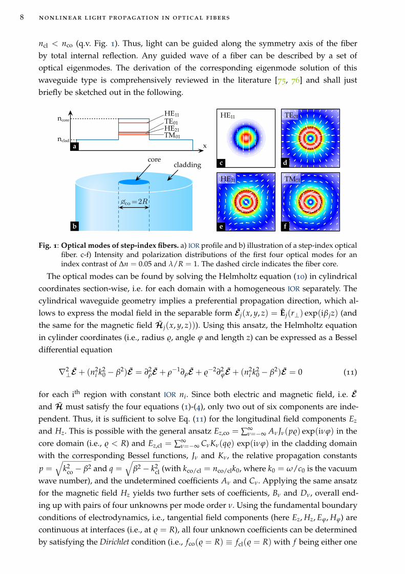
Fig. 1: Optical modes of step-index fibers. a) IOR profile and b) illustration of a step-index opticalfiber. c-f) Intensity and polarization distributions of the first four optical modes for anindex contrast of ∆n = 0.05 and λ/R = 1. The dashed circle indicates the fiber core.
The optical modes can be found by solving the Helmholtz equation (10) in cylindrical
coordinates section-wise, i.e. for each domain with a homogeneous IOR separately. The
cylindrical waveguide geometry implies a preferential propagation direction, which al-
lows to express the modal field in the separable form Ej(x, y, z) = Ej(r⊥) exp(iβ jz) (and
the same for the magnetic field Hj(x, y, z))). Using this ansatz, the Helmholtz equation
in cylinder coordinates (i.e., radius , angle ϕ and length z) can be expressed as a Bessel
differential equation
∇2⊥E + (n2
i k20 − β2)E = ∂2
ρE + ρ−1∂ρE + −2∂2ϕE + (n2
i k20 − β2)E = 0 (11)
for each ith region with constant IOR ni. Since both electric and magnetic field, i.e. E
and H must satisfy the four equations (1)-(4), only two out of six components are inde-
pendent. Thus, it is sufficient to solve Eq. (11) for the longitudinal field components Ez
and Hz. This is possible with the general ansatz Ez,co = ∑∞ν=−∞ Aν Jν(p) exp(iνϕ) in the
core domain (i.e., < R) and Ez,cl = ∑∞ν=−∞ CνKν(q) exp(iνϕ) in the cladding domain
with the corresponding Bessel functions, Jν and Kν, the relative propagation constants
p =√
k2co − β2 and q =
√
β2 − k2cl (with kco/cl = nco/clk0, where k0 = ω/c0 is the vacuum
wave number), and the undetermined coefficients Aν and Cν. Applying the same ansatz
for the magnetic field Hz yields two further sets of coefficients, Bν and Dν, overall end-
ing up with pairs of four unknowns per mode order ν. Using the fundamental boundary
conditions of electrodynamics, i.e., tangential field components (here Ez, Hz, Eϕ, Hϕ) are
continuous at interfaces (i.e., at = R), all four unknown coefficients can be determined
by satisfying the Dirichlet condition (i.e., fco( = R) ≡ fcl( = R) with f being either one
2.1 fundamental wave equation of optics 9
of the field components Ez, Hz, Eϕ, and Hϕ). This yields four equations which can be ex-
pressed in matrix form, whereas the characteristic function of the coefficient matrix (i.e.,
by demanding the determinant of the matrix to be zero) yields a compact transcendental
dispersion relation [76, 75]
[
∂ρ Jν(pR)
pJν(pR)+
∂ρKν(qR)
qKν(qR)
] [
k21∂ρ Jν(pR)
pJν(pR)+
k22∂ρKν(qR)
qKν(qR)
]
=
(βν
R
)2( 1p2 +
1q2
)2
. (12)
For a given fiber (i.e., nco, ncl, R) and mode (i.e., ν, λ) the µth roots of this function over
β denote for the eigenvalue of the propagating mode, and thus the modal propagation
constant βνµ. For simplicity, in this work, appropriate optical materials are assumed to
the greatest extent transparent, and fiber modes to be bound, which limits β to a real
codomain within kco > β > kcl. Finding the root of Eq. (12) is a numerical practice.
2.1.2 Linear fiber mode properties in brief
Depending on the inner (core) diameter (co) and the numerical aperture (NA) of the
fiber, i.e., NA =√
n2co − n2
cl, the fiber supports from one to multiple modes. Modes are
distinguished in their propagation constant β (i.e., here β = βnm) , their field distribution,
and their polarization. The mode with the largest effective mode index neff = β/k0 is
called the fundamental mode. Different to ridge or slab waveguides, the fundamental
fiber mode is a hybrid electric (HE) mode (i.e., all electric field components are non-zero)
with mode order n = 1 and mode number m = 1. The HE11 mode features a Gauss-like
intensity distribution with the largest field overlap with the core domain compared to
all other fiber modes (cf. intensity patterns in Fig. 1c-f). Also in contrast to higher-order
modes, the HE11 has no cut-off frequency (i.e., a minimum frequency below which the
mode is not bound anymore). However, it shall be noted, that in practice microbends
and other fabrication imperfections introduce high losses due to scattering, which limits
single-mode operation on the low frequency side.
Thus, a practical parameter to estimate the quality of the guide becomes necessary,
which can be found in the so-called V-parameter [75]
V = k0 · R · NA . (13)
A fiber operates in the single-mode regime as long as the single-mode criterion (SMC)
V < 2.405 is fulfilled. Scattering losses limit the parameter range additionally to V >
Vcrit, whereas the critical limit has to be determined empirically for each fiber type. The
V-parameter can also be used to estimate the number of modes M supported in the fiber
using the empiric relation M ≈ V2/2.
Further, the linear propagation characteristics of both optical waves and pulses in any
given fiber mode is described by the frequency-dependent propagation parameter β. To
10 nonlinear light propagation in optical fibers
expose this information β(ω) can be expanded in a Taylor series around a given central
frequency ω0
β(ω) ≈ β0 + β1(ω − ω0) +12 β2(ω − ω0)
2 +O(ω3) with β j =djβ
dω j
∣∣∣∣ω0
. (14)
According to the bandwidth of the pulse more terms have to be added in the series. The
coefficients of the individual terms play a specific role in the propagation of an optical
pulse. Whereas β0 describes the fast carrier oscillation of the pulse (i.e., the central wave
number), β1 is the inverse of the group velocity of the pulse (i.e., vg = dω/dβ), and
β2 is the group velocity dispersion (often used in units of fs2/m). The group velocity
dispersion describes the relative difference between the group velocities of higher and
lower frequency components of a spectrally broadband optical pulse, and, thus, is a
measure of how strong a pulse disperses along propagation. In detail, the broadening of
a pulse with duration THP over a propagation length L can be estimated with β2L/THP
(in units of fs). Third and fourth order dispersions (i.e., β3 and β4) might also play a role
if the pulse width is in the order of sub-picoseconds.
In practice, the dispersion is often expressed in terms of the technical dispersion para-
meter
D = − λ
c0
d2neff
dλ2 =2πc0
λ2d2β
dω, (15)
with wavelength λ = 2πc0/ω. D is usually given in units of ps/(nm·km), which corres-
ponds to temporal pulse spreading per bandwidth and propagation length. This para-
meter is denoted as group velocity dispersion (GVD) throughout this work to investigate
fiber designs, whereas all values of D are given units of fs/(nm·cm) to account for the
pulse widths and fiber lengths usually used in the experiments. The fiber dispersion is
distinguished in normal dispersion domain (NDD) (i.e., D < 0) and anomalous disper-
sion domain (ADD) (i.e., D > 0). The wavelength, where the dispersion changes from
ADD to NDD or vice versa, is denoted as zero-dispersion wavelength (ZDW). It is an
important benchmark of nonlinear fiber designs, as explained in sec. 2.3.1.
2.2 Nonlinear pulse propagation in optical fibers
2.2.1 Intensity-dependent refractive index
The strong confinement of optical fiber modes along meter- to kilometer-long propaga-
tion lengths significantly boosts the relevance of optical nonlinear effects. One way to
understand the generation of new frequencies via nonlinear light-matter interactions, is
to think of an refractive index grating (with period length n(ω)k0) inscribed by the field
intensity, at which the field refracts causing an energy transfer to field components at dis-
tant wavelengths. This index modulation can particularly be understood by introducing
a practical quantity, namely the nonlinear refractive index.
2.2 nonlinear pulse propagation in optical fibers 11
This is possible by simplifying the general nonlinear polarization PNL in Eq. (6). A first
practical assumption is to consider only linear polarized electric fields and isotropic (or
weakly anisotropic), and lossless, nonlinear media, resulting in identical polarization of
all involved fields, i.e., E/|E | = PNL/|PNL|. The assumption further allows to drastically
reduce the 21 nonzero elements of the third-order susceptibility tensor χ(3) to a single
independent component [77, 78], which is straightforwardly denoted as χ(3)eff = χ
(3)xxxx
in the common literature (e.g., [79]). Under those assumptions, the general nonlinear
polarization field can be simplified in the frequency domain to [78]
PNL(ω) = ε0C(3)χ(3)eff (ω; ω′, ω′′, ω′′′)E(ω′)E(ω′′)E(ω′′′) . (16)
The permutation factor is C(3) = 3, if third-harmonic effects are neglected and only self-
induced nonlinear effects are assumed (i.e., PNL(ω = ω + ω − ω) ∝ E E E∗). In general,
the material response χ(3) can be assumed as linear combination of different nonlinear
contributions, such as instantaneous electronic motions and noninstantaneous nuclear
effects (e.g., stimulated Raman scattering, or molecular reorientation). This general treat-
ment is reviewed in appendix B. For now, only electronic effects, as major source of non-
linearity in most optical glasses, shall be considered, which allows to express Eq. (16) in
its most simple form
PNL(ω) = 3ε0χ(3)eff (ω)E(ω)E∗(ω)E(ω) . (17)
Inserting Eq. (17) into Eq. (9), allows to define a field-dependent IOR, based on the
definition of the dielectric function from sec. 2.1
n2(ω, E) = 1 + χeff(ω, E) = 1 + χ(1) + 3χ(3)eff |E |2 . (18)
In first-order approximation n(ω, E) can be expressed in terms of linear perturbation ∆n,
i.e., n(ω, E)2 = (n0(ω) + ∆n(ω, I))2 ≈ n20 + 2n0∆n. Finally, combined with the definition
of the intensity I(ω) = 2n0ε0c0|E(ω)|2, the nonlinear refractive index (NRI) n2 (in units
of m2/W) can be found [78]
∆n(ω, I) =3χ
(3)eff
2n0|E |2 =
3χ(3)
4n20ε0c0
I(ω) ≡ n2 I =⇒ n2 =3χ
(3)eff
4n20ε0c0
. (19)
The corresponding phase term ∆nk0 = k0n2 I can be seen as an additional momentum
acting on certain frequency components of the pulse causing an energy transfer. The NRI
is widely used in experimental work to evaluate the nonlinearity of different materials.
It will be applied in a modified form to slowly responding nonlinear liquids in sec. 3.3.1.
2.2.2 Nonlinear Schrödinger equation
The nonlinear pulse dynamic in optical fibers can become quite complex, and requires
a rigorous model involving all relevant effects. However, to solve the general vectorial
12 nonlinear light propagation in optical fibers
nonlinear wave equation in Eq. (9) is a nontrivial and computational resource consum-
ing task. Thus, many simplified nonlinear propagation equations were used in literature
(e.g., a very good overview is given in the review [80]), each owing their own benefits
and limitations. Within the framework of this work, the nonlinear Schrödinger equa-
tion in the generalized form was chosen to investigate pulse propagation in the special
fiber systems numerically. To understand its limitations and to form the theoretical back-
ground for specialized versions introduced later the derivation of the this widely used
amplitude equation shall be outlined in the following. Note that, different to many pub-
lications, the derivation does not follow the approach by Agrawal presented in his book
[79], but the more general derivation presented by Mamyshev and Chernikov [81]. Al-
ternative mathematically rigorous derivations can be found, e.g., in the works by Kolesik
and Moloney [82] and the review by Courairon et al. [80].
The solution of the linear wave equation (11) can be used to simplify the nonlinear
wave equation (9). Therefore, the monochromatic field ansatz is extended to
E = e0F(r⊥; ω)U(z; ω) exp(iβ j(ω)z) , (20)
where β j = nj,eff(ω, E)ω/c0 is the propagation constant of the jth perturbed fiber mode
in the nonlinear system. Heuristically, the ansatz separates a slowly varying envelope U
from the fast carrier wave oscillating with ω. The real transversal field pattern F is real.
Inserting the perturbation ansatz from Eq. (20) into Eq. (9) and splitting of the Laplace
operator into its transversal and perpendicular parts (i.e., ∇2 = ∇2⊥ + ∂2
z) yields
U[
∇2⊥ F + n2
i k20F − β2
j F]
︸ ︷︷ ︸
Eq. (11) ⇒ 0
+ F∂2zU
︸ ︷︷ ︸
SVEA ⇒ 0
+ 2iβ j F∂zU
= −µ0ω2PNL(F, U)e−iβ jz(21)
The first term is the eigenmode problem and becomes zero in waveguides assuming the
nonlinear perturbation of the propagation constant β j to be weak. Note that the latter is
intrinsically given by the ansatz in Eq. (20) already, since the transversal field is assumed
real and propagation invariant, i.e., F 6= f (z). Further, we assume that the field envelope
U(ω, z) varies only slowly along the propagation along z, so that ∂2zU ≪ β j∂zU. This
allows neglecting the second z-derivative in Eq. (21), commonly known as slowly varying
envelope approximation (SVEA). Both assumptions allow to simplify Eq. (21) to
F∂zU = i3µ0ω2
2β j(ω)PNL(F, U)e−iβ j(ω)z . (22)
Indeed, Eq. (22) confirms the nonlinear polarization as source of the slow field variation
along the propagation. The general nonlinear polarization PNL is derived in detail for
2.2 nonlinear pulse propagation in optical fibers 13
an isotropic noninstantaneous medium in appendix B. Using the expression in Eq. (83)
from there, PNL in the propagation equation can be expressed in U
F∂zU = i3k0
2neff,j(ω)
∫
dω′∫
dω′′[FU](ω′)[FU]∗(ω′ + ω′′ − ω)
× [FU](ω′′)χ(3)(ω − ω′)ei∆βz ,(23)
with the phase mismatch ∆β = β j(ω′) + β j(ω
′′)− β j(ω′ + ω′′ − ω)− β j(ω). We normal-
ize Eq. (23) to the power by (1) multiplying F from the left side, (2) integrating over the
transversal coordinates r⊥, and (3) dividing the equation by∫
d2r⊥ F2. Thus, Eq. (23)
∂zU = i3k0
2neff,j(ω)
∫
dω′∫
dω′′G(ω, ω′, ω′′)U(ω′)
× U∗(ω′ + ω′′ − ω)U(ω′′)χ(3)(ω − ω′)ei∆βz ,(24)
with the mode field overlap
G(ω, ω′, ω′′) =
∫d2r⊥ F(r⊥; ω)F(r⊥; ω′)F(r⊥; ω′ + ω′′ − ω)F(r⊥; ω′′)
∫d2r⊥ F2(r⊥; ω)
. (25)
In practice, it is useful normalize U to the power of the field P =∫
d2r⊥ I = 2neff,jε0c0
×∫
F2d2r⊥|U|2. This yields the normalized amplitude A′(z; ∆ω) =√
2neff,jε0c0∫
d2r⊥F2
×U exp(i[β j(ω)− β j,0 − β j,1∆ω]z) with ∆ω = ω − ω0. The phase of this substituent is
chosen such that it incorporates the full fiber dispersion minus the fast carrier oscillation
(associated with β j,0) and the group velocity of the pulse (associated with β j,1). The latter
corresponds to the common transformation in time domain to a reference frame moving
with the pulse at the group velocity vg = β−1j,1 [81, 79].
The normalization changes G to G′ = G/∫
d2r⊥ F2. To the first order, G′ can be ap-
proximated with G′(ω, ω′, ω′′) ≈ [Aeff(ω)Aeff(ω′)Aeff(ω
′′)Aeff(ω′ + ω′′ − ω)]−1/4 [83],
which introduces the effective mode area Aeff = (∫
d2r⊥ F2)2/∫
d2r⊥ F4. The linear separ-
ation in G′ now justifies a further renormalization of the field amplitude to A = A′/A1/4eff ,
so that A is in units of intensity W/m. Finally, we obtain the so-called generalized non-
linear Schrödinger equation (GNSE) [81]
∂z A(z; ω)− i[β j(ω)− β j,0 − β j,1∆ω
]A
Eq. (14)= ∂z A − i ∑
k≥2
1k!
β j,k∆ωk A
= i3k0
4n2eff,jε0c0
4√
Aeff
∫
dω′∫
dω′′ A(ω′)A∗(ω′ + ω′′ − ω)A(ω′′)χ(3)(ω − ω′)
= iγ(ω)F−1
A(z; t)[
R ∗ |A|2]
, (26)
with the modified nonlinear gain parameter γ = k0n2/A1/4eff , the convolution operator
[∗], and the nonlinear response function (NRF) R(t) (normalized to∫
dtR = 1 and
14 nonlinear light propagation in optical fibers
introduced with Eq. (82) in appendix B). The last step in Eq. (26) also incorporated the
definition of the NRI in Eq. (19).
Equation (26) is the most physical representation of the different GNSEs known from
literature and used throughout this thesis. It features the full dispersion of the propaga-
tion parameter β j(ω) and the nonlinearity γ(ω). Broadband loss (or gain) can straight-
forwardly be included adding the term 12 α(ω)A on the left-hand side. Most notably, the
renormalization to the field A incorporates the frequency dependent mode area in the
temporal convolution, since the temporal envelope is now A(z; t) = FA(z; ω)/ 4√
Aeff.
This normalization is often forgotten in the recent literature, but was explicitly proposed
as correction, e.g., by Laegsgaard [83].
From Eq. (26) the more prominent version of the GNSE can be derive by applying the
following operations:
1. Assume the effective mode areas to be frequency independent, i.e., [Aeff(ω)Aeff(ω′)
Aeff(ω′′)Aeff(ω
′ + ω′′ − ω)]1/4 ≈ Aeff(ω0), whereas the A−1/4eff factors from the
field normalization can be combined to the common nonlinear gain parameter
γ(ω) = k0n2/Aeff,
2. Expand the nonlinear parameter in a Taylor series, i.e., γ(∆ω) ≈ γ0 + γ1∆ω, with
γk = ∂kωγ(ω)|ω0 ,
3. Transform Eq. (26) into the time domain.
These changes result in the GNSE commonly known from literature (cf. Eq. (2.3.36) in
[79])
∂z A(z; t) +α
2A − ∑
k≥2ik+1β j,k∂k
t A = iγ0
(
1 + iγ1
γ0∂t
)(
A(z, t)[
R ∗ |A|2])
. (27)
At this point, further simplifications can be made on Eq. (27) to achieve different model
systems, which are useful to study specific nonlinear effects in optical fibers. The most
relevant for this work, is the specialized nonlinear Schrödinger equation (NSE)
∂z A(z; t) + i12 β j,2∂2
t A = iγ0|A|2A , (28)
which allows to find optical solitons as introduced in sec. 2.3.3.1. The specialized NSE
can be obtained assuming a lossless (i.e., α = 0), second-order dispersive (i.e., β j,k = 0
for k > 2) fiber with non-dispersive nonlinear gain (i.e., γ1 = 0), and instantaneous
nonlinear response (i.e., R(t) = δ(t)).
2.2.3 Nonlinear gain parameter of step-index fibers
With the GNSE the nonlinear gain parameter γ was introduced, which combined the
material-specific NRI n2 with the mode-specific effective mode area Aeff. It has been
shown in the scope of this work [84] and others [85], that the standard definition of
Aeff deviates strongly from the accurate vectorial mode area. A powerful alternative is
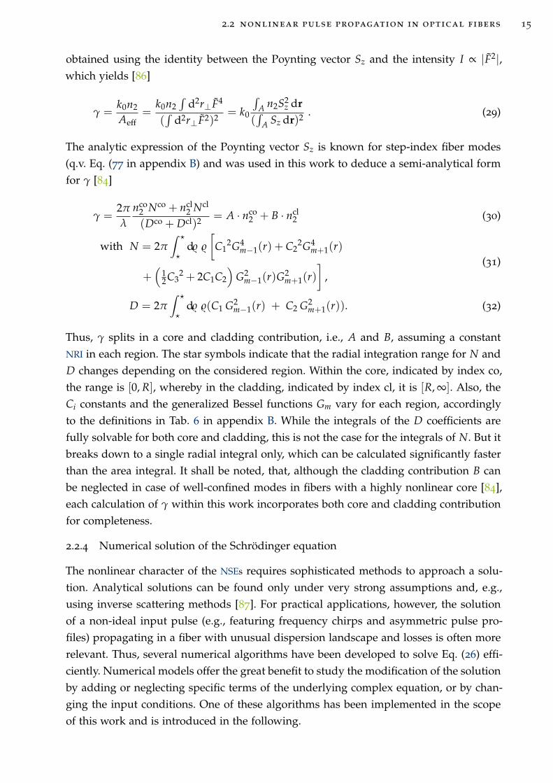
2.2 nonlinear pulse propagation in optical fibers 15
obtained using the identity between the Poynting vector Sz and the intensity I ∝ |F2|,which yields [86]
γ =k0n2
Aeff=
k0n2∫
d2r⊥ F4
(∫
d2r⊥ F2)2= k0
∫
A n2S2z dr
(∫
A Sz dr)2 . (29)
The analytic expression of the Poynting vector Sz is known for step-index fiber modes
(q.v. Eq. (77 in appendix B) and was used in this work to deduce a semi-analytical form
for γ [84]
γ =2π
λ
nco2 Nco + ncl
2 Ncl
(Dco + Dcl)2 = A · nco2 + B · ncl
2 (30)
with N = 2π∫
⋆
⋆
d
[
C12G4
m−1(r) + C22G4
m+1(r)
+(
12C3
2 + 2C1C2
)
G2m−1(r)G
2m+1(r)
]
,(31)
D = 2π∫
⋆
⋆
d (C1 G2m−1(r) + C2 G2
m+1(r)). (32)
Thus, γ splits in a core and cladding contribution, i.e., A and B, assuming a constant
NRI in each region. The star symbols indicate that the radial integration range for N and
D changes depending on the considered region. Within the core, indicated by index co,
the range is [0, R], whereby in the cladding, indicated by index cl, it is [R, ∞]. Also, the
Ci constants and the generalized Bessel functions Gm vary for each region, accordingly
to the definitions in Tab. 6 in appendix B. While the integrals of the D coefficients are
fully solvable for both core and cladding, this is not the case for the integrals of N. But it
breaks down to a single radial integral only, which can be calculated significantly faster
than the area integral. It shall be noted, that, although the cladding contribution B can
be neglected in case of well-confined modes in fibers with a highly nonlinear core [84],
each calculation of γ within this work incorporates both core and cladding contribution
for completeness.
2.2.4 Numerical solution of the Schrödinger equation
The nonlinear character of the NSEs requires sophisticated methods to approach a solu-
tion. Analytical solutions can be found only under very strong assumptions and, e.g.,
using inverse scattering methods [87]. For practical applications, however, the solution
of a non-ideal input pulse (e.g., featuring frequency chirps and asymmetric pulse pro-
files) propagating in a fiber with unusual dispersion landscape and losses is often more
relevant. Thus, several numerical algorithms have been developed to solve Eq. (26) effi-
ciently. Numerical models offer the great benefit to study the modification of the solution
by adding or neglecting specific terms of the underlying complex equation, or by chan-
ging the input conditions. One of these algorithms has been implemented in the scope
of this work and is introduced in the following.
16 nonlinear light propagation in optical fibers
∆z
D DSpectral domain:
Time domain:FT FT−1
N
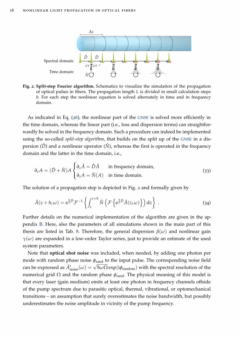
Fig. 2: Split-step Fourier algorithm. Schematics to visualize the simulation of the propagationof optical pulses in fibers. The propagation length L is divided in small calculation stepsh. For each step the nonlinear equation is solved alternately in time and in frequencydomain.
As indicated in Eq. (26), the nonlinear part of the GNSE is solved more efficiently in
the time domain, whereas the linear part (i.e., loss and dispersion terms) can straightfor-
wardly be solved in the frequency domain. Such a procedure can indeed be implemented
using the so-called split-step algorithm, that builds on the split up of the GNSE in a dis-
persion (D) and a nonlinear operator (N), whereas the first is operated in the frequency
domain and the latter in the time domain, i.e.,
∂z A = (D + N)A
∂z A = DA in frequency domain,
∂z A = N(A) in time domain.(33)
The solution of a propagation step is depicted in Fig. 2 and formally given by
A(z + h; ω) = eh2 DF−1
∫ z+h
zN(
F
eh2 D A(z; ω)
)
dz
. (34)
Further details on the numerical implementation of the algorithm are given in the ap-
pendix B. Here, also the parameters of all simulations shown in the main part of this
thesis are listed in Tab. 8. Therefore, the general dispersion β(ω) and nonlinear gain
γ(ω) are expanded in a low-order Taylor series, just to provide an estimate of the used
system parameters.
Note that optical shot noise was included, when needed, by adding one photon per
mode with random phase noise φrand to the input pulse. The corresponding noise field
can be expressed as A′noise(ω) =
√hωΩ exp(iφrandom) with the spectral resolution of the
numerical grid Ω and the random phase φrand. The physical meaning of this model is
that every laser (gain medium) emits at least one photon in frequency channels offside
of the pump spectrum due to parasitic optical, thermal, vibrational, or optomechanical
transitions – an assumption that surely overestimates the noise bandwidth, but possibly
underestimates the noise amplitude in vicinity of the pump frequency.
2.3 relevant nonlinear effects for supercontinuum generation 17
2.3 Relevant nonlinear effects for supercontinuum generation
2.3.1 Overview of third-order nonlinear effects in fibers
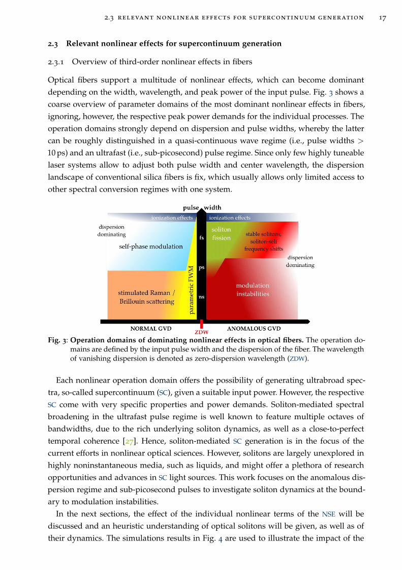
Optical fibers support a multitude of nonlinear effects, which can become dominant
depending on the width, wavelength, and peak power of the input pulse. Fig. 3 shows a
coarse overview of parameter domains of the most dominant nonlinear effects in fibers,
ignoring, however, the respective peak power demands for the individual processes. The
operation domains strongly depend on dispersion and pulse widths, whereby the latter
can be roughly distinguished in a quasi-continuous wave regime (i.e., pulse widths >
10 ps) and an ultrafast (i.e., sub-picosecond) pulse regime. Since only few highly tuneable
laser systems allow to adjust both pulse width and center wavelength, the dispersion
landscape of conventional silica fibers is fix, which usually allows only limited access to
other spectral conversion regimes with one system.
Fig. 3: Operation domains of dominating nonlinear effects in optical fibers. The operation do-mains are defined by the input pulse width and the dispersion of the fiber. The wavelengthof vanishing dispersion is denoted as zero-dispersion wavelength (ZDW).
Each nonlinear operation domain offers the possibility of generating ultrabroad spec-
tra, so-called supercontinuum (SC), given a suitable input power. However, the respective
SC come with very specific properties and power demands. Soliton-mediated spectral
broadening in the ultrafast pulse regime is well known to feature multiple octaves of
bandwidths, due to the rich underlying soliton dynamics, as well as a close-to-perfect
temporal coherence [27]. Hence, soliton-mediated SC generation is in the focus of the
current efforts in nonlinear optical sciences. However, solitons are largely unexplored in
highly noninstantaneous media, such as liquids, and might offer a plethora of research
opportunities and advances in SC light sources. This work focuses on the anomalous dis-
persion regime and sub-picosecond pulses to investigate soliton dynamics at the bound-
ary to modulation instabilities.
In the next sections, the effect of the individual nonlinear terms of the NSE will be
discussed and an heuristic understanding of optical solitons will be given, as well as of
their dynamics. The simulations results in Fig. 4 are used to illustrate the impact of the
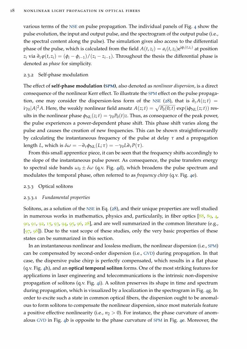
18 nonlinear light propagation in optical fibers
various terms of the NSE on pulse propagation. The individual panels of Fig. 4 show the
pulse evolution, the input and output pulse, and the spectrogram of the output pulse (i.e.,
the spectral content along the pulse). The simulation gives also access to the differential
phase of the pulse, which is calculated from the field A(t, zi) = ai(t, zi)eiφi(t,zi) at position
zi via ∂z ϕ(t, zi) = (φi − φi−1)/(zi − zi−1). Throughout the thesis the differential phase is
denoted as phase for simplicity.
2.3.2 Self-phase modulation
The effect of self-phase modulation (SPM), also denoted as nonlinear dispersion, is a direct
consequence of the nonlinear Kerr effect. To illustrate the SPM effect on the pulse propaga-
tion, one may consider the dispersion-less form of the NSE (28), that is ∂z A(z; t) =
iγ0|A|2A. Here, the weakly nonlinear field ansatz A(z; t) =√
P0(0; t) exp(iφNL(z; t)) res-
ults in the nonlinear phase φNL(z; t) = γ0P0(t)z. Thus, as consequence of the peak power,
the pulse experiences a power-dependent phase shift. This phase shift varies along the
pulse and causes the creation of new frequencies. This can be shown straightforwardly
by calculating the instantaneous frequency of the pulse at delay τ and a propagation
length L, which is δω = −∂τφNL(L; τ) = −γ0L∂τP(τ).
From this small apprentice piece, it can be seen that the frequency shifts accordingly to
the slope of the instantaneous pulse power. As consequence, the pulse transfers energy
to spectral side bands ω0 ± δω (q.v. Fig. 4d), which broadens the pulse spectrum and
modulates the temporal phase, often referred to as frequency chirp (q.v. Fig. 4e).
2.3.3 Optical solitons
2.3.3.1 Fundamental properties
Solitons, as a solution of the NSE in Eq. (28), and their unique properties are well studied
in numerous works in mathematics, physics and, particularily, in fiber optics [88, 89, 4,
90, 91, 92, 15, 93, 94, 95, 96, 28], and are well summarized in the common literature (e.g.,
[97, 98]). Due to the vast scope of these studies, only the very basic properties of these
states can be summarized in this section.
In an instantaneous nonlinear and lossless medium, the nonlinear dispersion (i.e., SPM)
can be compensated by second-order dispersion (i.e., GVD) during propagation. In that
case, the dispersive pulse chirp is perfectly compensated, which results in a flat phase
(q.v. Fig. 4h), and an optical temporal soliton forms. One of the most striking features for
applications in laser engineering and telecommunications is the intrinsic non-dispersive
propagation of solitons (q.v. Fig. 4i). A soliton preserves its shape in time and spectrum
during propagation, which is visualized by a localization in the spectrogram in Fig. 4g. In
order to excite such a state in common optical fibers, the dispersion ought to be anomal-
ous to form solitons to compensate the nonlinear dispersion, since most materials feature
a positive effective nonlinearity (i.e., n2 > 0). For instance, the phase curvature of anom-
alous GVD in Fig. 4b is opposite to the phase curvature of SPM in Fig. 4e. Moreover, the
2.3 relevant nonlinear effects for supercontinuum generation 19
0.8
1
1.2fr
equ
ency
[ω0]
−30 0
Out
In
0
0.5
1
1.5
inte
nsit
y[I
0]
−10 0 10 2002468
10
leng
th[L
D]
0
1
OutIn
−10 0 10 20
ω0
In Out
−10 0 10 20
time delay [τ0]
recoil
NSR
Out
NSR
soliton
0 20 40 60
SSFS
NSR
Out
22
23
24
25
26
dif
f.p
hase
[L−
1D
]
NSR
soliton
0 20 40 60
GVD only
a
b
c
SPM only
d
e
f
GVD & SPM
g
h
i
TOD
j
k
l
TOD & Raman
m
n
o
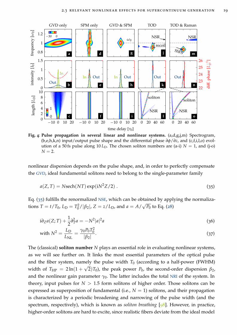
Fig. 4: Pulse propagation in several linear and nonlinear systems. (a,d,g,j,m) Spectrogram,(b,e,h,k,n) input/output pulse shape and the differential phase ∂φ/∂z, and (c,f,i,l,o) evol-ution of a 50 fs pulse along 10 LD. The chosen soliton numbers are (a-i) N = 1, and (j-o)N = 2.
nonlinear dispersion depends on the pulse shape, and, in order to perfectly compensate
the GVD, ideal fundamental solitons need to belong to the single-parameter family
a(Z, T) = Nsech(NT) exp(iN2Z/2) . (35)
Eq. (35) fulfills the renormalized NSE, which can be obtained by applying the normaliza-
tions T = t/T0, LD = T20 /|β2|, Z = z/LD, and a = A/
√P0 to Eq. (28)
i∂Za(Z; T) +12
∂2Ta = −N2|a|2a (36)
with N2 =LD
LNL=
γ0P0T20
|β2|. (37)
The (classical) soliton number N plays an essential role in evaluating nonlinear systems,
as we will see further on. It links the most essential parameters of the optical pulse
and the fiber system, namely the pulse width T0 (according to a half-power (FWHM)
width of THP = 2 ln(1 +√
2)T0), the peak power P0, the second-order dispersion β2,
and the nonlinear gain parameter γ0. The latter includes the total NRI of the system. In
theory, input pulses for N > 1.5 form solitons of higher order. Those solitons can be
expressed as superposition of fundamental (i.e., N = 1) solitons, and their propagation
is characterized by a periodic broadening and narrowing of the pulse width (and the
spectrum, respectively), which is known as soliton breathing [98]. However, in practice,
higher-order solitons are hard to excite, since realistic fibers deviate from the ideal model
20 nonlinear light propagation in optical fibers
in dispersion and nonlinearity. Those deviations act as perturbation on the higher-order
soliton propagation causing characteristic effects, which are briefly described in q.v. sec.
2.3.3.2, 2.3.3.3 and 2.3.4.
The normalization of Eq. (36) introduces two further helpful quantities, which are
the dispersion length LD = T20 /|β2| and the nonlinear length LNL = (γ0P0)
−1. The
length scales can be used to estimate whether dispersive (for L ≥ LD) or nonlinear
effects (for L ≥ LNL) dominate the pulse propagation in a fiber of length L. If the fiber
length is longer than or comparable to both lengths (i.e., L ≥ [LD, LNL]), an interplay of
both dispersion and nonlinearity leads to a characteristically different pulse propagation,
which may evoke the formation of solitons.
Finally, it is important to note that most realistic fiber systems underlie deviations from
the ideal model described with Eq. (36), which includes losses, mode field dispersion
(often forgotten), higher order dispersion, or nonlinear scattering effects. In some cases,
those deviations can be handled as perturbations on the soliton, which modify its prop-
erties (q.v. sec. 2.3.3.2 and 2.3.3.3). In other cases, those perturbations are too strong and
the soliton, although potentially created in the fiber, decays after a certain propagation
length, which in turn conflicts with the self-maintaining character of a soliton. Moreover,
in some narrower definitions, solitons are solutions of integrable mathematical equations
and have to withstand collisions with other solitons of the same type, which is not al-
ways easy to proof. Thus, throughout this work, the term soliton is used in the wider
framework of a solitary wave, which is characterized by a self-similar pulse shape (in
time and spectrum) over a limited propagation length. In particular, the use of the term
soliton does not imply the mathematical integrability of the governing NSE, which is
used as soliton condition in theory.
2.3.3.2 Impact of third-order dispersion
The effect of third-order dispersion (TOD) can straightforwardly be added to Eq. (36)
with the term δ3∂3Ta with δ = β3/(6|β2|T0). This term can be understood as perturbation
on the ideal β2 soliton, which has been extensively studied theoretically (e.g., [99, 100,
4, 101, 102, 103, 104]) and utilized in many experiments in fibers [105, 106, 42, 107] and
ridge waveguides [108, 109, 110]. In proximity to the ZDW, the soliton spectrum may
overlap with perfectly phase-matched resonance frequencies of linear waves to which
the soliton transfers energy. The efficiency of this process depends on the spectral seed
energy (i.e., spectral overlap), and the group-velocity mismatch between soliton and the
phase-locked radiated wave. The process shows similarities to the emission of radiation
from an accelerated charged particle in relativistic physics, the linear wave emitted from
a soliton is often called (Vavilov–)Cherenkov radiation, but also known as non-solitonic
radiations (NSRs), or dispersive waves. If the perturbation is strong enough, TOD can lead
to a split-up of the pulse into maximum N consecutive fundamental solitons, which is
known as soliton fission and is briefly described in sec. 2.3.4.
2.3 relevant nonlinear effects for supercontinuum generation 21
The coupling between NSR and solitons is well studied theoretically in many works
(e.g. by Gordon [90], Akhmediev et al. [15], Herrmann et al. [111], Biancalana et al. [93], or
Efimov et al. [112]). Those studies reveal a phase matching condition (resonance condi-
tion), that links a fundamental optical soliton to its radiated NSR, given by
∆β ≈ β(ω)− βs − (ω − ωs)β1,s − 12 γ0P0 ≡ 0 . (38)
The condition compares the flat phase of a soliton (i.e., βs +12 γ0P0) with the general
dispersion of a linear wave (i.e., β(ω)) in the moving frame of the soliton (i.e., (ω −ωs)β1,s), which accounts for the group velocity match. Condition (38) can be used to
calculate the frequency of the radiated NSR in case the soliton frequency is given, or vice
versa. However, it shall be noted that the exhaust of energy to NSR causes the soliton
to shift deeper into the ADD. This shift is called the soliton recoil (q.v. Fig. 4j) and can
heuristically be explained by momentum conservation between the radiated field and
the soliton [15, 93]. The recoil modifies the soliton net phase (cf. red curve in Fig. 4k) and,
thus, causes a temporal shift. However, this shift depends on a multitude of parameters
(e.g., amplitudes and frequencies of each field involved) and is hard to take into account
when determining the frequencies of solitons and NSR from a measured spectrum.
Optical trapping of NSR and further nonlinear energy exchange between solitons and
NSR (as well as other linear waves) is possible via four-wave mixing under certain condi-
tions and may lead to a continuous red-shift of the soliton frequency and a blue-shift of
the NSR [113, 114, 112, 95].
Note that, despite the reasonable understanding of NSR generation, the theoretical de-
scription lacks in a discrete description of the wave mixing mechanics and proper energy
conservation laws. Thus, NSR generation is still object of recent investigations. Alternat-
ive descriptions of this effects include spectral coupling between nonlinear radiation
modes [115], or cascaded four wave mixing through the spectral valley between soliton
and NSR [116].
2.3.3.3 Impact of short-term noninstantaneous nonlinearities
Short-term noninstantaneous nonlinear effects in the NSE were studied in the frame-
work of stimulated Raman scattering in silica fibers. The temporal response (and the
spectral gain, respectively) of the Raman effect in silica is well measured and modelled
[117, 118, 119]. The Raman effect is mostly included in the NSE by the quasi-instantaneous
approximation of the general convolution term in Eq. (27). Therefore, the response func-
tion R is assumed to be
R(t) = (1 − fR)δ(t) + fRhR(t) , (39)
with the Dirac delta function δ(t) representing the instantaneous electronic nonlinear
effect, the Raman fraction fR ≈ 0.18, and the characteristic Raman response of silica
hR [119]. When the pulse width is assumed to be much longer than the response time
22 nonlinear light propagation in optical fibers
(i.e., T0 ≫ TR = 32 fs), the field intensity can be expanded in a Taylor series (i.e., |A(z; t−t′)|2 ≈ |A(z; t)|2 + t′∂t|A(z; t)|2) and the convolution integral can be approximated with
∫ ∞
−∞dτ hR(τ) ∗ |A(z; t − τ)|2 ≈ |A|2 + TR∂t|A|2 , (40)
with the response time TR = fR
∫ ∞
0 dthR(t). It is possible to find a modified soliton solu-
tion of the NSE (36) extended by the (renormalized) Raman term from Eq. (40) [89, 120].
The Raman term leads to a linear frequency red-shift of solitons over propagation, also
known as soliton self-frequency shift (SFS) [121] or intrapulse (i.e., self-induced) Raman
scattering. The strength of red-shift increases for decreasing pulse width, or increas-
ing spectral overlap between pulse spectrum and Raman gain spectrum, respectively.
Moreover, the soliton adiabatically adjusts its pulse width when shifting into domains
of higher or lower dispersion to maintain its fundamental soliton condition N = 1.
SFS serves as formidable mechanism to tune the frequency of soliton-governed light
sources [14], whereas it has detrimental effects for the channel stability of soliton tele-
communication networks [11]. It also has been found, that the SFS can be cancelled by
TOD, where the radiation pressure of an emitted NSR can de- or accelerate the soliton
in its Raman driven motion [93]. Notably, the consecutive stabilized state of this mani-
fold perturbed system can still be described as soliton [120], which is in perfect balance
between higher-order dispersion, dispersive nonlinearity, and noninstantaneous effects,
indeed forming a separate family of meta-stable states.
2.3.4 Soliton-mediated supercontinuum generation
2.3.4.1 Key properties of supercontinua
The complex interplay of multiple nonlinear optical effects, such as SPM, four-wave mix-
ing, soliton fission, and stimulated Raman scattering can generate broadband supercon-
tinuum (SC) spectra. Those spectra feature key properties, such as bandwidth, spectral
density, and temporal coherence, which strongly depend on the governing nonlinear
mechanics. In general, the complex nonlinear interactions depend manifold on the fiber
dispersion and the nonlinear gain. Thus, it is not straightforward to predict or estimate
the bandwidth or even the spectral envelope of a nonlinear supercontinuum (SC) source.
However, quantifying the spectral properties gives insights into the nonlinear dynamics
of the broadening process and potentially allows to optimize it.
The most obvious benchmark of a SC, is the spectral bandwidth, which is often meas-
ured in terahertz or octaves. Octaves count the amount of frequency doublings that are
needed to go from the low-frequency edge of the spectrum to the high-frequency edge
(e.g., a spectral extent from ω1 to ω2 = 3ω1 spans 1.5 octaves). The bandwidth is typic-
ally measured between the most outlying edges of a continous spectrum. The minimum
spectral contrast forming the edge threshold (i.e., the minimum spectral power dens-
ity, relative to the maximum spectral power density, considered to be within the band-
width), should always be noted with the bandwidth. Typical bandwidths are given at
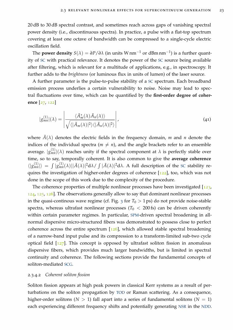
2.3 relevant nonlinear effects for supercontinuum generation 23
20 dB to 30 dB spectral contrast, and sometimes reach across gaps of vanishing spectral
power density (i.e., discontinuous spectra). In practice, a pulse with a flat-top spectrum
covering at least one octave of bandwidth can be compressed to a single-cycle electric
oscillation field.
The power density S(λ) = ∂P/∂λ (in units W nm−1 or dBm nm−1) is a further quant-
ity of SC with practical relevance. It denotes the power of the SC source being available
after filtering, which is relevant for a multitude of applications, e.g., in spectroscopy. It
further adds to the brightness (or luminous flux in units of lumen) of the laser source.
A further parameter is the pulse-to-pulse stability of a SC spectrum. Each broadband
emission process underlies a certain vulnerability to noise. Noise may lead to spec-
tral fluctuations over time, which can be quantified by the first-order degree of coher-
ence [27, 122]
|g(1)mn|(λ) =
∣∣∣∣∣∣
〈A∗m(λ)An(λ)〉
√
〈|Am(λ)|2〉〈|An(λ)|2〉
∣∣∣∣∣∣
, (41)
where A(λ) denotes the electric fields in the frequency domain, m and n denote the
indices of the individual spectra (m 6= n), and the angle brackets refer to an ensemble
average. |g(1)mn|(λ) reaches unity if the spectral component at λ is perfectly stable over
time, so to say, temporally coherent. It is also common to give the average coherence
〈|g(1)mn|〉 =∫|g(1)mn(λ)||A(λ)|2dλ/
∫|A(λ)|2dλ. A full description of the SC stability re-
quires the investigation of higher-order degrees of coherence [122], too, which was not
done in the scope of this work due to the complexity of the procedure.
The coherence properties of multiple nonlinear processes have been investigated [123,
124, 125, 126]. The observations generally allow to say that dominant nonlinear processes
in the quasi-continous wave regime (cf. Fig. 3 for T0 > 1 ps) do not provide noise-stable
spectra, whereas ultrafast nonlinear processes (T0 < 200 fs) can be driven coherently
within certain parameter regimes. In particular, SPM-driven spectral broadening in all-
normal dispersive micro-structured fibers was demonstrated to possess close to perfect
coherence across the entire spectrum [126], which allowed stable spectral broadening
of a narrow-band input pulse and its compression to a transform-limited sub-two cycle
optical field [127]. This concept is opposed by ultrafast soliton fission in anomalous
dispersive fibers, which provides much larger bandwidths, but is limited in spectral
continuity and coherence. The following sections provide the fundamental concepts of
soliton-mediated SCG.
2.3.4.2 Coherent soliton fission
Soliton fission appears at high peak powers in classical Kerr systems as a result of per-
turbations on the soliton propagation by TOD or Raman scattering. As a consequence,
higher-order solitons (N > 1) fall apart into a series of fundamental solitons (N = 1)
each experiencing different frequency shifts and potentially generating NSR in the NDD.
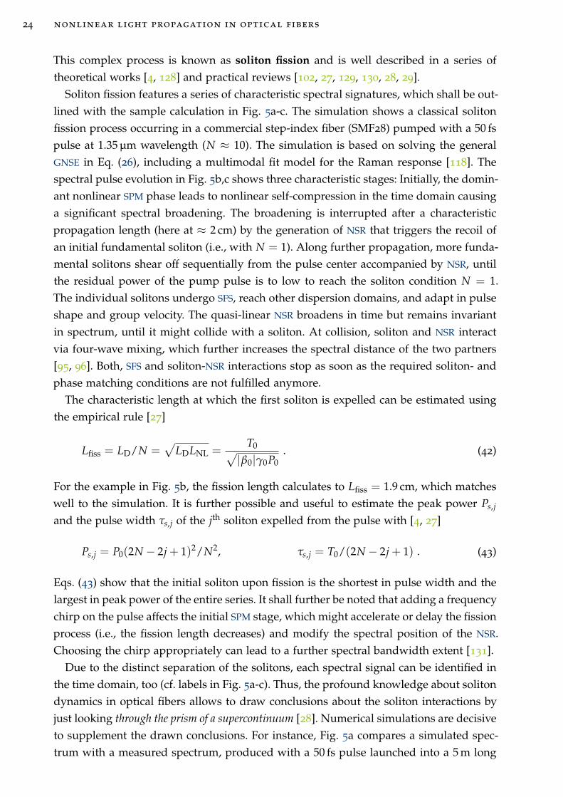
24 nonlinear light propagation in optical fibers
This complex process is known as soliton fission and is well described in a series of
theoretical works [4, 128] and practical reviews [102, 27, 129, 130, 28, 29].
Soliton fission features a series of characteristic spectral signatures, which shall be out-
lined with the sample calculation in Fig. 5a-c. The simulation shows a classical soliton
fission process occurring in a commercial step-index fiber (SMF28) pumped with a 50 fs
pulse at 1.35 µm wavelength (N ≈ 10). The simulation is based on solving the general
GNSE in Eq. (26), including a multimodal fit model for the Raman response [118]. The
spectral pulse evolution in Fig. 5b,c shows three characteristic stages: Initially, the domin-
ant nonlinear SPM phase leads to nonlinear self-compression in the time domain causing
a significant spectral broadening. The broadening is interrupted after a characteristic
propagation length (here at ≈ 2 cm) by the generation of NSR that triggers the recoil of
an initial fundamental soliton (i.e., with N = 1). Along further propagation, more funda-
mental solitons shear off sequentially from the pulse center accompanied by NSR, until
the residual power of the pump pulse is to low to reach the soliton condition N = 1.
The individual solitons undergo SFS, reach other dispersion domains, and adapt in pulse
shape and group velocity. The quasi-linear NSR broadens in time but remains invariant
in spectrum, until it might collide with a soliton. At collision, soliton and NSR interact
via four-wave mixing, which further increases the spectral distance of the two partners
[95, 96]. Both, SFS and soliton-NSR interactions stop as soon as the required soliton- and
phase matching conditions are not fulfilled anymore.
The characteristic length at which the first soliton is expelled can be estimated using
the empirical rule [27]
Lfiss = LD/N =√
LDLNL =T0
√
|β0|γ0P0. (42)
For the example in Fig. 5b, the fission length calculates to Lfiss = 1.9 cm, which matches
well to the simulation. It is further possible and useful to estimate the peak power Ps,j
and the pulse width τs,j of the jth soliton expelled from the pulse with [4, 27]
Ps,j = P0(2N − 2j + 1)2/N2, τs,j = T0/(2N − 2j + 1) . (43)
Eqs. (43) show that the initial soliton upon fission is the shortest in pulse width and the
largest in peak power of the entire series. It shall further be noted that adding a frequency
chirp on the pulse affects the initial SPM stage, which might accelerate or delay the fission
process (i.e., the fission length decreases) and modify the spectral position of the NSR.
Choosing the chirp appropriately can lead to a further spectral bandwidth extent [131].
Due to the distinct separation of the solitons, each spectral signal can be identified in
the time domain, too (cf. labels in Fig. 5a-c). Thus, the profound knowledge about soliton
dynamics in optical fibers allows to draw conclusions about the soliton interactions by
just looking through the prism of a supercontinuum [28]. Numerical simulations are decisive
to supplement the drawn conclusions. For instance, Fig. 5a compares a simulated spec-
trum with a measured spectrum, produced with a 50 fs pulse launched into a 5 m long
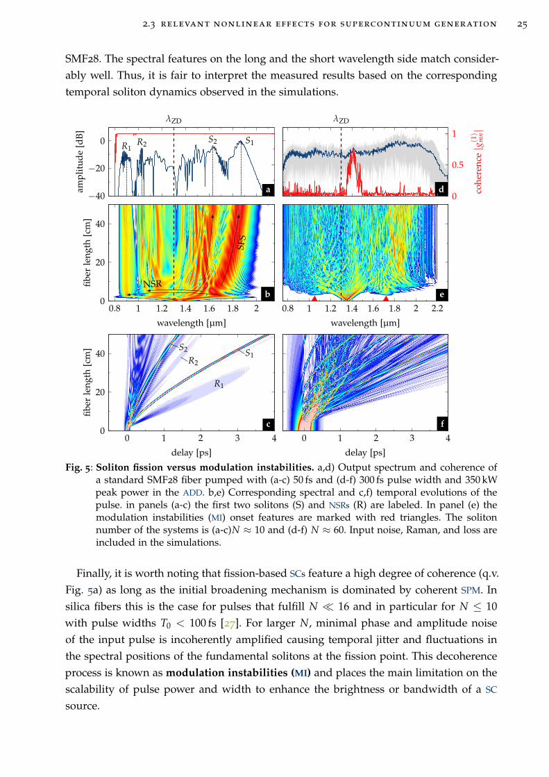
2.3 relevant nonlinear effects for supercontinuum generation 25
SMF28. The spectral features on the long and the short wavelength side match consider-
ably well. Thus, it is fair to interpret the measured results based on the corresponding
temporal soliton dynamics observed in the simulations.
S1
R1
S2
R2
0 1 2 3 40
20
40
delay [ps]
fibe
rle
ngth
[cm
]
NSR
SFS
0.8 1 1.2 1.4 1.6 1.8 20
20
40
wavelength [µm]
fibe
rle
ngth
[cm
]
S1S2R1
R2
−40
−20
0
amp
litu
de
[dB
]
λZD
0 1 2 3 4
delay [ps]
0.8 1 1.2 1.4 1.6 1.8 2 2.2
wavelength [µm]
λZD
0
0.5
1
cohe
renc
e|g
(1)
mn|
c
b
f
e
a d
Fig. 5: Soliton fission versus modulation instabilities. a,d) Output spectrum and coherence ofa standard SMF28 fiber pumped with (a-c) 50 fs and (d-f) 300 fs pulse width and 350 kWpeak power in the ADD. b,e) Corresponding spectral and c,f) temporal evolutions of thepulse. in panels (a-c) the first two solitons (S) and NSRs (R) are labeled. In panel (e) themodulation instabilities (MI) onset features are marked with red triangles. The solitonnumber of the systems is (a-c)N ≈ 10 and (d-f) N ≈ 60. Input noise, Raman, and loss areincluded in the simulations.
Finally, it is worth noting that fission-based SCs feature a high degree of coherence (q.v.
Fig. 5a) as long as the initial broadening mechanism is dominated by coherent SPM. In
silica fibers this is the case for pulses that fulfill N ≪ 16 and in particular for N ≤ 10
with pulse widths T0 < 100 fs [27]. For larger N, minimal phase and amplitude noise
of the input pulse is incoherently amplified causing temporal jitter and fluctuations in
the spectral positions of the fundamental solitons at the fission point. This decoherence
process is known as modulation instabilities (MI) and places the main limitation on the
scalability of pulse power and width to enhance the brightness or bandwidth of a SC
source.
26 nonlinear light propagation in optical fibers
2.3.4.3 Noise-driven modulation instabilities
MI arise from the parametric amplification of optical shot noise (i.e., phase and amplitude
noise of the input pulse) in spectral side bands. This parametric process originated from
perfectly phase-matched four-wave mixing [27, 29] following the conditions
2βp − βi − βs + 2γ0P0 ≡ 0 and 2ωp = ωi + ωs , (44)
where the indices correspond to the pump (p), the signal (s) and the idler (i) wave. In the
degenerate case shown in Eq. (44), the signal and idler sidebands appear symmetrically
around the pump frequency. In the ADD, the frequency splitting is mainly controlled by
the small nonlinear phase term 2γ0P0. Thus, the highly resonant domains are in close
proximity of the pump, and host a huge parametric amplification gain being affected by
the smallest fluctuations, such as photon noise.
The spectral broadening of ultrashort pulses with N > 10, and in particular T0 >
100 fs, is mostly dominated by MI due to the large parametric gain, which increases with
input power [27], and the missing coherent seed signal of the side bands provided by
SPM. Contrariwise, the process is inhibited by the significantly stronger SPM broadening
of shorter pulses, which quickly provides the spectral overlap with the parametric gain
and coherently seeds (and saturates) the parametric amplification.
The spectral characteristic of MI-driven SCG is distinctly different from soliton fission,
as exemplarily shown for a 300 fs pulse (N ≈ 60) in Fig. 5d-f: The initial SPM stage is
interrupted by emerging spectral side lobes (q.v. red labels in Fig. 5f) symmetric around
the pump. This length is often denoted as the fission point, too. In fact, along further
propagation the side lobes are amplified and cascade, which quickly forms temporal
modulations. These modulations individually evolve to uncorrelated solitons, which
may occasionally emit NSR or undergo SFS. This random soliton burst decreases the spec-
tral coherence drastically, as shown in Fig. 5d. This decrease in pulse-to-pulse stability
gives rise to very flat spectra in the average of several hundred to thousand measure-
ments (q.v. Fig. 5d). Hence, flat-top spectra obtained by pumping in the ADD do not
necessarily turn out useful for certain applications where shot-by-shot spectral stability
is required.
3O P T I C A L P R O P E RT I E S O F L I Q U I D - C O R E F I B E R S
3.1 Overview of promising liquid candidates
This chapter is denoted to identify suitable liquids for optical waveguiding and soliton
propagation, focussing on the formidable optical properties of heavy organic solvents.
The work will extend the common models for the IOR dispersion known from literat-
ure by additional terms, to account for the dispersive molecular resonances in the MIR
wavelength domain. This will be done on basis of IOR data published over the last 80
years. In particular, the data base of CS2 will allow to build an original thermodynamical
dispersion model involving the thermo- and piezo-optical effects. Further, absorption
measurements of bulk liquids will be presented to get an estimate for the transmis-
sion properties of the potential fiber-core liquids. The current state-of-the-art nonlinear
response models of liquids will then be reviewed, which was applied in this work to
deduce a response model for tetrachloroethylene (C2Cl4) – a highly transparent solvent
largely overlooked by the optofluidic community today. Finally, the elaborated mater-
ial models will be used to investigate the dispersion and the nonlinear gain of liquid-
infiltrated silica capillaries in order to identified accessible ADDs, providing the oppor-
tunities to study soliton dynamics in those LCFs. The results of this study are partly
published in [132, 133].
Nonlinear optics in liquids is a vast field with a long history. The variety of liquids
suitable for optics in the VIS to NIR seems large. However, demands on chemical, phys-
ical and in particular optical properties exclude a big part of liquid candidates already.
This work focuses on liquid carbonates, sometimes referred to as organic solvents, with
simple molecular structure, which fulfill the following criteria:
data availability Studying nonlinear light generation requires extensive knowledge
of dispersion, absorption and nonlinearity of the material over a large bandwidth.
There are many potentially transparent and nonlinear liquids (e.g., inorganic solvents
such as Ge-/Si-Cl4) for which this data basis is not provided.
high transparency in the NIR Effective light guidance along centimeters of an op-
tical fiber requires low losses, which is generally not given in long organic mo-
lecules with many CH, CO, or OH bonds. Thus, long-chained alkanes, alcohols,
aromates, esters, and oils (such as the well characterized Cargille™ oils [134]) were
not considered despite their reasonably good transparency in the VIS.
suitable IOR for silica fibers Liquids, such as short-chained alkanes, alkohols and
some polar solvents (e.g., acetone, water), were excluded from this work, because
their IOR is lower than silica, and they do not allow light guidance in silica capillar-
ies. This also excludes the interesting class of liquid flourides (e.g., perfluorohexane
C6F14, hexafluorobenzene C6F6), despite their promising transparency in the NIR.
27
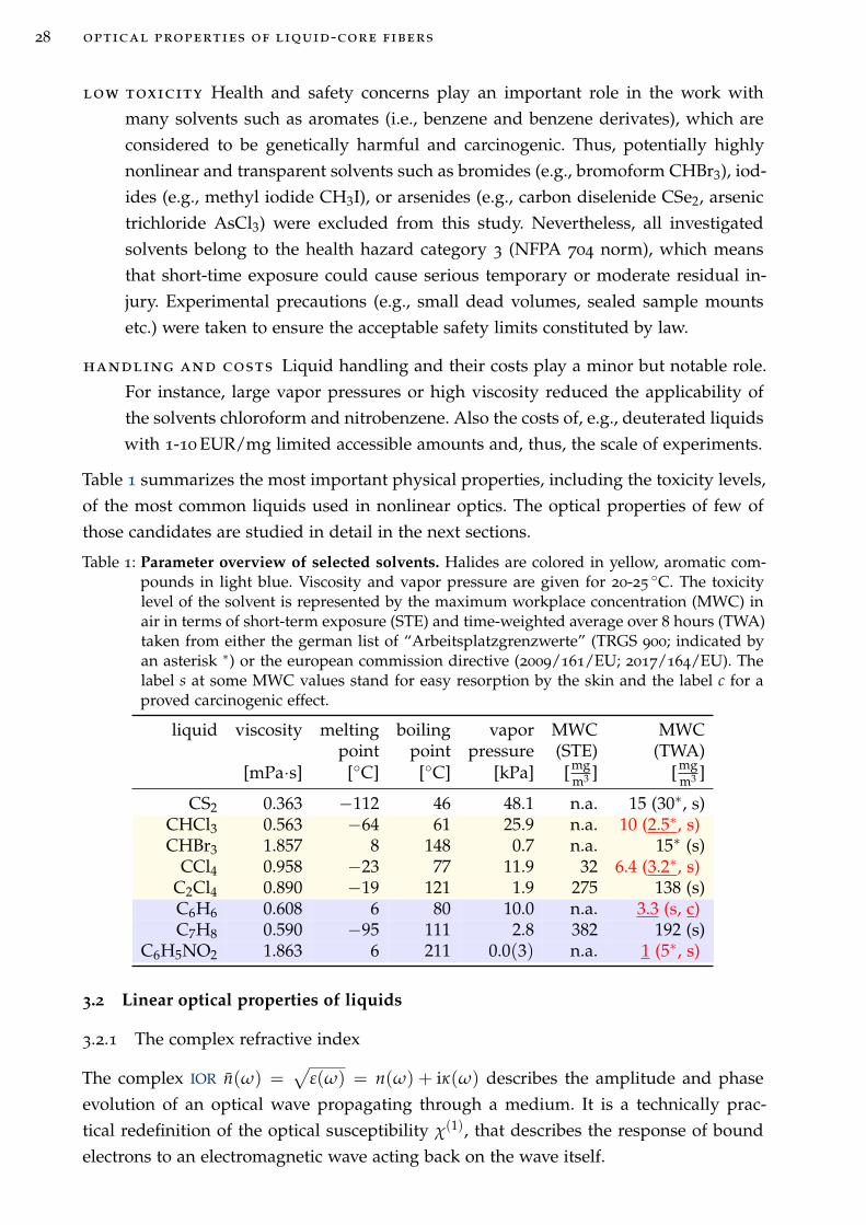
28 optical properties of liquid-core fibers
low toxicity Health and safety concerns play an important role in the work with
many solvents such as aromates (i.e., benzene and benzene derivates), which are
considered to be genetically harmful and carcinogenic. Thus, potentially highly
nonlinear and transparent solvents such as bromides (e.g., bromoform CHBr3), iod-
ides (e.g., methyl iodide CH3I), or arsenides (e.g., carbon diselenide CSe2, arsenic
trichloride AsCl3) were excluded from this study. Nevertheless, all investigated
solvents belong to the health hazard category 3 (NFPA 704 norm), which means
that short-time exposure could cause serious temporary or moderate residual in-
jury. Experimental precautions (e.g., small dead volumes, sealed sample mounts
etc.) were taken to ensure the acceptable safety limits constituted by law.
handling and costs Liquid handling and their costs play a minor but notable role.
For instance, large vapor pressures or high viscosity reduced the applicability of
the solvents chloroform and nitrobenzene. Also the costs of, e.g., deuterated liquids
with 1-10 EUR/mg limited accessible amounts and, thus, the scale of experiments.
Table 1 summarizes the most important physical properties, including the toxicity levels,
of the most common liquids used in nonlinear optics. The optical properties of few of
those candidates are studied in detail in the next sections.
Table 1: Parameter overview of selected solvents. Halides are colored in yellow, aromatic com-pounds in light blue. Viscosity and vapor pressure are given for 20-25 C. The toxicitylevel of the solvent is represented by the maximum workplace concentration (MWC) inair in terms of short-term exposure (STE) and time-weighted average over 8 hours (TWA)taken from either the german list of “Arbeitsplatzgrenzwerte” (TRGS 900; indicated byan asterisk ∗) or the european commission directive (2009/161/EU; 2017/164/EU). Thelabel s at some MWC values stand for easy resorption by the skin and the label c for aproved carcinogenic effect.
liquid viscosity melting boiling vapor MWC MWCpoint point pressure (STE) (TWA)
[mPa·s] [C] [C] [kPa] [mgm3 ] [mg
m3 ]
CS2 0.363 −112 46 48.1 n.a. 15 (30∗, s)CHCl3 0.563 −64 61 25.9 n.a. 10 (2.5∗, s)CHBr3 1.857 8 148 0.7 n.a. 15∗ (s)
CCl4 0.958 −23 77 11.9 32 6.4 (3.2∗, s)C2Cl4 0.890 −19 121 1.9 275 138 (s)C6H6 0.608 6 80 10.0 n.a. 3.3 (s, c)C7H8 0.590 −95 111 2.8 382 192 (s)
C6H5NO2 1.863 6 211 0.0(3) n.a. 1 (5∗, s)
3.2 Linear optical properties of liquids
3.2.1 The complex refractive index
The complex IOR n(ω) =√
ε(ω) = n(ω) + iκ(ω) describes the amplitude and phase
evolution of an optical wave propagating through a medium. It is a technically prac-
tical redefinition of the optical susceptibility χ(1), that describes the response of bound
electrons to an electromagnetic wave acting back on the wave itself.
3.2 linear optical properties of liquids 29
The dielectric function can be linked to the intrinsic electronic motions in an electric
field. Assuming multiple electronic resonances the generalized Lorentz-Drude model can
be found to be [135]
ε(ω) = 1 + χ(∞) + ∑m
χm(ω) = ε(∞) + ωp ∑m
fm
ω2m − ω2 + iωΓm
, (45)
with the experimentally unaccessible resonances combined in the constant ε(∞) = 1 +
χ(∞), the individual oscillator strengths fm, the resonance frequencies ωm and the atten-
uation constants Γm. In the lossless case (i.e., Γm = 0), Eq. (45) can be transferred to the
empiric model for the real part of the IOR found by Sellmeier in 1871 [136]
n2(λ) = ε(λ) = A + ∑m
Bmλ2
λ2 − C2m
, (46)
with the individual Sellmeier coefficients A = ε(∞), Bm = ωpω−2m fm, and Cm = λm,
and the vacuum wavelength λ (in µm). Each term represents the phase change near an
absorption resonance with strength Bm at spectral location Cm. The Sellmeier equation
has been serving as powerful fit model for IOR data in numerous work [137, 77, 50, 51].
It shall be noted, that another common model is often used in experimental work
[50, 51, 138], too, called the Cauchy equation. This model is based on a Taylor series of
the IOR respective to the wavelength λ (in µm)
n2(λ) = A−1λ2 + A0 + A1λ−2 + A2λ−4 + . . . =N
∑n=−1
Anλ−2n , (47)
with the expansion coefficients An. The Cauchy equation is especially practical in data fit
algorithms. However, it misses a physical-phenomenological origin and, thus, does not
necessarily follow natural dispersion slopes. This is different in case of the resonance-
based Sellmeier equation, which allows physical relevant extrapolations and higher or-
der derivations of the refractive index. Hence, all refractive index fits and dispersion
studies in this work are based on Sellmeier equations, beside few designated exceptions.
The dispersion properties of several selected liquids is discussed in sec. 3.2.3.
In fact, it is possible to derive a fit model for the absorption from the Lorentz-Drude
model, too. However, modeling the absorption spectrum becomes increasingly complic-
ated with increasing number of resonances and exceeds the scope of this work. In the
following section, the absorption properties of selected liquids is discussed by means
of the absorption coefficient α. This absorption coefficient is a technical redefinition of
the imaginary part of the refractive index, that is given by α = −20 log(e)k0κ in units
of dB/m. Similar to the dispersion parameter D, α enables direct comparability of the
here-presented LCFs with commercial fibers and allows to quickly estimate the output
power Pout after a propagation length L following the definition αL ≡ −10 log(Pout/Pin).
30 optical properties of liquid-core fibers
3.2.2 Absorption
3.2.2.1 General overview
Classical optical devices underly efficiency and bandwidth limits imposed by the ab-
sorption of their incorporated materials. The need of integrated optical sources and
waveguides for the NIR and MIR triggered a lot research in glass chemistry with a strong
focus on flouride (F) and chalcogenite (S, Se, Te) compound glasses. Those novel glass
types are called soft-glasses due to their low melting temperatures of a few hundred
degree Celsius. They enable a low-loss operation up to 5 µm wavelength (e.g. for ZrF4-
BaF2-LaF3-AlF3-NaF composition, also called ZBLAN glass, or for ZnTe glass) and even
beyond in case of some special chalcogenite compounds (e.g. As2S3) [139]. The optical
transmission limits of some prominent examples of this material class are compared
with fused silica (SiO2) in Fig. 6.
Many materials of the same chemical class are in liquid phase and largely unex-
plored for optical applications. The transmission of such liquids is not well quantified to
date, although they promise similar transmission benefits as their amorphous partners.
However, their loss characteristics is fundamentally different to solids or amorphous
materials. The electronic and molecular optical transitions of liquid molecules are less
broadened due to much weaker phonon lattice coupling to the thermal background than
in solids or amorphous materials. Thus, absorption lines in simple (i.e., short-chained)
binary molecular liquids generally appear sparse and narrow, opening many optical
operation regimes from the VIS to presumably the MIR.
For instance, a larger range of halides (i.e. binary compounts containing F, Cl, Br, I) is
reported in literature with remarkably broad transmission windows from the VIS to the
MIR as indicated in Fig. 6. In particular the predicted transmission of tetrachloroethylene
(C2Cl4) even exceeds the bandwidth of some arsenic chalcogenides, which are the current
record holders in terms of MIR transparency.
However, the data for the liquids in Fig. 6 should be taken with care since they are
mainly based on a single measurement from which a 1 dB/m absorption threshold was
estimated. This data base (esp. Ref. [140]) is hard to confirm. Despite the long period
of active research in the field of optofluidics quantitative models for the absorption
coefficient are barely available across the optical domain. Only few work exists were
transmission along centimeters of propagation through highly transparent liquids was
measured, so that absorption values in application-relevant units (e.g., dB cm−1) can ac-
tually be given [51, 141]. Moreover, most loss studies exclude the domain between 1.7
and 3 µm due to sensitivity limits of the used spectrometers or spectrophotometers. The
lack of quantitative data, especially in the NIR, leaves large uncertainties in the applicab-
ility of liquids as core material for optical fibers.
In the scope of this work, the transmission limits in the VIS to the NIR of the liquid
candidates in Tab. 1 are studied, with special focus on the erbium and thulium laser oper-
ation ranges around 1.55 µm and 2 µm wavelength. In the following, absorption analysis
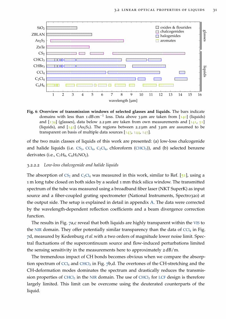
3.2 linear optical properties of liquids 31
oxides & flourideschalcogenideshalogenidesaromates
1 2 3 4 5 6 7 8 9 10 11 12 13 14 15 16
C6H6
C2Cl4
CCl4
CHBr3
CHCl3
CS2
ZnTe
As2S3
ZBLAN
SiO2
wavelength [µm]
glassesliqu
ids
Fig. 6: Overview of transmission windows of selected glasses and liquids. The bars indicatedomains with less than 1 dB cm−1 loss. Data above 3 µm are taken from [140] (liquids)and [139] (glasses), data below 2.2 µm are taken from own measurements and [141, 51](liquids), and [142] (As2S3). The regions between 2.2 µm and 3 µm are assumed to betransparent on basis of multiple data sources [143, 144, 145].
of the two main classes of liquids of this work are presented: (a) low-loss chalcogenide
and halide liquids (i.e. CS2, CCl4, C2Cl4, chloroform (CHCl3)), and (b) selected benzene
derivates (i.e., C7H8, C6H5NO2).
3.2.2.2 Low-loss chalcogenide and halide liquids
The absorption of CS2 and C2Cl4 was measured in this work, similar to Ref. [51], using a
1 m long tube closed on both sides by a sealed 1 mm thick silica window. The transmitted
spectrum of the tube was measured using a broadband fiber laser (NKT SuperK) as input
source and a fiber-coupled grating spectrometer (National Instruments, Spectro320) at
the output side. The setup is explained in detail in appendix A. The data were corrected
by the wavelength-dependent reflection coefficients and a beam divergence correction
function.
The results in Fig. 7a,c reveal that both liquids are highly transparent within the VIS to
the NIR domain. They offer potentially similar transparency than the data of CCl4 in Fig.
7d, measured by Kedenburg et al.with a two orders of magnitude lower noise limit. Spec-
tral fluctuations of the supercontinuum source and flow-induced perturbations limited
the sensing sensitivity in the measurements here to approximately 2 dB/m.
The tremendous impact of CH bonds becomes obvious when we compare the absorp-
tion spectrum of CCl4 and CHCl3 in Fig. 7b,d. The overtones of the CH-stretching and the
CH-deformation modes dominates the spectrum and drastically reduces the transmis-
sion properties of CHCl3 in the NIR domain. The use of CHCl3 for LCF design is therefore
largely limited. This limit can be overcome using the deuterated counterparts of the
liquid.
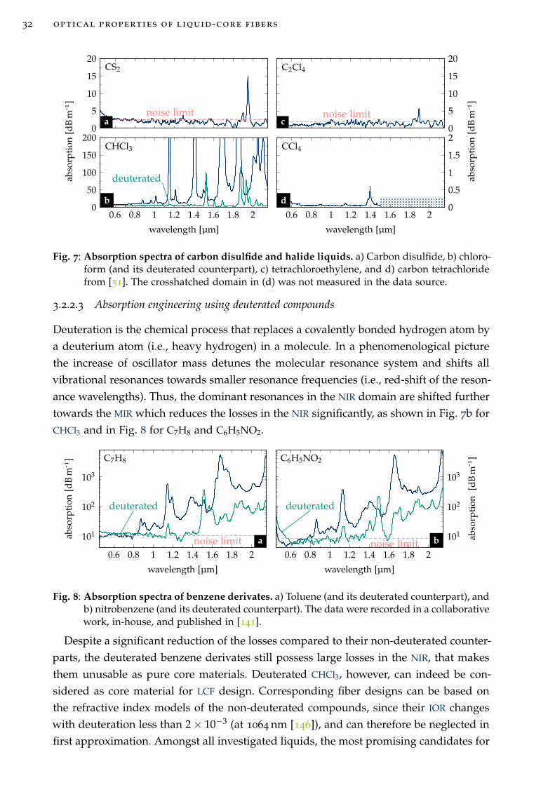
32 optical properties of liquid-core fibers
noise limit
0
5
10
15
20
noise limit0
5
10
15
20
0.6 0.8 1 1.2 1.4 1.6 1.8 20
0.5
1
1.5
2
wavelength [µm]
abso
rpti
on[d
Bm
-1]
deuterated
0.6 0.8 1 1.2 1.4 1.6 1.8 20
50
100
150
200
wavelength [µm]
abso
rpti
on[d
Bm
-1]
a
CS2
c
C2Cl4
b
CHCl3
d
CCl4
Fig. 7: Absorption spectra of carbon disulfide and halide liquids. a) Carbon disulfide, b) chloro-form (and its deuterated counterpart), c) tetrachloroethylene, and d) carbon tetrachloridefrom [51]. The crosshatched domain in (d) was not measured in the data source.
3.2.2.3 Absorption engineering using deuterated compounds
Deuteration is the chemical process that replaces a covalently bonded hydrogen atom by
a deuterium atom (i.e., heavy hydrogen) in a molecule. In a phenomenological picture
the increase of oscillator mass detunes the molecular resonance system and shifts all
vibrational resonances towards smaller resonance frequencies (i.e., red-shift of the reson-
ance wavelengths). Thus, the dominant resonances in the NIR domain are shifted further
towards the MIR which reduces the losses in the NIR significantly, as shown in Fig. 7b for
CHCl3 and in Fig. 8 for C7H8 and C6H5NO2.
noise limit
deuterated
0.6 0.8 1 1.2 1.4 1.6 1.8 2
101
102
103
wavelength [µm]
abso
rpti
on[d
Bm
-1]
noise limit
deuterated
0.6 0.8 1 1.2 1.4 1.6 1.8 2
101
102
103
wavelength [µm]
abso
rpti
on[d
Bm
-1]
a
C7H8
b
C6H5NO2
Fig. 8: Absorption spectra of benzene derivates. a) Toluene (and its deuterated counterpart), andb) nitrobenzene (and its deuterated counterpart). The data were recorded in a collaborativework, in-house, and published in [141].
Despite a significant reduction of the losses compared to their non-deuterated counter-
parts, the deuterated benzene derivates still possess large losses in the NIR, that makes
them unusable as pure core materials. Deuterated CHCl3, however, can indeed be con-
sidered as core material for LCF design. Corresponding fiber designs can be based on
the refractive index models of the non-deuterated compounds, since their IOR changes
with deuteration less than 2 × 10⁻³ (at 1064 nm [146]), and can therefore be neglected in
first approximation. Amongst all investigated liquids, the most promising candidates for
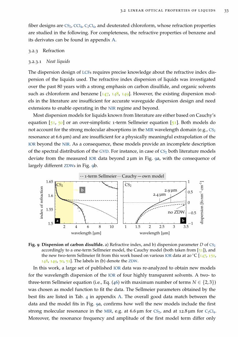
3.2 linear optical properties of liquids 33
fiber designs are CS2, CCl4, C2Cl4, and deuterated chloroform, whose refraction properties
are studied in the following. For completeness, the refractive properties of benzene and
its derivates can be found in appendix A.
3.2.3 Refraction
3.2.3.1 Neat liquids
The dispersion design of LCFs requires precise knowledge about the refractive index dis-
persion of the liquids used. The refractive index dispersion of liquids was investigated
over the past 80 years with a strong emphasis on carbon disulfide, and organic solvents
such as chloroform and benzene [147, 148, 149]. However, the existing dispersion mod-
els in the literature are insufficient for accurate waveguide dispersion design and need
extensions to enable operating in the NIR regime and beyond.
Most dispersion models for liquids known from literature are either based on Cauchy’s
equation [51, 50] or an over-simplistic 1-term Sellmeier equation [51]. Both models do
not account for the strong molecular absorptions in the MIR wavelength domain (e.g., CS2
resonance at 6.6 µm) and are insufficient for a physically meaningful extrapolation of the
IOR beyond the NIR. As a consequence, these models provide an incomplete description
of the spectral distribution of the GVD. For instance, in case of CS2 both literature models
deviate from the measured IOR data beyond 2 µm in Fig. 9a, with the consequence of
largely different ZDWs in Fig. 9b.
b
2 4 6 8 101.5
1.55
1.6
1.65
wavelength [µm]
ind
exof
refr
acti
on
2.4 µm2.9 µm
no ZDW
1 1.5 2 2.5 3 3.5−1
−0.5
0
0.5
1
wavelength [µm]
dis
per
sion
[fsn
m-1
cm-1
]
1-term Sellmeier Cauchy own model
a
CS2
b
CS2
Fig. 9: Dispersion of carbon disulfide. a) Refractive index, and b) dispersion parameter D of CS2
accordingly to a one-term Sellmeier model, the Cauchy model (both taken from [51]), andthe new two-term Sellmeier fit from this work based on various IOR data at 20 C [147, 150,148, 149, 50, 51]. The labels in (b) denote the ZDW.
In this work, a large set of published IOR data was re-analyzed to obtain new models
for the wavelength dispersion of the IOR of four highly transparent solvents. A two- to
three-term Sellmeier equation (i.e., Eq. (46) with maximum number of terms N ∈ 2, 3)
was chosen as model function to fit the data. The Sellmeier parameters obtained by the
best fits are listed in Tab. 4 in appendix A. The overall good data match between the
data and the model fits in Fig. 9a, confirms how well the new models include the first
strong molecular resonance in the MIR, e.g. at 6.6 µm for CS2, and at 12.8 µm for C2Cl4.
Moreover, the resonance frequency and amplitude of the first model term differ only
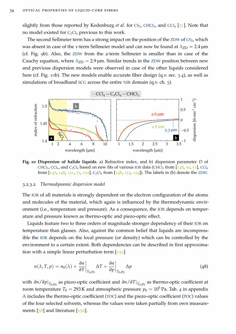
34 optical properties of liquid-core fibers
slightly from those reported by Kedenburg et al. for CS2, CHCl3, and CCl4 [51]. Note that
no model existed for C2Cl4 previous to this work.
The second Sellmeier term has a strong impact on the position of the ZDW of CS2, which
was absent in case of the 1-term Sellmeier model and can now be found at λZD = 2.4 µm
(cf. Fig. 9b). Also, the ZDW from the 2-term Sellmeier is smaller than in case of the
Cauchy equation, where λZD = 2.9 µm. Similar trends in the ZDW position between new
and previous dispersion models were observed in case of the other liquids considered
here (cf. Fig. 10b). The new models enable accurate fiber design (q.v. sec. 3.4), as well as
simulations of broadband SCG across the entire NIR domain (q.v. ch. 5).
b
SiO2
1 2 4 6 8 101.4
1.45
1.5
wavelength [µm]
ind
exof
refr
acti
on
2.6 µm
2.6 µm
3.3 µm
1 1.5 2 2.5 3 3.5−1
−0.5
0
0.5
1
wavelength [µm]
dis
per
sion
[fsn
m-1
cm-1
]
CCl4 C2Cl4 CHCl3
a b
Fig. 10: Dispersion of halide liquids. a) Refractive index, and b) dispersion parameter D ofCHCl3, CCl4, and C2Cl4 based on new fits of various IOR data (CHCl3 from [148, 50, 51], CCl4from [147, 148, 151, 51, 152], C2Cl4 from [148, 153, 154]). The labels in (b) denote the ZDW.
3.2.3.2 Thermodynamic dispersion model
The IOR of all materials is strongly dependent on the electron configuration of the atoms
and molecules of the material, which again is influenced by the thermodynamic envir-
onment (i.e., temperature and pressure). As a consequence, the IOR depends on temper-
ature and pressure known as thermo-optic and piezo-optic effect.
Liquids feature two to three orders of magnitude stronger dependency of their IOR on
temperature than glasses. Also, against the common belief that liquids are incompress-
ible the IOR depends on the local pressure (or density) which can be controlled by the
environment to a certain extent. Both dependencies can be described in first approxima-
tion with a simple linear perturbation term [152]
n(λ, T, p) = n0(λ) +∂n
∂T
∣∣∣∣T0,p0
∆T +∂n
∂p
∣∣∣∣T0,p0
∆p (48)
with ∂n/∂p|T0,p0as piezo-optic coefficient and ∂n/∂T|T0,p0
as thermo-optic coefficient at
room temperature T0 = 293 K and atmospheric pressure p0 = 105 Pa. Tab. 4 in appendix
A includes the thermo-optic coefficient (TOC) and the piezo-optic coefficient (POC) values
of the four selected solvents, whereas the values were taken partially from own measure-
ments [58] and literature [152].
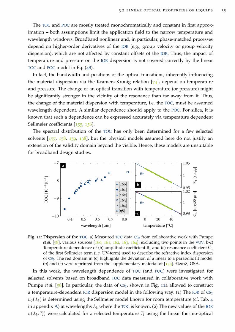
3.2 linear optical properties of liquids 35
The TOC and POC are mostly treated monochromatically and constant in first approx-
imation – both assumptions limit the application field to the narrow temperature and
wavelength windows. Broadband nonlinear and, in particular, phase-matched processes
depend on higher-order derivatives of the IOR (e.g., group velocity or group velocity
dispersion), which are not affected by constant offsets of the IOR. Thus, the impact of
temperature and pressure on the IOR dispersion is not covered correctly by the linear
TOC and POC model in Eq. (48).
In fact, the bandwidth and positions of the optical transitions, inherently influencing
the material dispersion via the Kramers-Kronig relation [74], depend on temperature
and pressure. The change of an optical transition with temperature (or pressure) might
be significantly stronger in the vicinity of the resonance than far away from it. Thus,
the change of the material dispersion with temperature, i.e. the TOC, must be assumed
wavelength dependent. A similar dependence should apply to the POC. For silica, it is
known that such a dependence can be expressed accurately via temperature dependent
Sellmeier coefficients [155, 156].
The spectral distribution of the TOC has only been determined for a few selected
solvents [157, 158, 159, 138], but the physical models assumed here do not justify an
extension of the validity domain beyond the visible. Hence, these models are unsuitable
for broadband design studies.
fit
0.95
1
1.05
B1
[1.4
99]
0.4 0.5 0.6 0.7 0.8−10
−9
−8
−7
wavelength [µm]
TOC
[10−
4 K−
1 ]
[160]
[161]
[162]
[163]
[164]
[58]
fit
0 20 400.98
1
1.02
temperature [C]
C1
[0.1
78
8µ
m]
a
b
c
Fig. 11: Dispersion of the TOC. a) Measured TOC data CS2 from collaborative work with Pumpeet al. [58], various sources [160, 161, 162, 163, 164], excluding two points in the VUV. b-c)Temperature dependence of (b) amplitude coefficient B1 and (c) resonance coefficient C1of the first Sellmeier term (i.e. UV-term) used to describe the refractive index dispersionof CS2. The red domain in (c) highlights the deviation of a linear to a parabolic fit model.(b) and (c) were reprinted from the supplementary material of [133]. ©2018, OSA.
In this work, the wavelength dependence of TOC (and POC) were investigated for
selected solvents based on broadband TOC data measured in collaborative work with
Pumpe et al. [58]. In particular, the data of CS2, shown in Fig. 11a allowed to construct
a temperature-dependent IOR dispersion model in the following way: (1) The IOR of CS2
n0(λk) is determined using the Sellmeier model known for room temperature (cf. Tab. 4
in appendix A) at wavelengths λk where the TOC is known. (2) The new values of the IOR
n(λk, Tl) were calculated for a selected temperature Tl using the linear thermo-optical
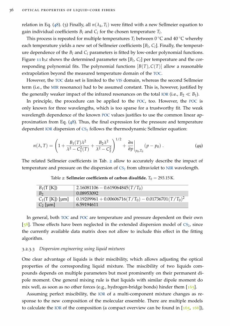
36 optical properties of liquid-core fibers
relation in Eq. (48). (3) Finally, all n(λk, Tl) were fitted with a new Sellmeier equation to
gain individual coefficients Bl and Cl for the chosen temperature Tl.
This process is repeated for multiple temperatures Tl between 0 C and 40 C whereby
each temperature yields a new set of Sellmeier coefficients [Bl, Cl]. Finally, the temperat-
ure dependence of the Bl and Cl parameters is fitted by low-order polynomial functions.
Figure 11 b,c shows the determined parameter sets [Bl, Cl] per temperature and the cor-
responding polynomial fits. The polynomial functions [B(T), C(T)] allow a reasonable
extrapolation beyond the measured temperature domain of the TOC.
However, the TOC data set is limited to the VIS domain, whereas the second Sellmeier
term (i.e., the MIR resonance) had to be assumed constant. This is, however, justified by
the generally weaker impact of the infrared resonances on the total IOR (i.e., B2 ≪ B1).
In principle, the procedure can be applied to the POC, too. However, the POC is
only known for three wavelengths, which is too sparse for a trustworthy fit. The weak
wavelength dependence of the known POC values justifies to use the common linear ap-
proximation from Eq. (48). Thus, the final expression for the pressure and temperature
dependent IOR dispersion of CS2 follows the thermodynamic Sellmeier equation:
n(λ, T) =
(
1 +B1(T)λ
2
λ2 − C21(T)
+B2λ2
λ2 − C22
)1/2
+∂n
∂p
∣∣∣∣
p0,T0
(p − p0) . (49)
The related Sellmeier coefficients in Tab. 2 allow to accurately describe the impact of
temperature and pressure on the dispersion of CS2 from ultraviolet to NIR wavelength.
Table 2: Sellmeier coefficients of carbon disulfide. T0 = 293.15 K.
B1(T [K]) 2.16081106 − 0.619064845(T/T0)B2 0.08953092C1(T [K]) [µm] 0.19209961 + 0.00606716(T/T0)− 0.01736701(T/T0)
2
C2 [µm] 6.59194611
In general, both TOC and POC are temperature and pressure dependent on their own
[58]. Those effects have been neglected in the extended dispersion model of CS2, since
the currently available data matrix does not allow to include this effect in the fitting
algorithm.
3.2.3.3 Dispersion engineering using liquid mixtures
One clear advantage of liquids is their miscibility, which allows adjusting the optical
properties of the corresponding liquid mixture. The miscibility of two liquids com-
pounds depends on multiple parameters but most prominently on their permanent di-
pole moment. One general mixing rule is that liquids with similar dipole moment do
mix well, as soon as no other forces (e.g., hydrogen-bridge bonds) hinder them [165].
Assuming perfect miscibility, the IOR of a multi-component mixture changes as re-
sponse to the new composition of the molecular ensemble. There are multiple models
to calculate the IOR of the composition (a compact overview can be found in [165, 166]),
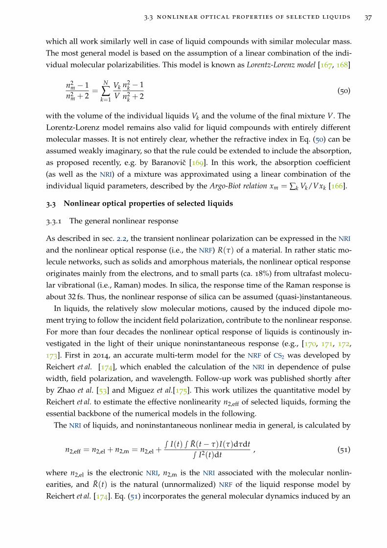
3.3 nonlinear optical properties of selected liquids 37
which all work similarly well in case of liquid compounds with similar molecular mass.
The most general model is based on the assumption of a linear combination of the indi-
vidual molecular polarizabilities. This model is known as Lorentz-Lorenz model [167, 168]
n2m − 1
n2m + 2
=N
∑k=1
Vk
V
n2k − 1
n2k + 2
(50)
with the volume of the individual liquids Vk and the volume of the final mixture V. The
Lorentz-Lorenz model remains also valid for liquid compounds with entirely different
molecular masses. It is not entirely clear, whether the refractive index in Eq. (50) can be
assumed weakly imaginary, so that the rule could be extended to include the absorption,
as proposed recently, e.g. by Baranovic [169]. In this work, the absorption coefficient
(as well as the NRI) of a mixture was approximated using a linear combination of the
individual liquid parameters, described by the Argo-Biot relation xm = ∑k Vk/Vxk [166].
3.3 Nonlinear optical properties of selected liquids
3.3.1 The general nonlinear response
As described in sec. 2.2, the transient nonlinear polarization can be expressed in the NRI
and the nonlinear optical response (i.e., the NRF) R(τ) of a material. In rather static mo-
lecule networks, such as solids and amorphous materials, the nonlinear optical response
originates mainly from the electrons, and to small parts (ca. 18%) from ultrafast molecu-
lar vibrational (i.e., Raman) modes. In silica, the response time of the Raman response is
about 32 fs. Thus, the nonlinear response of silica can be assumed (quasi-)instantaneous.
In liquids, the relatively slow molecular motions, caused by the induced dipole mo-
ment trying to follow the incident field polarization, contribute to the nonlinear response.
For more than four decades the nonlinear optical response of liquids is continously in-
vestigated in the light of their unique noninstantaneous response (e.g., [170, 171, 172,
173]. First in 2014, an accurate multi-term model for the NRF of CS2 was developed by
Reichert et al. [174], which enabled the calculation of the NRI in dependence of pulse
width, field polarization, and wavelength. Follow-up work was published shortly after
by Zhao et al. [53] and Miguez et al.[175]. This work utilizes the quantitative model by
Reichert et al. to estimate the effective nonlinearity n2,eff of selected liquids, forming the
essential backbone of the numerical models in the following.
The NRI of liquids, and noninstantaneous nonlinear media in general, is calculated by
n2,eff = n2,el + n2,m = n2,el +∫ I(t) ∫ R(t − τ)I(τ)dτdt
∫ I2(t)dt, (51)
where n2,el is the electronic NRI, n2,m is the NRI associated with the molecular nonlin-
earities, and R(t) is the natural (unnormalized) NRF of the liquid response model by
Reichert et al. [174]. Eq. (51) incorporates the general molecular dynamics induced by an
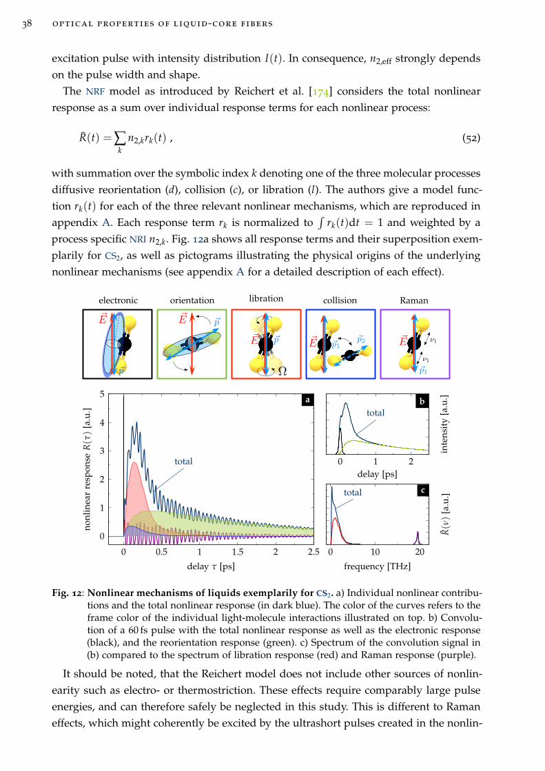
38 optical properties of liquid-core fibers
excitation pulse with intensity distribution I(t). In consequence, n2,eff strongly depends
on the pulse width and shape.
The NRF model as introduced by Reichert et al. [174] considers the total nonlinear
response as a sum over individual response terms for each nonlinear process:
R(t) =∑k
n2,krk(t) , (52)
with summation over the symbolic index k denoting one of the three molecular processes
diffusive reorientation (d), collision (c), or libration (l). The authors give a model func-
tion rk(t) for each of the three relevant nonlinear mechanisms, which are reproduced in
appendix A. Each response term rk is normalized to∫
rk(t)dt = 1 and weighted by a
process specific NRI n2,k. Fig. 12a shows all response terms and their superposition exem-
plarily for CS2, as well as pictograms illustrating the physical origins of the underlying
nonlinear mechanisms (see appendix A for a detailed description of each effect).
total
0 0.5 1 1.5 2 2.5
0
1
2
3
4
5
delay τ [ps]
nonl
inea
rre
spon
seR(τ)
[a.u
.] total
0 1 2delay [ps]
inte
nsit
y[a
.u.]
total
0 10 20
frequency [THz]
R(ν)
[a.u
.]
~E ~p
Ω
~E ~p1~p2
~E ~p~E
~p
~E
~p1
ν1
ν1
librationelectronic orientation collision Raman
a b
c
Fig. 12: Nonlinear mechanisms of liquids exemplarily for CS2. a) Individual nonlinear contribu-tions and the total nonlinear response (in dark blue). The color of the curves refers to theframe color of the individual light-molecule interactions illustrated on top. b) Convolu-tion of a 60 fs pulse with the total nonlinear response as well as the electronic response(black), and the reorientation response (green). c) Spectrum of the convolution signal in(b) compared to the spectrum of libration response (red) and Raman response (purple).
It should be noted, that the Reichert model does not include other sources of nonlin-
earity such as electro- or thermostriction. These effects require comparably large pulse
energies, and can therefore safely be neglected in this study. This is different to Raman
effects, which might coherently be excited by the ultrashort pulses created in the nonlin-
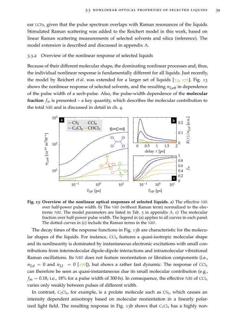
3.3 nonlinear optical properties of selected liquids 39
ear LCFs, given that the pulse spectrum overlaps with Raman resonances of the liquids.
Stimulated Raman scattering was added to the Reichert model in this work, based on
linear Raman scattering measurements of selected solvents and silica (reference). The
model extension is described and discussed in appendix A.
3.3.2 Overview of the nonlinear response of selected liquids
Because of their different molecular shape, the dominating nonlinear processes and, thus,
the individual nonlinear response is fundamentally different for all liquids. Just recently,
the model by Reichert et al. was extended for a larger set of liquids [53, 175]. Fig. 13
shows the nonlinear response of selected solvents, and the resulting n2,eff in dependence
of the pulse width of a sech-pulse. Also, the pulse-width dependence of the molecular
fraction fm is presented – a key quantity, which describes the molecular contribution to
the total NRI and is discussed in detail in ch. 4.
S SC
Cl
Cl Cl
Cl
10−1 100 101
101
102
103
THP [ps]
n2,
eff
[10
-20
m2 W
-1]
CS2 CCl4C2Cl4 CHCl3
0 0.5 1 1.5 20
0.1
0.2
delay τ [ps]
R(τ)/
n2,
el[a
.u.]
10−1 100 10100.20.40.60.81
THP [ps]f m
ba
c
Fig. 13: Overview of the nonlinear optical responses of selected liquids. a) The effective NRI
over half-power pulse width. b) The NRF (without Raman term) normalized to the elec-tronic NRI. The model parameters are listed in Tab. 5 in appendix A. c) The molecularfraction over half-power pulse width. The legend in (a) applies to all curves in each panel.The dotted curves in (c) include the Raman terms in the NRF.
The decay times of the response functions in Fig. 13b are characteristic for the molecu-
lar shapes of the liquids. For instance, CCl4 features a quasi-isotropic molecular shape
and its nonlinearity is dominated by instantaneous electronic excitations with small con-
tributions from intermolecular dipole-dipole interactions and intramolecular vibrational
Raman oscillations. Its NRF does not feature reorientation or libration components (i.e.,
n2,d = 0 and n2,l = 0 [176]), but shows a rather fast dynamic. The response of CCl4
can therefore be seen as quasi-instantaneous due its small molecular contribution (e.g.,
fm = 0.18, i.e., 18% for a pulse width of 300 fs). In consequence, the effective NRI of CCl4
varies only weakly between pulses of different width.
In contrast, C2Cl4, for example, is a prolate molecule such as CS2, which causes an
intensity dependent anisotropy based on molecular reorientation in a linearly polar-
ized light field. The resulting response in Fig. 13b shows that C2Cl4 has a highly non-
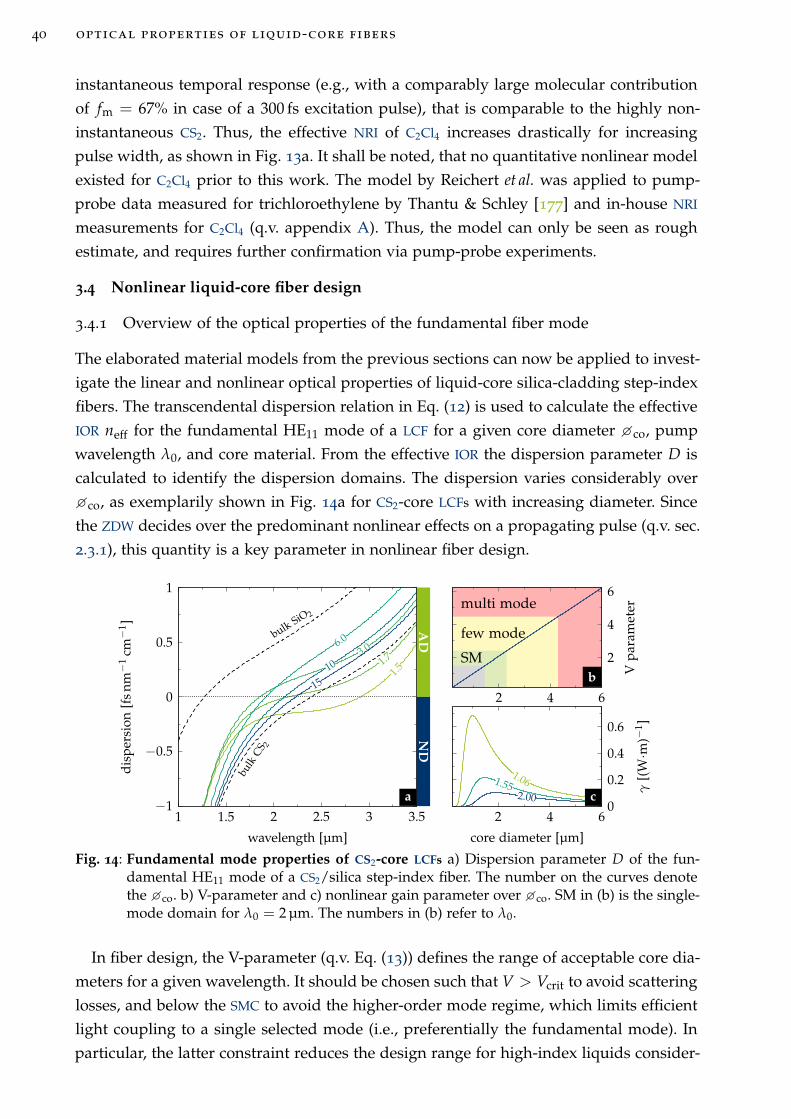
40 optical properties of liquid-core fibers
instantaneous temporal response (e.g., with a comparably large molecular contribution
of fm = 67% in case of a 300 fs excitation pulse), that is comparable to the highly non-
instantaneous CS2. Thus, the effective NRI of C2Cl4 increases drastically for increasing
pulse width, as shown in Fig. 13a. It shall be noted, that no quantitative nonlinear model
existed for C2Cl4 prior to this work. The model by Reichert et al. was applied to pump-
probe data measured for trichloroethylene by Thantu & Schley [177] and in-house NRI
measurements for C2Cl4 (q.v. appendix A). Thus, the model can only be seen as rough
estimate, and requires further confirmation via pump-probe experiments.
3.4 Nonlinear liquid-core fiber design
3.4.1 Overview of the optical properties of the fundamental fiber mode
The elaborated material models from the previous sections can now be applied to invest-
igate the linear and nonlinear optical properties of liquid-core silica-cladding step-index
fibers. The transcendental dispersion relation in Eq. (12) is used to calculate the effective
IOR neff for the fundamental HE11 mode of a LCF for a given core diameter co, pump
wavelength λ0, and core material. From the effective IOR the dispersion parameter D is
calculated to identify the dispersion domains. The dispersion varies considerably over
co, as exemplarily shown in Fig. 14a for CS2-core LCFs with increasing diameter. Since
the ZDW decides over the predominant nonlinear effects on a propagating pulse (q.v. sec.
2.3.1), this quantity is a key parameter in nonlinear fiber design.
1.5
1.73.06.0
10
15
bulk
CS 2
bulkSiO2
1 1.5 2 2.5 3 3.5−1
−0.5
0
0.5
1
wavelength [µm]
dis
per
sion
[fsn
m−
1cm
−1 ]
1.061.552.00
2 4 60
0.2
0.4
0.6
core diameter [µm]
γ[(
W·m
)−1 ]
multi mode
few mode
SM
2 4 6
2
4
6
Vp
aram
eter
AD
ND
a
b
c
Fig. 14: Fundamental mode properties of CS2-core LCFs a) Dispersion parameter D of the fun-damental HE11 mode of a CS2/silica step-index fiber. The number on the curves denotethe co. b) V-parameter and c) nonlinear gain parameter over co. SM in (b) is the single-mode domain for λ0 = 2 µm. The numbers in (b) refer to λ0.
In fiber design, the V-parameter (q.v. Eq. (13)) defines the range of acceptable core dia-
meters for a given wavelength. It should be chosen such that V > Vcrit to avoid scattering
losses, and below the SMC to avoid the higher-order mode regime, which limits efficient
light coupling to a single selected mode (i.e., preferentially the fundamental mode). In
particular, the latter constraint reduces the design range for high-index liquids consider-
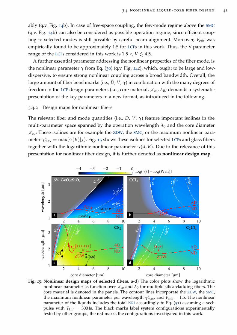
3.4 nonlinear liquid-core fiber design 41
ably (q.v. Fig. 14b). In case of free-space coupling, the few-mode regime above the SMC
(q.v. Fig. 14b) can also be considered as possible operation regime, since efficient coup-
ling to selected modes is still possible by careful beam alignment. Moreover, Vcrit was
empirically found to be approximately 1.5 for LCFs in this work. Thus, the V-parameter
range of the LCFs considered in this work is 1.5 < V . 4.5.
A further essential parameter addressing the nonlinear properties of the fiber mode, is
the nonlinear parameter γ from Eq. (30) (q.v. Fig. 14c), which, ought to be large and low-
dispersive, to ensure strong nonlinear coupling across a broad bandwidth. Overall, the
large amount of fiber benchmarks (i.e., D, V, γ) in combination with the many degrees of
freedom in the LCF design parameters (i.e., core material, co, λ0) demands a systematic
presentation of the key parameters in a new format, as introduced in the following.
3.4.2 Design maps for nonlinear fibers
The relevant fiber and mode quantities (i.e., D, V, γ) feature important isolines in the
multi-parameter space spanned by the operation wavelength λ0 and the core diameter
co. These isolines are for example the ZDW, the SMC, or the maximum nonlinear para-
meter γλmax = max(γ(R)|λ). Fig. 15 shows these isolines for selected LCFs and glass fibers
together with the logarithmic nonlinear parameter γ(λ, R). Due to the relevance of this
presentation for nonlinear fiber design, it is further denoted as nonlinear design map.
SMC
γλ max
V crit
ZDW
ND
ADSMF28
SM980
2 4 6 8 101
2
3
wav
elen
gth
[µm
]
−4 −3 −2 −1 0log(γ) [− log(W m)]
SMC
γλ m
ax
Vcr
it
ZDWND
AD[132,133][133]
[67][68]
2 4 6 8 101
2
3
core diameter [µm]
wav
elen
gth
[µm
]
SMC
γλm
ax
Vcrit
ZDWND
AD
2 4 6 8 10
core diameter [µm]
SMC
γλ m
ax
Vcr
it
ZDWND
AD[178]
2 4 6 8 10
core diameter [µm]
a
5% GeO2:SiO2
c
CS2
b
CCl4
d
C2Cl4
Fig. 15: Nonlinear design maps of selected fibers. a-d) The color plots show the logarithmicnonlinear parameter as function over co and λ0 for multiple silica-cladding fibers. Thecore material is denoted in the panels. The contour lines incorporate the ZDW, the SMC,the maximum nonlinear parameter per wavelength γλ
max, and Vcrit = 1.5. The nonlinearparameter of the liquids includes the total NRI accordingly to Eq. (51) assuming a sechpulse with THP = 300 fs. The black marks label system configurations experimentallytested by other groups, the red marks the configurations investigated in this work.
42 optical properties of liquid-core fibers
The nonlinear design maps in Fig. 15 give intuitive impressions of the design possib-
ilities of step-index LCFs, compared to standard step-index GeO2-doped silica fibers. In
case of the standard glass fiber geometry, the low core index enables single-mode opera-
tion for large core diameters easily accessible by large-scale fiber drawing facilities. The
large core diameters keep the nonlinear parameter low, which is desirable for error-free
telecommunication purposes. The ZDW varies only weakly over co.
Compared to silica fibers, CCl4-core LCFs allow single-mode operation for even larger
core diameters (i.e., co > 8 µm; q.v. Fig. 15b) at even lower nonlinearity. The mono-
tonic increase of the ZDW with increasing co provides broad access to the NDD for the
most common fiber laser lines (i.e., λ0 < 2 µm). For smaller core diameters (i.e., co
< 8 µm) light guidance becomes critical. Thus, the design capabilities of pure CCl4 fibers
are limited, which can be overcome by an admixture of a high-index liquid.
In contrast, high-index LCFs filled with CS2 or C2Cl4 commonly show robust guidance,
whereby the SMC is located at comparably small core diameters (q.v. Fig. 15c,d). Notably,
the SMC gives a good approximation for the design parameters exhibiting maximum
nonlinearity in those fibers – a finding that was published in the scope of this thesis [84].
The nonlinear maps of CS2 and C2Cl4 reveal a local minimum of the ZDW at comparably
large core diameters in the few-mode regime (e.g., 3-5 µm in case of CS2 fibers in Fig.15c).
This ZDW minimum benefits from a comparably large nonlinear gain and grants access
to the ADD at operation wavelengths about 2 µm.
In conclusion of this chapter, the new material dispersion models developed in this
work allow accurate optical system design in the NIR domain towards the MIR domain.
The large variety of liquids allows to widely select the IOR, the effective NRI, and the
NRF appropriately to the given pulse shape and to the demands of the experiment. The
parameter range can be further enlarged by incorporating miscibility and thermody-
namic optical detuning of liquids. Absorption manifests the primary limit of operation
in this wavelength domain. However, especially hydrogen-less carbon chlorides and
CS2 feature a remarkably high transparency (i.e., below 0.025 dB/cm loss) across large
parts of the VIS to the NIR, offering a wide application potential for optical waveguid-
ing. Incorporated into silica capillaries, those liquids form step-index LCFs and grant
access to the ADD at easy-to-couple core diameters and operation wavelengths readily
provided by thulium-doped fiber lasers. They therefore offer a platform to study optical
solitons. However, the effect of the shown noninstantaneous nonlinearities of the liquids
on soliton formation is poorly understood and requires proper theoretical groundwork.
The following section provides the first steps to a modified soliton theory, which ac-
counts for the liquid nonlinearities.
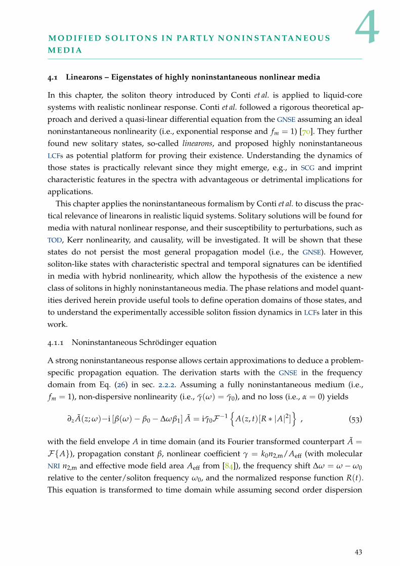
4M O D I F I E D S O L I T O N S I N PA RT LY N O N I N S TA N TA N E O U S
M E D I A
4.1 Linearons – Eigenstates of highly noninstantaneous nonlinear media
In this chapter, the soliton theory introduced by Conti et al. is applied to liquid-core
systems with realistic nonlinear response. Conti et al. followed a rigorous theoretical ap-
proach and derived a quasi-linear differential equation from the GNSE assuming an ideal
noninstantaneous nonlinearity (i.e., exponential response and fm = 1) [70]. They further
found new solitary states, so-called linearons, and proposed highly noninstantaneous
LCFs as potential platform for proving their existence. Understanding the dynamics of
those states is practically relevant since they might emerge, e.g., in SCG and imprint
characteristic features in the spectra with advantageous or detrimental implications for
applications.
This chapter applies the noninstantaneous formalism by Conti et al. to discuss the prac-
tical relevance of linearons in realistic liquid systems. Solitary solutions will be found for
media with natural nonlinear response, and their susceptibility to perturbations, such as
TOD, Kerr nonlinearity, and causality, will be investigated. It will be shown that these
states do not persist the most general propagation model (i.e., the GNSE). However,
soliton-like states with characteristic spectral and temporal signatures can be identified
in media with hybrid nonlinearity, which allow the hypothesis of the existence a new
class of solitons in highly noninstantaneous media. The phase relations and model quant-
ities derived herein provide useful tools to define operation domains of those states, and
to understand the experimentally accessible soliton fission dynamics in LCFs later in this
work.
4.1.1 Noninstantaneous Schrödinger equation
A strong noninstantaneous response allows certain approximations to deduce a problem-
specific propagation equation. The derivation starts with the GNSE in the frequency
domain from Eq. (26) in sec. 2.2.2. Assuming a fully noninstantaneous medium (i.e.,
fm = 1), non-dispersive nonlinearity (i.e., γ(ω) = γ0), and no loss (i.e., α = 0) yields
∂z A(z; ω)−i [β(ω)− β0 − ∆ωβ1] A = iγ0F−1
A(z, t)[R ∗ |A|2]
, (53)
with the field envelope A in time domain (and its Fourier transformed counterpart A =
FA), propagation constant β, nonlinear coefficient γ = k0n2,m/Aeff (with molecular
NRI n2,m and effective mode field area Aeff from [84]), the frequency shift ∆ω = ω − ω0
relative to the center/soliton frequency ω0, and the normalized response function R(t).
This equation is transformed to time domain while assuming second order dispersion
43
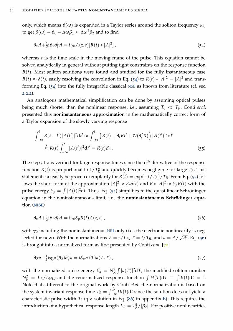
44 modified solitons in partly noninstantaneous media
only, which means β(ω) is expanded in a Taylor series around the soliton frequency ω0
to get β(ω)− β0 − ∆ωβ1 ≈ ∆ω2β2 and to find
∂z A+ 12 iβ2∂2
t A = iγ0A(z, t)[R(t) ∗ |A|2] , (54)
whereas t is the time scale in the moving frame of the pulse. This equation cannot be
solved analytically in general without putting tight constraints on the response function
R(t). Most soliton solutions were found and studied for the fully instantaneous case
R(t) ≈ δ(t), easily resolving the convolution in Eq. (54) to R(t) ∗ |A|2 = |A|2 and trans-
forming Eq. (54) into the fully integrable classical NSE as known from literature (cf. sec.
2.2.2).
An analogous mathematical simplification can be done by assuming optical pulses
being much shorter than the nonlinear response, i.e., assuming T0 ≪ TR. Conti et al.
presented this noninstantaneous approximation in the mathematically correct form of
a Taylor expansion of the slowly varying response
∫ t
−∞R(t − t′)|A(t′)|2dt′ ≈
∫ t
−∞
(
R(t) + ∂tRt′ +O(∂2t R))
|A(t′)|2dt′
⋆≈ R(t)∫ t
−∞|A(t′)|2dt′ = R(t)Ep . (55)
The step at ⋆ is verified for large response times since the nth derivative of the response
function R(t) is proportional to 1/TnR and quickly becomes negligible for large TR. This
statement can easily be proven exemplarily for R(t) = exp(−t/TR)/TR. From Eq. (55) fol-
lows the short form of the approximation |A|2 ≈ Epδ(t) and R ∗ |A|2 ≈ EpR(t) with the
pulse energy Ep =∫|A(t)|2dt. Thus, Eq. (54) simplifies to the quasi-linear Schrödinger
equation in the noninstantaneous limit, i.e., the noninstantaneous Schrödinger equa-
tion (NISE)
∂z A+ 12 iβ2∂2
t A = iγ0EpR(t)A(z, t) , (56)
with γ0 including the noninstantaneous NRI only (i.e., the electronic nonlinearity is neg-
lected for now). With the normalizations Z = z/LR, T = t/TR, and a = A/√
P0, Eq. (56)
is brought into a normalized form as first presented by Conti et al. [70]
∂Za+ 12 isgn(β2)∂
2Ta = iEaH(T)a(Z, T) , (57)
with the normalized pulse energy Ea = N2R
∫|a(T)|2dT, the modified soliton number
N2R = LR/LNL, and the renormalized response function
∫H(T)dT ≡
∫R(t)dt = 1.
Note that, different to the original work by Conti et al. the normalization is based on
the system invariant response time TR =∫ ∞
−∞tR(t)dt since the solution does not yield a
characteristic pulse width T0 (q.v. solution in Eq. (86) in appendix B). This requires the
introduction of a hypothetical response length LR = T2R/|β2|. For positive nonlinearities
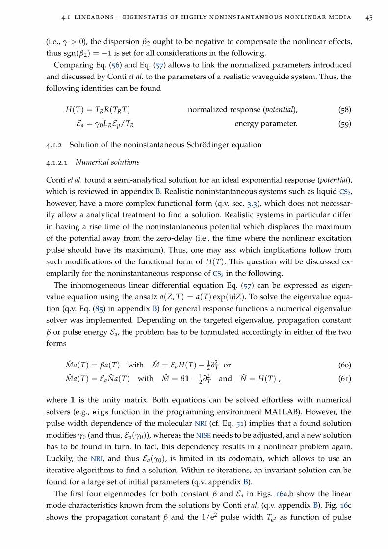
4.1 linearons – eigenstates of highly noninstantaneous nonlinear media 45
(i.e., γ > 0), the dispersion β2 ought to be negative to compensate the nonlinear effects,
thus sgn(β2) = −1 is set for all considerations in the following.
Comparing Eq. (56) and Eq. (57) allows to link the normalized parameters introduced
and discussed by Conti et al. to the parameters of a realistic waveguide system. Thus, the
following identities can be found
H(T) = TRR(TRT) normalized response (potential), (58)
Ea = γ0LREp/TR energy parameter. (59)
4.1.2 Solution of the noninstantaneous Schrödinger equation
4.1.2.1 Numerical solutions
Conti et al. found a semi-analytical solution for an ideal exponential response (potential),
which is reviewed in appendix B. Realistic noninstantaneous systems such as liquid CS2,
however, have a more complex functional form (q.v. sec. 3.3), which does not necessar-
ily allow a analytical treatment to find a solution. Realistic systems in particular differ
in having a rise time of the noninstantaneous potential which displaces the maximum
of the potential away from the zero-delay (i.e., the time where the nonlinear excitation
pulse should have its maximum). Thus, one may ask which implications follow from
such modifications of the functional form of H(T). This question will be discussed ex-
emplarily for the noninstantaneous response of CS2 in the following.
The inhomogeneous linear differential equation Eq. (57) can be expressed as eigen-
value equation using the ansatz a(Z, T) = a(T) exp(iβZ). To solve the eigenvalue equa-
tion (q.v. Eq. (85) in appendix B) for general response functions a numerical eigenvalue
solver was implemented. Depending on the targeted eigenvalue, propagation constant
β or pulse energy Ea, the problem has to be formulated accordingly in either of the two
forms
Ma(T) = βa(T) with M = EaH(T)− 12 ∂2
T or (60)
Ma(T) = EaNa(T) with M = β1 − 12 ∂2
T and N = H(T) , (61)
where 1 is the unity matrix. Both equations can be solved effortless with numerical
solvers (e.g., eigs function in the programming environment MATLAB). However, the
pulse width dependence of the molecular NRI (cf. Eq. 51) implies that a found solution
modifies γ0 (and thus, Ea(γ0)), whereas the NISE needs to be adjusted, and a new solution
has to be found in turn. In fact, this dependency results in a nonlinear problem again.
Luckily, the NRI, and thus Ea(γ0), is limited in its codomain, which allows to use an
iterative algorithms to find a solution. Within 10 iterations, an invariant solution can be
found for a large set of initial parameters (q.v. appendix B).
The first four eigenmodes for both constant β and Ea in Figs. 16a,b show the linear
mode characteristics known from the solutions by Conti et al. (q.v. appendix B). Fig. 16c
shows the propagation constant β and the 1/e2 pulse width Te2 as function of pulse
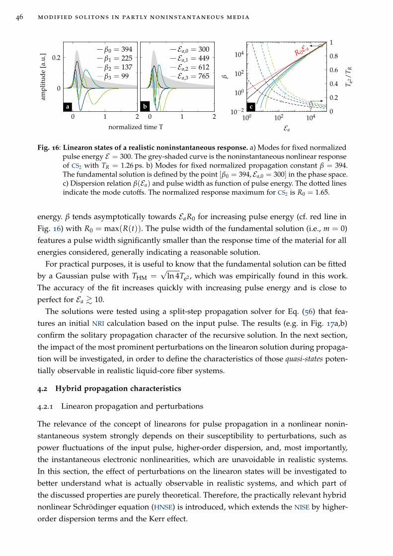
46 modified solitons in partly noninstantaneous media
0 1 2
0
0.2
normalized time T
amp
litu
de
[a.u
.]β0 = 394β1 = 225β2 = 137β3 = 99
0 1 2
Ea,0 = 300Ea,1 = 449Ea,2 = 612Ea,3 = 765
012
3
0
0.2
0.4
0.6
0.8
1
Te2
/T
R
R0E a
100 102 10410−2
100
102
104
Ea
β
a b c
Fig. 16: Linearon states of a realistic noninstantaneous response. a) Modes for fixed normalizedpulse energy E = 300. The grey-shaded curve is the noninstantaneous nonlinear responseof CS2 with TR = 1.26 ps. b) Modes for fixed normalized propagation constant β = 394.The fundamental solution is defined by the point [β0 = 394, Ea,0 = 300] in the phase space.c) Dispersion relation β(Ea) and pulse width as function of pulse energy. The dotted linesindicate the mode cutoffs. The normalized response maximum for CS2 is R0 = 1.65.
energy. β tends asymptotically towards EaR0 for increasing pulse energy (cf. red line in
Fig. 16) with R0 = max(R(t)). The pulse width of the fundamental solution (i.e., m = 0)
features a pulse width significantly smaller than the response time of the material for all
energies considered, generally indicating a reasonable solution.
For practical purposes, it is useful to know that the fundamental solution can be fitted
by a Gaussian pulse with THM =√
ln 4Te2 , which was empirically found in this work.
The accuracy of the fit increases quickly with increasing pulse energy and is close to
perfect for Ea & 10.
The solutions were tested using a split-step propagation solver for Eq. (56) that fea-
tures an initial NRI calculation based on the input pulse. The results (e.g. in Fig. 17a,b)
confirm the solitary propagation character of the recursive solution. In the next section,
the impact of the most prominent perturbations on the linearon solution during propaga-
tion will be investigated, in order to define the characteristics of those quasi-states poten-
tially observable in realistic liquid-core fiber systems.
4.2 Hybrid propagation characteristics
4.2.1 Linearon propagation and perturbations
The relevance of the concept of linearons for pulse propagation in a nonlinear nonin-
stantaneous system strongly depends on their susceptibility to perturbations, such as
power fluctuations of the input pulse, higher-order dispersion, and, most importantly,
the instantaneous electronic nonlinearities, which are unavoidable in realistic systems.
In this section, the effect of perturbations on the linearon states will be investigated to
better understand what is actually observable in realistic systems, and which part of
the discussed properties are purely theoretical. Therefore, the practically relevant hybrid
nonlinear Schrödinger equation (HNSE) is introduced, which extends the NISE by higher-
order dispersion terms and the Kerr effect.
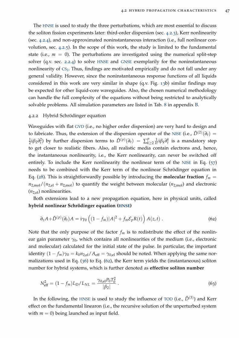
4.2 hybrid propagation characteristics 47
The HNSE is used to study the three perturbations, which are most essential to discuss
the soliton fission experiments later: third-order dispersion (sec. 4.2.3), Kerr nonlinearity
(sec. 4.2.4), and non-approximated noninstantaneous interaction (i.e., full nonlinear con-
volution, sec. 4.2.5). In the scope of this work, the study is limited to the fundamental
state (i.e., m = 0). The perturbations are investigated using the numerical split-step
solver (q.v. sec. 2.2.4) to solve HNSE and GNSE exemplarily for the noninstantaneous
nonlinearity of CS2. Thus, findings are motivated empirically and do not fall under any
general validity. However, since the noninstantaneous response functions of all liquids
considered in this work are very similar in shape (q.v. Fig. 13b) similar findings may
be expected for other liquid-core waveguides. Also, the chosen numerical methodology
can handle the full complexity of the equations without being restricted to analytically
solvable problems. All simulation parameters are listed in Tab. 8 in appendix B.
4.2.2 Hybrid Schrödinger equation
Waveguides with flat GVD (i.e., no higher order dispersion) are very hard to design and
to fabricate. Thus, the extension of the dispersion operator of the NISE (i.e., D(2)(∂t) =12 iβ2∂2
t ) by further dispersion terms to D(p)(∂t) = ∑pk≥2
1k! iβk∂k
t is a mandatory step
to get closer to realistic fibers. Also, all realistic media contain electrons and, hence,
the instantaneous nonlinearity, i.e., the Kerr nonlinearity, can never be switched off
entirely. To include the Kerr nonlinearity the nonlinear term of the NISE in Eq. (57)
needs to be combined with the Kerr term of the nonlinear Schrödinger equation in
Eq. (28). This is straightforwardly possible by introducing the molecular fraction fm =
n2,mol/(n2,el + n2,mol) to quantify the weight between molecular (n2,mol) and electronic
(n2,el) nonlinearities.
Both extensions lead to a new propagation equation, here in physical units, called
hybrid nonlinear Schrödinger equation (HNSE)
∂z A+D(p)(∂t)A = iγ0
(
(1 − fm)|A|2 + fmEpR(t))
A(z, t) . (62)
Note that the only purpose of the factor fm is to redistribute the effect of the nonlin-
ear gain parameter γ0, which contains all nonlinearities of the medium (i.e., electronic
and molecular) calculated for the initial state of the pulse. In particular, the important
identity (1 − fm)γ0 = k0n2,el/Aeff = γ0,el should be noted. When applying the same nor-
malizations used in Eq. (36) to Eq. (62), the Kerr term yields the (instantaneous) soliton
number for hybrid systems, which is further denoted as effective soliton number
N2eff = (1 − fm)LD/LNL =
γ0,elP0T20
|β2|. (63)
In the following, the HNSE is used to study the influence of TOD (i.e., D(3)) and Kerr
effect on the fundamental linearon (i.e., the recursive solution of the unperturbed system
with m = 0) being launched as input field.
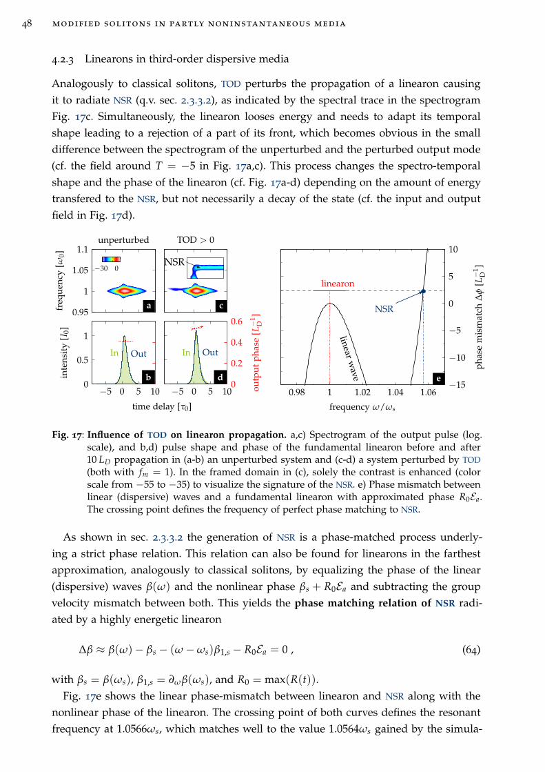
48 modified solitons in partly noninstantaneous media
4.2.3 Linearons in third-order dispersive media
Analogously to classical solitons, TOD perturbs the propagation of a linearon causing
it to radiate NSR (q.v. sec. 2.3.3.2), as indicated by the spectral trace in the spectrogram
Fig. 17c. Simultaneously, the linearon looses energy and needs to adapt its temporal
shape leading to a rejection of a part of its front, which becomes obvious in the small
difference between the spectrogram of the unperturbed and the perturbed output mode
(cf. the field around T = −5 in Fig. 17a,c). This process changes the spectro-temporal
shape and the phase of the linearon (cf. Fig. 17a-d) depending on the amount of energy
transfered to the NSR, but not necessarily a decay of the state (cf. the input and output
field in Fig. 17d).
0.95
1
1.05
1.1
freq
uen
cy[ω
0]
−30 0
In Out
−5 0 5 100
0.5
1
inte
nsit
y[I
0]
NSR
In Out
−5 0 5 10
time delay [τ0]
0
0.2
0.4
0.6
outp
ut
pha
se[L
−1
D]
linearw
ave
linearon
NSR
0.98 1 1.02 1.04 1.06−15
−10
−5
0
5
10
frequency ω/ωs
pha
sem
ism
atch
∆φ
[L−
1D
]
a
unperturbed
b
c
TOD > 0
d e
Fig. 17: Influence of TOD on linearon propagation. a,c) Spectrogram of the output pulse (log.scale), and b,d) pulse shape and phase of the fundamental linearon before and after10 LD propagation in (a-b) an unperturbed system and (c-d) a system perturbed by TOD
(both with fm = 1). In the framed domain in (c), solely the contrast is enhanced (colorscale from −55 to −35) to visualize the signature of the NSR. e) Phase mismatch betweenlinear (dispersive) waves and a fundamental linearon with approximated phase R0Ea.The crossing point defines the frequency of perfect phase matching to NSR.
As shown in sec. 2.3.3.2 the generation of NSR is a phase-matched process underly-
ing a strict phase relation. This relation can also be found for linearons in the farthest
approximation, analogously to classical solitons, by equalizing the phase of the linear
(dispersive) waves β(ω) and the nonlinear phase βs + R0Ea and subtracting the group
velocity mismatch between both. This yields the phase matching relation of NSR radi-
ated by a highly energetic linearon
∆β ≈ β(ω)− βs − (ω − ωs)β1,s − R0Ea = 0 , (64)
with βs = β(ωs), β1,s = ∂ωβ(ωs), and R0 = max(R(t)).
Fig. 17e shows the linear phase-mismatch between linearon and NSR along with the
nonlinear phase of the linearon. The crossing point of both curves defines the resonant
frequency at 1.0566ωs, which matches well to the value 1.0564ωs gained by the simula-
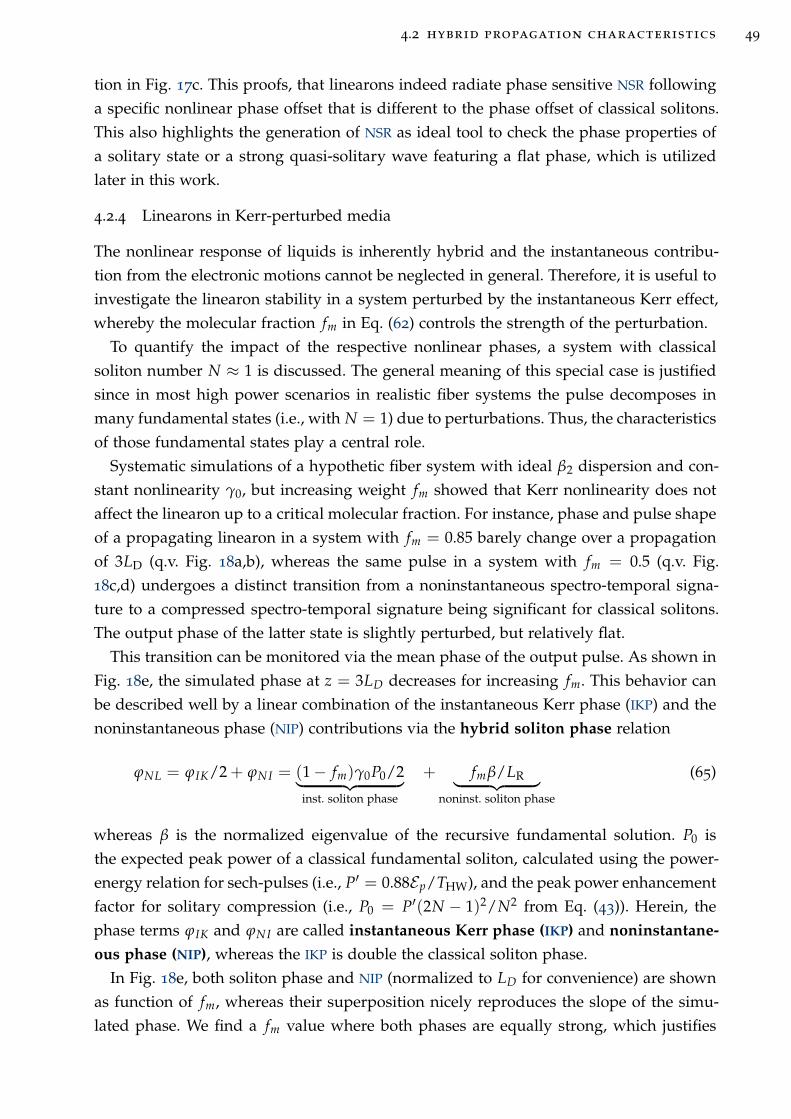
4.2 hybrid propagation characteristics 49
tion in Fig. 17c. This proofs, that linearons indeed radiate phase sensitive NSR following
a specific nonlinear phase offset that is different to the phase offset of classical solitons.
This also highlights the generation of NSR as ideal tool to check the phase properties of
a solitary state or a strong quasi-solitary wave featuring a flat phase, which is utilized
later in this work.
4.2.4 Linearons in Kerr-perturbed media
The nonlinear response of liquids is inherently hybrid and the instantaneous contribu-
tion from the electronic motions cannot be neglected in general. Therefore, it is useful to
investigate the linearon stability in a system perturbed by the instantaneous Kerr effect,
whereby the molecular fraction fm in Eq. (62) controls the strength of the perturbation.
To quantify the impact of the respective nonlinear phases, a system with classical
soliton number N ≈ 1 is discussed. The general meaning of this special case is justified
since in most high power scenarios in realistic fiber systems the pulse decomposes in
many fundamental states (i.e., with N = 1) due to perturbations. Thus, the characteristics
of those fundamental states play a central role.
Systematic simulations of a hypothetic fiber system with ideal β2 dispersion and con-
stant nonlinearity γ0, but increasing weight fm showed that Kerr nonlinearity does not
affect the linearon up to a critical molecular fraction. For instance, phase and pulse shape
of a propagating linearon in a system with fm = 0.85 barely change over a propagation
of 3LD (q.v. Fig. 18a,b), whereas the same pulse in a system with fm = 0.5 (q.v. Fig.
18c,d) undergoes a distinct transition from a noninstantaneous spectro-temporal signa-
ture to a compressed spectro-temporal signature being significant for classical solitons.
The output phase of the latter state is slightly perturbed, but relatively flat.
This transition can be monitored via the mean phase of the output pulse. As shown in
Fig. 18e, the simulated phase at z = 3LD decreases for increasing fm. This behavior can
be described well by a linear combination of the instantaneous Kerr phase (IKP) and the
noninstantaneous phase (NIP) contributions via the hybrid soliton phase relation
ϕNL = ϕIK/2 + ϕNI = (1 − fm)γ0P0/2︸ ︷︷ ︸
inst. soliton phase
+ fmβ/LR︸ ︷︷ ︸
noninst. soliton phase
(65)
whereas β is the normalized eigenvalue of the recursive fundamental solution. P0 is
the expected peak power of a classical fundamental soliton, calculated using the power-
energy relation for sech-pulses (i.e., P′ = 0.88Ep/THW), and the peak power enhancement
factor for solitary compression (i.e., P0 = P′(2N − 1)2/N2 from Eq. (43)). Herein, the
phase terms ϕIK and ϕNI are called instantaneous Kerr phase (IKP) and noninstantane-
ous phase (NIP), whereas the IKP is double the classical soliton phase.
In Fig. 18e, both soliton phase and NIP (normalized to LD for convenience) are shown
as function of fm, whereas their superposition nicely reproduces the slope of the simu-
lated phase. We find a fm value where both phases are equally strong, which justifies
50 modified solitons in partly noninstantaneous media
0.95
1
1.05
1.1fr
equ
ency
[ω0]
−30 0
In Out
−5 0 5 100
0.5
1
inte
nsit
y[I
0]compression
In Out
−5 0 5 10
time delay [τ0]
00.20.40.60.81
outp
ut
pha
se[L
−1
D] output at 3LD
soliton
linearonf
equilm
0 0.5 10
0.5
1
mol. fraction fR
pha
se[L
−1
D]
a
fm = 0.85
b
c
fm = 0.5
d e
Fig. 18: Influence of Kerr effect on linearon propagation a,c) Spectrogram of the output pulse(log. scale), and b,d) pulse shape and phase of the fundamental linearon before and after10 LD propagation in (a-b) a system weakly perturbed by the Kerr effect (i.e., fm = 0.85),and (c-d) a system strongly perturbed by the Kerr effect (i.e., fm = 0.5). e) Phase ofthe simulated output pulse after 3LD propagation as function of the molecular fraction,compared to the ideal soliton phase (reduced by 1 − fm) and the linearon phase β. Thered mark highlight the equilibrium fraction f
equilm = 0.68, where both phases are equally
strong.
the name equilibrium point fequilm . For fm < f
equilm the IKP dominates and the solitary
characteristics can mainly be described by classical soliton physics described by Neff.
For fm > fequilm the NIP takes over and linearon-like states may form. In the highly
energetic limit the hybrid nonlinear phase in Eq. (65) can be approximated with
ϕNLEp→∞−−−→ (1 − fm)γ0P0/2 + fmγ0EpR0 . (66)
The expression in Eq. (66) is of general use, since it does not require to solve the NISE to
gain the eigenvalue β and, thus, it allows to identify the equilibrium point for a wide set
of pulse parameters as shown later. In a realistic medium, however, fm cannot freely be
chosen for a given pulse energy but follows the constraints of the intrinsic pulse width
dependence of the NRI (i.e., Eq. (51), also cf. Fig. 13c). This introduces a new material-
specific limit that needs to be evaluated for each noninstantaneous system separately.
4.2.5 Linearons in media with realistic hybrid nonlinearity
Getting closer to a realistic system one must give up on the noninstantaneous approxim-
ation and handle the nonlinear response by the general convolution with pulse intensity
to enforce causality. Thus, linearon propagation is investigated here using the GNSE from
Eq. (27) instead of the HNSE used before. The discussion is limited to the lossless case of
the GNSE with constant γ0 (i.e., γ1 = 0) and β2 only.
First, a hypothetical system is considered, without electronic contributions (i.e., fm =
1). The linearon looses its solitary character along propagation, as exemplarily depicted
in Fig. 19c. This is due to a temporal delay between the approximated nonlinear poten-
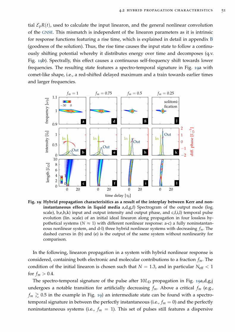
4.2 hybrid propagation characteristics 51
tial EpR(t), used to calculate the input linearon, and the general nonlinear convolution
of the GNSE. This mismatch is independent of the linearon parameters as it is intrinsic
for response functions featuring a rise time, which is explained in detail in appendix B
(goodness of the solution). Thus, the rise time causes the input state to follow a continu-
ously shifting potential whereby it distributes energy over time and decomposes (q.v.
Fig. 19b). Spectrally, this effect causes a continuous self-frequency shift towards lower
frequencies. The resulting state features a spectro-temporal signature in Fig. 19a with
comet-like shape, i.e., a red-shifted delayed maximum and a train towards earlier times
and larger frequencies.
0.9
1
1.1
freq
uen
cy[ω
0]
−30 0
In
Out0
0.5
1
inte
nsit
y[I
0]
0 2002468
10
leng
th[L
D]
0
1
In
Out
0 20
time delay [τ0]
InOut
0 20
solitoni-fication
InOut
−2
−1
0
1
2
dif
f.p
hase
[L−
1D
]0 20
a
fm = 1
b
c
d
fm = 0.75
e
f
g
fm = 0.5
h
i
j
fm = 0.25
k
l
Fig. 19: Hybrid propagation characterisitics as a result of the interplay between Kerr and non-instantaneous effects in liquid media a,d,g,f) Spectrogram of the output mode (log.scale), b,e,h,k) input and output intensity and output phase, and c,f,i,l) temporal pulseevolution (lin. scale) of an initial ideal linearon along propagation in four lossless hy-pothetical systems (N ≈ 1) with different nonlinear response: a-c) a fully noninstantan-eous nonlinear system, and d-l) three hybrid nonlinear systems with decreasing fm. Thedashed curves in (b) and (e) is the output of the same system without nonlinearity forcomparison.
In the following, linearon propagation in a system with hybrid nonlinear response is
considered, containing both electronic and molecular contributions to a fraction fm. The
condition of the initial linearon is chosen such that N = 1.3, and in particular Neff < 1
for fm > 0.4.
The spectro-temporal signature of the pulse after 10LD propagation in Fig. 19a,d,g,j
undergoes a notable transition for artificially decreasing fm. Above a critical fm (e.g.,
fm & 0.5 in the example in Fig. 19) an intermediate state can be found with a spectro-
temporal signature in between the perfectly instantaneous (i.e., fm = 0) and the perfectly
noninstantaneous systems (i.e., fm = 1). This set of pulses still features a dispersive
52 modified solitons in partly noninstantaneous media
pulse front, but a temporally shorter trailing confinement compared to the noninstant-
aneous case (cf. Fig. 19e,h with a). Decreasing the molecular fraction below the critical
fm increases the trailing confinement up to a point where the Kerr effect dominates.
Here, any input mode is transformed into a classical solitary wave with a compressed
spectro-temporal shape (q.v. Fig. 19j) if the fundamental soliton condition Neff = 1 can
be fullfilled. This solitonification process to classical solitons is exemplarily shown in Fig.
19l. The weak noninstantaneous phase causes a temporal shift as known from intra-pulse
Raman scattering (q.v. sec. 2.3.3.3), indicated by a linearly increasing phase (q.v. Fig. 19k),
but no further modification of the spectro-temporal signature of the state.
In contrast, output states of systems with large molecular fractions (e.g., fm & 0.5 in
Fig. 19) do not loose the comet-like spectro-temporal features during propagation (cf. Fig.
19d,g) being a result of the inevitable NIP. Yet, the IKP imposes a less dispersive, quasi-
solitary propagation characteristics for increasing fm (cf. Fig. 19e,h). With notable pulse
features from both nonlinear phase contributions (e.g., the comet-like spectrogram with
enhanced confinement), those states are referred to as hybrid solitary waves (HSWs)
in analogy to so-called solitary waves as detectable residuals of ideal Kerr solitons in
perturbed glass fiber systems.
Most notably, amongst the iteratively tested parameter sets, there are subsets that
yield HSWs with relatively flat phase. One of those occasionally found states is exemplar-
ily shown in Fig. 19e. Offset and tilt of the pulse phase remains mainly constant along
the last 3LD. Smaller phase oscillations (less than 2% deviation from the mean value)
potentially originate from non-perfect excitation conditions and cause further weak but
continuous energy dispersion of the pulse. However, these special cases indicate the ex-
istence of parameter domains, where dispersion, IKP, and NIP might compensate each
other to form a quasi-stationary state not underlying temporal or spectral shifts, and,
thus, obeying true soliton character. Since those states might be formed by solitonific-
ation from an arbitrary input field, similar to the example in Fig. 19f, they are real
eigenstates of a hybrid nonlinear system and justify the name hybrid soliton state (HSS).
They seem to be unique points in a multi-parameter space spanned by instantaneous
and noninstantaneous NRI, NRF, width and energy of the pulse. The complexity of this
parameter space requires further systematic studies to identify the underlying character-
istics and parameter domains of those states. Hence, the existence of HSSs can only be
postulated in the framework of this thesis and not formally verified.
Finally, the hybrid nonlinear phase as introduced in sec. 4.2.4 shall be demonstrated
as versatile tool to separate the classical soliton-like regime from the hybrid state regime.
Therefore, the propagation of multiple linearon states with N ≈ 1 to 5 was simulated
and the output after 10LD was analysed. For N > 1.5 a split-up of the input pulse into
fundamental solitary states is observed, i.e., soliton fission occurs (q.v. Fig. 20a). The
number of states after fission can be estimated with the effective soliton number Neff
from Eq. (63).
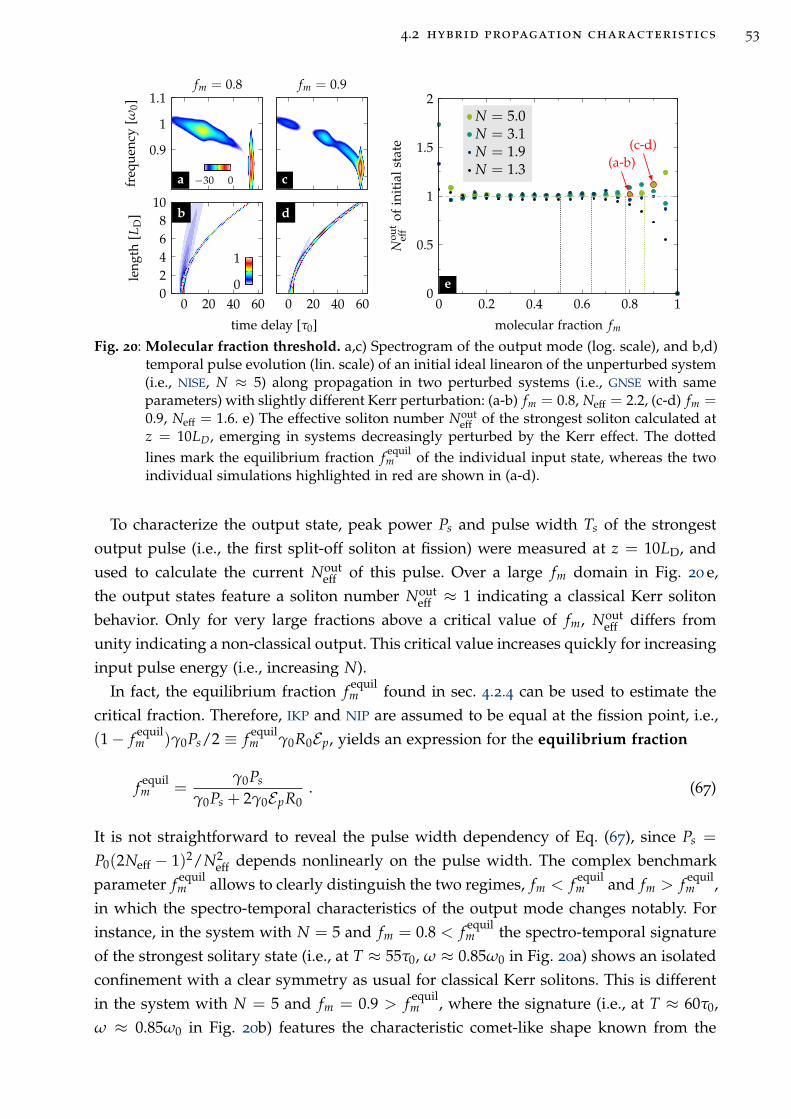
4.2 hybrid propagation characteristics 53
0.9
1
1.1
freq
uen
cy[ω
0]
−30 0
0 20 40 6002468
10
leng
th[L
D]
0
1
0 20 40 60
time delay [τ0]
(a-b)(c-d)
0 0.2 0.4 0.6 0.8 10
0.5
1
1.5
2
molecular fraction fm
Nou
tef
fof
init
ials
tate
N = 5.0N = 3.1N = 1.9N = 1.3
a
fm = 0.8
b
c
fm = 0.9
d
e
Fig. 20: Molecular fraction threshold. a,c) Spectrogram of the output mode (log. scale), and b,d)temporal pulse evolution (lin. scale) of an initial ideal linearon of the unperturbed system(i.e., NISE, N ≈ 5) along propagation in two perturbed systems (i.e., GNSE with sameparameters) with slightly different Kerr perturbation: (a-b) fm = 0.8, Neff = 2.2, (c-d) fm =0.9, Neff = 1.6. e) The effective soliton number Nout
eff of the strongest soliton calculated atz = 10LD, emerging in systems decreasingly perturbed by the Kerr effect. The dottedlines mark the equilibrium fraction f
equilm of the individual input state, whereas the two
individual simulations highlighted in red are shown in (a-d).
To characterize the output state, peak power Ps and pulse width Ts of the strongest
output pulse (i.e., the first split-off soliton at fission) were measured at z = 10LD, and
used to calculate the current Nouteff of this pulse. Over a large fm domain in Fig. 20 e,
the output states feature a soliton number Nouteff ≈ 1 indicating a classical Kerr soliton
behavior. Only for very large fractions above a critical value of fm, Nouteff differs from
unity indicating a non-classical output. This critical value increases quickly for increasing
input pulse energy (i.e., increasing N).
In fact, the equilibrium fraction fequilm found in sec. 4.2.4 can be used to estimate the
critical fraction. Therefore, IKP and NIP are assumed to be equal at the fission point, i.e.,
(1 − fequilm )γ0Ps/2 ≡ f
equilm γ0R0Ep, yields an expression for the equilibrium fraction
fequilm =
γ0Ps
γ0Ps + 2γ0EpR0. (67)
It is not straightforward to reveal the pulse width dependency of Eq. (67), since Ps =
P0(2Neff − 1)2/N2eff depends nonlinearly on the pulse width. The complex benchmark
parameter fequilm allows to clearly distinguish the two regimes, fm < f
equilm and fm > f
equilm ,
in which the spectro-temporal characteristics of the output mode changes notably. For
instance, in the system with N = 5 and fm = 0.8 < fequilm the spectro-temporal signature
of the strongest solitary state (i.e., at T ≈ 55τ0, ω ≈ 0.85ω0 in Fig. 20a) shows an isolated
confinement with a clear symmetry as usual for classical Kerr solitons. This is different
in the system with N = 5 and fm = 0.9 > fequilm , where the signature (i.e., at T ≈ 60τ0,
ω ≈ 0.85ω0 in Fig. 20b) features the characteristic comet-like shape known from the
54 modified solitons in partly noninstantaneous media
HSW. This proves the use of the hybrid nonlinear phase to distinguish between IKP- and
NIP-dominant regimes.
4.3 Intermediate conclusion
In this chapter, the NISE introduced by Conti et al. was utilized to reveal solitary solu-
tions, so-called linearons, in lossless liquid-like media with natural nonlinear response,
using a rigorous numerical eigenmode solver. The NISE was extended to the HNSE, which
allowed to demonstrate the robustness of the linearon states during propagation in sys-
tems perturbed by instantaneous nonlinearity and TOD. The results revealed important
phase conditions for NSR generation and solitonification (i.e., soliton formation in a hy-
brid nonlinear system).
However, linearon states disperse as soon as the approximate noninstantaneous term
is replaced by the general convolution term of the GNSE. The convolution leads to a
continuously shifting potential, which hinders the launched linearon to reach a steady
state while inevitably distributing energy. The temporal drift cannot be overcome by
adjusting the input (linearon) parameters, as it is intrinsic for all media possessing a
nonlinear response with a rise time, such as liquids. The predicted existence of linearons
in realistic LCFs can therefore not be confirmed.
Nonetheless, the hybrid nonlinear phase relation in Eq. (66) and the equilibrium frac-
tion fequilm found in this chapter allow to predict another non-classical soliton regime.
This regime presumably hosts modified solitary states (i.e., HSW) with shared spectro-
temporal properties from both sides, classical solitons and noninstantaneous states. How-
ever, this study also exposed fundamental limits on measuring HSWs. Large noninstant-
aneous nonlinearities are required which demands considerably long pulses and highly
noninstantaneous liquids. Potential candidates are CS2 or C2Cl4, which provide molecular
fractions of fm > 0.6 for pulse widths of 300 fs or more (q.v. sec. 3.3.2), and thus grant
access to the NIP-dominated regime. Such long pulses require meter-long propagation
lengths (i.e., L ≫ LD) in the ADD to undergo the necessary adiabatic transitions of the
input pulse to a hybrid state. But, as shown in ch. 3.4, the wavelength domain of the
ADD regime is situated relatively far in the NIR, in case of step-index fibers, where losses
are more dominant (e.g., q.v. Fig. 14b). Facilitated fiber designs, such as selectively filled
micro-structured fibers, might enable access to the ADD in other wavelength domains
with lower losses. However, their design and error-free fabrication along meters is very
challenging.
In this work, another approach is followed. With the theoretical background obtained
in this section, it should be possible to identify measurable observables of HSWs in
soliton-mediated supercontinua generated in the more lossy ADD domains of easily ac-
cessible step-index LCFs. The definition of these potential observables and the systematic
investigation of the impact of highly noninstantaneous nonlinearity on supercontinuum
spectra is the central purpose of the next chapter.
5H Y B R I D S O L I T O N D Y N A M I C S T H R O U G H T H E P R I S M O F
S U P E R C O N T I N U U M S P E C T R A
5.1 Methodology
In the previous chapter, a new hypothesis was formulated, which predicts a new class of
solitary waves (i.e., HSW) resulting from a hybrid electronic-molecular nonlinear system.
A hybrid nonlinear phase relation appears as key parameter to identify the dominant
nonlinearities. In this chapter, the impact of noninstantaneous nonlinearities on soliton-
mediated supercontinuum generation (SCG) will be investigated. It will be shown that it
is not sufficient to treat noninstantaneous systems as electronic systems with effectively
reduced NRI. Instead, SC parameters such as bandwidth, fission onset, and coherence
will show distinct dependencies on the molecular contribution. The signature of HSWs
will show up in the SC spectra, indicating their relevance in the broadening process. The
results of this chapter are partly published in [132].
In the closer scope of this work, we will immediately proceed to high soliton numbers
and not investigate the few soliton regime. However, the calculations for N > 1 shown in
sec. 4.2.5 allow the following conclusions:
1. Small contribution of noninstantaneous nonlinearity will cause the fission of solit-
ary waves. For increasing molecular weight fm (at constant total nonlinearity γ0),
the number of states created at fission is reduced.2. The nonlinear compression of the pulse causes a successive transition from an
potentially NIP-dominated regime to an IKP-dominated pulse regime. The equilib-
rium fraction fequilm can be used to estimate the dominating nonlinear phase at
the fission point. For increasing soliton number N (i.e., not Neff), fequilm converges
towards unity (q.v. Fig. 20), and, thus, instantaneous effects dominate the fission
process. How fast fequilm increases with N depends on the pulse width.
3. The effective soliton number Neff (q.v. Eq. (63)) is an appropriate quantity to estim-
ate the maximum number of created states after fission.
The findings in this chapter are based on systematic simulations of the nonlinear pulse
propagation in the fundamental fiber mode (i.e., HE11) using the full dispersive, lossless
GNSE from q.v. Eq. (26). For practical purposes, simulation parameters will be given
in realistic units. Pulse and fiber parameters are chosen to be close to experimentally
accessible domains of anomalously dispersive CS2-core silica-cladding fibers (q.v. ch. 3.4).
In particular, the laser wavelength is limited to the thulium laser band (i.e., 1.9− 2.0 µm).
The study starts in sec. 5.2 with comparing the SCG process in four selected systems,
pumped with a 450 fs sech (noiseless) pulse at 1.95 µm center wavelength. The findings
will help to classify the experimental SCG results in sec. 6.2. All four systems feature
the same mode dispersion β(ω), and frequency dependence of the effective mode area
Aeff(ω) (q.v. Tab. 8 in appendix B for more details). They are only distinguished in their
NRI and molecular fraction fm, which are chosen to mimic the following four nonlinear
systems:
55
56 hybrid soliton dynamics through the prism of supercontinuum spectra
1©overestimated case This is a hypothetical glass-type system with entirely instant-
aneous nonlinear response, i.e. fm = 0, and NRI as large as the total nonlinearity of
a liquid system, i.e. n2,tot = n2,el + n2,m. It features a classical soliton number N.
2©conservative case This is a hypothetical glass-type system with entirely instant-
aneous nonlinear response, i.e. fm = 0, and NRI reduced to the electronic nonlin-
earity of a liquid system, i.e. n2,tot = n2,el. Hence, the system’s soliton number N is
smaller than in case 1©.
3©realistic case This is a system assumed to be closest to a realistic CS2 system with
hybrid nonlinearity, whereas fm is calculated pulse width dependent after Eq. 51
(e.g., as herein often used fm(450 fs) = 0.85 for CS2), and NRI as large as the total
nonlinearity of a liquid system, i.e. n2,tot = n2,el + n2,m. The effective soliton number
Neff of this system is equal the soliton number N in case 2©.
4©unrealistic case This is a hypothetical system with entirely noninstantaneous
nonlinear response, i.e. fm = 1, and NRI as large as the total nonlinearity of a
CS2 system, i.e. n2,tot = n2,el + n2,m. It features the same large soliton number N as
case 1©.
In sec. 5.3, bandwidth, onset energy, and coherence of the generated SCs are sys-
tematically investigated in dependence on the molecular weight fm, pulse width, and
pump wavelength to carefully identify operation regimes, where the noninstantaneous
response contributes significantly to the broadening characteristics. Different to the sec-
tion before, noise is added to the input pulse (q.v. sec. 2.2.4) to trigger noise seeded
phenomena like MI (q.v. sec. 2.3.4.3). All data are shown in average of 20 individual runs
with random input noise.
Finally, in sec. 5.4, the gathered insights will allow to formulate a theory to explain
the impact of a strong noninstantaneous nonlinearity at each stage of the soliton-driven
broadening process.
5.2 Hybrid fission characteristics
The broadening process in all four cases is exemplarily shown in Fig. 21 to elucidate
the impact of the different non-linear contributions on the soliton fission process. Spe-
cific differences in the transition from instantaneous and noninstantaneous dominated
systems can be identified.
Both instantaneous systems (i.e., cases 1© and 2© in Fig. 21a,b and c,d) show conventio-
nal soliton fission: after initial pulse compression going along with self-phase modula-
tion up to the ZDW, a burst of solitons is released from the center of the pulse at a fission
length of approximately 2 cm, and 5 cm, respectively. In detail, the strongly compressed
pulse breaks up turbulently into multiple fundamental solitons on the long wavelength
side (domain B), which shed energy towards shorter wavelengths via the generation of
NSR (domain A). During further propagation the turbulent soliton burst is going over to
deterministic soliton fission where solitons are sequentially sheared off from the outer
zones of the pulse (domain C, not yet visible in case 2© in Fig. 21c). In the transition of
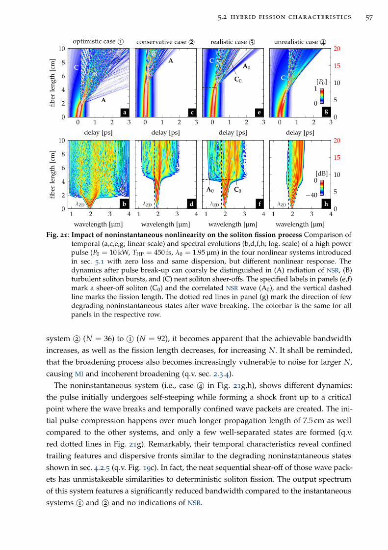
5.2 hybrid fission characteristics 57
A
BC
0 1 2 30
2
4
6
8
10
delay [ps]
fibe
rle
ngth
[cm
]
optimistic case 1©
λZD
1 2 3 40
2
4
6
8
10
wavelength [µm]
fibe
rle
ngth
[cm
]A
B
0 1 2 3
delay [ps]
conservative case 2©
λZD
1 2 3 4
wavelength [µm]
CA0
C0
0 1 2 3
delay [ps]
realistic case 3©
λZD
C0A0
1 2 3 4
wavelength [µm]
C
0 1 2 30
5
10
15
20
delay [ps]
unrealistic case 4©
0
1[P0]
λZD
1 2 3 40
5
10
15
20
wavelength [µm]
−40
0[dB]
a
b
c
d
e
f
g
h
Fig. 21: Impact of noninstantaneous nonlinearity on the soliton fission process Comparison oftemporal (a,c,e,g; linear scale) and spectral evolutions (b,d,f,h; log. scale) of a high powerpulse (P0 = 10 kW, THP = 450 fs, λ0 = 1.95 µm) in the four nonlinear systems introducedin sec. 5.1 with zero loss and same dispersion, but different nonlinear response. Thedynamics after pulse break-up can coarsly be distinguished in (A) radiation of NSR, (B)turbulent soliton bursts, and (C) neat soliton sheer-offs. The specified labels in panels (e,f)mark a sheer-off soliton (C0) and the correlated NSR wave (A0), and the vertical dashedline marks the fission length. The dotted red lines in panel (g) mark the direction of fewdegrading noninstantaneous states after wave breaking. The colorbar is the same for allpanels in the respective row.
system 2© (N = 36) to 1© (N = 92), it becomes apparent that the achievable bandwidth
increases, as well as the fission length decreases, for increasing N. It shall be reminded,
that the broadening process also becomes increasingly vulnerable to noise for larger N,
causing MI and incoherent broadening (q.v. sec. 2.3.4).
The noninstantaneous system (i.e., case 4© in Fig. 21g,h), shows different dynamics:
the pulse initially undergoes self-steeping while forming a shock front up to a critical
point where the wave breaks and temporally confined wave packets are created. The ini-
tial pulse compression happens over much longer propagation length of 7.5 cm as well
compared to the other systems, and only a few well-separated states are formed (q.v.
red dotted lines in Fig. 21g). Remarkably, their temporal characteristics reveal confined
trailing features and dispersive fronts similar to the degrading noninstantaneous states
shown in sec. 4.2.5 (q.v. Fig. 19c). In fact, the neat sequential shear-off of those wave pack-
ets has unmistakeable similarities to deterministic soliton fission. The output spectrum
of this system features a significantly reduced bandwidth compared to the instantaneous
systems 1© and 2© and no indications of NSR.
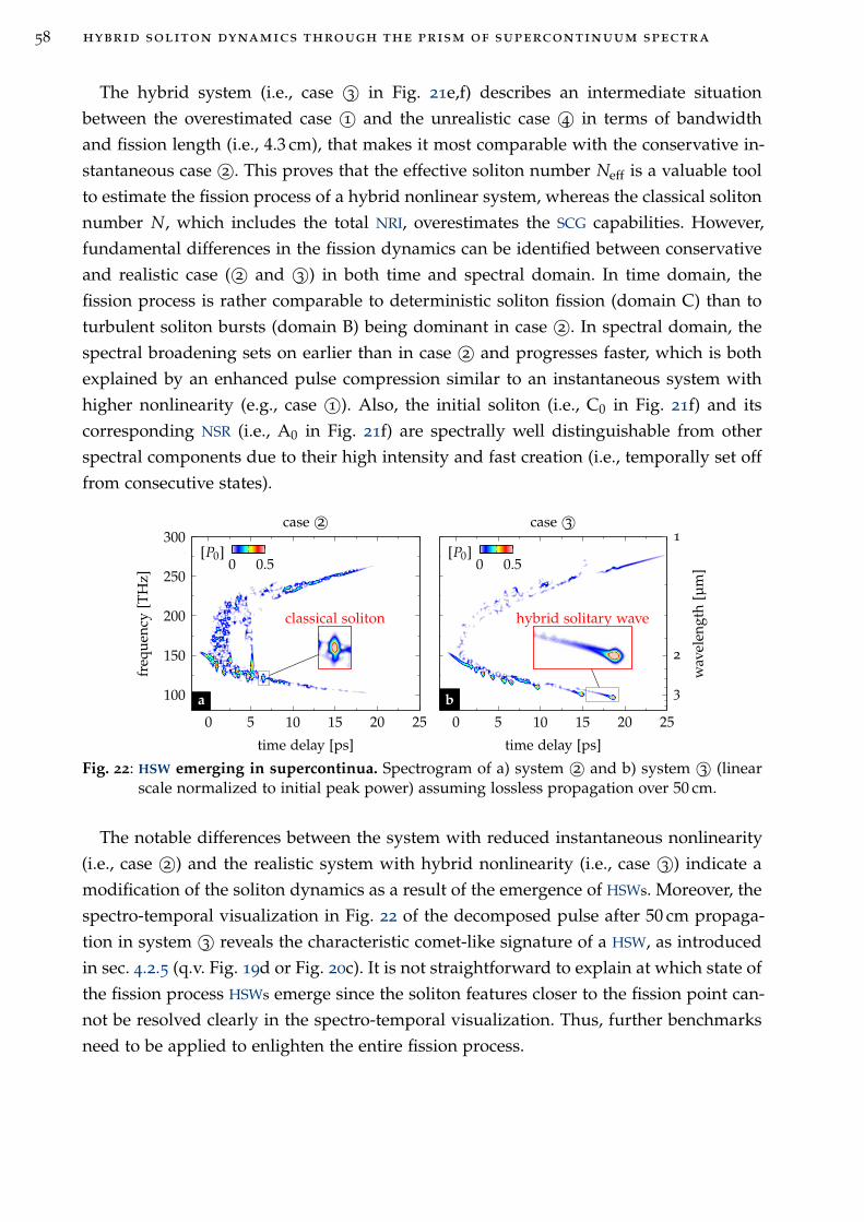
58 hybrid soliton dynamics through the prism of supercontinuum spectra
The hybrid system (i.e., case 3© in Fig. 21e,f) describes an intermediate situation
between the overestimated case 1© and the unrealistic case 4© in terms of bandwidth
and fission length (i.e., 4.3 cm), that makes it most comparable with the conservative in-
stantaneous case 2©. This proves that the effective soliton number Neff is a valuable tool
to estimate the fission process of a hybrid nonlinear system, whereas the classical soliton
number N, which includes the total NRI, overestimates the SCG capabilities. However,
fundamental differences in the fission dynamics can be identified between conservative
and realistic case ( 2© and 3©) in both time and spectral domain. In time domain, the
fission process is rather comparable to deterministic soliton fission (domain C) than to
turbulent soliton bursts (domain B) being dominant in case 2©. In spectral domain, the
spectral broadening sets on earlier than in case 2© and progresses faster, which is both
explained by an enhanced pulse compression similar to an instantaneous system with
higher nonlinearity (e.g., case 1©). Also, the initial soliton (i.e., C0 in Fig. 21f) and its
corresponding NSR (i.e., A0 in Fig. 21f) are spectrally well distinguishable from other
spectral components due to their high intensity and fast creation (i.e., temporally set off
from consecutive states).
hybrid solitary wave
0 5 10 15 20 25
time delay [ps]
case 3©
0 0.5[P0]
3
2
1
wav
elen
gth
[µm
]
classical soliton
0 5 10 15 20 25
100
150
200
250
300
time delay [ps]
freq
uen
cy[T
Hz]
case 2©
0 0.5[P0]
a b
Fig. 22: HSW emerging in supercontinua. Spectrogram of a) system 2© and b) system 3© (linearscale normalized to initial peak power) assuming lossless propagation over 50 cm.
The notable differences between the system with reduced instantaneous nonlinearity
(i.e., case 2©) and the realistic system with hybrid nonlinearity (i.e., case 3©) indicate a
modification of the soliton dynamics as a result of the emergence of HSWs. Moreover, the
spectro-temporal visualization in Fig. 22 of the decomposed pulse after 50 cm propaga-
tion in system 3© reveals the characteristic comet-like signature of a HSW, as introduced
in sec. 4.2.5 (q.v. Fig. 19d or Fig. 20c). It is not straightforward to explain at which state of
the fission process HSWs emerge since the soliton features closer to the fission point can-
not be resolved clearly in the spectro-temporal visualization. Thus, further benchmarks
need to be applied to enlighten the entire fission process.
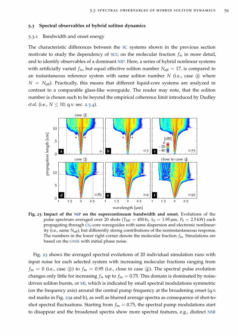
5.3 spectral observables of hybrid soliton dynamics 59
5.3 Spectral observables of hybrid soliton dynamics
5.3.1 Bandwidth and onset energy
The characteristic differences between the SC systems shown in the previous section
motivate to study the dependency of SCG on the molecular fraction fm in more detail,
and to identify observables of a dominant NIP. Here, a series of hybrid nonlinear systems
with artificially varied fm, but equal effective soliton number Neff = 17, is compared to
an instantaneous reference system with same soliton number N (i.e., case 2© where
N = Neff). Practically, this means that different liquid-core systems are analyzed in
contrast to a comparable glass-like waveguide. The reader may note, that the soliton
number is chosen such to be beyond the empirical coherence limit introduced by Dudley
et al. (i.e., N ≤ 10; q.v. sec. 2.3.4).
0
5
10
pro
pag
atio
nle
ngth
[cm
]
−40−20
0[dB]
1 1.5 2 2.50
5
10
1 1.5 2 2.5
wavelength [µm]
1 1.5 2 2.5
a 0
case 2©
0.5b 0.75c
0.85d
case 3©
0.9e 0.95
close to case 4©
f
Fig. 23: Impact of the NIP on the supercontinuum bandwidth and onset. Evolutions of thepulse spectrum averaged over 20 shots (THP = 450 fs, λ0 = 1.95 µm, P0 = 2.5 kW) eachpropagating through CS2-core waveguides with same dispersion and electronic nonlinear-ity (i.e., same Neff), but differently strong contributions of the noninstantaneous response.The numbers in the lower right corner denote the molecular fraction fm. Simulations arebased on the GNSE with initial phase noise.
Fig. 23 shows the averaged spectral evolutions of 20 individual simulation runs with
input noise for each selected system with increasing molecular fractions ranging from
fm = 0 (i.e., case 2©) to fm = 0.95 (i.e., close to case 4©). The spectral pulse evolution
changes only little for increasing fm up to fm = 0.75. This domain is dominated by noise-
driven soliton bursts, or MI, which is indicated by small spectral modulations symmetric
(on the frequency axis) around the central pump frequency at the broadening onset (q.v.
red marks in Fig. 23a and b), as well as blurred average spectra as consequence of shot-to-
shot spectral fluctuations. Starting from fm = 0.75, the spectral pump modulations start
to disappear and the broadened spectra show more spectral features, e.g., distinct NSR
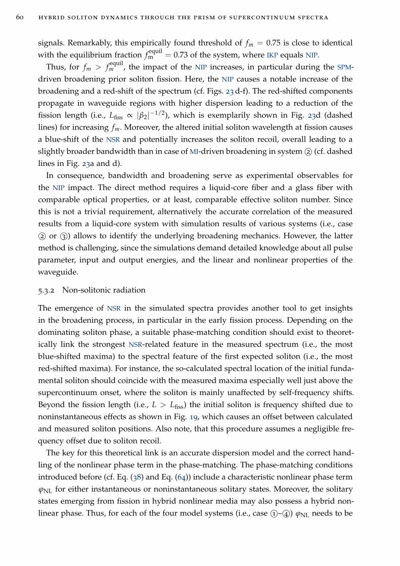
60 hybrid soliton dynamics through the prism of supercontinuum spectra
signals. Remarkably, this empirically found threshold of fm = 0.75 is close to identical
with the equilibrium fraction fequilm = 0.73 of the system, where IKP equals NIP.
Thus, for fm > fequilm , the impact of the NIP increases, in particular during the SPM-
driven broadening prior soliton fission. Here, the NIP causes a notable increase of the
broadening and a red-shift of the spectrum (cf. Figs. 23 d-f). The red-shifted components
propagate in waveguide regions with higher dispersion leading to a reduction of the
fission length (i.e., Lfiss ∝ |β2|−1/2), which is exemplarily shown in Fig. 23d (dashed
lines) for increasing fm. Moreover, the altered initial soliton wavelength at fission causes
a blue-shift of the NSR and potentially increases the soliton recoil, overall leading to a
slightly broader bandwidth than in case of MI-driven broadening in system 2© (cf. dashed
lines in Fig. 23a and d).
In consequence, bandwidth and broadening serve as experimental observables for
the NIP impact. The direct method requires a liquid-core fiber and a glass fiber with
comparable optical properties, or at least, comparable effective soliton number. Since
this is not a trivial requirement, alternatively the accurate correlation of the measured
results from a liquid-core system with simulation results of various systems (i.e., case2© or 3©) allows to identify the underlying broadening mechanics. However, the latter
method is challenging, since the simulations demand detailed knowledge about all pulse
parameter, input and output energies, and the linear and nonlinear properties of the
waveguide.
5.3.2 Non-solitonic radiation
The emergence of NSR in the simulated spectra provides another tool to get insights
in the broadening process, in particular in the early fission process. Depending on the
dominating soliton phase, a suitable phase-matching condition should exist to theoret-
ically link the strongest NSR-related feature in the measured spectrum (i.e., the most
blue-shifted maxima) to the spectral feature of the first expected soliton (i.e., the most
red-shifted maxima). For instance, the so-calculated spectral location of the initial funda-
mental soliton should coincide with the measured maxima especially well just above the
supercontinuum onset, where the soliton is mainly unaffected by self-frequency shifts.
Beyond the fission length (i.e., L > Lfiss) the initial soliton is frequency shifted due to
noninstantaneous effects as shown in Fig. 19, which causes an offset between calculated
and measured soliton positions. Also note, that this procedure assumes a negligible fre-
quency offset due to soliton recoil.
The key for this theoretical link is an accurate dispersion model and the correct hand-
ling of the nonlinear phase term in the phase-matching. The phase-matching conditions
introduced before (cf. Eq. (38) and Eq. (64)) include a characteristic nonlinear phase term
ϕNL for either instantaneous or noninstantaneous solitary states. Moreover, the solitary
states emerging from fission in hybrid nonlinear media may also possess a hybrid non-
linear phase. Thus, for each of the four model systems (i.e., case 1©– 4©) ϕNL needs to be
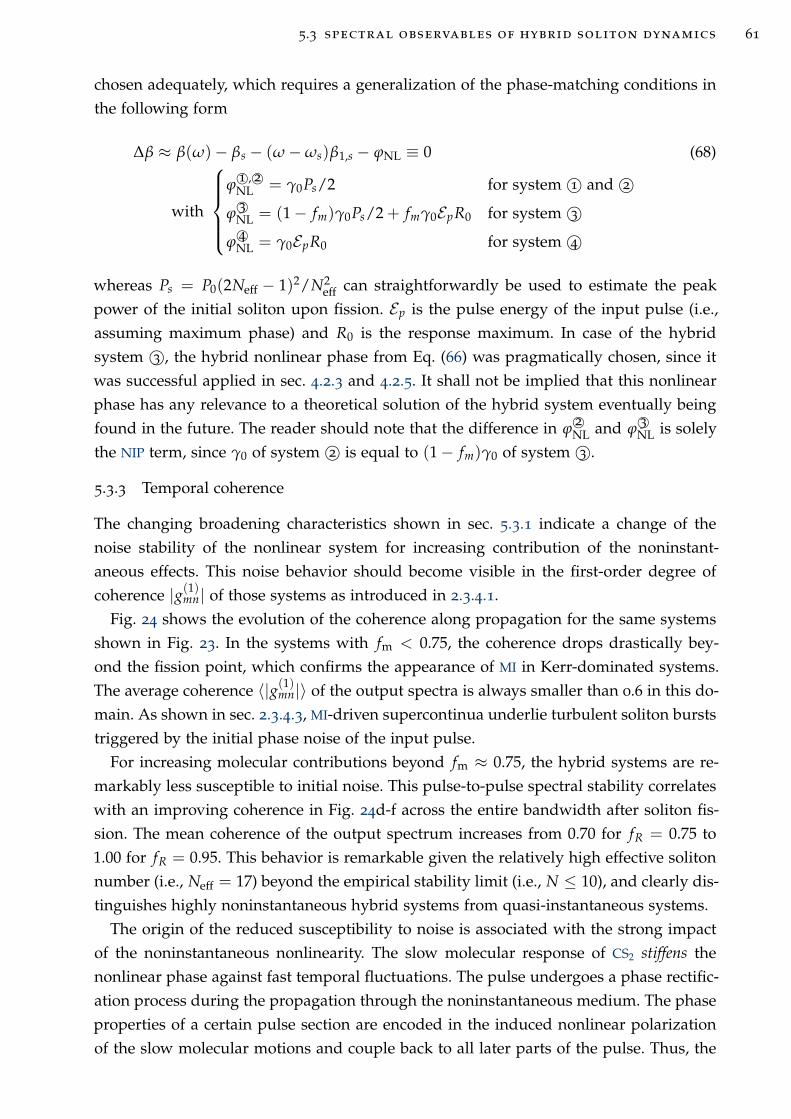
5.3 spectral observables of hybrid soliton dynamics 61
chosen adequately, which requires a generalization of the phase-matching conditions in
the following form
∆β ≈ β(ω)− βs − (ω − ωs)β1,s − ϕNL ≡ 0 (68)
with
ϕ1©, 2©NL = γ0Ps/2 for system 1© and 2©
ϕ3©NL = (1 − fm)γ0Ps/2 + fmγ0EpR0 for system 3©
ϕ4©NL = γ0EpR0 for system 4©
whereas Ps = P0(2Neff − 1)2/N2eff can straightforwardly be used to estimate the peak
power of the initial soliton upon fission. Ep is the pulse energy of the input pulse (i.e.,
assuming maximum phase) and R0 is the response maximum. In case of the hybrid
system 3©, the hybrid nonlinear phase from Eq. (66) was pragmatically chosen, since it
was successful applied in sec. 4.2.3 and 4.2.5. It shall not be implied that this nonlinear
phase has any relevance to a theoretical solution of the hybrid system eventually being
found in the future. The reader should note that the difference in ϕ2©NL and ϕ
3©NL is solely
the NIP term, since γ0 of system 2© is equal to (1 − fm)γ0 of system 3©.
5.3.3 Temporal coherence
The changing broadening characteristics shown in sec. 5.3.1 indicate a change of the
noise stability of the nonlinear system for increasing contribution of the noninstant-
aneous effects. This noise behavior should become visible in the first-order degree of
coherence |g(1)mn| of those systems as introduced in 2.3.4.1.
Fig. 24 shows the evolution of the coherence along propagation for the same systems
shown in Fig. 23. In the systems with fm < 0.75, the coherence drops drastically bey-
ond the fission point, which confirms the appearance of MI in Kerr-dominated systems.
The average coherence 〈|g(1)mn|〉 of the output spectra is always smaller than 0.6 in this do-
main. As shown in sec. 2.3.4.3, MI-driven supercontinua underlie turbulent soliton bursts
triggered by the initial phase noise of the input pulse.
For increasing molecular contributions beyond fm ≈ 0.75, the hybrid systems are re-
markably less susceptible to initial noise. This pulse-to-pulse spectral stability correlates
with an improving coherence in Fig. 24d-f across the entire bandwidth after soliton fis-
sion. The mean coherence of the output spectrum increases from 0.70 for fR = 0.75 to
1.00 for fR = 0.95. This behavior is remarkable given the relatively high effective soliton
number (i.e., Neff = 17) beyond the empirical stability limit (i.e., N ≤ 10), and clearly dis-
tinguishes highly noninstantaneous hybrid systems from quasi-instantaneous systems.
The origin of the reduced susceptibility to noise is associated with the strong impact
of the noninstantaneous nonlinearity. The slow molecular response of CS2 stiffens the
nonlinear phase against fast temporal fluctuations. The pulse undergoes a phase rectific-
ation process during the propagation through the noninstantaneous medium. The phase
properties of a certain pulse section are encoded in the induced nonlinear polarization
of the slow molecular motions and couple back to all later parts of the pulse. Thus, the
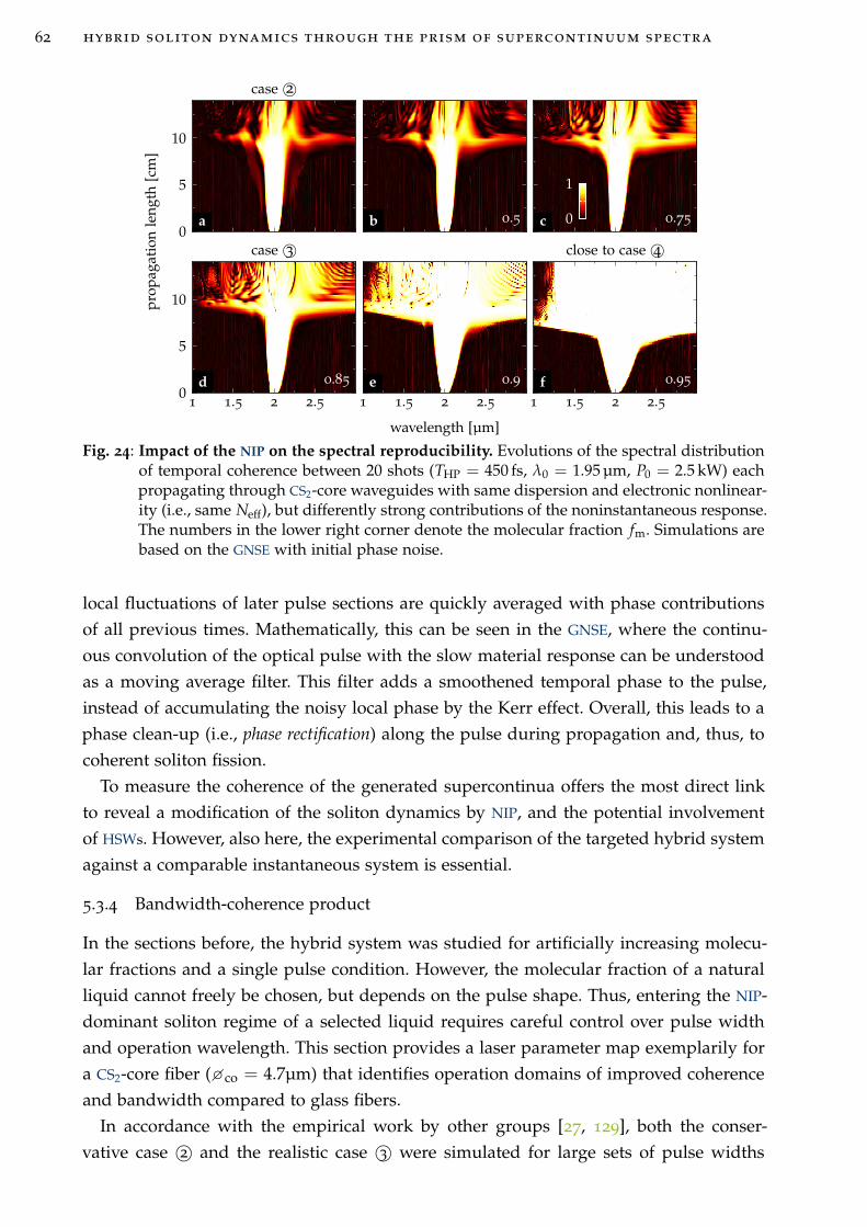
62 hybrid soliton dynamics through the prism of supercontinuum spectra
0
5
10p
rop
agat
ion
leng
th[c
m]
0
1
1 1.5 2 2.50
5
10
1 1.5 2 2.5
wavelength [µm]
1 1.5 2 2.5
a 0
case 2©
0.5b 0.75c
0.85d
case 3©
0.9e 0.95
close to case 4©
f
Fig. 24: Impact of the NIP on the spectral reproducibility. Evolutions of the spectral distributionof temporal coherence between 20 shots (THP = 450 fs, λ0 = 1.95 µm, P0 = 2.5 kW) eachpropagating through CS2-core waveguides with same dispersion and electronic nonlinear-ity (i.e., same Neff), but differently strong contributions of the noninstantaneous response.The numbers in the lower right corner denote the molecular fraction fm. Simulations arebased on the GNSE with initial phase noise.
local fluctuations of later pulse sections are quickly averaged with phase contributions
of all previous times. Mathematically, this can be seen in the GNSE, where the continu-
ous convolution of the optical pulse with the slow material response can be understood
as a moving average filter. This filter adds a smoothened temporal phase to the pulse,
instead of accumulating the noisy local phase by the Kerr effect. Overall, this leads to a
phase clean-up (i.e., phase rectification) along the pulse during propagation and, thus, to
coherent soliton fission.
To measure the coherence of the generated supercontinua offers the most direct link
to reveal a modification of the soliton dynamics by NIP, and the potential involvement
of HSWs. However, also here, the experimental comparison of the targeted hybrid system
against a comparable instantaneous system is essential.
5.3.4 Bandwidth-coherence product
In the sections before, the hybrid system was studied for artificially increasing molecu-
lar fractions and a single pulse condition. However, the molecular fraction of a natural
liquid cannot freely be chosen, but depends on the pulse shape. Thus, entering the NIP-
dominant soliton regime of a selected liquid requires careful control over pulse width
and operation wavelength. This section provides a laser parameter map exemplarily for
a CS2-core fiber (co = 4.7µm) that identifies operation domains of improved coherence
and bandwidth compared to glass fibers.
In accordance with the empirical work by other groups [27, 129], both the conser-
vative case 2© and the realistic case 3© were simulated for large sets of pulse widths
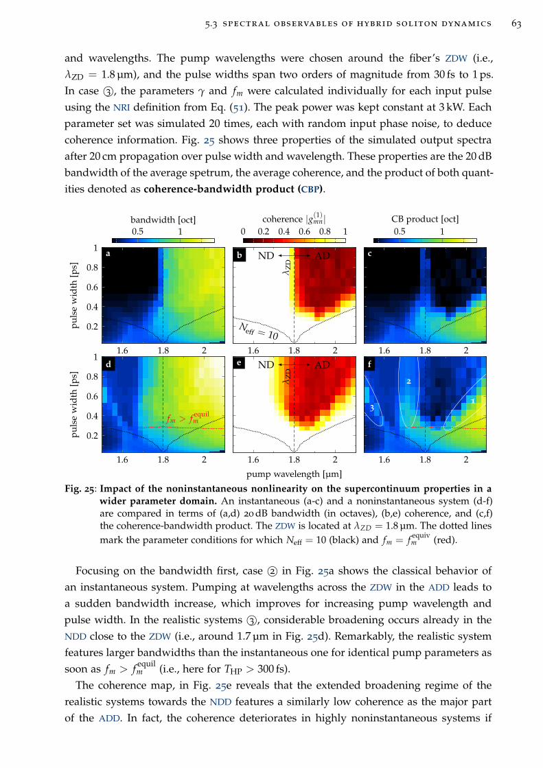
5.3 spectral observables of hybrid soliton dynamics 63
and wavelengths. The pump wavelengths were chosen around the fiber’s ZDW (i.e.,
λZD = 1.8 µm), and the pulse widths span two orders of magnitude from 30 fs to 1 ps.
In case 3©, the parameters γ and fm were calculated individually for each input pulse
using the NRI definition from Eq. (51). The peak power was kept constant at 3 kW. Each
parameter set was simulated 20 times, each with random input phase noise, to deduce
coherence information. Fig. 25 shows three properties of the simulated output spectra
after 20 cm propagation over pulse width and wavelength. These properties are the 20 dB
bandwidth of the average spetrum, the average coherence, and the product of both quant-
ities denoted as coherence-bandwidth product (CBP).
1.6 1.8 2
0.2
0.4
0.6
0.8
1
pu
lse
wid
th[p
s]
0.5 1bandwidth [oct]
λZ
D
ND AD
Neff = 101.6 1.8 2
0 0.2 0.4 0.6 0.8 1coherence |g(1)mn|
1.6 1.8 2
0.5 1CB product [oct]
fm > fequilm
1.6 1.8 2
0.2
0.4
0.6
0.8
1
pu
lse
wid
th[p
s]
λZ
D
ND AD
1.6 1.8 2
pump wavelength [µm]
3
2
1
1.6 1.8 2
a b c
d e f
Fig. 25: Impact of the noninstantaneous nonlinearity on the supercontinuum properties in awider parameter domain. An instantaneous (a-c) and a noninstantaneous system (d-f)are compared in terms of (a,d) 20 dB bandwidth (in octaves), (b,e) coherence, and (c,f)the coherence-bandwidth product. The ZDW is located at λZD = 1.8 µm. The dotted linesmark the parameter conditions for which Neff = 10 (black) and fm = f
equivm (red).
Focusing on the bandwidth first, case 2© in Fig. 25a shows the classical behavior of
an instantaneous system. Pumping at wavelengths across the ZDW in the ADD leads to
a sudden bandwidth increase, which improves for increasing pump wavelength and
pulse width. In the realistic systems 3©, considerable broadening occurs already in the
NDD close to the ZDW (i.e., around 1.7 µm in Fig. 25d). Remarkably, the realistic system
features larger bandwidths than the instantaneous one for identical pump parameters as
soon as fm > fequilm (i.e., here for THP > 300 fs).
The coherence map, in Fig. 25e reveals that the extended broadening regime of the
realistic systems towards the NDD features a similarly low coherence as the major part
of the ADD. In fact, the coherence deteriorates in highly noninstantaneous systems if
64 hybrid soliton dynamics through the prism of supercontinuum spectra
pumped in the NDD close to the ZDW. In the ADD, however, an improvement of the
coherence can be noted in the vicinity of the classical coherence threshold (i.e., Neff = 10
in Fig. 25b). The coherent domain of the realistic systems clearly exceed this threshold,
unambiguously confirming the coherence improvement as an accessible phenomena in
natural liquid-core waveguides.
Since both benchmarks, bandwidth and coherence, ought to be large in well perform-
ing SC sources, the introduction of a combined quantity in form of the product of both
appears meaningful. The CBP can be understood as shot-to-shot reproducible bandwidth
of the nonlinear system. It allows to clearly distinguish divergent parameter domains
between nonlinear systems within a single graphical visualization per system.
The CBP of the realistic system 3© reveals three improved parameter domains com-
pared to the instantaneous systems 2©. The first domain is the before-mentioned domain
of improved coherence in the ADD close to the classical coherence limit Neff = 10 (q.v.
domain 1 in Fig. 25f). A second domain opens in the weak NDD around 1.7 µm (q.v. do-
main 2 in Fig. 25f), which clearly correlates with the shifted broadening onset towards
the ZDW mentioned before. Third, a highly coherent domain with moderate bandwidth
can be identified far in the NDD above Neff = 10 (q.v. domain 3 in Fig. 25f). Most notably,
all three domains occur in systems with molecular fractions larger than the equilibrium
fraction fequilm (q.v. red line in Fig. 25f), which entirely attributes the observed changes in
the CBP to the dominant noninstantaneous effects.
The origin of domain 1 was discussed in earlier sections. Domain 2 and 3 need further
explanations, which shall be sketched out here briefly. Domain 2 is a result of the strong
spectral red-shift during SPM broadening, leading to efficient energy transfer towards
and across the ZDW, which in turn triggers soliton fission or MI. Thus, soliton-mediated
broadening can be achieved in hybrid systems at pump wavelengths significantly shorter
than the ZDW.
Domain 3 originates from self-seeded four-wave mixing between multiple spectral
parts of an SPM-broadened spectrum. First, energy is efficiently transferred close to the
ZDW due to the red-shifted SPM, delivering the pump energy for the four-wave mix-
ing process. Weaker spectral components of the SPM spectrum may overlap with phase-
matched spectral domains and serve as seed for the parametric process. In time, the
pulse forms a shock-front providing the necessary overlap between pump and seed,
which finally triggers efficient energy conversion from the pump (i.e., the field compon-
ents close to the ZDW) to spectrally symmetric side bands. This situation is in absolute
balance between (1) the right amount of SPM, to provide enough pump energy at the
ZDW, (2) the decelerated temporal pulse spreading and shock-front formation, and (3)
the spectral overlap with the phase-matched mixing components. This process might
be much more efficient in LCFs due to the NIP-enhanced red-shift of the SPM towards
the pump domain close to the ZDW. Also it may allow to transfer a notable part of the
pulse energy across the ZDW into the ADD, and may possibly allow for the excitation of
fundamental solitons while pumping in the NDD.
5.4 theory of noninstantaneously dominated supercontinuum generation 65
5.4 Theory of noninstantaneously dominated supercontinuum generation
The large scale parameter study of the hybrid nonlinear systems allows to form the
following conclusion: SCs generated in highly noninstantaneous systems are unambigu-
ously influenced by the slow nonlinearity, and in particular the dominant NIP. In con-
sequence, both bandwidth and coherence (i.e., pulse-to-pulse spectral stability) increase,
while the fission length decreases, for increasing molecular fraction fm. Most impress-
ively, the broadening characteristics for large soliton numbers undergoes a transition,
starting with noise-driven modulation instabilities at small fm to coherent soliton fission
at large fm. An empirical critical molecular fraction, beyond which the noninstantaneous
effects become non-negligible, was found to be fm = 0.75, which matches well with the
theoretical equilibrium fraction fequilm = 0.73
Remarkably, the spectro-temporal signature of HSWs were found in SCs from systems
with large fm, revealing the involvement of those states in the broadening process. How-
ever, the question remains at which part of the process these states occur. Two theories
become apparent:
fission theory During the entire fission process the NIP plays a major role and can-
not be neglected. Despite the temporal compression towards the fission point, the
NIP is not dominated by the IKP, and sets the phase of the consecutive solitons at
fission. The phase of these states might change during further propagation, (i.e.,
the temporal isolation from other parts of the pulse train), but the NIP dominates
over the Kerr phase at all times.
transition theory The temporal compression before the fission point is highly phase-
stabilized and enhanced by the NIP, that causes a strong peak power increase up to
the fission point. At the fission point, the IKP dominates over the NIP, and the com-
pressed pulse spawns a series of classical solitons. In the temporal window of the
compressed pulse, the NIP acts just as a quasi-static offset. During further propaga-
tion, the classical solitons experience a temporal delay due to SFS. As soon as a
soliton is temporally isolated from other components of the pulse train, and the
quasi-static phase offset they cause, this soliton accumulates dynamic NIP caused
by its own field, which initiates the transition from a classical soliton to a HSW.
A suitable experimental system might provide further insights into the process. Meas-
urements of SC spectra from LCFs might reveal the impact of a long-lasting response on
the soliton dynamics. This is analogous to associating measured SFSs with Raman ef-
fects in conventional silica systems. Exposing the dominant impact of NIP gives probable
cause for the involvement of HSWs. The next chapter aims to identify suitable laser and
fiber systems, which show NIP-dominant SCG, and potentially host HSWs. The spectral
observables introduced in this chapter will serve as benchmarks for those systems.
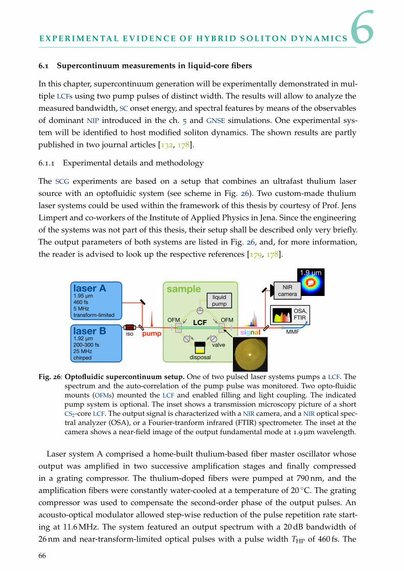
6E X P E R I M E N TA L E V I D E N C E O F H Y B R I D S O L I T O N D Y N A M I C S
6.1 Supercontinuum measurements in liquid-core fibers
In this chapter, supercontinuum generation will be experimentally demonstrated in mul-
tiple LCFs using two pump pulses of distinct width. The results will allow to analyze the
measured bandwidth, SC onset energy, and spectral features by means of the observables
of dominant NIP introduced in the ch. 5 and GNSE simulations. One experimental sys-
tem will be identified to host modified soliton dynamics. The shown results are partly
published in two journal articles [132, 178].
6.1.1 Experimental details and methodology
The SCG experiments are based on a setup that combines an ultrafast thulium laser
source with an optofluidic system (see scheme in Fig. 26). Two custom-made thulium
laser systems could be used within the framework of this thesis by courtesy of Prof. Jens
Limpert and co-workers of the Institute of Applied Physics in Jena. Since the engineering
of the systems was not part of this thesis, their setup shall be described only very briefly.
The output parameters of both systems are listed in Fig. 26, and, for more information,
the reader is advised to look up the respective references [179, 178].
sample
OFM OFM
pump signal
LCF
MMF
1.9 µm
liquid
pump
disposal
valve
1.95 µm
460 fs
5 MHz
transform-limited
laser A NIR
camera
1.92 µm
200-300 fs
25 MHz
chirped
laser B
OSA,
FTIR
iso
Fig. 26: Optofluidic supercontinuum setup. One of two pulsed laser systems pumps a LCF. Thespectrum and the auto-correlation of the pump pulse was monitored. Two opto-fluidicmounts (OFMs) mounted the LCF and enabled filling and light coupling. The indicatedpump system is optional. The inset shows a transmission microscopy picture of a shortCS2-core LCF. The output signal is characterized with a NIR camera, and a NIR optical spec-tral analyzer (OSA), or a Fourier-tranform infrared (FTIR) spectrometer. The inset at thecamera shows a near-field image of the output fundamental mode at 1.9 µm wavelength.
Laser system A comprised a home-built thulium-based fiber master oscillator whose
output was amplified in two successive amplification stages and finally compressed
in a grating compressor. The thulium-doped fibers were pumped at 790 nm, and the
amplification fibers were constantly water-cooled at a temperature of 20 C. The grating
compressor was used to compensate the second-order phase of the output pulses. An
acousto-optical modulator allowed step-wise reduction of the pulse repetition rate start-
ing at 11.6 MHz. The system featured an output spectrum with a 20 dB bandwidth of
26 nm and near-transform-limited optical pulses with a pulse width THP of 460 fs. The
66
6.1 supercontinuum measurements in liquid-core fibers 67
pulse reconstruction from the Fourier transform of the output spectrum and a third-
order phase offset (D3 = −0.025 ps3) matches the recorded auto-correlation very well.
Laser system B consisted of a commercial thulium-based fiber oscillator delivering
pulses of 500 fs duration, centered at 1.92 µm, at a repetition rate of 25 MHz. These
pulses were stretched in 25 cm anomalous dispersive single-mode fiber (Corning SMF-28)
and 4 m normal dispersive ultra-high NA fiber (Thorlabs UHNA4). Before amplification,
their polarization was controlled by a combination of a half- and a quarter-wave-plate. Fi-
nally, this (seed) signal (≈3 mW average) was coupled to a water-cooled thulium-doped
photonic crystal fiber and desirably amplified up to 1 W average power. The initial pos-
itive chirp from the oscillator output was partly compensated during nonlinear pulse
compression in the anomalous dispersive amplifier fiber. Hence, the pulse duration (i.e.,
THP) was adjustable between 200 and 300 fs by decreasing the amplification, and, thus,
the nonlinear compression. However, the final output pulse is not transform limited since
the last isolator adds a non-negligible chirp. The output pulse shape and spectrum of
the laser system were controlled online with two reflexes coupled into an autocorrelator
and a spectrometer at any time of the experiments, ensuring stable pulse conditions.
The fabrication of the LCFs can straightforwardly be implemented by mounting each
end of a silica capillary in an OFM (i.e., small aluminum tank with sealed sapphire win-
dow). The mounts are filled successively with a syringe, while giving enough time in-
between that the capillary force can entirely fill the capillary. The fabrication process in
described in more detail in appendix C. The properties of the LCFs used for the main
data sets are tabulated in Tab. 3. After fabrication in a fume hood, the fiber’s OFMs are
placed each in front of a fiber coupling stage (i.e. a three-axis translation stage). Light
was coupled free-space in and out the fiber using aspheric lenses (e.g., Thorlabs A375,
A397, C230) with suitable NA to account for the NA of the LCF and to avoid clipping
of the output mode (i.e., NAinput < NALCF < NAoutput). The coupling was optimized at
power levels of a few milliwatts, where no significant spectral broadening is observed.
Since most LCFs used in the experiments supported few modes, efficient excitation of the
fundamental mode was ensured by imaging the output mode patterns with an extended
InGaAs camera (Xenics XEVA) or a thermal camera (MCT detector, FLIR SC7000) while
optimizing the coupling. Coupling efficiencies up to η = 55 % were reached estimated
using η = Poutmeas/(Tout
L ToutW · Pin
measTinL Tin
W TLCF), taking into account modal attenuation
(i.e., fiber transmission TLCF) and reflections at lenses (i.e., transmission TL) and OFM
windows (i.e., transmission TW) each at in- and output side of the LCF. The coupling
was stable over several days under atmospheric pressure and even while flushing the
opto-fluidic mounts with flow rates up to 10 ml min−1.
After coupling optimization, the fiber output was collimated for the pump wavelength
and detected with an InF3 multimode fiber (co = 100 µm) directly placed in the collim-
ated beam and connected to a suitable spectral analyzer (Yokogawa NIR and MIR OSA,
Thorlabs FTIR OSA305, Jasco FTIR 6300). The mountings of the LCFs prevented a cut-
back of the fibers. Thus, a typical measurement included recording the output spectra
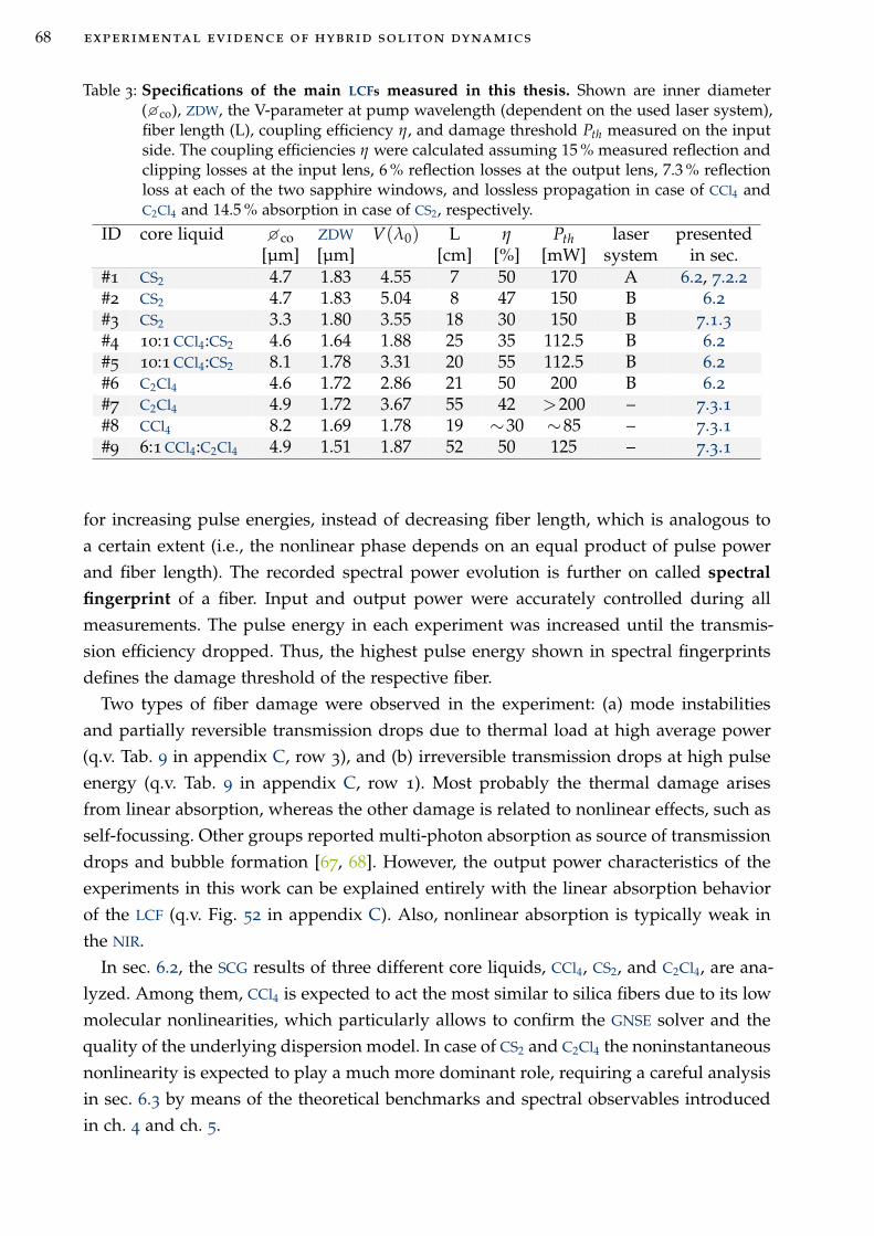
68 experimental evidence of hybrid soliton dynamics
Table 3: Specifications of the main LCFs measured in this thesis. Shown are inner diameter(co), ZDW, the V-parameter at pump wavelength (dependent on the used laser system),fiber length (L), coupling efficiency η, and damage threshold Pth measured on the inputside. The coupling efficiencies η were calculated assuming 15 % measured reflection andclipping losses at the input lens, 6 % reflection losses at the output lens, 7.3 % reflectionloss at each of the two sapphire windows, and lossless propagation in case of CCl4 andC2Cl4 and 14.5 % absorption in case of CS2, respectively.
ID core liquid co ZDW V(λ0) L η Pth laser presented[µm] [µm] [cm] [%] [mW] system in sec.
#1 CS2 4.7 1.83 4.55 7 50 170 A 6.2, 7.2.2#2 CS2 4.7 1.83 5.04 8 47 150 B 6.2#3 CS2 3.3 1.80 3.55 18 30 150 B 7.1.3#4 10:1 CCl4:CS2 4.6 1.64 1.88 25 35 112.5 B 6.2#5 10:1 CCl4:CS2 8.1 1.78 3.31 20 55 112.5 B 6.2#6 C2Cl4 4.6 1.72 2.86 21 50 200 B 6.2#7 C2Cl4 4.9 1.72 3.67 55 42 >200 – 7.3.1#8 CCl4 8.2 1.69 1.78 19 ∼30 ∼85 – 7.3.1#9 6:1 CCl4:C2Cl4 4.9 1.51 1.87 52 50 125 – 7.3.1
for increasing pulse energies, instead of decreasing fiber length, which is analogous to
a certain extent (i.e., the nonlinear phase depends on an equal product of pulse power
and fiber length). The recorded spectral power evolution is further on called spectral
fingerprint of a fiber. Input and output power were accurately controlled during all
measurements. The pulse energy in each experiment was increased until the transmis-
sion efficiency dropped. Thus, the highest pulse energy shown in spectral fingerprints
defines the damage threshold of the respective fiber.
Two types of fiber damage were observed in the experiment: (a) mode instabilities
and partially reversible transmission drops due to thermal load at high average power
(q.v. Tab. 9 in appendix C, row 3), and (b) irreversible transmission drops at high pulse
energy (q.v. Tab. 9 in appendix C, row 1). Most probably the thermal damage arises
from linear absorption, whereas the other damage is related to nonlinear effects, such as
self-focussing. Other groups reported multi-photon absorption as source of transmission
drops and bubble formation [67, 68]. However, the output power characteristics of the
experiments in this work can be explained entirely with the linear absorption behavior
of the LCF (q.v. Fig. 52 in appendix C). Also, nonlinear absorption is typically weak in
the NIR.
In sec. 6.2, the SCG results of three different core liquids, CCl4, CS2, and C2Cl4, are ana-
lyzed. Among them, CCl4 is expected to act the most similar to silica fibers due to its low
molecular nonlinearities, which particularly allows to confirm the GNSE solver and the
quality of the underlying dispersion model. In case of CS2 and C2Cl4 the noninstantaneous
nonlinearity is expected to play a much more dominant role, requiring a careful analysis
in sec. 6.3 by means of the theoretical benchmarks and spectral observables introduced
in ch. 4 and ch. 5.
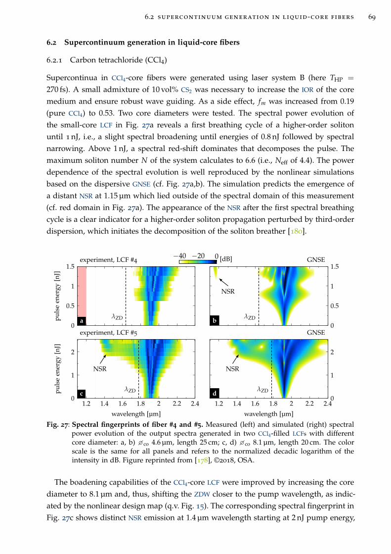
6.2 supercontinuum generation in liquid-core fibers 69
6.2 Supercontinuum generation in liquid-core fibers
6.2.1 Carbon tetrachloride (CCl4)
Supercontinua in CCl4-core fibers were generated using laser system B (here THP =
270 fs). A small admixture of 10 vol% CS2 was necessary to increase the IOR of the core
medium and ensure robust wave guiding. As a side effect, fm was increased from 0.19
(pure CCl4) to 0.53. Two core diameters were tested. The spectral power evolution of
the small-core LCF in Fig. 27a reveals a first breathing cycle of a higher-order soliton
until 1 nJ, i.e., a slight spectral broadening until energies of 0.8 nJ followed by spectral
narrowing. Above 1 nJ, a spectral red-shift dominates that decomposes the pulse. The
maximum soliton number N of the system calculates to 6.6 (i.e., Neff of 4.4). The power
dependence of the spectral evolution is well reproduced by the nonlinear simulations
based on the dispersive GNSE (cf. Fig. 27a,b). The simulation predicts the emergence of
a distant NSR at 1.15 µm which lied outside of the spectral domain of this measurement
(cf. red domain in Fig. 27a). The appearance of the NSR after the first spectral breathing
cycle is a clear indicator for a higher-order soliton propagation perturbed by third-order
dispersion, which initiates the decomposition of the soliton breather [180].
λZD
0
0.5
1
1.5
pu
lse
ener
gy[n
J]
−40 −20 0 [dB]
λZD
NSR
0
0.5
1
1.5
λZD
NSR
1.2 1.4 1.6 1.8 2 2.2 2.40
1
2
wavelength [µm]
pu
lse
ener
gy[n
J]
λZD
NSR
1.2 1.4 1.6 1.8 2 2.2 2.40
1
2
wavelength [µm]
experiment, LCF #4 GNSE
experiment, LCF #5 GNSE
a b
c d
Fig. 27: Spectral fingerprints of fiber #4 and #5. Measured (left) and simulated (right) spectralpower evolution of the output spectra generated in two CCl4-filled LCFs with differentcore diameter: a, b) co 4.6 µm, length 25 cm; c, d) co 8.1 µm, length 20 cm. The colorscale is the same for all panels and refers to the normalized decadic logarithm of theintensity in dB. Figure reprinted from [178], ©2018, OSA.
The boadening capabilities of the CCl4-core LCF were improved by increasing the core
diameter to 8.1 µm and, thus, shifting the ZDW closer to the pump wavelength, as indic-
ated by the nonlinear design map (q.v. Fig. 15). The corresponding spectral fingerprint in
Fig. 27c shows distinct NSR emission at 1.4 µm wavelength starting at 2 nJ pump energy,
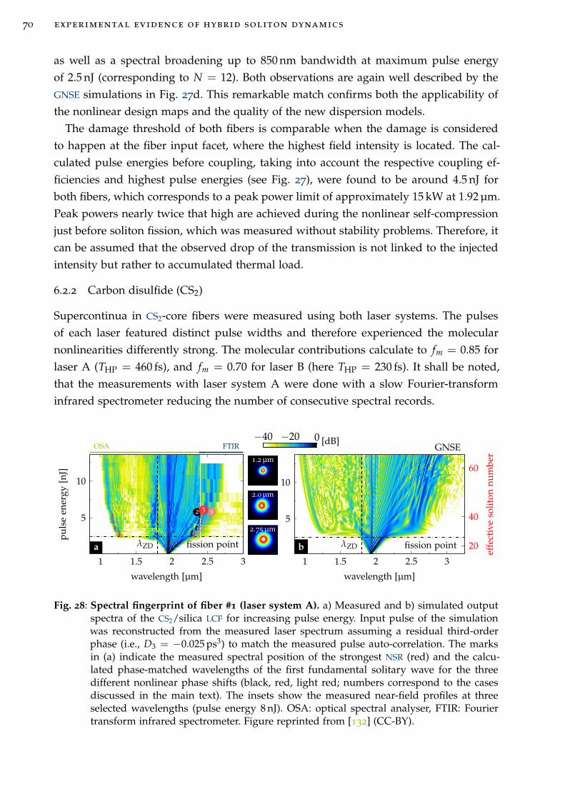
70 experimental evidence of hybrid soliton dynamics
as well as a spectral broadening up to 850 nm bandwidth at maximum pulse energy
of 2.5 nJ (corresponding to N = 12). Both observations are again well described by the
GNSE simulations in Fig. 27d. This remarkable match confirms both the applicability of
the nonlinear design maps and the quality of the new dispersion models.
The damage threshold of both fibers is comparable when the damage is considered
to happen at the fiber input facet, where the highest field intensity is located. The cal-
culated pulse energies before coupling, taking into account the respective coupling ef-
ficiencies and highest pulse energies (see Fig. 27), were found to be around 4.5 nJ for
both fibers, which corresponds to a peak power limit of approximately 15 kW at 1.92 µm.
Peak powers nearly twice that high are achieved during the nonlinear self-compression
just before soliton fission, which was measured without stability problems. Therefore, it
can be assumed that the observed drop of the transmission is not linked to the injected
intensity but rather to accumulated thermal load.
6.2.2 Carbon disulfide (CS2)
Supercontinua in CS2-core fibers were measured using both laser systems. The pulses
of each laser featured distinct pulse widths and therefore experienced the molecular
nonlinearities differently strong. The molecular contributions calculate to fm = 0.85 for
laser A (THP = 460 fs), and fm = 0.70 for laser B (here THP = 230 fs). It shall be noted,
that the measurements with laser system A were done with a slow Fourier-transform
infrared spectrometer reducing the number of consecutive spectral records.
2 13
λZD fission point
1 1.5 2 2.5 3
5
10
wavelength [µm]
pu
lse
ener
gy[n
J]
λZD fission point
1 1.5 2 2.5 3
5
10
wavelength [µm]
−40 −20 0 [dB]
20
40
60
effe
ctiv
eso
liton
num
ber
FTIROSA GNSE
a b
1.2 µm
2.0 µm
2.75 µm
Fig. 28: Spectral fingerprint of fiber #1 (laser system A). a) Measured and b) simulated outputspectra of the CS2/silica LCF for increasing pulse energy. Input pulse of the simulationwas reconstructed from the measured laser spectrum assuming a residual third-orderphase (i.e., D3 = −0.025 ps3) to match the measured pulse auto-correlation. The marksin (a) indicate the measured spectral position of the strongest NSR (red) and the calcu-lated phase-matched wavelengths of the first fundamental solitary wave for the threedifferent nonlinear phase shifts (black, red, light red; numbers correspond to the casesdiscussed in the main text). The insets show the measured near-field profiles at threeselected wavelengths (pulse energy 8 nJ). OSA: optical spectral analyser, FTIR: Fouriertransform infrared spectrometer. Figure reprinted from [132] (CC-BY).
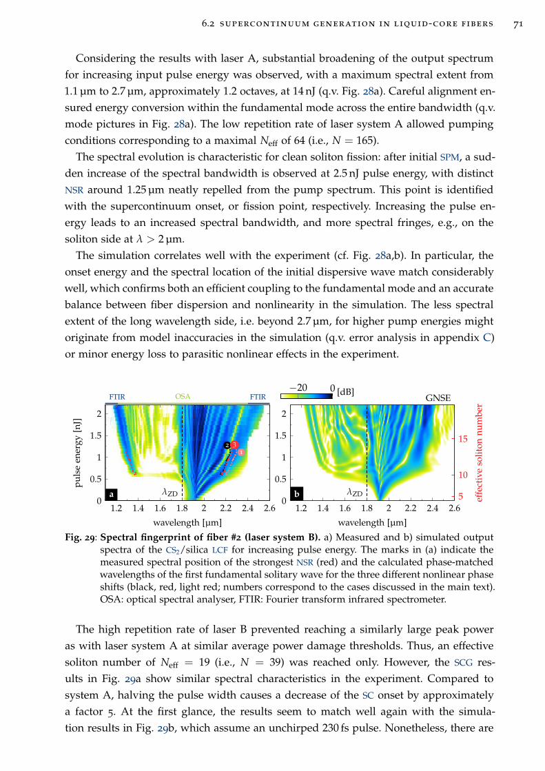
6.2 supercontinuum generation in liquid-core fibers 71
Considering the results with laser A, substantial broadening of the output spectrum
for increasing input pulse energy was observed, with a maximum spectral extent from
1.1 µm to 2.7 µm, approximately 1.2 octaves, at 14 nJ (q.v. Fig. 28a). Careful alignment en-
sured energy conversion within the fundamental mode across the entire bandwidth (q.v.
mode pictures in Fig. 28a). The low repetition rate of laser system A allowed pumping
conditions corresponding to a maximal Neff of 64 (i.e., N = 165).
The spectral evolution is characteristic for clean soliton fission: after initial SPM, a sud-
den increase of the spectral bandwidth is observed at 2.5 nJ pulse energy, with distinct
NSR around 1.25 µm neatly repelled from the pump spectrum. This point is identified
with the supercontinuum onset, or fission point, respectively. Increasing the pulse en-
ergy leads to an increased spectral bandwidth, and more spectral fringes, e.g., on the
soliton side at λ > 2 µm.
The simulation correlates well with the experiment (cf. Fig. 28a,b). In particular, the
onset energy and the spectral location of the initial dispersive wave match considerably
well, which confirms both an efficient coupling to the fundamental mode and an accurate
balance between fiber dispersion and nonlinearity in the simulation. The less spectral
extent of the long wavelength side, i.e. beyond 2.7 µm, for higher pump energies might
originate from model inaccuracies in the simulation (q.v. error analysis in appendix C)
or minor energy loss to parasitic nonlinear effects in the experiment.
21
3
λZD
1.2 1.4 1.6 1.8 2 2.2 2.4 2.60
0.5
1
1.5
2
wavelength [µm]
pu
lse
ener
gy[n
J]
λZD
1.2 1.4 1.6 1.8 2 2.2 2.4 2.60
0.5
1
1.5
2
wavelength [µm]
−20 0 [dB]
5
10
15
effe
ctiv
eso
liton
num
ber
FTIRFTIR OSA GNSE
a b
Fig. 29: Spectral fingerprint of fiber #2 (laser system B). a) Measured and b) simulated outputspectra of the CS2/silica LCF for increasing pulse energy. The marks in (a) indicate themeasured spectral position of the strongest NSR (red) and the calculated phase-matchedwavelengths of the first fundamental solitary wave for the three different nonlinear phaseshifts (black, red, light red; numbers correspond to the cases discussed in the main text).OSA: optical spectral analyser, FTIR: Fourier transform infrared spectrometer.
The high repetition rate of laser B prevented reaching a similarly large peak power
as with laser system A at similar average power damage thresholds. Thus, an effective
soliton number of Neff = 19 (i.e., N = 39) was reached only. However, the SCG res-
ults in Fig. 29a show similar spectral characteristics in the experiment. Compared to
system A, halving the pulse width causes a decrease of the SC onset by approximately
a factor 5. At the first glance, the results seem to match well again with the simula-
tion results in Fig. 29b, which assume an unchirped 230 fs pulse. Nonetheless, there are
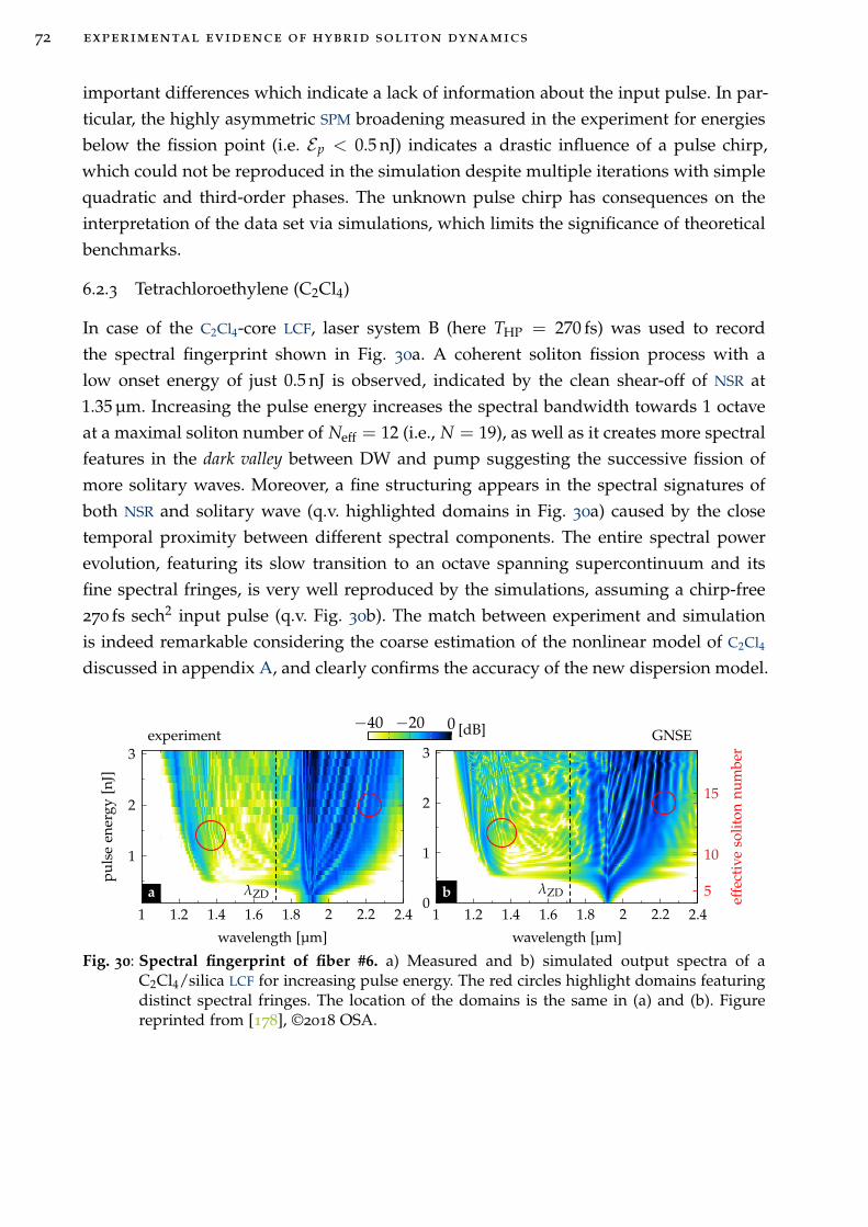
72 experimental evidence of hybrid soliton dynamics
important differences which indicate a lack of information about the input pulse. In par-
ticular, the highly asymmetric SPM broadening measured in the experiment for energies
below the fission point (i.e. Ep < 0.5 nJ) indicates a drastic influence of a pulse chirp,
which could not be reproduced in the simulation despite multiple iterations with simple
quadratic and third-order phases. The unknown pulse chirp has consequences on the
interpretation of the data set via simulations, which limits the significance of theoretical
benchmarks.
6.2.3 Tetrachloroethylene (C2Cl4)
In case of the C2Cl4-core LCF, laser system B (here THP = 270 fs) was used to record
the spectral fingerprint shown in Fig. 30a. A coherent soliton fission process with a
low onset energy of just 0.5 nJ is observed, indicated by the clean shear-off of NSR at
1.35 µm. Increasing the pulse energy increases the spectral bandwidth towards 1 octave
at a maximal soliton number of Neff = 12 (i.e., N = 19), as well as it creates more spectral
features in the dark valley between DW and pump suggesting the successive fission of
more solitary waves. Moreover, a fine structuring appears in the spectral signatures of
both NSR and solitary wave (q.v. highlighted domains in Fig. 30a) caused by the close
temporal proximity between different spectral components. The entire spectral power
evolution, featuring its slow transition to an octave spanning supercontinuum and its
fine spectral fringes, is very well reproduced by the simulations, assuming a chirp-free
270 fs sech2 input pulse (q.v. Fig. 30b). The match between experiment and simulation
is indeed remarkable considering the coarse estimation of the nonlinear model of C2Cl4
discussed in appendix A, and clearly confirms the accuracy of the new dispersion model.
λZD
1 1.2 1.4 1.6 1.8 2 2.2 2.4
1
2
3
wavelength [µm]
pu
lse
ener
gy[n
J]
−40 −20 0 [dB]
λZD
1 1.2 1.4 1.6 1.8 2 2.2 2.40
1
2
3
wavelength [µm]
5
10
15
effe
ctiv
eso
liton
num
ber
experiment GNSE
a b
Fig. 30: Spectral fingerprint of fiber #6. a) Measured and b) simulated output spectra of aC2Cl4/silica LCF for increasing pulse energy. The red circles highlight domains featuringdistinct spectral fringes. The location of the domains is the same in (a) and (b). Figurereprinted from [178], ©2018 OSA.
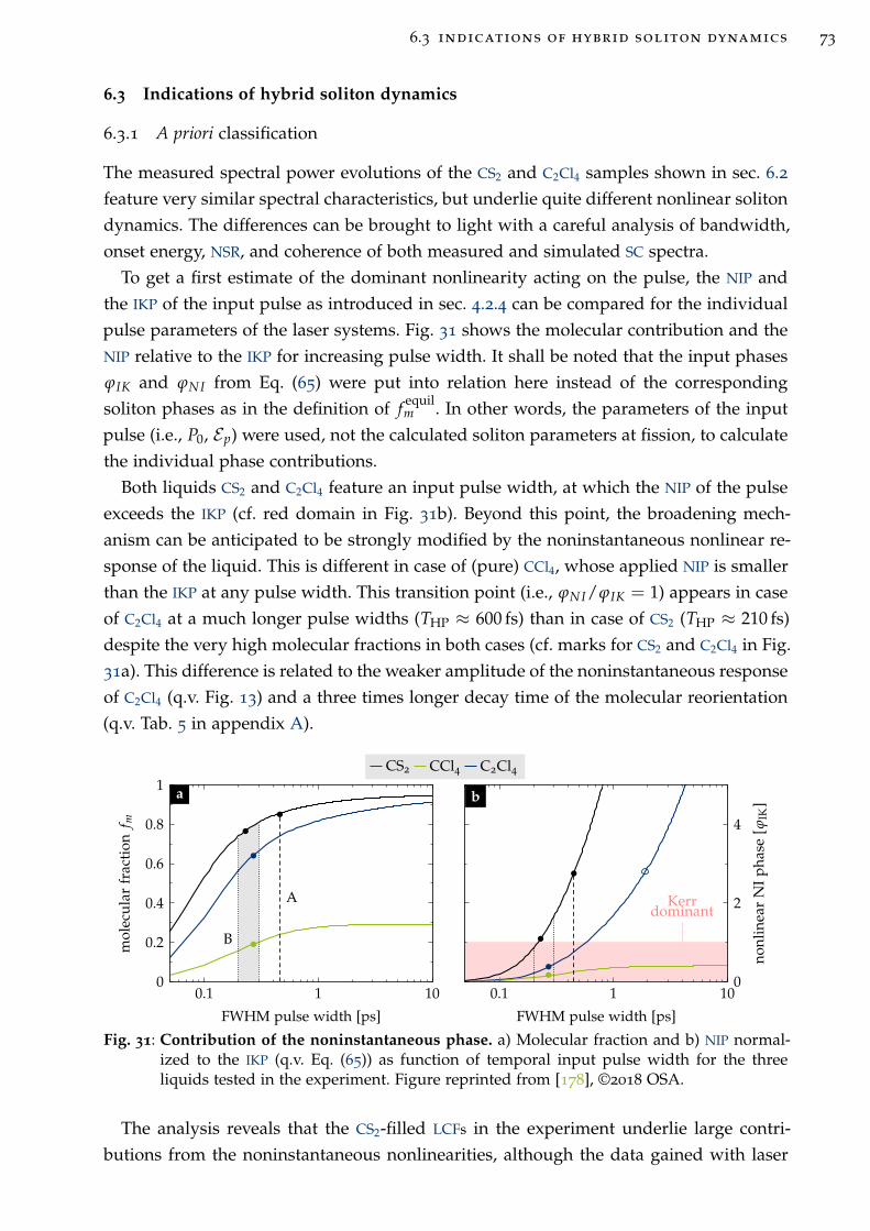
6.3 indications of hybrid soliton dynamics 73
6.3 Indications of hybrid soliton dynamics
6.3.1 A priori classification
The measured spectral power evolutions of the CS2 and C2Cl4 samples shown in sec. 6.2
feature very similar spectral characteristics, but underlie quite different nonlinear soliton
dynamics. The differences can be brought to light with a careful analysis of bandwidth,
onset energy, NSR, and coherence of both measured and simulated SC spectra.
To get a first estimate of the dominant nonlinearity acting on the pulse, the NIP and
the IKP of the input pulse as introduced in sec. 4.2.4 can be compared for the individual
pulse parameters of the laser systems. Fig. 31 shows the molecular contribution and the
NIP relative to the IKP for increasing pulse width. It shall be noted that the input phases
ϕIK and ϕNI from Eq. (65) were put into relation here instead of the corresponding
soliton phases as in the definition of fequilm . In other words, the parameters of the input
pulse (i.e., P0, Ep) were used, not the calculated soliton parameters at fission, to calculate
the individual phase contributions.
Both liquids CS2 and C2Cl4 feature an input pulse width, at which the NIP of the pulse
exceeds the IKP (cf. red domain in Fig. 31b). Beyond this point, the broadening mech-
anism can be anticipated to be strongly modified by the noninstantaneous nonlinear re-
sponse of the liquid. This is different in case of (pure) CCl4, whose applied NIP is smaller
than the IKP at any pulse width. This transition point (i.e., ϕNI/ϕIK = 1) appears in case
of C2Cl4 at a much longer pulse widths (THP ≈ 600 fs) than in case of CS2 (THP ≈ 210 fs)
despite the very high molecular fractions in both cases (cf. marks for CS2 and C2Cl4 in Fig.
31a). This difference is related to the weaker amplitude of the noninstantaneous response
of C2Cl4 (q.v. Fig. 13) and a three times longer decay time of the molecular reorientation
(q.v. Tab. 5 in appendix A).
B
A
0.1 1 100
0.2
0.4
0.6
0.8
1
FWHM pulse width [ps]
mol
ecu
lar
frac
tion
f m
CS2 CCl4 C2Cl4
Kerrdominant
0.1 1 100
2
4
FWHM pulse width [ps]
nonl
inea
rN
Ip
hase
[ϕIK
]
a b
Fig. 31: Contribution of the noninstantaneous phase. a) Molecular fraction and b) NIP normal-ized to the IKP (q.v. Eq. (65)) as function of temporal input pulse width for the threeliquids tested in the experiment. Figure reprinted from [178], ©2018 OSA.
The analysis reveals that the CS2-filled LCFs in the experiment underlie large contri-
butions from the noninstantaneous nonlinearities, although the data gained with laser
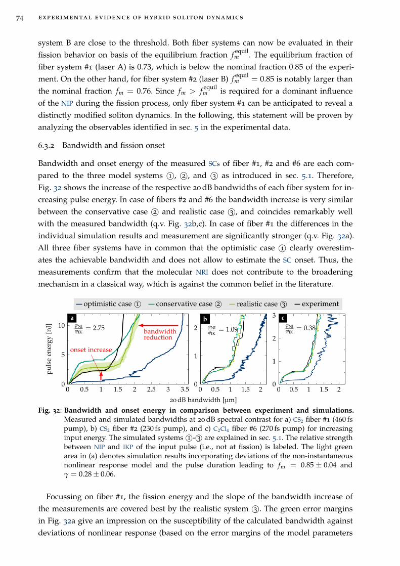
74 experimental evidence of hybrid soliton dynamics
system B are close to the threshold. Both fiber systems can now be evaluated in their
fission behavior on basis of the equilibrium fraction fequilm . The equilibrium fraction of
fiber system #1 (laser A) is 0.73, which is below the nominal fraction 0.85 of the experi-
ment. On the other hand, for fiber system #2 (laser B) fequilm = 0.85 is notably larger than
the nominal fraction fm = 0.76. Since fm > fequilm is required for a dominant influence
of the NIP during the fission process, only fiber system #1 can be anticipated to reveal a
distinctly modified soliton dynamics. In the following, this statement will be proven by
analyzing the observables identified in sec. 5 in the experimental data.
6.3.2 Bandwidth and fission onset
Bandwidth and onset energy of the measured SCs of fiber #1, #2 and #6 are each com-
pared to the three model systems 1©, 2©, and 3© as introduced in sec. 5.1. Therefore,
Fig. 32 shows the increase of the respective 20 dB bandwidths of each fiber system for in-
creasing pulse energy. In case of fibers #2 and #6 the bandwidth increase is very similar
between the conservative case 2© and realistic case 3©, and coincides remarkably well
with the measured bandwidth (q.v. Fig. 32b,c). In case of fiber #1 the differences in the
individual simulation results and measurement are significantly stronger (q.v. Fig. 32a).
All three fiber systems have in common that the optimistic case 1© clearly overestim-
ates the achievable bandwidth and does not allow to estimate the SC onset. Thus, the
measurements confirm that the molecular NRI does not contribute to the broadening
mechanism in a classical way, which is against the common belief in the literature.
onset increase
bandwidthreduction
0 0.5 1 1.5 2 2.5 3 3.50
5
10
20 dB bandwidth [µm]
pu
lse
ener
gy[n
J]
optimistic case 1© conservative case 2© realistic case 3© experiment
0 0.5 1 1.5 20
1
2
0 0.5 1 1.5 20
1
2
3aϕNIϕIK
= 2.75b
ϕNIϕIK
= 1.09
cϕNIϕIK
= 0.38
Fig. 32: Bandwidth and onset energy in comparison between experiment and simulations.Measured and simulated bandwidths at 20 dB spectral contrast for a) CS2 fiber #1 (460 fspump), b) CS2 fiber #2 (230 fs pump), and c) C2Cl4 fiber #6 (270 fs pump) for increasinginput energy. The simulated systems 1©- 3© are explained in sec. 5.1. The relative strengthbetween NIP and IKP of the input pulse (i.e., not at fission) is labeled. The light greenarea in (a) denotes simulation results incorporating deviations of the non-instantaneousnonlinear response model and the pulse duration leading to fm = 0.85 ± 0.04 andγ = 0.28 ± 0.06.
Focussing on fiber #1, the fission energy and the slope of the bandwidth increase of
the measurements are covered best by the realistic system 3©. The green error margins
in Fig. 32a give an impression on the susceptibility of the calculated bandwidth against
deviations of nonlinear response (based on the error margins of the model parameters
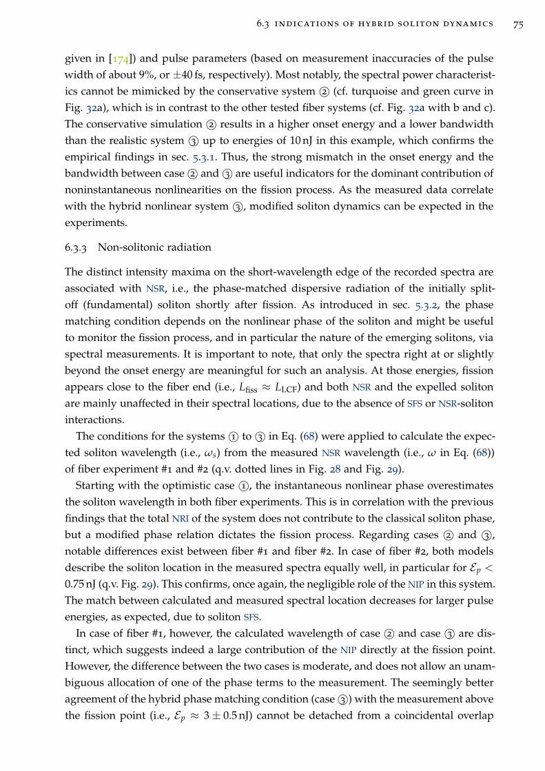
6.3 indications of hybrid soliton dynamics 75
given in [174]) and pulse parameters (based on measurement inaccuracies of the pulse
width of about 9%, or ±40 fs, respectively). Most notably, the spectral power characterist-
ics cannot be mimicked by the conservative system 2© (cf. turquoise and green curve in
Fig. 32a), which is in contrast to the other tested fiber systems (cf. Fig. 32a with b and c).
The conservative simulation 2© results in a higher onset energy and a lower bandwidth
than the realistic system 3© up to energies of 10 nJ in this example, which confirms the
empirical findings in sec. 5.3.1. Thus, the strong mismatch in the onset energy and the
bandwidth between case 2© and 3© are useful indicators for the dominant contribution of
noninstantaneous nonlinearities on the fission process. As the measured data correlate
with the hybrid nonlinear system 3©, modified soliton dynamics can be expected in the
experiments.
6.3.3 Non-solitonic radiation
The distinct intensity maxima on the short-wavelength edge of the recorded spectra are
associated with NSR, i.e., the phase-matched dispersive radiation of the initially split-
off (fundamental) soliton shortly after fission. As introduced in sec. 5.3.2, the phase
matching condition depends on the nonlinear phase of the soliton and might be useful
to monitor the fission process, and in particular the nature of the emerging solitons, via
spectral measurements. It is important to note, that only the spectra right at or slightly
beyond the onset energy are meaningful for such an analysis. At those energies, fission
appears close to the fiber end (i.e., Lfiss ≈ LLCF) and both NSR and the expelled soliton
are mainly unaffected in their spectral locations, due to the absence of SFS or NSR-soliton
interactions.
The conditions for the systems 1© to 3© in Eq. (68) were applied to calculate the expec-
ted soliton wavelength (i.e., ωs) from the measured NSR wavelength (i.e., ω in Eq. (68))
of fiber experiment #1 and #2 (q.v. dotted lines in Fig. 28 and Fig. 29).
Starting with the optimistic case 1©, the instantaneous nonlinear phase overestimates
the soliton wavelength in both fiber experiments. This is in correlation with the previous
findings that the total NRI of the system does not contribute to the classical soliton phase,
but a modified phase relation dictates the fission process. Regarding cases 2© and 3©,
notable differences exist between fiber #1 and fiber #2. In case of fiber #2, both models
describe the soliton location in the measured spectra equally well, in particular for Ep <
0.75 nJ (q.v. Fig. 29). This confirms, once again, the negligible role of the NIP in this system.
The match between calculated and measured spectral location decreases for larger pulse
energies, as expected, due to soliton SFS.
In case of fiber #1, however, the calculated wavelength of case 2© and case 3© are dis-
tinct, which suggests indeed a large contribution of the NIP directly at the fission point.
However, the difference between the two cases is moderate, and does not allow an unam-
biguous allocation of one of the phase terms to the measurement. The seemingly better
agreement of the hybrid phase matching condition (case 3©) with the measurement above
the fission point (i.e., Ep ≈ 3 ± 0.5 nJ) cannot be detached from a coincidental overlap
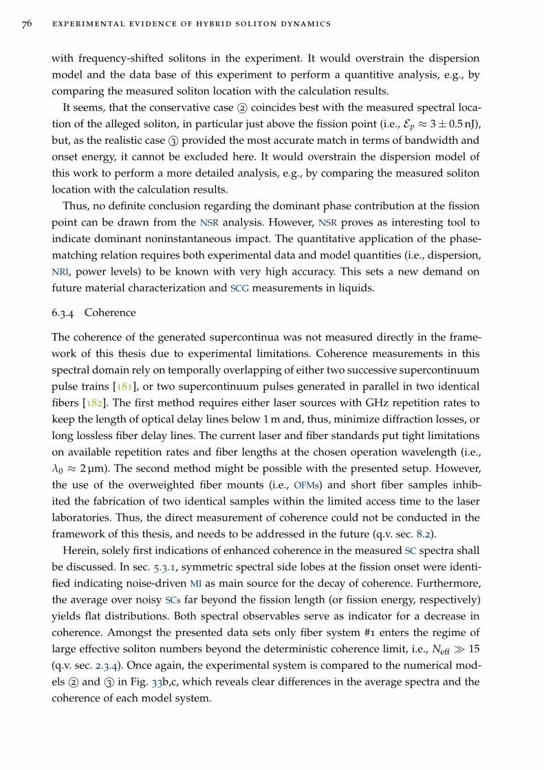
76 experimental evidence of hybrid soliton dynamics
with frequency-shifted solitons in the experiment. It would overstrain the dispersion
model and the data base of this experiment to perform a quantitive analysis, e.g., by
comparing the measured soliton location with the calculation results.
It seems, that the conservative case 2© coincides best with the measured spectral loca-
tion of the alleged soliton, in particular just above the fission point (i.e., Ep ≈ 3 ± 0.5 nJ),
but, as the realistic case 3© provided the most accurate match in terms of bandwidth and
onset energy, it cannot be excluded here. It would overstrain the dispersion model of
this work to perform a more detailed analysis, e.g., by comparing the measured soliton
location with the calculation results.
Thus, no definite conclusion regarding the dominant phase contribution at the fission
point can be drawn from the NSR analysis. However, NSR proves as interesting tool to
indicate dominant noninstantaneous impact. The quantitative application of the phase-
matching relation requires both experimental data and model quantities (i.e., dispersion,
NRI, power levels) to be known with very high accuracy. This sets a new demand on
future material characterization and SCG measurements in liquids.
6.3.4 Coherence
The coherence of the generated supercontinua was not measured directly in the frame-
work of this thesis due to experimental limitations. Coherence measurements in this
spectral domain rely on temporally overlapping of either two successive supercontinuum
pulse trains [181], or two supercontinuum pulses generated in parallel in two identical
fibers [182]. The first method requires either laser sources with GHz repetition rates to
keep the length of optical delay lines below 1 m and, thus, minimize diffraction losses, or
long lossless fiber delay lines. The current laser and fiber standards put tight limitations
on available repetition rates and fiber lengths at the chosen operation wavelength (i.e.,
λ0 ≈ 2 µm). The second method might be possible with the presented setup. However,
the use of the overweighted fiber mounts (i.e., OFMs) and short fiber samples inhib-
ited the fabrication of two identical samples within the limited access time to the laser
laboratories. Thus, the direct measurement of coherence could not be conducted in the
framework of this thesis, and needs to be addressed in the future (q.v. sec. 8.2).
Herein, solely first indications of enhanced coherence in the measured SC spectra shall
be discussed. In sec. 5.3.1, symmetric spectral side lobes at the fission onset were identi-
fied indicating noise-driven MI as main source for the decay of coherence. Furthermore,
the average over noisy SCs far beyond the fission length (or fission energy, respectively)
yields flat distributions. Both spectral observables serve as indicator for a decrease in
coherence. Amongst the presented data sets only fiber system #1 enters the regime of
large effective soliton numbers beyond the deterministic coherence limit, i.e., Neff ≫ 15
(q.v. sec. 2.3.4). Once again, the experimental system is compared to the numerical mod-
els 2© and 3© in Fig. 33b,c, which reveals clear differences in the average spectra and the
coherence of each model system.
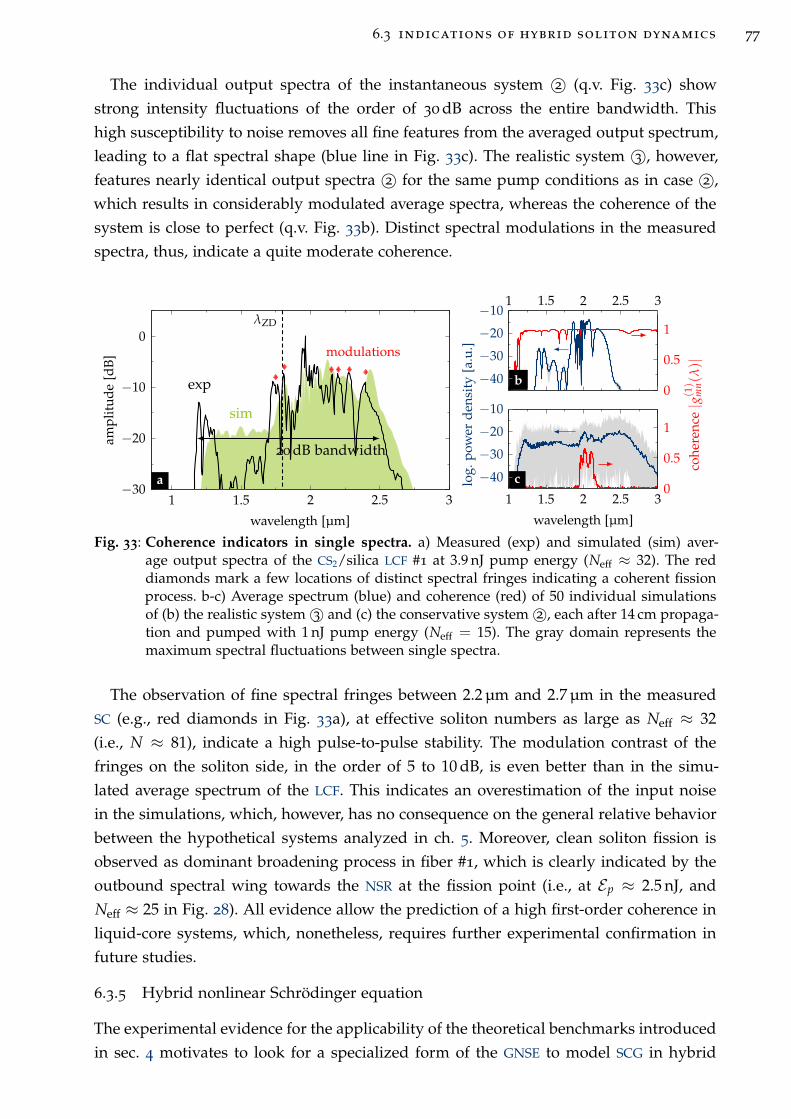
6.3 indications of hybrid soliton dynamics 77
The individual output spectra of the instantaneous system 2© (q.v. Fig. 33c) show
strong intensity fluctuations of the order of 30 dB across the entire bandwidth. This
high susceptibility to noise removes all fine features from the averaged output spectrum,
leading to a flat spectral shape (blue line in Fig. 33c). The realistic system 3©, however,
features nearly identical output spectra 2© for the same pump conditions as in case 2©,
which results in considerably modulated average spectra, whereas the coherence of the
system is close to perfect (q.v. Fig. 33b). Distinct spectral modulations in the measured
spectra, thus, indicate a quite moderate coherence.
λZD
exp
sim
modulations
20 dB bandwidth
1 1.5 2 2.5 3−30
−20
−10
0
wavelength [µm]
amp
litu
de
[dB
]
1 1.5 2 2.5 3
−40
−30
−20
−10
log.
pow
erd
ensi
ty[a
.u.]
0
0.5
1
cohe
renc
e|g
(1)
mn(λ
)|
−40
−30
−20
−10
1 1.5 2 2.5 30
0.5
1
wavelength [µm]
a
b
c
Fig. 33: Coherence indicators in single spectra. a) Measured (exp) and simulated (sim) aver-age output spectra of the CS2/silica LCF #1 at 3.9 nJ pump energy (Neff ≈ 32). The reddiamonds mark a few locations of distinct spectral fringes indicating a coherent fissionprocess. b-c) Average spectrum (blue) and coherence (red) of 50 individual simulationsof (b) the realistic system 3© and (c) the conservative system 2©, each after 14 cm propaga-tion and pumped with 1 nJ pump energy (Neff = 15). The gray domain represents themaximum spectral fluctuations between single spectra.
The observation of fine spectral fringes between 2.2 µm and 2.7 µm in the measured
SC (e.g., red diamonds in Fig. 33a), at effective soliton numbers as large as Neff ≈ 32
(i.e., N ≈ 81), indicate a high pulse-to-pulse stability. The modulation contrast of the
fringes on the soliton side, in the order of 5 to 10 dB, is even better than in the simu-
lated average spectrum of the LCF. This indicates an overestimation of the input noise
in the simulations, which, however, has no consequence on the general relative behavior
between the hypothetical systems analyzed in ch. 5. Moreover, clean soliton fission is
observed as dominant broadening process in fiber #1, which is clearly indicated by the
outbound spectral wing towards the NSR at the fission point (i.e., at Ep ≈ 2.5 nJ, and
Neff ≈ 25 in Fig. 28). All evidence allow the prediction of a high first-order coherence in
liquid-core systems, which, nonetheless, requires further experimental confirmation in
future studies.
6.3.5 Hybrid nonlinear Schrödinger equation
The experimental evidence for the applicability of the theoretical benchmarks introduced
in sec. 4 motivates to look for a specialized form of the GNSE to model SCG in hybrid
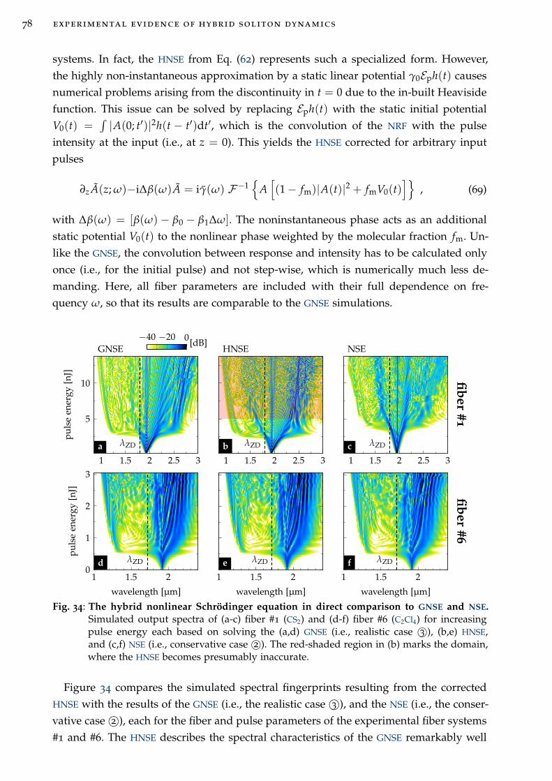
78 experimental evidence of hybrid soliton dynamics
systems. In fact, the HNSE from Eq. (62) represents such a specialized form. However,
the highly non-instantaneous approximation by a static linear potential γ0Eph(t) causes
numerical problems arising from the discontinuity in t = 0 due to the in-built Heaviside
function. This issue can be solved by replacing Eph(t) with the static initial potential
V0(t) =∫|A(0; t′)|2h(t − t′)dt′, which is the convolution of the NRF with the pulse
intensity at the input (i.e., at z = 0). This yields the HNSE corrected for arbitrary input
pulses
∂z A(z; ω)−i∆β(ω)A = iγ(ω) F−1
A[
(1 − fm)|A(t)|2 + fmV0(t)]
, (69)
with ∆β(ω) = [β(ω) − β0 − β1∆ω]. The noninstantaneous phase acts as an additional
static potential V0(t) to the nonlinear phase weighted by the molecular fraction fm. Un-
like the GNSE, the convolution between response and intensity has to be calculated only
once (i.e., for the initial pulse) and not step-wise, which is numerically much less de-
manding. Here, all fiber parameters are included with their full dependence on fre-
quency ω, so that its results are comparable to the GNSE simulations.
λZD
1 1.5 20
1
2
3
wavelength [µm]
pu
lse
ener
gy[n
J]
λZD
1 1.5 2
wavelength [µm]
λZD
1 1.5 2
wavelength [µm]
λZD
1 1.5 2 2.5 3
5
10
pu
lse
ener
gy[n
J]
−40 −20 0[dB]
λZD
1 1.5 2 2.5 3
λZD
1 1.5 2 2.5 3
GNSE HNSE NSE
fib
er#
6fi
ber
#1
d e f
a b c
Fig. 34: The hybrid nonlinear Schrödinger equation in direct comparison to GNSE and NSE.Simulated output spectra of (a-c) fiber #1 (CS2) and (d-f) fiber #6 (C2Cl4) for increasingpulse energy each based on solving the (a,d) GNSE (i.e., realistic case 3©), (b,e) HNSE,and (c,f) NSE (i.e., conservative case 2©). The red-shaded region in (b) marks the domain,where the HNSE becomes presumably inaccurate.
Figure 34 compares the simulated spectral fingerprints resulting from the corrected
HNSE with the results of the GNSE (i.e., the realistic case 3©), and the NSE (i.e., the conser-
vative case 2©), each for the fiber and pulse parameters of the experimental fiber systems
#1 and #6. The HNSE describes the spectral characteristics of the GNSE remarkably well
6.4 evaluation of significance of the indicators 79
in both fiber systems, especially around the supercontinuum onset (cf. spectra in Fig.
34a,b for Ep < 5 nJ, or spectra in Fig. 34d,e). In both systems, the fission point appears
at the same energy level, and bandwidth, and spectral features, like NSR, SPM, and the
supercontinuum onset behavior on the long wavelength side are very well captured.
For increasing input energies, however, there is an obvious change in the broaden-
ing behavior between the HNSE simulations of fiber #1 and #6. This mismatch can be
explained by cross-checking the results from the HNSE with the NSE (cf. spectra in Fig.
34b,c, or spectra in Fig. 34e,f). Whereas fiber system #6 is still well covered by the NSE, its
results for fiber system #1 differ strongly from the HNSE (and GNSE). Thus, the instantan-
eous phase term, which is the same in GNSE, NSE and HNSE, dominates the broadening
in the C2Cl4 fiber #6 making the new noninstantaneous term of the HNSE insignificant. In
the CS2 fiber #1 otherwise, the NIP has a non-negligible impact and the broadening beha-
vior cannot be described solely by the NSE (as found already in the bandwidth analysis
in sec. 6.3.2), but it is considerably well covered by the new specialized phase term of
the HNSE.
The HNSE from Eq. (69) starts to become inaccurate first for long fiber lengths (i.e.
L ≥ LD) and large soliton numbers (Neff > 40 in Fig. 34b), since strongly delayed wave
packets (e.g., NSR, or solitons) temporally shift out of the initial potential V0(t), whereby
the mismatch between fully convolved phase (i.e., GNSE) and approximated phase (i.e.,
HNSE) becomes inevitable.
Overall, due to the acceptable match between the new hybrid model and the general
(realistic) model at the fission point, the specialized HNSE promises to be a quick tool to
evaluate hybrid systems in close comparison to the NSE results. It also forms a strong
link to the HSW theory and might evolve to become a key tool to further understand
hybrid soliton dynamics in future studies.
6.4 Evaluation of significance of the indicators
In the presented methodology, the indicators are not entirely unambiguous without ac-
curate knowledge of the waveguide and pulse parameters. Especially onset energy and
bandwidth crucially depend on all kinds of loss, dispersion, nonlinearity, and the in-
dividual wavelength dispersion of those quantities (e.g., TOD, mode area dispersion).
These dependencies inherently underlie multiple experimental uncertainties such as in-
sufficient knowledge of material dispersion or the nonlinear response of the liquid. Oth-
erwise, phase matching of NSR and temporal coherence have few uncertainties since they
rely on a single system property only, such as modal dispersion in case of NSR, or the
nonlinear response in case of coherence.
In consequence, a convincing conclusion from the spectral analysis is possible only
if the results are analyzed for their vulnerability to model uncertainties. Such an error
analysis was performed in case of fiber #1, with regard to fiber dispersion, NRI, losses,
and pulse chirp (details can be found in appendix C).
80 experimental evidence of hybrid soliton dynamics
The impact of variations of all tested quantities on the SC spectra is moderate and,
most importantly, measurable. The strength of the presented data lies in the accurate
modeling of the close-to-perfect step-index LCF geometry chosen for the experiments. In
this context, the good match between our GNSE simulations and experiments, without
having applied any artificial model adaptions or data corrections, highlights the quality
of the experimental data, as well as the material models used in the simulations. Specific-
ally the experiment in CS2 with moderate noninstantaneous contribution (i.e., fiber #2)
confirms the applicability of the models for loss, dispersion and nonlinear parameter,
without relying significantly on the nonlinear response model, overall supporting the
plausibility of the revealed modified soliton dynamics in fiber #1.
Nonetheless, further studies are desirable to confirm or improve the current material
models. In particular, the nonlinear liquid response turns out to be the most vulnerable
parameter in the domain fm ≈ fequilm , and a confirmation of the NRF models would con-
solidate the significance of the presented findings. Also, material dispersion and losses of
highly transparent liquids, (e.g. CS2, CCl4, and C2Cl4) require more precise measurements
and models. However, the residual deviations between GNSE simulations and experiment
in fiber #1 (e.g. remaining bandwidth mismatch and the strong residual pump light) are
anticipated to originate from parasitic nonlinear processes, such as polarization rotation
or energy transfer to higher order modes. The involvement of those effects requires an
ingenious multimode treatment of the GNSE [82] in future work.
6.5 Theory of noninstantaneously dominated soliton fission
In conclusion, a single LCF system (i.e., fiber #1) was identified amongst all SCG experi-
ments to be severely influenced by the noninstantaneous nonlinearity of the core liquid.
The behavior of spectral benchmarks, such as bandwidth, onset energy, and spectral
features both on the NSR and the soliton side, correlate very well with the simulation res-
ults of the hybrid nonlinear system 3©, and confirm the spectral observables introduced
in ch. 5 as useful indicators for modified soliton dynamics. A simplified description of
this special experimental system, e.g., using the reduced instantaneous system 2©, is not
possible, which is in clear contrast to all other LCF systems investigated in the exper-
iment. Instead, the early fission process of the system could be reconstructed notably
well by a modified HNSE, which incorporated the NIP as static linear potential. Moreover,
a practical soliton-independent phase relation ϕNI/ϕIK was found to provide a straight-
forward and general tool to classify the initial conditions of a partly noninstantaneous
system, which is different to the phase estimate at the fission point given by fequilm .
The insights gained by the analysis of the four indicators allow to understand the
complicated interplay between IKP and NIP in each of the three stages of the fission
process in more detail:
nonlinear pulse compression The significantly lower onset energy in the experi-
ment, compared to the conservative case 2©, confirms the dominant impact of the
NIP to the nonlinear pulse compression (i.e., SPM stage). In particular, the distinct
6.5 theory of noninstantaneously dominated soliton fission 81
red-shift of the SPM spectrum leads to a shock-front formation, which boosts the
compression process and leads to an earlier fission point (i.e., lower onset energy).
The HNSE covers this process very well. Moreover, the dominant NIP leads to an
optical phase rectification, which reduces the impact of initial phase noise, and
promotes coherent soliton fission. The clean shear-off of NSR at fission and distinct
soliton features in the experimental spectra underpin this statement.
soliton fission In the maximally compressed state, just before soliton fission, the
molecular contribution is reduced due to the short pulse form, and the instantan-
eous phase impact becomes stronger. Nonetheless, the phase-matching analysis of
the NSR generation process revealed a non-negligible impact of the NIP at the fis-
sion point. This is again confirmed by the HNSE, which reconstructs the spectrum
at the fission point remarkably well, while assuming a constantly dominating NIP.
Prominent spectral fringes in the measured spectra up to soliton numbers as large
as Neff = 64 let assume a uniquely coherent fission dynamic throughout the entire
measurement of fiber #1 as a result of the all-time-present NIP. However, despite the
notable difference in the phase-matching conditions between both models 2© and3©, the data (as well as the current material models) do not allow an unambiguous
allocation of any of the two calculated soliton wavelengths to the experiment. Thus,
no irrevocable interpretation with regard to the original nature of the solitary wave
upon fission can be stated. Nevertheless, the NSR phase-matching relations from
Eq. (68) and the HNSE were successfully demonstrated as useful tools to expose the
fission dynamics in future work.
post-fission propagation After fission, the broadening process can still be mon-
itored by the bandwidth increase for increasing pulse energy. The measured band-
width increase is significantly reduced compared to the fast bandwidth increase of
the conservative electronic system 2©. Most notably, the bandwidth behavior in the
electronic system is not related to soliton SFS, but to the increasingly strong soliton
recoil effect. Those results might indicate a hindered soliton repulsion due to a
restoring force by the noninstantaneous nonlinear potential. This effect is intrins-
ically incorporated by the HNSE simulation, too, which reproduces the bandwidth
behavior around the SC onset. Despite the gained insights, the correlations do not
unambiguously confirm the emergence of HSW in the measurements, but give a
proper first support of this hypothesis.
7T U N I N G C A PA B I L I T I E S O F L I Q U I D - C O R E F I B E R S
7.1 Temperature tuning
Unraveling the complex soliton dynamics of LCFs might benefit from external control
over the soliton formation and radiation. In this chapter, the tuning capabilities of LCFs
will be investigated as further potential degree of freedom in terms of soliton control.
The phase matching condition of NSR in Eqs. (68) clearly suggests that any change of
dispersion has direct consequences on the wavelength of the generated NSR. Hence, a
straightforward tuning scheme providing external control over the soliton’s exhaust of
energy relies on changing the ambient temperature of the respective device. Within fiber
optics, however, the thermo-optical coefficients of most glasses and in particular that of
silica glasses are rather low (e.g., 8.6 × 10⁻⁶ K−1 for fused silica [183]) and the impact of
temperature on modal properties is limited. Liquid-filled fibers overcome this limit and
host a great potential for external control over both linear and nonlinear optical proper-
ties, based on their miscibility and strong thermodynamic effects. In particular the large
thermo-optical response of liquid-infiltrated fibers suggests strong impact on the optical
properties, which was utilized for temperature sensing [184, 185], wavelength detuning
of microfluidic lasers both on-chip [186, 187] and potentially in-fibre [55], spatial mode
coupling [188, 189], and nonlinear signal detuning [190]. Here, the impact of temperat-
ure, pressure (i.e., density), and liquid composition on SCG will be investigated in three
proof-of-concept experiments using CS2-core fibers. The fiber design and data analysis
successfully involves the thermodynamic Sellmeier model (q.v. Eq. (49)), derived in this
work, and the common mixing rule from Eq. (50). It will be shown, that NSR generation is
not only potentially suited to monitor modifications of the soliton fission process in LCFs,
but also that it paves the way for tunable selective wavelength sources as schematically
shown in Fig. 35a. The results of this chapter are partly published in [133].
7.1.1 Device principle and design
The temperature dependence of NSR is exemplarily shown for CS2 in Fig. 35b. For 40 K
temperature increase, the ZDW is shifted towards longer wavelengths causing a redshift
of the NSR by few hundreds of nanometers, given a frequency-stable soliton. The spectral
tuning domain of the NSR can widely be shifted without exceeding a realistic temperat-
ure range between 0 C (water condensation limit) and 46 C (boiling point of CS2) by
additionally shifting the initial soliton wavelength (q.v. inset of Fig. 35b). It is important
to note that the TOC of silica is about two orders of magnitude smaller than that of CS2
and is thus negligible for the experiments reported here.
The dispersion design map of step-index CS2-based LCFs in Fig. 35c reveals that the
strongest impact of temperature on ZDW and NSR can be found for core diameters
between 2.5 µm and 4 µm in a region omitted by other studies up to date and operate-
able in the ADD with thulium-doped fiber lasers. LCFs with core diameters larger than
82
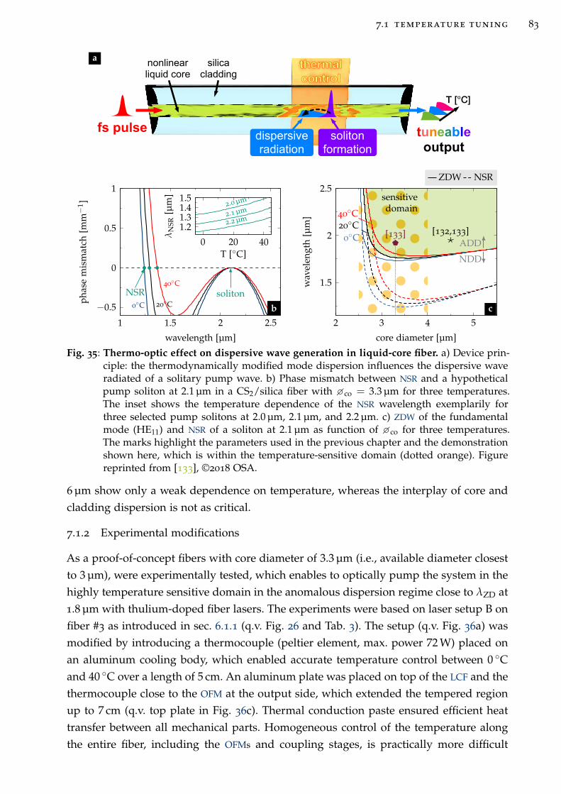
7.1 temperature tuning 83
0C 20C
40CNSR soliton
1 1.5 2 2.5
−0.5
0
0.5
1
wavelength [µm]
pha
sem
ism
atch
[mm
−1 ] 2.0 µm
2.1 µm
2.2 µm
0 20 40
1.21.31.41.5
T [C]
λN
SR[µ
m]
0C20C40C
NDD
ADD
sensitivedomain
[132,133][133]
2 3 4 5
1.5
2
2.5
core diameter [µm]
wav
elen
gth
[µm
]
ZDW NSR
fs pulse
thermalcontrol
silicacladding
nonlinearliquid core
solitonformation
dispersiveradiation
tuneableoutput
T [°C]
a
b c
Fig. 35: Thermo-optic effect on dispersive wave generation in liquid-core fiber. a) Device prin-ciple: the thermodynamically modified mode dispersion influences the dispersive waveradiated of a solitary pump wave. b) Phase mismatch between NSR and a hypotheticalpump soliton at 2.1 µm in a CS2/silica fiber with co = 3.3 µm for three temperatures.The inset shows the temperature dependence of the NSR wavelength exemplarily forthree selected pump solitons at 2.0 µm, 2.1 µm, and 2.2 µm. c) ZDW of the fundamentalmode (HE11) and NSR of a soliton at 2.1 µm as function of co for three temperatures.The marks highlight the parameters used in the previous chapter and the demonstrationshown here, which is within the temperature-sensitive domain (dotted orange). Figurereprinted from [133], ©2018 OSA.
6 µm show only a weak dependence on temperature, whereas the interplay of core and
cladding dispersion is not as critical.
7.1.2 Experimental modifications
As a proof-of-concept fibers with core diameter of 3.3 µm (i.e., available diameter closest
to 3 µm), were experimentally tested, which enables to optically pump the system in the
highly temperature sensitive domain in the anomalous dispersion regime close to λZD at
1.8 µm with thulium-doped fiber lasers. The experiments were based on laser setup B on
fiber #3 as introduced in sec. 6.1.1 (q.v. Fig. 26 and Tab. 3). The setup (q.v. Fig. 36a) was
modified by introducing a thermocouple (peltier element, max. power 72 W) placed on
an aluminum cooling body, which enabled accurate temperature control between 0 C
and 40 C over a length of 5 cm. An aluminum plate was placed on top of the LCF and the
thermocouple close to the OFM at the output side, which extended the tempered region
up to 7 cm (q.v. top plate in Fig. 36c). Thermal conduction paste ensured efficient heat
transfer between all mechanical parts. Homogeneous control of the temperature along
the entire fiber, including the OFMs and coupling stages, is practically more difficult
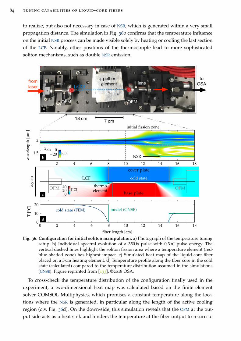
84 tuning capabilities of liquid-core fibers
to realize, but also not necessary in case of NSR, which is generated within a very small
propagation distance. The simulation in Fig. 36b confirms that the temperature influence
on the initial NSR process can be made visible solely by heating or cooling the last section
of the LCF. Notably, other positions of the thermocouple lead to more sophisticated
soliton mechanisms, such as double NSR emission.
lens lens
OFMOFM
LiCOF
peltier
element
7 cm 18 cm
from
laser
to
OSA
λZD
NSR
2 4 6 8 10 12 14 16 18
1.5
2
wav
elen
gth
[µm
]
−200
[dB]
initial fission zone
base plate
cover plate
OFMOFM thermoelement
LCF cold state
02040
[C]
2.5
cm
model (GNSE)cold state (FEM)
0 2 4 6 8 10 12 14 16 180
10
20
fiber length [cm]
T[
C]
a
b
c
d
Fig. 36: Configuration for initial soliton manipulation. a) Photograph of the temperature tuningsetup. b) Individual spectral evolution of a 350 fs pulse with 0.3 nJ pulse energy. Thevertical dashed lines highlight the soliton fission area where a temperature element (red-blue shaded zone) has highest impact. c) Simulated heat map of the liquid-core fiberplaced on a 5 cm heating element. d) Temperature profile along the fiber core in the coldstate (calculated) compared to the temperature distribution assumed in the simulations(GNSE). Figure reprinted from [133], ©2018 OSA.
To cross-check the temperature distribution of the configuration finally used in the
experiment, a two-dimensional heat map was calculated based on the finite element
solver COMSOL Multiphysics, which promises a constant temperature along the loca-
tions where the NSR is generated, in particular along the length of the active cooling
region (q.v. Fig. 36d). On the down-side, this simulation reveals that the OFM at the out-
put side acts as a heat sink and hinders the temperature at the fiber output to return to
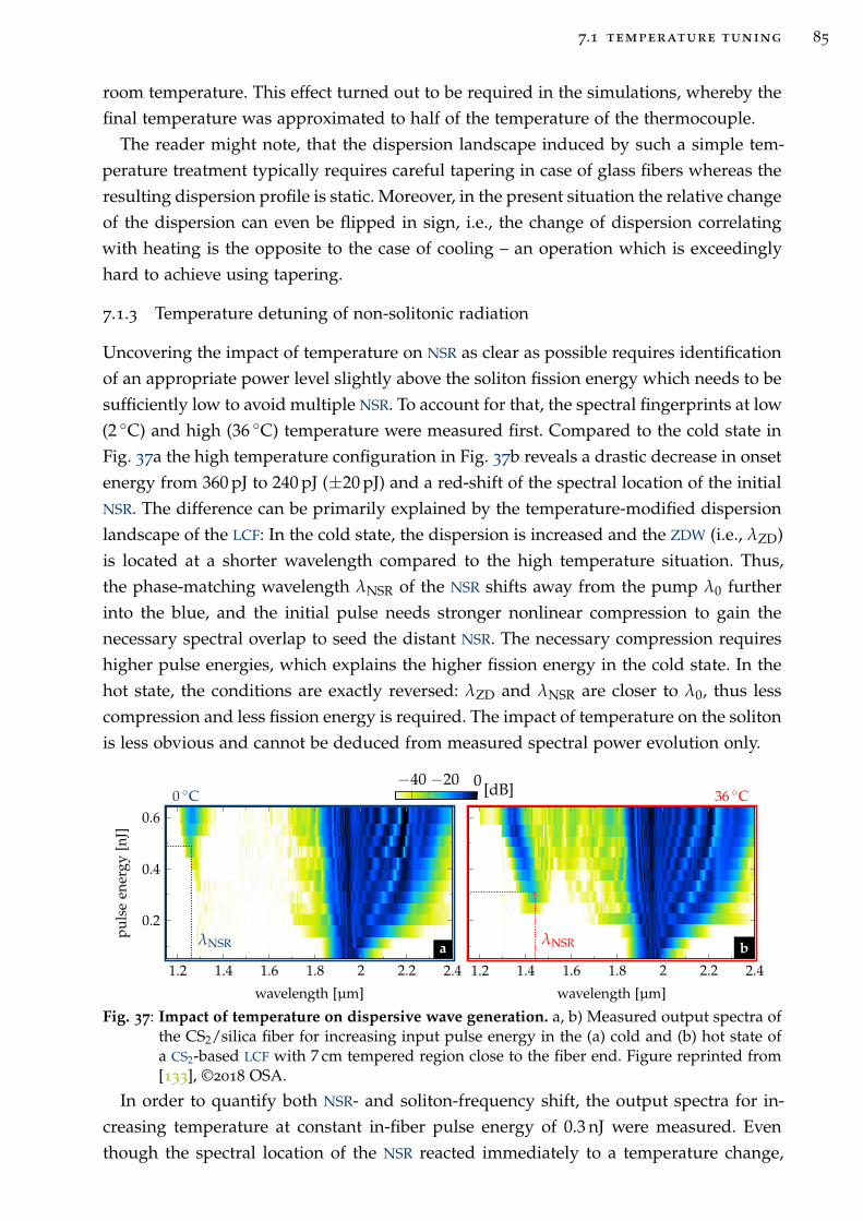
7.1 temperature tuning 85
room temperature. This effect turned out to be required in the simulations, whereby the
final temperature was approximated to half of the temperature of the thermocouple.
The reader might note, that the dispersion landscape induced by such a simple tem-
perature treatment typically requires careful tapering in case of glass fibers whereas the
resulting dispersion profile is static. Moreover, in the present situation the relative change
of the dispersion can even be flipped in sign, i.e., the change of dispersion correlating
with heating is the opposite to the case of cooling – an operation which is exceedingly
hard to achieve using tapering.
7.1.3 Temperature detuning of non-solitonic radiation
Uncovering the impact of temperature on NSR as clear as possible requires identification
of an appropriate power level slightly above the soliton fission energy which needs to be
sufficiently low to avoid multiple NSR. To account for that, the spectral fingerprints at low
(2 C) and high (36 C) temperature were measured first. Compared to the cold state in
Fig. 37a the high temperature configuration in Fig. 37b reveals a drastic decrease in onset
energy from 360 pJ to 240 pJ (±20 pJ) and a red-shift of the spectral location of the initial
NSR. The difference can be primarily explained by the temperature-modified dispersion
landscape of the LCF: In the cold state, the dispersion is increased and the ZDW (i.e., λZD)
is located at a shorter wavelength compared to the high temperature situation. Thus,
the phase-matching wavelength λNSR of the NSR shifts away from the pump λ0 further
into the blue, and the initial pulse needs stronger nonlinear compression to gain the
necessary spectral overlap to seed the distant NSR. The necessary compression requires
higher pulse energies, which explains the higher fission energy in the cold state. In the
hot state, the conditions are exactly reversed: λZD and λNSR are closer to λ0, thus less
compression and less fission energy is required. The impact of temperature on the soliton
is less obvious and cannot be deduced from measured spectral power evolution only.
λNSR
1.2 1.4 1.6 1.8 2 2.2 2.4
0.2
0.4
0.6
wavelength [µm]
pu
lse
ener
gy[n
J]
−40 −20 0 [dB]
λNSR
1.2 1.4 1.6 1.8 2 2.2 2.4
wavelength [µm]
0 C 36 C
a b
Fig. 37: Impact of temperature on dispersive wave generation. a, b) Measured output spectra ofthe CS2/silica fiber for increasing input pulse energy in the (a) cold and (b) hot state ofa CS2-based LCF with 7 cm tempered region close to the fiber end. Figure reprinted from[133], ©2018 OSA.
In order to quantify both NSR- and soliton-frequency shift, the output spectra for in-
creasing temperature at constant in-fiber pulse energy of 0.3 nJ were measured. Even
though the spectral location of the NSR reacted immediately to a temperature change,
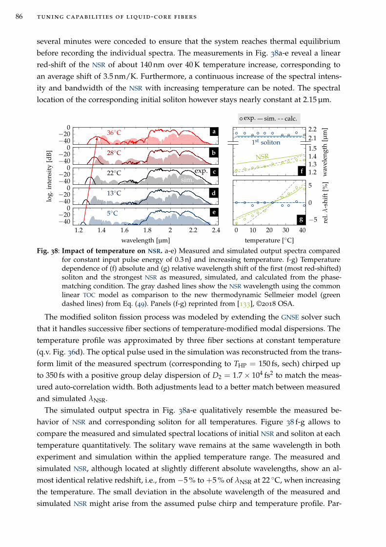
86 tuning capabilities of liquid-core fibers
several minutes were conceded to ensure that the system reaches thermal equilibrium
before recording the individual spectra. The measurements in Fig. 38a-e reveal a linear
red-shift of the NSR of about 140 nm over 40 K temperature increase, corresponding to
an average shift of 3.5 nm/K. Furthermore, a continuous increase of the spectral intens-
ity and bandwidth of the NSR with increasing temperature can be noted. The spectral
location of the corresponding initial soliton however stays nearly constant at 2.15 µm.
22C exp.sim.−40
−200
log.
inte
nsit
y[d
B] 28C
−40−20
0
36C−40−20
0
13C−40−20
0
5C
1.2 1.4 1.6 1.8 2 2.2 2.4−40−20
0
wavelength [µm]
0 10 20 30 40
−5
0
5
temperature [C]
rel.
λ-s
hift
[%]
exp. sim. calc.
1st soliton2.12.2
NSR
1.21.31.41.5
wav
elen
gth
[µm
]
f
g
a
b
c
d
e
Fig. 38: Impact of temperature on NSR. a-e) Measured and simulated output spectra comparedfor constant input pulse energy of 0.3 nJ and increasing temperature. f-g) Temperaturedependence of (f) absolute and (g) relative wavelength shift of the first (most red-shifted)soliton and the strongest NSR as measured, simulated, and calculated from the phase-matching condition. The gray dashed lines show the NSR wavelength using the commonlinear TOC model as comparison to the new thermodynamic Sellmeier model (greendashed lines) from Eq. (49). Panels (f-g) reprinted from [133], ©2018 OSA.
The modified soliton fission process was modeled by extending the GNSE solver such
that it handles successive fiber sections of temperature-modified modal dispersions. The
temperature profile was approximated by three fiber sections at constant temperature
(q.v. Fig. 36d). The optical pulse used in the simulation was reconstructed from the trans-
form limit of the measured spectrum (corresponding to THP = 150 fs, sech) chirped up
to 350 fs with a positive group delay dispersion of D2 = 1.7 × 10⁴ fs2 to match the meas-
ured auto-correlation width. Both adjustments lead to a better match between measured
and simulated λNSR.
The simulated output spectra in Fig. 38a-e qualitatively resemble the measured be-
havior of NSR and corresponding soliton for all temperatures. Figure 38 f-g allows to
compare the measured and simulated spectral locations of initial NSR and soliton at each
temperature quantitatively. The solitary wave remains at the same wavelength in both
experiment and simulation within the applied temperature range. The measured and
simulated NSR, although located at slightly different absolute wavelengths, show an al-
most identical relative redshift, i.e., from −5 % to +5 % of λNSR at 22 C, when increasing
the temperature. The small deviation in the absolute wavelength of the measured and
simulated NSR might arise from the assumed pulse chirp and temperature profile. Par-
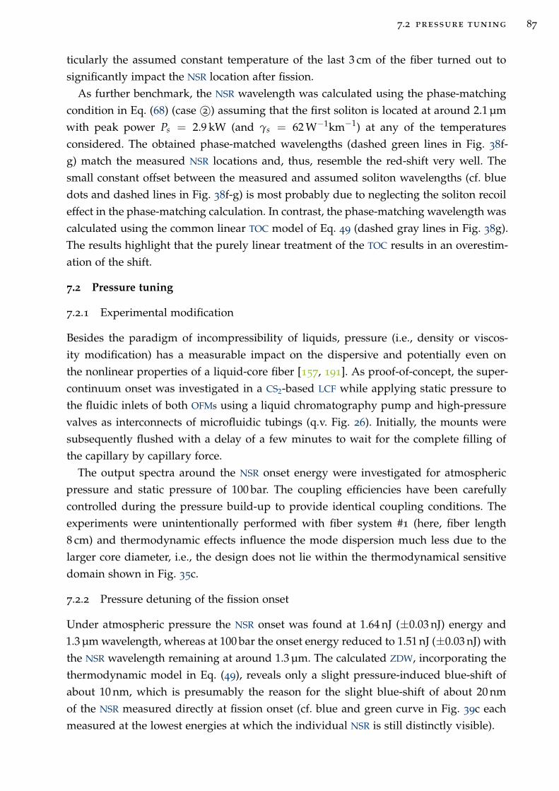
7.2 pressure tuning 87
ticularly the assumed constant temperature of the last 3 cm of the fiber turned out to
significantly impact the NSR location after fission.
As further benchmark, the NSR wavelength was calculated using the phase-matching
condition in Eq. (68) (case 2©) assuming that the first soliton is located at around 2.1 µm
with peak power Ps = 2.9 kW (and γs = 62 W−1km−1) at any of the temperatures
considered. The obtained phase-matched wavelengths (dashed green lines in Fig. 38f-
g) match the measured NSR locations and, thus, resemble the red-shift very well. The
small constant offset between the measured and assumed soliton wavelengths (cf. blue
dots and dashed lines in Fig. 38f-g) is most probably due to neglecting the soliton recoil
effect in the phase-matching calculation. In contrast, the phase-matching wavelength was
calculated using the common linear TOC model of Eq. 49 (dashed gray lines in Fig. 38g).
The results highlight that the purely linear treatment of the TOC results in an overestim-
ation of the shift.
7.2 Pressure tuning
7.2.1 Experimental modification
Besides the paradigm of incompressibility of liquids, pressure (i.e., density or viscos-
ity modification) has a measurable impact on the dispersive and potentially even on
the nonlinear properties of a liquid-core fiber [157, 191]. As proof-of-concept, the super-
continuum onset was investigated in a CS2-based LCF while applying static pressure to
the fluidic inlets of both OFMs using a liquid chromatography pump and high-pressure
valves as interconnects of microfluidic tubings (q.v. Fig. 26). Initially, the mounts were
subsequently flushed with a delay of a few minutes to wait for the complete filling of
the capillary by capillary force.
The output spectra around the NSR onset energy were investigated for atmospheric
pressure and static pressure of 100 bar. The coupling efficiencies have been carefully
controlled during the pressure build-up to provide identical coupling conditions. The
experiments were unintentionally performed with fiber system #1 (here, fiber length
8 cm) and thermodynamic effects influence the mode dispersion much less due to the
larger core diameter, i.e., the design does not lie within the thermodynamical sensitive
domain shown in Fig. 35c.
7.2.2 Pressure detuning of the fission onset
Under atmospheric pressure the NSR onset was found at 1.64 nJ (±0.03 nJ) energy and
1.3 µm wavelength, whereas at 100 bar the onset energy reduced to 1.51 nJ (±0.03 nJ) with
the NSR wavelength remaining at around 1.3 µm. The calculated ZDW, incorporating the
thermodynamic model in Eq. (49), reveals only a slight pressure-induced blue-shift of
about 10 nm, which is presumably the reason for the slight blue-shift of about 20 nm
of the NSR measured directly at fission onset (cf. blue and green curve in Fig. 39c each
measured at the lowest energies at which the individual NSR is still distinctly visible).
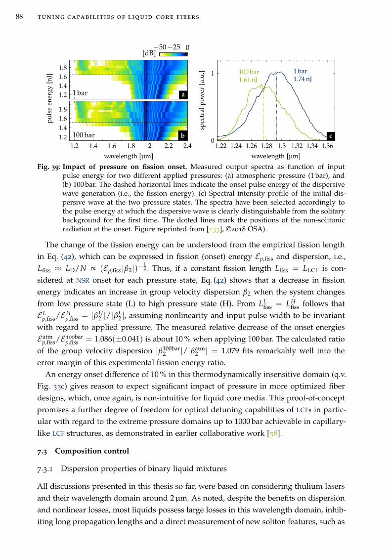
88 tuning capabilities of liquid-core fibers
1 bar1.21.41.61.8
pu
lse
ener
gy[n
J]−50−25 0
[dB]
100 bar1.2 1.4 1.6 1.8 2 2.2 2.4
1.21.41.61.8
wavelength [µm]
1 bar1.74 nJ
100 bar1.61 nJ
1.22 1.24 1.26 1.28 1.3 1.32 1.34 1.360
1
wavelength [µm]
spec
tral
pow
er[a
.u.]
a
b c
Fig. 39: Impact of pressure on fission onset. Measured output spectra as function of inputpulse energy for two different applied pressures: (a) atmospheric pressure (1 bar), and(b) 100 bar. The dashed horizontal lines indicate the onset pulse energy of the dispersivewave generation (i.e., the fission energy). (c) Spectral intensity profile of the initial dis-persive wave at the two pressure states. The spectra have been selected accordingly tothe pulse energy at which the dispersive wave is clearly distinguishable from the solitarybackground for the first time. The dotted lines mark the positions of the non-solitonicradiation at the onset. Figure reprinted from [133], ©2018 OSA).
The change of the fission energy can be understood from the empirical fission length
in Eq. (42), which can be expressed in fission (onset) energy Ep,fiss and dispersion, i.e.,
Lfiss ≈ LD/N ∝ (Ep,fiss|β2|)−12 . Thus, if a constant fission length Lfiss = LLCF is con-
sidered at NSR onset for each pressure state, Eq. (42) shows that a decrease in fission
energy indicates an increase in group velocity dispersion β2 when the system changes
from low pressure state (L) to high pressure state (H). From LLfiss = LH
fiss follows that
E Lp,fiss/EH
p,fiss = |βH2 |/|βL
2 |, assuming nonlinearity and input pulse width to be invariant
with regard to applied pressure. The measured relative decrease of the onset energies
Eatmp,fiss/E100bar
p,fiss = 1.086(±0.041) is about 10 % when applying 100 bar. The calculated ratio
of the group velocity dispersion |β100bar2 |/|βatm
2 | = 1.079 fits remarkably well into the
error margin of this experimental fission energy ratio.
An energy onset difference of 10 % in this thermodynamically insensitive domain (q.v.
Fig. 35c) gives reason to expect significant impact of pressure in more optimized fiber
designs, which, once again, is non-intuitive for liquid core media. This proof-of-concept
promises a further degree of freedom for optical detuning capabilities of LCFs in partic-
ular with regard to the extreme pressure domains up to 1000 bar achievable in capillary-
like LCF structures, as demonstrated in earlier collaborative work [58].
7.3 Composition control
7.3.1 Dispersion properties of binary liquid mixtures
All discussions presented in this thesis so far, were based on considering thulium lasers
and their wavelength domain around 2 µm. As noted, despite the benefits on dispersion
and nonlinear losses, most liquids possess large losses in this wavelength domain, inhib-
iting long propagation lengths and a direct measurement of new soliton features, such as
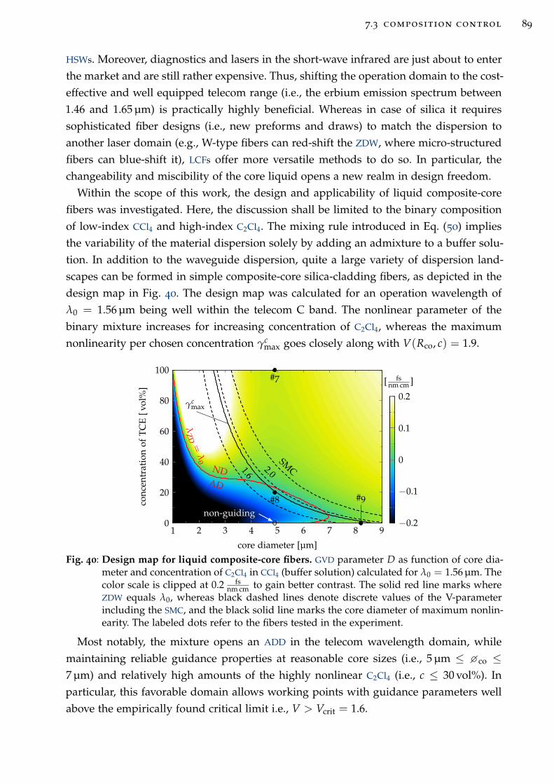
7.3 composition control 89
HSWs. Moreover, diagnostics and lasers in the short-wave infrared are just about to enter
the market and are still rather expensive. Thus, shifting the operation domain to the cost-
effective and well equipped telecom range (i.e., the erbium emission spectrum between
1.46 and 1.65 µm) is practically highly beneficial. Whereas in case of silica it requires
sophisticated fiber designs (i.e., new preforms and draws) to match the dispersion to
another laser domain (e.g., W-type fibers can red-shift the ZDW, where micro-structured
fibers can blue-shift it), LCFs offer more versatile methods to do so. In particular, the
changeability and miscibility of the core liquid opens a new realm in design freedom.
Within the scope of this work, the design and applicability of liquid composite-core
fibers was investigated. Here, the discussion shall be limited to the binary composition
of low-index CCl4 and high-index C2Cl4. The mixing rule introduced in Eq. (50) implies
the variability of the material dispersion solely by adding an admixture to a buffer solu-
tion. In addition to the waveguide dispersion, quite a large variety of dispersion land-
scapes can be formed in simple composite-core silica-cladding fibers, as depicted in the
design map in Fig. 40. The design map was calculated for an operation wavelength of
λ0 = 1.56 µm being well within the telecom C band. The nonlinear parameter of the
binary mixture increases for increasing concentration of C2Cl4, whereas the maximum
nonlinearity per chosen concentration γcmax goes closely along with V(Rco, c) = 1.9.
1.6
2.0
SMC
γcmax
λZ
D=
λ0
AD
ND
#7
#8 #9
non-guiding
1 2 3 4 5 6 7 8 90
20
40
60
80
100
core diameter [µm]
conc
entr
atio
nof
TC
E[v
ol%
]
−0.2
−0.1
0
0.1
0.2
[ fsnm cm ]
Fig. 40: Design map for liquid composite-core fibers. GVD parameter D as function of core dia-meter and concentration of C2Cl4 in CCl4 (buffer solution) calculated for λ0 = 1.56 µm. Thecolor scale is clipped at 0.2 fs
nm cm to gain better contrast. The solid red line marks whereZDW equals λ0, whereas black dashed lines denote discrete values of the V-parameterincluding the SMC, and the black solid line marks the core diameter of maximum nonlin-earity. The labeled dots refer to the fibers tested in the experiment.
Most notably, the mixture opens an ADD in the telecom wavelength domain, while
maintaining reliable guidance properties at reasonable core sizes (i.e., 5 µm ≤ co ≤7 µm) and relatively high amounts of the highly nonlinear C2Cl4 (i.e., c ≤ 30 vol%). In
particular, this favorable domain allows working points with guidance parameters well
above the empirically found critical limit i.e., V > Vcrit = 1.6.
90 tuning capabilities of liquid-core fibers
7.3.2 Soliton fission in liquid composite-core fibers
To confirm the applicability of the design map, four parameter sets were tested in the
experiment (q.v. Fig.40). A mixture with 20 vol% C2Cl4 in CCl4 (8 ml C2Cl4 in 40 ml CCl4,
i.e., 5 : 1 ratio) was used as core material for a capillary with co = 4.9 µm to get an
anomalous dispersive composite LCF (q.v. fiber #8 from Tab. 3). This fiber was opposed
to two normal dispersive LCFs with the same co but filled with neat CCl4 and C2Cl4 (q.v.
fiber #7 from Tab. 3). The neat CCl4 fiber, however, showed only 6 % transmission due
to a low mode confinement in the weak step-index guide, since V(λ0) = 1.068. Thus, a
larger core size close to maximum nonlinearity (q.v. γcmax curve in Fig. 40) at c = 0 vol%)
was chosen as nonlinear test system (q.v. fiber #9 from Tab. 3).
An off-the-shelf femtosecond laser with THP = 30 fs and λ0 = 1.56 µm (Toptica Femto-
Power Pro IRS) was used as pump source. The fiber coupling setup and output dia-
gnostics is as introduced in sec. 6.1.1, whereas an InGaAs camera (ABS Jena, IK1513)
was used to monitor the output mode in the C band.
λZD
1.2 1.4 1.6 1.8 2
0.1
0.2
0.3
pu
lse
ener
gy[n
J]
−20 0[dB]
ND AD
λZD
solitonNSR
1.2 1.4 1.6 1.8 2
0.2
0.4
0.6
FWM
1.2 1.4 1.6 1.8 2
0.2
0.4
0.6
0.8 ND AD
λZD
1.2 1.4 1.6 1.8 2
0.1
0.2
0.3
wavelength [µm]
pu
lse
ener
gy[n
J]
λZD
Neff = 2.5
1.2 1.4 1.6 1.8 2
0.2
0.4
0.6
wavelength [µm]
λZD
Neff = 2.5
1.2 1.4 1.6 1.8 2
0.2
0.4
0.6
0.8
wavelength [µm]
fiber #9 fiber #8 fiber #7
experim
entG
NSE
a b c
d e f
Fig. 41: Spectral fingerprint of fibers #9, #8 (composite LCF) and #7. (a-c) Measured and (d-f)calculated (GNSE) output spectrum for increasing pulse energy for three fibers with (a,d)8.2 µm neat CCl4 core (#9), (b, e) 4.9 µm C2Cl4:CCl4 composite core (#8), or (c,f) 4.9 µm neatC2Cl4 core (#7). FWM denotes four-wave mixing. The input pulse for the simulations isreconstructed from the measured laser spectrum and propagated through 5 mm silica toemulate the chirp of the coupling lens.
The spectral fingerprints in Fig. 41 are clearly distinguishable from each other. All
three systems are remarkably well described by the GNSE simulation, given the uncer-
tainties of the underlying nonlinear models, which allows to unambiguously explain the
respective broadening mechanism.
7.3 composition control 91
Starting with the CCl4-based LCF (#9), no spectral broadening is observed (q.v. Fig.
41a,d). The large mode area and the small nonlinearity of CCl4 result in a relatively
small nonlinear parameter (q.v. Tab. 8) and a nonlinear length approximately double the
dispersion length for the maximum pulse energy (i.e., LD = 3.5 cm < LNL = 7.5 cm).
Thus, the pulse propagation is dominated by temporal pulse broadening in the NDD.
Each of the two other fibers exhibits an individual feature-rich broadening process.
The composite LCF #8 shows the characteristic spectral features of a split-off soliton on
the red side and of NSR on the blue side of the spectrum, confirming operation in the
ADD accordingly to the calculated λZD in Fig. 41b. The neat C2Cl4-filled LCF #7 misses
any distinct spectral feature on the short wavelength side, but shows a much further
extent towards the infrared despite the lower maximum soliton number of the system
(cf. red labels in Fig. 41e,f). The broadening mechanism is an involved combination
of SPM, shock-front formation, and four-wave mixing close to the ZDW (i.e., similar to
domain 2 in sec. 5.3.4). Without going further into detail, it shall just be mentioned that
this mechanism may serve as alternative route to efficiently excite fundamental solitons,
as well as to generate highly coherent SC spectra while still operating in the NDD.
To conclude this chapter, the presented proof-of-principle experiments, and their good
match to simulations and calculations, prove the applicability of temperature, pressure,
and liquid composition for straightforward dispersion adjustment, simultaneously con-
firming the underlying material models and the nonlinear design maps. In particular, a
binary mixture of C2Cl4 and CCl4 straightforwardly infiltrated in a silica capillary opens
the ADD for the telecom laser branch. Similar and partly better results could be achieved
with deuterated toluene and deuterated nitrobenzene, each mixed in CCl4, in the master
thesis by Walther [192]. This additional dispersion control in LCFs might also be imple-
mented online via concentration- and flow-controlled micro-fluidic circuitry based on
commercial liquid-chromatography pumps and valves, similar to the equipment used in
sec. 7.2.2 to perform the high pressure experiments. Altogether, the dispersion landscape
of an optical soliton propagating in a LCF can be manipulated to a considerable extent,
which highlights this fiber type as promising dynamic platform for local and dynamic
fission control.
8D E D U C T I O N A N D V I S I O N
8.1 Conclusion
This work explored the potential of LCFs as platform for novel solitons dynamics and
tunable soliton fission. It combined (1) thorough material analysis and fiber design, (2)
with semi-analytical and numerical theoretical studies on novel hybrid solitary waves
(HSW) and SCG in LCFs, as well as (3) with first experiments on SCG in the HSW regime
and external soliton control. The theoretical part consistently links the predictions by
Conti et al. [70] with the observations to the spectral features in simulated SCs in LCF
found by other groups [193], and puts them into a well rounded practical picture. The
experimental findings of this work allow the scientific community to catch a first glance
on the soliton dynamics in highly noninstantaneous liquid systems, and are in good
agreement to the newly elaborated theoretical expectations and benchmarks.
In detail, the new material dispersion dispersion models found in this work proved
valuable for accurate LCF design and thermodynamical control of liquid systems (the lat-
ter exclusively for CS2). In particular, high-index heavy organics, such as carbon chlorides
and CS2, were measured to possess formidable transmission and IOR properties for robust
light guidance from the VIS to the starting MIR (i.e., proof of hypothesis H1). As a res-
ult, unexplored ADDs have been identified in easily producible step-index silica-cladding
LCFs filled with CS2, CCl4, and C2Cl4 with user-friendly core sizes of about 4.5 µm. These
operation domains grant access to the soliton domain with state-of-the-art thulium fiber
lasers (i.e., proof of H2).
The experimental accessibility to the ADD justified a closer look into the special soliton
propagation characteristic of slowly responding nonlinear LCFs. In particular, the lin-
earon hypothesis, introduced by Conti et al. in 2010, was revised for the realistic nonlin-
ear response of liquids. Following a semi-analytical eigenmode approach, linearon states
were found in form of solutions of a quasi-linear Schrödinger equation. A numerical per-
turbation analysis, however, exposed the instability of these states over propagation due
to violation of the principles of causality in case of realistic nonlinear responses. In detail,
the linear states are localized in the minimum of the response potential, distant from the
anticipated location at the field-induced origin of the response. This mismatch causes
the pulse to adiabatically adapt to a solution of a steadily moving potential, while con-
tinuously distributing energy. The observation leads to the falsification of the hypothesis
(H3) that linearons may be found in highly noninstantaneous LCFs.
Nonetheless, the here-elaborated theory extended the governing model to a hybrid-
nonlinear Schrödinger equation (i.e., the HNSE), which combines the well-known in-
stantaneous NSE with the NISE by Conti et al.. The HNSE describes the nonlinear pulse
propagation in realistic liquid-core waveguides considerably well within a certain para-
meter regime. The individual nonlinear phase terms of the HNSE allowed to relate the
noninstantaneous phase (i.e., NIP or linearon phase) with the instantaneous Kerr phase
(i.e., IKP or soliton phase) and, thus, to identify a critical molecular fraction fequilm , at
92
8.1 conclusion 93
which the NIP equals the IKP. Above this fraction, the pulse propagation in the ADD
significantly alters from classical soliton propagation. Most remarkably, under certain
conditions, which were found only empirically in this work, the altered solitary wave
(i.e., HSW) features a flat phase, indicating true solitary character. Thus, Conti’s hypo-
thesis (H3) may be extended to the existence of hybrid soliton states (HSS) in realistic
liquid-core media. Those states promise access to so-far unexplored nonlinear regimes
being potentially usable for laser engineering, nonlinear light steering, and emulation of
unaccessible systems e.g. in physics, math or biochemistry.
The identified experimental regime inhibits the direct observation of fundamental HSW
propagation, since the losses at the thulium laser wavelength limit the maximum fiber
length to sub-meter lengths, which is below the dispersion length of the required pulses.
Hence, this work followed the approach to identify indications of emerging HSW in the
spectra resulting from a complex soliton fission process along few ten centimeters of
fiber (i.e., SCG). Large parameter studies of SCG in CS2-core fibers, based on a general-
ized model (GNSE), revealed NIP-dominant parameter domains featuring unique spectral
properties of the SCs in comparison to glass-type systems with same electronic nonlin-
earity. The iterative study is fully consistent with the theoretically found condition for
dominating NIP (i.e., fm > fequilm ) and identified the spectro-temporal signatures of HSWs
in the simulated output spectra of lossless LCF systems. The imposed changes on the SC
spectra for increasing molecular fraction fm can therefore be attributed to the emergence
of HSWs (i.e., proof of H4). The impact of the NIP becomes apparent in bandwidth and
onset energy of the SC, both in agreement with the empirical findings by Pricking et al.
[193], but also in the spectral location of the NSR, and the coherence. These numeric-
ally found observables correlate with the experimental observations (i.e., proof of H6),
and strengthen the hypothesis of emerging HSWs at some point during SCG (H5). Nev-
ertheless, the coherence properties of the SC spectra could only be assessed qualitatively
by interpreting distinct spectral features, which do not occur in incoherent broadening
schemes, and additional experiments are necessary to further support the findings.
In particular, the observations in the simulations justified the formulation of two
soliton fission theories, which differ in the question whether HSWs are created directly at
the fission point or shortly after via an adiabatic transformation of classical solitons into
a hybrid state. This question might be answered by measuring the phase of the solitary
unit created at the fission point. The spectral location of the NSR together with the hybrid
nonlinear phase matching condition found in this work provides the ideal tool to access
this phase information. However, despite the considerable difference between hybrid sol-
itary phase and conventional solitary phase, the distinction is not large enough in the
presented systems to definitely assign one of two solitary states with the measurement.
Dispersion tailored micro-structured LCFs may be able to increase the phase difference
and provide an answer on the nature of the soliton at the fission point. Yet, none of the
both theories can be disproved in this work, but, although the central question of the
94 deduction and vision
origin of HSWs within the fission process (H5) remains open, this study gives profound
evidence for their existence.
The external tuneability of the optical properties of the LCFs might become essential
to further investigate the origin of HSW, but also to study soliton propagation and dy-
namics in general. Temperature, pressure, and core composition were shown to notably
influence the mode dispersion in a LCF (i.e., proof of H7). The dispersion control allows
to accurately steer soliton fission processes, and particularly the frequency and strength
of the radiated NSR (i.e., proof of H8). The here-derived thermodynamical models for
CS2 proved quantitatively useful and allow valuable suggestions on bandwidth and co-
herence improvements of SCG, as shown in the outlook.
Altogether, the presented study contributes to the fundamental understanding of spec-
tral broadening in liquids and the underlying soliton dynamics. It comprehensively
demonstrates LCFs as dynamic platform for exploring new solitary states and soliton
interactions, as well as for broadband tuneable light generation. LCFs may offer a further
playground, next to gas-filled fibers, with many degrees of freedom, which will poten-
tially expand the possibilities of fiber-based emulation systems to study manifold effects
of other fields of physics and science. Some anticipated examples are discussed in the
following on conclusion of this thesis.
8.2 Future prospects
Light guides for the near- to mid-infrared
The advent of new laser sources for the MIR (e.g., quantum cascade lasers) demands
new fiber materials for lossless light transport in this technically important wavelength
domain. This work demonstrated halide liquids with a high transparency in the NIR to-
wards the MIR domain as potential alternative to soft-glasses. In particular, the use of
halide mixtures, may allow designing broadband single-mode fibers for the MIR do-
main. Preliminary design studies using a 10 mol% C2Cl4 in CCl4 mixture as core material
embedded in silica with co = 6 µm reveal a robust single-mode guidance domain (with
1.820 < V < 2.405) from 0.9 to 6.8 µm, i.e., well beyond the transmission limit of fused
silica. This result gives confidence for similar waveguide domains when incorporating
other cladding materials. Hence, to fully further explore the MIR potential of LCFs, new
MIR-friendly glasses (e.g., fluorides) might be investigated as cladding material.
Moreover, there are many halide and chalcogenide liquids with moderate toxicity
which are unexplored in terms of their promising transparency and nonlinearity. Few
examples are SiCl4, GeCl4, CBrCl3, CHCl3, ICl, IF5, C6F14, CSe2, or AsCl3. Accurate
measurements on the absorption and dispersion in the MIR of those liquids are required
to extend the material models and to make fiber designs possible in future.
Picosecond pulse compression
The superior reduction of the noise impact on nonlinear pulse propagation found in this
work might enable the pulse compression of multi-picosecond pulses. In particular C2Cl4
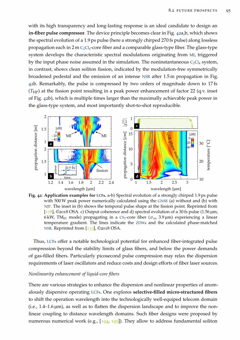
8.2 future prospects 95
with its high transparency and long-lasting response is an ideal candidate to design an
in-fiber pulse compressor. The device principle becomes clear in Fig. 42a,b, which shows
the spectral evolution of a 1.9 ps pulse (here a strongly chirped 270 fs pulse) along lossless
propagation each in 2 m C2Cl4-core fiber and a comparable glass-type fiber. The glass-type
system develops the characteristic spectral modulations originating from MI, triggered
by the input phase noise assumed in the simulation. The noninstantaneous C2Cl4 system,
in contrast, shows clean soliton fission, indicated by the modulation-free symmetrically
broadened pedestal and the emission of an intense NSR after 1.5 m propagation in Fig.
42b. Remarkably, the pulse is compressed by two orders of magnitude down to 17 fs
(THP) at the fission point resulting in a peak power enhancement of factor 22 (q.v. inset
of Fig. 42b), which is multiple times larger than the maximally achievable peak power in
the glass-type system, and most importantly shot-to-shot reproducible.
0
1|g
(1)
12|
1 1.5 2 2.5 30
5
10
15
wavelength [µm]
pro
pag
atio
nd
ista
nce
[cm
]
−40−20
0[dB]
λZD
NSR
phasem
atching
10
20
30
tem
per
atu
re[
C]
MIMI1
1.5
2
pro
pag
atio
nd
ista
nce
[m]
−40−20
0[dB]
fission
1.2 1.4 1.6 1.8 2 2.2 2.4
1
1.5
2
wavelength [µm]
17 fs
time
pow
er
a
b
c
d
Fig. 42: Application examples for LCFs. a-b) Spectral evolution of a strongly chirped 1.9 ps pulsewith 500 W peak power numerically calculated using the GNSE (a) without and (b) withNIP. The inset in (b) shows the temporal pulse shape at the fission point. Reprinted from[178], ©2018 OSA. c) Output coherence and d) spectral evolution of a 30 fs pulse (1.56 µm,6 kW, TM01 mode) propagating in a CS2-core fiber (co 3.9 µm) experiencing a lineartemperature gradient. The lines indicate the ZDWs and the calculated phase-matchedNSR. Reprinted from [133], ©2018 OSA.
Thus, LCFs offer a notable technological potential for enhanced fiber-integrated pulse
compression beyond the stability limits of glass fibers, and below the power demands
of gas-filled fibers. Particularly picosecond pulse compression may relax the dispersion
requirements of laser oscillators and reduce costs and design efforts of fiber laser sources.
Nonlinearity enhancement of liquid-core fibers
There are various strategies to enhance the dispersion and nonlinear properties of anom-
alously dispersive operating LCFs. One explores selective-filled micro-structured fibers
to shift the operation wavelength into the technologically well-equiped telecom domain
(i.e., 1.4–1.6 µm), as well as to flatten the dispersion landscape and to improve the non-
linear coupling to distance wavelength domains. Such fiber designs were proposed by
numerous numerical work (e.g., [194, 195]). They allow to address fundamental soliton
96 deduction and vision
propagation in a much more favorable regime in terms of dispersion and loss. Exciting
this regime with sub-picosecond pulses (favourably 400–600 fs) might enable the direct
observation of HSW, and prove (or falsify) the above-stated hypothesis of the existence
of HSS in liquid-core fibers.
Further, ionic salt solutions may be explored as core medium. The nonlinear coupling
to ions in a solution were shown to significantly alter the nonlinear behavior of the
buffer liquid with interesting consequences on SCG [196]. Also this approach requires
substantial material characterization to gain broadband dispersion and loss data, and an
estimate for the nonlinearity of the liquid media.
Beside the improvement of the NRI, the nonlinear response can be engineered using
liquid mixtures as core material. For instance, the combination of CCl4, CHCl3, and C2Cl4
(ordered by increasing response time) might allow the cancelation of the detrimental rise
time of the response and to mimic the conditions of the ideal exponential noninstantan-
eous system, in which Conti et al. predicted linearon states.
Techniques for enhancing supercontinuum generation
This work opened multiple promising approaches to explore the bandwidth capabilities
of LCFs as nonlinear light source. The large-scale parameter study in sec. 5.3.4 revealed
three operation domains which feature an improved bandwidth and coherence, com-
pared to glass fibers. All three domains are unique for highly noninstantaneous systems
and offer a plethora of research opportunities. In particular, the two unexplored domains
in the NDD may host novel nonlinear mechanisms to excite both fundamental solitary
states and soliton fission in the ADD across the ZDW. Future experimental and numerical
studies in those domains might expose this potential for SCG and oberving HSWs.
Much attention should be paid to the coherence of the output spectra. The simula-
tions predicted an increase of the coherence threshold in highly noninstantaneous LCFs.
Measuring the transition from incoherent to coherent SCG in a LCF and a comparable
instantaneous system would not only support the modified soliton theory elaborated
in this work, but also allow to identify the physical origins of the rich nonlinear noise
dynamics in high energy systems beyond the simple one-photon-per-mode noise model.
Moreover, the presented study gives a first glance of the great potential of thermody-
namic tuning of dispersion properties of LCF using straightforward accessible external
controls such as temperature or pressure. From the fundamental science perspective,
temperature tuning might become a key tool to dynamically change the fiber dispersion
along the propagation direction to directly observe and to control complex soliton dy-
namics to an extent that is only possible with in dispersion-oscillating micro-structured
glass fibers to date [204, 205]. To demonstrate the potential of thermodynamic tuning,
SCG in a CS2/silica step-index LCF was simulated for one mode (TM01) which features two
ZDWs embracing an interval of anomalous dispersion in the telecom L-band. Launching
femtosecond pump pulses with powers easily available from commercial erbium fiber
lasers (here: 30 fs, 6 kW, 1.56 µm) into this mode yields a spectrum featuring two pro-
8.2 future prospects 97
nounced NSR wavelengths (q.v. Fig. 42d). Via the application of an experimentally feas-
ible linear temperature gradient along the LCF, the ZDWs is continuously modified im-
plying a change of the NSR phase matching condition. The dispersion steadily increases
along the fiber, which enforces a continuous transfer of energy from the soliton trapped
in the ADD to the phase-matched NSR in the NDD. As a consequence, a broadband soliton-
based SC between 1 and 3 µm is obtained featuring high spectral flatness and exceptional
pulse-to-pulse coherence (q.v. Fig. 42c). Similar spectra could be produced in preliminary
experiments utilizing the described system design.
The example demonstrates that the soliton dynamic can be controlled locally in LCFs,
providing a unique platform to study optical states and novel light generation schemes.
In particular the use of a thermo-couple array might enable complex dispersion land-
scapes, which can be dynamically changed to alter the generated signal wavelengths.
The large set of accessible parameters (i.e., temperature amplitude and profile, pulse
widths, and fiber mode) opens much potential to investigate machine-learning assisted
wavelength tuning and spectral optimization schemes. Also, accessing other thermody-
namic regimes, such as the supercritical state, surely hosts a multitude of interesting
nonlinear effects and observations.
Hybrid soliton states
The empiric approach in this work allowed to predict the existence of a new soliton state,
i.e., the HSS, emerging in LCFs. Further theoretical and experimental work is needed
to support this hypothesis. Proofing the existence of HSS might enable highly noise
stable soliton lasers and a novel platform to emulate the soliton physics of other areas
in science. A direct measurement of HSSs is challenging but possible. To demonstrate the
self-maintaining properties of HSS, pulse form, spectrum and phase of the pulse at the
input and the output of a LCF need to be measured. Since sub-picosecond pulses are
required to access the highly noninstantaneous regime (i.e., fm > fequilm ), several meters
of optical fiber are needed for a convincing measurement (i.e., L > LD). Hence, operation
in a low-loss wavelength domain is mandatory for such a measurement, which makes
C2Cl4 a good candidate for future experiments.
Most notably, the concept of using NSR as monitor of the soliton dynamic demon-
strated in this thesis can be expanded in multiple ways. In case of a stably propagating
state, the (mean) phase be determined by selectively heating or cooling different loca-
tions along the fiber, which may slightly perturb the soliton during its propagation and
cause the exhaust of weak NSR. The relative spectral location between NSR and soliton
allows to estimate the (mean) phase of the soliton at the position of applied heat via the
phase matching condition, as demonstrated in Fig. 38 in sec. 7.1.3. This technique might
serve as measure of phase stability along the fiber.
This technique can also serve as powerful tool to identify the character of solitary
states at the fission point, as indicated in sec. 6.3.3. Here, an accurate conclusion de-
pends on the discrepancy between the two nonlinear phase terms (i.e., classical soliton
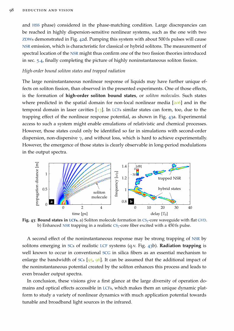
98 deduction and vision
and HSS phase) considered in the phase-matching condition. Large discrepancies can
be reached in highly dispersion-sensitive nonlinear systems, such as the one with two
ZDWs demonstrated in Fig. 42d. Pumping this system with about 500 fs pulses will cause
NSR emission, which is characteristic for classical or hybrid solitons. The measurement of
spectral location of the NSR might thus confirm one of the two fission theories introduced
in sec. 5.4, finally completing the picture of highly noninstantaneous soliton fission.
High-order bound soliton states and trapped radiation
The large noninstantaneous nonlinear response of liquids may have further unique ef-
fects on soliton fission, than observed in the presented experiments. One of those effects,
is the formation of high-order soliton bound states, or soliton molecules. Such states
where predicted in the spatial domain for non-local nonlinear media [206] and in the
temporal domain in laser cavities [13]. In LCFs similar states can form, too, due to the
trapping effect of the nonlinear response potential, as shown in Fig. 43a. Experimental
access to such a system might enable emulations of relativistic and chemical processes.
However, those states could only be identified so far in simulations with second-order
dispersion, non-dispersive γ, and without loss, which is hard to achieve experimentally.
However, the emergence of those states is clearly observable in long-period modulations
in the output spectra.
solitonmolecule
0 2 40
0.5
1
time [ps]
pro
pag
atio
nd
ista
nce
[m]
trapped NSR
hybrid states
0 10 20 30 40
0.8
1
1.2
1.4
delay [T0]
freq
uen
cy[ω
0]
0
−30
[dB]
a b
Fig. 43: Bound states in LCFs. a) Soliton molecule formation in CS2-core waveguide with flat GVD.b) Enhanced NSR trapping in a realistic CS2-core fiber excited with a 450 fs pulse.
A second effect of the noninstantaneous response may be strong trapping of NSR by
solitons emerging in SCs of realistic LCF systems (q.v. Fig. 43b). Radiation trapping is
well known to occur in conventional SCG in silica fibers as an essential mechanism to
enlarge the bandwidth of SCs [95, 96]. It can be assumed that the additional impact of
the noninstantaneous potential created by the soliton enhances this process and leads to
even broader output spectra.
In conclusion, these visions give a first glance at the large diversity of operation do-
mains and optical effects accessible in LCFs, which makes them an unique dynamic plat-
form to study a variety of nonlinear dynamics with much application potential towards
tunable and broadband light sources in the infrared.
B I B L I O G R A P H Y
[1] E. Fermi, J. Pasta, S. Ulam, and M. Tsingou. Studies of the Nonlinear Problems. I.
Los Alamos Report, LA-1940:1–20, 1955. (Cited on page 1.)
[2] J. S. Russell. Notice of the reduction of an anomalous fact in hydrodynamics, and
of a new law of the resistance of fluids to the motion of floating bodies. Report
British Association, 4:531–534, 1834. (Cited on page 1.)
[3] C. Kharif and E. Pelinovsky. Physical mechanisms of the rogue wave phenomenon.
European Journal of Mechanics - B/Fluids, 22(6):603–634, nov 2003. (Cited on page 1.)
[4] Y. Kodama and A. Hasegawa. Nonlinear Pulse Propagation in a Monomode Dielec-
tric Guide. IEEE Journal of Quantum Electronics, 23(5):510–524, 1987. (Cited on
pages 1, 18, 20, and 24.)
[5] E. Seidel and W. M. Suen. Oscillating soliton stars. Physical Review Letters,
66(13):1659–1662, 1991. (Cited on page 1.)
[6] K. E. Strecker, G. B. Partridge, A. G. Truscott, and R. G. Hulet. Formation and
propagation of matter-wave soliton trains. Nature, 417(6885):150–153, 2002. (Cited
on page 1.)
[7] T. Heimburg and A. D. Jackson. On soliton propagation in biomembranes and
nerves. Proceedings of the National Academy of Sciences, 102(28):9790–9795, 2005.
(Cited on page 1.)
[8] A. Hasegawa and F. Tappert. Transmission of stationary nonlinear optical pulses
in dispersive dielectric fibers. I. Anomalous dispersion. Applied Physics Letters,
23(3):142—144, 1973. (Cited on page 1.)
[9] P. Emplit, J.P. Hamaide, F. Reynaud, C. Froehly, and A. Barthelemy. Picosecond
steps and dark pulses through nonlinear single mode fibers. Optics Communications,
62(6):374—379, 1987. (Cited on page 2.)
[10] L. F. Mollenauer and K. Smith. Demonstration of soliton transmission over more
than 4000 km in fiber with loss periodically compensated by Raman gain. Optics
Letters, 13(8):675–677, 1988. (Cited on page 2.)
[11] J. M. Arnold. Solitons in Communications. Electronics & Communication Engineering
Journal, (April):88–96, 1996. (Cited on pages 2 and 22.)
[12] K. Tamura, H. A. Haus, and E. P. Ippen. Self-starting additive pulse mode-locked
erbium fibre ring laser. Electronics Letters, 28(24):2226, 1992. (Cited on page 2.)
[13] P. Grelu and N. Akhmediev. Dissipative solitons for mode-locked lasers. Nature
Photonics, 6(2):84–92, 2012. (Cited on pages 2 and 98.)
99
100 bibliography
[14] Y. Tang, L. G Wright, K. Charan, T. Wang, C. Xu, and F. W. Wise. Generation of
intense 100 fs solitons tunable from 2 to 4,3 µm in fluoride fiber. Optica, 3(9):948–
951, 2016. (Cited on pages 2 and 22.)
[15] N. Akhmediev and M. Karlsson. Cherenkov radiation emitted by solitons in op-
tical fibers. Physical Review A, 51(3):2602–2607, 1995. (Cited on pages 2, 18, and 21.)
[16] D. R. Solli, C. Ropers, P. Koonath, and B. Jalali. Optical rogue waves. Nature,
450(7172):1054–1057, 2007. (Cited on page 2.)
[17] J. M. Dudley, F. Dias, M. Erkintalo, and G. Genty. Instabilities, breathers and rogue
waves in optics. Nature Photonics, 8(10):755–764, 2014. (Cited on page 2.)
[18] A. Armaroli, C. Conti, and F. Biancalana. Rogue solitons in optical fibers: a dy-
namical process in a complex energy landscape? Optica, 2(5):497, 2015. (Cited on
page 2.)
[19] T. G. Philbin, C. Kuklewicz, S. Robertson, S. Hill, F. Konig, and U. Leonhardt. Fiber-
Optical Analog of the Event Horizon. Science, 319(5868):1367–1370, 2008. (Cited
on page 2.)
[20] T. Gottschall, T. Meyer, M. Baumgartl, C. Jauregui, M. Schmitt, J. Popp, J. Limpert,
and A. Tünnermann. Fiber-based light sources for biomedical applications of
coherent anti-Stokes Raman scattering microscopy. Laser & Photonics Reviews,
9(5):435–451, 2015. (Cited on page 2.)
[21] C. F. Kaminski, R. S. Watt, A. D. Elder, J. H. Frank, and J. Hult. Supercontinuum
radiation for applications in chemical sensing and microscopy. Applied Physics B,
92(3):367–378, 2008. (Cited on page 2.)
[22] J. M. Langridge, T. Laurila, R. S. Watt, R. L. Jones, C. F. Kaminski, and J. Hult.
Cavity enhanced absorption spectroscopy of multiple trace gas species using a
supercontinuum radiation source. Optics express, 16(14):10178–88, 2008. (Cited on
page 2.)
[23] A. G. Griffith, R. K. W. Lau, J. Cardenas, Y. Okawachi, A. Mohanty, R. Fain, Y. H. D.
Lee, M. Yu, C. T. Phare, C. B. Poitras, A. L. Gaeta, and M. Lipson. Silicon-chip mid-
infrared frequency comb generation. Nature Communications, 6:6299, 2015. (Cited
on page 2.)
[24] T. Udem, R. Holzwarth, and T. W. Hänsch. Optical frequency metrology. Nature,
416(6877):233–237, 2002. (Cited on page 2.)
[25] R. Slavík, F. Parmigiani, J. Kakande, C. Lundström, M. Sjödin, P. A. Andrekson, R.
Weerasuriya, S. Sygletos, A. D. Ellis, L. Grüner-Nielsen, D. Jakobsen, S. Herstrøm,
R. Phelan, J. O’Gorman, A. Bogris, D. Syvridis, S. Dasgupta, P. Petropoulos, and
bibliography 101
D. J. Richardson. All-optical phase and amplitude regenerator for next-generation
telecommunications systems. Nature Photonics, 4(10):690–695, 2010. (Cited on
page 2.)
[26] J. Pfeifle, V. Brasch, M. Lauermann, Y. Yu, D. Wegner, T. Herr, K. Hartinger, Ph.
Schindler, J. Li, D. Hillerkuss, R. Schmogrow, C. Weimann, R. Holzwarth, W.
Freude, J. Leuthold, T. J. Kippenberg, and Ch. Koos. Coherent terabit communic-
ations with microresonator Kerr frequency combs. Nature Photonics, 8(5):375–380,
2014. (Cited on page 2.)
[27] J. M. Dudley, G. Genty, and S. Coen. Supercontinuum generation in photonic
crystal fiber. Reviews of Modern Physics, 78(4):1135–1184, 2006. (Cited on pages 2,
17, 23, 24, 25, 26, and 62.)
[28] D. V. Skryabin and A. V. Gorbach. Colloquium : Looking at a soliton through the
prism of optical supercontinuum. Reviews of Modern Physics, 82(2):1287–1299, 2010.
(Cited on pages 2, 18, and 24.)
[29] J. C. Travers. Blue extension of optical fibre supercontinuum generation. Journal of
Optics, 12(11):113001, 2010. (Cited on pages 2, 24, and 26.)
[30] L. Shen, N. Healy, L. Xu, H. Y. Cheng, T. D. Day, J. H. V. Price, J. V. Badding, and
A. C. Peacock. Four-wave mixing and octave-spanning supercontinuum generation
in a small core hydrogenated amorphous silicon fiber pumped in the mid-infrared.
Optics Letters, 39(19):5721, 2014. (Cited on page 2.)
[31] M. A. Schmidt, A. Argyros, and F. Sorin. Hybrid Optical Fibers - An Innovative
Platform for In-Fiber Photonic Devices. Advanced Optical Materials, 4(1):13–36, 2016.
(Cited on page 2.)
[32] Ch. Markos, J. C. Travers, A. Abdolvand, B. J. Eggleton, and O. Bang. Hybrid
photonic-crystal fiber. Reviews of Modern Physics, 89(4):045003, 2017. (Cited on
page 2.)
[33] J. H. V. Price, T. M. Monro, H. Ebendorff-Heidepriem, F. Poletti, P. Horak, V.
Finazzi, J. Y. Y. Leong, P. Petropoulos, J. C. Flanagan, G. Brambilla, X. Feng, and D. J.
Richardson. Mid-IR Supercontinuum Generation From Nonsilica Microstructured
Optical Fibers. IEEE Journal of Selected Topics in Quantum Electronics, 13(3):738–749,
2007. (Cited on page 3.)
[34] Ch. Rosenberg Petersen, U. Møller, I. Kubat, B. Zhou, S. Dupont, J. Ramsay, T.
Benson, S. Sujecki, N. Abdel-Moneim, Z. Tang, D. Furniss, A. Seddon, and O.
Bang. Mid-infrared supercontinuum covering the 1.4–13.3 µm molecular finger-
print region using ultra-high NA chalcogenide step-index fibre. Nature Photonics,
8(11):830–834, 2014. (Cited on page 3.)
102 bibliography
[35] P. Domachuk, N. A. Wolchover, M. Cronin-Golomb, A. Wang, A. K. George,
C. M. B. Cordeiro, J. C. Knight, and F. G. Omenetto. Over 4000 nm bandwidth
of mid-IR supercontinuum generation in sub-centimeter segments of highly non-
linear tellurite PCFs. Optics Express, 16(10):7161–7168, 2008. (Cited on page 3.)
[36] U. Møller, Y. Yu, I. Kubat, Ch. R. Petersen, X. Gai, L. Brilland, D. Méchin, C. Cail-
laud, J. Troles, B. Luther-Davies, and O. Bang. Multi-milliwatt mid-infrared su-
percontinuum generation in a suspended core chalcogenide fiber. Optics Express,
23(3):3282, 2015. (Cited on page 3.)
[37] X. Jiang, N. Y. Joly, M. A. Finger, F. Babic, G. K. L. Wong, J. C. Travers, and Ph.
St. J. Russell. Deep-ultraviolet to mid-infrared supercontinuum generated in solid-
core ZBLAN photonic crystal fibre. Nature Photonics, 9(2):133–139, 2015. (Cited on
page 3.)
[38] M. F. Saleh and F. Biancalana. Soliton dynamics in gas-filled hollow-core photonic
crystal fibers. Journal of Optics, 18(1):013002, 2016. (Cited on page 3.)
[39] M. Nisoli, S. Stagira, S. De Silvestri, O. Svelto, S. Sartania, Z. Cheng, M. Lenzner,
Ch. Spielmann, and F. Krausz. A novel-high energy pulse compression system:
Generation of multigigawatt sub-5-fs pulses. Applied Physics B: Lasers and Optics,
65(2):189–196, 1997. (Cited on page 3.)
[40] P. Hölzer, W. Chang, J. C. Travers, A. Nazarkin, J. Nold, N. Y. Joly, M. F. Saleh,
F. Biancalana, and P. St. J. Russell. Femtosecond Nonlinear Fiber Optics in the
Ionization Regime. Physical Review Letters, 107(20):203901, 2011. (Cited on page 3.)
[41] F. Tani, J. C. Travers, and P. St. J. Russell. PHz-wide Supercontinua of Nondis-
persing Subcycle Pulses Generated by Extreme Modulational Instability. Physical
Review Letters, 111(3):033902, 2013. (Cited on page 3.)
[42] F. Belli, A. Abdolvand, W. Chang, J. C. Travers, and Ph. St. J. Russell. Vacuum-
ultraviolet to infrared supercontinuum in hydrogen-filled photonic crystal fiber.
Optica, 2(4):292–300, 2015. (Cited on pages 3 and 20.)
[43] R. Sollapur, D. Kartashov, M. Zürch, A. Hoffmann, T. Grigorova, G. Sauer, A. Har-
tung, A. Schwuchow, J. Bierlich, J. Kobelke, M. Chemnitz, M. A. Schmidt, and Ch.
Spielmann. Resonance-enhanced multi-octave supercontinuum generation in anti-
resonant hollow-core fibers. Light: Science & Applications, 6(12):e17124, 2017. (Cited
on page 3.)
[44] K. F. Mak, J. C. Travers, P. Holzer, N. Y. Joly, and P. S. Russell. Tunable vacuum-UV
to visible ultrafast pulse source based on gas-filled Kagome-PCF. Optics Express,
21(9):10942–10953, 2013. (Cited on page 3.)
bibliography 103
[45] P. S. J. Russell, P. Hölzer, W. Chang, A. Abdolvand, and J. C. Travers. Hollow-core
photonic crystal fibres for gas-based nonlinear optics. Nature Photonics, 8(4):278–
286, 2014. (Cited on page 3.)
[46] M. F. Saleh, W. Chang, J. C. Travers, P. S. J. Russell, and F. Biancalana. Plasma-
induced asymmetric self-phase modulation and modulational instability in gas-
filled hollow-core photonic crystal fibers. Physical Review Letters, 109(11):1–5, 2012.
(Cited on page 3.)
[47] D. Novoa, M. Cassataro, J. C. Travers, and P. S. T. Russell. Photoionization-
Induced Emission of Tunable Few-Cycle Midinfrared Dispersive Waves in Gas-
Filled Hollow-Core Photonic Crystal Fibers. Physical Review Letters, 115(3):1–5,
2015. (Cited on page 3.)
[48] G. J. Ogilvie, R. J. Esdaile, and G. P. Kidd. Transmission loss of tetrachloroethylene-
filled liquid-core-fibre light guide. Electronics Letters, 8(22):533, 1972. (Cited on
page 3.)
[49] J. Stone. Optical transmission loss in liquid-core hollow fibers. IEEE Journal of
Quantum Electronics, 8(3):386–388, 1972. (Cited on page 3.)
[50] A. Samoc. Dispersion of refractive properties of solvents: Chloroform, toluene,
benzene, and carbon disulfide in ultraviolet, visible, and near-infrared. Journal of
Applied Physics, 94(9):6167–6174, 2003. (Cited on pages 4, 29, 33, 34, 118, and 134.)
[51] S. Kedenburg, M. Vieweg, T. Gissibl, and H. Giessen. Linear refractive index
and absorption measurements of nonlinear optical liquids in the visible and near-
infrared spectral region. Optical Materials Express, 2(11):1588–1611, 2012. (Cited on
pages 4, 29, 30, 31, 32, 33, 34, 118, and 134.)
[52] M. Reichert, H. Hu, M. R. Ferdinandus, M. Seidel, P. Zhao, T. R. Ensley, D. Peceli,
J. M. Reed, D. A. Fishman, S. Webster, D. J. Hagan, and E. W. Van Stryland. Tem-
poral, spectral, and polarization dependence of the nonlinear optical response of
carbon disulfide: erratum. Optica, 3(6):657, 2016. (Cited on page 4.)
[53] P. Zhao, M. Reichert, S. Benis, D. J. Hagan, and E. W. Van Stryland. Temporal
and polarization dependence of the nonlinear optical response of solvents. Optica,
5(5):583, 2018. (Cited on pages 4, 37, 39, 120, and 121.)
[54] D. Lopez-Cortes, O. Tarasenko, and W. Margulis. All-fiber Kerr cell. Optics Letters,
37(15):3288–3290, 2012. (Cited on page 4.)
[55] R. M. Gerosa, A. Sudirman, L. de S. Menezes, W. Margulis, and Ch. J. S. de Ma-
tos. All-fiber high repetition rate microfluidic dye laser. Optica, 2(2):186–193, 2015.
(Cited on pages 4 and 82.)
104 bibliography
[56] H. W. Lee, M. A. Schmidt, P. Uebel, H. Tyagi, N. Y. Joly, M. Scharrer, and P. St. J.
Russell. Optofluidic refractive-index sensor in step-index fiber with parallel hollow
micro-channel. Optics Express, 19(9):8200–8207, 2011. (Cited on page 4.)
[57] Y. Peng, J. Hou, Y. Zhang, Z. Huang, R. Xiao, and Q. Lu. Temperature sensing
using the bandgap-like effect in a selectively liquid-filled photonic crystal fiber.
Optics Letters, 38(3):263, 2013. (Cited on page 4.)
[58] S. Pumpe, M. Chemnitz, J. Kobelke, and M. A. Schmidt. Monolithic optofluidic
mode coupler for broadband thermo- and piezo-optical characterization of liquids.
Optics Express, 25(19):22932–22946, 2017. (Cited on pages 4, 34, 35, 36, 88, and 118.)
[59] M. Schmidt, A. M. Cubillas, N. Taccardi, T. G. Euser, T. Cremer, F. Maier, H.-P. Stein-
rück, P. S. J. Russell, P. Wasserscheid, and B. J. M. Etzold. Chemical and (Photo)-
Catalytical Transformations in Photonic Crystal Fibers. ChemCatChem, 5(3):641–650,
2013. (Cited on page 4.)
[60] D. Yan, J. Popp, M. W. Pletz, and T. Frosch. Highly sensitive broadband Raman
sensing of antibiotics in step-index hollow-core photonic crystal fibers. ACS Photon-
ics, 4(1):138–145, 2017. (Cited on page 4.)
[61] M. Nissen, B. Doherty, J. Hamperl, J. Kobelke, K. Weber, T. Henkel, and M. A.
Schmidt. UV absorption spectroscopy in water-filled antiresonant hollow core
fibers for pharmaceutical detection. Sensors (Switzerland), 18(2):1–12, 2018. (Cited
on page 4.)
[62] J. Meister, R. Franzen, G. Eyrich, J. Bongartz, N. Gutknecht, and P. Hering. First
clinical application of a liquid-core light guide connected to an Er:YAG laser for
oral treatment of leukoplakia. Lasers in Medical Science, 25(5):669–673, 2010. (Cited
on page 4.)
[63] A. R. Chraplyvy and T. J. Bridges. Infrared generation by means of multiple-order
stimulated Raman scattering in CCl(4)- and CBrCl(3)-filled hollow silica fibers.
Optics letters, 6(12):632–633, 1981. (Cited on page 4.)
[64] K. Kieu and L. Schneebeli. Integrated liquid-core optical fibers for ultra-efficient
nonlinear liquid photonics. Optics Express, 20(7):8148–8154, 2012. (Cited on page 4.)
[65] G. Fanjoux, A. Sudirman, J.-Ch. Beugnot, L. Furfaro, W. Margulis, and T. Sylvestre.
Stimulated Raman-Kerr scattering in an integrated nonlinear optofluidic fiber ar-
rangement. Optics Letters, 39(18):5407–5410, 2014. (Cited on page 4.)
[66] S. Kedenburg, A. Steinmann, R. Hegenbarth, T. Steinle, and H. Giessen. Nonlinear
refractive indices of nonlinear liquids: wavelength dependence and influence of
retarded response. Applied Physics B, 117(3):803–816, 2014. (Cited on page 4.)
bibliography 105
[67] D. Churin, T. N. Nguyen, K. Kieu, R. A. Norwood, and N. Peyghambarian. Mid-
IR supercontinuum generation in an integrated liquid-core optical fiber filled with
CS2. Optical Materials Express, 3(9):1358–1364, 2013. (Cited on pages 4 and 68.)
[68] S. Kedenburg, T. Gissibl, T. Steinle, A. Steinmann, and H. Giessen. Towards in-
tegration of a liquid-filled fiber capillary for supercontinuum generation in the
1.2-2.4µm range. Optics Express, 23(7):8281–8289, 2015. (Cited on pages 4 and 68.)
[69] S. Pricking and H. Giessen. Generalized retarded response of nonlinear media
and its influence on soliton dynamics. Optics Express, 19(4):2895, 2011. (Cited on
page 4.)
[70] C. Conti, M. A. Schmidt, P. S. J. Russell, and F. Biancalana. Highly Noninstant-
aneous Solitons in Liquid-Core Photonic Crystal Fibers. Physical Review Letters,
105(26):263902, 2010. (Cited on pages 4, 43, 44, 92, 126, 127, and 129.)
[71] M. Vieweg, T. Gissibl, S. Pricking, B. T. Kuhlmey, D. C. Wu, B. J. Eggleton, and
H. Giessen. Ultrafast nonlinear optofluidics in selectively liquid-filled photonic
crystal fibers. Optics Express, 18(24):25232–25240, 2010. (Cited on page 4.)
[72] A. Bozolan, C.J. de Matos, C. M. Cordeiro, E. M. Dos Santos, and J. Travers. Su-
percontinuum generation in a water-core photonic crystal fiber. Optics Express,
16(13):9671–9676, 2008. (Cited on page 4.)
[73] J. Bethge, A. Husakou, F. Mitschke, F. Noack, U. Griebner, G. Steinmeyer, and
J. Herrmann. Two-octave supercontinuum generation in a water-filled photonic
crystal fiber. Optics Express, 18(6):6230–6240, 2010. (Cited on page 4.)
[74] B. E. A. Saleh and M. C. Teich. Electromagnetic Optics. In Fundamentals of Photonics,
chapter 5, pages 157–192. John Wiley & Sons, Inc., New York, Chichester, Brisbane,
Toronto, Singapore, 1991. (Cited on pages 7 and 35.)
[75] A. W. Snyder and J. D. Love. Waveguides with exact solutions. In Optical Waveguide
Theory, chapter 12, pages 238–279. Chapman and Hall, London, New York, 1983.
(Cited on pages 8, 9, and 124.)
[76] C. Yeh and F. I. Shimabukuro. Circular dielectric waveguides. In The Essence of
Dielectric Waveguides, chapter 5, pages 137–177. Springer, New York, 2008. (Cited
on pages 8 and 9.)
[77] R. W. Hellwarth. Third-order optical susceptibilities of liquids and solids. Progress
in Quantum Electronics, 5:1–68, 1979. (Cited on pages 11, 29, and 126.)
[78] R. W. Boyd. The intensity-dependent refractive index. In Nonlinear Optics,
chapter 4, pages 207–252. Academic Press, 3rd edition, 2007. (Cited on pages 11,
119, 125, and 126.)
106 bibliography
[79] G. P. Agrawal. Nonlinear Pulse Propagation. In Nonlinear Fiber Optics, chapter 2,
pages 27–56. Academic Press, Boston, 5th edition, 2013. (Cited on pages 11, 12, 13,
14, 125, and 126.)
[80] A. Couairon, E. Brambilla, T. Corti, D. Majus, O. de J. Ramírez-Góngora, and
M. Kolesik. Practitioner’s guide to laser pulse propagation models and simulation.
The European Physical Journal Special Topics, 199(1):5–76, 2011. (Cited on page 12.)
[81] P. V. Mamyshev and S. V. Chernikov. Ultrashort-pulse propagation in optical fibers.
Optics Letters, 15(19):1076, 1990. (Cited on pages 12, 13, and 126.)
[82] M. Kolesik and J. V. Moloney. Nonlinear optical pulse propagation simulation:
From Maxwell’s to unidirectional equations. Physical Review E, 2004. (Cited on
pages 12 and 80.)
[83] J. Laegsgaard. Mode profile dispersion in the generalized nonlinear Schrödinger
equation. Optics Express, 15(24):16110–16123, 2007. (Cited on pages 13 and 14.)
[84] M. Chemnitz and M. A. Schmidt. Single mode criterion - a benchmark figure to
optimize the performance of nonlinear fibers. Optics Express, 24(14):16191–16205,
2016. (Cited on pages 14, 15, 42, 43, and 124.)
[85] S. Afshar V. and T. M. Monro. A full vectorial model for pulse propagation in emer-
ging waveguides with subwavelength structures part I: Kerr nonlinearity. Optics
Express, 17(4):2298–2318, 2009. (Cited on page 14.)
[86] M. Artiglia and G. Coppa. Mode field diameter measurements in single-mode op-
tical fibers. Journal of Lightwave Technology, 7(8):1139–1152, 1989. (Cited on page 15.)
[87] V. E. Zakharovand and A. B. Shabat. Exact Theory of Two-Dimensional Self-
Focusing and One- Dimensional Self-Modulation of Waves in Nonlinear Media.
Zh. Eksp. Teor. Fiz, 34(61):118–134, 1972. (Cited on page 15.)
[88] Y. Kodama. Optical solitons in a monomode fiber. Journal of Statistical Physics,
39(5-6):597–614, 1985. (Cited on page 18.)
[89] J. P. Gordon. Theory of the soliton self-frequency shift. Optics Letters, 11(10):662,
1986. (Cited on pages 18 and 22.)
[90] J. P. Gordon. Dispersive perturbations of solitons of the nonlinear Schrödinger
equation. J. Opt. Soc. Am. B, 9(1):91–97, 1992. (Cited on pages 18 and 21.)
[91] J. N. Elgin. Soliton propagation in an optical fiber with third-order dispersion.
Optics Letters, 17(20):1409, 1992. (Cited on page 18.)
[92] D. V. Skryabin. Soliton Self-Frequency Shift Cancellation in Photonic Crystal Fibers.
Science, 301(5640):1705–1708, 2003. (Cited on page 18.)
bibliography 107
[93] F. Biancalana, D. V. Skryabin, and A. V. Yulin. Theory of the soliton self-frequency
shift compensation by the resonant radiation in photonic crystal fibers. Physical
Review E - Statistical, Nonlinear, and Soft Matter Physics, 70(1 2):1–9, 2004. (Cited on
pages 18, 21, and 22.)
[94] A. V Gorbach, D. V. Skryabin, J. M. Stone, and J. C. Knight. Four-wave mixing
of solitons with radiation and quasi-nondispersive wave packets at the short-
wavelength edge of a supercontinuum. Optics Express, 14(21):9854–9863, 2006.
(Cited on page 18.)
[95] A. V. Gorbach and D. V. Skryabin. Light trapping in gravity-like potentials and
expansion of supercontinuum spectra in photonic-crystal fibres. Nature Photonics,
1(11):653–657, 2007. (Cited on pages 18, 21, 24, and 98.)
[96] A. V. Gorbach and D. V. Skryabin. Theory of radiation trapping by the accelerating
solitons in optical fibers. Physical Review A - Atomic, Molecular, and Optical Physics,
76(5), 2007. (Cited on pages 18, 24, and 98.)
[97] G. P. Agrawal. Optical Solitons. In Nonlinear Fiber Optics, chapter 5, pages 129–191.
Academic Press, Boston, 5th edition, 2013. (Cited on page 18.)
[98] N. Akhmediev and A. Ankiewicz. Solitons: Non-linear pulses and beams. Chapman
and Hall, London, Weinheim, New York, Tokyo, Melbourne, Madras, 1st edition,
1997. (Cited on pages 18 and 19.)
[99] P. K. A. Wai, C. R. Menyuk, Y. C. Lee, and H. H. Chen. Nonlinear pulse propaga-
tion in the neighborhood of the zero-dispersion wavelength of monomode optical
fibers. Optics Letters, 11(7):464, 1986. (Cited on page 20.)
[100] P. K. A. Wai, C. R. Menyuk, H. H. Chen, and Y. C. Lee. Soliton at the zero-group-
dispersion wavelength of a single-model fiber. Optics letters, 12(8):628–630, 1987.
(Cited on page 20.)
[101] J. N. Elgin, T. Brabec, and S. M.J. Kelly. A perturbative theory of soliton propaga-
tion in the presence of third order dispersion. Optics Communications, 114(3-4):321–
328, 1995. (Cited on page 20.)
[102] A. V. Husakou and J. Herrmann. Supercontinuum generation, four-wave mixing,
and fission of higher-order solitons in photonic-crystal fiber. Journal Of The Optical
Society Of America B Optical Physics, 19(9):2171–2182, 2002. (Cited on pages 20
and 24.)
[103] S. Roy, S. K. Bhadra, and G. P. Agrawal. Dispersive waves emitted by solitons
perturbed by third-order dispersion inside optical fibers. Physical Review A,
79(2):023824, 2009. (Cited on page 20.)
108 bibliography
[104] R. Driben, A. V. Yulin, and A. Efimov. Resonant radiation from oscillating higher
order solitons. Optics Express, 23(15):19112, 2015. (Cited on page 20.)
[105] I. Cristiani, R. Tediosi, L. Tartara, and V. Degiorgio. Dispersive wave generation by
solitons in microstructured optical fibers. Optics express, 12(1):124–135, 2004. (Cited
on page 20.)
[106] N. Granzow, M. A. Schmidt, W. Chang, L. Wang, Q. Coulombier, J. Troles,
P. Toupin, I. Hartl, K. F. Lee, M. E. Fermann, L. Wondraczek, and P. S.J. Rus-
sell. Mid-infrared supercontinuum generation in As_2S_3-silica “nano-spike” step-
index waveguide. Optics Express, 21(9):10969, 2013. (Cited on page 20.)
[107] M. Chemnitz, J. Wei, C. Jain, B. P. Rodrigues, T. Wieduwilt, J. Kobelke, L. Won-
draczek, and M. A. Schmidt. Octave-spanning supercontinuum generation in hy-
brid silver metaphosphate/silica step-index fibers. Optics Letters, 41(15):3519, 2016.
(Cited on page 20.)
[108] F. Leo, J. Safioui, B. Kuyken, G. Roelkens, and S.-P. Gorza. Generation of coher-
ent supercontinuum in a-Si:H waveguides: experiment and modeling based on
measured dispersion profile. Optics Express, 22(23):28997–29007, 2014. (Cited on
page 20.)
[109] V. Brasch, T. Herr, M. Geiselmann, G. Lihachev, M. H. P. Pfeiffer, M. L. Gorodetsky,
and T. J. Kippenberg. Photonic chip-based optical frequency comb using soliton
Cherenkov radiation. Science, 351(6271):357–360, 2016. (Cited on page 20.)
[110] D. Grassani, E. Tagkoudi, H. Guo, C. Herkommer, T. J. Kippenberg, and C.-S. Brès.
Highly efficient 4 micron light generation through fs-fiber laser driven supercon-
tinuum in Si3N4 waveguides. arXiv:1806.06633, 1–9, 2018. (Cited on page 20.)
[111] J. Herrmann, U. Griebner, N. Zhavoronkov, A. Husakou, D. Nickel, J. C. Knight,
W. J. Wadsworth, P. S. J. Russell, and G. Korn. Experimental evidence for supercon-
tinuum generation by fission of higher-order solitons in photonic fibers. Physical
Review Letters, 88(17):173901, 2002. (Cited on page 21.)
[112] A. Efimov, A. V. Yulin, D. V. Skryabin, J. C. Knight, N. Joly, F. G. Omenetto, A. J.
Taylor, and P. Russell. Interaction of an Optical Soliton with a Dispersive Wave.
Physical Review Letters, 95(21):1–4, 2005. (Cited on page 21.)
[113] A.. V Yulin, D. V. Skryabin, and P. S. J. Russell. Four-wave mixing of linear waves
and solitons in fibers with higher-order dispersion. Optics Letters, 29(20):2411–2413,
2004. (Cited on page 21.)
[114] D. V. Skryabin and A. V. Yulin. Theory of generation of new frequencies by mixing
of solitons and dispersive waves in optical fibers. Physical Review E - Statistical,
Nonlinear, and Soft Matter Physics, 72(016619):1–10, 2005. (Cited on page 21.)
bibliography 109
[115] H. Guo, S. Wang, X. Zeng, and M. Bache. Understanding soliton spectral tunneling
as a spectral coupling effect. IEEE Photonics Technology Letters, 25(19):1928–1931,
2013. (Cited on page 21.)
[116] K. E. Webb, M. Erkintalo, Y. Xu, N. G. R. Broderick, J. M. Dudley, G. Genty, and
S. G. Murdoch. Nonlinear optics of fibre event horizons. Nature Communications,
5:4969, 2014. (Cited on page 21.)
[117] R. H. Stolen, W. J. Tomlinson, H. A. Haus, and J. P. Gordon. Raman response
function of silica-core fibers. Journal of the Optical Society of America B, 6(6):1159,
1989. (Cited on page 21.)
[118] D. Hollenbeck and C. D. Cantrell. Multiple-vibrational-mode model for fiber-optic
Raman gain spectrum and response function. Journal of the Optical Society of America
B, 19(12):2886–2892, 2002. (Cited on pages 21, 24, and 120.)
[119] Q. Lin and G. P. Agrawal. Raman response function for silica fibers. Optics Letters,
31(21):3086, 2006. (Cited on page 21.)
[120] K. Porsezian and K. Nakkeeran. Optical solitons in presence of Kerr dispersion
and self-frequency shift. Physical Review Letters, 76(21):3955–3958, 1996. (Cited on
page 22.)
[121] F. M. Mitschke, L. F. Mollenauer, and J. P. Gordon. Discovery of the soliton self-
frequency shift. Physics Today, 26(10):26–26, 1987. (Cited on page 22.)
[122] G. Genty, M. Surakka, J. Turunen, and A. T. Friberg. Complete characterization
of supercontinuum coherence. Journal of the Optical Society of America B, 28(9):2301,
2011. (Cited on page 23.)
[123] I. Zeylikovich, V. Kartazaev, and R. R. Alfano. Spectral, temporal, and coherence
properties of supercontinuum generation in microstructure fiber. Journal of the
Optical Society of America B, 22(7):1453, 2005. (Cited on page 23.)
[124] M. Erkintalo, G. Genty, B. Wetzel, and J. M. Dudley. Limitations of the linear Ra-
man gain approximation in modeling broadband nonlinear propagation in optical
fibers. Optics Express, 18(24):25449–60, 2010. (Cited on page 23.)
[125] S. Dupont, Z. Qu, S. S. Kiwanuka, L. E. Hooper, J. C. Knight, S. R. Keiding, and C. F.
Kaminski. Ultra-high repetition rate absorption spectroscopy with low noise su-
percontinuum radiation generated in an all-normal dispersion fibre. Laser Physics
Letters, 11(7):1–8, 2014. (Cited on page 23.)
[126] A. M. Heidt, J. S. Feehan, J. H. V. Price, and T. Feurer. Limits of coherent super-
continuum generation in normal dispersion fibers. Journal of the Optical Society of
America B, 34(4):764, 2017. (Cited on page 23.)
110 bibliography
[127] A. M. Heidt, J. Rothhardt, A. Hartung, H. Bartelt, E. G. Rohwer, J. Limpert, and A.
Tünnermann. High quality sub-two cycle pulses from compression of supercon-
tinuum generated in all-normal dispersion photonic crystal fiber. Optics Express,
19(15):13873–13879, 2011. (Cited on page 23.)
[128] A. V. Husakou and J. Herrmann. Supercontinuum Generation of Higher-Order
Solitons by Fission in Photonic Crystal Fibers. Physical Review Letters, 87(20):203901,
2001. (Cited on page 24.)
[129] G. Genty, S. Coen, and J. M. Dudley. Fiber supercontinuum sources (Invited).
Journal of the Optical Society of America B, 24(8):1771, 2007. (Cited on pages 24
and 62.)
[130] N. Karasawa and K. Tada. Optical Solitons from a Photonic Crystal Fiber and Their
Applications. In Photonic Crystals, chapter 10, pages 201–224. IntechOpen, Rijeka,
2007. (Cited on page 24.)
[131] H. Zhang, S. Yu, J. Zhang, and W. Gu. Effect of frequency chirp on supercontinuum
generation in photonic crystal fibers with two zero-dispersion wavelengths. Optics
express, 15(3):1147–1154, 2007. (Cited on pages 24 and 135.)
[132] M. Chemnitz, M. Gebhardt, C. Gaida, F. Stutzki, J. Kobelke, J. Limpert, A. Tünner-
mann, and M. A. Schmidt. Hybrid soliton dynamics in liquid-core fibres. Nature
Communications, 8(1):42, 2017. (Cited on pages 27, 55, 66, and 70.)
[133] M. Chemnitz, R. Scheibinger, Ch. Gaida, M. Gebhardt, F. Stutzki, S. Pumpe, J.
Kobelke, A. Tünnermann, J. Limpert, and M. A. Schmidt. Thermodynamic control
of soliton dynamics in liquid-core fibers. Optica, 5(6):695, 2018. (Cited on pages 27,
35, 82, 83, 84, 85, 86, 88, and 95.)
[134] C.-S. Laboratories Inc. Cargille Microscope Immersion Oils, 2018. (Cited on
page 27.)
[135] J. D. Jackson. Frequency Dispersion Characteristics of Dielectrics, Conductors, and
Plasmas. In John David Jackson, editor, Classical Electrodynamics, chapter 7.5, pages
309–316. John Wiley & Sons, Inc., Berkeley, 3rd edition, 1999. (Cited on page 29.)
[136] W. v. Sellmeier. Zur Erklärung der abnormen Farbenfolge im Spectrum einiger Sub-
stanzen. Annalen der Physik und Chemie, 219(6):272–282, 1871. (Cited on page 29.)
[137] J. W. Fleming. Dispersion in GeO2-SiO2 glasses. Applied Optics, 23(24):4486–4493,
1984. (Cited on page 29.)
[138] K. Moutzouris, M. Papamichael, S. C. Betsis, I. Stavrakas, G. Hloupis, and D. Tri-
antis. Refractive, dispersive and thermo-optic properties of twelve organic solvents
in the visible and near-infrared. Applied Physics B, 116(3):617–622, 2013. (Cited on
pages 29 and 35.)
bibliography 111
[139] T. M. Monro and H. Ebendorff-Heidepriem. Progress in Microstructured Optical
Fibers. Annual Review of Materials Research, 36(1):467–495, 2006. (Cited on pages 30
and 31.)
[140] B. D. Mistry. A Handbook of Spectroscopic Data Chemistry. Oxford Book Company,
Jaipur, 2009. (Cited on pages 30 and 31.)
[141] M. Plidschun, M. Chemnitz, and M. A. Schmidt. Low-loss deuterated or-
ganic solvents for visible and near-infrared photonics. Optical Materials Express,
7(4):1122–1130, 2017. (Cited on pages 30, 31, and 32.)
[142] F. Théberge, P. Mathieu, N. Thiré, J.-F. Daigle, B. E. Schmidt, J. Fortin, R. Vallée, Y.
Messaddeq, and F. Légaré. Mid-infrared nonlinear absorption in As_2S_3 chalco-
genide glass. Optics Express, 24(21):24600, 2016. (Cited on page 31.)
[143] NIST Mass Spec Data Center. Infrared Spectra. In W.G. Mallard and P.J. Linstrom,
editors, NIST Chemistry WebBook. National Institute of Standards and Technology,
Gaithersburg MD, nist stand edition. (Cited on pages 31 and 131.)
[144] E. K. Plyler and C. J. Humphreys. Infrared absorption spectrum of carbon disulfide.
Journal of research of the National Bureau of Standards, 39(1):59–65, 1947. (Cited on
page 31.)
[145] D. E. Mann, N. Acquista, and E. K. Plyler. Vibrational spectra of tetrafluoroethyl-
ene and tetrachloroethylene. Journal of Research of the National Bureau of Standards,
52(2):67–72, 1954. (Cited on page 31.)
[146] D. P. Shelton. Refractive index measured by laser beam displacement at λ=1064nm
for solvents and deuterated solvents. Applied Optics, 50(21):4091, 2011. (Cited on
page 32.)
[147] A. H. Pfund. The Dispersion of CS2 and CCl2 in the Infrared. Journal of the Optical
Society of America, 25(11):351–354, 1935. (Cited on pages 33, 34, and 118.)
[148] R. E. Kagarise. Infrared Dispersion of Some Organic Liquids. Journal of the Optical
Society of America, 50(1):36–39, 1960. (Cited on pages 33, 34, and 118.)
[149] B. Wilhelmi. Über die Anwendung von Dispersionsrelationen zur Bestimmung
optischer Konstanten. Annalen der Physik, 474(5-6):244–252, 1967. (Cited on
pages 33 and 118.)
[150] S. Ghosal, J. L. Ebert, and S. A. Self. The infrared refractive indices of CHBr3, CCl4
and CS2. Infrared Physics, 34(6):621–628, 1993. (Cited on pages 33 and 118.)
[151] S. Valkai, J. Liszi, and I. Szalai. Temperature dependence of the refractive index for
three chloromethane liquids at 514.5 nm and 632.8 nm wavelengths. The Journal of
Chemical Thermodynamics, 30(7):825–832, 1998. (Cited on page 34.)
112 bibliography
[152] M. J. Weber. Liquids. In Handbook of Optical Materials, chapter 5, pages 383–445.
CRC Press, Boca Raton, London, New York, Washington, D.C., 2003. (Cited on
pages 34 and 118.)
[153] J. Vincent-Geisse. Dispersion de quelques liquides organiques dans l’infrarouge.
détermination des intensités de bandes et des polarisations. Journal de Physique,
26(6):289–296, 1965. (Cited on pages 34 and 118.)
[154] J. Yarwood and W. J. Orville-Thomas. Infra-red dispersion studies. Part 7 Band
intensities and atomic polarizations of CX2= CCl2(X = H, F, Cl) molecules. Transac-
tions of the Faraday Society, 62(1):3294–3309, 1966. (Cited on pages 34 and 118.)
[155] J. Matsuoka, N. Kitamura, S. Fujinaga, T. Kitaoka, and H. Tamashita. Temperat-
ure dependence of refractive index of SiO2 glass. Journal of Non-Crystaline Solids,
135:86–89, 1991. (Cited on page 35.)
[156] G. Ghosh, M. Endo, and T. Iwasaki. Temperature-Dependent sellmeier Coefficients
and Chromatic Dispersions for Some Optical fiber glasses. Journal of Lightwave
Technology, 12(8):1338–1342, 1994. (Cited on page 35.)
[157] E. Reisler, H. Eisenberg, and A. P. Minton. Temperature and density dependence
of the refractive index of pure liquids. Journal of the Chemical Society, Faraday Trans-
actions 2, 68:1001, 1972. (Cited on pages 35 and 87.)
[158] C. D. Keefe and S. Mac Innis. Temperature dependence of the optical properties
of liquid toluene between 4000 and 400cm-1 from 30 to 105°C. Journal of Molecular
Structure, 737(2-3):207–219, 2005. (Cited on page 35.)
[159] H. El-Kashef. Study of the refractive properties of laser dye solvents: Toluene,
carbon disulphide, chloroform, and benzene. Optical Materials, 20(2):81–86, 2002.
(Cited on page 35.)
[160] W. Hauf and U. Grigull. Optical methods in heat transfer. In James P. Hartnett
and Thomas F. Irvine, editors, Advances in Heat Transfer, chapter 2, pages 133–366.
Academic Press, 1970. (Cited on page 35.)
[161] E. W. Washburn. International Critical Tables of Numerical Data, Physics, Chemistry
and Technology, Vol. VII. McGraw-Hill, New York, 1st edition, 1930. (Cited on
page 35.)
[162] H. El-Kashef. Optical and electrical properties of materials. Review of Scientific
Instruments, 65(6):2056–2061, 1994. (Cited on page 35.)
[163] H. El-Kashef. Thermo-optical and dielectric constants of laser dye solvents. Review
of Scientific Instruments, 69(3):1243–1245, 1998. (Cited on page 35.)
bibliography 113
[164] D. J. Coumou, E. L. Mackor, and J. Hijmans. Isotropic light-scattering in pure
liquids. Transactions of the Faraday Society, 60(0):1539–1547, 1964. (Cited on page 35.)
[165] J. C. R. Reis, I. M. S. Lampreia, Â. F. S. Santos, M. Luísa C. J. Moita, and G.
Douhéret. Refractive Index of Liquid Mixtures: Theory and Experiment. ChemPhy-
sChem, 11(17):3722–3733, 2010. (Cited on page 36.)
[166] N. An, B. Zhuang, M. Li, Y. Lu, and Z.-G. Wang. Combined Theoretical and Exper-
imental Study of Refractive Indices of Water-Acetonitrile-Salt Systems. The Journal
of Physical Chemistry B, 119(33):10701–10709, 2015. (Cited on pages 36 and 37.)
[167] L. Lorenz. Ueber die Refractionsconstante. Annalen der Physik, 247(9):70–103, 1880.
(Cited on page 37.)
[168] H. A. Lorentz. Theory of Electrons. Teubner, Leipzig, Berlin, 2nd edition, 1916.
(Cited on page 37.)
[169] G. Baranovic. Refractive Index Mixing Rules and Excess Infrared Spectra of Binary
Mixtures. Applied Spectroscopy, 71(5):1039–1049, 2017. (Cited on page 37.)
[170] R. W. Hellwarth, A. Owyoung, and N. George. Origin of the Nonlinear Refractive
Index of Liquid C Cl 4. Physical Review A, pages 5–10, 1971. (Cited on page 37.)
[171] P. P. Ho and R. R. Alfano. Optical Kerr effect in liquids. Physical Review A, 20:2170–
2187, 1979. (Cited on page 37.)
[172] D. McMorrow, W.T. Lotshaw, and G.A. Kenney-Wallace. Femtosecond optical Kerr
studies on the origin of the nonlinear responses in simple liquids. IEEE Journal of
Quantum Electronics, 24(2):443–454, 1988. (Cited on page 37.)
[173] W. T. Lotshaw, D. McMorrow, N. Thantu, J. S. Melinger, and R. Kitchenham. Inter-
molecular vibrational coherence in molecular liquids. Journal of Raman Spectroscopy,
26(7):571–583, 1995. (Cited on page 37.)
[174] M. Reichert, H. Hu, M. R. Ferdinandus, M. Seidel, P. Zhao, T. R Ensley, D. Peceli,
J. M. Reed, D. A. Fishman, S. Webster, D. J. Hagan, and E. W. Van Stryland. Tem-
poral, spectral, and polarization dependence of the nonlinear optical response of
carbon disulfide. Optica, 1(6):436–445, 2014. (Cited on pages 37, 38, and 75.)
[175] M. L. Miguez, T. G. B. De Souza, E. C. Barbano, S. C. Zilio, and L. Misoguti. Meas-
urement of third-order nonlinearities in selected solvents as a function of the pulse
width. Optics Express, 25(4):3553, 2017. (Cited on pages 37, 39, and 120.)
[176] P. Zhao, M. Reichert, T. R. Ensley, W. M. Shensky, A. G. Mott, D. J. Hagan, and
E. W. Van Stryland. Nonlinear refraction dynamics of solvents and gases. Non-
linear Frequency Generation and Conversion: Materials, Devices, and Applications XV,
9731:97310F, 2016. (Cited on pages 39 and 122.)
114 bibliography
[177] N. Thantu and R. S. Schley. Ultrafast third-order nonlinear optical spectroscopy of
chlorinated hydrocarbons. Vibrational Spectroscopy, 32(2):215–223, 2003. (Cited on
pages 40 and 122.)
[178] M. Chemnitz, Ch. Gaida, M. Gebhardt, F. Stutzki, J. Kobelke, A. Tünnermann, J.
Limpert, and M. A. Schmidt. Carbon chloride-core fibers for soliton mediated su-
percontinuum generation. Optics Express, 26(3):3221–3235, 2018. (Cited on pages 66,
69, 72, 73, and 95.)
[179] M. Gebhardt, C. Gaida, S. Hädrich, F. Stutzki, C. Jauregui, J. Limpert, and A. Tün-
nermann. Nonlinear compression of an ultrashort-pulse thulium-based fiber laser
to sub-70 fs in Kagome photonic crystal fiber. Optics Letters, 40(12):2770, 2015.
(Cited on page 66.)
[180] G. P. Agrawal. Novel Nonlinear Phenomena. In Nonlinear Fiber Optics, chapter 12,
pages 497–551. Academic Press, Boston, 5th edition, 2013. (Cited on page 69.)
[181] M. Klimczak, G. Sobon, R. Kasztelanic, K. M. Abramski, and R. Buczynski. Direct
comparison of shot-to-shot noise performance of all normal dispersion and anom-
alous dispersion supercontinuum pumped with sub-picosecond pulse fiber-based
laser. Scientific Reports, 6:19284, 2016. (Cited on page 76.)
[182] X. Gu, M. Kimmel, A. Shreenath, R. Trebino, J. Dudley, S. Coen, and R. Windeler.
Experimental studies of the coherence of microstructure-fiber supercontinuum. Op-
tics Express, 11(21):2697–2703, 2003. (Cited on page 76.)
[183] G. Ghosh. Model for the thermo-optic coefficients of some standard optical glasses.
Journal of Non-Crystalline Solids, 189(1-2):191–196, 1995. (Cited on page 82.)
[184] H. W. Lee, M. A. Schmidt, P. Uebel, H. Tyagi, N. Y. Joly, M. Scharrer, and P. St. J.
Russell. Optofluidic refractive-index sensor in step-index fiber with parallel hollow
micro-channel. Optics Express, 19(9):8200–8207, 2011. (Cited on page 82.)
[185] Y. Xu, X. Chen, and Y. Zhu. High Sensitive Temperature Sensor Using a Liquid-
core Optical Fiber with Small Refractive Index Difference Between Core and Clad-
ding Materials. Sensors, 8(3):1872–1878, 2008. (Cited on page 82.)
[186] Z. Li and D. Psaltis. Optofluidic dye lasers. Microfluidics and Nanofluidics, 4(1-
2):145–158, 2008. (Cited on page 82.)
[187] X. Fan and S.-H. Yun. The potential of optofluidic biolasers. Nature Methods,
11(2):141–147, 2014. (Cited on page 82.)
[188] M. Vieweg, S. Pricking, T. Gissibl, Y. Kartashov, L. Torner, and H. Giessen. Tunable
ultrafast nonlinear optofluidic coupler. Optics Letters, 37(6):1058–1060, 2012. (Cited
on page 82.)
bibliography 115
[189] B. T. Kuhlmey, B. J. Eggleton, and D. K. C. Wu. Fluid-Filled Solid-Core Photonic
Bandgap Fibers. Journal of Lightwave Technology, 27(11):1617–1630, 2009. (Cited on
page 82.)
[190] L. Velázquez-Ibarra, A. Díez, E. Silvestre, and M. V. Andrés. Wideband tuning of
four-wave mixing in solid-core liquid-filled photonic crystal fibers. Optics Letters,
41(11):2600–2603, 2016. (Cited on page 82.)
[191] R. W. Boyd and G. L. Fischer. Nonlinear Optical Materials. Encyclopedia of Materials:
Science and Technology, 2nd edition, 6237–6244, 2001. (Cited on page 87.)
[192] N. Walther. Dispersion design of liquid composite-core fibers for the generation of super-
continua. Master thesis, Friedrich-Schiller University Jena, 2018. (Cited on page 91.)
[193] S. Pricking, M. Vieweg, and H. Giessen. Influence of the retarded response on
an ultrafast nonlinear optofluidic fiber coupler. Optics Express, 19(22):21673, 2011.
(Cited on pages 92 and 93.)
[194] R. Zhang, J. Teipel, and H. Giessen. Theoretical design of a liquid-core photonic
crystal fiber for supercontinuum generation. Optics Express, 14(15):6800–6812, 2006.
(Cited on page 95.)
[195] R. Raei. Supercontinuum generation in organic liquid-liquid core-cladding
photonic crystal fiber in visible and near-infrared regions. Journal of the Optical
Society of America B, 35(2):323–330, 2018. (Cited on page 95.)
[196] T. Jimbo, V. L. Caplan, Q. X. Li, Q. Z. Wang, P. P. Ho, and R. R. Alfano. Enhance-
ment of ultrafast supercontinuum generation in water by the addition of Znˆ2+
and Kˆ+ cations. Optics Letters, 12(7):477, 1987. (Cited on page 96.)
[197] A. Idrissi, M. Ricci, P. Bartolini, and R. Righini. Optical Kerr-effect investigation of
the reorientational dynamics of CS2 in CCl4 solutions. Journal of Chemical Physics,
111(1999):4148–4152, 1999.
[198] J. E. Bertie and Z. Lan. The refractive index of colorless liquids in the visible and
infrared: Contributions from the absorption of infrared and ultraviolet radiation
and the electronic molar polarizability below 20 500 cm1. The Journal of Chemical
Physics, 103(23):10152, 1995.
[199] G. S. He. Nonlinear Optics and Photonics. Oxford University Press, 1st edition, 2015.
(Cited on page 119.)
[200] N. Tang and R. L. Sutherland. Time-domain theory for pump-probe experiments
with chirped pulses. Journal of the Optical Society of America B, 14(12):3412–3423,
1997. (Cited on page 125.)
116 bibliography
[201] A. Martínez-Rios, A. N. Starodumov, Y. O. Barmenkov, V. N. Filippov, and I. Torres-
Gomez. Influence of the symmetry rules for Raman susceptibility on the accuracy
of nonlinear index measurements in optical fibers. Journal of the Optical Society of
America B, 18(6):794, 2001. (Cited on pages 125 and 126.)
[202] C. Conti, M. Schmidt, P. St. J. Russell, and F. Biancalana. Linearons: highly non-
instantaneous solitons in liquid-core photonic crystal fibers. arXiv:1010.0331, 2010.
(Cited on page 128.)
[203] J. Hult. A Fourth-Order Runge-Kutta in the Interaction Picture Method for Simulat-
ing Supercontinuum Generation in Optical Fibers. Journal of Lightwave Technology,
25(12):3770–3775, 2007. (Cited on page 131.)
[204] A. Bendahmane, F. Braud, M. Conforti, B. Barviau, A. Mussot, and A. Kudlinski.
Dynamics of cascaded resonant radiations in a dispersion-varying optical fiber.
Optica, 1(4):243-–249, 2014. (Cited on page 96.)
[205] A. Mussot, M. Conforti, S. Trillo, F. Copie, and A. Kudlinski. Modulation instability
in dispersion oscillating fibers. Advances in Optics and Photonics, 10(1):1–42, 2018.
(Cited on page 96.)
[206] A. W. Snyder and D. J. Mitchell. Accessible Solitons. Science, 276(5318):1538—1541,
1997. (Cited on page 98.)
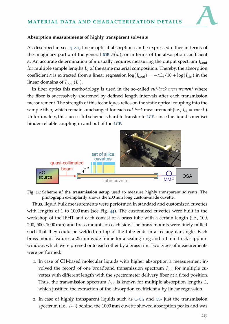
AM AT E R I A L D ATA A N D C H A R A C T E R I Z AT I O N D E TA I L S
Absorption measurements of highly transparent solvents
As described in sec. 3.2.1, linear optical absorption can be expressed either in terms of
the imaginary part κ of the general IOR n(ω), or in terms of the absorption coefficient
α. An accurate determination of α usually requires measuring the output spectrum Ii,out
for multiple sample lengths Li of the same material composition. Thereby, the absorption
coefficient α is extracted from a linear regression log(Ii,out) = −αLi/10 + log(Ii,in) in the
linear domains of Ii,out(Li).
In fiber optics this methodology is used in the so-called cut-back measurement where
the fiber is successively shortened by defined length intervals after each transmission
measurement. The strength of this techniques relies on the static optical coupling into the
sample fiber, which remains unchanged for each cut-back measurement (i.e., Iin = const.).
Unfortunately, this successful scheme is hard to transfer to LCFs since the liquid’s menisci
hinder reliable coupling in and out of the LCF.
tube cuvette
set of silicacuvettes
SCsource OSA
quasi-collimatedbeam
MMF
Fig. 44: Scheme of the transmission setup used to measure highly transparent solvents. Thephotograph exemplarily shows the 200 mm long custom-made cuvette.
Thus, liquid bulk measurements were performed in standard and customized cuvettes
with lengths of 1 to 1000 mm (see Fig. 44). The customized cuvettes were built in the
workshop of the IPHT and each consist of a brass tube with a certain length (i.e., 100,
200, 500, 1000 mm) and brass mounts on each side. The brass mounts were finely milled
such that they could be welded on top of the tube ends in a rectangular angle. Each
brass mount features a 25 mm wide frame for a sealing ring and a 1 mm thick sapphire
window, which were pressed onto each other by a brass rim. Two types of measurements
were performed:
1. In case of CH-based molecular liquids with higher absorption a measurement in-
volved the record of one broadband transmission spectrum Iout for multiple cu-
vettes with different length with the spectrometer delivery fiber at a fixed position.
Thus, the transmission spectrum Iout is known for multiple absorption lengths L,
which justified the extraction of the absorption coefficient α by linear regression.
2. In case of highly transparent liquids such as C2Cl4 and CS2 just the transmission
spectrum (i.e., Iout) behind the 1000 mm cuvette showed absorption peaks and was
117
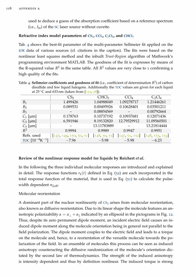
118 appendix a
used to deduce a guess of the absorption coefficient based on a reference spectrum
(i.e., Iin) of the SC laser source without cuvette.
Refractive index model parameters of CS2, CCl4, C2Cl4, and CHCl3
Tab. 4 shows the best-fit parameter of the multi-parameter Sellmeier fit applied on the
IOR data of various sources (cf. citations in the caption). The fits were based on the
nonlinear least squares method and the inbuilt Trust-Region algorithm of Mathwork’s
programming environment MATLAB. The goodness of the fit is expresses by means of
the R-squared value R2 in the same table. All R2 values are very close to 1 confirming a
high quality of the fits.
Table 4: Sellmeier coefficients and goodness of fit (i.e., coefficient of determination R2) of carbondisulfide and few liquid halogens. Additionally the TOC values are given for each liquidat 25 C and 633 nm (taken from [152, 58]).
CS2 CHCl3 CCl4 C2Cl4B1 1.499426 1.04988049 1.09278717 1.21446261B2 0.089531 0.00495926 0.10628401 0.03501211B3 – 0.08854569 – 0.00792664C1 [µm] 0.178763 0.10737192 0.10937681 0.12071436C2 [µm] 6.591946 8.19132820 12.79529912 11.09560501C3 [µm] – 13.11783889 – 13.21814444R2 0.9994 0.9989 0.9947 0.9951Refs. used [147, 149, 150, 50, 51] [148, 50, 51] [147, 51, 152] [148, 153, 154]TOC [10−4K−1] −7.96 −5.98 −5.98 −6.23
Review of the nonlinear response model for liquids by Reichert et al.
In the following the three individual molecular responses are introduced and explained
in detail. The response functions rk(t) defined in Eq. (52) are each incorporated in the
total response function of the material, that is used in Eq. (51) to calculate the pulse-
width dependent n2,eff.
Molecular reorientation
A dominant part of the nuclear nonlinearity of CS2 arises from molecular reorientation,
also known as diffusive reorientation. Due to its linear shape the molecule features an an-
isotropic polarizability α = α⊥ + α‖ indicated by an ellipsoid in the pictograms in Fig. 12.
Thus, despite its zero permanent dipole moment, an incident electric field causes an in-
duced dipole moment along the molecule orientation being in general not parallel to the
field polarization. The dipole moment couples to the electric field and leads to a torque
on the molecule and, hence, to a reorientation of the versatile molecule towards the po-
larization of the field. In an ensemble of molecules this process can be seen as induced
anisotropy counteracting the diffusive randomization of the molecule’s orientation dic-
tated by the second law of thermodynamics. The strength of the induced anisotropy
is intensity dependent and thus by definition nonlinear. The induced torque is strong
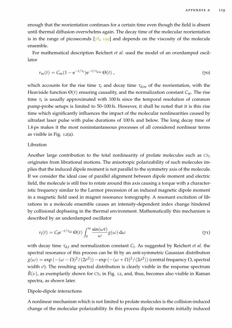
appendix a 119
enough that the reorientation continues for a certain time even though the field is absent
until thermal diffusion overwhelms again. The decay time of the molecular reorientation
is in the range of picoseconds [78, 199] and depends on the viscosity of the molecule
ensemble.
For mathematical description Reichert et al. used the model of an overdamped oscil-
lator
rre(t) = Cre(1 − e−t/τr)e−t/τd,re Θ(t) , (70)
which accounts for the rise time τr and decay time τd,re of the reorientation, with the
Heaviside function Θ(t) ensuring causality, and the normalization constant Cre. The rise
time τr is usually approximated with 100 fs since the temporal resolution of common
pump-probe setups is limited to 50–100 fs. However, it shall be noted that it is this rise
time which significantly influences the impact of the molecular nonlinearities caused by
ultrafast laser pulse with pulse durations of 100 fs and below. The long decay time of
1.6 ps makes it the most noninstantaneous processes of all considered nonlinear terms
as visible in Fig. 12(a).
Libration
Another large contribution to the total nonlinearity of prolate molecules such as CS2
originates from librational motions. The anisotropic polarizability of such molecules im-
plies that the induced dipole moment is not parallel to the symmetry axis of the molecule.
If we consider the ideal case of parallel alignment between dipole moment and electric
field, the molecule is still free to rotate around this axis causing a torque with a character-
istic frequency similar to the Larmor precession of an induced magnetic dipole moment
in a magnetic field used in magnet resonance tomography. A resonant excitation of lib-
rations in a molecule ensemble causes an intensity-dependent index change hindered
by collisional dephasing in the thermal environment. Mathematically this mechanism is
described by an underdamped oscillator
rl(t) = Cle−t/τd,l Θ(t)
∫ ∞
0
sin(ωt)
ωg(ω)dω (71)
with decay time τd,l and normalization constant Cl. As suggested by Reichert et al. the
spectral resonance of this process can be fit by an anti-symmetric Gaussian distribution
g(ω) = exp (−(ω − Ω)2/(2σ2))− exp (−(ω + Ω)2/(2σ2)) (central frequency Ω, spectral
width σ). The resulting spectral distribution is clearly visible in the response spectrum
R(ν), as exemplarily shown for CS2 in Fig. 12, and, thus, becomes also visible in Raman
spectra, as shown later.
Dipole-dipole interactions
A nonlinear mechanism which is not limited to prolate molecules is the collision-induced
change of the molecular polarizability. In this process dipole moments initially induced
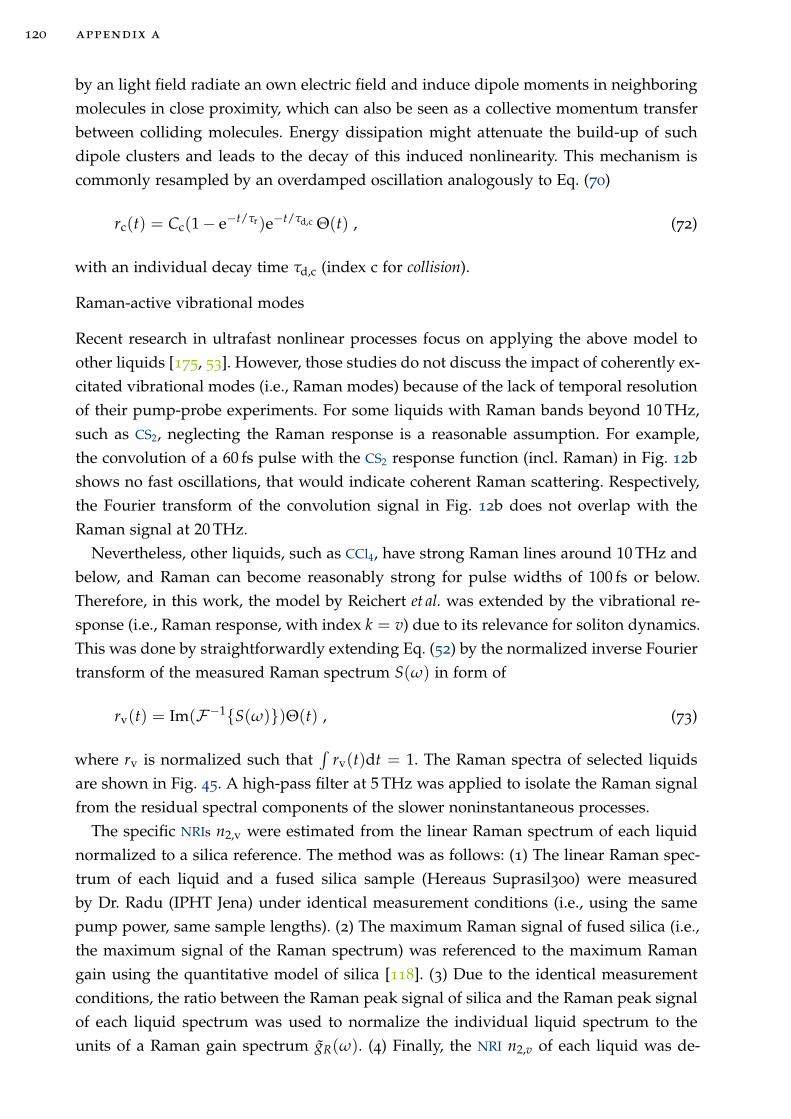
120 appendix a
by an light field radiate an own electric field and induce dipole moments in neighboring
molecules in close proximity, which can also be seen as a collective momentum transfer
between colliding molecules. Energy dissipation might attenuate the build-up of such
dipole clusters and leads to the decay of this induced nonlinearity. This mechanism is
commonly resampled by an overdamped oscillation analogously to Eq. (70)
rc(t) = Cc(1 − e−t/τr)e−t/τd,c Θ(t) , (72)
with an individual decay time τd,c (index c for collision).
Raman-active vibrational modes
Recent research in ultrafast nonlinear processes focus on applying the above model to
other liquids [175, 53]. However, those studies do not discuss the impact of coherently ex-
citated vibrational modes (i.e., Raman modes) because of the lack of temporal resolution
of their pump-probe experiments. For some liquids with Raman bands beyond 10 THz,
such as CS2, neglecting the Raman response is a reasonable assumption. For example,
the convolution of a 60 fs pulse with the CS2 response function (incl. Raman) in Fig. 12b
shows no fast oscillations, that would indicate coherent Raman scattering. Respectively,
the Fourier transform of the convolution signal in Fig. 12b does not overlap with the
Raman signal at 20 THz.
Nevertheless, other liquids, such as CCl4, have strong Raman lines around 10 THz and
below, and Raman can become reasonably strong for pulse widths of 100 fs or below.
Therefore, in this work, the model by Reichert et al. was extended by the vibrational re-
sponse (i.e., Raman response, with index k = v) due to its relevance for soliton dynamics.
This was done by straightforwardly extending Eq. (52) by the normalized inverse Fourier
transform of the measured Raman spectrum S(ω) in form of
rv(t) = Im(F−1S(ω))Θ(t) , (73)
where rv is normalized such that∫
rv(t)dt = 1. The Raman spectra of selected liquids
are shown in Fig. 45. A high-pass filter at 5 THz was applied to isolate the Raman signal
from the residual spectral components of the slower noninstantaneous processes.
The specific NRIs n2,v were estimated from the linear Raman spectrum of each liquid
normalized to a silica reference. The method was as follows: (1) The linear Raman spec-
trum of each liquid and a fused silica sample (Hereaus Suprasil300) were measured
by Dr. Radu (IPHT Jena) under identical measurement conditions (i.e., using the same
pump power, same sample lengths). (2) The maximum Raman signal of fused silica (i.e.,
the maximum signal of the Raman spectrum) was referenced to the maximum Raman
gain using the quantitative model of silica [118]. (3) Due to the identical measurement
conditions, the ratio between the Raman peak signal of silica and the Raman peak signal
of each liquid spectrum was used to normalize the individual liquid spectrum to the
units of a Raman gain spectrum gR(ω). (4) Finally, the NRI n2,v of each liquid was de-
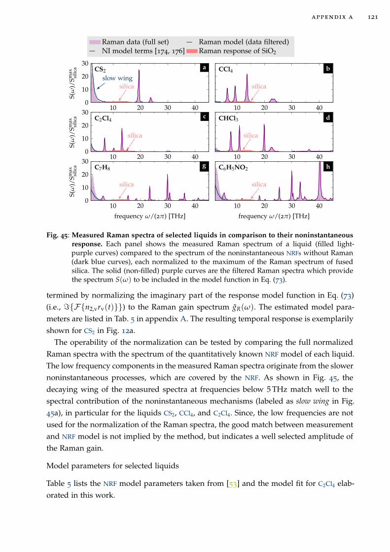
appendix a 121
silicaslow wing
10 20 30 400
10
20
30S(
ω)/
Smax
silic
a
Raman data (full set) Raman model (data filtered)NI model terms [174, 176] Raman response of SiO2
silica
10 20 30 40
silica
10 20 30 400
10
20
30
S(ω
)/Sm
axsi
lica
silica
10 20 30 40
silica
10 20 30 400
10
20
30
frequency ω/(2π) [THz]
S(ω
)/Sm
axsi
lica
silica
10 20 30 40
frequency ω/(2π) [THz]
aCS2 bCCl4
cC2Cl4 dCHCl3
gC7H8 hC6H5NO2
Fig. 45: Measured Raman spectra of selected liquids in comparison to their noninstantaneousresponse. Each panel shows the measured Raman spectrum of a liquid (filled light-purple curves) compared to the spectrum of the noninstantaneous NRFs without Raman(dark blue curves), each normalized to the maximum of the Raman spectrum of fusedsilica. The solid (non-filled) purple curves are the filtered Raman spectra which providethe spectrum S(ω) to be included in the model function in Eq. (73).
termined by normalizing the imaginary part of the response model function in Eq. (73)
(i.e., ℑFn2,vrv(t)) to the Raman gain spectrum gR(ω). The estimated model para-
meters are listed in Tab. 5 in appendix A. The resulting temporal response is exemplarily
shown for CS2 in Fig. 12a.
The operability of the normalization can be tested by comparing the full normalized
Raman spectra with the spectrum of the quantitatively known NRF model of each liquid.
The low frequency components in the measured Raman spectra originate from the slower
noninstantaneous processes, which are covered by the NRF. As shown in Fig. 45, the
decaying wing of the measured spectra at frequencies below 5 THz match well to the
spectral contribution of the noninstantaneous mechanisms (labeled as slow wing in Fig.
45a), in particular for the liquids CS2, CCl4, and C2Cl4. Since, the low frequencies are not
used for the normalization of the Raman spectra, the good match between measurement
and NRF model is not implied by the method, but indicates a well selected amplitude of
the Raman gain.
Model parameters for selected liquids
Table 5 lists the NRF model parameters taken from [53] and the model fit for C2Cl4 elab-
orated in this work.
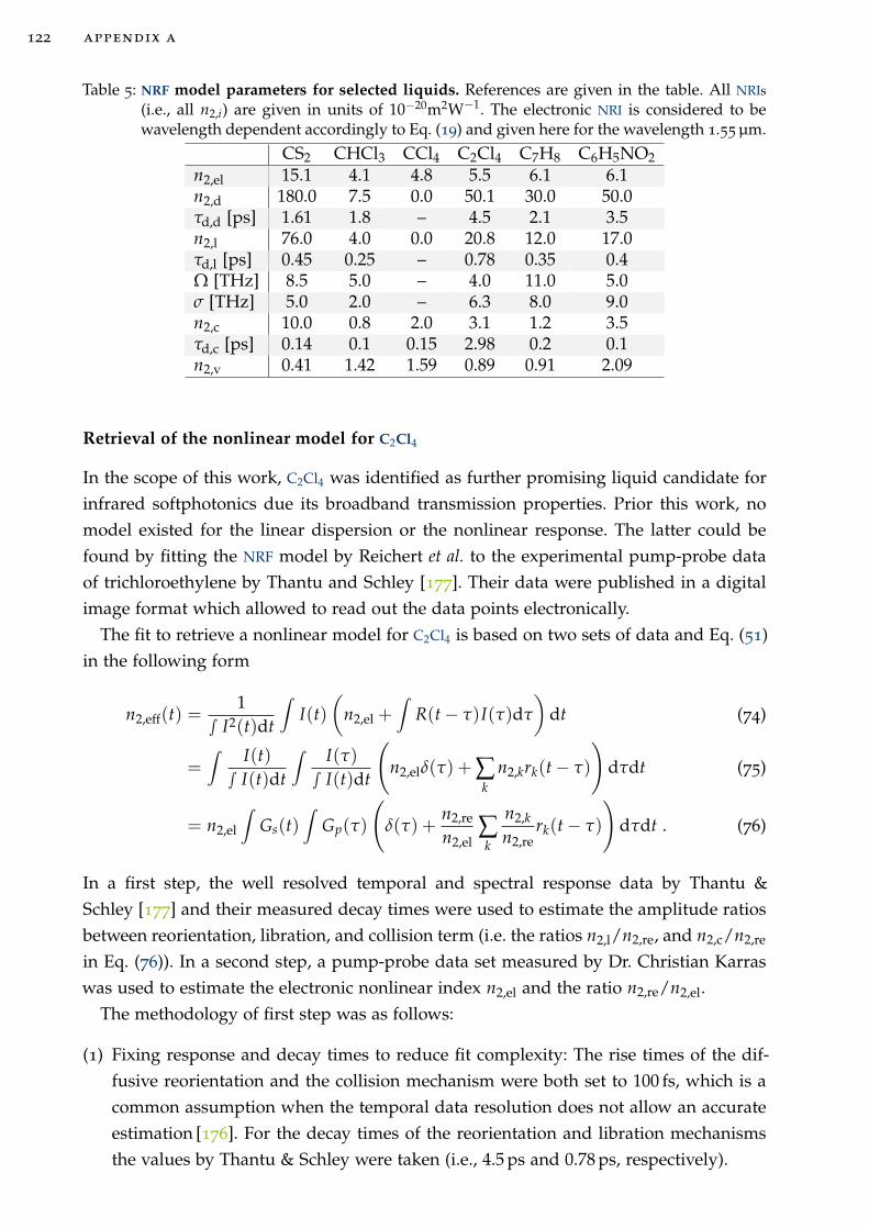
122 appendix a
Table 5: NRF model parameters for selected liquids. References are given in the table. All NRIs
(i.e., all n2,i) are given in units of 10−20m2W−1. The electronic NRI is considered to bewavelength dependent accordingly to Eq. (19) and given here for the wavelength 1.55 µm.
CS2 CHCl3 CCl4 C2Cl4 C7H8 C6H5NO2n2,el 15.1 4.1 4.8 5.5 6.1 6.1n2,d 180.0 7.5 0.0 50.1 30.0 50.0τd,d [ps] 1.61 1.8 – 4.5 2.1 3.5n2,l 76.0 4.0 0.0 20.8 12.0 17.0τd,l [ps] 0.45 0.25 – 0.78 0.35 0.4Ω [THz] 8.5 5.0 – 4.0 11.0 5.0σ [THz] 5.0 2.0 – 6.3 8.0 9.0n2,c 10.0 0.8 2.0 3.1 1.2 3.5τd,c [ps] 0.14 0.1 0.15 2.98 0.2 0.1n2,v 0.41 1.42 1.59 0.89 0.91 2.09
Retrieval of the nonlinear model for C2Cl4
In the scope of this work, C2Cl4 was identified as further promising liquid candidate for
infrared softphotonics due its broadband transmission properties. Prior this work, no
model existed for the linear dispersion or the nonlinear response. The latter could be
found by fitting the NRF model by Reichert et al. to the experimental pump-probe data
of trichloroethylene by Thantu and Schley [177]. Their data were published in a digital
image format which allowed to read out the data points electronically.
The fit to retrieve a nonlinear model for C2Cl4 is based on two sets of data and Eq. (51)
in the following form
n2,eff(t) =1
∫ I2(t)dt
∫
I(t)
(
n2,el +∫
R(t − τ)I(τ)dτ
)
dt (74)
=∫
I(t)
∫ I(t)dt
∫I(τ)
∫ I(t)dt
(
n2,elδ(τ) + ∑k
n2,krk(t − τ)
)
dτdt (75)
= n2,el
∫
Gs(t)∫
Gp(τ)
(
δ(τ) +n2,re
n2,el∑k
n2,k
n2,rerk(t − τ)
)
dτdt . (76)
In a first step, the well resolved temporal and spectral response data by Thantu &
Schley [177] and their measured decay times were used to estimate the amplitude ratios
between reorientation, libration, and collision term (i.e. the ratios n2,l/n2,re, and n2,c/n2,re
in Eq. (76)). In a second step, a pump-probe data set measured by Dr. Christian Karras
was used to estimate the electronic nonlinear index n2,el and the ratio n2,re/n2,el.
The methodology of first step was as follows:
(1) Fixing response and decay times to reduce fit complexity: The rise times of the dif-
fusive reorientation and the collision mechanism were both set to 100 fs, which is a
common assumption when the temporal data resolution does not allow an accurate
estimation [176]. For the decay times of the reorientation and libration mechanisms
the values by Thantu & Schley were taken (i.e., 4.5 ps and 0.78 ps, respectively).
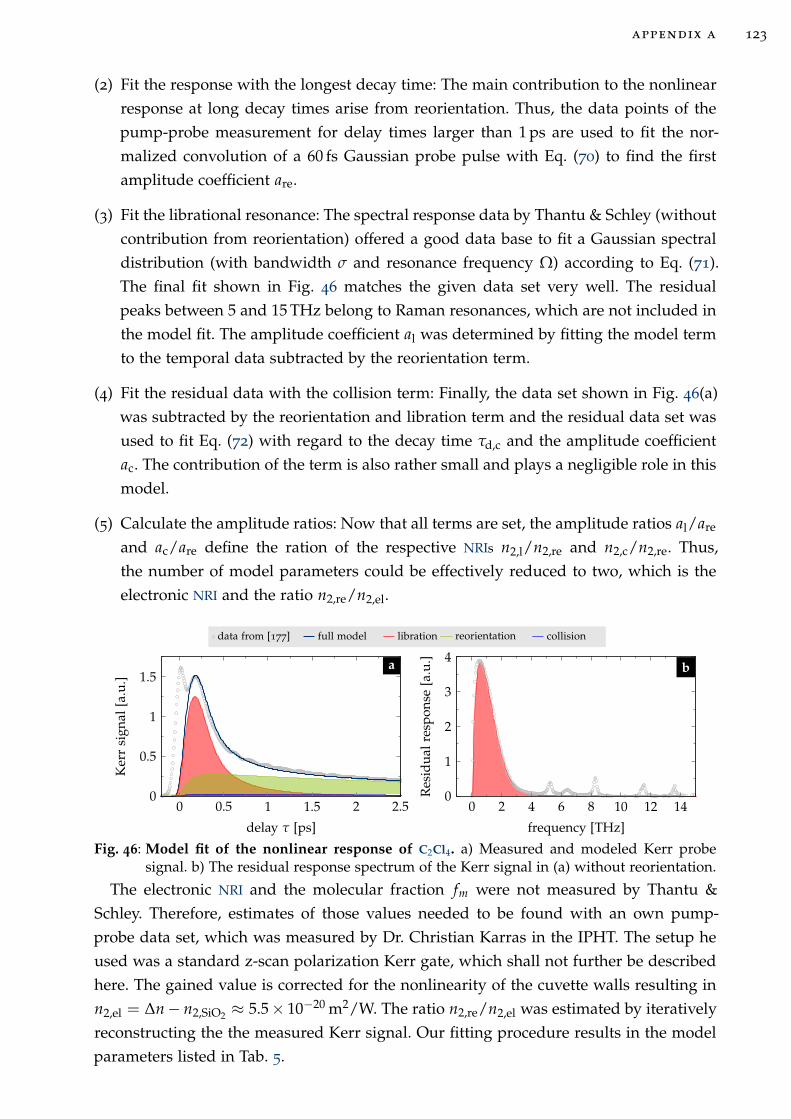
appendix a 123
(2) Fit the response with the longest decay time: The main contribution to the nonlinear
response at long decay times arise from reorientation. Thus, the data points of the
pump-probe measurement for delay times larger than 1 ps are used to fit the nor-
malized convolution of a 60 fs Gaussian probe pulse with Eq. (70) to find the first
amplitude coefficient are.
(3) Fit the librational resonance: The spectral response data by Thantu & Schley (without
contribution from reorientation) offered a good data base to fit a Gaussian spectral
distribution (with bandwidth σ and resonance frequency Ω) according to Eq. (71).
The final fit shown in Fig. 46 matches the given data set very well. The residual
peaks between 5 and 15 THz belong to Raman resonances, which are not included in
the model fit. The amplitude coefficient al was determined by fitting the model term
to the temporal data subtracted by the reorientation term.
(4) Fit the residual data with the collision term: Finally, the data set shown in Fig. 46(a)
was subtracted by the reorientation and libration term and the residual data set was
used to fit Eq. (72) with regard to the decay time τd,c and the amplitude coefficient
ac. The contribution of the term is also rather small and plays a negligible role in this
model.
(5) Calculate the amplitude ratios: Now that all terms are set, the amplitude ratios al/are
and ac/are define the ration of the respective NRIs n2,l/n2,re and n2,c/n2,re. Thus,
the number of model parameters could be effectively reduced to two, which is the
electronic NRI and the ratio n2,re/n2,el.
0 0.5 1 1.5 2 2.50
0.5
1
1.5
delay τ [ps]
Ker
rsi
gnal
[a.u
.]
data from [177] full model libration reorientation collision
0 2 4 6 8 10 12 140
1
2
3
4
frequency [THz]
Res
idu
alre
spon
se[a
.u.]a b
Fig. 46: Model fit of the nonlinear response of C2Cl4. a) Measured and modeled Kerr probesignal. b) The residual response spectrum of the Kerr signal in (a) without reorientation.
The electronic NRI and the molecular fraction fm were not measured by Thantu &
Schley. Therefore, estimates of those values needed to be found with an own pump-
probe data set, which was measured by Dr. Christian Karras in the IPHT. The setup he
used was a standard z-scan polarization Kerr gate, which shall not further be described
here. The gained value is corrected for the nonlinearity of the cuvette walls resulting in
n2,el = ∆n − n2,SiO2 ≈ 5.5× 10⁻²⁰ m2/W. The ratio n2,re/n2,el was estimated by iteratively
reconstructing the the measured Kerr signal. Our fitting procedure results in the model
parameters listed in Tab. 5.
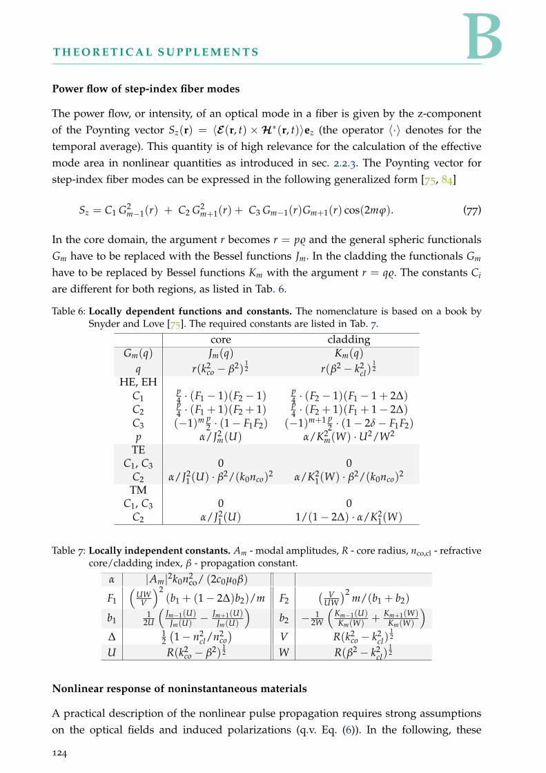
BT H E O R E T I C A L S U P P L E M E N T S
Power flow of step-index fiber modes
The power flow, or intensity, of an optical mode in a fiber is given by the z-component
of the Poynting vector Sz(r) = 〈E(r, t) ×H∗(r, t)〉ez (the operator 〈·〉 denotes for the
temporal average). This quantity is of high relevance for the calculation of the effective
mode area in nonlinear quantities as introduced in sec. 2.2.3. The Poynting vector for
step-index fiber modes can be expressed in the following generalized form [75, 84]
Sz = C1 G2m−1(r) + C2 G2
m+1(r) + C3 Gm−1(r)Gm+1(r) cos(2mϕ). (77)
In the core domain, the argument r becomes r = p and the general spheric functionals
Gm have to be replaced with the Bessel functions Jm. In the cladding the functionals Gm
have to be replaced by Bessel functions Km with the argument r = q. The constants Ci
are different for both regions, as listed in Tab. 6.
Table 6: Locally dependent functions and constants. The nomenclature is based on a book bySnyder and Love [75]. The required constants are listed in Tab. 7.
core claddingGm(q) Jm(q) Km(q)
q r(k2co − β2)
12 r(β2 − k2
cl)12
HE, EHC1
p4 · (F1 − 1)(F2 − 1) p
4 · (F2 − 1)(F1 − 1 + 2∆)C2
p4 · (F1 + 1)(F2 + 1) p
4 · (F2 + 1)(F1 + 1 − 2∆)C3 (−1)m p
2 · (1 − F1F2) (−1)m+1 p2 · (1 − 2δ − F1F2)
p α/J2m(U) α/K2
m(W) · U2/W2
TEC1, C3 0 0
C2 α/J21(U) · β2/(k0nco)2 α/K2
1(W) · β2/(k0nco)2
TMC1, C3 0 0
C2 α/J21(U) 1/(1 − 2∆) · α/K2
1(W)
Table 7: Locally independent constants. Am - modal amplitudes, R - core radius, nco,cl - refractivecore/cladding index, β - propagation constant.
α |Am|2k0n2co/ (2c0µ0β)
F1
(UW
V
)2(b1 + (1 − 2∆)b2)/m F2
(V
UW
)2m/(b1 + b2)
b11
2U
(Jm−1(U)
Jm(U)− Jm+1(U)
Jm(U)
)
b2 − 12W
(Km−1(U)Km(W)
+ Km+1(W)Km(W)
)
∆ 12
(1 − n2
cl/n2co
)V R(k2
co − k2cl)
12
U R(k2co − β2)
12 W R(β2 − k2
cl)12
Nonlinear response of noninstantaneous materials
A practical description of the nonlinear pulse propagation requires strong assumptions
on the optical fields and induced polarizations (q.v. Eq. (6)). In the following, these
124

appendix b 125
assumptions are introduced and applied to deduce a practical form of the nonlinear
polarization for partly noninstantaneous nonlinear media (e.g. Raman media).
The third-order nonlinear contribution to the total polarization in Eq. (6) can be written
in the most general vectorial form in the frequency domain [78]
Pi,NL(ω) = ε0C(3) ∑jkl
χ(3)ijkl(ω; ω′, ω′′, ω′′′)Ej(ω
′)Ek(ω′′)El(ω
′′′) , (78)
with the permutation factor C(3). The sum over the polarization components j, k, l will
not be written in the following according to the Einstein summation convention.
Fourier-transforming Eq. (78) leads to the general temporal expression of the third-
order nonlinear polarization [79, 78]
Pi,NL(t) = ε0
t∫
−∞
dτ1
t∫
−∞
dτ2
t∫
−∞
dτ3Rijkl(t − τ1, t − τ2, t − τ3)Ej(τ1)Ek(τ2)El(τ3) (79)
with the nonlinear response function Rijkl being the Fourier transform of the third-order
susceptibility
Rijkl(τ1, τ2, τ3) = C(3)∞∫
−∞
dω′∞∫
−∞
dω′′∞∫
−∞
dω′′′χ(3)ijkl(ω; ω′, ω′′, ω′′′)
× e−iω′τ1e−iω′′τ2e−iω′′′τ3 .(80)
The integration limits in Eq. (79) are chosen such, that the response term fulfills the
principles of causality, i.e., it is zero for all negative times. The response function can be a
linear combination of different nonlinear contributions, such as instantaneous electronic
motions and noninstantaneous nuclear effects (e.g., stimulated Raman scattering), i.e.,
Rijkl = Relijkl + Rmol
ijkl . In case of electronic effects, Relijkl can be expressed as product of
Kronecker delta functions [200, 201]: Relijkl = 3χel
ijklδ(τ1)δ(τ2)δ(τ3). The reader should
note, that the factor 3 is the permutation factor for the optical Kerr effect. Thus, only the
terms for PNL(ω = ω + ω − ω) ∝ E E E∗ are considered in the following accordingly to
[78].
In case of noninstantaneous effects, the response function is known in the following
symmetric form [200, 201]
Rmolijkl (τ1, τ2, τ3) = χmol
ijkl [R(τ1)δ(τ2)δ(τ3 − τ1) + δ(τ1 − τ2)R(τ2)δ(τ3)
+ δ(τ1)δ(τ2 − τ3)R(τ3)] ,(81)
whereas R(t) includes the Heaviside function to ensure causality, and is normalized to∫
R(t)dt = 1. Physically, e.g., the term δ(τ1 − τ2)R(τ2)δ(τ3) means that the distortion is
created by the fields 1 and 2 at the moment τ2 before field 3 arrives at the later time τ3 to
126 appendix b
experience the nonlinearity [201]. Inserting Eq. (81) in the nonlinear polarization in Eq.
(79) yields the well-known Raman-Kerr expression [79]
Pi,NL(t) = 3ε0χmolijkl
[∫ ∞
−∞dτ R(t − τ)Ej(τ)E (∗)
k (τ)
]
El(t) . (82)
For the derivation of nonlinear pulse propagation equations, the frequency represent-
ation of Eq. (82) is useful, which is [81]
Pi,NL(ω) = 3ε0
∞∫
−∞
dω′∞∫
−∞
dω′′χ(3)ijkl(ω − ω′)Ej(ω
′′)E∗l (ω
′ + ω′′ − ω)Ek(ω′) . (83)
Eq. 83 can incorporate both electronic and molecular nonlinearities in a linear combina-
tion of the response terms, i.e., χ(3)ijkl(ω) = Fχel
ijklδ(t) + χmolijkl R(t).
The general polarization in Eq. (83) is still rather complicated, and further assumption
are needed to simplify this term. In general (i.e., materials with triclinic symmetry), the
third-order susceptibility tensor χ(3) has 81 nonzero and independent elements, which,
however, can be drastically reduced to 21 nonzero elements, of which only three are in-
dependent, when assuming isotropic (or weakly anisotropic) nonlinear materials [77, 78].
These three components can be further reduced to a single independent component as-
suming non-resonant nonlinear processes (i.e., lossless materials) and linearly polarized
intrapulse wave mixing (i.e., self-induced nonlinear refraction with ω = ω + ω − ω
and identical polarization of all involved fields, i.e., E/|E | = PNL/|PNL|). This relevant
single element is straightforwardly denoted as χ(3)eff = χ
(3)xxxx in the common literature
(e.g., [79]). Under those assumptions, it is valid to simplify Eq. (83) to
PNL(ω) = 3ε0χ(3)eff (ω)E(ω)E∗(ω)E(ω) , (84)
exemplarily for an instantaneous nonlinear medium.
Review of the semi-analytic solution of the noninstantaneous Schrödinger equation
The inhomogeneous linear differential equation Eq. (57) can be expressed as eigenvalue
equation. Therefore, the ansatz a(Z, T) = a(T) exp(ıβZ) was used to find the normalized
Conti eigenvalue equation [70]
βa+ 12sgn(β2)∂
2Ta = EaH(T)a(Z, T) , (85)
with normalized propagation constant β.
Equation (85) is an inhomogeneous eigenvalue equation and can be solved for very
special noninstantaneous cases analytically. In the analytical example by Conti et al. the
authors assumed a single exponential response function H(T) = Θ(T) exp(−T) to ap-
appendix b 127
proximate the noninstantaneous response of liquids. They found a set of linear solutions
of the mathematical form [70]
am(T) = N
exp(√
2βmT)
for T < 0
Jν
(√8Ea exp(−T/2)
)/Jν
(√8Ea
)for T > 0
(86)
with the bessel functions of the first kind Jν with the order ν =√
8βm, and the nor-
malization constant N , which can be found by imposing∫ ∞
−∞a(T)dT ≡ Ea/N2
R. The
eigenvalues βm are implicitly given by ∑∞n=0 (−2Ea)n/n!(
√8βm)n ≡ 0, where (x)n =
Γ(x + n)/Γ(x) is the rising factorial. This provides a dispersion relation β(Ea) and can
be solved numerically for a healthy parameter set, i.e., for small orders ν of the Bessel
function. The chosen normalization to the response time TR reduces the parameter space
to a single dimension, i.e., the normalized pulse energy Ea only, whereas it was possible
to discuss the general set of solutions by solely varying this parameter.
The first four modes of the solution set are exemplarily depicted for Ea = 300 in
Fig. 47(a). They may be classified by counting the number of nodes m (cf. labels in Fig.
47a), whereas higher mode numbers have smaller propagation constants, or eigenvalues,
respectively.
Fig. 47(b) shows the propagation constant β and the 1/e2 pulse width Te2 of all four
modes for pulse energies easily addressable by low- to medium-power lasers (i.e., Ep =
0.1 pJ. . . 100 nJ for CS2 with TR = 1.26 ps and γ0LR = 0.125). The propagation constants of
all modes converge towards an upper limit (q.v. red curve in Fig. 47(b)). This limit can be
found by pushing the noninstantaneous approximation even further to approximate the
field amplitude of the fundamental mode by a0(T) =√Eaδ(T − Tc), whereas the time
Tc marks the pulse center. Thus, the noninstantaneous term becomes E3/2a R(T)δ(T − Tc)
and with a transition of Eq. (85) to frequency space the condition is found
β =12
ω2s + EaR(Tc)
Ea→∞−−−→ EaR0 , (87)
where R0 = max(R(T)). The last asymptotic step is justified, since in the high-energy
limit the pulse center Tc tends into the minimum of the response potential. Thus, for
large energies the pulse underlies a maximum phase shift of R0Ea, which is in accordance
to the theoretical prediction by Conti et al. besides a factor of (2/π)2.
The phase discrimination of the individual modes decreases drastically for increasing
pulse energy, i.e., above Ea = 103 the modes are nearly indistinguishable which can be
understood as an increasing density of states to a continuum with increasing potential
depth (i.e., Ea). Necessary conditions for the excitation of linearons are given by the
validity of the noninstantaneous approximation being dependent on the pulse width
(i.e., TR/T0 ≫ 1). The pulse width of the states decreases from T0 & TR low energy to
T0 < TR. Thus, the solutions justify the noninstantaneous approximation increasingly
more for higher energies. The pulse energy Ea has to be chosen such that the calculated
states fulfill the noninstantaneous conditions (i.e., pulse width T0 ≪ response time TR).
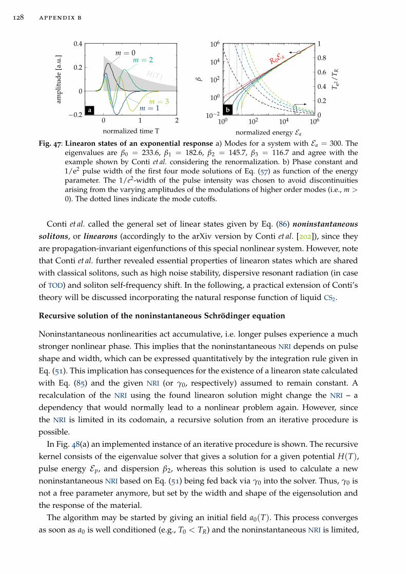
128 appendix b
H(T)
m = 0
m = 1
m = 2
m = 3
0 1 2−0.2
0
0.2
0.4
normalized time T
amp
litu
de
[a.u
.]
0 1 2 3
0
0.2
0.4
0.6
0.8
1
Te2
/T
R
R0E a
100 102 104 10610−2
100
102
104
106
normalized energy Ea
β
a b
Fig. 47: Linearon states of an exponential response a) Modes for a system with Ea = 300. Theeigenvalues are β0 = 233.6, β1 = 182.6, β2 = 145.7, β3 = 116.7 and agree with theexample shown by Conti et al. considering the renormalization. b) Phase constant and1/e2 pulse width of the first four mode solutions of Eq. (57) as function of the energyparameter. The 1/e2-width of the pulse intensity was chosen to avoid discontinuitiesarising from the varying amplitudes of the modulations of higher order modes (i.e., m >
0). The dotted lines indicate the mode cutoffs.
Conti et al. called the general set of linear states given by Eq. (86) noninstantaneous
solitons, or linearons (accordingly to the arXiv version by Conti et al. [202]), since they
are propagation-invariant eigenfunctions of this special nonlinear system. However, note
that Conti et al. further revealed essential properties of linearon states which are shared
with classical solitons, such as high noise stability, dispersive resonant radiation (in case
of TOD) and soliton self-frequency shift. In the following, a practical extension of Conti’s
theory will be discussed incorporating the natural response function of liquid CS2.
Recursive solution of the noninstantaneous Schrödinger equation
Noninstantaneous nonlinearities act accumulative, i.e. longer pulses experience a much
stronger nonlinear phase. This implies that the noninstantaneous NRI depends on pulse
shape and width, which can be expressed quantitatively by the integration rule given in
Eq. (51). This implication has consequences for the existence of a linearon state calculated
with Eq. (85) and the given NRI (or γ0, respectively) assumed to remain constant. A
recalculation of the NRI using the found linearon solution might change the NRI – a
dependency that would normally lead to a nonlinear problem again. However, since
the NRI is limited in its codomain, a recursive solution from an iterative procedure is
possible.
In Fig. 48(a) an implemented instance of an iterative procedure is shown. The recursive
kernel consists of the eigenvalue solver that gives a solution for a given potential H(T),
pulse energy Ep, and dispersion β2, whereas this solution is used to calculate a new
noninstantaneous NRI based on Eq. (51) being fed back via γ0 into the solver. Thus, γ0 is
not a free parameter anymore, but set by the width and shape of the eigensolution and
the response of the material.
The algorithm may be started by giving an initial field a0(T). This process converges
as soon as a0 is well conditioned (e.g., T0 < TR) and the noninstantaneous NRI is limited,
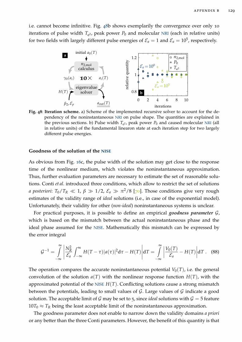
appendix b 129
i.e. cannot become infinitive. Fig. 48b shows exemplarily the convergence over only 10
iterations of pulse width Te2 , peak power P0 and molecular NRI (each in relative units)
for two fields with largely different pulse energies of Ea = 1 and Ea = 105, respectively.
initial a0(T)
n2,molcalculus
10×eigenvalue
solver
γ0(ai)
H(T)
β2, Ep
ai(T)
aout(T)
Ea =100
Ea =105
0 2 4 6 8 10
0.8
1
1.2
iterations
rela
tive
quan
tity
n2,molP0Te2
a
b
Fig. 48: Iteration scheme. a) Scheme of the implemented recursive solver to account for the de-pendency of the noninstantaneous NRI on pulse shape. The quantities are explained inthe previous sections. b) Pulse width Te2 , peak power P0 and caused molecular NRI (allin relative units) of the fundamental linearon state at each iteration step for two largelydifferent pulse energies.
Goodness of the solution of the NISE
As obvious from Fig. 16c, the pulse width of the solution may get close to the response
time of the nonlinear medium, which violates the noninstantaneous approximation.
Thus, further evaluation parameters are necessary to estimate the set of reasonable solu-
tions. Conti et al. introduced three conditions, which allow to restrict the set of solutions
a posteriori: T0/TR ≪ 1, β ≫ 1/2, Ea ≫ π2/8 [70]. Those conditions give very rough
estimates of the validity range of ideal solutions (i.e., in case of the exponential model).
Unfortunately, their validity for other (non-ideal) noninstantaneous systems is unclear.
For practical purposes, it is possible to define an empirical goodness parameter G,
which is based on the mismatch between the actual noninstantaneous phase and the
ideal phase assumed for the NISE. Mathematically this mismatch can be expressed by
the error integral
G−1 =
∞∫
−∞
∣∣∣∣∣
N2R
Ea
∫ ∞
−∞H(T − τ)|a(τ)|2dτ − H(T)
∣∣∣∣∣dT =
∞∫
−∞
∣∣∣∣
V0(T)
Ea− H(T)
∣∣∣∣dT . (88)
The operation compares the accurate noninstantaneous potential V0(T), i.e. the general
convolution of the solution a(T) with the nonlinear response function H(T), with the
approximated potential of the NISE H(T). Conflicting solutions cause a strong mismatch
between the potentials, leading to small values of G. Large values of G indicate a good
solution. The acceptable limit of G may be set to 5, since ideal solutions with G = 5 feature
10T0 ≈ TR being the least acceptable limit of the noninstantaneous approximation.
The goodness parameter does not enable to narrow down the validity domains a priori
or any better than the three Conti parameters. However, the benefit of this quantity is that
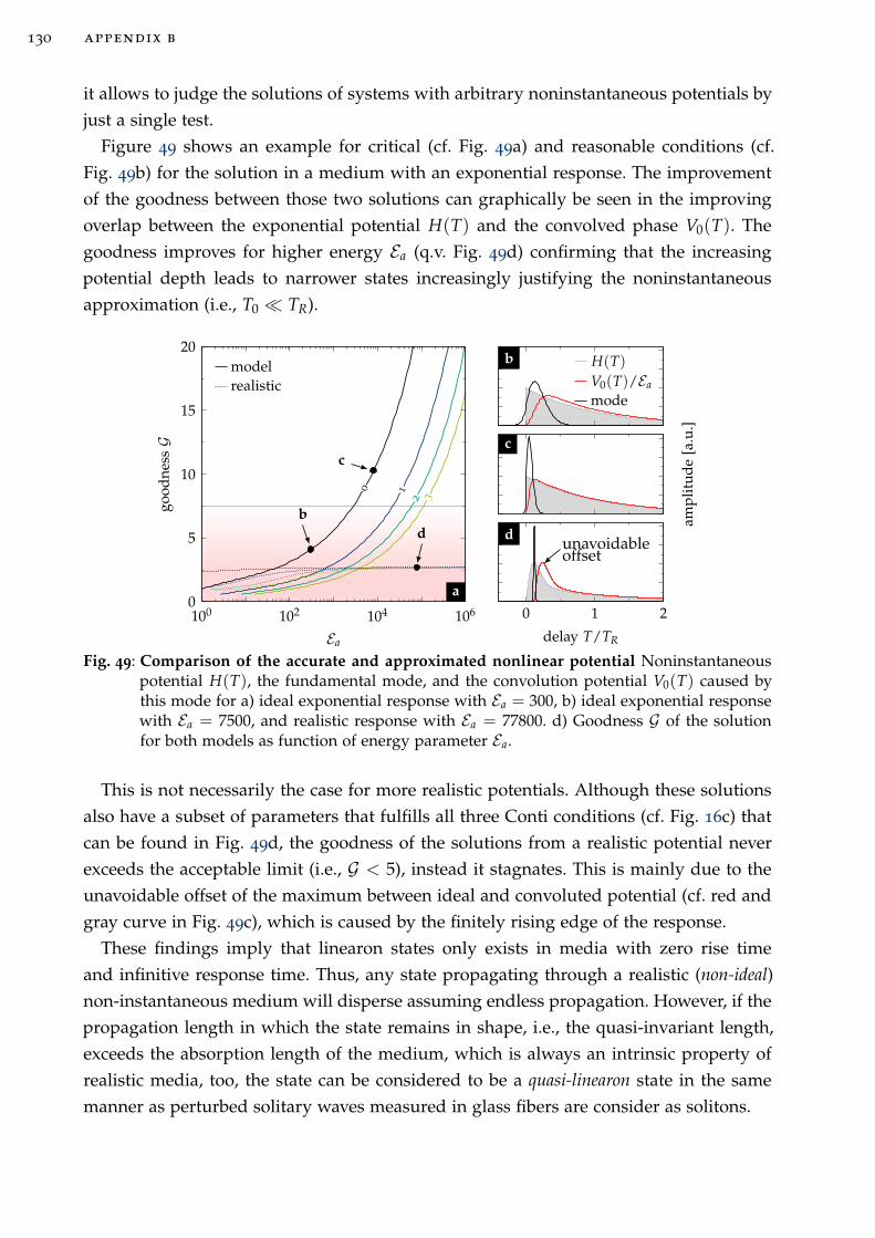
130 appendix b
it allows to judge the solutions of systems with arbitrary noninstantaneous potentials by
just a single test.
Figure 49 shows an example for critical (cf. Fig. 49a) and reasonable conditions (cf.
Fig. 49b) for the solution in a medium with an exponential response. The improvement
of the goodness between those two solutions can graphically be seen in the improving
overlap between the exponential potential H(T) and the convolved phase V0(T). The
goodness improves for higher energy Ea (q.v. Fig. 49d) confirming that the increasing
potential depth leads to narrower states increasingly justifying the noninstantaneous
approximation (i.e., T0 ≪ TR).
0
b
c
1
2 3
d
100 102 104 1060
5
10
15
20
Ea
good
ness
G
modelrealistic
H(T)
V0(T)/Ea
mode
amp
litu
de
[a.u
.]
unavoidableoffset
0 1 2
delay T/TR
b
c
d
a
Fig. 49: Comparison of the accurate and approximated nonlinear potential Noninstantaneouspotential H(T), the fundamental mode, and the convolution potential V0(T) caused bythis mode for a) ideal exponential response with Ea = 300, b) ideal exponential responsewith Ea = 7500, and realistic response with Ea = 77800. d) Goodness G of the solutionfor both models as function of energy parameter Ea.
This is not necessarily the case for more realistic potentials. Although these solutions
also have a subset of parameters that fulfills all three Conti conditions (cf. Fig. 16c) that
can be found in Fig. 49d, the goodness of the solutions from a realistic potential never
exceeds the acceptable limit (i.e., G < 5), instead it stagnates. This is mainly due to the
unavoidable offset of the maximum between ideal and convoluted potential (cf. red and
gray curve in Fig. 49c), which is caused by the finitely rising edge of the response.
These findings imply that linearon states only exists in media with zero rise time
and infinitive response time. Thus, any state propagating through a realistic (non-ideal)
non-instantaneous medium will disperse assuming endless propagation. However, if the
propagation length in which the state remains in shape, i.e., the quasi-invariant length,
exceeds the absorption length of the medium, which is always an intrinsic property of
realistic media, too, the state can be considered to be a quasi-linearon state in the same
manner as perturbed solitary waves measured in glass fibers are consider as solitons.
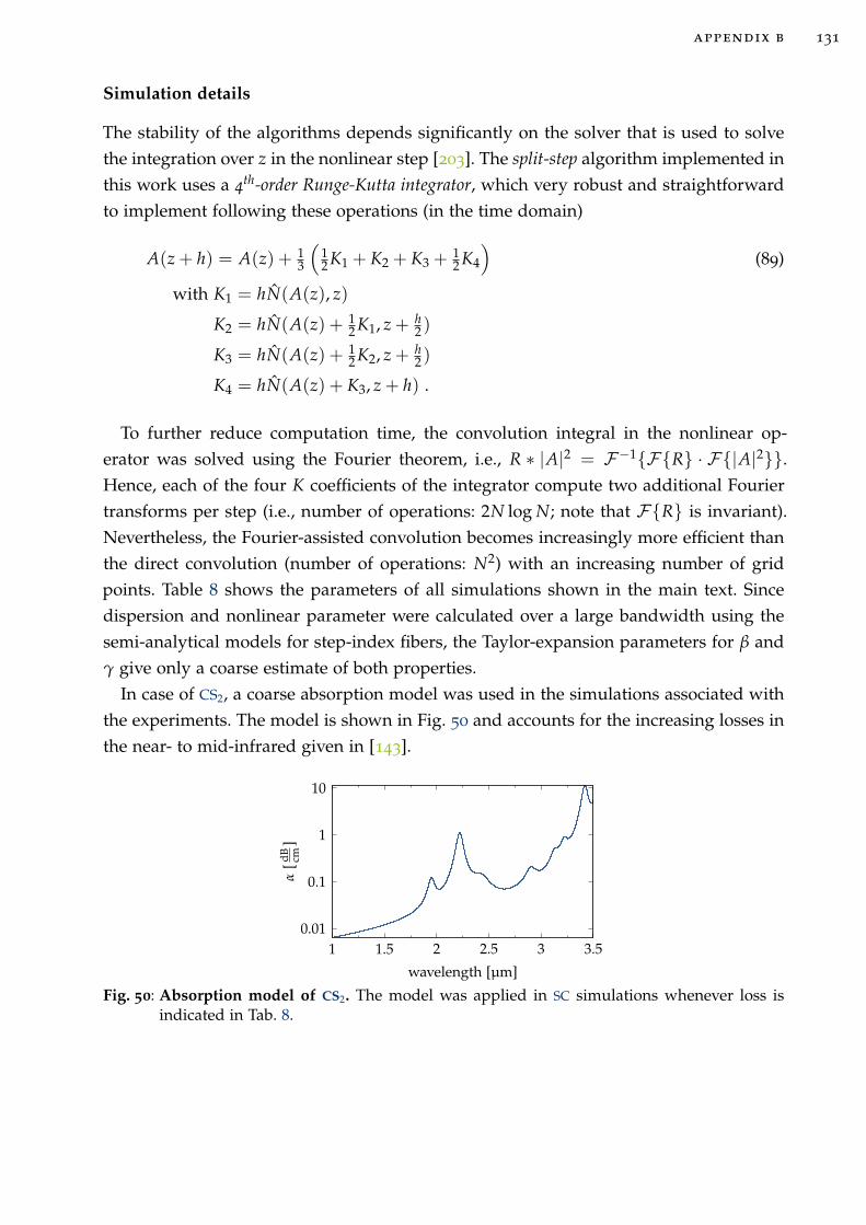
appendix b 131
Simulation details
The stability of the algorithms depends significantly on the solver that is used to solve
the integration over z in the nonlinear step [203]. The split-step algorithm implemented in
this work uses a 4th-order Runge-Kutta integrator, which very robust and straightforward
to implement following these operations (in the time domain)
A(z + h) = A(z) + 13
(12 K1 + K2 + K3 +
12 K4
)
(89)
with K1 = hN(A(z), z)
K2 = hN(A(z) + 12 K1, z + h
2 )
K3 = hN(A(z) + 12 K2, z + h
2 )
K4 = hN(A(z) + K3, z + h) .
To further reduce computation time, the convolution integral in the nonlinear op-
erator was solved using the Fourier theorem, i.e., R ∗ |A|2 = F−1FR · F|A|2.
Hence, each of the four K coefficients of the integrator compute two additional Fourier
transforms per step (i.e., number of operations: 2N log N; note that FR is invariant).
Nevertheless, the Fourier-assisted convolution becomes increasingly more efficient than
the direct convolution (number of operations: N2) with an increasing number of grid
points. Table 8 shows the parameters of all simulations shown in the main text. Since
dispersion and nonlinear parameter were calculated over a large bandwidth using the
semi-analytical models for step-index fibers, the Taylor-expansion parameters for β and
γ give only a coarse estimate of both properties.
In case of CS2, a coarse absorption model was used in the simulations associated with
the experiments. The model is shown in Fig. 50 and accounts for the increasing losses in
the near- to mid-infrared given in [143].
1 1.5 2 2.5 3 3.50.01
0.1
1
10
wavelength [µm]
α[d
Bcm
]
Fig. 50: Absorption model of CS2. The model was applied in SC simulations whenever loss isindicated in Tab. 8.
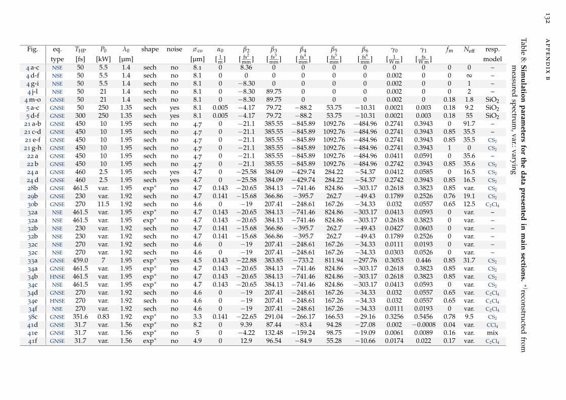
132
ap
pe
nd
ixb
Table8:S
imu
lationp
arameters
forth
ed
atap
resented
inm
ainsection
s.∗)reconstru
ctedfrom
measu
redsp
ectrum
,var.:varyingFig. eq. THP P0 λ0 shape noise co α0 β2 β3 β4 β5 β6 γ0 γ1 fm Neff resp.
type [fs] [kW] [µm] [µm] [ 1m ] [ fs2
mm ] [ fs3
mm ] [ fs4
mm ] [ fs5
mm ] [ fs6
mm ] [ 1W m ] [ fs
W m ] model4 a-c NSE 50 5.5 1.4 sech no 8.1 0 8.36 0 0 0 0 0 0 0 0 –4 d-f NSE 50 5.5 1.4 sech no 8.1 0 0 0 0 0 0 0.002 0 0 ∞ –4 g-i NSE 50 5.5 1.4 sech no 8.1 0 −8.30 0 0 0 0 0.002 0 0 1 –4 j-l NSE 50 21 1.4 sech no 8.1 0 −8.30 89.75 0 0 0 0.002 0 0 2 –
4 m-o GNSE 50 21 1.4 sech no 8.1 0 −8.30 89.75 0 0 0 0.002 0 0.18 1.8 SiO25 a-c GNSE 50 250 1.35 sech yes 8.1 0.005 −4.17 79.72 −88.2 53.75 −10.31 0.0021 0.003 0.18 9.2 SiO25 d-f GNSE 300 250 1.35 sech yes 8.1 0.005 −4.17 79.72 −88.2 53.75 −10.31 0.0021 0.003 0.18 55 SiO2
21 a-b GNSE 450 10 1.95 sech no 4.7 0 −21.1 385.55 −845.89 1092.76 −484.96 0.2741 0.3943 0 91.7 –21 c-d GNSE 450 10 1.95 sech no 4.7 0 −21.1 385.55 −845.89 1092.76 −484.96 0.2741 0.3943 0.85 35.5 –21 e-f GNSE 450 10 1.95 sech no 4.7 0 −21.1 385.55 −845.89 1092.76 −484.96 0.2741 0.3943 0.85 35.5 CS2
21 g-h GNSE 450 10 1.95 sech no 4.7 0 −21.1 385.55 −845.89 1092.76 −484.96 0.2741 0.3943 1 0 CS2
22 a GNSE 450 10 1.95 sech no 4.7 0 −21.1 385.55 −845.89 1092.76 −484.96 0.0411 0.0591 0 35.6 –22 b GNSE 450 10 1.95 sech no 4.7 0 −21.1 385.55 −845.89 1092.76 −484.96 0.2742 0.3943 0.85 35.6 CS2
24 a GNSE 460 2.5 1.95 sech yes 4.7 0 −25.58 384.09 −429.74 284.22 −54.37 0.0412 0.0585 0 16.5 CS2
24 d GNSE 460 2.5 1.95 sech yes 4.7 0 −25.58 384.09 −429.74 284.22 −54.37 0.2742 0.3943 0.85 16.5 CS2
28b GNSE 461.5 var. 1.95 exp∗ no 4.7 0.143 −20.65 384.13 −741.46 824.86 −303.17 0.2618 0.3823 0.85 var. CS2
29b GNSE 230 var. 1.92 sech no 4.7 0.141 −15.68 366.86 −395.7 262.7 −49.43 0.1789 0.2526 0.76 19.1 CS2
30b GNSE 270 11.5 1.92 sech no 4.6 0 −19 207.41 −248.61 167.26 −34.33 0.032 0.0557 0.65 12.5 C2Cl432a NSE 461.5 var. 1.95 exp∗ no 4.7 0.143 −20.65 384.13 −741.46 824.86 −303.17 0.0413 0.0593 0 var. –32a NSE 461.5 var. 1.95 exp∗ no 4.7 0.143 −20.65 384.13 −741.46 824.86 −303.17 0.2618 0.3823 0 var. –32b NSE 230 var. 1.92 sech no 4.7 0.141 −15.68 366.86 −395.7 262.7 −49.43 0.0427 0.0603 0 var. –32b NSE 230 var. 1.92 sech no 4.7 0.141 −15.68 366.86 −395.7 262.7 −49.43 0.1789 0.2526 0 var. –32c NSE 270 var. 1.92 sech no 4.6 0 −19 207.41 −248.61 167.26 −34.33 0.0111 0.0193 0 var. –32c NSE 270 var. 1.92 sech no 4.6 0 −19 207.41 −248.61 167.26 −34.33 0.0303 0.0526 0 var. –33a GNSE 459.0 7 1.95 exp∗ yes 4.5 0.143 −22.88 383.85 −733.2 811.94 −297.76 0.3053 0.446 0.85 31.7 CS2
34a GNSE 461.5 var. 1.95 exp∗ no 4.7 0.143 −20.65 384.13 −741.46 824.86 −303.17 0.2618 0.3823 0.85 var. CS2
34b HNSE 461.5 var. 1.95 exp∗ no 4.7 0.143 −20.65 384.13 −741.46 824.86 −303.17 0.2618 0.3823 0.85 var. CS2
34c NSE 461.5 var. 1.95 exp∗ no 4.7 0.143 −20.65 384.13 −741.46 824.86 −303.17 0.0413 0.0593 0 var. CS2
34d GNSE 270 var. 1.92 sech no 4.6 0 −19 207.41 −248.61 167.26 −34.33 0.032 0.0557 0.65 var. C2Cl434e HNSE 270 var. 1.92 sech no 4.6 0 −19 207.41 −248.61 167.26 −34.33 0.032 0.0557 0.65 var. C2Cl434f NSE 270 var. 1.92 sech no 4.6 0 −19 207.41 −248.61 167.26 −34.33 0.0111 0.0193 0 var. C2Cl438c GNSE 351.6 0.83 1.92 exp∗ no 3.3 0.141 −22.65 291.04 −266.17 166.53 −29.16 0.3256 0.5456 0.78 9.5 CS2
41d GNSE 31.7 var. 1.56 exp∗ no 8.2 0 9.39 87.44 −83.4 94.28 −27.08 0.002 −0.0008 0.04 var. CCl441e GNSE 31.7 var. 1.56 exp∗ no 5 0 −4.22 132.48 −159.24 98.75 −19.09 0.0061 0.0089 0.16 var. mix41f GNSE 31.7 var. 1.56 exp∗ no 4.9 0 12.9 96.54 −84.9 55.28 −10.66 0.0174 0.022 0.17 var. C2Cl4
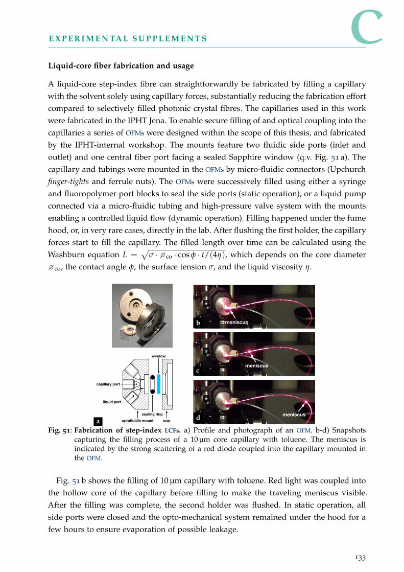
CE X P E R I M E N TA L S U P P L E M E N T S
Liquid-core fiber fabrication and usage
A liquid-core step-index fibre can straightforwardly be fabricated by filling a capillary
with the solvent solely using capillary forces, substantially reducing the fabrication effort
compared to selectively filled photonic crystal fibres. The capillaries used in this work
were fabricated in the IPHT Jena. To enable secure filling of and optical coupling into the
capillaries a series of OFMs were designed within the scope of this thesis, and fabricated
by the IPHT-internal workshop. The mounts feature two fluidic side ports (inlet and
outlet) and one central fiber port facing a sealed Sapphire window (q.v. Fig. 51 a). The
capillary and tubings were mounted in the OFMs by micro-fluidic connectors (Upchurch
finger-tights and ferrule nuts). The OFMs were successively filled using either a syringe
and fluoropolymer port blocks to seal the side ports (static operation), or a liquid pump
connected via a micro-fluidic tubing and high-pressure valve system with the mounts
enabling a controlled liquid flow (dynamic operation). Filling happened under the fume
hood, or, in very rare cases, directly in the lab. After flushing the first holder, the capillary
forces start to fill the capillary. The filled length over time can be calculated using the
Washburn equation L =√
σ ·co · cos φ · t/(4η), which depends on the core diameter
co, the contact angle φ, the surface tension σ, and the liquid viscosity η.
optofluidic mount cap
sealing ring
window
capillary port
liquid port
meniscus
meniscus
meniscus
a
b
ca d
c
b
Fig. 51: Fabrication of step-index LCFs. a) Profile and photograph of an OFM. b-d) Snapshotscapturing the filling process of a 10 µm core capillary with toluene. The meniscus isindicated by the strong scattering of a red diode coupled into the capillary mounted inthe OFM.
Fig. 51 b shows the filling of 10 µm capillary with toluene. Red light was coupled into
the hollow core of the capillary before filling to make the traveling meniscus visible.
After the filling was complete, the second holder was flushed. In static operation, all
side ports were closed and the opto-mechanical system remained under the hood for a
few hours to ensure evaporation of possible leakage.
133
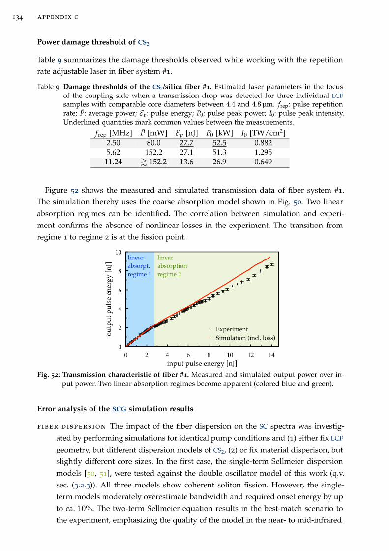
134 appendix c
Power damage threshold of CS2
Table 9 summarizes the damage thresholds observed while working with the repetition
rate adjustable laser in fiber system #1.
Table 9: Damage thresholds of the CS2/silica fiber #1. Estimated laser parameters in the focusof the coupling side when a transmission drop was detected for three individual LCF
samples with comparable core diameters between 4.4 and 4.8 µm. frep: pulse repetitionrate; P: average power; Ep: pulse energy; P0: pulse peak power; I0: pulse peak intensity.Underlined quantities mark common values between the measurements.
frep [MHz] P [mW] Ep [nJ] P0 [kW] I0 [TW/cm2]2.50 80.0 27.7 52.5 0.8825.62 152.2 27.1 51.3 1.29511.24 & 152.2 13.6 26.9 0.649
Figure 52 shows the measured and simulated transmission data of fiber system #1.
The simulation thereby uses the coarse absorption model shown in Fig. 50. Two linear
absorption regimes can be identified. The correlation between simulation and experi-
ment confirms the absence of nonlinear losses in the experiment. The transition from
regime 1 to regime 2 is at the fission point.
0 2 4 6 8 10 12 14
input pulse energy [nJ]
0
2
4
6
8
10
ou
tpu
t p
uls
e en
erg
y [
nJ]
Experiment
Simulation (incl. loss)
linear
absorpt.
regime 1
linear
absorption
regime 2
Fig. 52: Transmission characteristic of fiber #1. Measured and simulated output power over in-put power. Two linear absorption regimes become apparent (colored blue and green).
Error analysis of the SCG simulation results
fiber dispersion The impact of the fiber dispersion on the SC spectra was investig-
ated by performing simulations for identical pump conditions and (1) either fix LCF
geometry, but different dispersion models of CS2, (2) or fix material disperison, but
slightly different core sizes. In the first case, the single-term Sellmeier dispersion
models [50, 51], were tested against the double oscillator model of this work (q.v.
sec. (3.2.3)). All three models show coherent soliton fission. However, the single-
term models moderately overestimate bandwidth and required onset energy by up
to ca. 10%. The two-term Sellmeier equation results in the best-match scenario to
the experiment, emphasizing the quality of the model in the near- to mid-infrared.
appendix c 135
The second test was performed for three distinctly different core diameters close
to the experimental one (4.4 µm, 4.7 µm, 5.0 µm). Whereas the bandwidth shows
up to be relatively independent on variation of the core size, the onset energy
changes moderately in the order of 5% per 300 nm in this example. However, this
uncertainty was minimized in this work by using electron microscopes to measure
the core diameter with tens of nanometer precision.
nonlinear refractive index The most recent model of the nonlinear refractive in-
dex of CS2 has been included in the presented work (q.v. sec. 3.3.1), whereas the
model parameters were given with rather large error margins. Only small devi-
ations of the response function influence the NRI and, thus, the molecular fraction
fm, with a strong influence on bandwidth, fission length, and noise characteristics
of the SCs, especially for fm ≈ fequilm . For instance, Fig. 32 a shows the deviation
of the bandwidth evolution within the error margins of the CS2 model. Whereas
the influence on the maximum bandwidth is minor, a drastic variation of the onset
energy becomes apparent, which highlights the required accuracy of the response
model for presented SCG studies.
unknown losses Further reductions in bandwidth and onset energy are possible due
to additional linear losses at mid-infrared wavelengths or nonlinear losses, whereas
the latter become particularly dominant at lower wavelengths. The numerical solv-
ers applied here include only a very coarse numerical fit model for the linear ab-
sorption of CS2. However, a direct comparison of the input-to-output power charac-
teristics of fiber #1 (q.v. Fig. 52) shows an acceptable match between measurements
and simulations, and no evidence for an unknown dominant source of loss in the
experiment. Thus, a rough estimation of the system loss appears to be sufficient
to get the correct correlation between bandwidth and onset energy. These findings
also justify to neglect nonlinear losses in the propagation models.
pulse chirp Adding a quadratic spectral phase to the pump pulse at constant input
bandwidth (i.e., second-order chirp) impacts the SC bandwidth and onset energy,
whereas the bandwidth reaches maximum for a certain non-zero chirp [131]. Thus,
knowing and, in the best case, controlling the input chirp in the experiment is
necessary to obtain a reasonable match between measurements and simulations. In
this work, the pulse from laser system A can be assumed free from second-order
chirp due the phase compensation by the grating compressor. The residual third-
order phase of the pulse was included in the simulations and had a negligible
influence on the broadening process. The pulses from laser system B, however,
accumulated a relatively strong second-order phase from the last isolator. However,
assuming a chirp-free pulse with a pulse width corresponding to the measured
auto-correlation resulted in the best match between simulation and experiment, in
particular in case of fibers #4, #5, and #6. Thus, measuring the auto-correlation of
the input pulse is the bare minimum for relevant simulation results.


DA C K N O W L E D G E M E N T S
I thank Prof. Dr. Markus Schmidt for his excellent scientific support and dedicated ment-
oring throughout my entire PhD time.
I thank Prof. Dr. Limpert and his co-workers Dr. Fabian Stutzki, Martin Gebhardt, and
Christian Gaida for their scientific input and the opportunity to work with their world-
leading thulium fiber lasers.
I acknowledge the support by Dr. Falk Eilenberger, who introduced me to the numerical
methods to efficiently solve nonlinear propagation equations.
I acknowledge fruitful discussions with Prof. Dr. Claudio Conti and Prof. Dr. Fabio Bi-
ancalana about theoretical concepts and methods.
I am grateful for the theoretical hints by Prof. Dr. Ulf Peschel, that made me think more
carefully about claiming new soliton states.
I thank Prof. Dr. Christopher G. Poulton for many helpful discussions and particularly
for helping me to solve the linear eigenvalue problem presented in this work.
I thank Prof. Dr. John Travers for pointing out an inaccuracy in my simulation model.
I thank Dr. Christian Karras and Dr. Andreaa Radu for measuring nonlinear refractive
indices and Raman spectra of selected liquids.
I thank Dr. Alessandro Tuniz for personal support and the continuous improvement of
my English writing.
I thank my students Malte Plidschun, Sebastian Pumpe, Nico Walter, Gregor Sauer, and
Ramona Scheibinger for acquiring a wider knowledge base about liquids and liquid-core
fibers with their excellent work.
I acknowledge the many discussions with Kay Schaarschmidt that helped to reconsider
some aspects of my work.
I thank all my former and recent colleagues for the great time in the Fiber Photonics
group.
Finally, I thank all my friends and family for the long-term support during my PhD, and
in particular my life partner Margarethe for backing me up many times in those years.
137

EP U B L I C AT I O N L I S T A N D AT TA C H M E N T S
Journal articles
1. M. Baumgartl, M. Chemnitz, C. Jauregui, T. Meyer, B. Dietzek, J. Popp, J. Limpert,
and A. Tünnermann, "All-fiber laser source for CARS microscopy based on fiber
optical parametric frequency conversion," Optics Express 20, 4484-4493 (2012).
2. M. Chemnitz, M. Baumgartl, T. Meyer, C. Jauregui, B. Dietzek, J. Popp, J. Limpert,
and A. Tünnermann, "Widely tuneable fiber optical parametric amplifier for co-
herent anti-Stokes Raman scattering microscopy," Optics Express 20, 26583-26595
(2012).
3. T. Meyer, M. Chemnitz, M. Baumgartl, T. Gottschall, T. Pascher, C. Matthäus, B. F.
M. Romeike, B. R. Brehm, J. Limpert, A. Tünnermann, M. Schmitt, B. Dietzek, and
J. Popp, "Expanding multimodal microscopy by high spectral resolution coherent
anti-Stokes Raman scattering imaging for clinical disease diagnostics.," Analytical
Chemistry 85, 6703–6715 (2013).
4. M. Chemnitz and M. A. Schmidt, "Single mode criterion - a benchmark figure
to optimize the performance of nonlinear fibers," Optics Express 24, 16191–16205
(2016).
5. T. Wieduwilt, M. Zeisberger, M. Thiele, B. Doherty, M. Chemnitz, A. Csaki, W.
Fritzsche, and M. A. Schmidt, "Gold-reinforced silver nanoprisms on optical fiber
tapers—A new base for high precision sensing," APL Photonics 1, 066102 (2016).
6. M. Chemnitz, J. Wei, C. Jain, B. P. Rodrigues, T. Wieduwilt, J. Kobelke, L. Won-
draczek, and M. A. Schmidt, "Octave-spanning supercontinuum generation in hy-
brid silver metaphosphate/silica step-index fibers," Optics Letters 41, 3519-3522
(2016).
7. S. C. Warren-Smith, J. Wie, M. Chemnitz, R. Kostecki, H. Ebendorff-Heidepriem,
T. M. Monro, and M. A. Schmidt, "Third harmonic generation in exposed-core
microstructured optical fibers," Optics Express 24, 17860-17867 (2016).
8. M. Chemnitz, G. Schmidl, A. Schwuchow, M. Zeisberger, U. Hübner, K. Weber,
and M. A. Schmidt, "Enhanced sensitivity in single-mode silicon nitride stadium
resonators at visible wavelengths," Optics Letters 41, 5377-5380 (2016).
9. S. Pumpe, M. Chemnitz, J. Kobelke, and M. A. Schmidt, "Monolithic optofluidic
mode coupler for broadband thermo- and piezo-optical characterization of liquids,"
Optics Express 25, 22932-22946 (2017).
10. M. Chemnitz, M. Zeisberger, and M. A. Schmidt, "Performance limits of single
nano-object detection with optical fiber tapers," Journal of the Optical Society of
America B 34, 1833-1841 (2017).
139
140 publications
11. M. Chemnitz, M. Gebhardt, C. Gaida, F. Stutzki, J. Kobelke, J. Limpert, A. Tünner-
mann, and M. A. Schmidt, "Hybrid soliton dynamics in liquid-core fibres," Nature
Communications 8, 42 (2017).
12. S. C. Warren-Smith, M. Chemnitz, H. Schneidewind, R. Kostecki, H. Ebendorff-
Heidepriem, T. M. Monro, and M. A. Schmidt, "Nanofilm-induced spectral tuning
of third harmonic generation," Optics Letters 42, 1812-1815 (2017).
13. A. Tuniz, M. Chemnitz, J. Dellith, S. Weidlich, and M. A. Schmidt, "Hybrid-Mode-
Assisted Long-Distance Excitation of Short-Range Surface Plasmons in a Nanotip-
Enhanced Step-Index Fiber," Nano Letters 17, 631-637 (2017).
14. R. Sollapur, D. Kartashov, M. Zürch, A. Hoffmann, T. Grigorova, G. Sauer, A. Har-
tung, A. Schwuchow, J. Bierlich, J. Kobelke, M. Chemnitz, M. A. Schmidt, and C.
Spielmann, "Resonance-enhanced multi-octave supercontinuum generation in anti-
resonant hollow-core fibers," Light: Science & Applications 6, e17124 (2017).
15. M. Plidschun, M. Chemnitz, and M. A. Schmidt, "Low-loss deuterated organic
solvents for visible and near-infrared photonics," Optical Materials Express 7, 1122-
1130 (2017).
16. M. Chemnitz, J. Wei, C. Jain, B. P. Rodrigues, L. Wondraczek, and M. Schmidt,
"Externally tunable fibers for tailored nonlinear light sources," SPIE Newsroom
2–4 (2017).
17. M. Chemnitz, R. Scheibinger, C. Gaida, M. Gebhardt, F. Stutzki, S. Pumpe, J. Ko-
belke, A. Tünnermann, J. Limpert, and M. A. Schmidt, "Thermodynamic control of
soliton dynamics in liquid-core fibers," Optica 5, 695-703 (2018).
18. M. Chemnitz, C. Gaida, M. Gebhardt, F. Stutzki, J. Kobelke, A. Tünnermann, J.
Limpert, and M. A. Schmidt, "Carbon chloride-core fibers for soliton mediated
supercontinuum generation," Optics Express 26, 3221-3235 (2018).
Conference proceedings
1. M. Chemnitz, M. Baumgartl, C. M. Jauregui, J. Limpert, and A. Tünnermann,
"Justagefreie ps-Faserlaserquelle auf Basis von Vierwellenmischung für kohärente
Raman-Mikroskopie," in 75. Jahrestagung Der DPG Und DPG Frühjahrstagung
(Deutsche Physikalische Gesellschaft, 2011), p. Q 63.2.
2. M. Baumgartl, M. Chemnitz, C. Jauregui, T. Gottschall, T. Meyer, B. Dietzek, J.
Popp, J. Limpert, and A. Tünnermann, "Fiber Optical Parametric Frequency Con-
version: Alignment and Maintenance Free All-fiber Laser Concept for CARS Micro-
scopy," in Conference on Lasers and Electro-Optics 2012 (OSA, 2012), p. CF1B.4.
publications 141
3. M. Baumgartl, M. Chemnitz, C. Jauregui, T. Meyer, B. Dietzek, J. Popp, J. Limpert,
and A. Tünnermann, "Alignment and maintenance free all-fiber laser source for
CARS microscopy based on frequency conversion by four-wave-mixing," in Proc.
SPIE 8247, A. Heisterkamp, M. Meunier, and S. Nolte, eds. (2012), p. 82470F–7.
4. M. Baumgartl, M. Chemnitz, C. Jauregui, T. Meyer, B. Dietzek, J. Popp, J. Limpert,
and A. Tunnermann, "Fiber optical parametric frequency conversion: Alignment
and maintenance free all-fiber laser concept for CARS microscopy," in 2012 Confer-
ence on Lasers and Electro-Optics, CLEO 2012 (2012).
5. T. Gottschall, M. Baumgartl, M. Chemnitz, J. Abreu-Afonso, T. Meyer, B. Diet-
zek, J. Popp, J. Limpert, and A. Tunnermann, "All-fiber laser source for CARS-
microscopy," in 2013 Conference on Lasers & Electro-Optics Europe & International
Quantum Electronics Conference CLEO EUROPE/IQEC (IEEE, 2013), pp. 1–1.
6. M. Chemnitz, Z. Qu, S. Dupont, S. R. Keiding, and C. F. Kaminski, "Supercon-
tinuum generation in an all-normal dispersion fiber for broadband MHz absorp-
tion spectroscopy," in Doctoral Conference on Optics DoKDoK (2013), pp. 32–33.
7. A. Tuniz, M. Chemnitz, J. Dellith, S. Weidlich, and M. A. Schmidt, "Deep sub-
wavelength and broadband light delivery using an all-fiber plasmonic nanotip-
enhanced near-field probe," in Frontiers in Optics 2016 (OSA, 2016), FW3E.4.
8. M. Chemnitz, C. Gaida, M. Gebhardt, F. Stutzki, J. Limpert, and M. Schmidt,
"Temperature-based wavelength tuning of non-solitonic radiation in liquid-core
fibers," in 2017 European Conference on Lasers and Electro-Optics and European
Quantum Electronics Conference (2015), Vol. 7, p. 10953.
9. M. Chemnitz and M. A. Schmidt, "The wet journey towards widely tunable MIR
light sources : highly nonlinear liquid-core fibers," in Doctoral Conference on Op-
tics DoKDoK (2015), p. 20–21.
10. M. Chemnitz, M. Gebhardt, C. Gaida, F. Stutzki, J. Limpert, and M. A. Schmidt,
"Soliton-based MIR generation until 2.4µm in a CS2-core step-index fiber," in Fron-
tiers in Optics 2015 (OSA, 2015), p. FW5F.2.
11. M. Chemnitz, C. Jain, and M. A. Schmidt, "Transformable material fibers - A new
route for tunable broadband light sources," in Doctoral Conference on Optics DoK-
DoK (2016), pp. 48–49.
12. M. Chemnitz, M. Gebhardt, C. Gaida, F. Stutzki, J. Limpert, and M. A. Schmidt,
"Indications of new solitonic states within mid-IR supercontinuum generated in
highly non-instantaneous fiber," in Conference on Lasers and Electro-Optics (OSA,
2016), p. FF1M.4.

142 publications
13. S. C. Warren-Smith, J. Wei, M. Chemnitz, R. Kostecki, H. Ebendorff-Heidepriem,
T. M. Monro, and M. A. Schmidt, "Wavelength shifted third harmonic generation
in an exposed-core microstructured optical fiber," in 2017 Opto-Electronics and
Communications Conference, OECC 2017 and Photonics Global Conference, PGC
2017 (2017).
E H R E N W Ö RT L I C H E E R K L Ä R U N G
Ich erkläre hiermit ehrenwörtlich, dass ich die vorliegende Arbeit selbstständig, ohne
unzulässige Hilfe Dritter und ohne Benutzung anderer als der angegebenen Hilfsmittel
und Literatur angefertigt habe. Die aus anderen Quellen direkt oder indirekt übernom-
menen Daten und Konzepte sind unter Angabe der Quelle gekennzeichnet.
Bei der Auswahl und Auswertung folgenden Materials haben mir die nachstehend aufge-
führten Personen in der jeweils beschriebenen Weise unentgeltlich geholfen:
1. Dr. Christian Karras mit der Bereitstellung von Messdaten zu dem nichtlinearen
Verhalten von Flüssigkeiten.
2. Dr. Andreea-Ioana Radu mit der Bereitstellung von gemessenen Raman-Spektren
von Flüssigkeiten.
3. Malte Plidschun mit der Bereitstellung von gemessenen Transmissionspektren von
einigen Flüssigkeiten.
Weitere Personen waren an der inhaltlich-materiellen Erstellung der vorliegenden Arbeit
nicht beteiligt. Insbesondere habe ich hierfür nicht die entgeltliche Hilfe von Vermittlungs-
bzw. Beratungsdiensten (Promotionsberater oder andere Personen) in Anspruch gen-
ommen. Niemand hat von mir unmittelbar oder mittelbar geldwerte Leistungen für
Arbeiten erhalten, die im Zusammenhang mit dem Inhalt der vorgelegten Dissertation
stehen.
Die Arbeit wurde bisher weder im In- noch Ausland in gleicher oder ähnlicher Form
einer anderen Prüfungsbehörde vorgelegt.
Die geltende Promotionsordnung der Physikalisch-Astronomischen Fakultät ist mir be-
kannt. Ich versichere ehrenwörtlich, dass ich nach bestem Wissen die reine Wahrheit
gesagt und nichts verschwiegen habe.
Jena, 9th November 2018
Mario Chemnitz
Related Documents