Author's personal copy 2.07 Solid-State NMR of Polymers K Saalwächter, Martin-Luther-Universität Halle-Wittenberg, Halle, Germany HW Spiess, Max Planck Institute for Polymer Research, Mainz, Germany © 2012 Elsevier B.V. All rights reserved. 2.07.1 Introduction 185 2.07.2 Fundamentals of Solid-State NMR 186 2.07.2.1 Anisotropic Spin Interactions 187 2.07.2.1.1 Chemical shift anisotropy 187 2.07.2.1.2 Dipole–dipole couplings 189 2.07.2.1.3 Quadrupole couplings 190 2.07.2.1.4 Overview of NMR interactions 190 2.07.2.2 Using and Manipulating Anisotropic Interactions 191 2.07.2.2.1 Magic-angle spinning 191 2.07.2.2.2 Echoes and refocusing 192 2.07.2.2.3 2D NMR spectroscopy: separation, correlation, and exchange 193 2.07.2.2.4 Decoupling, recoupling, and CP 193 2.07.2.2.5 DQ spectroscopy 194 2.07.2.2.6 Spin diffusion 195 2.07.2.3 Dynamics and Relaxation 196 2.07.2.3.1 Motional regimes and ‘NMR timescales’ 196 2.07.2.3.2 Dynamic averaging of anisotropic interactions 196 2.07.2.3.3 Transverse relaxation and intermediate motions 199 2.07.2.3.4 Exchange NMR 202 2.07.3 Polymer Applications of Solid-State NMR 203 2.07.3.1 Polymers Above T g : Elastomers and Melts 203 2.07.3.1.1 High-resolution MAS 204 2.07.3.1.2 MQ NMR on elastomers and melts 205 2.07.3.2 Polymers Around and Below T g 207 2.07.3.2.1 Conformations of polymers in the glassy state 207 2.07.3.2.2 Local molecular motions in the glassy state 208 2.07.3.2.3 Chain dynamics at the glass transition 209 2.07.3.2.4 Memory effects 209 2.07.3.3 Multiphase Polymers 210 2.07.3.3.1 Block copolymers 210 2.07.3.3.2 Semicrystalline polymers 211 2.07.3.4 Self-Assembled and Advanced Functional Polymers 213 2.07.3.4.1 Hydrogen-bonded supramolecular polymers 213 2.07.3.4.2 Proton-conducting polymers 214 2.07.3.4.3 Supramolecular assembly of dendritic polymers 216 2.07.3.4.4 Self-assembly and dynamics of polypeptides 217 2.07.4 Conclusions 217 References 218 2.07.1 Introduction processing conditions, thus replacing the need for sophisticated The molecular-scale understanding of structure and dynamics of macromolecules of well-defined architecture provides the basis for rational materials design in today’s polymer science. For instance, diverse technological challenges such as efficient fuel cells, photonic materials and devices, or gene delivery systems all require transport of molecules, electrons, holes, protons, or other ions. Therefore, their functions are intimately linked to the molecular properties of the underlying, often complex, polymer systems. Along a different line, the mechan- ical properties of conventional polymers used in construction applications can be substantially improved and tailored by controlling, for example, their microstructure and the synthesis procedures. In both areas, the properties of macro- molecular systems critically depend on the arrangement of the building blocks of the material relative to each other and their mobility on very different length and timescales. Therefore, progress in polymer science requires develop- ment and use of characterization techniques that are able to provide information on these aspects. This is not only needed to improve materials, but also to gain new insights into open questions in polymer physics. Today’s advanced experimental possibilities and the ever-increasing power of modern compu- ter simulations have in fact revived interest in classical yet unsolved problems such as the flow properties of simple linear-chain melts, 1 but have also widened the scope toward, Polymer Science: A Comprehensive Reference, Volume 2 doi:10.1016/B978-0-444-53349-4.00025-X 185

Welcome message from author
This document is posted to help you gain knowledge. Please leave a comment to let me know what you think about it! Share it to your friends and learn new things together.
Transcript

Author's personal copy
Po
2.07 Solid-State NMR of Polymers K Saalwächter, Martin-Luther-Universität Halle-Wittenberg, Halle, Germany HW Spiess, Max Planck Institute for Polymer Research, Mainz, Germany
© 2012 Elsevier B.V. All rights reserved.
2.07.1 Introduction 185
2.07.2 Fundamentals of Solid-State NMR 186 2.07.2.1 Anisotropic Spin Interactions 187 2.07.2.1.1 Chemical shift anisotropy 187 2.07.2.1.2 Dipole–dipole couplings 189 2.07.2.1.3 Quadrupole couplings 190 2.07.2.1.4 Overview of NMR interactions 190 2.07.2.2 Using and Manipulating Anisotropic Interactions 191 2.07.2.2.1 Magic-angle spinning 191 2.07.2.2.2 Echoes and refocusing 192 2.07.2.2.3 2D NMR spectroscopy: separation, correlation, and exchange 193 2.07.2.2.4 Decoupling, recoupling, and CP 193 2.07.2.2.5 DQ spectroscopy 194 2.07.2.2.6 Spin diffusion 195 2.07.2.3 Dynamics and Relaxation 196 2.07.2.3.1 Motional regimes and ‘NMR timescales’ 196 2.07.2.3.2 Dynamic averaging of anisotropic interactions 196 2.07.2.3.3 Transverse relaxation and intermediate motions 199 2.07.2.3.4 Exchange NMR 202 2.07.3 Polymer Applications of Solid-State NMR 203 2.07.3.1 Polymers Above Tg: Elastomers and Melts 203 2.07.3.1.1 High-resolution MAS 204 2.07.3.1.2 MQ NMR on elastomers and melts 205 2.07.3.2 Polymers Around and Below Tg 207 2.07.3.2.1 Conformations of polymers in the glassy state 207 2.07.3.2.2 Local molecular motions in the glassy state 208 2.07.3.2.3 Chain dynamics at the glass transition 209 2.07.3.2.4 Memory effects 209 2.07.3.3 Multiphase Polymers 210 2.07.3.3.1 Block copolymers 210 2.07.3.3.2 Semicrystalline polymers 211 2.07.3.4 Self-Assembled and Advanced Functional Polymers 213 2.07.3.4.1 Hydrogen-bonded supramolecular polymers 213 2.07.3.4.2 Proton-conducting polymers 214 2.07.3.4.3 Supramolecular assembly of dendritic polymers 216 2.07.3.4.4 Self-assembly and dynamics of polypeptides 217 2.07.4 Conclusions 217 References 2182.07.1 Introduction
The molecular-scale understanding of structure and dynamics of macromolecules of well-defined architecture provides the basis for rational materials design in today’s polymer science. For instance, diverse technological challenges such as efficient fuel cells, photonic materials and devices, or gene delivery systems all require transport of molecules, electrons, holes, protons, or other ions. Therefore, their functions are intimately linked to the molecular properties of the underlying, often complex, polymer systems. Along a different line, the mechanical properties of conventional polymers used in construction applications can be substantially improved and tailored by controlling, for example, their microstructure and the
lymer Science: A Comprehensive Reference, Volume 2 doi:10.1016/B978-0-444-
processing conditions, thus replacing the need for sophisticated synthesis procedures. In both areas, the properties of macromolecular systems critically depend on the arrangement of the building blocks of the material relative to each other and their mobility on very different length and timescales.
Therefore, progress in polymer science requires development and use of characterization techniques that are able to provide information on these aspects. This is not only needed to improve materials, but also to gain new insights into open questions in polymer physics. Today’s advanced experimental possibilities and the ever-increasing power of modern computer simulations have in fact revived interest in classical yet unsolved problems such as the flow properties of simple linear-chain melts,1 but have also widened the scope toward,
53349-4.00025-X 185
Author's personal copy186 Characterization by Spectroscopy | Solid-State NMR of Polymers
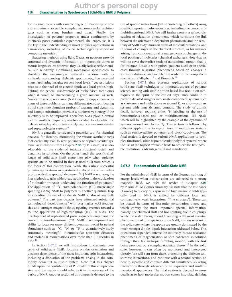
for instance, blends with variable degree of miscibility or now more routinely accessible complex macromolecular architectures such as stars, brushes, and rings.2 Finally, the investigation of polymer properties under confinement by interfaces poses particular experimental challenges, yet it is the key to the understanding of novel polymer applications in nanoscience, including of course technologically important composite materials.
Scattering methods using light, X-rays, or neutrons provide structural and dynamic information on mesoscopic down to atomic length scales; however, they usually lack specific chemical site selectively. Combining mechanical spectroscopy to elucidate the macroscopic material’s response with its molecular-scale analog, dielectric spectroscopy, has provided many fascinating insights on very local levels,3 yet restrictions arise as to the need of an electric dipole as a local probe, highlighting the general disadvantage of probe-based techniques when it comes to characterizing a given material as such. Nuclear magnetic resonance (NMR) spectroscopy circumvents many of these problems, as many different atomic spin-bearing nuclei constitute abundant probes of structure and dynamics, and isotope substitution provides a noninvasive strategy if the selectivity is to be improved. Therefore, NMR plays a central role in multitechnique approaches needed to elucidate the delicate interplay of structure and dynamics in macromolecular and supramolecular systems.4
NMR is generally considered a powerful tool for chemical analysis, for instance, monitoring the various synthetic steps that eventually lead to new polymers or supramolecular systems. As is obvious from Chapter 2.06 by P. Rinaldi, it is also adaptable to the study of intricate structural detail and dynamics in solution. On the other hand, the specific challenges of solid-state NMR come into play when polymer systems are to be studied in their as-used bulk state, which is the focus of this contribution. While the earliest successful polymer applications were restricted to the study of featureless proton wide-line spectra,5 deuteron (2H) NMR was among the first methods to gain widespread application in the elucidation of molecular processes underlying the function of polymers.6
The application of 13C cross-polarization (CP) magic-angle spinning (MAS) NMR to polymers is another quantum leap in extending the use of solid-state NMR to almost any bulk polymer.7 The past two decades have witnessed substantial technological developments,8 with ever higher MAS frequencies and stronger magnetic fields opening avenues toward a routine application of high-resolution (HR) 1H NMR. The development of sophisticated pulse sequences employing the concept of two-dimensional (2D) NMR9 have improved our ability to focus on many different common nuclei in natural abundance such as 13C, 15N, or 31P to quantitatively study structurally meaningful intermolecular spin-spin distances and molecular reorientations over more than 10 decades in time.10
In Section 2.07.2, we will first address fundamental concepts of solid-state NMR, focusing on the orientation and distance dependence of the most important spin interactions, including a discussion of the problems arising in the commonly dense 1H multispin system. Note that this chapter builds upon the contribution of P. Rinaldi in this comprehensive, and the reader should refer to it in its coverage of the basics of NMR. Another section of this chapter is devoted to the
use of specific interactions (while ‘switching off’ others) using specific, important pulse sequences, including the concepts of multidimensional NMR. We will further present a refined discussion of relaxation phenomena, which constitute the link between the orientation-dependent phenomena and the sensitivity of NMR to dynamics in terms of molecular rotations, and in terms of changes in the chemical structure, as for instance arising from conformational rearrangements or changes in the local packing of molecules (chemical exchange). Note that we will not cover the explicit study of translational motion that is, for instance, possible with pulsed-gradient NMR or in special cases through relaxation phenomena based on changes in spin-spin distance, and we refer the reader to the comprehensive texts of Callaghan11 and Kimmich.12
Section 2.07.3 then presents applications of various solid-state NMR techniques to important aspects of polymer science, starting with simple proton-based low-resolution techniques in the spirit of the earliest days. They continue to provide detailed insights into single-component systems such as elastomers and melts above or around Tg, or also two-phase systems with large dynamic contrast. The study of atomic detail, however, requires either 2H labeling or the use of heteronucleus-based one- or multidimensional HR NMR, which will be highlighted by the example of the dynamics of systems around and below Tg. This section is followed by different applications to typical two- or multiphase systems such as semicrystalline polymers and block copolymers. The final section is devoted to various NMR applications to complex functional, often supramolecular polymer systems, where the use of the highest available fields to achieve the best possible resolution is advantageous if not mandatory.
2.07.2 Fundamentals of Solid-State NMR
For the principles of NMR in terms of the Zeeman splitting of energy levels when nuclear spins are subjected to a strong magnetic field, we refer the reader to Chapter 2.06 by P. Rinaldi. As a quick summary, we note that the resonance (Larmor) frequency of a spin in the high magnetic fields typically used in NMR is shifted by different local and comparatively weak interactions (‘fine structure’). These can be treated in terms of first-order perturbation theory and which convey the most important spectral information, namely, the chemical shift and line splitting due to couplings. While the scalar through-bond J coupling is the most essential phenomenon of this type in solution NMR, it is less relevant in the solid state, where the spectra are usually dominated by the much stronger dipole–dipole interaction addressed below. This orientation-dependent interaction indirectly leads to relaxation phenomena of magnetization or spin coherence in solution through their fast isotropic tumbling motion, with the link being provided by a complex statistical theory.13 In the solid state, however, it can often be monitored and interpreted directly. We will start from there, presenting the different anisotropic interactions, and continue with a second section on how to separate and correlate different simultaneously acting interactions through advanced pulse sequences and multidimensional approaches. The final section is devoted to more details as to how molecular motion comes into play, defining

Author's personal copyCharacterization by Spectroscopy | Solid-State NMR of Polymers 187
the transition from a rigid solid through soft materials with anisotropic local mobility, to the isotropic melt or solution.
2.07.2.1 Anisotropic Spin Interactions
Anisotropy in NMR generally means that the position of a spectral line changes with the orientation of the molecular segment containing the spin in question with respect to the external magnetic field B0. This implies that the interaction is tied to asymmetries in the local magnetic environment of the spin, arising from different origins: (1) shielding of the primary field by the surrounding electrons (chemical shift), (2) additional magnetic fields arising from nearby spins (dipole–dipole interaction), and (3) local electric field gradients for the special case that the nuclear spin exceeds I = ½ and thus has a static electric quadrupole moment (quadrupolar interaction).
These three phenomena, arising from diverse and complex physical origins, can be cast into the same formalism, namely, the description of the actual change of the interaction frequency ω = 2πν (line position or size of spectral splitting in rad s−1 or Hz, respectively) in terms of a Cartesian tensor, that is, a 3 � 3 matrix.10 Note that all spectral frequencies discussed in this chapter are rotating-frame frequencies, that is, after subtraction of the suitably referenced Larmor frequency ωL in the megahertz range, resulting in a lower spectral frequency in the kilohertz range. The general interaction matrix contains only three truly independent entries, which are the principal values, that is, the frequencies that are measured when either one of the three different local symmetry axes that are obtained by suitable diagonalization (=principal axes transformation) is parallel to B0:
ωxx 0 0
APAS ¼0
1@ 0 ωyy 0
0 0 ωzz
A
In this principal axes system (PAS) representation, the matrix has only three diagonal entries, and since B0 is commonly taken to be along z, simply the lower-right (zz) entry is the measured frequency for the given orientation. The orientation of the local symmetry axes for specific interactions is often chemically intuitive, that is, along certain bond directions, as we will see in the following. Angle-dependent changes in the interaction are described by simple rotations of the matrix in terms of bilinear products with rotation matrices depending on Euler angles, B ¼ R−1ðα,β,γÞAPASRðα,β,γÞ. After rotation out of the PAS, the matrix is not diagonal any more (i.e., it has up to nine nonzero entries), but the measured interaction frequency for the given orientation is still given by the lower-right entry, Bzz. Note that for simple rotations around the y-axis, the Euler angle β is simply associated with the polar angle θ, and if this angle is the only significant one, as is the case for axially symmetric interactions, such as the dipole–dipole coupling, the angle dependence of the NMR frequency is given by
ωðθÞ ¼ ω0P2ðcos θÞ ¼ ω01 ð3cos2θ−1Þ 2
where P2 is the second Legendre polynomial and ω0 the coupling constant describing the size of the interaction. Thus, in the majority of cases, the time dependence of the real part of a detected NMR signal (free induction decay, FID) in the
� �
� �
rotating frame (i.e., subtracting the large Larmor frequency) is given by
1 IFIDðtÞ∝ Refexp½i …�gn ∝cos ω0 ð3cos2θ−1Þ � t
2
Note that for the chemical-shift interaction, which distinguishes the sign of ω0 (i.e., leads to a single spectral peak, not a doublet), the full complex FID and not just the real part is to be taken into account. In any case, such a single-frequency oscillation is observed only if the sample consists of molecules that all share the same orientation, which can be realized in single crystals or oriented liquid crystals. In the other more common cases, one measures a superposition of frequencies corresponding to all possible orientation angles θ. Such an isotropic powder average can be obtained by integration in spherical coordinates,
1 ⟩IFIDðtÞ∝ ⟨ cos ω0 ð3cos2θ−1Þ � t 2 θ,�
π � � Z ¼ cos ω0
1 ð3cos2θ−1Þ � t sin θ d θ 2
0
We note that in many cases, the integration result is not analytical, which is why spectral simulations often involve a simple summation over a sufficiently large number of angles. The spectra discussed in the following sections are all the result of this simple procedure, obtained of course by Fourier transformation of the FID, converting the summed cosine oscillations into a sum of δ functions (peaks) located at the different frequencies ω01=2ð3cos2θ−1Þ, forming a continuous broad spectral shape typically referred to as powder or ‘Pake’ pattern (see Figures 1 and 2, respectively). Including T2 relaxation, the subpeaks have a finite width, and are then described by Lorentzian functions, and the Pake patterns are thus slightly broadened, that is, rounded at the edges.
2.07.2.1.1 Chemical shift anisotropy The chemical shift, commonly introduced as a shielding phenomenon of the B0 field exerted by the electrons surrounding a specific nucleus, is also orientation dependent. This is not common knowledge, as in the solution state, fast isotropic tumbling motion (rotational diffusion) reduces this interaction to its isotropic average (see also Section 2.07.2.3.2 on dynamic averaging). In the solid state, however, it is rather intuitive that, for instance, the orientation of the electron cloud corresponding to a lone p orbital or a π bond of sp2-hybridized carbons atom exerts its specific shielding on the 13C nucleus and it therefore matters how it is oriented with respect to B0. For 13C, the chemical shift anisotropy (CSA) is particularly strong for sp2-hybridized carbons, but is significant for any bonding environment of almost any NMR-active nucleus. It is generally small, however, for 1H and, in fact, is often neglected apart from protons in hydrogen bonds.
We will not discuss the physical origin of the chemical shift phenomenon in detail, and merely note that it is based on a rather complicated quantum-mechanical interaction between the B0 field and the paired bonding electrons and lone pairs, leading to a local magnetic field at the position of the nucleus that is in most cases reduced as compared to the hypothetical ‘bare’ nuclear spin. We would like to note, however, that a

Author's personal copy188 Characterization by Spectroscopy | Solid-State NMR of Polymers
Figure 1 Line shapes due to (a) symmetric and (b) asymmetric chemical shift anisotropy (CSA) of 13C in, for example, a methyl group and a carbonyl/ aromatic group, respectively. The sharp dashed peak in each spectrum indicates the signal of a single molecular orientation, while the whole line shape arises as a powder average. (c) Static 13C spectrum of poly(methyl methacrylate) (PMMA), demonstrating significant overlap of the different CSA tensors and low signal-to-noise ratio (S/N) for broad signals.
(a) Δω = DCH (het.) or 3/2 DHH (hom.)
(b)
Δω
40 20 0 –20 kHz
Figure 2 Line shapes due to (a) a single dipolar (or quadrupolar) coupling and (b) joint action of multiple homonuclear dipolar couplings. In a, the subspectra corresponding to the two possible spin states of the coupling partner (analogs of the shape shown in Figure 1(a)) are indicated as thin solid lines, and the doublet corresponding to a single orientation as dashed line. (b) The Gaussian line of a dense 1H spin system is homogeneous, in sense that the subspectra corresponding to single-orientation line pairs are (almost) as broad as the whole spectrum.
σxxωL =
σisoωL
σzzωL || B0
ω−δ/2δ
σyyωL ⊥ B0
(a)
ppm0100200300400
COO
CH3CH2
OCH3(c)
σxxωL
σisoωL
σzzωL || B0
σyyωL(b)
δη1
2
ω−δ/2δ
C
COOCH3
CH2
CH3
n
hand-waving model in terms of ‘ring currents’ may give an intuitive understanding in some cases such as aromatic systems, but may be severely misleading in others. The overall effect is rather small and proportional to B0, which is why it is given in parts per million (ppm) of the Larmor frequency.8–10
The chemical shift is dominated by the local bonding environment of a given nucleus, but secondary effects are commonly observed: First, intermolecular packing can strongly affect the chemical shift in cases where a nucleus comes close to an
extended π-bonding system, which is in fact the scenario where the ring-current picture is commonly used. Weaker but still perceptible changes arise for almost any fixed internuclear packing, making the chemical shift a very sensitive marker of structures, the interpretation of which of course requires quantum-chemical calculations.14 Second, rotations around bonds (conformations) are another source of significant shift changes, as they affect the proximity of the given nucleus to more distant functional groups. This phenomenon, mostly referred to as γ-gauche effect,15 is probably one of the richest sources of structural information for polymers, as it provides a link to the conformational statistics also in the solid state.16
To account for CSA, we obviously need three parameters to characterize the full chemical shift phenomenon in terms of the frequency measured for a specific orientation, ωcs ¼ ωL½σ � ,zz
with the CSA tensor given by 0 1
σxx 0 0 σPAS ¼ @ A0 σyy 0
0 0 σzz 0 11 − ð1 þ ηÞ 0 0 B 2 C B Cδ B C¼ σiso þ B 1 C
ωL B 0 − ð1−ηÞ 0 C @ 2 A
0 0 1
To obtain resonance frequencies corresponding to different orientations away from σzz || B0, rotation matrices are of course employed as described above. The above equation contains the two most common strategies to describe a given interaction tensor, namely, in terms of the Cartesian principal values σii, which simply give the shielding in ppm when one of the principal (symmetry) axes is oriented along B0, and in terms of another set of so-called invariants (tensor invariants are

Author's personal copyCharacterization by Spectroscopy | Solid-State NMR of Polymers 189
generally not orientation dependent) based on spherical components, that is, components that follow the symmetries of spherical harmonics. The latter have the advantage of more favorable (i.e., computationally simple) transformation properties upon rotation. The relation of all discussed tensorial quantities to the actual spectral line shape is illustrated in Figure 1 for the example of powder spectral of symmetric and asymmetric CSA tensors.
The isotropic shift σiso is simply the arithmetic average of the three σii, and is still observable under conditions of fast averaging in solution. More generally for a CSA tensor in any orientation, σiso ¼ Tracefσg=3. For the following, the convention jσzz − σisoj ≥ jσxx − σisoj ≥ jσyy − σisoj applies. Thus, the principal value that is farthest away from σiso defines the anisotropy parameter δ ¼ ðσzz − σisoÞωL in units of rad s−1. Itcharacterizes the overall width of the spectral line shape. Having identified two invariants, namely, σiso and δ, the last one missing is the dimensionless asymmetry parameter η ¼ σxx − σyy =ðσzz − σisoÞ, which quantifies the separation of the central spectral singularity and the closest spectral edge (see Figure 1(b)). Both sets of tensor invariants, either three Cartesian principal values {σii} or the set {σiso,δ,η}, are commonly used and listed in the literature.
The advantage of the {σiso,δ,η} invariants is most apparent when writing out the actual orientation dependence of CSA for cases when η ≠ 0. Then, in addition to the polar angle θ, anazimuthal angle φ becomes important, and
ωcsðθ,�Þ ¼ σisoωL þ δP2ðcosθÞ−0:5δη sin2θcos2�
The analogous formula using {σii} is much less compact, emphasizing the advantage of a spherical representation of a tensor when discussing its change upon rotation.10,13
� �
2.07.2.1.2 Dipole–dipole couplings The dipole–dipole coupling is in principle the most easy to understand of all discussed spin interactions. It simply results from the additional magnetic field felt by one spin due to the magnetic dipole moments of the other spins in its vicinity, which exhibit a dipolar field that acts on top of B0. The energy correction is thus the potential energy of a magnetic dipole in the field of another dipole, and can be found in any textbook on electrodynamics. In the rotating frame, the magnetic dipole of any nucleus is oriented along B0 and a sign that is determined by the actual spin state (up or down). From this it is clear that the dipole– dipole interaction (1) leads to a spectral doublet, arising from the two possible spin states of the coupling partner that affect the sign of the interaction, (2) depends on the distance between the spins �1/r3, and (3) depends as well on the orientation of the internuclear vector with respect to B0. The dipole–dipole tensor describing the latter is traceless, that is, it is averaged to zero in solution, and it is further symmetric (except for cases of asymmetric dynamic averaging), thus ηD = 0. It is thus described in terms of a single parameter, the dipole–dipole coupling constant
μ0 γ1γ2ℏ D12 ¼ 34π r12
in units of rad s−1, taking the role of the δ parameter for chemical shift. Otherwise, the same tensor equations and conventions apply, and the spectral shape shown in Figure 2 is simply the combination of two ‘wings’ describing the
� �
orientation dependence of a symmetric tensorial interaction, with the inverted doublet arising from the sign change for the presence of an up or down spin as coupling partner. As it is obvious, the dipole–dipole coupling depends upon the magnetogyric ratios of the involved nuclei, γi, and is thus particularly strong for 1H and 19F, where solid-state NMR spectra can be as broad as around 50 kHz.
In order to further understand the specific features of dipole– dipole couplings, namely, the difference between homo- and heteronuclear couplings, we need to make a short excursion into spin quantum mechanics. We start with the dipole–dipole Hamiltonian (first-order correction to the Zeeman Hamiltonian),
3cos2θ−1 ~~HD ¼ D12 ð3I1zI2z−I1I2Þ 2
The use of this Hamiltonian to calculate spin evolution and thus, for instance, an FID is not trivial due to the scalar product of spin operator vectors. It can be rewritten on the basis of ~~I1I2 ¼ I1zI2z þ I1xI2x þ I1yI2y, which identifies the transverse components Ix/y as the ones that lead to interesting differences and also complications. Two limiting cases are distinguished: First, for the case of heteronuclear dipole–dipole coupling, the different spins are associated with different rotating frames, which effectively lead to an ‘averaging’ of the transverse contributions to zero. The Hamiltonian is then simply
Hhet ¼ D12P2ðcos θÞ 3I1zI1z and the spectral frequency is ωhet ¼ �D12P2ðcos θÞ. For the single orientation θ = 0, we thus have a spectral doublet separated by Δω =2D12 (the ‘horns’ of the Pake representing θ = 90° are separated by half this value).
For the homonuclear case, the quantum mechanics is more involved, and the final result is ωhom ¼ � 3 D12P2ðcos θÞ, that 2
is, the spectral splitting is larger by a factor of 1.5. This is not the only distinction between hetero- and homonuclear couplings. More seriously, the transverse components lead to complications when many abundant spins (such as 1H nuclei) interact. In this case, many pairwise Hij
D act simultaneously, and since the operators describing coupling of one spin to two different ones do not commute, calculations are involved and spectral features become nontrivial. Effectively, the situation is not like in the heteronuclear or J coupling case, where one can observe a splitting of a splitting of a splitting…, but even lines associated with individual powder orientations become severely broadened (‘homogeneously’ broadened line, as opposed to the ‘inhomogeneous’ case pertaining to CSA or heteronuclear dipole–dipole coupling). This is illustrated in Figure 2(b).
The behavior can be rationalized by realizing that the transverse spin operator products can be written as I1xI2x þ I1yI2y ¼ I1þI2– þ I1–I2þ, where the definition of spin state raising and lowering operators I� ¼ Ix � iIy has been used. The transverse terms are the so-called ‘flip-flop’ contributions, which enable an energy-conserving exchange of spin polarization between next neighbors. This leads not only to the complex homogeneously broadened spectral line, but also to the important phenomenon of spin diffusion, that is, exchange of z-magnetization over larger distances on the nanometer scale when the magnetization is not distributed evenly in the sample. The local flip-flop exchange thus constitutes the basic step of a random-walk process in a similar sense as in
Author's personal copy190 Characterization by Spectroscopy | Solid-State NMR of Polymers
Brownian motion. The experimental use of this phenomenon is addressed in Section 2.07.2.2.6.
Finally, we note that the roughly 1 order of magnitude weaker scalar J coupling bears some relation to dipole–dipole couplings, but also important differences. First, J coupling arises also from the magnetic dipole moment of the nuclei, but is transmitted indirectly through bond electrons and not through space, which is a rather complicated quantum-mechanical phenomenon, and constitutes the reason for its usually weak orientation dependence. Second, in the case where the chemical shift separation of the involved nuclei is large (‘weak coupling limit’, which is trivially the case for heteronuclei), its Hamiltonian, thus its quantum-mechanical treatment, is identical to that of the heteronuclear dipole– dipole interaction. However, for a homonuclear spin pair (‘strong coupling limit’, ‘magnetic equivalence’), the J coupling is not observable (no splitting), while we have seen above that the homonuclear dipole–dipole interaction is well existent, in fact strongest, in this case. For both types of interactions, the regime where the coupling is on the order of the shift separation (neither ‘strong’ nor ‘weak’ coupling) is complicated and the spectral features can only be calculated by aid of numerical simulations. The well-known ‘roofing effects’ in solution spectral of J-coupled nuclei belong to this class of phenomena.
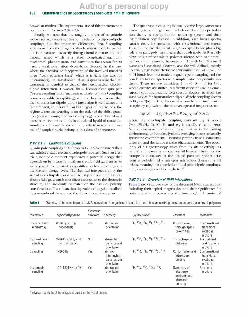
2.07.2.1.3 Quadrupole couplings Quadrupole couplings arise for spins I > 1/2, as the nuclei then can exhibit a static electric quadrupole moment. Such an electric quadrupole moment experiences a potential energy that depends on its interaction with an electric field gradient in its vicinity, and this potential energy difference leads to changes in the Zeeman energy levels. The chemical interpretation of the size of a quadrupole coupling is actually rather simple, as local electric field gradients bear a direct connection to the electronic structure, and are easily estimated on the basis of polarity considerations. The orientation dependence is again described by a second-rank tensor, and the above formalism applies.
Table 1 Overview of the most important NMR interactions in organic solid
Electronic Interaction Typical magnitude structure Geometry
Chemical shift (anisotropy)
0–200 ppm (B0
dependent) Yes Intrinsic and
orientation
Dipole–dipole coupling
2–30 kHz (at typical bond distance)
No Internuclear distance and orientation
J coupling 1–200 Hz Yes Intrinsic, internuclear distance, and orientation
Quadrupole coupling
100–150 kHz for 2H Yes Intrinsic and orientation
The typical magnitudes of the interactions depend on the type of nucleus.
The quadrupole coupling is usually quite large, sometimes exceeding tens of megahertz, in which case first-order perturbation theory is not applicable, rendering spectra and their interpretation complicated. In addition, such broad spectra cannot easily be measured with conventional equipment. This, and the fact that most I > 1/2 isotopes do not play a big role in organic polymers, means that quadrupole NMR usually plays only a minor role in polymer science, with one prominent exception, namely, the deuteron, 2H, with I = 1. The small number of associated electrons and the well-defined, mostly uniaxially symmetric electronic environment in C–H, O–H, or N–H bonds lead to a moderate quadrupolar coupling and the possibility to treat spectra with simple first-order perturbation theory. There are two transitions (–1 ↔ 0, 0 ↔ –1) for I =1, whose energies are shifted in different directions by the quadrupolar coupling, leading to a spectral doublet in much the same way as for homonuclear dipole–dipole coupling shown in Figure 2(a). In fact, the quantum-mechanical treatment is completely equivalent. The observed spectral frequencies are
ωQðθ,�Þ ¼ �χQP2ðcos θÞ � 0:5χQηQsin2 θcos 2�
where the quadrupole coupling constant χQ is about 2π � 125 kHz for C– 2H, and ηQ is usually close to zero. Nonzero asymmetry arises from asymmetries in the packing environment, or from fast dynamic averaging in non-uniaxially symmetric environments. Hydroxyl protons have a somewhat larger χQ, and the tensor is more often asymmetric. The popularity of 2H spectroscopy arises from its site selectivity. Its natural abundance is almost negligibly small, but once the isotope is introduced at the desired position, spectra arise from a well-defined single-spin interaction dominating all others, meaning that chemical shifts, dipole–dipole couplings, and J couplings can all be neglected.6
2.07.2.1.4 Overview of NMR interactions Table 1 shows an overview of the discussed NMR interactions, including their typical magnitudes, and their significance for certain questions concerning structure and/or dynamics of
s and their uses in characterizing the structure and dynamics of polymers
Typical nuclei Structure Dynamics
1H, 13C, 15N, 19F, 29Si, 31P Conformation, through-space proximities
Conformational transitions, rotational motions
1H, 13C, 15N, 19F, 29Si, 31P Through-space distances
Translational and rotational motions
1H, 13C, 15N, 19F, 29Si, 31P Conformation and intergroup binding
Conformational transitions, rotational motions
2H, 14N, 17O, 23Na, 27Al Symmetry of electronic environment,
Rotational motions
chemical bonding

Author's personal copyCharacterization by Spectroscopy | Solid-State NMR of Polymers 191
polymers. We emphasize that several nuclear spin interactions discussed in this section are usually present simultaneously, that is, ωðθ,�Þ ¼ ωcsðθ,�Þ þ ωDðθ,�Þ þ ωJ ½þωQðθ,�Þ�. Although one of these interactions may dominate for specific nuclei in specific environments, it is always important to consider all relevant ones in understanding a spectrum, and thus often the spectrum will be complex, broad, and featureless. As we will see in the following, it is possible to actually manipulate or isolate any of the individual interactions at will of the experimenter, using sample-spinning techniques and/or specific pulse sequences. Thus, the power of today’s solid-state NMR relies on our growing ability to control the relevant spin interactions and measure or use them selectively.
2.07.2.2 Using and Manipulating Anisotropic Interactions
Due to the weakness of the interactions that dominate the NMR spectra, these interactions can be modified and manipulated at will of the experimenter.8–10 In particular, interactions can be switched on and off for certain times of the experiments. This leads to an enormous variety of NMR experiments that can be adjusted for optimum detection of site-specific information on structure, dynamics, and order of polymers. Examples of such experiments are outlined here only schematically. Further details are given when describing specific examples in later sections.
2.07.2.2.1 Magic-angle spinning The most prominent technique in solid-state NMR for line narrowing is MAS. Here, the angular-dependent part of the interactions is modulated by rapid mechanical spinning of the sample around an axis inclined at an angle Θ with respect to the magnetic field. If the spinning axis is chosen along the so-called magic-angle Θm = 54.7°, the relevant scaling factor (3cos2Θ – 1)/2 becomes zero and the anisotropic part of the
B0
θ m
ωR
S
(a)B0
B0 θ
ωR
θ m
ωR
B0
Figure 3 Effect of magic-angle spinning (MAS) on static line shapes. (a) The sof spinning sidebands reflecting ‘inhomogeneous’ broadening. Clearly, within trepresent the ‘isotropic’ chemical shift. (b) Static line shape dominated by homincreasing MAS, the signal splits into a lesser number of spinning sidebands
interaction vanishes (Figure 3). Today, very fast MAS with rotation frequencies reaching 70 kHz17 and more are commercially available, thus providing unprecedented ‘high spectral resolution’, particularly in solid-state 1H and 19F NMR. In addition, MAS largely simplifies the network of strongly dipolar-coupled protons18 that typically preclude the use of the dipole–dipole couplings among 1H spins for specific structural investigations in non-spinning (static) solid samples. In order to effectively reduce or remove line broadening due to anisotropic interactions, the rotation frequency ωR should be larger than the magnitude of the respective anisotropic interaction (e.g., the 1H-1H dipole–dipole coupling ωD). In fact, for most organic solids, the 1H-1H dipole–dipole couplings, for example, in CH2 groups with a proton–proton distance of 0.18 nm are of the order of ωD ≈ 2π·21 kHz. Thus, at fast MAS, the condition ωR ≥ ωD can be met even for the strongest dipole–dipole couplings.
MAS modulates the spin interactions periodically, which means that it generates so-called rotational echoes and the NMR data acquisition can be performed in two ways: If only the echo height is monitored (e.g., in a rotor-synchronized acquisition), a single line results in the NMR spectrum for each spectroscopically resolved site and the information about anisotropic couplings is lost. On the other hand, if the whole echo train is monitored, a spinning sideband pattern results that contains information about the anisotropic couplings, yet with spectral resolution of the different sites (Figure 3). This is important for a precise structural elucidation based on dipole–dipole couplings as well as using this interaction to study molecular dynamics. Note that MAS works for all anisotropic interactions introduced above, including homonuclear dipole–dipole coupling. Moreover, on account of its angular dependence, molecular motion leads to an averaging of observable dipole–dipole couplings. Monitoring this reduction of the dipole–dipole coupling thus allows an
tatic
MAS
Fas
t S
low
(b)
tatic powder pattern due to chemical shift anisotropy splits into a manifold he sideband pattern, the signal with highest intensity does not necessarily onuclear dipolar couplings, for example, among abundant protons. Upon where the isotropic center peak is easily identified.

Author's personal copy192 Characterization by Spectroscopy | Solid-State NMR of Polymers
identification of dynamic processes present in the sample. Indeed, this is well known, for example, from NMR investigations of liquid crystals, where the reduced NMR couplings yield site-specific values for the Maier–Saupe order parameter S = < 1/2 (3 cos2 Θ – 1)>.19 The extreme case is reached in solution, where fast isotropic tumbling of the molecules (‘Brownian’ motion) leads to an almost complete averaging of line broadening due to dipole–dipole couplings and other anisotropic interactions.
2.07.2.2.2 Echoes and refocusing Another fundamental aspect of NMR spectroscopy is the possibility to form echoes by applying refocusing pulses. The simplest version is the Hahn echo20 refocusing the spread in frequencies due to magnetic field inhomogeneities, chemical shift dispersion, resonance offsets, and heteronuclear dipole– dipole coupling, where the refocusing pulse has an optimal flip angle of 180°, see Figure 4(b). For frequency dispersions due to interactions bilinear in the spin operators, such as homonuclear dipole–dipole or J coupling and quadrupolar coupling the optimal flip angle is 90° and the echoes are often referred to as ‘solid echoes’. For generating other forms of coherence,8–10 such as spin alignment or double-quantum (DQ) coherences, other flip angles are employed, in particular 45°.
The refocusing of coherence has two very different aspects. The first is technical, as the generation of an echo allows one to record the NMR signal at ‘zero time’ in order to circumvent
Dead time
Free indu(a)
Frequency ω
t1 t2 (b)
ω1 ω2
t1 tm
(c)
ω1
(d) t1 t2tm1 tm2
ω1 ω2
Figure 4 Schematic pulse sequences for (a) spectrum acquisition, (b) echo exchange spectroscopy. Note that in reality, the oscillation frequencies may di
the limitations due to the finite duration of the pulses and the ‘dead time’ that prevents recording the signal immediately after application of a pulse (see Figure 4(a)). The second reason is more important as dynamics processes, which change the NMR frequency during the time needed for refocusing, will lead to incomplete echo formation and can, in this way, be studied both concerning the time frame and details of the dynamics processes, see, for example, References 6 and 10–12. Moreover, the signals (coherences) can be refocused several times, Figure 4(d), providing access to studying dynamic processes on longer timescales, and/or correlating the dynamic behavior at several times, See Section 2.07.2.3.
So far, we have discussed echo formation for simple cases, where no more than two spins are involved. There, the refocusing pulse leaves the interactions themselves intact. As discussed in Section 2.07.2.1.2, in solids the dipole–dipole couplings typically involve many spins, leading to ‘homogeneous’ line broadening, see Figure 2(b). Even then, such multispin interactions between protons can be reversed by a ‘time-reversal’ sequence, leading to the so-called magic-sandwich echo.21 For inhomogeneous dipole–dipole couplings, such as 13C-1H, echoes can be formed by applying a 180° pulse on either of the two channels. For more efficient removal of this interaction, decoupling sequences among the protons and/or between 13C and protons have to be applied, vide infra Section 2.07.2.2.4, to allow echo formation for the remaining interactions as discussed above.
ction decay (FID)
Time t
Spin (‘Hahn’) echo, solid echo 2D spectroscopy
Stimulated echo 2D exchange spectroscopy
t2
ω2
4D Echo
4D Exchange spectroscopy
t4tm3t3
ω3 ω4
formations, (c) stimulated echo and exchange, and (d) higher-order ffer for the various cases and pulse lengths and phases can be different.

Author's personal copyCharacterization by Spectroscopy | Solid-State NMR of Polymers 193
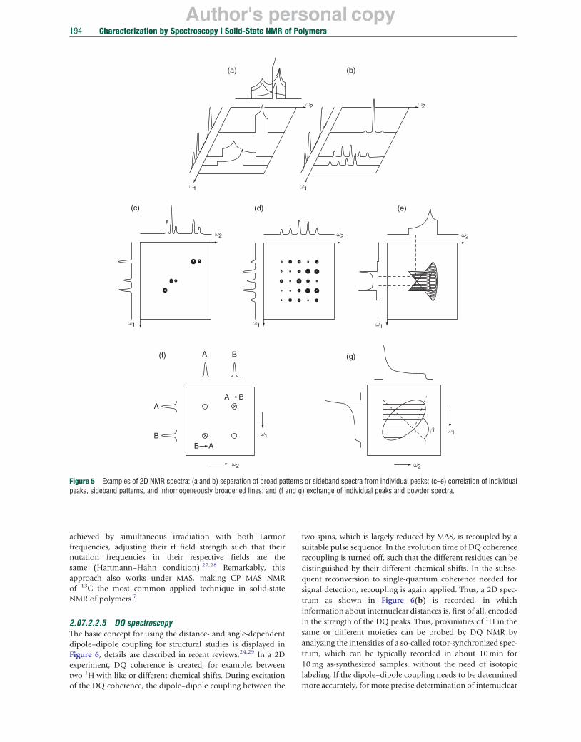
2.07.2.2.3 2D NMR spectroscopy: separation, correlation, and exchange Many, if not most, advanced NMR techniques make use of 2D spectroscopy, because of the superb increase of resolution and ease of information encoding.9,10 In general, a 2D NMR experiment is divided into several time periods that follow each other. In order to record a 2D NMR spectrum, a 2D data set is acquired as a function of two time variables t1 and t2 as shown schematically in Figures 4(b) and 4(c). The sequence is preceded by a so-called preparation period in which coherences are excited by a suitable pulse sequence, which in the simplest case is only one radiofrequency (rf) pulse. Unlike conventional (1D) NMR spectroscopy after recording an FID, the excited signal is not directly acquired but is allowed to evolve in the so-called evolution period under influence of the relevant spin interactions. The evolution time t1 is incremented in subsequent experiments and provides the first time dimension of the 2D experiment. After the evolution period (and an optional mixing time), the remaining signal is directly detected in the detection period for each time increment, thus generating a 2D data set. 2D Fourier transformation then gives the 2D spectrum. Optionally, a so-called mixing period of length tm can be inserted between the evolution and detection periods. During tm, changes in the system can occur, for instance, by molecular motions, spin interactions, relaxation, or spin manipulation.
The different aspects of 2D NMR spectroscopy are reflected in the different variants that can be distinguished. One variant, ‘separation’ spectroscopy, is used to separate different interactions taking advantage of spin manipulation techniques (the simplest of which are actually echoes or decoupling pulse sequences). For instance, during the evolution period the spin manipulation can be made such that only the isotropic chemical shift is acquired while in the detection period the full spectrum is acquired. In this way, the anisotropy can be studied site-selectively. Conceptually similar, but technically more demanding is the separation of isotropic chemical shifts and heteronuclear dipole–dipole couplings (separated-local-field (SLF) spectroscopy).9,10 A simple MAS variant separates the different broad-line spectra associated with the protons (which are not resolved at moderate MAS) bound to different carbons (for which moderate MAS is fast enough to provide sharp peaks), which is termed wide-line separation (WISE) NMR.
Other 2D NMR techniques, so-called ‘correlation’ techniques, aim at obtaining new information by correlating different interactions, Figures 5(c)–5(e). In the simplest case, isotropic chemical shifts are just correlated with isotropic chemical shifts of the same or another nucleus type (homonuclear or heteronuclear shift correlation, respectively), providing information on connectivity or through-space proximity (Figure 5(c)). This latter type of structural information depends upon whether the correlation is established by J or dipole–dipole couplings, respectively. Further, the 13C CSA can be correlated with the (mostly heteronuclear) dipole–dipole coupling anisotropy (DIPSHIFT). Such experiments can be conducted either under slow MAS with many spinning sidebands (Figure 5(d)) or under static conditions (Figure 5(e)), and in both cases, one can obtain information on the relative orientation of the two tensors. The experiment in its faster-MAS version or in oriented static samples is also sometimes referred to as ‘SLF’ spectroscopy, for separated local field. Then, the X nucleus as
identified by its isotropic shift is correlated with the X-H dipole–dipole (identified by a dipolar splitting in the oriented static case or by weak spinning sidebands), see Figure 9 for an example. Considering the manifold of spin manipulation techniques, there is a wealth of such 2D NMR techniques that can be derived for different purposes.
Finally, introducing a mixing time tm, 2D ‘exchange’ spectroscopy can be performed, Figures 5(f) and 5(g). The most important application of such exchange techniques with respect to polymer investigations is the study of slow molecular dynamics. In these experiments, reorientations due to molecular dynamics are allowed to take place during the mixing time tm and lead to characteristic off-diagonal patterns in the resulting 2D spectra. If the mixing time is increased in a series of 2D experiments, slow dynamics in the range of milliseconds to seconds can be investigated in detail. For instance, rotation of molecules by a well-defined angle leads to an elliptical exchange ridge for a powder. This can be viewed as a Lissajous figure, from which the angle, by which the molecules have rotated, can directly be read off by a ruler.22 The measuring time can be dramatically reduced in a 1D variant under MAS.23 See Section 2.07.2.3.4 for more details on this topic.
2.07.2.2.4 Decoupling, recoupling, and CP In order to record HR solid-state NMR spectra, the line broadening of homo- and heteronuclear dipole–dipole interactions has to be eliminated. This is usually achieved by continuous-wave or multiple-pulse irradiation of the nonobserved nuclei. The rapid fluctuations of the spin orientation with respect to the magnetic field then cancel the local fields produced by their magnetic moments, thereby eliminating the effects of dipole–dipole coupling. For homonuclear ‘decoupling’, a variety of multiple-pulse irradiation schemes have been developed, for details see References 9 and 10. Often, such decoupling is needed within an indirectly detected dimension (i.e., an evolution period) of a 2D experiment. To this end, the frequency-switched Lee–Goldburg (FSLG) sequence uses continuous off-resonance irradiation with 360° pulses of the spins. The pulses are set off-resonance to an amount such that the effective field that the spins experience in the rotating frame is oriented at the magic angle relative to the static field. This and more sophisticated schemes lead to remarkable spectral resolution.24 In MAS NMR, where pulse irradiation and spinning are combined (combined rotation and multiple pulse spectroscopy (CRAMPS)), care has to be taken to synchronize the pulse sequences with the MAS, such that interference between the two is avoided.
The effect of MAS eliminating anisotropic interactions can also be at will reduced by appropriate pulse sequences, thus ‘recoupling’ the interaction. The simplest way is the application of two 180° pulses per rotor period, partially restoring heteronuclear dipole–dipole coupling, termed rotational-echo double resonance (REDOR).25 Numerous strategies of achieving such recoupling of homonuclear and heteronuclear dipole–dipole couplings have been developed, which differ in symmetry properties, efficiency, and whether or not the rotor phase is encoded.26 The idea of recoupling can likewise be applied to other anisotropic interactions such as CSA.23
Last but not least, the transfer of magnetization from abundant to rare nuclei, for example, from 1H to 13C, termed ‘crosspolarization’, should be appreciated. In its simplest form, it is
Author's personal copy
(a) (b)
ω2 ω2
ω1ω1
(c) (d) (e)
ω2 ω2 ω2
ω1 ω1 ω1
(f) A B (g)
A B A
β ω1ω1
B A B
ω2 ω2
194 Characterization by Spectroscopy | Solid-State NMR of Polymers
Figure 5 Examples of 2D NMR spectra: (a and b) separation of broad patterns or sideband spectra from individual peaks; (c–e) correlation of individual peaks, sideband patterns, and inhomogeneously broadened lines; and (f and g) exchange of individual peaks and powder spectra.
achieved by simultaneous irradiation with both Larmor frequencies, adjusting their rf field strength such that their nutation frequencies in their respective fields are the same (Hartmann–Hahn condition).27,28 Remarkably, this approach also works under MAS, making CP MAS NMR of 13C the most common applied technique in solid-state NMR of polymers.7
2.07.2.2.5 DQ spectroscopy The basic concept for using the distance- and angle-dependent dipole–dipole coupling for structural studies is displayed in Figure 6, details are described in recent reviews.24,29 In a 2D experiment, DQ coherence is created, for example, between two 1H with like or different chemical shifts. During excitation of the DQ coherence, the dipole–dipole coupling between the
two spins, which is largely reduced by MAS, is recoupled by a suitable pulse sequence. In the evolution time of DQ coherence recoupling is turned off, such that the different residues can be distinguished by their different chemical shifts. In the subsequent reconversion to single-quantum coherence needed for signal detection, recoupling is again applied. Thus, a 2D spectrum as shown in Figure 6(b) is recorded, in which information about internuclear distances is, first of all, encoded in the strength of the DQ peaks. Thus, proximities of 1H in the same or different moieties can be probed by DQ NMR by analyzing the intensities of a so-called rotor-synchronized spectrum, which can be typically recorded in about 10 min for 10 mg as-synthesized samples, without the need of isotopic labeling. If the dipole–dipole coupling needs to be determined more accurately, for more precise determination of internuclear

Author's personal copy
(a) Detection Excitation Evolution Reconversion
x –xy –y x –xy –y x
(b) H H''H' (c) 0.21 nm
H H
rHH 0.24 nm H''
H' H'
0.27 nm
5 3 1 –1 –3 –57 –79 –9
Characterization by Spectroscopy | Solid-State NMR of Polymers 195
Figure 6 Principle of double-quantum NMR spectroscopy. (a) Pulse sequence, (b) rotor-synchronized spectra, and (c) sideband patterns.
distances or MD, see above, DQ sideband spectra, as displayed in Figure 6(c), are recorded. The measurement time is then considerably longer, typically overnight.
Such DQ spectra can be recorded for both homonuclear 1H-1H, and heteronuclear 1H-13C, 1H-15N coherences, exploit-ing for the latter the much higher site selectivity of 13C and 15N chemical shifts.30 In the heteronuclear case, polarization trans-fer and recoupling take advantage of the popular REDOR technique introduced above.25 Moreover, the sensitivity of such heteronuclear experiments can significantly be increased
15Nby detecting the signal of the rare spin, in particular through 1H.
Inte
nsity
MagnetizationSelection
(a)
MZ
A B A
x
(b) A B A
A
ωCS
NMR spectra
Figure 7 Scheme of NMR spin diffusion experiments. (a) The magnetization(b) After selection of the magnetization of one component (A in our case) by a sphases, which can be followed by the decay of signal A and the growth of sig
2.07.2.2.6 Spin diffusion Transfer of magnetization between like spins also happens spontaneously, if the spatial distribution of magnetization is not uniform. Typical examples are phase separated in two-component systems such as block copolymers or polymer blends.31 This is depicted in Figure 7. The basic idea of a spin diffusion experiment involves selection of one component due to differences in mobility or chemical structure by appropriate pulse squences.9,10 The phase structure can be determined by following either the buildup of the suppressed signals or the decay of the remaining signals as indicated. The time develop-ment follows a simple diffusion equation. Therefore, the time
Spin diffusion
A A B
BB
Spin diffusion time tm
reflects the morphology of a two-component system with equal fractions. uitable pulse sequence, spin diffusion equilibrates magnetization of the two nal B.
Author's personal copy196 Characterization by Spectroscopy | Solid-State NMR of Polymers
data are plotted as sqrt(time). Likewise, the mixing time can be incorporated in 2D experiments, for example, 2D WISE, making the technique particularly site selective. Such techniques are also helpful for studying the interfaces between the different components. Limitations arise from the uncertainty of the spin diffusion constant in mobile polymers, and the effect of the dimensionality on the spin diffusion curves. Here, calibration experiments on structures that can also be studied by X-ray scattering or electron microscopy are particularly helpful.
2.07.2.3 Dynamics and Relaxation
As we have seen in the preceding sections, the measurement of anisotropic interactions, using advanced pulse sequences if necessary to achieve site and/or interaction selectivity, yields information on static atomic-scale structural features of a material, such as internuclear distances and the symmetry of the electronic environment of a given nucleus. The second no less relevant part of solid-state NMR comprises dynamics.10
Generally, dynamics affects NMR observables because it takes time to measure them, the simplest example being the duration of an FID. If the interaction changes during this time, for instance, by a molecular rotation that changes the frequency of an anisotropic interaction, specific and interpretable changes in the spectrum will result.
2.07.2.3.1 Motional regimes and ‘NMR timescales’ As mentioned, the duration of the FID, or the duration of a more complex pulse sequence, is the most natural timescale that needs to be considered. These times are determined by the interaction frequencies to be measured or used, as it requires at least one oscillation period to properly define a frequency. Since most NMR interactions are in the kilohertz range (see Table 1), and since they are measured in the rotating frame relative to the fast Larmor oscillation, we are typically dealing with timescales of milliseconds. Dynamics that occurs on this timescale of the inverse change in interaction frequency (1/Δω) associated with a dynamic process is referred to as the ‘intermediate motional regime’, and it is characterized by the most dramatic changes in the spectra. Relative to this timescale, we define the ‘slow’ and the ‘fast’ motion limits, where the dynamics is either too slow to lead to apparent spectral changes or so fast that only a time-averaged interaction frequency is measured (fast dynamic averaging, see next section).
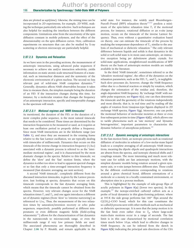
A second ‘NMR timescale’, completely different from the discussed interaction timescales, is given by the Larmor precession. Just looking at spectra, dynamics that occurs on this timescale corresponds to the fast dynamic averaging limit, which means that the timescale cannot be obtained from the spectra. However, very relevant changes occur for the NMR relaxation times T1 and T2, and one again introduces a different set of dynamic regimes (from ‘slow’ to ‘extreme narrowing’) as referenced to 1/ωL. Thus, the measurement of the two relaxation times by saturation/inversion recovery or echo pulse sequences, respectively, possibly performed at different temperatures or even different magnetic fields (field-cycling relaxometry12) allows for the characterization of fast dynamics in the nanoseconds to microseconds range, or even the milliseconds range if very low primary fields are used. The associated phenomena are thoroughly described in Chapter 2.06 by P. Rinaldi, and remain applicable in the
solid state. For instance, the widely used Bloembergen– Purcell–Pound (BPP) relaxation theory13,32 predicts a minimum of the spin-lattice relaxation time T1 if the motional process, for instance, rotational diffusion or an n-site jump motion, occurs on the timescale of the inverse Larmor frequency. Thus, even without a quantitative evaluation based on theory, one can estimate the timescale of the process by studying the temperature-dependence of T1, similar to the analysis of mechanical or dielectric relaxation.3 The only relevant difference between liquids and solids is that dynamics in the solid or soft-solid state is in most cases anisotropic, an instructive exception being per definitionem plastic crystals. For solid-state applications, straightforward modifications of BPP theory on the basis of anisotropic-motion models are readily available in the literature.
In the third ‘NMR timescale’, sometimes referred to as the ‘ultraslow motional regime’, the effect of the dynamics on the relaxation parameters, such as the FID, T1, and T2, is negligible. Such slow processes do, however, change the NMR frequency either due to a chemical reaction or simply by rotation, which changes the orientation of the residue and, therefore, the angle-dependent NMR frequency. By ‘exchange NMR’ with suitable pulse sequences, see Figure 4(c), one can then determine the timescale and the geometry of the rotations independently and most directly, that is, in real time and by reading off the angles of rotation from Lissajous-type figures displayed in 2D exchange NMR spectra, Figure 5(g). Moreover, one can probe the motional behavior of molecular moieties at three or even four subsequent points in time (Figure 4(d)), which allows one to tackle phenomena such as ‘rate memory’ and ‘dynamic heterogeneities’, important parameters to characterize the dynamic behavior of amorphous polymers.10
2.07.2.3.2 Dynamic averaging of anisotropic interactions In the fast-motion limit, an isotropic process such as rotational diffusion of molecules in solution of a low-molar-mass liquid leads to a complete averaging of all anisotropic NMR interactions, meaning the dipole–dipole and quadrupole interactions are absent from the spectra, and isotropic chemical shifts and J couplings remain. The more interesting and much more relevant case for solids are fast anisotropic motions, with the simplest dynamic models being rotation around a given symmetry axis, or n-site jumps between different sites. These could be the different conformations corresponding to rotations around a given chemical bond, different orientations of a molecule or a moiety in a locally constrained environment, or absorption sites in a porous medium.
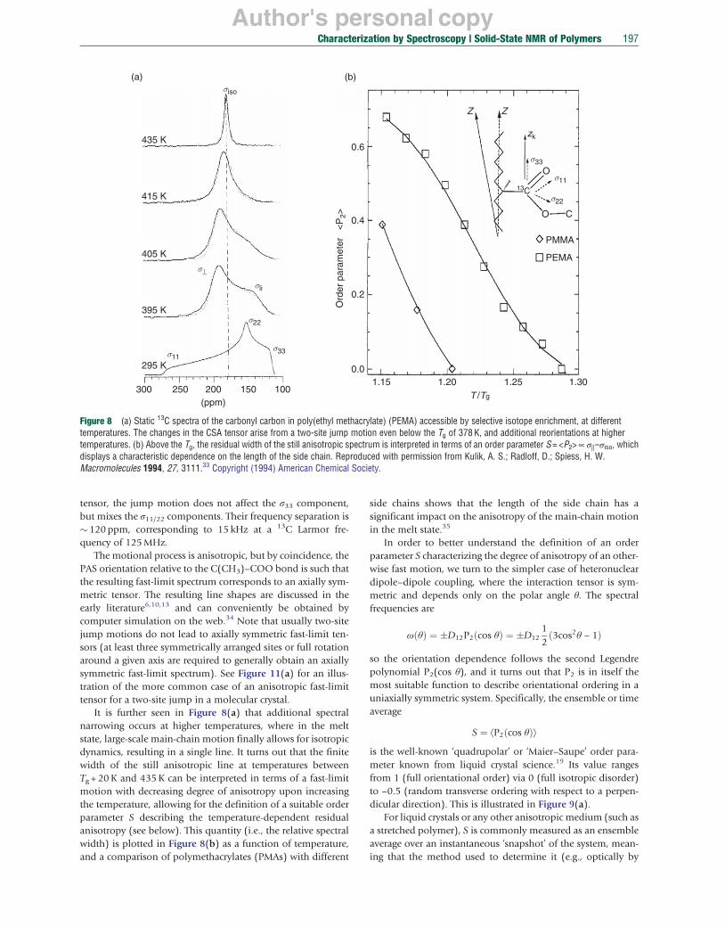
This is highlighted by the example of side-group flips of acrylic polymers in Figure 8(a) (lower two spectra). In this example,33 the isotope-enriched carbonyl carbon acts as a probe of local dynamics in this glass-forming polymer, where at 395 K the side group performs fast 180° flips around the C(CH3)–COO bond, which for this case constitutes the so-called β process seen with other methods such as mechanical or dielectric spectroscopy. It is seen that the jump motion is in the fast limit even rather close to Tg, where large-scale main-chain motions occur in a range of seconds. The fast limit is in this case characterized by motional correlation times much below 10 μs, which lead to effective changes in NMR frequency. As can be inferred from the sketch in Figure 8(b) indicating the principal axis directions of the CSA
Author's personal copy
(a) σiso
(b)
Z Z
415 K
435 K 0.6
O
zk
13C
σ33
σ11
σ22
Ord
er p
aram
eter
<
P2> O C
0.4
PMMA
PEMA
0.2
405 K
σ⊥
σli
395 K σ22
σ33σ11 295 K 0.0
1.15 1.20 1.25 1.30 300 250 200 150 100
T /Tg(ppm)
Characterization by Spectroscopy | Solid-State NMR of Polymers 197
Figure 8 (a) Static 13C spectra of the carbonyl carbon in poly(ethyl methacrylate) (PEMA) accessible by selective isotope enrichment, at different temperatures. The changes in the CSA tensor arise from a two-site jump motion even below the Tg of 378 K, and additional reorientations at higher temperatures. (b) Above the Tg, the residual width of the still anisotropic spectrum is interpreted in terms of an order parameter S = <P2> ∝ σ||–σiso, which displays a characteristic dependence on the length of the side chain. Reproduced with permission from Kulik, A. S.; Radloff, D.; Spiess, H. W. Macromolecules 1994, 27, 3111.33 Copyright (1994) American Chemical Society.
tensor, the jump motion does not affect the σ33 component, but mixes the σ11/22 components. Their frequency separation is � 120 ppm, corresponding to 15 kHz at a 13C Larmor frequency of 125 MHz.
The motional process is anisotropic, but by coincidence, the PAS orientation relative to the C(CH3)–COO bond is such that the resulting fast-limit spectrum corresponds to an axially symmetric tensor. The resulting line shapes are discussed in the early literature6,10,13 and can conveniently be obtained by computer simulation on the web.34 Note that usually two-site jump motions do not lead to axially symmetric fast-limit tensors (at least three symmetrically arranged sites or full rotation around a given axis are required to generally obtain an axially symmetric fast-limit spectrum). See Figure 11(a) for an illustration of the more common case of an anisotropic fast-limit tensor for a two-site jump in a molecular crystal.
It is further seen in Figure 8(a) that additional spectral narrowing occurs at higher temperatures, where in the melt state, large-scale main-chain motion finally allows for isotropic dynamics, resulting in a single line. It turns out that the finite width of the still anisotropic line at temperatures between Tg + 20 K and 435 K can be interpreted in terms of a fast-limit motion with decreasing degree of anisotropy upon increasing the temperature, allowing for the definition of a suitable order parameter S describing the temperature-dependent residual anisotropy (see below). This quantity (i.e., the relative spectral width) is plotted in Figure 8(b) as a function of temperature, and a comparison of polymethacrylates (PMAs) with different
side chains shows that the length of the side chain has a significant impact on the anisotropy of the main-chain motion in the melt state.35
In order to better understand the definition of an order parameter S characterizing the degree of anisotropy of an otherwise fast motion, we turn to the simpler case of heteronuclear dipole–dipole coupling, where the interaction tensor is symmetric and depends only on the polar angle θ. The spectral frequencies are
ωðθÞ ¼ �D12P2ðcos θÞ ¼ �D12 1 ð3cos2θ − 1Þ 2
so the orientation dependence follows the second Legendre polynomial P2(cos θ), and it turns out that P2 is in itself the most suitable function to describe orientational ordering in a uniaxially symmetric system. Specifically, the ensemble or time average
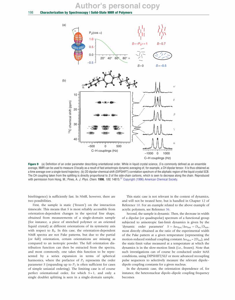
S ¼ ⟨P2ðcos θÞ⟩ is the well-known ‘quadrupolar’ or ‘Maier–Saupe’ order parameter known from liquid crystal science.19 Its value ranges from 1 (full orientational order) via 0 (full isotropic disorder) to –0.5 (random transverse ordering with respect to a perpendicular direction). This is illustrated in Figure 9(a).
For liquid crystals or any other anisotropic medium (such as a stretched polymer), S is commonly measured as an ensemble average over an instantaneous ‘snapshot’ of the system, meaning that the method used to determine it (e.g., optically by
Author's personal copy
N
4′ 3′ 2′
1′
1
2 3
4
δ β
γ ω
(a)
α P2(cos α)
1.0
0.5 S = <P2> = 1 S ≈ 0.7
−0.5
0.0 20° 40° 60° α80°
S ≈ 0 S = −0.5
α(b)
ω
10
δ
20
β
30
γ
40
C–H couplings (Hz)
–500 0 500
–1000 0 1000
C–H couplings (Hz)
α
13C
che
mic
al s
hift
(ppm
)
198 Characterization by Spectroscopy | Solid-State NMR of Polymers
Figure 9 (a) Definition of an order parameter describing orientational order. While in liquid crystal science, S is commonly defined as an ensemble average, NMR can be used to measure S locally as a result of fast anisotropic dynamic averaging of, for example, a CH dipolar tensor. It is thus obtained as a time average over a single-bond trajectory. (b) 2D dipolar-chemical shift (DIPSHIFT) correlation spectrum of the aliphatic region of the liquid crystal 5CB. The CH coupling taken from the splitting is directly proportional to S of the side-chain carbons, which is seen to decrease along the chain. Reproduced with permission from Hong, M.; Pines, A. J. Phys. Chem. 1996, 100, 14815.37 Copyright (1996) American Chemical Society.
birefringence) is sufficiently fast. In NMR, however, there are two possibilities.
First, the sample is static (‘frozen’) on the interaction timescale. This means that S is most reliably accessible from orientation-dependent changes in the spectral line shape, obtained from measurements of a single-domain sample (for instance, a piece of stretched polymer or an oriented liquid crystal) at different orientations of its symmetry axis with respect to B0. In this case, the orientation-dependent NMR spectra are not Pake patterns, but due to the partial (or full) orientation, certain orientations are missing as compared to an isotropic powder. The full orientation distribution function can then be extracted from the spectra, and most commonly, one takes this function to be represented by a series expansion in terms of spherical harmonics, where the prefactor of P2 represents the order parameter S (expanding up to P2 is often sufficient for cases of simple uniaxial ordering). The limiting case is of course perfect orientational order, for which S = 1, and only a single doublet splitting is seen in a single-domain sample.
This static case is not relevant in the context of dynamics, and will not be treated here, but is handled in Chapter 12 of Reference 10. For an example related to the above example of acrylic polymers, see Reference 36.
Second, the sample is dynamic. Then, the decrease in width of a dipolar (or quadrupolar) spectrum of a functional group subjected to anisotropic fast-limit dynamics is given by the ‘dynamic order parameter’ S ¼ Δωdyn=Δωstat ¼ Dres =Dstat , most directly obtained as the ratio of the experimental width of the Pake pattern at a given temperature (representing the motion-reduced residual coupling constant Δωdyn =2Dres), and the static-limit value measured at a temperature at which the dynamics is in the slow-motion limit (i.e., frozen). Note that such investigations can of course be conducted under MAS conditions, using DIPSHIFT/SLF or more advanced recoupling pulse sequences to selectively measure the relevant dipole– dipole coupling constants for a given nucleus.
In the dynamic case, the orientation dependence of, for instance, the heteronuclear dipole–dipole coupling frequency becomes

Author's personal copy
(a)
π/2
(b) ωa = σa γB0 ωb = σb γB0
k/Δν =0.5Slow limit
k/Δν =1.0 T2
decreases k/Δν =4.0
‘Intermediate motional regime’ k/Δν =10
Characterization by Spectroscopy | Solid-State NMR of Polymers 199
ωðθÞ ¼ �Dstat ⟨P2ðcosθÞ⟩t ¼ DstatS 1 ð3cos2β−1Þ,2
where S ¼ ⟨P2ðcosαÞ⟩t ¼ Dres =Dstat
This relation is easily derived on the basis of addition theorems for Legendre polynomials for a system with uniaxially symmetric dynamics. The interpretation is simple: the time dependence has to be evaluated only for the angle α of the instantaneous tensor orientation with respect to the ‘symmetry axis of fast motion’, and β describes the orientation of this symmetry axis within the sample with respect to the B0 field. The sample can thus well be an isotropic powder, for instance, a multidomain liquid crystal sample, meaning that the usual powder average is to be taken over β. S then characterizes the ‘local anisotropy’ of the dynamic process, and it is often identical to the ensemble-averaged S measured from a ‘snapshot’ experiment on a monodomain with fixed orientation β. The possibility to determine S in a powder sample is a significant experimental advantage, which makes NMR the method of choice for the determination of orientational order parameters in liquid crystal (and polymer) science. In Figure 9(b), we see the use of anadvanced 2D experiment (SLF, or also DIPSHIFT) correlating the 13C chemical shift with the 13C-1H dipole–dipole couplings, which allows for the site-resolved study of order parameters associated with the different functional groups of complex molecules.37
T2k/Δν=π√2 increases
k/Δν =40 Fast limit
ω = 1 (ωa + ωb)2
Figure 10 T2 phenomena and intermediate motions. (a) Spin-resolved picture of intermediate motions (bottom trace), leading to frequency jumps during the acquisition (FID) time. For sufficiently fast jumps, the sum of many such random trajectories, even when only two oscillation frequencies are involved, results in a singly exponential decay envelope (thick line), corresponding to a Lorentzian line in the spectrum. In comparison, the summed powder average in a solid sample (top trace), made up of many frequencies that are constant in time, also leads to a decaying function, which, however, is not an exponential but rather exhibits a Gaussian-like initial decay. (b) Dynamic coalescence of two spectral lines of separation Δν = (ωa − ωb)/2π as a result of a frequency(spin) exchange process with rate constant k.
2.07.2.3.3 Transverse relaxation and intermediate motions Transverse relaxation and the corresponding ‘T2 relaxation time’ in solids are subject to a number of ambiguities that are often not properly treated in the literature. We thus start with a few general comments on transverse relaxation. First of all, the superposition of cosine oscillations with different frequencies as arising from the different powder orientation in a solid leads to an FID that decays rather quickly. This is, in essence, an interference phenomenon, and sometimes the decay is assigned a T2
*, the asterisk indicating that we are dealing with an apparent relaxation time. The phenomenon holds for CSA and dipole–dipole/quadrupole couplings alike, and generally, the decay function is not exponential but rather has a Gaussian shape. This is demonstrated in Figure 10(a), top trace. One may assign a T2
* to such a decay, and this is exactly this short apparent T2
* time that is the rigid-limit result of the BPP relaxation theory.
We need to keep in mind that the destructive interference phenomenon can always be time reversed by forming an echo, which in the simplest case is a Hahn echo taking care of CSA and also magnetic-field inhomogeneities. As mentioned above (Section 2.07.2.2.2), analogous echoes exist for the dipole– dipole or quadrupole interaction (solid echo, magic-sandwich echo), meaning that the true T2 relaxation time in a solid measured with an appropriate echo pulse sequence can be rather long. This is not covered by BPP theory, but indicates that T2 in solids in fact also has a minimum!
This T2 minimum is reached when a dynamic process changes the NMR precession frequency on the same timescale as the precession itself, a scenario that is also depicted in Figure 10(a), bottom trace. Random frequency changes for signals associated with the precession of a single spin are of course not refocusable with any echo, defining a true T2.
For a simple scenario of a random two-frequency exchange process, it is possible to treat the problem analytically.38 Such a phenomenon, termed coalescence, is often measured in pure form in liquids, where the random process can simply be a chemical reaction, with a simple example being the exchange of a proton between two molecules, that is, an acid–base reaction (AH + B → A− +BH+). Taking two frequencies ωa and ωb for the proton in its two positions, and k as the rate constant of the exchange process, the spectrum is obtained as
2kðωa − ωbÞ2
SðωÞ ¼ 2 2 2ðω − ωaÞ ðω − ωbÞ þ k2ðω − ωa þ ωbÞThis equation fully describes the phenomenon, and corresponding spectra are depicted in Figure 10(b). The essential

Author's personal copy200 Characterization by Spectroscopy | Solid-State NMR of Polymers
control parameter is the ratio Δν/k, with Δν = (ωa – ωb)/2π, and spectral coalescence, that is, the merging of two distinguishable resonances into one, is observed for a value of Δν/k =1/π√2. It is further seen that for a slow process Δν ≫ k, the line width steadily increases with increasing k (faster exchange) while the opposite is observed for the range Δν ≪ k. The exchange contribution to the line width at half maximum, δν = δω/2π =1/πT2, is inversely related to the true, non-refocusable T2 relaxation time, which thus has a minimum. In the two limits (very slow or very fast exchange), the shape of the individual lines is Lorentzian L(ω) = (1/T2)
2/[(ω–ω0)2+1/T2
2], with T2 =2/k or T2 = k/π2Δν2, respectively. Given such a simple proportionality of T2 and rate constant, it is clear that the activation energy of a process can simply be determined by temperature variation, where �Ea/RT is the slope in a linear fit of log T2(T) versus 1/T, where the sign depends on whether the experiments are performed in the slow or the fast branch. Such a protocol is also often used in solid-state NMR. Note that the slow-exchange case has a rather simple phenomenological explanation. This is the well-known lifetime broadening, rationalized in terms of a energy(frequency)–time uncertainty relationship ΔEΔt > h/2π (or ΔνΔt >1/2π) with the time uncertainty given by Δt =1/k: the nucleus simply does not stay in the state of its characteristic spectral frequency long enough to be precisely measured.
(a)
S
O O (b)
H3C
108° CH3 C2 ω⊥
T =337°K k = 8168s–1
395 K
T =323°K k = 3519s–1
375 K
T =315°K k = 1728s–1
355 K
T =304°K k = 867s–1
335 K
T =295°K k = 314s–1
ω11 295 K
ω⊥ = ωa ωc 300 250 200 ω⊥ = ωa ωc TMS TMS (ppm)ωb ω lI ωb ω lI
Figure 11 (a) Static 13C spectra of the methyl groups in dimethyl sulfone (symmetry-conserving two-site jump that occurs in this molecular crystal. Thtensor that is typical for methyl groups, and an anisotropic fast-limit tensor,quantitative information on the correlation time (inverse rate constant) of the jsingle orientations undergoing typical coalescence. Reproduced with permiss1983, 87, 2940.39 (b) Static 13C spectra of the carbonyl carbon in PEMA, acReproduced with permission from Kulik, A. S.; Radloff, D.; Spiess, H. W. Ma
groups and the phenyl rings in polycarbonate, identifying phenyl 180° flips aColloid Polym. Sci. 1984, 261, 193.6
Having understood the phenomenon of spectral coalescence and the limiting behaviors, it is only a small step toward understanding the seemingly complex spectral changes that occur when intermediate motions occur in static solids. Simply, for any powder orientation, represented by a single sharp subpeak within the powder spectrum, a molecular jump process connects this line with one or more other frequency positions corresponding to the other accessible sites/ orientations. In summary, the powder spectrum is then a superposition of families of single lines undergoing coalescence, and the analysis, albeit computationally more involved, is straightforward and can easily be performed, for example, on the web.34
The data in Figure 11(a) demonstrate the CSA line shapes observed for a simple two-site jump process in a molecular crystal, where we see the not untypical case of an asymmetric fast-limit spectrum that can arise even for a CSA tensor that is symmetric in the static limit.39 The intermediate spectra are sensitive to the correlation time of the process, and can be extracted over a wide temperature range. The data in Figure 11(b) are for the carbonyl carbon of PEMA, now for the lower temperature range during which we observe the transition from the static limit to the fast limit of the two-site jump of the site group occurring below Tg. Figure 11(c)
(c)
ωlI
Methyl-2H
T = 293 K
50 KHZ
T = 380 K
CH3 CH3 CH3 CH3 OC C C X
O O
Phenyl-2H ω22
T = 293 K ω33
100 KHZ T = 380 K
150 100Observed Calculated
DMS) as a function of temperature. The spectral changes are due to the e slow- and fast-limit spectra are characterized by the symmetric CSA respectively. The ‘intermediate’ line shapes can be fitted to obtain ump motion. The dotted lines represent two sample subsignals from two ion from Solum, M. S.; Zilm, K. W.; Michl, J.; Grant, D. M. J. Phys. Chem. cessible by selective isotope enrichment, at temperatures close to Tg. cromolecules 1994, 27, 4746.33 (c) 2H NMR line shapes of the methyl s the sub-Tg β process. Reproduced with permission from Spiess, H. W.

Author's personal copyCharacterization by Spectroscopy | Solid-State NMR of Polymers 201
demonstrates the same phenomena for the 2H quadrupolar spectra of bisphenol-A-polycarbonate (PC) that was 2H-labeled at the ring, identifying 180° ring flips via their temperature dependence as the molecular origin of the β process in this type of polymer.4,6
Finally, we address the special case of static 1H spectra and time-domain signals, where the dominating spin interaction is the homonuclear dipole–dipole coupling, for which we have seen in Section 2.07.2.1.2 and Figure 2(b) that the flip-flop terms in the multispin Hamiltonian lead to the appearance of ‘homogeneously’ broadened, rather featureless Gaussian spectra. The rigid-limit second moment (width) of such a Gaussian spectrum depends on the average spin-spin distances, but also in this case, molecular dynamics has a distinct influence.
The FID of polystyrene (PS) at room temperature shown in Figure 12(a) is a quickly decaying Gaussian function (with the initial part being unobservable due to the finite receiver dead time), which corresponds to an equally Gaussian-shaped, broad spectrum in the frequency domain.
(a) 100
80
Rel
. int
ensi
ty
(b)
477 K τc
60 458 K: 0.18 μs 438 K: 0.52 μs 419 K: 2.4 μs
40 400 K: 19 μs rdt. 390 K: 17 μs
20 351 K: 50 μs 312 K: ∞
0
0.00 0.02 0.04 0.06 0.08 0.10 0.12
Acq. time (ms)
100
Rel
. mag
ic e
cho
inte
nsity
80
60
40
20 ~ Tg + 50 K
0 320 360 400 440 480
Temperature (K)
Figure 12 (a) Static proton-free induction decays of a PS sample at different temperatures, measured on a 20-MHz low-field instrument. The first � 12 μs are not accessible due to the receiver dead time (rdt.), yet I(t = 0) for every trace can be calibrated relative to the melt state by a temperature correction using a Curie factor T/Tmelt (solid circle). Above Tg (� 370 K), the FID starts to decay more slowly, indicating the presence of isotropic segmental motions on the milliseconds timescale or lower. The dotted lines are fits to the Anderson–Weiss function, yielding average correlation times. (b) Spectral intensities after a 80 μs dipolar (magic-sandwich) echo, indicating a minimum of the true refocused T2 at about 50 K above Tg, where the correlation time of the α process is on the 10 μs scale. The low-temperature intensity loss is due to imperfections of the echo pulse sequence. Unpublished data, kindly provided by Dipl. Phys. Anja Kuhnhold.
� �
� �� �
β rather the α process). We see that relevant information can be obtained by analysis of simple time-domain signals without the need for Fourier transformation, which is possible because dipolar effects completely dominate and chemical shift information is irrelevant. This is also why such studies can be performed on simple low-field spectrometers (tens of megahertz Larmor frequency) that do not require very homogeneous magnetic fields.
One can further use dedicated dipolar refocusing pulse sequences such as the magic-sandwich echo21 to determine the ‘true’ T2 relaxation time, noting that the decay in
As noted, the presence of the multispin system and the flip-flop terms in the pairwise Hamiltonians lead to a ‘smearing’ of the typical features of a Pake doublet. Far above Tg, the α process (segmental relaxation) is fast enough so as to completely average the dipole–dipole couplings, leading to a slowly decaying FID or, correspondingly, to narrow spectral lines. A simple theoretical treatment is based upon the assumption that the molecular motion can be approximated by a singly exponential orientation autocorrelation function,
t CðtÞ ¼ ⟨P2ðcosθðτÞÞP2ðcosθðt þ τÞÞ⟩τ ¼ exp −
τc
where τc =1/k is the correlation time. This function describes the ‘orientational memory’ of a spin, whose orientation is probed by one of the anisotropic NMR interactions. The above form is strictly correct for rotational diffusion (random small-step orientation changes), but provides a good approximation for many other scenarios (vide infra). Provided further that the frequency distribution is Gaussian (which is approximately the case even for a Pake spectrum, and usually well justified in a 1H multispin system), and one can use the theory of Anderson and Weiss38 to arrive at an equation describing the time signal,
IFIDðtÞ ¼ ⟨cos tþτ
ωðθ,t ′ Þdt ′⟩ω,τ Z
τ
t−t=τc¼ exp −M2τ2 e þ −1c τc
where the second moment of the spectral line M2 ≈ 9=20D2 is dominated by the largest pair dipole–dipole couplings (D) in the system. It is easily obtained by spectral analysis, or in the time domain by fitting the slow limit ðτc→∞Þ of the above equation, IFIDðtÞ ¼ exp½− 1 M2t2�, to the FID at low temperature. 2 Corresponding fits are displayed in Figure 7(a) (note that the low-temperature results for τc reflect local phenyl flips, i.e., the
Figure 12(a) is dominated by dipolar dephasing. We do not go into detail here, but we highlight a simple approach, noting that the initial FID intensity (corresponding to the integrated 1H signal) taken after a given echo time exhibits a clear minimum, corresponding to a T2 minimum at pffiffiffiffiffiffiffiffiffiffiffiffi τc ≈ 1=M2≈D−1, as expected for a typical coalescence process, here indeed arising from a process that is well modeled by rotational diffusion. For polymers, the T2 minimum arising from the α process is typically reached at Tg + 50 K, as inferred from the Vogel–Fulcher law.3 We note that the rather fundamental concepts discussed herein can straightforwardly be extended to more complicated, for instance, static multiple-quantum (MQ) pulse sequences, which allow for a
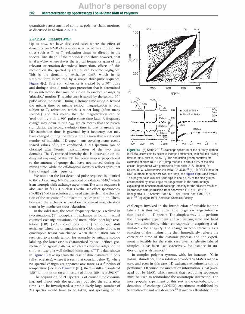
Author's personal copy202 Characterization by Spectroscopy | Solid-State NMR of Polymers
Figure 13 (a) Static 2D 13C exchange spectrum of the carbonyl carbon in PEMA, accessible by selective isotope enrichment, with 500 ms mixing time at 298 K, that is, below Tg. The simulation (inset) confirms the existence of slow 180° � 20° jump motions in about 40% of the side chains. Reproduced with permission from Kulik, A. S.; Radloff, D.; Spiess, H. W. Macromolecules 1994, 27, 4746.33 (b) 1D CODEX data for DMS (a model for a perfect two-site jump, see Figure 11(a)) and PMMA. This polymer also exhibits 180° flips in about 40% of the side groups, accompanied by small-angle rearrangements in the surroundings, explaining the observation of exchange intensity for the adjacent residues. Reproduced with permission from deAzevedo E. R.; Hu, W.-G.; Bonagamba, T. J; Schmidt-Rohr, K. J. Am. Chem. Soc. 1999, 121, 8411.23 Copyright 1999, American Chemical Society.
(a)
CH3
CH3
CH3
OCH3CH2CC
C
COOn
OO/8
900 ms
tm=
300 ms
75 ms
1 ms
300 200 100 0 ppm 0.2
E (
t m, δ
Nt R
)
ω11 ω22 ω33
0
DMS at 288 K
PMMA at 288 K
PMMA
4/53/42/3
1/2
DMS
0.4 0.6 0.80.0
0.2
0.4
0.6
0.8
1 s
(ppm)
(ppm
)
250 200 150 100
150
250
100
200
(b)
quantitative assessment of complex polymer chain motions, as discussed in Section 2.07.3.1.
2.07.2.3.4 Exchange NMR Up to now, we have discussed cases where the effect of dynamics on NMR observables is reflected in simple quantities such as T1 or T2 relaxation times, or directly in the spectral line shape. If the motion is too slow, however, that is, if k ≪ Δω, where Δω is the typical frequency span of the relevant orientation-dependent interaction, effects of this motion on the spectral quantities can become negligible.
the mixing time or mixing period, magnetization is only subject to T1 relaxation, which is rather long (often many seconds), and this means that the magnetization can be ‘read out’ by a third 90° pulse some time later. A frequency change may occur during tmix, which means that the precession during the second evolution time t2, that is, usually the FID acquisition time, is governed by a frequency that may
This is the domain of exchange NMR, which in its simplest form is realized by a simple three-pulse sequence, Figure 4(c). First, spin coherence is created by a 90° pulse and during a time t1 undergoes precession that is determined by an interaction that may be subject to random changes by ‘ultraslow’ motion. This coherence is stored by the second 90° pulse along the z-axis. During a storage time along z, termed
have changed during the mixing time. Given that a sufficient number of individual 1D experiments covering many evenly spaced values of t1 are conducted, a 2D spectrum can be obtained after Fourier transformation of the two time domains. The T1-corrected intensity that is observable on the diagonal (ω1 = ω2) of this 2D frequency map is proportional to the amount of groups that have not moved during the mixing time, while the off-diagonal intensity reflects spins that have changed their frequency.
We note that the just described pulse sequence is identical to the 2D exchange NMR experiment of solution NMR,8 which is an isotropic-shift exchange experiment. The same sequence is also used in 1H 2D nuclear Overhauser effect spectroscopy (NOESY) NMR in solution and used extensively in the elucidation of the structure of biomacromolecules in solution. There, however, the exchange is based on incoherent magnetization transfer by incoherent cross-relaxation.9
In the solid state, the actual frequency change is realized in two situations: (1) isotropic shift exchange, as found in actual chemical exchange situations, and measurable under high resolution (HR) (MAS) conditions or (2) anisotropic shift exchange, where the orientations of a CSA, dipole–dipole, or quadrupole tensor can change. When the situation can be restricted to a single tensor, for example, by suitable isotope labeling, the latter case is characterized by well-defined geometric off-diagonal patterns, which are elliptical ridges for the simplest case of a well-defined jump angle.10 The data shown in Figure 13 take up again the case of slow dynamics in poly (alkyl acrylates), where it is seen that even far below Tg, where no spectral changes are apparent any more as a function of temperature (see also Figure 11(b)), there is still a disordered 180° jump motion on a timescale of about 100 ms at 298 K.40
The acquisition of 2D spectra is of course time consuming, and if not only the geometry but also the correlation time is to be investigated, a prohibitively large number of 2D spectra would have to be taken, not speaking of the
challenges involved in the introduction of suitable isotope labels. It is thus highly desirable to get exchange information also from 1D spectra. The simplest way is to perform the three-pulse experiment at fixed mixing time and fixed first evolution delay, which corresponds to acquiring a stimulated echo at t2 = t1. The change in echo intensity as a function of the mixing time then immediately reflects the correlation time of the dynamic process, and the experiment is feasible for the static case given single-site labeled samples. It has been used extensively, for instance, in studies of glassy dynamics.41
In complex polymer systems, with, for instance, 13C innatural abundance, site resolution provided by MAS is mandatory, and even in this case, 1D exchange experiments can be performed. Of course, the orientation information is lost (averaged out by MAS), which means that recoupling sequences must be used to reintroduce the anisotropic interaction. The most popular experiment of this sort is the centerband-only detection of exchange (CODEX) experiment established by Schmidt-Rohr and collaborators.23 It involves flexibility in the

Author's personal copyCharacterization by Spectroscopy | Solid-State NMR of Polymers 203
Time
Se 2
Low MW High MW
C(t) Fast segmental
modes ns…μs (~τα, τs)
Slower cooperative
modes μs…s
Networks
1
0.1
0.01
0.001
0.0001 ∼τe
Figure 14 Schematic segmental orientation autocorrelation function of entangled or cross-linked polymers above Tg. Sufficiently long entangled chains exhibit an intermediate plateau that is related to the entanglement spacing (tube diameter) and a transition to the isotropic case only at long times exceeding the disentanglement time. Networks exhibit permanent plateaus related to the density of cross-links.
recoupling of the CSA interaction, where systematic changes of the length of the recoupling time (NtR) allow for an estimate of the jump angle, while the mixing-time dependence gives the correlation time. The final exchange intensity plateau at long mixing and recoupling times is further dependent on the number of distinguishable sites accessible to the process. One always observes the 13C signal intensity of the site of interest, which means that different moieties of large molecules are monitored simultaneously. The scheme also involves a clever strategy to normalize for effects of T1 relaxation during the mixing time, which would otherwise lead to unwanted signal decay. See Figure 13(b) for CODEX data taken on PMMA, where in analogy to the PEMA case in Figure 13(a), the side-chain COO groups perform two-site jumps.23 The intensity plateau of 0.2 is compatible with a fraction of 40% mobile side groups. This highlights the potential of this versatile technique that has already found a large number of applications in polymer science. Recent work of one of the authors has, for instance, focused on extending the CODEX experiment to measuring reorientations of 1H-15N dipole–dipole tensors of amide groups in a full-size protein, providing for the first time a site-resolved picture of slow dynamics in such a large macromolecule.42
Formally, when the exchange intensity Figure 13(b) isplotted as 1 – E(tmix;δNtR), it is identical to an orientation auto-correlation function of the process. In the case of CODEX, the recoupling (encoding) time NtR determines the angular sensitivity (δ is the anisotropy parameter of the chemical shift tensor), and the exact mathematics is somewhat involved due to the MAS. In case of static stimulated-echo experiments mentioned above, one obtains essentially analogous, but a mathematically even simpler signal function, that is, the ‘sine-sine’ correlation function of P2,
Fsinðtmix Þ ¼ ⟨ sin½δt1 P2ðcos θðτÞÞ�sin½δt1 P2ðcos θðtmix þ τÞÞ�⟩τ At a fixed and long evolution (encoding) time t1, this function decays to zero for infinite mixing time when the motion is diffusive, but to a finite plateau if there is a fraction of immobile groups, or a jump process among a finite number of sites. The explanation for the latter is simple: a return jump means that the angle θ has not changed during the mixing time, which means a constant <sin2φ> contribution. Otherwise, the values of θ before and after tmix are uncorrelated and the ensemble average over the product of the two sine functions is zero. We also note that the Fsin function is closely related to the P2
autocorrelation function C(t) addressed in Section 2.07.2.3.3, precisely, Fsinðtmix Þ ≈ Cðtmix Þδ2t2 for short fixed evolution1
(encoding) time t1. Finally, it should be noted that the possibilities of exchange
NMR go much beyond the direct measurement of such single-time autocorrelation functions. It is in fact possible to combine two (or more) (encode-tmix-decode) exchange pulse sequences in a single, then multidimensional exchange experiment,10 see Figure 4(d), providing access to higher time-correlation functions of the form
Fsinðtm1,tm2,…Þ ¼ ⟨ sin �ðτÞ sin �ðτ þ tm1Þ sin �ðτ þ tm1
þ tm2Þ � ⋯ ⟩τ
When the mixing times are independently varied, one can probe subtle and fascinating properties of the dynamic
process, such as correlations between forward and backward jumps, rate memory, and many more details.10 Such tools were instrumental for the important contributions of solid-state NMR for the understanding of polymer dynamics at the glass transition, which are addressed in Section 2.07.3.2.4.
2.07.3 Polymer Applications of Solid-State NMR
2.07.3.1 Polymers Above Tg: Elastomers and Melts
Heating a polymer far above its Tg, or above Tm if the sample is semicrystalline, provides the interesting situation that the molecular dynamics is almost liquid-like. ‘Almost’ means that we are still dealing with a soft solid, for instance, with an elastomer if the sample exhibits permanent cross-links or with a viscoelastic melt if the molecular weight (MW) is high, and the polymer is entangled. In these cases, the special physical properties, based on entropic elasticity, ultimately arise from the fact that segmental motion is not isotropic. Thus, there is a residual degree of local chain orientation (or chain order), which is best described by the orientation autocorrelation function introduced in Section 2.07.2.3.3. Different scenarios are sketched in Figure 14, where we see that starting in the glassy state at short times t < τα, glassy and segmental dynamics afford a progressive reduction of C(t). A well-defined plateau value is reached for highly entangled melts and elastomers, and this plateau value is associated with the local pffiffiffiffiffiffiffiffiffiffiffiffiffiffiffiffiffiffiffi dynamic order parameter S ¼ Cðt > τeÞ ≈ 3=5N, which according to the theory of Kuhn and Grün43 can be related to the number of statistical (Kuhn) segments N between constraints (entanglements or cross-links). Thus, this quantity is, on the one hand, directly related to important structural parameters of the polymer system, that is, the number of segments per entangled strand or the number of segments per network chain. On the other hand, the finite local orientation is directly proportional to residual anisotropic interactions (e.g., Dres = S � Dstat for dipole–dipole coupling), leading to solid-like NMR phenomena.44

Author's personal copy
Si(CH3)2O—[ Si(CH3)2O]—[Si(CH3) ]— (a) n m
+
1.0 0.5 0.0 –0.5–1.0
1.0 0.5 0.0 –0.5–1.0
6.0 5.9 5.8 5.76.0 5.9 5.8 5.7
6 4 2 0 ppm
(b)
(c)
6.0 5.9 5.8 5.7
x100
Irel = 2.1%
Irel = 0.36%
(H(CH3)2Si)2O
↓ (Pt cat.)
H(CH3)2SiO—Si(CH3)2 —CH2
—
H2C
[ Si(CH3)2O ] Si(CH3)—
—
— — n
6 4 2 0 ppm
204 Characterization by Spectroscopy | Solid-State NMR of Polymers
Figure 15 NMR analysis of polydimethylsiloxane (PDMS) elastomer formation by cross-linking of PDMS with methylvinyl siloxane co-units and a difunctional silane cross-linker: (a) reaction scheme, (b) 1H solution spectrum of the linear precursor polymer, and (c) 1H MAS spectrum of the bulk elastomer. The insets are vertically magnified by a factor of � 100. For comparison, a static spectrum of octane-swollen PDMS is shown as dotted line in panel c.
8:105 CH2
αB4+ αB4+
αB4+
αB4+
∗B4+
∗B4+∗B2
∗B2 αB2 αB2
αB2
7:105 CH2
42 40 38 36 3413C chemical
Figure 16 Quantification of low branch content in PE by optimized melt-state branches in 100 000 CH2 groups. Reproduced with permission from Klimke, KCopyright 2000, by John Wiley & Sons, Inc.
2.07.3.1.1 High-resolution MAS The situation far above Tg is favorable for NMR, because the typical anisotropic broadening of the rigid-limit case is reduced to a rather low level. This means that moderate MAS (one or a few kilohertz) is sufficient to almost completely remove the residual anisotropic interactions, which is particularly favorable for 1H, where liquid-like HR is still out of reach for rigid solids, but is now easily achieved. This condition has found the name ‘HR-MAS’, and in order to optimize experimental conditions, specialized MAS rotors minimizing susceptibility artifacts and MAS probes featuring a deuterium lock are commercially available. However, even conventional MAS probes can be used to easily obtain very satisfactory HR spectra, opening new experimental possibilities. As an example, Figure 15 displays results on the determination of absolute cross-link conversion in end-linking reactions of polysiloxanes.
Even though 13C resolution in rigid solids suffers less from residual spectral broadening due to the inhomogeneous nature of the 13C CSA and the good decoupling sequences available today, melting the sample and observing 13C under HR-MAS conditions can also open new perspectives. For instance, the 13C chemical shift dispersion due to mixed conformations in the glassy state or the amorphous fraction of a semicrystalline polymer is often still substantial, which means that the achievable signal-to-noise ratio (S/N) is still limited.
HR-MAS also solves this problem, as the line positions are then unique because of fast averaging between different conformations in analogy to the solution case. Under well-optimized conditions, it is therefore even possible to analyze very low levels of branch point concentrations in branched polyethylene (PE) with 13C in natural abundance, that is, in
45,46as-made samples. This is illustrated in Figure 16.
δ + γ
32 30 28 26
shift (ppm)
direct-polarization 13C NMR under MAS, with reliable determination of 7–8 45 .; Parkinson, M.; Piel, C.; et al. Macromol. Chem. Phys. 2006, 207, 382.

Author's personal copyCharacterization by Spectroscopy | Solid-State NMR of Polymers 205
2.07.3.1.2 MQ NMR on elastomers and melts As outlined in the introduction to this section, the residual anisotropic NMR interactions provide valuable information on the microstructure of elastomers on the one hand, and on entangled chain dynamics in linear melts and other topologies on the other hand. There is a long history in studying the simple transverse relaxation behavior of elastomers, and it is long known that inverse T2 relaxation time of protons, dominated by homonuclear dipole–dipole couplings and suitably determined from a usually nonexponential Hahn-echo decay, is proportional to the cross-link density, provided that the temperature is high enough (‘T2 plateau’). The phenomenon can be understood by reference to Figure 14, where it is seen that the plateau of the correlation function is higher than the entanglement level when the cross-link separations (∼ Mc) are smaller than the entanglement length (∼ Me). The plateau is thus S ≈ 3/5Nc at sufficiently high cross-link densities νc =2/Mc = 2/M0Nc (here assuming 4-functional cross-links, and M0 as the mass of Kuhn segment). The finite high-temperature pffiffiffiffiffiffiffiffiffiffiffiffiffiffiffiffiffiffiffi order parameter S ¼ Cðt > τeÞ ≈ Dres =Dstat =a (with a <1 describing preaveraging of motions within a Kuhn segment) is proportional to a well-defined residual dipole–dipole coupling
τecho
Φ′ = ∫ ωdip(t)d(a) 0
Hahn echo τecho/2 π τech
τDQ τ
τDQ
DQ recoDQ excitation MQ experiment
Φ = k ∫ ωdip(t )dt 0
(b) FID/Hahn echo:
tails Spectra Idip = Iecho –
StructureIdeal
= <cos Φ′>
FT
Time t
Structure +Real
dynamics
Freq.
Figure 17 (a) Comparison of the timings of the Hahn-echo and MQ experimdelays. (b) Schematic comparison of spectra and time-domain signals for Hahrealistic multispin system.
Dres, that simply leads to non-refocusable dipolar dephasing with an apparent T2∝D−1. If the temperature is not high res
enough, the apparent Dres (or T2) is still influenced by segmental motions in a region where C(t) has not reached itsplateau.
In recent years, substantial progress was achieved in the precise direct measurement of residual dipole–dipole couplings in elastomers, and in even measuring C(t) directly and quantitatively, which is of interest to elucidate details of the reptation (tube) model of polymer dynamics.47 The technique of choice turned out to be static multiple-quantum (MQ) NMR,29 which has decisive advantages over simple T2 experiments. This is illustrated in Figure 17, where in panel a the two pulse sequences are compared. Both techniques have in common that the spin evolution is dominated by (residual) dipole–dipole couplings, leading to similar phase factors. While in the Hahn echo, we have a net free dipolar evolution over the whole echo time, the MQ experiment features two blocks, during the first of which higher-quantum coherences (not only between like spins, mostly protons, but also in single quadrupolar nuclei) are created. These are unobservable, and the second block serves to reconvert these coherences back to
t
o/2 Idip
DQ
nversionIDQ,ref
MQ experiment: IΣΜQ = IDQ + Iref – tails
= <sin2Φ> + <cos2Φ>
0.5
ΣMQ
DQ
IDQ = <sin2Φ>
DQ
nDQ = DQ/ΣMQ:ΣMQ: Structure only!
Dynamicsonly!
0.5
tails due to mobile impurities (chain ends, sol…)
ents, with indicated dipolar phase factors acquired during the evolution n-echo and MQ experiments, performed on an isolated spin pair and on a

Author's personal copy206 Characterization by Spectroscopy | Solid-State NMR of Polymers
observable magnetization that is finally read out by a pulse. The primary spin states of interest are DQ coherences between individual spin pairs, which acquire a phase factor Φ that is different from the free-evolution case (Φ′) only by a pulsesequence-dependent factor k (usually between 0.5 and 1).
More details of the responses of the two experiments are sketched in Figure 17(b). The advantages arises from the fact that the MQ experiment can be performed in ways that differ in the receiver phase: using appropriate phase cycling, an intensity IDQ related only to the buildup of DQ coherences (� sin Φ) can be measured, but also a signal Iref related the part of the magnetization (� cos Φ) that has not evolved into DQ coherence after excitation. These two signals are complementary, the final intensity associated with the former following <sin2Φ> and the latter following <cos2Φ>, since both pick up another cos or sin phase factor, respectively, during reconversion. Thus essentially, the two signals differ from the Hahn echo (Iecho � <cos Φ′>) only by the trigonometric function of Φ′ = kΦ. The powder average of the sin2 function reflects much more directly the action of residual couplings: it is a buildup function, where relaxation effects (due to motions on the NMR timescale when C(t) is not in the plateau) lead to a decay at long times. In the T2 experiment, ambiguities arise because both dipolar dephasing and incoherent relaxation lead to decays alike. Furthermore, the sum I∑MQ = IDQ + Iref (after suitable subtraction of slowly relaxation signal tails that are
(a)
0.6
0
Rel
. am
plitu
de
DQ
inte
nsity 0.4 % short chains:
0net0 net10 net20 0net30 net50 0.2 net70 0net90 net100
00.0 0.0 0.5 1.0 1.5 2.0 2.5 3.0 3.5
DQ evolution time (ms)
(b) (c) 0
0.8 NR1 pure NR1 33 wt% silica 00.7 NR2 pure
0.6 NR2 31 wt% carbon black
Rel
. am
plitu
de
Rel
. am
plitu
de 0
0
0
0.5
0.4
0.3
0.2
0.1 0
0.0 00.0 0.5 1.0
Dres /2π (kHz)
Figure 18 (a) Normalized DQ buildup functions and corresponding distributmodel-inhomogeneous PDMS networks, made by end-cross-linking of very shoobtained by numerical analysis, while the dashed lines are merely superpositiowithout any fits the presence of subnetwork structures with conserved mesh srubber, pure and filled with nanometric carbon black and silica particles, and (
associated with isotropically mobile defect fractions such as chain ends) is a relaxation-only function, as it is ultimately a full dipolar echo in the same sense as a magic-sandwich echo. This sum function can be used to point-by-point normalize away the relaxation effect in IDQ (lower right of Figure 17(b)), which gives a dipolar buildup function InDQ = IDQ/I∑MQ that is free of relaxation effects due to the segmental dynamics even before the plateau of C(t) is reached on the experimental time-scale. In networks, where C(t) has a plateau to infinite time, one thus obtains a buildup function that is independent of temperature and reflects only the structural effect of the cross-links.
It should be stressed that the discussed effects, especially when referring to proton NMR, are essentially field independent, which means that the described experiments can be carried out on simple low-field spectrometers, provided that chemical resolution is not needed, which is the case for most single-component elastomers and melts.
Figure 18(a) presents normalized proton DQ buildup functions of end-linked polydimethylsiloxane model networks prepared by mixing and subsequent cross-linking of very short and rather long chains. Such bimodal networks are known to consist of clusters of highly cross-linked regions embedded in a long-chain elastomer matrix. The buildup curves as well as the cross-link density distributions (i.e., the distributions of Dres) derived from these show clear bimodal
.8 100%
90%.6 70%
50% .4
30%
20%.2
10%
0%.00.0 0.4 0.8 1.2 1.6
/2π (kHz)Dres
.6NR-peroxideNR-sulfur conventional.5 NR-sulfur efficient
.4
.3
.2
.1
.0 0.0 0.2 0.4 0.6 0.8 1.0
Dres /2π (kHz)
ions of residual dipolar couplings reflecting the cross-link density for rt (0.8 kDa) and very long (47 kDa) precursor chains. The distributions are ns of the pure-component curves weighted by stoichiometry, proving ize. (b) Residual coupling (cross-link density) distributions of natural c) natural rubber vulcanized with different cure systems.

Author's personal copy
(a) C
φ C
C
Sub- Free Constrained Reptation Free segmental Rouse Rouse diffusion
t 1 1
log
< (r
(t )
− r (
0) )
2> 10−6 m
0 I II III IV t −1
log C(t)
t −1/4 t 1/2 10−4
10−8 m t −1/2
t 1/4
10−10 t 1/2m 10−8
ps ns ns – μs μs – ms ms – days τs τe τR τd
(b) log t
100
101
t−0.85
PB2.8k (Z = 1.5) PB4.6k (Z = 3) PB9.5k (Z = 5) PB11.4k (Z = 8) PB18k (Z = 10)
T1 field cycling (Rößler group)
10−1
10−2 S 2 ~ 1/N 2
e e
0
I
PB23k (Z = 12) PB35k (Z = 19) PB87k (Z = 47) PB2000k (Z = 1100)
low-field MQ NMR (this work)
e II10−3
10−4 NSE 500 ns (T = 243 K) 10−5
10−6 NSE 500 ns III,IV (T = 383 K)
10−8
10−7
10−4 10−3 10−2 10−1 100 101 102 103 104 105
t / τe
(c)
7 IVτd6 τR5 3.42 III 2.164 ± 0.07
log
τ/τ e
± 0.253 2 II1
1.0 0.85 0.8
C(t
/ τ
)
Characterization by Spectroscopy | Solid-State NMR of Polymers 207
behavior. Regions of high and low cross-link density in elastomers can thus be distinguished with the MQ technique. The use of this new experimental possibility is highlighted in Figures 18(b) and 18(c), where it is demonstrated that contrary to common literature assumptions, the presence of nanometric fillers does not necessarily lead to detectable changes in the cross-link density of network fractions close to the filler surface, Figure 18(b). However, peroxide cross-linking indeed induces substantial network inhomogeneities, Figure 18(c), arising from the formation of multifunctional cross-links via radial chain reactions involving the double bonds.
Finally, Figure 19 summarizes data measured on polymer melts,47 where the shape of the normalized DQ buildup curves is sensitively influenced by the large-scale motion of the chains, that is, the reptation dynamics. In fact, the initial part (early rise) of InDQ(τDQ) can be shown to be directly proportional to C(τDQ)τ
2DQ , which means that the correlation function C(t)
can be directly measured in the time domain by combining experiments at different temperatures and using the time– temperature superposition principle. This is an advantage over the extraction of C(t) from T1 relaxation times from field-cycling experiments, which are also shown in Figure 14(b), because here the relation is given by a Fourier transform, requiring full coverage of even the lowest frequencies. This is not possible for high MWs because the reptation process cannot reach the fast limit with respect to the lowest possible Larmor frequencies (which are currently limited by the Earth’s field). However, the combination of T1 relaxometry and MQ NMR provides access to essentially the whole time range of interest (more than 10 decades), enabling a thorough experimental test of the tube model of polymer dynamics. Results of the analysis of the experimental C(t) with respect to the theoretical predictions are summarized in Figure 14(c). The regime transition times indeed follow the predicted MW dependences, however, in regime II (constrained Rouse motion within the tube) significant deviations from the predicted –1/4 time scaling exponent were observed, indicating that the reptation ‘tube’ is not a static constraint but undergoes significant dynamics, which in turn affects the motion of the probe chain. In Reference 47, it is shown by dilution in deuterated matrix chains that these deviations are due to the chains that form the tube, rather than being single-chain effects.
0.6 ε
Mc ≈ 2.5 Me
0.28
0.0 0.2 0.4
103 104 105 106
Mw (Da)
Figure 19 (a) Tube-model prediction for the correlation functions C(t), along with the Doi–Edwards regimes formulated for the mean-square displacement. (b) C(t) determined by MQ NMR for linear polybutadiene (PB) melts, from which the characteristic times of the tube model can be extracted. The plot includes early-time and low molar mass (M) data for C(t) that is accessible by complementary field-cycling T1 relaxometry. Z is the number of entangled units of mass Me. (c) Rouse and disentanglement times for PB of different M, log-log plotted vs. M, demonstrating the correct scaling exponents predicted by the tube model, but showing that the regime-II scaling exponent ε is not constant but rather larger than expected and further M dependent, highlighting deviations from the tube model. Reproduced with permission from Chávez, F. V.; Saalwächter, K. Phys. Rev. Lett. 2010, 104, 198305.47 Copyright 2010, American Physical Society.
2.07.3.2 Polymers Around and Below Tg
2.07.3.2.1 Conformations of polymers in the glassy state The basis of probing local conformation by NMR is the famous ‘γ-gauche effect’ introduced above, which says that the chemical shift of the central carbon in a vinyl polymer in an extended trans conformation is reduced by about 5 ppm for every γ-neighbor being in a gauche position.15 In amorphous polymers, however, the dihedral angles may differ from perfect geometry. This became evident when the local conformations in the solid state could directly be probed by HR-MAS 13C NMR, combined with quantum chemical calculations of the chemical shift, see the example of polypropylene in Figure 20.16 While the bands can roughly be assigned to specific local conformations as indicated, the individual spectral lines calculated after geometry optimization reveal a multitude of geometries with dihedral angles deviating for their ‘ideal

Author's personal copy
trans /trans (t∗.∗t)
Experiment
CH2 CH3
trans /gauche (t∗.∗g)
gauche /gauche (g∗.∗g) CH3
CH
C C
H
nH
( ) H
60
Theory
50 40
δ (ppm)
30 20 10
50 40
δ (ppm)
30 20 10
t∗.∗g
t∗.∗t g∗.∗g
208 Characterization by Spectroscopy | Solid-State NMR of Polymers
Figure 20 Scheme of local conformations (right) and 13C MAS NMR spectra of the CH2 group in amorphous atactic polypropylene. Reproduced with permission from Born, R.; Spiess, H. W. Macromolecules 1995, 28, 7785–7795.16 Copyright 1995, American Chemical Society.
values’. This leads to often broad and even featureless lines in the glassy state.
2.07.3.2.2 Local molecular motions in the glassy state As far as sub-Tg dynamics (often called β-relaxation) and its relation to ductility is concerned, bisphenol-A polycarbonate (PC) is one of the most studied, yet still controversial systems. For a recent review of the field, see Reference 48. From 2H NMR line shapes, large-angle phenylene rotations described by 180° flips augmented by additional oscillations were identified at room temperature and above.6 Such 180° flips were subsequently confirmed by 13C NMR line shape studies and 2H 2D
(a) 180° Phenyl filps 90° Phenyl filps
σ = 90°
0° 60° 120° 180° 240° 300° 360° 330°270° 30° 90° 270°210°150°
σ = 70°
0° 60° 120° 180° 240° 300° 360° 330°270° 30° 90° 270°210°150°
σ = 50°
0° 60° 120° 180° 240° 300° 360° 330°270° 30° 90° 270°210°150°
300 250 200 150 100 50 0 300 250 200 150 100Chemical shift (ppm) Chemical shift (ppm
Figure 21 Heterogeneous phenylene dynamics in polycarbonate (PC). (a) Liheterogeneous Gaussian distributions of flip angles centered at 180° and 90° wspectra for the two distinct phenylene carbon positions in PC fitted to a heterogangles centered at 180°, dashed line. Reproduced with permission from Graf, R2007, American Institute of Physics.
exchange NMR at lower temperatures. The timescale of the phenylene motion is in remarkable agreement with that of sub-Tg mechanical relaxation. Triggered by the interpretation of recent quasi-elastic neutron scattering data49 concluding that in addition to 180° flips the phenylene rings in PC exhibit a third motion, namely, flips by 90° with correlation times in the range between 1 ns and 1 ps at temperatures 300–400 K, the phenylene dynamics was revisited with advanced 2D NMR techniques. Probing the 13C anisotropic chemical shift, the geometry of the phenylene motion can be probed differently than via 2H quadrupole coupling and as seen in Figure 21(a), rapid 180° and 90° flips result in vastly different line shapes,
O
(b) O O
σiso = 129 ppm σiso = 122 ppm
T = 370 K
250 200 150 100 50 ppm 250 200 150 100 50 ppm
T = 300 K
50 0 250 200 150 100 50 ppm 250 200 150 100 50 ppm )
ne shape simulations for motionally narrowed 13C NMR spectra for ith different standard deviations σ as indicated. (b) Experimental 13C NMR eneous Gaussian distribution with full width at half maximum of 80° of flip .; Ewen, B.; Spiess, H. W. J. Chem. Phys. 2007, 50126, 041104. Copyright
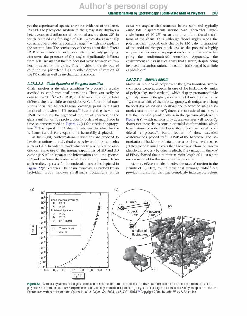
Author's personal copyCharacterization by Spectroscopy | Solid-State NMR of Polymers 209
yet the experimental spectra show no evidence of the latter. Instead, the phenylene motion in the glassy state displays a heterogeneous distribution of rotational angles, about 80° in width, centered at a flip angle of 180°, which stays essentially constant over a wide temperature range,50 which also explains the neutron data. The consistency of the results of the different NMR experiments and neutron scattering is truly gratifying. Moreover, the presence of flip angles significantly different from 180° means that the flip does not occur between equivalent positions of the group. This provides a simple way of coupling the phenylene flips to other degrees of motion of the PC chain as well as mechanical relaxation.
2.07.3.2.3 Chain dynamics at the glass transition Chain motion at the glass transition (α process) is usually ascribed to ‘conformational’ transitions. These can easily be detected by 2D 13C MAS NMR, as different conformers exhibit different chemical shifts as noted above. Conformational transitions then lead to off-diagonal exchange peaks in 2D and motional narrowing in 1D spectra.10 By combining the various NMR techniques, the segmental motion of polymers at the glass transition can be probed over 14 orders of magnitude in time as demonstrated in Figure 22(a) for atactic polypropylene.51 The typical non-Arrhenius behavior described by the Williams–Landel–Ferry equation3 is beautifully displayed.
At first sight, conformational transitions are expected to involve rotations of individual groups by typical bond angles such as 120°. In order to check whether this is indeed the case, one can make use of the unique capabilities of 2D and 3D exchange NMR to separate the information about the ‘geometry’ and the ‘time dependence’ of the chain dynamics. From such studies, a picture for the molecular motion as depicted in Figure 22(b) emerges. The chain dynamics as probed by an individual group involves small-angle fluctuations, which
(a) 104
(b)
103
102 Conformational dynamics
PP29
101 PP27
100 Rotational dynamics
PP29
10–1 PP27
10–2 2D 2H-NMR
⟨τ⟩ /
s 10–3 13C relaxation
10–4 WLF fit
10–5
10–6
10–7
10–8
10–9
10–10
10–11 0,4 0,5 0,6 0,7 0,8 0,9 1,0 1,1
Tg / T
Figure 22 Complex dynamics at the glass transition of soft matter from mulpolypropylene from different NMR experiments. (b) Geometry of rotational moReproduced with permission from Spiess, H. W. J. Polym. Sci. 2004, A42, 50
occur via angular displacements below 0.5° and typically cause total displacements around 2–4°. Thereafter, ‘large’angle jumps of 10–25° occur due to conformational transitions of the chain. Thus, although ‘bond angles’ along the polymer chain undoubtedly change by 120°, the ‘orientation’ of the residues changes much less, as the process is highly cooperative involving many repeat units around the one undergoing the conformational transition. Apparently, the environment adjusts in such a way that a group, despite being involved in a conformational transition, is displaced by as little as possible.52
2.07.3.2.4 Memory effects Molecular motions of polymers at the glass transition involve even more complex aspects. In case of the backbone dynamicsof poly(n-alkyl methacrylates), which display pronounced side group dynamics in the glassy state as noted above, the anisotropic 13C chemical shift of the carboxyl group with unique axis along the local chain direction also allows one to detect possible anisotropic chain motion above Tg due to conformational memory. In fact, the nice CSA powder pattern in the spectrum displayed in Figure 8(a), which narrows only at temperatures well above Tg, shows that these chains contain extended conformations, which have lifetimes considerably longer than the conventionally considered α process.35 Randomization of these extended conformations, probed by 13C NMR of the backbone, and isotropization of backbone orientation occur on the same timescale, yet they are both much slower than the slowest relaxation process identified previously by other methods. The variation in the MW of PEMA showed that a minimum chain length of 5–10 repeat units is required for this memory effect to occur.
Memory effects can also involve the rates of motion in the vicinity of Tg. Here, multidimensional exchange NMR10 can provide information that was completely inaccessible before.
a: jump (c)
b’: back b: forward jump jump
small angle fluctuations
ξhet
tidimensional NMR. (a) Correlation times of chain motion of atactic tions. (c) Dynamic heterogeneities as visualized by computer simulation.
5231–5044. Copyright 2004, by John Wiley & Sons, Inc.

Author's personal copy
(a)
0.00 0.05 0.10 0.15 0.20 0.0
0.2
0.4
0.6
0.8
1.0
Nor
mal
ized
inte
nsity
MAPE-filtered mobile: Tm = 0.73 μs, νm = 1.24
DQ-filtered rigid: Gaussian,Tr = 18.3 μs
Rigid-interfacial:T ri = 25.5 μs, νri = 0.82
∗
~10% Mobile loss due to 500 μs MAPE filter
Full (refocused) FID: fr = 0.65, fri ′ = 0.18
∗
∗
Acquisition time (ms) (b)
0.8
1.0
ity
210 Characterization by Spectroscopy | Solid-State NMR of Polymers
As the geometry and the timescale of molecular motion are probed separately and, moreover, the motional behavior can be probed at up to 4 subsequent times, questions can be tackled such as ‘is the probability of undergoing a jump different after the group has performed a jump?’ In a series of pioneering papers,53 the nature of nonexponential relaxation in polymers in the vicinity of the glass transition was examined. This led to the concepts of ‘rate memory’ and ‘dynamic heterogeneities’, which today are recognized as a signature of fragile glass formers.54,55 The unique capabilities of NMR were exploited to develop a technique combining 4D NMR with spin diffusion that allowed one to detect not only the timescale of such heterogeneities, but also their length scale in the nanometer range. It was found that the number of statistically independent units engaged in these heterogeneities is below 100. Therefore, it is tempting to relate them to the ‘cooperatively rearranging’ units first postulated by Adam and Gibbs.56
Indeed, computer simulations57 show that such heterogeneities can even occur in simple hard-sphere systems as displayed in Figure 22(c).
0.2
0.4
0.6
Nor
mal
ized
inte
nsMAPE-filtered mobile MAPE-filtered rigid sat. rec. mobile sat. rec. rigid
Rigid fraction
0 5 10 15 20 25 30 0.0
Sqrt(spin diffusion time ms)
Figure 23 (a) Example of the decomposition of a magic-echo refocused low-field 1H FID of a PS-PB block copolymer into three components, based on component selection using magnetization filters. (b) Spin diffusion curves of the rigid (including the rigid-interfacial) and mobile components after selection of the mobile phase. Simultaneous numerical fitting of spin diffusion as well as phase-resolved saturation recovery data with a two-phase layer model provides accurate information on the domain sizes despite competing T1 relaxation effects, which are particularly strong at low field. Reproduced from Mauri, M.; Thomann, Y.; Schneider, H.; Saalwächter, K. Solid State Nucl. Magn. Reson. 2008, 34, 125.58 Copyright 2008, with permission from Elsevier.
2.07.3.3 Multiphase Polymers
It is a well-known fact that the vast majority of polymers for applications relying on advanced and tailor-made mechanical (and other) properties consist of systems that are dynamically and/or compositionally inhomogeneous on the nanometer length scale. This holds for compatibilized blends, for block copolymers, and, of course, for semicrystalline polymers. The understanding of molecular-scale properties, such as molecular dynamics and domain sizes, is at the very heart of establishing meaningful structure–property relations, and NMR is continuing to contribute significant insights in these areas. Here, we focus on recent progress in using both established and simple methods such as spin diffusion experiments at low field, but also more advanced high resolution SLF experiments, to reveal new insights into, for example, the interphase in common block copolymers, or the dynamics of crystalline phases in functional polymers.
2.07.3.3.1 Block copolymers Easy qualitative access to the dynamic properties of the individual block copolymer phases is provided by standard 13C CP MAS spectroscopy and its variants, as introduced in Section 2.07.2.2.4. While 13C provides site resolution, the signal intensities associated with different groups or domains can, for instance, be monitored as a function of CP time. A fast or a slow rise indicates low or high mobility, respectively, for instance, when the subphase is either below or well above Tg. Alternatively, one can introduce an indirect proton dimension into the CP sequence directly after the initial 1H excitation pulse, which is the WISE experiment. Under moderate MAS conditions, the Fourier transform of this indirect proton dimension is dominated by the 1H line width, again reflecting mobility in the respective microphase that is identified by the CP transfer to the next One can further elaborate13C. the experiment by adding a 1H spin diffusion segment after the indirect dimension (or, alternatively, use a very long CP). See Section 2.07.2.2.6 for an introduction into the spin diffusion effect and its applications. Comparing WISE spectra without and with spin diffusion, one can get a first insight
into the spatial proximity of the high- and low-mobility regions.10
13C-based NMR is most often performed in natural isotopic abundance on as-made samples. The experimental times on the order of a day for 2D spectra, however, often challenge the feasibility of a multiparameter study. We therefore highlight some recent work using only 1H NMR. As shown in Figure 12, a simple 1H FID acquired on a simple low-field spectrometer carries valuable dynamic information, and when an efficient short magic-sandwich echo is used, one can even overcome almost quantitatively the problems of probes with dead times on the order of 10 μs, with which the meaningful initial part of the FID cannot be measured. Suitable fits of FIDs of block copolymers can thus yield the amount of material in domains with different mobility, provided that the fits are stable and meaningful.
A possible strategy is shown in Figure 23(a), where the FIDs of the isolated rigid and mobile fractions in a PS–polybutadiene (PS-PB) block copolymer were measured
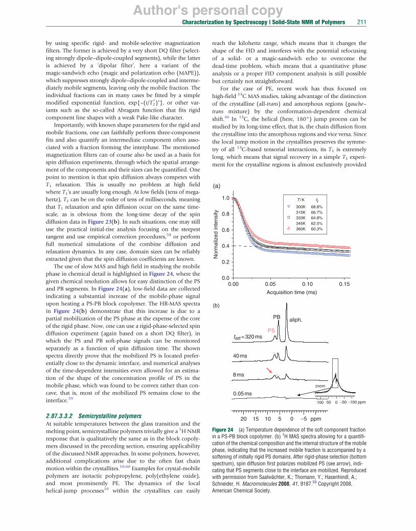
Author's personal copy
(a)
1.0 T /K fr
Nor
mal
ized
inte
nsity
300K 68.8% 315K 66.7%0.8 333K 64.8% 345K 62.5% 360K 60.3%0.6
0.4
0.2
0.0 0.00 0.05 0.10 0.15
Acquisition time (ms)
(b)
PB aliph.
PS 320ms tdiff =
40 ms
8ms
zoom
0.05 ms
100 50 0 −50 −100 ppm
20 15 10 5 0 −5 ppm
Characterization by Spectroscopy | Solid-State NMR of Polymers 211
Figure 24 (a) Temperature dependence of the soft component fraction in a PS-PB block copolymer. (b) 1H MAS spectra allowing for a quantification of the chemical composition and the internal structure of the mobile phase, indicating that the increased mobile fraction is accompanied by a softening of initially rigid PS domains. After rigid-phase selection (bottom spectrum), spin diffusion first polarizes mobilized PS (see arrow), indicating that PS segments close to the interface are mobilized. Reproduced with permission from Saalwächter, K.; Thomann, Y.; Hasenhindl, A.; Schneider, H. Macromolecules 2008, 41, 9187.59 Copyright 2008, American Chemical Society.
by using specific rigid- and mobile-selective magnetization filters. The former is achieved by a very short DQ filter (selecting strongly dipole–dipole-coupled segments), while the latter is achieved by a ‘dipolar filter’, here a variant of the magic-sandwich echo (magic and polarization echo (MAPE)), which suppresses strongly dipole–dipole-coupled and intermediately mobile segments, leaving only the mobile fraction. The individual fractions can in many cases be fitted by a simple modified exponential function, exp{–(t/T2
*)ν}, or other variants such as the so-called Abragam function that fits rigid component line shapes with a weak Pake-like character.
Importantly, with known shape parameters for the rigid and mobile fractions, one can faithfully perform three-component fits and also quantify an intermediate component often associated with a fraction forming the interphase. The mentioned magnetization filters can of course also be used as a basis for spin diffusion experiments, through which the spatial arrangement of the components and their sizes can be quantified. One point to mention is that spin diffusion always competes with T1 relaxation. This is usually no problem at high field where T1 ’s are usually long enough. At low fields (tens of megahertz), T1 can be on the order of tens of milliseconds, meaning that T1 relaxation and spin diffusion occur on the same time-scale, as is obvious from the long-time decay of the spin diffusion data in Figure 23(b). In such situations, one may still use the practical initial-rise analysis focusing on the steepest tangent and use empirical correction procedures,58 or perform full numerical simulations of the combine diffusion and relaxation dynamics. In any case, domain sizes can be reliably extracted given that the spin diffusion coefficients are known.
The use of slow MAS and high field in studying the mobile phase in chemical detail is highlighted in Figure 24, where the given chemical resolution allows for easy distinction of the PS and PB segments. In Figure 24(a), low-field data are collected indicating a substantial increase of the mobile-phase signal upon heating a PS-PB block copolymer. The HR-MAS spectra in Figure 24(b) demonstrate that this increase is due to a partial mobilization of the PS phase at the expense of the core of the rigid phase. Now, one can use a rigid-phase-selected spin diffusion experiment (again based on a short DQ filter), in which the PS and PB soft-phase signals can be monitored separately as a function of spin diffusion time. The shown spectra directly prove that the mobilized PS is located preferentially close to the dynamic interface, and numerical analyses of the time-dependent intensities even allowed for an estimation of the shape of the concentration profile of PS in the mobile phase, which was found to be convex rather than concave, that is, most of the mobilized PS remains close to the interface.59
2.07.3.3.2 Semicrystalline polymers At suitable temperatures between the glass transition and the melting point, semicrystalline polymers trivially give a 1H NMR response that is qualitatively the same as in the block copolymers discussed in the preceding section, ensuring applicability of the discussed NMR approaches. In some polymers, however, additional complications arise due to the often fast chain motion within the crystallites.10,60 Examples for crystal-mobile polymers are isotactic polypropylene, poly(ethylene oxide), and most prominently PE. The dynamics of the local helical-jump processes10 within the crystallites can easily
reach the kilohertz range, which means that it changes the shape of the FID and interferes with the potential refocusing of a solid- or a magic-sandwich echo to overcome the dead-time problem, which means that a quantitative phase analysis or a proper FID component analysis is still possible but certainly not straightforward.
For the case of PE, recent work has thus focused on high-field 13C MAS studies, taking advantage of the distinction of the crystalline (all-trans) and amorphous regions (gauche– trans mixture) by the conformation-dependent chemical shift.46 In 13C, the helical (here, 180°) jump process can be studied by its long-time effect, that is, the chain diffusion from the crystalline into the amorphous regions and vice versa. Since the local jump motion in the crystallites preserves the symmetry of all 13C-based tensorial interactions, its T1 is extremely long, which means that signal recovery in a simple T1 experiment for the crystalline regions is almost exclusively provided

Author's personal copy
(a)
1.0
Melt crystallized0.8
Solution crystallized
0.6
0.4
0.2
0.0 0 5 10 15 20
t0.5 (s0.5)
(b)
Solution crystallized Melt crystallized
13C CP MAS spectra
Crystalline Noncrystalline
36 34 32 30 28 Chemical shift (ppm) Chemical shift (ppm)
Nor
mal
ized
inte
nsity
25
36 34 32 30 28
Experiment Simulation
13C-1H dipolar sidebands (noncryst.)
−6 −4 −2 0 2 4 6 −6 −4 −2 0 2 4 6 ω/ωR ω/ωR
212 Characterization by Spectroscopy | Solid-State NMR of Polymers
Figure 25 (a) Decay of the crystalline PE signals of melt- vs. solution-crystallized samples, measured with a simple exchange-type experiment (z filter). The decay is dominated by the diffusion into the amorphous phase, where the signal relaxes quickly due to the short T1. Intracrystalline chain diffusion is seen to be much faster in solution-crystallized samples. (b) 13C spectra and amorphous-phase CH dipolar sidebands from DIPSHIFT-type experiments, demonstrating a more constrained amorphous-phase dynamics in the solution-crystallized sample. Reproduced with permission from Yao, Y.-F.; Graf, R.; Spiess, H. W.; et al. Phys. Rev. E 2007, 76, 060801(R).46 Copyright 2007, American Physical Society.
by chain transport from the quickly relaxing amorphous regions. Corresponding data are shown in Figure 25, compar-ing melt- and solution-crystallized samples. It was found that the crystal-amorphous chain diffusion is much faster in the solution-crystallized samples (and also in as-made high-MW reactor powders, which are made up of highly crystalline single-chain lamellae), which was explained by the lower acti-vation entropy for a chain that is moving through tight and conformationally better-defined adjacent-reentry loops of a very small amorphous phase. The higher conformational order in the amorphous phase of the latter systems was in fact directly observed in DIPSHIFT/SLF-type experiments, measur-ing the motionally reduced CH dipole–dipole coupling (Figure 25(b)).
Advanced 2D experiments’ correlating anisotropic interactions with the isotropic chemical shift were also the key to elucidating the dynamics in special PE samples with well-defined, perfectly regularly spaced defects.61 When the defects are just methyl groups, they can be included in the crystallites, and thus change the dynamics of the chains therein. Using an experiment correlating isotropic 13C chemical shifts with the CSA tensor of the same carbon, one can observe again the result of fast-limit dynamics of variable amplitude on the motion-averaged CSA tensor in a site-resolved fashion. The data shown in Figure 26 suggest that the CH2 stretches between the incorporated defects are increasingly less mobile away from the defect sites, while at the defect positions, the data (including 2H spectra of the labeled methyl branches) are consistent

Author's personal copy
PE
PE 21-CD3
33.8 ppm
33.0 ppm
PE 15-CD3
40 35 30 25 20 ppm 60 40 20 0 ppm
PE21-CD3
Characterization by Spectroscopy | Solid-State NMR of Polymers 213
Figure 26 13C CP MAS spectra of PE chains with regularly spaced methyl branches, and 13C CSA tensor spectra corresponding to the main-chain CH2
resonances. The latter were obtained by a dedicated isotropic–anisotropic shift correlation experiment at the given isotropic shift positions. For PE21, the chain center between the branches (33.8 ppm) is seen to be similar to regular PE, while for PE15, all main-chain methylenes perform large-angle excursions, yielding an almost axially symmetric CSA tensor. Reproduced with permission from Wei, Y.; Graf, R.; Sworen, J. C. Angew. Chem., Int. Ed. 2009, 48, 4617.61 Copyright 2009, by John Wiley & Sons, Inc.
with rocking amplitudes of about 40°. When the distance between the branches is shortened from 21 to 15 carbons, the whole chain takes part in the rocking motion.
Moving away from semicrystalline polymers that are mostly used for their mechanical performance, we turn to examples where the crystallinity (or, more precisely, well-defined local packing) plays a key role for another advanced function: electrical conductivity. Most conducting polymers, of potential use in optoelectronic or photovoltaic applications, are stiff-chain polymers with rather weak dynamic contrast between crystalline and amorphous phases. It is often not even clear whether such polymers are highly crystalline, or just locally ordered, and we present two examples of NMR applications shedding light into these questions.
First, we focus on poly[2-methoxy-5-(2′-ethylhexoxy)-1,4phenylenevinylene] (MEH-PPV), which is a typical representative of ‘hairy-rod’ polymers, where flexible side chains provide the solubility needed for easy processing and chemical contrast driving nanophase separation between main chain and side chain, potentially optimizing the main-chain packing and thus the electronic properties. The SLF data in Figure 27, acquired with the DIPSHIFT experiment, could be analyzed in terms of a helical-jump geometry of the CH group at the branch of the side chain, proving a disordered arrangement. The decay of the time modulation curves (incomplete refocusing at t1 = TR, i.e., after 1 rotor period) could further be used to quantitatively extract the correlation time of this process as a function of temperature, providing an in-depth picture of the side-chain dynamics that enable the processing of the polymer and local optimization in the main-chain packing.
As a final example, Figure 28 demonstrates the use of the conformation dependence of the 13C chemical shift of the side
chains in regioregular poly(3-hexyl thiophene) (P3HT), which is a material characterized by a complex sequence of partially coexisting crystalline and liquid crystalline phases. It holds promise as one of the most efficient conducting polymers for organic solar-cell applications. By deconvolution of the terminal CH3 signal in quantitative one-pulse spectra with sufficiently long relaxation delay, it was possible to determine the amount of the side-chain-ordered crystalline phase I, which provides a minimum estimate of the crystallinity of this material.62 In low MW samples, the crystallinity was found to be on the order of 35%, which was a factor of 3 higher than previously speculated on the basis of X-ray scattering and differential scanning calorimetry (DSC) data. Again, SLF experiments were used in order to prove the differences in side-chain mobility in the two distinct crystalline phases, and also that the crystalline phase I is converted into phase II at higher temperatures. Comparison of SLF data of higher MW samples showed that the latter, exhibiting about twice the DSC crystallinity, has only phase II crystallites. Obviously at higher MWs, the low-temperature phase I cannot be formed for kinetic reasons.
2.07.3.4 Self-Assembled and Advanced Functional Polymers
2.07.3.4.1 Hydrogen-bonded supramolecular polymers Hydrogen bonds provide probably the most important secondary interactions exploited in natural and supramolecular systems. In fact, using bifunctional monomers with two ureido-pyrimidinone moieties inspired by nucleic acids linear supramolecular polymers held together by quadruple hydrogen bonds have been synthesized.63 These systems are sometimes called ‘smart materials’, as the hydrogen bonds can reversibly rearrange at elevated temperatures, which

Author's personal copy
Δσ = 2 decades
17 CH3
16 CH2
10 12 13 14 15 O CH2 CH CH2 CH2 CH2 CH35 6 11
4 7(a) 1
3 2 8 nOCH3
1.0 <K> = 105 (Hz) T = –20 °C
0.9 Δσ (decades)
Nor
mal
ized
inte
nsity 0.0
0.8 0.5 1.0
0.7 1.5 2.0
0.6 3.0 4.0
0.5
0.4 0.0 0.2 0.4 0.6 0.8 1.0
t1/ TR
(b) 1.0
0.8
Nor
mal
ized
inte
nsity
0.6
0.4 <K> (Hz)
6.0.107
T (°C) + 40
6.0.106 + 20
0.2 2.0.106 0
1.0.105 – 20
0.0 2.0.104 – 40
0.0 0.2 0.4 0.6 0.8 1.0
t1/ TR
S
ε
CH
S
α
β
γ
δ
ε
n
CH3
CH3
ε
α − δ(a)
70 °C
50 °C
20 °C
Cryst. phase I
Cryst. phase II, amorphous
40 35 30 25 20 15 ppm(b)
0.0
0.2
0.4
0.6
0.8
1.0
0.0 0.2 0.4 0.6 0.8 1.0 N
orm
aliz
ed in
tens
ity
Phase I Amorphous 20 °C Phase I Amorphous 50 °C Phase II + Amorphous 70 °C
t1 / TR
214 Characterization by Spectroscopy | Solid-State NMR of Polymers
Figure 27 DIPSHIFT modulation curves detected at the side-chain branch (C11), reflecting the size of the CH dipolar coupling that is averaged by a tetrahedral jump motion. (a) The motion is not in the fast limit, as reflected in the incomplete refocusing of the signal at t1 = TR. Analysis of this T2-type effect allows for the extraction of the rate constant of the process, and of the width of the correlation time distribution. (b) A distribution width of 2 decades fits data from all
Figure 28 (a) Quantitative 13C single-pulse excitation MAS spectra of regioregular P3HT at different temperatures. The split CH3 side-chain resonance is assigned to the side-chain-ordered (I) and sidechain-disordered (II) crystalline and the amorphous phases, allowing for crystallinity determination. (b) DIPSHIFT modulation curves of the CH3
side-chain resonance(s), reflecting temperature-dependent large-amplitude side-chain motions, which are more anisotropic in the crystalline phase I. A crystal–crystal phase transformation converts phase I into phase II above 60 °C, and the resulting modulation curve of the now overlapping crystal and amorphous components has a modulation depth in-between the lower-temperature cases. This indicates that the side-chain motions are still strongly anisotropic motions in phase II as well. Reproduced with permission from Pascui, O. F.; Lohwasser, R.; Sommer, M.; et al. Macromolecules 2010, 43, 9401–9410.62 Copyright 2010, American Chemical Society.
temperatures; the obtained average rate constants are consistent with an activation energy of � 60 kJ mol−1. Reproduced with permission from deAzevedo, E. R.; Hu, W.-G.; Bonagamba, T. J; Schmidt-Rohr, K. J. Chem. Phys. 2008, 128, 104505. Copyright 2008, American Institute of Physics.
makes them suitable for use in hot melts and coatings, where a reversible, strongly temperature-dependent rheology is highly desirable. In order to exploit fully the advantages offered by this approach, a detailed characterization of the hydrogen-bonded moieties in the solid state is essential. The homonuclear 1H-1H 2D DQ NMR spectra differ markedly for the two forms, see Figure 29, making it possible to determine the 1H-1H as well as the 1H-15N distances (after moderate
15N-labeling) with high accuracy. Thus, the complex hydrogen bonding of the linker group is fully elucidated.64 This should be particularly appreciated in view of the fact that these polymers do not crystallize. Moreover, data acquisition of 1H-NMR is rapid enough to follow the tautomeric rearrangement in thissystem in real time, providing thermodynamic and kinetic parameters.65
2.07.3.4.2 Proton-conducting polymers The growing necessity for clean energy sources to substitute fossil energy has created high demands for batteries and fuel cells. Therefore, various approaches have been proposed aiming at developing new classes of proton-conducting membranes for high-temperature applications. Nafion®, the most widely used membrane material, is a perfluorinated polymer that stands out for its high selective permeability to water and small cations, in particular protons. The chemical structure
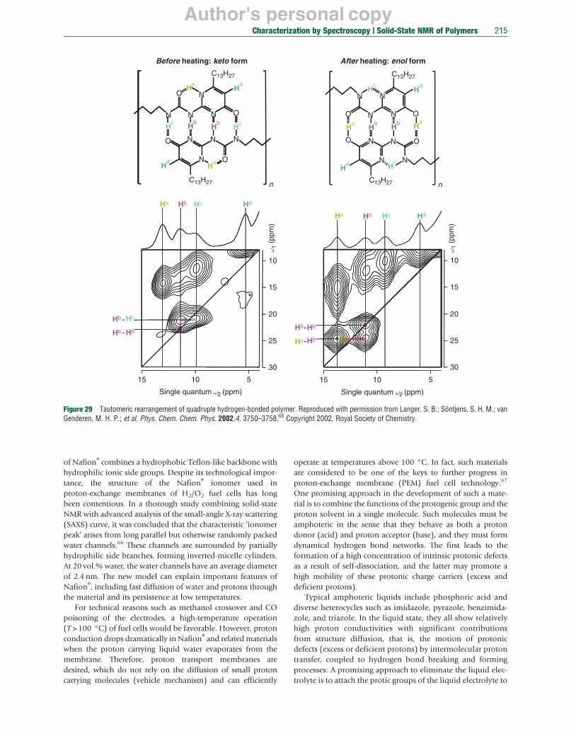
Author's personal copy
NO H
a H
d
C13H27
Before heating: keto form
Hc
Hd
C13H27
NN
After heating: enol form
Hc
N
O
Hb
N
N
N
Hb
N
Hc
O
N
Ha
O
O
Hb
N
N
Hb
N
N
Ha
O
O
Hd
C13H27
HaN O
n
Hd H
c
C13H27
N N
n
Ha Hb Hc Hd
Ha Hb Hc Hd
ω 1 (
ppm
)
ω 1 (
ppm
)
10 10
15 15
-Hb Hc 20 20
-HbHb Hb Hb-
25 Ha Hb- 25
30 30
15 10 5 15 10 5
Single quantum ω2 (ppm) Single quantum ω2 (ppm)
Characterization by Spectroscopy | Solid-State NMR of Polymers 215
Figure 29 Tautomeric rearrangement of quadruple hydrogen-bonded polymer. Reproduced with permission from Langer, S. B.; Söntjens, S. H. M.; van Genderen, M. H. P.; et al. Phys. Chem. Chem. Phys. 2002,4, 3750–3758.65 Copyright 2002, Royal Society of Chemistry.
of Nafion® combines a hydrophobic Teflon-like backbone with hydrophilic ionic side groups. Despite its technological importance, the structure of the Nafion® ionomer used in proton-exchange membranes of H2/O2 fuel cells has long been contentious. In a thorough study combining solid-state NMR with advanced analysis of the small-angle X-ray scattering (SAXS) curve, it was concluded that the characteristic ‘ionomer peak’ arises from long parallel but otherwise randomly packed water channels.66 These channels are surrounded by partially hydrophilic side branches, forming inverted-micelle cylinders. At 20 vol.% water, the water channels have an average diameter of 2.4 nm. The new model can explain important features of Nafion®, including fast diffusion of water and protons through the material and its persistence at low temperatures.
For technical reasons such as methanol crossover and CO poisoning of the electrodes, a high-temperature operation (T > 100 °C) of fuel cells would be favorable. However, proton conduction drops dramatically in Nafion® and related materials when the proton carrying liquid water evaporates from the membrane. Therefore, proton transport membranes are desired, which do not rely on the diffusion of small proton carrying molecules (vehicle mechanism) and can efficiently
operate at temperatures above 100 °C. In fact, such materials are considered to be one of the keys to further progress in proton-exchange membrane (PEM) fuel cell technology.67
One promising approach in the development of such a material is to combine the functions of the protogenic group and the proton solvent in a single molecule. Such molecules must be amphoteric in the sense that they behave as both a proton donor (acid) and proton acceptor (base), and they must form dynamical hydrogen bond networks. The first leads to the formation of a high concentration of intrinsic protonic defects as a result of self-dissociation, and the latter may promote a high mobility of these protonic charge carriers (excess and deficient protons).
Typical amphoteric liquids include phosphoric acid and diverse heterocycles such as imidazole, pyrazole, benzimidazole, and triazole. In the liquid state, they all show relatively high proton conductivities with significant contributions from structure diffusion, that is, the motion of protonic defects (excess or deficient protons) by intermolecular proton transfer, coupled to hydrogen bond breaking and forming processes. A promising approach to eliminate the liquid electrolyte is to attach the protic groups of the liquid electrolyte to
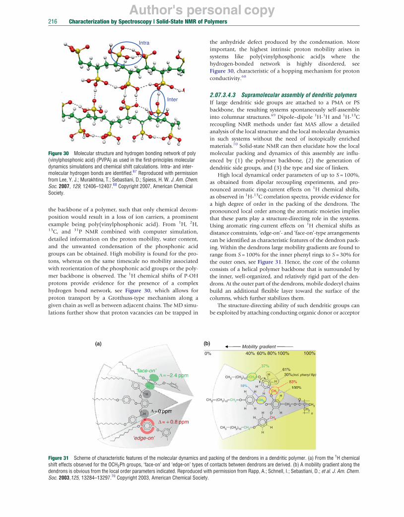
Author's personal copy216 Characterization by Spectroscopy | Solid-State NMR of Polymers
Intra
Inter
Figure 30 Molecular structure and hydrogen bonding network of poly (vinylphosphonic acid) (PVPA) as used in the first-principles molecular dynamics simulations and chemical shift calculations. Intra- and intermolecular hydrogen bonds are identified.67 Reproduced with permission from Lee, Y. J.; Murakhtina, T.; Sebastiani, D.; Spiess, H. W. J. Am. Chem. Soc. 2007, 129, 12406–12407.68 Copyright 2007, American Chemical Society.
the backbone of a polymer, such that only chemical decomposition would result in a loss of ion carriers, a prominent example being poly(vinylphosphonic acid). From 1H, 2H, 13C, and 31P NMR combined with computer simulation, detailed information on the proton mobility, water content, and the unwanted condensation of the phosphonic acid groups can be obtained. High mobility is found for the protons, whereas on the same timescale no mobility associated with reorientation of the phosphonic acid groups or the polymer backbone is observed. The 1H chemical shifts of P-OH protons provide evidence for the presence of a complex hydrogen bond network, see Figure 30, which allows for proton transport by a Grotthuss-type mechanism along a given chain as well as between adjacent chains. The MD simulations further show that proton vacancies can be trapped in
Figure 31 Scheme of characteristic features of the molecular dynamics and shift effects observed for the OCH2Ph groups, ‘face-on’ and ‘edge-on’ types ofdendrons is obvious from the local order parameters indicated. Reproduced wiSoc. 2003,125, 13284–13297.70 Copyright 2003, American Chemical Society.
(a) (b(a) (b
‘faf ce-e-on’on’Δ =–2.4 ppppmpmpp
Δ = + 0.0 88 ppppppmp
‘ed‘edge-ge on’
H
H
H
OO
O
O
O
O
O
O
O
ΔΔΔΔ≈≈≈≈≈≈≈00000000000000000000000 pppppppppppppppmppppmppmppppppppppp
C
0%
the anhydride defect produced by the condensation. More important, the highest intrinsic proton mobility arises in systems like poly(vinylphosphonic acid)s where the hydrogen-bonded network is highly disordered, see Figure 30, characteristic of a hopping mechanism for proton conductivity.68
2.07.3.4.3 Supramolecular assembly of dendritic polymers If large dendritic side groups are attached to a PMA or PS backbone, the resulting systems spontaneously self-assemble into columnar structures.69 Dipole–dipole 1H-1H and 1H-13C recoupling NMR methods under fast MAS allow a detailed analysis of the local structure and the local molecular dynamics in such systems without the need of isotopically enriched materials.70 Solid-state NMR can then elucidate how the local molecular packing and dynamics of this assembly are influenced by (1) the polymer backbone, (2) the generation of dendritic side groups, and (3) the type and size of linkers.
High local dynamical order parameters of up to S = 100%, as obtained from dipolar recoupling experiments, and pronounced aromatic ring-current effects on 1H chemical shifts, as observed in 1H-13C correlation spectra, provide evidence for a high degree of order in the packing of the dendrons. The pronounced local order among the aromatic moieties implies that these parts play a structure-directing role in the systems. Using aromatic ring-current effects on 1H chemical shifts as distance constraints, ‘edge-on’- and ‘face-on’-type arrangements can be identified as characteristic features of the dendron packing. Within the dendrons large mobility gradients are found to range from S = 100% for the inner phenyl rings to S = 30% for the outer ones, see Figure 31. Hence, the core of the column consists of a helical polymer backbone that is surrounded by the inner, well-organized, and relatively rigid part of the dendrons. At the outer part of the dendrons, mobile dodecyl chains build an additional flexible layer toward the surface of the columns, which further stabilizes them.
The structure-directing ability of such dendritic groups can be exploited by attaching conducting organic donor or acceptor
packing of the dendrons in a dendritic polymer. (a) From the 1H chemical contacts between dendrons are derived. (b) A mobility gradient along the th permission from Rapp, A.; Schnell, I.; Sebastiani, D.; et al. J. Am. Chem.
))
CH3
H3
CH3
(CH2)10
(CH2)10
(CH2)10
37%
83%
100%
CH2
CH2
CH2
CH2
CH2
CH2
CH2
C C
n
CH3CH2
O
40%
Mobility gradient
60% 80% 100% 100%
H H
H
H
HH
H
H
HH
H
H
30%(incl. phenyl flip)
61%H
H
OO
O
O
O
O
O
59%
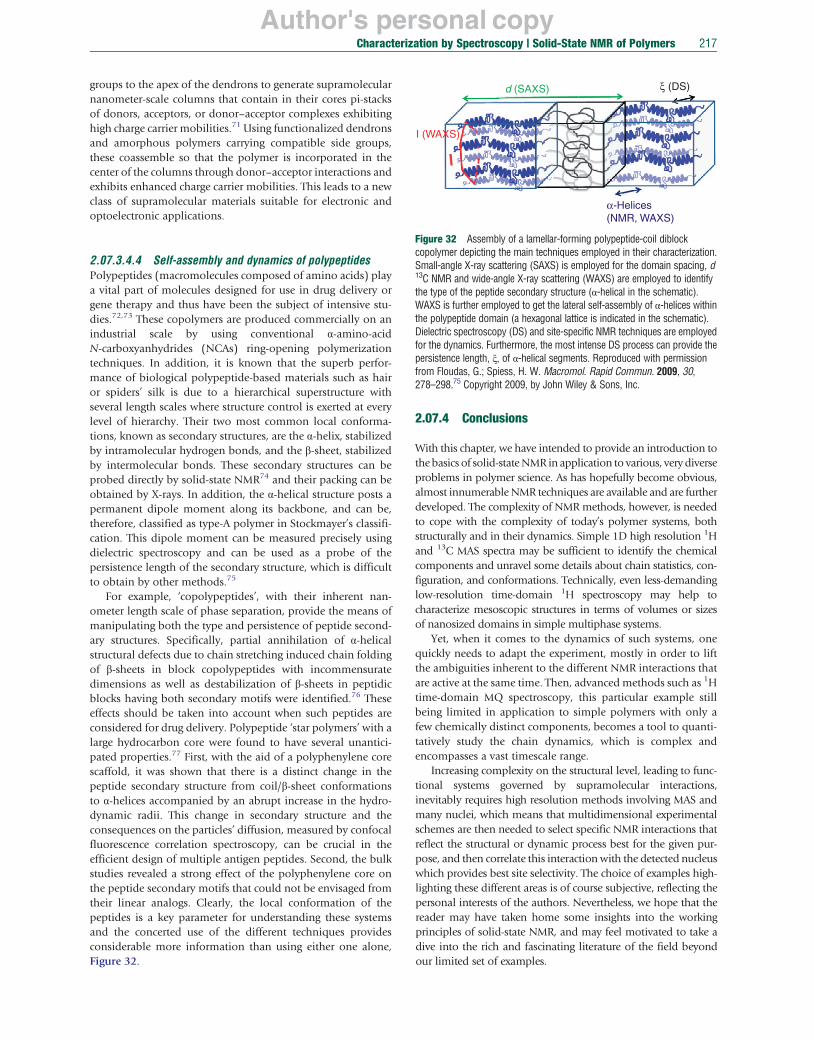
Author's personal copy
d (SAXS) ξ (DS)
I (WAXS)
α-Helices (NMR, WAXS)
Characterization by Spectroscopy | Solid-State NMR of Polymers 217
groups to the apex of the dendrons to generate supramolecular nanometer-scale columns that contain in their cores pi-stacks of donors, acceptors, or donor–acceptor complexes exhibiting high charge carrier mobilities.71 Using functionalized dendrons and amorphous polymers carrying compatible side groups, these coassemble so that the polymer is incorporated in the center of the columns through donor–acceptor interactions and exhibits enhanced charge carrier mobilities. This leads to a new class of supramolecular materials suitable for electronic and optoelectronic applications.
Figure 32 Assembly of a lamellar-forming polypeptide-coil diblock copolymer depicting the main techniques employed in their characterization. Small-angle X-ray scattering (SAXS) is employed for the domain spacing, d 13C NMR and wide-angle X-ray scattering (WAXS) are employed to identify the type of the peptide secondary structure (α-helical in the schematic). WAXS is further employed to get the lateral self-assembly of α-helices within the polypeptide domain (a hexagonal lattice is indicated in the schematic). Dielectric spectroscopy (DS) and site-specific NMR techniques are employed for the dynamics. Furthermore, the most intense DS process can provide the persistence length, ξ, of α-helical segments. Reproduced with permission from Floudas, G.; Spiess, H. W. Macromol. Rapid Commun. 2009, 30, 278–298.75 Copyright 2009, by John Wiley & Sons, Inc.
2.07.3.4.4 Self-assembly and dynamics of polypeptides Polypeptides (macromolecules composed of amino acids) play a vital part of molecules designed for use in drug delivery or gene therapy and thus have been the subject of intensive studies.72,73 These copolymers are produced commercially on an industrial scale by using conventional α-amino-acid N-carboxyanhydrides (NCAs) ring-opening polymerization techniques. In addition, it is known that the superb performance of biological polypeptide-based materials such as hair or spiders’ silk is due to a hierarchical superstructure with several length scales where structure control is exerted at every level of hierarchy. Their two most common local conformations, known as secondary structures, are the α-helix, stabilized by intramolecular hydrogen bonds, and the β-sheet, stabilized by intermolecular bonds. These secondary structures can be probed directly by solid-state NMR74 and their packing can be obtained by X-rays. In addition, the α-helical structure posts a permanent dipole moment along its backbone, and can be, therefore, classified as type-A polymer in Stockmayer’s classification. This dipole moment can be measured precisely using dielectric spectroscopy and can be used as a probe of the persistence length of the secondary structure, which is difficult to obtain by other methods.75
For example, ‘copolypeptides’, with their inherent nanometer length scale of phase separation, provide the means of manipulating both the type and persistence of peptide secondary structures. Specifically, partial annihilation of α-helical structural defects due to chain stretching induced chain folding of β-sheets in block copolypeptides with incommensurate dimensions as well as destabilization of β-sheets in peptidic blocks having both secondary motifs were identified.76 These effects should be taken into account when such peptides are considered for drug delivery. Polypeptide ‘star polymers’ with a large hydrocarbon core were found to have several unanticipated properties.77 First, with the aid of a polyphenylene core scaffold, it was shown that there is a distinct change in the peptide secondary structure from coil/β-sheet conformations to α-helices accompanied by an abrupt increase in the hydrodynamic radii. This change in secondary structure and the consequences on the particles’ diffusion, measured by confocal fluorescence correlation spectroscopy, can be crucial in the efficient design of multiple antigen peptides. Second, the bulk studies revealed a strong effect of the polyphenylene core on the peptide secondary motifs that could not be envisaged from their linear analogs. Clearly, the local conformation of the peptides is a key parameter for understanding these systems and the concerted use of the different techniques provides considerable more information than using either one alone, Figure 32.
2.07.4 Conclusions
With this chapter, we have intended to provide an introduction to the basics of solid-state NMR in application to various, very diverse problems in polymer science. As has hopefully become obvious, almost innumerable NMR techniques are available and are further developed. The complexity of NMR methods, however, is needed to cope with the complexity of today’s polymer systems, both structurally and in their dynamics. Simple 1D high resolution 1H and 13C MAS spectra may be sufficient to identify the chemical components and unravel some details about chain statistics, configuration, and conformations. Technically, even less-demanding low-resolution time-domain 1H spectroscopy may help to characterize mesoscopic structures in terms of volumes or sizes of nanosized domains in simple multiphase systems.
Yet, when it comes to the dynamics of such systems, one quickly needs to adapt the experiment, mostly in order to lift the ambiguities inherent to the different NMR interactions that are active at the same time. Then, advanced methods such as 1H time-domain MQ spectroscopy, this particular example still being limited in application to simple polymers with only a few chemically distinct components, becomes a tool to quantitatively study the chain dynamics, which is complex and encompasses a vast timescale range.
Increasing complexity on the structural level, leading to functional systems governed by supramolecular interactions, inevitably requires high resolution methods involving MAS and many nuclei, which means that multidimensional experimental schemes are then needed to select specific NMR interactions that reflect the structural or dynamic process best for the given purpose, and then correlate this interaction with the detected nucleus which provides best site selectivity. The choice of examples highlighting these different areas is of course subjective, reflecting the personal interests of the authors. Nevertheless, we hope that the reader may have taken home some insights into the working principles of solid-state NMR, and may feel motivated to take a dive into the rich and fascinating literature of the field beyond our limited set of examples.

Author's personal copy218 Characterization by Spectroscopy | Solid-State NMR of Polymers
References
1. McLeish, T. C. B. Adv. Phys. 2002, 51, 1379. 2. Matyjaszewski, K.; Gnanou, Y.; Leibler, L. Eds.; Macromolecular Engineering;
Wiley-VCH: Weinheim, Germany, 2007, Vol. 2. 3. McCrum, N. G.; Read, B. E.; Williams, G. Anelastic and Dielectric Effects in
Polymeric Solids; Wiley: London, 1967. Kremer, F.; Schönhals, A. Broadband Dielectric Spectroscopy; Springer: Berlin, Germany, 2003.
4. Spiess, H. W. Macromolecules 2010, 43, 5479. 5. Fischer, E. W.; Peterlin, A. Makromol. Chem. 1964, 74, 1. 6. Spiess, H. W. Colloid Polym. Sci. 1984, 261, 193. 7. Schaefer, J.; Stejskal, E. O. J. Am. Chem. Soc. 1976, 98, 1031. 8. Grant D. M.; Harris, R. K., Eds.; Encyclopedia of Nuclear Magnetic Resonance;
Wiley: Chichester, UK, 2002, 2007. 9. Ernst, R. R.; Bodenhausen, G.; Wokaun, A. Principles of NMR in One and Two
Dimensions; Clarendon Press: Oxford, UK, 1987. 10. Schmidt-Rohr, K.; Spiess, H. W. Multidimensional Solid-State NMR and Polymers;
Academic Press: London, UK, 1994. 11. Callaghan, P. T. Principles of Nuclear Magnetic Resonance Microscopy; Clarendon
Press: Oxford, UK, 1993. 12. Kimmich, R. NMR: Tomography, Diffusometry, Relaxometry; Springer: Berlin,
Germany, 1997. 13. Spiess, H. W. NMR, Basic Principles and Progress; Springer: Berlin, Germany,
1978; Vol. 15, p 55. 14. Sebastiani, D. ChemPhysChem. 2006, 7, 164–175. 15. Tonelli, A. E. NMR Spectroscopy and Polymer Microstructure: The Conformational
Connection; VCH: Weinheim, Germany, 1989. 16. Born, R.; Spiess, H. W. Macromolecules 1995, 28, 7785–7795. 17. Samoson, A. Encyclopedia of Nuclear Magnetic Resonance; Grant, D. M.;
Harris, R. K. Eds.; Wiley: Chichester, UK, 2002, Vol. 9, pp 59–64. 18. Filip, C.; Hafner, S.; Schnell, I.; et al. J. Chem. Phys. 1999, 110, 423. 19. Demus, D.; Goodby, J. W.; Gray, G. W.; et al., Eds.; Handbook of Liquid Crystals;
Wiley-VCH: Weinheim, Germany, 1998. 20. Hahn, E. L. Phys. Rev. 1950, 80, 580. 21. Rhim, W.-K.; Pines, A.; Waugh, J. S. Phys. Rev. B 1971, 3, 684. 22. Schmidt, C.; Wefing, S.; Blümich, B.; Spiess, H. W. Chem. Phys. Lett. 1986, 130, 84. 23. deAzevedo, E. R.; Hu, W.-G.; Bonagamba, T. J.; Schmidt-Rohr, K. J. Am. Chem.
Soc. 1999, 121, 8411. 24. Brown, S. P. Prog. Nucl. Magn. Reson. Spectrosc. 2007, 50, 199. 25. Gullion, T.; Schaefer, J. Adv. Magn. Reson. 1989, 13, 57. 26. Levitt, M. Encyclopedia of Nuclear Magnetic Resonance; Grant, D. M.; Harris, R. K.
Eds.; Wiley: Chichester, UK, 2002, Vol. 9, p 165. 27. Hartmann, S. R.; Hahn, E. L. Phys. Rev. 1962, 128, 2042. 28. Pines., A.; Gibby, M.; Waugh, J. S. J. Chem. Phys. 1973, 59, 569. 29. Saalwächter, K. Prog. Nucl. Magn. Reson. Spectrosc. 2007, 51, 1. 30. Saalwächter, K.; Spiess, H. W. J. Chem. Phys. 2001, 114, 5707. 31. Hadjichristidis, N.; Pispas, S.; Floudas, G. Block Copolymers: Synthetic Strategies,
Physical Properties and Applications; Wiley: Street Hoboken, NJ, 2003. 32. Bloembergen, N.; Purcell, E. M.; Pound, R. V. Phys. Rev. 1948, 73, 679. 33. Kulik, A. S.; Radloff, D.; Spiess, H. W. Macromolecules 1994, 27, 3111. 34. Macho, V.; Brombacher, L.; Spiess, H. W. Appl. Magn. Reson. 2001, 20, http://
www.mpip-mainz.mpg.de/weblab41/. 35. Wind, M.; Graf, R.; Heuer, A.; Spiess, H. W. Phys. Rev. Lett. 2003, 91, 155702. 36. Kulik, A. S.; Spiess, H. W. Macromol. Chem. Phys. 1994, 195, 1755. 37. Hong, M.; Pines, A.; Caldarelli, S. J. Phys. Chem. 1996, 100, 14815.
38. Anderson, P. W.; Weiss, P. R. Rev. Mod. Phys. 1953, 25, 269. 39. Solum, M. S.; Zilm, K. W.; Michl, J.; Grant, D. M. J. Phys. Chem. 1983, 87, 2940. 40. Kulik, A. S.; Beckham, H. W.; Schmidt-Rohr, K.; et al. Macromolecules 1994,
27, 4746. 41. Böhmer, R.; Diezemann, G.; Hinze, G.; Rössler, E. Prog. Nucl. Magn. Reson.
Spectrosc. 2001, 39, 191. 42. Krushelnitzky, A.; deAzevedo, E. R.; Linser, R.; et al. J. Am. Chem. Soc. 2009,
131, 12097. 43. Kuhn, W.; Grün, F. Kolloid-Z. 1942, 101, 248. 44. Cohen-Addad, J. P. Prog. Nucl. Magn. Reson. Spectrosc. 1993, 25, 1–316. 45. Klimke, K.; Parkinson, M.; Piel, C.; et al. Macromol. Chem. Phys. 2006,
207, 382. 46. Yao, Y.-F.; Graf, R.; Spiess, H. W.; et al. Phys. Rev. E 2007, 76, 060801(R). 47. Chávez, F. V.; Saalwächter, K. Phys. Rev. Lett. 2010, 104, 198305. 48. Monnerie, L.; Lauprêtre, F.; Halary, J. L. Adv. Polym. Sci. 2005, 187, 35. 49. Arrese-Igor, S.; Arbe, A.; Alegría, A.; et al. J. Chem. Phys. 2005, 123, 014907. 50. Graf, R.; Ewen, B.; Spiess, H. W. J. Chem. Phys. 2007, 126, 041104. 51. Zemke, K.; Schmidt-Rohr, K.; Spiess, H. W. Acta Polym. 1994, 45, 148. 52. Spiess, H. W. J. Polym. Sci. 2004, A42, 5031–5044. 53. (a) Schmidt-Rohr, K.; Spiess, H. W. Phys. Rev. Lett. 1991, 66, 3020.
(b) Heuer, A.; Wilhelm, M.; Zimmermann, H.; Spiess, H. W. Phys. Rev. Lett. 1995, 75, 2851. (c) Tracht, U.; Wilhelm, M.; Heuer, A.; et al. Phys. Rev. Lett. 1998, 81, 2727.
54. Sillescu, H. J. Non-Cryst. Solids 1999, 243, 81. 55. Ediger, M. D. Annu. Rev. Phys. Chem. 2000, 51, 99. 56. Adam, G.; Gibbs, J. H. J. Chem. Phys. 1965, 43, 139. 57. Reinsberg, S. A.; Heuer, A.; Doliwa, B.; et al. J. Non-Cryst. Solids 2002, 208,
307–310. 58. Mauri, M.; Thomann, Y.; Schneider, H.; Saalwächter, K. Solid State Nucl. Magn.
Reson. 2008, 34, 125. 59. Saalwächter, K.; Thomann, Y.; Hasenhindl, A.; Schneider, H. Macromolecules
2008, 41, 9187. 60. Hu, W.-G.; Schmidt-Rohr, K. Acta Polym. 1999, 50, 271–285. 61. Wei, Y.; Graf, R.; Sworen, J. C.; et al. Angew. Chem., Int. Ed. 2009, 48, 4617. 62. Pascui, O. F.; Lohwasser, R.; Sommer, M.; et al. Macromolecules 2010, 43,
9401–9410. 63. Sijbesma, R. P.; Beijer, F. H.; Brunsveld, L.; et al. Science 1997, 278, 1601. 64. Schulz-Dobrick, M.; Metzroth, T.; Spiess, H. W.; et al. ChemPhysChem. 2005,
6, 315. 65. Schnell, I.; Langer, B.; Söntjens, S. H. M.; et al. Phys. Chem. Chem. Phys. 2002, 4,
3750–3758. 66. Schmidt-Rohr, K.; Chen, Q. Nat. Mater. 2007, 7, 75. 67. Steininger, H.; Schuster, M.; Kreuer, K. D.; et al. Phys. Chem. Chem. Phys. 2007,
9, 1764. 68. Lee, Y. J.; Murakhtina, T.; Sebastiani, D.; Spiess, H. W. J. Am. Chem. Soc. 2007,
129, 12406–12407. 69. Percec, V.; Ahn, C.-H.; Ungar, G.; et al. Nature 1998, 391, 161. 70. Rapp, A.; Schnell, I.; Sebastiani, D.; et al. J. Am. Chem. Soc. 2003, 125,
13284–13297. 71. Percec, V.; Glodde, M.; Bera, T. K.; et al. Nature 2002, 419, 384. 72. Walton, A. G.; Blackwell, J. Biopolymers; Academic Press: New York, NY, 1973. 73. Klok, H.-A.; Lecommandoux, S. Adv. Polym. Sci. 2006, 202, 75. 74. (a) van Beek, J. D.; Beaulieu, L.; Schafer, L. H.; et al. Nature 2000, 405, 1077.
(b) Tycko, R. Annu. Rev. Phys. Chem. 2001, 52, 575. 75. Floudas, G.; Spiess, H. W. Macromol. Rapid Commun. 2009, 30, 278–298. 76. Gitsas, A.; Floudas, G.; Mondeshki, M. N.; et al. Biomacromolecules 2008, 9, 1959. 77. Koynov, K.; Mihov, G.; Mondeshki, M.; et al. Biomacromolecules 2007, 8, 1745.

Author's personal copyCharacterization by Spectroscopy | Solid-State NMR of Polymers 219
Biographical Sketches
Kay Saalwächter, born in 1970, obtained his diploma in chemistry in 1997 from the Institute of Macromolecular Chemistry of the University of Freiburg, working on light scattering of polymer solutions with Walter Burchard, and got his doctorate degree in physical chemistry in 2000 working with Hans W. Spiess at the Max Planck Institute for Polymer Research in Mainz, focusing on methods of development in solid-state NMR. After a short period as project leader at the same institute, he switched back to Freiburg to obtain his habilitation in 2004 on NMR applications in the field of dynamics in solid polymers, again at the Institute of Macromolecular Chemistry in the group of Heino Finkelmann. In 2005, he was appointed professor of experimental physics at the Martin-Luther-Universität Halle-Wittenberg. Since his first contact with solid-state NMR on an exchange year at the University of Massachusetts (Amherst, USA) working with Klaus Schmidt-Rohr (now at Ames, Iowa), his continuing research interest has been the development and application of NMR techniques to the study of structure and dynamics in polymeric, liquid crystalline, and other ‘soft’ materials, which have been published in about 70 papers so far. He is a member of the editorial board of Solid State Nucl. Magn. Reson., J. Magn. Reson., and Colloid Polym. Sci., and since 2008, he has served as a review board member in chemistry and referee for polymer research for the Deutsche Forschungsgemeinschaft (DFG).
Hans-Wolfgang Spiess, born in 1942, received his doctoral degree in physical chemistry in 1968 from the University of Frankfurt with H. Hartmann. After a postdoctoral stay at Florida State University (with R. K. Sheline), he returned to Germany in 1970 and joined the Max Planck Institute for Medical Research (with K. H. Hausser), taking part in the rapid development of novel NMR techniques for studying molecular motion in liquids and solids. In 1978, he finished his habilitation in physical chemistry at the University of Mainz in the group of H. Sillescu. Subsequently, he held professorships of physical chemistry at the University of Münster (1981–82) and of macromolecular chemistry at the University of Bayreuth (1983–84). In 1984, he was appointed a director of the newly founded Max Planck Institute for Polymer Research in Mainz. His research interests include the development of magnetic resonance techniques for elucidating the structure, dynamics, phase behavior, and order of synthetic macromolecules and supramolecular systems. He applies these methods to the study of new polymer materials to relate their microscopic and macroscopic behavior. He has served as chairman of the European Polymer Federation (1991–92) and as chairman of the Capital Investment Committee of the German Science Foundation (1994–96). From 1999 until 2005, he was a member of the Scientific Council of the Federal Republic of Germany. His achievements have been honored by several distinctions, including the Leibniz Prize of the German Research
Foundation in 1987, the European Ampere Prize, the Liebig Medal of the German Chemical Society, the Award of the Society of Polymer Science (Japan) in 2002, the Walther-Nernst Medal of the German Bunsen Society for Physical Chemistry in 2007, and the Paul J. Flory Research Prize in 2010. He is doctor honoris causa of the Technical University of Cluj-Napoca, Romania (1997) and of Adam Mickiewicz University, Poznan, Poland (1998).
Related Documents


