SOLID-LIQUID MIXING IN MECHANICALLY AGITATED VESSELS

SOLID-LIQUID MIXING

IN MECHANICALLY AGITATED VESSELS

Thesis submitted for the degree of Doctor of Philosophyin the University of London by:

Andrew Tsz-Chung Mak, MEng

Ramsay Memorial LaboratoiyDepartment of Chemical and Biochemical EngineeringUniversity College LondonTorrington PlaceLondon WC1E 7JEEngland

June 1992

© Andrew Mak 1992

BIBL

LONDON

UNIV

2

ABSTRACT

Experimental data are reported for solids suspension and distribution in four

geometrically similar vessels with diameters equal to 0.31, 0.61, 1.83 and 2.67 m. Agitation

was provided by a series of pitched blade turbines with impeller to vessel diameter ratios from

0.3 to 0.6 and pitched angles between 30° and 90°. The effect of impeller clearance on solids

suspension was examined for a clearance range of T/4 to T/8. Dual impeller systems were

also studied, covering two combinations (dual pitched and flat/pitched) and impeller spacing

of half to two diameters apart. The majority of the experiments were carried out with 150-2 10

pm round-grained sand (density: 2630 kg m 3 and settling velocity: 0.015 m s') and tap water.

Solids concentration was varied between 0.1 to 40% by weight.

Four parameters were measured; impeller speed, using an optical tachometer, power

input, calculated from the shaft torque given by strain gauges, just suspension speed,

ascertained both visually and by use of an ultrasonic Doppler flowmetering (UDF) technique

and the local solids concentration, measured by a in-house solids concentration probe. In

addition extensive flow visualisations were made with the 0.61 m vessel in order to establish

both liquid and particles flow patterns during the experiments.

Results from this study were compared with previous publications in order to examine

the effects of some of the important geometrical variables on solids suspension and

distribution. This work revealed that for the range of parameters covered, the smallest

(DiT=0.3) and the largest (DIF=0.6) impellers are the most and least efficient ones for solids

suspension. Distribution tests with the three geometrically similar impellers show that the

results are neither correlated in terms of tip speed nor power input but are best described by

the thrust force generated by the impellers. In general, dual impeller systems improve solids

distribution but require more power to just suspend solids compared with a single impeller.

The scaling effect proposed by Zwietering (1958) for solids suspension has been confirmed

by this study for vessel up to 2.67 m in diameter. The constant tip speed rule for solids

distribution, which is based on one-dimensional dispersion models was found to underestimate

the power requirement in large scale applications. This study indicates that equal power per

unit volume is required to achieve the same degree of homogeneity.

3

ACKNOWLEDGEMENTS

I am most grateful to my colleagues, Mr Robert Burnapp and Mr Kevin Lee, who

proof read this thesis. They have been a constant source of help, support and inspiration

during all these years in BHR Group Ltd, without them completion of this thesis would not

have been possible.

Thanks are also due to:

My brothers and sister; Yan, King and Kin for sharing out my house duties and

keeping my parents company while I was abroad.

My friends and colleagues; Lorna Brooker, I S Fan, Emily and Jack Ho, Steve and

Marie-Ann Hobbs, Maha Soundra-Nayagam, Trevor Sparks, Mike Whitton and Ming

Zhu for their encouragement and interest in this work.

Fred and Theresea Haines for providing me with a nice comfortable home.

My industrial supervisor, Andrew Green, for his moral support.

The author also wishes to thank the members of the Fluid Mixing Processes

Consortium for their permission to publish part of the generic research results.

Finally, my deepest gratitude to my supervisor, Dr P Ayazi Shamlou, for his

enthusiasm, guidance and friendship, from whom I have learnt so much.

4

Human kind cannot bear much reality

T. S. Eliot

Dedicated to my parents to whom I owe so much

that can never be repaid

All this I tested by wisdom and I said, "I am determined to be wise" - but this was beyond

me. Whatever wisdom may be, it is far off and most profound - who can discover it? So I

turned my mind to understand, to investigate and to search out wisdom and the scheme of

things and to understand the stupidity of wickedness and the madness of folly.

Ecclesiastes 6: 23-25

$\)

6

LIST OF CONTENTS

Page No

Title Page

Abstract

2

Acknowledgements

3

Dedication

4

Nomenclature

10

Chapter 1 Introduction

15

1.1 Background

15

1.2 Research Needs for Solid-liquid Mixing

16

1.3 Aims, Approach and Thesis Layout

17

Chapter 2 Literature Survey

21

2.1

Solids Suspension

21

2.1.1 Zwietering's Empirical Correlation

21

2.1.2 Baldi et a! Turbulence Model

23

2.1.3 Mersmann et al Two Basic Laws of Solids Suspension

26

2.1.4 Shamlou and Zolfagharian's Average Velocity Model

28

2.1.5 Molerus and Latzel's Two Suspending Mechanisms

30

2.1.6 Wichterle's Characteristic Velocity Model

34

2.1.7 Other Models

36

2.1.8 Summary of the Suspension Models

39

2.2

Solids Disthbution

45

2.2.1 Relative Standard Deviation and Variance

45

2.2.2 The One Dimensional Dispersion Models

46

2.2.3 Buurman's Constant Froude No. Model

51

2.2.4 Other Models

52

7

Chapter 3 Test Facilities and Methods

57

3.1

Base Configurations 58

3.2 The Vessels 58

3.3

The Vessel Bases 58

3.4

Baffles 59

3.5

Impellers and Clearances 59

3.6

Test Media 60

3.7

Impeller Rotational Speed 66

3.8

Shaft Torque 66

3.8.1 General Outline 66

3.8.2 Calibration and Accuracy 66

3.9

Minimum Speed for Solids Suspension 67

3.9.1 Visual Observation Method 68

3.9.2 Measurement of N with an Ultrasonic Doppler Flowmeter (UDF) 68

3.9.3 Calibration of the UDF Technique 70

3.10 Local Solids Distribution 71

3.10.1 The Solids Concentration Probe 72

3.10.2 Probe Calibration 73

3.10.3 Probe Location and Orientation 74

Chapter 4 Results and Discussion

83

4.1

Particle Flow Pattern

83

4.1.1 An Overall View

83

4.1.2 Flow Pattern at Vessel Base

85

4.2

Power Requirement for Solid-liquid Mixing

93

4.2.1 Solid-liquid Mixing Power

93

4.2.2 Just Suspension Power and Power Index

96

4.3

Effect of Impeller Diameter

106

4.3.1 Experimental Results

106

4.3.2 Just Suspension Speed

108

4.3.3 Just Suspension Power

112

4.3.4 Solids Distribution

120

8

4.3.5 Verification of Tip Speed Criterion

122

4.4 Effect of Impeller Pitch Angle 132

4.4.1 Power Numbers

132

4.4.2 Flow Pattern

134

4.4.3 Solids Suspension

134


140

4.5 Dual Impeller Systems

145

4.5.1 Power Consumption

146

4.5.2 Flow pattern

147


148


163

4.6 Scaling-up

173

4.6.1 Power Numbers

173


174


182

4.6.4 Comparison between the Two Scale-up Rules

183

4.7 Further Discussion

192

4.7.1 Overall Suspension Results

192

4.7.2 Comparing to the Suspension Models

193

(i) Single Correlation Models

194

(ii) Correlations with a Critical Dividing Parameter 197

(iii) Models with a Continual Variation of Exponents

199

4.7.3 A Final Remark on Solids Suspension Modelling

200

4.7.4 Modelling of Solids Distribution

201

Chapter 5 Conclusions and Recommendations

207

5.1 Conclusions

207

5.2 Suggestions for Future Work

210

References 211

9

Appendkes

A Solids Distribution Data for the Three Geometrically Similar Impellers 219

B Solids Distribution Data for Pitched Angle Experiments 222

C Solids Distribution Data for Dual Impeller Systems 224

D Just Suspension Results Measured in Four Scales 232

E Solids Distribution Results Measured in Three Scales 235

F Just Suspension Results from Previous Study 245

G The One Dimensional Dispersion Model 246

Symbol

A

a

A

Am

B

C

C

CD

Cii

CL

CM

Ct

Cv

Cz

D

De,p

d

d

F

FB

FD

FL

F

g

H

h

H,,

NOMENCLATURE

Meaning

A Calibration Constant

A Parameter

A Constant

A Parameter Which Depends on Impeller Type

Projected Area of the Particle

A Critical Constant for Just Suspension Condition

Impeller Bottom Clearance

A Parameter

Drag Coefficient

Local Solids Distribution at ith Speed and th Position

Lift Coefficient

Mean Volume Fraction of Solids

Top Impeller Clearance in Dual Impeller Systems

Volume Fraction of Solids

Mean Volume Fraction of Solids across Height z

Impeller Diameter

Liquid Diffusion Coefficient

Particle Dispersion Coefficient

Particle Diameter

A Normalised Particle Diameter

Thrust Force Generated by an Impeller

Buoyancy Force Acting on the Particle

Drag Force Acting on the Particle

Lift Force Acting on the Particle

Effect Weight of Particle

Gravitational Acceleration

Height of Slurty

Height of Clear Liquid/Solid-liquid Interface

Impeller Hub Height

Impeller Hub Outside Diameter

10

Units

m2

m

m

m

m2 s1

m2

m

N

N

N

N

N

m 52

m

m

m

m

11

k

A Constant -

K

A Parameter -

L

Length Scale of Large Energy Containing Eddies m

L0 Length Scale of Small Eddies m

L

Characteristic Linear Dimension m

M

Mass of Slurry kg

ML Mass of Liquid in Vessel kg

M

Mass of Solids in Vessel kg

N

Impeller Speed rev r' (or rpm)

n

Number of Blades -

N

Just Suspension Speed rev s (or rpm)

N,0 Just Suspension Speed by Visual Observation rev s' (or rpm)

Just Suspension Speed by Ultrasonic Doppler Flowmeter rev s 1 (or rpm)

np Number of Particles -

P

Power W

P1 Power Index (P1 = Po s3 D24 ) m215

Pj Power Drawn by Impeller at N, W

Po

Power Number ( Po = P /p N3 D5 ) -

Poc Combined Power Number in Multiple Impeller Systems -

r

Correlation Coefficient -

RSD

Relative Standard Deviation of Solids Concentration -

S

Geometrical Constant in Zwietering Correlation -

Si Modified Geometrical Constant -

T

Vessel Diameter m

U

Linear velocity m S_I

UI1 Axial Component of Local Velocity of Liquid at Point of

Incipient Particle Motion m s4

Ufo Mean Upward Velocity Outside the Fictitious Tube m S'

Uf Eulerian Velocity of Fluid at z Direction m s'

Urn Mean Liquid Velocity near the Base of Vessel m s1

Upz Eulerian Velocity of Particles at z Direction m 5'

Un Radial Component of Local Velocity of Liquid at Point of

Incipient Particle Motion m s'

Us Terminal Velocity of Particles in a Swarm m 5'

UI

Ut0, U11

Ut

U..

V

v,

yr

Vz

w

wp

x

z

z

a13

'YB

Po

LP$tat

Cm

ep

C1

Cv

lb

icc

Km

K0

x

p

pay

Terminal Velocity

Terminal Velocity at Stagnant and Turbulent Medium

Shear Stress Velocity

Maximum Fluid Velocity Close to the Boundary Layer

Volume of the Slurry

Fluctuating Velocity of the Critical Eddies

Mean Radial Velocity

Mean Axial Velocity

Blade Width

Projected Blade Width

Percentage Mass Ratio of Solids to Liquid in Suspension

A Constant

Cartesian Coordinate in Axial Direction

Blade Angle to Horizontal

A Constant

A Constant

Characteristic Shear Rate at Vessel Base

Static Pressure Difference Inside Impeller Region

Static Pressure Difference Outside Impeller Region

Static Pressure Difference

Power per unit Mass

Power Dissipation for Entrainment of Single Particle

Total Power Dissipation for Complete Suspension

Average Power per unit Volume

Power per Unit Volume near the Vessel Base

A Proportionality Constant

Characteristic Eddy Scale

Corrected Conductivity

Measured Conductivity

Conductivity of Water at Measured Temperature

Conductivity of Water at Reference Temperature

Blade Thickness

Density

Average Density of Vessel Contents

12

m s

m S'

m s

m S'

m3

m S1

m s

m s'

m

m

m

s-i

Nm2

Nm2

Nni2

W kg'

Wm3

Wm3

Wm3

Wm3

m

microsiemens

microsiemens

microsiemens

microsiemens

m

kg m3

kg m3

Ii

V

$ 'V

PL

Ps

13

kg m3

kg m3

Nm

Nn12

kg m1 s1

m2 s'

Density of Liquid

Density of Solids

Standard Deviation

Torque

Wall Shear Stress

Dynamic Viscosity

Kinematic Viscosity

Nondimensional Group for Pumping Characteristics

Particle Resistance Coefficient for Free Fall at Stagnant

and in Turbulent Medium

Nondimensional Group for Pumping Characteristics

14

Dimensionless Groups

Ar Archimedes Numberg ip d

v2 PL

Eu Euler Number for Particulate Fluidisationd g (1 -C)2

3 P. U2

Fl Flow Number QND3

Fr Froude Number N2 D

g

Fr Modified Froude NumberN2 D 2 p L

d ip g

Ft Thrust Number F

p N2 D4

Pe Peclet NumberU H

D

Pe Modified Peclet Number U0 L

D,p

Po Power Number P

pN3D5

Re Reynolds Number P U d

It

Re1Impeller Reynolds Number p N D2

Re Modified Reynolds Number N D3

vT

R; Reynolds Number for Shear Stress d U

V

15

CHAPTER 1: INTRODUCTION

1.1 BACKGROUND

Mixing is one of the most widely used unit operations in the chemical and allied

industries. There is a general acceptance of the importance of mixing processes for the

commercial success of industrial operations. In 1989 during a workshop conducted by the

Mixing 3A of AIChE (Mixing 3A 1989), it was found that in many case studies presented,

the monetary values of the solutions to the particular problems represented a saving in the

region of $0.5 to $5M. Increasing process yields, avoiding the need for expensive and

prolonged pilot plant development together with improved exploitation times in bringing new

products onto the market, might represent a monetary value in the region of 1 to 3% of

turnover for the chemical process industries, which for the USA was around $10 bn per year

in 1989.

A stirred tank unit typically consists of a rotating impeller in a vessel. Fluid motion

is promoted by the transfer of energy from the impeller into the process fluid. The process

fluid may be single phase (eg viscous, Newtonian and non-Newtonian) or multiple phases (eg

solids, liquid and gas) and, in some cases, physical changes may take place during the

operation (eg suspension polymerisation and dissolution of solids in liquid).

Mixing processes are usually classified according to the type of the process materials,

eg viscous liquid, solid-liquid, gas-liquid, liquid-liquid, etc, and of these, solid-liquid is

certainly one of the most important. This has been highlighted in the survey conducted by

the Mixing 3A Workshop which found that 80% of the chemical products made involved

solid-liquid processing.

The main objectives of agitation in solid-liquid systems can be divided into three

categories;

a) to avoid solids accumulation in a stirred tank

b) to maximise the contacting area between the solids and liquid

c) to ensure the solids particles are uniformly distributed throughout the vessel

16

In many operations, it is essential to ensure that all the solids are kept in motion in

order to prevent the building up of solids on the vessel base which may, in extreme cases,

invoke system malfunction. Examples of such operations include settling tanks for filter cakes

and absorber sump of a flue gas desulphurisation process. The stirred tank may also be used

as a reactor, for example when catalysts are to be suspended for mass transfer operations. The

mass transfer rate per unit energy input is at its maximum when the interfacial area between

the solids and liquid is maximised. This happens when the fluid motion is vigorous enough

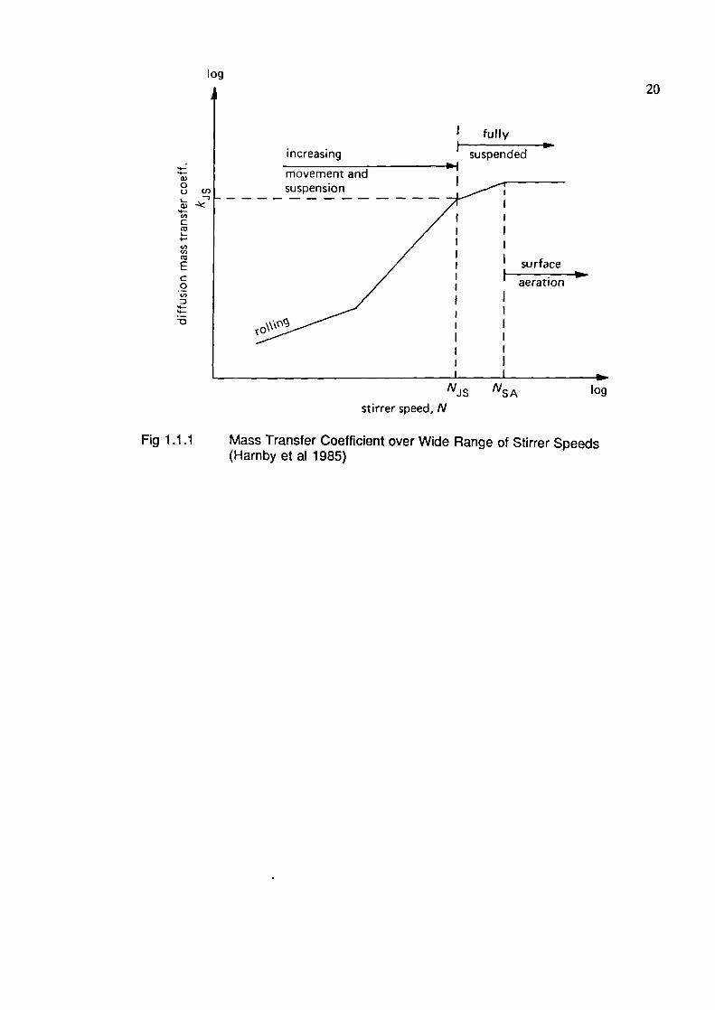
to keep all particles in motion (i.e. at N, Fig 1.1.1). Even though the design objectives for

(a) and (b) set out to achieve different goals, both require good knowledge of the just

suspension speed (Np) prediction, that is the impeller speed at which no solid particle rests

on the vessel base.

However operating the stirred vessel at the just suspension condition may not be

sufficient in certain processes. For example, the ratio between the mean solids concentration

in the vessel and that in the withdrawal tube depends on the position of the tube thus, solids

distribution information is required to ensure good mass balance between inward and outward

flow in a Continuous stirred tank reactor. Sometimes the product characteristics depend on

the distribution quality, knowledge of which is then becomes vital for quality control.

In this work, flow pattern, power consumption, solids suspension and distribution for

a wide range of geometries and scales were investigated.

1.2 RESEARCH NEEDS FOR SOLID-LIQUID MIXING

The Zwietering correlation (1958) is generally being accepted as the best correlation

for just suspension prediction for low viscosity systems. This empirical correlation is based

on more than a thousand experiments together with dimensionless analysis. However, there

are a number of other correlations which are different and, in some ways, contradictory to

Zwietering (eg effect of particle size and scale) and most of them have their own experimental

data to back them up. Unfortunately, the discrepancies between many of these correlations

are large.

Most of the contradictions are believed to be caused by a lack of understanding of the

suspension mechanism and reliable large scale data which can be used to verify existing

17

models. Some of the assumptions adopted in establishing the theoretical models bear little

resemblance to the actual suspension mechanisms. Therefore, more detailed observations of

particle flow patterns would help to clarify this point. Scale-up data in literature is inadequate

and extrapolation beyond the experimental range can be disastrous. For the just suspension

conditions, published literature recommended oc 1" with n ranging from 0.5 (eg Kneule

1967) to -1 (eg Bourne 1974) (e = power per unit volume, T = tank diameter). For 100-fold

change in scale, the two extremes give 1000-fold difference in power requirement prediction.

An incorrectly sized mixing vessel could cause shut down of the whole plant and millions of

pounds in lost production. Large scale data is urgently needed to verify the scale-up rules and

the data should shed light on the validity of various models.

Another important feature for the evaluation of solid-liquid mixing performance is the

distribution of solids throughout the vessel. However, quantitative information in this area is

limited and mostly are confmed to low concentration in small vessels. The distribution of

solids in an agitated vessel is a rather complex function of the velocity field, distribution of

turbulence and solid-liquid interaction. Progress has been hampered by the difficulties in

establishing a reliable measuring technique to be used in a wide range of geometrical set-ups

which can provide useful information for modelling.

In the past agitation units were often greatly over-specified, in order to accommodate

for the uncertainty in design. This may lower the yield (eg side reactions) and quality (eg

particles breakage in crystallisation) of the desirable product. In additional, over-specification

may lead to extra initial and operating costs Apart from that, treatment of undesirable

products means extra production cost.

13 AIMSI APPROACH AND THESIS LAYOUT

This thesis is an experimental study of solid-liquid mixing in mechanically agitated

vessels. It is confmed to the mixing of sinking particles with water in the turbulent regime.

All impellers tested are downwards pumping unless otherwise stated. This is because over

95% of solid-liquid mixing processes use downwards pumping impellers. Upward pumping

is employed only if other design constraints have to be imposed, such as gas dispersion in a

3-phase (solid-liquid-gas) reactor, and this is out of the scope of this thesis. This work has

the following objectives:

18

To obtain an insight into the hydrodynamic conditions which govern the suspension

and distribution of solid particles in mixing vessels.

To gain an understanding of the effects of some of the more important system

parameters (eg geometric scale) on solid-liquid mixing.

To utilise the qualitative and quantitative information obtained, together with

theoretical understanding to formulate and/or refme the existing models.

This work commences with a literature survey on solids suspension and distribution

models (Chapter 2). Mathematical models developed in the literature to interpret the two

phase flow mechanisms in stirred vessels are compared and contrasted. The survey highlights

areas which demand more research effort and the type of measurements which ought to be

made in order to verify/improve some of the existing models (eg particle flow pattern near the

just suspension condition).

Chapter 3 describes the test facilities, methods and various physical and geometrical

parameters that were encompassed in this programme. Three types of measurements were

made in this work, namely just suspension speed (Ni), shaft torque for power calculation (t)

and local solids concentration at ith speed and th position (C1 ). Extensive flow visualisations

were made during the experiments to aid interpretation of the results. The selection and

verification of reliable and consistent methods for solids suspension and distribution

measurements across a wide range of scale and geometries constitute a very important part

of this thesis. The development and calibration of ultrasonic and conductivity techniques are

also presented in Chapter 3.

In Chapter 4, the effects of the experimental parameters on flow pattern, N and C

are investigated. Four major geometrical effects were included in this study namely, the scale

of equipment, number of impellers, impeller to tank diameter ratio and pitch angle of the

turbines. They were chosen because of their importance and the lack of conclusive

information in the literature. The results are analysed and compared with data from previous

studies. Information obtained from the experiments is also utilised to verify/refme the existing

models. A common criticism of the literature is that too many papers have based their models

on small scale work (eg ^ 0.3 m vessel). The correlations so developed to a large extent

19

contradict each other. One of the major tasks of this work is to validate the correlations by

conducting a series experiments in four geometrically similar vessels (T = 0.31 to 2.67 m).

The final chapter (Chapter 5) draws together the major conclusions and

recommendations for future work are made. Most of the suspension data are presented within

the text of the thesis but, due to spatial considerations, distribution data are included in the

appendices.

4-4-a)0() Cl)

_,

4-

I-4-.

(

Ec0U)

.4-9-

-o

fully

suspended

surface

aeration

increasing

movement andsuspension

log20

NJ s NSA log

stirrer speed, N

Fig 1.11 Mass Transfer Coefficient over Wide Range of Stirrer Speeds(Harnby et al 1985)

21

CHAPTER 2: LITERATURE SURVEY

There are three objectives to this chapter. It generalises the present state of the art in

understanding and designing a solid-liquid agitated vessel. It compares and contrasts the

various mathematical models so developed to interpret the various phenomena taking place

in the vessel. Furthermore, scaling up implications as well as particle-fluid mechanisms are

commented upon in this section.

Solid-liquid mixing phenomenon in stirred vessels can be categorised into two regimes,

namely solids suspension and distribution. Solids suspension is concerned with the last

suspended particles on the vessel base and thus would be very geometry dependent, compared

to solids distribution in which the bulk mixing of the vessel contents has to be taken into

consideration. However, solids suspension and distribution are related, a solid particle has

firstly be lifted by the fluid (suspension) before disthbuted into the bulk of the vessel contents

(distribution).

2.1 SOLIDS SUSPENSION

2.1.1 Zwietering's Empirical Correlation (1958)

Zwietering published a classical paper on solids suspension in 1958 in which he

adopted a rigid defmition for the determination of just suspension speed (Na). He defined thiS

as being the minimum stirring speed at which no solid particle remains stationary on the

vessel base for more than one to two seconds and claimed that this could be measured within

an accuracy of 2 to 3%. This helped to bring many solid-liquid mixing research techniques

together, as confusion had arisen in the past when researchers had not used a common N,

defmition that would allow results to be compared.

He conducted more than a thousand experiments on vessels with diameters ranging

between 0.15 and 0.60 m. A variety of impellers were used: 2-bladed paddles, 6-bladed disc

turbine, vane disc and marine propeller. Sand and sodium chloride were used as the test

solids and he covered concentrations between 0.5 and 20% by weight with particle sizes

between 125 and 850 jim in three relatively narrow size distributions. By using different

fluids, a liquid density range of 790 to 1600 kg m 3 and a viscosity range of 0.31 x iO 3 to

22

9.3 x iO 3 Pa s were covered.

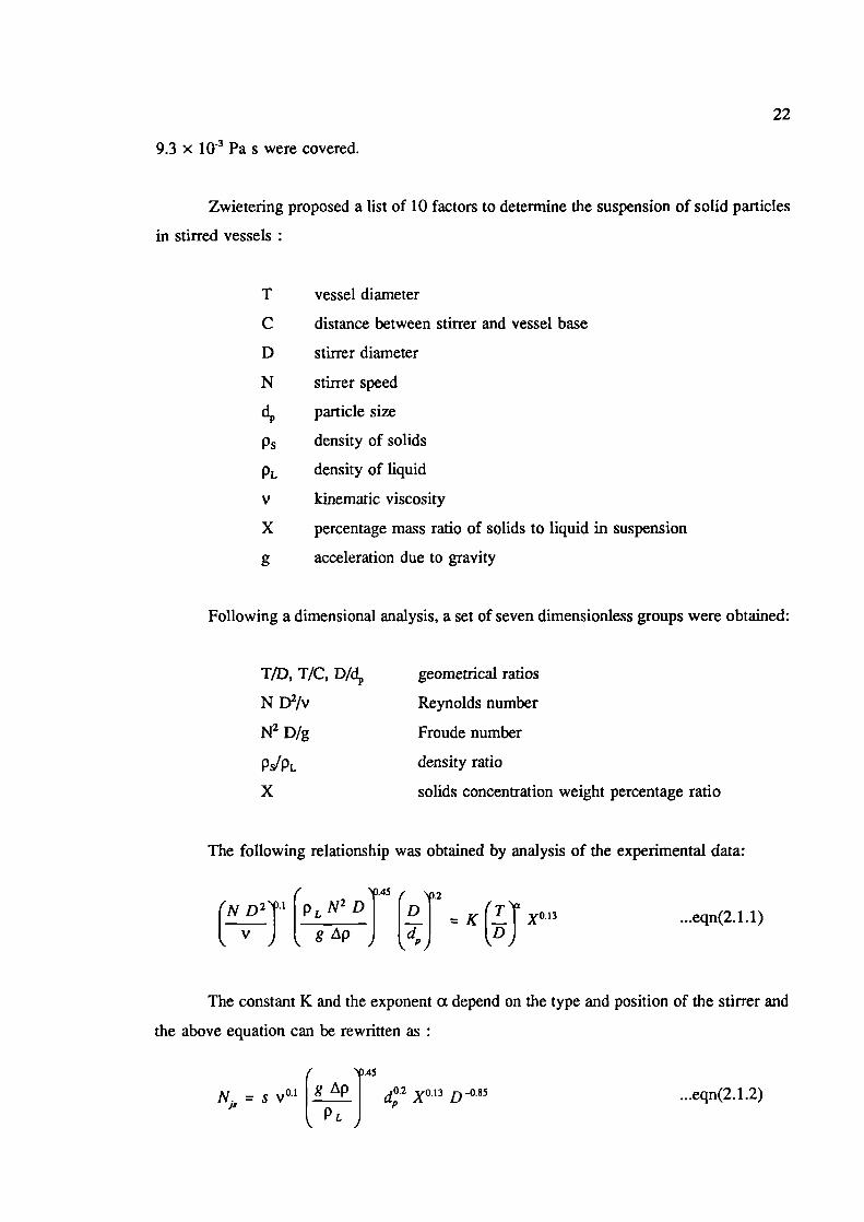
Zwietering proposed a list of 10 factors to determine the suspension of solid particles

in stirred vessels

T

vessel diameter

C

distance between stirrer and vessel base

D

stirrer diameter

N

stirrer speed

d

particle size

Ps density of solids

PL density of liquid

V kinematic viscosity

x percentage mass ratio of solids to liquid in suspension

g acceleration due to gravity

Following a dimensional analysis, a set of seven dimensionless groups were obtained:

TID, TIC, D/d geometrical ratios

N D2/v Reynolds number

N2 Dig Froude number

PSIPL density ratio

X solids concentration weight percentage ratio

The following relationship was obtained by analysis of the experimental data:

42(ND2 1

PL N2 D I ID IK ( T T °.13

H Jgp J J...eqn(2.1.1)

The constant K and the exponent a depend on the type and position of the stirrer and

the above equation can be rewritten as

45

N1, = s v°' Ig

J d 2 X°•13 D° 85 ...eqn(2.1.2)

P

23

The parameter "s" in eqn 2.1.2 is the geometrical constant and it is a function of the

vessel and impeller configuration.

The Zwietering correlation is widely used for estimation of the just suspension speed.

Its advantage is that it was based on a very large number of experiments and is dimensionless

but, because it is an empirical correlation, it should not be applied outside its test range. Even

though it has been re-confirmed by a number of researchers (eg Chapman 1981, Nienow

1968), the range of test parameters are still limited. So, it would be useful to expand the

experimental conditions to discover under what circumstances this correlation would become

invalid.

Zwietering used a mass ratio, X, defmed as the percentage mass of solids to liquid in

the vessel, to quantify the solids concentration but one would expect volume fraction to be

a better parameter to account for the fluid-particle effects.

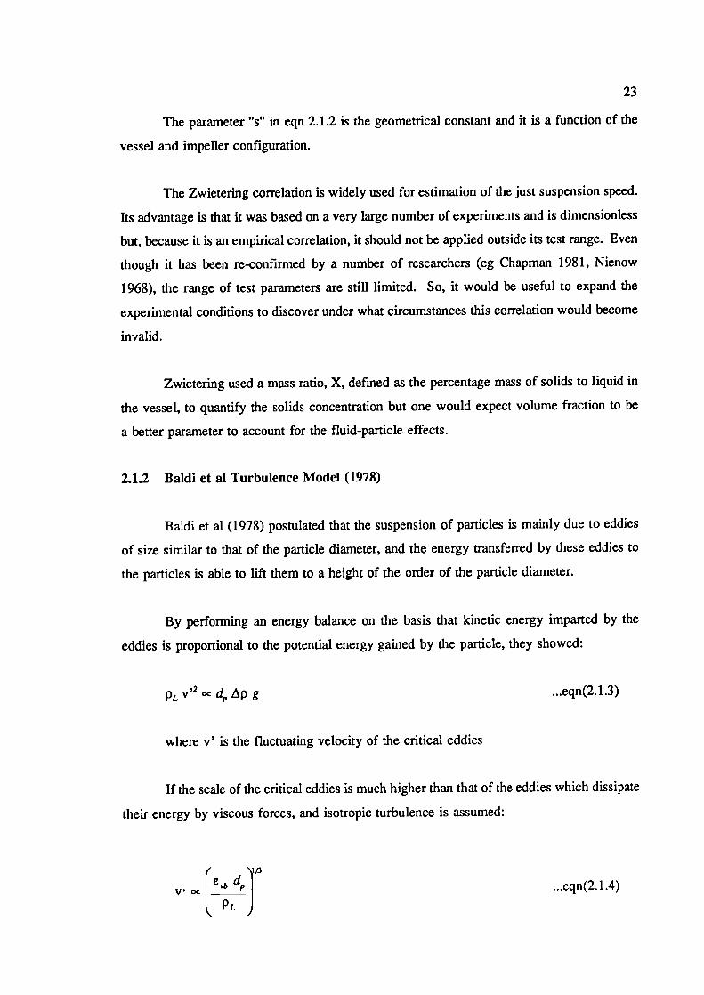
2.1.2 Baldi et at Turbulence Model (1978)

Baldi et al (1978) postulated that the suspension of particles is mainly due to eddies

of size similar to that of the particle diameter, and the energy transferred by these eddies to

the particles is able to lift them to a height of the order of the particle diameter.

By performing an energy balance on the basis that kinetic energy imparted by the

eddies is proportional to the potential energy gained by the particle, they showed:

PL V oc d ip g ...eqn(2.1.3)

where v' is the fluctuating velocity of the critical eddies

If the scale of the critical eddies is much higher than that of the eddies which dissipate

their energy by viscous forces, and isotropic turbulence is assumed:

/ \113

F CVb d I ...eqn(2.1.4)vocl____ I

PL J

volume, c

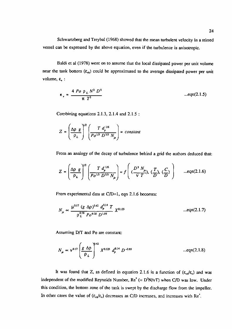
4 Po PL N 3 D5e = _______

irT3...eqn(2.1.5)

24

Schwartzberg and Treybal (1968) showed that the mean turbulent velocity in a stirred

vessel can be expressed by the above equation, even if the turbulence is anisotropic.

Baldi et at (1978) went on to assume that the local dissipated power per unit volume

near the tank bottom (evb) could be approximated to the average dissipated power per unit

Combining equations 2.1.3, 2.1.4 and 2.1.5

ITd' 'z = [PJ I ________

PL Po113 D 513 N J -I.'. is)

From an analogy of the decay of turbulence behind a grid the authors deduced that:

z = g ( Ti D 3 N.

()] ...eqn(2.1.6)Js),(P. J [PO"3 D513 N) V T

From experimental data at CID=1, eqn 2.1.6 becomes:

N. oc i0•17 (g Ap)° 42 d° 14 T

0.58PL Po° 28 D'89

...eqn(2.1.7)

Assuming Dfl and Po are constant:

N oc °•'7 [LP

j42

X°. '25 dA 1 D -0.89 ...eqn(2.1.8)

It was found that Z, as defined in equation 2.1.6 is a function of (c1,/c) and was

independent of the modified Reynolds Number, Re (= D3N/vT) when C/D was low. Under

this condition, the bottom zone of the tank is swept by the discharge flow from the impeller.

In other cases the value of decreases as C/D increases, and increases with Re.

25

The semi-theoretical model (eqn 2.1.8) was verified by Conti and Baldi (1978) in a

variety of flat bottomed tanks equipped with baffles; tank diameter varied between 0.122 and

0.229 m. The impellers used were 8-bladed disc and axial turbines. Seven classes of sand

(42-540 .tm) and nine classes of ballotini (97-1200 tim) were tested. Both mono-modal and

bi-modal particle size distributions were employed.

The conclusion was drawn that the effect of particle size on N. is N, oc d,,', where the

value of 'a' is between 0.14 and 0.16. However, they commented that particles with

d < 200 im generally do not follow their model and suggested that the smaller particles are

subject to a different suspension mechanism as yet not fully understood. Their results also

suggested a strong clearance effect, and the exponents on eqn 2.1.8 will change with C/I).

It is very likely that the solids suspension mechanism involves more than one hydrodynarnic

regime and that these are a function of the geometrical configuration.

The authors justified their application of turbulent theory to solids suspension by

arguing that the solid particles can be seen to be periodically picked up and re-deposited on

the vessel base, a phenomenon difficult to explain using the alternative average velocity

theory. Although this is a reasonable assumption, turbulence cannot be solely responsible for

the suspension of solids. This has been demonstrated by filming of the suspension

phenomenon in a viscous fluid (Shamlou 1991).

The reasoning that suspension of particles is mainly due to eddies of a certain critical

scale is also somewhat arguable. It is quite correct to say that eddies of smaller size than the

critical one do not possess enough energy to move particles from rest. However, despite the

fact that large scale eddies have frequencies lower than those of critical size and have a lower

probability to "hit" and suspend the particle, there is no reason why a large eddy (i.e. a vortex)

could not generate enough pressure difference to entrain particles within the vortex itself.

Remember, in autumn, it is not uncommon to see dead leaves being picked up from the

ground by vortices. Rotating vortices beneath an impeller have been observed (Tatterson

1980). During a three phase mixing study in a 2.1 m diameter vessel with side entering

mixers, Mak (1990) found that the vortices close to the vessel base are the primary vehicle

responsible for the suspension of solids and they are related to the vortices on the water

surface.

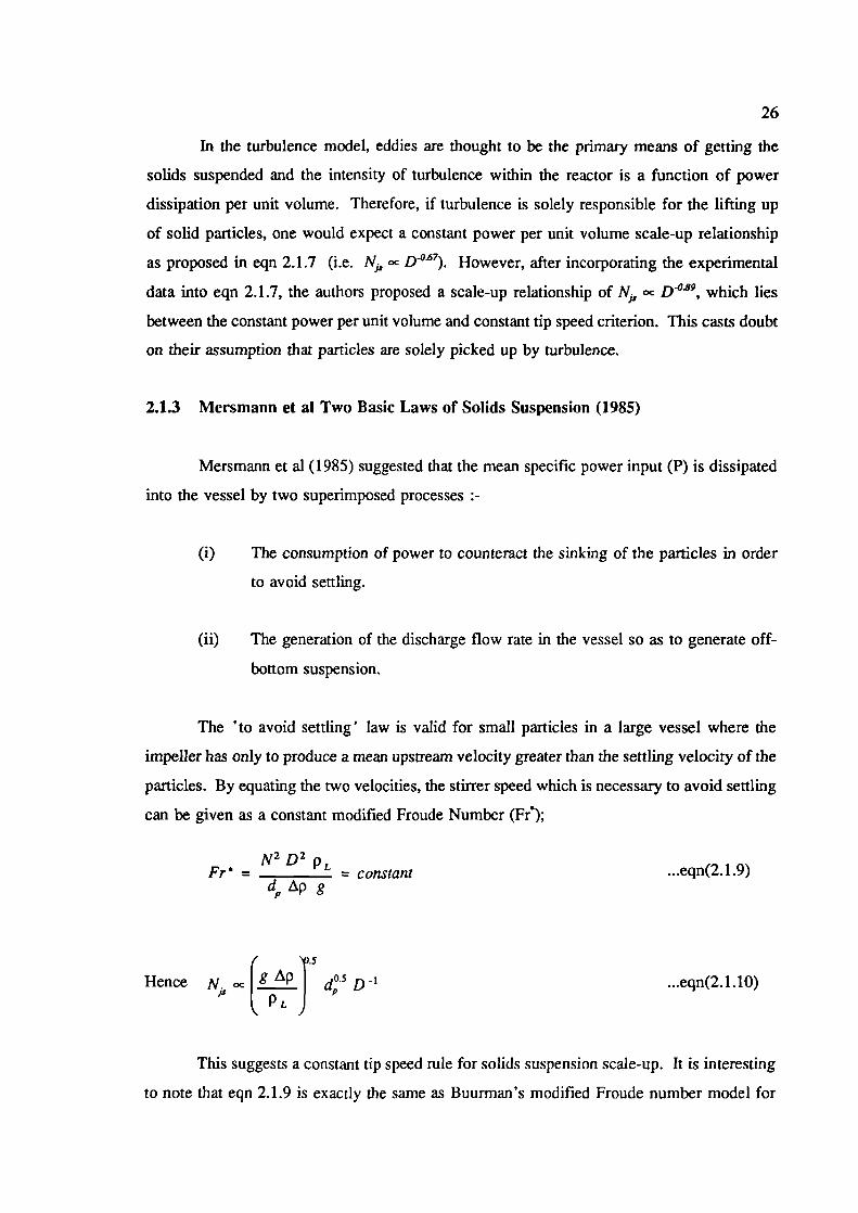
N2 D2 PLFr = ________ constant

d p g...eqn(2.1.9)

26

In the turbulence model, eddies are thought to be the primary means of getting the

solids suspended and the intensity of turbulence within the reactor is a function of power

dissipation per unit volume. Therefore, if turbulence is solely responsible for the lifting up

of solid particles, one would expect a constant power per unit volume scale-up relationship

as proposed in eqn 2.1.7 (i.e. Nfr oc D° 67). However, after incorporating the experimental

data into eqn 2.1.7, the authors proposed a scale-up relationship of N oc D° 9, which lies

between the constant power per unit volume and constant tip speed criterion. This casts doubt

on their assumption that particles are solely picked up by turbulence.

2.1.3 Mersmann et at Two Basic Laws of Solids Suspension (1985)

Mersmann et al (1985) suggested that the mean specific power input (P) is dissipated

into the vessel by two superimposed processes :-

(i) The consumption of power to counteract the sinking of the particles in order

to avoid settling.

(ii) The generation of the discharge flow rate in the vessel so as to generate off-

bottom suspension.

The 'to avoid settling' law is valid for small particles in a large vessel where the

impeller has only to produce a mean upstream velocity greater than the settling velocity of the

particles. By equating the two velocities, the stirrer speed which is necessary to avoid settling

can be given as a constant modified Froude Number (Fr);

/

Hence N1, oc f g I d 5 D'PL)

...eqn(2. 1.10)

This suggests a constant tip speed rule for solids suspension scale-up. It is interesting

to note that eqn 2.1.9 is exactly the same as Buurman's modified Froude number model for

N2D2p L TFr = ______

dApg d...eqn(2.1.11)

27

solids distribution (eqn 2.2.26, Buurman 1985), even though the two authors were adopting

different approaches and trying to describe different mixing phenomena (Sec 2.2.3).

When suspending large particles, the authors suggested that the stirrer has to provide

sufficient kinetic energy in the liquid to compensate for the difference between potential

energy of the deposited solids and for homogeneous suspension.

I'

i.e. N.F g Ap I

D°5

I' PJ.eqn(2. 1.12)

Eqn 2.1.12 suggests power input per unit volume has to be increased with scale in

order to maintain the solids in suspension.

To establish when the power input was being consumed to counteract the sinking of

the particle in order to avoid settling, as opposed to the circumstances when it was generating

discharge flow in the vessel to get off-bottom suspension, the authors used a characteristic

diameter ratio (d,/T) to distinguish between these two basic suspension mechanisms. The

ratio is a function of settling velocity, discharge coefficient, solids volume fraction, porosity

and the liquid depth to tank diameter ratio. If the real diameter ratio (d/F) is smaller than

its characteristic diameter ratio, it is relevant to assume avoidance of settling. On the other

hand, the off-bottom suspension law should apply if Cd/F)> (d/F).

This hypothesis was verified with a T/3 diameter marine-type propeller with a particle

diameter ratio 10 ^ (d/F) ^ 10 (Mersmann 1985). The transition point between the two

basic suspension laws was found to be at (d/F) - iO 3, which agreed well with Ditl's

transition region of 4.05 x iO 3 ^ d/F ^ 1.7 x 102 (Diti 1985).

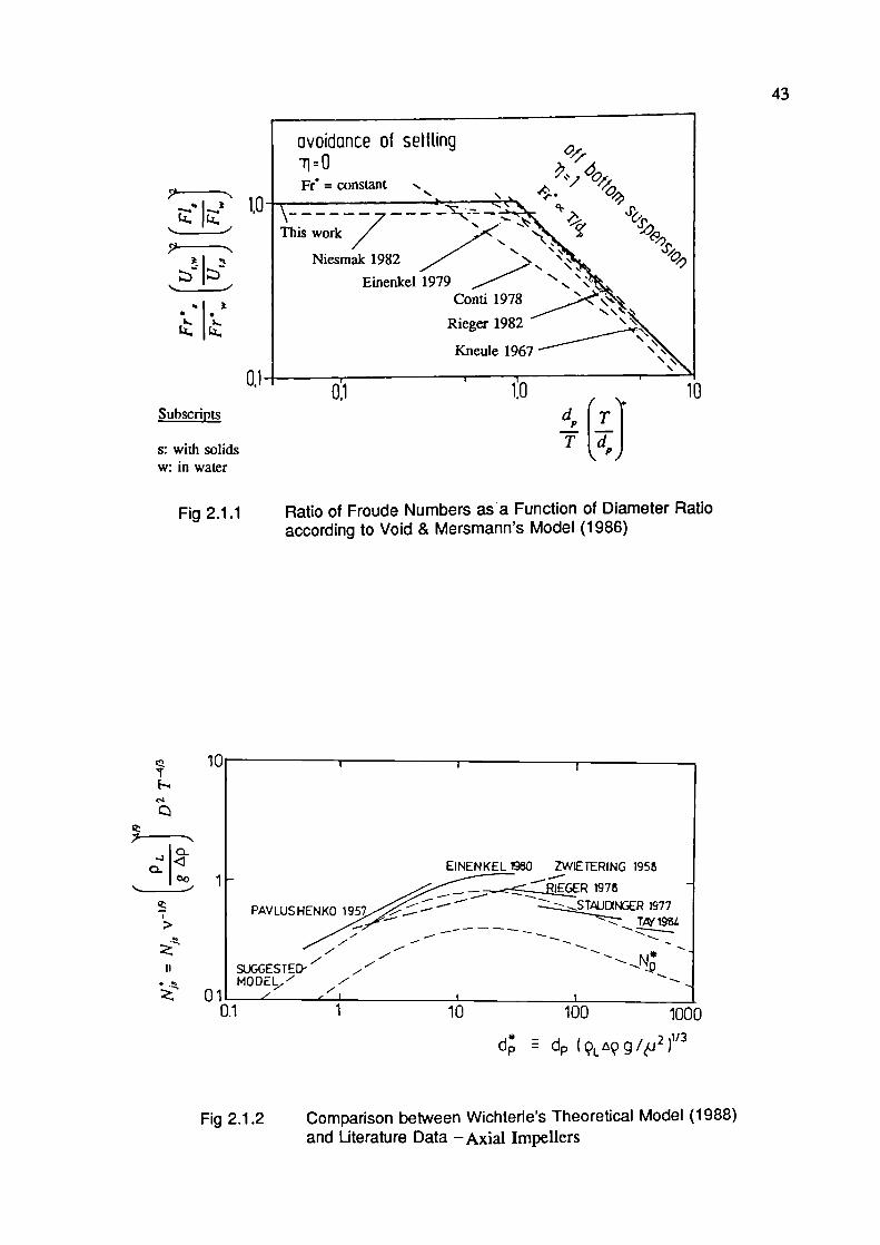
In a subsequent paper Voit and Mersmann (1986) claimed that the Fr=constant

relationship (eqn 2.1.9) for small particles was confirmed experimentally for an agitated vessel

28

with T = 14 m with a d)T ratio of 7 x 10 6. By plotting the ratio of Froude number as a

function of the diameter ratio, they showed that a number of other researchers' results could

fit into their model very well (Fig 2.1.1). However, based on the plots in the paper, the

validity of this could not be substantiated.

2.1.4 Shamlou and Zolfagharian's Average Velocity Model (1987)

Shamlou and Zolfagharian (1987) proposed a model for the estimation of the necessary

conditions for the incipient motion of particles, which was based upon the average velocity

of the fluid near the bottom of the tank and the hydrodynamic forces of lift, drag, buoyancy

and gravity acting upon the particles resting at the tank base.

They suggested that at the point of dislodgement, assuming that all the forces are

acting through the centre of mass of the particle, the moment of these forces about point 0

(Fig 2.1.3) must be zero, i.e.

xF - xFB = yF + ...eqn(2.1.13)

F,, = . CD p , U, A,, and FL = . CL P L U A,, ...eqn(2.1.14)

icd 3 PLUrnA

6 (pS-pL)g=

2...eqn(2. 1.15)

i.e U ocr' gLpd

m

L P L (CL + CD)J

...eqn(2.1.16)

Shamlou (1990) refined the model by assuming that at the point of incipient

suspension of a particle, the rate of dissipation of fluid energy for particle lift-off is due to and

given by the total flow forces acting on the particle (Oroskar and Turian 1980).

C,, = (FL + FD)

29

= PL U UO, AP (CL + CCD) ...eqn(2.1.17)

He further assumed that the total rate of energy dissipation, €, required to entrain all

the particles is proportional to the total number of particles, n,,, in the liquid. Since U0, oc Urn,

A,, oc d,,2 and (CL + CC0) constant, from 2.1.17:

Cl PL U d,,2 n

PL C,, 7'3

dP

From the power number relationship: P = Po PL N3 D5

Cvb = k P = k Po PL N3 D5

...eqn(2.1.18)

...eqn(2.1.19)

...eqn(2. 1.20)

Since U0, oc oc Urn and C,,b oc C,, combining eqn 2.1.16, 2.1.19 and 2.1.20:

Nfr A Po'0 Ig J'2LPL

d, C,'° T D 513 ...eqn(2.2.21)

This equation suggests a particle size effect of and a scale-up effect of D on

N (assuming D oc 7), as compared to d° 2 and D as proposed by the Zwietering

correlation. The author confirmed his model by testing several 4-bladed pitched blade turbines

in a 0.24 m diameter glass vessel. The particle diameters ranged between 175 and 3015 Jim.

Their results produced a value of N proportional to d°' 7 D° 67 which is in good agreement

with the theoretical model.

An important feature of Shamlou et al (1987, 1990)'s work is that their concise

theoretical derivation is completely free from any experimental adjustment, therefore the

validity of the model is not restricted by experimental conditions, as long as the underlying

hypothesis is satisfied. To justify their average velocity model, Shamlou (1991) showed that

solid particles can be lifted up by fluid velocity alone (in the absence of any turbulence).

30

Now the question is, could the solid particles be lifted up by turbulence or even a combination

of both flow and turbulence? If so, should the exponent on D be different? It is interesting

to note that the exponents on Shamlou and Zolfagharian's model are very similar to that of

Baldi's, even though their initial assumptions differ. The exponent of -0.67 on D (constant

power per unit volume) suggests that for whichever type of suspension mechanism is

involved, its intensity is a function of power input.

2.1.5 Molerus and Latzel's Two Suspending Mechanisms (1987)

Molerus and Latzel (1987) suggested that the suspension of solid particles in a stirred

vessel is governed by two different mechanisms, depending on the Archimedes number. The

fust one defmes the complete suspension of fme grained particles (Ar ^ 40) being attained at

sufficiently high shear stresses in the wall boundary layer of the vessel. The second criterion,

generally applicable to coarse grained particles (Ar> 40), is based on an analysis of the pump

characteristics of an agitated vessel.

(i) Fine Particles (Ar ^ 40)

The authors observed that the settling velocity of 66 pm glass ballotini suspended in

water was almost two orders of magnitude lower than its circulation velocity in a 1.5 m

diameter vessel. This leads to the conclusion that the region responsible for the complete

suspension of the particle is the wall boundary layer of the vessel where the local fluid

velocities are similar to the particle settling velocity.

They took the maximum fluid velocity U,. close to the boundary layer as a reference

velocity. Measurements in three geometrically similar vessels (T = 0.19, 0.45 and 1.5 m)

showed a linear dependence of U_ on the circumferential stirrer velocity (ie U_ oc N D).

Close to the bottom of an agitated vessel, the streamlines are curved and flow is

axisymmetric. The wall shear stress in the critical point is approximated by a plane

turbulent boundary layer flow along a flat plate at a distance of T/2 from the leading edge of

the plate.

I 3It

U =i¶

(PL...eqn(2. 1.22)

31

This gives the shear stress velocity of:

From the wall shear stress relationship described by Schlichting (1965)

= 0.182 v°' U..° 9 r°•' ...eqn(2. 1.23)

In order to establish the flow forces exerted on particles settled in the boundary layer,

the shear stress for a particle layer is assumed to cover the wall surface and hence;

7td2 itd3( 4 ) t=i p( 6)g ...eqn(2. 1.24)

and Re = [dutJ

Combining eqn 2.1.22, 2.1.24 and 2.1.25

- ___ArRe—

JJ- 3

...eqn(2.1.25)

...eqn(2.1.26)

The above equation was confirmed with tests on various sizes of glass and steel beads

(34 ^ d ^ 1937 j.tm), with a concentration range of 0.5 to 30% by volume, in geometrically

similar vessels (T = 0.19, 0.45 and 1.5 m). Tap water and water/ethylene glycol mixtures

were used as the test fluid. The experimental results agreed with the model in the regime

Ar ^ 40.

From equation 2.1.26;

I'I d g Ap I

U oc " ...eqn(2.1.27)PL )

32

Substituting into equation 2.1.23;

g Apv-° •" T°"-

P,. )

Since U.. ocND, thus;

_ g p IN [d ___36

PL J v°" D' T°1'

...eqn(2.1.28)

...eqn(2.1.29)

The above equation suggests a particle size effect of N, oc d° 6 and a scale effect of

N oc D°29 for geometrically similar vessels, but that just suspension speed is independent of

solids concentration.

(ii) Coarse Particles (Ar> 40)

Molerus and Latzel (1987) also developed a criterion for predicting minimum speed

for solids suspension for coarse particles, which was based on:

(i) An appropriate representation of the dependence of the drag on fluidised particles on

the concentration and

(ii) An analysis of the pump characteristics of an agitated vessel, analogous to the

theory of similarity of fluid-kinetic machines.

They started by assuming a fictitious tube of a diameter D around the impeller.

Assuming complete fluidisation outside the impeller region, the static pressure difference

required by the stirrer, iP can be given by:

&'J at = AP0 - ...eqn(2.1.30)

= 1 Cp5-s-(l-C)pL]gH-pgH

= Cp (PsPL) g H ...eqn(2.1.31)

UJo(1-C,,) D N

...eqn(2. 1.35)

(1-C,,)2 AP=

[(I-C,,) PL C,, Ps U102...eqn(2. 1.36)

33

Where P1 and P0 are the static pressure difference between the top and bottom,

inside and outside the impeller region respectively.

From the Euler Number for particulate fluidisation

Eu = ± .e. ..! (1-C,,)23 P. U2

...eqn(2.1.32)

Eu = ±_Al'd (1-C,,)2

fi 3PLL'JOH cv

and for constant Eu, from eqn 2.1.32:

p d gUIO2 oc (1-C,,)2

PL

...eqn(2. 1.33)

..eqn(2.1.34)

By comparing the flow in an agitated vessel with a pumping system, the authors

generated two nondimensional groups to describe the pumping characteristics of two-phase

flows in agitated vessels

Experiments were performed in two geometrically similar vessels (T=0.19 and 1.5 m)

with marine propellers. Glass ballotini and iron particles of dimensional range 220 to 1900

J.tm were used. The solids concentration covered a range of 0.5 to 30% Vol.

34

It was found that (,)2.77 for Ar> 40, hence:

(1-C,)2 AD ( 102.77

LU__________________ oc ________

[(l-C,)p + , P] u 2L( 1_c,) D N}

...eqn(2.1.37)

Jo

Substituting and Uf0 and for a given scale, (1-C,,) 1k + C, Ps constant

N.Ap d IC, H P L

.36

P i E)2 ) d

i.e. Nfr (g ip)°3

[J.14

(C, jj)036 D-' ...eqn(2.1.38)

The above equation suggested the influence of particle size and scale on N,, were

and DOM. It is interesting to note that their effect of liquid density on N, (i.e. N,, oc PL°'4)

is much smaller than that are proposed by the other researchers. Moreover, the dividing

criterion of Molerus's model (Archimedes Number) depends on densities, particle size and

viscosity but not tank diameter as proposed by Mersmann nor power input as in Diii's model.

Influence of solids concentration is included in Molerus's model only when Ar> 40, for Ar

^ 40, the authors observed no dependence of N,, on solids concentration.

2.1.6 Wichterle's Characteristic Velocity Model (1988)

Wichterle (1988) developed a theoretical model for solids suspension based on the

comparison of the terminal settling velocity of a particle and the characteristic velocity of the

agitated liquid around the particle at the vessel base. He suggested that the flow acting on

a particle of diameter d. lying on the bottom can be characterized by a velocity B (Fig 2.1.4)

and V8 = 'YB d. If VB is higher than the settling velocity of the particle (U,), the particle will

be suspended and thus, the suspension condition can be related by a critical value B,, which

is a function of particle shape;

B. = 'y 8 d

...eqn(2.l.39)is

dN = _______

18 + 0.6

...eqn(2.1.45)

35

The relationship between the particle diameter and settling velocity was related by a

semi-empirical correlation:

U, dP p L Ar

(18 + 0.6 Ar°5)

He defmed a normalised particle diameter, d'

Ar == d PL g

...eqn(2.l.40)

...eqn(2.1.41)

From a laminar boundary layer of an impinging jet

lB = N A Re1°5 .eqn(2. 1.42)

Where A,, is a minimum value of a constant A, which is dependent on the

geometrical configuration of the mixing vessel according to the author's electrodiffusion

experiments. A,, is equal to 2.5 for disc turbines at T/3 clearance and 3.5 for 6-bladed

pitched bladed turbines at T/2.5 to T/5 clearance.

Wichterle then introduced a dimensionless critical impeller speed for just suspension,

N, where:

(PLNi;=Nv-1 gp J D2T .eqn(2. 1.43)

From equations 2.1.40, 2.1.42 and 2.1.43

• (BrN1= ...eqn(2.1.44)

36

The proposed correlation was verified by plotting other researchers' results in the

format of N, against d (Fig 2.1.2). From open publications (Einenkel 1980, Paviushenko

1967, Rieger 1982, Staudinger, Tay 1984 and Zwietering 1958), a value of 10 ± 2 was

estimated for B,.

The author's model predicts that in the whole range of variables, a single-power

function N oc D 213 (D/T) 3 applies (eqn 2.1.43), which suggests a constant power per unit

volume scale up rule. However, influences of other parameters (d 1.1, PL and p) on N are

a function of the normalised d, i.e. Ar' 3 (eqn 2.1.41). A single power law relationship will

be given for a constant Ar. Work conducted by other researchers had already suggested that

the effect of particle size on just suspension speed is not a simple single power law

relationship, but divided by critical values, which could be a function of Ar (Molerus 1987,

Rieger 1982). Wichterle further proposed that there were not just two different exponents on

d, but a continual variation of exponents both on d and other parameters.

The scale-up rule of D on just suspension speed is somewhat questionable. The

reasons are two fold; firstly, the author did not deduce the scale-up relationship theoretically

but instead, assumed a dimensionless critical speed (eqn 2.1.43) for solids suspension without

proof. Secondly, the other researchers' data with which the author tested his model were all

obtained from a rather limited range of vessel sizes. If the particle is being picked up by flow

rather than turbulence as the author suggested, one would expect scale-up to be more likely

to be governed by constant tip speed criterion.

2.1.7 Other Models

Narayanan et al (1969) derived an expression for N, based on a balance of the vertical

forces acting on a particle. It was assumed there was no slip between the particle and the

fluid, the fraction of solids inside the agitated vessel was very low compared to the bulk

volume of the liquid and that the solids were uniformly dispersed throughout the liquid. The

necessary knowledge of fluid velocities was obtained from the mean circulation time data

produced by Holmes et al (1964) without taking account of the local conditions on the vessel

base where suspension occurred. By equating the circulation time constant with the flow

pattern and correlating for the discrepancy between the experimental and theoretical results;

N = 1.782 X22 (T)2 __1__ [D 2T-D

2d(2 g ip) [.......L +

3p L

HX

100 (p^X PL)

37

...eqn(2.1.46)

Although the above equation showed very good agreement with the experimental

results, its fundamental assumptions were somewhat questionable and its range of application

should thus be restricted to that within which the empirical constants were established.

However, the approach adopted by the author does look somewhat more appropriate to

describe the distribution of solids in a stirred vessel.

Subbarao and Taneja (1979) proposed a simplistic model based on a balance of the

fluid velocity and particle settling velocity for a propeller agitated system. The particle

settling velocity was estimated from a correlation for the porosity of a liquid fluidised bed as

a function of liquid velocity. Their model indicated a negative exponent on d in all

circumstances which is questionable.

Kolar (1961) proposed that the mixing energy at the critical condition can be related

to the potential energy of the particles (i.e. power input equal to the effective weight of solids

times the particle free falling velocity) and that the particle settling velocity is proportional

to the impeller tip speed. The author tried to account for the effect of turbulent dissipation

on the settling velocity by the relation;

•, U 2 = UO2...eqn(2. 1.47)

However, his assumption is too simplistic to describe the actual suspension

phenomenon.

Did and Rieger (1985) utilised a similar turbulence concept to that of Baldi et al

(1978), to model the suspension of solid particles. They suggested that particles were picked

up by different sizes of eddies (primary, small and medium). If the particle size is comparable

with the size of the eddies, the suspension mechanism is therefore governed by them. In other

words, the suspension of larger particles is governed by the motion of primary eddies whereas

the suspension mechanism for the smaller ones is determined by the small and medium eddies.

...eqn(2.1.48)

38

They postulated that the dividing criterion between different mechanisms can be

defined by the relative size of particles to characteristic eddies. For the smaller particles the

characteristic scale can be given as:

Thus "4 Po 1dp '"1\'_D2 PL 1 (r 3i

nHJ J 4 ...eqn(2.1.49)

Results from thirty eight set of experiments were correlated, to evaluate the critical

particle diameter. Based on statistical analysis:

0.45 (d ' (T -0.56

Re cc Ar (TJ J

...eqn(2. 1.50)

For large particles; (d / Th) ^ 32, 13 = -1.42

= Ni,, cc d°°7 and D°58

For small particles; (d, / r) <32, 13 = -1.25

= N cc d°' and D°75

The authors conducted their tests in 0.15-0.4 m vessels and covered a much wider

range of particle sizes (85-4000 l.tm) than Zwietering and Baldi. The exponents of d for

small particles were lower than those of Baldi et al's. Even though the two models seem to

be based on similar theories, Baldi also introduces empirical reasoning to adjust the exponents

on d and X. Diti et al do not use their experimental data to correct their model and therefore

their model is in a way more absolute than Baldi's. Once again, the negative exponent of d

for large particles looks very doubtful. The scale-up factor of -0.58 for large particles

implying the power per unit mass has to be increased with scale is very suspicious. It is also

interesting to note that the authors' model does not account for the effect of solids

concentration.

p N D413_________ = constantg p d"

...eqn(2.1.52)

39

Musil and Vik (1978) based their theory on the balance of the liquid and particle

kinetic energies, which was very similar to Kolar's initial assumption. Their results were

expressed in the form of a critical Reynolds Number, which is a function of Archimedes and

Particle Reynolds Number. However, their mathematical reasoning for the derivation is

impossible to follow. It has been pointed out that there are a number of mistakes in Musil's

physical assumptions and mathematical treatment (Diti 1980).

Buurman et a! (1985) employed a similar hypothesis to that of Baldi et al, relating the

kinetic energy of the eddies to the potential energy of the particles;

p v 2 d oc g ip d ...eqn(2.1.51)

The equation led to the form of a modified Froude Number, which suggests a constant

power per unit volume scale-up relationship;

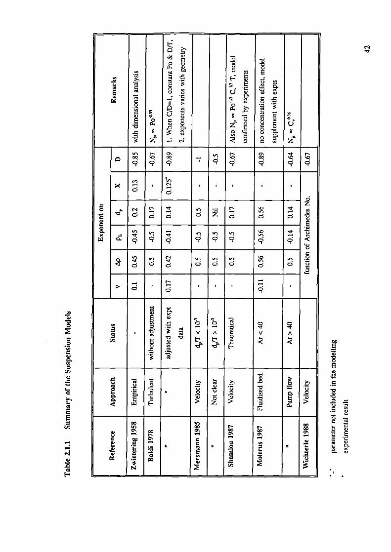
2.1.8 Summary of the Suspension Models

According to the suspension mechanisms, the theoretical models which have been

reviewed so far can generally be classified into two categories; namely those in which

particles are believed to be picked up by turbulent eddies (eg Baldi 1978, Diii 1985) and those

in which particles are believed to be picked up by fluid flow (eg Shamlou 1987, Wichterle

1988). There is a third category in which the suspension model is not based on an

independent mechanism but is simulated by another phenomenon of which the researchers had

more modelling experience, such as pump flow or fluidisation (Molerus 1987). This section

will compare and contrast models derived from the first two categories, as they gave a better

fundamental understanding of the suspension mechanism as compared to the simulation

models.

The proposed turbulence models argue that the solid particles are being periodically

picked up and re-deposited on the vessel base, an observation difficult to explain by the

40

average velocity concept. However, the turbulence models on their own cannot explain why

axial flow impellers, which have a lower power number than their radial flow counterparts and

hence, a lower level of turbulence, are nevertheless able to suspend solids at a lower energy

input, bearing in mind that an axial flow impeller is generally flow dominated. Moreover,

Al-Dhahir (1990) has shown that solids suspension is possible with viscous liquid operating

in the laminar regimes well before turbulence sets in.

Although both of these theories display considerable merit, there remain a few

questions to be answered. In the turbulent model, mean energy dissipation is assumed and

the related kinematic quantities are usually derived according to the concepts of

Kolomogoroff's theory of homogeneous turbulence. However, it is obvious that the energy

input does not dissipate uniformly throughout the vessel and there is as yet insufficient

knowledge of the dissipation intensity in the vicinity of the bottom where the solid particles

are to be suspended. Moreover, the damping effect due to the presence of solids is extremely

difficult to quantify. It has also been reported (Squires 1990) that the turbulence field was

modified differently by light particles than by heavy particles. Moreover, the validity of

Kolomogoroff's theory in a mechanically agitated vessel has yet to be verified.

On the other hand, the velocity model approach also presents problems. The flow

model assumes that regardless of the flow condition in the core (turbulent or laminar), flow

near the base is not turbulent during suspension. Most of the models that have been reviewed

were too simplistic to quantify the complex interaction between fluid flow and geometry. For

example, flow within the core of the vessel could be very different from flow near the vessel

base. The location of the last suspension region depends on a combined effect between vessel

base and impeller discharge flow. The influence of geometrical configuration on N, may vary

from one location to another due to differences in flow nature. If one wishes to explain the

periodically picked up and re-deposited motion of the particles on the vessel base by means

of the velocity model approach, one has to accept that the fluid velocity must be unsteady,

varying considerably across the vessel base. Therefore, a more accurate way of relating the

impeller rotational speed to the fluid flow adjacent to the solid particle to be suspended is

necessary.

The suspension models reviewed are summarised in Table 2.1. According to the

various theoretical models compared, the prediction of the viscosity and density effects agree

41

reasonably well. They suggest v and p exponents ranging from 0.11 to 0.17 and 0.42 to

0.56 respectively. However, almost all the turbulence models suggest an exponent of 0.17 (eg

Baldi 1978) and -0.67 (eg Buurman 1985) for the particle size and scale-up effect and the

flow model recommended an exponent of 0.5 (eg Mersmann 1985) and -1 (eg Molerus 1987)

for the corresponding effect. Incidently, most of the exponents reported in open literature lie

between 0.14 and 0.5 for particle size effect and -0.67 and -1 for scale-up effect. This makes

one wonder if the solid particles are being picked up by a combination of these two effects

and that the magnitude of the exponent is dependent upon the proportion of particles being

picked up by each of the two mechanisms.

Most of the models formulated have not allowed for the effect of liquid viscosity and

solids concentration. These are extremely important, for both the liquid velocity and

turbulence intensity will be modified by these parameters. Shamlou (1990) considers the

concentration effect by relating the number of particles in the vessel to the power input and

he found that N, C,,''3. Buurman (1990) suggests that the effect of solids concentration is

a function of liquid and solid density, particle size and scale of equipment. Until models have

been developed which account for all these complex interactions, it is unlikely that any pure

theoretical model will be able to bring all the available experimental data together.

To summarise, there has been much effort devoted to the modelling of the suspension

mechanism but these models still require refinement. There remains a need for confirmation

of the models by conducting flow visualisation tests and validation by conducting

experiments in more critical conditions, such as high solids concentration and large scale tests.

This is because many models developed have only been verified in limited test range (eg in

relatively small scales).

I

hi- bO E Ec 'S -.' US ' )g.

o 0

? °o - C) C)z' U

'S

r- C\ N r-00 O 00 - '1 O 00 O Oqqq '9q q qq

cn- • I I I I

o

-N Na. - - ' C)

I,) ir

.9< C C 0 d C

___ ___ ___ -N -- I - I I -

d

-C)

a)

. 9

. .2

.° . - C) .•a2:

00 InIn 00 N N

00 00 00- N -

- (I)._ =

. UC) .

N

C)

Ea).5

C.)

-.

0-

I-.C) C)

._... 1,0

—__—,

1

'- -,

• •

- L

0,1

Subscripts

s: with solidsw: in water

Fig 2.1.1

I

e4

1

0.1

43

avoidance of settling

m=0

Fr = constant •%

Niesm EanenkelCon 1978

Rieger 1982

Kneule 1967

0, i;o

d IT

10

T

Ratio of Froude Numbers as'a Function of Diameter Ratioaccording to Void & Mersmann's Model (1986)

10

EINENKEL 8O ZWIETERING 1958

1978

- - jER 1977TN l9Zh

—

SUGGESTED- 7 -N*

MODc/' -—-, I

0.1

•1

10 100 1000

d E d (Qg/J2)hh'3

Fig 2.1.2

Comparison between Wichterle's Theoretical Model (1988)and Literature Data —Axial Impellers

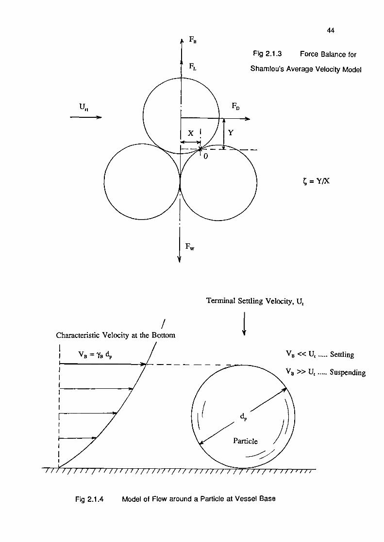
ig 2.1.3 Force Balance for

amlou's Average Velocity Model

;=yix

Un

Settling

Suspending

441-.

4FW

Terminal Settling Velocity, U1

/ 4.Characteristic Velocity at the Bottom

Fig 2.1.4 Model of Flow around a Particle at Vessel Base

45

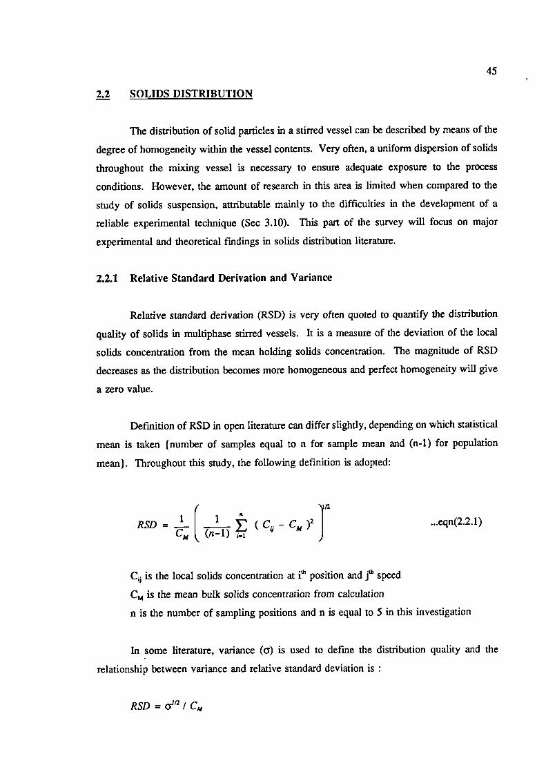
2.2 SOLIDS DISTRIBUTION

The distribution of solid particles in a stirred vessel can be described by means of the

degree of homogeneity within the vessel contents. Very often, a uniform dispersion of solids

throughout the mixing vessel is necessary to ensure adequate exposure to the process

conditions. However, the amount of research in this area is limited when compared to the

study of solids suspension, attributable mainly to the difficulties in the development of a

reliable experimental technique (Sec 3.10). This part of the survey will focus on major

experimental and theoretical fmdings in solids distribution literature.

2.2.1 Relative Standard Derivation and Variance

Relative standard derivation (RSD) is very often quoted to quantify the distribution

quality of solids in multiphase stirred vessels. It is a measure of the deviation of the local

solids concentration from the mean holding solids concentration. The magnitude of RSD

decreases as the distribution becomes more homogeneous and perfect homogeneity will give

a zero value.

Defmition of RSD in open literature can differ slightly, depending on which statistical

mean is taken (number of samples equal to n for sample mean and (n-i) for population

mean). Throughout this study, the following defmition is adopted:

RSD- 1 ( 1-(n-i)

(C - CM )2

J...eqn(2.2.l)

C1 is the local solids concentration at th position and th speed

CM is the mean bulk solids concentration from calculation

n is the number of sampling positions and n is equal to 5 in this investigation

In some literature, variance (a) is used to define the distribution quality and the

relationship between variance and relative standard deviation is

RSD = &12 I CM

46

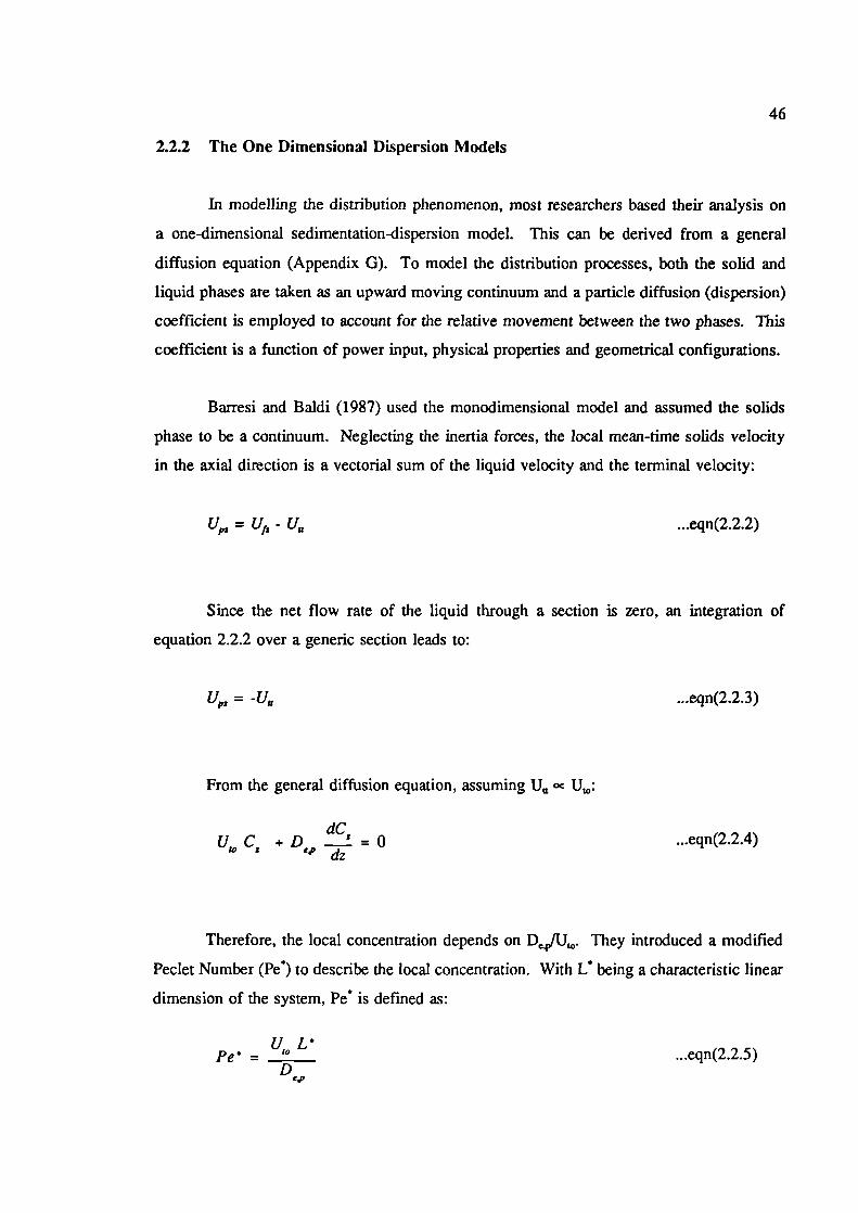
2.2.2 The One Dimensional Dispersion Models

In modelling the distribution phenomenon, most researchers based their analysis on

a one-dimensional sedimentation-dispersion model. This can be derived from a general

diffusion equation (Appendix G). To model the distribution processes, both the solid and

liquid phases are taken as an upward moving continuum and a particle diffusion (dispersion)

coefficient is employed to account for the relative movement between the two phases. This

coefficient is a function of power input, physical properties and geometrical configurations.

Barresi and Baldi (1987) used the monodimensional model and assumed the solids

phase to be a continuum. Neglecting the inertia forces, the local mean-time solids velocity

in the axial direction is a vectorial sum of the liquid velocity and the terminal velocity:

U,,, = - U ...eqn(2.2.2)

Since the net flow rate of the liquid through a section is zero, an integration of

equation 2.2.2 over a generic section leads to:

Upz = Uts ...eqn(2.2.3)

From the general diffusion equation, assuming U oc U:

dCU 0 C +D

'' dz...eqn(2.2.4)

Therefore, the local concentration depends on They introduced a modified

Peclet Number (Pe) to describe the local concentration. With L being a characteristic linear

dimension of the system, Pe is defined as:

ULPe = ______ ...eqn(2.2.5)

D

U10Peoc

Po"3ND...eqn(2.2.6)

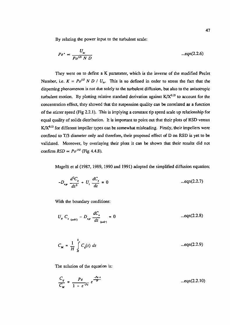
47

By relating the power input to the turbulent scale:

They went on to define a K parameter, which is the inverse of the modified Peclet

Number, i.e. K = Po"3 N D / U,. This is so defmed in order to stress the fact that the

dispersing phenomenon is not due solely to the turbulent diffusion, but also to the anisotropic

turbulent motion. By plotting relative standard derivation against K/X°' 3 to account for the

concentration effect, they showed that the suspension quality can be correlated as a function

of the stirrer speed (Fig 2.2.1). This is implying a constant tip speed scale up relationship for

equal quality of solids distribution. It is important to point out that their plots of RSD versus

K/X°'3 for different impeller types can be somewhat misleading. Firstly, their impellers were

confined to T/3 diameter only and therefore, their proposed effect of D on RSD is yet to be

validated. Moreover, by overlaying their plots it can be shown that their results did not

confirm RSD oc Po 3 (Fig 4.4.8).

Magelli et a! (1987, 1989, 1990 and 1991) adopted the simplified diffusion equation;

d2C dC-D __Z+UZO

ep dz2 ' dz

With the boundary conditions:

dCUC -D - =0

(z'.0) dz (gO•)

...eqn(2.2.7)

.eqn(2.2.8)

0

CM ! 5 Cz) dz ...eqn(2.2.9)H

The solution of the equation is:

C j = Pe —Pe z

.eqn(2.2. 10)l_e1'e

RSD = (C -CM n

...eqn(2.2. 11)

48

The authors suggested that suspension inhomogeneity can be characterized by the

relative standard deviation (RSD) of the solids concentration with respect to the mean value

and RSD can be expressed as a function of Peclet number (Pe). Note that their defmition of

RSD differs slightly from that presented in this investigation.

RSD=1 e'-1 _iJ°2 (e r'- 1)2

...eqn(2.2.12)

and Pe= -UH...eqn(2.2.13)

D'4'

They conducted a series of experiments in a 0.23 6 m diameter stirred vessel, with

various liquid depth (2.3 ^ HTF ^ 4) and impeller combinations. A variety of solids and fluids

were also tested. They established that a single interpolating line can be obtained for all the

geometries studied, for each particle size and liquid viscosity. Therefore, they proposed the

following relationship in order to account for the physical and geometrical parameters;

Pe = A. ___ I____NDJ

...eqn(2.2.14)

Based on test results from Rushton turbines, the exponents on (I-hF) ratio and

(v3/cm d) were found to equal 2 and 0.095 respectively. They observed a lower distribution

efficiency of radial impellers in comparison to axial impellers. Incorporating results from

axial impellers (with the above two exponents kept constant), further analysis yielded the

following correlation (Fig 2.2.4):

..'i17

H (0 I (v3Pe = 330 TJ D ) d:J

...eqn(2.2.15)

or depletion of the particles;

dCUC +D =0'' dh

.eqn(2.2. 17)

d (lnC) - - U,1

dh De,p

...eqn(2.2.18)

49

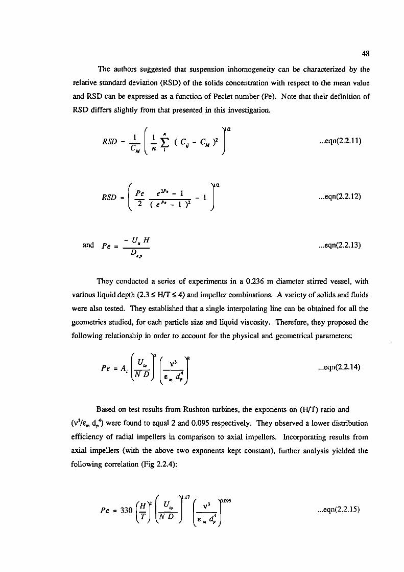
By assuming a power law dependence of RSD on Pe, equation 2.2.12 can be

simplified as:

RSD = 0.29 Pe°'92 for 0 Pe ^ 6 ...eqn(2.2.16)

An important contribution of Magelli et al's work is the successful demonstration that

all physical and geometrical parameters they have tested so far can be presented in terms of

a single adjustable parameter (Pe - Peclet No, eqn 2.2.14). The relative standard derivation

of solids concentration can be related to the Peclet number by a power law approximation.

Thus, the homogeneity of a solids distribution system can be predicted from equation eqns

2.2.15 and 2.2.16. Since , oc N3 and therefore Pe cc N446 and RSD cc N'24. A scale up

implication of N cc D° 93 can be deduced from these two equations.

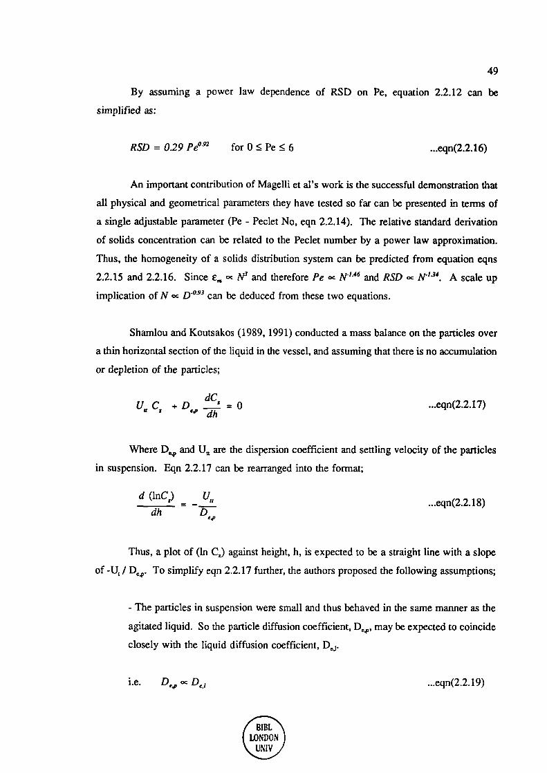
Shamlou and Koutsakos (1989, 1991) conducted a mass balance on the particles over

a thin horizontal section of the liquid in the vessel, and assuming that there is no accumulation

Where D4, and U are the dispersion coefficient and settling velocity of the particles

in suspension. Eqn 2.2.17 can be rearranged into the format;

Thus, a plot of (in C) against height, h, is expected to be a straight line with a slope

of -U, / To simplify eqn 2.2.17 further, the authors proposed the following assumptions;

- The particles in suspension were small and thus behaved in the same manner as the

agitated liquid. So the particle diffusion coefficient, D o.,,, may be expected to coincide

closely with the liquid diffusion coefficient,

i.e. De4, cc ...eqn(2.2.19)

8IBLLONDON

UNIV

50

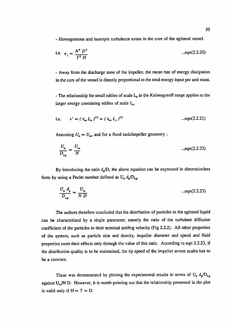
- Homogeneous and isotropic turbulence exists in the core of the agitated vessel.

i.e. N3D5 ...eqn(2.2.20)

£ T2H

- Away from the discharge zone of the impeller, the mean rate of energy dissipation

in the core of the vessel is directly proportional to the total energy input per unit mass.

- The relationship for small eddies of scale L in the Kolmogoroff range applies to the

larger energy containing eddies of scale L.

i.e. v' ( Cm L0 )"3oc (CmLe)"3 ..eqn(2.2.21)

Assuming U ec U,47 , and for a fixed tank/impeller geometry:

U,:Uu, ...eqn(2.2.22)

By introducing the ratio d/D, the above equation can be expressed in dimensionless

form by using a Peclet number defined as U d.JD

U,: d (J,, ...eqn(2.2.23)D ND

The authors therefore concluded that the distribution of particles in the agitated liquid

can be characterized by a single parameter, namely the ratio of the turbulent diffusion

coefficient of the particles to their terminal settling velocity (Fig 2.2.2). All other properties

of the system, such as particle size and density, impeller diameter and speed and fluid

properties exert their effects only through the value of this ratio. According to eqn 2.2.23, if

the distribution quality is to be maintained, the tip speed of the impeller across scales has to

be a constant.

These was demonstrated by plotting the experimental results in terms of U,: dpfDcp

against UJN D. However, it is worth pointing Out that the relationship presented in the plot

is valid only if H oc T oc D.

51

All three models used the settling velocity (single particle in still fluid) to account for

the solids and liquid properties. Baldi et a! (1987) used RSD oc to account for the effect

of solids concentration in homogeneity, an arbitrary correction taken from Zwietering's

correlation for solids suspension which seemed to work well for low solids concentration.

Apart from that, no analysis has been conducted to include this important parameter in their

models. The models all point roughly to a constant tip speed scale-up implication. This was

deduced by testing impellers of different diameter in the same vessel (ie varying DIF ratio).

If turbulent eddies were responsible for the distribution of the solids as was assumed, one

would expect power per unit volume must be kept constant between scales in order to produce

the same degree of turbulence. Moreover, Buurman (Sec 2.2.3) correlated the solids

distribution data taken from various sized vessels (0.24 5 T S 4.26 m) and he concluded a

N oc D° 78 scale-up relationship. It may be the case that constant tip speed criteria work for

different D/T ratios but not necessarily so if the different tank sizes were used with DTl'

maintained constant. This is a subject of further investigation in this thesis.

2.2.3 Buurman's Modified Froude No. Model (1985)

In order to achieve a certain degree of homogeneity in a stirred vessel, the solid

particles have to be lifted up from the vessel base and then transported throughout the whole

vessel. Buurman et a! suggested that it is not only the eddies of the inertia! sub-range that

are isponsible for the mechanism but that the largest eddies (i.e. circulation) also play a role.

They assume the fluctuating velocity, which is responsible for entrainment of the

particles, to be proportional to the circulation velocity, i.e to the impeller tip speed.

V oc ND ...eqn(2.2.24)

From an energy balance between the kinetic energy of eddies and the potential energy

of the particles:

PL d 3 v 2 oc g ip d 3 d ...eqn(2.2.25)

N2 D2_________ = constantg Ap d

...eqn(2.2.26)

is:

52

Combining equations 2.2.24 and 2.2.25

The authors conducted a series of experiments in T=0.24, 0.48 and 4.26 vessels, with

a T12.5 diameter downward pumping pitched bladed turbine mounted at T/3 clearance.

Particle sizes in the range of 157 to 2200 p.m were used. The data were correlated in terms

of height of homogeneous zone with a modified Froude No (Fig 2.2.3):

h PL N2 D 2 (dP)O45•')

D J...eqn(2.2.27)

For h - 0.9T (H/T = 1), the necessary condition to maintain homogeneity across scales

I '0.45

pN2 D 2 IdIgLpd LJ

^20 ...eqn(2.2.28)

3 f 'fU7S

(gzp 1dINRSD ^

P ,.. J 1J...eqn(2.2.29)

This indicates a scale up relationship of N oc D° 78 for constant particle diameter.

2.2.4 Other Models

Penaz et al (1978) developed a solids concentration distribution model, again based

on an equation of continuity and assuming molecular diffusion for particle flux due to

turbulence. The model is very similar to those described in Section 2.2.2 except in this case,

cylindrical coordinates were used and the radial solids distribution has also been accounted

for. The model has been tested by measuring concentration distribution in a 0.447 m vessel

equipped with 4 baffles and 450 pitched bladed turbines. They also demonstrated that the

tangential liquid velocity component close to the impeller region is not negligible.

53

Einenkel (1980) measured the suspension and distribution behaviour of glass beads in

0.365 and 0.790 m stirred vessels. His results show that the behaviour of the particles in the

swarm is very important and the influence of particle diameter, density difference and

viscosity can be deduced from the settling behaviour of corresponding solid particles in non-

stirred media. He suggested the ratio of settling velocity of a single particle to that of a

swarm should be used instead of d.JD. Likewise, volume fraction is morn appropriate that

mass fraction. Based on the results, a relationship of P/V oc T° is recommended by the

author for solids distribution scale-up. A criticism of Einenkel's work is that the concepts of

solids suspension and distribution were mixed together when the results were discussed.

Bohnet and Niesmak (1980) measured solids distribution for a range of process and

geometric parameters in a 0.29 m flat based vessel using a helium-neon laser. They suggested

that the attainment of the lift-off impeller speed is not in itself sufficient to ensure

homogeneity of the suspension. Nor does the determination of height reached by the slurry

liquid interface, which is a function of impeller speed, help with the assessment of solids

distribution. Their results were presented in graphical form, mostly by plotting solids

concentration or relative quality of distribution against impeller speed. They found that among

the impellers tested, the best results with respect to energy consumption were achieved for

propellers with D=T/3 at C=D/2. Moreover, they showed that increase in the impeller speed

does not automatically produce better results and this could due to the influence of centrifugal

forces in the vicinity of the impeller which may have caused the segregation of the solids

particles.

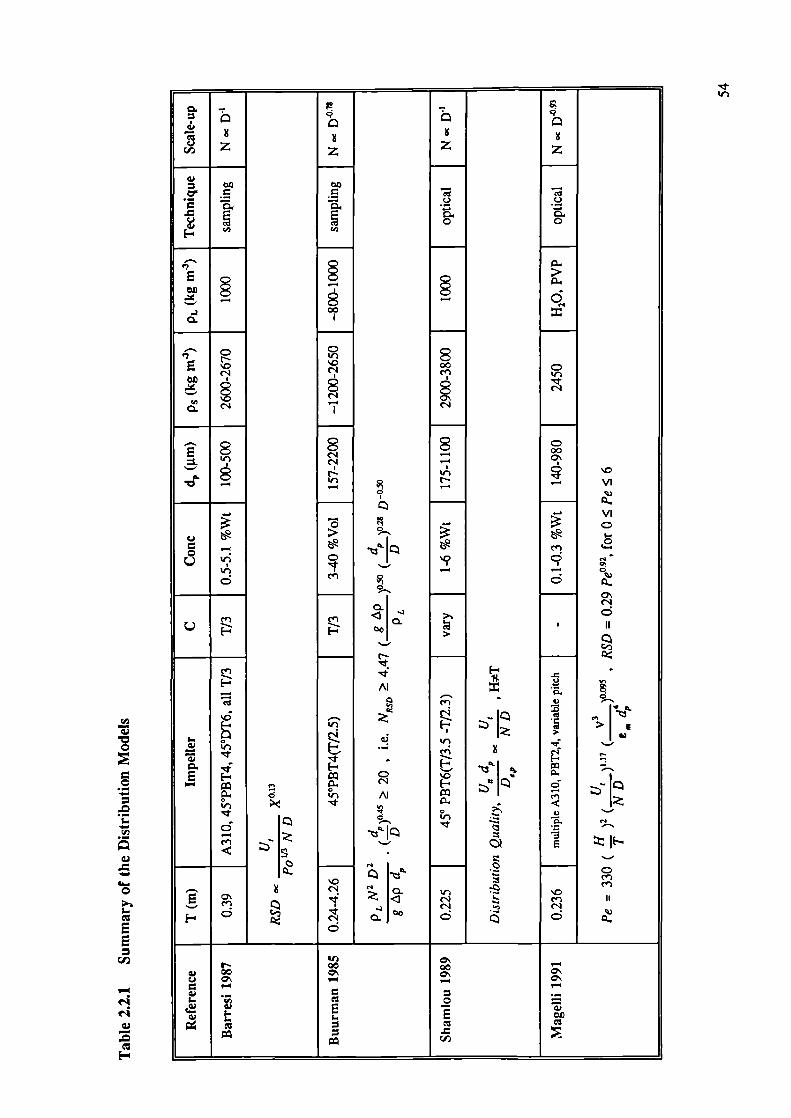
ltD

0

.0I-

0

I.

EE

'ID

.0

z

bo-

E0 0

- 000.

C 8E %O

'0 00

boen

c'1

-r

a c' — 0'._, -' I

r- '0

— v-- — — VI

0

- - -VICI-U

en

ç5 v-c C I q— —

d en- 9- - --

0. C

- -en -

- 9-'- I'

>IEIs- ?, -; 0

E E- C— E

d Al meI/)

C

p. N-

'I.-

— Iz -

'E

S.-,

-- I N - -CI . en

0\

. en 1< en

d o.j0° dC

In00 00 —

00 0' 0'

U C - 0'-

0 =0.)I._

I- -CO

(ID

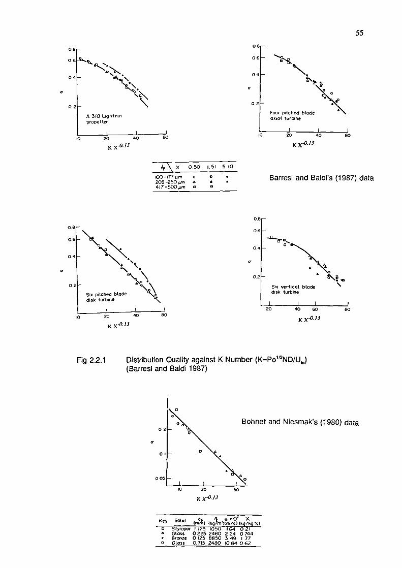
8080

55

08-

06-

04 -

02-

Four pitcIaxiaL turbine

0 20 40

K X'3

08

06

04

02

I4 310I terprope

0 20 40

K X0'3

Barresi and Baldi's (1987) data

)hnet and Niesmak's (1980) data

005

02

C.

ci

4\o.50 1.51 510

K0-l77m 0 C208-250gm a a4I7-500m C

0.61

0 .4 -'a

0

S0.2-

Six pitched bladedisk turbine

20 40 80

K X°'3

a0.4-

0•

0.2 -S

Six vertical bladedisk turbine

20 40 60 80

K X013

Fig 2.2.1 Distribution Quality against K Number (K=Po'ND/U10)(Barresi and Baldi 1987)

Xl 20 50

K X°13

Key Solid d5 I u,xIO' X(mm) (kg/m(m/s)(kg/kg%)

C Styropor 1125 1050 164 021A GLoss 0225 2480 2 24 0 744+ Bronze 0 125 8850 3 49 I 77o Gloss 0.715 2480 (084 062

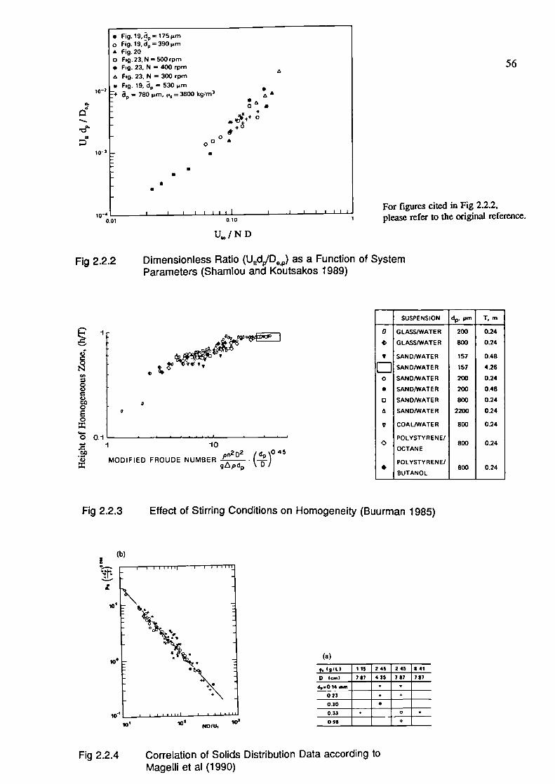
10•

10'

10'

(b)

I

10'

NOW,

• Fig.19,d0 = 175rno Fig.19.d390im£ fig.20o Fug.23.N=SOOrprn• Fig.23.N=400rpm

AA Fig. 23. N = 300 rpm* Fig. 19. = 530 m .

' = 780 &rn. ,=3800 kg/rn 3 A £

o &

• 0 a

- .

U

IU

I I I I I I I I I I IFor figures cited in Fig 2.2.2,

0.10 1 please refer to the original reference.

Uk /N D

Fig 2.2.2 Dimensionless Ratio (UdJD 0, ) as a Function of SystemParameters (Shamlou and Koutsakos 1989)

56

10-2

p.

iO-

iO- I0.01

100,

j

N4,U,

84)80 00

0

0

0011 10

pn2 02 fd\0454) MODIFIED FROUDE NUMBER

gEpdp

SUSPENSION d. pm T. m

o GLASS/WATER 200 0.24

• GLASS/WATER 800 0.24

V SAND/WATER 167 0.48

[] SAND/WATER 157 4.26

0 SAND/WATER 200 0.24

• SAND/WATER 200 0.48

Ci SAND/WATER 800 0.24

A SAND/WATER 2200 0.24

V COAL/WATER 800 0.24

POLYSTYRENE!O 800 0.24

OCTANE

POLYSTYR EN E/• 800 0.24

BUTANOL

Fig 2.2.3

Effect of Stirring Conditions on Homogeneity (Buurman 1985)

(a)

p. (giL) _!L !_!_ !!_ !___

D (em) 797 435 797 797

023 -

030 •

0.33 * 0

099 0

Fig 2.2.4 Correlation of Solids Distribution Data according toMagelli et al (1990)

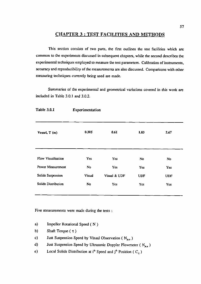
57

CHAPTER 3 : TEST FACILITIES AND METHODS

This section consists of two parts, the first outlines the test facilities which are

common to the experiments discussed in subsequent chapters, while the second describes the

experimental techniques employed to measure the test parameters. Calibration of instruments,

accuracy and reproducibility of the measurements are also discussed. Comparisons with other

measuring techniques currently being used are made.

Summaries of the experimental and geometrical variations covered in this work are

included in Table 3.0.1 and 3.0.2.

Table 3.0.1 Experimentation

Vessel, T (m)

0.305 0.61 1.83 2.67

Flow Visualisation Yes Yes No

No

Power Measurement

No Yes Yes

Yes

Solids Suspension Visual

Visual & UDF

UDF

UDF

Solids Distribution No

Yes

Yes

Yes

Five measurements were made during the tests

a) Impeller Rotational Speed (N)

b) Shaft Torque ( t)

c) Just Suspension Speed by Visual Observation ( N)d) Just Suspension Speed by Ultrasonic Doppler Flowmeter ( N)

e) Local Solids Distribution at th Speed and th Position (C)

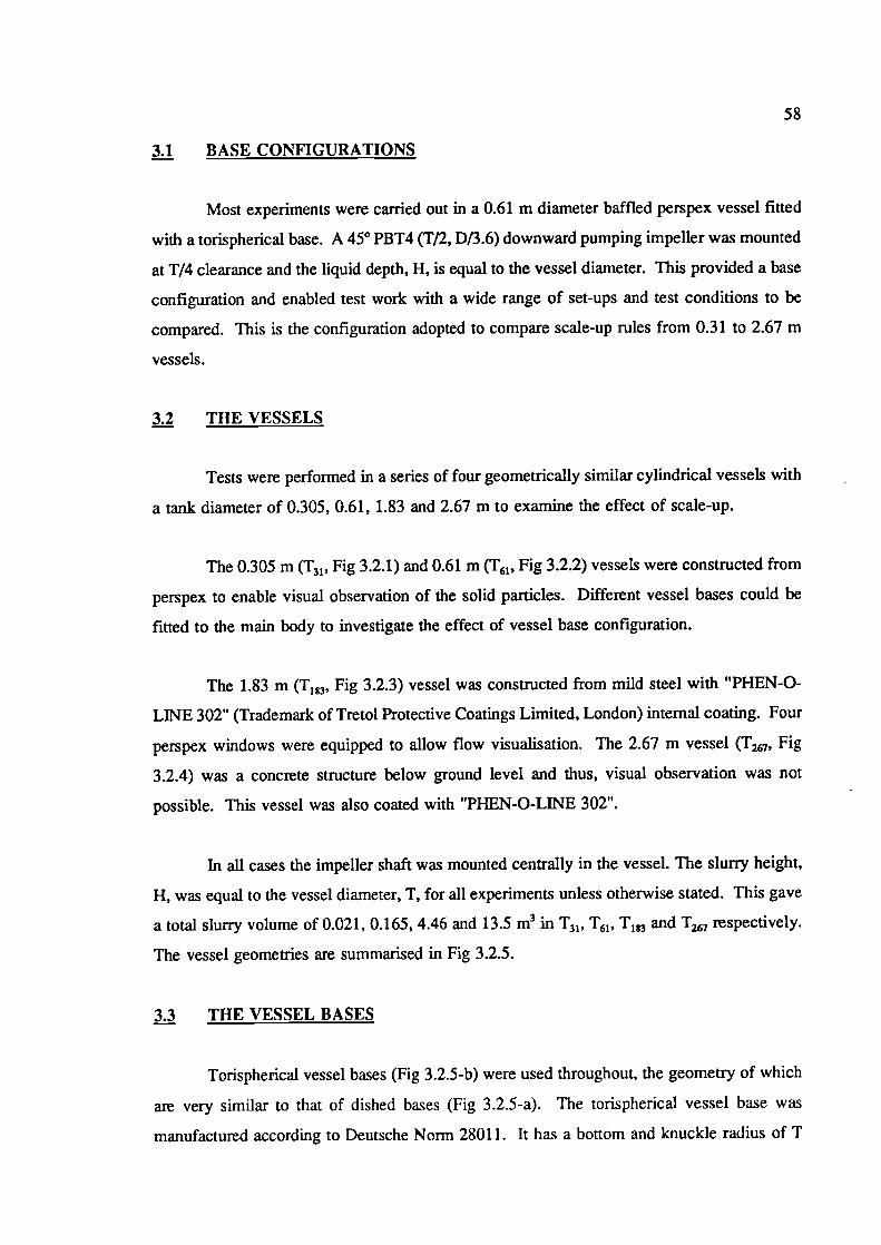
58

3.1 BASE CONFIGURATIONS

Most experiments were carried Out in a 0.61 m diameter baffled perspex vessel fitted

with a torispherical base. A 450 PBT4 (T/2, D13.6) downward pumping impeller was mounted

at T/4 clearance and the liquid depth, H, is equal to the vessel diameter. This provided a base

configuration and enabled test work with a wide range of set-ups and test conditions to be

compared. This is the configuration adopted to compare scale-up rules from 0.31 to 2.67 m

vessels.

3.2 THE VESSELS

Tests were performed in a series of four geometrically similar cylindrical vessels with

a tank diameter of 0.305, 0.61, 1.83 and 2.67 m to examine the effect of scale-up.

The 0.305 m (T31 , Fig 3.2.1) and 0.61 m (T61 , Fig 3.2.2) vessels were constructed from

perspex to enable visual observation of the solid particles. Different vessel bases could be

fitted to the main body to investigate the effect of vessel base configuration.

The 1.83 m (T1 g3, Fig 3.2.3) vessel was constructed from mild steel with 'PHEN-O-

LINE 302" (Trademark of Tretol Protective Coatings Limited, London) internal coating. Four

perspex windows were equipped to allow flow visualisation. The 2.67 m vessel (T, 7, Fig

3.2.4) was a concrete structure below ground level and thus, visual observation was not

possible. This vessel was also coated with "Pl-[EN-O-LINE 302".

In all cases the impeller shaft was mounted centrally in the vessel. The slurry height,

H, was equal to the vessel diameter, T, for all experiments unless otherwise stated. This gave

a total slurry volume of 0.021, 0.165, 4.46 and 13.5 m 3 in 'F31 , 1'61 , T183 and T 7 respectively.

The vessel geometries are summarised in Fig 3.2.5.

3.3 THE VESSEL BASES

Torispherical vessel bases (Fig 3.2.5-b) were used throughout, the geometry of which

are very similar to that of dished bases (Fig 3.2.5-a). The torispherical vessel base was

manufactured according to Deutsche Norm 28011. It has a bottom and knuckle radius of T

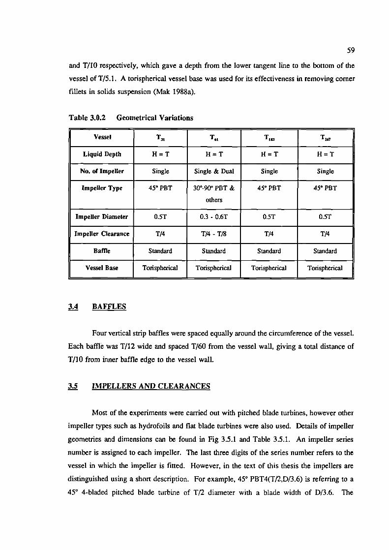
59

and T/l0 respectively, which gave a depth from the lower tangent line to the bottom of the

vessel of T15.1. A torispherical vessel base was used for its effectiveness in removing corner

fillets in solids suspension (Mak 1988a).

Tabie 3.0.2 GeometricaL Variations

Vessel T31 T1 T1 T

LiquidDepth H=T H=T H=T H=T

No. of Impeller Single Single & Dual Single Single

Impeller Type 45° PBT 3O09O0 PBT & 45° PBT 45° PBT

others

ImpeHer Diameter 0.51 0.3 - 0.6T 0.5T 0.5T

Impeller Clearance T/4 T/4 - T/8 T/4 T/4

Bame Standard Standard Standard Standard

Vessel Base Torispherical Torispherical Torispherical Torispherical

3.4 BAFFLES

Four vertical strip baffles were spaced equally around the circumference of the vessel.

Each baffle was T/12 wide and spaced T/60 from the vessel wall, giving a total distance of

T/l0 from inner baffle edge to the vessel wall.

3.5 IMPELLERS AND CLEARANCES

Most of the experiments were carried out with pitched blade turbines, however other

impeller types such as hydrofoils and flat blade turbines were also used. Details of impeller

geometries and dimensions can be found in Fig 3.5.1 and Table 3.5.1. An impeller series

number is assigned to each impeller. The last three digits of the series number refers to the

vessel in which the impeller is fitted. However, in the text of this thesis the impellers are

distinguished using a short description. For example, 45° PBT4(T/2,D/3.6) is referring to a

45° 4-bladed pitched blade turbine of T12 diameter with a blade width of D/3.6. The

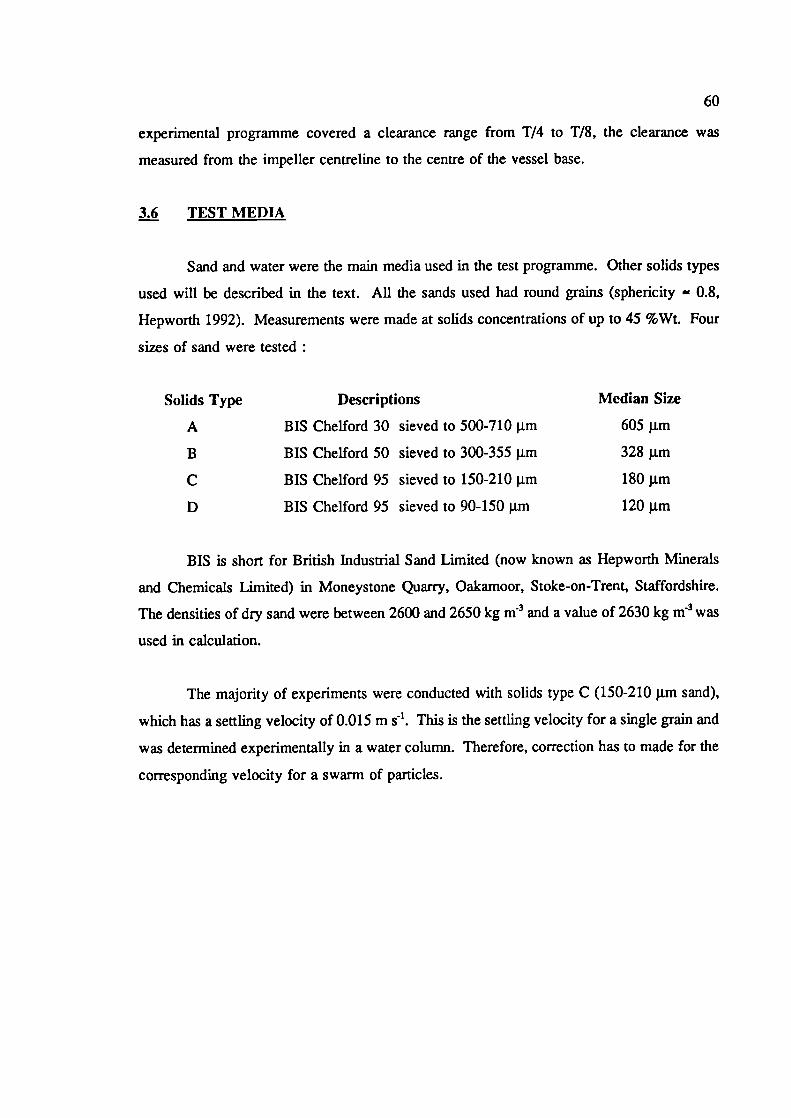
60

experimental programme covered a clearance range from T/4 to 1/8, the clearance was

measured from the impeller centreline to the centre of the vessel base.

TEST MEDIA

Sand and water were the main media used in the test programme. Other solids types

used will be described in the text. All the sands used had round grains (sphericity 0.8,

Hepworth 1992). Measurements were made at solids concentrations of up to 45 %Wt. Four

sizes of sand were tested

Solids Type

A

B

C

D

Descriptions

BIS Chelford 30 sieved to 500-710 p.m




Median Size

605 p.m

328 p.m

180 p.m

120 p.m

BIS is short for British Industrial Sand Limited (now known as Hepworth Minerals

and Chemicals Limited) in Moneystone Quarry, Oakamoor, Stoke-on-Trent, Staffordshire.

The densities of dry sand were between 2600 and 2650 kg m 3 and a value of 2630 kg n1 3 was

used in calculation.

The majority of experiments were conducted with solids type C (150-210 p.m sand),

which has a settling velocity of 0.015 m s ' . This is the settling velocity for a single grain and

was determined experimentally in a water column. Therefore, correction has to made for the

corresponding velocity for a swarm of particles.

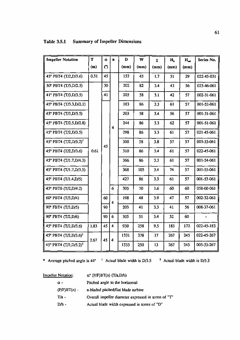
61

Table 3.5.1 Summary of Impeller Dimensions

Impeller Notation T a n D W x H1 H Series No.

(m) (°) (mm) (mm) (mm) (mm) (mm)

450 PBT4 (T/2,D/3.6) 0.31 45 153 43 1.7 31 29 022-45-031

30° PBT4 (T/3,D/2.5) 30 202 82 3.4 43 56 023-46-061

41° PBT4 (Tf3,D/3.5) 41 203 58 3.1 42 57 002-31-061

45° PBT4 (T/3.3,Df2.1) - 183 86 3.3 61 57 001-52-061

450 PBT4 (Tf3,D13.5) 203 58 3.4 56 57 001-31-061

45° PBT4 (Tf2.5,D/2.8) 244 86 3.3 62 57 001-51-061______________________ 4 _______ _______ _______ _______ _______ ___________45° PBT4 (Tj2,D/3.5) 298 86 3.3 61 57 021-45-061

45° PBT4 (Tf2,D/5.2)° 300 58 3.8 57 57 003-33-061_____________________ 45 ______ ______ ______ ______ _______ ___________450 PBT4 (T,2,D/3.6) 0.61 310 86 3.4 61 57 022-45-061

45° PBT4 (T/1.7,D/4.3) 366 86 3.3 61 57 001-54-061

450 PBT4 (T/1.7,D/3.5) 368 105 3.4 74 57 001-55-061

450 PBT4 (T/1.4,D/5) 427 86 3.3 61 57 001-53-061

450 PBT6 (T/2,D/4.2) 6 305 70 1.6 60 60 058-00-061

60° PBT4 (T/3,D/4) 60 198 48 3.9 47 57 002-32-061___________ —4 ___ ___ ___ ____ ____ ______90° FBT4 (T/3,D/5) 90 203 41 3.3 41 56 008-37-061

900 FBT4 (T12,D/6) 90 6 305 51 3.4 52 60 -

45° PBT4 (Tf2,D/3.6 1.83 45 4 930 258 9.5 183 172 022-45-183

450 PBT4 (T12,D/3.6)' - 1331 378 17 267 245 022-45-267___________________ 2.67 45 4 ______ ______ ______ ______ ______ __________450 PBT4 (T4t2,D/5.2)21333 250 13 267 245 003-33-267

* Average pitched angle is 440 1 Actual blade width is D/3.5 2 Actual blade width is D/5.3

Impeller Notation: a° (P/F)BT(n) (T/a,D/b)

a - Pitched angle to the horizontal

(P/F)BT(n) - n-bladed pitched/flat blade turbine

T/a - Overall impeller diameter expressed in terms of "T

D/b - Actual blade width expressed in terms of

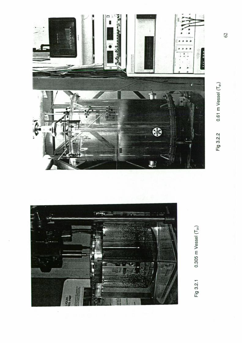
'--.4---

P7_v p• .

S

• S

- -

CD

I-

C)U)(I)a)>

E

0

I-

C)U)U)C)>

EIt)0(Y)

0

rcv)

C)U-

---- .---_//

,'I%I

- __i-

114! - ..-..-- ___

IL;cv)

C)IL

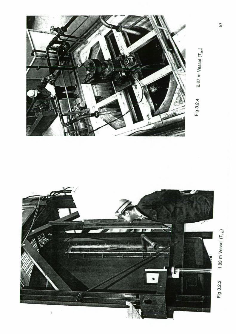
F-

a)(I,C')C)>

Ec)c

C,,

0)

U-

I

1

a)C')(I)C)

/

>

r

Er-.

cc?

c..J

C)0)

LJ

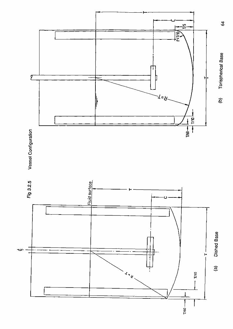
U,Co

CoC.)

a,

0U)

0I-

a,C/)Co

a,

Cl,

a

CT

C)

00a,U,Cl,a,>

a,'UIcs.J '-II

I I -

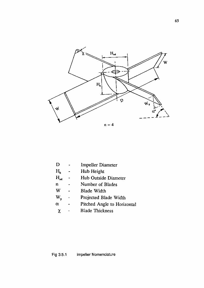
,1

w

65

n=4

D - Impeller Diameter

Hh - Hub HeightH - Hub Outside Diametern - Number of Blades

W - Blade Width

W - Projected Blade Widtha - Pitched Angle to Horizontal

x - Blade Thickness

Fig 3.5.1 Impeller Nomenclature

(Po) were calculated

P =2 ittN ...eqn(3.8.1)

PPo = _____

p N 3 D5...eqn(3.8.2)

66

IMPELLER ROTATIONAL SPEED

The impeller rotational speed was measured using an optical device in which a toothed

wheel is fixed to the shaft, interrupted by a light beam to generate on-off pulses from a

photocell operated the tachometer. The tachometer meter had a visual display and analogue

output to the computer for real time sampling. An accuracy of ± 0.5 rpm was obtained in the

visual display. The instruments are all made in-house. Regular calibration of the system was

carried out to ensure accuracy of shaft speed was maintained.

3 SHAFT TORQUE

3.8.1 General Outline

Torque was measured by strain gauges mounted on the shaft. The signal was

transmitted from the rotating shaft via a pre-amplifier and a low noise slip ring unit to the

major instrumentation chain (Fig 3.8.1). A full bridge of four gauges were cemented along

the principal axes of torsion. Effects of temperature change were compensated for in this

system.

From the torque data,, the power dissipated into the fluid (P) and the power number

Power number is a vital parameter to be measured in the test programme for two

reasons; it allows comparison of solid-liquid performance of various systems at the same

power input and also provides information on the likely forms of flow mechanism that are

present in the vessel.

3.8.2 Calibration and Accuracy

The system was calibrated by applying a series of known static torques to the shaft.

67

By correlating the applied torques to the change in output signal in the system, a linear

relationship was established from which a calibration factor was worked out to be used for

future analysis.

This direct measuring technique is one of the most accurate ways of ascertaining shaft

torque in agitated systems. Since the only check of accuracy available is the reproducibility

of test, the calibration is conducted on a very regular basis. Impellers with standard power

number (eg Rushton Turbine and Lightnin A310) were often used to re-confirxn the calibration

prior to the start of experimentation. The reproducibility is good. For example, some torque

measurements in T61 were conducted twice, with a two year interval between, during which

the shaft was completely re-strain-gauged and re-calibrated. The results were proved to be

highly repeatable. The accuracy of the torque data is estimated to be in the region of ± 2%.

39 MINIMUM SPEED FOR SOLIDS SUSPENSION

The minimum speed for solids suspension was measured by two methods, visual

observation and using an ultrasonic Doppler flowmeter (UDF). The visual technique is widely

adopted in solid-liquid mixing research to determine N. However, this technique is very

subjective and can only be applied when using a vessel with a transparent vessel base. The

ultrasonic device offers a convenient means of measuring N in large vessels or when visual

observations are not possible. The technique has been fully tested over a range of test

conditions during this research which will be discussed in more details in section 3.9.3.

Many other measuring techniques have been developed in recent years. Many

researchers have suggested that N can be extrapolated from the solids concentration profiles

(eg Koutsakos 1989). This technique must be interpreted with great care because some

impellers are better for off-bottom suspension than homogeneity and vice versa as has already

been proved in this research programme (Sec 4.3.2). Some (Bourne and Sharma 1974) deduce

N. from slurry samples removed just above the vessel base. This method has the potential

of being less dependent on human observation and judgement than the normal visual

technique, but there are severe experimental difficulties in withdrawing a representative

sample.

68

3.9.1 Visual Observation Method

This method of estimating N, visually through a perspex vessel base was first

described by Zwietering (1958). The criterion used in this work is the minimum speed at

which no solid particles remained stationary on the vessel base for more than one to two

seconds. This technique is simple, direct and rigorous but often restricted to research

environments.

A layer of solid particles rested on the vessel base at low impeller speeds. As the

speed was increased, solids were partly entrained by the liquid. At the point at which no solid

particles rested on the base for more than 1 to 2 seconds, observations were continued for a

period of one minute to confirm the judgement. If some particles re-deposited on the base

and remained stationary for more than 1 to 2 seconds during the observation, the impeller

speed was increased further until the underlying criterion was satisfied.

The N, measurement was repeated at least twice to ensure repeatability. The

reproducibility of results was generally very good, especially at low solids concentration. The

N, judgement became more difficult at high concentration (i.e.> 30% Wt). In general, the

visual results are repeatable to approximately ± 3 % on average, though occasionally only to

± in high solids concentrations.

3.9.2 Measurement of N 1 with an Ultrasonic Doppler Flowmeter

An ultrasonic device was adopted to monitor the bottom motion of the solids, so that

just suspension speed could be determined in metal bottomed vessels enabling scale-up

relationship to be established. Moreover, possible error due to subjectivity in measuring N,

visually can be greatly reduced. This section describes the underlying principle of this

technique and the experimental procedures developed.

(i) Principle

Buurman et al (1985) have described the use of an ultrasonic Doppler flowmeter

(UDF) for the measurement of just suspension speed. This instrument offers a convenient

means of measuring N, in large vessels or where visual observations are not possible. An

69

extensive evaluation has been carried out in Fluid Mixing Processes (FMP) of BHR Group

Ltd to determine the most suitable technique for scale-up investigations. The UDF technique

appeared to be the most convenient and reliable one. The benefits of this technique is that

the measurement is non-intrusive, independent of scale and unaffected by the material of the

vessel wall.

The UDF measures the Doppler frequency shift of an ultrasonic signal reflected from

discontinuities in flowing liquid. The discontinuities can be suspended solids (eg dust

particles), bubbles or interfaces caused by turbulent eddies in the flow. It is normally used

for measuring flow in pipes. The sensor is mounted on the outside of the pipe wall and an

ultrasonic beam, generated by electrical excitation of a ceramic piezo crystal, is transmitted

through the pipe into the fluid at an angle to the flow. Reflected signals are received by a

second piezo-electric crystal in the same sensor. The Doppler shift can be converted to a

velocity if the instrument is suitably calibrated.

The UDF can be used to measure the just suspension speed of solid particles if

mounted on the vessel base. Knowledge of the last suspended position is required to mount

the probe at the right position (eg centre bottom for torispherical vessel base with T/2

diameter impellers). This is normally determined from test results from 0.305 and 0.61 m

perspex vessels. Without this information, experiments have to be conducted with various

probe mounting locations to establish N. At low impeller speeds, the ultrasonic signal is

reflected from the static layer of solids on the vessel base and there is no response from the

meter. As the impeller speed is increased, solid particles are entrained by the fluid and

become fully mobile and there is a large increase in the indicated velocity. As the impeller

speed increases beyond N, the indicated velocity continues to increase, but at a slower rate

(Fig 3.9.1 & 3.9.2).

(ii) Experimental Methods

With all impellers tested to date, visual observation indicated that the position where

suspension finally occurs was directly beneath the impeller and this is where the UDF sensor

was mounted. However, for some D ^ T/3 impellers, it is possible to have the last suspension

position on the periphery of the vessel base. This is expected to be more likely to occur with

a flat vessel base.

70

Prior to the start of the experiment, exploratory tests were conducted to optimise the

incoming signals without picking up interference from the surroundings. This can easily be

done by adjusting the signal and noise levels in the meter. The average penetration depth or

focal point of the transmit and receive polar diagrams, known as the flow information

window, is 10-20 mm into the fluid when the particle concentration is less than approximately

10% Vol. With high particle concentration applications the signal penetration may only be

2-3 mm into the fluid. PVC shims were used to space the UDF sensor away from the base

of the vessel to ensure focus of the detection point right on the inner surface of the vessel

base.

The output from the meter is connected to a computer (Fig 3.8.1). A program was

written to allow a real time graphical display of the Doppler velocity. The Doppler velocity

was then sampled for a range of stirrer speeds. Tangents to the curve were drawn at the point

of maximum slope, and also the line of higher stirrer speed. N was the point at which the

two tangents crossed (Fig 3.9.1).

The repeatability of results is good (< ± in small scales), especially in large

vessels, and their transition points were very sharp. However, a less distinct transition was

found in T61 . This is probably because the sand beds are proportionally thinner in the small

vessel. A similar finding was also reported by Buurinan (1985).

3.9.3 Calibration of the UDF Technique

An extensive comparison was made between the two experimental techniques, using

the same configuration. This was done to gain confidence in the newly developed UDF

arrangement and to establish the relationship between the two data sets so that they could all

be used for future scale-up analysis. This included measurements from other researchers, with

tests on four impellers, three solids types and two vessel bases.

Comparisons of 38 independent sets of data was made. It was found that the

measurements made using the UDF technique followed the same trends as measurements of

N made visually. The dependence of N on d and X was nearly identical using the two

measuring techniques (Mak 1988a). It was discovered that the visual N results were

consistently slightly higher than the corresponding UDF values, with one or two exceptions

71

at high solids concentrations. The results are presented as piots of UDF N against visual N

in Fig 3.9.3.

The data can be conlated in the form of:

Visual N = k UDF Nfr ...eqn(3.9.1)

k was found to be equal to 1.07 with a standard deviation a 1 = 0.04, and 95 %

confidence limits of ± 0.01

ie k = 1.07 ± 0.01

It is sufficient to assume k=1 for design purposes. However, the constant k (= 1.07)

is to be retained in this work to correct the visual results for scale-up comparison. This

investigation has given enough confidence to apply the UDF technique to large vessels, from

which scale-up data is urgently needed.

3.10 LOCAL SOLIDS DISTRIBUTION

Good distribution of solid particles in a stirred vessel is very often required in solid-

liquid processing. For example, a uniform dispersion of solid particles throughout the mixing

vessel is necessary to ensure uniform exposure to the process conditions.

There are many different techniques adopted by researchers in the measurement of

local solids concentration. Visual observation was employed in the early days, tracer and

streak photography were used to complement the technique. This has provided a useful

understanding of the flow patterns produced by different types of impellers and configurations

but is limited to qualitative observations at low solids concentrations.

Predicting just suspension speed or solids homogeneity from the slurry interface in the

vessel could be misleading. A high liquid/solid-liquid interface does not necessarily guarantee

a good distribution within the bulk (Sec 4.3.4). Distinct differences in solids concentration

at different heights has been reported in literature (Einenkel 1977). In fact, experience within

BHR Group Ltd suggests that a hydrofoil impeller can produce a far better solids distribution

72

with a low level of slurry interface, compared to a T/2 diameter pitched blade turbine (Mak

1987).

Due to their non-intrusive nature and the capability of measuring solids concentration

in localised regions, optical methods are very popular and much useful work has been

produced (eg Magelli 1991, Shamlou 1989). However, this technique is usually limited to a

low solids concentration, depending on the transparency of the test media, and to small scale

vessels. Re-calibration is very often required for different test media.

Sample removal is another widely used technique (eg Barresi 1987). It is simple and

convenient and has much potential. For example, it is the only existing method by which

local particle size distribution can be determined. However, it is labour intensive and there

is still uncertainty over how well it can measure the true local concentration. Further research

on the understanding of isokinetic sampling is required.

The conductivity method does offer many advantages in measuring solids distribution.

The equipment is relatively cheap and easy to construct. It can measure a solids concentration

range from under 5 % up to 50 % by volume and can reliably detect a 1 % change in

concentration. Of course, like all the other techniques, the conductivity method has its

shortfalls; it is intrusive and therefore a certain degree of flow disturbance must be expected.

Any solids likely to cause a rapid change in base conductivity (conductivity of the fluid) are

undesirable. The conductivity technique is the one which has been adopted by this research

in measuring solids distribution.

3.10.1 The Solids Concentration Probe

The solids distribution results in this work were acquired by means of a solids

concentration probe. The probe was developed in Fluid Mixing Processes Group (FMP) in

conjunction with the Instrumentation Department in BHR Group Ltd, based on a design used

at the Warren Spring Laboratory. It consists of a "Y" shaped epoxy resin body and a stainless

steel tube handle (Fig 3.10.1). This is so designed to be robust yet causes a minimum of flow

disturbance. Two 10 x 10 mm platinum electrodes are mounted 10 mm apart, at both ends

of the epoxy body, to give a measuring volume of 1 cm 3 . The conductivity between the two

electrodes is measured and transmitted to a computer via a solids concentration meter (Fig

73

concentration meter (Fig 3.8.1). The local temperature is measured simultaneously by using

a platinum resistance thermometer, enabling correction for the effect of temperature upon

conductivity measurement.

This technique is based on the principle that the conductivity of a liquid will be

modified by the presence of foreign bodies. Thus, when solids particles pass between the two

electrodes of the probe, a change of conductivity will be registered, from which the local

concentration can be calculated, given that the relationship between change in conductivity and

volume fraction of solids is known.

2.10.2 Probe Calibration

The probe was calibrated in a 200 mm diameter liquid fluidised bed (Ruszkowski

1985, Fig 3.10.2). Round grained silica sand up to 55 % volume was used. The sand was

sieved to 500-700 jim and acid washed to remove impurities. The conductivity measured by

the probe, after correcting for temperature, was found to be inversely proportional to the

volume fraction of solids. There is some scatter in the results of these calibrations, due to the

difficulty of maintaining perfectly homogeneous and steady conditions in the fluidised bed.

A typical output is presented in Fig 3.10.3.

Further tests were conducted in a small stirred vessel in order to confirm the

calibration. The vessel had a diameter of 150 mm and 90-150 p.m round grained sands (Type

D) were used as the test solids. The solution was agitated intensely to maintain a

homogeneous distribution of solids in the vessel. The homogeneity of the distribution was

verified by making measurements at several points and heights in the vessel. The results of

this stirred vessel verification were limited to 10% solids concentration by volume, since at

higher concentration a homogenous solids distribution could not be maintained without

drawing air down into the suspension. A typical result for a stirred vessel calibration is shown

in Fig 3.10.5. There is much less scatter, and this is the case for all stirred vessel calibrations

carried out with a number of different solid types.

74

All the solids tested, with particle diameters ranging from 20 p.m up to 700 p.m, gave

the same relationship

ic = 'c- (1 - A C) ...eqn(3.10.1)

where iç and K(, are the corrected conductivity and the conductivity of water at

reference temperature respectively. The calibration constant, A, was 1.4 in all cases.

Machon et a! (1982) obtained the same functional relationship between conductivity

and solids concentration, working with a radically different probe geometry. Unfortunately,

the value of the calibration constant was not reported.

The measured conductivity, iç, and the reference conductivity, iç, were corrected for

variations in temperature with the following equation:

= iç ( ;, / K) ...eqn(3.l0.2)

3.10.3 Probe Location and Orientation

Most of the solids distribution measurements have been concentrated on a single radial

location, the probe being placed midway between two baffles and at T/6 clearance from vessel

wall. The radial solids concentration profiles with 30% Wt 150-210 p.m sand in T 183 were

also studied (Fig 3.10.4). The radial concentration profiles were flat, except when the probe

was at the clear liquid/solid-liquid interface (eg Fig 4.6.6). This normally happened when the

probe was mounted towards the top of the vessel, with the impeller running at relatively low

speed. The flatness of the radial profiles has already been reported by other authors (eg

Barresi 1987, Shamlou 1989) but their results were established from vessels of limited sizes

(T = 0.39 and 0.225 m). It is encouraging to have the results confirmed at a larger scale. The

use of one-dimensional steady state model by a number of researchers (eg Magelli 1990) is

justified. Thus, to focus on a single radial position (ie T/6 from the vessel wall ) for system

comparison is acceptable.

Prior to the start of experiments, tests were carried out to check the effect of probe

orientation, and the reproducibility of results. For tests with standard baffled vessels, the

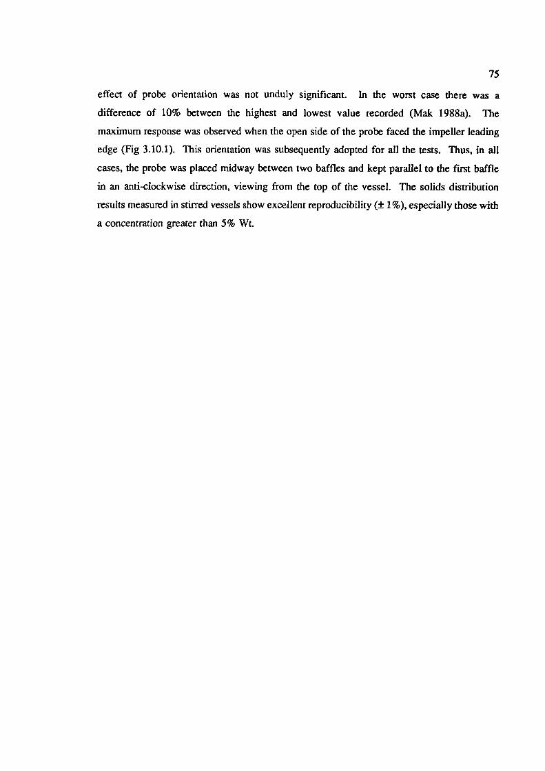
75

effect of probe orientation was not unduly significant. In the worst case there was a

difference of 10% between the highest and lowest value recorded (Mak 1988a). The

maximum response was observed when the open side of the probe faced the impeller leading

edge (Fig 3.10.1). This orientation was subsequently adopted for all the tests. Thus, in all

cases, the probe was placed midway between two baffles and kept parallel to the first baffle

in an anti-clockwise direction, viewing from the top of the vessel. The solids distribution

results measured in stirred vessels show excellent reproducibility (± 1%), especially those with

a concentration greater than 5% Wt.

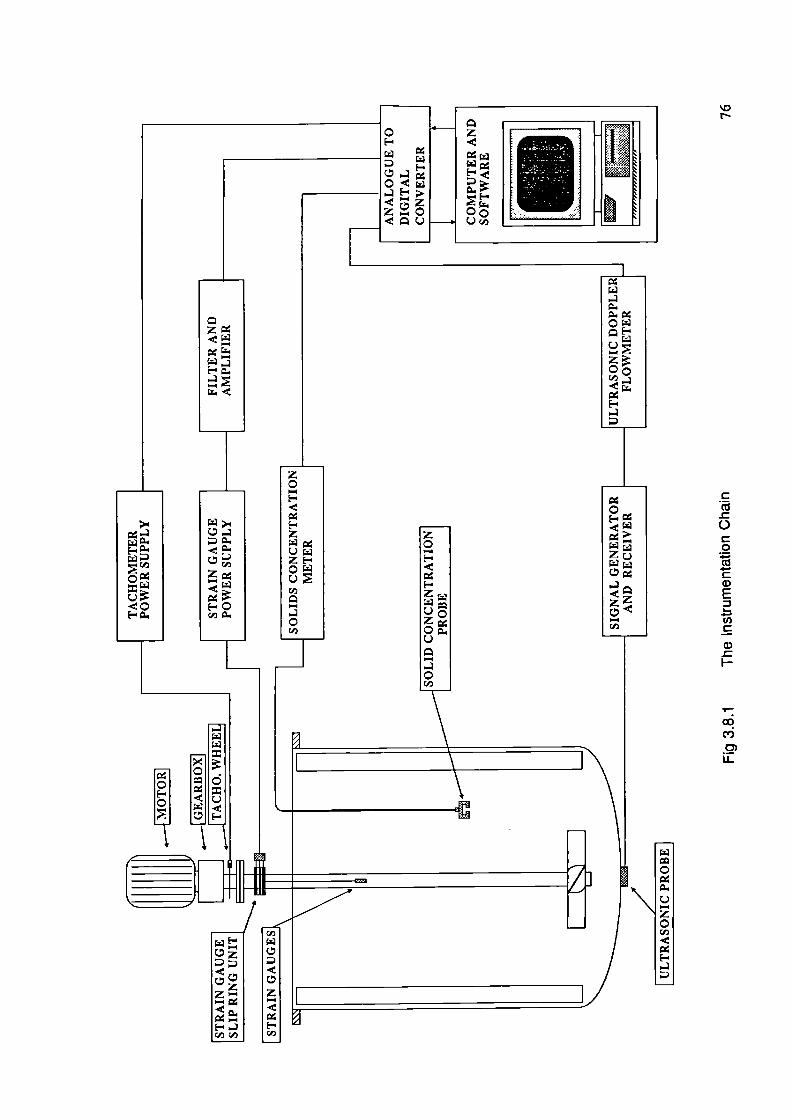
z

E-C

0

z

Cl)

CCl)

z0

c)0z

C.)

-4

CCl)

0

Zç)

-4Cl)

C-)C0

Ca)E

U)Ca,

I-

I Iz-I

C,,

N

0

Iiif-.i

z-0c)

z oc

0C

ccv,

C)LL

CC

C

<L)

>'

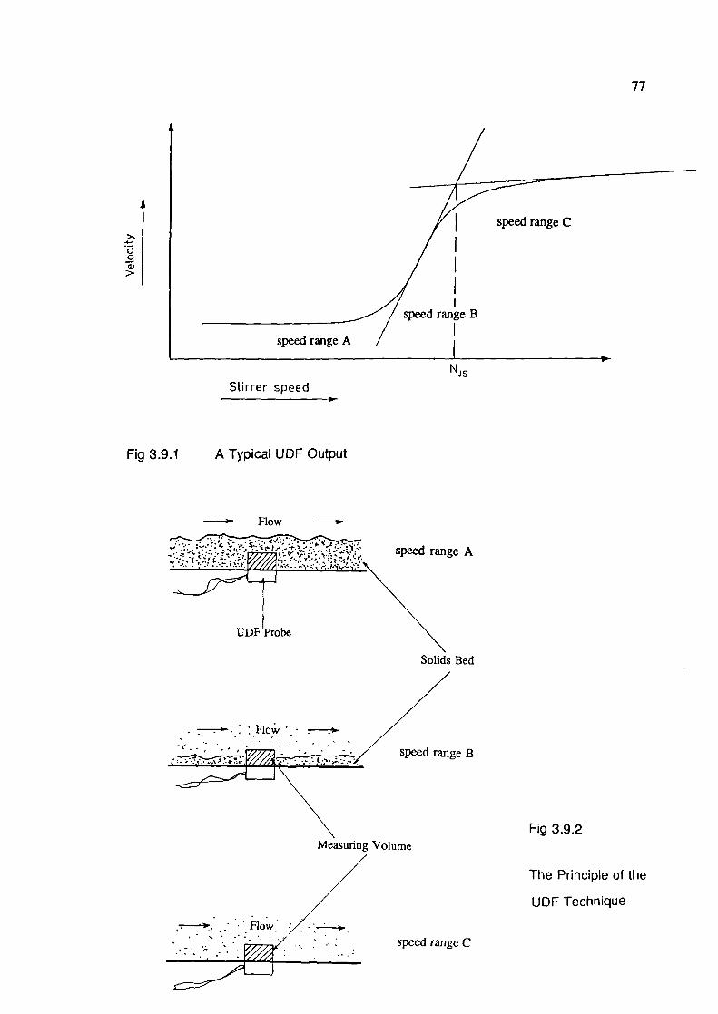
U0

>

A

Fig 3.9.2

ge B

The Principle of the

UDF Technique

77

speed range C

speed range B

I'1Js

Stirrer speed

Fig 3.9.1 A Typical UDF Output

Flow

. _1

_;.f3 :speed range A

UDF

Solids Bed

Measuring Volume

•..: io ___

Speed range C

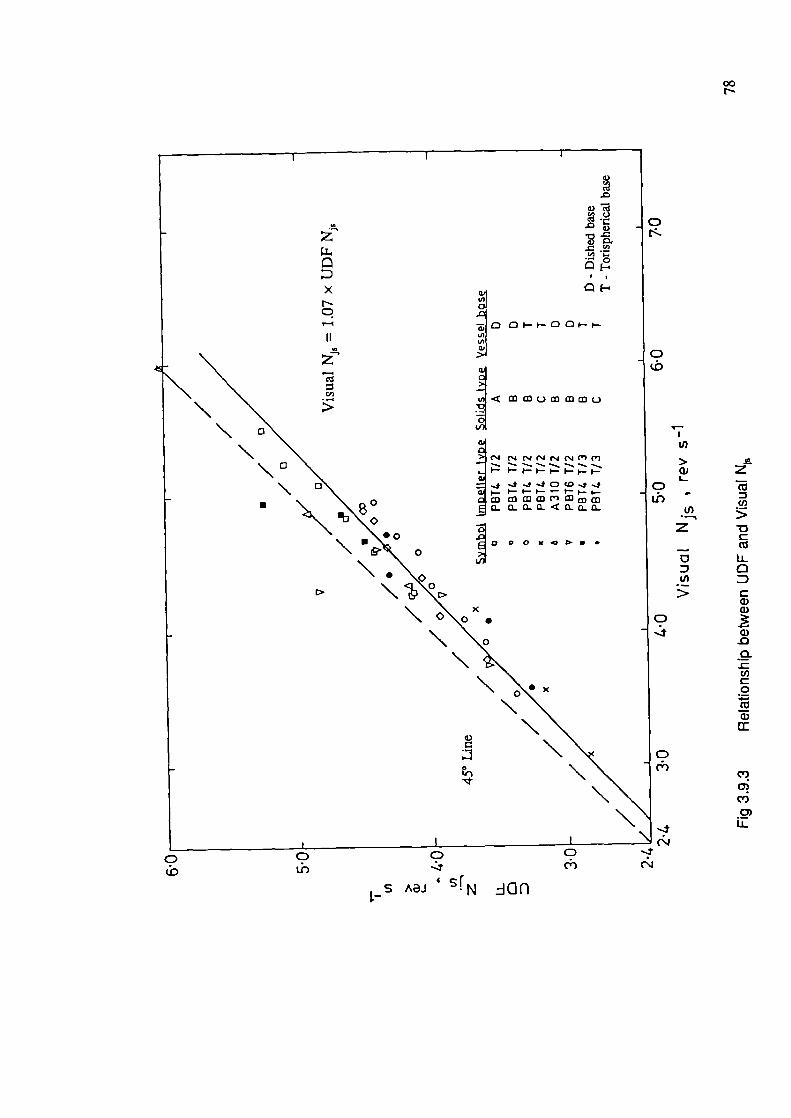
rU)

>a)L.

D

U)

z

U)

>

C)

zcr3U)

>

cr3

U-a

Ca)a)

a).D

0

U)C0

Cr3

a)a:

C)

C)

s AaJ SIN

1

C)(;)

zIOfl

C)0

'4(N

00

S

D

c

— F-

x

1- 01p

II U,,

UIa,'

m m i m m m i

N

N N N N N\ C -. - -. - -. -. -. -

._I •- I— - I— - p.— I-

0p.-. I— P— I— P

• \CO CO CO CO m CO

\ 't

' • 0 0 0 x . - •\ & o

0

\ Xo .

N

0

\

C)

0)

U-

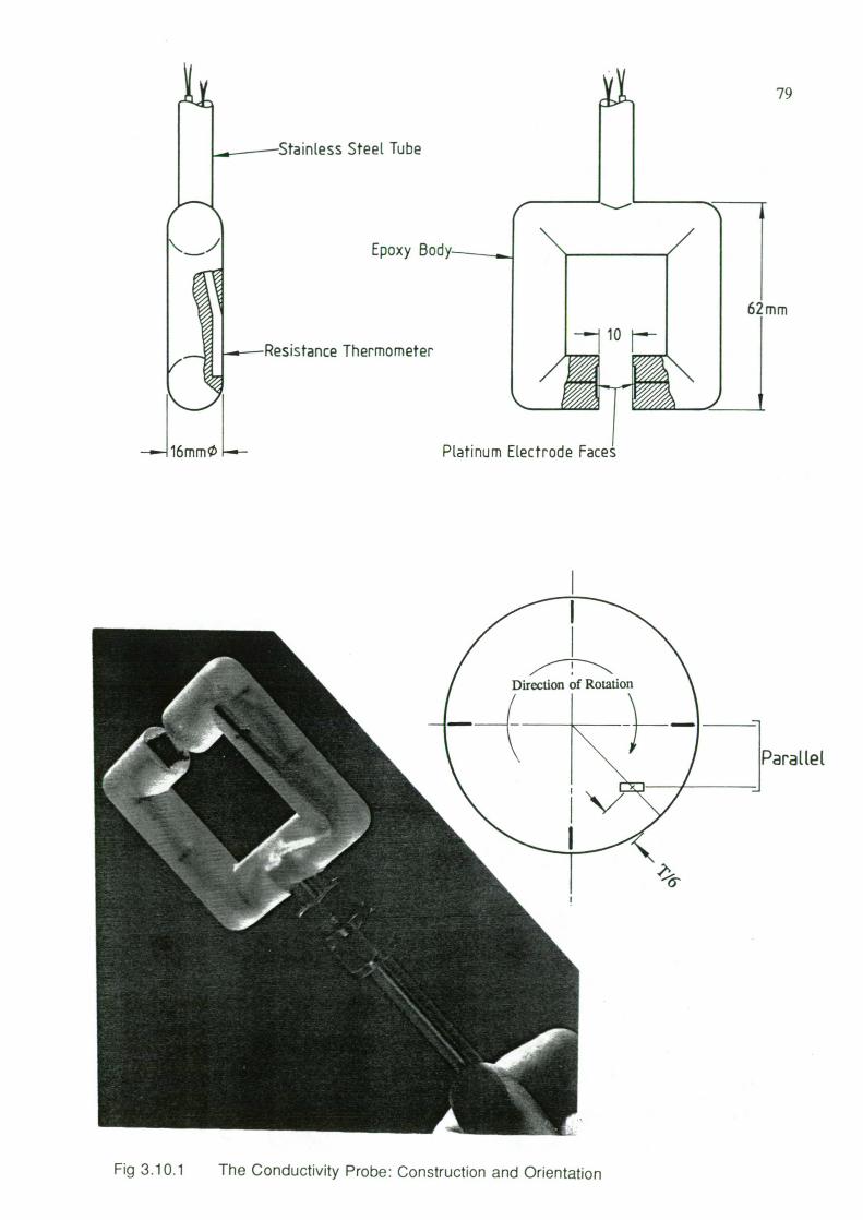
inless Steel Tube

Epoxy Bod

tance Thermometer

79

nm

Rotation

Fig 3.10.1

The Conductivity Probe: Construction and Orientation

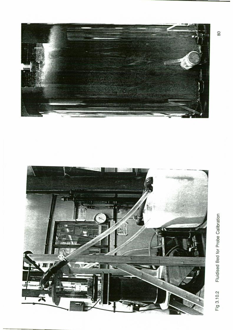
4L

0

cj0a)00

a-10

-aa)

-oa)C,)

D

U-

Q

C')

0)U-

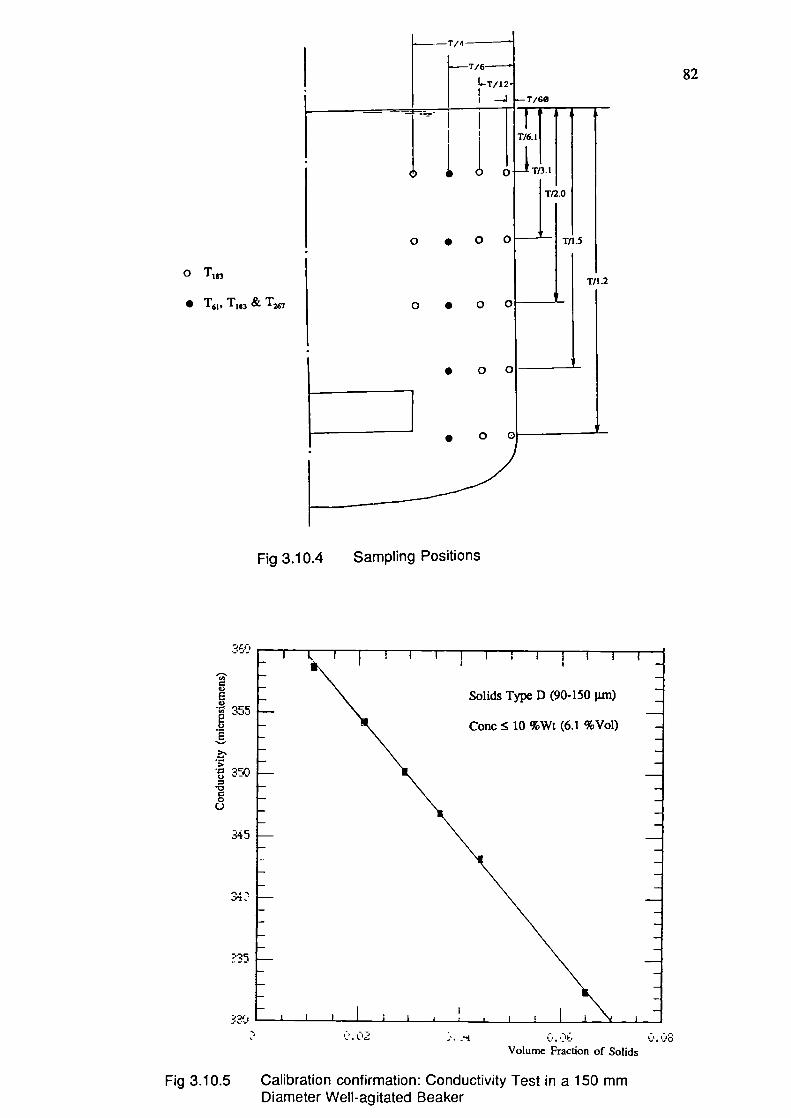
0

o T1

• T61 , T183 & T7 0

T/4

82LT/12

—.1 T/60

I I

1 1T/6.I

T/2.O

• 0 0 T115

T/t .2

• o c

• 0 0

• 0

Fig 3.10.4 Sampling Positions

E355

. 350•00U

345

E35

.c-N


Fig 3.10.5

Calibration confirmation: Conductivity Test in a 150 mmDiameter Well-agitated Beaker

83

CHAPTER 4: RESULTS AND DISCUSSION

4.1 PARTICLE FLOW PATTERN

Flow pattern depends critically upon the impeller and vessel configuration. It is

always useful to check the particles flow pattern in conjunction with any measurement in

order to reveal the mixing mechanisms and to facilitate interpretation of the results. Flow

visualisation of the experiments were made whenever possible during this study. Although

solid-liquid mixing flow patterns have been investigated by a number of researchers, their

results were confmed to limited geometries and little effort has been made to relate their

results to the observed flow pattern.

Most of the flow visualisation tests were made in the two transparent vessels (T31 and

T61). At high solids concentrations (eg> 15% vol), visualisations were inevitably confined

to flow patterns near the vessel wall and on the vessel base. For tests in which an

understanding of the internal flow loops were important, such as flow interactions in dual

impeller systems, black PVC cylinders (cylindrical in shape, diameter = 1.5 mm, length = 4.5

mm, SG = 1.31 and U, = 0.088 m s 1 ) were used as flow followers to trace circulation within

the vessel. Laser Doppler Anemometry measurements were also made available to facilitate

the interpretation of the results. However, it must be realised that the presence of solid

particles will have some modifying effect on the flow regime and the flow pattern at high

solids concentration is not going to match exactly as that of low solids concentration.

This section describes an overall view on solid-liquid mixing flow pattern and the

particles movements on the vessel base are generalised. The concepts and analogies

introduced in this section will be used in later stages to explain some more specific

investigations.

4.1.1 An Overall View

At low impeller speeds, the impeller pushes the solids sideways and digs a pit in the

solids bed. As the speed increases, the solids bed is partially fluidised and this produces three

distinct zones; a clear liquid layer at the top of the vessel, an unsuspended solids layer on the

base and a region of fluidised mixture in between (Fig 4.1.1). The relative proportion of the

84

three zones depends on how easily the particles are picked by the fluid and how efficient the

mixer is in producing bulk mixing. For example, impellers with a high pumping capacity tend

to generate good overall mixing and hence, a relatively small clear liquid layer. On the other

hand, mixing of heavy particles will result in a larger clear top region at the same power

input.

Referring to Fig 4.1.1. As the impeller speed continues to increase, the fluidised

region expands, while the amount of unsuspended solids decreases and eventually disappears

(Ni. attained). With a further increase in impeller speed, the clear liquid layer in the upper

region also gradually disappears and the solid-liquid mixture reaches the point of maximum

homogeneity before the solids redistribute themselves axially and radially. In the case of axial

redistribution, this is believed to be caused by the circulation pattern produced by the impeller,

which confmes the particles to certain trajectories (eg Fig 4.1.4). The strong centrifugal force

generated by the impeller at high speed tends to move the solid particles towards the

circumference and thus radial redistribution occurs.

Referring to the same figures, if a sampling point is established close to the liquid

surface (Position A) it will measure a gradual increase in solids concentration until the

contents reach maximum homogeneity. Conversely, if the sampling point is positioned near

the vessel base (Position C), it will experience a gradual decrease in solids concentration until

the contents reach maximum homogeneity. However, if the sampling point is positioned

midway in the vessel (Position B), it will first show a gradual increase in solids concentration

with speed until the fluidised bed expands to reach the conductivity probe whereupon it will

then measure a solids concentration greater than homogeneity. Subsequently, as the fluidised

region expands still further the concentration at position B will decrease until it attains the

value corresponding to the best homogeneity. A plot of relative solids concentration against

impeller speed for positions A, B and C is presented in Fig 4.1.2.

When N - N, three distinct flow regimes were seen visually through the vessel wall

(Fig 4.1.3). At the lower part of the vessel, the solids adjacent to the wall all move vertically

upward indicating that the fluid velocity was strong and the solid particles were following a

well defined trajectory. Eddies were found in a second region, immediately above the first.

Here, the solid particles were swirling in all directions and there were seen to be frequent

interactions between the particles within an eddy and its neighbourhood. Similar observations

85

were recorded by Hockey et al (1989) in their flow visualisation tests with Newtonian and

Non-Newtonian fluids in stirred vessels (Fig 4.1.4). In the upper part of the vessel, the third

region, there was a layer of clear liquid with very low solids concentration. This last

phenomenon was more distinct with the hydrofoils and T/3 diameter pitched bladed turbines

in which axial flow was dominated. The flow pattern directly beneath the impeller is rather

complex, being a function of impeller type, clearance, diameter and vessel geometry and this

will be discussed in more detail in the forthcoming sections.

4.1.2 Flow Pattern at Vessel Base

The flow pattern of particles on the vessel base was observed by means of a mirror

placed beneath it. It was found possible to interpret the results according to the impeller

discharge flow (Fig 4.1.6). Three types of flow were observed, swirl flow was found directly

underneath the impeller and was primarily responsible for the suspension of the central piles

of solids. Axial and radial flow were present outside the swirl flow region. The results are

summarised in Fig 4.1.5 and 4.1.7.

(i) Vortexing

This is normally found at the centre of the base, rotating slightly off-centre in the same

direction as the impellers (Fig 4.1.6 and 4.1.7). This is believed to be generated by the

trailing vortices at the impeller tip and driven by high speed jets to the vessel base (Tatterson

et al 1980, Fig 4.1.8). In certain impeller/clearance combinations, planetary motion is

observed (Fig 4.1.5-a). The suspension of the central pile of particles with a dished base

relies primarily on this vortexing effect.

(ii) Radial Flow

Radial flow is generated by the axial component of the impeller discharge. The flow

turns radially outwards towards the vessel wall as it impinges on the vessel base (Fig 4.1.5

& 4.1.8). Radial flow starts outside the vortexing region and extends as far as the

circumferential flow region of the base (Fig 4.1.7). This flow regime is very distinct with

strong axial flow impellers such as Lighmin A310 and 30° PBT4 (1/3).

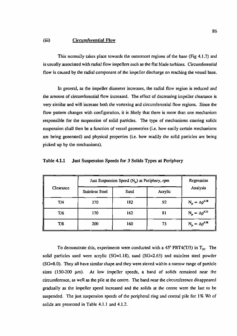
86

(iii) Circumferential Flow

This normally takes place towards the outermost regions of the base (Fig 4.1.7) and

is usually associated with radial flow impellers such as the flat blade turbines. Circumferential

flow is caused by the radial component of the impeller discharge on reaching the vessel base.

In general, as the impeller diameter increases, the radial flow region is reduced and

the amount of circumferential flow increased. The effect of decreasing impeller clearance is

very similar and will increase both the vortexing and circumferential flow regions. Since the

flow pattern changes with configuration, it is likely that there is more than one mechanism

responsible for the suspension of solid particles. The type of mechanisms causing solids

suspension shall then be a function of vessel geometries (i.e. how easily certain mechanisms

are being generated) and physical properties (i.e. how readily the solid particles are being

picked up by the mechanisms).

Table 4.1.1 Just Suspension Speeds for 3 Solids Types at Periphery

Just Suspension Speed (N) at Periphery. rpm Regression

Clearance AnalysisStainless Steel Sand Acrylic

T/4 170 182 92 N,

T/6 170 162 81 N, ec p0.21

178 200 160 73 oc

To demonstrate this, experiments were conducted with a 450 PBT4(T/3) in 'F3 ,. The

solid particles used were acrylic (SG=1.18), sand (SG=2.63) and stainless steel powder

(SG=8.0). They all have similar shape and they were sieved within a narrow range of particle

sizes (150-200 tm). At low impeller speeds, a band of solids remained near the

circumference, as well as the pile at the centre. The band near the circumference disappeared

gradually as the impeller speed increased and the solids at the centre were the last to be

suspended. The just suspension speeds of the peripheral ring and central pile for 1% Wt of

solids are presented in Table 4.1.1 and 4.1.2.

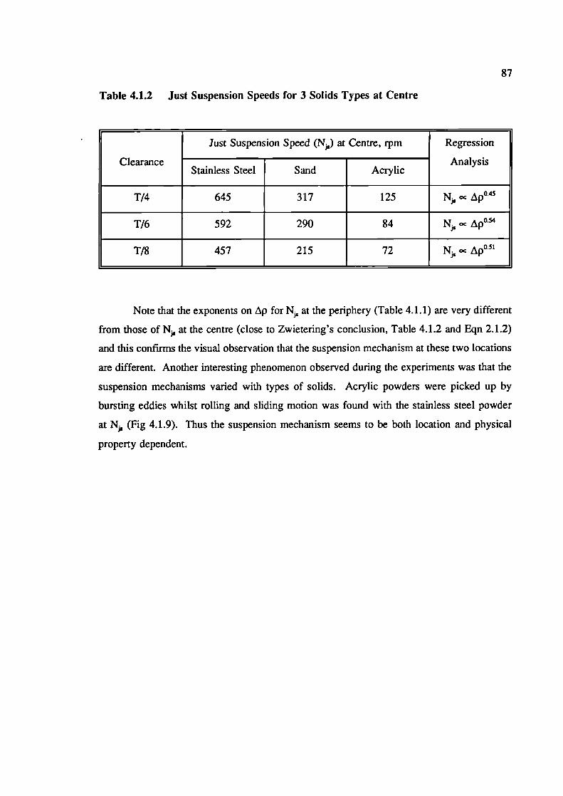
87

Table 4.1.2 Just Suspension Speeds for 3 Solids Types at Centre

Just Suspension Speed (Np) at Centre, rpm Regression

Clearance AnalysisStainless Steel Sand Acrylic

T/4 645 317 125 N oc

T/6 592 290 84 N,,

T/8 457 215 72 N

Note that the exponents on Ap for N at the periphery (Table 4.1.1) are very different

from those of N at the centre (close to Zwietering's conclusion, Table 4.1.2 and Eqn 2.1.2)

and this confirms the visual observation that the suspension mechanism at these two locations

are different. Another interesting phenomenon observed during the experiments was that the

suspension mechanisms varied with types of solids. Acrylic powders were picked up by

bursting eddies whilst rolling and sliding motion was found with the stainless steel powder

at N (Fig 4.1.9). Thus the suspension mechanism seems to be both location and physical

property dependent.

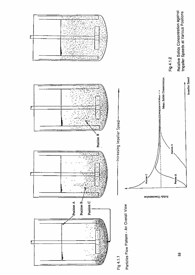
1:l; t

CflC/)CC• .2

. .2

0>C —0jO(/)

Cl) 0

o cCJ)U)

c'J.

.? -

-0)

a)U-

0

4)U

0C,,

4)

g:

u0I1.qu3u0O Sp!IOS

a)U

C-a)

a)cD.

cy%

(0C-Li

U

>

I-a)>0C

C1.ci)

cci

0IL

C/)ci)0I-cci

0000

0)U-

.

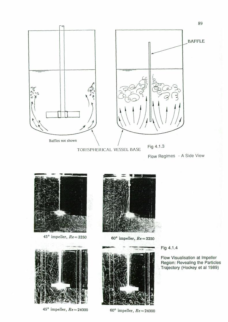
BAFFLE

? )

45° impeller, Re= 3250

I

.1

600 impeller, Re= 3250

- Fig 4.1.4

600 impeller, Reoz24000

Flow Visualisation at ImpellerRegion: Revealing the ParticlesTrajectory (Hockey et al 1989)

89

Baffles not shown/

TOIUSPI LERICAL VESSEL RASE Fig 4.1.3

Flow Regimes - A Side View

I45° impeller, Re=24000

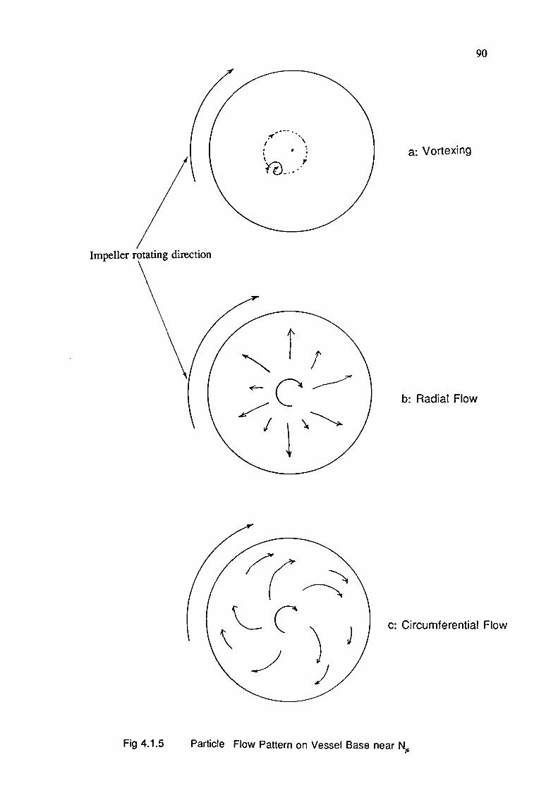
a: VorteXing

90

b: Radial Flow

C: Circumferential Flow

Impeller rotating direction

Fig 4.1.5 Particle Flow Pattern on Vessel Base near

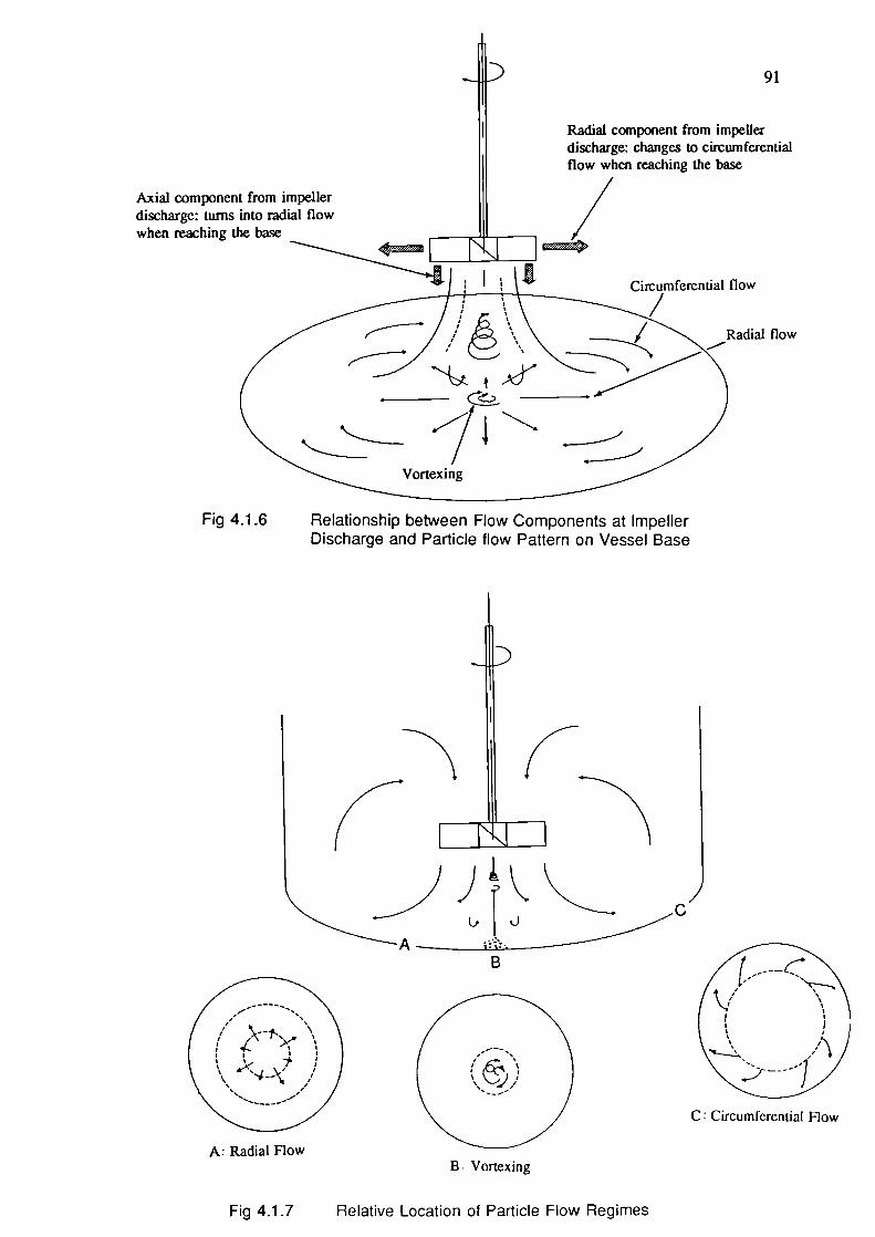
91

ipellerimferennal

flow

Eadia1 flow

Axial componendischarge: turnswhen reaching ti

B. Vortexing

A

I,(i ifl71\ 'I

----.,

A: Radial Flow

C: Circumferential Flow

Fig 4.1.6

Relationship between Flow Components at ImpellerDischarge and Particle flow Pattern on Vessel Base

Fig 4.1.7 Relative Location of Particle Flow Regimes

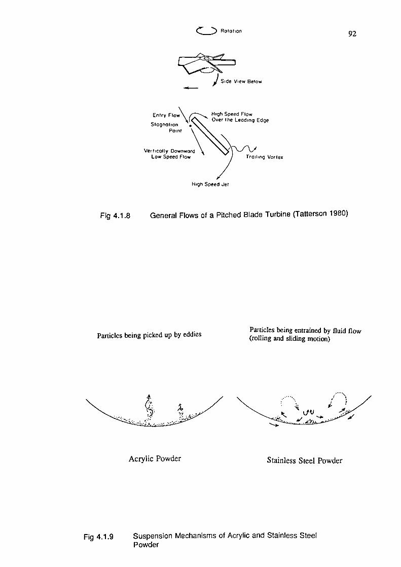
Rotation 92

) Side View Below

Entry FlOw'\(. High Speed FlowOver the Leading Edge

StagnationPoint

ing VortexVertically Downwar

Low Speed Flow

High Speed Jet

Fig 4.1.8

General Flows of a Pitched Blade Turbine (Tatterson 1980)

Particles being picked up by eddiesParticles being entrained by fluid flow(rolling and sliding motion)

Acrylic Powder

Stainless Steel Powder

Fig 4.1.9 Suspension Mechanisms of Acrylic and Stainless SteelPowder

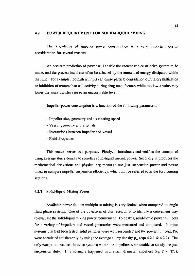
93

4.2 POWER REQUIREMENT FOR SOLID-LIQUID MIXING

The knowledge of impeller power consumption is a very important design

consideration for several reasons.

An accurate prediction of power will enable the correct choice of drive system to be

made, and the process itself can often be affected by the amount of energy dissipated within

the fluid. For example, too high an input can cause particle degradation during crystallization

or inhibition of mammalian cell activity during drug manufacture, while too low a value may

lower the mass transfer rate to an unacceptable level.

Impeller power consumption is a function of the following parameters:

- Impeller size, geometry and its rotating speed

- Vessel geometry and internals

- Interactions between impeller and vessel

- Fluid Properties

This section serves two purposes. Firstly, it introduces and verifies the concept of

using average slurry density to correlate solid-liquid mixing power. Secondly, it produces the

mathematical derivations and physical arguments to use just suspension power arid power

index to compare impeller suspension efficiency, which will be referred to in the forthcoming

sections.

4.2.1 Solid-liquid Mixing Power

Available power data on multiphase mixing is very limited when compared to single

fluid phase systems. One of the objectives of this research is to identify a convenient way

to evaluate the solid-liquid mixing power requirement. To do this, solid-liquid power numbers

for a variety of impellers and vessel geometries were measured and compared. In most

systems that had been tested, solid particles were well suspended and the power numbers, Po,

were correlated satisfactorily by using the average slurry density p 1 , (eqn 4.2.1 & 4.2.2). The

only exception occurred in those systems where the impellers were unable to satisfy the just

suspension duty. This normally happened with small diameter impellers (eg D < T/3),

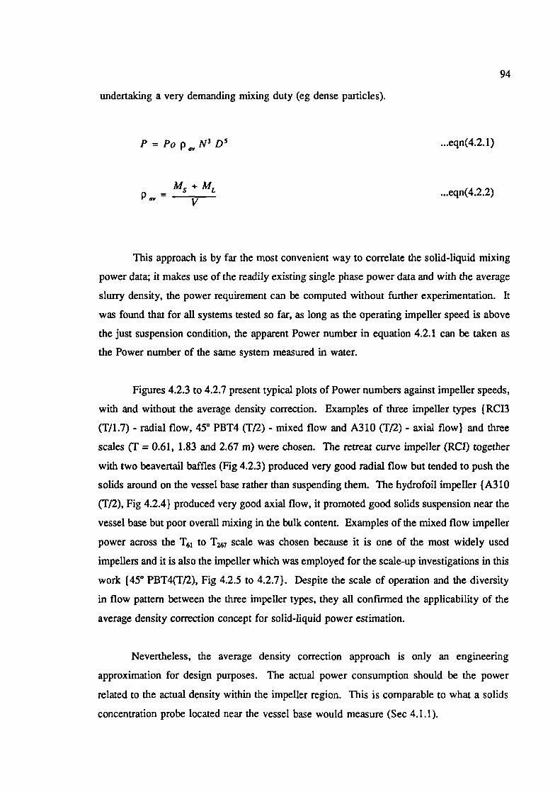
94

undertaking a very demanding mixing duty (eg dense particles).

P = Po p N 3 D5 ...eqn(4.2.1)

Pav M + ML ...eqn(4.2.2)

This approach is by far the most convenient way to correlate the solid-liquid mixing

power data; it makes use of the readily existing single phase power data and with the average

slurry density, the power requirement can be computed without further experimentation. It

was found that for all systems tested so far, as long as the operating impeller speed is above

the just suspension condition, the apparent Power number in equation 4.2.1 can be taken as

the Power number of the same system measured in water.

Figures 4.2.3 to 4.2.7 present typical plots of Power numbers against impeller speeds,

with and without the average density correction. Examples of three impeller types (RCI3

(T/1.7) - radial flow, 450 PBT4 (Ta) - mixed flow and A310 (Tf2) - axial flow) and three

scales (T = 0.61, 1.83 and 2.67 m) were chosen. The retreat curve impeller (RCI) together

with two beavertail baffles (Fig 4.2.3) produced very good radial flow but tended to push the

solids around on the vessel base rather than suspending them. The hydrofoil impeller (A310

(T/2), Fig 4.2.4) produced very good axial flow, it promoted good solids suspension near the

vessel base but poor overall mixing in the bulk content. Examples of the mixed flow impeller

power across the T61 to T 7 scale was chosen because it is one of the most widely used

impellers and it is also the impeller which was employed for the scale-up investigations in this

work (45° PBT4(T12), Fig 4.2.5 to 4.2.7). Despite the scale of operation and the diversity

in flow pattern between the three impeller types, they all confumed the applicability of the

average density correction concept for solid-liquid power estimation.

Nevertheless, the average density correction approach is only an engineering

approximation for design purposes. The actual power consumption should be the power

related to the actual density within the impeller region. This is comparable to what a solids

concentration probe located near the vessel base would measure (Sec 4.1.1).

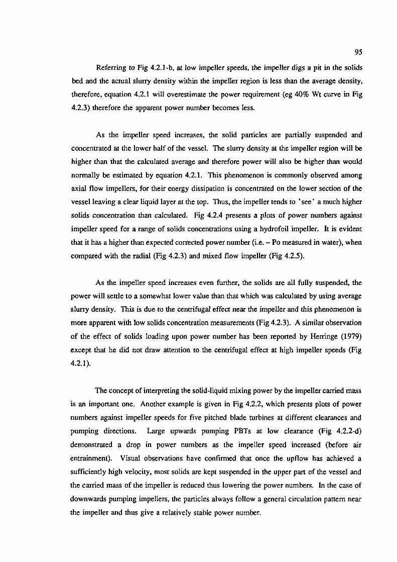
95

Referring to Fig 4.2.1-b, at low impeller speeds, the impeller digs a pit in the solids

bed and the actual slurry density within the impeller region is less than the average density,

therefore, equation 4.2.1 will overestimate the power requirement (eg 40% Wt curve in Fig

4.2.3) therefore the apparent power number becomes less.

As the impeller speed increases, the solid particles are partially suspended and

concentrated at the lower half of the vessel. The slurry density at the impeller region will be

higher than that the calculated average and therefore power will also be higher than would

normally be estimated by equation 4.2.1. This phenomenon is commonly observed among

axial flow impellers, for their energy dissipation is concentrated on the lower section of the

vessel leaving a clear liquid layer at the top. Thus, the impeller tends to 'see' a much higher

solids concentration than calculated. Fig 4.2.4 presents a plots of power numbers against

impeller speed for a range of solids concentrations using a hydrofoil impeller. It is evident

that it has a higher than expected corrected power number (i.e. - Po measured in water), when

compared with the radial (Fig 4.2.3) and mixed flow impeller (Fig 4.2.5).

As the impeller speed increases even further, the solids are all fully suspended, the

power will settle to a somewhat lower value than that which was calculated by using average

slurry density. This is due to the centrifugal effect near the impeller and this phenomenon is

more apparent with low solids concentration measurements (Fig 4.2.3). A similar observation

of the effect of solids loading upon power number has been reported by Herringe (1979)

except that he did not draw attention to the centrifugal effect at high impeller speeds (Fig

4.2.1).

The concept of interpreting the solid-liquid mixing power by the impeller carried mass

is an important one. Another example is given in Fig 4.2.2, which presents plots of power

numbers against impeller speeds for five pitched blade turbines at different clearances and

pumping directions. Large upwards pumping PBTs at low clearance (Fig 4.2.2-d)

demonstrated a drop in power numbers as the impeller speed increased (before air

entrainment). Visual observations have confirmed that once the upflow has achieved a

sufficiently high velocity, most solids are kept suspended in the upper part of the vessel and

the carried mass of the impeller is reduced thus lowering the power numbers. In the case of

downwards pumping impellers, the particles always follow a general circulation pattern near

the impeller and thus give a relatively stable power number.

96

The effect of particle size on power number is similar to that of solids concentration -

it increases the mixing duty. Fig 4.2.5-b and 4.2.8 present the corrected power number curves

for 45° PBT4 (Tf2,D/3.6) with 180 and 605 p.m sand respectively. Fig 4.2.5-b shows that

even with 40% wt of solids, the 180 p.m particles are well distributed. Since the actual solids

concentration carried by the impeller is somewhat less than the calculated average, the

corrected power number for higher concentrations are less than water for reasons explained

above. However, when a more demanding duty is imposed (i.e. bigger particles, Fig 4.2.8),

the solids are only partially fluidised (Fig 4.2.1-b). The impeller is handling a higher than

average concentration and this leads to higher corrected power numbers.

Additional experiments had been conducted to measured the local solids concentration

near the impeller region and use the local slurry density to correlate the power data. This

technique did not improve the correlation between data measured at different solids

concentrations, and has the added difficulty of requiring local solids concentration

measurements before power numbers can be calculated. The approach was eventually

abandoned due to the extra effort and complexity involved.

4.2.2 Just Suspension Power and Power Index

The concept of just suspension power (Pp) is introduced to compare the suspension

efficiency of an impeller. It is defined as the power delivered by an impeller into the vessel

at the just suspension speed.

P1, = Po N, D 5 ...eqn(4.2.3)

The just suspension power is a function of physical properties and geometrical

configurations. Therefore, comparison can be made only if the suspension experiments are

undertaken within the same test condition where the most efficient system will exhibit the

lowest just suspension power. However, it is not always possible to do so and a common

technique to compare impeller performance between different set-ups is to use the power

index (Harnby et al 1985). This is essentially correcting the physical properties effects by

substituting Zwietering's correlation into the Power number relationship:

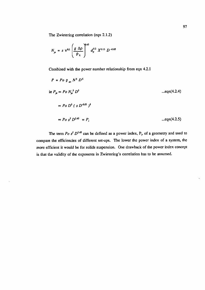
97

The Zwietering correlation (eqn 2.1.2)

/

N. = s v°' g I

d° 2 X°'3 D -0.85I, PLJ

Combined with the power number relationship from eqn 4.2.1

P = Po N 3 D5

ieP,,ocPoN3D5 ...eqn(4.2.4)

ocPoD5(sD°85/

ocPoD245 ...p ...eqn(4.2.5)

The term Po S' can be defmed as a power index, P 1, of a geometry and used to

compare the efficiencies of different set-ups. The lower the power index of a system, the

more efficient it would be for solids suspension. One drawback of the power index concept

is that the validity of the exponents in Zwietering's correlation has to be assumed.

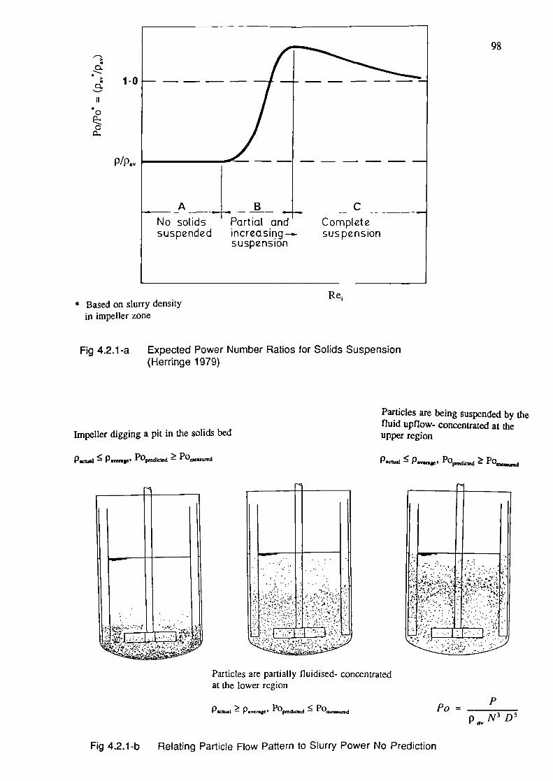
98>a

a.

a- 10

0

C0

p/ply

* Based on slurry density Re1

in impeller zone

Fig 4.2.1-a Expected Power Number Ratios for Solids Suspension(Herringe 1979)

Particles are being suspended by thefluid upflow- concentrated at the

Impeller digging a pit in the solids bed upper region

P.civai ^ P.venigc ' POpic1ed ^ Po p ^ p1 , Po. ^

Particles are partially fluidised- concentratedat the lower region

Plctu.I ^ P.,.ge ' Po ^P

Po=N3 D5

Fig 4.2.1-b Relating Particle Flow Pattern to Slurry Power No Prediction

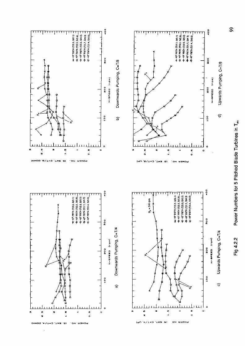
00N

0E C)0 C

. •a_

0 E00NW Q

UIa )w .0

C

0000

0o cot,)

0C)

I c.a E

U-000 (I)N bi -D

U)I Cz

00

0

2

00

• IlilIllIllIl 0

El N I) 1) 0

N 0

(NMOO £-.3 1M% ) ON bJM0d

00

00.i a)

I—ft0C)

- -, CaI

0 0..00N UI

UI .0a

z 0.

00

0

N I) Cl C - II 0

N 0

(fl G/i-. iM% ) ON W3MOd

0\

00

11111111111111111 II 11111111 I 0

N C N II C 0

N 0

(NMOO /i-D .LM% c) 0N MOd

00

00N

'7ISaI. 0)

C000NW E

UI

I U)z .0

CU

3-

00

C.)

0

N El N El -. Il 0

N .. 0

(fl fi3 .IM% ) ON I2M0

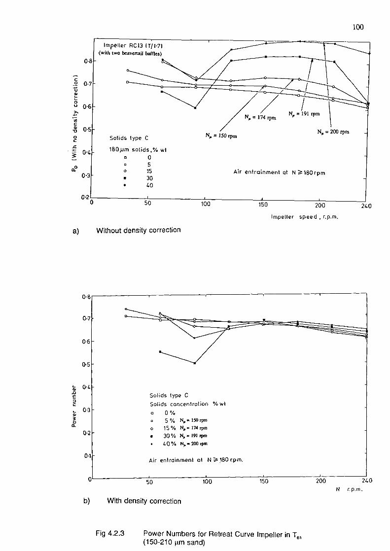
iou 150 200 240

Impeller speed r.p.m.

C

C.9 CUI-I-0(JO>'

C-D0C

0•U

0-1

0-

; 0..0EC'. o

0a-

0 lb

100

a) Without density correction

0-

0.

Solids type C

Solids concentration OJ WI

o 0%

o 5% N15Orpm

o 15% N114rpm

• 30% N 191 rpm

• 40% N.=2OOrpm

Air entrainment at N i8O rpm.

ar nr 21.0

Nr.p.m.

b) With density correction

Fig 4.2.3 Power Numbers for Retreat Curve Impeller in T61(150-210 .tm sand)

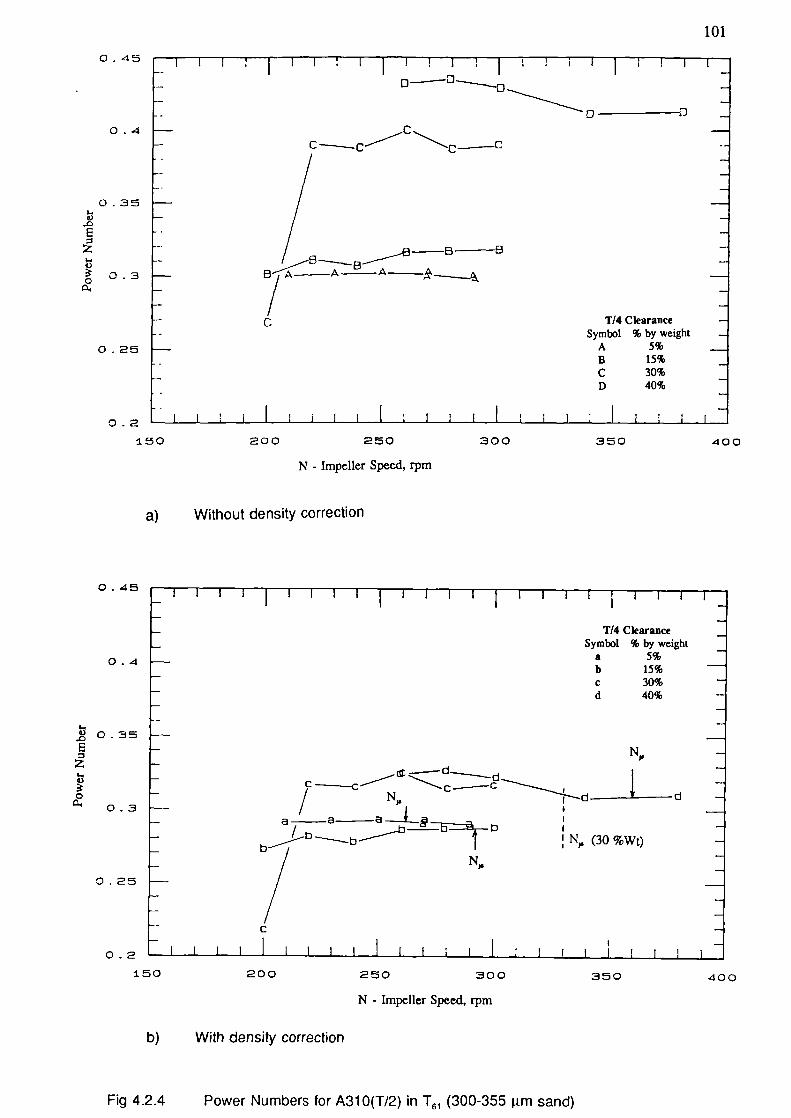
/ BB_°

C

T14 ClearanceSymbol % by weight

A 5%

B 15%

C 30%

D 40%

101

0.45

0.4

0 . 35I-V

8-.

I-

0.3

0 . 25

-i

I -- ri

0 -

C C_C

0.2

150 200 250 300 350 400

N - Impeller Speed, rpm


0.45

0.4

0.368

z

U

00.3

0 . 25

0.2

T14 ClearanceSymbol % by weight

a 5%b 15%c 30%d 40%

N

/

C C ___________d

____ ________________________________________

ba a ___

I(30%Wt)

b/

C

1 I t I

1.50 200 250 300 350 400



Fig 4.2.4 Power Numbers for A310(T/2) in T6, (300-355 m sand)

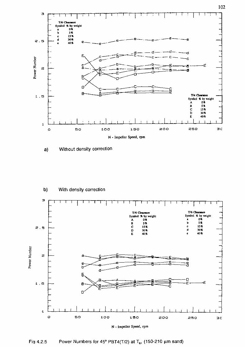
2.5

T/6 aeannoeSymbol % by weight

a 0%b 5%C 15%d 30%e 40%

T/4 Clearance

Symbol % by weightA 0%B 5%C 15%D 30%E 40%

1023

2.5

Z 2

I,

0

:t .5

I I I I IT IT16 Clearance

Symbol % by weighta 0%

d 30% e— —e-- —e- e 40% e - e -.

• _d— __d_-.----d--.__.-_.dE- \ - C---C---

\ .- d-

..-b----. —E

Dc

T14 Clearance -Symbol % by weight

A 0% -B 5% -C 15%D 30% -E 40% -

Ii ii

0 50 100 150 200 250 3C




3 i-

4).0

z

4)

0

:1. .5

I L__I I I I I I I I I I I I ] I I I I I I

0 50 100 150 200 250

3C


Fig 4.2.5 Power Numbers for 45° PBT4(T/2) at T6, (150-210 p.m sand)

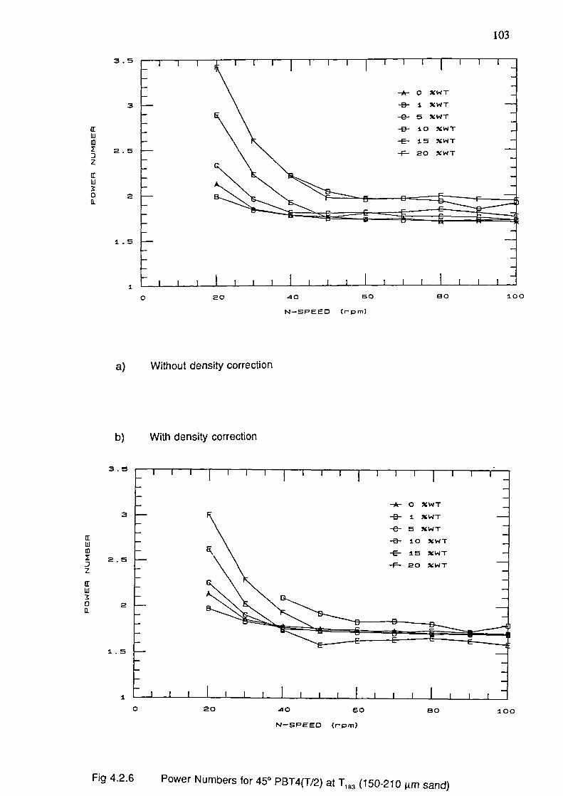
3.5

3

'IUi

2.5z

a:Ui

o 2a.

1.5

I0 20 .40 60 80 100

N-SPEED (rpm)

a:UI

2.5z

ifUI

2a-

3-*- 0 %WT

-B- I %WTS %WT10 WT

-E- 15 WT

-F- 20 %WT

103



3.5 r I

1.5

1L_

0 20 40 60 60 100

N-SPEED (rpm)

Fig 4.2.6 Power Numbers for 450 PBT4(T/2) at T 183 (150-210 tm sand)

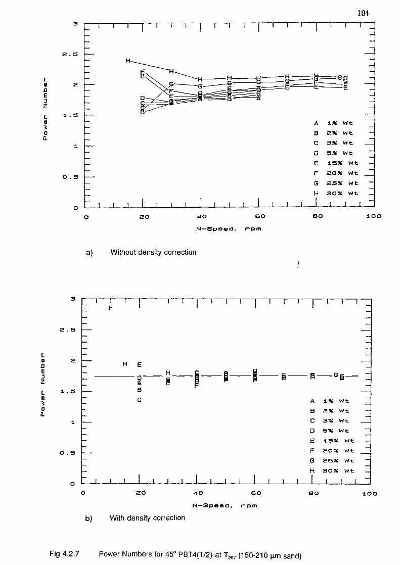
1043

2.5

I-2

E3zC.V0a-

I

0.5

80 1.000

0 20 40 60

N-Spee. rpm


1

3F

2.5

C-W 2

LiE3z

C_V0a.

I

0.5

0

U

G A 1% WtS 2% WtC 3% Wt0 5% WtE 15% Wt

F 20% Wt

G 25% Wt

H 30% Wt

i I i i i 1 i

0 20 40 60 80 100

14-Speed. rpm


Fig 4.2.7 Power Numbers for 45° PBT4(T/2) at T267 (150-210 p.m sand)

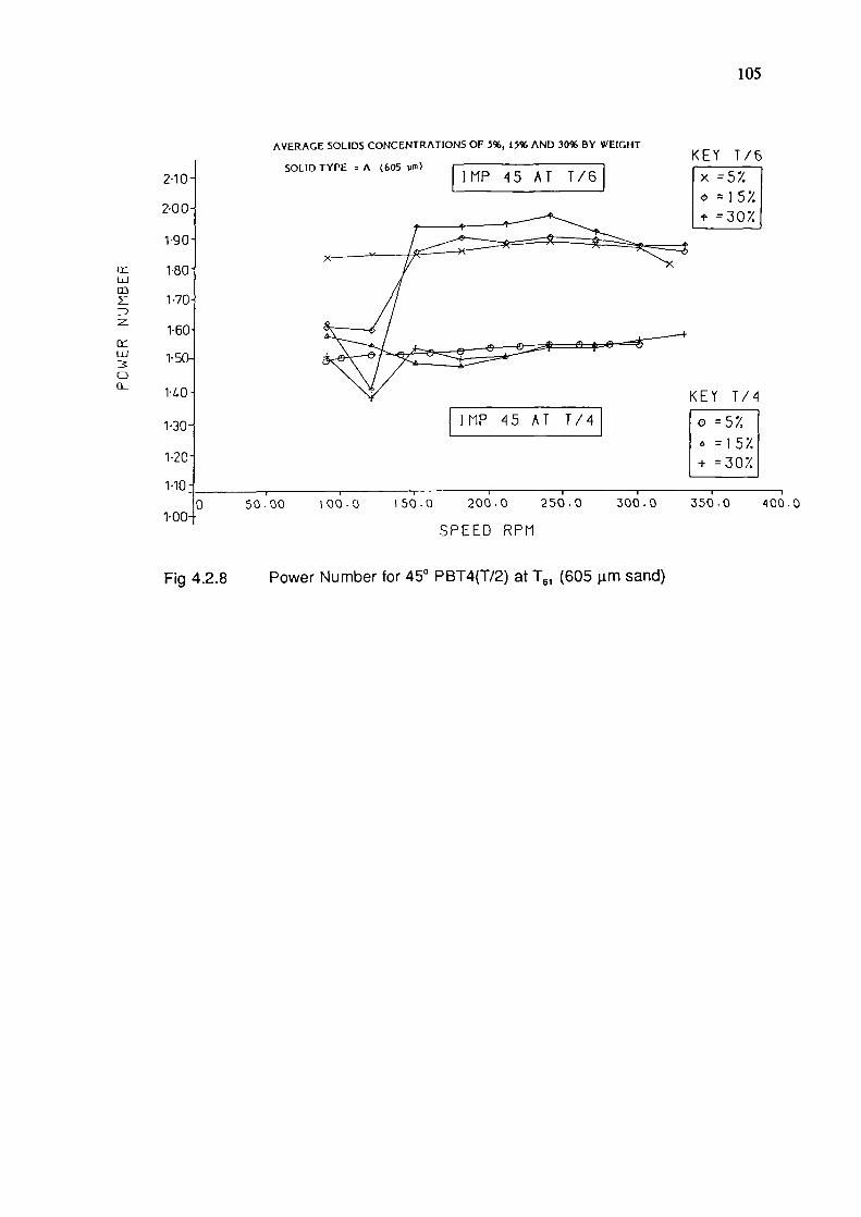
(IMP 45 AT

1 .10_ I

0 50.00 00.0 i50.0 200.0

250.0 300.01•00

SPEED RPM

105

210

200

190

180uJ

1 70

16

Ui 1 . 5C00

140

130

AVERAGE SOLIDS CONCENTRATIONS OF 5%, 15% AND 30% BY WEIGIIT

SOLID TYPE A (605 urn)rIMP 45 AT T/6J

KEY T/6

x =57.7'' =157.

=:30z

KEY T/4

O =57,

=157.+ =3o7.

350.0 400.0

Fig 4.2.8 Power Number for 450 PBT4(T/2) at T61 (605 jim sand)

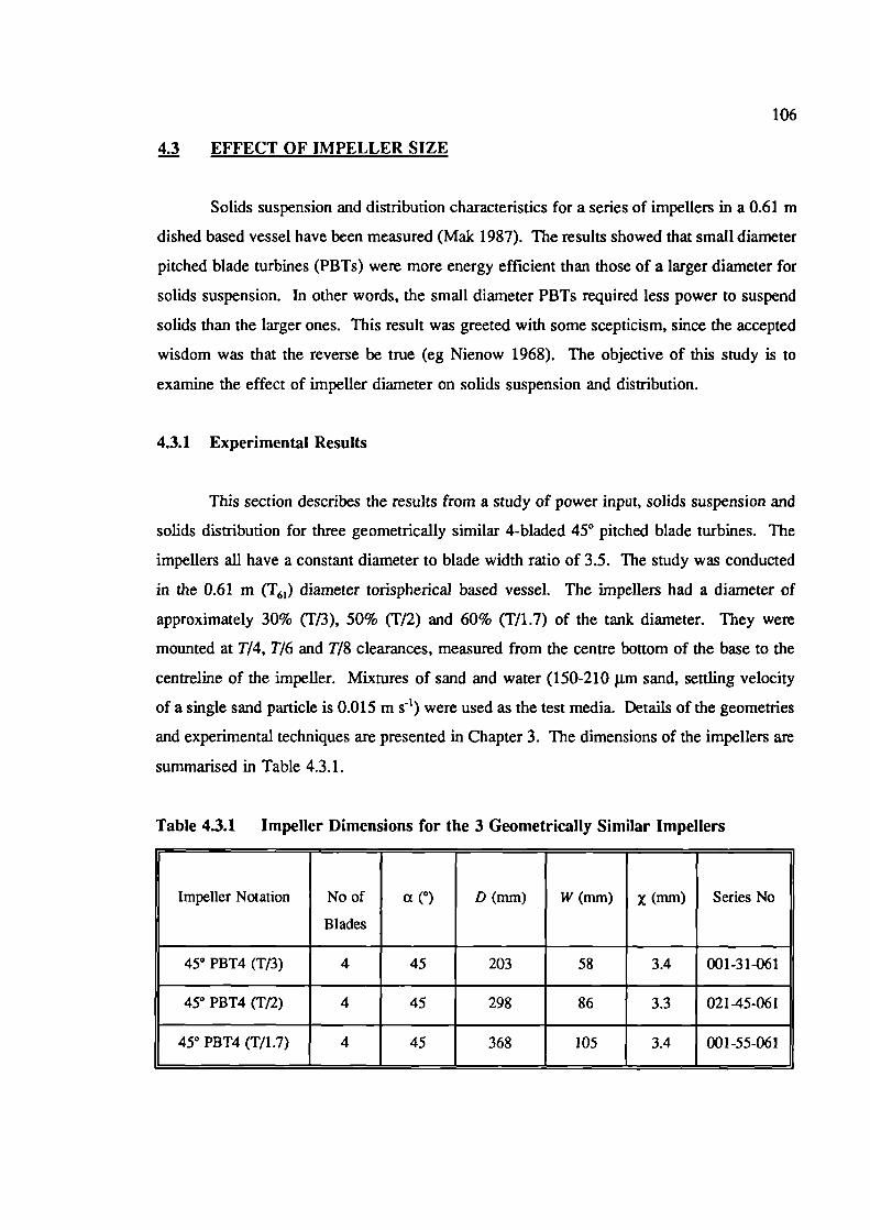
106

43 EFFECT OF IMPELLER SIZE

Solids suspension and distribution characteristics for a series of impellers in a 0.61 m

dished based vessel have been measured (Mak 1987). The results showed that small diameter

pitched blade turbines (PBTs) were more energy efficient than those of a larger diameter for

solids suspension. In other words, the small diameter PBTs required less power to suspend

solids than the larger ones. This result was greeted with some scepticism, since the accepted

wisdom was that the reverse be true (eg Nienow 1968). The objective of this study is to

examine the effect of impeller diameter on solids suspension and distribution.

4.3.1 Experimental Results

This section describes the results from a study of power input, solids suspension and

solids distribution for three geometrically similar 4-bladed 45° pitched blade turbines. The

impellers all have a constant diameter to blade width ratio of 3.5. The study was conducted

in the 0.61 m (T61 ) diameter torispherical based vessel. The impellers had a diameter of

approximately 30% (T13), 50% (T/2) and 60% (T/1.7) of the tank diameter. They were

mounted at T/4, T/6 and T/8 clearances, measured from the centre bottom of the base to the

centreline of the impeller. Mixtures of sand and water (150-210 p.m sand, settling velocity

of a single sand particle is 0.015 m s 1 ) were used as the test media. Details of the geometries

and experimental techniques are presented in Chapter 3. The dimensions of the impellers are

summarised in Table 4.3.1.

Table 4.3.1 Impeller Dimensions for the 3 Geometrically Similar Impellers

Impeller Notation No of a (0) D (mm) W (mm) x (mm) Series No

Blades

450 PBT4 (T/3) 4 45 203 58 3.4 001-31-061

450 PBT4 (T/2) 4 45 298 86 3.3 021-45-061

450 PBT4 (T/1.7) 4 45 368 105 3.4 001-55-061

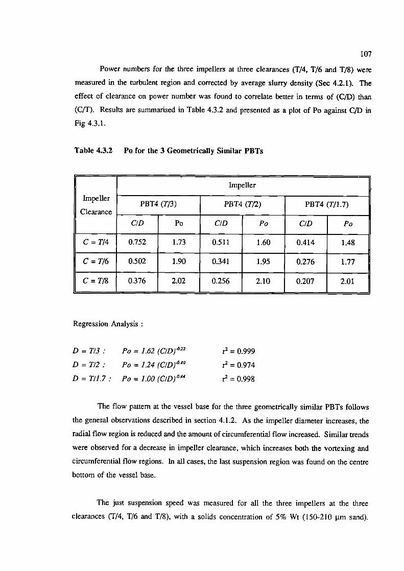
107

Power numbers for the three impellers at three clearances (1/4, T/6 and T/8) were

measured in the turbulent region and corrected by average slurry density (Sec 4.2.1). The

effect of clearance on power number was found to correlate better in terms of (CID) than

(CIF). Results are summarised in Table 4.3.2 and presented as a plot of Po against C/D in

Fig 4.3.1.

Table 4.3.2 Po for the 3 Geometrically Similar PBTs

Impeller

ImpellerPBT4 (T/3) PBT4 (T12) PBT4 (T/1.7)

Clearance___________ ___________ ___________ ___________ ___________ __________

CID Po CID Po CID Po

C = T/4 0.752 1.73 0.511 1.60 0.414 1.48

C = T/6 0.502 1.90 0.341 1.95 0.276 1.77

C = T/8 0.376 2.02 0.256 2.10 0.207 2.01

Regression Analysis:

D = T/3

Po = 1.62 (C/D)°22

r2=0.999

D = T/2. Po = 1.24 (C/Dy040

r2 = 0.974

D = T/1.7: Po 1.00 (C/D)°44

r2 = 0.998

The flow pattern at the vessel base for the three geometrically similar PBTs follows

the general observations described in section 4.1.2. As the impeller diameter increases, the

radial flow region is reduced and the amount of circumferential flow increased. Similar trends

were observed for a decrease in impeller clearance, which increases both the vortexing and

circumferential flow regions. In all cases, the last suspension region was found on the centre

bottom of the vessel base.

The just suspension speed was measured for all the three impellers at the three

clearances (T/4, 1/6 and 1/8), with a solids concentration of 5% Wt (150-2 10 m sand).

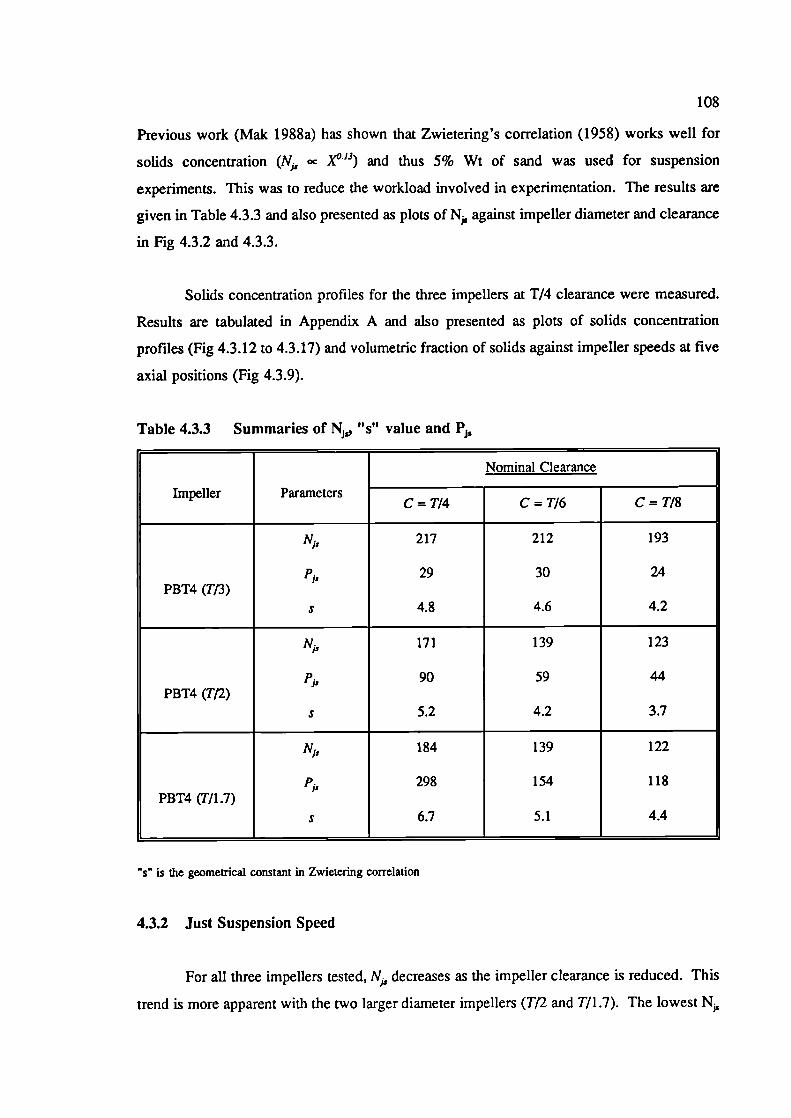
108

Previous work (Mak 1988a) has shown that Zwietering's correlation (1958) works well for

solids concentration (N1, oc X°'3) and thus 5% Wt of sand was used for suspension

experiments. This was to reduce the workload involved in experimentation. The results are

given in Table 4.3.3 and also presented as piots of N, against impeller diameter and clearance

in Fig 4.3.2 and 4.3.3.

Solids concentration profiles for the three impellers at T/4 clearance were measured.

Results are tabulated in Appendix A and also presented as plots of solids concentration

profiles (Fig 4.3.12 to 4.3.17) and volumetric fraction of solids against impeller speeds at five

axial positions (Fig 4.3.9).

Table 4.3.3 Summaries of Ni,, 's" value and P1.

Nominal Clearance

Impeller ParametersC=T/4 C=T/6 C=T/8

N1, 217 212 193

29 30 24PBT4 (T/3)

s 4.8 4.6 4.2

N1, 171 139 123

P1, 90 59 44PBT4 (Ta)

s 5.2 4.2 3.7

N1, 184 139 122

P 5298 154 118PBT4 (T/l.7)

s 6.7 5.1 4.4

"s" is the geometrical constant in Zwietering correlation

4.3.2 Just Suspension Speed

For all three impellers tested, N1, decreases as the impeller clearance is reduced. This

trend is more apparent with the two larger diameter impellers (T and T/1.7). The lowest N,,

109

was given by the Tf2 and T/1.7 impellers positioned at T/8 clearance (Fig 4.3.3). However,

comparing the just suspension speed alone does not necessarily give the correct indication of

the most efficient configuration. This is because even though the large diameter impeller has

a relatively low N, its power input at N (i.e. P) could be higher than that of a smaller

diameter impeller at N, (eqn 3.8.2, P1, oc Po N3 J)5)•

Based on Zwietering's correlation for solids suspension, the geometrical constants "s"

for various configurations were calculated. They are tabulated in Table 4.3.3.

Zwietering's Correlation

- (gipN — s V01

L

d°2 X°'3 D -0.85 ...eqn(4.3.1)

The "s" value is a constant introduced in order to account for the geometrical effects.

It is a function of impeller type, clearance and impeller diameter to tank diameter ratio. It can

be used as a indicator to detect any change in flow pattern.

Zwietering (1958) suggested:

s oc (T/D) with t3 = 0.82 for a propeller ...eqn(4.3.2)

By plotting the "s" value against (TID), Zwietering found that the propellers exhibited

a minimum at DIT = 0.45. He observed that for a D <0.45T propeller, the solid particles

moved radially outward along the bottom and the last piles of particles occurred at the

periphery. However, when D> 0.45T the solids moved inward and centrally up into the

propeller. This agrees well with our observed change in flow pattern from radial to

circumferential flow as the impeller diameter is increased (Sec 4.1.2). A plot of "s" values

against (TID) for various TIC is presented in Fig 4.3.4, with the position of Zwietering's

minimum at D=O.45T marked.

In this thesis, the effect of impeller diameter on was studied. The results were

firstly analysed by keeping the clearance constant. For the nine configurations tested, the

110

influence of impeller diameter on N, is as follows:

T/4 Clearance N, oc D°32

r2 = 0.62

T/6 Clearance N D°76

r2 = 0.88

T/8 Clearance N1, oc D°82

r2 = 0.89

The above relationships give an indication of the trends. The few data (only three

points for each clearance) give a poor fit as shown by the low regression coefficient. The

results suggest that the effect of impeller diameter on N1, is not a simple power law

relationship. Further attempts were made to correlate data by including the effects of impeller

clearance (C/D and CIF). No quantitative conclusion could be drawn based on statistical

analysis as there were insufficient data points.

Impeller diameter has a greater effect on N1, at low clearance (i.e. C=T/8, N oc

than at high clearance (i.e. C=T/4, N1, oc D°32). Rao (1988) suggested that this is because

solids suspension is due to fluid flow and turbulence and the turbulence intensity decays along

the length of the flow path. With an increase in the impeller diameter, less decay in the

turbulence will occur because of a reduction in path length. Moreover, the liquid velocity also

increases with an increase in the impeller diameter. The overall effect of increased liquid

velocity and reduced decay in turbulence makes the dependence on the impeller diameter very

strong. Furthermore, the power per unit volume below the impeller increases more rapidly

with increasing impeller diameter at low clearances than at high clearances. This is because

the actual volume underneath the impeller becomes smaller at low clearances.

It has been pointed Out earlier that there is a change of flow pattern, from radially

outwards to circumferential flow as the impeller diameter is increased. This change of flow

pattern is reflected by the minima in Figure 4.3.4, where geometrical constants are plotted

against (T/D). Similarly, a plot of N against impeller diameter for the three clearances shows

that in all cases the just suspension speed decreases when the impeller diameter increases from

T/3 to T/2, while a further increase in impeller diameter leads to either constant or slight

increase in N (Fig 4.3.2). Regression analysis of the T/3 and T/2 diameter results for all

three clearances suggests Nfr oc D'°2 with r2 equal to 0.88.

Comparison was made between this result and the literature (Table 4.3.4). The

111

comparison is confined to the suspension of solids with axial or mixed flow impellers, i.e.

propellers and pitched bladed turbines and most of the data were extracted from master and

doctorate theses, in which the original data are accessible for analysis.

Referring to Table 4.3.4, there are two points which need to be resolved. Firstly, is

there a minimum in the relationship between impeller diameter and N,? Out of the eight

references compared, three reported a minimum in their N, results which were at D=O.36, 0.45

and 0.5T (Koutsakos 1989, Zwietering 1958 and Zolfagharian 1990 respectively). With the

exception of Rao's results (1988), the three papers are among the highest DiT configurations

tested. It is likely that the maximum (D/T) ranges in the others' work are too close to the

transition point and therefore it is difficult to detect the minimum point as such.

The second question is, what is the effect of impeller diameter on just suspension

speed? Excellent agreement is found between this work, which utilised a torispherical base

(N1, oc U'°2), and Koutsakos' (N,, oc U'°6) where a profiled base was used. Table 4.3.4

showed that excluding Rao's value of -1.16, the exponent on D for a flat based vessel ranged

from -1.5 (Chapman 1981) to -1.90 (Bujalski 1986). Rao's results should perhaps be treated

with some caution because of the remarkable agreement between their data points and the

Zwietering correlation. The author contacted Prof Joshi (Rao's co-author) two years ago,

hoping to obtain their raw data for further analysis to resolve the above discrepancy and is

still awaiting a reply.

The difference in the effect of impeller diameter on N, between dished and flat based

vessels has demonstrated the fact that the influence is a function of geometry. This leads to

a fundamental question about the adequacy in the definition of just suspension speed. In other

words, should there be different correlations for different geometries? Or, should there be

another parameter to be included to account for the difference in geometries?

Power numbers were not included in the above analysis for it is difficult to obtain a

good statistical fit with so few data. An overall regression in Section 4.7.1 shows that if

power number were included (eqn 4.7.1), the exponent on D reduced to -0.89.

D \-O.89

N, oc Po° 33 T°79

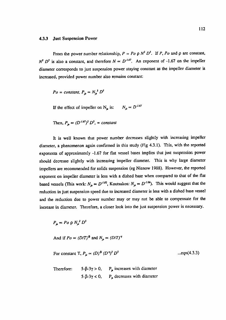
112

4.3.3 Just Suspension Power

From the power number relationship, P = Po p N3 f)5• If P, Po and p are constant,

N3 D is also a constant, and therefore N U' 67. An exponent of -1.67 on the impeller

diameter corresponds to just suspension power staying constant as the impeller diameter is

increased, provided power number also remains constant:

Po = constant, P N 3 l)

If the effect of impeller on N is: N cc D'67

Then, p, oc (D' 67)3 D5, = constant

It is well known that power number decreases slightly with increasing impeller

diameter, a phenomenon again confirmed in this study (Fig 4.3.1). This, with the reported

exponents of approximately -1.67 for flat vessel bases implies that just suspension power

should decrease slightly with increasing impeller diameter. This is why large diameter

impellers are recommended for solids suspension (eg Nienow 1988). However, the reported

exponent on impeller diameter is less with a dished base when compared to that of the flat

based vessels (This work: N cc D'°2, Koutsakos: N, cc D'°6). This would suggest that the

reduction in just suspension speed due to increased diameter is less with a dished base vessel

and the reduction due to power number may or may not be able to compensate for the

increase in diameter. Therefore, a closer look into the just suspension power is necessary.

PocPopND5

And if Po cc (DIT) and N cc (D/T)

For constant T, cc (D) (D)3 D5

Therefore: 5-13-3y> 0, P increases with diameter

5-[3-3y < 0, P,, decreases with diameter

...eqn(4.3.3)

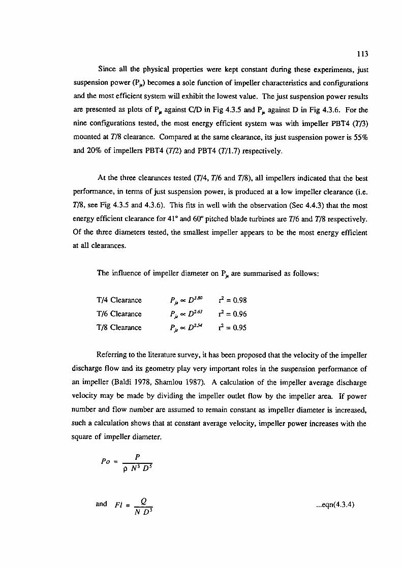
113

Since all the physical properties were kept constant during these experiments, just

suspension power (Pp) becomes a sole function of impeller characteristics and configurations

and the most efficient system will exhibit the lowest value. The just suspension power results

are presented as plots of P against CID in Fig 4.3.5 and P against D in Fig 4.3.6. For the

nine configurations tested, the most energy efficient system was with impeller PBT4 (T/3)

mounted at T/8 clearance. Compared at the same clearance, its just suspension power is 55%

and 20% of impellers PBT4 (Ta) and PBT4 (T/1.7) respectively.

At the three clearances tested (T/4, T/6 and T/8), all impellers indicated that the best

performance, in terms of just suspension power, is produced at a low impeller clearance (i.e.

T/8, see Fig 4.3.5 and 4.3.6). This fits in well with the observation (Sec 4.4.3) that the most

energy efficient clearance for 41° and 600 pitched blade turbines are T/6 and T/8 respectively.

Of the three diameters tested, the smallest impeller appears to be the most energy efficient

at all clearances.

The influence of impeller diameter on P are summarised as follows:

T/4 Clearance

P1, oc r2 = 0.98

T/6 Clearance

P oc D263

r2 = 0.96

T/8 Clearance

P oc D23'

r2 = 0.95

Referring to the literature survey, it has been proposed that the velocity of the impeller

discharge flow and its geometry play very important roles in the suspension performance of

an impeller (Baldi 1978, Shamlou 1987). A calculation of the impeller average discharge

velocity may be made by dividing the impeller outlet flow by the impeller area. If power

number and flow number are assumed to remain constant as impeller diameter is increased,

such a calculation shows that at constant average velocity, impeller power increases with the

square of impeller diameter.

PPo = ____

pN3D5

and F! = _____ ...eqn(4.3.4)ND3

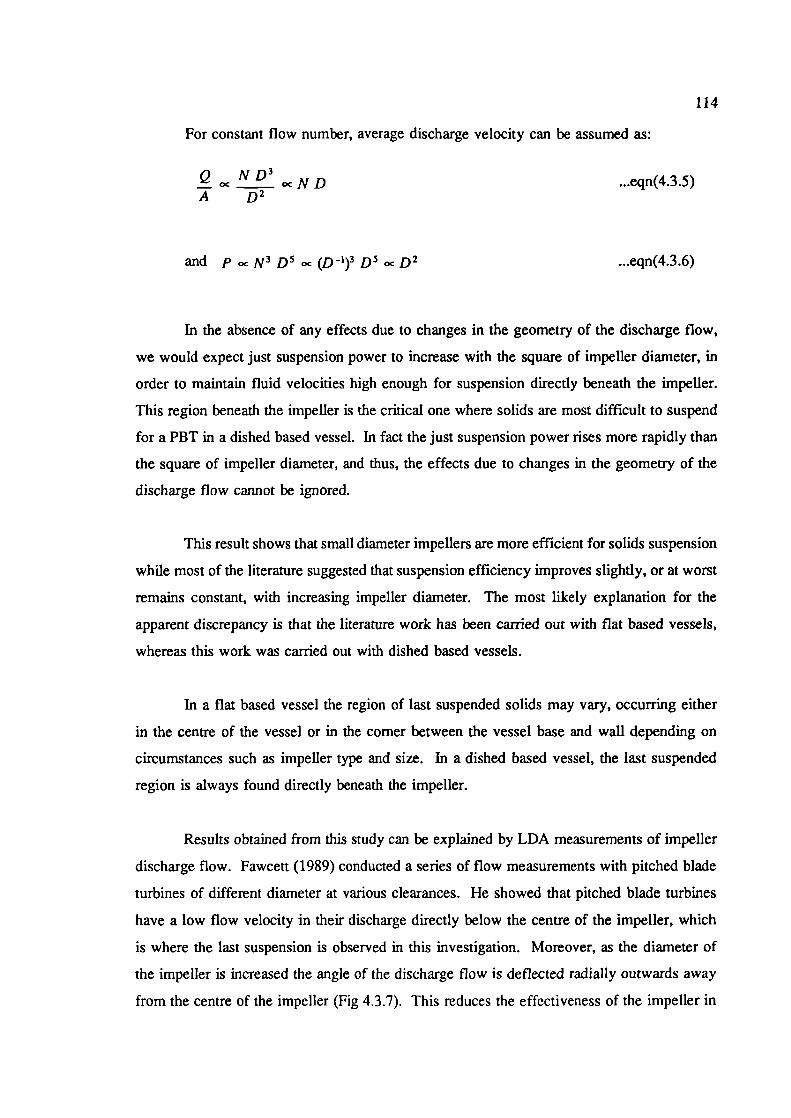
() ND3___ ocNDA D2

...eqn(4.3.5)

114

For constant flow number, average discharge velocity can be assumed as:

and PocN3D5oc(D')3D5ocD2 .eqn(4.3 .6)

In the absence of any effects due to changes in the geometry of the discharge flow,

we would expect just suspension power to increase with the square of impeller diameter, in

order to maintain fluid velocities high enough for suspension directly beneath the impeller.

This region beneath the impeller is the critical one where solids are most difficult to suspend

for a PBT in a dished based vessel. In fact the just suspension power rises more rapidly than

the square of impeller diameter, and thus, the effects due to changes in the geometry of the

discharge flow cannot be ignored.

This result shows that small diameter impellers are more efficient for solids suspension

while most of the literature suggested that suspension efficiency improves slightly, or at worst

remains constant, with increasing impeller diameter. The most likely explanation for the

apparent discrepancy is that the literature work has been carried out with flat based vessels,

whereas this work was carried out with dished based vessels.

In a flat based vessel the region of last suspended solids may vary, occurring either

in the centre of the vessel or in the corner between the vessel base and wall depending on

circumstances such as impeller type and size. In a dished based vessel, the last suspended

region is always found directly beneath the impeller.

Results obtained from this study can be explained by LDA measurements of impeller

discharge flow. Fawcett (1989) conducted a series of flow measurements with pitched blade

turbines of different diameter at various clearances. He showed that pitched blade turbines

have a low flow velocity in their discharge directly below the centre of the impeller, which

is where the last suspension is observed in this investigation. Moreover, as the diameter of

the impeller is increased the angle of the discharge flow is deflected radially outwards away

from the centre of the impeller (Fig 4.3.7). This reduces the effectiveness of the impeller in

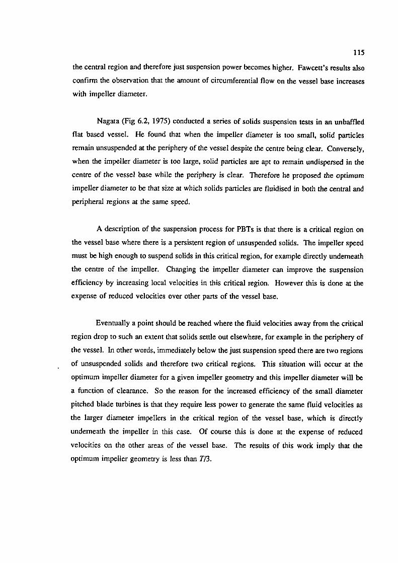
115

the central region and therefore just suspension power becomes higher. Fawcett's results also

confirm the observation that the amount of circumferential flow on the vessel base increases

with impeller diameter.

Nagata (Fig 6.2, 1975) conducted a series of solids suspension tests in an unbaffled

fiat based vessel. He found that when the impeller diameter is too small, solid particles

remain unsuspended at the periphery of the vessel despite the centre being clear. Conversely,

when the impeller diameter is too large, solid particles are apt to remain undispersed in the

centre of the vessel base while the periphery is clear. Therefore he proposed the optimum

impeller diameter to be that size at which solids particles are fluidised in both the central and

peripheral regions at the same speed.

A description of the suspension process for PBTs is that there is a critical region on

the vessel base where there is a persistent region of unsuspended solids. The impeller speed

must be high enough to suspend solids in this critical region, for example directly underneath

the centre of the impeller. Changing the impeller diameter can improve the suspension

efficiency by increasing local velocities in this critical region. However this is done at the

expense of reduced velocities over other parts of the vessel base.

Eventually a point should be reached where the fluid velocities away from the critical

region drop to such an extent that solids settle out elsewhere, for example in the periphery of

the vessel. In other words, immediately below the just suspension speed there are two regions

of unsuspended solids and therefore two critical regions. This situation will occur at the

optimum impeller diameter for a given impeller geometry and this impeller diameter will be

a function of clearance. So the reason for the increased efficiency of the small diameter

pitched blade turbines is that they require less power to generate the same fluid velocities as

the larger diameter impellers in the critical region of the vessel base, which is directly

underneath the impeller in this case. Of course this is done at the expense of reduced

velocities on the other areas of the vessel base. The results of this work imply that the

optimum impeller geometry is less than T/3.

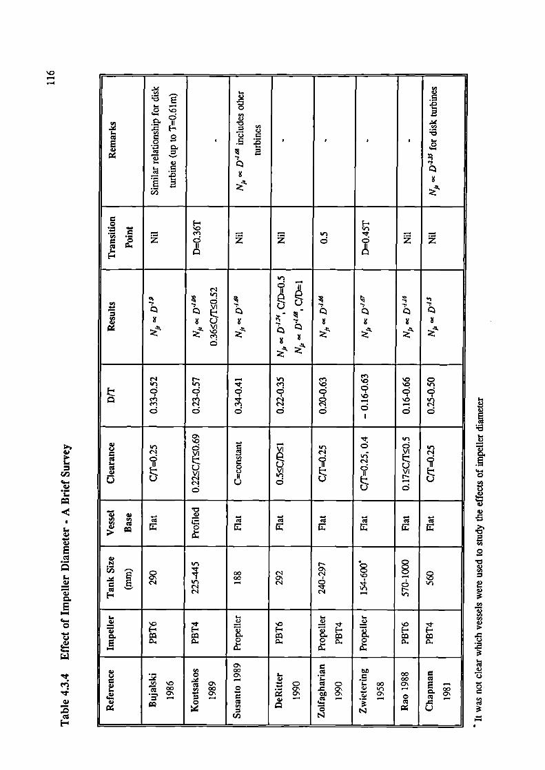
\0

4)

4)

'I4)

4)

E

'I4)

4)0.

0

cJ

'I.4)

.0

.

.0o I..

—

2E4)

I- )

C,)

0

= = =d Z Z Z

4).. VI

d

— '0 CIt-i cn '0 oq q q qCfl —

Cd d d d d d

0' . V'a0 -. — d aa

§VIVIo 0 aa

4) . — — — — .r#) c cv0

4)

0'00 c.'1—00

c..1 c.l —

I-.

0

0.

C'00 00

00 C

'0 0' C C C 00 0' E —00 00 0 4) V — 00

0' 0' 0

— — — —N

(ID N

I-

I

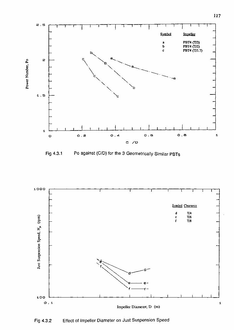
0

0

2

0

1.5

117

2.5

Symbol

abC

bN

b.

NN

N.N

Impeller

PBT4 ('Ff3)PBT4 (Ta)PBT4 Cr11.7)

1.

Fig 4.3.1

0.2 0.4 0.6 0.8

C /0

P0 against (C/D) for the 3 Geometrically Similar PBTs

1000

Symbol Clearance

d T/4

E

e T/6f T/8

z-

4)

C,,

0

100 '-

0.1 IImpeller Diameter, D (m)

Fig 4.3.2 Effect of Impeller Diameter on Just Suspension Speed

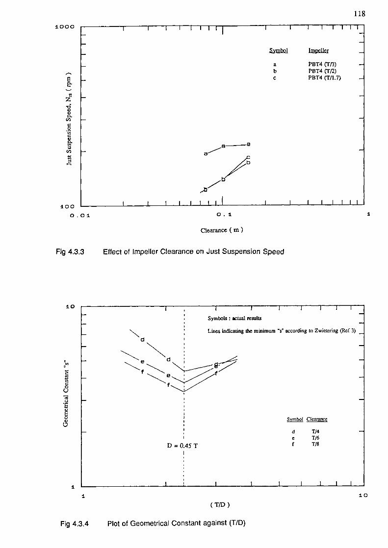
118

1000

Symbol

Impeller

a

PBT4 cFf3)b

PBT4 Cr,2)C

PBT4 (T/l.7)

z

4)V

crJ

0

4)

L_..

0.01 0.1

I

Clearance (in)

Fig 4.3.3 Effect of Impeller Clearance on Just Suspension Speed

10 I I I --

Symbols actual results

N Lines indicating the minimum according to Zwietcring (Ref 3)

4)U,

0U

U

4)E0V

;

D = 0.45 T

I jL _i____

I

(T/D)

Symbol Clearance

d T/4e T/6f T/8

10

Fig 4.3.4 Plot of Geometrical Constant against (T/D)

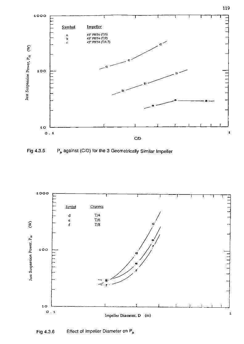
119

U,

0..I-.

:

1.00

1000

I-V

100

0U,

4)

U,

C,)

U,

-.

10

0.1

C/D

Fig 4.3.5

P against (C/D) for the 3 Geometrically Similar Impeller

1.000

Symbol Clcarancc

I

d T/4/e T16

f 1/8 d

d

1

10

0. IImpeller Diameter, D (m)

I

Fig 4.3.6 Effect of Jmpeller Diameter on P

120


In the previous sections, it was shown that small diameter PBTs are more energy

efficient for suspending solids in dished based vessels, than those of large diameter. This

section focuses on the influence of impeller diameter on solids distribution. Solids

concentration measurements were made with three geometrically similar PBTs (D=T/3, Tfl

& T/1.7, dimensions are summarised in Table 4.3.1) mounted at T/4 clearance. The results

are tabulated in Appendix A. Fig 4.3.9 presents a plot of local solids concentration against

impeller speed for the five sampling positions. This is taken from the 45° PBT4(T12) results.

However, all three impellers exhibited a similar trend and they confirmed the overall flow

pattern generalised from visual observation (Sec 4.1.1).

Relative standard deviation at different speeds (RSD, eqn 2.2.1) is employed to

quantify the level of homogeneity achieved by agitation. RSD for the three pitched blade

turbines are plotted against impeller speed and are presented in Fig 4.3.10. As expected from

flow visualisation, the degree of homogeneity increases as agitation is increased (hence RSD

is decreased). The value of RSD goes through a minimum (RSD,,,.) and any further increase

in impeller speed gives rise to an increase in RSD. This is believed to be caused by solids

redistribution due to centrifugal forces (Bohnet and Niesmak 1980).

Referring to Fig 4.3.10, the speed required by the impeller to produce RSD, IrnI iS

highest for the T/3 impeller and lowest for the T/1 .7 impeller. In other words, the large

diameter impeller achieves its minimum relative standard deviation at lower impeller speed

than the small diameter impeller. A similar pattern is displayed in the plot of RSD against

power input (Fig 4.3.11) which again suggests that large diameter PBTs achieve their RSD,,..

at a lower power input than small diameter PBTs. The difference in power input at individual

RSD, is very significant. The T/3, T/2 and T/1.7 PBTs required 217, 125 and 57W to

achieve their RSD, respectively. In other words, the T/3 PBT needed 3.8 times more power

than T/1.7 PBT to achieve its point of maximum homogeneity. However, this trend is in

reverse order when compared to the effect of impeller diameter on N, i.e. T/3 PBT is most

energy efficient impeller for suspension (Sec 4.3.2).

To explain this rather interesting finding, N for the three impellers at 30% Wt are

calculated based on the 5% Wt results. The concentration effect is corrected according to

121

Zwietering's correlation (i.e. Nfr X°'3). The results are then marked on the same plot to

facilitate the analysis (Fig 4.3.10). For the large diameter PBTs, RSD,, is achieved at a

lower impeller speed than its corresponding just suspension speed whereas, for the small

diameter impeller, the opposite is the case. Large diameter impellers generally produce more

"top to bottom" flow than small diameter impellers for the same power input. It is the bulk

flow which is primarily responsible for the distribution of the solid particles. Thus, large

diameter PBTs achieve RSDmII, at lower power input than that of small diameter PBTs.

Moreover, the direction of the discharge flow between impellers of different diameter are not

the same (Fawcett 1989). Due to the influence of vessel base on flow profiles, large diameter

PBTs produce a higher level of radial component flow than the small diameter PBTs (Fig

4.3.7), whereas the discharge flow of a small PBT is less radial and targeted directly on the

last suspension region on the vessel base which gives rise to its low N (Fig 4.3.8).

To prove the hypothesis quantitatively, concentration profiles at impeller speeds close

to N for the three impellers are presented in Fig 4.3.15 to 4.3.17. In case of the small

diameter impeller (T/3 PBT), the calculated just suspension is at 285 rpm. The concentration

profile at 250 rpm (below N) shows that of the 5 measuring positions, the top sampling point

is 50% of the average concentration while the lower 4 sampling points all exhibit very similar

concentrations and they are approximately 30% higher than the average. At 300 rpm (above

Nt), the five sampling positions still have a concentration approximately 8% higher than the

theoretical average, indicating that a portion of clear liquid still exists at the top. Further

increase in impeller speed (eg 350 rpm) still shows improvement in the concentration profile

(further reduction in RSD). In cases of the two large diameter PBTs (T and T/1.7, Fig

4.3.16 and 4.3.17), concentrations measured at the top sampling position are similar to the

predicted average. Moreover, the concentration profiles for impeller speed around N are very

similar and an increase in impeller speed above N does not improve the homogeneity of the

particles, showing that the solids are already well distributed. This once again confirmed the

results which show that just suspension speed occurs at lower power input than RSD, and

vice versa with large diameter PBTs.

Despite the fact that the large diameter impeller (eg D=T/1 .7) achieves its RSD mm at

a lower impeller speed than that of a small diameter impeller (eg D=T13), the absolute value

of RSD,, is lower (more homogeneous) in the case of the small diameter impeller. This is

achieved at the expense of high power input (Fig 4.3.11).

122

Concentration profiles for the three impellers at various power inputs are presented in

Fig 4.3.12 to 4.3.14. They are plotted as height from vessel base against solids concentration

for the three impellers at low, medium and high power inputs. At low power inputs (Fig

4.3.12), the concentration profile of the T/3 PBT shows that there is more than one third of

the vessel height of clear liquid in the vessel, the solids concentration beneath the clear layer

is much higher than average and that there is little difference in concentration beneath the

clear liquid region. On the other hand, the T/1 .7 PBT does not have any clear liquid layer

on the top of the vessel (at least according at the top most measuring point) but there is

considerable variation in concentration within the profile itself when compared to the T/3

PBT. At medium power input (Fig 4.3.13), the clear liquid layer in the upper region for T/3

PBT has disappeared and the deviation from the mean concentration gradient within the vessel

is still less than that of the large diameter impellers. At high power input (Fig 4.3.14), the

concentration profile for T13 PBT improves still further (more homogeneous) while

redistribution starts to occur in the large PBTs (Sec 4.1.1) and this increases the magnitude

of RSD.

Therefore, uniformity of solids distribution is not a good parameter to assess the

condition of solids suspension arid vice versa. Moreover, the use of homogeneity data as the

criterion for just suspension speed determination should be interpreted with great care, as some

impellers attain N before their most homogeneous points. For other impellers, just

suspension speed requires higher speed or power input than

4.3.5 Verification of Tip Speed Criterion

Most theoretical models developed for solids distribution are based upon one

dimensional dispersion analysis and the impeller tip speed (itND) is normally assumed to

counterbalance the particle settling velocity (Sec 2.2.2). This gives rise to a constant tip speed

criterion for impeller diameter as well as scale-up effect. Fig 4.3.18 is a plot of RSD against

ND for the three geometrically similar impellers. Using ND = constant brings the three

curves closer to each other but a stronger diameter effect is required to match them.

ratio (D[F) to be more useful:

Fl = (DT1)°5

ND3...eqn(4.3.7)

(ri\-2.S Iui\

FlocI±Ll I--IPo°7

T) T)...eqn(4.3.8)

123

Brodkey (1988) suggested an expanded pumping number including the impeller to tank

Q oc F! N D3 [D}O.5

The relative pumping rate can be estimated according to Nagata's correlation (1975):

A plot of RSD against relative discharge rate is presented in Fig 4.3.20 and the data

does not seem to correlate in this format.

Regression analysis gives a poor regression coefficient but suggests a diameter effect

close to ND2 (Fig 4.3.19), which is similar to the Thrust number as proposed by ITT Flygt

(Karslen 1992).

Thrust force generated by an impeller:

FocpQV ...eqn(4.3.9)

oc p (N D3) (N D)

ocpN2D4

And the Thrust number (Ft) is defmed as:

FtF ...eqn(4.3.1O)

p N2D4

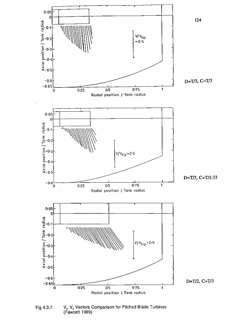
005

0

aI-

.2-03In0

a>c

U25 0.5 0.75

Radial position I Tank radius

-0

0• C

In

00

Ca-U

I-

C.2-0

In0

-0ax<-0

_0.u0 025 0.5 075

Radial position j Tank radius

0 C

In

0...0I-

-0•

-0• E

0 0•25 05 0•75

Radial position I Tank radius

D=T/2, C=T/3

124

D=T/3, C=T13

D=T/3, C=T/3.33

Fig 4.3.7 Vr, V Vectors Comparison for Pitched Blade Turbines(Fawcett 1989)

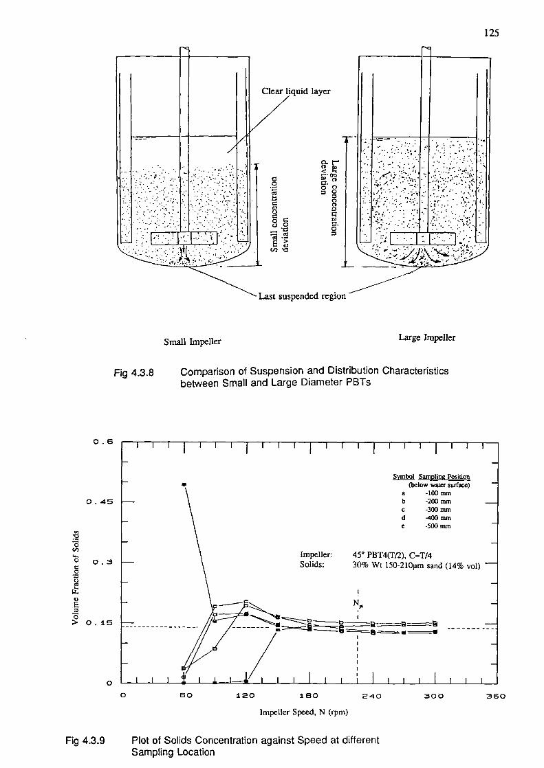
125

Clear liquid layer

CDL, . ........

– . cq . .,z...: ,..

CD I

0_ C. S - - --.

:'"-.. - -CD•...•'.'.

-, L I I

Last suspended region

Small Impeller Large Impeller

Fig 4.3.8 Comparison of Suspension and Distribution Characteristicsbetween Small and Large Diameter PBTs

0Cl

4)C-,

C)

. .

0.6

0.45

0

o 0.3

0

I> 0.15

QL

0

Fig 4.3.9

Symbol Sampling Position(below waler suiface)

a -100mmb -200mmc -300mmd -400mme -500mm

Impeller: 450 PBT4(T/2), C=T/4Solids: 30% Wt 150-2lOpm sand (14% vol) -

•—z

I

I -

I-

- I I I I I

60 120 180 240 300 360

Impeller Speed, N (rpm)

Plot of Solids Concentration against Speed at differentSampling Location

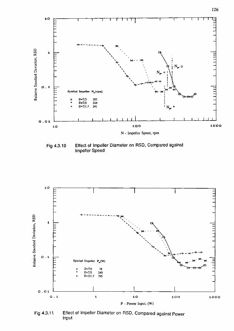
C/)

0•0

CO

>V

0•0

CO

Cl)

4)>

CO

4)

I

0.1 -

±000

126

10

Cl)

0

Co

4)

ICl) 0.14)>

Co

4)

-4-- -*

S.

S.

'1C••••

"S.

•.

'S.. N,+i

4 .. IIS. I

S..

S. ..f-44- I

Symbol Impeller N,(rpm)

o D=Tf3 225* D=T/2 224+ D=T/1.7 241

l Ni,, *

0.0±

10

±00

±000


Fig 4.3.10

Effect of Impeller Diameter on RSD, Compared againstImpeller Speed

10

0.01 L_

0.1

+ ------------'S

S.'S

.5'S

'S

Symbol Impeller P(W)

o D=T/3 78* D=Tf2 240+ D=T/1 .7 795

± 10 100

P - Power Input, (W)

Fig 4.3.11 Effect of Impeller Diameter on RSD, Compared against PowerInput

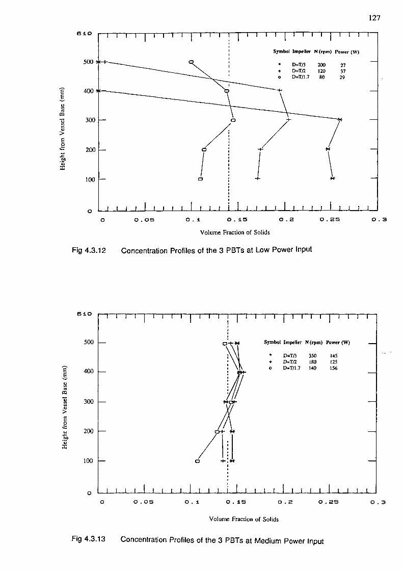
Symbol Impeller N (rpm) Power (W)

* D=T/3 200 27+ D=Tf2 120 37o D=T/1 .7 80 29

- .4-

I \

127

610

500

400E

'I,

- 300'CV>

E

200

100

/I0

0 0.05 0.1 0.15 0.2 0.25 0.3


Fig 4.3.12 Concentration Profiles of the 3 PBTs at Low Power Input

610

500

400

VI.,

300'CV>

200

Vz

100


* D=T13 350 145+ D=T(2 180 125o D=T/1.7 140 156

0 0.O 01 0.15 02 0.25 0.3


Fig 4.3.13 Concentration Profiles of the 3 PBTs at Medium Power Input

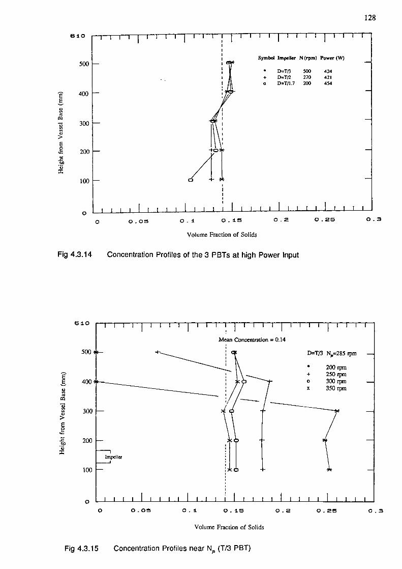
128

610

500

? 400

4)

• 3 300t1

4)>

E

200

-c

V

100


* D=T[3 500 424+ DT12 270 421o D=T/1.7 200 454

0 0.05 0.1 0.15 0.2 0.25 0.3


Fig 4.3.14 Concentration Profiles of the 3 PBTs at high Power Input

I Impellez

610

500

E400

4)U,

300

200

100

I l I I Il1

Mean Concentration = 0.14

D=T13 N,=285 rpm

* 200rpm+ 250rpmo 300rpmx 350rpm

0 0.05 0.1. 0.15

0.2 0.25 0.3


Fig 4.3.15 Concentration Profiles near N (T/3 PBT)

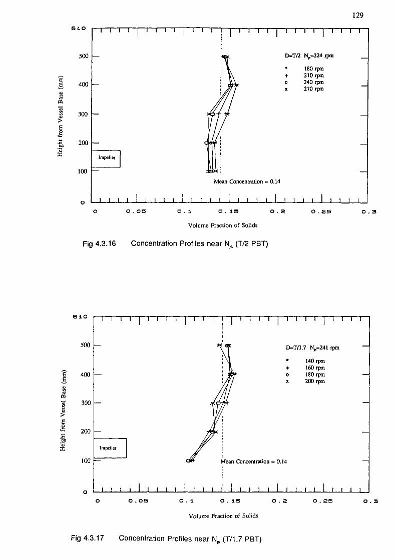
610

500 D=T12 N=224 rpm


4004)

300

200

100

129

Mean Concentration = 0.14

0

I i i I

0 0.05 0.1 0.15 0.2 0.25 0.3


Fig 4.3.16 Concentration Profiles near N, (T/2 PBT)

610

500

400-

4)U,

300-

200 —

Impeller

D=T11.7 N=24l rpm


100 - Mean Concentration = 0.14

0 I t i i i_I i 1_i I i i i i I

0 0.05 0.1 0.15 0.2 0 . 25 0.3


Fig 4.3.17 Concentration Profiles near N 5 (T/1.7 PBT)

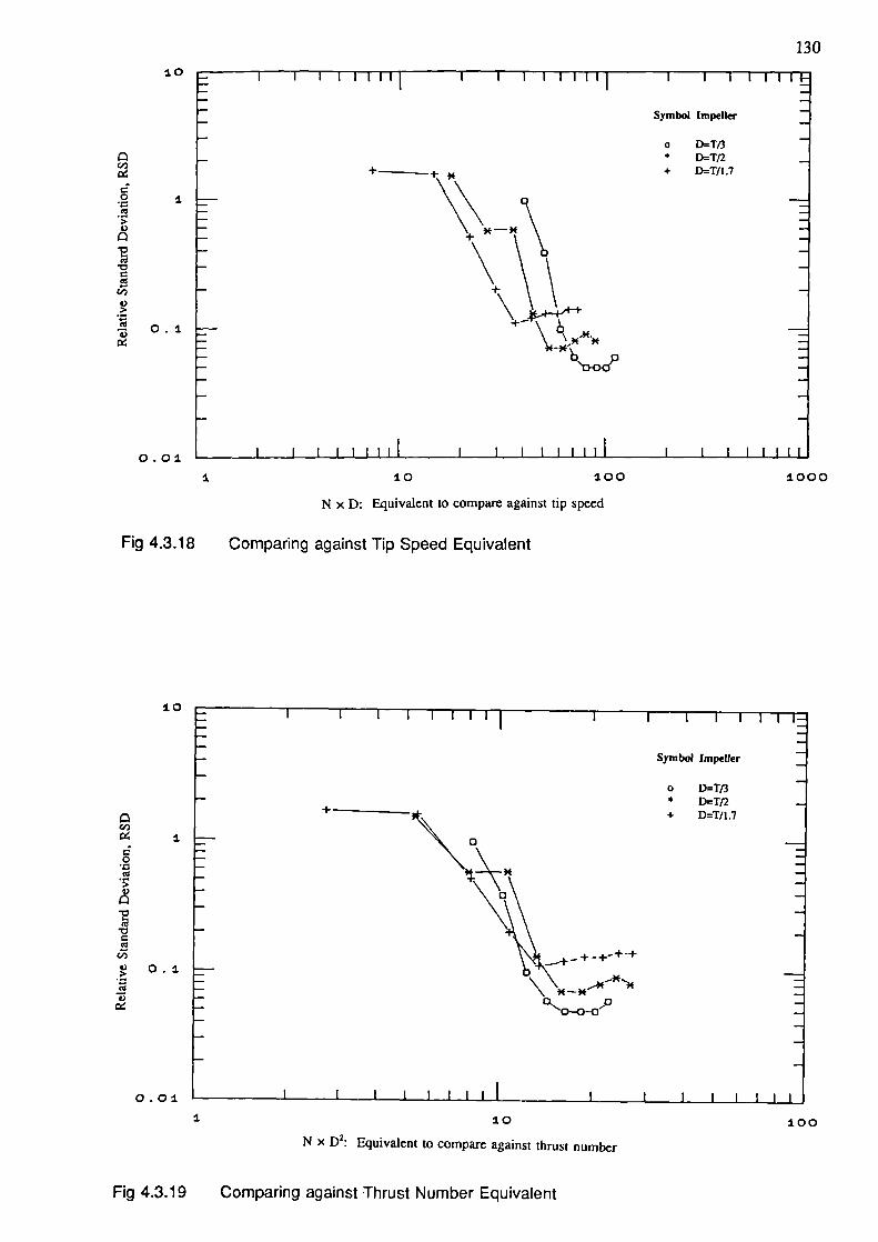
130

10

I

0.1

0.011 10 100 1000

N x D: Equivalent to compare against tip speed

Fig 4.3.18 Comparing against Tip Speed Equivalent

10

I0>

I0.1

V

0.011 10 100

N x D2: Equivalent to compare against thrust number

Fig 4.3.19 Comparing against Thrust Number Equivalent

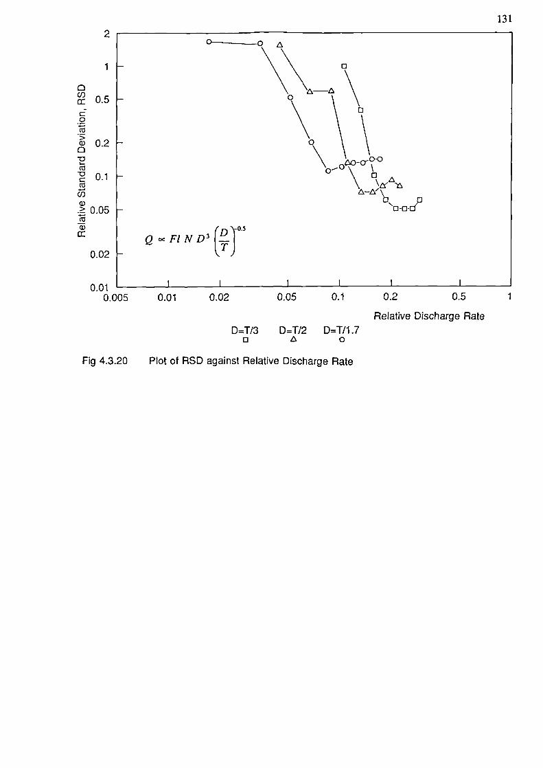
131

2

1

a(I)a: 0.5C0

I:.2 0.05ctj0)a:

0.02

0.010.005

Fig 4.3.20

0-____O

\

0-0-

Q oc Fl N D3 (DIJO.5

0.01 0.02 0.05 0.1 0.2 0.5

Relative Discharge Rate

D=T/3 D=T/2 D=T/1.70 0

Plot of RSD against Relative Discharge Rate

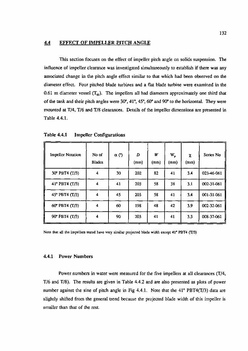
132

44 EFFECT OF IMPELLER PITCH ANGLE

This section focuses on the effect of impeller pitch angle on solids suspension. The

influence of impeller clearance was investigated simultaneously to establish if there was any

associated change in the pitch angle effect similar to that which had been observed on the

diameter effect. Four pitched blade turbines and a flat blade turbine were examined in the

0.61 m diameter vessel (T61 ). The impellers all had diameters approximately one third that

of the tank and their pitch angles were 30°, 410, 45°, 60° and 90° to the horizontal. They were

mounted at T/4, T/6 and T/8 clearances. Details of the impeller dimensions are presented in

Table 4.4.1.

Table 4.4.1 Impeller Configurations

Impeller Notation No of a (°) D W W, x Series No

Blades (mm) (mm) (mm) (mm)

30° PBT4 (Tf3) 4 30 202 82 41 3.4 023-46-061

41° PBT4 (T/3) 4 41 203 58 38 3.1 002-31-061

450 PBT4 (T/3) 4 45 203 58 41 3.4 001-31-061

60° PBT4 (l'13) 4 60 198 48 42 3.9 002-32-061

90° FBT4 (Tf3) 4 90 203 41 41 3.3 008-37-061

Note that all the impellers tested have very similar projected blade width except 41 PBT4 (T/3)

4.4.1 Power Numbers

Power numbers in water were measured for the five impellers at all clearances (1/4,

T/6 and T/8). The results are given in Table 4.4.2 and are also presented as plots of power

number against the sine of pitch angle in Fig 4.4.1. Note that the 41° PBT4(T/3) data are

slightly shifted from the general trend because the projected blade width of this impeller is

smaller than that of the rest.

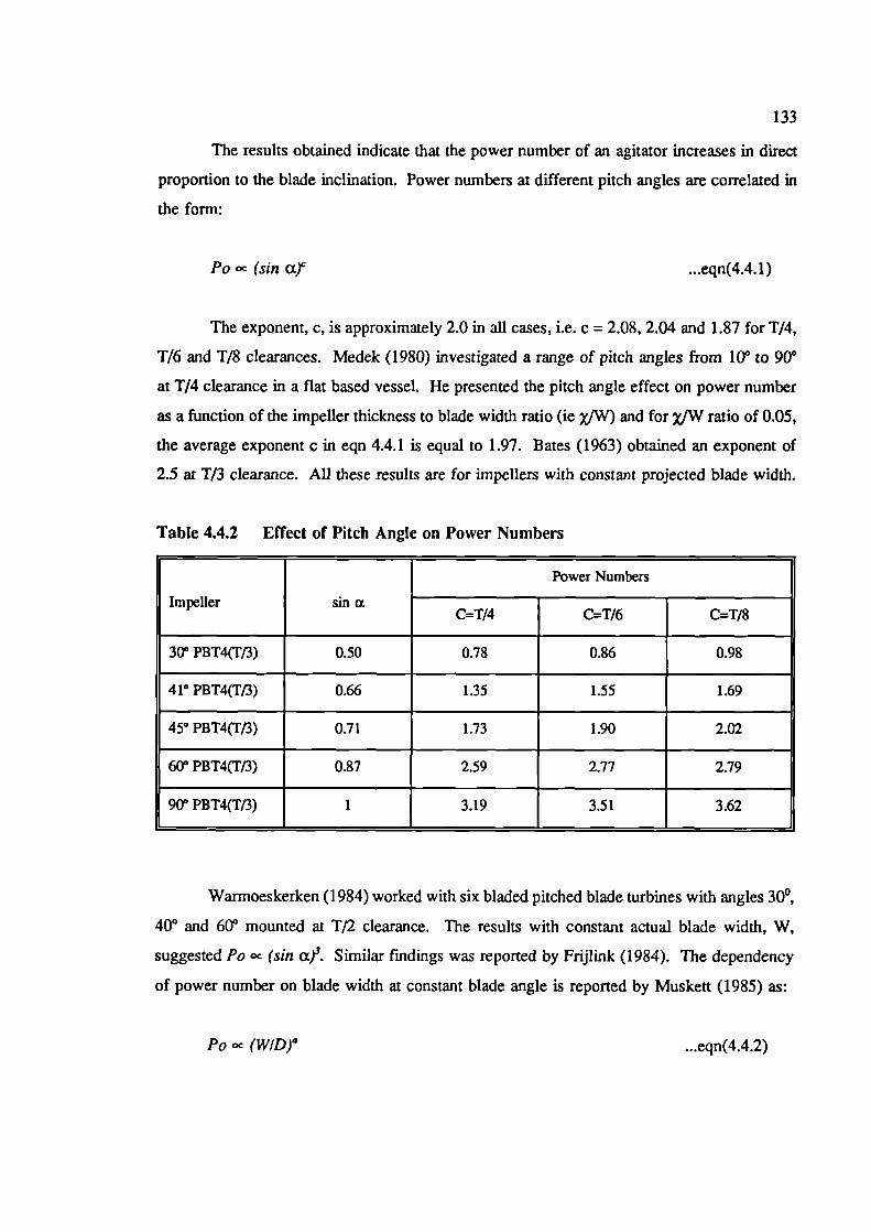
133

The results obtained indicate that the power number of an agitator increases in direct

proportion to the blade inclination. Power numbers at different pitch angles are correlated in

the form:

Po (sin cxr ...eqn(4.4. 1)

The exponent, c, is approximately 2.0 in all cases, i.e. c = 2.08, 2.04 and 1.87 for T/4,

T/6 and T/8 clearances. Medek (1980) investigated a range of pitch angles from 10° to 90°

at T/4 clearance in a flat based vessel. He presented the pitch angle effect on power number

as a function of the impeller thickness to blade width ratio (ie yjW) and for jW ratio of 0.05,

the average exponent c in eqn 4.4.1 is equal to 1.97. Bates (1963) obtained an exponent of

2.5 at T/3 clearance. All these results are for impellers with constant projected blade width.

Table 4.4.2 Effect of Pitch Angle on Power Numbers

Power Numbers

Impeller sin cxC=T/4 C=T/6 C=T/8

30° PBT4(T/3) 0.50 0.78 0.86 0.98

41° PBT4(T13) 0.66 1.35 1.55 1.69

45° PBT4(Tf3) 0.71 1.73 1.90 2.02

60° PBT4(Tf3) 0.87 2.59 2.77 2.79

900 PBT4(T13) 1 3.19 3.51 3.62

Warmoeskerken (1984) worked with six bladed pitched blade turbines with angles 30°,

40° and 60° mounted at Tf2 clearance. The results with constant actual blade width, W,

suggested Po oc (sin (x/. Similar fmdings was reported by Frijlink (1984). The dependency

of power number on blade width at constant blade angle is reported by Muskett (1985) as:

Po oc (WIDt ...eqn(4.4.2)

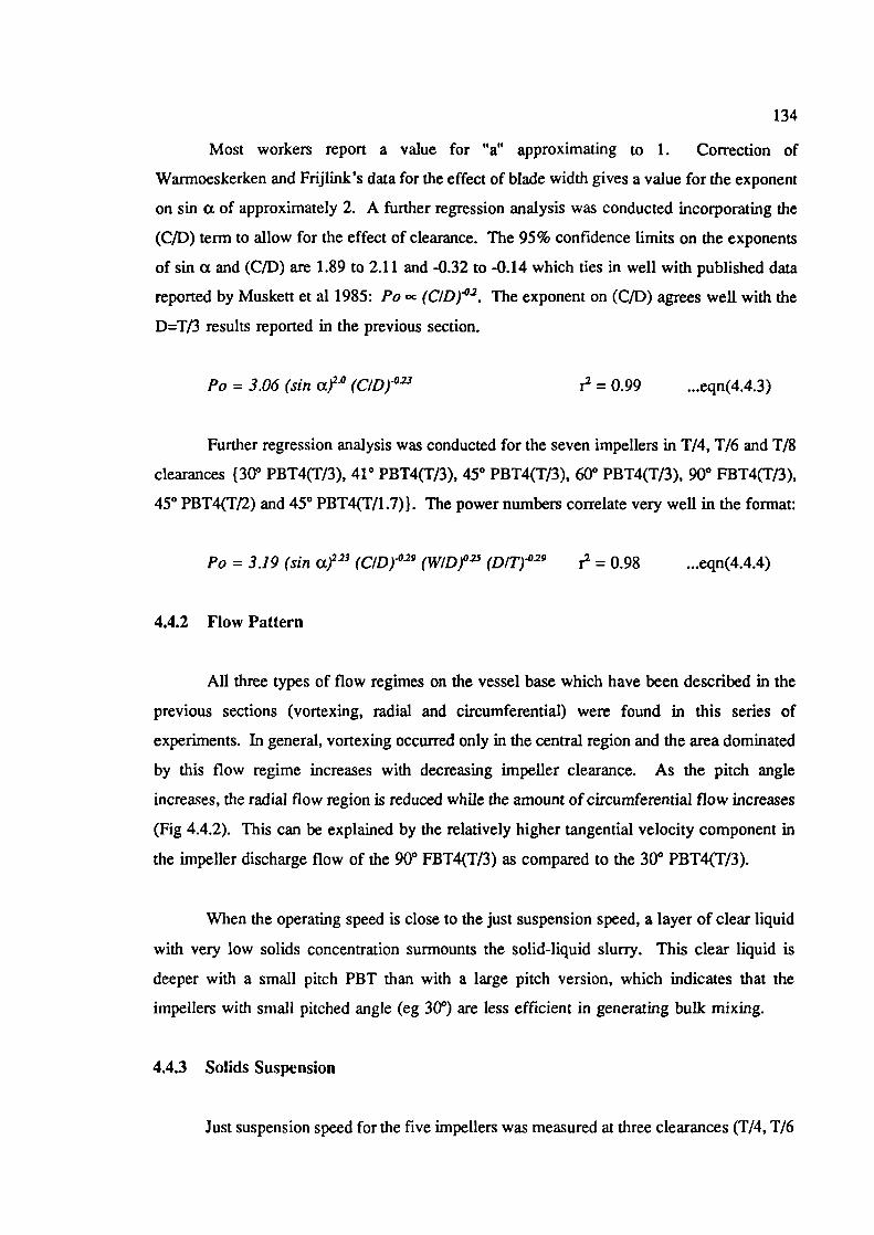
134

Most workers report a value for "a" approximating to 1. Correction of

Warmoeskerken and Frijlink's data for the effect of blade width gives a value for the exponent

on sin a of approximately 2. A further regression analysis was conducted incorporating the

(CID) term to allow for the effect of clearance. The 95% confidence limits on the exponents

of sin a and (C/D) are 1.89 to 2.11 and -0.32 to -0.14 which ties in well with published data

reported by Muskett et a! 1985: Po (C/D)°2. The exponent on (C/D) agrees well with the

D=T/3 results reported in the previous section.

Po = 3.06 (sin )20 (C/D)°23 r2 = 0.99 ...eqn(4.4.3)

Further regression analysis was conducted for the seven impellers in T/4, T/6 and T/8

clearances (30° PBT4(T/3), 41° PBT4(T/3), 45° PBT4(T/3), 60° PBT4(T/3), 90° FBT4(T/3),

45° PBT4(T/2) and 45° PBT4(T/1.7)}. The power numbers correlate very well in the format:

Po = 3.19 (sin a)' (C/D)°29 (W/D)°' (D/T)°29 r2 = 0.98 ...eqn(4.4.4)

4.4.2 Flow Pattern

All three types of flow regimes on the vessel base which have been described in the

previous sections (vortexing, radial and circumferential) were found in this series of

experiments. In general, vortexing occurred only in the central region and the area dominated

by this flow regime increases with decreasing impeller clearance. As the pitch angle

increases, the radial flow region is reduced while the amount of circumferential flow increases

(Fig 4.4.2). This can be explained by the relatively higher tangential velocity component in

the impeller discharge flow of the 90° FBT4(T/3) as compared to the 30° PBT4(T/3).

When the operating speed is close to the just suspension speed, a layer of clear liquid

with very low solids concentration surmounts the solid-liquid slurry. This clear liquid is

deeper with a small pitch PBT than with a large pitch version, which indicates that the

impellers with small pitched angle (eg 30°) are less efficient in generating bulk mixing.


Just suspension speed for the five impellers was measured at three clearances (T/4, T/6

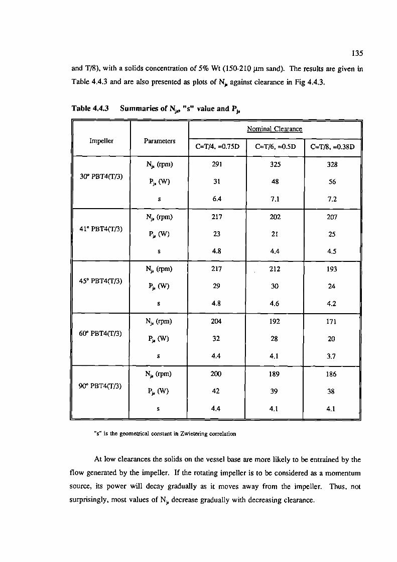
135

and T/8), with a solids concentration of 5% Wt (150-210 p.m sand). The results are given in

Table 4.4.3 and are also presented as plots of N against clearance in Fig 4.4.3.

Table 4.4.3 Summaries of N 0 "s" value and P

Nominal Clearance

Impeller ParametersC=T/4, =0.75D C=T/6, =0.5D C=T/8. =0.38D

N 1 (rpm) 291 325 328

30° PBT4(T/3)P (W) 31 48 56

s 6.4 7.1 7.2

N,, (rpm) 217 202 207

41° PBT4(T/3)P (W) 23 21 25

s 4.8 4.4 4.5

N 1 (rpm) 217 212 193

450 PBT4(T/3)P(W) 29 30 24

s 4.8 4.6 4.2

(rpm) 204 192 171

60° PBT4(T13)P,1(W) 32 28 20

s 4.4 4.1 3.7

N (rpm) 200 189 186

90° PBT4Ff3)P,(W) 42 39 38

s 4.4 4.1 4.1

"s is the geometrical constant in Zwietering correlation

At low clearances the solids on the vessel base are more likely to be entrained by the

flow generated by the impeller. If the rotating impeller is to be considered as a momentum

source, its power will decay gradually as it moves away from the impeller. Thus, not

surprisingly, most values of N decrease gradually with decreasing clearance.

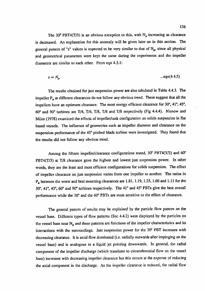
136

The 30° PBT4(T13) is an obvious exception to this, with N. increasing as clearance

is decreased. An explanation for this anomaly will be given later on in this section. The

general pattern of "s" values is expected to be very similar to that of N,, since all physical

and geometrical parameters were kept the same during the experiments and the impeller

diameters are similar to each other. From eqn 4.3.1:

oc N, ...eqn(4.4.5)

The results obtained for just suspension power are also tabulated in Table 4.4.3. The

impeller P, at different clearances do not follow any obvious trend. These suggest that all the

impellers have an optimum clearance. The most energy efficient clearance for 300 41° 45°,

600 and 90° turbines are 1/4, 1/6, T/8, T/8 and T/8 respectively (Fig 4.4.4). Nienow and

Miles (1978) examined the effects of impeller/tank configuration on solids suspension in flat

based vessels. The influence of geometries such as impeller diameter and clearance on the

suspension performance of the 450 pitched blade turbine were investigated. They found that

the results did not follow any obvious trend.

Among the fifteen impeller/clearance configurations tested, 30° PBT4(T/3) and 60°

PBT4(T/3) at T/8 clearance gave the highest and lowest just suspension power. In other

words, they are the least and most efficient configurations for solids suspension. The effect

of impeller clearance on just suspension varies from one impeller to another. The ratios in

P, between the worst and best mounting clearances are 1.81, 1.19, 1.25, 1.60 and 1.11 for the

30°, 41°, 45°, 60° and 90° turbines respectively. The 41° and 45° PBTs give the best overall

performance while the 30° and the 60° PBTs are most sensitive to the effect of clearance.

The general pattern of results may be explained by the particle flow pattern on the

vessel base. Different types of flow patterns (Sec 4.4.2) were displayed by the particles on

the vessel base near N, and these patterns are functions of the impeller characteristics and its

interactions with the surroundings. Just suspension power for the 30° PBT increases with

decreasing clearance. It is axial flow dominated (i.e. radially outwards after impinging on the

vessel base) and is analogous to a liquid jet pointing downwards. In general, the radial

component of the impeller discharge (which translates to circumferential flow on the vessel

base) increases with decreasing impeller clearance but this occurs at the expense of reducing

the axial component in the discharge. As the impeller clearance is reduced, the radial flow

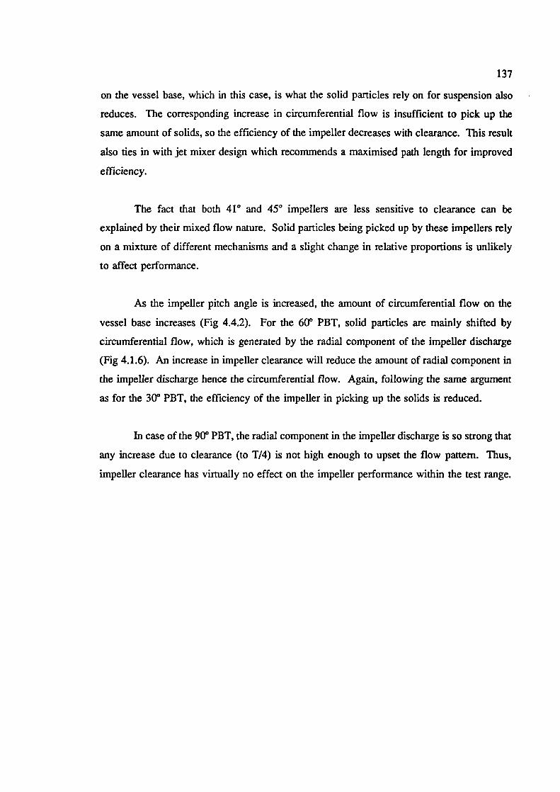
137

on the vessel base, which in this case, is what the solid particles rely on for suspension also

reduces. The corresponding increase in circumferential flow is insufficient to pick up the

same amount of solids, so the efficiency of the impeller decreases with clearance. This result

also ties in with jet mixer design which recommends a maximised path length for improved

efficiency.

The fact that both 41° and 450 impellers are less sensitive to clearance can be

explained by their mixed flow nature. Solid particles being picked up by these impellers rely

on a mixture of different mechanisms and a slight change in relative proportions is unlikely

to affect performance.

As the impeller pitch angle is increased, the amount of circumferential flow on the

vessel base increases (Fig 4.4.2). For the 600 PBT, solid particles are mainly shifted by

circumferential flow, which is generated by the radial component of the impeller discharge

(Fig 4.1.6). An increase in impeller clearance will reduce the amount of radial component in

the impeller discharge hence the circumferential flow. Again, following the same argument

as for the 30° PBT, the efficiency of the impeller in picking up the solids is reduced.

In case of the 90° PBT, the radial component in the impeller discharge is so strong that

any increase due to clearance (to T/4) is not high enough to upset the flow pattern. Thus,

impeller clearance has virtually no effect on the impeller performance within the test range.

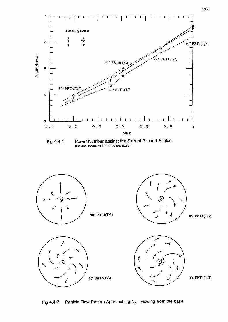
300 PBT4(T13) 450 PBT4(T13)

1384

3

I-V

Ez

2

C

1

Symbol Cicarance

C T/4f 1_ia

g T. FBT4/3)

PBT4/3)450 PBT4(T/3

e300 PBT4(T 0 PBT4(T/3)

o '-0.4 0.5 0.6 0.7 0.8 0.9 1.

Sin a

Fig 4.4.1

Power Number against the Sine of Pitched Angles(Po are measured in turbulent region)

7t\(t_

)600 PBT4) 900 FBT4(T13)

Fig 4.4.2 Particle Flow Pattern Approaching N - viewing from the base

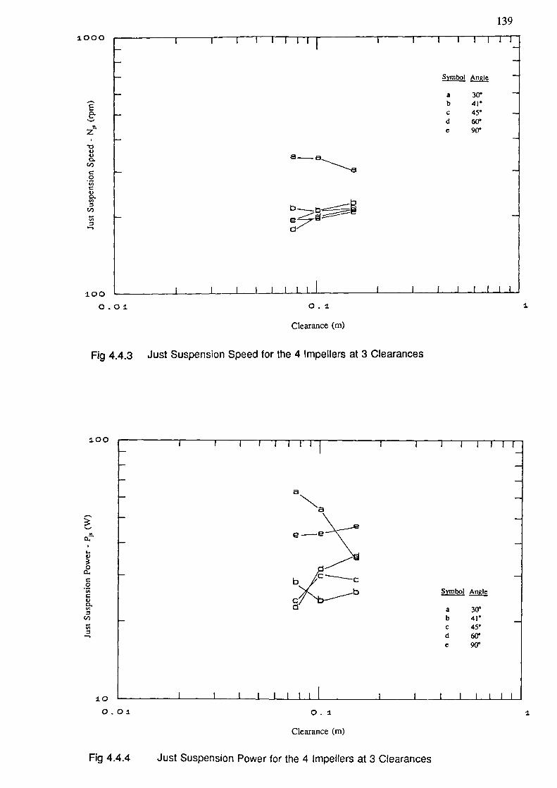
a -.__ a

E

z

.UU

C,,

0C,,

U

0,

C,)

0,

—C

- bEC

Symbol

a 30°b 41•C 45°d 60°e 90°

139

1000

I-4)

0

0U,

U0.ci,

C,)

U,

100 L-

0.01

0.1

I

Clearance (m)

Fig 4.4.3 Just Suspension Speed for the 4 Impellers at 3 Clearances

100

Na

ee

Symbol n!!

a 30°b 41°C 45°d 60°e 90°

10 '-

0.01 0.1

1

Clearance (m)

Fig 4.4.4 Just Suspension Power for the 4 Impellers at 3 Clearances

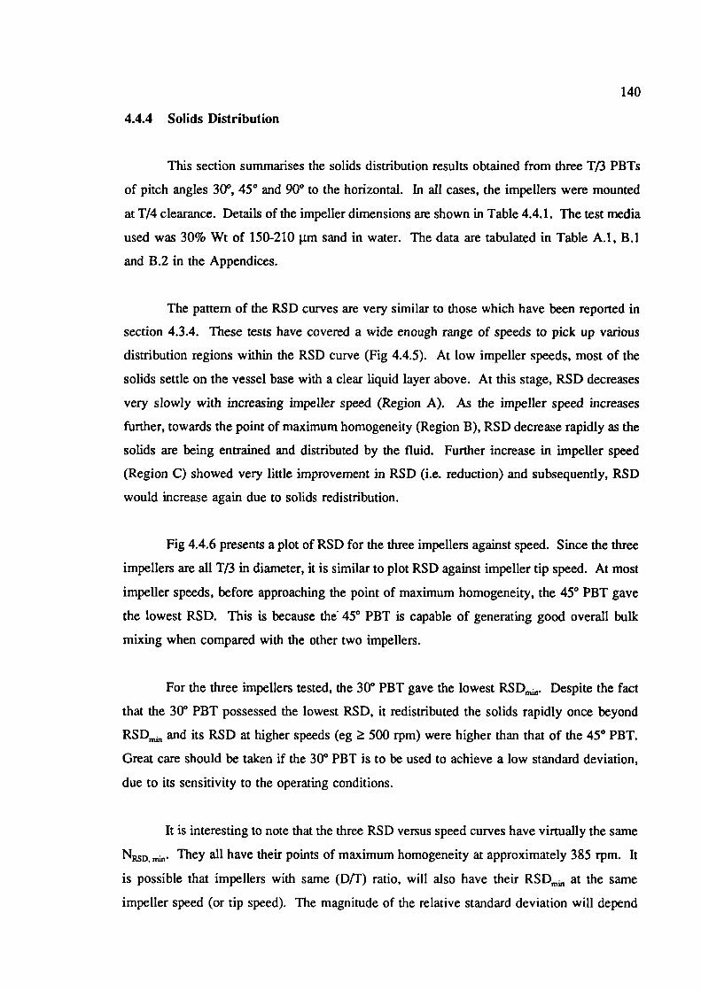
140


This section summarises the solids distribution results obtained from three T/3 PBTs

of pitch angles 300, 45° and 90° to the horizontal. In all cases, the impellers were mounted

at T/4 clearance. Details of the impeller dimensions are shown in Table 4.4.1. The test media

used was 30% Wt of 150-210 p.m sand in water. The data are tabulated in Table A.1, B.1

and B.2 in the Appendices.

The pattern of the RSD curves are very similar to those which have been reported in

section 4.3.4. These tests have covered a wide enough range of speeds to pick up various

distribution regions within the RSD curve (Fig 4.4.5). At low impeller speeds, most of the

solids settle on the vessel base with a clear liquid layer above. At this stage, RSD decreases

very slowly with increasing impeller speed (Region A). As the impeller speed increases

further, towards the point of maximum homogeneity (Region B), RSD decrease rapidly as the

solids are being entrained and distributed by the fluid. Further increase in impeller speed

(Region C) showed very little improvement in RSD (i.e. reduction) and subsequently, RSD

would increase again due to solids redistribution.

Fig 4.4.6 presents a plot of RSD for the three impellers against speed. Since the three

impellers are all T/3 in diameter, it is similar to plot RSD against impeller tip speed. At most

impeller speeds, before approaching the point of maximum homogeneity, the 45° PBT gave

the lowest RSD. This is because th& 450 PBT is capable of generating good overall bulk

mixing when compared with the other two impellers.

For the three impellers tested, the 30° PBT gave the lowest RSD,,.,. Despite the fact

that the 300 PBT possessed the lowest RSD, it redistributed the solids rapidly once beyond

RSD,,..,, and its RSD at higher speeds (eg ^ 500 rpm) were higher than that of the 45° PBT.

Great care should be taken if the 30° PBT is to be used to achieve a low standard deviation,

due to its sensitivity to the operating conditions.

It is interesting to note that the three RSD versus speed curves have virtually the same

N D ,,,,,,. They all have their points of maximum homogeneity at approximately 385 rpm. It

is possible that impellers with same (D/T) ratio, will also have their RSDmm at the same

impeller speed (or tip speed). The magnitude of the relative standard deviation will depend

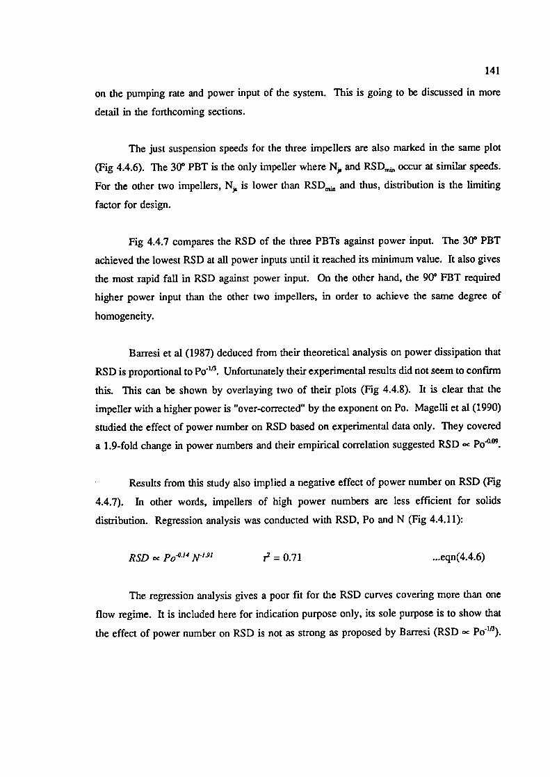
141

on the pumping rate and power input of the system. This is going to be discussed in more

detail in the forthcoming sections.

The just suspension speeds for the three impellers are also marked in the same plot

(Fig 4.4.6). The 30° PBT is the only impeller where N. and RSD IT.. occur at similar speeds.

For the other two impellers, N is lower than RSD,,,,,, and thus, distribution is the limiting

factor for design.

Fig 4.4.7 compares the RSD of the three PBTs against power input. The 30° PBT

achieved the lowest RSD at all power inputs until it reached its minimum value. It also gives

the most rapid fall in RSD against power input. On the other hand, the 90° FBT required

higher power input than the other two impellers, in order to achieve the same degree of

homogeneity.

Barresi et al (1987) deduced from their theoretical analysis on power dissipation that

RSD is proportional to Po 113 . Unfortunately their experimental results did not seem to confirm

this. This can be shown by overlaying two of their plots (Fig 4.4.8). It is clear that the

impeller with a higher power is "over-corrected" by the exponent on Po. Magelli et al (1990)

studied the effect of power number on RSD based on experimental data only. They covered

a 1.9-fold change in power numbers and their empirical correlation suggested RSD Po°°9.

Results from this study also implied a negative effect of power number on RSD (Fig

4.4.7). In other words, impellers of high power numbers are less efficient for solids

distribution. Regression analysis was conducted with RSD, Po and N (Fig 4.4.11):

RSD cc Po°'4 N's' r2 = 0.71 ...eqn(4.4.6)

The regression analysis gives a poor fit for the RSD curves covering more than one

flow regime. It is included here for indication purpose only, its sole purpose is to show that

the effect of power number on RSD is not as strong as proposed by Barresi (RSD cc Po).

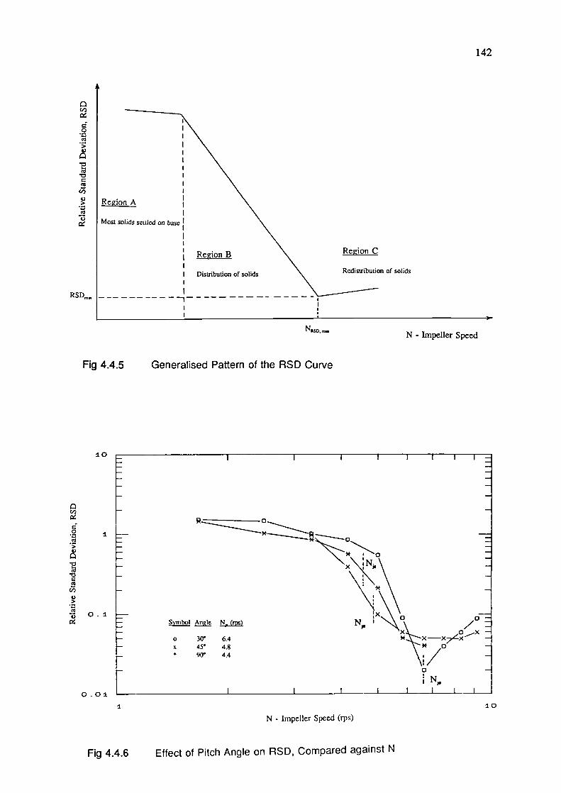
142

Region C

Redistribution of solids

0Co

4)

I R g ion A

Most solids settled on base

Region B

I Distribution of solids

RSDm.—I ---- --------- -

-—I

N - Impeller Speed

0,

0Co

I

Fig 4.4.5 Generalised Pattern of the RSD Curve

10

1.0.1

&!!!!^21 fl8i N. (rps)

o 30 6.4

x 45 4.8

* 90 4.4

0.01

,* oN, \

/0N

x7Lx

0

N,,,

I 10

N - Impeller Speed (rps)

Fig 4.4.6 Effect of Pitch Angle on RSD, Compared against N

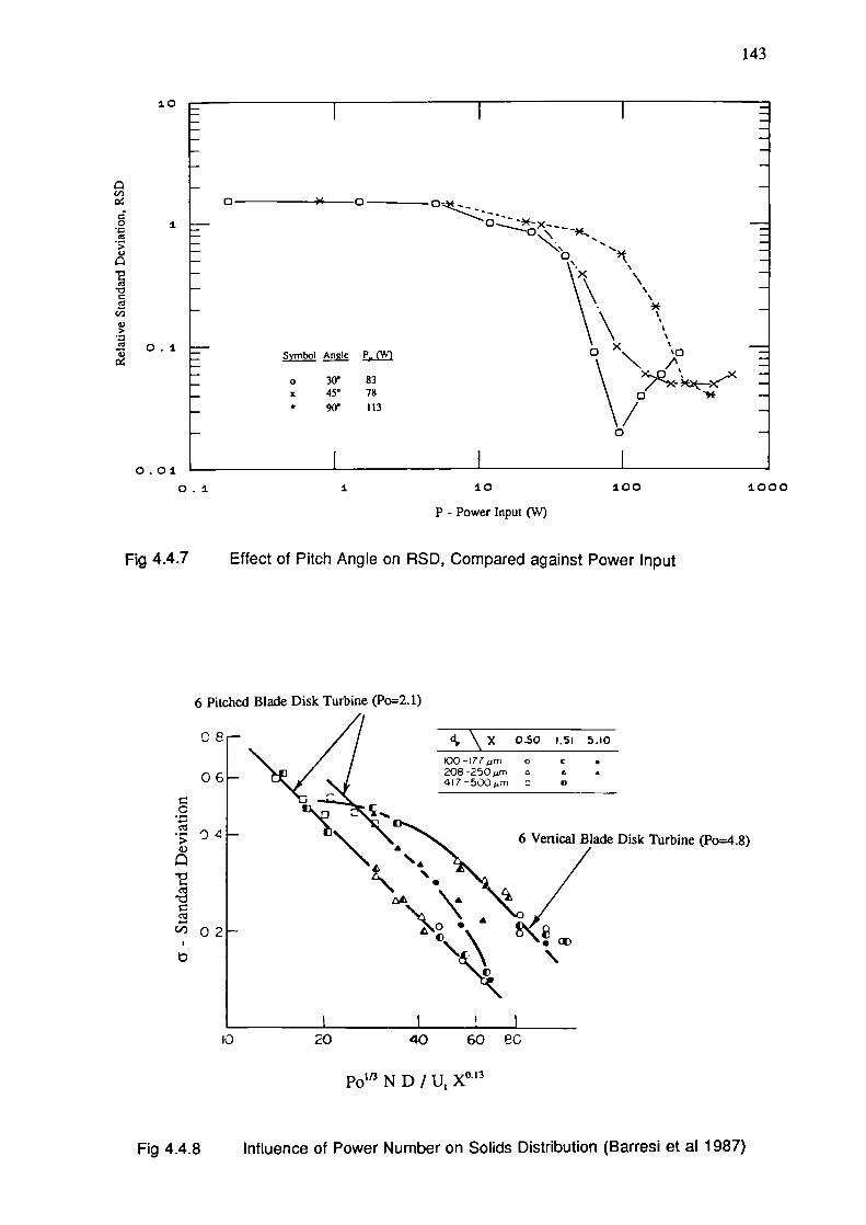
143

10

U,

I0.1

0 *

0

\'\\ 9

xI!!1iii! nzi 0 '0

\t

o 30 83x 45• 78* 90 113 /10

0

0.010.1 10 100 1000

P - Power Input (W)

Fig 4.4.7

Effect of Pitch Angle on RSD, Compared against Power Input

6 Pitched Blade Disk Turbine (Po=2.I)

Ce

06

0

04

02

20

d1 \ X 0.50 1.51 i.I0

O-177&m o c206-25Orn A £ -

4I7-5QOm ci

6 Vertical Blade Disk Turbine (Po=4.8)

40 60 ec

Po"3 N D I U1 X°13

Fig 4.4.8 Influence of Power Number on Solids Distribution (Barresi et al 1987)

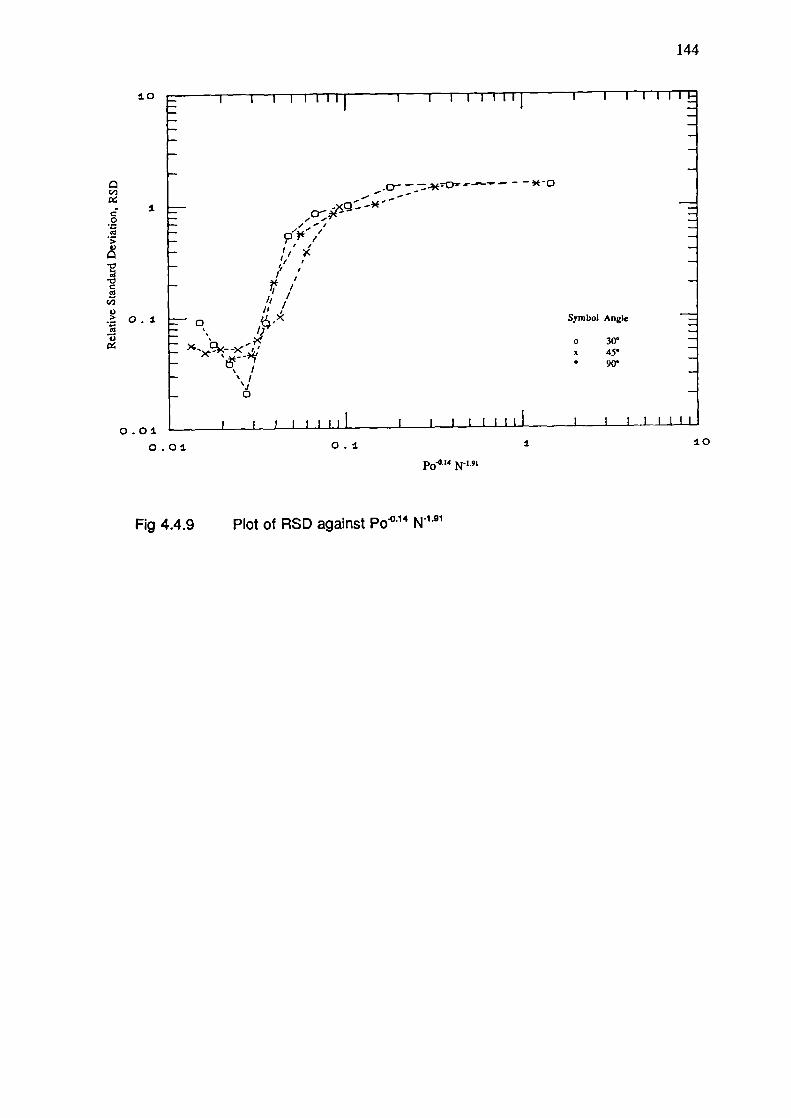
Symbol Angle

30•45.90

144

1.0

C,,

1.0

>4)

I. 0.1.

4)

_.Q--.30-' - —,-0

--

, /I , <

'I I

I'

'III /

I,

0 44X

>'i

0.01.

0.01. 0.1. 1.0

Po414 N9'

Fig 4.4.9 Plot of RSD against Po° 14 N191

145

4.5 DUAL IMPELLER SYSTEMS

Multiple impeller configurations are often adopted in stirid tank designs especially

where aspect ratios (i.e. HIT) are greater than one. It is generally believed that an additional

impeller will enhance the overall mixing of the vessel, the upper impeller helping to distribute

the solids throughout the tank and ease the suspension duty of the bottom impeller. Therefore,

the solids suspension and distribution performance should be improved.

However, despite the wide use of multiple impeller systems in industry, design

information is limited and research effort in the area has been small. For example, there is

no standard impeller spacing for solids suspension design and the improved performance with

an additional impeller has yet to be quantified. This section looks into the effects of an extra

impeller on solids suspension and distribution with the following objectives:

- To compare the performance between a variety of dual impeller configurations and

also with that of single impellers.

- To generalise the suspension and distribution results and to use the results to

improve knowledge of the solid-liquid mixing process.

- To make recommendations for future research, based on this initial work.

Two dual impeller systems, dual pitched and flat/pitched were included in this study.

They are all downward pumping. The three impellers were all T13 in diameter and

geometrical details can be found in Table 4.4.1. Configurations examined in this test program

are summarised in Table 4.5.1.

Lower impeller Upper Impeller

System 1 41° PBT4(T/3) No. 002-31-061 41° PBT4(T/3) No. 003-31-061

System 2 90° FBT4(T/3) No. 008-37-061 410 PBT4(T/3) No. 003-31-061

In all experiments, the bottom impeller position was fixed at a low clearance (C=T/8)

where it is likely to give good solids suspension performance and will allow mixing to

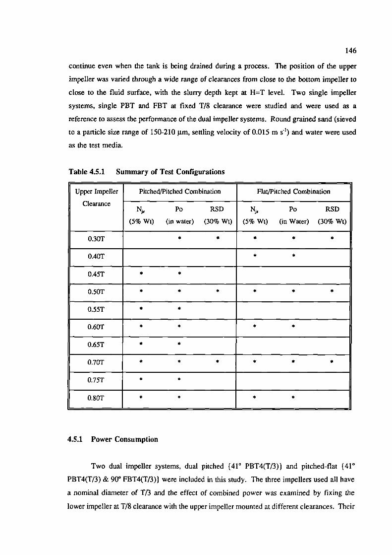
146

continue even when the tank is being drained during a process. The position of the upper

impeller was varied through a wide range of clearances from close to the bottom impeller to

close to the fluid surface, with the slurry depth kept at H=T level. Two single impeller

systems, single PBT and FBT at fixed T/8 clearance were studied and were used as a

reference to assess the performance of the dual impeller systems. Round grained sand (sieved

to a particle size range of 150-210 pPm, settling velocity of 0.0 15 m s') and water were used

as the test media.

Table 4.5.1 Summary of Test Conrigurations

Upper Impeller Pitched/Pitched Combination flat/Pitched Combination

ClearanceN Po RSD N, Po RSD

(5% Wi) (in water) (30% Wi) (5% Wt) (in Water) (30% Wt)

0.30T * * * * *

0.40T * *

0.45T * *

0.50T * * * * * *

0.55T * *

0.60T * * * *

0.65T * *

0.70T * * * * * *

O.75T * *

0.801' * * * *

4.5.1 Power Consumption

Two dual impeller systems, dual pitched (41° PBT4(T/3)) and pitched-flat (41°

PBT4(T/3) & 90° FBT4(T/3)} were included in this study. The three impellers used all have

a nominal diameter of T/3 and the effect of combined power was examined by fixing the

lower impeller at T/8 clearance with the upper impeller mounted at different clearances. Their

147

combined power numbers are tabulated in Table 4.5.2 and 4.5.3 and presented graphically in

Fig 4.5.1. The power dissipation of a dual impeller system depends upon two parameters;

impeller type and spacing between the two impellers. Fig 4.5.1 shows that the total power

drawn by the dual impeller combinations is always smaller than the sum of power of the two

impellers at T/8 and T/3 clearance (C=T/3 was highest upper clearance tested).

Bates et al (1963) examined the power characteristics of three dual impeller systems,

namely dual flat, pitched-flat and dual pitched. Results were plotted in terms of power ratio,

which was the combined power divided by power of a flat bladed turbine, against impeller

spacing (Fig 4.5.2). In all cases, the combined power approached some constant values,

which were either equal to (pitched-flat) or less than (dual flat and dual pitched) the

summation of the two single impeller powers when the spacings were greater than one

impeller diameter. However, the dual flat combination developed a total power almost 25%

greater than the sum of the two when the spacing was less than one diameter. This could due

to the fact that the two flat bladed turbines behaved as one when they were close together and

the effect of blade width on power is greater than linear proportionality (i.e. doubling the

blade width increases the power number by a factor of more than two).

In the forthcoming sections, solids suspension and distribution performance will be

compared in terms of power input. Instead of using the combined power numbers, which is

based on the nominal diameter, actual power input wifi be used. Since P = Po p N3 D5,

plotting power input against N 3 should give a straight line with slope of k and k = Po p D5

(Fig 4.5.3-4). Therefore, just suspension power of a configuration can be given as k N3.

4.5.2 Flow Pattern

The flow pattern of solids on the vessel base was examined by placing a mirror below

the vessel. It can differ dramatically from a single impeller system, depending on the impeller

clearances. Generally speaking, in the pitched-pitched configuration, radial flow is dominant

on the base (Fig 4.1.5-b). Increasing the spacing between the two impeller introduces slow

moving regions both at the centre and the circumference (eg Fig 4.5.6 C=O.7T).

Circumferential flow dominates in the pitched/flat combination. As the upper impeller

(pitched) is moved upwards, the central vortexing region increases and a certain amount of

radial flow between the central vortexing region and outer circumferential region is observed

148

(eg Fig 4.5.8 C1=O.7T). Detailed sketches of the particle flow pattern on the vessel base are

presented in Fig 4.5.6 and 4.5.8.

Flow visualisation tests of the whole vessel were conducted using PVC particles as

flow followers. In the case of dual pitched bladed turbines, if the two impellers were placed

very close together (eg < D apart), they behaved as a single unit but with an improved

pumping effect (Fig 4.5.13). If the pitched blade turbines were spaced further apart,

circulating zones as well as swirls were observed (Fig 4.5.15). The swirls were rotating anti-

clockwise looking inwards and were located somewhere between the two impellers. Their

exact position depended largely on impeller type and clearance between them. The swirls are

thought to be caused by interactions between the outflow of upper and lower impeller in

which the discharge from the upper impeller baullcs the circulation pattern of the lower

impeller. This is likely to be the reason why an additional impeller does not necessarily

reduce the just suspension speed (Sec 4.5.3).

The situation in a system equipped with a flat bladed turbine (lower) and a pitched

bladed turbine (upper) is similar except that the circulation zones are less apparent (Fig 4.5.13-

15). This is attributed to the lower pumping capacity with a flat bladed turbine as compared

to a pitched bladed turbine. Therefore, one can expect that the combined flow pattern of a

dual hydrofoil or upwards/downwards pumping pitched blade turbine systems would be very

different from that which has so far been examined (Fig 4.5.16-17).


The Po, N and P, data at 5% Wt solids concentration are tabulated in Table 4.5.2 for

pitched/pitched combination and in Table 4.5.3 for flat/pitched combination. The just

suspension results are also presented graphically in Fig 4.5.5 and 4.5.7. The just suspension

speeds at 30% Wt are referred to in the solids distribution section. They are calculated from

the 5% Wt and used Zwietering's correlation to correct for solids concentration: Nfr

Pitched/pitched Configuration

Referring to Fig 4.5.5, for most of the top impeller clearances tested, N results are

unexpectly higher than that of a single PBT at T/8 clearance (i.e. bottom impeller only).

149

There is a reduction in N,, only when the impeller spacing between the upper and lower

impellers exceeds 1.7 times the impeller diameter. The lowest dual impeller N, is recorded

when the upper impeller is mounted at the highest clearance tested (0.8T) where there is 3.5%

reduction in N,. Since the power drawn by a dual impeller system is approximately equal to

the summation of power consumed by the upper and lower impellers (section 4.5.1), it can

be seen that an increase in efficiency through using dual impellers is possible only when the

reduction in N, is greater than 21%.

Since? = Po pN3D5

i.e. P oc Po N,,,

Power number for pitched/pitched combination is roughly twice that of the single

pitched. In order to make the power input between the systems comparable, N, in the dual

impeller system has to be reduced:

P oc 2 Po N , dad

(Nfr thl (1 )1 - 0.79

•

Fig 4.5.9 presents a plot of just suspension power of dual pitched configuration at

different upper impeller clearances. The corresponding power for a single PBT at T/8

clearance (25 W) is marked on the same plot for comparison. At all impeller clearances

tested, P, for dual pitched configuration is higher than that of a single PBT, even when the

upper impeller is mounted near the fluid surface at which dual N, is less than that of single

N,. In other words, the reduction in N, with dual pitched configuration cannot outweigh the

increase in power consumption.

SinceP=27trN ,i.e.PoctN ...eqn(4.5.1)

As the increase in just suspension power is higher than the reduction in just suspension

speed, that means the impeller torque required to produce just suspension is greater in the dual

pitched configuration.

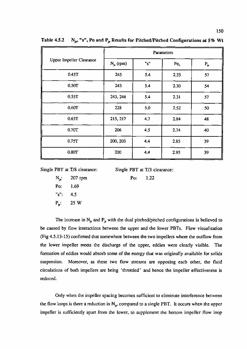
150

Table 4.5.2

"5", Po and P. Results for Pitched/Pitched Configurations at 5% Wt

Parameters

Upper Impeller ClearanceN5 (rpm) "s" Po

0.45T 245 5.4 2.33 57

0.50T 243 5.4 2.30 54

0.55T 243, 246 5.4 2.31 57

0.60T 228 5.0 2.52 50

0.65T 215, 217 4.7 2.84 48

0.701' 206 4.5 2.74 40

0.75T 200, 203 4.4 2.85 39

0.80T 200 4.4 2.95 39

Single PBT at T/8 clearance:

N: 207 rpm

Po: 1.69

"s": 4.5

P;: 25W

Single PBT at T/3 clearance:

Po: 1.22

The increase in N and Pa,, with the dual pitched/pitched configurations is believed to

be caused by flow interactions between the upper and the lower PBTs. Flow visualisation

(Fig 4.5.13-15) confirmed that somewhere between the two impellers where the outflow from

the lower impeller meets the discharge of the upper, eddies were clearly visible. The

formation of eddies would absorb some of the energy that was originally available for solids

suspension. Moreover, as these two flow streams are opposing each other, the fluid

circulations of both impellers are being 'throttled and hence the impeller effectiveness is

reduced.

Only when the impeller spacing becomes sufficient to eliminate interference between

the flow loops is there a reduction in N, compared to a single PBT. It occurs when the upper

impeller is sufficiently apart from the lower, to supplement the bottom impeller flow loop

151

instead of distorting it (Fig 4.5.15).

The plot of Po versus impeller clearance for the pitched/pitched configuration (Fig

4.5.1) consists of two nearly flax portions (below top impeller clearances of O.55T and above

top impeller clearance of O.65T) with a transition in between. The positions of the flat regions

and the transition correspond almost exactly to the flat regions and transitions in the N plot

(Fig 4.5.5). It is likely that as the upper impeller clearance is increased there is a change of

flow pattern and this change affects both power number and N.

Flat/Pitched Configuration

Referring to Fig 4.5.7, the behaviour of the flat/pitched configuration is very different

from that of the pitched/pitched configuration. Over the entire range of cLearances tested (0.3

to 0.8T), the just suspension speed for the flat/pitched configuration is less than that of a

single flat blade turbine at T/8 clearance. It starts at a relatively low value when the two

impellers are close together (i.e. 0.5D apart), rises to a maximum when they are approximately

one impeller diameter apart and then falls again as the spacing increases still further.

A possible explanation of the flat/pitched N results is that the two impellers behave

as one when they are in close proximity to each other. Their combined axial and radial flows

complement each other which facilitates the suspension of solids (Fig 4.5.8 C=O.3T to C=O.ST

and Fig 4.5.13). As the upper impeller clearance is increased, a recirculating loop forms

between the top and bottom impeller (Fig 4.5.14) which would undoubtedly absorb some of

the energy available for suspension. Any reduction in N, would obviously depend upon how

much of the bottom impeller's suction is being throttled and how much "help" the top impeller

can contribute to the suspension. As the upper impeller is raised, the recirculating loop moves

further away from the lower impeller and hence its influence is reduced. Coincidentally, the

suction of the upper impeller seems to entrain fluid from near the circumference of the vessel

(Fig 4.5.15-b) and this augments the discharge flow of the lower impeller hence reducing the

just suspension speed again.

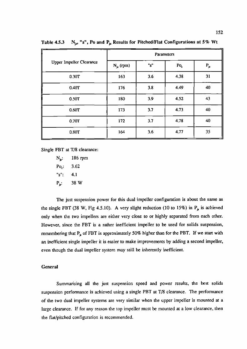
152

Table 4.5.3 "s", Po and P Results for Pitched/Flat Configurations at 5% Wt

Parameters

Upper Impeller Clearance N5 (rpm) "s" Po

0.301 163 3.6 4.38 31

0.401 176 3.8 4.49 40

0.50T 180 3.9 4.52 43

0.60T 173 3.7 4.73 4.0

0.70T 172 3.7 4.78 40

0.801 164 3.6 4.77 35

Single FBT at T/8 clearance:

N: 186 rpm

Poe : 3.62

"s": 4.1

P: 38W

The just suspension power for this dual impeller configuration is about the same as

the single FBT (38 W, Fig 4.5.10). A very slight reduction (10 to 15%) in P,, is achieved

only when the two impellers are either very close to or highly separated from each other.

However, since the FBT is a rather inefficient impeller to be used for solids suspension,

remembering that P, of FBI is approximately 50% higher than for the PBT. If we start with

an inefficient single impeller it is easier to make improvements by adding a second impeller,

even though the dual impeller system may still be inherently inefficient.

General

Summarising all the just suspension speed and power results, the best solids

suspension performance is achieved using a single PBT at T/8 clearance. The performance

of the two dual impeller systems are very similar when the upper impeller is mounted at a

large clearance. If for any reason the top impeller must be mounted at a low clearance, then

the flat/pitched configuration is recommended.

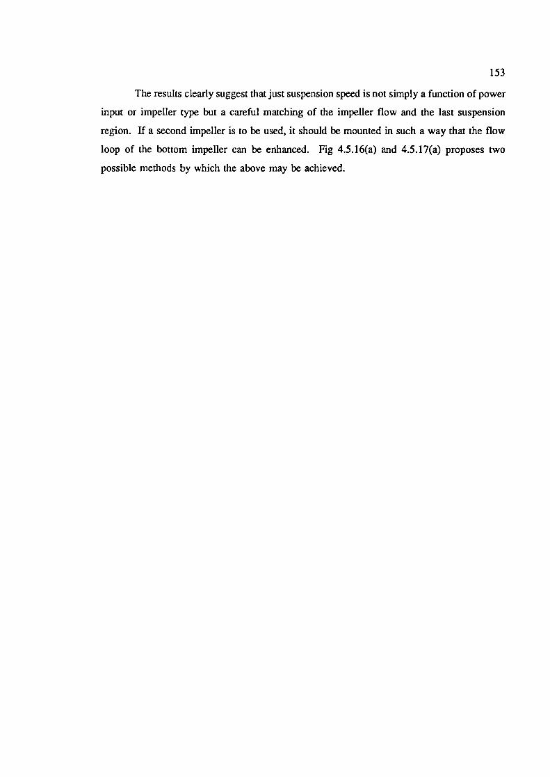
153

The results clearly suggest that just suspension speed is not simply a function of power

input or impeller type but a careful matching of the impeller flow and the last suspension

region. If a second impeller is to be used, it should be mounted in such a way that the flow

loop of the bottom impeller can be enhanced. Fig 4.5.16(a) and 4.5.17(a) proposes two

possible methods by which the above may be achieved.

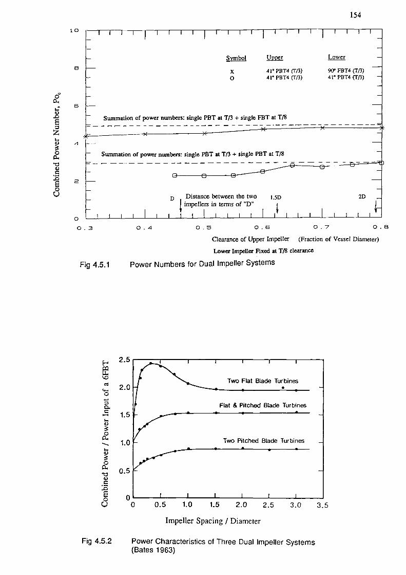
10

ou

6I-.

z

I-.'1) 4

0

.-E

200

154

8

00.3 0.4 0.5 0.6 0.7 0.8

Clearance of Upper Impeller (Fraction of Vessel Diameter)

Lower Impeller Fixed at T/8 clearance

Fig 4.5.1

Power Numbers for Dual Impeller Systems

F' 2.5

Two Flat Blade Turbines

Flat & Pitched Blade Turbines

Two Pitched Blade Turbines

d 0 0.5 1.0 1.5 2.0 2.5 3.0 3.5

Impeller Spacing / Diameter

Fig 4.5.2 Power Characteristics of Three Dual Impeller Systems(Bates 1963)

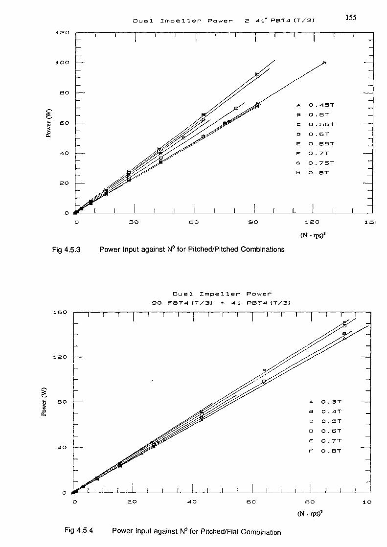
120

100

Dual Impeller Power 2 410 PBT4(T/3) 155

80

A 0.45T

B 0.5T60 C 0.56T

ID 06T

E 0.65T40 F 0.7T

G 0.75T

H 0.8T

20

0 I I I I I

0 30 60 90

Fig 4.5.3 Power Input against N 3 for Pitched/Pitched Combinations

120 151

(N-rps)3

Dual Impeller Powergo F674 (T/3) 4- 41 PBT4 (T/3)

.60

120

80 A 0.3T

a 0.4TC 0.ST

o 0.6T

E 0.7T40 F 0.8T

o0 20 40 60 60 10

(N - rps)3

Fig 4.5.4 Power Input against N 3 for Pitched/Flat Combination

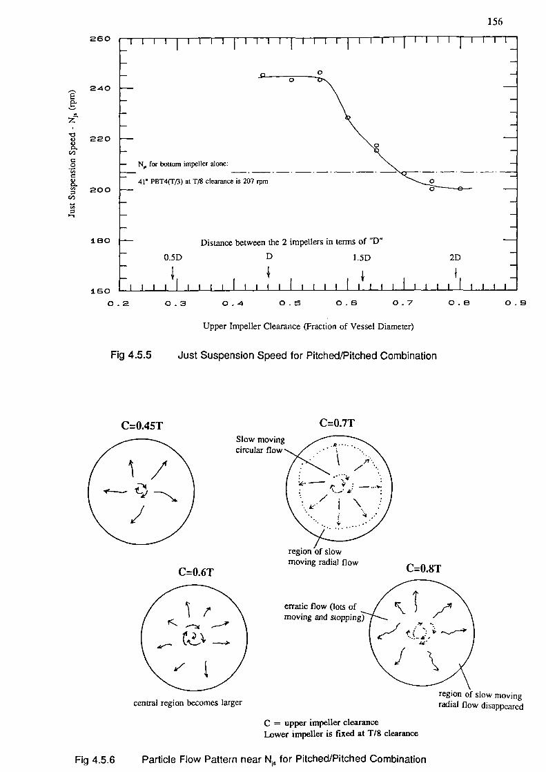
Slow movingcircular flow

C=O.6T

156

240

z

220I)0.

C,)

0

0. 200C,)

0

260

180

1.600.2

Fig 4.5.5

0.3 0.4 0.5 0.6 0.7 0.8 0.9

Upper Impeller Clearance (Fraction of Vessel Diameter)

Just Suspension Speed for Pitched/Pitched Combination

CO.45T

,c _-j1;9V-._- -*

C=O.7T

region of slowmoving radial flow

C=O.8T

erratic flow (lots ofmoving and stoppin

,___f

region of slow movingradial flow disappearedcentral region becomes larger

C = upper impeller clearanceLower impeller is fixed at T/8 clearance

Fig 4.5.6 Particle Flow Pattern near N1 for Pitched/Pitched Combination

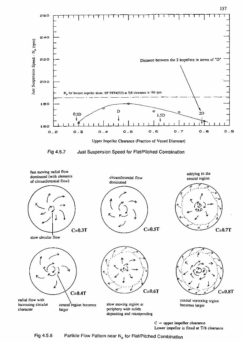
circumferential flowdominated

IC=O.5T0.3T

fast moving radial flowdominated (with elementsof circumferential flow)

slow circular flow

eddying in thecentral region

c

-a.

c=o7T

6T

157

240

2204)

c.#)

0

4)

200

260

180

1600.2 o.g

Fig 4.5.7

0.3 0.4 0.5 0.6 0.7 0.8


Just Suspension Speed for Flat/Pitched Combination

radial flow withincreasing circularcharacter

Fig 4.5.8

:' c:

.;.••'•i C=O.8T

central vortexing regioncentral 'region becomes slow moving region at becomes largerlarger periphery with solids

depositing and resuspending

C = upper impeller clearanceLower impeller is fixed at T/8 clearance

Particle Flow Pattern near N for Flat'Pitched Combination

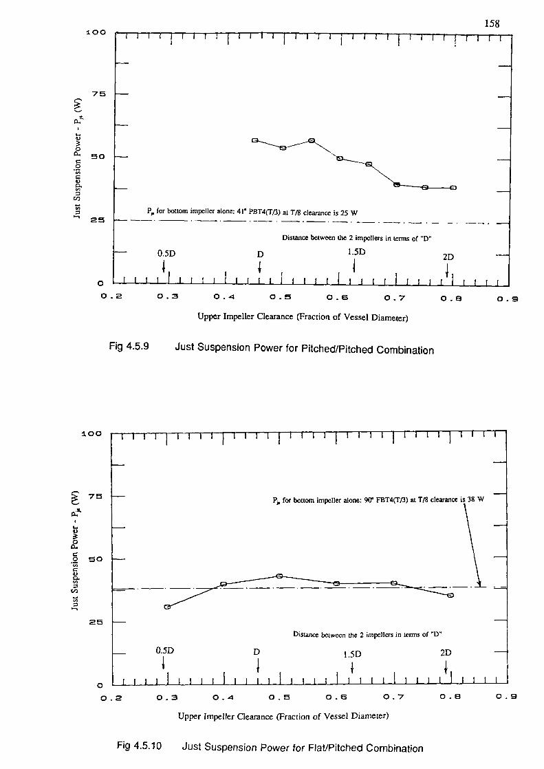
158100

75

0.

I-.V

050

00U,0V0.U,

C,,

U,

25

0

P, for bottom impeller alone: 41 PBT4çFJ3) at T/8 cleaj-ance is 25 W

Distance bctween the 2 impcllers in terms of D

O.5D D 1.5D2D

I I 1

__J IIII I 11(111111 ff11 (((I I I I I I

0.2 0.3 0.4 0.5 0.6 0.7 0.6 0.9


Fig 4.5.9 Just Suspension Power for Pitched/Pitched Combination

1.00

1', for bottom impeller alone: 9(r FBT4(F/3) at T18 clearance is 38 W

0• 50U,0V0.U,

C,)

U,

25Distance between the 2 impellers in Icons of D"

0.SD

D l.5D 2D

111 I I II 1 II 1! I I Ill

0.2 0.3 0.4 0.5 0.6 0.7 0.8


Fig 4.5.10 Just Suspension Power for Flat/Pitched Combination

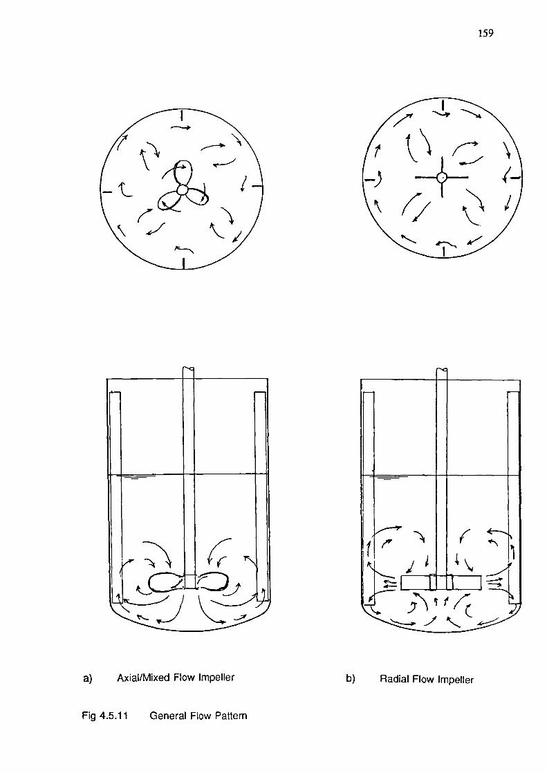
159

\

a) Axial/Mixed Flow Impeller

b) Radial Flow Impeller

Fig 4.5.11 General Flow Pattern

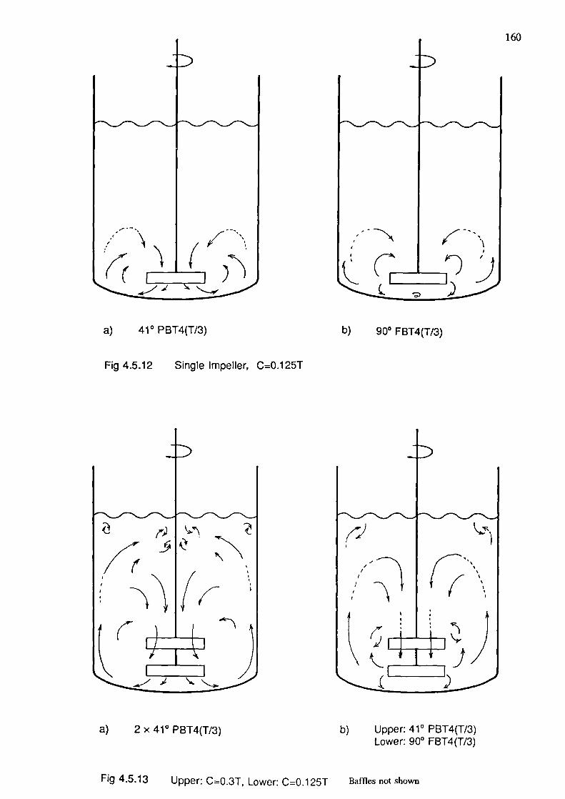
160

a) 41° PBT4(T/3)

b) 90° FBT4(T/3)

Fig 4.5.12 Single Impeller, C=0.125T

(:2I

'7()_J')

Ii

a) 2 x 41° PBT4(T/3)

b) Upper: 41° PBT4(T/3)Lower: 90° FBT4(T/3)

Fig 4.5.13 Upper: C=0.3T, Lower: C=0.125T Baffles not shown

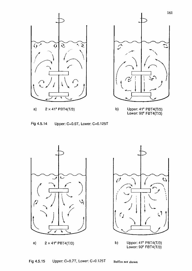
161

H 9)— .___J I '

a) 2x41°PBT4(T/3)

b) Upper: 41° PBT4(T/3)Lower: 900 FBT4(T/3)

Fig 4.5.14 Upper: C=0.5T, Lower: C=O.125T

1( I I

//_I\I' \__r1 I _'

..,"

__ }

a) 2x41°PBT4(T/3)

b) Upper: 41° PBT4(T/3)Lower: 900 FBT4(T/3)

Fig 4.5.15 Upper: C=0.7T, Lower: C0.125T Baffles not shown

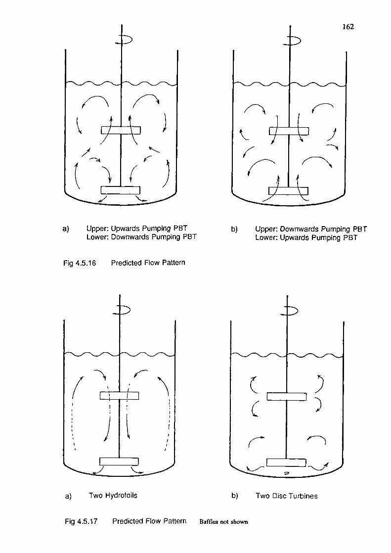
a) Upper: Upwards Pumping PBT

b)

Upper: Downwards Pumping PBTLower: Downwards Pumping PBT

Lower: Upwards Pumping PBT

Fig 4.5.16 Predicted Flow Pattern

a) Two Hydrotoils

b) Two Disc Turbines

Fig 4.5.17 Predicted Flow Pattern Baffles not shown

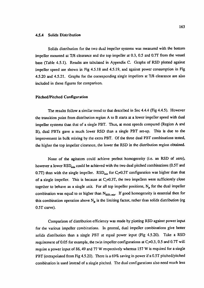
163


Solids distribution for the two dual impeller systems was measured with the bottom

impeller mounted at T/8 clearance and the top impeller at 0.3, 0.5 and 0.7T from the vessel

base (Table 4.5.1). Results are tabulated in Appendix C. Graphs of RSD plotted against

impeller speed are shown in Fig 4.5.18 and 4.5.19, and against power consumption in Fig

4.5.20 and 4.5.21. Graphs for the corresponding single impellers at T/8 clearance are also

included in these figures for comparison.

Pitched/Pitched Configuration

The results follow a similar trend to that described in Sec 4.4.4 (Fig 4.4.5). However

the transition point from distribution region A to B starts at a lower impeller speed with dual

impeller systems than that of a single PBT. Thus, at most speeds compared (Region A and

B), dual PBTs gave a much lower RSD than a single PBT set-up. This is due to the

improvement in bulk mixing by the extra PBT. Of the three dual PBT combinations tested,

the higher the top impeller clearance, the lower the RSD in the distribution region obtained.

None of the agitators could achieve perfect homogeneity (i.e. an RSD of zero),

however a lower RSD,,,,,, could be achieved with the two dual pitched combinations (0.5T and

0.7T) than with the single impeller. RSD for C1=0.3T configuration was higher than that

of a single impeller. This is because at C 1=O.3T, the two impellers were sufficiently close

together to behave as a single unit. For all top impeller positions, N for the dual impeller

combination was equal to or higher than N D . if good homogeneity is essential then for

this combination operation above N; is the limiting factor, rather than solids distribution (eg

0.5T curve).

Comparison of distribution efficiency was made by plotting RSD against power input

for the various impeller combinations. In general, dual impeller combinations give better

solids distribution than a single PBT at equal power input (Fig 4.5.20). Take a RSD

requirement of 0.05 for example, the twin impeller configurations at C=O.3, 0.5 and 0.7T will

require a power input of 86, 49 and 77 W respectively whereas 157 W is required for a single

PBT (extrapolated from Fig 4.5.20). There is a 69% saving in power if a 0.5T pitched/pitched

combination is used instead of a single pitched. The dual configurations also need much less

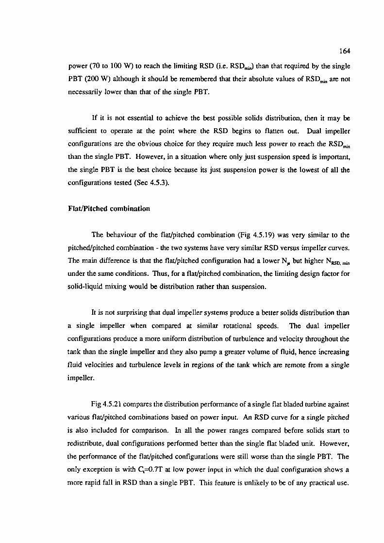
164

power (70 to 100 W) to reach the limiting RSD (i.e. RSD m .) than that required by the single

PBT (200 W) although it should be remembered that their absolute values of RSD mm are not

necessarily lower than that of the single PBT.

If it is not essential to achieve the best possible solids distribution, then it may be

sufficient to operate at the point where the RSD begins to flatten out. Dual impeller

configurations are the obvious choice for they require much less power to reach the RSD,,..,

than the single PBT. However, in a situation where only just suspension speed is important,

the single PBT is the best choice because its just suspension power is the lowest of all the

configurations tested (Sec 4.5.3).

Flat/Pitched combination

The behaviour of the flat/pitched combination (Fig 4.5.19) was very similar to the

pitched/pitched combination - the two systems have very similar RSD versus impeller curves.

The main difference is that the flat/pitched configuration had a lower N but higher ,

under the same conditions. Thus, for a flat/pitched combination, the limiting design factor for

solid-liquid mixing would be distribution rather than suspension.

It is not surprising that dual impeller systems produce a better solids distribution than

a single impeller when compared at similar rotational speeds. The dual impeller

configurations produce a more uniform distribution of turbulence and velocity throughout the

tank than the single impeller and they also pump a greater volume of fluid, hence increasing

fluid velocities and turbulence levels in regions of the tank which are remote from a single

impeller.

Fig 4.5.2 1 compares the distribution performance of a single flat bladed turbine against

various flat/pitched combinations based on power input. An RSD curve for a single pitched

is also included for comparison. In all the power ranges compared before solids start to

redistribute, dual configurations performed better than the single flat bladed unit. However,

the performance of the flat/pitched configurations were still worse than the single PBT. The

only exception is with C1=0.7T at low power input in which the dual configuration shows a

more rapid fall in RSD than a single PBT. This feature is unlikely to be of any practical use.

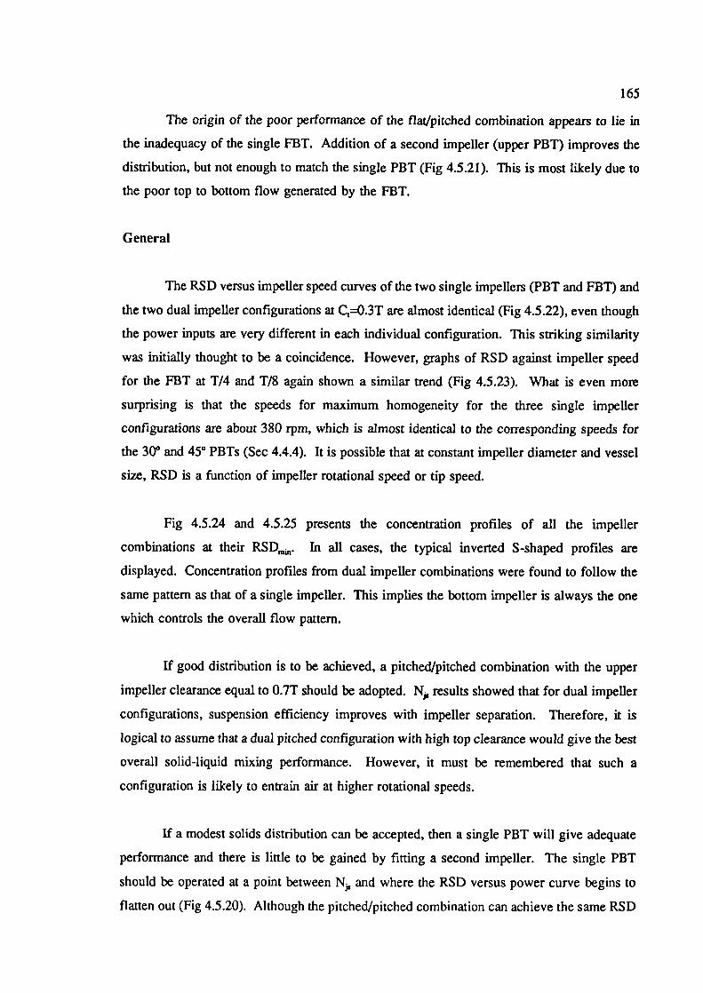
165

The origin of the poor performance of the flat/pitched combination appears to lie in

the inadequacy of the single FBT. Addition of a second impeller (upper PBT) improves the

distribution, but not enough to match the single PBT (Fig 4.5.21). This is most likely due to

the poor top to bottom flow generated by the FBT.

General

The RSD versus impeller speed curves of the two single impellers (PBT and FBI) and

the two dual impeller configurations at C 1=0.3T are almost identical (Fig 4.5.22), even though

the power inputs are very different in each individual configuration. This striking similarity

was initially thought to be a coincidence. However, graphs of RSD against impeller speed

for the FBT at T/4 and T/8 again shown a similar trend (Fig 4.5.23). What is even more

surprising is that the speeds for maximum homogeneity for the three single impeller

configurations are about 380 rpm, which is almost identical to the corresponding speeds for

the 300 and 45° PBTs (Sec 4.4.4). It is possible that at constant impeller diameter and vessel

size, RSD is a function of impeller rotational speed or tip speed.

Fig 4.5.24 and 4.5.25 presents the concentration profiles of all the impeller

combinations at their RSD,,...U . In all cases, the typical inverted S-shaped profiles are

displayed. Concentration profiles from dual impeller combinations were found to follow the

same pattern as that of a single impeller. This implies the bottom impeller is always the one

which controls the overall flow pattern.

If good distribution is to be achieved, a pitched/pitched combination with the upper

impeller clearance equal to 0.7T should be adopted. N,, results showed that for dual impeller

configurations, suspension efficiency improves with impeller separation. Therefore, it is

logical to assume that a dual pitched configuration with high top clearance would give the best

overall solid-liquid mixing performance. However, it must be remembered that such a

configuration is likely to entrain air at higher rotational speeds.

if a modest solids distribution can be accepted, then a single PBT will give adequate

performance and there is little to be gained by fitting a second impeller. The single PBT

should be operated at a point between N and where the RSD versus power curve begins to

flatten out (Fig 4.5.20). Although the pitched/pitched combination can achieve the same RSD

166

at lower power consumption, for some combinations it would have to operate below its Nft

(eg C1=O.7T), leaving a persistent region of unsuspended solids on the vessel base. To remove

these unsuspended solids requires a larger power input which subsequently may cause solids

redistribution.

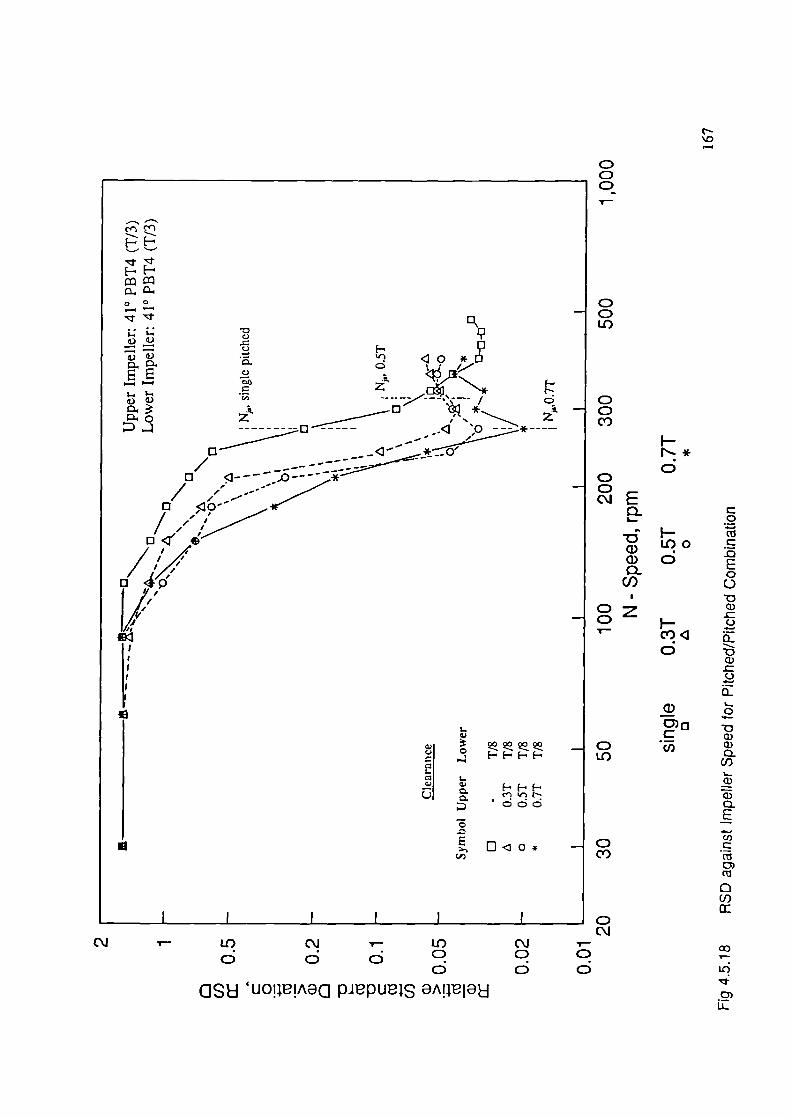
0

Cu

-oE00

a)

0

0

a)

0

0

0

0a)a)0

Ci)

a)a)0.E

C')

Cu0)Cu

0C/)cc

a)

0)IL.

LC)

00Co

00c'E

a-

C) LOC) 0a--

C',

0z7- Cl,l

0

S\0

R

F-.10*

.2

Cd -----;-----'c--- / q

0 .1 — — — —

•1-- — --

/

C)

j—

Dio *—

I I oC'J

CJ — Lt) C•\J ,— LI) CJ

d d Q Q 00 0 0

GSH 'uo!1iAec piepus eA!Ie}:j

o 0

— —

I-. $-

0

Ea-

a) LOQ) 0a-

zI-0)10

C)CD('4

00

0

CDCD0

00'0—I

çCfl

E-4H

o 0qQ

ELU—.--

0.. 0.. .

— — -- I,

.- ______D___ )

z/,,r

/7 )*

LI

00LU

00c)

C)0C

- (I)0000 C)

LU

c I L.

o coc.3

- 00)

I I('4

('4 LU ('4 10 (NCD 0 C) Q

0 dGSEI 'UO!!A9Q DJDUj3 OAIEjO}J

0)

LL)

0)IL

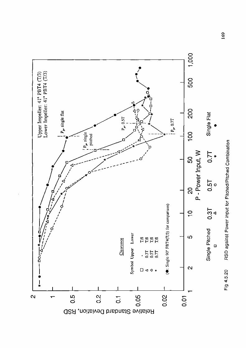
CDCDIC)

c'J

10

C)

C40C1G)

0

0

C1

IC)

C)C)1

0CDc'J Li

0)C

C/)

F—

C)

1-L1)0

0

F-

0

0

10

C0

-aE00

a)

0

a-

a)

0

U-4.-0

0C4.-0.)

0a-

U)Cc'j0)C',a(I)a:

Q

to

0)It.

C''-4

C)CDCD

/S

N,0

vil

C

o\I/. . D

- -, - - w-

. *•

CO- -

.p

//

/ 0

• /11, 0-

/ / ,

/

'0'/ D" '

/0'9O s' /

U

0.I

0Id'p//I

/

0

I'

I ', - -'II

0

CO

Do*

c\J LU C\i IC) C'J

0 CDC) CD

GS 'UO!!A8 PJPUS 'flIEI

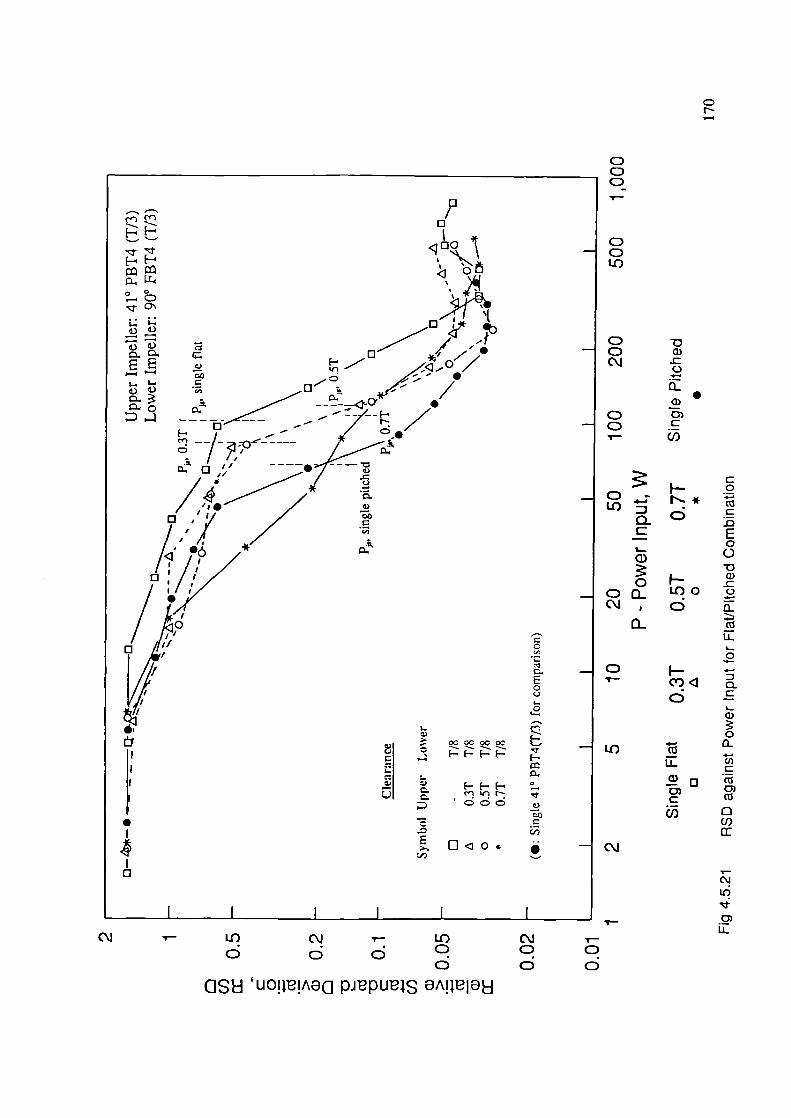
CD0LU

CD -oo C)

0C)S

oCD

C/)

LULL

0)C

C/)

c\j

1

C)L1

CD

CD

0 0 LOC\j • 0

0

0

0

0LU

C0cjC

E00-DC)0C-cTiLL10

a-CC)0a-U)C0)

aC/)cc

CN-4

CDCDCD

'p0

-

o

D ____ / '•

E C)

'-4 '-4- .

_ i-.

0) 0) 0

/

I - *0.

/ —i- I ''a "I, /0 , C_)

*

/1,. V0

I, , ! *//1 •

/I.ii

V,

I-

- • —-E-U c.

000.40

GSH 'UO!e!AeQeA!IeH

C

I-

ECU

CJ LU (J LU CJ

d d o Q

0 CD

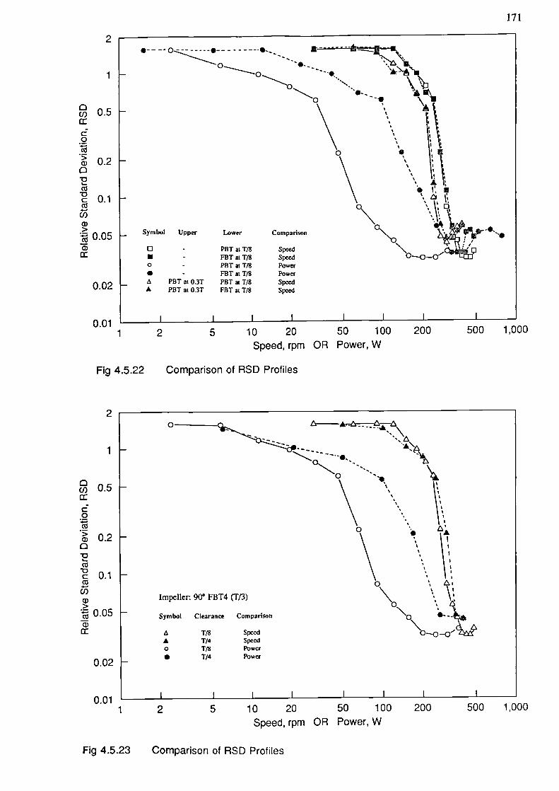
•____0-j_0_ --e-..----.--.- f -

- - •01

171

2

0 0.5

C0

>

0-D(

c 0.1(

C')a,>

0.05C,

0.02

Symbol Upper Lower Compa

o - PBTatT/8 Spee- FBTatT/8 Speed

o - PBT at 1/8 Power• - FBTatTI8 Power

PBT at O.3T P81 at 1/8 SpeedA PBT at O.3T FBI at 1/8 Speed

0.01 1 2 5 10 20 50 100 200

500 1,000

Speed, rpm OR Power, W

Fig 4.5.22 Comparison of RSD Profiles

2

1

0cj- 0.5ccC0

>a)a

c 0.1C',

C/)a,>

0.05C)cc

0.02

- -.-•-- - -

"S."." \\0\

\\\ \\

Impeller. 90° FBT4 (T/3)

vmhoI Clpar,,nr, Comnarison -

1/8 SpeedA 1/4 Speedo 1/8 Powcr• 1/4 Power

500 1,0000.01 I

I

1 2 5 10 20 50 100 200

Speed, rpm OR Power, W

Fig 4.5.23 Comparison of RSD Profiles

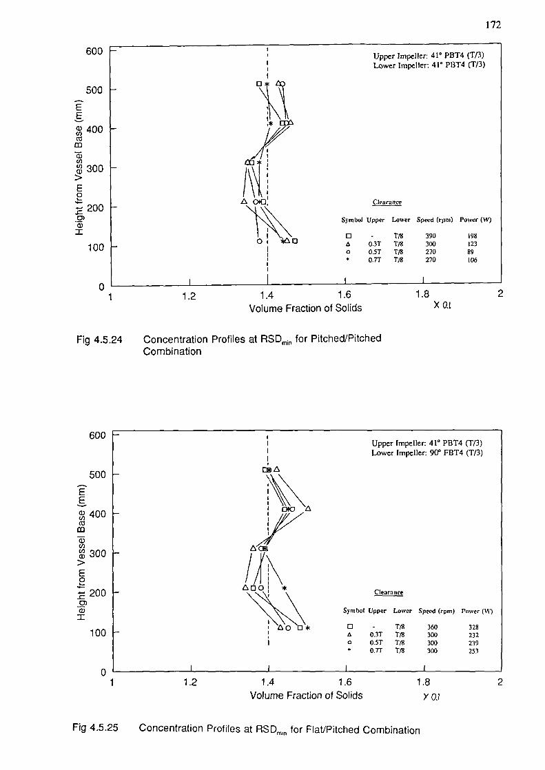
100

0'1

172

600 Upper Impeller: 41° PBT4 (T/3)Lower Impeller: 41° PBT4 (T/3)

500

EE

400CO

0)C',U)ci)

>

E0

200

D\

,* LEA

.oIa Clearance

Symbol Upper Lower Speed (rpm) Power (W)

o - 1/8 390 198A 0.31 T/8 300 123o 0.5T 1/8 270 89* 0.7T 1/8 270 106

1.2 1.4 1.6 1.8 2

Volume Fraction of Solids X 0.1

Fig 4.5.24

Concentration Profiles at RSD m1n for Pitched/PitchedCombination

600Upper Impeller: 41° PBT4 (T/3)Lower Impeller: 900 FBT4 (T/3)

500

EE

400CO

ca0)U,U)U)>

E0k..

2000)0)I

100

Ad"

//Ift\ADO' *

0*

Clearance

Symbol Upper Lower Speed (rpm) Power (W)

o - 1/8 360 328A 0.3T 1/8 300 232o 0.5T 1/8 300 239• 0.7T 1/8 300 253

0'1.2 1.4 1.6 1.8 2


Fig 4.5.25 Concentration Profifes at RSD m1n for Flat/Pitched Combination

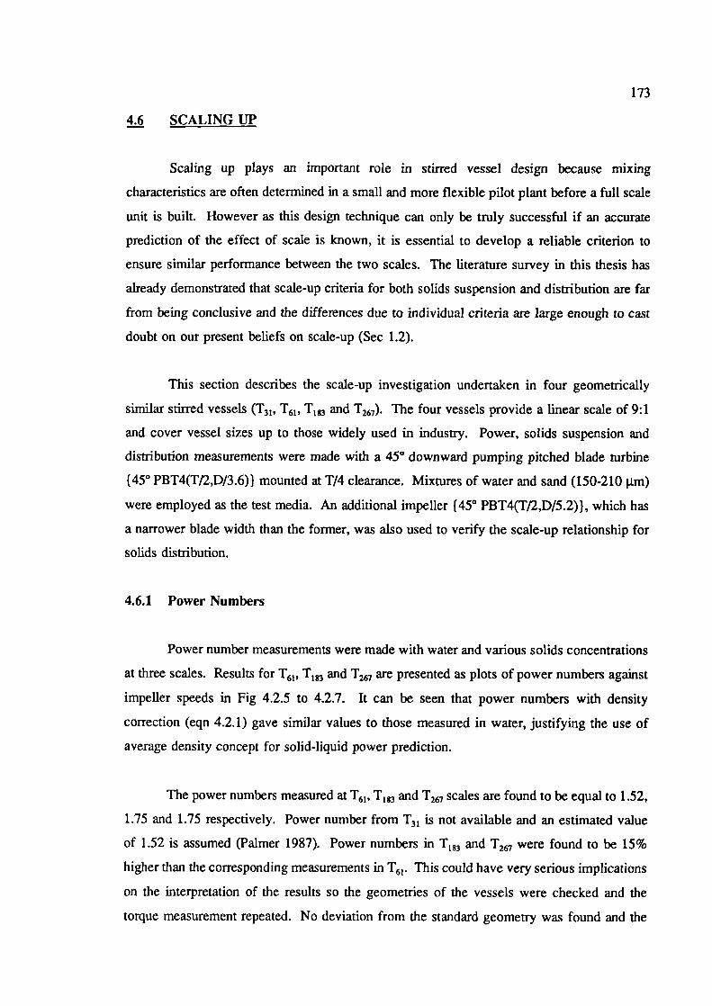
173

4_ SCALING UP

Scaling up plays an important role in stirred vessel design because mixing

characteristics are often determined in a small and more flexible pilot plant before a full scale

unit is built. However as this design technique can only be truly successful if an accurate

prediction of the effect of scale is known, it is essential to develop a reliable criterion to

ensure similar performance between the two scales. The literature survey in this thesis has

already demonstrated that scale-up criteria for both solids suspension and distribution are far

from being conclusive and the diffemnces due to individual criteria are large enough to cast

doubt on our present beliefs on scale-up (Sec 1.2).

This section describes the scale-up investigation undertaken in four geometrically

similar stirred vessels (T31, T61 , T1 and T267). The four vessels provide a linear scale of 9:1

and cover vessel sizes up to those widely used in industry. Power, solids suspension and

distribution measurements were made with a 45° downward pumping pitched blade turbine

(45° PBT4(Tf2,D/3.6) mounted at T/4 clearance. Mixtures of water and sand (150-210 jim)

were employed as the test media. An additional impeller f 45° PBT4(Tf2,D/5.2)), which has

a narrower blade width than the former, was also used to verify the scale-up relationship for

solids distribution.

4.6.1 Power Numbers

Power number measurements were made with water and various solids concentrations

at three scales. Results for T61 , T1 and T267 are presented as plots of power numbers against

impeller speeds in Fig 4.2.5 to 4.2.7. It can be seen that power numbers with density

correction (eqn 4.2.1) gave similar values to those measured in water, justifying the use of

average density concept for solid-liquid power prediction.

The power numbers measured ax T 61 , T1 and T267 scales are found to be equal to 1.52,

1.75 and 1.75 respectively. Power number from 'F31 is not available and an estimated value

of 1.52 is assumed (Palmer 1987). Power numbers in T1 and T267 were found to be 15%

higher than the corresponding measurements in T 61 . This could have very serious implications

on the interpretation of the results so the geometries of the vessels were checked and the

torque measurement repeated. No deviation from the standard geometry was found and the

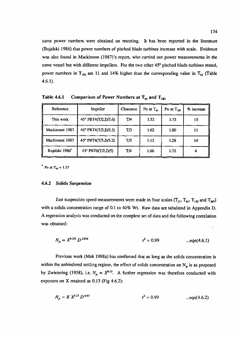
174

same power numbers were obtained on retesting. It has been reported in the literature

(Bujalski 1986) that power numbers of pitched blade turbines increase with scale. Evidence

was also found in Mackinnon (1987)'s report, who carried out power measurements in the

same vessel but with different impellers. For the two other 45° pitched blade turbines tested,

power numbers in T are 11 and 14% higher than the corresponding value in T61 (Table

4.6.1).

Table 4.6.1 Comparison of Power Numbers at T 61 and T1

Reference Impeller Clearance Po at T61 Po at T1 % increase

This work 45° PBT4(T12,Df3.6) T/4 1.52 1.75 15

Mackinnon 1987 45° PBT4(T/3,Df3.5) Tf3 1.62 1.80 11

Mackinnon 1987 45° PBT4(Tf3,D/5.2) Tf3 1.12 1.28 14

Bujaiski 1986 45° PBT6(T12,D/5) T/4 1.66 1.72 4

* Po at T4, = 1.57


Just suspension speed measurements were made in four scales T1, T1 and T7)

with a solids concentration range of 0.1 to 40% Wt. Raw data are tabulated in Appendix D.

A regression analysis was conducted on the complete set of data and the following correlation

was obtained:

N,, oc Xo•'25 D° 824

r2 = 0.99 ...eqn(4.6.1)

Previous work (Mak 1988a) has confirmed that as long as the solids concentration is

within the unhindered settling regime, the effect of solids concentration on N is as proposed

by Zwietering (1958), i.e. N oc X°'3. A further regression was therefore conducted with

exponent on X retained as 0.13 (Fig 4.6.2):

N, K X°'3 D°23 = 0.99 ...eqn(4.6.2)

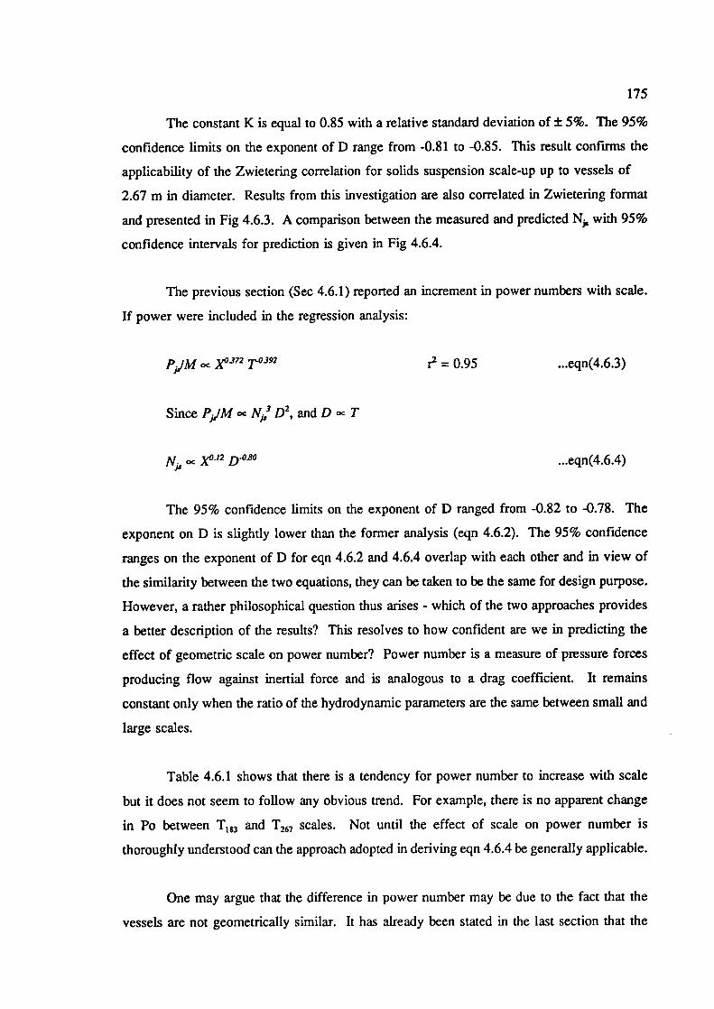
175

The constant K is equal to 0.85 with a relative standard deviation of ± 5%. The 95%

confidence limits on the exponent of D range from -0.81 to -0.85. This result confirms the

applicability of the Zwietering correlation for solids suspension scale-up up to vessels of

2.67 m in diameter. Results from this investigation are also correlated in Zwietering format

and presented in Fig 4.6.3. A comparison between the measured and predicted N, with 95%

confidence intervals for prediction is given in Fig 4.6.4.

The previous section (Sec 4.6.1) reported an increment in power numbers with scale.

If power were included in the regression analysis:

PJJ/M oc x0372 r2 = 0.95 ...eqn(4.6.3)

SincePjJMocN3D2,andDocT

Nfr OC X°•'2 D°2° ...eqn(4.6.4)

The 95% confidence limits on the exponent of D ranged from -0.82 to -0.78. The

exponent on D is slightly lower than the former analysis (eqn 4.6.2). The 95% confidence

ranges on the exponent of D for eqn 4.6.2 and 4.6.4 overlap with each other and in view of

the similarity between the two equations, they can be taken to be the same for design purpose.

However, a rather philosophical question thus arises - which of the two approaches provides

a better description of the results? This resolves to how confident are we in predicting the

effect of geometric scale on power number? Power number is a measure of pressure forces

producing flow against inertial force and is analogous to a drag coefficient. It remains

constant only when the ratio of the hydrodynamic parameters are the same between small and

large scales.

Table 4.6.1 shows that there is a tendency for power number to increase with scale

but it does not seem to follow any obvious trend. For example, there is no apparent change

in Po between T183 and T267 scales. Not until the effect of scale on power number is

thoroughly understood can the approach adopted in deriving eqn 4.6.4 be generally applicable.

One may argue that the difference in power number may be due to the fact that the

vessels are not geometrically similar. It has already been stated in the last section that the

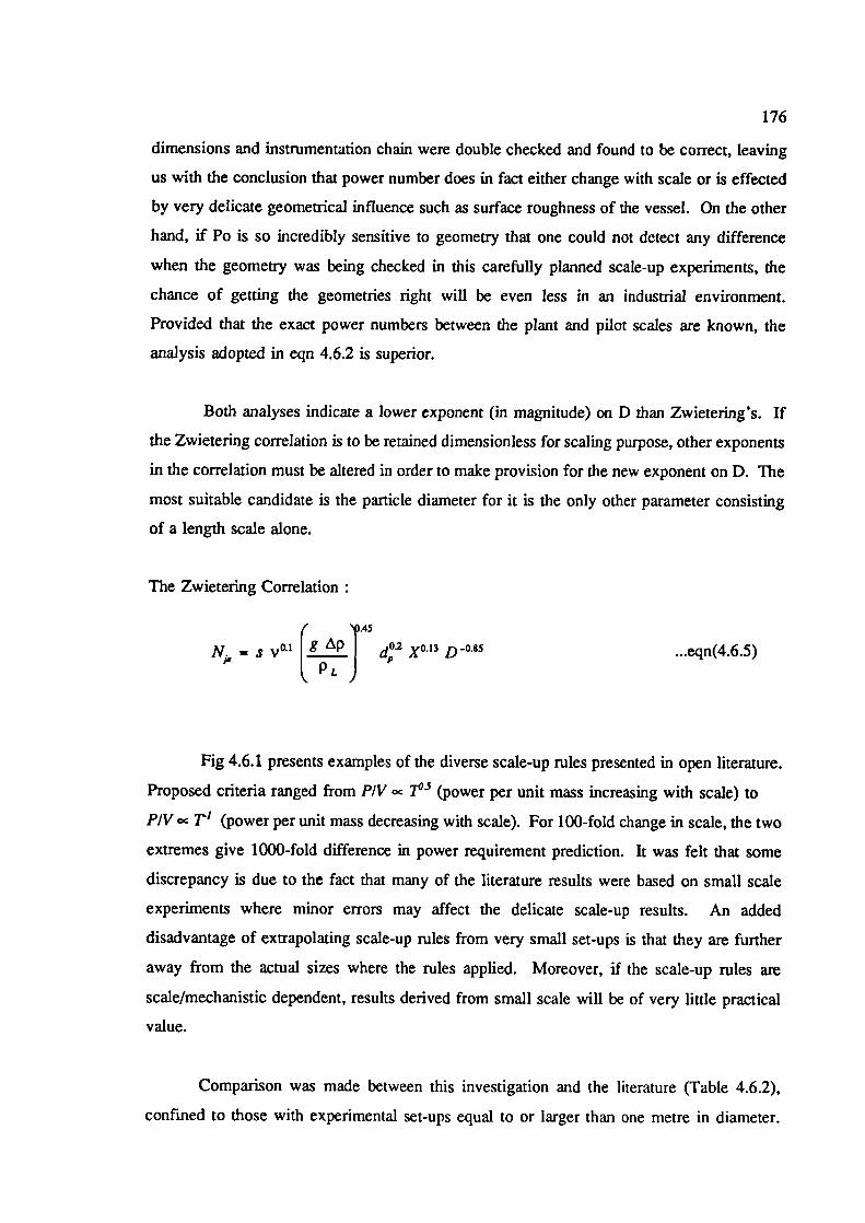
176

dimensions and instrumentation chain were double checked and found to be correct, leaving

us with the conclusion that power number does in fact either change with scale or is effected

by very delicate geometrical influence such as surface roughness of the vessel. On the other

hand, if Po is so incredibly sensitive to geometry that one could not detect any difference

when the geometry was being checked in this carefully planned scale-up experiments, the

chance of getting the geometries right will be even less in an industrial environment.

Provided that the exact power numbers between the plant and pilot scales are known, the

analysis adopted in eqn 4.6.2 is superior.

Both analyses indicate a lower exponent (in magnitude) on D than Zwietering's. If

the Zwietering correlation is to be retained dimensionless for scaling purpose, other exponents

in the correlation must be altered in order to make provision for the new exponent on D. The

most suitable candidate is the particle diameter for it is the only other parameter consisting

of a length scale alone.

The Zwietering Correlation:

II g pN = s v°'

J d°2 X° 13 D-° 85 ...eqn(4.6.5)

Fig 4.6.1 presents examples of the diverse scale-up rules presented in open literature.

Proposed criteria ranged from P/V 7' (power per unit mass increasing with scale) to

P/V oc 7" (power per unit mass decreasing with scale). For 100-fold change in scale, the two

extremes give 1000-fold difference in power requirement prediction. It was felt that some

discrepancy is due to the fact that many of the literature results were based on small scale

experiments where minor errors may affect the delicate scale-up results. An added

disadvantage of extrapolating scale-up rules from very small set-ups is that they are further

away from the actual sizes where the rules applied. Moreover, if the scale-up rules are

scale/mechanistic dependent, results derived from small scale will be of very little practical

value.

Comparison was made between this investigation and the literature (Table 4.6.2),

confined to those with experimental set-ups equal to or larger than one metre in diameter.

177

Zwietering's results (1958) is also included by virtue of its popularity. It was found that with

the exception of Chudacek (1986)'s results on flat base vessels, all the exponents on scale lie

roughly between -0.85 (Zwietering's correlation) and -0.67 (constant power per unit mass).

Chudacek's flat base results (N1, oc D°53) look somewhat doubtful because his correlation

predicted a particle size effect of d° on Ni,, which is higher than that is generally quoted

in the literature. Most results exhibited a change in exponent due to scale, impeller type,

concentration arid particle sizes (eg Zwietering, Herringe, Chudacek and Bujaiski). This

change is likely to be hydrodynamic/mechanistic driven. Results from this study are also

presented as plot of NjX°'3 against impeller diameter, with Zwietering, constant tip speed and

constant power input scale-up rules marked on the same plot for comparison.

Chudacek suggested that in the ideal case, mean upward velocity should be kept

constant in geometrically similar vessels, implying that constant tip speed should be used for

scaling up. Deviation from the ideal case decreases as the recirculation flow in a mixed tank

becomes structured so that systems with draft tubes approach the ideal scale up relationship.

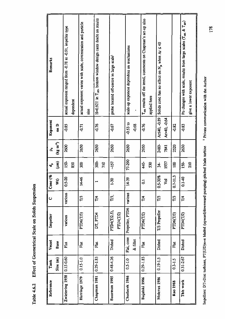
0

V

00

0ri

V

riD

U

VE0V

0

C)

'.0'I.V.0

0.

i0.

— 9 VIU

1) .

00 . 9VE

V9

o . 0 -9 0 U I-.

& 0)'a)

.2 a) 0

a)°2

a) ) I-'0. a,

0 0I.. C. a)

a-. & a)0. .0 bOO

-o.

U a)0

__ __ __ __ __ __ __ bOU V U

9

- '.0 00 '.0 • c'l en

00 N '0 '.0 N • 00 00

q q q cc q qq•

I,

E c o o c 6 - c c00 C' en

'.0 '.0 '.0 '.0 0'. '0

00\

en enN r& Cfl —N

'-. '.0 -en -- C? • -

0r-) . .

I-- .-' C) r. -

0

I•

'-4

C)

(I, .

en '.0 en00

('I 0 00 V '.0

, 9 - - - -'I; en -

— . '1

CID d 0 d 0

00 '000 00 00

C'. C,'

— — — — — C'. 0'. 000 - — C

V 0 —V 9 E E 0 •VV 0. - . .0

1 0 0

V .0 0 .0

N

00

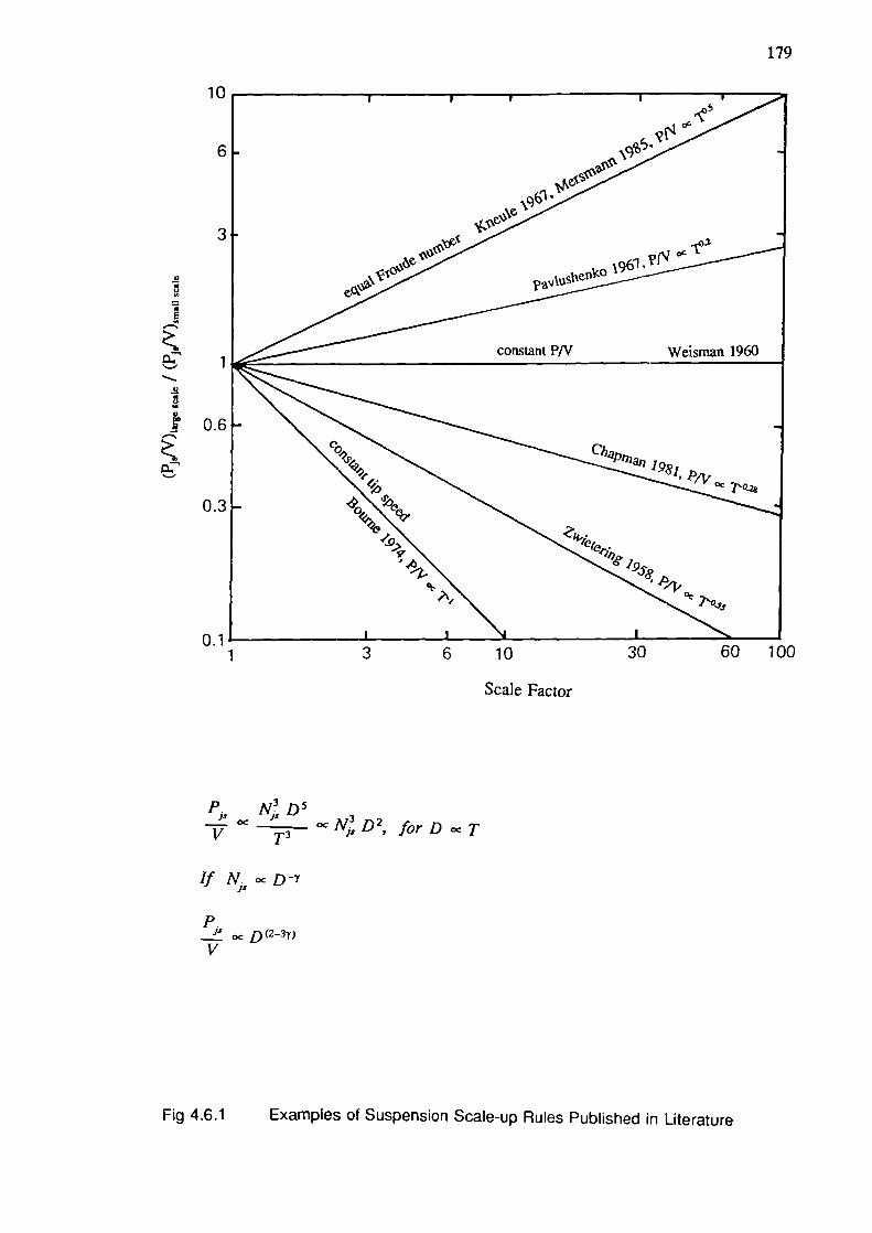
179

P. NDS3

is J- oc

V is

If tocDY

P.oc

V

forD ocT

3 6 10 30 60 100

Scale Factor

0

aE

1U

0.6

0.1

0.3

10

6

3

Fig 4.6.1 Examples of Suspension Scale-up Rules Published in Literature

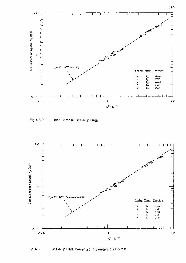
180

z0V4)0.

c/a

.9'C

C4)0.'C

c/a

N, o Xou D°25 (Zwictering Formal)C1

-,

10

-0VI)c.

(/)

0'C

4)0.

c/a

0.1

0.1

Fig 4.6.2

1

X°' 3 D°

Best Fit for all Scale-up Data

10

:1.0

7±-=

--

SymI Vessel Thnigue

x T, visualo T1 UDF+ T61 visual* T113 UDFw T, UDF

0 .1 L_.

0.1

1. 10

X°' 3 D°5

Fig 4.6.3 Scale-up Data Presented in Zwietering's Format

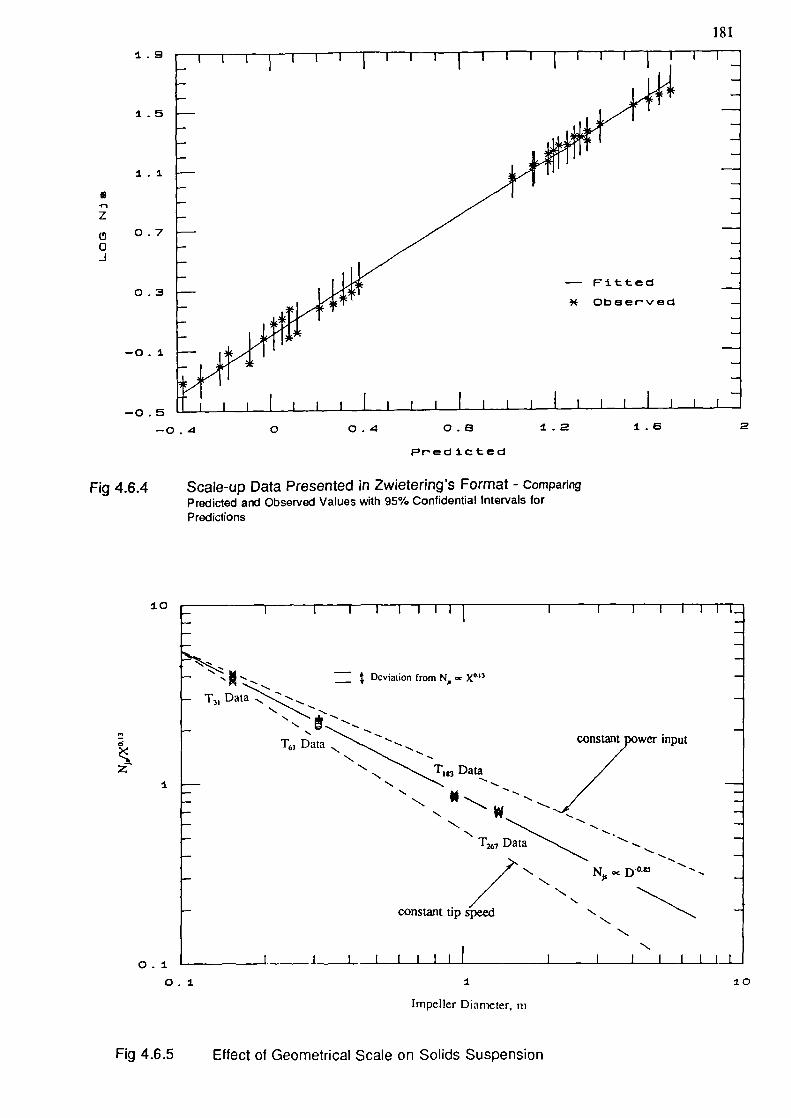
1.9

1.5

1.1

lfl

z

0.70J

0.3

-0 . 1.

-0 . 5-0.4 0 0.4 0.8 1.2

Pr-ed icted

Fig 4.6.4 Scale-up Data Presented in Zwieterings Format - ComparingPredicted and Observed Values with 95% Confidential Intervals forPredictions

1.6 2

10

1.

100.1

0.1 I

Impeller Dianeter, ni

181

Fig 4.6.5 Effect of Geometrical Scale on Solids Suspension

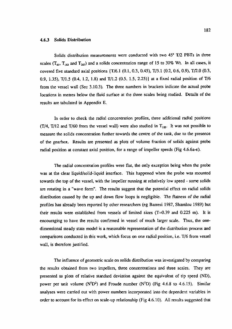
182


Solids distribution measurements were conducted with two 450 Tf2 PBTs in three

scales (T61 , T1 and 1267) and a solids concentration range of 15 to 30% Wt. In all cases, it

covered five standard axial positions (T/6.1 (0.1, 0.3, 0.45), T/3.l (0.2, 0.6, 0.9), T12.O (0.3,

0.9, 1.35), T/l.5 (0.4, 1.2, 1.8) and T/1.2 (0.5, 1.5, 2.25)) at a fixed radial position of T/6

from the vessel wall (Sec 3.10.3). The three numbers in brackets indicate the actual probe

locations in metres below the fluid surface at the three scales being studied. Details of the

results are tabulated in Appendix E.

In order to check the radial concentration profiles, three additional radial positions

(T/4, T/12 and 1/60 from the vessel wall) were also studied in 1183. It was not possible to

measure the solids concentration further towards the centre of the tank, due to the presence

of the gearbox. Results are presented as plots of volume fraction of solids against probe

radial position at constant axial position, for a range of impeller speeds (Fig 4.6.6a-e).

The radial concentration profiles were flat, the only exception being when the probe

was at the clear liquid/solid-liquid interface. This happened when the probe was mounted

towards the top of the vessel, with the impeller running at relatively low speed - some solids

are rotating in a "wave form". The results suggest that the potential effect on radial solids

distribution caused by the up and down flow loops is negligible. The flatness of the radial

profiles has already been reported by other researchers (eg Barresi 1987, Shamlou 1989) but

their results were established from vessels of limited sizes (T=0.39 and 0.225 m). It is

encouraging to have the results confirmed in vessel of much larger scale. Thus, the one-

dimensional steady state model is a reasonable representation of the distribution process and

comparisons conducted in this work, which focus on one radial position, i.e. T/6 from vessel

wall, is therefore justified.

The influence of geometric scale on solids distribution was investigated by comparing

the results obtained from two impellers, three concentrations and three scales. They are

presented as plots of relative standard deviation against the equivalent of tip speed (ND),

power per unit volume (N3D2) and Froude number (N2D) (Fig 4.6.8 to 4.6.15). Similar

analyses were carried out with power numbers incorporated into the dependent variables in

order to account for its effect on scale-up relationship (Fig 4.6.10). All results suggested that

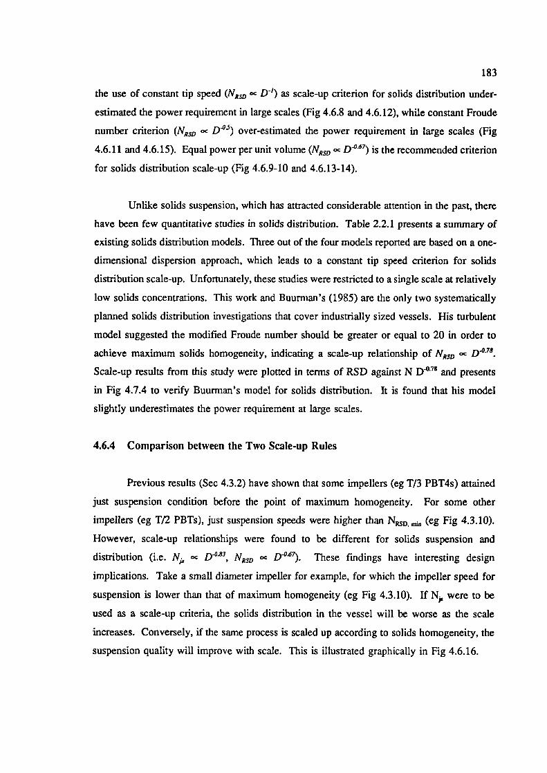
183

the use of constant tip speed (NRSD D') as scale-up criterion for solids distribution under-

estimated the power requirement in large scales (Fig 4.6.8 and 4.6.12), while constant Froude

number criterion (NR oc D°) over-estimated the power requirement in large scales (Fig

4.6.11 and 4.6.15). Equal power per unit volume (NRSD D° 67) is the recommended criterion

for solids distribution scale-up (Fig 4.6.9-10 and 4.6.13-14).

Unlike solids suspension, which has attracted considerable attention in the past, there

have been few quantitative studies in solids distribution. Table 2.2.1 presents a summary of

existing solids distribution models. Three out of the four models reported are based on a one-

dimensional dispersion approach, which leads to a constant tip speed criterion for solids

distribution scale-up. Unfortunately, these studies were restricted to a single scale at relatively

low solids concentrations. This work and Buurman's (1985) are the only two systematically

planned solids distribution investigations that cover industrially sized vessels. His turbulent

model suggested the modified Froude number should be greater or equal to 20 in order to

achieve maximum solids homogeneity, indicating a scale-up relationship of NRSD D°78.

Scale-up results from this study were plotted in terms of RSD against N D° 78 and presents

in Fig 4.7.4 to verify Buurman's model for solids distribution. It is found that his model

slightly underestimates the power requirement at large scales.

4.6.4 Comparison between the Two Scale-up Rules

Previous results (Sec 4.3.2) have shown that some impellers (eg T/3 PBT4s) attained

just suspension condition before the point of maximum homogeneity. For some other

impellers (eg T/2 PBTs), just suspension speeds were higher than N D ,, (eg Fig 4.3.10).

However, scale-up relationships were found to be different for solids suspension and

distribution (i.e. N oc D°23, N 0 oc D° 67). These findings have interesting design

implications. Take a small diameter impeller for example, for which the impeller speed for

suspension is lower than that of maximum homogeneity (eg Fig 4.3.10). If N were to be

used as a scale-up criteria, the solids distribution in the vessel will be worse as the scale

increases. Conversely, if the same process is scaled up according to solids homogeneity, the

suspension quality will improve with scale. This is illustrated graphically in Fig 4.6.16.

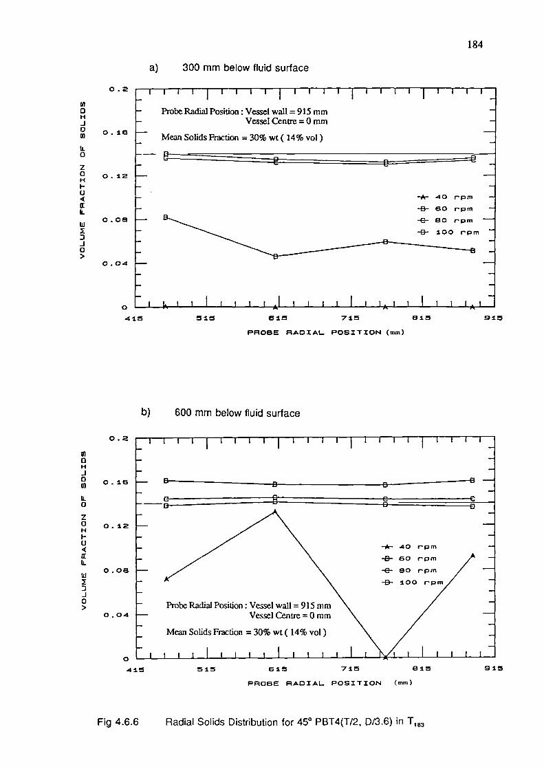
0.2

In0HJ

0.16

12.0z2 0.12

I-(J4

II.

0.08

I3-I0>

0.04

B

Probe Radial Position: Vessel wall = 915 mmVessel Centre =0 mm

Mean Solids Fraction = 30% wt (14% vol)

0.2

U,0HJ

0.18

0

z

2 0.12

I-U4

12.

lii 0.08I3J0>

0 .04

•-*- 40 rpm-9- 60 rpm-6-- 60 rpm-9- 100 rpm

184

a) 300 mm below fluid surface

b Pmbe Radial Position: Vessel wall = 915 mmVessel Centre = 0 mm


-A- 40 rpm-6- 60 rpm-6- 80 rpm-B- 100 rpm

0 I-416 516 615 715 815 916

PROBE RADIAL POSITION (mm)

b) 600 mm below fluid surface

O '-

415

615 616 715 815 915


Fig 4.6.6 Radial Solids Distribution for 45° PBT4(T/2, D/3.6) in T1

185

0.2

m0HJ

0.16

II.0z

0.12I-04a:Ii.Iii 0.08

3J0>

0 .04

0415 515 615 715 815 915


c) 900 mm below fluid surface

d) 1200 mm below fluid surface

0.2

UI0HJ

0.16

tL0z

0.12F-04a:IL

0 . 08Iii3I0>

0 .04

-*- 40 rpm-B- 60 rpm-9-- 80 rpm-9- 100 rpm Probe Radial Position: Vessel wall = 915 mm

Vessel Centie =0 mm


0415 515 615 715 815 915


Fig 4.6.6 Radial Solids Distribution for 45° PBT4(T/2, D/3.6) in T183

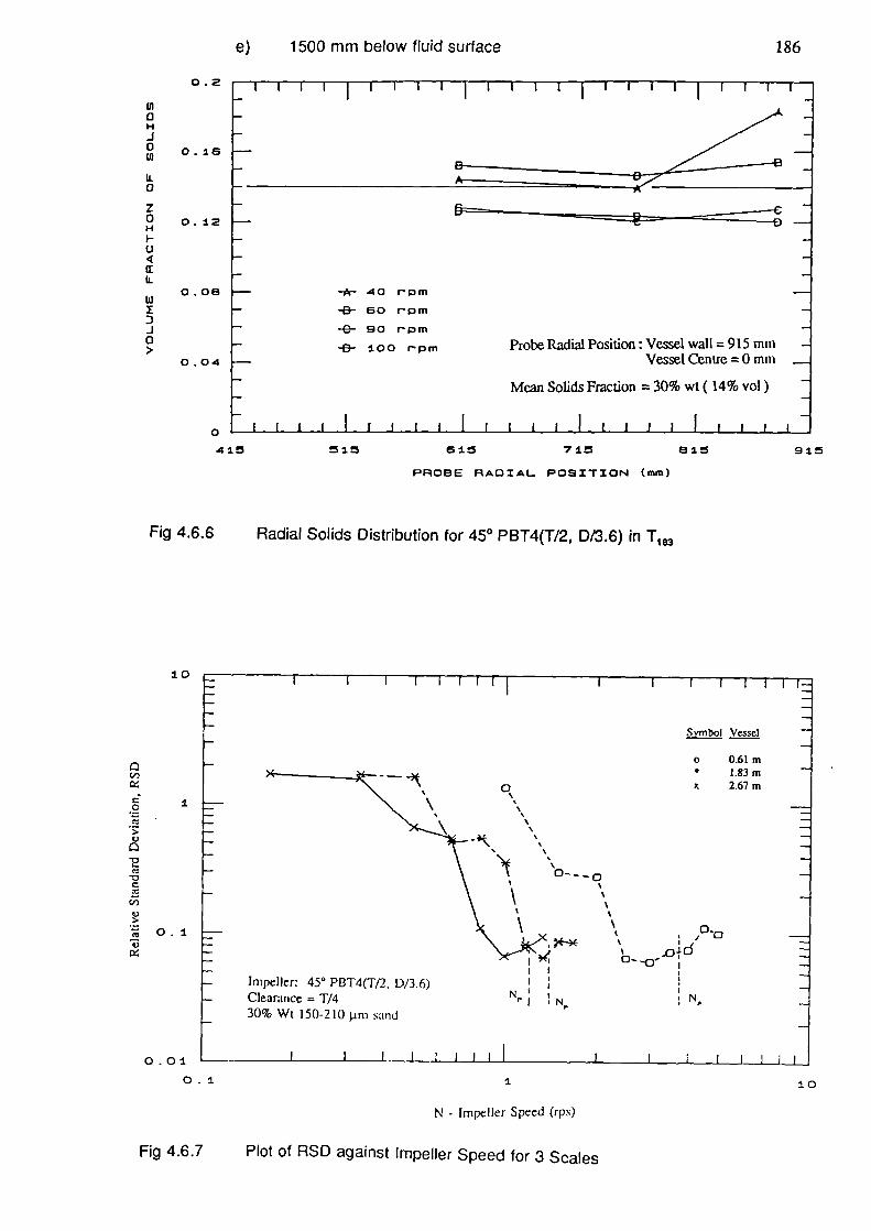
e) 1500 mm below fluid surface 186

0.2

U,0HJ0In 0.16

II-0

z0 0.12HI-U4a:IL.

0 .08IiiIJ0>

0.04

0415

Fig 4.6.6

Radial Solids Distribution for 45° PBT4(T/2, D/3.6) in T1

10

C,,

IC

>0

C/-i

U>

0.1U

0.01

0.1 I

N - Impel!er Speed (rps)

Fig 4.6.7 Plot of RSD against Impeller Speed for 3 Scales

10

515 61 715 815 915


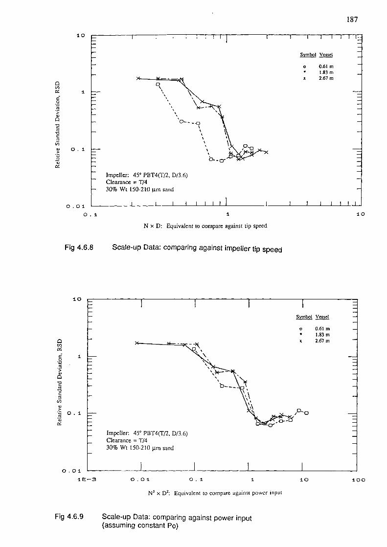
187

10

C/)I

CC

>t)

C

0.1

U

Impeller: 450 PBT4(T12, D/3.6)Clearance = T/430% Wt 150-210 sand

Symbol Vcsscl

o O.61m* I.83mx 2.67m

0.01 '- I

0.1 I

10


Fig 4.6.8

Scale-up Data: comparing against impeller tip speed

10

(fJ

I>U

0C

C/)U>

0. 1U

Symbol Vessel

o O.61m* 1.83mx 2.67m

0../ 0

0.01 L_.

1 E-3

Impeller: 45° PBT4(T/2, D/3.6)Clearance = T/430% Wt 150-210 im sand

0.01 0.1 1

N 3 x D2 : Equivalent to compare against power input

10 100

Fig 4.6.9 Scale-up Data: comparing against power input(assuming constant P0)

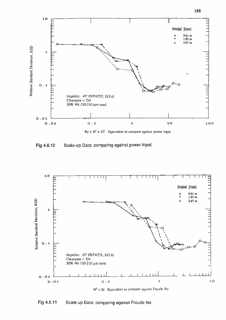
Impeller: 450 PBT4(T12, D13.6)Clearance = T/430% Wt 150-210 urn sand

188

10

(1)I

C0

>4)

C

C

0.1

4)

Symbol Vessel

o O.61m* l.83mx 2.67m

Impeller: 45° PBT4(T/2, D/3.6)Clearance = T/430% Wt 150-210 J.Lni sand

0.01. L__

0.01 0.1 1. 10 L)U

Po x N3 x D2: Equivalent to compare against power input

Fig 4.6.10 Scale-up Data: comparing against power input

10

('3

CC'3>I)

'30C'3

('35)>

0.14)

Symbol Vessel

o O.61m* 1.83m- 2.67m

0 . 0 1

0.01 0.1 1 10

N2 x D: Equivalent to compare agtinst Froude No

Fig 4.6.11 Scale-up Data: comparing against Froude No

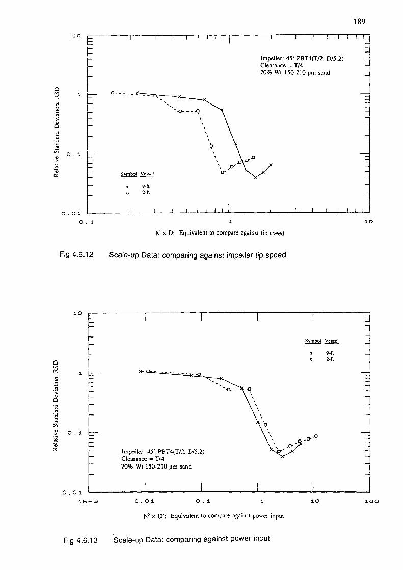
0_____

Symbol Vessel

x 9-ft0 2-ft

0

0CI)

1CC

>4)0

C')

CC')

C',

4)> 0.1C')

4)

lmpellClearance =20% Wt 150-2 10 pm sand

189

10

Impeller: 450 PBT4(T/2, D/5.2)Clearance T/420% Wt 150-210 pm sand

0(,j jcrC0

>4)00I-

•0C

CI) 0.14)>

0)

9-ft

0

2-ft

0.01 I-

0.1

1 10


Fig 4.6.12

Scale-up Data: comparing against impeller tip speed

10

0.01 '-IE-3 0.01 0.1 1 10 100

N3 x D): Equivalent to compare against power input

Fig 4.6.13 Scale-up Data: comparing against power input

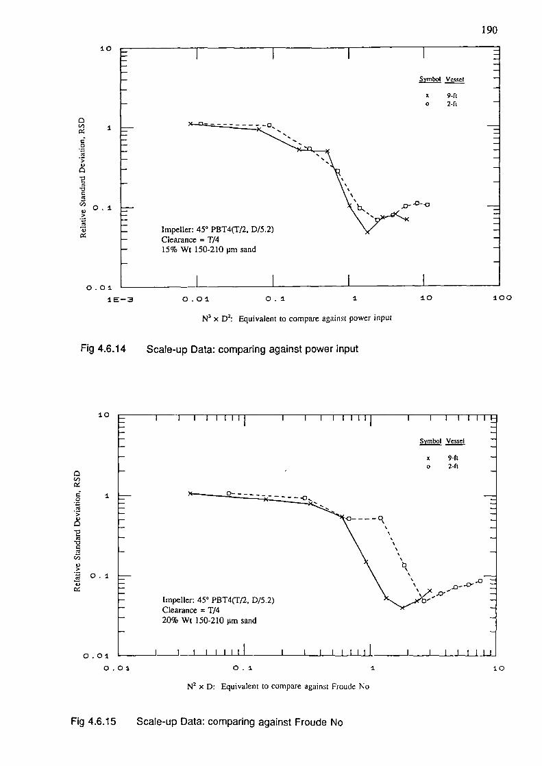
0C,.,

C0

>V0•0•0C

0.1

4) ImpelleClearance = T/415% Wt 150-210 pm sand

,0

0Cr3

I

>I)0

•0C

U,

I)>

• 0.14)

ImpelleC1earar,. -20% Wt 150-210 pm sand

190

10

Symbol Vessel

x 9-ft

0 2-ft

0.01 L.._

I E-3 0.01 0.1 1 10 100

N3 x D2: Equiva'ent to compare against power input

Fig 4.6.14

Scale-up Data: comparing against power input

10

Symbol Vessel

x 9-ft

0 2-ft

0.01 '-0.01 01

10

N2 x D: Equivalent to compare against Froude No

Fig 4.6.15 Scale-up Data: comparing against Froude No

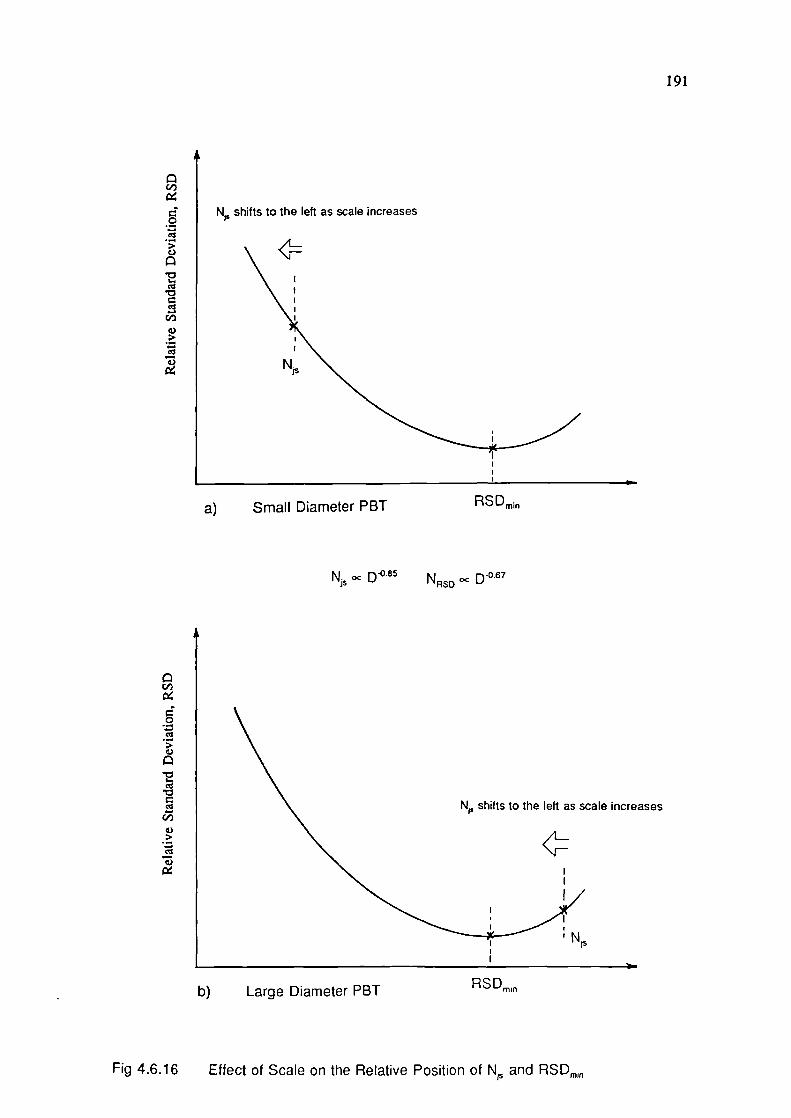
C/)

0

C)

C)

-a

C)

C#D

0

C)

CC

CC

'1,

C)>

CC

C)

ases

191

a) Small Diameter PBT RSDmjn

oc D° 85 NRSD oc D°67

b) Large Diameter PBT RSDmin

Fig 4.6.16 Effect of Scale on the Relative Position of N1 and RSDmJn

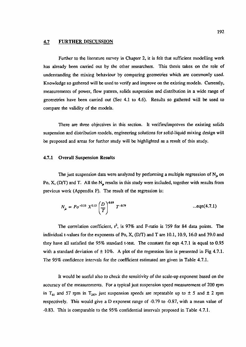
192

&7 FURTHER DISCUSSION

Further to the literature survey in Chapter 2, it is felt that sufficient modelling work

has already been carried out by the other researchers. This thesis takes on the role of

understanding the mixing behaviour by comparing geometries which are commonly used.

Knowledge so gathered will be used to verify and improve on the existing models. Currently,

measurements of power, flow pattern, solids suspension and distribution in a wide range of

geometries have been carried out (Sec 4.1 to 4.6). Results so gathered will be used to

compare the validity of the models.

There aie three objectives in this section. It verifies/improves the existing solids

suspension and distribution models, engineering solutions for solid-liquid mixing design will

be proposed and areas for further study will be highlighted as a result of this study.

4.7.1 Overall Suspension Results

The just suspension data were analyzed by performing a multiple regression of N on

Po, X, (D/T) and T. All the N results in this study were included, together with results from

previous work (Appendix F). The result of the regression is:

N oc Po° 33 X° 13 D "-°

...eqn(4.7.1)

The correlation coefficient, r2, is 97% and F-ratio is 759 for 84 data points. The

individual t-values for the exponents of Po, X, (D/T) and T are 10.1, 10.9, 16.0 and 39.0 and

they have all satisfied the 95% standard t-test. The constant for eqn 4.7.1 is equal to 0.95

with a standard deviation of ± 10%. A plot of the regression line is presented in Fig 4.7.1.

The 95% confidence intervals for the coefficient estimated are given in Table 4.7.1.

It would be useful also to check the sensitivity of the scale-up exponent based on the

accuracy of the measurements. For a typical just suspension speed measurement of 200 rpm

in T61 and 57 rpm in T267, just suspension speeds are repeatable up to ± S and ± 2 rpm

respectively. This would give a D exponent range of -0.79 to -0.87, with a mean value of

-0.83. This is comparable to the 95% confidential intervals proposed in Table 4.7.1.

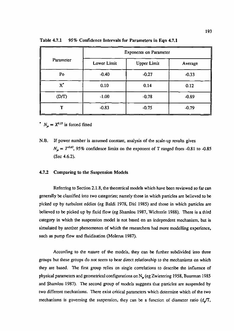
193

Table 4.7.1 95% Confidence Intervals for Parameters in Eqn 4.7.1

Exponents on Parameter

Parameter .Lower Limit Upper Limit Average

Po -0.40 -0.27 -0.33

X 0.10 0.14 0.12

(Dir) -1.00 -0.78 -0.89

T -0.83 -0.75 -0.79

Nfr oc X°'3 is forced fitted

N.B. If power number is assumed constant, analysis of the scale-up results gives

N oc T°-, 95% confidence limits on the exponent of T ranged from -0.81 to -0.85

(Sec 4.6.2).

4.7.2 Comparing to the Suspension Models

Referring to Section 2.1.8, the theoretical models which have been reviewed so far can

generally be classified into two categories; namely those in which particles are believed to be

picked up by turbulent eddies (eg Baldi 1978, Did 1985) and those in which particles are

believed to be picked up by fluid flow (eg Shamlou 1987, Wichterle 1988). There is a third

category in which the suspension model is not based on an independent mechanism, but is

simulated by another phenomenon of which the researchers had more modelling experience,

such as pump flow and fluidisation (Molerus 1987).

According to the nature of the models, they can be further subdivided into three

groups but these groups do not seem to bear direct relationship to the mechanisms on which

they are based. The first group relies on single correlations to describe the influence of

physical parameters and geometrical configurations on N (eg Zwietering 1958, Buurman 1985

and Shamlou 1987). The second group of models suggests that particles are suspended by

two different mechanisms. There exist critical parameters which determine which of the two

mechanisms is governing the suspension, they can be a function of diameter ratio (d/F,

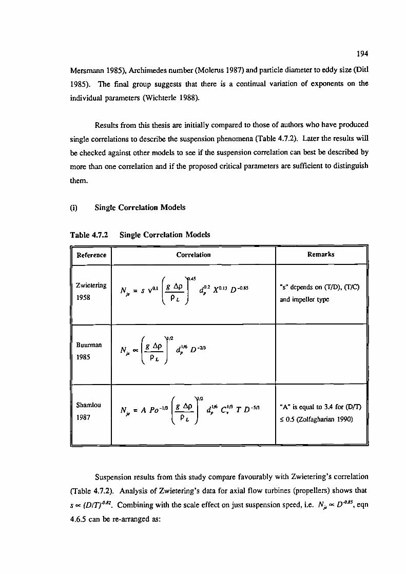
194

Mersmann 1985), Archimedes number (Molerus 1987) and particle diameter to eddy size (Diti

1985). The final group suggests that there is a continual variation of exponents on the

individual parameters (Wichterle 1988).

Results from this thesis are initially compared to those of authors who have produced

single correlations to describe the suspension phenomena (Table 4.7.2). Later the results will

be checked against other models to see if the suspension correlation can best be described by

more than one correlation and if the proposed critical parameters are sufficient to distinguish

them.

(I) Single Correlation Models

Table 4.7.2 Single Correlation Models

Reference Correlation Remarks

/ 45

ZwieteringN = s v°'

g d,2 x°'3 D-°85 "s" depends on (T/D), (TIC)

1958 P L J and impellei type

/ \1f2Buurman

NocFl dD1985 PL )

12

Shamlou

Nfr = A Po"3d C T D513 "A is equal to 3.4 for (DIT)

1987 P t. J ^ 0.5 (Zolfagharian 1990)

Suspension results from this study compare favourably with Zwietering's correlation

(Table 4.7.2). Analysis of Zwietering's data for axial flow turbines (propellers) shows that

s cc (D/Tj°. Combining with the scale effect on just suspension speed, i.e. Nj: cc D°25, eqn

4.6.5 can be re-arranged as:

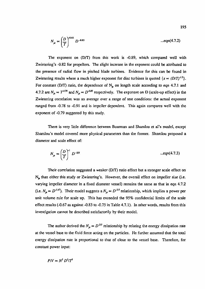
/ '-fl.82N. oc1.j D°85

P T)...eqn(4.7.2)

195

The exponent on (D/T) from this work is -0.89, which compared well with

Zwietering's -0.82 for propellers. The slight increase in the exponent could be attributed to

the presence of radial flow in pitched blade turbines. Evidence for this can be found in

Zwietering results where a much higher exponent for disc turbines is quoted (s oc (D/T)'3).

For constant (D/T) ratio, the dependence of N on length scale according to eqn 4.7.1 and

4.7.2 are N,, cc T° 79 and N U°25 respectively. The exponent on D (scale-up effect) in the

Zwietering correlation was an average over a range of test conditions: the actual exponent

ranged from -0.78 to -0.91 and is impeller dependent. This again compares well with the

exponent of -0.79 suggested by this study.

There is very little difference between Buurman and Shamlou et al's model, except

Shamlou's model covered more physical parameters than the former. Shamlou proposed a

diameter and scale effect of:

...eqn(4.7.3)

Their correlation suggested a weaker (DIF) ratio effect but a stronger scale effect on

N than either this study or Zwietering's. However, the overall effect on impeller size (i.e.

varying impeller diameter in a fixed diameter vessel) remains the same as that in eqn 4.7.2

(i.e. N,, D'47). Their model suggests a N,, cc D 3 relationship, which implies a power per

unit volume rule for scale up. This has exceeded the 95% confidential limits of the scale

effect results (-0.67 as against -0.83 to -0.75 in Table 4.7.1). In other words, results from this

investigation cannot be described satisfactorily by their model.

The author derived the Ni,, cc D 713 relationship by relating the energy dissipation rate

at the vessel base to the fluid force acting on the particles. He further assumed that the total

energy dissipation rate is proportional to that of close to the vessel base. Therefore, for

constant power input:

P/V cc N3 D5/T6

N.I'

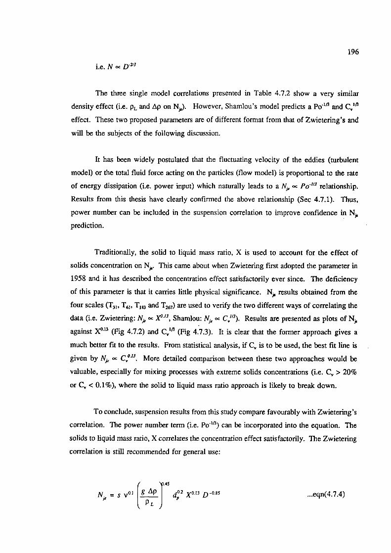
196

i.e. N oc

The three single model correlations presented in Table 4.7.2 show a very similar

density effect (i.e. PL and on NJ. However, Shamlou's model predicts a Po"3 and C"3

effect. These two proposed parameters are of different format from that of Zwietering's and

will be the subjects of the following discussion.

It has been widely postulated that the fluctuating velocity of the eddies (turbulent

model) or the total fluid force acting on the particles (flow model) is proportional to the rate

of energy dissipation (i.e. power input) which naturally leads to a N oc Po"3 relationship.

Results from this thesis have clearly confirmed the above relationship (Sec 4.7.1). Thus,

power number can be included in the suspension correlation to improve confidence in N,

prediction.

Traditionally, the solid to liquid mass ratio, X is used to account for the effect of

solids concentration on N. This came about when Zwietering first adopted the parameter in

1958 and it has described the concentration effect satisfactorily ever since. The deficiency

of this parameter is that it carries little physical significance. N results obtained from the

four scales (T31 , T61 , T183 and T267) are used to verify the two different ways of correlating the

data (i.e. Zwietering: Nk cc x°•'3, Shamlou: Nj,, oc C"3). Results are presented as plots of N,

against X°'3 (Fig 4.7.2) and C" (Fig 4.7.3). It is clear that the former approach gives a

much better fit to the results. From statistical analysis, if C is to be used, the best fit line is

given by N1, oc c°•'3 More detailed comparison between these two approaches would be

valuable, especially for mixing processes with extreme solids concentrations (i.e. C > 20%

or C, < 0.1%), where the solid to liquid mass ratio approach is likely to break down.

To conclude, suspension results from this study compare favourably with Zwietering's

correlation. The power number term (i.e. Po w) can be incorporated into the equation. The

solids to liquid mass ratio, X correlates the concentration effect satisfactorily. The Zwietering

correlation is still recommended for general use:

/g

d2 X°' 3 D° 85 ...eqn(4.7.4)N, = S v°'PL J

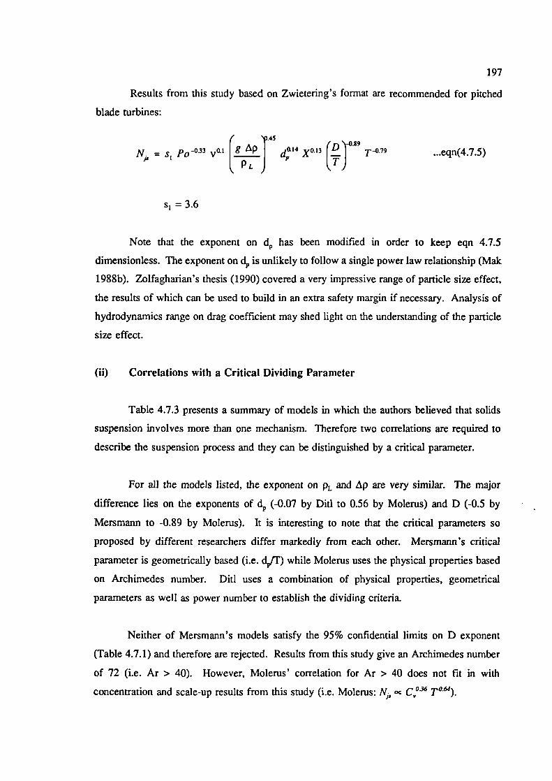
197

Results from this study based on Zwietering's format are recommended for pitched

blade turbines:

(I g p I

N = s 1 Po° 33 v°' (

PL Jd,'4 X°' 3 I I T° 79 ...eqn(4.7.5)

T)

s = 3.6

Note that the exponent on d has been modified in order to keep eqn 4.7.5

dimensionless. The exponent on d is unlikely to follow a single power law relationship (Mak

1988b). Zolfagharian's thesis (1990) covered a very impressive range of particle size effect,

the results of which can be used to build in an extra safety margin if necessary. Analysis of

hydrodynamics range on drag coefficient may shed light on the understanding of the particle

size effect.

(ii) Correlations with a Critical Dividing Parameter

Table 4.7.3 presents a summary of models in which the authors believed that solids

suspension involves more than one mechanism. Therefore two correlations are required to

describe the suspension process and they can be distinguished by a critical parameter.

For all the models listed, the exponent on PL and p are very similar. The major

difference lies on the exponents of d (-0.07 by Diii to 0.56 by Molerus) and D (-0.5 by

Mersmann to -0.89 by Molerus). It is interesting to note that the critical parameters so

proposed by different researchers differ markedly from each other. Mersrnann's critical

parameter is geometrically based (i.e. d/F) while Molerus uses the physical properties based

on Archimedes number. Did uses a combination of physical properties, geometrical

parameters as well as power number to establish the dividing criteria.

Neither of Mersmann's models satisfy the 95% confidential limits on D exponent

(Table 4.7.1) and therefore are rejected. ResuLts from this study give an Archimedes number

of 72 (i.e. Ar > 40). However, Molerus' correlation for Ar > 40 does not fit in with

concentration and scale-up results from this study (i.e. Molerus: N oc C°6 TAM).

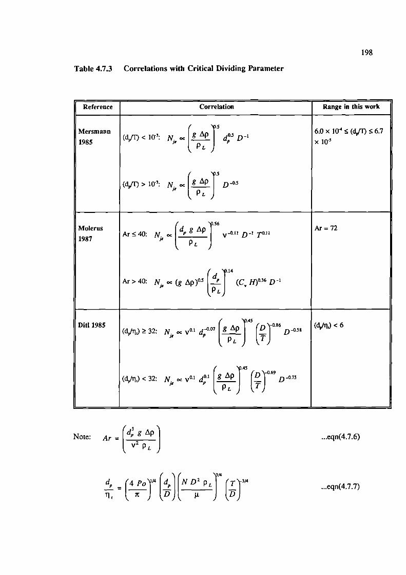
...eqn(4.7.6)

198

Table 4.7.3 Correlations with Critical Dividing Parameter

Reference Correlation Range in this work

( 6.Ox 10^(d.JI)^6.7Mersmann I g Ap 1 d D' io-1985(dJ) < 10: N

)

(Cd/I')> i0: N. _

I g Ap I D°5'ArL )

/Ar = 72

d, g Ap I -0.11 D ToHAr^40: N ______Molerus

P. J

1987

14

Ar> 40: N - (g p)03 (d

J

(C 0.36 D

DitI 1985(d.Jm) ^ 32: N. v°' d g P I 1'D -0.86 (dpflit) < 6

[

PL JD°58

(dJq) < 32: N oc v° 1 d g ip I D'01 [

is "PL J (jj

D°75

Note:(d g Ap

Ar = ________V2

= (4_Po

11 1 (it )

d ND2pL'(T13/4 ..eqn(4.7.7)

199

Results from this work are analysed according to Dill's critical particle diameter (i.e.

dE/flJ and it was found that in all cases (d1 L) is small than 6. According to Diti the

following correlation applies:

I

(d/i) < 32: N v°' d' g(Dr°

P J JD 75 ...eqn(4.7.8)

The exponent of D lies within the 95% confindential interval of this analysis while the

exponent of (D/T) is outside the limits (Table 4.7.1). Further statistical analysis was

conducted by substituting the experimental data from this investigation into eqn 4.7.8. A

relative standard deviation of ± 16% is given, as against ± 10% in eqn 4.7.1.

Although it is possible that the particles are suspended by two mechanisms according

to a critical parameter, the correlations presented are inadequate to describe the data produced

in this study. Another concern is that the critical parameters adopted by the various authors

are of a very diverse physical nature and this is reflected by the contradictory theories of

solids suspension mechanism.

(iii) Models with a Continual Variation of Exponents

Some researchers suggested that there is a continual variation of exponents in the

suspension correlation. The models so established are not fully proven. Baldi et al (1978)

used a turbulent model and from an analogy of the decay of turbulence behind a grid, they

deduced a similar correlation to Zwietering's when C is equal to D (eqn 2.1.7). They

commented that if the (Cm) ratio is changed the exponents in their correlation will also

change. The exponents at (C/D) of 1 were determined experimentally and no theoretical

relationship between the (CID) ratio and predicted exponents were given in his paper. It is

interesting to note that the critical parameter adopted by them (i.e. CID) is again different

from what had been reviewed previously.

Wichterle's model suggested that the exponents on physical properties will change

according to Archimedes number but a single-power function N1 oc (D/T)'"3 D 213 applies.

However, his assumed exponent on scale does not agree with the results from this study.

200

Wichterle proposed:

N; = N,, .t-" (g tp)" pr D 2 T'3 = I ( d ) ...eqn(4.7.9)

In the current study:

g L\pd; d[

= jL2J = constant

Therefore:

( \419

N ID '3

isLPLJ _JD2'3 ...eqn(4.7.10)

4.7.3 A Final Remark on Solids Suspension Modelling

This study has demonstrated qualitatively and quantitatively that more than one

mechanism is involved in suspending particles in a stirred vessel. The occurrence of a certain

mechanism is geometry (Sec 4.1.2, Fig 4.1.6, Table 4.1.1 and 4.1.2) and physical property

(Fig 4.1.9) dependent. Evidence is found in literature of a diverse range of exponents on

(eg 0 to 0.52 in Zolfagharian 1990) and D (Table 4.6.2).

A review of solids suspension models indicates that theoretical models can generally

be classified into two categories; those in which particles are believed to be picked up by

turbulent eddies and those where particles are picked up by fluid flow. Although both of

these theories display considerable merit, there remains a number of questions to be iesolved

(Sec 2.1.8). To complicate the matter further, results from this study show that the suspension

is also geometry dependent. Examples include flow interaction in dual impeller systems (Sec

4.5.3) and the removal of the central dead zone by a pitched blade turbine which depends on

the impeller discharge and the curvature of the vessel base.

The added difficulty in modelling these complicated influences is that they are inter-

related so that it is virtually impossible to study each effect in isolation. Until models are

developed which can take account of these complex mechanisms, it is unlikely that any purely

201

theoretical model will be able to correlate the available experimental data. The suspension

phenomenon is best described by empirical or semi-empirical models.

4.7.4 Modelling of Solids Distribution

Fig 4.4.5 has described the general behaviour of a RSD curve. In order to model a

distribution process successfully, it is felt that two types of inter-related models are required,

first one to identify the point of maximum homogeneity and second, a method of describing

the rate of decreasing RSD relating to impeller speed/power input, for a given condition

(Region B, Fig 4.4.5).

Results from this study show that power per unit volume has to remain constant in

order to maintain the same degree of homogeneity across scales. A review of the available

distribution models shows that most imply a constant tip speed scale up criterion (eg Barresi

1987, Shamlou 1989, Sec 2.2.2). Buurman measured the height of the slurry liquid interface

and his model indicates a scale-up relationship of NRSD D°78.

/ 'p• ( 'l.275

Ig p I d D°5° ...eqn(4.7.11)NRSD ^PL J I)

His model comes the closest in describing the results from this study (i.e. f(Fr) results

presented in the Appendices) but it still underestimates the power requirement for scaling up

(Fig 4.7.4).

A basic distributed model can be established to predict the distribution quality (Region

B, Fig 4.4.5) based on the results from this study:

Analysis of the scale-up results indicates a constant power per unit volume criterion.

Therefore, the impeller speed required to achieve a certain degree of homogeneity, N D can

be given as:

NRSD oc T213 ...eqn(4.7.12)

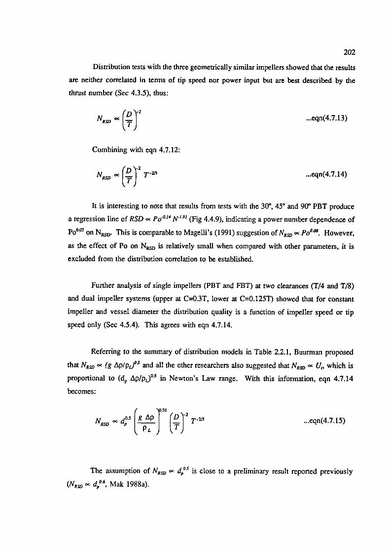
202

Distribution tests with the three geometrically similar impellers showed that the results

are neither correlated in terms of tip speed nor power input but are best described by the

thrust number (Sec 4.3.5), thus:

NRSD °c (DJ2 ...eqn(4.7.13)

Combining with eqn 4.7.12:

NRSD °c (DJ2 T ...eqn(4.7.14)

It is interesting to note that results from tests with the 30°, 450 and 900 PBT produce

a regression line of RSD Po°'4 N's' (Fig 4.4.9), indicating a power number dependence of

Po°°7 on ND. This is comparable to Mageffi's (1991) suggestion of NR oc Po°°8. However,

as the effect of Po on ND is relatively small when compared with other parameters, it is

excluded from the distribution correlation to be established.

Further anaiysis of single impellers (PBT and FBT) at two clearances (T/4 and T/8)

and dual impeller systems (upper at C=O.3T, lower at C=0.125T) showed that for constant

impeller and vessel diameter the distribution quality is a function of impeller speed or tip

speed only (Sec 4.5.4). This agrees with eqn 4.7.14.

Referring to the summary of distribution models in Table 2.2.1, Buurnian proposed

that NRSD (g Ap/p1)° and all the other researchers also suggested that NRSD oc U,, which is

proportional to (d 4/p1)°3 in Newton's Law range. With this information, eqn 4.7.14

becomes:

.50

NRSD oc dPL J bJ

T ...eqn(4.7.15)

The assumption of NRSD oc d°5 is close to a preliminary result reported previously

(NRSD oc d° 6, Mak 1988a).

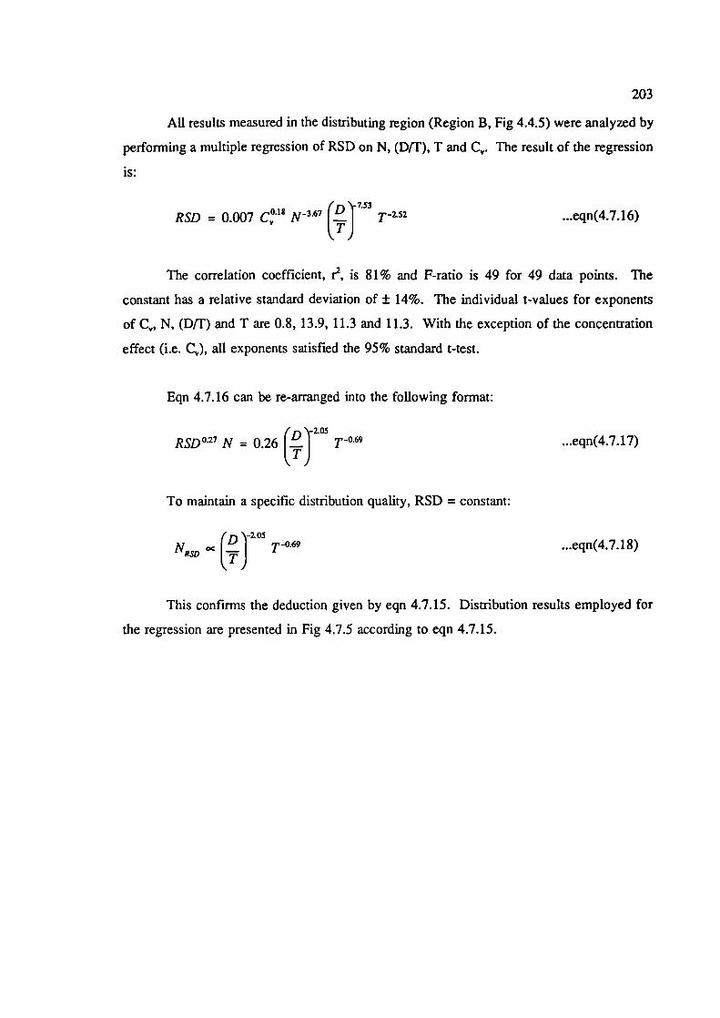
203

All results measured in the distributing region (Region B, Fig 4.4.5) were analyzed by

performing a multiple regression of RSD on N, (D/T), T and Ci,. The result of the regression

is:

RSD = 0.007 C°' 8 N 367 T252 ...eqn(4.7.16)TJ

The correlation coefficient, r2, is 81% and F-ratio is 49 for 49 data points. The

constant has a relative standard deviation of ± 14%. The individual t-values for exponents

of C, N, (D[F) and T are 0.8, 13.9, 11.3 and 11.3. With the exception of the concentration

effect (i.e. Cr), all exponents satisfied the 95% standard t-test.

Eqn 4.7.16 can be re-arranged into the following format:

"D '\2.O5

RSD° 27 N = 0.26 T°69 ...eqn(4.7.17)

To maintain a specific distribution quality, RSD = constant:

D \-2O5

NRSD oc tTJT°69 ...eqn(4.7.18)

This confirms the deduction given by eqn 4.7.15. Distribution results employed for

the regression are presented in Fig 4.7.5 according to eqn 4.7.15.

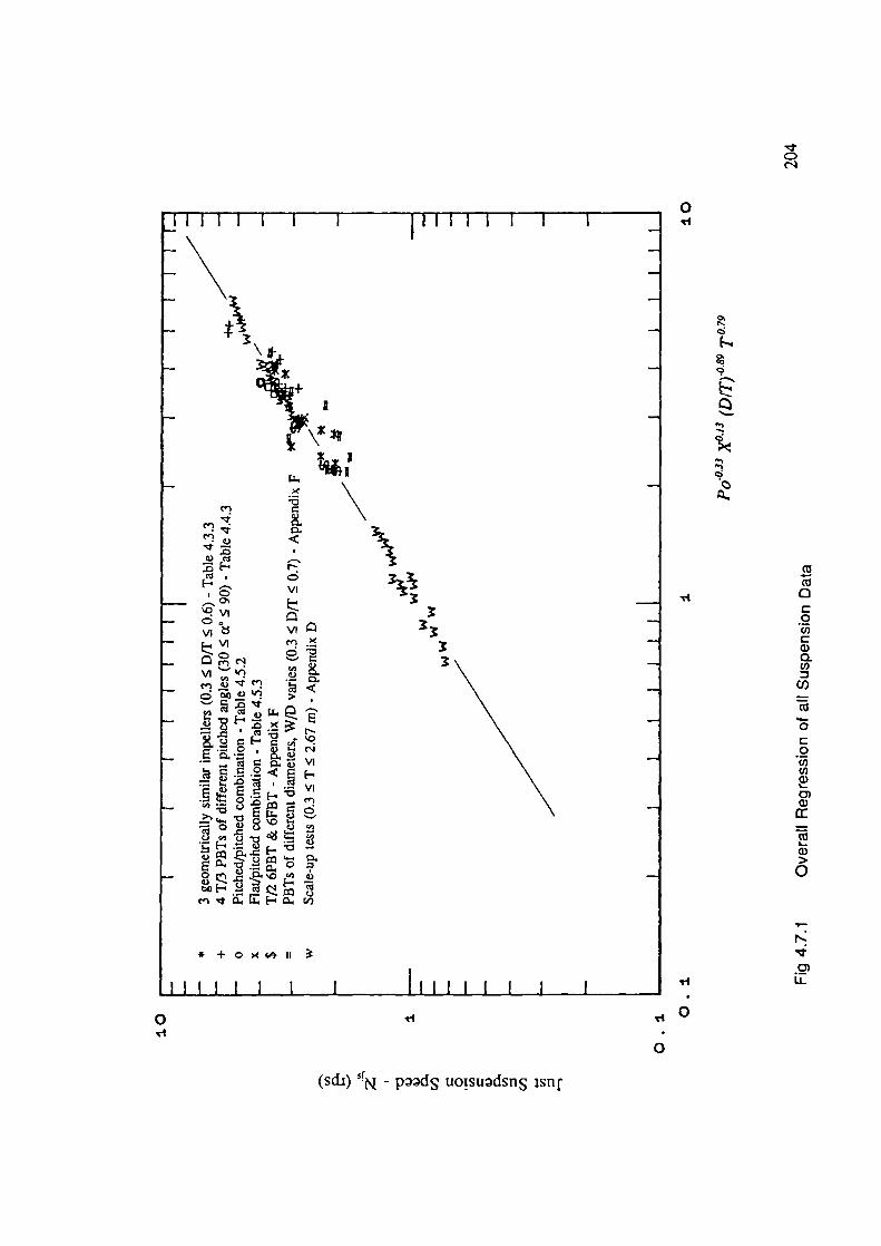
cli

cli

ii

a

C0(I)CC)0U,

0C0C,,U)a)5-0)a)cr

Cli5-a)>

0

101

N

0)LL

'4

0

1

0

* +

01

\\

ena

en

VI

'vI

VI VI• VI efl<

c1VI

en:I VI

(sth) SIN - pd uoisudsn lSflf

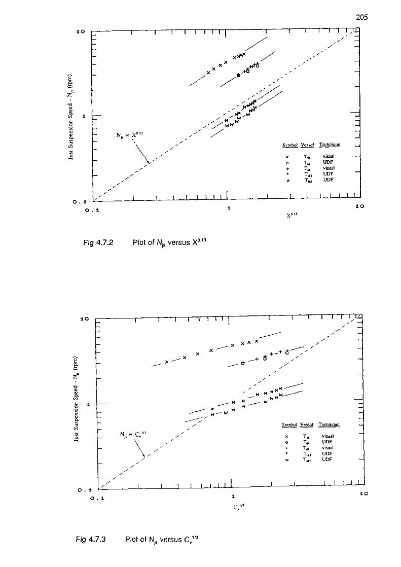
205

1.0

E

z

I)V

C/DC0

CV0.

C,,

-,

._l 4

-

- x'x

_ x

-- 9 w

-- oc X° -

— Qj Vcsscl TcchnQue

- -x T,1 visual

- o T1 UDF+ T1 visual

- 7 * UDF•ii,w T IJDF

/

0.1. 1.

10

x°

Fig 4.7.2

P'ot of versus X°13

10

z

I)V0.

1

C4)0.

C,,

U,

I I I I I i lii'

xx x—

- x + ++

_+ -

7

- 7

/- 3*- WW

- ____3* *___Ww- ___-3* w

- _w_w-

- -— rni Vessel Technique

N oc C -- x 131 visual

- - 0 T L.JI)F- - + visualN * •i,'

- w T,, UDF-

7

7 L I I I IlL

0.1 I

lu

c:'3

Fig 4.7.3 Piot of versus CV11

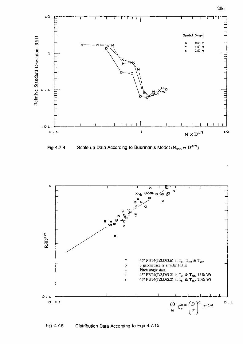
(fj

0

>4.)

1

&) 0.1>

c

4.)

0

0-0

\

Symbol Vessel

o O.61m• l.83mx 2.67m

0.1

0.1 L

0.0160

0.'8 (D"r2TJ T°67

206

10

.01 '•-

0.1

I

N x10

Fig 4.7.4

Scale-up Data According to Buurman's Model (N 0 D°78)

II x

\PXM S \S0

Sx

vvoS0

x

i::10

C,)

* 450 PBT4(T/2,D13.6) in T61 , T1 & T7o 3 geometrically similar PBTs+ Pitch angle datas 450 PBT4(T/2,D/5.2) in 1 61 & T 7, 15% Wtv 450 PBT4(T12,D/5.2) in T61 & T 7, 20% Wt

Fig 4.7.5

Distribution Data According to Eqn 4.7.15

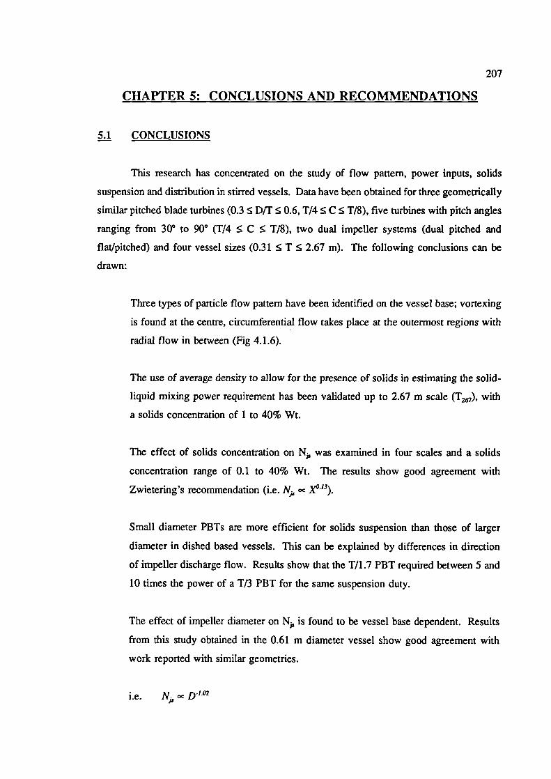
207

CHAPTER 5: CONCLUSIONS AND RECOMMENDATIONS

5.1 CONCLUSIONS

This research has concentrated on the study of flow pattern, power inputs, solids

suspension and distribution in stirred vessels. Data have been obtained for three geometrically

similar pitched blade turbines (0.3 ^ DIF ^ 0.6, T/4 ^ C ^ T/8), five turbines with pitch angles

ranging from 30° to 90° (T/4 ^ C ^ T18), two dual impeller systems (dual pitched and

flax/pitched) and four vessel sizes (0.31 ^ T ^ 2.67 m). The following conclusions can be

drawn:

Three types of particle flow pattern have been identified on the vessel base; vortexing

is found at the centre, circumferential flow takes place at the outermost regions with

radial flow in between (Fig 4.1.6).

The use of average density to allow for the presence of solids in estimating the solid-

liquid mixing power requirement has been validated up to 2.67 m scale (T 7), with

a solids concentration of 1 to 40% Wt.

The effect of solids concentration on N, was examined in four scales and a solids

concentration range of 0.1 to 40% Wt. The results show good agreement with

Zwietering's recommendation (i.e. N, oc X°'3).

Small diameter PBTs are more efficient for solids suspension than those of larger

diameter in dished based vessels. This can be explained by differences in direction

of impeller discharge flow. Results show that the T/1.7 PBT required between 5 and

10 times the power of a T/3 PBT for the same suspension duty.

The effect of impeller diameter on N is found to be vessel base dependent. Results

from this study obtained in the 0.61 m diameter vessel show good agreement with

work reported with similar geometries.

i.e. Nj,, oc

208

Just suspension data from the pitch angle impellers show that for each angle there is

an optimum clearance.

Both dual impeller combinations tested in this study require significantly more power

to just suspend solids than the single impeller. This is believed to be caused by the

interaction between the flow patterns of the upper and the lower impeller.

The scaling effect put forward by Zwietering for solids suspension has been confirmed

by this study up to vessel diameters of 2.67 m.

The overall correlation for N based on data from this study (with Po) is given as:

(D '-O.89

N cc Po° 33 X° 13D°79

for dual impeller systems, Pa should be replaced by Poe.

Compared with just suspension speed, impeller power number appears to have less

influence on solids distribution.

Distribution tests with the three geometrically similar impellers show that the results

are neither correlated in terms of tip speed nor power input but are best described by

the thrust number (i.e. N 2 D4).

In general, dual impeller systems improve solids distribution compared with those of

a single impeller.

The radial concentration profiles measured in T 183 were flat, except when the probe

was at the clear-liquid/solid-liquid interface. Although the flatness of radial profile

has already been reported by other authors, it is the first time this result has confirmed

in vessel of industrial scale. The use of a one-dimensional steady state model by other

researchers is therefore justified.

The use of constant tip speed as the scale-up criterion for solids distribution

underestimates the power requirement. This study indicates that equal power per unit

209

volume is required to achieve the same degree of homogeneity.

Summarising all the distribution results, the following equation can be used to describe

the speed requirement to match a specific RSD:

03 g p (D'2NRSD oc d

30

[PU

T

This study has shown that some impellers (eg DTT=0.3) attained the just suspension

condition before the point of maximum homogeneity. For some other impellers (eg

DfI'=0.5), just suspension speeds are higher than N D ,,... Therefore, the use of

homogeneity data as the criterion for N should be interpreted with care.

The scale-up relationships were found to be different for solids suspension and

distribution (i.e. N D°23 and NRsD oc D° 67). If the just suspension condition was

used as the scale-up criterion, the solids distribution quality will be worse as the scale

increases.

In addition to these conclusions, the following improvements on experimental

techniques were made:

The ultrasonic Doppler flowmeter technique initiated by Buurman in 1985 to measure

the just suspension speed was adopted in this study. Back to back comparisons were

made between the visual and UDF techniques and the following relationship was

obtained:

Visual Nfr = k UDF N. k = 1.07 ± 0.01

Application of such a correction factor to the visual observation allowed direct

comparison of N over the full range of scales.

Local solids concentrations were measured by a solids concentration probe developed

by BHR Group Ltd from a design used at the Warren Spring Laboratory. The initial

210

calibration was largely conducted by Ruszkowski (1985). This study has demonstrated

the suitability of this technique to large scale work and overcomes the problem of

limited concentration range encountered by optical techniques.

5.2 SUGGESTIONS FOR FUTURE WORK

In conducting the present isearch programme a number of important questions arose

which could not be answered as part of this work. It is recommended that the following could

form part of any future investigation into the area of solid-liquid mixing:

It appears that there is more than one mechanism responsible for solids suspension.

It would be valuable to design experiments in which only one mechanism is

controlling and hence study the suspension behaviour accordingly. In addition, laser

measurements of velocity and energy distribution at vessel base are recommended.

This information aid to clarify the nature of suspension mechanism(s) at just

suspension condition.

The flow pattern of an impeller has been shown to have a substantial influence on

solids suspension and distribution but these effects are virtually impossible to quantify

by normal experimental means. A computational fluid dynamics study on flow

interactions and their effects on solid-liquid mixing may be the most effective way of

clarifying this area.

In view of the similarities between the suspension of particles, fluidisation,

transportation of sediments and solids, a comparative study of present knowledge in

these processes would be a fruitful exercise.

This study demonstrates that power number increases with vessel sizes. This does not

affect the validity of the scale-up rules as long as geometrical similarity is assumed.

However, it will certainly affect the choice of motor and gear box. Further study is

necessary to clarify the effect of scale on power number.

211

REFERENCE

Al-Dhahir, L., "Solids Suspension in Viscous Newtonian and Non-Newtonian Liquids" PhD

Thesis, University College London, Nov 1990

Barresi, A. and Baldi, G., "Solid Dispersion in an Agitated Vessel" Chem Eng Sd, Vol 42, No

12, pp 2949-2956, 1987

Barresi, A. and Baldi, G., Shorter Communication: "Solid Dispersion in an Agitated Vessel: Effect

of Particle Shape and Density" Chem Eng Sci, Vol 42, No 12, pp 2969-2972, 1987

Bates, R. L., Fondy, P. L. and Corpstein, R. R., "An Examination of Some Geometric Parameters

of Impeller Power" I & E C Process Design and Dev, Vol 2, No 4, pp 310-314, Oct 1963

Brodkey, R. S. and Hershey, H. C., "Transport Phenomena - A Unified Approach" McGraw-Hill,

1988

Bohnet, M. and Niesmak, G., "Distribution of Solids in Stirred Suspensions" German Chem Eng,

Vol 3, pp 57-65, 1980

Boume, J. R. and Sharma, R. N., "Suspension Characteristics of Solid Particles in Propeller-

agitated Tanks" l European Conf on Mixing and Centrifugal Separation, Cambridge, England,

BHRA. Paper B3 (9-11 Sept 1974)

Bujalski, W., "Three Phase Mixing: Studies of Geometry, Viscosity and Scale" PhD Thesis,

University of Birmingham, Dec 1986

Buunnan, C., Resoort, G. and Plaschkes, A., "Scale-up Rules for Solids Suspension in Stirred

Vessels" 5th European Conf on Mixing, Wurzburg, W Germany, BHRA. Paper 5 (10-12 June

1985)

Buurman, C., "Stirring of Concentrated Slurries: A Semi-empirical Model for Complete

Suspension at High Solids Concentrations and 5 m3 Verification Experiments" Fluid Mixing IV,

I Chem E Symposium Series No 121, pp 343-350, Sept 1990

212

Chapman, C. M., "Studies of Gas-Liquid-Particle Mixing in Stirred Vessels" PhD Thesis,

University College London, Sept 1981

Chudacek, M. W., "Solids Suspension Behaviour in Profiled Bottom and Flat Bottom Mixing

Tanks N Chem Eng Sci, Vol 40, No 3, pp 385-392, 1985

Chudacek, M. W., "Relationship between Solids Suspension Criteria, Mechanism of Suspension,

Tank Geometzy and Scale-up Parameters in Stirred Tanks" md Eng Chem Fundam, Vol 25, pp

391-401, 1986

Conti, R. and Baldi, G., "Complete Suspension of Particles in Mechanically Agitated Vessels

Effect of System Geometry" mt Sym on Mixing, Faculte Poly de Mons, Paper B2, 2124th Feb

1978

DeRitter, G. R., "Multiphase Solid-liquid-liquid Mixing in Stirred Tanks" MSc Thesis, New Jersey

Institute of Technology, 1990

Diii, P. and Rieger, F., "Suspension of Solid Particles" -Letter to the Editors, Chem Eng Sci, Vol

35, pp 764-765, 1980

Diii, P. and Rieger, F., "Suspension of Solids Particle - Relative Velocity of Particles in Turbulent

Mixing" 5th European Conf on Mixing, Wurzburg, W Germany, BHRA. Paper 8 (10-12 June,

1985)

Einenkel, W. D., "Influence of Physical Properties and Equipment Design on the Homogeneity of

Suspensions in Agitated Vessels" Ger Chem Eng, Vol 3, pp 118-124, 1980

Einenkel, W. D. and Mersmann, A., "Erforderliche Drehzahlen zum Suspendieren in RUhrwerken"

Verfabrenstechnik (Mainz), Vol 11, No 2, pp 90-94, 1977

Fawcett, N. S. J., "The Mean Flow Field in the Discharge of Pitched-blade Turbines" FMP Interim

Report 1046, BHRA, October 1989

Frijlink, J. J., Kolijn, M. and Smith, J. M., "Suspension of Solids with Aerated Pitched Blade

Turbines" IChemE Sym Series No 89, Fluid Mixing II, Bradford, 1984

213

Hamby. N., Edwards, M. F. and Nienow, A. W., "Mixing in the Process Industries" Butterworths,

1985

Hepworth Minerals and Chemicals Limited, Private communication with The Technical

Department of Building Materials Division, July 1992

Herringe, R. A., "The Behaviour of Mono-size Particle Slurries in a Fully Baffled Turbulent

Mixer" 3 European Conference on Mixing, York, England, BHRA Paper Dl, 46th April 1979

Hirsekom, F. S. and Miller, S. A., "Agitation of Viscous Solid-Liquid Suspensions" Chem Eng

Prog, Vol 49, No 9, pp 459-466, 1953

Hockey, R. M., Noun, J. M. and Pinho, F., "Flow Visualisation of Newtonian and Non-Newtonian

Fluids in a Stirred Reactor" Proceedings of the 5th mt Sym on Flow Visualization, Prague,

Czechoslovakia, Hemisphere Publishing Corp. pp 976-987 (2125th August, 1989)

Holmes, D. B., Voncken, R. M. and Dekker, J. A., "Fluid Flow in Turbine-stirred, Baffled Tanks,

I. Circulation Time, II. Dispersion during Circulation" Chem Eng Sci, Vol 19, pp 201-2 13, 1964

Karsien, H., Private communication with Flygt iTT Fluid Technology Corporation, Solna, Sweden,

June 1992

Kneule, F. and Weinspach, P. M., "Suspendierenvon Feststoffpartikeln im RUhrgefal3"

Verfahrenstechnik, No 12, pp 531-540, 1967

Kolar, V., "Studies on Mixing X - Suspending Solid Particles in Liquids by means of Mechanical

Agitation" Coil Czech Chem Comm. Vol 26, pp 613-627, 1961

Koutsakos, E., "Solids Suspension in Mechanically Agitated Vessels" PhD Thesis, University

College London, April 1989

Machon. V., Fort, I. and Skrivanek, J., "Local Solids Distribution in the Space of a Stirred Vessel"

4th European Coni on Mixing, Noordwijkerhout, The Netherlands, BHRA (27-29 April 1982)

Mackinnon, C., "Research Review: Comparative Mixing times" FMP 029, April 1987, BHRA

214

Magelli, F., Fajner, D., Nocentini, M. and Pasquali, G., "Solids Concentration Profiles in Slurry

Reactors Stirred with Multiple Impellers: Recent Results" Engg Foundation Mixing XI, New

Hampshire, USA, 2-7 August, 1987

Magelli, F., Fajner, D., Nocentini, M. and Pasquali, 0., "Solids Concentration Distribution in

Slurry Reactors Stirred with Multiple Axial Impellers" Engg Foundation Mixing XII, Potosi, USA,

6-11 August, 1989

Magelli, F., Fajner, D., Nocentini, M. and Pasquali, G., "Novel Data about Solids Concentration

Distribution in Vessels Stirred with Multiple Impellers" CHISA 87, Paper E5.5, Prague, 31 Aug-

4 Sept, 1987

Magelli, F., Fajner, D., Nocentini, M. and Pasquali, G., "Solid Distribution in Vessels Stirred with

Multiple Impellers" Chem Eng Sci, Vol 45, No 3, pp 615-625, 1990

Magelli, F., Fajner, D., Nocentini, M., Pasquali, G., Marisko, V. and Diti, P., "Solids

Concentration Distribution in Slurry Reactors Stirred with Multiple Axial Impellers" Chem Eng

Process, Vol 29, pp 27-32, 1991

Mak, A., "Measurement of Solids Concentration and N 1 in a 0.61 m Diameter Torispherical Base

Stirred Vessel" FMP 1016, BHRA, March 1987

Mak, A., "Research Review : The Measurement of Power, Solids Suspension and Distribution in

a 0.61 m Diameter Stirred Vessel" FMP 032, BHRA, April 1988(a)

Mak, A., "The Effect of Particle Size on Solids Suspension: A Literature Survey" FMP 1036,

BHRA, August 1988(b)

Mak, A., Presentation to Fluid Mixing Processes (FMP) Steering Committee Meeting, 11-1 3th April

1989

Mak, A., Green, A. and Bumapp, R. T., "Flue Gas Desuiphurisation Model Tests" Confidential

Report for Babcock Contractors Limited, BHR Group Ltd, April 1990

Mak, A. and Ruszkowski, S. W., "Scaling-up of Solids Distribution in Stirred Vessels" IChemE

215

Sym Series No. 121, pp 379-395, 1990

Medek, J., "Power Characteristics of Agitators with Flat Inclined Blades" mt Chem Engg, Vol 20,

No 4, pp 664-672, 1980

Mersmann, A., "Scale-up of Agitated Vessels for Suspension" 5th European Conf on Mixing,

Wurzburg, W Germany, BHRA Additional Paper (10-12 June 1985)

Mersmann, A. and Laufliutte, H. D., "Scale-up of Agitated Vessels for Different Mixing Process"5th European Conf on Mixing, Wurzburg, W German, BHRA Paper 28 (10-12 June 1985)

Molerus, 0. and Latzel, W., "Suspension of Solid Particles in Agitated Vessel - I. Archimedes

Numbers ^ 40, II. Archimedes Numbers > 40, Reliable Prediction of Minimum Stirrer Angular

Velocities" Chem Eng Sci, Vol 6, pp 1423-1437, 1987

Musil, L. and Vik, J., "Suspending Solid Particles in an Agitated Conical-Bottom Tank" Chem Eng

Sci, Vol 33, pp 21-25, 1978

Muskett, M, J. and Ruszkowski, S., "The measurement of Shaft Power and Blending Loads for

a series of Impeller Types and Vessel Internals in a 0.61 m Diameter Stirred Vessel" FMP Report

007, January 1985, BHRA

Nagata, S., "Mixing - Principles and Applications" John Wiley & Sons, 1975

Narayanan, S., Bhatia, V. K., Guha, D. K. and Rao, M. N., "Suspension of Solids by Mechanical

Agitation" diem Eng Sci, Vol 24, pp 223-230, 1969

Nienow, A. W., "Suspension of Solids Particles in Turbine Agitated Baffled Vessels" Chem Eng

Sci, Vol 33, pp 1453-1459, 1968

Nienow, A. W. and Miles, D., "The Effect of Impellerfrank Configurations on Fluid-Particle Mass

Transfer" diem Eng Journal, Vol 15, pp 13-24, 1978

Niesmak, G., "Feststoffverteilung und Leistungsbedarf GerUhrter Suspensionen" PhD Thesis, TU

Braunschweig, 1982

216

Oroskar, A. R. and Turian, R. M., "The Critical Velocity in Pipeline Flow of Slurries" AIChE 3,

Vol 21, No 4, pp 550-558, 1980

Paviushenko, I. S., Kostin, N. M. and Matveev, S. F., "About the Impeller Speed for Agitation of

Suspensions" (in Russian) Zh Prikl Khim, Vol 30, pp 1160-1169, 1967

Penaz, F., Rod, V. and Rehakova, M., "Concentration Distribution of Suspension in a Mixed

Vessel" Coil Czech Chem Commum, Vol 43, pp 848-86 1, 1978

Palmer, M. H., "Design Guide for Impeller Power Numbers" FM? 028, April 1987, BHRA

Raghav Rao, K. S. M. S., Rewatkar, V. B. and Joshi, J. B., "Critical Impeller Speed For Solid

Suspension in Mechanically Agitated Contactors" AIChE J, Vol 34, No 8, pp 1332-1340, August

1988

Rieger, F. and DitI, P., "Suspension of Solid Particles in Agitated Vessel" 4th European Conf on

Mixing, Noordwijkerhout, The Netherlands, BHRA, pp 263-273, 2729th April 1982

Rieger, F., Ditl, P. and Havelkova, 0., "Suspension of Solid Particles - Concentration Profiles and

Particle Layer on the Vessel Bottom" 6th European Conference on Mxing, Pavia, Italy, BHRA, pp

25 1-258, 2426th May 1988

Ruszkowski, S., "Calibration of a Solids Concentration Probe and Measurement of Solids

Distribution in a Stirred Vessel" FMP 004, BHRA, October 1985

Schlichting, H., "Boundary-Layer Theory" 7th Ed, McGraw-Hill, 1979

Schwartzberg, H. G and Treybal, R. E., "Fluid and Particle Motion in Turbulent Stirred Tanks"

I & EC Fund., Vol 7, pp 1-12, Feb 1968

Shamlou, P. A. "Mechanism of Suspension of Coarse Particles in Liquids in Stirred Vessels"

IChemE Sym Series No 121, pp 397-4 12, 1990

Shamlou, P. A., "Mechanisms of Particle Suspension in Liquids" Presentation, I Chem E Fluid

Mixing Subject Group Meeting on Mechanics of Solids Suspension, University College London,

217

11th April 1991

Shamlou, P. A. and Koutsakos, E., "Solids Suspension and Distribution in Liquids under Turbulent

Agitation" Chem Eng Sci, Vol 44, No 3, pp 529-542, 1989

Shamlou, P. A. and Zolfagharian, A., "Incipient Solid Motion in Liquids in Mechanically Agitated

Vessels" I Chem E Symposium Series No. 108, pp 195-208, 1987

Squires, K. D. and Eaton, I. K., "Particle Response and Turbulence Modification in Isotropic

Turbulence" Phys Fluids A, Vol 2, No 7, pp 1191-1203, July 1990

Subbarao, D. and Taneja, V. K., "Three Phase Suspensions in Agitated Vessels" 3" European

Conference on Mixing, York, England, BHRA Paper D3 (46th April 1979)

Susanto, J., "Multiphase Soild-liquid and Solid-liquid-gas Mixing in Stirred Tanks" MSc Thesis,

New Jersey Institute of Technology, 1989

Staudinger, G., "Auslegung von Ruehrapparaten zum Suspendieren von Feststoffen"

Verfahrenstechnik (Mainz), Vol 11, No 9, pp 508-5 16, 1977

Tatterson, G. B., Yuan, H-H. S. and Brodkey, R. S., "Stereoscopic Visualisation of the Flows for

Pitched Blade Turbines" Chem Eng Sd, Vol 35, pp 1369-1375, 1980

Tay, M., Deutschlander, B and Tatterson, G., "Suspension Characteristics of Large Cylinders in

Agitated Tanks" Chem Eng Commun, Vol 29, pp 89-99, 1984

Voit, H. and Mersmann, A., "General Statemant for the Minimum Stirrer Speed During

Suspension" German Chem Eng, Vol 9, pp 101-106, 1986

Waimoeskerken, M. M. C. G., Speur, J. and Smith, J. M., "Gas-liquid Dispersion with Pitched

Blade Turbines" Chem Eng Commun, Vol 25, pp 11-29, 1984

Weisman, I and Efferding, L. E., "Suspension of Slurries by Mechanical Mixers" AIChE J, Vol

6, No 3, pp 419-426, 1960

218

Wichterle, K. "Conditions for Suspension of Solids in Agitated Vessels" (Them Eng Sd, Vol 43,

No 3, pp 467-471, 1988

Wiedmann, J. A., Steiff, A. and Weinspach, P. M., "Suspension Behaviour of Two and Three

Phrase Stirred Reactors" German Chem Eng, Vol 8, pp 321-335, 1985

Zolfagharian, A., "Solid Suspension in Rotary-stirred and in Liquid-jet Stirred Vessels" PhD

Thesis, University College London, June 1990

Zwietering, Th. N. "Suspending of Solid Particles in Liquid by Agitators" Chem Eng Sci, Vol 8,

pp 244-253, 1958

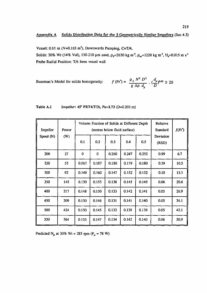
219

Appendix A Solids Distribution Data for the 3 Geometrically Similar Impellers (Sec 4.3)

Vessel: 0.61 m (V=0.165 m3), Downwards Pumping, C=T/4,

Solids: 30% Wt (14% Vol), 150-210 jnTI sand, p=:2630 kg m 3, p=1228 kg m 3, U=0.015 m s'

Probe Radial Position: T/6 from vessel wall

Buurman's Model for solids homogeneity: I (Fr') = L N2 D 2 (dP)O.45 ^ 20

gLpd D

Table A.1 Impeller: 45° PBT4(T/3), Po=1.73 (D=0.203 m)

Volume Fraction of Solids at Different Depth Relative

Impeller Power (metres below fluid surface) Standard f(Fr')

Speed (N) (W) Deviation

0.1 0.2 0.3 0.4 0.5 (RSD)

200 27 0 0 0.260 0.247 0.252 0.99 6.7

250 53 0.067 0.187 0.180 0.179 0.180 0.39 10.5

300 92 0.149 0.160 0.147 0.152 0.152 0.10 15.1

350 145 0.150 0.153 0.138 0.145 0.145 0.06 20.6

400 217 0.148 0.150 0.133 0.142 0.141 0.05 26.9

450 309 0.150 0.146 0.131 0.141 0.140 0.05 34.1

500 424 0.150 0.145 0.132 0.139 0.139 0.05 42.1

550 564 0.153 0.147 0.134 0.142 0.140 0.06 50.9

Predicted N, at 30% Wt = 285 rpm (PC,, = 78 W)

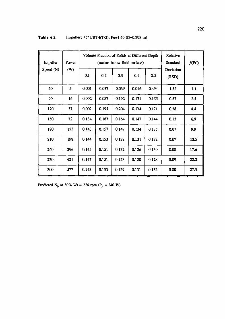
220

Table A.2 Impeller: 450 PBT4(T/2), Po=1.60 (D=0.298 m)


Impeller Power (metres below fluid surface) Standard f(Fr)

speed (N) çw) Deviation0.1 0.2 0.3 0.4 0.5 (RSD)

60 5 0.001 0.037 0.039 0.016 0.494 1.52 1.1

90 16 0.002 0.087 0.192 0.171 0.155 0.57 2.5

120 37 0.007 0.194 0.204 0.174 0.171 0.58 4.4

150 72 0.134 0.167 0.164 0.147 0.144 0.13 6.9

180 125 0.143 0.157 0.147 0.134 0.135 0.07 9.9

210 198 0.144 0.153 0.138 0.131 0.132 0.07 13.5

240 296 0.145 0.151 0.132 0.126 0.130 0.08 17.6

270 421 0.147 0.151 0.128 0.128 0.128 0.09 22.2

300 577 0.148 0.153 0.129 0.131 0.132 0.08 27.5

Predicted N, at 30% Wt = 224 rpm (P = 240 W)

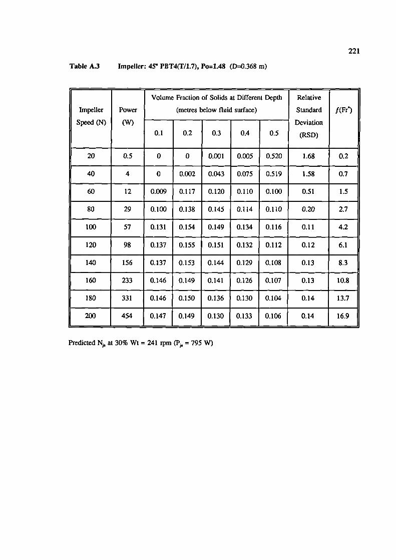
221

Table A.3 Impeller: 45 PBT4(T/1.7), Po=1.48 (D=0.368 m)


Impeller Power (metres below fluid surface) Standard f(Fre)


0.1 0.2 0.3 0.4 0.5 (RSD)

20 0.5 0 0 0.001 0.005 0.520 1.68 0.2

40 4 0 0.002 0.043 0.075 0.519 1.58 0.7

60 12 0.009 0.117 0.120 0.110 0.100 0.51 1.5

80 29 0.100 0.138 0.145 0.114 0.110 0.20 2.7

100 57 0.131 0.154 0.149 0.134 0.116 0.11 4.2

120 98 0.137 0.155 0.151 0.132 0.112 0.12 6.1

140 156 0.137 0.153 0.144 0.129 0.108 0.13 8.3

160 233 0.146 0.149 0.141 0.126 0.107 0.13 10.8

180 331 0.146 0.150 0.136 0.130 0.104 0.14 13.7

200 454 0.147 0.149 0.130 0.133 0.106 0.14 16.9

Predicted N at 30% Wt = 241 rpm (P = 795 W)

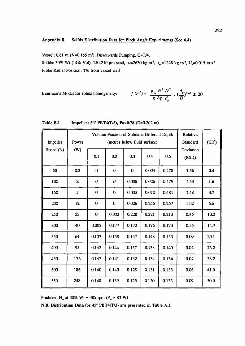
222

Appendix B Solids Distribution Data for Pitch Angle Experiments (Sec 4.4)


Solids: 30% Wt (14% Vol), 150-210 jun sand, p=263O kg m 3, p1 =1228 kg m 3, U=0.015 m s

Probe Radial Position: T/6 from vessel wall

n N2 D 2 dBuurman's Model for solids homogeneity: f (Fr) = r .. (P)O.45 ^ 20

gApd D

Table B.1 Impeller: 300 PBT4(T/3), Po=0.78 (D=0.202 m)


Impeller Power (metres below fluid surface) Standard f(Fre)


0.1 0.2 0.3 0.4 0.5 (RSD)

50 0.2 0 0 0 0.004 0.478 1.56 0.4

100 2 0 0 0.008 0.026 0.479 1.53 1.6

150 5 0 0 0.035 0.072 0.481 1.48 3.7

200 12 0 0 0.026 0.266 0.257 1.02 6.6

250 23 0 0.002 0.228 0.221 0.213 0.86 10.2

300 40 0.002 0.177 0.172 0.176 0.173 0.55 14.7

350 64 0.133 0.158 0.147 0.148 0.153 0.09 20.1

400 95 0.142 0.144 0.137 0.138 0.140 0.02 26.2

450 136 0.142 0.141 0.132 0.134 0.136 0.04 33.2

500 186 0.140 0.140 0.128 0.131 0.133 0.06 41.0

550 248 0.140 0.139 0.125 0.120 0.133 0.09 50.0

Predicted at 30% Wt = 385 rpm (P = 83 W)

N.B. Distribution Data for 450 PBT4(T/3) are presented in Table A.1

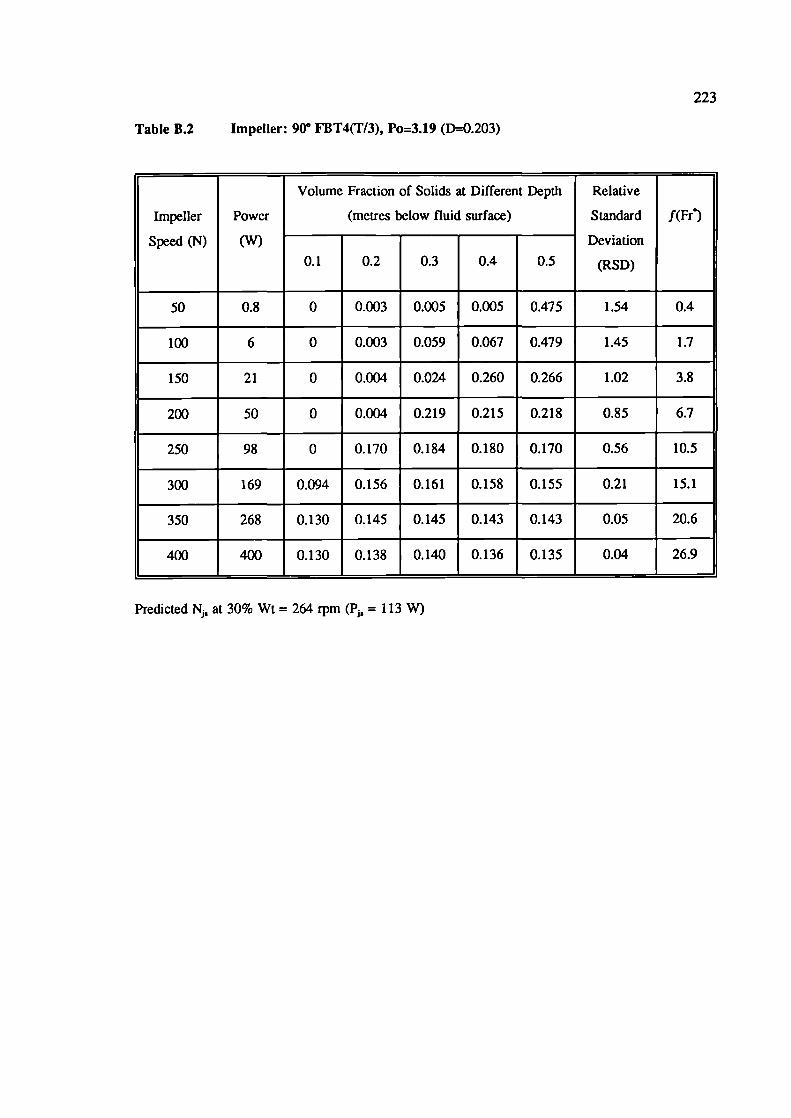
223

Table B.2 Impeller: 90° FBT4(T/3), Po=3.19 (D=0.203)




0.1 0.2 0.3 0.4 0.5 (RSD)

50 0.8 0 0.003 0.005 0.005 0.475 1.54 0.4

100 6 0 0.003 0.059 0.067 0.479 1.45 1.7

150 21 0 0.004 0.024 0.260 0.266 1.02 3.8

200 50 0 0.004 0.219 0.215 0.218 0.85 6.7

250 98 0 0.170 0.184 0.180 0.170 0.56 10.5

300 169 0.094 0.156 0.161 0.158 0.155 0.21 15.1

350 268 0.130 0.145 0.145 0.143 0.143 0.05 20.6

400 400 0.130 0.138 0.140 0.136 0.135 0.04 26.9

Predicted N, at 30% Wi = 264 rpm (P 1 = 113 W)

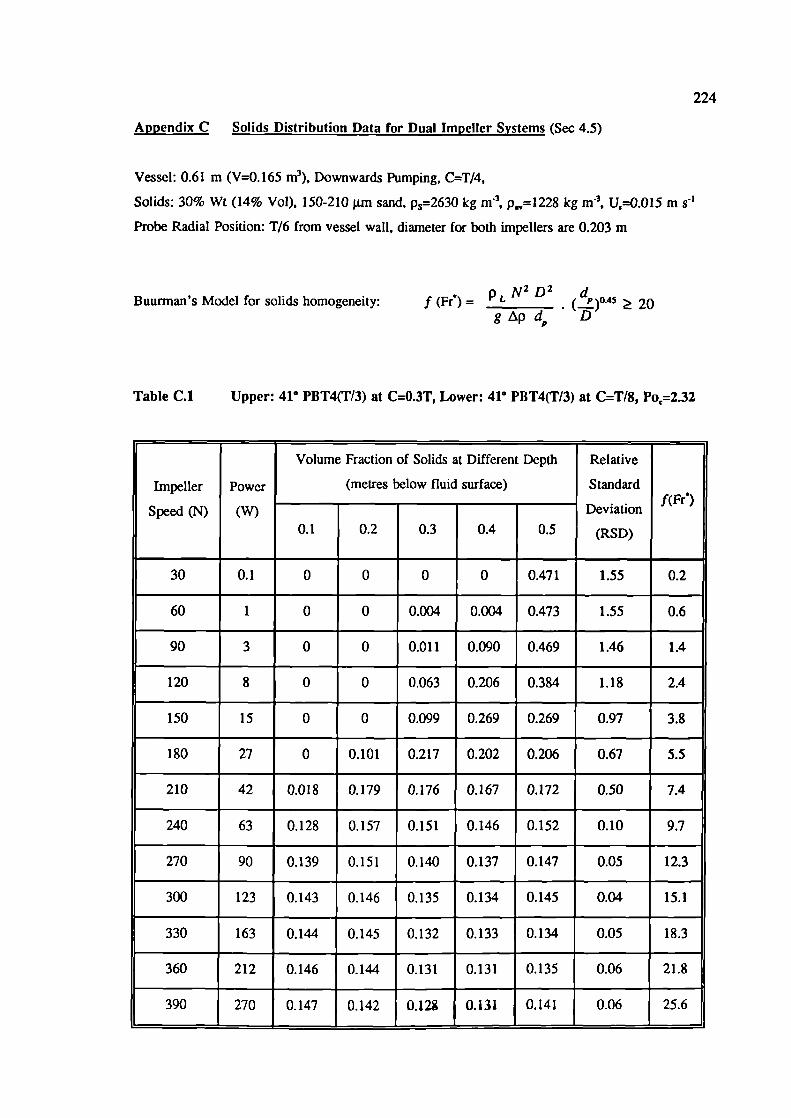
224

Appendix C Solids Distribution Data for Dual Impeller Systems (Sec 4.5)


Solids: 30% WE (14% Vol), 150-210 jim sand, p=263O kg m 3, p,,,= 1228 kg m 3, U,=0.015 m s

Probe Radial Position: T/6 from vessel wall, diameter for both impellers are 0.203 m

n N2 D 2 dBuurman's Model for solids homogeneity: f (Ff) = ' L. (P)O.45 ^ 20gpd D

Table C.1 Upper: 41° PBT4(T/3) at C=O.3T, Lower: 41° PBT4(T/3) at C=T/8, Po=2.32


Impeller Power (metres below fluid surface) Standardf(Fr')


0.1 0.2 0.3 0.4 0.5 (RSD)

30 0.1 0 0 0 0 0.471 1.55 0.2

60 1 0 0 0.004 0.004 0.473 1.55 0.6

90 3 0 0 0.011 0.090 0.469 1.46 1.4

120 8 0 0 0.063 0.206 0.384 1.18 2.4

150 15 0 0 0.099 0.269 0.269 0.97 3.8

180 27 0 0.101 0.217 0.202 0.206 0.67 5.5

210 42 0.018 0.179 0.176 0.167 0.172 0.50 7.4

240 63 0.128 0.157 0.151 0.146 0.152 0.10 9.7

270 90 0.139 0.151 0.140 0.137 0.147 0.05 12.3

300 123 0.143 0.146 0.135 0.134 0.145 0.04 15.1

330 163 0.144 0.145 0.132 0.133 0.134 0.05 18.3

360 212 0.146 0.144 0.131 0.131 0.135 0.06 21.8

390 270 0.147 0.142 0.12g0.131 0.141 0.06 25.6

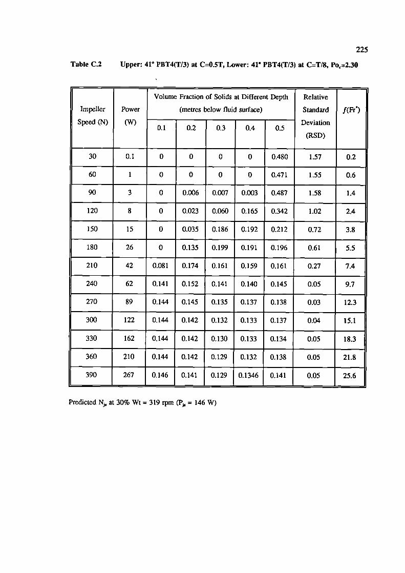
225

Table C.2 Upper: 41° PBT4(T/3) at C=O.5T, Lower: 41° PBT4(T/3) at C=T18, Po2.3O


Impeller Power (metres below fluid surface) Standard f(Fr°)

Speed (N) (W)0.1 0.2 0.3 0.4 05

Deviation

(RSD)

30 0.1 0 0 0 0 0.480 1.57 0.2

60 1 0 0 0 0 0.471 1.55 0.6

90 3 0 0.006 0.007 0.003 0.487 1.58 1.4

120 8 0 0.023 0.060 0.165 0.342 1.02 2.4

150 15 0 0.035 0.186 0.192 0.212 0.72 3.8

180 26 0 0.135 0.199 0.191 0.196 0.61 5.5

210 42 0.081 0.174 0.161 0.159 0.161 0.27 7.4

240 62 0.141 0.152 0.141 0.140 0.145 0.05 9.7

270 89 0.144 0.145 0.135 0.137 0.138 0.03 12.3

300 122 0.144 0.142 0.132 0.133 0.137 0.04 15.1

330 162 0.144 0.142 0.130 0.133 0.134 0.05 18.3

360 210 0.144 0.142 0.129 0.132 0.138 0.05 21.8

390 267 0.146 0.141 0.129 0.1346 0.141 0.05 25.6

Predicted N1 at 30% Wt = 319 rpm (P = 146 W)

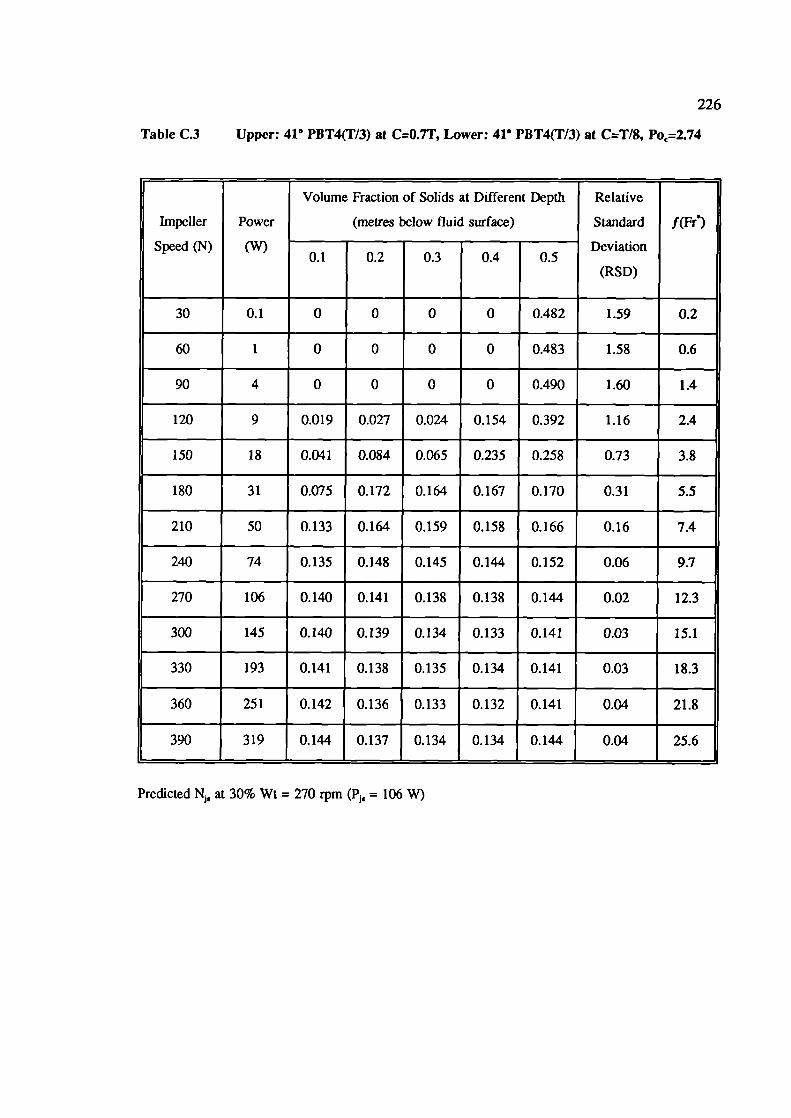
226

Table C.3 Upper: 410 PBT4(T/3) at C=O.7T, Lower: 41° PBT4(T/3) at C=T/S, P0=2.74



Speed ('\')0.1 0.2 0.3 0.4 0.5

Deviation

(RSD)

30 0.1 0 0 0 0 0.482 1.59 0.2

60 1 0 0 0 0 0.483 1.58 0.6

90 4 0 0 0 0 0.490 1.60 1.4

120 9 0.019 0.027 0.024 0.154 0.392 1.16 2.4

150 18 0.041 0.084 0.065 0.235 0.258 0.73 3.8

180 31 0.075 0.172 0.164 0.167 0.170 0.31 5.5

210 50 0.133 0.164 0.159 0.158 0.166 0.16 7.4

240 74 0.135 0.148 0.145 0.144 0.152 0.06 9.7

270 106 0.140 0.141 0.138 0.138 0.144 0.02 12.3

300 145 0.140 0.139 0.134 0.133 0.141 0.03 15.1

330 193 0.141 0.138 0.135 0.134 0.141 0.03 18.3

360 251 0.142 0.136 0.133 0.132 0.141 0.04 21.8

390 319 0.144 0.137 0.134 0.134 0.144 0.04 25.6


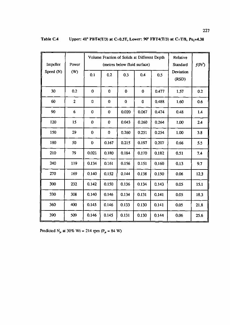
227

Table C.4 Upper: 41° PBT4(T13) at C=O.3T, Lower: 900 FBT4(1'13) at C=T/8, P0=4.38



Speed (N)0.1 0.2 0.3 0.4 0.5

Deviation

(RSD)

30 0.2 0 0 0 0 0.477 1.57 0.2

60 2 0 0 0 0 0.488 1.60 0.6

90 6 0 0 0.020 0.067 0.474 0.48 1.4

120 15 0 0 0.043 0.260 0.264 1.00 2.4

150 29 0 0 0.260 0.251 0.254 1.00 3.8

180 50 0 0.167 0.215 0.197 0.207 0.66 5.5

210 79 0.021 0.180 0.184 0.170 0.182 0.51 7.4

240 119 0.134 0.161 0.156 0.151 0.160 0.13 9.7

270 169 0.140 0.152 0.144 0.138 0.150 0.06 12.3

300 232 0.142 0.150 0.136 0.134 0.143 0.05 15.1

330 308 0.140 0.146 0.134 0.131 0.141 0.05 18.3

360 400 0.145 0.146 0.133 0.130 0.141 0.05 21.8

390 509 0.146 0.145 0.131 0.130 0.144 0.06 25.6


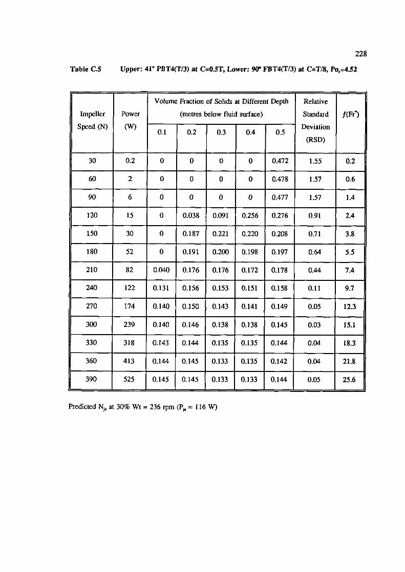
228

Table C.5 Upper: 410 PBT4(T/3) at C=0.5T, Lower: 90° FBT4(T/3) at C=T/8, P0=4.52


Impeller Power (metres below fluid surface) Standard f(Fr')

Speed (N)0.1 0.2 0.3 0.4 0.5

Deviation

(RSD)

30 0.2 0 0 0 0 0.472 1.55 0.2

60 2 0 0 0 0 0.478 1.57 0.6

90 6 0 0 0 0 0.477 1.57 1.4

120 15 0 0.038 0.091 0.256 0.276 0.91 2.4

150 30 0 0.187 0.221 0.220 0.208 0.71 3.8

180 52 0 0.191 0.200 0.198 0.197 0.64 5.5

210 82 0.040 0.176 0.176 0.172 0.178 0.44 7.4

240 122 0.131 0.156 0.153 0.151 0.158 0.11 9.7

270 174 0.140 0.150 0.143 0.141 0.149 0.05 12.3

300 239 0.140 0.146 0.138 0.138 0.145 0.03 15.1

330 318 0.143 0.144 0.135 0.135 0.144 0.04 18.3

360 413 0.144 0.145 0.133 0.135 0.142 0.04 21.8

390 525 0.145 0.145 0.133 0.133 0.144 0.05 25.6

Predicted N at 30% Wt = 236 rpm (P, = 116 W)

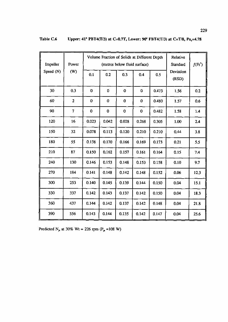
229

Table C.6 Upper: 41 PBT4(T/3) at C=O.7T, Lower: 90 FBT4(T13) at C=T18, P0=4.78



Speed (N) (W)0.1 0.2 0.3 0.4 0.5

Deviation

(RSD)

30 0.3 0 0 0 0 0.473 1.56 0.2

60 2 0 0 0 0 0.480 1.57 0.6

90 7 0 0 0 0 0.482 1.58 1.4

120 16 0.023 0.042 0.028 0.268 0.305 1.00 2.4

150 32 0.078 0.113 0.120 0.210 0.210 0.44 3.8

180 55 0.138 0.170 0.166 0.169 0.173 0.21 5.5

210 87 0.150 0.162 0.157 0.161 0.164 0.15 7.4

240 130 0.146 0.153 0.148 0.153 0.158 0.10 9.7

270 184 0.141 0.148 0.142 0.148 0.152 0.06 12.3

300 253 0.140 0.145 0.139 0.144 0.150 0.04 15.1

330 337 0.142 0.143 0.137 0.142 0.150 0.04 18.3

360 437 0.144 0.142 0.137 0.142 0.148 0.04 21.8

390 556 0.143 0.144 0.135 0.142 0.147 0.04 25.6

Predicted N, at 30% Wt = 226 rpm (P =108 W)

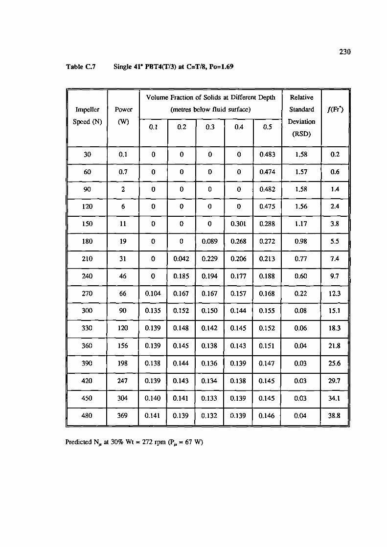
230

Table C.7 Single 41 PBT4(T13) at C=T18, Po=1.69


Impeller Power (metres below fluid surface) Standard f(Ff)


0.1 0.2 0.3 0.4 0.5(RSD)

30 0.1 0 0 0 0 0.483 1.58 0.2

60 0.7 0 0 0 0 0.474 1.57 0.6

90 2 0 0 0 0 0.482 1.58 1.4

120 6 0 0 0 0 0.475 1.56 2.4

150 11 0 0 0 0.301 0.288 1.17 3.8

180 19 0 0 0.089 0.268 0.272 0.98 5.5

210 31 0 0.042 0.229 0.206 0.213 0.77 7.4

240 46 0 0.185 0.194 0.177 0.188 0.60 9.7

270 66 0.104 0.167 0.167 0.157 0.168 0.22 12.3

300 90 0.135 0.152 0.150 0.144 0.155 0.08 15.1

330 120 0.139 0.148 0.142 0.145 0.152 0.06 18.3

360 156 0.139 0.145 0.138 0.143 0.151 0.04 21.8

390 198 0.138 0.144 0.136 0.139 0.147 0.03 25.6

420 247 0.139 0.143 0.134 0.138 0.145 0.03 29.7

450 304 0.140 0.141 0.133 0.139 0.145 0.03 34.1

480 369 0.141 0.139 0.132 0.139 0.146 0.04 38.8

Predicted at 30% Wt = 272 rpm (Ps,, = 67 W)

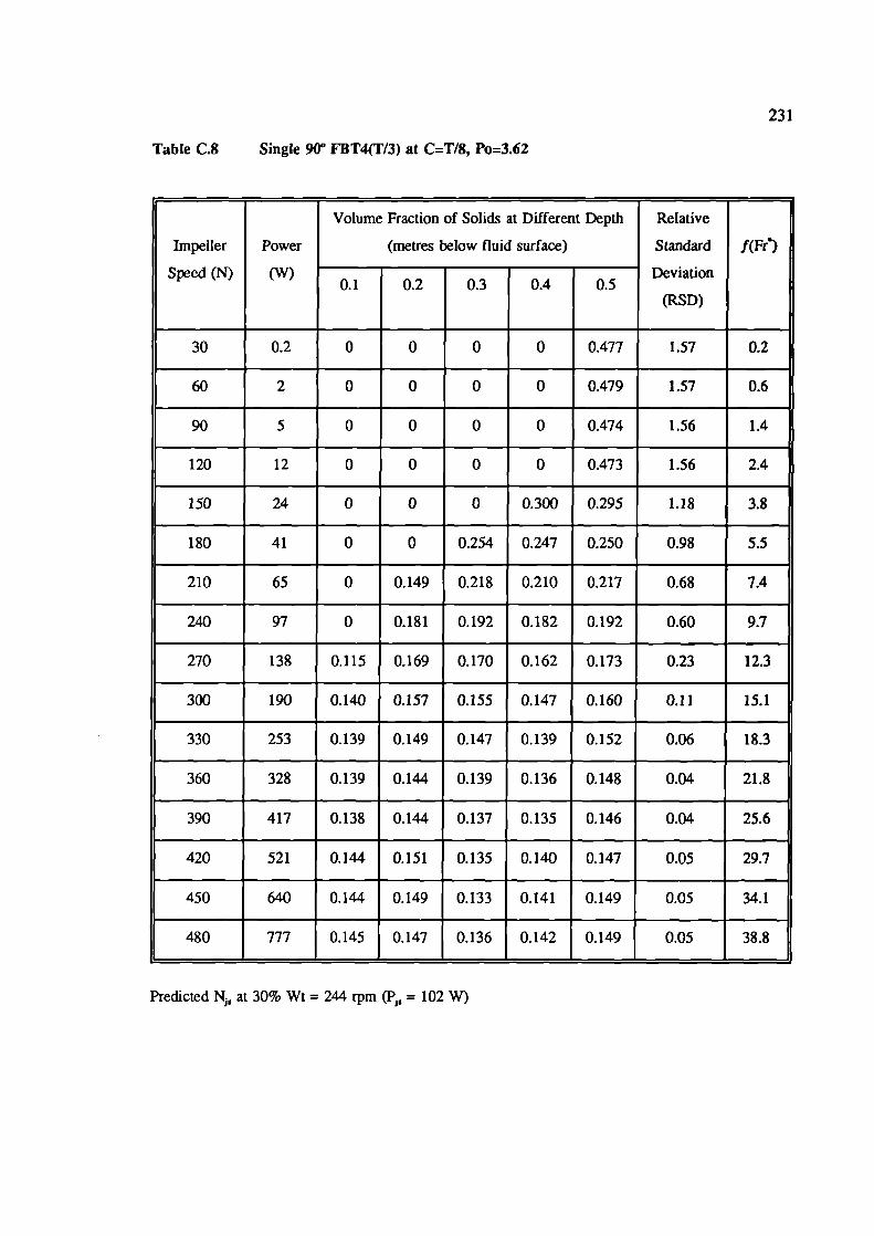
231

Table C.8 Single 90° FBT4(T13) at C=T/8, Po=3.62




0.1 0.2 0.3 0.4 0.5(RSD)

30 0.2 0 0 0 0 0.477 1.57 0.2

60 2 0 0 0 0 0.479 1.57 0.6

90 5 0 0 0 0 0.474 1.56 1.4

120 12 0 0 0 0 0.473 1.56 2.4

150 24 0 0 0 0.300 0.295 1.18 3.8

180 41 0 0 0.254 0.247 0.250 0.98 5.5

210 65 0 0.149 0.218 0.210 0.217 0.68 7.4

240 97 0 0.181 0.192 0.182 0.192 0.60 9.7

270 138 0.115 0.169 0.170 0.162 0.173 0.23 12.3

300 190 0.140 0.157 0.155 0.147 0.160 0.11 15.1

330 253 0.139 0.149 0.147 0.139 0.152 0.06 18.3

360 328 0.139 0.144 0.139 0.136 0.148 0.04 21.8

390 417 0.138 0.144 0.137 0.135 0.146 0.04 25.6

420 521 0.144 0.151 0.135 0.140 0.147 0.05 29.7

450 640 0.144 0.149 0.133 0.141 0.149 0.05 34.1

480 777 0.145 0.147 0.136 0.142 0.149 0.05 38.8

Predicted N. at 30% Wt = 244 rpm (P = 102 W)

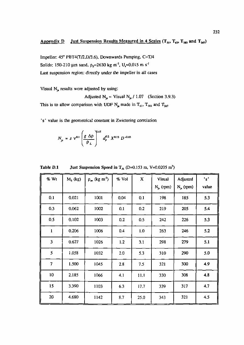
232

Appendix D Just Suspension Results Measured in 4 Scales (T31 , T61, T1 and T7)

Impeller: 45° PBT4(Tf2,D/3.6), Downwards Pumping, CT/4

Solids: 150-210 j.un sand, p=2630 kg m 3 , U0.O15 m s'

Last suspension region: directly under the impeller in all cases

Visual N results were adjusted by using:

Adjusted = Visual N / 1.07 (Section 3.9.3)

This is to allow comparison with UDF made in T61 , T183 and T267

's' value is the geometrical constant in Zwietering correlation

I

N. = s v°' I g A4D I

d X°' 3 D°85is(PLJ

Table D.1 Just Suspension Speed in T31 (D=O.153 m, V=0.0205 m3)

% Wt M (kg) p•, (kg m 3) % Vol X Visual Adjusted

N, (rpm) (rpm) value

0.1 0.021 1001 0.04 0.1 198 185 5.3

0.3 0.062 1002 0.1 0.2 219 205 5.4

0.5 0.102 1003 0.2 0.5 242 226 5.3

1 0.206 1006 0.4 1.0 263 246 5.2

3 0.627 1026 1.2 3.1 298 279 5.1

5 1.058 1032 2.0 5.3 310 290 5.0

7 1.500 1045 2.8 7.5 321 300 4.9

10 2.185 1066 4.1 11.1 330 308 4.8

15 3.390 1103 6.3 17.7 339 317 4.7

20 4.680 1142 8.7 25.0 343 321 4.5

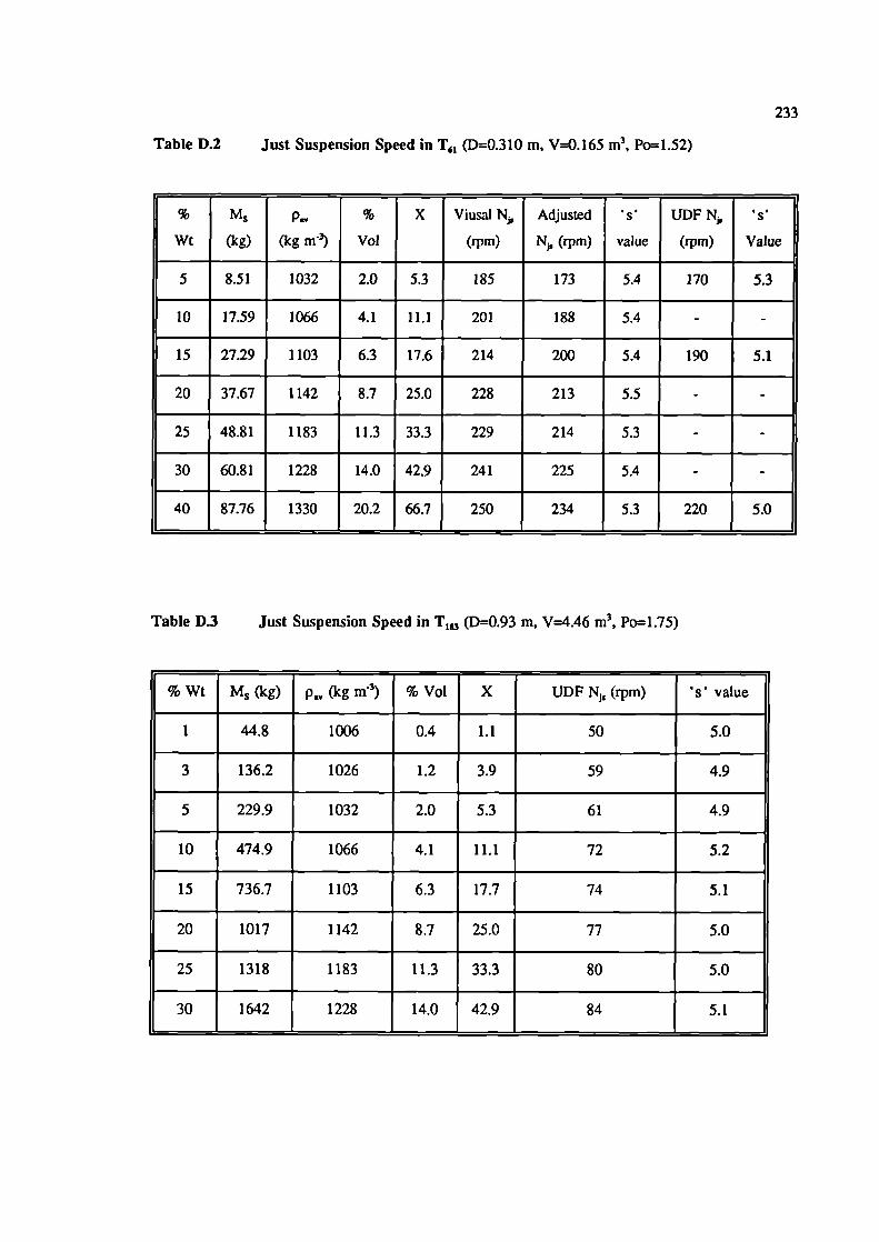
233

Table D.2 Just Suspension Speed in T 1 (D=O.310 m, V=0.165 m3, P0=1.52)

% M Pr. X Viusal N, Adjusted s UDF N, s

Wt (kg) (kg m) Vol (rpm) N, (rpm) value (rpm) Value

5 8.51 1032 2.0 5.3 185 173 5.4 170 5.3

10 17.59 1066 4.1 11.1 201 188 5.4 - -

15 27.29 1103 6.3 17.6 214 200 5.4 190 5.1

20 37.67 1142 8.7 25.0 228 213 5.5 - -

25 48.81 1183 11.3 33.3 229 214 5.3 - -

30 60.81 1228 14.0 42.9 241 225 5.4 - -

40 87.76 1330 20.2 66.7 250 234 5.3 220 5.0

Table D.3 Just Suspension Speed in T1 (D=0.93 m, V=4.46 m3, P0=1.75)

% Wi M (kg) p (kg mS') % Vol X UDF Njg (rpm) s' value

1 44.8 1006 0.4 1.1 50 5.0

3 136.2 1026 1.2 3.9 59 4.9

5 229.9 1032 2.0 5.3 61 4.9

10 474.9 1066 4.1 11.1 72 5.2

15 736.7 1103 6.3 17.7 74 5.1

20 1017 1142 8.7 25.0 77 5.0

25 1318 1183 11.3 33.3 80 5.0

30 1642 1228 14.0 42.9 84 5.1

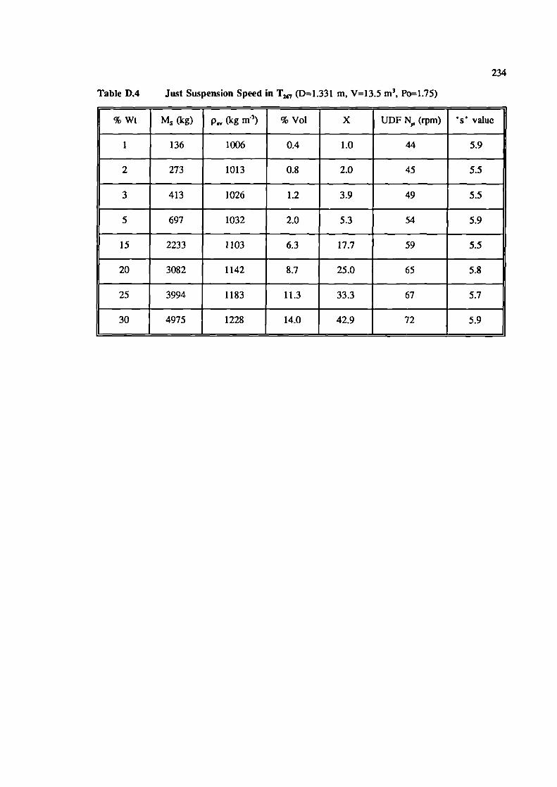
234

Table D.4 Just Suspension Speed in T, (D=1.331 m, V=13.5 m 3 , Po=1.75)

% Wt M (kg) p (kg in') % Vol X UDF N (rpm) s value

1 136 1006 0.4 1.0 44 5.9

2 273 1013 0.8 2.0 45 5.5

3 413 1026 1.2 3.9 49 5.5

5 697 1032 2.0 5.3 54 5.9

15 2233 1103 6.3 17.7 59 5.5

20 3082 1142 8.7 25.0 65 5.8

25 3994 1183 11.3 33.3 67 5.7

30 4975 1228 14.0 42.9 72 5.9

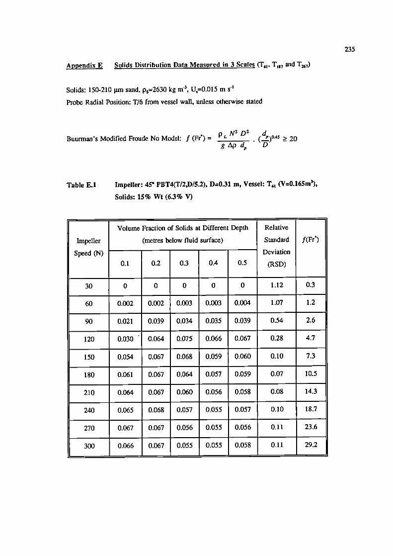
235

Appendix E Solids Distribution Data Measured in 3 Scales (T61 , T183 and T7)

Solids: 150-210 jun sand, p=2630 kg m 3, U1=0.015 m s

Probe Radial Position: T/6 from vessel wall, unless otherwise stated

Buurman's Modified Froude No Model: f (Fr') = P L N2 D 2 (dP)045 ^ 20

gLpd D

Table E.1 Impeller: 450 PBT4(I'12,D15.2), D=O.31 m, Vessel: T 1 (V=O.165m3),

Solids: 15% Wt (6.3% V)


Impeller (metres below fluid surface) Standard f(Fr')

Speed (N) Deviation

0.1 0.2 0.3 0.4 0.5 (RSD)

30 0 0 0 0 0 1.12 0.3

60 0.002 0.002 0.003 0.003 0.004 1.07 1.2

90 0.021 0.039 0.034 0.035 0.039 0.54 2.6

120 0.030 0.064 0.075 0.066 0.067 0.28 4.7

150 0.054 0.067 0.068 0.059 0.060 0.10 7.3

180 0.061 0.067 0.064 0.057 0.059 0.07 10.5

210 0.064 0.067 0.060 0.056 0.058 0.08 14.3

240 0.065 0.068 0.057 0.055 0.057 0.10 18.7

270 0.067 0.067 0.056 0.055 0.056 0.11 23.6

300 0.066 0.067 0.055 0.055 0.058 0.11 29.2

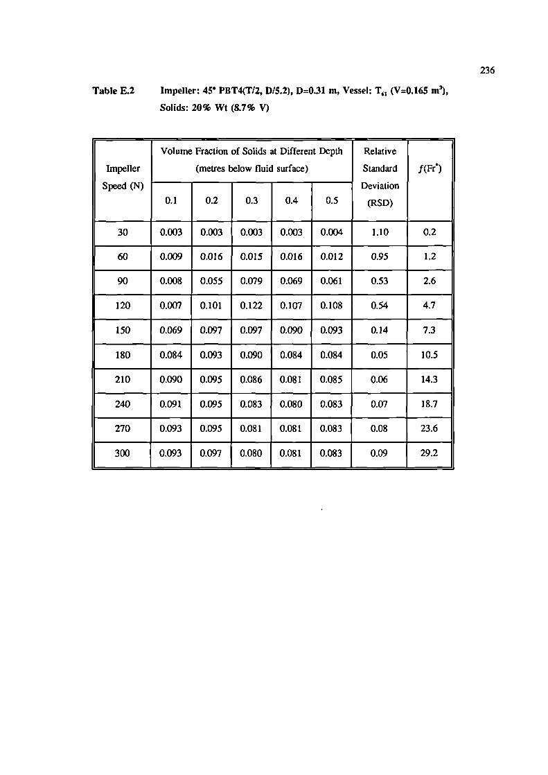
236

Table E.2 Impeller: 45' PBT4(T12, D/S.2), D=0.31 m, Vessel: T 1 (V=O.165 m3),

Solids: 20% Wt (8.7% V)


Impeller (metres below fluid surface) Standard f(Fr)

Speed (N) Deviation

0.1 0.2 0.3 0.4 0.5 (RSD)

30 0.003 0.003 0.003 0.003 0.004 1.10 0.2

60 0.009 0.016 0.015 0.016 0.012 0.95 1.2

90 0.008 0.055 0.079 0.069 0.06 1 0.53 2.6

120 0.007 0.101 0.122 0.107 0.108 0.54 4.7

150 0.069 0.097 0.097 0.090 0.093 0.14 7.3

180 0.084 0.093 0.090 0.084 0.084 0.05 10.5

210 0.090 0.095 0.086 0.081 0.085 0.06 14.3

240 0.091 0.095 0.083 0.080 0.083 0.07 18.7

270 0.093 0.095 0.081 0.081 0.083 0.08 23.6

300 0.093 0.097 0.080 0.08 1 0.083 0.09 29.2

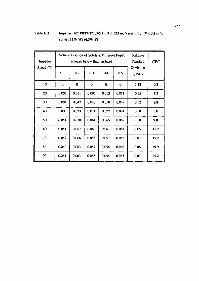
237

Table E.3 Impeller: 450 PBT4(T12,D15.2), D=1.333 m, Vessel: T 1 (V=13.S m'),

Solids: 15% Wt (6.3% V)



Speed (N) Deviation

0.1 0.2 0.3 0.4 0.5 (RSD)

10 0 0 0 0 0 1.12 0.3

20 0.007 0.011 0.007 0.013 0.011 0.95 1.2

30 0.004 0.047 0.047 0.050 0.049 0.52 2.8

40 0.003 0.073 0.071 0.072 0.074 0.50 5.0

50 0.054 0.070 0.064 0.065 0.069 0.10 7.8

60 0.061 0.067 0.060 0.061 0.061 0.05 11.2

70 0.059 0.066 0.058 0.057 0.062 0.07 15.2

80 0.060 0.063 0.057 0.056 0.060 0.08 19.9

90 0.064 0.063 0.058 0.056 0.063 0.07 25.2

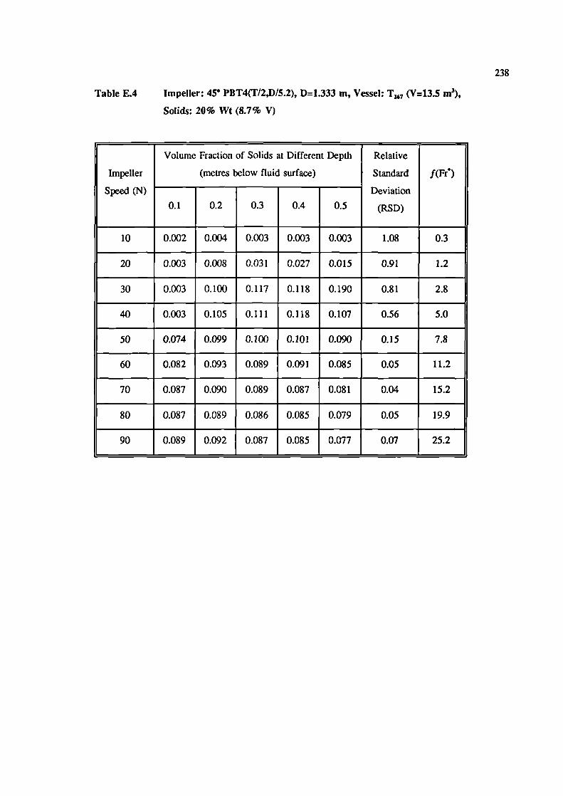
238

Table E.4 Impeller: 45' PBT4(T/2,D/5.2), D=1.333 m, Vessel: T7 (V=13.5 m3),

Solids: 20% Wt (8.7% V)



Speed (N) Deviation

0.1 0.2 0.3 0.4 0.5 (RSD)

10 0.002 0.004 0.003 0.003 0.003 1.08 0.3

20 0.003 0.008 0.031 0.027 0.015 0.91 1.2

30 0.003 0.100 0.117 0.118 0.190 0.81 2.8

4.0 0.003 0.105 0.111 0.118 0.107 0.56 5.0

50 0.074 0.099 0.100 0.101 0.090 0.15 7.8

60 0.082 0.093 0.089 0.091 0.085 0.05 11.2

70 0.087 0.090 0.089 0.087 0.081 0.04 15.2

80 0.087 0.089 0.086 0.085 0.079 0.05 19.9

90 0.089 0.092 0.087 0.085 0.077 0.07 25.2

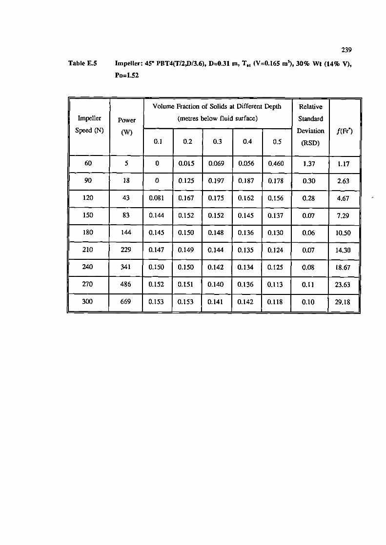
239

Table E.5 Impeller: 45 PBT4(T/2,D/3.6), Drn0.31 m, T 1 (V=0.165 m 3), 30% Wt (14% V),

Po=1.52


Impeller Power (metres below fluid surface) Standard

Speed (N) (W) Deviation f(Ff)

0.1 0.2 0.3 0.4 0.5 (RSD)

60 5 0 0.015 0.069 0.056 0.460 1.37 1.17

90 18 0 0.125 0.197 0.187 0.178 0.30 2.63

120 43 0.081 0.167 0.175 0.162 0.156 0.28 4.67

150 83 0.144 0.152 0.152 0.145 0.137 0.07 7.29

180 144 0.145 0.150 0.148 0.136 0.130 0.06 10.50

210 229 0.147 0.149 0.144 0.135 0.124 0.07 14.30

240 341 0.150 0.150 0.142 0.134 0.125 0.08 18.67

270 486 0.152 0.151 0.140 0.136 0.113 0.11 23.63

300 669 0.153 0.153 0.141 0.142 0.118 0.10 29.18

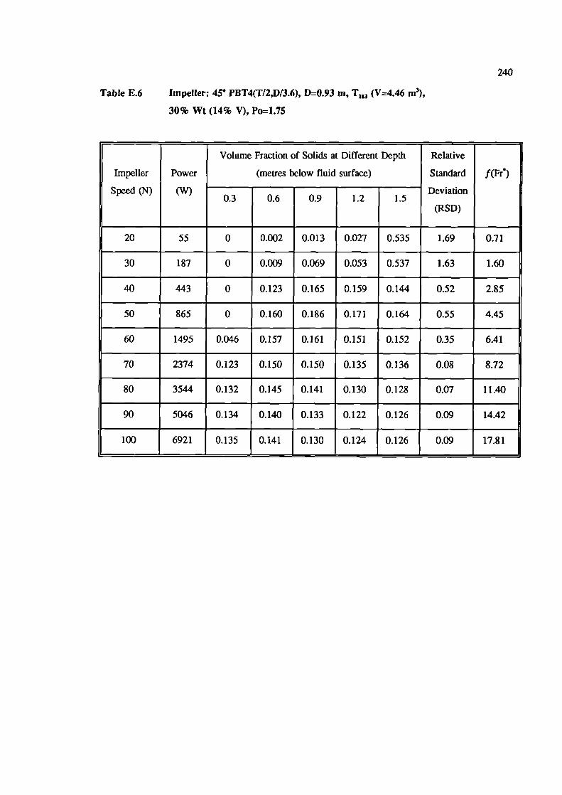
240

Table E.6 Impeller: 450 PBT4(T/2,D/3.6), D=0.93 m, T 1 (V=4.46 m3),

30% Wt (14% V), Po=1.75



Speed (N) (W)0.3 0.6 0.9 1.2 1.5

Deviation

(RSD)

20 55 0 0.002 0.013 0.027 0.535 1.69 0.71

30 187 0 0.009 0.069 0.053 0.537 1.63 1.60

40 443 0 0.123 0.165 0.159 0.144 0.52 2.85

50 865 0 0.160 0.186 0.171 0.164 0.55 4.45

60 1495 0.046 0.157 0.161 0.151 0.152 0.35 6.41

70 2374 0.123 0.150 0.150 0.135 0.136 0.08 8.72

80 3544 0.132 0.145 0.141 0.130 0.128 0.07 11.40

90 5046 0.134 0.140 0.133 0.122 0.126 0.09 14.42

100 6921 0.135 0.141 0.130 0.124 0.126 0.09 17.81

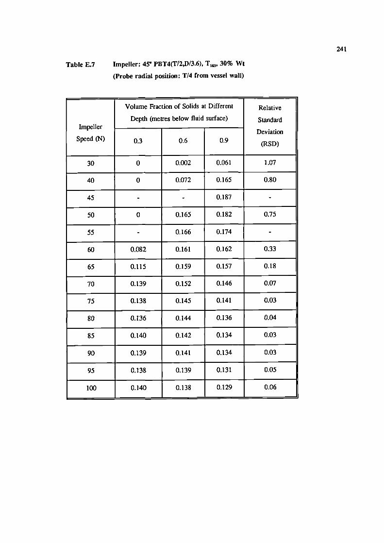
241

Table E.7 Impeller: 450 PBT4(T/2,D/3.6), T 1 , 30% Wt

(Probe radial position: T14 from vessel wall)

Volume Fraction of Solids at Different Relative

Depth (metres below fluid surface) Sd&dImpeller

Deviation

Speed (N) 0.3 0.6 0.9 (RSD)

30 0 0.002 0.061 1.07

40 0 0.072 0.165 0.80

45 - - 0.187 -

50 0 0.165 0.182 0.75

55 - 0.166 0.174 -

60 0.082 0.161 0.162 0.33

65 0.115 0.159 0.157 0.18

70 0.139 0.152 0.146 0.07

75 0.138 0.145 0.141 0.03

80 0.136 0.144 0.136 0.04

85 0.140 0.142 0.134 0.03

90 0.139 0.141 0.134 0.03

95 0.138 0.139 0.131 0.05

100 0.140 0.138 0.129 0.06

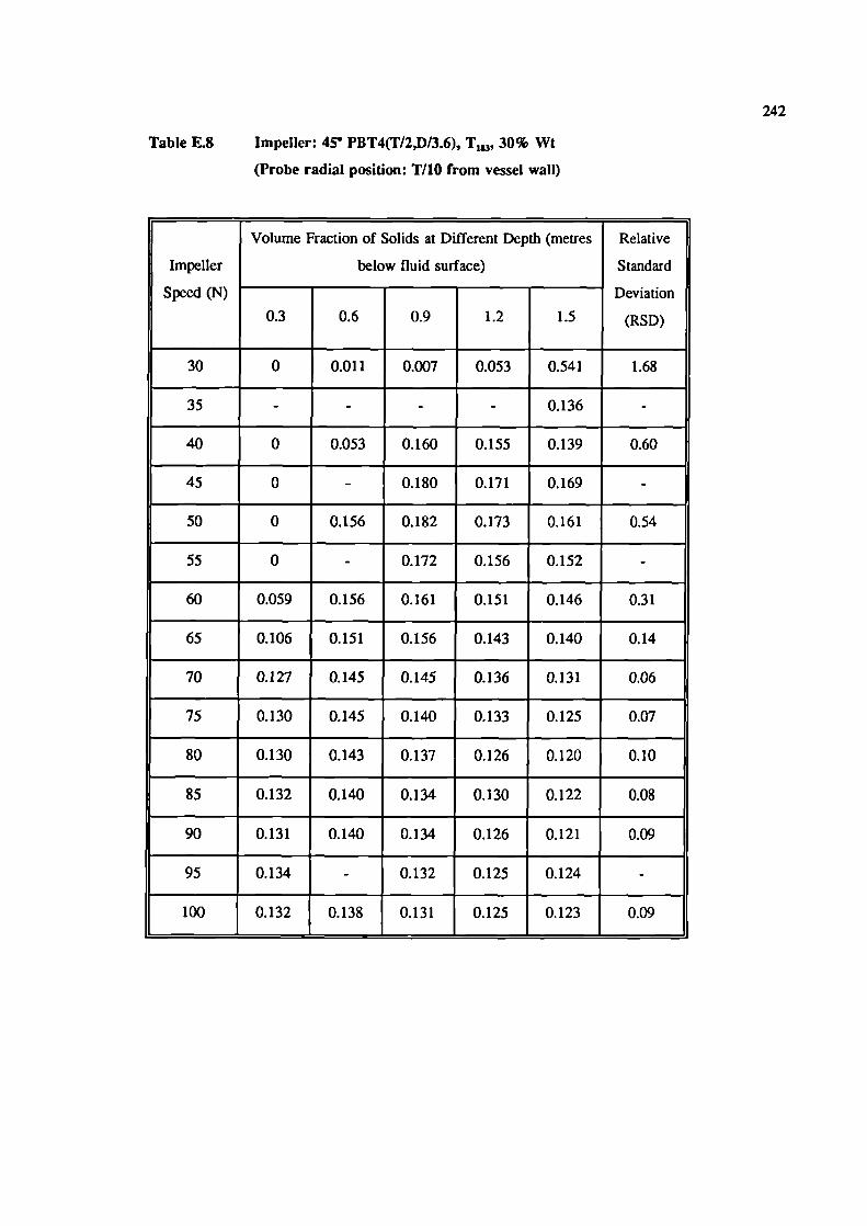
242

Table E.8 Impeller: 45 PBT4(T12,D13.6), T1 , 30% Wt

(Probe radial position: TI10 from vessel wall)

Volume Fraction of Solids at Different Depth (metres Relative

Impeller below fluid surface) Standard

Speed (N) Deviation

0.3 0.6 0.9 1.2 1.5 (RSD)

30 0 0.011 0.007 0.053 0.541 1.68

35 - - - - 0.136 -

40 0 0.053 0.160 0.155 0.139 0.60

45 0 - 0.180 0.171 0.169 -

50 0 0.156 0.182 0.173 0.161 0.54

55 0 - 0.172 0.156 0.152 -

60 0.059 0.156 0.161 0.151 0.146 0.31

65 0.106 0.151 0.156 0.143 0.140 0.14

70 0.127 0.145 0.145 0.136 0.131 0.06

75 0.130 0.145 0.140 0.133 0.125 0.07

80 0.130 0.143 0.137 0.126 0.120 0.10

85 0.132 0.140 0.134 0.130 0.122 0.08

90 0.131 0.140 0.134 0.126 0.121 0.09

95 0.134 - 0.132 0.125 0.124 -

100 0.132 0.138 0.131 0.125 0.123 0.09

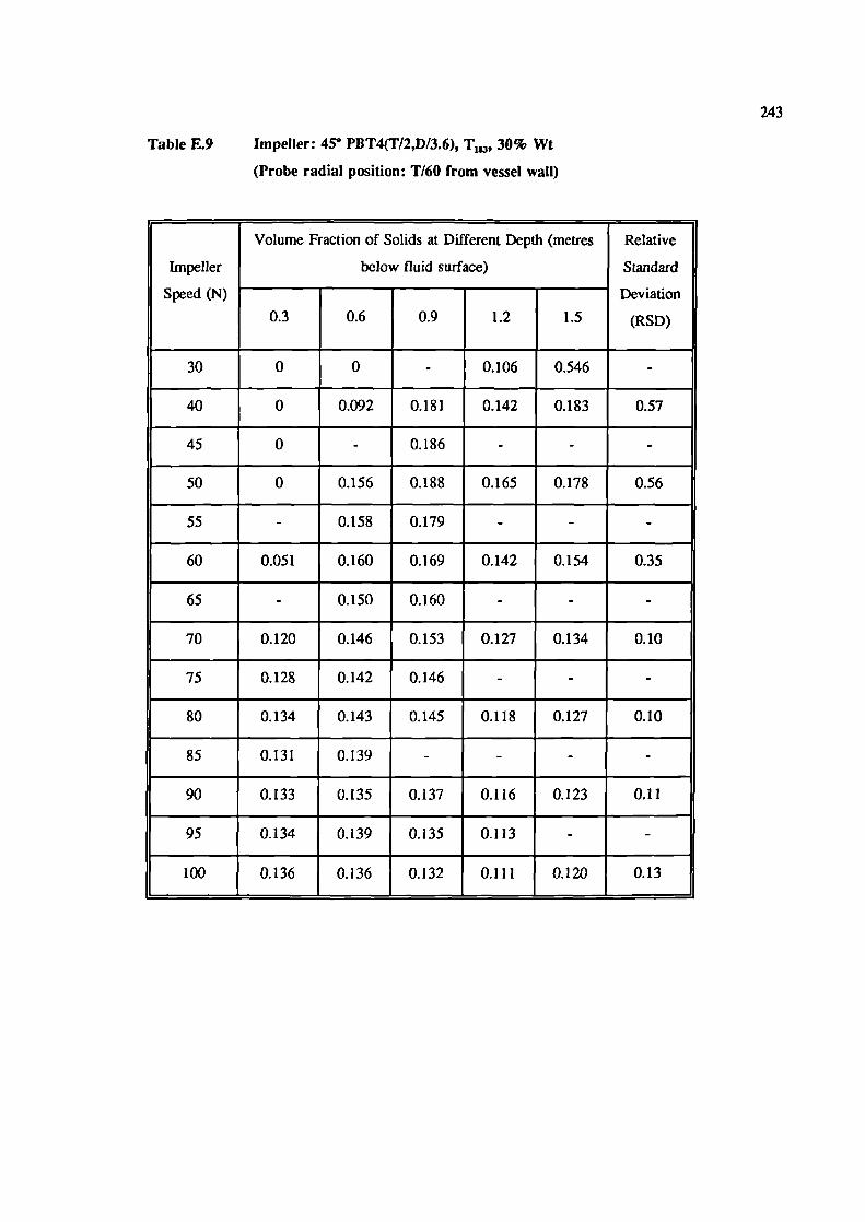
243

Table E.9 Impeller: 45 PBT4(T/2,D/3.6), T11 ,, 30% Wt

(Probe radial position: T/60 from vessel wall)

Volume Fraction of Solids at Different Depth (metres Relative

Impeller below fluid surface) Standard

Speed (N) Deviation

0.3 0.6 0.9 1.2 1.5 (RSD)

30 0 0 - 0.106 0.546 -

40 0 0.092 0.181 0.142 0.183 0.57

45 0 - 0.186 - - -

50 0 0.156 0.188 0.165 0.178 0.56

55 - 0.158 0.179 - - -

60 0.051 0.160 0.169 0.142 0.154 0.35

65 - 0.150 0.160 - - -

70 0.120 0.146 0.153 0.127 0.134 0.10

75 0.128 0.142 0.146 - - -

80 0.134 0.143 0.145 0.118 0.127 0.10

85 0.131 0.139 - - - -

90 0.133 0.135 0.137 0.116 0.123 0.11

95 0.134 0.139 0.135 0.113 - -

100 0.136 0.136 0.132 0.111 0.120 0.13

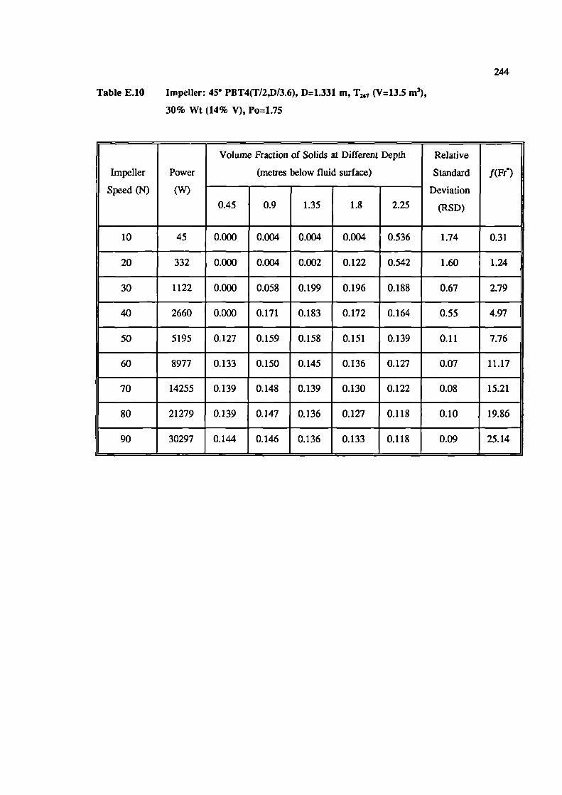
244

Table E.10 Impeller: 45 PBT4(T/2,D13.6), D=1.331 m, T 7 (V=13.5 m3),

30% Wt (14% V), Po=1.75




0.45 0.9 1.35 1.8 2.25 (RSD)

10 45 0.000 0.004 0.004 0.004 0.536 1.74 0.31

20 332 0.000 0.004 0.002 0.122 0.542 1.60 1.24

30 1122 0.000 0.058 0.199 0.196 0.188 0.67 2.79

40 2660 0.000 0.171 0.183 0.172 0.164 0.55 4.97

50 5195 0.127 0.159 0.158 0.151 0.139 0.11 7.76

60 8977 0.133 0.150 0.145 0.136 0.127 0.07 11.17

70 14255 0.139 0.148 0.139 0.130 0.122 0.08 15.21

80 21279 0.139 0.147 0.136 0.127 0.118 0.10 19.86

90 30297 0.144 0.146 0.136 0.133 0.118 0.09 25.14

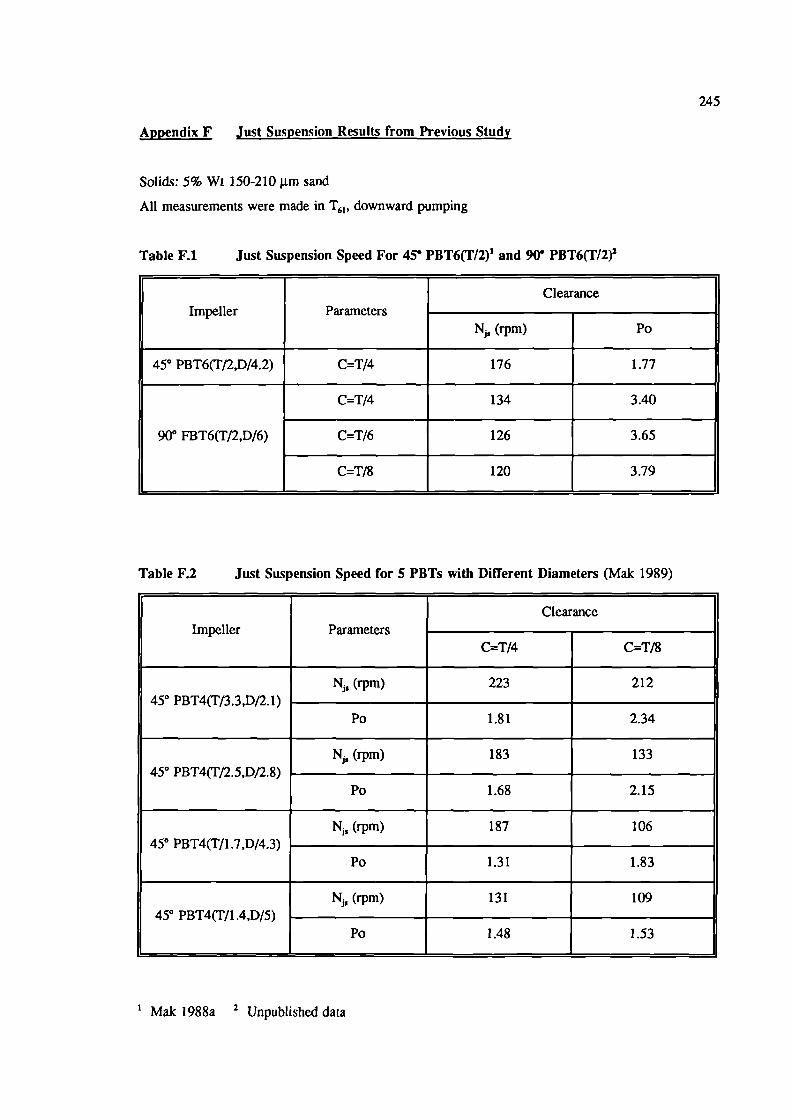
245

Appendix F Just Suspension Results from Previous Study

Solids: 5% Wt 150-210 im sand

All measurements were made in T61 , downward pumping

Table F.! Just Suspension Speed For 450 PBT6(T/2) 1 and 90° PBT6(T/2)2

ClearanceImpeller Parameters

N, (rpm) Po

450 PBT6(T/2,D/4.2) C=T/4 176 1.77

C=T/4 134 3.40

900 FBT6(T/2,D/6) C=T/6 126 3.65

C=T18 120 3.79

Table F.2 Just Suspension Speed for S PBTs with Different Diameters (Mak 1989)

ClearanceImpeller Parameters

CT/4 C=T/8

212223N (rpm)450 PBT4(T/3.3,D/2.1)

1.81 2.34Po

183 133N (rpm)450 PBT4(T/2.5,D/2.8)

1.68 2.15Pa

187 106N (rpm)450 PBT4(T/1.7,D/4.3)

1.31 1.83Po

109131N, (rpm)450 PBT4T/1 .4,D/5)

1.48 1.53Pa

Mak 1988a 2 Unpublished data

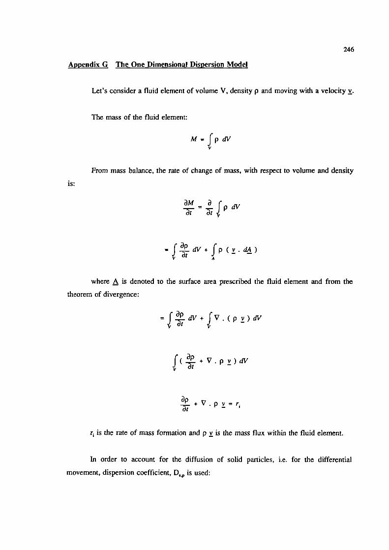
246

Appendix G The One Dimensiona! Dispersion Model

Let's consider a fluid element of volume V, density p and moving with a velocity v.

The mass of the fluid eLement:

M =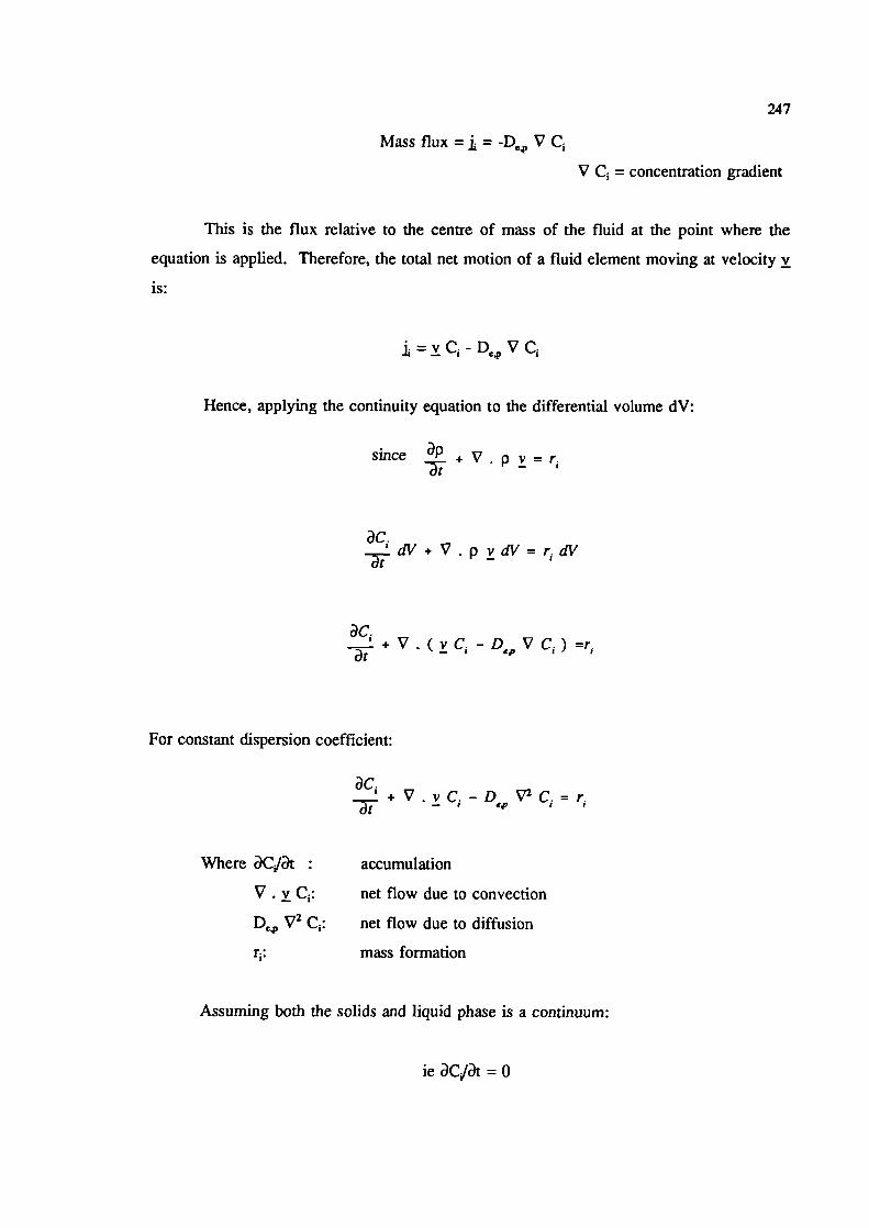![ dV

From mass balance, the rate of change of mass, with respect to volume and density

is:

aM_ adV

dV +

(!-')

where is denoted to the surface area prescribed the fluid element and from the

theorem of divergence:

= dv + 5 V. (p v) dV

r ap

..+

. P !) dV

ap + V . p V =

-i

r is the rate of mass formation and p V is the mass flux within the fluid element.

In order to account for the diffusion of solid particles, i.e. for the differential

movement, dispersion coefficient, D ,1, is used:

247

Mass flux = = V C1

V C1 = concentration gradient

This is the flux relative to the centre of mass of the fluid at the point where the

equation is applied. Therefore, the total net motion of a fluid element moving at velocity v

is:

= C1 - De,p V C

Hence, applying the continuity equation to the differential volume dV:

since .+V.pv=r1

ac.dV + V . P ! dV = r1 dV

-T

dci—+V ( ! C• - V C ) =r1

For constant dispersion coefficient:

ac,! C, - V2 C, =

Where dCjdt accumulation

V.vC1: net flow due to convection

D ,4, V2 C1: net flow due to diffusion

r1: mass formation

Assuming both the solids and liquid phase is a continuum:

ie dCjdt = 0

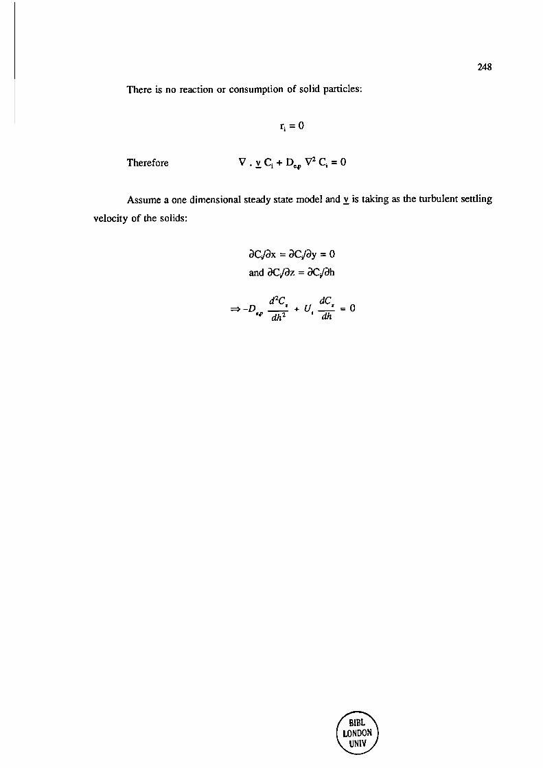
248

There is no reaction or consumption of solid particles:

r1 = 0

Therefore V v C1 + D ,1, V2 C1 = 0

Assume a one dimensional steady state model and ! is taking as the turbulent settling

velocity of the solids:

= aCjy = 0

and aC/az =

d2C dC=.-D +U=O

'dh

BIBLLONDON

UNIV

SOLID-LIQUID MIXING IN MECHANICALLY AGITATED VESSELS

Documents