INTERNATIONAL JOURNAL OF CLIMATOLOGY Int. J. Climatol. 25: 713–733 (2005) Published online in Wiley InterScience (www.interscience.wiley.com). DOI: 10.1002/joc.1156 SOLAR-INDUCED AND INTERNAL CLIMATE VARIABILITY AT DECADAL TIME SCALES MIHAI DIMA, a,b * GERRIT LOHMANN a,b and IOANA DIMA c a Department of Geoscience, University of Bremen, Bremen, Germany b Alfred Wegener Institute for Polar and Marine Research, Bremerhaven, Germany c University of Washington, Seattle, WA, USA Received 1 July 2004 Revised 8 December 2004 Accepted 8 December 2004 ABSTRACT Statistical analyses of long-term instrumental and proxy data emphasize a distinction between two quasi-decadal modes of climate variability. One mode is linked to atmosphere–ocean interactions (‘the internal mode’) and the other one is associated with the solar sunspots cycle (‘the solar mode’). The distinct signatures of these two modes are also detected in a high-resolution sediment core located in the Cariaco basin. In the oceanic surface temperature the internal mode explains about three times more variance than the solar mode. In contrast, the solar mode dominates over the internal mode in the sea-level pressure and upper atmospheric fields. The heterogeneous methods and data sets used in this study underline the distinction between these decadal modes and enable estimation of their relative importance. The distinction between these modes is important for the understanding of climate variability, the recent global warming trend and the interpretation of high-resolution proxy data. Copyright 2005 Royal Meteorological Society. KEY WORDS: decadal variability; climate; solar influence; atmosphere–ocean interaction 1. INTRODUCTION The solar influence on climate variability has been a controversial research problem for a long time (Hoyt and Schatten, 1997; Waple and Bradley, 1999; Mitchell et al., 2001). Counting the number of sunspots, periodic signals have been identified in association with the solar forcing, like the ∼11 year Schwabe cycle, the ∼22 year Hayle cycle and the ∼76–90 year Gleissberg cycle (e.g. Hoyt and Schatten, 1997). The connection between the sunspot cycle (hereafter SSC) and the Earth surface was emphasized through modelling studies. Such studies have shown that a decrease of just 0.1% in the solar activity associated with the ∼11 year solar cycle would affect the surface climate through dynamical effects originating in the stratospheric ozone and associated temperature changes (Haigh, 1999; Shindell et al., 1999). The established connection between the solar mode and the stratospheric vortex (Labitzke, 2001) may be viewed as a first step in Sun’s ‘path’ towards the surface. Furthermore, changes in the strength of the stratospheric polar vortex affect the variability of the surface fields (Black, 2002), specifically the sea-level pressure (SLP) and the Arctic oscillation (AO) associated variations (Thompson and Wallace, 1998). Since the AO has a strong fingerprint in the North Atlantic area, where it identifies with the more regional North Atlantic oscillation (NAO; Hurrel, 1995), it appears natural to search for a possible solar signature in this region. Another important advantage of investigating the North Atlantic area is the relatively good coverage and quality of the observational data here. Modes of variability that arise from atmosphere–ocean interactions also have a strong projection onto the climate in the Atlantic area (Gr¨ otzner et al., 1997). One particular mode of Atlantic climate variability is * Correspondence to: Mihai Dima, Department of Geoscience, University of Bremen, 28359 Bremen, Germany; e-mail: [email protected] Copyright 2005 Royal Meteorological Society

Welcome message from author
This document is posted to help you gain knowledge. Please leave a comment to let me know what you think about it! Share it to your friends and learn new things together.
Transcript
INTERNATIONAL JOURNAL OF CLIMATOLOGY
Int. J. Climatol. 25: 713–733 (2005)
Published online in Wiley InterScience (www.interscience.wiley.com). DOI: 10.1002/joc.1156
SOLAR-INDUCED AND INTERNAL CLIMATE VARIABILITYAT DECADAL TIME SCALES
MIHAI DIMA,a,b* GERRIT LOHMANNa,b and IOANA DIMAc
a Department of Geoscience, University of Bremen, Bremen, Germanyb Alfred Wegener Institute for Polar and Marine Research, Bremerhaven, Germany
c University of Washington, Seattle, WA, USA
Received 1 July 2004Revised 8 December 2004
Accepted 8 December 2004
ABSTRACT
Statistical analyses of long-term instrumental and proxy data emphasize a distinction between two quasi-decadal modesof climate variability. One mode is linked to atmosphere–ocean interactions (‘the internal mode’) and the other one isassociated with the solar sunspots cycle (‘the solar mode’). The distinct signatures of these two modes are also detectedin a high-resolution sediment core located in the Cariaco basin. In the oceanic surface temperature the internal modeexplains about three times more variance than the solar mode. In contrast, the solar mode dominates over the internalmode in the sea-level pressure and upper atmospheric fields. The heterogeneous methods and data sets used in this studyunderline the distinction between these decadal modes and enable estimation of their relative importance. The distinctionbetween these modes is important for the understanding of climate variability, the recent global warming trend and theinterpretation of high-resolution proxy data. Copyright 2005 Royal Meteorological Society.
KEY WORDS: decadal variability; climate; solar influence; atmosphere–ocean interaction
1. INTRODUCTION
The solar influence on climate variability has been a controversial research problem for a long time (Hoyt andSchatten, 1997; Waple and Bradley, 1999; Mitchell et al., 2001). Counting the number of sunspots, periodicsignals have been identified in association with the solar forcing, like the ∼11 year Schwabe cycle, the∼22 year Hayle cycle and the ∼76–90 year Gleissberg cycle (e.g. Hoyt and Schatten, 1997). The connectionbetween the sunspot cycle (hereafter SSC) and the Earth surface was emphasized through modelling studies.Such studies have shown that a decrease of just 0.1% in the solar activity associated with the ∼11 year solarcycle would affect the surface climate through dynamical effects originating in the stratospheric ozone andassociated temperature changes (Haigh, 1999; Shindell et al., 1999). The established connection between thesolar mode and the stratospheric vortex (Labitzke, 2001) may be viewed as a first step in Sun’s ‘path’ towardsthe surface. Furthermore, changes in the strength of the stratospheric polar vortex affect the variability of thesurface fields (Black, 2002), specifically the sea-level pressure (SLP) and the Arctic oscillation (AO) associatedvariations (Thompson and Wallace, 1998). Since the AO has a strong fingerprint in the North Atlantic area,where it identifies with the more regional North Atlantic oscillation (NAO; Hurrel, 1995), it appears naturalto search for a possible solar signature in this region. Another important advantage of investigating the NorthAtlantic area is the relatively good coverage and quality of the observational data here.
Modes of variability that arise from atmosphere–ocean interactions also have a strong projection onto theclimate in the Atlantic area (Grotzner et al., 1997). One particular mode of Atlantic climate variability is
* Correspondence to: Mihai Dima, Department of Geoscience, University of Bremen, 28359 Bremen, Germany;e-mail: [email protected]
Copyright 2005 Royal Meteorological Society

714 M. DIMA, G. LOHMANN AND I. DIMA
found at decadal time scales (Deser and Blackmon, 1993). The associated sea-surface temperature (SST)signature of this mode is characterized by a North Atlantic tripolar pattern, whereas the corresponding SLPpattern is represented by a basin-scale north–south dipole and midlatitudinal anomalous westerly winds. Ithas been proposed that this mode results from ocean–atmosphere and tropics–midlatitudes interactions in theNorth Atlantic basin (Dima et al., 2001).
To quantify the solar effects on climate one has to make a distinction between contributions resulting frominternal climate variability and those related to other forcings, because the former type of variability may maskthe signals coming from the Sun (Rind, 2002). It is the goal of the study to emphasize a distinction betweentwo decadal modes of climate variability of different origins and to estimate their relative importance.
The data and the methods used in this study are presented in Section 2, and the modes identified throughstatistical analyses of instrumental data are evaluated in Section 3. The modes are also distinguished in uppertroposphere reanalysis data (Section 4) and in patterns associated with a high-resolution marine sedimentrecord originating in the southern Caribbean (Section 5). The results are summarized and discussed andconclusions are drawn through the final two sections of the paper.
2. DATA AND METHODS
Unlike previous investigations, where the separation between forced and internal climate variability wasemphasised through numerical model experiments (e.g. Hansen and Lacis, 1990; Cubasch et al., 1997), thefocus here is to identify the characteristic patterns related to solar-induced variability and internal climatevariability at decadal time scales, based on analyses of instrumental, reanalysis and reconstructed data sets.In order to compensate for the quality and limited time extension of the data, different types of statisticalmethods and data are applied in our analyses.
2.1. Data
Instrumental SST data are obtained from the Comprehensive Ocean–Atmosphere Data Set (COADS; daSilva et al., 1994). Other SST fields used are derived from the Kaplan et al. (1998) data set, which wascompiled from an extended version of the COADS (Smith and Reynolds, 2003) and the GISST (Parker et al.,1995) data sets. The analysis is concentrated on the North Atlantic Ocean, which, by comparison with otherareas, is relatively well covered by direct measurements.
SLP fields are obtained from Trenberth and Paolino (1980) and they partially cover the Northern Hemisphere(15–90 °N). Furthermore, monthly National Centers for Environmental Prediction–National Center forAtmospheric Research (NCEP–NCAR) reanalysis zonal and meridional wind data at 200 hPa (Kalnay et al.,1996; Kistler et al., 2001) mapped on a global grid are used to calculate the horizontal streamfunction fieldat that level.
To complete the analysis, a high-resolution time series of marine sediments from the Cariaco basin in thesouthern Caribbean region is analysed in order to identify its embedded periodic time-components (Blacket al., 1999). The data set provides a sub-decadal resolved record of Atlantic climate variability. The numbersof individuals per gram of sediment for the planktic foraminifer Globigerina bulloides are collected from theCariaco basin, Venezuela. The record has yearly resolution and exhibits strong decadal to centennial climatevariability. The time series most likely reflects variations in the SST, the strength of the trade winds and theposition of the intertropical convergence zone. The age model is based on a combination of varve counts(210Pb) and accelerator mass spectrometry (14C) dates.
As a proxy for the sunspot cycle we use the monthly sunspots number time series (McKinnon, 1987).Independent solar data reconstructions by Hoyt and Schatten (1994) and Lean et al. (1995) are based ondifferent Sun-related data (the length and amplitude of the ∼11 year Schabe cycle, but also other extrainformation) and show some phase differences. Since our study is strictly focused on the 11 year cycle, weresume to using the ‘raw’ number of sunspots to define the ‘sunspot time series’ in our study. A synthesis ofthe data sets used in the present study and their characteristics is presented in Table I.
Copyright 2005 Royal Meteorological Society Int. J. Climatol. 25: 713–733 (2005)

SOLAR INDUCED AND INTERNAL CLIMATE VARIABILITY 715
Table I. Characteristics of the data sets used in the present study
Field Source Period Spatial resolution Temporal resolution
SST (COADS) Da Silva et al. (1994) 1945–89 4° × 4° MonthlySST (Kaplan et al.) Kaplan et al. (1998) 1856–1991 5° × 5° AnnualSST (extendedCOADS)
Smith and Reynolds(2003)
1854–1997 4° × 4° Annual
SST (GISST) Parker et al. (1995) 1870–1998 2.8° × 2.8° AnnualSLP (Trenberth andPaolino)
Trenberth and Paolino(1980)
1950–97 5° × 5° Monthly
Streamfunction(NCEP/NCARreanalysis)
Kalnay et al. (1996),Kistler et al. (2001)
1948–98 2.5° × 2.5° Monthly
Cariaco proxy record Black et al. (1999) 1166–1990 — AnnualSunspot number timeseries
McKinnon (1987) 1700–2000 — Annual
2.2. Methods
Our approach in identifying climatic modes is based on multivariate analyses such as the empiricalorthogonal functions (EOFs) and the principal oscillation pattern (POP). For a detailed description of thesemethods, refer to von Storch and Zwiers (1999). The term ‘mode’ is used throughout the paper to refer to aset of physical processes that are part of a large-scale coherent spatial structure and that have a quasi-periodictime evolution.
By construction, the EOF method is effective in separating modes with different characteristic spatialpatterns. As a complementary approach, the POP method (Hasselmann, 1988; von Storch and Zwiers, 1999)provides modes with distinct spatial structures as well as associated characteristic time scales.
The POP technique is a multivariate method used empirically to infer characteristics of the space–timevariations of a complex system in a high-dimensional space. Whereas the EOF method provides only a staticdescription for a mode (the spatial structure at a particular phase and the corresponding time evolution),the POP technique allows the building of a dynamic picture for a mode. A pattern identified through theEOF method may completely change with time, whereas an eigenvector identified through the POP methodmaintains its structure during its dynamical evolution. The real and imaginary parts of the POP describedifferent phases in the evolution of the mode. Assuming that a mode shows a quasi-periodic evolution, theimaginary and real structures of a POP may be used to reconstruct the dynamics of a mode over the completecycle. The evolution of the spatial structure of a POP eigenvector results from the following sequence:
Imaginary ≥ Real ≥ −Imaginary ≥ −Real (1)
The significance of a POP identified mode may be inferred using several criteria:
• The percentage of explained variance: a high value of explained variance signals a significant mode, butnot necessarily a periodic or stable mode as well.
• The quasi-periodic nature of the time components corresponding to the imaginary and real POP; theseindicate that the respective mode is quasi-periodic.
• The time components associated with the imaginary and real parts of a POP are in quadrature (constantlyshifted in time); this indicates a standing mode.
• The value of the ratio between the period and the damping time is used to infer the stability and persistenceof a mode: when the damping time is comparable to or longer than the period, then this is an indicationthat the respective mode is stable.
Copyright 2005 Royal Meteorological Society Int. J. Climatol. 25: 713–733 (2005)
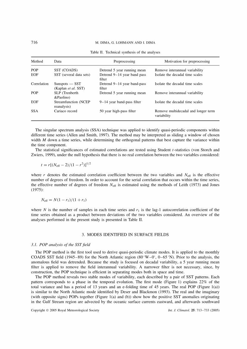
716 M. DIMA, G. LOHMANN AND I. DIMA
Table II. Technical synthesis of the analyses
Method Data Preprocessing Motivation for preprocessing
POP SST (COADS) Detrend 5 year running mean Remove interannual variabilityEOF SST (several data sets) Detrend 9–14 year band pass
filterIsolate the decadal time scales
Correlation Sunspots — SST(Kaplan et al. SST)
Detrend 9–14 year band-passfilter
Isolate the decadal time scales
POP SLP (Trenberth&Paolino)
Detrend 5 year running mean Remove interannual variability
EOF Streamfunction (NCEPreanalysis)
9–14 year band-pass filter Isolate the decadal time scales
SSA Cariaco record 50 year high-pass filter Remove multidecadal and longer termvariability
The singular spectrum analysis (SSA) technique was applied to identify quasi-periodic components withindifferent time series (Allen and Smith, 1997). The method may be interpreted as sliding a window of chosenwidth M down a time series, while determining the orthogonal patterns that best capture the variance withinthe time component.
The statistical significances of estimated correlations are tested using Student t-statistics (von Storch andZwiers, 1999), under the null hypothesis that there is no real correlation between the two variables considered:
t = r[(Neff − 2)/(1 − r2)]1/2
where r denotes the estimated correlation coefficient between the two variables and Neff is the effectivenumber of degrees of freedom. In order to account for the serial correlation that occurs within the time series,the effective number of degrees of freedom Neff is estimated using the methods of Leith (1973) and Jones(1975):
Neff = N(1 − r1)/(1 + r1)
where N is the number of samples in each time series and r1 is the lag-1 autocorrelation coefficient of thetime series obtained as a product between deviations of the two variables considered. An overview of theanalyses performed in the present study is presented in Table II.
3. MODES IDENTIFIED IN SURFACE FIELDS
3.1. POP analysis of the SST field
The POP method is the first tool used to derive quasi-periodic climate modes. It is applied to the monthlyCOADS SST field (1945–89) for the North Atlantic region (80 °W–0°, 0–65 °N). Prior to the analysis, theanomalous field was detrended. Because the study is focused on decadal variability, a 5 year running meanfilter is applied to remove the field interannual variability. A narrower filter is not necessary, since, byconstruction, the POP technique is efficient in separating modes both in space and time.
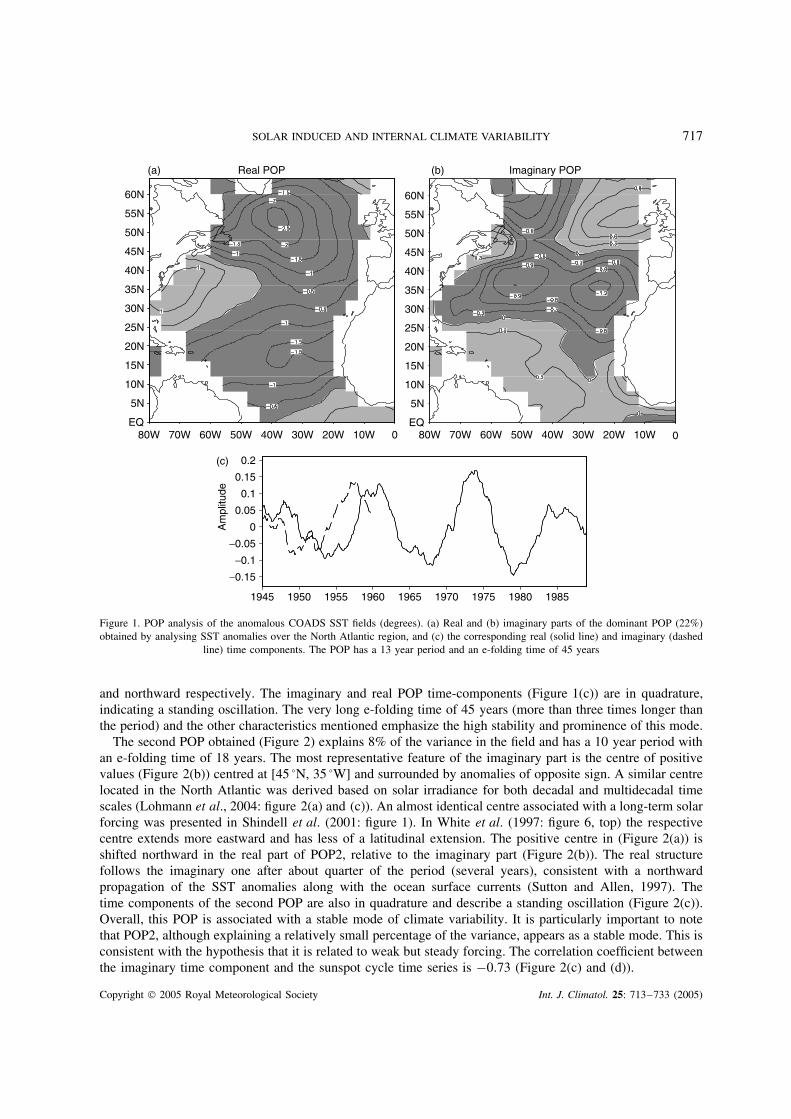
The POP method reveals two stable modes of variability, each described by a pair of SST patterns. Eachpattern corresponds to a phase in the temporal evolution. The first mode (Figure 1) explains 22% of thetotal variance and has a period of 13 years and an e-folding time of 45 years. The real POP (Figure 1(a))is similar to the North Atlantic mode identified by Deser and Blackmon (1993). The real and the imaginary(with opposite signs) POPs together (Figure 1(a) and (b)) show how the positive SST anomalies originatingin the Gulf Stream region are advected by the oceanic surface currents eastward, and afterwards southward
Copyright 2005 Royal Meteorological Society Int. J. Climatol. 25: 713–733 (2005)
SOLAR INDUCED AND INTERNAL CLIMATE VARIABILITY 717
60N
55N
50N
45N
40N
35N
30N
25N
20N
15N
10N
5N
80W 70W 60W 50W 40W 30W 20W 10W 0EQ
60N
55N
50N
45N
40N
35N
30N
25N
20N
15N
10N
5N
80W 70W 60W 50W 40W 30W 20W 10W 0EQ
(a) Real POP (b) Imaginary POP
0.2
0.15
−0.15
0
0.05
−0.05
0.1
−0.1
1945 1950 1955 1960 1965 1985198019751970
(c)
Am
plitu
de
Figure 1. POP analysis of the anomalous COADS SST fields (degrees). (a) Real and (b) imaginary parts of the dominant POP (22%)obtained by analysing SST anomalies over the North Atlantic region, and (c) the corresponding real (solid line) and imaginary (dashed
line) time components. The POP has a 13 year period and an e-folding time of 45 years
and northward respectively. The imaginary and real POP time-components (Figure 1(c)) are in quadrature,indicating a standing oscillation. The very long e-folding time of 45 years (more than three times longer thanthe period) and the other characteristics mentioned emphasize the high stability and prominence of this mode.
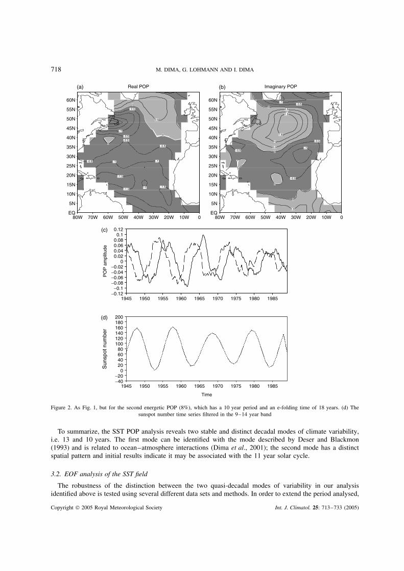
The second POP obtained (Figure 2) explains 8% of the variance in the field and has a 10 year period withan e-folding time of 18 years. The most representative feature of the imaginary part is the centre of positivevalues (Figure 2(b)) centred at [45 °N, 35 °W] and surrounded by anomalies of opposite sign. A similar centrelocated in the North Atlantic was derived based on solar irradiance for both decadal and multidecadal timescales (Lohmann et al., 2004: figure 2(a) and (c)). An almost identical centre associated with a long-term solarforcing was presented in Shindell et al. (2001: figure 1). In White et al. (1997: figure 6, top) the respectivecentre extends more eastward and has less of a latitudinal extension. The positive centre in (Figure 2(a)) isshifted northward in the real part of POP2, relative to the imaginary part (Figure 2(b)). The real structurefollows the imaginary one after about quarter of the period (several years), consistent with a northwardpropagation of the SST anomalies along with the ocean surface currents (Sutton and Allen, 1997). Thetime components of the second POP are also in quadrature and describe a standing oscillation (Figure 2(c)).Overall, this POP is associated with a stable mode of climate variability. It is particularly important to notethat POP2, although explaining a relatively small percentage of the variance, appears as a stable mode. This isconsistent with the hypothesis that it is related to weak but steady forcing. The correlation coefficient betweenthe imaginary time component and the sunspot cycle time series is −0.73 (Figure 2(c) and (d)).
Copyright 2005 Royal Meteorological Society Int. J. Climatol. 25: 713–733 (2005)
718 M. DIMA, G. LOHMANN AND I. DIMA
55N
50N
45N
40N
35N
30N
25N
20N
15N
10N
5N
80W 70W 60W 50W 40W 30W 20W 10W 0
0
0
0
0.5
Real POP
−0.5
−0.5
−0.5
−1.5
−1.5 −1
−1
−1.5
−1
−1
−0.5
−0.5
EQ
60N
80W 70W 60W 50W 40W 30W 20W 10W 0
Imaginary POP
−0.5
−0.5
−0.5
−0.5
−1
−1
0.50
1.5
1.5
1
0.5
0
1
0.5
0
0
0
55N
50N
45N
40N
35N
30N
25N
20N
15N
10N
5N
EQ
60N
1945 1950 1955 1960 1965 1970 1975 1980 1985
0.10.080.060.040.02
0−0.02−0.04−0.06−0.08
−0.1
1945 1950 1955 1960 1965 1970 1975 1980 1985
PO
P a
mpl
itude
−0.12
0.12
(d)
(c)
(a) (b)
Sun
spot
num
ber
200180160140120100806040200
−20−40
Time
Figure 2. As Fig. 1, but for the second energetic POP (8%), which has a 10 year period and an e-folding time of 18 years. (d) Thesunspot number time series filtered in the 9–14 year band
To summarize, the SST POP analysis reveals two stable and distinct decadal modes of climate variability,i.e. 13 and 10 years. The first mode can be identified with the mode described by Deser and Blackmon(1993) and is related to ocean–atmosphere interactions (Dima et al., 2001); the second mode has a distinctspatial pattern and initial results indicate it may be associated with the 11 year solar cycle.
3.2. EOF analysis of the SST field
The robustness of the distinction between the two quasi-decadal modes of variability in our analysisidentified above is tested using several different data sets and methods. In order to extend the period analysed,
Copyright 2005 Royal Meteorological Society Int. J. Climatol. 25: 713–733 (2005)
SOLAR INDUCED AND INTERNAL CLIMATE VARIABILITY 719
we used the longer SST data set provided by Kaplan et al. (1998), covering the 1856–1991 period. In order toemphasize modes in the decadal band, the annual data are filtered in the 9–14 year band prior to performingan EOF analysis on the data. The linear trend was also subtracted at every grid point prior to the analysis.
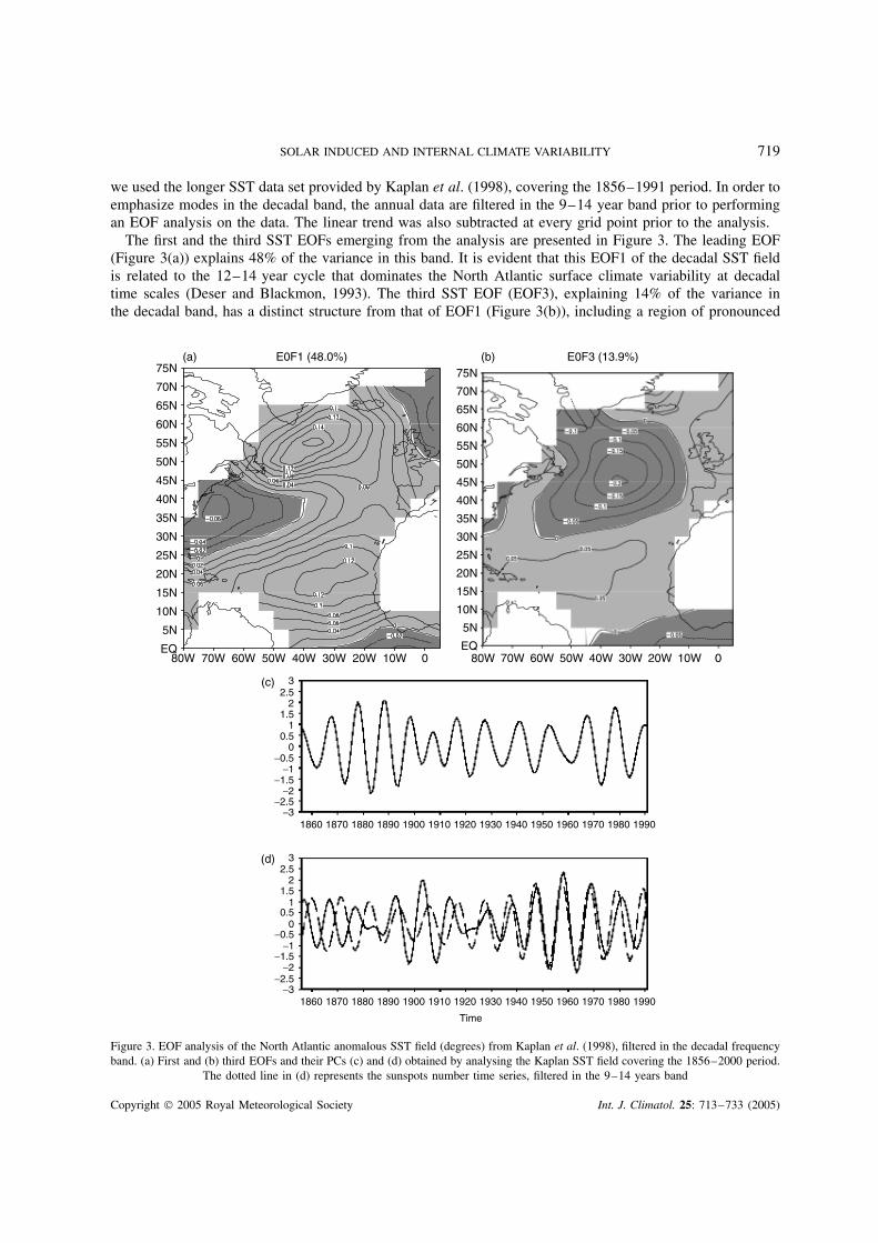
The first and the third SST EOFs emerging from the analysis are presented in Figure 3. The leading EOF(Figure 3(a)) explains 48% of the variance in this band. It is evident that this EOF1 of the decadal SST fieldis related to the 12–14 year cycle that dominates the North Atlantic surface climate variability at decadaltime scales (Deser and Blackmon, 1993). The third SST EOF (EOF3), explaining 14% of the variance inthe decadal band, has a distinct structure from that of EOF1 (Figure 3(b)), including a region of pronounced
60N
65N
70N
75N
55N
50N
45N
40N
35N
30N
25N
20N
15N
10N
5N
EQ
(b)
80W 70W 60W 50W 40W 30W 20W 10W 0
E0F3 (13.9%)
32.5
21.5
10.5
0−0.5
−1−1.5
−2−2.5
−31860 1870 1880 1890 1900 1910 1920 1930 1940 1950 1960 1970 1980 1990
32.5
21.5
10.5
0−0.5
−1−1.5
−2−2.5
−31860 1870 1880 1890 1900 1910 1920 1930 1940
Time
1950 1960 1970 1980 1990
(c)
(d)
60N
65N
70N
75N
55N
50N
45N
40N
35N
30N
25N
20N
15N
10N
5N
EQ
(a)
80W 70W 60W 50W 40W 30W 20W 010W
E0F1 (48.0%)
Figure 3. EOF analysis of the North Atlantic anomalous SST field (degrees) from Kaplan et al. (1998), filtered in the decadal frequencyband. (a) First and (b) third EOFs and their PCs (c) and (d) obtained by analysing the Kaplan SST field covering the 1856–2000 period.
The dotted line in (d) represents the sunspots number time series, filtered in the 9–14 years band
Copyright 2005 Royal Meteorological Society Int. J. Climatol. 25: 713–733 (2005)
720 M. DIMA, G. LOHMANN AND I. DIMA
negative values centred at about 42 °N. The second EOF (not shown) is characterized by negative anomaliessouth of Greenland and positive values over almost all the rest of the basin and has a time component thatis not significantly correlated at any lags with the principal components (PCs) PC1 or PC3. This spatiallyhomogeneous pattern resembles very well the SST structure of the Atlantic multidecadal mode investigatedin previous studies (Delworth and Mann, 2000). Since this mode is not of interest for the present study itwill not be considered further.
The first and third PCs resulting from the filtered analysis are shown in Figure 3(c) and (d). No significantlag-correlation between PC1 and PC3 is obtained, consistent with the hypothesis that EOF1 and EOF3 dorepresent distinct modes of variability. An additional EOF analysis performed on the unfiltered SST data (notshown) reveals first (30.1%) and third (11.8%) EOFs that are practically identical to the corresponding modesidentified using the filtered SST field.
PC3 and the sunspot number time series filtered in the 9–14 year band are shown in Figure 3(d). Thecorrelation between the two time series is 0.47 for the whole period (1856–1991), and this increases to0.65 when the more recent time period (1900–91) is considered (both correlations are significant at the 90%confidence level). These values further support the association between the two time components. On closerinspection one may notice that the two time series show in-phase variability during part of the last century,as well as some phase differences, mainly during the 19th century. If PC3 and SSC are connected, as webelieve is the case, then the respective phase shifts may be explained if we consider that:
• PC3 is obtained by projecting EOF3 on the filtered SST data, a field where this mode explains a relativelysmall percentage of the variance (14%) and EOF1 is by far the dominant mode. Because the patterns ofthe two modes (EOF1 and EOF3) also include common characteristics (e.g. the region of positive valuessouth of 25 °N), information related to the 12 year mode (EOF1/PC1) might be implicitly included in thethird mode (EOF3/PC3), thus affecting the phase of the latter mode.
• The two decadal modes may also interact nonlinearly; therefore, linear methods like the EOF cannot derivethe associated time components perfectly accurately.
These results do not rule out that PC3 and SSC might not be truly related as we assumed, and instead ofEOF3 representing a mode of solar origins it might just represent another mode of internal origins, differentfrom EOF1. Further analyses are performed in order to derive new constraints that support the solar originhypothesis for EOF3.
The mode associated with the third SST EOF (Figure 3(b)) can also be obtained through EOF analysesperformed on two different SST data sets in the North Atlantic sector: extended-COADS (Smith and Reynolds,2003) and GISST (Parker et al., 1995) (not shown). In each of these analyses, the pattern associated with thethird eigenvector (explaining 13% total variance for extended-COADS and 10% total variance for GISST) isclose to identical to EOF3 in Figure 3.
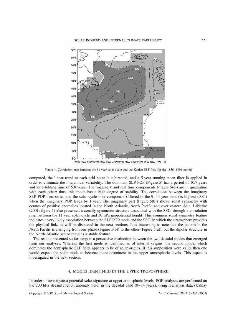
Additional evidence for the link between the third surface mode described above (Figure 3(b)) and thesunspot solar cycle is given by the correlation map between the detrended decadal SSTs (Kaplan et al., 1998)and the solar cycle time component (Figure 4). The 11 year solar cycle was obtained by filtering the sunspotnumber time series in the 9–14 year band. The correlation coefficients between the solar mode and the SSTfield (Figure 4) are as large as −0.6. But by computing correlations one is not able to separate influencesfrom other SST modes, which may explain why the correlation values are not uniformly high and significantover the whole North Atlantic basin. However, the close resemblance between the structure of this correlationmap and the structures of the second imaginary POP (Figure 2(b)) and EOF3 in the SST data (Figure 3(b)),together with the 10 year period of the second POP, all provide strong support for considering this mode tobe of solar origins.
3.3. POP analysis of the SLP field
In order to investigate the dominant modes of atmospheric variability, a POP analysis is performed onthe Northern Hemisphere winter (December–February (DJF)) SLP field (20–90 °N) for the 1950–97 period(Trenberth and Paolino, 1980). Prior to the analysis, anomalies with respect to climatological values are
Copyright 2005 Royal Meteorological Society Int. J. Climatol. 25: 713–733 (2005)
SOLAR INDUCED AND INTERNAL CLIMATE VARIABILITY 721
0
60N
65N
70N
55N
50N
45N
40N
35N
30N
25N
20N
15N
10N
5N
EQ70W 60W65W 50W55W 40W45W 30W35W 20W25W 10W 5W15W 0
0.2
0−0.2
−0.2
0
−0.4
−0.6
−0.6
−0.4
0.4
0.4
−0.2
0.2
0
Figure 4. Correlation map between the 11 year solar cycle and the Kaplan SST field for the 1856–1991 period
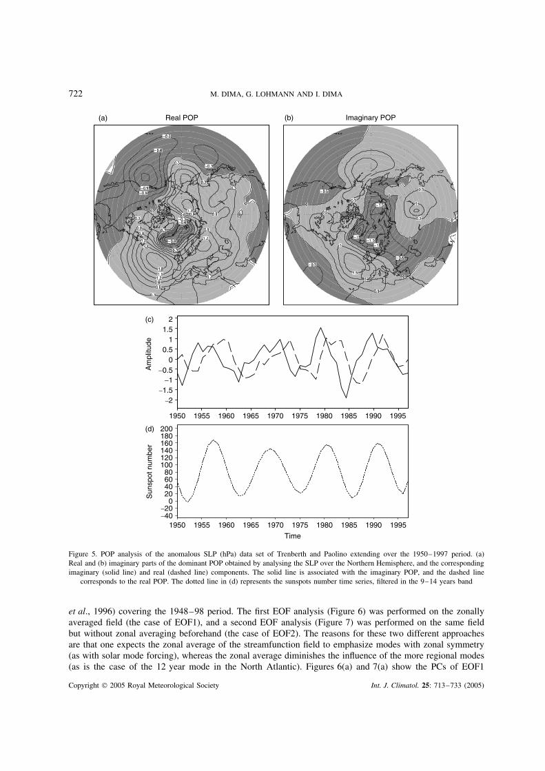
computed, the linear trend at each grid point is subtracted, and a 5 year running-mean filter is applied inorder to eliminate the interannual variability. The dominant SLP POP (Figure 5) has a period of 10.7 yearsand an e-folding time of 5.8 years. The imaginary and real time components (Figure 5(c)) are in quadraturewith each other; thus, this mode has a high degree of stability. The correlation between the imaginarySLP POP time series and the solar cycle time component (filtered in the 9–14 year band) is highest (0.84)when the imaginary POP leads by 1 year. The imaginary part (Figure 5(b)) shows zonal symmetry withcentres of positive anomalies located in the North Atlantic, North Pacific and over eastern Asia. Labitzke(2001: figure 1) also presented a zonally symmetric structure associated with the SSC, through a correlationmap between the 11 year solar cycle and 30 hPa geopotential height. This common zonal symmetry featureindicates a very likely association between the SLP POP mode and the SSC, in which the stratosphere providesthe physical link, as will be discussed in the next sections. It is interesting to note that the pattern in theNorth Pacific is changing from one phase (Figure 5(b)) to the other (Figure 5(a)), but the dipolar structure inthe North Atlantic sector remains a stable feature.
The results presented so far support a persuasive distinction between the two decadal modes that emergedfrom our analyses. Whereas the first mode is identified as of internal origins, the second mode, whichdominates the hemispheric SLP field, appears to be of solar origins. If this supposition were valid, then onewould expect the solar mode to become more prominent in the upper atmospheric levels. This aspect isinvestigated in the next section.
4. MODES IDENTIFIED IN THE UPPER TROPOSPHERE
In order to investigate a potential solar signature at upper atmospheric levels, EOF analyses are performed onthe 200 hPa streamfunction anomaly field, in the decadal band (9–14 years), using reanalysis data (Kalnay
Copyright 2005 Royal Meteorological Society Int. J. Climatol. 25: 713–733 (2005)
722 M. DIMA, G. LOHMANN AND I. DIMA
(a) Real POP (b) Imaginary POP
(c) 2
−2
1.51
0.5
−0.5
−1.5−1
0
1950 1960 1965 1975 1985 19951970 1980 19901955
Am
plitu
de
(d)
1950 1960 1965 1975 1985 19951970 1980 19901955
20018016014012010080604020
−20−40
0
Sun
spot
num
ber
Time
Figure 5. POP analysis of the anomalous SLP (hPa) data set of Trenberth and Paolino extending over the 1950–1997 period. (a)Real and (b) imaginary parts of the dominant POP obtained by analysing the SLP over the Northern Hemisphere, and the correspondingimaginary (solid line) and real (dashed line) components. The solid line is associated with the imaginary POP, and the dashed line
corresponds to the real POP. The dotted line in (d) represents the sunspots number time series, filtered in the 9–14 years band
et al., 1996) covering the 1948–98 period. The first EOF analysis (Figure 6) was performed on the zonallyaveraged field (the case of EOF1), and a second EOF analysis (Figure 7) was performed on the same fieldbut without zonal averaging beforehand (the case of EOF2). The reasons for these two different approachesare that one expects the zonal average of the streamfunction field to emphasize modes with zonal symmetry(as with solar mode forcing), whereas the zonal average diminishes the influence of the more regional modes(as is the case of the 12 year mode in the North Atlantic). Figures 6(a) and 7(a) show the PCs of EOF1
Copyright 2005 Royal Meteorological Society Int. J. Climatol. 25: 713–733 (2005)
SOLAR INDUCED AND INTERNAL CLIMATE VARIABILITY 723
55
4
2
0
−2
−457 59 61 63 65 67 69 71 73 75 77 79 81 83 85 87 89
PC1 of [Ψ] (79.2%)
Years
(a)
0 30 60 90 120 150 180 210 240 270 300 330 360
90N75N60N45N30N15N
45S30S15SEQ
60S75S90S
Longitude
Regression of Ψ upon PC1 of 200hPa [Ψ](b) (c) 90N
60N
30N
EQ
30S
60S
90S−0.2 0.20
Zon. Avg.
Latit
ude
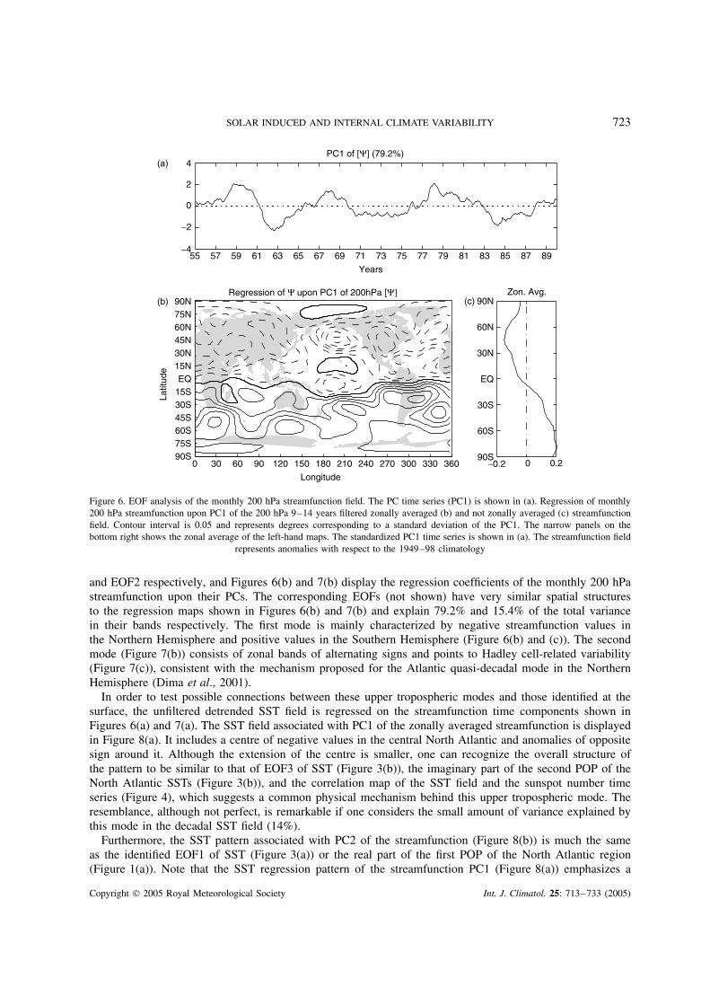
Figure 6. EOF analysis of the monthly 200 hPa streamfunction field. The PC time series (PC1) is shown in (a). Regression of monthly200 hPa streamfunction upon PC1 of the 200 hPa 9–14 years filtered zonally averaged (b) and not zonally averaged (c) streamfunctionfield. Contour interval is 0.05 and represents degrees corresponding to a standard deviation of the PC1. The narrow panels on thebottom right shows the zonal average of the left-hand maps. The standardized PC1 time series is shown in (a). The streamfunction field
represents anomalies with respect to the 1949–98 climatology
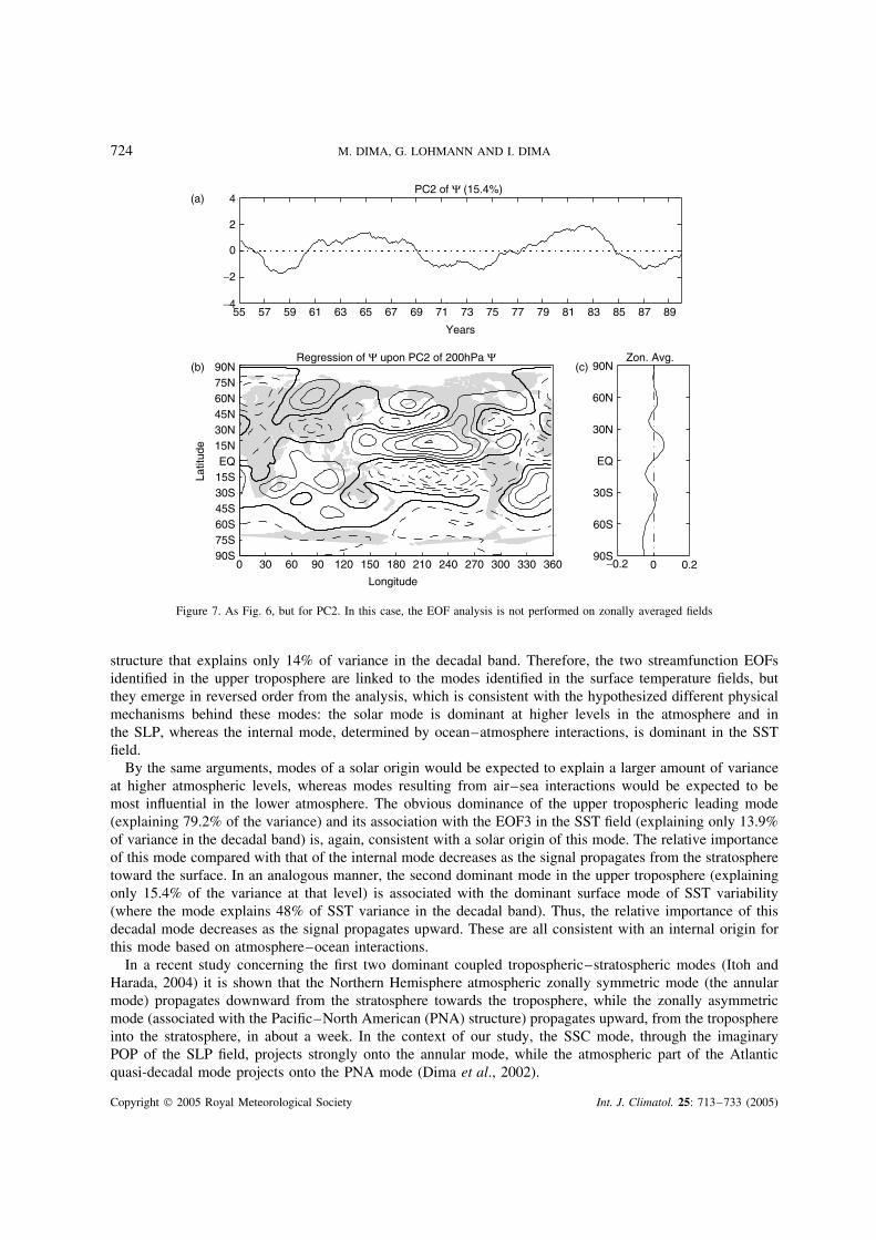
and EOF2 respectively, and Figures 6(b) and 7(b) display the regression coefficients of the monthly 200 hPastreamfunction upon their PCs. The corresponding EOFs (not shown) have very similar spatial structuresto the regression maps shown in Figures 6(b) and 7(b) and explain 79.2% and 15.4% of the total variancein their bands respectively. The first mode is mainly characterized by negative streamfunction values inthe Northern Hemisphere and positive values in the Southern Hemisphere (Figure 6(b) and (c)). The secondmode (Figure 7(b)) consists of zonal bands of alternating signs and points to Hadley cell-related variability(Figure 7(c)), consistent with the mechanism proposed for the Atlantic quasi-decadal mode in the NorthernHemisphere (Dima et al., 2001).
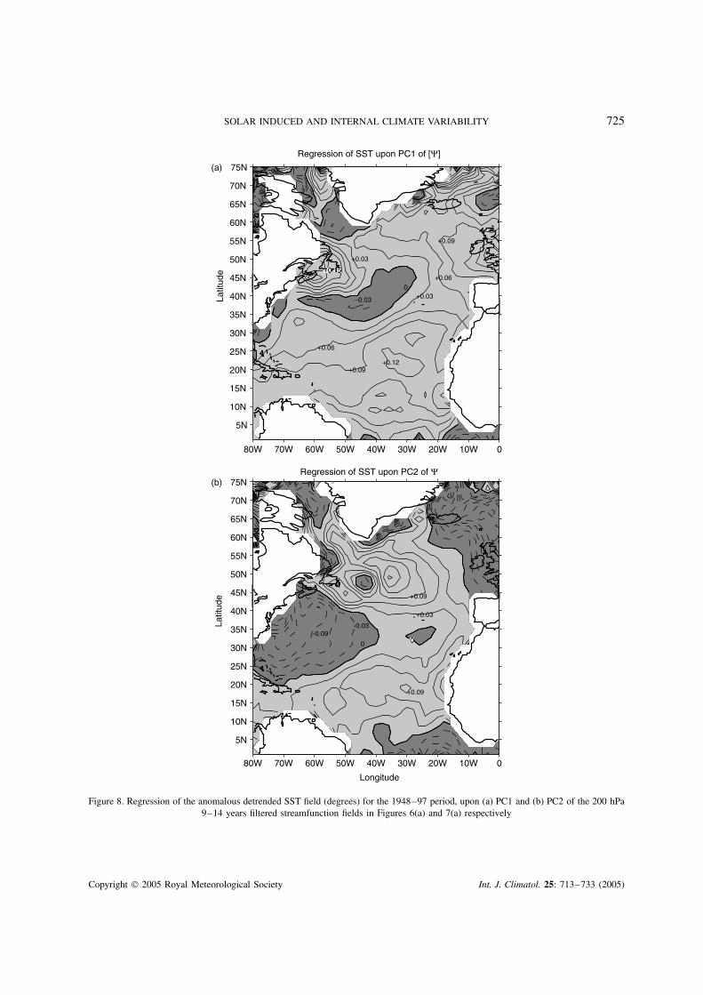
In order to test possible connections between these upper tropospheric modes and those identified at thesurface, the unfiltered detrended SST field is regressed on the streamfunction time components shown inFigures 6(a) and 7(a). The SST field associated with PC1 of the zonally averaged streamfunction is displayedin Figure 8(a). It includes a centre of negative values in the central North Atlantic and anomalies of oppositesign around it. Although the extension of the centre is smaller, one can recognize the overall structure ofthe pattern to be similar to that of EOF3 of SST (Figure 3(b)), the imaginary part of the second POP of theNorth Atlantic SSTs (Figure 3(b)), and the correlation map of the SST field and the sunspot number timeseries (Figure 4), which suggests a common physical mechanism behind this upper tropospheric mode. Theresemblance, although not perfect, is remarkable if one considers the small amount of variance explained bythis mode in the decadal SST field (14%).
Furthermore, the SST pattern associated with PC2 of the streamfunction (Figure 8(b)) is much the sameas the identified EOF1 of SST (Figure 3(a)) or the real part of the first POP of the North Atlantic region(Figure 1(a)). Note that the SST regression pattern of the streamfunction PC1 (Figure 8(a)) emphasizes a
Copyright 2005 Royal Meteorological Society Int. J. Climatol. 25: 713–733 (2005)
724 M. DIMA, G. LOHMANN AND I. DIMA
4
2
0
−2
−455 57 59 61 63 65 67 69 71 73 75 77 79 81 83 85 87 89
Years
(a)PC2 of Ψ (15.4%)
(b) 90N75N
45N
15N
60N
30N
EQ
30S15S
45S60S
90S75S
0 30 300 330 36060 90 120 150 180 210 240 270
Longitude
Regression of Ψ upon PC2 of 200hPa Ψ
EQ
Zon. Avg.90N
60N
30N
30S
60S
90S−0.2 0 0.2
(c)
Latit
ude
Figure 7. As Fig. 6, but for PC2. In this case, the EOF analysis is not performed on zonally averaged fields
structure that explains only 14% of variance in the decadal band. Therefore, the two streamfunction EOFsidentified in the upper troposphere are linked to the modes identified in the surface temperature fields, butthey emerge in reversed order from the analysis, which is consistent with the hypothesized different physicalmechanisms behind these modes: the solar mode is dominant at higher levels in the atmosphere and inthe SLP, whereas the internal mode, determined by ocean–atmosphere interactions, is dominant in the SSTfield.
By the same arguments, modes of a solar origin would be expected to explain a larger amount of varianceat higher atmospheric levels, whereas modes resulting from air–sea interactions would be expected to bemost influential in the lower atmosphere. The obvious dominance of the upper tropospheric leading mode(explaining 79.2% of the variance) and its association with the EOF3 in the SST field (explaining only 13.9%of variance in the decadal band) is, again, consistent with a solar origin of this mode. The relative importanceof this mode compared with that of the internal mode decreases as the signal propagates from the stratospheretoward the surface. In an analogous manner, the second dominant mode in the upper troposphere (explainingonly 15.4% of the variance at that level) is associated with the dominant surface mode of SST variability(where the mode explains 48% of SST variance in the decadal band). Thus, the relative importance of thisdecadal mode decreases as the signal propagates upward. These are all consistent with an internal origin forthis mode based on atmosphere–ocean interactions.
In a recent study concerning the first two dominant coupled tropospheric–stratospheric modes (Itoh andHarada, 2004) it is shown that the Northern Hemisphere atmospheric zonally symmetric mode (the annularmode) propagates downward from the stratosphere towards the troposphere, while the zonally asymmetricmode (associated with the Pacific–North American (PNA) structure) propagates upward, from the troposphereinto the stratosphere, in about a week. In the context of our study, the SSC mode, through the imaginaryPOP of the SLP field, projects strongly onto the annular mode, while the atmospheric part of the Atlanticquasi-decadal mode projects onto the PNA mode (Dima et al., 2002).
Copyright 2005 Royal Meteorological Society Int. J. Climatol. 25: 713–733 (2005)
SOLAR INDUCED AND INTERNAL CLIMATE VARIABILITY 725
75N
70N
65N
60N
55N
50N
45N
35N
40N
30N
25N
15N
10N
5N
20N
Latit
ude
80W 70W 060W 50W 40W 30W 20W 10W
(a)
Regression of SST upon PC1 of [Ψ]
+0.03
−0.03 +0.030
+0.06
+0.09
+0.06
+0.09+0.12
75N
70N
65N
60N
55N
50N
45N
35N
40N
30N
25N
15N
10N
5N
20N
Latit
ude
80W 70W 060W 50W 40W 30W 20W 10W
Longitude
(b)Regression of SST upon PC2 of Ψ
-0.09-0.03
0
+0.09
+0.09
+0.03
Figure 8. Regression of the anomalous detrended SST field (degrees) for the 1948–97 period, upon (a) PC1 and (b) PC2 of the 200 hPa9–14 years filtered streamfunction fields in Figures 6(a) and 7(a) respectively
Copyright 2005 Royal Meteorological Society Int. J. Climatol. 25: 713–733 (2005)
726 M. DIMA, G. LOHMANN AND I. DIMA
3500
3000
2500
2000
1200 1300 1400 1500 1600 1700 1800 1900
1500
1000
500
0
Time
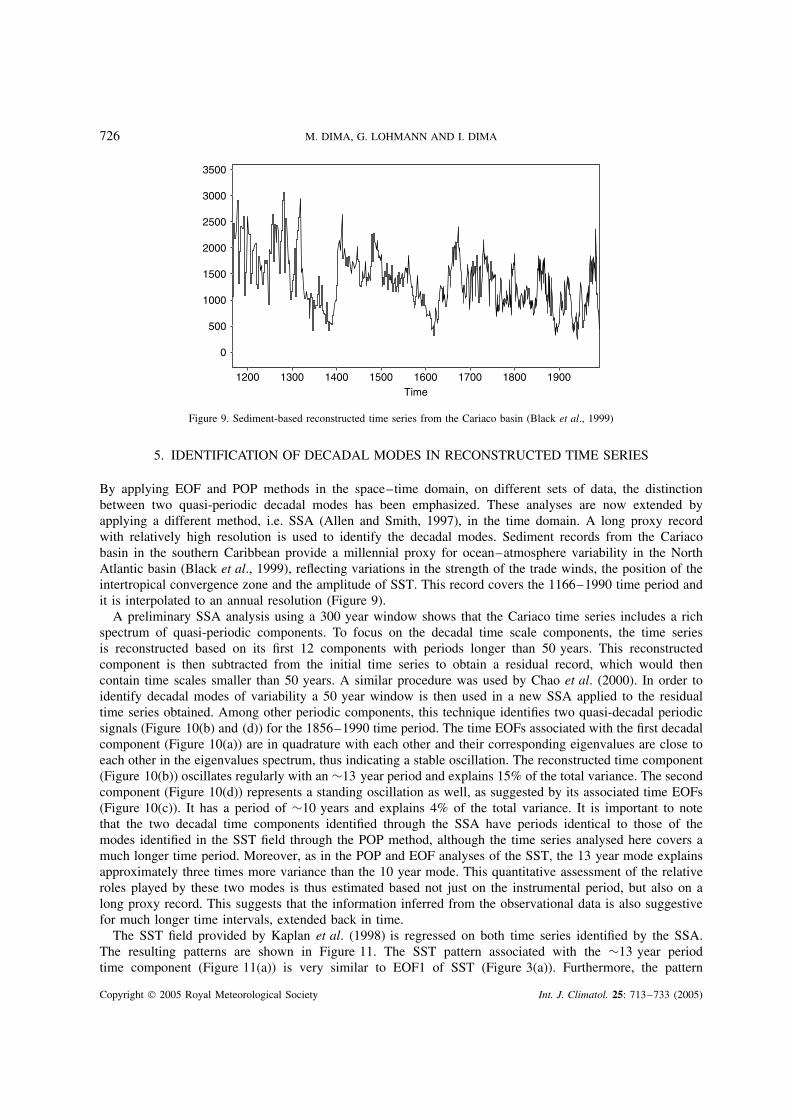
Figure 9. Sediment-based reconstructed time series from the Cariaco basin (Black et al., 1999)
5. IDENTIFICATION OF DECADAL MODES IN RECONSTRUCTED TIME SERIES
By applying EOF and POP methods in the space–time domain, on different sets of data, the distinctionbetween two quasi-periodic decadal modes has been emphasized. These analyses are now extended byapplying a different method, i.e. SSA (Allen and Smith, 1997), in the time domain. A long proxy recordwith relatively high resolution is used to identify the decadal modes. Sediment records from the Cariacobasin in the southern Caribbean provide a millennial proxy for ocean–atmosphere variability in the NorthAtlantic basin (Black et al., 1999), reflecting variations in the strength of the trade winds, the position of theintertropical convergence zone and the amplitude of SST. This record covers the 1166–1990 time period andit is interpolated to an annual resolution (Figure 9).
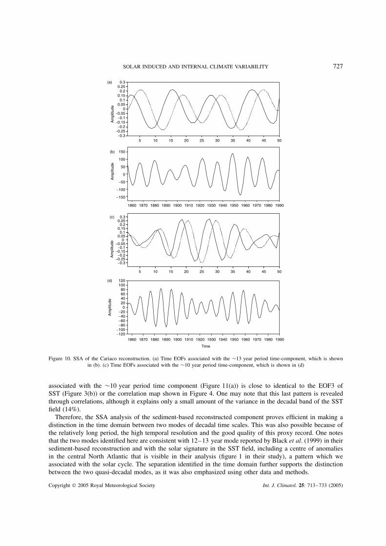
A preliminary SSA analysis using a 300 year window shows that the Cariaco time series includes a richspectrum of quasi-periodic components. To focus on the decadal time scale components, the time seriesis reconstructed based on its first 12 components with periods longer than 50 years. This reconstructedcomponent is then subtracted from the initial time series to obtain a residual record, which would thencontain time scales smaller than 50 years. A similar procedure was used by Chao et al. (2000). In order toidentify decadal modes of variability a 50 year window is then used in a new SSA applied to the residualtime series obtained. Among other periodic components, this technique identifies two quasi-decadal periodicsignals (Figure 10(b) and (d)) for the 1856–1990 time period. The time EOFs associated with the first decadalcomponent (Figure 10(a)) are in quadrature with each other and their corresponding eigenvalues are close toeach other in the eigenvalues spectrum, thus indicating a stable oscillation. The reconstructed time component(Figure 10(b)) oscillates regularly with an ∼13 year period and explains 15% of the total variance. The secondcomponent (Figure 10(d)) represents a standing oscillation as well, as suggested by its associated time EOFs(Figure 10(c)). It has a period of ∼10 years and explains 4% of the total variance. It is important to notethat the two decadal time components identified through the SSA have periods identical to those of themodes identified in the SST field through the POP method, although the time series analysed here covers amuch longer time period. Moreover, as in the POP and EOF analyses of the SST, the 13 year mode explainsapproximately three times more variance than the 10 year mode. This quantitative assessment of the relativeroles played by these two modes is thus estimated based not just on the instrumental period, but also on along proxy record. This suggests that the information inferred from the observational data is also suggestivefor much longer time intervals, extended back in time.
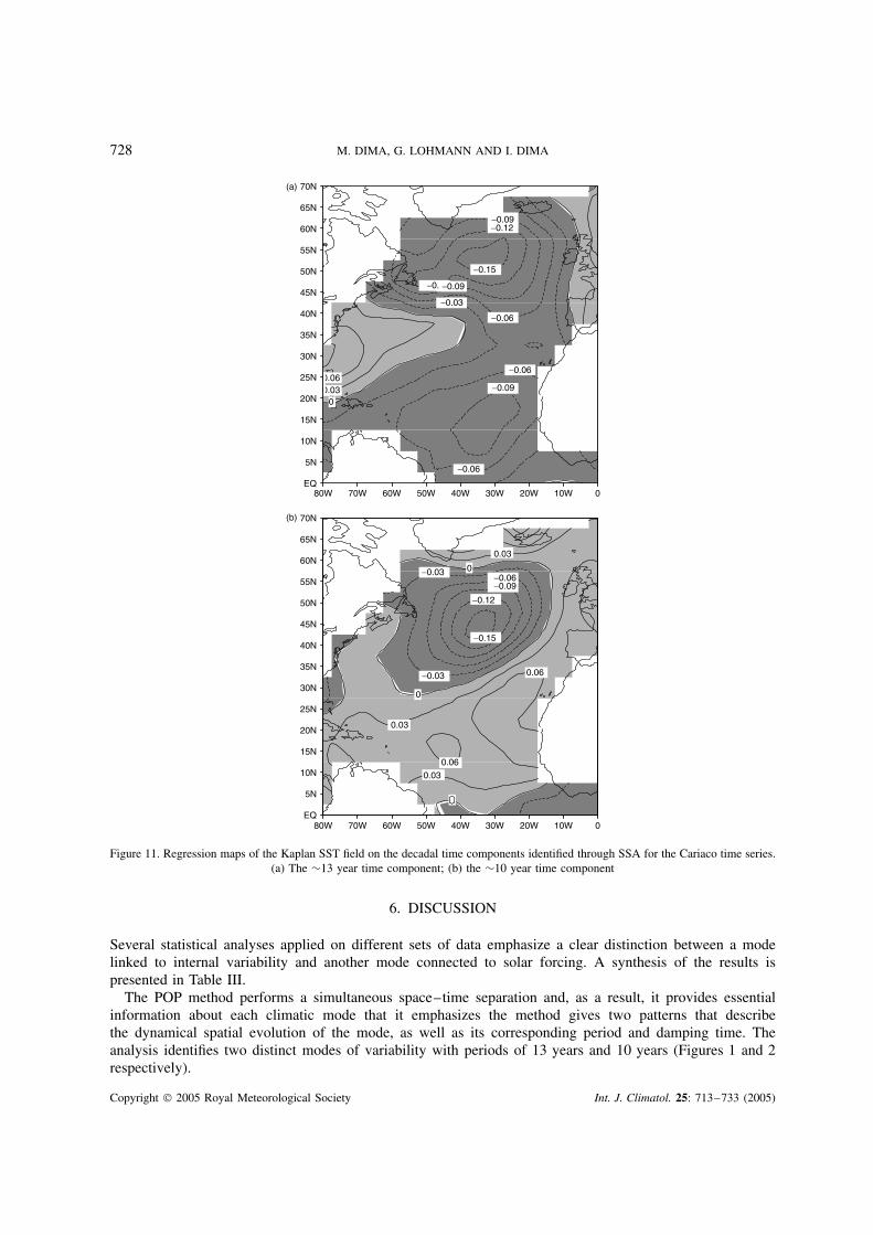
The SST field provided by Kaplan et al. (1998) is regressed on both time series identified by the SSA.The resulting patterns are shown in Figure 11. The SST pattern associated with the ∼13 year periodtime component (Figure 11(a)) is very similar to EOF1 of SST (Figure 3(a)). Furthermore, the pattern
Copyright 2005 Royal Meteorological Society Int. J. Climatol. 25: 713–733 (2005)
SOLAR INDUCED AND INTERNAL CLIMATE VARIABILITY 727
0.30.250.2
0.150.1
0.05
−0.050
−0.1−0.15
−0.2−0.25
−0.35 10 15 20 25 30 35 40 45 50
Am
plitu
de
(a)
150
100
50
0
−50
−100
−150
1860 1870 1880 1890 1900 1910 1920 1930 1940 1950 1960 1970 1980 1990
Am
plitu
de
(b)
5 10 15 20 25 30 35 40 45 50
0.30.250.2
0.150.1
0.050
−0.05−0.1
−0.15−0.2
−0.25−0.3
Am
plitu
de
(c)
1860 1870 1880 1890 1900 1910 1920 1930 1940 1950 1960 1970 1980 1990
120100806040200
−20−40−60−80
−100−120
Am
plitu
de
(d)
Time
Figure 10. SSA of the Cariaco reconstruction. (a) Time EOFs associated with the ∼13 year period time-component, which is shownin (b). (c) Time EOFs associated with the ∼10 year period time-component, which is shown in (d)
associated with the ∼10 year period time component (Figure 11(a)) is close to identical to the EOF3 ofSST (Figure 3(b)) or the correlation map shown in Figure 4. One may note that this last pattern is revealedthrough correlations, although it explains only a small amount of the variance in the decadal band of the SSTfield (14%).
Therefore, the SSA analysis of the sediment-based reconstructed component proves efficient in making adistinction in the time domain between two modes of decadal time scales. This was also possible because ofthe relatively long period, the high temporal resolution and the good quality of this proxy record. One notesthat the two modes identified here are consistent with 12–13 year mode reported by Black et al. (1999) in theirsediment-based reconstruction and with the solar signature in the SST field, including a centre of anomaliesin the central North Atlantic that is visible in their analysis (figure 1 in their study), a pattern which weassociated with the solar cycle. The separation identified in the time domain further supports the distinctionbetween the two quasi-decadal modes, as it was also emphasized using other data and methods.
Copyright 2005 Royal Meteorological Society Int. J. Climatol. 25: 713–733 (2005)
728 M. DIMA, G. LOHMANN AND I. DIMA
70N
65N
60N
55N
50N
45N
40N
35N
30N
25N
20N
15N
10N
5N
EQ
70N
65N
60N
55N
50N
45N
40N
35N
30N
25N
20N
15N
10N
5N
EQ
80W 70W 60W 50W 40W 30W 20W 10W 0
80W 70W 60W 50W 40W 30W 20W 10W 0
(a)
(b)
−0.09−0.12
−0.15
−0. −0.09
−0.03
−0.06
−0.06
−0.09
−0.06
0.060.03
0
0.03
−0.06
0.06
−0.09
−0.12
−0.15
−0.03
−0.03
0.03
0.03
0.06
0
0
Figure 11. Regression maps of the Kaplan SST field on the decadal time components identified through SSA for the Cariaco time series.(a) The ∼13 year time component; (b) the ∼10 year time component
6. DISCUSSION
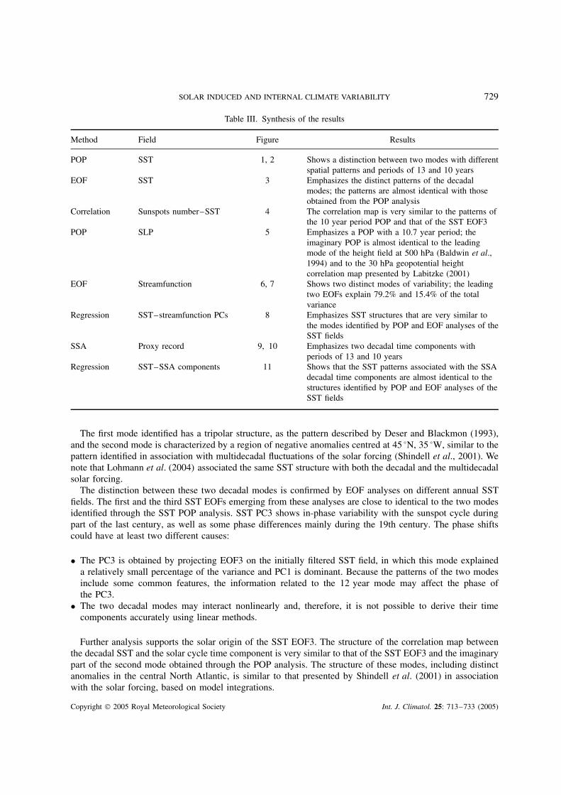
Several statistical analyses applied on different sets of data emphasize a clear distinction between a modelinked to internal variability and another mode connected to solar forcing. A synthesis of the results ispresented in Table III.
The POP method performs a simultaneous space–time separation and, as a result, it provides essentialinformation about each climatic mode that it emphasizes the method gives two patterns that describethe dynamical spatial evolution of the mode, as well as its corresponding period and damping time. Theanalysis identifies two distinct modes of variability with periods of 13 years and 10 years (Figures 1 and 2respectively).
Copyright 2005 Royal Meteorological Society Int. J. Climatol. 25: 713–733 (2005)
SOLAR INDUCED AND INTERNAL CLIMATE VARIABILITY 729
Table III. Synthesis of the results
Method Field Figure Results
POP SST 1, 2 Shows a distinction between two modes with differentspatial patterns and periods of 13 and 10 years
EOF SST 3 Emphasizes the distinct patterns of the decadalmodes; the patterns are almost identical with thoseobtained from the POP analysis
Correlation Sunspots number–SST 4 The correlation map is very similar to the patterns ofthe 10 year period POP and that of the SST EOF3
POP SLP 5 Emphasizes a POP with a 10.7 year period; theimaginary POP is almost identical to the leadingmode of the height field at 500 hPa (Baldwin et al.,1994) and to the 30 hPa geopotential heightcorrelation map presented by Labitzke (2001)
EOF Streamfunction 6, 7 Shows two distinct modes of variability; the leadingtwo EOFs explain 79.2% and 15.4% of the totalvariance
Regression SST–streamfunction PCs 8 Emphasizes SST structures that are very similar tothe modes identified by POP and EOF analyses of theSST fields
SSA Proxy record 9, 10 Emphasizes two decadal time components withperiods of 13 and 10 years
Regression SST–SSA components 11 Shows that the SST patterns associated with the SSAdecadal time components are almost identical to thestructures identified by POP and EOF analyses of theSST fields
The first mode identified has a tripolar structure, as the pattern described by Deser and Blackmon (1993),and the second mode is characterized by a region of negative anomalies centred at 45 °N, 35 °W, similar to thepattern identified in association with multidecadal fluctuations of the solar forcing (Shindell et al., 2001). Wenote that Lohmann et al. (2004) associated the same SST structure with both the decadal and the multidecadalsolar forcing.
The distinction between these two decadal modes is confirmed by EOF analyses on different annual SSTfields. The first and the third SST EOFs emerging from these analyses are close to identical to the two modesidentified through the SST POP analysis. SST PC3 shows in-phase variability with the sunspot cycle duringpart of the last century, as well as some phase differences mainly during the 19th century. The phase shiftscould have at least two different causes:
• The PC3 is obtained by projecting EOF3 on the initially filtered SST field, in which this mode explaineda relatively small percentage of the variance and PC1 is dominant. Because the patterns of the two modesinclude some common features, the information related to the 12 year mode may affect the phase ofthe PC3.
• The two decadal modes may interact nonlinearly and, therefore, it is not possible to derive their timecomponents accurately using linear methods.
Further analysis supports the solar origin of the SST EOF3. The structure of the correlation map betweenthe decadal SST and the solar cycle time component is very similar to that of the SST EOF3 and the imaginarypart of the second mode obtained through the POP analysis. The structure of these modes, including distinctanomalies in the central North Atlantic, is similar to that presented by Shindell et al. (2001) in associationwith the solar forcing, based on model integrations.
Copyright 2005 Royal Meteorological Society Int. J. Climatol. 25: 713–733 (2005)
730 M. DIMA, G. LOHMANN AND I. DIMA
The POP analysis performed on the Northern Hemisphere winter SLP field (20–90 °N) for the 1950–97time period (Trenberth and Paolino, 1980) emphasizes a dominant mode with a period of 10.7 years and ane-folding time of 5.8 years, connected with the sunspots time series. The SLP POP provides the key linkbetween the solar forcing and its fingerprint in the SST field (Figures 3(b) and (4)). The POP imaginarypart (Figure 5(b)) shows a strong zonal symmetry with centres of positive anomalies located in the NorthAtlantic, North Pacific and over eastern Asia. The structure of the imaginary SLP POP is close to identicalto the DJF 500 hPa height map presented by Baldwin et al. (1994). The pattern in their study (emergingas a leading mode) was derived through a singular value decomposition analysis between the DJF 500 and50 hPa height fields (figure 3 in their study). This very close resemblance between a zonally symmetric modeidentified in the SLP field and a 500 hPa height structure strongly coupled to the height field at 50 hPa clearlysuggests that the SLP structure is induced from the stratosphere. This is consistent with the observation thatthe dominant mode in the SLP field may be interpreted as the surface modulation in the strength of thepolar vortex (Thompson and Wallace, 1998). This is also supported by Black (2002), who showed that theAO-related surface climate variations are strongly linked to the strength of the stratospheric polar vortex.These surface climate variations are due to large-scale potential vorticity anomalies in the lower stratosphere,associated with changes in the strength of the stratospheric polar vortex that induces zonally symmetric zonalwind perturbations extending downward to the surface. This is characterized as a large-scale annular stirringof the troposphere from above (Black, 2002) and is consistent with the fingerprint of the 11 year solar cycleidentified in the lower atmosphere by Coughlin and Tung (2004).
Our results are also supported by the study of Labitzke (2001). For example, the structure of the imaginarySLP POP (Figure 5(b)) is very similar to the correlation map between the 11 year solar cycle and 30 hPageopotential height presented by Labitzke (2001). A dynamical link between solar irradiance and thestratospheric polar vortex has been attributed to an interaction between ultraviolet radiation and ozone inthe stratosphere (Balachandran et al., 1999) and a downward propagation of stratospheric events (Baldwinand Dunkerton, 1999; Christiansen, 2000). The new information provided by the SLP POP analysis is theperiod of the dominant mode in this field. Therefore, aside from the similarity with leading upper atmospheremodes, the dominant POP has an ∼10 year period, consistent with a sunspot cycle origin. Furthermore,together the almost identical structure of the real SLP POP, the 500 hPa mode presented by Baldwin et al.(1994) and the 30 hPa correlation map (Labitzke, 2001), in association with the identified 10 year period ofthe SLP POP, provide strong support for a fingerprint of the solar mode in the troposphere.
In order to complete the analysis of the solar forcing mechanism down to the ocean, it is worth analysing therelation between the SLP POP and the ocean surface conditions. The structure of the SLP POP in the NorthAtlantic sector is qualitatively the same in the imaginary (Figure 5(b)) and the real POPs (Figure 5(a)). Thebipolar structure resembles the NAO. It is important to observe that the position of the dipole zonal axis (theimaginary line perpendicular to the maximum SLP gradient) is shifted northward relative to that correspondingto the NAO-like structure associated with the SST tripole, which is disposed at approximately 50 °N (Dimaet al., 2001). A similar northward shift of the centre of positive SST anomalies extending eastward from NorthAmerica is observed in Figures 1(a) and 2(b), in association with the 13 year and 10 year modes. In the caseof the tripolar SST mode, the associated NAO-like structure appears to induce SST anomalies that expandeastward from the Gulf Stream region through the associated wind conditions (Figure 1(a)), in a similar wayto that described by Dima et al. (2001). In a similar manner, the shifted NAO structure associated with thesolar forcing (Figure 5(a)) may determine the amplitude of the SST anomalies centred at 47 °N (Figure 2(b)).In other words, in the solar mode case (Figure 5(a) and (b)), since the zonal axis of the SLP dipole is beingshifted northward, the SST fingerprint is consequently shifted northward as well, from the position noted inthe 13 year mode case.
Our results are consistent with the model integration of Shindell et al. (2001), which emphasizes a surfacetemperature pattern in the North Atlantic sector that is close to identical to that in Figure 2(b). Note that intheir experiment the ocean included only a mixed layer; therefore, ocean dynamics are not responsible forgenerating that particular structure. Furthermore, the EOF analysis of the streamfunction fields at 200 hPaemphasizes a dominant mode with pronounced zonal symmetry (Figure 6) consistent with that mode being
Copyright 2005 Royal Meteorological Society Int. J. Climatol. 25: 713–733 (2005)
SOLAR INDUCED AND INTERNAL CLIMATE VARIABILITY 731
of solar origin. Regression of this mode onto the SST field gives a pattern similar to EOF3 of the SST field(Figure 3(b)).
An SSA performed on a time series reconstructed from sediment records in the Cariaco basin (Black et al.,1999) covering the 1166–1990 period emphasizes two modes with decadal time scales. When regressed ontothe SST fields, these time components generate two distinct structures very similar to the corresponding modesderived from the POP and EOF analyses of the SST fields. It is worth noting that in three analyses (POP andEOF analyses of the SST and SSA on the Cariaco proxy record), the 13 year mode explains approximatelythree times more variance than the 10 year mode, thus providing a mutually consistent quantitative assessmentof the relative roles played by these two modes in the oceanic surface layers.
Overall, the solar mode appears as having a relatively weak, but still stable, fingerprint in the SST field,which is consistent with a weak but steady solar forcing. The fact that a mode explaining moderate percentagesof the variance in the SST field is consistently recovered in different analyses and data sets may be explainedby the integrating effect of the ocean on the solar component while filtering the atmospheric noise.
To summarize, the robustness of the distinction between the two decadal modes of variability identified issupported by the following considerations:
1. Different statistical techniques are used: POP (space–time domain), EOF (space domain), and SSA (timedomain).
2. Different data sets (not all of them are totally independent) are considered for the calculations: SST (daSilva et al., 1989; Parker et al., 1995; Kaplan et al., 1998; Smith and Reynolds, 2003), streamfunction(Kalnay et al., 1996; Kistler et al., 2001) and a sediment-based reconstruction from the Cariaco basin(Black et al., 1999).
The solar origin of the mode associated with EOF3 (Figure 3(b)) derived from the SST data (Kaplan et al.,1998) is supported by several results:
1. The structure of the correlation map between the sunspots number time series and the SST field (Figure 4)is almost identical to that of the SST EOF3.
2. The associated time component (PC3) is significantly correlated to the sunspots number time series.3. The second POP of the COADS SST data has the same structure as the correlation map and as the SST
EOF3 map, and its period is 10 years, very close to the recurrence interval of the sunspot numbers.4. The SST EOF3 (Figure 3(b)) is not the dominant mode of variability at the surface, but it becomes the
leading mode of variability at the 200 hPa level (Figures 6 and 8(a)); therefore, the amplitude of thesignature of this mode decreases as the signal propagates toward the surface.
5. The results presented here, corroborated by previous studies (Baldwin et al., 1994; Labitzke, 2001), areconsistent with the mechanism through which the solar influence is transmitted from the stratosphere tothe surface (Black, 2002).
7. CONCLUDING REMARKS
Our analysis shows two distinct modes of climate variability at a decadal time scale. Statistical methodsapplied to instrumental, reanalysis and proxy data emphasize the North Atlantic fingerprint of a quasi-decadalmode (Deser and Blackmon, 1993), which has been connected to atmosphere–ocean interactions (Dimaet al., 2001). Furthermore, a pattern that explains less variance in the SST is obtained that is very similar towhat is found in numerical experiments in association with solar forcing (Shindell et al., 1999, 2001) andin observational data (Lohmann et al., 2004) for decadal and multidecadal time scales associated with theSchwabe and Gleissberg solar irradiance cycles (Hoyt and Schatten, 1997). In the upper atmospheric levelsand in the SLP, this mode dominates the climate variability at decadal time scales.
A dynamical link between the solar irradiance and the stratospheric polar vortex has been attributed to aninteraction between ultraviolet radiation and the ozone in the stratosphere (Balachandran et al., 1999). The
Copyright 2005 Royal Meteorological Society Int. J. Climatol. 25: 713–733 (2005)
732 M. DIMA, G. LOHMANN AND I. DIMA
present results are consistent with the view in which potential vorticity anomalies in the lower stratosphere,associated with changes in the strength of the stratospheric polar vortex, induce zonally symmetric zonal windperturbations extending downward to the surface, like a large-scale annular stirring of the troposphere fromabove (Black, 2002). In turn, these atmospheric circulation anomalies affect the ocean surface conditions.
For a mechanistic understanding of the solar–climate link and the separation of internal and solar-inducedvariations, long-term measurements and modelling studies are required, especially in the upper atmosphere,where the solar influence on climate is strongest (Haigh, 1999; Shindell et al., 1999). Our approach usesseveral observational, reanalysis and proxy data sets and complementary statistical methods in order to reducethe uncertainty in the results. Consequently, if these distinct analyses based on different data sets provideconvergent results which are consistent with our hypothesis and with previous studies, then this providessupport for our assumption and suggests that the limitations of the data sets were successfully minimized.
The study shows that the internal mode and the cycle linked to the sunspot number variations are detectedin the spatial domain of long-term instrumental and reanalysis data, as well as in the time domain throughthe time series analysis of a high-resolution sediment core from Cariaco basin. The heterogeneous set ofdata and methods emphasize the distinction between the two decadal modes and their associated differentorigins and quantifies their relative importance in the surface and upper atmospheric layers. At the surface,the mode linked to atmosphere–ocean interactions explains about three times more variance than the modeassociated with the solar sunspots cycle. The solar mode dominates the variability at higher levels of theatmosphere, providing support for a mechanism through which the solar influence is transmitted downwardfrom the stratosphere. Identifying these modes and being able to separate them is important for understandingthe past and future, natural and forced climate variability.
ACKNOWLEDGEMENTS
We thank two anonymous reviewers for helpful comments and acknowledge the support of the Alexandervon Humboldt Foundation, the German Federal Ministry for Education and Research through the DEKLIMproject and the German Science Foundation DFG through the Research Centre of Ocean Margins. This articlehas AWI number 14 988. I. M. Dima was supported by the NSF grant ATM 0 318 675.
REFERENCES
Allen M, Smith LA. 1997. Optimal filtering in singular spectrum analysis. Physics Letters 234: 419–428.Balachandran NK, Rind D, Lonergan P, Shindell DT. 1999. Effects of solar cycle variability on the lower stratosphere and troposphere.
Journal of Geophysical Research 104: 27 321–27 339.Baldwin MP, Dunkerton TJ. 1999. Downward propagation of the Arctic oscillation from the stratosphere to the troposphere. Journal of
Geophysical Research 104: 30 937–30 946.Baldwin MP, Cheng X, Dunkerton TJ. 1994. Observed correlations between winter-mean tropospheric and stratospheric circulation
anomalies. Geophysical Research Letters 12: 1141–1144.Black XR. 2002. Stratospheric forcing of surface climate in the Arctic oscillation. Journal of Climate 15: 268–277.Black DE, Peterson LC, Overpeck JT, Kaplan A, Evans MN, Kashgarian M. 1999. Eight centuries of North Atlantic ocean–atmosphere
variability. Science 286: 1709–1713.Chao Y, Ghil M, McWilliams JC. 2000. Pacific interdecadal variability in this century’s sea surface temperatures. Geophysical Research
Letters 27: 2261–2264.Christiansen B. 2000. A model study of the dynamical connection between the Arctic oscillation and stratospheric vacillations. Journal
of Geophysical Research 105: 29 461–29 474.Coughlin K, Tung KK. 2004. Eleven-year solar cycle signal throughout the lower atmosphere. Journal of Geophysical Research 109:
1–17. DOI: 10.1029/2004JD004873.Cubasch U, Voss R, Hegerl GC, Waszkewitz J, Crowley TJ. 1997. Simulation of the influence of solar radiation variations on the global
climate with an ocean–atmosphere circulation model. Climate Dynamics 13: 757–767.Da Silva AM, Young AC, Levitus S. 1994. Algorithms and Procedures. Vol. 1, Atlas of Surface Marine Data 1994. National Oceanic
and Atmospheric Administration.Delworth TL, Mann ME. 2000. Observed and simulated multidecadal variability in the Northern Hemisphere. Climate Dynamics 16:
661–676.Deser C, Blackmon ML. 1993. Surface climate variations over the North Atlantic Ocean during winter: 1900–1989. Journal of Climate
6: 1743–1753.Dima M, Rimbu N, Stefan S, Dima I. 2001. Quasi-decadal variability in the Atlantic basin involving tropics–midlatitudes and
ocean–atmosphere interactions. Journal of Climate 14: 823–832.Dima M, Rimbu N, Dima I. 2002. Arctic oscillation variability generated through inter-ocean interactions. Geophysical Research Letters
29(14): 22:1–4. DOI: 10.1029/2002GL014717.
Copyright 2005 Royal Meteorological Society Int. J. Climatol. 25: 713–733 (2005)
SOLAR INDUCED AND INTERNAL CLIMATE VARIABILITY 733
Grotzner AM, Latif M, Barnett TP. 1997. A decadal climate cycle in the North Atlantic Ocean as simulated by the ECHO coupledGCM. Journal of Climate 11: 831–847.
Haigh JD. 1999. A GCM study of climate change in response to the 11-year solar cycle. Quaterly Journal of the Royal MeteorologicalSociety 125: 871–892.
Hansen JE, Lacis AA. 1990. Sun and dust versus green-house gases: an assessment of their relative roles in global climate change.Nature 346: 713–719.
Hasselman K. 1988. PIPs and POPs: the reduction of complex dynamical systems using principal interaction and oscillation patterns.Journal of Geophysical Research 93: 11 015–11 021.
Hoyt DV, Schatten KH. 1997. The Role of the Sun in Climate Change. Oxford University Press: New York.Hurrel JW. 1995. Decadal trends in the North Atlantic oscillation: regional temperatures and precipitation. Science 269: 676–679.Itoh H, Harada K. 2004. Coupling between tropospheric and stratospheric leading modes. Journal of Climate 17(2): 320–336.Jones RH. 1975. Estimating the variance of time averages. Journal of Applied Meteorology 14: 159–163.Kalnay E, Kanamitsu M, Kistler R, Collins W, Deaven D, Ganolin L, Iredell M, Saha S, White G, Woollen J, Zhu Y, Leetmaa A,
Reynolds B, Chelliah M, Ebisuzaki W, Higgins W, Janowiale J, Mo KC, Ropelewski C, Wang J, Jenne R, Joseph D. 1996. TheNCEP/NCAR reanalysis project. Bulletin of the American Meteorological Society 77: 437–471.
Kaplan A, Cane MA, Kushnir Y, Clement AC, Blumenthal MB, Rajagopalan B. 1998. Analyses of global sea surface temperature1856–1991. Journal of Geophysical Research 103: 27 835–27 860.
Kistler R, Kalnay E, Collins W, Saha S, White G, Woollen J, Chelliah M, Ebisuzaki W, Kanamitsu M, Kousky V, van den Dool H,Jenne R, Fionino M. 2001. The NCEP–NCAR 50-year reanalysis: monthly means CD-Rom and documentation. Bulletin of theAmerican Meteorological Society 82: 247–267.
Labitzke K. 2001. The global signal of the 11-year sunspot cycle in the stratosphere: differences between solar maxima and minima.Meteorologische Zeitschrift 10: 83–90.
Lean J, Beer J, Bradley R. 1995. Reconstruction of solar irradiance since 1610: implications for climate change. Geophysical ResearchLetters 22(23): 3195–3198.
Leith CE. 1973. The standard error of time-average estimates of climatic means. Journal of Applied Meteorology 12: 1066–1069.Lohmann G, Rimbu N, Dima M. 2004. Climate signature of solar irradiance variations: analysis of long-term instrumental, historical
and proxy data. International Journal of Climatology 24: 1045–1056.McKinnon JA. 1987. Sunspot numbers 1610–1985. World Data Center A for Solar Terrestrial Physics, Boulder.Mitchell JFB, Karoly DJ, Hegerl GC, Zwiers FW, Allen MR, Marengo J. 2001. Detection of climate change and attribution of causes.
In Climate Change 2001: The Scientific Basis, Houghton JT, Ding Y, Griggs DJ, Noguer M, van der Linden PJ, Dai X, Maskell K,Johnson CA (eds). Cambridge University Press: Cambridge, UK/New York, USA.
Parker DE, Folland CK, Bevan A, Ward MN, Jackson M, Maskell F. 1996. Marine surface data for analysis of climate fluctuationson interannual to century time-scales. In Natural Climate Variability on Decade-to-century-timescales, National Research Council,Martinson DG, Bryan K, Ghill M, Hall MM, Karl TR, Sarachik ES, Sorooshian S, Talley LD (eds). National Academy Press:Washington DC; 241–250.
Rind D. 2002. The sun’s role in climate variations. Science 296: 673–677.Shindell D, Rind D, Balachandran N, Lean J, Lonergan P. 1999. Solar cycle variability, ozone, and climate. Science 284: 305.Shindell DT, Schmidt GA, Mann ME, Rind D, Waple A. 2001. Solar forcing of regional climate change during the Maunder minimum.
Science 294: 2149–2152.Smith TM, Reynolds RW, 2003. Extended reconstruction of global sea surface temperatures based on COADS data (1854–1997).
Journal of Climate 16: 1495–1510.Sutton RT, Allen MR. 1997. Decadal predictability of North Atlantic sea surface temperature anomalies on the North Atlantic oscillation.
Journal of Climate 13: 122–138.Thompson DWJ, Wallace JM. 1998. The Arctic oscillation signature in the wintertime geopotential height and temperature fields.
Geophysical Research Letters 25(9): 1297–1300.Trenberth KE, Paolino Jr DA. 1980. The Northern Hemisphere sea-level pressure data set: trends, errors and discontinuities. Monthly
Weather Review 108: 855–872.Von Storch HV, Zwiers FW. 1999. Statistical Analysis in Climate Research. Cambridge University Press.Waple AM, Bradley RS. 1999. The sun–climate relationship in recent centuries: a review. Progress in Physical Geography 23(3):
309–328.White WB, Lean J, Cayan DR, Dettinger MD. 1997. Response of global upper ocean temperature to changing solar irradiance, Journal
of Geophysical . Research 102: 3255–3266.
Copyright 2005 Royal Meteorological Society Int. J. Climatol. 25: 713–733 (2005)
Related Documents


![[insu-00311666, v1] Decadal variability of sea surface ...](https://static.cupdf.com/doc/110x72/61908feeac970618b3042d4f/insu-00311666-v1-decadal-variability-of-sea-surface-.jpg)