Thesis Report Solar Collector Efficiency Testing Unit A report submitted to the School of Engineering and Energy, Murdoch University in partial fulfilment of the requirements for the degree of Bachelor of Engineering. Author: Amer Alasi Unit Co-ordinator: Dr. Gareth Lee Thesis Supervisor: Associate Prof. Graeme Cole 23 th November 2012

Welcome message from author
This document is posted to help you gain knowledge. Please leave a comment to let me know what you think about it! Share it to your friends and learn new things together.
Transcript
Thesis Report
Solar Collector Efficiency Testing Unit
A report submitted to the School of Engineering and Energy, Murdoch University in partial fulfilment
of the requirements for the degree of Bachelor of Engineering.
Author: Amer Alasi
Unit Co-ordinator: Dr. Gareth Lee
Thesis Supervisor: Associate Prof. Graeme Cole
23th November 2012
ENG460 Engineering Thesis Murdoch University
ENG460 Engineering Thesis Page 2 / 66
ACKNOWLEDGMENT First, I thank God for all his blessings. I also thank my project supervisor Associate Prof.
Graeme Cole for all his support, time, effort, and guidance throughout the years. Moreover, I
want to thank John Boulton, Will Stirling, Dr. Linh Vu, and Lafeta ‘Jeff’ Laava for their
technical support throughout the project.
Last but not least I would love to thank my father and mother and all my siblings and friends
for their support through my exciting journey.
ENG460 Engineering Thesis Murdoch University
ENG460 Engineering Thesis Page 3 / 66
ABSTRACT This project concentrates on the development and testing of the solar efficiency unit. This
was achieved by defining the capabilities of the system, and developing a control strategy to
control the temperature and flow rate of the fluid leaving the unit. The prime objective was to
develop the unit’s control performance to fulfil the ‘Australian and New Zealand Standard
AS/NZS 2535.1.2007’ for testing the efficiency of solar collectors. This will enable the system
to perform multiple tests a day, with a high level of accuracy. The AS/NZS 2535.1.2007
standard suggests that the fluid’s flow-rate and temperature at the outlet of the unit should
have an accuracy of ±1% and ±1°C respectively throughout the duration of the test, which is
15 minutes.
The text outlines the test procedures, along with the instrument and software modifications
that were implemented in order to achieve the project’s goal. The report provides analysis of
the steady-state performance of the system, and highlights how the system was able to
achieve accurate flow-rate control, and how the unit’s capabilities denied the system from
achieving a temperature control performance that complies with the accuracy specified by
the standard.
Major progress was achieved in developing the unit’s control performance, and yet the unit
failed to achieve the requirements by the standard, still the report highlights some important
factors that will produce more accurate control.
.
ENG460 Engineering Thesis Murdoch University
ENG460 Engineering Thesis Page 4 / 66
TABLE OF CONTENTS Acknowledgment ................................................................................................................... 2
Abstract ................................................................................................................................. 3
Table of Contents .................................................................................................................. 4
Table of Figures .................................................................................................................... 7
Table Of Equations ................................................................................................................ 9
Table Of Tables ....................................................................................................................10
Table Of Acronyms ...............................................................................................................11
1 Introduction ....................................................................................................................12
2 Project History ...............................................................................................................14
2.1 Previous Setup Construction ..................................................................................14
2.2 Previous Control Strategies and Results .................................................................15
3 Proposed model .............................................................................................................20
3.1 Current Setup Construction ....................................................................................20
4 Equipments and Devices ...............................................................................................21
4.1 Physical devices .....................................................................................................21
4.1.1 Temperature transmitters ..................................................................................21
4.1.2 Flow-meters ......................................................................................................21
4.1.3 Pressure Transmitter .........................................................................................21
4.1.4 Circulation Pumps .............................................................................................22
4.1.5 Heating Unit ......................................................................................................22
4.1.6 Water Storage Tank ..........................................................................................22
4.2 Field-Point Modules ................................................................................................23
4.2.1 FP-1000 ............................................................................................................23
4.2.2 FP-AI-110 .........................................................................................................23
4.2.3 FP-AI-111 .........................................................................................................23
4.2.4 FP-A0-200.........................................................................................................24
ENG460 Engineering Thesis Murdoch University
ENG460 Engineering Thesis Page 5 / 66
4.2.5 FP-PWM 520 ....................................................................................................24
4.3 Additional Required Equipments .............................................................................24
5 PC and Software Packages ...........................................................................................25
5.1 PC specifications ....................................................................................................25
5.2 Measurement and Automation Explorer (MAX) .......................................................25
5.3 LabView Program and Graphical User Interface .....................................................25
5.3.1 Block Diagram ...................................................................................................25
5.3.2 Front Panel .......................................................................................................26
6 Instrument Modifications ................................................................................................27
6.1 Mixing Control Valve ...............................................................................................27
7 Instrument Calibration ....................................................................................................29
7.1 Temperature Sensors .............................................................................................29
7.2 Flow Meters ............................................................................................................31
7.3 Valve Characterisation and Hysteresis Test............................................................32
8 Project Adjustments .......................................................................................................34
8.1 Tank Water Temperature Control ...........................................................................34
Hot Water Tank Control .................................................................................................34
8.2 Unit Capabilities ......................................................................................................37
8.3 Pressure Effect on Unit Performance ......................................................................38
8.4 Valve Performance Comparison .............................................................................40
8.5 External Microcontroller ..........................................................................................42
8.6 Implementation of Percentage Decoupler ...............................................................44
9 Results ...........................................................................................................................48
9.1 Test Procedure .......................................................................................................48
9.1.1 Interpretation of Steady-State ...........................................................................48
9.2 Steady-state Performance Under Percentage Decoupler........................................49
9.2.1 Steady-State Temperatures under Percentage Decoupler ................................49
ENG460 Engineering Thesis Murdoch University
ENG460 Engineering Thesis Page 6 / 66
9.2.2 Steady-State Flow rates Under Percentage Decoupler .....................................50
9.3 Investigating Pressure Effect Flow rate Control Performance .................................52
9.4 Steady-state Performance Under Valves Decoupler ...............................................54
9.4.1 Steady-State Temperatures under Values Decoupler .......................................54
9.4.2 Steady- State Flow rates under Values Decoupler ............................................55
9.5 Noisy Open-loop signals .........................................................................................56
9.6 Project Outcomes ...................................................................................................57
9.7 Future Suggestions .................................................................................................58
9.7.1 Open-loop signal ...................................................................................................58
9.7.2 Synchronization of Control Loops ......................................................................58
9.7.3 Firmware ...........................................................................................................58
10 Bibliography ...................................................................................................................59
Appendix A ...........................................................................................................................60
FP Wiring Diagrams ..........................................................................................................60
Appendix B ...........................................................................................................................61
Steady-state Results under Percentage Decoupler ...........................................................61
Appendix C ...........................................................................................................................64
EPV-250B Proportional Control Valve Specifications ........................................................64
Appendix d ...........................................................................................................................65
PID Tuning Parameters .....................................................................................................65
Appendix E ...........................................................................................................................66
Valve Tunning ...................................................................................................................66
ENG460 Engineering Thesis Murdoch University
ENG460 Engineering Thesis Page 7 / 66
TABLE OF FIGURES Figure 1: Solar collector efficiency test .................................................................................12
Figure 2: Schematic diagram of the previous setup of the unit ..............................................14
Figure 3: Schematic diagram of control scheme in 2007 ......................................................15
Figure 4: Schmatic diagram of control scheme in 2009 (values decoupler) ..........................17
Figure 5: Schematic diagram of the current unit (Adopted from (Mousa, 2009)) ...................20
Figure 6: LabView program front panel .................................................................................26
Figure 7: The Intellifaucet RK 250 mixing control valve ........................................................27
Figure 8: Mixing control valve operation diagram ..................................................................28
Figure 9: Previous Temperature Transmitter Calibration test done in 2006 ..........................29
Figure 10: Temperature transmitters’ stability test on the current unit ...................................30
Figure 11: Valve characteristics test .....................................................................................33
Figure 12: Flow rate of the hot water stream during hot water control test ...........................36
Figure 13: Temperature of hot water tank during the hot water control test ..........................36
Figure 14: Temperatures during 60°C steady-state test........................................................37
Figure 15: Flow rates during 60°C steady state test .............................................................38
Figure 16: Pressure, final flow rate, and final temperature during pressure effect test ..........39
Figure 17: Flow-rate control comparisons between the old and the new valves at 45°C .......41
Figure 18: Temperature control comparisons between the old and the new valve at 45°C ...42
Figure 19: A picture of the microcontroller that was used to control the valve .......................43
Figure 20: Schematic diagram of the current control scheme (percentage decoupler) ..........45
Figure 21: The temperature errors under the percentage decoupler .....................................50
Figure 22: The flow rate errors under the percentage decoupler ..........................................51
Figure 23: the hot water valve opening at 30⁰C ....................................................................52
Figure 24: Comparisons between the values and the percentage decouplers flow rate errors
at during 30⁰C steady-state test .....................................................................................53
Figure 25: Temperature errors under the values decoupler ..................................................54
ENG460 Engineering Thesis Murdoch University
ENG460 Engineering Thesis Page 8 / 66
Figure 26: The flow rate errors under the values decoupler ..................................................55
Figure 27: Open-loop flow rate signal of hot water stream ....................................................56
Figure 28: EPV – 250B Control Valve ...................................................................................64
ENG460 Engineering Thesis Murdoch University
ENG460 Engineering Thesis Page 9 / 66
TABLE OF EQUATIONS
Equation 1: Power balance ...................................................................................................34
Equation 2: The power required to heat 3 litres of water from 19°C to 70°C in one minute. ..35
Equation 5: Cold water flow rate set-point ............................................................................46
Equation 6: Hot water flow rate set-point ..............................................................................46
Equation 7: The implemented change on the decoupler algorithm .......................................47
Equation 8: Hot valve approximate first order transfer function .............................................66
Equation 9: Cold valve approximate first order transfer function ...........................................66
ENG460 Engineering Thesis Murdoch University
ENG460 Engineering Thesis Page 10 / 66
TABLE OF TABLES Table 1: Flow rate and Temperature Statistics at 55°C for the unit in 2008 ..........................16
Table 2: Flow rate and Temperature Statistics at 60°C for the unit in 2008 ..........................16
Table 3: Steady stat Temperature Statistics at 30°C for the unit in 2009 ..............................18
Table 4: Steady stat Temperature Statistics at 45°C for the unit in 2009 .............................18
Table 5: Steady-state flow rate Statistics at 30°C and 45°C for the unit in 2009 ..................18
Table 6: The additional equipments that were used in the project ........................................24
Table 7: Flow meters Calibration details ...............................................................................32
Table 8: AS/NZS 2535. 1:2007 standard specifications for solar testing ...............................48
Table 9: Steady-state Temperature errors at 45°C (using the percentage decoupler) ..........61
Table 10: Steady-state Flow rate errors at 45°C (using the percentage decoupler) ..............61
Table 11: Steady-state Temperature errors at 60°C (using the percentage decoupler) ........62
Table 12: Steady-state Flow rate errors at 60°C (using the percentage decoupler) ..............62
Table 13: Steady-state Temperature errors at 30°C (using the percentage decoupler) ........63
Table 14: Steady-state Flow rate errors at 30°C (using the percentage decoupler) ..............63
Table 15: Ziegler Nichols Tuning Parameters .......................................................................65
Table 16: Cohen Coon Tuning Parameters ..........................................................................65
ENG460 Engineering Thesis Murdoch University
ENG460 Engineering Thesis Page 11 / 66
TABLE OF ACRONYMS TT: Temperature Transmitter
FM: Flow Meter
FP: Field-point
TMix -TT: Mixed Stream Temperature Transmitter
HT - TT: Hot Tank Temperature Transmitter
CT - TT: Cold Tank Temperature Transmitter
HS - TT: Hot Stream Temperature Transmitter
CS – TT: Cold Stream Temperature Transmitter
CV: Control Valve
HS – CV: Hot Stream Control Valve
CS – CV: Cold Stream Control Valve
HS - FR: Hot Stream Flow-rate
CS - FR: Cold Stream Flow-rate
SSR: Solid State Relay
RTD – Resistance Temperature Device
W: Watts
J: Joules
ENG460 Engineering Thesis Murdoch University
ENG460 Engineering Thesis Page 12 / 66
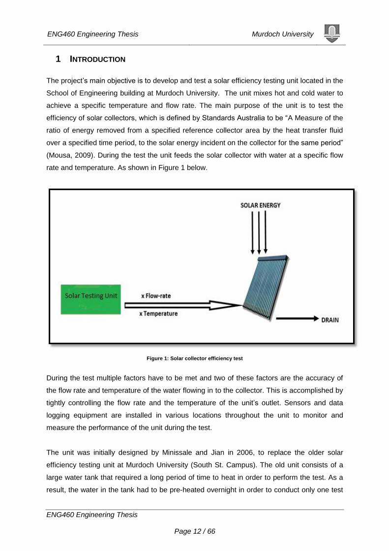
1 INTRODUCTION
The project’s main objective is to develop and test a solar efficiency testing unit located in the
School of Engineering building at Murdoch University. The unit mixes hot and cold water to
achieve a specific temperature and flow rate. The main purpose of the unit is to test the
efficiency of solar collectors, which is defined by Standards Australia to be “A Measure of the
ratio of energy removed from a specified reference collector area by the heat transfer fluid
over a specified time period, to the solar energy incident on the collector for the same period”
(Mousa, 2009). During the test the unit feeds the solar collector with water at a specific flow
rate and temperature. As shown in Figure 1 below.
Figure 1: Solar collector efficiency test
During the test multiple factors have to be met and two of these factors are the accuracy of
the flow rate and temperature of the water flowing in to the collector. This is accomplished by
tightly controlling the flow rate and the temperature of the unit’s outlet. Sensors and data
logging equipment are installed in various locations throughout the unit to monitor and
measure the performance of the unit during the test.
The unit was initially designed by Minissale and Jian in 2006, to replace the older solar
efficiency testing unit at Murdoch University (South St. Campus). The old unit consists of a
large water tank that required a long period of time to heat in order to perform the test. As a
result, the water in the tank had to be pre-heated overnight in order to conduct only one test
ENG460 Engineering Thesis Murdoch University
ENG460 Engineering Thesis Page 13 / 66
per day. The new unit allows the users to perform several efficiency tests on the solar
collector in one day. Since then, improvements have been made to the unit, particularly by
Mousa in 2009 so that the efficiency tests could comply with the ‘Australian and New
Zealand Standard AS/NZS 2535.1:2007’ for a solar collector efficiency testing unit. (Mousa,
2009)
To meet this, the mixing unit should have the ability to control the outlet flow rate and
temperature with an accuracy of ±1% and ±1°C respectively. In addition, the outlet flow rate
must be kept at 3 litres per minute for the entire duration, which is 15 minutes. (Mousa, 2009)
The project involves instrument calibration, finding the capabilities of the unit, implementing
an appropriate control strategy for the unit, and finally evaluating the final steady-state
performance of the unit.
ENG460 Engineering Thesis Murdoch University
ENG460 Engineering Thesis Page 14 / 66
2 PROJECT HISTORY
2.1 PREVIOUS SETUP CONSTRUCTION
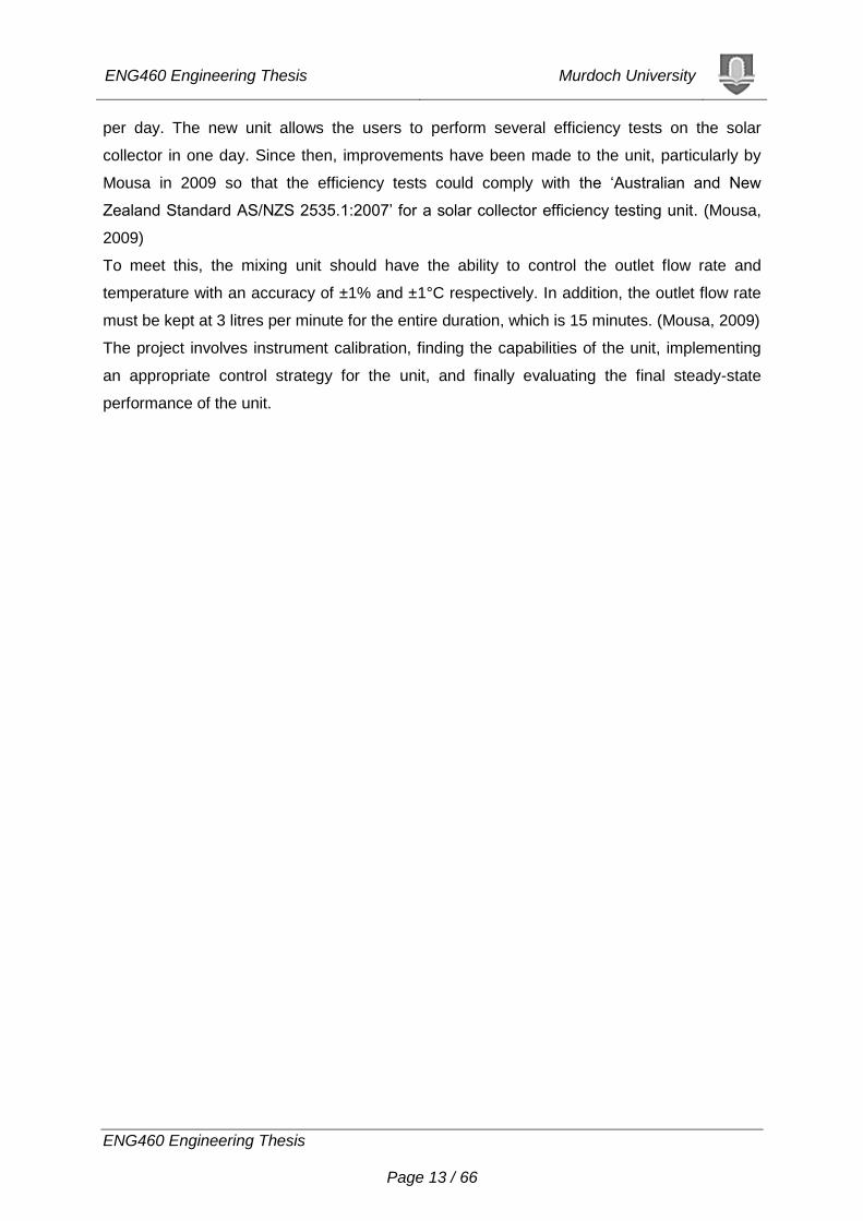
After being constructed in 2006, the unit has undergone constant development. The
schematic diagram in Figure 2 shows the unit’s setup during the last development attempt on
the project.
Figure 2: Schematic diagram of the previous setup of the unit
Source: (Mousa, 2009)
The unit consists of two tanks, the hot water tank and the cold water tank. Each tank is fitted
with solid state relays in order to control the heating element inside the tanks. A temperature
transmitter is mounted just next to the tank’s outlet to enable the temperatures inside the
tanks to be measured. In each stream there is a recycle stream with a circulation pump
installed in it. The main function of this is to help the heat distribution throughout the fluid.
Each stream also has a flow-meter and a temperature transmitter installed close to the
valves in order to measure the flow rate and the temperature of the fluid entering the valve.
The only instrument in the final mixed stream is a temperature transmitter that measures the
ENG460 Engineering Thesis Murdoch University
ENG460 Engineering Thesis Page 15 / 66
temperature of the fluid leaving the unit. The mixing unit operates in a continues mode with
fresh water from the mains being supplied to both hot and cold water tanks.
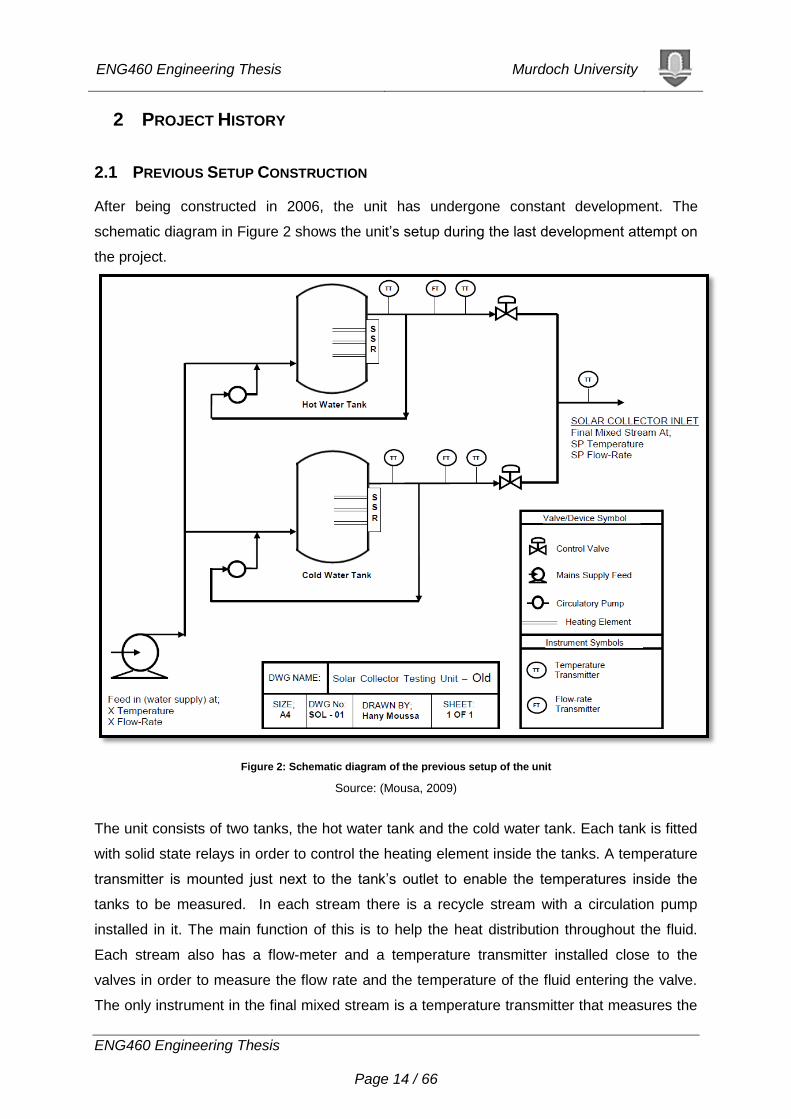
2.2 PREVIOUS CONTROL STRATEGIES AND RESULTS
The Relative Gain Analysis (RGA) performed on the ‘Multiple Input Multiple Output’ (MIMO)
unit by Al-Senaid in 2007 showed that the mixing unit was highly interactive, as each stream
has the same effect on the final mixed stream. (Mousa, 2009)
Figure 3 shows the structure of the decoupler control strategy Al-Senaid (2007) used at that
time.
Figure 3: Schematic diagram of control scheme in 2007
Source: (Mousa, 2009)
Two temperature set-point tests chosen from Al-Senaid’s project are shown below:
ENG460 Engineering Thesis Murdoch University
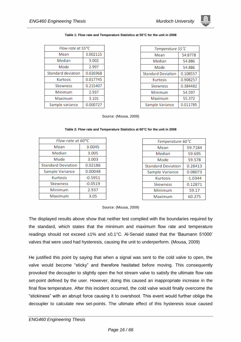
ENG460 Engineering Thesis Page 16 / 66
Table 1: Flow rate and Temperature Statistics at 55°C for the unit in 2008
Source: (Mousa, 2009)
Table 2: Flow rate and Temperature Statistics at 60°C for the unit in 2008
Source: (Mousa, 2009)
The displayed results above show that neither test complied with the boundaries required by
the standard, which states that the minimum and maximum flow rate and temperature
readings should not exceed ±1% and ±0.1°C. Al-Senaid stated that the ‘Baumann 51000’
valves that were used had hysteresis, causing the unit to underperform. (Mousa, 2009)
He justified this point by saying that when a signal was sent to the cold valve to open, the
valve would become “sticky” and therefore hesitated before moving. This consequently
provoked the decoupler to slightly open the hot stream valve to satisfy the ultimate flow rate
set-point defined by the user. However, doing this caused an inappropriate increase in the
final flow temperature. After this incident occurred, the cold valve would finally overcome the
“stickiness” with an abrupt force causing it to overshoot. This event would further oblige the
decoupler to calculate new set-points. The ultimate effect of this hysteresis issue caused
ENG460 Engineering Thesis Murdoch University
ENG460 Engineering Thesis Page 17 / 66
substantial fluctuations in the final flow and temperature, which is evident in the minimum
and maximum readings shown in the results above.” (Mousa, 2009).
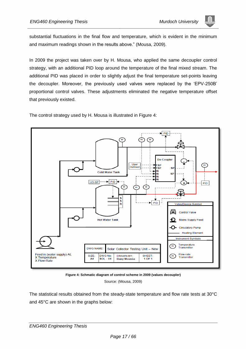
In 2009 the project was taken over by H. Mousa, who applied the same decoupler control
strategy, with an additional PID loop around the temperature of the final mixed stream. The
additional PID was placed in order to slightly adjust the final temperature set-points leaving
the decoupler. Moreover, the previously used valves were replaced by the ‘EPV-250B’
proportional control valves. These adjustments eliminated the negative temperature offset
that previously existed.
The control strategy used by H. Mousa is illustrated in Figure 4:
Figure 4: Schmatic diagram of control scheme in 2009 (values decoupler)
Source: (Mousa, 2009)
The statistical results obtained from the steady-state temperature and flow rate tests at 30°C
and 45°C are shown in the graphs below:
ENG460 Engineering Thesis Murdoch University
ENG460 Engineering Thesis Page 18 / 66
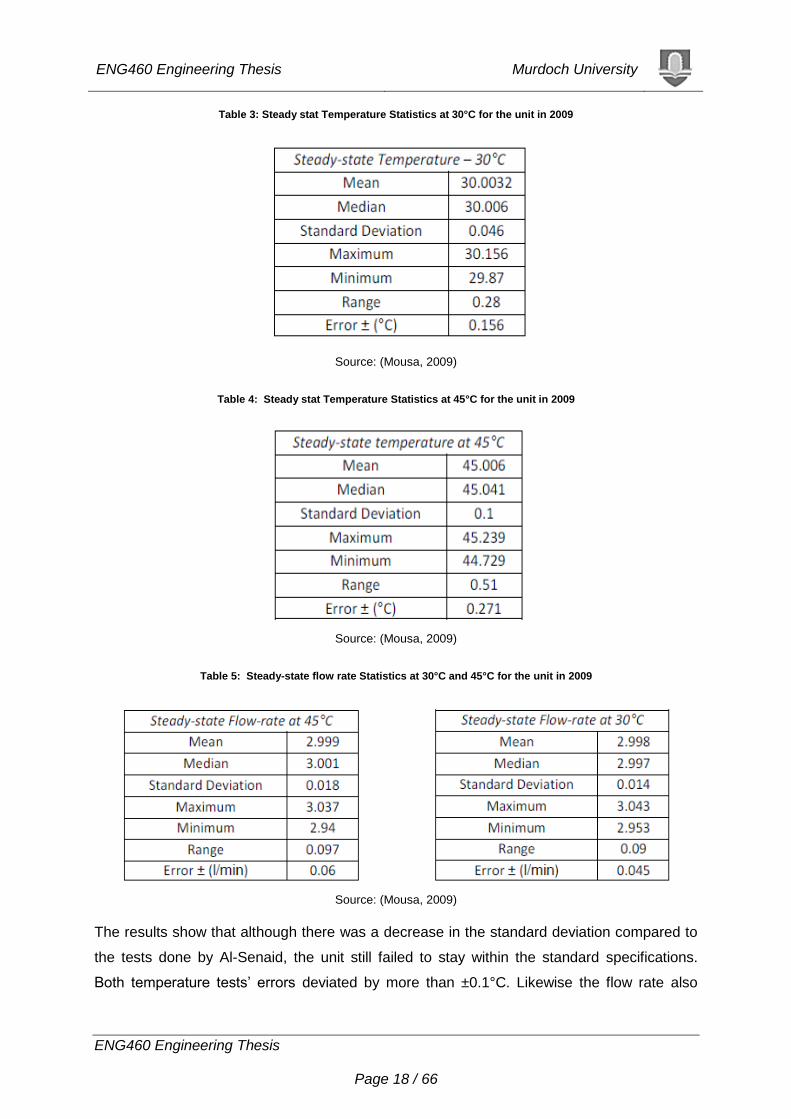
Table 3: Steady stat Temperature Statistics at 30°C for the unit in 2009
Source: (Mousa, 2009)
Table 4: Steady stat Temperature Statistics at 45°C for the unit in 2009
Source: (Mousa, 2009)
Table 5: Steady-state flow rate Statistics at 30°C and 45°C for the unit in 2009
Source: (Mousa, 2009)
The results show that although there was a decrease in the standard deviation compared to
the tests done by Al-Senaid, the unit still failed to stay within the standard specifications.
Both temperature tests’ errors deviated by more than ±0.1°C. Likewise the flow rate also
ENG460 Engineering Thesis Murdoch University
ENG460 Engineering Thesis Page 19 / 66
deviated beyond the specification of ±1% (±0.03 L/min). It is also noticeable that as
temperature increases the likelihood of errors increases.
Although H. Mousa’s attempt resulted in a substantial improvement in the unit’s performance,
it still failed to comply with the standard.
ENG460 Engineering Thesis Murdoch University
ENG460 Engineering Thesis Page 20 / 66
3 PROPOSED MODEL
3.1 CURRENT SETUP CONSTRUCTION
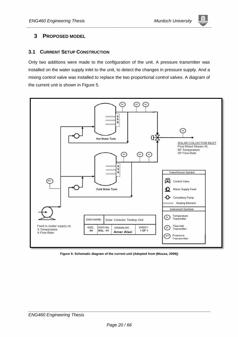
Only two additions were made to the configuration of the unit. A pressure transmitter was
installed on the water supply inlet to the unit, to detect the changes in pressure supply. And a
mixing control valve was installed to replace the two proportional control valves. A diagram of
the current unit is shown in Figure 5.
Figure 5: Schematic diagram of the current unit (Adopted from (Mousa, 2009))
ENG460 Engineering Thesis Murdoch University
ENG460 Engineering Thesis Page 21 / 66
4 EQUIPMENTS AND DEVICES
4.1 PHYSICAL DEVICES
The testing unit consists of the following devices:
Five temperature transmitters
Two flow-meters
One pressure transmitter
Two circulation pumps
Two heating units
One mixing control valve
Two water storage tanks
4.1.1 Temperature transmitters
There five identical temperature transmitter installed on different positions of the unit. They
enable the measurement of the temperature in the tanks and streams. They are ‘Resistance
Temperature Detectors’ (RTD) type ‘PT-100’, that have the ability to detect temperatures
ranging from 0°C to 150°C. The temperatures are scaled proportionally and outputted as 4-
20mA current signals. An empirical test was conducted by Minissale on the same
transmitters, and it was found that they have an accuracy of ±0.15%. (Mousa, 2009)
4.1.2 Flow-meters
The two identical flow-meters are ‘Promag 10H’ models, manufactured by ‘Endress +
Hauser’. The flow-meters measure water flow-rates in the hot and cold streams. The flow-
meters measure flow rate from 0 L/min to 5.5 L/min. This range is scaled and outputted as 4-
20mA. The flow-meters are equipped with a human interface on the front panel of the flow-
meter. This panel allows the user to change multiple features. The default password is
“1000”. (Mousa, 2009)
4.1.3 Pressure Transmitter
The ‘MBS 33’ pressure transmitter made by ‘DANFOSS’ was installed on the inlet stream of
the unit; to enable the user to monitor the pressure change in the water coming from the
main supply. The transmitter uses a 12VDC power supply to measures the pressures
ranging from 0 to 1MPa of any fluid at temperatures ranging from 0°C to 85°C. The pressure
ENG460 Engineering Thesis Murdoch University
ENG460 Engineering Thesis Page 22 / 66
measurements are sent as current signals between 4mA to 20mA to the current based
measurement system. (DANFOSS Manufacturing)
4.1.4 Circulation Pumps
The two identical pumps are manufactured by ‘Davey Pumps’. Each of the circulation pumps
is mounted on the recycle streams. They continuously pump the heated water from the tank
outlet to the fresh water prior to the tank inlet. This action ensures that heat is distributed
evenly throughout the fluid in the tank. The pumps are powered by 230VDC in order to
operate. There are three optional speeds of the pump’s motors. The speeds are:
1000 RPM at 45W
1450 RPM at 66W
1950 RPM at 89W
The maximum speed was used in all the tests, in order to achieve maximum heat distribution
in the tanks. (Mousa, 2009)
4.1.5 Heating Unit
Each storage tank is equipped with a heating unit to heat up the water in the tanks. Each unit
consists of three heating elements that are powered with a sum of 14.4 kW. To vary the
temperature in the tanks the thermostat installed by the manufacturer was removed and a
Pulse Width Modulation signal produced from the ‘PWM-520’ Field-point was used to control
the heating elements. The signals pass through Solid state Relays before reaching the
heating element. The three heating elements are bridged so that they can work
simultaneously. (Mousa, 2009)
4.1.6 Water Storage Tank
The water storage tanks are a product of ‘Rheem’. They have a maximum volume of 50 litres
and can operate at a maximum pressure of 1000kPa. The tanks are situated on top of each
other, with the hot water tank on top. An insulation layer is installed between the two tanks to
prevent heat transfer between them. (Mousa, 2009)
ENG460 Engineering Thesis Murdoch University
ENG460 Engineering Thesis Page 23 / 66
4.2 FIELD-POINT MODULES
Field-point modules are remote I/O devices that are used in the industry to manage the data
acquisition system between the PC and the field instruments. They enable the user to
read/write analogue/digital signals (Mousa, 2009). In this project five ‘National Instruments’
Field-point modules were employed to manage the communication. A diagram of the wiring
is illustrated in Appendix A. The Field-point modules (FP) that were used in the project is
described in the sections below.
4.2.1 FP-1000
This is the main FP that interfaces with the PC via a serial communication cable. It has a
very vital role, where it gathers information from the other FP units and sends it to the PC. It
also sends commands from the PC and distributes them to the output FP units. A 24V power
supply is connected to it, to provide power to the other FP units. The module has a range of
baud rate from 300 to 115200kbps. The maximum baud rate was used to achieve the fastest
data transfer. (Mousa, 2009)
4.2.2 FP-AI-110
This FP unit is concerned only with reading the analogue input signals coming from the
instruments in the field. It is able to read voltage and current, but during the project it was set
to read only current signals from 4mA to 20mA. Moreover, it has an in-built low-pass filter
that is configured by the user to reject 50Hz to 60Hz noise signals. During the running of the
project this field-point was used to measure all temperature, and flow rate measurements.
(Mousa, 2009)
4.2.3 FP-AI-111
This FP unit is very similar to the FP-AI-110. The only difference between the two is that the
FP-AI-100 has 8 input channels, and the FP-AI-111 has 16 input channels. The only
instrument that was connected to this field-point during the project was the pressure
transmitter.
ENG460 Engineering Thesis Murdoch University
ENG460 Engineering Thesis Page 24 / 66
4.2.4 FP-A0-200
This FP unit takes in the output signals from the PC and sends them out to the instruments. It
has 8 current output channels that have 12 bits of resolution. There are two output ranges
that can be used on this module: 0-20mA and 4-20mA. This module is mainly used to control
actuators, and in this project it was used to control the openings of the valves. (Mousa, 2009)
4.2.5 FP-PWM 520
Similar to the FP-AO-200, the FP-PWM-520 module also has 8 outputs, but they’re voltage
output channels that are able to supply 5, 12, and 24VDC at a maximum current of 1A. The
module is specialized, outputting pulse width modulated (PMW) signals that have a
frequency up to 1 kHz with a duty cycle from 0% to 100%. Varying the duty cycle, varies the
electrical energy going into the heaters, and therefore varying the temperature of the water in
the tanks. The 12V signal was connected to the SSRs that are connected to the heating
elements in the water tanks, to enable water temperature control by the user. (Mousa, 2009)
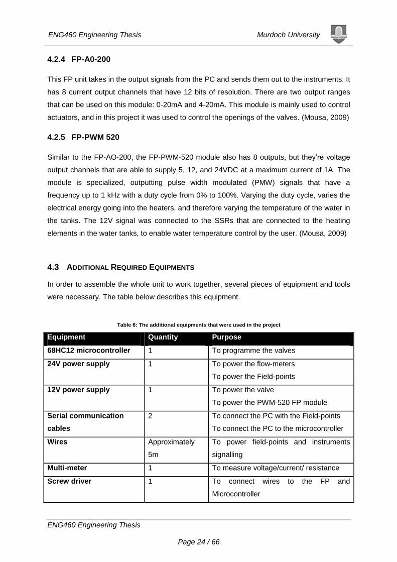
4.3 ADDITIONAL REQUIRED EQUIPMENTS
In order to assemble the whole unit to work together, several pieces of equipment and tools
were necessary. The table below describes this equipment.
Table 6: The additional equipments that were used in the project
Equipment Quantity Purpose
68HC12 microcontroller 1 To programme the valves
24V power supply 1 To power the flow-meters
To power the Field-points
12V power supply 1 To power the valve
To power the PWM-520 FP module
Serial communication
cables
2 To connect the PC with the Field-points
To connect the PC to the microcontroller
Wires Approximately
5m
To power field-points and instruments
signalling
Multi-meter 1 To measure voltage/current/ resistance
Screw driver 1 To connect wires to the FP and
Microcontroller
ENG460 Engineering Thesis Murdoch University
ENG460 Engineering Thesis Page 25 / 66
5 PC AND SOFTWARE PACKAGES
5.1 PC SPECIFICATIONS
For this project one PC was required to control, run, and monitor the efficiency testing unit.
The PC that was used had Windows XP installed and serial communication ports that were
used to connect the PC with FP units and the microcontroller. An advanced PC specification
was important, because a small loop time was used to control and monitor the unit (Mousa,
2009). The PC that will was used has the following specification:
Intel Core 2 Duo processor
2.33 GHz CPU
3.25GB RAM
Window XP Professional (Mousa, 2009)
5.2 MEASUREMENT AND AUTOMATION EXPLORER (MAX)
The Measurement and Automation Explorer (MAX) 5.0 is a product of National Instruments.
MAX provides access to all National Instrument products. MAX was used to:
Configure and establish a connection between the PC and the Field-point devices
Scale the instruments’ signals
Verifying signals and wire connections by reading/writing signals to/from the field
devices
5.3 LABVIEW PROGRAM AND GRAPHICAL USER INTERFACE
A pre-designed LabVIEW program done by P. Minissale in 2006 and modified by H. Al-
Senaid (2007) and H. Mousa (2009) was employed to monitor, control, and record data from
the unit. This section of the report highlights the modifications on the block diagram and the
front panel that were implemented, and also demonstrate some of the pre-existing features
that were used.
5.3.1 Block Diagram
The following modifications were implemented on the software’s block diagram:
In the last development attempt on the unit the heating element in the cold tank was
damaged. In this attempt the heating element was fixed, therefore a PID control loop
was introduced to control the water temperature in the cold water tank.
The pressure transmitter signal from the field-point module was added to the block
diagram.
ENG460 Engineering Thesis Murdoch University
ENG460 Engineering Thesis Page 26 / 66
The old control arrangement used in the previous years was replaced by the new
control strategy.
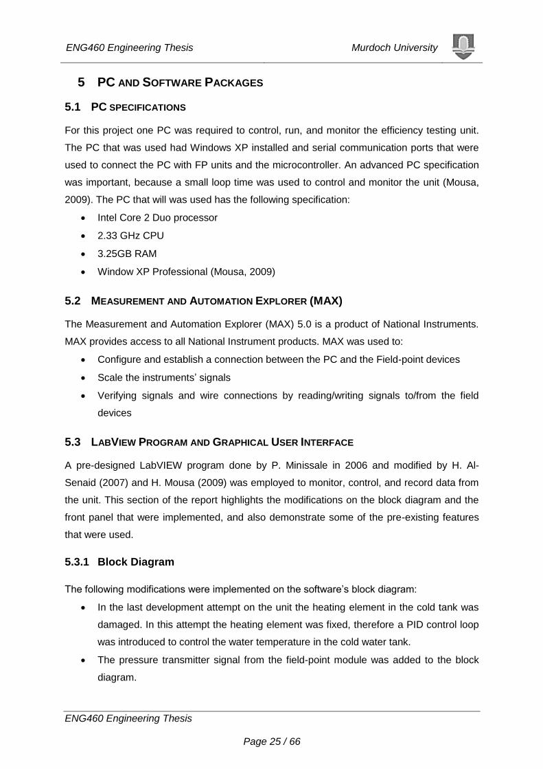
5.3.2 Front Panel
The pre-designed program allows the user to move between three different front panels that
provide different information obtained from the unit. The only panel that was altered was the
control parameter screen to provide more graphical information about the changes in the
unit. A screenshot of the control parameters panel is shown in Figure 6.
Figure 6: LabView program front panel
The control parameter screen displays the PID controllers’ parameters. The screen also
allows the user to switch the valve mode between auto (set point set by software) and
manual (set point set by button on the valve’s front panel). It also displays the temperature,
flow rate and pressure charts, which continuously track the changes in the unit.
ENG460 Engineering Thesis Murdoch University
ENG460 Engineering Thesis Page 27 / 66
6 INSTRUMENT MODIFICATIONS In the previous attempts on the project by Mousa, two ‘EPV-250B’ proportional control valves
were used as the final control elements of the unit. Information on that valve can be found in
Appendix C.
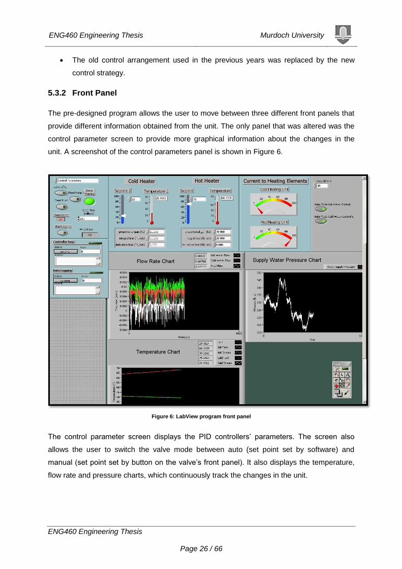
6.1 MIXING CONTROL VALVE
The mixing control valve “Intellifaucet RK 250” was designed by Hass Manufacturing
Company to accurately control and regulates the water temperature by employing two motor
driven valves and a highly complex onboard control algorithm. The valve comes as one unit
with three ports: two inlet ports for the cold and the hot stream, and an outlet port for the final
product of both streams. The specifications of the valve are:
Maximum CV =0.6.
¼ inch port size.
4-20mA or 1.5VDC input signal.
No backlash or hysteresis.
4.5°C to 93°C temperature operation.
Temperature accuracy of ±0.1°C.
Valves repositioned 60 times per second
Fully automatic self-control.
Requires 12 VDC power.
0-19 liters/min. (Hass Manufacturing
Company)
The most appealing feature of the mixing valve is that it promises to deliver a temperature
accuracy control of ±1°C, which exactly meets the standard test temperature requirement.
However, the manual does not mention the accuracy limits provided by the valve in flow rate
Figure 7: The Intellifaucet RK 250 mixing control valve
Source: (Hass Manufacturing Company)
ENG460 Engineering Thesis Murdoch University
ENG460 Engineering Thesis Page 28 / 66
control. Moreover the valve considers the flow rate control as a secondary function, while
prioritizing the temperature control as the primary focus. The only way to control the flow rate
through the valve is by adjusting the percentage flow rate by 1% increments using the button
on the valve’s front panel. The valve manual also explains that the valve’s temperature
control is unaffected by pressure and temperature fluctuations in both hot and cold inlet
streams to the valve.
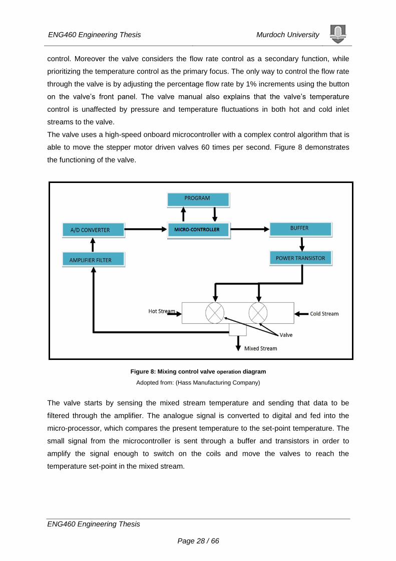
The valve uses a high-speed onboard microcontroller with a complex control algorithm that is
able to move the stepper motor driven valves 60 times per second. Figure 8 demonstrates
the functioning of the valve.
Figure 8: Mixing control valve operation diagram
Adopted from: (Hass Manufacturing Company)
The valve starts by sensing the mixed stream temperature and sending that data to be
filtered through the amplifier. The analogue signal is converted to digital and fed into the
micro-processor, which compares the present temperature to the set-point temperature. The
small signal from the microcontroller is sent through a buffer and transistors in order to
amplify the signal enough to switch on the coils and move the valves to reach the
temperature set-point in the mixed stream.
ENG460 Engineering Thesis Murdoch University
ENG460 Engineering Thesis Page 29 / 66
7 INSTRUMENT CALIBRATION
Instrument calibration is an essential step prior to doing any testing on the unit. Calibration is
done by conducting a certain procedure to reduce or eliminate any bias in the instruments’
readings relative to a reference base measurement. Calibrating the instruments ensures that
they are not the source of underperformance in the unit. All the flow meters and the
temperature sensors were calibrated to ensure that they were able to meet the accuracy
requirements of the AS/NZS standard.
The outlined procedure and the results of calibrating the temperature sensors and the flow
meters are described in the sections below.
7.1 TEMPERATURE SENSORS
The calibration section in the standard specifies that the temperature measurement at the
outlet water flow should be measured to within ±0.1°C. Moreover the standard mentions that
the sensors should be monitored closely, to detect any deviation with time, and it
recommends that the temperature signal resolution should be at least ± 0.02°C. (Mousa,
2009)
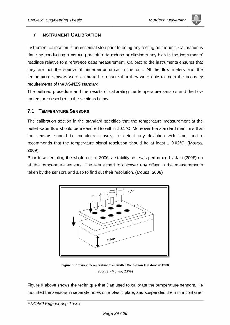
Prior to assembling the whole unit in 2006, a stability test was performed by Jain (2006) on
all the temperature sensors. The test aimed to discover any offset in the measurements
taken by the sensors and also to find out their resolution. (Mousa, 2009)
Figure 9: Previous Temperature Transmitter Calibration test done in 2006
Source: (Mousa, 2009)
Figure 9 above shows the technique that Jian used to calibrate the temperature sensors. He
mounted the sensors in separate holes on a plastic plate, and suspended them in a container
ENG460 Engineering Thesis Murdoch University
ENG460 Engineering Thesis Page 30 / 66
of water at ambient temperature. The sensors were continuously monitored and logged for
an extended period of time. (Mousa, 2009)
The results collected by Jian indicated that the transmitters’ readings were changing at the
same the rate, but they had a minor offset between them. He also explained that the offset
was the result of the different hardware settings of each sensor. Jian also proved
experimentally that the sensors had an accuracy of ±0.15%. The test also indicated that the
sensors had a resolution of ±0.0225 and therefore they failed to reach the resolution
recommended by the standard, which is ±0.02°C. (Mousa, 2009)
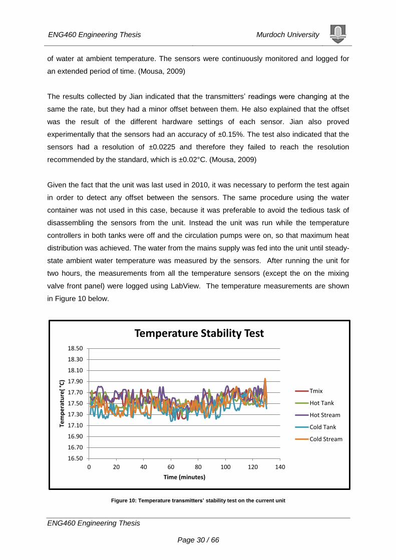
Given the fact that the unit was last used in 2010, it was necessary to perform the test again
in order to detect any offset between the sensors. The same procedure using the water
container was not used in this case, because it was preferable to avoid the tedious task of
disassembling the sensors from the unit. Instead the unit was run while the temperature
controllers in both tanks were off and the circulation pumps were on, so that maximum heat
distribution was achieved. The water from the mains supply was fed into the unit until steady-
state ambient water temperature was measured by the sensors. After running the unit for
two hours, the measurements from all the temperature sensors (except the on the mixing
valve front panel) were logged using LabView. The temperature measurements are shown
in Figure 10 below.
Figure 10: Temperature transmitters’ stability test on the current unit
16.50
16.70
16.90
17.10
17.30
17.50
17.70
17.90
18.10
18.30
18.50
0 20 40 60 80 100 120 140
Tem
pe
ratu
re(
°C)
Time (minutes)
Temperature Stability Test
Tmix
Hot Tank
Hot Stream
Cold Tank
Cold Stream
ENG460 Engineering Thesis Murdoch University
ENG460 Engineering Thesis Page 31 / 66
The Figure shows that there is a negligible offset between the temperature sensors in the
unit; therefore no alterations were made to the temperature signals. When statically
analysing the results, it showed that the sensors fluctuated near an average of 17.51°C.
7.2 FLOW METERS
As specified by the AS/NZS standard, the accuracy of the outlet water flow rate
measurement must be within ±1% of the desired flow rate (3 L/min) (Mousa, 2009). As
mentioned earlier the mixing valve considers flow rate control to be a secondary function that
can only be adjusted using the buttons on the mixing valve front panel. The mixing valve
uses percentages to describe the volume of flow passing through the valve. The maximum
percentage is 100% and the minimum is 20%. The valve’s manual confirms that it’s able to
control the flow rate from 1.89 L/min to 15.14 L/min, but it does not mention anything about
the flow rate accuracy, therefore it is not certain that the valve will in fact control the flow rate
with the desired accuracy.
Initially, to ensure that the flow meters were giving out the actual flow rate, the sum of both
hot and cold water streams flow rates was calibrated to the actual outlet flow rate. This was
done by collecting the outlet water using a volumetric cylinder, in parallel with counting the
time needed for the water to be collected using a stopwatch. Then the calculated flow rate
was compared to the sum of the two water streams’ flow rates. In order to verify the
calculated experimental flow rate, each flow rate was collected twice, and the average of the
calculated experimental flow rate was taken into account. The results are presented in Table
7.
ENG460 Engineering Thesis Murdoch University
ENG460 Engineering Thesis Page 32 / 66
Table 7: Flow meters Calibration details
Actual
Flow
Rate
(L/min)
Time
(min)
Volume
(L)
Time
(min)
Volume
(L)
Average
Volume (L)
Average
Time
(min)
Experimental
Flow Rate
(L/min)
Error
(%)
4.51 0.20 0.95 0.17 0.8 0.87 0.189 4.62 2.60
3.95 0.21 0.87 0.20 0.84 0.85 0.21 4.08 3.29
2.81 0.22 0.66 0.264 0.71 0.68 0.24 2.81 0.04
1.93 0.328 0.6 0.308 0.61 0.60 0.31 1.90 1.35
1.32 0.43 0.58 0.42 0.55 0.56 0.42 1.31 0.13
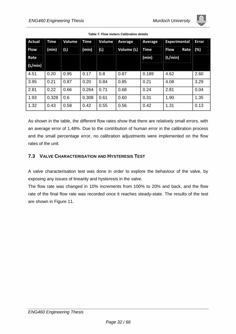
As shown in the table, the different flow rates show that there are relatively small errors, with
an average error of 1.48%. Due to the contribution of human error in the calibration process
and the small percentage error, no calibration adjustments were implemented on the flow
rates of the unit.
7.3 VALVE CHARACTERISATION AND HYSTERESIS TEST
A valve characterisation test was done in order to explore the behaviour of the valve, by
exposing any issues of linearity and hysteresis in the valve.
The flow rate was changed in 10% increments from 100% to 20% and back, and the flow
rate of the final flow rate was recorded once it reaches steady-state. The results of the test
are shown in Figure 11.
ENG460 Engineering Thesis Murdoch University
ENG460 Engineering Thesis Page 33 / 66
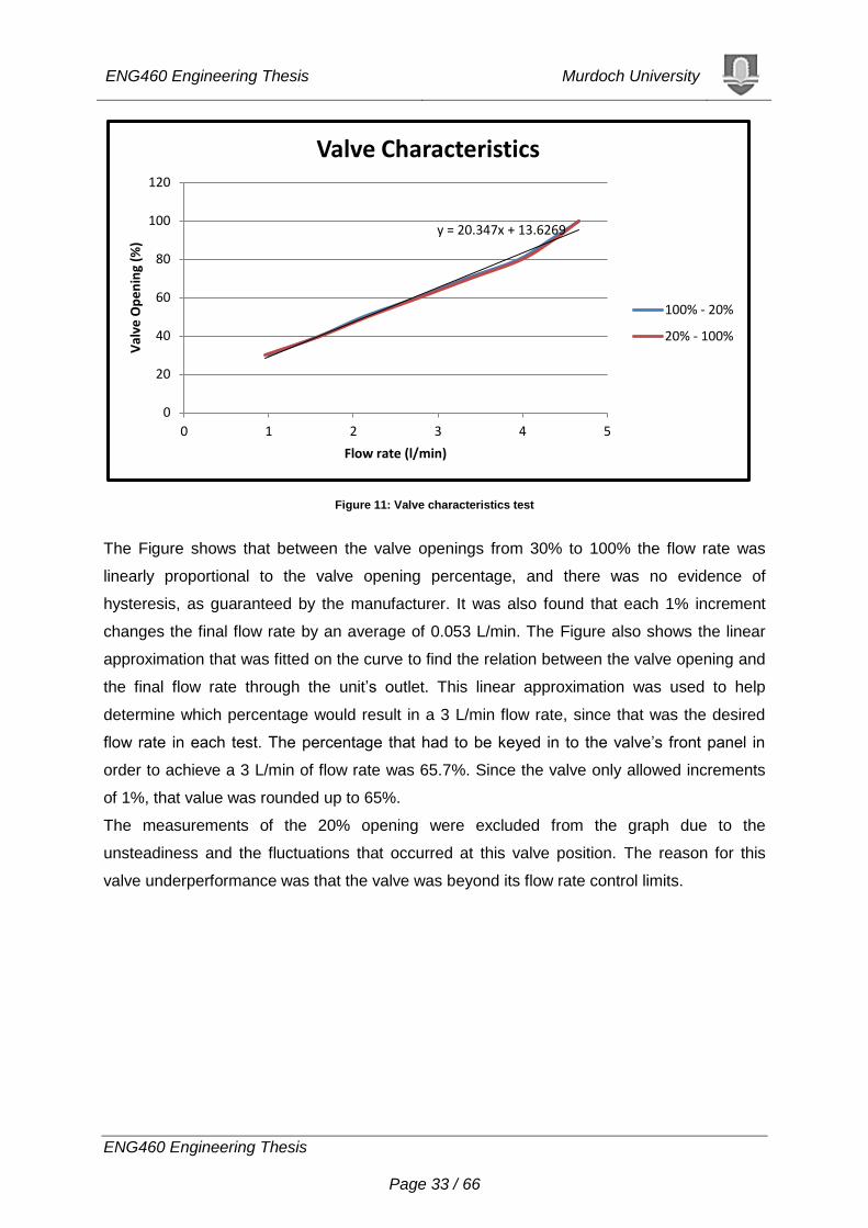
Figure 11: Valve characteristics test
The Figure shows that between the valve openings from 30% to 100% the flow rate was
linearly proportional to the valve opening percentage, and there was no evidence of
hysteresis, as guaranteed by the manufacturer. It was also found that each 1% increment
changes the final flow rate by an average of 0.053 L/min. The Figure also shows the linear
approximation that was fitted on the curve to find the relation between the valve opening and
the final flow rate through the unit’s outlet. This linear approximation was used to help
determine which percentage would result in a 3 L/min flow rate, since that was the desired
flow rate in each test. The percentage that had to be keyed in to the valve’s front panel in
order to achieve a 3 L/min of flow rate was 65.7%. Since the valve only allowed increments
of 1%, that value was rounded up to 65%.
The measurements of the 20% opening were excluded from the graph due to the
unsteadiness and the fluctuations that occurred at this valve position. The reason for this
valve underperformance was that the valve was beyond its flow rate control limits.
y = 20.347x + 13.6269
0
20
40
60
80
100
120
0 1 2 3 4 5
Val
ve O
pe
nin
g (%
)
Flow rate (l/min)
Valve Characteristics
100% - 20%
20% - 100%
ENG460 Engineering Thesis Murdoch University
ENG460 Engineering Thesis Page 34 / 66
8 PROJECT ADJUSTMENTS
8.1 TANK WATER TEMPERATURE CONTROL
As shown above the unit consists of two water tanks. To achieve fair efficiency tests, the
water in each tank should be set to the same specific temperature in each test. The steady-
state tests that are recommended by the AS/NZS standard range from 30°C to 70°C,
therefore the temperatures in the hot water tank must sustain a temperature of 70°C or
higher, and the temperature in the cold tank must sustain a temperature of 30°C or lower.
This section tests the ability of the tanks to deliver such temperatures and assesses the
performance of the conventional PI controller in maintaining the tanks’ temperatures during
the tests. (Mousa, 2009)
Hot Water Tank Control
With no water circulation in the unit the heating element is able to heat the water in the hot
water tank to 78°C, but that becomes difficult to sustain when circulation adds more fresh
water from the mains into the tank, producing temperature disturbance at a faster rate
(Mousa, 2009). First, a theoretical examination of the ability of the tank to deliver 70°C hot
water at 3 L/min was performed. At the time this experiment was performed the ambient
temperature of the mains water that is supplied to the unit is about 19°C, therefore the
question is: how much power is required to heat the 19°C supply water flowing at 3L/min to
70°C? Is it more or less than the maximum power used by the heating element (14400 W)?
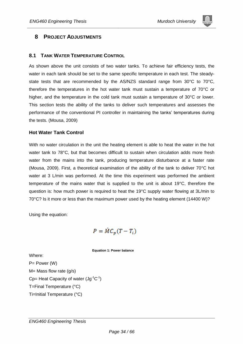
Using the equation:
Where:
P= Power (W)
M= Mass flow rate (g/s)
Cp= Heat Capacity of water (Jg-1C-1)
T=Final Temperature (°C)
Ti=Initial Temperature (°C)
Equation 1: Power balance
ENG460 Engineering Thesis Murdoch University
ENG460 Engineering Thesis Page 35 / 66
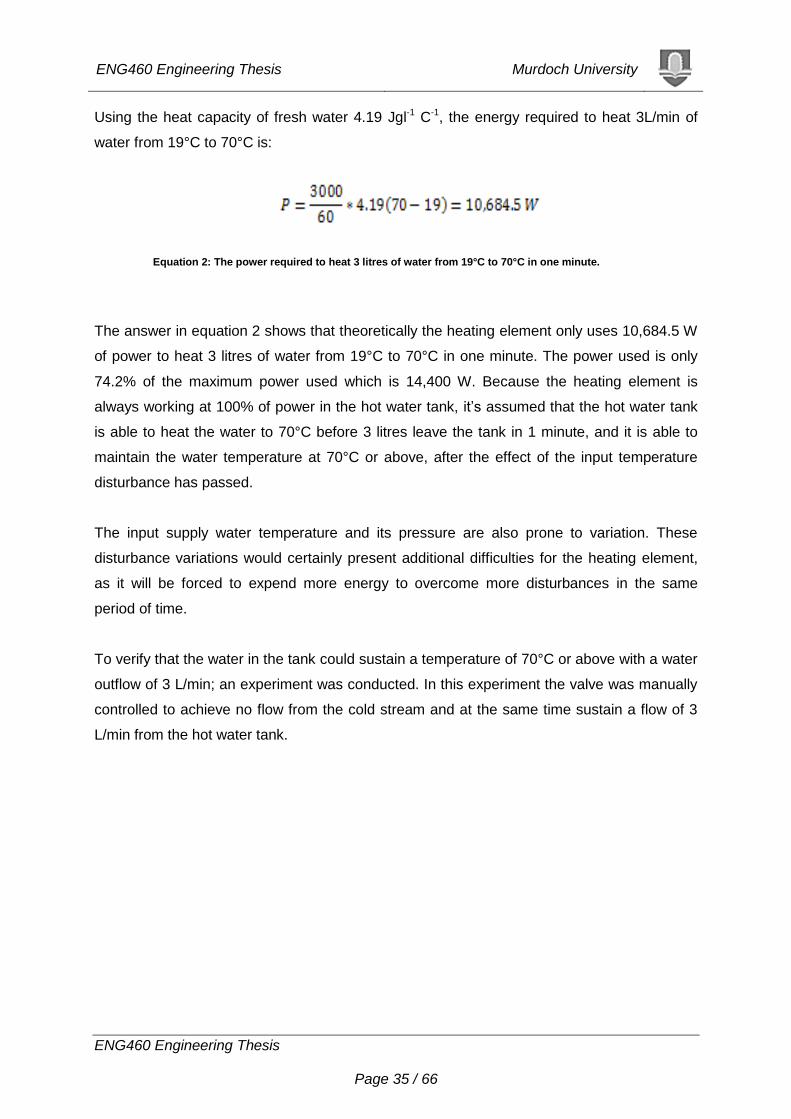
Using the heat capacity of fresh water 4.19 Jgl-1 C-1, the energy required to heat 3L/min of
water from 19°C to 70°C is:
The answer in equation 2 shows that theoretically the heating element only uses 10,684.5 W
of power to heat 3 litres of water from 19°C to 70°C in one minute. The power used is only
74.2% of the maximum power used which is 14,400 W. Because the heating element is
always working at 100% of power in the hot water tank, it’s assumed that the hot water tank
is able to heat the water to 70°C before 3 litres leave the tank in 1 minute, and it is able to
maintain the water temperature at 70°C or above, after the effect of the input temperature
disturbance has passed.
The input supply water temperature and its pressure are also prone to variation. These
disturbance variations would certainly present additional difficulties for the heating element,
as it will be forced to expend more energy to overcome more disturbances in the same
period of time.
To verify that the water in the tank could sustain a temperature of 70°C or above with a water
outflow of 3 L/min; an experiment was conducted. In this experiment the valve was manually
controlled to achieve no flow from the cold stream and at the same time sustain a flow of 3
L/min from the hot water tank.
Equation 2: The power required to heat 3 litres of water from 19°C to 70°C in one minute.
ENG460 Engineering Thesis Murdoch University
ENG460 Engineering Thesis Page 36 / 66
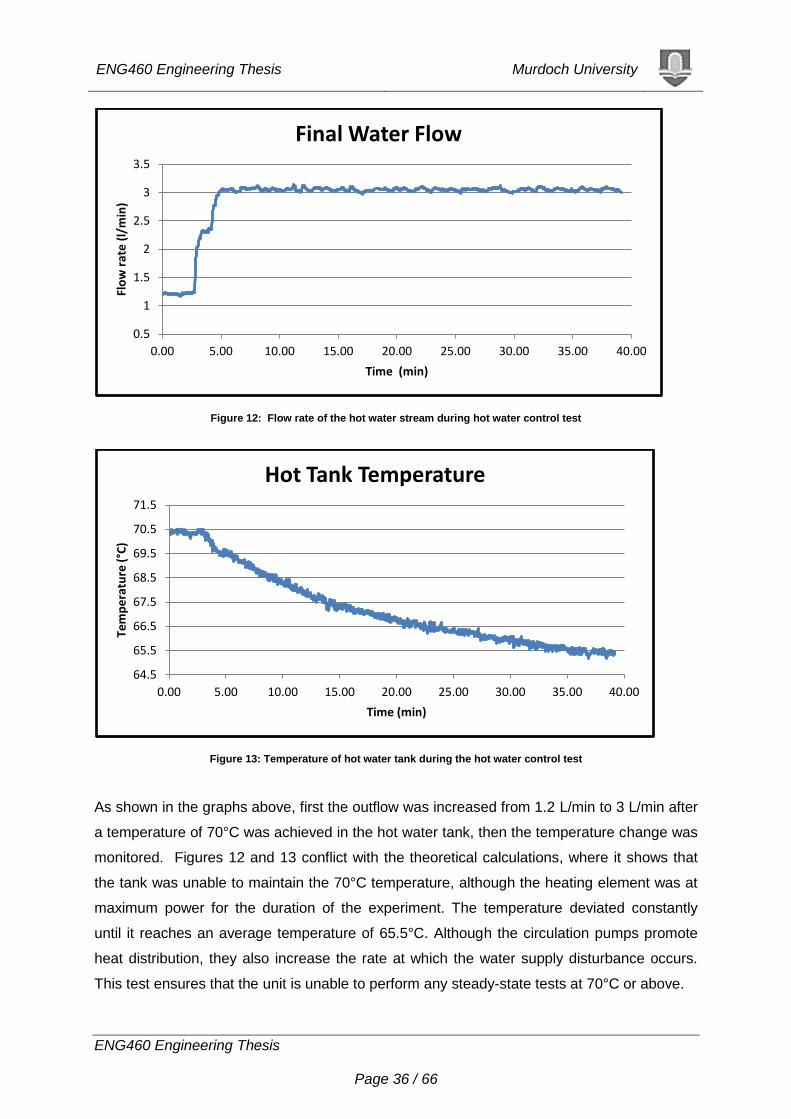
Figure 12: Flow rate of the hot water stream during hot water control test
Figure 13: Temperature of hot water tank during the hot water control test
As shown in the graphs above, first the outflow was increased from 1.2 L/min to 3 L/min after
a temperature of 70°C was achieved in the hot water tank, then the temperature change was
monitored. Figures 12 and 13 conflict with the theoretical calculations, where it shows that
the tank was unable to maintain the 70°C temperature, although the heating element was at
maximum power for the duration of the experiment. The temperature deviated constantly
until it reaches an average temperature of 65.5°C. Although the circulation pumps promote
heat distribution, they also increase the rate at which the water supply disturbance occurs.
This test ensures that the unit is unable to perform any steady-state tests at 70°C or above.
0.5
1
1.5
2
2.5
3
3.5
0.00 5.00 10.00 15.00 20.00 25.00 30.00 35.00 40.00
Flo
w r
ate
(l/
min
)
Time (min)
Final Water Flow
64.5
65.5
66.5
67.5
68.5
69.5
70.5
71.5
0.00 5.00 10.00 15.00 20.00 25.00 30.00 35.00 40.00
Tem
pe
ratu
re (
°C)
Time (min)
Hot Tank Temperature
ENG460 Engineering Thesis Murdoch University
ENG460 Engineering Thesis Page 37 / 66
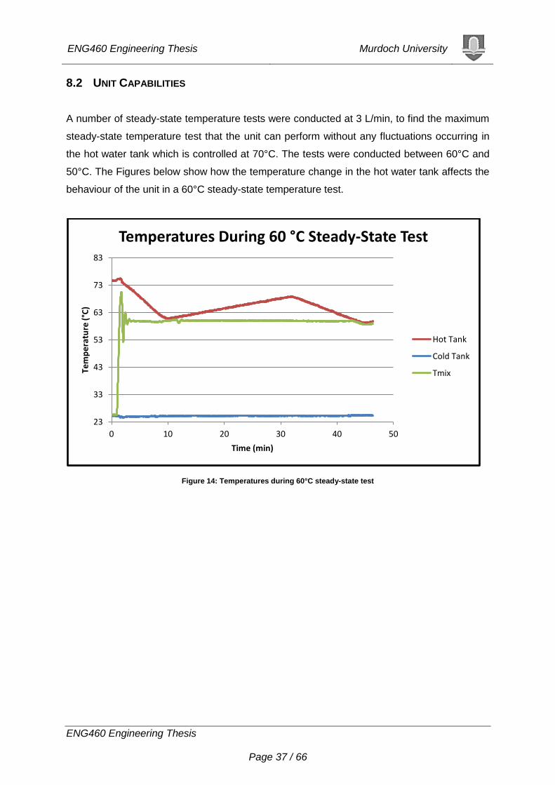
8.2 UNIT CAPABILITIES
A number of steady-state temperature tests were conducted at 3 L/min, to find the maximum
steady-state temperature test that the unit can perform without any fluctuations occurring in
the hot water tank which is controlled at 70°C. The tests were conducted between 60°C and
50°C. The Figures below show how the temperature change in the hot water tank affects the
behaviour of the unit in a 60°C steady-state temperature test.
Figure 14: Temperatures during 60°C steady-state test
23
33
43
53
63
73
83
0 10 20 30 40 50
Tem
pe
ratu
re (
°C)
Time (min)
Temperatures During 60 °C Steady-State Test
Hot Tank
Cold Tank
Tmix
ENG460 Engineering Thesis Murdoch University
ENG460 Engineering Thesis Page 38 / 66
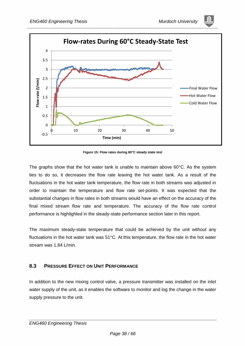
Figure 15: Flow rates during 60°C steady state test
The graphs show that the hot water tank is unable to maintain above 60°C. As the system
ties to do so, it decreases the flow rate leaving the hot water tank. As a result of the
fluctuations in the hot water tank temperature, the flow rate in both streams was adjusted in
order to maintain the temperature and flow rate set-points. It was expected that the
substantial changes in flow rates in both streams would have an effect on the accuracy of the
final mixed stream flow rate and temperature. The accuracy of the flow rate control
performance is highlighted in the steady-state performance section later in this report.
The maximum steady-state temperature that could be achieved by the unit without any
fluctuations in the hot water tank was 51°C. At this temperature, the flow rate in the hot water
stream was 1.84 L/min.
8.3 PRESSURE EFFECT ON UNIT PERFORMANCE
In addition to the new mixing control valve, a pressure transmitter was installed on the inlet
water supply of the unit, as it enables the software to monitor and log the change in the water
supply pressure to the unit.
-0.5
0
0.5
1
1.5
2
2.5
3
3.5
4
0 10 20 30 40 50
Flo
w-r
ate
(l/
min
)
Time (min)
Flow-rates During 60°C Steady-State Test
Final Water Flow
Hot Water Flow
Cold Water Flow
ENG460 Engineering Thesis Murdoch University
ENG460 Engineering Thesis Page 39 / 66
As mentioned earlier, the unit is located at Murdoch University‘s Pilot Plant in the
Engineering and Energy School, therefore the operation of the pilot plant requires a
significant amount of water, which is sufficient to disturb the water supply pressure. To
analyse the effect of this disturbance on the unit’s performance, the steepest change in
pressure was highlighted in parallel with its effect on the final water stream’s flow rate and
temperature.
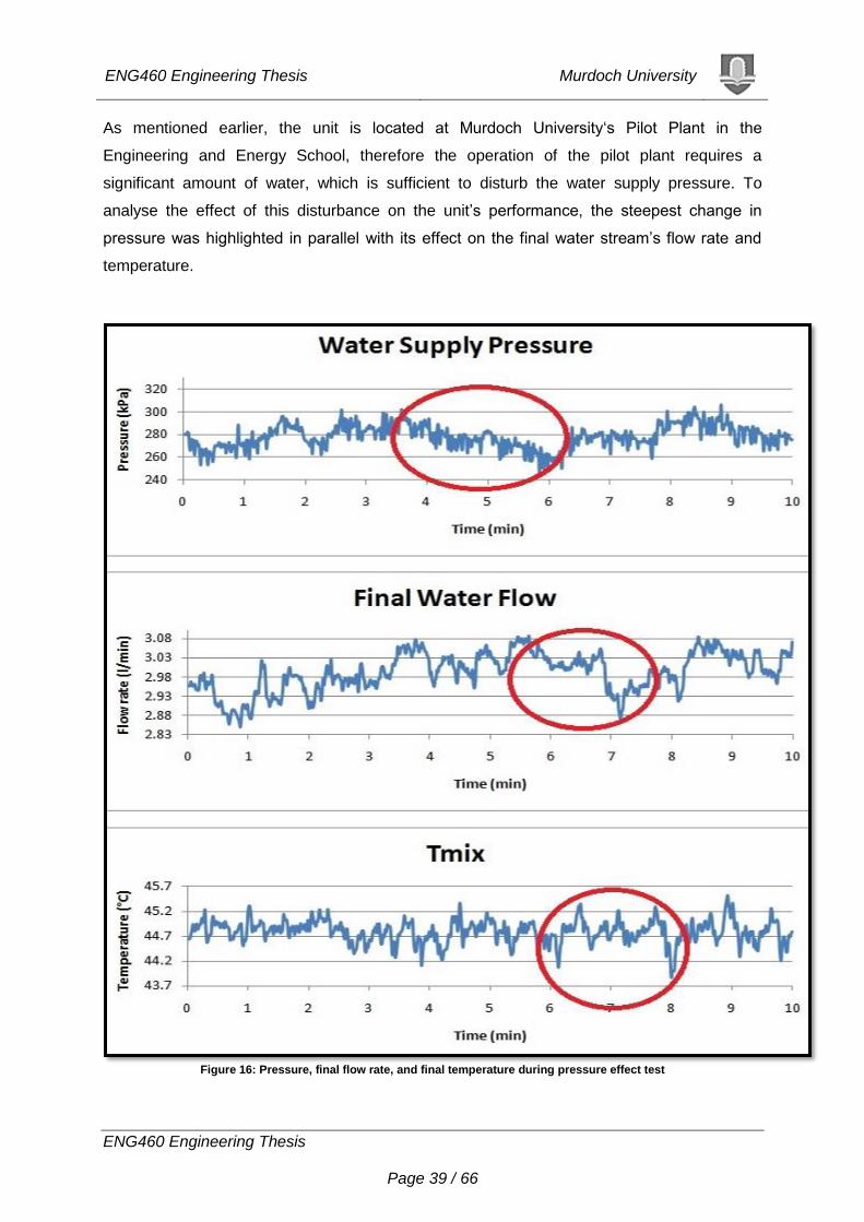
Figure 16: Pressure, final flow rate, and final temperature during pressure effect test
ENG460 Engineering Thesis Murdoch University
ENG460 Engineering Thesis Page 40 / 66
The water supply pressure graph at the top indicates that the operation of the pilot plant
definitively causes oscillations in the pressure supply to the unit.
After 3.58 minutes, the water supply pressure began descending from 302.44 kPa and
reached 249.13 kPa at 5.89 minutes. As a result of that descent, the flow rate dropped from
3.05 L/min at 5.85 minutes to 2.86 L/min at 7.15 minutes. The change in flow rate due to
pressure had direct effect on the outlet’s temperature. This was evident when the sharp
decent in flow rate at time equal to 6.80 minutes occurred, resulting in a similar drop in the
temperature, from 45.3°C at 7.73 minutes to 43.88°C at 8.00 minutes.
The time delay in the change in outlet flow rate is an indication of the time that the pressure
takes to travel through the unit to reach the final outlet flow of the unit. Although the graphs
do not show this, the change in the outlet’s temperature is almost parallel to the change in
the flow rate. Because the final flow-rate is calculated based on the readings of two
separately installed flow meters in the hot and cold streams before the mixing valve, the
change in flow rate is observed before the change in temperature.
8.4 VALVE PERFORMANCE COMPARISON
To evaluate the performance of the newly installed control valve, a few steady-state tests
were performed. The mixing valve’s performance was compared to the pair of proportional
control valves that were used by H. Mousa in 2009. In both tests the flow rate set point was 3
L/min and the temperature was set to 45°C. Although the valves showed no signs of
hysteresis, the proportional control valves should yield better performance in flow rate
control, since the mixing valve considers flow rate control to be a secondary priority and it’s
affected by pressure disturbance as proven in the section above.
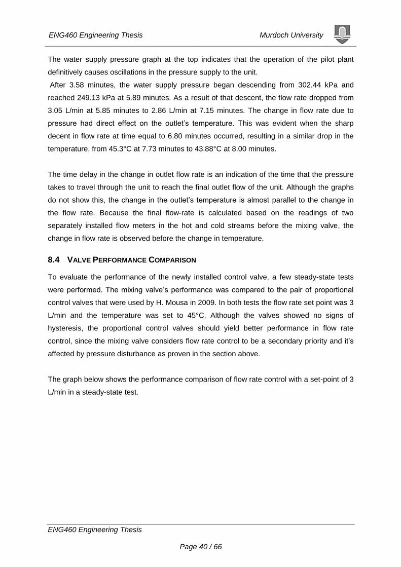
The graph below shows the performance comparison of flow rate control with a set-point of 3
L/min in a steady-state test.
ENG460 Engineering Thesis Murdoch University
ENG460 Engineering Thesis Page 41 / 66
Figure 17: Flow-rate control comparisons between the old and the new valves at 45°C
As expected, the proportional control valves’ response to steady-state flow rate was superior
to the new mixing valve. The flow rate under the mixing valve control violates the flow rate
range (±1%= ±0.03 L/min) more frequently and by a larger magnitude than the flow rate
under the proportional control valves. These inconsistent fluctuations experienced by the flow
rate under the mixing valve control are a result of the pressure changes in the water supplied
to the unit.
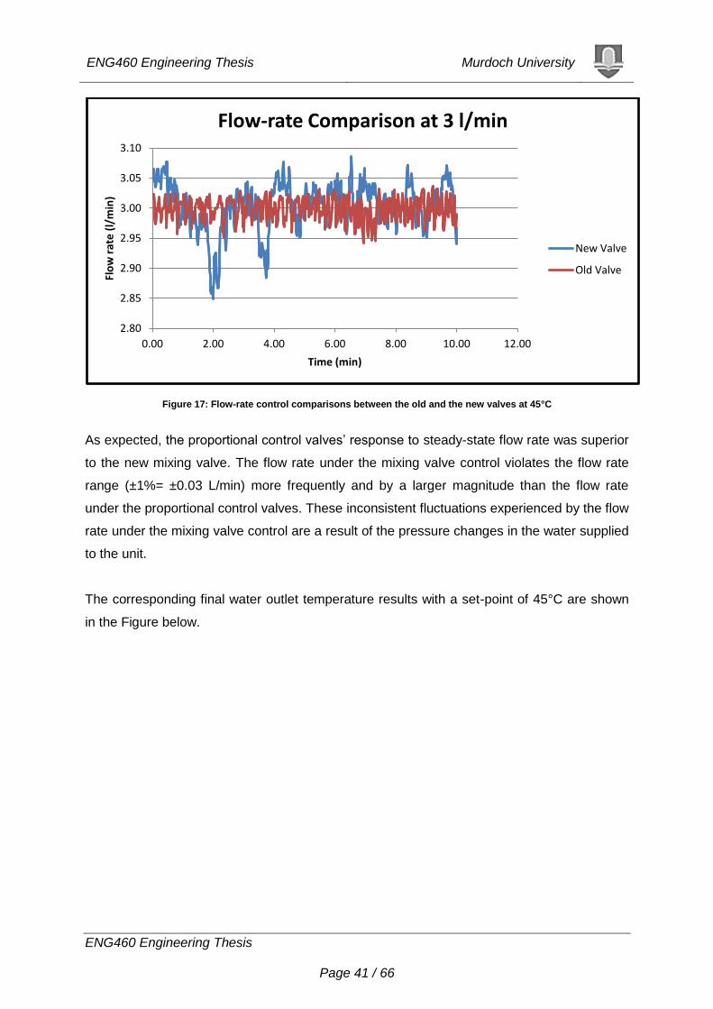
The corresponding final water outlet temperature results with a set-point of 45°C are shown
in the Figure below.
2.80
2.85
2.90
2.95
3.00
3.05
3.10
0.00 2.00 4.00 6.00 8.00 10.00 12.00
Flo
w r
ate
(l/
min
)
Time (min)
Flow-rate Comparison at 3 l/min
New Valve
Old Valve
ENG460 Engineering Thesis Murdoch University
ENG460 Engineering Thesis Page 42 / 66
Figure 18: Temperature control comparisons between the old and the new valve at 45°C
The Figure above shows an approximately similar steady-state performance by the valves,
but there are some discrepancies between them. The proportional control valves
performance exhibits roughly uniform fluctuation around the set point. On the other hand, the
mixing valve exhibits better performance at most times during the test, with smaller
fluctuations. Nevertheless, the performance is still affected by the flow rate changes that are
prompted by the uncontrollable pressure changes. This is evident from the inconsistent
shape produced by the temperature readings on Figure 18.
8.5 EXTERNAL MICROCONTROLLER
The pressure disturbances have a serious effect on the flow rate control of the valve and the
valves’ underperformance compared to the proportional control valves. This indicated that
the valve would have difficulty controlling the flow rate and the temperature within the limits
required by the standard. On the positive side, the valve still had very good mechanism that
could be employed to achieve better performance. To obtain a better understanding of how
the valve works, it was opened and its electronic circuit was analysed. The valve contains
two circuit boards. The first is attached to the control front panel of the valve, and the
temperature sensor in the valves’ outlet, where it receives all the commands. The signals
from the first circuit board are sent to the other circuit board on the back of the valve. The
second circuit board contains the microcontroller which receives the commands and works
44.60
44.70
44.80
44.90
45.00
45.10
45.20
45.30
45.40
0.00 2.00 4.00 6.00 8.00 10.00 12.00
Tem
pe
ratu
re (
°C)
Time (min)
Temperature Comparison at 45°C
New Valve
Old Valve
ENG460 Engineering Thesis Murdoch University
ENG460 Engineering Thesis Page 43 / 66
out the magnitude of voltage signals to be sent to each of the coils in the motors in order to
achieve set-point. Prior to every coil there are transistors which amplify the signal.
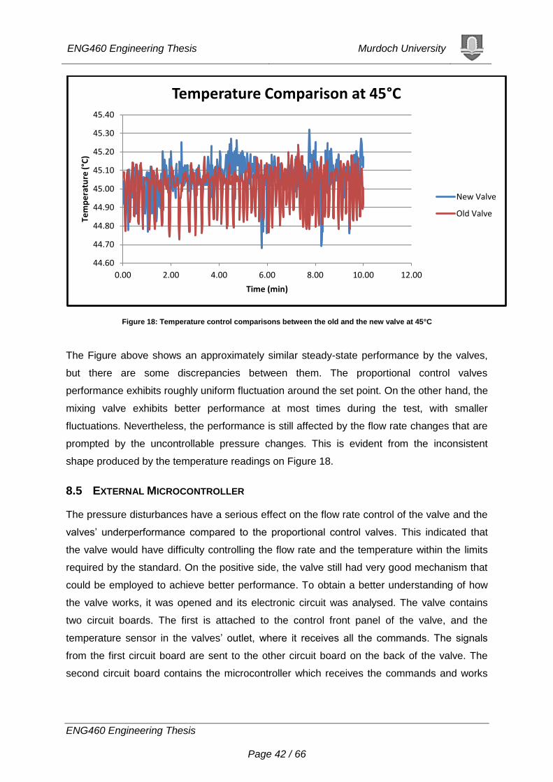
To enhance the flow rate control, an external 68HC12 microcontroller was used to replace
the one in the valve. The external microcontroller will receive the command signals from the
analogue output field-point module instead of from the valve’s front control panel, and it will
send the control signals to the transistors. A picture of the external microcontroller is shown
in the Figure below.
Figure 19: A picture of the microcontroller that was used to control the valve
As shown in Figure 19 the microcontroller is powered with a 5V power supply. Eight outputs
(P0P3, T1T4) were employed to send command signals for each coil on the two stepper
motors. On the other hand only two inputs (PAD0 and PAD1) were used in order to receive
the percentage opening set-point of each valve. Since the microcontroller only receives
voltage signals ranging from 0V to 5V, a resistor on each input was used to convert and
scale the 0mA to 21mA coming from the analogue output module to the volts at the that
ENG460 Engineering Thesis Murdoch University
ENG460 Engineering Thesis Page 44 / 66
range. The reset button was used to clear the uploaded program on the microcontroller and
a serial communication port was used to connect the microcontroller to the PC.
The following are only a few of the functions that the microcontroller was programmed to
perform:
Re-calibrate the valves to 0% opening once the program is loaded; in order for the
microcontroller to identify the position of each valve.
In every loop the microcontroller receives the set-point voltage, which is converted to
the number of steps. It detects the valve’s current step position, compares it to the
set-point position, and calculates how many steps are needed to reach the set-point.
Finally it sends the necessary magnitude of voltage signals to the coils. This action is
repeated every 100ms.
The integration of the external microcontroller provides the user with full control over the
opening of the valves, and allows the user to implement different control strategies on the
unit using LabView software on the PC.
8.6 IMPLEMENTATION OF PERCENTAGE DECOUPLER
Due to the highly interactive nature of the unit, all the previous attempts on this project
employed the decoupler arrangement to control the flow rate and the temperature of the final
outlet stream. As mentioned earlier, in 2007, the decoupler arrangement was initially
designed by H. Al-Senaid. During that attempt on the project, the unit consisted of two
‘Baumann 51000’ valves. The valves had hysteresis, causing some non-linearity in the
process, and resulting in the deterioration of the decoupler (Bahri, 2011). Due to the
deterioration, the controller’s performance experienced some control offset.
In 2009 the valves were replaced to eliminate the hysteresis and non-linearity. The same
arrangement was used with an additional third PID loop that adjusted the set-point leaving
the decoupler block and entering the PID controllers, according to the feedback from the final
temperature in the mixed stream. The addition of the PID corrected the offset in the control
performance, and achieved good results. This arrangement is referred to as the ‘values
decoupler’ throughout this report.
In this project, a new decoupler arrangement was used. Instead of the decoupler sending the
set-points to the controllers, the controllers were used to directly monitor the final
temperature of the product stream, and the sum of the flow rates of both streams. The
ENG460 Engineering Thesis Murdoch University
ENG460 Engineering Thesis Page 45 / 66
outputs of each controller were used and inputted to the decoupler. This allowed the
decoupler to be continuously updated with the changes in the final temperature and flow rate
of the outlet stream, and a third PID controller will be unnecessary. The representation of the
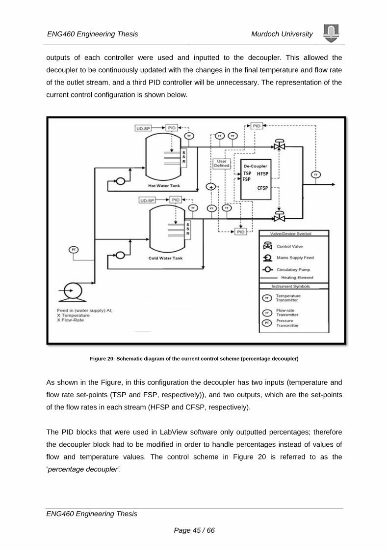
current control configuration is shown below.
Figure 20: Schematic diagram of the current control scheme (percentage decoupler)
As shown in the Figure, in this configuration the decoupler has two inputs (temperature and
flow rate set-points (TSP and FSP, respectively)), and two outputs, which are the set-points
of the flow rates in each stream (HFSP and CFSP, respectively).
The PID blocks that were used in LabView software only outputted percentages; therefore
the decoupler block had to be modified in order to handle percentages instead of values of
flow and temperature values. The control scheme in Figure 20 is referred to as the
‘percentage decoupler’.
ENG460 Engineering Thesis Murdoch University
ENG460 Engineering Thesis Page 46 / 66
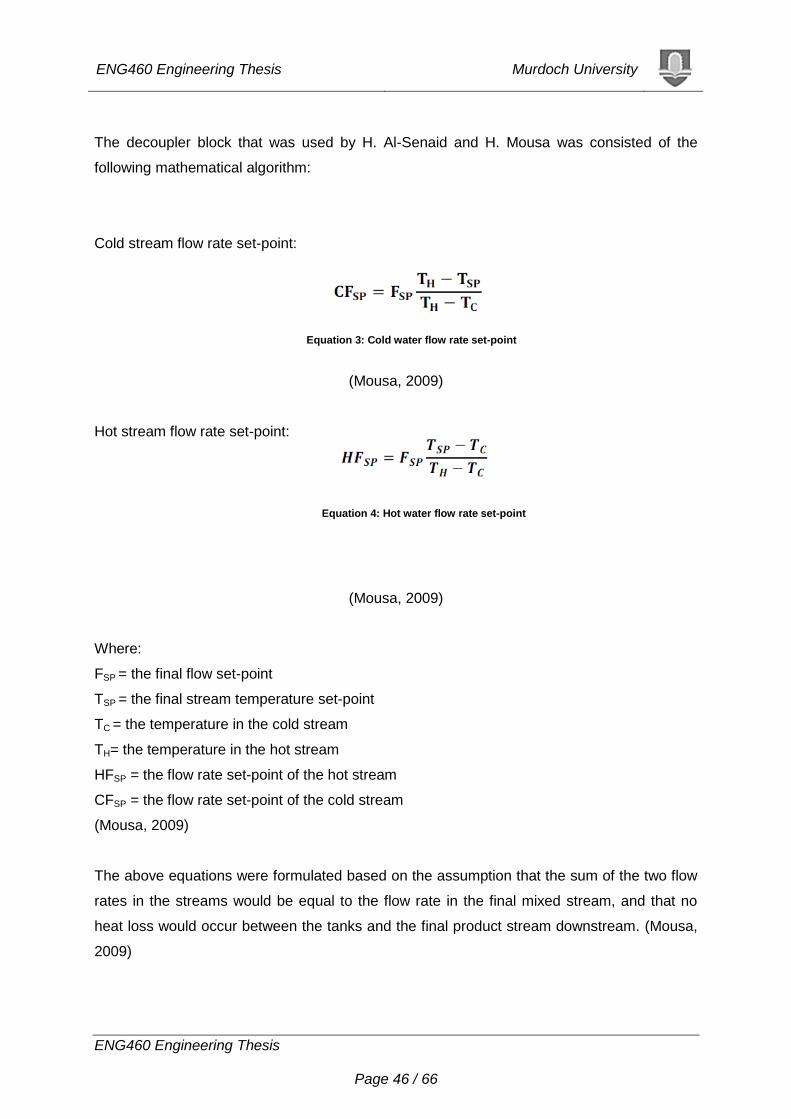
The decoupler block that was used by H. Al-Senaid and H. Mousa was consisted of the
following mathematical algorithm:
Cold stream flow rate set-point:
(Mousa, 2009)
Hot stream flow rate set-point:
(Mousa, 2009)
Where:
FSP = the final flow set-point
TSP = the final stream temperature set-point
TC = the temperature in the cold stream
TH= the temperature in the hot stream
HFSP = the flow rate set-point of the hot stream
CFSP = the flow rate set-point of the cold stream
(Mousa, 2009)
The above equations were formulated based on the assumption that the sum of the two flow
rates in the streams would be equal to the flow rate in the final mixed stream, and that no
heat loss would occur between the tanks and the final product stream downstream. (Mousa,
2009)
Equation 3: Cold water flow rate set-point
Equation 4: Hot water flow rate set-point
ENG460 Engineering Thesis Murdoch University
ENG460 Engineering Thesis Page 47 / 66
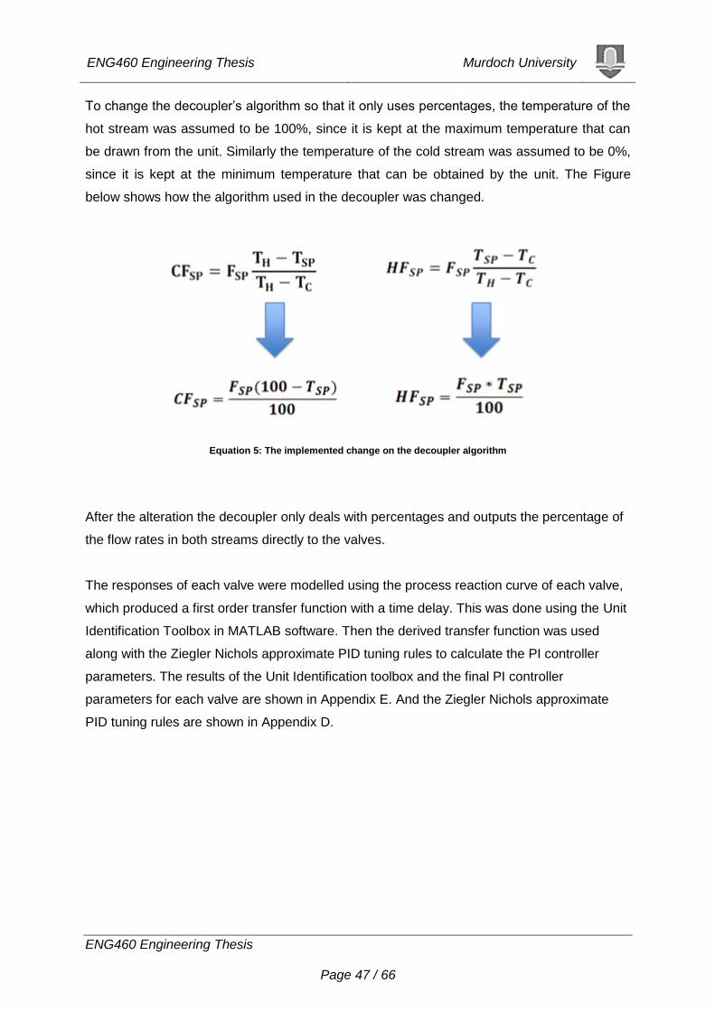
To change the decoupler’s algorithm so that it only uses percentages, the temperature of the
hot stream was assumed to be 100%, since it is kept at the maximum temperature that can
be drawn from the unit. Similarly the temperature of the cold stream was assumed to be 0%,
since it is kept at the minimum temperature that can be obtained by the unit. The Figure
below shows how the algorithm used in the decoupler was changed.
Equation 5: The implemented change on the decoupler algorithm
After the alteration the decoupler only deals with percentages and outputs the percentage of
the flow rates in both streams directly to the valves.
The responses of each valve were modelled using the process reaction curve of each valve,
which produced a first order transfer function with a time delay. This was done using the Unit
Identification Toolbox in MATLAB software. Then the derived transfer function was used
along with the Ziegler Nichols approximate PID tuning rules to calculate the PI controller
parameters. The results of the Unit Identification toolbox and the final PI controller
parameters for each valve are shown in Appendix E. And the Ziegler Nichols approximate
PID tuning rules are shown in Appendix D.
ENG460 Engineering Thesis Murdoch University
ENG460 Engineering Thesis Page 48 / 66
9 RESULTS
9.1 TEST PROCEDURE
The AS/NZS standard specifies that the unit must have the ability to perform at least four
different inlet water temperatures. The temperatures have to be spread out evenly over the
range within which the unit operate. The test starts after achieving the steady-state values of
temperature and flow rate, and ends after a 15 minute time frame. The permitted deviation of
the process variables during a solar collector efficiency test is presented in the table below.
Table 8: AS/NZS 2535. 1:2007 standard specifications for solar testing
Parameter Permitted deviation from the mean value
Test solar irradiance ±50W/m2
Surrounding air temperature ±1oC
Fluid mass flow rate ±1%
Fluid temperature at collector inlet ±0.1oC
The only parameters that this project is concerned with are the flow rate and the
temperature. This section clarifies the interpretation of steady-state by the standard, prior to
analysing the unit’s final steady-state performance.
9.1.1 Interpretation of Steady-State
The standard has two interpretations of steady-state which the unit has to achieve to
complete an efficiency test.
First interpretation:
“A collector is considered to have been operating in steady-state conditions over a given
measurement period if none of the experimental parameters deviate from their mean values
over the measurement period by more than the limits given in table 8” (Standards Australia,
2007)
Second interpretation:
ENG460 Engineering Thesis Murdoch University
ENG460 Engineering Thesis Page 49 / 66
“To establish that a steady-state exists, average values of each parameter taken over
successive periods of 30 seconds shall be compared with the mean value over the
measurement period.” (Standards Australia, 2007)
The first interpretation implies that the unit should never breach the constraints displayed in
Table 8 during the test. This interpretation seems hard to achieve considering that the unit is
still in the development stage. On the other hand, the second interpretation seems to be
more realistically achievable. The first interpretation should be attempted in order to improve
the unit’s performance, after achieving the second interpretation which is easier to achieve.
The section below displays the final results that were conducted by the unit to verify if the
unit is able to achieve the accuracy stated by the standard. It includes the results performed
by the percentage decoupler and the values decoupler implemented by H. Mousa in 2009.
9.2 STEADY-STATE PERFORMANCE UNDER PERCENTAGE DECOUPLER
To test the final control performance; three steady-state tests were performed at 30°C, 45°C,
and 60°C. Each test was conducted for 15 minutes and the samples were recorded at a rate
of 1 sample per second. In each of the tests, the temperature in the cold tank was
maintained at a temperature of 25°C and the temperature in the hot water tank was
maintained at 70°C.The steady-state performance was evaluated according to the second
interpretation of steady-state.
9.2.1 Steady-State Temperatures under Percentage Decoupler
First, the temperature error of each of the three steady-state tests was calculated. Figure 21
displays the final temperature results.
ENG460 Engineering Thesis Murdoch University
ENG460 Engineering Thesis Page 50 / 66
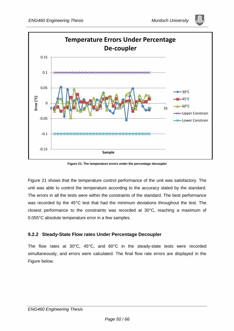
Figure 21: The temperature errors under the percentage decoupler
Figure 21 shows that the temperature control performance of the unit was satisfactory. The
unit was able to control the temperature according to the accuracy stated by the standard.
The errors in all the tests were within the constraints of the standard. The best performance
was recorded by the 45°C test that had the minimum deviations throughout the test. The
closest performance to the constraints was recorded at 30°C, reaching a maximum of
0.055°C absolute temperature error in a few samples.
9.2.2 Steady-State Flow rates Under Percentage Decoupler
The flow rates at 30°C, 45°C, and 60°C in the steady-state tests were recorded
simultaneously, and errors were calculated. The final flow rate errors are displayed in the
Figure below.
-0.15
-0.1
-0.05
0
0.05
0.1
0.15
0 5 10 15 20 25 30 35 Erro
r (°
C)
Sample
Temperature Errors Under Percentage De-coupler
30°C
45°C
60°C
Upper Constrain
Lower Constrain
ENG460 Engineering Thesis Murdoch University
ENG460 Engineering Thesis Page 51 / 66
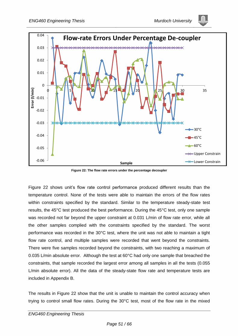
Figure 22: The flow rate errors under the percentage decoupler
Figure 22 shows unit’s flow rate control performance produced different results than the
temperature control. None of the tests were able to maintain the errors of the flow rates
within constraints specified by the standard. Similar to the temperature steady-state test
results, the 45°C test produced the best performance. During the 45°C test, only one sample
was recorded not far beyond the upper constraint at 0.031 L/min of flow rate error, while all
the other samples complied with the constraints specified by the standard. The worst
performance was recorded in the 30°C test, where the unit was not able to maintain a tight
flow rate control, and multiple samples were recorded that went beyond the constraints.
There were five samples recorded beyond the constraints, with two reaching a maximum of
0.035 L/min absolute error. Although the test at 60°C had only one sample that breached the
constraints, that sample recorded the largest error among all samples in all the tests (0.055
L/min absolute error). All the data of the steady-state flow rate and temperature tests are
included in Appendix B.
The results in Figure 22 show that the unit is unable to maintain the control accuracy when
trying to control small flow rates. During the 30°C test, most of the flow rate in the mixed
-0.06
-0.05
-0.04
-0.03
-0.02
-0.01
0
0.01
0.02
0.03
0.04
0 5 10 15 20 25 30 35
Erro
r (l
/min
)
Sample
Flow-rate Errors Under Percentage De-coupler
30°C
45°C
60°C
Upper Constrain
Lower Constrain
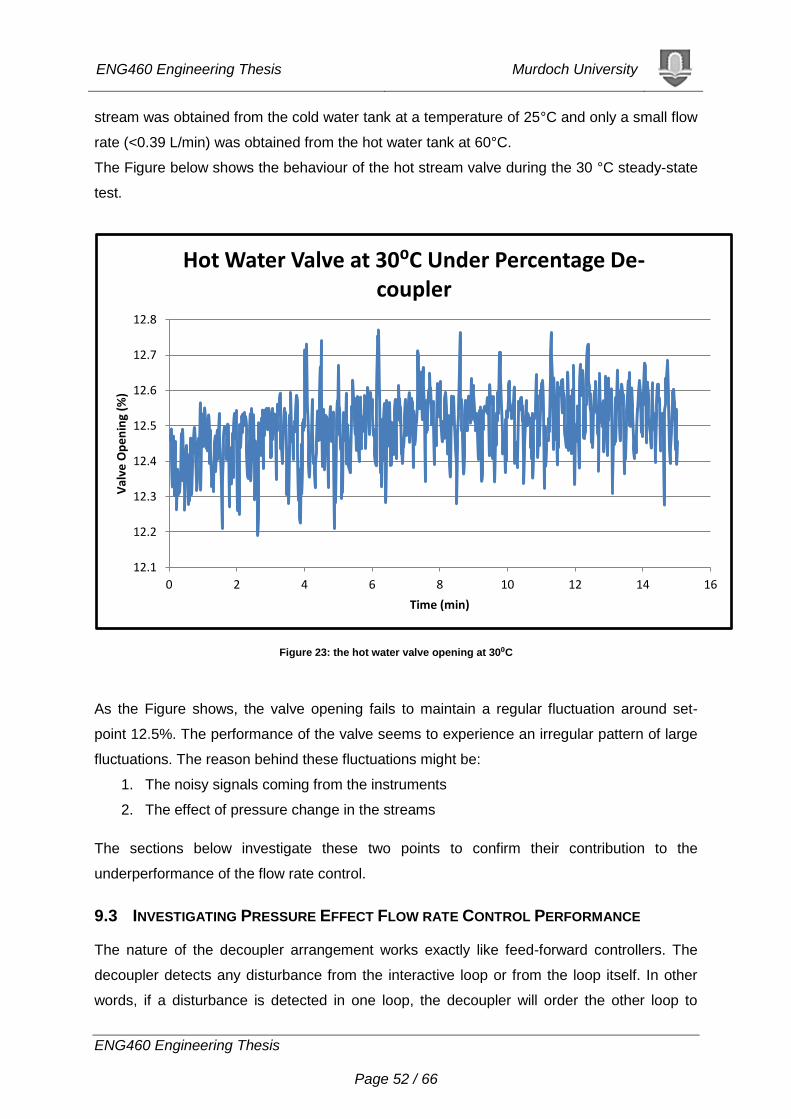
ENG460 Engineering Thesis Murdoch University
ENG460 Engineering Thesis Page 52 / 66
stream was obtained from the cold water tank at a temperature of 25°C and only a small flow
rate (<0.39 L/min) was obtained from the hot water tank at 60°C.
The Figure below shows the behaviour of the hot stream valve during the 30 °C steady-state
test.
Figure 23: the hot water valve opening at 30⁰C
As the Figure shows, the valve opening fails to maintain a regular fluctuation around set-
point 12.5%. The performance of the valve seems to experience an irregular pattern of large
fluctuations. The reason behind these fluctuations might be:
1. The noisy signals coming from the instruments
2. The effect of pressure change in the streams
The sections below investigate these two points to confirm their contribution to the
underperformance of the flow rate control.
9.3 INVESTIGATING PRESSURE EFFECT FLOW RATE CONTROL PERFORMANCE
The nature of the decoupler arrangement works exactly like feed-forward controllers. The
decoupler detects any disturbance from the interactive loop or from the loop itself. In other
words, if a disturbance is detected in one loop, the decoupler will order the other loop to
12.1
12.2
12.3
12.4
12.5
12.6
12.7
12.8
0 2 4 6 8 10 12 14 16
Val
ve O
pe
nin
g (%
)
Time (min)
Hot Water Valve at 30⁰C Under Percentage De-coupler
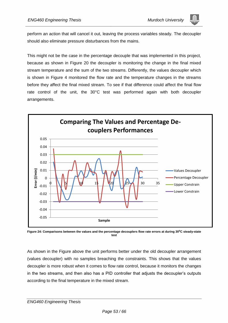
ENG460 Engineering Thesis Murdoch University
ENG460 Engineering Thesis Page 53 / 66
perform an action that will cancel it out, leaving the process variables steady. The decoupler
should also eliminate pressure disturbances from the mains.
This might not be the case in the percentage decouple that was implemented in this project,
because as shown in Figure 20 the decoupler is monitoring the change in the final mixed
stream temperature and the sum of the two streams. Differently, the values decoupler which
is shown in Figure 4 monitored the flow rate and the temperature changes in the streams
before they affect the final mixed stream. To see if that difference could affect the final flow
rate control of the unit, the 30°C test was performed again with both decoupler
arrangements.
Figure 24: Comparisons between the values and the percentage decouplers flow rate errors at during 30⁰C steady-state test
As shown in the Figure above the unit performs better under the old decoupler arrangement
(values decoupler) with no samples breaching the constraints. This shows that the values
decoupler is more robust when it comes to flow rate control, because it monitors the changes
in the two streams, and then also has a PID controller that adjusts the decoupler’s outputs
according to the final temperature in the mixed stream.
-0.05
-0.04
-0.03
-0.02
-0.01
0
0.01
0.02
0.03
0.04
0.05
0 5 10 15 20 25 30 35
Erro
r (l
/min
)
Sample
Comparing The Values and Percentage De-couplers Performances
Values Decoupler
Percentage Decoupler
Upper Constrain
Lower Constrain
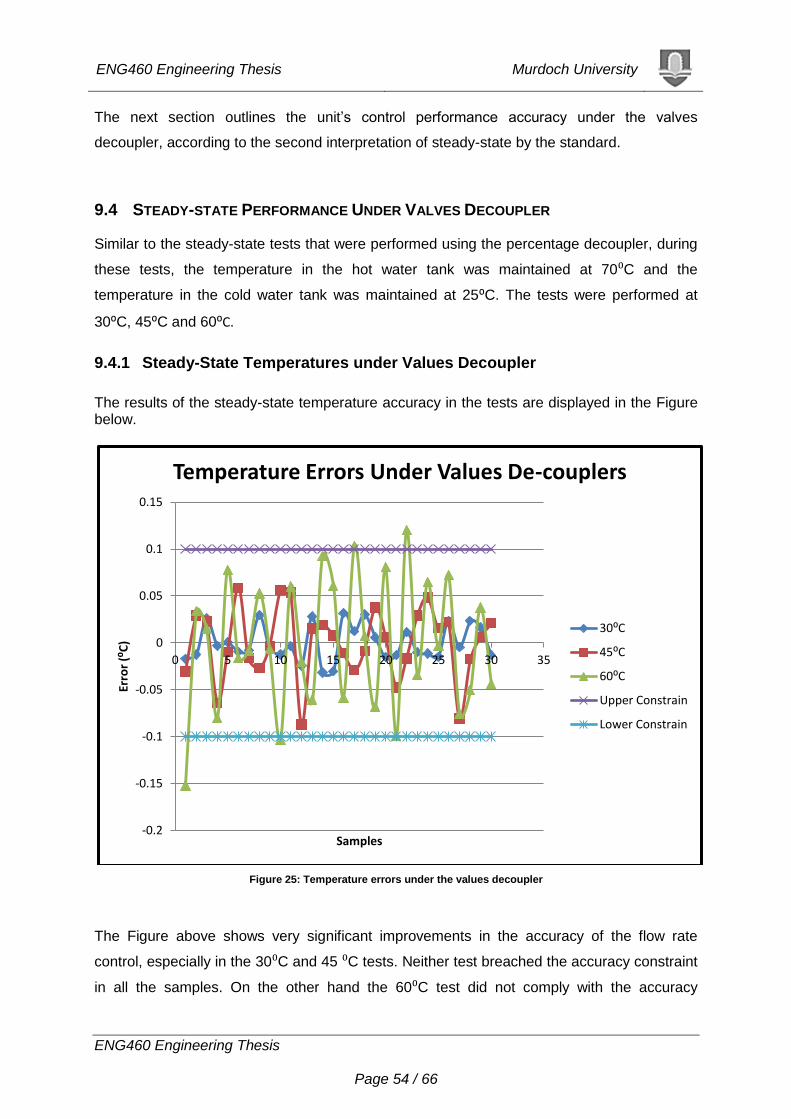
ENG460 Engineering Thesis Murdoch University
ENG460 Engineering Thesis Page 54 / 66
The next section outlines the unit’s control performance accuracy under the valves
decoupler, according to the second interpretation of steady-state by the standard.
9.4 STEADY-STATE PERFORMANCE UNDER VALVES DECOUPLER
Similar to the steady-state tests that were performed using the percentage decoupler, during
these tests, the temperature in the hot water tank was maintained at 70⁰C and the
temperature in the cold water tank was maintained at 25⁰C. The tests were performed at
30⁰C, 45⁰C and 60⁰C.
9.4.1 Steady-State Temperatures under Values Decoupler
The results of the steady-state temperature accuracy in the tests are displayed in the Figure below.
Figure 25: Temperature errors under the values decoupler
The Figure above shows very significant improvements in the accuracy of the flow rate
control, especially in the 30⁰C and 45 ⁰C tests. Neither test breached the accuracy constraint
in all the samples. On the other hand the 60⁰C test did not comply with the accuracy
-0.2
-0.15
-0.1
-0.05
0
0.05
0.1
0.15
0 5 10 15 20 25 30 35
Erro
r (⁰
C)
Samples
Temperature Errors Under Values De-couplers
30⁰C
45⁰C
60⁰C
Upper Constrain
Lower Constrain
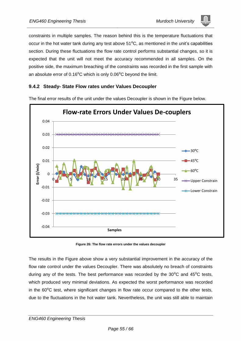
ENG460 Engineering Thesis Murdoch University
ENG460 Engineering Thesis Page 55 / 66
constraints in multiple samples. The reason behind this is the temperature fluctuations that
occur in the hot water tank during any test above 51⁰C, as mentioned in the unit’s capabilities
section. During these fluctuations the flow rate control performs substantial changes, so it is
expected that the unit will not meet the accuracy recommended in all samples. On the
positive side, the maximum breaching of the constraints was recorded in the first sample with
an absolute error of 0.16⁰C which is only 0.06⁰C beyond the limit.
9.4.2 Steady- State Flow rates under Values Decoupler
The final error results of the unit under the values Decoupler is shown in the Figure below.
Figure 26: The flow rate errors under the values decoupler
The results in the Figure above show a very substantial improvement in the accuracy of the
flow rate control under the values Decoupler. There was absolutely no breach of constraints
during any of the tests. The best performance was recorded by the 30⁰C and 45⁰C tests,
which produced very minimal deviations. As expected the worst performance was recorded
in the 60⁰C test, where significant changes in flow rate occur compared to the other tests,
due to the fluctuations in the hot water tank. Nevertheless, the unit was still able to maintain
-0.04
-0.03
-0.02
-0.01
0
0.01
0.02
0.03
0.04
0 5 10 15 20 25 30 35
Erro
r (l
/min
)
Samples
Flow-rate Errors Under Values De-couplers
30⁰C
45⁰C
60⁰C
Upper Constrain
Lower Constrain
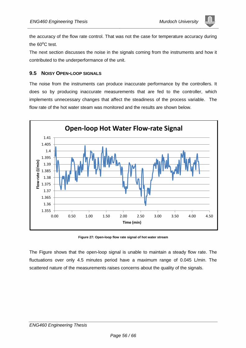
ENG460 Engineering Thesis Murdoch University
ENG460 Engineering Thesis Page 56 / 66
the accuracy of the flow rate control. That was not the case for temperature accuracy during
the 60⁰C test.
The next section discusses the noise in the signals coming from the instruments and how it
contributed to the underperformance of the unit.
9.5 NOISY OPEN-LOOP SIGNALS
The noise from the instruments can produce inaccurate performance by the controllers. It
does so by producing inaccurate measurements that are fed to the controller, which
implements unnecessary changes that affect the steadiness of the process variable. The
flow rate of the hot water steam was monitored and the results are shown below.
Figure 27: Open-loop flow rate signal of hot water stream
The Figure shows that the open-loop signal is unable to maintain a steady flow rate. The
fluctuations over only 4.5 minutes period have a maximum range of 0.045 L/min. The
scattered nature of the measurements raises concerns about the quality of the signals.
1.355
1.36
1.365
1.37
1.375
1.38
1.385
1.39
1.395
1.4
1.405
1.41
0.00 0.50 1.00 1.50 2.00 2.50 3.00 3.50 4.00 4.50
Flo
w-r
ate
(l/
min
)
Time (min)
Open-loop Hot Water Flow-rate Signal
ENG460 Engineering Thesis Murdoch University
ENG460 Engineering Thesis Page 57 / 66
9.6 PROJECT OUTCOMES
As mentioned earlier, the unit was developed in order to achieve an appropriate performance
that complies with the AS/NZS 2535.1:2007. To achieve that aim the following modifications
were performed:
Hysteresis and characteristic test for the new control valve – the valves has no
hysteresis and a linear characteristic
Finding the maximum temperature at 3L/min- 65°C
Finding the maximum steady-state test that can be performed without any fluctuations
in the hot water tank- 51°C
Testing the effect of the changes in water supply pressure on the performance of the
unit
Using an external microcontroller to control the stepper motor driven valves- this
produced tighter control of flow rate and temperature
Implementation of the percentage decoupler and comparison of its performance to
the performance of the values decoupler.
The best performance was produced under the values decoupler. No samples
breached the constraints during the flow rates steady-state tests, and only one
sample breached the constraints during the temperatures steady-state tests.
Although the standard recommends that the 70°C steady-state test be performed, the ‘Hot
Water Tank Control’ section proves that the unit is unable to maintain that temperature or
more at 3 L/min. The maximum temperature that can be obtained at 3 L/min is 65°C.
Prior to using the external microcontroller, the valve did not have tight control over the flow
rate. As a result the changes in the water supply pressure caused a direct effect on the flow
rate, and consequently on the temperature. To solve this issue the microcontroller was
utilised to enable the user to implement different control strategies in the unit and have a
tighter control on the flow rate.
The percentage decoupler that was implemented produced good temperature accuracy, but
when compared to the performance of the values decoupler, the latter had better results.
Under the values decoupler no flow rates breached the constraints, and there were multiple
samples that breached the constraints only in the temperature steady-state at 60⁰C. This was
expected, because during the test, the temperature in the hot water tank was fluctuating.
This will cause the controller to perform significant changes in flow rate compared to the
changes performed in the other tests, resulting in a less accurate steady-state performance.
ENG460 Engineering Thesis Murdoch University
ENG460 Engineering Thesis Page 58 / 66
The next section suggests some actions that could improve the performance of the unit.
9.7 FUTURE SUGGESTIONS
9.7.1 Open-loop signal
The quality of the signals coming from the instruments can be improved by passing the
signals through low-pass digital filters created in LabView software. Moreover a mechanical
RC low-pass filter could be installed on the wire connection between the analogue output
field-point and the microcontroller input. The filter can smooth the signals and improve the
unit’s overall performance. The parameters of the filters have to be chosen so that they
cause minimal delay.
9.7.2 Synchronization of Control Loops
The external microcontroller was programmed to execute the control loop every 100ms. On
the other hand the control loop in LabView software is executed every 250ms. The two loops
are not in sync, because they are executed by different program. This unsynchronized
execution of the loops causes some delay in picking up the set-point signals from the Lab-
View software, therefore causing a delay in the motion of the valves. The two loops should
be synchronized so that as soon as the set-point signal reaches the microcontroller, it is
picked up and executed with no delay. This will improve the accuracy of the unit’s
performance controller.
9.7.3 Firmware
When using the microcontroller inside the mixing valve, it was programmed to shut down the
voltage signals to the coils, once the set-point is achieved. Doing so prevents heat from
building up in the power transistors before the coils. When using the external microcontroller
this feature was not programmed. This must be done to prevent any major damage to the
valve’s electronics.
ENG460 Engineering Thesis Murdoch University
ENG460 Engineering Thesis Page 59 / 66
10 BIBLIOGRAPHY Babatunde Ogunnaike, W. H. (1994). Process Dynamics, Modelling and Control. Oxford
University Press.
Bahri, P. (2011). ENG420: Instrumentation and Control Units Desgin. Murdoch University.
DANFOSS Manufacturing. (n.d.). 060G3011 MBS33 Pressure Transmitter. Retrieved 9 5,
2012, from DANFOSS:
http://www.danfoss.com/Pacific/Products/Categories/Detail/IA/Pressure-transmitters/MBS-
33-Pressure-transmitters-for-general-industry/060G3011/026b18d5-2409-4dc1-a6b2-
6f2d99f0e50c/edf3b9b8-e440-47a9-916b-8701ab529aed.html
Hass Manufacturing Company. (n.d.). Intellifaucet K series owner’s manual. Retrieved 9 25,
2012, from http://www.hassmfg.com/manuals/k.manual.pl/1235706283-76982
Mousa, H. (2009). Solar Collector Efficiency Testing Unit. Murdoch University press .
Standards Australia. (2007). AS/NZS 2535.1:2007 Test methods fo solar collectors- Part 2:
Qualification test procedures. ISO 9805-2:2007 .
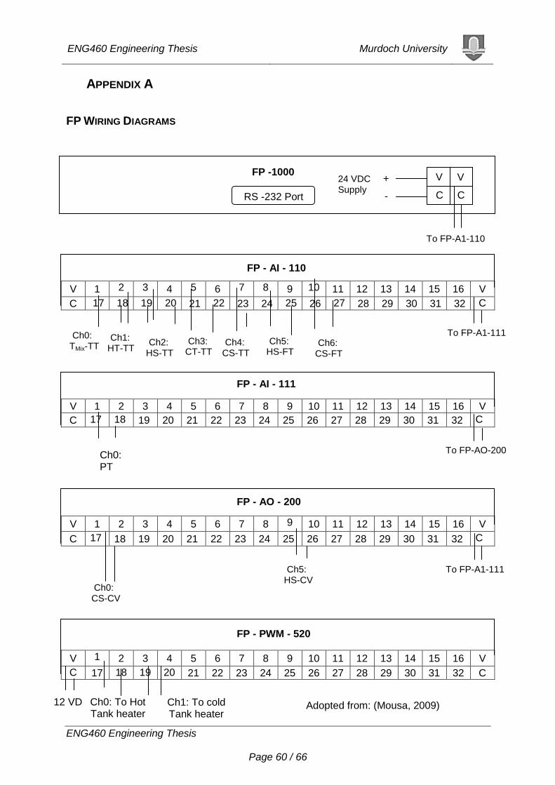
ENG460 Engineering Thesis Murdoch University
ENG460 Engineering Thesis Page 60 / 66
APPENDIX A
FP WIRING DIAGRAMS
V 1 2 3 4 5 6 7 8 9 10 11 12 13 14 15 16 V
C 17 18 19 20 21 22 23 24 25 26 27 28 29 30 31 32 C
V 1 2 3 4 5 6 7 8 9 10 11 12 13 14 15 16 V
C 17 18 19 20 21 22 23 24 25 26 27 28 29 30 31 32 C
V 1 2 3 4 5 6 7 8 9 10 11 12 13 14 15 16 V
C 17 18 19 20 21 22 23 24 25 26 27 28 29 30 31 32 C
V 1 2 3 4 5 6 7 8 9 10 11 12 13 14 15 16 V
C 17 18 19 20 21 22 23 24 25 26 27 28 29 30 31 32 C
24 VDC Supply
V V
C C
FP -1000
FP - AI - 110
FP - AI - 111
FP - AO - 200
FP - PWM - 520
RS -232 Port
+
-
Ch1: To cold Tank heater
To FP-A1-110
To FP-AO-200
12 VDC
Ch0: CS-CV
Ch5: HS-CV
Ch0: CS-CV
To FP-A1-111
To FP-A1-111 Ch5: HS-FT
Ch4: CS-TT
Ch6: CS-FT
Ch2: HS-TT
Ch3: CT-TT
Ch1: HT-TT
Ch0: TMix-TT
Ch0: PT
Ch0: To Hot Tank heater
Adopted from: (Mousa, 2009)
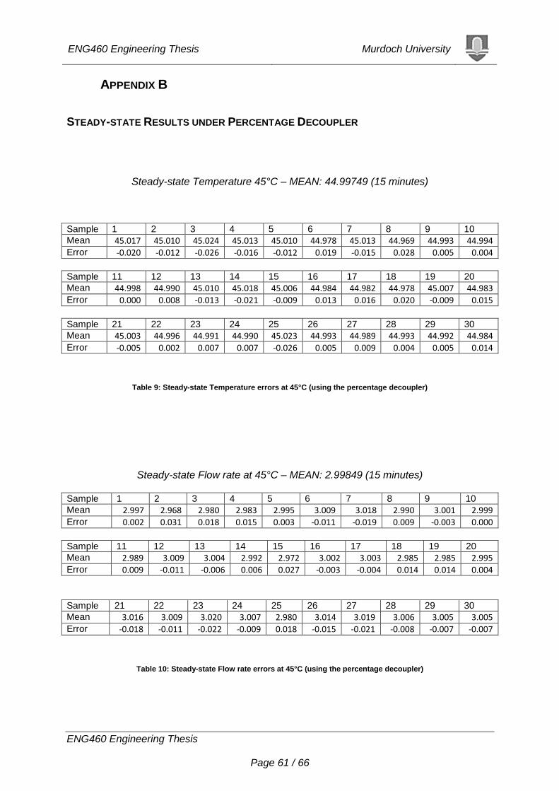
ENG460 Engineering Thesis Murdoch University
ENG460 Engineering Thesis Page 61 / 66
APPENDIX B
STEADY-STATE RESULTS UNDER PERCENTAGE DECOUPLER
Steady-state Temperature 45°C – MEAN: 44.99749 (15 minutes)
Sample 1 2 3 4 5 6 7 8 9 10
Mean 45.017 45.010 45.024 45.013 45.010 44.978 45.013 44.969 44.993 44.994
Error -0.020 -0.012 -0.026 -0.016 -0.012 0.019 -0.015 0.028 0.005 0.004
Sample 11 12 13 14 15 16 17 18 19 20
Mean 44.998 44.990 45.010 45.018 45.006 44.984 44.982 44.978 45.007 44.983
Error 0.000 0.008 -0.013 -0.021 -0.009 0.013 0.016 0.020 -0.009 0.015
Sample 21 22 23 24 25 26 27 28 29 30
Mean 45.003 44.996 44.991 44.990 45.023 44.993 44.989 44.993 44.992 44.984
Error -0.005 0.002 0.007 0.007 -0.026 0.005 0.009 0.004 0.005 0.014
Table 9: Steady-state Temperature errors at 45°C (using the percentage decoupler)
Steady-state Flow rate at 45°C – MEAN: 2.99849 (15 minutes)
Sample 1 2 3 4 5 6 7 8 9 10
Mean 2.997 2.968 2.980 2.983 2.995 3.009 3.018 2.990 3.001 2.999
Error 0.002 0.031 0.018 0.015 0.003 -0.011 -0.019 0.009 -0.003 0.000
Sample 11 12 13 14 15 16 17 18 19 20
Mean 2.989 3.009 3.004 2.992 2.972 3.002 3.003 2.985 2.985 2.995
Error 0.009 -0.011 -0.006 0.006 0.027 -0.003 -0.004 0.014 0.014 0.004
Sample 21 22 23 24 25 26 27 28 29 30
Mean 3.016 3.009 3.020 3.007 2.980 3.014 3.019 3.006 3.005 3.005
Error -0.018 -0.011 -0.022 -0.009 0.018 -0.015 -0.021 -0.008 -0.007 -0.007
Table 10: Steady-state Flow rate errors at 45°C (using the percentage decoupler)
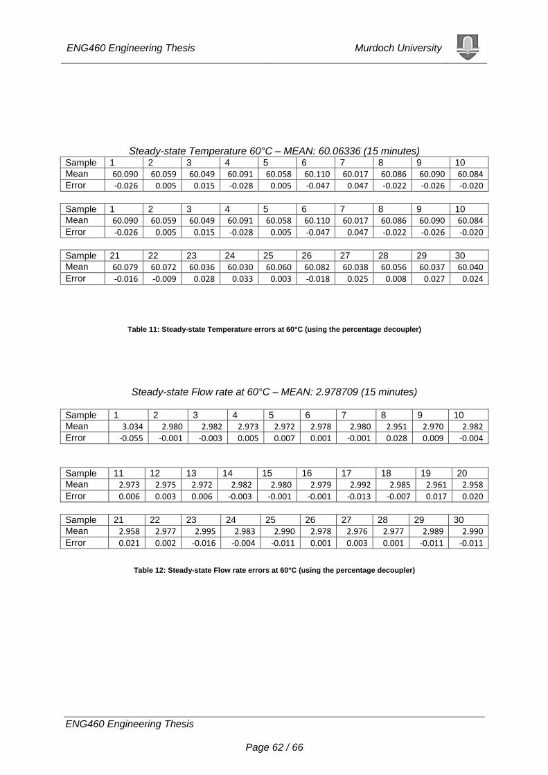
ENG460 Engineering Thesis Murdoch University
ENG460 Engineering Thesis Page 62 / 66
Steady-state Temperature 60°C – MEAN: 60.06336 (15 minutes) Sample 1 2 3 4 5 6 7 8 9 10
Mean 60.090 60.059 60.049 60.091 60.058 60.110 60.017 60.086 60.090 60.084 Error -0.026 0.005 0.015 -0.028 0.005 -0.047 0.047 -0.022 -0.026 -0.020
Sample 1 2 3 4 5 6 7 8 9 10
Mean 60.090 60.059 60.049 60.091 60.058 60.110 60.017 60.086 60.090 60.084
Error -0.026 0.005 0.015 -0.028 0.005 -0.047 0.047 -0.022 -0.026 -0.020
Sample 21 22 23 24 25 26 27 28 29 30
Mean 60.079 60.072 60.036 60.030 60.060 60.082 60.038 60.056 60.037 60.040
Error -0.016 -0.009 0.028 0.033 0.003 -0.018 0.025 0.008 0.027 0.024
Table 11: Steady-state Temperature errors at 60°C (using the percentage decoupler)
Steady-state Flow rate at 60°C – MEAN: 2.978709 (15 minutes)
Sample 1 2 3 4 5 6 7 8 9 10
Mean 3.034 2.980 2.982 2.973 2.972 2.978 2.980 2.951 2.970 2.982 Error -0.055 -0.001 -0.003 0.005 0.007 0.001 -0.001 0.028 0.009 -0.004
Sample 11 12 13 14 15 16 17 18 19 20
Mean 2.973 2.975 2.972 2.982 2.980 2.979 2.992 2.985 2.961 2.958
Error 0.006 0.003 0.006 -0.003 -0.001 -0.001 -0.013 -0.007 0.017 0.020
Sample 21 22 23 24 25 26 27 28 29 30
Mean 2.958 2.977 2.995 2.983 2.990 2.978 2.976 2.977 2.989 2.990
Error 0.021 0.002 -0.016 -0.004 -0.011 0.001 0.003 0.001 -0.011 -0.011
Table 12: Steady-state Flow rate errors at 60°C (using the percentage decoupler)
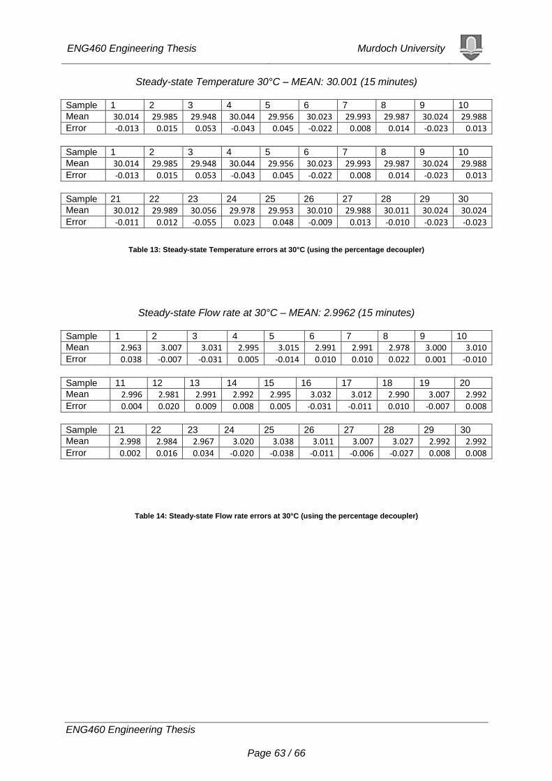
ENG460 Engineering Thesis Murdoch University
ENG460 Engineering Thesis Page 63 / 66
Steady-state Temperature 30°C – MEAN: 30.001 (15 minutes)
Sample 1 2 3 4 5 6 7 8 9 10
Mean 30.014 29.985 29.948 30.044 29.956 30.023 29.993 29.987 30.024 29.988 Error -0.013 0.015 0.053 -0.043 0.045 -0.022 0.008 0.014 -0.023 0.013
Sample 1 2 3 4 5 6 7 8 9 10
Mean 30.014 29.985 29.948 30.044 29.956 30.023 29.993 29.987 30.024 29.988
Error -0.013 0.015 0.053 -0.043 0.045 -0.022 0.008 0.014 -0.023 0.013
Sample 21 22 23 24 25 26 27 28 29 30
Mean 30.012 29.989 30.056 29.978 29.953 30.010 29.988 30.011 30.024 30.024
Error -0.011 0.012 -0.055 0.023 0.048 -0.009 0.013 -0.010 -0.023 -0.023
Table 13: Steady-state Temperature errors at 30°C (using the percentage decoupler)
Steady-state Flow rate at 30°C – MEAN: 2.9962 (15 minutes)
Sample 1 2 3 4 5 6 7 8 9 10
Mean 2.963 3.007 3.031 2.995 3.015 2.991 2.991 2.978 3.000 3.010
Error 0.038 -0.007 -0.031 0.005 -0.014 0.010 0.010 0.022 0.001 -0.010
Sample 11 12 13 14 15 16 17 18 19 20
Mean 2.996 2.981 2.991 2.992 2.995 3.032 3.012 2.990 3.007 2.992
Error 0.004 0.020 0.009 0.008 0.005 -0.031 -0.011 0.010 -0.007 0.008
Sample 21 22 23 24 25 26 27 28 29 30
Mean 2.998 2.984 2.967 3.020 3.038 3.011 3.007 3.027 2.992 2.992
Error 0.002 0.016 0.034 -0.020 -0.038 -0.011 -0.006 -0.027 0.008 0.008
Table 14: Steady-state Flow rate errors at 30°C (using the percentage decoupler)
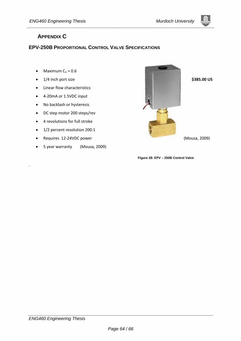
ENG460 Engineering Thesis Murdoch University
ENG460 Engineering Thesis Page 64 / 66
APPENDIX C
EPV-250B PROPORTIONAL CONTROL VALVE SPECIFICATIONS
Maximum CV = 0.6
1/4 inch port size $385.00 US
Linear flow characteristics
4-20mA or 1.5VDC input
No backlash or hysteresis
DC step motor 200 steps/rev
4 revolutions for full stroke
1/2 percent resolution 200:1
Requires 12-24VDC power (Mousa, 2009)
5 year warranty (Mousa, 2009)
Figure 28: EPV – 250B Control Valve
.
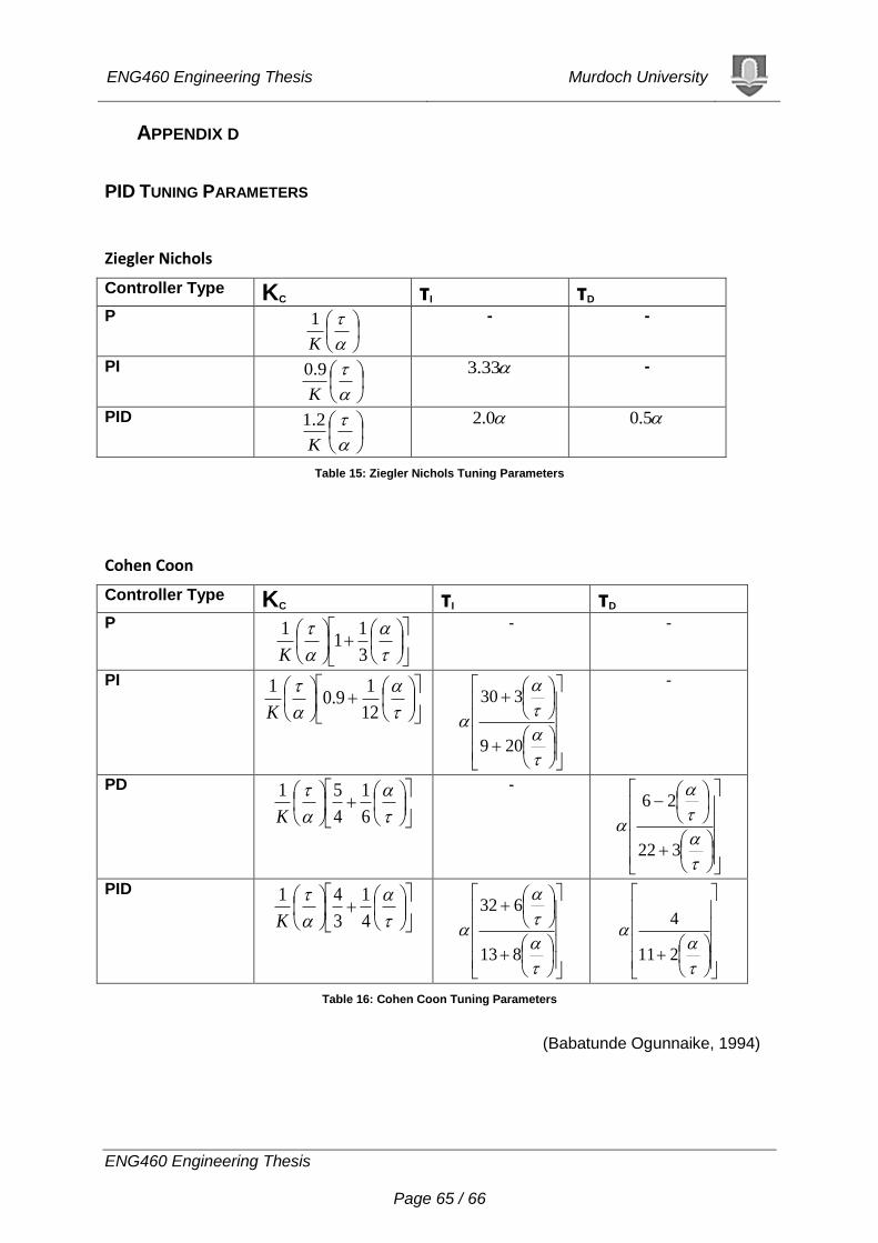
ENG460 Engineering Thesis Murdoch University
ENG460 Engineering Thesis Page 65 / 66
APPENDIX D
PID TUNING PARAMETERS
Ziegler Nichols
Controller Type KC τI τD
P
K
1
- -
PI
K
9.0
33.3 -
PID
K
2.1
0.2 5.0
Table 15: Ziegler Nichols Tuning Parameters
Cohen Coon
Controller Type KC τI τD
P
3
11
1
K
- -
PI
12
19.0
1
K
209
330
-
PD
6
1
4
51
K
-
322
26
PID
4
1
3
41
K
813
632
211
4
Table 16: Cohen Coon Tuning Parameters
(Babatunde Ogunnaike, 1994)
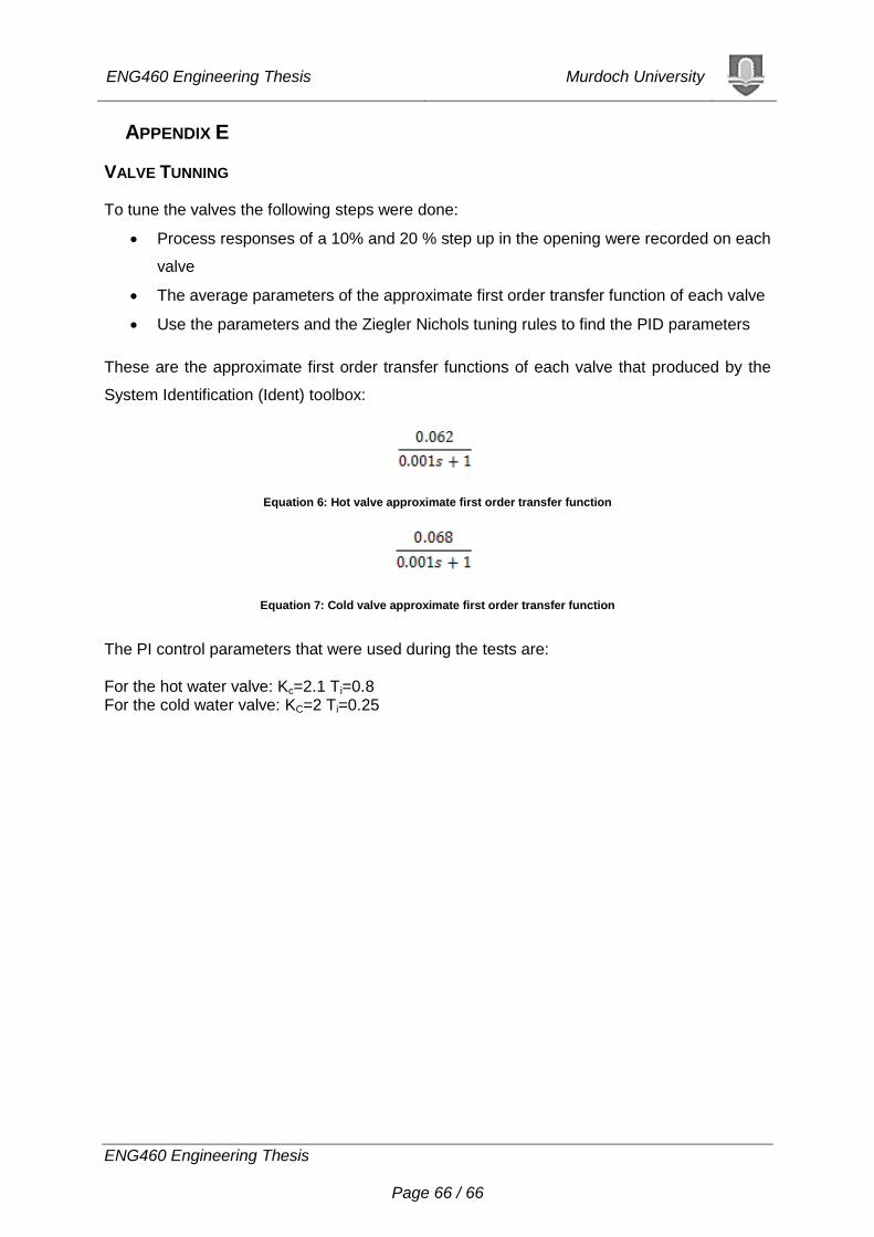
ENG460 Engineering Thesis Murdoch University
ENG460 Engineering Thesis Page 66 / 66
APPENDIX E
VALVE TUNNING
To tune the valves the following steps were done:
Process responses of a 10% and 20 % step up in the opening were recorded on each
valve
The average parameters of the approximate first order transfer function of each valve
Use the parameters and the Ziegler Nichols tuning rules to find the PID parameters
These are the approximate first order transfer functions of each valve that produced by the
System Identification (Ident) toolbox:
Equation 6: Hot valve approximate first order transfer function
Equation 7: Cold valve approximate first order transfer function
The PI control parameters that were used during the tests are: For the hot water valve: Kc=2.1 Ti=0.8 For the cold water valve: KC=2 Ti=0.25
Related Documents