SOIL-STRUCTURE INTERACTION OF STEEL FIBRE REINFORCED ...

SOIL-STRUCTURE INTERACTION OF STEEL FIBRE REINFORCED CONCRETE SLAB STRIPS ON GRADE WITH

GEOGRID REINFORCEMENT

by

Olivia Renata Hernandez Cardenas

BScE, University of New Brunswick, 2012

A report submitted in Partial Fulfillment of the Requirements for the Degree of

Master of Engineering

in the Graduate Academic Unit of Civil Engineering

Supervisors: Peter Bischoff, PhD, PEng., Department of Civil Engineering Hany El Naggar, PhD, PEng., Department of Civil Engineering

Examining Board: Brian Cooke, PhD, PEng., Department of Civil Engineering Allison Schriver, PhD, PEng., Department of Civil Engineering

This report is accepted by the Dean of Graduate Studies

THE UNIVERSITY OF NEW BRUNSWICK

April, 2014

© Olivia Renata Hernandez Cardenas, 2014

ii

ABSTRACT

Performance of slabs on grade is mainly governed by the mutual coupled performance of

the slab stiffness and the subgrade support. The use of reinforcement geogrids to increase

the structural capacity of the subgrade support can be potentially advantageous, but is

currently poorly understood (especially under frequent transient loading conditions).

The objective of this experimental study is to investigate the beneficial use of geogrids as a

reinforcing material in a loose subgrade. Experiments on three slab strips (300 mm x 150

mm x 2500 mm) are completed by the author. Two slab strips contain steel fibres and one

slab strip is reinforced with welded wire fabric (WWF). All slab strips are tested under a

central point load and are restrained from uplift at the ends. Both monotonic and cyclic

loads are considered.

The responses for each slab strip are compared to previous tests carried out at UNB for an

unreinforced loose subgrade. It is noted that the geogrid increases the bottom surface

cracking load of the slab strip, does not affect the top surface cracking load, and increases

the ultimate load carrying capacity of the slab strip. The SFRC proves to be successful in

providing post-cracking strength to maintain slab integrity when compared to the WWF

reinforced slab strip used in this investigation.

The analysis of beams on grade is carried out for the elastic and post-cracking regions. The

elastic analysis is based on an analytical solution, and the post-cracking stage is developed

by using a plasticity based approach. The predicted values for the SFRC slab strip under

monotonic load are compared to the measured load-deformation response. The

comparison indicates that the theoretical data underestimate the capacity of the SFRC slab

strip.

iii

ACKNOWLEDGEMENTS

I would first like to express my gratitude to my supervisors Dr. Peter Bischoff and Dr. Hany

El Naggar for their continuous guidance and supervision throughout the research. I would

also like to thank Mr. David Fuerth from Terrafix Geosynthetics for providing the geogrids

used for the experimental work. Appreciation also goes out to Andrew Sutherland, Chris

Forbes and Scott Fairburn for their technical assistance in the laboratory experiments

carried out for this project. Finally, I would like to give a big thank-you to my parents for

their encouragement and support.

iv

TABLE OF CONTENTS

ABSTRACT ii

ACKNOWLEDGEMENTS iii

TABLE OF CONTENTS iv

LIST OF TABLES vi

LIST OF FIGURES vii

1 INTRODUCTION 1

1.1 Objectives 1

1.2 Scope 2

1.3 Layout of report 2

2 BACKGROUND 4

2.1 Slabs on grade 4

2.1.1 Subgrade preparation 5

2.1.2 Design of slabs on grade 5

2.2 Geogrids 7

2.3 Fibre reinforced concrete 9

2.3.1 Steel fibre reinforced concrete (SFRC) 10

2.3.2 SFRC slabs on grade 13

2.4 Literature review 13

2.4.1 Research on SFRC slabs on grade 14

2.4.2 Research on subgrade reinforcement 17

2.4.3 Summary 20

3 EXPERIMENTAL INVESTIGATION 21

3.1 Introduction 21

3.2 Test program 21

3.3 Subgrade and geogrid 22

3.4 Concrete slab strips 23

3.4.1 SFRC slab strips 23

3.4.2 WWF slab strip 23

3.5 Casting 24

3.6 Control tests 26

3.6.1 Concrete material properties 26

3.6.2 Geogrid tensile test 27

3.6.3 Welded wire mesh tensile test 28

3.6.4 Subgrade density 28

v

3.6.5 Plate load tests 29

3.7 Test set-up 30

3.8 Test procedure 33

3.8.1 Monotonic loading 33

3.8.2 Cyclic loading 34

4 RESULTS AND DISCUSSION 37

4.1 Introduction 37

4.2 Plate load tests 37

4.2.1 Behaviour of reinforced subgrade under monotonic loading 37

4.2.2 Behaviour of reinforced subgrade under cyclic loading 38

4.3 Slab strip tests on subgrade reinforced with a geogrid 40

4.3.1 SFRC slab strip under monotonic loading 40

4.3.2 SFRC slab strip under cyclic loading 43

4.3.3 WWF slab strip under cyclic loading 47

5 ANALYSIS OF BEAMS ON GRADE 50

5.1 Introduction 50

5.2 Overview 50

5.3 Elastic analysis (pre-cracking) 51

5.4 Post-cracking analysis 53

5.4.1 Introduction 53

5.4.2 Post-cracking analysis: stage I 54

5.4.3 Post-cracking analysis: stage II 57

5.5 Frame analysis (pre- and post-cracking) 60

5.6 Summary 64

6 CONCLUSIONS 66

6.1 Conclusions 66

6.2 Future research 67

REFERENCES 69

APPENDIX A: CONCRETE MATERIAL PROPERTIES 72

APPENDIX B: GEOGRID TENSION TEST 83

APPENDIX C: WELDED WIRE MESH TENSILE TEST 86

APPENDIX D: SUBGRADE DENSITY 88

APPENDIX E: FAILURE PATTERNS OF SLAB STRIPS AND MEASURED CRACK WIDTHS 90

APPENDIX F: CORRECTION TO POST-CRACKING STAGE II ANALYSIS 94

APPENDIX G: KIHWAN HAN’S TEST DATA (UNREINFORCED SUBGRADE) 98

VITA

vi

LIST OF TABLES

Table 2.1 Factors of safety used for slabs on grade (ACI 360R-10)

7

Table 3.1 Testing scheme

21

Table 3.2 Geogrid properties

22

Table 3.3 Summary of slab strip dimensions, casting date, and age of testing

23

Table 3.4 Mix design for concrete mix

24

Table 3.5 Concrete specification

24

Table 3.6 Concrete material properties

26

Table 3.7 WWF properties

28

Table 3.8 Subgrade density values

28

Table 3.9 Loading protocol for cyclic tests

35

Table 4.1 Summary of monotonic plate load test results

37

Table 4.2 Summary of slab strip test results

40

Table 4.3 Cumulative cyclic deflections for SFRC cyclic test

46

Table 4.4 Cumulative cyclic deflections for WWF cyclic test

48

Table 5.1 Summary of frame analysis, theoretical analysis, and experimental results

51

Table 5.2 Parameters for elastic analysis of beams on subgrade

52

Table 5.3 Parameters for post-cracking analysis of beams on subgrade

56

Table 5.4 Comparison between plane frame analysis results and theoretical analysis

64

vii

LIST OF FIGURES

Figure 2.1 Slab on grade support system (ACI 360R-10, 2010)

4

Figure 2.2 Types of geogrids (Koerner, 1998)

9

Figure 2.3 Steel fibres with different geometries (ACI 544.1R, 2010)

11

Figure 3.1 Geogrid used for experimental tests

22

Figure 3.2 Welded Wire Fabric reinforcement

24

Figure 3.3 Casting of slab strips and control specimens

25

Figure 3.4 Test set-up for plate load test

29

Figure 3.5 Schematic representation of the test set-up (all dimensions in mm)

30

Figure 3.6 Layout of slab strips and geogrids (all dimensions in mm)

31

Figure 3.7 Schematic representation of test set-up (all dimensions in mm)

32

Figure 3.8 End restraint set-up

32

Figure 3.9 Test set-up for slab strip tests

33

Figure 3.10 SFRC monotonic slab strip with visible cracks

34

Figure 3.11 SFRC cyclic test

36

Figure 3.12 WWF cyclic test

36

Figure 4.1 Test results for plate load test for subgrade with and without geogrid under monotonic loading

38

Figure 4.2 Results for plate load test for subgrade with geogrid under monotonic and cyclic loading

39

Figure 4.3 Results for plate load test for subgrade with and without geogrid under cyclic loading

39

Figure 4.4 Test results for SFRC with and without geogrid under monotonic loading

41

Figure 4.5 Deformation profile for SFRC with geogrid under monotonic loading

42

Figure 4.6 End restraint loads for SFRC with geogrid under monotonic loading 43

viii

Figure 4.7 Test results for monotonic and cyclic loading for SFRC with geogrid

44

Figure 4.8 Test results for SFRC slab strip with and without geogrid under cyclic loading (intermediate cycles removed for clarity)

45

Figure 4.9 End restraint loads for SFRC with geogrid under cyclic loading (intermediate cycles removed for clarity)

46

Figure 4.10 Test results for SFRC and WWF slab strips with geogrid under cyclic loading (intermediate cycles removed for clarity)

47

Figure 4.11 Test results for WWF slab strip with and without geogrid under cyclic loading (intermediate cycles removed for clarity)

47

Figure 4.12 End restraint loads for WWF with geogrid under cyclic loading (intermediate cycles removed for clarity)

49

Figure 5.1 Elastic Analysis Model for Beam on Subgrade

51

Figure 5.2 Comparison of load-deformation responses for SFRC slab strip on grade with geogrid reinforcement – Elastic region

53

Figure 5.3 Post-cracking Analysis Model for Beam on Subgrade, Stage I

54

Figure 5.4 Bending moment diagram of half the beam for a load corresponding to cracking at the top surface (Pcr2 = 68.4 kN)

56

Figure 5.5 Comparison of load-deformation responses for SFRC slab strip on grade with geogrid reinforcement – Post-cracking Stage I

56

Figure 5.6 Post-cracking Analysis Model for Beam on Subgrade, Stage II

57

Figure 5.7 Comparison of load-deformation responses for SFRC slab strip on grade with geogrid reinforcement – Post-cracking Stage II

60

Figure 5.8 Frame analysis model: Pre-cracking

62

Figure 5.9 Frame analysis model: Post-cracking Stage I

62

Figure 5.10 Frame analysis model: Post-cracking Stage II

62

Figure 5.11 Comparison between plane frame analysis, theoretical analysis, and experimental results

63

Figure 5.12 Deformation profile obtained with plane frame analysis 64

1

1 INTRODUCTION

1.1 Objectives

Steel fibre reinforced concrete (SFRC) has become popular for use in the construction of

slabs on grade. Steel fibres are used to give post-cracking strength, flexural toughness,

crack-width control, fatigue endurance, and impact resistance. However, when

constructing on poor soil conditions, additional reinforcement of the subgrade may be

advantageous. Previous research completed at the University of New Brunswick has

mainly considered the reinforcement of the concrete and not the soil underneath it. The

use of geogrids for subgrade reinforcement is yet to be further investigated.

The purpose of this research project is to investigate the behaviour of concrete slab strips

on ground under a central point load with the subgrade reinforced with a geogrid. The slab

strips are restrained from uplift and contain either plain concrete with welded wire fabric

(WWF) or steel fibre reinforced concrete (SFRC). The more specific objectives of this

investigation are as follows:

To investigate the effect of soil reinforcement on the subgrade modulus (soil stiffness).

To compare the response of SFRC slab strips on grade with geogrid reinforcement in

the subgrade to the response of SFRC slab strips supported on an unreinforced

subgrade.

To compare the observed monotonic response of a concrete slab strip to theoretical

models for the analysis of beams on grade in the elastic and post-cracking stage. This is

done to assess the ability of the available solutions to predict the performance of SFRC

slabs on grade with geogrid reinforcement.

2

To compare the monotonic and cyclic response of a SFRC slab strip supported on both

an unreinforced and reinforced subgrade.

To compare the response of SFRC and WWF slab strips under cyclic loading conditions.

1.2 Scope

Laboratory experiments were performed on three slab strips cast on a loose subgrade

reinforced with a single layer of geogrid. Two of the slabs strips were reinforced with steel

fibres (SFRC), and one with WWF. The dimensions of the slabs strips were 150 mm thick,

300 mm in width, and 2500 mm in length. All three slab strips were restrained from uplift

after cracking. The results obtained from these tests are compared to the data obtained by

Han et al. (2013) for three identical slab strips resting on an unreinforced loose subgrade

(see Appendix G for data from Han’s tests).

Prior to performing the analysis, plate load tests (monotonic and cyclic) were performed

on the geogrid reinforced loose subgrade to determine the modulus of subgrade reaction.

The deformation response under monotonic loading was investigated for a SFRC slab strip,

and the response under cyclic loading was investigated for SFRC and WWF slab strips. All

slabs were cast on grade. Analysis of the elastic range was based on a closed formed

solution, and the post-cracking analysis was based on a plasticity based approach.

Comparisons between the observed and theoretical behaviour are presented.

1.3 Layout of report

The report is sectioned into six chapters, the first one being the Introduction, which

presents the main objectives of the experimental research, as well as the scope of the

project. Chapter Two provides a brief background on slabs on grade, SFRC, and geogrids, as

well as a literature review of work done in the past years. Chapter Three describes the

3

experimental investigation; starting with the test program, continued by a description of

all the tests performed, and finalized by an explanation of the test procedure.

Chapter Four interprets the results obtained for each test carried out, and the behaviour of

the slab strips tested by the author are compared to those obtained by Han et al. (2013).

Chapter Five provides the analytical predictions for the monotonic behaviour of the SFRC

slab strip tested on a reinforced subgrade using a closed-form solution for the elastic

region, a plasticity-based approach for the post-cracking region, and a plane frame analysis

for both the pre- and post-cracking regions. Finally, Chapter Six contains the final

conclusions drawn from the interpretation of the results.

4

2 BACKGROUND

2.1 Slabs on grade

The term “slab on grade” is used to describe a system consisting of a concrete slab,

reinforced or unreinforced, resting on a continuous subgrade. The slab support system

consists of a subgrade, usually a base, and sometimes a sub-base (Figure 2.1). The most

common applications of concrete slabs on grade are industrial flooring and pavement

systems. The thickness of the slab can vary depending on the type and magnitude of

loading on the floor, as well as the characteristics of the supporting subgrade.

Figure 2.1 Slab on grade support system (ACI 360R-10, 2010)

ACI 360R-10 (2010) suggests four basic slab types for slab on ground construction:

1. Unreinforced concrete slab

2. Slabs reinforced for crack-width control

a. Non pre-stressed steel bar, wire reinforcement, or fibre reinforcement with

closely spaced joints

b. Continuously reinforced, free of saw-cut, contraction joints

3. Slabs reinforced to prevent cracking

5

a. Shrinkage-compensating concrete

b. Post-tensioned

4. Structural slabs

a. Plain concrete

b. Reinforced concrete

2.1.1 Subgrade preparation

The subgrade that will support the slab on grade requires careful preparation to ensure

that the entire system’s performance is satisfactory. It is commonly assumed that the soil is

uniform; however, this is rarely the case. The subgrade has irregularities which may result

in some cracking of the slab. Therefore, it is important to prepare the soil so it can be as

uniform as possible. A poorly compacted and prepared soil ranks high as a cause of

settlement cracking and failure to carry the applied loads (PCA, 1983).

The strength of the soil, its supporting capacity, and resistance to movement or

consolidation, is important to the performance of slabs on ground, particularly when these

must carry heavy loads.

2.1.2 Design of slabs on grade

Most slabs are subjected to non-uniform loading; therefore, methods of analysis for such

cases are similar to those developed for beams on elastic foundations. Usually, the slab is

assumed to be homogeneous, isotropic, and elastic; the reaction of the subgrade is

assumed to be only vertical and proportional to the deflection (Winter and Nilson, 1972).

This modeling of the soil is known as the Winkler model. The subgrade acts as a linear

spring with proportionality constant ks with units of pressure per unit deformation. This

6

constant is defined as the modulus of subgrade reaction, and is determined from static

plate load tests.

The analysis of slabs supporting concentrated loads is based largely on the work of

Westergaard. Three separate cases, differentiated on the basis of the location of the load

with respect to the edge of the slab, are considered (Knapton, 2003). For each case, the

thickness of the slab is determined using an allowable concrete flexural tensile stress.

(a) Patch load in mid-slab (i.e. more than 0.5 m from the slab edge)

( )

(

) (2.1)

(b) Patch load at the edge of the slab:

( )

(

) (2.2)

(c) Patch load at the corner of the slab:

( (

)

) (2.3)

√

(2.4)

(

( ))

(2.5)

where: fmax = maximum flexural stress

ν = Poisson’s ratio

P = point load (i.e. wheel load)

h = slab thickness

E = modulus of elasticity of concrete

7

ks = modulus of subgrade reaction

p = contact stress between wheel and floor

l = radius of relative stiffness

Slabs are normally designed to remain uncracked due to applied loads; therefore, the

designer must select the appropriate factor of safety to minimize the likelihood of

serviceability failure related to cracking. Table 2.1 shows some commonly used factors of

safety (FOS) for various types of slab loadings.

Table 2.1 Factors of safety used for slabs on grade (ACI 360R-10, 2010) Load type FOS

Moving wheel loads 1.7 to 2.0 Concentrated loads 1.7 to 2.0 Uniform loads 1.7 to 2.0 Line and strip loads 1.7 Construction loads 1.4 to 2.0

Establishing slab joint spacing, thickness, and reinforcement requirements is of major

importance. The specified joint spacing is a principal factor dictating the amount of random

cracking to be experienced. Transfer of loads across joints is also of importance.

2.2 Geogrids

Geogrids are one of the soil improvement materials that have been used effectively to

reinforce several types of soil structures. They generally mobilize high soil-reinforcement

bond stress, provide high tensile stiffness, and enhanced load-settlement characteristics

(Laman and Yildiz 2003). Geogrids are strong in tension, which allows them to transfer

forces to a larger area of soil than would otherwise be the case.

Geogrid reinforcement is formed by a patented process of punching holes in a sheet of

undrawn polyethylene or polypropylene material which is then drawn in either one or two

directions. The key feature of geogrids is that the openings between the adjacent sets of

8

longitudinal and transverse ribs, called “apertures,” are large enough to allow for soil to

strike-through from one side of the geogrid to the other (Koerner, 1998). This jamming

causes resistance to horizontal soil displacement; thus, it mobilizes bearing resistance of

soft soils.

The main use of geogrids is for retaining walls, to add strength to the wall by integrating

the fill material behind the wall with the structure of the wall itself. The apertures allow for

the interlocking of the compacted fill materials with the geogrid. Beyond retaining walls,

geogrids are also used as a stabilizing force for pavements. In this application, the

interlocking material provides increased strength to the pavement by distributing loads

over a larger area.

Reinforcement strengthens soil by developing bond through frictional contact between the

soil particles and the planar surface areas of the reinforcement. Deformation in the soil

causes tensile or compressive force to develop in the reinforcement, depending on whether

the reinforcement is inclined in a direction of tensile or compressive strain in the soil.

(Jewell, 1996).

There are two main types of geogrids: biaxial geogrids and uniaxial geogrids (Figure 2.2).

Biaxial geogrids are used to improve the structural integrity of roadways by confining and

distributing load forces, while uniaxial geogrids are used to help soils stand at any desired

angle. Biaxial geogrids are generally less strong than uniaxial geogrids (Jewell, 1996).

The main advantage of using geogrids as soil reinforcement is the reduction in

construction costs. Geogrid reinforcement can be used instead of compaction of the soil,

thus reducing labour and equipment requirements.

9

Figure 2.2 Types of geogrids (Koerner, 1998)

2.3 Fibre reinforced concrete

Concrete on its own is known to have low tensile strength and no ductility. In order to

counteract these disadvantages, concrete is usually reinforced with steel reinforcing bars

which are embedded in the concrete before it sets. The use of fibres is also widely used as

an alternative to reinforcing steel in non-structural applications. Fibres include steel, glass,

synthetic and natural fibres, each of which lend varying properties to the concrete. Many of

these types are available as either macro or micro fibres.

Glass fibres are divided into borosilicate glass fibres (E-glass) and soda-lime-silica glass

fibres (A-glass). However, due to the high alkalinity in the cement-based matrix, an alkali-

resistant type of glass fibre was developed and named AR-glass fibre, and is the most

widely used system for the manufacture of glass-fibre reinforced concrete (GFRC)

products. The largest application of GFRC has been the manufacture of exterior building

façade panels. Other application areas in which GFRC use is continuing to increase are

surface bonding, building restoration, and water applications, e.g. drainage and sewage

pipes.

10

Synthetic fibres are a result of research and development in the petrochemical and textile

industries. Fibres that have been tried in Portland cement concrete are acrylic, aramid,

carbon, nylon, polyester, polyethylene, and polypropylene. Commercial use of synthetic

fibre-reinforced concrete (SNFRC) exists primarily in applications of cast-in-place concrete

and factory manufactured products, such as cladding panels, siding, shingles, and vaults.

Natural fibres can be used in their unprocessed or processed state. Unprocessed natural

fibres are used in the manufacture of low fibre content reinforced concrete, while

processed natural fibres undergo manufacturing processes to produce thin sheet high fibre

content reinforced concrete. Some of the best known natural fibres are sisal, coconut,

sugarcane bagasse, plantain, and palm. Natural fibre-reinforced concrete (NFRC) is suitable

for low-cost construction, which is very desirable for developing countries.

2.3.1 Steel fibre reinforced concrete (SFRC)

SFRC is a composite material made with Portland cement, aggregate, and steel fibres. The

fibres are added to the concrete primarily to improve the toughness, or energy absorption

capacity. In addition, they control early thermal contraction, cracking, and can enhance the

tensile capacity of the concrete at high dosages.

Steel fibres are defined as short, discrete lengths of steel having an aspect ratio (length to

diameter) from about 20 to 100 (ACI 544.1R, 1996), and that are sufficiently small to be

randomly dispersed in freshly-mixed concrete. Steel fibres are produced with a several

cross-section shapes (Figure 2.3), and their composition includes carbon steel and

stainless steel.

ASTM A820/A820M-06 (2010) provides classification for five general types of steel fibers,

based primarily on the product or process used in their manufacture:

11

Type I: Cold-drawn wire

Type II: Cut sheet

Type III: Melt-extracted

Type IV: Mill cut

Type V: Modified cold-drawn wire

Figure 2.3 Steel fibres with different geometries (ACI 544.1R, 1996)

Studies to determine strength properties of steel fibre reinforced concrete and mortar

began in the laboratories of the Portland Cement Association in the late 1950’s (Monfore

1968). Results of flexural strength tests indicated that strength increased when steel fibres

were included in the matrix. Other studies indicated that the fibres act as crack arresters,

by restricting the growth of microcracks in concrete (Romualdi & Batson, 1963).

Steel fibres improve the ductility of concrete under all modes of loading, but their

effectiveness in improving strength varies among compression, tension, shear, torsion, and

flexure. In compression, the ultimate strength is only slightly affected by the presence of

12

fibres, with observed increases ranging from 0 to 15 percent. In direct tension, the

improvement in strength can be significant, with increases of the order of 30 to 40 percent.

Steel fibres generally increase the shear and torsional strength of concrete. In flexure, steel

fibres can increase the strength by 50 to 70 percent more than that of plain concrete (ACI

544.1R, 1996)

Today, the most common applications for SFRC are industrial floors and pavements. Other

major applications include external paved areas, sprayed concrete, precast elements and

refractory concrete.

Typical steel fibre dosages in floor construction range from 0.3% to 0.5% by volume or 24

kg/m3 to 36 kg/m3 (ACI 544.1R, 1996). The increase in flexural strength is sensitive to the

fibre dosage and the aspect ratio of the fibres. As the fibre dosage increases, the post-

cracking strength is increased as well; however, the workability becomes critical.

Fibres most commonly used for slabs on grade are synthetic and steel fibres. Synthetic

fibres are used to reinforce concrete slabs on grade against plastic shrinkage and drying

shrinkage stresses. Steel fibers are used to provide impact resistance, flexural toughness,

and random crack control, among others. The length of fibers used for slab on ground

applications can range between 0.5 to 2.5 inches (ACI 360R-10, 2010).

Microsynthetic fibres are added at low dosages of 0.1% or less of concrete volume for

plastic shrinkage crack control, and macrosynthetic fibres are added at rates of 0.25 to 1%

by volume for drying shrinkage crack control (ACI 360R-10, 2010). Macrosynthetic fibers

can also provide increased post-cracking residual strength to slabs on ground.

As with conventional reinforcement, steel fibers at volumes of 0.25 to 0.5% (ACI 360R-10,

2010) can increase the number of cracks in slabs on grade and thus, reduce crack widths.

13

The presence of steel fibers in quantities less than 0.5% by volume, as expected in most

slabs on ground, does not affect the concrete’s modulus of rupture (ACI 360R-10, 2010).

2.3.2 SFRC slabs on grade

Five methods available for determining the thickness of SFRC slabs on grade are described

in ACI 360R-10 (2010):

Portland Cement Association thickness design method (PCA)

Wire Reinforcement Institute (WRI) thickness design method

United States Army Corps of Engineers (COE) thickness design method

Elastic method

Yield line method

Nonlinear finite modeling

Combined steel FRC and bar reinforcement

Each of these methods seeks to avoid live load induced cracks through the provision of

adequate slab cross section by using an appropriate factor of safety against rupture. The

first three methods (PCA, WRI, COE) are for unreinforced concrete slabs, but can also be

applied to SFRC concrete.

Several advantages of using steel fibres on concrete slabs are increased load bearing

capacity, reduction of concrete slab thickness, increased durability, improved flexural

properties, and reduction in crack-width.

2.4 Literature review

Previous work has been reviewed in order to gain more knowledge on SFRC slabs on grade

and subgrade reinforcement. The investigations on SFRC slabs on grade, as well as De

14

Merchant’s (2001) study on geogrid-reinforced subgrade were performed at the University

of New Brunswick. Chung and Cascante’s (2007) research was undertaken at the

University of Waterloo, and El Sawwaf and Nazir’s (2010) work was carried out at

Alexandria University in Egypt.

Research on SFRC slabs on grade

Irving (1999) investigated the suitability and effectiveness of using different types of fibre

reinforced concrete for concrete floor slabs. Lin (2001) examined the response of SFRC

beams on grade for both elastic and post-cracking behaviour. Briggs (2006) studied the

soil-structure interaction of SFRC beams on grade subjected to monotonic and cyclic

loading. Thompson (2011) investigated the post-cracking behaviour of fibre-reinforced

concrete slabs on grade, with emphasis on repetitive loading.

Research on subgrade reinforcement

An experimental investigation was conducted by DeMerchant (2001) to evaluate the soil

stiffness of a geogrid reinforced lightweight aggregate using plate load tests. Chung and

Cascante (2007) presented an experimental and numerical study of soil-reinforcement

effects on the low-strain stiffness and bearing capacity of shallow foundations. El Sawwaf

and Nazir (2010) studied the effect of geosynthetic reinforcement on the settlement of

cyclically-loaded footings on reinforced sand.

2.4.1 Research on SFRC slabs on grade

Irving (1999)

Irving (1999) investigated the response of 2.5 m x 2.5 m x 150 mm thick slabs tested under

a central point load on both loose and compacted light-weight aggregate. A total of thirteen

15

slabs were tested. The soil-structure interaction of each slab was investigated in order to

identify several parameters which affected the post-cracking behaviour of concrete slabs

on grade. The parameters studied were the subgrade stiffness and reinforcement type and

dosage. Three types of reinforcement were considered: steel fibre reinforced concrete

(SFRC), polypropylene fibre reinforced concrete (PFRC), and welded wire fabric (WWF).

The study showed that the PFRC was not a suitable alternative in comparison to the SFRC

and WWF. The steel fibres and welded wire mesh could withstand a load after cracking

greater than the first cracking load, while the polypropylene fibres could not carry a load

higher than the cracking load. It was also noted that an increase in steel fibre dosage from

0.1% to 0.4% by volume resulted in a higher first cracking load. The effect of subgrade

compaction was also found to be significant.

Lin (2001)

Lin’s (2001) work investigated the behaviour of SFRC beams on grade. A total of four

beams were tested, and his analysis also included data from Irving (1999) and Forbes

(2000). The beams were tested on loose light-weight aggregate and Styrofoam. Two

different end restraint conditions were tested, free ends and ends-restrained from uplift.

Results were used to compare the experimental data with theoretically predicted values.

The elastic region was based on a closed form solution, while the post-cracking behaviour

was predicted using a plasticity-based approach. The test set-up consisted of a point load

placed at the centre of each beam, which was applied with a hydraulic ram. For the end-

restrained beams, two small hydraulic jacks were placed at either end of the beam to

prevent uplift after cracking to simulate a continuous slab.

The results of the investigation indicated that theoretical values underestimate the

stiffness of the beam response, and the predicted cracking loads were significantly smaller

16

than the measured cracking loads. It was also concluded that the subgrade modulus

influenced the post-cracking response of the beams.

Briggs (2006)

Briggs (2006) studied the pre- and post-cracking response of SFRC beams on grade under

monotonic and cyclic loads. Fourteen beams were cast on three different subgrade types:

loose and compact light-weight aggregate, and Styrofoam. The beam dimensions were 150

mm thick x 300 mm wide x 2500 mm long. One of the beams on Styrofoam was restrained

from uplift at the ends. The measured response of the beams was compared to theoretical

predictions developed using the Winkler model to assess the suitability of the elastic

model.

It was noted that the application of a cyclic load in the elastic range did not affect the initial

cracking load, but did result in a 28% increase in centre span deflection at cracking when

compared to a monotonic load. The increase in central deflection was due to the

accumulation of small plastic deformations that occur in the soil during cyclic loading. It

was also determined that the Winkler model was not able to account for the small plastic

deformations that occur as a result of cyclic loading.

Thompson (2011)

Thompson (2011) investigated the post-cracking performance of fibre reinforced concrete

beams supported on a light-weight aggregate bed. The beam dimensions were 300 mm x

150 mm x 2500 mm (width x depth x length). The purpose of the analysis was to study the

effect of different types of reinforcement and subgrade compaction on the serviceability of

the concrete beams on grade. Tests were carried out under both monotonic and cyclic

loading. In addition, a method was developed to extrapolate data from flexure prism tests

17

to estimate the cracking loads for the beams subjected to either monotonic or cyclic

loadings.

The data collected suggested that the influence of the nature of loading and type of

reinforcement on the cracking load is not significant. However, these factors, along with

the level of subgrade compaction, do affect the post-cracking deformation of the beams. It

was also concluded that a longer duration of load application results in larger deflection at

the location of load application. The correlation between the modulus of rupture of the

flexure beams tested and the cracking load of the beams on grade resulted in a plausible

factor of 10 kN/MPa, meaning that the cracking load of a beam on grade is approximately

10 times greater than the flexural strength of the concrete. It was suggested that this factor

could be applied to the modulus of rupture data to predict the cracking loads for beams on

grade.

2.4.2 Research on subgrade reinforcement

DeMerchant (2001)

The experimental program of DeMerchant (2001) studied the soil stiffness of a geogrid

reinforced lightweight aggregate. The goal of this study was to determine the optimum

parameters to achieve maximum subgrade modulus. The parameters studied included

depth of geogrid, width of geogrid, number of geogrid layers and type of geogrid

reinforcement. Plate load tests were performed on a 1.6 m x 2.2 m x 3.2 m (depth x width x

length) test pit using a 305 mm diameter steel plate. Square geogrid sheets were used for

this study, and the load was applied at the centre of the area enclosing the geogrid.

Test results showed that the addition of a geogrid as a soil reinforcement increased the soil

stiffness. The ideal position of the geogrid layer was determined to be when the depth of

18

the geogrid (u) to the diameter of the test plate (B) ratio was 0.25. The optimum width of

the geogrid was found to be 3 times the diameter of the test plate. It was also determined

that the addition of a second geogrid layer located 305 mm below the first layer only

achieved a small increased in soil stiffness; hence a smaller distance between layers was

recommended. Finally, the author concludes that the type of geogrid used also affects the

subgrade modulus, but only at high pressure levels.

Chung and Cascante (2007)

Chung and Cascante (2007) performed an experimental and numerical study of soil

reinforcement effects on the low-strain stiffness (linear load-displacement behaviour) and

bearing capacity of shallow foundations. Silica sand and fiberglass mesh was used for all

tests, except for one test performed using aluminum mesh in order to study the effect of

the reinforcement stiffness. The tests were conducted using a square footing of 85 mm

(width and length) x 38 mm (depth). The effect of the location and number of

reinforcement layers was investigated, and one smaller and bigger size of square footing

was tested to examine any boundary effects.

A critical zone of depth between 0.3 and 0.5B (B = footing width) was identified for

maximizing the benefits of soil reinforcement, and it was observed that the use of multiple

layers of reinforcement was beneficial only if the first reinforcement layer is located at the

critical depth zone, and if the spacing between layers is smaller than 0.3B. However, the

reinforcement was no longer effective when placed at a depth of B below the footing. The

bearing capacity was observed to increase by a factor of 2, 3 and 4 when the sand was

reinforced with one, two, and three layers of reinforcement, respectively. The test

performed with the aluminum mesh resulted in a higher bearing capacity and stiffness of

the soil, although this material had a lower tensile strength. This was because the tensile

19

stiffness of the aluminum specimen is 72% higher than the stiffness of the fiberglass

specimens. It was concluded that the bearing capacity and stiffness of the subgrade

increase with the increase of tensile stiffness of the reinforcement, and the tensile strength

of the reinforcement does not affect these parameters. Finally, it was observed that a

smaller footing resulted in a similar bearing capacity, while a bigger footing resulted in a

lower bearing capacity. This was because the sandbox boundaries interacted with the

pressure bulb.

El Sawwaf and Nazir (2010)

Sawwaf and Nazir presented an experimental study on the effect of geogrid reinforcement

on repeatedly loaded footings resting on sand. The footings were 80 mm in width, 120 mm

in length and 16 mm in thickness. The sand used in the tests was medium silica sand. The

parameters studied included ultimate bearing capacity, number of geogrid layers, geogrid

layer width, initial monotonic load level, number of load cycles, and relative density of

sand.

It was observed that the inclusion of geogrid layers improves the bearing capacity of the

footing as well as the stiffness of the foundation bed. The optimum number of layers of

geogrid reinforcement was determined to be three, after which the rate of load

improvement became much less. It was also observed that the ultimate bearing capacity of

the sand increased as the geogrid layer width increased; however this improvement was

only significant until a value of b/B (length of geogrid/width of footing) was equal to 5. The

cumulative settlement was observed to increase with increasing monotonic load level, and

the cumulative cyclic settlement increased at a gradually decreasing rate with the increase

in number of cycles. Finally, it was concluded that density has a more significant effect on

the settlement in the unreinforced sand than that in the reinforced sand.

20

2.4.3 Summary

Based on the information obtained from all of the sources mentioned above, it can be

concluded that SFRC mainly improves the post-cracking behaviour of concrete beams and

slabs on grade by providing additional strength after cracking. A higher initial cracking

load can be obtained for slabs by increasing the steel fibre dosage up to 0.4% by volume.

Cyclic loading does not affect the initial cracking load of a slab strip in the elastic range, but

does increase the centre span deflection before and after cracking when compared to

monotonic loading. The existing closed-form solutions used to analyze beams on grade

underestimate the strength of the beams, and are not appropriate for cyclic loading, since

these do not account for the plastic deformations that occur in the soil.

The addition of a geogrid improves the bearing capacity and stiffness of the subgrade, as

long as the reinforcement layer is located in the critical zone. The depth at which optimal

results are obtained is between 0.25B and 0.3B, where B is the footing width, and the

maximum number of layers that can be used to improve the bearing capacity and stiffness

of the subgrade is three. The ideal spacing between geogrids layer is 0.3B, and this is only

significant if the geogrid length is at least five times the footing width.

The tests performed at the University of New Brunswick used the same type of light-weight

aggregate as the subgrade used during the author’s investigation; therefore a direct

comparison can be made between test results.

21

3 EXPERIMENTAL INVESTIGATION

3.1 Introduction

The main focus of this investigation is to study the behaviour of SFRC slab strips on a

reinforced subgrade subjected to monotonic and cyclic loads. The experimental program

consisted of testing three slab strips on loose aggregate reinforced with a polypropylene

geogrid.

The objective of this experimental work is to understand the coupled effect of reinforcing

concrete slab strips with either SFRC of WWF, and reinforcing the subgrade with a geogrid.

3.2 Test program

The testing scheme consisted of testing three slab strips on a reinforced subgrade. One slab

strip consisted of plain concrete reinforced with welded wire fabric (WWF), and the

second and third slab strips were reinforced with steel fibres. The testing scheme is

summarized in Table 3.1. The slab strips were subjected to a concentric point load at

midspan in order to investigate the performance of each one. The load was applied with

either a hydraulic ram (for monotonic loading) or an MTS actuator (for cyclic loading)

through a 300 mm x 62 mm x 50 mm (width x thickness x length) rigid steel plate bedded

with Durabond located at midspan.

Table 3.1 Testing scheme

Subgrade Loading and Reinforcement type

SFRC slab strip SFRC slab strip WWF slab strip

Loose with a

geogrid

Monotonic loading

to failure

Cyclic loading and

loading to failure

Cyclic loading and

loading to failure

22

3.3 Subgrade and geogrid

A uniformly graded lightweight aggregate was used as the subgrade for the tests

performed in this research. Three TBX3000 polypropylene geogrids were used to reinforce

the subgrade used in the tests (Figure 3.1). The geogrid dimension was 810 mm x 6000

mm (width x length). Table 3.2 lists the physical and mechanical properties of the geogrid,

as provided by the manufacturer. The subgrade was prepared by the loose placement of a

600 mm deep layer of aggregate, followed by the placement of the geogrids, and then

adding another 200 mm thick layer of loose aggregate. Each geogrid was stretched to

obtain a 2% strain value in the longitudinal direction in order to increase tensile stiffness.

End fasteners were used to simulate continuity of the geogrid and avoid any stress

concentration in the geogrid.

Figure 3.1 Geogrid used for experimental tests

Table 3.2 Geogrid properties Property Value

Polymer type polypropylene Structure biaxial Aperture size 39 x 39 mm pH Resistance 2 - 13 Ultimate tensile strength 30 kN/m Tensile strength at 2% strain 12 kN/m Tensile strength at 5% strain 21.6 kN/m

23

3.4 Concrete slab strips

The dimensions of the slab strips were 150 mm thick, 300 mm in width, and 2500 mm in

length. Table 3.3 presents the average cross-sectional dimensions, dates of testing, and age

at testing for each slab strip tested.

Table 3.3 Summary of slab strip dimensions, casting date, and age at testing Slab type SFRC monotonic SFRC cyclic WWF cyclic Cast 10-Jul-13 10-Jul-13 10-Jul-13 Tested 08-Oct-13 23-Oct-13 05-Dec-13 Age at testing (days) 90 105 148 Height (mm) 152.3 148.7 152.8 Width (mm) 295.0 299.8 299.5

3.4.1 SFRC slab strips

Dramix hooked-end steel fibres were used as reinforcement in the SFRC slab strips. The

dosage used was 30 kg/m3 and the fibres were 60 mm in length with an aspect ratio of 80.

The fibres and superplasticizer were added to the ready mixed concrete that remained

after the WWF slab strip specimen and plain concrete controls were cast.

3.4.2 WWF slab strip

One of the three specimens was reinforced with one layer of standard style 152 x 152 MW

18.7 x MW 18.7 (6 x 6 6/6) welded smooth wire fabric placed 100 mm from the bottom of

the slab to simulate field conditions for this type of construction. The wire diameter was

approximately 4.8 mm. The wire cross-sectional area was taken as 18.7 mm2 (CAC, 2006)

for percent reinforcement calculations. The WWF was placed by drilling holes on the sides

of the formwork so that the grid could slide in (Figure 3.2), and was positioned such that

the centre point of the applied load coincided with the central bar in the mesh.

24

Figure 3.2 Welded Wire Fabric reinforcement

3.5 Casting

Casting of all slab strips and control specimens was done on July 10th, 2013. Ready mixed

concrete having an expected compressive strength of 35 MPa was used for all of the

specimens, and the maximum size of aggregate used was 20 mm. The mix proportions for

the concrete are presented in Table 3.4, and results from the air entrainment and slump

tests performed prior to casting are found in Table 3.5.

Table 3.4 Mix design for concrete mix Weight (kg/m3)

Cement Water Coarse aggregate Sand 335 151 976 944

Table 3.5 Concrete specification Concrete specification (actual)

Pour date Air Entrainment Slump 10-Jul-13 1.7% 90 mm

The same concrete batch was used to cast both the plain concrete and SFRC. One slab strip

(WWF) and accompanying control specimens (12 cylinders and six prisms) were first cast

before adding the steel fibres and 500 mL of superplasticizer to the remaining mix. The

25

remaining two slab strips were then cast, followed by the SFRC control specimens (12

cylinders and three prisms). After casting was complete, the slab strips were covered in

wet burlap and plastic and moist cured. After 7 days, the burlap and plastic were removed

and the slab strips were air dried until testing began. The cylinders and prisms were match

cured. Figure 3.3 presents photographs taken during casting.

(a) Finishing of slab strips (b) Concrete cylinders

(c) Concrete prisms (d) Moist curing

Figure 3.3 Casting of slab strips and control specimens

26

3.6 Control tests

3.6.1 Concrete material properties

Control specimens were cast along with each slab to determine the concrete material

properties summarized in Table 3.6. The detailed test data for each specimen are provided

in Appendix A.

Table 3.6 Concrete material properties Slab type

Percent reinforcing

(MPa) Ec

(MPa) fsp(ult)

(MPa) fr

(MPa) RT,150

fpc (MPa)

Plain 0 43.77 27,420 3.38 4.96 - - SFRC 0.38(1) 40.91 25,184 4.15 4.38 0.91 4.01 WWF 0.24(2) - - - 4.87 - -

(1) Percent reinforcement by volume of concrete (2) ρ = As/bd (3) fpc = RT,150 x fr

Compressive strength of concrete,

Compressive strength tests (ASTM C39/C39M-12a, 2010) for three SFRC cylinders were

carried out immediately after testing the SFRC slab strip under monotonic loading. Three

additional SFRC cylinders were tested after the SFRC slab strip under cyclic loading test to

verify that there was no significant increase in strength. Three plain concrete cylinders

were tested before and after the WWF cyclic test. The cylinders were ground down to

achieve an even surface for testing. All cylinders had a nominal dimension of 150 mm x 300

mm (diameter x height).

Splitting tensile strength of concrete, fsp

A total of six 150 mm x 300 mm cylinders were used for splitting tensile tests (ASTM

C496/C496M-04, 2010). Three cylinders were SFRC, and three were plain concrete. The

ultimate load each cylinder could support was recorded.

27

Modulus of elasticity of concrete, Ec

In accordance with ASTM C469-02 (2010), six 150 mm x 300 mm concrete cylinders (three

SFRC, three plain) were tested for modulus of elasticity. The cylinders were ground down

from both sides.

Flexure prism tests, fr

Flexure prism tests for the SFRC and WWF reinforced concrete were performed according

to ASTM C78-09 (2010). The dimensions of the prisms were 150 mm x 150 mm x 536 mm

(width x depth x length). The flexural beams were subjected to third point loading and a

yoke was used to measure the centre deflection relative to the end supports. Testing of the

SFRC and WWF reinforced prisms continued up to a midspan deflection of 5 mm. The

residual strength factor RT,150 and average post-cracking stress fpc were also calculated for

the SFRC prisms (see Appendix A for details).

3.6.2 Geogrid tensile test

The Single-Rib Tensile Method of the ASTM Standard (ASTM DD6637-01, 2010) was

followed when testing the tensile strength of the geogrid. A total of six trials were

performed, and the average ultimate tensile strength for the geogrid was determined to be

25.6 kN/m. Referring to Table 3.2, this strength is in close agreement to the properties

provided by the manufacturer. The average axial rigidity, EA, was determined to be 873.9

kN/m. Details for each trial can be found in Appendix B.

28

3.6.3 Welded wire mesh tensile test

Testing for the properties of steel was carried out on the welded wire mesh. The test set-up

followed ASTM A370-09a (2010). Two series of tests were performed, one series included

a welded joint, and the second series did not include a weld. Three specimens were tested

for each series. Table 3.7 presents the average values determined for each series of tests.

Complete results for the mesh properties can be found in Appendix C.

Table 3.7 WWF properties Series Es (MPa) fy (MPa) fult (MPa) one welded joint 196,028 609 658 no weld joint 185,776 558 629

Es – Elastic Modulus fy – yield strength fult – ultimate strength

3.6.4 Subgrade density

The soil density was determined using two methods. The first method consisted of placing

the aggregate in a proctor mold and determining the density from the mass and volume of

the mold. The second method consisted of using a Troxler 3411-B nuclear gauge to

determine the density of the subgrade. Average density and moisture content values for

each method are shown in Table 3.8. Details on each individual test are provided in

Appendix D.

Table 3.8 Subgrade density values

Method Dry density

(kg/m3) Wet density

(kg/m3) Moisture

content (%) Proctor mold 798.4 847.5 5.8 Nuclear gauge 1,131 1,116 3.3

29

3.6.5 Plate load tests

Prior to casting the slab strips, plate load tests were carried out on the loose subgrade to

obtain the stress versus deflection behaviour of the aggregate, which was then used to

determine the modulus of subgrade. The deflection rate was 2 mm/min, and the maximum

settlement of the soil was limited to 35 millimetres.

Figure 3.4 Test set-up for plate load test

Monotonic and cyclic loads were applied with the hydraulic actuator though a 305 mm

circular rigid plate (Figure 3.4). Two linear strain convertors (LSC’s) were placed on both

sides of the circular plate to measure the deflection, and the average value between these

two was utilized.

The modulus of subgrade reaction, ks, for the reinforced subgrade was determined to be 31

MN/m3. A value of 22 MN/m3 was obtained by Han et al. (2013) for the unreinforced

subgrade.

30

20

0

80

08

00

3000

Reaction beam

Hydraulic ram or MTS Actuator

C-section beam

Slab strip

Loose aggregate

Steel plate

Geogrid

3.7 Test set-up

The laboratory testing scheme was undertaken in a large-scale geotechnical testing facility

(LSGTF) located in Head Hall at the University of New Brunswick’s Fredericton Campus.

Figures 3.5 and 3.6 are side and plan views of the LSGTF, respectively. It is a 6 m x 3 m

(length x width) test pit with concrete walls and floors, having a depth of 1.6 m. Two steel

C-sections were mounted on both sides of the pit in order to support an I-shaped reaction

beam. The beam was used to fix a hydraulic actuator or ram, which in turn applied the load.

The slab strips and corresponding geogrids were equally spaced from each other.

Figure 3.5 Schematic representation of the LSGTF (all dimensions in mm)

31

3000

60

00

25

00

17

50

17

50

WWF SFRC

300 300 300525 525 525 525

810 810 81015 15270 270

SFRC

Figure 3.6 Layout of slab strips and geogrids (all dimensions in mm)

32

100 275 375 380 120 120 380 375 275 100

2500

16 15 11 12 10 9 14 13

LSCHydraulic jack and pressure transducer

Point load

“I” steel beam

Slab strip end

Steel plate

Hydraulic jack with pressure transducer

“I” steel beam

Loose aggregate

Figure 3.7 Schematic representation of test set-up (all dimensions in mm)

Figure 3.8 End restraint set-up

Figure 3.7 presents a schematic of the test set-up. Eight Linear Strain Convertors (LSCs)

were installed along the slab strip to measure the settlement. Two small hydraulic rams

were positioned at both ends of the slab strip and were held by two I-shaped steel beams

to prevent uplift after cracking and simulate the effect of a continuous slab (Figure 3.8). A

load cell was used to measure the centrally applied load and two pressure transducers

were used to measure the restraint loads at either end of the slab strip. Durabond was used

to bed a 300 mm x 62 mm x 50 mm (width x thickness x length) steel plate at the point of

33

load application, and to bed thin steel plates at each LSC and hydraulic restraint jack

location.

Figure 3.9 Test set-up for slab strip tests

3.8 Test procedure

The signals from the LSCs and pressure transducers were recorded by a Data Acquisition

system, and readings were taken every 0.1 seconds during the entire test. End

deformations were noted at each load step for the monotonic test, and at the beginning and

end of each group of load cycles for the cyclic test. The hydraulic rams at each end of the

slab strip were jacked if the deformations indicated that the ends were lifting.

3.8.1 Monotonic loading

The first SFRC slab strip was tested under monotonic loading. The load was applied with a

hydraulic ram in 5 kN increments up to the appearance of the first crack. After cracking,

the load was increased every 10 kN up to failure. After each load increment, a visual

inspection of the slab strip was undertaken, and crack widths were measured (refer to

Appendix E). It was noted that as the load increased, so did the crack width for both the

34

bottom and top surface cracks. Figure 3.10 shows the slab strip after it was tested to failure

under the monotonic load.

Figure 3.10 SFRC monotonic slab strip with visible cracks

The first (bottom) crack was observed at a load of 34 kN. The first top surface cracking

load occurred at 85 kN, and the second top surface crack appeared at a load of 101 kN. The

top surface cracks appeared at a distance of 615 mm and 663 mm from the location of the

centre point load. The measured values of the first and second cracking loads were used to

determine the applied loading regime for the cyclic load tests carried out on the second

SFRC slab strip and remaining WWF slab strip.

3.8.2 Cyclic loading

For the remaining two beams (one SFRC and one WWF), cyclic loads were applied using

the MTS actuator before and after the initial cracking load (Pcr1). The loading protocol

(summarized in Table 3.9) consisted of 10 cycles at 25% of the first cracking load, followed

by 50 cycles at 50% of the first cracking load. Once the 50 cycles were completed, the slab

strip was loaded to first cracking, and the resulting cracking load was cycled 10 times.

First crack Second crack Third crack

35

After this, the beam was cycled at a load in between the initial and top surface cracking

load for 3 sets of 10 cycles. The slab strip was then loaded until the first top surface crack

appeared. For the SFRC slab strip, this load was cycled 5 times afterwards. For the WWF

slab strip, the load was cycled 10 times after the first top surface crack appeared and 10

times after the second top surface crack appeared. The 100 kN capacity of the MTS

actuator was reached before the appearance of the first top surface crack for the SFRC slab

strip, so the test was paused and continued with the hydraulic jack.

Table 3.9 Loading protocol for cyclic tests

Cycle group

SFRC WWF Load (kN)

% of Pcr1

No. of cycles

Load (kN)

% of Pcr1

No. of cycles

1 8.5 25(1) 1 + 10 8.5 25(1) 1 + 10 2 17 50(1) 50 17 50(1) 50 3 39 100 10 39 100 10 4 59.5 153 3 x 10 59.5 153 3 x 10 5 110 282 5 87 223 10 6 - - - 95 244 10

(1) This is based on Pcr1 = 34 kN, taken from monotonic test.

After the appearance of the bottom crack, the crack width at peak and zero loads was

measured at the beginning and end of each loading cycle. It was observed that the crack

width increased as the load increased during the load cycle, and returned to its original

width when the load was removed. The crack widths were greater for the load cycles with

a higher load. Full details of crack width measurements are provided in Appendix E.

For the SFRC slab strip (Figure 3.11), the bottom crack occurred at 39 kN, and the first top

crack appeared at 110 kN. The load at which the second top crack developed is uncertain,

but it is estimated that it occurred close to the top of the fourth loading cycle.

36

The WWF slab strip (Figure 3.12) first cracked at a load of 39 kN. The first top surface

cracked developed at a load of 87 kN, and the second top surface crack appeared at 95 kN.

Test results are summarized in more detail in Chapter 4.

Figure 3.11 SFRC cyclic test

Figure 3.12 WWF cyclic test

37

4 RESULTS AND DISCUSSION

4.1 Introduction

The results obtained from the plate load tests, as well as the slab strip tests are presented

in this chapter. The responses for each slab strip are described by plotting the centrally-

applied load versus the central deformation of the slab strip. Test results for the plate load

tests and slab strips tested on an unreinforced subgrade (Han et al., 2013) are also

provided in this chapter to determine the effect of geogrid reinforcement on the settlement

and load capacity of the slabs strips, as well as the modulus of subgrade of the aggregate.

4.2 Plate load tests

4.2.1 Behaviour of reinforced subgrade under monotonic loading

Prior to testing the bearing capacity of the subgrade with the geogrid installed, the

modulus of subgrade without the geogrid was determined using the average values from

two monotonic plate load tests performed by Han et al. (2013). The tests were carried out

using a 305 mm bearing plate. Once the loose aggregate was properly reinforced with the

geogrid, the plate load test was repeated. Table 4.1 presents a comparison between the

subgrade moduli determined for the reinforced and unreinforced subgrade.

Table 4.1 Summary of monotonic plate load test results Subgrade modulus

Units Reinforced subgrade Unreinforced subgrade

(Han et al., 2013) MN/m3 31 22

38

0

10

20

30

40

50

60

0 5 10 15 20 25 30 35

Lo

ad (

kN

)

Settlement (mm)

With geogrid

Without geogrid(Han et al., 2013)

ks = 31 MN/m3

ks = 22 MN/m3

The monotonic response of the subgrade with the geogrid mesh is compared to the

response of the soil without the geogrid in Figure 4.1. It is noted that there is an increase in

subgrade modulus of about 40%, demonstrating that a reinforced soil provides a higher

stiffness and bearing capacity than the soil without reinforcement.

Figure 4.1 Test results for plate load tests on subgrade with and without geogrid under

monotonic loading

DeMerchant (2001) suggested that the depth of the geogrid should be one-quarter of the

plate width to obtain optimum results; therefore the modulus of subgrade for the

reinforced subgrade could be increased by reducing the geogrid depth from 200 mm to 75

mm. In addition, the geogrid used for the plate load test has a width that is 2.7 times (810

mm/305 mm) greater than the plate diameter, which is comparable to the ideal geogrid

width to plate diameter factor that DeMerchant (2001) proposed.

4.2.2 Behaviour of reinforced subgrade under cyclic loading

Figure 4.2 provides a comparison of the monotonic and cyclic plate load tests for the

reinforced subgrade. The shapes of both load-settlement responses look very similar,

except for the regions of loading and unloading. Deflection increased during each regime of

39

0

10

20

30

40

50

60

0 5 10 15 20 25 30 35 40 45

Loa

d (

kN)

Settlement (mm)

Monotonic loading

Cyclic loading

0

5

10

15

20

25

30

35

0 5 10 15 20 25

Lo

ad (

kN

)

Settlement (mm)

With geogrid

Without geogrid (Han et al., 2013)

cyclic loading, and the response returned to the monotonic response (although slightly

softened) following each set of cyclic loads.

Figure 4.3 compares the cyclic plate load test results obtained for the reinforced subgrade

to the cyclic plate load test data obtained by Han et al. (2013) for the unreinforced

subgrade. As expected, the maximum load the soil can withstand is greater when the

subgrade is reinforced. However, the amount of plastic settlement under cyclic loading

appears to be similar for the unreinforced and reinforced subgrades.

Figure 4.2 Results for plate load tests on subgrade with geogrid under monotonic and cyclic

loading

Figure 4.3 Results for plate load tests on subgrade with and without geogrid under cyclic

loading

40

4.3 Slab strip tests on subgrade reinforced with a geogrid

Table 4.2 presents all cracking loads observed for each slab strip test, as well as their

corresponding central deformations. The results obtained from the slab strips tested on an

unreinforced subgrade (Han et al., 2013) are also presented in this table for comparison

purposes. The first cracking load located at the bottom of the slab (due to positive

moment) is labelled as Pcr1, the second cracking load that forms at the top surface of the

slab (due to negative moment) is labelled as Pcr2, and the third cracking load that also

forms at the top surface of the slab (but on the opposite side) is labelled as Pcr3.

Table 4.2 Summary of slab strip test results

SFRC monotonic SFRC cyclic WWF cyclic With

geogrid Without geogrid

With geogrid

Without geogrid

With geogrid

Without geogrid

(MPa) 40.91 45.59 40.91 45.59 43.77 47.44

fr (MPa) 4.38 4.24 4.38 4.24 4.96 4.47 ks (MN/m3) 31 22 31 22 31 22 Pcr1 (kN) 34.46 27.67 39.04 27.89 39.07 33.34 Δcr1 (mm) 1.06 1.45 1.18 1.71 2.30 4.17 Pcr2 (kN) 85.04 84.18 109.59(1) 93.19 86.99 85.41 Δcr2 (mm) 4.57 13.59 8.59 20.45 7.93 21.47 Pcr3 (kN) 100.99(1) N/A(2) N/A(2) N/A(2) 95.02 N/A(4) Δcr3 (mm) 6.86 N/A(2) N/A(2) N/A(2) 11.01 N/A(4) (1) MTS actuator reached load limit before top surface crack appeared. Test was paused and continued with the hydraulic jack. (2) Load at which crack occurred was not identified (4) Slab strip failed after first top surface crack

4.3.1 SFRC slab strip under monotonic loading

Figure 4.4 compares the monotonic load-settlement curves for the SFRC slab strip on a

reinforced and unreinforced subgrade (Han et al., 2013). The addition of a geogrid

increased the stiffness of the load-deflection response at initial cracking by 37%, with a

subsequent increase in the initial cracking load of 25% (from 27.7 kN to 34.5 kN). The top

surface cracking load occurred at similar loads for both cases; however, the settlement for

41

0

20

40

60

80

100

120

140

0 5 10 15 20 25

Lo

ad (

kN

)

Settlement (mm)

With geogrid


Pcr1

Pcr2

Pcr2

the reinforced subgrade was about one-third of that of the unreinforced subgrade. It can

also be observed that the ultimate load-carrying capacity for the slab strip on the

reinforced subgrade is greater than that of the unreinforced subgrade.

The responses of both slab strips indicate that they are linear until the first (bottom) crack

appears. After the bottom crack formation in the centre of the slab strip, the slope of the

load-settlement curve decreases significantly. The slope also changes upon the formation

of the second and third top surface cracks.

Figure 4.4 Test results for SFRC with and without geogrid under monotonic loading

A detailed deformation profile for the SFRC slab strip on a reinforced subgrade under

monotonic loading is presented in Figure 4.5. It can be seen that the deformation at each

end of the slab strip is close to zero after cracking due to the restraint from uplift. It can

also be perceived from the profiles the location at which plastic hinges form at each crack

by observing the change in slope of the deformation profile. The loads of 34, 85, and 100

kN represent the loads immediately before each crack occurs.

42

0

0.5

1

1.5

2

2.5

0 500 1000 1500 2000 2500

Def

lect

ion

(m

m)

Position (mm)

10 kN20 kN30 kN34 kN40 kN50 kN

0

1

2

3

4

5

6

0 500 1000 1500 2000 2500

Def

lect

ion

(m

m)

Position (mm)

50 kN60 kN70 kN80 kN85 kN90 kN

0

4

8

12

16

0 500 1000 1500 2000 2500

Def

lect

ion

(m

m)

Position (mm)

90 kN

100 kN

110 kN

120 kN

130 kN

(a)Load from 10 kN to 50 kN (b) Load from 50 kN to 90 kN

(c) Load from 90 kN to 130 kN

Figure 4.5 Deformation profile for SFRC with geogrid under monotonic loading

The restraint loads recorded at each end of the slab strip are shown in Figure 4.6. The

theoretical restraint loads were calculated using an equation developed by Lin (2001)

(Equation 4.1) and are plotted as well. Initially, the end restraint loads were set to a value

of approximately zero, and did not change until the member cracked at midspan. There is

an increase in the restraint load immediately after cracking as the ends of the slab are

prevented from lifting up off the subgrade, and the restraint load increases as centre

applied load increases. In other words, more restraint is required to prevent uplift at the

ends as the central load increases. The load increases appear as “steps” because the

adjustment to the restraint loads was only made at each load interval. By comparing these

loads to the theoretical restraint loads, it can be seen that the theoretical prediction

43

0

10

20

30

40

50

60

70

80

90

0 2 4 6 8 10 12

Cen

tre

span

load

(k

N)

Restraint loads at ends of slab strip (kN)

Loadcell 1

Loadcell 2

Theoretical

Initial cracking load

underestimates the end restraint loads; however, it follows the same trend as the

experimental restraint loads.

(4.1)

where: R = end restraint load

P= applied load at centre of slab strip

Mpc = post-cracking moment capacity (see Appendix A)

L = slab strip length

Figure 4.6 End restraint loads for SFRC with geogrid under monotonic loading

4.3.2 SFRC slab strip under cyclic loading

Figure 4.7 compares the load-settlement responses of the SFRC slab strips under cyclic and

monotonic loading. Up to a load of 15 kN, the slope of the cyclically loaded beam is similar

to that of the monotonically loaded beam. With the increase in loading cycles, the slope of

the response increased as a result of the stiffening of the subgrade.

44

0

20

40

60

80

100

120

140

0 2 4 6 8 10 12 14 16

Lo

ad (

kN

)

Settlement (mm)

SFRC monotonic

SFRC cyclic

Pcr1

Pcr2

Figure 4.7 Test results for monotonic and cyclic loading for SFRC with geogrid

Referring to Table 4.2, it is noted that the central deformation corresponding to the bottom

surface cracking load was 11% greater for the cyclic loading case when compared to the

monotonic loading case. This may be due to the accumulation of small plastic deformations

in the soil. The initial cracking load for the cyclic test was 13% greater than that for the

monotonic test, and the top surface cracking load for the cyclic test was much larger than

the load for the monotonic test (almost 30% greater). A possible explanation for this might

be that the soil has become stiffer from the repeated cyclic loading.

Han et al.’s (2013) tests on the unreinforced subgrade have comparable results to those

obtained for the reinforced subgrade, but not to the same extent. The initial cracking loads

for the monotonic and cyclic tests on an unreinforced subgrade are very similar, and the

central deformation for the cyclic test was 18% greater than that for the monotonic test.

The top surface cracking load was about 11% greater for the cyclic test.

Briggs’ (2006) research showed that the centre span deflection at the point of initial

cracking of a slab strip loaded monotonically increased by 28% when loaded cyclically,

while maintaining a constant cracking load. One of the cyclically loaded SFRC beams tested

45

0

20

40

60

80

100

120

140

0 5 10 15 20 25

Lo

ad (

kN

)

Settlement (mm)

With geogrid


Pcr1

Pcr2

Pcr2

by Thompson (2011) had an initial cracking load 17% greater than that of the SFRC beam

tested monotonically; however, this increase was not considered significant. Thompson

(2011) concluded that longer duration of load application results in larger deflection at the

location of load application. By comparing the author’s test results with the results

obtained by Briggs (2006) and Thompson (2011), it is concluded that the initial cracking

load for a SFRC slab strip on grade under monotonic and cyclic loading does not increase

significantly. However, test results for this investigation show a slight increase in initial

cracking load between the monotonic and cyclic loading cases.

Figure 4.8 presents the behaviour under cyclic loading for the SFRC slab strips cast on a

reinforced and unreinforced (Han et al., 2013) subgrade. Note that for all cyclic loading

plots, intermediate cycles have been removed for clarity, and only the first and last cycles

at each load increment are shown. As with the monotonic test, the initial and top surface

cracking loads are greater when the subgrade is reinforced. This can be attributed to the

increase in subgrade stiffness obtained by reinforcing the subgrade with a geogrid.

Figure 4.8 Test results for SFRC slab strip with and without geogrid under cyclic loading

(intermediate cycles removed for clarity)

Table 4.3 presents the cumulative change in central deflection over the course of the cyclic

load application for a particular load increment, i.e. the difference between the deflection

46

0

10

20

30

40

50

60

70

80

90

100

0 1 2 3 4 5 6 7 8

Cen

tre

span

lo

ad (

kN

)


Loadcell 1

Loadcell 2


at the beginning of the first cycle and at the end of the last cycle, for the SFRC slab strip

with geogrid reinforcement. It can be observed that the pre-cracking deflections are elastic

deformations; the values are not zero because the time between loading and unloading was

insufficient for the beam to return to its original position. Once the beam cracks, the

deflection does not go back to its original state.

Table 4.3 Cumulative cyclic deflections for SFRC cyclic test

Number of cycles

Load (kN) Cumulative central

deflection(mm) Pre-cracking 10 8.5 0.005

50 17 0.005 Post-cracking 10 39 0.53

Figure 4.9 is a plot of the end restraint loads during the cyclic test. Similar observations to

those of the monotonic test are made. Before cracking, the loads at the ends of the slab

strip are minimal and constant since the ends have not lifted yet. After cracking, the ends

were jacked at the end of each set of load cycles. During each load reversal, the ends would

return to their horizontal position. It can be observed that the magnitude of the restraint

loads is similar to that of the monotonic test.

Figure 4.9 End restraint loads for SFRC with geogrid under cyclic loading (intermediate

cycles removed for clarity)

47

0

20

40

60

80

100

120

140

0 2 4 6 8 10 12 14 16 18

Lo

ad (

kN

)

Settlement (mm)

SFRC with geogrid

WWF with geogrid

Pcr1

Pcr2

Pcr1

0

10

20

30

40

50

60

70

80

90

100

0 5 10 15 20 25

Lo

ad (

kN

)

Settlement (mm)

With geogrid


Pcr1

Pcr2

Pcr2

4.3.3 WWF slab strip under cyclic loading

Figure 4.10 compares the cyclic responses of the WWF slab strip to the SFRC slab strip,

both with geogrid reinforcement. Both slab strips had almost identical initial cracking

loads, but the top surface cracking load for the SFRC slab strip was 26% higher than the

cracking load for the WWF slab strip.

Figure 4.10 Test results for SFRC and WWF slab strips with geogrid under cyclic loading


Figure 4.11 Test results for WWF slab strip with and without geogrid under cyclic loading


48

Figure 4.11 provides a comparison between the load-deformation responses obtained for

the cyclic WWF slab strip on the unreinforced (Han et al., 2013) and reinforced subgrade.

Without the geogrid, the WWF slab strip collapsed immediately after the formation of the

top surface cracks, while the WWF slab strip on the reinforced subgrade remained ductile

and was able to sustain further levels of cyclic loading. It is also noted that the settlement

at the second cracking load for the slab strip with geogrid reinforcement was reduced by

more than one third than that of the slab strip without geogrid reinforcement.

Table 4.4 presents the cumulative change in central deflection over the course of the cyclic

load application for a particular load increment for the WWF slab strip with a geogrid. The

deflection never returned to its original state, even before cracking. This might be because

the load was not held long enough for the deflection to return back to its original position.

However, by looking at the post-cracking cumulative central deflection, it can be noted that

this deflection is much higher than the pre-cracking deflections.

Table 4.4 Cumulative cyclic deflections for WWF cyclic test

Number of cycles

Load (kN) Cumulative central

deflection(mm) Pre-cracking 10 8.5 0.075

50 17 0.28 Post-cracking 10 39 0.755

Figure 4.12 presents the end restraint loads for the WWF cyclic test. A similar

interpretation to that of the SFRC cyclic test can be made. Only one side of the slab strip

required the application of pressure to prevent uplift.

49

0

10

20

30

40

50

60

70

80

90

100

0 1 2 3 4 5 6 7 8

Ce

ntr

al

spa

n l

oa

d (

kN

)


Loadcell 1

Loadcell 2


Figure 4.12 End restraint loads for WWF with geogrid under cyclic loading (intermediate

cycles removed for clarity)

50

5 ANALYSIS OF BEAMS ON GRADE

5.1 Introduction

This chapter discusses the monotonic analysis of beams on elastic foundation, and

compares the predicted response of a SFRC slab strip on grade with geogrid reinforcement

to the experimental results. Both pre- and post-cracking behaviour are examined.

5.2 Overview

The response of a beam under a central point load has two main stages: pre-cracking, also

known as the elastic stage, and post-cracking. The post-cracking stage is divided into two

sub-stages: Stage I, which is valid up to the formation of the top surface crack; and Stage II,

which begins after top surface cracking and continues until failure.

The pre-cracking stage of the beam is analyzed with Hetenyi’s (1964) relationship, and the

post-cracking stage follows a plasticity based approach proposed by Lin (2001). The beam

is also modeled using a plane frame analysis to assess the validity of the equations used. It

is important to note that all analyses follow the Winkler model for the subgrade (discussed

in Section 2.1.2).

Table 5.1 provides a summary of the results obtained for the frame analysis, the theoretical

calculations, and the experimental tests for both the reinforced and unreinforced subgrade.

The next sections discuss the responses obtained for the reinforced subgrade only. Details

such as the parameters used and plotted responses for the slab strip on the unreinforced

subgrade are provided in Appendix G.

51

b a e

Table 5.1 Summary of frame analysis, theoretical analysis, and experimental results Theoretical Frame Analysis Experimental With

geogrid Without geogrid

With geogrid

Without geogrid

With geogrid

Without geogrid

Pcr1 (kN) 19.17 17.68 19.18 17.69 34.46 27.67 Δcr1(mm) 1.16 1.40 1.16 1.41 1.06 1.45

Pcr2 (kN) 68.35 62.78 70.21 64.06 85.04 84.18

(mm) 3.99 5.29 4.05 5.31 2.31(1) N/A x (mm) 631 640 650 650 635 N/A (1) Crack occurred between LSCs. Values was interpolated from data

Pcr1 – bottom surface cracking load

Δcr1 – centre span deflection at bottom cracking load

Pcr2 – top surface cracking load

– deflection at location of top surface crack (at the load Pcr2)

x – distance to crack from edge of slab

5.3 Elastic analysis (pre-cracking)

Figure 5.1 Elastic Analysis Model for Beam on Subgrade

The elastic analysis assumes that the beam has not cracked and that the load versus

deflection response is linear. This analysis also assumes free ends, as shown on Figure 5.1.

A closed-form solution (Equation 5.1) for the mid-point deflection of an elastic beam of

finite length subjected to a centre point load was determined using Hetenyi’s (1964)

relationship. This analysis follows the approach used by Lin (2001).

( ) ( )

( ) ( ) (5.1)

52

√

(5.2)

where: yc= deflection at mid-point of slab P = concentrated load at the center of slab λ = characteristic factor of relative stiffness ks = stiffness of subgrade b = beam width L = beam length Ec = modulus of elasticity of concrete I = moment of inertia of beam

The theoretical cracking load Pcr is determined by the following equation, also derived by

Hetenyi (1964):

( )

(5.3)

The cracking moment is based on the flexural strength of the concrete and cross-sectional

properties of the beam. It is calculated as follows:

(5.4)

where: Mcr = cracking moment fr = flexural strength of concrete I = moment of inertia of beam y = neutral axis location (h/2)

h = beam depth

The parameters used for the elastic analysis of the SFRC slab strip on grade reinforced with

a geogrid are presented in Table 5.2.

Table 5.2 Parameters for elastic analysis of beams on subgrade Slab strip Subgrade

fr (MPa) Ec (MPa) I x 106(mm4) ks (MN/m3) 4.24 25,184 84.375 31

53

0

20

40

60

80

100

120

140

0 5 10 15 20

Lo

ad (

kN

)

Settlement (mm)

Experimental

Theoretical Pre-crack

Theoretical Pre-crackTheoretical initial cracking load = 19.2 kNxx

Figure 5.2 provides a comparison between the results of the closed form solution and the

experimental results obtained for the SFRC slab strip on grade with geogrid reinforcement.

The ends of the beam are only restrained from uplift after cracking; therefore, the elastic

analysis is the same for a free-free beam and an ends-restrained beam. The theoretical

initial cracking load is much smaller than the experimental initial cracking load for both

the reinforced and unreinforced subgrade. The initial cracking load for the experimental

test for the reinforced subgrade is 1.8 times larger than the analytical prediction. These

results compare well with previous work by Thompson (2001), Briggs (2006), and Lin

(2001), showing the conservative nature of the Winkler model.

Figure 5.2 Comparison of load-deformation responses for SFRC slab strip on grade with

geogrid reinforcement – Elastic region

5.4 Post-cracking analysis

5.4.1 Introduction

Lin (2001) proposed two stages for the post-cracking analysis of a concrete beam on loose

subgrade, accounting for restraint at the ends to avoid uplift after cracking. Both stages are

based on analysis of real forces acting on a virtual displacement. The principle of work was

used to determine the midspan deflection due to the centrally applied load.

54

Δ

P

L/2

θ

Mpc

ksbΔ

δ

L/2

5.4.2 Post-cracking analysis: stage I

Figure 5.3 Post-cracking analysis model for beam on subgrade, stage I (adapted from Lin,

2001)

Figure 5.3 shows the model used for the first stage of the plastic analysis. The pressure

exerted by soil is shown separately for clarity purposes. This stage starts at the theoretical

cracking load Pcr1 = 19.2 kN (under the point of load application). The deflection at the mid-

point of the beam can be determined by the principle of work:

(5.5)

The internal wok can be presented as:

(5.6)

where: Mpc = post-cracking moment

θ = rotation angle shown in Figure 5.3

δ = virtual displacement at point load of application

L = beam length

The external work due to the load P applied at the centre of the beam is:

(5.7)

55

The external work done by the soil pressure is:

(

) ( )( ) (

)

(5.8)

where: ks = subgrade modulus

b = beam width

Δ = centre span deflection

By substituting equations 5.6 to 5.8 into equation 5.5, the deflection at the centre of the

beam can be obtained as:

(5.9)

To determine the top surface cracking load and its location, the shear and bending moment

diagrams are plotted using equations 5.10 and 5.11, respectively (obtained from section

free body diagrams) (Lin, 2001). It is important to note that these equations are positive

for negative values of shear and moment and vice versa. Only half of the slab strip was

analyzed due to symmetry. The location at which the shear force is equal to zero is where

the negative moment reaches its maximum value, and is where the top surface crack

occurs. Figure 5.4 plots the bending moment diagram of half the slab strip when the top

surface crack develops at Pcr2 = 68.4 kN. This theoretical crack location differs by less than

1% to the experimental location, showing the validity of the analysis (see Table 5.1).

( ) (

) (

) (5.10)

( )

(

) (5.11)

56

-6

-4

-2

0

2

4

6

0 150 300 450 600 750 900 1050 1200

Mo

men

t (k

N-m

)

Location (mm)

Mcr = -4.93 kN-m

0

20

40

60

80

100

120

140

0 5 10 15 20

Lo

ad (

kN

)

Settlement (mm)

Experimental


Theoretical Post-crack Stage I (Lin, 2001)


Theoretical top cracking load = 68.4 kNx

Figure 5.4 Bending moment diagram of half the beam for a load corresponding to cracking

at the top surface (Pcr2 = 68.4 kN)

The parameters used for this stage are those presented in Table 5.3. Figure 5.5 compares

the analytical predictions to the experimental tests results. The slope of the theoretical

response is smaller than the experimental results, and the load-carrying capacity of the

slab strip is underestimated; this shows the conservative nature of the analysis.

Table 5.3 Parameters for post-cracking analysis of beams on subgrade Slab Strip Subgrade

fr (MPa) I x 106 (mm4) Ec (MPa) Mcr (kN-m)(1) Mpc (kN-m)(2) ks (MN/m3) 4.38 84.38 25,184 4.93 4.48 31

(1) Mcr is obtained from Equation 5.4 (2) Mpc = RT,150 x Mcr = 0.91 x 4.93 kN-m = 4.48 kN-m


geogrid reinforcement – Post-cracking Stage I

57

Δ’cr = αΔcr

P

Mpc

Mpc

Mpc

L/2L/2

αL/2αL/2 (1-α)L/2 (1-α)L/2

A A’B’B

Δcr

Δ’

δθ

ksbΔ’

ksbΔ’cr

5.4.3 Post-cracking analysis: stage II

Figure 5.6 Post-cracking analysis model for beam on subgrade, stage II (adapted from Lin,

2001)

The beam enters stage II once the top surface (negative moment) cracks appear at a

theoretical load of Pcr2 = 68.4 kN. This part of the analysis accounts for the plastic hinges

that develop from cracking on the top face of the beam. Analysis in this post-cracking stage

assumes the slab strip can develop a plastic moment at each crack (in other words, is

reinforced). The parameters used for this stage are the same ones used for the Stage I

analysis (Table 5.3).

Figure 5.6 shows assumptions for the plastic analysis in this final stage. In this case, the

lines AB and A’B’ are assumed to deflect by the same amount. This analysis assumes that

any additional soil pressure (and deflection) is only exerted in the region between the top

surface cracks (between points B and B’).

58

This stage is also analyzed by implementing the principal of virtual work. The internal

work can be presented as:

( ) (5.12)

where: θ = rotation angle shown in Figure 5.6



(5.13)

The external work done by the soil pressure is given as (Lin, 2001):

(

) ( )[( ) ] (

) (

)[( ) ] (

)

( )

( )

(5.14)

where: Δ’ = additional centre span deflection after formation of top surface cracks

= deflection at location of top surface crack (at the load Pcr2)

α = surface crack location/half of slab strip length

By substituting equations 5.12 to 5.14 into equation 5.5, the additional deflection Δ’ at the

centre of the beam due to the formation of plastic hinges at the location of the top surface

cracks can be expressed as:

( )

( )

( )

(5.15)

The total centre span deflection can be then computed as:

59

(5.16)

where: Δ = centre span deflection

Δcr = centre span deflection at location of bottom crack (Δcr2 corresponding

to the load causing formation of top surface cracks)

This gives:

( )

( )

( )

( )

( ) ( )

(

) (5.17)

Figure 5.7 compares the measured data with the theoretical predictions for the SFRC slab

strip on grade with geogrid reinforcement. The second stage of the post-cracking analysis

underestimates the load capacity and stiffness of the response; however, the predicted

slope in this region is similar to that observed from the test.

It is noted that Lin’s (2001) analysis does not take into consideration the work from all of

the soil pressure components. Equation 5.18 includes this correction, and is presented in

Figure 5.7 for comparison. The corrected response shows that it is stiffer than Lin’s (2001)

derivation. Details on the derivation of this equation are provided in Appendix F.

( )

( )

( )

( ) ( )

(5.18)

60

0

20

40

60

80

100

120

140

0 5 10 15 20 25 30 35

Lo

ad (

kN

)

Settlement (mm)

Experimental



Theoretical Post-crack Stage II (Lin, 2001)

Theoretical Post-crack Stage II (corrected)

Theoretical top cracking load = 68.4 kN

x x


geogrid reinforcement – Post-cracking Stage II

5.5 Frame analysis (pre- and post-cracking)

A plane frame analysis (PFA) was carried out in order to compare the bottom surface

cracking load, top surface cracking load, mid-span deflections at each load, and location of

top surface cracks to those obtained using Hetenyi’s (1964) and Lin’s (2001) relationships.

The subgrade is based on a Winkler model, consisting of a series of vertical springs along

the length of the beam. The springs are modeled as vertical bars with an assumed elastic

modulus, area and length that simulate the stiffness of the subgrade (Equation 5.19). The

outermost vertical bars have half the stiffness of the interior bars. The parameters used for

the frame analysis are listed in Table 5.3.

(5.19)

where: kspring = spring stiffness

ks = subgrade modulus

b = width of beam

s = spring spacing

E = modulus of elasticity of bar element

A = area of bar element

61

L = length of bar element

Figures 5.8, 5.9, and 5.10 depict the models used for the elastic, post-cracking Stage I, and

post-cracking Stage II analyses, respectively. Due to symmetry, half of the slab strip is

modelled. The initial cracking load is determined by increasing the load P until the moment

at the edge node (where the load is applied) is equal to the cracking moment. For the post-

cracking Stage I analysis, the beam is remodeled with a plastic hinge at the end of (half) the

slab strip to account for the first crack (Figure 5.9). The post-cracking moment Mpc,

determined from the residual strength factor (RT,150) obtained from the flexure prism tests,

is placed at this location. The top surface cracking load and location of the crack is obtained

by changing the load P until the negative bending moment at one of the nodes equals the

cracking moment Mcr. For the post-cracking Stage II phase, the plastic hinge that forms due

to the top surface crack is modeled by separating the nodes at the top surface crack

location, and assigning the same vertical displacement, but different rotations. Negative

post cracking moments are placed at both of these nodes (Figure 5.10). ). It is noted that

part of the slab strip (from the end of the member to the negative hinge location) starts to

move upward after the formation of the top surface cracks. For loads greater than P = 120

kN, a portion of the slab strip begins to uplift off the subgrade, making some of the soil

springs go into tension. Since soil can only resist compression, the frame analysis is then

remodelled with these springs having negligible stiffness.

62

s

011 011 011 011 011 011 011 011 011 011 010

000 000 000 000 000 000 000 000 000 000 000

L

x zy

1: can move 0: cannot move

Pinned connectionFixed connection

P/2

s

001 011 011 011 011 011 011 011 011 011 011

000 000 000 000 000 000 000 000 000 000 000

L

x zy

1: can move 0: cannot move


P/2

Mpc

s

001 011 011 011 011 011

000 000 000 000 000 000

000 000 000 000 000

L

x zy

1: can move 0: cannot moveN: same DOF as node N


P/2

0N1 011 011 011 011 011Mpc

Mpc

Mpc

Figure5.8 Frame analysis model: pre-cracking

Figure 5.9 Frame analysis model: post-cracking stage I

Figure 5.10 Frame analysis model: post-cracking stage II

63

0

20

40

60

80

100

120

140

0 5 10 15 20 25 30

Lo

ad (

kN

)

Settlement (mm)

Experimental

PFA pre-crack

PFA post-crack Stage I

PFA post-crack Stage II

Theoretical pre-crack

Theoretical post-crack Stage I (Lin, 2001)

Theoretical post-crack Stage II (Lin, 2001)

Theoretical post-crack Stage II (corrected)

Figure 5.11 compares the results obtained for the frame analysis with the theoretical

analysis. The experimental results are also shown for comparison purposes. Referring to

Table 5.1, the initial cracking load (Pcr1) and corresponding central deflection (Δcr1)

calculated with the plane frame analysis is identical to that obtained using Hetenyi’s

(1964) relationship. For the post-cracking Stage I analysis, the accuracy of the crack

location for the plane frame analysis is limited to the number of joints used; hence, this

value is different than that obtained using Lin’s (2001) analysis. This also affects the post-

cracking Stage II analysis, since the crack location is based on the Stage I analysis. The post-

cracking Stage II response modeled with the plane frame analysis is more flexible than

Lin’s (2001) plasticity analysis. This is because of the upward movement of the slab strip at

the location of the negative hinges (Figure 5.12), which results in less soil pressure than

that assumed in the region between the end of the slab strip and the plastic hinge (points A

to B and A’ to B’ in Figure 5.6).

Figure 5.11 Comparison between plane frame analysis, theoretical analysis, and

experimental results

64

-5

0

5

10

15

20

25

30

0 500 1000 1500 2000 2500

Def

lect

ion

(m

m)

Position (mm)

70.2 kN (Stage I)

70.2 kN (Stage II)

120 kN (Stage II)

130 kN (Stage II)

Figure 5.12 Deformation profile obtained with plane frame analysis

5.6 Summary

The analysis of beams on grade consists of three stages: pre-cracking, post-cracking stage I,

and post-cracking stage II. The pre-cracking stage is based on a closed form solution, and

the post-cracking stage is a plasticity-based approach. The pre-cracking stage is the elastic

region of the beam and is valid up to the initial cracking load. After initial cracking, the

beam enters stage I of the post-cracking analysis. This stage models the behaviour of the

beam up to the formation of the top surface cracks. Stage II of the post-cracking analysis

starts after the top surface of the beam cracks, and assumes that any subsequent loading

applies additional pressure to the soil in the region between the two top surface cracks. A

plane frame analysis can also be used to model beams on grade for all three stages, and the

degree of accuracy increases as the number of nodes increases.

Overall, all analysis methods underestimate the monotonic response of the SFRC slab strip.

As suggested by Lin (2001), using a higher modulus of subgrade would increase the slope

of the theoretical responses and provide a better predicted response.

65

Analysis on cyclic loading was not carried out due to the nonlinearity and plasticity of the

soil under cyclic loading. None of the approaches used account for the small plastic

deformations that occur in the subgrade with each cycle, and are therefore not appropriate

for cyclic loading analysis.

66

6 CONCLUSIONS

6.1 Conclusions

An experimental investigation was conducted to assess the behaviour of SFRC slab strips

on a subgrade with geogrid reinforcement. Conclusions are based on the tests and

subsequent investigations carried out on three slab strips, as well as evaluating previous

tests carried out by Han et al. (2013) on an unreinforced subgrade. The following

conclusions are drawn:

The plate load tests for the subgrade with and without the geogrid demonstrate that a

reinforced soil will have a higher modulus of subgrade (ks = 31 MN/m3) than an

unreinforced soil (ks = 22 MN/m3). Hence, reinforcing the subgrade with a geogrid will

increase the subgrade stiffness and give a greater bearing capacity.

The load-deformation response of the subgrade under cyclic loading was observed to

be very similar to the response under monotonic loading, except for the regions of

cyclic loading, where plastic deformation occurred.

The addition of geogrid reinforcement increases the stiffness of the load-settlement

response for both the elastic and post-cracking behaviour of the SFRC slab strip. The

initial cracking load is increased as well, but there is little difference for the load

causing top surface cracking. The ultimate load-carrying capacity of the slab strip

increases when the subgrade is reinforced.

67

The elastic analysis (Hetenyi, 1964) for a free-free beam on grade is the same as for an

ends-restrained beam, since the ends do not contact the end restraints until the beam

cracks and uplifts if not restrained.

Lin’s (2001) plastic analysis underestimates the load-deflection behaviour of a beam

on grade subjected to a concentric point load. A higher modulus of subgrade would

better approximate the predicted responses.

The deformation at the first cracking load is 11% greater during cyclic loading than

that for monotonic loading. This difference in loads is not as significant as the results

obtained by Briggs (2006), but shows the same trend. This increase in settlement is

attributed to the small plastic deformations formed in the subgrade during cyclic

loading. These plastic deformations increase the bottom and top surface cracking loads

by further compacting the soil with increasing number of load cycles, causing the soil

to become stiffer.

The WWF slab strip without geogrid reinforcement failed immediately after the surface

crack appeared; however, with the addition of a geogrid, it was able to sustain

additional load after the top surface cracked.

6.2 Future research

It is recommended that further research is carried out on the performance of SFRC slab

strips on grade with geogrid reinforcement to support the conclusions drawn from this

report. Future work should include:

68

Further testing to study the effect of subgrade reinforcement on the bottom and top

cracking loads of a slab strip on grade.

Development of theoretical predictions for the analysis of slab strips on grade under

cyclic loading.

Research on how the depth of geogrid layer affects the load-deformation response of

the slab strip, as well as the number of geogrid layers, and spacing between layers.

Prediction of slab strip on grade behaviour using a finite element model, and

comparing these results to the theoretical, experimental, and plane frame analysis

results.

69

REFERENCES

ACI Committee 360, 2010. Guide to Design of Slabs-on-Ground (ACI 360R-10). American

Concrete Institute, Farmington Hills, Michigan.

ACI Committee 544, 1996. Fiber Reinforced Concrete (ACI 544.1R). American Concrete

Institute, Farmington Hills, Michigan

ASTM, 2010. Standard Test Methods and Definitions for Mechanical Testing of Steel

Products (ASTM A370-09a). ASTM Standards, V.01.04, West Conshohocken, PA,

197 – 243.

ASTM, 2010. Standard Specification for Steel Fibers for Fiber-Reinforced Concrete (ASTM

A820/A820M-06). ASTM Standards, V.01.04, West Conshohocken, PA, 464 – 467.

ASTM, 2010. Standard Test Method for Compressive Strength of Cylindrical Concrete

Specimens (ASTM C39/C39M-09a). ASTM Standards, V.04.02, West Conshohocken,

PA, 23 – 29.

ASTM, 2010. Standard Test Method for Flexural Strength of Concrete (Using Simple Beam

with Third-Point Loading) (ASTM C78-09). ASTM Standards, V.04.02, West

Conshohocken, PA, 41 – 44.

ASTM, 2010. Standard Test Method for Static Modulus of Elasticity and Poisson's Ratio of

Concrete in Compression (ASTM C469-02). ASTM Standards, V.04.02, West


ASTM, 2010. Standard Test Method for Splitting Tensile Strength of Cylindrical Concrete

Specimens (ASTM C496/C496M-04). ASTM Standards, V.04.02, West


ASTM, 2010. Standard Test Method for Determining Tensile Properties of Geogrids by the

Single of Multi-Rib Tensile Method (ASTM D6637-01). ASTM Standards, V.04.13,

West Conshohocken, PA, 400 – 405.

Cement Association of Canada, 2006. Concrete Design Handbook. Canadian Standards

Association

Briggs, M. A, 2006. Soil Structure Interaction of Steel Fibre Reinforced Concrete Beams on

Grade. Master’s Thesis. Department of Civil Engineering. University of New

Brunswick.

70

Chung, W. and Cascante, G., 2007. Experimental and numerical study of soil-reinforcement

effects on the low-strain stiffness and bearing capacity of shallow foundations.

Geotechnical. Geotechnical and Geological Engineering, 25(3): 265 – 281.

DeMerchant, M., 2001. Subgrade Modulus of Geogrid Reinforced Lightweight Aggregate.

Master’s Report. Department of Civil Engineering. University of New Brunswick.

El Sawwaf, M. and Nazir, A.K., 2010. Behavior of repeatedly loaded rectangular footings

resting on reinforced sand. Alexandria Engineering Journal, 49: 349 – 356.

Forbes, J., 2000. Fibre Reinforced Beams on Grade. Senior Report. Department of Civil

Engineering. University of New Brunswick.

Han, K.; El Naggar, H., Bischoff, P., 2013. Performance of Fibre Reinforced Concrete Slabs on

Ground under Cyclic Loading. CSCE General Conference. Montreal, Quebec.

Hetenyi, M., 1964. Beams on elastic foundation. The University of Michigan Press, Ann

Arbor, USA

Irving, J., 1999. Soil Structure Interaction of Fibre Reinforced Concrete Floor Slabs on

Grade. Master’s Thesis. Department of Civil Engineering. University of New

Brunswick.

Jewell, R.A., 1996. Soil Reinforcement with Geotextiles. CIRIA, London, UK.

Knapton, J., 2003. Ground bearing concrete slabs. Thomas Telford Publishing, London, UK.

Koerner, R., 1998. Designing with Geosynthetics. Prentice Hall, New Jersey, USA.

Laman, M. and Yildiz, A., 2003. Model Studies of Ring Footings on Geogrid-Reinforced Sand.

Geosynthetics International, 10(5): 142 – 152.

Lin, S., 2001. Soil Structure Interaction of Steel Fiber Reinforced Concrete Beams and Slabs

on Grade. Master’s Thesis. Department of Civil Engineering. University of New

Brunswick.

Monfore, G.E., 1968. A Review of Fiber Reinforcement of Portland Cement Paste, Mortar,

and Concrete. Journal of the PCA Research and Development Laboratories, 10: 43 –

49.

Porltand Cement Association, 1983. Concrete Floors on Ground. Portland Cement

Association, Illionis, USA.

Romualdi, J.P. and Batson, G.B., 1963. The Mechanics of Crack Arrest in Concrete. Journal of

the Engineering Mechanics Division, American Society of Civil Engineers, 89: 147-

168.

71

Thompson. 2011. Soil-Structure Interaction of Fibre Reinforced Concrete Beams-on-Grade:

Post-Crack Analysis. Master’s Thesis. Department of Civil Engineering. University of

New Brunswick.

Winter, G. and Nilson, A.H., 1972. Design of Concrete Structures. McGraw-Hill, USA.

72

APPENDIX A: CONCRETE MATERIAL PROPERTIES

A.1 Compressive strength of concrete,

The compressive strength of SFRC and plain concrete was determined by testing 150 mm

diameter, 300 mm long concrete cylinders. Prior to testing, the average diameter and

length of each cylinder was measured. The ends were ground to achieve an even surface on

both sides. The test followed ASTM C39/C39M-09a (2010) standards, and the peak load

was recorded upon failure. Complete details for each cylinder test are provided in Tables

A-1 through A-4.

Table A-1 Measurement of size of cylinders corresponding to SFRC

ID Diameter (mm) Average

(mm) Height (mm) Average

(mm) 1st 2nd 3rd 1st 2nd 3rd F1 154 153 152 153 303 302 303 302.7 F2 152 153 154 153 301 301 302 301.3 F3 152 153 154 153 304 304 302 303.3

F10 151 152 154 152.3 304 304 304 304 F11 153.5 153 151.5 152.7 304 304 304 304 F12 153 152.5 151.5 152.3 302 302 302 302

Table A-2 Compressive strength results corresponding to SFRC ID Age (days) Area (mm2) Ultimate load (N)

(MPa) F1 91 18385.4 774435 42.1 F2 91 18385.4 739295 40.2 F3 91 18385.4 742675 40.4

Average 40.9 F10 146 18225.5 753529 41.3 F11 146 18305.4 764516 41.8 F12 146 18225.5 756287 41.5

Average 41.5

73

Table A-3 Measurement of size of cylinders corresponding to plain concrete



(mm) 1st 2nd 3rd 1st 2nd 3rd P1 151 152 153 152 302 301 301 301.3 P2 152 152.5 153.5 152.7 301 302 303 302 P3 153.5 152.5 151.5 152.5 302 302 302 302

P10 151.5 152 153.5 152.3 301 300 300 300.3 P11 153.5 152 151.5 152.3 302 303 302 302.3 P12 153.5 152 151.5 152.3 303 304 303 303.3

Table A-4 Compressive strength results corresponding to plain concrete ID Age (days) Area (mm2) Ultimate load (N)

(MPa) P1 146 18145.8 782442 43.1 P2 146 18305.4 806552 44.1 P3 146 18265.4 806018 43.0

Average 43.8 P10 152 18225.5 787068 43.2 P11 152 18225.5 801525 44.0 P12 152 18225.5 784488 43.0

Average 43.4

A.2 Density of concrete

The density of the SFRC and plain concrete was based on the average dimensions and

weight of the compression test cylinders. The density was calculated by dividing the mass

of each cylinder by its volume. Tables A-5 and A-6 provide the density obtained for each

SFRC and plain cylinder, respectively, as well as the average density of the concrete.

Table A-5 Concrete density for SFRC cylinders ID Diameter (mm) Height (mm) Mass (kg) Density (kg/m3) F1 153 302.7 12.9 2,315.2 F2 153 303.3 12.9 2,320.8 F3 153 303.3 13 2,333.5

F10 152.3 304 13 2,340.2 F11 152.7 304 12.9 2,311.2 F12 152.3 302 12.8 2,322.9

Average 2,322.1

74

Table A-6 Concrete density for plain cylinders ID Diameter (mm) Height (mm) Mass (kg) Density (kg/m3) P1 152 301.3 12.8 2,339.3 P2 152.7 302 12.9 2,325.3 P3 152.5 302 12.9 2,333

P10 152.3 300.3 12.7 2,319.9 P11 152.3 302.3 12.8 2,329.7 P12 152.3 303.3 12.9 2,333.1

Average 2,330.1

A.3 Splitting tensile strength of concrete, fsp

The splitting tensile strength of SFRC and plain concrete was determined by conducting

splitting tensile tests on 150 x 300 mm (diameter x height) cylinders. The diameter and

height of each cylinder was measured prior to testing. The cylinders were tested in

accordance with ASTM C496/C496M-04 (2010). The load at failure was recorded for each

test, and the splitting tensile stress was calculated using equation A.1. Results for each

cylinder tested are listed in Tables A-6 through A-8.

(A.1)

where: fsp = splitting tensile strength P = ultimate load L = length of cylinder D = diameter of cylinder




(mm) 1st 2nd 3rd 1st 2nd 3rd F4 151.5 152.5 154 152.7 304 305 308 305.7 F5 151.5 152.5 154 152.7 305 300 301 302 F6 152 152.5 153.5 152.7 300 301 305 302

Table A-8 Splitting tensile strength results corresponding to SFRC ID Age (days) Ultimate load (N) fsp (MPa) F4 91 334821 4.6 F5 91 267000 3.7 F6 91 304007 4.2

Average 4.2

75




(mm) 1st 2nd 3rd 1st 2nd 3rd P4 151.5 152.5 153.5 152.5 306 307 306 306.3 P5 151 152 153.5 152.2 304 305 306 305 P6 151.5 152 154 152.5 305 306 307 306

Table A-10 Splitting tensile strength results corresponding to plain concrete ID Age (days) Ultimate load (N) fsp (MPa) P4 149 222597 3.0 P5 149 274833 3.8 P6 149 245591 3.4

Average 3.4

A.4 Modulus of elasticity of concrete, Ec

Concrete cylinders measuring 150 mm in diameter and 300 mm in length were tested to

determine the elastic modulus of SFRC and plain concrete. The cylinders were placed into a

compressometer frame and tested following ASTM C469-02 (2010) standards. A 10 mm

LSC was used to measure the deformation over a 152 mm gauge length. The cylinders were

loaded up to 40% of the ultimate strength (obtained from compression tests) of the

concrete for four cycles. Data from the first cycle was not utilized; calculations were based

on the subsequent cycles. The modulus of elasticity of the concrete was calculated using

equation A.2.

( )

( ) (A.2)

where: Ec = elastic modulus

S2 = stress corresponding to 40% of ultimate load

S1 = stress corresponding to a longitudinal strain of 50 με

ε2 = longitudinal strain produced by stress S2

Tables A-10 through A-13 present the results obtained for each cylinder tested. Figures A-1

shows the stress-strain diagrams for each cylinder tested.

76

0

2

4

6

8

10

12

14

16

18

0 200 400 600 800

Stre

ss (

MP

a)

Strain (με)

Cylinder F70

2

4

6

8

10

12

14

16

18

0 200 400 600 800

Str

ess

(M

Pa

)

Strain (με)

Cylinder F8




(mm) 1st 2nd 3rd 1st 2nd 3rd F7 153 153 154 153.3 298 299 299 298.7 F8 151.5 153 153.5 152.7 301 301 301 301 F9 151.5 152 154 152.5 304 303 303 303.3

Table A-12 Modulus of elasticity results corresponding to SFRC ID Age (days) Ec (MPa) F7 99 24,405 F8 99 25,093 F9 99 25,054

Average 25,184


ID Age

(days) Diameter (mm) Average


(mm) 1st 2nd 3rd 1st 2nd 3rd P7 149 151.5 152.5 153.5 1521.5 301 301 301 301 P8 149 153.5 152.5 151.5 152.5 303 303 303 303 P9 149 153.5 152.5 151.5 152.5 303 303 303 303

Table A-14 Modulus of elasticity results corresponding to SFRC ID Age (days) Ec (MPa) P7 149 27,437 P8 149 27,090 P9 149 27,734

Average 27,420

(a) Specimen F7 (SFRC) (b) Specimen F8 (SFRC)

77

0

2

4

6

8

10

12

14

16

18

0 200 400 600 800

Stre

ss (

MP

a)

Strain (με)

Cylinder F9

0

2

4

6

8

10

12

14

16

18

0 200 400 600 800

Stre

ss (

MP

a)

Strain (με)

Cylinder P7

0

2

4

6

8

10

12

14

16

18

0 200 400 600 800

Stre

ss (

MP

a)

Strain (με)

Cylinder P8

0

2

4

6

8

10

12

14

16

18

0 200 400 600 800

Stre

ss (

MP

a)Strain (με)

Cylinder P9

(c) Specimen F9 (SFRC) (d) Specimen P7 (plain concrete)

(e) Specimen P8 (plain concrete) (f) Specimen P9 (plain concrete)

Figure A-1 Stress-strain diagrams for modulus of elasticity tests

A.5 Flexural strength (rupture modulus) of concrete, fr

Flexural strength of SFRC and WWF concrete prisms was determined through a four-point

bending test described by ASTM C78-09 (2010). The flexural prisms were 150 mm in

width (b), 150 mm in depth (h), and 536 mm in length (l). The span length (L) used for the

test was 457.2 mm. A 10 mm LSC was attached to a yoke to measure the midspan

deflection relative to end supports. Figure A-2 is a photograph of the test set-up. Durabond

was used to bed thin steel plates at the points of load application and reaction points for

the SFRC and WWF prisms in order to transfer the loads into the supports without any

localized crushing of the concrete. The plain concrete prisms were tested on their side. The

dosage of steel fibres was 30 kg/m3 for the SFRC prisms, and the welded wire mesh was

78

placed 50 mm from the top of the prism for the WWF prisms. These conditions followed

the same as those for the slab strips.

The applied load was controlled by the cross-head movement, which was set to 1.2

mm/min before cracking and 0.1 mm/min after cracking in order to obtain a mid-span

deflection rate of approximately 0.06 mm/min and 0.18 mm/min for the pre- and post-

cracking stages, respectively. Table A-15 gives the actual load rates (rate of deformation)

for each prism tested.

Figure A-2 Test set-up for third-point bending test

Table A-15 Loading rates for flexure prism tests Loading rate (mm/min)

ID Before cracking After cracking Fibres 1(1) - - Fibres 2 0.054 0.177 Fibres 3 0.066 0.0138 Mesh 1 0.048 0.138 Mesh 2 0.060 0.192 Mesh 3 0.066 0.156 Plain 1(2) 0.066 - Plain 2(2) 0.072 - Plain 3(2) 0.054 - (1) Result discarded due to test malfunction (2) Test ended upon cracking

79

The modulus of rupture for each prism was calculated using equation A.3. The residual

strength factor for the SFRC and WWF flexure prisms was determined by calculating the

area under the load-deflection curve using Simpson’s rule up to a midspan deflection of 3

mm (L/150), and then applying equation A.4. The average post-cracking (residual) stress

up to a mispan deformation of 3 mm was calculated using equation A.5.

(A.3)

(A.4)

(A.5)

where: fr = flexural strength

P = ultimate load

L = span length (457.2 mm)

b = width of prism

h = height of prism

T150 = area under load-deflection curve up to Δ = 3 mm

(457.2/150 = 3.05 mm ≈ 3 mm)

fpc = post-cracking stress

Table A-16 through A-21 present the results obtained for the flexural prism tests

performed on SFRC, WWF, and plain concrete prisms. Figures A-3, A-4, and A-5 are the

load-deflection plots for the SFRC, WWF, and plain concrete prisms, respectively. Sketches

for the location of cracks for each beam tested are shown in Figure A-6.

Table A-16 Measurement of size of flexural prisms corresponding to SFRC ID Measurement 1st 2nd 3rd Average (mm)

Fibres 1 b (mm) 151 153 152 152 h (mm) 150 150 151 150.3 l (mm) 534 535 533 534

Fibres 2 b (mm) 151 152 153 152 h (mm) 150 151 150 150.3 l (mm) 537 538 539 538

Fibres 3 b (mm) 152 153 152 152.3 h (mm) 151 151 150 150.7 l (mm) 538 538 538 538

80

Table A-17 Flexural strength results corresponding to SFRC prisms ID Age (days) Ultimate load (kN) fr (MPa) RT,150 fpc (MPa)

Fibres 1 132 - - - - Fibres 2 141 30.5 4.06 0.81 3.29 Fibres 3 141 35.7 4.72 1.00 4.72

Average 4.39 0.91 4.01

Table A-18 Measurement of size of flexural prisms corresponding to WWF reinforcement ID Measurement 1st 2nd 3rd Average (mm)

Mesh 1 b (mm) 152 152 153 152.3 h (mm) 152 151 151 151.3 l (mm) 526 527 528 527

Mesh 2 b (mm) 153 154 153 153.3 h (mm) 153 152 152 152.3 l (mm) 528 529 527 528

Mesh 3 b (mm) 152 153 152 152.3 h (mm) 150 150 151 150.3 l (mm) 525 524 523 524

Table A-19 Flexural strength results corresponding to WWF reinforcement ID Age (days) Ultimate load (kN) fr (MPa) RT,150 fpc (MPa)

Mesh 1 145 37.1 4.86 0.29 1.41 Mesh 2 145 34.4 4.42 0.17 0.77 Mesh 3 145 40.2 5.34 0.34 1.80

Average 4.87 0.26 1.28

Table A-20 Measurement of size of flexural prisms corresponding to plain concrete ID Measurement 1st 2nd 3rd Average (mm)

Mesh 1 b (mm) 152 152 152 152 h (mm) 150 150 151 150.3 l (mm) 536 536 536 536

Mesh 2 b (mm) 151 151 153 151.7 h (mm) 153 153 153 153 l (mm) 537 539 538 538

Mesh 3 b (mm) 151 150 151 150.7 h (mm) 153 154 153 153.3 l (mm) 539 539 539 539

Table A-21 Flexural strength results corresponding to plain concrete prisms ID Age (days) Ultimate load (kN) fr (MPa)

Mesh 1 142 40.6 5.41 Mesh 2 142 34.5 4.44 Mesh 3 142 39.0 5.04

Average 4.96

81

0

5

10

15

20

25

30

35

40

0 0.1 0.2 0.3 0.4 0.5

Lo

ad (

kN

)

Deflection (mm)

Fibres 2

Fibres 3

0

5

10

15

20

25

30

35

40

45

0 0.1 0.2 0.3 0.4 0.5

Lo

ad (

kN

)

Deflection (mm)

Mesh 1

Mesh 2

Mesh 3

0

5

10

15

20

25

30

35

40

45

0 0.01 0.02 0.03 0.04 0.05 0.06

Lo

ad (

kN

)

Deflection (mm)

Plain 1

Plain 2

Plain 3

Figure A-3 Load-deflection curves for SFRC flexural prisms (up to a 0.5-mm central

deflection)

Figure A-4 Load-deflection curves for WWF flexural prisms (up to a 0.5-mm central

deflection)

Figure A-5 Load-deflection curves for plain concrete flexural prisms (up to a 0.06-mm central

deflection)

82

(a) Fibres 2 (b) Fibres 3

(c) Mesh 1 (d) Mesh 2

(e) Mesh 3 (f) Plain 1

(g) Plain 2 (h) Plain 3

Figure A-6 Sketches for the location of cracks for flexural beam test

152.4 mm

152.4 mm

152.4 mm

199.6 mm

crack

152.4 mm

152.4 mm

152.4 mm

189.6 mm

crack

152.4 mm

152.4 mm

152.4 mm

298.1 mm

crack

152.4 mm

152.4 mm

152.4 mm

250 mm

crack

152.4 mm

152.4 mm

152.4 mm

180.6 mm

crack

152.4 mm

152.4 mm

152.4 mm

303.6 mm

crack

152.4 mm

152.4 mm

152.4 mm

219.6 mm

crack

152.4 mm

152.4 mm

152.4 mm

233.1 mm

crack

83

68

345

34

34

34

APPENDIX B: GEOGRID TENSION TEST

A total of six specimens were tested in accordance with the Single-Rib Tensile Method in

the ASTM D6637-01 (2010) standard requirements. A diagram of the test specimen is

shown in Figure B-1. The aperture size was measured as 34 x 34 mm (width x depth) from

centerline to centerline, and the cross sectional dimensions of the rib were measured as 2.9

x 1.53 mm (width x depth). The strain was measured with a video extensometer, using a

gauge length of 68 mm. The outermost ribs were cut prior to testing to prevent slippage

from occurring within the grips. The extension rate was 20 mm/min. A photograph of the

test set-up is provided in Figure B-2. The ultimate tensile strength and tensile strength at

2% strain were obtained by dividing the measured load by the tributary width, i.e. the

aperture size. The elastic modulus was obtained from the measured stress-strain diagram,

and then used to determine the axial rigidity, EA, per unit width. Test results are shown in

detail in Table B-1, and the stress-strain diagrams for each test are shown in Figure B-3.

Figure B-1 Test specimen for geogrid tensile test (all dimensions in mm)

84

Table B-1 Measured data from geogrid tensile test

ID Ultimate

tensile strength (kN/m)

Tensile strength at 2% strain

(kN/m)

Axial rigidity (kN/m)

G1 24.6 10.8 693.9 G2 25.14 12.0 759.9 G3 26.3 12.0 850.7 G4 25.7 12.7 984.7 G5 25.6 11.8 882.2 G6 26.3 13.7 1,071.9

Average 25.61 12.17 873.9

Figure B-2 Test set-up for geogrid tensile test

85

0

50

100

150

200

250

0 0.05 0.1 0.15 0.2

Stre

ss (

MP

a)

Strain (mm/mm)

G10

50

100

150

200

250

0 0.05 0.1 0.15 0.2

Str

ess

(MP

a)

Strain (mm/mm)

G2

0

50

100

150

200

250

0 0.05 0.1 0.15 0.2

Stre

ss (

MP

a)

Strain (mm/mm)

G30

50

100

150

200

250

0 0.05 0.1 0.15 0.2St

ress

(M

Pa)

Strain (mm/mm)

G4

0

50

100

150

200

250

0 0.05 0.1 0.15 0.2

Stre

ss (

MP

a)

Strain (mm/mm)

G50

50

100

150

200

250

0 0.05 0.1 0.15 0.2 0.25

Stre

ss (

MP

a)

Strain (mm/mm)

G6

(a)Specimen G1 (b) Specimen G2

(c) Specimen G3 (d) Specimen G4

(e) Specimen G5 (f) Specimen G6

Figure B-3 Stress-strain diagram for geogrid tensile tests

86

APPENDIX C: WELDED WIRE MESH TENSILE TEST

The testing for mechanical properties of the welded wire mesh followed the ASTM A370-

09a (2010) standard requirements. A clip-on gauge was used to measure the deformation

across a 50-mm gauge length. The extension rate was 0.56 mm/min. Testing of the wire

mesh was divided into two series:

Series A - Flat reinforcing bar tensile test: Three 11 inch long steel bars were cut

from the wire mesh, and the joints were ground off to obtain a flat bar without any

joints, as shown in Figure B-1(a), and were tested to determine steel properties.

Series B - Mesh tensile test: Three 11 inch long steel bars were cut from the wire

mesh including one welding joint, as shown in Figure B-1(b), and were tested to

determine steel properties.

(a) Bar with no joint (b) Bar with one joint

Figure C-1 Dimensions of wire mesh specimens

Test results are provided in detail in Tables C-1 and C-2. Figures C-2 and C-3 show the

stress-strain diagrams for each specimen tested.

279.4 mm

Gauge length = 50 mm

279.4 mm

Gauge length = 50 mm

87

0

100

200

300

400

500

600

700

0 0.005 0.01 0.015 0.02 0.025 0.03 0.035

Stre

ss (

MP

a)

Strain (mm/mm)

A1

A2

A3

0

100

200

300

400

500

600

700

0 0.01 0.02 0.03 0.04 0.05

Stre

ss (

MP

a)

Strain (mm/mm)

B1

B2

B3

Table C-1 Series A test results

ID Bar diameter

(mm) Es (MPa) fy (MPa) fult(MPa)

A1 4.855 191,995 569.28 633.41 A2 4.88 189,685 635.94 678.81 A3 4.815 206,405 621.56 661.40

Average 196,028 609 658

Table C-2 Series B test results

ID Bar diameter

(mm) Es (MPa) fy (MPa) fult(MPa)

B1 4.805 219,343 541.17 628.54 B2(1) 4.815 166,421 551.90 641.71 B3(1) 4.825 171,564 581.33 617.95

Average 185,776 558 629 (1)Failure occurred outside of gauge length

Figure C-2 Stress-Strain diagram for Series A tests

Figure C-3 Stress-Strain diagram for Series B tests

88

APPENDIX D: SUBGRADE DENSITY

Two methods were used to determine the density of the light weight aggregate used for the

experimental work:

Proctor mold: Three proctor molds were filled with the aggregate and the wet density

was obtained by dividing the mass of the aggregate by the volume of the mold. The

molds were then placed in a drying oven overnight and the dry density and moisture

content were calculated the next day.

Nuclear density gauge: A Troxler 3411-B nuclear density gauge was used to

determine the dry and wet density of the light-weight aggregate, as well as the

moisture content. The test was performed in three different locations, as shown in

Figure D-1.

Results obtained for both tests are show in Tables D-1 to D-3.

Table D-1 Measurement of size of proctor molds for subgrade density test

ID Measured diameter (mm) Average

(mm) Measured height (mm) Average

(mm) 1st 2nd 3rd 1st 2nd 3rd 6 152.14 152.28 152.81 152.41 177.65 177.49 177.13 177.42 5 152.3 152.25 152.2 152.25 177.34 177.6 178.09 177.68 4 152.78 152.69 152.76 152.74 177.96 176.41 177.78 177.38

Table D-2 Measured data for proctor mold test ID Wet density (kg/m3) Dry density (kg/m3) Moisture content (%) 6 862.84 810.56 6.06 5 838.50 782.79 6.60 4 841.08 801.80 4.67

Average 847.47 798.38 5.79

89

Table D-3 Measured data for nuclear density gauge test Trial no. Wet density (kg/m3) Dry density (kg/m3) Moisture content (%)

1 1138 1105 3.0 2 1149 1109 3.6 3 1139 1102 3.3

Average 1116 1131 3.3

Figure D-1 Approximate locations of nuclear density gauge for each trial

3000

30

00

12

50

17

50

SFRC SFRC WWF

Axis of symmetry

Trial 1 Trial 2

Trial 3

90

5

615 663

1150 1170

50.27

62

66.45

P

8

432 461

1140 1153

68

62

75

P

APPENDIX E: FAILURE PATTERNS OF SLAB STRIPS AND

MEASURED CRACK WIDTHS

E.1 Failure patterns of slab strips

Measurements for crack locations and slab strip dimensions were taken upon completion

of each test (Figures E-1 to E-3). It is observed that there is a loading eccentricity of 10 mm

for the SFRC monotonic slab strip, and 6.5 mm for the SFRC cyclic slab strip. A possible

explanation to this could be that the formwork shifted by a small amount during pouring of

the concrete. The end restraints were applied at the centre of each bearing plate.

Figure E-1 Location of cracks for SFRC monotonic (all measurements in mm)

Figure E-2 Location of cracks for SFRC cyclic (all measurements in mm)

91

65

625 725

1118 1118

65

62

75

P

Figure E-3 Location of cracks for WWF cyclic (all measurements in mm)

E.2 Crack width measurements

Crack widths were measured throughout the test for each slab strip. For the monotonic

test, the crack width was measured at each load increment. For the cyclic tests, the crack

widths were measured at peak and zero loads at the beginning and end of each set of load

cycles. Tables E-1, E-2, and E-3 present the crack width measurements for the SFRC

monotonic, SFRC cyclic, and WWF cyclic tests, respectively.

Table E-1 Crack width measurements for SFRC monotonic test

Load (kN) Crack width (mm)

Bottom crack First top crack Second top crack 35(1) N/A(4) - - 40 0.15 - - 50 0.20 - - 60 0.20 - - 70 0.55 - - 80 0.80 - -

85(2) 0.9 0.2 - 101(3) 1.5 1.0 0.2 110 4.0 1.5 0.5

(1) Bottom surface crack appearance (2) First top surface crack appearance (3) Second top surface crack appearance

(4) Crack width at cracking load was not visible

92

Table E-2 Crack width measurements for SFRC cyclic test


Bottom crack

First top crack

Second top crack

39(1) 0.1 - -

1st load cycle at 39 kN 0 0.15 - -

39 0.10 - -

10th load cycle at 39 kN 0 0.30 - -

39 0.15 - - 59.9 0.40 - - 1st load cycle of 2nd set at 59.5 kN

0 0.30 - - 59.5 0.55 - -

10th load cycle of 2nd set at 59.5 kN

0 0.30 - - 59.5 0.55 - -

110(2) - 0.8 - 2nd load cycle at 110 kN 110 - 1.5 - 4th load cycle at 110 kN N/A(3) - - 0.9 (1) Bottom surface cracking load (2) First top surface cracking load (3) Load at which second top surface crack occurred was not identified

93

Table E-3 Crack width measurements for WWF cyclic test


Bottom crack

First top crack

Second top crack

39(1) 0.8 - -

1st load cycle at 39 kN 0 0.9 - -

39 0.4 - -

10th load cycle at 39 kN 0 1.25 - -

39 0.4 - - 59.5 1.5 - - 1st load cycle of 1st set at 59.5 kN

0 0.6 - - 59.5 1.25 - -

10th load cycle of 1st set at 59.5 kN

0 0.8 - - 59.5 1.5 - -

1st load cycle of send set at 59.5 kN

0 0.7 - - 59.5 1.5 - -

2nd load cycle of 2nd set at 59.5 kN

0 0.8 - - 59.5 >1.5 - -

1st load cycle of 3rd set at 59.5 kN

0 0.9 - - 59.5 >1.5 - -

10th load cycle of 3rd set at 59.5 kN

0 0.9 - - 59.5 1.7 - -

87(2) - 0.4 - 95(3) - 0.9 0.5

(1) Bottom surface cracking load (2) First top surface cracking load (3) Second top surface cracking load

94

P

Mpc

Mpc

Mpc

L/2L/2

αL/2αL/2 (1-α)L/2 (1-α)L/2

A A’

B’BΔcr

Δ’

δ

ksbΔ’

ksbΔ’cr = ksbαΔcr

ksb(Δcr - Δ’cr) = ksb(1-α)Δcr

θ

Δ’cr = αΔcr

x

1

2

3

APPENDIX F: CORRECTION TO POST-CRACKING STAGE II ANALYSIS

Lin’s (2001) analysis for post-cracking Stage II leaves out part of the virtual work done by

the soil pressure acting between points B to B’ (Figure F-1). The correction includes this

additional pressure (compare Figure F-1 to Figure 5.6).

Figure F-1 Corrected Post-Cracking Stage II Analysis for Beam on Subgrade

Following the same procedure as that used for Lin’s (2001) analysis, the central deflection

Δ’ that occurs after the formation of the top surface cracks is determined using the

principle of work:

(F.1)

The internal work can be presented as:

95

( ) (F.2)

where: Mpc = post-cracking moment

θ = rotation angle shown in Figure F-1


L = beam length


(F.3)

The external work done by the soil pressure is divided into three sections. There is no

virtual work done by the soil pressure from A to B and A’ to B’ because the virtual

displacement is zero in this region. Due to symmetry, each derivation is obtained by

integrating the work done from x = 0 to x = (1-α)L/2 and then multiplying this by 2

(equation F.4).

∫ ∫ ( ) ( )

( )

(F.4)

where: w(x) = soil pressure at x

The virtual work due to the first distributed soil pressure is:

∫ ( ) (

( ) )

( )

( )

(F.5)

The virtual work due to the second distributed soil pressure is:

96

∫ ( ( )

( ) )(

( ) ⁄)

( )

( )

(F.6)

The virtual work due to the third distributed soil pressure is:

∫ (

( ) )(

( ) ⁄)

( )

( )

(F.7)

where: w = soil pressure

ks = subgrade modulus

b = beam width

Δ’ = additional centre span deflection after formation of top surface cracks

Δcr= midspan deflection due to bottom crack

α = surface crack location from slab end/half of slab strip length

The total external work from the soil pressure is obtained by adding the work from all

three components:

( ) [

( )] (F.8)

By substituting equations F.2, F.3, and F.8 into equation F.1, the additional deflection at the

centre of the beam due to the formation of plastic hinges at the top surface cracks can be

expressed as:

( )

( ) [ (

)]

(

) (F.9)

97

Compare this with Lin’s (2001) equation for Δ’ given by Equation 5.15.

The total centre span deflection Δ is computed as:

(F.10)

By substituting equation F.9 into equation F.10, the total centre span deflection can be

calculated as:

( )

( )

( )

( ) ( )

(F.11)

Compare this with Lin’s (2001) equation for Δ given by Equation 5.17.

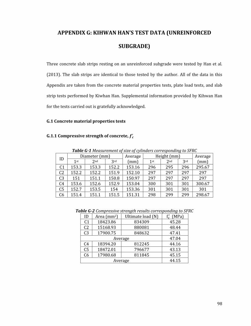
98

APPENDIX G: KIHWAN HAN’S TEST DATA (UNREINFORCED

SUBGRADE)

Three concrete slab strips resting on an unreinforced subgrade were tested by Han et al.

(2013). The slab strips are identical to those tested by the author. All of the data in this

Appendix are taken from the concrete material properties tests, plate load tests, and slab

strip tests performed by Kiwhan Han. Supplemental information provided by Kihwan Han

for the tests carried out is gratefully acknowledged.

G.1 Concrete material properties tests

G.1.1 Compressive strength of concrete,

Table G-1 Measurement of size of cylinders corresponding to SFRC



(mm) 1st 2nd 3rd 1st 2nd 3rd C1 153.3 153.3 152.2 153.16 296 295 296 295.67 C2 152.2 152.2 151.9 152.10 297 297 297 297 C3 151 151.1 150.8 150.97 297 297 297 297 C4 153.6 152.6 152.9 153.04 300 301 301 300.67 C5 152.7 153.5 154 153.36 301 301 301 301 C6 151.4 151.1 151.5 151.31 298 299 299 298.67

Table G-2 Compressive strength results corresponding to SFRC ID Area (mm2) Ultimate load (N)

(MPa) C1 18423.86 834309 45.28 C2 15168.93 880081 48.44 C3 17900.75 848632 47.41

Average 47.04 C4 18394.20 812245 44.16 C5 18472.01 796677 43.13 C6 17980.68 811845 45.15

Average 44.15

99

Table G-3 Measurement of size of cylinders for corresponding to plain concrete



(mm) 1st 2nd 3rd 1st 2nd 3rd C7 151.2 151.2 150.7 151.06 298 299 298 298.33 C8 151.1 151 151.2 151.11 297 297 297 297 C9 151.3 151.6 151.4 151.43 298 297 298 297.67

Table G-4 Compressive strength results corresponding to plain concrete ID Area (mm2) Ultimate load (N)

(MPa) C7 17921.31 839113 46.82 C8 17933.17 845073 47.12 C9 18010 870962 48.36

Average strength 47.44

G.1.2 Density of concrete

Table G-5 Concrete density for SFRC cylinders ID Diameter (mm) Height (mm) Mass (kg) Density (kg/m3) C1 153.16 295.67 12.63 2,318.1 C2 152.10 297 12.79 2,370 C3 150.97 297 12.75 2,398.8 C4 153.04 300.67 12.89 2,330.2 C5 153.36 301 12.93 2,325.8 C6 151.31 298.67 12.80 2,382.4

Average 2,354

Table G-6 Concrete density for plain cylinders ID Diameter (mm) Height (mm) Mass (kg) Density (kg/m3) C7 151.06 298.33 12.64 2,364.1 C8 151.11 297 12.59 2,364.7 C9 151.43 297.67 12.64 2,357.4

Average 2,362

G.1.3 Splitting tensile strength of concrete, fsp




(mm) 1st 2nd 3rd 1st 2nd 3rd S1 150.7 150.8 150.8 150.78 305 306 306 305.67 S2 151 151 150.8 150.95 305 306 306 305.67 S3 150.7 150.9 150.9 150.81 305 306 304 305

100

Table G-8 Splitting tensile strength results corresponding to SFRC ID Ultimate load (N) fsp (MPa) S1 328105 4.53 S2 325878 4.5 S3 291926 4.04

Average 4.36

Table G-9 Measurement of size of cylinders corresponding to plain concrete



(mm) 1st 2nd 3rd 1st 2nd 3rd S4 151.5 151.3 151.5 151.45 305 305 305 305 S5 152.3 152.4 152.7 152.5 305 306 305 305.33 S5 151 150.9 151.3 151.07 303 306 305 604.67

Table G-10 Splitting tensile strength results corresponding to plain concrete ID Ultimate load (N) fsp (MPa) S4 238885 3.29 S5 273324 3.74 S6 213930 2.96

Average 3.33

G.1.4 Modulus of elasticity of concrete, Ec




(mm) 1st 2nd 3rd 1st 2nd 3rd E1 151.3 151.5 151 151.26 297 297 297 297 E2 151.1 151 150.8 150.95 298 298 298 298 E3 151.3 151.5 151.2 151.3 296 297 297 296.67

Table G-12 Measured data for modulus of elasticity test ID Ec (MPa) E1 24,431 E2 25,197 E3 25,250

Average 24,959

101

0

5

10

15

20

0 200 400 600 800 1000

Stre

ss (

MP

a)

Strain (με)

Cylinder E1

0

5

10

15

20

0 200 400 600 800 1000

Stre

ss (

MP

a)

Strain (με)

Cylinder E2

0

5

10

15

20

0 200 400 600 800 1000

Stre

ss (

MP

a)

Strain (με)

Cylinder E4

0

5

10

15

20

0 200 400 600 800 1000

Stre

ss (

MP

a)

Strain (με)

Cylinder E3

Table G-13 Measurement of size of cylinders corresponding to plain concrete



(mm) 1st 2nd 3rd 1st 2nd 3rd E4 153.1 153.2 153 153.12 297 296 296 296.33 E5 153.1 153.6 152.8 153.15 297 298 297 297.33 E6 151.2 151 151 151.03 296 296 297 296.33

Table G-14 Measured data for modulus of elasticity test ID Ec (MPa) E4 24,652 E5 22,943 E6 23,768

Average 23,788

(a) Specimen E1 (SFRC) (b) Specimen E2 (SFRC)

(c) Specimen E3 (SFRC) (d) Specimen E4 (plain concrete)

102

0

5

10

15

20

0 200 400 600 800 1000

Stre

ss (

MP

a)

Strain (με)

Cylinder E5

0

5

10

15

20

0 200 400 600 800 1000

Stre

ss (

MP

a)

Strain (με)

Cylinder E6

(e) Specimen E5 (plain concrete) (f) Specimen E6 (plain concrete)

Figure G-2 Stress vs Strain diagrams for modulus of elasticity tests

G.1.5 Flexural strength of concrete, fr

For beams B2, B5 and B8, crack occurred outside middle third of beam. For this reason

equation G.1 was used to determine the flexural strength of these three prisms..

(G.1)

where: fr = flexural strength P = ultimate load a = distance to crack (when a < L/3) b = width of prism

Table G-15 Measurement of size of flexural prisms corresponding to SFRC ID Measurement 1st 2nd 3rd Average (mm)

B1 b (mm) 154 154 154 154 h (mm) 151.38 151.59 151.37 151.44 l (mm) - - - 457.2

B2 b (mm) 154.65 154.41 154.48 154.51 h (mm) 152.81 152.36 152.79 152.65 a (mm) - - - 163.5

B3 b (mm) 154.32 154.86 154.76 154.65 h (mm) 151.27 151.31 151.15 151.24 l (mm) - - - 457.2

103

Table G-16 Flexural strength results for SFRC prisms ID Ultimate load (kN) fr (MPa) RT,150 fpc (MPa) B1 30.3 3.92 0.79 3.11 B2 34.34 4.68 0.66 3.10 B3 31.81 4.11 0.90 3.71

Average 4.24 0.79 3.31

Table G-17 Measurement of size of flexural prisms corresponding to WWF reinforcement ID Measurement 1st 2nd 3rd Average (mm)

B4 b (mm) 154.74 154.26 154.31 154.43 h (mm) 152.14 152.1 152.18 152.14 l (mm) - - - 457.2

B5 b (mm) 153.58 154.18 155.9 154.55 h (mm) 153.95 153.49 153.66 153.7 a (mm) - - - 179.5

B6 b (mm) 154.08 154.9 155.69 154.89 h (mm) 155.89 154.47 154.16 154.84 l (mm) - - - 457.2

Table G-18 Flexural strength results for WWF prisms ID Ultimate load (kN) fr (MPa) RT,150 fpc (MPa) B4 35.79 4.58 0.22 1.00 B5 33.73 1.66 0.95 1.58 B6 31.55 3.88 0.22 0.87

Average strength 3.37 0.46 1.15

Table G-19 Measurement of size of flexural prisms corresponding to plain concrete ID Age (days) Measurement 1st 2nd 3rd Average (mm)

B7 N/A b (mm) 152.09 304.72 152.62 152.36 h (mm) 153.08 153.31 153.76 153.38 l (mm) - - - 457.2

B8 N/A b (mm) 154.44 154.85 155.95 155.08 h (mm) 153.73 153.73 154.61 154.02 a (mm) - - - 141.5

B9 N/A b (mm) 153.17 152.25 153.12 152.84 h (mm) 153.05 153.29 153.59 153.31 l (mm) - - - 457.2

Table G-20 Flexural strength results for plain concrete prisms ID Ultimate load (kN) Strength fr (MPa) B7 28.39 3.62 B8 25.84 0.99 B9 29.20 3.72

Average strength 2.78

104

0

5

10

15

20

25

30

35

40

0 0.1 0.2 0.3 0.4 0.5L

oad

(k

N)

Deflection (mm)

B1

B2

B3

0

5

10

15

20

25

30

35

40

0 0.1 0.2 0.3 0.4 0.5

Lo

ad (

kN

)

Deflection (mm)

B4

B5

B6

0

5

10

15

20

25

30

0 0.01 0.02 0.03 0.04 0.05 0.06

Lo

ad (

kN

)

Deflection (mm)

B7

B8

B9

Figure G-3 Load-deflection curves for SFRC flexural prisms (up to a 0.5-mm central

deflection)

Figure G-4 Load-deflection curves for WWF flexural prisms (up to a 0.5-mm central

deflection)

Figure G-5 Load-deflection curves for plain concrete flexural prisms (up to a 0.06-mm central deflection)

105

(a) Specimen B1 (SFRC) (b) Specimen B2 (SFRC)

(c) Specimen B3 (SFRC) (d) Specimen B4 (WWF)

(e) Specimen B5 (WWF) (f) Specimen B6 (WWF)

(g) Specimen B7 (plain) (h) Specimen B8 (plain)

152.4 mm 152.4 mm 152.4 mm

237.5 mm

crack

152.4 mm 152.4 mm 152.4 mm

303.5 mm

crack

152.4 mm 152.4 mm 152.4 mm

223.7mm

crack

152.4 mm 152.4 mm 152.4 mm

241.2 mm

crack

152.4 mm 152.4 mm 152.4 mm

179.5 mm

crack

152.4 mm 152.4 mm 152.4 mm

250.7 mm

crack

152.4 mm 152.4 mm 152.4 mm

213.5 mm

crack

152.4 mm 152.4 mm 152.4 mm

315.5 mm

crack

106

0

5

10

15

20

25

30

35

0 10 20 30 40

Lo

ad (

kN

)

Settlement(mm)

Plate Load Test 1

Plate Load Test 2

(i) Specimen B9 (plain)

Figure G-6 Sketches for the location of cracks for flexural beam test

G.2 Plate load tests

Two monotonic and two cyclic plate load tests were performed by Han et al. (2013). For

comparison purposes during the report, the mean value of each set of tests was used. The

average subgrade modulus was determined to be 22 MN/m3. Figure G-7 and G-8 present

the test results for the plate load tests.

Figure G-7 Monotonic plate load tests on unreinforced subgrade (Han et al., 2013)

152.4 mm 152.4 mm 152.4 mm

270.5 mm

crack

107

0

5

10

15

20

25

30

35

40

0 10 20 30 40 50

Lo

ad (

kN

)

Settlement (mm)

Plate Load Test 1

Plate Load Test 2

Figure G-8 Cyclic plate load tests on unreinforced subgrade (Han et al., 2013)

G.3 Slab strip tests

Three slab strips were tested by Han et al. (2013), all resting on an unreinforced subgrade.

The first slab strip was a SFRC slab strip under monotonic loading (Figure G-9), the second

slab strip was a SFRC slab strip under cyclic loading (Figure G-10), and the final slab strip

was a WWF slab strip under cyclic loading (Figure G-11).

The SFRC monotonic slab strip was analyzed using the elastic and post-cracking analyses

described in Chapter 5, as well as the frame analysis. Table F-19 lists the parameters used

for the analyses, and the theoretical predictions are presented in Figures G-12 through G-

15.

Table F-19 Parameters for analysis of beams on subgrade without geogrid Slab Strip Subgrade

fr (MPa) I x 106 (mm4) Ec(MPa) Mcr (kN-m)(1) Mpc (kN-m)(2) ks (MN/m3) 4.24 84.38 25,000 4.77 3.77 22

(1) Mcr is obtained from Equation 5.4 (2) Mpc = R x Mcr = 0.79 x 4.77 kN-m = 3.77 kN-m

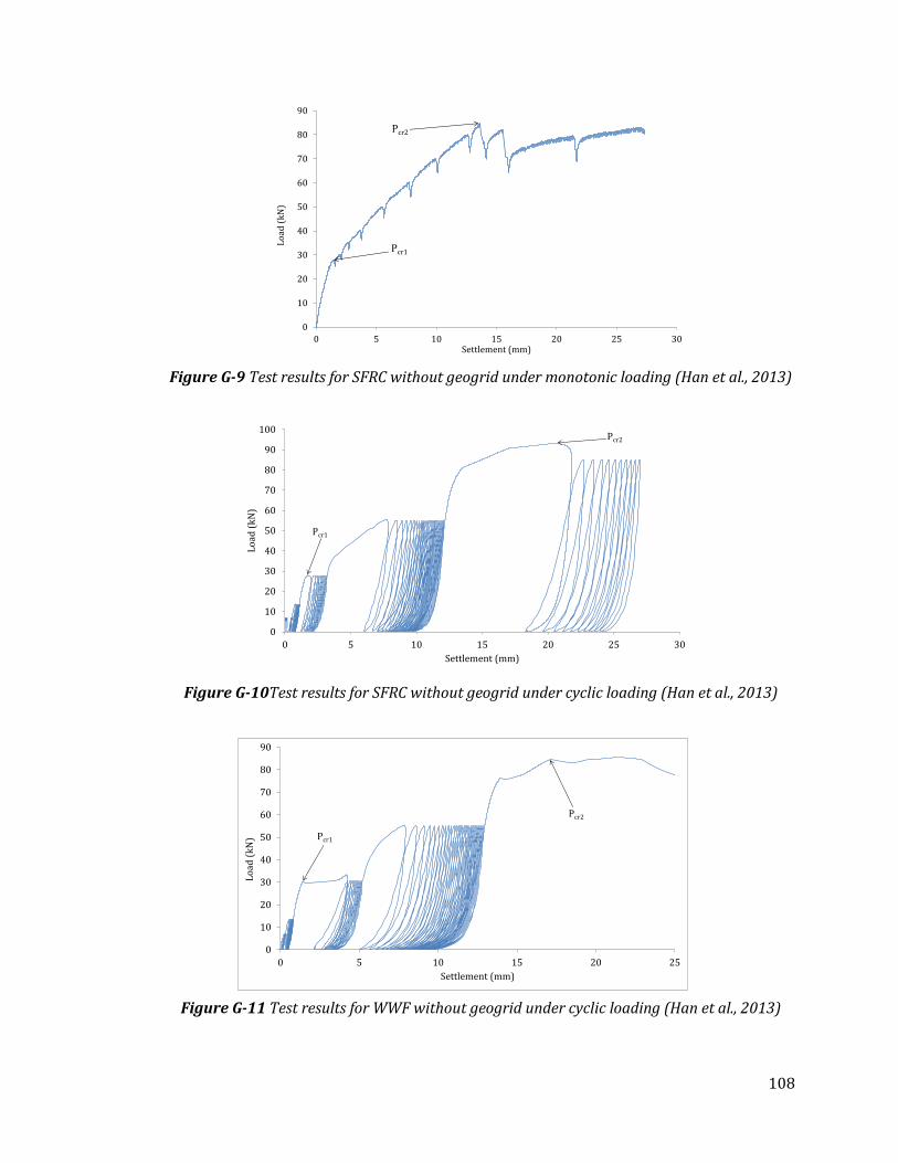
108

0

10

20

30

40

50

60

70

80

90

0 5 10 15 20 25 30

Lo

ad (

kN

)

Settlement (mm)

Pcr1

Pcr2

0

10

20

30

40

50

60

70

80

90

100

0 5 10 15 20 25 30

Lo

ad (

kN

)

Settlement (mm)

Pcr1

Pcr2

0

10

20

30

40

50

60

70

80

90

0 5 10 15 20 25

Lo

ad (

kN

)

Settlement (mm)

Pcr1

Pcr2

Figure G-9 Test results for SFRC without geogrid under monotonic loading (Han et al., 2013)

Figure G-10Test results for SFRC without geogrid under cyclic loading (Han et al., 2013)

Figure G-11 Test results for WWF without geogrid under cyclic loading (Han et al., 2013)

109

0

10

20

30

40

50

60

70

80

90

0 5 10 15 20 25 30

Lo

ad (

kN

)

Settlement (mm)

Experimental





0

10

20

30

40

50

60

70

80

90

0 5 10 15 20 25 30

Lo

ad (

kN

)

Settlement (mm)


Experimental


Theoretical initial cracking load = 17.7 kNx

0

10

20

30

40

50

60

70

80

90

0 5 10 15 20 25 30

Lo

ad (

kN

)

Settlement (mm)

Experimental





Figure G-12 Comparison of load-deformation responses for SFRC slab strip on grade - Elastic

Region

Figure G-13 Comparison of load-deformation responses for SFRC slab strip on grade – Post-

cracking Stage I

Figure G-14 Comparison of load-deformation responses for SFRC slab strip on grade – Post-

cracking Stage II

110

0

10

20

30

40

50

60

70

80

90

0 5 10 15 20 25 30

Lo

ad (

kN

)

Settlement (mm)

Experimental

PFA Pre-crack

PFA Post-crack Stage I

PFA Post-crack Stage II



Theoretical post-crack Stage II (Lin, 2001)

Theoretical Post-crack Stage II (corrected)

Figure G-15 Comparison between plane frame analysis, theoretical analysis, and

experimental results

VITA

Candidate’s full name: Olivia Renata Hernandez Cardenas

Universities attended: University of New Brunswick, Bachelor of Science in Engineering,

2012

Publications:

Hernandez, O., El Naggar, H., and Bischoff, P. (2013). Predicted performance of fibre

reinforced concrete slabs on grade with subgrade reinforced with geogrids. GeoMontreal

2013 Annual Conference. Montreal, QC.

SOIL-STRUCTURE INTERACTION OF STEEL FIBRE REINFORCED ...

Documents