Soil mechanics a_one-dimensional_introduction_wood

P1: KAE

FM CUUS648/Muir 978 0 521 51773 7 August 11, 2009 20:13

SOIL MECHANICS

A one-dimensional introduction

This introductory course on soil mechanics presents the key conceptsof stress, stiffness, seepage, consolidation, and strength within a one-dimensional framework. Consideration of the mechanical behaviour ofsoils requires us to consider density alongside stresses, thus permittingthe unification of deformation and strength characteristics. Soils aredescribed in a way which can be integrated with concurrent teachingof the properties of other engineering materials. The book includes amodel of the shearing of soil and some examples of soil-structure inter-action which are capable of theoretical analysis using one-dimensionalgoverning equations. The text contains many worked examples, andexercises are given for private study at the end of all chapters. Somesuggestions for laboratory demonstrations that could accompany suchan introductory course are sprinkled through the book.

David Muir Wood has taught soil mechanics and geotechnical engi-neering at the universities of Cambridge, Glasgow and Bristol since1975 and has contributed to courses on soil mechanics in many coun-tries around the world. He is the author of numerous research papersand book chapters. His previous books include Soil behaviour and crit-ical state soil mechanics (1990) and Geotechnical modelling (2004). Hewas co-chairman of the United Kingdom GeotechniCAL computer-aided learning project.

i

P1: KAE


ii

P1: KAE


Soil mechanics

A ONE-DIMENSIONAL INTRODUCTION

David Muir WoodUniversity of Bristol

iii

P1: KAE


cambridge university pressCambridge, New York, Melbourne, Madrid, Cape Town, Singapore,Sao Paulo, Delhi, Dubai, Tokyo

Cambridge University Press32 Avenue of the Americas, New York, NY 10013-2473, USA

www.cambridge.orgInformation on this title: www.cambridge.org/

C© David Muir Wood 2009

This publication is in copyright. Subject to statutory exceptionand to the provisions of relevant collective licensing agreements,no reproduction of any part may take place without the writtenpermission of Cambridge University Press.

First published 2009

Printed in the United States of America

A catalog record for this publication is available from the British Library.

Library of Congress Cataloging in Publication data

Muir Wood, David, 1949–Soil mechanics : a one-dimensional introduction / David Muir Wood.

p. cm.Includes bibliographical references and index.ISBN 978-0-521-51773-7 (hardback) – ISBN 978-0-521-74132-3 (pbk.)1. Soil mechanics. I. Title.

TA710.W5983 2009624.1′5136 – dc22 2009020445

ISBN 978-0-521-51773-7 HardbackISBN 978-0-521-74132-3 Paperback

Cambridge University Press has no responsibility for the persistence oraccuracy of URLs for external or third-party Internet Web sites referred to inthis publication and does not guarantee that any content on such Web sites is,or will remain, accurate or appropriate.

iv

9780521517737

http://www.cambridge.org

http://www.cambridge.org/9780521517737

P1: KAE


Contents

Preface page ix

1 Introduction . . . . . . . . . . . . . . . . . . . . . . . . . . . . . . . . . . . . . . . . 1

1.1 Introduction 11.2 Soil mechanics 21.3 Range of problems/applications 21.4 Scope of this book 101.5 Mind maps 11

2 Stress in soils . . . . . . . . . . . . . . . . . . . . . . . . . . . . . . . . . . . . . . . 12

2.1 Introduction 122.2 Equilibrium 122.3 Gravity 132.4 Stress 162.5 Exercises: Stress 182.6 Vertical stress profile 19

2.6.1 Worked examples 212.7 Water in the ground: Introduction to hydrostatics 23

2.7.1 Worked example: Archimedes uplift on spherical object 262.8 Total and effective stresses 28

2.8.1 Worked examples 322.9 Summary 372.10 Exercises: Profiles of total stress, effective stress, pore pressure 37

3 Density . . . . . . . . . . . . . . . . . . . . . . . . . . . . . . . . . . . . . . . . . . . 40

3.1 Introduction 403.2 Units 403.3 Descriptions of packing and density 41

3.3.1 Volumetric ratios 433.3.2 Water content 443.3.3 Densities 44

v

P1: KAE


vi Contents

3.3.4 Unit weights 463.3.5 Typical values 46

3.4 Measurement of packing 473.4.1 Compaction 50

3.5 Soil particles 523.6 Laboratory exercise: particle size distribution and other

classification tests 563.6.1 Sieving 563.6.2 Sedimentation 573.6.3 Particle shape 613.6.4 Sand: relative density 61

3.7 Summary 623.8 Exercises: Density 64

3.8.1 Multiple choice questions 643.8.2 Calculation exercises 65

4 Stiffness . . . . . . . . . . . . . . . . . . . . . . . . . . . . . . . . . . . . . . . . . . 67

4.1 Introduction 674.2 Linear elasticity 674.3 Natural and true strain 704.4 One-dimensional testing of soils 70

4.4.1 Hooke’s Law: confined one-dimensional stiffness ♣ 724.5 One-dimensional (confined) stiffness of soils 744.6 Calculation of strains 78

4.6.1 Worked examples: Calculation of settlement 794.7 Overconsolidation 82

4.7.1 Worked examples: Overconsolidation 844.8 Summary 874.9 Exercises: Stiffness 87

5 Seepage . . . . . . . . . . . . . . . . . . . . . . . . . . . . . . . . . . . . . . . . . . 90

5.1 Introduction 905.2 Total head: Bernoulli’s equation 905.3 Poiseuille’s equation 965.4 Permeability 99

5.4.1 Darcy or Forchheimer? 1025.5 Measurement of permeability 1045.6 Permeability of layered soil 1065.7 Seepage forces 1085.8 Radial flow to vertical drain 1115.9 Radial flow to point drain 1125.10 Worked examples: Seepage 113

5.10.1 Example: flow through soil column 1135.10.2 Example: effect of changing reference datum 116

P1: KAE


Contents vii

5.10.3 Example: pumping from aquifer 1175.10.4 Example: flow into excavation 119

5.11 Summary 1215.12 Exercises: Seepage 123

6 Change in stress . . . . . . . . . . . . . . . . . . . . . . . . . . . . . . . . . . . . 127

6.1 Introduction 1276.2 Stress change and soil permeability 1276.3 Worked examples 130

6.3.1 Example 1 1306.3.2 Example 2 1316.3.3 Example 3 133

6.4 Summary 1346.5 Exercises: Change in stress 136

7 Consolidation . . . . . . . . . . . . . . . . . . . . . . . . . . . . . . . . . . . . . . 138

7.1 Introduction 1387.2 Describing the problem 1407.3 Parabolic isochrones 1427.4 Worked examples 149

7.4.1 Example 1: Determination of coefficient of consolidation 1497.4.2 Example 2 1527.4.3 Example 3 1547.4.4 Example 4 155

7.5 Consolidation: exact analysis ♣ 1557.5.1 Semi-infinite layer 1597.5.2 Finite layer 161

7.6 Summary 1657.7 Exercises: Consolidation 167

8 Strength . . . . . . . . . . . . . . . . . . . . . . . . . . . . . . . . . . . . . . . . . 169

8.1 Introduction 1698.2 Failure mechanisms 1698.3 Shear box and strength of soils 1718.4 Strength model 1738.5 Dilatancy 1748.6 Drained and undrained strength 1778.7 Clay: overconsolidation and undrained strength 1798.8 Pile load capacity 1818.9 Infinite slope 185

8.9.1 Laboratory exercise: Angle of repose 1918.10 Undrained strength of clay: fall-cone test 1938.11 Simple model of shearing ♣ 195

8.11.1 Stiffness 196

P1: KAE


viii Contents

8.11.2 Strength 1978.11.3 Mobilisation of strength 1978.11.4 Dilatancy 1988.11.5 Complete stress:strain relationship 1998.11.6 Drained and undrained response 2008.11.7 Model: summary 203

8.12 Summary 2038.13 Exercises: Strength 205

9 Soil-structure interaction . . . . . . . . . . . . . . . . . . . . . . . . . . . . . . 208

9.1 Introduction 2089.2 Pile under axial loading ♣ 211

9.2.1 Examples 2159.3 Bending of an elastic beam ♣ 2169.4 Elastic beam on elastic foundation ♣ 2209.5 Pile under lateral loading ♣ 2249.6 Soil-structure interaction: next steps 2269.7 Summary 2279.8 Exercises: Soil-structure interaction 227

10 Envoi . . . . . . . . . . . . . . . . . . . . . . . . . . . . . . . . . . . . . . . . . . . 230

10.1 Summary 23010.2 Beyond the single dimension 231

Exercises: numerical answers . . . . . . . . . . . . . . . . . . . . . . . . . . . . . . 232

Index 237

P1: KAE


Preface

This book has emerged from a number of stimuli.There is a view that soils are special: that their characteristics are so extra-

ordinary that they can only be understood by a small band of specialists. Obviously,soils do have some special properties: the central importance of density and changeof density merits particular attention. However, in the context of teaching princi-ples of soil mechanics to undergraduates in the early years of their civil engineeringdegree programmes, I believe that there is advantage to be gained in trying to in-tegrate this teaching with other teaching of properties of engineering materials towhich the students are being exposed at the same time.

It is a fundamental tenet of critical state soil mechanics – with which I grew upin my undergraduate days – that consideration of the mechanical behaviour of soilsrequires us to consider density alongside effective stresses, thus permitting the uni-fication of deformation and strength characteristics. This can be seen as a broadinterpretation of the phrase critical state soil mechanics. I believe that such a unifi-cation can aid the teaching and understanding of soil mechanics.

There is an elegant book by A. J. Roberts1 which demonstrates in a unifiedway how a common mathematical framework can be applied to problems of solidmechanics, fluid mechanics, traffic flow and so on. While I cannot hope to emulatethis elegance, the title prompted me to explore a similar one-dimensional themefor the presentation of many of the key concepts of soil mechanics: density, stress,stiffness, strength and fluid flow.

This one-dimensional approach to soil mechanics has formed the basis for anintroductory course of ten one-hour lectures with ten one-hour problem classes andone three-hour laboratory afternoon for first-year civil engineering undergraduatesat Bristol University. The material of that course is contained in this book. I haveadded a chapter on the analysis of one-dimensional consolidation, which fits neatlywith the theme of the book. I have also included a model of the shearing of soil andsome examples of soil-structure interaction which are capable of theoretical analysisusing essentially one-dimensional governing equations.

1 Roberts, A. J. (1994). A one-dimensional introduction to continuum mechanics. World Scientific.

ix

P1: KAE


x Preface

Simplification of more or less realistic problems leads to differential equationswhich can be readily solved: this is the essence of modelling with which engineersneed to engage (and to realise that they are engaging) all the time. A few of thesetopics require some modest mathematical ability – a bit of integration, solution ofordinary and partial differential equations – but nothing beyond the eventual expec-tations of an undergraduate engineering degree programme. Sections that might, asa consequence, be omitted on a first reading, or until the classes in mathematics havecaught up, are indicated by the symbol ♣.

Exercises are given for private study at the end of all chapters and some sug-gestions for laboratory demonstrations that could accompany such an introductorycourse are sprinkled through the book.

I am grateful to colleagues at Bristol and elsewhere – especially DanutaLesniewska, Erdin Ibraim and Dick Clements – who have provided advice and com-ments on drafts of this book to which I have tried to respond. Erdin in particular hashelped enormously by using material and examples from a draft of this book in hisown teaching and has made many useful suggestions for clarification. However, theblame for any remaining errors must remain with me.

I am grateful to Christopher Bambridge, Ross Boulanger, Sarah Dagostino,David Eastaff, David Nash and Alan Powderham for their advice and help in lo-cating and giving permission to reproduce suitable pictures.

I thank Bristol University for awarding me a University Research Fellowshipfor the academic year 2007–8 which gave me some breathing space after a particu-larly heavy four years of administrative duty.

I am particularly grateful to Peter Gordon for his editorial guidance and wisdomand his intervention at times of stress.

I acknowledge with gratitude Helen’s indulgence and support while I have beenpreparing and revising this book.

David Muir WoodAbbots LeighJune 2009

P1: KAE


SOIL MECHANICS

A one-dimensional introduction

xi

P1: KAE


xii

P1: KAE

OneDim00a CUUS648/Muir 978 0 521 51773 7 August 17, 2009 19:12

1 Introduction

1.1 Introduction

In this chapter, we set the scene for the rest of the book. It may be helpful to remindreaders of the relevance and importance of soil mechanics for all civil engineeringconstruction: everything we construct sits on the ground in some way or other atsome stage in its life. Even aircraft land on runways, and cars drive along roads; ineach case there is some stiff layer (pavement) between the wheels and the preparedground underneath. This stiff layer will help to spread the vehicular load but, inthe end, this load must still be supported by the ground. Some examples of typicalgeotechnical design problems are presented in the next sections.

The term soil mechanics refers to the mechanical properties of soils; theterm geotechnical engineering refers to the application of those mechanical prop-erties to the design and construction of those parts of civil engineering systemswhich are concerned with the active or passive use of soils. Soils are the materi-als that we find in the ground: the term ground engineering is somewhat equiva-lent to geotechnical engineering. We will talk a little about the nature of soils inChapter 3.

The term soil means different things to different people.1 To an agriculturalengineer, the soil is the upper layer of the ground which the farmer ploughs andharrows and in which crops are sown. To the civil engineer, this is the topsoil: it isrecognised as valuable for agricultural purposes but usually too open in structureto be well suited for load bearing. Typically, the topsoil will be stripped from a con-struction site and stockpiled before serious construction activity begins. Underneaththe topsoil is the soil with whose engineering properties we are concerned here. Aswe go further down into the ground, we will eventually encounter materials that no-one would have any hesitation in describing as rock. However, on the way there aremany materials which can be described as hard soils or soft rocks: there is no precise

1 Chambers’ Dictionary defines soil as “the ground: the mould in which plants grow: the earth whichnourishes plants” (from Latin solum, ground); but curiously soil mechanics, defined as “a branch ofcivil engineering concerned with the ability of different soils to withstand the use to which they arebeing put”, is given as a sub-heading linked with Old French souil, wallowing place.

1

P1: KAE


2 Introduction

distinction and, although we are concerned primarily with soils in this book, muchof what is presented will apply equally to weak rocks.

1.2 Soil mechanics

Soil mechanics is concerned with the mechanics of soils: a truism! It is an unfor-tunate feature of most civil engineering degree programmes that an atomistic ap-proach to teaching is adopted: the teaching is broken down typically into structures,soils and water (with ancillary courses on mathematics, computing, and so on) andthese subjects are developed in progressively greater detail through the three or fouryears of the degree with little opportunity being given to the embryonic engineers tointegrate the separate elements and to recognise the importance of seeing the wholesystem as well as the parts. The whole may well combine elements that do not comefrom traditional civil engineering disciplines (mechanical or electrical, for example)and it is quite usual for systems to display emergent behaviours which had not beenanticipated from the study of the constituent parts.

This book declares itself to be concerned with soil mechanics and therefore ap-pears to perpetuate this segregation. However, opportunities will be taken wherepossible to demonstrate the behaviour of simple interactive systems: the interac-tion of soil with structural elements is a prime example where separate treatmentof the different components is doomed to lead to erroneous expectations. But thisbook also attempts to integrate by addressing from a geotechnical point of viewconcepts which engineering students will be meeting as part of parallel courseson structures/materials or fluids/hydrostatics. Concepts of stress, stiffness, strength,fluid pressure, fluid flow and diffusion will, no doubt, be encountered in differentcontexts. The different treatments should not only indicate that there is a commonthread of mechanics linking all aspects of engineering, but also encourage versatilityand, further, provide reinforcement of learning.

1.3 Range of problems/applications

It is often said that the challenge of geotechnical engineering is that the soils haveto be taken as they are found. Whereas structural materials such as steel and con-crete can be designed to have particular desirable properties, the ground is as it isas a result of millennia of geological and geomorphological actions. The design ofthe geotechnical system will have to accommodate whatever properties the groundpossesses. There may, on occasion, be some possibilities of modifying the in-situproperties of the ground to some extent. And where filling is required to build anembankment or a dam or to build up the ground behind a retaining wall, then it maybe possible to consider this as a “designer soil”.

From the point of view of design or analysis, the usual starting point with ageotechnical problem is to ensure that failure will not occur. Such stability or ul-timate limit state calculations are often reasonably straightforward – certainly bycomparison with the possibly more significant calculations of displacements under

P1: KAE


1.3 Range of problems/applications 3

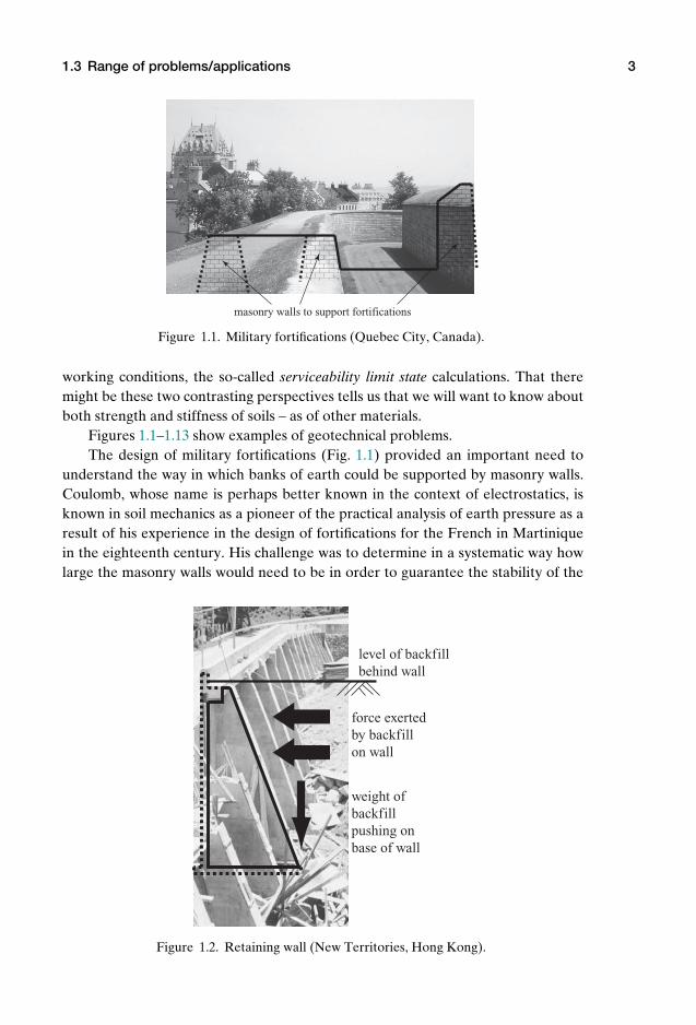
masonry walls to support fortifications

Figure 1.1. Military fortifications (Quebec City, Canada).

working conditions, the so-called serviceability limit state calculations. That theremight be these two contrasting perspectives tells us that we will want to know aboutboth strength and stiffness of soils – as of other materials.

Figures 1.1–1.13 show examples of geotechnical problems.The design of military fortifications (Fig. 1.1) provided an important need to

understand the way in which banks of earth could be supported by masonry walls.Coulomb, whose name is perhaps better known in the context of electrostatics, isknown in soil mechanics as a pioneer of the practical analysis of earth pressure as aresult of his experience in the design of fortifications for the French in Martiniquein the eighteenth century. His challenge was to determine in a systematic way howlarge the masonry walls would need to be in order to guarantee the stability of the

level of backfill behind wall

force exerted by backfill on wall

weight of backfill pushing on base of wall

Figure 1.2. Retaining wall (New Territories, Hong Kong).

P1: KAE


4 Introduction

a. b.

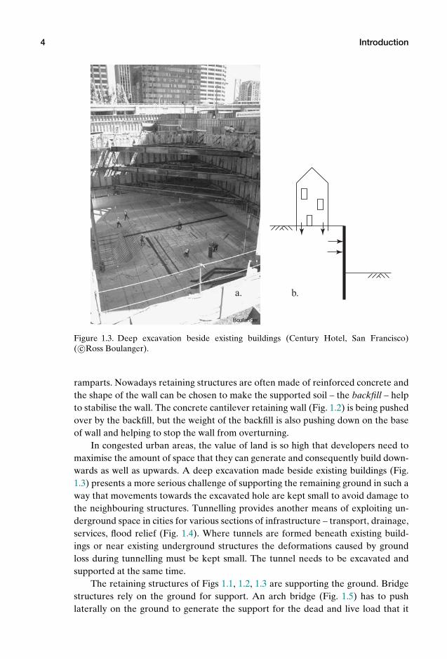
Figure 1.3. Deep excavation beside existing buildings (Century Hotel, San Francisco)( c©Ross Boulanger).

ramparts. Nowadays retaining structures are often made of reinforced concrete andthe shape of the wall can be chosen to make the supported soil – the backfill – helpto stabilise the wall. The concrete cantilever retaining wall (Fig. 1.2) is being pushedover by the backfill, but the weight of the backfill is also pushing down on the baseof wall and helping to stop the wall from overturning.

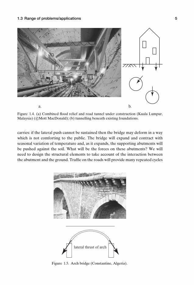
In congested urban areas, the value of land is so high that developers need tomaximise the amount of space that they can generate and consequently build down-wards as well as upwards. A deep excavation made beside existing buildings (Fig.1.3) presents a more serious challenge of supporting the remaining ground in such away that movements towards the excavated hole are kept small to avoid damage tothe neighbouring structures. Tunnelling provides another means of exploiting un-derground space in cities for various sections of infrastructure – transport, drainage,services, flood relief (Fig. 1.4). Where tunnels are formed beneath existing build-ings or near existing underground structures the deformations caused by groundloss during tunnelling must be kept small. The tunnel needs to be excavated andsupported at the same time.

The retaining structures of Figs 1.1, 1.2, 1.3 are supporting the ground. Bridgestructures rely on the ground for support. An arch bridge (Fig. 1.5) has to pushlaterally on the ground to generate the support for the dead and live load that it

P1: KAE



a. b.

Figure 1.4. (a) Combined flood relief and road tunnel under construction (Kuala Lumpur,Malaysia) ( c©Mott MacDonald); (b) tunnelling beneath existing foundations.

carries: if the lateral push cannot be sustained then the bridge may deform in a waywhich is not comforting to the public. The bridge will expand and contract withseasonal variation of temperature and, as it expands, the supporting abutments willbe pushed against the soil. What will be the forces on these abutments? We willneed to design the structural elements to take account of the interaction betweenthe abutment and the ground. Traffic on the roads will provide many repeated cycles

lateral thrust of arch

Figure 1.5. Arch bridge (Constantine, Algeria).

P1: KAE


6 Introduction

a.

b. c.

Figure 1.6. (a) Embankments on soft ground (M4 motorway and overbridge approach em-bankments, Bristol, UK) ( c©Sarah Dagostino); (b) settlement of embankment; (c) failure ofside slopes of embankment.

of loading on the ground. The foundations of roads are usually engineered to ensurethat the deformations of the road surface are tolerable.

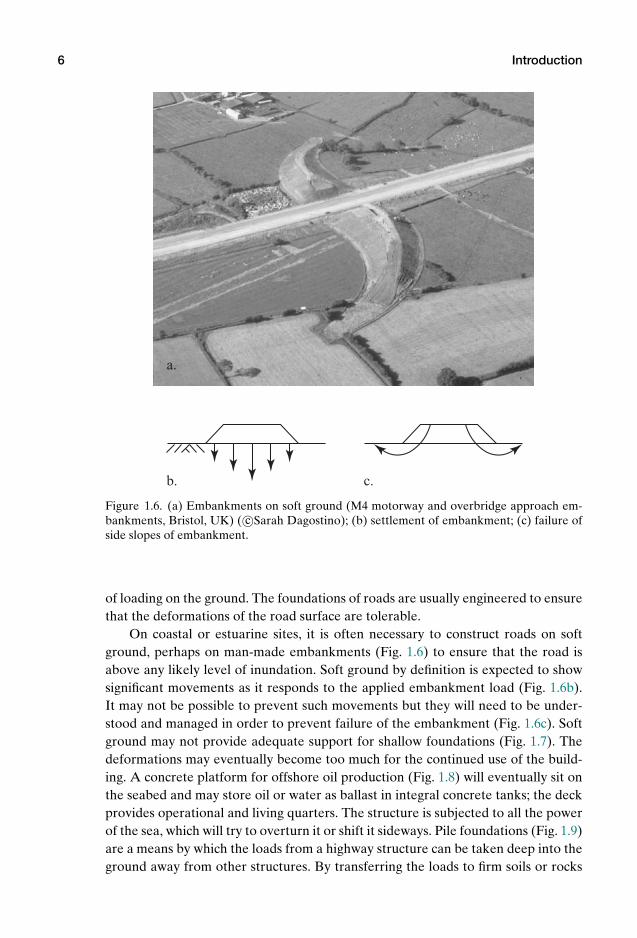
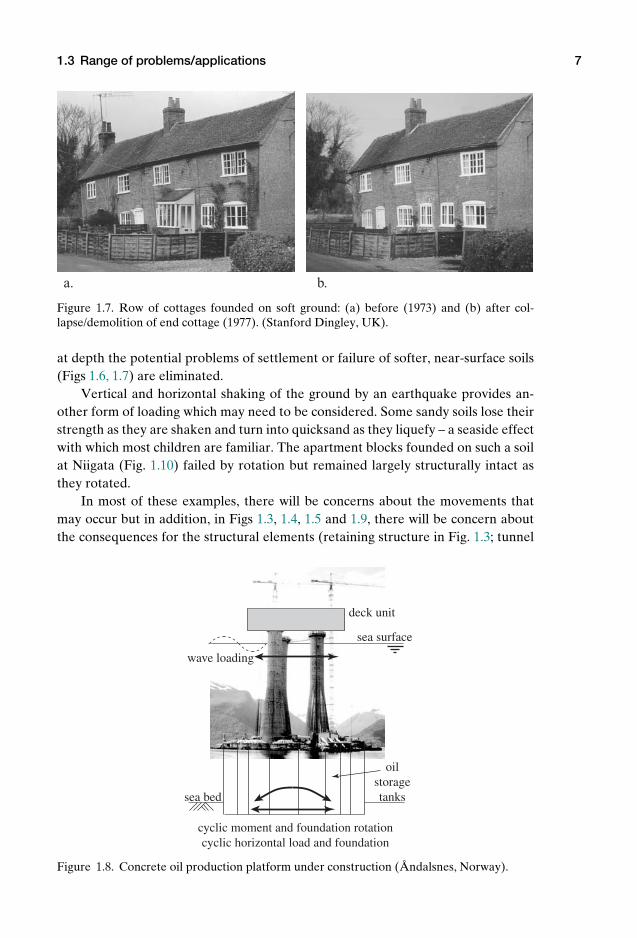
On coastal or estuarine sites, it is often necessary to construct roads on softground, perhaps on man-made embankments (Fig. 1.6) to ensure that the road isabove any likely level of inundation. Soft ground by definition is expected to showsignificant movements as it responds to the applied embankment load (Fig. 1.6b).It may not be possible to prevent such movements but they will need to be under-stood and managed in order to prevent failure of the embankment (Fig. 1.6c). Softground may not provide adequate support for shallow foundations (Fig. 1.7). Thedeformations may eventually become too much for the continued use of the build-ing. A concrete platform for offshore oil production (Fig. 1.8) will eventually sit onthe seabed and may store oil or water as ballast in integral concrete tanks; the deckprovides operational and living quarters. The structure is subjected to all the powerof the sea, which will try to overturn it or shift it sideways. Pile foundations (Fig. 1.9)are a means by which the loads from a highway structure can be taken deep into theground away from other structures. By transferring the loads to firm soils or rocks

P1: KAE



a. b.

Figure 1.7. Row of cottages founded on soft ground: (a) before (1973) and (b) after col-lapse/demolition of end cottage (1977). (Stanford Dingley, UK).

at depth the potential problems of settlement or failure of softer, near-surface soils(Figs 1.6, 1.7) are eliminated.

Vertical and horizontal shaking of the ground by an earthquake provides an-other form of loading which may need to be considered. Some sandy soils lose theirstrength as they are shaken and turn into quicksand as they liquefy – a seaside effectwith which most children are familiar. The apartment blocks founded on such a soilat Niigata (Fig. 1.10) failed by rotation but remained largely structurally intact asthey rotated.

In most of these examples, there will be concerns about the movements thatmay occur but in addition, in Figs 1.3, 1.4, 1.5 and 1.9, there will be concern aboutthe consequences for the structural elements (retaining structure in Fig. 1.3; tunnel

sea bed

sea surface

oil storage tanks

deck unit

wave loading

cyclic moment and foundation rotationcyclic horizontal load and foundation

Figure 1.8. Concrete oil production platform under construction (Andalsnes, Norway).

P1: KAE


8 Introduction

piles to transfer loads from highway columns to strong ground at depth

Figure 1.9. Highway structure founded on piles (Kowloon, Hong Kong).

or culvert linings in Fig. 1.4; bridge abutments in Fig. 1.5; pile foundations in Fig. 1.9;existing buildings in Figs 1.3, 1.4) of these movements. These are certainly exampleswhere potential soil-structure interaction issues will need to be considered.

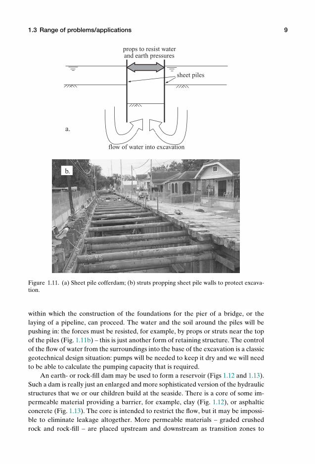
It will become clear that water plays an important part in the mechanics ofsoils and geotechnical engineering. It may be necessary to create dry excavationswithin or near a lake, river or sea protected by a cofferdam of driven sheet piles assketched in Fig. 1.11a. Sheet piles are driven into the ground to form an enclosedspace protecting the excavation from inflow of water and provide an environment

Figure 1.10. Failure of apartment blocks at Niigata, Japan as result of liquefaction inducedby earthquake in 1964.

P1: KAE



flow of water into excavation

sheet piles

a.

props to resist waterand earth pressures

b.

Figure 1.11. (a) Sheet pile cofferdam; (b) struts propping sheet pile walls to protect excava-tion.

within which the construction of the foundations for the pier of a bridge, or thelaying of a pipeline, can proceed. The water and the soil around the piles will bepushing in: the forces must be resisted, for example, by props or struts near the topof the piles (Fig. 1.11b) – this is just another form of retaining structure. The controlof the flow of water from the surroundings into the base of the excavation is a classicgeotechnical design situation: pumps will be needed to keep it dry and we will needto be able to calculate the pumping capacity that is required.

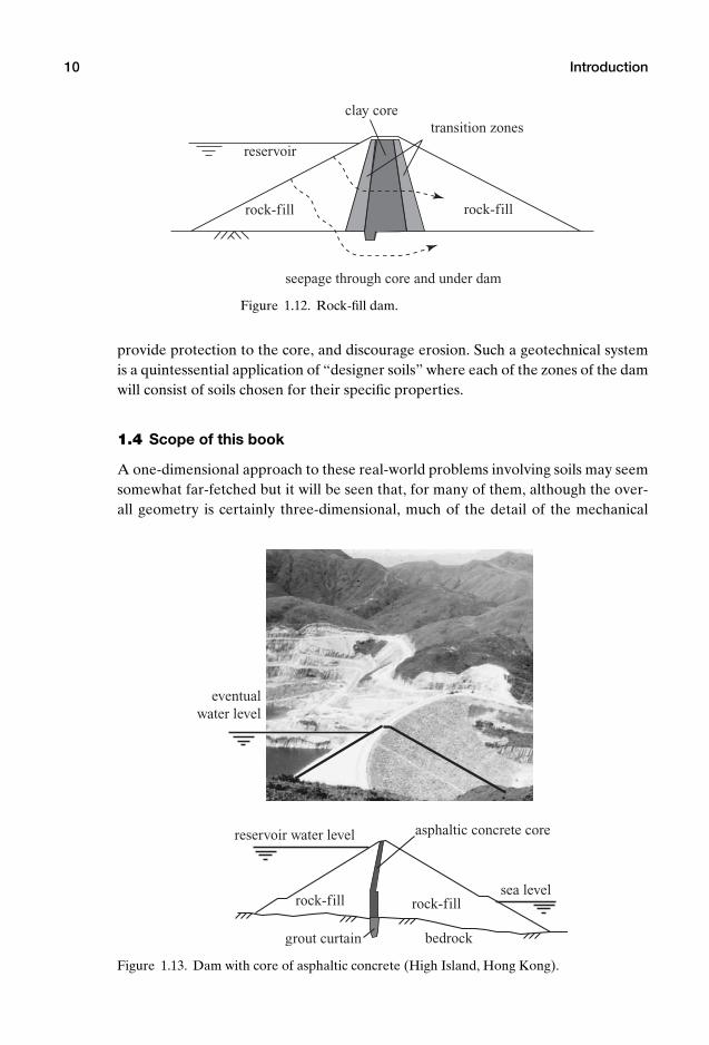
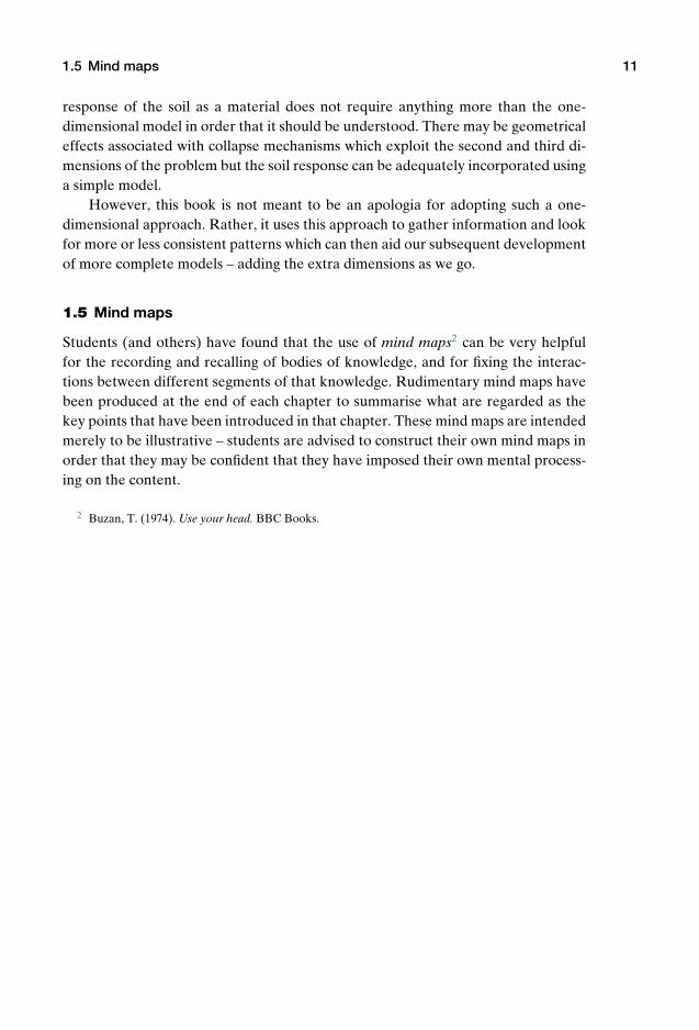
An earth- or rock-fill dam may be used to form a reservoir (Figs 1.12 and 1.13).Such a dam is really just an enlarged and more sophisticated version of the hydraulicstructures that we or our children build at the seaside. There is a core of some im-permeable material providing a barrier, for example, clay (Fig. 1.12), or asphalticconcrete (Fig. 1.13). The core is intended to restrict the flow, but it may be impossi-ble to eliminate leakage altogether. More permeable materials – graded crushedrock and rock-fill – are placed upstream and downstream as transition zones to

P1: KAE


10 Introduction

reservoir

transition zones

rock-fill rock-fill

clay core

seepage through core and under dam

Figure 1.12. Rock-fill dam.

provide protection to the core, and discourage erosion. Such a geotechnical systemis a quintessential application of “designer soils” where each of the zones of the damwill consist of soils chosen for their specific properties.

1.4 Scope of this book

A one-dimensional approach to these real-world problems involving soils may seemsomewhat far-fetched but it will be seen that, for many of them, although the over-all geometry is certainly three-dimensional, much of the detail of the mechanical

rock-fill rock-fillsea level

reservoir water level asphaltic concrete core

eventualwater level

bedrockgrout curtain

Figure 1.13. Dam with core of asphaltic concrete (High Island, Hong Kong).

P1: KAE


1.5 Mind maps 11

response of the soil as a material does not require anything more than the one-dimensional model in order that it should be understood. There may be geometricaleffects associated with collapse mechanisms which exploit the second and third di-mensions of the problem but the soil response can be adequately incorporated usinga simple model.

However, this book is not meant to be an apologia for adopting such a one-dimensional approach. Rather, it uses this approach to gather information and lookfor more or less consistent patterns which can then aid our subsequent developmentof more complete models – adding the extra dimensions as we go.

1.5 Mind maps

Students (and others) have found that the use of mind maps2 can be very helpfulfor the recording and recalling of bodies of knowledge, and for fixing the interac-tions between different segments of that knowledge. Rudimentary mind maps havebeen produced at the end of each chapter to summarise what are regarded as thekey points that have been introduced in that chapter. These mind maps are intendedmerely to be illustrative – students are advised to construct their own mind maps inorder that they may be confident that they have imposed their own mental process-ing on the content.

2 Buzan, T. (1974). Use your head. BBC Books.

P1: KAE


2 Stress in soils

2.1 Introduction

In this chapter, we introduce the concept of stress and demonstrate how we cancalculate stresses in the ground, recalling that we are only concerned with config-urations that can be described as one-dimensional. Initial sections rehearse someof the ideas of mechanics – Newton’s First Law, the distinction between mass andweight, and the idea of gravity. The single dimension of our problems allows us toimpose some notions of symmetry which are helpful in simplifying our calculationsof stresses in soils.

We need then to introduce the possible presence of water in the ground. Somebackground discussion of basic hydrostatics is required in order that we may de-scribe the pressures that exist in the water. We end with a powerful hypothesis aboutthe way in which stresses are shared between the water and the soil.

2.2 Equilibrium

Newton’s First Law of Motion says that an object will remain in its state of rest orof uniform motion in a straight line unless acted upon by an out-of-balance force.1

We need not concern ourselves here with the possibility of motion – our soils areexpected to be rather stationary or at least to move only very slowly as a result ofsome construction process. The condition of rest or stasis therefore requires that theforces acting on an object should be in balance.

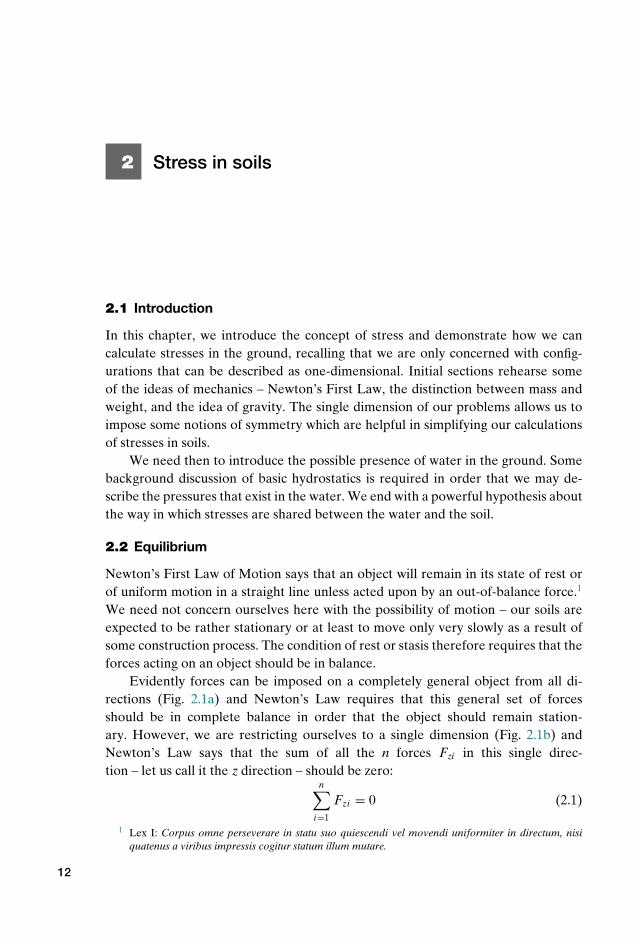
Evidently forces can be imposed on a completely general object from all di-rections (Fig. 2.1a) and Newton’s Law requires that this general set of forcesshould be in complete balance in order that the object should remain station-ary. However, we are restricting ourselves to a single dimension (Fig. 2.1b) andNewton’s Law says that the sum of all the n forces Fzi in this single direc-tion – let us call it the z direction – should be zero:

n∑i=1

Fzi = 0 (2.1)

1 Lex I: Corpus omne perseverare in statu suo quiescendi vel movendi uniformiter in directum, nisiquatenus a viribus impressis cogitur statum illum mutare.

12

P1: KAE


2.3 Gravity 13

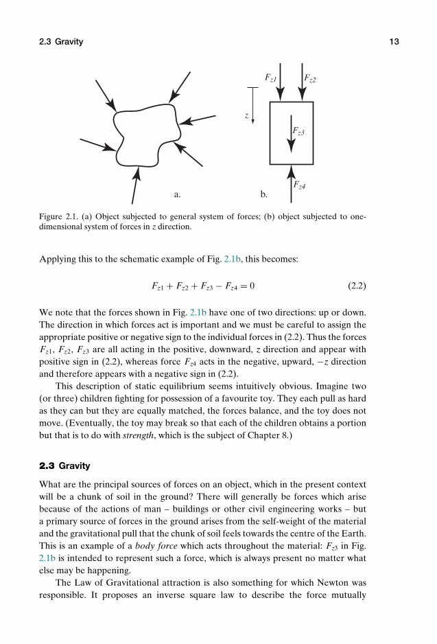
a. b.

Fz1 Fz2

Fz3

Fz4

z

Figure 2.1. (a) Object subjected to general system of forces; (b) object subjected to one-dimensional system of forces in z direction.

Applying this to the schematic example of Fig. 2.1b, this becomes:

Fz1 + Fz2 + Fz3 − Fz4 = 0 (2.2)

We note that the forces shown in Fig. 2.1b have one of two directions: up or down.The direction in which forces act is important and we must be careful to assign theappropriate positive or negative sign to the individual forces in (2.2). Thus the forcesFz1, Fz2, Fz3 are all acting in the positive, downward, z direction and appear withpositive sign in (2.2), whereas force Fz4 acts in the negative, upward, −z directionand therefore appears with a negative sign in (2.2).

This description of static equilibrium seems intuitively obvious. Imagine two(or three) children fighting for possession of a favourite toy. They each pull as hardas they can but they are equally matched, the forces balance, and the toy does notmove. (Eventually, the toy may break so that each of the children obtains a portionbut that is to do with strength, which is the subject of Chapter 8.)

2.3 Gravity

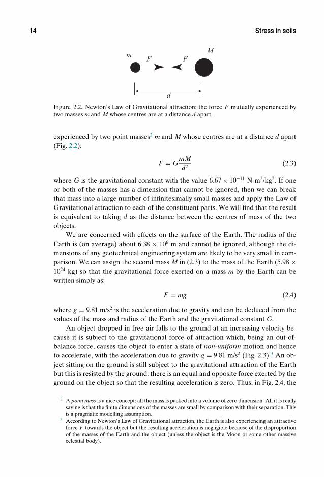
What are the principal sources of forces on an object, which in the present contextwill be a chunk of soil in the ground? There will generally be forces which arisebecause of the actions of man – buildings or other civil engineering works – buta primary source of forces in the ground arises from the self-weight of the materialand the gravitational pull that the chunk of soil feels towards the centre of the Earth.This is an example of a body force which acts throughout the material: Fz3 in Fig.2.1b is intended to represent such a force, which is always present no matter whatelse may be happening.

The Law of Gravitational attraction is also something for which Newton wasresponsible. It proposes an inverse square law to describe the force mutually

P1: KAE


14 Stress in soils

mM

d

F F

Figure 2.2. Newton’s Law of Gravitational attraction: the force F mutually experienced bytwo masses m and M whose centres are at a distance d apart.

experienced by two point masses2 m and M whose centres are at a distance d apart(Fig. 2.2):

F = GmMd2

(2.3)

where G is the gravitational constant with the value 6.67 × 10−11 N-m2/kg2. If oneor both of the masses has a dimension that cannot be ignored, then we can breakthat mass into a large number of infinitesimally small masses and apply the Law ofGravitational attraction to each of the constituent parts. We will find that the resultis equivalent to taking d as the distance between the centres of mass of the twoobjects.

We are concerned with effects on the surface of the Earth. The radius of theEarth is (on average) about 6.38 × 106 m and cannot be ignored, although the di-mensions of any geotechnical engineering system are likely to be very small in com-parison. We can assign the second mass M in (2.3) to the mass of the Earth (5.98 ×1024 kg) so that the gravitational force exerted on a mass m by the Earth can bewritten simply as:

F = mg (2.4)

where g = 9.81 m/s2 is the acceleration due to gravity and can be deduced from thevalues of the mass and radius of the Earth and the gravitational constant G.

An object dropped in free air falls to the ground at an increasing velocity be-cause it is subject to the gravitational force of attraction which, being an out-of-balance force, causes the object to enter a state of non-uniform motion and henceto accelerate, with the acceleration due to gravity g = 9.81 m/s2 (Fig. 2.3).3 An ob-ject sitting on the ground is still subject to the gravitational attraction of the Earthbut this is resisted by the ground: there is an equal and opposite force exerted by theground on the object so that the resulting acceleration is zero. Thus, in Fig. 2.4, the

2 A point mass is a nice concept: all the mass is packed into a volume of zero dimension. All it is reallysaying is that the finite dimensions of the masses are small by comparison with their separation. Thisis a pragmatic modelling assumption.

3 According to Newton’s Law of Gravitational attraction, the Earth is also experiencing an attractiveforce F towards the object but the resulting acceleration is negligible because of the disproportionof the masses of the Earth and the object (unless the object is the Moon or some other massivecelestial body).

P1: KAE


2.3 Gravity 15

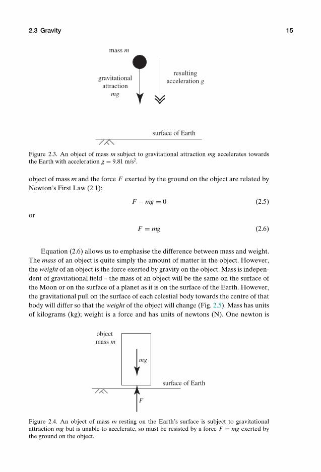
mass m

gravitational attraction

mg

resulting acceleration g

surface of Earth

Figure 2.3. An object of mass m subject to gravitational attraction mg accelerates towardsthe Earth with acceleration g = 9.81 m/s2.

object of mass m and the force F exerted by the ground on the object are related byNewton’s First Law (2.1):

F − mg = 0 (2.5)

or

F = mg (2.6)

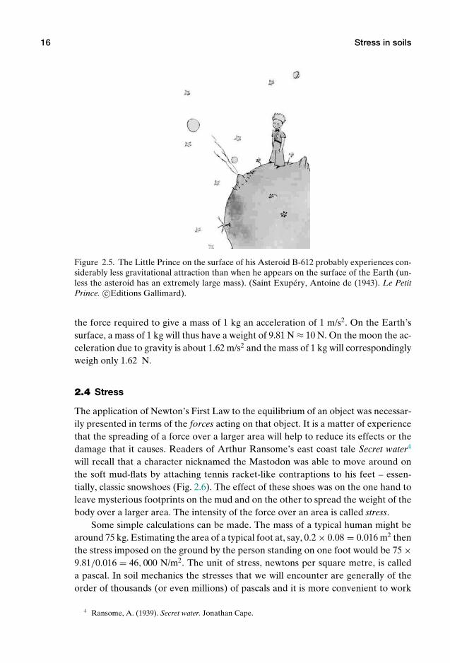
Equation (2.6) allows us to emphasise the difference between mass and weight.The mass of an object is quite simply the amount of matter in the object. However,the weight of an object is the force exerted by gravity on the object. Mass is indepen-dent of gravitational field – the mass of an object will be the same on the surface ofthe Moon or on the surface of a planet as it is on the surface of the Earth. However,the gravitational pull on the surface of each celestial body towards the centre of thatbody will differ so that the weight of the object will change (Fig. 2.5). Mass has unitsof kilograms (kg); weight is a force and has units of newtons (N). One newton is

F

mg

object mass m

surface of Earth

Figure 2.4. An object of mass m resting on the Earth’s surface is subject to gravitationalattraction mg but is unable to accelerate, so must be resisted by a force F = mg exerted bythe ground on the object.

P1: KAE


16 Stress in soils

Figure 2.5. The Little Prince on the surface of his Asteroid B-612 probably experiences con-siderably less gravitational attraction than when he appears on the surface of the Earth (un-less the asteroid has an extremely large mass). (Saint Exupery, Antoine de (1943). Le PetitPrince. c©Editions Gallimard).

the force required to give a mass of 1 kg an acceleration of 1 m/s2. On the Earth’ssurface, a mass of 1 kg will thus have a weight of 9.81 N ≈ 10 N. On the moon the ac-celeration due to gravity is about 1.62 m/s2 and the mass of 1 kg will correspondinglyweigh only 1.62 N.

2.4 Stress

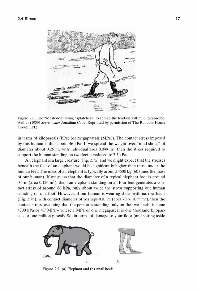
The application of Newton’s First Law to the equilibrium of an object was necessar-ily presented in terms of the forces acting on that object. It is a matter of experiencethat the spreading of a force over a larger area will help to reduce its effects or thedamage that it causes. Readers of Arthur Ransome’s east coast tale Secret water4

will recall that a character nicknamed the Mastodon was able to move around onthe soft mud-flats by attaching tennis racket-like contraptions to his feet – essen-tially, classic snowshoes (Fig. 2.6). The effect of these shoes was on the one hand toleave mysterious footprints on the mud and on the other to spread the weight of thebody over a larger area. The intensity of the force over an area is called stress.

Some simple calculations can be made. The mass of a typical human might bearound 75 kg. Estimating the area of a typical foot at, say, 0.2 × 0.08 = 0.016 m2 thenthe stress imposed on the ground by the person standing on one foot would be 75 ×9.81/0.016 = 46, 000 N/m2. The unit of stress, newtons per square metre, is calleda pascal. In soil mechanics the stresses that we will encounter are generally of theorder of thousands (or even millions) of pascals and it is more convenient to work

4 Ransome, A. (1939). Secret water. Jonathan Cape.

P1: KAE


2.4 Stress 17

Figure 2.6. The “Mastodon” using “splatchers” to spread the load on soft mud. (Ransome,Arthur (1939) Secret water Jonathan Cape. Reprinted by permission of The Random HouseGroup Ltd.)

in terms of kilopascals (kPa) (or megapascals (MPa)). The contact stress imposedby this human is thus about 46 kPa. If we spread the weight over “mud-shoes” ofdiameter about 0.25 m, with individual area 0.049 m2, then the stress required tosupport the human standing on two feet is reduced to 7.5 kPa.

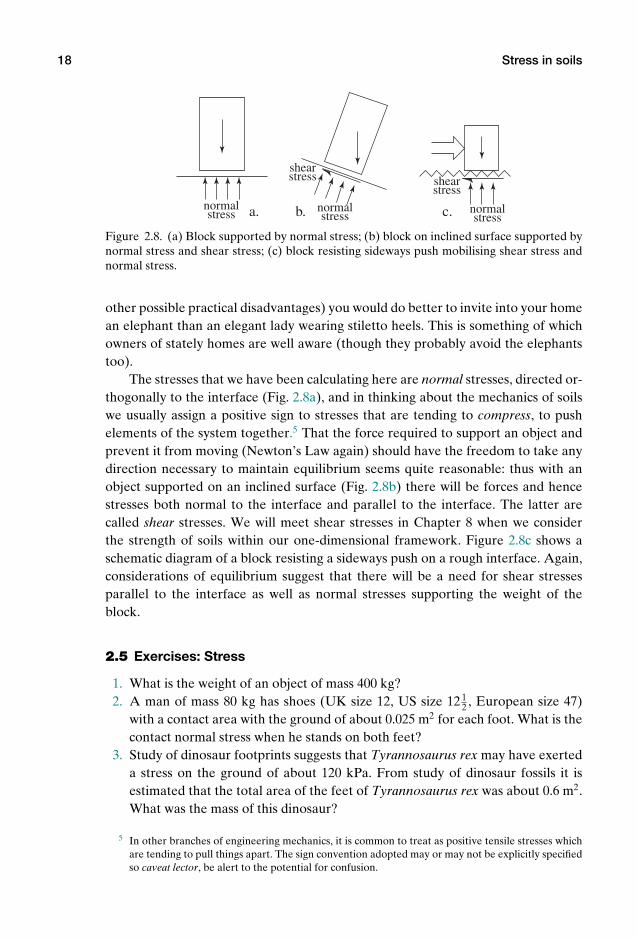
An elephant is a large creature (Fig. 2.7a) and we might expect that the stressesbeneath the feet of an elephant would be significantly higher than those under thehuman feet. The mass of an elephant is typically around 4500 kg (60 times the massof our human). If we guess that the diameter of a typical elephant foot is around0.4 m (area 0.126 m2), then, an elephant standing on all four feet generates a con-tact stress of around 88 kPa, only about twice the stress supporting our humanstanding on one foot. However, if our human is wearing shoes with narrow heels(Fig. 2.7b), with contact diameter of perhaps 0.01 m (area 78 × 10−6 m2), then thecontact stress, assuming that the person is standing only on the two heels, is some4700 kPa or 4.7 MPa – where 1 MPa or one megapascal is one thousand kilopas-cals or one million pascals. So, in terms of damage to your floor (and setting aside

a. b.

Figure 2.7. (a) Elephant and (b) small heels.

P1: KAE


18 Stress in soils

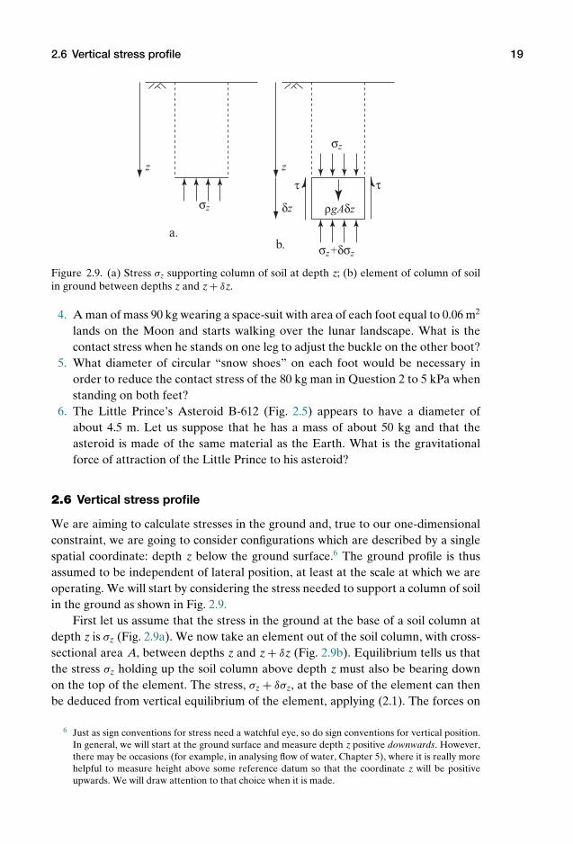
a. b. c.normal stress normal

stressnormal stress

shear stress shear

stress

Figure 2.8. (a) Block supported by normal stress; (b) block on inclined surface supported bynormal stress and shear stress; (c) block resisting sideways push mobilising shear stress andnormal stress.

other possible practical disadvantages) you would do better to invite into your homean elephant than an elegant lady wearing stiletto heels. This is something of whichowners of stately homes are well aware (though they probably avoid the elephantstoo).

The stresses that we have been calculating here are normal stresses, directed or-thogonally to the interface (Fig. 2.8a), and in thinking about the mechanics of soilswe usually assign a positive sign to stresses that are tending to compress, to pushelements of the system together.5 That the force required to support an object andprevent it from moving (Newton’s Law again) should have the freedom to take anydirection necessary to maintain equilibrium seems quite reasonable: thus with anobject supported on an inclined surface (Fig. 2.8b) there will be forces and hencestresses both normal to the interface and parallel to the interface. The latter arecalled shear stresses. We will meet shear stresses in Chapter 8 when we considerthe strength of soils within our one-dimensional framework. Figure 2.8c shows aschematic diagram of a block resisting a sideways push on a rough interface. Again,considerations of equilibrium suggest that there will be a need for shear stressesparallel to the interface as well as normal stresses supporting the weight of theblock.

2.5 Exercises: Stress

1. What is the weight of an object of mass 400 kg?2. A man of mass 80 kg has shoes (UK size 12, US size 12 1

2 , European size 47)with a contact area with the ground of about 0.025 m2 for each foot. What is thecontact normal stress when he stands on both feet?

3. Study of dinosaur footprints suggests that Tyrannosaurus rex may have exerteda stress on the ground of about 120 kPa. From study of dinosaur fossils it isestimated that the total area of the feet of Tyrannosaurus rex was about 0.6 m2.What was the mass of this dinosaur?

5 In other branches of engineering mechanics, it is common to treat as positive tensile stresses whichare tending to pull things apart. The sign convention adopted may or may not be explicitly specifiedso caveat lector, be alert to the potential for confusion.

P1: KAE


2.6 Vertical stress profile 19

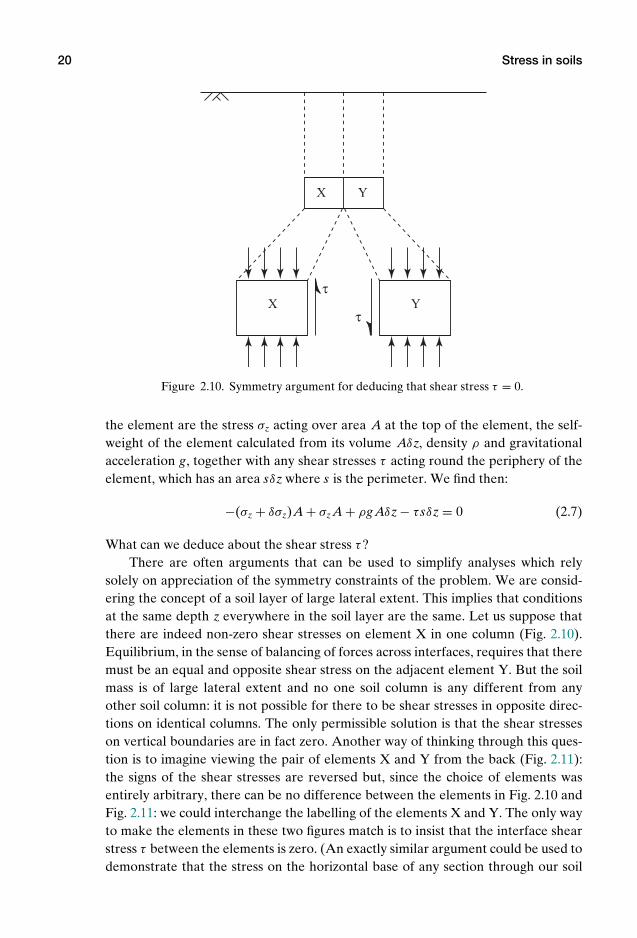
δz

z

σz+δσz

σz

ρgAδz

τ τz

σz

a.b.

Figure 2.9. (a) Stress σz supporting column of soil at depth z; (b) element of column of soilin ground between depths z and z + δz.

4. A man of mass 90 kg wearing a space-suit with area of each foot equal to 0.06 m2

lands on the Moon and starts walking over the lunar landscape. What is thecontact stress when he stands on one leg to adjust the buckle on the other boot?

5. What diameter of circular “snow shoes” on each foot would be necessary inorder to reduce the contact stress of the 80 kg man in Question 2 to 5 kPa whenstanding on both feet?

6. The Little Prince’s Asteroid B-612 (Fig. 2.5) appears to have a diameter ofabout 4.5 m. Let us suppose that he has a mass of about 50 kg and that theasteroid is made of the same material as the Earth. What is the gravitationalforce of attraction of the Little Prince to his asteroid?

2.6 Vertical stress profile

We are aiming to calculate stresses in the ground and, true to our one-dimensionalconstraint, we are going to consider configurations which are described by a singlespatial coordinate: depth z below the ground surface.6 The ground profile is thusassumed to be independent of lateral position, at least at the scale at which we areoperating. We will start by considering the stress needed to support a column of soilin the ground as shown in Fig. 2.9.

First let us assume that the stress in the ground at the base of a soil column atdepth z is σz (Fig. 2.9a). We now take an element out of the soil column, with cross-sectional area A, between depths z and z + δz (Fig. 2.9b). Equilibrium tells us thatthe stress σz holding up the soil column above depth z must also be bearing downon the top of the element. The stress, σz + δσz, at the base of the element can thenbe deduced from vertical equilibrium of the element, applying (2.1). The forces on

6 Just as sign conventions for stress need a watchful eye, so do sign conventions for vertical position.In general, we will start at the ground surface and measure depth z positive downwards. However,there may be occasions (for example, in analysing flow of water, Chapter 5), where it is really morehelpful to measure height above some reference datum so that the coordinate z will be positiveupwards. We will draw attention to that choice when it is made.

P1: KAE


20 Stress in soils

τ

τX

X

Y

Y

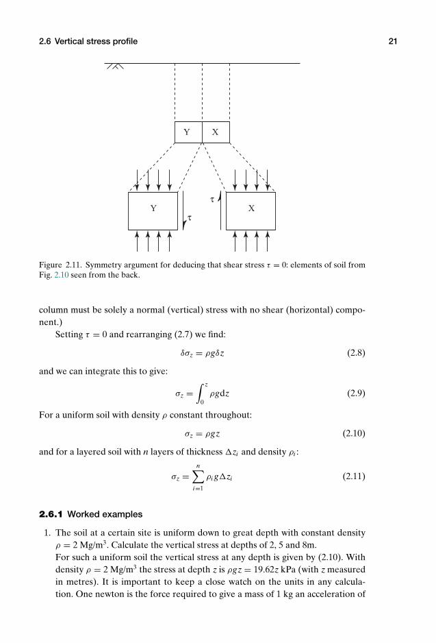
Figure 2.10. Symmetry argument for deducing that shear stress τ = 0.

the element are the stress σz acting over area A at the top of the element, the self-weight of the element calculated from its volume Aδz, density ρ and gravitationalacceleration g, together with any shear stresses τ acting round the periphery of theelement, which has an area sδz where s is the perimeter. We find then:

−(σz + δσz)A + σzA + ρg Aδz − τ sδz = 0 (2.7)

What can we deduce about the shear stress τ?There are often arguments that can be used to simplify analyses which rely

solely on appreciation of the symmetry constraints of the problem. We are consid-ering the concept of a soil layer of large lateral extent. This implies that conditionsat the same depth z everywhere in the soil layer are the same. Let us suppose thatthere are indeed non-zero shear stresses on element X in one column (Fig. 2.10).Equilibrium, in the sense of balancing of forces across interfaces, requires that theremust be an equal and opposite shear stress on the adjacent element Y. But the soilmass is of large lateral extent and no one soil column is any different from anyother soil column: it is not possible for there to be shear stresses in opposite direc-tions on identical columns. The only permissible solution is that the shear stresseson vertical boundaries are in fact zero. Another way of thinking through this ques-tion is to imagine viewing the pair of elements X and Y from the back (Fig. 2.11):the signs of the shear stresses are reversed but, since the choice of elements wasentirely arbitrary, there can be no difference between the elements in Fig. 2.10 andFig. 2.11: we could interchange the labelling of the elements X and Y. The only wayto make the elements in these two figures match is to insist that the interface shearstress τ between the elements is zero. (An exactly similar argument could be used todemonstrate that the stress on the horizontal base of any section through our soil

P1: KAE


2.6 Vertical stress profile 21

τ

τY

Y

X

X

Figure 2.11. Symmetry argument for deducing that shear stress τ = 0: elements of soil fromFig. 2.10 seen from the back.

column must be solely a normal (vertical) stress with no shear (horizontal) compo-nent.)

Setting τ = 0 and rearranging (2.7) we find:

δσz = ρgδz (2.8)

and we can integrate this to give:

σz =∫ z

0ρgdz (2.9)

For a uniform soil with density ρ constant throughout:

σz = ρgz (2.10)

and for a layered soil with n layers of thickness zi and density ρi :

σz =n∑

i=1

ρi gzi (2.11)

2.6.1 Worked examples

1. The soil at a certain site is uniform down to great depth with constant densityρ = 2 Mg/m3. Calculate the vertical stress at depths of 2, 5 and 8m.For such a uniform soil the vertical stress at any depth is given by (2.10). Withdensity ρ = 2 Mg/m3 the stress at depth z is ρgz = 19.62z kPa (with z measuredin metres). It is important to keep a close watch on the units in any calcula-tion. One newton is the force required to give a mass of 1 kg an acceleration of

P1: KAE


22 Stress in soils

1 m/s2. If you work consistently in kilograms and metres, calculations of stresseswill emerge in pascals where one pascal (1 Pa) is equal to one newton per squaremetre (1 N/m2). However, it may often be convenient to deal with recognisedmultiples of these basic units such that the numbers themselves can be writtenmore conveniently (though of course the magnitudes of the quantities do notchange). Thus densities might be written in megagrams (Mg) rather than kilo-grams (kg) per cubic metre: density of water is 1 Mg/m3 – or 1000 kg/m3; densityof soil is typically around 1.5–2 Mg/m3 – or 1500–2000 kg/m3. Typical stressesin the ground are in the thousands of pascals, as we see here: it makes sense touse kilopascals as the unit. Thus in using the given information about densityin Mg/m3 and producing a result for vertical stress in kPa we have incorporatedtwo cancelling factors of 1000 in this expression. We have defined our densityρ in terms of megagrams (1 megagram = 1000 kilograms) and have produced aresult in kilopascals (1 kilopascal = 1000 pascals). Beware!At depth 2 m, σz = 39.24 kPa, at depth 5 m, σz = 98.1 kPa, and at depth 8 mσz = 156.96 kPa.It is often convenient to approximate the acceleration due to gravity as 10 m/s2

which makes mental arithmetic calculation slightly simpler and the numbersrounder. The three stresses in this example would then become 40, 100 and160 kPa at depths 2, 5 and 8 m, respectively.

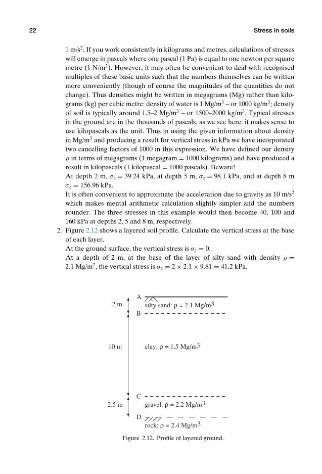
2. Figure 2.12 shows a layered soil profile. Calculate the vertical stress at the baseof each layer.At the ground surface, the vertical stress is σz = 0.At a depth of 2 m, at the base of the layer of silty sand with density ρ =2.1 Mg/m2, the vertical stress is σz = 2 × 2.1 × 9.81 = 41.2 kPa.

silty sand: ρ = 2.1 Mg/m3

clay: ρ = 1.5 Mg/m3

gravel: ρ = 2.2 Mg/m3

rock: ρ = 2.4 Mg/m3

2 m

10 m

2.5 m

A

B

C

D

Figure 2.12. Profile of layered ground.

P1: KAE


2.7 Water in the ground: Introduction to hydrostatics 23

z

u

small horizontal

plate

Figure 2.13. Pressure in pool of water acting on small horizontal pressure plate.

At a depth of 12 m, at the base of the clay layer with density ρ = 1.5 Mg/m3, thevertical stress is the sum of the effects of the layer of silty sand and the layer ofclay: σz = 2 × 2.1 × 9.81 + 10 × 1.5 × 9.81 = 41.2 + 147.1 = 188.3 kPa.At a depth of 14.5 m, at the base of the gravel layer with density ρ = 2.2 Mg/m3,the vertical stress is the sum of the effects of the layer of silty sand and thelayer of clay and the layer of gravel: σz = 2 × 2.1 × 9.81 + 10 × 1.5 × 9.81 +2.5 × 2.2 × 9.81 = 188.3 + 54.0 = 242.3 kPa.

2.7 Water in the ground: Introduction to hydrostatics

If you dig a hole on the beach then it is likely that you will eventually encounterwater because of the proximity of the sea. In fact in temperate climates (suchas the United Kingdom) there is quite a good chance that any hole will en-counter water if it is dug deep enough. The height above sea level at which thiswater table is encountered will depend on local topography and ground conditions.We need to understand how the presence of water will influence our thoughts aboutthe stresses existing in the ground. We therefore introduce a brief discussion abouthydrostatics.

Hydrostatics is that branch of mechanics which is concerned with fluids whichare stationary. We will encounter (slowly) moving fluids in Chapter 5. For the mostpart, the fluid with which we will be concerned will be water – though there maybe situations where there are hydrocarbons or other liquids present. We start bythinking of a pool of water – a swimming pool or a lake – with no soil present. Thefirst idea to be grasped is that of fluid pressure. Following an argument similar tothat used to calculate the vertical stress in soils in Section 2.6 we can deduce that thestress acting on a little horizontal plate at a depth z below the surface of the pool(Fig. 2.13) will be:

u = ρwgz (2.12)

where ρw is the density of the water.

P1: KAE


24 Stress in soils

z

u u u u

small pressure measurement

plates

Figure 2.14. Pressure in pool of water acting on small pressure plates at different orienta-tions.

The density of fresh water is ρw = 1 Mg/m3 = 1000 kg/m3. However, the dis-solved salts in sea water increase the density. Typical ocean water has a salt contentof about 3.5% and a density of around 1.027 Mg/m3. The Dead Sea has a salt contentof around 35% and density 1.24 Mg/m3, thus making it easier to float. By contrast,a somewhat enclosed sea like the Baltic, with much regular injection of fresh water,has a salt content typically around 1% and density only slightly greater than freshwater.

It is a property of fluids at rest that the stress exerted is independent of theorientation of the little measuring plate on which it is acting but is dependent onlyon the depth below the free surface (Fig. 2.14). Stationary water cannot transmitshear stresses. We can then imagine that these little measuring plates are in fact justmeasuring planes drawn in the fluid but having no material presence: the resultingstress on each plane is, as before, the same. Such a “hydrostatic” stress in a fluid ismore usually described as a fluid pressure and, since we are not usually concerned totry to pull fluids apart, pressure is helpfully deemed to be positive in compression.

Another way of visualising this intuitive property is to imagine standpipes withvarious geometries inserted in the pool at the same depth as shown in Fig. 2.15. Thewater in each standpipe will rise to the level of the water surface. The pressure atthe mouth of each standpipe is found directly from the height z of the free surfaceabove the opening.

We know that objects float in water. Archimedes’ principle says that an objectwholly or partially immersed in a fluid (water will be a particular fluid) is buoyed upby a force equal to the weight of the displaced fluid. We can understand this resultby applying our recently acquired knowledge of pressure in fluids. Let us consider acuboidal object wholly submerged in the pool of water with the faces of the cuboidaligned with vertical and horizontal axes, as shown in Fig. 2.16. The lengths of thesides of the object are x, y and z and the top surface of the object is at a depthz below the water surface. There will be forces Fx1, Fx2, Fy1, Fy2, Fz1, Fz2 actingon the faces of the object, as shown. We can calculate the magnitude of each ofthese forces by integrating the water pressure over each face. Because of the chosen

P1: KAE



A B C D E

z

Figure 2.15. Standpipes A, B, C, D, E in pool of water with opening at depth z: the waterrises to exactly the same level in each of the standpipes.

orientation of the object, the forces on opposite vertical faces must balance exactly:Fx1 = Fx2, Fy1 = Fy2. The water pressure acts perpendicularly to the face and forevery little element on one face acted on by a certain magnitude of water pressurethere is an identical element on the opposite face acted on by the same magnitude ofwater pressure. The water pressure varies linearly with depth and hence the averagepressure on each of the faces of the element shown in Fig. 2.16 can be calculatedat the midpoint of that face. Thus Fx1 = Fx2 = ρwg(z + z/2)yz; Fy1 = Fy2 =ρwg(z + z/2)xz. (These forces act on the faces of the cuboidal element at alevel z + 2z/3 below the surface of the pool.)

In the vertical, z, direction we can calculate the force on the top of the objectfrom the pressure – ρwgz, from (2.12) – and the area over which it acts (xy):

Fz1 = ρwgzxy (2.13)

Similarly, the force on the bottom of the object can be calculated as:

Fz2 = ρwg(z + z)xy (2.14)

∆x

∆z

z

∆y

Fx1

Fy1

Fz1

Fz2

Fx2

Fy2

Figure 2.16. Cuboidal object submerged in a pool of water: water pressure produces forcesFx1, . . . on each face of the object.

P1: KAE


26 Stress in soils

Figure 2.17. Hot air balloon taking advantage of Archimedes uplift.

The out-of-balance force tending to push the object upwards is:

Fz2 − Fz1 = ρwg(z + z)xy − ρwgzxy = ρwgzxy (2.15)

and this is precisely the weight of the water displaced by the object. This is an out-of-balance force from the water pressures: the object will tend to move up or movedown or stay where it is depending on its own weight in relation to the weight of thewater that it displaces. A submerged object with a weight less than the weight of thedisplaced water will have to be tethered in some way to maintain its position; if it hasa greater weight then it will have to be propped if it is not to sink. A hot air balloonhas neutral buoyancy and floats in its surrounding fluid – air – with its weight exactlymatching the Archimedean uplift (Fig. 2.17). The density of the Earth’s atmospheredecreases with height above the Earth’s surface so, to enable the balloon to climb,the air in the balloon is heated to decrease its density and hence its weight: theballoon rises until a vertical equilibrium is again attained.

Our calculation of the buoyancy force on the cuboidal object in Fig. 2.16 can beapplied to an element of any size – we can make x, y and z as small as we like,even infinitesimally small. Any object of any shape can be thought of as made up ofa large number of very small elements and, applying principles of calculus, we canintegrate the out-of-balance force to discover that it is always equal to the weight ofthe water that is displaced.

2.7.1 Worked example: Archimedes uplift on spherical object

1. A solid sphere of aluminium alloy with diameter 50 mm is suspended from awire in a bowl of fresh water (Fig. 2.18). What is the force F1 in the wire?

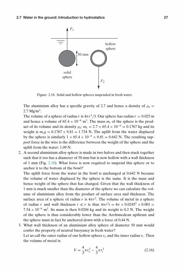
P1: KAE



solid sphere

hollow sphere

50 mm

F1

F2

Figure 2.18. Solid and hollow spheres suspended in fresh water.

The aluminium alloy has a specific gravity of 2.7 and hence a density of ρa =2.7 Mg/m3.The volume of a sphere of radius r is 4πr3/3. Our sphere has radius r = 0.025 mand hence a volume of 65.4 × 10−6 m3. The mass ms of the sphere is the prod-uct of its volume and its density ρa : ms = 2.7 × 65.4 × 10−6 = 0.1767 kg and itsweight is ms g = 0.1767 × 9.81 = 1.734 N. The uplift from the water displacedby the sphere is similarly 1 × 65.4 × 10−6 × 9.81 = 0.642 N. The resulting sup-port force in the wire is the difference between the weight of the sphere and theuplift from the water: 1.09 N.

2. A second aluminium alloy sphere is made in two halves and then stuck togethersuch that it too has a diameter of 50 mm but is now hollow with a wall thicknessof 1 mm (Fig. 2.18). What force is now required to suspend this sphere or toanchor it to the bottom of the bowl?The uplift force from the water in the bowl is unchanged at 0.642 N becausethe volume of water displaced by the sphere is the same. It is the mass andhence weight of the sphere that has changed. Given that the wall thickness of1 mm is much smaller than the diameter of the sphere we can calculate the vol-ume of aluminium alloy from the product of surface area and thickness. Thesurface area of a sphere of radius r is 4πr2. The volume of metal in a sphereof radius r and wall thickness t r is thus 4πr2t = 4π × 0.02452 × 0.001 =7.54 × 10−6 m3. Its mass is then 0.0204 kg and its weight is 0.2 N. The weightof the sphere is thus considerably lower than the Archimedean upthrust andthe sphere must in fact be anchored down with a force of 0.44 N.

3. What wall thickness of an aluminium alloy sphere of diameter 50 mm wouldconfer the property of neutral buoyancy in fresh water?Let us call the outer radius of our hollow sphere ro and the inner radius ri . Thenthe volume of metal is:

V = 43πr3

o − 43πr3

i (2.16)

P1: KAE


28 Stress in soils

and neutral buoyancy requires that:

ρag[

43πr3

o − 43πr3

i

]= ρwg

43πr3

o (2.17)

so that: [ri

ro

]3

= ρa − ρw

ρa(2.18)

We have ρa = 2.7ρw and ro = 0.025 m so that ri = 0.021 m and the required wallthickness of the hollow sphere is 3.6 mm.

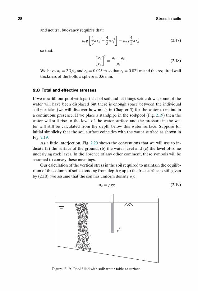
2.8 Total and effective stresses

If we now fill our pool with particles of soil and let things settle down, some of thewater will have been displaced but there is enough space between the individualsoil particles (we will discover how much in Chapter 3) for the water to maintaina continuous presence. If we place a standpipe in the soil/pool (Fig. 2.19) then thewater will still rise to the level of the water surface and the pressure in the wa-ter will still be calculated from the depth below this water surface. Suppose forinitial simplicity that the soil surface coincides with the water surface as shown inFig. 2.19.

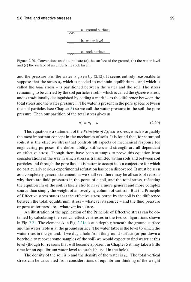
As a little interjection, Fig. 2.20 shows the conventions that we will use to in-dicate (a) the surface of the ground, (b) the water level and (c) the level of someunderlying rock layer. In the absence of any other comment, these symbols will beassumed to convey these meanings.

Our calculation of the vertical stress in the soil required to maintain the equilib-rium of the column of soil extending from depth z up to the free surface is still givenby (2.10) (we assume that the soil has uniform density ρ):

σz = ρgz (2.19)

z

Figure 2.19. Pool filled with soil: water table at surface.

P1: KAE


2.8 Total and effective stresses 29

a. ground surface

b. water level

c. rock surface

Figure 2.20. Conventions used to indicate (a) the surface of the ground, (b) the water leveland (c) the surface of an underlying rock layer.

and the pressure u in the water is given by (2.12). It seems entirely reasonable tosuppose that the stress σz which is needed to maintain equilibrium – and which iscalled the total stress – is partitioned between the water and the soil. The stressremaining to be carried by the soil particles itself – which is called the effective stress,and is traditionally distinguished by adding a mark ′ – is the difference between thetotal stress and the water pressure u. The water is present in the pore spaces betweenthe soil particles (see Chapter 3) so we call the water pressure in the soil the porepressure. Then our partition of the total stress gives us:

σ ′z = σz − u (2.20)

This equation is a statement of the Principle of Effective stress, which is arguablythe most important concept in the mechanics of soils. It is found that, for saturatedsoils, it is the effective stress that controls all aspects of mechanical response forengineering purposes: the deformability, stiffness and strength are all dependenton effective stress. Though there have been attempts to prove this equation fromconsiderations of the way in which stress is transmitted within soils and between soilparticles and through the pore fluid, it is better to accept it as a conjecture for whichno particularly serious experimental refutation has been discovered. It must be seenas a completely general statement: as we shall see, there may be all sorts of reasonswhy there are fluid pressures in the pores of a soil, and the total stress, reflectingthe equilibrium of the soil, is likely also to have a more general and more complexsource than simply the weight of an overlying column of wet soil. But the Principleof Effective stress states that the effective stress borne by the soil is the differencebetween the total, equilibrium, stress – whatever its source – and the fluid pressureor pore water pressure – whatever its source.

An illustration of the application of the Principle of Effective stress can be ob-tained by calculating the vertical effective stresses in the two configurations shownin Fig. 2.21. The element A in Fig. 2.21a is at a depth z beneath the ground surfaceand the water table is at the ground surface. The water table is the level to which thewater rises in the ground. If we dug a hole from the ground surface (or put down aborehole to recover some samples of the soil) we would expect to find water at thislevel (though for reasons that will become apparent in Chapter 5 it may take a littletime for an equilibrium water level to establish itself in the hole).

The density of the soil is ρ and the density of the water is ρw. The total verticalstress can be calculated from considerations of equilibrium thinking of the weight

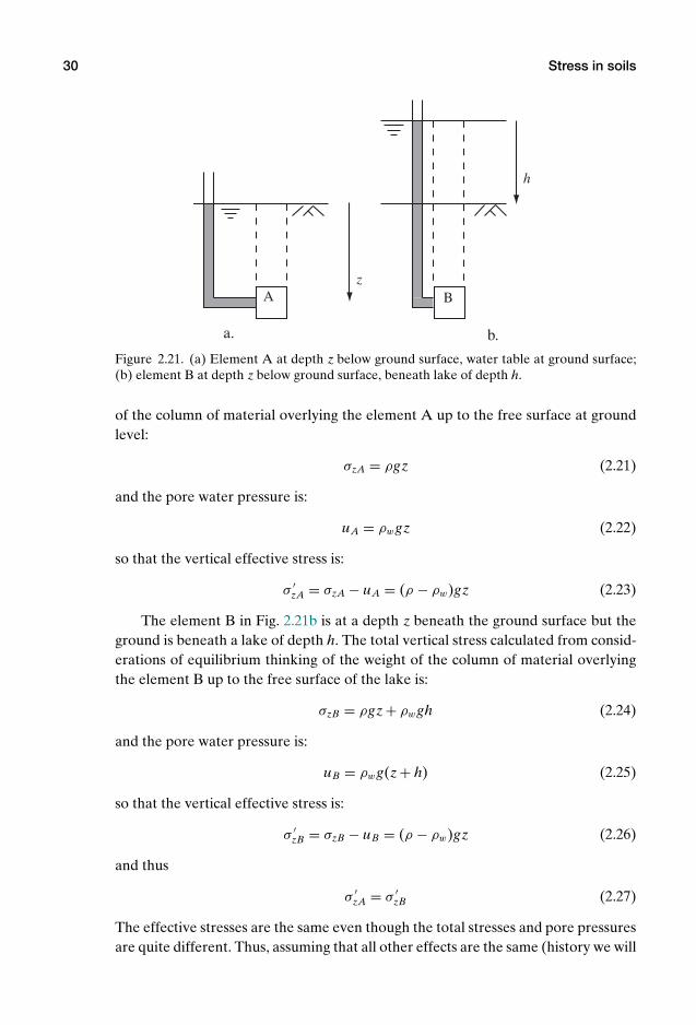
P1: KAE


30 Stress in soils

a. b.

Az

h

B

Figure 2.21. (a) Element A at depth z below ground surface, water table at ground surface;(b) element B at depth z below ground surface, beneath lake of depth h.

of the column of material overlying the element A up to the free surface at groundlevel:

σzA = ρgz (2.21)

and the pore water pressure is:

uA = ρwgz (2.22)

so that the vertical effective stress is:

σ ′zA = σzA − uA = (ρ − ρw)gz (2.23)

The element B in Fig. 2.21b is at a depth z beneath the ground surface but theground is beneath a lake of depth h. The total vertical stress calculated from consid-erations of equilibrium thinking of the weight of the column of material overlyingthe element B up to the free surface of the lake is:

σzB = ρgz + ρwgh (2.24)

and the pore water pressure is:

uB = ρwg(z + h) (2.25)

so that the vertical effective stress is:

σ ′zB = σzB − uB = (ρ − ρw)gz (2.26)

and thus

σ ′zA = σ ′

zB (2.27)

The effective stresses are the same even though the total stresses and pore pressuresare quite different. Thus, assuming that all other effects are the same (history we will

P1: KAE



a. b.

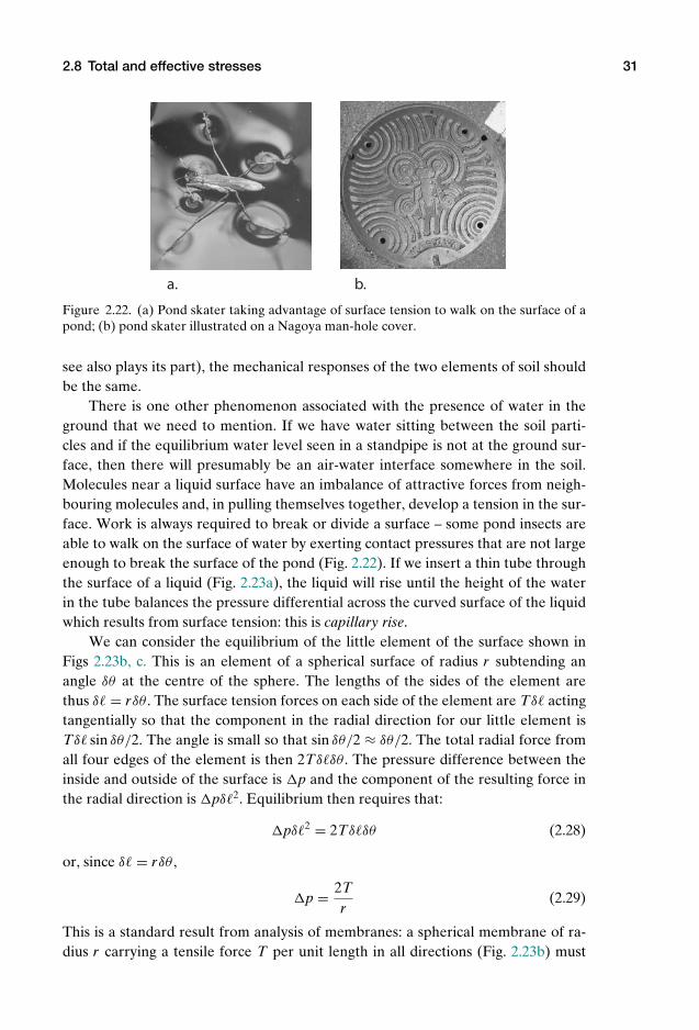
Figure 2.22. (a) Pond skater taking advantage of surface tension to walk on the surface of apond; (b) pond skater illustrated on a Nagoya man-hole cover.

see also plays its part), the mechanical responses of the two elements of soil shouldbe the same.

There is one other phenomenon associated with the presence of water in theground that we need to mention. If we have water sitting between the soil parti-cles and if the equilibrium water level seen in a standpipe is not at the ground sur-face, then there will presumably be an air-water interface somewhere in the soil.Molecules near a liquid surface have an imbalance of attractive forces from neigh-bouring molecules and, in pulling themselves together, develop a tension in the sur-face. Work is always required to break or divide a surface – some pond insects areable to walk on the surface of water by exerting contact pressures that are not largeenough to break the surface of the pond (Fig. 2.22). If we insert a thin tube throughthe surface of a liquid (Fig. 2.23a), the liquid will rise until the height of the waterin the tube balances the pressure differential across the curved surface of the liquidwhich results from surface tension: this is capillary rise.

We can consider the equilibrium of the little element of the surface shown inFigs 2.23b, c. This is an element of a spherical surface of radius r subtending anangle δθ at the centre of the sphere. The lengths of the sides of the element arethus δ = rδθ . The surface tension forces on each side of the element are Tδ actingtangentially so that the component in the radial direction for our little element isTδ sin δθ/2. The angle is small so that sin δθ/2 ≈ δθ/2. The total radial force fromall four edges of the element is then 2Tδδθ . The pressure difference between theinside and outside of the surface is p and the component of the resulting force inthe radial direction is pδ2. Equilibrium then requires that:

pδ2 = 2Tδδθ (2.28)

or, since δ = rδθ ,

p = 2Tr

(2.29)

This is a standard result from analysis of membranes: a spherical membrane of ra-dius r carrying a tensile force T per unit length in all directions (Fig. 2.23b) must

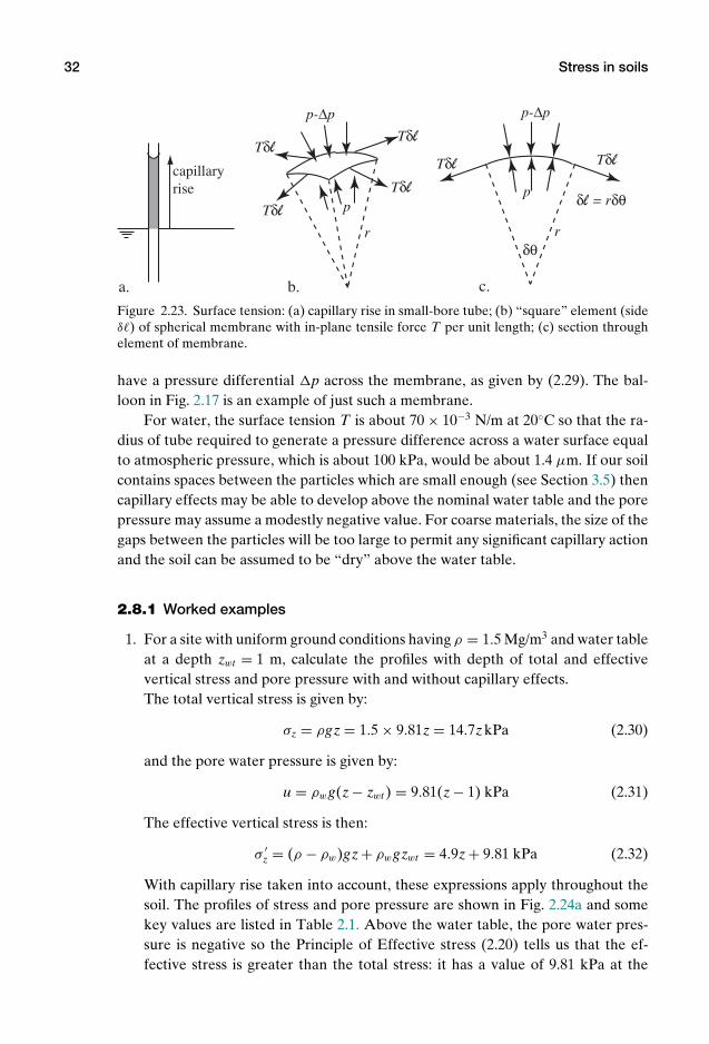
P1: KAE


32 Stress in soils

capillaryrise

r r

Tδl

Tδlδl = rδθ

δθ

Tδl TδlTδl

Tδl

a. b. c.

pp

p-∆p p-∆p

Figure 2.23. Surface tension: (a) capillary rise in small-bore tube; (b) “square” element (sideδ) of spherical membrane with in-plane tensile force T per unit length; (c) section throughelement of membrane.

have a pressure differential p across the membrane, as given by (2.29). The bal-loon in Fig. 2.17 is an example of just such a membrane.

For water, the surface tension T is about 70 × 10−3 N/m at 20C so that the ra-dius of tube required to generate a pressure difference across a water surface equalto atmospheric pressure, which is about 100 kPa, would be about 1.4 µm. If our soilcontains spaces between the particles which are small enough (see Section 3.5) thencapillary effects may be able to develop above the nominal water table and the porepressure may assume a modestly negative value. For coarse materials, the size of thegaps between the particles will be too large to permit any significant capillary actionand the soil can be assumed to be “dry” above the water table.

2.8.1 Worked examples

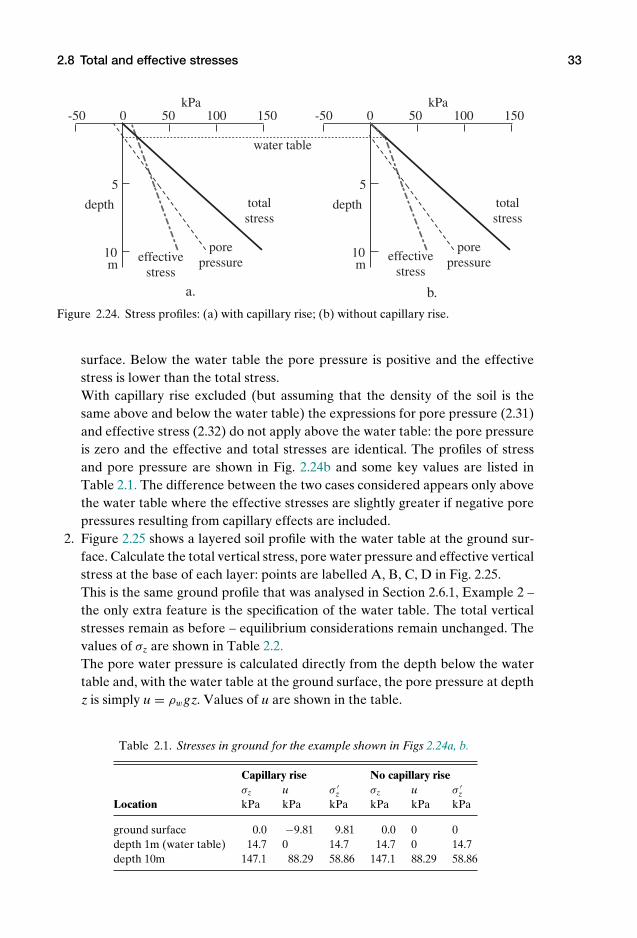
1. For a site with uniform ground conditions having ρ = 1.5 Mg/m3 and water tableat a depth zwt = 1 m, calculate the profiles with depth of total and effectivevertical stress and pore pressure with and without capillary effects.The total vertical stress is given by:

σz = ρgz = 1.5 × 9.81z = 14.7zkPa (2.30)

and the pore water pressure is given by:

u = ρwg(z − zwt ) = 9.81(z − 1) kPa (2.31)

The effective vertical stress is then:

σ ′z = (ρ − ρw)gz + ρwgzwt = 4.9z + 9.81 kPa (2.32)

With capillary rise taken into account, these expressions apply throughout thesoil. The profiles of stress and pore pressure are shown in Fig. 2.24a and somekey values are listed in Table 2.1. Above the water table, the pore water pres-sure is negative so the Principle of Effective stress (2.20) tells us that the ef-fective stress is greater than the total stress: it has a value of 9.81 kPa at the

P1: KAE



-50 0 50 100 150kPa

-50 0 50 100 150kPa

5

10m

depth

5

10m

depthtotalstress

porepressure

totalstress

effectivestress

effectivestress

porepressure

a. b.

water table

Figure 2.24. Stress profiles: (a) with capillary rise; (b) without capillary rise.

surface. Below the water table the pore pressure is positive and the effectivestress is lower than the total stress.With capillary rise excluded (but assuming that the density of the soil is thesame above and below the water table) the expressions for pore pressure (2.31)and effective stress (2.32) do not apply above the water table: the pore pressureis zero and the effective and total stresses are identical. The profiles of stressand pore pressure are shown in Fig. 2.24b and some key values are listed inTable 2.1. The difference between the two cases considered appears only abovethe water table where the effective stresses are slightly greater if negative porepressures resulting from capillary effects are included.

2. Figure 2.25 shows a layered soil profile with the water table at the ground sur-face. Calculate the total vertical stress, pore water pressure and effective verticalstress at the base of each layer: points are labelled A, B, C, D in Fig. 2.25.This is the same ground profile that was analysed in Section 2.6.1, Example 2 –the only extra feature is the specification of the water table. The total verticalstresses remain as before – equilibrium considerations remain unchanged. Thevalues of σz are shown in Table 2.2.The pore water pressure is calculated directly from the depth below the watertable and, with the water table at the ground surface, the pore pressure at depthz is simply u = ρwgz. Values of u are shown in the table.

Table 2.1. Stresses in ground for the example shown in Figs 2.24a, b.

Capillary rise No capillary riseσz u σ ′

z σz u σ ′z

Location kPa kPa kPa kPa kPa kPa

ground surface 0.0 −9.81 9.81 0.0 0 0depth 1m (water table) 14.7 0 14.7 14.7 0 14.7depth 10m 147.1 88.29 58.86 147.1 88.29 58.86

P1: KAE


34 Stress in soils





2 m

10 m

2.5 m

A

B

C

D

water table

Figure 2.25. Example 2: Profile of layered ground.

Then the effective vertical stress is calculated from the difference between thetotal vertical stress and the pore water pressure. The effective stress is the stressthat remains to be supported by the soil after removing the contribution of thewater pressure to the vertical equilibrium of the soil column at any depth. Val-ues of σ ′

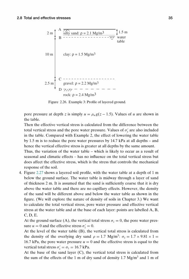
z are also included in the table.3. Figure 2.26 shows the same layered soil profile but with the water table at a

depth of 1.5 m below the ground surface. Calculate the total vertical stress, porewater pressure and effective vertical stress at the base of each layer: points arelabelled A, B, C, D. We will assume that the silty sand layer just beneath theground surface is able to support capillary suction.This is the same ground profile that was analysed in Example 2 – the only fea-ture that has changed is the location of the water table. The total vertical stressesremain as before – equilibrium considerations remain unchanged. The values ofσz are shown in Table 2.2.The pore water pressure is calculated directly from the depth below the watertable and, with the water table at a depth of 1.5 m below the ground surface, the

Table 2.2. Stresses in ground (Figs 2.25 and 2.26).

Water table at Water table atsurface (Fig. 2.25) depth 1.5 m (Fig. 2.26)σz u σ ′

z σz u σ ′z

Location kPa kPa kPa kPa kPa kPa

ground surface A 0.0 0.0 0.0 0.0 −14.7 14.7base of silty sand B 41.2 19.6 21.6 41.2 4.9 36.3base of clay C 188.3 117.7 70.6 188.3 103.0 85.3base of gravel D 242.3 142.2 100.1 242.3 127.5 114.8

P1: KAE







2 m

10 m

2.5 m

1.5 mA

B

C

D

water table


pore pressure at depth z is simply u = ρwg(z − 1.5). Values of u are shown inthe table.Then the effective vertical stress is calculated from the difference between thetotal vertical stress and the pore water pressure. Values of σ ′

z are also includedin the table. Compared with Example 2, the effect of lowering the water tableby 1.5 m is to reduce the pore water pressures by 14.7 kPa at all depths – andhence the vertical effective stress is greater at all depths by the same amount.Thus, the variation of the water table – which is likely to occur as a result ofseasonal and climatic effects – has no influence on the total vertical stress butdoes affect the effective stress, which is the stress that controls the mechanicalresponse of the soil.

4. Figure 2.27 shows a layered soil profile, with the water table at a depth of 1 mbelow the ground surface. The water table is midway through a layer of sandof thickness 2 m. It is assumed that the sand is sufficiently coarse that it is dryabove the water table and there are no capillary effects. However, the densityof the sand will be different above and below the water table as shown in thefigure. (We will explore the nature of density of soils in Chapter 3.) We wantto calculate the total vertical stress, pore water pressure and effective verticalstress at the water table and at the base of each layer: points are labelled A, B,C, D, E.At the ground surface (A), the vertical total stress σz = 0, the pore water pres-sure u = 0 and the effective stress σ ′

z = 0.At the level of the water table (B), the vertical total stress is calculated fromthe density of the overlying dry sand ρ = 1.7 Mg/m3: σz = 1.7 × 9.81 × 1 =16.7 kPa, the pore water pressure u = 0 and the effective stress is equal to thevertical total stress σ ′

z = σz = 16.7 kPa.At the base of the sand layer (C), the vertical total stress is calculated fromthe sum of the effects of the 1 m of dry sand of density 1.7 Mg/m3 and 1 m of

P1: KAE


36 Stress in soils

sand (dry): ρ = 1.7 Mg/m3

sand (saturated): ρ = 2.0 Mg/m3


sand: ρ = 2.1 Mg/m3


1 m

1 m

6 m

1 m

A

B

C

D

E

water table


saturated sand of density ρ = 2.0 Mg/m3: σz = 1.7 × 9.81 × 1 + 2.0 × 9.81 × 1 =36.3 kPa. The pore water pressure at a depth of 1 m below the water table isequivalent to a head of 1 m of water: u = 9.81 kPa and the effective stress is thedifference: σ ′

z = σz − u = 36.3 − 9.81 = 26.5 kPa.At the base of the clay layer (D), the vertical total stress is calculated from thesum of the effects of the 1 m of dry sand of density 1.7 Mg/m3, 1 m of satu-rated sand of density 2.0 Mg/m3, and 6 m of clay of density ρ = 1.6 Mg/m3: σz =1.7 × 9.81 × 1 + 2.0 × 9.81 × 1 + 1.6 × 9.81 × 6 = 130.5 kPa. The pore waterpressure at a depth of 7 m below the water table is equivalent to a head of7 m of water: u = 7 × 9.81 = 68.7 kPa and the effective stress is the difference:σ ′

z = σz − u = 130.5 − 68.7 = 61.8 kPa.At the base of the lower sand layer (E), the vertical total stress is calculated fromthe sum of the effects of the 1 m of dry sand, 1 m of saturated sand, 6 m of clay,and 1 m of sand of density ρ = 2.1 Mg/m3: σz = 1.7 × 9.81 × 1 + 2.0 × 9.81 ×1 + 1.6 × 9.81 × 6 + 2.1 × 9.81 × 1 = 151.1 kPa. The pore water pressure at a

Table 2.3. Stresses in ground (Fig. 2.27).

σz u σ ′z

Location kPa kPa kPa

ground surface A 0.0 0.0 0.0water table B 16.7 0.0 16.7base of sand C 36.3 9.8 26.5base of clay D 130.5 68.7 61.8base of sand E 151.1 78.5 72.6

P1: KAE


2.9 Summary 37

depth of 8 m below the water table is equivalent to a head of 8 m of water:u = 8 × 9.81 = 78.5 kPa and the effective stress is the difference: σ ′

z = σz − u =151.1 − 78.5 = 72.6 kPa.These values are shown in Table 2.3.

2.9 Summary

Here is a concise list of the key messages from this chapter, which are also encapsu-lated in the mind map (Fig. 2.28).

1. Newton’s First Law requires the forces acting on stationary objects to be inequilibrium.

2. Weight is the effect on mass of a local gravitational field. Weight is a force. Ifmass is measured in kilograms (kg) then force is measured in newtons (N). Amass of 1 kg at the surface of the Earth weighs about 10 N.

3. Stress is an indication of the areal intensity of force and is measured in pascals(Pa): 1 Pa = 1 N/m2. Typically, stresses in soils will be quoted in kilopascals(kPa) and compression stresses will be taken as positive.

4. The vertical total stress at a particular depth in the ground can be calculatedfrom the thickness and density of the layers making up the soil column abovethat depth.

5. At a point in a fluid at rest, the pressure is the same in all directions and iscalculated from the depth below the free fluid (water) surface.

6. The total stress in the ground calculated from equilibrium is divided betweenthe water pressure in the pores of the soil and the effective stress which is carriedby the soil itself.

7. The Principle of Effective stress is fundamental to understanding of soil be-haviour: mechanical properties of soils are controlled by the effective stresses.Effective stress is the difference between total stress and pore water pressure.

2.10 Exercises: Profiles of total stress, effective stress, pore pressure

1. A ground profile consists of 3 m of silty sand of density ρ = 2.0 Mg/m3 overlying12 m of clay with ρ = 1.6 Mg/m3 which is underlain by 5 m of gravel with ρ =2.3 Mg/m3 and then rock. Calculate the total vertical stress at depths 0, 3, 15 and20 m.

2. The water table for the ground profile described in Question 1 is at the groundsurface. Calculate the total vertical stress, pore water pressure and effective ver-tical stress at depths 0, 3, 15 and 20 m.

3. The water table for the ground profile in Question 1 is at depth 1.5 m below theground surface. Assume that the density of the silty sand is the same above andbelow the water table. Calculate the total vertical stress, pore water pressureand effective vertical stress at depths 0, 3, 15 and 20 m.

4. The ground profile at a certain site consists of 3 m of coarse sand, overlying 4 mof fine sand, which overlies 2 m of sandy gravel and then rock. The water table

P1:K

AE

OneD

im00a

CU

US648/M

uir978

0521

517737

August17,2009

19:12

stress in soils

equilibrium

σz= ρgdz0

z

or σz = Σ ρg∆z

zσz

layers?

stress: areal intensity of force

normal stress

shear stress

z

z

u

hydrostatics

water pressure

pore water pressure in soil u = ρwgz

u = ρwgz

Principle of Effective stress

effective stress = total stress - pore pressure

from equilibriumσ'z = σz - u

effective stresses indicated by '

mechanical behaviour of soils controlled by

effective stresses

massweight

kg N

Pa

N/m2

Figure 2.28. Mind map: stress in soils.

38

P1: KAE


2.10 Exercises: Profiles of total stress, effective stress, pore pressure 39

is at a depth of 3 m. The densities of the three layers are: coarse sand 1.8 Mg/m3,fine sand 2.0 Mg/m3, sandy gravel 1.9 Mg/m3. Calculate the total vertical stress,pore water pressure and effective vertical stress at depths 3, 7 and 9 m.

5. At the site in Question 2.10 the water table rises to a depth of 1.5 m belowthe ground surface. The density of the coarse sand below the water table is2.1 Mg/m3. Calculate the total vertical stress, pore water pressure and effectivevertical stress at depths 3, 7 and 9 m, and hence calculate the change in effectivestress at each of these depths.

6. At a coastal site the ground conditions consist of 8 m of silty sand, overlying2 m of gravel and then rock. The density of the silty sand is 1.7 Mg/m3 abovethe water table and 1.9 Mg/m3 below the water table. The density of the gravelis 2.1 Mg/m3. The water table varies regularly between 1 m and 4 m below theground surface. What are the maximum and minimum vertical effective stressesat a depth of 4 m?

P1: KAE


3 Density

3.1 Introduction

In Chapter 2 we calculated profiles of vertical stress in the ground on the assumptionthat we knew the value of the density of each of the several layers of soil. We alsonoted that soils consist of individual particles packed together in such a way thatthere will generally be spaces between them – voids – which may contain air or wateror a combination of air and water (or other fluid). Knowing the relative proportionsof space occupied by solid and liquid and gas, and knowing the densities of theindividual components, we can estimate the density of the overall mixture that isthe soil.

Density is obviously essential for the calculation of stress, but the mechanicalbehaviour of soils is also strongly influenced by the way in which the soil particlesare packed together. It seems intuitively obvious that the greater the proportionof the volume of a material that is occupied by “nothing” the lower will be the re-sistance of that material to imposition of loads, so we will need to explore densityand packing in parallel. It is unfortunate that soil mechanics has been endowed witha plethora of different ways of describing aspects of the distribution of materialswithin the mixture – the effectiveness of the packing of the particles – and, althoughreally only two or three of these are necessary (and indeed sufficient) for the presen-tation and understanding of the response of soils, some familiarity is required withall of them. Porous materials obviously occur in other contexts – sintered metals andfoams are just two examples – and it is probably inevitable that different disciplineshave produced different variables to characterise the nature of the relationship be-tween solid and pore space. Such differences help to preserve the hermetic mysteryof the mechanics of soils.

3.2 Units

The density of a material is its mass per unit volume, and we will measure it typicallyin kilograms per cubic metre (kg/m3). The density of water is ρw = 1000 kg/m3 andwe can save ourselves some zeroes (or powers of 10) by working in terms of mega-grams per cubic metre (Mg/m3) so that the density of water becomes ρw = 1 Mg/m3.

40

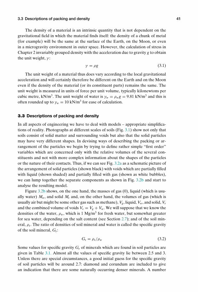
P1: KAE


3.3 Descriptions of packing and density 41

The density of a material is an intrinsic quantity that is not dependent on thegravitational field in which the material finds itself: the density of a chunk of metal(for example) will be the same at the surface of the Earth, on the Moon, or evenin a microgravity environment in outer space. However, the calculation of stress inChapter 2 invariably grouped density with the acceleration due to gravity g to obtainthe unit weight, γ :

γ = ρg (3.1)

The unit weight of a material thus does vary according to the local gravitationalacceleration and will certainly therefore be different on the Earth and on the Mooneven if the density of the material (or its constituent parts) remains the same. Theunit weight is measured in units of force per unit volume, typically kilonewtons percubic metre, kN/m3. The unit weight of water is γw = ρwg = 9.81 kN/m3 and this isoften rounded up to γw = 10 kN/m3 for ease of calculation.

3.3 Descriptions of packing and density

In all aspects of engineering we have to deal with models – appropriate simplifica-tions of reality. Photographs at different scales of soils (Fig. 3.1) show not only thatsoils consist of solid matter and surrounding voids but also that the solid particlesmay have very different shapes. In devising ways of describing the packing or ar-rangement of the particles we begin by trying to define rather simple “first order”variables which are concerned only with the relative volumes of the several con-stituents and not with more complex information about the shapes of the particlesor the nature of their contacts. Thus, if we can see Fig. 3.2a as a schematic picture ofthe arrangement of solid particles (shown black) with voids which are partially filledwith liquid (shown shaded) and partially filled with gas (shown as white bubbles),we can lump together the separate components as shown in Fig. 3.2b and start toanalyse the resulting model.

Figure 3.2b shows, on the one hand, the masses of gas (0), liquid (which is usu-ally water) Mw, and solid Ms and, on the other hand, the volumes of gas (which isusually air but might be some other gas such as methane), Vg , liquid, Vw, and solid, Vs

and the combined volume of voids Vv = Vg + Vw. We will suppose that we know thedensities of the water, ρw, which is 1 Mg/m3 for fresh water, but somewhat greaterfor sea water, depending on the salt content (see Section 2.7); and of the soil min-eral, ρs . The ratio of densities of soil mineral and water is called the specific gravityof the soil mineral, Gs :

Gs = ρs/ρw (3.2)

Some values for specific gravity Gs of minerals which are found in soil particles aregiven in Table 3.1. Almost all the values of specific gravity lie between 2.5 and 3.Unless there are special circumstances, a good initial guess for the specific gravityof soil particles will be around 2.7: diamond and corundum are included to givean indication that there are some naturally occurring denser minerals. A number

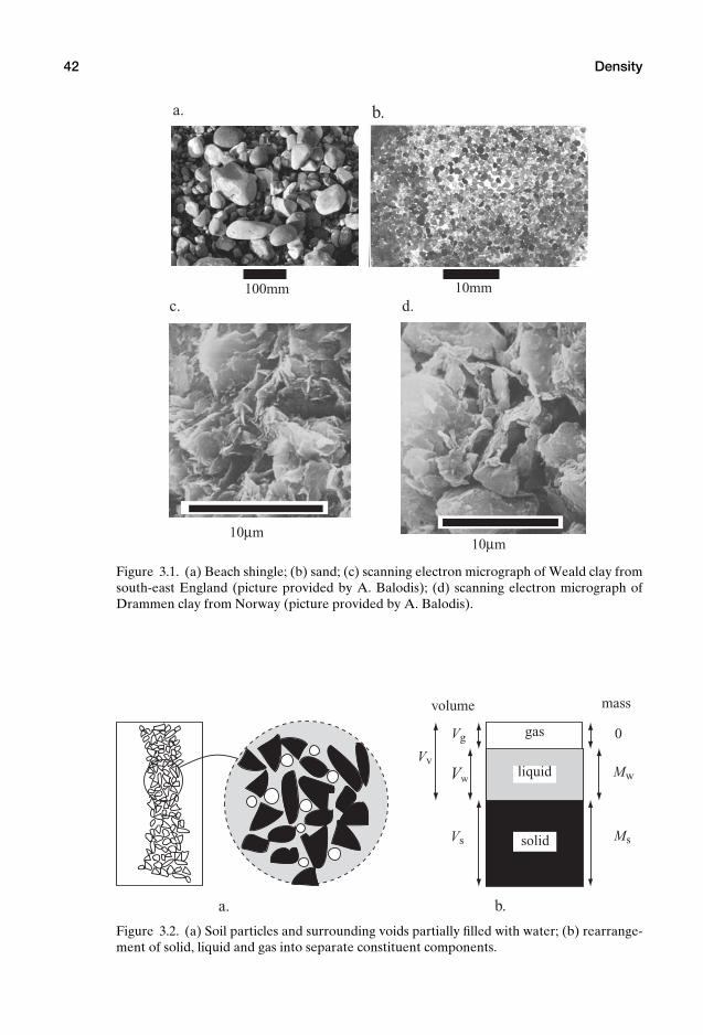
P1: KAE


42 Density

10mm

10µm10µm

a.

c. d.

b.

100mm

Figure 3.1. (a) Beach shingle; (b) sand; (c) scanning electron micrograph of Weald clay fromsouth-east England (picture provided by A. Balodis); (d) scanning electron micrograph ofDrammen clay from Norway (picture provided by A. Balodis).

gas

liquid

solid

massvolume

0Vg

Vw Mw

Vv

Vs Ms

a. b.

Figure 3.2. (a) Soil particles and surrounding voids partially filled with water; (b) rearrange-ment of solid, liquid and gas into separate constituent components.

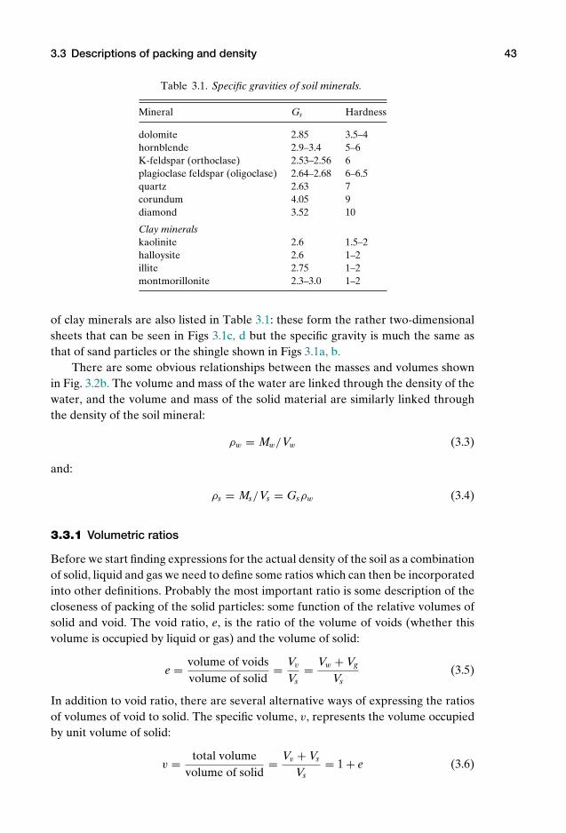
P1: KAE



Table 3.1. Specific gravities of soil minerals.

Mineral Gs Hardness

dolomite 2.85 3.5–4hornblende 2.9–3.4 5–6K-feldspar (orthoclase) 2.53–2.56 6plagioclase feldspar (oligoclase) 2.64–2.68 6–6.5quartz 2.63 7corundum 4.05 9diamond 3.52 10

Clay mineralskaolinite 2.6 1.5–2halloysite 2.6 1–2illite 2.75 1–2montmorillonite 2.3–3.0 1–2

of clay minerals are also listed in Table 3.1: these form the rather two-dimensionalsheets that can be seen in Figs 3.1c, d but the specific gravity is much the same asthat of sand particles or the shingle shown in Figs 3.1a, b.

There are some obvious relationships between the masses and volumes shownin Fig. 3.2b. The volume and mass of the water are linked through the density of thewater, and the volume and mass of the solid material are similarly linked throughthe density of the soil mineral:

ρw = Mw/Vw (3.3)

and:

ρs = Ms/Vs = Gsρw (3.4)

3.3.1 Volumetric ratios

Before we start finding expressions for the actual density of the soil as a combinationof solid, liquid and gas we need to define some ratios which can then be incorporatedinto other definitions. Probably the most important ratio is some description of thecloseness of packing of the solid particles: some function of the relative volumes ofsolid and void. The void ratio, e, is the ratio of the volume of voids (whether thisvolume is occupied by liquid or gas) and the volume of solid:

e = volume of voidsvolume of solid

= Vv

Vs= Vw + Vg

Vs(3.5)

In addition to void ratio, there are several alternative ways of expressing the ratiosof volumes of void to solid. The specific volume, v, represents the volume occupiedby unit volume of solid:

v = total volumevolume of solid

= Vv + Vs

Vs= 1 + e (3.6)

P1: KAE


44 Density

In other contexts, where a partitioning approach is to be used to estimate the prop-erties of a mixture, it is common to make use of the solid volume fraction, fvol :

fvol = volume of solidtotal volume

= Vs

Vv + Vs= 1

v(3.7)

Whereas this volume fraction is rarely used in description of soils, it will reappearshortly as a ratio of densities. A more frequently used variable is porosity, n (whichis often expressed as a percentage):

n = volume of voidstotal volume

= Vv

Vv + Vs= e

1 + e= v − 1

v(3.8)

Finally, we must have some way of recording the fact that the voids are not fullof liquid but actually contain a mixture of liquid and gas. The degree of saturation,Sr , describes the proportion of the void space that is filled with water (and is oftenexpressed as a percentage):

Sr = volume of liquidvolume of voids

= Vw

Vv

= Vw

Vw + Vg(3.9)

But even here there is an alternative variable: the air void ratio, a, which confus-ingly is a ratio of volume of gas (air) to total volume (and is often expressed as apercentage):

a = volume of gastotal volume

= Vg

Vv + Vs= (1 − Sr )e

1 + e(3.10)

3.3.2 Water content

Volumes are not easy to measure – especially when the volumes concerned have theirregular boundaries of soil particles. Masses are easier to measure accurately. Themost frequently used mass ratio is the water content, w. This is simply the ratio ofthe mass of water to the mass of dry soil. It can be measured by weighing a sampleof soil before and after drying it in an oven. The difference in the masses is the massof water in the original sample. Thus, water content is given by:

w = mass of watermass of dry soil

= Mw

Ms(3.11)

Water content can be related to the volumetric ratios we have already presented:

w = Mw

Ms= ρwVw

ρs Vs= 1

Gs

Sr e1

(3.12)

3.3.3 Densities

Having defined these volume ratios, we can next find expressions for density. Thereare three densities to be defined: the density of the soil in its present, probably un-saturated, state which is the bulk density, ρ; the density of the soil in its currentvolumetric configuration but with the voids entirely filled with water, the saturated

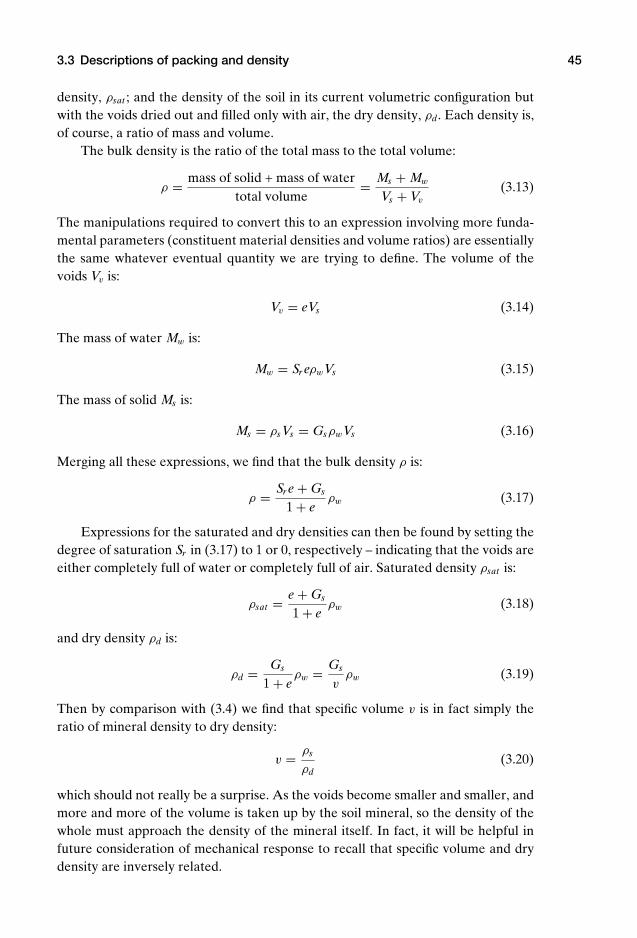
P1: KAE



density, ρsat ; and the density of the soil in its current volumetric configuration butwith the voids dried out and filled only with air, the dry density, ρd. Each density is,of course, a ratio of mass and volume.

The bulk density is the ratio of the total mass to the total volume:

ρ = mass of solid + mass of watertotal volume

= Ms + Mw

Vs + Vv

(3.13)

The manipulations required to convert this to an expression involving more funda-mental parameters (constituent material densities and volume ratios) are essentiallythe same whatever eventual quantity we are trying to define. The volume of thevoids Vv is:

Vv = eVs (3.14)

The mass of water Mw is:

Mw = Sr eρwVs (3.15)

The mass of solid Ms is:

Ms = ρs Vs = GsρwVs (3.16)

Merging all these expressions, we find that the bulk density ρ is:

ρ = Sr e + Gs

1 + eρw (3.17)

Expressions for the saturated and dry densities can then be found by setting thedegree of saturation Sr in (3.17) to 1 or 0, respectively – indicating that the voids areeither completely full of water or completely full of air. Saturated density ρsat is:

ρsat = e + Gs

1 + eρw (3.18)

and dry density ρd is:

ρd = Gs

1 + eρw = Gs

vρw (3.19)

Then by comparison with (3.4) we find that specific volume v is in fact simply theratio of mineral density to dry density:

v = ρs

ρd(3.20)

which should not really be a surprise. As the voids become smaller and smaller, andmore and more of the volume is taken up by the soil mineral, so the density of thewhole must approach the density of the mineral itself. In fact, it will be helpful infuture consideration of mechanical response to recall that specific volume and drydensity are inversely related.

P1: KAE


46 Density

3.3.4 Unit weights

Calculation of in-situ stresses in Chapter 2 always combined density with gravita-tional acceleration to calculate the profiles of vertical stress. For each density, wecan define a corresponding unit weight. In practice, there are three unit weights thatare regularly used: the bulk unit weight γ = ρg,1 the unit weight of water γw = ρwg,and a buoyant unit weight γ ′ = γ − γw.

The buoyant unit weight naturally emerges below the water table where thegradient of increase of total vertical stress σz with depth is:

dσz

dz= ρg = γ (3.21)

and the gradient of increase of pore water pressure with depth is:

dudz

= ρwg = γw (3.22)

We saw in Section 2.8 that the behaviour of soils is controlled by an effectivestress which is calculated as the difference between total stress and pore pressure.The total stress guarantees equilibrium and the water pressure takes some of thisstress – the soil carries the remainder. We defined effective stress σ ′

z using the Prin-ciple of Effective stress:

σ ′z = σz − u (3.23)

If we work in gradients of the several components of stress with depth, we can write:

dσ ′z

dz= dσz

dz− du

dz= γ − γw = γ ′ (3.24)

thus demonstrating the relevance of the buoyant unit weight.A word of warning, however. The use of buoyant unit weight to calculate vari-

ations of effective vertical stress is limited to situations where there is no flow oc-curring. We will encounter effects of seepage and flow in Chapter 5. If in doubt,calculate effective stresses from total stresses and pore pressures rather than rely-ing on buoyant unit weight γ ′ to produce the correct result. The significance of thiswarning will be appreciated subsequently.

3.3.5 Typical values

It is helpful to have an idea of the typical values of density and unit weight thatengineering soils are likely to have. This not only provides some control on theplausibility of quoted values – so that “impossible” values can be identified andeliminated – but also leaves the possibility of making use of reasonable estimates ifno actual measurements of density are available.

1 Beneath the water table, the soil will usually be more or less saturated so that the bulk unit weightγ will be the saturated unit weight.

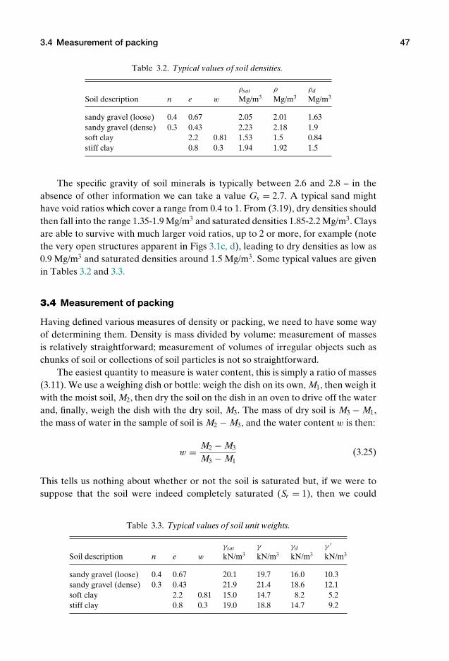
P1: KAE


3.4 Measurement of packing 47

Table 3.2. Typical values of soil densities.

ρsat ρ ρd

Soil description n e w Mg/m3 Mg/m3 Mg/m3

sandy gravel (loose) 0.4 0.67 2.05 2.01 1.63sandy gravel (dense) 0.3 0.43 2.23 2.18 1.9soft clay 2.2 0.81 1.53 1.5 0.84stiff clay 0.8 0.3 1.94 1.92 1.5

The specific gravity of soil minerals is typically between 2.6 and 2.8 – in theabsence of other information we can take a value Gs = 2.7. A typical sand mighthave void ratios which cover a range from 0.4 to 1. From (3.19), dry densities shouldthen fall into the range 1.35-1.9 Mg/m3 and saturated densities 1.85-2.2 Mg/m3. Claysare able to survive with much larger void ratios, up to 2 or more, for example (notethe very open structures apparent in Figs 3.1c, d), leading to dry densities as low as0.9 Mg/m3 and saturated densities around 1.5 Mg/m3. Some typical values are givenin Tables 3.2 and 3.3.

3.4 Measurement of packing

Having defined various measures of density or packing, we need to have some wayof determining them. Density is mass divided by volume: measurement of massesis relatively straightforward; measurement of volumes of irregular objects such aschunks of soil or collections of soil particles is not so straightforward.

The easiest quantity to measure is water content, this is simply a ratio of masses(3.11). We use a weighing dish or bottle: weigh the dish on its own, M1, then weigh itwith the moist soil, M2, then dry the soil on the dish in an oven to drive off the waterand, finally, weigh the dish with the dry soil, M3. The mass of dry soil is M3 − M1,the mass of water in the sample of soil is M2 − M3, and the water content w is then:

w = M2 − M3

M3 − M1(3.25)

This tells us nothing about whether or not the soil is saturated but, if we were tosuppose that the soil were indeed completely saturated (Sr = 1), then we could

Table 3.3. Typical values of soil unit weights.

γsat γ γd γ ′

Soil description n e w kN/m3 kN/m3 kN/m3 kN/m3

sandy gravel (loose) 0.4 0.67 20.1 19.7 16.0 10.3sandy gravel (dense) 0.3 0.43 21.9 21.4 18.6 12.1soft clay 2.2 0.81 15.0 14.7 8.2 5.2stiff clay 0.8 0.3 19.0 18.8 14.7 9.2

P1: KAE


48 Density

ground glass stopper with central capillary

Figure 3.3. Specific gravity bottle, or pycnometer.

calculate the void ratio, e (or any other measure of volumetric packing), from (3.12):

e = Gsw (3.26)

However, this conversion requires knowledge of the specific gravity of the soil par-ticles, Gs .

Accurate determination of specific gravity requires the use of a specific gravitybottle, or pycnometer (Fig. 3.3). The specific gravity bottle is a carefully made glassbottle with a closely fitting ground glass stopper through which there is a narrowtubular hole. When the bottle is filled with liquid and the stopper inserted, surplusliquid escapes through the hole and can be carefully wiped clear in such a way thatthe volume of liquid contained in the bottle is accurately the same every time thebottle is used.

Specific gravity is a ratio of densities of a substance under study and pure water(3.2). If the substance is a liquid other than water (for example, sea water or someother saline pore fluid, Section 2.7), then we can determine its specific gravity byweighing the bottle first empty, M1, then full of water, M2, and finally full of theliquid, M3. The volumes of liquid and water are identical, so the specific gravity ofthe liquid, Gl is:

Gl = M3 − M1

M2 − M1(3.27)

To determine the specific gravity of the soil mineral we proceed in a slightlydifferent way. First, we weigh the bottle on its own, M1, then place some of thedry soil particles in the bottle and weigh it again, M2. Then we fill the bottle, stillcontaining the soil particles, with water, making sure that absolutely no air is trappedin or around the soil and weigh it again, M3. Finally, having emptied out the soil andcleaned the bottle, we fill it with water and weigh it, M4. The mass of the soil particlesis evidently M2 − M1. The mass of the quantity of water which has a volume identicalto the volume of the soil particles is then (M4 − M1) − (M3 − M2), and hence thespecific gravity of the soil particles is:

Gs = M2 − M1

M4 − M3 + M2 − M1(3.28)

To discover the degree of saturation we have no choice but to determine thedensity of the soil. For this we need to know the volume of the soil sample whose

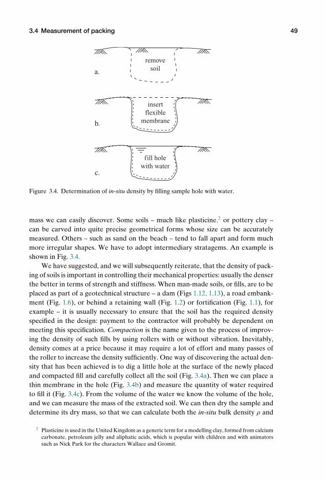
P1: KAE



a.

b.

c.

remove soil

insert flexible

membrane

fill hole with water

Figure 3.4. Determination of in-situ density by filling sample hole with water.

mass we can easily discover. Some soils – much like plasticine,2 or pottery clay –can be carved into quite precise geometrical forms whose size can be accuratelymeasured. Others – such as sand on the beach – tend to fall apart and form muchmore irregular shapes. We have to adopt intermediary stratagems. An example isshown in Fig. 3.4.

We have suggested, and we will subsequently reiterate, that the density of pack-ing of soils is important in controlling their mechanical properties: usually the denserthe better in terms of strength and stiffness. When man-made soils, or fills, are to beplaced as part of a geotechnical structure – a dam (Figs 1.12, 1.13), a road embank-ment (Fig. 1.6), or behind a retaining wall (Fig. 1.2) or fortification (Fig. 1.1), forexample – it is usually necessary to ensure that the soil has the required densityspecified in the design: payment to the contractor will probably be dependent onmeeting this specification. Compaction is the name given to the process of improv-ing the density of such fills by using rollers with or without vibration. Inevitably,density comes at a price because it may require a lot of effort and many passes ofthe roller to increase the density sufficiently. One way of discovering the actual den-sity that has been achieved is to dig a little hole at the surface of the newly placedand compacted fill and carefully collect all the soil (Fig. 3.4a). Then we can place athin membrane in the hole (Fig. 3.4b) and measure the quantity of water requiredto fill it (Fig. 3.4c). From the volume of the water we know the volume of the hole,and we can measure the mass of the extracted soil. We can then dry the sample anddetermine its dry mass, so that we can calculate both the in-situ bulk density ρ and

2 Plasticine is used in the United Kingdom as a generic term for a modelling clay, formed from calciumcarbonate, petroleum jelly and aliphatic acids, which is popular with children and with animatorssuch as Nick Park for the characters Wallace and Gromit.

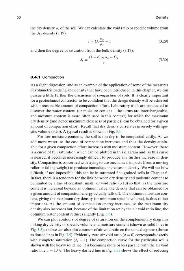
P1: KAE


50 Density

the dry density ρd of the soil. We can calculate the void ratio or specific volume fromthe dry density (3.19):

e = Gsρw

ρd− 1 (3.29)

and then the degree of saturation from the bulk density (3.17):

Sr = (1 + e)ρ/ρw − Gs

e(3.30)

3.4.1 Compaction

As a slight digression, and as an example of the application of some of the measuresof volumetric packing and density that have been introduced in this chapter, we canpursue a little further the discussion of compaction of soils. It is clearly importantfor a geotechnical contractor to be confident that the design density will be achievedwith a reasonable amount of compaction effort. Laboratory trials are conducted todiscover the water content (or moisture content – the terms are interchangeable,and moisture content is more often used in this context) for which the maximumdry density (and hence maximum closeness of particles) can be obtained for a givenamount of compaction effort. Recall that dry density correlates inversely with spe-cific volume (3.20). A typical result is shown in Fig. 3.5.

For low moisture contents, the soil is too dry to be compacted easily. As weadd more water, so the ease of compaction increases and thus the density attain-able for a given compaction effort increases with moisture content. However, thereis a curve of full saturation which can be plotted in this diagram and, as this curveis neared, it becomes increasingly difficult to produce any further increase in den-sity. Compaction is concerned with trying to use mechanical impacts (from a movingroller or falling weight) to produce immediate increases in density. We will see howdifficult, if not impossible, this can be in saturated fine grained soils in Chapter 6.In fact, there is a tendency for the link between dry density and moisture content tobe limited by a line of constant, small, air void ratio (3.10) so that, as the moisturecontent is increased beyond an optimum value, the density that can be obtained fora given amount of compaction energy actually falls off. The optimum moisture con-tent, giving the maximum dry density (or minimum specific volume), is thus ratherimportant. As the amount of compaction energy increases, so the maximum drydensity also increases but, because of the limitation set by the air void ratio line, theoptimum water content reduces slightly (Fig. 3.5).

We can plot contours of degree of saturation on the complementary diagramslinking dry density or specific volume and moisture content (shown as solid lines inFig. 3.5); and we can also plot contours of air void ratio on the same diagrams (shownas dotted lines in Fig. 3.5). Evidently, zero air void ratio (a = 0) corresponds exactlywith complete saturation (Sr = 1). The compaction curve for the particular soil isshown with the heavy solid line: it is becoming more or less parallel with the air voidratio line a = 10%. The heavy dashed line in Fig. 3.5a shows the effect of reducing

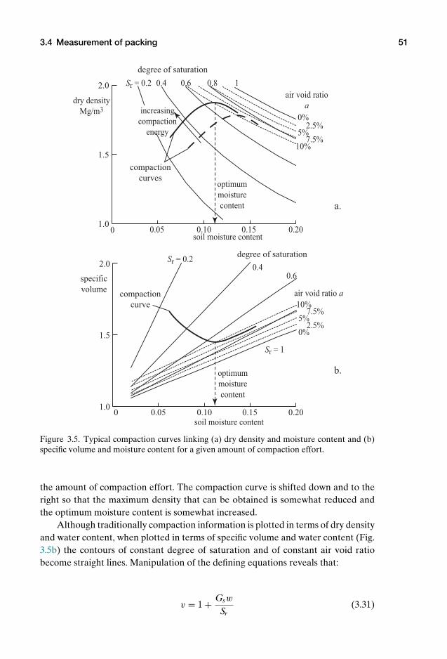
P1: KAE



1.0

1.5

2.0

0 0.05 0.10 0.15 0.20

0%

0%

2.5%

2.5%

5%

5%

7.5%

7.5%

10%

10%

Sr = 0.2

Sr = 0.2

0.4

0.4

0.6

0.6

0.8 1

Sr = 1

optimum

moisture

content

optimum

moisture

content

increasing

compaction

energy

soil moisture content

soil moisture content

dry density

Mg/m3

0 0.05 0.10 0.15 0.201.0

1.5

2.0

specific

volume

a.

b.

air void ratio

a

air void ratio a

compaction

curves

compaction

curve

degree of saturation

degree of saturation

Figure 3.5. Typical compaction curves linking (a) dry density and moisture content and (b)specific volume and moisture content for a given amount of compaction effort.

the amount of compaction effort. The compaction curve is shifted down and to theright so that the maximum density that can be obtained is somewhat reduced andthe optimum moisture content is somewhat increased.

Although traditionally compaction information is plotted in terms of dry densityand water content, when plotted in terms of specific volume and water content (Fig.3.5b) the contours of constant degree of saturation and of constant air void ratiobecome straight lines. Manipulation of the defining equations reveals that:

v = 1 + Gsw

Sr(3.31)

P1: KAE


52 Density

which produces a series of radiating lines through the point v = 1 and w = 0; and:

v = 1 + Gsw

1 − a(3.32)

which produces a series of lines of slope Gs/(1 − a) which for the small values of aplotted in Fig. 3.5b appear almost parallel.

3.5 Soil particles

Even a cursory glance at the pictures of soil particles in Fig. 3.1 should trigger twothoughts: the very wide range of sizes of particles that may make up a soil; and theenormous contrasts in particle shape. Soil particles are formed by a combination ofprocesses of erosion, weathering and transport from parent rocks. The constituentsof these rocks are minerals such as quartz, feldspar, mica and hornblende, which aremore or less resistant to effects of temperature, humidity and chemical weathering.The specific gravities of many commonly occurring minerals were given in Table3.1. That table also gives the hardness values of the various minerals on Moh’s hard-ness scale (Table 3.4: fingernails have a hardness of about 2.5). Quartz, a mineralwhose chemical composition is silicon dioxide (SiO2), is a particularly stable andhard mineral which makes up much of the sand and gravel deposits of the world –it may succumb to mechanical effects as the particles are bounced around the sur-face of the Earth so that particles become progressively more round as the cornersare removed (look at the very round shingle particles in Fig. 3.1a) but the chemicalcomposition remains intact. The transport process is clearly important in controllingthe nature of the soils that we see around us today.

The four means of transport are by gravity (as a landslide or debris flow), ice,water and air (wind) and, moving through this sequence, the size of “particles” thatcan be transported becomes progressively smaller. At one extreme, debris flows caninclude enormous boulders but wind will only lift rather small particles. Ice – in theform of glaciers – smoothes the underlying rocks and is able to carry a great range

Table 3.4. Moh’s hardness scale.

Hardness Mineral

0 liquid1 talc2 gypsum3 calcite4 fluorite5 apatite6 orthoclase7 quartz8 topaz9 corundum

10 diamond

P1: KAE


3.5 Soil particles 53

Figure 3.6. Ice movement in glaciers smoothes the underlying rocks and carries a greatrange of particle sizes (Nigardsbreen, Jostedalen, Norway).

of particle sizes including reasonably large boulders (Fig. 3.6). The size of particlethat can be moved by water depends on the speed of flow of the water. As the speedof flow of a river reduces, so the coarser particles will be progressively deposited.The finer particles will be able to remain in suspension for longer – their rate offall through the water will be slow. A river disemboguing into a lake or sea will stillbe able to carry the finest particles even past the mouth of the river (Fig. 3.7). Thefine particles will slowly fall to the lake floor, forming a layered sediment which maywell show some seasonal variations in particle size depending on the flow rates inthe tributary rivers.

However, some rock minerals are more susceptible to chemical decompositionand clay minerals such as those seen in Figs 3.1c, d are decomposition products.

Figure 3.7. Island in the Irrawaddy (Myanmar) streaked with silt by receding floodwaters.

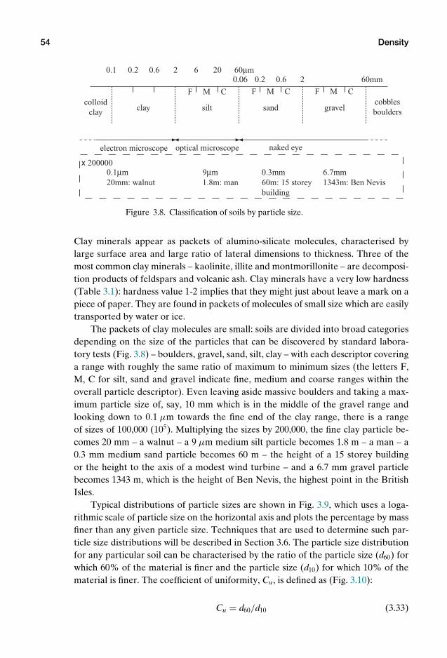
P1: KAE


54 Density

cobbles bouldersgravelsandsiltclay

colloid clay

F M C F M C F M C

0.1 0.20.2

0.60.6

22

6 20 60µm60mm0.06

electron microscope optical microscope naked eye

x 2000000.1µm20mm: walnut

9µm1.8m: man

0.3mm60m: 15 storey building

6.7mm1343m: Ben Nevis

Figure 3.8. Classification of soils by particle size.

Clay minerals appear as packets of alumino-silicate molecules, characterised bylarge surface area and large ratio of lateral dimensions to thickness. Three of themost common clay minerals – kaolinite, illite and montmorillonite – are decomposi-tion products of feldspars and volcanic ash. Clay minerals have a very low hardness(Table 3.1): hardness value 1-2 implies that they might just about leave a mark on apiece of paper. They are found in packets of molecules of small size which are easilytransported by water or ice.

The packets of clay molecules are small: soils are divided into broad categoriesdepending on the size of the particles that can be discovered by standard labora-tory tests (Fig. 3.8) – boulders, gravel, sand, silt, clay – with each descriptor coveringa range with roughly the same ratio of maximum to minimum sizes (the letters F,M, C for silt, sand and gravel indicate fine, medium and coarse ranges within theoverall particle descriptor). Even leaving aside massive boulders and taking a max-imum particle size of, say, 10 mm which is in the middle of the gravel range andlooking down to 0.1 µm towards the fine end of the clay range, there is a rangeof sizes of 100,000 (105). Multiplying the sizes by 200,000, the fine clay particle be-comes 20 mm – a walnut – a 9 µm medium silt particle becomes 1.8 m – a man – a0.3 mm medium sand particle becomes 60 m – the height of a 15 storey buildingor the height to the axis of a modest wind turbine – and a 6.7 mm gravel particlebecomes 1343 m, which is the height of Ben Nevis, the highest point in the BritishIsles.

Typical distributions of particle sizes are shown in Fig. 3.9, which uses a loga-rithmic scale of particle size on the horizontal axis and plots the percentage by massfiner than any given particle size. Techniques that are used to determine such par-ticle size distributions will be described in Section 3.6. The particle size distributionfor any particular soil can be characterised by the ratio of the particle size (d60) forwhich 60% of the material is finer and the particle size (d10) for which 10% of thematerial is finer. The coefficient of uniformity, Cu, is defined as (Fig. 3.10):

Cu = d60/d10 (3.33)

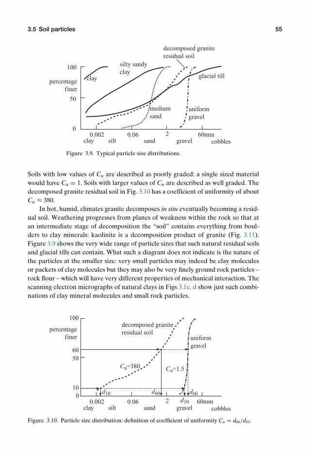
P1: KAE


3.5 Soil particles 55

100

50

0

percentage finer

silt sand gravelclay0.002 0.06 2 60mm

clay

silty sandy clay

medium sand

uniform gravel

glacial till

cobbles

decomposed granite residual soil

Figure 3.9. Typical particle size distributions.

Soils with low values of Cu are described as poorly graded: a single sized materialwould have Cu = 1. Soils with larger values of Cu are described as well graded. Thedecomposed granite residual soil in Fig. 3.10 has a coefficient of uniformity of aboutCu ≈ 380.

In hot, humid, climates granite decomposes in situ eventually becoming a resid-ual soil. Weathering progresses from planes of weakness within the rock so that atan intermediate stage of decomposition the “soil” contains everything from boul-ders to clay minerals: kaolinite is a decomposition product of granite (Fig. 3.11).Figure 3.9 shows the very wide range of particle sizes that such natural residual soilsand glacial tills can contain. What such a diagram does not indicate is the nature ofthe particles at the smaller size: very small particles may indeed be clay moleculesor packets of clay molecules but they may also be very finely ground rock particles –rock flour – which will have very different properties of mechanical interaction. Thescanning electron micrographs of natural clays in Figs 3.1c, d show just such combi-nations of clay mineral molecules and small rock particles.

100

5060

100

percentage finer

silt sand gravelclay0.002 0.06 2 60mm

cobbles

d60 d60d10

d10

Cu=380 Cu=1.5

uniform gravel

decomposed granite residual soil

Figure 3.10. Particle size distribution: definition of coefficient of uniformity Cu = d60/d10.

P1: KAE


56 Density

10 metres (approximately)

Figure 3.11. Excavation through in-situ weathered granite (Sha Tin, New Territories, HongKong).

Looking back at the photographs of soil particles (Fig. 3.1) we see that the sandgrains and shingle have a compact shape with a low specific surface, the ratio ofsurface area to volume. A sphere is the solid shape which has the lowest specificsurface. The interaction between such particles is broadly mechanical through trans-mission of forces at the contacts with neighbouring grains. On the other hand, theclay has a high specific surface and much smaller particles. As clay molecules as-semble, the distribution of charge is not uniform and there is variation of the elec-trostatic charge over the surface of the molecules: the faces of the molecules arepositively charged and the edges negatively charged. Groups of clay molecules areformed in which positively charged surfaces attract negatively charged particles toform more or less stable packets. The electrostatic forces between adjacent particlesare the most significant contributor to the transmission of forces through the partic-ulate assembly for a clay. The presence of such electrostatic forces leads to ratheropen structures with high void ratios and consequent low densities (Figs 3.1c, d andTables 3.2, 3.3).

3.6 Laboratory exercise: particle size distributionand other classification tests

3.6.1 Sieving

The distributions of particle sizes shown in Fig. 3.9 treat the soil particles as thoughthey were equivalent spheres – this seems to be a good starting point in our soil

P1: KAE


3.6 Laboratory exercise: particle size distribution and other classification tests 57

Figure 3.12. Particle sizes determined by sieving.

classification model even if we know that the particles may actually not be particu-larly spherical. An obvious way to discover the proportions of different sized parti-cles is by sieving, using standard sieves with different mesh sizes. The soil is pouredinto the top of a stack of sieves, with the coarsest sieve at the top. The stack is shakenand the quantity of material retained on each sieve is measured. Figure 3.12 illus-trates the way in which particles of very different shapes will be able to pass throughthe same square mesh opening and be recorded as below that particular equivalentdiameter: this is a first order model for which this approximate equivalent sphericalestimate will suffice.

3.6.2 Sedimentation

For a soil with finer particles, sieving is no longer feasible. It would not be possibleto construct a sieve with a size of opening small enough to retain particles with atypical dimension of a few microns. An alternative procedure is required. Stokes’Law describes the terminal velocity of spheres falling through a viscous fluid (Fig.3.13). We can approach Stokes’ Law through a consideration of the resistance to themovement of a spherical object through a viscous liquid using the ideas of dimen-sional analysis.3

The resistance force or drag on an object can be expected to depend on the vis-cosity of the fluid which is trying to resist the motion of the object. We will meetviscosity in Chapter 5 when we look at the way in which water flows through therestricted passages provided by natural soils. It is an indication of the shear stressgenerated when there is a velocity gradient in the fluid: the faster-flowing fluid triesto pull the slower fluid along with it. The material constant of proportionality link-ing shear stress and velocity gradient is the viscosity, η. Viscosity has dimensions ofmass/(length×time), so it could be expressed in units of kilograms per metre per sec-ond. However, understanding its origin as a description of the shear stress generatedby a velocity gradient, it is more appropriate to see it in units of pascal-seconds. Vis-cosity is also quoted in units of centipoise: 1 centipoise = 1 mPa-s. The viscosity ofwater at room temperature is about 1 mPa-s, 1 millipascal-second (or 1 centipoise).The viscosity of water is quite sensitive to temperature, as the values quoted in Table3.5 indicate.

3 See, for example, Palmer, A.C. (2008) Dimensional analysis and intelligent experimentation, WorldScientific Publishing Company, Singapore.

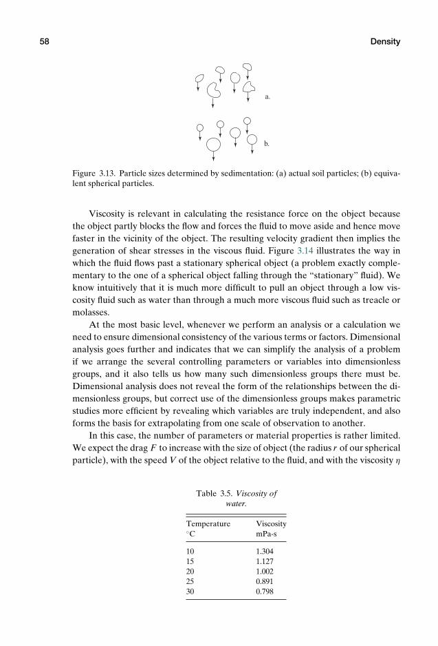
P1: KAE


58 Density

a.

b.

Figure 3.13. Particle sizes determined by sedimentation: (a) actual soil particles; (b) equiva-lent spherical particles.

Viscosity is relevant in calculating the resistance force on the object becausethe object partly blocks the flow and forces the fluid to move aside and hence movefaster in the vicinity of the object. The resulting velocity gradient then implies thegeneration of shear stresses in the viscous fluid. Figure 3.14 illustrates the way inwhich the fluid flows past a stationary spherical object (a problem exactly comple-mentary to the one of a spherical object falling through the “stationary” fluid). Weknow intuitively that it is much more difficult to pull an object through a low vis-cosity fluid such as water than through a much more viscous fluid such as treacle ormolasses.

At the most basic level, whenever we perform an analysis or a calculation weneed to ensure dimensional consistency of the various terms or factors. Dimensionalanalysis goes further and indicates that we can simplify the analysis of a problemif we arrange the several controlling parameters or variables into dimensionlessgroups, and it also tells us how many such dimensionless groups there must be.Dimensional analysis does not reveal the form of the relationships between the di-mensionless groups, but correct use of the dimensionless groups makes parametricstudies more efficient by revealing which variables are truly independent, and alsoforms the basis for extrapolating from one scale of observation to another.

In this case, the number of parameters or material properties is rather limited.We expect the drag F to increase with the size of object (the radius r of our sphericalparticle), with the speed V of the object relative to the fluid, and with the viscosity η

Table 3.5. Viscosity ofwater.

Temperature ViscosityC mPa-s

10 1.30415 1.12720 1.00225 0.89130 0.798

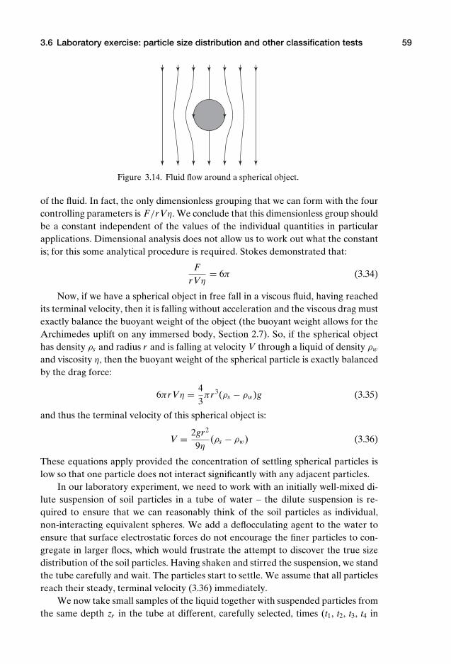
P1: KAE



Figure 3.14. Fluid flow around a spherical object.

of the fluid. In fact, the only dimensionless grouping that we can form with the fourcontrolling parameters is F/r Vη. We conclude that this dimensionless group shouldbe a constant independent of the values of the individual quantities in particularapplications. Dimensional analysis does not allow us to work out what the constantis; for this some analytical procedure is required. Stokes demonstrated that:

Fr Vη

= 6π (3.34)

Now, if we have a spherical object in free fall in a viscous fluid, having reachedits terminal velocity, then it is falling without acceleration and the viscous drag mustexactly balance the buoyant weight of the object (the buoyant weight allows for theArchimedes uplift on any immersed body, Section 2.7). So, if the spherical objecthas density ρs and radius r and is falling at velocity V through a liquid of density ρw

and viscosity η, then the buoyant weight of the spherical particle is exactly balancedby the drag force:

6πr Vη = 43πr3(ρs − ρw)g (3.35)

and thus the terminal velocity of this spherical object is:

V = 2gr2

9η(ρs − ρw) (3.36)

These equations apply provided the concentration of settling spherical particles islow so that one particle does not interact significantly with any adjacent particles.

In our laboratory experiment, we need to work with an initially well-mixed di-lute suspension of soil particles in a tube of water – the dilute suspension is re-quired to ensure that we can reasonably think of the soil particles as individual,non-interacting equivalent spheres. We add a deflocculating agent to the water toensure that surface electrostatic forces do not encourage the finer particles to con-gregate in larger flocs, which would frustrate the attempt to discover the true sizedistribution of the soil particles. Having shaken and stirred the suspension, we standthe tube carefully and wait. The particles start to settle. We assume that all particlesreach their steady, terminal velocity (3.36) immediately.

We now take small samples of the liquid together with suspended particles fromthe same depth zr in the tube at different, carefully selected, times (t1, t2, t3, t4 in

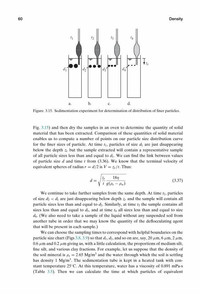
P1: KAE


60 Density

t1 t2 t3 t4

a. b. c. d.

zr

d1 d2 d3 d4

Figure 3.15. Sedimentation experiment for determination of distribution of finer particles.

Fig. 3.15) and then dry the samples in an oven to determine the quantity of solidmaterial that has been extracted. Comparison of these quantities of solid materialenables us to compute a number of points on our particle size distribution curvefor the finer sizes of particle. At time t1, particles of size d1 are just disappearingbelow the depth zr but the sample extracted will contain a representative sampleof all particle sizes less than and equal to d1. We can find the link between valuesof particle size d and time t from (3.36). We know that the terminal velocity ofequivalent spheres of radius r = d/2 is V = zr/t . Thus:

d =√

zr

t18η

g(ρs − ρw)(3.37)

We continue to take further samples from the same depth. At time t2, particlesof size d2 < d1 are just disappearing below depth zr and the sample will contain allparticle sizes less than and equal to d2. Similarly, at time t3 the sample contains allsizes less than and equal to d3, and at time t4 all sizes less than and equal to sized4. (We also need to take a sample of the liquid without any suspended soil fromanother tube in order that we may know the quantity of the deflocculating agentthat will be present in each sample.)

We can choose the sampling times to correspond with helpful boundaries on theparticle size chart (Figs 3.8, 3.9) so that d1, d2, and so on are, say, 20 µm, 6 µm, 2 µm,0.6 µm and 0.2 µm giving us, with a little calculation, the proportions of medium silt,fine silt, and various clay fractions. For example, let us suppose that the density ofthe soil mineral is ρs = 2.65 Mg/m3 and the water through which the soil is settlinghas density 1 Mg/m3. The sedimentation tube is kept in a heated tank with con-stant temperature 25C. At this temperature, water has a viscosity of 0.891 mPa-s(Table 3.5). Then we can calculate the time at which particles of equivalent

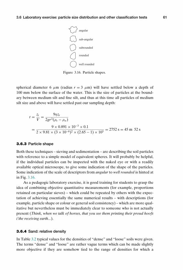
P1: KAE



angular

sub-angular

subrounded

rounded

well rounded

Figure 3.16. Particle shapes.

spherical diameter 6 µm (radius r = 3 µm) will have settled below a depth of100 mm below the surface of the water. This is the size of particles at the bound-ary between medium silt and fine silt, and thus at this time all particles of mediumsilt size and above will have settled past our sampling depth:

t = zr

V= 9ηzr

2gr2(ρs − ρw)

= 9 × 0.891 × 10−3 × 0.12 × 9.81 × (3 × 10−6)2 × (2.65 − 1) × 103

= 2752 s = 45 m 52 s

3.6.3 Particle shape

Both these techniques – sieving and sedimentation – are describing the soil particleswith reference to a simple model of equivalent spheres. It will probably be helpful,if the individual particles can be inspected with the naked eye or with a readilyavailable optical microscope, to give some indication of the shape of the particles.Some indication of the scale of descriptors from angular to well rounded is hinted atin Fig. 3.16.

As a pedagogic laboratory exercise, it is good training for students to grasp theidea of combining objective quantitative measurements (for example, proportionsretained on particular sieves) – which could be repeated by others with the expec-tation of achieving essentially the same numerical results – with descriptions (forexample, particle shape or colour or general soil consistency) – which are more qual-itative but nevertheless must be immediately clear to someone who is not actuallypresent (Think, when we talk of horses, that you see them printing their proud hoofsi’the receiving earth...).

3.6.4 Sand: relative density

In Table 3.2 typical values for the densities of “dense” and “loose” soils were given.The terms “dense” and “loose” are rather vague terms which can be made slightlymore objective if they are somehow tied to the range of densities for which a

P1: KAE


62 Density

particular sandy or gravelly soil can exist. More or less standard laboratory tests4

can be used to characterise this range – discovering a maximum density or mini-mum void ratio and a minimum density or maximum void ratio for the particularsoil in its dry state.

A standard vibratory procedure is used to discover the minimum void ratio,emin, of the soil. A series of repeated inversions of a large tube containing a sampleof the sandy soil is used to estimate the maximum void ratio, emax. The maximumand minimum void ratios determined in this way do not actually define the actualextremes of packing; they merely provide a useful index for the soil. In reality, theabsolute lowest value of void ratio must be zero when the stresses have been in-creased so enormously that all the particles have broken and there are no longerany visible voids. And there is a maximum void ratio – a very loose packing – forwhich the particles are not really in proper stationary contact, and the material isnot able to transmit stress from one side to the other.

However, given these index or reference values of void ratio, if the soil is pre-pared or found to exist at any other void ratio, e, then a relative density, Dr , can bedefined:

Dr = emax − eemax − emin

(3.38)

This range of void ratios depends on the range of particle sizes and the typical parti-cle shapes. For example, angular particles are able to exist in rather looser packingsthan rounded particles. Well-graded soils – soils such as the glacial till shown in Fig.3.9 with a wide range of particle sizes – tend to have low void ratios because forany size of particles there exist smaller particles which are happy to sit in the spacesthat would exist around the larger particles. The most efficient packing of particleswould be linked with a self-similar fractal distribution of particle sizes in which thearrangement of particles has the same general appearance no matter at what scalethe soil is observed. Then the proportion of particles within a range of sizes havingthe same ratio would be the same, so that if d1/d2 = d3/d4 then the proportion in thesize range d2 to d1 would be the same as that in the size range d4 to d3, and so on.

Classification tests of this type are valuable in providing information which isexpected to correlate, broadly, with stiffness and strength properties of the soil thatmay be relevant for calculation of the performance of geotechnical structures ofwhich that soil forms part.

3.7 Summary


1. Soils are composed of mineral particles separated by voids which may be par-tially or wholly filled with liquid.

4 Kolbuszewski, J.J. (1948) An experimental study of the maximum and minimum porosities of sands.Proc. 2nd Int. Conf. on Soil mechanics and foundation engineering, Rotterdam 1 158–165.

P1:K

AE

OneD

im00a

CU

US648/M

uir978

0521

517737

August17,2009

19:12

density

Mg/m3

kN/m3

unit weight

gas

liquid

solid

mass

0

Mw

Ms

volume

Vg

Vw

Vv

Vs

mechanical behaviour depends on volumetric

packing

void ratio especific volume v

saturation Sr

water content w

measurement: ratio of masses

water ρwsoil mineral ρsbulk density ρdry density ρd

soil particles

weathering:mechanicalchemical

transport:gravity

icewater

airclays:

packets of moleculessilicates, aluminateshigh specific surfaceelectrostatic forces sands etc:

stable mineralsilica, feldspar

low specific surfacemechanical interaction

buoyant unit weight

particle sizes by sedimentation

particle sizes by sieving

Figure 3.17. Mind map: density.63

P1: KAE


64 Density

2. Many aspects of the behaviour of soils are strongly influenced by the density ofpacking of the mineral particles: it is necessary to define density or volumetricvariables to characterise the packing.

3. Ratios of volumes are used to define void ratio, e, specific volume, v and poros-ity, n. The volumetric proportion of the voids filled with water is the degree ofsaturation, Sr .

4. Water content, w, is a ratio of masses and is straightforward to measure.5. Determination of density requires some means of estimating the volume of a

soil sample.6. For a given amount of compaction energy, there is an optimum moisture con-

tent which produces the maximum density or minimum specific volume.7. Soil particles originate from weathering of rocks and subsequent transport.8. The sizes of particles that may be found in natural or man-made soils cover a

very wide range.9. The distribution of sizes of coarser particles can be found by sieving; the distri-

bution of sizes of finer particles can be found by sedimentation.10. Significant electrostatic forces between packets of clay molecules encourage

open structures with high void ratios.11. The larger inert grains of sands and gravels interact through interparticle con-

tact forces.

3.8 Exercises: Density

3.8.1 Multiple choice questions

Choose the correct answer from the alternatives provided.

1. Void ratio e = (a) volume of soil particlesvolume of voids ; (b) volume of voids

total volume ;

(c) volume of voidsvolume of soil particles .

2. Specific volume v = (a) 1 + e; (b) 1 − e; (c) 1/e.3. Water content w = (a) volume of water

volume of soil particles ; (b) mass of watertotal mass ;

(c) mass of watermass of soil particles .

4. Degree of saturation Sr = (a) volume of watertotal volume ; (b) volume of water

volume of voids ;

(c) volume of watervolume of soil particles .

5. Density ρ = (a) massarea ; (b) weight

volume; (c) massvolume.

6. Dry density ρd = (a) Gsρw; (b) Gsρw

1+e ; (c) ρw

w.

7. Bulk unit weight γ = (a) (1 + w)ρd; (b) (1 + w)ρw; (c) (1 + w)ρdg.8. Buoyant unit weight γ ′ = (a) γ − γw; (b) γ + γw; (c) γ

γw.

9. Gs = 2.7, w = 24%, Sr = 100%.e = (a) 0.548; (b) 0.648; (c) 0.748v = (a) 1.548; (b) 1.748; (c) 1.648

P1: KAE


3.8 Exercises: Density 65

ρd = (a) 1.64 Mg/m3; (b) 0.64 Mg/m3; (c) 1.71 Mg/m3

ρsat = (a) 2.25 Mg/m3; (b) 2.03 Mg/m3; (c) 1.98 Mg/m3

ρ = (a) 1.9 Mg/m3; (b) 2.3 Mg/m3; (c) 2.03 Mg/m3

γ = (a) 19.9 kN/m3; (b) 19.5 kN/m3; (c) 20.5 kN/m3

γsat = (a) 19.0 kN/m3; (b) 19.9 kN/m3; (c) 20.5 kN/m3

10. Gs = 2.64, w = 35%, Sr = 75%e = (a) 1.232; (b) 1.105; (c) 1.302v = (a) 1.105; (b) 2.302; (c) 2.232ρd = (a) 1.18 Mg/m3; (b) 1.28 Mg/m3; (c) 1.81 Mg/m3


ρ = (a) 1.55 Mg/m3; (b) 1.6 Mg/m3; (c) 1.65 Mg/m3

γ = (a) 15.7 kN/m3; (b) 15.1 kN/m3; (c) 16.3 kN/m3


11. M = 6 kg, V = 0.003 m3, Ms = 5 kg, Gs = 2.68e = (a) 0.580; (b) 0.608; (c) 0.751v = (a) 1.608; (b) 1.580; (c) 1.751w = (a) 15%; (b) 25%; (c) 20%Sr = (a) 88%; (b) 83%; (c) 81%ρd = (a) 1.67 Mg/m3; (b) 1.75 Mg/m3; (c) 1.62 Mg/m3


ρ = (a) 1.9 Mg/m3; (b) 2 Mg/m3; (c) 2.2 Mg/m3

γ = (a) 19.9 kN/m3; (b) 19.6 kN/m3; (c) 19.1 kN/m3


3.8.2 Calculation exercises

1. A soil has bulk density ρ = 1.8 Mg/m3 and dry density ρd = 1.5 Mg/m3. Thespecific gravity of the soil particles is Gs = 2.7. Calculate the water content,specific volume, void ratio and degree of saturation.

2. A soil is found to have water content w = 30% and degree of saturation Sr =85%. The specific gravity of soil particles is Gs = 2.65. Calculate the void ratio,specific volume, dry density and bulk density.

3. A sample of soil of volume 0.0024 m3 is found to weigh 5.066 kg. After dryingin an oven it is found to weigh 4.54 kg. The specific gravity of soil particles isGs = 2.7. Calculate the bulk density, dry density, specific volume, void ratio,water content and degree of saturation.

4. A specimen of saturated soil (soil = soil particles + water) is placed in a mea-suring tin and weighed, then dried in an oven and then weighed again. The fol-lowing data are recorded. Find the water content, void ratio and specific volumeof the soil. Assume Gs = 2.67.

weight of tin 10.05 gweight of tin + wet soil 35.74 gweight of tin + dry soil 29.61 g

P1: KAE


66 Density

5. An undisturbed sample of saturated soil has a volume of 143 cm3 (143 ×10−6 m3) and a mass of 260 g. Determine its void ratio, specific volume, wa-ter content, density and dry density. Assume Gs = 2.7. (Hint: First find massesand volumes of soil and water components.)

6. A sample of soil has a bulk density of 1.9 Mg/m3 and a water content of 30%.Find the degree of saturation, void ratio, specific volume and dry density of thesoil. Assume Gs = 2.7.

7. In a density determination, a sample of clay was weighed in air and its mass wasfound to be 683 g. It was coated with paraffin of specific gravity 0.89 to seal it.The combined mass of the clay and the wax was 690.6 g. To find its volume,the wax-coated specimen was suspended by a thread from a balance, immersedin water, and the balance read. Its apparent mass was found to have reducedto 340.6 g. The sample was then broken open and appropriate tests gave watercontent w = 16.8% and particle specific gravity Gs = 2.73. Determine the bulkdensity, void ratio, specific volume, degree of saturation and dry density of theclay. (Hint: Archimedes’ principle indicates that the upthrust on a body is equalto the weight of water displaced by the body Section 2.7.)

8. Clay excavated from an underground tunnel of diameter 4.5 m under con-struction in central London is to be used to fill some old gravel workings nearHeathrow. The gravel pits cover an area of 5000 m2 and have an average depthof 10 m. Water fills the pits to just below the adjacent ground level. The clay willbe transported by lorry and end tipped.

The clay in situ is fully saturated, with water content 12% and specific gravityGs = 2.7. Pilot tests show that, after tipping is completed, the uncompacted fillwill remain saturated, but the average water content will rise to 23.5%. Estimatethe length of tunnel needed to fill the pits and the number of 10 m3 lorry loadsrequired. Assume the soil increases its volume by 15% when tipped into thelorry.

P1: KAE


4 Stiffness

4.1 Introduction

The two principal mechanical properties of all materials that are required for en-gineering design are some way of knowing how strong the material is: how muchstress it will tolerate – its strength – and some indication of the way in which it willchange in size when subjected to load – its stiffness. These characteristics essentiallyform the basis of what are called, respectively, ultimate limit state design and service-ability limit state design. We will take a one-dimensional look at strength in Chapter8. Here we will explore some aspects of stiffness of soils.

4.2 Linear elasticity

The standard experiment that can be performed on metal rods or wires to discovertheir deformation properties consists of the stretching of an appropriate specimenbetween suitable grips and measuring the link between the load applied and theresulting extension. In fact, the sort of experiment that can be performed at homemight use a metal wire fixed to the ceiling and loaded by means of weights on asmall pan (Fig. 4.1): the force transmitted to the wire is visibly obvious and, if wehave sufficiently accurate position measuring devices – perhaps some optical systemto magnify the displacement – we can have direct information about the extensionas well (Fig. 4.1a).

For most metals, provided the loads that are applied are not excessive, the re-lationship between load, P, and extension, , of such a wire is more or less linear(Fig. 4.1b). We can extract a material property, the elastic stiffness or elastic mod-ulus, from the slope of this relationship. We could simply report the slope, P/,but this would only provide a result relevant to the particular specimen of partic-ular cross-section and particular length. We expect that the deformation resultingfrom the application of a given load will depend on the area of the cross-sectionover which it is spread. In Chapter 2 we introduced the concept of stress as an indi-cation of the areal intensity of force. The axial stress in the wire of radius r will beσa = P/πr2.

67

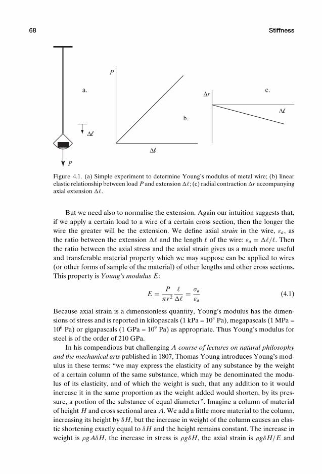
P1: KAE


68 Stiffness

P

P

∆l

∆l

∆l

∆ra.

b.

c.

Figure 4.1. (a) Simple experiment to determine Young’s modulus of metal wire; (b) linearelastic relationship between load P and extension ; (c) radial contraction r accompanyingaxial extension .

But we need also to normalise the extension. Again our intuition suggests that,if we apply a certain load to a wire of a certain cross section, then the longer thewire the greater will be the extension. We define axial strain in the wire, εa , asthe ratio between the extension and the length of the wire: εa = /. Thenthe ratio between the axial stress and the axial strain gives us a much more usefuland transferable material property which we may suppose can be applied to wires(or other forms of sample of the material) of other lengths and other cross sections.This property is Young’s modulus E:

E = Pπr2

= σa

εa(4.1)

Because axial strain is a dimensionless quantity, Young’s modulus has the dimen-sions of stress and is reported in kilopascals (1 kPa = 103 Pa), megapascals (1 MPa =106 Pa) or gigapascals (1 GPa = 109 Pa) as appropriate. Thus Young’s modulus forsteel is of the order of 210 GPa.

In his compendious but challenging A course of lectures on natural philosophyand the mechanical arts published in 1807, Thomas Young introduces Young’s mod-ulus in these terms: “we may express the elasticity of any substance by the weightof a certain column of the same substance, which may be denominated the modu-lus of its elasticity, and of which the weight is such, that any addition to it wouldincrease it in the same proportion as the weight added would shorten, by its pres-sure, a portion of the substance of equal diameter”. Imagine a column of materialof height H and cross sectional area A. We add a little more material to the column,increasing its height by δH, but the increase in weight of the column causes an elas-tic shortening exactly equal to δH and the height remains constant. The increase inweight is ρg AδH, the increase in stress is ρgδH, the axial strain is ρgδH/E and

P1: KAE


4.2 Linear elasticity 69

the shortening of the column is ρgHδH/E. Hence the height of the column isH = E/ρg and we can quote values of Young’s modulus (as Thomas Young does)in units of length! Young quotes the modulus of steel as about 1500 miles (2400 km).The density of steel is about 7.8 Mg/m3 so 2400 km corresponds to 184 GPa – a bitlow (Young’s modulus for steel is usually around 200 GPa) but of the correct orderof magnitude. A closer estimate would be 2600 km (or 1600 miles).

The observation of the extension of the wire is more or less straightforward.However, it is again not particularly surprising that, as we pull the wire and makeit longer, it also becomes narrower and, with a sufficiently sensitive micrometer, wecould measure the change in radius r , which we would discover also varied linearlywith the applied load (Fig. 4.1c). Converting this change in radius to a radial strain,εr = r/r , we could determine a second elastic property of the metal. The ratio ofradial to axial strain is called Poisson’s ratio ν:

ν = −r/r/

= − εr

εa(4.2)

the negative sign being needed because the radial strain will be compressive if theaxial strain is tensile and vice versa. We could also see Poisson’s ratio as an indica-tion of an unexpected coupled stiffness: we have pulled the wire in the axial direc-tion but we are observing deformations in the radial direction even though we areapplying no stresses in this direction. We could express this unexpected stiffness asa proportion of Young’s modulus:

Pπr2

rr

= σa

εr= − E

ν(4.3)

The value of Poisson’s ratio tells us something about the change in volume ofthe specimen that occurs as it is being pulled. The volume of the wire is V = πr2.If the radius changes to r + r , where r r , and the length changes to +

where , the new volume of the wire will be V + V:

V + V = π(r + r)2( + ) = πr2 + πr2 + 2πrr

= V + πr2 + 2πrr(4.4)

neglecting second order small quantities (terms involving products of r and ).Calculating a volumetric strain εvol in the same way that we calculated axial andradial strain – as the ratio of change in volume to original volume – and introducingthe definitions of axial and radial strain and Poisson’s ratio, we find:

εvol = VV

=

+ 2

rr

= (1 − 2ν)εa (4.5)

We can deduce the general result that a material which has Poisson’s ratio ν = 0.5deforms at constant volume.

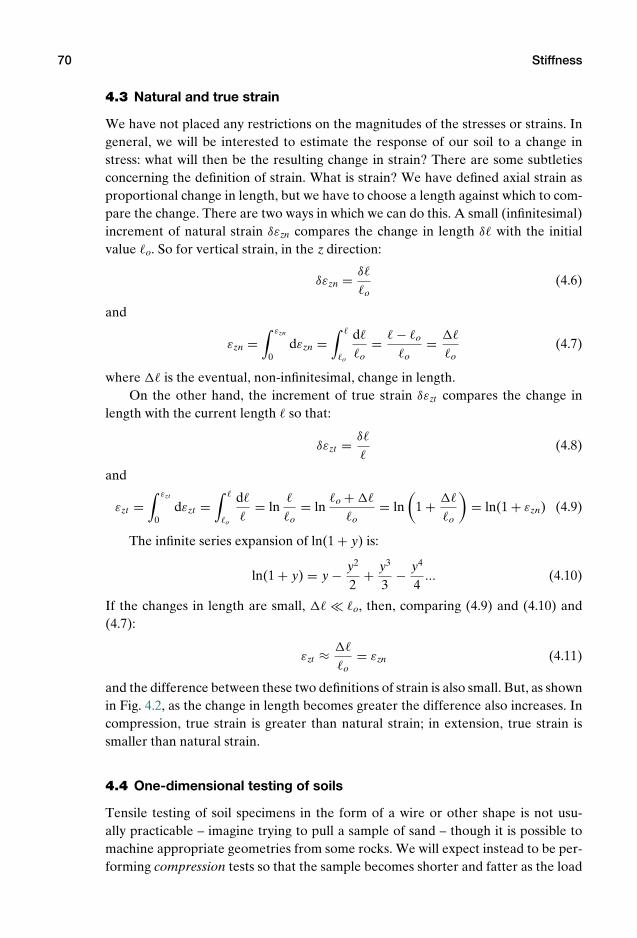
P1: KAE


70 Stiffness

4.3 Natural and true strain

We have not placed any restrictions on the magnitudes of the stresses or strains. Ingeneral, we will be interested to estimate the response of our soil to a change instress: what will then be the resulting change in strain? There are some subtletiesconcerning the definition of strain. What is strain? We have defined axial strain asproportional change in length, but we have to choose a length against which to com-pare the change. There are two ways in which we can do this. A small (infinitesimal)increment of natural strain δεzn compares the change in length δ with the initialvalue o. So for vertical strain, in the z direction:

δεzn = δ

o(4.6)

and

εzn =∫ εzn

0dεzn =

∫

o

d

o= − o

o=

o(4.7)

where is the eventual, non-infinitesimal, change in length.On the other hand, the increment of true strain δεzt compares the change in

length with the current length so that:

δεzt = δ

(4.8)

and

εzt =∫ εzt

0dεzt =

∫

o

d

= ln

o= ln

o +

o= ln

(1 +

o

)= ln(1 + εzn) (4.9)

The infinite series expansion of ln(1 + y) is:

ln(1 + y) = y − y2

2+ y3

3− y4

4... (4.10)

If the changes in length are small, o, then, comparing (4.9) and (4.10) and(4.7):

εzt ≈

o= εzn (4.11)

and the difference between these two definitions of strain is also small. But, as shownin Fig. 4.2, as the change in length becomes greater the difference also increases. Incompression, true strain is greater than natural strain; in extension, true strain issmaller than natural strain.

4.4 One-dimensional testing of soils

Tensile testing of soil specimens in the form of a wire or other shape is not usu-ally practicable – imagine trying to pull a sample of sand – though it is possible tomachine appropriate geometries from some rocks. We will expect instead to be per-forming compression tests so that the sample becomes shorter and fatter as the load

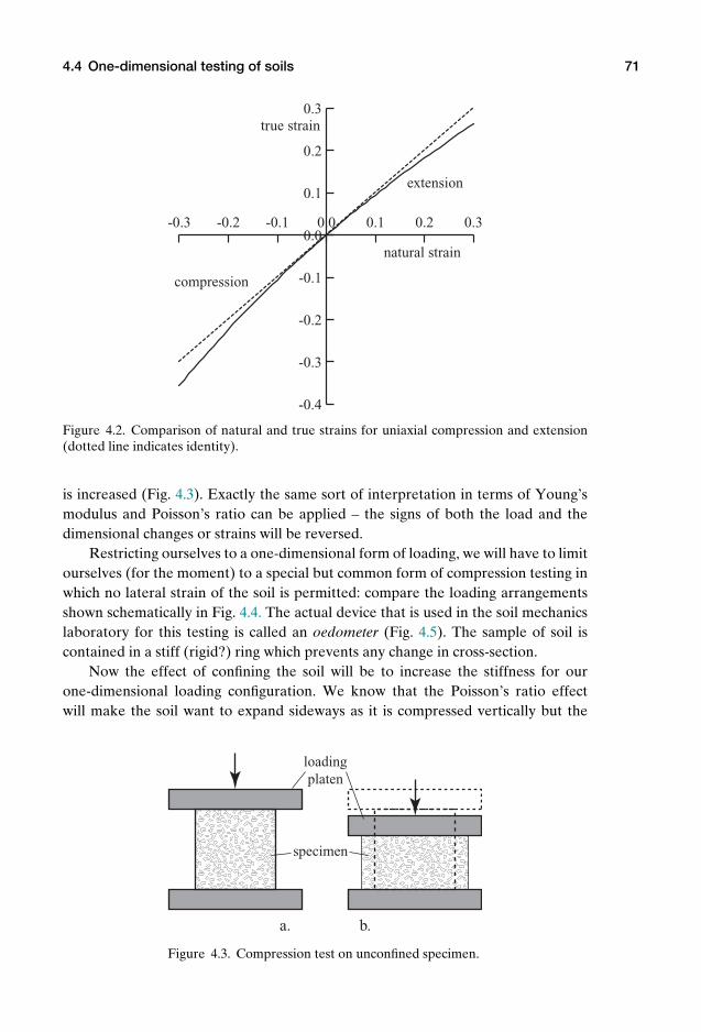
P1: KAE


4.4 One-dimensional testing of soils 71

natural strain

true strain

-0.3 -0.2 -0.1 0.0 0.1 0.2 0.3

-0.4

-0.3

-0.2

-0.1

0.0

0.1

0.2

0.3

extension

compression

Figure 4.2. Comparison of natural and true strains for uniaxial compression and extension(dotted line indicates identity).

is increased (Fig. 4.3). Exactly the same sort of interpretation in terms of Young’smodulus and Poisson’s ratio can be applied – the signs of both the load and thedimensional changes or strains will be reversed.

Restricting ourselves to a one-dimensional form of loading, we will have to limitourselves (for the moment) to a special but common form of compression testing inwhich no lateral strain of the soil is permitted: compare the loading arrangementsshown schematically in Fig. 4.4. The actual device that is used in the soil mechanicslaboratory for this testing is called an oedometer (Fig. 4.5). The sample of soil iscontained in a stiff (rigid?) ring which prevents any change in cross-section.

Now the effect of confining the soil will be to increase the stiffness for ourone-dimensional loading configuration. We know that the Poisson’s ratio effectwill make the soil want to expand sideways as it is compressed vertically but the

specimen

loading platen

a. b.

Figure 4.3. Compression test on unconfined specimen.

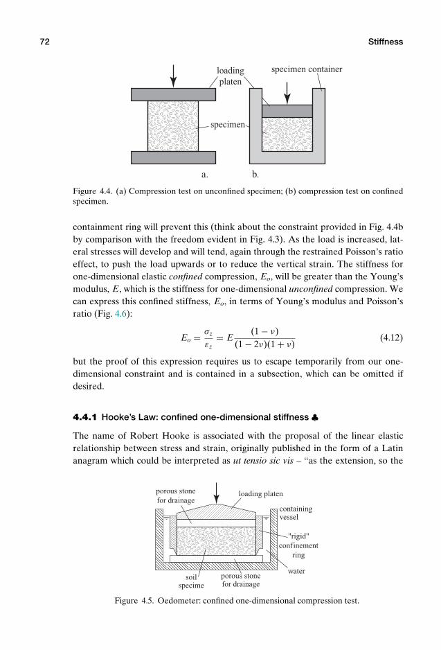
P1: KAE


72 Stiffness

specimen

loading platen

a. b.

specimen container

Figure 4.4. (a) Compression test on unconfined specimen; (b) compression test on confinedspecimen.

containment ring will prevent this (think about the constraint provided in Fig. 4.4bby comparison with the freedom evident in Fig. 4.3). As the load is increased, lat-eral stresses will develop and will tend, again through the restrained Poisson’s ratioeffect, to push the load upwards or to reduce the vertical strain. The stiffness forone-dimensional elastic confined compression, Eo, will be greater than the Young’smodulus, E, which is the stiffness for one-dimensional unconfined compression. Wecan express this confined stiffness, Eo, in terms of Young’s modulus and Poisson’sratio (Fig. 4.6):

Eo = σz

εz= E

(1 − ν)(1 − 2ν)(1 + ν)

(4.12)

but the proof of this expression requires us to escape temporarily from our one-dimensional constraint and is contained in a subsection, which can be omitted ifdesired.

4.4.1 Hooke’s Law: confined one-dimensional stiffness ♣The name of Robert Hooke is associated with the proposal of the linear elasticrelationship between stress and strain, originally published in the form of a Latinanagram which could be interpreted as ut tensio sic vis – “as the extension, so the

containing vessel

soil specime

porous stone for drainage

porous stone for drainage

"rigid" confinement

ring

loading platen

water

Figure 4.5. Oedometer: confined one-dimensional compression test.

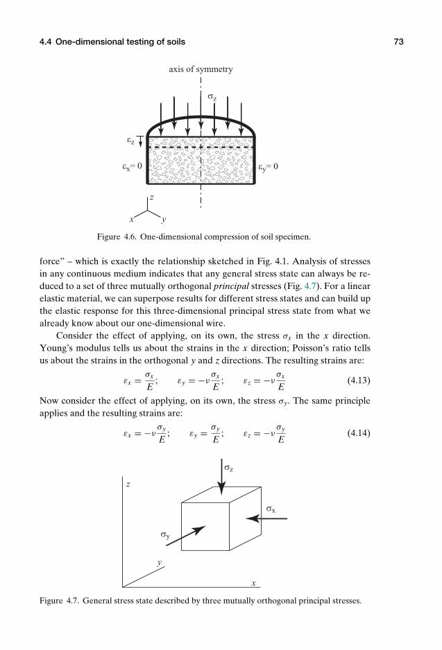
P1: KAE


4.4 One-dimensional testing of soils 73

σz

εz

εx= 0 εy= 0

axis of symmetry

z

yx

Figure 4.6. One-dimensional compression of soil specimen.

force” – which is exactly the relationship sketched in Fig. 4.1. Analysis of stressesin any continuous medium indicates that any general stress state can always be re-duced to a set of three mutually orthogonal principal stresses (Fig. 4.7). For a linearelastic material, we can superpose results for different stress states and can build upthe elastic response for this three-dimensional principal stress state from what wealready know about our one-dimensional wire.

Consider the effect of applying, on its own, the stress σx in the x direction.Young’s modulus tells us about the strains in the x direction; Poisson’s ratio tellsus about the strains in the orthogonal y and z directions. The resulting strains are:

εx = σx

E; εy = −ν

σx

E; εz = −ν

σx

E(4.13)

Now consider the effect of applying, on its own, the stress σy. The same principleapplies and the resulting strains are:

εx = −νσy

E; εy = σy

E; εz = −ν

σy

E(4.14)

x

y

z

σx

σz

σy

Figure 4.7. General stress state described by three mutually orthogonal principal stresses.

P1: KAE


74 Stiffness

Finally, consider the effect of applying, on its own, the stress σz. The resulting strainsare:

εx = −νσz

E; εy = −ν

σz

E; εz = σz

E(4.15)

Then we superpose all these strains to find the effect of applying all three principalstresses:

εx = σx

E− ν

σy

E− ν

σz

E; εy = −ν

σx

E+ σy

E− ν

σz

E; εz = −ν

σx

E− ν

σy

E+ σz

E(4.16)

and this is Hooke’s Law of linear elasticity stated in terms of principal stresses andstrains.

Now the one-dimensional constrained compression of the elastic material in theoedometer is just a special case of this general elastic stress condition. We imposetwo conditions:

The stress state has a symmetry about the vertical z axis (Fig. 4.6) so that thestresses in the x and y directions must be identical σx = σy.

The constrained nature of the compression requires that the strains in the x andy directions must both be zero, εx = εy = 0.

Applying these two conditions to (4.16) we find first that:

σx = σy = ν

1 − νσz (4.17)

and second, after a little manipulation, having substituted these values of σx and σy,that the one-dimensional confined stiffness, Eo, is:

Eo = σz

εz= E

(1 − ν)(1 − 2ν)(1 + ν)

(4.18)

and it should not surprise us that, if Poisson’s ratio ν = 0.5, which we saw impliedconstant volume elastic response, then the one-dimensional stiffness Eo is infinite –the material cannot expand laterally and therefore cannot compress axially either.The more general conclusion that we can draw is that, if we observe stiffness in thisway, we will only be able to discover the composite elastic property, Eo (4.18), andwill not be able to discover the separate values of Young’s modulus and Poisson’sratio. The relationship between the ratio Eo/E and Poisson’s ratio ν is shown inFig. 4.8.

4.5 One-dimensional (confined) stiffness of soils

Some examples of one-dimensional compression of soils are shown in Fig. 4.9, plot-ted in terms of vertical stress and specific volume rather than volumetric or verticalstrain. Two characteristics of these responses are immediately evident: the com-pression is very nonlinear and it is irreversible. We will discuss these two featuresseparately but there is one immediate consequence of the combination of the twocharacteristics: we have to recognise that the stiffness that we observe as an incre-mental response is not an elastic stiffness. For a truly elastic material, the behaviour

P1: KAE


4.5 One-dimensional (confined) stiffness of soils 75

0.0 0.1 0.2 0.3 0.4 0.51.0

1.5

2.0

2.5

3.0

Poisson's ratio: ν

Eo/E

Figure 4.8. Ratio of confined modulus and Young’s modulus as function of Poisson’s ratio ν.

on loading and unloading would be the same and we would recover the same den-sity of packing when we found ourselves applying once again the same load. So aword of warning is needed: geotechnical engineers are a bit slack in using the lan-guage of elasticity to describe behaviour which is certainly not elastic in the strictsense. A material that is linear and elastic follows the principle of superposition(this was implicit in the way in which we made use of Hooke’s Law, Section 4.4.1),and this will not be strictly possible for real soils.

A thought experiment concerning the one-dimensional compression of soil isshown in Fig. 4.10. This is a completely generic picture which indicates our expec-tation that stiffness will increase as the density of the soil increases or its specific

2.4 2.2 2.0specific volume: vspecific volume: v

600

600

400

400

200200

800

00

kPakPavertical stress σ'z

vertical stress σ'z b.a.

1.8 1.78 1.76 1.74 1.54 1.52

loose

dense

Figure 4.9. One-dimensional (confined) compression of (a) sand and (b) clay.

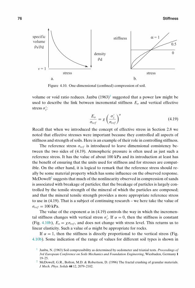
P1: KAE


76 Stiffness

densityρd

specific volumeρs/ρd

stress stress

stiffness

0

0.5

α = 1

a. b.

v = 1

Figure 4.10. One-dimensional (confined) compression of soil.

volume or void ratio reduces. Janbu (1963)1 suggested that a power law might beused to describe the link between incremental stiffness Eo and vertical effectivestress σ ′

z:

Eo

σre f= χ

(σ ′

z

σre f

)α

(4.19)

Recall that when we introduced the concept of effective stress in Section 2.8 wenoted that effective stresses were important because they controlled all aspects ofstiffness and strength of soils. Here is an example of their role in controlling stiffness.

The reference stress σre f is introduced to leave dimensional consistency be-tween the two sides of (4.19). Atmospheric pressure is often used as just such areference stress. It has the value of about 100 kPa and its introduction at least hasthe benefit of ensuring that the units used for stiffness and for stresses are compat-ible. On the other hand, it is logical to remark that the reference stress should re-ally be some material property which has some influence on the observed response.McDowell2 suggests that much of the nonlinearity observed in compression of sandsis associated with breakage of particles; that the breakage of particles is largely con-trolled by the tensile strength of the mineral of which the particles are composed;and that the mineral tensile strength provides a more appropriate reference stressto use in (4.19). That is a subject of continuing research – we here take the value ofσre f = 100 kPa.

The value of the exponent α in (4.19) controls the way in which the incremen-tal stiffness changes with vertical stress σ ′

z. If α = 0, then the stiffness is constant(Fig. 4.10b), Eo = χσre f , and does not change with stress level. This returns us tolinear elasticity. Such a value of α might be appropriate for rocks.

If α = 1, then the stiffness is directly proportional to the vertical stress (Fig.4.10b). Some indication of the range of values for different soil types is shown in

1 Janbu, N. (1963) Soil compressibility as determined by oedometer and triaxial tests. Proceedings of3rd European Conference on Soils Mechanics and Foundation Engineering, Wiesbaden, Germany 119–25.

2 McDowell, G.R., Bolton, M.D. & Robertson, D. (1996) The fractal crushing of granular materials.J Mech. Phys. Solids 44 12, 2079–2102.

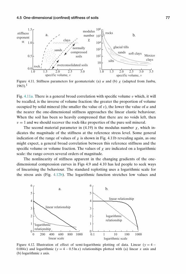
P1: KAE


4.5 One-dimensional (confined) stiffness of soils 77

1.0 1.5 2.0 2.5 3.00.0

0.5

1.0

1.5

rock

sands

clays

normally compressed

soils

specific volume, v specific volume, v

stiffness exponent

α

overconsolidated soils

1.0 1.5 2.0 2.5 3.0 3.51

10

102

103

104

105

106modulus number

χ

rocks

glacial tills

sands

silts

soft claysMexico

clays

a. b.

Figure 4.11. Stiffness parameters for geomaterials: (a) α and (b) χ (adapted from Janbu,1963).1

Fig. 4.11a. There is a general broad correlation with specific volume v which, it willbe recalled, is the inverse of volume fraction: the greater the proportion of volumeoccupied by solid mineral (the smaller the value of v), the lower the value of α andthe nearer the one-dimensional stiffness approaches the linear elastic behaviour.When the soil has been so heavily compressed that there are no voids left, thenv = 1 and we should recover the rock-like properties of the pure soil mineral.

The second material parameter in (4.19) is the modulus number χ , which in-dicates the magnitude of the stiffness at the reference stress level. Some generalindication of the range of values of χ is shown in Fig. 4.11b revealing again, as onemight expect, a general broad correlation between this reference stiffness and thespecific volume or volume fraction. The values of χ are indicated on a logarithmicscale: the range covers several orders of magnitude.

The nonlinearity of stiffness apparent in the changing gradients of the one-dimensional compression curves in Figs 4.9 and 4.10 has led people to seek waysof linearising the behaviour. The standard replotting uses a logarithmic scale forthe stress axis (Fig. 4.12b). The logarithmic function stretches low values and

0 200 400 600 800 10000

1

2

3

4

5

6

0.1 1 10 100 10000

1

2

3

4

5

6

linear relationship

linear relationship

logarithmic relationship

logarithmic relationship

linear scale logarithmic scale

a. b.

Figure 4.12. Illustration of effect of semi-logarithmic plotting of data. Linear (y = 4 −0.004x) and logarithmic (y = 4 − 0.5 ln x) relationships plotted with (a) linear x axis and(b) logarithmic x axis.

P1: KAE


78 Stiffness

compresses high values and is often an effective way of removing curvature fromobserved patterns of response.

If we choose a value of α = 1 in (4.19), then the one-dimensional stiffness be-comes:

Eo = δσ ′z

δεz= χσ ′

z (4.20)

so that the increment of axial strain:

δεz = δσ ′z

Eo= δσ ′

z

χσ ′z

(4.21)

We can integrate this to give:

εz =∫

dσ ′z

χσ ′z

= 1χ

lnσ ′

z

σ ′zo

(4.22)

where σ ′zo is an initial value of vertical stress at which the strain is deemed to be zero.

Thus this value of α = 1 is directly compatible with the logarithmic plotting of stresswhich, from Fig. 4.11, we can expect to be particularly appropriate for presenting thebehaviour of clays. However, the actual range of values of α should remind us thatthis logarithmic plotting of stress may not always be helpful. It is always tempting totry to fit the same simple model to materials who do not think that they know of itsexistence.

When we work in terms of specific volumes, volumetric strain in the oedometeris the same as vertical strain because there is no lateral strain which is able to con-tribute to the change in volume: δεz = δεvol = −δv/v (keeping a sign convention ofpositive strains in compression). If we choose to work with the true strain, then werecall the logarithmic definition of strain from (4.9) and (4.7):

εzt = − ln

o= − ln

v

vo= ln vo − ln v (4.23)

We might choose to plot the observed response in terms of true strain and logarithmof stress to straighten out the experimental response. This would then be an appli-cation of a double logarithmic treatment of the data of specific volume and verticalstress.

4.6 Calculation of strains

We have an expression for the variation of stiffness with stress (4.19) and we canintegrate this equation to discover the strain in an element of soil, one-dimensionallyconfined, caused by an increase in stress, and hence we can calculate the resultingchange in dimension of the element of soil. The increment of strain, δεz, is the ratioof the increment of effective stress, δσ ′

z, and the stiffness, Eo:

δεz = δσ ′z

Eo(4.24)

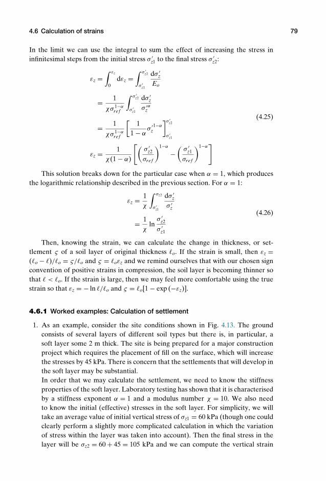
P1: KAE


4.6 Calculation of strains 79

In the limit we can use the integral to sum the effect of increasing the stress ininfinitesimal steps from the initial stress σ ′

z1 to the final stress σ ′z2:

εz =∫ εz

0dεz =

∫ σ ′z2

σ ′z1

dσ ′z

Eo

= 1

χσ 1−αre f

∫ σ ′z2

σ ′z1

dσ ′z

σ ′zα

= 1

χσ 1−αre f

[1

1 − ασ ′

z1−α

]σ ′z2

σ ′z1

εz = 1χ(1 − α)

[(σ ′

z2

σre f

)1−α

−(

σ ′z1

σre f

)1−α]

(4.25)

This solution breaks down for the particular case when α = 1, which producesthe logarithmic relationship described in the previous section. For α = 1:

εz = 1χ

∫ σz2

σ ′z1

dσ ′z

σ ′z

= 1χ

lnσ ′

z2

σ ′z1

(4.26)

Then, knowing the strain, we can calculate the change in thickness, or set-tlement ς of a soil layer of original thickness o. If the strain is small, then εz =(o − )/o = ς/o and ς = oεz and we remind ourselves that with our chosen signconvention of positive strains in compression, the soil layer is becoming thinner sothat < o. If the strain is large, then we may feel more comfortable using the truestrain so that εz = − ln /o and ς = o[1 − exp (−εz)].

4.6.1 Worked examples: Calculation of settlement

1. As an example, consider the site conditions shown in Fig. 4.13. The groundconsists of several layers of different soil types but there is, in particular, asoft layer some 2 m thick. The site is being prepared for a major constructionproject which requires the placement of fill on the surface, which will increasethe stresses by 45 kPa. There is concern that the settlements that will develop inthe soft layer may be substantial.In order that we may calculate the settlement, we need to know the stiffnessproperties of the soft layer. Laboratory testing has shown that it is characterisedby a stiffness exponent α = 1 and a modulus number χ = 10. We also needto know the initial (effective) stresses in the soft layer. For simplicity, we willtake an average value of initial vertical stress of σz1 = 60 kPa (though one couldclearly perform a slightly more complicated calculation in which the variationof stress within the layer was taken into account). Then the final stress in thelayer will be σz2 = 60 + 45 = 105 kPa and we can compute the vertical strain

P1: KAE


80 Stiffness

soft layer2m

45kPa

Figure 4.13. Site conditions for calculation of settlement.

from (4.26):

εz = 110

ln10560

= 0.056 (4.27)

Thus the placement of the fill produces a vertical strain in the soft layer of someεz = 5.6%. The layer has a thickness of z = 2 m so that the vertical settlementin that layer is ς = εzz = 112 mm.

2. More generally, if we are interested in summing the settlements from a numbern of layers of thickness zi (Fig. 4.14 – and one way of dealing with the variationof initial stress within a single soil layer is to divide it into thinner sub-layerswhich can individually be treated as uniform), then this calculation is repeatedfor each layer and the total settlement ς is deduced by summation.

ς =n∑

i=1

εzizi (4.28)

Figure 4.15 shows a site where 6 m of soft soil overlie rock. The soft soil hasunit weight γ = 17 kN/m3 and is characterised by values of stiffness exponentα = 0.8 and modulus number χ = 15. The water table is at the ground surface.The site is being prepared by placing a layer of fill generating a uniform increasein stress of σz = 25 kPa. We want to calculate the resulting settlement. We will

sub-layers

∆zi

i = 1

i = n

Figure 4.14. Layered site conditions for calculation of settlement.

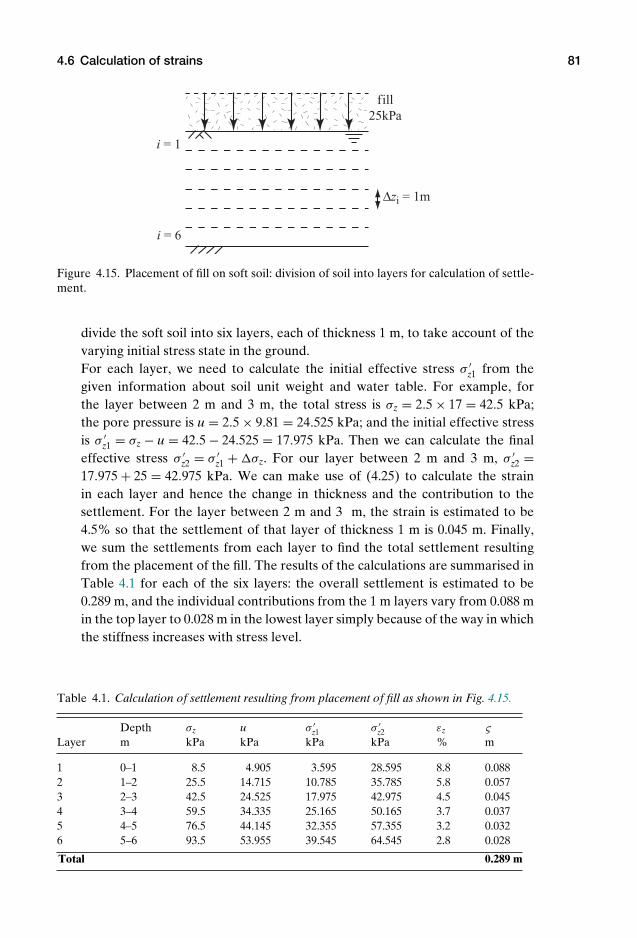
P1: KAE


4.6 Calculation of strains 81

∆zi = 1m

i = 1

i = 6

fill 25kPa

Figure 4.15. Placement of fill on soft soil: division of soil into layers for calculation of settle-ment.

divide the soft soil into six layers, each of thickness 1 m, to take account of thevarying initial stress state in the ground.For each layer, we need to calculate the initial effective stress σ ′

z1 from thegiven information about soil unit weight and water table. For example, forthe layer between 2 m and 3 m, the total stress is σz = 2.5 × 17 = 42.5 kPa;the pore pressure is u = 2.5 × 9.81 = 24.525 kPa; and the initial effective stressis σ ′

z1 = σz − u = 42.5 − 24.525 = 17.975 kPa. Then we can calculate the finaleffective stress σ ′

z2 = σ ′z1 + σz. For our layer between 2 m and 3 m, σ ′

z2 =17.975 + 25 = 42.975 kPa. We can make use of (4.25) to calculate the strainin each layer and hence the change in thickness and the contribution to thesettlement. For the layer between 2 m and 3 m, the strain is estimated to be4.5% so that the settlement of that layer of thickness 1 m is 0.045 m. Finally,we sum the settlements from each layer to find the total settlement resultingfrom the placement of the fill. The results of the calculations are summarised inTable 4.1 for each of the six layers: the overall settlement is estimated to be0.289 m, and the individual contributions from the 1 m layers vary from 0.088 min the top layer to 0.028 m in the lowest layer simply because of the way in whichthe stiffness increases with stress level.

Table 4.1. Calculation of settlement resulting from placement of fill as shown in Fig. 4.15.

Depth σz u σ ′z1 σ ′

z2 εz ς

Layer m kPa kPa kPa kPa % m

1 0–1 8.5 4.905 3.595 28.595 8.8 0.0882 1–2 25.5 14.715 10.785 35.785 5.8 0.0573 2–3 42.5 24.525 17.975 42.975 4.5 0.0454 3–4 59.5 34.335 25.165 50.165 3.7 0.0375 4–5 76.5 44.145 32.355 57.355 3.2 0.0326 5–6 93.5 53.955 39.545 64.545 2.8 0.028

Total 0.289 m

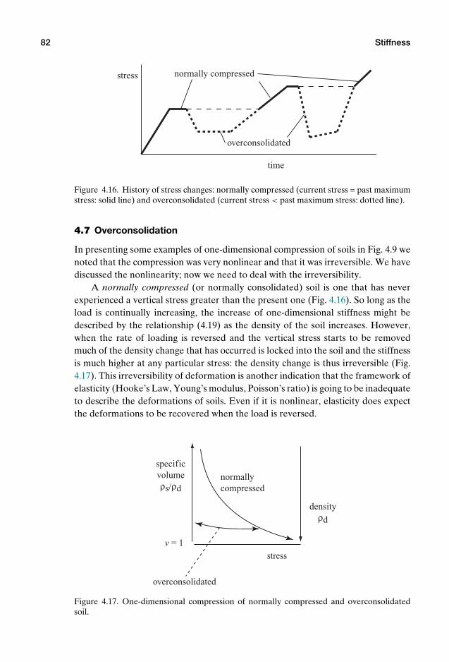
P1: KAE


82 Stiffness

time

stress normally compressed

overconsolidated

Figure 4.16. History of stress changes: normally compressed (current stress = past maximumstress: solid line) and overconsolidated (current stress < past maximum stress: dotted line).

4.7 Overconsolidation

In presenting some examples of one-dimensional compression of soils in Fig. 4.9 wenoted that the compression was very nonlinear and that it was irreversible. We havediscussed the nonlinearity; now we need to deal with the irreversibility.

A normally compressed (or normally consolidated) soil is one that has neverexperienced a vertical stress greater than the present one (Fig. 4.16). So long as theload is continually increasing, the increase of one-dimensional stiffness might bedescribed by the relationship (4.19) as the density of the soil increases. However,when the rate of loading is reversed and the vertical stress starts to be removedmuch of the density change that has occurred is locked into the soil and the stiffnessis much higher at any particular stress: the density change is thus irreversible (Fig.4.17). This irreversibility of deformation is another indication that the framework ofelasticity (Hooke’s Law, Young’s modulus, Poisson’s ratio) is going to be inadequateto describe the deformations of soils. Even if it is nonlinear, elasticity does expectthe deformations to be recovered when the load is reversed.

densityρd


stress

normally compressed

overconsolidated

v = 1

Figure 4.17. One-dimensional compression of normally compressed and overconsolidatedsoil.

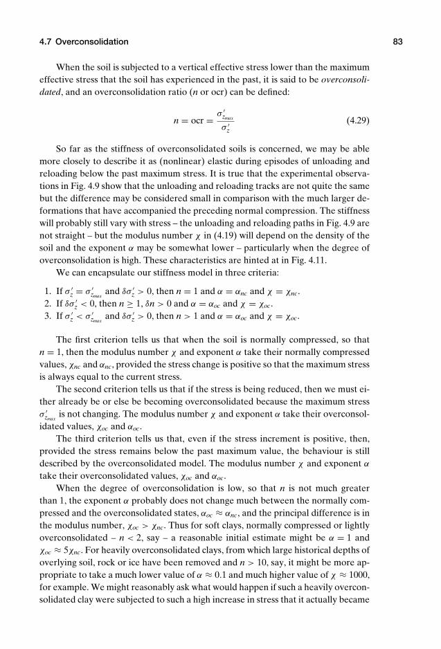
P1: KAE


4.7 Overconsolidation 83

When the soil is subjected to a vertical effective stress lower than the maximumeffective stress that the soil has experienced in the past, it is said to be overconsoli-dated, and an overconsolidation ratio (n or ocr) can be defined:

n = ocr = σ ′zmax

σ ′z

(4.29)

So far as the stiffness of overconsolidated soils is concerned, we may be ablemore closely to describe it as (nonlinear) elastic during episodes of unloading andreloading below the past maximum stress. It is true that the experimental observa-tions in Fig. 4.9 show that the unloading and reloading tracks are not quite the samebut the difference may be considered small in comparison with the much larger de-formations that have accompanied the preceding normal compression. The stiffnesswill probably still vary with stress – the unloading and reloading paths in Fig. 4.9 arenot straight – but the modulus number χ in (4.19) will depend on the density of thesoil and the exponent α may be somewhat lower – particularly when the degree ofoverconsolidation is high. These characteristics are hinted at in Fig. 4.11.

We can encapsulate our stiffness model in three criteria:

1. If σ ′z = σ ′

zmaxand δσ ′

z > 0, then n = 1 and α = αnc and χ = χnc.2. If δσ ′

z < 0, then n ≥ 1, δn > 0 and α = αoc and χ = χoc.3. If σ ′

z < σ ′zmax

and δσ ′z > 0, then n > 1 and α = αoc and χ = χoc.

The first criterion tells us that when the soil is normally compressed, so thatn = 1, then the modulus number χ and exponent α take their normally compressedvalues, χnc and αnc, provided the stress change is positive so that the maximum stressis always equal to the current stress.

The second criterion tells us that if the stress is being reduced, then we must ei-ther already be or else be becoming overconsolidated because the maximum stressσ ′

zmaxis not changing. The modulus number χ and exponent α take their overconsol-

idated values, χoc and αoc.The third criterion tells us that, even if the stress increment is positive, then,

provided the stress remains below the past maximum value, the behaviour is stilldescribed by the overconsolidated model. The modulus number χ and exponent α

take their overconsolidated values, χoc and αoc.When the degree of overconsolidation is low, so that n is not much greater

than 1, the exponent α probably does not change much between the normally com-pressed and the overconsolidated states, αoc ≈ αnc, and the principal difference is inthe modulus number, χoc > χnc. Thus for soft clays, normally compressed or lightlyoverconsolidated – n < 2, say – a reasonable initial estimate might be α = 1 andχoc ≈ 5χnc. For heavily overconsolidated clays, from which large historical depths ofoverlying soil, rock or ice have been removed and n > 10, say, it might be more ap-propriate to take a much lower value of α ≈ 0.1 and much higher value of χ ≈ 1000,for example. We might reasonably ask what would happen if such a heavily overcon-solidated clay were subjected to such a high increase in stress that it actually became

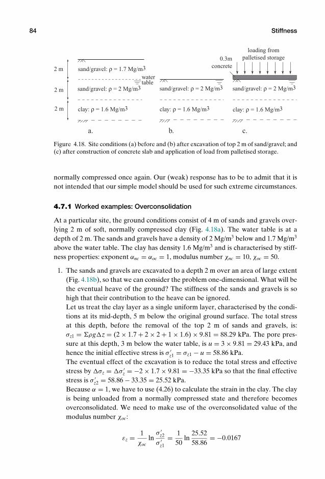
P1: KAE


84 Stiffness

sand/gravel: ρ = 1.7 Mg/m3

clay: ρ = 1.6 Mg/m3 clay: ρ = 1.6 Mg/m3 clay: ρ = 1.6 Mg/m3

sand/gravel: ρ = 2 Mg/m3 sand/gravel: ρ = 2 Mg/m3 sand/gravel: ρ = 2 Mg/m3

2 m

2 m

2 m

water table

a. b. c.

0.3m concrete

loading from palletised storage

Figure 4.18. Site conditions (a) before and (b) after excavation of top 2 m of sand/gravel; and(c) after construction of concrete slab and application of load from palletised storage.

normally compressed once again. Our (weak) response has to be to admit that it isnot intended that our simple model should be used for such extreme circumstances.

4.7.1 Worked examples: Overconsolidation

At a particular site, the ground conditions consist of 4 m of sands and gravels over-lying 2 m of soft, normally compressed clay (Fig. 4.18a). The water table is at adepth of 2 m. The sands and gravels have a density of 2 Mg/m3 below and 1.7 Mg/m3

above the water table. The clay has density 1.6 Mg/m3 and is characterised by stiff-ness properties: exponent αnc = αoc = 1, modulus number χnc = 10, χoc = 50.

1. The sands and gravels are excavated to a depth 2 m over an area of large extent(Fig. 4.18b), so that we can consider the problem one-dimensional. What will bethe eventual heave of the ground? The stiffness of the sands and gravels is sohigh that their contribution to the heave can be ignored.Let us treat the clay layer as a single uniform layer, characterised by the condi-tions at its mid-depth, 5 m below the original ground surface. The total stressat this depth, before the removal of the top 2 m of sands and gravels, is:σz1 = ρgz = (2 × 1.7 + 2 × 2 + 1 × 1.6) × 9.81 = 88.29 kPa. The pore pres-sure at this depth, 3 m below the water table, is u = 3 × 9.81 = 29.43 kPa, andhence the initial effective stress is σ ′

z1 = σz1 − u = 58.86 kPa.The eventual effect of the excavation is to reduce the total stress and effectivestress by σz = σ ′

z = −2 × 1.7 × 9.81 = −33.35 kPa so that the final effectivestress is σ ′

z2 = 58.86 − 33.35 = 25.52 kPa.Because α = 1, we have to use (4.26) to calculate the strain in the clay. The clayis being unloaded from a normally compressed state and therefore becomesoverconsolidated. We need to make use of the overconsolidated value of themodulus number χoc:

εz = 1χoc

lnσ ′

z2

σ ′z1

= 150

ln25.5258.86

= −0.0167

P1: KAE


4.7 Overconsolidation 85

or a strain of −1.67%. The negative sign indicates that the clay is heaving orexpanding in thickness because of the reduction of effective stress. This is thestrain; the heave is the product of the strain and the thickness of the layer ofclay: ς = εzz = −0.0167 × 2 = −0.033 m.

2. The excavation was part of the initial stage of construction of a large warehousewhich will consist roughly of a concrete floor 0.3 m thick, of density 2.4 Mg/m3,and subsequent palletised stored contents (Fig. 4.18c). What will be the eventualsettlement of the site – which again means just the clay – if the stored materialsgenerate a pressure of (a) 25 kPa or (b) 40 kPa?The concrete floor generates a surface pressure of 0.3 × 2.4 × 9.81 = 7.06 kPa.With a loading of 25 kPa from the stored materials, the total increase in appliedvertical stress is 7.06 + 25 = 32.06 kPa, which is just a little less than the stressremoved by the excavation of the top 2 m of sands and gravels (33.35 kPa). Thewhole of this stress increase can thus be absorbed within the overconsolidatedresponse of the clay. The vertical effective stress changes from σ ′

z2 = 25.52 kPato σ ′

z3 = 25.52 + 32.06 = 57.58 kPa and the resulting vertical strain is:

εz = 1χoc

lnσ ′

z3

σ ′z2

= 150

ln57.5825.52

= 0.0163

or a strain of 1.63%. The settlement is the product of the strain and the thick-ness of the layer of clay: ς = εzz = 0.0163 × 2 = 0.032 m. The nett effect ofthe construction activities is to produce a negligible heave with a magnitude ofabout 1 mm.With an applied operational loading of 40 kPa, we can see that we will be takingour clay back into the normally compressed region. The total increase in effec-tive stress is the sum of the stress generated by the concrete slab and this appliedloading: 7.06 + 40 = 47.06 kPa. We have to divide this increase in vertical effec-tive stress into two parts: the first part, 33.35 kPa, exactly matches the stressremoved through excavation of the top 2 m of sands and gravels. This will ex-actly recover in settlement the heave of 0.033 m that occurred as a result of theexcavation. The remainder, 47.06 − 33.35 = 13.71 kPa, is compressing the clayin the normally compressed, less stiff region. The final vertical effective stress isσ ′

z4 = 25.52 + 47.06 = 72.58 kPa and we can apply (4.26) to calculate the strain,using the normally compressed value of the modulus number χnc:

εz = 1χnc

lnσ ′

z4

σ ′z1

= 110

ln72.5858.86

= 0.0209

or a strain of 2.09%. The total strain resulting from the use of the warehousewith this level of loading is therefore 0.0167 + 0.0209 = 0.0376 or 3.76%, andthe settlement is 0.075 m. The nett effect of the construction activities is to pro-duce a settlement of about 0.042 m.

It is evident that the settlement increases rapidly once the loading takes the clayinto a normally compressed state of stress. There is obvious advantage in trying to

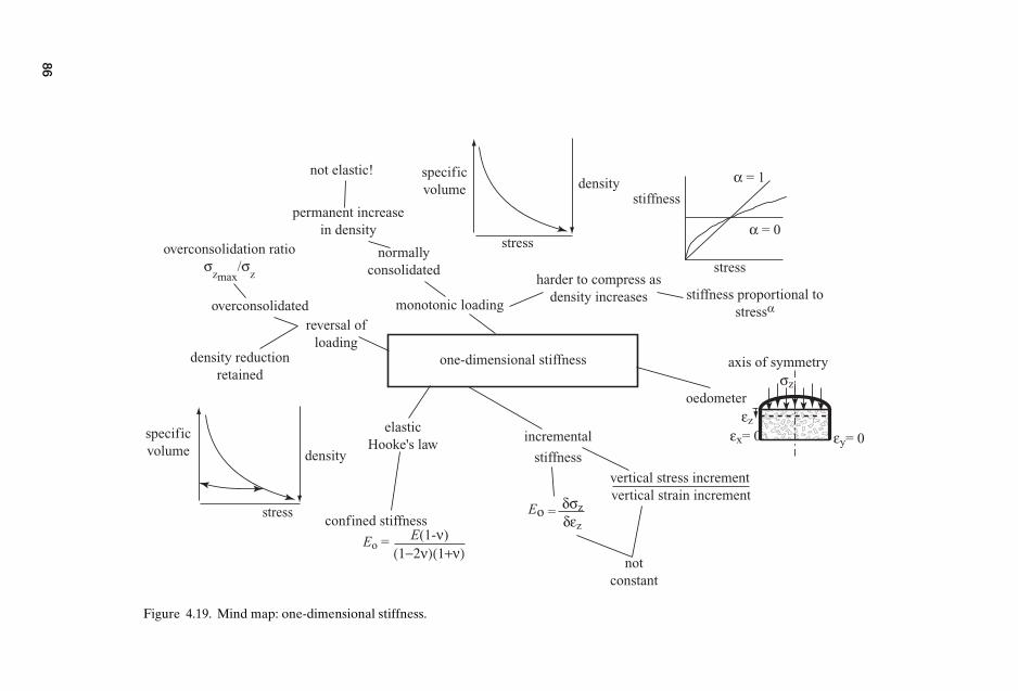
P1:K

AE

OneD

im00a

CU

US648/M

uir978

0521

517737

August17,2009

19:12

one-dimensional stiffness

elasticHooke's law

confined stiffness

Eo = E(1-ν)(1−2ν)(1+ν)

incremental

stiffness

Eo =δσz

δεz

vertical stress incrementvertical strain increment

not constant

oedometer

stress

density

density

specific volume

specific volume

stress

stiffness

α = 1

α = 0

monotonic loading

normally consolidated

permanent increase in density

not elastic!

harder to compress as density increases stiffness proportional to

stressαreversal of

loading

overconsolidated

density reduction retained

overconsolidation ratioσ

zmax/σ

z

stress

σz

εz

εx= 0 εy= 0

axis of symmetry

Figure 4.19. Mind map: one-dimensional stiffness.

86

P1: KAE


4.8 Summary 87

design a balanced excavation in which the stress removed through excavation moreor less matches the eventual working loading that the ground will have to sustain.

4.8 Summary


1. Stiffness is a general term describing the link between changes in strain andchanges in stress.

2. Linear elasticity is a particular (simple) form of stiffness model described, forexample, by Hooke’s Law.

3. As soils are compressed one-dimensionally in an oedometer, the density in-creases and the stiffness also increases.

4. A power-law expression links one-dimensional stiffness to the current stresswith an exponent α and a modulus number χ . Various different types of re-sponse can be described using different values of α: α = 0 implies constant stiff-ness or linear elasticity.

5. There is some correlation between the values of χ and soil density.6. The compression of soils is often irreversible: unloading is accompanied by

smaller changes in volume and higher stiffnesses and permanent increase indensity.

7. Overconsolidation ratio (ocr) describes the ratio of maximum past verticalstress to current vertical stress.

8. Normally compressed soils have an overconsolidation ratio ocr = 1.

4.9 Exercises: Stiffness

1. Using the general expression for incremental one-dimensional stiffness Eo withreference stress σre f = 100 kPa calculate the stiffnesses for the geotechnical ma-terials in Table 4.2 at a vertical effective stress σz = 150 kPa.

Table 4.2. Stiffness properties for Question 1.

α χ

rock 0 105

glacial till 0.2 103

sand 0.5 102

clay 1 10

2. Use the stiffnesses calculated in Question 1 to calculate the strain generatedwhen the vertical effective stress increases from 150 kPa to 165 kPa. (Hint: As-sume that the stress increment is sufficiently small for the stiffness to be re-garded as constant over the increment.)

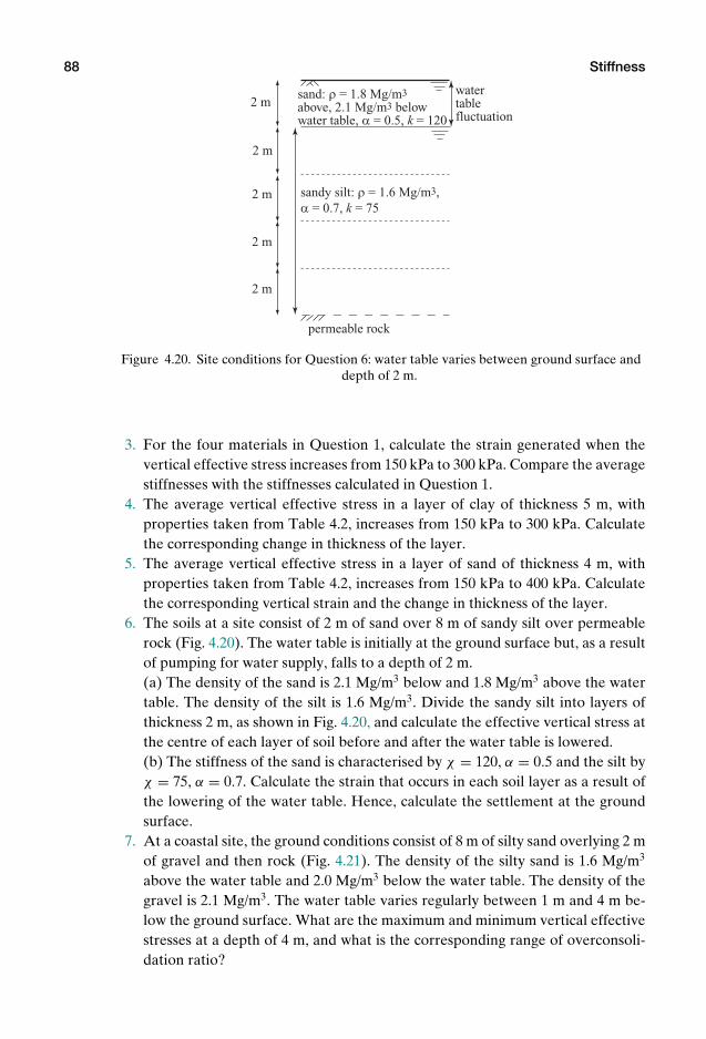
P1: KAE


88 Stiffness

sand: ρ = 1.8 Mg/m3 above, 2.1 Mg/m3 below water table, α = 0.5, k = 120

sandy silt: ρ = 1.6 Mg/m3, α = 0.7, k = 75

2 m

2 m

2 m

water table fluctuation

permeable rock

2 m

2 m

Figure 4.20. Site conditions for Question 6: water table varies between ground surface anddepth of 2 m.

3. For the four materials in Question 1, calculate the strain generated when thevertical effective stress increases from 150 kPa to 300 kPa. Compare the averagestiffnesses with the stiffnesses calculated in Question 1.

4. The average vertical effective stress in a layer of clay of thickness 5 m, withproperties taken from Table 4.2, increases from 150 kPa to 300 kPa. Calculatethe corresponding change in thickness of the layer.

5. The average vertical effective stress in a layer of sand of thickness 4 m, withproperties taken from Table 4.2, increases from 150 kPa to 400 kPa. Calculatethe corresponding vertical strain and the change in thickness of the layer.

6. The soils at a site consist of 2 m of sand over 8 m of sandy silt over permeablerock (Fig. 4.20). The water table is initially at the ground surface but, as a resultof pumping for water supply, falls to a depth of 2 m.(a) The density of the sand is 2.1 Mg/m3 below and 1.8 Mg/m3 above the watertable. The density of the silt is 1.6 Mg/m3. Divide the sandy silt into layers ofthickness 2 m, as shown in Fig. 4.20, and calculate the effective vertical stress atthe centre of each layer of soil before and after the water table is lowered.(b) The stiffness of the sand is characterised by χ = 120, α = 0.5 and the silt byχ = 75, α = 0.7. Calculate the strain that occurs in each soil layer as a result ofthe lowering of the water table. Hence, calculate the settlement at the groundsurface.

7. At a coastal site, the ground conditions consist of 8 m of silty sand overlying 2 mof gravel and then rock (Fig. 4.21). The density of the silty sand is 1.6 Mg/m3

above the water table and 2.0 Mg/m3 below the water table. The density of thegravel is 2.1 Mg/m3. The water table varies regularly between 1 m and 4 m be-low the ground surface. What are the maximum and minimum vertical effectivestresses at a depth of 4 m, and what is the corresponding range of overconsoli-dation ratio?

P1: KAE


4.9 Exercises: Stiffness 89

silty sand: ρ = 1.6 Mg/m3 above, 2.0 Mg/m3 below water table


1 m

3 m

4 m

water table fluctuation

rock

2 m

Figure 4.21. Site conditions for Question 7: water table varies between depths of 1 m and4 m.

Making reasonable assumptions, choose values of stiffness exponent α andmodulus number χ (Fig. 4.11) for the silty sand and estimate the heave andsettlement that occur each time the water table varies between its extremelevels.

8. As a result of a change in the economic climate, the design for the warehouse inSection 4.7.1 (Fig. 4.18) has been changed. The sands and gravels will now onlybe excavated to a depth of 1 m. Calculate the heave that will result from thisexcavation and the eventual settlement under working storage loads of 25 kPaand 40 kPa. The thickness of the concrete slab remains unchanged at 0.3 m.

9. The results of an oedometer test on reconstituted Gault clay are given in Table4.3. The specific volume of the clay at the end of the test was found to be 1.979.Estimate the value of modulus number χ and stiffness exponent α for this clayin its normally consolidated and overconsolidated states.

Table 4.3. Oedometer test onreconstituted Gault clay (Question 9).

Vertical Samplestress heightkPa mm

0 19.0550 17.95

100 16.77200 15.56400 14.49100 14.96

50 15.28

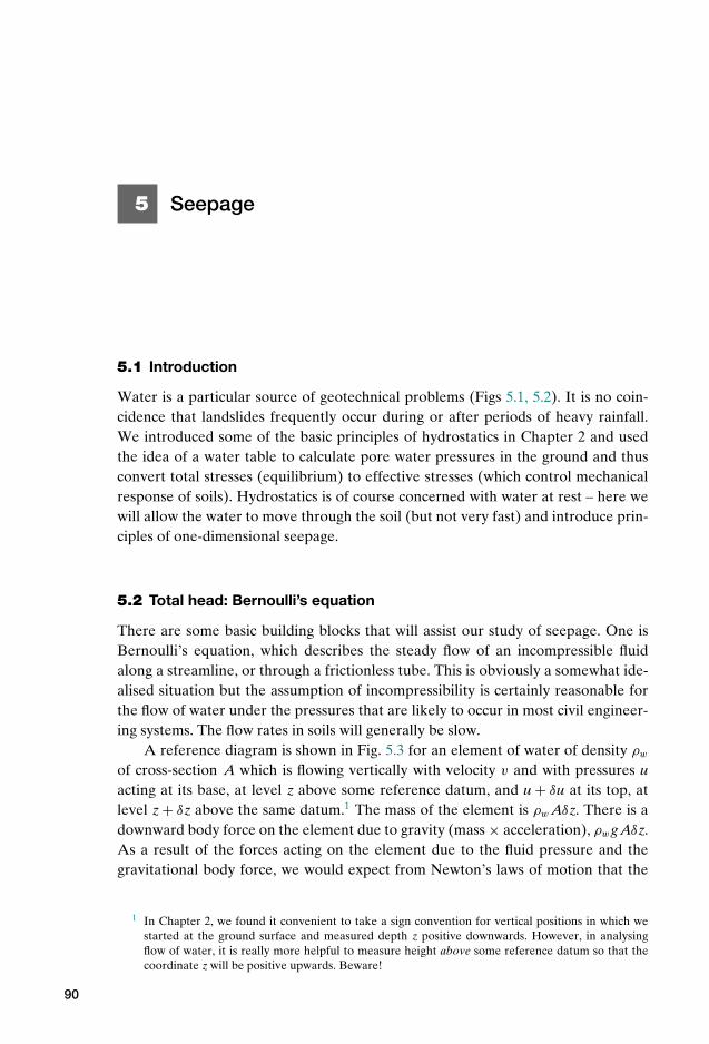
P1: KAE


5 Seepage

5.1 Introduction

Water is a particular source of geotechnical problems (Figs 5.1, 5.2). It is no coin-cidence that landslides frequently occur during or after periods of heavy rainfall.We introduced some of the basic principles of hydrostatics in Chapter 2 and usedthe idea of a water table to calculate pore water pressures in the ground and thusconvert total stresses (equilibrium) to effective stresses (which control mechanicalresponse of soils). Hydrostatics is of course concerned with water at rest – here wewill allow the water to move through the soil (but not very fast) and introduce prin-ciples of one-dimensional seepage.

5.2 Total head: Bernoulli’s equation

There are some basic building blocks that will assist our study of seepage. One isBernoulli’s equation, which describes the steady flow of an incompressible fluidalong a streamline, or through a frictionless tube. This is obviously a somewhat ide-alised situation but the assumption of incompressibility is certainly reasonable forthe flow of water under the pressures that are likely to occur in most civil engineer-ing systems. The flow rates in soils will generally be slow.

A reference diagram is shown in Fig. 5.3 for an element of water of density ρw

of cross-section A which is flowing vertically with velocity v and with pressures uacting at its base, at level z above some reference datum, and u + δu at its top, atlevel z + δz above the same datum.1 The mass of the element is ρw Aδz. There is adownward body force on the element due to gravity (mass × acceleration), ρwg Aδz.As a result of the forces acting on the element due to the fluid pressure and thegravitational body force, we would expect from Newton’s laws of motion that the

1 In Chapter 2, we found it convenient to take a sign convention for vertical positions in which westarted at the ground surface and measured depth z positive downwards. However, in analysingflow of water, it is really more helpful to measure height above some reference datum so that thecoordinate z will be positive upwards. Beware!

90

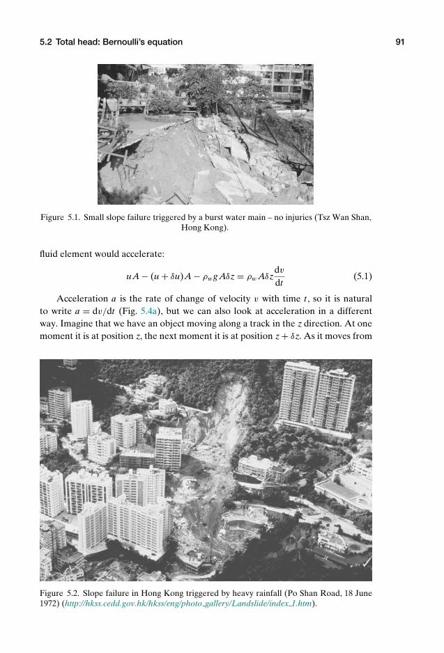
P1: KAE


5.2 Total head: Bernoulli’s equation 91

Figure 5.1. Small slope failure triggered by a burst water main – no injuries (Tsz Wan Shan,Hong Kong).

fluid element would accelerate:

uA − (u + δu)A − ρwg Aδz = ρw Aδzdv

dt(5.1)

Acceleration a is the rate of change of velocity v with time t , so it is naturalto write a = dv/dt (Fig. 5.4a), but we can also look at acceleration in a differentway. Imagine that we have an object moving along a track in the z direction. At onemoment it is at position z, the next moment it is at position z + δz. As it moves from

Figure 5.2. Slope failure in Hong Kong triggered by heavy rainfall (Po Shan Road, 18 June1972) (http://hkss.cedd.gov.hk/hkss/eng/photo gallery/Landslide/index 1.htm).

http://hkss.cedd.gov.hk/hkss/eng/photogallery/Landslide/index1.htm

P1: KAE


92 Seepage

z

δz

u

u+δu

v

ρwgAδz

datum

cross section

A

Figure 5.3. Element of water subject to self weight and gradient of pore pressure.

z to z + δz, the velocity changes from v to v + δv (Fig. 5.4b). The velocity evidentlychanges with both position and time: we can write v = v(t) or v = v(z), but of coursethe two are not independent. The time taken to move from position z to positionz + δz is δt = δz/v (neglecting the small change of velocity that occurs during themove). The rate of change of velocity with time – the acceleration a – is then:

a = δv

δt= δv

δz/v= v

δv

δz(5.2)

and in the limit, as the changes in position and time become infinitesimally small:

a = dv

dt= v

dv

dz(5.3)

and it is often convenient to make use of this alternative differential form of theacceleration.2

Thus (5.1) becomes:

δu + ρwgδz + ρwvdv

dzδz = 0 (5.4)

The pore pressure u varies with position, so we can write u = u(z) and:

δu = dudz

δz (5.5)

We can then write (5.4) as:

(dudz

+ ρwg + ρwvdv

dz

)δz = 0 (5.6)

2 We could deduce the same result by using the chain rule for differentiation of the function for thevelocity v = v(z):

dv

dt= dv

dzdzdt

= vdv

dz

noting that v = dz/dt .

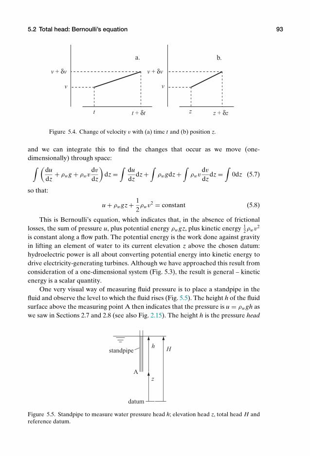
P1: KAE



v + δv v + δv

z + δzt + δt

vv

zt

a. b.

Figure 5.4. Change of velocity v with (a) time t and (b) position z.

and we can integrate this to find the changes that occur as we move (one-dimensionally) through space:∫ (

dudz

+ ρwg + ρwvdv

dz

)dz =

∫dudz

dz +∫

ρwgdz +∫

ρwvdv

dzdz =

∫0dz (5.7)

so that:

u + ρwgz + 12ρwv2 = constant (5.8)

This is Bernoulli’s equation, which indicates that, in the absence of frictionallosses, the sum of pressure u, plus potential energy ρwgz, plus kinetic energy 1

2ρwv2

is constant along a flow path. The potential energy is the work done against gravityin lifting an element of water to its current elevation z above the chosen datum:hydroelectric power is all about converting potential energy into kinetic energy todrive electricity-generating turbines. Although we have approached this result fromconsideration of a one-dimensional system (Fig. 5.3), the result is general – kineticenergy is a scalar quantity.

One very visual way of measuring fluid pressure is to place a standpipe in thefluid and observe the level to which the fluid rises (Fig. 5.5). The height h of the fluidsurface above the measuring point A then indicates that the pressure is u = ρwgh aswe saw in Sections 2.7 and 2.8 (see also Fig. 2.15). The height h is the pressure head

h

z

H

datum

A

standpipe

Figure 5.5. Standpipe to measure water pressure head h; elevation head z, total head H andreference datum.

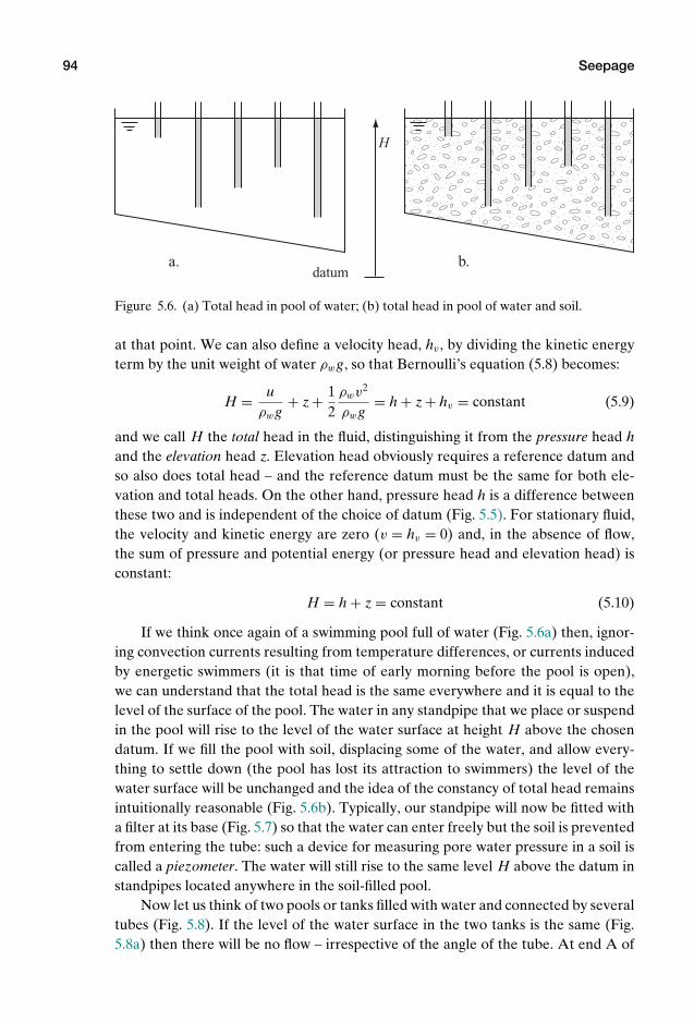
P1: KAE


94 Seepage

H

a. b.datum

Figure 5.6. (a) Total head in pool of water; (b) total head in pool of water and soil.

at that point. We can also define a velocity head, hv , by dividing the kinetic energyterm by the unit weight of water ρwg, so that Bernoulli’s equation (5.8) becomes:

H = uρwg

+ z + 12

ρwv2

ρwg= h + z + hv = constant (5.9)

and we call H the total head in the fluid, distinguishing it from the pressure head hand the elevation head z. Elevation head obviously requires a reference datum andso also does total head – and the reference datum must be the same for both ele-vation and total heads. On the other hand, pressure head h is a difference betweenthese two and is independent of the choice of datum (Fig. 5.5). For stationary fluid,the velocity and kinetic energy are zero (v = hv = 0) and, in the absence of flow,the sum of pressure and potential energy (or pressure head and elevation head) isconstant:

H = h + z = constant (5.10)

If we think once again of a swimming pool full of water (Fig. 5.6a) then, ignor-ing convection currents resulting from temperature differences, or currents inducedby energetic swimmers (it is that time of early morning before the pool is open),we can understand that the total head is the same everywhere and it is equal to thelevel of the surface of the pool. The water in any standpipe that we place or suspendin the pool will rise to the level of the water surface at height H above the chosendatum. If we fill the pool with soil, displacing some of the water, and allow every-thing to settle down (the pool has lost its attraction to swimmers) the level of thewater surface will be unchanged and the idea of the constancy of total head remainsintuitionally reasonable (Fig. 5.6b). Typically, our standpipe will now be fitted witha filter at its base (Fig. 5.7) so that the water can enter freely but the soil is preventedfrom entering the tube: such a device for measuring pore water pressure in a soil iscalled a piezometer. The water will still rise to the same level H above the datum instandpipes located anywhere in the soil-filled pool.

Now let us think of two pools or tanks filled with water and connected by severaltubes (Fig. 5.8). If the level of the water surface in the two tanks is the same (Fig.5.8a) then there will be no flow – irrespective of the angle of the tube. At end A of

P1: KAE



open end of tube

filter

standpipe

water level in standpipe

pressure headh = u/ρwg

Figure 5.7. Standpipe piezometer for measuring pore water pressure in the ground.

a typical tube (Fig. 5.8b), at elevation z1 relative to the datum, the pressure head ish1; at end B of the tube, at elevation z2 relative to the datum, the pressure head ish2. However, as indicated in Fig. 5.8b, the total head, H = h1 + z1 = h2 + z2, is thesame at both ends A and B of the tube. Even though the pressure head may be verydifferent at the two ends of the tube (Fig. 5.8b), the differences in elevation headcompensate so that the total head is the same.

This conclusion is independent of the size (bore) of the connecting tube, so letus make the diameter of the tube progressively smaller (Fig. 5.9). Provided the totalhead in each tank is the same, there will be no flow through the tube (Fig. 5.9a). Butsuppose that we now lower the water level in one of the tanks (Fig. 5.9b). Waterwill flow from the tank with the higher water level (higher total head) to the tankwith the lower water level (lower total head) – and again the direction of flow willbe independent of the orientation of the connecting tube. For a large diameter ofconnecting tube, the flow rate would be as fast as we could top up the tank withthe higher total head, and the velocity head in Bernoulli’s equation (5.8, 5.9) might

H

z1

h1

z2

h2

a. b.

A

B

Figure 5.8. (a) Two tanks of water connected by tubes at different inclinations; (b) differentpressure heads but equal total heads.

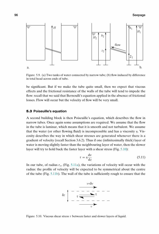
P1: KAE


96 Seepage

H

H2

H1

z1

h1

z2

h2

a. b.

flow

Figure 5.9. (a) Two tanks of water connected by narrow tube; (b) flow induced by differencein total head across ends of tube.

be significant. But if we make the tube quite small, then we expect that viscouseffects and the frictional resistance of the walls of the tube will tend to impede theflow: recall that we said that Bernoulli’s equation applied in the absence of frictionallosses. Flow will occur but the velocity of flow will be very small.

5.3 Poiseuille’s equation

A second building block is then Poiseuille’s equation, which describes the flow innarrow tubes. Once again some assumptions are required. We assume that the flowin the tube is laminar, which means that it is smooth and not turbulent. We assumethat the water (or other flowing fluid) is incompressible and has a viscosity η. Vis-cosity describes the way in which shear stresses are generated whenever there is agradient of velocity (recall Section 3.6.2). Thus if one (infinitesimally thick) layer ofwater is moving slightly faster than the neighbouring layer of water, then the slowerlayer will try to hold back the faster layer with a shear stress (Fig. 5.10):

τ = ηdv

dz(5.11)

In our tube, of radius ro, (Fig. 5.11a), the variations of velocity will occur with theradius: the profile of velocity will be expected to be symmetrical about the centreof the tube (Fig. 5.11b). The wall of the tube is sufficiently rough to ensure that the

δz

v+δv

v

ττ

Figure 5.10. Viscous shear stress τ between faster and slower layers of liquid.

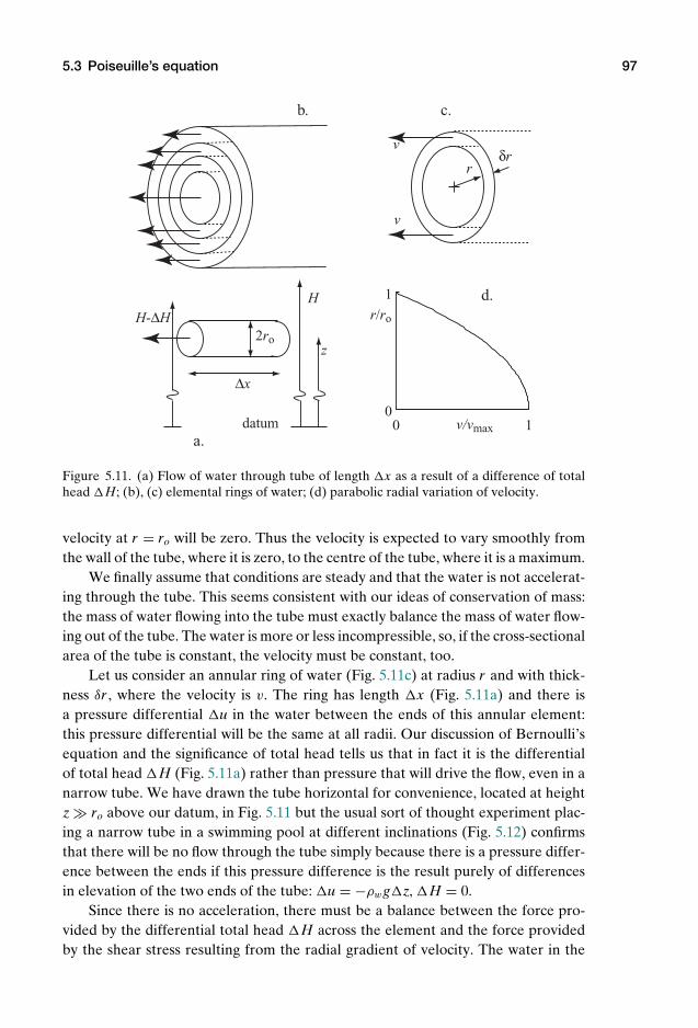
P1: KAE


5.3 Poiseuille’s equation 97

δrr

v

v

0 10

1

r/ro

v/vmax

b.

a.

c.

d.

2ro

∆x

HH-∆H

z

datum

Figure 5.11. (a) Flow of water through tube of length x as a result of a difference of totalhead H; (b), (c) elemental rings of water; (d) parabolic radial variation of velocity.

velocity at r = ro will be zero. Thus the velocity is expected to vary smoothly fromthe wall of the tube, where it is zero, to the centre of the tube, where it is a maximum.

We finally assume that conditions are steady and that the water is not accelerat-ing through the tube. This seems consistent with our ideas of conservation of mass:the mass of water flowing into the tube must exactly balance the mass of water flow-ing out of the tube. The water is more or less incompressible, so, if the cross-sectionalarea of the tube is constant, the velocity must be constant, too.

Let us consider an annular ring of water (Fig. 5.11c) at radius r and with thick-ness δr , where the velocity is v. The ring has length x (Fig. 5.11a) and there isa pressure differential u in the water between the ends of this annular element:this pressure differential will be the same at all radii. Our discussion of Bernoulli’sequation and the significance of total head tells us that in fact it is the differentialof total head H (Fig. 5.11a) rather than pressure that will drive the flow, even in anarrow tube. We have drawn the tube horizontal for convenience, located at heightz ro above our datum, in Fig. 5.11 but the usual sort of thought experiment plac-ing a narrow tube in a swimming pool at different inclinations (Fig. 5.12) confirmsthat there will be no flow through the tube simply because there is a pressure differ-ence between the ends if this pressure difference is the result purely of differencesin elevation of the two ends of the tube: u = −ρwgz, H = 0.

Since there is no acceleration, there must be a balance between the force pro-vided by the differential total head H across the element and the force providedby the shear stress resulting from the radial gradient of velocity. The water in the

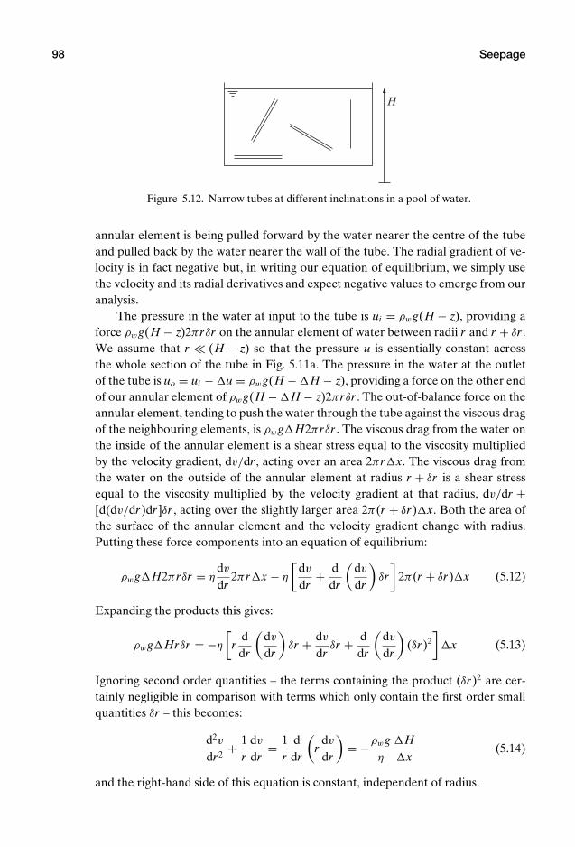
P1: KAE


98 Seepage

H

Figure 5.12. Narrow tubes at different inclinations in a pool of water.

annular element is being pulled forward by the water nearer the centre of the tubeand pulled back by the water nearer the wall of the tube. The radial gradient of ve-locity is in fact negative but, in writing our equation of equilibrium, we simply usethe velocity and its radial derivatives and expect negative values to emerge from ouranalysis.

The pressure in the water at input to the tube is ui = ρwg(H − z), providing aforce ρwg(H − z)2πrδr on the annular element of water between radii r and r + δr .We assume that r (H − z) so that the pressure u is essentially constant acrossthe whole section of the tube in Fig. 5.11a. The pressure in the water at the outletof the tube is uo = ui − u = ρwg(H − H − z), providing a force on the other endof our annular element of ρwg(H − H − z)2πrδr . The out-of-balance force on theannular element, tending to push the water through the tube against the viscous dragof the neighbouring elements, is ρwgH2πrδr . The viscous drag from the water onthe inside of the annular element is a shear stress equal to the viscosity multipliedby the velocity gradient, dv/dr , acting over an area 2πrx. The viscous drag fromthe water on the outside of the annular element at radius r + δr is a shear stressequal to the viscosity multiplied by the velocity gradient at that radius, dv/dr +[d(dv/dr)dr ]δr , acting over the slightly larger area 2π(r + δr)x. Both the area ofthe surface of the annular element and the velocity gradient change with radius.Putting these force components into an equation of equilibrium:

ρwgH2πrδr = ηdv

dr2πrx − η

[dv

dr+ d

dr

(dv

dr

)δr

]2π(r + δr)x (5.12)

Expanding the products this gives:

ρwgHrδr = −η

[r

ddr

(dv

dr

)δr + dv

drδr + d

dr

(dv

dr

)(δr)2

]x (5.13)

Ignoring second order quantities – the terms containing the product (δr)2 are cer-tainly negligible in comparison with terms which only contain the first order smallquantities δr – this becomes:

d2v

dr2+ 1

rdv

dr= 1

rddr

(r

dv

dr

)= −ρwg

η

Hx

(5.14)

and the right-hand side of this equation is constant, independent of radius.

P1: KAE


5.4 Permeability 99

Integrating this:

rdv

dr= −ρwg

2η

Hx

r2 + J1 (5.15)

where J1 is a constant of integration. However, from symmetry the gradient of radialvelocity must be zero at the centre of the tube, r = 0, and hence J1 = 0 and:

dv

dr= −ρwg

2η

Hx

r (5.16)

and the (linear) variation of shear stress with radius is:

τ = ηdv

dr= −ρwg

2Hx

r (5.17)

Integrating (5.16):

v = −ρwg4η

Hx

r2 + J2 (5.18)

The velocity is zero at the wall of the tube r = ro, and hence the integration constantJ2 is:

J2 = ρwg4η

Hx

r2o (5.19)

and we have recovered a parabolic velocity profile (Fig. 5.11d):

v = ρwg4η

Hx

(r2o − r2) (5.20)

The volumetric flow rate through the tube is:

q =∫ ro

02πrvdr = ρwgπ

2η

Hx

∫ ro

0r(r2

o − r2)dr = ρwgπr4o

8η

Hx

(5.21)

so that the average velocity v through the tube is:

v = qπr2

o= ρwgr2

o

8η

Hx

(5.22)

These are alternative ways of presenting Poiseuille’s equation.

5.4 Permeability

What is the relevance of Poiseuille’s equation to the flow of water through soils?Soils obviously do not consist of straight cylindrical tubes. In fact the pore spacesthrough which water has to flow are geometrically significantly more complex thancylinders (Fig. 3.1). There is no such thing as a “cross section” and the path thatthe water has to follow is extremely tortuous. However, what Poiseuille does tellus is that the ease with which water flows through an opening will be proportionalto the square of the size of that opening. We have seen (Fig. 3.8) that the size ofsoil particles varies over a range of many orders of magnitude – gravel particles aretypically some 105 times larger than clay particles – and we might expect that the

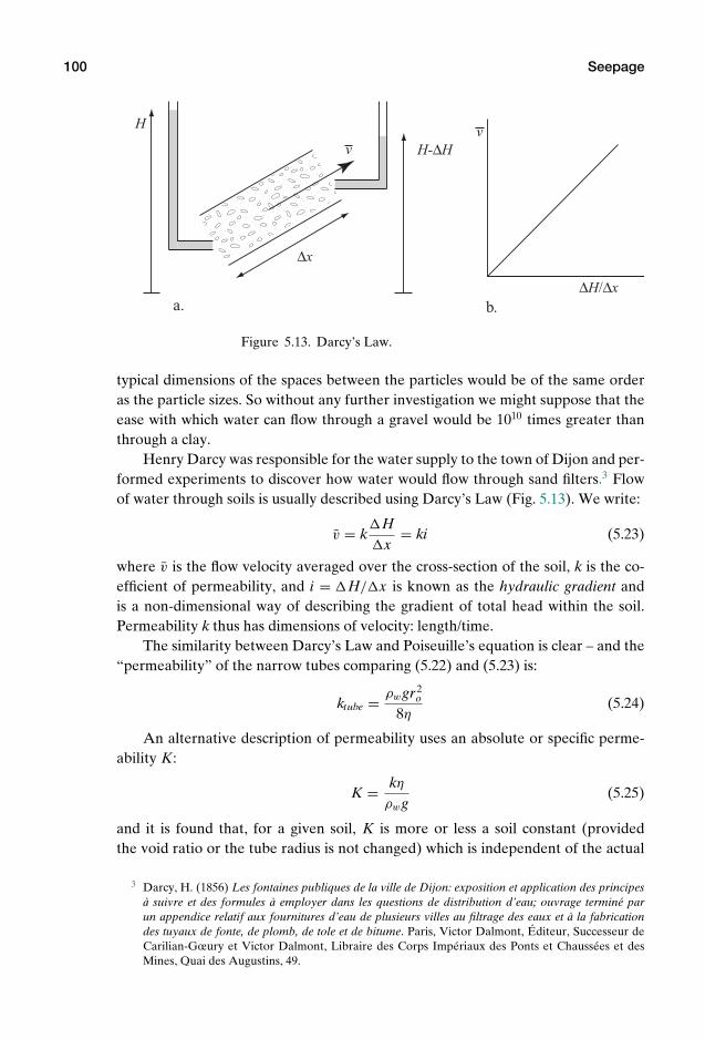
P1: KAE


100 Seepage

∆x

vv

H

H-∆H

∆H/∆xa. b.

Figure 5.13. Darcy’s Law.

typical dimensions of the spaces between the particles would be of the same orderas the particle sizes. So without any further investigation we might suppose that theease with which water can flow through a gravel would be 1010 times greater thanthrough a clay.

Henry Darcy was responsible for the water supply to the town of Dijon and per-formed experiments to discover how water would flow through sand filters.3 Flowof water through soils is usually described using Darcy’s Law (Fig. 5.13). We write:

v = kHx

= ki (5.23)

where v is the flow velocity averaged over the cross-section of the soil, k is the co-efficient of permeability, and i = H/x is known as the hydraulic gradient andis a non-dimensional way of describing the gradient of total head within the soil.Permeability k thus has dimensions of velocity: length/time.

The similarity between Darcy’s Law and Poiseuille’s equation is clear – and the“permeability” of the narrow tubes comparing (5.22) and (5.23) is:

ktube = ρwgr2o

8η(5.24)

An alternative description of permeability uses an absolute or specific perme-ability K:

K = kη

ρwg(5.25)

and it is found that, for a given soil, K is more or less a soil constant (providedthe void ratio or the tube radius is not changed) which is independent of the actual

3 Darcy, H. (1856) Les fontaines publiques de la ville de Dijon: exposition et application des principesa suivre et des formules a employer dans les questions de distribution d’eau; ouvrage termine parun appendice relatif aux fournitures d’eau de plusieurs villes au filtrage des eaux et a la fabricationdes tuyaux de fonte, de plomb, de tole et de bitume. Paris, Victor Dalmont, Editeur, Successeur deCarilian-Gœury et Victor Dalmont, Libraire des Corps Imperiaux des Ponts et Chaussees et desMines, Quai des Augustins, 49.

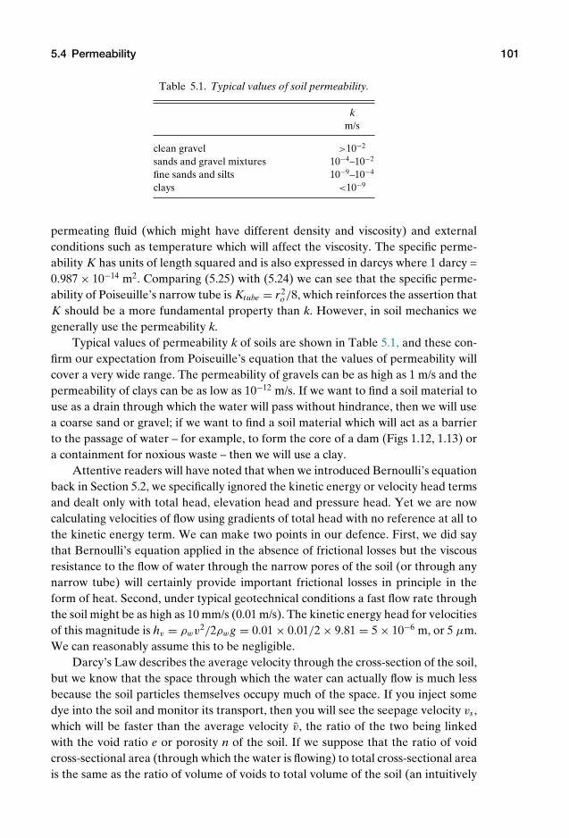
P1: KAE


5.4 Permeability 101

Table 5.1. Typical values of soil permeability.

km/s

clean gravel >10−2

sands and gravel mixtures 10−4–10−2

fine sands and silts 10−9–10−4

clays <10−9

permeating fluid (which might have different density and viscosity) and externalconditions such as temperature which will affect the viscosity. The specific perme-ability K has units of length squared and is also expressed in darcys where 1 darcy =0.987 × 10−14 m2. Comparing (5.25) with (5.24) we can see that the specific perme-ability of Poiseuille’s narrow tube is Ktube = r2

o/8, which reinforces the assertion thatK should be a more fundamental property than k. However, in soil mechanics wegenerally use the permeability k.

Typical values of permeability k of soils are shown in Table 5.1, and these con-firm our expectation from Poiseuille’s equation that the values of permeability willcover a very wide range. The permeability of gravels can be as high as 1 m/s and thepermeability of clays can be as low as 10−12 m/s. If we want to find a soil material touse as a drain through which the water will pass without hindrance, then we will usea coarse sand or gravel; if we want to find a soil material which will act as a barrierto the passage of water – for example, to form the core of a dam (Figs 1.12, 1.13) ora containment for noxious waste – then we will use a clay.

Attentive readers will have noted that when we introduced Bernoulli’s equationback in Section 5.2, we specifically ignored the kinetic energy or velocity head termsand dealt only with total head, elevation head and pressure head. Yet we are nowcalculating velocities of flow using gradients of total head with no reference at all tothe kinetic energy term. We can make two points in our defence. First, we did saythat Bernoulli’s equation applied in the absence of frictional losses but the viscousresistance to the flow of water through the narrow pores of the soil (or through anynarrow tube) will certainly provide important frictional losses in principle in theform of heat. Second, under typical geotechnical conditions a fast flow rate throughthe soil might be as high as 10 mm/s (0.01 m/s). The kinetic energy head for velocitiesof this magnitude is hv = ρwv2/2ρwg = 0.01 × 0.01/2 × 9.81 = 5 × 10−6 m, or 5 µm.We can reasonably assume this to be negligible.

Darcy’s Law describes the average velocity through the cross-section of the soil,but we know that the space through which the water can actually flow is much lessbecause the soil particles themselves occupy much of the space. If you inject somedye into the soil and monitor its transport, then you will see the seepage velocity vs ,which will be faster than the average velocity v, the ratio of the two being linkedwith the void ratio e or porosity n of the soil. If we suppose that the ratio of voidcross-sectional area (through which the water is flowing) to total cross-sectional areais the same as the ratio of volume of voids to total volume of the soil (an intuitively

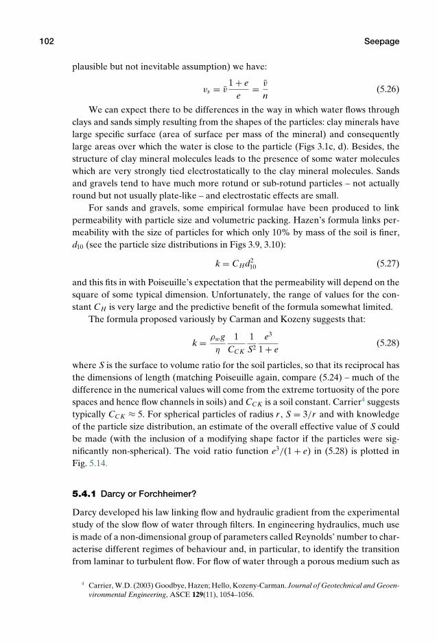
P1: KAE


102 Seepage

plausible but not inevitable assumption) we have:

vs = v1 + e

e= v

n(5.26)

We can expect there to be differences in the way in which water flows throughclays and sands simply resulting from the shapes of the particles: clay minerals havelarge specific surface (area of surface per mass of the mineral) and consequentlylarge areas over which the water is close to the particle (Figs 3.1c, d). Besides, thestructure of clay mineral molecules leads to the presence of some water moleculeswhich are very strongly tied electrostatically to the clay mineral molecules. Sandsand gravels tend to have much more rotund or sub-rotund particles – not actuallyround but not usually plate-like – and electrostatic effects are small.

For sands and gravels, some empirical formulae have been produced to linkpermeability with particle size and volumetric packing. Hazen’s formula links per-meability with the size of particles for which only 10% by mass of the soil is finer,d10 (see the particle size distributions in Figs 3.9, 3.10):

k = CHd210 (5.27)

and this fits in with Poiseuille’s expectation that the permeability will depend on thesquare of some typical dimension. Unfortunately, the range of values for the con-stant CH is very large and the predictive benefit of the formula somewhat limited.

The formula proposed variously by Carman and Kozeny suggests that:

k = ρwgη

1CCK

1S2

e3

1 + e(5.28)

where S is the surface to volume ratio for the soil particles, so that its reciprocal hasthe dimensions of length (matching Poiseuille again, compare (5.24) – much of thedifference in the numerical values will come from the extreme tortuosity of the porespaces and hence flow channels in soils) and CCK is a soil constant. Carrier4 suggeststypically CCK ≈ 5. For spherical particles of radius r , S = 3/r and with knowledgeof the particle size distribution, an estimate of the overall effective value of S couldbe made (with the inclusion of a modifying shape factor if the particles were sig-nificantly non-spherical). The void ratio function e3/(1 + e) in (5.28) is plotted inFig. 5.14.

5.4.1 Darcy or Forchheimer?

Darcy developed his law linking flow and hydraulic gradient from the experimentalstudy of the slow flow of water through filters. In engineering hydraulics, much useis made of a non-dimensional group of parameters called Reynolds’ number to char-acterise different regimes of behaviour and, in particular, to identify the transitionfrom laminar to turbulent flow. For flow of water through a porous medium such as

4 Carrier, W.D. (2003) Goodbye, Hazen; Hello, Kozeny-Carman. Journal of Geotechnical and Geoen-vironmental Engineering, ASCE 129(11), 1054–1056.

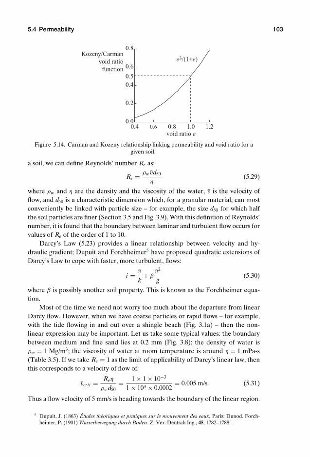
P1: KAE


5.4 Permeability 103

0.4 0.6 0.8 1.0 1.20.0

0.2

0.4

0.6

0.8

void ratio e

0.5

Kozeny/Carman void ratio

function

e3/(1+e)

Figure 5.14. Carman and Kozeny relationship linking permeability and void ratio for agiven soil.

a soil, we can define Reynolds’ number Re as:

Re = ρwvd50

η(5.29)

where ρw and η are the density and the viscosity of the water, v is the velocity offlow, and d50 is a characteristic dimension which, for a granular material, can mostconveniently be linked with particle size – for example, the size d50 for which halfthe soil particles are finer (Section 3.5 and Fig. 3.9). With this definition of Reynolds’number, it is found that the boundary between laminar and turbulent flow occurs forvalues of Re of the order of 1 to 10.

Darcy’s Law (5.23) provides a linear relationship between velocity and hy-draulic gradient; Dupuit and Forchheimer5 have proposed quadratic extensions ofDarcy’s Law to cope with faster, more turbulent, flows:

i = v

k+ β

v2

g(5.30)

where β is possibly another soil property. This is known as the Forchheimer equa-tion.

Most of the time we need not worry too much about the departure from linearDarcy flow. However, when we have coarse particles or rapid flows – for example,with the tide flowing in and out over a shingle beach (Fig. 3.1a) – then the non-linear expression may be important. Let us take some typical values: the boundarybetween medium and fine sand lies at 0.2 mm (Fig. 3.8); the density of water isρw = 1 Mg/m3; the viscosity of water at room temperature is around η = 1 mPa-s(Table 3.5). If we take Re = 1 as the limit of applicability of Darcy’s linear law, thenthis corresponds to a velocity of flow of:

vcri t = Reη

ρwd50= 1 × 1 × 10−3

1 × 103 × 0.0002= 0.005 m/s (5.31)

Thus a flow velocity of 5 mm/s is heading towards the boundary of the linear region.

5 Dupuit, J. (1863) Etudes theoriques et pratiques sur le mouvement des eaux. Paris: Dunod. Forch-heimer, P. (1901) Wasserbewegung durch Boden. Z. Ver. Deutsch Ing., 45, 1782–1788.

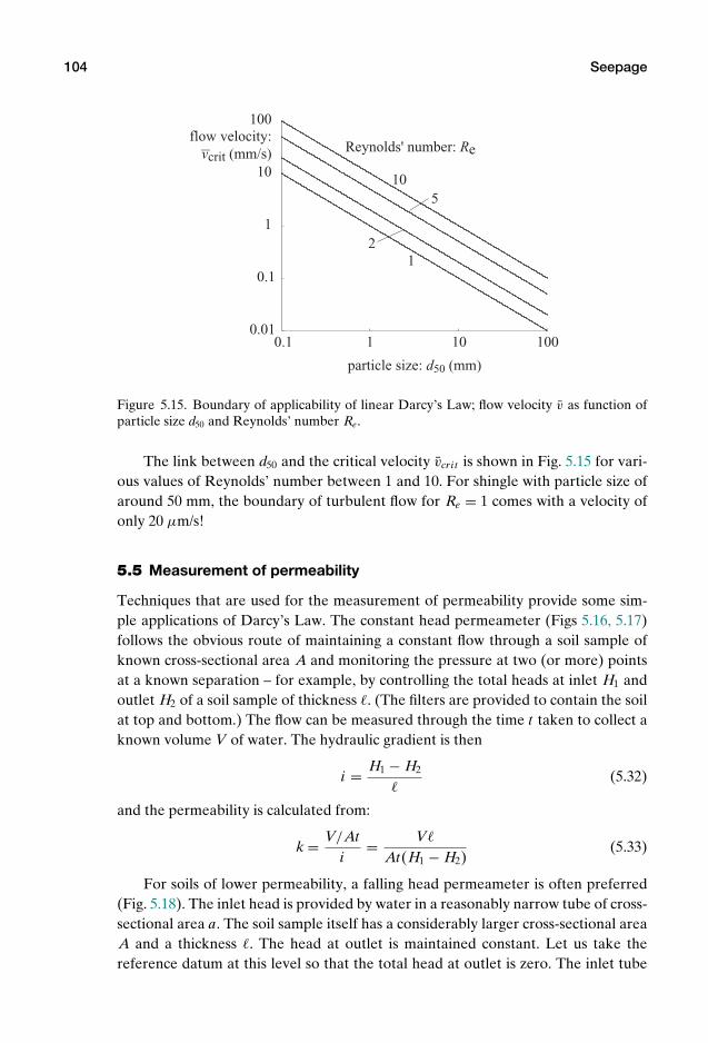
P1: KAE


104 Seepage

0.1 1 10 1000.01

0.1

1

10

100

particle size: d50 (mm)

flow velocity:

⎯vcrit (mm/s) Reynolds' number: Re

105

21

Figure 5.15. Boundary of applicability of linear Darcy’s Law; flow velocity v as function ofparticle size d50 and Reynolds’ number Re.

The link between d50 and the critical velocity vcri t is shown in Fig. 5.15 for vari-ous values of Reynolds’ number between 1 and 10. For shingle with particle size ofaround 50 mm, the boundary of turbulent flow for Re = 1 comes with a velocity ofonly 20 µm/s!

5.5 Measurement of permeability

Techniques that are used for the measurement of permeability provide some sim-ple applications of Darcy’s Law. The constant head permeameter (Figs 5.16, 5.17)follows the obvious route of maintaining a constant flow through a soil sample ofknown cross-sectional area A and monitoring the pressure at two (or more) pointsat a known separation – for example, by controlling the total heads at inlet H1 andoutlet H2 of a soil sample of thickness . (The filters are provided to contain the soilat top and bottom.) The flow can be measured through the time t taken to collect aknown volume V of water. The hydraulic gradient is then

i = H1 − H2

(5.32)

and the permeability is calculated from:

k = V/Ati

= V

At(H1 − H2)(5.33)

For soils of lower permeability, a falling head permeameter is often preferred(Fig. 5.18). The inlet head is provided by water in a reasonably narrow tube of cross-sectional area a. The soil sample itself has a considerably larger cross-sectional areaA and a thickness . The head at outlet is maintained constant. Let us take thereference datum at this level so that the total head at outlet is zero. The inlet tube

P1: KAE


5.5 Measurement of permeability 105

Figure 5.16. Apparatus used by Darcy to determine the permeability of the filters for thewater supply of the town of Dijon.3

is filled up and the variation of the difference in total head across the sample H isrecorded at different times t . The flow rate through the sample at any time is:

q = −adHdt

(5.34)

because the flow comes from the falling head of water in the inlet tube of crosssectional area a. The velocity of flow through the sample is:

v = qA

= − aA

dHdt

(5.35)

Applying Darcy’s Law, we know that:

v = ki = kH

(5.36)

and rearranging (5.36) and (5.35):

dHH

= −kAa

dt (5.37)

with solution:

lnHHi

= −kAa

(t − ti ) (5.38)

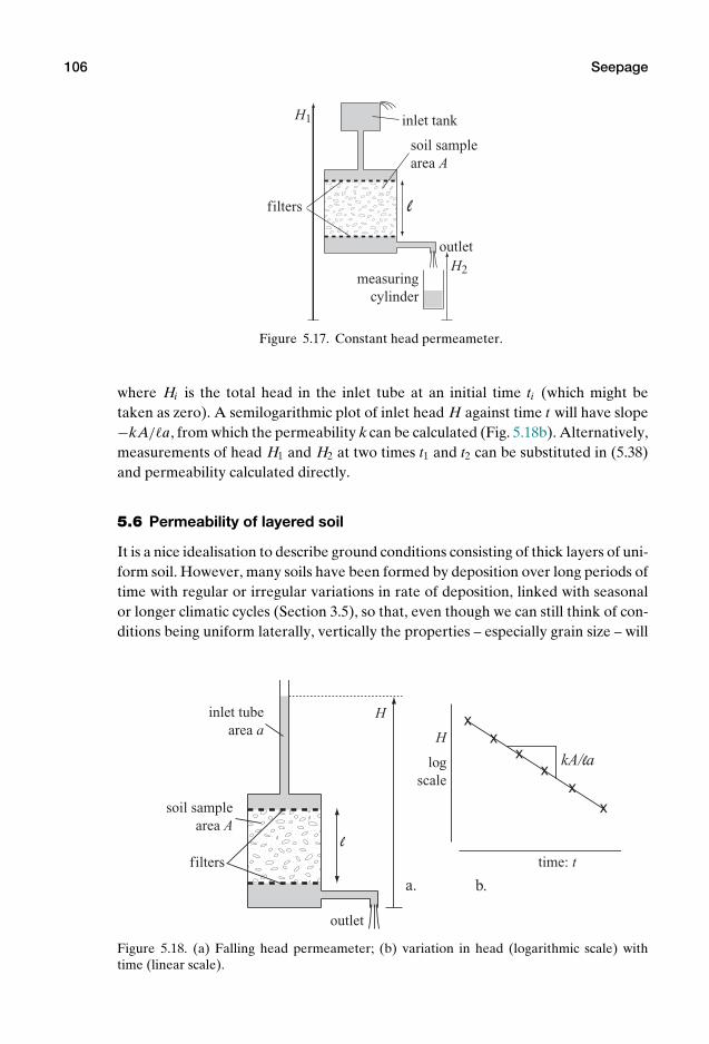
P1: KAE


106 Seepage

H1

H2measuring

cylinder

soil sample area A

inlet tank

outlet

filters

Figure 5.17. Constant head permeameter.

where Hi is the total head in the inlet tube at an initial time ti (which might betaken as zero). A semilogarithmic plot of inlet head H against time t will have slope−kA/a, from which the permeability k can be calculated (Fig. 5.18b). Alternatively,measurements of head H1 and H2 at two times t1 and t2 can be substituted in (5.38)and permeability calculated directly.

5.6 Permeability of layered soil

It is a nice idealisation to describe ground conditions consisting of thick layers of uni-form soil. However, many soils have been formed by deposition over long periods oftime with regular or irregular variations in rate of deposition, linked with seasonalor longer climatic cycles (Section 3.5), so that, even though we can still think of con-ditions being uniform laterally, vertically the properties – especially grain size – will

soil sample area A

inlet tube area a

H

H

log scale

time: t

xx

xx

xx

a. b.

filters

outlet

Figure 5.18. (a) Falling head permeameter; (b) variation in head (logarithmic scale) withtime (linear scale).

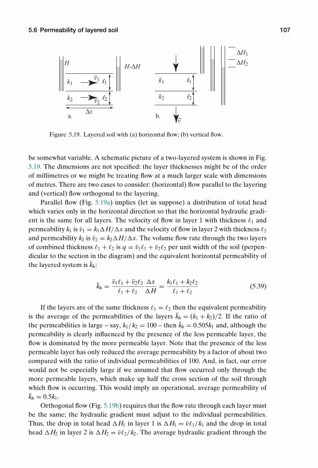
P1: KAE


5.6 Permeability of layered soil 107

H H-∆H

∆H1

∆H2

k1 l1v1

k2

k1

k2l2v2

l1

l2

a. b.v

∆x

Figure 5.19. Layered soil with (a) horizontal flow; (b) vertical flow.

be somewhat variable. A schematic picture of a two-layered system is shown in Fig.5.19. The dimensions are not specified: the layer thicknesses might be of the orderof millimetres or we might be treating flow at a much larger scale with dimensionsof metres. There are two cases to consider: (horizontal) flow parallel to the layeringand (vertical) flow orthogonal to the layering.

Parallel flow (Fig. 5.19a) implies (let us suppose) a distribution of total headwhich varies only in the horizontal direction so that the horizontal hydraulic gradi-ent is the same for all layers. The velocity of flow in layer 1 with thickness 1 andpermeability k1 is v1 = k1H/x and the velocity of flow in layer 2 with thickness 2

and permeability k2 is v2 = k2H/x. The volume flow rate through the two layersof combined thickness 1 + 2 is q = v11 + v22 per unit width of the soil (perpen-dicular to the section in the diagram) and the equivalent horizontal permeability ofthe layered system is kh:

kh = v11 + v22

1 + 2

xH

= k11 + k22

1 + 2(5.39)

If the layers are of the same thickness 1 = 2 then the equivalent permeabilityis the average of the permeabilities of the layers kh = (k1 + k2)/2. If the ratio ofthe permeabilities is large – say, k1/k2 = 100 – then kh = 0.505k1 and, although thepermeability is clearly influenced by the presence of the less permeable layer, theflow is dominated by the more permeable layer. Note that the presence of the lesspermeable layer has only reduced the average permeability by a factor of about twocompared with the ratio of individual permeabilities of 100. And, in fact, our errorwould not be especially large if we assumed that flow occurred only through themore permeable layers, which make up half the cross section of the soil throughwhich flow is occurring. This would imply an operational, average permeability ofkh = 0.5k1.

Orthogonal flow (Fig. 5.19b) requires that the flow rate through each layer mustbe the same; the hydraulic gradient must adjust to the individual permeabilities.Thus, the drop in total head H1 in layer 1 is H1 = v1/k1 and the drop in totalhead H2 in layer 2 is H2 = v2/k2. The average hydraulic gradient through the

P1: KAE


108 Seepage

R1

R1

R2

R2

Vi

I1

I2

IVo

a. b.

Figure 5.20. (a) Electrical resistors in parallel; (b) electrical resistors in series.

two layers is:

i = H1 + H2

1 + 2= v

1/k1 + 2/k2

1 + 2(5.40)

and the equivalent vertical permeability of the layered system is kv :

kv = 1 + 2

1/k1 + 2/k2= k1k2(1 + 2)

k21 + k12(5.41)

If the layers are of the same thickness, then the equivalent permeability is:

kv = 2k1k2

k1 + k2(5.42)

If the ratio of the permeabilities is large – say, k1/k2 = 100 – then kv = 1.98k2 andthe flow rate is primarily controlled by the less permeable layer. The presence ofthe more permeable layer has only increased the average permeability by a factorof about two compared with the ratio of individual permeabilities of 100. And forthis configuration, we could treat the more permeable layer as having infinite perme-ability k1 = ∞ so that the entire pressure drop occurred only in the low permeabilitylayer. The resulting calculated average permeability would then be kv = 2k2 or, formore general layer thicknesses, kv = k2(1 + 2)/2.

The analysis can be extended to a large number of layers of different thicknessesand different permeabilities, but the general conclusions remain: horizontal flow isdominated by the more permeable layers; vertical flow is dominated by the lesspermeable layers.

There is an obvious analogy with electricity and the resistance of parallel andseries networks of resistors. Resistors in parallel (Fig. 5.20a) experience a commondrop in voltage while the current is shared between the resistors: the flow of currentwill be dominated by the lower resistor if the ratio of resistances is large. Resistorsin series (Fig. 5.20b) share the same current; the drop in voltage will be dominatedby the larger resistor if the ratio of the resistances is large.

5.7 Seepage forces

A gradient of total head is required to drive flow through a narrow tube or throughthe soil because of the resistance provided by the tube or soil particles trying toimpede the flow. Every action has an equal and opposite reaction, so we conclude

P1: KAE


5.7 Seepage forces 109

z

δz

u u

u+δu u+δu

v

ρwgAδz ρgAδz

datum

H

H+δH

FsAδzarea A

σv

σv+δσv

a. b.

Figure 5.21. Seepage force on soil element.

that the flowing water must in turn be applying a force on the soil through which itis trying to pass. Consider the element of soil in Fig. 5.21 of cross-sectional area A.Water is flowing upwards (v > 0) and there are algebraic increases in pressure δuand total head δH across the element (although we know that δH must be negativeto give this positive direction of flow). The apparent imbalance of forces on thewater allows us to find an expression for the seepage force Fs (which we know mustbe directed upwards), usefully expressed as a body force per unit volume of the soil:

Aδu + ρwg Aδz + Fs Aδz = 0 (5.43)

and from the definition of total head δH (5.9):

ρwgδH = δu + ρwgδz (5.44)

so that:

Fs = −ρwgδHδz

= −ρwgi (5.45)

where i is the hydraulic gradient – the variation of total head with position. Asshown in Fig. 5.21, the hydraulic gradient must in fact be negative to sustain theupward flow and the seepage force as a resistance to the water must be directeddownwards.

Alternatively, we can argue that, if there is no flow, then the variation in waterpressure across an element exactly matches the variation in elevation head, δu =−ρwgδz, and there is no seepage-induced force acting on the soil. So the fact that,as a result of the occurrence of seepage, there is a change in total head then thisdirectly translates into the seepage force exerted by the soil on the water:

Fs Aδz = −ρwg AδH (5.46)

and hence:

Fs = −ρwgδHδz

= −ρwgi (5.47)

P1: KAE


110 Seepage

The downward resistance on the water becomes an upward force on the soil. Inthe absence of seepage forces, the vertical total stress across the soil element varieswith depth with the bulk density of the soil:

δσv = −ρgδz (5.48)

However, if the pore pressure gradient is too severe, then the pore pressuresmay eliminate the normal build-up of total stress with depth. The weight of theelement of soil is ρg Aδz (Fig. 5.21b). The critical condition comes when the out ofbalance pore pressure stress −δu = ρwgδz − ρwgδH (5.44), acting over the area Aof the section, exactly balances the weight of the element, which implies:

ρwgδz − ρwgδH = ρgδz (5.49)

which with a little rearrangement becomes an expression for the critical hydraulicgradient, icri t :

−δHδz

= −icri t = ρ − ρw

ρw

= ρ

ρw

− 1 = Gs − 11 + e

(5.50)

taking the expression for bulk density from Section 3.3. For many soils, the ratioρ/ρw ∼ 2 and the critical hydraulic gradient −icri t ∼ 1. The negative sign provides areminder that it is an upward hydraulic gradient that will cause problems: with ourposition z measured positive upwards, an upward hydraulic gradient implies that thetotal head H must be falling with increasing z, or δH/δz < 0.

The same result can be obtained by thinking in terms of effective stresses. Ifthe upward seepage force just balances the buoyant unit weight of the soil, γ ′ =γ − γw = (ρ − ρw)g, then there is no gradient of effective stress in the soil:

−ρwδH = (ρ − ρw)gδz (5.51)

or:

−icri t = −δHδz

= ρ

ρw

− 1 (5.52)

If there is any tendency of the hydraulic gradient to increase above icri t , then the soilcan be lifted up by the flowing water and is said to pipe. As the term suggests, theoccurrence of a failure in the soil as a result of excessive upward seepage flow willtend to seek out minor weaknesses or inhomogeneities in the soil and form pipesrather than necessarily producing a general instability. But the occurrence of suchflow channels, lifting up the soil in the process, will not be conducive to continuedsatisfactory operation of some hydraulic containment structure (such as a dam orthe sheet pile support to an excavation).

On the other hand, downward flow tends to compress the soil and increase thestresses. In fact, downward flow of water through a soil element or structure hasbeen used as a route to the artificial increase in stresses which, to some extent, caneliminate the effects of scale on the stress level in a small model (see Exercise 10 inSection 5.12).

P1: KAE


5.8 Radial flow to vertical drain 111

rδr

a. b.

l

drain

aquifer

impermeable layer

0 10 20 30 40 500

1

2

3

4

r/ro

c.

2ro

drainradius ro

2πkl(H-Ho)/q

Figure 5.22. Radial flow to vertical drain: (a) section; (b) plan; (c) variation of total head withradius.

5.8 Radial flow to vertical drain

Although we are restricting ourselves to one-dimensional problems, we can be alittle adventurous and admit problems which have only a single degree of spatialfreedom even though they do not just involve parallel unidirectional flow. Thereare two problems which are concerned with radial flow with the radius from a drainas the only degree of freedom. Analysis of these problems is instructive anywaybecause there are many problems in engineering which have radial symmetry andneed to be analysed in polar or spherical coordinates (compare the analysis leadingto Poiseuille’s equation, in Section 5.3).

First, we consider flow to a vertical drain which is being used to lower the totalhead in a confined aquifer (Fig. 5.22). We have to make the problem tractable sowe conveniently specify a drain which extends through the full height of the aquifer,and we make the aquifer confined so that we can reasonably assume that it remainsfully saturated even while we pump from the drain.

The governing equation describes the steady flow through concentric annuli(Fig. 5.22b). Conservation of mass requires that the flow rate through each annu-lus must be the same but the circumference of each annulus depends on its radius,so that the area through which the water is flowing reduces as we get closer to thedrain. Hence, the velocity of flow must increase and the hydraulic gradient mustincrease as we near the drain.

For an aquifer of permeability k and thickness , the volume flow rate out of thedrain is q, or q/ per unit height of drain. The drain has a radius ro and the total head

P1: KAE


112 Seepage

0 5 100.0

0.5

1.0

r/ro

a.

b.

drainradius ro

4πkro(H-Ho)/q

Figure 5.23. Radial flow to point drain.

at the drain is Ho. At radius r , the velocity of flow v = −kdH/dr (with the negativesign because the water flows down the hydraulic gradient). The volume flow ratethrough the radius r is −v2πr = q, and, from continuity of flow, the volume flowrate q must be the same at every radius:

2πrkdHdr

= constant = q (5.53)

so that the governing differential equation is:

2πk

qdH = dr

r(5.54)

with solution:

H − Ho = q2πk

lnrro

(5.55)

where Ho is the head at the drain. The total head thus varies logarithmically withradius from the drain, as shown in Fig. 5.22c.

5.9 Radial flow to point drain

A similar analysis can be performed for the case of spherical flow to a point drain ofradius ro (Fig. 5.23). Once again, the problem has a single degree of spatial freedom:assuming that we are looking at a volume of soil which is large by comparison withro and does not reach any significant layer boundaries or obstacles, everything canvary only with radius r . The same considerations apply to this spherical flow as tothe cylindrical flow of Section 5.8: the flow through each spherical layer must be thesame and equal to the volumetric outflow rate from the drain q. The cross-sectionalarea of a layer at radius r is 4πr2, so our governing equation is:

4πr2kdHdr

= q (5.56)

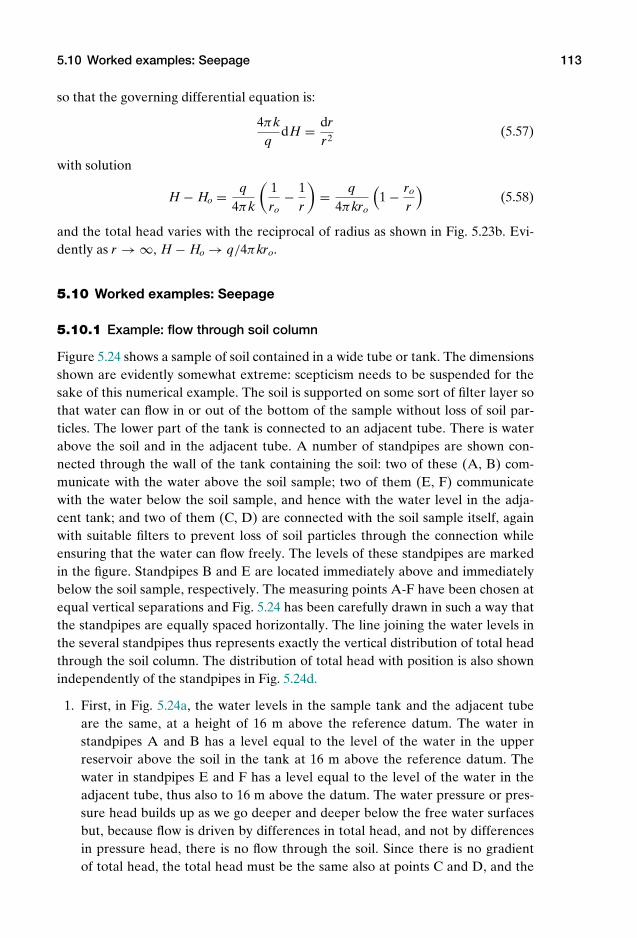
P1: KAE


5.10 Worked examples: Seepage 113

so that the governing differential equation is:

4πkq

dH = drr2

(5.57)

with solution

H − Ho = q4πk

(1ro

− 1r

)= q

4πkro

(1 − ro

r

)(5.58)

and the total head varies with the reciprocal of radius as shown in Fig. 5.23b. Evi-dently as r → ∞, H − Ho → q/4πkro.

5.10 Worked examples: Seepage

5.10.1 Example: flow through soil column

Figure 5.24 shows a sample of soil contained in a wide tube or tank. The dimensionsshown are evidently somewhat extreme: scepticism needs to be suspended for thesake of this numerical example. The soil is supported on some sort of filter layer sothat water can flow in or out of the bottom of the sample without loss of soil par-ticles. The lower part of the tank is connected to an adjacent tube. There is waterabove the soil and in the adjacent tube. A number of standpipes are shown con-nected through the wall of the tank containing the soil: two of these (A, B) com-municate with the water above the soil sample; two of them (E, F) communicatewith the water below the soil sample, and hence with the water level in the adja-cent tank; and two of them (C, D) are connected with the soil sample itself, againwith suitable filters to prevent loss of soil particles through the connection whileensuring that the water can flow freely. The levels of these standpipes are markedin the figure. Standpipes B and E are located immediately above and immediatelybelow the soil sample, respectively. The measuring points A-F have been chosen atequal vertical separations and Fig. 5.24 has been carefully drawn in such a way thatthe standpipes are equally spaced horizontally. The line joining the water levels inthe several standpipes thus represents exactly the vertical distribution of total headthrough the soil column. The distribution of total head with position is also shownindependently of the standpipes in Fig. 5.24d.

1. First, in Fig. 5.24a, the water levels in the sample tank and the adjacent tubeare the same, at a height of 16 m above the reference datum. The water instandpipes A and B has a level equal to the level of the water in the upperreservoir above the soil in the tank at 16 m above the reference datum. Thewater in standpipes E and F has a level equal to the level of the water in theadjacent tube, thus also to 16 m above the datum. The water pressure or pres-sure head builds up as we go deeper and deeper below the free water surfacesbut, because flow is driven by differences in total head, and not by differencesin pressure head, there is no flow through the soil. Since there is no gradientof total head, the total head must be the same also at points C and D, and the

P1: KAE


114 Seepage

datum

datum

datum

16m

12

10

8

6

4

2

0

16m

12

10

8

6

4

2

0

16m

12

10

8

6

4

2

0

a.

a.

b.

b.

c.

c.

A

AB

EF

A

B

EF

B

EF

C

D

C

D

C

D

total head(m)

16

12

8

4

A B C D E F

d.

soil

soil sample

filters

Figure 5.24. Example: flow through soil column.

water in these standpipes rises to the same level. The values of elevation, pres-sure head and total head for points A-F are shown in Table 5.2. In every case,the pressure head h is simply the difference between the total head H and theelevation z.

2. Second, in Fig. 5.24b, the water level in the adjacent tube is lowered by 4 m to12 m above the reference datum. We now have a difference in the total headsabove and below the soil sample and, as a result, there will be flow from hightotal head to low total head; in other words, from the large tank through thesoil to the adjacent tube. The elevations z of the measurement points A-F do

P1: KAE



Table 5.2. Example: flow through soil column (Fig. 5.24).

Fig. 5.24a Fig. 5.24b Fig. 5.24cz H h H h H h

Point m m m m m m m

A 12 16 4 16 4 12 0B 10 16 6 16 6 12 2C 8 16 8 14.7 6.7 13.3 5.3D 6 16 10 13.3 7.3 14.7 8.7E 4 16 12 12 8 16 12F 2 16 14 12 10 16 14

not change. The total head at points A and B does not change: the water abovethe soil has a free surface at 16 m above the datum.Below the soil, the path through the water to the free surface in the adjacenttube shows that the total head at points E and F is 12 m above the datum. If weassume that the soil is uniform and that the permeability is the same through-out, then, since the cross-sectional area of the soil sample in the tank is con-stant, the flow velocity must also be constant at all levels. Consequently, wecan deduce that the hydraulic gradient must be the same everywhere in the soilsample and thus determine the total heads at C and D by interpolation. Becausethe measurement points are equally spaced, the drop in total head from B to Cis the same as that from C to D and from D to E in Figs 5.24d (chain dotted line)and b. The resulting numerical values are given in Table 5.2. Again, the pressureheads h are determined as the difference between the elevation and the totalhead at each point. The water pressure head below the soil, at point E, is 8 mand that at the top of the soil sample, at point B, is 6 m but the differences in el-evation of points B and E more than compensate for these pressure differencesand the flow is downwards, following the gradient of total head (and apparentlyagainst the gradient of pore pressure). The hydraulic gradient through the soilis the ratio of the change in total head, H = 4 m, and the thickness of the soilsample over which it occurs, z = 6 m: hence, i = −H/z = −0.667.

3. Third, in Fig. 5.24c, the water level in the tube is restored to 16 m above thedatum and the water level in the tank is lowered to 12 m above datum. We nowhave a difference in total head above and below the soil sample and, as a result,there will be flow from high total head, below the sample, to low total head,above the sample: in other words, from the adjacent tube into the large tankand upwards through the soil. The elevations z of the measurement points A-Fdo not change. The total head at points E and F reverts to the original valueof 16 m above datum: follow the path through the water to the nearest freesurface in the adjacent tank. Above the soil, the measurement points A and Bare directly aware of the water level in the tank and the total head at pointsA and B is 12 m above the datum. We can again deduce that the hydraulicgradient must be the same everywhere in the soil sample, because the flow is

P1: KAE


116 Seepage

datum

datum

12m

8

6

4

2

0

-2

-4

12m

8

6

4

2

0

-2

-4

a.

b.

AB

EF

AB

EF

C

D

C

D

Figure 5.25. Example: flow through soil column with changed reference datum (compareFig. 5.24).

steady and the area of the cross section is constant, and thus determine the totalheads at C and D by interpolation. Because the measurement points are equallyspaced, the rise in head from B to C is the same as that from C to D and fromD to E in Figs 5.24d (dashed line) and c. The resulting numerical values aregiven in Table 5.2. Again, the pressure heads h are determined as the differencebetween the elevation and the total head at each point. The hydraulic gradientis calculated in the same way: H = −4 m, z = 6 m, i = 0.667 and the flow isupwards.

5.10.2 Example: effect of changing reference datum

It is important to recall that elevation z and total head H only have meaning withreference to some datum. The choice of location of this datum is often arbitrary andmay be chosen for convenience to ensure, for example, that all heads are positive.It is necessary only that the reference datum should be the same for all points andthe same for calculation of both elevation and total head. Figure 5.25 repeats theconfigurations of Figs 5.24a and b but with the datum chosen at the base of the soil

P1: KAE



Table 5.3. Example: flow through soil column (Fig. 5.25).

Fig. 5.25a Fig. 5.25bz H h H h

Point m m m m m

A 8 12 4 12 4B 6 12 6 12 6C 4 12 8 10.7 6.7D 2 12 10 9.3 7.3E 0 12 12 8 8F −2 12 14 8 10

sample in the tank instead of 2 m below the base of the tank. The correspondingvalues of elevation, total head and pressure head are shown in Table 5.3.

The consideration of this problem need not detain us long. We have lifted thedatum by 4 m; consequently, all elevations and all total heads are 4 m lower thanin Table 5.2. Differences in heads referred to the datum are unchanged so the hy-draulic gradient across the soil sample has not changed: the difference between thetotal heads at points B and E is the same in Tables 5.2 and 5.3. Pressure head iscalculated as a difference between quantities referred to the datum and the valuesdo not change with change of datum. Change in the choice of datum does not affectthe conclusion that flow occurs downwards from top to bottom of the sample.

5.10.3 Example: pumping from aquifer

A schematic diagram of the ground conditions at a particular site is shown in Fig.5.26a. A layer of sand overlies a layer of silty clay, which in turn overlies a sandaquifer. An aquifer is a water-bearing layer which usually has some spatial connec-tivity to a natural or artificial source of water which controls the water pressure inthe layer. The water table is naturally at a depth of 2 m below the ground surface,and this represents also the total head for the aquifer assuming that we do not inter-fere with the groundwater conditions. We consider two configurations.

1. First, the water is static and not flowing. By definition, the total head H will beconstant with depth, with height 24 m above the datum as shown by the solidline in Fig. 5.26b. The elevation head z increases linearly from zero at the datumas shown by the dashed line in Fig. 5.26b: it matches the total head at the levelof the water table. The pressure head h = u/ρwg is the difference between thetotal and elevation heads and varies linearly with depth, as shown by the chaindotted line in Fig. 5.26b. The pressure head is zero at the water table and is 24 mat the level of the datum.

2. Second, we consider the case when there is vigorous pumping from the aquiferto provide water for a small town such that the total head in the aquifer fallsto 18 m above the datum (Fig. 5.26c). The water table in the upper sand layerremains unchanged – it is fed from some near surface water sources such as

P1: KAE


118 Seepage

sand

sand

sand aquifer

sand aquifer

water table

water table

silty clay

silty clay

sand

sand aquifer

silty clay

datum 0

6

16

2426

0

0

10

10

20

20

0

10

20

30m 0 10 20 30m

H

H

z

z

u/ρwgu/ρwg

b. d.

a.

height above datum: m

height above datum: m

c.

Figure 5.26. (a, b) Ground conditions and heads (heights above datum in metres) withoutflow; (c, d) ground conditions and heads with pumping from aquifer.

a river or lake. The silty clay is able to sustain the difference in total headand, after a while, a steady seepage regime is established (there is a transientphase during which the new flow conditions settle down – this is the subject ofChapter 7).The variation of total head with depth now has three sections, as shown in Fig.5.26d. In the aquifer, the lower sand layer, the total head is constant at 18 mabove the datum. In the upper sand layer, the total head is constant at 24 mabove the datum (as in the no-flow condition). Through the silty clay the flowrate must be constant (from conservation of mass), so the hydraulic gradientmust be uniform and the total head must vary linearly with depth. There is a6 m drop in total head over a thickness of 10 m of silty clay, so that the constanthydraulic gradient through the silty clay is 0.6. The tripartite variation of H is

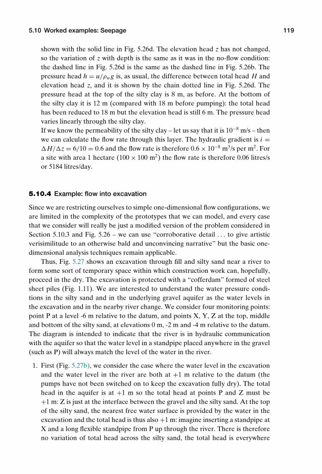
P1: KAE



shown with the solid line in Fig. 5.26d. The elevation head z has not changed,so the variation of z with depth is the same as it was in the no-flow condition:the dashed line in Fig. 5.26d is the same as the dashed line in Fig. 5.26b. Thepressure head h = u/ρwg is, as usual, the difference between total head H andelevation head z, and it is shown by the chain dotted line in Fig. 5.26d. Thepressure head at the top of the silty clay is 8 m, as before. At the bottom ofthe silty clay it is 12 m (compared with 18 m before pumping): the total headhas been reduced to 18 m but the elevation head is still 6 m. The pressure headvaries linearly through the silty clay.If we know the permeability of the silty clay – let us say that it is 10−8 m/s – thenwe can calculate the flow rate through this layer. The hydraulic gradient is i =H/z = 6/10 = 0.6 and the flow rate is therefore 0.6 × 10−8 m3/s per m2. Fora site with area 1 hectare (100 × 100 m2) the flow rate is therefore 0.06 litres/sor 5184 litres/day.

5.10.4 Example: flow into excavation

Since we are restricting ourselves to simple one-dimensional flow configurations, weare limited in the complexity of the prototypes that we can model, and every casethat we consider will really be just a modified version of the problem considered inSection 5.10.3 and Fig. 5.26 – we can use “corroborative detail . . . to give artisticverisimilitude to an otherwise bald and unconvincing narrative” but the basic one-dimensional analysis techniques remain applicable.

Thus, Fig. 5.27 shows an excavation through fill and silty sand near a river toform some sort of temporary space within which construction work can, hopefully,proceed in the dry. The excavation is protected with a “cofferdam” formed of steelsheet piles (Fig. 1.11). We are interested to understand the water pressure condi-tions in the silty sand and in the underlying gravel aquifer as the water levels inthe excavation and in the nearby river change. We consider four monitoring points:point P at a level -6 m relative to the datum, and points X, Y, Z at the top, middleand bottom of the silty sand, at elevations 0 m, -2 m and -4 m relative to the datum.The diagram is intended to indicate that the river is in hydraulic communicationwith the aquifer so that the water level in a standpipe placed anywhere in the gravel(such as P) will always match the level of the water in the river.

1. First (Fig. 5.27b), we consider the case where the water level in the excavationand the water level in the river are both at +1 m relative to the datum (thepumps have not been switched on to keep the excavation fully dry). The totalhead in the aquifer is at +1 m so the total head at points P and Z must be+1 m: Z is just at the interface between the gravel and the silty sand. At the topof the silty sand, the nearest free water surface is provided by the water in theexcavation and the total head is thus also +1 m: imagine inserting a standpipe atX and a long flexible standpipe from P up through the river. There is thereforeno variation of total head across the silty sand, the total head is everywhere

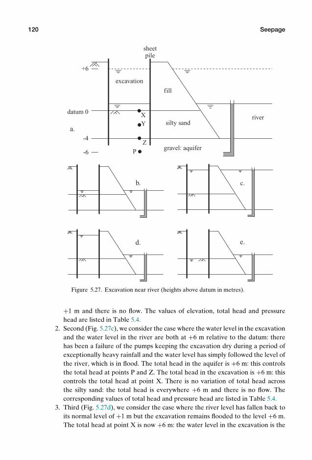
P1: KAE


120 Seepage

datum 0

-4

fill

silty sand

gravel: aquifer

sheet pile

excavation

riverXY

Z

P-6

+6

a.

b. c.

d. e.

Figure 5.27. Excavation near river (heights above datum in metres).

+1 m and there is no flow. The values of elevation, total head and pressurehead are listed in Table 5.4.

2. Second (Fig. 5.27c), we consider the case where the water level in the excavationand the water level in the river are both at +6 m relative to the datum: therehas been a failure of the pumps keeping the excavation dry during a period ofexceptionally heavy rainfall and the water level has simply followed the level ofthe river, which is in flood. The total head in the aquifer is +6 m: this controlsthe total head at points P and Z. The total head in the excavation is +6 m: thiscontrols the total head at point X. There is no variation of total head acrossthe silty sand: the total head is everywhere +6 m and there is no flow. Thecorresponding values of total head and pressure head are listed in Table 5.4.

3. Third (Fig. 5.27d), we consider the case where the river level has fallen back toits normal level of +1 m but the excavation remains flooded to the level +6 m.The total head at point X is now +6 m: the water level in the excavation is the

P1: KAE


5.11 Summary 121

Table 5.4. Example: excavation near river (Fig. 5.27).

Fig. 5.27b Fig. 5.27c Fig. 5.27d Fig. 5.27ez H h H h H h H h

Point m m m m m m m m m

X 0 +1 1 +6 6 +6 6 0 0Y −2 +1 3 +6 8 +3.5 5.5 +0.5 2.5Z −4 +1 5 +6 10 +1 5 +1 5P −6 +1 7 +6 12 +1 7 +1 7flow? no no down up

nearest free water surface. The total head at points P and Z is back to +1 m, sothat there is a drop of 5 m in the total head across the silty sand. The gradientof total head will lead to downward flow taking place through the silty sand.Because the flow velocity must be uniform, the gradient of total head throughthe silty sand must be constant and the value of the total head at Y can bedetermined as +3.5 m by linear interpolation between the values for points Xand Z. The pressure heads can be calculated from the total heads and elevationsas usual; they are listed in Table 5.4. The hydraulic gradient downwards throughthe silty sand is i = −H/z = 5/4 = 1.25.

4. Fourth (Fig. 5.27e), we consider the case where the river level is at its usuallevel of +1 m and the excavation is being pumped dry, so that the water levelis coincident with the base of the excavation at level 0 m, coinciding with thedatum. Construction works can at last proceed in the dry as planned. The totalhead at point X is now 0 m. The total head at points P and Z is +1 m. Thereis thus an upward hydraulic gradient across the silty sand leading to upwardflow. The total head at point Y is found by linear interpolation between thevalues at X and Z: it is +0.5 m. The pressure heads can be calculated from thetotal heads and elevations as usual; they are listed in Table 5.4. The hydraulicgradient upwards through the silty sand is i = −H/z = −1/4 = −0.25.Given a value for the permeability of the silty sand, say 10−5 m/s, and a width forthe excavation, say 6 m, we can calculate the flow rate down from the excavationin the third case and up into the excavation in the fourth case. With the riverat +1 m and the total head in the excavation at +6 m, the hydraulic gradientis 1.25 and the flow rate is 1.25 × 10−5 × 6 = 7.5 × 10−5 m3/s per metre lengthof excavation. With the river at +1 m and the total head in the excavation at0 m, the hydraulic gradient is 0.25 and the flow rate is 0.25 × 10−5 × 6 = 1.5 ×10−5 m3/s per metre length of excavation.

5.11 Summary


P1:K

AE

OneD

im00a

CU

US648/M

uir978

0521

517737

August17,2009

19:12

seepage

H

H H-∆H

∆z

z

h

datum

total head H = z+h

total head H relative to datum

elevation head z relative to datum

pressure head h independent of datumpore pressure u = ρwgh

Bernoulli: H constant in absence of flow

Darcy: flow proportional to hydraulic gradient i

i=∆H/∆z v = ki

permeability k

gravels: k > 10-1 m/ssands: 10-4 to 10-1 m/ssilts: 10-7 to 10-4 m/sclays: < 10-7 m/s

constant head permeameter falling head

permeameter

seepage : body force ρwgi

piping: icrit = ρ/ρw-1~1

v

measurement

permeability correlated with particle size

Figure 5.28. Mind map: seepage.

122

P1: KAE


5.12 Exercises: Seepage 123

1. Total head H is defined as the sum of elevation head z and pressure head h =u/ρwg. Total head and elevation head must be referred to a datum; pressurehead is independent of datum.

2. Flow is driven by gradients of total head H: hydraulic gradient i = dH/dz.3. Darcy’s Law relates velocity of flow with hydraulic gradient, introducing a con-

stant of proportionality, the permeability of the soil k.4. Permeability is closely correlated with particle size: the permeability of grav-

els may be 8 to 10 orders of magnitude greater than the permeability of clays.Hence, gravels are used for drains and clays are used for barriers to flow.

5. Permeability can be measured using constant head or falling head configura-tions.

6. Flow of water through soils generates a seepage force, a body force ρwgi perunit volume; the critical upward hydraulic gradient for piping uplift failure ofthe soil – in which the upward seepage force balances the weight of the soil – isof the order of unity.

7. Flow through layered soil parallel to the layers is dominated by the most perme-able layers; flow orthogonal to the layers is dominated by the least permeablelayers.

8. Analysis of radial flow under conditions of cylindrical or spherical symme-try produces simple expressions for the nonlinear variation of total head withradius.

5.12 Exercises: Seepage

1. A vertical tube containing fine sand with permeability 0.05 m/s is inserted into atank of water (Fig. 5.29). Initially, the water levels are the same in the tube andthe tank. The column of sand is 0.6 m high and it is held with the base of the sand(Z) 0.2 m above the base of the tank and the top of the sand (X) 0.2 m belowthe water surface. Plot the variation of total head, pressure head and elevationhead with height. Find the pressures at points X, Y, Z at the top, centre, andbase of the sand.

0.2m

0.2m

0.6m

X

Y

Z

finesand

Figure 5.29. Diagram for Question 1.

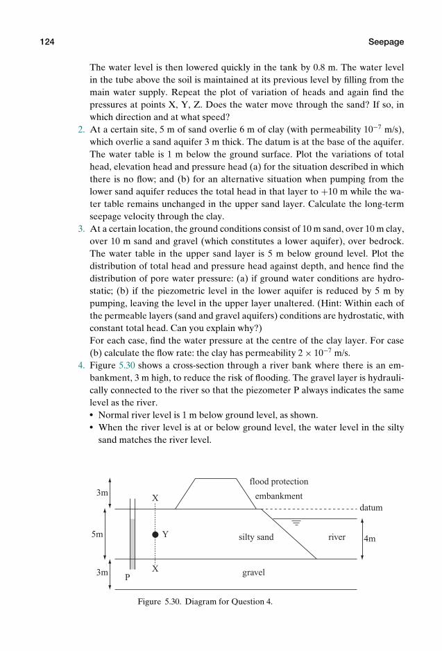
P1: KAE


124 Seepage

The water level is then lowered quickly in the tank by 0.8 m. The water levelin the tube above the soil is maintained at its previous level by filling from themain water supply. Repeat the plot of variation of heads and again find thepressures at points X, Y, Z. Does the water move through the sand? If so, inwhich direction and at what speed?

2. At a certain site, 5 m of sand overlie 6 m of clay (with permeability 10−7 m/s),which overlie a sand aquifer 3 m thick. The datum is at the base of the aquifer.The water table is 1 m below the ground surface. Plot the variations of totalhead, elevation head and pressure head (a) for the situation described in whichthere is no flow; and (b) for an alternative situation when pumping from thelower sand aquifer reduces the total head in that layer to +10 m while the wa-ter table remains unchanged in the upper sand layer. Calculate the long-termseepage velocity through the clay.

3. At a certain location, the ground conditions consist of 10 m sand, over 10 m clay,over 10 m sand and gravel (which constitutes a lower aquifer), over bedrock.The water table in the upper sand layer is 5 m below ground level. Plot thedistribution of total head and pressure head against depth, and hence find thedistribution of pore water pressure: (a) if ground water conditions are hydro-static; (b) if the piezometric level in the lower aquifer is reduced by 5 m bypumping, leaving the level in the upper layer unaltered. (Hint: Within each ofthe permeable layers (sand and gravel aquifers) conditions are hydrostatic, withconstant total head. Can you explain why?)For each case, find the water pressure at the centre of the clay layer. For case(b) calculate the flow rate: the clay has permeability 2 × 10−7 m/s.

4. Figure 5.30 shows a cross-section through a river bank where there is an em-bankment, 3 m high, to reduce the risk of flooding. The gravel layer is hydrauli-cally connected to the river so that the piezometer P always indicates the samelevel as the river. Normal river level is 1 m below ground level, as shown. When the river level is at or below ground level, the water level in the silty

sand matches the river level.

silty sand river

gravel

flood protection

embankment

Y

P

datum

3m

3m

5m 4m

X

X


P1: KAE


5.12 Exercises: Seepage 125

The land behind the flood embankment is usually drained to no higher thanground level unless catastrophic overtopping of the embankment occurs.

Plot distributions of total head and water pressure with depth at the section XXand determine the water pressure at point Y at the centre of the silty sand layer:

a. When the river level is normal at −1 m (and the water level in the siltysand is also at −1 m);

b. When the river level is at 0 m (and the water level in the silty sand isalso at 0 m);

c. When the river level is just below +3 m (and drainage keeps the waterlevel in the silty sand at 0 m);

d. When the river level is just above +3 m and the drains are overloaded,so that the land beyond the embankment is flooded to a depth of 3 m;

e. When the river level has fallen back to -1 m, leaving the drains over-loaded and the land beyond the embankment flooded to +3 m.

In each case, indicate whether water is flowing through the silty sand and, ifso, in which direction and at what rate. The permeability of the silty sand is10−4 m/s. Assume that the seepage through the silty sand is vertical and that acondition of steady flow has been attained.

5. A layer of silty clay 4 m thick with permeability k = 10−7 m/s is sandwichedbetween two layers of sand, each 4 m thick, with permeability k = 10−2 m/s. Thewater table in the upper layer of sand is at the ground surface. The lower layerof sand has an artesian pressure 3 m above ground level. Calculate the pressurehead and pore pressure at the top and bottom of the silty clay and calculate theflow rate through the silty clay.

6. A layer of sand 4 m thick with permeability k = 10−2 m/s is sandwiched be-tween two layers of silty clay each 4 m thick with permeability k = 10−7 m/s. Thelower layer of silty clay is underlain by a gravel aquifer under artesian pressurewith total head 3 m above ground level. The total head at the top of the upperlayer of silty clay is at ground level. What are the total head (relative to groundlevel) and pressure head at the top and bottom of the layer of sand? What is theflow rate through the silty clay? What is the drop in total head across the sandlayer?

7. Seasonal deposition has produced a varved deposit which consists of alternatelayers of silt of thickness 1 mm and of fine sand of thickness 2 mm, with perme-abilities 5 × 10−5 m/s and 2 × 10−3 m/s, respectively. Calculate the permeabili-ties of the varved soil to horizontal and vertical flow.

8. A layer of clay 4 m thick (permeability k = 10−8 m/s) lies between two layers ofsand each 3 m thick, the top of the upper layer of sand being at ground level. Thewater table is 1m below the ground level but the lower layer of sand is underartesian pressure, the total head being 3 m above ground level. The saturateddensity of the clay is 2 Mg/m3 and that of the sand is 1.9 Mg/m3; above thewater table, the sand has density 1.65 Mg/m3. Calculate the total head (relativeto ground level), pressure head, pore pressure, total stress and effective stress

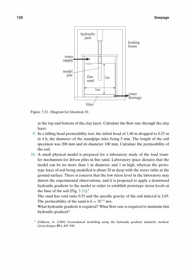
P1: KAE


126 Seepage

loading frame

model pile

water supply

water drainage

filter

fine sand

hydraulic jack

1m

1m


at the top and bottom of the clay layer. Calculate the flow rate through the claylayer.

9. In a falling head permeability test, the initial head of 1.00 m dropped to 0.25 min 4 h, the diameter of the standpipe inlet being 5 mm. The length of the soilspecimen was 200 mm and its diameter 100 mm. Calculate the permeability ofthe soil.

10. A small physical model is prepared for a laboratory study of the load trans-fer mechanism for driven piles in fine sand. Laboratory space dictates that themodel can be no more than 1 m diameter and 1 m high, whereas the proto-type layer of soil being modelled is about 20 m deep with the water table at theground surface. There is concern that the low stress level in the laboratory maydistort the experimental observations, and it is proposed to apply a downwardhydraulic gradient to the model in order to establish prototype stress levels atthe base of the soil (Fig. 5.31).6

The sand has void ratio 0.55 and the specific gravity of the soil mineral is 2.65.The permeability of the sand is k = 10−4 m/s.What hydraulic gradient is required? What flow rate is required to maintain thishydraulic gradient?

6 Zelikson, A. (1969) Geotechnical modelling using the hydraulic gradient similarity method.Geotechnique 19 4, 495–508.

P1: KAE


6 Change in stress

6.1 Introduction

In Chapter 4 we introduced the concept of the stiffness of soils under one-dimensional loading and were able to calculate the change in vertical strain, andhence the change in thickness of a soil layer that might occur as a result of a changein effective stress. In Chapter 5, we encountered the concept of permeability of soilsand noted in particular the huge range of values of permeability for soils, broadly,of different particle sizes (but also influenced by the mineralogy and shape of theparticles). The permeability of clays is many orders of magnitude lower than thepermeability of sands and gravels. Change in effective stress implies change in ver-tical dimension of the soil layers, which implies the squeezing out or the suckingin of water (assuming that the soil is saturated). In a soil of very low permeabilitythis cannot happen rapidly, and, in this chapter, we will make deductions about theshort-term and long-term conditions that must apply. The analysis of the processthat spans between the short term and the long term is called consolidation and isthe subject of Chapter 7.

6.2 Stress change and soil permeability

Figure 6.1 provides an analogy for the behaviour of a soil with low permeabilitywhen it is subjected to a change in external stresses. The spring represents the soil,and the loads taken by the spring represent the effective stress carried by the soilparticles. The spring is contained in a cylinder (like an oedometer) of cross sectionalarea A, which is full of water (the pore fluid in the soil) and capped by a rather tightlyfitting piston. When a sudden change in external load P is applied to the piston, thespring would like to compress. However, for the spring to compress water needsto escape past the piston, and this cannot occur rapidly. Equilibrium tells us thatthe load P must be carried somehow: it cannot be carried by the spring unless thespring compresses, so it must be carried by the water. The water is comparativelyincompressible (which means that its stiffness for one-dimensional confined defor-mation is pretty high) so if we call the pressure in the water u then, immediately

127

P1: KAE


128 Change in stress

a. b. c.P

P

time

external load P

spring load P'

water pressure uA

B

O

piston

cylinder: area Awater

spring 0

Figure 6.1. (a, b) Spring and tightly fitting piston; (c) gradual transfer of applied load frompore pressure to spring load.

after the load P is applied, the force provided by the water pressure acting over thecross-section A of the cylinder is:

uA = P (6.1)

as indicated by the chain dotted line OB at time t = 0 in Fig. 6.1c.Now the very narrow gaps around the piston, which are analogous to the fine

and tortuous pores in our low permeability soil, are also broadly equivalent tothe narrow tubes to which Poiseuille’s equation refers (Section 5.3). With a pres-sure gradient across the thin annular gap, flow will occur at a rate proportional tothe pressure difference between the water inside the cylinder and the free water sit-ting on top of the piston. As flow occurs, so the spring will be able to compress and,as time goes on, the external load P will be completely transferred to the spring andthe pressure in the water will ultimately be zero again. If we call the force in thespring at any time P′, then we can propose that at all times during this process:

P = uA + P′ (6.2)

with the limiting conditions that, for t = 0, P′ = 0, u = P/A and, as t → ∞, P′ → P(dashed line) and u → 0 (chain dotted line) (Fig. 6.1c). We will call this pore pres-sure u, which is tending to disappear with time, the excess pore pressure. In thischapter, we will concern ourselves only with these two limiting conditions: t = 0and t → ∞.

Exactly the same sort of thought process can be used to describe what happenswhen the external total vertical stress σz acting on the loading platen of an oedome-ter containing a sample of clay (Fig. 6.2) is changed. The deformation of the soilrequires change in the volumetric packing of the soil particles. The voids around thesoil particles are filled with water, so that change in the packing can only occur if thewater is able to flow through the voids. The permeability of this clay sample is low,so there is no possibility of immediate change in volumetric packing. Equilibriumtells us that at all times the total vertical stress can only be supported by a combina-tion of effective stress σ ′

z between the soil particles – the “soil spring” – and pressure

P1: KAE


6.2 Stress change and soil permeability 129

a. b. c.

∆σz

σz

σ'z

∆σz

∆σz

∆σz

time

stress

0

u

soil

loading platen

Figure 6.2. (a, b) Clay sample in oedometer; (c) gradual transfer of change in total stress σz

from pore pressure to effective stress.

u in the water surrounding the soil particles:

σz = σ ′z + u (6.3)

and this subdivision applies equally for changes in each of the stress components:

σz = σ ′z + u (6.4)

At the moment that the total stress is changed there is no possibility of the effectivestress changing, and consequently the change in external total vertical stress σz

must be converted into a change in pore water pressure u: u = σz (Fig. 6.2c).Just as for the spring in the cylinder (Fig. 6.1), with time the water is able to

flow and the soil spring is able to compress and the effective stress is able to take upthe change in external stress σ ′

z = σz. Our limiting conditions become, as before:t = 0, σ ′

z = 0, u = σz and, as t → ∞, σ ′z → σz and u → 0 (Fig. 6.2c).

The terms undrained and drained are used to describe these two extremes ofresponse. Undrained signifies the condition immediately after the change in exter-nal loading at time t = 0 before the water has had time to move or drain from thevoids in the soil. Drained signifies the long-term establishment of pore water equi-librium – which may be an equilibrium of steady flow, but a flow regime that doesnot change with time – and the transfer of total stress from initially non-equilibratedpore pressure to effective stress. The classification of events as undrained or drainedobviously depends on the soil type – primarily, its permeability – and the nature ofthe loading. If we propose that sands and gravels, having high permeability, willalmost invariably respond in a drained manner because the pore water can flow eas-ily, we must accept that even for such soils there may be occasions when the rate atwhich the external load is changing is so high – as a result of an explosion, for ex-ample, or an earthquake – or the distance over which the water has to flow to reachfreedom is so great, that the pore pressure changes from its equilibrium value andthe response, even for a short period, is that of an undrained soil.

P1: KAE



σz

εz

Figure 6.3. Soil sample in oedometer (Section 6.3.1). Compare Figs 4.5, 4.6.

6.3 Worked examples

6.3.1 Example 1

Let us first look at a simple example: a sample of clay in an oedometer (Fig. 6.3).Let us suppose that the current externally applied vertical total stress σz = 200 kPais in equilibrium with the effective stress σ ′

z carried by the soil particles and that thepore pressure is zero, u = 0, so that σ ′

z = σz − u = 200 kPa.

1. At time t = 0, we increase the external stress by σz = 100 kPa to σz = 300 kPa.The clay is not able to deform rapidly so the effective stress is not able to changeand the increase in total stress is transferred to the pore pressure: u = σz =100 kPa and σ ′

z = 0.In the long term, the pore pressure is allowed to dissipate so that, once again,u = 0. The externally imposed vertical total stress has not changed, so the ver-tical effective stress is calculated as the difference between the total stress andthe zero pore pressure, σ ′

z = 300 kPa, and the eventual change in effective stressmatches the original change in total stress at time t = 0. Thus, after a long time(t → ∞), σ ′

z = 100 kPa.2. Exactly the same procedure can be followed when the total stress is lowered

rather than increased. The clay would now like to increase in volume as thestress decreases but the low permeability prevents this happening rapidly:the pore pressure has to take a negative value to hold back the loading capof the oedometer. Suppose the total stress is lowered by σz = −50 kPa sothat σz = 250 kPa. The effective stress is unchanged at σ ′

z = 300 kPa. The porepressure is as ever given by the difference between total and effective stresses:u = σz − σ ′

z = 250 − 300 = −50 kPa.1

Once again, though, if we leave the oedometer long enough, the pore pressurewill be able to re-establish its equilibrium value u = 0 and the long-term changein effective stress will match the reduction of total stress: σ ′

z = σz = −50 kPa,so that σ ′

z = σz = 250 kPa.

1 The negative sign for the pore pressure should not worry us – though if the negative pore pressureapproaches the value of atmospheric pressure, around 100 kPa, then the absolute pressure in thepore fluid becomes close to zero and there is a danger that cavitation of the pore water may occur.Air bubbles would then come out of solution and the assumption that the pore fluid is incompress-ible would no longer be tenable.

P1: KAE


6.3 Worked examples 131

clay: γ = 19kN/m310m

fill: γ = 17kN/m31m

a.

z

z

z z

σz

σz

σz

σ'z

σ'zσ'zuu

u

100 2000 kPa

100 2000 kPa100 2000 kPa

b: initial conditions

c: after placement of filld: long term

total stress

Figure 6.4. Soil conditions for Example 2, Section 6.3.2: distributions of total stress σz, effec-tive stress σ ′

z and pore pressure u.

6.3.2 Example 2

A bed of clay 10 m thick with the water table at its surface is loaded with a layer offill 1 m thick over a large site (Fig 6.4). Calculate and sketch the profiles of total ver-tical stress, effective vertical stress and pore pressure (a) just before the fill has beenplaced; (b) just after the fill has been placed; and (c) in the long term when porepressure equilibrium has been re-established with the water table still at the sur-face of the clay. Calculate the immediate and the long-term settlements of the claysurface. The clay has bulk unit weight γ = 19 kN/m3 and average one-dimensionalstiffness Eo = 1.5 MPa. The fill has unit weight γ = 17 kN/m3.

Before the fill is placed, the vertical total stress is calculated from the bulk unitweight and varies with depth according to the relation:

σz = γ z = 19z kPa

The pore pressure is similarly calculated from the depth below the water table,which is conveniently located at the ground surface:

u = γwz = 9.81z kPa

P1: KAE



The vertical effective stress is just the difference between these two profiles:

σ ′z = (γ − γw)z = (19 − 9.81)z = 9.19z kPa

These profiles of stress and pore pressure are shown in Fig. 6.4b.When the fill is placed, there is an increase of total stress at all depths equal to

17 kPa (1 m of fill of unit weight 17 kN/m3). So, if we continue to measure depthsfrom the surface of the clay (and not from the new ground surface, which wouldconfuse), we can describe the total vertical stress:

σz = 19z + 17 kPa

The vertical effective stress in the clay is not able to change rapidly so, immediatelyafter the fill has been placed it has the same variation with depth as before:

σ ′z = 9.19z kPa

and, as usual, the pore pressure has to take up the difference:

u = σz − σ ′z = 9.81z + 17 kPa

and, of course, the change in pore pressure is 17 kPa at all depths in the clay. Theseprofiles of stress and pore pressure are shown in Fig. 6.4c with the heavy lines; thelighter lines show the distributions of σz and u in the original state before the place-ment of the fill.

In the long term, the pore pressure will be able to re-establish an equilibriumwith the unchanged water table:

u = 9.81z kPa

The total stress has not changed:

σz = 19z + 17 kPa

and the effective stress is once again the difference between total stress and porepressure:

σ ′z = σz − u = 9.19z + 17 kPa

and now the change in effective stress is 17 kPa at all depths in the clay. Theseprofiles of stress and pore pressure are shown in Fig. 6.4d with the heavy lines; thelighter lines show the distributions of σ ′

z and u at the time immediately after theplacement of the fill.

We can calculate the settlements from knowledge of the changes in effectivestress and from the given one-dimensional stiffness of the clay.2 Immediately afterthe fill is placed there is, for this one-dimensional situation, no possibility of changeof effective stress and hence no settlement. In the long term, the effective stress

2 A single value of Eo has been quoted for simplicity as the average stiffness relevant to the currenteffective stress and change in effective stress. A more elaborate calculation of settlement could bemade using a stiffness which varies with stress level, as described in Section 4.6.1.

P1: KAE



silty clay6 m

2 m

fill1 m

sand

rock

water table

X

Figure 6.5. Soil conditions for Example 3, Section 6.3.3.

changes by 17 kPa throughout the clay and the vertical strain is simply the ratio ofchange in effective stress and stiffness:

εz = σ ′z

Eo= 17

1.5 × 1000= 1.1%

so that the long-term settlement occurring over the 10 m thick clay layer is 0.011 ×10 = 0.11 m.

6.3.3 Example 3

The soils at a certain site consist of 2 m of sand with void ratio e = 0.6 overlying6 m of silty clay with void ratio e = 1.2 (Fig 6.5). The silty clay is underlain by rock.The specific gravity of the soil particles of both soils is Gs = 2.7. The water table isat a depth of 1 m. Above the water table the sand is dry (Sr = 0), and below thewater table the sand and silty clay are fully saturated (Sr = 1). The site is preparedfor construction by the addition of a layer of sandy gravel of thickness 1 m. Thismaterial has a void ratio e = 0.5 and Gs = 2.7. The silty clay has a one-dimensionalstiffness Eo = 1500 kPa. Calculate the history of stress changes at a point X at themid-height of the silty clay layer and calculate the long-term settlement of the topof the silty clay, at the interface with the sand.

This example allows us to pull together concepts that we have introduced inseveral of the preceding chapters. We have to start by converting the informationof void ratios and degrees of saturation into densities or unit weights. Then we cananalyse the in-situ stress and water pressure conditions. Next, we can explore whathappens to the stresses and water pressures in the short term and in the long termand, using information about the stiffness of the soils, discover what the eventualsettlement will be across the site.

For the sand above the water table, ρ = Gsρw/(1 + e) = 1.69 Mg/m3; for thesand below the water table, ρ = (Gs + e)ρw/(1 + e) = 2.06 Mg/m3. For the silty clay,ρ = (Gs + e)ρw/(1 + e) = 1.77 Mg/m3.

P1: KAE



Point X is at the centre of the silty clay (at a depth below the ground surfaceof 5 m). Before the site preparation works begin, the total vertical stress is σz =(1 × 1.69 + 1 × 2.06 + 3 × 1.77) × 9.81 = 88.96 kPa. The pore pressure is calculatedfrom the known level of the water table: u = 4 × 1 × 9.81 = 39.24 kPa. The effectivevertical stress is σ ′

z = σz − u = 49.72 kPa.The density of the sandy gravel that is used to provide the fill is ρ = Gsρw/(1 +

e) = 1.8 Mg/m3, so that the change in total vertical stress everywhere from the place-ment of 1 m of this material must be σz = 1 × 1.8 × 9.81 = 17.66 kPa. At all timesafter the placement of this fill, the total vertical stress at the centre of the silty clayat point X is thus σz = 88.96 + 17.66 = 106.62 kPa. The effective stresses in the siltyclay are not able to change until the pore water has been able to flow out of thevoids, so the effective stress at point X remains σ ′

z = 49.72 kPa immediately afterthe placement of the fill. The pore pressure has to take up the difference to sat-isfy vertical equilibrium: u = 106.62 − 49.72 = 56.90 kPa. The deductive sequenceof this calculation for time t = 0 is thus: total stress → effective stress → pore pres-sure.

In the long term, pore pressure equilibrium is re-established, with the watertable at its original level. The total stresses have not changed but the effective stresshas taken up that part of the total stress that was for the time being carried by thepore pressure. Therefore, at point X the total vertical stress after a long time willstill be σz = 106.62 kPa. The pore pressure will have reverted to its original value,u = 39.24 kPa, and the effective stress is the difference between total stress and porepressure, σ ′

z = σz − u = 67.38 kPa. We can check that the increase in effective stresscompared with the original value before filling began is equal to the increase in totalstress caused by the addition of the layer of fill: σ ′

z = 67.38 − 49.72 = 17.66 kPa.The deductive sequence of this calculation for time t → ∞ is thus: total stress →pore pressure → effective stress.

This change in vertical effective stress will occur throughout the silty clay layerso, taking an average view of the stress change and of the properties of the clay,the vertical strain in the long term will be: εz = σ ′

z/Eo = 17.66/1500 = 0.012 or1.2% throughout the clay layer, which can be converted into a settlement ς =vertical strain × layer thickness = 0.012 × 6 = 0.071 m.

6.4 Summary


1. The Principle of Effective stress tells us that total stress can be shared betweenthe pore pressure in the water in the voids of the soil and the effective stresscarried by the soil particles: σz = u + σ ′

z.2. Change in effective stress σ ′

z implies deformation of the “soil spring”. Defor-mation of the “soil spring” requires movement of the pore fluid from or to thevoids around the soil particles. For low-permeability soils saturated with water

P1:K

AE

OneD

im00a

CU

US648/M

uir978

0521

517737

August17,2009

19:12

1-D change in stress

saturated soil

change in stresschange in volume

change in volumeflow of water through voids

flow of water governed by permeabilty

permeability = flow rate/pressure gradient

sands/gravels

large particles

high permeability

rapid response to stress change

clayssmall particles

tortuous voids

low permeability

delayed response to stress change

analogy

spring + tight fitting pistonclay in oedometer

clay layer in ground

t = 0, ∆u = ∆σz, ∆σ'z = 0

σ'z

σz

∆σz

∆σz

time

too, ∆u = 0, ∆σ'z = ∆σz

u

spring

external load

water pressure

0

"drained"

"undrained"

Figure 6.6. Mind map: one-dimensional change in stress.

135

P1: KAE



(which is essentially incompressible), this fluid flow cannot occur rapidly andimmediate changes in total stress σz become corresponding changes in porewater pressure u.

3. At time t = 0, σ ′z = 0, u = σz; as t → ∞, σ ′

z → σz and u → 0.4. The immediate response is described as undrained and the long-term response

as drained.5. The distinction between undrained and drained response depends on the per-

meability of the soil, the nature of the loading, and the thickness of the soil layerwhich needs to drain.

6.5 Exercises: Change in stress

1. A sample of clay is subjected to a total vertical stress σz = 150 kPa. The porepressure is u = 10 kPa. What is the vertical effective stress σ ′

z?2. The total stress on the sample in Question 1 is increased to 200 kPa. What

are the new values of u and σ ′z? The one-dimensional stiffness of the clay is

Eo = 1500 kPa. What is the vertical strain immediately after the vertical stressis increased?

3. The total stress on the sample of clay in Question 2 remains unchanged for avery long time, and the pore pressure eventually returns to its initial value of10 kPa. What are the long-term values of σz, u and σ ′

z? What is the eventualvertical strain in the sample?

4. An oedometer sample of clay of diameter 100 mm and thickness 20 mm is inequilibrium under an external load of 1.2 kN with zero pore pressure. Calculatethe vertical total stress and vertical effective stress.

5. The load on the sample in Question 4 is increased to 1.8 kN. What are the valuesof total stress, effective stress and pore pressure immediately after the increasein load? The clay has a stiffness Eo = 1750 kPa. What is the immediate changein height of the sample?

6. The load on the sample in Question 5 is maintained at 1.8 kN for a long time.What are the eventual total stress, effective stress and pore pressure, and whatare the final vertical strain and the final height of the sample?

7. A bed of clay 10 m thick with the water table always at its surface (saturatedunit weight 18 kN/m3) is overlain by a layer of sand 2 m thick (dry unit weight16.5 kN/m3). Calculate and sketch the variation with depth of total verticalstress, pore pressure and effective vertical stress through these soils.The top 1 m of sand is removed. Calculate and sketch the total and effectivestress and pore pressure profiles (a) immediately after the sand is removed and(b) in the long term.Calculate the immediate and long-term change in thickness of the clay. Theone-dimensional confined stiffness is Eo = 1.7 MPa.

8. A bed of clay 10 m thick with the water table at its surface is overlain by a layerof sand 2 m thick. The bed of clay is underlain by a second layer of sand. Theproperties of the soils are the same as in Question 7.

P1: KAE


6.5 Exercises: Change in stress 137

Water is now pumped from the lower layer of sand while the free water tableremains at the surface of the clay. The long-term effect is to produce a linearvariation of pore pressure from zero at the surface of the clay to only 65 kPa atthe base of the clay.Calculate and sketch the variation of total vertical stress, pore pressure andeffective vertical stress in the long term. Calculate the long-term movement ofthe surface of the clay.

9. At a site where a large factory is to be built, exploratory borings are made,and the information obtained from samples taken from one borehole near thecentre of the site reveals 3 m of sand over 4 m of clay underlain by bedrock. Thewater table is at a depth of 1 m. The sand has a void ratio 0.6 and specific gravityGs = 2.7. It is dry above the water table (Sr = 0) and saturated below the watertable (Sr = 1). It has a high permeability, and offers no resistance to the flow ofwater.The clay is saturated with unit weight γ = 20 kN/m3. It has a low permeabilityand has a one-dimensional confined stiffness of Eo = 1.6 MPa. The rock may beregarded as impermeable.Calculate and sketch the distribution with depth of total vertical stress σz, porepressure u, and effective vertical stress σ ′

z.If the top 0.5 m of soil were excavated over the entire site, what immediatechanges would you expect in any of these pressures or stresses? Assuming thatthe water table remains unchanged, plot the distributions of total and effectivestresses and pore pressure (a) immediately after excavation and (b) in the longterm.What will be the long-term change in thickness of the clay?

10. The soil underlying the city of Venice is a clay layer of thickness about 300 mwith an average saturated unit weight γ = 19 kN/m3. Water has been pumpedout of an underlying aquifer for many years so that a stable linear profile ofpore pressure has developed from 0 kPa at the ground surface to only 2700 kPaat the base of the clay. Calculate profiles of total and effective stress and porepressure.International pressure forces the city to stop pumping from the aquifer and thepore pressure eventually returns to the equilibrium hydrostatic value through-out the clay. Estimate the resulting movement of the city of Venice. The averagestiffness of the clay is Eo = 108 MPa.

P1: KAE


7 Consolidation

7.1 Introduction

In previous chapters, we have noted that soils of low permeability – typically, clayeysoils – will not be able to respond rapidly to changes in stresses which require defor-mation, which in turn implies, for our one-dimensional systems, change in volume.We suggested in Section 6.2 that there would be a transient process between timet = 0 and time t → ∞ during which the temporary disequilibrium of pore pressureswould disappear as deformation of the soil spring permitted stresses to be trans-ferred from pore pressure to effective stresses supported by the soil itself. The de-tail of this process was not considered: we merely looked at the two extremes ofthe immediate aftermath of the change in external stress (at t = 0) and the eventualequilibrium at infinite time (t → ∞). In this chapter, we will explore various aspectsof the analysis of the transient process between these two extremes. The transientprocess is known as consolidation.

We will first produce an approximate solution which forces us to concentrateon the important physical aspects of the problem. However, the governing differ-ential equation – the diffusion equation – is one that is common to many problemswhich involve gradient driven flow: heat flows down a temperature gradient, pol-lution flows down a concentration gradient, pore water flows down a gradient oftotal head (Sections 5.2, 5.4). The diffusion equation is common to a range of prob-lems, and the development and solution of the governing equation provides a fairlystraightforward example of the use of mathematics in the service of the mechanicsof soils. It is instructive to see how the exact solutions and the approximate solutionscompare for different regimes of consolidation.

It is helpful to separate that part of the pore pressure which is associated witha stable flow regime (which might be a regime of no flow or a regime of steadyflow) from that part of the pore pressure which forms part of the transient responseto some perturbation. We will call this second part the excess pore pressure, whichwill become zero in the steady long-term state. We will use the symbol u′ to de-note this excess pore pressure. In the language of Chapter 5 and the analysis ofone-dimensional flow, the first part of the pore pressure is associated with either

138

P1: KAE


7.1 Introduction 139

sand

sand

clayz

z

u: t = 0u: t < 0 u: t oo

0

a. c.b. d.

z

0

z

0

excess pore pressure

hydrostatic pore pressure

←

Figure 7.1. (a) Layer of clay between layers of sand: problem definition; (b) pore pressure attime t < 0; (c) pore pressure at time t = 0; (d) pore pressure at time t → ∞.

constant total head H or linearly varying total head throughout the soil layer of in-terest. Thus, Figs 7.1 and 7.2 are equivalent: the first shows the distributions of porepressure; the second shows the distributions of excess pore pressure. Figures 7.1b, dand 7.2b, d show the steady state distributions, which are here assumed hydrostaticthrough all soil layers, at times t < 0 and t → ∞; Figs 7.1c and 7.2c show the dis-tributions at time t = 0 just after some surcharge has been placed which can onlybe supported in the impermeable clay layer by an increase in pore pressure. This

sand

sand

clayz

u'i: t = 0

u': t < 0 u': t oo

00 0

a. c.b. d.

←

Figure 7.2. (a) Layer of clay between layers of sand: problem definition; (b) excess pore pres-sure at time t < 0; (c) excess pore pressure at time t = 0; (d) excess pore pressure at timet → ∞ (compare Fig. 7.1).

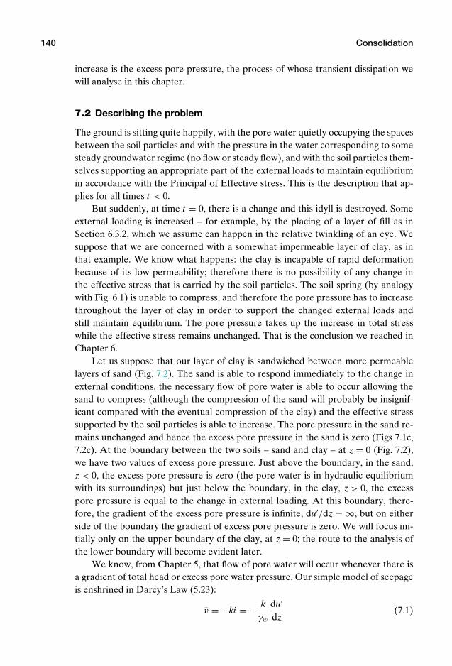
P1: KAE


140 Consolidation

increase is the excess pore pressure, the process of whose transient dissipation wewill analyse in this chapter.

7.2 Describing the problem

The ground is sitting quite happily, with the pore water quietly occupying the spacesbetween the soil particles and with the pressure in the water corresponding to somesteady groundwater regime (no flow or steady flow), and with the soil particles them-selves supporting an appropriate part of the external loads to maintain equilibriumin accordance with the Principal of Effective stress. This is the description that ap-plies for all times t < 0.

But suddenly, at time t = 0, there is a change and this idyll is destroyed. Someexternal loading is increased – for example, by the placing of a layer of fill as inSection 6.3.2, which we assume can happen in the relative twinkling of an eye. Wesuppose that we are concerned with a somewhat impermeable layer of clay, as inthat example. We know what happens: the clay is incapable of rapid deformationbecause of its low permeability; therefore there is no possibility of any change inthe effective stress that is carried by the soil particles. The soil spring (by analogywith Fig. 6.1) is unable to compress, and therefore the pore pressure has to increasethroughout the layer of clay in order to support the changed external loads andstill maintain equilibrium. The pore pressure takes up the increase in total stresswhile the effective stress remains unchanged. That is the conclusion we reached inChapter 6.

Let us suppose that our layer of clay is sandwiched between more permeablelayers of sand (Fig. 7.2). The sand is able to respond immediately to the change inexternal conditions, the necessary flow of pore water is able to occur allowing thesand to compress (although the compression of the sand will probably be insignif-icant compared with the eventual compression of the clay) and the effective stresssupported by the soil particles is able to increase. The pore pressure in the sand re-mains unchanged and hence the excess pore pressure in the sand is zero (Figs 7.1c,7.2c). At the boundary between the two soils – sand and clay – at z = 0 (Fig. 7.2),we have two values of excess pore pressure. Just above the boundary, in the sand,z < 0, the excess pore pressure is zero (the pore water is in hydraulic equilibriumwith its surroundings) but just below the boundary, in the clay, z > 0, the excesspore pressure is equal to the change in external loading. At this boundary, there-fore, the gradient of the excess pore pressure is infinite, du′/dz = ∞, but on eitherside of the boundary the gradient of excess pore pressure is zero. We will focus ini-tially only on the upper boundary of the clay, at z = 0; the route to the analysis ofthe lower boundary will become evident later.

We know, from Chapter 5, that flow of pore water will occur whenever there isa gradient of total head or excess pore water pressure. Our simple model of seepageis enshrined in Darcy’s Law (5.23):

v = −ki = − kγw

du′

dz(7.1)

P1: KAE


7.2 Describing the problem 141

u'0 u'i

clay

∆σ'z

isochrone: t = t1

z

sand

Figure 7.3. Consolidation front penetrating distance into layer of clay at time t = t1, defin-ing isochrone of excess pore pressure for t = t1.

where v is the flow velocity averaged over the cross-section of the soil, k is the coeffi-cient of permeability, and i is the hydraulic gradient which describes the gradient oftotal head within the soil. In analysing transient consolidation, it is helpful to workwith excess pore pressure u′ rather than head: pressure and head are linked throughthe unit weight γw = ρwg of the water. The negative sign in (7.1) is included as a for-mal indication that the water flows down the gradient of excess pore pressure or totalhead. It is convenient to suppose for simplicity here that there is no flow except thatresulting from the change in external stress, so that in the long term, once hydraulicequilibrium has been re-established at t → ∞, i = (1/γw)du′/dz = dH/dz = 0. Ev-erything that we do is concerned with the departure from this eventual steady state.

Darcy’s Law tells us that, for an instant, there will be an infinite flow rate at theboundary of the clay; but it also tells us that within the clay layer there will be noflow because there is no gradient of excess pore pressure: at z = 0, i = ∞; for z > 0,i = 0 (Fig. 7.2b). The clay within the layer is quite oblivious to the fact that there isa boundary at z = 0, from which drainage has started to occur. It will take time forthis knowledge to penetrate.

Flow implies movement of pore water and basic ideas of conservation of massmust apply. In fact, since we are assuming that both the water and the soil particlesare incompressible, conservation of mass implies conservation of volume. The soilskeleton which describes the locations of the soil particles is not incompressible: aswater flows out of or into the voids, the volume defined by the soil skeleton andoccupied by the soil particles will change. For a saturated soil, this is the only way inwhich volume change can occur. Conservation of volume then tells us that, if water isflowing out of the clay and into the sand, then the volume of the clay (or, better, thevolume occupied by the clay) must be decreasing. The volume is decreasing becauseof the transfer of total stress from pore water pressure to effective stress. The rate atwhich the clay is compressing must exactly balance the rate at which water is flowingout of the clay.

The concept of infinity is difficult to handle, so let us consider a time t1 > 0which is typical of the process of gradual penetration of the consolidation front intothe clay (Fig. 7.3). There will be some variation of excess pore pressure through the

P1: KAE


142 Consolidation

clay, which we can describe using an isochrone.1 At the boundary of the clay, z = 0,the slope of the pore pressure isochrone defines the rate of flow of water out of theclay. For cross-sectional area A of the clay, the volumetric rate of flow is q:

q = Akγw

[du′

dz

]z=0

(7.2)

This flow rate must balance the rate of change in volume of the clay resulting fromthe change in effective stress. If the consolidation front has penetrated a distance

(Fig. 7.3), then at each depth 0 < z < the strain in the clay is related to the changein effective stress σ ′

z scaled by the one-dimensional stiffness of the clay, Eo. Thechange in effective stress is the separation of the initial pore pressure isochrone fort = 0 (for which the excess pore pressure is u′

i throughout the layer) and the currentpore pressure isochrone: σ ′

z = u′i − u′ (Fig. 7.3). The vertical strain at depth z is

εz = σ ′z/Eo and the accumulated settlement of the layer is:

ς =∫

0εzdz = 1

Eo

∫

0(u′

i − u′)dz (7.3)

Conservation of volume requires that the rate of flow of water out of the clay mustmatch the rate of settlement of the clay layer:

q = Adς

dt(7.4)

or, with (7.2):

kγw

[du′

dz

]z=0

= ddt

[1

Eo

∫

0(u′

i − u′)dz]

(7.5)

This looks rather a tricky equation to solve but it becomes tractable if we makesome reasonable assumption about the shape of the pore pressure isochrone at timet = t1. We then have immediate access to both the exit gradient controlling the flowrate at z = 0 and the average effective stress change from the integral of the areabetween the isochrones for t = 0 and t = t1.

7.3 Parabolic isochrones

Let us assume that at all times the pore pressure isochrones have a common geomet-ric shape. The assumption of an appropriate plausible shape function for the varia-tion of some quantity within a defined region is a standard approximation techniquewhich will be encountered in other engineering applications. In principle, we couldassume any shape. It turns out that the mathematics becomes particularly simple ifwe assume that the isochrones are parabolic.2 The excess pore pressure is assumedto vary parabolically with distance from the drainage boundary (Fig. 7.3). The ef-fective stresses are given by the difference between the applied total stress and this

1 isochrone: from Greek “equal time”.2 Schofield, A.N. and Wroth, C.P. ( 1968) Critical state soil mechanics, McGraw-Hill, London.

P1: KAE


7.3 Parabolic isochrones 143

focus F

directrix

-a a x

y

O

PDa.

b.

Figure 7.4. Geometry of the parabola: (a) conic section; (b) focus and directrix.

pore pressure so that the volume change of the clay is linked with the area above theparabolic isochrone scaled with the one-dimensional stiffness, Eo. The rate at whichwater flows out of the clay is controlled by the slope of the parabolic isochrone atthe drainage boundary. The problem enshrined in (7.5) then reduces to a simple dif-ferential equation, deduced from the geometry of the parabola, linking the rate ofchange of volume of the soil with the rate at which water flows out of the soil.

The parabola is a curve obtained by cutting a cone parallel to its sloping side(Fig. 7.4a). Its equation can be derived by noting that it is the locus of points whichare equidistant from a point – the focus, F: (x, y) = (a, 0) – and a straight line – thedirectrix: x = −a (Fig. 7.4b). For any point P, PF = PD, or:√

(x − a)2 + y2 = a + x (7.6)

or, squaring both sides and rearranging:

y2 = 4ax or y = 2√

ax (7.7)

Differentiating this equation, we can show that the slope of the parabola at P is:

dydx

= y2x

(7.8)

which is half the slope of the line from the origin O to P, the diagonal of the enclosingrectangle y/x.

Integrating (7.7), we can find the area under the parabola from O to P:

area =∫ x

02√

axdx = 43

x√

ax = 23

xy (7.9)

and the area is two thirds of the enclosing rectangle. The elements of the geometry ofthe parabola that we need to use in our interpretation of the process of consolidationare thus rather simple (Fig. 7.5).

We can now tackle our governing equation (7.5). From (7.8), the left hand sidecan be written:

kγw

[du′

dz

]z=0

= 2ku′i

γw(7.10)

P1: KAE


144 Consolidation

L/2

L/2

B

area = 2BL/3

Figure 7.5. Geometry of parabolic isochrone.

and from (7.9) the right hand side can be written:

ddt

[1

Eo

∫

0(u′

i − u′)dz]

= ddt

[u′

i

3Eo

]= u′

i

3Eo

d

dt(7.11)

Equating these, we find the first order ordinary differential equation:

u′i

3Eo

d

dt= 2ku′

i

γw(7.12)

or:

2d = 12kEo

γw

dt (7.13)

which we can integrate to give:

=√

12kEo

γw

t (7.14)

This is an expression for the distance that the boundary disturbance (the sen-sation of the pore pressure discontinuity at z = 0 and t = 0) is able to penetrate intime t . We note, firstly, that this expression is independent of u′

i – the magnitude ofthe pore pressure disturbance is not important. We note, secondly, that the locationof the consolidation front, the value of , is proportional to the square root of time.And we note, thirdly, that the soil property controlling the process is a compositequantity which is called the coefficient of consolidation cv :

cv = kEo

γw

(7.15)

The coefficient of consolidation has dimensions of (length2/time) and shouldbe quoted in standard SI units of metres2/second. The range of values of cv is highand the values that are likely to be encountered for geotechnical problem whereeffects of consolidation are a crucial design factor tend to be quite low, so that non-standard units are often used. This merely calls for care in ensuring consistency

P1: KAE



Table 7.1. Typical values of coefficient of consolidation, cv.

Quoted units m2/s

8 × 10−2 m2/day 0.93 × 10−6

60 × 10−6 m2/min 1.00 × 10−6

0.01 ha/year 3.17 × 10−6

0.4 m2/year 12.7 × 10−9

1.3 mm2/min 21.7 × 10−9

0.1 m2/month 38.6 × 10−9

8 × 10−4 cm2/s 80.0 × 10−9

in any calculation. A quick trawl of a random selection of literature produces thevalues and units shown in Table 7.1 for the coefficient of consolidation of clays.They have been converted to standard units in the final column.

Knowing how far the sensation of consolidation has penetrated is part of thestory; it is useful also to know how much settlement has occurred and how rapidly itis occurring. Settlement was given by (7.3) and this becomes:

ς = 1Eo

∫

0(u′

i − u′)dz = u′i

3Eo= u′

i

3Eo

√12

kEo

γw

t = u′i

√4kt

3Eoγw

(7.16)

The settlement also varies with the square root of time but is, not surprisingly, pro-portional to the pore pressure discontinuity.

There is no restriction on the thickness of the clay layer to which this analysiscan be applied, but it will cease to be valid once the entire clay layer is aware ofthe occurrence of drainage. We can imagine two simple examples of layers of finitethickness: a layer of thickness L sandwiched between a layer of permeable sand anda layer of impermeable rock (Fig. 7.6a); and a layer of thickness 2L sandwichedbetween two layers of permeable sand (Fig. 7.6b). In fact, from symmetry, the twoconfigurations are equivalent. The boundary drainage in Fig. 7.6b creeps in simulta-neously from top and bottom and the whole layer is consolidating once = L. Fromsymmetry, there can be no flow across the mid-height of the layer at distance L fromeither boundary, and hence du′/dz = 0 at z = L for 0 < t < ∞. This plane of sym-metry might just as well be an impermeable plane. The boundary drainage in Fig.7.6a creeps in from the top boundary only and the whole layer is consolidating once = L. The real impermeability of the lower boundary means that the isochronesmust always meet it orthogonally and du′/dz = 0 at z = L for 0 < t < ∞.

We will consider the layer of thickness L, noting that the rate of consolidationwill be the same for both layers but that the settlements will be doubled for thelayer of thickness 2L. The first stage of the consolidation ends when = L at t =tA = L2/12cv . At this time, the excess pore pressure at depth z = L is still just equalto the original value u′

i . In the second stage of the consolidation, the entire layeris participating, and the pore pressure at the base of the layer falls progressivelyto zero. The typical isochrone for some intermediate time tA ≤ t < ∞ is shown inFig. 7.7 with pore pressure u′

L at the lower boundary. Exactly the same physical

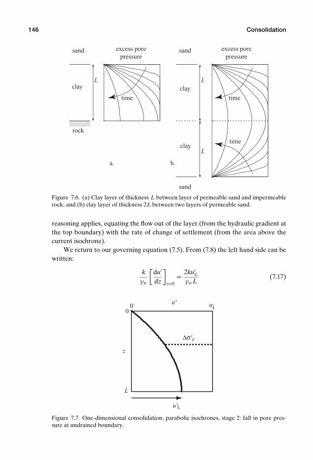
P1: KAE


146 Consolidation

sandsand

sand

clay

clay

rock

LL

L

a. b.

timetime

time



clay

Figure 7.6. (a) Clay layer of thickness L between layer of permeable sand and impermeablerock; and (b) clay layer of thickness 2L between two layers of permeable sand.

reasoning applies, equating the flow out of the layer (from the hydraulic gradient atthe top boundary) with the rate of change of settlement (from the area above thecurrent isochrone).

We return to our governing equation (7.5). From (7.8) the left hand side can bewritten:

kγw

[du′

dz

]z=0

= 2ku′L

γw L(7.17)

u'

z

00 ui

L

u'L

∆σ'z

Figure 7.7. One-dimensional consolidation, parabolic isochrones, stage 2: fall in pore pres-sure at undrained boundary.

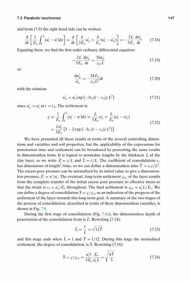
P1: KAE



and from (7.9) the right hand side can be written:

ddt

[1

Eo

∫ L

0(u′

i − u′)dz]

= ddt

[L

3Eou′

L + LEo

(u′i − u′

L)]

= − 2L3Eo

du′L

dt(7.18)

Equating these, we find the first order ordinary differential equation:

− 2L3Eo

du′L

dt= 2ku′

L

γw L(7.19)

or:

du′L

u′L

= −3kEo

γw L2dt (7.20)

with the solution:

u′L = u′

i exp(−3cv(t − tA)/L2) (7.21)

since u′L = u′

i at t = tA. The settlement is:

ς = 1Eo

∫ L

0(u′

i − u′)dz = L3Eo

u′L + L

Eo(u′

i − u′L)

= Lu′i

3Eo

[3 − 2 exp

(−3cv(t − tA)/L2)] (7.22)

We have presented all these results in terms of the several controlling dimen-sions and variables and soil properties, but the applicability of the expressions forpenetration time and settlement can be broadened by presenting the same resultsin dimensionless form. It is logical to normalise lengths by the thickness L of theclay layer, so we write Z = z/L and L = /L. The coefficient of consolidation cv

has dimensions of length2/time, so we can define a dimensionless time T = cvt/L2.The excess pore pressure can be normalised by its initial value to give a dimension-less pressure, U = u′/u′

i . The eventual, long-term settlement ς∞ of the layer resultsfrom the complete transfer of the initial excess pore pressure to effective stress sothat the strain is εz = u′

i/Eo throughout. The final settlement is ς∞ = u′i L/Eo. We

can define a degree of consolidation S = ς/ς∞ as an indication of the progress of thesettlement of the layer towards this long-term goal. A summary of the two stages ofthe process of consolidation, described in terms of these dimensionless variables, isshown in Fig. 7.8.

During the first stage of consolidation (Fig. 7.8a), the dimensionless depth ofpenetration of the consolidation front is L. Rewriting (7.14):

L =

L=

√12T (7.23)

and this stage ends when L = 1 and T = 1/12. During this stage the normalisedsettlement, the degree of consolidation, is S. Rewriting (7.16):

S = ς/ς∞ = u′i

3Eo

Eo

u′i L

=√

4T3

(7.24)

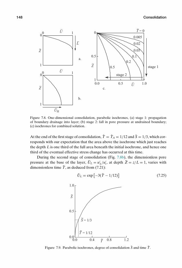
P1: KAE


148 Consolidation

0.0 0.5 1.01

0.5

0

U

U

U

Z

Z

Z

0.005

0.02

0.05

0.2

0.1

0.5

T = 0

stage 1

stage 2

c.

00

00

1

1

1

1

L

UH

a.

b.

∼ ∼

∼

∼

∼∼

∼

∼

∼

Figure 7.8. One-dimensional consolidation, parabolic isochrones, (a) stage 1: propagationof boundary drainage into layer; (b) stage 2: fall in pore pressure at undrained boundary;(c) isochrones for combined solution.

At the end of the first stage of consolidation, T = TA = 1/12 and S = 1/3, which cor-responds with our expectation that the area above the isochrone which just reachesthe depth L is one third of the full area beneath the initial isochrone, and hence onethird of the eventual effective stress change has occurred at this time.

During the second stage of consolidation (Fig. 7.8b), the dimensionless porepressure at the base of the layer, UL = u′

L/u′i , at depth Z = z/L = 1, varies with

dimensionless time T , as deduced from (7.21):

UL = exp[−3(T − 1/12)

](7.25)

0.0 0.4 0.8 1.20.0

0.5

1.0

T

S

T = 1/12

S = 1/3

~

~

~

~

Figure 7.9. Parabolic isochrones, degree of consolidation S and time T .

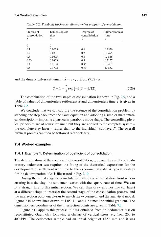
P1: KAE



Table 7.2. Parabolic isochrones, dimensionless progress of consolidation.

Degree of Dimensionless Degree of Dimensionlessconsolidation time consolidation timeS T S T

0 00.1 0.0075 0.6 0.25360.2 0.03 0.7 0.34950.3 0.0675 0.8 0.48460.33 0.0833 0.9 0.71570.4 0.1184 0.95 0.94670.5 0.1792 0.99 1.4832

and the dimensionless settlement, S = ς/ς∞, from (7.22), is:

S = 1 − 23

exp[−3(T − 1/12)

](7.26)

The combination of the two stages of consolidation is shown in Fig. 7.9, and atable of values of dimensionless settlement S and dimensionless time T is given inTable 7.2.

We conclude that we can capture the essence of the consolidation problem bystanding one step back from the exact equation and adopting a simpler mathemati-cal description – imposing a particular parabolic mode shape. The controlling phys-ical principles are of course retained but they are applied to the complete system –the complete clay layer – rather than to the individual “sub-layers”. The overallphysical process can then be followed rather clearly.

7.4 Worked examples

7.4.1 Example 1: Determination of coefficient of consolidation

The determination of the coefficient of consolidation, cv , from the results of a lab-oratory oedometer test requires the fitting of the theoretical expressions for thedevelopment of settlement with time to the experimental data. A typical strategyfor the determination of cv is illustrated in Fig. 7.10.

During the initial stage of consolidation, while the consolidation front is pen-etrating into the clay, the settlement varies with the square root of time. We canfit a straight line to this initial section. We can then draw another line (or lines)at a different slope to intersect the second stage of the consolidation process, andthe intersection point enables us to match the experiment and the analytical model.Figure 7.10 shows lines drawn at 1.05, 1.1 and 1.2 times the initial gradient. Thedimensionless coordinates of the intersection points are given in Table 7.3.

Figure 7.11 applies this process to data obtained from an oedometer test onreconstituted Gault clay following a change of vertical stress, σz, from 200 to400 kPa. The oedometer sample had an initial height of 15.56 mm and it was

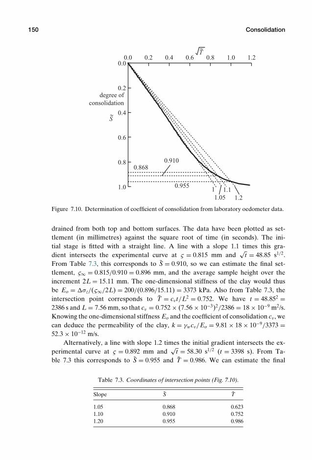
P1: KAE


150 Consolidation

0.0 0.2 0.4 0.6 0.8 1.0 1.2

1.0

0.8

0.6

0.4

0.2

0.0

degree of consolidation

S

T

11.05

1.11.2

0.8680.910

0.955

~

~

Figure 7.10. Determination of coefficient of consolidation from laboratory oedometer data.

drained from both top and bottom surfaces. The data have been plotted as set-tlement (in millimetres) against the square root of time (in seconds). The ini-tial stage is fitted with a straight line. A line with a slope 1.1 times this gra-dient intersects the experimental curve at ς = 0.815 mm and

√t = 48.85 s1/2.

From Table 7.3, this corresponds to S = 0.910, so we can estimate the final set-tlement, ς∞ = 0.815/0.910 = 0.896 mm, and the average sample height over theincrement 2L = 15.11 mm. The one-dimensional stiffness of the clay would thusbe Eo = σz/(ς∞/2L) = 200/(0.896/15.11) = 3373 kPa. Also from Table 7.3, theintersection point corresponds to T = cvt/L2 = 0.752. We have t = 48.852 =2386 s and L = 7.56 mm, so that cv = 0.752 × (7.56 × 10−3)2/2386 = 18 × 10−9 m2/s.Knowing the one-dimensional stiffness Eo and the coefficient of consolidation cv , wecan deduce the permeability of the clay, k = γwcv/Eo = 9.81 × 18 × 10−9/3373 =52.3 × 10−12 m/s.

Alternatively, a line with slope 1.2 times the initial gradient intersects the ex-perimental curve at ς = 0.892 mm and

√t = 58.30 s1/2 (t = 3398 s). From Ta-

ble 7.3 this corresponds to S = 0.955 and T = 0.986. We can estimate the final

Table 7.3. Coordinates of intersection points (Fig. 7.10).

Slope S T

1.05 0.868 0.6231.10 0.910 0.7521.20 0.955 0.986

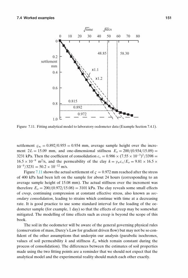
P1: KAE



settlementmm

time secs

x1.1

x1.2

48.85 58.30

0.815

0.892

0 10 20 30 40 50 60 70 80

1.0

0.8

0.6

0.4

0.2

0

0.972

Figure 7.11. Fitting analytical model to laboratory oedometer data (Example Section 7.4.1).

settlement ς∞ = 0.892/0.955 = 0.934 mm, average sample height over the incre-ment 2L = 15.09 mm, and one-dimensional stiffness Eo = 200/(0.934/15.09) =3231 kPa. Then the coefficient of consolidation cv = 0.986 × (7.55 × 10−3)2/3398 =16.5 × 10−9 m2/s, and the permeability of the clay k = γwcv/Eo = 9.81 × 16.5 ×10−9/3231 = 50.2 × 10−12 m/s.

Figure 7.11 shows the actual settlement of ς = 0.972 mm reached after the stressof 400 kPa had been left on the sample for about 24 hours (corresponding to anaverage sample height of 15.08 mm). The actual stiffness over the increment wastherefore Eo = 200/(0.972/15.08) = 3101 kPa. The clay reveals some small effectsof creep, continuing compression at constant effective stress, also known as sec-ondary consolidation, leading to strains which continue with time at a decreasingrate. It is good practice to use some standard interval for the loading of the oe-dometer sample (for example, 1 day) so that the effects of creep may be somewhatmitigated. The modelling of time effects such as creep is beyond the scope of thisbook.

The soil in the oedometer will be aware of the general governing physical rules(conservation of mass, Darcy’s Law for gradient driven flow) but may not be so con-fident of the other assumptions that underpin our analysis (parabolic isochrones,values of soil permeability k and stiffness Eo which remain constant during theprocess of consolidation). The differences between the estimates of soil propertiesmade using the two fitting points are a reminder that we should not expect that theanalytical model and the experimental reality should match each other exactly.

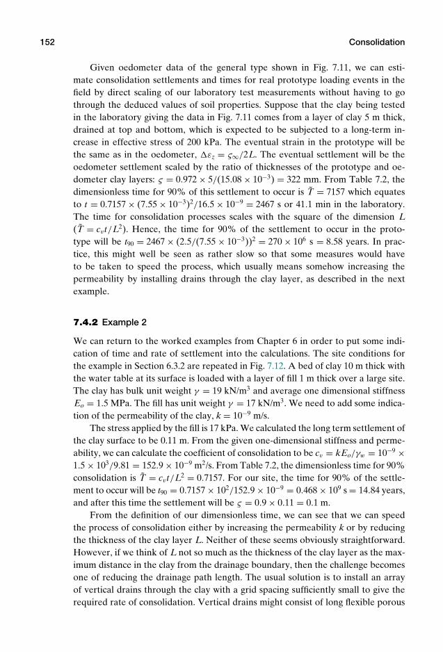
P1: KAE


152 Consolidation

Given oedometer data of the general type shown in Fig. 7.11, we can esti-mate consolidation settlements and times for real prototype loading events in thefield by direct scaling of our laboratory test measurements without having to gothrough the deduced values of soil properties. Suppose that the clay being testedin the laboratory giving the data in Fig. 7.11 comes from a layer of clay 5 m thick,drained at top and bottom, which is expected to be subjected to a long-term in-crease in effective stress of 200 kPa. The eventual strain in the prototype will bethe same as in the oedometer, εz = ς∞/2L. The eventual settlement will be theoedometer settlement scaled by the ratio of thicknesses of the prototype and oe-dometer clay layers: ς = 0.972 × 5/(15.08 × 10−3) = 322 mm. From Table 7.2, thedimensionless time for 90% of this settlement to occur is T = 7157 which equatesto t = 0.7157 × (7.55 × 10−3)2/16.5 × 10−9 = 2467 s or 41.1 min in the laboratory.The time for consolidation processes scales with the square of the dimension L(T = cvt/L2). Hence, the time for 90% of the settlement to occur in the proto-type will be t90 = 2467 × (2.5/(7.55 × 10−3))2 = 270 × 106 s = 8.58 years. In prac-tice, this might well be seen as rather slow so that some measures would haveto be taken to speed the process, which usually means somehow increasing thepermeability by installing drains through the clay layer, as described in the nextexample.

7.4.2 Example 2

We can return to the worked examples from Chapter 6 in order to put some indi-cation of time and rate of settlement into the calculations. The site conditions forthe example in Section 6.3.2 are repeated in Fig. 7.12. A bed of clay 10 m thick withthe water table at its surface is loaded with a layer of fill 1 m thick over a large site.The clay has bulk unit weight γ = 19 kN/m3 and average one dimensional stiffnessEo = 1.5 MPa. The fill has unit weight γ = 17 kN/m3. We need to add some indica-tion of the permeability of the clay, k = 10−9 m/s.

The stress applied by the fill is 17 kPa. We calculated the long term settlement ofthe clay surface to be 0.11 m. From the given one-dimensional stiffness and perme-ability, we can calculate the coefficient of consolidation to be cv = kEo/γw = 10−9 ×1.5 × 103/9.81 = 152.9 × 10−9 m2/s. From Table 7.2, the dimensionless time for 90%consolidation is T = cvt/L2 = 0.7157. For our site, the time for 90% of the settle-ment to occur will be t90 = 0.7157 × 102/152.9 × 10−9 = 0.468 × 109 s = 14.84 years,and after this time the settlement will be ς = 0.9 × 0.11 = 0.1 m.

From the definition of our dimensionless time, we can see that we can speedthe process of consolidation either by increasing the permeability k or by reducingthe thickness of the clay layer L. Neither of these seems obviously straightforward.However, if we think of L not so much as the thickness of the clay layer as the max-imum distance in the clay from the drainage boundary, then the challenge becomesone of reducing the drainage path length. The usual solution is to install an arrayof vertical drains through the clay with a grid spacing sufficiently small to give therequired rate of consolidation. Vertical drains might consist of long flexible porous

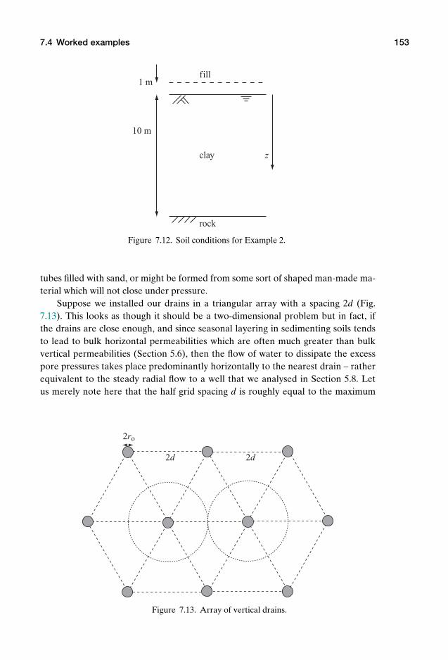
P1: KAE



clay

rock

10 m

fill1 m

z

Figure 7.12. Soil conditions for Example 2.

tubes filled with sand, or might be formed from some sort of shaped man-made ma-terial which will not close under pressure.

Suppose we installed our drains in a triangular array with a spacing 2d (Fig.7.13). This looks as though it should be a two-dimensional problem but in fact, ifthe drains are close enough, and since seasonal layering in sedimenting soils tendsto lead to bulk horizontal permeabilities which are often much greater than bulkvertical permeabilities (Section 5.6), then the flow of water to dissipate the excesspore pressures takes place predominantly horizontally to the nearest drain – ratherequivalent to the steady radial flow to a well that we analysed in Section 5.8. Letus merely note here that the half grid spacing d is roughly equal to the maximum

2d 2d

2ro

Figure 7.13. Array of vertical drains.

P1: KAE


154 Consolidation

silty clay6 m

2 m

fill1 m

sand

rock

water table

X

Figure 7.14. Soil conditions for Example 3 (see also Fig. 6.5).

drainage path length.3 So if we place our drains through our 10 m layer of clay withspacing 2d = 2 m, then we can expect the time for 90% consolidation settlement toscale by the square of the drainage path length and to be reduced to something ofthe order of 14.84 × 12/102 = 0.15 years or around 1.8 months, which is likely to bequite acceptable from the point of view of the geotechnical construction.

7.4.3 Example 3

In the example of Section 6.3.3 (Fig. 7.14), we were told that the soils at a certainsite consist of 2 m of sand with void ratio e = 0.6 overlying 6 m of silty clay with voidratio e = 1.2. The silty clay is underlain by impermeable rock. The specific gravity ofthe particles of both soils is Gs = 2.7. The water table is at a depth of 1 m. Above thewater table, the sand is dry (Sr = 0); below the water table, the sand and silty clayare fully saturated (Sr = 1). The site is prepared for construction by the addition ofa layer of sandy gravel of thickness 1 m. This material has a void ratio e = 0.5 andGs = 2.7. The silty clay has a one-dimensional stiffness Eo = 1500 kPa, and we willadd that the permeability of the silty clay is k = 10−8 m/s. We calculated that thesilty clay layer would experience an increase of vertical effective stress of 17.66 kPaand that the eventual settlement of the clay would be 0.071 m. Let us estimate thetime that will be taken for 50% and 90% of this settlement to occur.

We need to calculate the coefficient of consolidation, cv = kEo/γw, for the clay.From the values given, we have cv = 10−8 × 1500/9.81 = 1.53 × 10−6 m2/s. For 50%consolidation, we have dimensionless time T = 0.1792 from Table 7.2. Our claylayer has thickness L = 6 m, since it is underlain by impermeable rock. Hence for50% consolidation, t50 = 62 × 0.1792/1.53 × 10−6 = 4.22 × 106 s = 48.8 days, andthe settlement of the surface of the clay will be 0.035 m. For 90% consolidation, wehave dimensionless time T = 0.7157 from Table 7.2. Hence for 90% consolidation,

3 The maximum path is evidently a little greater than d and the converging flow to each drain com-plicates the analysis a little.

P1: KAE


7.5 Consolidation: exact analysis ♣ 155

t90 = 62 × 0.7157/1.53 × 10−6 = 16.8 × 106 s = 194.9 days, and the settlement of thesurface of the clay will be 0.064 m.

7.4.4 Example 4

At a particular site, there is a clay layer of thickness 5 m sandwiched between layersof sand and gravel, which are able to drain freely. The ground level at the site is to beraised by 2 m by placing a layer of fill of unit weight 21 kN/m3. To estimate the timethat it will take for the clay to settle under this increased stress, a small sample ofclay 100 mm in diameter and 20 mm thick is prepared for testing in an oedometer. Atan appropriate representative effective stress level, the one-dimensional incremen-tal stiffness is found to be Eo = 1400 kPa and it is found that a time of 47 minutesis required for 80% of the settlement to occur under the corresponding stress incre-ment. Calculate the coefficient of consolidation cv for the clay and the permeabilityk. How long will it take for 80% of the settlement of the prototype clay layer tooccur?

We will use the method of parabolic isochrones. We can use (7.26) to findthe value of non-dimensional time T corresponding to a degree of consolidationS = 0.8. We need to check that the consolidation process is indeed in the secondphase and that the value of T > 1/12.

T = 112

− 13

ln[

32

(1 − S)]

(7.27)

and for S = 0.8, T = 0.485. We know that T = cvt/L2. For our oedometer sam-ple with drainage from both top and bottom, L = 0.01 m and we are told thatt = 47 min = 2820 s. Hence, the coefficient of consolidation cv = 1.7 × 10−8 m2/s.The coefficient of consolidation is a function of permeability, stiffness and the unitweight of water: cv = kEo/γw and hence, given Eo = 1400 kPa, we can find the per-meability k = 1.2 × 10−10 m/s.

For our clay layer in situ we need only to know that the time for any chosendegree of consolidation is proportional to the square of the layer thickness, providedthat the drainage conditions are equivalent (for example, as here, drainage fromtop and bottom boundaries in both the oedometer and the prototype). Thus thetime for 80% consolidation of the clay layer of thickness 5 = 2 × 2.5 m will be 47 ×(2.5/0.01)2 = 2.94 × 106 minutes = 5.59 years. This would be an unacceptably longtime to wait for settlement to be nearing completion, and it would be necessary totake some action to speed up the process – the most obvious route being somehowto reduce the drainage path by installing some artificial network of drains, as wehave seen in Section 7.4.2.

7.5 Consolidation: exact analysis ♣The process that we have just analysed approximately using the assumed parabolicshape of isochrones of excess pore pressure can also be treated exactly. We need to

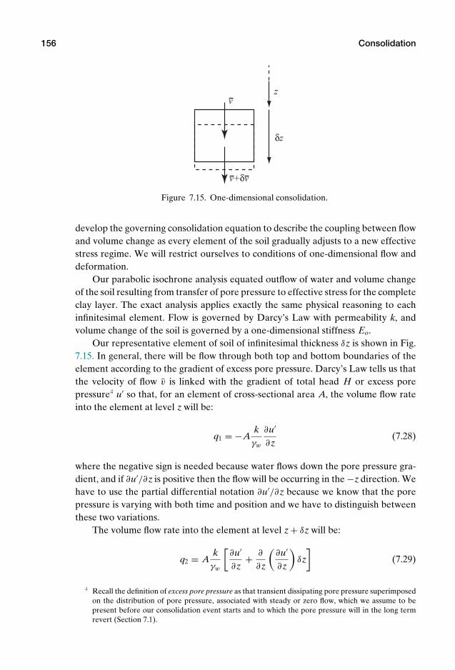
P1: KAE


156 Consolidation

z

δz

v

v+δv

Figure 7.15. One-dimensional consolidation.

develop the governing consolidation equation to describe the coupling between flowand volume change as every element of the soil gradually adjusts to a new effectivestress regime. We will restrict ourselves to conditions of one-dimensional flow anddeformation.

Our parabolic isochrone analysis equated outflow of water and volume changeof the soil resulting from transfer of pore pressure to effective stress for the completeclay layer. The exact analysis applies exactly the same physical reasoning to eachinfinitesimal element. Flow is governed by Darcy’s Law with permeability k, andvolume change of the soil is governed by a one-dimensional stiffness Eo.

Our representative element of soil of infinitesimal thickness δz is shown in Fig.7.15. In general, there will be flow through both top and bottom boundaries of theelement according to the gradient of excess pore pressure. Darcy’s Law tells us thatthe velocity of flow v is linked with the gradient of total head H or excess porepressure4 u′ so that, for an element of cross-sectional area A, the volume flow rateinto the element at level z will be:

q1 = −Akγw

∂u′

∂z(7.28)

where the negative sign is needed because water flows down the pore pressure gra-dient, and if ∂u′/∂z is positive then the flow will be occurring in the −z direction. Wehave to use the partial differential notation ∂u′/∂z because we know that the porepressure is varying with both time and position and we have to distinguish betweenthese two variations.

The volume flow rate into the element at level z + δz will be:

q2 = Akγw

[∂u′

∂z+ ∂

∂z

(∂u′

∂z

)δz

](7.29)

4 Recall the definition of excess pore pressure as that transient dissipating pore pressure superimposedon the distribution of pore pressure, associated with steady or zero flow, which we assume to bepresent before our consolidation event starts and to which the pore pressure will in the long termrevert (Section 7.1).

P1: KAE



so that the rate of change of volume V of the element resulting from the flow ofwater will be:

∂V∂t

= q1 + q2 = Akγw

∂2u′

∂z2δz (7.30)

The volume of the soil element can only change if the effective stress in theelement is changing. From the Principle of Effective stress (Section 2.8), effectivestress is the difference between total stress and pore pressure, σ ′

z = σz − u. We willassume that the total stress is not changing – having placed a load of fill across oursite, we are going to sit back and await the effects of consolidation – so the changein effective stress matches the change in pore pressure. There will in general besome in-situ equilibrium pore pressure in the ground which is not changing, but itis the excess pore pressure u′ which is gradually being dissipated and transferred toeffective stress. Thus, we can write:

δσ ′z = −δu′ (7.31)

The changing effective stress results in vertical strain in the element, which is thesame as volumetric strain for our one-dimensional system:

δεz = δσ ′z

Eo(7.32)

The change in volume of the element of cross-section A and thickness δz is:

δV = −Aδzδσ ′

z

Eo(7.33)

where the negative sign is needed because an increase in effective stress leads to adecrease in volume. The rate of change of volume of the element is:

∂V∂t

= − AδzEo

∂σ ′z

∂t= Aδz

Eo

∂u′

∂t(7.34)

The rate of change in volume of the element resulting from change in effectivestress (7.34) must be equal to the rate of change in volume of the element resultingfrom flow (7.30):

∂V∂t

= Akγw

∂2u′

∂z2δz = Aδz

Eo

∂u′

∂t(7.35)

or:

kEo

γw

∂2u′

∂z2= ∂u′

∂t(7.36)

We should not be surprised to find that the governing soil properties are gath-ered together in the same way that we found in Section 7.3, defining a coefficient ofconsolidation (7.15), cv = kEo/γw, so that our consolidation equation becomes:

cv

∂2u′

∂z2= ∂u′

∂t(7.37)

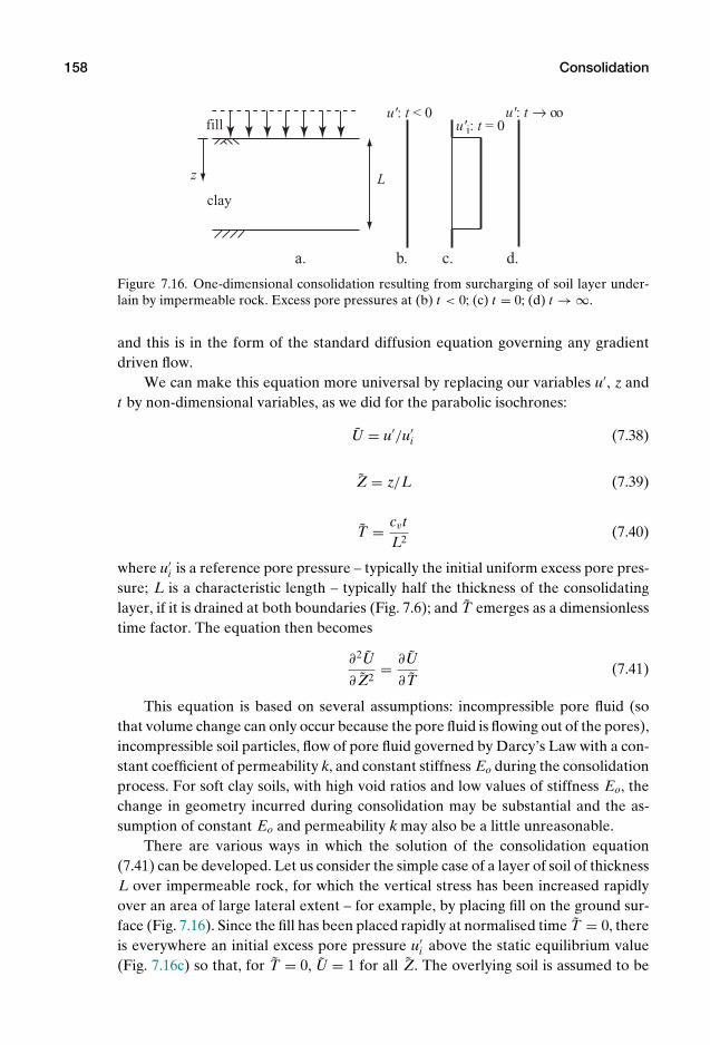
P1: KAE


158 Consolidation

Lz

fill

clay

u'i: t = 0u': t < 0 u': t oo←

a. b. c. d.

Figure 7.16. One-dimensional consolidation resulting from surcharging of soil layer under-lain by impermeable rock. Excess pore pressures at (b) t < 0; (c) t = 0; (d) t → ∞.

and this is in the form of the standard diffusion equation governing any gradientdriven flow.

We can make this equation more universal by replacing our variables u′, z andt by non-dimensional variables, as we did for the parabolic isochrones:

U = u′/u′i (7.38)

Z = z/L (7.39)

T = cvtL2

(7.40)

where u′i is a reference pore pressure – typically the initial uniform excess pore pres-

sure; L is a characteristic length – typically half the thickness of the consolidatinglayer, if it is drained at both boundaries (Fig. 7.6); and T emerges as a dimensionlesstime factor. The equation then becomes

∂2U

∂ Z2= ∂U

∂ T(7.41)

This equation is based on several assumptions: incompressible pore fluid (sothat volume change can only occur because the pore fluid is flowing out of the pores),incompressible soil particles, flow of pore fluid governed by Darcy’s Law with a con-stant coefficient of permeability k, and constant stiffness Eo during the consolidationprocess. For soft clay soils, with high void ratios and low values of stiffness Eo, thechange in geometry incurred during consolidation may be substantial and the as-sumption of constant Eo and permeability k may also be a little unreasonable.

There are various ways in which the solution of the consolidation equation(7.41) can be developed. Let us consider the simple case of a layer of soil of thicknessL over impermeable rock, for which the vertical stress has been increased rapidlyover an area of large lateral extent – for example, by placing fill on the ground sur-face (Fig. 7.16). Since the fill has been placed rapidly at normalised time T = 0, thereis everywhere an initial excess pore pressure u′

i above the static equilibrium value(Fig. 7.16c) so that, for T = 0, U = 1 for all Z. The overlying soil is assumed to be

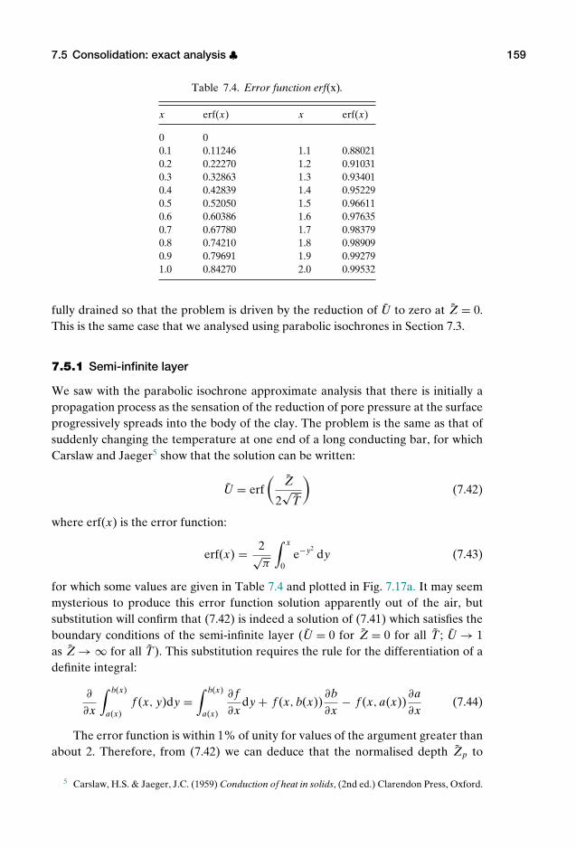
P1: KAE



Table 7.4. Error function erf(x).

x erf(x) x erf(x)

0 00.1 0.11246 1.1 0.880210.2 0.22270 1.2 0.910310.3 0.32863 1.3 0.934010.4 0.42839 1.4 0.952290.5 0.52050 1.5 0.966110.6 0.60386 1.6 0.976350.7 0.67780 1.7 0.983790.8 0.74210 1.8 0.989090.9 0.79691 1.9 0.992791.0 0.84270 2.0 0.99532

fully drained so that the problem is driven by the reduction of U to zero at Z = 0.This is the same case that we analysed using parabolic isochrones in Section 7.3.

7.5.1 Semi-infinite layer

We saw with the parabolic isochrone approximate analysis that there is initially apropagation process as the sensation of the reduction of pore pressure at the surfaceprogressively spreads into the body of the clay. The problem is the same as that ofsuddenly changing the temperature at one end of a long conducting bar, for whichCarslaw and Jaeger5 show that the solution can be written:

U = erf(

Z

2√

T

)(7.42)

where erf(x) is the error function:

erf(x) = 2√π

∫ x

0e−y2

dy (7.43)

for which some values are given in Table 7.4 and plotted in Fig. 7.17a. It may seemmysterious to produce this error function solution apparently out of the air, butsubstitution will confirm that (7.42) is indeed a solution of (7.41) which satisfies theboundary conditions of the semi-infinite layer (U = 0 for Z = 0 for all T ; U → 1as Z → ∞ for all T). This substitution requires the rule for the differentiation of adefinite integral:

∂

∂x

∫ b(x)

a(x)f (x, y)dy =

∫ b(x)

a(x)

∂ f∂x

dy + f (x, b(x))∂b∂x

− f (x, a(x))∂a∂x

(7.44)

The error function is within 1% of unity for values of the argument greater thanabout 2. Therefore, from (7.42) we can deduce that the normalised depth Zp to

5 Carslaw, H.S. & Jaeger, J.C. (1959) Conduction of heat in solids, (2nd ed.) Clarendon Press, Oxford.

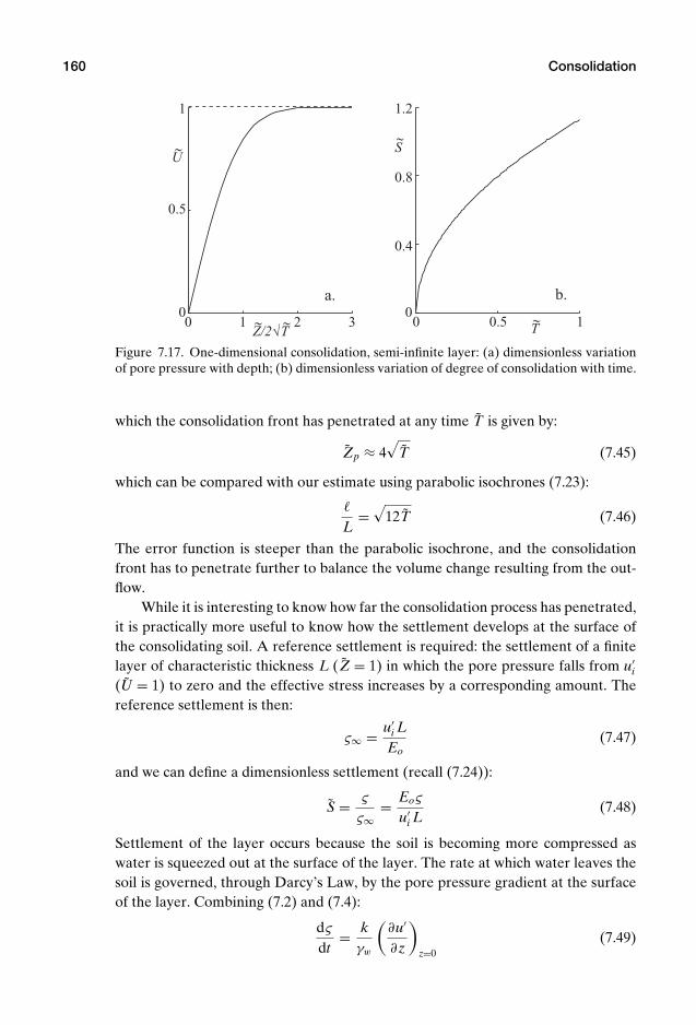
P1: KAE


160 Consolidation

0 1 2 30

0.5

1

Z/2√T

U

a.

0 0.5 10

0.4

0.8

1.2

T

b.

~

~ ~~

S~

Figure 7.17. One-dimensional consolidation, semi-infinite layer: (a) dimensionless variationof pore pressure with depth; (b) dimensionless variation of degree of consolidation with time.

which the consolidation front has penetrated at any time T is given by:

Zp ≈ 4√

T (7.45)

which can be compared with our estimate using parabolic isochrones (7.23):

L=

√12T (7.46)

The error function is steeper than the parabolic isochrone, and the consolidationfront has to penetrate further to balance the volume change resulting from the out-flow.

While it is interesting to know how far the consolidation process has penetrated,it is practically more useful to know how the settlement develops at the surface ofthe consolidating soil. A reference settlement is required: the settlement of a finitelayer of characteristic thickness L (Z = 1) in which the pore pressure falls from u′

i

(U = 1) to zero and the effective stress increases by a corresponding amount. Thereference settlement is then:

ς∞ = u′i L

Eo(7.47)

and we can define a dimensionless settlement (recall (7.24)):

S = ς

ς∞= Eoς

u′i L

(7.48)

Settlement of the layer occurs because the soil is becoming more compressed aswater is squeezed out at the surface of the layer. The rate at which water leaves thesoil is governed, through Darcy’s Law, by the pore pressure gradient at the surfaceof the layer. Combining (7.2) and (7.4):

dς

dt= k

γw

(∂u′

∂z

)z=0

(7.49)

P1: KAE



which we can convert to a equation in terms of dimensionless quantities:

dS

dT= Eo

u′i L

L2

cv

dς

dt= Eo

u′i L

L2

cv

kγw

(∂u′

∂z

)z=0

= Lu′

i

(∂u′

∂z

)z=0

=(

∂U

∂ Z

)Z=0

(7.50)

Differentiating (7.42) (noting (7.44)):(∂U

∂ Z

)Z=0

= 1√π T

(7.51)

and hence:

S =√

4Tπ

(7.52)

which is plotted in Fig. 7.17b. The degree of consolidation varies with the squareroot of time (compare S =

√4T/3 for parabolic isochrones (7.24)).6

This first analysis will be valid also for a finite clay layer, of normalised thick-ness Z = 1, provided that the distance that the consolidation front has penetratedis less than the thickness of the layer or, approximately, from (7.45), T < 1/16 ort < L2/16cv – which can be compared with our parabolic isochrone estimate of theend of this stage of consolidation occurring at T = 1/12.

7.5.2 Finite layer

If we know from the beginning that we are dealing with a finite layer, then we canobtain a single analytical solution to the governing equation (7.41). Let us repeatthe definition of the problem. A finite layer of compressible soil of thickness L isunderlain by impermeable rock (Fig. 7.16). The pore pressure throughout the layeris initially equal to u′

i (U = 1 at t = T = 0). The governing partial differential equa-tion can be solved using the standard technique of separation of variables.

We assume that the solution will be of the form U = Z(Z)T (T), where Z(Z)and T (T) are functions only of Z and T , respectively. Then:

∂2U

∂ Z2= T d2Z

dZ2(7.53)

and:

∂U

∂ T= Z dT

dT(7.54)

so that:

T d2ZdZ2

= Z dTdT

(7.55)

6 Note that U is a local variable describing the normalised excess pore pressure, whereas S is a systemvariable describing the overall settlement of a particular consolidating system.

P1: KAE


162 Consolidation

Since this must apply for all Z and all T , we can rearrange and deduce that solutionsmust satisfy:

1Z

d2ZdZ2

= 1T

dTdT

= −ω2 (7.56)

where ω takes values necessary to satisfy the boundary conditions of our problem.We now have two ordinary differential equations to solve.

The equation:

d2ZdZ2

+ ω2Z = 0 (7.57)

is the equation of simple harmonic motion with general solution:

Z = J1 sin ωZ + J2 cos ωZ (7.58)

But we know that the pore pressure is zero at Z = 0 at all times, so J2 = 0. We alsoknow that there is no flow through the impermeable boundary at Z = 1 (z = L),which requires that the solution must be built up from terms which are formed onlyof odd harmonics:

ω = (2m + 1)π

2(7.59)

where m can take any integer value m ≥ 0.The other part of the equation describes the time dependency of the pore pres-

sure change:

dTdT

+ ω2T = 0 (7.60)

with solution

T = Jm exp[−ω2T

] = Jm exp[−π2(2m + 1)2T/4

](7.61)

and the complete solution is the sum of terms of the form:

U =∞∑

m=0

Jm exp

[−π2(2m + 1)2T/4]

sin[(2m + 1)

π

2Z

](7.62)

We have one other boundary condition to apply. At time t = T = 0, the non-dimensional pore pressure is constant throughout the layer U = Uo = 1 for 0 < Z <

1. Thus:

Uo = 1 =∞∑

m=0

Jm sin

[(2m + 1)

π

2Z

](7.63)

We can find the values of the coefficients Jm by multiplying both sides of (7.63)by sin

[(2n + 1)π

2 Z]

and integrating over the range 0 < Z < 1. The right-hand side

P1: KAE



consists of terms of the form:

Jm

∫ 1

0sin

[(2m + 1)

π

2Z

]sin

[(2n + 1)

π

2Z

]dZ

= Jm

∫ 1

0

12

cos

[(2m − 2n)

π

2Z

]− cos

[(2m + 2n + 2)

π

2Z

]dZ

= Jm12

2

π(2m − 2n)sin

[(2m − 2n)

π

2Z

]

− 2π(2m + 2n + 2)

sin[(2m + 2n + 2)

π

2Z

]

= 0 for m = n

(7.64)

since m and n are integers. For m = n, the only remaining term on the right-handside of (7.64) becomes:

Jm

∫ 1

0sin2

[(2m + 1)

π

2Z

]dZ = Jm

∫ 1

0

12

1 + cos

[(2m + 1)π Z

]dZ = Jm

2(7.65)

The left-hand side is:∫ 1

0sin

[(2m + 1)

π

2Z

]dZ = 2

(2m + 1)π

[− cos

(2m + 1)

π

2Z

]1

0= 2

(2m + 1)π(7.66)

Hence:

Jm = 4(2m + 1)π

(7.67)

and the complete Fourier series solution of the consolidation equation is:

U = 4π

∞∑m=0

1

2m + 1exp

[−π2(2m + 1)2 T

4

]sin

[(2m + 1)

π

2Z

](7.68)

where m takes integral values from 0 to ∞. The degree of consolidation S at time Tis found from the integration of U over the range 0 < Z < 1:

S = 1 − 8π2

∞∑m=0

1

(2m + 1)2exp

[−π2(2m + 1)2 T

4

](7.69)

This Fourier series solution considers the entire clay layer throughout the anal-ysis and is not at all concerned with the propagation of disturbances into the layerfrom a boundary. It can be used to generate a family of isochrones showing the spa-tial variation of pore pressure at different times (Fig. 7.18a). The Fourier series so-lution struggles to match the initial condition of uniform pore pressure through thesummation of harmonic functions: a very large number of terms from the infiniteseries (7.68, 7.69) has to be included to begin to produce an accurate representationof the early stages of the analysis and to match the physical constraints. Figure 7.19compares the effect of taking the first 10 terms or the first 500 terms of the Fourier

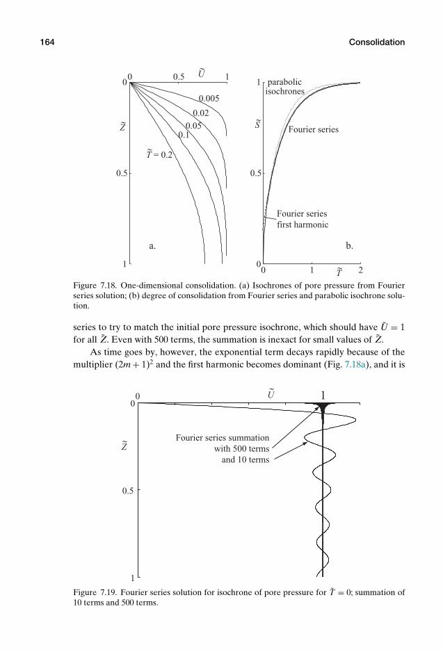
P1: KAE


164 Consolidation

0 0.5 1

1

0.5

0U

Z

a.

0.005

0.02

0.050.1

T = 0.2

0 1 20

0.5

1

T

b.

Fourier series

Fourier seriesfirst harmonic

parabolicisochrones

S~

~

~

~

~

Figure 7.18. One-dimensional consolidation. (a) Isochrones of pore pressure from Fourierseries solution; (b) degree of consolidation from Fourier series and parabolic isochrone solu-tion.

series to try to match the initial pore pressure isochrone, which should have U = 1for all Z. Even with 500 terms, the summation is inexact for small values of Z.

As time goes by, however, the exponential term decays rapidly because of themultiplier (2m + 1)2 and the first harmonic becomes dominant (Fig. 7.18a), and it is

0 1

1

0.5

0U

ZFourier series summation

with 500 termsand 10 terms

~

~

Figure 7.19. Fourier series solution for isochrone of pore pressure for T = 0; summation of10 terms and 500 terms.

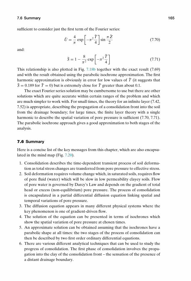
P1: KAE


7.6 Summary 165

sufficient to consider just the first term of the Fourier series:

U = 4π

exp[−π2 T

4

]sin

π Z2

(7.70)

and:

S = 1 − 8π2

exp[−π2 T

4

](7.71)

This relationship is also plotted in Fig. 7.18b together with the exact result (7.69)and with the result obtained using the parabolic isochrone approximation. The firstharmonic approximation is obviously in error for low values of T (it suggests thatS = 0.189 for T = 0) but is extremely close for T greater than about 0.1.

The exact Fourier series solution may be cumbersome to use but there are othersolutions which are quite accurate within certain ranges of the problem and whichare much simpler to work with. For small times, the theory for an infinite layer (7.42,7.52) is appropriate, describing the propagation of a consolidation front into the soilfrom the drainage boundary; for large times, the finite layer theory with a singleharmonic to describe the spatial variation of pore pressure is sufficient (7.70, 7.71).The parabolic isochrone approach gives a good approximation to both stages of theanalysis.

7.6 Summary


1. Consolidation describes the time-dependent transient process of soil deforma-tion as total stress changes are transferred from pore pressure to effective stress.

2. Soil deformation requires volume change which, in saturated soils, requires flowof pore fluid (water) which will be slow in low permeability clayey soils. Flowof pore water is governed by Darcy’s Law and depends on the gradient of totalhead or excess (non-equilibrium) pore pressure. The process of consolidationis encapsulated in a partial differential diffusion equation linking spatial andtemporal variations of pore pressure.

3. The diffusion equation appears in many different physical systems where thekey phenomenon is one of gradient-driven flow.

4. The solution of the equation can be presented in terms of isochrones whichshow the spatial variation of pore pressure at chosen times.

5. An approximate solution can be obtained assuming that the isochrones have aparabolic shape at all times: the two stages of the process of consolidation canthen be described by two first order ordinary differential equations.

6. There are various different analytical techniques that can be used to study theprogress of consolidation. The first phase of consolidation involves the propa-gation into the clay of the consolidation front – the sensation of the presence ofa distant drainage boundary.

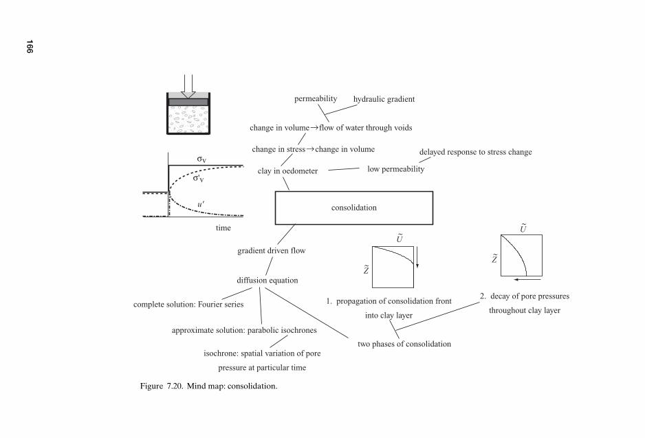
P1:K

AE

OneD

im00a

CU

US648/M

uir978

0521

517737

August17,2009

19:12

consolidation

change in stress→change in volume

change in volume→flow of water through voids

low permeability

delayed response to stress change

clay in oedometerσ'v

σv

time

u'

hydraulic gradientpermeability

gradient driven flow

diffusion equation

complete solution: Fourier series

approximate solution: parabolic isochrones

isochrone: spatial variation of pore

pressure at particular time

two phases of consolidation

1. propagation of consolidation front

into clay layer

2. decay of pore pressures

throughout clay layer

ZZ

U

~

~U~

~

Figure 7.20. Mind map: consolidation.

166

P1: KAE


7.7 Exercises: Consolidation 167

7. When the complete clay layer is participating in the consolidation process, thenthe isochrones take on a simple sinusoidal mode shape.

7.7 Exercises: Consolidation

Make use of the simplified parabolic isochrones analysis to solve Problems 1–4.

1. The sample of clay in Section 6.5, Questions 1/2 has a thickness of 20 mm.Drainage is able to occur from both the top and bottom boundaries of the sam-ple. The permeability of the clay is 10−9 m/s. What is the value of the coefficientof consolidation cv? How long after the change in applied total stress does theclay at the centre of the sample become aware of the consolidation process?How long after the change in applied total stress has the settlement of the clayreached 80% of its final magnitude?

2. The sample of clay in Section 6.5, Questions 1/2 is representative of a clay layerwith a thickness of 3 m contained between layers of sand and gravel. The site isbeing prepared by rapidly placing a layer of fill at the ground surface. How longafter the placement of this fill will the settlement of the clay reach 80% of itsfinal magnitude? Does this time depend on the magnitude of the stress changegenerated by the placement of the fill?

3. The sample of clay in Section 6.5, Questions 4/5 is found to reach 50% of itsfinal consolidation settlement in 95 minutes. It is representative of a clay layerof thickness 2.4 m. How long will it take for 90% settlement of this clay layer tooccur?

4. Oedometer tests on a sample from the bed of clay described in Section 6.5,Question 7 show that, for an appropriate stress increment, the coefficient ofpermeability is 10−9 m/s. How long will it take for the effect of the removal ofthe top 1 m of sand to be felt as a change of effective stress at the middle of theclay?

5. Any mathematical shape that satisfies the boundary conditions could be as-sumed for the typical isochrone of excess pore pressure in Fig. 7.8. In this chap-ter we have assumed a parabolic form. Repeat the analysis of the two stagesof consolidation for a layer of thickness L with drainage only from the up-per boundary using a sinusoidal function so that in the first stage the typicalisochrone is u′ = u′

i sin πz/2 and in the second stage the typical isochrone isu′ = u′

L sin πz/2L. Find expressions for the variation of degree of consolidationS = ς/ς∞ with dimensionless time T = cvt/L2 during the two stages.

6. Results of one increment of loading (from 200 to 400 kPa) in an oedometer teston reconstituted Gault clay are given in Table 7.5. At the start of the incrementthe height of the sample was 15.56 mm. The sample was able to drain from topand bottom.Using a procedure similar to that described in Section 7.4.1, use the exact anal-ysis encapsulated in (7.52) and (7.71) to estimate the one-dimensional stiff-ness, coefficient of consolidation, and permeability of the clay. Estimate the

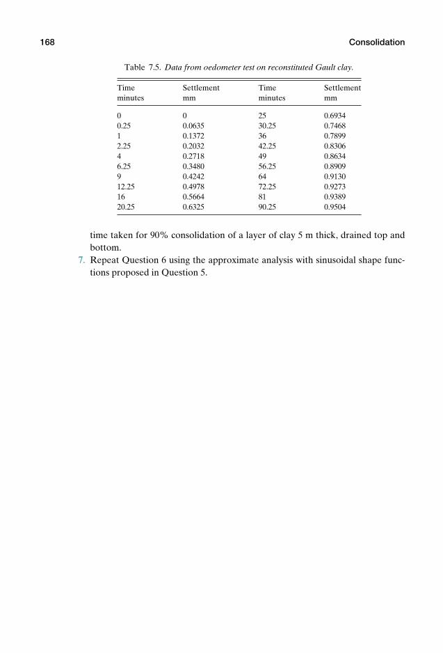
P1: KAE


168 Consolidation

Table 7.5. Data from oedometer test on reconstituted Gault clay.

Time Settlement Time Settlementminutes mm minutes mm

0 0 25 0.69340.25 0.0635 30.25 0.74681 0.1372 36 0.78992.25 0.2032 42.25 0.83064 0.2718 49 0.86346.25 0.3480 56.25 0.89099 0.4242 64 0.913012.25 0.4978 72.25 0.927316 0.5664 81 0.938920.25 0.6325 90.25 0.9504

time taken for 90% consolidation of a layer of clay 5 m thick, drained top andbottom.

7. Repeat Question 6 using the approximate analysis with sinusoidal shape func-tions proposed in Question 5.

P1: KAE


8 Strength

8.1 Introduction

In the context of our chosen one-dimensional approach to the mechanics of soils,we are somewhat limited in what we can say about the strength of soils but thereare some ideas which can usefully be presented. Stiffness is concerned with the de-formations of geotechnical systems – the serviceability limit states under operationalor working loads. Strength is concerned with the collapse of geotechnical systems –the ultimate limit states for which failure of the geotechnical system will occur. Clas-sically, it has always been easier to make statements about ultimate collapse condi-tions than about deformations, and geotechnical design often proceeds by startingwith a collapse calculation and then factoring down the loading sufficiently that,from experience, the resulting reduced load would not be expected to produce ex-cessive displacements. This is always a rather uncertain route by which to controlthose displacements, especially if the nature of the problem under consideration ismore than somewhat different from those previously experienced – a proper un-derstanding of stiffness is really more satisfactory. However, it does emphasise thetraditional importance of understanding the strength of soils and the modes of fail-ure of geotechnical systems.

8.2 Failure mechanisms

Figure 8.1 shows a schematic picture of a pile foundation. A pile is a long slenderstiff structural member which is used to transfer loads from some surface structurethrough more or less soft soils to a certain depth in the ground (Fig. 1.9). The surfaceload P is shared with the soil over the length of the pile by the generation of shearstresses τ – the so-called shaft resistance – and by some end bearing stress σb at thebase of the pile. The relative proportions of the load taken through shaft resistanceand end bearing will depend on the ground conditions but we can imagine that, ifthe load P is increased until the pile fails, then, at failure, the pile is being pusheduncontrollably into the ground, and there will be some limiting strength of the soilτ f being mobilised down the length of the pile at the interface between the pile(steel or concrete or timber) and the soil.

169

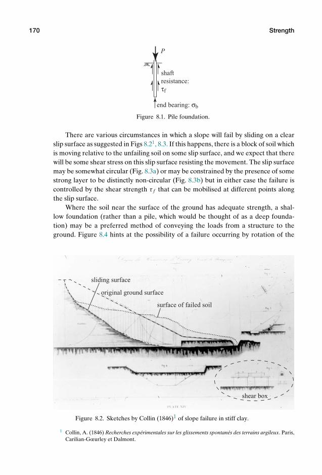
P1: KAE


170 Strength

P

shaft resistance: τf

end bearing: σb

Figure 8.1. Pile foundation.

There are various circumstances in which a slope will fail by sliding on a clearslip surface as suggested in Figs 8.21, 8.3. If this happens, there is a block of soil whichis moving relative to the unfailing soil on some slip surface, and we expect that therewill be some shear stress on this slip surface resisting the movement. The slip surfacemay be somewhat circular (Fig. 8.3a) or may be constrained by the presence of somestrong layer to be distinctly non-circular (Fig. 8.3b) but in either case the failure iscontrolled by the shear strength τ f that can be mobilised at different points alongthe slip surface.

Where the soil near the surface of the ground has adequate strength, a shal-low foundation (rather than a pile, which would be thought of as a deep founda-tion) may be a preferred method of conveying the loads from a structure to theground. Figure 8.4 hints at the possibility of a failure occurring by rotation of the

original ground surface

sliding surface

surface of failed soil

shear box

Figure 8.2. Sketches by Collin (1846)1 of slope failure in stiff clay.

1 Collin, A. (1846) Recherches experimentales sur les glissements spontanes des terrains argileux. Paris,Carilian-Gœurley et Dalmont.

P1: KAE


8.3 Shear box and strength of soils 171

τf τf

a. b.

Figure 8.3. Slope failure, block of soil sliding with well-defined slip surface: (a) circular mech-anism; (b) non-circular mechanism.

foundation, once again mobilising some limiting shear stress τ f along the slidingsurface separating moving soil from the soil which is left behind.

What these examples all have in common is the suggestion that failure, when itoccurs – by increasing the load on the deep or shallow foundation or by increasingthe height or steepening the angle of a slope – may often occur by the formation ofa mechanism of failure within the soil which involves sliding along a defined surfacein the soil.2 With that observation of actual failure mechanisms in mind, one of theearly pieces of equipment developed for determining the strength of soils in thelaboratory (by Collin in the 1840s) was the shear box (Figs 8.5, 8.6). This piece ofequipment remains in widespread use today and has excellent pedagogic value forthe insights it can give into the behaviour of soils.

8.3 Shear box and strength of soils

The shear box is a laboratory test device which is used to force a failure surfaceto form within a soil sample contained within a split box (Fig. 8.6a). Typical shearboxes might have cross-sections 60 × 60 mm, or 100 × 100 mm or 300 × 300 mm (orlarger) depending on the largest sizes of the particles in the soil being tested. Theupper and lower parts of the box are initially aligned and filled with the soil. Thesoil is then loaded through a platen with a force P which generates a vertical stressσz = P/A, where A is the cross-sectional area of the failure plane. There may be a

P

τf

Figure 8.4. Failure of shallow foundation.

2 However, this is not inevitable and sometimes geotechnical failures will occur by some more diffusemode of deformation for which the model of soil behaviour developed in Section 8.11 is appropriate.

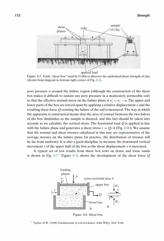
P1: KAE


172 Strength

sample of clayyoke

applied load

shear planes

Figure 8.5. Early “shear box” used by Collin to discover the undrained shear strength of clay(drawn from diagram in bottom right corner of Fig. 8.2).

pore pressure u around the failure region (although the construction of the shearbox makes it difficult to sustain any pore pressure in a moderately permeable soil)so that the effective normal stress on the failure plane is σ ′

z = σz − u. The upper andlower parts of the box are forced apart by applying a relative displacement x and theresulting shear force Q resisting the failure of the soil is measured. The way in whichthe apparatus is constructed means that the area of contact between the two halvesof the box diminishes as the sample is sheared, and this fact should be taken intoaccount as we calculate the vertical stress. The horizontal load Q is applied in linewith the failure plane and generates a shear stress τ = Q/A (Fig. 8.6b). We assumethat the normal and shear stresses calculated in this way are representative of theaverage stresses on the failure plane (in practice, the distribution of stresses willbe far from uniform). It is also a good discipline to measure the downward verticalmovement z of the upper half of the box as the shear displacement x is increased.

A typical set of test results from shear box tests on dense and loose sandsis shown in Fig. 8.7.3 Figure 8.7a shows the development of the shear force Q

Q

Pz

x

a. b.

τ

τσ'z

σ'z

cross-sectional area A

loading platen

upper box

lower box

Figure 8.6. Shear box.

3 Taylor, D.W. (1948) Fundamentals of soil mechanics. John Wiley, New York.

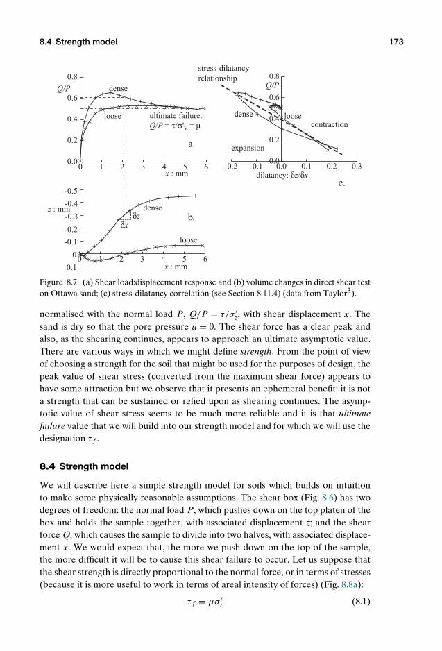
P1: KAE


8.4 Strength model 173

0 1 2 3 4 5 6

0 1 2 3 4 5 6

0.0

0.2

0.4

0.6

0.8

x : mm

x : mm

z : mm

Q/P Q/P

loose loose

loose

dense

dense

dense

0

0.1

-0.2

-0.1

-0.3

-0.4

-0.5

a.

c.

b.

-0.2 -0.1 0.0 0.1 0.2 0.30.0

0.2

0.4

0.6

0.8

dilatancy: δz/δx

δzδx

expansion

contraction

stress-dilatancy relationship

ultimate failure: Q/P = τ/σ'v = µ

Figure 8.7. (a) Shear load:displacement response and (b) volume changes in direct shear teston Ottawa sand; (c) stress-dilatancy correlation (see Section 8.11.4) (data from Taylor3).

normalised with the normal load P, Q/P = τ/σ ′z, with shear displacement x. The

sand is dry so that the pore pressure u = 0. The shear force has a clear peak andalso, as the shearing continues, appears to approach an ultimate asymptotic value.There are various ways in which we might define strength. From the point of viewof choosing a strength for the soil that might be used for the purposes of design, thepeak value of shear stress (converted from the maximum shear force) appears tohave some attraction but we observe that it presents an ephemeral benefit: it is nota strength that can be sustained or relied upon as shearing continues. The asymp-totic value of shear stress seems to be much more reliable and it is that ultimatefailure value that we will build into our strength model and for which we will use thedesignation τ f .

8.4 Strength model

We will describe here a simple strength model for soils which builds on intuitionto make some physically reasonable assumptions. The shear box (Fig. 8.6) has twodegrees of freedom: the normal load P, which pushes down on the top platen of thebox and holds the sample together, with associated displacement z; and the shearforce Q, which causes the sample to divide into two halves, with associated displace-ment x. We would expect that, the more we push down on the top of the sample,the more difficult it will be to cause this shear failure to occur. Let us suppose thatthe shear strength is directly proportional to the normal force, or in terms of stresses(because it is more useful to work in terms of areal intensity of forces) (Fig. 8.8a):

τ f = µσ ′z (8.1)

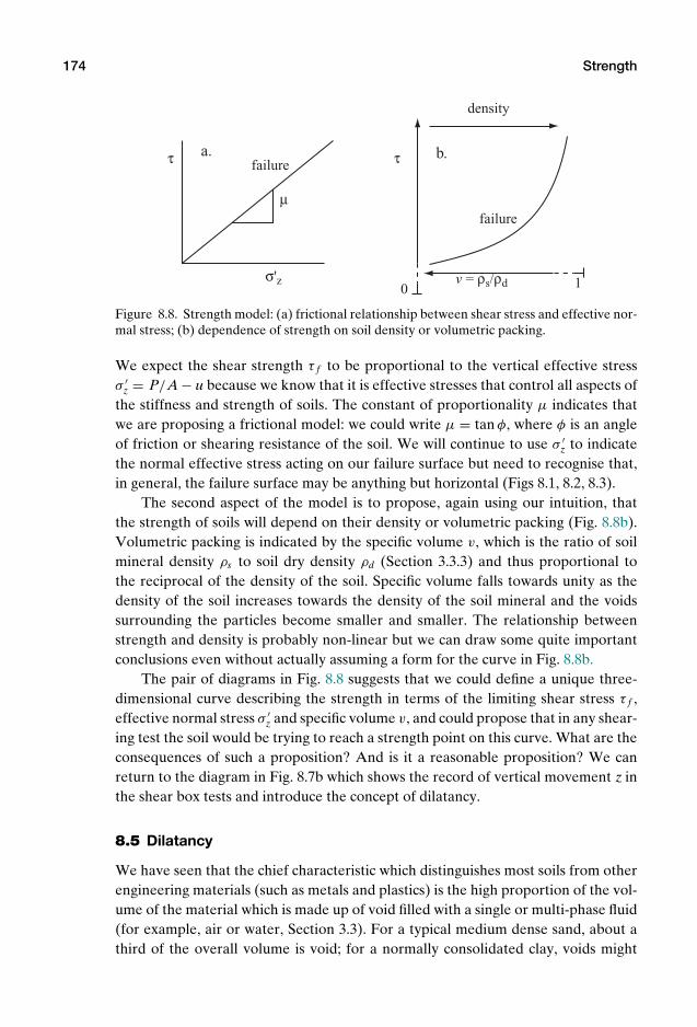
P1: KAE


174 Strength

σ'z

µ

τ τ

density

v = ρs/ρd

a. b.

10

failure

failure

Figure 8.8. Strength model: (a) frictional relationship between shear stress and effective nor-mal stress; (b) dependence of strength on soil density or volumetric packing.

We expect the shear strength τ f to be proportional to the vertical effective stressσ ′

z = P/A − u because we know that it is effective stresses that control all aspects ofthe stiffness and strength of soils. The constant of proportionality µ indicates thatwe are proposing a frictional model: we could write µ = tan φ, where φ is an angleof friction or shearing resistance of the soil. We will continue to use σ ′

z to indicatethe normal effective stress acting on our failure surface but need to recognise that,in general, the failure surface may be anything but horizontal (Figs 8.1, 8.2, 8.3).

The second aspect of the model is to propose, again using our intuition, thatthe strength of soils will depend on their density or volumetric packing (Fig. 8.8b).Volumetric packing is indicated by the specific volume v, which is the ratio of soilmineral density ρs to soil dry density ρd (Section 3.3.3) and thus proportional tothe reciprocal of the density of the soil. Specific volume falls towards unity as thedensity of the soil increases towards the density of the soil mineral and the voidssurrounding the particles become smaller and smaller. The relationship betweenstrength and density is probably non-linear but we can draw some quite importantconclusions even without actually assuming a form for the curve in Fig. 8.8b.

The pair of diagrams in Fig. 8.8 suggests that we could define a unique three-dimensional curve describing the strength in terms of the limiting shear stress τ f ,effective normal stress σ ′

z and specific volume v, and could propose that in any shear-ing test the soil would be trying to reach a strength point on this curve. What are theconsequences of such a proposition? And is it a reasonable proposition? We canreturn to the diagram in Fig. 8.7b which shows the record of vertical movement z inthe shear box tests and introduce the concept of dilatancy.

8.5 Dilatancy

We have seen that the chief characteristic which distinguishes most soils from otherengineering materials (such as metals and plastics) is the high proportion of the vol-ume of the material which is made up of void filled with a single or multi-phase fluid(for example, air or water, Section 3.3). For a typical medium dense sand, about athird of the overall volume is void; for a normally consolidated clay, voids might

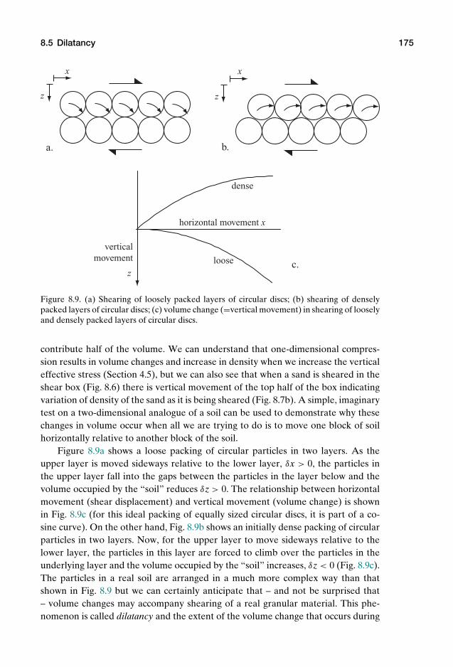
P1: KAE


8.5 Dilatancy 175

x

horizontal movement x

x

z z

z

a. b.

c.

dense

loose

vertical movement

Figure 8.9. (a) Shearing of loosely packed layers of circular discs; (b) shearing of denselypacked layers of circular discs; (c) volume change (=vertical movement) in shearing of looselyand densely packed layers of circular discs.

contribute half of the volume. We can understand that one-dimensional compres-sion results in volume changes and increase in density when we increase the verticaleffective stress (Section 4.5), but we can also see that when a sand is sheared in theshear box (Fig. 8.6) there is vertical movement of the top half of the box indicatingvariation of density of the sand as it is being sheared (Fig. 8.7b). A simple, imaginarytest on a two-dimensional analogue of a soil can be used to demonstrate why thesechanges in volume occur when all we are trying to do is to move one block of soilhorizontally relative to another block of the soil.

Figure 8.9a shows a loose packing of circular particles in two layers. As theupper layer is moved sideways relative to the lower layer, δx > 0, the particles inthe upper layer fall into the gaps between the particles in the layer below and thevolume occupied by the “soil” reduces δz > 0. The relationship between horizontalmovement (shear displacement) and vertical movement (volume change) is shownin Fig. 8.9c (for this ideal packing of equally sized circular discs, it is part of a co-sine curve). On the other hand, Fig. 8.9b shows an initially dense packing of circularparticles in two layers. Now, for the upper layer to move sideways relative to thelower layer, the particles in this layer are forced to climb over the particles in theunderlying layer and the volume occupied by the “soil” increases, δz < 0 (Fig. 8.9c).The particles in a real soil are arranged in a much more complex way than thatshown in Fig. 8.9 but we can certainly anticipate that – and not be surprised that– volume changes may accompany shearing of a real granular material. This phe-nomenon is called dilatancy and the extent of the volume change that occurs during

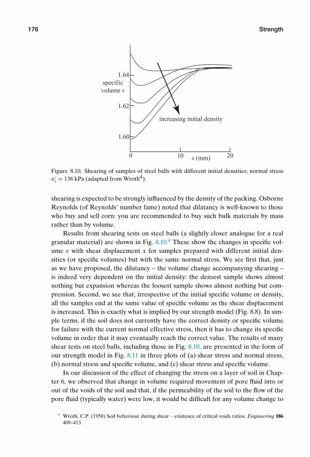
P1: KAE


176 Strength

increasing initial density

1.62

1.64

1.60

0 10 20x (mm)

specific volume v

Figure 8.10. Shearing of samples of steel balls with different initial densities; normal stressσ ′

z = 138 kPa (adapted from Wroth4).

shearing is expected to be strongly influenced by the density of the packing. OsborneReynolds (of Reynolds’ number fame) noted that dilatancy is well-known to thosewho buy and sell corn: you are recommended to buy such bulk materials by massrather than by volume.

Results from shearing tests on steel balls (a slightly closer analogue for a realgranular material) are shown in Fig. 8.10.4 These show the changes in specific vol-ume v with shear displacement x for samples prepared with different initial den-sities (or specific volumes) but with the same normal stress. We see first that, justas we have proposed, the dilatancy – the volume change accompanying shearing –is indeed very dependent on the initial density: the densest sample shows almostnothing but expansion whereas the loosest sample shows almost nothing but com-pression. Second, we see that, irrespective of the initial specific volume or density,all the samples end at the same value of specific volume as the shear displacementis increased. This is exactly what is implied by our strength model (Fig. 8.8). In sim-ple terms, if the soil does not currently have the correct density or specific volumefor failure with the current normal effective stress, then it has to change its specificvolume in order that it may eventually reach the correct value. The results of manyshear tests on steel balls, including those in Fig. 8.10, are presented in the form ofour strength model in Fig. 8.11 in three plots of (a) shear stress and normal stress,(b) normal stress and specific volume, and (c) shear stress and specific volume.

In our discussion of the effect of changing the stress on a layer of soil in Chap-ter 6, we observed that change in volume required movement of pore fluid into orout of the voids of the soil and that, if the permeability of the soil to the flow of thepore fluid (typically water) were low, it would be difficult for any volume change to

4 Wroth, C.P. (1958) Soil behaviour during shear – existence of critical voids ratios. Engineering 186409–413.

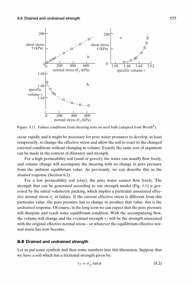
P1: KAE


8.6 Drained and undrained strength 177

a.

b.

c.

0 00

0 200

200

200 200

400

400 600

600

τ (kPa) τ (kPa)

normal stress σ'z (kPa)

normal stress σ'z (kPa)

1.68

1.68

1.64

1.64 1.62

1.66

1.66

shear stress shear stress

specific volume v

specific volume v

Figure 8.11. Failure conditions from shearing tests on steel balls (adapted from Wroth4).

occur rapidly and it might be necessary for pore water pressures to develop, at leasttemporarily, to change the effective stress and allow the soil to react to the changedexternal conditions without changing in volume. Exactly the same sort of argumentcan be made in the context of dilatancy and strength.

For a high permeability soil (sand or gravel), the water can usually flow freely,and volume change will accompany the shearing with no change in pore pressurefrom the ambient equilibrium value. As previously, we can describe this as thedrained response (Section 6.2).

For a low permeability soil (clay), the pore water cannot flow freely. Thestrength that can be generated according to our strength model (Fig. 8.8) is gov-erned by the initial volumetric packing, which implies a particular associated effec-tive normal stress σ ′

z at failure. If the current effective stress is different from thisparticular value, the pore pressure has to change to produce that value: this is theundrained response. Of course, in the long term we can expect that the pore pressurewill dissipate and reach some equilibrium condition. With the accompanying flow,the volume will change and the eventual strength τ f will be the strength associatedwith the original effective normal stress – or whatever the equilibrium effective nor-mal stress has now become.

8.6 Drained and undrained strength

Let us put some symbols and then some numbers into this discussion. Suppose thatwe have a soil which has a frictional strength given by:

τ f = σ ′zf tan φ (8.2)

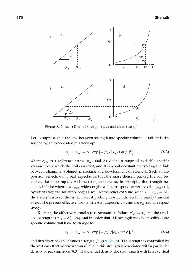
P1: KAE


178 Strength

σ'z σ'zi

σ'ziσ'zf σ'z

τ

τ

τ

τ

τf1

τf2

v

v vi

vfvi

a.

c. d.

b.

1

1

0

0

µ

µ

∆u

∆v

Figure 8.12. (a, b) Drained strength; (c, d) undrained strength.

Let us suppose that the link between strength and specific volume at failure is de-scribed by an exponential relationship:

v f = vmin + v exp−(τ f /[σre f tan φ])β

(8.3)

where σre f is a reference stress, vmin and v define a range of available specificvolumes over which the soil can exist, and β is a soil constant controlling the linkbetween change in volumetric packing and development of strength. Such an ex-pression reflects our broad expectation that the more densely packed the soil be-comes, the more rapidly will the strength increase. In principle, the strength be-comes infinite when v = vmin, which might well correspond to zero voids, vmin ≈ 1,by which stage the soil is no longer a soil. At the other extreme, when v = vmin + v,the strength is zero: this is the loosest packing in which the soil can barely transmitstress. The present effective normal stress and specific volume are σ ′

zi and vi , respec-tively.

Keeping the effective normal stress constant, at failure σ ′zf 1 = σ ′

zi and the avail-able strength is τ f 1 = σ ′

zi tan φ and in order that this strength may be mobilised thespecific volume will have to change to:

v f 1 = vmin + v exp−(τ f 1/[σre f tan φ])β

(8.4)

and this describes the drained strength (Figs 8.12a, b). The strength is controlled bythe vertical effective stress from (8.2) and this strength is associated with a particulardensity of packing from (8.3). If the initial density does not match with this eventual

P1: KAE


8.7 Clay: overconsolidation and undrained strength 179

density it has to change, and the density change implies movement of pore fluid(water, if the soil is saturated) and hence drainage of the soil.

On the other hand, if we keep the specific volume constant so that at failurev f 2 = vi , the strength that we can mobilise is, by inversion of (8.3):

τ f 2 = σre f tan φ

[ln

(v

vi − vmin

)]1/β

(8.5)

and the effective normal stress must change to σ ′zf 2 = τ f 2/ tan φ in order that it may

become compatible with this strength. If the total normal stress remains constant,the pore pressure must change by an amount u = σ ′

zi − σ ′zf 2 (Fig. 8.12c, d). We are

not permitting any movement of pore fluid, and the process of development of thisstrength is consequently described as undrained.

Suppose we have a soil with an angle of shearing resistance φ = 25 andwith σre f = 100 kPa, vmin = 1.1, v = 0.9, β = 0.6; and suppose we have initialconditions: specific volume vi = 1.6, vertical total stress σzi = 75 kPa, pore pres-sure u = 0, to give vertical effective stress σ ′

zi = 75 kPa. In the drained case, thestrength is governed by the effective normal stress so that the eventual strengthis τ f 1 = σ ′

zi tan φ = 75 tan 25 = 35 kPa. The corresponding value of specific volumeis v f = vmin + v exp

−(τ f /[σre f tan φ])β = 1.1 + 0.9 exp−(35/[100 tan 25])0.6 =

1.488 and the change of volume accompanying the shearing to this ultimate strengthis v = 1.488 − 1.6 = −0.112, which implies a compression of the soil, an increasein density.

In the undrained case, the strength is governed by the initial volumetric packingso that this strength is, from (8.5):

τ f 2 = 100 × tan 25[ln(0.9/(1.6 − 1.1))]1/0.6 = 19.2 kPa (8.6)

Mobilisation of such a strength implies an effective normal stress at failure σ ′zf 2 =

τ f 2/ tan φ = 19.2/ tan 25 = 41.2 kPa. The required change in effective normal stressis thus u = σ ′

zi − σ ′zf 2 = 75 − 41.2 = 33.8 kPa.

The calculation logic is thus: for high permeability soil: σ ′zi → τ f 1 → v f (the

strength is controlled by the vertical effective stress and the density adjusts accord-ingly); and for low permeability soil: vi → τ f 2 → σ ′

zf → u (the strength is con-trolled by the density and the vertical effective stress adjusts accordingly). For lowpermeability soil the undrained strength is often given the symbol cu or su.

8.7 Clay: overconsolidation and undrained strength

Overconsolidation was seen in Section 4.7 to be a route by which reductions in spe-cific volume (increases in density) could be locked into the soil. Figure 8.13 illus-trates this phenomenon. The dotted curve AC shows the volumetric compression onoriginal loading in an oedometer to the maximum, preconsolidation pressure σ ′

zmax

at point C on the normal compression line. The vertical stress is then reduced to thecurrent, initial stress σ ′

zi at point I with specific volume vi . The unloading stiffnessof soils is usually considerably higher than the original stiffness in “virgin” loading

P1: KAE


180 Strength

σ'zi

specific volume v vi 10

failure

C

I

normalstress σ'z

unloading

normal

compression

σ'zmax

A

Figure 8.13. Overconsolidation: vertical effective stress and specific volume.

(compare AC and CI, Section 4.7). The overconsolidation ratio, the ratio of pastmaximum to present vertical effective stress, n = σ ′

zmax/σ ′

zi , characterises the extentto which the load, historically applied, has been removed.

The solid curve in Fig. 8.13 represents the link between specific volume andvertical effective stress at failure. The curves for normal compression and for failurein Fig. 8.13 have been drawn with a similar shape but this is not necessarily the case:see Exercise 7 in Section 8.13. The non-coincidence of these two curves indicatesthe need for adjustment of effective stress or specific volume during shearing tofailure. The curves from Fig. 8.13 have been reproduced in Fig. 8.14c together withthe link between shear stress τ and specific volume v at failure (Fig. 8.14b) and thelink between shear stress τ and normal effective stress σ ′

z at failure (Fig. 8.14a).The density of the soil – and hence the current strength of the soil – is primar-

ily determined by the past maximum effective stress (Figs 8.13, 8.14c). The currentdensity or specific volume vi determines the undrained strength τ f = cu (Fig. 8.14b),which then determines the effective normal stress at failure σ ′

zf (Fig. 8.14a). Thedensity change on unloading and reloading of overconsolidated clays is probablyrelatively small. It is not unreasonable to suggest a link between the compressionand strength behaviour for clays such that the undrained strength τ f = cu is relatedto the maximum precompression stress, or preconsolidation pressure σ ′

zmax, by a sim-

ple empirical relationship:

cu = σ ′zmax

= nσ ′zi ≈ 0.2nσ ′

zi (8.7)

With knowledge of in-situ stress and overconsolidation ratio, we can produce anestimate of the undrained strength. Such an estimate can be useful for initial studiesof design feasibility before more direct data become available from which the actualstrength of the soil can be directly discovered.

P1: KAE


8.8 Pile load capacity 181

normal stress σ'z

normal stress σ'z

σ'zf

σ'zf

σ'zi

σ'zmax

shear stress τ

shear stress τ

specific volume v

specific volume v

vi

vi

a.

c.

b.

1

1

0

0

failure

failure failure

compressionC

I

τf = cuτf = cu

Figure 8.14. Overconsolidation and undrained strength.

8.8 Pile load capacity

The estimation of the load capacity of a pile provides a simple example of the ap-plication of the strength model. Let us suppose that we have a long slender pileof length being loaded axially (Fig. 8.15). We will assume that the pile is longenough and slender enough that all the load is transferred to the surrounding soilthrough shaft resistance – that is, through the mobilisation of shear stresses down thelength of the pile, so that the base resistance σb in Fig. 8.1 is negligible. The vertical

P

τf

σ'z

Pb

z

l

a. b.

Figure 8.15. Pile foundation, load transfer through shaft resistance.

P1: KAE


182 Strength

effective stress in the ground varies linearly with depth σ ′z = ρgz. Let us suppose,

first, that we are concerned with a pile in dry sand so that we are not worried aboutpore pressures. We are trying cautiously to retain our restriction to a single dimen-sion in our applications so, while it is reasonable to propose that this vertical effec-tive stress gives a general indication of the level of stress in the soil around the pile,we cannot really insist that it is exactly the normal stress pushing on the shaft ofthe pile.

We saw in Section 4.4.1 that, according to elastic theory, in one-dimensionalcompression the soil will push laterally onto its container with a stress which is aproportion ν/(1 − ν) of the vertical stress, where ν is Poisson’s ratio. Our estimateof the available shear stress on the side of the pile when it is failing by penetratingslowly but inexorably into the ground is then:

τ f = ν

1 − νσ ′

z tan φ = ν

1 − νρgz tan φ (8.8)

If the pile has perimeter s, the ultimate load for this axial failure of the pile is ob-tained by integrating this shear resistance over the length of the pile:

Pu = ν

(1 − ν)ρgs tan φ

∫

0zdz = ν

2(1 − ν)ρgs2 tan φ (8.9)

In a dry sand with density 1.7 Mg/m3, angle of shearing resistance φ = 30 (tan φ =0.58) and Poisson’s ratio ν = 0.2, a circular pile of length = 15 m and diameter2r = 0.3 m (perimeter s = 2πr = 0.94 m) will have an axial capacity Pu = 0.25 ×1.7 × 9.81 × 0.94 × 152 × 0.58/2 = 255 kN.

Piles are deliberately much stiffer than the ground through which they aredriven or inserted. They are used precisely to transmit the loads from the surface,where the stress level in the soil is definitely low and the strength probably low. Butother things may be happening on the site around the pile foundations – for exam-ple, some site preparation such as raising the ground level by placement of a layerof fill (as in the examples in Section 6.3). Such filling increases the total stresses inthe ground and causes the ground to compress – such compression occurring slowlyif the ground is a low permeability clay. If the foundation pile is sitting on an under-lying hard layer, the settling ground will generate downward shear stresses on theshaft of the pile – down-drag – which act in the same direction as the load applied atthe surface Pt (Fig. 8.16). So far as the stresses in the pile are concerned, which willgovern its structural design – the necessary strength of the concrete, for example –the largest stress is not at the ground surface, where the load is applied, as mightinitially be supposed.

Shaft resistance τ f develops with relative movement between pile and soil. As asecond example, consider a pile in normally compressed clay in which the maximumshaft resistance that can be developed can be related to the in-situ vertical effectivestress σ ′

z through a constant (8.7).The ultimate load of an end-bearing pile of length and radius r (perimeter

s = 2πr) in consolidating clay (Fig. 8.16) is calculated assuming a failure mechanismin which the pile moves steadily downwards and is made up from a combination of

P1: KAE


8.8 Pile load capacity 183

τfς

z z

ςo

l

Pt

Pb a. b. c.

fill

clay

Figure 8.16. Pile foundation: (a) down-drag from settling ground; (b) variation of soil set-tlement with depth; (c) assumed full mobilisation of available shear strength at all depths.

the shaft shear stresses, producing a force Ps – which would be generated with thepile moving down relative to the soil – and the end bearing at the toe of the pile,generating a force Pb, so that the ultimate load is Pf = Ps + Pb, and in this failurecondition the force remaining in the pile at its toe is Pf − Ps . The shaft resistance is:

Ps = πρ ′gr2 (8.10)

assuming that vertical effective stress is being generated uniformly with depth in asaturated soil with density ρ and buoyant density ρ ′ = ρ − ρw.

Under working or serviceability conditions, on the other hand, the direction ofrelative movement between the soil and the pile is reversed, and the soil movingdownwards generates an additional load P at the toe of pile given by:

P =∫

02πrτdz = 2πr

∫

0σ ′

zdz (8.11)

giving

PPs

= 1 (8.12)

and the stress at the toe of the pile is considerably increased.Let us assume that we have a pile of length = 15 m and diameter 2r = 0.3 m

in clay with density ρ = 1.5 Mg/m3 and = 0.2. The pile capacity Ps = 104 kN andthe extra load arising from the down-drag will similarly be 104 kN over the crosssection of the pile of diameter 0.3 m, representing an extra stress of 1.47 MPa.

The ultimate load capacity of the pile is not affected by down-drag. If the pile isfailing, the mechanism of failure implies sufficient downward movement of the pileto generate full positive shaft shear stresses resisting the movement. However, if thepile design has overlooked the contribution to axial load that the settling surround-ing soft soil may provide, there may be insufficient relative downward movement ofthe pile to ensure that the shear stresses round the perimeter of the pile are helpingto reduce the axial force in the pile rather than increasing it.

P1: KAE


184 Strength

τfς

z

z

ςpile

l1

l

Pt

neutral point

a. b. c.

fill

clay

Figure 8.17. (a) Down-drag of “floating” pile; (b) settlement of soil ς matches settlementof pile ςpile at neutral point at depth 1; (c) variation with depth of shear stress at pile:soilinterface.

A slightly more complicated configuration is obtained when considering “float-ing” friction piles (Fig. 8.17). Now there is no end bearing contribution to the ca-pacity of the pile, Pb = 0, and under any working loading the contributions from theshear stresses around the pile must combine with the applied load Pt at the groundsurface to give overall vertical equilibrium. The pile will move downwards by somedistance ςpile (Fig. 8.17b) so that there is a neutral point at depth 1 at which there isno relative displacement between the pile and the soil, and at which the direction ofthe shaft shear stress reverses (Fig. 8.17b, c). We assume that shaft shear stresses –either upwards or downwards – always fully mobilise the available strength. We alsoassume that the pile is rigid, or at least much stiffer than the settling soil so that de-formation of the pile can be neglected.

Vertical equilibrium requires that the downward forces on the upper part of thepile, down to depth 1, should exactly balance the upward forces on the lower partof the pile, between depths 1 and :

Pt +∫ 1

02πrρ ′gzdz =

∫

1

2πrρ ′gzdz (8.13)

giving:

Pt + πrρ ′g21 = πrρ ′g

(2 − 2

1

)(8.14)

so that: (1

)2

= 12

(1 − Pt

πρ ′gr2

)= 1

2

(1 − Pt

Pf

)(8.15)

where Pf = πρ ′gr2 is the overall capacity of this friction pile (8.10).The variation of axial load in the pile is then, for 0 < z < 1:

PPf

= Pt

Pf+

(z

)2(8.16)

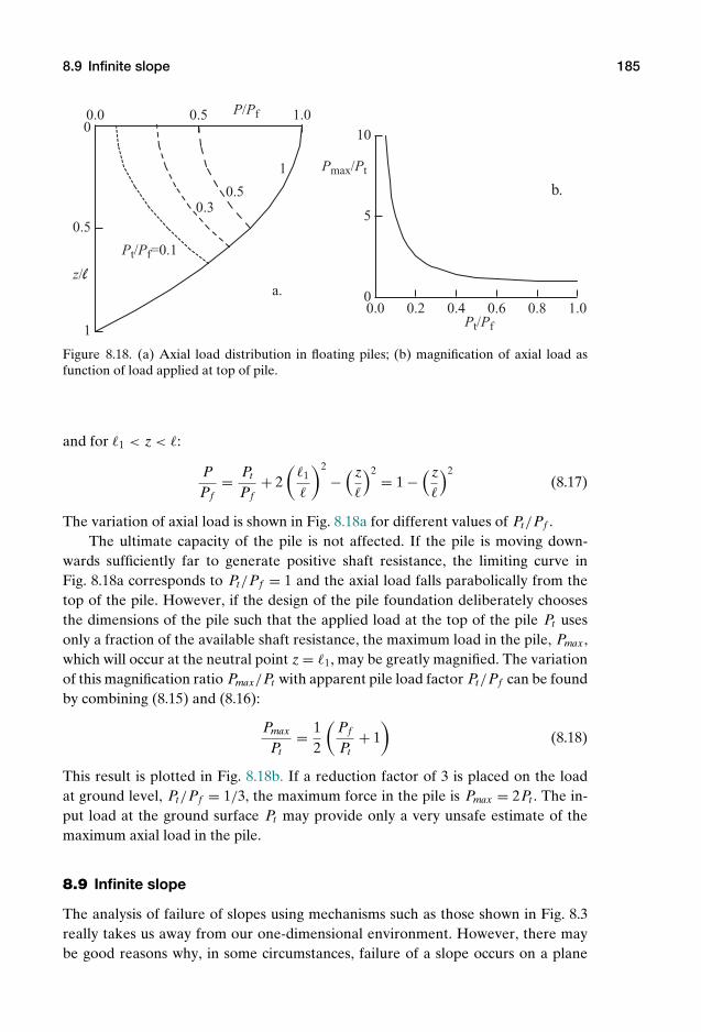
P1: KAE


8.9 Infinite slope 185

0.0 0.5 1.0

1

0.5

0

z/l

P/Pf

Pt/Pf=0.1

0.30.5

1

a.0.0 0.2 0.4 0.6 0.8 1.00

5

10

b.

Pt/Pf

Pmax/Pt

Figure 8.18. (a) Axial load distribution in floating piles; (b) magnification of axial load asfunction of load applied at top of pile.

and for 1 < z < :

PPf

= Pt

Pf+ 2

(1

)2

−(z

)2= 1 −

(z

)2(8.17)

The variation of axial load is shown in Fig. 8.18a for different values of Pt/Pf .The ultimate capacity of the pile is not affected. If the pile is moving down-

wards sufficiently far to generate positive shaft resistance, the limiting curve inFig. 8.18a corresponds to Pt/Pf = 1 and the axial load falls parabolically from thetop of the pile. However, if the design of the pile foundation deliberately choosesthe dimensions of the pile such that the applied load at the top of the pile Pt usesonly a fraction of the available shaft resistance, the maximum load in the pile, Pmax,which will occur at the neutral point z = 1, may be greatly magnified. The variationof this magnification ratio Pmax/Pt with apparent pile load factor Pt/Pf can be foundby combining (8.15) and (8.16):

Pmax

Pt= 1

2

(Pf

Pt+ 1

)(8.18)

This result is plotted in Fig. 8.18b. If a reduction factor of 3 is placed on the loadat ground level, Pt/Pf = 1/3, the maximum force in the pile is Pmax = 2Pt . The in-put load at the ground surface Pt may provide only a very unsafe estimate of themaximum axial load in the pile.

8.9 Infinite slope

The analysis of failure of slopes using mechanisms such as those shown in Fig. 8.3really takes us away from our one-dimensional environment. However, there maybe good reasons why, in some circumstances, failure of a slope occurs on a plane

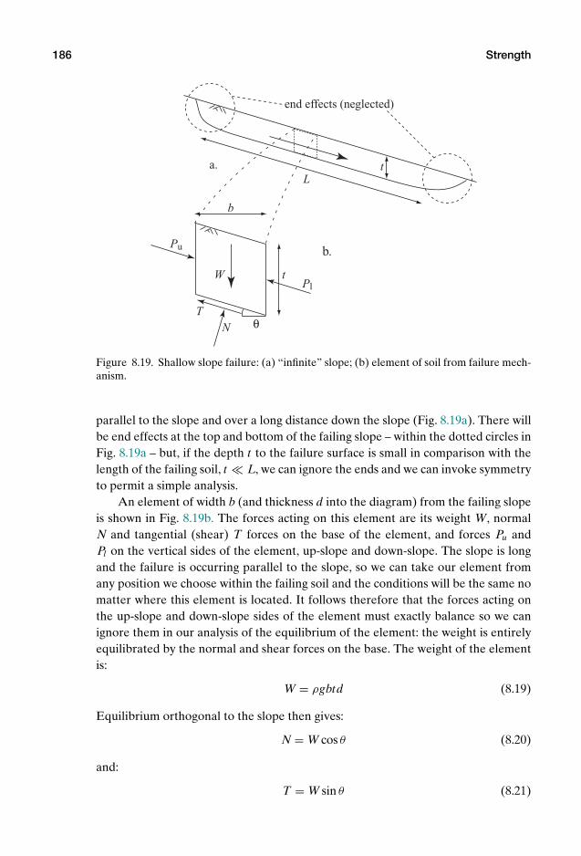
P1: KAE


186 Strength

Lt

t

a.

θ

W

b

N

T

Pu

Pl

b.

end effects (neglected)

Figure 8.19. Shallow slope failure: (a) “infinite” slope; (b) element of soil from failure mech-anism.

parallel to the slope and over a long distance down the slope (Fig. 8.19a). There willbe end effects at the top and bottom of the failing slope – within the dotted circles inFig. 8.19a – but, if the depth t to the failure surface is small in comparison with thelength of the failing soil, t L, we can ignore the ends and we can invoke symmetryto permit a simple analysis.

An element of width b (and thickness d into the diagram) from the failing slopeis shown in Fig. 8.19b. The forces acting on this element are its weight W, normalN and tangential (shear) T forces on the base of the element, and forces Pu andPl on the vertical sides of the element, up-slope and down-slope. The slope is longand the failure is occurring parallel to the slope, so we can take our element fromany position we choose within the failing soil and the conditions will be the same nomatter where this element is located. It follows therefore that the forces acting onthe up-slope and down-slope sides of the element must exactly balance so we canignore them in our analysis of the equilibrium of the element: the weight is entirelyequilibrated by the normal and shear forces on the base. The weight of the elementis:

W = ρgbtd (8.19)

Equilibrium orthogonal to the slope then gives:

N = W cos θ (8.20)

and:

T = W sin θ (8.21)

P1: KAE



We can convert the normal force N and shear force T to corresponding normaland shear stresses, noting that the cross-sectional area of the base of the element isbd/ cos θ :

σn = N cos θ

bd(8.22)

τ = T cos θ

bd(8.23)

Rearranging we find:

σn = ρgt cos2 θ (8.24)

and:

τ = ρgt cos θ sin θ (8.25)

In general, there will also be a pore pressure u and corresponding equivalent forceU = ubd/ cos θ on the base of the element, so that the effective normal stress iscorrespondingly reduced to σ ′

n = σn − u. There is some benefit to be obtained byrelating the pore pressure to the total vertical stress through a pore pressure ratioru = u/ρgt , so that the effective normal stress can be written σ ′

n = ρgt(cos2 θ − ru).The mobilised friction on the base of the soil element is:

tan φmob = τ

σ ′n

= cos θ sin θ

cos2 θ − ru= tan θ

1 − ru sec2 θ(8.26)

There are various cases that we can consider. If we suppose that the slope isdry, so that there are no pore water pressures, ru = 0, the normal stress in (8.24) isan effective stress σn = σ ′

n, and the mobilised angle of friction, φmob, for the base ofthe soil element is given by:

tan φmob = τ/σ ′n = tan θ (8.27)

or φmob = θ , and we can say that the slope will be stable provided θ < φ, where φ isthe available angle of shearing resistance.

A second possibility would be a slope in clay in which a rapid failure is con-trolled by the undrained strength cu. Now the normal stress is not important – porepressures will change as we have seen in Section 8.6 to guarantee that the correctcombination of effective normal stress, shear strength and density is reached for fail-ure of the soil. If we know that the failure is occurring at a depth t , our equation ofstability requires:

τ = ρgt cos θ sin θ < cu (8.28)

which becomes an equation for a limiting slope angle given knowledge that failureis likely to occur at a certain depth t :

θ = 12

sin−1[

2cu

ρgt

](8.29)

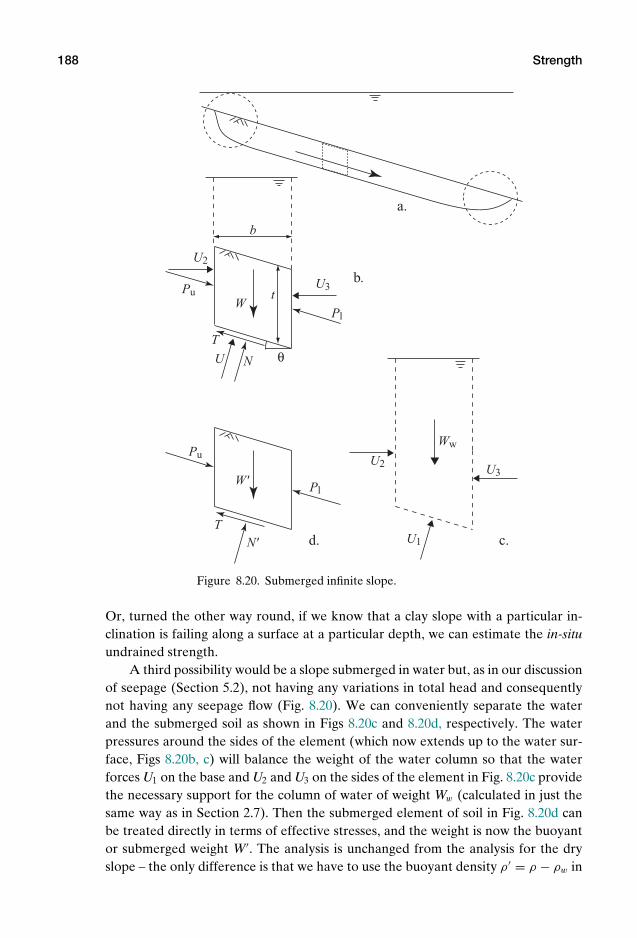
P1: KAE


188 Strength

t

a.

θ

W

W'

b

N

N'

T

T

Pu

Pu

Pl

Pl

b.

c.d.

U

U1

U2

U2

U3

U3

Ww

Figure 8.20. Submerged infinite slope.

Or, turned the other way round, if we know that a clay slope with a particular in-clination is failing along a surface at a particular depth, we can estimate the in-situundrained strength.

A third possibility would be a slope submerged in water but, as in our discussionof seepage (Section 5.2), not having any variations in total head and consequentlynot having any seepage flow (Fig. 8.20). We can conveniently separate the waterand the submerged soil as shown in Figs 8.20c and 8.20d, respectively. The waterpressures around the sides of the element (which now extends up to the water sur-face, Figs 8.20b, c) will balance the weight of the water column so that the waterforces U1 on the base and U2 and U3 on the sides of the element in Fig. 8.20c providethe necessary support for the column of water of weight Ww (calculated in just thesame way as in Section 2.7). Then the submerged element of soil in Fig. 8.20d canbe treated directly in terms of effective stresses, and the weight is now the buoyantor submerged weight W′. The analysis is unchanged from the analysis for the dryslope – the only difference is that we have to use the buoyant density ρ ′ = ρ − ρw in

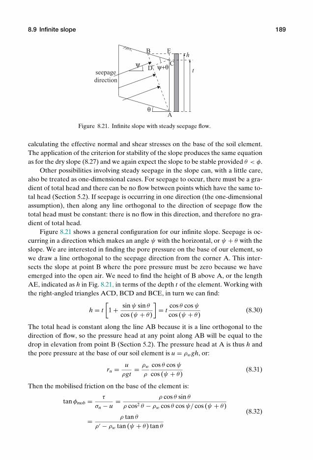
P1: KAE



θ

ψ+θψt

h

A

B

CD

E

seepage direction

Figure 8.21. Infinite slope with steady seepage flow.

calculating the effective normal and shear stresses on the base of the soil element.The application of the criterion for stability of the slope produces the same equationas for the dry slope (8.27) and we again expect the slope to be stable provided θ < φ.

Other possibilities involving steady seepage in the slope can, with a little care,also be treated as one-dimensional cases. For seepage to occur, there must be a gra-dient of total head and there can be no flow between points which have the same to-tal head (Section 5.2). If seepage is occurring in one direction (the one-dimensionalassumption), then along any line orthogonal to the direction of seepage flow thetotal head must be constant: there is no flow in this direction, and therefore no gra-dient of total head.

Figure 8.21 shows a general configuration for our infinite slope. Seepage is oc-curring in a direction which makes an angle ψ with the horizontal, or ψ + θ with theslope. We are interested in finding the pore pressure on the base of our element, sowe draw a line orthogonal to the seepage direction from the corner A. This inter-sects the slope at point B where the pore pressure must be zero because we haveemerged into the open air. We need to find the height of B above A, or the lengthAE, indicated as h in Fig. 8.21, in terms of the depth t of the element. Working withthe right-angled triangles ACD, BCD and BCE, in turn we can find:

h = t[

1 + sin ψ sin θ

cos (ψ + θ)

]= t

cos θ cos ψ

cos (ψ + θ)(8.30)

The total head is constant along the line AB because it is a line orthogonal to thedirection of flow, so the pressure head at any point along AB will be equal to thedrop in elevation from point B (Section 5.2). The pressure head at A is thus h andthe pore pressure at the base of our soil element is u = ρwgh, or:

ru = uρgt

= ρw

ρ

cos θ cos ψ

cos (ψ + θ)(8.31)

Then the mobilised friction on the base of the element is:

tan φmob = τ

σn − u= ρ cos θ sin θ

ρ cos2 θ − ρw cos θ cos ψ/ cos (ψ + θ)

= ρ tan θ

ρ ′ − ρw tan (ψ + θ) tan θ

(8.32)

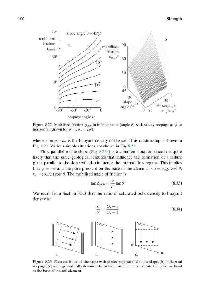
P1: KAE


190 Strength

-90° -60° -30° 00

30°

60°30o

15°

5°

90°

-90-60

-300

0

15

30

450

30

60

90

mobilised friction

φmobmobilised

friction φmob°

slope angle θ = 45°

slope angle θ°

seepage angle ψ

seepage angle ψ°

a.b.

Figure 8.22. Mobilised friction φmob in infinite slope (angle θ) with steady seepage at ψ tohorizontal (drawn for ρ = 2ρw = 2ρ ′).

where ρ ′ = ρ − ρw is the buoyant density of the soil. This relationship is shown inFig. 8.22. Various simple situations are shown in Fig. 8.23.

Flow parallel to the slope (Fig. 8.23a) is a common situation since it is quitelikely that the same geological features that influence the formation of a failureplane parallel to the slope will also influence the internal flow regime. This impliesthat ψ = −θ and the pore pressure on the base of the element is u = ρwgt cos2 θ ,ru = (ρw/ρ) cos2 θ . The mobilised angle of friction is:

tan φmob = ρ

ρ ′ tan θ (8.33)

We recall from Section 3.3.3 that the ratio of saturated bulk density to buoyantdensity is:

ρ

ρ ′ = Gs + eGs − 1

(8.34)

a. b. c.

Figure 8.23. Element from infinite slope with (a) seepage parallel to the slope; (b) horizontalseepage; (c) seepage vertically downwards. In each case, the bars indicate the pressure headat the base of the soil element.

P1: KAE



where the specific gravity of the soil mineral Gs is probably in the range 2.6 to 2.7,and the void ratio e might be anything in the range of 0.3 to 1 (or more). Even withthis range of void ratios, the variation of ρ/ρ ′ is only from about 1.8 to 2.1 so wecan say as a generalisation that it will be of the order of 2 and the mobilised angleof friction is of the order of twice the slope angle. The stable angle of the slope willbe of the order of φ/2, where φ is the available frictional strength of the soil. Thepresence of seepage parallel to the slope thus has a very damaging effect on thestability of the slope.

Figure 8.23b shows seepage occurring horizontally, perhaps driven by some un-derlying impermeable horizontal layer. The pore pressure head on the base of theelement is equal to the depth t : the line orthogonal to the direction of flow goesstraight up to meet the free surface with h = t . For this case, ψ = 0 and the mo-bilised angle of friction is:

tan φmob = tan θ

1 − (ρw/ρ) sec2 θ(8.35)

For ρ/ρw = 2, this implies that φmob = 2θ .Finally, Fig. 8.23c shows downward vertical flow, which might arise as a result

of infiltration of rainfall from the surface of the slope. A horizontal line (orthogonalto the direction of flow) through the bottom corner of the element reaches daylightat the same level as that corner, so the pressure head at the base of the element iszero. The flow is driven by gravity, without modification: the downward hydraulicgradient is i = 1. The downward flow produces a seepage body force as a result ofthe resistance to flow provided by the tortuous paths around and between the soilparticles (Section 5.7). This seepage force (a body force of ρwgi = ρwg) leads to anincrease in the apparent unit weight of the soil by an amount that exactly balancesthe Archimedes uplift. Fitting this information into the reference geometry of thesection, we find ψ = −π/2 and the pore pressure on the base of the element, u = 0.We can calculate the mobilised angle of friction using (8.32):

tan φmob = ρ tan θ

ρ ′ + ρw

= tan θ (8.36)

and the condition for stability of the slope is the same as for the dry slope with noseepage: θ < φ.

We note that, although we have confined ourselves to a one-dimensional viewof the world, we can nevertheless make rational statements about the stability ormargin of safety for some quite realistic geotechnical systems.

8.9.1 Laboratory exercise: Angle of repose

There is a simple laboratory experiment that can be performed without any elabo-rate equipment to apply the understanding of slope stability that we have just gainedand thus to estimate the angle of shearing resistance φ in the strength model of agranular soil (sand or fine gravel). All we need is a largish beaker, some sand, and aprotractor for measuring angles (Fig. 8.24).

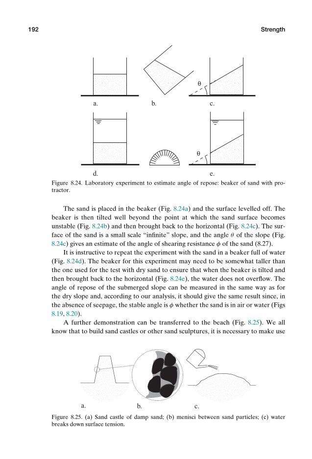
P1: KAE


192 Strength

θ

θ

a.

d.

b. c.

e.Figure 8.24. Laboratory experiment to estimate angle of repose: beaker of sand with pro-tractor.

The sand is placed in the beaker (Fig. 8.24a) and the surface levelled off. Thebeaker is then tilted well beyond the point at which the sand surface becomesunstable (Fig. 8.24b) and then brought back to the horizontal (Fig. 8.24c). The sur-face of the sand is a small scale “infinite” slope, and the angle θ of the slope (Fig.8.24c) gives an estimate of the angle of shearing resistance φ of the sand (8.27).

It is instructive to repeat the experiment with the sand in a beaker full of water(Fig. 8.24d). The beaker for this experiment may need to be somewhat taller thanthe one used for the test with dry sand to ensure that when the beaker is tilted andthen brought back to the horizontal (Fig. 8.24e), the water does not overflow. Theangle of repose of the submerged slope can be measured in the same way as forthe dry slope and, according to our analysis, it should give the same result since, inthe absence of seepage, the stable angle is φ whether the sand is in air or water (Figs8.19, 8.20).

A further demonstration can be transferred to the beach (Fig. 8.25). We allknow that to build sand castles or other sand sculptures, it is necessary to make use

a. b. c.

Figure 8.25. (a) Sand castle of damp sand; (b) menisci between sand particles; (c) waterbreaks down surface tension.

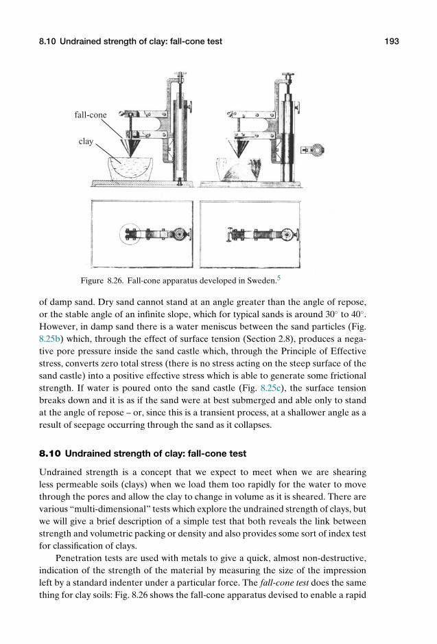
P1: KAE


8.10 Undrained strength of clay: fall-cone test 193

clay

fall-cone

Figure 8.26. Fall-cone apparatus developed in Sweden.5

of damp sand. Dry sand cannot stand at an angle greater than the angle of repose,or the stable angle of an infinite slope, which for typical sands is around 30 to 40.However, in damp sand there is a water meniscus between the sand particles (Fig.8.25b) which, through the effect of surface tension (Section 2.8), produces a nega-tive pore pressure inside the sand castle which, through the Principle of Effectivestress, converts zero total stress (there is no stress acting on the steep surface of thesand castle) into a positive effective stress which is able to generate some frictionalstrength. If water is poured onto the sand castle (Fig. 8.25c), the surface tensionbreaks down and it is as if the sand were at best submerged and able only to standat the angle of repose – or, since this is a transient process, at a shallower angle as aresult of seepage occurring through the sand as it collapses.

8.10 Undrained strength of clay: fall-cone test

Undrained strength is a concept that we expect to meet when we are shearingless permeable soils (clays) when we load them too rapidly for the water to movethrough the pores and allow the clay to change in volume as it is sheared. There arevarious “multi-dimensional” tests which explore the undrained strength of clays, butwe will give a brief description of a simple test that both reveals the link betweenstrength and volumetric packing or density and also provides some sort of index testfor classification of clays.

Penetration tests are used with metals to give a quick, almost non-destructive,indication of the strength of the material by measuring the size of the impressionleft by a standard indenter under a particular force. The fall-cone test does the samething for clay soils: Fig. 8.26 shows the fall-cone apparatus devised to enable a rapid

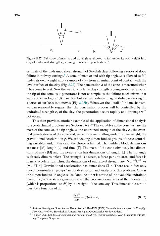
P1: KAE


194 Strength

mω

cud

a. b.

Figure 8.27. Fall-cone of mass m and tip angle ω allowed to fall under its own weight intoclay of undrained strength cu, coming to rest with penetration d.

estimate of the undrained shear strength of Swedish clays following a series of slopefailure in railway cuttings.5 A cone of mass m and with tip angle ω is allowed to fallunder its own weight into a sample of clay from an initial point of contact with thelevel surface of the clay (Fig. 8.27). The penetration d of the cone is measured whenit has come to rest. Now the way in which the clay strength is being mobilised aroundthe tip of the cone as it penetrates is not as simple as the failure mechanisms thatwere shown in Figs 8.1, 8.3 and 8.4, but we can perhaps imagine sliding occurring ona series of surfaces as it moves (Fig. 8.27b). Whatever the detail of the mechanism,we can reasonably suggest that the penetration process will be controlled by theundrained strength cu of the clay: the penetration occurs rapidly and drainage willnot occur.

This then provides another example of the application of dimensional analysisto a geotechnical problem (see Section 3.6.2).6 The variables in the cone test are themass of the cone m, the tip angle ω, the undrained strength of the clay cu, the even-tual penetration d of the cone and, since the cone is falling under its own weight, thegravitational acceleration g. We are seeking dimensionless groups of these control-ling variables and, in this case, the choice is limited. The building block dimensionsare mass [M], length [L] and time [T]. The mass of the cone obviously has dimen-sions of mass [M] and the penetration has dimensions of length [L]. The tip angleis already dimensionless. The strength is a stress, a force per unit area, and force ismass × acceleration. Thus, the dimensions of undrained strength are [MLT−2L−2] or[ML−1T−2]. Gravitational acceleration has dimensions LT−2. There are in fact onlytwo dimensionless “groups” in the description and analysis of this problem. One isthe dimensionless tip angle ω itself and the other is a ratio of the available undrainedstrength cu to the stress generated over the cross-sectional area of the indentation(which is proportional to d2) by the weight of the cone mg. This dimensionless ratiomust be a function of ω:

cud2

mg= f (ω) = kω (8.37)

5 Statens Jarnvagars Geotekniska Kommission 1914–1922 (1922) Slutbetankande avgivet til KungligaJarnvagsstyrelsen, Stockholm: Statens Jarnvagar, Geotekniska Meddelanden 2.

6 Palmer, A.C. (2008) Dimensional analysis and intelligent experimentation, World Scientific Publish-ing Company, Singapore.

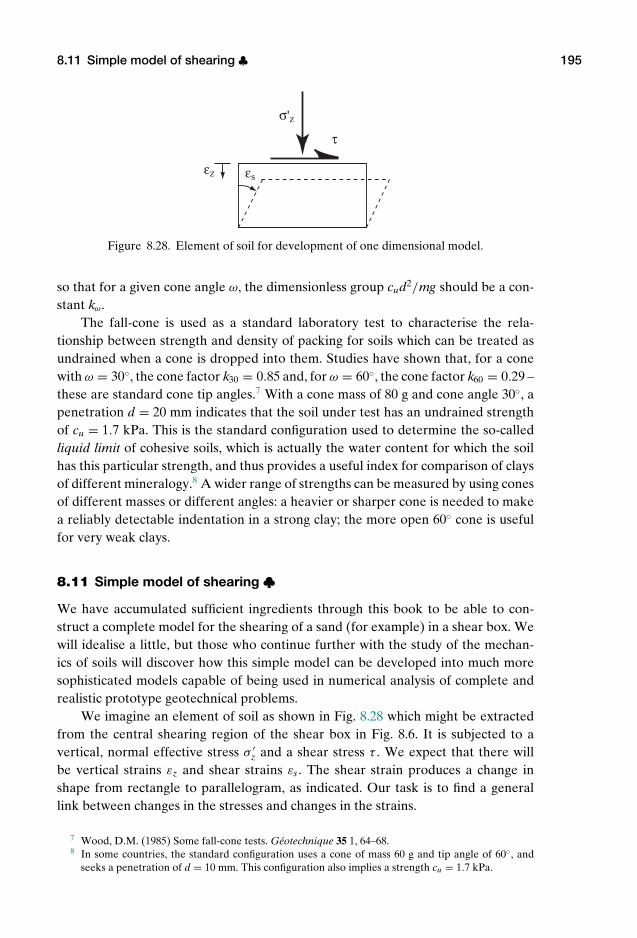
P1: KAE


8.11 Simple model of shearing ♣ 195

τ

σ'z

εz εs

Figure 8.28. Element of soil for development of one dimensional model.

so that for a given cone angle ω, the dimensionless group cud2/mg should be a con-stant kω.

The fall-cone is used as a standard laboratory test to characterise the rela-tionship between strength and density of packing for soils which can be treated asundrained when a cone is dropped into them. Studies have shown that, for a conewith ω = 30, the cone factor k30 = 0.85 and, for ω = 60, the cone factor k60 = 0.29 –these are standard cone tip angles.7 With a cone mass of 80 g and cone angle 30, apenetration d = 20 mm indicates that the soil under test has an undrained strengthof cu = 1.7 kPa. This is the standard configuration used to determine the so-calledliquid limit of cohesive soils, which is actually the water content for which the soilhas this particular strength, and thus provides a useful index for comparison of claysof different mineralogy.8 A wider range of strengths can be measured by using conesof different masses or different angles: a heavier or sharper cone is needed to makea reliably detectable indentation in a strong clay; the more open 60 cone is usefulfor very weak clays.

8.11 Simple model of shearing ♣We have accumulated sufficient ingredients through this book to be able to con-struct a complete model for the shearing of a sand (for example) in a shear box. Wewill idealise a little, but those who continue further with the study of the mechan-ics of soils will discover how this simple model can be developed into much moresophisticated models capable of being used in numerical analysis of complete andrealistic prototype geotechnical problems.

We imagine an element of soil as shown in Fig. 8.28 which might be extractedfrom the central shearing region of the shear box in Fig. 8.6. It is subjected to avertical, normal effective stress σ ′

z and a shear stress τ . We expect that there willbe vertical strains εz and shear strains εs . The shear strain produces a change inshape from rectangle to parallelogram, as indicated. Our task is to find a generallink between changes in the stresses and changes in the strains.

7 Wood, D.M. (1985) Some fall-cone tests. Geotechnique 35 1, 64–68.8 In some countries, the standard configuration uses a cone of mass 60 g and tip angle of 60, and

seeks a penetration of d = 10 mm. This configuration also implies a strength cu = 1.7 kPa.

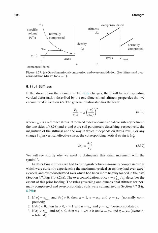
P1: KAE


196 Strength

densityρd


stress stress

normally compressed

normally compressed

overconsolidated

overconsolidated

v = 1

stiffness Eo

σ'zmax

a. b.

Figure 8.29. (a) One-dimensional compression and overconsolidation; (b) stiffness and over-consolidation (drawn for α = 1).

8.11.1 Stiffness

If the stress σ ′z on the element in Fig. 8.28 changes, there will be corresponding

vertical deformation described by the one-dimensional stiffness properties that weencountered in Section 4.5. The general relationship has the form:

Eo

σre f= χ

(σ ′

z

σre f

)α

(8.38)

where σre f is a reference stress introduced to leave dimensional consistency betweenthe two sides of (8.38) and χ and α are soil parameters describing, respectively, themagnitude of the stiffness and the way in which it depends on stress level. For anychange δσ ′

z in vertical effective stress, the corresponding vertical strain is δε′z:

δε′z = δσ ′

z

Eo(8.39)

We will see shortly why we need to distinguish this strain increment with thesymbol ′.

In describing stiffness, we had to distinguish between normally compressed soilswhich were currently experiencing the maximum vertical stress they had ever expe-rienced, and overconsolidated soils which had been more heavily loaded in the past(Section 4.7, Figs 8.148.29a). The overconsolidation ratio, n = σ ′

zmax/σ ′

z, describes theextent of this prior loading. The rules governing one-dimensional stiffness for nor-mally compressed and overconsolidated soils were summarised in Section 4.7 (Fig.8.29b):

1. If σ ′z = σ ′

zmaxand δσ ′

z > 0, then n = 1, α = αnc and χ = χnc (normally com-pressed);

2. If δσ ′z < 0, then δn > 0, n ≥ 1, and α = αoc and χ = χoc (overconsolidated);

3. If σ ′z < σ ′

zmaxand δσ ′

z > 0, then n > 1, δn < 0, and α = αoc and χ = χoc (overcon-solidated);

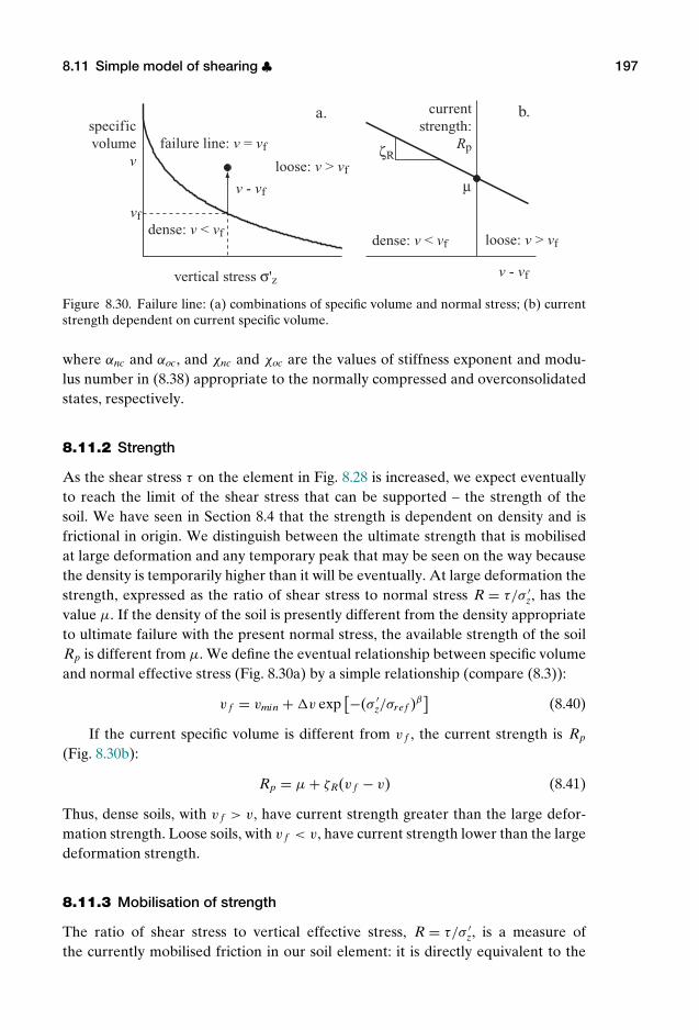
P1: KAE



failure line: v = vf

vf

v - vf

loose: v > vf

dense: v < vfdense: v < vf

a. b.current strength:

Rp

specificvolume

v

vertical stress σ'z v - vf

loose: v > vf

µ

ζR

Figure 8.30. Failure line: (a) combinations of specific volume and normal stress; (b) currentstrength dependent on current specific volume.

where αnc and αoc, and χnc and χoc are the values of stiffness exponent and modu-lus number in (8.38) appropriate to the normally compressed and overconsolidatedstates, respectively.

8.11.2 Strength

As the shear stress τ on the element in Fig. 8.28 is increased, we expect eventuallyto reach the limit of the shear stress that can be supported – the strength of thesoil. We have seen in Section 8.4 that the strength is dependent on density and isfrictional in origin. We distinguish between the ultimate strength that is mobilisedat large deformation and any temporary peak that may be seen on the way becausethe density is temporarily higher than it will be eventually. At large deformation thestrength, expressed as the ratio of shear stress to normal stress R = τ/σ ′

z, has thevalue µ. If the density of the soil is presently different from the density appropriateto ultimate failure with the present normal stress, the available strength of the soilRp is different from µ. We define the eventual relationship between specific volumeand normal effective stress (Fig. 8.30a) by a simple relationship (compare (8.3)):

v f = vmin + v exp[−(σ ′

z/σre f )β]

(8.40)

If the current specific volume is different from v f , the current strength is Rp

(Fig. 8.30b):

Rp = µ + ζR(v f − v) (8.41)

Thus, dense soils, with v f > v, have current strength greater than the large defor-mation strength. Loose soils, with v f < v, have current strength lower than the largedeformation strength.

8.11.3 Mobilisation of strength

The ratio of shear stress to vertical effective stress, R = τ/σ ′z, is a measure of

the currently mobilised friction in our soil element: it is directly equivalent to the

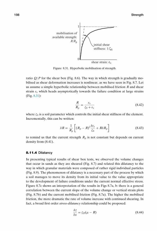
P1: KAE


198 Strength

1

0

initial shear stiffness: 1/ζS

mobilisation ofavailable strength:

R/Rp

shear strain: εs

Figure 8.31. Hyperbolic mobilisation of strength.

ratio Q/P for the shear box (Fig. 8.6). The way in which strength is gradually mo-bilised as shear deformation increases is nonlinear, as we have seen in Fig. 8.7. Letus assume a simple hyperbolic relationship between mobilised friction R and shearstrain εs which heads asymptotically towards the failure condition at large strains(Fig. 8.31):

RRp

= εs

ζS + εs(8.42)

where ζS is a soil parameter which controls the initial shear stiffness of the element.Incrementally, this can be written:

δR = 1Rp

[(Rp − R)2 δεs

ζS+ RδRp

](8.43)

to remind us that the current strength Rp is not constant but depends on currentdensity from (8.41).

8.11.4 Dilatancy

In presenting typical results of shear box tests, we observed the volume changesthat occur in sands as they are sheared (Fig. 8.7) and related this dilatancy to theway in which granular materials were composed of rather rigid individual particles(Fig. 8.9). The phenomenon of dilatancy is a necessary part of the process by whicha soil manages to move its density from its initial value to the value appropriateto the development of failure conditions under the current normal effective stress.Figure 8.7c shows an interpretation of the results in Figs 8.7a, b: there is a generalcorrelation between the current slope of the volume change or vertical strain plots(Fig. 8.7b) and the current mobilised friction (Fig. 8.7a). The higher the mobilisedfriction, the more dramatic the rate of volume increase with continued shearing. Infact, a broad first order stress-dilatancy relationship could be proposed:

δzδx

= ζD(µ − R) (8.44)

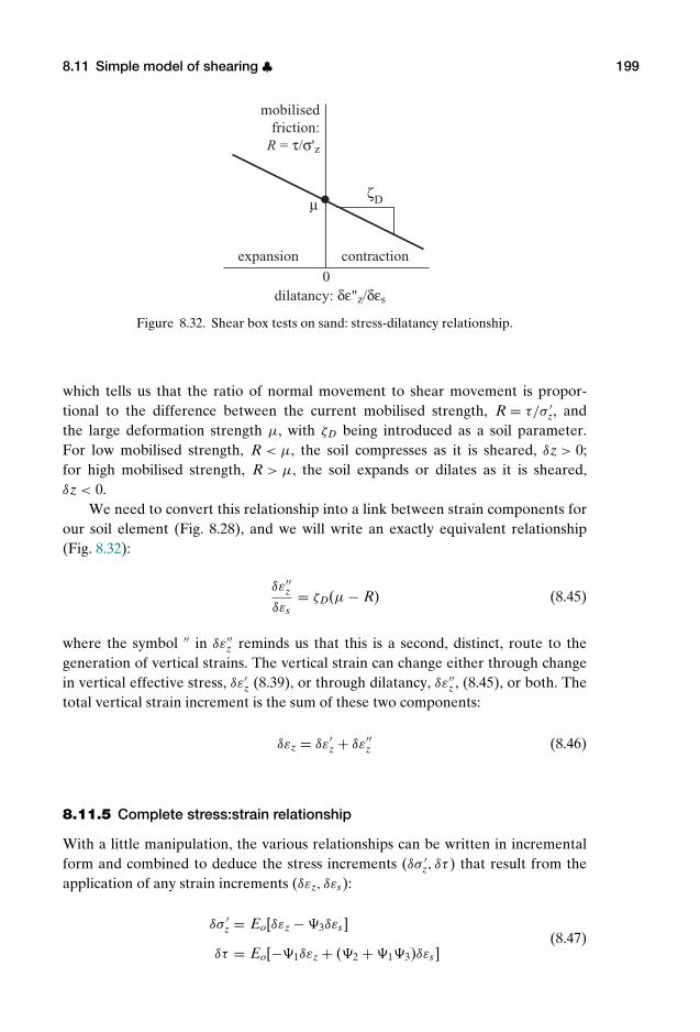
P1: KAE



mobilised friction:

R = τ/σ'z

µ

0

contractionexpansion

dilatancy: δε"z/δεs

ζD

Figure 8.32. Shear box tests on sand: stress-dilatancy relationship.

which tells us that the ratio of normal movement to shear movement is propor-tional to the difference between the current mobilised strength, R = τ/σ ′

z, andthe large deformation strength µ, with ζD being introduced as a soil parameter.For low mobilised strength, R < µ, the soil compresses as it is sheared, δz > 0;for high mobilised strength, R > µ, the soil expands or dilates as it is sheared,δz < 0.

We need to convert this relationship into a link between strain components forour soil element (Fig. 8.28), and we will write an exactly equivalent relationship(Fig. 8.32):

δε′′z

δεs= ζD(µ − R) (8.45)

where the symbol ′′ in δε′′z reminds us that this is a second, distinct, route to the

generation of vertical strains. The vertical strain can change either through changein vertical effective stress, δε′

z (8.39), or through dilatancy, δε′′z , (8.45), or both. The

total vertical strain increment is the sum of these two components:

δεz = δε′z + δε′′

z (8.46)

8.11.5 Complete stress:strain relationship

With a little manipulation, the various relationships can be written in incrementalform and combined to deduce the stress increments (δσ ′

z, δτ ) that result from theapplication of any strain increments (δεz, δεs):

δσ ′z = Eo[δεz − 3δεs]

δτ = Eo[−1δεz + (2 + 13)δεs](8.47)

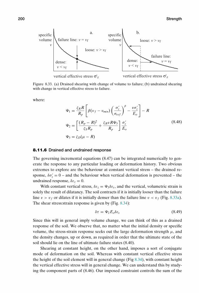
P1: KAE


200 Strength

specific volume

v

specific volume

v

vertical effective stress σ'z vertical effective stress σ'z



loose: v > vf

loose: v > vf

dense: v < vf

dense: v < vf

a. b.

Figure 8.33. (a) Drained shearing with change of volume to failure; (b) undrained shearingwith change in vertical effective stress to failure.

where:

1 = ζR RRp

[β(v f − vmin)

(σ ′

z

σre f

)β

− vσ ′z

Eo

]− R

2 =[

(Rp − R)2

ζS Rp+ ζRvR3

Rp

]σ ′

z

Eo

3 = ζD(µ − R)

(8.48)

8.11.6 Drained and undrained response

The governing incremental equations (8.47) can be integrated numerically to gen-erate the response to any particular loading or deformation history. Two obviousextremes to explore are the behaviour at constant vertical stress – the drained re-sponse, δσ ′

z = 0 – and the behaviour when vertical deformation is prevented – theundrained response, δεz = 0.

With constant vertical stress, δεz = 3δεs , and the vertical, volumetric strain issolely the result of dilatancy. The soil contracts if it is initially looser than the failureline v > v f or dilates if it is initially denser than the failure line v < v f (Fig. 8.33a).The shear stress:strain response is given by (Fig. 8.34):

δτ = 2 Eoδεs (8.49)

Since this will in general imply volume change, we can think of this as a drainedresponse of the soil. We observe that, no matter what the initial density or specificvolume, the stress-strain response seeks out the large deformation strength µ, andthe density changes, up or down, as required in order that the ultimate state of thesoil should lie on the line of ultimate failure states (8.40).

Shearing at constant height, on the other hand, imposes a sort of conjugatemode of deformation on the soil. Whereas with constant vertical effective stressthe height of the soil element will in general change (Fig 8.34), with constant heightthe vertical effective stress will in general change. We can understand this by study-ing the component parts of (8.46). Our imposed constraint controls the sum of the

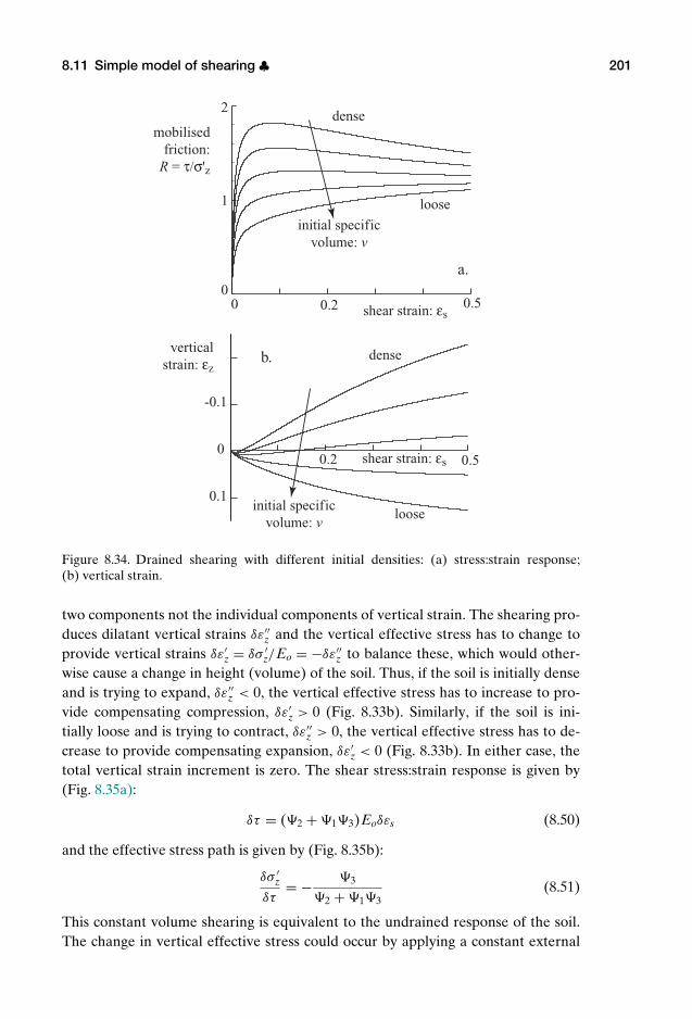
P1: KAE



-0.1

0

0.1

0.2

0.2

0.5

0.5

shear strain: εs

shear strain: εs

vertical strain: εz

0

2

1

0

mobilised friction:

R = τ/σ'z

a.

b.

initial specific volume: v


dense

loose

dense

loose

Figure 8.34. Drained shearing with different initial densities: (a) stress:strain response;(b) vertical strain.

two components not the individual components of vertical strain. The shearing pro-duces dilatant vertical strains δε′′

z and the vertical effective stress has to change toprovide vertical strains δε′

z = δσ ′z/Eo = −δε′′

z to balance these, which would other-wise cause a change in height (volume) of the soil. Thus, if the soil is initially denseand is trying to expand, δε′′

z < 0, the vertical effective stress has to increase to pro-vide compensating compression, δε′

z > 0 (Fig. 8.33b). Similarly, if the soil is ini-tially loose and is trying to contract, δε′′

z > 0, the vertical effective stress has to de-crease to provide compensating expansion, δε′

z < 0 (Fig. 8.33b). In either case, thetotal vertical strain increment is zero. The shear stress:strain response is given by(Fig. 8.35a):

δτ = (2 + 13)Eoδεs (8.50)

and the effective stress path is given by (Fig. 8.35b):

δσ ′z

δτ= − 3

2 + 13(8.51)

This constant volume shearing is equivalent to the undrained response of the soil.The change in vertical effective stress could occur by applying a constant external

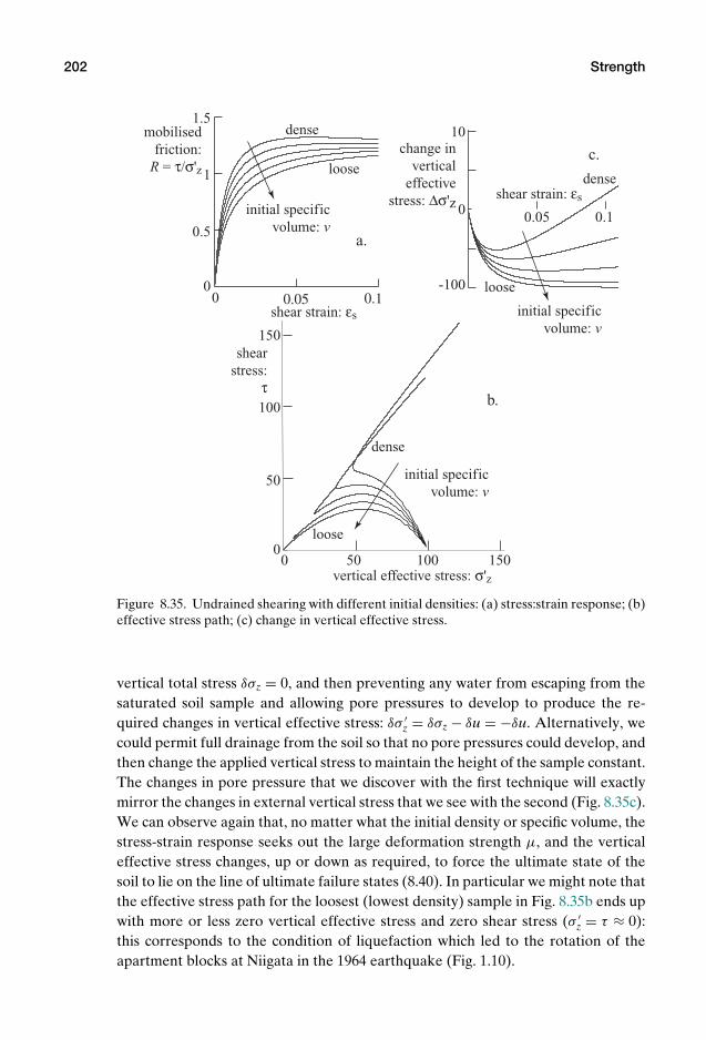
P1: KAE


202 Strength

150

100

50

00 50 100 150

vertical effective stress: σ'z

shear stress:

τ




dense

dense

dense

loose

loose

loose

b.

10

0

0-100

change in vertical

effective stress: ∆σ'z

shear strain: εs

shear strain: εs

0.05

0.05

0.1

0.1

c.

a.

0

0.5

1

1.5mobilised

friction: R = τ/σ'z

Figure 8.35. Undrained shearing with different initial densities: (a) stress:strain response; (b)effective stress path; (c) change in vertical effective stress.

vertical total stress δσz = 0, and then preventing any water from escaping from thesaturated soil sample and allowing pore pressures to develop to produce the re-quired changes in vertical effective stress: δσ ′

z = δσz − δu = −δu. Alternatively, wecould permit full drainage from the soil so that no pore pressures could develop, andthen change the applied vertical stress to maintain the height of the sample constant.The changes in pore pressure that we discover with the first technique will exactlymirror the changes in external vertical stress that we see with the second (Fig. 8.35c).We can observe again that, no matter what the initial density or specific volume, thestress-strain response seeks out the large deformation strength µ, and the verticaleffective stress changes, up or down as required, to force the ultimate state of thesoil to lie on the line of ultimate failure states (8.40). In particular we might note thatthe effective stress path for the loosest (lowest density) sample in Fig. 8.35b ends upwith more or less zero vertical effective stress and zero shear stress (σ ′

z = τ ≈ 0):this corresponds to the condition of liquefaction which led to the rotation of theapartment blocks at Niigata in the 1964 earthquake (Fig. 1.10).

P1: KAE


8.12 Summary 203

8.11.7 Model: summary

The current state of the soil is described by its specific volume v, and by the stressesσ ′

z and τ , often combined in their ratio R. The quantities 1, 2 and 3 (8.48) areconvenient short-hand groupings of the various constitutive properties of the soiltogether with the variables that define the current state of the soil. The model mayappear a little complicated in its eventual formulation but it is in fact built up froma small number of simple building blocks.

A one-dimensional stiffness relationship (8.39) defining normal stiffness Eo,which introduces soil properties χ , α and σre f (8.38) in order to reproduce theexpected nonlinearity.

A hyperbolic relationship between mobilised strength and shear strain (8.42)with soil property ζS.

A stress-dilatancy relationship describing the volume changes accompanyingshearing (8.45) requiring property ζD.

A link between specific volume (or density) and vertical effective stress at ulti-mate failure, which introduces properties vmin, v and β (8.40).

A link between current strength and volumetric distance from this failure line(8.41), requiring properties µ and ζR.

Each of these relationships is mathematically rather simple: the apparent com-plexity arises because of their interlocking.

However, the model is rather powerful. It shows how the shearing responsedepends on the initial density of the soil. It shows how the volume changes accom-panying shearing inexorably move the soil from its initial condition to the failureline in drained tests, and the vertical effective stress has to change to allow the soilto move to the failure line in undrained tests.

For any complex model, there is a simpler model lurking inside which we canfind by eliminating some of the special effects. Thus, we could eliminate the non-linearity of normal stiffness by setting α = 0; we could eliminate the dilatancy (thechange in volume induced by shearing) by setting ζD = 0; we could eliminate thevariation of strength with density by setting ζR = 0. Exploration of the consequencesof switching off these features will be left for the reader to pursue.

8.12 Summary


1. In many geotechnical systems, failure occurs by sliding on a clear slip surface,mobilising the shear strength of the soil.

2. The shear box is a laboratory test device which mimics the development of afailure surface in soil.

3. A simple model proposes a frictional strength linking maximum shear stresswith the normal effective stress on the surface of failure.

P1:K

AE

OneD

im00a

CU

US648/M

uir978

0521

517737

August17,2009

19:12

strength

shear box

slopefoundation

pile

downdrag

failure (mechanism)importance of SHEARING

propose frictional strength

expect link between strength and density

change σzhigh permeability soil

σ'z changes → density changes → strength changes

“drained” strength

controlled by final effective stresses

drained σ'z → τf → ρ

low permeability soil

long termshort term

σ'z unchanged → density unchanged → strrength unchanged

“undrained” strengthcontrolled by initial/current density

consolidation history: σ'z, n → ρundrained ρ → τf → σ'z

pore pressure u = σz-σ'zundrained strength of clays τf = cu~0.2nσ'z

overconsolidation ratio n = σ'zmax/σ'z

v ρ

shear stress τ

σ'z

Q

Pz

x

infinite slope

shearstress

τ

failure

Figure 8.36. Mind map: strength.

204

P1: KAE


8.13 Exercises: Strength 205

4. We also expect the strength to be linked with the density of the soil – the denserthe soil, the higher the strength.

5. This simple model allows us to make clear statements about drained andundrained strengths of soils.

6. High permeability soils (or low permeability soils after a long time) are able tochange in volume when the normal stress is changed and the strength and thefinal density are controlled by the final effective stress.

7. Low permeability soils are not able to change in volume rapidly when thenormal stress is changed: the strength is controlled by the initial density. Thestrength then implies a certain normal effective stress at failure, and the differ-ence between the total and effective normal stresses allows us to estimate thepore pressure at failure.

8. A model can be generated to describe the shearing and compression of soilsand to reproduce the effects of different initial densities and different drainageconditions.

8.13 Exercises: Strength

1. A sample of normally compressed clay whose strength is described by an ex-pression of the form τ f = σ ′

z with = 0.3, has current vertical total stressσz = σ ′

zmax= 170 kPa and pore pressure u = 50 kPa. What is the current vertical

effective stress? What is the current strength?2. The total stress on the sample in Question 1 changes to 250 kPa without

drainage (so that there is no change in density of the sample). What are thenew values of pore pressure, vertical effective stress and strength?

3. The total stress on the sample of Question 2 is maintained constant at 250 kPaand the pore pressure falls slowly to zero: drainage is permitted and the densityof the clay is able to change. What is the eventual value of the vertical effectivestress? Does the density of the clay increase or decrease with time? What is theeventual undrained strength?

4. A shallow slope failure occurred at Jackfield, Shropshire, after a period of heavyrain in the winter 1952–1953.9 The slope angle was found to be about 10.5 andfailure was found to have occurred on a thin surface parallel to the slope ata depth of about 5 m. What shear strength must have been mobilised on thefailure plane? The unit weight of the clay was 20.4 kN/m3.Laboratory tests showed an angle of shearing resistance for the clay of about21. Field tests indicated that seepage was occurring more or less parallel tothe slope. Calculate the mobilised angle of friction on the failure surface andconfirm that the margin of stability would have been small.

5. Figure 8.37 shows an approximate section through the landslide that occurred atPo Shan Road in Hong Kong in 1972, shown in Fig. 5.2. A slip surface formed at

9 Henkel, D.J. & Skempton, A.W. (1955) A landslide at Jackfield, Shropshire in a heavily overcon-solidated clay. Geotechnique 5 2, 131–7.

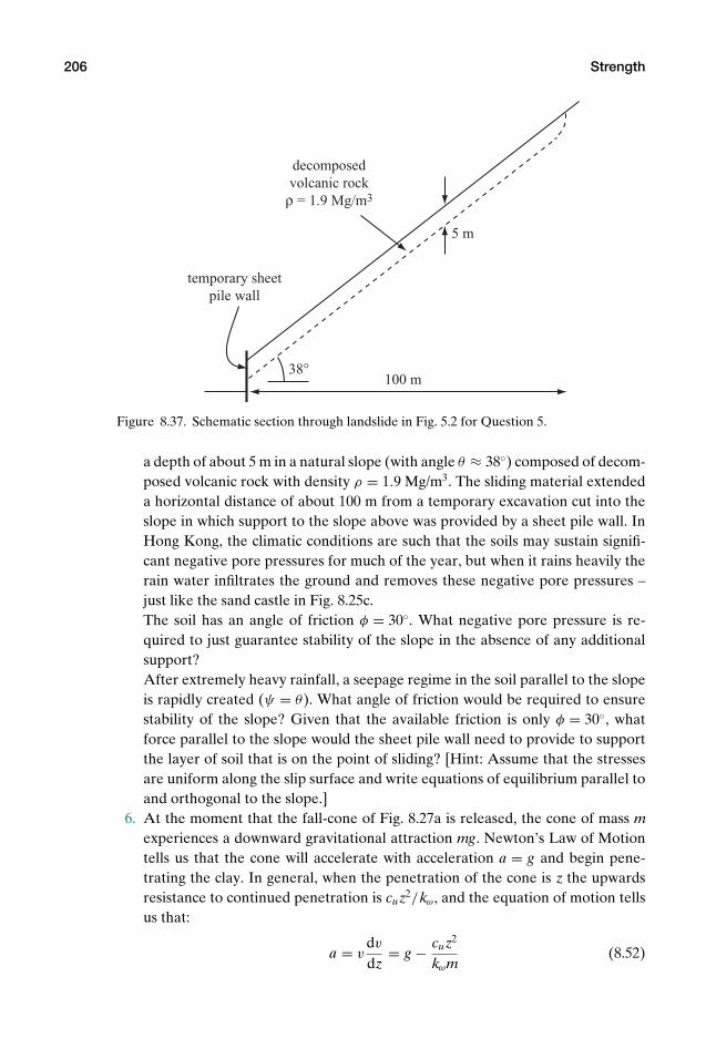
P1: KAE


206 Strength

38°100 m

5 m

temporary sheet pile wall

decomposed volcanic rock

ρ = 1.9 Mg/m3

Figure 8.37. Schematic section through landslide in Fig. 5.2 for Question 5.

a depth of about 5 m in a natural slope (with angle θ ≈ 38) composed of decom-posed volcanic rock with density ρ = 1.9 Mg/m3. The sliding material extendeda horizontal distance of about 100 m from a temporary excavation cut into theslope in which support to the slope above was provided by a sheet pile wall. InHong Kong, the climatic conditions are such that the soils may sustain signifi-cant negative pore pressures for much of the year, but when it rains heavily therain water infiltrates the ground and removes these negative pore pressures –just like the sand castle in Fig. 8.25c.The soil has an angle of friction φ = 30. What negative pore pressure is re-quired to just guarantee stability of the slope in the absence of any additionalsupport?After extremely heavy rainfall, a seepage regime in the soil parallel to the slopeis rapidly created (ψ = θ). What angle of friction would be required to ensurestability of the slope? Given that the available friction is only φ = 30, whatforce parallel to the slope would the sheet pile wall need to provide to supportthe layer of soil that is on the point of sliding? [Hint: Assume that the stressesare uniform along the slip surface and write equations of equilibrium parallel toand orthogonal to the slope.]

6. At the moment that the fall-cone of Fig. 8.27a is released, the cone of mass mexperiences a downward gravitational attraction mg. Newton’s Law of Motiontells us that the cone will accelerate with acceleration a = g and begin pene-trating the clay. In general, when the penetration of the cone is z the upwardsresistance to continued penetration is cuz2/kω, and the equation of motion tellsus that:

a = vdv

dz= g − cuz2

kωm(8.52)

P1: KAE


8.13 Exercises: Strength 207

The penetration of the cone in Fig. 8.27 is a dynamic process leading to an even-tual penetration d. At what penetration ds would a cone of the same tip angleω encounter a resistance to penetration equal to its weight mg if it were to bepushed in at essentially zero velocity? [Hint: The fall-cone will have zero accel-eration at the moment when its penetration is z = ds but it still has a non-zerovelocity, and eventually comes to rest with z = d > ds . You are asked to dis-cover the ratio ds/d.]

7. This exercise brings together the stiffness model of Chapter 4 and the strengthmodel of the present chapter.The one-dimensional stiffness of a sandy-silt is characterised by the stiffnessproperties αnc = αoc = 0.5, χnc = 100, χoc = 400. When the vertical effectivestress σ ′

z = 1 kPa, v = 1.9. By appropriate integration of (4.21) find an expres-sion for the normal compression line linking values of σ ′

z and v.The failure conditions for the sandy-silt are described by (8.3) and (8.2) withφ = 25, vmin = 1.2, v = 1.5, β = 0.3, σre f = 100 kPa.a. The soil is normally compressed to a vertical effective stress σ ′

z = 100 kPa.What is the specific volume? What are the drained and undrained strengths?What is the vertical effective stress at undrained failure?

b. The soil is further compressed to a vertical effective stress σ ′z = 500 kPa.

What is the specific volume? What are the drained and undrained strengths?What is the vertical effective stress at undrained failure?

c. The soil is unloaded to a vertical effective stress σ ′z = 100 kPa. What is the

specific volume? What are the drained and undrained strengths? What is thevertical effective stress at undrained failure?

d. The additional properties of the soil required to complete the deforma-tion model are ζS = 0.005, ζD = 1, ζR = 0.3, µ = tan φ. Estimate the verticalstrain εz and shear strain εs when the stress ratio R = µ/2 for each of thesamples in (a), (b) and (c). [Hint: The numerical integration of (8.47) can beachieved with a small number of increments.]

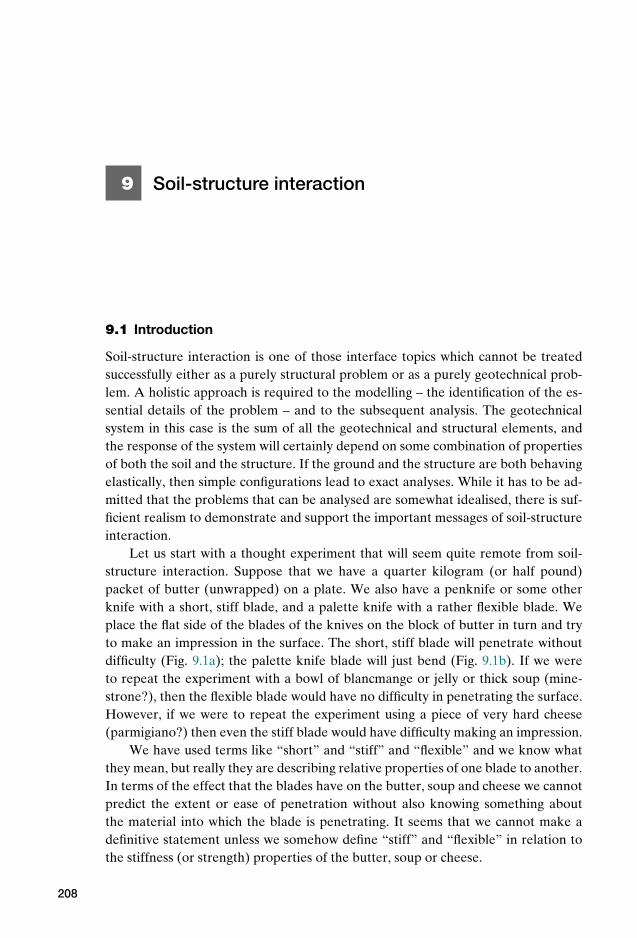
P1: KAE


9 Soil-structure interaction

9.1 Introduction

Soil-structure interaction is one of those interface topics which cannot be treatedsuccessfully either as a purely structural problem or as a purely geotechnical prob-lem. A holistic approach is required to the modelling – the identification of the es-sential details of the problem – and to the subsequent analysis. The geotechnicalsystem in this case is the sum of all the geotechnical and structural elements, andthe response of the system will certainly depend on some combination of propertiesof both the soil and the structure. If the ground and the structure are both behavingelastically, then simple configurations lead to exact analyses. While it has to be ad-mitted that the problems that can be analysed are somewhat idealised, there is suf-ficient realism to demonstrate and support the important messages of soil-structureinteraction.

Let us start with a thought experiment that will seem quite remote from soil-structure interaction. Suppose that we have a quarter kilogram (or half pound)packet of butter (unwrapped) on a plate. We also have a penknife or some otherknife with a short, stiff blade, and a palette knife with a rather flexible blade. Weplace the flat side of the blades of the knives on the block of butter in turn and tryto make an impression in the surface. The short, stiff blade will penetrate withoutdifficulty (Fig. 9.1a); the palette knife blade will just bend (Fig. 9.1b). If we wereto repeat the experiment with a bowl of blancmange or jelly or thick soup (mine-strone?), then the flexible blade would have no difficulty in penetrating the surface.However, if we were to repeat the experiment using a piece of very hard cheese(parmigiano?) then even the stiff blade would have difficulty making an impression.

We have used terms like “short” and “stiff” and “flexible” and we know whatthey mean, but really they are describing relative properties of one blade to another.In terms of the effect that the blades have on the butter, soup and cheese we cannotpredict the extent or ease of penetration without also knowing something aboutthe material into which the blade is penetrating. It seems that we cannot make adefinitive statement unless we somehow define “stiff” and “flexible” in relation tothe stiffness (or strength) properties of the butter, soup or cheese.

208

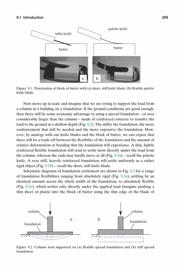
P1: KAE


9.1 Introduction 209

butter butter

table knifepalette knife

a. b.

Figure 9.1. Penetration of block of butter with (a) short, stiff knife blade; (b) flexible paletteknife blade.

Now move up in scale and imagine that we are trying to support the load froma column in a building on a foundation. If the ground conditions are good enough,then there will be some economic advantage in using a spread foundation – of areaconsiderably larger than the column – made of reinforced concrete to transfer theload to the ground at a shallow depth (Fig. 9.2). The stiffer the foundation, the morereinforcement that will be needed and the more expensive the foundation. How-ever, by analogy with our knife blades and the block of butter, we can expect thatthere will be a trade-off between the flexibility of the foundation and the amount ofrelative deformation or bending that the foundation will experience. A thin, lightlyreinforced flexible foundation will tend to settle most directly under the load fromthe column, whereas the ends may hardly move at all (Fig. 9.2a) – recall the paletteknife. A very stiff, heavily reinforced foundation will settle uniformly as a ratherrigid object (Fig. 9.2b) – recall the short, stiff knife blade.

Schematic diagrams of foundation settlement are shown in Fig. 9.3 for a rangeof foundation flexibilities ranging from absolutely rigid (Fig. 9.3a), settling by anidentical amount across the whole width of the foundation, to absolutely flexible(Fig. 9.3e), which settles only directly under the applied load (imagine pushing athin sheet of plastic into the block of butter using the thin edge of the blade of

a. b.

column column

foundationfoundation

Figure 9.2. Column load supported on (a) flexible spread foundation and (b) stiff spreadfoundation.

P1: KAE



rigid flexible

a. b. c. d. e.

Figure 9.3. Influence of foundation stiffness on settlement across foundation.

a knife). These are extremes, but we expect again that the detail of this responsecannot only depend on the structural properties of the concrete foundation slabbut must also be affected by the properties of the ground. What will constitute aflexible or a stiff foundation in the character of its performance under load cannotactually be assessed without knowing something also about the stiffness propertiesof the ground on which the foundation is placed. This is the problem analysed inSection 9.4.

Next, imagine that you are pitching a tent and need to anchor the fly-sheet to en-sure that it does not blow away (Fig. 9.4). The ties are held down using tent pegs. Wemight use rather stiff chunky wooden pegs (Fig. 9.4b) or we might use much moreflexible metal pegs (Fig. 9.4c). If the wind gets up, or the tension in the ties is toogreat, or the ground is too soft, then the peg may move or deform. The stiff peg willmerely rotate (Fig. 9.4b) but the flexible metal peg will probably bend (Fig. 9.4c).However, if the ground is soft enough then even the flexible peg will only rotatewithout bending. The performance of the pegs depends on the stiffness propertiesof both the peg and the ground.

Replace the tent with a floating offshore structure for oil exploration and pro-duction which has to be tethered to the seabed: the scale is different but the mechan-ics are the same. The tent pegs are replaced by piles which are pulled sideways bythe tethering cables. The response of these piles will depend on the stiffness prop-erties of the piles themselves and of the ground into which they have been driven.This is the problem analysed in Section 9.5.

Both these examples (spread foundations and laterally loaded piles) involvebending of the structural elements, and the underpinning analysis of bending ofbeams is summarised in Section 9.3. However, we begin with a slightly simpler

a. b. c.

Figure 9.4. (a) Fly-sheet of tent anchored by tent pegs: (b) stiff peg; (c) flexible peg.

P1: KAE


9.2 Pile under axial loading ♣ 211

example which involves only axial loading of the structural element: an axiallyloaded pile.

9.2 Pile under axial loading ♣As we have seen in Sections 1.3 and 8.8, a pile is a structural element that is used totransfer a load (such as the column load in Fig. 9.2) into the ground at a depth belowthe surface. The load is transferred to the ground by a combination of shaft resis-tance down the sides of the pile and end bearing at its toe. In Section 8.8 we wereconsidering the strength of the soil at the interface with the pile and therefore reallyonly concerned with failure conditions for this interface. Now we want to explorethe possibilities of making some estimates of the performance of such a pile underworking conditions in which we can treat both the pile and the ground as elastic.We will model the interface between the pile and the soil in a somewhat simplisticway in order that we may be able to reduce the problem, which is obviously reallythree dimensional, to a one-dimensional problem in which the single dimension isthe position down the pile.

To appreciate at least qualitatively the nature of the soil-structure interaction inthis problem, let us initially consider two extremes. In the first, the pile is extremelystiff axially and the soil is very weak. Because the pile is stiff, the axial displacementwill be virtually the same all the way down the pile, and because the soil is weak,there will be very little load shed to the ground through shaft resistance along thelength of the pile. Just about all of the load applied to the pile at the ground surfacewill be transferred to the toe of the pile to be carried in end bearing.

At the other extreme, we will have an extremely compressible pile in very stiffsoil. As any point on the pile moves downward relative to the distant undeformingground, the stiffness of the soil will lead to the generation of shear stresses roundthe pile, and this shaft resistance will reduce the load in the pile. As we go deeperinto the ground, the load shed to the ground increases but the deformation of thepile reduces because of the falling axial load. The settlement at the toe of the pilewill be much less than that at the ground surface – in fact, if the pile is compressibleenough, then it may be that there is no load left in the pile by the time we get to itstoe, and all the load will have been transferred to shaft resistance. We have againused terms such as “stiff”, “weak”, “compressible” to describe the pile and the soilbut we will not be surprised to find that they are in fact relative terms which have tocombine properties of both the soil and the structural elements.

We will analyse an elastic pile which is being loaded axially in an elastic soil.We can obtain an exact closed-form solution for the load distribution within the pileand the settlement distribution down the pile. We will assume the pile to be circularin cross-section for the calculation of its perimeter and cross-sectional area.

At a depth z down the pile (Fig. 9.5), the pile has a settlement ς relative tothe distant undeforming ground. The shear stress τ that develops at the interfacebetween the pile and the soil will be dependent on the stiffness of the soil. Since weare assuming that the soil is elastic, we can plausibly assume that this shear stress τ

P1: KAE



z

Pt

Pb

ς

l

ςt

ςb

Figure 9.5. Axially loaded pile in elastic soil.

is linearly related to the settlement ς normalised with the radius ro of the pile.1:

τ = λς

ro(9.1)

Now we can consider the equilibrium of an element of the pile of thickness δz atdepth z (Fig. 9.6). The axial load at the top of the element is P and at the bottom ofthe element P + δP. The settlement of the pile relative to the distant soil is ς and,as a result of this settlement, there is a shear stress τ round the perimeter of the pilewhich will support part of the axial load. Equilibrium tells us that:

δP = −2πroδzτ = −2πλςδz (9.2)

or in the limit:

dPdz

= −2πλς (9.3)

and, as expected, δP turns out to be negative.The pile is elastic and compresses under axial stress. Compression of the pile

implies that the settlement varies down the pile. The settlement at the top of theelement is ς and at the bottom ς + δς (Fig. 9.6). If the settlement varies across theelement, then there will be a tensile axial strain in the pile εa = δς/δz, and an axial

1 A more extensive discussion of this axial pile analysis is provided by Fleming, W.G.K., Weltman,A.J., Randolph, M.F. and Elson, W.K. (1985) Piling engineering. Surrey University Press, Glasgowand John Wiley, New York. They, unconstrained by the need to consider only a single dimension,link the shear stress τ with the shear modulus G of the soil and find that τ ≈ ςG/4ro. Thus, thestiffness constant used here is λ = G/4.

P1: KAE



P+δP

P z

δzτ

2ro

ς

ς+δς

Figure 9.6. Equilibrium of element of axially loaded pile in elastic soil. Note: exaggeratedindication of settlement.

stress related to the axial strain through Young’s modulus Ep for the pile:

dς

dz= − P

πr2o Ep

(9.4)

The negative sign is required because the pile is in compression and every elementof the pile must be getting shorter, dς/dz < 0.

Combining (9.3) and (9.4), the governing equation for the axially loaded pile is:

d2ς

dz2= 2λς

Epr2o

(9.5)

This has a general solution:

ς = J1 exp[z] + J2 exp[−z] (9.6)

where:

= 1ro

√2λ

Ep(9.7)

The problem is characterised by the value of the parameter which has dimensionsof length−1 and combines, as expected, the stiffness of the pile Ep and the stiffnessof the pile-soil interaction λ. We have to apply the general solution (9.6) to theboundary conditions of our particular problem.

For all piles, the load at the top of the pile is equal to the applied load Pt :

Pz=0 = −πr2o Ep

(dς

dz

)z=0

= Pt (9.8)

where the negative sign is required because the pile is in compression and the rela-tive pile-soil movement ς decreases down the pile as load is shed to the surroundingsoil.

If the pile is very long (where “long” is a relative term) then as z → ∞, ς → 0.Then, in (9.6), J1 = 0 and J2 = (Pt/πro)/

√(2λEp) and the load varies exponentially

down the pile:

PPt

= exp[−z] (9.9)

P1: KAE



or:

lnPPt

= −z (9.10)

We could introduce an effective length 100 at which the axial load in the pile haddropped to 1% of its top value, P/Pt = 0.01. We have 100 = ln 100 or 100/ro =ln 100

√Ep/2λ and the definition of “long” involves Ep and λ as well as the pile

radius ro. If the pile is very compressible (low Ep) and the soil stiff (high λ), then verylittle load reaches the base of the pile – in accord with our qualitative introductorydiscussion.

On the other hand, for a pile with finite length (Fig. 9.5), there will in generalbe some load Pb remaining at the base of the pile which must be compatible with thebase settlement ςb of the pile and this is the boundary condition at z = . Assumingelastic base load transfer (closed form analysis is not straightforward without suchan assumption), then, for z = :

Pb

πr2b

= λbςb

rb(9.11)

where rb is the radius of the base of the pile (which might be deliberately constructedby a technique called “under-reaming” to a larger radius than the pile itself).2 Theimposition of this boundary condition in (9.6) leads to a more cumbersome result:

J1 = Pt

2πr2o Ep

(ξ − 1) (1 − tanh )1 + ξ tanh

(9.12)

J2 = Pt

2πr2o Ep

(ξ + 1) (1 + tanh )1 + ξ tanh

(9.13)

where:

ξ = r2o Ep

λbrb= ro

rb

√2Epλ

λb(9.14)

and ξ combines the geometrical ratio ro/rb with a composite stiffness ratio whichincludes not only the pile stiffness Ep but also both the pile-soil transfer stiffnessesλ and λb.

The settlement ςt at the top of the pile, at z = 0 (Fig. 9.5), which is required toestimate the overall pile stiffness Pt/ςt , is:

ςt = Pt

πr2o Ep

(ξ + tanh )(1 + ξ tanh )

(9.15)

and the load variation down the pile is given by:

PPt

= (ξ + 1) (1 + tanh ) e−z − (ξ − 1) (1 − tanh ) ez

2 (1 + ξ tanh )(9.16)

2 Again, pushing at the boundaries of our one-dimensional constraints, the base stiffness could berelated to elastic properties (Poisson’s ratio νb and shear modulus Gb) of the continuous soil beneaththe base of the pile, λb = 4Gb/[π (1 − νb)], which is the equation for the stiffness of a circular plateon the surface of an elastic material.

P1: KAE



0

1

01

z/l

ς/ςt P/Pt

settlement

load

Θl=1: 'short'

Θl=4: 'long'

Figure 9.7. Axially loaded pile in elastic soil; distributions of axial load and axial displace-ment.

The parameter (9.7) that characterises the solution is a function of the ratioof the stiffnesses of the pile and the soil shaft resistance transfer. In fact, alwaysappears in the solution in combination with either the length or a distance down thepile. Thus = (/ro)

√2λ/Ep is the appropriate dimensionless group which con-

trols the overall response of a pile of length so that z = (z/). We have man-aged to characterise the entire performance of the pile (9.16) in terms of dimension-less groups for load and position P/Pt and z/, and for appropriate combinations ofmaterial and geometric properties and ξ . The result is thus of completely generalapplicability. Results are shown in Fig. 9.7 for = 1 and 4 – these values produceclassic “short” and “long” pile response, respectively. For a short pile (low valuesof ), the base of the pile takes a significant load, and develops a correspondinglysignificant settlement. For a longer pile, little load reaches the base of the pile.

9.2.1 Examples

1. Let us suppose that we have a concrete pile of radius ro = 0.25 m and Young’smodulus Ep = 25 GPa. The pile is installed in a firm clay with undrainedstrength cu = 200 kPa. The stiffness of clays is quite well correlated withundrained strength as we have seen – both depend on the density of packingand loading history. Assume that the stiffness of the pile-soil load transfer isλ = 50cu. Calculate the distance 100 down the pile at which the load has fallento 1% of the surface value.First, calculate Ep/λ = 2500. For the load to fall to 1% of the surface value,100/ro = ln 100

√(Ep/2λ) = 163, corresponding to an effective length of 100 ≈

41 m.2. A pile of length =25 m and radius ro = rb =0.3 m is made of concrete with

Young’s modulus Ep =25 GPa in soil with shaft shear transfer stiffness λ =

P1: KAE



neutral axis

dAz z

stress

a. b.

c.

r

θ

Figure 9.8. Bending of beam.

6.25 MPa and base load transfer stiffness λb = 125/π MPa. Find the stiffnessof the pile Pt/ςt .First, calculate the various stiffness ratios: ξ = 14.05, = 1.863, tanh =0.953. Then from (9.15), the stiffness of the pile is Pt/ςt = 505 MN/m. The pro-portion of the surface settlement seen at the base of the pile is 28% but theproportion of the surface load received at the base of the pile is only 2%. It isseen in Fig. 9.7 that the axial load in the pile typically falls off with depth fasterthan the pile settlement.

9.3 Bending of an elastic beam ♣The soil-structure interaction problems that we will analyse in Sections 9.4 and 9.5involve the bending of beam elements. The problems remain one-dimensional –the one dimension being the distance measured along the beam. The basic build-ing block is the bending equation, the differential equation which links the loadingon an elastic beam with the resulting deformations. This will almost certainly havebeen encountered in parallel courses on structural mechanics but is included herefor completeness and to emphasise that soil-structure interaction cannot be under-stood without understanding the basic responses of both structural and geotechnicalelements.

We consider bending about one axis (Fig. 9.8). The analysis of the bending of abeam of arbitrary cross-section assumes that plane sections remain plane, which is tosay that a straight line across the section of the beam remains straight when the beamis bent under external loading so that the deformation can be completely describedby the radius of curvature r (Fig. 9.8c). If we think about “fibres” in the section ofthe beam – such as the element dA shown in Fig. 9.8a – we can imagine that, as aresult of the bending, some fibres will be extended and develop tensile stresses andothers will become shorter and develop compressive stresses. There will be a lineacross the section – the neutral axis (Fig. 9.8) – separating the parts of the beamwhich are in tension and those that are in compression. Along the neutral axis, the

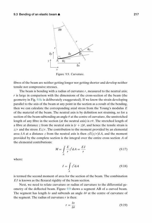
P1: KAE


9.3 Bending of an elastic beam ♣ 217

θ1

θ2

δθ

δs

r

r

A

B

x

y

δx

δy

Figure 9.9. Curvature.

fibres of the beam are neither getting longer nor getting shorter and develop neithertensile nor compressive stresses.

The beam is bending with a radius of curvature r , measured to the neutral axis;r is large in comparison with the dimensions of the cross-section of the beam (thegeometry in Fig. 9.8c is deliberately exaggerated). If we know the strain developingparallel to the axis of the beam at any point in the section as a result of the bending,then we can calculate the corresponding axial stress from the Young’s modulus Eof the material of the beam. The neutral axis is by definition not straining, so for asection of the beam subtending an angle θ at the centre of curvature, the unstretchedlength of any fibre in the section (at the neutral axis) is rθ . The stretched length ofa fibre at distance z from the neutral axis is (r + z)θ , and hence the tensile strain isz/r and the stress Ez/r . The contribution to the moment provided by an elementalarea δA at a distance z from the neutral axis is then zE(z/r)δA, and the momentprovided by the complete section is the integral over the entire cross section A ofthe elemental contributions:

M =∫A

Er

z2dA = EIr

(9.17)

where:

I =∫A

z2dA (9.18)

is termed the second moment of area for the section of the beam. The combinationEI is known as the flexural rigidity of the beam section.

Next, we need to relate curvature or radius of curvature to the differential ge-ometry of the deflected beam. Figure 9.9 shows a segment AB of a curved beam.The segment has length δs and subtends an angle δθ at the centre of curvature ofthe segment. The radius of curvature r is then:

r = δsδθ

(9.19)

P1: KAE



and the inverse of the radius is the curvature κ :

κ = 1r

= δθ

δs(9.20)

The length of the segment δs is given approximately by:

δs =√

(δx2 + δy2) (9.21)

The slope angle θ1 at A is related to the slope of the curve:

tan θ1 = dydx

(9.22)

and the slope angle θ2 at B:

tan θ2 = dydx

+ ddx

(dydx

)δx = dy

dx+ d2 y

dx2δx (9.23)

The subtended angle δθ is the difference between the slope angles at the two endsof the segment:

δθ = θ2 − θ1 (9.24)

so that:

tan δθ = tan(θ2 − θ1) = tan θ2 − tan θ1

1 + tan θ2 tan θ1

=d2 ydx2 δx

1 +(

dydx

)2

(9.25)

neglecting third order small quantities in the denominator.For an infinitesimal length of beam we can write tan δθ ≈ δθ , and then combin-

ing (9.25), (9.20) and (9.21) we find an expression for the curvature:

κ =d2 ydx2[

1 +(

dydx

)2]3/2 (9.26)

For a beam undergoing small deformations, we can write the curvature approxi-mately and simply as:

κ ≈ d2 ydx2

(9.27)

since (dy/dx)2 1. Then combination with (9.17) shows us that:

M = EId2 ydx2

(9.28)

The final step in generating the differential equation governing the mechanicalbehaviour of a beam in bending is shown in Fig. 9.10. An infinitesimal section ofbeam of length δx is loaded with a transverse force w per unit length. Imaginingthe section cut from a longer beam, there will be force resultants on each end of

P1: KAE


9.3 Bending of an elastic beam ♣ 219

wδx

δx

FM

F+δFM+δM

x

y

Figure 9.10. Element of beam.

the section: a shear force F and a bending moment M. In general, these will changewith position along the beam.

We have to declare and take care over our sign convention. Figure 9.10 showsa reference set of (x, y) axes with y, the transverse deflection of the beam, mea-sured positive downwards. From (9.27), positive curvature requires a slope dy/dxwhich increases with position x. We define a positive moment as one which tendsto encourage such a downward curvature – known as a hogging moment, with ten-sion in the upper fibres of the beam. We define a positive shear force as a clockwiseshear force, with the beam beyond the cut tending to pull down on the neighbouringsection of the beam. The directions of the moments and shear forces shown in Fig.9.10 are consistent with these definitions. The direction of the applied loading w ispositive in the direction y of deflection of the beam.

Vertical (transverse) equilibrium of the section tells us:

δF + wδx = 0 (9.29)

and moment equilibrium of the section tells us:

δM + F δx = 0 (9.30)

neglecting second order small quantities. Therefore, with (9.28):

F = −dMdx

= −EId3 ydx3

(9.31)

Combining these:

w = −dFdx

= d2 Mdx2

(9.32)

and, again substituting for the moment from (9.28):

w = EId4 ydx4

(9.33)

and this is the equation that we will use in our next examples of analytical soil-structure interaction.

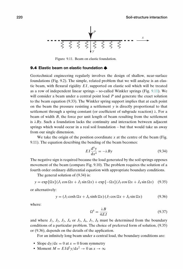
P1: KAE



P

x

y

Figure 9.11. Beam on elastic foundation.

9.4 Elastic beam on elastic foundation ♣Geotechnical engineering regularly involves the design of shallow, near-surfacefoundations (Fig. 9.2). The simple, related problem that we will analyse is an elas-tic beam, with flexural rigidity EI , supported on elastic soil which will be treatedas a row of independent linear springs – so-called Winkler springs (Fig. 9.11). Wewill consider a beam under a central point load P and generate the exact solutionto the beam equation (9.33). The Winkler spring support implies that at each pointon the beam the pressure resisting a settlement y is directly proportional to thatsettlement through a spring constant (or coefficient of subgrade reaction) λ. For abeam of width B, the force per unit length of beam resulting from the settlementis λBy. Such a foundation lacks the continuity and interaction between adjacentsprings which would occur in a real soil foundation – but that would take us awayfrom our single dimension.

We take the origin of the position coordinate x at the centre of the beam (Fig.9.11). The equation describing the bending of the beam becomes:

EId4 ydx4

= −λBy (9.34)

The negative sign is required because the load generated by the soil springs opposesmovement of the beam (compare Fig. 9.10). The problem requires the solution of afourth order ordinary differential equation with appropriate boundary conditions.

The general solution of (9.34) is:

y = exp [x] (J1 cos x + J2 sin x) + exp [−x] (J3 cos x + J4 sin x) (9.35)

or alternatively:

y = (J5 cosh x + J6 sinh x) (J7 cos x + J8 sin x) (9.36)

where:

4 = λB4EI

(9.37)

and where J1, J2, J3, J4 or J5, J6, J7, J8 must be determined from the boundaryconditions of a particular problem. The choice of preferred form of solution, (9.35)or (9.36), depends on the details of the application.

For an infinitely long beam under a central load, the boundary conditions are:

Slope dy/dx = 0 at x = 0 from symmetry Moment M = EId2 y/dx2 → 0 as x → ∞

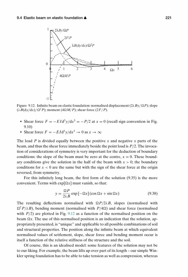
P1: KAE


9.4 Elastic beam on elastic foundation ♣ 221

0 1 2 3 4 5 6

1

-1

0

Ωx

2λBy/ΩP

λB(dy/dx)/Ω2P

4ΩM/P

2F/P

Figure 9.12. Infinite beam on elastic foundation: normalised displacement (2λBy/P); slope(λB(dy/dx)/2 P); moment (4M/P); shear force (2F/P).

Shear force F = −EId3 y/dx3 = −P/2 at x = 0 (recall sign convention in Fig.9.10)

Shear force F = −EId3 y/dx3 → 0 as x → ∞

The load P is divided equally between the positive x and negative x parts of thebeam, and thus the shear force immediately beside the point load is P/2. The invoca-tion of considerations of symmetry is very important for the deduction of boundaryconditions: the slope of the beam must be zero at the centre, x = 0. These bound-ary conditions give the solution in the half of the beam with x > 0; the boundaryconditions for x < 0 are the same but with the sign of the shear force at the originreversed, from symmetry.

For this infinitely long beam, the first form of the solution (9.35) is the moreconvenient. Terms with exp[x] must vanish, so that:

y = P2λB

exp [−x] (cos x + sin x) (9.38)

The resulting deflections normalised with P/2λB, slopes (normalised with2 P/λB), bending moment (normalised with P/4) and shear force (normalisedwith P/2) are plotted in Fig. 9.12 as a function of the normalised position on thebeam x. The use of this normalised position is an indication that the solution, ap-propriately presented, is “unique” and applicable to all possible combinations of soiland structural properties. The position along the infinite beam at which equivalentnormalised values of settlement, slope, shear force and bending moment occur isitself a function of the relative stiffness of the structure and the soil.

Of course, this is an idealised model: some features of the solution may not beto our liking. For example, the beam lifts up over part of its length – our simple Win-kler spring foundation has to be able to take tension as well as compression, whereas

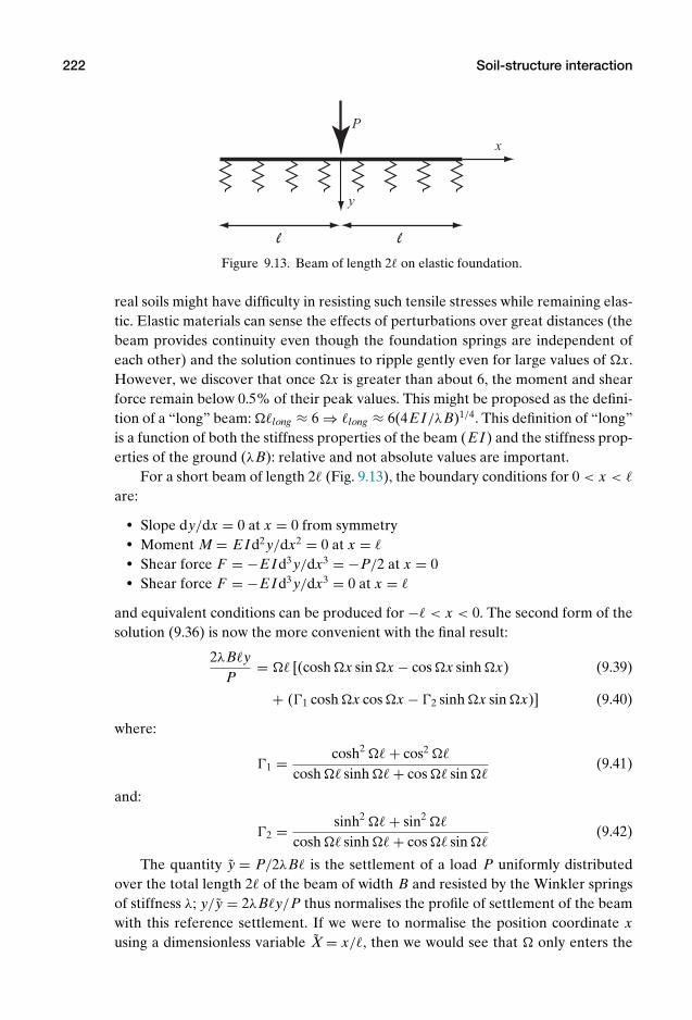
P1: KAE



P

x

y

l l

Figure 9.13. Beam of length 2 on elastic foundation.

real soils might have difficulty in resisting such tensile stresses while remaining elas-tic. Elastic materials can sense the effects of perturbations over great distances (thebeam provides continuity even though the foundation springs are independent ofeach other) and the solution continues to ripple gently even for large values of x.However, we discover that once x is greater than about 6, the moment and shearforce remain below 0.5% of their peak values. This might be proposed as the defini-tion of a “long” beam: long ≈ 6 ⇒ long ≈ 6(4EI/λB)1/4. This definition of “long”is a function of both the stiffness properties of the beam (EI) and the stiffness prop-erties of the ground (λB): relative and not absolute values are important.

For a short beam of length 2 (Fig. 9.13), the boundary conditions for 0 < x <

are:

Slope dy/dx = 0 at x = 0 from symmetry Moment M = EId2 y/dx2 = 0 at x = Shear force F = −EId3 y/dx3 = −P/2 at x = 0 Shear force F = −EId3 y/dx3 = 0 at x =

and equivalent conditions can be produced for − < x < 0. The second form of thesolution (9.36) is now the more convenient with the final result:

2λByP

= [(cosh x sin x − cos x sinh x) (9.39)

+ (1 cosh x cos x − 2 sinh x sin x)] (9.40)

where:

1 = cosh2 + cos2

cosh sinh + cos sin (9.41)

and:

2 = sinh2 + sin2

cosh sinh + cos sin (9.42)

The quantity y = P/2λB is the settlement of a load P uniformly distributedover the total length 2 of the beam of width B and resisted by the Winkler springsof stiffness λ; y/y = 2λBy/P thus normalises the profile of settlement of the beamwith this reference settlement. If we were to normalise the position coordinate xusing a dimensionless variable X = x/, then we would see that only enters the

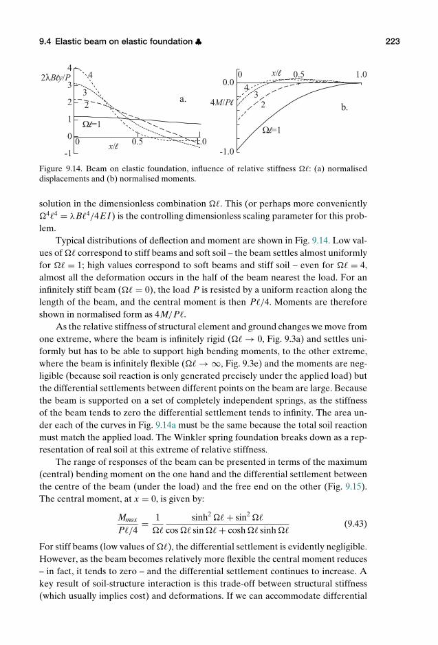
P1: KAE


9.4 Elastic beam on elastic foundation ♣ 223

0 0.5 1.0-1

0

1

2

3

4x/l

x/l

Ωl=1Ωl=1

233

2

42λBly/P 0 0.5 1.0

-1.0

0.04

4M/Pla.

b.

Figure 9.14. Beam on elastic foundation, influence of relative stiffness : (a) normaliseddisplacements and (b) normalised moments.

solution in the dimensionless combination . This (or perhaps more conveniently44 = λB4/4EI) is the controlling dimensionless scaling parameter for this prob-lem.

Typical distributions of deflection and moment are shown in Fig. 9.14. Low val-ues of correspond to stiff beams and soft soil – the beam settles almost uniformlyfor = 1; high values correspond to soft beams and stiff soil – even for = 4,almost all the deformation occurs in the half of the beam nearest the load. For aninfinitely stiff beam ( = 0), the load P is resisted by a uniform reaction along thelength of the beam, and the central moment is then P/4. Moments are thereforeshown in normalised form as 4M/P.

As the relative stiffness of structural element and ground changes we move fromone extreme, where the beam is infinitely rigid ( → 0, Fig. 9.3a) and settles uni-formly but has to be able to support high bending moments, to the other extreme,where the beam is infinitely flexible ( → ∞, Fig. 9.3e) and the moments are neg-ligible (because soil reaction is only generated precisely under the applied load) butthe differential settlements between different points on the beam are large. Becausethe beam is supported on a set of completely independent springs, as the stiffnessof the beam tends to zero the differential settlement tends to infinity. The area un-der each of the curves in Fig. 9.14a must be the same because the total soil reactionmust match the applied load. The Winkler spring foundation breaks down as a rep-resentation of real soil at this extreme of relative stiffness.

The range of responses of the beam can be presented in terms of the maximum(central) bending moment on the one hand and the differential settlement betweenthe centre of the beam (under the load) and the free end on the other (Fig. 9.15).The central moment, at x = 0, is given by:

Mmax

P/4= 1

sinh2 + sin2

cos sin + cosh sinh (9.43)

For stiff beams (low values of ), the differential settlement is evidently negligible.However, as the beam becomes relatively more flexible the central moment reduces– in fact, it tends to zero – and the differential settlement continues to increase. Akey result of soil-structure interaction is this trade-off between structural stiffness(which usually implies cost) and deformations. If we can accommodate differential

P1: KAE



1

0.5

0 0

0.05

0.1 1 10Ωl

4|Mmax|P/l2λBl∆y/P

moment differential settlement

Figure 9.15. Central moment and differential settlement for beam on elastic foundation asfunction of relative beam stiffness .

displacements of parts of our structure, then we may be able to economise on stiff-ness.

9.5 Pile under lateral loading ♣Now we return to the generalised analysis of the tent peg (Fig. 9.4) or laterallyloaded pile (Fig. 9.16). A pile of width B in an elastic soil loaded by a lateral forceP at the ground surface is analytically very similar to the beam on an elastic foun-dation. The one dimension of the analysis is now the position z down the pile (Fig.9.16a). The pressure generated on the pile by the elastic soil is directly proportionalto the relative movement of the pile and the soil according to a stiffness λ suppliedby a series of independent linear Winkler springs, which act identically whicheverway the pile moves relative to the soil (Fig. 9.16b, c). The governing equation for thebending of a beam resisted by loads proportional to the displacement is exactly thesame as (9.34), as are the general forms of the solution (9.35), (9.36). The boundaryconditions are slightly different.

For an infinitely long pile, the boundary conditions are: Moment M = EId2 y/dz2 = 0 at z = 0 Moment M = EId2 y/dz2 → 0 as z → ∞

z

P P

y

yo

y

spring force per unit

length of pile λB

a. b.c.

Figure 9.16. Laterally loaded pile in elastic soil.

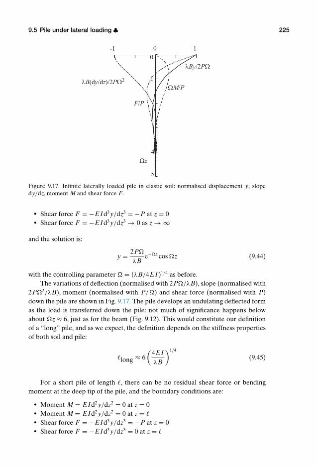
P1: KAE


9.5 Pile under lateral loading ♣ 225

0

1

4

5

Ωz

λBy/2PΩ

λB(dy/dz)/2PΩ2ΩM/P

F/P

-1 0 1

Figure 9.17. Infinite laterally loaded pile in elastic soil: normalised displacement y, slopedy/dz, moment M and shear force F .

Shear force F = −EId3 y/dz3 = −P at z = 0 Shear force F = −EId3 y/dz3 → 0 as z → ∞

and the solution is:

y = 2P

λBe−z cos z (9.44)

with the controlling parameter = (λB/4EI)1/4 as before.The variations of deflection (normalised with 2P/λB), slope (normalised with

2P2/λB), moment (normalised with P/) and shear force (normalised with P)down the pile are shown in Fig. 9.17. The pile develops an undulating deflected formas the load is transferred down the pile: not much of significance happens belowabout z ≈ 6, just as for the beam (Fig. 9.12). This would constitute our definitionof a “long” pile, and as we expect, the definition depends on the stiffness propertiesof both soil and pile:

long ≈ 6(

4EIλB

)1/4

(9.45)

For a short pile of length , there can be no residual shear force or bendingmoment at the deep tip of the pile, and the boundary conditions are:

Moment M = EId2 y/dz2 = 0 at z = 0 Moment M = EId2 y/dz2 = 0 at z = Shear force F = −EId3 y/dz3 = −P at z = 0 Shear force F = −EId3 y/dz3 = 0 at z =

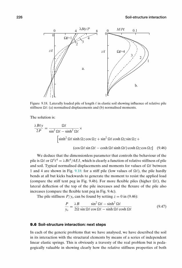
P1: KAE



00 0

04

2

2

8

4

1

1

1

z/l z/l

λBly/P

Ωl=1

Ωl=4

3

3

a.

0.1M/Pl

b.

Figure 9.18. Laterally loaded pile of length in elastic soil showing influence of relative pilestiffness : (a) normalised displacements and (b) normalised moments.

The solution is:

λBy2P

=

sin2 − sinh2 ×

[sinh2 sinh zcos z + sin2 cosh zsin z+

(cos sin − cosh sinh ) cosh zcos z] (9.46)

We deduce that the dimensionless parameter that controls the behaviour of thepile is or 44 = λB4/4EI , which is clearly a function of relative stiffness of pileand soil. Typical normalised displacements and moments for values of between1 and 4 are shown in Fig. 9.18: for a stiff pile (low values of ), the pile hardlybends at all but kicks backwards to generate the moment to resist the applied load(compare the stiff tent peg in Fig. 9.4b). For more flexible piles (higher ), thelateral deflection of the top of the pile increases and the flexure of the pile alsoincreases (compare the flexible tent peg in Fig. 9.4c).

The pile stiffness P/yo can be found by setting z = 0 in (9.46):

Pyo

= λB2

sin2 − sinh2

sin cos − sinh cosh (9.47)

9.6 Soil-structure interaction: next steps

In each of the generic problems that we have analysed, we have described the soilin its interaction with the structural elements by means of a series of independentlinear elastic springs. This is obviously a travesty of the real problem but is peda-gogically valuable in showing clearly how the relative stiffness properties of both

P1: KAE


9.8 Exercises: Soil-structure interaction 227

the structural elements and the soil springs interact to control the overall characterof the soil-structure interaction. The analyses also show the way in which changingthe relative stiffness exchanges deformations for structural resultants. Control ofdisplacements requires stiffer structures able to sustain higher forces or moments:the designer needs to decide on the desirable balance.

We have described both the structural elements and the soil as strictly linearand elastic in their response to changing loads. Elasticity formally requires that theapplication and removal of any load should leave no permanent deformation. Lin-earity of response is an extra constraint. In reality, although the structural elementsmay behave elastically, it is very unlikely that the behaviour of the soil interactingwith the structural element will be linear and elastic except under extremely smalldeformations: we have seen the nonlinearity of soil stiffness in Sections 4.5 and 8.11.It is possible to extend our analysis to include non-linearity of the spring modelwhile still maintaining the one-dimensional treatment, but this would require theuse of numerical solution techniques. However, no matter by what route nonlinearor two/three-dimensional problems of soil-structure interaction are analysed, it willalways be found that the emergent response is dependent on the relative stiffnessproperties of the soil and the structural elements.

9.7 Summary


1. Many geotechnical prototypes include structural elements. Calculation of theresponse of such prototypes under working loads – serviceability limit states –requires consideration of stiffness characteristics of both the geotechnical andstructural materials.

2. The significance of soil-structure interaction depends on relative stiffness ofstructure and ground.

3. Analyses of elastic structures interacting with elastic ground are capable of ex-act solution in terms of dimensionless relative stiffnesses.

4. Examples of soil-structure interaction provide opportunities to integrate as-pects of civil engineering education, which are often treated entirely indepen-dently.

9.8 Exercises: Soil-structure interaction

1. A axially loaded pile of radius ro = 0.5 m and length = 40 m is made of con-crete with Young’s modulus Ep = 25 GPa. It is driven through soil with shaftshear transfer stiffness λ = 4 MPa and ends with its toe in firmer ground withbase transfer stiffness λb = 100/π MPa. The base of the pile is under-reamedto a radius of rb = 1 m. What is the axial stiffness of the pile Pt/ςt , and whatproportion of the load reaches the toe of the pile?

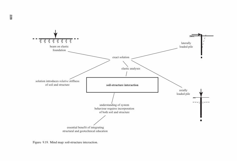
P1:K

AE

OneD

im00a

CU

US648/M

uir978

0521

517737

August17,2009

19:12

soil-structure interaction

elastic analyses

exact solution

solution introduces relative stiffness of soil and structure

understanding of system behaviour requires incorporation

of both soil and structure

beam on elastic foundation

laterally loaded pile

axially loaded pile

essential benefit of integrating structural and geotechnical education

Figure 9.19. Mind map: soil-structure interaction.

228

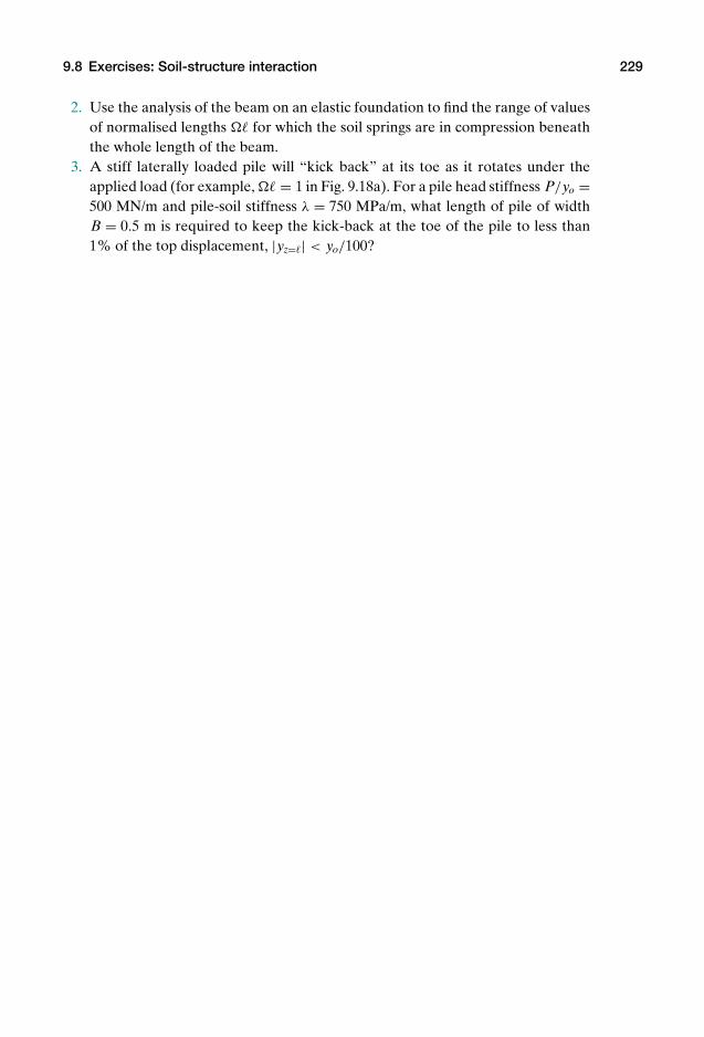
P1: KAE


9.8 Exercises: Soil-structure interaction 229

2. Use the analysis of the beam on an elastic foundation to find the range of valuesof normalised lengths for which the soil springs are in compression beneaththe whole length of the beam.

3. A stiff laterally loaded pile will “kick back” at its toe as it rotates under theapplied load (for example, = 1 in Fig. 9.18a). For a pile head stiffness P/yo =500 MN/m and pile-soil stiffness λ = 750 MPa/m, what length of pile of widthB = 0.5 m is required to keep the kick-back at the toe of the pile to less than1% of the top displacement, |yz=| < yo/100?

P1: KAE


10 Envoi

10.1 Summary

Each chapter has ended with a summary of the key points. Here it is appropriate toreiterate the primary intentions of this book and to point the way towards the nextstages of soil mechanics education.

There are two themes which have been developed in this book: The model of soil stiffness and strength links effective stresses and density.

Changes in mechanical behaviour of soils can only be properly understood whenthe stresses and volumetric packing are considered in parallel. The role that his-tory plays in changes in density – which tend to be locked into soils as loadsare applied and then removed – is key for the subsequent understanding ofthe strength of soils. There is then a link with permeability and the ease withwhich water (or other pore fluid) can move through the voids of the soil, andthus the ability of the soil to respond rapidly to changes in stress. The conceptsof drained and undrained response again bring together the thoughts about ef-fective stresses and volumetric packing. This is the essence of critical state soilmechanics,1 which at its simplest level (Fig. 10.1) tells us that we cannot hope tounderstand the behaviour of soils unless we think all the time in parallel of thechanges in effective stress and of density.

The second theme is that it is perhaps surprising how far we can get in the pre-sentation of fundamental ideas of soil mechanics without straying beyond thesingle dimension. We have seen that there are a number of modestly realisticapplications which can be discussed with only one dimension in the govern-ing equations – examples of consolidation and gain in strength, slope stability,and soil-structure interaction show basic features of response on which we maywish to elaborate in future multi-dimensional analyses but whose messages willremain intact. The final application, soil-structure interaction, is seen as partic-ularly important because the teaching of civil engineering in universities tendstoo much to separate soil mechanics/geotechnical engineering and structuralengineering in a way that leads specialists in each area to lose sight of the need

1 Schofield, A.N. & Wroth, C.P. (1968) Critical state soil mechanics. McGraw-Hill, London; MuirWood, D. (1990) Soil behaviour and critical state soil mechanics. Cambridge University Press.

230

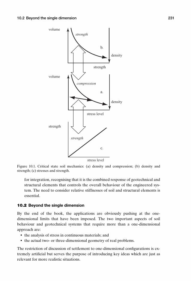
P1: KAE


10.2 Beyond the single dimension 231

volume

volume

density

density

compression

strength

strength

strength

stress level

stress level

strength

a.

c.

b.

Figure 10.1. Critical state soil mechanics: (a) density and compression; (b) density andstrength; (c) stresses and strength.

for integration, recognising that it is the combined response of geotechnical andstructural elements that controls the overall behaviour of the engineered sys-tem. The need to consider relative stiffnesses of soil and structural elements isessential.

10.2 Beyond the single dimension

By the end of the book, the applications are obviously pushing at the one-dimensional limits that have been imposed. The two important aspects of soilbehaviour and geotechnical systems that require more than a one-dimensionalapproach are:

the analysis of stress in continuous materials; and the actual two- or three-dimensional geometry of real problems.

The restriction of discussion of settlement to one-dimensional configurations is ex-tremely artificial but serves the purpose of introducing key ideas which are just asrelevant for more realistic situations.

P1: KAE


Exercises: numerical answers

Chapter 2

Answers: Section 2.5

1. 3.92 kN2. 15.7 kPa on two feet, 31.4 kPa on one foot3. 7.34 Mg4. 2.43 kPa5. 0.45 m on one foot, 0.32 m on two feet6. 173×10−6 N


1. 0, 58.9, 247.2, 360.0 kPa2. σz: 0, 58.9, 247.2, 360.0 kPa; u: 0, 29.4, 147.2, 196.2 kPa; σ ′

z: 0, 29.4, 100.1,163.8 kPa

3. σz: 0, 58.9, 247.2, 360.0 kPa; u: 0/−14.7, 14.7, 132.4, 181.5 kPa; σ ′z: 0/14.7, 47.1,

114.8, 178.5 kPa4. σz: 53.0, 131.5, 168.7 kPa; u: 0, 39.2, 58.9 kPa; σ ′

z: 53.0, 92.2, 109.9 kPa5. σz: 57.4, 135.9, 173.1 kPa; u: 14.7, 53.9, 73.6 kPa; σ ′

z: 42.7, 81.9, 99.6 kPa; σ ′z:

−10.3, −10.3, −10.3 kPa6. maximum 66.7 kPa; minimum 43.2 kPa

Chapter 3

Answers: Section 3.8.1

1. (c); 2. (a); 3. (c); 4. (b); 5. (c); 6. (b); 7. (c); 8. (a); 9. (b), (c), (a), (b), (c), (a), (b);10. (a), (c), (a), (a), (b), (a), (b); 11. (b), (a), (c), (a), (a), (b), (b), (b), (b)

Answers: Section 3.8.2

1. w = 0.2, v = 1.8, e = 0.8, Sr = 0.6752. e = 0.93, v = 1.93, ρd = 1.37 Mg/m3, ρ = 1.78 Mg/m3

232

P1: KAE


Exercises: numerical answers 233

3. ρ = 2.11 Mg/m3, ρd = 1.89 Mg/m3, v = 1.43, e = 0.43, w = 0.11, Sr = 0.724. w = 31.3%, e = 0.837, v = 1.8375. e = 1.078, v = 2.078, w = 39.9%, ρ = 1.82 Mg/m3, ρd = 1.30 Mg/m3

6. Sr = 96%, e = 0.847, v = 1.847, ρd = 1.46 Mg/m3

7. ρ = 2 Mg/m3, e = 0.594, v = 1.594, Sr = 77%, ρd = 1.71 Mg/m3

8. 2.55 km, 4658 loads

Chapter 4


1. 10 GPa, 108 MPa, 12.2 MPa, 1.5 MPa2. 0.00015%, 0.014%, 0.123%, 1%3. 0.0015%, 0.13%, 1.0%, 6.9%4. 0.345 m5. 1.55%, 0.062 m6. (a) before 10.8 kPa, 27.5 kPa, 39.2 kPa, 51.0 kPa, 62.8 kPa; after 17.6 kPa,

41.2 kPa, 53.0 kPa, 64.7 kPa, 76.5 kPa; (b) 0.15%, 0.39%, 0.32%, 0.27%, 0.24%;0.027 m

7. 62.8 kPa, 45.1 kPa; ocr varies between 1 and 1.4; α ≈ 0.6?, χ ≈ 100?; Eo variesbetween about 6200 kPa and 7560 kPa, average ≈ 6900 kPa; settlement 20 mm

8. heave on excavation 0.013 m; settlement for 25 kPa 0.033 m; settlement for40 kPa 0.070 m

9. χnc = 9.15, χoc = 33.94, αnc = αoc = 1.05 (or αnc = αoc = 1, χnc = 9.2, χoc =34.5)

Chapter 5


1. 1.96, 4.91, 7.85 kPa; 1.96, 0.98, 0 kPa; down; 0.067 m/s2. 5 × 10−8 m/s downward3. 98.1, 73.6 kPa; 10−7 m/s downwards4. 14.71 kPa, no flow; 24.52 kPa, no flow; 39.24 kPa, up 0.6 × 10−4 m/s; 53.95 kPa,

no flow; 34.34 kPa, down 0.8 × 10−4 m/s5. 4 m, 11 m, 39.24 kPa, 107.91 kPa, 7.5 × 10−8 m/s6. total heads: 1.5 m, 1.5 m; pressure heads: 5.5 m, 9.5 m; flow rate: 3.75 × 10−8 m/s;

total head drop across sand: 0.015 m7. horizontal: kh = 1.35 × 10−3 m/s; vertical: kv = 14.3 × 10−5 m/s8. total head: −1 m, +3 m; pressure head: 2 m, 10 m; pore pressure: 19.6 kPa,

98.1 kPa; total stress: 53.46 kPa, 131.94 kPa; effective stress: 33.84 kPa,33.84 kPa; flow rate 1 × 10−8 m/s

9. k = 4.8 × 10−8 m/s

P1: KAE


234 Exercises: numerical answers

10. ρ = 2.06 Mg/m3; at base of prototype: σ ′z = 208.85 kPa; at base of model without

downward flow: σ ′z = 10.44 kPa; seepage force ρwgi acting over height of model

supplies the difference: i = 20.2 or total head difference of 20.2 m or 198.4 kPa;flow rate: 0.0016 m3/s=1.6 litres/sec

Chapter 6


1. 140 kPa2. 60 kPa, 140 kPa, 0%3. 200 kPa, 10 kPa, 190 kPa, 3.33%4. 152.8 kPa, 152.8 kPa5. 229.2 kPa, 152.8 kPa, 76.4 kPa, no change6. 229.2 kPa, 229.2 kPa, 0 kPa, 4.4%, 19.13 mm7. values of σz, u, σ ′

z at the base of the sand and at the top and bottom of clay layerinitially: 33, 0, 33; 33, 0, 33; 213, 98.1, 114.9 kPaimmediately after sand is removed: 16.5, 0, 16.5; 16.5, −16.5, 33; 196.5, 81.6,114.9 kPalong term: 16.5, 0, 16.5; 16.5, 0, 16.5, 196.5, 98.1, 98.4 kPaheave: no change immediately, 0.097 m in long term

8. values of σz, u, σ ′z at the top and bottom of the clay in the long term 33, 0, 33;

213, 65, 148 kPa; long term settlement 0.097 m9. values of σz, u, σ ′

z at base of sand and at top and bottom of clayinitially: 57.01, 19.62, 37.39; 57.01, 19.62, 37.39; 137.01, 58.86, 78.15 kPaimmediately after excavation: 48.73, 19.62, 29.11; 48.73, 11.34, 37.39; 128.73,50.58, 78.15 kPalong term: 48.73, 19.62, 29.11; 48.73, 19.62, 29.11; 128.73, 58.86, 69.87 kPalong term heave: 0.021 m

10. initially σz = 19z, u = 9z, σ ′z = 10z; finally σz = 19z, u = 9.81z, σ ′

z = 9.19z; aver-age increase in pore pressure and reduction in vertical effective stress 121.5 kPa;heave 0.3375 m

Chapter 7


1. cv = 1.5 × 10−7 m2/s; consolidation front reaches centre at T = 1/12, t = 54.5 s;80% consolidation for T = 0.485, t = 317 s

2. L = 1.5 m, time for 80% consolidation t = 82.5 days; independent of stress in-crement

3. cv = 3.14 × 10−9 m2/s; 10.4 years4. 139 days

P1: KAE


Exercises: numerical answers 235

5. Stage 1: S =√

(π − 2)T until T = TA = (π − 2)/π2; Stage 2: S = 1 −2π

exp−π2(T − TA)/46. Intersection slope ×1.1: S = 0.8527, T = 0.6910, cv = 16.5 × 10−9 m2/s, k =

51.2 × 10−12 m/s; intersection slope ×1.2: S = 0.9259, T = 0.9695, cv = 16.2 ×10−9 m2/s, k = 50.8 × 10−12 m/s; S = 0.9 for T = 0.848, 10.2 yrs (slope×1.1),10.4 yrs (slope×1/2).

7. Intersection slope ×1.1: S = 0.8965, T = 0.852, cv = 20.4 × 10−9 m2/s, k =60.2 × 10−12 m/s; intersection slope ×1.2: S = 0.9485, T = 1.135, cv = 19.0 ×10−9 m2/s, k = 58.1 × 10−12 m/s; S = 0.9 for T = 0.866, 8.4 yrs (slope×1.1),9.0 yrs (slope×1.2).

Chapter 8


1. 120 kPa, 36 kPa2. 130 kPa, 120 kPa, 36 kPa3. 250 kPa, 75 kPa; density increases as water is squeezed out as effective stress

and strength increase4. mobilised strength 18.3 kPa; mobilised angle of friction 19.7 – close to available

frictional strength 21

5. ru = −0.22 throughout; pore pressure at depth 5 m: u = −20.4 kPa; with seep-age parallel to slope φmob = 58.8; ru = 0.327; support force 2.94 MN/m

6. ds = d/√

37. normal compression line

ln(v1

v

)= 1

χ(1 − α)

[(σ ′

z

σre f

)1−α

−(

σ ′z1

σre f

)1−α]

if α = 1, v = v1[σ ′z1/σ

′z](1/χ), where v = v1 for σ ′

z = σz1.(a) normal compression v = 1.866; drained τ f = 46.63 kPa, v f = 1.752;undrained τ f = 23.27 kPa, σ ′

zf = 49.90 kPa. (b) normal compression v =1.820; drained τ f = 233.15 kPa, v f = 1.497; undrained τ f = 30.76 kPa, σ ′

zf =65.96 kPa. (c) overconsolidated v = 1.832; drained τ f = 46.63 kPa, v f = 1.752;undrained τ f = 28.71 kPa, σ ′

zf = 61.57 kPa.(d) Normal compression to 100 kPa: drained τ = 23.53 kPa, σ ′

z = 100 kPa, v =1.863, εz = 0.19%, εs = 0.59%; undrained τ = 18.24 kPa, σ ′

z = 78.25 kPa, v =1.866, εz = 0, εs = 0.71%.Normal compression to 500 kPa: drained τ = 117.0 kPa, σ ′

z = 500 kPa, v =1.814, εz = 0.37%, εs = 1.21%; undrained τ = 54.57 kPa, σ ′

z = 234.1 kPa, v =1.820, εz = 0, εs = 4.54%.Overconsolidation to 100 kPa: drained τ = 23.52 kPa, σ ′

z = 100 kPa, v = 1.828,εz = 0.18%, εs = 0.56%; undrained τ = 11.76 kPa, σ ′

z = 50.55 kPa, v = 1.832,εz = 0, εs = 0.42%.

P1: KAE


236 Exercises: numerical answers

Chapter 9


1. pile stiffness Pt/ςt = 644 MN/m; proportion of load at toe Pb/Pt = 0.0622. ≤ π/23. = 3.772, = 10.07 m

P1: KAE


Index

acceleration, 91angle of repose, 191–193aquifer, 111Archimedes, 24, 26, 59

Balodis, A., 42beam, 216–219bending moment, 222, 223Bernoulli’s equation, 90, 93–95, 97, 101body force, 13Bolton, M.D., 76boulders, 53, 54boundary conditions, 162, 220, 222, 224, 225bridge

abutment, 6arch, 5

buoyancy, 26, 59, 188Buzan, T., 11

capillary rise, 31Carman, 102Carrier, W.D., 102Carslaw, H.S., 159clay, 47, 49, 54–56, 64, 75, 83, 99, 101, 102, 123,

127, 140, 141, 145, 177, 182, 187, 193Drammen, 42mineral, 43, 54, 102, 195Weald, 42

coefficientof consolidation, 144, 145, 147, 149, 150, 157of permeability, see permeabilityof sub-grade reaction, 220of uniformity, 54, 55

collapse, 169Collin, 170–172compaction, 49–52, 64compression

confined, 72, 73, 76unconfined, 71, 72

conic section, 143consolidation, ix, 127, 138

degree of, 147, 163finite layer, 161front, 141, 144, 147, 160, 161, 165secondary, 151

Coulomb, 3creep, 151critical state soil mechanics, ix, 230

dam, 2, 9, 10, 49, 101, 110Darcy’s Law, 100–105, 123, 140, 141, 151, 156,

160, 165datum, 90, 94, 123deformation, 4, 6density, 47, 87, 230

bulk, 44, 45, 49buoyant, 188, 190dry, 45, 47, 50, 51, 174mineral, 174relative, 62saturated, 45, 47, 190water, 24, 41

diffusion equation, 138, 165dilatancy, 174, 175, 177, 198–200dimensional analysis, 57, 58, 194down-drag, 182–185drained response, 129, 136, 177–179, 200, 201,

205, 230Dupuit, J., 103

Earth, 14, 15, 37, 41, 52earthquake, 7, 8, 129effective stress, 28–32, 37, 46, 76, 90, 128, 134, 141,

142, 165, 174, 177, 202, 230Principle of, 29, 37, 46, 129, 134, 140, 157, 193

elasticity, 67, 68, 74, 76, 82, 83, 87, 182, 208,211, 227

electrical resistors, 108Elson, W.K., 212embankment, 6end bearing, 169, 211equilibrium, 12, 13, 16, 18–20, 26, 28–31, 37, 46

237

P1: KAE


238 Index

erosion, 52error function, 159excavation, 4, 8

fall-cone, 193–195Fleming, W.G.K., 212Forchheimer, P., 103foundation, 6, 7, 170, 171, 208–210, 220–224Fourier series, 163, 165friction, 174, 203

angle of, 174mobilised, 187, 189–191

gravel, 47, 52, 54, 64, 99, 101, 102, 123, 127,129, 177

gravitational constant, 14gravity, 13–16, 41, 93, 194

hardness, 52, 54Hazen, 102head

elevation, 93–95, 101, 109, 123, 189pressure, 93–95, 101, 123, 189total, 93–95, 97, 100, 101, 104, 106–113, 123, 138,

140, 141, 156, 165, 188, 189Henkel, D.J., 205Hooke’s Law, 72, 74, 75, 82, 87hydraulic gradient, 100, 104, 109, 123, 141,

146, 156critical, 110

hydrostatics, 23–26, 90

isochrone, 142, 145, 148, 163, 165parabolic, 142, 144, 146, 149, 151, 156, 160,

161, 165

Jaeger, J.C., 159Janbu, N., 76, 77

kinetic energy, 93, 94, 101Kolbuszewski, J.J., 62Kozeny, 102

laboratory test, 47, 54, 56, 57, 61, 149, 151,191, 192

landslide, 90, 91, 170liquid limit, 195

mass, 15, 37McDowell, G.R., 76mind map, 11, 37, 62, 87, 121, 134, 165,

203, 227minerals, 52modelling, 126modulus number, 77, 83, 87Moh hardness scale, 52moisture content, see water contentMoon, 15, 41Muir Wood, D., 230

NewtonLaw of Gravitational attraction, 13, 14Law of Motion, 12, 15, 16, 37, 90

normal compression, 82, 83, 179, 180, 196

oedometer, 71, 72, 87, 127, 128, 149–151, 179overconsolidation, 82, 83, 87, 179–181, 196

ratio, 83, 87, 180, 196

Palmer, A.C., 57, 194parabola, 143, 144particle

breakage, 76shape, 41, 52, 61, 62, 127size, 52, 54, 55, 62, 64, 99, 123, 127

distribution, 54–56, 59, 64penetration test, 193permeability, 100, 101, 123, 127–129, 134, 136, 141,

151, 158, 176, 179, 230layered soil, 107, 123specific, 100

permeameterconstant head, 105, 106, 123falling head, 104, 106, 123

piezometer, 94, 95pile, 6, 8, 169, 170, 181–185, 210–215, 224–226

axial load, 211–215sheet, 8, 9

piping, 110, 123Poiseuille’s equation, 96, 99–102, 111, 128Poisson’s ratio, 69, 71–75, 82, 182pore pressure, 29, 37, 46, 90, 127, 128, 134, 165

excess, 128, 138–142, 156, 157, 165porosity, 44, 64potential energy, 93preconsolidation pressure, 180pycnometer, 48

quartz, 52

radial flow, 111, 123Randolph, M.F., 212Ransome, A., 16, 17retaining structure, 3, 7, 49Reynolds, 176Reynolds’ number, 103, 104Roberts, A.J., ixRobertson, D., 76

Saint Exupery, A. de, 16sand, 42, 47, 49, 52, 54, 56, 64, 75, 102, 103, 127,

129, 140, 145, 177, 182dense, 61, 175loose, 61, 175

saturationdegree of, 44, 48, 50, 51, 64

scanning electron micrograph, 42, 55Schofield, A.N., 142, 230sedimentation, 60, 64

P1: KAE


Index 239

seepage, 9, 189–191force, 109, 123velocity, 101

serviceability limit state, 3, 67, 169, 183settlement, 142, 145, 160

differential, 209, 223dimensionless, 149, 160

shaft resistance, 169, 181–183, 211shape function, 142shear box, 171–173, 175, 195, 199, 203shear force, 222shearing resistance

angle of, 174, 182, 187, 191shingle, 42, 56, 103sieving, 57, 64silt, 54simple harmonic motion, 162Skempton, A.W., 205slip surface, 170, 171, 186, 203slope, 91, 170, 171, 230

infinite, 185–191soil, 1soil mineral, 43, 77, 127, 191soil-structure interaction, ix, 8, 208–227,

230pile under lateral loading, 226

specific gravity, 41, 43, 47, 48, 191bottle, see pycnometer

specific surface, 56, 102specific volume, 43, 45, 50, 51, 64, 174, 178,

180, 197spherical flow, 112standpipe, 24, 28, 93–95Statens Jarnvagars Geotekniska Kommission,

193, 194steel balls, 176, 177stiffness, 3, 67, 169, 230

confined, 72, 74–76, 127, 142, 143, 151,158, 196

relative, 208, 213, 215, 222, 226, 227, 231stiffness exponent, 76Stokes’ Law, 57, 59strain

axial, 68natural, 70, 71true, 70, 71, 78, 79volumetric, 69

strength, 3, 13, 67, 169, 174, 230frictional, 174mobilised, 198peak, 173, 197ultimate, 173, 174, 197

stress, 16–18effective, see effective stressnormal, 18principal, 73shear, 18, 20, 57total, see total stress

stress-dilatancy relationship, 198, 199surface tension, 31, 32, 192, 193symmetry, 20, 145, 186, 221, 222

Taylor, D.W., 172, 173time

dimensionless, 147–149, 158, 161total stress, 28–32, 37, 46, 90, 128, 134, 165transport, 52, 64

by air, 52by gravity, 52by ice, 52–54by water, 52–54

tunnel, 4, 5

ultimate limit state, 67, 169, 182, 183, 185under-reaming, 214undrained response, 129, 136, 177–181, 187,

193–195, 200–202, 205, 230unit weight, 41, 47

bulk, 46buoyant, 46water, 41, 46

viscosity, 57, 58, 96, 101, 103of water, 57, 58

void ratio, 43, 47, 48, 50, 56, 64, 101, 191air, 44, 50, 51maximum, 62minimum, 62

volume fraction, 44

watercontent, 44, 47, 50, 51, 64sea, 24, 41table, 23, 28–30, 32, 46, 90

weathering, 52, 56, 64weight, 15, 37Weltman, A.J., 212Winkler springs, 220–223Wood, D.M., 195Wroth, C.P., 142, 176, 177, 230

Young’s modulus, 68, 71–75, 82, 213

Zelikson, A., 126

Soil mechanics a_one-dimensional_introduction_wood

Documents

examples of soil

soil behaviour

shearing of soil

c david muir wood

publication data muir

universities of cambridge

book chapters

hardback isbn