SOFTWARE SYSTEM DEFECT CONTENT PREDICTION FROM DEVELOPMENT PROCESS AND PRODUCT CHARACTERISTICS by Allen Peter Nikora A Dissertation Presented to the FACULTY OF THE GRADUATE SCHOOL UNIVERSITY OF SOUTHERN CALIFORNIA In Partial Fulfillment of the Requirements for the Degree DOCTOR OF PHILOSOPHY (Computer Science) May 1998 Copyright 1998 Allen Peter Nikora

Welcome message from author
This document is posted to help you gain knowledge. Please leave a comment to let me know what you think about it! Share it to your friends and learn new things together.
Transcript

SOFTWARE SYSTEM DEFECT CONTENT
PREDICTION FROM
DEVELOPMENT PROCESS AND
PRODUCT CHARACTERISTICS
by
Allen Peter Nikora
A Dissertation Presented to the
FACULTY OF THE GRADUATE SCHOOL
UNIVERSITY OF SOUTHERN CALIFORNIA
In Partial Fulfillment of the
Requirements for the Degree
DOCTOR OF PHILOSOPHY
(Computer Science)
May 1998
Copyright 1998 Allen Peter Nikora

ii
Acknowledgments
The author wishes to acknowledge the NASA Independent Validation andVerification (IV&V) Facility and the United States Air Force Operational and TestEvaluation Center (AFOTEC) for their support of portions of the work describedherein. The author also wishes to acknowledge the support provided by theCASSINI project at the Jet Propulsion Laboratory.
iii
Table of Contents
PART I: INTRODUCTION.................................................................1
1. INTRODUCTION TO SOFTWARE RELIABILITYMODELING .................................................................................2
1.1 The Software Reliability Issue ................................................................. 21.2 Definitions .................................................................................................. 51.3 Software Reliability Model Descriptions ................................................ 6
1.3.1 The Jelinski-Moranda and Shooman Models ...................................... 71.3.2 Other Exponential Software Reliability Models.................................. 8
1.3.2.1 Non-Homogeneous Poisson Process Model ................................ 91.3.2.2 Musa-Okumoto Logarithmic Poisson Model ............................. 10
1.3.3 Littlewood-Verrall Bayesian Model .................................................. 121.4 Benefits of Software Reliability Modeling ............................................ 141.5 Limitations of Software Reliability Modeling ...................................... 18
1.5.1 Applicability of Assumptions ............................................................ 181.5.2 Availability of Required Data............................................................ 221.5.3 The Nature of Reliability Model Predictions..................................... 241.5.4 Applicable Development Phases ....................................................... 25
PART II: RELATED WORK.............................................................27
2. CURRENT PRETEST RELIABILITY PREDICTIONMETHODS .................................................................................28
2.1 Rome Air Development Center (RADC) Model ................................... 282.2 Defect Content Estimation Based on Relative Complexity ................. 332.3 Phase-Based Model ................................................................................. 352.4 Jet Propulsion Laboratory Empirical Model ....................................... 382.5 Classification Methods............................................................................ 402.6 Limitations of the Models ....................................................................... 41
2.6.1 RADC Model..................................................................................... 412.6.2 Models Based on Relative Complexity ............................................. 432.6.3 Phase-Based model ............................................................................ 452.6.4 JPL Empirical Model ......................................................................... 472.6.5 Classification Methods ...................................................................... 482.6.6 A General Discussion of Predictive Model Limitations.................... 50
PART III: CONTRIBUTION............................................................52
iv
3. A DEFECT CONTENT PREDICTION MODEL ....................533.1 Factors Influencing Introduction of Defects......................................... 573.2 A Model for the Rate of Defect Insertion.............................................. 603.3 Measuring the Evolution of a Software System ................................... 62
3.3.1 A Measurement Baseline................................................................... 623.3.2 Module Sets And Versions ................................................................ 683.3.3 Code Churn and Code Deltas ............................................................ 713.3.4 Obtaining Average Build Values....................................................... 733.3.5 Software Evolution And The Defect Injection Process ..................... 773.3.6 Measuring Changes in the Development Process.............................. 79
3.4 Use of the Model ...................................................................................... 803.4.1 Estimating Residual Defect Content at the System and Module
Levels................................................................................................. 813.4.2 Forecasting Residual Defect Content at the System Level ................ 86
3.4.2.1 Birth and Death Model Implementation..................................... 913.4.2.2 Implementation Issues................................................................ 95
3.5 Limitations of the Model......................................................................... 97
4. DATA SOURCES .....................................................................103
5. MEASUREMENT TECHNIQUES AND ISSUES.................1065.1 Measuring the Structure of Evolving Systems ................................... 1065.2 Counting Defects ................................................................................... 107
5.2.1 What is a Defect?............................................................................. 1095.2.2 The Relationship Between Defects and Failures ............................. 1105.2.3 Rules for Identifying and Counting Defects .................................... 114
6. DEFECT INSERTION RATES ..............................................1266.1 Determination of the Defect Insertion Rate ........................................ 127
6.1.1 Correlations...................................................................................... 1286.1.2 Linear Regressions........................................................................... 1306.1.3 Linear vs. Nonlinear Model of Defect Insertion Rate...................... 1356.1.4 Effect of Development Team Experience on Defect Insertion
Rate .................................................................................................. 1376.1.5 Crossvalidation ................................................................................ 1406.1.6 Analysis of Residuals....................................................................... 1466.1.7 Defect Insertion Rate – Summary.................................................... 149
6.2 Forecasting Residual Defect Content .................................................. 1506.2.1 Defect Insertion Rate ....................................................................... 1516.2.2 Determining the Defect Removal Rate............................................ 1526.2.3 Forecasting Results .......................................................................... 156
v
7. SUMMARY AND CONCLUSIONS ........................................159
8. RECOMMENDATIONS FOR FURTHER WORK................1678.1 Measuring System Structure During Earlier Phases......................... 1678.2 Counting Defects ................................................................................... 168
PART IV: REFERENCES AND APPENDICES...........................173
9. REFERENCES.........................................................................174
10. COMPUTING THE DISTRIBUTION OF REMAININGDEFECTS.................................................................................179
11. SUMMARY OF ANALYSIS - FROM RADC TR-87-171VOLUME 1 TABLE 5-22.........................................................189
12. OBSERVED AND ESTIMATED DISTRIBUTION OFDEFECTS PER “N” FAILURES ...........................................190
12.1 Tabulated Values for the Distribution of the Number ofDefects for 1 Failure.............................................................................. 190
12.2 Convolution of Distributions................................................................ 19012.3 Expected Number of Defects and Hinge Points.................................. 192
13. DETAILED PROJECT DATA ................................................19313.1 Defect Locations for Version 2.0 Development Library.................... 19313.2 Defect Locations for Version 2.1a Development Library.................. 20913.3 Defect Locations for Version 2.1b Development Library.................. 22113.4 Summary of Defects Locations for Version 2.0 Development
Library ................................................................................................... 23013.5 Summary of Defects Locations for Version 2.1a Development
Library ................................................................................................... 23613.6 Summary of Defects Locations for Version 2.1b Development
Library ................................................................................................... 24013.7 Observed Defect Counts and Values of Code Churn, Code
Delta, and Cumulative Workmonths................................................... 24513.8 COCOMO II Characterization of Development Effort..................... 247
vi
14. DETAILS OF STATISTICAL ANALYSIS – DERIVINGRATES OF DEFECT INSERTION FOR CASSINI CDSFLIGHT SOFTWARE .............................................................251
14.1 Correlations between Code Churn, Code Delta, and Number ofDefects Inserted in an Increment......................................................... 252
14.2 Linear Regressions – Number of Defects as a Function of CodeChurn, Code Delta, and Cumulative Workmonths ........................... 257
14.3 Crossvalidation...................................................................................... 26514.3.1 Predicted Residual Squares for Linear Regressions Through
Origin............................................................................................... 26714.3.2 Ratio of Predicted to Observed Values for Excluded
Observations .................................................................................... 26814.3.3 Predicted Squared Residuals – Standardized with Respect to
the Three Parameter Regression ...................................................... 26914.3.4 Ratio of Predicted to Actual Values for Excluded
Observations – Stand-ardized with Respect to the ThreeParameter Regression ...................................................................... 270
vii
Figures
Figure 1 - Phase-Based Model Defect Discovery Profile................................... 37
Figure 2 - Example of Regression Tree.............................................................. 41
Figure 3 – Net Change in Relative Complexity for a Selected Module.............. 70
Figure 4 - Net Change in Relative Complexity for One Version ofCASSINI CDS Flight Software ......................................................... 73
Figure 5 - Birth and Death Model ...................................................................... 86
Figure 6 - Example program results ................................................................... 93
Figure 7 - Idealized Distribution for the Number of Defects per Failure......... 111
Figure 8 - Actual Distribution of Defects per Failure ...................................... 111
Figure 9 - Probability Density Functions, Number of Defects per nFailures ............................................................................................ 112
Figure 10 - Probability Density Functions, Number of Defects per nFailures, n from 3 to 10.................................................................... 113
Figure 11 - Plot of Means, Hinge Points, and Number of Defects BetweenHigh and Low Hinge Points............................................................. 113
Figure 12 - Deletion of Execution Paths Within Conditional ExecutionBlock................................................................................................ 122
Figure 13 - Addition of New Function............................................................... 123
Figure 14 - Composition of Two Defect Types.................................................. 124
Figure 15 - Second Composition of Two Defect Types..................................... 125
Figure 16 - Histograms of Predicted Squared Residuals for ExcludedObservations .................................................................................... 143
Figure 17 - Histograms of Ratio of Predicted to Observed Number ofDefects for Excluded Observations ................................................. 143
viii
Figure 18 - Histograms of Predicted Squared Residuals for ExcludedObservations, Standardized with Respect to 3-ParameterRegression........................................................................................ 144
Figure 19 - Histograms of Ratio of Predicted to Observed Number ofDefects for Excluded Observations, Standardized withRespect to 3-Parameter Regression ................................................. 144
Figure 20 - Predicted Residuals vs. Number of Observed Defects forLinear Regression with Churn ......................................................... 147
Figure 21 - Predicted Residuals vs. Number of Observed Defects forLinear Regression with Churn and Workmonths ............................ 147
Figure 22 - Predicted Residuals vs. Number of Observed Defects forLinear Regression with Churn and Delta......................................... 148
Figure 23 - Predicted Residuals vs. Number of Observed Defects forLinear Regression with Churn, Delta, and Workmonths................. 148
Figure 24 - Cumulative Failures vs. Elapsed Workmonths DuringDevelopment.................................................................................... 153
Figure 25 - CASSINI CDS Developmental Failure History - Laplace TestResults.............................................................................................. 154
Figure 26 - Output of Birth and Death Model – Probability of “n”Residual Defects .............................................................................. 158
Figure 27 - Correlation between Number of Defects Inserted perIncrement and Code Churn – Version 2.0 ....................................... 252
Figure 28 - Correlation between Number of Defects Inserted perIncrement and Code Delta – Version 2.0......................................... 252
Figure 29 - Correlation between Number of Defects Inserted perIncrement and Code Churn – Version 2.1a...................................... 253
Figure 30 - Correlation between Number of Defects Inserted perIncrement and Code Delta – Version 2.1a....................................... 253
Figure 31 - Correlation between Number of Defects Inserted perIncrement and Code Churn – Version 2.1b ..................................... 254
ix
Figure 32 - Correlation between Number of Defects Inserted perIncrement and Code Delta – Version 2.1b....................................... 254
Figure 33 - Correlation between Number of Defects Inserted perIncrement and Code Churn – Versions 2.0, 2.1a, and 2.1bCombined......................................................................................... 255
Figure 35 - Linear Regression with Constant Term – Defects Inserted perIncrement as a Function of Code Churn .......................................... 257
Figure 36 - Linear Regression with Constant Term – Defects Inserted perIncrement as a Function of Code Churn and Cumulative WorkMonths ............................................................................................. 258
Figure 37 - Linear Regression with Constant Term – Defects Inserted perIncrement as a Function of Code Churn and Code Delta ................ 259
Figure 38 - Linear Regression with Constant Term – Defects Inserted perIncrement as a Function of Code Churn, Code Delta, andCumulative Work Months ............................................................... 260
Figure 39 - Linear Regression Through Origin – Defects Inserted perIncrement as a Function of Code Churn .......................................... 261
Figure 40 - Linear Regression Through Origin – Defects Inserted perIncrement as a Function of Code Churn and Cumulative WorkMonths ............................................................................................. 262
Figure 41 - Linear Regression Through Origin – Defects Inserted perIncrement as a Function of Code Churn and Code Delta ................ 263
Figure 42 - Linear Regression Through Origin – Defects Inserted perIncrement as a Function of Code Churn, Code Delta, andCumulative Work Months ............................................................... 264
x
Tables
Table 1 - A Measurement Example .................................................................... 64
Table 2 - A Baseline Example ............................................................................ 65
Table 3 - Software Metric Definitions.............................................................. 106
Table 4 - Correlations Between Code Delta, Code Churn, and InsertedDefects............................................................................................... 128
Table 5 - Linear Regression Coefficients ......................................................... 130
Table 6 - R2 and Residual Sum of Squares for Linear Regressions ................. 130
Table 7 - Comparison of R2 for Regressions Through Origin.......................... 135
Table 8 - PRESS Scores for Linear and Nonlinear Regressions ...................... 137
Table 9 - Linear and Nonlinear Regression Formulations................................ 137
Table 10 - Values of R2, DOF, k, Fk,n-k-1, and dn,k for R2-adequate Test ............ 138
Table 11 - R2-adequate Test Threshold Values .................................................. 139
Table 12 - Predicted Squared Residuals for Linear Regressions........................ 141
Table 13 - Ratio of Predicted Defects to Observed Defects for Linear Re-gressions ............................................................................................ 142
Table 14 - Predicted Squared Residuals for Linear Regressions, Stan-dardized with Respect to 3 Parameter Model.................................... 142
Table 15 - Ratio of Predicted Defects to Observed Defects for Linear Re-gressions, Standardized with Respect to 3 Parameter Model............ 142
Table 16 - Wilcoxon Signed Ranks Test for Linear Regressions Throughthe Origin........................................................................................... 146
Table 17 - Birth and Death Model Statistics ...................................................... 158

i
ABSTRACT
Society has become increasingly dependent on software controlled systems
(e.g., banking systems, nuclear power station control systems, and air traffic
control systems). These systems have been growing in complexity – the number
of lines of source code in the Space Shuttle, for instance, is estimated to be 10
million, and the number of lines of source code that will fly aboard Space Station
Alpha has been estimated to be up to 100 million. As we become more dependent
on software systems, and as they grow more complex, it becomes necessary to
develop new methods to ensure that the systems perform reliably.
One important aspect of ensuring reliability is being able to measure and
predict the system’s reliability accurately. The techniques currently being applied
in the software industry are largely confined to the application of software
reliability models during test. These are statistical models that take as their input
failure history data (i.e., time since last failure, or number of failures discovered in
an interval), and produce estimates of system reliability and failure intensity. To
better control a system’s quality, we need the ability to measure the system’s
reliability prior to test, when it is possible to influence the development process
and change the system’s structure.
We develop a model for predicting the rate at which defects are inserted
into a system, using measured changes in a system’s structure and development
process as predictors, and show how to:

ii
• Estimate the number of residual defects in any module at any time.
• Determine whether additional resources should be allocated to finding and
repairing defects in a module.
In order to calibrate the model and estimate the number of remaining defects in a
system, it is necessary to accurately identify and count the number of defects that
have been introduced into a system. We develop a set of rules that can be used to
count the number of defects that are present in the system, based on observed
changes that have been made to the system as a result of repair actions.

1
Part I: Introduction
In this section, we introduce the importance of being able to estimate and
predict the reliability of software systems. We survey the current state of practice
in this area, and conclude with a discussion of the benefits and limitations of
current methods. The limitations of currently available methods provide the
motivation for the work described in later chapters.

2
1. Introduction to Software Reliability Modeling
1.1 The Software Reliability Issue
In recent years, society has grown increasingly dependent upon software-
controlled systems, and the systems themselves have been growing in complexity.
The financial systems on which we rely for our banking needs contain millions of
lines of source code, an increasingly large number of civil aircraft have flight
surfaces that are controlled by computers, the automobiles we drive rely on
computer-controlled components (e.g., fuel-injection systems, anti-lock brakes), and
CAD packages assist in the design of potentially hazardous systems, such as power
plants, bridges, and dams. As our dependence on these systems increases, and as
they grow more complex, new methods of assuring that these systems perform
reliably must be developed.
One specific method of providing this type of assurance is through software
reliability modeling . Since the first software reliability models were published in
1971, a substantial amount of research has been done in this area. A large number
of software reliability models have been published, and a subset of these models has
been implemented in automated tools that can be used to model software reliability
during the later phases of a development effort. These models are based on the
same mathematical techniques that are used to model hardware reliability.
However, hardware reliability models focus on predicting the way reliability
decreases over time through the wearing-out of a system's components, while

3
software reliability models predict the way in which the software reliability
improves with additional testing and removal of defects. When a hardware
component wears out and creates a defect, it is replaced, thereby restoring the
reliability of the system to its previous level. When a software defect is discovered
and repaired, the reliability of the software system tends to increase. Unlike many
hardware defects, software failures do not result from a system's physical
deterioration. Rather, they result from the exposure of defects in the software
requirements, design, or code. After these defects are corrected, the probability of
the software's being more reliable increases because the defects that were removed
will never again be exposed. Because software reliability tends to improve after
defects are removed, these models are sometimes referred to as software reliability
growth models.
While the software reliability modeling techniques developed over the past
twenty-five years do not directly assist in preventing defects from being inserted into
a software system during its development, many of them do provide developers and
managers with reasonably accurate quantitative estimates of the software's reliability
behavior during development and operations. If such estimates of software
reliability behavior are available, it then becomes possible for managers and
developers to make more accurate estimates of the probability of mission success.
These estimates can be used to determine the testing resources that will be required
to achieve an acceptable reliability figure, to assess the risk to the mission if the
reliability figures are not achieved, and to support release readiness decisions.

4
Many software reliability models currently used make the following
assumptions about the software, the testing process, and the defect removal process:
a. During testing, the software is executed in a manner similar to the
anticipated operational usage. This assumption is often made to
relate the reliability observed during testing to that observed during
the system's operational phase.
b. There is an upper limit to the number of failures that will be
observed during testing. This assumption is made to produce a
simpler model, making the reliability computations more tractable.
Models making this assumption characterize all defects as being the
same "size" (i.e., each defect in the system has the same probability
of being discovered as any other defect). This makes the hazard rate
decrease linearly with the number of defects observed, which is a
type of model for which parameter estimates and reliability
computations can be made quite easily.
c. No new defects are introduced into the code during the correction
process. Although there is always the possibility of introducing new
defects during debugging, many models make this assumption to
simplify the reliability calculations. For models that do not make
this assumption (e.g., the Littlewood-Verrall model, Section 1.3.3),
computation of the model parameters is considerably more
complicated.

5
d. Detections of defects are independent of one another. The reason for
making this assumption is that it enormously simplifies the
estimation of model parameters, since the computation of joint
probability density functions that is done as part of producing
maximum-likelihood estimates of the model parameters is much
easier than would be the case if this assumption was not made.
A few of the better-known and more widely-used software reliability models are
presented in Section 1.3 below. Prior to discussing these models, we briefly define
some terms that will be used in the rest of this work.
1.2 Definitions
In this section, we define terms related to reliability measurement that will
be used throughout the remaining chapters. The definitions are based on the
following, quoted from IEEE standards Std 982.1-1988 [IEEE88] and 729-1983
[IEEE83].
• Defect – A product anomaly. Examples include such things as (1) omissions
and imperfections found during early life cycle phases and (2) faults contained
in software sufficiently mature for test or operation. See also fault .
• Error – Human action that results in software containing a fault. Examples
include omission or misinterpretation of user requirements in a software
specification, incorrect translation, or omission of a requirement in the design
specification.

6
• Failure – (1) The termination of the ability of a functional unit to perform its
required function. (2) An event in which a system or system component does not
perform a required function within specified limits. A failure may be produced
when a fault is encountered.
• Fault – (1) An accidental condition that causes a functional unit to fail to
perform its required function. (2) A manifestation of an error in software. A
fault, if encountered, may cause a failure.
We see that these definitions partially overlap each other. To clarify matters, we
will use the term defect to mean (1) those portions of a software system that are
changed in response to an observed failure during execution, or (2) imperfections
found during technical reviews of the system’s specification, design, and
implementation. A fault is interpreted as a sequence of events that triggers the
execution of a defect, which is then observed as a failure. We will take an error to
be a set of actions on the part of the software developer that results in the insertion
of a defect into the system being developed.
1.3 Software Reliability Model Descriptions
In this section, we present brief descriptions of some of the better-known
and more widely used software reliability models. The assumptions made by each
model about the testing and development processes are given, as are the
mathematical forms of the models’ estimates of mean time to the next failure and
reliability.

7
1.3.1 The Jelinski-Moranda and Shooman Models
This model, generally regarded as the first software reliability model, was
published in 1971 by Jelinski and Moranda. The model was developed for use on a
Navy software development program as well as a number of modules of the Apollo
program. Working independently of Jelinski and Moranda, Shooman published an
identical model in 1971. The Jelinski-Moranda model makes the following
assumptions about the software and the development process:
1. The number of defects in the code is fixed.
2. No new defects are introduced into the code through the defect
correction process ("perfect debugging").
3. The number of machine instructions is essentially constant.
4. Detections of defects are independent.
5. During testing, the software is used in a similar manner as the
anticipated operational usage.
6. The defect detection rate is proportional to the number of defects
remaining in the software.
From the sixth assumption, the hazard rate, z(t), can be written as:
(t)KE = z(t) r (1.1)
• K is a proportionality constant.
• Er(t) is the number of defects remaining in the program
after a testing interval of length t has elapsed, normal-
8
ized with respect to the total number of instructions in
the code.
The failure rate, Er(t), in turn, is written as:
rT
TCE (t) = E
I - E (t) (1.2)
• ET is the number of defects initially in the program
• IT is the number of machine instructions in the program
• Ec(t) is the cumulative number of defects repaired in the
interval 0 to t, normalized by the number of machine
instructions in the program.
The simple form of the hazard rate (exponentially decreasing with time,
linearly decreasing with the number of defects discovered) makes reliability
estimation and prediction using this model a relatively easy task. The only unknown
parameters are K and ET; these can be found using maximum likelihood estimation
techniques.
1.3.2 Other Exponential Software Reliability Models
The Jelinski-Moranda and Shooman models belong to a class of software
reliability models known as exponential models. Several other models belong to
this class. Two other members of this family, the Non-Homogeneous Poisson
Process (NHPP) and Musa-Okumoto logarithmic models, are described in the
following sections.

9
1.3.2.1 Non-Homogeneous Poisson Process Model
One of the most widely used software reliability models today is the Goel-
Okumoto Nonhomogeneous Poisson Process (NHPP) model. This model, proposed
by Amrit Goel of Syracuse University and Kazu Okumoto in 1979, assumes that
defect counts over non-overlapping time intervals follow a Poisson distribution.
The model also assumes that the expected number of defects in an interval of time is
proportional to the remaining number of defects in the program at that time. Note
the similarity of this assumption to assumption 6 in the Jelinski-Moranda model.
More formally, the assumptions of this model are:
1. The number of defects, (f1, f2,..., fn) detected in each of the respective
time intervals [(0,t1),(t1,t2),..,(tn-1,tn)] are independent for any finite
collection of times t1<t2<...<tn.
2. The cumulative number of defects observed by time t, N(t), follows
a Poisson distribution with mean m(t). m(t) is such that the
expected number of defect occurrences for any time (t, t+∆t), is
proportional to the number of undetected defects at time t.
3. The expected cumulative number of defects function, m(t), is
assumed to be a bounded, nondecreasing function of t with the
following boundary conditions:
m(t) = 0 for t = 0, and m(t) = a for t = ∞
where a is the expected total number of defects that would be
detected if the testing were continued for an infinite amount of time.

10
4. Every defect has the same chance of being detected and is of the
same severity as any other defect.
5. The software is operated in a similar manner as the operational
usage.
These assumptions result in the following expressions for m(t) and the failure rate attime t, λ(t):
)e - a(1 = m(t) -bt(1.3)
λ(t) = dm(t)
dt = abe-bt
(1.4)
• a is the expected total number of defects in the system
• b is the defect detection rate per defect
When using this reliability model to estimate software failure behavior, the
unknown parameters are a and b. As with the Jelinski-Moranda model, these
parameters can be found using maximum likelihood estimation techniques.
1.3.2.2 Musa-Okumoto Logarithmic Poisson Model
The Musa-Okumoto model has been found to be especially applicable when the
testing is done according to a non-uniform operational profile. In this model, early
defect corrections have a larger impact on the failure intensity than later corrections.
The failure intensity function tends to be convex with decreasing slope for this
situation. The assumptions of this model are:
1. The software is operated in a similar manner as the anticipated
operational usage.

11
2. The detections of defects are independent.
3. The expected number of defects is a logarithmic function of time.
4. The failure intensity decreases exponentially with the expected
failures experienced.
5. The number of software failures has no upper bound.
In this model, the failure intensity, λ(τ), is an exponentially decreasing function oftime:
( ) ( )λ τ λ θµ τ= −0e (1.5)
• τ = execution time elapsed since the start of test
• λ0 = initial failure intensity
• λ(τ) = failure intensity at time τ
• θ = failure intensity decay parameter
• µ(τ) = expected number of failures at time τ
The expected cumulative number of failures at time τ, µ(τ), can be derived from the
expression for failure intensity. Recalling that the failure intensity is the time
derivative of the expected number of failures, the following differential equation
relating these two quantities can be written as:
( ) ( )d
d eµ τ
τ λ θµ τ= −0
(1.6)
Noting that the mean number of defects at τ = 0 is zero, the solution to this
differential equation is:
( ) ( )1ln1 += θτθ
τµ λo (1.7)
12
The reliability of the program, R(τi`|τi-1), is written as:
R( | ) = +1
( + )i‘
i-1
1
0 i-1
0 i-1 i’τ τ λ θτ
λ θ τ τ
θ
(1.8)
• τi-1 is the cumulative time elapsed by the time the i-1'th
failure is observed
• τi' is the cumulative time by which the i'th failure would
be observed
The mean time to failure (MTTF) is defined only if the decay parameter is greater
than 1. According to [Musa87], This is generally the case for actual development
efforts. The MTTF, Θ[τi-1], is given by:
Θ [ ] = 1 -
( + 1)i-1
1-1
0 i -1τθ
θλ θ τ
θ(1.9)
Further details of this model can be found in [Musa87].
1.3.3 Littlewood-Verrall Bayesian Model
The Littlewood-Verrall model differs from the models described above in
several important ways. The above models assume that all defects contribute
equally to the reliability of a program. The Littlewood-Verrall model disposes of
this assumption, based on the observation that a program with defects in rarely
exercised sections of the code will be more reliable than the same program with the
same number of defects in frequently exercised portions of the code. This model
also assumes that the failure rate, instead of being constant, is a random variable.
13
Finally, this model attempts to account for defect generation in the
correction process by allowing for the probability that the program could be made
less reliable by correcting an defect. This is an important departure from the other
models described above, all of which assume perfect debugging.
Formally, the assumptions of this model are:
1. Successive execution times between failures, i.e., Xi, i=1, 2, 3, ..., are
independent random variables with probability density functions
( ) e XXf ii
iiλλ −= (1.10)
where λi are the failure rates. Xi is assumed to be exponential with
parameter λi.
2. The λi's form a sequence of random variables, each with a gamma
distribution of parameters α and Ψ(i), such that:
( ) [ ] ( )
( )gi
i i
iieλ λ
α α λ
α=
− −Ψ Ψ
Γ
1
(1.11)
Ψ(i) is an increasing function of the number of defects, i, that
describes the "quality" of the programmer and the "difficulty" of the
programming task. A good programmer should have a more rapidly
increasing function Ψ(i) than a poorer programmer. By requiring
Ψ(i) to be increasing, the condition
P( (i) < x) > P( (i -1) < x)λ λ (1.12)

14
is satisfied for all i. This reflects that it is the intention to make the
program better after a defect is detected and corrected. It also
reflects the reality that sometimes corrections will make the program
worse. For the function Ψ(i), Littlewood and Verrall suggest either
of the two forms β0 + β1i or β0 + β1i2. Assuming a uniform a priori
distribution for α, the parameters β0 and β1 can be found by
maximum likelihood estimation.
3. During test, the software is operated in a similar manner as the
anticipated operational usage.
The mean time between the (i-1)'th and the i'th failure, Θ(i), is given by:
Θ Ψ(i) = t + (i)i
α(1.13)
• α is a parameter of the gamma distribution for the failure
intensities
• Ψ(i) is as defined above.
1.4 Benefits of Software Reliability Modeling
There are three major areas in which advantage can be gained by the use of
software reliability models. These are planning and scheduling, risk assessment,
and technology evaluation. These areas are briefly discussed below.
In the area of planning and scheduling, software reliability measurement can
be used to:
15
- Determine when a reliability goal has been achieved. If a reliability
requirement has been set earlier in the development process, the outputs of a
reliability model can be used produce an estimate of the system's current
reliability. This estimate can then be compared to the reliability requirement
to determine whether or not that requirement has been met to within a
specified confidence interval. This presupposes that reliability requirements
have been set during the design and implementation phases of the
development.
- Control application of test resources. Since reliability models allow
predictions of future reliability as well as estimates of current reliability to
be made, practitioners can use the modeling results to determine the amount
of time that will be needed to achieve a specific reliability requirement. This
is done by determining the difference between the current reliability estimate
and the required reliability, and using the selected model to compute the
amount of additional testing time required to achieve the requirement. This
amount of time can then be translated into the amount of testing resources
that will be needed.
- Determine a release date for the software. Since reliability models can be
used to predict the additional amount of testing time that will be required to
achieve a reliability goal, a release date for the system can be easily
determined.

16
- Evaluate status during the test phase. Obviously, reliability measurement
can be used to determine whether the testing activities are increasing the
reliability of the software by monitoring the failure/hazard rates. If the times
between failures or failure frequency starts deviating significantly from
predictions made by the model after a large enough number of failures have
been observed (empirical evidence suggests that this often occurs 1/3 of the
way through the testing effort), this can be used to identify problems in the
testing effort. For instance, if the decrease in failure intensity has been
continuous over a sustained period of time, and then suddenly decreases in a
discontinuous manner, this would indicate that for some reason, the
efficiency of the testing staff in detecting defects has decreased. Possible
causes would include decreased performance in or unavailability of test
equipment, large-scale staff changes, test staff reduction, or unplanned
absences of experienced test staff. It would then be up to line and project
management to determine the cause(s) of the change in failure behavior and
determine proper corrective action.
Likewise, if the failure intensity were to suddenly rise after a period
of consistent decrease, this could indicate either an increase in testing
efficiency or other problems with the development effort. Possible causes
would include large-scale changes to the software after testing had started,
replacement of less experienced testing staff with more experienced
personnel, higher testing equipment throughput, greater availability of test

17
equipment, or changes in the testing approach. As above, the cause(s) of the
change in failure behavior would have to be identified and proper corrective
action determined by more detailed investigation. Changes to the failure
rate would only indicate that one or more of these causes might be operating.
Software reliability models can be used to assess the risk of releasing the
system at a chosen time during the test phase. As noted, reliability models can
predict the additional testing time required to achieve a reliability requirement. This
testing time can be compared to the actual resources (schedule and budget)
available. If the available resources are not sufficient to achieve the reliability
requirement, the reliability model can be used to determine to what extent the
predicted reliability will differ from the reliability requirement if no further
resources are allocated. These results can then be used to decide whether further
testing resources should be allocated, or whether the system can be released to
operational usage with a lower reliability.
Finally, software reliability models can be used to assess the impact of new
technologies on the development process. To do this, however, it is first necessary
to have a well-documented history of previous projects and their reliability behavior
during test. The idea of assessing the impact of new technology is quite simple - a
project incorporating new technology is monitored through the testing and
operational phases using software reliability modeling techniques. The results of the
modeling effort are then compared to the failure behavior of similar historical
projects. By comparing the reliability measurements, it is possible to see if the new

18
technology results in higher or lower failure rates, makes it easier or more difficult
to detect failures in the software, and requires more or fewer testing resources to
achieve the same reliability as the historical projects. This analysis can be
performed for different types of development efforts to identify those for which the
new technology appears to be particularly well or particularly badly suited. The
results of this analysis can then be used to determine whether the technology being
evaluated should be incorporated into future projects.
1.5 Limitations of Software Reliability Modeling
In this section, the limitations of current software reliability modeling
techniques are briefly discussed. These limitations have to do with:
1. Applicability of the model assumptions
2. Availability of required data
3. The nature of reliability model predictions.
4. The life cycle phases during which the models can be applied.
1.5.1 Applicability of Assumptions
Here we explore in greater detail some of the model assumptions first given
in Section 1.1. Generally, these assumptions are made to cast the models into a
mathematically tractable form. However, there may be situations in which the
assumptions for a particular model or models do not apply to a development effort.
In the following paragraphs, specific model assumptions are listed and the effects
they may have on the accuracy of reliability estimates are described.

19
a. During testing, the software is executed in a manner similar to the
anticipated operational usage. This assumption is often made to establish a
relationship between the reliability behavior during testing and the
operational reliability of the software. In practice, the usage pattern during
testing can vary significantly from the operational usage. For instance,
functionality that is not expected to be frequently used during operations
(e.g., system fault protection) will be extensively tested to ensure that it
functions as required when it is invoked.
One way of dealing with this issue is the concept of the testing
compression factor [Musa87]. The testing compression factor is simply the
ratio of the time it would take to cover the equivalence classes of the input
space of a software system in normal operations to the amount of time it
would to cover those equivalence classes by testing. If the testing
compression factor can be established, it can be used to predict reliability
and reliability-related measures during operations. For instance, with a
testing compression factor of 10, a failure intensity of 1 failure per 10 hours
measured during testing is equivalent to 1 failure for every 100 hours during
operations. Since test cases are usually designed to cover the input space as
efficiently as possible, it will usually be the case that the testing compression
factor is greater than 1. To determine the testing compression factor, of
course, it is necessary to have a good estimate of the system's operational
profile (the frequency distribution of the different input equivalence classes)

20
from which the expected amount of time to cover the input space during the
operational phase can be computed.
b. There is an upper limit to the number of failures that will be observed during
testing. Because the mechanisms by which defects are introduced into a
program during its development are poorly understood at present, this
assumption is often made to make the reliability calculations more tractable.
Models making this assumption should not be applied to development
efforts during which the software version being tested is simultaneously
undergoing significant changes (e.g., 20% or more of the existing code is
being changed, or the amount of code is increasing by 20% or more). The
models in Section 1.3 that make this assumption are the Jelinski-Moranda
and the NHPP models. However, if the major source of change to the
software during test is the correction process, and if the corrections made do
not significantly change the software, it is generally safe to make this
assumption. This would tend to limit application of models making this
assumption to subsystem-level integration or later testing phases.
c. No new defects are introduced into the code during the correction process.
Although there is always the possibility of introducing new defects during
the defect removal process, many models make this assumption to simplify
the reliability calculations. The only model in Section 1.3 not making this
assumption is the Littlewood-Verrall model. In many development efforts,
the introduction of new defects during correction tends to be a minor effect,

21
and is often reflected in a small readjustment of the values of the model
parameters. In [Lyu91], several models making this assumption performed
quite well over the data sets used for model evaluation. If the volume of
software, measured in source lines of code, being changed during correction
is not a significant fraction of the volume of the entire program, and if the
effects of repairs tend to be limited to the areas in which the corrections are
made, it is generally safe to make this assumption.
d. Detections of defects are independent of one another. This assumption is
not necessarily valid. Indeed, there is evidence that detections of defects
occur in groups, and that there are some dependencies in detecting defects.
The reason for this assumption is that it enormously simplifies the
estimation of model parameters. Determining the maximum likelihood
estimator of a model parameter requires the computation of a joint
probability density function (pdf) involving all of the observed events. The
assumption of independence allows this joint pdf to be computed as the
product of the individual pdfs for each observation, keeping the
computational requirements for parameter estimation within practical limits.
Practitioners using any of the models described in this chapter
have no choice but to make this assumption. All of the models analyzed
and reported on in [Lyu91], [Lyu91a], [Lyu91b] make this assumption.
Nevertheless, several development organizations, including AT&T and IBM
Federal Systems (now part of Lockheed-Martin) report that the models
22
produce fairly accurate estimates of current reliability in many situations
[Erli91, Schn92] in spite of this limitation of current models.
1.5.2 Availability of Required Data
Most software reliability models require input in the form of time between
successive failures. This data is often difficult to collect accurately. Inaccurate data
collection reduces the usefulness of model predictions. For instance, the noise may
be great enough that the model predictions do not fit the data well as measured by
traditional goodness-of-fit tests. In some cases, the data may be so noisy that it is
impossible to obtain estimates for the model's parameters. Although more accurate
predictions can be obtained using data in this form [Musa87], many software
development efforts do not track this data accurately. A notable exception is
AT&T, which has been using this data for over 10 years to predict the reliability of
their switching systems [Musa87].
Some models have been formulated to take input in the form of a sequence
of pairs, in which each pair has the form of (number of failures per test interval, test
interval length). For the study reported in [Lyu91, Lyu91a, Lyu91b], all of the
failure data was available in this form. Personal experience indicates that more
software development efforts would have this type of information readily available,
since they have tended to track the following data during testing:
1. Date and time at which a failure was observed.

23
2. Starting and ending times for each test interval, found in test logs
that each tester is required to maintain.
3. Identity of the software component tested during each test interval.
With these three data items, the number of failures per test interval and the length of
each test interval can be determined. Using the third data item, the reliability of
each software component can be modeled separately, and the overall reliability of
the system can be determined by constructing a reliability block diagram. Of these
three items, the starting and ending times of test intervals may not be systematically
recorded, although there is often a project requirement that such logs be maintained.
Under schedule pressures, however, the test staff may not always maintain the test
logs, and a project's enforcement of this requirement may not be sufficiently
rigorous to assure accurate test log entries.
Even if a rigorous data collection mechanism is set up to collect the required
information, there appear to be two other limitations to failure history data:
1. It is not always possible to determine when a failure has occurred. There
may be a chain of events such that a particular component of the system
fails, causing others to fail at a later time (perhaps hours or even days later),
finally resulting in a user’s observation that the system is no longer operating
as expected. Individuals responsible for the maintenance of the Space
Transportation System (STS) Primary Avionics Software System have
reported in private discussions several occurrences of this type of latency.

24
This raises the possibility that even the most carefully collected set of failure
history has a noise component of unknown, and possibly large, magnitude.
2. Not all failures are observed. Again, discussions with individuals associated
with maintaining the STS flight software have included reports of failures
that occurred and were not observed because none the STS crew was
looking at the display on which the failure behavior occurred. Only
extensive analysis of post-flight telemetry revealed these previously
unobserved failures. There is no reason to expect that this would not occur
in the operation of other software systems. This describes another possible
source of noise in even the most carefully collected set of failure data.
1.5.3 The Nature of Reliability Model Predictions
The nature of the predictions made by software reliability is itself a
limitation. As we have seen above, software reliability models can be used to make
estimates and forecasts of a software system’s reliability (probability of not failing
within a specified time in a specified environment), its failure intensity, and the
expected time to the next failure. However, it is difficult to use these models to
estimate the number of defects remaining in the system. To be sure, some of the
models, such as the Jelinski-Moranda model, do make the assumption that there is
an upper bound to the number of failures that will be observed over the testing
period, and include it as a model parameter to be estimated from the observed
failure history. It would seem that the residual number of failures could be

25
computed simply by subtracting the number of failures already observed from the
model’s estimate of the total number of failures that will be eventually observed.
However, the models making this assumption do not relate this parameter to any
measures of the development process or to the way in which the system’s structure
evolves over time. Like the other model parameters, the upper bound on the number
of failures to be observed is estimated solely from the observed history of failure
observations, which in turn is dependent on the way the system is tested.
1.5.4 Applicable Development Phases
Perhaps the greatest limitation of the software reliability models described in
this chapter is that they can only be used during the testing phases of a development
effort. In addition, they usually cannot be used during unit test, since the number of
failures found in each unit will not be large enough to make meaningful estimates
for model parameters. These techniques, then, are useful as a management tool for
estimating and controlling the resources for the testing phases. However, the
models do not include any product or process characteristics which could be used to
make tradeoffs between development methods, budget, and reliability.
If there were models that could be used to predict the operational reliability
of a software system prior to the testing phases, the models might be used to indicate
where changes in the system's design or the development process should be made to
improve reliability. Although there are no mature models of this type, this is a topic

26
of great interest to the software reliability community. The next chapter discusses
current work in this area.

27
Part II: Related Work
In this section, we discuss recent work in predicting the defect content of a
software system prior to the test and operational phases. The assumptions and
limitations of these methods are discussed. We conclude with a description of the
specific limitations that we would like to address in our work.
28
2. Current Pretest Reliability Prediction Methods
Several recent research efforts have attempted to determine the way in which
product and process measures available prior to the start of test can be used to
predict the operational reliability of a software system. To distinguish them from
the models discussed in Chapter 1, we identify them as predictive models. This is
not to be confused with the idea of using statistical models to produce forecasts.
The more promising recent efforts are summarized in Sections 2.1 - 2.5. Section
2.6 discusses some of the more important limitations of these efforts.
2.1 Rome Air Development Center (RADC) Model
One of the best-known models that relates software reliability to product and
process measures is the result of a study sponsored by the Rome Air Development
Center (now Rome Laboratories) lead by McCall and Cavano [McCa87]. The
purpose of the study was to develop a method for predicting software reliability in
the life cycle phases prior to test. Although McCall et al. expressed a preference for
measures that would lead directly to predictions of reliability or failure rates, they
considered as acceptable predictions in a form that could be translated to failure
rates. Of the types of predictions they felt could be relatively easily transformed to
failure rates, they chose defect density. They cited the following advantages of
defect density as a software reliability figure of merit:

29
1. It appears to be a fairly invariant number. In other words, the
execution environment of the system does not appear to affect its
value.
2. It can be obtained from commonly available data.
3. It is not directly affected by variables in the environment, although
testing in a stressful environment may produce a higher value than
testing in a more passive environment.
4. Conversion among defect density metrics is fairly straightforward.
5. This metric makes it possible to include defects by inspection with
those found during testing and operations, since the time-dependent
elements of the latter do not need to be accounted for.
The major disadvantages cited are:
1. This metric cannot be combined with hardware reliability metrics.
2. This metric does not relate to observations in the user environment.
It is far easier for users to observe the availability of their systems
than their defect density, and users tend to be far more concerned
about how frequently they can expect the system to go down.
3. There is no assurance that all of the defects have been found.
Given these advantages and disadvantages, McCall et al. decided to attempt
prediction of defect density during the early phases of a development effort, and to
develop a transformation function that could be used to interpret the predicted defect
density as a failure rate. The driving factor seemed to be that data available early in

30
the life cycle could be much more easily used to predict defect densities directly
than failure rates.
McCall et al. postulated that measures representing development
environment and product characteristics could be used as inputs to a model that
would predict the defect density, measured in defects per line of code, at the start of
the testing phase. The measures would be taken and used to compute the initial
defect density, δ0, as follows:
0= A * D *(SA *ST *SQ) * (SL*SS *SM *SU *SX *SR)δ (2.1)
where the measures are:
A Application Type (e.g., real-time control system, scientific
computation system, information management system)
D Development Environment (characterized by development
methodology and available tools). The types of development
environments considered are the organic, semi-detached, and
embedded modes developed by Boehm for the COCOMO
software cost model detailed in [Boehm81].
"Requirements and Design Representation Metrics"
SA Anomaly Management
ST Traceability
SQ Incorporation of Quality Review results into the
software

31
"Software Implementation Metrics"
SL Language Type (e.g., assembly, high-order language,
fourth generation language)
SS Program Size
SM Modularity
SU Extent of Reuse
SX Complexity
SR Incorporation of Standards Review results into the
software
McCall et al. chose these particular measurements for consideration because they
were familiar from previous investigation, and were felt to be the most promising
measurements of those available. McCall et al. also noted that these metrics were
already part of several software development standards. Appendix 11 contains a
table, taken from [McCa87], describing how to compute these quantities.
After calculating δ0, the estimated defect density can be used to estimate the
software reliability for that system if certain dynamic characteristics of the system
are known. Once the initial defect density has been found, a prediction of the initial
failure rate, λ0, can be made.
0 0
0 0
= F* K *( *Number of lines of source code)
or
= F* K *W
λ δ
λ(2.2)
• δ0 is the initial defect density

32
• F is the program's linear execution frequency
• K is the defect exposure ratio (reported as 1.4*10-7 ≤ K
≤ 10.6*10-7, with an average value of 4.2*10-7)
• W0 is the number of inherent defects
We can rewrite λ0 in terms of what we know about the system's dynamic properties.
Given that:
• F is the linear execution frequency, as above
• R is the average instruction rate
• K is the defect exposure ratio given above
• W0 is the inherent number of defects
• I is the number of object instructions in the program
• I S is the number of source instructions
• QX is the code expansion ratio (the ratio of machine
instructions to source instructions, which has an average value
of 4 according to this model).
and knowing that:
F=R/I
I=I S*QX
we find that λ0 is given by the following expression:
0
0
X
=RK WQλ
SI(2.3)

33
Many of these quantities can be measured or estimated during requirements
specification, design, and coding, although some will be easier to measure or
estimate than others. For example, McCabe complexity would usually not be
available during the requirements specification phase, while traceability metrics
(e.g., requirements traceability) should be relatively simple to compute.
2.2 Defect Content Estimation Based on Relative Complexity
The relative complexity measure, developed by Munson and Khoshgoftaar
[Muns91], is an attempt to handle the complications caused by integrating all of the
available program measurements into the metric calculation. This complication is
handled by a technique known as spectral decomposition, whose purpose is to
decompose a set of correlated measures into a set of eigenvalues and eigenvectors.
This technique has been used by Khoshgoftaar and Munson to reduce the
dimensionality of the software complexity problem through a factorization of the
complexity metrics according to the program characteristic they assess. With this
technique, various complexity measurements (e.g., number of nodes, number of
edges, number of operators, number of operands) of a piece of software are taken.
A factor analysis is then done to determine which ones have the most impact. In
factor analysis, the eigenvalues from the correlation matrix are extracted in a
sequential manner, largest to smallest. Given a set of random variables
X=(X1,X2,...,Xp) having a multivariate distribution with mean u=(u1,u2,...,up) and a
covariance matrix Σ, the factor model postulates that X is linearly dependent upon a
34
few unobservable random variables F1,F2,...,Fm and p additional sources of variation
ε1,ε2,..., ε m. The form of the factor model is:
i
j=1
m
ij j iX = F + , i = 1, 2, ... , p∑α ε (2.4)
The coefficient αij is called the loading of the ith variable on the jth factor. The
random variables F1,F2,...,Fm are assumed to be uncorrelated with unit variances.
The technique of factor analysis is concerned with estimating the factor loadings αij .
One of the products of a factor analysis is a factor score coefficient matrix F.
For each program being analyzed, a raw data vector of complexity measure is input
to the factor analysis. This raw data vector is converted to a new standard score
vector, z. Then, for each data vector, a new vector of factor scores, f, is computed: f
= zF. The matrix F is then used to map the standardized matrix of complexity
metrics, z, onto the identified orthogonal factors. The relative complexity metric, ρ,
can be represented as:
ρ = zF = fT TΛ Λ (2.5)
where Λ is a vector of eigenvalues associated with the selected factor dimensions.
In the vector ρ = (ρ1, ρ2,..., ρp), the ith entry, ρi, represents the relative complexity of
the ith module in the program. The relative complexity metric has shown promise in
being to identify defect-prone modules [Muns91]. Khoshgoftaar and Munson have
also developed an extension to the relative complexity metric [Khos92]. The
extension measures the system in an absolute sense, meaning that the metric is

35
potentially useful in comparing systems from independent development
environments.
2.3 Phase-Based Model
The phase-based model, developed by John Gaffney, Jr. and Charles F.
Davis of the Software Productivity Consortium [Gaff88, Gaff90], makes use of
defect statistics obtained during technical review of requirements, design and the
implementation to predict software reliability during test and operations. This
model can also use failure data during testing to estimate reliability. The model
makes the following three assumptions about the development process:
1. The development effort's current staffing level is directly related to
the number of defects discovered during a development phase.
2. The defect discovery curve is monomodal.
3. Code size estimates are available during early phases of a
development effort. This is an important assumption because the
model expects that defect densities will be expressed in terms of the
number of defects per thousand lines of source code, which means
that defects found during requirements analysis and software design
will have to be normalized by the code size estimates.
The first two assumptions, plus Norden's observation that the Rayleigh curve
represents the "correct" way of applying to a development effort, results in the
following expression for the number of defects discovered during a life cycle phase:
36
tV E e -e= -B(t - 1)2 -Bt2∆
(2.6)
• ∆Vt = number of defects discovered during a life cycle phase
• E = Total Lifetime Defect Rate, given in Defects per Thousand
Source Lines of Code (KSLOC)
• t = Defect Discovery Phase index
Note that t does not represent ordinary calendar time. Rather, t represents a phase in
the development process. The values of t and the corresponding life cycle phases
given by Gaffney and Davis in [Gaff88] are:
t = 1 - Requirements Analysist = 4 - Unit Test
t = 2 - Software Design t = 5 - Software Integration Test
t = 3 - Implementation t = 6 - System Test
t = 7 - Acceptance Test
B = 1
(2 )p2τ
(2.7)
τp, the Defect Discovery Phase Constant, is the location of the peak in a continuous
fit to the failure data. This is the point at which 39% of the defects have been
discovered. Vt, the number of defects per KSLOC that have been discovered
through phase t, is given by the following equation:
tV E 1-e= -Bt2
(2.8)

37
A typical defect detection profile for this model is shown in Figure 1 below.
The first seven development phases in Figure 1 correspond to those listed above;
phase 8 is added to represent the operational phase. A value of 60 defects per
thousand lines of code was chosen for E - this is a fairly typical defect density
reported by development organizations. A value of 2.5 (between the software
design and implementation phases) was arbitrarily chosen for τ.
0
2
4
6
8
10
12
14
16
1 2 3 4 5 6 7 8
Development Phase
Def
ects
per
Tho
usan
d Li
nes
of S
ourc
e C
ode
per
Pha
se
Figure 1 - Phase-Based Model Defect Discovery Profile
Once two or more data points have been obtained, the quantities B and E
can be estimated. The equation for ∆Vt is used to estimate defect discovery rates
after the initial estimates for B and E have been made. As data becomes available
from technical reviews during later phases, new estimates for E and B can be made
to improve the model's accuracy.
38
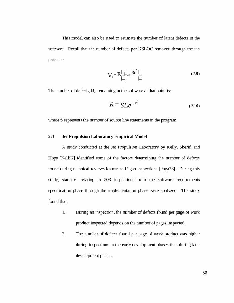
This model can also be used to estimate the number of latent defects in the
software. Recall that the number of defects per KSLOC removed through the t'th
phase is:
e-1EV
2Bt-=
t(2.9)
The number of defects, R, remaining in the software at that point is:
SEe = R Bt- 2
(2.10)
where S represents the number of source line statements in the program.
2.4 Jet Propulsion Laboratory Empirical Model
A study conducted at the Jet Propulsion Laboratory by Kelly, Sherif, and
Hops [Kell92] identified some of the factors determining the number of defects
found during technical reviews known as Fagan inspections [Faga76]. During this
study, statistics relating to 203 inspections from the software requirements
specification phase through the implementation phase were analyzed. The study
found that:
1. During an inspection, the number of defects found per page of work
product inspected depends on the number of pages inspected.
2. The number of defects found per page of work product was higher
during inspections in the early development phases than during later
development phases.

39
During this study, an empirical predictive model for defect densities encountered
during Fagan inspections was developed. The defect density during a development
phase, d, is given by:
d = 3.19e-0.61t(2.11)
• d is the number of defects per page for the product being
developed during a particular phase
• t is a development phase index having the following values:
• t=1 for the software requirements specification phase
• t=2 for the architectural design phase
• t=3 for the detailed design phase
• t=4 for the implementation phase
This model can be considered to be a variation of the phase-based model. The main
difference is that this model empirically derives the distribution of defects
throughout the life cycle from historical data, while the phase-based model assumes
that the distribution of defects throughout the life cycle follows a Rayleigh
distribution. As reported in [Kell92], this model appears to make satisfactory
predictions concerning the defect densities that will be encountered during the
specification, design, and implementation phases. It would be possible to extend it
into the testing and operational phases in the same fashion as for the phase-based
model. This is strictly an empirical model, and does not make its predictions based
on any measurable characteristics of the product being developed or the
40
development process. A more useful model would take into account measurable
aspects of the development method and the product being developed. Managers
could then use the model to determine which of the available development methods
and schedules would produce the most reliable software.
2.5 Classification Methods
Studies undertaken by Selby and Basili [Selb91], Porter and Selby
[Port90], Ghokale and Lyu [Ghok97], and Schneidewind [Schn97] have attempted
to develop methods of classifying modules in a software system as being either
defect-prone or free from defects. Selby and Basili used measures of data
interaction, called data bindings, to compute coupling and strength within
software systems. They then used the ratio of coupling to strength to compare
defect densities for modules within a selected system. Porter and Selby
developed a method of generating metrics-based classification trees, using metrics
from previous releases of a software system or previous projects, to identify
components likely to have a specified high-risk property (e.g., defect densities
greater than the mean). Schneidewind developed a set of Boolean Discriminant
Functions (BDFs) that can be used to differentiate modules that are prone to
containing defects from those that are not. BDFs include more than metrics; they
include threshold values of metrics, referred to as critical values, that are used to
either accept or reject modules when the modules are inspected during the quality
control process. Ghokale and Lyu have developed a method for classifying
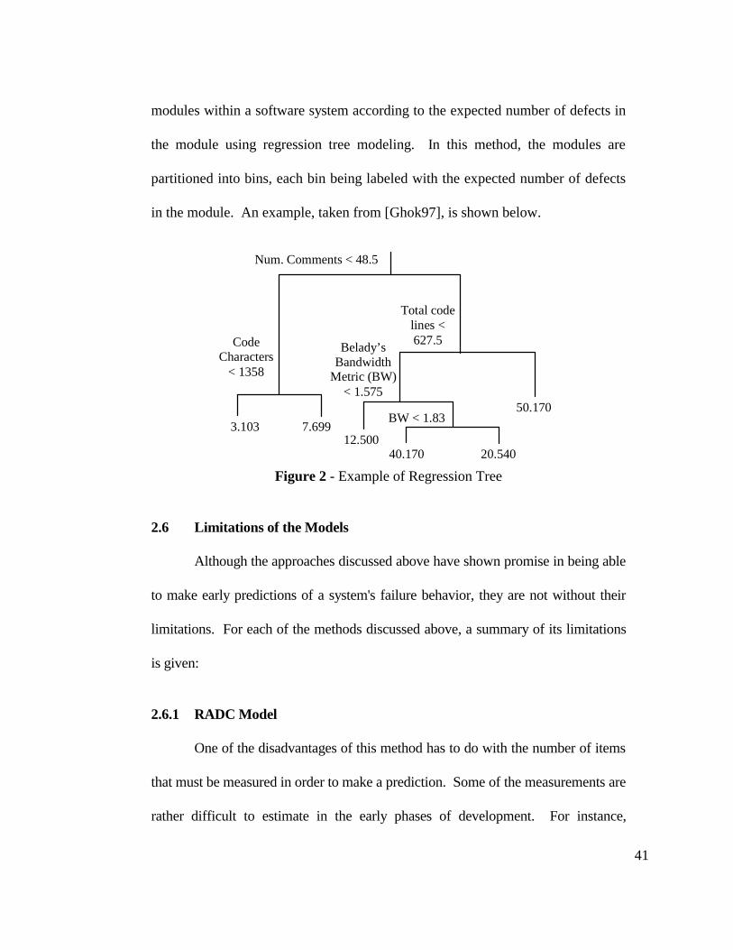
41
modules within a software system according to the expected number of defects in
the module using regression tree modeling. In this method, the modules are
partitioned into bins, each bin being labeled with the expected number of defects
in the module. An example, taken from [Ghok97], is shown below.
Num. Comments < 48.5
CodeCharacters
< 1358
3.103 7.699
Total codelines <627.5
Belady’sBandwidth
Metric (BW)< 1.575
BW < 1.83
12.500
50.170
40.170 20.540
Figure 2 - Example of Regression Tree
2.6 Limitations of the Models
Although the approaches discussed above have shown promise in being able
to make early predictions of a system's failure behavior, they are not without their
limitations. For each of the methods discussed above, a summary of its limitations
is given:
2.6.1 RADC Model
One of the disadvantages of this method has to do with the number of items
that must be measured in order to make a prediction. Some of the measurements are
rather difficult to estimate in the early phases of development. For instance,

42
measurements concerning module size in executable lines of code would not be
available until well into the design phase, as would measurements of McCabe
Cyclomatic Complexity. In addition, even though the error on each metric may be
relatively small, given that there are 11 drivers in the model, even small errors for
each individual measurement can result in wide confidence intervals for this model's
predictions. There may be questions about some of the statistical analysis during the
study, as well. For instance, in relating development modes to defect density, the
analysis for the organic development mode used only six data points.
The major limitation, however, has to do with the fact that the form of the
model does not take elapsed time during the development effort into account. It
may be the case, for instance, that aspects of the development method change at
some point after the start of the effort (e.g., use of CASE tools, adoption of
configuration management methods and tools), or that development practices are
not applied consistently across a development effort (e.g., use of Fagan inspections
during the requirements specification phase, but not during subsequent phases). The
model described in Section 2.1 and [McCa87] does not readily take such "mid-
course corrections" into account. To illustrate, suppose that a software development
effort starts by using a set of development methods, identified as A. Work
progresses, and after a time t, intermediate products such as requirements
specifications and architectural designs are produced. Suppose now that after time t,
a different set of development methods, B, is used. This would result in executable
code that had been produced by two different methods. In using the RADC model

43
to predict defect densities, valid predictions could not be made by using the
characteristics for method A or method B alone, since both methods were clearly
involved in the production of the software. Since the RADC method only makes
predictions about the defect density at the start of the testing phase, it would not
be possible to make an "intermediate" prediction for method A, and then update that
prediction using the characteristics of method B. There would have to be some way
of weighting the contributions of methods A and B to the overall defect density, but
there is no way of doing this for the RADC model. It would be preferable to have a
model that could make predictions up to some time τ after the start of the
development effort. If the development method were to change after time τ, the
parameters of the model could be adjusted to make new predictions starting at time
τ through the scheduled end of the development effort. These predictions could
then be concatenated with those made from the start of the development effort
through time τ.
2.6.2 Models Based on Relative Complexity
Although Munson and Khoshgoftaar have shown that relative complexity is
strongly correlated to the number of defects in a software module, one of its chief
limitation is that it can only be used on products whose complexity can be
measured. Practically speaking, this usually means source code, possibly detailed
design, and occasionally architectural design. There is an additional issue of what
complexity measures to use, although Munson and Khoshgoftaar suggest working

44
with "primitive" measures, which can be directly measured (e.g., number of nodes,
number of edges), rather than measures which are computed from lower-level
measures (e.g., cyclomatic complexity, Halstead length). It is reasonable to suppose
that this method could be applied earlier in the development phase if there were
methods to measure the complexity of design and specification documents. Indeed,
at the detailed design level, some of the same complexity factors measured during
implementation could be used. The measurements used in computing object points
[Bank91] and function points [Albr83, Symo88], for instance, could be used at
higher design levels, and possibly during requirements specification. Additional
methods of measuring product complexity prior to implementation have been
proposed [Niko92], in which structural measurements of a specification written in a
formal specification language (e.g., Z, PVS, Larch) could be taken. However, only
preliminary work has been done this area, and no conclusive findings have yet
emerged relating specification complexity to defect content. Furthermore, many
development organizations tend to write requirement specifications and design
documentation in natural language, the complexity of which is difficult or
impossible to measure. In these cases, the use of relative complexity is limited to
the implementation and later phases, at which point it is too late to make major
changes to the system if there are schedule or budgetary limitations. The other
limitation of this method is that by its nature, it does use any measurements of the
development process in computing the defect content of a software system.

45
2.6.3 Phase-Based model
The Phase-Based model has the advantage that its predictions are easily
updated by using Fagan inspection statistics from later development phases as this
data becomes available. It does, however, have the following limitations:
1. This model assumes that staffing and budget profiles during the
development life cycle follow a Rayleigh curve. Although this is the
idealized case, it does not necessarily hold for every software
development effort. Personal experience developing flight software
for one of the GALILEO flight control computers, the Command and
Data Subsystem, indicates that more resources than indicated by the
Rayleigh curve may be applied during the implementation and
testing phases.
2. There is an implicit assumption that during each phase, the entire
work product developed during that phase is inspected. Although
Fagan [Faga76] recommends that all products be completely
inspected, not all development efforts follow this recommendation.
For many development efforts at JPL, for instance, the source code is
not inspected at all. The Phase-Based model does not take this into
account. Other situations not handled by the Phase-Based model are
those in which during a particular development phase, only a fraction
of that phase's work product is inspected. For instance, during the
implementation phase of one JPL development effort sponsored by

46
the FAA, less than one-half of the source code was inspected. For
spacecraft ground support systems, it may be the case that only
enough resources to inspect the components of the system directly in
the uplink or downlink paths (e.g., spacecraft sequence generation
and uplink, telemetry reception and decommutation) are available.
3. The Phase-Based model assumes that estimates of the delivered
number of source lines of code are available during the early life
cycle phases. This information is not always available, and if it is, it
may be unreliable.
4. The Phase-Based model does not take into account any product
characteristics that may influence the number of defects initially
introduced into a work product or the number of defects found
during inspections. It might be expected that in terms of this model,
product characteristics might influence the height of the Rayleigh
curve, but there are no such factors for this model. As far as
development methods are concerned, the Phase-Based model does
not take into account any other factor than the use of Fagan
inspections. Certainly arguments can be made for taking other
aspects of the development environment into account [McCa87]. In
fact, one of the models mentioned in Section 1.3, the Littlewood-
Verrall model, attempts to factor the expertise of the development
team into its predictions.

47
5. The Phase-Based model does not directly take into account the
elapsed time since the start of the development effort. If the
inspection characteristics were to significantly change in the middle
of a development life cycle phase in a fashion that would affect the
number of defects discovered during an inspection, it would be very
difficult to update the model's predictions to accommodate the
changes. For example, it might be the case that only requirements
and architectural design are inspected. In this case, the Phase-Based
model could not be used because:
a. There would be no inspection statistics during detailed
design and coding that the model could use to update its
predictions.
b. The assumption that all work products are completely
inspected would be violated. This could lead to a different
defect discovery profile than that assumed by this model. At
this time, the model cannot take this departure from the
assumptions into account.
2.6.4 JPL Empirical Model
The limitations of the JPL empirical model are essentially the same as those
of the Phase-Based model. Like the Phase-Based model, the empirical model
developed in this study does not attempt to relate any product or development
48
method characteristics to the number of defects that will eventually be observed.
Although this model makes no explicit assumptions about the development process
or the product being developed, there is at least the implicit assumption that during
each development phase, the entire work product is inspected. Looking at the form
of the model, one can see that it would be quite difficult to make predictions if
inspections were to be eliminated during one or more development phases. There is
also the limitation that this study has not been extended to the testing phases to see
if the empirical model developed for the requirements specification, design and
implementation phases also applies to the code under test. Although such an
extension to the study should be, in principle, a straightforward task, the funds
required to monitor the projects analyzed during the original study into the testing
and operational phases and analyze the data have never been allocated.
2.6.5 Classification Methods
The classification methods identified in Section 2.5 have demonstrated
their ability to discriminate between software modules that are prone to containing
defects from those that tend to be defect-free. However, these methods do have
their limitations. With the exceptions of the studies reported in [Selb91] and
[Ghok97], the classification methods can be used only to distinguish between
those modules that are prone to containing defects and those that are not. While
the ability to identify defect-prone modules can help to identify areas that will be
troublesome during test, the classification methods do not provide a direct means

49
of estimating the number of defects in any particular module. If a module has
been classified as being prone to defects, a logical next step would be to estimate
how many defects were remaining in the module at various points in the testing
process.
The methods reported by Selby and Basili [Selb91], and Ghokale and Lyu
[Ghok97], can be used to estimate the number of defects in a system. However,
Selby and Basili measured only the data bindings, although there are other
physical properties of a software system that can be measured (e.g., size, control
complexity). The regression tree modeling technique described by Ghokale and
Lyu results in a tree whose terminals are labeled with the number of defects a
module at that terminal is expected to contain. In the example previously shown in
Figure 2, we see that the regression tree technique can only predict the number of
defects as a discrete quantity. A module might be classified as having an
estimated 3.103 or 7.699 defects, but we could not determine whether the module
had 5.0 defects without redefining the classification criteria.
Finally, there is the question of how to look at the system during various
points in its development. The classification studies listed in Section 2.5 do not
answer the question of whether the classification criteria that are valid at one point
in a system’s development (e.g., near the start of the implementation phase) are
also valid at other points in its development (e.g., closer to the end of the
development phase). As with the other prediction methods, then, the classifica-

50
tion methods do not take into account the elapsed time since the start of the
development effort.
2.6.6 A General Discussion of Predictive Model Limitations
From the previous discussion of the limitations of the individual predictive
models, we can summarize their major limitations as follows:
1. The currently available techniques do not take elapsed development
time into account. None of the predictive models discussed in the
previous sections allow practitioners to make estimates of how many
defects will have been inserted into the software system at an
arbitrary time, t. The Phase-Based and JPL Empirical models come
closest to this goal, but each time increment in these models
represents a development phase rather than a standard unit of time.
Per the discussion of the RADC model (Section 2.1), this makes it
difficult to update a model's predictions if the development process
or product characteristics change in the middle of a development
effort.
2. With the exception of the RADC model, none of the predictive
models takes both development process and product characteristics
into account. From the discussion in Sections 2.1 - 2.5, there is good
reason to suppose that these characteristics play an important part in
determining the overall defect content of the system; any model

51
attempting to predict the total number of defects in a software system
should account for both process and product characteristics. We can
find an analogy in the COCOMO and COCOMO II cost models
[Boehm81, Boehm95], in which both process and product
characteristics are used producing an estimate of the cost of
developing a software system.
3. With the exception of the RADC model, none of the models
computes reliability or a measure directly related to reliability (e.g.,
Mean Time To Failure, Hazard Rate). All of other predictive models
are confined to predicting measures related to defect content.
Although this can be a useful measure to developers, it is not easily
related to dynamic measures of more interest to the user (e.g.,
reliability, failure intensity).
In the next chapter, we propose to build on the work that has already been
done in the area of developing predictive models. The method of estimating a
software system’s defect content proposed in Chapter 3 is intended to address the
limitations described above. A method overcoming these limitations would make it
easier for software developers and managers to make more informed trade-offs
between resources, development practices, functionality, and quality, and to do so
earlier in the development effort.

52
Part III: Contribution
The method we propose to estimate and predict the defect content of
software systems prior to the testing and operational phases is described in this
section. We describe the method, the types of inputs it might require, how it could
be used to estimate and forecast a software system’s defect content, and the forms it
might take. Techniques to measure product structure and development
characteristics of real development efforts are described. We conclude with a
discussion of what we have learned about the utility of this method in predicting
defect content, as well as a set of recommendations for future work.

53
3. A Defect Content Prediction Model
This chapter develops a method of estimating the defect content of a
software system that could be applied prior to the testing phases. We propose to
address the general limitations discussed in Section 2.6 as follows:
1. The currently available techniques do not take calendar time into
account. This is the limitation which we are the most interested in
overcoming. If it is possible to do so, we will be able to follow the
development process and estimate the number of defects in a
software system at any arbitrary time t, rather than being limited to
estimating the defect content at discrete times (e.g., the end of each
development phase, as in the Phase-based and JPL Empirical
models, or the start of system test, as for the RADC model). The
model described in Section 3.3 overcomes this limitation by relating
measurements of structural change over time and measured change
in the development process to the rate at which defects are inserted
into the system. In order to do this, we must develop methods of
measuring a system’s structural evolution and the way that the
development process changes over time. The ability to estimate the
number of defects present in the system at any arbitrary time t would
increase visibility into the system, allowing software developers to
exert greater control over their system by making it possible to

54
identify problem areas earlier on and reducing the costs of taking the
appropriate corrective action.
2. With the exception of the RADC model, none of the predictive
models takes both development process and product characteristics
into account. The proposed model takes into account both system
structure and development process characteristics. The rate at which
defects are introduced into the system is a function of each type of
characteristic.
3. With the exception of the RADC model, none of the models
computes reliability or a measure directly related to reliability (e.g.,
Mean Time To Failure, Hazard Rate). This is a more complicated
issue than the first two. Although the relationship between defect
density and failure intensity developed for the RADC model can be
used, this will not necessarily produce an accurate prediction of
reliability. The reason for this is that the reliability of a software
system depends on the system's operational profile. Recall that for a
software system, the input to that system determines whether or not a
defect will be exposed, and whether that defect exposure will result
in a failure. If the system's operational profile is such that the most
frequent inputs are those that will expose defects, the system will be
appear to be unreliable. However, if the operational profile is such

55
that most of the inputs to a system do not expose defects, the system
will appear to be reliable.
The difficulty is that operational profiles tend to be
unavailable for systems under development. First of all, personal
experience indicates that most software development efforts do not
attempt to develop an operational profile. Even for those systems for
which estimates of the operational profile are made by analyzing the
usage patterns of previous, similar systems, the actual operational
profile can still differ significantly from the estimate. This leads to
the second and more important difficulty, which is that
determination of the operational profile can usually not be
accomplished by simple analysis of the system's requirements and
design. A large part of the problem is that the system's users may not
know themselves exactly how they intend to use the system, and
therefore cannot accurately estimate the operational profile.
In view of this situation, it may not be possible to develop a
model that produces reliability or reliability-related estimates from
information available prior to the test phases. However, since static
measures such as defect counts do not depend on the environment in
which the software executes, it should be possible to develop a
model to make predictions of this type. If information about the
dynamic characteristics of the system is available, it would then be

56
possible to use the outputs of the static model to make reliability
estimates and forecasts.
In addition, it is desirable that the model be sufficiently adaptable to use the
measurements of software structure and development process characteristics that are
available during each phase in a development effort. For instance, development
process characteristics that are available early in a development effort would include
a set of development practices to be followed, staffing profile estimates, and a plan
for phasing the development effort. As far as structural characteristics are
concerned, function points or object points might be considered for the early phases
of a development effort, as might the complexity categorizations associated with the
COCOMO II software cost model developed by Boehm et al. [Boehm95]. while
more detailed structural information (e.g., fan-in-fan-out, call-tree depth, number of
edges and nodes) would be available in later phases.
Finally, the predictions should be expressed in useful forms. Ideally,
predictions should be expressed in a form useful to both users and developers.
Preferably, the predictions should be given in a form that can be related to
reliability, since the reliability or lack thereof is what users will be observing during
operations. This would also be useful to developers, since it would give them a
target failure rate to which they could design. Given such a model, a development
organization could then be used to perform sensitivity analyses to identify the
product characteristics and development methods that would minimize the failure
rate.

57
Forms such as defect counts would not be as useful to the users, since these
measurements do not directly translate into failure rates. However, if we assume
that defects are more or less evenly distributed throughout the program, a rough
computation of failure intensity can be made as previously described in Section 2.1.
Under this assumption, software with a low defect content would be likely to fail
less frequently than software with a higher defect content.1 Defect counts would
still be useful to developers, in that this would provide a quantitative measure of the
software's quality. With this type of model, a development organization could
identify the product characteristics and development methods that would minimize
the defect content of the executable software.
3.1 Factors Influencing Introduction of Defects
There are several factors that may influence the rate at which defects are
introduced into a work product which we will attempt to measure in developing the
model. Some of these factors are described below, and include several of the
product and process characteristics that were described in [Boehm95]. We will
attempt to measure these factors for the development efforts included in this study,
and determine the effects they have on the defect insertion and removal rates.
1 Note that this is not necessarily a valid assumption. The research described in
[Khos92,Muns90, Muns91], as well as recent work by Munson and Schneidewind, indicatesthat defect densities will be higher in more complex software. If the software executes themore complex modules frequently, the failure intensity will be higher than if those moduleswere less frequently executed.

58
• Development environment - One can easily speculate that the development
environment will have an effect on the number of defects introduced into the
system and the rate at which they are introduced. Imagine two identical
development efforts, except for the fact that the first effort uses structured
development methods (e.g., dataflow diagrams, state transition diagrams)
and tools associated with these methods, while the second makes no use of
these methods. In the first development environment, many ambiguities and
inconsistencies can be discovered by using the tools, leaving the
development team to focus more on other types of defects, such as
incomplete specifications. The first development team would tend to
discover more defects during each phase, which would leave fewer defects
to be propagated into the operational system. In the second environment, the
developers would have no automated assistance, and would tend to discover
fewer defects of all types during each development phase, resulting in an
operational system containing more defects. The development environment
categorization that will be used in developing the model will be based on the
categorizations found in [Boehm81] and [Boehm95].
• Product characteristics - As in [Khos92], [McCa87], and [Muns91], we
would expect measurable characteristics of the product being developed to
be related to the number of defects introduced into the system and the rate at
which they are introduced. For this study, we will analyze software system
structure and determine the effect, if any, it has on the rate of defect

59
introduction. Since there may be more than one aspect of a software
system's complexity that could influence the defect introduction rate (e.g.,
number of edges, number of nodes, number of unique operands, fan-in and
fan-out), it would seem reasonable to use measures which would be readily
available during the implementation and later phases to as inputs to a factor
analysis similar to that described in [Khos92] and [Muns91]. Using only a
single measure of system structure, such as McCabe’s cyclomatic
complexity measure or data bindings [Selb91], would be needlessly
restrictive.
• Number of defects already in the product - The number of defects already in
the work product may influence the defect introduction rate. As a
development phase progresses, new sections of a work product are
integrated into the sections that have already been produced. Some of new
sections will depend on information in the existing sections. There will be
two types of defects inserted into the new sections:
• Defects that are local to the new section. For example, the design for
a sorting module could contain conceptual defects in determining
how to partition the input prior to doing the sort.
• Defects related to defects in older sections on which the newer
sections depend. For example, one piece of a specification could
mistakenly specify the position and accuracy of items in a data
stream output from that piece. If these defects were not discovered

60
and removed, the specification of a process dependent on this data
stream would contain defects based on the defect specification of the
data stream.
We can think of the rate of defect introduction as being composed of two
terms. The first term would simply be the rate at which a developer makes
defects in a specification, design, or other product. The second term is the
rate at which the developer carries forward defects from other portions of the
work item into the current portion. This is the term that depends on the
number of defects present in the existing work items.
3.2 A Model for the Rate of Defect Insertion
We propose to model the rate at which defects are inserted into a software
system. In general, we will model the rate as functions of the measured structural
change in a software system over any given development increment and the
measured changes in the development process over that same increment, given by
( )dsfi xxxx ∆∆= , , (3.1)
where i x is the rates at which defects are inserted and deleted when x defects are
already in the system, and ( )dsf xxx ∆∆ , is a function of the measured structural
change, sx∆ , and the measured development process change, dx∆ , over a
development increment at the start of which x defects were in the system.
The function ( )dsf xxx ∆∆ , is not required to be constrained to any particular
form, and may indeed vary from development phase to development phase within a

61
software development effort. However, previous work [Muns94] shows that during
the implementaton phase, the correlation of measurements of system structure (but
not structural change) and the system’s defect content is 0.90, and that the
relationship between measurements of system structure and the defect content is
linear. For the implementation phase, then, we will take as our starting point the
hypothesis that the rate of fault insertion is linearly related to the measured structural
change and development process change during a development increment:
dkski xxxxx ∆+∆= ,1,0 , (3.2)
where sx∆ and dx∆ are as defined above, and k x,0 and k x,1 are constants relating
the measured structural and development process change to the rates of defect
insertion and removal at the start of a development increment in which the system
contains x defects.
In the simplest case, the constants k x,0 and k x,1 would be the same for all
values of x. Furthermore, if the development process were to remain constant
across a particular development phase, the term for the effects of change to the
development process, dk xx ∆,1 , would assume a value of 0. The effects of the
development process would be taken into account in the constants k x,0 . This would
make it particularly simple to estimate the number of defects in the system at any
given time. We describe in Section 3.4.1 how the number of defects in the system
could be estimated under these conditions. If, on the other hand, the rate at which
defects were inserted into the system were to vary with the number of defects

62
already in the system, estimating the number of defects in the system at any time
would be more complicated. One possible method of dealing with this situation is
described in Section 3.4.2.
Before discussing additional details of this model and its use, we must
describe how to measure the structural evolution of a system and changes to the
development process. This is done in the following sections.
3.3 Measuring the Evolution of a Software System
This section develops a method for measuring the structural evolution of a
software system, and relating measures of structural evolution to the rate at which
defects are inserted into and removed from the system. This is an extension of the
methods reported in [Muns96] and [Niko97].
3.3.1 A Measurement Baseline
The measurement of an evolving software system is not an easy task.
Perhaps one of the most difficult issues relates to the establishment of a baseline
against which the evolving systems may be compared. This problem is very
similar to that encountered by the surveying profession. If we were to buy a piece
of property, there are certain physical attributes that we would like to know about
that property. Among these properties is the topography of the site. To establish
the topological characteristics of the land, we will have to seek out a benchmark.
This benchmark represents an arbitrary point somewhere on the subject property.
The distance and the elevation of every other point on the property may then be

63
established in relation to the measurement baseline. Interestingly enough, we can
pick any point on the property, establish a new baseline, and get exactly the same
topography for the property. The property does not change. Only our perspective
changes.
When measuring software evolution, we need to establish a measurement
baseline for the same purpose described above. We need a fixed point against
which all others can be compared. Our measurement baseline also needs to
maintain the property that, when another point is chosen, the exact same picture of
software evolution emerges, only the perspective changes. The individual points
involved in measuring software evolution are individual builds of the system.
One problem with using raw measurements is that they are all on different
scales. The comparison of different modules within a software system by using
raw measurement data is complicated by this fact. Take for example the data in
Table 1. This table provides the values for two metrics; lines of code, LOC, and
cyclomatic complexity, V(g). These measurements are taken for two different
builds of the system. Based on these two metrics, it is difficult to assert that
Module A is more complex than Module B on Build 1. Certainly, LOC is less
than that for module B, but V(g) is greater. Now consider the same two modules
for build 2. Has the system, as represented by these two modules, become more
complex or less complex between these two builds? The total number of lines of
code has decreased by ten, but cyclomatic complexity has increased by two.
Again, it is difficult to assert that there has been an increase or decrease in overall
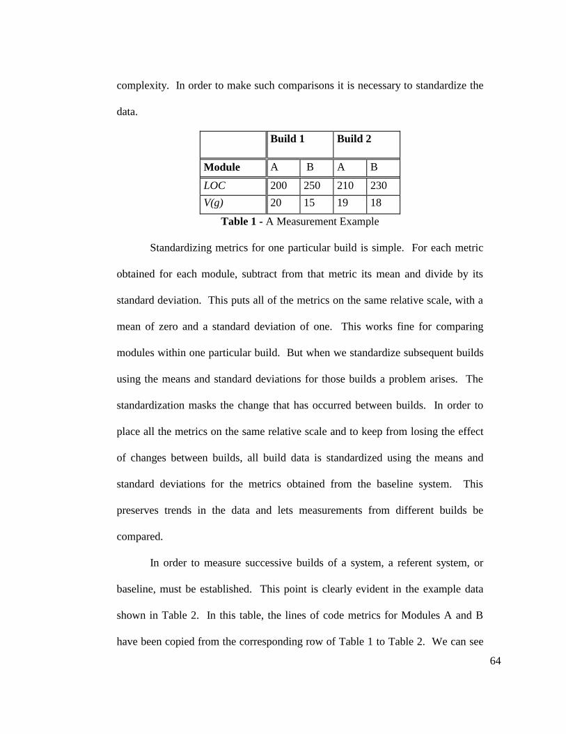
64
complexity. In order to make such comparisons it is necessary to standardize the
data.
Build 1 Build 2
Module A B A B
LOC 200 250 210 230
V(g) 20 15 19 18
Table 1 - A Measurement Example
Standardizing metrics for one particular build is simple. For each metric
obtained for each module, subtract from that metric its mean and divide by its
standard deviation. This puts all of the metrics on the same relative scale, with a
mean of zero and a standard deviation of one. This works fine for comparing
modules within one particular build. But when we standardize subsequent builds
using the means and standard deviations for those builds a problem arises. The
standardization masks the change that has occurred between builds. In order to
place all the metrics on the same relative scale and to keep from losing the effect
of changes between builds, all build data is standardized using the means and
standard deviations for the metrics obtained from the baseline system. This
preserves trends in the data and lets measurements from different builds be
compared.
In order to measure successive builds of a system, a referent system, or
baseline, must be established. This point is clearly evident in the example data
shown in Table 2. In this table, the lines of code metrics for Modules A and B
have been copied from the corresponding row of Table 1 to Table 2. We can see

65
from these tables that Module A has increased 10 lines of code from Build 1 to
Build 2. We can also see that Module B has decreased by 20 lines between these
two builds. What is not apparent from this table is the relative size of Modules A
and B to other modules in the same build. To make this difference visible each of
the LOC values is normalized by subtracting the mean value, LOC, for each build,
and dividing by the standard deviation of LOC for that build. This will yield the
row labeled zLOC in Table 2. With these normalized metric values, we can see that
Module A has not changed in LOC relative to all other program modules. The
same thing is true for Module B from Build 1 to Build 2. Module A is of average
size on both Build 1 and Build 2. If, on the other hand, we normalize the Build 2
modules by the mean and standard deviation of Build 1, we obtain a new row for
Table 2 labeled Base LOCz . Build 2 may now be compared directly to Build 1.
We can see that Module 2 is 0.4 standard deviations greater than it was on Build
1. Further, while Module B was fully two standard deviations above the mean
LOC for Build 1, on Build 2 it has diminished to 1.6 standard deviations above
the mean.
Build 1 Build 2
Module A B A BLOC 200 250 210 230zLOC 0.0 2.0 0.0 2.0Base zLOC 0.0 2.0 0.4 1.6LOC 200 210
LOCδ 25 15Table 2 - A Baseline Example

66
For each raw metric in the baseline build, we may compute a mean and a
standard deviation. Let us denote the vector of mean values for the baseline build
as Bx and the vector of standard deviations as Bs . The standardized baseline
metric values for any module j in an arbitrary build i, then, may be derived from
raw metric values as
Bj
Bj
iBjiB
j s
xwz
−=
,, (3.3)
The process of standardizing the raw metrics certain makes them more
tractable. Among other things, it now permits the comparison of metric values
from one build to the next. This standardization does not solve the main problem.
There are too many metrics collected on each module over many builds. We
need to reduce the dimensionality of the problem. We have successfully used
principal components analysis for reducing the dimensionality of the problem.
The principal components technique will reduce a set of highly correlated metrics
to a much smaller set of uncorrelated or orthogonal measures. One of the
products of the principal components technique is an orthogonal transformation
matrix T that will send the standardized scores (the matrix z) onto a reduced set of
domain scores thusly, zTd = .
In the same manner as the baseline means and standard deviations were
used to transform the raw metric of any build relative to a baseline build, the
transformation matrix BT derived from the baseline build will be used in
subsequent builds to transform standardized metric values obtained from that
67
build to the reduced set of domain metrics as follows: BiBiB Tzd ,, = , where iB,z
are the standardized metric values from build i baselined on build B .
Another artifact of the principal components analysis is the set of
eigenvalues that are generated for each of the new principal components.
Associated with each of the new measurement domains is an eigenvalue, λ .
These eigenvalues are large or small varying directly with the proportion of
variance explained by each principal component. We have successfully exploited
these eigenvalues to create a new metric called relative complexity, ρ , that is the
weighted sum of the domain metrics to wit:
∑=
+=m
jjji d
1
1050 λρ , (3.4)
where m is the dimensionality of the reduced metric set.
As was the case for the standardized metrics and the domain metrics,
relative complexity may be baselined as well using the eigenvalues and the
baselined domain values as follows:
∑=
=m
j
Bj
Bj
Bi d
1
λρ (3.5)
If the raw metrics that are used to construct the relative complexity metric
are carefully chosen for their relationship to software defects then the relative
complexity metric will vary in exactly the same manner as the defects. The
relative complexity metric in this context is a defect surrogate. Whereas we
cannot measure the defects in a program directly we can measure the relative
68
complexity of the program modules that contain the defects. Those modules
having a large relative complexity value will ultimately be found to be those with
the largest number of defects.
3.3.2 Module Sets And Versions
A software system consists of one or more software modules. As the
system grows and modifications are made, the code is recompiled and a new
version, or build, is created. Each build is constructed from a set of software
modules. The new version may contain some of the same modules as the
previous version, some entirely new modules and it may even omit some modules
that were present in an earlier version. Of the modules that are common to both
the old and new version, some may have undergone modification since the last
build. When evaluating the change that occurs to the system between any two
builds i, and j, we are interested in three sets of modules. The first set, jicM , , is
the set of modules present in both builds of the system. These modules may have
changed since the earlier version but were not removed. The second set, jiaM , , is
the set of modules that were in the early build and were removed prior to the later
build. The final set, jibM , , is the set of modules that have been added to the
system since the earlier build.
As an example, let build i consist of the following set of modules.
{ }54321 ,,,, mmmmmM i =
Between build i and j module 3m is removed giving

69
{ } { } { }{ }5421
354321
,,
,,,
,,,,
mmmm
mmmmmm
MMMM jia
jib
ij
=−∪=
−∪=
Then between builds j and k two new modules, 7m and 8m are added and module
2m is deleted giving
{ } { } { }{ }87541
2875421
,,
,,,,
,,,,
mmmmm
mmmmmmm
MMMM kja
kjb
jk
=−∪=
−∪=
With a suitable baseline in place, and the module sets defined above, it is
now possible to measure software evolution across a full spectrum of software
metrics. We can do this first by comparing average metric values for the different
builds. Secondly, we can measure the increase or decrease in system complexity
as measured by a selected metric, code delta, or we can measure the total amount
of change the system has undergone between builds, code churn.
We can now see that establishing the complexity of a system across builds
in the face of changing modules and changing sets of modules is in itself a very
complex problem. In terms of the example above, the relative complexity of the
system iBR , at build i, the early build, is given by
∑∈
=i
c Mm
iBc
iBR ,, ρ , (3.5)
where iBc
,ρ is the relative complexity of module cm on this build baselined by
build B.
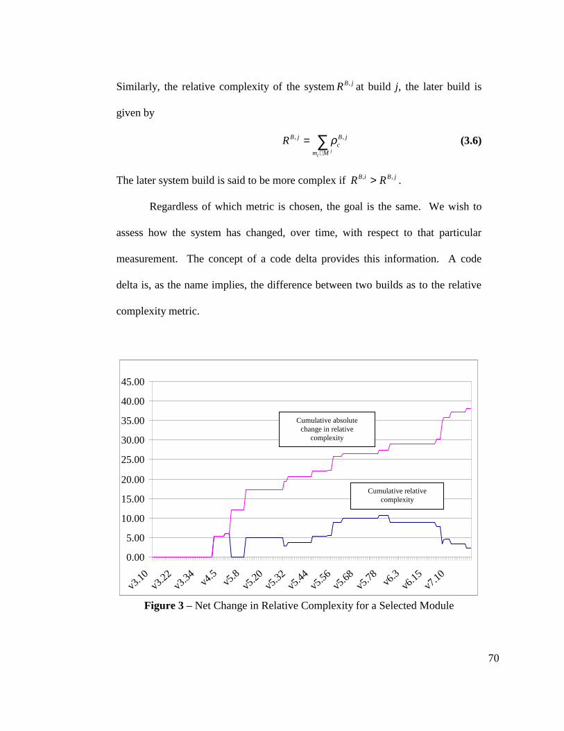
70
Similarly, the relative complexity of the system jBR , at build j, the later build is
given by
∑∈
=j
c Mm
jBc
jBR ,, ρ (3.6)
The later system build is said to be more complex if jBiB RR ,, > .
Regardless of which metric is chosen, the goal is the same. We wish to
assess how the system has changed, over time, with respect to that particular
measurement. The concept of a code delta provides this information. A code
delta is, as the name implies, the difference between two builds as to the relative
complexity metric.
0.00
5.00
10.00
15.00
20.00
25.00
30.00
35.00
40.00
45.00
v3.10
v3.22
v3.34 v4
.5v5
.8v5
.20v5
.32v5
.44v5
.56v5
.68v5
.78 v6.3
v6.15
v7.10
Figure 3 – Net Change in Relative Complexity for a Selected Module
Cumulative absolutechange in relative
complexity
Cumulative relativecomplexity
71
For purposes of demonstration, an embedded real-time system, the flight
software for the CASSINI Command and Data Subsystem (see Chapter 4), has
been evaluated. This is a real time control system of approximately 45 KLOC in
900 Ada modules (functions). The overall trend in the relative complexity
between successive builds for a selected module is shown in Figure 3 above. The
pattern shown here is quite typical of an evolving software system. In looking at
this figure we can see that there are periods of relative quiescence and also periods
of great change in the system. The overall trend is always towards increased
complexity.
3.3.3 Code Churn and Code Deltas
The change in the relative complexity in a single module between two
builds may be measured in one of two distinct ways. First, we may simply
compute the simple difference in the module relative complexity between build i
and build j. We will call this value the code delta for the module am , or
iBa
jBa
jia
,,, ρρδ −= . The absolute value of the code delta is a measure of code
churn. In the case of code churn, what is important is the absolute measure of the
nature that code has been modified. From the standpoint of defect insertion,
removing a lot of code is can be as significant as adding a lot. The new measure
of code churn, χ , for module am is simply iBa
jBa
jia
jia
,,,, ρρδχ −== .
The total net change of the system is the sum of the code delta’s for a
system between two builds i and j is given by

72
∑∑∑∈∈∈
+−=∆ji
bbji
aai
c Mm
jBb
Mm
iBa
Mm
jic
ji
,,
,,,, ρρδ (3.7)
With a suitable baseline in place, and the module sets defined above, it is
now possible to measure software evolution across a full spectrum of software
metrics. We can do this first by comparing average metric values for the different
builds. Secondly, we can measure the increase or decrease in system complexity
as measured by a selected metric, code delta, or we can measure the total amount
of change the system has undergone between builds, code churn.
A limitation of measuring code deltas is that it doesn’t give an indicator as
to how much change the system has undergone. If, between builds, several
software modules are removed and are replaced by modules of roughly equivalent
complexity, the code delta for the system will be close to zero. The overall
complexity of the system, based on the metric used to compute deltas, will not
have changed much. However, the reliability of the system could have been
severely effected by the process of replacing old modules with new ones. What
we need is a measure to accompany code delta that indicates how much change
has occurred. Code churn is a measurement, calculated in a similar manner to
code delta, that provides this information. The net code churn of the same system
over the same builds is
∑∑∑∈∈∈
++=∇ji
bbji
aacc Mm
jBb
Mm
iBa
Mm
jic
ji
,,
,,,, ρρχ (3.8)
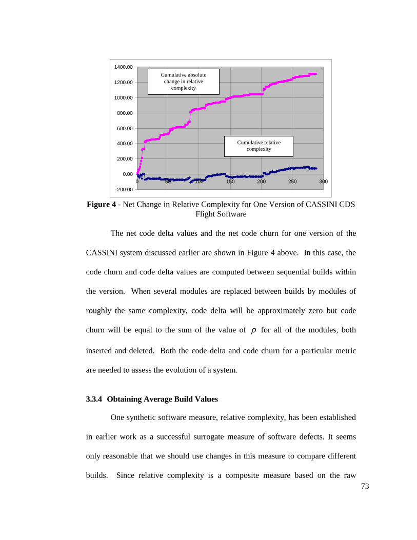
73
-200.00
0.00
200.00
400.00
600.00
800.00
1000.00
1200.00
1400.00
0 50 100 150 200 250 300
Figure 4 - Net Change in Relative Complexity for One Version of CASSINI CDSFlight Software
The net code delta values and the net code churn for one version of the
CASSINI system discussed earlier are shown in Figure 4 above. In this case, the
code churn and code delta values are computed between sequential builds within
the version. When several modules are replaced between builds by modules of
roughly the same complexity, code delta will be approximately zero but code
churn will be equal to the sum of the value of ρ for all of the modules, both
inserted and deleted. Both the code delta and code churn for a particular metric
are needed to assess the evolution of a system.
3.3.4 Obtaining Average Build Values
One synthetic software measure, relative complexity, has been established
in earlier work as a successful surrogate measure of software defects. It seems
only reasonable that we should use changes in this measure to compare different
builds. Since relative complexity is a composite measure based on the raw
Cumulative absolutechange in relative
complexity
Cumulative relativecomplexity

74
measurements, it incorporates the information represented by LOC, V(g), η1 , η2 ,
and all the other raw metrics of interest. Relative complexity is a single value that
is representative of the complexity of the system which incorporates all of the
complexity attributes we have measured (e.g., size, control flow, style, data
structures, etc.).
By definition, the average relative complexity, ρ , of the baseline system
will be
501
1
== ∑=
BN
i
BiB
B
Nρρ (3.9)
where BN is the cardinality of the set of modules on build B, the baseline build.
Relative complexity for the baseline build is calculated from standardized values
using the mean and standard deviation from the baseline metrics. The relative
complexities are then scaled to have a mean of 50 and a standard deviation of 10.
For that reason, the average relative complexity for the baseline system will
always be a fixed point. Subsequent builds are standardized using the means and
standard deviations of the metrics gathered from the baseline system to allow
comparisons. The average relative complexity for subsequent builds is given by
∑=
=kN
i
kBik
k
N 1
,1 ρρ (3.10)
where N k is the cardinality of the set of program modules in the thk build and
kBi
,ρ is the baselined relative complexity for the thi module of that set.
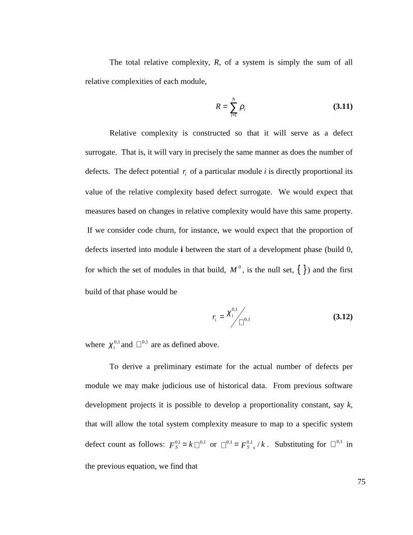
75
The total relative complexity, R, of a system is simply the sum of all
relative complexities of each module,
∑=
=N
iiR
1
ρ (3.11)
Relative complexity is constructed so that it will serve as a defect
surrogate. That is, it will vary in precisely the same manner as does the number of
defects. The defect potential ri of a particular module i is directly proportional its
value of the relative complexity based defect surrogate. We would expect that
measures based on changes in relative complexity would have this same property.
If we consider code churn, for instance, we would expect that the proportion of
defects inserted into module i between the start of a development phase (build 0,
for which the set of modules in that build, 0M , is the null set, { }) and the first
build of that phase would be
∇= 1,0
1,0χ iir (3.12)
where 1,0iχ and 1,0∇ are as defined above.
To derive a preliminary estimate for the actual number of defects per
module we may make judicious use of historical data. From previous software
development projects it is possible to develop a proportionality constant, say k,
that will allow the total system complexity measure to map to a specific system
defect count as follows: ∇= 1,01,0 kF S or kF sS /1,01,0 =∇ . Substituting for 1,0∇ in
the previous equation, we find that

76
∇= 1,0
1,0χ ii
kr (3.13)
Thus, our best estimate for the number of defects in module i in the initial
configuration of the system is
Frg Sii1,01 = (3.14)
After an interval of testing a number of defects will be found and fixes
made to the code to remedy the defects. Let jF be the total number of defects
found in the total system up to and including the j th build of the software. In a
particular module i there will be 2if defects found in the second build that are
attributable to this module. The estimated number of defects remaining in module
i will then be
212iii fgg −= , (3.15)
assuming that we have only fixed defects in the code and not added any new ones.
Our ability to locate the remaining defects in a system will relate directly
to our exposure to these defects. If, for example, at thethj build of a system there
are jig remaining defects in module i , we can not expect to identify any of these
defects unless some test activity is allocated to exercising module i.
As the code is modified over time, defects will be found and fixed.
However, new defects will be introduced into the code as a result of the change.
In fact, this defect injection process is directly proportional to change in the
program modules from one version to the next. As a module is changed from one
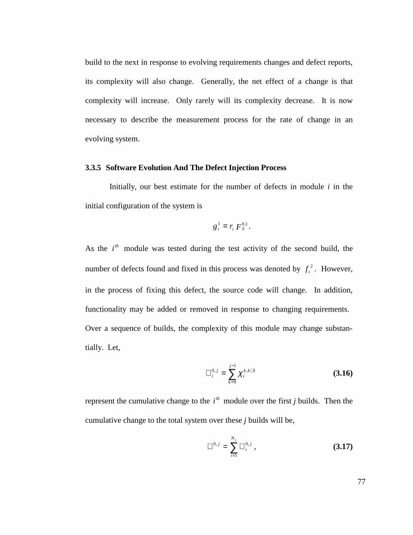
77
build to the next in response to evolving requirements changes and defect reports,
its complexity will also change. Generally, the net effect of a change is that
complexity will increase. Only rarely will its complexity decrease. It is now
necessary to describe the measurement process for the rate of change in an
evolving system.
3.3.5 Software Evolution And The Defect Injection Process
Initially, our best estimate for the number of defects in module i in the
initial configuration of the system is
Frg Sii1,01 = .
As the thi module was tested during the test activity of the second build, the
number of defects found and fixed in this process was denoted by 2if . However,
in the process of fixing this defect, the source code will change. In addition,
functionality may be added or removed in response to changing requirements.
Over a sequence of builds, the complexity of this module may change substan-
tially. Let,
∑−
=
+=∇1
0
1,,0j
k
kki
ji χ (3.16)
represent the cumulative change to the thi module over the first j builds. Then the
cumulative change to the total system over these j builds will be,
∑=
∇=∇jN
i
ji
j
1
,0,0 , (3.17)

78
where jN is the cardinality of the set of all modules that were in existence over
these j builds. As a result of these changes, the proportion of defects in the thi
module will have changed over the sequence of j builds. If the number of defects
inserted into the ith module since the establishment of the baseline is proportional
to the amount of change it has experienced, and if the proportionality constant
remains the same over all builds, the new value of the proportion of defects will
be:
)()(
,0
,0
j
jij
ir ∇∇= . (3.18)
Returning for a moment to our defect proportionality constant, k, we now
observe that our estimate of the number of defects in the system has now changed.
On the thj build there will no longer be sF defects in the system. There will
have been )( ,0 jjs kF ∇= defects inserted into the system. Each module will have
had
js
ji
ji Frh = (3.19)
defects introduced in it either from the initial build or on subsequent builds. Thus,
our revised estimated of the number of defects remaining in module i on build j
will be
ji
ji
ji fhg −= . (3.20)

79
The rate of defect insertion is directly related to the change activity that a
module will receive from one build to the next. At the system level, we can see
that the expected number of injected defects from build j to build j+1 will be
1,
,01,0
,01,01
)(+
+
++
∇=
∇−∇=
∇−∇=−
jj
jj
jjjs
jx
k
k
kkFF
. (3.21)
At the module level, the rate of defect injection will, again, be proportional to the
level of change activity. Hence, the expected number of injected defects between
build j to build j+1 on module i will be simply ji
ji hh −+1 .
3.3.6 Measuring Changes in the Development Process
In addition to measuring the structural evolution of a software system, we
can also measure changes in the development process. Unlike structural change,
we will measure changes in the development at the system level. This is done for
two reasons:
• Experience in developing software systems indicates that the same develop-
ment method will tend to be applied to an entire system, rather than having
different development methods applied to different modules in the system.
• Any differences in development practices between different sets of modules in
a system will tend to lie in individual differences between members of the
development team. Accurately measuring the individual differences between
members of a development team is extremely difficult for the following two
reasons:

80
• Members of the development team will argue that they don’t have time to
record all of the information and still deliver the system on schedule.
• There will usually be great concern about managers misusing this type of
data to punish individual developers. For instance, if the rate of defect in-
sertion for a particular individual was found to be significantly higher than
that for the other developers, this individual could be punished by being
demoted or receiving a smaller raise than the other developers.
We will measure the development process using the questionnaire
developed for calibration of the COCOMO II software cost model [Boehm95].
Many characteristics of the development process will tend to be constant across
individual development phases (e.g., Defect Prevention and Detection Methods,
Software Understanding, and Platform Cost Drivers), but there are some attributes
among the Personnel Cost Drivers for which we will be able to measure changes
over time. We will use cumulative work effort as well as information about the
development team’s previous experience to measure the way in which Applications
Experience, Platform Experience, and Language and Tool Experience change over
time.
3.4 Use of the Model
In this section, we describe two ways in which a model of the defect
insertion rate might be used. The first way to use the model would be a simple
method of estimating the number of residual defects in the system at the module

81
level, using only measurements of the system's structural evolution, and develop-
ment process characteristics. This method would be applicable in the situation for
which the rate of defect insertion is linearly proportional to changes in the system’s
structure and development processes, and for which the proportionality constants do
not vary. Software development managers could use this estimation method to
identify portions of the system to which more testing resources should be allocated.
The proportion of residual defects in the troublesome areas would guide the
application of technical review and testing resources.
The second way is a more sophisticated method of estimating and
forecasting the residual number of defects which makes use of a birth-and-death
model [Klei75, Klei76]. In order to use this method, it is necessary to have
estimates of the rate of defect removal as well as the rate of defect insertion.
3.4.1 Estimating Residual Defect Content at the System and Module Levels
If the relationship between the amount of structural change in a development
increment, measured changes to the development process within that increment, and
the number of defects inserted during that interval do not change from increment to
increment, estimating the number of residual defects in the system is quite
straightforward. We can use the measures of code churn and code delta (Section
3.3.3 above) as our measures of structural change. Measurable development process
characteristics that may change over time include the programmers’ and analysts’
experience with the development environment and the application. The estimated

82
number of defects, d ji,0 , inserted into a module i between build 0 and a particular
build j is
( )
otherwise 0
0if 1,
1
0
1,2
1,1
1,0
,0
≠∇
∆+∆+∇=
+
−
=
+++∑mm
i
j
m
mmmmi
mmi
ji dkkkd
, (3.22)
where k0 is the proportionality constant associated with code churn, k1 is the
proportionality constant associated with code delta, and k2 is the proportionality
constant associated with measured changes in the development process, d mm∆ +1, .
The estimated number of defects that have been inserted into the system as a
whole at the jth build, d j,0 , is given by
∑=
=N
i
ji
j dd1
,0,0 , (3.23)
where d ji,0 is the estimated number of defects that have been inserted into module
i by the jth build, and N is the number of modules in the system.
We include code delta as an estimator, because the type of change made to
a system (addition of functionality vs. removal of functionality) may affect the
number of defects inserted into a system between two successive builds j and j+1.
At least for the implementation phase, we can easily track the amount of structural
change that has been made to a system from build to build, provided that changes
to the system are captured with a revision control system such as SCCS or RCS.
We discuss this in more detail in Chapter 5. Note that changes in the

83
development process are associated with the system as a whole, rather than with
an individual module. This is done for practical reasons – it is extremely difficult
to identify certain aspects of the development process for individual modules. For
instance, we know of no accurate method of determining the analysts’ and
developers’ experience with an individual module, although their experience with
the system as a whole is easily measured.
If a development effort uses a problem reporting system to record failures
and the associated defects found during a system’s development, the number of
defects remaining in the system at any time is easily estimated. The estimated
residual number of defects, n ji,0 , in a module i at build j is given by
fdnj
ij
ij
i,0,0,0 −= , (3.24)
wheref ji,0 represents the number of defects that have been recorded for the ith
module in the problem reporting system between the initial and the jth builds. The
estimated number of residual defects in the system as a whole at the jth build is given
by
∑=
=N
i
ji
j nn1
,0,0 , (3.25)
where n ji,0 is the estimated number of residual defects in module i at the jth build.
The practical aspects of developing an adequate defect tracking system are discussed
in greater detail in Chapter 5.
Once we have estimated the number of residual defects in each module, we
can use this information to help manage resources during the development effort.

84
For each module, we can compute the proportion of defects that have been found to
the total number of defects in the system. This is given by
nn jji
ji
,0,0,0 =φ , (3.26)
where n ji,0 represents the estimated residual number of defects in module i at the jth
build (Equation 3.24), and n j,0 (Equation 3.25) represents the estimated number of
defects in the system as a whole. The proportion of number of defects found in
module i to the total number of defects found in the system between the initial and
jth builds is given by
ff jji
ji
,0,0,0 =ϕ , (3.27)
where f ji,0 specifies the total number of defects found in module i by the jth build,
and f j,0 specifies the total number of defects found in the system by the jth build.
We can compare φ ji,0 to ϕ j
i,0 to identify those modules that may require additional
effort to find and remove defects. For any module i, if φ ji,0 is significantly greater
than ϕ ji,0 , this means that there are more residual defects remaining in that module
than we would expect. For these modules, additional resources should be allocated
to finding and removing defects in proportion to the difference between φ ji,0 and
ϕ ji,0 . Conversely, in those modules for which φ j
i,0 is significantly less than ϕ j
i,0 ,
defect discovery and repair resources allocated to those modules might be
reallocated to those modules for which φ ji,0 is significantly greater than ϕ j
i,0 . In this
85
case, the expected number of additional defects that would have to be found in the
module is:
−1,0
,0,0
ϕφ
ji
jij
if . (3.28)
Suppose that instead of being constant, the rate at which defects are
inserted into a system varies with the number of defects already present in the
system. We could still use the ideas described above to estimate the number of
residual defects at the module level. The cumulative number of defects inserted
into a module between build 0 and the jth build is given by
( )
otherwise 0
0if 1,
1
0
1,,2
1,,1
1,,0
,0
≠∇
∆+∆+∇=
+
−
=
+++∑mm
i
j
m
mmx
mmix
mmix
ji dkkkd
, (3.29)
where k x,0 is the proportionality constant associated with code churn when there
are x defects in the ith module, k x,1 is the proportionality constant associated with
code delta when there are x defects in the ith module, and k x,2 is the
proportionality constant associated with measured changes in the development
process, d mm∆ +1, , when there are x defects in the ith module. The number of
residual defects in the ith module and the proportion of residual defects in the ith
module can be calculated as described above. The principal difficulty with
nonhomogeneous rates is determining the way in which they vary with the number
of defects already in the system.
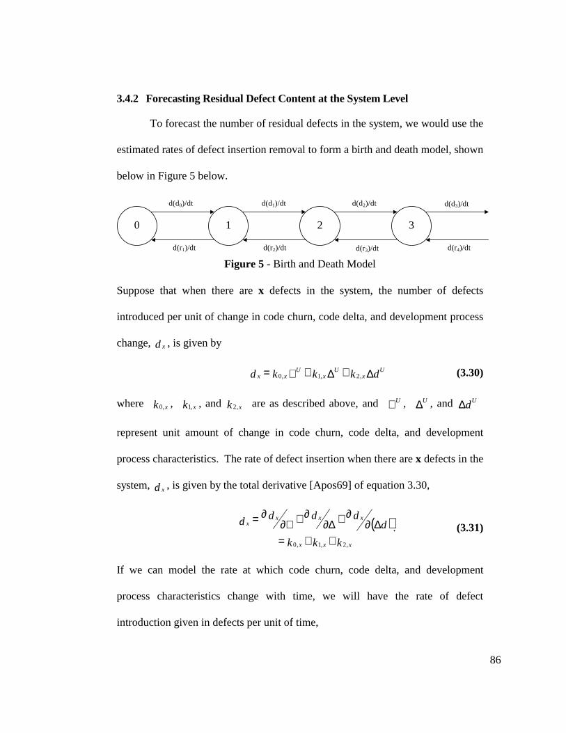
86
3.4.2 Forecasting Residual Defect Content at the System Level
To forecast the number of residual defects in the system, we would use the
estimated rates of defect insertion removal to form a birth and death model, shown
below in Figure 5 below.
0 1 2 3
d(d0)/dt d(d1)/dt d(d2)/dt d(d3)/dt
d(r1)/dt d(r2)/dt d(r3)/dt d(r4)/dt
Figure 5 - Birth and Death Model
Suppose that when there are x defects in the system, the number of defects
introduced per unit of change in code churn, code delta, and development process
change, dx , is given by
dkkkd Ux
Ux
Uxx ∆+∆+∇= ,2,1,0 (3.30)
where k x,0 , k x,1 , and k x,2 are as described above, and ∇U , ∆U , and dU∆
represent unit amount of change in code churn, code delta, and development
process characteristics. The rate of defect insertion when there are x defects in the
system, dx� , is given by the total derivative [Apos69] of equation 3.30,
( )kkk
ddddd
xxx
xxxx
,2,1,0 ++=∆∂
∂+∆∂∂+∂∇
∂=�
. (3.31)
If we can model the rate at which code churn, code delta, and development
process characteristics change with time, we will have the rate of defect
introduction given in defects per unit of time,
87
( ) ( ) ( )( )
( ) ( ) ( )
∂
∆∂+∂∆∂+∂
∂∇=
∂∆∂
∆∂∂+∂
∆∂∆∂
∂+∂∂∇
∂∇∂=
td
ktktk
td
dd
td
td
dtdd
xxx
xxxx
,2,1,0
. (3.32)
Similarly, if the rate of defect removal, dtrd x , depends on structural and
development process characteristics, we write:
( ) ( ) ( )
∂
∆∂+∂∆∂+∂
∂∇= td
ltltldtrd
xxxx
,2,1,0 , (3.33)
where l x,0 , l x,1 , and l x,2 are proportionality constants associated with code churn,
code delta, and changes in the development process.
The Markov chains are assumed to be non-exploding - for an arbitrarily
small interval of time dt , as dt approaches 0, for any given number of defects
introduced into the software, x, the probability of remaining in the state for dt
amount of time approaches 1. This is just another way of saying that we don't
expect to be introducing defects in 0 amount of time, nor do we expect to discover
defects in 0 amount of time.
We can use one of these Markov chains for each life cycle development
phase to make estimates of the expected number of defects in a work product
produced during that phase. In addition to the expected number of defects, the
probability of the system containing a particular number of defects would also be
available. This probability distribution, together with information about how the
remaining defects multiply during the next phase, would be used as input to the
Markov chain representing the next phase of development.

88
For each life cycle phase, the transition probability matrix ( )tP must be
calculated. First, we must find a size for ( )tP . We can do this by estimating the
mean number of defects that will be introduced during a particular phase.
Depending on the forms of dtdd x and dt
rd x in Figure 5, we may be able to do
this analytically. For instance, if dtdd x and dt
rd x are both linear functions of the
system’s structure and the development process characteristics, and if these
quantities are independent of the number of defects currently in the system, the
expected number of defects is simply Tdtrd
dtdd xx •
− , where T is the amount
of time allocated for that development phase. This is a representation for a Poisson
process. If the expected number of defects cannot be found analytically, numerical
methods could be employed.
Once the expected number of defects, ( )tµ , has been found, an appropriate
size for the probability transition matrix ( )tP can be determined. If we're not
concerned with confidence limits at this point, we can set ( )tP to ( ) ( )tt µµ × . Now
recall that the time derivative of ( )tP , A , is given by the following matrix:
( ) ( ) ( )( ) ( ) ( ) ( )
( ) ( ) ( ) ( )A = dP(t)
dt =
n
n
n
λ α αα λ α α
α λ α α
0 01 0
10 1 12 1
21 2 2 3 2
• • • •• • •
• • •• • • • • • •• • • • • • •
(3.34)

89
The elements of the matrix are defined below:
1. α(x|y) represents the rate of probability flow from state x to state y, as
follows:
a. α(0|1), the rate at which the system progresses from having 0 defects
to having 1 defect, is dtdd 0 .
b. α(3|2), the rate at which the system progresses from having 3 defects
to having 2, is dtrd 3 .
Since the system is modeled as progressing from having x defects to having
either x+1 or x-1 defects, the α(x|y) terms are non-zero only when y = x+1
or y = x-1.
2. λ(x) represents the rate for the system to remain in state x. For a birth and
death model, this is simply the additive inverse of the sum of the rates at
which the system progresses from state x-1 to x and from x+1 to x, as shown
below
a. λ(0) is simply dtrd 1− .
b. λ(3) is dtrd
dtdd 42 −− .
c. In general, λ(x) is
+− +−dt
rddt
dd xx 11 .
The probability transition matrix, ( )tP , is simply eAt , where A is the time
derivative of ( )tP given above. At the end of a development phase, the state vector

90
giving the probabilities of having the system containing x defects, where x ranges
from 0 to the number of rows in ( )tP , is given by ( )tP times the initial state vector.
For the first development phase, the initial state vector is all zeros, except for the
first entry, which is 1. This is because a development effort initially starts with no
defects in the work products (probability of 0 defects = 1). For subsequent phases,
the input state vector of phase n+1 is the output state vector of phase n.
If this model is a good representation of defect introduction and removal
during the development process, product structure and development process
information could be used at the start of a development effort to estimate the defect
introduction and discovery rates, dtdd x and dt
rd x , for the different life cycle
phases. Once estimates for these rates have been formed, the model can be applied
to estimate the number of residuals defects remaining in the product at the start of
the testing phase. At this point, there would be two possibilities for continued
prediction. The first would be to keep applying the model through the testing
phases, using the available information to estimate defect introduction and removal
rates during the testing phases. This would yield an estimate of the number of
defects that would be seen during the operational phase.
The second possibility would be to apply one or more of the software
reliability models discussed in Chapter 1 to the test data from a previous similar
project. This would allow developers to predict the reliability during test. The
parameters obtained from applying the selected model(s) to the historical data could

91
be scaled to reflect the current development effort. For instance, if a reliability
model that assumes an upper bound on the number of defects is used at this point, it
then becomes possible to estimate the number of defects that will be discovered
during the current effort by comparing the current effort’s lines of code, relative
complexity, or other appropriate metric to that of the historical project. If this
approach is chosen, great care must be taken to ensure that the current project and
the historical project are comparable. Parameter scaling can be properly done only
if the historical project and the current effort can be compared. Otherwise, the
approach described in the previous paragraph should be used to predict the number
of remaining defects. Although this is an important issue, it is beyond the scope of
this study.
If it is possible to measure defect introduction and discovery rates and
construct a model such as the one being proposed, software managers would be able
to do sensitivity analyses early in the development cycle to determine the effects of
different staffing profiles, schedules, and development methods on the operational
failure behavior of the software.
3.4.2.1 Birth and Death Model Implementation
An annotated prototype implementation of the birth and death model
discussed in Section 3.4.2 is found in Appendix 10. The implementation is in the
programming language for the symbolic mathematics package Maple V, Release 2.
Although this example is only for a single development phase, the implementations

92
for other development phases would be nearly identical. The only differences
would be in the rate equations used in computing the transition probabilities.
Briefly, the program does the following:
a. Estimates an initial size for the input defect probability vector based on the
number of workmonths estimated to complete a development phase. This
vector specifies the probabilities of the system's containing a specific
number of defects at the start of a development phase - the n'th entry of the
vector is the probability that the system will have n-1 defects.
b. Generates the rate matrix from the product and process measures that are
passed into the program.
c. Computes the probability transition matrix from the rate matrix.
d. Computes the output defect probability vector. This vector has the same
form as the input defect probability vector, except that it specifies the
probabilities of the system's containing a specific number of defects at the
end of a development phase - the n'th entry of the vector is the probability
that the system will have had n-1 defects introduced into it at the end of the
development phase.
e. Computes the following set of statistics:
o Mean and median numbers of defects at the end of the development
phase.
o High and low x% confidence values of the number of defects, with
the confidence bounds supplied by the user as input parameters.

93
The sample program was run with the following parameter values:
a1 = 2.0 Measurement of product structureb1 = 2.0 Measurement of development
process characteristicstime = 1.6 Amount of time this development
phase is expected to takethresh = 0.001 The difference between the results of
successive iterations must be lessthan this value for the program tostop iterating
prob_thresh = 0.00001 The sum of each column in theprobability transition matrix mustdeviate from 1 by less than thisamount, else the probabilitytransition matrix is recalculated.
iter = 3 Maximum number of iterations forthis program is 3.
errvect = (1.0,0) Initial input defect probability vector.results = (0,0,0,0,0,0,0,0,0,0,0,0,0) Initial results matrix.pdf, cdf, pfd_diff, and cdf_diff = [0] Initial values and sizes for the
pdf, cdf, pdf difference, andcdf difference matrices.
rate and ptrans = [0] Initial values and sizes for theglobal rate and probabilitytransition matrices.
lowhinge = 0.05 Low confidence bound is 5%.midhinge = 0.50 Middle hinge is the median.highhinge = 0.95 High confidence bound is 95%.
The program was called with the following calling sequence:
ratemodel(a1, b1, time, thresh, prob_tol, lowhinge, midhinge, highhinge,iter, errvect, results, pdf, cdf, pdf_diff, cdf_diff, rate, ptrans);
Figure 6 - Example program results

94
The statistics computed for this example are shown in Figure 6 above.
The program needed only two iterations to complete execution. The results are
interpreted as follows:
o The first row identifies the iteration.
o Row 2 shows the expected number of defects in the system at the end of
the phase for each iteration. The value in the rightmost column should be
interpreted as the final value.
o Rows 3, 4, and 5 show the 5%, 50%, and 95% values for the number of
defects that will be introduced into the system. The value in the rightmost
column should be interpreted as the final value.
o Row 6 shows the size of the rate and probability transition matrices. We
see that the final size of these matrices was 40x40.
o Row 7 shows the difference between the results of iteration i and iteration
i-1.
o Row 8 shows the differences between iteration i's computation for the
mean number of defects and the same computation for iteration i-1.
o Rows 9, 10, and 11 show the differences between iteration i's estimates of
the high, middle, and low confidence values and those computed by
iteration i-1.
o Row 12 shows the differences between the result computed in iteration i
and that computed in iteration i-1.

95
3.4.2.2 Implementation Issues
Because of the assumption that there is no upper bound on the number of
defects that may be introduced into a product during a particular development phase,
there is no upper bound on ( )tP . This presents difficulties in determining
appropriate values for ( )tP . For a particular development phase, we might want to
specify a value for ( )tP that would yield an output state vector for which the sum
of the probabilities over all states would be a specific value. If the birth and death
rates in Figure 5 are in a form from which confidence intervals for ( )tµ can be
analytically determined (e.g., for a Poisson process), we can specify the confidence
intervals, compute the upper limit of ( )tµ within those confidence intervals, and
then use that upper limit to specify ( )tP . It may be, however, that the birth and
death rates are not in a form for which confidence limits can be analytically
determined. In such a case, numerical methods would have to be used. These
methods could involve choosing initial values for ( )tP , computing ( )tP times the
input state vector, and seeing if the sum of the probabilities in the output state vector
is equal to or greater than the desired confidence level. If this method is used,
binary search methods could be used to determine an appropriate value for ( )tP , as
illustrated in the example program. Other methods could involve fixing the initial
value of ( )tP at ( )tµ and seeing if the ( )tµ values in the output state vector fit any
known distribution to an appropriate significance level. In this case, it would be

96
possible to use the fitted distribution to determine a new value for ( )tP that would
yield an output state vector which would give the desired confidence limits. If the
system is ergodic, and if the probability of being in the initial state is greater than 0,
it would be possible to compute the steady-state probabilities of ending up in each
state at the end of a particular phase. A running sum of the probabilities could be
kept. When the running sum passed a given threshold, the probabilities of ending up
in any one of n states would have been computed. We could set the size of ( )tP as
nn× .
There is the additional handicap of working with large matrices when using
this type of model. Since we would be applying these models to medium and large
systems, it is quite possible that there would be thousands of defects in the system
during the later development phases. For such large matrices, finding the
eigenvalues and eigenvectors when computing ( )tP from A could prove to be
extremely time consuming. Fortunately, the matrices are quite sparse, and amenable
to solution by standard techniques, such as those found in EISPACK.
As noted at the beginning of this chapter, this model can provide an estimate
with confidence bounds rather than just a point estimate. This is because of the
nature of the model output, which is a vector giving the probability of any particular
number of defects remaining in the system. It is quite easy to read confidence
intervals directly from this type of output. Contrast this to the outputs of the JPL
empirical model and the RADC model, which only provide point estimates. The
Phase-Based model can provide confidence limits, since its parameters can be

97
estimated with maximum likelihood estimation. However, recall that this model
suffers from the limitation that its predictions cannot be easily updated to account
for changes in the development process.
3.5 Limitations of the Model
At this point, we see how well the model developed in this chapter addresses
the limitations on predictive models given in Section 2.6. Recall that these
limitations are:
1. The currently available techniques do not take calendar time into
account. The model makes use of measures of a system’s structural
evolution and changes in the development process, allowing the
system under development to be continuously monitored. As the
system’s structure and development process change, measurements
of code churn, code delta, and development process change are used
in Equations 3.22 through 3.27 to update estimates of:
• Number of defects inserted into a given module.
• Number of residual defects in a given module.
• Number of defects inserted into the system as a whole
• Number of residual defects in the system as a whole.
• Proportion of residual defects in a given module, which can be
compared to that module’s proportion of discovered defects to

98
identify modules which will required additional defect discovery
and removal resources.
For the birth and death model discussed in Section 3.4.2,
predictions can be easily updated as well. For example, suppose that
the development process characteristics change in a discontinuous
manner at a time τ, then undergo no further discontinuous changes.
The discontinuous change to the development process would be
taken into account as follows:
i. Use the model to predict the number of defects remaining at
time τ. This is simply ( ) IP •τ , where I is the initial
probability state vector. From the discussion above, recall
that this would be a vector u of length n, the x'th entry of u
denoting the probability of x defects remaining in the system.
ii. Using the new development process characteristics, use the
model to predict how many defects will be added between τ
and the end of the development effort. Since the model
explicitly deals with rates, this is quite straightforward. First,
select τ as the starting point of the predictions. Next, write
down the new rate matrix A , as defined above. Compute the
probability transition matrix ( )τ−tP as e tA )( τ−− , where t
ranges from τ to the completion of the development effort.

99
The number of defects remaining at completion is simply
( ) u•−τtP , where u is the vector giving the pdf the
predicted number of defects remaining at time τ, described
above.
However, it does not seem possible to use the birth and death
model to forecast the number of residual defects at the module level.
This is because determining the defect removal rate for an item as
small as an individual module is extremely difficult. To determine
the defect removal rate for an individual module, it would be
necessary to:
• Identify and record all of the defects observed within an
individual module. As we shall see later, only about 10% of the
observed failures can be related to an individual module for the
project that was studied. Furthermore, a module would have to
contain enough defects so that the parameter estimates for a
model of the defect removal rate would converge. For the
project studied in this task, it appears that there are modules that
contain less than 10 defects, which is often too small of a sample
from which to form parameter estimates.
• Determine the amount of time an individual module executed
between the discovery and removal of successive defects, or
determine the amount of time it executed during an interval in

100
which multiple defects were discovered in and removed from it.
Although this might be possible by using a profiler, no such tools
were used for the development effort that was studied.
• Determine the operational profile for the module during each
testing session, and relate the operational profiles to one another.
None of the other models described in Chapter 2 can update
their predictions this simply. As previously discussed, the RADC
model allows no such updates at all. It would also appear that the
Phase-Based and JPL empirical models lack the ability to update
their predictions. These models do not take into account any
measured characteristics of the development process, but make fairly
restrictive assumptions about its nature (i.e., the Rayleigh curve
staffing profile for the Phase-Based model, and the "standard JPL"
staffing profile and method implicit in the JPL empirical model). As
noted in Chapter 2, any deviations from these assumptions could
easily render invalid any predictions made with these models.
Finally, it is difficult to see how the classification methods described
in Chapter 2 could be applied to make estimates about the rates of
defect insertion.
2. With the exception of the RADC model, none of the predictive
models takes both development process and product characteristics
into account. The proposed model takes both product and process

101
characteristics into account, using the information available at the
various phases in the development effort. This gives developers and
managers a more complete picture of the way in which development
practices, as well as product characteristics, influence the quality of
the system. Given the schedule, staffing, and cost information
available near the start of a project, a manager would be able to use
the model to evaluate which of the available staffing, schedule, cost,
and development method combinations would be the most likely to
result in the fewest number of defects inserted into the system.
Managers would then be able to include an aspect of software quality
in their trade-off decisions, rather than concentrating on budget and
schedule only.
3. With the exception of the RADC model, none of the models
computes reliability or a measure directly related to reliability (e.g.,
Mean Time To Failure, Hazard Rate). This is still a limitation for
this particular model. Like all of the other models discussed in
Chapter 2, it returns predictions related to defect counts rather than
reliability. The nature of this limitation was discussed at the start of
this chapter. The limitation remains for the model developed in this
chapter because the rate expressions do not use any information
about the operational profile. Even if information about the
operational profile were available, including it in a form that could

102
be used in this model would be significant challenge. Personal
experience indicates that collection of the required information is a
complicated task, and may be appreciably more involved than the
collection of the information required to calibrate the model.

103
4. Data Sources
In this Section, we briefly describe the CASSINI project, which provided
the data that was analyzed in calibrating the model. The overall CASSINI mission
is described, as well as the type of data collected from the development of one of
the CASSINI engineering subsystems, the Command and Data Subsystem (CDS).
Exploration of Saturn and Titan is the goal of the Cassini mission, a project
jointly developed by NASA, the European Space Agency and the Italian Space
Agency. CASSINI was launched in October 1997 on a Titan IV-Centaur rocket
from Cape Canaveral, Florida. CASSINI will first execute two gravity-assist flybys
of Venus, then one each of the Earth and Jupiter. These flybys will transfer enough
momentum to allow CASSINI to arrive at Saturn in June 2004. After arriving at the
ringed planet, the CASSINI orbiter will release a probe, called Huygens, which will
descend to the surface of Titan. The CASSINI orbiter will then continue on a
mission of at least four years in orbit around Saturn.
Upon reaching Saturn, CASSINI will swing close to the planet, to an altitude
only one-sixth the diameter of Saturn itself, to begin the first of some five dozen
orbits during the rest of its four-year mission. In late 2004, CASSINI will release
the European-built Huygens probe for a descent lasting up to three hours through
Titan's dense atmosphere. The instrument-laden probe will beam its findings to the
CASSINI orbiter to be stored and finally relayed to Earth.

104
During the course of the CASSINI orbiter's mission, it will execute some
three dozen close flybys of particular bodies of interest -- including more than 30
encounters of Titan and at least four of selected icy satellites of greatest interest. In
addition, the orbiter will make at least two dozen more distant flybys of the
Saturnian moons. CASSINI'S orbits will also allow it to study Saturn's polar regions
in addition to the planet's equatorial zone.
The Command and Data Subsystem (CDS) for CASSINI is responsible for
commanding the other spacecraft subsystems via sequence or real-time control,
collecting and transmitting engineering and instrument telemetry to the ground, and
placing the spacecraft into a safe state in the event of an on-board failure. The CDS
will provide information for the calibration and validation of this model. The
information available from this software development effort includes:
• The contents of the development libraries for each delivered version of the
flight software. The configuration of these development libraries is managed
by the SCCS revision control system .
It should be noted that the development libraries in which defects were
traceable to their points of origin represent the middle of the implementation
effort for the CASSINI CDS. The CASSINI CDS flight software development
effort can be best characterized as a phased implementation in which new
functionality was incrementally delivered. During this development interval,
new deliveries were marked by increasing functionality and increasing design

105
difficulty. Unfortunately, we were not able to trace defects to their points of
origin in all of the development libraries.
• Staffing profiles and schedules.
• Problem reports written against the flight software during development and
system-level testing.
• Complete characterization of the development process according to CO-
COMO 2.0 (see Appendix 13.8).

106
5. Measurement Techniques and Issues
5.1 Measuring the Structure of Evolving Systems
To measure the structural evolution of the CASSINI CDS flight software, we
measured the code delta and code churn for each increment of each module
contained in the SCCS development library. For each increment of each source
file, we did the following:
• We checked out the jth increment of a source file that was checked into the
SCCS development library. The UX-Metric tool from SET Laboratories, Inc.
[SETL93] was used to measure each module within that source file. The
measurements taken by UX-Metric are given in Table 3 below.
Metrics Definition
1η Count of unique operators
2η Count of unique operands
1N Count of total operators
2N Count of total operands
P/R Purity ratio: ratio of Halstead’s N�
to total program vocabularyV(g) McCabe’s cyclomatic complexityDepth Maximum nesting level of program blocksAveDepth Average nesting level of program blocksLOC Number of lines of codeBlk Number of blank linesCmt Count of commentsCmtWds Total words used in all commentsStmts Count of executable statementsLSS Number of logical source statementsPSS Number of physical source statementsNonEx Number of non-executable statementsAveSpan Average number of lines of code between references to each variableVl Average variable name length
Table 3 - Software Metric Definitions

107
• The raw metric scores for each module were converted to relative complexity
using the technique described in Chapter 3. A tool developed specifically for
this purpose, the RCM tool [Muns97] was used to perform the computations.
The raw metric scores were standardized with respect to an established base-
line, as described in Chapter 3.
• The relative complexity scores for the modules in the j-1st increment were
subtracted from those in the jth increment. For any module i, the absolute
value of that difference yields code churn, jji
,1−∇ , while the difference yields
code delta, jji
,1−∆ .
It is important to note that code churn and code delta were not computed as
part of the process of checking a source file into a development library, as would
be done in a production environment. Rather, the development libraries con-
trolled by SCCS were already in place and populated when this work was done.
Because the source files were under SCCS control, and because of the relatively
uncomplicated structure of the development libraries, it was a straightforward
matter to retrieve each successive increment of each source file and compute
churn and code delta. Identifying and counting defects was a more time-
consuming task, as we shall see in the next section.
5.2 Counting Defects
In developing models to predict defect content and the rate of defect
introduction based on a software system’s structural characteristics and develop-

108
ment process, it is necessary to have accurate calibration data. In the matter of
measuring a system’s structure, we can measure the evolution of a software
system as described in [Muns95a], [Muns96], and [Niko97] - a baseline version of
the system is established, and changes in the relative complexity [Muns91, Lyu96]
of a system from build to build (or from increment to increment within a build)
are used to produce the measures of system evolution, code delta and code churn.
At least in analyzing source code, a high degree of accuracy is possible. Previous
experience indicates that different measurement tools operating on the same set of
source code will produce structural measures that differ by only a few percent. In
most cases, the differences may be ascribed to ambiguities in the programming
language specifications, which may be handled differently by each tool.
In measuring the development process, it is possible to use a standardized
questionnaire in a Delphi survey to characterize the development method with a
fairly high degree of accuracy. For this study, the questionnaire used to gather
information for the COCOMO II cost model [Boehm95] was used to collect
measurements of the development method. Responses were obtained from the
software product assurance lead engineer as well as the software development
manager. This information was used to identify relationships between software
system defect content and characteristics of the development process.
The most difficult thing to count accurately is defects. In calibrating our
model, we would like to know how to count defects in an accurate and repeatable
manner. In measuring the evolution of the system to talk about the rate of defect

109
introduction, we measure in units to the way that the system changes over time.
Changes to the system are visible at the module level, and we attempt to measure
at that level of granularity. Since the measurements of system structure are
collected at the module level (by module we mean procedures and functions), we
would like information about defects at same level of granularity. We would also
like to know if there are quantities that are related to defect counts that can be
used to make our calibration task easier. We explore these issues in the remainder
of this section.
5.2.1 What is a Defect?
Simply put, a defect is a structural imperfection in a software system that
may lead to the system’s eventually failing. In other words, it is a physical
characteristic of the system of which the type and extent may be measured using
the same ideas used to measure the properties of more traditional physical
systems. Defects are introduced into a system by people making errors in their
tasks - these errors may be errors of commission or errors of omission. We can
make an analogy by considering the task of constructing a high-rise building in
downtown Los Angeles. Among other things, the engineer for the project is
responsible for analyzing the static and dynamic loads to which the building will
be subjected during construction and after completion. The engineer may make
an error of commission by incorrectly analyzing the vibrational modes and
stresses that would result from a known geologic defect. An error of omission
110
would be made if the engineer were to neglect to take into account the potential
effects of the Newport-Inglewood Fault, which runs directly under downtown Los
Angeles. Either one of these errors would result in an incorrect specification for
the building, which would be translated into a set of engineering and architectural
drawings (analogous to system design), and the necessary girders, welding
materials, and other building materials (the implementation).
Taking our example a step further, it could also be the case that the
analysis of loads was correctly done, but errors occurred during the actual
construction. For instance, the rivets at a particular joint might have been
incorrectly fastened, resulting in a joint that might fail at loads lower than
expected. This would correspond to an implementation defect in a software
system in which the programmer misinterpreted the design.
5.2.2 The Relationship Between Defects and Failures
There is often a temptation to count failures and use these counts as a
substitute for defect counts. If feasible, this would ease the task of counting
defects, since a failure is behavior of the system readily apparent to the user
(presuming the existence of an accurate and complete specification), while a
defect is the set of structural deficiencies hidden in the system that need to be
discovered after a failure is observed. In order to use failure counts as a substitute
for defect counts, the following conditions would have to hold:
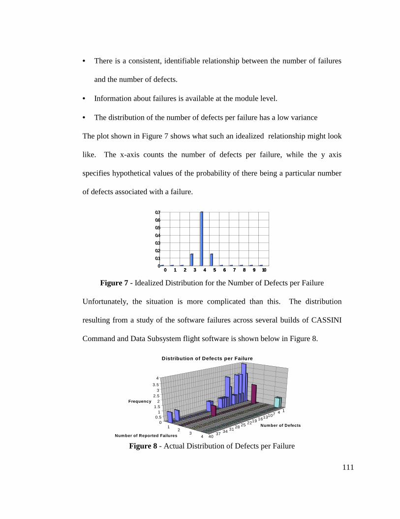
111
• There is a consistent, identifiable relationship between the number of failures
and the number of defects.
• Information about failures is available at the module level.
• The distribution of the number of defects per failure has a low variance
The plot shown in Figure 7 shows what such an idealized relationship might look
like. The x-axis counts the number of defects per failure, while the y axis
specifies hypothetical values of the probability of there being a particular number
of defects associated with a failure.
0 1 2 3 4 5 6 7 8 9 100
0.1
0.2
0.3
0.4
0.5
0.6
0.7
0 1 2 3 4 5 6 7 8 9 10
Figure 7 - Idealized Distribution for the Number of Defects per Failure
Unfortunately, the situation is more complicated than this. The distribution
resulting from a study of the software failures across several builds of CASSINI
Command and Data Subsystem flight software is shown below in Figure 8.
1471013161922252831343740
12
34
00.5
11.5
22.5
33.5
4
Frequency
Number of Defects
Number of Reported Failures
Distribution of Defects per Failure
Figure 8 - Actual Distribution of Defects per Failure

112
In Figure 8, almost all of the observations count the number of defects
associated with one failure. The four observations of the number of defects for
more than one failure are an artifact of the way that information about defects and
failures is recorded. Occasionally, an increment of a module is being worked on
to repair defects associated with more than one failure report. With the informa-
tion available for this study, it was sometimes impossible to determine which
defects are associated with which failure.
If we take the distribution of defects for one failure as our baseline
distribution, we can see what would happen if we were to use failure counts as a
surrogate for defect counts. Figures 9 and 10 below show the distribution of the
number of defects per n failures, n ranging from 1 to 10. The distribution for n+1
failures is produced by performing a discrete convolution of the distribution for n
failures with the distribution for one failure (the distribution of the number of
defects for one failure, as well as the Maple V release 2 program to do the
convolutions, are given in Appendix 12). From Figure 10, we see that even if 10
failures were observed, the distribution of defects per failure is still very broad.
11 12 13 14 15 16 17 18 19 11 0 11 1 11 2 11 3 11 4 1
1 23 4
56
78
91 0
0 .0 0
0 .0 2
0 .0 4
0 .0 6
0 .0 8
0 .1 0
0 .1 2
0 .1 4
pd
f v
alu
e
N u m b e r o fD e fe c ts
N u m b e r o fF a i lu re s
C o n v o lv in g P ro b a b il it y D e n s ity F u n c t io n s - N u m b e r o f D e fe c tsp e r “ n ” F a i lu re s
Figure 9 - Probability Density Functions, Number of Defects per n Failures
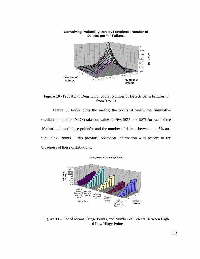
113
1112131415161718191101111121131141
34
56
78
910
0.000
0.005
0.010
0.015
0.020
0.025
0.030
pdf v
alue
Number ofDefects
Number ofFailures
Convolving Probability Density Functions - Number ofDefects per “n” Failures
Figure 10 - Probability Density Functions, Number of Defects per n Failures, nfrom 3 to 10
Figure 11 below plots the means; the points at which the cumulative
distribution function (CDF) takes on values of 5%, 50%, and 95% for each of the
10 distributions (“hinge points”); and the number of defects between the 5% and
95% hinge points. This provides additional information with respect to the
broadness of these distributions.
1
3
5
7
9
Meannumber ofdefects per
failure report
5% pointnumber of
defects
50% pointnumber of
defects
95% pointnumber of
defects
Number ofdefects
between 5%and 95%
points
0.0020.0040.0060.0080.00
100.00120.00140.00160.00
Num
ber
of
Def
ects
Number of Failures
Value Type
Means, Medians, and Hinge Points
Figure 11 - Plot of Means, Hinge Points, and Number of Defects Between Highand Low Hinge Points

114
If we were attempting to count a very large number of defects, it might be
feasible to use failure counts - from the Central Limit Theorem, one would expect
the distribution of the number of defects per n failures to have an increasingly
strong central tendency as n became sufficiently large. In a system with several
hundred failures, it is likely that we would be able to count failures and estimate
the number of defects in the system as a whole with a fair degree of accuracy.
However, remember that in developing our model, we take measurements of the
system at the module level. Considering that the total number of failures recorded
over the lifetime of an individual module is typically in the single to low double-
digits, we can see that the distribution of defects per n failures is too broad to
produce sufficiently accurate estimates of the number of defects. During model
calibration, at least, it is actually necessary to count the number of defects that
were encountered. The rules developed to identify and count defects are
described in the next section.
5.2.3 Rules for Identifying and Counting Defects
In order to count defects, we needed to develop a method of identification
that is repeatable, consistent, and identifies defects at the same level of granularity
as our structural measurements. Returning to the construction example in the
previous section, an incorrectly riveted joint in a skyscraper would be analogous
to an implementation defect affecting only one module in which the programmer
incorrectly initializes a variable local to the routine. This type of defect is simple

115
to count, since it is occurs only in one module. In our construction example, a
defect with global consequences might be a flaw in the process used to produce
the steel used in the building, resulting in steel with less strength than required to
bear the calculated loads. Each girder used in the construction would have the
particular defect of having less than the required strength. This is analogous to a
software defect spanning multiple modules - for instance, each module containing
an include file with a particular defect would have that defect. Another example
would be a defective global data definition - each module referencing that global
data item would contain the defect associated with that data item. In identifying
and counting defects, we must deal with defects that span only one module as well
as those that span several.
In analyzing the flight software for the CASSINI project, the following
information was available to us:
• Problem reporting information from the JPL institutional problem reporting
system. For the software used in this study, failures were recorded in this
system starting at subsystem-level integration, and continuing through space-
craft integration and test. Failure reports typically contain descriptions of the
failure at varying levels of detail, as well as descriptions of what was done to
correct the defect(s) that caused the failure. Detailed information regarding
the underlying defects (e.g., where were the code changes made in each af-
fected module) is generally unavailable from the problem reporting system.

116
• The Software Configuration Control System (SCCS) files for several versions
of the flight software. The way in which SCCS was used in this development
effort makes it possible to track changes to the system at a module level - each
SCCS file stores the baseline version of that file (which may contain one or
more modules) as well as the changes required to produce each subsequent
increment (SCCS revision) of that file. When a module was created, or
changed in response to a failure report or engineering change request, the file
in which the module is contained was checked into SCCS as a new revision.
This allowed us to track changes to the system at the module level as it
evolved over time. For approximately 10% of the failure reports, we were
generally able to identify the source file increment in which the defect(s)
associated with a particular failure report were repaired. This information was
available either in the comments inserted by the developer into the SCCS file
as part of the check-in process, or as part of the set of comments at the begin-
ning of a module that track its development history.
Using the information described above, we performed the following steps to
identify defects:
• For each problem report, search all of the SCCS files to identify all modules
and the increment(s) of each module for which the software was changed in
response to the problem report.
• For each increment of each module identified in the previous step, assume that
all differences between the increment in which repairs are implemented and

117
the previous increment are due solely to defect repair. Note that this is not
necessarily a valid assumption - developers may be making functional en-
hancements to the system in the same increment that defect repairs are being
made. Careful analysis of failure reports for which there is sufficiently de-
tailed descriptive information can serve to separate areas of defect repair from
other changes. However, the level of detail required to perform this analysis
was not consistently available.
• Use a differential comparator (e.g., Unix “diff”) to obtain the differences
between the increment(s) in which the defect(s) were repaired, and the imme-
diately preceding increment(s). The results indicate the areas to be searched
for defects.
After completing the last step, we still had to identify and count the defects - the
results of the differential comparison cannot simply be counted up to give a total
number of defects. In order to do this, we developed a taxonomy for identifying
and counting defects. An example of why the differential comparison results
cannot always be used directly is found within the following discussion of the
taxonomy.
Note that this taxonomy differs from others in that it does not seek to
identify the root cause of the defect. Rather, it is based on the types of changes
made to the software to repair the defects associated with failure reports - in other
words, it constitutes an operational definition of a defect. Although identifying
the root causes of defects is important in improving the development process
118
[Chil92, IEEE93], it is first necessary to identify the defects. This is the specific
issue addressed by our taxonomy. We do not claim that this is the only way to
identify and count defects, nor do we claim that this taxonomy is complete.
However, we have found that this taxonomy has allowed us to successfully
identify defects in the software used in the study in a consistent manner at the
appropriate level of granularity. Briefly, there are three categories of defects -
defects associated with variables, defects associated with constants, and control
flow defects.
• Defects Associated with Variables
• Definition and use of new variables in a module – The initial version
of the rule was to count one defect for each reference to a newly-
defined variable in each module referencing it. This satisfied the goal
of identifying and counting defects at the module level. For example,
the definition of a new global variable would be visible at the module
level because every module’s references to it would be counted. It also
relates more directly to the execution profile of the system, which is
concerned only with references to the data items and not with their
declarations.
However, analysis of the data relating defect content to measures
of structural change revealed that counting only the new assignment
statement as a single defect rather than counting each individual refer-
ence produced better results. This seems to be related to the way that
119
the syntactic analyzer used in this study performs its measurements.
This issue is discussed in more detail in the next chapter.
• Redefinition of existing variables – the initial version of this rule was
that for each reference to a data item that is redefined, one defect
within the module making the reference is counted. Examples of rede-
fining data items include changing the type of an existing variable,
changing the length of a character array, or changing the allowable
range of an enumerated data type.
This is a good example of why the results of the differential com-
parison, listed as the last step in the process of locating the defect-
containing areas, cannot be directly counted to yield a defect total. A
differential comparison between two increments of the same module
would reveal that a type of an existing variable had changed. How-
ever, the differential comparison would not necessarily reveal all of the
references to that variable.
As with the rule about counting the number of defects related to the
introduction of a new variable, analysis of the available data showed
that a better relationship between the number of introduced defects and
the amount of structural change that occurred is obtained if one defect
is counted only for the declaration statement in which the variable is
redefined. With this version of the rule, references to the modified
variable are not counted as defects.

120
• Deletion of an existing variable – the initial version of this rule was to
count one defect for each reference to the data item that was removed
in the system in response to a failure report. As a result of our analy-
sis, this rule was modified to count one defect for the declaration
statement that was removed, and to ignore the references that were re-
moved.
• Change of value in an existing variable assignment statement - each
assignment statement in which the value assigned to an existing vari-
able changes in response to a failure report is counted as one defect
within the module in which the change is made.
• Defects Associated with Constants
• Definition and use of new constants in a module – initially, one defect
was counted for each reference to a new constant that is defined in re-
sponse to a failure report. As with the rule relating to the definition of
new variables, this rule was modified to count only the statement de-
fining the constant as a defect.
• Redefinition of existing constants – initially, each reference to a con-
stant whose value is redefined in response to a failure report was
counted as a defect. As a result of analyzing the data, this rule was
modified to count one defect for the definition statement that was
modified, and ignore the references to the redefined constant.

121
• Deletion of an existing constant - if a constant definition was removed
in response to a failure report, each deleted reference to the constant
was initially counted as one defect against the module in which the
reference was deleted. As with the previous two rules, this was modi-
fied to count only the removed definition statement as a defect, and to
ignore all of the removed references.
• Control defects
• Addition of new source code block - for each new contiguous block of
source code added to an existing module in response to a failure report,
one defect is counted.
• Deletion of erroneous conditionally-executed path(s) within a source
code block - for each execution path within a conditional-execution
block that is deleted in response to a failure report, one defect is
counted. Figure 12 on the following page shows an example. The
number of defects that should be counted in the situation shown in
Figure 12 is two, since two execution paths were removed from the
block. This assumes that the only changes were the removal of the
execution paths, and that the execution conditions for the remaining
blocks did not change.
• Addition of execution path(s) within a source code block - for each
execution path within a conditional-execution block that is added in
response to a failure report, one defect is counted. Again, this assumes
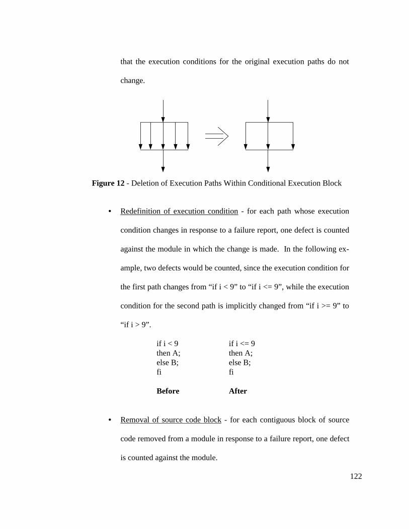
122
that the execution conditions for the original execution paths do not
change.
Figure 12 - Deletion of Execution Paths Within Conditional Execution Block
• Redefinition of execution condition - for each path whose execution
condition changes in response to a failure report, one defect is counted
against the module in which the change is made. In the following ex-
ample, two defects would be counted, since the execution condition for
the first path changes from “if i < 9” to “if i <= 9”, while the execution
condition for the second path is implicitly changed from “if i >= 9” to
“if i > 9”.
if i < 9 if i <= 9 then A; then A; else B; else B; fi fi
Before After
• Removal of source code block - for each contiguous block of source
code removed from a module in response to a failure report, one defect
is counted against the module.
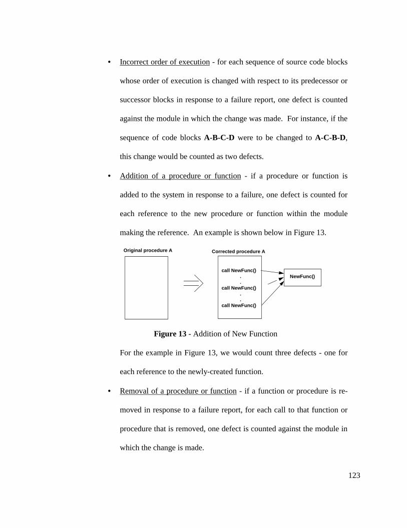
123
• Incorrect order of execution - for each sequence of source code blocks
whose order of execution is changed with respect to its predecessor or
successor blocks in response to a failure report, one defect is counted
against the module in which the change was made. For instance, if the
sequence of code blocks A-B-C-D were to be changed to A-C-B-D,
this change would be counted as two defects.
• Addition of a procedure or function - if a procedure or function is
added to the system in response to a failure, one defect is counted for
each reference to the new procedure or function within the module
making the reference. An example is shown below in Figure 13.
Original procedure A
NewFunc()call NewFunc()
.
.call NewFunc()
.
.call NewFunc()
Corrected procedure A
Figure 13 - Addition of New Function
For the example in Figure 13, we would count three defects - one for
each reference to the newly-created function.
• Removal of a procedure or function - if a function or procedure is re-
moved in response to a failure report, for each call to that function or
procedure that is removed, one defect is counted against the module in
which the change is made.
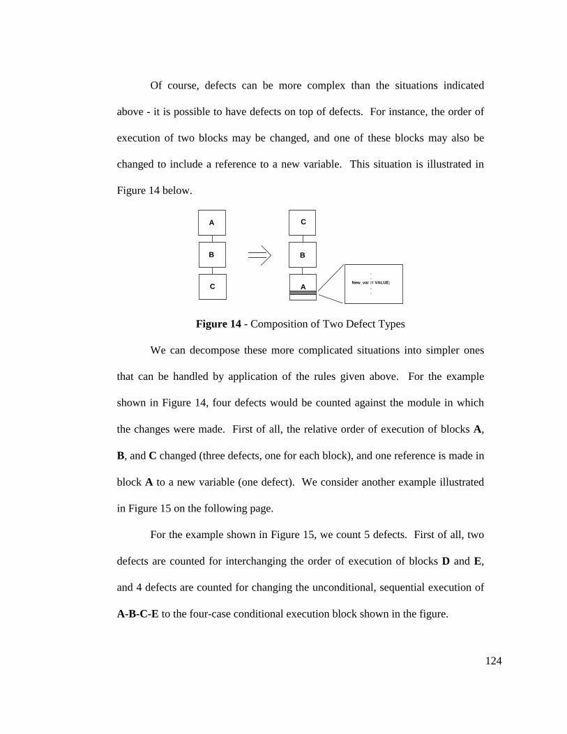
124
Of course, defects can be more complex than the situations indicated
above - it is possible to have defects on top of defects. For instance, the order of
execution of two blocks may be changed, and one of these blocks may also be
changed to include a reference to a new variable. This situation is illustrated in
Figure 14 below.
A
A
B B
C
C
.
.New_var := VALUE;
.
.
Figure 14 - Composition of Two Defect Types
We can decompose these more complicated situations into simpler ones
that can be handled by application of the rules given above. For the example
shown in Figure 14, four defects would be counted against the module in which
the changes were made. First of all, the relative order of execution of blocks A,
B, and C changed (three defects, one for each block), and one reference is made in
block A to a new variable (one defect). We consider another example illustrated
in Figure 15 on the following page.
For the example shown in Figure 15, we count 5 defects. First of all, two
defects are counted for interchanging the order of execution of blocks D and E,
and 4 defects are counted for changing the unconditional, sequential execution of
A-B-C-E to the four-case conditional execution block shown in the figure.
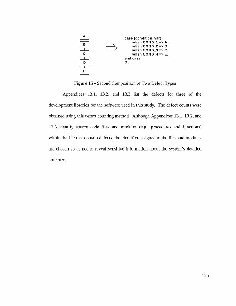
125
A
B
C
D
case (condition_var)when COND_1 => A;when COND_2 => B;when COND_3 => C;when COND_4 => E;
end caseD;
E
Figure 15 - Second Composition of Two Defect Types
Appendices 13.1, 13.2, and 13.3 list the defects for three of the
development libraries for the software used in this study. The defect counts were
obtained using this defect counting method. Although Appendices 13.1, 13.2, and
13.3 identify source code files and modules (e.g., procedures and functions)
within the file that contain defects, the identifier assigned to the files and modules
are chosen so as not to reveal sensitive information about the system’s detailed
structure.

126
6. Defect Insertion Rates
The source of the data analyzed for the implementation phase was the
CASSINI CDS flight software. The following information was collected:
• Over 600 flight software failure reports written during developmental testing
and system integration. Failure reports contain the following information:
� A description of how the system’s behavior deviated from expectations.
This information may be referenced to a requirements specification, and is
usually referenced to a test procedure and test data
� The date on which the failure was observed.
� A description of the corrective action that was taken. However, this in-
formation is not consistently at the level of detail required to calibrate the
model, as the problem tracking system is not designed to collect informa-
tion at such high resolution. The description is usually in terms of how the
overall design was changed, or how the functionality was changed, rather
than specifically identifying the module(s) that were changed, the specifics
of source code changes, and the increment in which repairs were made.
• Development process characteristics for the CASSINI flight software
development effort, as characterized by COCOMO II [Boehm95]. This in-
formation is found in Appendix 13.8.
• Structural measurements for each increment of the source code in the 5 most
recent build libraries for the CASSINI flight software. This constitutes over

127
2000 incremental deliveries of source code files to the development libraries.
The following measurements were collected:
� Raw structural measurements, as measured by the UX-Metric tool from
SET Laboratories, Inc. [SETL93].
� Relative complexity, computed from the raw structural measurements.
� The system evolution measures of code delta and code churn. These are
computed from relative complexity [Muns95a, Niko97]. Code delta is the
difference between the relative complexity of two successive increments
of a module, while code churn is the absolute value of code delta.
6.1 Determination of the Defect Insertion Rate
In relating the number of defects inserted in an increment to measures of a
module’s structural change, we had only a small number of observations with
which to work. There were three difficulties that had to be dealt with:
• Identifying the defect(s) associated with a reported failure. For only about
10% of the failure reports were we able to identify the module(s) that had been
changed, and in which increment those changes were made. Although the
development practices used on this project included the placement of com-
ments in the source code to identify repair activities resulting from each prob-
lem report, this requirement was not consistently enforced.
• Tracing an identified defect to its point of origin. Once a defect has been
identified, it is necessary to trace it back to the increment in which it first
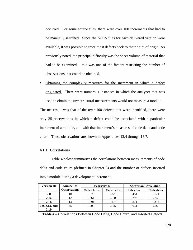
128
occurred. For some source files, there were over 100 increments that had to
be manually searched. Since the SCCS files for each delivered version were
available, it was possible to trace most defects back to their point of origin. As
previously noted, the principal difficulty was the sheer volume of material that
had to be examined – this was one of the factors restricting the number of
observations that could be obtained.
• Obtaining the complexity measures for the increment in which a defect
originated. There were numerous instances in which the analyzer that was
used to obtain the raw structural measurements would not measure a module.
The net result was that of the over 100 defects that were identified, there were
only 35 observations in which a defect could be associated with a particular
increment of a module, and with that increment’s measures of code delta and code
churn. These observations are shown in Appendices 13.4 through 13.7.
6.1.1 Correlations
Table 4 below summarizes the correlations between measurements of code
delta and code churn (defined in Chapter 3) and the number of defects inserted
into a module during a development increment.
Pearson’s R Spearman CorrelationVersion ID Number ofObservations Code churn Code delta Code churn Code delta
2.0 10 .376 -.323 .451 -.1212.1a 12 .661 .700 .793 .5622.1b 13 .891 -.276 .871 -.233
2.0, 2.1a, and2.1b
35 .508 .125 .631 .087
Table 4 – Correlations Between Code Delta, Code Churn, and Inserted Defects
129
This table is a summary of Appendix 14.2, which shows more details of the
correlations between these measurements.
For versions 2.1a and 2.1b, we see from Table 4 that there is a strong
association between the number of defects per increment and the code churn
measure. In Table 4, we see that there is also a strong association between the
number of defects per increment and the value of code delta for version 2.1a. This
is because most of the changes made to modules in version 2.1a were additions to
the software, so the measures of code delta tended to have the same sign. This
was not the case in versions 2.0 and 2.1b, in which there were both additions to
and deletions from the code.
Combining the observations for the three versions, we see in Table 4 that
there appears to be an association between the number of faults inserted per
increment and the measured value of code churn, while there is no significant
association between the number of faults inserted in an increment and the value of
code delta. Since code churn can be considered a measure of the amount of
change that has occurred, it is not surprising that there should be a relationship
between how much change has occurred and the number of defects that were
inserted. Since code delta can assume both positive and negative values,
depending upon whether code has been added to or taken away from a module,
one might expect there to be no significant association between the number of
defects inserted and the measured value of code delta.
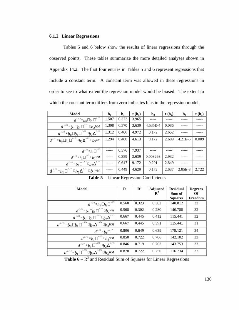
130
6.1.2 Linear Regressions
Tables 5 and 6 below show the results of linear regressions through the
observed points. These tables summarize the more detailed analyses shown in
Appendix 14.2. The first four entries in Tables 5 and 6 represent regressions that
include a constant term. A constant term was allowed in these regressions in
order to see to what extent the regression model would be biased. The extent to
which the constant term differs from zero indicates bias in the regression model.
Model b0 b1 t (b1) b2 t (b2) b3 t (b3)
∇+++ = bbd
jjjj
101,1, 1.507 0.373 3.965 ----- ----- ----- -----
WMbbbdjjjj
2101,1, += ∇+
++ 1.308 0.370 3.639 4.535E-4 0.086 ----- -----
∆∇++++ += bbbd
jjjjjj
2101,1,1, 1.312 0.460 4.972 0.172 2.652 ----- -----
WMbbbbdjjjjjj
3210
1,1,1, ++= ∆∇++++ 1.294 0.480 4.613 0.172 2.609 4.21E-5 0.009
∇++ = bd
jjjj
1
1,1, ----- 0.576 7.937 ----- ----- ----- -----
WMbbdjjjj
211,1, += ∇
++ ----- 0.359 3.639 0.003293 2.932 ----- -----
∆∇+++ += bbd
jjjjjj
21
1,1,1, ----- 0.647 9.172 0.201 2.849 ----- -----
WMbbbdjjjjjj
3211,1,1, ++= ∆∇
+++ ----- 0.449 4.629 0.172 2.637 2.85E-3 2.722
Table 5 – Linear Regression Coefficients
Model R R2 AdjustedR2
ResidualSum ofSquares
DegreesOf
Freedom
∇+++ = bbd
jjjj
10
1,1, 0.568 0.323 0.302 140.812 33
WMbbbdjjjj
210
1,1, += ∇+++ 0.568 0.302 0.280 140.780 32
∆∇++++ += bbbd
jjjjjj
2101,1,1, 0.667 0.445 0.412 115.441 32
WMbbbbdjjjjjj
32101,1,1, ++= ∆∇+
+++ 0.667 0.445 0.391 115.441 31
∇++ = bd
jjjj
1
1,1, 0.806 0.649 0.639 179.121 34
WMbbdjjjj
21
1,1, += ∇++ 0.850 0.722 0.706 142.102 33
∆∇+++ += bbd
jjjjjj
21
1,1,1, 0.846 0.719 0.702 143.753 33
WMbbbdjjjjjj
3211,1,1, ++= ∆∇
+++ 0.878 0.722 0.750 116.734 32
Table 6 – R2 and Residual Sum of Squares for Linear Regressions

131
The second four rows of Tables 5 and 6, on the other hand are the results
of regressions that were forced through the origin. The assumption that was made
for running the regressions in this manner was that if there was no change made to
a module, no defects would be inserted into it.
We see in Table 5 that the constant term in the regression assumes values
between just below 1.3 to just above 1.5. This is an indicator that there aspects of
the system’s structure that are not being measured by our syntactic analyzer. For
instance, if the execution order of two blocks are changed between two increments
(e.g., from A-B-C to C-B-A), this will not be visible to the analyzer, and the
measured structural change may be zero. If the defect being repaired is to change
the execution order of two blocks (e.g., back to A-B-C from C-B-A), we will
observe that the defect in block sequencing was introduced with no associated
structural change. It seems unreasonable to suppose that defects are introduced
into a software system without making any structural changes, so we hypothesize
that there are classes of structural change that we have not been able to measure in
this work. Further discussion is presented in Chapter 8 (Recommendations for
Further Work).
Note that some of the regression models include a term for cumulative
workmonths (WM). This represents the number of work months from the start of
the implementation phase, as reported by the timekeeping system for the
CASSINI CDS flight software development effort. Since the development team
experienced very little turnover, this effort data can be used as a unified measure

132
of the programming team’s experience with the application, the development
platform, and the language and tools (AEXP, PEXP, and LTEX for COCOMO II).
We see in the regression results shown in the first 4 rows of Table 6 that
there is an association between the amount of change that occurs to the structure
of a system and the number of defects inserted into the system. We take as our
null hypothesis that changing the system’s structure has no effect on the number
of defects inserted into the system (i.e., the coefficients for the code churn and
code delta terms in the linear regression are 0). If we look at the columns “t (b1)”,
“t (b1)”, and “t (b3)” in Table 5, which give the t-test statistic associated with the
estimates for b1, b2, and b3, we see that we can reject this hypothesis at a
significance level of better than 5%. For the regression models with an intercept
term, however, we cannot reject the hypothesis that the elapsed number of work
months has no effect on the number of defects inserted.
We see in Table 6 that code churn explains the greatest amount of
variability of the dependent variable (number of defects inserted) in the regression
models. This indicates that the size of the structural change is the most important
element in determining how many defects were inserted. However, these results
also indicate that the type of change (addition of or removal of code) is also a
significant element in determining the number of defects that are introduced.
Changes that involve removing source seem to introduce fewer defects than
changes involving adding source code.

133
In Table 6, we see that the highest value of R2 is 0.445, and the largest
value of adjusted R2 is 0.412. Again, this suggests an association between
measured structural change to the system and the number of defects inserted into
it. It also suggests the following:
• There are additional, unmeasured aspects of the system’s structure that are
related to the number of defects introduced.
• There are unmeasured development process characteristics related to the
number of defects inserted into the system.
Also recall that uncertainty about the point at which each observed defect first
appears in the source code contributes an unknown amount of noise to the
observations. Although there are methods that we plan to apply in future work to
reduce the significance of this problem (see Chapter 7), they cannot be applied
retrospectively to the observations used in this study.
At this point, we examine the regression results shown as the second group
of four models in Tables 5 and 6. These are linear regressions forced through the
origin to satisfy the assumption that if no structural change is made to a particular
increment of a software system, no defects are introduced. These regressions
demonstrate an association between measures of structural change and the number
of defects introduced into the system. Unlike the regression results that include a
constant term, however, the elapsed implementation time is related to the number
of defects that are inserted into the system during its development.

134
Unlike the regression models with an intercept term, the results for the re-
gressions through the origin shown in Tables 5 and 6 indicate that we can reject
the hypothesis that the amount of elapsed development time has no relationship to
the number of defects inserted – the values of the t statistic for the parameter
estimates shown in the columns “t (b1)”, “t (b2),” and “t (b3)” indicate that this
hypothesis can be rejected at better than a 5% significance level. The regression
models through the origin summarized in Tables 5 and 6 indicate that the rate at
which defects are inserted into the system grows linearly with amount of effort
spent in the implementation phase. We might expect that as developers grow
increasingly familiar with the system being developed, the rate at which defects
are introduced would become smaller. However, an increase in the rate at which
defects are inserted might be explained by:
• Developers implementing the easily understood portions of the system early in
the implementation phase, and progressing to more difficult portions later in
the development effort.
• Developers becoming complacent as the implementation phase progresses,
causing them to not pay as much as attention as required to the implementa-
tion details. Interviews with the developers and personal experience make this
an unlikely explanation, however. A more plausible alternative would be
increasing schedule pressure during the later stages of implementation, caus-
ing the members of the development team to assume significantly greater
workloads as the development effort progresses. Unfortunately, there are no
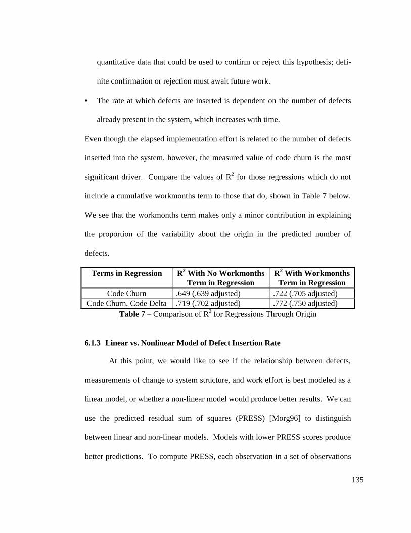
135
quantitative data that could be used to confirm or reject this hypothesis; defi-
nite confirmation or rejection must await future work.
• The rate at which defects are inserted is dependent on the number of defects
already present in the system, which increases with time.
Even though the elapsed implementation effort is related to the number of defects
inserted into the system, however, the measured value of code churn is the most
significant driver. Compare the values of R2 for those regressions which do not
include a cumulative workmonths term to those that do, shown in Table 7 below.
We see that the workmonths term makes only a minor contribution in explaining
the proportion of the variability about the origin in the predicted number of
defects.
Terms in Regression R2 With No WorkmonthsTerm in Regression
R2 With WorkmonthsTerm in Regression
Code Churn .649 (.639 adjusted) .722 (.705 adjusted)Code Churn, Code Delta .719 (.702 adjusted) .772 (.750 adjusted)
Table 7 – Comparison of R2 for Regressions Through Origin
6.1.3 Linear vs. Nonlinear Model of Defect Insertion Rate
At this point, we would like to see if the relationship between defects,
measurements of change to system structure, and work effort is best modeled as a
linear model, or whether a non-linear model would produce better results. We can
use the predicted residual sum of squares (PRESS) [Morg96] to distinguish
between linear and non-linear models. Models with lower PRESS scores produce
better predictions. To compute PRESS, each observation in a set of observations
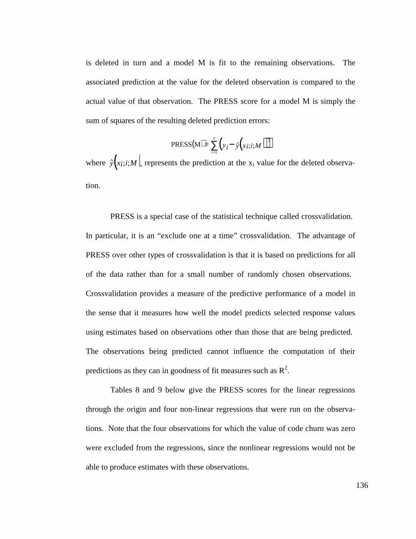
136
is deleted in turn and a model M is fit to the remaining observations. The
associated prediction at the value for the deleted observation is compared to the
actual value of that observation. The PRESS score for a model M is simply the
sum of squares of the resulting deleted prediction errors:
( ) ( )( )∑ −=
=n
iMixiyyi
1
2
;;ˆMPRESS
where ( )Mixiy ;;ˆ represents the prediction at the xi value for the deleted observa-
tion.
PRESS is a special case of the statistical technique called crossvalidation.
In particular, it is an “exclude one at a time” crossvalidation. The advantage of
PRESS over other types of crossvalidation is that it is based on predictions for all
of the data rather than for a small number of randomly chosen observations.
Crossvalidation provides a measure of the predictive performance of a model in
the sense that it measures how well the model predicts selected response values
using estimates based on observations other than those that are being predicted.
The observations being predicted cannot influence the computation of their
predictions as they can in goodness of fit measures such as R2.
Tables 8 and 9 below give the PRESS scores for the linear regressions
through the origin and four non-linear regressions that were run on the observa-
tions. Note that the four observations for which the value of code churn was zero
were excluded from the regressions, since the nonlinear regressions would not be
able to produce estimates with these observations.
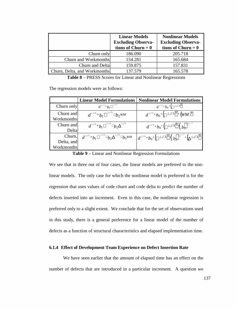
137
Linear ModelsExcluding Observa-tions of Churn = 0
Nonlinear ModelsExcluding Observa-tions of Churn = 0
Churn only 186.090 205.718Churn and Workmonths 154.281 165.684
Churn and Delta 159.875 157.831Churn, Delta, and Workmonths 137.579 165.578
Table 8 – PRESS Scores for Linear and Nonlinear Regressions
The regression models were as follows:
Linear Model Formulations Nonlinear Model FormulationsChurn only ∇
++ = bdjjjj
11,1, ( )∇ +∗=+ 1,
011, jj b
bdjj
Churn andWorkmonths
WMbbdjjjj
21
1,1, += ∇++ ( ) ( )WMbd bjj bjj 211,
01, ∗+∗= ∇
+
Churn andDelta
∆∇+++ += bbd
jjjjjj
211,1,1, ( ) ( )bbd
jj
jj bjj
21,
0
1,
11, ∇∗+∗=+
∇+
Churn,Delta, and
Workmonths
WMbbbdjjjjjj
3211,1,1, ++= ∆∇
+++ ( ) ( ) ( )∆∇ +∗∇∗+∗=+
+ 1,2
1,0
1
1,
11, jj bjj bbbd
jj
jj
Table 9 – Linear and Nonlinear Regression Formulations
We see that in three out of four cases, the linear models are preferred to the non-
linear models. The only case for which the nonlinear model is preferred is for the
regression that uses values of code churn and code delta to predict the number of
defects inserted into an increment. Even in this case, the nonlinear regression is
preferred only to a slight extent. We conclude that for the set of observations used
in this study, there is a general preference for a linear model of the number of
defects as a function of structural characteristics and elapsed implementation time.
6.1.4 Effect of Development Team Experience on Defect Insertion Rate
We have seen earlier that the amount of elapsed time has an effect on the
number of defects that are introduced in a particular increment. A question we
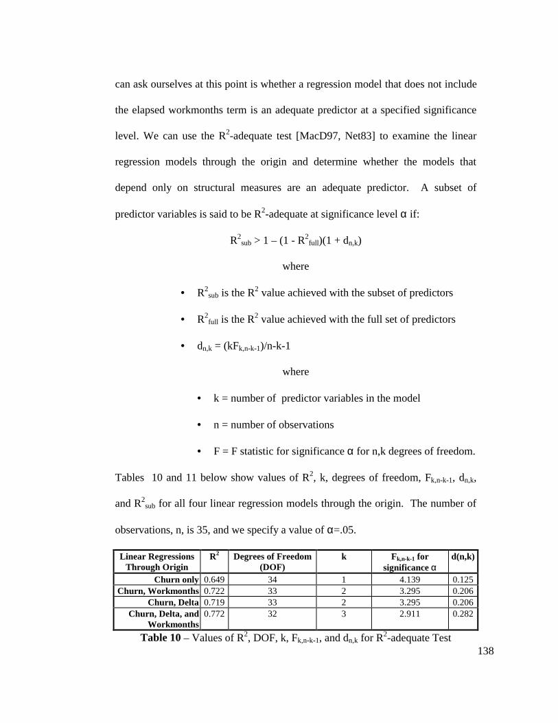
138
can ask ourselves at this point is whether a regression model that does not include
the elapsed workmonths term is an adequate predictor at a specified significance
level. We can use the R2-adequate test [MacD97, Net83] to examine the linear
regression models through the origin and determine whether the models that
depend only on structural measures are an adequate predictor. A subset of
predictor variables is said to be R2-adequate at significance level α if:
R2sub > 1 – (1 - R2
full)(1 + dn,k)
where
• R2sub is the R2 value achieved with the subset of predictors
• R2full is the R2 value achieved with the full set of predictors
• dn,k = (kFk,n-k-1)/n-k-1
where
• k = number of predictor variables in the model
• n = number of observations
• F = F statistic for significance α for n,k degrees of freedom.
Tables 10 and 11 below show values of R2, k, degrees of freedom, Fk,n-k-1, dn,k,
and R2sub for all four linear regression models through the origin. The number of
observations, n, is 35, and we specify a value of α=.05.
Linear RegressionsThrough Origin
R2 Degrees of Freedom(DOF)
k Fk,n-k-1 forsignificance α
d(n,k)
Churn only 0.649 34 1 4.139 0.125Churn, Workmonths 0.722 33 2 3.295 0.206
Churn, Delta 0.719 33 2 3.295 0.206Churn, Delta, and
Workmonths0.772 32 3 2.911 0.282
Table 10 – Values of R2, DOF, k, Fk,n-k-1, and dn,k for R2-adequate Test
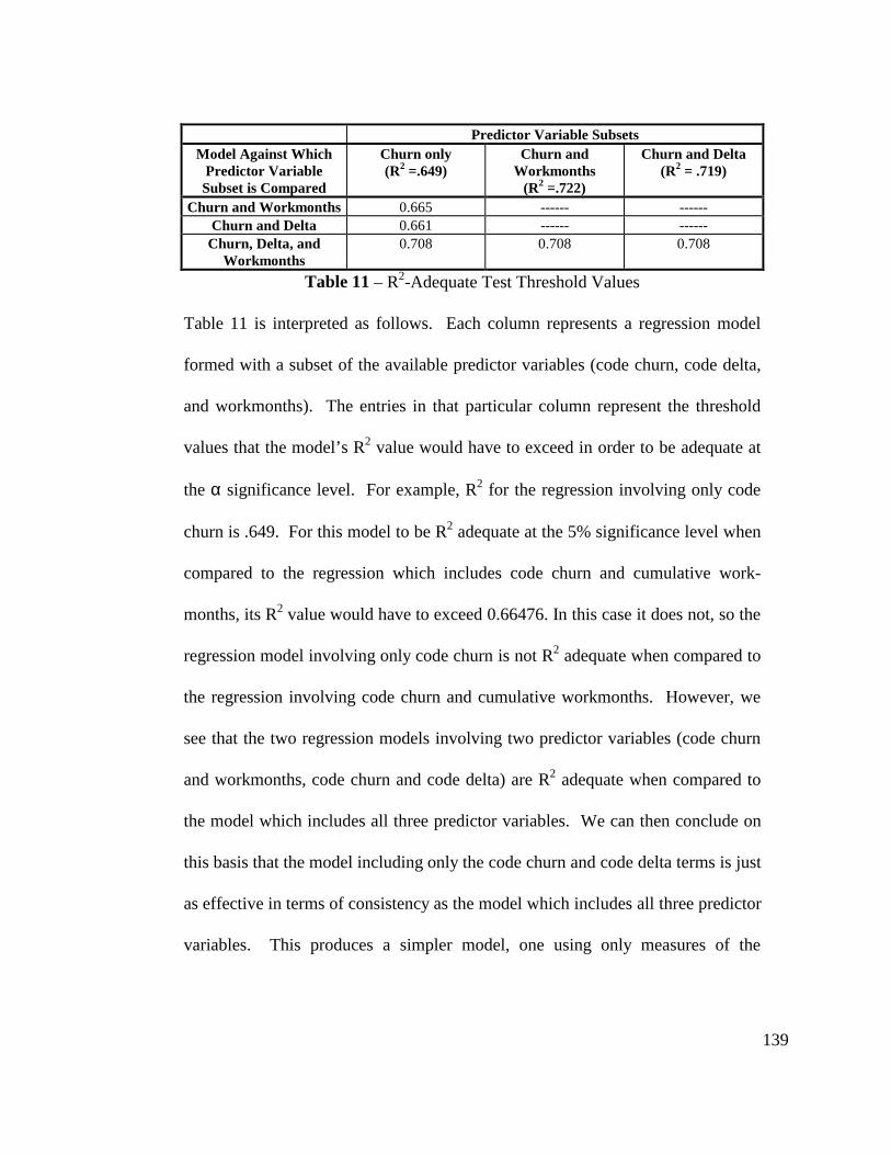
139
Predictor Variable SubsetsModel Against Which
Predictor VariableSubset is Compared
Churn only(R2 =.649)
Churn andWorkmonths
(R2 =.722)
Churn and Delta(R2 = .719)
Churn and Workmonths 0.665 ------ ------Churn and Delta 0.661 ------ ------Churn, Delta, and
Workmonths0.708 0.708 0.708
Table 11 – R2-Adequate Test Threshold Values
Table 11 is interpreted as follows. Each column represents a regression model
formed with a subset of the available predictor variables (code churn, code delta,
and workmonths). The entries in that particular column represent the threshold
values that the model’s R2 value would have to exceed in order to be adequate at
the α significance level. For example, R2 for the regression involving only code
churn is .649. For this model to be R2 adequate at the 5% significance level when
compared to the regression which includes code churn and cumulative work-
months, its R2 value would have to exceed 0.66476. In this case it does not, so the
regression model involving only code churn is not R2 adequate when compared to
the regression involving code churn and cumulative workmonths. However, we
see that the two regression models involving two predictor variables (code churn
and workmonths, code churn and code delta) are R2 adequate when compared to
the model which includes all three predictor variables. We can then conclude on
this basis that the model including only the code churn and code delta terms is just
as effective in terms of consistency as the model which includes all three predictor
variables. This produces a simpler model, one using only measures of the

140
software system’s structural change, rather than changes both in its structure and
its development process (i.e., cumulative workmonths).
6.1.5 Crossvalidation
Since the set of observations was sparse, the only way in which we could
evaluate the predictive ability of the regression models was to do a crossvalida-
tion. We performed a specific type of crossvalidation, excluding one observation
at a time and examining the prediction made with the remaining observations. For
our set of 35 observations, 35 different predictions were made for each regression
model. Tables 12-15 below summarize the crossvalidation results for each of the
four linear regression models through the origin, which are tabulated in Appendi-
ces 14.3.1 – 14.3.4. For each of the four linear regressions through the origin,
Tables 12-15 show statistics for:
• Predicted squared residuals. For each observation, a regression model is
formed that excludes that observation. The resulting model then uses the
value of the excluded observation to predict the number of defects inserted.
This prediction is then subtracted from the number of defects actually ob-
served for the excluded observation. This residual is then squared, thereby
forming the predicted squared residual.
• Ratio of predicted number of defects to observed number of defects, where
predictions are made for excluded observations. For each excluded observa-
tion, a prediction is made as described above. The ratio of the prediction
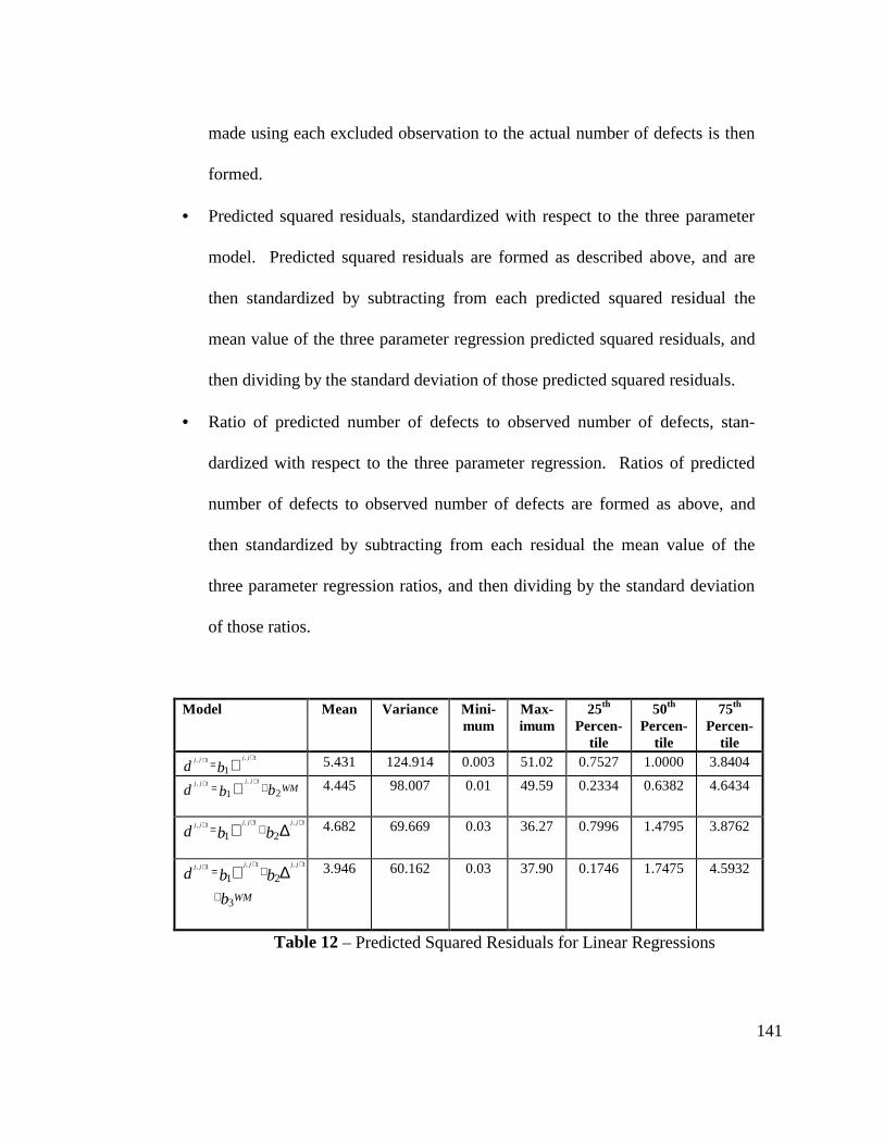
141
made using each excluded observation to the actual number of defects is then
formed.
• Predicted squared residuals, standardized with respect to the three parameter
model. Predicted squared residuals are formed as described above, and are
then standardized by subtracting from each predicted squared residual the
mean value of the three parameter regression predicted squared residuals, and
then dividing by the standard deviation of those predicted squared residuals.
• Ratio of predicted number of defects to observed number of defects, stan-
dardized with respect to the three parameter regression. Ratios of predicted
number of defects to observed number of defects are formed as above, and
then standardized by subtracting from each residual the mean value of the
three parameter regression ratios, and then dividing by the standard deviation
of those ratios.
Model Mean Variance Mini-mum
Max-imum
25th
Percen-tile
50th
Percen-tile
75th
Percen-tile
∇++ =bd
jjjj
11,1, 5.431 124.914 0.003 51.02 0.7527 1.0000 3.8404
WMbbdjjjj
211,1, += ∇
++ 4.445 98.007 0.01 49.59 0.2334 0.6382 4.6434
∆∇+++ += bbd
jjjjjj
211,1,1, 4.682 69.669 0.03 36.27 0.7996 1.4795 3.8762
WMb
bbdjjjjjj
3
21
1,1,1,
+
+= ∆∇+++ 3.946 60.162 0.03 37.90 0.1746 1.7475 4.5932
Table 12 – Predicted Squared Residuals for Linear Regressions
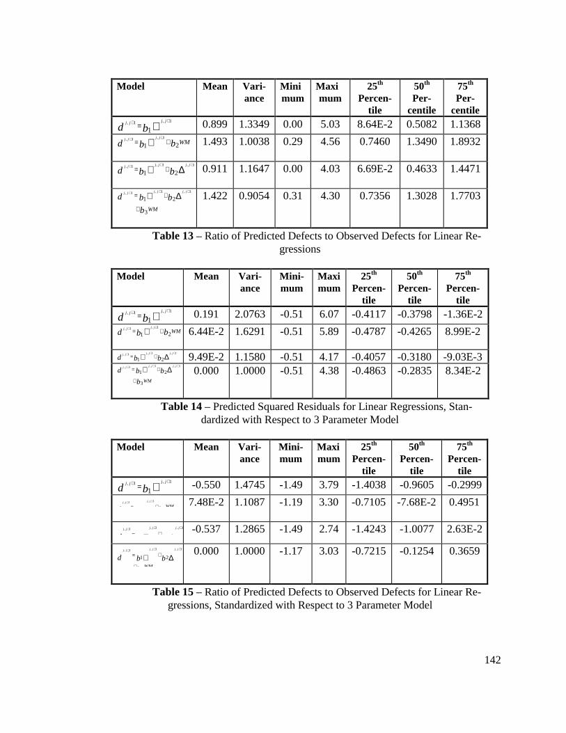
142
Model Mean Vari-ance
Minimum
Maximum
25th
Percen-tile
50th
Per-centile
75th
Per-centile
∇++ = bd
jjjj
11,1, 0.899 1.3349 0.00 5.03 8.64E-2 0.5082 1.1368
WMbbdjjjj
211,1, += ∇
++ 1.493 1.0038 0.29 4.56 0.7460 1.3490 1.8932
∆∇+++ += bbd
jjjjjj
211,1,1, 0.911 1.1647 0.00 4.03 6.69E-2 0.4633 1.4471
WMb
bbdjjjjjj
3
211,1,1,
+
+= ∆∇+++ 1.422 0.9054 0.31 4.30 0.7356 1.3028 1.7703
Table 13 – Ratio of Predicted Defects to Observed Defects for Linear Re-gressions
Model Mean Vari-ance
Mini-mum
Maximum
25th
Percen-tile
50th
Percen-tile
75th
Percen-tile
∇++ = bd
jjjj
11,1, 0.191 2.0763 -0.51 6.07 -0.4117 -0.3798 -1.36E-2WMbbd
jjjj
21
1,1, += ∇++ 6.44E-2 1.6291 -0.51 5.89 -0.4787 -0.4265 8.99E-2
∆∇+++ += bbd
jjjjjj
211,1,1, 9.49E-2 1.1580 -0.51 4.17 -0.4057 -0.3180 -9.03E-3
WMb
bbdjjjjjj
3
211,1,1,
+
+= ∆∇+++ 0.000 1.0000 -0.51 4.38 -0.4863 -0.2835 8.34E-2
Table 14 – Predicted Squared Residuals for Linear Regressions, Stan-dardized with Respect to 3 Parameter Model
Model Mean Vari-ance
Mini-mum
Maximum
25th
Percen-tile
50th
Percen-tile
75th
Percen-tile
∇++ = bd
jjjj
11,1, -0.550 1.4745 -1.49 3.79 -1.4038 -0.9605 -0.2999
WMbdjjjj
2
1,1,
+= ∇++ 7.48E-2 1.1087 -1.19 3.30 -0.7105 -7.68E-2 0.4951
∆∇+++
+=djjjjjj 1,1,1, -0.537 1.2865 -1.49 2.74 -1.4243 -1.0077 2.63E-2
WMb
bbdjjjjjj
3
21
1,1,1,
+
+= ∆∇+++ 0.000 1.0000 -1.17 3.03 -0.7215 -0.1254 0.3659
Table 15 – Ratio of Predicted Defects to Observed Defects for Linear Re-gressions, Standardized with Respect to 3 Parameter Model
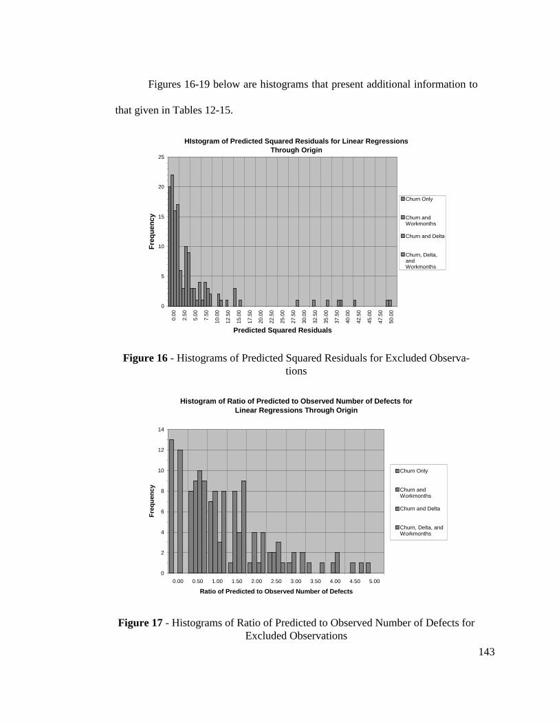
143
Figures 16-19 below are histograms that present additional information to
that given in Tables 12-15.
HIstogram of Predicted Squared Residuals for Linear Regressions Through Origin
0
5
10
15
20
25
0.00
2.50
5.00
7.50
10.0
0
12.5
0
15.0
0
17.5
0
20.0
0
22.5
0
25.0
0
27.5
0
30.0
0
32.5
0
35.0
0
37.5
0
40.0
0
42.5
0
45.0
0
47.5
0
50.0
0
Predicted Squared Residuals
Fre
quen
cy
Churn Only
Churn andWorkmonths
Churn and Delta
Churn, Delta,andWorkmonths
Figure 16 - Histograms of Predicted Squared Residuals for Excluded Observa-tions
Histogram of Ratio of Predicted to Observed Number of Defects for Linear Regressions Through Origin
0
2
4
6
8
10
12
14
0.00 0.50 1.00 1.50 2.00 2.50 3.00 3.50 4.00 4.50 5.00
Ratio of Predicted to Observed Number of Defects
Fre
quen
cy
Churn Only
Churn andWorkmonths
Churn and Delta
Churn, Delta, andWorkmonths
Figure 17 - Histograms of Ratio of Predicted to Observed Number of Defects forExcluded Observations
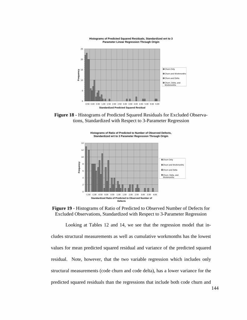
144
Histograms of Predicted Squared Residuals, Standardized wrt to 3 Parameter Linear Regression Through Origin
0
5
10
15
20
25
-0.50 0.00 0.50 1.00 1.50 2.00 2.50 3.00 3.50 4.00 4.50 5.00 5.50 6.00
Standardized Predicted Squared Residual
Fre
quen
cy
Churn Only
Churn and Workmonths
Churn and Delta
Churn, Delta, andWorkmonths
Figure 18 - Histograms of Predicted Squared Residuals for Excluded Observa-tions, Standardized with Respect to 3-Parameter Regression
Histograms of Ratio of Predicted to Number of Observed Defects, Standardized wrt to 3 Parameter Regression Through Origin
0
2
4
6
8
10
12
14
-1.50 -1.00 -0.50 0.00 0.50 1.00 1.50 2.00 2.50 3.00 3.50 4.00
Standardized Ratio of Predicted to Observed Number of Defects
Fre
quen
cy
Churn Only
Churn and Workmonths
Churn and Delta
Churn, Delta, andWorkmonths
Figure 19 - Histograms of Ratio of Predicted to Observed Number of Defects forExcluded Observations, Standardized with Respect to 3-Parameter Regression
Looking at Tables 12 and 14, we see that the regression model that in-
cludes structural measurements as well as cumulative workmonths has the lowest
values for mean predicted squared residual and variance of the predicted squared
residual. Note, however, that the two variable regression which includes only
structural measurements (code churn and code delta), has a lower variance for the
predicted squared residuals than the regressions that include both code churn and
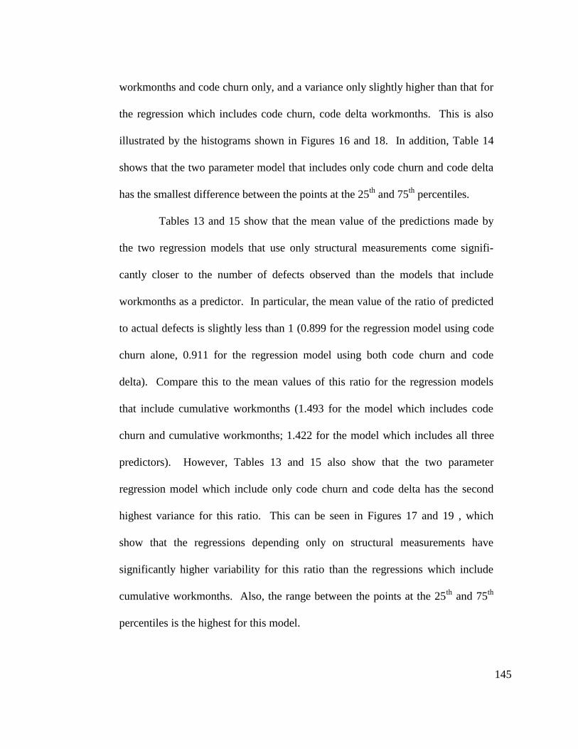
145
workmonths and code churn only, and a variance only slightly higher than that for
the regression which includes code churn, code delta workmonths. This is also
illustrated by the histograms shown in Figures 16 and 18. In addition, Table 14
shows that the two parameter model that includes only code churn and code delta
has the smallest difference between the points at the 25th and 75th percentiles.
Tables 13 and 15 show that the mean value of the predictions made by
the two regression models that use only structural measurements come signifi-
cantly closer to the number of defects observed than the models that include
workmonths as a predictor. In particular, the mean value of the ratio of predicted
to actual defects is slightly less than 1 (0.899 for the regression model using code
churn alone, 0.911 for the regression model using both code churn and code
delta). Compare this to the mean values of this ratio for the regression models
that include cumulative workmonths (1.493 for the model which includes code
churn and cumulative workmonths; 1.422 for the model which includes all three
predictors). However, Tables 13 and 15 also show that the two parameter
regression model which include only code churn and code delta has the second
highest variance for this ratio. This can be seen in Figures 17 and 19 , which
show that the regressions depending only on structural measurements have
significantly higher variability for this ratio than the regressions which include
cumulative workmonths. Also, the range between the points at the 25th and 75th
percentiles is the highest for this model.

146
6.1.6 Analysis of Residuals
Table 16 below shows the results of the Wilcoxon Signed Ranks test, as
applied to the predictions for the excluded observations and the number of defects
observed for each of the four linear regression models through the origin. For the
regression models based only on structural measurements, about 2/3 of the
estimates tend to be less than the number of defects observed. For the other two
regression models, about 60% of the estimates tend to be less than the number of
defects observed.
Sample Pair N MeanRank
Sumof
Ranks
TestStatistic
Z
Asymptot-ic Signifi-
cance(2-tailed)
Observed Defects;Estimated Number ofDefects Based on ChurnOnly
Negative RanksPositive RanksTiesTotal
25a
10b
0c
35
17.5219.20
438.00192.00
-2.015d .044
Observed Defects;Estimated Number ofDefects Based on Churnand WM
Negative RanksPositive RanksTiesTotal
15a
20b
0c
35
17.9318.05
269.00361.00
-.753e .451
Observed Defects;Estimated Number ofDefects Based on Churnand Delta
Negative RanksPositive RanksTiesTotal
24a
11b
0c
35
16.9220.36
406.00224.00
-1.491d .136
Observed Defects;Estimated Number ofDefects Based on Churn,Delta, and WM
Negative RanksPositive RanksTiesTotal
14a
21b
0c
35
20.3616.43
285.00345.00
-.491e .623
a. Observed Defects > Regression model predictionsb. Observed Defects < Regression model predictionsc. Observed Defects = Regression model predictionsd. Based on positive rankse. Based on negative ranks
Table 16 – Wilcoxon Signed Ranks Test for Linear Regressions Through theOrigin
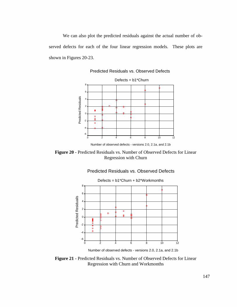
147
We can also plot the predicted residuals against the actual number of ob-
served defects for each of the four linear regression models. These plots are
shown in Figures 20-23.
Predicted Residuals vs. Observed Defects
Defects = b1*Churn
Number of observed defects - versions 2.0, 2.1a, and 2.1b
121086420
Pre
dict
ed R
esid
uals
8
6
4
2
0
-2
-4
-6
Figure 20 - Predicted Residuals vs. Number of Observed Defects for LinearRegression with Churn
Predicted Residuals vs. Observed Defects
Defects = b1*Churn + b2*Workmonths
Number of observed defects - versions 2.0, 2.1a, and 2.1b
121086420
Pre
dict
ed R
esid
uails
8
6
4
2
0
-2
-4
-6
Figure 21 - Predicted Residuals vs. Number of Observed Defects for LinearRegression with Churn and Workmonths
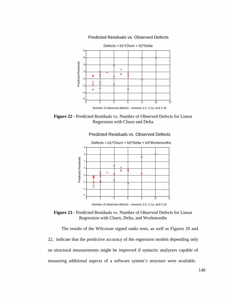
148
Predicted Residuals vs. Observed Defects
Defects = b1*Churn + b2*Delta
Number of observed defects - versions 2.0, 2.1a, and 2.1b
121086420
Pre
dict
ed R
esid
uals
8
6
4
2
0
-2
-4
-6
Figure 22 - Predicted Residuals vs. Number of Observed Defects for LinearRegression with Churn and Delta
Predicted Residuals vs. Observed Defects
Defects = b1*Churn + b2*Delta + b3*Workmonths
Number of observed defects - versions 2.0, 2.1a, and 2.1b
121086420
Pre
dict
ed R
esid
uals
8
6
4
2
0
-2
-4
-6
Figure 23 - Predicted Residuals vs. Number of Observed Defects for LinearRegression with Churn, Delta, and Workmonths
The results of the Wilcoxon signed ranks tests, as well as Figures 20 and
22, indicate that the predictive accuracy of the regression models depending only
on structural measurements might be improved if syntactic analyzers capable of
measuring additional aspects of a software system’s structure were available.

149
Compare this to the regression models which include a term for workmonths. As
shown in Table 16 and Figures 21 and 23, these models tend to be more balanced
between overestimating and underestimating the number of defects inserted into
the system. This appears to indicate the presence of bias related to the work-
months term. Were the measurements of the system’s structure to be more
accurate, it would appear that the regression models which include the work-
months term would not benefit to the same extent as the regression models
dependent only on structural measurements, since the additional variability of the
estimate contributed by the workmonths term would not be compensated for by
the increased accuracy of the structural measurements.
6.1.7 Defect Insertion Rate – Summary
Based on the above analyses, we can make the following conclusions:
• There is a relationship between the number of defects inserted in a
development increment and changes in a software system’s structure and
the development process.
• Of the relationships analyzed, the one that appears to fit best with respect
to PRESS score and R2-adequate criteria is a linear relationship in which
the number of defects inserted is proportional to:
• The amount of change made to the system during a development
increment (measured by code churn). Of the factors observed and
analyzed, the amount of change is the major contributing factor.

150
• The type of change made (i.e., addition to or deletion from the
system), measured by code delta.
• Although cumulative work effort appears to be a factor in the number of
defects inserted during a development increment, it also appears to be a
minor contributor. The R2-adequacy test shows that for the system con-
sidered in this study, measurements of the system’s structural change are
an adequate set of predictor variables at the 5% significance level. If we
accept the two parameter regression model based on structural change
alone ( ∆∇+++ += bbd
jjjjjj
211,1,1, ), we see that the number of defects inserted into
the CASSINI CDS flight software per unit of change (i.e., code churn and
code delta) remains constant throughout the implementation phase.
• The predictive accuracy of the regression models depending only on
structural measures may be increased by developing syntactic analyzers
that measure aspects of the system’s structure that could not be done with
the analyzer used in this study [SETL93]. In particular, analyzers should
be able to measure changes in variable definition and usage as well
changes to the sequencing of blocks within the system.
6.2 Forecasting Residual Defect Content
We can use the birth and death model previously described in Section
3.4.2 to forecast the number of residual defects at the end of a development
interval of given length (e.g., “What will be the expected number of residual

151
defects in the system after the next 5 workmonths?”). We will not attempt to
estimate the number of residual defects in the system over the entire development
effort. Although it is quite simple to develop a model that would do so, an
inordinate amount of computation would be required. For this particular
development effort, we estimate that at least several thousand defects have been
inserted into the system during the implementation phase. A birth and death
model for the entire implementation phase would require a rate matrix with
several thousand rows and columns. To exponentiate a rate matrix of 150x150
takes between two and three hours using the prototype shown in Appendix 10.
The rate matrix for the entire implementation phase would be between 50 and 100
times larger, and the time required to exponentiate the rate matrix to form the
probability transition matrix goes as the square of the size of the matrix. Instead,
we will look at a subset of the implementation phase and the defect insertion and
removal rates given above to form a small birth and death model.
6.2.1 Defect Insertion Rate
To use the birth and death model, we will need to determine rates of defect
insertion and removal. To determine the rate of defect insertion (defects inserted
per workmonth), we will need to determine the following:
• Defects inserted per unit of structural change. For the example below, we will
use a simplified form of the relationship between the number of defects in-
serted in an increment and the amount of code churn that has occurred. Recall

152
from Section 6.1 that this relationship is given by ∇++ = bd
jjjj
1
1,1, , where b1 is
0.576.
• The amount of code churn per development increment. An analysis of the
available data shows that this can be modeled by a linear relationship in which
the amount of code churn per development increment is 4.72.
• The number of development increments per workmonth. The available data
shows that this can be modeled by a linear relationship in which development
increments are checked into the development library at 0.167 workmonths
intervals. This gives us 5.988 development increments per workmonth.
The defect insertion rate of 16.28 defects per workmonth is the product of these
three items.
6.2.2 Determining the Defect Removal Rate
For the CASSINI CDS flight software, we were not able to directly ob-
serve the number of defects removed. However, there was sufficient data to make
some observations about the rate at which failures were discovered during
developmental testing, and to use those results to estimate the rate of defect
removal. Figure 24 on the following page shows the cumulative number of
failures observed during developmental testing as a function of the cumulative
workmonths spent in development from the start of implementation through June
30, 1997. Note that there is no trend toward increasing reliability increase shown
in this plot. Rather, there is a tendency for the number of failures observed to
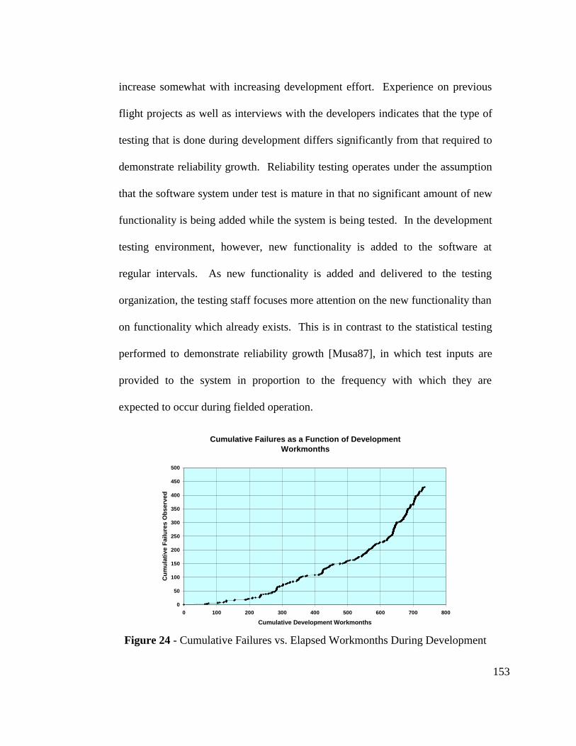
153
increase somewhat with increasing development effort. Experience on previous
flight projects as well as interviews with the developers indicates that the type of
testing that is done during development differs significantly from that required to
demonstrate reliability growth. Reliability testing operates under the assumption
that the software system under test is mature in that no significant amount of new
functionality is being added while the system is being tested. In the development
testing environment, however, new functionality is added to the software at
regular intervals. As new functionality is added and delivered to the testing
organization, the testing staff focuses more attention on the new functionality than
on functionality which already exists. This is in contrast to the statistical testing
performed to demonstrate reliability growth [Musa87], in which test inputs are
provided to the system in proportion to the frequency with which they are
expected to occur during fielded operation.
Cumulative Failures as a Function of Development Workmonths
0
50
100
150
200
250
300
350
400
450
500
0 100 200 300 400 500 600 700 800
Cumulative Development Workmonths
Cum
ulat
ive
Fai
lure
s O
bser
ved
Figure 24 - Cumulative Failures vs. Elapsed Workmonths During Development

154
We can apply the Laplace test [Lyu96] to identify and quantify trends to-
ward reliability growth or reliability decrease during development testing. A plot
of the Laplace test results is shown in Figure 25 below. In order to obtain the
results, the observations first had to be transformed from grouped data (test
interval lengths and failures per test interval) to interfailure times. Although the
test intervals were one calendar week in length, the number of workmonths per
test interval varied over the testing effort. The Laplace Test cannot be applied to
grouped data in which the intervals are of unequal length [Lyu96]. The transfor-
mation was done by assigning random times to failures within each test interval,
using the CASRE software reliability modeling tool [Niko94]. The Laplace Test
was then applied to the transformed set of failure observations.
CASSINI CDS Developmental SW PRs - Laplace TestDevelopment Workmonths Used as Time Base
-4.00E+00
-2.00E+00
0.00E+00
2.00E+00
4.00E+00
6.00E+00
8.00E+00
1.00E+01
1.20E+01
1.40E+01
1.60E+01
1.80E+01
0 50 100 150 200 250 300 350 400
Failure Number
Lapl
ace
Tes
t Sta
tistic
Figure 25 - CASSINI CDS Developmental Failure History - Laplace Test Results

155
The following rules are applied to interpret the Laplace test results [Lyu96]:
• Reject the null hypothesis that occurrences of failures follow a Homogeneous
Poisson Process (HPP) in favor of the hypothesis of reliability growth at the
5% significance level if the test statistic is less than or equal to the value at
which the cumulative distribution function for the normal distribution is 0.05.
• Reject the null hypothesis that occurrences of failures follow a Homogeneous
Poisson Process (HPP) in favor of the hypothesis of reliability decrease at the
5% significance level if the test statistic is greater than or equal to the value at
which the CDF for the normal distribution is 0.95.
• Reject the null hypothesis that there is either reliability growth or reliability
decrease in favor of the hypothesis that there is no trend at the 5% significance
level if the statistic is between the values at which the CDF for the normal
distribution is 0.025 and 0.975. These boundaries are given by the two bold
horizontal lines near y=-2 and y=2 in Figure 25 above.
Overall, we see that there is a trend toward reliability decrease as the development
effort progresses. We also see in the interval between failures 50 and 250, we
cannot identify a trend towards either reliability growth or reliability decrease –
the Laplace Test statistic is centered around a value of 6, with excursions down to
4 and up to 8. For this interval, we can accept the hypothesis of occurrences of
failures following an HPP, which would result in a linear relationship between the
cumulative number of failures observed and cumulative development effort.
We can estimate the rate of defect removal by:

156
• Finding the rate at which failures are observed. We can do this by analyzing
the data that went into producing Figure 24 above. This yields a rate of 0.411
failures observed (and presumably removed) per workmonth. We assume that
the defects responsible for a failure are repaired upon observation of the fail-
ure.
• Multiplying the rate at which failures are observed by the mean number of
defects per reported failure (10.57, as seen in Appendix 12.3).
The defect removal rate, 4.34 defects per workmonth, is the product of these two
items. It is interesting to note that this is approximately one-fourth the rate of
defect insertion given above.
6.2.3 Forecasting Results
Before showing the model results, we should note here that the purpose of
this example is to show how the defect insertion and removal rates are used in a
birth and death model to estimate the number of residual defects in a system. We
made the following approximations that would not be made if this estimate were
being made in a production environment:
• The amount of code churn per development increment is approximated as a
linear relationship. Better fits to the data are obtained with quadratic and
cubic polynomial fits, as measured by the Residual Sum of Squares (RSS).
However, the linear approximation suffices for this purpose.

157
• The number of development increments per workmonth is also approximated
as a linear relationship. A logistic curve provides a better fit to the data than a
linear approximation, as measured by RSS. However, a linear relationship
suffices for purposes of this example, especially considering that we will only
be looking at a small portion of the implementation phase.
• The rate of defect removal is approximated as a linear relationship. Since we
are looking at only a small portion of the implementation phase, we can
choose a region in which this approximation is valid (e.g., the region between
200 and 500 workmonths, in which the occurrences of failures can be taken to
follow an HPP).
Again, the main purpose of this example is to show the usage of defect insertion
and removal rates in a birth and death model. In a production environment, the
amount of effort that went into determining the relationship between the structural
evolution of a software system and the number of defects inserted into the system
would have gone into refining the relationships listed above.
Figure 26 on the following page shows the output of the birth and death
model formed using the defect insertion and removal rates given above. The
program that was run is a variant of that shown in Appendix 10, and was run
under the following conditions:
• The length of the development period considered was one work month.
• It was assumed that at the start of the development period, there were no
defects present in the system.
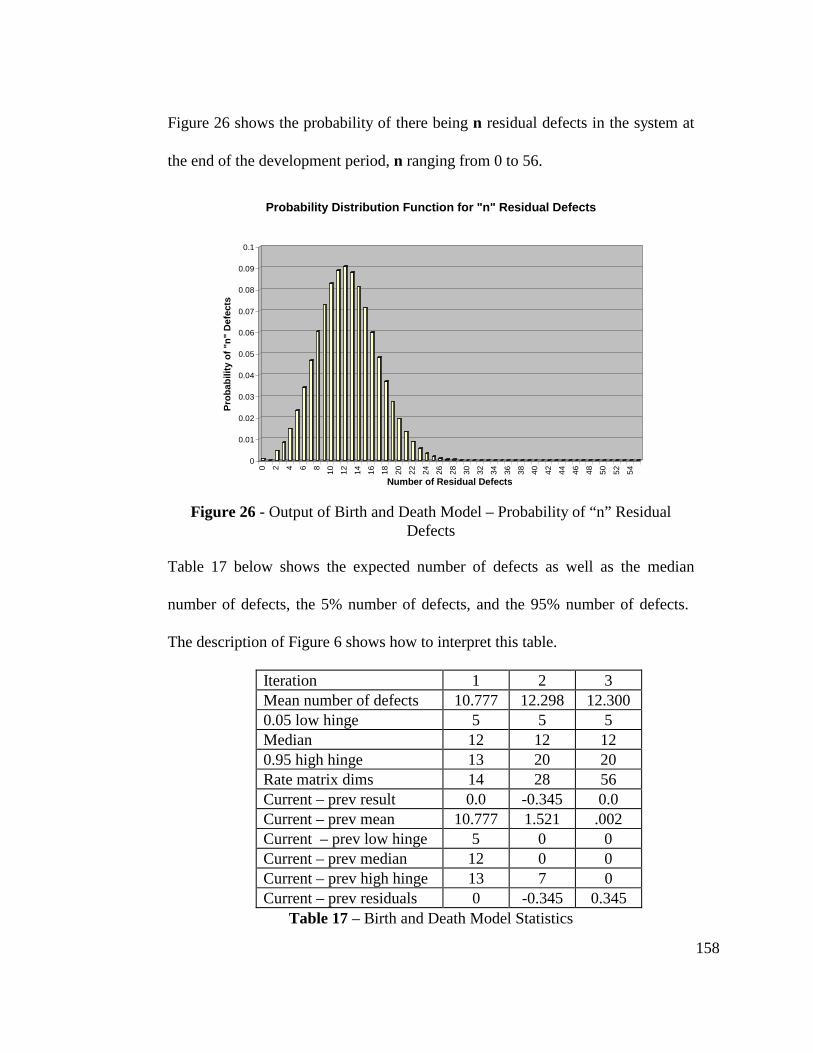
158
Figure 26 shows the probability of there being n residual defects in the system at
the end of the development period, n ranging from 0 to 56.
0
0.01
0.02
0.03
0.04
0.05
0.06
0.07
0.08
0.09
0.1
Pro
babi
lity
of "
n" D
efec
ts
0 2 4 6 8
10 12 14 16 18 20 22 24 26 28 30 32 34 36 38 40 42 44 46 48 50 52 54
Number of Residual Defects
Probability Distribution Function for "n" Residual Defects
Figure 26 - Output of Birth and Death Model – Probability of “n” ResidualDefects
Table 17 below shows the expected number of defects as well as the median
number of defects, the 5% number of defects, and the 95% number of defects.
The description of Figure 6 shows how to interpret this table.
Iteration 1 2 3Mean number of defects 10.777 12.298 12.3000.05 low hinge 5 5 5Median 12 12 120.95 high hinge 13 20 20Rate matrix dims 14 28 56Current – prev result 0.0 -0.345 0.0Current – prev mean 10.777 1.521 .002Current – prev low hinge 5 0 0Current – prev median 12 0 0Current – prev high hinge 13 7 0Current – prev residuals 0 -0.345 0.345
Table 17 – Birth and Death Model Statistics

159
7. Summary and Conclusions
We have shown that there is a relationship between software defects and
measurable software attributes. This is in itself not a new result or observation.
What is new and interesting, however, is:
• The fact that this endeavor has shown that within the accuracy of the data that
was collected, there is an identifiable association between the rate of defect
insertion over the evolutionary history of a software system and the degree of
change that is taking place in each of the program modules.
• We were able to develop self-consistent and repeatable methods of measuring
the structural evolution of a software system.
• We developed a set of rules to assist in the accurate, consistent, and repeatable
identification and counting of defects.
Some changes will have the potential of introducing very few defects while others
may have a serious impact on the number of residual defects. The association is
sufficiently strong to warrant further investigation and elaboration as discussed in
the next chapter, “Recommendations for Further Work”.
For the system we studied in detail, the multiple versions of the CASSINI
CDS flight software source code, the rate of defect insertion is specified by the
proportionality constants k0 and k1 in the formula
1,1
1,0
1 +++ ∆+∇=− jjjjjs
js kkFF , (7.1)

160
where 1, +∇ jj represents the total system code churn between the jth and j+1st
builds, 1, +∆ jj represents the code delta between the jth and j+1st builds, and jsF is
the number of total defects in the system at the thj build. We demonstrated two
ways in which we could use the estimated rates of defect insertion:
• The estimated rates of defect insertion can be used at the module level to
estimate the number of defects that have been inserted in the ith module at the
jth build. By subtracting the number of defects found in the ith module, we can
then estimate the number of residual defects left in that module. We can then
compare the proportion of estimated residual defects in the ith module to the
proportion of defects actually found in that module. In the case for which the
proportion of estimated residual defects is significantly greater than the pro-
portion of defects found, we can identify the ith module as one to which further
defect discovery and repair resources should be allocated.
• At the system level, we can use estimated rates of defect insertion and defect
removal to estimate the number of residual defects in the system at any arbi-
trary future time t. We can form a birth and death model using these rates as
entries in the rate matrix, as was shown in Section 6.2. The output of the birth
and death model is a vector for which the ith entry is the probability of i-1
defects remaining in the system at time t. A prototype of this type of model
was implemented in the Maple V programming language, and is shown in
Appendix 10. The prototype was used to forecast the residual number of

161
defects over a small portion of the implementation phase for the CASSINI
CDS development effort.
In either case, the model easily adapts to changes in the system’s structure
development process changes, since it takes as inputs measures of the system’s
structural evolution (code churn and code delta) and change in the development
process.
In order for the rate criterion measure to be meaningful, the defect data
must be very carefully collected. In this study, the data were extracted ex post
facto as a very labor intensive effort. While many software development
organizations are very enthusiastically collecting data on software metrics with
automated tools, defect data cannot be collected with the same degree of
convenience. However, two straightforward changes in the development process
will greatly simplify the task of collecting defect data for future software
development efforts.
• A well defined defect standard and defect taxonomy must be developed and
maintained as part of the software development process. Further, all software
developers should be thoroughly trained in its use. A viable standard is one
that may be used to unambiguously classify any defect, and for which any one
person will classify a defect exactly the same as any other person. As part of
our work, we have developed an initial version of such a taxonomy, which is
described in Chapter 5. Unlike other categorization schemes which seek to
determine the root causes of failures and defects, such as Orthogonal Defect

162
Classification [Chil92], our taxonomy is based on the types of editing changes
that are made to the system being repaired. Our purpose in creating this tax-
onomy was to make it possible to consistently and repeatably identify and
count defects, and to localize defects to the level of individual modules as
much as possible to be consistent with the granularity of the structural meas-
urements. We are using the taxonomy developed in Chapter 5 in an on-going
JPL development effort, as well as in a commercial development environment.
We hope to be able to refine the taxonomy and expand it to include areas not
currently included, such as defects in real-time constructs and defects peculiar
to object-oriented systems.
• Problem reporting and repair mechanisms must be designed with the idea of
capturing information about defects as well as failures. For each problem
report, the defects that were repaired should be clearly identified. The module
name, source code file, and version identifier for the source code file should
be clearly listed on the problem report for each defect that was repaired.
Conversely, the version of the source code in which a repair is made should be
commented so as to identify each defect, listing the problem report with which
the repair is associated.
Furthermore, changes made to a system for purposes of enhancing its
functionality must be kept separated from changes that are made for the pur-
pose of repairing defects. Some of the noise in the observations of the CAS-
SINI CDS flight software was caused by uncertainty about what changes were

163
due to defect repair, and which changes were made to add functionality. In a
current development effort at JPL, we are attempting to make this separation
by requiring that developers check source code in to the development reposi-
tory immediately after completing defect repair and unit testing, and not make
any changes to enhance functionality in the increment in which the repairs are
made. There has been some resistance to this requirement, although it has
been pointed out that it makes sense from another point of view – prior to
adding to the functionality of something that is known to be broken, it is best
to first repair what doesn’t work, test it to make sure that the repairs have been
made correctly, check it in to the development library as a working compo-
nent, and only then consider enhancing its functionality.
If problem reporting and repair mechanisms with these characteristics are
implemented on a development effort, we should be able to unambiguously
identify defects as they are repaired. If each defect is traceable to a specific
module, instead of the less than 10% traceability we encountered in our work, we
would expect that many more observations would be available in future work than
were available for this study.
Finally, the whole notion of measuring the rate of defect injection is its
ultimate value as a measure of software process. The software engineering
literature is replete with examples of how software process improvement can be
achieved through the use of some new software development technique. What is
almost absent from the same literature is a controlled study to validate the fact that

164
the new process is meaningful. For our purposes in software reliability, a
significant process improvement will have been achieved if our criterion
measures, the coefficients of code churn and code delta k0 and k1 in Equation 7.1,
are demonstrably smaller as a direct result of the application of the new process.
We did encounter some difficulties that should be mentioned. The most
challenging aspect of the task was the identification and counting of defects in the
CASSINI CDS flight software. Although all of the problem reports written
against this software were available for analysis, no mechanism had been
established to relate a problem report to one or more changes in a particular
increment of the module(s) in which repairs were made. Manually searching the
source code files revealed that comments identifying specific problem reports
were made for less than 10% of the problem reports that were written. For this
subset of the problem reports, it was possible to trace only 35 defects to the source
code increments in which they originally appeared. Although we were still able to
identify relationships between measured of a system’s structural evolution during
a development increment and the number of defects inserted during that incre-
ment, we would hope that future development efforts would implement the
problem reporting and repair mechanisms described above, which would allow
many more observations to be taken.
Another limitation is related to the fact that we were only able to study one
system in detail, the CASSINI CDS flight software. Although this did not prevent
us from identifying relationships between the amount of structural change in a

165
system and the number of defects inserted, it did severely limit the original intent
of determining the effect characteristics of the development process would have
on rates of defect insertion and removal. Since only one project was involved,
and all of the development process characteristics except the programmers’
experience with the application and the development environment remained
constant during the time this study was conducted, the only effect we were able to
measure was that of the amount of experience. Determining the effects of other
development process characteristics will require the characterization and analysis
of many more development efforts, which we hope to do in the future.
We had also originally hoped to be able to estimate rates of defect
insertion and removal during the development phases prior to implementation.
Although we were able to estimate rates of defect insertion prior to the testing
phase for the CASSINI CDS flight software, the scarcity of available information
about the earlier development phases prevented us from estimating defect
insertion rates during the design and specification phases. This issue is further
discussed in the next chapter, “Recommendations for Further Work”.
Finally, we should mention that we would not expect the relationships
between structural evolution and the rate of defect insertion for other development
efforts to be precisely the same as that reported in Chapter 6. We would expect
that different development methods and programming languages would lead to
different relationships being found. However, we would expect that the meas-
urement techniques we developed to measure a system’s structural evolution and

166
the number of defects discovered in that system would be applicable to other
development efforts. We would also expect there to be identifiable relationships
between the amount of evolutionary change in a system and the rate of defect
insertion.

167
8. Recommendations for Further Work
8.1 Measuring System Structure During Earlier Phases
Although we have found a way of measuring a system’s evolution for the
implementation phase, we had no opportunity to try it for earlier development
activities. We would like to be able to measure structural aspects of a system
prior to the implementation phase to extend the idea of relating rates of defect
introduction and removal to measurements of a system’s structure. The following
issues constrained us to focusing on source code for this work [Niko97]:
1. While there is a wide variety of automated tools to measure source code, there
are few tools available for measuring requirements and design documentation.
2. Requirements and design documentation, at least for the efforts that have been
analyzed for this work, tend to be in forms that cannot be easily measured.
Requirements especially tend to be in natural language or semi-formal notation
that cannot easily be measured without expending great effort in translating the
requirements into a formal notation that can be read by automated tools.
3. Unlike source code, requirements and design documentation is not usually
managed by revision control systems such as SCCS and RCS. This makes it
difficult to identify any particular “build” of the requirements or design, making
any measurements analogous to code delta and code churn during these phases
extremely difficult as well as rendering them suspect.
There is no reason to believe that these difficulties cannot be overcome - for
instance, the methods of analyzing a set of software metrics to produce a relative

168
complexity measurement are equally applicable to measurement collected during
the earlier development phases as they are during implementation. The issues
related to exercising the appropriate level of configuration over a design or
requirements specification are more managerial than technical; there are
commercially-available tools that will allow this to be done. The issue of
producing designs and requirements that are easily measurable is somewhat more
difficult, since this involves the selection of a tool or tools that would use the
appropriate formalisms in producing a design or requirements specification. Tool
selection and training may require additional effort on the part of the development
staff, and the schedule and budget for this type of evaluation may be even less
available in today’s climate of “faster, better, cheaper”. Assuming that the
selection of appropriate formalisms and tools had been made, however, recent
work indicates how the artifacts produced with these formalisms may be
measured. For instance, to measure requirements specifications, Morasca has
developed a candidate set of measures that are applicable to Petri nets [Mora97].
We would like to examine these ideas in more detail to see how they relate to
other types of specifications, and how they might be measured in a real
development effort.
8.2 Counting Defects
We have developed a method of identifying and counting the defects in a
software system based on failures that have been reported against the system. The

169
rules for identifying and counting defects are based on the types of structural
changes that are made to the system in response to a failure, and are designed to
localize defects at the level of individual modules. Application of these rules
appears to result in defect identifications and defect counts that are consistent and
repeatable.
The defect counts reported in this study were obtained only with consider-
able manual effort - there were no tools in place that would allow automated
identification of defects as they were corrected. This prevented some types of
defects from being counted - for instance, we did not count those defects
associated with operator overloading, simply because of the amount of effort that
would have been required to search the code. The amount of manual labor
involved makes it impractical for developers to count defects for any sort of real
development effort. Yet, it is important to count defects to estimate a system’s
operational risk of exposure to residual defects, and in relating a system’s defect
content to its structural and development process characteristics. A practical
defect counting method must have the following characteristics:
• the defect counting method must be accurate
• defect counts must be self-consistent
• the counting method must be simple
• the counting method must be non-intrusive and perceived as non-threatening
This last characteristic may be the most important aspect. Developers are not
always motivated to report on their activities - we have experienced instances in

170
which measurements of a software system have been used to punish individual
developers rather than to improve the product or the development process. Even
if developers are interested in measuring their system and reporting this informa-
tion, it is often the case that they are too occupied with tasks directly related to the
development of their systems to devote any significant amount of effort to other
tasks.
One focus of future work might be the reduction of the complexity and
intrusive nature of defect counting by the construction of appropriate tools. For
instance, editors might be developed that could keep track of blocks of source
code that have been deleted, added, or moved. Once identified and tracked, these
blocks could be counted according to the defect counting rules given earlier.
Editors might also be developed that allow programmers to manually tag or untag
areas that have been added or changed in response to a failure. Tools could also
be developed that could be invoked as part of checking a source code file into a
development library. These types of tools might do the following:
• Count the number of references to new or changed variables and constants.
This type of post check-in analysis would count the defects associated with
changes to variables and constants.
• Build a call tree to count number of calls to new functions. This analysis
would ensure that defects associated with the creation of new functions or
changes to an existing function in response to a failure are properly counted in
the modules in which reference to the new or changed functions are made.

171
• Count the areas tagged as defects and compose the tagged areas to account for
situations more complicated than those counted by the basic defect counting
rules.
We might also address the issue of classifying defects in systems coded in
an object-oriented programming language. Since the system we studied was not
implemented in an object-oriented language, we did not develop any rules that
would address inheritance. Considering that the use of object-oriented methods is
becoming increasingly popular, we believe that methods of identifying and
counting defects in these types of systems should be developed in order to better
understand their susceptibility to defect insertion. Also, we would like to extend
this work into the area of identifying and counting defects in real-time and
distributed software systems.
An additional area might be to formalize the defect identification and
counting rules given in Chapter 5. Currently, these are strictly an empirical set of
rules that can be used to produce useful results. However, there is no underlying
formalism relating these ideas to programming language theory or formal
behavioral specification. We would also like to further examine the idea of
composing defect types to deal with those defects more complicated than the
simple cases handled by the above rules, perhaps using as a starting point the
ideas developed in [Abd96] to categorize and compose software architectures. If
it is possible to identify any such relationships, there would then be the possibility
of using these relationships to make more accurate predictions of both the number

172
and type of defects in the system, increasing the accuracy of estimates of the
system’s risk of exposure to residual defects.
Finally, we note that the defect identification and counting methods given
earlier apply strictly to source code. We would like to be able to extend these
ideas to activities earlier in a development effort, such as the detailed and
architectural design phases.
173
Part IV: References and Appendices
This section contains references relevant to the work discussed herein, as
well as appendices describing detailed data from the development efforts that
were studied, a prototype implementation of the birth and death model discussed
in Sections 3.4.2 and 6.2, and detailed tabulations of the statistical analyses
summarized in Chapter 6.
174
9. References
[Abd96] A. A. Abd-Allah, “Composing Heterogeneous Software Architectures”,Dissertation presented to the Faculty of the Graduate School (ComputerScience), University of Southern California, August, 1996.
[Abde86] A. A. Abdel-Ghaly, P. Y. Chan, and B. Littlewood; "Evaluation ofCompeting Software Reliability Predictions," IEEE Transactions onSoftware Engineering; vol. SE-12, pp. 950-967; Sep. 1986.
[Albr83] A. J. Albrecht and J. E. Gaffney, “Software Function, Source Lines ofCode and Development Effort Prediction: A Software ScienceValidation,” IEEE Transactions on Software Engineering, vol. SE-9, no. 6,pp. 639-647.
[Apos69] T. M. Apostol, Calculus, Volume II – Multi-Variable Calculus and LinearAlgebra, with Applications to Differential Equations and Probability,Second Edition, Blaisdell Publishing Company, Waltham, MA, 1969,Library of Congress Card Number 67-14605
[Bank91] R. Banker, R. Kauffman and R. Kumar, "An Empirical Assessment ofObject-Based Output Measurement Metrics in Computer Aided SoftwareEngineering", Journal of Management Information Systems, vol. 6, Winter1991-1992.
[Boehm81] B. W. Boehm, Software Engineering Economics, Prentice-Hall, Inc., 1981.
[Boehm95] B. Boehm, B. Clark, E. Horowitz, C. Westland, R. Madachy, R. Selby,“Cost Models for Future Software Life Cycle Processes: COCOMO 2.0,”Annals of Software Engineering, volume 1, J.C. Baltzer SciencePublishers, Amsterdam, The Netherlands, 1995, pp. 57-94.
[Chil92] R. Chillarege, I. Bhandari, J. Chaar, M. Halliday, D. Moebus, B. Ray, M.-Y. Wong, “Orthogonal Defect Classification - A Concept for In-ProcessMeasurement”, IEEE Transactions on Software Engineering, November,1992, pp. 943-946.
[Erli91] W. K. Erlich, A. Iannino, B. S. Prasanna, J. P. Stampfel, and J. R. Wu,"How Faults Cause Software Failures: Implications for SoftwareReliability Engineering", published in proceedings of the InternationalSymposium on Software Reliability Engineering, pp 233-241, May 17-18,1991, Austin, TX
175
[Faga76] M. E. Fagan, "Design and Code Inspections to Reduce Errors in ProgramDevelopment," IBM Systems Journal, Volume 15, Number 3, pp 182-211,1976
[Faga86] M. E. Fagan, "Advances in Software Inspections", IEEE Transactions onSoftware Engineering, vol SE-12, no 7, July, 1986, pp 744-751
[Gaff88] J. E. Gaffney, Jr. and C. F. Davis, "An Approach to Estimating SoftwareErrors and Availability," SPC-TR-88-007, version 1.0, March, 1988,proceedings of Eleventh Minnowbrook Workshop on Software Reliability,July 26-29, 1988, Blue Mountain Lake, NY
[Gaff90] J. E. Gaffney, Jr. and J. Pietrolewicz, "An Automated Model for SoftwareEarly Error Prediction (SWEEP)," Proceedings of ThirteenthMinnowbrook Workshop on Software Reliability, July 24-27, 1990, BlueMountain Lake, NY
[Ghok97] S. S. Gokhale, M. R. Lyu, “Regression Tree Modeling for the Predictionof Software Quality”, published in proceedings of the Third ISSATInternational Conference on Reliability and Quality in Design, pp 31-36,Anaheim, CA, March 12-14, 1997
[Goel91] A. L. Goel, S. N. Sahoo, "Formal Specifications and Reliability: AnExperimental Study", published in proceedings of the InternationalSymposium on Software Reliability Engineering, pp 139-142, May 17-18,1991, Austin, TX
[IEEE83] “IEEE Standard Glossary of Software Engineering Terminology”, IEEEStd 729-1983, Institute of Electrical and Electronics Engineers, 1983.
[IEEE88] “IEEE Standard Dictionary of Measures to Produce Reliable Software”,IEEE Std 982.1-1988, Institute of Electrical and Electronics Engineers,1989.
[IEEE93] “IEEE Standard Classification for Software Anomalies”, IEEE Std 1044-1993, Institute of Electrical and Electronics Engineers, 1994
[Kell92] J. C. Kelly, J. S. Sherif, J. Hops, "An Analysis of Defect Densities FoundDuring Software Inspections", Journal of Systems Software, vol 17, pp111-117, 1992
[Khos92] T. M. Khoshgoftaar and J. C. Munson., "A Measure of Software SystemComplexity and its Relationship to Faults," proceedings of 1992
176
International Simulation Technology Conference and 1992 Workshop onNeural Networks (SIMTEC'92 - sponsored by the Society for ComputerSimulation), pp. 267-272, November 4-6, 1992, Clear Lake, TX
[Klei75] L. Kleinrock, Queueing Systems, Volume 1: Theory, John Wiley andSons, New York, 1975
[Klei76] L. Kleinrock, Queueing Systems, Volume 2: Computer Applications, JohnWiley and Sons, New York, 1976
[Lyu91] M. Lyu, "Measuring Reliability of Embedded Software: An EmpiricalStudy with JPL Project Data," published in the Proceedings of theInternational Conference on Probabilistic Safety Assessment andManagement; February 4-6, 1991, Los Angeles, CA.
[Lyu91a] M. R. Lyu and A. P. Nikora, "A Heuristic Approach for SoftwareReliability Prediction: The Equally-Weighted Linear Combination Model,"published in the proceedings of the IEEE International Symposium onSoftware Reliability Engineering, May 17-18, 1991, Austin, TX
[Lyu91b] M. R. Lyu and A. P. Nikora, "Software Reliability Measurements ThroughCombination Models: Approaches, Results, and a CASE Tool," publishedin the Proceedings of the 15th Annual International Computer Softwareand Applications Conference (COMPSAC91), September 11-13, 1991,Tokyo, Japan
[Lyu92] M. R. Lyu and A. P. Nikora., "Applying Reliability Models MoreEffectively", IEEE Software, vol. 9, no. 4, pp. 43-52, July, 1992
[Lyu96] M. Lyu ed., Handbook of Software Reliability Engineering, McGraw-Hill,1996, ISBN 0-07-039400-8, pp.493-504
[McCa87] J. McCall, J. Cavano, "Methodology for Software Reliability Predictionand Assessment," Rome Air Development Center (RADC) TechnicalReport RADC-TR-87-171. volumes 1 and 2, 1987
[MacD97] S. G. MacDonell, M. J. Shepperd, P. J. Sallis, “Metrics for DatabaseSystems: An Empirical Study”, Proceedings of the Fourth InternationalSoftware Metrics Symposium, November 5-7, 1997, Albuquerque, NM,pp. 99-107
177
[Mora97] S. Morasca, “Defining Measures for Petri Net-based Specifications ofConcurrent Software”, Proceedings of the Annual Oregon Workshop onSoftware Metrics, May 11-13, 1997, Coeur d’Alene, ID.
[Morg96] J. A. Morgan and G. J. Knafl, “Residual Fault Density Prediction usingRegression Methods”, Proceedings of the Seventh International Sympo-sium on Software Reliability Engineering, White Plains, NY, October1996, pp. 87-92.
[Muns90] J. Munson and T. Khoshgoftaar, "The Use of Software Metrics inReliability Models," presented at the initial meeting of the IEEESubcommittee on Software Reliability Engineering, April 12-13, 1990,Washington, DC
[Muns91] J. C. Munson and T. M. Khoshgoftaar, "The Use of Software ComplexityMetrics in Software Reliability Modeling", proceedings of theInternational Symposium on Software Reliability Engineering, pp 2-11,May 17-18, 1991, Austin, TX
[Muns92] J. C. Munson and T. M. Khoshgoftaar "The Detection of Fault-PronePrograms," IEEE Transactions on Software Engineering, SE-18, No. 5,1992, pp. 423-433.
[Muns94] J. C. Munson, “Canonical Correlations of Software Quality Measures andSoftware Code Measures,” proceedings of the SSQ Conference: AchievingQuality IV, January 1994, San Diego, CA
[Muns95] J. C. Munson, "Software Measurement: Problems and Practice," Annals ofSoftware Engineering, Vol 1. No. 2, J. C. Baltzer AG, Amsterdam 1995,pp. 255-285.
[Muns95a] J. C. Munson and G. A. Hall, “Dynamic Program Complexity andSoftware Testing,” Proceedings of the 1995 IEEE International Test Con-ference, IEEE Computer Society Press, pp. 730-737.
[Muns96] J. C. Munson and D. S. Werries, “Measuring Software Evolution,”Proceedings of the 1996 IEEE International Software Metrics Symposium, IEEE Computer Society Press, pp. 41-51.
[Muns97] Private communication with John Munson, Computer Science Depart-ment, University of Idaho, June, 1997
178
[Musa87] John D. Musa., Anthony Iannino, Kazuhiro Okumoto, SoftwareReliability: Measurement, Prediction, Application; McGraw-Hill, 1987;ISBN 0-07-044093-X.
[Net83] J. Neter, W. Wasserman, M. H. Kutner, Applied Linear RegressionModels, Irwin: Homewood, IL, 1983
[Niko92] A. P. Nikora, R. G. Covington, J. C. Kelly, W. J. Cullyer, "Measuring theComplexity of Formal Specifications", proposal to the JPL Director'sDiscretionary Fund, August 28, 1992
[Niko94] A. P. Nikora, “Computer Aided Software Reliability Estimation (CASRE)User’s Guide”, version 2.0, October 25, 1994 (available from NASA’sCOSMIC Software Repository – direct inquiries to the following address:[email protected]).
[Niko97] A. P. Nikora, N. F. Schneidewind, J. C. Munson, “IV&V Issues inAchieving High Reliability and Safety in Critical Control System Soft-ware”, proceedings of the International Society of Science and AppliedTechnology conference, March 10-12, 1997, Anaheim, CA, pp 25-30.
[Port90] A. Porter, R. Selby, “Empirically Guided Software Development UsingMetric-Based Classification Trees”, IEEE Software, March, 1990, pp 46-54.
[Schn92] Norman F. Schneidewind, Ted W, Keller, "Applying Reliability Models tothe Space Shuttle", IEEE Software, pp 28-33, July, 1992.
[Schn97] Norman F. Schneidewind, “Software Metrics Model for IntegrationQuality Control and Prediction”, published in proceedings of the 8th
International Symposium on Software Reliability Engineering, pp 402-411, Nov 2-5, 1997, Albuquerque, NM.
[Selb91] R. W. Selby, V. R. Basili, “Analyzing Error-Prone Software”, IEEETransactions on Software Engineering, February, 1991, pp 141-152.
[SETL93] “User’s Guide for UX-Metric 4.0 for Ada”, SET Laboratories, Mulino,OR, SET Laboratories, 1987-1993
[Symo88] C. R. Symons, “Function Point Analysis: Difficulties and Improvements,”IEEE Transactions on Software Engineering, vol SE-14, no. 1, pp 2-11.
179
Appendices
10. Computing the Distribution of Remaining Defects
The prototype program shown here, written in the Maple V release 2 programminglanguage, takes as input characteristics of the development process and the system’sstructural measurements and uses these to formulate expressions for the rates of defectintroduction and removal during a particular development phase. These rates are put into arate matrix, from which the probability transition matrix, P, is computed. Once theprobability transition matrix has been computed, P can be used directly to determine thedistribution for the number of defects that will remain in the system at the end of aparticular development phase.
ratemodel :=
proc(a:float,b:float,t:float,percentdiff:float,prob_thresh:float,lowpercent:float, midpercent:float,highpercent:float,iterations:integer,errors:vector,sumstats:matrix, PDF:matrix,CDF:matrix,PDF_Diff:matrix,CDF_Diff:matrix,Rate:matrix,Ptrans:matrix)
# a and b are measurements denoting product and process characterstics, respectively.# In a real application, there would be more than 2 measurements. For the purposes# of this prototype, however, 2 measures serve to illustrate the concept.
# t is the estimated effort for a development phase (e.g., workmonths).
# percentdiff is a threshold that is used to determine when to end the program. Since# the size of the rate and probability transition matrices may not be finite, we have to# search for a matrix size that will yield acceptably accurate results. During each iter-# ation of the program, the sizes of the rate and probability transition matrices are# increased, and the output defect probability vector (see above) is computed. During the# n'th iteration of the program, the current output defect probability vector is compared to# that computed during iteration n-1. If the difference between the two vectors at a# specified point is less than percentdiff, the program will terminate.
# prob_thresh is used in computing the probability transition matrix from the rate# matrix. Each column of the probability transition matrix must sum to 1 - if the# difference between the sum of any column in the probability transition matrix and 1 is# greater than prob_thresh, the computation precision is increased by increasing the# appropriate environment variable, and the probability transition matrix is recomputed.
# As part of the output, we want to display confidence bounds as well as the mean# number of defects that we expect to be introduced into the system. We display the
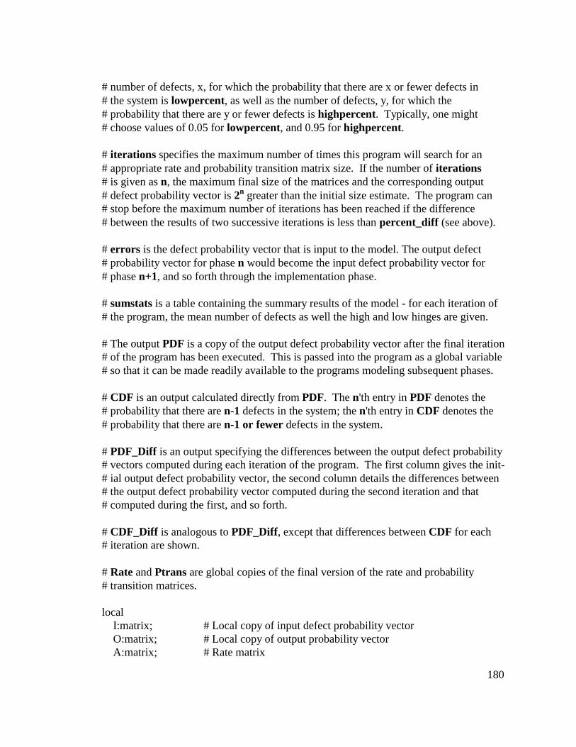
180
# number of defects, x, for which the probability that there are x or fewer defects in# the system is lowpercent, as well as the number of defects, y, for which the# probability that there are y or fewer defects is highpercent. Typically, one might# choose values of 0.05 for lowpercent, and 0.95 for highpercent.
# iterations specifies the maximum number of times this program will search for an# appropriate rate and probability transition matrix size. If the number of iterations# is given as n, the maximum final size of the matrices and the corresponding output# defect probability vector is 2n greater than the initial size estimate. The program can# stop before the maximum number of iterations has been reached if the difference# between the results of two successive iterations is less than percent_diff (see above).
# errors is the defect probability vector that is input to the model. The output defect# probability vector for phase n would become the input defect probability vector for# phase n+1, and so forth through the implementation phase.
# sumstats is a table containing the summary results of the model - for each iteration of# the program, the mean number of defects as well the high and low hinges are given.
# The output PDF is a copy of the output defect probability vector after the final iteration# of the program has been executed. This is passed into the program as a global variable# so that it can be made readily available to the programs modeling subsequent phases.
# CDF is an output calculated directly from PDF. The n'th entry in PDF denotes the# probability that there are n-1 defects in the system; the n'th entry in CDF denotes the# probability that there are n-1 or fewer defects in the system.
# PDF_Diff is an output specifying the differences between the output defect probability# vectors computed during each iteration of the program. The first column gives the init-# ial output defect probability vector, the second column details the differences between# the output defect probability vector computed during the second iteration and that# computed during the first, and so forth.
# CDF_Diff is analogous to PDF_Diff, except that differences between CDF for each# iteration are shown.
# Rate and Ptrans are global copies of the final version of the rate and probability# transition matrices.
local I:matrix; # Local copy of input defect probability vector O:matrix; # Local copy of output probability vector A:matrix; # Rate matrix

181
P:matrix; # Probability transition matrix - generated from rate matrix count:integer; # Used in copying values from input probability vector to local
# copy. n1:integer; # Index variable into rate and probability transition matrices. n2:integer; # Index variable into rate and probability transition matrices. n3:integer; # Index variable into rate and probability transition matrices. n4:integer; # Counts number of retries in computing probability transition
# matrix. retry_flag:integer; # Specifies whether probability transition matrix needs to be
# computed - if 0, no recomputation is necessary. runsum:float; # Used as a running sum in computing the output cumulative
# distribution function m:integer; # Initial size estimate for the input defect probability vector. n:integer; # Tracks size of rate and probability transition matrices. k1:float; # Constant for the rate equations. k2:float; # Constant for the rate equations. k3:float; # Constant for the rate equations. k4:float; # Constant for the rate equations. k5:float; # Constant for the rate equations. k6:float; # Constant for the rate equations. prevresult:float; # Used in determining the number of iterations this program will
# run. curresult:float; # Used in determining the number of iterations this program will
# run. resultdiff:float; # Used in determining the number of iterations to execute. previndex:integer; # Maximum number of iterations this program will run. mean:float; # Number of defects expected to be introduced into the system. percent5:integer; # Number of defects, x, for which the probability of there being x
# or fewer defects in the system is lowpercent. percent50:integer; # The median number of defects introduced into the system. percent95:integer; # Number of defects, y, for which the probability of there being y
# or fewer defects in the system is highpercent.
with(linalg); # forces use of Maple's linear algebra libraries
# Now set up the constants for the rates of defect introduction and defect# removal. The forms for these rates are k1*a*k2*b*exp(k3*n) and# k4*a*k5*b*exp(k6*n), respectively, where n represents the number# of defects already in the system. NOTE THAT THESE ARE NOT# ACTUAL MEASURED RATES, BUT ARE MEANT ONLY TO# SERVE AS AN EXAMPLE.
182
k1 := 1.1 ; k2 := 1.15 ; k3 := .2*10^(-1); k4 := 1.1*1/sqrt(2.0 ); k5 := 1.15*1/sqrt(2.0 ); k6 := .2*10^(-1);
# Now estimate the initial size for the local copy of the input defect probability# vector. This estimate is recorded in the variable "n".
m := vectdim(errors); runsum := 0; n := 1; while runsum < t do runsum := runsum-1.0*1/k1/k2/a/b/exp(k3*n)+1.0*1/k4/k5/a/b/exp(k6*n); n := n+1 od; if 2*n < m then n := m else n := 2*n fi;
if n < 10 then Digits := 10 else Digits := 10+ilog10(n) fi; # Adjust computation# precision.
# Initial sizing of rate and probability transition matrices as well as# output vectors and arrays. The sizes of all of these, except for sumstats,# will increase with each iteration of the program.
A := matrix(n,n); I := matrix(n,1); O := matrix(n,1); sumstats := matrix(12,2); sumstats[1,1] := iteration; sumstats[2,1] := `mean number of errors`; sumstats[3,1] := cat(convert(lowpercent,string),` low hinge`); sumstats[4,1] := median; sumstats[5,1] := cat(convert(highpercent,string),` high hinge`); sumstats[6,1] := `rate matrix dims`; sumstats[7,1] := `current - prev result`; sumstats[8,1] := `current - prev mean`; sumstats[9,1] := `current - prev low hinge`; sumstats[10,1] := `current - prev median`; sumstats[11,1] := `current - prev high hinge`; sumstats[12,1] := `current - prev residuals`; PDF := matrix(n,1);

183
CDF := matrix(n,1); PDF_Diff := matrix(n,1); CDF_Diff := matrix(n,1);
# Make a local copy of the input defect probability matrix.
count := 1; while count <= n do if count < m+1 then I[count,1] := errors[count] else I[count,1] := 0 fi; count := count+1 od;
resultdiff := 2.0*percentdiff; # Initialize the threshold to stop iterating. prevresult := -1.0 ;
n3 := iterations; # Make a local copy of the number of iterations. printf(`Remaining iterations: %d, computing for %d estimated errors.`,n3,n);
# Keep iterating until either the difference between results of two successive# iterations is less than percentdiff or the maximum number of iterations have# been executed.
while percentdiff < abs(resultdiff) and 0 < n3 do retry_flag := 1; # Compute the probability transition matrix at least once per
# iteration. n4 := 0;
# During each iteration, increase the precision of the computation until the# probability transition matrix are correctly computed. If each column of# the probability transition matrix sums to 1, then it is correct.
while 0 < retry_flag do n1 := 1; while n1 < n+1 do n2 := 1;
# Form the tri-diagonal rate matrix A.
while n2 < n+1 do if n1 = n2 then A[n1,n2] := -k1*k2*a*b*exp(k3*(n1-1))-k4*k5*a*b*exp(k6*(n1-1))
184
elif n2 = n1+1 then A[n1,n2] := k4*k5*a*b*exp(k6*(n2-1)) elif n2 = n1-1 then A[n1,n2] := k1*k2*a*b*exp(k3*(n2-1)) else A[n1,n2] := 0 fi; n2 := n2+1 od; n1 := n1+1 od; A[1,1] := -A[2,1]; A[n,n] := -A[n-1,n]; n2 := 2;
# To the limits of Maple's precision (set by the environmental variable# Digits), make sure that the rate matrix has the proper form. Rate# matrices must have each column summing to zero ("conservation# of probability mass flow").
while n2 < n do if sum(A['n1',n2],'n1' = n2-1 .. n2+1) <> 0 then printf( `Iteration %d.%d - rate matrix diagonal element at %d, %d, being adjusted to maintain conservation of probability mass flow.`,iterations-n3+1,n4,n2,n2); A[n2,n2] := -A[n2-1,n2]-A[n2+1,n2] fi; n2 := n2+1 od;
# The probability transition matrix is obtained by exponentiating# the rate matrix. NOTE: In a production system, the computation# would have to be faster than what is provided by Maple V, since# in real systems the rate matrix could have hundreds or thousands# of rows or columns. On a 100MHz Pentium machine, the computation# for an 80x80 matrix takes approximately an hour with this prototype# program.
P := evalf(exponential(A,t)); retry_flag := 0;
# Check to see that the sum of each column of the probability transition# matrix is 1. If for any column this sum is not within specified limits,# set the retry flag to non-zero, increase the precision, and recompute the# matrix.

185
n2 := 1; while n2 <= n do if prob_thresh < abs(sum(P['n1',n2],'n1' = 1 .. n)-1.0 ) then retry_flag := retry_flag+1 fi; n2 := n2+1 od; if retry_flag <> 0 then printf( `Iteration %d.%d - number of times probability transition matrix column
sums\n deviated from 1 by %f is %d. Matrix needs to be recomputed.` ,iterations-n3+1,n4,prob_thresh,retry_flag) else printf(
`Iteration %d.%d - number of times probability transition matrix columnsums\n deviated from 1 by %f is %d. No further matrix recomputationneeded.` ,iterations-n3+1,n4,prob_thresh,retry_flag)
fi; if 0 < retry_flag then Digits := Digits+ilog10(n)+1; n4 := n4+1 fi od;
# This is a safety check to identify entries in the probability transition matrix# that are outside of the allowable limits (0 <= entry <= 1). Rounding errors# in the computation of the matrix can cause the matrix entries to fall outside# of these limits. Any such entries are reported in a diagnostic message.# As long as the entries in each column of the matrix sum to 1 within the limits# of Maple's precision, individual entries that are barely out of the allowable# range are tolerated in this prototype (e.g., x = -0.00000001is tolerated).# This issue would be dealt with more rigorously in a production system.
n1 := 1; while n1 <= n do n2 := 1; while n2 <= n do if P[n1,n2] < 0 or 1.0 < P[n1,n2] then printf( `Iteration %d - probability transition matrix element %d, %d is less than zero or greater than 1 with value %e.`,iterations-n3+1,n1,n2,P[n1,n2]) fi; n2 := n2+1 od; n1 := n1+1 od;
186
# Compute the output defect probability vector for this iteration.
O := multiply(P,I);
# At this point, we've computed the rate and probability transition matrices for# the current iteration. We print them out to show progress in the computation# and to make them available for later analysis, if desired. The input and output# defect probability vectors for the current iteration are also printed at this time.
print(A); print(P); print(I,O);
# Here we compare the results obtained during this iteration with those computed# during the previous one. The difference is stored in the variable resultdiff . # If this value is less than the tolerance passed in via the parameter percentdiff,# no further iterations of the program are executed, and the final results are# produced.
runsum := 0; n1 := 1; n2 := iterations-n3+1; while n1 <= n do PDF[n1,n2] := O[n1,1]; runsum := runsum+O[n1,1]; CDF[n1,n2] := runsum; if n2 = 1 then PDF_Diff[n1,n2] := 0 else PDF_Diff[n1,n2] := PDF[n1,n2]-PDF[n1,n2-1] fi; if n2 = 1 then CDF_Diff[n1,n2] := 0 else CDF_Diff[n1,n2] := CDF[n1,n2]-CDF[n1,n2-1] fi; n1 := n1+1 od; if prevresult < 0 then n1 := 1; curresult := 0; while curresult < highpercent do curresult := O[n1,1]+curresult; n1 := n1+1 od; prevresult := curresult; previndex := n1-1 else
187
curresult := sum(O['n1',1],'n1' = 1 .. previndex); resultdiff := curresult-prevresult; printf( `Difference between previous and current CDFs for error %d denoting the %f confidence value is %e.`,previndex-1,highpercent,resultdiff); previndex := 1; prevresult := 0; while prevresult < highpercent do prevresult := O[previndex,1]+prevresult; previndex := previndex+1 od; previndex := previndex-1 fi;
# Place the summary results for this iteration into the matrix sumstats.
n2 := iterations-n3+1; sumstats[1,n2+1] := n2; sumstats[2,n2+1] := sum(O['n1',1]*'n1-1','n1' = 1 .. n); n1 := 1; while CDF[n1,n2] < lowpercent do n1 := n1+1 od; sumstats[3,n2+1] := n1-1; while CDF[n1,n2] < midpercent do n1 := n1+1 od; sumstats[4,n2+1] := n1-1; while CDF[n1,n2] < highpercent do n1 := n1+1 od; sumstats[5,n2+1] := n1-1; sumstats[6,n2+1] := n; sumstats[7,n2+1] := curresult-prevresult; if n2 = 1 then sumstats[8,2] := sumstats[2,2] else sumstats[8,n2+1] := sumstats[2,n2+1]-sumstats[2,n2] fi; if n2 = 1 then sumstats[9,2] := sumstats[3,2] else sumstats[9,n2+1] := sumstats[3,n2+1]-sumstats[3,n2] fi; if n2 = 1 then sumstats[10,2] := sumstats[4,2] else sumstats[10,n2+1] := sumstats[4,n2+1]-sumstats[4,n2] fi; if n2 = 1 then sumstats[11,2] := sumstats[5,2] else sumstats[11,n2+1] := sumstats[5,n2+1]-sumstats[5,n2] fi; if n2 = 1 then sumstats[12,2] := sumstats[7,2] else sumstats[12,n2+1] := sumstats[7,n2+1]-sumstats[7,n2] fi;
188
# If another iteration must be executed (the difference between the results of# the current and previous iterations is greater than or equal than the specified# threshold, and the number of iterations has not been decremented to 0), the# size of the input defect probability vector, the output defect probability vector,# the rate matrix, and the probability transition matrix are doubled. The en-# vironment variable controlling the precision of Maple's computation is in-# creased to compensate for the increased matrix size.
if 0 < n3 and percentdiff < abs(resultdiff) then I := extend(I,n,0,0); O := extend(O,n,0,0); A := extend(A,n,n,0); PDF := extend(PDF,n,1,0); CDF := extend(CDF,n,1,1.0 ); PDF_Diff := extend(PDF_Diff,n,1,0); CDF_Diff := extend(CDF_Diff,n,1,0); sumstats := extend(sumstats,0,1,0); Digits := Digits+ilog10(n); printf(`Predict %d remaining iterations, computing for %d estimated errors.`,n3-1,2*n) elif abs(resultdiff) <= percentdiff then printf(`Run complete at %d remaining iterations, computed for %d estimated errors.`,n3-1,n) else printf(`%d remaining iterations, computed for %d estimated errors.`,n3-1,n) fi; n3 := n3-1; n := 2*n od;
# At this point, the last iteration of the program has been executed. The global# copies of the final rate matrix and probability transition matrix are produced,# so they can be made available for further analysis if desired.
Rate := matrix(1/2*n,1/2*n); Rate := A; Ptrans := matrix(1/2*n,1/2*n); Ptrans := Pend
189
11. Summary of Analysis - From RADC TR-87-171 Volume 1 Table 5-22
METRIC EXPECTED FORM OF RELATIONSHIP
Application (A) Table of Average Fault Densities by Category
Development Environment (D) D = DO where DO = 1.3 (Embedded) .1 (Semidetached) .76 (Organic)or DM = (.109*DC - .4)/.014 (Embedded) (.008*DC - .003)/.013 (Semidetached) (.018*DC - .003)/.008 (Organic)
where DC = Fraction of items checked on developmentpractices checklist on previous page.
Anomaly Management (SA) SA = .9 if AM > .6 1 if .4 < AM < .6 1.1 if AM < .4
Traceability (ST) ST = 1.1 if (NR - DR)/NR < .9 1 if (NR - DR)/NR ≥ .9
Quality Review (SQ) SQ = 1.1 if AR/NR > .5 1 if AR/NR £ .5
Language (SL) SL = 1 * (% High Order Language) + 1.4 * (% AssemblyLanguage)
Size (SS) 1 (No relationship was found)
Modularity (SM) SM = .9u + w + 2xwhere u is the number of modules having < 200 executablelines of codew is the number of modules having 200 < size < 3000x is the number of modules having more than 3000 lines ofexecutable code
Reuse (SU) 1 (No relationship was found)
Complexity (SX) SX = 1.5a + b + .8cwhere a is the number of modules having a McCabeCyclomatic Complexity (C) ≥ 20b is the number of modules with 20≥C≥7c is the number of modules with C < 7
Standards Review (SR) SR = 1.5 if PR/NM ³ .5 1 if .5 ≥ PR/NM ≥ .25 .75 if PR/NM < .25
190
12. Observed and Estimated Distribution of Defects per “n” Failures
12.1 Tabulated Values for the Distribution of the Number of Defects for 1 Failure
The table below gives the values of the pdfs for the observed number of defectsper failure for the CASSINI CDS flight software.
Number ofDefects
Probability ofOccurrence
1 0.00000E+002 1.00000E-013 1.33333E-014 3.33333E-025 1.00000E-016 3.33333E-027 1.00000E-018 3.33333E-029 3.33333E-0210 0.00000E+0011 6.66667E-0212 1.00000E-0113 3.33333E-0214 3.33333E-0215 3.33333E-0216 3.33333E-0217 0.00000E+0018 0.00000E+0019 0.00000E+0020 0.00000E+00
Number ofDefects
Probability ofOccurrence
21 3.33333E-0222 3.33333E-0223 0.00000E+0024 0.00000E+0025 0.00000E+0026 0.00000E+0027 0.00000E+0028 0.00000E+0029 0.00000E+0030 0.00000E+0031 0.00000E+0032 0.00000E+0033 0.00000E+0034 0.00000E+0035 0.00000E+0036 0.00000E+0037 3.33333E-0238 0.00000E+0039 0.00000E+0040 3.33333E-02
12.2 Convolution of Distributions
The following program, written in the programming language for Maple V release2, was used to produce the defects per n failures distributions shown in Figures 9 and 10. This program takes as inputs real-valued vectors A, B, and C. A and B are the distribu-tions of the number of defects for x and y failures, and C is a vector of dimensionality|A|+|B|-1. C is also the output vector, and gives the distribution of the number of defectsfor x + y failures. It can be viewed by entering “print(C)” at the Maple V prompt.
To compute the distribution of the number of defects for two failures, use thisprogram to convolve the distribution given in 12.1 with itself. To find the distribution ofthe number of defects for three failures, convolve the distribution given in 12.1 with thedistribution of the number of defects for two failures.
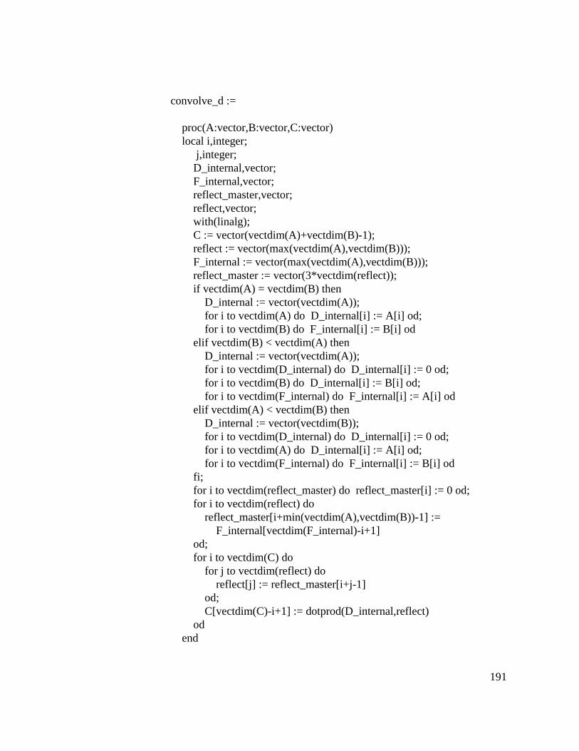
191
convolve_d :=
proc(A:vector,B:vector,C:vector) local i,integer; j,integer; D_internal,vector; F_internal,vector; reflect_master,vector; reflect,vector; with(linalg); C := vector(vectdim(A)+vectdim(B)-1); reflect := vector(max(vectdim(A),vectdim(B))); F_internal := vector(max(vectdim(A),vectdim(B))); reflect_master := vector(3*vectdim(reflect)); if vectdim(A) = vectdim(B) then D_internal := vector(vectdim(A)); for i to vectdim(A) do D_internal[i] := A[i] od; for i to vectdim(B) do F_internal[i] := B[i] od elif vectdim(B) < vectdim(A) then D_internal := vector(vectdim(A)); for i to vectdim(D_internal) do D_internal[i] := 0 od; for i to vectdim(B) do D_internal[i] := B[i] od; for i to vectdim(F_internal) do F_internal[i] := A[i] od elif vectdim(A) < vectdim(B) then D_internal := vector(vectdim(B)); for i to vectdim(D_internal) do D_internal[i] := 0 od; for i to vectdim(A) do D_internal[i] := A[i] od; for i to vectdim(F_internal) do F_internal[i] := B[i] od fi; for i to vectdim(reflect_master) do reflect_master[i] := 0 od; for i to vectdim(reflect) do reflect_master[i+min(vectdim(A),vectdim(B))-1] := F_internal[vectdim(F_internal)-i+1] od; for i to vectdim(C) do for j to vectdim(reflect) do reflect[j] := reflect_master[i+j-1] od; C[vectdim(C)-i+1] := dotprod(D_internal,reflect) od end
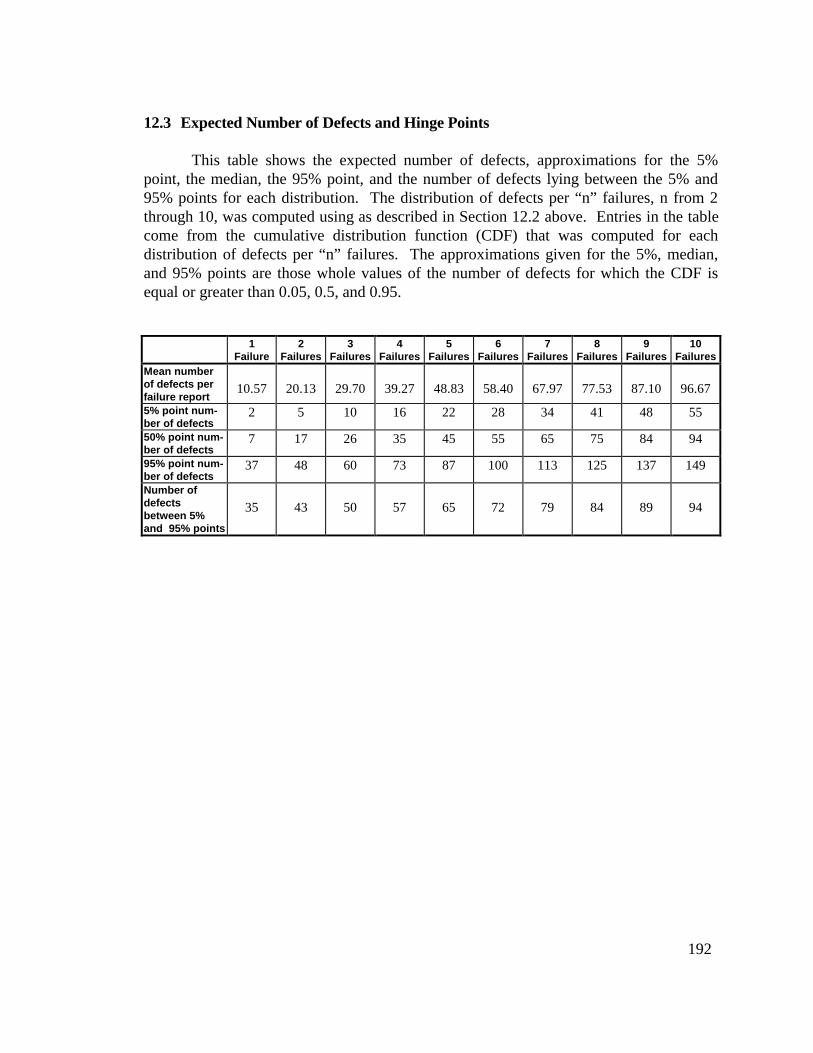
192
12.3 Expected Number of Defects and Hinge Points
This table shows the expected number of defects, approximations for the 5%point, the median, the 95% point, and the number of defects lying between the 5% and95% points for each distribution. The distribution of defects per “n” failures, n from 2through 10, was computed using as described in Section 12.2 above. Entries in the tablecome from the cumulative distribution function (CDF) that was computed for eachdistribution of defects per “n” failures. The approximations given for the 5%, median,and 95% points are those whole values of the number of defects for which the CDF isequal or greater than 0.05, 0.5, and 0.95.
1Failure
2Failures
3Failures
4Failures
5Failures
6Failures
7Failures
8Failures
9Failures
10Failures
Mean numberof defects perfailure report
10.57 20.13 29.70 39.27 48.83 58.40 67.97 77.53 87.10 96.67
5% point num-ber of defects
2 5 10 16 22 28 34 41 48 55
50% point num-ber of defects
7 17 26 35 45 55 65 75 84 94
95% point num-ber of defects
37 48 60 73 87 100 113 125 137 149
Number ofdefectsbetween 5%and 95% points
35 43 50 57 65 72 79 84 89 94

193
13. Detailed Project Data
The following appendices contain the measurements of process and product characteristics for the CASSINI Command andData Subsystem (CDS) flight software development effort that were used in calibrating and validating the model.
13.1 Defect Locations for Version 2.0 Development Library
The following tables detail the locations of defects found in the flight software for the CASSINI CDS flight software usingthe defect identification and counting rules described in Chapter 5. Each line in a table represents a distinct defect. Each of thethree tables gives information about defects within a specific development library, where a development library is defined as aunique set of SCCS modules. The tables contain the following information:
Anonymous PR x ID: gives an anonymous problem report identifier related to the problem report ID in JPL’s institutionalproblem reporting system. Four columns are given, because it was observed that up to fourproblem reports can be related to an individual defect.
Anonymous Source File ID: gives an anonymous identifier for the source code file containing the defect.Anonymous Module ID: gives an anonymous identifier for each procedure or function containing a defect. The module is
contained in the file identified in the second column.Defect Line Num(s): gives the line number(s) within the version of the source file that was repaired which contained the
defect. Line numbers are referenced with respect to the start of the source file, rather than to thestart of each module.
Repair Increment: identifies the source file increment in which the defect was repaired. The increment is given in theSCCS R.ID format.
Repair Date: gives the date on which the source file was checked back into the development library.Insertion Version: gives the version (development library) in which the defect was first inserted. The development
libraries have the following identifiers: 1.0, 1.1, 2.0, 2.1a, and 2.1b. Data is only available forthose defects that were repaired in versions 2.0, 2.1a, or 2.1b.
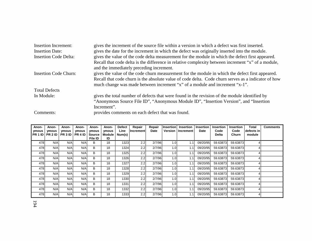
194
Insertion Increment: gives the increment of the source file within a version in which a defect was first inserted.Insertion Date: gives the date for the increment in which the defect was originally inserted into the module.Insertion Code Delta: gives the value of the code delta measurement for the module in which the defect first appeared.
Recall that code delta is the difference in relative complexity between increment “x” of a module,and the immediately preceding increment.
Insertion Code Churn: gives the value of the code churn measurement for the module in which the defect first appeared. Recall that code churn is the absolute value of code delta. Code churn serves as a indicator of howmuch change was made between increment “x” of a module and increment “x-1”.
Total DefectsIn Module: gives the total number of defects that were found in the revision of the module identified by
“Anonymous Source File ID”, “Anonymous Module ID”, “Insertion Version”, and “InsertionIncrement”.
Comments: provides comments on each defect that was found.
Anon-ymousPR 1 ID
Anon-ymousPR 2 ID
Anon-ymousPR 3 ID
Anon-ymousPR 4 ID
Anon-ymousSourceFile ID
Anon-ymousModule
ID
DefectLine
Num(s)
RepairIncrement
RepairDate
InsertionVersion
InsertionIncrement
InsertionDate
InsertionCodeDelta
InsertionCodeChurn
Totaldefects inmodule
Comments
478 N/A N/A N/A B 18 1323 2.2 2/7/96 1.0 1.1 09/20/95 59.63873 59.63873 4
478 N/A N/A N/A B 18 1324 2.2 2/7/96 1.0 1.1 09/20/95 59.63873 59.63873 4
478 N/A N/A N/A B 18 1325 2.2 2/7/96 1.0 1.1 09/20/95 59.63873 59.63873 4
478 N/A N/A N/A B 18 1326 2.2 2/7/96 1.0 1.1 09/20/95 59.63873 59.63873 4
478 N/A N/A N/A B 18 1327 2.2 2/7/96 1.0 1.1 09/20/95 59.63873 59.63873 4
478 N/A N/A N/A B 18 1328 2.2 2/7/96 1.0 1.1 09/20/95 59.63873 59.63873 4
478 N/A N/A N/A B 18 1329 2.2 2/7/96 1.0 1.1 09/20/95 59.63873 59.63873 4
478 N/A N/A N/A B 18 1330 2.2 2/7/96 1.0 1.1 09/20/95 59.63873 59.63873 4
478 N/A N/A N/A B 18 1331 2.2 2/7/96 1.0 1.1 09/20/95 59.63873 59.63873 4
478 N/A N/A N/A B 18 1332 2.2 2/7/96 1.0 1.1 09/20/95 59.63873 59.63873 4
478 N/A N/A N/A B 18 1333 2.2 2/7/96 1.0 1.1 09/20/95 59.63873 59.63873 4
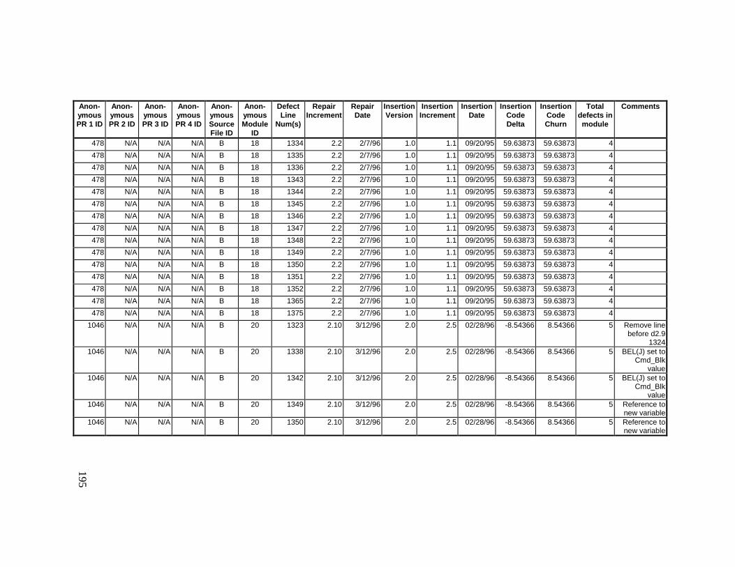
195
Anon-ymousPR 1 ID
Anon-ymousPR 2 ID
Anon-ymousPR 3 ID
Anon-ymousPR 4 ID
Anon-ymousSourceFile ID
Anon-ymousModule
ID
DefectLine
Num(s)
RepairIncrement
RepairDate
InsertionVersion
InsertionIncrement
InsertionDate
InsertionCodeDelta
InsertionCodeChurn
Totaldefects inmodule
Comments
478 N/A N/A N/A B 18 1334 2.2 2/7/96 1.0 1.1 09/20/95 59.63873 59.63873 4
478 N/A N/A N/A B 18 1335 2.2 2/7/96 1.0 1.1 09/20/95 59.63873 59.63873 4
478 N/A N/A N/A B 18 1336 2.2 2/7/96 1.0 1.1 09/20/95 59.63873 59.63873 4
478 N/A N/A N/A B 18 1343 2.2 2/7/96 1.0 1.1 09/20/95 59.63873 59.63873 4
478 N/A N/A N/A B 18 1344 2.2 2/7/96 1.0 1.1 09/20/95 59.63873 59.63873 4
478 N/A N/A N/A B 18 1345 2.2 2/7/96 1.0 1.1 09/20/95 59.63873 59.63873 4
478 N/A N/A N/A B 18 1346 2.2 2/7/96 1.0 1.1 09/20/95 59.63873 59.63873 4
478 N/A N/A N/A B 18 1347 2.2 2/7/96 1.0 1.1 09/20/95 59.63873 59.63873 4
478 N/A N/A N/A B 18 1348 2.2 2/7/96 1.0 1.1 09/20/95 59.63873 59.63873 4
478 N/A N/A N/A B 18 1349 2.2 2/7/96 1.0 1.1 09/20/95 59.63873 59.63873 4
478 N/A N/A N/A B 18 1350 2.2 2/7/96 1.0 1.1 09/20/95 59.63873 59.63873 4
478 N/A N/A N/A B 18 1351 2.2 2/7/96 1.0 1.1 09/20/95 59.63873 59.63873 4
478 N/A N/A N/A B 18 1352 2.2 2/7/96 1.0 1.1 09/20/95 59.63873 59.63873 4
478 N/A N/A N/A B 18 1365 2.2 2/7/96 1.0 1.1 09/20/95 59.63873 59.63873 4
478 N/A N/A N/A B 18 1375 2.2 2/7/96 1.0 1.1 09/20/95 59.63873 59.63873 4
1046 N/A N/A N/A B 20 1323 2.10 3/12/96 2.0 2.5 02/28/96 -8.54366 8.54366 5 Remove linebefore d2.9
13241046 N/A N/A N/A B 20 1338 2.10 3/12/96 2.0 2.5 02/28/96 -8.54366 8.54366 5 BEL(J) set to
Cmd_Blkvalue
1046 N/A N/A N/A B 20 1342 2.10 3/12/96 2.0 2.5 02/28/96 -8.54366 8.54366 5 BEL(J) set toCmd_Blk
value1046 N/A N/A N/A B 20 1349 2.10 3/12/96 2.0 2.5 02/28/96 -8.54366 8.54366 5 Reference to
new variable1046 N/A N/A N/A B 20 1350 2.10 3/12/96 2.0 2.5 02/28/96 -8.54366 8.54366 5 Reference to
new variable
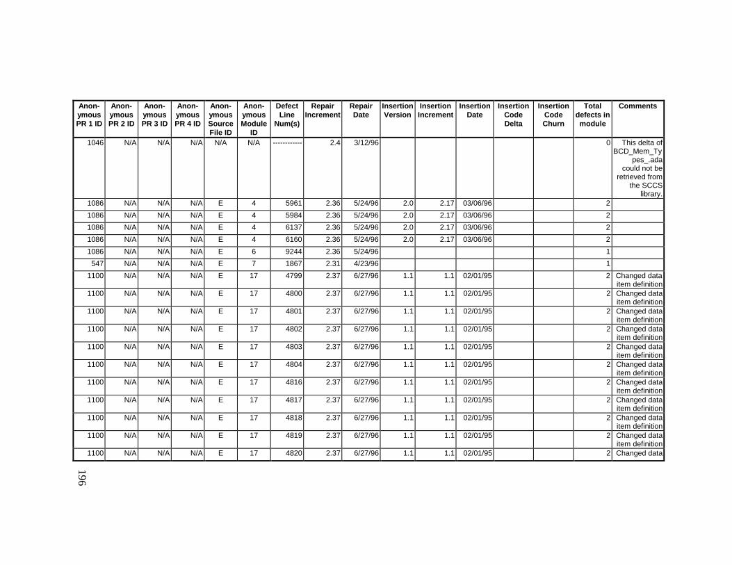
196
Anon-ymousPR 1 ID
Anon-ymousPR 2 ID
Anon-ymousPR 3 ID
Anon-ymousPR 4 ID
Anon-ymousSourceFile ID
Anon-ymousModule
ID
DefectLine
Num(s)
RepairIncrement
RepairDate
InsertionVersion
InsertionIncrement
InsertionDate
InsertionCodeDelta
InsertionCodeChurn
Totaldefects inmodule
Comments
1046 N/A N/A N/A N/A N/A ------------ 2.4 3/12/96 0 This delta ofBCD_Mem_Ty
pes_.adacould not be
retrieved fromthe SCCS
library.1086 N/A N/A N/A E 4 5961 2.36 5/24/96 2.0 2.17 03/06/96 2
1086 N/A N/A N/A E 4 5984 2.36 5/24/96 2.0 2.17 03/06/96 2
1086 N/A N/A N/A E 4 6137 2.36 5/24/96 2.0 2.17 03/06/96 2
1086 N/A N/A N/A E 4 6160 2.36 5/24/96 2.0 2.17 03/06/96 2
1086 N/A N/A N/A E 6 9244 2.36 5/24/96 1
547 N/A N/A N/A E 7 1867 2.31 4/23/96 1
1100 N/A N/A N/A E 17 4799 2.37 6/27/96 1.1 1.1 02/01/95 2 Changed dataitem definition
1100 N/A N/A N/A E 17 4800 2.37 6/27/96 1.1 1.1 02/01/95 2 Changed dataitem definition
1100 N/A N/A N/A E 17 4801 2.37 6/27/96 1.1 1.1 02/01/95 2 Changed dataitem definition
1100 N/A N/A N/A E 17 4802 2.37 6/27/96 1.1 1.1 02/01/95 2 Changed dataitem definition
1100 N/A N/A N/A E 17 4803 2.37 6/27/96 1.1 1.1 02/01/95 2 Changed dataitem definition
1100 N/A N/A N/A E 17 4804 2.37 6/27/96 1.1 1.1 02/01/95 2 Changed dataitem definition
1100 N/A N/A N/A E 17 4816 2.37 6/27/96 1.1 1.1 02/01/95 2 Changed dataitem definition
1100 N/A N/A N/A E 17 4817 2.37 6/27/96 1.1 1.1 02/01/95 2 Changed dataitem definition
1100 N/A N/A N/A E 17 4818 2.37 6/27/96 1.1 1.1 02/01/95 2 Changed dataitem definition
1100 N/A N/A N/A E 17 4819 2.37 6/27/96 1.1 1.1 02/01/95 2 Changed dataitem definition
1100 N/A N/A N/A E 17 4820 2.37 6/27/96 1.1 1.1 02/01/95 2 Changed data
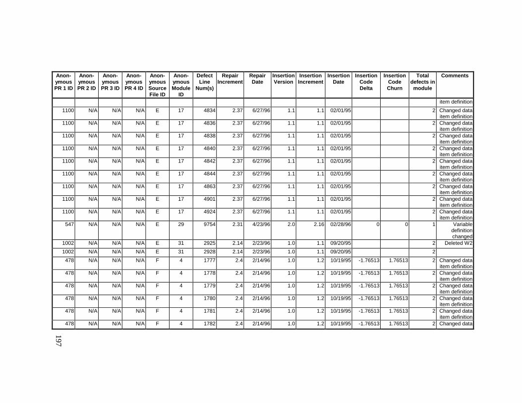
197
Anon-ymousPR 1 ID
Anon-ymousPR 2 ID
Anon-ymousPR 3 ID
Anon-ymousPR 4 ID
Anon-ymousSourceFile ID
Anon-ymousModule
ID
DefectLine
Num(s)
RepairIncrement
RepairDate
InsertionVersion
InsertionIncrement
InsertionDate
InsertionCodeDelta
InsertionCodeChurn
Totaldefects inmodule
Comments
item definition
1100 N/A N/A N/A E 17 4834 2.37 6/27/96 1.1 1.1 02/01/95 2 Changed dataitem definition
1100 N/A N/A N/A E 17 4836 2.37 6/27/96 1.1 1.1 02/01/95 2 Changed dataitem definition
1100 N/A N/A N/A E 17 4838 2.37 6/27/96 1.1 1.1 02/01/95 2 Changed dataitem definition
1100 N/A N/A N/A E 17 4840 2.37 6/27/96 1.1 1.1 02/01/95 2 Changed dataitem definition
1100 N/A N/A N/A E 17 4842 2.37 6/27/96 1.1 1.1 02/01/95 2 Changed dataitem definition
1100 N/A N/A N/A E 17 4844 2.37 6/27/96 1.1 1.1 02/01/95 2 Changed dataitem definition
1100 N/A N/A N/A E 17 4863 2.37 6/27/96 1.1 1.1 02/01/95 2 Changed dataitem definition
1100 N/A N/A N/A E 17 4901 2.37 6/27/96 1.1 1.1 02/01/95 2 Changed dataitem definition
1100 N/A N/A N/A E 17 4924 2.37 6/27/96 1.1 1.1 02/01/95 2 Changed dataitem definition
547 N/A N/A N/A E 29 9754 2.31 4/23/96 2.0 2.16 02/28/96 0 0 1 Variabledefinitionchanged
1002 N/A N/A N/A E 31 2925 2.14 2/23/96 1.0 1.1 09/20/95 2 Deleted W2
1002 N/A N/A N/A E 31 2928 2.14 2/23/96 1.0 1.1 09/20/95 2
478 N/A N/A N/A F 4 1777 2.4 2/14/96 1.0 1.2 10/19/95 -1.76513 1.76513 2 Changed dataitem definition
478 N/A N/A N/A F 4 1778 2.4 2/14/96 1.0 1.2 10/19/95 -1.76513 1.76513 2 Changed dataitem definition
478 N/A N/A N/A F 4 1779 2.4 2/14/96 1.0 1.2 10/19/95 -1.76513 1.76513 2 Changed dataitem definition
478 N/A N/A N/A F 4 1780 2.4 2/14/96 1.0 1.2 10/19/95 -1.76513 1.76513 2 Changed dataitem definition
478 N/A N/A N/A F 4 1781 2.4 2/14/96 1.0 1.2 10/19/95 -1.76513 1.76513 2 Changed dataitem definition
478 N/A N/A N/A F 4 1782 2.4 2/14/96 1.0 1.2 10/19/95 -1.76513 1.76513 2 Changed data
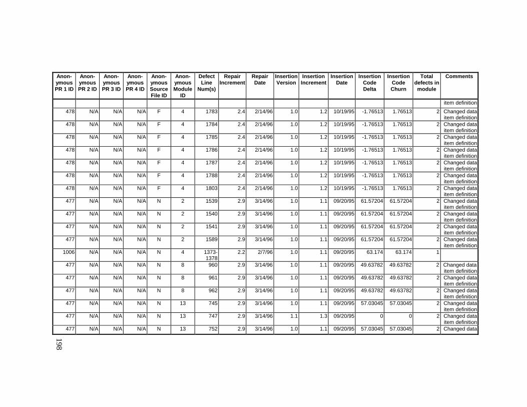
198
Anon-ymousPR 1 ID
Anon-ymousPR 2 ID
Anon-ymousPR 3 ID
Anon-ymousPR 4 ID
Anon-ymousSourceFile ID
Anon-ymousModule
ID
DefectLine
Num(s)
RepairIncrement
RepairDate
InsertionVersion
InsertionIncrement
InsertionDate
InsertionCodeDelta
InsertionCodeChurn
Totaldefects inmodule
Comments
item definition
478 N/A N/A N/A F 4 1783 2.4 2/14/96 1.0 1.2 10/19/95 -1.76513 1.76513 2 Changed dataitem definition
478 N/A N/A N/A F 4 1784 2.4 2/14/96 1.0 1.2 10/19/95 -1.76513 1.76513 2 Changed dataitem definition
478 N/A N/A N/A F 4 1785 2.4 2/14/96 1.0 1.2 10/19/95 -1.76513 1.76513 2 Changed dataitem definition
478 N/A N/A N/A F 4 1786 2.4 2/14/96 1.0 1.2 10/19/95 -1.76513 1.76513 2 Changed dataitem definition
478 N/A N/A N/A F 4 1787 2.4 2/14/96 1.0 1.2 10/19/95 -1.76513 1.76513 2 Changed dataitem definition
478 N/A N/A N/A F 4 1788 2.4 2/14/96 1.0 1.2 10/19/95 -1.76513 1.76513 2 Changed dataitem definition
478 N/A N/A N/A F 4 1803 2.4 2/14/96 1.0 1.2 10/19/95 -1.76513 1.76513 2 Changed dataitem definition
477 N/A N/A N/A N 2 1539 2.9 3/14/96 1.0 1.1 09/20/95 61.57204 61.57204 2 Changed dataitem definition
477 N/A N/A N/A N 2 1540 2.9 3/14/96 1.0 1.1 09/20/95 61.57204 61.57204 2 Changed dataitem definition
477 N/A N/A N/A N 2 1541 2.9 3/14/96 1.0 1.1 09/20/95 61.57204 61.57204 2 Changed dataitem definition
477 N/A N/A N/A N 2 1589 2.9 3/14/96 1.0 1.1 09/20/95 61.57204 61.57204 2 Changed dataitem definition
1006 N/A N/A N/A N 4 1373-1378
2.2 2/7/96 1.0 1.1 09/20/95 63.174 63.174 1
477 N/A N/A N/A N 8 960 2.9 3/14/96 1.0 1.1 09/20/95 49.63782 49.63782 2 Changed dataitem definition
477 N/A N/A N/A N 8 961 2.9 3/14/96 1.0 1.1 09/20/95 49.63782 49.63782 2 Changed dataitem definition
477 N/A N/A N/A N 8 962 2.9 3/14/96 1.0 1.1 09/20/95 49.63782 49.63782 2 Changed dataitem definition
477 N/A N/A N/A N 13 745 2.9 3/14/96 1.0 1.1 09/20/95 57.03045 57.03045 2 Changed dataitem definition
477 N/A N/A N/A N 13 747 2.9 3/14/96 1.1 1.3 09/20/95 0 0 2 Changed dataitem definition
477 N/A N/A N/A N 13 752 2.9 3/14/96 1.0 1.1 09/20/95 57.03045 57.03045 2 Changed data
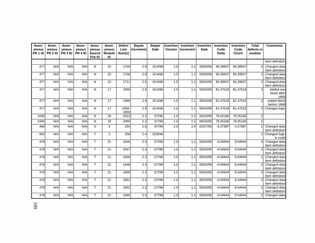
199
Anon-ymousPR 1 ID
Anon-ymousPR 2 ID
Anon-ymousPR 3 ID
Anon-ymousPR 4 ID
Anon-ymousSourceFile ID
Anon-ymousModule
ID
DefectLine
Num(s)
RepairIncrement
RepairDate
InsertionVersion
InsertionIncrement
InsertionDate
InsertionCodeDelta
InsertionCodeChurn
Totaldefects inmodule
Comments
item definition
477 N/A N/A N/A N 15 1704 2.9 3/14/96 1.0 1.1 09/20/95 56.39507 56.39507 2 Changed dataitem definition
477 N/A N/A N/A N 15 1706 2.9 3/14/96 1.0 1.1 09/20/95 56.39507 56.39507 2 Changed dataitem definition
477 N/A N/A N/A N 15 1711 2.9 3/14/96 1.0 1.1 09/20/95 56.39507 56.39507 2 Changed dataitem definition
477 N/A N/A N/A N 17 1959 2.9 3/14/96 1.0 1.1 09/20/95 81.47518 81.47518 3 Added oneblock after
1959477 N/A N/A N/A N 17 1969 2.9 3/14/96 1.0 1.1 09/20/95 81.47518 81.47518 3 Added block
before 1969477 N/A N/A N/A N 17 1956-
19592.9 3/14/96 1.0 1.1 09/20/95 81.47518 81.47518 3 Changed logic
1006 N/A N/A N/A N 18 2013 2.2 2/7/96 1.0 1.1 09/20/95 78.05166 78.05166 2
1006 N/A N/A N/A N 18 2069 2.2 2/7/96 1.0 1.1 09/20/95 78.05166 78.05166 2
466 N/A N/A N/A S 3 254 2.6 3/7/96 2.0 2.4 02/27/96 -0.27987 0.27987 1 Changed dataitem definition
950 N/A N/A N/A T 2 256 2.4 2/28/96 1 Changed logicin code
478 N/A N/A N/A T 21 1646 2.3 2/7/96 1.0 1.1 09/20/95 -9.54944 9.54944 2 Changed dataitem definition
478 N/A N/A N/A T 21 1647 2.3 2/7/96 1.0 1.1 09/20/95 -9.54944 9.54944 2 Changed dataitem definition
478 N/A N/A N/A T 21 1648 2.3 2/7/96 1.0 1.1 09/20/95 -9.54944 9.54944 2 Changed dataitem definition
478 N/A N/A N/A T 21 1649 2.3 2/7/96 1.0 1.1 09/20/95 -9.54944 9.54944 2 Changed dataitem definition
478 N/A N/A N/A T 21 1650 2.3 2/7/96 1.0 1.1 09/20/95 -9.54944 9.54944 2 Changed dataitem definition
478 N/A N/A N/A T 21 1651 2.3 2/7/96 1.0 1.1 09/20/95 -9.54944 9.54944 2 Changed dataitem definition
478 N/A N/A N/A T 21 1652 2.3 2/7/96 1.0 1.1 09/20/95 -9.54944 9.54944 2 Changed dataitem definition
478 N/A N/A N/A T 21 1665 2.3 2/7/96 1.0 1.1 09/20/95 -9.54944 9.54944 2 Changed data
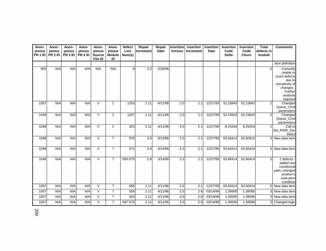
200
Anon-ymousPR 1 ID
Anon-ymousPR 2 ID
Anon-ymousPR 3 ID
Anon-ymousPR 4 ID
Anon-ymousSourceFile ID
Anon-ymousModule
ID
DefectLine
Num(s)
RepairIncrement
RepairDate
InsertionVersion
InsertionIncrement
InsertionDate
InsertionCodeDelta
InsertionCodeChurn
Totaldefects inmodule
Comments
item definition
950 N/A N/A N/A N/A N/A 0 2.2 2/28/96 0 Currentlyunable to
count defectsdue to
complexity ofchanges.
Furtheranalysisrequired
1057 N/A N/A N/A V 2 1253 2.11 4/11/96 2.0 2.1 12/27/95 52.23843 52.23843 2 ChangedQueue_Cmd
parameters1048 N/A N/A N/A V 2 1257 2.11 4/11/96 2.0 2.1 12/27/95 52.23843 52.23843 2 Changed
Queue_Cmdparameters
1048 N/A N/A N/A V 2 323 2.11 4/11/96 2.0 2.1 12/27/95 -8.25204 8.25204 1 Call toSet_PWR_Sta
tistics1048 N/A N/A N/A V 7 570 2.9 3/14/96 2.0 2.1 12/27/95 63.60414 63.60414 5 New data item
1048 N/A N/A N/A V 7 571 2.9 3/14/96 2.0 2.1 12/27/95 63.60414 63.60414 5 New data item
1048 N/A N/A N/A V 7 550-570 2.9 3/14/96 2.0 2.1 12/27/95 63.60414 63.60414 5 2 defects -added oneconditional
path, changedanother'sexecutioncondition
1057 N/A N/A N/A V 7 556 2.11 4/11/96 2.0 2.1 12/27/95 63.60414 63.60414 5 New data item
1057 N/A N/A N/A V 7 559 2.11 4/11/96 2.0 2.9 03/14/96 1.39595 1.39595 3 New data item
1057 N/A N/A N/A V 7 563 2.11 4/11/96 2.0 2.9 03/14/96 1.39595 1.39595 3 New data item
1057 N/A N/A N/A V 7 567-572 2.11 4/11/96 2.0 2.9 03/14/96 1.39595 1.39595 3 Changed logic
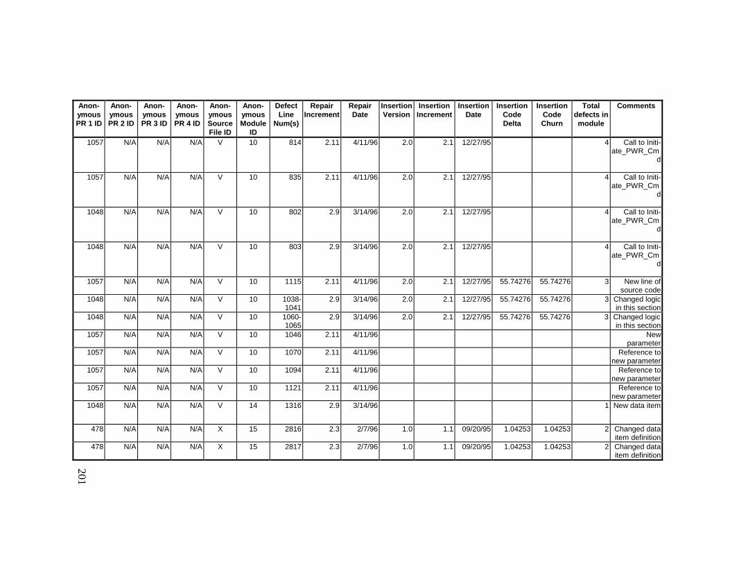
201
Anon-ymousPR 1 ID
Anon-ymousPR 2 ID
Anon-ymousPR 3 ID
Anon-ymousPR 4 ID
Anon-ymousSourceFile ID
Anon-ymousModule
ID
DefectLine
Num(s)
RepairIncrement
RepairDate
InsertionVersion
InsertionIncrement
InsertionDate
InsertionCodeDelta
InsertionCodeChurn
Totaldefects inmodule
Comments
1057 N/A N/A N/A V 10 814 2.11 4/11/96 2.0 2.1 12/27/95 4 Call to Initi-ate_PWR_Cm
d
1057 N/A N/A N/A V 10 835 2.11 4/11/96 2.0 2.1 12/27/95 4 Call to Initi-ate_PWR_Cm
d
1048 N/A N/A N/A V 10 802 2.9 3/14/96 2.0 2.1 12/27/95 4 Call to Initi-ate_PWR_Cm
d
1048 N/A N/A N/A V 10 803 2.9 3/14/96 2.0 2.1 12/27/95 4 Call to Initi-ate_PWR_Cm
d
1057 N/A N/A N/A V 10 1115 2.11 4/11/96 2.0 2.1 12/27/95 55.74276 55.74276 3 New line ofsource code
1048 N/A N/A N/A V 10 1038-1041
2.9 3/14/96 2.0 2.1 12/27/95 55.74276 55.74276 3 Changed logicin this section
1048 N/A N/A N/A V 10 1060-1065
2.9 3/14/96 2.0 2.1 12/27/95 55.74276 55.74276 3 Changed logicin this section
1057 N/A N/A N/A V 10 1046 2.11 4/11/96 Newparameter
1057 N/A N/A N/A V 10 1070 2.11 4/11/96 Reference tonew parameter
1057 N/A N/A N/A V 10 1094 2.11 4/11/96 Reference tonew parameter
1057 N/A N/A N/A V 10 1121 2.11 4/11/96 Reference tonew parameter
1048 N/A N/A N/A V 14 1316 2.9 3/14/96 1 New data item
478 N/A N/A N/A X 15 2816 2.3 2/7/96 1.0 1.1 09/20/95 1.04253 1.04253 2 Changed dataitem definition
478 N/A N/A N/A X 15 2817 2.3 2/7/96 1.0 1.1 09/20/95 1.04253 1.04253 2 Changed dataitem definition
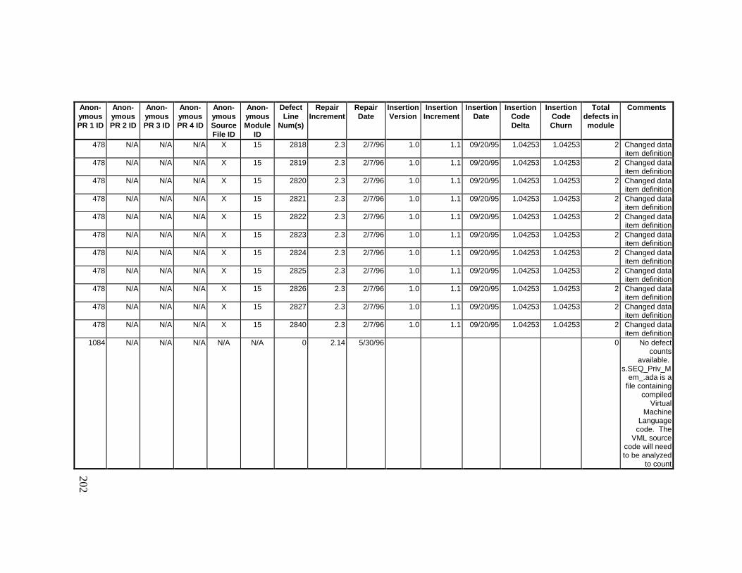
202
Anon-ymousPR 1 ID
Anon-ymousPR 2 ID
Anon-ymousPR 3 ID
Anon-ymousPR 4 ID
Anon-ymousSourceFile ID
Anon-ymousModule
ID
DefectLine
Num(s)
RepairIncrement
RepairDate
InsertionVersion
InsertionIncrement
InsertionDate
InsertionCodeDelta
InsertionCodeChurn
Totaldefects inmodule
Comments
478 N/A N/A N/A X 15 2818 2.3 2/7/96 1.0 1.1 09/20/95 1.04253 1.04253 2 Changed dataitem definition
478 N/A N/A N/A X 15 2819 2.3 2/7/96 1.0 1.1 09/20/95 1.04253 1.04253 2 Changed dataitem definition
478 N/A N/A N/A X 15 2820 2.3 2/7/96 1.0 1.1 09/20/95 1.04253 1.04253 2 Changed dataitem definition
478 N/A N/A N/A X 15 2821 2.3 2/7/96 1.0 1.1 09/20/95 1.04253 1.04253 2 Changed dataitem definition
478 N/A N/A N/A X 15 2822 2.3 2/7/96 1.0 1.1 09/20/95 1.04253 1.04253 2 Changed dataitem definition
478 N/A N/A N/A X 15 2823 2.3 2/7/96 1.0 1.1 09/20/95 1.04253 1.04253 2 Changed dataitem definition
478 N/A N/A N/A X 15 2824 2.3 2/7/96 1.0 1.1 09/20/95 1.04253 1.04253 2 Changed dataitem definition
478 N/A N/A N/A X 15 2825 2.3 2/7/96 1.0 1.1 09/20/95 1.04253 1.04253 2 Changed dataitem definition
478 N/A N/A N/A X 15 2826 2.3 2/7/96 1.0 1.1 09/20/95 1.04253 1.04253 2 Changed dataitem definition
478 N/A N/A N/A X 15 2827 2.3 2/7/96 1.0 1.1 09/20/95 1.04253 1.04253 2 Changed dataitem definition
478 N/A N/A N/A X 15 2840 2.3 2/7/96 1.0 1.1 09/20/95 1.04253 1.04253 2 Changed dataitem definition
1084 N/A N/A N/A N/A N/A 0 2.14 5/30/96 0 No defectcounts
available. s.SEQ_Priv_M
em_.ada is afile containing
compiledVirtual
MachineLanguage
code. TheVML source
code will needto be analyzed
to count
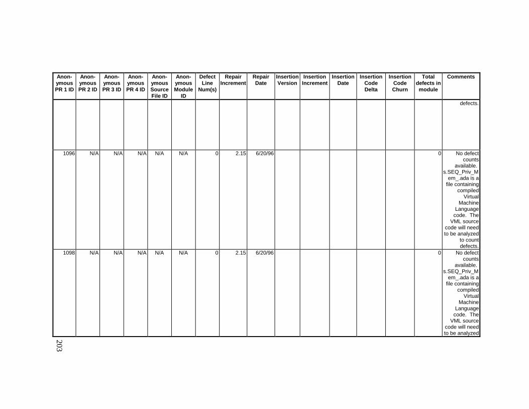
203
Anon-ymousPR 1 ID
Anon-ymousPR 2 ID
Anon-ymousPR 3 ID
Anon-ymousPR 4 ID
Anon-ymousSourceFile ID
Anon-ymousModule
ID
DefectLine
Num(s)
RepairIncrement
RepairDate
InsertionVersion
InsertionIncrement
InsertionDate
InsertionCodeDelta
InsertionCodeChurn
Totaldefects inmodule
Comments
defects.
1096 N/A N/A N/A N/A N/A 0 2.15 6/20/96 0 No defectcounts
available. s.SEQ_Priv_M
em_.ada is afile containing
compiledVirtual
MachineLanguage
code. TheVML source
code will needto be analyzed
to countdefects.
1098 N/A N/A N/A N/A N/A 0 2.15 6/20/96 0 No defectcounts
available. s.SEQ_Priv_M
em_.ada is afile containing
compiledVirtual
MachineLanguage
code. TheVML source
code will needto be analyzed
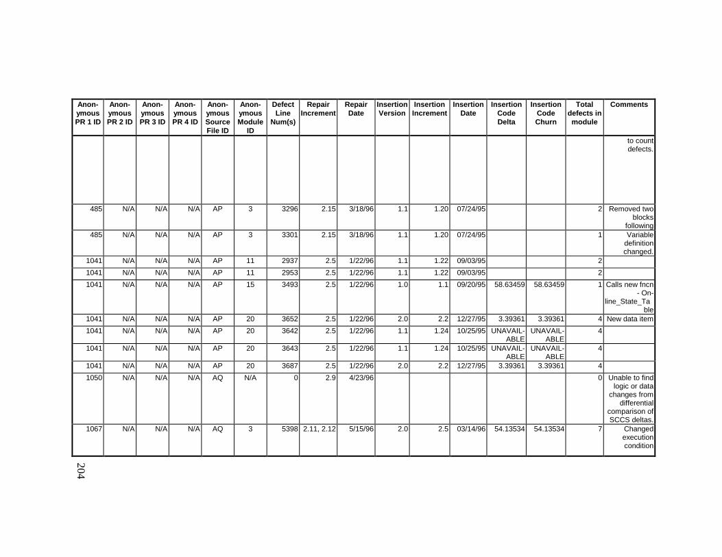
204
Anon-ymousPR 1 ID
Anon-ymousPR 2 ID
Anon-ymousPR 3 ID
Anon-ymousPR 4 ID
Anon-ymousSourceFile ID
Anon-ymousModule
ID
DefectLine
Num(s)
RepairIncrement
RepairDate
InsertionVersion
InsertionIncrement
InsertionDate
InsertionCodeDelta
InsertionCodeChurn
Totaldefects inmodule
Comments
to countdefects.
485 N/A N/A N/A AP 3 3296 2.15 3/18/96 1.1 1.20 07/24/95 2 Removed twoblocks
following485 N/A N/A N/A AP 3 3301 2.15 3/18/96 1.1 1.20 07/24/95 1 Variable
definitionchanged.
1041 N/A N/A N/A AP 11 2937 2.5 1/22/96 1.1 1.22 09/03/95 2
1041 N/A N/A N/A AP 11 2953 2.5 1/22/96 1.1 1.22 09/03/95 2
1041 N/A N/A N/A AP 15 3493 2.5 1/22/96 1.0 1.1 09/20/95 58.63459 58.63459 1 Calls new fncn- On-
line_State_Table
1041 N/A N/A N/A AP 20 3652 2.5 1/22/96 2.0 2.2 12/27/95 3.39361 3.39361 4 New data item
1041 N/A N/A N/A AP 20 3642 2.5 1/22/96 1.1 1.24 10/25/95 UNAVAIL-ABLE
UNAVAIL-ABLE
4
1041 N/A N/A N/A AP 20 3643 2.5 1/22/96 1.1 1.24 10/25/95 UNAVAIL-ABLE
UNAVAIL-ABLE
4
1041 N/A N/A N/A AP 20 3687 2.5 1/22/96 2.0 2.2 12/27/95 3.39361 3.39361 4
1050 N/A N/A N/A AQ N/A 0 2.9 4/23/96 0 Unable to findlogic or data
changes fromdifferential
comparison ofSCCS deltas.
1067 N/A N/A N/A AQ 3 5398 2.11, 2.12 5/15/96 2.0 2.5 03/14/96 54.13534 54.13534 7 Changedexecutioncondition
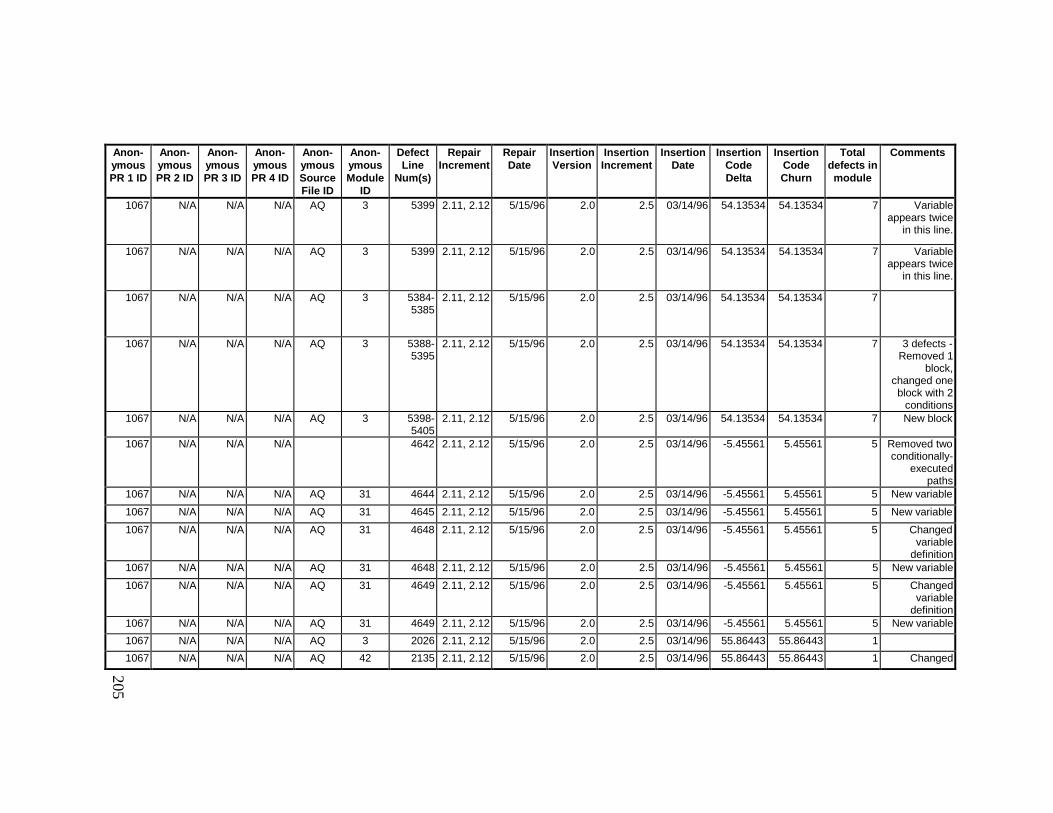
205
Anon-ymousPR 1 ID
Anon-ymousPR 2 ID
Anon-ymousPR 3 ID
Anon-ymousPR 4 ID
Anon-ymousSourceFile ID
Anon-ymousModule
ID
DefectLine
Num(s)
RepairIncrement
RepairDate
InsertionVersion
InsertionIncrement
InsertionDate
InsertionCodeDelta
InsertionCodeChurn
Totaldefects inmodule
Comments
1067 N/A N/A N/A AQ 3 5399 2.11, 2.12 5/15/96 2.0 2.5 03/14/96 54.13534 54.13534 7 Variableappears twice
in this line.
1067 N/A N/A N/A AQ 3 5399 2.11, 2.12 5/15/96 2.0 2.5 03/14/96 54.13534 54.13534 7 Variableappears twice
in this line.
1067 N/A N/A N/A AQ 3 5384-5385
2.11, 2.12 5/15/96 2.0 2.5 03/14/96 54.13534 54.13534 7
1067 N/A N/A N/A AQ 3 5388-5395
2.11, 2.12 5/15/96 2.0 2.5 03/14/96 54.13534 54.13534 7 3 defects -Removed 1
block,changed oneblock with 2
conditions1067 N/A N/A N/A AQ 3 5398-
54052.11, 2.12 5/15/96 2.0 2.5 03/14/96 54.13534 54.13534 7 New block
1067 N/A N/A N/A 4642 2.11, 2.12 5/15/96 2.0 2.5 03/14/96 -5.45561 5.45561 5 Removed twoconditionally-
executedpaths
1067 N/A N/A N/A AQ 31 4644 2.11, 2.12 5/15/96 2.0 2.5 03/14/96 -5.45561 5.45561 5 New variable
1067 N/A N/A N/A AQ 31 4645 2.11, 2.12 5/15/96 2.0 2.5 03/14/96 -5.45561 5.45561 5 New variable
1067 N/A N/A N/A AQ 31 4648 2.11, 2.12 5/15/96 2.0 2.5 03/14/96 -5.45561 5.45561 5 Changedvariable
definition1067 N/A N/A N/A AQ 31 4648 2.11, 2.12 5/15/96 2.0 2.5 03/14/96 -5.45561 5.45561 5 New variable
1067 N/A N/A N/A AQ 31 4649 2.11, 2.12 5/15/96 2.0 2.5 03/14/96 -5.45561 5.45561 5 Changedvariable
definition1067 N/A N/A N/A AQ 31 4649 2.11, 2.12 5/15/96 2.0 2.5 03/14/96 -5.45561 5.45561 5 New variable
1067 N/A N/A N/A AQ 3 2026 2.11, 2.12 5/15/96 2.0 2.5 03/14/96 55.86443 55.86443 1
1067 N/A N/A N/A AQ 42 2135 2.11, 2.12 5/15/96 2.0 2.5 03/14/96 55.86443 55.86443 1 Changed
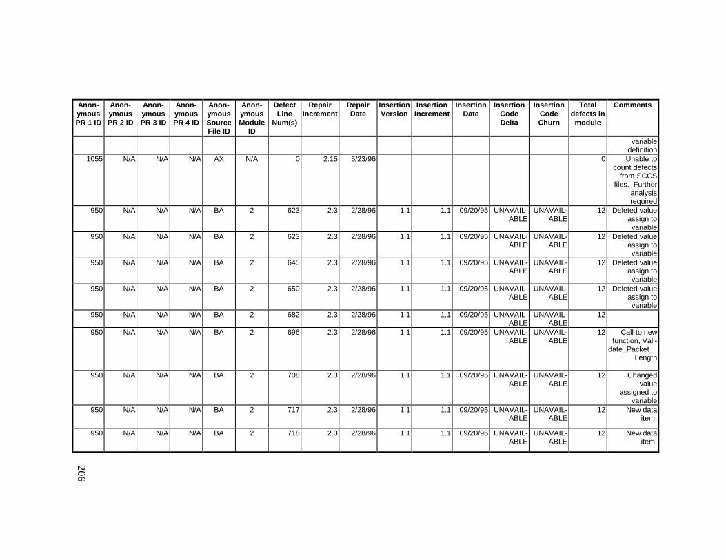
206
Anon-ymousPR 1 ID
Anon-ymousPR 2 ID
Anon-ymousPR 3 ID
Anon-ymousPR 4 ID
Anon-ymousSourceFile ID
Anon-ymousModule
ID
DefectLine
Num(s)
RepairIncrement
RepairDate
InsertionVersion
InsertionIncrement
InsertionDate
InsertionCodeDelta
InsertionCodeChurn
Totaldefects inmodule
Comments
variabledefinition
1055 N/A N/A N/A AX N/A 0 2.15 5/23/96 0 Unable tocount defects
from SCCSfiles. Further
analysisrequired
950 N/A N/A N/A BA 2 623 2.3 2/28/96 1.1 1.1 09/20/95 UNAVAIL-ABLE
UNAVAIL-ABLE
12 Deleted valueassign tovariable
950 N/A N/A N/A BA 2 623 2.3 2/28/96 1.1 1.1 09/20/95 UNAVAIL-ABLE
UNAVAIL-ABLE
12 Deleted valueassign tovariable
950 N/A N/A N/A BA 2 645 2.3 2/28/96 1.1 1.1 09/20/95 UNAVAIL-ABLE
UNAVAIL-ABLE
12 Deleted valueassign tovariable
950 N/A N/A N/A BA 2 650 2.3 2/28/96 1.1 1.1 09/20/95 UNAVAIL-ABLE
UNAVAIL-ABLE
12 Deleted valueassign tovariable
950 N/A N/A N/A BA 2 682 2.3 2/28/96 1.1 1.1 09/20/95 UNAVAIL-ABLE
UNAVAIL-ABLE
12
950 N/A N/A N/A BA 2 696 2.3 2/28/96 1.1 1.1 09/20/95 UNAVAIL-ABLE
UNAVAIL-ABLE
12 Call to newfunction, Vali-
date_Packet_Length
950 N/A N/A N/A BA 2 708 2.3 2/28/96 1.1 1.1 09/20/95 UNAVAIL-ABLE
UNAVAIL-ABLE
12 Changedvalue
assigned tovariable
950 N/A N/A N/A BA 2 717 2.3 2/28/96 1.1 1.1 09/20/95 UNAVAIL-ABLE
UNAVAIL-ABLE
12 New dataitem.
950 N/A N/A N/A BA 2 718 2.3 2/28/96 1.1 1.1 09/20/95 UNAVAIL-ABLE
UNAVAIL-ABLE
12 New dataitem.
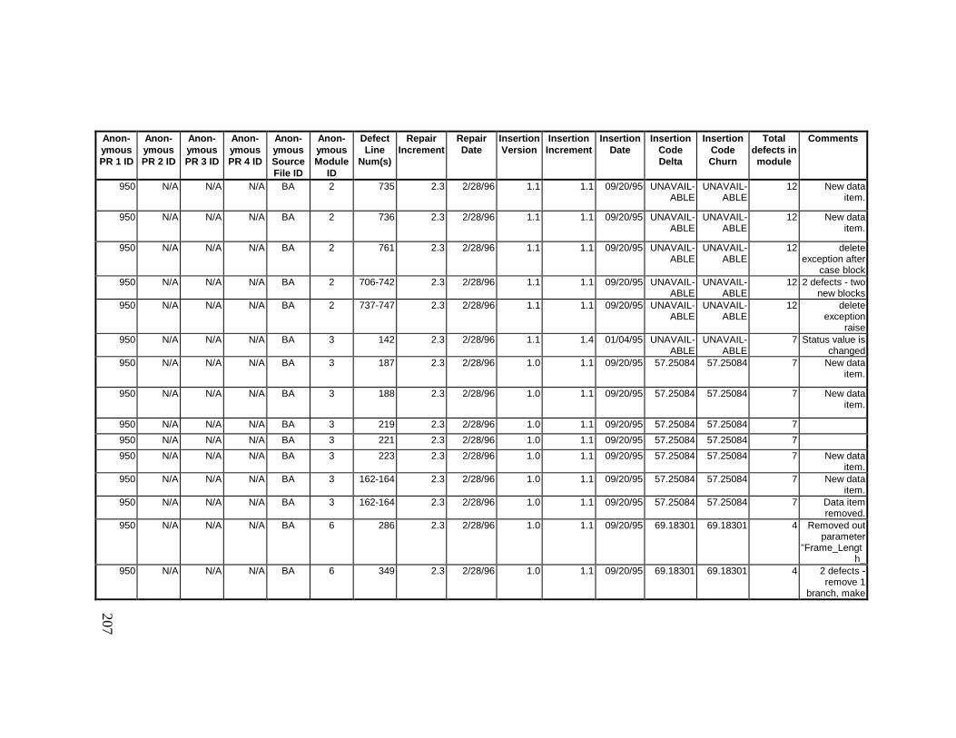
207
Anon-ymousPR 1 ID
Anon-ymousPR 2 ID
Anon-ymousPR 3 ID
Anon-ymousPR 4 ID
Anon-ymousSourceFile ID
Anon-ymousModule
ID
DefectLine
Num(s)
RepairIncrement
RepairDate
InsertionVersion
InsertionIncrement
InsertionDate
InsertionCodeDelta
InsertionCodeChurn
Totaldefects inmodule
Comments
950 N/A N/A N/A BA 2 735 2.3 2/28/96 1.1 1.1 09/20/95 UNAVAIL-ABLE
UNAVAIL-ABLE
12 New dataitem.
950 N/A N/A N/A BA 2 736 2.3 2/28/96 1.1 1.1 09/20/95 UNAVAIL-ABLE
UNAVAIL-ABLE
12 New dataitem.
950 N/A N/A N/A BA 2 761 2.3 2/28/96 1.1 1.1 09/20/95 UNAVAIL-ABLE
UNAVAIL-ABLE
12 deleteexception after
case block950 N/A N/A N/A BA 2 706-742 2.3 2/28/96 1.1 1.1 09/20/95 UNAVAIL-
ABLEUNAVAIL-
ABLE12 2 defects - two
new blocks950 N/A N/A N/A BA 2 737-747 2.3 2/28/96 1.1 1.1 09/20/95 UNAVAIL-
ABLEUNAVAIL-
ABLE12 delete
exceptionraise
950 N/A N/A N/A BA 3 142 2.3 2/28/96 1.1 1.4 01/04/95 UNAVAIL-ABLE
UNAVAIL-ABLE
7 Status value ischanged
950 N/A N/A N/A BA 3 187 2.3 2/28/96 1.0 1.1 09/20/95 57.25084 57.25084 7 New dataitem.
950 N/A N/A N/A BA 3 188 2.3 2/28/96 1.0 1.1 09/20/95 57.25084 57.25084 7 New dataitem.
950 N/A N/A N/A BA 3 219 2.3 2/28/96 1.0 1.1 09/20/95 57.25084 57.25084 7
950 N/A N/A N/A BA 3 221 2.3 2/28/96 1.0 1.1 09/20/95 57.25084 57.25084 7
950 N/A N/A N/A BA 3 223 2.3 2/28/96 1.0 1.1 09/20/95 57.25084 57.25084 7 New dataitem.
950 N/A N/A N/A BA 3 162-164 2.3 2/28/96 1.0 1.1 09/20/95 57.25084 57.25084 7 New dataitem.
950 N/A N/A N/A BA 3 162-164 2.3 2/28/96 1.0 1.1 09/20/95 57.25084 57.25084 7 Data itemremoved.
950 N/A N/A N/A BA 6 286 2.3 2/28/96 1.0 1.1 09/20/95 69.18301 69.18301 4 Removed outparameter
"Frame_Length_
950 N/A N/A N/A BA 6 349 2.3 2/28/96 1.0 1.1 09/20/95 69.18301 69.18301 4 2 defects -remove 1
branch, make
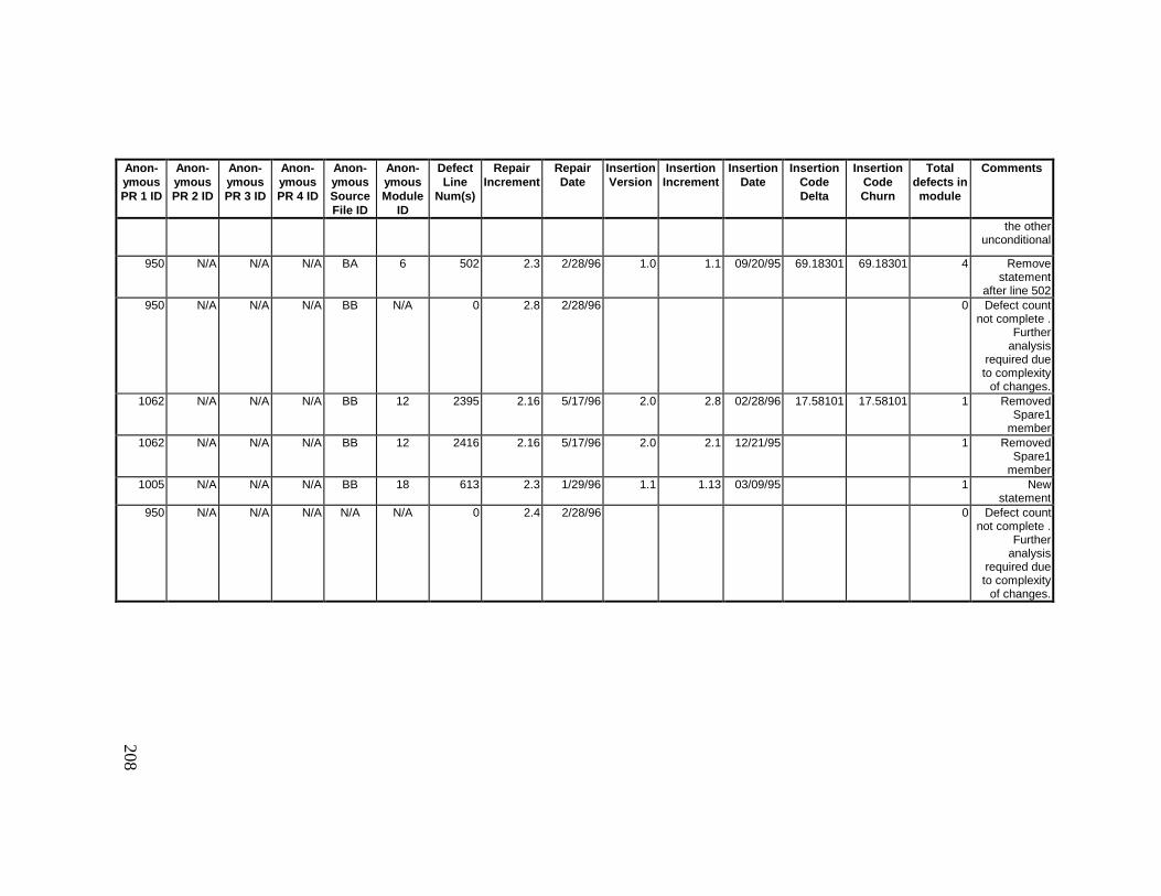
208
Anon-ymousPR 1 ID
Anon-ymousPR 2 ID
Anon-ymousPR 3 ID
Anon-ymousPR 4 ID
Anon-ymousSourceFile ID
Anon-ymousModule
ID
DefectLine
Num(s)
RepairIncrement
RepairDate
InsertionVersion
InsertionIncrement
InsertionDate
InsertionCodeDelta
InsertionCodeChurn
Totaldefects inmodule
Comments
the otherunconditional
950 N/A N/A N/A BA 6 502 2.3 2/28/96 1.0 1.1 09/20/95 69.18301 69.18301 4 Removestatement
after line 502950 N/A N/A N/A BB N/A 0 2.8 2/28/96 0 Defect count
not complete . Furtheranalysis
required dueto complexity
of changes.1062 N/A N/A N/A BB 12 2395 2.16 5/17/96 2.0 2.8 02/28/96 17.58101 17.58101 1 Removed
Spare1member
1062 N/A N/A N/A BB 12 2416 2.16 5/17/96 2.0 2.1 12/21/95 1 RemovedSpare1
member1005 N/A N/A N/A BB 18 613 2.3 1/29/96 1.1 1.13 03/09/95 1 New
statement950 N/A N/A N/A N/A N/A 0 2.4 2/28/96 0 Defect count
not complete . Furtheranalysis
required dueto complexity
of changes.

209
13.2 Defect Locations for Version 2.1a Development Library
Anon-ymousPR 1 ID
Anon-ymousPR 2 ID
Anon-ymousPR 3 ID
Anon-ymousPR 4 ID
Anon-ymousSourceFile ID
Anon-ymousModule
ID
DefectLine
Num(s)
RepairIncrement
RepairDate
InsertionVersion
InsertionIncrement
InsertionDate
InsertionCodeDelta
InsertionCodeChurn
Totaldefects inmodule
Comments
1170 1094 N/A N/A B 20 1423-1427
2.6 10/1/96 2.0 2.11 03/12/96 2.63791 2.63791 8 Moved fromelsewhere in
procedure1170 1094 N/A N/A B 20 1445-
14542.6 10/1/96 2.0 2.11 03/12/96 2.63791 2.63791 8 Moved into "if"
of line 14371170 1094 N/A N/A B 20 1457-
15122.6 10/1/96 2.0 2.11 03/12/96 2.63791 2.63791 8 6 branches
added1085 N/A N/A N/A N 17 0 2.1 9/17/96 0 Currently
unable tocount defects. Defects were
corrected indelta 1 of
version 2.1a. Further
analysisrequired.
1146 N/A N/A N/A AA 3 0 2.1 9/17/96 0 Currentlyunable to
count defects. Defects were
corrected indelta 1 of
version 2.1a. Further
analysisrequired.
990 991 N/A N/A AA 4 1537-1573
2.2 10/8/96 2.0 2.9 03/13/96 31.13491 31.13491 4 3 defects - twounconditional
blocks plusone execution
condition990 991 N/A N/A AA 4 1577 2.2 10/8/96 2.0 2.9 03/13/96 31.13491 31.13491 4 Calls
Load_REU
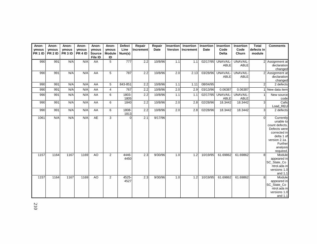
210
Anon-ymousPR 1 ID
Anon-ymousPR 2 ID
Anon-ymousPR 3 ID
Anon-ymousPR 4 ID
Anon-ymousSourceFile ID
Anon-ymousModule
ID
DefectLine
Num(s)
RepairIncrement
RepairDate
InsertionVersion
InsertionIncrement
InsertionDate
InsertionCodeDelta
InsertionCodeChurn
Totaldefects inmodule
Comments
990 991 N/A N/A AA 5 777 2.2 10/8/96 1.1 1.1 02/17/95 UNAVAIL-ABLE
UNAVAIL-ABLE
2 Assignment atdeclaration
changed990 991 N/A N/A AA 5 787 2.2 10/8/96 2.0 2.13 03/28/96 UNAVAIL-
ABLEUNAVAIL-
ABLE2 Assignment at
declarationchanged
990 991 N/A N/A AA 5 843-851 2.2 10/8/96 1.1 1.11 08/04/95 2 2 defects
990 991 N/A N/A AA 4 767 2.2 10/8/96 2.0 2.9 03/13/96 0.06387 0.06387 1 New data item
990 991 N/A N/A AA 6 1803-1805
2.2 10/8/96 1.1 1.1 02/17/95 UNAVAIL-ABLE
UNAVAIL-ABLE
1 New sourcecode
990 991 N/A N/A AA 6 1840 2.2 10/8/96 2.0 2.8 02/28/96 18.3442 18.3442 3 CallsLoad_REU
990 991 N/A N/A AA 6 1808-1813
2.2 10/8/96 2.0 2.8 02/28/96 18.3442 18.3442 3 2 defects
1061 N/A N/A N/A AE 3 0 2.1 9/17/96 0 Currentlyunable to
count defects. Defects were
corrected indelta 1 of
version 2.1a. Further
analysisrequired.
1157 1164 1167 1169 AO 2 4446-4450
2.3 9/30/96 1.0 1.2 10/19/95 61.69862 61.69862 8 Moduleappeared in
SC_State_Control.ada in
versions 1.0and 1.1
1157 1164 1167 1169 AO 2 4525-4527
2.3 9/30/96 1.0 1.2 10/19/95 61.69862 61.69862 8 Moduleappeared in
SC_State_Control.ada in
versions 1.0and 1.1
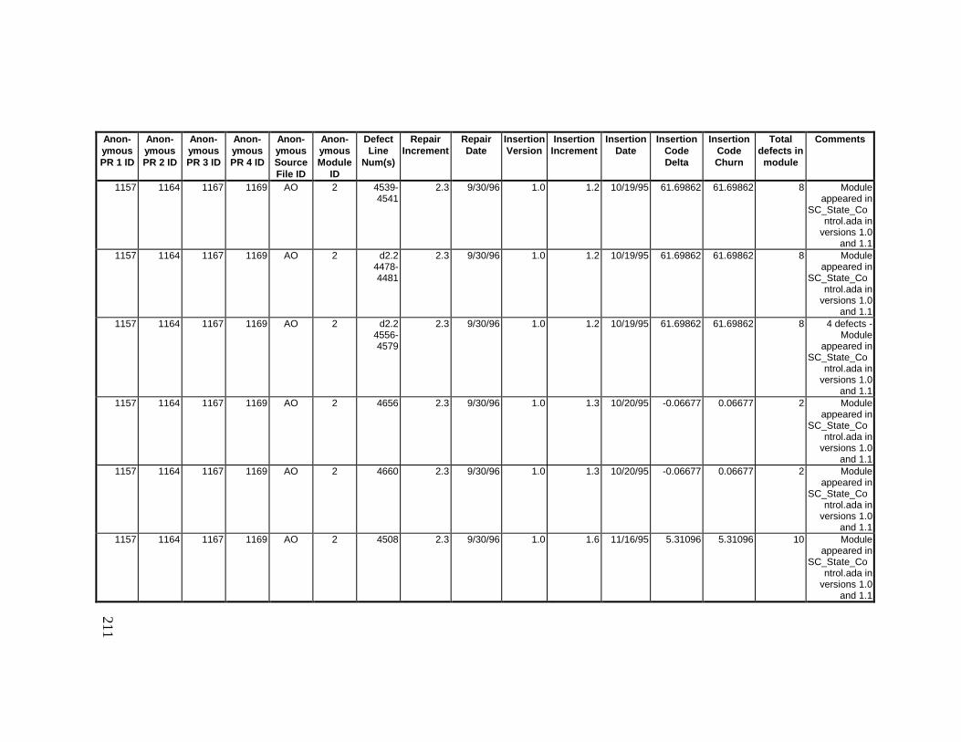
211
Anon-ymousPR 1 ID
Anon-ymousPR 2 ID
Anon-ymousPR 3 ID
Anon-ymousPR 4 ID
Anon-ymousSourceFile ID
Anon-ymousModule
ID
DefectLine
Num(s)
RepairIncrement
RepairDate
InsertionVersion
InsertionIncrement
InsertionDate
InsertionCodeDelta
InsertionCodeChurn
Totaldefects inmodule
Comments
1157 1164 1167 1169 AO 2 4539-4541
2.3 9/30/96 1.0 1.2 10/19/95 61.69862 61.69862 8 Moduleappeared in
SC_State_Control.ada in
versions 1.0and 1.1
1157 1164 1167 1169 AO 2 d2.24478-4481
2.3 9/30/96 1.0 1.2 10/19/95 61.69862 61.69862 8 Moduleappeared in
SC_State_Control.ada in
versions 1.0and 1.1
1157 1164 1167 1169 AO 2 d2.24556-4579
2.3 9/30/96 1.0 1.2 10/19/95 61.69862 61.69862 8 4 defects -Module
appeared inSC_State_Co
ntrol.ada inversions 1.0
and 1.11157 1164 1167 1169 AO 2 4656 2.3 9/30/96 1.0 1.3 10/20/95 -0.06677 0.06677 2 Module
appeared inSC_State_Co
ntrol.ada inversions 1.0
and 1.11157 1164 1167 1169 AO 2 4660 2.3 9/30/96 1.0 1.3 10/20/95 -0.06677 0.06677 2 Module
appeared inSC_State_Co
ntrol.ada inversions 1.0
and 1.11157 1164 1167 1169 AO 2 4508 2.3 9/30/96 1.0 1.6 11/16/95 5.31096 5.31096 10 Module
appeared inSC_State_Co
ntrol.ada inversions 1.0
and 1.1
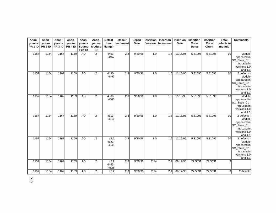
212
Anon-ymousPR 1 ID
Anon-ymousPR 2 ID
Anon-ymousPR 3 ID
Anon-ymousPR 4 ID
Anon-ymousSourceFile ID
Anon-ymousModule
ID
DefectLine
Num(s)
RepairIncrement
RepairDate
InsertionVersion
InsertionIncrement
InsertionDate
InsertionCodeDelta
InsertionCodeChurn
Totaldefects inmodule
Comments
1157 1164 1167 1169 AO 2 4453-4457
2.3 9/30/96 1.0 1.6 11/16/95 5.31096 5.31096 10 Moduleappeared in
SC_State_Control.ada in
versions 1.0and 1.1
1157 1164 1167 1169 AO 2 4490-4497
2.3 9/30/96 1.0 1.6 11/16/95 5.31096 5.31096 10 2 defects -Module
appeared inSC_State_Co
ntrol.ada inversions 1.0
and 1.11157 1164 1167 1169 AO 2 4500-
45052.3 9/30/96 1.0 1.6 11/16/95 5.31096 5.31096 10 Module
appeared inSC_State_Co
ntrol.ada inversions 1.0
and 1.11157 1164 1167 1169 AO 2 4513-
45162.3 9/30/96 1.0 1.6 11/16/95 5.31096 5.31096 10 2 defects -
Moduleappeared in
SC_State_Control.ada in
versions 1.0and 1.1
1157 1164 1167 1169 AO 2 d2.24622-4648
2.3 9/30/96 1.0 1.6 11/16/95 5.31096 5.31096 10 3 defects -Module
appeared inSC_State_Co
ntrol.ada inversions 1.0
and 1.11157 1164 1167 1169 AO 2 d2.2
4483-4528
2.3 9/30/96 2.1a 2.1 09/17/96 27.5631 27.5631 3
1157 1164 1167 1169 AO 2 d2.2 2.3 9/30/96 2.1a 2.1 09/17/96 27.5631 27.5631 3 2 defects
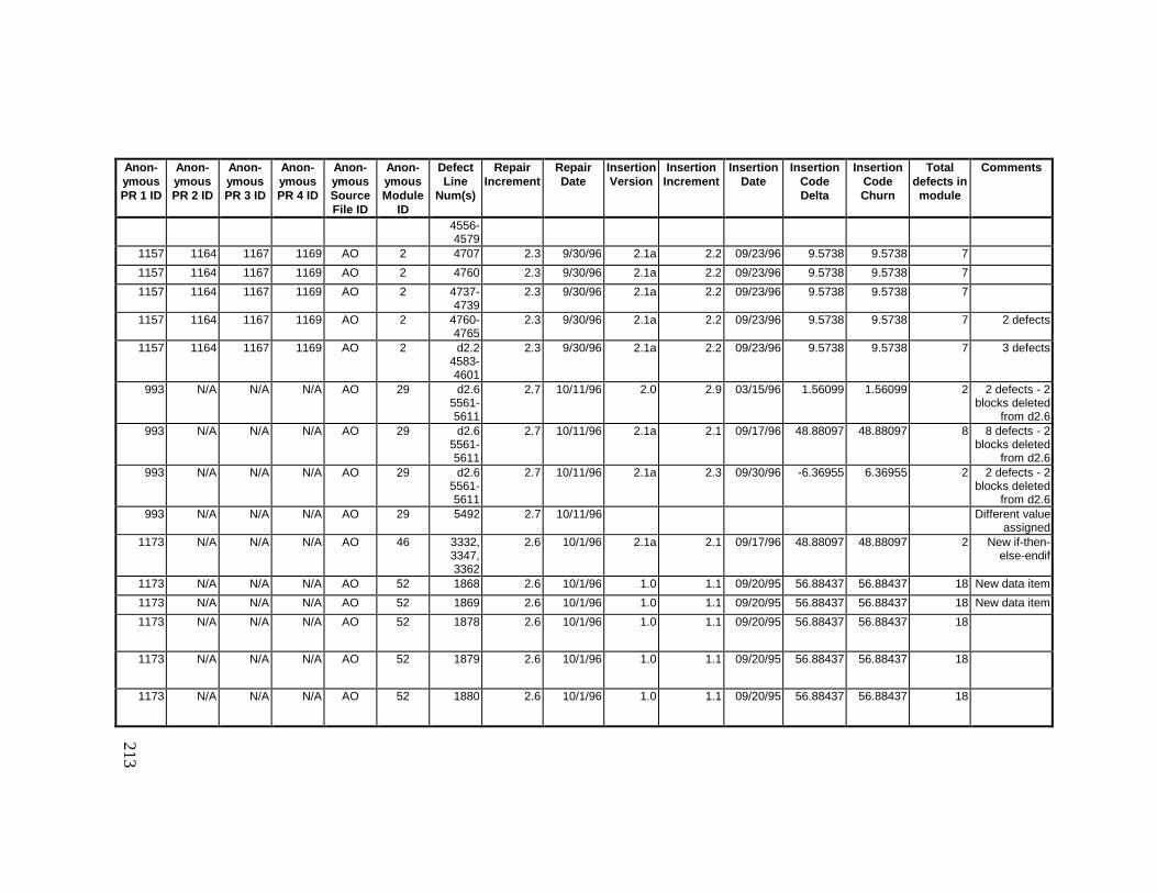
213
Anon-ymousPR 1 ID
Anon-ymousPR 2 ID
Anon-ymousPR 3 ID
Anon-ymousPR 4 ID
Anon-ymousSourceFile ID
Anon-ymousModule
ID
DefectLine
Num(s)
RepairIncrement
RepairDate
InsertionVersion
InsertionIncrement
InsertionDate
InsertionCodeDelta
InsertionCodeChurn
Totaldefects inmodule
Comments
4556-4579
1157 1164 1167 1169 AO 2 4707 2.3 9/30/96 2.1a 2.2 09/23/96 9.5738 9.5738 7
1157 1164 1167 1169 AO 2 4760 2.3 9/30/96 2.1a 2.2 09/23/96 9.5738 9.5738 7
1157 1164 1167 1169 AO 2 4737-4739
2.3 9/30/96 2.1a 2.2 09/23/96 9.5738 9.5738 7
1157 1164 1167 1169 AO 2 4760-4765
2.3 9/30/96 2.1a 2.2 09/23/96 9.5738 9.5738 7 2 defects
1157 1164 1167 1169 AO 2 d2.24583-4601
2.3 9/30/96 2.1a 2.2 09/23/96 9.5738 9.5738 7 3 defects
993 N/A N/A N/A AO 29 d2.65561-5611
2.7 10/11/96 2.0 2.9 03/15/96 1.56099 1.56099 2 2 defects - 2blocks deleted
from d2.6993 N/A N/A N/A AO 29 d2.6
5561-5611
2.7 10/11/96 2.1a 2.1 09/17/96 48.88097 48.88097 8 8 defects - 2blocks deleted
from d2.6993 N/A N/A N/A AO 29 d2.6
5561-5611
2.7 10/11/96 2.1a 2.3 09/30/96 -6.36955 6.36955 2 2 defects - 2blocks deleted
from d2.6993 N/A N/A N/A AO 29 5492 2.7 10/11/96 Different value
assigned1173 N/A N/A N/A AO 46 3332,
3347,3362
2.6 10/1/96 2.1a 2.1 09/17/96 48.88097 48.88097 2 New if-then-else-endif
1173 N/A N/A N/A AO 52 1868 2.6 10/1/96 1.0 1.1 09/20/95 56.88437 56.88437 18 New data item
1173 N/A N/A N/A AO 52 1869 2.6 10/1/96 1.0 1.1 09/20/95 56.88437 56.88437 18 New data item
1173 N/A N/A N/A AO 52 1878 2.6 10/1/96 1.0 1.1 09/20/95 56.88437 56.88437 18
1173 N/A N/A N/A AO 52 1879 2.6 10/1/96 1.0 1.1 09/20/95 56.88437 56.88437 18
1173 N/A N/A N/A AO 52 1880 2.6 10/1/96 1.0 1.1 09/20/95 56.88437 56.88437 18

214
Anon-ymousPR 1 ID
Anon-ymousPR 2 ID
Anon-ymousPR 3 ID
Anon-ymousPR 4 ID
Anon-ymousSourceFile ID
Anon-ymousModule
ID
DefectLine
Num(s)
RepairIncrement
RepairDate
InsertionVersion
InsertionIncrement
InsertionDate
InsertionCodeDelta
InsertionCodeChurn
Totaldefects inmodule
Comments
1173 N/A N/A N/A AO 52 1881 2.6 10/1/96 1.0 1.1 09/20/95 56.88437 56.88437 18
1173 N/A N/A N/A AO 52 1882 2.6 10/1/96 1.0 1.1 09/20/95 56.88437 56.88437 18
1173 N/A N/A N/A AO 52 1883 2.6 10/1/96 1.0 1.1 09/20/95 56.88437 56.88437 18
1173 N/A N/A N/A AO 52 1884 2.6 10/1/96 1.0 1.1 09/20/95 56.88437 56.88437 18
1173 N/A N/A N/A AO 52 1885 2.6 10/1/96 1.0 1.1 09/20/95 56.88437 56.88437 18
1173 N/A N/A N/A AO 52 1886 2.6 10/1/96 1.0 1.1 09/20/95 56.88437 56.88437 18
1173 N/A N/A N/A AO 52 1887 2.6 10/1/96 1.0 1.1 09/20/95 56.88437 56.88437 18
1173 N/A N/A N/A AO 52 1892 2.6 10/1/96 1.0 1.1 09/20/95 56.88437 56.88437 18
1173 N/A N/A N/A AO 52 1893 2.6 10/1/96 1.0 1.1 09/20/95 56.88437 56.88437 18
1173 N/A N/A N/A AO 52 1894 2.6 10/1/96 1.0 1.1 09/20/95 56.88437 56.88437 18
1173 N/A N/A N/A AO 52 1895 2.6 10/1/96 1.0 1.1 09/20/95 56.88437 56.88437 18
1173 N/A N/A N/A AO 52 1896 2.6 10/1/96 1.0 1.1 09/20/95 56.88437 56.88437 18
1173 N/A N/A N/A AO 52 1898 2.6 10/1/96 1.0 1.1 09/20/95 56.88437 56.88437 18
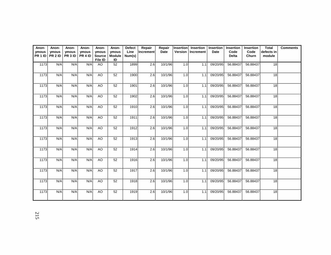
215
Anon-ymousPR 1 ID
Anon-ymousPR 2 ID
Anon-ymousPR 3 ID
Anon-ymousPR 4 ID
Anon-ymousSourceFile ID
Anon-ymousModule
ID
DefectLine
Num(s)
RepairIncrement
RepairDate
InsertionVersion
InsertionIncrement
InsertionDate
InsertionCodeDelta
InsertionCodeChurn
Totaldefects inmodule
Comments
1173 N/A N/A N/A AO 52 1899 2.6 10/1/96 1.0 1.1 09/20/95 56.88437 56.88437 18
1173 N/A N/A N/A AO 52 1900 2.6 10/1/96 1.0 1.1 09/20/95 56.88437 56.88437 18
1173 N/A N/A N/A AO 52 1901 2.6 10/1/96 1.0 1.1 09/20/95 56.88437 56.88437 18
1173 N/A N/A N/A AO 52 1902 2.6 10/1/96 1.0 1.1 09/20/95 56.88437 56.88437 18
1173 N/A N/A N/A AO 52 1910 2.6 10/1/96 1.0 1.1 09/20/95 56.88437 56.88437 18
1173 N/A N/A N/A AO 52 1911 2.6 10/1/96 1.0 1.1 09/20/95 56.88437 56.88437 18
1173 N/A N/A N/A AO 52 1912 2.6 10/1/96 1.0 1.1 09/20/95 56.88437 56.88437 18
1173 N/A N/A N/A AO 52 1913 2.6 10/1/96 1.0 1.1 09/20/95 56.88437 56.88437 18
1173 N/A N/A N/A AO 52 1914 2.6 10/1/96 1.0 1.1 09/20/95 56.88437 56.88437 18
1173 N/A N/A N/A AO 52 1916 2.6 10/1/96 1.0 1.1 09/20/95 56.88437 56.88437 18
1173 N/A N/A N/A AO 52 1917 2.6 10/1/96 1.0 1.1 09/20/95 56.88437 56.88437 18
1173 N/A N/A N/A AO 52 1918 2.6 10/1/96 1.0 1.1 09/20/95 56.88437 56.88437 18
1173 N/A N/A N/A AO 52 1919 2.6 10/1/96 1.0 1.1 09/20/95 56.88437 56.88437 18
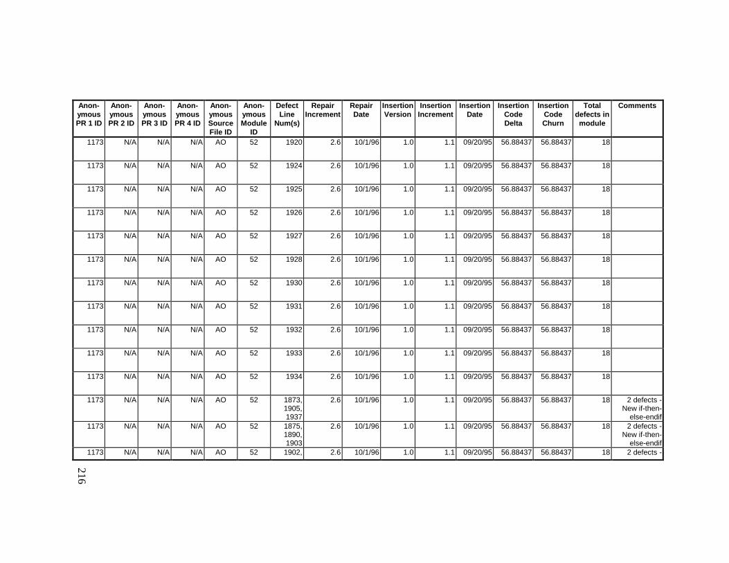
216
Anon-ymousPR 1 ID
Anon-ymousPR 2 ID
Anon-ymousPR 3 ID
Anon-ymousPR 4 ID
Anon-ymousSourceFile ID
Anon-ymousModule
ID
DefectLine
Num(s)
RepairIncrement
RepairDate
InsertionVersion
InsertionIncrement
InsertionDate
InsertionCodeDelta
InsertionCodeChurn
Totaldefects inmodule
Comments
1173 N/A N/A N/A AO 52 1920 2.6 10/1/96 1.0 1.1 09/20/95 56.88437 56.88437 18
1173 N/A N/A N/A AO 52 1924 2.6 10/1/96 1.0 1.1 09/20/95 56.88437 56.88437 18
1173 N/A N/A N/A AO 52 1925 2.6 10/1/96 1.0 1.1 09/20/95 56.88437 56.88437 18
1173 N/A N/A N/A AO 52 1926 2.6 10/1/96 1.0 1.1 09/20/95 56.88437 56.88437 18
1173 N/A N/A N/A AO 52 1927 2.6 10/1/96 1.0 1.1 09/20/95 56.88437 56.88437 18
1173 N/A N/A N/A AO 52 1928 2.6 10/1/96 1.0 1.1 09/20/95 56.88437 56.88437 18
1173 N/A N/A N/A AO 52 1930 2.6 10/1/96 1.0 1.1 09/20/95 56.88437 56.88437 18
1173 N/A N/A N/A AO 52 1931 2.6 10/1/96 1.0 1.1 09/20/95 56.88437 56.88437 18
1173 N/A N/A N/A AO 52 1932 2.6 10/1/96 1.0 1.1 09/20/95 56.88437 56.88437 18
1173 N/A N/A N/A AO 52 1933 2.6 10/1/96 1.0 1.1 09/20/95 56.88437 56.88437 18
1173 N/A N/A N/A AO 52 1934 2.6 10/1/96 1.0 1.1 09/20/95 56.88437 56.88437 18
1173 N/A N/A N/A AO 52 1873,1905,1937
2.6 10/1/96 1.0 1.1 09/20/95 56.88437 56.88437 18 2 defects -New if-then-
else-endif1173 N/A N/A N/A AO 52 1875,
1890,1903
2.6 10/1/96 1.0 1.1 09/20/95 56.88437 56.88437 18 2 defects -New if-then-
else-endif1173 N/A N/A N/A AO 52 1902, 2.6 10/1/96 1.0 1.1 09/20/95 56.88437 56.88437 18 2 defects -
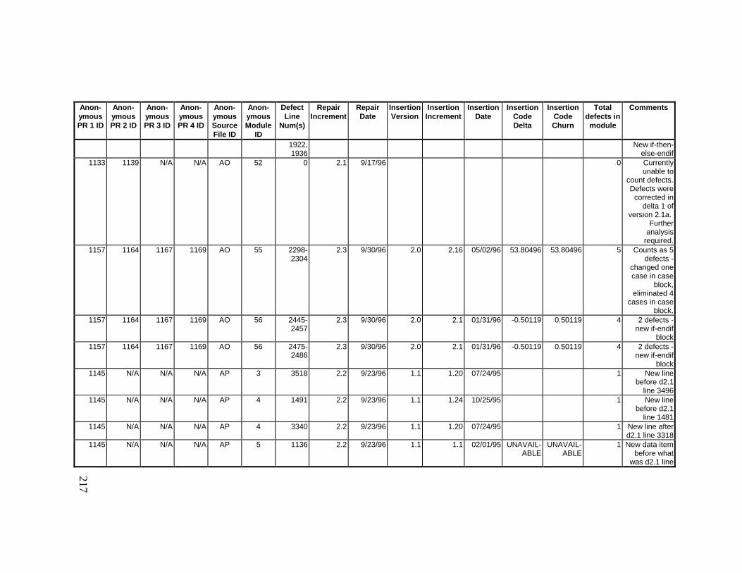
217
Anon-ymousPR 1 ID
Anon-ymousPR 2 ID
Anon-ymousPR 3 ID
Anon-ymousPR 4 ID
Anon-ymousSourceFile ID
Anon-ymousModule
ID
DefectLine
Num(s)
RepairIncrement
RepairDate
InsertionVersion
InsertionIncrement
InsertionDate
InsertionCodeDelta
InsertionCodeChurn
Totaldefects inmodule
Comments
1922,1936
New if-then-else-endif
1133 1139 N/A N/A AO 52 0 2.1 9/17/96 0 Currentlyunable to
count defects. Defects were
corrected indelta 1 of
version 2.1a. Further
analysisrequired.
1157 1164 1167 1169 AO 55 2298-2304
2.3 9/30/96 2.0 2.16 05/02/96 53.80496 53.80496 5 Counts as 5defects -
changed onecase in case
block,eliminated 4
cases in caseblock.
1157 1164 1167 1169 AO 56 2445-2457
2.3 9/30/96 2.0 2.1 01/31/96 -0.50119 0.50119 4 2 defects -new if-endif
block1157 1164 1167 1169 AO 56 2475-
24862.3 9/30/96 2.0 2.1 01/31/96 -0.50119 0.50119 4 2 defects -
new if-endifblock
1145 N/A N/A N/A AP 3 3518 2.2 9/23/96 1.1 1.20 07/24/95 1 New linebefore d2.1
line 34961145 N/A N/A N/A AP 4 1491 2.2 9/23/96 1.1 1.24 10/25/95 1 New line
before d2.1line 1481
1145 N/A N/A N/A AP 4 3340 2.2 9/23/96 1.1 1.20 07/24/95 1 New line afterd2.1 line 3318
1145 N/A N/A N/A AP 5 1136 2.2 9/23/96 1.1 1.1 02/01/95 UNAVAIL-ABLE
UNAVAIL-ABLE
1 New data itembefore what
was d2.1 line
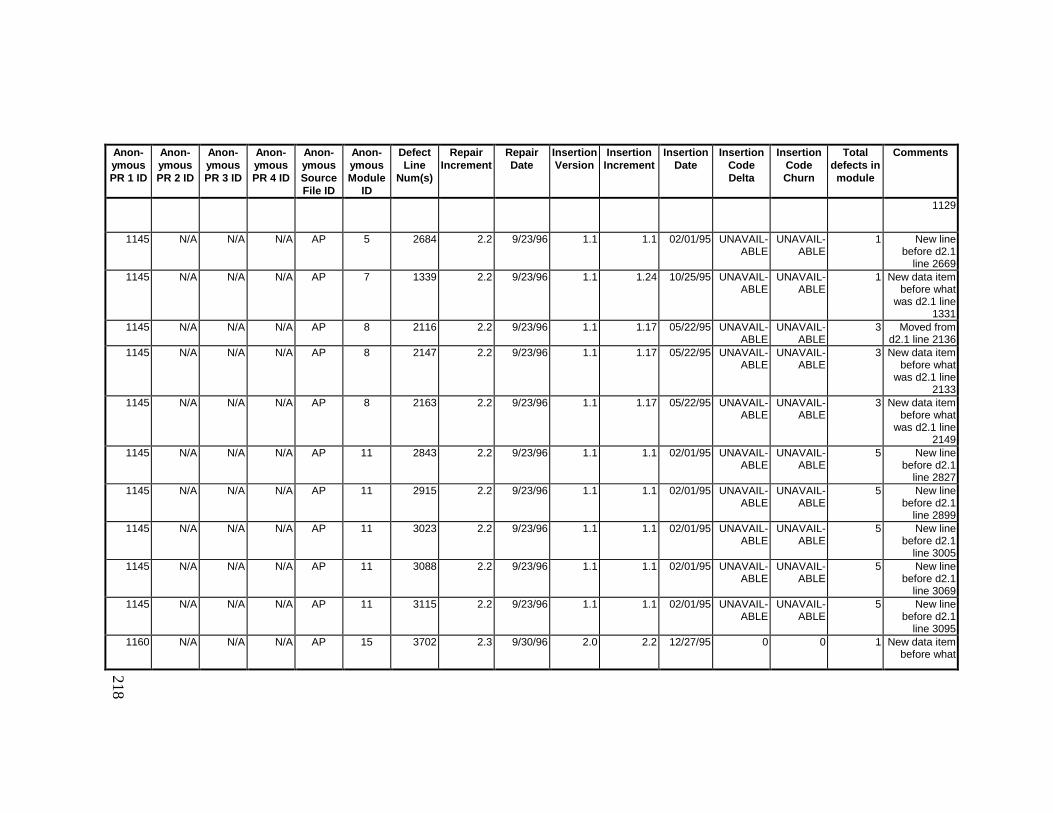
218
Anon-ymousPR 1 ID
Anon-ymousPR 2 ID
Anon-ymousPR 3 ID
Anon-ymousPR 4 ID
Anon-ymousSourceFile ID
Anon-ymousModule
ID
DefectLine
Num(s)
RepairIncrement
RepairDate
InsertionVersion
InsertionIncrement
InsertionDate
InsertionCodeDelta
InsertionCodeChurn
Totaldefects inmodule
Comments
1129
1145 N/A N/A N/A AP 5 2684 2.2 9/23/96 1.1 1.1 02/01/95 UNAVAIL-ABLE
UNAVAIL-ABLE
1 New linebefore d2.1
line 26691145 N/A N/A N/A AP 7 1339 2.2 9/23/96 1.1 1.24 10/25/95 UNAVAIL-
ABLEUNAVAIL-
ABLE1 New data item
before whatwas d2.1 line
13311145 N/A N/A N/A AP 8 2116 2.2 9/23/96 1.1 1.17 05/22/95 UNAVAIL-
ABLEUNAVAIL-
ABLE3 Moved from
d2.1 line 21361145 N/A N/A N/A AP 8 2147 2.2 9/23/96 1.1 1.17 05/22/95 UNAVAIL-
ABLEUNAVAIL-
ABLE3 New data item
before whatwas d2.1 line
21331145 N/A N/A N/A AP 8 2163 2.2 9/23/96 1.1 1.17 05/22/95 UNAVAIL-
ABLEUNAVAIL-
ABLE3 New data item
before whatwas d2.1 line
21491145 N/A N/A N/A AP 11 2843 2.2 9/23/96 1.1 1.1 02/01/95 UNAVAIL-
ABLEUNAVAIL-
ABLE5 New line
before d2.1line 2827
1145 N/A N/A N/A AP 11 2915 2.2 9/23/96 1.1 1.1 02/01/95 UNAVAIL-ABLE
UNAVAIL-ABLE
5 New linebefore d2.1
line 28991145 N/A N/A N/A AP 11 3023 2.2 9/23/96 1.1 1.1 02/01/95 UNAVAIL-
ABLEUNAVAIL-
ABLE5 New line
before d2.1line 3005
1145 N/A N/A N/A AP 11 3088 2.2 9/23/96 1.1 1.1 02/01/95 UNAVAIL-ABLE
UNAVAIL-ABLE
5 New linebefore d2.1
line 30691145 N/A N/A N/A AP 11 3115 2.2 9/23/96 1.1 1.1 02/01/95 UNAVAIL-
ABLEUNAVAIL-
ABLE5 New line
before d2.1line 3095
1160 N/A N/A N/A AP 15 3702 2.3 9/30/96 2.0 2.2 12/27/95 0 0 1 New data itembefore what
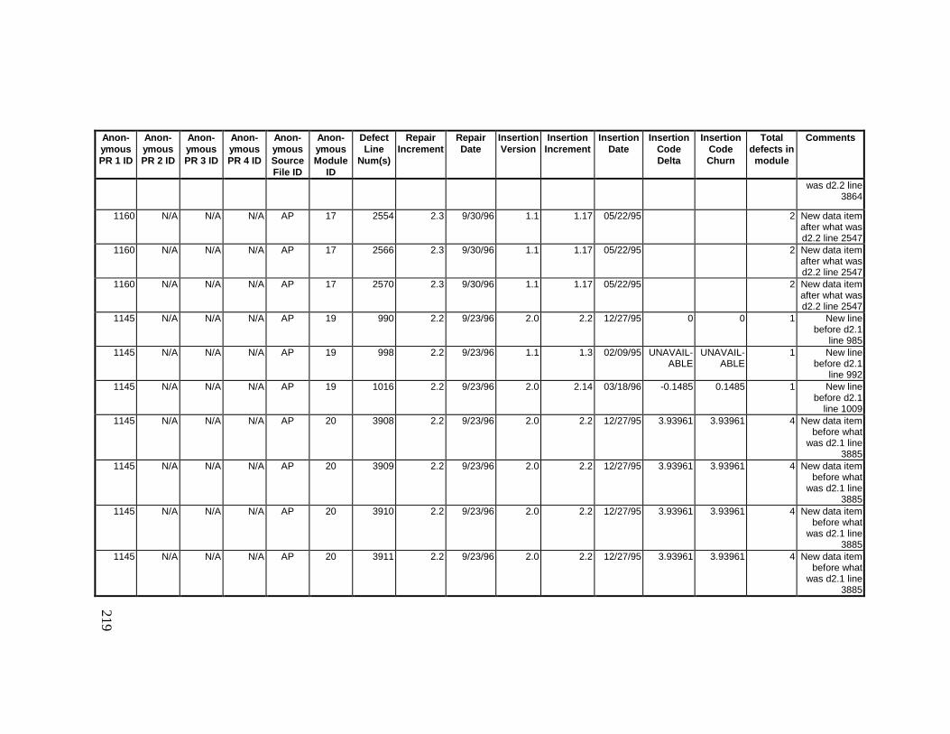
219
Anon-ymousPR 1 ID
Anon-ymousPR 2 ID
Anon-ymousPR 3 ID
Anon-ymousPR 4 ID
Anon-ymousSourceFile ID
Anon-ymousModule
ID
DefectLine
Num(s)
RepairIncrement
RepairDate
InsertionVersion
InsertionIncrement
InsertionDate
InsertionCodeDelta
InsertionCodeChurn
Totaldefects inmodule
Comments
was d2.2 line3864
1160 N/A N/A N/A AP 17 2554 2.3 9/30/96 1.1 1.17 05/22/95 2 New data itemafter what wasd2.2 line 2547
1160 N/A N/A N/A AP 17 2566 2.3 9/30/96 1.1 1.17 05/22/95 2 New data itemafter what wasd2.2 line 2547
1160 N/A N/A N/A AP 17 2570 2.3 9/30/96 1.1 1.17 05/22/95 2 New data itemafter what wasd2.2 line 2547
1145 N/A N/A N/A AP 19 990 2.2 9/23/96 2.0 2.2 12/27/95 0 0 1 New linebefore d2.1
line 9851145 N/A N/A N/A AP 19 998 2.2 9/23/96 1.1 1.3 02/09/95 UNAVAIL-
ABLEUNAVAIL-
ABLE1 New line
before d2.1line 992
1145 N/A N/A N/A AP 19 1016 2.2 9/23/96 2.0 2.14 03/18/96 -0.1485 0.1485 1 New linebefore d2.1
line 10091145 N/A N/A N/A AP 20 3908 2.2 9/23/96 2.0 2.2 12/27/95 3.93961 3.93961 4 New data item
before whatwas d2.1 line
38851145 N/A N/A N/A AP 20 3909 2.2 9/23/96 2.0 2.2 12/27/95 3.93961 3.93961 4 New data item
before whatwas d2.1 line
38851145 N/A N/A N/A AP 20 3910 2.2 9/23/96 2.0 2.2 12/27/95 3.93961 3.93961 4 New data item
before whatwas d2.1 line
38851145 N/A N/A N/A AP 20 3911 2.2 9/23/96 2.0 2.2 12/27/95 3.93961 3.93961 4 New data item
before whatwas d2.1 line
3885
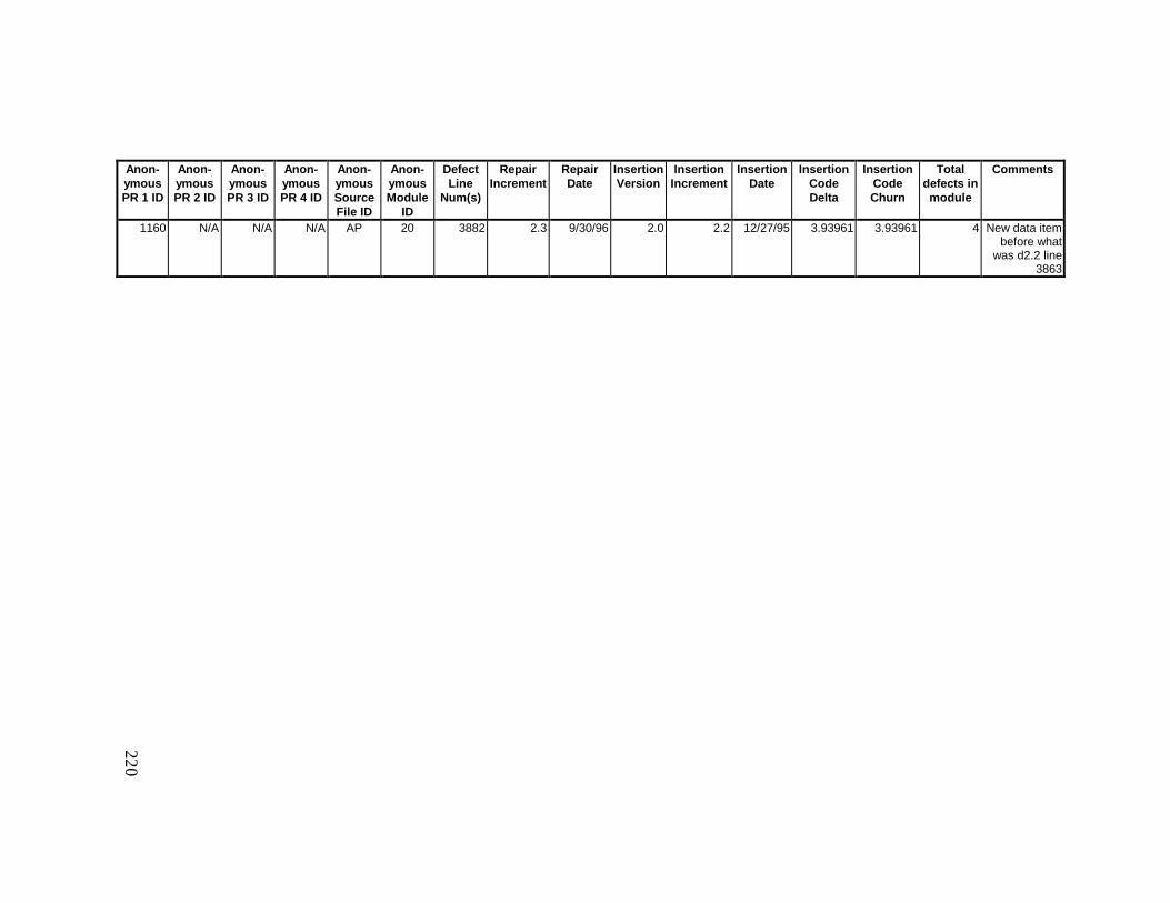
220
Anon-ymousPR 1 ID
Anon-ymousPR 2 ID
Anon-ymousPR 3 ID
Anon-ymousPR 4 ID
Anon-ymousSourceFile ID
Anon-ymousModule
ID
DefectLine
Num(s)
RepairIncrement
RepairDate
InsertionVersion
InsertionIncrement
InsertionDate
InsertionCodeDelta
InsertionCodeChurn
Totaldefects inmodule
Comments
1160 N/A N/A N/A AP 20 3882 2.3 9/30/96 2.0 2.2 12/27/95 3.93961 3.93961 4 New data itembefore what
was d2.2 line3863
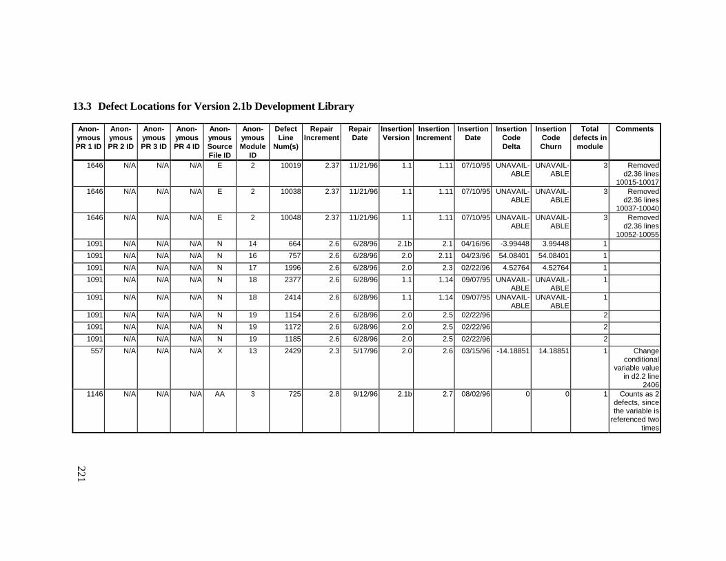
221
13.3 Defect Locations for Version 2.1b Development Library
Anon-ymousPR 1 ID
Anon-ymousPR 2 ID
Anon-ymousPR 3 ID
Anon-ymousPR 4 ID
Anon-ymousSourceFile ID
Anon-ymousModule
ID
DefectLine
Num(s)
RepairIncrement
RepairDate
InsertionVersion
InsertionIncrement
InsertionDate
InsertionCodeDelta
InsertionCodeChurn
Totaldefects inmodule
Comments
1646 N/A N/A N/A E 2 10019 2.37 11/21/96 1.1 1.11 07/10/95 UNAVAIL-ABLE
UNAVAIL-ABLE
3 Removedd2.36 lines
10015-100171646 N/A N/A N/A E 2 10038 2.37 11/21/96 1.1 1.11 07/10/95 UNAVAIL-
ABLEUNAVAIL-
ABLE3 Removed
d2.36 lines10037-10040
1646 N/A N/A N/A E 2 10048 2.37 11/21/96 1.1 1.11 07/10/95 UNAVAIL-ABLE
UNAVAIL-ABLE
3 Removedd2.36 lines
10052-100551091 N/A N/A N/A N 14 664 2.6 6/28/96 2.1b 2.1 04/16/96 -3.99448 3.99448 1
1091 N/A N/A N/A N 16 757 2.6 6/28/96 2.0 2.11 04/23/96 54.08401 54.08401 1
1091 N/A N/A N/A N 17 1996 2.6 6/28/96 2.0 2.3 02/22/96 4.52764 4.52764 1
1091 N/A N/A N/A N 18 2377 2.6 6/28/96 1.1 1.14 09/07/95 UNAVAIL-ABLE
UNAVAIL-ABLE
1
1091 N/A N/A N/A N 18 2414 2.6 6/28/96 1.1 1.14 09/07/95 UNAVAIL-ABLE
UNAVAIL-ABLE
1
1091 N/A N/A N/A N 19 1154 2.6 6/28/96 2.0 2.5 02/22/96 2
1091 N/A N/A N/A N 19 1172 2.6 6/28/96 2.0 2.5 02/22/96 2
1091 N/A N/A N/A N 19 1185 2.6 6/28/96 2.0 2.5 02/22/96 2
557 N/A N/A N/A X 13 2429 2.3 5/17/96 2.0 2.6 03/15/96 -14.18851 14.18851 1 Changeconditional
variable valuein d2.2 line
24061146 N/A N/A N/A AA 3 725 2.8 9/12/96 2.1b 2.7 08/02/96 0 0 1 Counts as 2
defects, sincethe variable is
referenced twotimes

222
Anon-ymousPR 1 ID
Anon-ymousPR 2 ID
Anon-ymousPR 3 ID
Anon-ymousPR 4 ID
Anon-ymousSourceFile ID
Anon-ymousModule
ID
DefectLine
Num(s)
RepairIncrement
RepairDate
InsertionVersion
InsertionIncrement
InsertionDate
InsertionCodeDelta
InsertionCodeChurn
Totaldefects inmodule
Comments
1194 N/A N/A N/A N/A N/A 0 2.15 10/21/96 0 s.SEQ_Priv_Mem_.ada is amodule thatcontains the
executablecode for the
System defectprotectionroutines.
However, thesource for
these routinesis written in a
sequencinglanguage
specific toJPL, "Virtual
MachineLanguage."
246 N/A N/A N/A N/A N/A 0 2.17 11/6/96 0 To computethe complexity
of this VMLcode, it wouldbe necessaryto develop an
analyzerspecific to that
language.247 N/A N/A N/A N/A N/A 0 2.17 11/6/96 0 To compute
the complexityof this VML
code, it wouldbe necessaryto develop an
analyzerspecific to that
language.
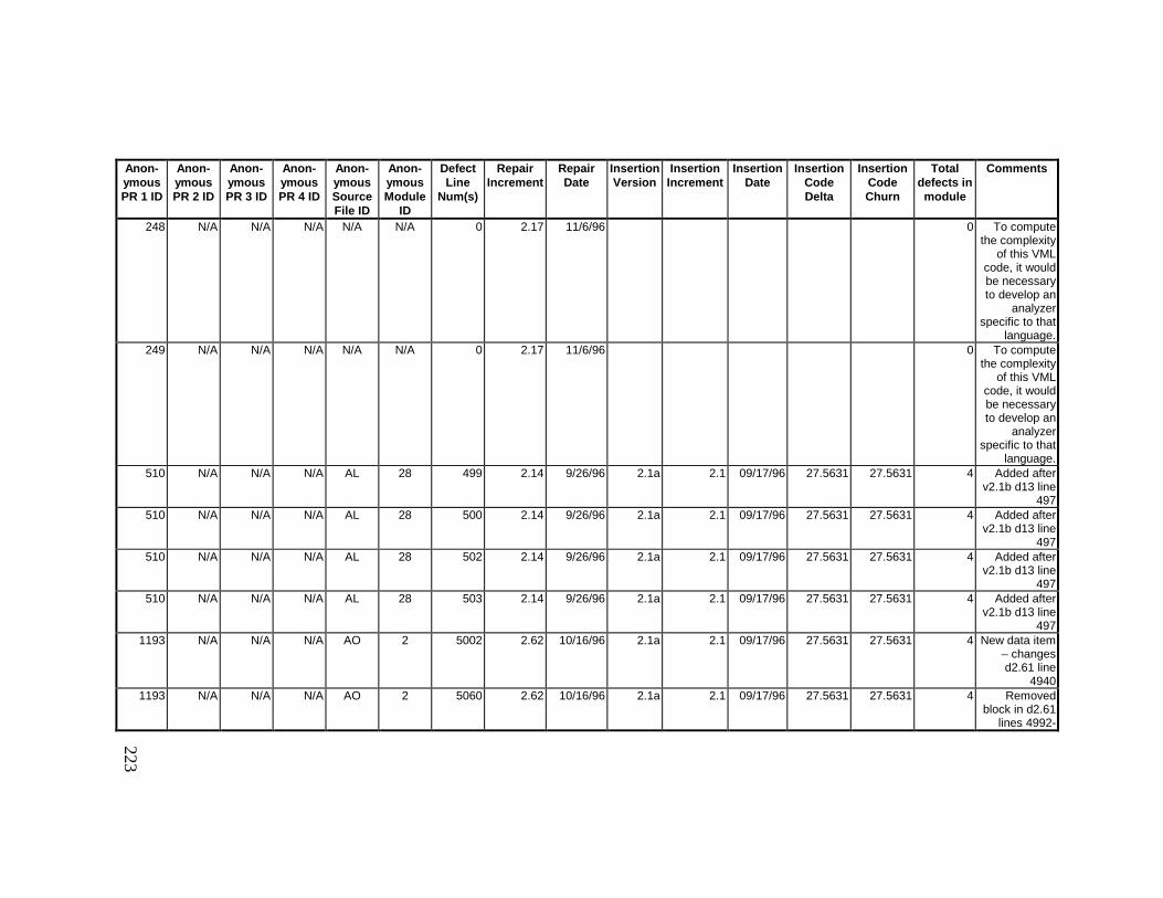
223
Anon-ymousPR 1 ID
Anon-ymousPR 2 ID
Anon-ymousPR 3 ID
Anon-ymousPR 4 ID
Anon-ymousSourceFile ID
Anon-ymousModule
ID
DefectLine
Num(s)
RepairIncrement
RepairDate
InsertionVersion
InsertionIncrement
InsertionDate
InsertionCodeDelta
InsertionCodeChurn
Totaldefects inmodule
Comments
248 N/A N/A N/A N/A N/A 0 2.17 11/6/96 0 To computethe complexity
of this VMLcode, it wouldbe necessaryto develop an
analyzerspecific to that
language.249 N/A N/A N/A N/A N/A 0 2.17 11/6/96 0 To compute
the complexityof this VML
code, it wouldbe necessaryto develop an
analyzerspecific to that
language.510 N/A N/A N/A AL 28 499 2.14 9/26/96 2.1a 2.1 09/17/96 27.5631 27.5631 4 Added after
v2.1b d13 line497
510 N/A N/A N/A AL 28 500 2.14 9/26/96 2.1a 2.1 09/17/96 27.5631 27.5631 4 Added afterv2.1b d13 line
497510 N/A N/A N/A AL 28 502 2.14 9/26/96 2.1a 2.1 09/17/96 27.5631 27.5631 4 Added after
v2.1b d13 line497
510 N/A N/A N/A AL 28 503 2.14 9/26/96 2.1a 2.1 09/17/96 27.5631 27.5631 4 Added afterv2.1b d13 line
4971193 N/A N/A N/A AO 2 5002 2.62 10/16/96 2.1a 2.1 09/17/96 27.5631 27.5631 4 New data item
– changesd2.61 line
49401193 N/A N/A N/A AO 2 5060 2.62 10/16/96 2.1a 2.1 09/17/96 27.5631 27.5631 4 Removed
block in d2.61lines 4992-
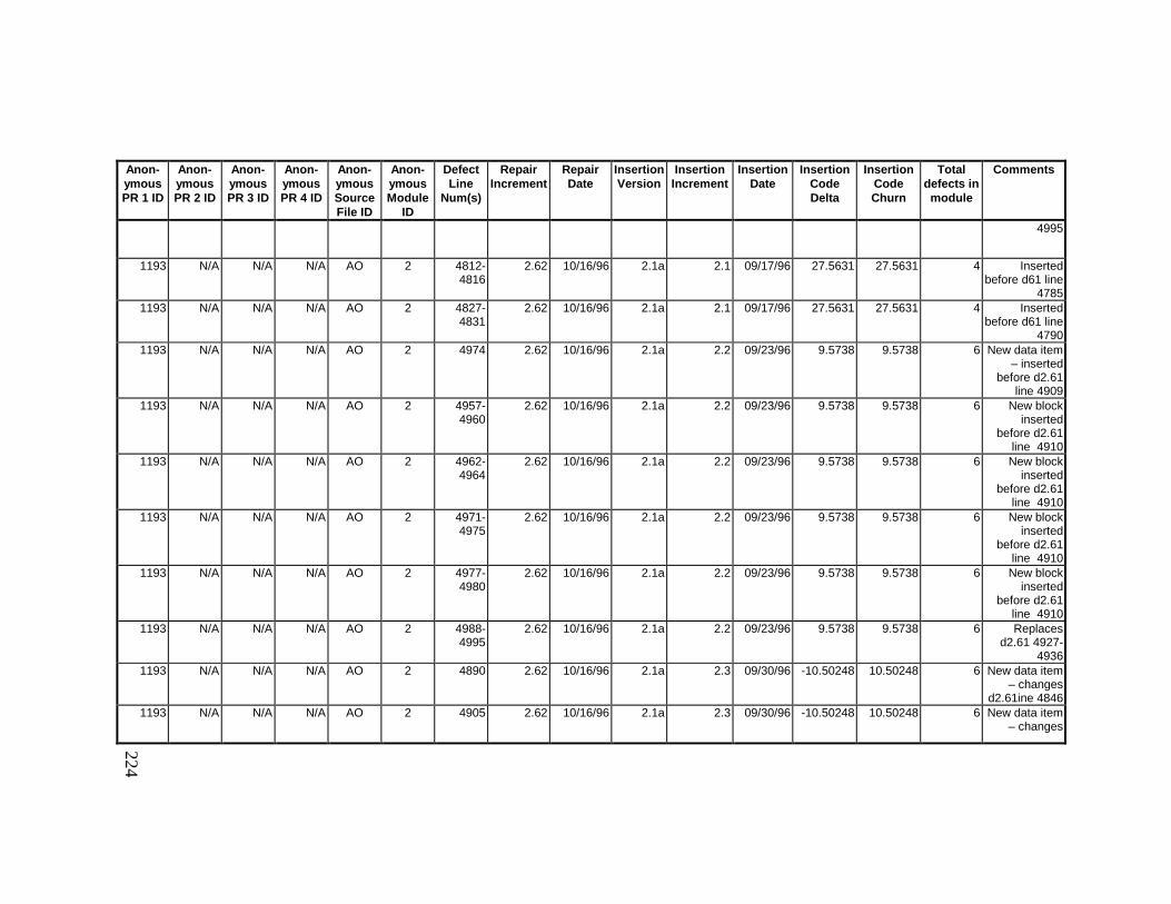
224
Anon-ymousPR 1 ID
Anon-ymousPR 2 ID
Anon-ymousPR 3 ID
Anon-ymousPR 4 ID
Anon-ymousSourceFile ID
Anon-ymousModule
ID
DefectLine
Num(s)
RepairIncrement
RepairDate
InsertionVersion
InsertionIncrement
InsertionDate
InsertionCodeDelta
InsertionCodeChurn
Totaldefects inmodule
Comments
4995
1193 N/A N/A N/A AO 2 4812-4816
2.62 10/16/96 2.1a 2.1 09/17/96 27.5631 27.5631 4 Insertedbefore d61 line
47851193 N/A N/A N/A AO 2 4827-
48312.62 10/16/96 2.1a 2.1 09/17/96 27.5631 27.5631 4 Inserted
before d61 line4790
1193 N/A N/A N/A AO 2 4974 2.62 10/16/96 2.1a 2.2 09/23/96 9.5738 9.5738 6 New data item– inserted
before d2.61line 4909
1193 N/A N/A N/A AO 2 4957-4960
2.62 10/16/96 2.1a 2.2 09/23/96 9.5738 9.5738 6 New blockinserted
before d2.61line 4910
1193 N/A N/A N/A AO 2 4962-4964
2.62 10/16/96 2.1a 2.2 09/23/96 9.5738 9.5738 6 New blockinserted
before d2.61line 4910
1193 N/A N/A N/A AO 2 4971-4975
2.62 10/16/96 2.1a 2.2 09/23/96 9.5738 9.5738 6 New blockinserted
before d2.61line 4910
1193 N/A N/A N/A AO 2 4977-4980
2.62 10/16/96 2.1a 2.2 09/23/96 9.5738 9.5738 6 New blockinserted
before d2.61line 4910
1193 N/A N/A N/A AO 2 4988-4995
2.62 10/16/96 2.1a 2.2 09/23/96 9.5738 9.5738 6 Replacesd2.61 4927-
49361193 N/A N/A N/A AO 2 4890 2.62 10/16/96 2.1a 2.3 09/30/96 -10.50248 10.50248 6 New data item
– changesd2.61ine 4846
1193 N/A N/A N/A AO 2 4905 2.62 10/16/96 2.1a 2.3 09/30/96 -10.50248 10.50248 6 New data item– changes
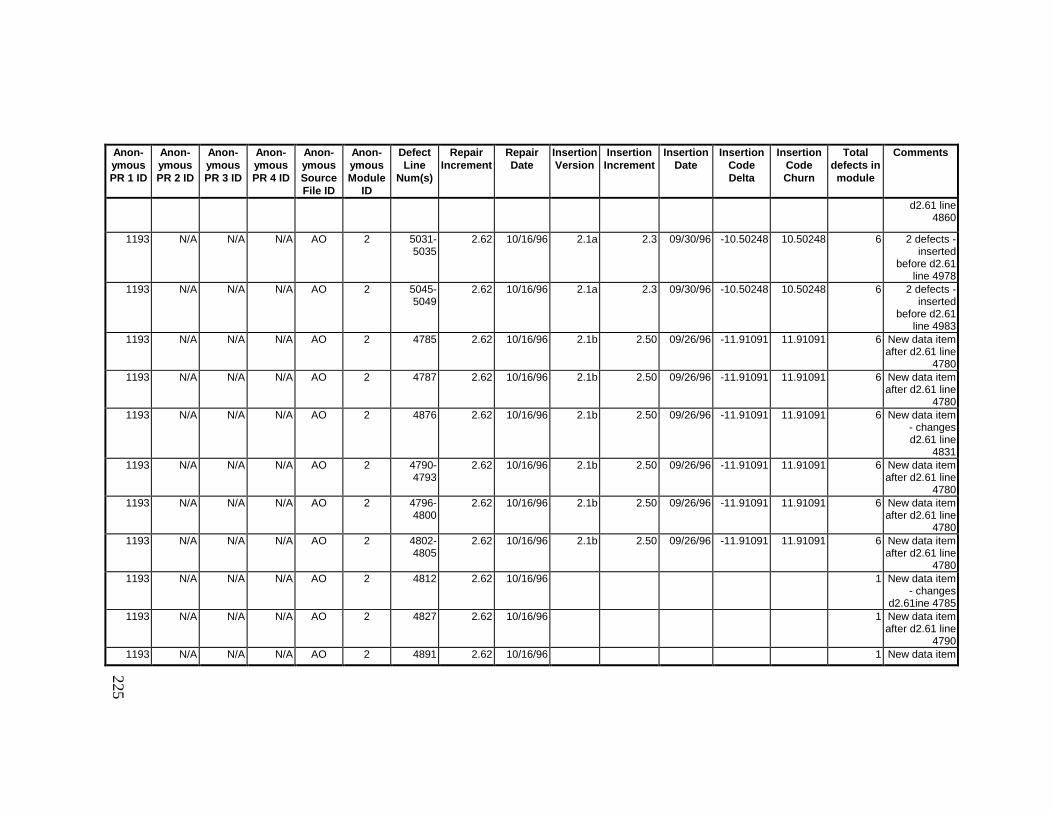
225
Anon-ymousPR 1 ID
Anon-ymousPR 2 ID
Anon-ymousPR 3 ID
Anon-ymousPR 4 ID
Anon-ymousSourceFile ID
Anon-ymousModule
ID
DefectLine
Num(s)
RepairIncrement
RepairDate
InsertionVersion
InsertionIncrement
InsertionDate
InsertionCodeDelta
InsertionCodeChurn
Totaldefects inmodule
Comments
d2.61 line4860
1193 N/A N/A N/A AO 2 5031-5035
2.62 10/16/96 2.1a 2.3 09/30/96 -10.50248 10.50248 6 2 defects -inserted
before d2.61line 4978
1193 N/A N/A N/A AO 2 5045-5049
2.62 10/16/96 2.1a 2.3 09/30/96 -10.50248 10.50248 6 2 defects -inserted
before d2.61line 4983
1193 N/A N/A N/A AO 2 4785 2.62 10/16/96 2.1b 2.50 09/26/96 -11.91091 11.91091 6 New data itemafter d2.61 line
47801193 N/A N/A N/A AO 2 4787 2.62 10/16/96 2.1b 2.50 09/26/96 -11.91091 11.91091 6 New data item
after d2.61 line4780
1193 N/A N/A N/A AO 2 4876 2.62 10/16/96 2.1b 2.50 09/26/96 -11.91091 11.91091 6 New data item- changesd2.61 line
48311193 N/A N/A N/A AO 2 4790-
47932.62 10/16/96 2.1b 2.50 09/26/96 -11.91091 11.91091 6 New data item
after d2.61 line4780
1193 N/A N/A N/A AO 2 4796-4800
2.62 10/16/96 2.1b 2.50 09/26/96 -11.91091 11.91091 6 New data itemafter d2.61 line
47801193 N/A N/A N/A AO 2 4802-
48052.62 10/16/96 2.1b 2.50 09/26/96 -11.91091 11.91091 6 New data item
after d2.61 line4780
1193 N/A N/A N/A AO 2 4812 2.62 10/16/96 1 New data item- changes
d2.61ine 47851193 N/A N/A N/A AO 2 4827 2.62 10/16/96 1 New data item
after d2.61 line4790
1193 N/A N/A N/A AO 2 4891 2.62 10/16/96 1 New data item
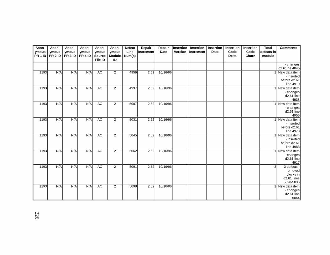
226
Anon-ymousPR 1 ID
Anon-ymousPR 2 ID
Anon-ymousPR 3 ID
Anon-ymousPR 4 ID
Anon-ymousSourceFile ID
Anon-ymousModule
ID
DefectLine
Num(s)
RepairIncrement
RepairDate
InsertionVersion
InsertionIncrement
InsertionDate
InsertionCodeDelta
InsertionCodeChurn
Totaldefects inmodule
Comments
- changesd2.61ine 4846
1193 N/A N/A N/A AO 2 4959 2.62 10/16/96 1 New data item- inserted
before d2.61line 4910
1193 N/A N/A N/A AO 2 4997 2.62 10/16/96 1 New data item- changesd2.61 line
49381193 N/A N/A N/A AO 2 5007 2.62 10/16/96 1 New date item
- changesd2.61 line
49561193 N/A N/A N/A AO 2 5031 2.62 10/16/96 1 New data item
- insertedbefore d2.61
line 49781193 N/A N/A N/A AO 2 5045 2.62 10/16/96 1 New data item
- insertedbefore d2.61
line 49831193 N/A N/A N/A AO 2 5062 2.62 10/16/96 1 New data item
- changesd2.61 line
49171193 N/A N/A N/A AO 2 5091 2.62 10/16/96 3 3 defects -
removedblocks in
d2.61 lines5028-5036
1193 N/A N/A N/A AO 2 5098 2.62 10/16/96 1 New data item- changesd2.61 line
5044
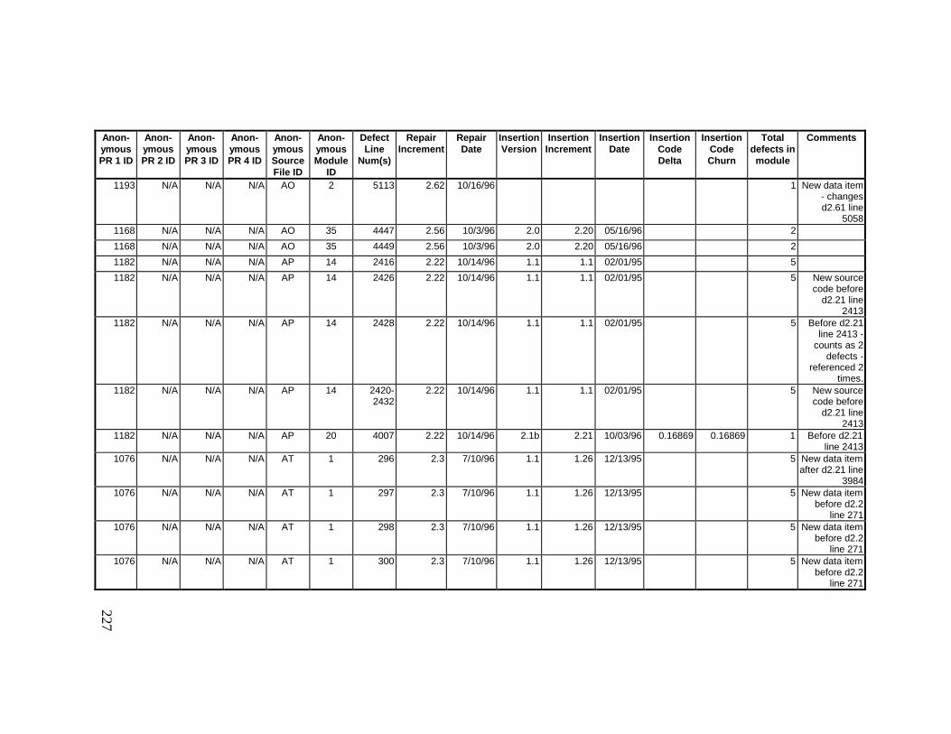
227
Anon-ymousPR 1 ID
Anon-ymousPR 2 ID
Anon-ymousPR 3 ID
Anon-ymousPR 4 ID
Anon-ymousSourceFile ID
Anon-ymousModule
ID
DefectLine
Num(s)
RepairIncrement
RepairDate
InsertionVersion
InsertionIncrement
InsertionDate
InsertionCodeDelta
InsertionCodeChurn
Totaldefects inmodule
Comments
1193 N/A N/A N/A AO 2 5113 2.62 10/16/96 1 New data item- changesd2.61 line
50581168 N/A N/A N/A AO 35 4447 2.56 10/3/96 2.0 2.20 05/16/96 2
1168 N/A N/A N/A AO 35 4449 2.56 10/3/96 2.0 2.20 05/16/96 2
1182 N/A N/A N/A AP 14 2416 2.22 10/14/96 1.1 1.1 02/01/95 5
1182 N/A N/A N/A AP 14 2426 2.22 10/14/96 1.1 1.1 02/01/95 5 New sourcecode before
d2.21 line2413
1182 N/A N/A N/A AP 14 2428 2.22 10/14/96 1.1 1.1 02/01/95 5 Before d2.21line 2413 -
counts as 2defects -
referenced 2times.
1182 N/A N/A N/A AP 14 2420-2432
2.22 10/14/96 1.1 1.1 02/01/95 5 New sourcecode before
d2.21 line2413
1182 N/A N/A N/A AP 20 4007 2.22 10/14/96 2.1b 2.21 10/03/96 0.16869 0.16869 1 Before d2.21line 2413
1076 N/A N/A N/A AT 1 296 2.3 7/10/96 1.1 1.26 12/13/95 5 New data itemafter d2.21 line
39841076 N/A N/A N/A AT 1 297 2.3 7/10/96 1.1 1.26 12/13/95 5 New data item
before d2.2line 271
1076 N/A N/A N/A AT 1 298 2.3 7/10/96 1.1 1.26 12/13/95 5 New data itembefore d2.2
line 2711076 N/A N/A N/A AT 1 300 2.3 7/10/96 1.1 1.26 12/13/95 5 New data item
before d2.2line 271
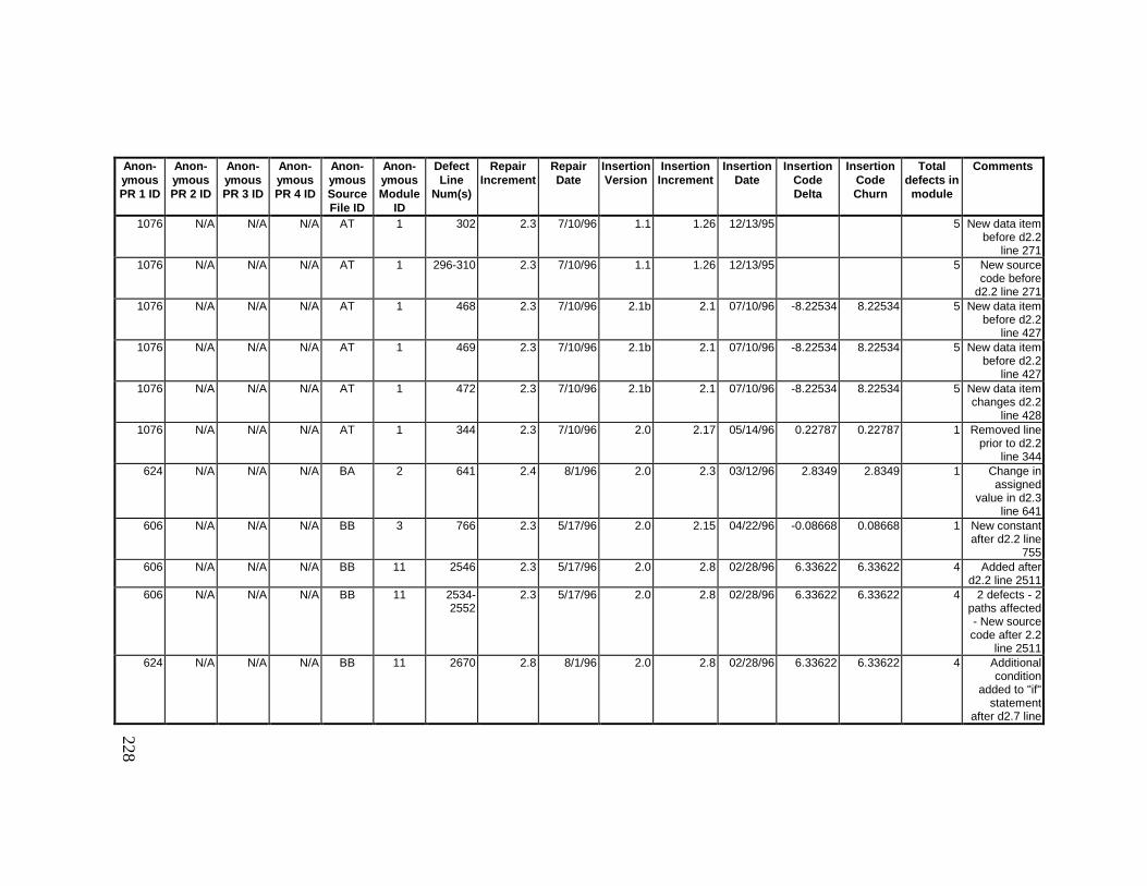
228
Anon-ymousPR 1 ID
Anon-ymousPR 2 ID
Anon-ymousPR 3 ID
Anon-ymousPR 4 ID
Anon-ymousSourceFile ID
Anon-ymousModule
ID
DefectLine
Num(s)
RepairIncrement
RepairDate
InsertionVersion
InsertionIncrement
InsertionDate
InsertionCodeDelta
InsertionCodeChurn
Totaldefects inmodule
Comments
1076 N/A N/A N/A AT 1 302 2.3 7/10/96 1.1 1.26 12/13/95 5 New data itembefore d2.2
line 2711076 N/A N/A N/A AT 1 296-310 2.3 7/10/96 1.1 1.26 12/13/95 5 New source
code befored2.2 line 271
1076 N/A N/A N/A AT 1 468 2.3 7/10/96 2.1b 2.1 07/10/96 -8.22534 8.22534 5 New data itembefore d2.2
line 4271076 N/A N/A N/A AT 1 469 2.3 7/10/96 2.1b 2.1 07/10/96 -8.22534 8.22534 5 New data item
before d2.2line 427
1076 N/A N/A N/A AT 1 472 2.3 7/10/96 2.1b 2.1 07/10/96 -8.22534 8.22534 5 New data itemchanges d2.2
line 4281076 N/A N/A N/A AT 1 344 2.3 7/10/96 2.0 2.17 05/14/96 0.22787 0.22787 1 Removed line
prior to d2.2line 344
624 N/A N/A N/A BA 2 641 2.4 8/1/96 2.0 2.3 03/12/96 2.8349 2.8349 1 Change inassigned
value in d2.3line 641
606 N/A N/A N/A BB 3 766 2.3 5/17/96 2.0 2.15 04/22/96 -0.08668 0.08668 1 New constantafter d2.2 line
755606 N/A N/A N/A BB 11 2546 2.3 5/17/96 2.0 2.8 02/28/96 6.33622 6.33622 4 Added after
d2.2 line 2511606 N/A N/A N/A BB 11 2534-
25522.3 5/17/96 2.0 2.8 02/28/96 6.33622 6.33622 4 2 defects - 2
paths affected- New sourcecode after 2.2
line 2511624 N/A N/A N/A BB 11 2670 2.8 8/1/96 2.0 2.8 02/28/96 6.33622 6.33622 4 Additional
conditionadded to "if"
statementafter d2.7 line
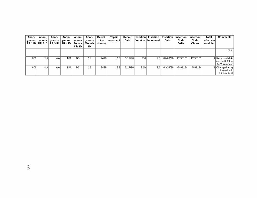
229
Anon-ymousPR 1 ID
Anon-ymousPR 2 ID
Anon-ymousPR 3 ID
Anon-ymousPR 4 ID
Anon-ymousSourceFile ID
Anon-ymousModule
ID
DefectLine
Num(s)
RepairIncrement
RepairDate
InsertionVersion
InsertionIncrement
InsertionDate
InsertionCodeDelta
InsertionCodeChurn
Totaldefects inmodule
Comments
2669
606 N/A N/A N/A BB 11 2410 2.3 5/17/96 2.0 2.8 02/28/96 17.58101 17.58101 1 Removed dataitem - d2.2 line2400 removed
606 N/A N/A N/A BB 12 2429 2.3 5/17/96 2.1b 2.1 04/16/96 -5.91194 5.91194 1 Changed arraydimension in2.2 line 2429

230
13.4 Summary of Defects Locations for Version 2.0 Development Library
The following table is a summary of the table shown in Appendix 13.1. Each line represents one particular increment of amodule that was checked into the development library. The number of defects inserted in that increment is recorded, as are thechanges in module complexity (code delta and code churn) from the immediately preceding increment and the cumulative numberof workmonths elapsed since the start of the implementation phase. For instance, we interpret the second row as saying that forincrement 4 of source file S in version 2.0, module 3 had 1 defect inserted into it. For increment 4 of source file S, module 3’srelative complexity decreased by –0.27 from its value in increment 3 of file S, and the absolute amount of change that was made tomodule 3 since increment 3 of file S was 0.27.
Those rows shown in bold represent observations that were used in the regressions to determine rates of defect insertion.
Version 2.0Anonymous
Filename
Version 2.0AnonymousModule ID
Version inwhich
observeddefects first
appeared
Increment inwhich
observeddefects first
appeared
SCCS checkin date
Cumulativeimplementa-tion phase
workmonths
Daysbetween
insertion ofdefects andopening of
problemreport
(should be apositivenumber)
Complexitychange in
module at dateof initial defect
appearance(code delta)
Absolute valueof complexity
change inmodule at dateof initial defect
appearance(code churn)
Number ofdefects
inserted intomodule
Comments
E 29 2.0 2.16 02/28/96 450.6443836 36 0 0 1 Variable definitionchanged
S 3 2.0 2.4 02/27/96 449.8586301 1403 -0.27987 0.27987 1 Changed data itemdefinition
X 15 1.0 1.1 09/20/95 343.1671233 128 1.04253 1.04253 2 Changed data itemdefinition
V 7 2.0 2.9 03/14/96 461.4739726 25 1.39595 1.39595 3 New data item
F 4 1.0 1.2 10/19/95 361.7424658 99 -1.76513 1.76513 2 Changed data itemdefinition
AP 20 2.0 2.2 12/27/95 404.5939726 1465 3.93961 3.93961 2
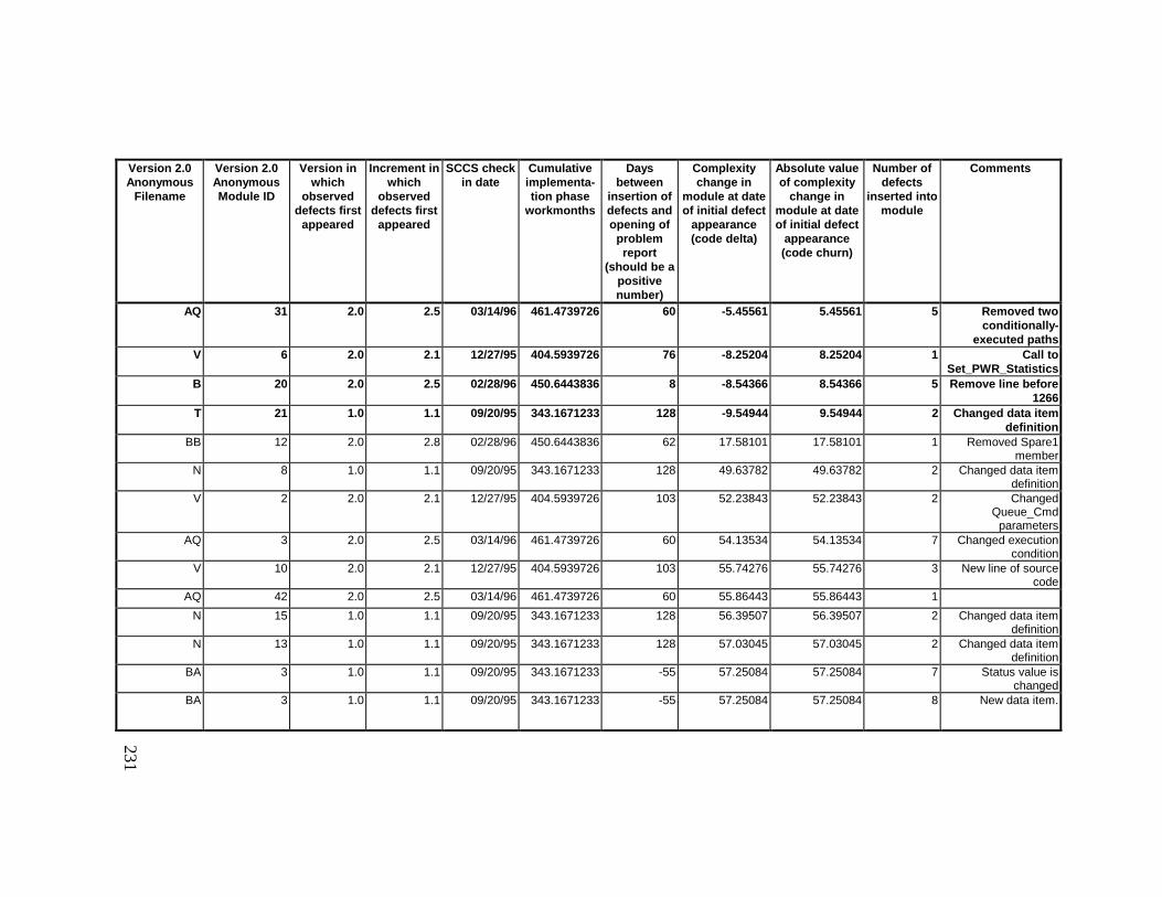
231
Version 2.0Anonymous
Filename
Version 2.0AnonymousModule ID
Version inwhich
observeddefects first
appeared
Increment inwhich
observeddefects first
appeared
SCCS checkin date
Cumulativeimplementa-tion phase
workmonths
Daysbetween
insertion ofdefects andopening of
problemreport
(should be apositivenumber)
Complexitychange in
module at dateof initial defect
appearance(code delta)
Absolute valueof complexity
change inmodule at dateof initial defect
appearance(code churn)
Number ofdefects
inserted intomodule
Comments
AQ 31 2.0 2.5 03/14/96 461.4739726 60 -5.45561 5.45561 5 Removed twoconditionally-
executed pathsV 6 2.0 2.1 12/27/95 404.5939726 76 -8.25204 8.25204 1 Call to
Set_PWR_StatisticsB 20 2.0 2.5 02/28/96 450.6443836 8 -8.54366 8.54366 5 Remove line before
1266T 21 1.0 1.1 09/20/95 343.1671233 128 -9.54944 9.54944 2 Changed data item
definitionBB 12 2.0 2.8 02/28/96 450.6443836 62 17.58101 17.58101 1 Removed Spare1
memberN 8 1.0 1.1 09/20/95 343.1671233 128 49.63782 49.63782 2 Changed data item
definitionV 2 2.0 2.1 12/27/95 404.5939726 103 52.23843 52.23843 2 Changed
Queue_Cmdparameters
AQ 3 2.0 2.5 03/14/96 461.4739726 60 54.13534 54.13534 7 Changed executioncondition
V 10 2.0 2.1 12/27/95 404.5939726 103 55.74276 55.74276 3 New line of sourcecode
AQ 42 2.0 2.5 03/14/96 461.4739726 60 55.86443 55.86443 1
N 15 1.0 1.1 09/20/95 343.1671233 128 56.39507 56.39507 2 Changed data itemdefinition
N 13 1.0 1.1 09/20/95 343.1671233 128 57.03045 57.03045 2 Changed data itemdefinition
BA 3 1.0 1.1 09/20/95 343.1671233 -55 57.25084 57.25084 7 Status value ischanged
BA 3 1.0 1.1 09/20/95 343.1671233 -55 57.25084 57.25084 8 New data item.
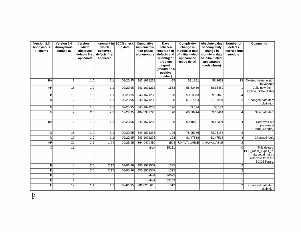
232
Version 2.0Anonymous
Filename
Version 2.0AnonymousModule ID
Version inwhich
observeddefects first
appeared
Increment inwhich
observeddefects first
appeared
SCCS checkin date
Cumulativeimplementa-tion phase
workmonths
Daysbetween
insertion ofdefects andopening of
problemreport
(should be apositivenumber)
Complexitychange in
module at dateof initial defect
appearance(code delta)
Absolute valueof complexity
change inmodule at dateof initial defect
appearance(code churn)
Number ofdefects
inserted intomodule
Comments
BA 2 1.0 1.1 09/20/95 343.1671233 -55 58.1651 58.1651 13 Deleted value assignto variable
AP 15 1.0 1.1 09/20/95 343.1671233 1563 58.63459 58.63459 1 Calls new fncn -Online_State_Table
B 18 1.0 1.1 09/20/95 343.1671233 128 59.63873 59.63873 4
N 2 1.0 1.1 09/20/95 343.1671233 128 61.57204 61.57204 2 Changed data itemdefinition
N 4 1.0 1.1 09/20/95 343.1671233 126 63.174 63.174 1
V 7 2.0 2.1 12/27/95 404.5939726 76 63.60414 63.60414 4 New data item
BA 6 1.0 1.1 09/20/95 343.1671233 -55 69.18301 69.18301 4 Removed outparameter
"Frame_Length_N 18 1.0 1.1 09/20/95 343.1671233 126 78.05166 78.05166 2
N 17 1.0 1.1 09/20/95 343.1671233 128 81.47518 81.47518 3 Changed logic
AP 20 1.1 1.24 10/25/95 364.9479452 1528 UNAVAILABLE UNAVAILABLE 2
C 11 #N/A 35131 0 This delta ofBCD_Mem_Types_.a
da could not beretrieved from the
SCCS library.E 4 2.0 2.17 03/06/96 455.2931507 1395 2
E 4 2.0 2.17 03/06/96 455.2931507 1395 2
E 6 #N/A 36525 1
E 7 #N/A 35159 1
E 17 1.1 1.1 02/01/95 201.8235616 512 2 Changed data itemdefinition
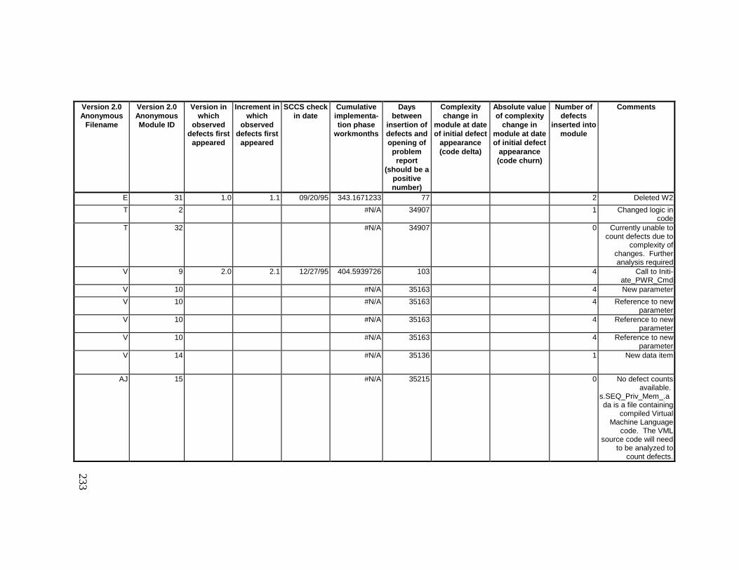
233
Version 2.0Anonymous
Filename
Version 2.0AnonymousModule ID
Version inwhich
observeddefects first
appeared
Increment inwhich
observeddefects first
appeared
SCCS checkin date
Cumulativeimplementa-tion phase
workmonths
Daysbetween
insertion ofdefects andopening of
problemreport
(should be apositivenumber)
Complexitychange in
module at dateof initial defect
appearance(code delta)
Absolute valueof complexity
change inmodule at dateof initial defect
appearance(code churn)
Number ofdefects
inserted intomodule
Comments
E 31 1.0 1.1 09/20/95 343.1671233 77 2 Deleted W2
T 2 #N/A 34907 1 Changed logic incode
T 32 #N/A 34907 0 Currently unable tocount defects due to
complexity ofchanges. Furtheranalysis required
V 9 2.0 2.1 12/27/95 404.5939726 103 4 Call to Initi-ate_PWR_Cmd
V 10 #N/A 35163 4 New parameter
V 10 #N/A 35163 4 Reference to newparameter
V 10 #N/A 35163 4 Reference to newparameter
V 10 #N/A 35163 4 Reference to newparameter
V 14 #N/A 35136 1 New data item
AJ 15 #N/A 35215 0 No defect countsavailable.
s.SEQ_Priv_Mem_.ada is a file containing
compiled VirtualMachine Language
code. The VMLsource code will need
to be analyzed tocount defects.

234
Version 2.0Anonymous
Filename
Version 2.0AnonymousModule ID
Version inwhich
observeddefects first
appeared
Increment inwhich
observeddefects first
appeared
SCCS checkin date
Cumulativeimplementa-tion phase
workmonths
Daysbetween
insertion ofdefects andopening of
problemreport
(should be apositivenumber)
Complexitychange in
module at dateof initial defect
appearance(code delta)
Absolute valueof complexity
change inmodule at dateof initial defect
appearance(code churn)
Number ofdefects
inserted intomodule
Comments
AJ 15 #N/A 35235 0 No defect countsavailable.
s.SEQ_Priv_Mem_.ada is a file containing
compiled VirtualMachine Language
code. The VMLsource code will need
to be analyzed tocount defects.
AJ 15 #N/A 35235 0 No defect countsavailable.
s.SEQ_Priv_Mem_.ada is a file containing
compiled VirtualMachine Language
code. The VMLsource code will need
to be analyzed tocount defects.
AP 3 1.1 1.20 07/24/95 256.2345205 224 2 Removed two blocksfollowing
AP 11 1.1 1.22 09/03/95 331.2065753 1580 2
AQ 23 #N/A 36525 0 Unable to find logic ordata changes from
differentialcomparison of SCCS
deltas.AX 12 #N/A 35158 0 Unable to count
defects from SCCSfiles. Further analysis
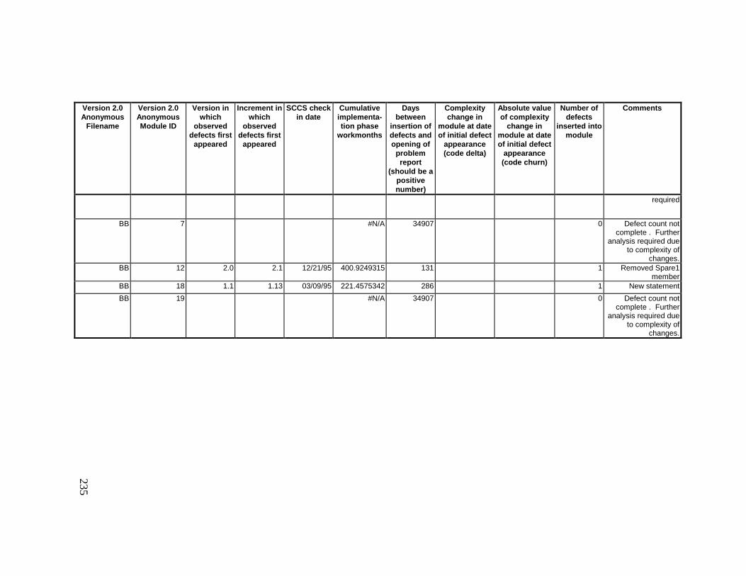
235
Version 2.0Anonymous
Filename
Version 2.0AnonymousModule ID
Version inwhich
observeddefects first
appeared
Increment inwhich
observeddefects first
appeared
SCCS checkin date
Cumulativeimplementa-tion phase
workmonths
Daysbetween
insertion ofdefects andopening of
problemreport
(should be apositivenumber)
Complexitychange in
module at dateof initial defect
appearance(code delta)
Absolute valueof complexity
change inmodule at dateof initial defect
appearance(code churn)
Number ofdefects
inserted intomodule
Comments
required
BB 7 #N/A 34907 0 Defect count notcomplete . Further
analysis required dueto complexity of
changes.BB 12 2.0 2.1 12/21/95 400.9249315 131 1 Removed Spare1
memberBB 18 1.1 1.13 03/09/95 221.4575342 286 1 New statement
BB 19 #N/A 34907 0 Defect count notcomplete . Further
analysis required dueto complexity of
changes.
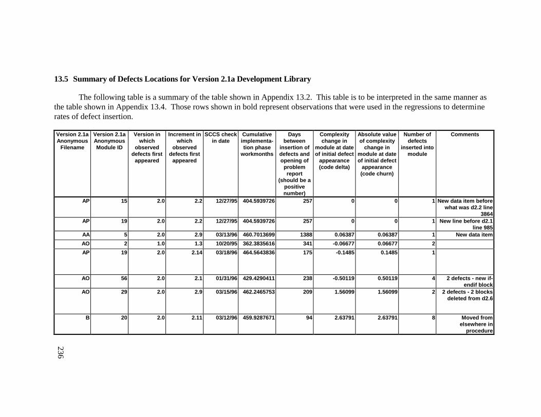
236
13.5 Summary of Defects Locations for Version 2.1a Development Library
The following table is a summary of the table shown in Appendix 13.2. This table is to be interpreted in the same manner asthe table shown in Appendix 13.4. Those rows shown in bold represent observations that were used in the regressions to determinerates of defect insertion.
Version 2.1aAnonymous
Filename
Version 2.1aAnonymousModule ID
Version inwhich
observeddefects first
appeared
Increment inwhich
observeddefects first
appeared
SCCS checkin date
Cumulativeimplementa-tion phase
workmonths
Daysbetween
insertion ofdefects andopening of
problemreport
(should be apositivenumber)
Complexitychange in
module at dateof initial defect
appearance(code delta)
Absolute valueof complexity
change inmodule at dateof initial defect
appearance(code churn)
Number ofdefects
inserted intomodule
Comments
AP 15 2.0 2.2 12/27/95 404.5939726 257 0 0 1 New data item beforewhat was d2.2 line
3864AP 19 2.0 2.2 12/27/95 404.5939726 257 0 0 1 New line before d2.1
line 985AA 5 2.0 2.9 03/13/96 460.7013699 1388 0.06387 0.06387 1 New data item
AO 2 1.0 1.3 10/20/95 362.3835616 341 -0.06677 0.06677 2
AP 19 2.0 2.14 03/18/96 464.5643836 175 -0.1485 0.1485 1
AO 56 2.0 2.1 01/31/96 429.4290411 238 -0.50119 0.50119 4 2 defects - new if-endif block
AO 29 2.0 2.9 03/15/96 462.2465753 209 1.56099 1.56099 2 2 defects - 2 blocksdeleted from d2.6
B 20 2.0 2.11 03/12/96 459.9287671 94 2.63791 2.63791 8 Moved fromelsewhere in
procedure
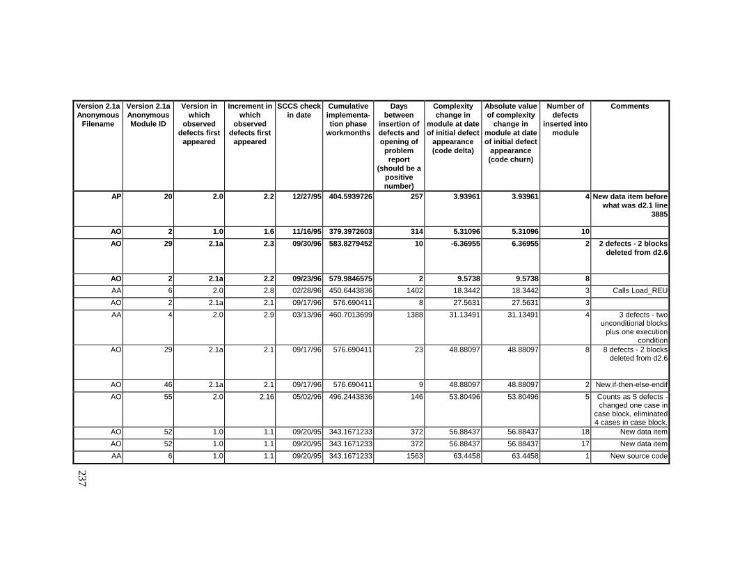
237
Version 2.1aAnonymous
Filename
Version 2.1aAnonymousModule ID
Version inwhich
observeddefects first
appeared
Increment inwhich
observeddefects first
appeared
SCCS checkin date
Cumulativeimplementa-tion phase
workmonths
Daysbetween
insertion ofdefects andopening of
problemreport
(should be apositivenumber)
Complexitychange in
module at dateof initial defect
appearance(code delta)
Absolute valueof complexity
change inmodule at dateof initial defect
appearance(code churn)
Number ofdefects
inserted intomodule
Comments
AP 20 2.0 2.2 12/27/95 404.5939726 257 3.93961 3.93961 4 New data item beforewhat was d2.1 line
3885
AO 2 1.0 1.6 11/16/95 379.3972603 314 5.31096 5.31096 10
AO 29 2.1a 2.3 09/30/96 583.8279452 10 -6.36955 6.36955 2 2 defects - 2 blocksdeleted from d2.6
AO 2 2.1a 2.2 09/23/96 579.9846575 2 9.5738 9.5738 8
AA 6 2.0 2.8 02/28/96 450.6443836 1402 18.3442 18.3442 3 Calls Load_REU
AO 2 2.1a 2.1 09/17/96 576.690411 8 27.5631 27.5631 3
AA 4 2.0 2.9 03/13/96 460.7013699 1388 31.13491 31.13491 4 3 defects - twounconditional blocks
plus one executioncondition
AO 29 2.1a 2.1 09/17/96 576.690411 23 48.88097 48.88097 8 8 defects - 2 blocksdeleted from d2.6
AO 46 2.1a 2.1 09/17/96 576.690411 9 48.88097 48.88097 2 New if-then-else-endif
AO 55 2.0 2.16 05/02/96 496.2443836 146 53.80496 53.80496 5 Counts as 5 defects -changed one case in
case block, eliminated4 cases in case block.
AO 52 1.0 1.1 09/20/95 343.1671233 372 56.88437 56.88437 18 New data item
AO 52 1.0 1.1 09/20/95 343.1671233 372 56.88437 56.88437 17 New data item
AA 6 1.0 1.1 09/20/95 343.1671233 1563 63.4458 63.4458 1 New source code
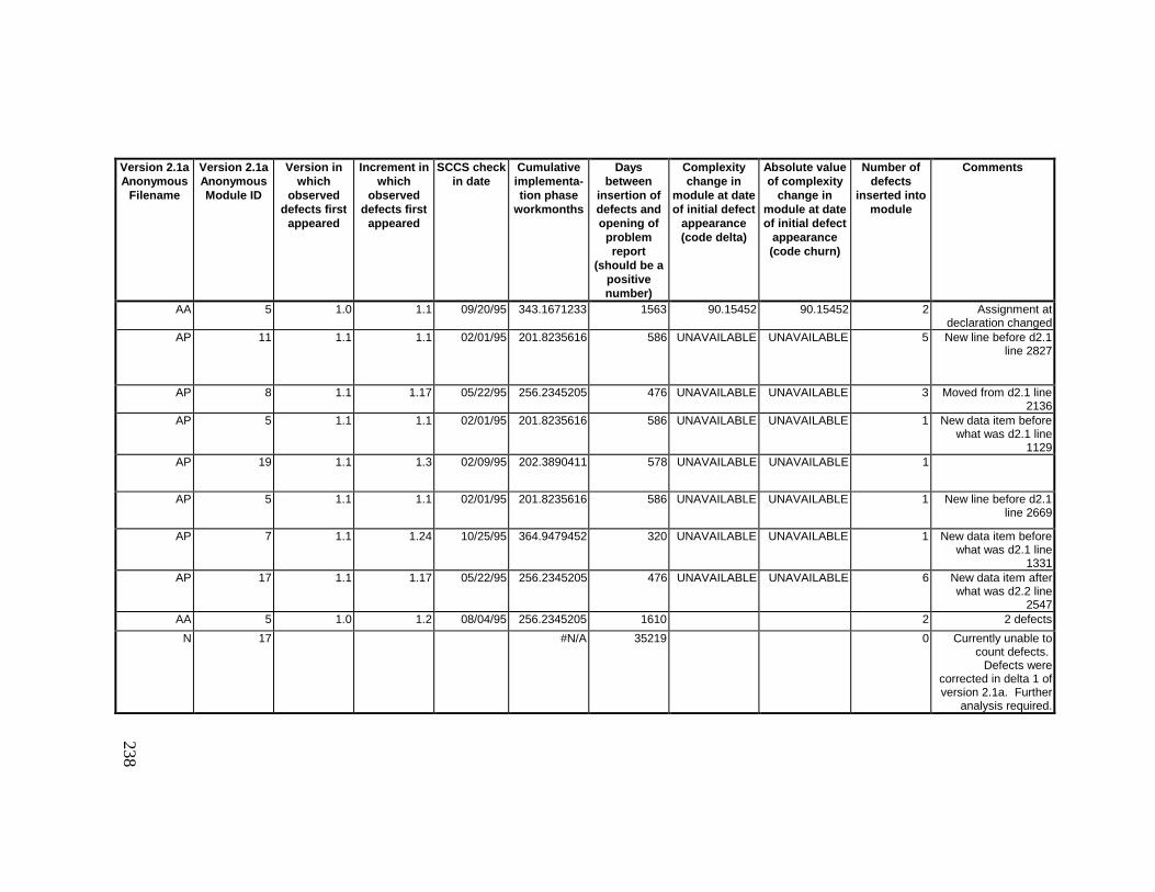
238
Version 2.1aAnonymous
Filename
Version 2.1aAnonymousModule ID
Version inwhich
observeddefects first
appeared
Increment inwhich
observeddefects first
appeared
SCCS checkin date
Cumulativeimplementa-tion phase
workmonths
Daysbetween
insertion ofdefects andopening of
problemreport
(should be apositivenumber)
Complexitychange in
module at dateof initial defect
appearance(code delta)
Absolute valueof complexity
change inmodule at dateof initial defect
appearance(code churn)
Number ofdefects
inserted intomodule
Comments
AA 5 1.0 1.1 09/20/95 343.1671233 1563 90.15452 90.15452 2 Assignment atdeclaration changed
AP 11 1.1 1.1 02/01/95 201.8235616 586 UNAVAILABLE UNAVAILABLE 5 New line before d2.1line 2827
AP 8 1.1 1.17 05/22/95 256.2345205 476 UNAVAILABLE UNAVAILABLE 3 Moved from d2.1 line2136
AP 5 1.1 1.1 02/01/95 201.8235616 586 UNAVAILABLE UNAVAILABLE 1 New data item beforewhat was d2.1 line
1129AP 19 1.1 1.3 02/09/95 202.3890411 578 UNAVAILABLE UNAVAILABLE 1
AP 5 1.1 1.1 02/01/95 201.8235616 586 UNAVAILABLE UNAVAILABLE 1 New line before d2.1line 2669
AP 7 1.1 1.24 10/25/95 364.9479452 320 UNAVAILABLE UNAVAILABLE 1 New data item beforewhat was d2.1 line
1331AP 17 1.1 1.17 05/22/95 256.2345205 476 UNAVAILABLE UNAVAILABLE 6 New data item after
what was d2.2 line2547
AA 5 1.0 1.2 08/04/95 256.2345205 1610 2 2 defects
N 17 #N/A 35219 0 Currently unable tocount defects.
Defects werecorrected in delta 1 ofversion 2.1a. Further
analysis required.
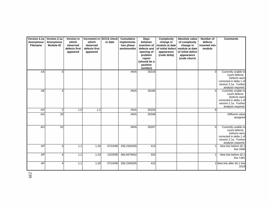
239
Version 2.1aAnonymous
Filename
Version 2.1aAnonymousModule ID
Version inwhich
observeddefects first
appeared
Increment inwhich
observeddefects first
appeared
SCCS checkin date
Cumulativeimplementa-tion phase
workmonths
Daysbetween
insertion ofdefects andopening of
problemreport
(should be apositivenumber)
Complexitychange in
module at dateof initial defect
appearance(code delta)
Absolute valueof complexity
change inmodule at dateof initial defect
appearance(code churn)
Number ofdefects
inserted intomodule
Comments
AA 3 #N/A 35319 0 Currently unable tocount defects.
Defects werecorrected in delta 1 ofversion 2.1a. Further
analysis required.AE 3 #N/A 35185 0 Currently unable to
count defects. Defects were
corrected in delta 1 ofversion 2.1a. Further
analysis required.AO 2 1.0 1.2 #N/A 35333 8
AO 29 #N/A 35348 Different valueassigned
AO 52 #N/A 35297 0 Currently unable tocount defects.
Defects werecorrected in delta 1 ofversion 2.1a. Further
analysis required.AP 3 1.1 1.20 07/24/95 256.2345205 413 1 New line before d2.1
line 3496
AP 4 1.1 1.24 10/25/95 364.9479452 320 1 New line before d2.1line 1481
AP 4 1.1 1.20 07/24/95 256.2345205 413 1 New line after d2.1 line3318

240
13.6 Summary of Defects Locations for Version 2.1b Development Library
The following table is a summary of the table shown in Appendix 13.3. This table is to be interpreted in the same manner asthe table shown in Appendix 13.4. Those rows shown in bold represent observations that were used in the regressions to determinerates of defect insertion.
Version 2.1bAnonymous
Filename
Version 2.1bAnonymousModule ID
Version inwhich
observeddefects first
appeared
Increment inwhich
observeddefects first
appeared
SCCS checkin date
Cumulativeimplementa-tion phase
workmonths
Daysbetweendefect
insertionand openingproblem re-port (shouldbe a positive
number)
Complexitychange inmodule at
date of initialdefect
appearance(code delta)
Absolutevalue of
complexitychange inmodule at
date of initialdefect
appearance(code churn)
Number ofdefects
inserted intomodule
Comments
AA 3 2.1b 2.7 08/02/96 550.8394521 40 0 0 1 Counts as 2 defects,since the variable is
referenced two timesBB 3 2.0 2.15 04/22/96 489.7972603 22 -0.08668 0.08668 1 New constant after d2.2
line 755AP 20 2.1b 2.21 10/03/96 584.9063014 2 0.16869 0.16869 1 Before d2.21 line 2413
AT 1 2.0 2.17 05/14/96 504.1742466 36525 0.22787 0.22787 1 Removed line prior tod2.2 line 344
BA 2 2.0 2.3 03/12/96 459.9287671 141 2.8349 2.8349 1 Change in assignedvalue in d2.3 line 641
N 14 2.1b 2.1 04/16/96 485.4575342 36 -3.99448 3.99448 1
N 17 2.0 2.3 02/22/96 445.929863 90 4.52764 4.52764 1
BB 12 2.1b 2.1 04/16/96 485.4575342 28 -5.91194 5.91194 1 Changed arraydimension in 2.2 line
2429BB 11 2.1b 2.1 02/28/96 450.6443836 76 6.33622 6.33622 4 Added after d2.2 line
2511
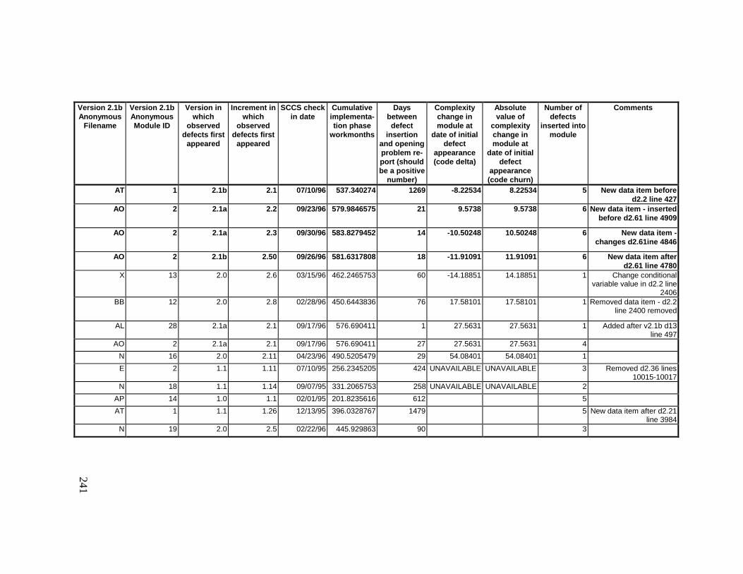
241
Version 2.1bAnonymous
Filename
Version 2.1bAnonymousModule ID
Version inwhich
observeddefects first
appeared
Increment inwhich
observeddefects first
appeared
SCCS checkin date
Cumulativeimplementa-tion phase
workmonths
Daysbetweendefect
insertionand openingproblem re-port (shouldbe a positive
number)
Complexitychange inmodule at
date of initialdefect
appearance(code delta)
Absolutevalue of
complexitychange inmodule at
date of initialdefect
appearance(code churn)
Number ofdefects
inserted intomodule
Comments
AT 1 2.1b 2.1 07/10/96 537.340274 1269 -8.22534 8.22534 5 New data item befored2.2 line 427
AO 2 2.1a 2.2 09/23/96 579.9846575 21 9.5738 9.5738 6 New data item - insertedbefore d2.61 line 4909
AO 2 2.1a 2.3 09/30/96 583.8279452 14 -10.50248 10.50248 6 New data item -changes d2.61ine 4846
AO 2 2.1b 2.50 09/26/96 581.6317808 18 -11.91091 11.91091 6 New data item afterd2.61 line 4780
X 13 2.0 2.6 03/15/96 462.2465753 60 -14.18851 14.18851 1 Change conditionalvariable value in d2.2 line
2406BB 12 2.0 2.8 02/28/96 450.6443836 76 17.58101 17.58101 1 Removed data item - d2.2
line 2400 removed
AL 28 2.1a 2.1 09/17/96 576.690411 1 27.5631 27.5631 1 Added after v2.1b d13line 497
AO 2 2.1a 2.1 09/17/96 576.690411 27 27.5631 27.5631 4
N 16 2.0 2.11 04/23/96 490.5205479 29 54.08401 54.08401 1
E 2 1.1 1.11 07/10/95 256.2345205 424 UNAVAILABLE UNAVAILABLE 3 Removed d2.36 lines10015-10017
N 18 1.1 1.14 09/07/95 331.2065753 258 UNAVAILABLE UNAVAILABLE 2
AP 14 1.0 1.1 02/01/95 201.8235616 612 5
AT 1 1.1 1.26 12/13/95 396.0328767 1479 5 New data item after d2.21line 3984
N 19 2.0 2.5 02/22/96 445.929863 90 3

242
Version 2.1bAnonymous
Filename
Version 2.1bAnonymousModule ID
Version inwhich
observeddefects first
appeared
Increment inwhich
observeddefects first
appeared
SCCS checkin date
Cumulativeimplementa-tion phase
workmonths
Daysbetweendefect
insertionand openingproblem re-port (shouldbe a positive
number)
Complexitychange inmodule at
date of initialdefect
appearance(code delta)
Absolutevalue of
complexitychange inmodule at
date of initialdefect
appearance(code churn)
Number ofdefects
inserted intomodule
Comments
X 4 #N/A 36525 0 Currently unable to countdefects. Unable to identify
PFR due to analyst errorin labelling PFRs. Further
analysis required.
AJ 15 #N/A 35342 0 s.SEQ_Priv_Mem_.ada isa module that contains
the executable code forthe System Defect
Protection routines. However, the source for
these routines is written ina sequencing languagespecific to JPL, "Virtual
Machine Language."AJ 15 #N/A 34711 0 To compute the
complexity of this VMLcode, it would be
necessary to develop ananalyzer specific to that
language.AJ 15 #N/A 34711 0 To compute the
complexity of this VMLcode, it would be
necessary to develop ananalyzer specific to that
language.AJ 15 #N/A 36525 0 To compute the
complexity of this VMLcode, it would be
necessary to develop ananalyzer specific to that
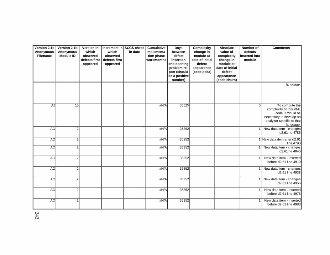
243
Version 2.1bAnonymous
Filename
Version 2.1bAnonymousModule ID
Version inwhich
observeddefects first
appeared
Increment inwhich
observeddefects first
appeared
SCCS checkin date
Cumulativeimplementa-tion phase
workmonths
Daysbetweendefect
insertionand openingproblem re-port (shouldbe a positive
number)
Complexitychange inmodule at
date of initialdefect
appearance(code delta)
Absolutevalue of
complexitychange inmodule at
date of initialdefect
appearance(code churn)
Number ofdefects
inserted intomodule
Comments
language.
AJ 15 #N/A 36525 0 To compute thecomplexity of this VML
code, it would benecessary to develop ananalyzer specific to that
language.AO 2 #N/A 35352 1 New data item - changes
d2.61ine 4785
AO 2 #N/A 35352 1 New data item after d2.61line 4790
AO 2 #N/A 35352 1 New data item - changesd2.61ine 4846
AO 2 #N/A 35352 1 New data item - insertedbefore d2.61 line 4910
AO 2 #N/A 35352 1 New data item - changesd2.61 line 4938
AO 2 #N/A 35352 1 New date item - changesd2.61 line 4956
AO 2 #N/A 35352 1 New data item - insertedbefore d2.61 line 4978
AO 2 #N/A 35352 1 New data item - insertedbefore d2.61 line 4983
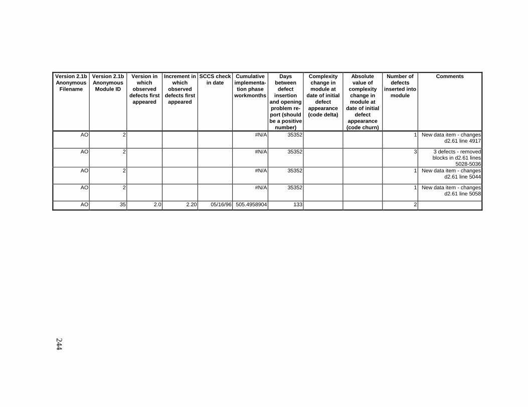
244
Version 2.1bAnonymous
Filename
Version 2.1bAnonymousModule ID
Version inwhich
observeddefects first
appeared
Increment inwhich
observeddefects first
appeared
SCCS checkin date
Cumulativeimplementa-tion phase
workmonths
Daysbetweendefect
insertionand openingproblem re-port (shouldbe a positive
number)
Complexitychange inmodule at
date of initialdefect
appearance(code delta)
Absolutevalue of
complexitychange inmodule at
date of initialdefect
appearance(code churn)
Number ofdefects
inserted intomodule
Comments
AO 2 #N/A 35352 1 New data item - changesd2.61 line 4917
AO 2 #N/A 35352 3 3 defects - removedblocks in d2.61 lines
5028-5036AO 2 #N/A 35352 1 New data item - changes
d2.61 line 5044
AO 2 #N/A 35352 1 New data item - changesd2.61 line 5058
AO 35 2.0 2.20 05/16/96 505.4958904 133 2
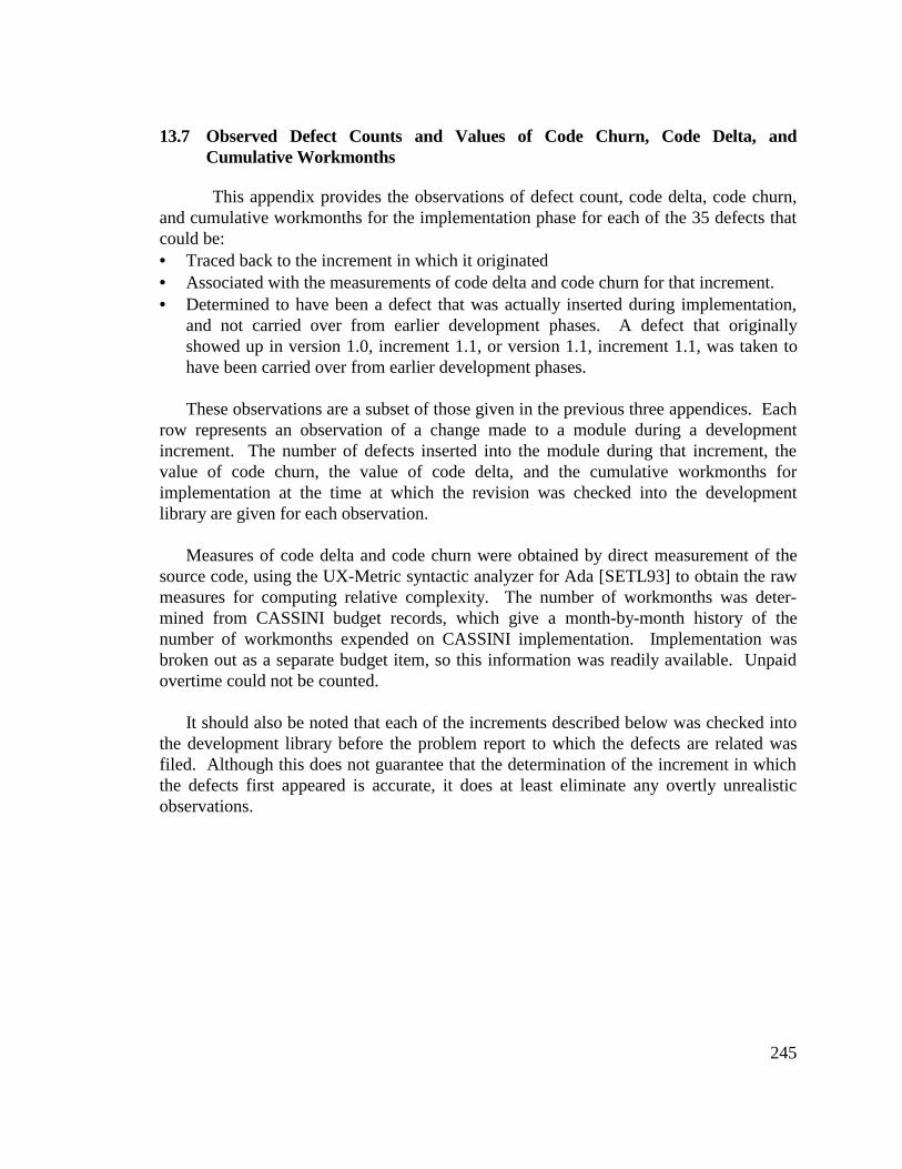
245
13.7 Observed Defect Counts and Values of Code Churn, Code Delta, andCumulative Workmonths
This appendix provides the observations of defect count, code delta, code churn,and cumulative workmonths for the implementation phase for each of the 35 defects thatcould be:• Traced back to the increment in which it originated• Associated with the measurements of code delta and code churn for that increment.• Determined to have been a defect that was actually inserted during implementation,
and not carried over from earlier development phases. A defect that originallyshowed up in version 1.0, increment 1.1, or version 1.1, increment 1.1, was taken tohave been carried over from earlier development phases.
These observations are a subset of those given in the previous three appendices. Eachrow represents an observation of a change made to a module during a developmentincrement. The number of defects inserted into the module during that increment, thevalue of code churn, the value of code delta, and the cumulative workmonths forimplementation at the time at which the revision was checked into the developmentlibrary are given for each observation.
Measures of code delta and code churn were obtained by direct measurement of thesource code, using the UX-Metric syntactic analyzer for Ada [SETL93] to obtain the rawmeasures for computing relative complexity. The number of workmonths was deter-mined from CASSINI budget records, which give a month-by-month history of thenumber of workmonths expended on CASSINI implementation. Implementation wasbroken out as a separate budget item, so this information was readily available. Unpaidovertime could not be counted.
It should also be noted that each of the increments described below was checked intothe development library before the problem report to which the defects are related wasfiled. Although this does not guarantee that the determination of the increment in whichthe defects first appeared is accurate, it does at least eliminate any overtly unrealisticobservations.
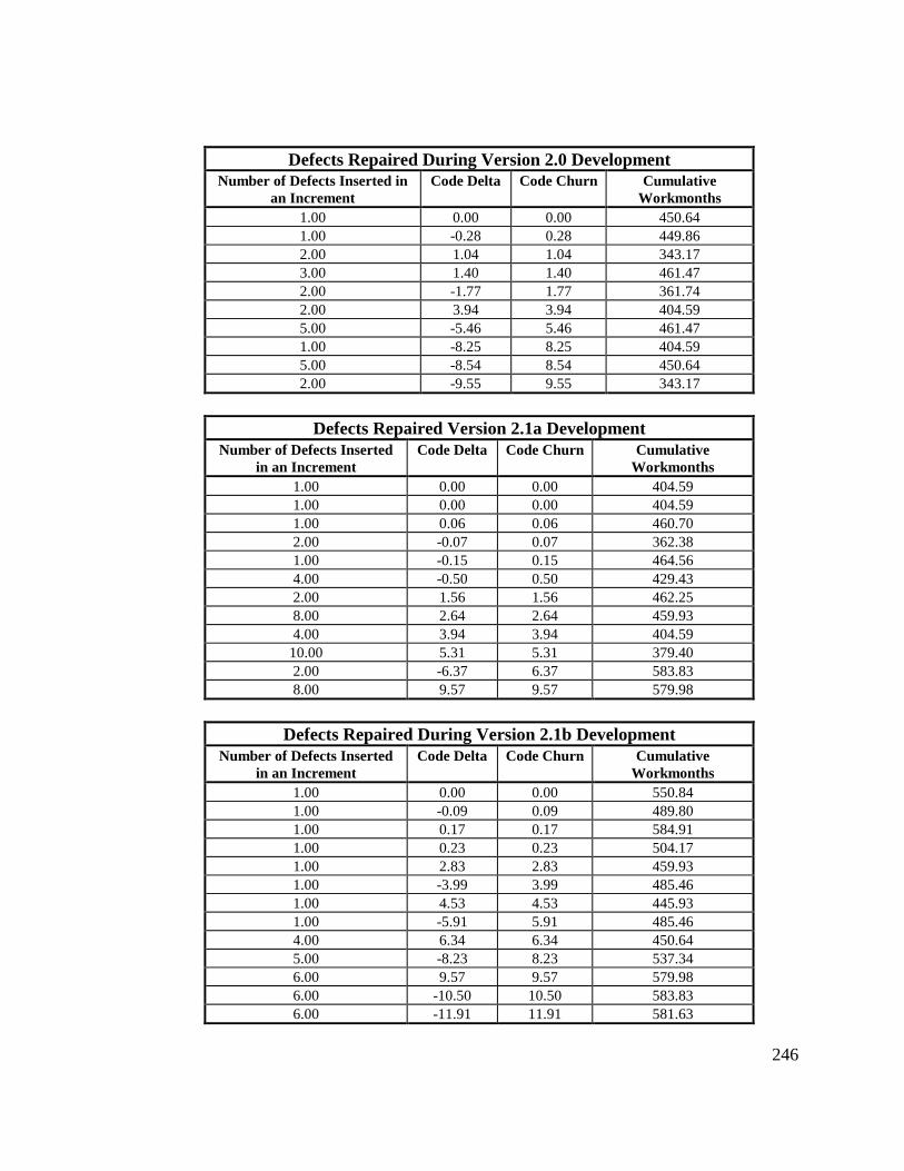
246
Defects Repaired During Version 2.0 DevelopmentNumber of Defects Inserted in
an IncrementCode Delta Code Churn Cumulative
Workmonths1.00 0.00 0.00 450.641.00 -0.28 0.28 449.862.00 1.04 1.04 343.173.00 1.40 1.40 461.472.00 -1.77 1.77 361.742.00 3.94 3.94 404.595.00 -5.46 5.46 461.471.00 -8.25 8.25 404.595.00 -8.54 8.54 450.642.00 -9.55 9.55 343.17
Defects Repaired Version 2.1a DevelopmentNumber of Defects Inserted
in an IncrementCode Delta Code Churn Cumulative
Workmonths1.00 0.00 0.00 404.591.00 0.00 0.00 404.591.00 0.06 0.06 460.702.00 -0.07 0.07 362.381.00 -0.15 0.15 464.564.00 -0.50 0.50 429.432.00 1.56 1.56 462.258.00 2.64 2.64 459.934.00 3.94 3.94 404.5910.00 5.31 5.31 379.402.00 -6.37 6.37 583.838.00 9.57 9.57 579.98
Defects Repaired During Version 2.1b DevelopmentNumber of Defects Inserted
in an IncrementCode Delta Code Churn Cumulative
Workmonths1.00 0.00 0.00 550.841.00 -0.09 0.09 489.801.00 0.17 0.17 584.911.00 0.23 0.23 504.171.00 2.83 2.83 459.931.00 -3.99 3.99 485.461.00 4.53 4.53 445.931.00 -5.91 5.91 485.464.00 6.34 6.34 450.645.00 -8.23 8.23 537.346.00 9.57 9.57 579.986.00 -10.50 10.50 583.836.00 -11.91 11.91 581.63

247
13.8 COCOMO II Characterization of Development Effort
This appendix characterizes the development effort for this particular project. Thefollowing information is derived from the responses to the COCOMO II questionnaireprovided by the Software Product Assurance lead engineer and the project’s SoftwareManager. These individuals were questioned separately, after which discrepancies intheir responses were resolved by working with both individuals together.
Attribute Name ValueApplication Type Command and ControlActivity Integration TestDevelopment Process Type Phased WaterfallDevelopment Process Iteration ThirdCOCOMO Model Post-ArchitectureSchedule Months 101Life Cycle Phases Covered by Schedule System Requirements
Software RequirementsPreliminary DesignDetailed DesignCode and Unit TestIntegration and Test
Project Exponential Cost DriversPrecedentedness (PREC) NominalDevelopment Flexibility (FLEX) NominalArchitecture Risk Resolution (RESL) Very HighTeam Cohesion (TEAM) High/Very High
Process Maturity (PMAT)Requirements Management About HalfSoftware Project Planning About HalfSoftware Project Tracking and Oversight Rarely if EverSoftware Subcontract Management Does not ApplySoftware Quality Assurance OccasionallySoftware Configuration Management Almost AlwaysOrganization Process Focus OccasionallyOrganization Process Definition Rarely if EverTraining Program Don’t KnowIntegrated Software Management Almost AlwaysSoftware Product Engineering OccasionallyIntergroup Coordination FrequentlyPeer Review OccasionallyQuantitative Process Management OccasionallySoftware Quality Management Rarely if Ever
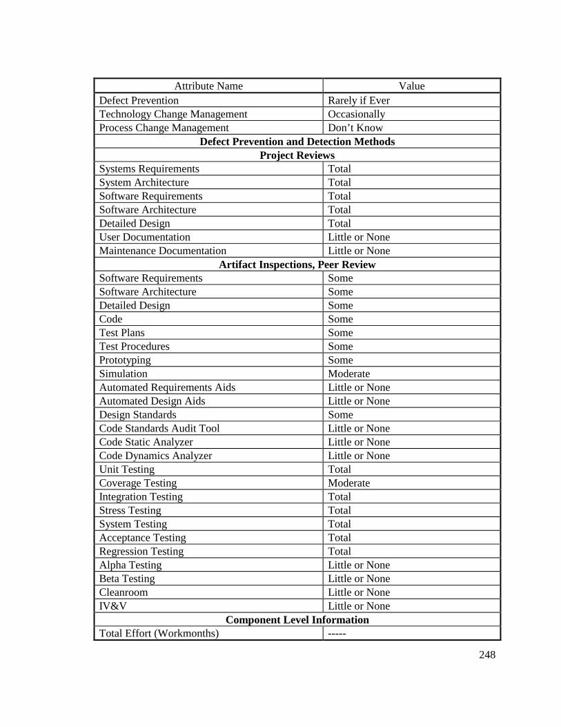
248
Attribute Name ValueDefect Prevention Rarely if EverTechnology Change Management OccasionallyProcess Change Management Don’t Know
Defect Prevention and Detection MethodsProject Reviews
Systems Requirements TotalSystem Architecture TotalSoftware Requirements TotalSoftware Architecture TotalDetailed Design TotalUser Documentation Little or NoneMaintenance Documentation Little or None
Artifact Inspections, Peer ReviewSoftware Requirements SomeSoftware Architecture SomeDetailed Design SomeCode SomeTest Plans SomeTest Procedures SomePrototyping SomeSimulation ModerateAutomated Requirements Aids Little or NoneAutomated Design Aids Little or NoneDesign Standards SomeCode Standards Audit Tool Little or NoneCode Static Analyzer Little or NoneCode Dynamics Analyzer Little or NoneUnit Testing TotalCoverage Testing ModerateIntegration Testing TotalStress Testing TotalSystem Testing TotalAcceptance Testing TotalRegression Testing TotalAlpha Testing Little or NoneBeta Testing Little or NoneCleanroom Little or NoneIV&V Little or None
Component Level InformationTotal Effort (Workmonths) -----

249
Attribute Name ValueLife-cycle Phases Covered -----Hours/Workmonth -----Labor Breakout UnknownPercentage of Code Breakage UnknownObject Points UnknownNew Unique SLOC Approximately 44,000 physical linesSLOC Count Type Physical SLOC (semicolons)Unadjusted Function Points UnknownProgramming Language ADA, 81%
Assembly, 19%Software Maintenance Parameters UnknownObject Points Reused UnknownASLOC Adapted NoneASLOC Count Type Does not ApplyDesign Modified NoneCode Modified NoneIntegration and Test None
Software Understanding (SU)Structure Very HighApplication Clarity Very HighSelf-Descriptiveness NominalAssessment and Assimilation (AA) NoneProgrammer Unfamiliarity (UNFM) 0.0 (Completely Familiar)Required Software Reliability (RELY) HighData Base Size (DATA) NominalRequired Reusability (RUSE) HighDocumentation match to life-cycle needs(DOCU)
Low
Product Complexity (CPLX) High (Unweighted average Value)Control Operations Extra HighComputation Operations NominalDevice-dependent Operations Extra HighData Management Operations HighUser interface Management Operations Very Low
Platform Cost DriversExecution Time Constraint (TIME) HighMain Storage Constraint (STOR) Very HighPlatform Volatility (PVOL) Very Low
Personnel Cost DriversAnalyst Capability (ACAP) High
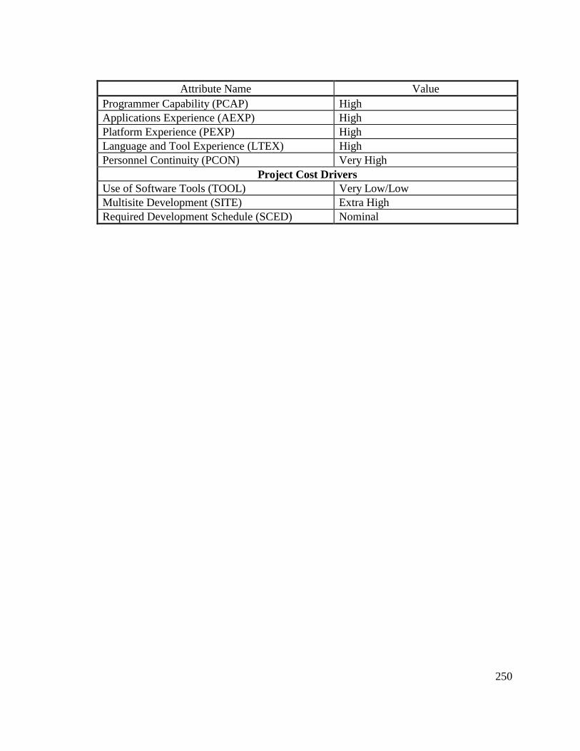
250
Attribute Name ValueProgrammer Capability (PCAP) HighApplications Experience (AEXP) HighPlatform Experience (PEXP) HighLanguage and Tool Experience (LTEX) HighPersonnel Continuity (PCON) Very High
Project Cost DriversUse of Software Tools (TOOL) Very Low/LowMultisite Development (SITE) Extra HighRequired Development Schedule (SCED) Nominal

251
14. Details of Statistical Analysis – Deriving Rates of Defect Insertion forCASSINI CDS Flight Software
This appendix contains the details of the statistical analysis used to determine therate of defect insertion for the CASSINI flight software. Unless otherwise noted, allcomputations were performed using SPSS for Windows, version 7.5.
252
14.1 Correlations between Code Churn, Code Delta, and Number of Defects Insertedin an Increment
1.732 .314
1.000 .314
.866 .314
.378 .243 1.547 .122
.400 .259 1.547 .122
.429 .275 1.547 .122
.451 .287 1.430 .190c
.376 .259 1.149 .284c
10
Phi
Cramer's V
ContingencyCoefficient
Nominal by Nominal
Kendall'stau-b
Kendall'stau-c
Gamma
SpearmanCorrelation
Ordinal by Ordinal
Pearson's RInterval by Interval
N of Valid Cases
ValueAsymp.
Std. Errora Approx. TbApprox.
Sig.
Symmetric Measures
Not assuming the null hypothesis.a.
Using the asymptotic standard error assuming the null hypothesis.b.
Based on normal approximation.c.
Figure 27 - Correlation between Number of Defects Inserted per Increment and CodeChurn – Version 2.0
1.732 .314
1.000 .314
.866 .314
-.076 .220 -.343 .731
-.080 .233 -.343 .731
-.086 .249 -.343 .731
-.121 .294 -.344 .740c
-.323 .249 -.967 .362c
10
Phi
Cramer's V
ContingencyCoefficient
Nominal by Nominal
Kendall'stau-b
Kendall'stau-c
Gamma
SpearmanCorrelation
Ordinal by Ordinal
Pearson's RInterval by Interval
N of Valid Cases
ValueAsymp.
Std. Errora Approx. TbApprox.
Sig.
Symmetric Measures
Not assuming the null hypothesis.a.
Using the asymptotic standard error assuming the null hypothesis.b.
Based on normal approximation.c.
Figure 28 - Correlation between Number of Defects Inserted per Increment and CodeDelta – Version 2.0
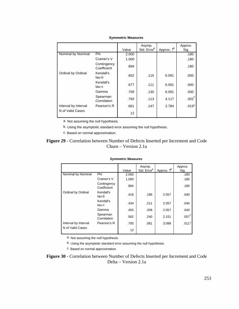
253
2.000 .180
1.000 .180
.894 .180
.652 .115 6.091 .000
.677 .111 6.091 .000
.709 .130 6.091 .000
.793 .113 4.117 .002c
.661 .147 2.784 .019c
12
Phi
Cramer's V
ContingencyCoefficient
Nominal by Nominal
Kendall'stau-b
Kendall'stau-c
Gamma
SpearmanCorrelation
Ordinal by Ordinal
Pearson's RInterval by Interval
N of Valid Cases
ValueAsymp.
Std. Errora Approx. TbApprox.
Sig.
Symmetric Measures
Not assuming the null hypothesis.a.
Using the asymptotic standard error assuming the null hypothesis.b.
Based on normal approximation.c.
Figure 29 - Correlation between Number of Defects Inserted per Increment and CodeChurn – Version 2.1a
2.000 .180
1.000 .180
.894 .180
.418 .196 2.057 .040
.434 .211 2.057 .040
.455 .208 2.057 .040
.562 .240 2.151 .057c
.700 .081 3.098 .011c
12
Phi
Cramer's V
ContingencyCoefficient
Nominal by Nominal
Kendall'stau-b
Kendall'stau-c
Gamma
SpearmanCorrelation
Ordinal by Ordinal
Pearson's RInterval by Interval
N of Valid Cases
ValueAsymp.
Std. Errora Approx. TbApprox.
Sig.
Symmetric Measures
Not assuming the null hypothesis.a.
Using the asymptotic standard error assuming the null hypothesis.b.
Based on normal approximation.c.
Figure 30 - Correlation between Number of Defects Inserted per Increment and CodeDelta – Version 2.1a
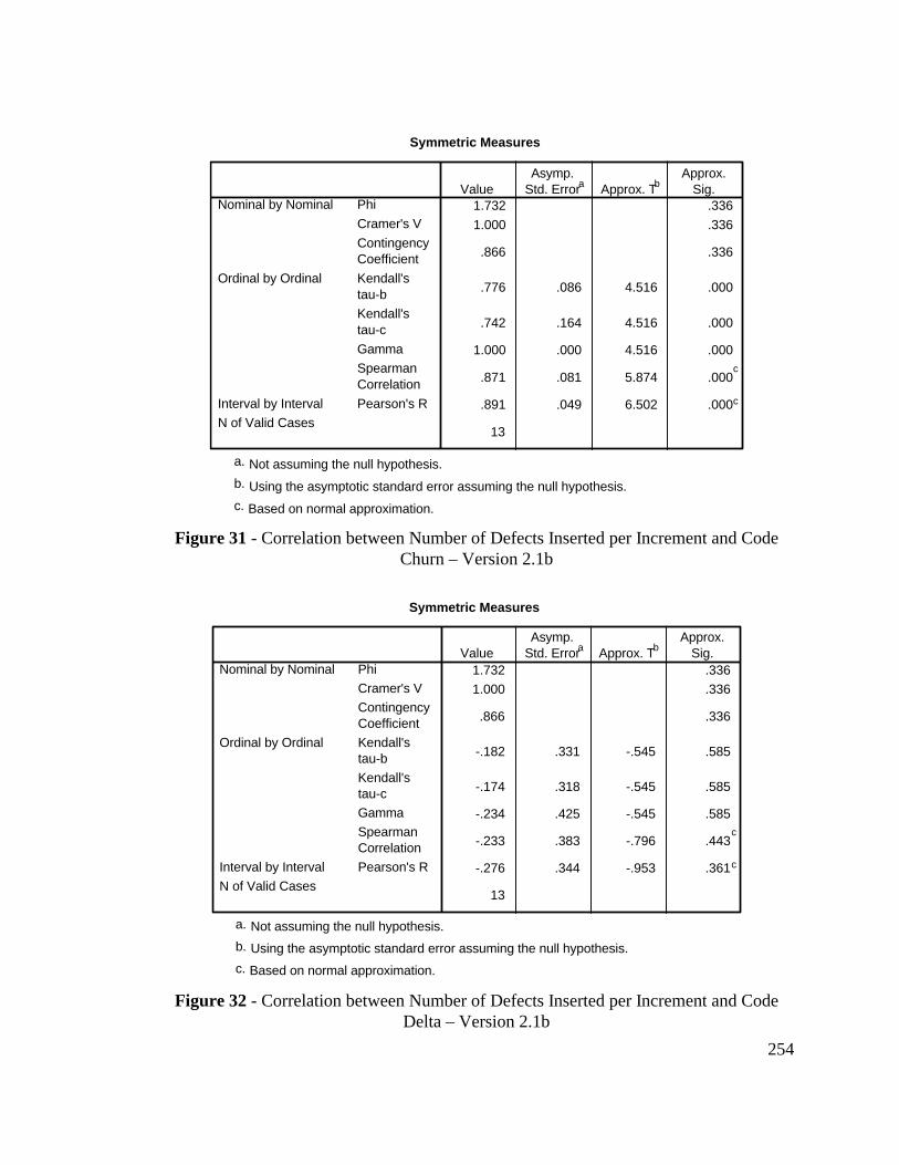
254
1.732 .336
1.000 .336
.866 .336
.776 .086 4.516 .000
.742 .164 4.516 .000
1.000 .000 4.516 .000
.871 .081 5.874 .000c
.891 .049 6.502 .000c
13
Phi
Cramer's V
ContingencyCoefficient
Nominal by Nominal
Kendall'stau-b
Kendall'stau-c
Gamma
SpearmanCorrelation
Ordinal by Ordinal
Pearson's RInterval by Interval
N of Valid Cases
ValueAsymp.
Std. Errora Approx. TbApprox.
Sig.
Symmetric Measures
Not assuming the null hypothesis.a.
Using the asymptotic standard error assuming the null hypothesis.b.
Based on normal approximation.c.
Figure 31 - Correlation between Number of Defects Inserted per Increment and CodeChurn – Version 2.1b
1.732 .336
1.000 .336
.866 .336
-.182 .331 -.545 .585
-.174 .318 -.545 .585
-.234 .425 -.545 .585
-.233 .383 -.796 .443c
-.276 .344 -.953 .361c
13
Phi
Cramer's V
ContingencyCoefficient
Nominal by Nominal
Kendall'stau-b
Kendall'stau-c
Gamma
SpearmanCorrelation
Ordinal by Ordinal
Pearson's RInterval by Interval
N of Valid Cases
ValueAsymp.
Std. Errora Approx. TbApprox.
Sig.
Symmetric Measures
Not assuming the null hypothesis.a.
Using the asymptotic standard error assuming the null hypothesis.b.
Based on normal approximation.c.
Figure 32 - Correlation between Number of Defects Inserted per Increment and CodeDelta – Version 2.1b
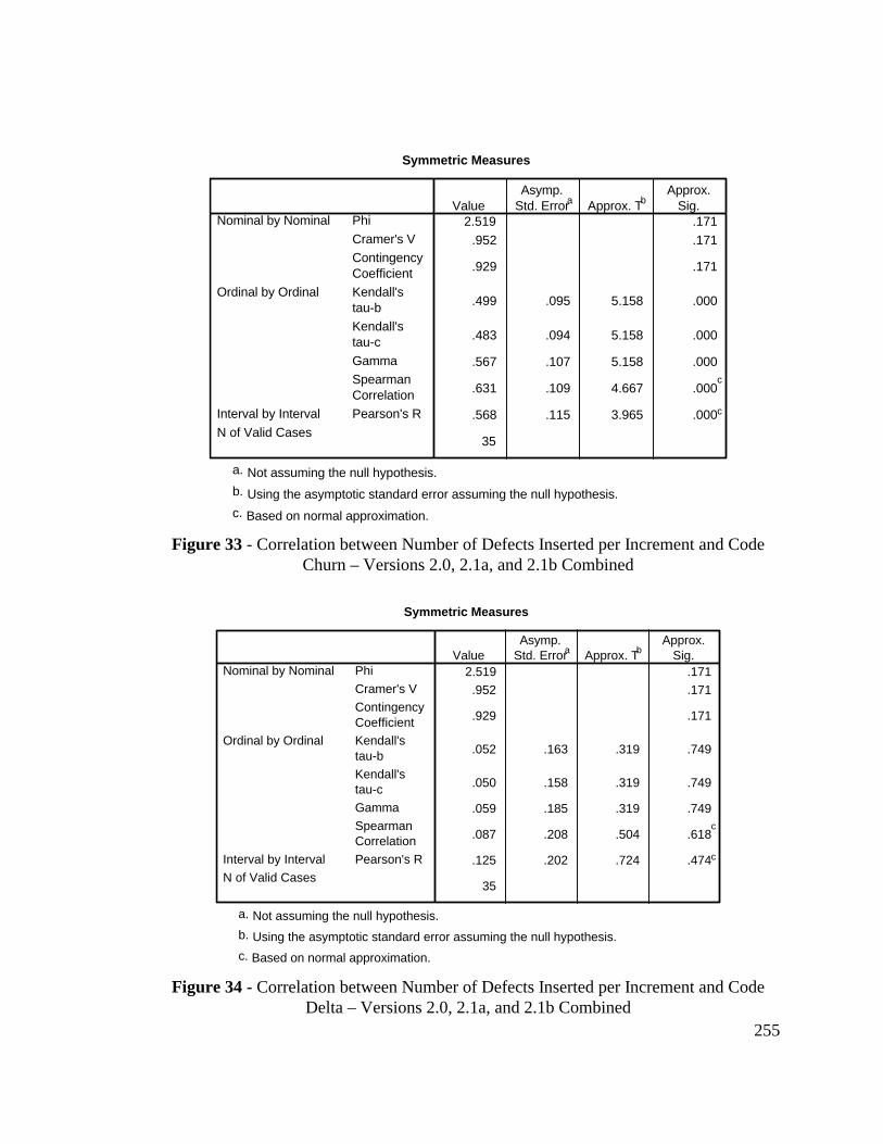
255
2.519 .171
.952 .171
.929 .171
.499 .095 5.158 .000
.483 .094 5.158 .000
.567 .107 5.158 .000
.631 .109 4.667 .000c
.568 .115 3.965 .000c
35
Phi
Cramer's V
ContingencyCoefficient
Nominal by Nominal
Kendall'stau-b
Kendall'stau-c
Gamma
SpearmanCorrelation
Ordinal by Ordinal
Pearson's RInterval by Interval
N of Valid Cases
ValueAsymp.
Std. Errora Approx. TbApprox.
Sig.
Symmetric Measures
Not assuming the null hypothesis.a.
Using the asymptotic standard error assuming the null hypothesis.b.
Based on normal approximation.c.
Figure 33 - Correlation between Number of Defects Inserted per Increment and CodeChurn – Versions 2.0, 2.1a, and 2.1b Combined
2.519 .171
.952 .171
.929 .171
.052 .163 .319 .749
.050 .158 .319 .749
.059 .185 .319 .749
.087 .208 .504 .618c
.125 .202 .724 .474c
35
Phi
Cramer's V
ContingencyCoefficient
Nominal by Nominal
Kendall'stau-b
Kendall'stau-c
Gamma
SpearmanCorrelation
Ordinal by Ordinal
Pearson's RInterval by Interval
N of Valid Cases
ValueAsymp.
Std. Errora Approx. TbApprox.
Sig.
Symmetric Measures
Not assuming the null hypothesis.a.
Using the asymptotic standard error assuming the null hypothesis.b.
Based on normal approximation.c.
Figure 34 - Correlation between Number of Defects Inserted per Increment and CodeDelta – Versions 2.0, 2.1a, and 2.1b Combined
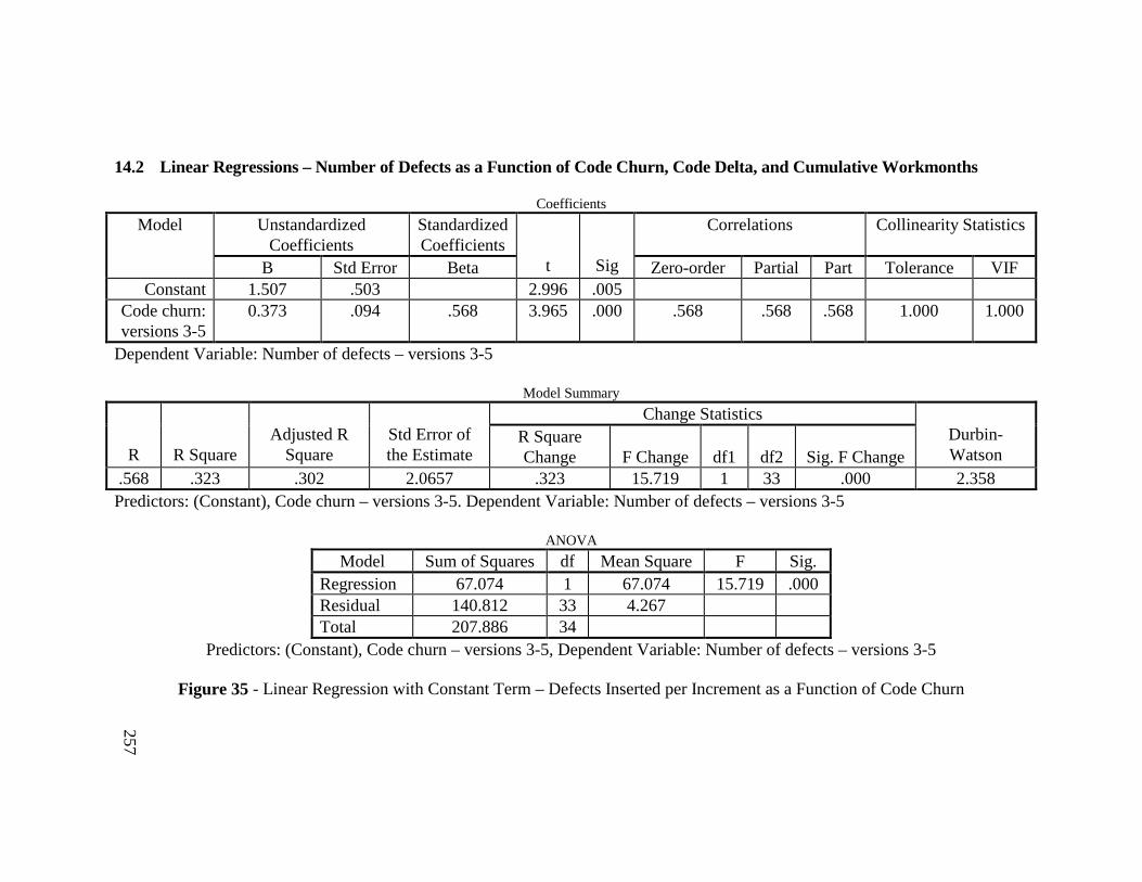
257
14.2 Linear Regressions – Number of Defects as a Function of Code Churn, Code Delta, and Cumulative Workmonths
Coefficients
UnstandardizedCoefficients
StandardizedCoefficients
Correlations Collinearity StatisticsModel
B Std Error Beta t Sig Zero-order Partial Part Tolerance VIFConstant 1.507 .503 2.996 .005
Code churn:versions 3-5
0.373 .094 .568 3.965 .000 .568 .568 .568 1.000 1.000
Dependent Variable: Number of defects – versions 3-5
Model Summary
Change Statistics
R R SquareAdjusted R
SquareStd Error ofthe Estimate
R SquareChange F Change df1 df2 Sig. F Change
Durbin-Watson
.568 .323 .302 2.0657 .323 15.719 1 33 .000 2.358Predictors: (Constant), Code churn – versions 3-5. Dependent Variable: Number of defects – versions 3-5
ANOVA
Model Sum of Squares df Mean Square F Sig.Regression 67.074 1 67.074 15.719 .000Residual 140.812 33 4.267Total 207.886 34
Predictors: (Constant), Code churn – versions 3-5, Dependent Variable: Number of defects – versions 3-5
Figure 35 - Linear Regression with Constant Term – Defects Inserted per Increment as a Function of Code Churn
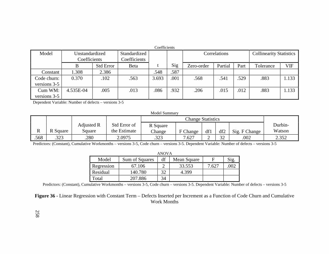
258
Coefficients
UnstandardizedCoefficients
StandardizedCoefficients
Correlations Collinearity StatisticsModel
B Std Error Beta t Sig Zero-order Partial Part Tolerance VIFConstant 1.308 2.386 .548 .587
Code churn:versions 3-5
0.370 .102 .563 3.693 .001 .568 .541 .529 .883 1.133
Cum WM:versions 3-5
4.535E-04 .005 .013 .086 .932 .206 .015 .012 .883 1.133
Dependent Variable: Number of defects – versions 3-5
Model Summary
Change Statistics
R R SquareAdjusted R
SquareStd Error ofthe Estimate
R SquareChange F Change df1 df2 Sig. F Change
Durbin-Watson
.568 .323 .280 2.0975 .323 7.627 2 32 .002 2.352Predictors: (Constant), Cumulative Workmonths – versions 3-5, Code churn – versions 3-5. Dependent Variable: Number of defects – versions 3-5
ANOVA
Model Sum of Squares df Mean Square F Sig.Regression 67.106 2 33.553 7.627 .002Residual 140.780 32 4.399Total 207.886 34
Predictors: (Constant), Cumulative Workmonths – versions 3-5, Code churn – versions 3-5. Dependent Variable: Number of defects – versions 3-5
Figure 36 - Linear Regression with Constant Term – Defects Inserted per Increment as a Function of Code Churn and CumulativeWork Months
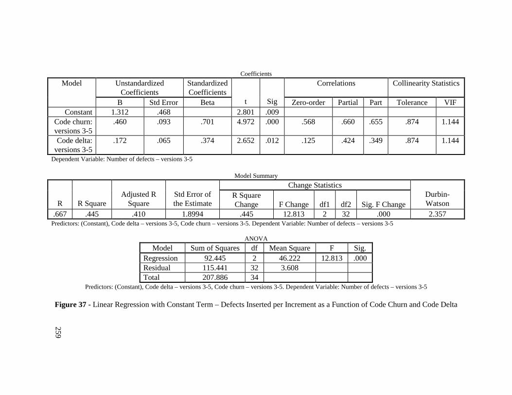
259
Coefficients
UnstandardizedCoefficients
StandardizedCoefficients
Correlations Collinearity StatisticsModel
B Std Error Beta t Sig Zero-order Partial Part Tolerance VIFConstant 1.312 .468 2.801 .009
Code churn:versions 3-5
.460 .093 .701 4.972 .000 .568 .660 .655 .874 1.144
Code delta:versions 3-5
.172 .065 .374 2.652 .012 .125 .424 .349 .874 1.144
Dependent Variable: Number of defects – versions 3-5
Model Summary
Change Statistics
R R SquareAdjusted R
SquareStd Error ofthe Estimate
R SquareChange F Change df1 df2 Sig. F Change
Durbin-Watson
.667 .445 .410 1.8994 .445 12.813 2 32 .000 2.357Predictors: (Constant), Code delta – versions 3-5, Code churn – versions 3-5. Dependent Variable: Number of defects – versions 3-5
ANOVA
Model Sum of Squares df Mean Square F Sig.Regression 92.445 2 46.222 12.813 .000Residual 115.441 32 3.608Total 207.886 34
Predictors: (Constant), Code delta – versions 3-5, Code churn – versions 3-5. Dependent Variable: Number of defects – versions 3-5
Figure 37 - Linear Regression with Constant Term – Defects Inserted per Increment as a Function of Code Churn and Code Delta
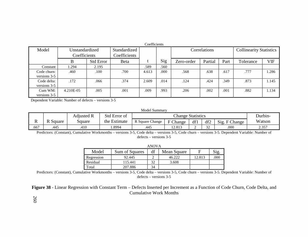
260
Coefficients
UnstandardizedCoefficients
StandardizedCoefficients
Correlations Collinearity StatisticsModel
B Std Error Beta t Sig Zero-order Partial Part Tolerance VIFConstant 1.294 2.195 .589 .560
Code churn:versions 3-5
.460 .100 .700 4.613 .000 .568 .638 .617 .777 1.286
Code delta:versions 3-5
.172 .066 .374 2.609 .014 .124 .424 .349 .873 1.145
Cum WM:versions 3-5
4.210E-05 .005 .001 .009 .993 .206 .002 .001 .882 1.134
Dependent Variable: Number of defects – versions 3-5
Model Summary
Change StatisticsR R Square
Adjusted RSquare
Std Error ofthe Estimate R Square Change F Change df1 df2 Sig. F Change
Durbin-Watson
.667 .445 .410 1.8994 .445 12.813 2 32 .000 2.357Predictors: (Constant), Cumulative Workmonths – versions 3-5, Code delta – versions 3-5, Code churn – versions 3-5. Dependent Variable: Number of
defects – versions 3-5
ANOVA
Model Sum of Squares df Mean Square F Sig.Regression 92.445 2 46.222 12.813 .000Residual 115.441 32 3.608Total 207.886 34
Predictors: (Constant), Cumulative Workmonths – versions 3-5, Code delta – versions 3-5, Code churn – versions 3-5. Dependent Variable: Number ofdefects – versions 3-5
Figure 38 - Linear Regression with Constant Term – Defects Inserted per Increment as a Function of Code Churn, Code Delta, andCumulative Work Months
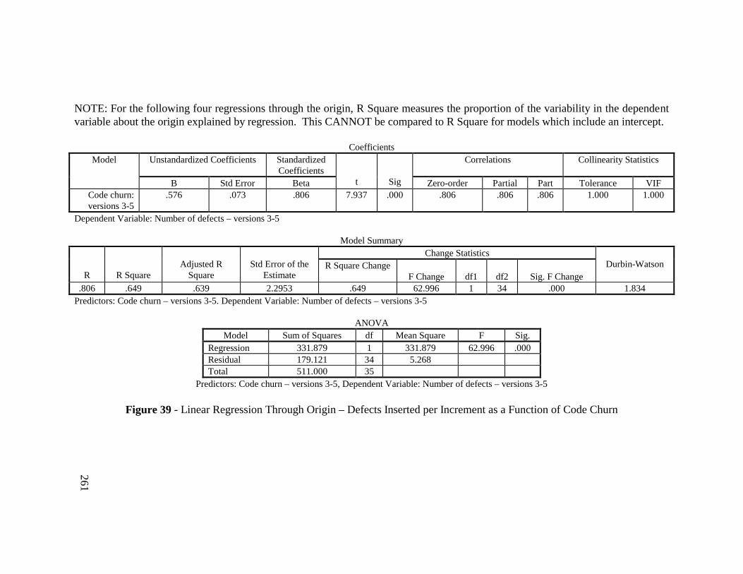
261
NOTE: For the following four regressions through the origin, R Square measures the proportion of the variability in the dependentvariable about the origin explained by regression. This CANNOT be compared to R Square for models which include an intercept.
CoefficientsUnstandardized Coefficients Standardized
CoefficientsCorrelations Collinearity StatisticsModel
B Std Error Beta t Sig Zero-order Partial Part Tolerance VIFCode churn:versions 3-5
.576 .073 .806 7.937 .000 .806 .806 .806 1.000 1.000
Dependent Variable: Number of defects – versions 3-5
Model SummaryChange Statistics
R R SquareAdjusted R
SquareStd Error of the
EstimateR Square Change
F Change df1 df2 Sig. F ChangeDurbin-Watson
.806 .649 .639 2.2953 .649 62.996 1 34 .000 1.834Predictors: Code churn – versions 3-5. Dependent Variable: Number of defects – versions 3-5
ANOVAModel Sum of Squares df Mean Square F Sig.
Regression 331.879 1 331.879 62.996 .000Residual 179.121 34 5.268Total 511.000 35
Predictors: Code churn – versions 3-5, Dependent Variable: Number of defects – versions 3-5
Figure 39 - Linear Regression Through Origin – Defects Inserted per Increment as a Function of Code Churn
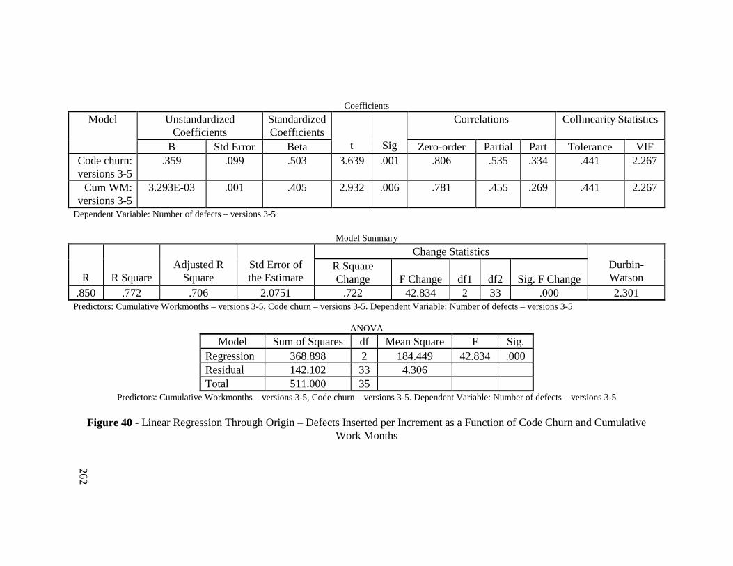
262
Coefficients
UnstandardizedCoefficients
StandardizedCoefficients
Correlations Collinearity StatisticsModel
B Std Error Beta t Sig Zero-order Partial Part Tolerance VIFCode churn:versions 3-5
.359 .099 .503 3.639 .001 .806 .535 .334 .441 2.267
Cum WM:versions 3-5
3.293E-03 .001 .405 2.932 .006 .781 .455 .269 .441 2.267
Dependent Variable: Number of defects – versions 3-5
Model Summary
Change Statistics
R R SquareAdjusted R
SquareStd Error ofthe Estimate
R SquareChange F Change df1 df2 Sig. F Change
Durbin-Watson
.850 .772 .706 2.0751 .722 42.834 2 33 .000 2.301Predictors: Cumulative Workmonths – versions 3-5, Code churn – versions 3-5. Dependent Variable: Number of defects – versions 3-5
ANOVA
Model Sum of Squares df Mean Square F Sig.Regression 368.898 2 184.449 42.834 .000Residual 142.102 33 4.306Total 511.000 35
Predictors: Cumulative Workmonths – versions 3-5, Code churn – versions 3-5. Dependent Variable: Number of defects – versions 3-5
Figure 40 - Linear Regression Through Origin – Defects Inserted per Increment as a Function of Code Churn and CumulativeWork Months
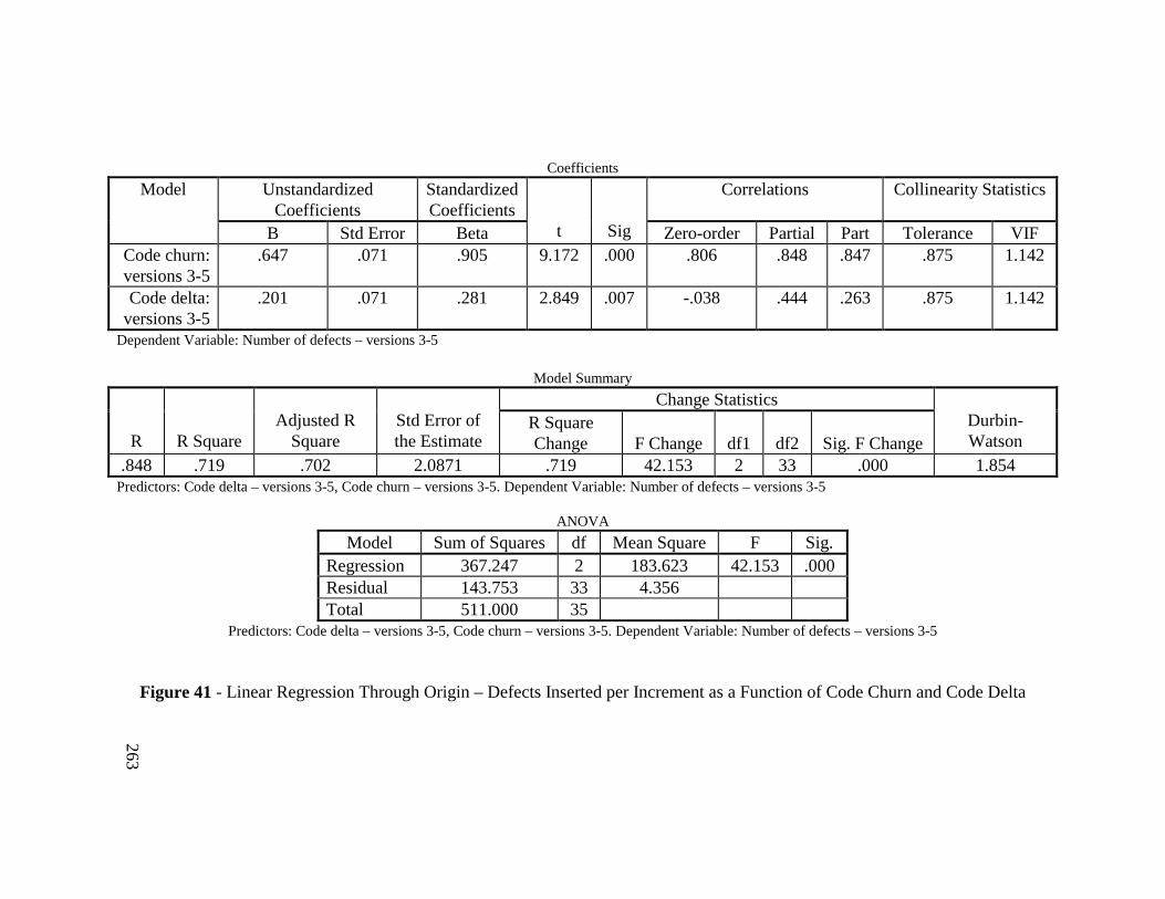
263
Coefficients
UnstandardizedCoefficients
StandardizedCoefficients
Correlations Collinearity StatisticsModel
B Std Error Beta t Sig Zero-order Partial Part Tolerance VIFCode churn:versions 3-5
.647 .071 .905 9.172 .000 .806 .848 .847 .875 1.142
Code delta:versions 3-5
.201 .071 .281 2.849 .007 -.038 .444 .263 .875 1.142
Dependent Variable: Number of defects – versions 3-5
Model Summary
Change Statistics
R R SquareAdjusted R
SquareStd Error ofthe Estimate
R SquareChange F Change df1 df2 Sig. F Change
Durbin-Watson
.848 .719 .702 2.0871 .719 42.153 2 33 .000 1.854Predictors: Code delta – versions 3-5, Code churn – versions 3-5. Dependent Variable: Number of defects – versions 3-5
ANOVA
Model Sum of Squares df Mean Square F Sig.Regression 367.247 2 183.623 42.153 .000Residual 143.753 33 4.356Total 511.000 35
Predictors: Code delta – versions 3-5, Code churn – versions 3-5. Dependent Variable: Number of defects – versions 3-5
Figure 41 - Linear Regression Through Origin – Defects Inserted per Increment as a Function of Code Churn and Code Delta
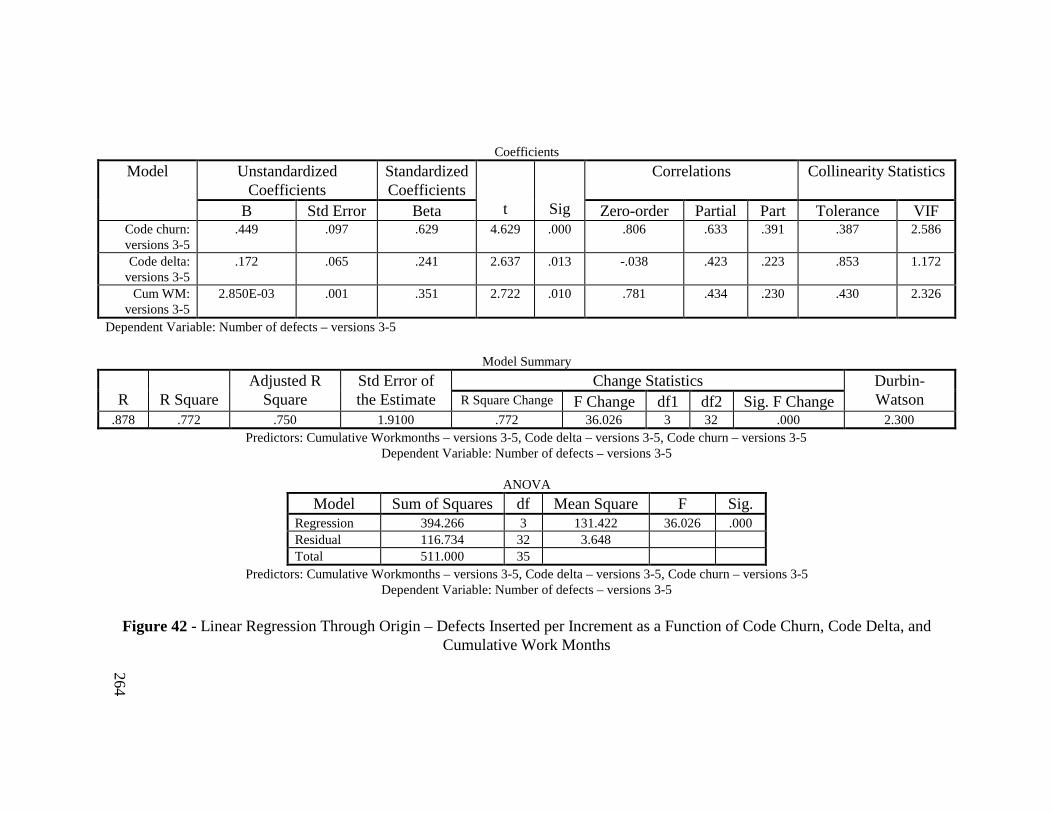
264
Coefficients
UnstandardizedCoefficients
StandardizedCoefficients
Correlations Collinearity StatisticsModel
B Std Error Beta t Sig Zero-order Partial Part Tolerance VIFCode churn:versions 3-5
.449 .097 .629 4.629 .000 .806 .633 .391 .387 2.586
Code delta:versions 3-5
.172 .065 .241 2.637 .013 -.038 .423 .223 .853 1.172
Cum WM:versions 3-5
2.850E-03 .001 .351 2.722 .010 .781 .434 .230 .430 2.326
Dependent Variable: Number of defects – versions 3-5
Model Summary
Change StatisticsR R Square
Adjusted RSquare
Std Error ofthe Estimate R Square Change F Change df1 df2 Sig. F Change
Durbin-Watson
.878 .772 .750 1.9100 .772 36.026 3 32 .000 2.300Predictors: Cumulative Workmonths – versions 3-5, Code delta – versions 3-5, Code churn – versions 3-5
Dependent Variable: Number of defects – versions 3-5
ANOVA
Model Sum of Squares df Mean Square F Sig.Regression 394.266 3 131.422 36.026 .000Residual 116.734 32 3.648Total 511.000 35
Predictors: Cumulative Workmonths – versions 3-5, Code delta – versions 3-5, Code churn – versions 3-5Dependent Variable: Number of defects – versions 3-5
Figure 42 - Linear Regression Through Origin – Defects Inserted per Increment as a Function of Code Churn, Code Delta, andCumulative Work Months
265
14.3 Crossvalidation
The following tables show results of the crossvalidation that was done for the 35observations given in Appendix 13.7. An “exclude one at a time” crossvalidation wasdone for this set of observations, which resulted in 35 predictions of excluded values.
The four tables in this Appendix provide the following information:
• Predicted squared residuals for each of the four linear regressions through theorigin. For each observation j , regression models relating the number of de-fects as a function of code churn, code delta, and cumulative workmonths areformed using all observations except the j th observation; the resulting modelsare then used to predict the dependent variable (number of inserted defects)based on the value of the excluded j th observation. For each model and eachexcluded observation, the prediction based on the excluded observation is thensubtracted from that actual number of observed defects. This residual quantityis then squared to form the predicted squared residual. Appendix 14.3.1 givesthe predicted squared residual for each excluded observation for the four typesof linear regression models through the origin. The j th row of this table givesthe predicted squared residual for each of the four models when the j th obser-vation is excluded from the computation of the regression model.
• Ratio of predicted to observed values based on excluded observations, shownin Appendix 14.3.2. As for the first table, each observation is excluded in turnfrom the computation of the regression models. A prediction of the dependentvariable is then made for the excluded observation, and the ratio of that pre-diction to the observed number of defects is then made. The j th row of this ta-ble gives the ratio of the predicted number of defects based on the excludedobservation to the actual number of observed defects for each of the four mod-els when the j th observation is excluded from the computation of the regres-sion model.
• Predicted squared residuals for each of the four linear regression modelsthrough the origin, standardized with respect to the 3 parameter regression,shown in Appendix 14.3.3. Again, each observation is excluded in turn fromthe computation of the regression models. For each excluded observation, thepredicted squared residuals are computed as for the first table. These valuesare then standardized with respect to the 3 parameter regression by subtractingfrom each predicted squared residual the mean value of the predicted squaredresiduals for the 3 parameter regression, the dividing by the standard deviationof predicted squared residual for the 3 parameter regression. The j th row ofthis table gives the standardized predicted squared residual for each of the fourmodels when the j th observation is excluded from the computation of the re-gression model.
266
• Ratio of predicted to observed values based on excluded observations, stan-dardized with respect to the 3 parameter regression, shown in Appendix14.3.4. Each observation is excluded in turn from computation of the regres-sion models. For each excluded value and each model, ratios of predicted toactual values are computed as above. A prediction of the dependent variableis then made for the excluded observation, and the ratio of that prediction tothe observed number of defects is then made. These ratios are then standard-ized by subtracting from each ratio the mean value of the ratio for the 3 pa-rameter regression, and then dividing by the standard deviation of the ratio forthe 3 parameter regression. The j th row of this table gives the standardized ra-tio of the predicted number of defects based on the excluded observation tothe actual number of observed defects for each of the four models when the j th
observation is excluded from the computation of the regression model.
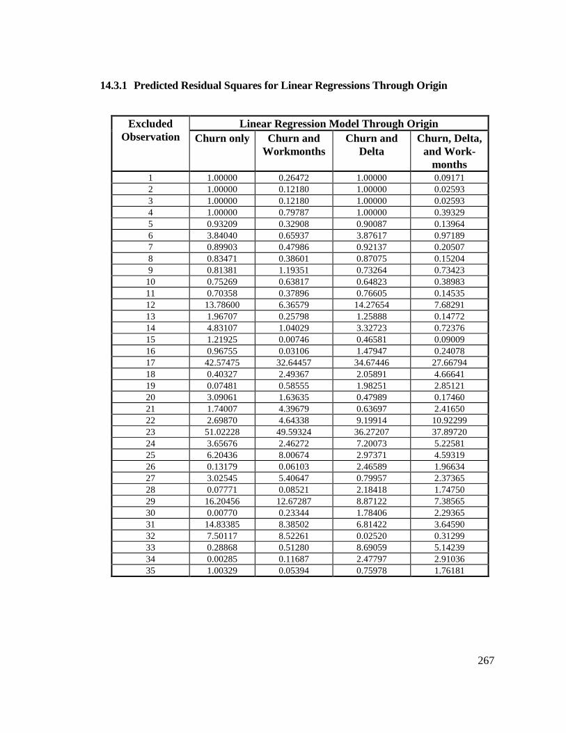
267
14.3.1 Predicted Residual Squares for Linear Regressions Through Origin
Linear Regression Model Through OriginExcludedObservation Churn only Churn and
WorkmonthsChurn and
DeltaChurn, Delta,
and Work-months
1 1.00000 0.26472 1.00000 0.091712 1.00000 0.12180 1.00000 0.025933 1.00000 0.12180 1.00000 0.025934 1.00000 0.79787 1.00000 0.393295 0.93209 0.32908 0.90087 0.139646 3.84040 0.65937 3.87617 0.971897 0.89903 0.47986 0.92137 0.205078 0.83471 0.38601 0.87075 0.152049 0.81381 1.19351 0.73264 0.7342310 0.75269 0.63817 0.64823 0.3898311 0.70358 0.37896 0.76605 0.1453512 13.78600 6.36579 14.27654 7.6829113 1.96707 0.25798 1.25888 0.1477214 4.83107 1.04029 3.32723 0.7237615 1.21925 0.00746 0.46581 0.0900916 0.96755 0.03106 1.47947 0.2407817 42.57475 32.64457 34.67446 27.6679418 0.40327 2.49367 2.05891 4.6664119 0.07481 0.58555 1.98251 2.8512120 3.09061 1.63635 0.47989 0.1746021 1.74007 4.39679 0.63697 2.4165022 2.69870 4.64338 9.19914 10.9229923 51.02228 49.59324 36.27207 37.8972024 3.65676 2.46272 7.20073 5.2258125 6.20436 8.00674 2.97371 4.5931926 0.13179 0.06103 2.46589 1.9663427 3.02545 5.40647 0.79957 2.3736528 0.07771 0.08521 2.18418 1.7475029 16.20456 12.67287 8.87122 7.3856530 0.00770 0.23344 1.78406 2.2936531 14.83385 8.38502 6.81422 3.6459032 7.50117 8.52261 0.02520 0.3129933 0.28868 0.51280 8.69059 5.1423934 0.00285 0.11687 2.47797 2.9103635 1.00329 0.05394 0.75978 1.76181
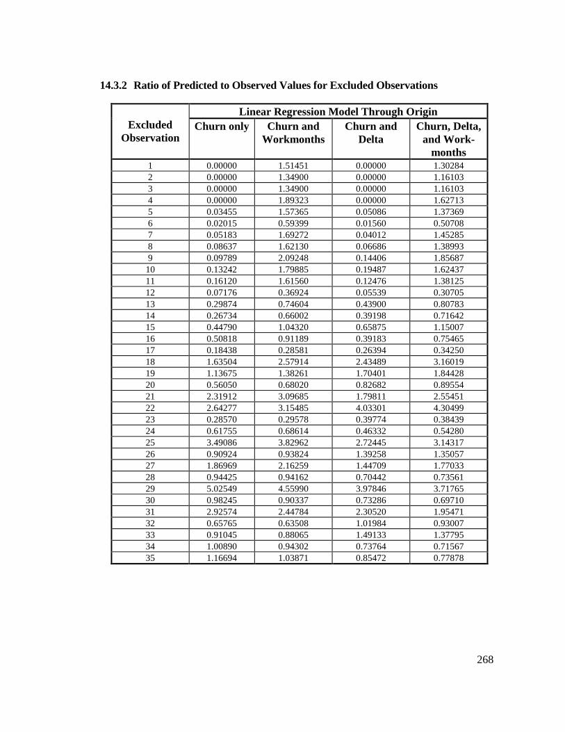
268
14.3.2 Ratio of Predicted to Observed Values for Excluded Observations
Linear Regression Model Through OriginExcluded
ObservationChurn only Churn and
WorkmonthsChurn and
DeltaChurn, Delta,
and Work-months
1 0.00000 1.51451 0.00000 1.302842 0.00000 1.34900 0.00000 1.161033 0.00000 1.34900 0.00000 1.161034 0.00000 1.89323 0.00000 1.627135 0.03455 1.57365 0.05086 1.373696 0.02015 0.59399 0.01560 0.507087 0.05183 1.69272 0.04012 1.452858 0.08637 1.62130 0.06686 1.389939 0.09789 2.09248 0.14406 1.8568710 0.13242 1.79885 0.19487 1.6243711 0.16120 1.61560 0.12476 1.3812512 0.07176 0.36924 0.05539 0.3070513 0.29874 0.74604 0.43900 0.8078314 0.26734 0.66002 0.39198 0.7164215 0.44790 1.04320 0.65875 1.1500716 0.50818 0.91189 0.39183 0.7546517 0.18438 0.28581 0.26394 0.3425018 1.63504 2.57914 2.43489 3.1601919 1.13675 1.38261 1.70401 1.8442820 0.56050 0.68020 0.82682 0.8955421 2.31912 3.09685 1.79811 2.5545122 2.64277 3.15485 4.03301 4.3049923 0.28570 0.29578 0.39774 0.3843924 0.61755 0.68614 0.46332 0.5428025 3.49086 3.82962 2.72445 3.1431726 0.90924 0.93824 1.39258 1.3505727 1.86969 2.16259 1.44709 1.7703328 0.94425 0.94162 0.70442 0.7356129 5.02549 4.55990 3.97846 3.7176530 0.98245 0.90337 0.73286 0.6971031 2.92574 2.44784 2.30520 1.9547132 0.65765 0.63508 1.01984 0.9300733 0.91045 0.88065 1.49133 1.3779534 1.00890 0.94302 0.73764 0.7156735 1.16694 1.03871 0.85472 0.77878
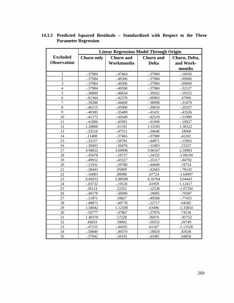
269
14.3.3 Predicted Squared Residuals – Standardized with Respect to the ThreeParameter Regression
Linear Regression Model Through OriginExcluded
ObservationChurn only Churn and
WorkmonthsChurn and
DeltaChurn, Delta,
and Work-months
1 -.37984 -.47464 -.37984 -.160362 -.37984 -.49306 -.37984 -.090003 -.37984 -.49306 -.37984 -.090004 -.37984 -.40590 -.37984 -.321275 -.38860 -.46634 -.39262 -.195526 -.01364 -.42376 -.00903 .479067 -.39286 -.44690 -.38998 -.234798 -.40115 -.45900 -.39650 -.203579 -.40385 -.35489 -.41431 -.4352610 -.41173 -.42649 -.42519 -.3199011 -.41806 -.45991 -.41000 -.1992712 1.26860 .31195 1.33185 1.3652213 -.25516 -.47551 -.34646 .1806014 .11408 -.37465 -.07980 .4120215 -.35157 -.50781 -.44871 -.1590316 -.38402 -.50476 -.31803 .2333717 4.98022 3.69996 3.96167 2.5998318 -.45678 -.18727 -.24332 -1.0819419 -.49912 -.43327 -.25317 -.8479220 -.11031 -.29780 -.44690 .1972421 -.28443 .05809 -.42665 -.7814222 -.16083 .08988 .67724 -1.6499723 6.06932 5.88508 4.16764 3.0444324 -.03732 -.19126 .41959 1.1241725 .29114 .52351 -.12538 -1.0735026 -.49178 -.50090 -.19085 -.7058727 -.11871 .18827 -.40568 -.7745528 -.49875 -.49778 -.22717 .6458229 1.58042 1.12509 .63496 -1.3585430 -.50777 -.47867 -.27876 .7413631 1.40370 .57228 .36976 -.9575232 .45833 .59002 -.50552 .2674933 -.47155 -.44265 .61167 -1.1352834 -.50840 -.49370 -.18929 .8363835 -.37942 -.50181 -.41081 .64850
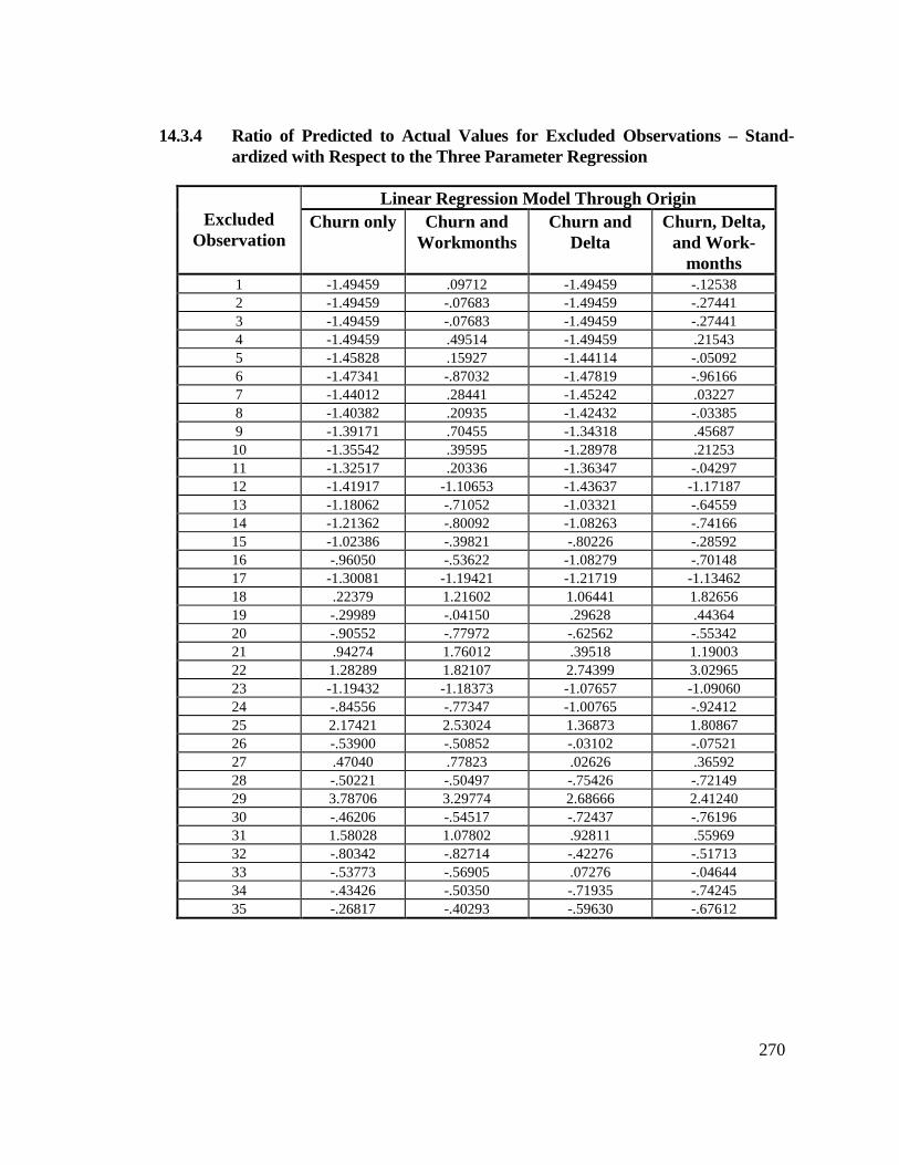
270
14.3.4 Ratio of Predicted to Actual Values for Excluded Observations – Stand-ardized with Respect to the Three Parameter Regression
Linear Regression Model Through OriginExcluded
ObservationChurn only Churn and
WorkmonthsChurn and
DeltaChurn, Delta,
and Work-months
1 -1.49459 .09712 -1.49459 -.125382 -1.49459 -.07683 -1.49459 -.274413 -1.49459 -.07683 -1.49459 -.274414 -1.49459 .49514 -1.49459 .215435 -1.45828 .15927 -1.44114 -.050926 -1.47341 -.87032 -1.47819 -.961667 -1.44012 .28441 -1.45242 .032278 -1.40382 .20935 -1.42432 -.033859 -1.39171 .70455 -1.34318 .4568710 -1.35542 .39595 -1.28978 .2125311 -1.32517 .20336 -1.36347 -.0429712 -1.41917 -1.10653 -1.43637 -1.1718713 -1.18062 -.71052 -1.03321 -.6455914 -1.21362 -.80092 -1.08263 -.7416615 -1.02386 -.39821 -.80226 -.2859216 -.96050 -.53622 -1.08279 -.7014817 -1.30081 -1.19421 -1.21719 -1.1346218 .22379 1.21602 1.06441 1.8265619 -.29989 -.04150 .29628 .4436420 -.90552 -.77972 -.62562 -.5534221 .94274 1.76012 .39518 1.1900322 1.28289 1.82107 2.74399 3.0296523 -1.19432 -1.18373 -1.07657 -1.0906024 -.84556 -.77347 -1.00765 -.9241225 2.17421 2.53024 1.36873 1.8086726 -.53900 -.50852 -.03102 -.0752127 .47040 .77823 .02626 .3659228 -.50221 -.50497 -.75426 -.7214929 3.78706 3.29774 2.68666 2.4124030 -.46206 -.54517 -.72437 -.7619631 1.58028 1.07802 .92811 .5596932 -.80342 -.82714 -.42276 -.5171333 -.53773 -.56905 .07276 -.0464434 -.43426 -.50350 -.71935 -.7424535 -.26817 -.40293 -.59630 -.67612
Related Documents