Software Reliability and System Reliability

2.1 Introduction

Chapter

Software Reliability and System Reliability

Jean-Claude Laprie and Karama Kanoun LAAS-CNRS, Toulouse, France

This chapter is mainly aimed at showing that, by using deliberately simple mathematics, the classical reliability theory can be extended in order to be interpreted from both hardware and software viewpoints. This is referred to as X-ware [Lapr89, Lapr92b] throughout this chapter. It will be shown that, even though the action mechanisms of the various classes of faults may be different from a physical viewpoint according to their causes, a single formulation can be used from the reliability modeling and statistical estimation viewpoints. A single formulation has several advantages, both theoretical and practical, such as (1) easier and more consistent modeling of hardware-software systems and of hardware-software interactions, (2) adaptability of models for hardware dependability to software systems and vice versa, and (3) mathematical tractability.

Section 2.2 gives a general overview of the dependability concepts. Section 2.3 is devoted to the failure behavior of an X-ware system, disregarding the effect of restoration actions (the quantities of interest are thus the time to the next failure or the associated failure rate), considering in turn atomic systems and systems made up of components. In Sec. 2.4, we deal with the behavior of an X-ware system with service restoration, focusing on the characterization of the sequence of the times to failure (i.e., the failure process); the measures of interest are thus the failure intensity, reliability, and availability. Section 2.5 outlines the state of art in dependability evaluation and specification. Finally, Sec. 2.6 summarizes the results obtained.

27

28 Technical Foundations

2.2 The Dependability Concept

2.2.1 Basic definitions

The basic definitions for dependability impairments, means, and attributes are given in Fig. 2.1, and the main characteristics of dependability are summarized in the form of a tree as shown in Fig. 2.2 [Lapr92a, Lapr93l.

2.2.2 On the impairments to dependability

Of primary importance are the impairments to dependability, as we have to know what we are faced with. The creation and manifestation mechanisms of faults, errors, and failures may be summarized as follows:

1. A fault is active when it produces an error. An active fault is either an internal fault previously dormant and activated by the computation process or an external fault. Most internal faults cycle between their dormant and active states. Physical faults can directly affect the hardware components only, whereas human-made faults may affect any component.

2. An error may be latent or detected. An error is latent when it has not been recognized as such; an error is detected by a detection algorithm or mechanism. An error may disappear before being detected. An error may, and in general does, propagate; by propagating, an error creates other-new-error(s). During operation, the presence of active faults is determined only by the detection of errors.

3. A failure occurs when an error passes through the system-user interface and affects the service delivered by the system. A component failure results in a fault (1) for the system which contains the component and (2) as viewed by the other component(s) with which it interacts; the failure modes of the failed component then become fault types for the components interacting with it.

Some examples illustrative of fault pathology:

• The result of a programmer's error is a (dormant) fault in the written software (faulty instruction(s) or data); upon activation (invoking the component where the fault resides and triggering the faulty instruction, instruction sequence, or data by an appropriate input pattern) the fault becomes active and produces an error; if and when the erroneous data affect the delivered service (in value and/or in the timing of their delivery), a failure occurs .

• A short circuit occurring in an integrated circuit is a failure. The consequence (connection stuck at a boolean value, modification of the

Software Reliability and System Reliability 29

Dependability is defined as the trustworthiness of a computer system such that reliance can justifiably be placed on the service it delivers. The service delivered by a system is its behavior as it is perceptible by its user(s); a user is another system (human or physical) interacting with the former.

Depending on the application(s) intended for the system, a different emphasis may be put on the various facets of dependability, that is, dependability may be viewed according to different, but complementary, properties, which enable the attributes of dependability to be defined:

• The readiness for usage leads to availability.

• The continuity of service leads to reliability.

• The nonoccurrence of catastrophic consequences on the environment leads to safety.

• The nonoccurrence of the unauthorized disclosure of information leads to confidentiality.

• The nonoccurrence of improper alterations of information leads to integrity.

• The ability to undergo repairs and evolutions leads to maintainability.

Associating availability and integrity with respect to authorized actions, together with confidentiality, leads to security.

A system failurel occurs when the delivered service deviates from fulfilling the system's function, the latter being what the system is intended for. An error is that part of the system state which is liable to lead to subsequent failure: an error affecting the service is an indication that a failure occurs or has occurred. The adjudged or hypothesized cause of an error is a fault.

The development of a dependable computing system calls for the combined utilization of a set of methods and techniques which can be classed into:

• Fault prevention: how to prevent fault occurrence or introduction.

• Fault removal: how to reduce the presence (number, seriousness) offaults.

• Fault tolerance: how to ensure a service capable of fulfilling the system's function in the presence of faults.

• Fault forecasting: how to estimate the present number, future incidence, and consequences of faults.

The notions introduced can be grouped into three classes:

• The impairments to dependability: faults, errors, failures; they are undesiredbut not in principle unexpected-circumstances causing or resulting from undependability (whose definition is very simply derived from the definition of dependability: reliance cannot or will no longer be placed on the service).

• The means for dependability: fault prevention, fault removal, fault tolerance, fault forecasting; these are the methods and techniques enabling one (1) to provide the ability to deliver a service on which reliance can be placed and (2) to reach confidence in this ability.

• The attributes of dependability: availability, reliability, safety, confidentiality, integrity, maintainability; these attributes (1) enable the properties which are expected from the system to be expressed and (2) allow the system quality resulting from the impairments and the means opposing them to be assessed.

Figure 2.1 Dependability basic definitions.


DEPENDABILITY

ATIRIBUTES

AVAILABILITY RELIABILITY SAFETY CONFIDENTIALITY INTEGRITY MAINTAINABILITY

-f FAULT PREVENTION FAULT REMOVAL

MEANS FAULT TOLERANCE FAULT FORECASTING

-E FAULTS

IMPAIRMENTS ERRORS FAILURES

Figure 2.2 The dependability tree.

circuit function, etc.) is a fault which will remain dormant as long as it has not been activated, the continuation of the process being identical to that of the previous example .

• An inappropriate human-machine interaction performed by an operator during the operation of the system is a fault (from the system viewpoint); the resulting altered processed data is an error.

• A maintenance or operating manual writer's error may result in a fault in the corresponding manual (faulty directives) which will remain dormant as long as the directives are not acted upon in order to deal with a given situation.

Figure 2.3 summarizes the fault classification; the upper part indicates the viewpoint according to which they are classified, and the lower part gives the likely combinations according to these viewpoints, as well as the usual labeling of these combinations-not their definition.

It is noteworthy that the very notion of fault is arbitrary, and in fact a facility provided for stopping the recursion induced by the causal relationship between faults, errors, and failures-hence the definition given: adjudged or hypothesized cause of an error. This cause may vary depending upon the viewpoint chosen: fault tolerance mechanisms, maintenance engineers, repair shop, developer, semiconductor physicist, etc. In fact, a fault is nothing other than the consequence of a failure of some other system (including the developer) that has delivered or is now delivering a service to the given system. A computing system is a human artifact apd, as such, any fault in it or affecting it is ultimately human-inade since it represents the human inability to master all the phenomena which govern the behavior of a system. Going further, any fault can be viewed as a permanent design fault. This is indeed true in

PHENOMENOLOGICAL CAUSE

/\


SYS1EM BOUNDARIES

/'\ PHASE

OF CREATION

/ '\ PERSIS1ENCE

I" ACCIDENTAL INTENTIONAL PHYSICAL HUMAN INTERNAL EXTERNAL DESIGN OPERATION PERMANENT TEMPORARY

I I I I -. • • • I I I _.

0 • • I I I I

-0 • • • I I I

-0 • • • I -. • • I I -. .--. •

! I 0 I . • j=c=~[ I I 0

I !=t=-=t=-• I I I I · • • • I I I I

-.

Figure 2.3 Fault classes.

I • I •

•

I •

I •

I

--h~~JE~~AL -T TRANSIENT

.- FAULTS

I '}INTERMITIENT I FAULTS

•

-+ DESIGN FAULTS

INTERACTION .- FAULTS

=b-MALICIOUS LOGIC

•

=G INTRUSIONS

an absolute sense, but not very helpful for system developers and assessors; hence the usefulness of the various fault classes when considering the (current) methods and techniques for procuring and validating dependability.

A system may not, and generally does not, always fail in the same way. The ways a system can fail are its failure modes. These can be characterized according to three viewpoints as shown in Fig. 2.4.

Given below are two additional comments regarding the words, or labels, fault, error, and failure:

DOMAIN

/\

FAILURES

I PERCEPTION BY SEVERAL

USERS

/ ~

CONSEQUENCES ON ENVIRONMENT

/ .. ~ VALUE TIMING CONSISTENT INCONSISTENT BENIGN CATASTROPHIC

(BYZANTINE)

Figure 2.4 Failure classification.


1. Their exclusive use in this book (except Chap. 9) does not preclude the use in special situations of words which designate, briefly and unambiguously, a specific class of impairment; this is especially applicable to faults (e.g., bug, defect, deficiency, flaw) and to failures (e.g., breakdown, malfunction, denial of service).

2. The assignment of the particular terms fault, error, and failure simply takes into account current usage: (1) fault prevention, tolerance, and diagnosis, (2) error detection and correction, and (3) failure rate.

2.2.3 On the attributes of dependability

The definition given for integrity-the avoidance of improper alterations of information-generalizes the usual definitions (e.g., prevention of unauthorized amendment or deletion of information [EEC91] or ensuring approved alteration of data [Jaco91]) which are directly related to a specific class of faults, that is, intentional faults (deliberately malevolent actiops). Our definition encompasses accidental faults as well (i.e., faults appearing or created fortuitously), and the use of the word information is intended to avoid being limited strictly to data: integrity of programs is also an essential concern; regarding accidental faults, error re<:overy is indeed aimed at restoring the system's integrity.

Confidentiality, not security, has been introduced as a basic attribute of dependability. Security is usually defined (see e.g., [EEC91]) as the combination of confidentiality, integrity, and availability, where the three notions are understood with respect to unauthorized actions. A definition of security encompassing the three aspects of [EEC91] is: the prevention of unauthorized access and/or handling of information; security issues are indeed dominated by intentional faults, but not restricted to them: an accidental (e.g., physical) fault can cause an unexpected leakage of information.

The definition given for maintainability-ability to undergo repairs and evolutions-deliberately goes beyond corrective maintenance, which relates to repairability only. Evolvability clearly relates to the two other forms of maintenance, that is, (1) adaptive maintenance, which adjusts the system to environmental changes and (2) perfective maintenance, which improves the system's function by responding to customer- and designer-~efined changes. The frontier between repairability and evolvability is not always clear, however (for instance, if the requested change is aimed at fixing a specification fault [Ghez91]). Maintainability actually conditions dependability when considering the whole operational life of a system: systems which do not undergo adaptive or perfective maintenance are likely to be exceptions.


The properties allowing the dependability attributes to be defined may be emphasized to a greater or lesser extent depending on the application intended for the computer system concerned. For instance, availability is always required (although to a varying degree, depending on the application), whereas reliability, safety, and confidentiality mayor may not be required according to the application. The variations in the emphasis to be put on the attributes of dependability have a direct influence on the appropriate balance of the means to be employed for the resulting system to be dependable. This problem is all the more difficult to address because certain attributes are antagonistic (e.g., availability and safety, availability and confidentiality), and call for tradeoffs. Given the three main design dimensions of a computer system (i.e., cost, performance and dependability), the problem is further exacerbated by the fact that the dependability dimension is not so well mastered as the cost-performance design space [Siew92].

2.2.4 On the means for dependability

All the how-tos which appear in the basic definitions given in Fig. 2.1 are in fact goals which cannot be fully reached, as all the corresponding activities are carried out by humans and therefore are prone to imperfections. These imperfections bring in dependencies which explain why it is only the combined utilization of the above methods-preferably at each step in the design and implementation process-that can best lead to a dependable computing system. These dependencies can be sketched as follows: despite fault prevention by means of design methodologies and construction rules (imperfect so as to be workable), faults are created-hence the need for fault removal. Fault removal itself is imperfect, just like all of the off-the-shelf system componentshardware or software-hence the importance of fault forecasting. Our increasing dependence on computing systems brings in the requirement for fault tolerance, which in turn is based on construction ruleshence fault removal, fault forecasting, etc. It must be noted that the process is even more recursive than it appears from the above: current computer systems are so complex that their design and implementation need computerized tools in order to be cost-effective (in a broad sense, including the capability of succeeding within an acceptable time scale). In turn, these tools themselves have to be dependable.

The preceding reasoning illustrates the close interactions between fault removal and fault forecasting and supports their gathering into the single term validation. This is despite the fact that validation is often limited to fault removal and associated with one of the main activities involved in fault removal: verification (e.g., in ''V and V" [Boeh79]). In such a case the distinction is related to the difference


between "building the system right" related to verification and "building the right system" related to validation. * What is proposed here is simply an extension of this concept: the answer to the question "am I building the right system?" (fault removal) being complemented by the additional question "how long will it be right?" (fault forecasting). In addition, fault removal is usually closely associated with fault prevention, together forming fault avoidance, that is, how to aim at a faultfree system. Besides highlighting the need for validating the procedures and mechanisms of fault tolerance, considering fault removal and fault forecasting as two constituents of the same activity-validation-is of great interest, as it leads to a better understanding of the notion of coverage, and thus of the important problem introduced by the above recursion: the validation of the validation, or how to reach confidence in the methods and tools used in building confidence in the system. Here coverage refers to a measure of the representativity of the situations to which the system is submitted during its validation compared to the actual situations it will be confronted with during its operational life. t Imperfect coverage strengthens the relation between fault removal and fault forecasting, as it can be considered that the need for fault forecasting stems from an imperfect coverage of fault removal.

The life of a system is perceived by its user(s) as an alternation between two states of the delivered service with respect to the specification:

• Correct service, where the delivered servIce fulfills the system function·

• Incorrect service, where the delivered service does not fulfill the system function

A failure is thus a transition from a correct to an incorrect service, while the transition from an incorrect service to a correct one is a restoration. Quantifying the correct-incorrect service alternation

* It is noteworthy that these assignments are sometimes reversed, as in the field of communication protocols (see, for example, [Rudi85j).

t The notion of coverage as defined here is very general; it may be made more precise by indicating its field of application; e.g.,

• Coverage of a software test with respect to its text, control graph, etc. • Coverage of an integrated circuit test with respect to a fault model • Coverage of fault tolerance with respect to a class of faults • Coverage of a design assumption with respect to reality

t We deliberately restrict the use of correct to the service delivered by a system, and do not use it for the system itself: in our opinion, nonfaulty systems hardly ever exist, there are only systems which have not yet failed.


enables reliability and availability to be defined as measures of dependability:

• Reliability. A measure of the continuous delivery of the correct service-or, equivalently, of the time to failure .

• Availability. A measure of the delivery of correct service with respect to the alternation of correct and incorrect service.

As a measure, safety can be viewed as an extension of reliability. Let us group together the state of a correct service with that of an incorrect service subsequent to benign failures into a safe state (in the sense of being free from catastrophic damage, not from danger); safety is then a measure of continuous safeness, or equivalently, of the time to catastrophic failure. Safety can thus be considered as reliability with respect to the catastrophic failures

For multi performing systems, several services can be distinguished, together with several modes of service delivery, ranging from full capacity to complete disruption, which can be seen as distinguishing less and less correct service deliveries. The performance-related measures of dependability for such systems are usually referred to as performability [Meye78, Smit88J.

2.3 Failure Behavior of an X-ware System

Section 2.;3.1 characterizes the behavior of atomic systems: discreteand continuous-time reliability expressions are derived. The behavior of systems made up of components is addressed in Sec. 2.3.2, where structural models of a system according to different types of relations are first derived, enabling a precise definition of the notion of interpreter; behavior of single-interpreter and of multi-interpreter systems are then successively considered.

2.3.1 Atomic systems

The simplest functional model of a system is regarded as performing a mapping of its input domain I into its output space 0.

An execution run of the system consists of selecting a sequence of input points. A trajectory in the input domain-not necessarily composed of contiguous points-can be associated with such a sequence. Thus, each element in I is mapped to a unique element in 0 if it is assumed that the state variables are considered as part of I and/or 0.

According to Sec. 2.2.2, a system failure may result from:

• The activation of a fault internal to the system, previously dormant; an internal fault may be a physical or design fault.


• The occurrence of an external fault, originating from either the physical or the human environment of the system.

Two subspaces in the input space can thus be identified:

• I fi , subspace of the faulty inputs

• I af, subspace of the inputs activating internal faults

The failure domain of the system is IF = Ir. u Iaf• When the input trajectory meets IF, an error occurs which leads to failure.

Thus, at each selection of an input point, there is a nonzero probability for the system to fail. Let p be this probability, assumed identical for the time being whatever the input point selected:

p = P{system failure at an input point selection I no failure at the previous input point selections}

Let Rik) be the probability of no system failure during an execution run comprising k input point selections. We then have

Rik) = (1 _ p)k (2.1)

where Rik) is the discrete-time system reliability. Let te be the execution duration associated with an input selection; te

is supposed for the moment to be identical irrespective of the input point selected. Let t denote the time elapsed since the start of execution: t = kte •

The notion of (isolated) input points is not very well suited for a number of situations, such as control systems, executive software, and hardware. Thus, let us assume that there exists a finite limit for plte when te becomes vanishingly small. Let 'A. be this limit:

'A. = lim p te-40 te

It turns out that the distribution becomes the exponential distribution:

R(t) = lim Rik) = exp (-'A.t) te~O

(2.2)

where R(t) is the continuous-time system reliability, and 'A. is its failure rate.

Let us now relax the identity assumption of p and te with respect to the input point selections; let the following be defined


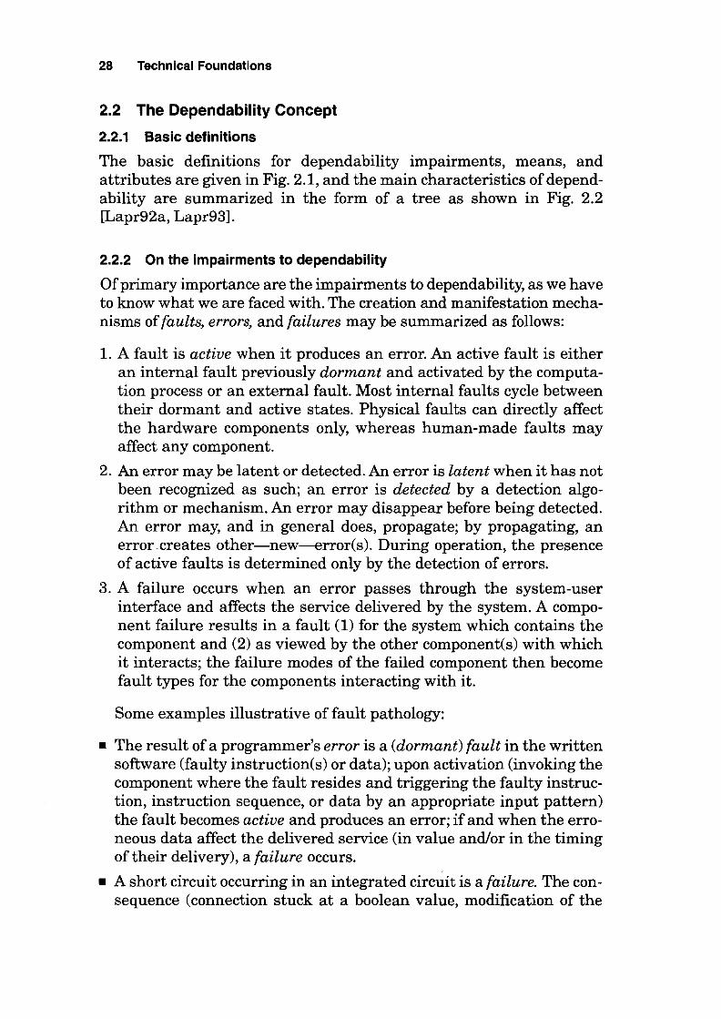
p(j) = P{system failure at the ith input point selection I no failure at the previous input point selections}

te(j) = execution duration associated with theith input selection

We then obtain

k k

Rik) = n [1- p(j)l t = I te(j) )=1 )=1

k

Rik) = n (I - "A(j) te(i) + 0 [te(j) l} )=1

R(t) = lim Rd(k) = exp (- (t "ACt) d't) Vj te(j)-->O Jo

(2.3)

Equation (2.3) is nothing other than the general expression of a system's reliability: see App. B (Sec. B.2), which describes the reliability theory in detail.

It could be argued that the preceding formulations are in fact better suited to design faults or to external faults than to physical faults, since they are based on the existence of a failure domain, which may be nonexistent with respect to physical faults as long as no hardware component fails. It should be remembered that, from the point of view of physics reliability, there is no sudden, unpredictable failure. In fact, a hardware failure is due to anomalies (errors) at the electronic level, caused by physicochemical defects (faults). Or to put it differently, there are no fault-free systems-either hardware or software-there are only systems which have not yet failed. However, the notion of operational fault (i.e., which develops during system operation, and thus did not exist at the start of operational life) is-although arbitrarily [Lapr92al-a convenient and usual notion. Incorporating the notion of operational fault in the previous formulation can be done as follows. Let io be the number of input point selections such that p(j) = ° for i <io, p(j) = p for i ::?io, and u(jo) the associated probability, i.e., u(io) = P{p(j) = O,j <jo; p(j) = p, j ::?jo).

The expression of discrete-time reliability becomes:

k k

Rd(k) = I (1 - p)k -ju u(io), with I u(jo) = 1 )0 = 0 )0 = 0

Going through the same steps as before, we get: R(t) = limte-->o Rik) =

exp (-"At).


What precedes shows that, although the action mechanisms of the various classes of faults may be different from a physical viewpoint according to their causes, a single formulation can be used from a probability modeling perspective. This formulation applies whatever the fault class considered, either internal or external, physical or designinduced. Xn the case of software, randomness results, at least from the trajectory in the input space that will activate the fault(s). In addition, it is now known that most of the software faults still present in operation, after validation, are "soft" faults, in the sense that their activation conditions are extremely difficult to reproduce, hence the difficulty of diagnosing and removing them, * which adds to the randomness.

The constancy ofthe conditional failure probability at execution with respect to the execution sequence is directly related to the constancy of the failure rate with respect to time, as evidenced by Eqs. (2.1) to (2.3). In other words, the points of an input trajectory are not correlated with respect to the failure process. This statement is all the more likely to be true if the failure probability is low, i.e., if the quality of the system is high, and thus applies more to systems in operational life than to those under development and validation. It is an abstraction, however, thus immediately raising the question of how well this abstraction reflects reality.

As far as hardware is concerned, it has been long shown that (see, for example, [Cart70]) the failure rates of electronic components as estimated from experimental data actually decrease with time-even after the period of infant mortality. However, the decrease is generally low enough to be neglected. Going further, the interpretation of the failure data for satellites, as described in [Hech87], establishes a distinction between (1) stable operating conditions where the failure rate is slowly decreasing (namely, a constant failure rate is a satisfactory assumption) and (2) varying operating conditions leading to failure rates significantly decreasing with time.

Similar phenomena have been noticed concerning software: (1) constant failure rates for given, stable, operating conditions [Nage82] and (2) high influence of system load [Cast81]. Also, a series of experimental studies conducted on computing systems have confirmed the significant influence of the system load on both hardware and software failure processes [Iyer82].

The influence of varying operating conditions can be introduced by considering that both the input trajectory and the failure domain IF

* By way of example, a large survey was conducted on Tandem systems [Gray861. From the examination of several dozens of spooler error logs, it was concluded that only one software fault out of 132 was not a soft fault.


may be subject to variations. The variation of the failure domain deserves some comments. It may be due to two phenomena [Iyer82b]:

1. Accumulation of physical faults which remain dormant under low load conditions and are progressively activated as the load increases [Meye88].

2. Creation of temporary faults resulting from the presence of seldomoccurring combinations of conditions. Examples are (1) patternsensitive faults in semiconductor memories, change in parameters of a hardware component (effect of temperature variation, delay in timing due to parasitic capacitance, etc.) or (2) situations occurring when system load rises beyond a certain threshold, such as marginal timing and synchronization. The latter situation may affect software as well as hardware: the notion of temporary faults-especially intermittent faults-also applies to software [Gray86]. Experimental work [McC079] has shown that the failure rates relative to temporary faults decrease significantly with time.

From a probabilistic viewpoint, the failure probability at execution in discrete time, or the failure rate in continuous time, may be considered as random variables. The system reliability then results from the mixture of two distributions:

1. In discrete time, the distribution of the number of nonfailed executions in given operating conditions, thus with a given, constant, failure probability at execution, and the distribution of the probability of failure at execution.

2. In continuous time, the distribution of the time to failure with a given, constant, failure rate, and the distribution ofthe failure rate.

Letgd(P) andgd(A) be the probability density functions of the distributions of the probability offailure at execution and of the failure rate, which may take G values relative to the realizations Pi> i = 1, ... , G, of p, and Ai, i = 1, ... , G, of A. The expression of discrete-time reliability becomes

G

Rd(k) = I (1 - py gipJ i = 1

Going through similar steps as before, we obtain

G

t =k I teigd(P;) i = 1

~ 1· Pi· 1 G lI.i = 1m -, £ = , ... , tei-->O tei


where tei and Ai are the execution time and the failure rate, respectively, for executions carried out under operating condition i, i = 1, ... , G. Finally we get

This is the mixed exponential distribution. Whenp is a co~tinuQus ralldom variable with density functiongc(p),

or A is a continuous random variable with density functiongc(A), we get

R(t) = r exp (-At) gc(A) dA

From the properties of the mixture of distributions (see, for example, [Bar175]), the system failure rate is nonincreasing with time, whatever the distributions gd ~nd gc.

A riwdel is of no use without data. This is where statistics come into play. Let M instances of the system be considered, executed independently. The term independently is a keyword in the following. This is a conventional assumption with respect to physical faults when several sets of hardware are run in parallel, supplied with the same input pattern sequences. Of course, this approach cannot be transposed to software. The independence of the executions of several systems means that they are supplied with independent input sequences. This reflects operational conditions when considering a base of deployed systems; for instance, the input sequences supplied to the same text-processing software by users in different places performing completely different activities are likely to exhibit independence with respect to residual fault activation.

Let M(k) and M(t) be the number of nonfailed instances after k executions of each instance; and after an elapsed time of t, respectively, since the start of the experiment (M(O) = M); an instance failing at the}th execution,} = 1, ... ,k, or at time 't, 't E [0, t], is no longer executed. The independency of execution of the various instances enable these executions to be considered as Bernoulli trials, and the discretetime reliability is thus Rd(k) = E[M(k)]IM(O), and the continuous-time reliability is R(t) = E[M(t)]IM(O). These equations are none other than the basic equations for the statistical interpretation of reliability as stated in the general systems reliability theory (e.g., [Sho073, KozI70]). Statistical estimators of Rd(k) and R(t) are then: Rd(k) = M(k)/M(O) and R(t) = M(t)/M(O). .

The preceding shows that the equations forming the core of the statistical estimation of reliability for a set of hardware systems apply


equally to software systems, provided the experimental conditions are in agreement with the underlying assumptions.

2.3.2 Systems made up of components

2.3.2.1 System models. Adopting the spirit of[Ande81], a system may be viewed from a structural viewpoint as a set of components bound together in order to interact; a component itself is a system, decomposed (again) into components, etc. The recursion ends when a system is considered atomic: no further internal structure can be discerned or is of interest, and can be ignored. The model corresponding to the relation "is composed of" is a tree, whose nodes are the components; the levels of a tree obviously constitute a hierarchy. Such a model does not enable the interactions between the components to be represented: the presence of arcs in a graphic representation would present only the relation "is composed of" existing between a node and the set of its immediate successors. The set of the elements of a level of the tree gives only the list of the system components, with more or less detail according to the tree level considered: the lower the level, the more detailed the list becomes. To obtain a more representative view of the system, the relations existing between the components have to be presented. This is achieved through interaction diagrams where the nodes are the system components and the arcs represent a common interface. An arc exists when two elements can interact. Although the relation "interacts with" is an essential relation when describing a system, it obviously does not infer any hierarchy.

The use of the relations in modeling a system is given in Fig. 2.5 for an intentionally simple system, where the components S1. S2, and S3 can, for instance, be the application software, the executive software, and the hardware.

The respective roles of a system and of its user(s) with respect to the notion of service are fIXed: the system is the producer of the service, and the user is the consumer. Therefore, there exists a natural hierarchy between the system and its user: the user uses the service of (or delivered by) the system.

With respect to the set of components of one given level of the decomposition tree, the relation "uses the service of"-a special form of the relation "interacts with"-allows for an accurate definition of a special class of components: if and only if all the components of the level may be hierarchically situated through the relation "uses the service," then they are layers. Or equivalently, components of a given detail level are layers (1) if any two components of that level playa fixed role with respect to this relation, i.e., either consumer or producer; similarly, (2) if the graph of the relation is a single branch tree. Conversely, if their


(a)

(b)

Figure 2.5 Components of a system. (a) System model according to the relation "is composed of." (b) System model according to the relation "interacts with."

respective consumer and producer roles can change, or if their interactions are not governed by such a relation, they are simply components. It is noteworthy that the notion of service has naturally-and implicitly-been generalized with respect to the layers: the service delivered by a given layer is its behavior as perceived by the upper layer, where the term upper has to be understood with respect to the relation "uses the serviee of." Also worth noting is the fact that the relation "uses the service of" induces an ordering of the time scales of the various layers: time granularity usually does not decrease with increasing layers. Considering the previous example in Fig. 2.5 leads to the model in Fig. 2.6.

Structuring into many layers may be considered for design purposes. Their actual relationship at execution is generally different: compilation removes-at least partially-the structuring, and several layers may, and generally are, executed on a single one. A third type of rela-

S 11 S 12 5 13 S 14

System model according to the relation «uses the service of»

Figure 2.6 Layers of a system.


tion thus has to be considered: "is interpreted by." The interpretive interface [AndeS1] between two layers or sets oflayers is characterized by the provision of objects and operations to manipulate those objects. A system may then be viewed as a hierarchy of interpreters, where a given interpreter may be viewed as providing a concrete representation of abstract objects in the above interpreter; this concrete representation is itself an abstract object for the interpreter beneath the considered one.

Considering again the previous example, the hardware layer interprets the application as well as the executive software layers. However, the executive software may be viewed as an extension of the hardware interpreter-e.g., through (1) the provision of "supervisor call" instructions or (2) the prevention of invoking certain "privileged" instructions. This leads to the system model depicted in Fig. 2.7.

Finally, note that the expression "abstraction level" has not been used so as to avoid any confusion: all the hierarchies defined are, strictly speaking, abstractions.

2.3.2.2 Behavior of a single-interpreter system. A system is assumed to be composed of C components, of respective failure rates Au i = 1, ... , C. The system behavior with respect to the execution process is modeled through a Markov chain with the following parameters:

• S: number ofthe states of the chain, a state being defined by the components under execution

• 1/y;: mean sojourn time in state},} = 1, ... ,S

• qjk = P{system makes a transition from state} to state k I start or end of execution of one or several components},} = 1, ... ,S, k = 1, ... ,S, If=1 qjk = 1

A system failure is caused by the failure of any of its components. The system failure rate ~j in state} is thus the sum of the failure rates of the components under execution in this state, denoted by

c Si = I Oi/Ai'} = 1, ... ,s

Interpretive

interfaces S 3

Figure 2.7 System interpreters.

i = 1

System model according to the relation «is interpreted by.

(2.4)


where OiJ is equal to 1 if component i is under execution in state j, or else it is equal to O.

The system failure behavior may be modeled by a Markov chain with S + 1 states, where the system delivers correct service in the first S states (components are under execution without failure occurrence); state S + 1 is the failure state, which is an absorbing state. Let A = [ajk] , j = 1, ... ,S, k = 1, ... ,S be the transition matrix associated with the nonfailed states. This matrix is such that its diagonal terms ajj are equal to -(Y.I + ~), and its nondiagonal terms ajkJj::F k, are equal to %1< Yi. The matrix A may be viewed as the sum oftwo matrices A' and A" such that: (1) the diagonal terms of N are equal to -Yi, its nondiagonal terms being equal to qjk Yi, and (2) the diagonal terms of A" are equal to -Si, its nondiagonal terms being equal to O.

The system behavior can thus be viewed as resulting from the superimposition of two processes: the execution process, of parameters Yi and qjk (transition matrix A'), and the failure process, governed by the failure rates ~j (transition matrix N').

A natural assumption is that the failure rates are small with respect to the rates governing the transitions from the execution process or, equivalently, that a large number of transitions resulting from the execution process will take place before the occurrence of a failure-a system that would not satisfy this assumption would be oflittle interest in practice. This assumption is expressed as follows: Yi » ~j.

Adopting a Markov approach for modeling the system behavior resulting from the compound execution-failure process is based on this assumption. Similar models have been proposed in the past for software systems [Litt81, Cheu80, Lapr84], with less generality than here, however, since those models assumed a sequential execution (one component only executed at a time). *

By definition, the system failure rate 'A(t) is given by

'A(t) = lim d1

P(failure between t and t + dt I dHO t c'l b . . . l' d } no 1al ure etween mitIa Instant an t

* In these references, the Markov approach was justified:

• Heuristically in [Cheu80, Lapr841, by analogy with performance models in the first reference, and with availability models in the second,

• From a weaker assumption, semi-Markov, in [Litt81]. It is shown there that the compound process of execution and failure converges toward a Poisson process, and that the contribution of the distribution functions of the component execution times is limited to their first moments.


Let Pj(t) denote the probability for the system to be in statej. It follows that

(2.5)

The consequence of the assumption YJ » ~) is that the execution process converges toward equilibrium before failure occurrence. T~e vector a == [aJ of the equilibrium probabilities is the solution of a . A' == 0, with L~=l (X) == 1. Thus, Pit) converges towards (X) before failure occurs, and Eq. (2.5) becomes*: .

s A== L (X)~)

j=l (2.6)

Equation (2.6) may be rewritten as follows, to account for Eq, (2.4):

Let

Equation (2.6) becomes

S

1ti == L ()iJ (X)

j=l

c A==L 1tiA;

i = 1

This equation has a simple physical interpretation:

(2.7)

(2.8)

• (X) represents the average proportion of time spent in state j in the absence of failure; thus 1ti is the average proportion of time when

* Another approach to this result is as follows. A given system component will be executed; thus the transition graph between the nonfailed states is strongly connected. As a result, the matrix A is irreducible and has one real negative eigenvalue whose absolute value cr is lower than the absolute values of the real parts of the other eigenvalues [Page80J. Asymptotically, the system failure behavior is then a Poisson process of rate cr. In our case, the asymptotic behavior is relative to the execution process; therefore, (1) it is reached rapidly and (2) cr = A, thus system reliability is: R(t) = exp(-At).


component i is under execution in th~ absence of failure. It is noteworthy that the sum ofthe 1t/s can be larger than 1:

c Os I1tiSC

i = 1

• Ai is the failure rate of component i assuming a continuous execution.

The term 1ti Ai can therefore be considered as the equivalent failure rate of component i.

Equation (2.8) deserves a few comments. First let us consider hardware systems. It is generally considered that all components are continuously active. This corresponds to making all the 1t/s equal to 1, leading to the usual equation

c A= I Iv;

i = 1

Consider software systems. The key question is how to estimate the component failure rates. There are two basic-and oppositeapproaches: (1) exploiting results of repetitive-run experiments without experiencing failures (i.e., through statistical testing [Curr86, Thev91]) and (2) exploiting failure data using a reliability growth model, the latter being applied to each software component, as performed in [Kan087, Kano91a, Kan093b]. It is important to stress the data representativeness in either approach; a condition is that the data are collected in a representative environment (i.e., being relative to components in interaction, real or simulated, with the other system components). If this condition is not fulfilled, a distinction has to be made between the interface failure rates (characterizing the failures occurring during interactions with other components) and the internal component failure rates, as in [Litt81], where the expression of a component failure rate has the form

Ai = 1;i + Yi I % Pi} j

the 1;i being the internal cOUlponent failure rates and Pij the interface failure probabilities. This leads to a complexity in the estimation ofthe order of C2 instead of C.

An important question is how to accour.t for different envirOllInents. If this question is interpreted as estimating the reliability bfa sqftware system of a base of deployed software systems, then the approach indicated in Sec. 2.3.1 where the failure rate was considered'as a random variable can be extended here; the 1t/s being considered as random


variables as well. Another interpretation of the previous question is: knowing the reliability in a given environment, how can the reliability be estimated in another environment? Let us consider sequential software systems. The parameters characterizing the execution process are then defined as follows:

• 1IYi: mean execution time of component i, i = 1, ... , C .

• qij = P{ component} starts execution I end of execution of component iI, i = 1, ... ,C,j = 1, ... ,C, L7=1 % = 1

The Markov chain modeling the compound execution-failure process is a (C + 1) state chain, state i being defined by the execution of componenti, and the rt/s reduce to the a/s (in the cilse of sequential software, (jii = 1 and all others are zeros). We have Ai = Pi 'Yb i = 1, ... ,C, where Pi is the failure probability at execution of component i; hence

c c A = L rti 'YiPi = L TIiPi (2.9)

i=1 i=1

where 11i = rti 'Yi is the visit rate of state i at equilibrium. The l1/s have a simple physical interpretation, as 1I11i is the mean recurrence time of state i (i.e., the mean time duration between two executions of component i in the absence of failure). Equation (2.9) is of interest as it enables a distinction to be made between (1) continuous time-execution process and (2) discrete time-failure process conditioned upon execution. If the p/s are intrinsic to the considered software and independent of the execution process, then it is possible to infer the software failure rate for a given environment from the knowledge of the l1/S for this environment and the knowledge of the p/s. The condition for this assumption to be verified in practice is that it is possible to find a suitable decomposition into components: the notion of component for a software is highly arbitrary, and the higher the number of co.mponents considered for a given software, the smaller the state space of each component, so the higher the likelihood of providing a satisfactory coverage of the input space for the component. A limit to such an approach is that the higher the number of components, the more difficult the estimiltion of the l1/s becomes. Also, time granularity (and near decomposability [Cour77]) can offer criteria to find suitable decompositions.

2.3.2.3 Behavior of a multi-interpreter system. When a system is viewed as a hierarchy of interpreters, as defined in Sec; 2.3.2.1, the execution relative to the selection of an input point for the highest interpreter (which directly interprets the requests originating from the system


user) is supported by a sequence of input point selections in the next lower interpreter, and so on up to the lowest considered interpreter. Assume the system is composed of I interpreters, the first interpreter being the top of the hierarchy and the Ith interpreter its base.

Each interpreter may be faulty and submitted to erroneous inputs. Failure of any interpreter during the computations relative to the input point selection of the next higher interpreter will lead to the failure of the latter, and thus by propagation to the top interpreter's failure (i.e., to system failure). Adopting the terminology of the conventional system reliability theory, the hierarchy interpreters constitute a series system. Intuitively, it may be deduced that the system failure rate is equal to the sum of the failure rates of interpreters of the hierarchy. If Ai(t), i = 1, ... , I denotes the failure rate of interpreter i, we then have (the demonstration is left as an exercise to you):

I

A(t) = I Ai(t) (2.10) i = 1

Now consider that each interpreter is composed of Ci components, i = 1, ... , 1. At execution, a component of interpreter i will use services of one or more components of interpreter i + 1, and so on. We may therefore define trees of utilization of services provided by components of interpreter i + 1 by the components of interpreter i, as indicated in Fig. 2.8.

Thus, with each pair of adjacent interpreters, it is possible to associate a service utilization matrix Ui,i + 1 = [Ujk],j = 1, ... , Cu k = 1,., Ci + 1.

Ui,i + 1 is a connectivity matrix whose terms Ujk are such that Ujk = 1 if, during execution, component j of interpreter i utilizes the services of component k of interpreter i + 1, or else U;k = O.

Let us define the following failure rate vectors:

• Ai = [Aij] , i = 1, ... ,I, j = 1, ... ,Ci, where AU is the failure rate of componentj of interpreter i .

• Q i = [roij], i = 1, ... ,I, j = 1, ... , Ci; roij is the aggregated failure rate of component j of interpreter i; the term aggregated means that the failure rates of components of interpreters i + 1, ... , I needed for execution are accounted for.

I ;+1,1 ;+1,2

components

interpreter ;

. 1 C 1 I interpreter;+ 1 1+, j+

Figure 2.8 Utilization trees between components of interpreters.


The vectors Oi are solutions of the following matrix equation:

Oi = Ai + Vi,i + 1 Oi + h i = 1, ... ,I - 1, OJ = AJ

It then follows that:

V k is the accessibility matrix of the top interpreter to interpreter k: V1 is the identity matrix of dimensions (C1 x C1), V k = V 1,2 ® V 2,3, •.. , ® V k -1,'" k = 2, ... ,I; where the symbol ® denotes the boolean product of matrices (a given component can contribute only once through its failure rate).

When applying Eq. (2.8) to the components of the upper interpreter in the hierarchy, we obtain the following system failure rate:

Cl

A = I 1t1,} W1,} j=l

where 1t1,} is the proportion oftime during which component} of the top interpreter is being executed, with an idle component period being characterized by W1,} = O.

Consider the important case in practice of a system composed of two interpreters: a software interpreter and a hardware interpreter. It is assumed that the software components are executed sequentially, and that all hardware components are together involved in the execution; it is further assumed that the system is in stable operating conditions. In the following, indices Sand H relate to software and hardware, respectively. Applying the above approach leads to the following equations:

CH

WS,} = AS,} + I AH,k k=l

Cs Cs CH

A = I 1tS,} WS,} = I 1tS,} AS,} + I AH,k j=l j=l k=l

(2.11)

The intuitive result expressed in Eq. (2.11) has thus been obtained through use of a rigorous approach.

2.4 Failure Behavior of an X-ware System with Service Restoration

In Sec. 2.3, the behavior of atomic and multicomponent systems was characterized without taking into account the effects of service restoration, thereby allowing expressions of the failure rate of such systems


and of the reliability to be derived. In this section, service restoration is taken into account, thus allowing the system behavior resulting from the compound action of failure and restoration processes to be modeled. Restoration activities may consist of a pure restart (supplying the system with an input pattern different from the one which led to failure) or they can be performed after introduction of modifications (corrections only orland specification changes).

System behavior is first characterized by the evolution of its failure intensity in Sec. 2.4.1. Section 2.4.2 introduces the various maintenance policies that can be carried out. Sections 2.4.3 and 2.4.4 address reliability and availability modeling, respectively.

2.4.1 Characterization of system behavior

The nature of the operations to be performed in order for the service to be restored (Le., delivered again to its user(s» after a failure has occurred enables stable reliability or reliability growth to be identified. This may be defined as follows:

• Stable reliability. The system's ability to deliver a proper service is preserved (stochastic identity of the successive times to failure).

• Reliability growth. The system's ability to deliver proper service is improved (stochastic increase of the successive times to failure).

Practical interpretations are as follows:

• Stable reliability. At a given restoration, the system is identical to what it was at the previous restoration. This corresponds to the following situations: (1) in the case of a hardware failure, the failed part is substituted for another one, identical and nonfailed; (2) in the case of a software failure, the system is restarted with an input pattern that differs from the one having led to failure.

• Reliability growth. The fault whose activation has led to failure is diagnosed as a design fault (in software or hardware) and removed.

Reliability decrease (stochastic decrease of the successive times to failure) is both theoretically and practically possible. In this case, it is hoped that the decrease is limited in time and that reliability is globally growing over a long observation time.

Reliability decrease may originate from (1) introduction of new faults during corrective actions, whose probability of activation is greater than that of the removed fault(s); (2) introduction of a new version with modified functionalities; (3) change in the operating conditions (e.g., an intensive testing period; see [Kan087], where such a situation is depicted); (4) dependencies between faults: some software faults can be masked by others, that is, they cannot be activated as long


as the latter are not removed [Ohba841; removal of the masking faults will lead to an increase in the failure intensity.

The reliability of a system is conveniently illustrated by the failure intensity, as it is a measure of the frequency of the system failures as noticed by its user(s). Failure intensity is typically first decreasing (reliability growth) due to the removal of residual design faults either in the software or hardware. It may become stable (stable reliability) after a certain period of operation; the failures due to internal faults occurring in this period are due either to physical faults or to unremoved design faults. Failure intensity generally exhibits an increase (reliability decrease) upon the introduction of new versions incorporating modified functionalities; then it tends toward an asymptote again, and so on. It is noteworthy that such a behavior is not restricted to the operational life of a system but also applies to situations occurring during the development phase of a system-for example, (1) during incremental development [Curr861 or (2) during system integration [Leve89, Tohm891.

Typical variations of the failure intensity may be represented as indicated in Fig. 2.9, curve a. Such a curve depends on the granularity of the observations, and may be felt as resulting from the smoothing of more noticeable variations (curve b); in turn, it may be smoothed into a continuously decreasing curve c. Although such a representation is very general and covers many practical situations (see, for example, [Kenn92]), there are situations which exhibit discontinuities important enough that the smoothing process cannot be considered as reasonable (e.g., upon introduction of a new system generation).

2.4.2 Maintenance pOlicies

The rate of reliability growth (i.e., failure intensity decrease) is closely related to the correction and maintenance policies retained for the sys-

Failure intensity

b

Time

Figure 2.9 Typical variations of a system's failure intensity.


tern [Kano89]. These policies may consist of either (1) system modification after each failure, or (2) system modification after a given number offailures, or even (3) preventive maintenance (i.e., introduction of modifications without any failure observed on the system considered). The status of a system between two modifications will be called a version.

A policy that accepts as special cases the specific cases mentioned above is as follows: the}th system modification takes place after aj failures have occurred since the (j - l)th system modification, which means that version) experiences aj failures.

Concerning the times to failure:

• Let 10,i denote the time between service restoration following the (i - l)th failure and the ith failure of version) .

• Let Zj denote the time between service restoration following the ajth failure of version} and service interruption for the introduction of the}th modification, that is, for the introduction of version (j + 1).

Considering now the times to restoration, two types of service restoration are to be distinguished: service restoration due to system restart after failure and service restoration after introduction of a new version. Let lj,i denote the restart duration after the ith failure of version}, and Wj denote the duration necessary for the introduction of the }th modification; the modification itself may have been performed offline. Finally, let Tj denote the time between two version introductions. We have: .

aj

Tj = I (10,i + lj) + Zj + Wj,} = 1,2, ... i = 1

The relationship between the various time intervals is given in Fig. 2.10.

The number of failures between two modifications (a) characterize the policy for maintenance and service restoration. It depends on sev-

Version 1 Version 2 Versionj

-~-- x· -J,I

~ .. J,I

o SystemUP _ System down after failure ~ System down for version introduction

Figure 2.10 Relationship between the various time intervals.


eral factors such as (1) the failure rate of the system, (2) the nature of the faults (e.g., time needed to diagnose the fault and the consequence of the failure due to the activation of this fault), (3) the considered phase in the life cycle (the policy may vary for a given system within the same phase), and (4) the availability of the maintenance team.

Three (extreme) special cases of this general policy are noteworthy:

1. aj = 1 and Zj = 0 Vj. Service is restored only after a system modification has been performed. This case relates to (1) a usual hypothesis for several software reliability (growth) models or (2) the case of critical systems after a (potentially) dangerous failure occurrence.

2. a1 = 00 and Zj = 0 Vj. Service is restored without any system modification ever being performed (stable reliability). This case relates to (1) hardware, when maintenance consists of replacing a failed part with an identical (new) one and (2) software, when no maintenance is performed; service restoration aiways corresponds to a restart with an input pattern different from the one having led to failure.

3. aj = o. The (j + l)th version is introduced before any failure occurrence since the last modification. This case corresponds to preventive maintenance, either corrective, adaptive, or perfective.

Although this policy is more general than those usually considered, it is a simplification of real life, and does not explicitly model such phenomena as interweaving of failures and corrections [Kano881 and failure rediscoveries [Adam841.

2.4.3 Reliability modeling

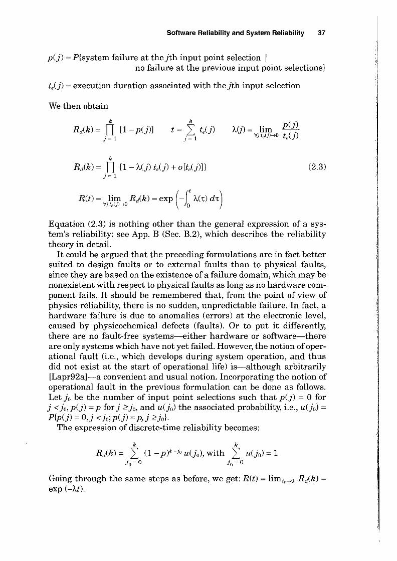
We focus here on the failure process and therefore do not consider the times to restoration or the (possible) time interval between a failure and the introduction of a modification (i.e., we assume the lj,/s, ~'s, and Z/s are zero, which means that the failure instants are also restoration instants). Let:

• to = 0 denote the considered initial instant (the system is assumed nonfailed).

• n = 1,2, ... denote the number of failures. As the nth system failure is in fact the ith failure ofversionj, the relationship between n, i, and J IS

n = (± ak _ 1) + i, j = 1,2, ... , i = 1, ... aj, ao = 0 k=1

• tu. n = 1,2, ... denote the instant of failure occurrence.


• f·dt),j = 1, 2, ... denote the probability density functions (pdf) of the times to failure Xj,i and sfxJt) denote their survival function (the one's complement of its distribution function). The Xj,;'s are assumed stochastically identical for a given version.

• <Pn(t) and n(t) denote, respectively, the pdf and the distribution function of the instants of failure occurrence, n = 1,2, ....

• N(t) denote the number of failures having occurred in [O,t] and R(t) denote its expectation: R(t) = E[N(t)].

Performing derivations adapted from the renewal theory (see, for example, [Gned69]) is relatively straightforward, provided that the Xj,;'s are assumed. stochastically independent. This assumption, although usual in both hardware and software models, is again a simplification of real life. The T/s can reasonably be considered as stochastically independent, as resuming execution after the introduction of a modification generally involves a so-called cold restart; however, it must be stated that imperfect maintenance, the consequences of which were noticed a long time ago [Lewi64], is also a source of stochastic dependency. The stochastic independence of the X j,;'S for a given j depends on (1) the extent to which the internal state of the system has been affected and (2) the nature of operations undertaken for execution resumption (Le., whether or not they involve state cleaning).

The following is then obtained under the stochastic independence assumption

<Pn(t) = 0 fx (t)*ak * (fX(t)*i),j = 1,2, ... , i = 1, ... ,aj, ao = ° (

j -1 )

k = 1 k 1

(2.12)

where * stands for the convolution operation, fXk(t)*ak, the ak-fold convolution offx./t) by itself, and @£=dXk(t), the convolution offxP), ... ,(x{t). In Eq. (2.12) the first term coversj - 1 versions and the second t~rm covers the i failures of versionj. We have

P{N(t) ;::: n} = P{tn < t} = n(t)

P{N(t) = n} = P{tn < t < tn + d = n(t) - n + it)

= = R(t) = I n P{N(t) = n} = I n [n(t) - n + let)]

n=1 n=1

= = =

R(t) = I n n(t) - I (n - 1) n(t) = I n(t) n=1 n=1 n=1


Let h(t) denote the rate of occurrence of failure [Asch84], or ROCOF, hCt) = dH(t)ldt, whence

hCt) = n~l~nCt) = j~l i~l (:$: CfxkCt)*ak) * (('/JCt)*i») C2.13)

As we do not consider simultaneous occurrences of failure, the failure process is regular or orderly, and the ROCOF is then the failure intensity [Asch84].

When considering reliability growth, a usual measure of reliability is conditional reliability [GoeI79, Musa84]; since the system has experienced n - 1 failures, conditional reliability is the survival function associated with failure n. It is defined as follows:

RnC 1) = P{Xj,i + 1 > 1 I tn - d = sfxC 1), for i < aj 1

C2.14)

This measure is mainly of interest when considering a system in its development phase, as we are then concerned with the time to next failure. However, when dealing with a system in operational life, the interest is in failure-free time intervals 1 whose starting instants are not necessarily conditioned on system failures; that is, they are likely to occur at any time t. In this case, we are concerned with the reliability over a given time interval independently of the number of failures experienced, that is, interval reliability. Interval reliability is then the probability for the system to experience no failure during the time interval [t, t + 1].

Consider the following exclusive events:

En = Itn < t < t + 1 < tn + 1}, n = 1,2, ...

Event En means that exactly n failures occurred prior to instant t, and that no failure occurs during the interval [t, t + 1]. The absence of failure during [t, t + 1] is the union of all events Em n = 0,1,2, ... The interval reliability, owing to the exclusivity of the events En> is then

~

RCt, t + 1) = L P{En }

n=O

The probability of event En is shown as

P{En } =Pltn < t <t + 1 < tn +Xj,i + 1}

P{En} = Jtp{x < tn < x + dx} P{Xj,i + 1> t + 1 - x} = Jtsfx (t + 1 - x) ~nCx) dx o 0 J

I


The reliability thus has the expression

= aj-l t

R(t,t + 't) = sfx,(t + 't) + j~l i~O t sfxP + 't - x) <Petak-I) + i (x) dx

which can be written as

(2.15)

This equation is obviously not easy to use. However, it is not difficult to derive, for 't« t, the following equation from Eqs. (2.13) and (2.15):

R(t,t + 't) = 1 - h(t) 't + o( 't) (2.16)

Besides its simplicity, Eq. (2.16) is highly important in practice, as it applies to systems for which the mission time 't is small with respect to the system lifetime t (e.g., systems on board airplanes).

The above derivation is a (simple) generalization of the renewal theory and of the notion of renewal process to non stationary processes; in the classical theory (stationary processes), (1) the Xj,/s are stochastically identical, that is, fxet) = fxU) Vj (the case where the first time to failure has a distributiJn different from the subsequent ones is referred to as modified renewal process in [Cox62, Biro74]) and (2) H(t) and h(t) are the renewal function and the renewal density, respectively.

Consider the case where the Xj,/s are exponentially distributed: fx(t) = Aj exp(-~t). The interfailure occurrence times in such a case constit~te a piecewise Poisson process. No assumption is made here on the sequence of magnitude of the ""s. However, it is assumed that the failure process is converging toward a Poisson process after r modifications have taken place. This assumption means that either (1) no more modifications are performed or (2) if some modifications are still being performed, they do not significantly affect the failure behavior ofthe system. Let {Al> A2, ••• ,

A,.} be the sequence ofthese failure rates (Fig. 2.11). The Laplace transform Ii(s) ofthe failure intensity h(t) (Eq. (2.13)) is:

Derivation of h(t) is very tedious (see Prob. 2.6). Thus our study will be limited to summarizing the properties of the failure intensity h(t) that can be derived:

• h(t) is a continuous function of time, with h(O) = Al and h(oo) = Ar.


A (t)

• • • -----1-------------------------

I

Figure 2.11 Sequence of failure rates .

• When the a/s are finite,

-A condition for h(t) to be a nonincreasing function of time (i.e., a condition for reliability growth) is 1.1 ~ 1.2 ~ ... ~ "-i ~ ... ~ Ar •

-The smaller the a/s, the faster the reliability growth becomes. -If a (local) increase in the failure rates occurs, then the failure

intensity correspondingly (locally) increases .

• When a1 = 00, no correction takes place and we are faced with a classical renewal process; then h(t) = 1.1 V t E [0,00]' which is the formulation of stable reliability.

These results are shown in Fig. 2.12, where the failure intensity is plotted for aj ::::! a Vj.

Typical variations of conditional reliability RnCr,) (Eq. (2.14)) are given by Fig. 2.13. When stable reliability is assumed, the underlying process is a classical renewal process with RnCt) = R 1(;;), n = 2, 3, .... For a so-called modified renewal process (the case where the first time to failure has a distribution different from the subsequent ones [Cox62, Biro74]), we usually have Rn(;;) < R 1(;;), n = 2, 3, ... ,with Rn(;;) = R 2(;;),

n ~ 3.

h(t)

8=fXl A1~------------~~----------------

8=1 1..(1- - - - -- - - - - - - - - -

Figure 2.12 Failure intensity.


•••

o t

Figure 2.13 Conditional reliability.

Interval reliability R(t,t + 1) for a given, finite, a (which corresponds to a given curve of Fig. 2.12) can then be derived from Eq. (2.16) for 1 « t. Figure 2.14 indicates typical variations of R(t,t + 1): reliability over mission time 1 increases with system lifetime t. In case of stable reliability (i.e., a classical renewal process), interval reliability is independent ofthe time origin t: the curves of Fig. 2.14 are thus not distinguishable; however, for a modified renewal process, depending on the granularity of time representation versus the mean time to failures, two groups of curves may be distinguished depending on the values of t compared to the mean time to failures.

Although still suffering from some limitations such as the assumed independency between the times to failure necessary for performing the renewal theory derivations, the derivations conducted in this section are more general than what has been previously published. The resulting model can be termed a knowledge model [Lapr91] with respect to the reliability growth models which have appeared in the literature, which can be termed action models. Support for this terminology, adapted from the Automatic Control theory, lies in the following remarks:

R(t,t+'t)

1

Figure 2.14 Interval reliability.


• The knowledge model allows the various phenomena to be taken into account explicitly and enables a number of properties to be derived; nevertheless, it is too complex in practice and not suitable for predictions .

• The action models, although based on more restrictive assumptions, are simplified models suitable for practical purposes.

The results obtained from the knowledge model thus derived in this section enable the action models reported in the literature to be classified as follows:

1. Models based on the relation between successive failure rates, which can be referred to as failure rate models; these models describe the behavior between two failures. Two categories offailure rate models can be distinguished according to the nature of the relationship between the successive failure rates: (1) deterministic relationship, which is the case for most failure rate models; see, for example, [Jeli72, Shoo73, Musa75l; (2) stochastic relationship [Kei183, Litt88l; the corresponding models are known as doubly stochastic reliability growth models in [Mill86l.

2. Models based on the failure intensity, thus called failure intensity models; these models describe the failure process, and are usually expressed as nonhomogeneous Poisson processes; see, for example, [Crown, Goe179, Yama83, Musa84, Lapr91l.

Most reliability growth models consider reliability growth stricto sensu, without taking into account possible stable reliability or reliability decrease periods: they assume that the failure rate and/or the failure intensity decrease monotically and become asymptotically zero with time. Note, however, that the S-shaped models [Yama83, Tohm89l relate to initial reliability decrease followed by reliability growth, and that the hyperexponential model [Lapr84, Kano87, Lapr91l relates to reliability growth converging toward stable reliability. Finally, it is noteworthy that the models referenced above have been established specifically for software; however, there is no impairment to apply them to hardware [Litt81l; conversely, the Duane's model [Duan64], derived for hardware has been successfully applied to software [KeiI83l. Chapter 3 provides a comprehensive survey of these reliability models.

Of prime importance when considering the practical use of the above models is the question of their application to real systems. Failure data can be collected under two forms: (1) times between failures or (2) number of failures per unit of time (failure-count data). Failure rate models are more naturally suited to data in the form oftimes between failures whereas failure intensity models are more naturally suited to data in


the form of number of failures per unit of time. However, some models accommodate both forms of failure data, such as the logarithmic Poisson model [Musa84] or the hyperexponential model. The collection of data under the form "number of failures per unit of time" is less constraining than the other form, since one does not have to record all failure times; the definition of the unit of time can be varied throughout the life cycle of the system according to the amount of failures experienced, e.g., from a few days to weeks during the development phase, and from a few weeks to months during the operational life.

As action models are based on precise hypotheses (particularly with respect to the reliability trends they can accommodate, as discussed above), it is helpful to process failure data before model application, in order to (1) determine the reliability trend exhibited by the data and (2) select the model(s) whose assumptions are in agreement with the evidenced trend [Kano91b]. Trend tests are given detailed treatment in Chap. 10.

2.4.4 Availability modeling

All the time intervals defined in Sec. 2.4.2 are now considered, i.e., the times to failure and the times to restoration: the lj,/s, Z/s, and llj's are no longer assumed to be zero. For simplicity, it is assumed that the times to restoration after failure are stochastically identical for a given version, i.e., lj,i = lj. Let:

• t"o = 0 denote the considered initial instant (the system is assumed nonfailed).

• n stand for the number of service restorations that took place before instant t.

• t'n and t"n, n = 1,2, ... be the instants when correct service is no longer delivered and when service is restored, respectively, either:

-Upon (respectively after) failure, with n = ILl (ak-1 + 1) + i, j = 1,2, ... , i = 1, ... aj, ao = 0

-Upon (respectively after) stopping the operation of system in order to introduce a modification, with n = L {: ~ (ak -1 + 1), j = 1,2, ... , ao = 0

• frit), fZj(t), fw/t),j = 1,2, ... denote the probability density functions (pdf's) of the lj's, Z/s, and W/s, respectively, and sf4t) the survival function of the Z/s.

• "'n(t) be the pdf of the instants of service restoration, n = 1,2, ...

Derivation of availability is performed as in the case of reliability, with the pdf ofthe instants of service restoration "'n(t) replacing the pdf


of the instants of failure occurrence <Pn(t). As in Sec. 2.4.3, we assume that the various time intervals under consideration are stochastically independent, which leads to:

)

• For n = I (ak - 1 + 1) + i k=1

)+1

• For n = I (ak - 1 + 1) k=1

)

'I'n(t) = 0 (fx (t) * f~;Ct»*ak * (fz (t) * f'W, (t») k=1 k k k k

Let us consider the event En = W: < t <t:+ 1}' n = 0,1,2, .... The event En means that exactly n service restorations took place before instant t, and that the system is nonfailed at instant t. The pointwise availability A(t), denoted simply by availability in the following, is then, due to the exclusivity of events En:

= A(t) = I P{En }

n=O

The probability of event En is:

)

• For n = I (ak -1 + 1) + i : P{En } = PW: < t < t + 't < t': + Xj,i + I} k=1

P{En} = It P{x < t': < x + dx} P{Xj,i + 1 > t - x} = It sfx(t - x) 'I'n(X) dx o 0 J

)+ 1

• For n = I (ak - 1 + 1) k=1

P{En} = PW: < t < t + 't < t': + Z) = It sfz(t -x) 'I'n(X) dx o J

The expression of A(t) is then

=

A(t) = sfx1(t) + I x )=1

( sfx}t) * ai 1 '1'( + ")(t) + sfzlt) * 'I'(j~l )(t)) i = 0 L.- (ak - 1 + 1) + , L.- (ak _ 1 + 1)

k=l k=l


Statistical E:stimation of the availability of a set of systems is given by the ratio of nonfailed systems at time t to the total number of systems in the set. When field data are related to times to failure and to times to restoration, considering the average availability rather than availability facilitates the estimation process, as the average availability is the expected proportion of timea system is nonfailed (see, for example, [Barl75]). The average availability over [O,t] is defined by

Aav(t) = ~ft A('t) d't t 0

Denoting respectively UTi the observed times where the system is operational, a statistical estiniator of Aav(t) is given by the following analytical expression

A 1 n Aav(t) = - I UTi

t i = 1

So far, no assumption has been made on the pdfs of the various times considered. To derive properties of the availability, consider the case where:

• A modification takes place after each failure, i.e., aj = 1, Zj = W; = 0 V j,

• The 10'/s and the Yj's are exponentially distributed: fxit) = Aj exp( -V), frit) = Ilj exp(-Ili), and that both corresponding piecewise Poisson processes converge toward Poisson processes after r modifications have taken place.

Then the Laplace transform A(s) of availability is

The times to failure are large with respect to the times to restoration, i.e., A)llj « 1. Performing a~ asymptotic development with respect to A)llj for the unavailability A(t) = 1 - A(t) leads to

- A r-1 A A(t) = _r + I aj exp (-Ai) - _1 exp (-1l1t)

Ilr j= 1 III (2.17)

with


The aj is linked by the following equation:

The following properties can be derived from Eq. (2.17), thus confirming and generalizing what had previously been established in [Cost78, Lapr84J through modeling via multistate Markov and semiMarkov chains:

PI. When reliability becomes stable, unavailability becomes constant: A( 00) '" A,/f.Lr.

P2. If (A/f.Ll) ~ (A'/f.Lr), then there is an overshoot of unavailability in comparison with the asymptotic value (Arlf.Lr).

P3. There is a single unavailability maximum (availability minimum) if (A.; + /f.Lj + 1) ~ (A/f.L), for j = 1, ... ; conversely, local maxima (minima) occur.

P4. If the piecewise Poisson process of the interfailure occurrence times is continuously nonincreasing from Al to An and if the times to failure are large with respect to the times to restoration, then Amax '" (A/f.Ll)'

P5. The time to reach the maximum unavailability (minimum availability) is of the ordf:)r of magnitude of the mean time to restoration (l/f.Ll)'

P6. The changes in availability are significantly more influenced by the stochastic changes in the times to failure than by the stochastic changes in the times to restoration, which can thus be assumed as stochastically identical over the system's life.

Figure 2.15 gives the typical shape of system unavailability in the presence of reliability growth.

A(t)

Figure 2.15 Typical system unavailability.


In case of stable reliability, ('A; = 1.1. j = 1, ... , r), assuming Ilj = Ill. j = 1, . ~ . , r, the maximu~ corresponds to the asymptotic unavailability. ThuEl we have A( 00) = Amax.

Although the availability of operational computing systems is usually significantly influeI1-<::ed in the field by reliability growth (for instance, the data displayed in [Wall84] for AT&T's ESS-4 show that

; "

unavailability is decreased by a factor of250 during 3.5 years of opera-tion), the only published action model for availability in the presence of reliab~lity growth is the hyp~rexponential model [Lapr91].

2.5 Situation with Respect to the State of the Art in Reliability Evaluation

Hardware evaluation and software evaluation have followed courses which could hardly have been more distant from each other.

Hardware evaluation has focused on the operational life, placing the emphasis on the influence of the system structure on dependability. A number of signific~nt results have been derived with respect to (1) the role and influence of the coverage of the fault-toleranc~ strategies and mechanisms [Bour69, Arno73]; (2) the construction [Beya81] and processing [Gros84, Bobb86, Cour77] oflarge, stiff, Markov models; (3) the definition and evaluation of performance-related measures of dependability, which are usually gathered in the concept of performability [Meye78, Smit88]. These results have been integrated into software packages, such as ARIES, HARP, SAVE, and SURF. As far as elementary data are concerned, reliance has generally been placed on databases such as the MIL-HDBK-217, whic4 are limited to permanent faults, whereas it is currently agreed that temporary faults constitute a major source of failure [Siew92]. In addition, it has largely been ignored that the reliability of hardware parts grows significantly during the whole system's life, as shown, for example, in the experimental data displayed in [Baue85].

Software evaluation has mainly focused on the development phase, and especially on the reliability growth of single-component (blackbox) systems. Many models have been proposed (see surveys such as [Rama82, Yama85] and Chap. 3). Less attention has been paid to accounting for th~ structure of a software Elystem, where most or'the corresponding work has been restricted to the failure process, either for non-fault-tolerant [Litt81, Lapr84] or for fault-tolerant software systems [Hech79, Grna80, Lapr84, Arla88]; only our recent work [Lapr91, Kano93a] deals with the evaluatlon of the reliability growth of a system from the reliability growth ofits components. In [Lapr91] a so-called transformation approach based on a Markov interpretation of the hyperexponential reliability growth model is derived: the pyperex-


ponential model is regarded as resulting from the transformation of a traditional Markov model (stable reliability) into another Markov model, which, through a suitable addition of states, enables reliability growth phenomena to be accounted for. This stable reliability-reliability growth transformation-is shown to be applicable to the Markov models of systems made up of components. In particular, it enables the reliability and the availability of systems to be evaluated from the reliability growth of their components. This approach has been applied to model the reliability growth of fault-tolerant software systems (recovery blocks, N-version programming and N self-checking programming; see Chap. 14) in [Kan093a].

From the practical utilization viewpoint, the situation can be summarized as follows:

• Hardware evaluation is fairly well included in the design process; although the estimations are usually carried out more as an adjunct to the design methodology than an integral part of producing an optimized design, predictive evaluations of operational dependability are routinely performed during the design of a system .

• In the vast majority of software developments, evaluation (if any) is extremely limited, and most of the published work devoted to applications on real data is in fact post mortem work.

However, when dealing with the assessment of dependability, the users of computing systems are interested in figures resulting from modeling mid evaluation of systems, composed of hardware and software, with respect to both physical and design faults. This statement may be supported by considering:

1. The requirements for systems in terms of dependability; an example is provided by the requirements for electronic switching systems [Clem87] (Fig. 2.16), in which it is explicitly stated that they apply to both hardware and software, especially in terms of reliability and availability.

2. The sources of failure of computing systems; an example of sources of failures is given in Fig. 2.17, showing results of a survey on the sources of unavailability for electronic switching systems and transaction processing systems [Toy85]. Clearly, an evaluation which would be performed with respect to hardware failures only would not be representative of the actual behavior of the considered systems, and this situation is exacerbated even more when considering (hardware) fault-tolerant systems, where software is the dependability bottleneck, as it contributes to more than half the system failures [Gray90].

II


The hardware and software for switching systems must be designed to meet the requirements shown in the table below.

Operation • Continuous (20 years)

Time shared channels • Thousands

Recovery time • Critical

Value of reliability • High 1 call per 100,000 call cut off

Downtime • <3 minutes/year

Synchronization • Network sync

Database changes System growth }

All must be done with the system on-line and operational Program changes Maintenance

Figure 2.16 Requirements for ESSs.

Faced with these user requirements, the evaluations of the system's dependability in terms of hardware and software are not common practice compared to the large amount of evaluations considering only hardware. Hardware and software evaluations generally address stable reliability [Rohn72, AveySO, AnguS2, StarS7, PignSS, Duga94l, with a few exceptions accounting for reliability growth [Cost7S, Lapr91]. Evaluations dedicated to reliability growth are based on either multistate Markov modeling [Cost7S] or on Markov modeling combined with the above-mentioned transformation approach [Lapr91]. For evaluations related to stable reliability, various modeling techniques are used: semiMarkov modeling [StarS7] or Markov modeling used either (1) alone [Rohn 72, AveySO, AnguS2] or (2) together with other techniques such as fault tree analysis [Duga94b] or block diagrams [PignSS].

In addition, standardization bodies and regulating agencies are increasingly aware of the need to perform evaluations encompassing

Unavailability Electronic Transaction sources switching processing

Hardware failures 40% 20%

Environment 5%

Software failures 15% 30%

Recovery deficiencies 35%

Incorrect procedures 20% 30%

Others such as u datin p g 5%

Figure 2.17 Sources of failures.


Studies have been conducted for ESA into software reliability requirements for ESA Space programmes. These studies, conducted in 1986, concluded:

a) Software failure is a process that appears to the observer to be "random", therefore the term "reliability" is meaningful when applied to a system which includes software, and the process can be modeled as stochastic.

b) The definition of "Reliability" is identical for a system which includes software as it is for a purely hardware system. It is the classical definition: "the probability of successful operation for a given period under given conditions".

c) The specification of numerical levels of reliability for a complete system is meaningless unless the reliability ofthe software which it contains is similarly quantified and the level of reliability achieved by that software is verified.

Figure 2.18 Statement from ESA.

both hardware and software. Two such examples are given in Figs. 2.18 and 2.19. The example in Fig. 2.18 is extracted from an invitation to tender from ESA, the European Space Agency [ESA88], and reports the conclusions derived from the studies conducted for ESA in 1986. The example in Fig. 2.19, extracted from the British Standard [BStd86] (Part 4) is more general since it addresses all types of systems containing software. Unfortunately, despite the existence of such recommendations made several years ago, the specification of software reliability is far from being a common activity.

Clearly, the results presented in this chapter show that the current limitation to the practicality of dependability evaluations of hardware

Specification of reliability for systems containing software (Section 3.1. 7)

The mechanisms for the specification of reliability requirements, from the point of view of the failure of an item to perform its function, should be no different for systems containing software than for any other. It is imperative that there should be no discrimination between failures due to logical faults in the system from those due to physical breakdown. The following areas, however, require special consideration:

a) In the prediction of reliability, allowance should be made for the contribution made by logical errors to the overall unreliability of the system. At the moment, prediction of such a contribution, particularly before testing begins, is neither accurate nor well understood. Experience from similar systems is the most likely source of such data.

b) The contribution of logical errors to system unavailability should be considered. Although there is no 'repair' in the strict sense, depending upon the design, considerable time may elapse after a after a failure before operation restart.

c) The principal area in which failures due to logical errors differ from physical failure is that such failures do not require spares, routine maintenance, and repair resources generally required for hardware. However, the inclusion of software in the system may indicate the need for a software facility and requirement for this facility should be separately considered.

Figure 2.19 Recommendations from British Standards.


and software systems is not due to theoretical impediments. The lack of credibility of predictive software reliability evaluations lies therefore in the capabilities of the current reliability growth models-the action models in our terminology-with regard to the failure data upon which their predictions are based. When the predictions and failure data are homogeneous, they apply to the same phase of the system life (either development or operation) and are commensurate; then the application of those models is greatly facilitated, and the evaluations done are meaningful. The problem lies in heterogeneous situations, typically predicting operational dependability from failure data collected during development. The current models, which are fundamentally performing extrapolations, then fall out (a typical situation is that the software will exhibit a reliability in operation that is hopefully much better than predicted from failure data collected during its development), and new approaches are needed, such as those proposed in (1) [Lapr92cl via the so-called product-in-a-process approach, aimed at enhancing the reliability prediction for a given software when exploiting field data collected for former, similar software or (2) [Ham1931 via the amplification of software reliability testing.

2.6 Summary

In this chapter, we addressed the problem of software reliability and system reliability. Following our discussion of the dependability concept, we dealt with system behavior up to the (next) failure. We also focused on the sequence of failures when considering restoration actions consecutive to various forms of maintenance. The assumptions made for derivation purposes were carefully stated and analyzed, and we commented at length on the results obtained in order to relate them to the existing body of results. Furthermore, we described a generalization of the classical, hardware-oriented, reliability theory in order to incorporate software as well. This chapter is then concerned with reliability growth phenomena; since most published material on reliability growth is software-oriented, this chapter can be regarded as a generalization to include hardware as well. Finally, we were devoted to position the results obtained with respect to the state of art in dependability evaluation, considering both hardware and software.

Problems

2.1 Some illustrative examples of sequences fault-error-failure are given in Sec. 2.2.2. Considering physical and design faults, give similarities and differences with respect to fault creation mode and manifestation mode.


2.2 Give other examples of the sequence fault-error-failure.

2.3 In Sec. 2.3.1, a general formulation of the reliability R(t) as a function of the distribution of the failure rate A (ge(A» is given. It is stated that a gamma distribution for A leads to a Pareto distribution for R(t). Demonstrate this result.

2.4 Considering a multi-interpreter system viewed as a hierarchy of interpreters, Eq. (2.10) gives the relationship between the failure rate of the system and the failure rates of its interpreters. Demonstrate this result.

2.5 The results ofthis chapter show that the same approaches can be applied to hardware and software systems; for those who are familiar with Markov modeling, construct the Markov chain of a multi-interpreter system with a hardware and a software interpreters. The hardware interpreter is made of two hardware redundant components (failure rate of a component Ah, repair rate /.1) and the software interpreter is made of one component (failure rate As> restart rate 0). Derive the reliability of the system.

2.6 Section 2.4.3 gives the expression of the Laplace transform of the failure intensity, h(s), related to the sequence of failure rates presented in Fig. 2.11. Assuming operation restart after correction only (aj = 1 V j), derive the equation given the temporal expression of the failure intensity function h(t).

2.7 As in the previous exercise, assuming operation restart after correction only (aj = 1 V j), derive the expression of the conditional reliability, Rn(t) from Eq. (2.14), and derive the plot of R(t) (Fig. 13).

2.8 As in the previous exercises, assuming operation restart after correction only (aj = 1 V j), derive the expression of the interval reliability, R(t, t + t) (Eq. (2.16) and Fig. 14).

2.9 Considering the following sequence offailure rates,

A.o = A, Al = [en - l)ln] A, A2 = [en - 2)!n] A ... An-1 = [lin] A, An = 0

derive the expressions of the failure intensity, the conditional reliability and the interval reliability.

I h !

I' i

Software Reliability and System Reliability

Documents