Freescale Semiconductor Application Note © 2008–2010 Freescale Semiconductor, Inc. The Fast Fourier Transform (FFT) is a numerically efficient algorithm used to compute the Discrete Fourier Transform (DFT). The Radix-2 and Radix-4 algorithms are used mostly for practical applications due to their simple structures. Compared with Radix-2 FFT, Radix-4 FFT provides a 25% savings in multipliers. For a complex N-point Fourier transform, the Radix-4 FFT reduces the number of complex multiplications from N 2 to 3(N/4)log 4 N and the number of complex additions from N 2 to 8(N/4)log 4 N, where log 4 N is the number of stages and N/4 is the number of butterflies in each stage. FFTs are of importance to a wide variety of applications, such as telecommunications (3GPP-LTE, WiMAX, and so on). For example, Orthogonal Frequency Division Multiplexing (OFDM) signals are generated using the FFT algorithm. This application note describes the implementation of the Radix-4 decimation-in-time (DIT) FFT algorithm using the Freescale StarCore SC3850 core. The document discusses how to use new features available in the SC3850 core, such as dual-multiplier, to improve the performance of the FFT. Code optimization and performance results are also investigated in this document. Typical reference code is included in this document to demonstrate the implementation details. Document Number: AN3666 Rev. 0, 11/2010 Contents 1. Introduction . . . . . . . . . . . . . . . . . . . . . . . . . . . . . . . . . 2 2. Radix-4 FFT Algorithm . . . . . . . . . . . . . . . . . . . . . . . 4 3. SC3850 Data Types and Instructions . . . . . . . . . . . . 15 4. Implementation on the SC3850 Core . . . . . . . . . . . . 21 5. Experimental Results . . . . . . . . . . . . . . . . . . . . . . . . 47 6. Conclusions . . . . . . . . . . . . . . . . . . . . . . . . . . . . . . . . 50 7. References . . . . . . . . . . . . . . . . . . . . . . . . . . . . . . . . . 50 Software Optimization of FFTs and IFFTs Using the SC3850 Core

Welcome message from author
This document is posted to help you gain knowledge. Please leave a comment to let me know what you think about it! Share it to your friends and learn new things together.
Transcript
Freescale SemiconductorApplication Note
© 2008–2010 Freescale Semiconductor, Inc.
The Fast Fourier Transform (FFT) is a numerically efficient algorithm used to compute the Discrete Fourier Transform (DFT). The Radix-2 and Radix-4 algorithms are used mostly for practical applications due to their simple structures. Compared with Radix-2 FFT, Radix-4 FFT provides a 25% savings in multipliers. For a complex N-point Fourier transform, the Radix-4 FFT reduces the number of complex multiplications from N2 to 3(N/4)log4N and the number of complex additions from N2 to 8(N/4)log4N, where log4N is the number of stages and N/4 is the number of butterflies in each stage. FFTs are of importance to a wide variety of applications, such as telecommunications (3GPP-LTE, WiMAX, and so on). For example, Orthogonal Frequency Division Multiplexing (OFDM) signals are generated using the FFT algorithm.
This application note describes the implementation of the Radix-4 decimation-in-time (DIT) FFT algorithm using the Freescale StarCore SC3850 core. The document discusses how to use new features available in the SC3850 core, such as dual-multiplier, to improve the performance of the FFT. Code optimization and performance results are also investigated in this document. Typical reference code is included in this document to demonstrate the implementation details.
Document Number: AN3666Rev. 0, 11/2010
Contents1. Introduction . . . . . . . . . . . . . . . . . . . . . . . . . . . . . . . . . 22. Radix-4 FFT Algorithm . . . . . . . . . . . . . . . . . . . . . . . 43. SC3850 Data Types and Instructions . . . . . . . . . . . . 154. Implementation on the SC3850 Core . . . . . . . . . . . . 215. Experimental Results . . . . . . . . . . . . . . . . . . . . . . . . 476. Conclusions . . . . . . . . . . . . . . . . . . . . . . . . . . . . . . . . 507. References . . . . . . . . . . . . . . . . . . . . . . . . . . . . . . . . . 50
Software Optimization of FFTs and IFFTs Using the SC3850 Core
Software Optimization of FFTs and IFFTs Using the SC3850 Core, Rev. 0
2 Freescale Semiconductor
Introduction
1 Introduction
1.1 OverviewThe discrete Fourier transform (DFT) plays an important role in the analysis, design, and implementation of discrete-time signal processing algorithms and systems because efficient algorithms exist for the computation of the DFT. These efficient algorithms are called Fast Fourier Transform (FFT) algorithms. In terms of multiplications and additions, the FFT algorithms can be orders of magnitude more efficient than competing algorithms.
It is well known that the DFT takes N2 complex multiplications and N2 complex additions for complex N-point transform. Thus, direct computation of the DFT is inefficient. The basic idea of the FFT algorithm is to break up an N-point DFT transform into successive smaller and smaller transforms known as butterflies (basic computational elements). The small transforms used can be 2-point DFTs known as Radix-2, 4-point DFTs known as Radix-4, or other points. A two-point butterfly requires 1 complex multiplication and 2 complex additions, and a 4-point butterfly requires 3 complex multiplications and 8 complex additions. Therefore, the Radix-2 FFT reduces the complexity of a N-point DFT down to (N/2)log2N complex multiplications and Nlog2N complex additions since there are log2N stages and each stage has N/2 2-point butterflies. For the Radix-4 FFT, there are log4N stages and each stage has N/4 4-point butterflies. Thus, the total number of complex multiplication is (3N/4)log4N = (3N/8)log2N and the number of required complex additions is 8(N/4)log4N = Nlog2N.
Above all, the radix-4 FFT requires only 75% as many complex multiplies as the radix-2 FFT, although it uses the same number of complex additions. These additional savings make it a widely-used FFT algorithm. Thus, we would like to use Radix-4 FFT if the number of points is power of 4. However, if the number of points is power of 2 but not power of 4, the Radix-2 algorithm must be used to complete the whole FFT process. In this application note, we will only discuss Radix-4 FFT algorithm.
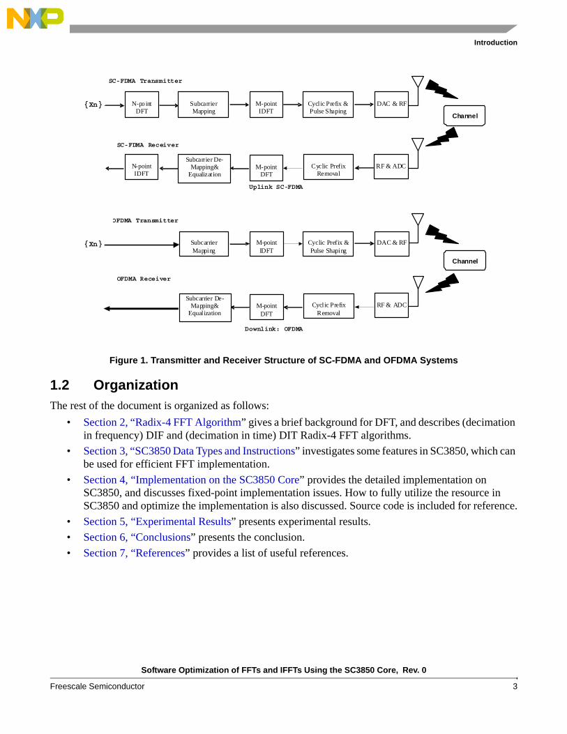
Now, let’s consider an example to demonstrate how FFTs are used in real applications. In the 3GPP-LTE (Long Term Evolution), M-point DFT and Inverse DFT (IDFT) are used to convert the signal between frequency domain and time domain. 3GPP-LTE aims to provide for an uplink speed of up to 50Mbps and a downlink speed of up to 100Mbps. For this purpose, 3GPP-LTE physical layer uses Orthogonal Frequency Division Multiple Access (OFDMA) on the downlink and Single Carrier - Frequency Division Multiple Access (SC-FDMA) on the uplink. Figure 1 shows the transmitter and receiver structure of OFDMA and SC-FDMA systems.
We can see from this example that DFT and IDFT are the key elements to represent changing signals in time and frequency domains. In real applications, FFTs are normally used to for high performance instead of direct DFT calculation.
Software Optimization of FFTs and IFFTs Using the SC3850 Core, Rev. 0
Freescale Semiconductor 3
Introduction
1.2 OrganizationThe rest of the document is organized as follows:
• Section 2, “Radix-4 FFT Algorithm” gives a brief background for DFT, and describes (decimation in frequency) DIF and (decimation in time) DIT Radix-4 FFT algorithms.
• Section 3, “SC3850 Data Types and Instructions” investigates some features in SC3850, which can be used for efficient FFT implementation.
• Section 4, “Implementation on the SC3850 Core” provides the detailed implementation on SC3850, and discusses fixed-point implementation issues. How to fully utilize the resource in SC3850 and optimize the implementation is also discussed. Source code is included for reference.
• Section 5, “Experimental Results” presents experimental results.
• Section 6, “Conclusions” presents the conclusion.
• Section 7, “References” provides a list of useful references.
Figure 1. Transmitter and Receiver Structure of SC-FDMA and OFDMA Systems
{ Xn }
SC-FDMA Transmitter
Channel
Subcarrier Mapping
Subcarrier De-Mapping&
Equalizat ion
M-point IDFT
Cyclic Prefix & Pulse Shaping
DAC & RF
M-point
DFT
Cyclic Prefix
Removal
RF & ADC
N-po int
DFT
N-point IDFT
{Xn}
Downlink: OFDMA
Channel
Subcarrier Mapping
Subcarrier De-Mapping&
Equalization
M-point
IDFT
Cyclic Prefix & Pulse Shaping
DAC & RF
M-point
DFT
Cyclic Prefix
Removal
RF & ADC
Uplink SC-FDMA
SC-FDMA Receiver
OFDMA Transmitter
OFDMA Receiver

Software Optimization of FFTs and IFFTs Using the SC3850 Core, Rev. 0
4 Freescale Semiconductor
Radix-4 FFT Algorithm
2 Radix-4 FFT Algorithm
2.1 DFT and IDFTThe Fast Fourier Transform (FFT) is a computationally efficient algorithm to calculate a Discrete Fourier Transform (DFT). The DFT X(k), k=0,1,2,...,N-1 of a sequence x(n), n=0,1,2,...,N-1 is defined as
Eqn. 1
Eqn. 2
In Equation 1 and Equation 2, N is the number of data, , and is the twiddle factor. Equation 1 is called the N-point DFT of the sequence of x(n). For each value of k, the value of X(k) represents the Fourier transform at the frequency . The IDFT is defined as follows:
Eqn. 3
Eqn. 4
Equation 3 is essentially the same as Equation 1. The differences are that the exponent of the twiddle factor in Equation 3 is the negative of the one in Equation 1 and the scaling factor is 1/N. The IDFT can be simply computed using the same algorithms for DFT but with conjugated twiddle factors. Alternatively, we can use the same twiddles factors for DFT with conjugated input and output to compute IDFT. Equation 1 is also called the analysis equation and Equation 3 the synthesis equation.
X k( ) x n( ) j2πnk
N-------------–⎝ ⎠
⎛ ⎞exp
n 0=
N 1–
∑=
x n( )WNnk
n 0=
N 1–
∑=
WNnk j
2πnkN
-------------–⎝ ⎠⎛ ⎞exp=
2πnkN
-------------⎝ ⎠⎛ ⎞cos j
2πnkN
-------------⎝ ⎠⎛ ⎞sin–=
j 1–= WNnk
2πkN
----------
x n( ) 1N---- X k( ) j
2πnkN
-------------⎝ ⎠⎛ ⎞exp
k 0=
N 1–
∑=
1N---- X k( )WN
nk–
k 0=
N 1–
∑=
WNnk– j
2πnkN
-------------⎝ ⎠⎛ ⎞exp=
2πnkN
-------------⎝ ⎠⎛ ⎞cos j
2πnkN
-------------⎝ ⎠⎛ ⎞sin+=
Software Optimization of FFTs and IFFTs Using the SC3850 Core, Rev. 0
Freescale Semiconductor 5
Radix-4 FFT Algorithm
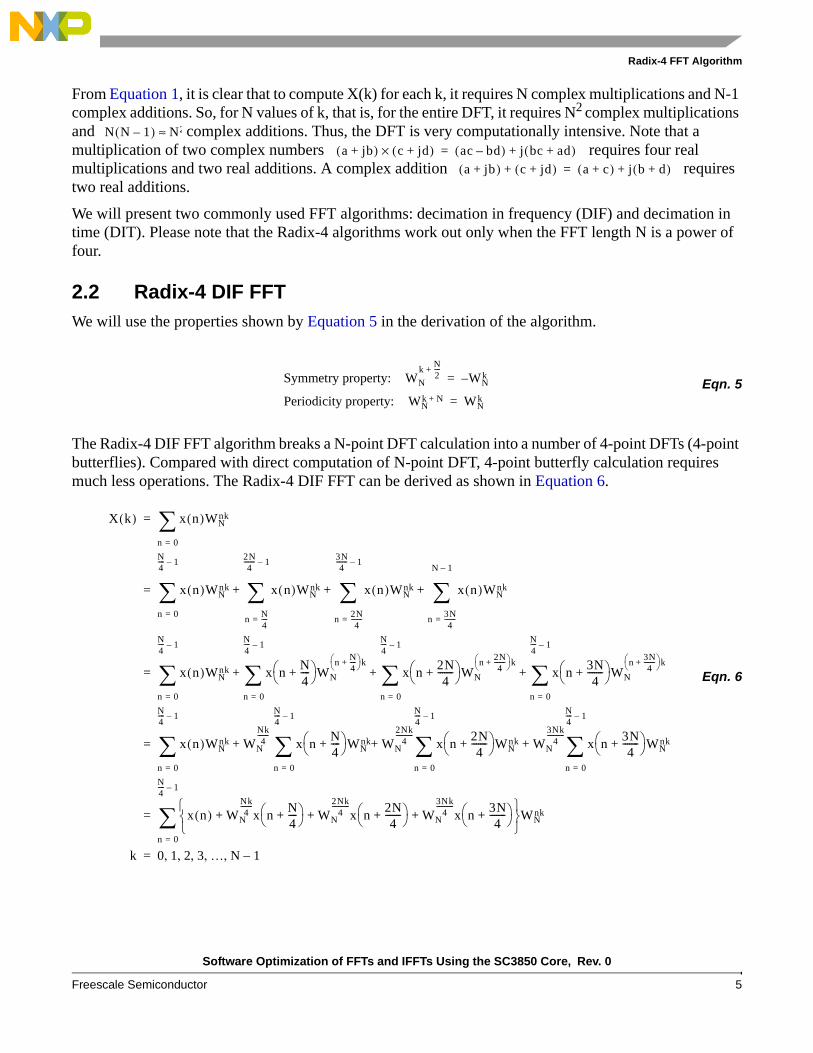
From Equation 1, it is clear that to compute X(k) for each k, it requires N complex multiplications and N-1 complex additions. So, for N values of k, that is, for the entire DFT, it requires N2 complex multiplications and complex additions. Thus, the DFT is very computationally intensive. Note that a multiplication of two complex numbers requires four real multiplications and two real additions. A complex addition requires two real additions.
We will present two commonly used FFT algorithms: decimation in frequency (DIF) and decimation in time (DIT). Please note that the Radix-4 algorithms work out only when the FFT length N is a power of four.
2.2 Radix-4 DIF FFTWe will use the properties shown by Equation 5 in the derivation of the algorithm.
Eqn. 5
The Radix-4 DIF FFT algorithm breaks a N-point DFT calculation into a number of 4-point DFTs (4-point butterflies). Compared with direct computation of N-point DFT, 4-point butterfly calculation requires much less operations. The Radix-4 DIF FFT can be derived as shown in Equation 6.
Eqn. 6
N N 1–( ) N2≈a jb+( ) c jd+( )× ac bd–( ) j bc ad+( )+=
a jb+( ) c jd+( )+ a c+( ) j b d+( )+=
Symmetry property: WN
kN2----+
WNk–=
Periodicity property: WNk N+ WN
k=
X k( ) x n( )WNnk
n 0=
∑=
x n( )WNnk
n 0=
N4---- 1–
∑ x n( )WNnk
nN4----=
2N4
------- 1–
∑ x n( )WNnk
n2N4
-------=
3N4
------- 1–
∑ x n( )WNnk
n3N4
-------=
N 1–
∑+ + +=
x n( )WNnk
n 0=
N4---- 1–
∑ x nN4----+⎝ ⎠
⎛ ⎞WN
nN4----+⎝ ⎠
⎛ ⎞ k
n 0=
N4---- 1–
∑ x n2N4
-------+⎝ ⎠⎛ ⎞WN
n2N4
-------+⎝ ⎠⎛ ⎞ k
n 0=
N4---- 1–
∑ x n3N4
-------+⎝ ⎠⎛ ⎞WN
n3N4
-------+⎝ ⎠⎛ ⎞ k
n 0=
N4---- 1–
∑+ + +=
x n( )WNnk
n 0=
N4---- 1–
∑ WN
Nk4
-------x n
N4----+⎝ ⎠
⎛ ⎞WNnk
n 0=
N4---- 1–
∑ WN
2Nk4
-----------x n
2N4
-------+⎝ ⎠⎛ ⎞WN
nk
n 0=
N4---- 1–
∑ WN
3Nk4
-----------x n
3N4
-------+⎝ ⎠⎛ ⎞WN
nk
n 0=
N4---- 1–
∑+ + +=
x n( ) WN
Nk4
-------x n
N4----+⎝ ⎠
⎛ ⎞ WN
2Nk4
-----------x n
2N4
-------+⎝ ⎠⎛ ⎞ WN
3Nk4
-----------x n
3N4
-------+⎝ ⎠⎛ ⎞+ + +
⎩ ⎭⎨ ⎬⎧ ⎫
WNnk
n 0=
N4---- 1–
∑=
k 0 1 2 3 … N 1–, , , , ,=
Software Optimization of FFTs and IFFTs Using the SC3850 Core, Rev. 0
6 Freescale Semiconductor
Radix-4 FFT Algorithm
The special factors of , , and in above equation can be calculated as shown in Equation 7.
Eqn. 7
Then, Equation 6 can be rewritten as shown in Equation 8.
Eqn. 8
Considering as one signal, Equation 8 looks very similar to a N/4-point FFT. However, it is not an FFT of length N/4 because the twiddle factor depends on N instead of N/4. To make this equation an N/4-point FFT, the transform X(k) can be broken into four parts as shown in Equation 9.
Eqn. 9
WN
Nk4
-------WN
2NK4
------------WN
3Nk4
-----------
WN
Nk4
-------j–2πkN
---------- N4----⋅⎝ ⎠
⎛ ⎞exp jπk2
------–⎝ ⎠⎛ ⎞exp j–( )k= = =
WN
2Nk4
-----------j–2πkN
---------- 2N4
-------⋅⎝ ⎠⎛ ⎞exp jπk–( )exp 1–( )k= = =
WN
3Nk4
-----------j–2πkN
---------- 3N4
-------⋅⎝ ⎠⎛ ⎞exp j
3πk2
----------–⎝ ⎠⎛ ⎞exp jk= = =
X k( ) x n( ) j–( )kx nN4----+⎝ ⎠
⎛ ⎞ 1–( )kx n2N4
-------+⎝ ⎠⎛ ⎞ jkx n
3N4
-------+⎝ ⎠⎛ ⎞+ + +
⎩ ⎭⎨ ⎬⎧ ⎫
WNnk
n 0=
N4---- 1–
∑=
k 0 1 2 3 … N 1–, , , , ,=
x n( ) j–( )kx n N 4⁄+( ) 1–( )kx n 2N( ) 4⁄+( ) jkx n 3N( ) 4⁄+( )+ + +{ }WN
nk
X 4k( ) x n( ) x nN4----+⎝ ⎠
⎛ ⎞ x n2N4
-------+⎝ ⎠⎛ ⎞ x n
3N4
-------+⎝ ⎠⎛ ⎞+ + +
⎩ ⎭⎨ ⎬⎧ ⎫
WN0 WN 4⁄
nk
n 0=
N4---- 1–
∑=
X 4k 1+( ) x n( ) jx nN4----+⎝ ⎠
⎛ ⎞– x n2N4
-------+⎝ ⎠⎛ ⎞– jx n
3N4
-------+⎝ ⎠⎛ ⎞+
⎩ ⎭⎨ ⎬⎧ ⎫
WNn WN 4⁄
nk
n 0=
N4---- 1–
∑=
X 4k 2+( ) x n( ) x nN4----+⎝ ⎠
⎛ ⎞– x n2N4
-------+⎝ ⎠⎛ ⎞ x n
3N4
-------+⎝ ⎠⎛ ⎞–+
⎩ ⎭⎨ ⎬⎧ ⎫
WN2nWN 4⁄
nk
n 0=
N4---- 1–
∑=
X 4k 3+( ) x n( ) jx nN4----+⎝ ⎠
⎛ ⎞ x n2N4
-------+⎝ ⎠⎛ ⎞– jx n
3N4
-------+⎝ ⎠⎛ ⎞–+
⎩ ⎭⎨ ⎬⎧ ⎫
WN3nWN 4⁄
nk
n 0=
N4---- 1–
∑=
k 0 1 2 3 … N4---- 1–, , , , ,=

Software Optimization of FFTs and IFFTs Using the SC3850 Core, Rev. 0
Freescale Semiconductor 7
Radix-4 FFT Algorithm
In Equation 9, the twiddle factors are obtained as shown in Equation 10.
Eqn. 10
If we use the definitions shown in Equation 11.
Eqn. 11
From Equation 9, we can see that X(4k), X(4k+1), X(4k+2), and X(4k+3) are N/4-point FFT of y(n), y(n+N/4), y(n+2n/4), and y(n+3N/4), respectively. As a result, an N-point DFT is reduced to the computation of four N/4-point DFTs.
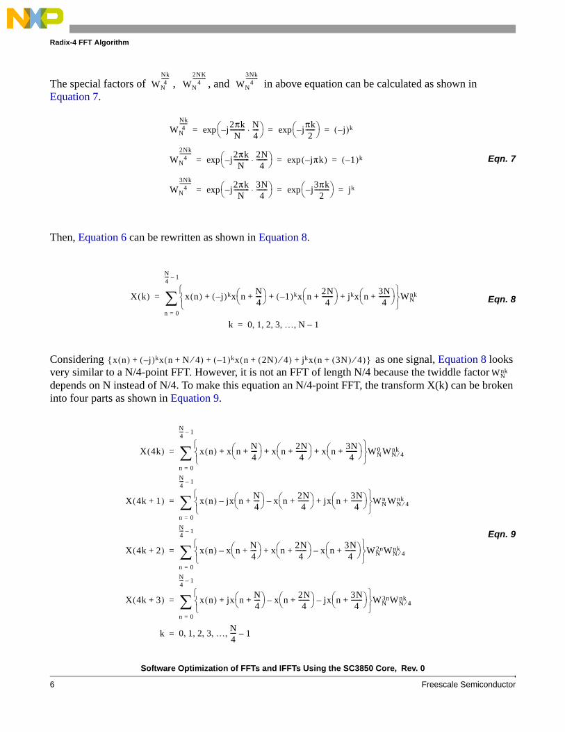
Figure 2 shows the corresponding Radix-4 butterfly calculation of Equation 11. Through further rearrangement, it can be shown that each Radix-4 DIF butterfly requires of 3 complex multiplications and 8 complex additions (12 real multiplications and 22 real additions). The decimation of the data sequences referred to as stage 1 of the decomposition. This process can be repeated again and again until the resulting sequences are reduced to one-point sequences. For N=4p, this decimation can be performed p=log4N times. An example is shown in Figure 4 to illustrate the whole process. Thus the total number of complex multiplications is 3(N/4)log4N since there are 3 complex multiplications each butterfly, N/4 butterflies each stage, and log4N stages. The number of complex additions is 8(N/4)log4N since there are 8 complex additions each butterfly, N/4 butterflies each stage, and log4N stages.
WN4nk j
2π 4nk⋅N
--------------------⎝ ⎠⎛ ⎞–⎝ ⎠
⎛ ⎞exp j2πnkN 4⁄-------------–⎝ ⎠
⎛ ⎞exp WN0 WN 4⁄
nk= = =
WNn 4k 1+( ) j
2π n 4k 1+( )⋅N
-----------------------------------⎝ ⎠⎛ ⎞–⎝ ⎠
⎛ ⎞exp j2πnN
----------– j2πnkN 4⁄-------------–⎝ ⎠
⎛ ⎞exp WNn WN 4⁄
nk= = =
WNn 4k 2+( ) j
2π n 4k 2+( )⋅N
-----------------------------------⎝ ⎠⎛ ⎞–⎝ ⎠
⎛ ⎞exp j2π 2n⋅
N-----------------– j
2πnkN 4⁄-------------–⎝ ⎠
⎛ ⎞exp WN2nWN 4⁄
nk= = =
WNn 4k 3+( ) j
2π n 4k 3+( )⋅N
-----------------------------------⎝ ⎠⎛ ⎞–⎝ ⎠
⎛ ⎞exp j2π 3n⋅
N-----------------– j
2πnkN 4⁄-------------–⎝ ⎠
⎛ ⎞exp WN3nWN 4⁄
nk= = =
y n( ) x n( ) x nN4----+⎝ ⎠
⎛ ⎞ x n2N4
-------+⎝ ⎠⎛ ⎞ x n
3N4
-------+⎝ ⎠⎛ ⎞+ + +
⎩ ⎭⎨ ⎬⎧ ⎫
WN0=
y n N 4⁄+( ) x n( ) jx nN4----+⎝ ⎠
⎛ ⎞– x n2N4
-------+⎝ ⎠⎛ ⎞– jx n
3N4
-------+⎝ ⎠⎛ ⎞+
⎩ ⎭⎨ ⎬⎧ ⎫
WNn=
y n 2N( ) 4⁄+( ) x n( ) x nN4----+⎝ ⎠
⎛ ⎞– x n2N4
-------+⎝ ⎠⎛ ⎞ x n
3N4
-------+⎝ ⎠⎛ ⎞–+
⎩ ⎭⎨ ⎬⎧ ⎫
WN2n=
y n 3N( ) 4⁄+( ) x n( ) jx nN4----+⎝ ⎠
⎛ ⎞ x n2N4
-------+⎝ ⎠⎛ ⎞– jx n
3N4
-------+⎝ ⎠⎛ ⎞–+
⎩ ⎭⎨ ⎬⎧ ⎫
WN3n=
Software Optimization of FFTs and IFFTs Using the SC3850 Core, Rev. 0
8 Freescale Semiconductor
Radix-4 FFT Algorithm
In Figure 2, each of output y(n), y(n + N / 4), y(n + 2N / 4), and y(n + 3N / 4) is a sum of four input signals x(n), x(n + N / 4), x(n + 2N / 4), and x(n + 3N / 4), each multiplied by either +1, –1, j, or –j, and then the sum is multiplied by a twiddle factor (1, WN
n, WN2n, WN
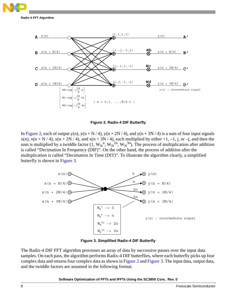
3n). The process of multiplication after addition is called “Decimation In Frequency (DIF)”. On the other hand, the process of addition after the multiplication is called “Decimation In Time (DIT)”. To illustrate the algorithm clearly, a simplified butterfly is shown in Figure 3.
The Radix-4 DIF FFT algorithm processes an array of data by successive passes over the input data samples. On each pass, the algorithm performs Radix-4 DIF butterflies, where each butterfly picks up four complex data and returns four complex data as shown in Figure 2 and Figure 3. The input data, output data, and the twiddle factors are assumed in the following format:
Figure 2. Radix-4 DIF Butterfly
Figure 3. Simplified Radix-4 DIF Butterfly
A
Wb
Wc
Wd
A’
B’
C’
D’
x(n)
B x(n + N/4)
C x(n + 2N/4)
D x(n + 3N/4)
(1,1,1,1)
(1,-j,-1,j)
(1,-1,1,-1)
(1,j,-1,-j)
y(n)
y(n + N/4)
y(n + 2N/4)
y(n + 3N/4)
y(n) : intermediate signal
⎪⎪⎪
⎩
⎪⎪⎪
⎨
⎧
⎟⎠⎞
⎜⎝⎛ ⋅−=
⎟⎠⎞
⎜⎝⎛ ⋅−=
⎟⎠⎞
⎜⎝⎛ ⋅−=
nN
jWd
nN
jWc
nN
jWb
32
exp
22
exp
2exp
π
π
π
( n = 0,1, ...,N/4-1 )
x(n)
x(n + N/4)
x(n + 2N/4)
x(n + 3N/4)
0
n
2n
3n
y(n)
y(n + N/4)
y(n + 2N/4)
y(n + 3N/4)
WN0 -> 0
WNn -> n
WN2n -> 2n
WN3n -> 3n
y(n) : intermediate signal
Software Optimization of FFTs and IFFTs Using the SC3850 Core, Rev. 0
Freescale Semiconductor 9
Radix-4 FFT Algorithm
Input data:
Eqn. 12
Output data:
Eqn. 13
Twiddle factors:
Eqn. 14
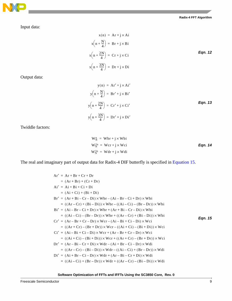
The real and imaginary part of output data for Radix-4 DIF butterfly is specified in Equation 15.
Eqn. 15
x n( ) Ar j Ai×+=
x nN4----+⎝ ⎠
⎛ ⎞ Br j Bi×+=
x n2N4
-------+⎝ ⎠⎛ ⎞ Cr j Ci×+=
x n3N4
-------+⎝ ⎠⎛ ⎞ Dr j Di×+=
y n( ) Ar′ j Ai′×+=
y nN4----+⎝ ⎠
⎛ ⎞ Br′ j Bi′×+=
y n2N4
-------+⎝ ⎠⎛ ⎞ Cr′ j Ci′×+=
y n3N4
-------+⎝ ⎠⎛ ⎞ Dr′ j Di× ′+=
WNn Wbr j Wbi×+=
WN2n Wcr j Wci×+=
WN3n Wdr j Wdi×+=
Ar′ Ar Br Cr Dr+ + +=
Ar Br+( ) Cr Dr+( )+=
Ai′ Ai Bi Ci Di+ + +=
Ai Ci+( ) Bi Di+( )+=
Br′ Ar Bi Cr– Di–+( ) Wbr Ai Br– Ci– Dr+( ) Wbi×–×=
Ar Cr–( ) Bi Di–( )+( ) Wbr Ai Ci–( ) Br Dr–( )–( ) Wbi×–×=
Bi′ Ai Br– Ci– Dr+( ) Wbr× Ar Bi Cr– Di–+( ) Wbi×+=
Ai Ci–( ) Br Dr–( )–( ) Wbr Ar Cr–( ) Bi Di–( )+( ) Wbi×+×=
Cr′ Ar Br– Cr Dr–+( ) Wcr Ai Bi– Ci Di–+( ) Wci×–×=
Ar Cr+( ) Br Dr+( )–( ) Wcr Ai Ci+( ) Bi Di+( )–( ) Wci×–×=
Ci′ Ai Bi– Ci Di–+( ) Wcr Ar Br– Cr Dr–+( ) Wci×+×=
Ai Ci+( ) Bi Di+( )–( ) Wcr Ar Cr+( ) Br Dr+( )–( ) Wci×+×=
Dr′ Ar Bi– Cr– Di+( ) Wdr Ai Br Ci– Dr–+( ) Wdi×–×=
Ar Cr–( ) Bi Di–( )–( ) Wdr Ai Ci–( ) Br Dr–( )+( ) Wdi×–×=
Di′ Ai Br Ci– Dr–+( ) Wdr Ar Bi– Cr– Di+( )+× Wdi×=
Ai Ci–( ) Br Dr–( )+( ) Wdr Ar Cr–( ) Bi Di–( )–( ) Wdi×+×=

Software Optimization of FFTs and IFFTs Using the SC3850 Core, Rev. 0
10 Freescale Semiconductor
Radix-4 FFT Algorithm
As we can see from Equation 15 that there are 12 real multiplications and 22 real additions (count only once for duplicated additions and multiplications). It is equivalent to 3 complex multiplications and 8 complex additions since one complex multiplication requires four real multiplications plus two real additions and one complex addition requires two real additions. As mentioned before, in Radix-4 DIF butterfly algorithm, the N-point FFT consists of log4(N) stages, and each stage consists of N/4-point Radix-4 DIF butterflies. Therefore, Radix-4 DIF butterfly calculation reduces the number of complex multiplication that are needed for a N-point DFT from N2 to 3(N/4)log4N (from 4N2 to 3Nlog4N in terms of real multiplications). For example, the number of real multiplications needed for a 1024-point DFT is reduced from to . The improvement of the Radix-4 DIF butterfly algorithm over the direct calculation of the DFT is approximately 273 times.
An example of 16-point Radix-4 DIF FFT diagram is shown in Figure 4 to illustrate the picture of an entire FFT algorithm. There are log416=2 stages and each stage has 16/4=4 butterflies in the figure.
Figure 4. An example of a 16-point Radix-4 DIF FFT
4N2 4194304= 3N N4log 15360=
Digit reversed order (quaternary system)
x(0)
x(1)
x(2)
x(3)
x(4)
x(5)
x(6)
x(7)
x(8)
x(9)
x(10)
x(11)
x(12)
x(13)
x(14)
x(15)
X(0)
X(4)
x(8)
X(12)
X(1)
X(5)
X(9)
X(13)
X(2)
X(6)
X(10)
X(14)
X(3)
X(7)
X(11)
X(15)
1
2
3
2
4
6
3
6
9
0
0
0
00
0
0
Software Optimization of FFTs and IFFTs Using the SC3850 Core, Rev. 0
Freescale Semiconductor 11
Radix-4 FFT Algorithm
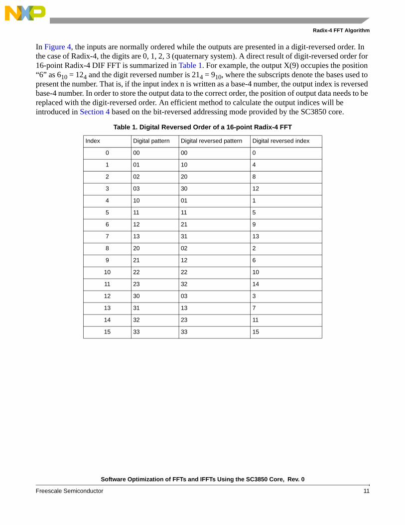
In Figure 4, the inputs are normally ordered while the outputs are presented in a digit-reversed order. In the case of Radix-4, the digits are 0, 1, 2, 3 (quaternary system). A direct result of digit-reversed order for 16-point Radix-4 DIF FFT is summarized in Table 1. For example, the output X(9) occupies the position “6” as 610 = 124 and the digit reversed number is 214 = 910, where the subscripts denote the bases used to present the number. That is, if the input index n is written as a base-4 number, the output index is reversed base-4 number. In order to store the output data to the correct order, the position of output data needs to be replaced with the digit-reversed order. An efficient method to calculate the output indices will be introduced in Section 4 based on the bit-reversed addressing mode provided by the SC3850 core.
Table 1. Digital Reversed Order of a 16-point Radix-4 FFT
Index Digital pattern Digital reversed pattern Digital reversed index
0 00 00 0
1 01 10 4
2 02 20 8
3 03 30 12
4 10 01 1
5 11 11 5
6 12 21 9
7 13 31 13
8 20 02 2
9 21 12 6
10 22 22 10
11 23 32 14
12 30 03 3
13 31 13 7
14 32 23 11
15 33 33 15
Software Optimization of FFTs and IFFTs Using the SC3850 Core, Rev. 0
12 Freescale Semiconductor
Radix-4 FFT Algorithm
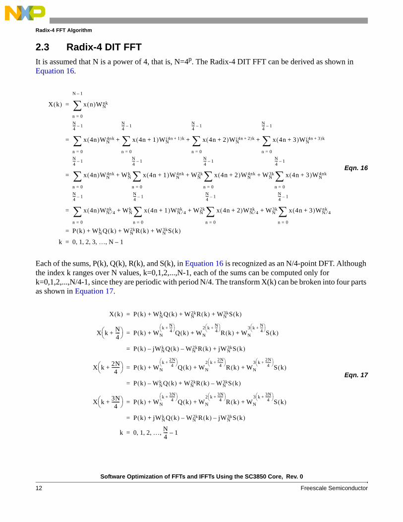
2.3 Radix-4 DIT FFTIt is assumed that N is a power of 4, that is, N=4p. The Radix-4 DIT FFT can be derived as shown in Equation 16.
Eqn. 16
Each of the sums, P(k), Q(k), R(k), and S(k), in Equation 16 is recognized as an N/4-point DFT. Although the index k ranges over N values, k=0,1,2,...,N-1, each of the sums can be computed only for k=0,1,2,...,N/4-1, since they are periodic with period N/4. The transform X(k) can be broken into four parts as shown in Equation 17.
Eqn. 17
X k( ) x n( )WNnk
n 0=
N 1–
∑=
x 4n( )WN4nk
n 0=
N4---- 1–
∑ x 4n 1+( )WN4n 1+( )k
n 0=
N4---- 1–
∑ x 4n 2+( )WN4n 2+( )k
n 0=
N4---- 1–
∑ x 4n 3+( )WN4n 3+( )k
n 0=
N4---- 1–
∑+ + +=
x 4n( )WN4nk
n 0=
N4---- 1–
∑ WNk x 4n 1+( )WN
4nk
n 0=
N4---- 1–
∑ WN2k x 4n 2+( )WN
4nk
n 0=
N4---- 1–
∑ WN3k x 4n 3+( )WN
4nk
n 0=
N4---- 1–
∑+ + +=
x 4n( )WN 4⁄nk
n 0=
N4---- 1–
∑ WNk x 4n 1+( )WN 4⁄
nk
n 0=
N4---- 1–
∑ WN2k x 4n 2+( )WN 4⁄
nk
n 0=
N4---- 1–
∑ WN3k x 4n 3+( )WN 4⁄
nk
n 0=
N4---- 1–
∑+ + +=
P k( ) WNk Q k( ) WN
2kR k( ) WN3kS k( )+ + +=
k 0 1 2 3 … N 1–, , , , ,=
X k( ) P k( ) WNk Q k( ) WN
2kR k( ) WN3kS k( )+ + +=
X kN4----+⎝ ⎠
⎛ ⎞ P k( ) WN
kN4----+⎝ ⎠
⎛ ⎞
Q k( ) WN
2 kN4----+⎝ ⎠
⎛ ⎞
R k( ) WN
3 kN4----+⎝ ⎠
⎛ ⎞
S k( )+ + +=
P k( ) jWNk Q k( )– WN
2kR k( )– jWN3kS k( )+=
X k2N4
-------+⎝ ⎠⎛ ⎞ P k( ) WN
k2N4
-------+⎝ ⎠⎛ ⎞
Q k( ) WN
2 k2N4
-------+⎝ ⎠⎛ ⎞
R k( ) WN
3 k2N4
-------+⎝ ⎠⎛ ⎞
S k( )+ + +=
P k( ) WNk Q k( )– WN
2kR k( ) WN3kS k( )–+=
X k3N4
-------+⎝ ⎠⎛ ⎞ P k( ) WN
k3N4
-------+⎝ ⎠⎛ ⎞
Q k( ) WN
2 k3N4
-------+⎝ ⎠⎛ ⎞
R k( ) WN
3 k3N4
-------+⎝ ⎠⎛ ⎞
S k( )+ + +=
P k( ) jWNk Q k( ) WN
2kR k( )– jWN3kS k( )–+=
k 0 1 2 … N4---- 1–, , , ,=

Software Optimization of FFTs and IFFTs Using the SC3850 Core, Rev. 0
Freescale Semiconductor 13
Radix-4 FFT Algorithm
Figure 5 shows the corresponding Radix-4 DIT butterfly diagram, and Figure 6 shows its simplified version.
We can see that Figure 2 and Figure 5 are similar. Note that the principal difference between DIT and DIF butterflies is that the order of calculation has changed. In the DIF algorithm, the time domain data was “twiddled” before the sub-transforms were performed. In DIT, however, the sub-transforms are performed first, and the output is obtained by “twiddling” the resulting frequency domain data.
Figure 5. Radix-4 DIT Butterfly
Figure 6. Simplified Radix-4 DIT Butterfly
A
Wb
Wc
Wd
A ’
B ’
C ’
D ’
P(k)
B
C
D
(1,1,1,1)
(k = 0,1, ...,N/4-1)
(1,-j,-1,j)
(1,-1,1,-1)
(1,j,-1,-j)
Q(k)
R(k)
S(k)
X(k)
X(k+N/4)
X(k+2N/4)
X(k+3N/4)
⎟⎠⎞
⎜⎝⎛−=
⎟⎠⎞
⎜⎝⎛−=
⎟⎠⎞
⎜⎝⎛−=
kN
jWd
kN
jWc
kN
jWb
32
exp
22
exp
2exp
π
π
π
A
B
C
D
0
n
2n
3n
A’
B’
C’
D’

Software Optimization of FFTs and IFFTs Using the SC3850 Core, Rev. 0
14 Freescale Semiconductor
Radix-4 FFT Algorithm
The real and imaginary part of output data for Radix-4 DIT butterfly is specified in Equation 18.
Eqn. 18
The number of multiplications and additions required by the DIT butterfly is the same as it required by the DIF butterfly, which can be seen from Figure 2 and Figure 5. Therefore, Radix-4 DIT butterfly calculation also reduces the number of complex multiplication that are needed for a N-point DFT from N2 to 3(N/4)log4N (from 4N2 to 3Nlog4N in terms of real multiplications). In the SC3850 core, dual MACs can be used to implement the DIT algorithm efficiently. Thus, this application note will describe the implementation of the DIT algorithm on the SC3850 core in Section 4.
Figure 7. An example of a 16-point Radix-4 DIT FFT
Ar′ Ar Cr Wcr× Ci Wci×–( ) Br Wbr× Bi Wbi×–( ) Dr Wdr× Di Wdi×–( )+ + +=
Ai′ Ai Cr Wci× Ci Wcr×+( ) Br Wbi× Bi Wbr×+( ) Dr Wdi× Di Wdr×+( )+ + +=
Br′ Ar Cr Wcr× Ci Wci×–( )– Br Wbi× Bi Wbr×+( ) Dr Wdi× Di Wdr×+( )–+=
Bi′ Ai Cr Wci× Ci Wcr×+( )– Br Wbr× Bi Wbi×–( )– Dr Wdr× Di Wdi×–( )+=
Cr′ Ar Cr Wcr× Ci Wci×–( ) Br Wbr× Bi Wbi×–( )– Dr Wdr× Di Wdi×–( )–+=
Ci′ Ai Cr Wci× Ci Wcr×+( ) Br Wbi× Bi Wbr×+( )– Dr Wdi× Di Wdr×+( )–+=
Dr′ Ar Cr Wcr× Ci Wci×–( )– Br Wbi× Bi Wbr×+( )– Dr Wdi× Di Wdr×+( )+=
Di′ Ai Cr Wci× Ci Wcr×+( )– Br Wbr× Bi Wbi×–( ) Dr Wdr× Di Wdi×–( )–+=
x(0)
x(4)
x(8)
x(12)
x(1)
x(5)
x(9)
x(13)
x(2)
x(6)
x(10)
x(14)
x(3)
x(7)
x(11)
x(15)
X(0)
X(1)
x(2)
X(3)
X(4)
X(5)
X(6)
X(7)
X(8)
X(9)
X(10)
X(11)
X(10)
X(11)
X(14)
X(15)
0
0
0
0
0
0
0
0
0
0
0
0
0
0
0
0
1
2
3
2
4
6
3
6
9
0
0
0
0
0
0
0

Software Optimization of FFTs and IFFTs Using the SC3850 Core, Rev. 0
Freescale Semiconductor 15
SC3850 Data Types and Instructions
An example of 16-point Radix-4 DIT FFT diagram is shown in Figure 7 to illustrate an entire DIT algorithm. There are log416=2 stages and each stage has 16/4=4 butterflies. In Figure 7, the inputs are digit-reversed ordered (refer to Table 1) while the outputs are presented in a normal order. Thus, bit-reversed addressing mode is used to load the input data samples to improve the performance of the DIT FFT algorithm.
3 SC3850 Data Types and InstructionsThis section discusses the data types, SIMD instructions, and complex arithmetic in the SC3850 architecture, which can be used to efficiently implement the Radix-4 DIT FFT algorithm.
3.1 StarCore Data Types
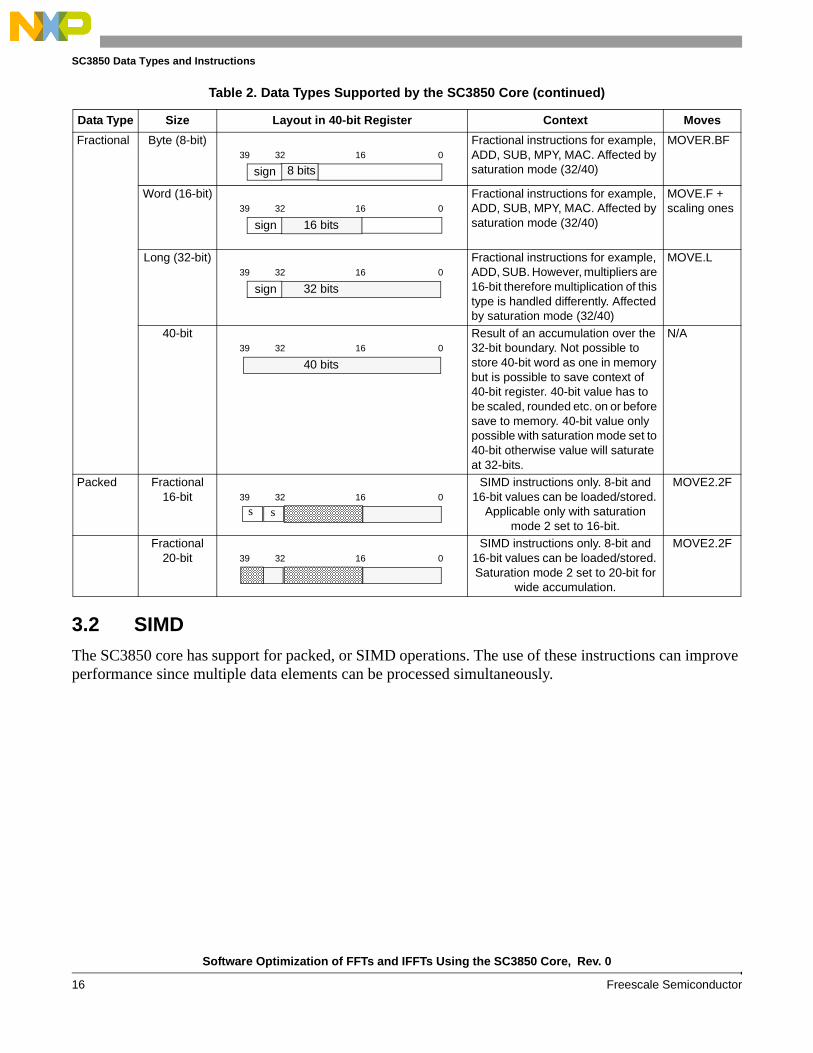
Table 2. Data Types Supported by the SC3850 Core
Data Type Size Layout in 40-bit Register Context Moves
Integer Byte (8-bit) Integer instructions, for example, IADD, ISUB, IMPY. Unaffected by saturation modes.
MOVE.B, MOVEU.B
Word (16-bit) Integer instructions, for example, IADD, ISUB, IMPY. Unaffected by saturation modes.
MOVE.W, MOVEU.W
Long (32-bit) Integer instructions, for example, IADD, ISUB. However, multipliers are 16-bit therefore multiplication of this type is handled differently. Unaffected by saturation modes.
MOVE.L, MOVEU.L
40-bit Result of an accumulation over the 32-bit boundary. Not possible to store 40-bit word as one in memory but is possible to save context of 40-bit register. 40-bit value must be adjusted before save to memory. Unaffected by saturation modes.
N/A
0163239
8 bitszero/sign
0163239
16 bitszero/sign
0163239
32 bitsz/s
0
40 bits163239
Software Optimization of FFTs and IFFTs Using the SC3850 Core, Rev. 0
16 Freescale Semiconductor
SC3850 Data Types and Instructions
3.2 SIMDThe SC3850 core has support for packed, or SIMD operations. The use of these instructions can improve performance since multiple data elements can be processed simultaneously.
Fractional Byte (8-bit) Fractional instructions for example, ADD, SUB, MPY, MAC. Affected by saturation mode (32/40)
MOVER.BF
Word (16-bit) Fractional instructions for example, ADD, SUB, MPY, MAC. Affected by saturation mode (32/40)
MOVE.F + scaling ones
Long (32-bit) Fractional instructions for example, ADD, SUB. However, multipliers are 16-bit therefore multiplication of this type is handled differently. Affected by saturation mode (32/40)
MOVE.L
40-bit Result of an accumulation over the 32-bit boundary. Not possible to store 40-bit word as one in memory but is possible to save context of 40-bit register. 40-bit value has to be scaled, rounded etc. on or before save to memory. 40-bit value only possible with saturation mode set to 40-bit otherwise value will saturate at 32-bits.
N/A
Packed Fractional 16-bit
SIMD instructions only. 8-bit and 16-bit values can be loaded/stored.
Applicable only with saturation mode 2 set to 16-bit.
MOVE2.2F
Fractional 20-bit
SIMD instructions only. 8-bit and 16-bit values can be loaded/stored. Saturation mode 2 set to 20-bit for
wide accumulation.
MOVE2.2F
Table 2. Data Types Supported by the SC3850 Core (continued)
Data Type Size Layout in 40-bit Register Context Moves
0163239
8 bitssign
0163239
16 bitssign
0163239
32 bitssign
0163239
40 bits
0163239
40 bitss s
0163239
40 bits
Software Optimization of FFTs and IFFTs Using the SC3850 Core, Rev. 0
Freescale Semiconductor 17
SC3850 Data Types and Instructions
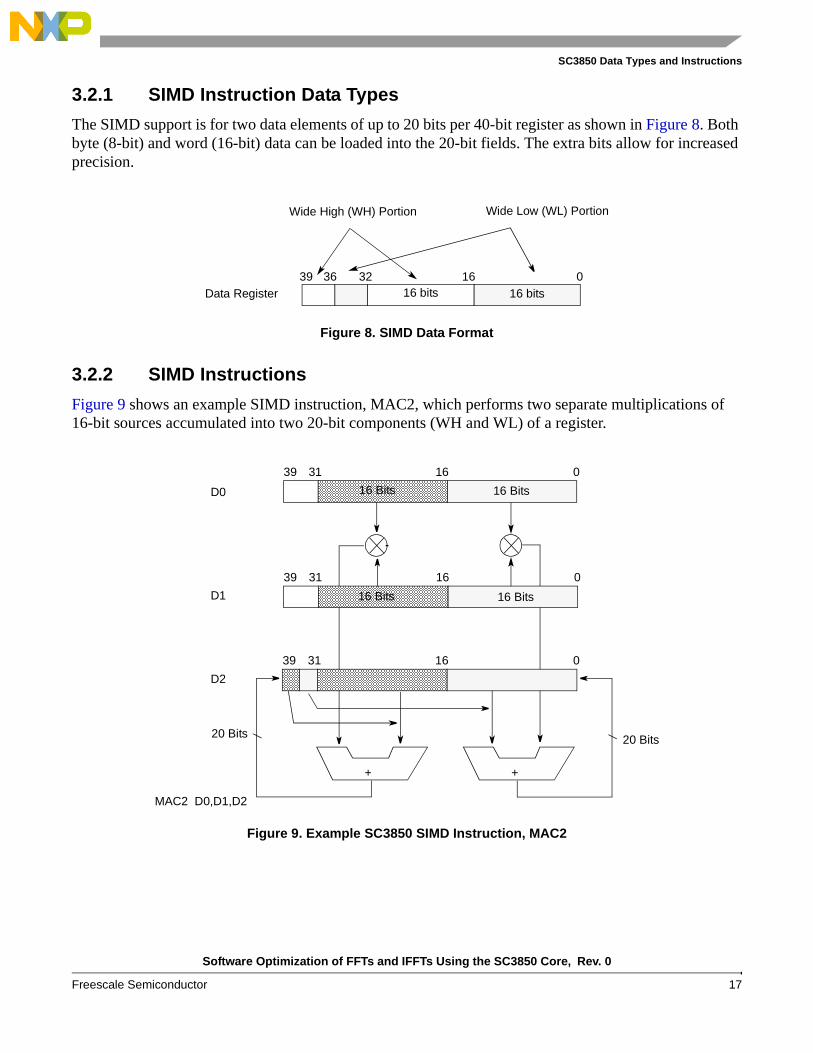
3.2.1 SIMD Instruction Data Types
The SIMD support is for two data elements of up to 20 bits per 40-bit register as shown in Figure 8. Both byte (8-bit) and word (16-bit) data can be loaded into the 20-bit fields. The extra bits allow for increased precision.
3.2.2 SIMD Instructions
Figure 9 shows an example SIMD instruction, MAC2, which performs two separate multiplications of 16-bit sources accumulated into two 20-bit components (WH and WL) of a register.
Figure 8. SIMD Data Format
Figure 9. Example SC3850 SIMD Instruction, MAC2
016323916 bits 16 bits
36
Wide Low (WL) PortionWide High (WH) Portion
Data Register
0163139
0163139
16 Bits 16 Bits
16 Bits 16 Bits
+
D0
D1
D2
0163139
+
20 Bits20 Bits
MAC2 D0,D1,D2

Software Optimization of FFTs and IFFTs Using the SC3850 Core, Rev. 0
18 Freescale Semiconductor
SC3850 Data Types and Instructions
Table 3 lists the SIMD instructions in the SC3850 core.
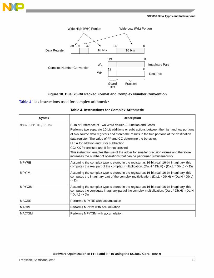
3.3 Complex Arithmetic Complex arithmetic is widely used in signal processing algorithms. Figure 10 shows a convention to represent a complex number using dual 20-bit packed format. For a complex addition, two additions are needed:
; Addition of a+jb and c+jd to form e+jfe=a+c;f=b+d;
For a complex multiplication, two signed addition operations and four multiplications are needed. ; Multiplication of a+jb and c+jd to form e+jfe=ac-bd;f=j(bc+ad);
Table 3. SIMD Instructions in the SC3850 Core
Instruction DescriptionBitwise compatible with legacy
architectures
ADD2 Packed addition yesSUB2 Packed subtraction yesNEG2 Two Words Negate yes
IMACSU2 Two integer multiply accumulate signed by unsigned yesPACK.2W Packs two words yesPACK.2F Packs two fractional words yes
ADD.W Add 16-bit or 20-bit value noABS2 Two Words Absolute Value noASL2 Arithmetic Shift Left by One of Two Word Operands no
ASLL2 Multiple-Bit Arithmetic Shift Left of Two Word Operands noASRR2 Multiple-Bit Arithmetic Shift Right of Two Word Operands noLSLL2 Multiple-Bit Bitwise Shift Left of Two Word Operands no
LSR2 Bitwise Shift Right One Bit of Two Word Operands noLSRR2 Multiple-Bit Bitwise Shift Right of Two Word Operands noSOD2ffcc Sum Or Difference of Two 16-Bit Values, function & cross no
MIN2 Transfer two 16-bit minimum signed values noMAX2 Transfer two 16-bit maximum signed values noSUB.W Subtract 16-bit or 20-bit value no
MPY2 Multiply 2 pairs of 16-bit data. N/AMPY2R Multiply 2 pairs of 16-bit data and round the lower 16 bits of the result. N/AMAC2 Multiply 2 pairs of 16-bit data, clip the lower 16 bits of each result into
16-bit word and accumulate it with 20-bit accumulator inputN/A
MAC2R Multiply 2 pairs of 16-bit data, round the lower 16 bits of each result into 16-bit word and accumulate it with 20-bit accumulator input.
N/A
CLIP20 Clip two 20-bit operands. N/A
SATU20.B Saturate two unsigned bytes. N/AMAC2ffggR Multiply 2 pairs of 16-bit data, add or subtract them from each portion
-specific format used for FFT calculation.N/A
MAC2ffggI N/A
Software Optimization of FFTs and IFFTs Using the SC3850 Core, Rev. 0
Freescale Semiconductor 19
SC3850 Data Types and Instructions
Table 4 lists instructions used for complex arithmetic:
Figure 10. Dual 20-Bit Packed Format and Complex Number Convention
Table 4. Instructions for Complex Arithmetic
Syntax Description
SOD2FFCC Da,Db,Dn Sum or Difference of Two Word Values—Function and CrossPerforms two separate 16-bit additions or subtractions between the high and low portions
of two source data registers and stores the results in the two portions of the destinationdata register. The value of FF and CC determine the behavior. FF: A for addition and S for subtraction
CC: XX for crossed and II for not crossedThis instruction enables the use of the adder for smaller precision values and therefore increases the number of operations that can be performed simultaneously.
MPYRE Assuming the complex type is stored in the register as 16-bit real, 16-bit imaginary, this computes the real part of the complex multiplication. (Da.H * Db.H) - (Da.L * Db.L) -> Dn
MPYIM Assuming the complex type is stored in the register as 16-bit real, 16-bit imaginary, this computes the imaginary part of the complex multiplication. (Da.L * Db.H) + (Da.H * Db.L) -> Dn
MPYCIM Assuming the complex type is stored in the register as 16-bit real, 16-bit imaginary, this computes the conjugate imaginary part of the complex multiplication. (Da.L * Db.H) - (Da.H * Db.L) -> Dn
MACRE Performs MPYRE with accumulation
MACIM Performs MPYIM with accumulation
MACCIM Performs MPYCIM with accumulation
016323916 bits 16 bits
36
Wide Low (WL) PortionWide High (WH) Portion
Real Part
Imaginary PartWL:
WH:
Data Register
Complex Number Convention
019
019
FractionBits
Guard

Software Optimization of FFTs and IFFTs Using the SC3850 Core, Rev. 0
20 Freescale Semiconductor
SC3850 Data Types and Instructions
3.4 Scaling, Rounding and Limiting
When moving fractional data to memory during DSP kernels, usually it is require to scale, round, and limit (saturate) the data on its way to the memory in order not to lose precision due to truncation that would otherwise occur. The data in the register itself is not modified to prevent accuracy loss when this register is used for subsequent operations in the core. For non-packed data types, these operations are performed by the MOVER instructions, which work in the following way:
• Scaling is done according to the scaling mode (SCM in SR). In 20-bit packed format, the scaling down uses the guard bits from the appropriate extension portion. Scaling is not performed when in the arithmetic saturation mode (SM for MOVER). Four scaling modes are supported:
— No scaling
— Scale down (1-bit arithmetic right shift)
— Scale up (1-bit arithmetic left shift)
— Scale down (2-bit arithmetic right shift)
• The data is rounded to the appropriate length (depending on the width of the transfer). Rounding is not done for 32-bit values (MOVER.L and MOEVR.2L instructions). Twos complement rounding or convergent rounding is performed according to the rounding mode bit in the SR (SR.RM).
• Limiting is done on the scaled data, looking at the value of all the MS bits that are shifted out (including guard bits for 40-bit input).
Table 5. MOVER Instructions
Instruction Description
MOVER.L Move a fractional long from a register to memory with scaling, and saturation. Note: no rounding takes place with this instruction.
MOVER.2L Move two fractional longs from a register pair to memory with calling and saturation. Note: no rounding takes place with this instruction.
MOVER.F Move a fractional word from a register to memory with rounding, scaling, and saturation
MOVER.2F Move two fractional words from a register pair to memory with rounding, scaling, and saturation
MOVER.4F Move four fractional words from a register quad to memory with rounding, scaling, and saturation
MOVERH.4F Move four fractional words from the wide high portions of a register quad with rounding, scaling, and saturation.
MOVERL.4F Move four fractional words from the wide low portions of a register quad with rounding, scaling and saturation.
MOVER.BF Move a fractional byte from a register to memory with rounding, scaling, and saturation
MOVER.2BF Move two fractional bytes from a register pair to memory with rounding, scaling, and saturation
MOVER.4BF Move four fractional bytes from a register quad to memory with rounding, scaling, and saturation

Software Optimization of FFTs and IFFTs Using the SC3850 Core, Rev. 0
Freescale Semiconductor 21
Implementation on the SC3850 Core
4 Implementation on the SC3850 CoreIn this section, an implementation of the Radix-4 DIT FFT algorithm is presented.
4.1 ScalingThe SC3850 core is a fixed-point digital signal processor. The data needs to be handled within the fixed-point range [-1, 1) in order to avoid overflow. For a Radix-4 FFT, the magnitude values computed in a butterfly stage can have a growth to . The real and imaginary parts of the butterfly can have a growth to 4. This is the output dynamic range. The fixed-scaling method scales down by a fixed factor at each stage to handle the bit growth. If scaling is insufficient, a butterfly output may grow beyond the dynamic range and causes an overflow. In the computation of the Radix-4 FFT on the SC3850 core, it is necessary to scale down the intermediate results by a factor of 4 to avoid any overflowing, which means that each stage of the FFT is divided by 4. If an FFT consists of M stages, the output is scaled down by 4M
(M = log4(N)), where N is the length of the FFT. The scaling results in the final output are modified by the factor of 1/4M. The output sequence X’(K) (k = 0, 1, 2, 3, … , N – 1) computed by the SC3850 processor is defined in Equation 19.
Eqn. 19
For example, the total scaling amount for 1024-point DIF FFT is 1/4M = 1/45 = 1/1024 (M = log4(1024) = 5). Note that if a Radix-4 algorithm uses a scaling of a factor of 4, the total scaling amount is equal to the factor of 1/N. Note that the MOVER instructions introduced in Section 3.4 can be used to efficiently scale the data.
4.2 Bit-Reversed AddressingThe StarCore DSP has a bit-reversed (or reverse-carry) addressing mode to support N-point FFT addressing, where N = 2k. This mode is useful for unscrambling N-point FFT data. Figure 11shows an example of reverse-carry addressing of 1024-point FFT. Before starting the reverse-carry addressing, the following registers need to be set:
1. Set “1” to the corresponding field in MCTL (Modifier Control) register
4 2 5.657≈
X′ k( ) 14M------- x n( ) j
2πnkN
-------------–⎝ ⎠⎛ ⎞exp
n 0=
N 1–
∑ 1N---- x n( ) j
2πnkN
-------------–⎝ ⎠⎛ ⎞exp
n 0=
N 1–
∑= =
M N4log=
k 0 1 2 3 … N 1–, , , , ,=
Software Optimization of FFTs and IFFTs Using the SC3850 Core, Rev. 0
22 Freescale Semiconductor
Implementation on the SC3850 Core
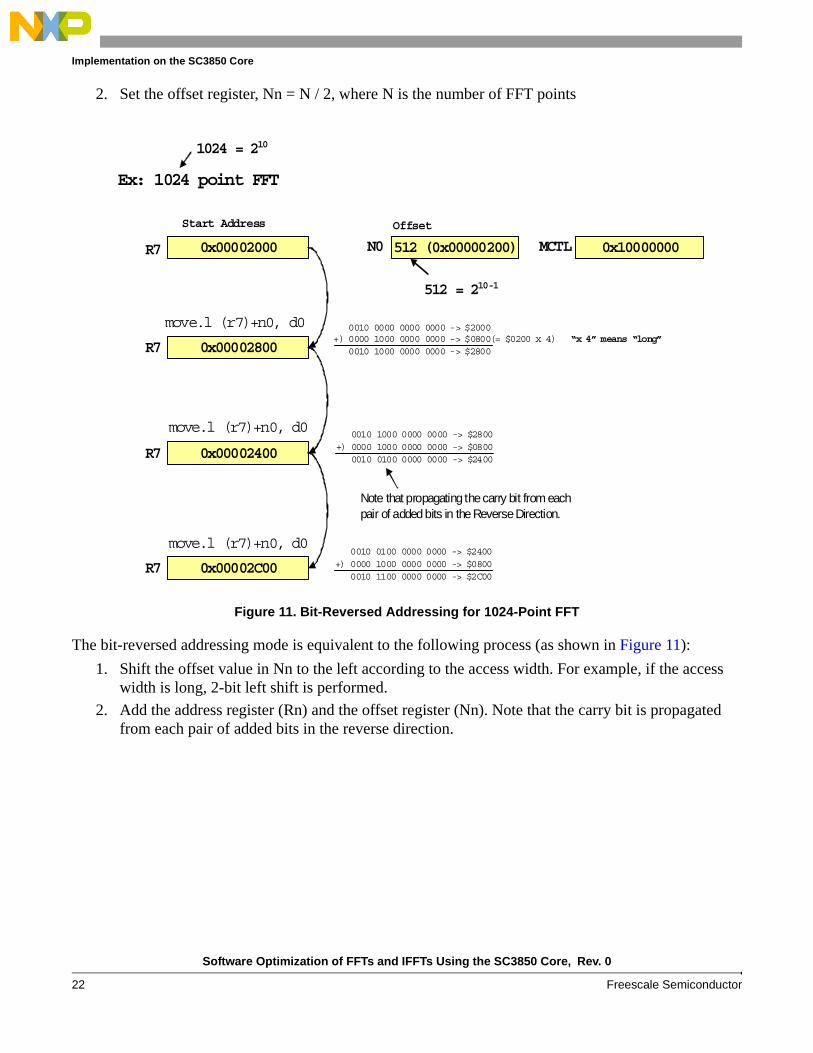
2. Set the offset register, Nn = N / 2, where N is the number of FFT points
The bit-reversed addressing mode is equivalent to the following process (as shown in Figure 11):
1. Shift the offset value in Nn to the left according to the access width. For example, if the access width is long, 2-bit left shift is performed.
2. Add the address register (Rn) and the offset register (Nn). Note that the carry bit is propagated from each pair of added bits in the reverse direction.
Figure 11. Bit-Reversed Addressing for 1024-Point FFT
Ex: 1024 point FFT
0x00002000R7 512 (0x00000200)N0 0x10000000MCTL
move.l (r7)+n0, d0
R7
1024 = 210
512 = 210-1
Start Address Offset
0010 0000 0000 0000 -> $2000+) 0000 1000 0000 0000 -> $0800(= $0200 x 4) “x 4” means “long”
0010 1000 0000 0000 -> $2800
0010 1000 0000 0000 -> $2800+) 0000 1000 0000 0000 -> $0800
0010 0100 0000 0000 -> $2400
0010 0100 0000 0000 -> $2400+) 0000 1000 0000 0000 -> $0800
0010 1100 0000 0000 -> $2C00
Note that propagating the carry bit from each pair of added bits in the Reverse Direction.
0x00002800
move.l (r7)+n0, d0
R7 0x00002400
move.l (r7)+n0, d0
R7 0x00002C00

Software Optimization of FFTs and IFFTs Using the SC3850 Core, Rev. 0
Freescale Semiconductor 23
Implementation on the SC3850 Core
The range of values for offset register, Nn, is from 0 to (232 – 1), which allows reverse-carry addressing for FFTs up to 4,294,967,296 points. The base address (start address) should be aligned to N × W, where W is the number of bytes in a data element. For instance, in a 1024-point FFT on a 16-bit complex array, the base address of the array needs to be aligned to:
1,024-point × 2-byte × 2IQ = 4,096 bytes
Table 6 lists the 16-point FFT bit-reversed order supported by StarCore SC3850 core.
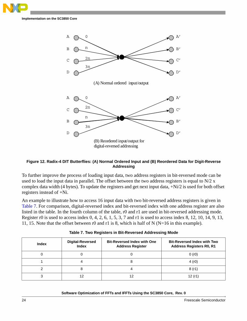
As mentioned in Section 2.3, the data are digit-reversed ordered in the Radix-4 DIT algorithm. A comparison between the digit-reversed order for Radix-4 (Table 1) and the bit-reversed order supported by the SC3850 DSP (Table 6) shows that the two middle output indices are interchanged. This means that the bit-reversed addressing mode can be used for the digit-reversed ordering in Radix-4 FFT with the exchange of the two middle indices. For this purpose, the algorithm interchanges the order of B and C of Radix-4 DIT butterfly as shown in Figure 12. Otherwise, the usual digital-reversed addressing is used.
Table 6. Bit-Reversed Order Supported by StarCore SC3850 DSPs
Index Bit Pattern Bit Reversed Pattern Bit Reversed Index
0 0000 0000 0
1 0001 1000 8
2 0010 0100 4
3 0011 1100 12
4 0100 0010 2
5 0101 1010 10
6 0110 0110 6
7 0111 1110 14
8 1000 0001 1
9 1001 1001 9
10 1010 0101 5
11 1011 1101 13
12 1100 0011 3
13 1101 1011 11
14 1110 0111 7
15 1111 1111 15
Software Optimization of FFTs and IFFTs Using the SC3850 Core, Rev. 0
24 Freescale Semiconductor
Implementation on the SC3850 Core
To further improve the process of loading input data, two address registers in bit-reversed mode can be used to load the input data in parallel. The offset between the two address registers is equal to N/2 x complex data width (4 bytes). To update the registers and get next input data, +Ni/2 is used for both offset registers instead of +Ni.
An example to illustrate how to access 16 input data with two bit-reversed address registers is given in Table 7. For comparison, digital-reversed index and bit-reversed index with one address register are also listed in the table. In the fourth column of the table, r0 and r1 are used in bit-reversed addressing mode. Register r0 is used to access index 0, 4, 2, 6, 1, 5, 3, 7 and r1 is used to access index 8, 12, 10, 14, 9, 13, 11, 15. Note that the offset between r0 and r1 is 8, which is half of N (N=16 in this example).
Figure 12. Radix-4 DIT Butterflies: (A) Normal Ordered Input and (B) Reordered Data for Digit-Reverse Addressing
Table 7. Two Registers in Bit-Reversed Addressing Mode
IndexDigital-Reversed
IndexBit-Reversed Index with One
Address RegisterBit-Reversed Index with Two
Address Registers R0, R1
0 0 0 0 (r0)
1 4 8 4 (r0)
2 8 4 8 (r1)
3 12 12 12 (r1)
A
B
C
D
0
n
2n
3n
A’
B’
C’
D’
A
C
B
D
0
2n
n
3n
A’
C’
B’
D’
(A) Normal ordered input/output
(B) Reordered input/output for digital-reversed addressing
Software Optimization of FFTs and IFFTs Using the SC3850 Core, Rev. 0
Freescale Semiconductor 25
Implementation on the SC3850 Core
The input data is a vector of N complex values represented as 16-bit two’s complement numbers that are decomposed as the real and imaginary components of the data sample. The implemented Radix-4 DIT butterfly equations are summarized in Equation 20.
Eqn. 20
Equation 20 shows the implementation of Radix-4 DIT butterfly equations on the SC3850 core. The output order of the implementation is different from the original order in Equation 18. Please note the interchanging locations of B and C enables the use of StarCore supported bit-reversed addressing. This means that instead of storing the output of Radix-4 DIT butterfly in the order of A’, B’, C’, D’, they are stored in the order of A’, C’, B’, D’, as shown in Figure 12.
4 1 2 2 (r0)
5 5 10 6 (r0)
6 9 6 10 (r1)
7 13 14 14 (r1)
8 2 1 1 (r0)
9 6 9 5 (r0)
10 10 5 9 (r1)
11 14 13 13 (r1)
12 3 3 3 (r0)
13 7 11 7 (r0)
14 11 7 11 (r1)
15 15 15 15 (r1)
Table 7. Two Registers in Bit-Reversed Addressing Mode (continued)
IndexDigital-Reversed
IndexBit-Reversed Index with One
Address RegisterBit-Reversed Index with Two
Address Registers R0, R1
Ar′ Ar Cr Wcr× Ci Wci×–( ) Br Wbr× Bi Wbi×–( ) Dr Wdr× Di Wdi×–( )+ + +=
Ai′ Ai Cr Wci× Ci Wcr×+( ) Br Wbi× Bi Wbr×+( ) Dr Wdi× Di Wdr×+( )+ + +=
Br′ Ar Cr Wcr× Ci Wci×–( ) Br Wbr× Bi Wbi×–( )– Dr Wdr× Di Wdi×–( )–+=
Bi′ Ai Cr Wci× Ci Wcr×+( ) Br Wbi× Bi Wbr×+( )– Dr Wdi× Di Wdr×+( )–+=
Cr′ Ar Cr Wcr× Ci Wci×–( )– Br Wbi× Bi Wbr×+( ) Dr Wdi× Di Wdr×+( )–+=
Ci′ Ai Cr Wci× Ci Wcr×+( )– Br Wbr× Bi Wbi×–( )– Dr Wdr× Di Wdi×–( )+=
Dr′ Ar Cr Wcr× Ci Wci×–( )– Br Wbi× Bi Wbr×+( )– Dr Wdi× Di Wdr×+( )+=
Di′ Ai Cr Wci× Ci Wcr×+( )– Br Wbr× Bi Wbi×–( ) Dr Wdr× Di Wdi×–( )–+=

Software Optimization of FFTs and IFFTs Using the SC3850 Core, Rev. 0
26 Freescale Semiconductor
Implementation on the SC3850 Core
4.3 Implementation of Radix-4 DIT FFTsFigure 13 shows the actual process of calculation for 1024-point FFT as an example.
In this implementation, the FFT is summarized as follows:
1. First stage: The input data are loaded in the bit-reversed addressing mode. The Radix-4 DIT butterfly calculation is repeated for N/4 times on the input data. In the first stage, the twiddle factors are all equal to 1. As a result, there is no multiplication in the first stage. The output can be scaled down by 0, 2, and 4 depending on the input parameter of the FFT function.
2. Middle stage: The N/4 times Radix-4 DIT butterfly calculation is repeated for (log4N - 2) times. The twiddle factors vary with stages. In the second stage, the twiddle factors are equal to (W16
k, W16
2k, W163k) (k = 0, 1, 2, 3). In the third stage, the twiddle factors are (W64
k, W642k, W64
3k) (k = 0, 1, 2, ... , 15). In the fourth stage, the twiddle factors are (W256
k, W2562k, W256
3k) (k = 0, 1, 2, ... , 63), and so on. The output at each stage can be scaled down by 0, 2, and 4 depending on the input parameter of the FFT function.
3. Last stage: The Radix-4 DIT butterfly calculation is repeated for N/4 times. The twiddle factors are (WN
k, WN2k, WN
3k) (k = 0, 1, 2, ... , N/4-1) in this stage. The output can be scaled down by 0, 2, and 4 depending on the input parameter of the FFT function.
The routine uses one first stage, log4N-2 middle stages, and one last stage to perform the radix-4 FFT algorithm, as shown in Figure 13. As we can see from the figure that there are N/4 butterflies in each stage. The N/4 butterflies can be classified into groups depending on which stage they are at. In the first stage, all twiddle factors are equal to one. Thus one loop is used to compute N/4 butterflies without loading the twiddle factors. In the middle stages, the butterflies with the same twiddle factors are grouped together to reduce the memory access. The radix-4 butterflies are classified into 4 groups for the first middle stage, 16 groups for the second middle stage, and so on. Therefore, the middle stages are written using three loops. The outermost loop “k” cycles through the (log4N-2) middle stages. The loop “j” cycles through the groups
Figure 13. Diagram of 1024-point FFT Calculation Using Radix-4 DIT Algorithm
Radix-4 FFT
Radix-4 FFT
Radix-4 FFT
Radix-4 FFT
Radix-4 FFT
Radix-4 FFT
Radix-4 FFT
Radix-4 FFT
0
1
2
3
252
253
254
255
Radix-4 FFT
Radix-4 FFT
Radix-4 FFT
Radix-4 FFT
Radix-4 FFT
Radix-4 FFT
Radix-4 FFT
Radix-4 FFT
Radix-4 FFT
Radix-4 FFT
Radix-4 FFT
Radix-4 FFT
Radix-4 FFT
Radix-4 FFT
Radix-4 FFT
Radix-4 FFT
Radix-4 FFT
Radix-4 FFT
Radix-4 FFT
Radix-4 FFT
Radix-4 FFT
Radix-4 FFT
Radix-4 FFT
Radix-4 FFT
Bit Reverse
N/4= 256
Ex. N = 1024
log4N = 5
First stage Middle stage Last stage
Radix-4 FFT
Radix-4 FFT
Radix-4 FFT
Radix-4 FFT
Radix-4 FFT
Radix-4 FFT
Radix-4 FFT
Radix-4 FFT
Software Optimization of FFTs and IFFTs Using the SC3850 Core, Rev. 0
Freescale Semiconductor 27
Implementation on the SC3850 Core
of butterflies with different twiddle factors, and loop “i” reuses the twiddle factors for the different butterflies within a stage. In the last stage, only one butterfly exist in each group, and thus one loop is used to go through all the groups. Table 8 shows the grouped butterflies at different stages.
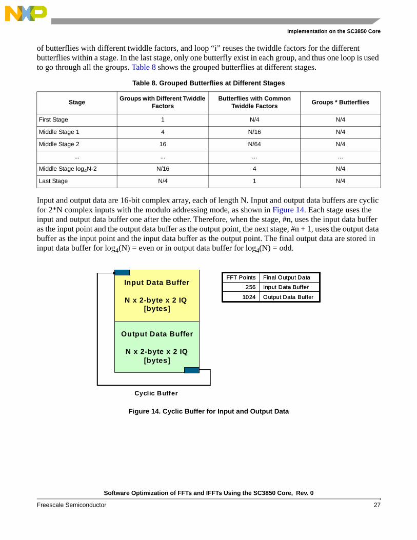
Input and output data are 16-bit complex array, each of length N. Input and output data buffers are cyclic for 2*N complex inputs with the modulo addressing mode, as shown in Figure 14. Each stage uses the input and output data buffer one after the other. Therefore, when the stage, #n, uses the input data buffer as the input point and the output data buffer as the output point, the next stage, #n + 1, uses the output data buffer as the input point and the input data buffer as the output point. The final output data are stored in input data buffer for log4(N) = even or in output data buffer for log4(N) = odd.
Table 8. Grouped Butterflies at Different Stages
StageGroups with Different Twiddle
FactorsButterflies with Common
Twiddle FactorsGroups * Butterflies
First Stage 1 N/4 N/4
Middle Stage 1 4 N/16 N/4
Middle Stage 2 16 N/64 N/4
... ... ... ...
Middle Stage log4N-2 N/16 4 N/4
Last Stage N/4 1 N/4
Figure 14. Cyclic Buffer for Input and Output Data
Output Data Buffer1024
Input Data Buffer256
Final Output DataFFT Points
Output Data Buffer1024
Input Data Buffer256
Final Output DataFFT PointsInput Data Buffer
N x 2-byte x 2 IQ [bytes]
Output Data Buffer
N x 2-byte x 2 IQ[bytes]
Cyclic Buffer
Software Optimization of FFTs and IFFTs Using the SC3850 Core, Rev. 0
28 Freescale Semiconductor
Implementation on the SC3850 Core
4.4 Optimization Used in FFT ImplementationThe optimization techniques improve the performance by taking special advantage of StarCore parallel computation capability. The SC3850 cores efficiently deploy a Variable Length Execution Set (VLES) instruction set. The SC3850 architecture has:
• Four parallel ALUs, each is capable of performing dual MAC and most other arithmetic operations
• Two Address Arithmetic Units (AAUs) for address arithmetic operations
A VLES can contain up to four data ALU instructions and two AAU instructions. To maximize the computational performance, four ALUs and two AAUs should be utilized simultaneously as much as possible. As the StarCore architecture has high instruction-level parallelism, it is possible to schedule independent blocks in parallel to increase performance.
Code optimization also considers the memory structure to improve the performance. The SC3850 architecture provides a total sixteen 40-bit data registers, D0-D15 and sixteen 32-bit address registers, R0-R15. The dual Harvard architecture in the SC3850 core is capable to access up to two 64-bit data per cycle.
The following subsections present the optimization techniques which were used to increase the speed of Radix-4 DIT FFT algorithm.
4.4.1 Basic Implementation of Radix-4 DIT Butterfly: SIMD Instructions and Parallel Computing
The multiplication and addition operations in the Radix-4 DIT butterfly can be calculated in parallel using the multiple ALUs in the SC3850 DSP. The SC3850 DSP has some instructions which enable faster implementation of the Radix-4 DIT butterfly algorithms. The instructions used for the computation are shown in Table 9.
The basic implementation on the SC3850 DSP is shown in Example 1. The move2.4f and move2.2f instructions are used to load the real and imaginary parts of input samples. The moverh.4f and moverl.4f instructions are used to store the real and imaginary parts of output samples. Single Instruction Multiple
Table 9. SC3850 SIMD Instructions for FFT
Instruction Description
SOD2FFCC Sum Or Difference of Two 16-Bit Values, function & crossMAC2ffggR SIMD2 Signed Fractional Multiply and Wide Accumulate - RealMAC2ffggI SIMD2 Signed Fractional Multiply and Wide Accumulate - Imaginary
MOVE2.2F Transfers 2 16-bit fractional data between the memory and one data registers in packed 20-bit format, in a single 32-bit access
MOVE2.4F Transfers 4 16-bit fractional data between the memory and two data registers in packed 20-bit format, in a single 64-bit access
MOVERH.4F Move Four Wide High Fractional Words to Memory With Scaling, Rounding, and Saturation (AGU)
MOVERL.4F Move Four Wide Low Fractional Words to Memory With Scaling, Rounding, and Saturation (AGU)
Software Optimization of FFTs and IFFTs Using the SC3850 Core, Rev. 0
Freescale Semiconductor 29
Implementation on the SC3850 Core
Data (SIMD) instructions, mac2ffggr and mac2ffggi, can be used for two 16-bit multiplication or accumulation between the high and low portions of two sources (real and imaginary).
Example 1. Radix-4 DIT Butterfly Implementation
;===========================================================; Radix-4 DIT FFT (SIMD Instruction and Parallel Computing ;=========================================================== [ move2.2f (r1),d2 ; Load WC1 move2.4F (r0)+,d0:d1 ; Load IA1:IC1 ] [ move2.4f (r0)+,d8:d9 ; Load IB1:ID1 move2.4f (r2)+n2,d10:d11 ; Load WB1:WD1 ] [ MAC2ASSAR d1,d2,d0.H,d12 ; M1_1.H = IA[re] + IC[re] * WC[re] - IC[im] * WC[im] ; M1_1.L = IA[re] - IC[re] * WC[re] + IC[im] * WC[im] MAC2AASSI d1,d2,d0.L,d13 ; M1_2.H = IA[im] + IC[re] * WC[im] + IC[im] * WC[re] ; M1_2.L = IA[im] - IC[re] * WC[im] - IC[im] * WC[re] ] [ MAC2ASSAR d8,d10,d12.H,d12 ; M2_1.H = M1_1.H + IB[re] * WB[re] - IB[im] * WB[im] ; M2_1.L = M1_1.H - IB[re] * WB[re] + IB[im] * WB[im] MAC2AASSI d8,d10,d12.L,d4 ; M2_2.H = M1_1.L + IB[re] * WB[im] + IB[im] * WB[re] ; M2_2.L = M1_1.L - IB[re] * WB[im] - IB[im] * WB[re] MAC2AASSI d8,d10,d13.H,d13 ; M2_3.H = M1_2.H + IB[re] * WB[im] + IB[im] * WB[re] ; M2_3.L = M1_2.H - IB[re] * WB[im] - IB[im] * WB[re] MAC2SAASR d8,d10,d13.L,d5 ; M2_4.H = M1_2.L - IB[re] * WB[re] + IB[im] * WB[im] ; M2_4.L = M1_2.L + IB[re] * WB[re] - IB[im] * WB[im] ] [ MAC2ASSAR d9,d11,d12 ; OA[re] = M2_1.H + ID[re] * WD[re] - ID[im] * WD[im] ; OB[re] = M2_1.L - ID[re] * WD[re] + ID[im] * WD[im] MAC2SSAAI d9,d11,d4 ; OC[re] = M2_2.H - ID[re] * WD[im] - ID[im] * WD[re] ; OD[re] = M2_2.L + ID[re] * WD[im] + ID[im] * WD[re] MAC2AASSI d9,d11,d13 ; OA[im] = M2_3.H + ID[re] * WD[im] + ID[im] * WD[re] ; OB[im] = M2_3.L - ID[re] * WD[im] - ID[im] * WD[re] MAC2ASSAR d9,d11,d5 ; OC[im] = M2_4.H + ID[re] * WD[re] - ID[im] * WD[im] ; OD[im] = M2_4.L - ID[re] * WD[re] + ID[im] * WD[im] ] [ MOVERH.4F d12:d13:d6:d7,(r4)+n0 ; save OA1:OA2 MOVERL.4F d12:d13:d6:d7,(r5)+n0 ; save OB1:OB2 ] [ MOVERH.4F d4:d5:d14:d15,(r4)+n1 ; save OC1:OC2 MOVERL.4F d4:d5:d14:d15,(r5)+n1 ; save OD1:OD2 ]
In the implementation, the parallel computing technique is used to maximize the usage of the StarCore multiple ALUs for the calculation of independent output values that have an overlap input source data values. For the Radix-4 DIT butterfly, A’, C’, B’, and D’ can be calculated in parallel.
In the StarCore architecture, most element combinations that are supported have data width up to 64-bit. This means that four short words (4 × 16-bits) or two long words (2 × 32-bits) can be fetched at the same time. For example, the move2.4f and moverh.4f instructions are used in the above code to efficiently load and store the data samples. For this purpose, the memory addresses should be aligned to the access width
Software Optimization of FFTs and IFFTs Using the SC3850 Core, Rev. 0
30 Freescale Semiconductor
Implementation on the SC3850 Core
of the instructions used. For example, 8-byte (4 × short words) accessing should be aligned to the 8-byte addresses.
4.4.2 Software PipeliningSoftware pipelining is an optimization technique where a sequence of instructions is transformed into a pipeline of several copies of the sequence. The sequences then work in parallel to leverage more of the available parallelism of the architecture. Software pipelined Radix-4 DIT butterfly is shown in Example 2. Two set of Radix-4 DIT butterflies can be calculated inside one loop with the software pipelining.
Example 2. Software Pipelined Radix-4 DIT Butterfly
;==================================================================; Radix-4 DIT FFT (Software Pipelining);==================================================================FALIGN_start_loop2_stage3: loopstart0 [ ;01 MAC2ASSAR d1,d2,d0.H,d12 ; M1_1.H = IA[re] + IC[re] * WC[re] - IC[im] * WC[im] ; M1_1.L = IA[re] - IC[re] * WC[re] + IC[im] * WC[im] MAC2AASSI d1,d2,d0.L,d13 ; M1_2.H = IA[im] + IC[re] * WC[im] + IC[im] * WC[re] ; M1_2.L = IA[im] - IC[re] * WC[im] - IC[im] * WC[re] MOVERH.4F d12:d13:d6:d7,(r4)+n0 ; save OA1:OA2 MOVERL.4F d12:d13:d6:d7,(r5)+n0 ; save OB1:OB2 ] [ ;02 MAC2ASSAR d8,d10,d12.H,d12 ; M2_1.H = M1_1.H + IB[re] * WB[re] - IB[im] * WB[im] ; M2_1.L = M1_1.H - IB[re] * WB[re] + IB[im] * WB[im] MAC2AASSI d8,d10,d12.L,d4 ; M2_2.H = M1_1.L + IB[re] * WB[im] + IB[im] * WB[re] ; M2_2.L = M1_1.L - IB[re] * WB[im] - IB[im] * WB[re] MAC2AASSI d8,d10,d13.H,d13 ; M2_3.H = M1_2.H + IB[re] * WB[im] + IB[im] * WB[re] ; M2_3.L = M1_2.H - IB[re] * WB[im] - IB[im] * WB[re] MAC2SAASR d8,d10,d13.L,d5 ; M2_4.H = M1_2.L - IB[re] * WB[re] + IB[im] * WB[im] ; M2_4.L = M1_2.L + IB[re] * WB[re] - IB[im] * WB[im] MOVERH.4F d4:d5:d14:d15,(r4)+n1 ; save OC1:OC2 MOVERL.4F d4:d5:d14:d15,(r5)+n1 ; save OD1:OD2 ] [ ;03 MAC2ASSAR d9,d11,d12 ; OA[re] = M2_1.H + ID[re] * WD[re] - ID[im] * WD[im] ; OB[re] = M2_1.L - ID[re] * WD[re] + ID[im] * WD[im] MAC2SSAAI d9,d11,d4 ; OC[re] = M2_2.H - ID[re] * WD[im] - ID[im] * WD[re] ; OD[re] = M2_2.L + ID[re] * WD[im] + ID[im] * WD[re] MAC2AASSI d9,d11,d13 ; OA[im] = M2_3.H + ID[re] * WD[im] + ID[im] * WD[re] ; OB[im] = M2_3.L - ID[re] * WD[im] - ID[im] * WD[re] MAC2ASSAR d9,d11,d5 ; OC[im] = M2_4.H + ID[re] * WD[re] - ID[im] * WD[im] ; OD[im] = M2_4.L - ID[re] * WD[re] + ID[im] * WD[im] MOVE2.4F (r0)+,d0:d1 ; Load IA2:IC2 move2.4f (r2)+,d10:d11 ; Load WB2:WD2 ];==================================================================; Another Radix-4 DIT butterfly calculation;================================================================== [ ;04 MAC2ASSAR d1,d3,d0.H,d6 ; M1_1.H = IA[re] + IC[re] * WC[re] - IC[im] * WC[im] ; M1_1.L = IA[re] - IC[re] * WC[re] + IC[im] * WC[im] MAC2AASSI d1,d3,d0.L,d7 ; M1_2.H = IA[im] + IC[re] * WC[im] + IC[im] * WC[re] ; M1_2.L = IA[im] - IC[re] * WC[im] - IC[im] * WC[re] move2.4f (r0)+,d8:d9 ; Load IB2:ID2 move2.4f (r1)+,d2:d3 ; Load WC1:WC2

Software Optimization of FFTs and IFFTs Using the SC3850 Core, Rev. 0
Freescale Semiconductor 31
Implementation on the SC3850 Core
] [ ;05 MAC2ASSAR d8,d10,d6.H,d6 ; M2_1.H = M1_1.H + IB[re] * WB[re] - IB[im] * WB[im] ; M2_1.L = M1_1.H - IB[re] * WB[re] + IB[im] * WB[im] MAC2AASSI d8,d10,d6.L,d14 ; M2_2.H = M1_1.L + IB[re] * WB[im] + IB[im] * WB[re] ; M2_2.L = M1_1.L - IB[re] * WB[im] - IB[im] * WB[re] MAC2AASSI d8,d10,d7.H,d7 ; M2_3.H = M1_2.H + IB[re] * WB[im] + IB[im] * WB[re] ; M2_3.L = M1_2.H - IB[re] * WB[im] - IB[im] * WB[re] MAC2SAASR d8,d10,d7.L,d15 ; M2_4.H = M1_2.L - IB[re] * WB[re] + IB[im] * WB[im] ; M2_4.L = M1_2.L + IB[re] * WB[re] - IB[im] * WB[im] MOVE2.4F (r0)+,d0:d1 ; Load IA1:IC1 ] [ ;06 MAC2ASSAR d9,d11,d6 ; OA[re] = M2_1.H + ID[re] * WD[re] - ID[im] * WD[im] ; OB[re] = M2_1.L - ID[re] * WD[re] + ID[im] * WD[im] MAC2SSAAI d9,d11,d14 ; OC[re] = M2_2.H - ID[re] * WD[im] - ID[im] * WD[re] ; OD[re] = M2_2.L + ID[re] * WD[im] + ID[im] * WD[re] MAC2AASSI d9,d11,d7 ; OA[im] = M2_3.H + ID[re] * WD[im] + ID[im] * WD[re] ; OB[im] = M2_3.L - ID[re] * WD[im] - ID[im] * WD[re] MAC2ASSAR d9,d11,d15 ; OC[im] = M2_4.H + ID[re] * WD[re] - ID[im] * WD[im] ; OD[im] = M2_4.L - ID[re] * WD[re] + ID[im] * WD[im] move2.4f (r0)+,d8:d9 ; Load IB1:ID1 move2.4f (r2)+,d10:d11 ; Load WB1:WD1 ] loopend0
On a Change of Flow (COF), the core has only filled one fetch buffer. If the destination VLES is within two fetch sets, the core will have to fill another fetch buffer and that will cause a stall. To avoid this situation, ensure that the destination VLES of all COF operations are contained within one fetch set. The falign directive will pad the previous VLES with NOP to ensure the following VLES is contained within one fetch set. Please note that falign is used before the loop in above example code.
4.4.3 Twiddle FactorsTwiddle factors are generated with a fixed scale factor; i.e., 32768 =215 for the 16-bit FFT functions. The twiddle factors are pre-calculated. The arrays for the complex input data, complex output data, and twiddle factors must be double-word aligned.
As mentioned in Section 4.3, three loops are used to go through the grouped radix-4 butterflies in the middle stages. In the inner loop, the FFT algorithm accesses the three twiddle factors (Wb, Wc, and Wd) per iteration, as the butterflies that reuse twiddle factors are lumped together. As a result, the number of memory accessed is reduced.

Software Optimization of FFTs and IFFTs Using the SC3850 Core, Rev. 0
32 Freescale Semiconductor
Implementation on the SC3850 Core
The C code in Example 3 is used to generate the twiddle factors.
Example 3. C Code to Generate Twiddle Factors
#define pi 3.1415926535897931void twiddle_factors_create(){
short twiddle_B[N/2];short twiddle_C[N/2];short twiddle_D[N/2];FILE *stream_twiddle_Wc_print_out;FILE *stream_twiddle_Wbd_print_out;
for(i=0;i<N/4;i++)// Wc{
twiddle_C[2*i+0] = (short)min(my_round(cos(-2*pi/N*2*i)*0x00008000),0x7FFF);twiddle_C[2*i+1] = (short)min(my_round(sin(-2*pi/N*2*i)*0x00008000),0x7FFF);
}for(i=0;i<N/4;i++)// Wb{
twiddle_B[2*i+0] = (short)min(my_round(cos(-2*pi/N*1*i)*0x00008000),0x7FFF);twiddle_B[2*i+1] = (short)min(my_round(sin(-2*pi/N*1*i)*0x00008000),0x7FFF);
}for(i=0;i<N/4;i++)// Wd{
twiddle_D[2*i+0] = (short)min(my_round(cos(-2*pi/N*3*i)*0x00008000),0x7FFF);twiddle_D[2*i+1] = (short)min(my_round(sin(-2*pi/N*3*i)*0x00008000),0x7FFF);
}
#if (N==256)stream_twiddle_Wc_print_out = fopen( "256/wctwiddles_256_printed.dat", "w" );stream_twiddle_Wbd_print_out = fopen( "256/wbdtwiddles_256_printed.dat", "w" );
#endif // #if (N==256)#if (N==1024)
stream_twiddle_Wc_print_out = fopen( "1024/wctwiddles_1024_printed.dat", "w" );stream_twiddle_Wbd_print_out = fopen( "1024/wbdtwiddles_1024_printed.dat", "w" );
#endif // #if (N==1024)#if (N==4096)
stream_twiddle_Wc_print_out = fopen( "4096/wctwiddles_4096_printed.dat", "w" );stream_twiddle_Wbd_print_out = fopen( "4096/wbdtwiddles_4096_printed.dat", "w" );
#endif // #if (N==4096)
for (i=0; i < N/4; i++){fprintf(stream_twiddle_Wc_print_out, "%04x\n",0x0000FFFF&(int)twiddle_C[2*i+0]); fprintf(stream_twiddle_Wc_print_out, "%04x\n",0x0000FFFF&(int)twiddle_C[2*i+1]); fprintf(stream_twiddle_Wbd_print_out,"%04x\n",0x0000FFFF&(int)twiddle_B[2*i+0]); fprintf(stream_twiddle_Wbd_print_out,"%04x\n",0x0000FFFF&(int)twiddle_B[2*i+1]); fprintf(stream_twiddle_Wbd_print_out,"%04x\n",0x0000FFFF&(int)twiddle_D[2*i+0]); fprintf(stream_twiddle_Wbd_print_out,"%04x\n",0x0000FFFF&(int)twiddle_D[2*i+1]); }fclose(stream_twiddle_Wc_print_out);fclose(stream_twiddle_Wbd_print_out);return;
}
Software Optimization of FFTs and IFFTs Using the SC3850 Core, Rev. 0
Freescale Semiconductor 33
Implementation on the SC3850 Core
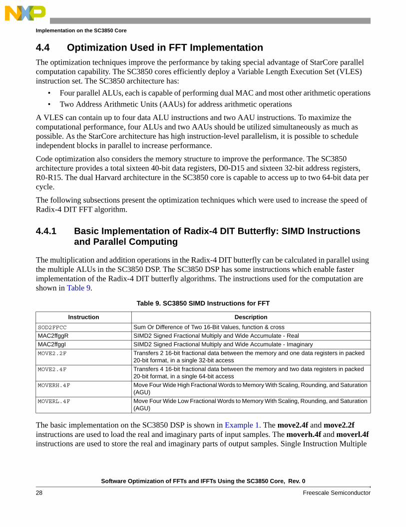
4.5 FFT Reference CodeIn the first stage, the input data A and B are loaded with address register r0, and input data C and D are loaded address registers r3. As described in Section 4.2, bit-reversed addressing mode is used for registers r0 and r3 to reorder the input data. The output data A’, B’, C’, and D’ are stored to memory using the address registers, r4, r5, r8, and r9, respectively. The diagram of the first stage is illustrated in Figure 15.
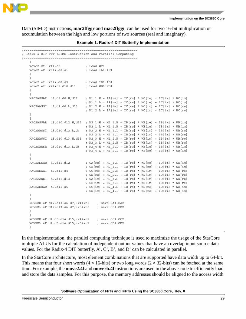
Figure 16 shows the diagram of the middle and the last stages. Although different number of loops are used for the middle and the last loops, the same registers are used to load and store data for the DIT butterfly. Thus the middle stages and the last stage share the same diagram.
Figure 15. Diagram of the First Stage
Figure 16. Diagram of the Middle and Last Stages
Software Optimization of FFTs and IFFTs Using the SC3850 Core, Rev. 0
34 Freescale Semiconductor
Implementation on the SC3850 Core
The procedure of Radix-4 DIT butterfly calculation is summarized as follows:
1. The input data [A, B, C, D] are loaded from memory. MOVE2.4F instruction is used to load the real and imaginary part in parallel.
2. In the first stage, SOD2ffcc computes the butterfly shown in Figure 15. The SOD2ffcc instruction performs two separate 16-bit additions or subtractions between the high and low portions of two source data registers, and stores the results in the two portions of the destination data register.
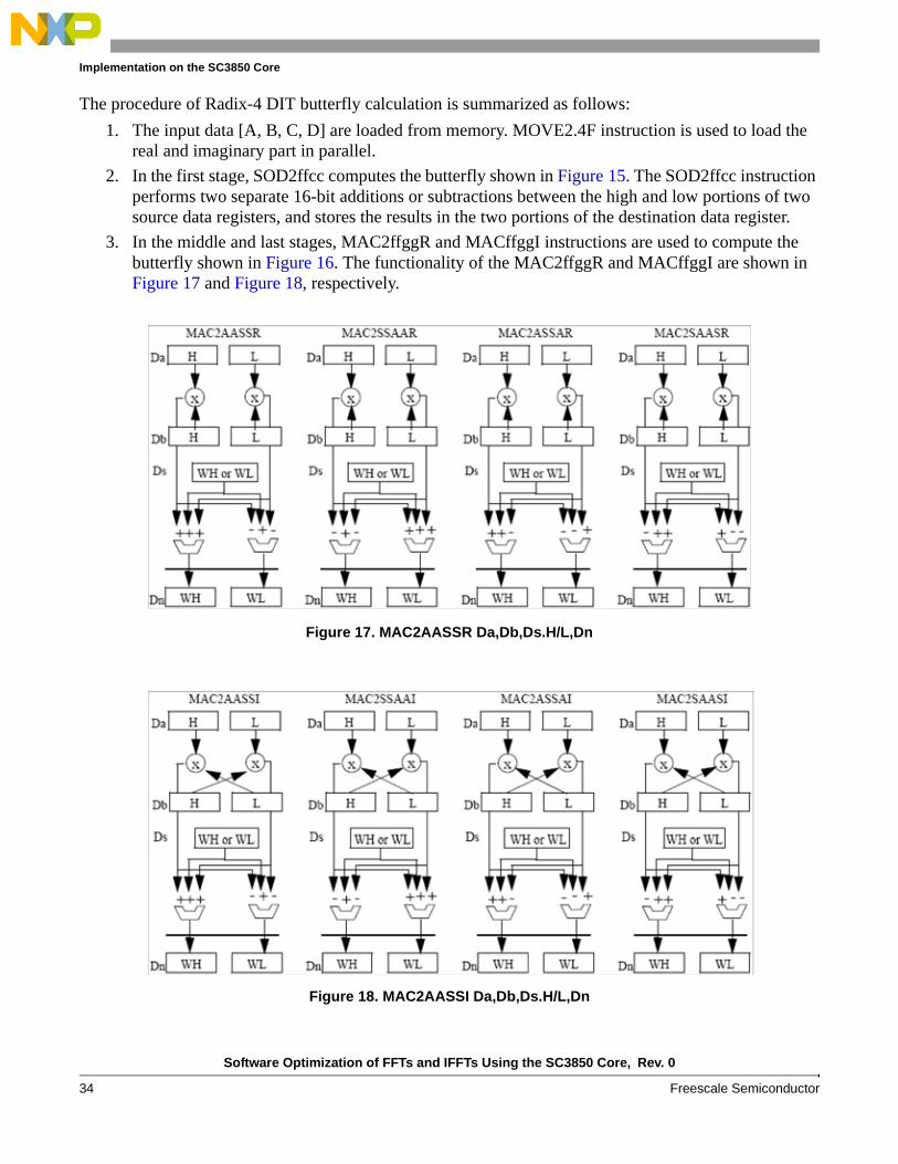
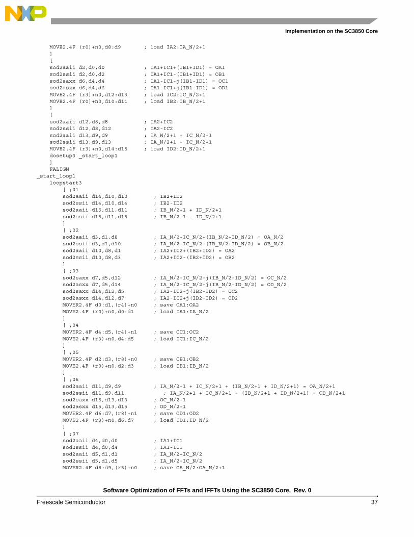
3. In the middle and last stages, MAC2ffggR and MACffggI instructions are used to compute the butterfly shown in Figure 16. The functionality of the MAC2ffggR and MACffggI are shown in Figure 17 and Figure 18, respectively.
Figure 17. MAC2AASSR Da,Db,Ds.H/L,Dn
Figure 18. MAC2AASSI Da,Db,Ds.H/L,Dn

Software Optimization of FFTs and IFFTs Using the SC3850 Core, Rev. 0
Freescale Semiconductor 35
Implementation on the SC3850 Core
4. MOVERH.4F and MOVERL.4F instructions are used to scale, round, and limit the output data samples and store they into memory. The scaling down factors can be 1, 2, 4.
The Radix-4 DIT FFT source code is shown Example 4. The arguments of this function are the pointer of data buffer (input and output), the pointers of twiddle factors, the number of FFT points, the number of stages, and the shift bits. As mentioned in Section 4.1, scaling can be used to avoid overflowing at each stage. This is why we have the shift as an input parameter of the FFT function. Shift can be 0, 1, and 2 for no scaling, scaling down by 2, and scaling down by 4, respectively.
Example 4. Radix-4 FFT Source Code
OPT BE SECTION .text;--------------BENCHMARK------------------------------------------------------ GLOBAL _sc3850_fft_radix4_complex_16x16_asm FALIGN_sc3850_fft_radix4_complex_16x16_asm_begin:_sc3850_fft_radix4_complex_16x16_asm type func ;// begin to count cyclesbenchmark:init: [ move.w (SP-14),d14 ; N move.l r0,d0 ; data_buffer; push.2l r6:r7 ] [ push.2l d6:d7 move.l #$00e41008,sr ;// scaling OFF, SM=0, SM2=0, two's-complement rounding, W20-bits mode ON; move.l #$00e41018,sr ;// scaling by1 ON, SM=0, SM2=0, two's-complement rounding, W20-bits mode ON; move.l #$00e41038,sr ;// scaling by2 ON, SM=0, SM2=0, two's-complement rounding, W20-bits mode ON; move.l #$00e41088,sr ;// scaling OFF, SM=0, SM2=1, two's-complement rounding, W20-bits mode ON; move.l #$00e40088,sr ;// scaling OFF, SM=0, SM2=1, two's-complement rounding, W20-bits mode OFF; move.l #$00e41018,sr ;// scaling ON, SM=0, SM2=0, two's-complement rounding, W20-bits mode ON; move.l #$00e41098,sr ;// scaling ON, SM=0, SM2=1, two's-complement rounding, W20-bits mode ON ] [ asl d14,d1 ; N*2 add d14,d0,d4 ; ->IB1 = data_buffer+N*1 asr d14,d15 ; N/2 push MCTL move.l #($00001001),MCTL ; set r0, r3 in bit reverse ] [ asr d15,d13 ; N/4 add d14,d4,d2 ; ->IC1 = data_buffer+N*2 asl d1,d3 ; N*4 move.l d14,m0 ; load m0=N move.w (SP-34),r2 ; r2 = Shift ] [ asr d13,d12 ; N/8 asl d3,d3 ; N*8 add d3,d0,d4 ; ->OA1 = data_buffer+N*4 move.l d1,m1 ; load m1=N*2 dosetup1 _start_loop1_stage2 ] [ add d13,d15,d13 ; N/2+N/4 add d15,d4,d5 ; ->OD1 = data_buffer+N*4+N/2 add d14,d4,d6 ; ->OC1 = data_buffer+N*5 move.l d2,r3 ; r3 = data_buffer+N*2

Software Optimization of FFTs and IFFTs Using the SC3850 Core, Rev. 0
36 Freescale Semiconductor
Implementation on the SC3850 Core
dosetup2 _start_loop2_stage2 ] [ asr d12,d9 ; N/16 asr d12,d11 ; N/16 neg d12 ; -N/8 add d14,d6,d6 ; ->OB1 = data_buffer+N*6 move.l d4,r4 ; data_buffer+N*4 = r4 move.l d12,n0 ; n0=N/8 ] cmpeqa.w #1,r2 ; if (Shift==1), T=1 ift move.l #$00e41018,sr ; scaling by1 ON, SM=0, SM2=0, two's-complement rounding, W20-bits mode ON cmpeqa.w #2,r2 ; if (Shift==2), T=1 ift move.l #$00e41038,sr ; scaling by2 ON, SM=0, SM2=0, two's-complement rounding, W20-bits mode ON [ add d15,d6,d7 ; ->OB_N/2 = data_buffer+N*6+N/2 add #1,d12 ; 1-N/8 addnc.w #-2,d11,d10 ; N/16-2 asrr #2,d14 ; N/4 push r4 ; data_buffer+N*4 tfra r0,b4 ; data_buffer ] [ asl d10,d10 ; (N/16-2)*2 move.l d6,r8 ; ->OB1 = data_buffer+N*6 move.l d5,r5 ; ->OA_N/2 = data_buffer+N*4+N/2 ] [ move.l d3,m2 ; load m2=N*8 move.l d13,n3 ; n3=N/2+N/4, ] [ move.l d11,n2 ; N/16 move.l d10,r15 ; (N/32-1)*4 = r15 ]kernel:;//////////////////////////////////FIRST LOOP (RADIX 4)/////////////////////////////////////////////////////////////////// ; FIRST LOOP (RADIX 4) ; Wb=Wd=Wc=1 [ move.l d12,n1 ; n1=1-N/8 MOVE2.4F (r0)+n0,d0:d1 ; load IA1:IA_N/2 ] [ sub #1,d9 MOVE2.4F (r3)+n0,d4:d5 ; load IC1:IC_N/2 MOVE2.4F (r0)+n0,d2:d3 ; load IB1:IB_N/2 ] [ sod2aaii d4,d0,d0 ; IA1+IC1 sod2ssii d4,d0,d4 ; IA1-IC1 sod2aaii d5,d1,d1 ; IA_N/2+IC_N/2 sod2ssii d5,d1,d5 ; IA_N/2-IC_N/2 move.l d7,r9 ; ->OB_N/2 = data_buffer+N*6+N/2 MOVE2.4F (r3)+n0,d6:d7 ; load ID1:ID_N/2 ] [ sod2aaii d6,d2,d2 ; IB1+ID1 sod2ssii d6,d2,d6 ; IB1-ID1 sod2aaii d7,d3,d3 ; IB_N/2+ID_N/2 sod2ssii d7,d3,d7 ; IB_N/2-ID_N/2 doen3 d9
Software Optimization of FFTs and IFFTs Using the SC3850 Core, Rev. 0
Freescale Semiconductor 37
Implementation on the SC3850 Core
MOVE2.4F (r0)+n0,d8:d9 ; load IA2:IA_N/2+1 ] [ sod2aaii d2,d0,d0 ; IA1+IC1+(IB1+ID1) = OA1 sod2ssii d2,d0,d2 ; IA1+IC1-(IB1+ID1) = OB1 sod2saxx d6,d4,d4 ; IA1-IC1-j(IB1-ID1) = OC1 sod2asxx d6,d4,d6 ; IA1-IC1+j(IB1-ID1) = OD1 MOVE2.4F (r3)+n0,d12:d13 ; load IC2:IC_N/2+1 MOVE2.4F (r0)+n0,d10:d11 ; load IB2:IB_N/2+1 ] [ sod2aaii d12,d8,d8 ; IA2+IC2 sod2ssii d12,d8,d12 ; IA2-IC2 sod2aaii d13,d9,d9 ; IA_N/2+1 + IC_N/2+1 sod2ssii d13,d9,d13 ; IA_N/2+1 - IC_N/2+1 MOVE2.4F (r3)+n0,d14:d15 ; load ID2:ID_N/2+1 dosetup3 _start_loop1 ] FALIGN_start_loop1 loopstart3 [ ;01 sod2aaii d14,d10,d10 ; IB2+ID2 sod2ssii d14,d10,d14 ; IB2-ID2 sod2aaii d15,d11,d11 ; IB_N/2+1 + ID_N/2+1 sod2ssii d15,d11,d15 ; IB_N/2+1 - ID_N/2+1 ] [ ;02 sod2aaii d3,d1,d8 ; IA_N/2+IC_N/2+(IB_N/2+ID_N/2) = OA_N/2 sod2ssii d3,d1,d10 ; IA_N/2+IC_N/2-(IB_N/2+ID_N/2) = OB_N/2 sod2aaii d10,d8,d1 ; IA2+IC2+(IB2+ID2) = OA2 sod2ssii d10,d8,d3 ; IA2+IC2-(IB2+ID2) = OB2 ] [ ;03 sod2saxx d7,d5,d12 ; IA_N/2-IC_N/2-j(IB_N/2-ID_N/2) = OC_N/2 sod2asxx d7,d5,d14 ; IA_N/2-IC_N/2+j(IB_N/2-ID_N/2) = OD_N/2 sod2saxx d14,d12,d5 ; IA2-IC2-j(IB2-ID2) = OC2 sod2asxx d14,d12,d7 ; IA2-IC2+j(IB2-ID2) = OD2 MOVER2.4F d0:d1,(r4)+n0 ; save OA1:OA2 MOVE2.4F (r0)+n0,d0:d1 ; load IA1:IA_N/2 ] [ ;04 MOVER2.4F d4:d5,(r4)+n1 ; save OC1:OC2 MOVE2.4F (r3)+n0,d4:d5 ; load IC1:IC_N/2 ] [ ;05 MOVER2.4F d2:d3,(r8)+n0 ; save OB1:OB2 MOVE2.4F (r0)+n0,d2:d3 ; load IB1:IB_N/2 ] [ ;06 sod2aaii d11,d9,d9 ; IA_N/2+1 + IC_N/2+1 + (IB_N/2+1 + ID_N/2+1) = OA_N/2+1 sod2ssii d11,d9,d11 ; IA_N/2+1 + IC_N/2+1 - (IB_N/2+1 + ID_N/2+1) = OB_N/2+1 sod2saxx d15,d13,d13 ; OC_N/2+1 sod2asxx d15,d13,d15 ; OD_N/2+1 MOVER2.4F d6:d7,(r8)+n1 ; save OD1:OD2 MOVE2.4F (r3)+n0,d6:d7 ; load ID1:ID_N/2 ] [ ;07 sod2aaii d4,d0,d0 ; IA1+IC1 sod2ssii d4,d0,d4 ; IA1-IC1 sod2aaii d5,d1,d1 ; IA_N/2+IC_N/2 sod2ssii d5,d1,d5 ; IA_N/2-IC_N/2 MOVER2.4F d8:d9,(r5)+n0 ; save OA_N/2:OA_N/2+1

Software Optimization of FFTs and IFFTs Using the SC3850 Core, Rev. 0
38 Freescale Semiconductor
Implementation on the SC3850 Core
MOVE2.4F (r0)+n0,d8:d9 ; load IA2:IA_N/2+1 ] [ ;08 sod2aaii d6,d2,d2 ; IB1+ID1 sod2ssii d6,d2,d6 ; IB1-ID1 sod2aaii d7,d3,d3 ; IB_N/2+ID_N/2 sod2ssii d7,d3,d7 ; IB_N/2-ID_N/2 MOVER2.4F d12:d13,(r5)+n1 ; save OC_N/2:OC_N/2+1 MOVE2.4F (r3)+n0,d12:d13 ; load IC2:IC_N/2+1 ] [ ;09 sod2aaii d2,d0,d0 ; IA1+IC1+(IB1+ID1) = OA1 sod2ssii d2,d0,d2 ; IA1+IC1-(IB1+ID1) = OB1 sod2saxx d6,d4,d4 ; IA1-IC1-j(IB1-ID1) = OC1 sod2asxx d6,d4,d6 ; IA1-IC1+j(IB1-ID1) = OD1 MOVER2.4F d10:d11,(r9)+n0 ; save OB_N/2:OB_N/2+1 MOVE2.4F (r0)+n0,d10:d11 ; load IB2:IB_N/2+1 ] [ ;10 sod2aaii d12,d8,d8 ; IA2+IC2 sod2ssii d12,d8,d12 ; IA2-IC2 sod2aaii d13,d9,d9 ; IA_N/2+1 + IC_N/2+1 sod2ssii d13,d9,d13 ; IA_N/2+1 - IC_N/2+1 MOVER2.4F d14:d15,(r9)+n1 ; save OD_N/2:OD_N/2+1 MOVE2.4F (r3)+n0,d14:d15 ; load ID2:ID_N/2+1 ] loopend3 [ ; 01 sod2aaii d14,d10,d10 ; IB2+ID2 sod2ssii d14,d10,d14 ; IB2-ID2 sod2aaii d15,d11,d11 ; IB_N/2+1 + ID_N/2+1 sod2ssii d15,d11,d15 ; IB_N/2+1 - ID_N/2+1 move.l (SP-36),b2 ; load b2 -> wbdtwiddles move.l (SP-36),r2 ; load b2 -> wbdtwiddles ] [ ;02 sod2aaii d3,d1,d8 ; IA_N/2+IC_N/2+(IB_N/2+ID_N/2) = OA_N/2 sod2ssii d3,d1,d10 ; IA_N/2+IC_N/2-(IB_N/2+ID_N/2) = OB_N/2 sod2aaii d10,d8,d1 ; IA2+IC2+(IB2+ID2) = OA2 sod2ssii d10,d8,d3 ; IA2+IC2-(IB2+ID2) = OB2 tfra r0,b5 ; data_buffer move.w #4,r14 ] [ ;03 sod2saxx d7,d5,d12 ; IA_N/2-IC_N/2-j(IB_N/2-ID_N/2) = OC_N/2 sod2asxx d7,d5,d14 ; IA_N/2-IC_N/2+j(IB_N/2-ID_N/2) = OD_N/2 sod2saxx d14,d12,d5 ; IA2-IC2-j(IB2-ID2) = OC2 sod2asxx d14,d12,d7 ; IA2-IC2=j(IB2-ID2) = OD2 MOVER2.4F d0:d1,(r4)+n0 ; save OA1:OA2 dosetup3 _start_loop3_stage2 ] [ ;04 MOVER2.4F d4:d5,(r4) ; save OC1:OC2 tfra b4,r4 ; data_buffer ] [ ;05 MOVER2.4F d2:d3,(r8)+n0 ; save OB1:OB2 move.w (SP-40),d3 ; LOG_4_N ] [ ;06 sod2aaii d11,d9,d9 ; IA_N/2+1 + IC_N/2+1 + (IB_N/2+1 + ID_N/2+1) = OA_N/2+1 sod2ssii d11,d9,d11 ; IA_N/2+1 + IC_N/2+1 - (IB_N/2+1 + ID_N/2+1) = OB_N/2+1 sub #2,d3 ; d3 = LOG_4_N - 2

Software Optimization of FFTs and IFFTs Using the SC3850 Core, Rev. 0
Freescale Semiconductor 39
Implementation on the SC3850 Core
MOVER2.4F d6:d7,(r8) ; save OD1:OD2 tfra r0,b0 ; data_buffer = b0,r0 ] [ ; sod2saxx d15,d13,d13 ; OC_N/2+1 sod2asxx d15,d13,d15 ; OD_N/2+1 MOVER2.4F d8:d9,(r5)+n0 ; save OA_N/2:OA_N/2+1 pop r0 ; data_buffer+4*N ] [ ; MOVER2.4F d12:d13,(r5) ; save OC_N/2:OC_N/2+1 move.l #($00AA098A),MCTL ; load MCTL: r0,r4,r5: M2 used—Modulo addressing, ; r1: M0 used—Modulo addressing. ; r2: M1 used—Modulo addressing, ; r3,r6,r7: linear addressing, ] [ ; MOVER2.4F d10:d11,(r9)+n0 ; save OB_N/2:OB_N/2+1 tfra r3,r5 ; data_buffer+2*N ] [ ; MOVER2.4F d14:d15,(r9) ; save OD_N/2:OD_N/2+1 tfra r1,b1 ; load b1 -> wctwiddles ];////////////DEBUG_START//////////////////////////////////////////////////; pop MCTL; pop.2l d6:d7; rtsd move.l (SP-4),d3; move.l d3,SR ;////////////DEBUG_END////////////////////////////////////////////////// ; 2 STALLS on MCTL;///////////////////////////////////////////////////////////////////////////////////////////////////// ; ENTRY TO THE MAIN ; LOOP (RADIX-4) ;/// n0=N/8, n1=1-N/8, n2=N/16, n3=3N/4, m0=N, m1=N*2, m2=N*8;///////////////////////////////////////////////////////////////////////////////////////////////////// [ dosetup0 _start_loop2_stage3 move2.2f (r1),d2 ; Load WC1 ] [;//_// doen1 d3 ; init. lc1;/// doen1 #1 ; DEBUG MOVE2.4F (r0)+,d0:d1 ; Load IA1:IC1 ] [ move2.4f (r0)+,d8:d9 ; Load IB1:ID1 move2.4f (r2)+n2,d10:d11 ; Load WB1:WD1 ] FALIGN_start_loop1_stage2: loopstart1 [ ;01 MAC2ASSAR d1,d2,d0.H,d12 ; M1_1.H = IA[re] + IC[re] * WC[re] - IC[im] * WC[im] ; M1_1.L = IA[re] - IC[re] * WC[re] + IC[im] * WC[im] MAC2AASSI d1,d2,d0.L,d13 ; M1_2.H = IA[im] + IC[re] * WC[im] + IC[im] * WC[re] ; M1_2.L = IA[im] - IC[re] * WC[im] - IC[im] * WC[re] doen2 r14 ; init. lc2 = 4, 16, ... N/64, N/16 asra r15 ; 2(N/32-1), 2(N/128-1), ... ] [ ;02 MAC2ASSAR d8,d10,d12.H,d12 ; M2_1.H = M1_1.H + IB[re] * WB[re] - IB[im] * WB[im]
Software Optimization of FFTs and IFFTs Using the SC3850 Core, Rev. 0
40 Freescale Semiconductor
Implementation on the SC3850 Core
; M2_1.L = M1_1.H - IB[re] * WB[re] + IB[im] * WB[im] MAC2AASSI d8,d10,d12.L,d4 ; M2_2.H = M1_1.L + IB[re] * WB[im] + IB[im] * WB[re] ; M2_2.L = M1_1.L - IB[re] * WB[im] - IB[im] * WB[re] MAC2AASSI d8,d10,d13.H,d13 ; M2_3.H = M1_2.H + IB[re] * WB[im] + IB[im] * WB[re] ; M2_3.L = M1_2.H - IB[re] * WB[im] - IB[im] * WB[re] MAC2SAASR d8,d10,d13.L,d5 ; M2_4.H = M1_2.L - IB[re] * WB[re] + IB[im] * WB[im] ; M2_4.L = M1_2.L + IB[re] * WB[re] - IB[im] * WB[im] asl2a r14 asra r15 ; N/32-1, N/128-1, ..., 7, 1 ] FALIGN_start_loop2_stage2: loopstart2 [ ;03 MAC2ASSAR d9,d11,d12 ; OA[re] = M2_1.H + ID[re] * WD[re] - ID[im] * WD[im] ; OB[re] = M2_1.L - ID[re] * WD[re] + ID[im] * WD[im] MAC2SSAAI d9,d11,d4 ; OC[re] = M2_2.H - ID[re] * WD[im] - ID[im] * WD[re] ; OD[re] = M2_2.L + ID[re] * WD[im] + ID[im] * WD[re] MAC2AASSI d9,d11,d13 ; OA[im] = M2_3.H + ID[re] * WD[im] + ID[im] * WD[re] ; OB[im] = M2_3.L - ID[re] * WD[im] - ID[im] * WD[re] MAC2ASSAR d9,d11,d5 ; OC[im] = M2_4.H + ID[re] * WD[re] - ID[im] * WD[im] ; OD[im] = M2_4.L - ID[re] * WD[re] + ID[im] * WD[im] MOVE2.4F (r0)+,d0:d1 ; Load IA2:IC2 doen3 r15 ; init. lc3 = N/32-1, N/128-1, ... ]; ########################################################################################### FALIGN_start_loop3_stage2: loopstart3 [ ;04 MAC2ASSAR d1,d2,d0.H,d6 ; M1_1.H = IA[re] + IC[re] * WC[re] - IC[im] * WC[im] ; M1_1.L = IA[re] - IC[re] * WC[re] + IC[im] * WC[im] MAC2AASSI d1,d2,d0.L,d7 ; M1_2.H = IA[im] + IC[re] * WC[im] + IC[im] * WC[re] ; M1_2.L = IA[im] - IC[re] * WC[im] - IC[im] * WC[re] move2.4f (r0)+,d8:d9 ; Load IB2:ID2 ] [ ;05 MAC2ASSAR d8,d10,d6.H,d6 ; M2_1.H = M1_1.H + IB[re] * WB[re] - IB[im] * WB[im] ; M2_1.L = M1_1.H - IB[re] * WB[re] + IB[im] * WB[im] MAC2AASSI d8,d10,d6.L,d14 ; M2_2.H = M1_1.L + IB[re] * WB[im] + IB[im] * WB[re] ; M2_2.L = M1_1.L - IB[re] * WB[im] - IB[im] * WB[re] MAC2AASSI d8,d10,d7.H,d7 ; M2_3.H = M1_2.H + IB[re] * WB[im] + IB[im] * WB[re] ; M2_3.L = M1_2.H - IB[re] * WB[im] - IB[im] * WB[re] MAC2SAASR d8,d10,d7.L,d15 ; M2_4.H = M1_2.L - IB[re] * WB[re] + IB[im] * WB[im] ; M2_4.L = M1_2.L + IB[re] * WB[re] - IB[im] * WB[im] MOVE2.4F (r0)+,d0:d1 ; Load IA1:IC1 ] [ ;06 MAC2ASSAR d9,d11,d6 ; OA[re] = M2_1.H + ID[re] * WD[re] - ID[im] * WD[im] ; OB[re] = M2_1.L - ID[re] * WD[re] + ID[im] * WD[im] MAC2SSAAI d9,d11,d14 ; OC[re] = M2_2.H - ID[re] * WD[im] - ID[im] * WD[re] ; OD[re] = M2_2.L + ID[re] * WD[im] + ID[im] * WD[re] MAC2AASSI d9,d11,d7 ; OA[im] = M2_3.H + ID[re] * WD[im] + ID[im] * WD[re] ; OB[im] = M2_3.L - ID[re] * WD[im] - ID[im] * WD[re] MAC2ASSAR d9,d11,d15 ; OC[im] = M2_4.H + ID[re] * WD[re] - ID[im] * WD[im] ; OD[im] = M2_4.L - ID[re] * WD[re] + ID[im] * WD[im] move2.4f (r0)+,d8:d9 ; Load IB1:ID1 ] [ ;01 MAC2ASSAR d1,d2,d0.H,d12 ; M1_1.H = IA[re] + IC[re] * WC[re] - IC[im] * WC[im] ; M1_1.L = IA[re] - IC[re] * WC[re] + IC[im] * WC[im] MAC2AASSI d1,d2,d0.L,d13 ; M1_2.H = IA[im] + IC[re] * WC[im] + IC[im] * WC[re] ; M1_2.L = IA[im] - IC[re] * WC[im] - IC[im] * WC[re]
Software Optimization of FFTs and IFFTs Using the SC3850 Core, Rev. 0
Freescale Semiconductor 41
Implementation on the SC3850 Core
MOVERH.4F d12:d13:d6:d7,(r4)+n0 ; save OA1:OA2 MOVERL.4F d12:d13:d6:d7,(r5)+n0 ; save OB1:OB2 ] [ ;02 MAC2ASSAR d8,d10,d12.H,d12 ; M2_1.H = M1_1.H + IB[re] * WB[re] - IB[im] * WB[im] ; M2_1.L = M1_1.H - IB[re] * WB[re] + IB[im] * WB[im] MAC2AASSI d8,d10,d12.L,d4 ; M2_2.H = M1_1.L + IB[re] * WB[im] + IB[im] * WB[re] ; M2_2.L = M1_1.L - IB[re] * WB[im] - IB[im] * WB[re] MAC2AASSI d8,d10,d13.H,d13 ; M2_3.H = M1_2.H + IB[re] * WB[im] + IB[im] * WB[re] ; M2_3.L = M1_2.H - IB[re] * WB[im] - IB[im] * WB[re] MAC2SAASR d8,d10,d13.L,d5 ; M2_4.H = M1_2.L - IB[re] * WB[re] + IB[im] * WB[im] ; M2_4.L = M1_2.L + IB[re] * WB[re] - IB[im] * WB[im] MOVERH.4F d4:d5:d14:d15,(r4)+n1 ; save OC1:OC2 MOVERL.4F d4:d5:d14:d15,(r5)+n1 ; save OD1:OD2 ] [ ;03 MAC2ASSAR d9,d11,d12 ; OA[re] = M2_1.H + ID[re] * WD[re] - ID[im] * WD[im] ; OB[re] = M2_1.L - ID[re] * WD[re] + ID[im] * WD[im] MAC2SSAAI d9,d11,d4 ; OC[re] = M2_2.H - ID[re] * WD[im] - ID[im] * WD[re] ; OD[re] = M2_2.L + ID[re] * WD[im] + ID[im] * WD[re] MAC2AASSI d9,d11,d13 ; OA[im] = M2_3.H + ID[re] * WD[im] + ID[im] * WD[re] ; OB[im] = M2_3.L - ID[re] * WD[im] - ID[im] * WD[re] MAC2ASSAR d9,d11,d5 ; OC[im] = M2_4.H + ID[re] * WD[re] - ID[im] * WD[im] ; OD[im] = M2_4.L - ID[re] * WD[re] + ID[im] * WD[im] MOVE2.4F (r0)+,d0:d1 ; Load IA2:IC2 ]; ########################################################################################### loopend3 [ ;04 MAC2ASSAR d1,d2,d0.H,d6 ; M1_1.H = IA[re] + IC[re] * WC[re] - IC[im] * WC[im] ; M1_1.L = IA[re] - IC[re] * WC[re] + IC[im] * WC[im] MAC2AASSI d1,d2,d0.L,d7 ; M1_2.H = IA[im] + IC[re] * WC[im] + IC[im] * WC[re] ; M1_2.L = IA[im] - IC[re] * WC[im] - IC[im] * WC[re] move2.4f (r0)+,d8:d9 ; Load IB2:ID2 addl2a n2,r1 ] [ ;05 MAC2ASSAR d8,d10,d6.H,d6 ; M2_1.H = M1_1.H + IB[re] * WB[re] - IB[im] * WB[im] ; M2_1.L = M1_1.H - IB[re] * WB[re] + IB[im] * WB[im] MAC2AASSI d8,d10,d6.L,d14 ; M2_2.H = M1_1.L + IB[re] * WB[im] + IB[im] * WB[re] ; M2_2.L = M1_1.L - IB[re] * WB[im] - IB[im] * WB[re] MAC2AASSI d8,d10,d7.H,d7 ; M2_3.H = M1_2.H + IB[re] * WB[im] + IB[im] * WB[re] ; M2_3.L = M1_2.H - IB[re] * WB[im] - IB[im] * WB[re] MAC2SAASR d8,d10,d7.L,d15 ; M2_4.H = M1_2.L - IB[re] * WB[re] + IB[im] * WB[im] ; M2_4.L = M1_2.L + IB[re] * WB[re] - IB[im] * WB[im] MOVE2.4F (r0)+,d0:d1 ; Load IA1:IC1 move2.2f (r1),d2 ; Load WC1 ] [ ;06 MAC2ASSAR d9,d11,d6 ; OA[re] = M2_1.H + ID[re] * WD[re] - ID[im] * WD[im] ; OB[re] = M2_1.L - ID[re] * WD[re] + ID[im] * WD[im] MAC2SSAAI d9,d11,d14 ; OC[re] = M2_2.H - ID[re] * WD[im] - ID[im] * WD[re] ; OD[re] = M2_2.L + ID[re] * WD[im] + ID[im] * WD[re] MAC2AASSI d9,d11,d7 ; OA[im] = M2_3.H + ID[re] * WD[im] + ID[im] * WD[re] ; OB[im] = M2_3.L - ID[re] * WD[im] - ID[im] * WD[re] MAC2ASSAR d9,d11,d15 ; OC[im] = M2_4.H + ID[re] * WD[re] - ID[im] * WD[im] ; OD[im] = M2_4.L - ID[re] * WD[re] + ID[im] * WD[im] move2.4f (r0)+,d8:d9 ; Load IB1:ID1 move2.4f (r2)+n2,d10:d11 ; Load WB1:WD1 ] [ ;01 MAC2ASSAR d1,d2,d0.H,d12 ; M1_1.H = IA[re] + IC[re] * WC[re] - IC[im] * WC[im] ; M1_1.L = IA[re] - IC[re] * WC[re] + IC[im] * WC[im]

Software Optimization of FFTs and IFFTs Using the SC3850 Core, Rev. 0
42 Freescale Semiconductor
Implementation on the SC3850 Core
MAC2AASSI d1,d2,d0.L,d13 ; M1_2.H = IA[im] + IC[re] * WC[im] + IC[im] * WC[re] ; M1_2.L = IA[im] - IC[re] * WC[im] - IC[im] * WC[re] MOVERH.4F d12:d13:d6:d7,(r4)+n0 ; save OA1:OA2 MOVERL.4F d12:d13:d6:d7,(r5)+n0 ; save OB1:OB2 ] [ ;02 MAC2ASSAR d8,d10,d12.H,d12 ; M2_1.H = M1_1.H + IB[re] * WB[re] - IB[im] * WB[im] ; M2_1.L = M1_1.H - IB[re] * WB[re] + IB[im] * WB[im] MAC2AASSI d8,d10,d12.L,d4 ; M2_2.H = M1_1.L + IB[re] * WB[im] + IB[im] * WB[re] ; M2_2.L = M1_1.L - IB[re] * WB[im] - IB[im] * WB[re] MAC2AASSI d8,d10,d13.H,d13 ; M2_3.H = M1_2.H + IB[re] * WB[im] + IB[im] * WB[re] ; M2_3.L = M1_2.H - IB[re] * WB[im] - IB[im] * WB[re] MAC2SAASR d8,d10,d13.L,d5 ; M2_4.H = M1_2.L - IB[re] * WB[re] + IB[im] * WB[im] ; M2_4.L = M1_2.L + IB[re] * WB[re] - IB[im] * WB[im] MOVERH.4F d4:d5:d14:d15,(r4)+n1 ; save OC1:OC2 MOVERL.4F d4:d5:d14:d15,(r5)+n1 ; save OD1:OD2 ] loopend2 [ asra n2 tfra b2,r2 ] [ asra n2 addl2a n3,r4 ; r4+OFFSET ] [ addl2a n3,r5 ; r5+OFFSET move2.4f (r2)+n2,d10:d11 ; Load WB1:WD1 ] loopend1;//////////////////////////////////LAST LOOP (RADIX-4)////////////////////////////////////////////////;//// the commented instructions in the following 2 VELS were computed in previous loop;///////////////////////////////////////////////////////////////////////////////////////////////////// [ ;01; MAC2ASSAR d1,d2,d0.H,d12 ; M1_1.H = IA[re] + IC[re] * WC[re] - IC[im] * WC[im]; ; M1_1.L = IA[re] - IC[re] * WC[re] + IC[im] * WC[im]; MAC2AASSI d1,d2,d0.L,d13 ; M1_2.H = IA[im] + IC[re] * WC[im] + IC[im] * WC[re]; ; M1_2.L = IA[im] - IC[re] * WC[im] - IC[im] * WC[re] move2.4f (r1)+,d2:d3 ; Load WC1:WC2 ] [ ;02; MAC2ASSAR d8,d10,d12.H,d12 ; M2_1.H = M1_1.H + IB[re] * WB[re] - IB[im] * WB[im]; ; M2_1.L = M1_1.H - IB[re] * WB[re] + IB[im] * WB[im]; MAC2AASSI d8,d10,d12.L,d4 ; M2_2.H = M1_1.L + IB[re] * WB[im] + IB[im] * WB[re]; ; M2_2.L = M1_1.L - IB[re] * WB[im] - IB[im] * WB[re]; MAC2AASSI d8,d10,d13.H,d13 ; M2_3.H = M1_2.H + IB[re] * WB[im] + IB[im] * WB[re]; ; M2_3.L = M1_2.H - IB[re] * WB[im] - IB[im] * WB[re]; MAC2SAASR d8,d10,d13.L,d5 ; M2_4.H = M1_2.L - IB[re] * WB[re] + IB[im] * WB[im]; ; M2_4.L = M1_2.L + IB[re] * WB[re] - IB[im] * WB[im] asra r14 ; N/8 MOVE2.4F (r0)+,d0:d1 ; Load IA2:IC2 ] [ ;03 MAC2ASSAR d9,d11,d12 ; OA[re] = M2_1.H + ID[re] * WD[re] - ID[im] * WD[im] ; OB[re] = M2_1.L - ID[re] * WD[re] + ID[im] * WD[im] MAC2SSAAI d9,d11,d4 ; OC[re] = M2_2.H - ID[re] * WD[im] - ID[im] * WD[re] ; OD[re] = M2_2.L + ID[re] * WD[im] + ID[im] * WD[re] MAC2AASSI d9,d11,d13 ; OA[im] = M2_3.H + ID[re] * WD[im] + ID[im] * WD[re] ; OB[im] = M2_3.L - ID[re] * WD[im] - ID[im] * WD[re] MAC2ASSAR d9,d11,d5 ; OC[im] = M2_4.H + ID[re] * WD[re] - ID[im] * WD[im] ; OD[im] = M2_4.L - ID[re] * WD[re] + ID[im] * WD[im] deca r14 ; N/8-1
Software Optimization of FFTs and IFFTs Using the SC3850 Core, Rev. 0
Freescale Semiconductor 43
Implementation on the SC3850 Core
move2.4f (r2)+,d10:d11 ; Load WB2:WD2 ]; ########################################################################################### [ ;04 MAC2ASSAR d1,d3,d0.H,d6 ; M1_1.H = IA[re] + IC[re] * WC[re] - IC[im] * WC[im] ; M1_1.L = IA[re] - IC[re] * WC[re] + IC[im] * WC[im] MAC2AASSI d1,d3,d0.L,d7 ; M1_2.H = IA[im] + IC[re] * WC[im] + IC[im] * WC[re] ; M1_2.L = IA[im] - IC[re] * WC[im] - IC[im] * WC[re] move2.4f (r0)+,d8:d9 ; Load IB2:ID2 move2.4f (r1)+,d2:d3 ; Load WC1:WC2 ] [ ;05 MAC2ASSAR d8,d10,d6.H,d6 ; M2_1.H = M1_1.H + IB[re] * WB[re] - IB[im] * WB[im] ; M2_1.L = M1_1.H - IB[re] * WB[re] + IB[im] * WB[im] MAC2AASSI d8,d10,d6.L,d14 ; M2_2.H = M1_1.L + IB[re] * WB[im] + IB[im] * WB[re] ; M2_2.L = M1_1.L - IB[re] * WB[im] - IB[im] * WB[re] MAC2AASSI d8,d10,d7.H,d7 ; M2_3.H = M1_2.H + IB[re] * WB[im] + IB[im] * WB[re] ; M2_3.L = M1_2.H - IB[re] * WB[im] - IB[im] * WB[re] MAC2SAASR d8,d10,d7.L,d15 ; M2_4.H = M1_2.L - IB[re] * WB[re] + IB[im] * WB[im] ; M2_4.L = M1_2.L + IB[re] * WB[re] - IB[im] * WB[im] doen0 r14 ; init. lc2 = N/8-1 MOVE2.4F (r0)+,d0:d1 ; Load IA1:IC1 ] [ ;06 MAC2ASSAR d9,d11,d6 ; OA[re] = M2_1.H + ID[re] * WD[re] - ID[im] * WD[im] ; OB[re] = M2_1.L - ID[re] * WD[re] + ID[im] * WD[im] MAC2SSAAI d9,d11,d14 ; OC[re] = M2_2.H - ID[re] * WD[im] - ID[im] * WD[re] ; OD[re] = M2_2.L + ID[re] * WD[im] + ID[im] * WD[re] MAC2AASSI d9,d11,d7 ; OA[im] = M2_3.H + ID[re] * WD[im] + ID[im] * WD[re] ; OB[im] = M2_3.L - ID[re] * WD[im] - ID[im] * WD[re] MAC2ASSAR d9,d11,d15 ; OC[im] = M2_4.H + ID[re] * WD[re] - ID[im] * WD[im] ; OD[im] = M2_4.L - ID[re] * WD[re] + ID[im] * WD[im] move2.4f (r0)+,d8:d9 ; Load IB1:ID1 move2.4f (r2)+,d10:d11 ; Load WB1:WD1 ] FALIGN_start_loop2_stage3: loopstart0 [ ;01 MAC2ASSAR d1,d2,d0.H,d12 ; M1_1.H = IA[re] + IC[re] * WC[re] - IC[im] * WC[im] ; M1_1.L = IA[re] - IC[re] * WC[re] + IC[im] * WC[im] MAC2AASSI d1,d2,d0.L,d13 ; M1_2.H = IA[im] + IC[re] * WC[im] + IC[im] * WC[re] ; M1_2.L = IA[im] - IC[re] * WC[im] - IC[im] * WC[re] MOVERH.4F d12:d13:d6:d7,(r4)+n0 ; save OA1:OA2 MOVERL.4F d12:d13:d6:d7,(r5)+n0 ; save OB1:OB2 ] [ ;02 MAC2ASSAR d8,d10,d12.H,d12 ; M2_1.H = M1_1.H + IB[re] * WB[re] - IB[im] * WB[im] ; M2_1.L = M1_1.H - IB[re] * WB[re] + IB[im] * WB[im] MAC2AASSI d8,d10,d12.L,d4 ; M2_2.H = M1_1.L + IB[re] * WB[im] + IB[im] * WB[re] ; M2_2.L = M1_1.L - IB[re] * WB[im] - IB[im] * WB[re] MAC2AASSI d8,d10,d13.H,d13 ; M2_3.H = M1_2.H + IB[re] * WB[im] + IB[im] * WB[re] ; M2_3.L = M1_2.H - IB[re] * WB[im] - IB[im] * WB[re] MAC2SAASR d8,d10,d13.L,d5 ; M2_4.H = M1_2.L - IB[re] * WB[re] + IB[im] * WB[im] ; M2_4.L = M1_2.L + IB[re] * WB[re] - IB[im] * WB[im] MOVERH.4F d4:d5:d14:d15,(r4)+n1 ; save OC1:OC2 MOVERL.4F d4:d5:d14:d15,(r5)+n1 ; save OD1:OD2 ] [ ;03 MAC2ASSAR d9,d11,d12 ; OA[re] = M2_1.H + ID[re] * WD[re] - ID[im] * WD[im] ; OB[re] = M2_1.L - ID[re] * WD[re] + ID[im] * WD[im] MAC2SSAAI d9,d11,d4 ; OC[re] = M2_2.H - ID[re] * WD[im] - ID[im] * WD[re] ; OD[re] = M2_2.L + ID[re] * WD[im] + ID[im] * WD[re]
Software Optimization of FFTs and IFFTs Using the SC3850 Core, Rev. 0
44 Freescale Semiconductor
Implementation on the SC3850 Core
MAC2AASSI d9,d11,d13 ; OA[im] = M2_3.H + ID[re] * WD[im] + ID[im] * WD[re] ; OB[im] = M2_3.L - ID[re] * WD[im] - ID[im] * WD[re] MAC2ASSAR d9,d11,d5 ; OC[im] = M2_4.H + ID[re] * WD[re] - ID[im] * WD[im] ; OD[im] = M2_4.L - ID[re] * WD[re] + ID[im] * WD[im] MOVE2.4F (r0)+,d0:d1 ; Load IA2:IC2 move2.4f (r2)+,d10:d11 ; Load WB2:WD2 ]; ########################################################################################### [ ;04 MAC2ASSAR d1,d3,d0.H,d6 ; M1_1.H = IA[re] + IC[re] * WC[re] - IC[im] * WC[im] ; M1_1.L = IA[re] - IC[re] * WC[re] + IC[im] * WC[im] MAC2AASSI d1,d3,d0.L,d7 ; M1_2.H = IA[im] + IC[re] * WC[im] + IC[im] * WC[re] ; M1_2.L = IA[im] - IC[re] * WC[im] - IC[im] * WC[re] move2.4f (r0)+,d8:d9 ; Load IB2:ID2 move2.4f (r1)+,d2:d3 ; Load WC1:WC2 ] [ ;05 MAC2ASSAR d8,d10,d6.H,d6 ; M2_1.H = M1_1.H + IB[re] * WB[re] - IB[im] * WB[im] ; M2_1.L = M1_1.H - IB[re] * WB[re] + IB[im] * WB[im] MAC2AASSI d8,d10,d6.L,d14 ; M2_2.H = M1_1.L + IB[re] * WB[im] + IB[im] * WB[re] ; M2_2.L = M1_1.L - IB[re] * WB[im] - IB[im] * WB[re] MAC2AASSI d8,d10,d7.H,d7 ; M2_3.H = M1_2.H + IB[re] * WB[im] + IB[im] * WB[re] ; M2_3.L = M1_2.H - IB[re] * WB[im] - IB[im] * WB[re] MAC2SAASR d8,d10,d7.L,d15 ; M2_4.H = M1_2.L - IB[re] * WB[re] + IB[im] * WB[im] ; M2_4.L = M1_2.L + IB[re] * WB[re] - IB[im] * WB[im] MOVE2.4F (r0)+,d0:d1 ; Load IA1:IC1 ] [ ;06 MAC2ASSAR d9,d11,d6 ; OA[re] = M2_1.H + ID[re] * WD[re] - ID[im] * WD[im] ; OB[re] = M2_1.L - ID[re] * WD[re] + ID[im] * WD[im] MAC2SSAAI d9,d11,d14 ; OC[re] = M2_2.H - ID[re] * WD[im] - ID[im] * WD[re] ; OD[re] = M2_2.L + ID[re] * WD[im] + ID[im] * WD[re] MAC2AASSI d9,d11,d7 ; OA[im] = M2_3.H + ID[re] * WD[im] + ID[im] * WD[re] ; OB[im] = M2_3.L - ID[re] * WD[im] - ID[im] * WD[re] MAC2ASSAR d9,d11,d15 ; OC[im] = M2_4.H + ID[re] * WD[re] - ID[im] * WD[im] ; OD[im] = M2_4.L - ID[re] * WD[re] + ID[im] * WD[im] move2.4f (r0)+,d8:d9 ; Load IB1:ID1 move2.4f (r2)+,d10:d11 ; Load WB1:WD1 ] loopend0 [ MOVERH.4F d12:d13:d6:d7,(r4)+n0 ; save OA1:OA2 MOVERL.4F d12:d13:d6:d7,(r5)+n0 ; save OB1:OB2 ] [ MOVERH.4F d4:d5:d14:d15,(r4) ; save OC1:OC2 pop MCTL ] [ MOVERL.4F d4:d5:d14:d15,(r5) ; save OD1:OD2 pop.2l d6:d7 ]; pop.2l r6:r7;//////////////////////////////////////////////////////////////////////////////////////////// global F_sc3850_fft_radix4_complex_16x16_asm_endF_sc3850_fft_radix4_complex_16x16_asm_end: ;// finish to count cyclesend_benchmark: rtsd move.l (SP-4),d3 move.l d3,SR ;--------------TEST LOOP------------------------------------------------------ ENDSEC;////////////////////////////////////////////////////////////////////////////////////////////

Software Optimization of FFTs and IFFTs Using the SC3850 Core, Rev. 0
Freescale Semiconductor 45
Implementation on the SC3850 Core
4.6 Fixed-Point Arithmetic and Bit AccuracyThe SC3850 core architecture uses the fixed-point representation. The finite precision for the Radix-4 DIT FFT is limited by the following parameters:
• Number of bits that are available in the input and output data
• Operations of finite arithmetic calculations (addition, subtraction, and multiplication with rounding)
The data of Radix-4 DIT butterfly can be scaled down by a factor of 1, 2, or 4 and is equivalent to an arithmetic right shift by 0, 1, or 2 bits to avoid the possibility of overflow. In the zero shift case, the final significant bits are 16-bit Q15 data, which uses all 16 bits at the risk of overflowing. If the output is scaled down by 4, the final significant bits are 14-bit Q13 data, which avoids the overflowing of the output data. In summary, the output of each butterfly should have 14 ~ 16-bit accuracy for fixed-scaling method (Q13-Q15 in Q format).
4.7 Implementation of Radix-4 DIT IFFTs
A common method to implement the Inverse Fast Fourier Transform (IFFT) is to change the sign of the twiddle factors and use the FFT subroutine. This method needs additional memory to store the twiddle factors. Therefore, it is not efficient for reduction of memory requirement.
If the complex conjugate of FFT (Equation 3) is considered, the equation is defined by Equation 21.
Eqn. 21
x∗ n( ) 1N---- X k( ) j
2πnkN
-------------⎝ ⎠⎛ ⎞exp
∗
k 0=
∑=
1N---- X∗ k( ) j–( )2πnk
N-------------⎝ ⎠
⎛ ⎞exp
k 0=
N 1–
∑=
1N---- X∗ k( ) 2πnk
N-------------⎝ ⎠⎛ ⎞cos j
2πnkN
-------------⎝ ⎠⎛ ⎞sin–
⎩ ⎭⎨ ⎬⎧ ⎫
N 1–
∑=
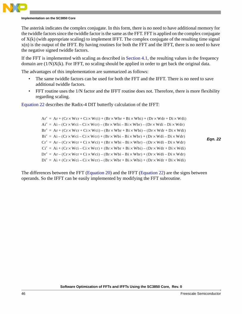
Software Optimization of FFTs and IFFTs Using the SC3850 Core, Rev. 0
46 Freescale Semiconductor
Implementation on the SC3850 Core
The asterisk indicates the complex conjugate. In this form, there is no need to have additional memory for the twiddle factors since the twiddle factor is the same as the FFT. FFT is applied on the complex conjugate of X(k) (with appropriate scaling) to implement IFFT. The complex conjugate of the resulting time signal x(n) is the output of the IFFT. By having routines for both the FFT and the IFFT, there is no need to have the negative signed twiddle factors.
If the FFT is implemented with scaling as described in Section 4.1, the resulting values in the frequency domain are (1/N)X(k). For IFFT, no scaling should be applied in order to get back the original data.
The advantages of this implementation are summarized as follows:
• The same twiddle factors can be used for both the FFT and the IFFT. There is no need to save additional twiddle factors.
• FFT routine uses the 1/N factor and the IFFT routine does not. Therefore, there is more flexibility regarding scaling.
Equation 22 describes the Radix-4 DIT butterfly calculation of the IFFT:
Eqn. 22
The differences between the FFT (Equation 20) and the IFFT (Equation 22) are the signs between operands. So the IFFT can be easily implemented by modifying the FFT subroutine.
Ar′ Ar Cr Wcr× Ci Wci×+( ) Br Wbr× Bi Wbi×+( ) Dr Wdr× Di Wdi×+( )+ + +=
Ai′ Ai Cr Wci× Ci Wcr×–( )– Br Wbi× Bi Wbr×–( )– Dr Wdi× Di Wdr×–( )–=
Br ′ Ar Cr Wcr× Ci Wci×+( ) Br Wbr× Bi Wbi×+( )– Dr Wdr× Di Wdi×+( )–+=
Bi′ Ai Cr Wci× Ci Wcr×–( )– Br Wbi× Bi Wbr×–( ) Dr Wdi× Di Wdr×–( )+ +=
Cr ′ Ar Cr Wcr× Ci Wci×+( )– Br Wbi× Bi Wbr×–( ) Dr Wdi× Di Wdr×–( )–+=
Ci′ Ai Cr Wci× Ci Wcr×–( ) Br Wbr× Bi Wbi×+( ) Dr Wdr× Di Wdi×+( )–+ +=
Dr′ Ar Cr Wcr× Ci Wci×+( )– Br Wbi× Bi Wbr×–( )– Dr Wdi× Di Wdr×–( )+=
Di′ Ai Cr Wci× Ci Wcr×–( ) Br Wbr× Bi Wbi×+( )– Dr Wdr× Di Wdi×+( )+ +=

Software Optimization of FFTs and IFFTs Using the SC3850 Core, Rev. 0
Freescale Semiconductor 47
Experimental Results
5 Experimental Results
5.1 Test VectorsTest vectors of length 256, 1024, 4096 are used to test the functionality of the corresponding FFT/IFFT SC3850 kernels. The 256-point test vector is shown in Figure 19.
Figure 19. Test Vector for 256-point FFT
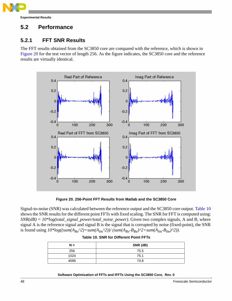
Software Optimization of FFTs and IFFTs Using the SC3850 Core, Rev. 0
48 Freescale Semiconductor
Experimental Results
5.2 Performance
5.2.1 FFT SNR Results
The FFT results obtained from the SC3850 core are compared with the reference, which is shown in Figure 20 for the test vector of length 256. As the figure indicates, the SC3850 core and the reference results are virtually identical.
Signal-to-noise (SNR) was calculated between the reference output and the SC3850 core output. Table 10 shows the SNR results for the different point FFTs with fixed scaling. The SNR for FFT is computed using: SNR(dB) = 10*log(total_signal_power/total_noise_power). Given two complex signals, A and B, where signal A is the reference signal and signal B is the signal that is corrupted by noise (fixed-point), the SNR is found using 10*log((sum(ARe^2)+sum(AIm^2))/ (sum(ARe-BRe)^2+sum(AIm-BIm)^2)).
Figure 20. 256-Point FFT Results from Matlab and the SC3850 Core
Table 10. SNR for Different Point FFTs
N = SNR (dB)
256 75.51024 75.1
4096 74.8

Software Optimization of FFTs and IFFTs Using the SC3850 Core, Rev. 0
Freescale Semiconductor 49
Experimental Results
5.2.2 Cycle Count MeasurementsThe real-time cycle counts for the implemented Radix-4 DIT FFT/IFFT kernel are measured using the SC3850 cycle accurate simulator. CodeWarrior Integrated Development Environment (IDE) R4.0 is used to compiler the FFT/IFFT kernels and the corresponding test harness.
The cycle count and memory usage for Radix-4 DIT FFT/IFFT kernel (256, 1024, and 4096 points) are summarized in Table 11. The conversion of the number of cycles into microseconds is also listed under an assumption that the SC3850 core frequency is 1GHz.
Table 11. Cycle Count and Memory Usage of FFT/IFFT Kernels
Kernel Cycle Count Time (µs) Memory Usage (Bytes)
256-FFT 792 0.79 950
1024-FFT 3773 3.77 950
4096-FFT 17986 17.99 950
256-IFFT 789 0.79 936
1024-IFFT 3770 3.77 936
4096-IFFT 17983 17.98 936
Software Optimization of FFTs and IFFTs Using the SC3850 Core, Rev. 0
50 Freescale Semiconductor
Conclusions
6 ConclusionsThe purpose of this application note is to develop Radix-4 DIT FFT algorithm implemented on the SC3850 core architecture. The implementation aspects of Radix-4 DIT FFT are based on the following SC3850 features:
• VLES execution model, which utilizes maximum parallelism by allowing multiple address generation and data arithmetic logic units to execute multiple instructions in a single cycle
• Special SIMD instructions, such as SOD2ffcc, MAC2ffggR, and MAC2ffggI
• MOVER instructions with scaling, rounding, and limiting to avoid overflowing
• Memory access with multiple data, such as MOVE2.4F, MOVE2.2f, MOVERH.4f, and MOVERL.4F.
• Bit-reversed (reverse-carry) addressing mode to support the bit-reversed order of data
The SC3850 fixed-point code incurs very little loss of accuracy compared to the floating-point Matlab results. The SC3850 core performance shows that the execution time of 1024 points FFT is 3.77 µs assuming the core frequency of 1 GHz. The data memory required to store input samples is 4N bytes, 4N bytes for output data, and 3N bytes for twiddle factors for N-point FFT. In addition, at each stage of the FFT algorithm, the output data can be scaled down by 1, 2, or 4 to avoid overflowing. The scaling factor is a parameter to the FFT kernel.
The powerful architecture and instruction set of the SC3850 core permits flexible and compact coding of the algorithms in assembly language. The optimization of Radix-4 DIT FFT is done by taking special advantage of StarCore parallel computation capabilities, such as SIMD, parallel computing, and software pipelining.
7 References1. Discrete-Time Signal Processing (Second Edition). Alan V. Oppenheim, Ronald W. Schafer, John
R. Buck, Prentice Hall International, 1999.
2. The Fast Fourier Transform and Its Applications. E. Oran Brigham, Prentice Hall, 1988.
3. SC3850 DSP Core Reference Manual. Freescale Semiconductor, available under NDA.
4. SC3850 Programmer’s Guide. available under NDA.

Software Optimization of FFTs and IFFTs Using the SC3850 Core, Rev. 0
Freescale Semiconductor 51
References
Document Number: AN3666Rev. 011/2010
Information in this document is provided solely to enable system and software
implementers to use Freescale Semiconductor products. There are no express or
implied copyright licenses granted hereunder to design or fabricate any integrated
circuits or integrated circuits based on the information in this document.
Freescale Semiconductor reserves the right to make changes without further notice to
any products herein. Freescale Semiconductor makes no warranty, representation or
guarantee regarding the suitability of its products for any particular purpose, nor does
Freescale Semiconductor assume any liability arising out of the application or use of
any product or circuit, and specifically disclaims any and all liability, including without
limitation consequential or incidental damages. “Typical” parameters which may be
provided in Freescale Semiconductor data sheets and/or specifications can and do
vary in different applications and actual performance may vary over time. All operating
parameters, including “Typicals” must be validated for each customer application by
customer’s technical experts. Freescale Semiconductor does not convey any license
under its patent rights nor the rights of others. Freescale Semiconductor products are
not designed, intended, or authorized for use as components in systems intended for
surgical implant into the body, or other applications intended to support or sustain life,
or for any other application in which the failure of the Freescale Semiconductor product
could create a situation where personal injury or death may occur. Should Buyer
purchase or use Freescale Semiconductor products for any such unintended or
unauthorized application, Buyer shall indemnify and hold Freescale Semiconductor
and its officers, employees, subsidiaries, affiliates, and distributors harmless against all
claims, costs, damages, and expenses, and reasonable attorney fees arising out of,
directly or indirectly, any claim of personal injury or death associated with such
unintended or unauthorized use, even if such claim alleges that Freescale
Semiconductor was negligent regarding the design or manufacture of the part.
Freescale, the Freescale logo, StarCore, and CodeWarrior are trademarks of Freescale Semiconductor, Inc., Reg. U.S. Pat. & Tm. Off. All other product or service names are the property of their respective owners.
© 2008–2010 Freescale Semiconductor, Inc.
How to Reach Us:
Home Page: www.freescale.com
Web Support: http://www.freescale.com/support
USA/Europe or Locations Not Listed: Freescale Semiconductor, Inc.Technical Information Center, EL5162100 East Elliot Road Tempe, Arizona 85284 +1-800-521-6274 or+1-480-768-2130www.freescale.com/support
Europe, Middle East, and Africa:Freescale Halbleiter Deutschland GmbHTechnical Information CenterSchatzbogen 781829 Muenchen, Germany+44 1296 380 456 (English) +46 8 52200080 (English)+49 89 92103 559 (German)+33 1 69 35 48 48 (French) www.freescale.com/support
Japan: Freescale Semiconductor Japan Ltd. HeadquartersARCO Tower 15F1-8-1, Shimo-Meguro, Meguro-ku Tokyo 153-0064Japan 0120 191014 or+81 3 5437 [email protected]
Asia/Pacific: Freescale Semiconductor China Ltd. Exchange Building 23FNo. 118 Jianguo RoadChaoyang DistrictBeijing 100022China+86 010 5879 [email protected]
For Literature Requests Only:Freescale Semiconductor
Literature Distribution Center +1-800 441-2447 or+1-303-675-2140Fax: +1-303-675-2150LDCForFreescaleSemiconductor
@hibbertgroup.com
Related Documents